Estimation of Air Mass Flow in Engines with Variable Valve ...

Master of Science Thesis in Electrical EngineeringDepartment of Electrical Engineering, Linköping University, 2018

Estimation of Air Mass Flowin Engines with VariableValve Timing

Elina Fantenberg

Master of Science Thesis in Electrical Engineering

Estimation of Air Mass Flow in Engines with Variable Valve Timing

Elina Fantenberg

LiTH-ISY-EX--18/5116--SE

Supervisor: Christian Andersson Naessethisy, Linköpings universitet

Erik HöckerdalScania CV AB

Examiner: Martin Enqvistisy, Linköpings universitet

Division of Automatic ControlDepartment of Electrical Engineering

Linköping UniversitySE-581 83 Linköping, Sweden

Copyright © 2018 Elina Fantenberg

Abstract

To control the combustion in an engine, an accurate estimation of the air massflow is required. Due to strict emission legislation and high demands on fuelconsumption from customers, a technology called variable valve timing is inves-tigated. This technology controls the amount of air inducted to the engine cylin-der and the amount of gases pushed out of the cylinder, via the inlet and exhaustvalves. The air mass flow is usually estimated by large look-up tables but whenintroducing variable valve timing, the air mass flow also depends on the angles ofthe inlet and exhaust valves causing these look-up tables to grow with two dimen-sions. To avoid this, models to estimate the air mass flow have been derived. Thishas been done with grey-box models, using physical equations together with un-known parameters estimated by solving a linear least-squares optimization prob-lem. To be able to implement the models in the electronic control unit in thefuture, only sensors implemented in a commercial vehicle are used as much aspossible.

The work has been done using an inline 6-cylinder diesel engine with mea-surements from steady-state conditions. All four models derived in this projectare based on the estimation methods in use today with fix cam phasing, and arederived from the ideal gas law together with a volumetric efficiency factor.

The first three models derived in this work only include sensors providedin commercial engines. The measurements needed as input signals are enginerotational speed, crank angle resolved pressure in the intake manifold, intakeand exhaust valve angles and intake manifold temperature. The fourth and lastmodel is divided into three sub-models to model different parts of the four-strokeengine cycle. This model also includes crank angle resolved exhaust manifoldpressure and exhaust manifold temperature, where the temperature is the onlysensor used in this project that is not provided in a commercial engine.

It has been concluded how influential it is to use correctly measured values forthe input signals. Since the manifold pressure and the cylinder volume vary dur-ing one four-stroke cycle, it is essential that these signal measurements are takenat the right crank angle degree. With wrong crank angle degree, the estimationis worse than if the cylinder volume is constant for all operating points and thepressure signals are taken as a mean value over the whole four-stroke cycle. Fur-ther development to reach better estimation results with lower relative error isneeded. However, for the work in this thesis, the model with best model fit isestimating the air mass flow well enough to use it as a basis for further control.

iii

Acknowledgments

First of all, I would like to thank my supervisor Erik Höckerdal at Scania forthe guidance and for always having time for me. You have helped me with allkinds of questions and how to proceed the work. I would also like to thank mysupervisor Christian Andersson Naesseth and my examiner Martin Enqvist atLinköping University. A big thank you to my family and friends without whomI wouldn’t have gotten this far. Last of all I would like to thank Pontus for all thesupport both during the past few years but most of all during this work.

Linköping, February 2018Elina Fantenberg

v

Contents

Notation ix

1 Introduction 11.1 Problem formulation . . . . . . . . . . . . . . . . . . . . . . . . . . 11.2 Method . . . . . . . . . . . . . . . . . . . . . . . . . . . . . . . . . . 21.3 Related work . . . . . . . . . . . . . . . . . . . . . . . . . . . . . . . 21.4 Thesis outline . . . . . . . . . . . . . . . . . . . . . . . . . . . . . . 3

2 System description 52.1 The four-stroke diesel engine . . . . . . . . . . . . . . . . . . . . . . 52.2 Variable valve timing . . . . . . . . . . . . . . . . . . . . . . . . . . 62.3 Valve timing strategies . . . . . . . . . . . . . . . . . . . . . . . . . 82.4 Experimental setup . . . . . . . . . . . . . . . . . . . . . . . . . . . 102.5 Assumptions . . . . . . . . . . . . . . . . . . . . . . . . . . . . . . . 11

3 Modeling 133.1 Parameter estimation . . . . . . . . . . . . . . . . . . . . . . . . . . 133.2 Model validation . . . . . . . . . . . . . . . . . . . . . . . . . . . . . 133.3 Cylinder volume . . . . . . . . . . . . . . . . . . . . . . . . . . . . . 153.4 Gas law . . . . . . . . . . . . . . . . . . . . . . . . . . . . . . . . . . 163.5 Volumetric efficiency . . . . . . . . . . . . . . . . . . . . . . . . . . 17

4 Reference model 194.1 Validation with fix valve timing . . . . . . . . . . . . . . . . . . . . 194.2 Validation with variable valve timing . . . . . . . . . . . . . . . . . 21

5 The extended models 255.1 Model 1 – Dynamic IVC volume . . . . . . . . . . . . . . . . . . . . 25

5.1.1 Modeling . . . . . . . . . . . . . . . . . . . . . . . . . . . . . 255.1.2 Result and discussion . . . . . . . . . . . . . . . . . . . . . . 26

5.2 Model 2 – Cam phase angle augmentation . . . . . . . . . . . . . . 285.2.1 Modeling . . . . . . . . . . . . . . . . . . . . . . . . . . . . . 285.2.2 Result and discussion . . . . . . . . . . . . . . . . . . . . . . 28

vii

viii Contents

5.3 Model 3 – Dynamic IVC pressure . . . . . . . . . . . . . . . . . . . 295.3.1 Modeling . . . . . . . . . . . . . . . . . . . . . . . . . . . . . 305.3.2 Result and discussion . . . . . . . . . . . . . . . . . . . . . . 31

6 Model 4 – Division into sub-models 336.1 Total mass trapped in cylinder at IVC . . . . . . . . . . . . . . . . . 34

6.1.1 Assumptions . . . . . . . . . . . . . . . . . . . . . . . . . . . 346.1.2 Results . . . . . . . . . . . . . . . . . . . . . . . . . . . . . . 34

6.2 Mass flow during valve overlap . . . . . . . . . . . . . . . . . . . . 366.2.1 Overlap factor . . . . . . . . . . . . . . . . . . . . . . . . . . 366.2.2 Assumptions and limitations . . . . . . . . . . . . . . . . . 376.2.3 Results . . . . . . . . . . . . . . . . . . . . . . . . . . . . . . 37

6.3 Total mass trapped in cylinder at EVC . . . . . . . . . . . . . . . . 386.3.1 Assumptions . . . . . . . . . . . . . . . . . . . . . . . . . . . 386.3.2 Results . . . . . . . . . . . . . . . . . . . . . . . . . . . . . . 39

6.4 Results and discussion . . . . . . . . . . . . . . . . . . . . . . . . . 40

7 Discussion and conclusions 437.1 Sensitivity analysis . . . . . . . . . . . . . . . . . . . . . . . . . . . 437.2 Discussion . . . . . . . . . . . . . . . . . . . . . . . . . . . . . . . . 447.3 Future work . . . . . . . . . . . . . . . . . . . . . . . . . . . . . . . 467.4 Conclusions . . . . . . . . . . . . . . . . . . . . . . . . . . . . . . . 46

Bibliography 49

Notation

Abbrevation MeaningBDC Bottom dead centerCAD Crank angle degreeCI Compression ignitionECU Electronic control unitEVC Exhaust valve closingEVO Exhaust valve openingIVC Inlet valve closingIVO Inlet valve openingOF Overlap factorSI Spark ignitionTDC Top dead centerVVT Variable valve timing

Symbol Description Unitαe Exhaust valve angle ◦

αi Inlet valve angle ◦

ηvol Volumetric efficiencync Number of cylindersNe Engine rotational speed rpmpem Exhaust manifold pressure Papim Intake manifold pressure PaRspec,air Specific gas constant for air J/kgKRspec,burned Specific gas constant for burned gases J/kgKTem Exhaust manifold temperature KTim Intake manifold temperature KVc Clearance volume m3

Vd Displaced volume m3

ix

1Introduction

Fuel consumption, emissions and performance largely depend on the amount ofair in the engine cylinder. Measuring air mass flow into the cylinder directly isnot cost effective and therefore accurate models are needed. To meet the increas-ingly strict emission legislations, high demands on fuel consumption and perfor-mance from customers, research on new technologies is an ongoing process. Oneof these technologies is called variable valve timing (VVT), which gives the oppor-tunity to control the opening and closing of the inlet and exhaust valves. Thesevalves control the amount of fresh air inducted into and the amount of gases ex-pelled out of the engine cylinder, respectively. VVT gives the opportunity to havegood performance at all operating points. Even higher demands on the air massflow estimation is required with VVT to be able to control the valves accurately.The air mass in the cylinder must also be known to control the amount of fuelinjected to get optimal combustion. The goal of this work is therefore to estimatethe air mass that flows through the engine with VVT.

1.1 Problem formulation

An accurate estimation of the engine air mass flow is vital to optimize engineoperation with respect to emissions, fuel consumption and performance. The airmass flow into the cylinder is important for combustion and the mass flow out ofthe cylinder is important for after treatment. One example is to keep emissionswithin allowed limits (García-Nieto et al., 2009).

One way to increase the performance of the engine is with VVT of the inletand exhaust valves (Gray, 1988). This makes it possible to control the amount ofair mass in the cylinder. However, this will add two dimensions to the now ex-isting methods for estimating the air mass flow, which are based on large lookuptables that grow exponentially with each additional variable. Therefore, the pur-

1

2 1 Introduction

pose of this work is to estimate the air mass flow when VVT is present, as wellas to reduce the model complexity. This will be done using grey-box models,combining physical insights with parameters learned from data.

1.2 Method

Measurement data from the engine were provided by Scania CV AB. The ap-proach was to first do a reference model that corresponds to the mapping usedin the electronic control unit (ECU) today. Then expanded models were devel-oped and validated. Finally another approach was used, where the estimation ofthe air mass flow was divided into sub-models. Each model derived in this workincludes several unknown parameters, which were trained with data by solvinga linear least-squares optimization problem. Cross-validation was used to vali-date the models and several methods, e.g. relative error, were used to validatethe accuracy of each model.

1.3 Related work

Most studies which estimate the air mass flow in an engine are done with fixcam phasing instead of VVT. Also, the studies regarding variable valve timingare often done on spark ignition (SI) engines instead of compression ignition (CI)engines, which is the engine used in this work. This is because there are higherbenefits of variable valve timing on SI engines.

In Wahlström and Eriksson (2011), a mean-value model of a diesel engineis determined, with the purpose to describe the dynamics of the gas flow in theengine. The unknown parameters in their model are estimated using both station-ary and dynamic measurements. The reference model in this work corresponds tothe model that estimates the total mass flow in their work. Their article presentsmodel derivation, estimation of the unknown parameters and model validation.

One common method to estimate the cylinder mass is with the ∆p-methodintroduced by Akimoto et al. (1989), using the in-cylinder pressure. This methodtakes two points from the compression stroke, which is later described in the four-stroke cycle, and relates the increase of the in-cylinder pressure between thesepoints to the mass trapped in the cylinder. The sensor measuring in-cylinder pres-sure is however not provided in commercial engines. A study that has adoptedthe ∆p-method is e.g. Desantes et al. (2010), which estimates the air mass flowon a diesel engine with fix cam phasing.

Gray (1988) has done a review of variable valve timing on gasoline and dieselengines. Benefits of the two engine types are presented and although the benefitsof gasoline engines are higher, improvements on diesel engines can still be donewith VVT.

Both Thomasson et al. (2018) and Leroy et al. (2009) model the fresh air in-ducted into the cylinder by dividing the model into several terms. Also bothworks are done on engines with variable valve timing actuators. Thomasson et al.(2018) use cylinder pressure to estimate cylinder charge in diesel engines with

1.4 Thesis outline 3

VVT. This is done by estimating different parts of the four-stroke cycle. This the-sis has Thomasson et al. (2018) as a basis when deriving the last model. Themodels in that article are validated on the same data from the same engine as inthis thesis work. Therefore, the model in their work is used as a reference whenvalidating the sub-models in this work. Leroy et al. (2009) present a model forthe fresh air that is inducted in the cylinder through the inlet valve of an SI en-gine with VVT. In this model, only sensors provided in commercial engines areused. The model is divided into three terms. The first term estimates the totalmass in the cylinder, the second term models the mass flowing through the valvesduring overlap and the third term gives the amount of residual gases trapped inthe cylinder from one four-stroke cycle to the next one. The analogy in Leroyet al. (2009) is used in this work when modeling the air mass flow, by dividing itinto three similar terms.

In Stefanopoulou et al. (1998), a third order polynomial is used to model theair mass flow into the cylinder, which depend on valve angle actuators, intakemanifold pressure and engine speed. Their work is done on an SI engine withdual equal valve cam timing.

1.4 Thesis outline

The system is described in Chapter 2 together with an explanation and back-ground to variable valve timing. The experimental setup is also presented in thischapter.

Chapter 3 describes how the models will be validated. Physical descriptionsrequired to derive models to estimate the air mass flow are presented.

In Chapter 4, the reference model, corresponding to the model to estimatethe air mass flow in use today will be presented. First, model validation with fixcam phasing is presented, followed by validation with VVT.

In Chapter 5 three different models, all extensions of the reference model,are derived. Results and discussion for each model will also be presented in thischapter.

Chapter 6 presents a new approach to estimate the air mass flow. This isbased on three sub-models, each estimating different parts of the four-stroke cy-cle. The chapter includes derivation of each sub-model together with validationand discussion as well as results for the final model.

Chapter 7 first presents a sensitivity analysis of how different input signalsinfluence the quality of a model dependent on inlet valve closing. Then all mod-els are discussed and finally suggestions on how to proceed in the future arepresented.

2System description

This chapter gives an overview of the system used in this project. The system con-sists of the cylinders in a diesel engine, the intake and exhaust manifold togetherwith actuators and sensors. First, a brief description of the different strokes ofa diesel engine are presented. Then variable valve timing (VVT) is described.Finally, the experimental setup is presented.

2.1 The four-stroke diesel engine

The diesel engine is a compression ignition (CI) engine and fuel is injected di-rectly into the engine cylinder. The working process of a CI engine is well docu-mented by Heywood (1988). The engine used in this project follows a four-strokeoperating cycle, see Figure 2.1. Top dead center (TDC) and bottom dead center(BDC) are defined as the highest and lowest positions that the piston reaches, re-spectively. Therefore TDC and BDC corresponds to the smallest and largest cylin-der volumes, respectively. When the piston is at TDC there is a small volume leftin the cylinder, called the clearance volume, Vc. The four-stroke operating cycleis described by

(a) Intake stroke (TDC to BDC): When the inlet valve is open, air from the in-take manifold flows into the cylinder as the piston moves from TDC downto BDC.

(b) Compression stroke (BDC to TDC): Both valves are closed while the pistonmoves from BDC to TDC. This causes the air in the cylinder to compress,which results in high pressure and temperature inside the cylinder.

(c) Expansion stroke (TDC to BDC): Right before the piston reaches TDC, dieselfuel is injected into the cylinder. Due to the heat the fuel ignites, which

5

6 2 System description

causes a rapid increase of pressure and temperature. The gas is then ex-panded while pushing the piston down, from TDC to BDC.

(d) Exhaust stroke (BDC to TDC): The exhaust valve opens and the gas is pushedout of the cylinder, and into the exhaust manifold, as the piston moves backto TDC and the exhaust valve closes. If all gases are not pushed out, the re-maining part in the cylinder when the valve closes is called residual gases.The cycle is complete and the next cycle starts with the inlet valve openingonce again.

Figure 2.1: The four strokes of a four-stroke engine, image courtesy of LarsEriksson (Eriksson and Nielsen, 2014).

The position of the piston is determined by the rotation of the crankshaft. Theposition of the crankshaft is defined using crank angle degrees (CAD), rangingbetween -360 and 360 degrees over one four stroke cycle, where 0 degrees is TDCfire.

2.2 Variable valve timing

One way to improve the engine performance is with variable valve timing (VVT).This gives freedom to control the amount of air mass and residual gases trappedin the cylinder. This affects for example emissions, fuel efficiency and outputpower. The valve timing is defined as the timing with respect to the crank angleat which the valves open and close, schematically shown in Figure 2.2. In theimage, notation used for valve timing is inlet valve opening (IVO) and closing(IVC), and exhaust valve opening (EVO) and closing (EVC).

With fix valve timing, a trade-off between performance at high and low loadsmust be done, as well as a trade-off between high and low engine speeds. There-fore, an optimization for different combinations of loads and engine speeds overa wide range can be done with VVT. This is done by the camshafts where onecamshaft controls the inlet valves and one camshaft controls the exhaust valves.See Figure 2.3 for an overview of the camshaft, valves and crankshaft.

2.2 Variable valve timing 7

Figure 2.2: Valve timing diagram, where IVO and IVC are inlet valve open-ing and closing. EVO and EVC are exhaust valve opening and closing.

There exist several forms of variable valve timing, were the form used in thisproject is called cam phasing. With cam phasing, the valves can open and closeearlier or later due to forward or backward rotation of the camshaft relative tothe crankshaft.

However, in this project, only late opening and closing of the inlet valve andearly opening and closing of the exhaust valve are possible. Also, in a cam phas-ing system, the lift and duration cannot be modified, i.e. the valve profiles willalways look the same. For different operating points different camshaft positions,relative to the crankshaft position, gives optimum output for emissions, fuel effi-ciency or power.

Figure 2.3: Overview of the camshaft, valves and crankshaft.


Valve overlap Valve overlap is when both intake and exhaust valves are open atthe same time, i.e. IVO occurs before EVC, shown as the overlap period in Fig-ure 2.2. When there is an overlap between EVC and IVO, what happens dependson the difference between the intake manifold pressure, pim, and the exhaustmanifold pressure, pem.

1) pim>pem causes air from the intake manifold to push out residual gases tothe exhaust manifold. Fresh air from the intake manifold is capable of flowingdirectly to the exhaust manifold, called scavenging. This results in less (or no)residual gases trapped in the cylinder to the next cycle.

2) pim<pem causes gases from the exhaust manifold to flow into the cylinderand push residual gases into the intake manifold. After the overlap, when theexhaust valve is closed, these residuals will flow back into the cylinder, which iscalled back-flow. This will lead to more residuals trapped in the cylinder.

2.3 Valve timing strategies

The camshafts that operate the valves are dual independent, i.e. the inlet andexhaust camshafts can be rotated independently of each other in relation to thecrankshaft. There are three strategies of valve timing that the models should beable to handle. Figure 2.4 shows the inlet and exhaust valve lifts for each case.The dashed lines correspond to the valve lift for an engine with cam phasersin the default position, also called pin position. Note that the lift profile is un-changed in height and duration, i.e. it is just shifted along the x-axis.

(a) Valve overlap: This occurs when the inlet valve opens before the exhaustvalve closes. Some characteristics for this is described in Section 2.2. Themodels must thus be able to estimate the mass that flows through the valvesdirectly from intake to exhaust. The overlap can in the figure be seen by theintake valve opening slightly before 360 CAD and the exhaust valve closingslightly after -360 CAD. For this engine, valve overlap is the default setting.

(b) Symmetric phasing: This is when the inlet and the exhaust valves are sym-metrically shifted. This gives the opportunity to change how much fresh airgets trapped in the cylinder. Symmetric cam phasing includes late openingand closing of the inlet valve which gives less air in the cylinder since airis pushed back into the intake manifold due to that the compression strokebegins before the valve is closed. Since it is symmetric phasing, the exhaustvalve has already closed early from the previous cycle, resulting in residualgases remaining in the cylinder when the inlet valve opens, causing evenless inducted fresh air.

(c) Early exhaust: Early opening and closing of the exhaust valve causes highergas temperatures since the valve is open before the expansion stroke is com-plete. This also results in more residual gases trapped in the cylinder to

2.3 Valve timing strategies 9

the next cycle due to closing of the exhaust valve before all the residualgases are fully pushed out. When the intake valve opens exhaust gases arebreathed out into the intake manifold.

-360 -270 -180 -90 0 90 180 270 360

IntakeExhaust(def)

(a) Valve overlap

-360 -270 -180 -90 0 90 180 270 360

IntakeExhaust(def)

(b) Symmetric phasing

-360 -270 -180 -90 0 90 180 270 360

IntakeExhaust(def)

(c) Early exhaust

Figure 2.4: The plots show the inlet and exhaust valve lifts for the three valvetiming strategies that the models should be able to handle.


2.4 Experimental setup

The engine used in this work is an inline 6-cylinder, 13 l, diesel engine with fuelinjected directly into the cylinder. Data is collected from the engine in a testcell at Scania CV AB during steady-state conditions. The data comes from a widerange of operating points of different engine speeds, engine loads and valve anglepositions. A schematic overview of the engine showing pressure and temperaturesensor locations is shown in Figure 2.5. The measured signals of interest are rota-tional engine speed, Ne, engine load, M, inlet- and exhaust valve angles, αi andαe, intake- and exhaust manifold temperatures, Tim and Tem, and crank angleresolved intake- and exhaust manifold pressures, pim and pem. The reason crankangle resolved pressure measurements are desired is that the pressure varies dur-ing the engine cycle. In the reference model, and other models in use today, themean value of the pressure during one whole cycle is used. Pressure variationsare due to pulsations caused by the opening and closing of the valves. The intakemanifold temperature is given by the mean value of all six intake temperaturesensors and with the mean value over one engine cycle. The exhaust manifoldtemperature is given by the mean value of all six exhaust temperature sensorsand with the mean value over one engine cycle. A mass flow sensor is installedin the test cell to use as a reference, with over 99 % accuracy. The sensors imple-mented in the test engine but not provided in a commercial engine are the massflow sensor and the exhaust manifold temperature sensors. Table 2.1 shows thesymbols and units of the measured signals, including ranges of the controllablesignals. Measurements have been used from Cylinder 6, which is placed furthestfrom the intake of fresh air.

Blank

123456

Intake

Temperatures

Exhaust

Temperatures

Crank Angle resolved pim

Crank Angle resolved pem

Figure 2.5: A schematic overview of the engine with pressure and tempera-ture sensor locations, adapted from Nikkar (2017).

2.5 Assumptions 11

Table 2.1: Description of the measured signals of interest for this projectwith ranges of the controllable signals.

Symbol Description Unit RangeNe Rotational engine speed rpm 600 to 1450M Load Nm -50 to 2500αi Intake valve angle ◦ 0 to 60αe Exhaust valve angle ◦ -70 to 0Pim (CAD) Intake manifold pressure PaPem (CAD) Exhaust manifold pressure PaTim Intake manifold temperature KTem Exhaust manifold temperature K

2.5 Assumptions

Several assumptions have been made to facilitate the work in this project. As-sumptions for specific models will be brought up in the corresponding section,but assumptions made for the whole system, regarding all models, will be pre-sented here.

As mentioned, the data is collected from an inline engine with six cylindersmeaning that the six cylinders are mounted in a straight line, with Cylinder 1closest to the fresh air intake and Cylinder 6 furthest away. The engine is notequipped with sensors for all cylinders and therefore the models are derived forone cylinder. The assumption is that the air mass flow is equally distributed inthe cylinders.

3Modeling

In this chapter the parameter estimation method is briefly presented and themodel validation process is described. The physical description required to de-rive a model to estimate the air mass flow will also be presented.

3.1 Parameter estimation

Each model contains a set of unknown parameters which are estimated fromdata by solving a linear least-squares optimization problem. This minimizes thesquared difference between the estimated and measured air mass flow.

A limitation when using the linear least squares method is that the input sig-nals are assumed to be free from error. Since the input signals come from sensors,this is not true. If the signals contain significant errors this approach might giveinaccurate results.

3.2 Model validation

To mitigate overfitting, cross-validation is used and the measurements are di-vided into estimation and validation data. The estimation data consists of 2/3of the samples and were used when estimating the unknown parameters. Thevalidation data consists of the remaining 1/3 part. The split is done using everythird sample as validation data to get as much information as possible in bothdata sets. Every third sample was used, rather than random samples, since themeasurements were done with varying engine speed and load. See Figure 3.1 forthe variation in the engine speed and the split of estimation and validation dataon all data.

13

14 3 Modeling

0 20 40 60 80 100 120 140 160500

600

700

800

900

1000

1100

1200

1300

1400

1500

Figure 3.1: Engine speed divided in 2/3 to estimation data and 1/3 to vali-dation data.

The relative error (3.1) is one way to validate the model. Here yi is the mea-sured air mass flow, mair , in sample i and yi is the estimated mair .

RE(i) =yi − yiyi

(3.1)

The air mass flow varies depending on the operating point, and this method ofevaluation will give higher error on small air mass flows. However, it is importantto know the error at each operating point since the estimation should be accurateeverywhere.

A second way to validate the models is with absolute error, given by

AE(i) = yi − yi . (3.2)

The reason for this is that for very small air mass flows, the relative error will bevery high while the difference in air mass flow is in fact very low. This equationshows a more reasonable value in that case.

The third way to validate the performance of each model is with normalizedmean-square error (NMSE) and normalized root mean-square error (NRMSE).The model fit based on NMSE and NRMSE is given by

NMSE model fit = 100(1 −||y − y||2

||y − y||2

)(3.3)

NRMSE model fit = 100(1 −||y − y||||y − y||

)(3.4)

where ‖ · ‖ indicates the L2-norm of a vector.

3.3 Cylinder volume 15

A model fit of 100 % corresponds to perfect fit, and 0 % means that the modeldoes not estimate the air mass flow better than a constant. If the model fit isnegative, the model is worse at estimating the air mass flow than a constant.

As mentioned before, 2/3 of the data is used as estimation data and 1/3 is usedas validation data. This is illustrated in Figure 3.1, where every third sample istaken as validation data, giving 110 estimation data points and 56 validation datapoints. An evaluation has been done on taking the first, second or third sampleas the starting point of the validation data. The difference in model quality whenestimating the air mass flow using the different divisions has been marginal.

3.3 Cylinder volume

In order to properly model the air mass flow, the displacement volume in thecylinder is needed. Figure 3.2 below shows the engine geometry over one cylin-der and Table 3.1 explains the dimension parameters in the figure (Eriksson andNielsen, 2014).

Figure 3.2: The geometry of an engine cylinder where B is bore, Vc is theclearance volume, Vd is the displacement volume and θ is the crank angledefined as 0 when the piston is at TDC. Note that L = 2a.

16 3 Modeling

Table 3.1: Engine parameters.

Parameter Defined asB Cylinder borel Connecting rod lengtha Crank radiusL Piston strokeθ Crank angleVc Clearance volumeVd Displaced volume

The volume for each cylinder, Vcyl , is given by

Vcyl = Vc + Vd , (3.5)

where the clearance volume, Vc, is constant and corresponds to the volume inthe cylinder when the piston is at TDC and is the smallest cylinder volume. Thedisplacement volume is given by

Vd =πB2

4(l + a − s(θ)), (3.6)

where

s(θ) = a cos(θ) +√l2 − a2 sin2(θ). (3.7)

The largest displacement volume is when θ = π and is then given by

Vd,max =πB2 · L

4, (3.8)

where L = 2a.

3.4 Gas law

The ideal gas law states that pV = nRT , where p is pressure, V is volume, n isthe amount of gaseous substance in moles, R is the ideal gas constant and T istemperature of the gas. With

n =mM, (3.9)

where m is mass and M is molar mass, the ideal gas law can be written as

pV = mRMT (3.10)

instead, where

3.5 Volumetric efficiency 17

RM

= Rspec (3.11)

and Rspec is the specific gas constant. This results in

pV = mRspecT . (3.12)

Assuming the same pressure and temperature in the intake manifold as in thecylinder, the total air mass in one cylinder is

ma =pimVd

Rspec,airTim, (3.13)

where ma is the air mass in the cylinder, pim is the intake manifold pressure, Vd isthe displaced volume, Rspec,air is the specific gas constant for air and Tim is intakemanifold temperature.

From this equation, a model to predict the theoretical air mass flow, ma, isgiven by

ma =pimVdncNe

120Rspec,airTim, (3.14)

whereNe is engine speed and nc is number of cylinders. 120 originates from 2 · 60,were 2 represents that air intake occurs once every 2 revolutions for a four-strokecycle and 60 to translate rpm to revolutions per second.

3.5 Volumetric efficiency

A volumetric efficiency factor, denoted by ηvol , is used to describe the ratio be-tween the actual amount of air mass inducted to the cylinder during the intakestroke and the displaced volume Vd . The volumetric efficiency is defined as

ηvol =120mairRspec,airTim

pimNeVdnc, (3.15)

where mair is the actual air mass flow.The volumetric efficiency can be calculated using the air mass flow sensor, if

measurements are done at steady-state over a wide operating range. With fixvalve timing, measurements over a wide range of operating points shows thatthe volumetric efficiency is highly dependent on engine speed and inlet manifoldpressure. This dependency appears to have a square root behavior, as discussedin Eriksson and Nielsen (2014). This is valid when not including cam phasing,resulting in modeling ηvol as

ηvol = c0 + c1√pim + c2

√Ne, (3.16)

where c0, c1 and c2 are the unknown parameters.This approach, other black-box models, as well as physical models are de-

scribed by Eriksson and Nielsen (2014). However, when including VVT, the volu-metric efficiency will depend on the cam phase angles as well.

4Reference model

Today at Scania, commercial vehicles have fix cam phasing and the air mass flowis estimated in the ECU using look-up tables, which is good enough in this case.However, with variable valve timing, the look-up tables do not take opening andclosing of the inlet and exhaust valves into consideration. This chapter describesa reference model corresponding to these look-up tables. Results on how well thismodel estimates the air mass flow with fix valve timing as well as with variablevalve timing will be presented.

From (3.14) and (3.16) in Section 3.4 and 3.5 a parametric model

mair = ηvolpimNeVdnc

120Rspec,airTim(4.1)

for the air mass flow in the cylinder was derived. Here Vd is constant and calcu-lated as in (3.8) with θ = π. The intake manifold pressure, pim is given as a meanvalue over one whole engine cycle.

4.1 Validation with fix valve timing

This section shows how accurately the reference model estimates the air massflow with fix valve timing. No measurements with fix valve timing, i.e. αi =αe = 0, are available, therefore only operating points with small valve angles areconsidered. The valve angles at each operating point can be seen in Figure 4.1.Angles are considered small if αi < 10◦ and αe > -10◦.

Table 4.1 below shows the validation result for the reference model with theparameters c0, c1 and c2 estimated when only small valve angles are consideredand the model fit is good. The reference model has a very low mean absoluterelative error and the largest absolute relative error is also very small.

19

20 4 Reference model

0 2 4 6 8 10 12 14 16 18-10

-8

-6

-4

-2

0

2

4

6

8

10

Figure 4.1: Valve angles in the validation data, only considering small an-gles.

Table 4.1: Validation results for the reference model for small valve angles.

fit NRMSE fit NMSE Mean |RE| Max |RE|Model [%] [%] [%] [%]

Reference model 95.94 99.84 1.08 9.06

In Figure 4.2 a comparison between the reference model and measurements ofthe air mass flow on validation data for small valve angles can be seen. The lowerright plot shows relative errors for the predicted air mass flow and note that therelative error axis is not centered around 0 %. The relative error is negative if themeasured air mass flow is lower than the predicted air mass flow and positive ifthe measured air mass flow higher than the predicted air mass flow. The referencemodel has a very low mean absolute relative error and can estimate the air massflow well in each operating point.

4.2 Validation with variable valve timing 21

0 2 4 6 8 10 12 14 16 180

0.05

0.1

0.15

0.2

0.25

0.3

0.35

0.4

0.45

0.5

0 0.1 0.2 0.3 0.4 0.50

0.1

0.2

0.3

0.4

0.5

0 0.1 0.2 0.3 0.4 0.5-10

-8

-6

-4

-2

0

2

Figure 4.2: Results for the reference model on validation data for small valveangles. The left plot shows a comparison between the reference model out-put and measurements for each sample. The right top plot shows measuredagainst predicted air mass flow. The bottom right plot shows the relativeerror for the reference model.

4.2 Validation with variable valve timing

This section includes validation of the reference model on all validation data toshow how accurately it predicts the air mass flow with variable valve timing. Fig-ure 4.3 shows the valve angles in each operating point for the validation data.Sample 1 to 11 correspond to strategy (c) Early exhaust, sample 12 to 56 corre-spond to strategy (b) Symmetric phasing and sample 19 to 46 correspond to strat-egy (a) Valve overlap.

22 4 Reference model

0 10 20 30 40 50 60-80

-60

-40

-20

0

20

40

60

Figure 4.3: Valve angles in the complete validation data set, where αi and αeare the inlet valve and the exhaust valve angles, respectively.

Table 4.2 below shows the validation of the reference model with the parame-ters c0, c1 and c2 estimated when valve angles are dual independent. The valida-tion shows that the reference model has a poor model fit and the largest absolutevalue of the relative error is over 100 %.

Table 4.2: Model validation results for the reference model when valve an-gles are dual independent.

Validation Reference modelFit NRMSE [%] 78.83Fit NMSE [%] 95.52Mean |RE| [%] 25.73Max |RE| [%] 139

Max positive AE [kg/s] 0.0422Max negative AE [kg/s] -0.0521

Figure 4.4 shows a comparison between the reference model and measure-ments of the air mass flow on validation data. The lower right plot shows relativeerrors for the predicted air mass flow and note that the relative error axis is notcentered around 0 %.

In the left plot in Figure 4.4, the predicted and measured air mass flow startto differ significantly in sample 12. If looking at Figure 4.3, from sample 11to sample 12, the inlet valve angle has increased from 6◦ to 45◦. Here αi=45◦

corresponds to very late intake valve opening and closing, causing less fresh airin the cylinder, described in Section 2.3 as (b) Symmetric phasing. Together withearly closing of the exhaust valve, trapping residuals in the cylinder, even lessair flows into the cylinder. Therefore, the measured air mass flow is very low,

4.2 Validation with variable valve timing 23

while the estimated air mass flow does not change as much since no regard istaken to the cam phasing in the reference model. Sample 12 to 18 have the worstestimated air mass flow, which also can be seen in the lower, right plot, with acluster with relative error between -86 % and -139 %.

0 10 20 30 40 50 600

0.1

0.2

0.3

0.4

0.5

0.6

0 0.1 0.2 0.3 0.4 0.5 0.60

0.1

0.2

0.3

0.4

0.5

0.6

0 0.1 0.2 0.3 0.4 0.5 0.6-150

-125

-100

-75

-50

-25

0

25

Figure 4.4: Results for the reference model on validation data. The left plotshows a comparison between the reference model output and measurementsfor each sample. The right top plot shows measured against predicted airmass flow. The bottom right plot shows the relative error for the referencemodel.

The relative error has an absolute value over 100 %, meaning that the differ-ence between the measured and the estimated air mass flow is greater than themeasured air mass flow. This is due to the very low measured air mass flow andmuch higher estimated air mass flow. If it was the other way around, the absolutevalue of the relative error would not exceed 100 %.

When the predicted air mass flow is lower than the measured air mass flowthis could be because of overlap. The air mass flow sensor registers all air mass,and some might flow directly from the intake manifold to the exhaust manifold,earlier referred to as scavenging.

The results show that with variable valve timing better models to estimate theair mass flow are needed.

5The extended models

This chapter includes three models which are all extensions of the referencemodel. Each section in this chapter presents derivation of a model together withresults and a discussion.

5.1 Model 1 – Dynamic IVC volume

In chapter 4 it was verified that the reference model estimates of the air massflow are inaccurate when dual independent variable valve timing is present andtherefore better models are needed. In this section a first model is derived toestimate the air mass flow more accurately than the reference model. Validationand a discussion of the results are presented.

5.1.1 Modeling

First of all, the reference model includes the displaced volume, Vd , in the cylinderas constant. This is true when the valve angles are fixed, because then the valvesalways open and close at the same points in the engine cycle. However, with VVTthe volume in the cylinder, and therefore how much air that is inducted into thecylinder, depends on when the inlet valve is closing. Therefore, Vd is replacedby Vd,IV C which is the displaced volume at intake valve closing (IVC). Using thereference model from (4.1) with the substituted displaced volume, the model,which is referred to as Model 1, becomes

mair =pimNeVd,IV Cnc120Rspec,airTim

(c01 + c11√pim + c21

√Ne). (5.1)

Here, Vd,IV C is calculated using (3.6) with θ = θIV C + αi , where θIV C is thedefault CAD at IVC for zero cam phasing.

25

26 5 The extended models

Figure 5.1 shows the volume in the cylinder, according to (3.5) and (3.6), andthe valve lift for the intake and exhaust valves during one engine cycle, here foran operating point with strategy (b) Symmetric phasing. The black circle in theupper plot shows which cylinder volume that corresponds to IVC. The figureshows how the cylinder volume changes during one engine cycle, and how thevolume depends on when IVC occur.

-360 -270 -180 -90 0 90 180 270 3600

1

2

3

-360 -270 -180 -90 0 90 180 270 360

CAD

0

5

10

15IntakeExhaust(def)

Figure 5.1: The upper plot shows the cylinder volume, Vcyl , during one cycleand the black circle corresponds to Vcyl at IVC, from (3.5). The lower plotshows the intake and exhaust valve lift during one cycle.

5.1.2 Result and discussion

Table 5.1 shows the validation results for Model 1 with the estimated parametersc01, c11 and c21 in (5.1), when valve angles are dual independent. The model fitfor Model 1 is better than the fit of the reference model. However, the absolutevalue of the relative error is still large.

Table 5.1: Model 1 validation results when valve angles are dual indepen-dent.

Validation Model 1Fit NRMSE [%] 84.96Fit NMSE [%] 97.74Mean |RE| [%] 18.20Max |RE| [%] 69.75


5.1 Model 1 – Dynamic IVC volume 27

Figure 5.2 shows a comparison between Model 1 outputs and measurementsof the air mass flow on validation data. The lower right plot shows relative errorsfor the predicted air mass flow. Again, note that the relative error axis is notcentered around 0 %.

0 10 20 30 40 50 600

0.05

0.1

0.15

0.2

0.25

0.3

0.35

0.4

0.45

0.5

0 0.1 0.2 0.3 0.4 0.50

0.1

0.2

0.3

0.4

0.5

0 0.1 0.2 0.3 0.4 0.5-80

-60

-40

-20

0

20

Figure 5.2: Results for Model 1 for dual independent valve angles on valida-tion data. The left plot shows a comparison between the output from Model1 and measurements for each sample. The right top plot shows measuredagainst predicted air mass flow. The bottom right plot shows the relativeerror for Model 1.

In the lower right plot, the cluster of the worst relative error, between -29 %and -70 %, corresponds to samples between 1 and 18 in the left plot. As can beseen in Figure 4.3, sample 1 to 11 correspond to strategy (c) and sample 12 to18 correspond to (b), with large inlet and exhaust cam phase angles. The lattercorresponds to very early opening and closing of the exhaust valve together withvery late opening and closing of the inlet valve. As for the reference model, thepoor estimation could depend on the residual gases remaining in the cylinderfrom early closing of the exhaust valve, causing less air to be inducted. The differ-ence between strategy (b) and (c) is that for (c) exhausts are breathed out into theintake manifold causing fresh air together with exhaust gases to be drawn intothe cylinder next cycle.

Model 1 estimates the air mass flow better than the reference model but im-provements are still needed since the maximum and mean relative errors are stilltoo large. Also, it is important to estimate the air mass flow accurately for allthree strategies, not only an overall good performance.


5.2 Model 2 – Cam phase angle augmentation

Although Model 1 estimates the air mass flow better than the reference modelit still has too poor performance for strategy (c) and large cam phase angles forstrategy (b). Another model is made, called Model 2, which extends the referencemodel with the valve angles. This section includes the derivation of Model 2together with model validation, results and discussion.

5.2.1 Modeling

The volumetric efficiency, ηvol , described in Section 3.5, only depends on intakemanifold pressure, pim, and rotational engine speed, Ne. With variable valvetiming, ηvol will also be dependent on the angles of the inlet valve, αi , and theexhaust valve, αe. Since the volumetric efficiency is a ratio between the amountof air mass that flows in through the inlet valve and the displaced volume, e.g.the amount of residuals trapped in the cylinder will have an effect. Therefore asecond approach will include these angles according to

mair =pimNeVdnc

120Rspec,airTim(c02 + c12

√pim + c22

√Ne + c32αi + c42αe) (5.2)

Note that in this model, Vd is constant, as in the reference model. This is tosee how much the accuracy of the estimated air mass flow increases when onlyincluding the inlet and the exhaust valve angles.


The estimated parameters in Model 2 are c02, c12, c22, c32 and c42 in (5.2). Table5.2 shows the validation results for Model 2 when valve angles are dual indepen-dent. Model 2 has a good model fit and a low mean relative error.




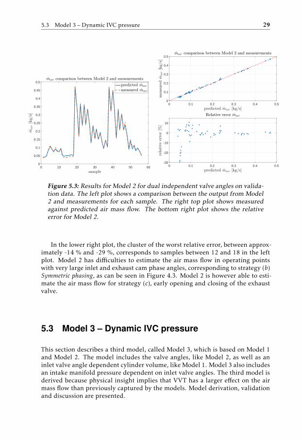
A comparison between Model 2 outputs and measurements of the air massflow is shown in Figure 5.3. The lower right plot shows relative errors for thepredicted air mass flow.

5.3 Model 3 – Dynamic IVC pressure 29

0 10 20 30 40 50 600

0.05

0.1

0.15

0.2

0.25

0.3

0.35

0.4

0.45

0.5

0 0.1 0.2 0.3 0.4 0.50

0.1

0.2

0.3

0.4

0.5

0 0.1 0.2 0.3 0.4 0.5-30

-20

-10

0

10


In the lower right plot, the cluster of the worst relative error, between approx-imately -14 % and -29 %, corresponds to samples between 12 and 18 in the leftplot. Model 2 has difficulties to estimate the air mass flow in operating pointswith very large inlet and exhaust cam phase angles, corresponding to strategy (b)Symmetric phasing, as can be seen in Figure 4.3. Model 2 is however able to esti-mate the air mass flow for strategy (c), early opening and closing of the exhaustvalve.

5.3 Model 3 – Dynamic IVC pressure

This section describes a third model, called Model 3, which is based on Model 1and Model 2. The model includes the valve angles, like Model 2, as well as aninlet valve angle dependent cylinder volume, like Model 1. Model 3 also includesan intake manifold pressure dependent on inlet valve angles. The third model isderived because physical insight implies that VVT has a larger effect on the airmass flow than previously captured by the models. Model derivation, validationand discussion are presented.


5.3.1 Modeling

The pressure in the intake manifold changes over one four-stroke cycle due to pul-sations caused by opening and closing of the valves. These pulsations are depen-dent on for example the engine speed. When variable valve timing is included,these pulsations vary even more, depending on the valve angles. Therefore themean intake manifold pressure, pim, which is a mean value of one whole cycle,has been replaced by a mean value over a small interval around IVC in Model 3.In Figure 5.4, the lower plot shows the pressure pulsations over one cycle and theblack circle corresponds to the pressure in the intake manifold at IVC.

-360 -270 -180 -90 0 90 180 270 3600

1

2

3

-360 -270 -180 -90 0 90 180 270 360

CAD

0

5

10

15IntakeExhaust(def)

-360 -270 -180 -90 0 90 180 270 3600.95

1

1.05

1.1

Figure 5.4: The upper plot shows the cylinder volume, Vcyl , during one cycleand the black circle corresponds to Vcyl at IVC. The middle plot shows theintake and exhaust valve lift during one cycle. The black circle in the lowerplot corresponds to the pressure in the intake manifold at IVC.

Model 3 is defined by

mair =pim,IV CNeVd,IV Cnc

120Rspec,airTim(c03 + c13

√pim,IV C + c23

√Ne + c33αi + c43αe), (5.3)

where pim,IV C and Vd,IV C are the intake manifold pressure and the displacedvolume at inlet valve closing, respectively.

5.3 Model 3 – Dynamic IVC pressure 31


The estimated parameters in Model 3 are c03, c13, c23, c33 and c43 in (5.3). Table5.3 shows the validation results for Model 3 when valve angles are dual indepen-dent. The model fit is good and the mean relative error is quite small.




Figure 5.5 shows a comparison between Model 3 outputs and measurementsof the air mass flow. The lower right plot shows relative errors for the predictedair mass flow.

0 10 20 30 40 50 600

0.05

0.1

0.15

0.2

0.25

0.3

0.35

0.4

0.45

0.5

0 0.1 0.2 0.3 0.4 0.50

0.1

0.2

0.3

0.4

0.5

0 0.1 0.2 0.3 0.4 0.5-40

-30

-20

-10

0

10



In the lower right plot, the cluster of the worst relative error, between -18 %and -35 %, corresponds to samples between 12 and 18 in the left plot. This modelshould be able to estimate the air mass flow better than Model 2, due to takingboth the intake manifold pressure as well as the displaced volume at IVC. How-ever, the model fit is slightly worse for Model 3 than for Model 2, even though itis marginal.

6Model 4 – Division into sub-models

Another approach to estimate the air mass flow, also studied by both Leroy et al.(2009) and by Thomasson et al. (2018), is to divide the estimation of the air massflow into several parts, each predicting different parts of the four-stroke cycle.Leroy et al. (2009) use physical models together with parameter estimation tomodel in-cylinder air mass on a spark ignition engine with only commercial sen-sors. Thomasson et al. (2018) use physical models together with in-cylinder pres-sure which is measured with a sensor not provided in commercial engines. Theapproach studied in Thomasson et al. (2018) is used as a reference to validatethe three sub-models derived in this work and is referred to when mentioning areference in Section 6.1 to Section 6.3.

By following the principles in Thomasson et al. (2018), the air mass flow esti-mation is divided into three terms. The first term models the total mass trappedin the cylinder at IVC. The second term describes the mass that flows through thevalves during the valve overlap. The third term estimates the total mass trappedin the cylinder at EVC. These three terms together describe the air mass in onecylinder as

mair = mIV C + mol −mEV C , (6.1)

where the direction of mol is defined positive if the mass flows from the intakemanifold to the exhaust manifold and negative if flowing from the exhaust mani-fold to the intake manifold.

The division is partly done because the inlet and exhaust cam phase anglesshould still affect the air mass flow more than previously modeled, i.e. more thanintake manifold pressure and displaced volume. Another benefit is in knowingeach of these masses individually. The mass trapped in the cylinder at IVC, mIV C ,influences combustion and engine out emissions. The masses mEV C and mol to-gether give the amount of residual gases that remain in the cylinder from the

33

34 6 Model 4 – Division into sub-models

previous cycle. These residual gases are important for, for example, after treat-ment, such as selective catalytic reduction (SCR) to reduce emission of nitrogenoxides (NOx) (Eriksson and Nielsen, 2014).

Conversion from air mass to air mass flow results in

mair =mairncNe

120. (6.2)

6.1 Total mass trapped in cylinder at IVC

The first term, mIV C , in (6.1) describes the total mass trapped in the cylinder atIVC. In the same way as the reference model is based on the ideal gas law togetherwith the volumetric efficiency to model the air mass that flows through the inletvalve, the total in-cylinder mass at IVC can be written as

mIV C =pim,IV CVIV CRspec,airTim

(c0 + c1√pim,IV C + c2

√Ne)︸︷︷︸

ηvol

, (6.3)

where VIV C is the cylinder volume at IVC (previously Vd,IV C has been used,which is the displaced volume at IVC). The parenthesis in (6.3) looks like (3.16),if changing pim,IV C to pim.

6.1.1 Assumptions

Depending on the cam phase angles, the ratio between residual gases and freshair in the cylinder changes. The model uses Rspec,air , and therefore assumes thatonly air is trapped in the cylinder at IVC. However, the specific gas constantsfor air and residual gases are almost the same and should not influence the es-timation that much. Because no sensors inside the cylinder are available, themodel assumes that, at IVC, the intake manifold pressure equals the in-cylinderpressure and that the intake manifold temperature equals the in-cylinder temper-ature. Because no CAD resolved temperature measurements are available, Tim isgiven as a mean value over one whole four-stroke cycle. Therefore, Tim will notcorrespond to the in-cylinder temperature at IVC.

6.1.2 Results

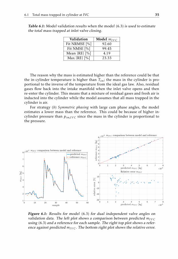
Table 6.1 shows the validation results when the model (6.3) is used to estimatethe mass trapped in the cylinder at IVC, with the estimated parameters c0, c1 andc2. The mean relative error is small and the model fit is good.

A comparison between the estimated in-cylinder mass at IVC using (6.3) andthe reference can be seen in Figure 6.1. The model has difficulties estimatingthe mass for strategy (c) Early exhaust. For this case, gases are pushed out intothe intake manifold from the cylinder when the inlet valve is open, and residualgases remain in the cylinder.

6.1 Total mass trapped in cylinder at IVC 35

Table 6.1: Model validation results when the model (6.3) is used to estimatethe total mass trapped at inlet valve closing.

Validation Model mIV CFit NRMSE [%] 92.60Fit NMSE [%] 99.45Mean |RE| [%] 4.19Max |RE| [%] 23.33

The reason why the mass is estimated higher than the reference could be thatthe in-cylinder temperature is higher than Tim; the mass in the cylinder is pro-portional to the inverse of the temperature from the ideal gas law. Also, residualgases flow back into the intake manifold when the inlet valve opens and thenre-enter the cylinder. This means that a mixture of residual gases and fresh air isinducted into the cylinder while the model assumes that all mass trapped in thecylinder is air.

For strategy (b) Symmetric phasing with large cam phase angles, the modelestimates a lower mass than the reference. This could be because of higher in-cylinder pressure than pim,IV C since the mass in the cylinder is proportional tothe pressure.

0 10 20 30 40 50 601

2

3

4

5

6

7

810-3

0 1 2 3 4 5 6 7 8

10-3

0

1

2

3

4

5

6

7

810-3

0 1 2 3 4 5 6 7 8

10-3

-30

-20

-10

0

10

Figure 6.1: Results for model (6.3) for dual independent valve angles onvalidation data. The left plot shows a comparison between predicted mIV Cusing (6.3) and a reference for each sample. The right top plot shows a refer-ence against predicted mIV C . The bottom right plot shows the relative error.


6.2 Mass flow during valve overlap

The second term in (6.1) predicts the mass that flows through the valves duringvalve overlap. The mass can flow either from the intake to the exhaust mani-fold or vice versa, depending on the pressure difference, and this term is definedpositive for the flow direction from the intake to the exhaust manifold.

The pressure difference is taken at the crankshaft angle where the intake andexhaust valve opening areas are equal, denoted IV = EV where IV is inlet valveand EV is exhaust valve. To describe the amount of mass that passes through thevalves during the overlap period an overlap factor (OF), defined in Section 6.2.1,is included in the model. The amount of mass transferred during the overlapperiod is also proportional to the inverse of the engine speed, Ne, because thisdescribes the time that the overlap is present. The model is thus given by

mol =

OFNe (c0 + c1(pim,(IV=EV ) − pem,(IV=EV ))) if pim > pem at IV=EV

−OFNe (c0 + c1(pim,(IV=EV ) − pem,(IV=EV ))) if pim < pem at IV=EV,(6.4)

where pim,(IV=EV ) and pem,(IV=EV ) are the pressures in the intake and exhaustmanifolds, at the CAD when intake and exhaust opening areas are equal, respec-tively.

6.2.1 Overlap factor

To describe the amount of mass that passes through the valves during the overlapperiod an overlap factor (OF) can be defined as in Leroy et al. (2009),

OF =

IV=EV∫IV O

Aintdθ +

EV C∫IV=EV

Aexhdθ, (6.5)

where Aint and Aexh are the areas under the valve area/crank angle curves, i.e.the effective opening areas of the intake and exhaust valves, respectively, see Fig-ure 6.2.

Figure 6.2: Valve overlap (Leroy et al., 2009).

6.2 Mass flow during valve overlap 37

The overlap factor is equal to zero if the exhaust valve closes before the inletvalve opens.

6.2.2 Assumptions and limitations

The assumption for this model is that the crank angle where the inlet and theexhaust opening areas are equal, IV = EV, is in the middle of IVO and EVC, ascan be seen in Figure 6.2. One limitation is that only measurements with flowfrom intake manifold to exhaust manifold were available in this work.

6.2.3 Results

Table 6.2 shows the validation of model mol in (6.4), with the estimated parame-ters c0 and c1. The mean relative error is not so small but the model fit is good.

Table 6.2: Model validation results when the model (6.4) is used to estimatethe mass transferred during valve overlap.

Validation Model molFit NRMSE [%] 92.53Fit NMSE [%] 99.44Mean |RE| [%] 10.38Max |RE| [%] 28.57

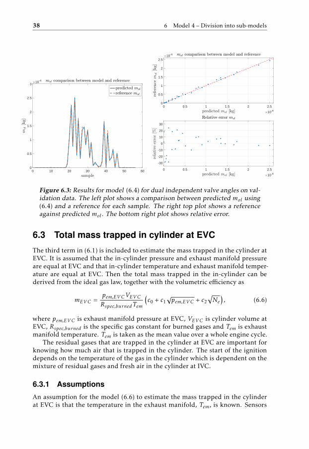
Figure 6.3 shows a comparison between the estimated mass, that flows throughthe valves during valve overlap using (6.4), and a reference. Note that the masstransferred during overlap is very small, a tenfold less than the mass trapped inthe cylinder at IVC. This should thus not influence the air mass estimation thatmuch. This model estimates the mass well over all. However, in the lower rightplot showing relative error, the error is large for very small masses.


0 10 20 30 40 50 600

0.5

1

1.5

2

2.5

310-4

0 0.5 1 1.5 2 2.5

10-4

0

0.5

1

1.5

2

2.510-4

0 0.5 1 1.5 2 2.5

10-4

-30

-20

-10

0

10

20

30

Figure 6.3: Results for model (6.4) for dual independent valve angles on val-idation data. The left plot shows a comparison between predicted mol using(6.4) and a reference for each sample. The right top plot shows a referenceagainst predicted mol . The bottom right plot shows relative error.

6.3 Total mass trapped in cylinder at EVC

The third term in (6.1) is included to estimate the mass trapped in the cylinder atEVC. It is assumed that the in-cylinder pressure and exhaust manifold pressureare equal at EVC and that in-cylinder temperature and exhaust manifold temper-ature are equal at EVC. Then the total mass trapped in the in-cylinder can bederived from the ideal gas law, together with the volumetric efficiency as

mEV C =pem,EV CVEV CRspec,burnedTem

(c0 + c1

√pem,EV C + c2

√Ne

), (6.6)

where pem,EV C is exhaust manifold pressure at EVC, VEV C is cylinder volume atEVC, Rspec,burned is the specific gas constant for burned gases and Tem is exhaustmanifold temperature. Tem is taken as the mean value over a whole engine cycle.

The residual gases that are trapped in the cylinder at EVC are important forknowing how much air that is trapped in the cylinder. The start of the ignitiondepends on the temperature of the gas in the cylinder which is dependent on themixture of residual gases and fresh air in the cylinder at IVC.

6.3.1 Assumptions

An assumption for the model (6.6) to estimate the mass trapped in the cylinderat EVC is that the temperature in the exhaust manifold, Tem, is known. Sensors

6.3 Total mass trapped in cylinder at EVC 39

measuring the exhaust temperature only exists in the test cell, not in commercialengines. To calculate Tem knowing the air mass flow is required (i.e. one of thereasons of this work and calculating Tem is a separate study). Furthermore, Temis given as a mean value over one four-stroke cycle and not at EVC.

Because Rspec,burned is a constant for burned gases, no consideration is takento that the mass trapped in the cylinder at EVC is not only burned gases. Inreality, the remaining gases after the compression stroke consists of both burnedgases and air. Also, in case of valve overlap and pim > pem, fresh air is injectedinto the cylinder before EVC, causing less burned gases in the cylinder.

6.3.2 Results

The estimated parameters for model mEV C in (6.6) are c0, c1 and c2 and table 6.3shows the validation results. The relative error is very large, both the mean andmax relative error. The model fit is not so good.

Table 6.3: Model validation results when the model (6.6) is used to estimatethe mass trapped in the cylinder at EVC.

Validation Model mEV CFit NRMSE [%] 78.43Fit NMSE [%] 95.35Mean |RE| [%] 19.10Max |RE| [%] 56.76

See Figure 6.4 for a comparison between the estimated mass using (6.6) that istrapped in the cylinder at EVC and a reference. Note that this mass is very small,a tenfold less than the mass trapped in the cylinder at IVC.

The model has difficulties to estimate the mass trapped in the cylinder at EVCin several parts. Mainly the estimation accuracy is poor for periods of valve over-lap. The model does not consider overlap, it assumes that all gases trapped inthe cylinder at EVC are burned gases. Because Tem comes from sensor measure-ments and is the mean value during one whole cycle this could be far from thetemperature in the cylinder at EVC.

Samples between 20 to 45 correspond to strategy (a) Valve overlap, where thebiggest overlap occurs from sample 20 to 30, where the estimation is worst. Thisshould be because more mass flows through the valves during the overlap in thisregion and therefore the model has difficulties in estimating the mass trapped atEVC.


0 10 20 30 40 50 600

1

2

3

4

5

6

7

8

910-4

0 1 2 3 4 5 6 7 8 9

10-4

0

1

2

3

4

5

6

7

8

910-4

0 1 2 3 4 5 6 7 8 9

10-4

-60

-40

-20

0

20

40

60

Figure 6.4: Results for model (6.6) for dual independent valve angles onvalidation data. The left plot shows a comparison between predicted mEV Cusing (6.6) and a reference for each sample. The right top plot shows a ref-erence against predicted mEV C . The bottom right plot shows relative error.

6.4 Results and discussion

In this section the validation of the air mass flow will be presented. This model,which comes from (6.1) and (6.2) containing the three sub-models from Section6.1 to 6.3, is called Model 4.

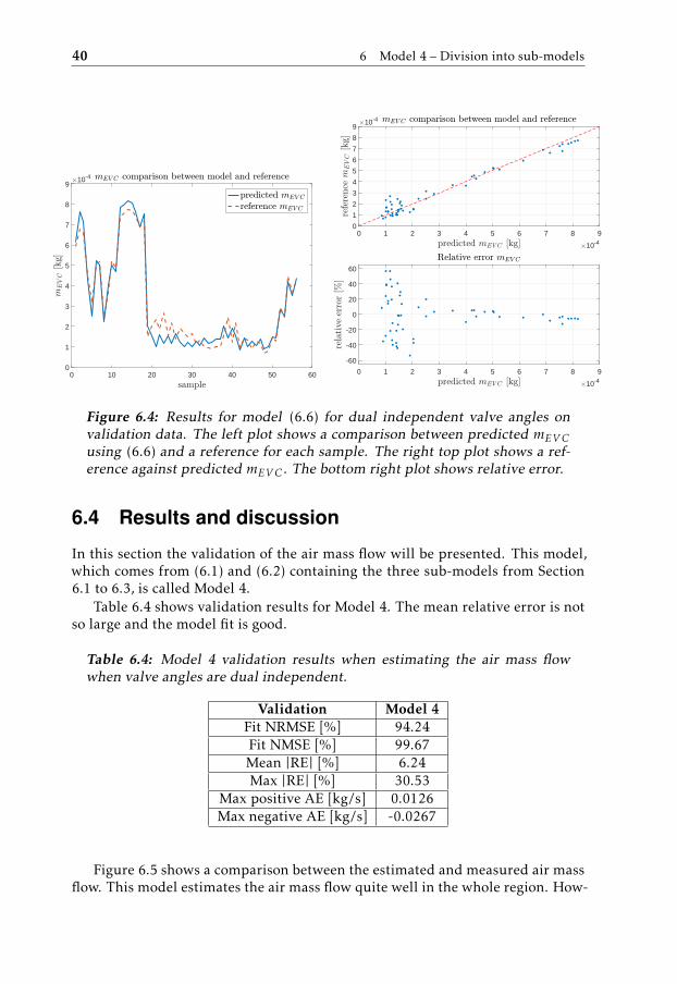
Table 6.4 shows validation results for Model 4. The mean relative error is notso large and the model fit is good.

Table 6.4: Model 4 validation results when estimating the air mass flowwhen valve angles are dual independent.



Figure 6.5 shows a comparison between the estimated and measured air massflow. This model estimates the air mass flow quite well in the whole region. How-

6.4 Results and discussion 41

ever, the validation results for Model 4 is almost equal to the validation resultsfor Model 2 and Model 3.

0 10 20 30 40 50 600

0.05

0.1

0.15

0.2

0.25

0.3

0.35

0.4

0.45

0.5

0 0.1 0.2 0.3 0.4 0.50

0.1

0.2

0.3

0.4

0.5

0 0.1 0.2 0.3 0.4 0.5

-30

-20

-10

0

10

20


Since the mass trapped in the cylinder at IVC is much larger than the massthat flows through the valves during overlap and the mass trapped in the cylinderat EVC, mIV C using (6.3) will have the largest influence on Model 4. ThereforeModel 4 overestimates the air mass flow from sample 1 to 11 corresponding tostrategy (c) Early exhaust and underestimates the air mass between sample 12 to18 corresponding to strategy (b) Symmetric phasing.

7Discussion and conclusions

This chapter includes a sensitivity analysis, a summarized discussion for all mod-els derived, and suggestions on how to proceed with the work on estimation ofthe air mass flow.

7.1 Sensitivity analysis

Opening and closing angles of the intake and exhaust valves, respectively, aredefined as an offset together with a valve clearance. For the intake valve, the valveclearance is defined as 0.45 mm and for the exhaust valve it is defined as 0.7 mm.The offset however, is defined differently depending on the manufacturer. In thisproject, the offset is set to 0.4 mm, from investigations looking at where the massflow into and out of the cylinder actually can be seen. However, a common valuefor the offset is 1 mm. The models that include signals with respect to valveclosing or opening will be affected due to that the offset gives different IVC, IVO,EVC and EVO. An investigation on Model 3 has been done, using the values ofthe parameters c03, c13 c23 c33 and c43 in (5.3) given by estimation data when theoffset is set to 0.4 mm. These parameters are then used with validation data withthe offsets 0.4 mm, 1 mm and 0.2 mm. In Model 3, both Vd,IV C and pim,IV C willbe affected. Table 7.1 shows validation results for offsets 0.4, 1 and 0.2 mm forModel 3. The results show that the model accuracy is dependent on the offsetvalue.

43

44 7 Discussion and conclusions

Table 7.1: Validation results for Model 3 for the offset values 0.4, 1 and 0.2mm.

fit NRMSE fit NMSE Mean |RE| Max |RE|Model 3 [%] [%] [%] [%]0.4 mm 94.41 99.69 6.38 35.281 mm 89.11 98.81 10.13 54.07

0.2 mm 92.37 99.42 6.75 27.09

7.2 Discussion

In this work, four different models have been derived, each with the goal to accu-rately estimate the air mass that flows through a diesel engine. Table 7.2 showsthe validation for all four models.

Table 7.2: Model validation results for all four models.

Validation Ref model Model 1 Model 2 Model 3 Model 4fit NRMSE [%] 78.83 84.96 95.07 94.41 94.24fit NMSE [%] 95.52 97.74 99.76 99.69 99.67

Mean |RE| [%] 25.73 18.20 5.25 6.38 6.24Max |RE| [%] 139 69.75 29.26 35.28 30.53

Max positive AE [kg/s] 0.0422 0.0304 0.0178 0.0184 0.0126Max negative AE [kg/s] -0.0521 -0.0333 -0.0110 -0.0136 -0.0267

All models seem to have most difficulty in estimating the air mass flow forstrategy (b) Symmetric phasing for very large inlet and exhaust cam phase angles.Model 1 also estimates strategy (c) Early exhaust very poorly and does not accu-rately model the dependency of the air mass flow on the cam phase angles. Hence,it is not enough to only know the volume of the engine cylinder at IVC. Model 2and 3 are however able to estimate the air mass flow for strategy (c).

Models 2 and 3 have a direct dependency on the inlet and exhaust cam phaseangles, which improves the estimation accuracy. In theory, Model 3 should esti-mate the air mass flow more accurately than Model 2, since it includes the cylin-der volume at IVC as well as the intake manifold pressure at IVC. In practice,however, Model 2 is slightly better. Model 4 should be able to estimate the airmass flow most accurately, given that each sub-model estimates its part well. Butas can be seen in Table 7.2 this is not the case.

Model 4 is based on more physical insight than the other models and it doesnot include a direct dependency on the inlet and exhaust cam phase angles result-ing in that the volumetric efficiency contains fewer parameters in Model 4 thanin Models 2 and 3.

7.2 Discussion 45

Models 1, 3 and 4, all include input signals that are dependent on a specificCAD. The CAD dependent signals are the manifold pressures and the cylindervolume since they are dependent on when the inlet and exhaust valves open andcloses. If a signal value is taken at the wrong CAD the value of the signal willbe wrong since it varies a lot over one four-stroke cycle. IVC and EVC for zerocam phasing are extracted from the valve profiles, i.e. the lift and duration. Ifthese values are wrong, then all volumes and pressures dependent on IVC orEVC will be wrong. One reason for this is if the valve duration in the engine doesnot equal the valve duration assumed when extracting IVC and EVC. Figure 7.1shows manifold and in-cylinder pressures. The circles show at which CAD thatthe intake manifold pressure value is taken. The diamonds show at which CADthat the exhaust manifold pressure value is taken.

-360 -270 -180 -90 0 90 180 270 3600.5

1

1.5

2

2.5

3

Figure 7.1: Manifold and in-cylinder pressures. The circles show at whichCAD that pim,IV C is taken and the diamonds show at which CAD thatpem,EV C is taken.

Looking at this plot, the cylinder pressures at IVC and EVC are much higherthan the manifold pressure, both for intake and exhaust. About 20 CAD beforeIVC and EVC, the intake manifold pressure and the exhaust manifold pressureare more close to the cylinder pressure. This can also be seen as the cylinder pres-sure increases before the circles and the diamonds, respectively, meaning that thevalve closes and the in-cylinder pressure rapidly increases.

46 7 Discussion and conclusions

7.3 Future work

There are several ways to continue with this work in the future. One issue todayis to know exactly when inlet valve opening and closing, as well as exhaust valveopening and closing, occurs. So in the future, more consideration should be putinto making these input signals more accurate in order for the models to betterestimate the air mass flow.

In this work, only measurements from one cylinder have been collected sincesensors have not been available for all cylinders. An assumption in this projectwas that the air mass flow was equally distributed over all cylinders. Since theyare implemented on a straight line, with different distance to the fresh air, forexample the intake manifold temperature will differ for each cylinder. One solu-tion is to have at least measurements from the cylinders closest to and furthestaway from the fresh air and assume a linear behavior between them, in order toget a more true distribution of the air mass flow for each cylinder.

When estimating the air mass that flows through the valves during the overlapperiod in Section 6.2.1, only data for the case where pim > pem were available.Measurements for pem > pim causing exhaust gas to be pushed out to the inletmanifold should also be studied.

Throughout this project only models linear in the parameters have been de-rived. In the future, non-linear models such as neural networks could be investi-gated.

7.4 Conclusions

The goal of this thesis has been to estimate the air mass flow through an enginewith variable valve timing. This has been done with physical insights combinedwith grey-box models where unknown parameters have been estimated from mea-surements. Throughout the work, only measurements from steady-state condi-tions have been used. One purpose has been to only use sensors in commercialvehicles which has been true for all models except one sub-model including thetemperature in the exhaust manifold. All models derived in this project havebeen based on the estimation approach in use today with fix cam phasing, whichis based on the ideal gas law together with a volumetric efficiency factor. It hasbeen seen that the best model fit occurs when only the inlet and exhaust camphase angles are directly included in the model. Further development to reachbetter estimation results with lower relative error is needed. However, for thework in this thesis, the models are estimating the air mass flow well enough touse as a base for further control. The best model fit presented in this thesis hasa mean absolute relative error of 5.25 % and a max absolute relative error of29.26 %. Comparing to existing methods with a mean and max absolute relativeerror of 25.73 % and 139 %, respectively, this is a big improvement. It has beenconcluded which parameters the air mass flow is dependent on. A major conclu-sion is how important it is to use input signals measured at the right CAD, sincethey vary during one four-stroke cycle. A constant volume and mean values of

7.4 Conclusions 47

pressure signals give more accurate estimates than if the signals are taken at thewrong CAD.

The models to develop further should therefore be Model 3, which includessignals taken at inlet valve closing, and Model 4, which includes signals at bothinlet valve and exhaust valve closing.

Bibliography

A. Akimoto, H. Itoh, and H. Suzuki. Development of Delta P method to opti-mize transient A/F-behavior in MPI Engine. JSAE Review, 10(4), 1989. Citedon page 2.

J. M. Desantes, J. Galindo, C. Guardiola, and V. Dolz. Air mass flow estimationin turbocharged diesel engines from in-cylinder pressure measurement. Ex-perimental Thermal and Fluid Science, 34(1):37–47, 2010. ISSN 0894-1777.Cited on page 2.

L. Eriksson and L. Nielsen. Modeling and Control of Engines and Drivelines.John Wiley & Sons, 2014. Cited on pages 6, 15, 17, and 34.

S. García-Nieto, J. Salcedo, M. Martínez, and D. Laurí. Air management in adiesel engine using fuzzy control techniques. Information Sciences, (179):3392–3409, 2009. Cited on page 1.

C. Gray. A Review of Variable Engine Valve Timing. SAE Technical Paper, 1988.ISSN 0148-7191. Cited on pages 1 and 2.

J. B. Heywood. Internal Combustion Engine Fundamentals. McGraw-Hill, Inc.,1988. Cited on page 5.

T. Leroy, G. Alix, J. Chauvin, and A. et al. Duparchy. Modeling Fresh Air Chargeand Residual Gas Fraction on a Dual Independent Variable Valve TimingSI Engine. SAE Int. J. Engines, 1(1):627–635, 2009. Cited on pages 2, 3, 33,and 36.

S. Nikkar. Estimation of In-cylinder Trapped Gas Mass and Composition. Dis-sertation, Linköping University, 2017. Cited on page 10.

A. G. Stefanopoulou, J. A. Cook, J. W. Grizzle, and J. S. Freudenberg. Control-Oriented Model of a Dual Equal Variable Cam Timing Spark Ignition En-gine. J. Dyn. Sys., Meas., Control, 120(2):257 – 266, 1998. Cited on page 3.

A. Thomasson, S. Nikkar, and E. Höckerdal. Cylinder Pressure Based Cylin-der Charge Estimation in Diesel Engines With Dual Independent Vari-able Valve Timing. SAE Int. J. Engines, 04 2018. ISSN 0148-7191. Citedon pages 2, 3, and 33.

49

50 Bibliography

J. Wahlström and L. Eriksson. Modeling diesel engines with a variable-geometry turbocharger and exhaust gas recirculation by optimization ofmodel parameters for capturing non-linear system dynamics. Proceedingsof the Institution of Mechanical Engineers, Part D, Journal of Automobile En-gineering, 225(7):960–986, 2011. Cited on page 2.

Estimation of Air Mass Flow in Engines with Variable Valve ...

Documents

Transcript of Estimation of Air Mass Flow in Engines with Variable Valve ...