
Spark ignition engine port air mass flow prediction using ...
220
UNIVERSITY OF TASMANIA SPARK IGNITION ENGINE PORT AIR MASS FLOW PREDICTION USING ARTIFICIAL NEURAL NETWORKS Nicholas Richard Jones BE (Hons) Mech Submitted in fulfilment of the requirements for the degree of Masters of Engineering Science (MEngSc) February 2003
-
Upload
khangminh22 -
Category
Documents
-
view
3 -
download
0
Transcript of Spark ignition engine port air mass flow prediction using ...

UNIVERSITY OF TASMANIA
SPARK IGNITION ENGINE PORT AIR MASS FLOW PREDICTION
USING
ARTIFICIAL NEURAL
NETWORKS
Nicholas Richard Jones
BE (Hons) Mech
Submitted in fulfilment of the requirements for the degree of Masters of Engineering Science (MEngSc)
February 2003

Declaration
DECLARATION & AUTHORITY OF ACCESS
This thesis contains no material that has been accepted for a degree or diploma by the
University of Tasmania or any other institution, except by way of background information
and has been duly acknowledged in the thesis, and to the best of the author's knowledge and
belief no material has been previously published or written by another person except where
due acknowledgment is made in the text of the thesis.
This thesis contains confidential information and is not to be disclosed or made available for
loan or copy without the expressed permission of the University of Tasmania (i). Once
released the thesis may be made available for loan and limited copying in accordance with the
Copyright Act 1968.
Inquires should be directed to the Research and Development Office.
Signed:
Dated this seventeen day of February 2003

Acknowledgments ii
ACKNOWLEDGMENTS
Firstly, I would like to thank my supervisor Associate Professor Vishy Karri for his guidance,
support and friendship throughout the completion of this project.
I thank the workshop staff for their patience, assistance and advice throughout the duration of
this project. In particular, I would like to thank Peter Seward for manufacturing and
constructing the various components of the inlet manifold. I would like to thank the electrical
technical staff for their assistance also.
I would like to extend my gratitude to the members of the 2001 & 2002 University of
Tasmania FSAE team. In particular David Butler, Garth Heron, Cranston Poison, Helen
Cunnignham, Robert Neben, Bent Rosenkilde and Nick Dwyer deserve a special mention for
their efforts in developing the 2001 car.
I owe a special debt of gratitude to Mr John White, Managing Director of Delta Hydraulics
and Hot White Racing, who kindly donated the use of his excellent chassis dynamometer. I
also wish to thank Mr David Griffards of Hot White Racing who provided assistance in using
the chassis dynamometer and advice in the experimental data collection. I also wish to thank
Cranston Poison and George Ivkovic for their help in the collection of the necessary
experimental data.
I wish to thank Cathy Sugden for tolerating my "unusual filing practices" in our shared room.
I also extend thanks to Tossapol Kiatcharoenpol for answering any questions I had relating to
ANN's in general and the associated ANN analysing software. I also wish to thank Oliver
Pechan for entertaining me with many interesting lunch time discussions.
Finally, I would like to thank my family, for their care, endless support and encouragement
throughout the completion of this project.

Abstract iii
ABSTRACT
In order to maintain the air fuel ratio within the stoichiometric operating window, which is
necessary for efficient catalytic converter operation an accurate estimation of the mass airflow
at the engine ports is critical. It is difficult to accurately represent the port air mass flow of an
Internal Combustion Spark Ignition engine as reciprocating engines are complex non-linear
systems based on a large number of interrelated parameters.
Conventional air fuel ratio control strategies use a number of three dimensional feedforward
look up tables to represent these complex nonlinear engine functions. These look up tables
are usually functions of only two engine variables, engine speed and engine load. Engine
load is either, calculated from the speed density relationship using an absolute manifold air
pressure sensor or measured directly using a mass air flow sensor. Conventional AFR control
algorithms perform poorly during transient conditions as the strategies inherent in look up
tables, are based on stationary or non-dynamic modelling techniques. Modern air fuel ratio
control strategies employ a large number of correction factors to compensate for transient
engine operation.
This research is a preliminary investigation into the feasibility of using Artificial Neural
Networks to represent transient nonlinear engine functions. This research develops offline
artificial neural network models of the port air mass flow of a Spark Ignition, based on
Hendricks' et al [1] accepted mean value engine model description of the manifold filling
phenomena. In particular two different Artificial Neural Network paradigms, namely the
Backpropagation algorithm and the fast converging Optimise Layer by Layer algorithm will
be trained on data collected through both steady state and transient chassis dynamometer
testing.
Both steady state and transient air mass flow models will be developed in this investigation.
The accuracy of the Backpropagation and Optimised Layer by Layer models will be analysed
both qualitatively and quantitatively and compared in terms of the Root Mean Squared
percentage error and computational time in an effort to evaluate the most appropriate model
for future online engine implementation.

Contents iv
CONTENTS
Declaration & Authority of Access
Acknowledgments II
Abstract
Contents IV
INTRODUCTION 1
2 LITERATURE SURVEY 6
2.1 INTRODUCTION TO INTERNAL COMBUSTION ENGINES 6 2.1.1 Major Components of the Reciprocating IC SI Engine 8 2.1.2 Special Terms Associated with the Reciprocating IC SI Engine 9 2.1.3 Operation of an IC SI Four Stroke Cycle Engine 10 2.1.4 Advantages of Multicylinder Engines 12 2.1.5 Combustion Formation in Spark Ignition Engines 13 2.1.6 An Introduction to Combustion Chemistry 16
2.2 AIR FUEL RATIO 18 2.2.1 Definition of Air Fuel Ratio 18 2.2.2 Definition of the Stoichiometric Air Fuel Ratio 18 2.2.3 Actual Air Fuel Ratio Relative to Stoichiometric Air Fuel Ratio 20 2.2.4 The Significance of Lambda and Air Fuel Equivalence Ratio Values 21 2.2.5 Actual SI Combustion Formation and Products 21 2.2.6 Cycle by Cycle Variations in Combustion 24
2.3 SI ENGINE PERFORMANCE 26 2.3.1 Factors that Effect SI Engine Performance 26 2.3.2 The Effect of the Air Fuel Ratio on Engine Performance 26 2.3.3 Engine Power, Fuel Consumption and Efficiency 27 2.3.4 Effect of AFR on Emissions Products 28
2.4 SELECTION OF THE APPROPRIATE AFR 30 2.4.1 Factors involved in AFR Selection 30
2.5 COMPONENTS USED IN AFR CONTROL 33 2.5.1 Conventual Hardware Used in AFR Control 33 2.5.2 Electronic Fuel Injection Systems 36 2.5.3 Major Components in Fuel Injection Systems 38 2.5.4 Engine Management 40 2.5.5 Lambda & Ignition Timing Control 41 2.5.6 ECU Corrections & Compensation Factors 44
2.6 CLOSED LOOP CONTROL OF FUEL INJECTION SYSTEMS & CATALYST EMISSION SYSTEMS 45
2.6.1 Closed Loop AFR Control 45 2.6.2 Three Way Catalytic Converter 47
2.7 DEVIATIONS IN THE AIR FUEL RATIO USING CONVENTIONAL ENGINE CONTROL 49

Contents
2.8 SUMMARY 52
3 MEAN VALUE ENGINE MODELLING & NEURAL NETWORK MODELS 53
3.1 ENGINE MODELLING 53 3.2 MEAN VALUE ENGINE MODELLING (MVEM) OF SI ENGINES 54
3.2.1 MVEM Time Scaling Relationships and State Variables 54 3.2.2 Fuel Flow Evaporation Dynamic Submodel 55 3.2.3 Manifold Filling Dynamics Submodel 57 3.2.4 Determination of the Air Mass Flow Rate through the Throttle 60 3.2.5 Determination of the Port Air Mass Flow Rate 62 3.2.6 Crankshaft Speed State Equation 64
3.3 COMPLEXITIES WITH CONVENTIONAL MEAN VALUE ENGINE MODELS 67 3.4 NEED FOR INTELLIGENT ENGINE MODELLING TECHNIQUES 70 3.5 THE ADVANTAGES & STRENGTHS OF ANN 73
3.5.1 Generality 73 3.5.2 Adaptively 74 3.5.3 Feature Selection 74 3.5.4 Tolerance 74 3.5.5 Imprecision 75 3.5.6 Self Programming 75
3.6 ANN APPLIED TO ENGINE MODELLING & ENGINE MANAGEMENT SYSTEMS 75 3.7 REVIEW OF THE NEURAL NETWORK ALGORITHMS USED IN THIS RESEARCH - BACK PROPAGATION NETWORK AND OPTIMISED LAYER BY LAYER NETWORK 83
3.7.1 Feedforward Networks 84 3.7.2 Backpropagation Network 85 3.7.3 Architecture 85 3.7.4 Backpropagation Learning Procedure 86 3.7.5 Backpropagation Training Algorithm 91 3.7.6 Optimised Layer by Layer Neural Network Learning Algorithm 92 3.7.7 Advantages of the OLL Network 94 3.7.8 OLL Learning Procedure 94 3.7.9 Optimised Layer By Layer Network Training Algorithm 97
3.8 SUMMARY 98
4 RESEARCH RATIONALE 99
4.1.1 Model Input Selection 100 4.1.2 Port Air Mass Flow Calculation 103 4.1.3 Significance of the Research in Enhancing AFR Control 104
4.2 SUMMARY 105
5 DESIGN & DEVELOPMENT OF EXPERIMENTAL TEST RIG 106
5.1 EXPERIMENTAL ENGINE 106 5.1.1 Custom Built Intake Manifold 108 5.1.2 Engine Management & Fuel Injection System 109
5.2 DATA ACQUISMON SYSTEM 111 5.3 SENSORS 113
5.3.1 Throttle Position Sensor 114 5.3.2 Manifold Air Pressure (MAP) & Manifold Temperature Sensors 114 5.3.3 Atmospheric Pressure Sensor 115 5.3.4 Throttle Air Mass Flow Rate & Throttle Temperature 115

Contents vi
5.3.5 Engine Speed 119 5.4 TESTING DYNAMOMETER 119 5.5 SUMMARY 121
6 CHAPTER 6 122
6.1 EXPERIMENTAL TESTING MATRIX 122 6.1.1 Sampling Rate 122 6.1.2 Calculation of the Port Air Mass Flow 123 6.1.3 Consideration of Accuracy in Port Air Mass flow Calculation 123 6.1.4 ANN Training & Testing Software 125 6.1.5 Definition of Error Evaluation Criteria Used in this Investigation 125 6.1.6 Process of Selecting Optimum ANN Architecture 126
6.2 STEADY STATE ENGINE PORT AIR MASS FLOW PREDICTION 127 6.2.1 Steady State Engine Data Collection 127 6.2.2 Steady State Data Parameter Conditioning 128 6.2.3 Prediction Using the Back Propagation Algorithm 129 6.2.4 Selection of Optimum Nehvork Architecture 131 6.2.5 Prediction Using OLL Algorithm 135 6.2.6 Selection of Optimum Network Architecture 137 6.2.7 Comparison of the Established BP & Developed OLL Steady State Models 140
6.3 TRANSIENT ENGINE OPERATION PORT AIR MASS FLOW PREDICTION 143 6.3.1 Transient State Engine Data Collection 144 6.3.2 Transient Data Parameter Conditioning 147 6.3.3 Throttle Position Derivative Model Importance Investigation 148 6.3.4 Number of Epochs Selected for Training 150 6.3.5 Selection of Optimum Network Architecture 151 6.3.6 Training Error Comparison of the Developed BP & OLL Transient Models 155 6.3.7 Testing Error Comparison of the Developed BP & OLL Transient Models 159
6.4 EVALUATION OF THE DEVELOPED DYNAMIC MODELS 163 6.4.1 Prediction Accuracy at Low Throttle Positions 163 6.4.2 Incorporating an Intelligent Model for Online Monitoring 165 6.4.3 Practical Application of the Transient Neural Network Model 167
6.5 CONCLUDING REMARKS 168
7 FINAL CONCLUDING REMARKS & PROPOSED FUTURE WORK 170
7.1 FUTURE WORK 173
REFERENCES 174
APPENDIX A: TRAINING BP & OLL MODEL OUTPUTS 181
APPENDIX B : TESTING BP & OLL MODEL OUTPUTS 182
APPENDIX C : BP & OLL MODELS PERCENTAGE ERROR AND DEVIATION VS THROTTLE POSITION GRAPHS 183
APPENDIX D : ENGINE SPECIFICATIONS 185
APPENDIX E : MOTEC M4 ECU SPECIFICATIONS 188
APPENDIX F : MOTEC ADL SPECIFICATIONS 193

Contents vii
APPENDIX G: SENSOR SPECIFICATIONS 196
APPENDIX H: DYNOMAX 450 4WD SPECIFICATION 208
APPENDIX I: NUMERICAL DIFFERENTIATION 212

Chapter One - Introduction Page 1
INTRODUCTION
In the 1950's the products of the engine combustion procesk were formally identified as
being a major source of urban air pollution. Consequently, governments around the world
began to implement exhaust gas emission legislation in an attempt to reduce automobile
generated air pollution. The advent of such legislation prompted automobile manufactures to
improve the designs of engine intake manifolds and fuel mixture systems in order to comply
with the new emission laws. Since the introduction of emission legislation four decades ago,
there have been significant improvements in the techniques used to deliver fuel to Internal
Combustion engines.
Successive amendments to the exhaust gas emission legislation have resulted in the continual
need for automotive manufactures to improve fuelling technology. In the late 1970's and
early 1980's emission legislation eventually reached a level where automotive manufactures
where no longer able to simply improve existing technologies and this encouraged research
and development into more reliable and accurate systems for controlling the air fuel ratio.
This meant the carburettor, which for so long had been used by automotive manufactures for
fuel-metering purposes could no longer be further improved to meet future emission
requirements. This led to the development of new fuel metering techniques and additional
hardware components to reduce harmful automotive emissions. The carburettor system was
replaced firstly by mechanical and then electronic fuel injection systems and catalytic
converters were developed to further reduce exhaust emissions. These advancements not
only reduced exhaust gas emissions but also had the added benefit of improving engine
power, enhancing drivability and decreasing engine fuel consumption.
Currently automobile emissions are regulated by using an electronic fuel injection system
using both feedforward and feedback control coupled with a three-way catalytic converter.
The typical feedback control arrangement uses a proportional integral term and the
information regarding the state of the air fuel ratio is supplied by an exhaust gas oxygen
sensor [2]. An electronic control unit controls the fuel injection timing, ignition timing and
load control through exhaust gas recirculation for emission management purposes.

Chapter One - Introduction Page 2
The critical device in this control arrangement is the catalytic converter as its emission
conversion efficiency is highly sensitive to excursions in the air fuel ratio and is maximum
only when a stoichiometric air_fue-i)ratiCAs used. Even a 1 % deviation in the air fuel ratio can ) cause up to a 50 % reduction in_the conversion efficiency of the catalytic converter in
reducing pollutants [3] [4]. Consequently, in order to maintain maximum operating
efficiency of the catalytic converter, precise control of the air fuel ratio is needed in all
driving conditions. Current air fuel ratio control strategies are able to meet these
requirenients only during steady state driving conditions as fuelling is primarily based on
feedforward look up tables which are developed from stationary experimental engine testing.
Correction factors are introduced into the control algorithm in an attempt to compensate for
transient driving conditions and currently this overall arrangement is sufficient to comply
with today's transient emission test cycles.
In reality current air fuel ratio control algorithms are unable to avoid large excursions in the
air fuel ratio during normal transient driving conditions. Research done by Rototest suggests
that the accelerations during normal driving conditions are far more rapid and severe than the
accelerations in the actual test cycles [5], [6]. Consequently real transient automotive
emissions for some exhaust gases are approximately ten times higher than what is reported in
the European test cycle [5], [6].
Many researchers have examined why AFR variations occur during transient driving
conditions [7] [8], [9], [10]. The main reason for the existence of AFR deviations is due to
the fact it is very difficult to accurately estimate the air flow at the actual engine cylinder
ports especially during transient operating conditions [11]. It is also difficult to place the fuel
in the intake manifold at the necessary location and at that instant [12]. This is because
during transient conditions the fuel injected does not equal the fuel flow into the cylinders of
the engine and the air mass flow either calculated or measured upstream of the throttle does
not correspond to the actual air mass flow inducted into the engine.
Future exhaust gas emission legislation will further reduce the tolerated levels of exhaust gas
pollution being emitted to the atmosphere. To illustrate this trend in 2003 the Californian
government will require 10 % of all new vehicles to be zero emission vehicles while the
remaining 90 % will have to reduce noxious emissions substantially [4], [13]. This trend is
also a concern for Australia as Australian emission standards for vehicles are generally based

Chapter One - Introduction Page 3
on obsolete European standards and U.S. emission legislation. Consequently, within the next
few years accurate air fuel ratio control will be required during both steady state and transient
driving conditions.
This can be achieved in one of three ways, by increasing the complexity of the existing
hardware that is used in the control system, by developing and designing new algorithms for
the control or a combination of both techniques. Up until now, automotive manufactures
have focused on improving the hardware side of the control problem, such as producing
sensors that are more sophisticated and implementing faster microprocessors for control
purposes. Over the past ten years, there have not been significant improvements made to the
actual algorithms used to control the fuel injection actuators. In order to comply with
increasing exhaust gas emission legislation requirements automotive manufactures have
simply incorporated additional look up tables to compensate for various dynamic effects.
Such an approach is labour intensive and expensive as the engine mapping process is based
on extensive engine dynamometer testing and associated complex engine tuning. The results
of this approach has seen only marginal improvements in air fuel control, sufficient only to
met new introduced emission legislation. Therefore there is a need for more sophisticated
and adaptive control algorithms than what is currently used in automobiles, that will not only
meet the requirements of future exhaust gas emission legislation, but will also have reduced
developmental times [14].
This study has been conducted as part of the "Intelligent Car Research Project" at the
University of Tasmania, which aims to investigate the feasibility of applying artificial
intelligent tools for potential automotive control applications. Previous research from this
project has primarily concerned the application of Artificial Neural Networks to chassis
parameter prediction [15], [16], [17].
This study is a preliminary investigation into developing nonlinear engine models using
artificial neural networks. Specifically a neural network port air mass flow engine model is
developed based on Hendricks' et al [1] first order differential port air mass flow
mathematical equation. The intention of this research is to determine the feasibility of using
neural networks as potential alternatives to engine look up tables, firstly by developing
stationary port air mass flow models and then developing transient port air mass flow engine
models. Two different types of feedforward neural networks architectures are applied in this

Chapter One - Introduction Page 4
research, namely the backpropagation algorithm and a fast converging optimised layer by
layer algorithm. The research entails developing offline artificial neural network engine
models using only chassis dynamometer collected data.
The inputs to the developed neural network models are based on those engine parameters
identified by Hendricks' et al [1] to model the air mass flow inducted into an engine. The rate
of change of throttle position is also included as a model input to provide representative
information on the rate of change of manifold pressure and hence compensate for the
manifold filling phenomena during transient testing conditions.
The performance of the individual ANN architectures in the estimation of the port air mass
flow is compared both qualitatively and quantitatively. Histograms are used to compare the
accuracy of the developed models and statistical techniques are used to determine if there is a
significant difference between the mean errors of the developed models. For each model, a
comprehensive investigation is carried out to determine the optimum model architecture.
This involves manipulating the number of nodes of each model over a suitable range in an
endeavour to find the optimum model, which has minimum Root Mean Squared (RMS)
prediction error, while at the same time having an acceptable model computational time. An
analysis is also undertaken to determine the number of training iterations that is required for
the convergence of model error. The overall aim of this investigation is to identify the most
appropriate model for future online learning and prediction purposes.
The following chapter of this thesis, Chapter Two, is a literature survey discussing the
fundamental operating principals of Internal Combustion Spark Ignition engines. This
chapter also describes the conventional techniques used for air fuel ratio and engine emission
control purposes. Chapter Three, is a review of Hendricks' [1] Mean Value Engine Models
(MVEM) and presents the potential advantages of applying Artificial Neural Networks to
nonlinear engine modelling. This chapter also provides a review of recent research that has
been published in the field of engine modelling using ANN and describes the features of the
Backpropagation and Optimised Layer by Layer network algorithms. Chapter Four, explains
the rationale behind this research, describes the selection of the model input parameters and
proposes the practical implications of this research. Chapter Five, gives a description of the
experimental test rig, which will be used in the collection of a reliable knowledge data base
for neural network testing and training. Chapter Six is a qualitative and quantitative analysis

Chapter One - Introduction Page 5
of the developed steady state and transient port mass air flow neural network models with the
intention of determining the most appropriate model for future online training and prediction
purposes. Chapter Seven provides the final concluding remarks of this research and provides
recommendations into possible future work.

Chapter Two— Literature Survey 6
2 LITERATURE SURVEY
The first section of this chapter discusses the fundamentals of Internal Combustion spark
Ignition engines. It introduces how and where Spark Ignition engines are used and the major
components of a Spark Ignition engine. This chapter describes the operation of the four-
stroke engine and briefly explains the combustion process. The concept of the air fuel ratio is
presented highlighting its significance in reliable engine operation, and its importance in
engine fuel consumption and power. The review also describes the conventional
technologies, strategies and specialised components used to deliver the fuel to the engine,
manage the exhaust gas emissions and maintain control of the air fuel ratio. The chapter
concludes by providing an explanation as to why conventional engine control strategies are
unable to avoid deviations in the air fuel ratio under particular driving conditions.
2.1 Introduction to Internal Combustion Engines
Combustion engines are designed to convert chemical energy contained within certain
substances into mechanical energy, by igniting the substance in the presence of air by some
means. The ignitable substance that contains the chemical energy is referred to as a fuel.
Automotive combustion is achieved by mixing some air with a small amount of fuel in a
enclosed space and igniting it to produce an "explosion" which releases an incredible amount
of energy in the form of hot expanding gases [18]. The increase in energy from the hot
expanding gases produces mechanical motion. At the completion of this energy conversion
process the gases are discharged to the atmosphere.
The most outstanding application of Internal Combustion (IC) engines is for transportation —
in automobiles, trucks and aeroplanes [19]. Small IC engines are used in many applications:
in the home (eg. lawn mowers, chain saws), in portable power generation, as outboard
motorboat engines and in motorbike engines [20]. Gas turbines can also be regarded as IC
engines, however the name is usually applied to reciprocating internal combustion engines
[21].

Chapter Two— Literature Survey 7
Reciprocating IC engines are typically used as the power generation facilities in cars, trucks,
buses and some trains. Reciprocating combustion engines consist of a piston that moves up
and down inside a special volume of space called the engine cylinder. The periodic linear
movement of the piston inside the engine cylinder generates an enclosed region of space with
a constantly changing volume. This region of space is called the combustion chamber and is
where the air fuel mixture is ignited and combustion takes place.
Internal Combustion (IC) engines are engines in which the combustion chamber is located
inside the actual boundaries of the engine. If the combustion chamber is foreign or lies
outside the boundaries of the engine, the engine is referred to as an External Combustion
(EC) engine. IC engines usually incorporate more than one combustion chamber in their
design and these types of engines are commonly referred to as multicylinder engines.
Reciprocating IC Engines may be subdivided into different categories in a number of ways
[22]. However the most general method of classification is according to their cycle of
operation (method of air charging) or by their combustion mode (method of ignition). There
are two cycles of operation, namely, the two-stroke cycle and the four-stroke cycle [23]. The
cycle of operation refers to how many strokes are required for the completion of one power
cycle.
There are two modes of combustion, namely, Spark Ignition (Si) and Compression Ignition
(Cl) [20]. SI engines use a device called a spark plug that generates an electric discharge in
the combustion chamber in order to ignite the air fuel mixture. In a CI engine the rise in
temperature and pressure during compression is sufficient to cause spontaneous ignition of
the fuel [24].
SI and CI engines use fuels with different combustion characteristics. Petrol also referred to
as gasoline is used in SI engine operation. Because of this SI engines are also commonly
referred to as petrol engines, gasoline or gas engines. Petrol fuels are designed to resist
combustion during piston compression (under conditions of increased pressure and
temperature) and are intended to combust only in the presence of an electric spark. Diesel
also known as fuel oil is used in the operation of CI engines. Diesel fuels are manufactured
so that they spontaneously combust in the high pressure and temperature environments
associated with piston compression.

Air (+ fuel)
Fuel
..- 'Products
Inlet valve I Exhaust valve
Piston
Connecting-rod
Crank case
Chapter Two— Literature Survey 8
Reciprocating Internal Combustion (IC) Spark Ignition (SI) four stroke cycle engines, are the
focus of this research and will be discussed in more detail below, beginning with a
description of the major components that make up an IC SI engine, special terms associated
with their use and how IC SI engines work.
2.1.1 Major Components of the Reciprocating IC SI Engine
The reciprocating internal combustion engine is composed of one or more combustion
chambers or cylinders inside which a single piston moves with reciprocating motion (upwards
and downwards). Each cylinder is fitted with a spark plug and a minimum of two valves, the
inlet valve and the exhaust valve. Each piston is independently attached to a shaft called a
crankshaft by means of a connecting rod. The connecting rod facilities the transmission of
the reciprocating motion of the piston into crankshaft rotary motion. Figure 2-1, below
depicts the general configuration of a single engine cylinder showing its major components.
Section 2.1.2 describes some special terms that are frequently used to describe reciprocating
IC SI engines.
Fuel injector/sparking plug
Crankshaft Sump
Figure 2-1 A four stroke IC SI engine, displaying important components [21]

Top dead centre 1
Stroke
Bottom I dead centre
Cylinder wall
Spark plug or fuel injector
Clearance volume
Reciprocating motion
Crank mechanism
Rotary motion
Chapter Two— Literature Survey 9
2.1.2 Special Terms Associated with the Reciprocating IC SI Engine
The diameter of the combustion chamber or cylinder of a reciprocating IC SI engine is
referred to as the bore. The term engine stroke is defined as the total distance the piston
travels between Top Dead Centre (TDC) and Bottom Dead Centre (BDC). TDC refers to the
piston position associated with minimum cylinder volume. This volume is called the
clearance volume. BDC refers to the piston position associated with maximum cylinder
volume. The compression ratio of an engine, usually denoted by r, is defined as the ratio of
maximum cylinder volume (piston at BDC) to minimum cylinder volume (piston at TDC).
The crankangle is measured from the vertical, in a clockwise direction to the point at which
the connecting rod is fixed to the crankshaft. TDC is equivalent to 0 crankangle degrees and
BTC is equivalent to 90 crankangle degrees. One revolution of the crankshaft equates to 360
crankangle degrees. These terms are labelled in Figure 2-2 below.
Figure 2-2 Nomenclature for reciprocating SI engine [18]

Chapter Two— Literature Survey 10
2.1.3 Operation of an IC SI Four Stroke Cycle Engine
SI engines convert chemical energy into mechanical energy by inducting a hydrocarbon fuel
and air mixture into the combustion chamber of the engine and igniting the mixture by an
electric discharge produced by a spark plug. The heat that is released from the combustion
reaction causes a large increase in the pressure within the cylinder, forcing the piston to move
downwards [25], In a four-stroke cycle engine this' process is achieved in four piston strokes.
The four-stroke engine cycle is also commonly referred to as the Otto Cycle after its inventor
Nicolaus Otto. Each cylinder requires four strokes of its piston — two revolutions of the
crankshaft or 720 cranlcangle degrees— to complete the sequence of events that produces one
power stroke [17]. The four-stroke cycle comprises of an induction stroke, compression
stroke, expansion or power stroke and an exhaust stroke. The execution of each stroke is
described below with reference to engine combustion chamber volume and engine piston and
valve movement.
The Induction Stroke
During this stroke the inlet valve is open and the piston travels down the cylinder to BDC
resulting in an increase in the volume of the combustion chamber. The rapid downward
motion of the piston creates a vacuum that draws (sucks) a pre-mixed air fuel mixture into the
combustion chamber.
The Compression Stroke
Both the inlet and exhaust valves are closed during this stroke and the piston inside the
cylinder travels upward to TDC. This piston movement reduces the volume of the
combustion chamber. The rapid upward motion of the piston compresses the air fuel mixture,
which increases the pressure and temperature of the air fuel mixture inside the combustion
chamber. At a certain angle before TDC, the compressed air fuel mixture is ignited by an
electric discharge from a spark plug.

Chapter Two— Literature Survey 11
The Expansion, Power or Working Stroke
The spark produced by the spark plug ignites the air fuel mixture contained within the
cylinder and combustion commences. The combustion reaction between the air and fuel
results in a rapid increase in the temperature and pressure inside the cylinder due to bonds
being broken and new compounds being formed. The increase in temperature and pressure
forces the piston downwards producing rotary motion of the crankshaft.
The Exhaust Stoke
After the combustion process has been completed the exhaust valve opens and the piston
travels upwards forcing the combustion products (the exhaust gases) from the cylinder
through the opening produced by the exhaust valve movement. The products of the
combustion process are forced into the exhaust manifold at high speeds, which discharges
them to the atmosphere.
Table 2-1 below summarises the four-stroke cycle with reference to the position of the intake
and exhaust valve, the movement of the piston and the onset of combustion.
STROKE INTAKE VALVE EXHAUST
VALVE
PISTON
MOVEMENT
COMBUSTION
Induction Open Closed Dowmvards None
Compression Closed Closed Upwards Ignition
Power Closed Closed Downwards Completed
Exhaust Closed Open Upwards None
Table 2-1 A summary of valve movement, piston movement and combustion in a four
cycle SI engine
Figure 2-3, below shows qualitatively the pressure-displacement variation of the combustion
chamber, for the four-stroke engine Cycle described above, with induction, compression,
power and exhaust strokes depicted on the diagram.

Exhaust valve closes
Co 0619 .
Exhaust
Exhaust valve opens
Intake valve closes
Intake
Chapter Two— Literature Survey 12
Top dead Bottom centre
dead centre Displacement
Figure 2-3 Pressure-displacement diagram for a reciprocating IC engine [18]
Section 2.1.4, below describes the advantages of multicylinder engines over single cylinder
engines.
2.1.4 Advantages of Multicylinder Engines
The basic operating principals of an IC SI engine have been described assuming an engine
comprised of a single cylinder (single combustion chamber) only. However, multicylinder
engines are by far the most common configurations of IC SI engines used in automobiles and
other transportation vehicles.
The main advantage of multicylinder engines compared with single cylinder engines is in
terms of improved engine balance, smoothness in operation and the advantage of smaller
engine cylinder volume required to produce the equivalent amount of power. This is mainly
due to a higher power stroke frequency in multicylinder engines, resulting in smoother torque
characteristics [17]. This is because multicylinder engines simultaneously have many
cylinders executing the four-stroke cycle of operation, which produces more power, more
power stokes per revolution of the crankshaft. The other major benefit is that the inertial
forces present from the accelerating and decelerating motion of the piston between TDC and

Chapter Two— Literature Survey 13
BDC can be balanced by running the pistons one stroke out of phase with each another.
Because of this reason even multiples (ie 2,4,6,8,10,12) engine cylinders are usually coupled
together.
The most common engine configurations used by the automotive industry are the four, six
and eight multicylinder engines. Four, six and eight cylinder engines produce two, three and
four power strokes also referred to as torque pulses respectively per engine revolution.
Multicylinder engine configurations can be arranged in a number of ways, including in-line,
V or flat [15]. These configurations will not be discussed here. Section 2.1.5, below presents
a basic overview of the combustion process in SI engines, describing normal and abnormal
combustion and some of the critical parameters that effect combustion quality and hence
torque generation.
2.1.5 Combustion Formation in Spark Ignition Engines
The combustion formation in spark ignition engines is complex and a complete and full
understanding of all the processes involved is still unknown. Therefore, only a simplified
description will be provided here.
Combustion in SI engines may occur in one of two ways, either normally or abnormally [21].
Normal or controlled combustion in SI engines is initiated by an electric discharge from a
spark plug near the conclusion of the compression stroke. The electric discharge is a single
high intensity spark of high temperature that passes from one electrode of the spark plug to
the other. The effect of this spark is that it leaves behind a small flame, in much literature
referred to as the flame nucleus [19], [21], [26] that propagates steadily throughout the entire
air fuel mixture enclosed in the combustion chamber until the entire air fuel mixture has been
consumed or burnt. The zone of active burning is known as the flame front which burns the
end gas [27]. The end gas is the unbumt air fuel mixture that is ahead of the flame front.

............ Flame front
Unburnt gas
2nd stage
1st stage
0 -120 -80 BTDC
0 40 810 120 TDC crankangle deg/ ATDC
A
-40
90
60
50
2 40
a) 3
12 30
20
10
Chapter Two— Literature Survey 14
Figure 2-4 Combustion in a SI engine [21] (7,
The normal combustion process is generally considered to develop in two distinct stages. The
first stage (AB) corresponds to the time of formation of the self propagating nucleus of the
flame and the second stage (BC) the propagation of the flame throughout the combustion
chamber [19]. Figure 2-5 below qualitatively shows the pressure-crank angle variation before
and after ignition, highlighting the combustion formation characteristics AB, BC described
above.
3000 rev/min Equivalence ratio 4)=1 . 0
Figure 2-5 Indicator diagram showing two stages of combustion in a SI engine [19]

Chapter Two— Literature Survey 15
Point C in Figure 2-5 above represents peak cylinder pressure and the completion of the flame
propagation phase of combustion. Turbulence that exists inside the combustion chamber due
to the reciprocating motion of the piston has a significant effect on the rate at which the
combustion reaction proceeds in both stages.
Abnormal combustion can occur in a number of different ways namely in the form of pre-
ignition and self-ignition. Pre-ignition occurs when the air fuel mixture makes contact with a
hot surface or body inside the engine cylinder and not initiated from the electrical discharge
of the sparkplug. Common hot surfaces that have been known to prompt ignition are the
exhaust valve(s) or products left over from previous combustion reactions usually in the form
carbon deposits. Self-ignition also known as knocking occurs when the pressure and
temperature inside the combustion chamber is sufficient to spontaneously ignite unburnt
regions of the air fuel mixture, this can occur before or after the firing of the spark plug. Pre-
ignition can lead to self-ignition and vice versa [21].
The firing time of spark plug is determined over a wide range of engine speeds and loads and
is usually set at a crank angle just before the occurrence of Maximum Brake Torque (MBT)
timing, the point at which mechanical power output from the engine is maximum. Figure 2-6
below shows that more advanced timing or retarded timing than the optimum value gives
lower power output [17].
24
26
32 Fixed: speed, throttle, air/fuel ratio
MBT timing
Knock
-
a
11
bmep lbw)
10
9
8
30
(%)
28
0 10 20
Ignition timing r btdc)
30
40
Figure 2-6 The effect of ignition timing on the output and efficiency of a spark ignition
engine [21]

Chapter Two— Literature Survey 16
Engine ignition timing is advanced slightly from the MBT timing as a precautionary measure
to allow for cycle to cycle variations, variation in manufacturing tolerances and engine aging.
This is known as the knock margin and is shown in Figure 2-6 above. This practice prevents
the likelihood of self-ignition or knock from occurring from engine to engine and during the
engine wearing process. Ignition timing effects the pressure and temperature development
inside the combustion chamber and is often varied to reduce the production of certain
emissions, especially NON, which forms because of high combustion temperatures. If the
ignition timing is too early then the work done by the piston in compressing the air fuel
mixture is reduced, but so is the work done on the piston during the expansion stroke [17],
[21]. If ignition timing is too late, it may not leave sufficient time for the completion of the
combustion reaction before the exhaust valve opens. This will result in the exhaust valve
becoming unnecessarily heated which is undesirable, as it may lead to pre-ignition of the air
fuel mixture on the surface of the hot exhaust valve during future engine cycles. If ignition is
too late there will be too much pressure rise before the end of the compression stroke and
power will be reduced [21].
As engine speed increases, the spark ignition timing is advanced to provide sufficient time for
the completion of the combustion reaction. That is at low speeds the ignition timing occurs at
a crankangle relatively close to TDC, while ignition timing at high speeds occurs at a more
advanced crankangle. Under normal driving conditions, the mixture is ignited around 15-30
degrees before the piston has reached TDC [28].
Ignition timing and the quality of the air fuel mixture influence many combustion
characteristics. In order to highlight the effect the air fuel mixture has on the combustion
process, it is necessary to look at the chemical reactions involved.
2.1.6 An Introduction to Combustion Chemistry
A description of the physical processes that occur inside the engine cylinder during
combustion formation was provided above. Combustion will now be looked at from a
chemical perspective. The combustion process is a chemical reaction in which chemical
energy stored within the reactants is released in order to produce motion. In all chemical
reactions bonds within the reactants are broken and atoms and electrons are rearranged to

Fuel
Air
Engine
Chen4a1 energkiii; the pet ol
aric oxygen
C onibustion)
Heat & EnerEtv build
up in the cylinders
Expansion of product gases
Figure 2-8 The conversion of chemical energy into mechanical energy
Chapter Two— Literature Survey 17
form products [18]. Oxygen and ignitable compounds called fuels are the reactants in
combustion reactions. The source of the oxygen is usually atmospheric air, consisting of
approximately 21% oxygen and 79% nitrogen on a molar basis. Automotive fuels are often
mixtures of hydrocarbons, with bonds between carbon atoms and between hydrogen and
carbon atoms [21]. Gasoline or petrol, used in the operation of SI engines, are mixtures of
paraffins, naphthenes and aromatics.
During the combustion process the hydrogen and carbon elements present in the fuel
chemically combine with oxygen to produce compounds ideally consisting of only carbon
dioxide water and nitrogen. This is shown below in Figure 2-7
Carbon dioxide
Water
Nitrogen
Figure 2-7 The theoretical combustion products for burning a hydrocarbon fuel [23]
During the formation of the new compounds, energy is released and this is apparent as a rise
in temperature and pressure (expansion) of the products. Figure 2-8 below shows the
conversion of chemical energy into mechanical energy. Due to this increase in temperature,
combustion reactions are referred to as exothermic reactions, reactions that transfer heat to
their surroundings.

Chapter Two— Literature Survey 18
The relative portions and quality of the reactants used in SI combustion, determines the types
and quantities of products formed and the quantity of energy released by the reaction. The
Air Fuel Ratio parameter is a convenient way in expressing the relative proportions of the
combustion reactants. This parameter will be defined below.
2.2 Air Fuel Ratio
2.2.1 Definition of Air Fuel Ratio
The Air Fuel Ratio (AFR) is defined as being the ratio of the air mass flow rate (ma) to the
fuel mass flow rate ( mf ) inducted into the engine for combustion purposes. Mathematically
this is expressed as:
Air/Fuel Ratio (AM) ma
Equation 2-1
2.2.2 Definition of the Stoichiometric Air Fuel Ratio
As mention above, IC engines generate power by relying on the energy that is released when
a mixture of air and a hydrocarbon fuel is ignited undergoing an exothermic chemical
reaction. The air fuel mixture before combustion and the burned products after combustion
are the actual working fluids of the energy conversion process [17]. The work transfer that
provides the desired power output occurs directly between these working fluids and the
mechanical components of the engine [17].
The stoichiometric AFR, is defined as the chemically correct or the theoretical proportions of
air and fuel that is required for the full conversion of all the fuel into completely oxidised
products [17]. This means that there is an optimum amount of air that can mix with a specific
hydrocarbon compound for the combustion reaction to completely bum all the carbon and

Chapter Two— Literature Survey 19
hydrogen, to produce reactants ideally consisting of only CO2, 1120, and N2. The air fuel ratio
can be determined from a balanced chemical equation for any hydrocarbon fuel that reacts
with air.
The chemical equations shown below describe this combustion process for a SI engine
between air (consisting of oxygen and nitrogen components, 02 + 3.773N 2) and a generally
represented hydrocarbon fuel (C aHb), assuming sufficient oxygen is available to completely
oxidise the hydrocarbon fuel.
b C b +(a +(O 2 + 3.773 N 2 )= aCO 2 -
bH 2 0 + 3.773 (a + —
b)N 2 + Energy
4 2 4
Equation 2-2
The stoichiometric AFR is therefore:
) (1+ 14 )(02 +3.772N,)
F s C +1.008y Equation 2-3
where y = —b a
Substituting the molecular weights of carbon (12.011), hydrogen (1.008), oxygen (32) and
nitrogen (28.16) into equation 2 above one obtains,
+ 1
(32 + 3.772 x 28.16) 4 Equation 2-4 12.011+1.008y
( A = 34.56(4 + y) ) s 12.011+1.008y
Equation 2-5
Equation 2-5, above is the generic relationship for the stoichiometric AFR for any
hydrocarbon (CaHb) fuel. The actual stoichiometric AFR depends on the type of the fuel

Chapter Two— Literature Survey 20
used, however for a SI engine (gasoline or petrol) it normally lies within the range of 14.4 to
14.7 [17]. The stoichiometric value also depends on the quality of the gasoline used [29].
The typical stoichiometric AFR value for gasoline is 14.6, however a value between 14.57-
14.7 is common to characterise the stoichiometric AFR value for petrol [17]. In this study a
value of 14.64 will be used to represent the stoichiometric AFR as this value was identified
by Falck et al [3] to be the AFR at which maximum conversion efficiency of the catalytic
converter occurs. The importance of the stoichiometric air fuel ratio on the efficiency of the
catalytic converter is discussed in detail in Section 2.6.2.
2.2.3 Actual Air Fuel Ratio Relative to Stoichiometric Air Fuel Ratio
The importance of the air fuel ratio on the combustion reaction, in particular regarding the
formation of fully oxidised products was described above. In the automotive industry a far
more informative parameter for defining mixture composition is the air fuel ratio that has
been normalised by the stoichiometric air fuel ratio for that particular fuel [17]. There are
two generally accepted methods in describing an engines actual AFR relative to the ideal
stoichiometric ratio. These are the Relative AFR also known as Lambda Ratio and the
Fuel/Air Equivalence Ratio. These two parameters will be defined below.
The relative AFR or lambda ratio ( 2) refers to the ratio between the actual AFR and
stoichiometric AFR (AFRs). Mathematically A is expressed as:
ma
f / actual (A F R ) actual A = . 14.64 ma
Lambda Value Equation 2-6
m ) s
The fuel air equivalence ratio is alternative way of describing the reactant mixture
composition relative to the air fuel ratio. The fuel/air equivalence ratio is symbolised by 0
and is simply the inverse or reciprocal of the lambda ratio, . Mathematically the fuel air
equivalence ratio is expressed as:

Chapter Two— Literature Survey 21
= 2-1 (FAR) aC!„al = (FAR)a„„al
(FAR) 5 (141.64)
Equation 2-7
The lambda ratio and equivalence ratio provide exactly the same information regarding the
fuel mixture composition relative to the stoichiometric mixture and both will be used
throughout this study. The significance of a using different lambda and equivalence ratio
values on engine performance will be described below.
2.2.4 The Significance of Lambda and Air Fuel Equivalence Ratio Values
A 2 ratio or 0 ratio of unity corresponds to the actual air fuel ratio mixture inducted into the
engine being equal to the ideal stoichiometric ratio. If the 2 ratio exceeds unity (0 ratio less
than unity) the mixture is referred to as being lean containing excess air in comparison to the
stoichiometric value (the actual air fuel ratio is greater than the typical value of 14.64). On
the other hand, if 2 is less than unity (0 ratio greater than unity) then the actual AFR is said
to be rich, which means the air fuel mixture composition is air deficient (the actual AFR that
is less than 14.64). The air/fuel mixture has to be close to stoichiometric (chemically correct)
for satisfactory spark ignition and flame propagation. [21]. The chemical compounds that are
actually produced as a result of automotive combustion will be described below, with
emphasis on those additional non oxidised compounds that are formed. Chemical and
physical reasons for the formation of these additional compounds will be presented,
highlighting those compounds that are regarded as pollutants.
2.2.5 Actual SI Combustion Formation and Products
The combustion process, so far, has been discussed from an ideal perspective based on
elementary combustion chemistry ignoring many of the complexities actually involved.
Combustion inside the engine cylinder is a result of a series of complicated and rapid
chemical reactions and the products that are formed depend on many factors [18]. In practical
engine operation it is impossible to control the combustion reaction to an extent to ensure that

H Carbon dioxide
Air
Water
Nitrogen
Carbon monoxide
Hydro-carbons
Nitrogen oxides
Particulate
Fuel 1
Engine
Chapter Two— Literature Survey 22
all combustion products are fully oxidised. This leads to the exhaust gas composition always
being a mixture of fully oxidised compounds and small traces of compounds that have not
been completely oxidised usually referred to as being pollutants. There are chemical and
physical explanations for this occurrence and these will be described below.
In Section 2.1.6 above, the theoretical products of the combustion were examined, namely
carbon dioxide, water and nitrogen, assuming complete combustion. During actual
combustion, the products differ from these theoretical results. Figure 2-9 below shows the
actual products of combustion including carbon dioxide, water nitrogen, and not fully
oxidised compounds consisting of carbon monoxide, nitric oxides, hydrocarbons and
particulate matter.
Figure 2-9 The actual products of hydrocarbon combustion [23]
The occurrence and reasons for the formation of these non-oxidised compounds will be
briefly explained below.
In practical engine operation the rate of formation of products from the reactants is retarded
by the rate of dissociation of the products back to the original reactants [19]. Energy is
released when combustion takes place due to oxygen atoms combining with carbon and
hydrogen atoms to form primarily carbon dioxide and water molecules. For a molecule to
break into atoms, an equivalent amount of energy must be consumed [30]. Dissociation
occurs when there is sufficient energy available to reverse the forward reaction ie break the
covalent bonds of the carbon dioxide and water molecules and return the molecules into other

Chapter Two— Literature Survey 23
not fully oxidised compounds. Dissociation reactions normally occur after ignition when
there is a sharp rise in temperature and pressure inside the combustion chamber. This
temperature rise is sufficient to provide what is called the molar heat of dissociation or bond
dissociation energy, which is required, for dissociation to proceed. The dissociation reactions
for carbon dioxide, water and oxygen are provided below for completeness.
CO +1/ 20, <=> CO, + energy
CO2 + H2 <=> CO ± H2 0 ± ener,D)
02 <=> 20+ energy
Equation 2-8
Equation 2-9
Equation 2-10
The sign <=> used in the above equations illustrates that the chemical equations can be
reversed if the required bond dissociation energy is available. At the onset of combustion the
above dissociation reactions proceed until equilibrium is reached and the final reaction
composition is a mixture of both the reactants and products of the above equations.
Dissociation ceases when the energy available is less than the bond dissociation energy. This
usually occurs during the expansion stroke when the temperature of the combustion products
decreases. Equilibrium thermodynamics is used to determine the degree of dissociation. The
dissociation process is in equilibrium when the Gibbs function is minimum. The existence of
dissociation during combustion, means that engine operation even with a stoichiometric AFR
ie 2 = 1, still results in combustion products containing small traces of non oxidised
products. Dissociation of carbon dioxide means that carbon monoxide will be present, even
for the combustion of weak mixtures [21].
Nitric oxides are generated, not as a result of the actual chemical combustion reaction, but as
a result of the environment that is created by the combustion reaction [17]. Nitric oxides,
generally represented by NO N, form after the onset of combustion in the high temperature
regions in the combustion chamber left behind by the flame front. The formation of nitric
oxides is due to the Zeldovich mechanism, a series of complex chemical reactions involving
oxygen and nitrogen. The formation rate of nitric oxides is dependent upon both flame
temperature and flame speed. High temperatures and low flame speeds result in maximum
nitric oxide formation. There are a number of methods used to reduce nitric oxide formation

Chapter Two— Literature Survey 24
in SI engines. One popular method is to employ Exhaust Gas Recirculation (EGR). This
involves mixing a fraction of the exhaust gases with the future inducted air fuel mixture. This
reduces the peak temperature inside the combustion chamber thus reducing the quantity of
nitric oxides produced.
Hydrocarbons are a product of combustion due to some of the fuel not being completely burnt
during the process. This may be due to some of the air fuel mixture entering crevices inside
the combustion chamber such as the small gaps that exists between the surface of the moving
piston and the surface of the engine cylinder. The combustion flame often fails to ignite the
fuel entrapped in these small spaces. The unbumt fuel is then emitted to the atmosphere
during the exhaust stroke. Another source is at the combustion chamber walls [17]. A
quench layer containing unburnt and partially burned air fuel mixture is left at the wall when
the flame is extinguished as it approaches the wall [17]. Engine oil deposited in a thin layer
on the cylinder wall is also believed to absorb some hydrocarbon matter during combustion,
which also avoids being burnt. Particulate matter has been reduced significantly since the
introduction of non-leaded fuel and is more a problem with the operation of compression
ignition engines.
Due to the random nature of the combustion process, the pressure developed inside the
combustion chamber after ignition varies from one cycle to the next. An explanation for this
phenomenon is presented below.
2.2.6 Cycle by Cycle Variations in Combustion
It has been assumed so far that a uniform air fuel mixture is ignited in the engine cylinder
from cycle to cycle. During practical engine operation a homogeneous air fuel mixture rarely
occurs even though engine components are designed to thoroughly mix the air fuel mixture.
This phenomenon can easily be verified by examining the pressure variations inside the
cylinder over a number of different engine cycles, shown in Figure 2-10 below.

Chapter Two— Literature Survey 25
Cycle 1
Cycle 2
— Cycle 3
— • — Cycle 4
—•• Cycle 5 2 30
r, 20
10
40
0 180
270 360
450
Crank angle
540
Figure 2-10 Cylinder pressure diagrams for successive cycles, illustrating the variations in
peak pressure [21]
The variations in peak pressure, shown above, are called cycle by cycle variations or cyclic
dispersion. Such variations exist due to turbulence within the cylinder varying from cycle to
cycle, the air fuel mixture not being homogenous and the exhaust gas recirculation not
completely mixing with the air fuel mixture charge [21]. Turbulence inside the engine
combustion chamber occurs in a random way, which results in different local air fuel
mixtures existing at the location of the spark plug from cycle to cycle. These mixture
variations significantly effect the flame nucleus formation stage of combustion resulting in
different rates of flame propagation throughout the mixture for successive cycles. In
multicylinder operation the mixture distribution flow rates to each cylinder is also not
uniform resulting in what is known as cylinder to cylinder variations.
The next section reviews how the AFR effects engine performance described in terms of
engine power, fuel economy, engine efficiency and the composition of the exhaust gas
emissions.

Chapter Two— Literature Survey 26
2.3 SI Engine Performance
2.3.1 Factors that Effect SI Engine Performance
Three major engine-operating variables are recognised in literature to govern the performance
of an IC SI engine. These are, spark timing, the proportion of recycled exhaust gases that
constitute the total amount of the inducted combustion mixture for the control of NO
emissions and in particular the lambda ratio or fuel equivalence ratio [17]. The importance of
spark timing on combustion formation was briefly covered in Section 2.1.5, and exhaust gas
recirculation was discussed above in Section 2.2.5. The effect of the air fuel ratio on engine
performance is the focus of the remaining part of this survey. Engine performance
comparisons are usually gauged by comparing engine-operating characteristic over a wide
range of engine loads and speeds. The engine operating parameters that are generally
investigated include different definitions of engine efficiency, engine torque or power, fuel
consumption and exhaust gas emission composition. The effect of the lambda ratio on engine
power, fuel efficiency and exhaust gas composition will be discussed in some detail below.
2.3.2 The Effect of the Air Fuel Ratio on Engine Performance
It has long been realised that the basic performance of any reciprocating engine is a function
of the air and fuel that flow through it. It has been shown that the air fuel mixture governs
engine power output, fuel conversion efficiency, fuel consumption, and the type and quantity
of exhaust gases emissions.
As mentioned in Section 2.2.4 above the air fuel ratio should be maintained as close as
possible to the stoichiometric value in order to guarantee consistent engine combustion and
therefore performance. However the combustion reaction, is able to proceed over a wide
range of AFR's above or below the stoichiometric value. Different AFR values are used in
engine operation depending on the desired engine performance criteria that is to be optimised.
Choosing different values of the AFR greatly effects the combustion reaction resulting in
changes in the amount of energy that is released and the types of emissions produced.
Generally there are three engine-operating characteristics that are optimised, either on an

Chapter Two— Literature Survey 27
individual basis or collectively depending on the application and use of the engine and
limitations imposed by various governmental authorities. These parameters are the engine
power output, engine fuel consumption and the permitted level of engine emissions.
2.3.3 Engine Power, Fuel Consumption and Efficiency
Maximum power in SI engine operation occurs when the air fuel mixture inducted into the
cylinders is slightly rich of stoichiometric. Peak power and maximum exhaust gas
temperatures usually occurs at a A value of approximately 0.90 (4) 1.1). Peak power occurs
at this point due to the chemical process known as dissociation described above in Section
2.2.5. The increase in temperature because of combustion causes dissociation to occur,
resulting in the presence of molecular oxygen in the combustion reactants. The available
oxygen present, from dissociation, allows a small amount of additional fuel to be added to the
air fuel mixture. This additional fuel undergoes combustion with the available oxygen
producing a greater temperature and pressure rise inside the cylinder resulting in increased
power. Engines operating with A values on either side of A 0.9 (4) 1.1) output less
power, this is shown below in Figure 2-11. Mixtures slightly rich of the stoichiometric
mixture produce peak power, however fuel consumption increases also.
SI engines operating with air fuel mixtures just lean of stoichiometric have lower fuel
consumption, produce less engine power and have lower exhaust gas temperatures in
comparison to mixtures just rich of stoichiometric. Running an engine on lean mixtures also
improves fuel conversion efficiency as a greater percentage of the fuels chemical energy is
converted to piston mechanical work and less energy is lost to the atmosphere as high
temperature exhaust gases. As the air fuel mixture becomes increasingly lean the resulting
quality of the combustion reaction decreases significantly. There exists a threshold lean
mixture value at which the air fuel mixture does not ignite resulting in combustion misfire. It
occurs as there is insufficient fuel mixed with the air for the combustion reaction to proceed.
Misfire should be avoided at all times as it has the potential to severely damage engine
components in particular the piston and the engine cylinder. Misfire normally occurs at a A
value greater than approximately 1.30 (4) 0.77), however this value depends on the design of
the engine in particular the combustion chamber geometry. Engine fuel consumption is

0.2 1 0
0.15
sfc (kg/raj) 0.1
0.05 Wide open throttle (WOT) . Constant speed
1.0 1.2 1.4 Rich
Equivalence ratio (0)
8
6
bmep (bar)
4
2
0.8 Lean
1.6 0 06
Chapter Two— Literature Survey 28
minimised when the Lambda ratio is equal to approximately 1.1 (4) 0.90). This is shown
below in Figure 2-11.
Figure 2-11 Response of specific fuel consumption (sfc) and power output to changes in
AFR [21]
2.3.4 Effect of AFR on Emissions Products
As mentioned above it is impossible for complete oxidation to occur even during
stoichiometric AFR engine operation due to chemical dissociation of carbon dioxide. A small
fraction of non-oxidised compounds are always present in the exhaust gases, which is
undesirable, as it is these exhaust gases that are the major contributors to urban air pollution.
The most common forms of these undesirable pollutants are carbon monoxide (CO), nitric
oxides (NO) and hydrocarbons (HC) in SI engine operation.
The lambda ratio is a critical factor that governs the composition of exhaust gas emissions
generated by SI engines and also the temperature of the exhaust gases. In Section 2.2.5 above
a brief explanation for the formation of these non-oxidised compounds was given, however
the significance of the air fuel ratio on their formation was not provided. This section

Chapter Two— Literature Survey 29
highlights the importance of the air fuel ratio on pollutant formation. Figure 2-12 below
shows the qualitative trends of NO, CO and HC pollutant formation with air fuel ratio
variation.
Volume (per cent) NOR , HC
Volume (per cent) CO, 02, H2
0.8 0.9 1.0 1 . 1 1 2 Lean Equivalence ratio, O R ich
Figure 2-12 Spark ignition engine emissions for different AFR [21]
Lower emissions occur during lean mixture operation, as the AFR is greater than the
stoichiometric value and there is additional air available for the complete combustion of all of
the fuel. Due to this reason during lean burn combustion a large percentage of the final
products are fully oxidised. The excess air present during combustion does not react and is
present in the exhaust gases as oxygen and nitrogen. Figure 2-12 above, shows that CO and
HC emissions are minimal during lean burn engine operation, until combustion quality
becomes poor (and eventually misfire occurs) and HC emissions rise sharply [17]. There
always exists some CO in the products due to dissociation. Lean mixture operation also
produces products at lower temperatures and consequently the dissociation of CO2 and H20
molecules is smaller in comparison to slightly rich mixtures (see Section 2.2.5 Equations 2-8
— 2-10).
If combustion occurs in a fuel rich environment or with an AFR less than the stoichiometric
value, there is insufficient oxygen to convert all of the hydrocarbon fuel into fully oxidised

Chapter Two— Literature Survey 30
products. As a result the reactants are composed of high levels of CO, HC, H2 which increase
nonlinearly with decreasing air fuel ratio or increasing equivalence ratio. Also during rich
mixture operation, (especially just rich of stoichiometric), the combustion products are at high
temperatures resulting in an increased rate of dissociation of CO2 and 14 20 molecules. The
rate of NO formation is dependent primarily on cylinder temperature and flame speed and as
a result maximum NO concentration occurs just lean of stoichiometric where there exists
sufficient oxygen and relatively high combustion temperatures. This can be seen above in
Figure 2-12.
Above it has been illustrated that the AFR has a significant effect on many engine
performance variables. Selecting the appropriate AFR to enhance or optimise, one specific
engine output parameter is often achieved at the detriment of others. For example increasing
engine power increases fuel consumption. The next section reviews the factors that are
considered when selecting the appropriate AFR for different engine operating conditions.
2.4 Selection of the Appropriate AFR
2.4.1 Factors involved in Ak It Selection
As demonstrated above, the lambda ratio or equivalence ratio plays a definitive role in the
determination of many engine performance criteria, including the power output, fuel
consumption and the composition of engine emissions. The concept of a theoretical AFR
(stoichiometric AFR value) has been introduced, illustrating its significance in terms of its
importance in governing exhaust gas emissions composition and ensuring correct combustion.
However, the optimum practical AFR for a spark ignition engines is that which gives the
required power output with the lowest fuel consumption, consistent with smooth and reliable
engine operation [17]. Power, low fuel consumption and reliable engine operation, in the past
were the only key parameters that were considered for the selection of an appropriate
operational AFR. Over the last four decades though, government imposed emission
legislation has often dictated the use of a different AFR than that which optimises power and
fuel consumption. Increasing government emission legislation has also required automotive
manufactures to develop techniques and hardware that further reduce emissions, normally at

Chapter Two— Literature Survey 31
the detriment of engine performance. Such techniques include Exhaust Gas Recirculation
(EGR), ignition timing delay and catalyst systems.
Additionally, what makes actual AFR selection difficult is that it is affected by the
operational conditions placed on the engine by the driver. That is the engine input is derived
from the drivers actions at the pedal. This is most conveniently measured in terms of the load
placed on the engine and the engines operating speed. The throttle position at any particular
time gives a good indication of the desired driving mode and therefore the response the driver
requires from the vehicle.
During automobile operation the driver commands a wide range of different types of driving
modes. The selection of the most appropriate AFR is crucial in these different driving modes
in order to satisfy driver power requirements, engine fuel efficiency and government exhaust
gas emission legislation. The selection of the ideal AFR in transportation vehicles is a
continual compromise between these three variables relative to the requirements of the driver.
The engine mixture composition is generally selected according to two engine-operating
conditions. These are at wide-open-throttle (WOT) or full engine load operation and part
throttle or part engine operation. During WOT operation the mass airflow inducted into the
engine is maximum due to the throttle valve being fully open. In such an instant the driver is
requesting a sharp increase in engine power. It is paramount during such operating conditions
that power output from the engine is maximum. Due to this, rich mixtures are used during
WOT operating conditions. At part load or part throttle engine operation drivers often require
less engine power (at a given speed) in comparison to WOT operation. Because of this
engine power is sacrificed and the efficient use of the fuel becomes more significant. To
increase the fuel efficiency of an engine, lean mixture operation is adopted, which is
advantageous as it reduces the quantity of generated pollutants making it easier to meet
exhaust gas emission legislation. Lean bum operation also improves the fuel conversion
efficiency of the engine as described briefly in Section 2.3.3 above.
Exhaust gas emission legislation has existed since the 1960's and regulates the types of
combustion products that are emitted to the atmosphere by automobiles. Due to this, lean or
stoichiometric mixtures are used over the majority of the working range of the engine. The
general approach taken by the automotive manufactures is to enrich the fuel mixture to just

A
Low yid High speed
No EGR
Eq
uiv
ale
nce
rat io y
b 12
14
16
18 20
100%
1.2
1.0
0.8
Chapter Two— Literature Survey 32
rich of stoichiometric when wide open throttle is approached to satisfy driver power
requirements and to use lean mixtures at lighter loads when fuel efficiency is more crucial.
Mixtures can be leaned out by either diluting the mixture with additional air or by recycling a
fraction of the exhaust gases (EGR) which reduces NO formation (see Section 2.2.5). The
percentage of EGR is normally zero at light loads, increases to a maximum at mid load and
decreases to zero as WOT is approached so maximum power can be obtained [17]. The
variation of EGR with respect to intake mass airflow rate is provided below in Figure 2-13.
t.4
20
100% Intake mass flow rate
Figure 2-13 Top diagram shows equivalence ratio variation with intake mass flow rate at
low, mid and high engine speeds. Bottom diagram shows EGR schedule as a
function of intake flow rate for low, mid and high speeds for stoichiometric
operation. [17] .
Approximately a decade after emission legislation was first introduced in the USA, a number
of new provisions were included to the legislation which meant that using a combination of
both ignition timing delay and EGR was no longer adequate in meeting the stricter legislation
requirements, without compromising reliable engine operation. The imposed stricter
legislation led to the development of catalyst systems and automobiles since have been fitted
with catalytic converters, devices which chemically convert the partially oxidised combustion
products into completely oxidised compounds before expelling them to the atmosphere. The

Chapter Two— Literature Survey 33
peak operating efficiency of the catalytic converter is strongly linked to the automobiles
working air fuel ratio. The relationship between the catalytic converters peak efficiency and
the AFR has now become the critical factor in the determination of an automobiles optimum
operational AFR. This will be described in more detail in Section 2.6.
Controlling the amount of air and fuel that enters the combustion chamber of an engine, that
is the AFR, is a challenging and complex task. The hardware that is used in MR control has
undergone significant changes within the last two decades. The carburettor, the standard fuel
metering device of the past, has been replaced by the more advanced Electronic Fuel Injection
(EFI) system in modem automobiles. The carburettor was replaced by EFI primarily because
of the need for improved AFR control due to the introduction of stricter emission standards.
Below the conventional hardware components involved in mixture preparation will be
discussed in some detail with special reference to EFI and engine management systems.
2.5 Components Used in AFR Control
2.5.1 Conventual Hardware Used in AIR Control
In SI engines the air and the fuel are usually mixed together in the intake system prior to entry
to the engine cylinder, using a carburettor or fuel injection system [17]. Before approximately
1980 the carburettor was the most common fuel-metering device used as the fuel managing
system in automobiles. The operation of the carburettor will be briefly described below for
completeness.
The carburettor is positioned upstream of the throttle plate of an automobile and incorporates
a converging diverging nozzle also known as a venturi in its design. As air is drawn into the
engine it passes through the venturi and the velocity of the air stream increases (satisfying the
continuity equation), until a maximum velocity is reached at throat of the venturi (the position
at which the cross sectional area of the venturi is minimum). The rise in air velocity
(dynamic pressure) at the throat of the venturi is offset by a decrease in the static pressure
(expansion) of the air stream in order to satisfy the Bernoulli equation.

Fuel in
Float valve
Float
Float chamber
Main jet orifice
Throttle valve
Venturi or choke
Venturi throat
Chapter Two— Literature Survey 34
The pressure differential that is set up between the carburettor inlet and the throat of the
nozzle is dependant upon the mass air flow rate passing through the venturi [21]. That is as
more air is inducted into the engine more fuel is also drawn into the carburettor. The pressure
difference causes a vacuum to exist between the throat and inlet, which is sufficient to draw
• an amount of fuel into the carburettor for that specific particular airflow rate. The fuel is
released into the throat of the venturi by the fuel discharge tube, which is connected to a fuel
reservoir which incorporates a float and needle valve assembly to ensure a constant level of
petrol in the float chamber [17].
Discharging the fuel at this position has two significant advantages in terms of the fuel
mixing with the air stream. The air attains maximum velocity at the venturi throat and this
promotes maximum fuel atomisation into the air and the minimum pressure at this point
promotes maximum fuel evaporation [21]. Mixing of the air and the fuel continues in the
intake manifold. Figure 2-14 depicts an elementary carburettor.
Air in
Figure 2-14 The layout of an elementary carburettor [21]
However, the major problem associated with the operation of the carburettor is that the
amount of fuel drawn in at the venturi is not proportional to the quantity of airflow inducted
into the engine at different operating engine speeds ie the AFR is constantly changing at
different engine speeds. To compensate for this either additional fuel or air is added to the
inducted air stream under certain driving conditions in order to maintain the required AFR.

Port Injection M P I
1970 1980 1990 2000
Carburettor
I'Direct Injection fGDIJ
Injector Injector
t
Iw
ill*144
Intake port lb.° Fuel Spray
Chapter Two— Literature Survey 35
A number of modifications have been made to the carburettor in an attempt to alleviate
fuelling problems, in an effort to provide improved accuracy in the control of the AFR during
different driving conditions. These modifications were necessary to minimise AFR
excursions and thus maintain reliable and smooth engine operation, to improvement engine
fuel consumption and to reduce exhaust gas emissions. Such modifications led to the
carburettor becoming an extremely complicated mechanism. Compensations were
implemented into the design of the carburettor for different driving modes and conditions
including at engine idle, accelerator and power enrichment and a chock mechanism for cold
starting [31].
However successive amendments to the emission standards, resulted in the carburettor
becoming obsolete in its application due to its inability to achieve the air fuel mixture control
demands required to pass emission legislation. Automotive manufactures developed fuel
injection, a new fuel supplying technique that provided improved air fuel mixture control in
comparison to the carburettor. Using fuel injection automotive manufactures were able to
satisfy the emission legislation requirements. Early fuel injection systems were controlled
mechanically, but the usual form of control is now electronic [21]. Figure 2-15 depicts the
transition from the carburettor to fuel injection systems.
Year
Figure 2-15 Transition of Fuel supply technologies from the carburettor to the fuel
injection systems [23]

Chapter Two— Literature Survey 36
The major components of the Electronic Fuel Injection (EFI) will be described below.
2.5.2 Electronic Fuel Injection Systems
Electronic fuel injection systems were first introduced approximately two decades ago and
today they have become the conventional fuel metering system adopted by automotive
manufactures. Fuel injection systems offer superior control of the air fuel mixture in
comparison to the carburettor technology, and therefore can provide increased reliability in
engine operation, improved fuel efficiency and compliance to current emission standards.
The basic operating principal of the fuel injection system is that if petrol is supplied to an
injector at a constant pressure then the amount of fuel injected will be directly proportional to
the injector open time [23]. Thus, fuel calculations can be performed based on fuel time
rather than fuel volume [30]
There are two main types of fuel injection systems, single point injection systems and
• multipoint injection systems. These two types of fuel injection systems are shown below in
Figure 2-16.

Engine
Air Air-flow meter
Manifold pressure sensor
Chapter Two— Literature Survey 37
Air C> Air-flow meter
Injector
Fuel metering Fuel
Figure 2-16 (a)
Manifold pressure sensor:cc _
--cCEI—CFCFC_
Fuel Fuel metering
Inject°
Engine
Figure 2-16 (b) --"VTC-CFCFC._
Figure 2-16 (a) depicts a single point fuel injection system, (b) depicts a multipoint fuel
injection system [23]
Single point fuel injection systems are composed of a single fuel injector that delivers fuel
upstream of the throttle into the inlet manifold. This system simply replaces the carburettor
with an electronic fuel injector. Multipoint fuel is a more complicated injection system
consisting of one fuel injector for every engine cylinder. Multipoint fuel injection systems
have become the standard fuel delivery systems used in modem automobiles as they provide
more accurate and quicker delivery of the fuel into the engine cylinders, hence engine
response is more rapid [32].

Fuel pump
Fuel rail
Pressure regulator
Fuel tank
41/1■
Fuel filter
Chapter Two— Literature Survey 38
2.5.3 Major Components in Fuel Injection Systems
Fuel injection systems consist of two sub systems, the fuel delivery system and the fuel
management system. The fuel delivery sub system consists of a fuel pump, fuel filter, fuel
rail, and one or more electromagnetic fuel injectors. The fuel control sub system consists of
number of engine sensors and a microprocessor. The microprocessor controls the fuel
injector opening time and thus controls the amount of fuel delivered to the individual engine
cylinders. -
Fuel is pumped from the fuel tank and passes through a fuel filter to the fuel rail. The main
components of the fuel delivery system are shown below in Figure 2-17.
Injectors Inlet Manifold
Figure 2-17 The main components in the fuel supply system [23]
Each fuel injector is essentially an electronically actuated valve [30]. When the fuel injector
is activated, an electromagnet moves a plunger that opens the valve allowing pressurised fuel
to squirt through a tinny nozzle [30]. The nozzle of a fuel injector is designed to atomise the
fuel and deliver it in the form of a fine misty spray on the back of the closed inlet valves. The
time the fuel injector is open is determined by the duration of the activation signal from the
ECU. At the commencement of the induction stroke fuel is drawn into the combustion
chamber and mixes with the inducted .air. The fuel pressure regulator maintains a constant
differential pressure of approximately 2.5 to 3 bar across each injector relative to the pressure

Chapter Two— Literature Survey 39
of the inlet manifold. A self-adjusting valve contained within the pressure regulator
compensates for fluctuations in the manifold air pressure.
Fuel injection systems are controlled by a microprocessor called an Electronic Control Unit
(ECU) also referred to as an engine management system. Figure 2-18 (below) shows a
simplified fuel injection and injection block diagram depicting the inputs to and outputs from
the ECU. Engine sensors provide information regarding the actual engine operating
conditions to the ECU. The most commonly used sensors include, a mass air flow sensor,
one or more oxygen or lambda sensors, a throttle position sensor, an engine temperature
sensor, voltage sensors, a manifold absolute pressure sensor and an engine speed sensor [30].
The information from these sensors is received by the ECU, which then controls the fuel
injector opening time thus metering the appropriate amount of fuel into the cylinders per
engine cycle.
Engine speed
Ignition
Engine load
ECU Engine
temperature
Fuel
Voltage
Figure 2-18 General block diagram of the inputs to the ECU and the controlled outputs of
the delivered fuel and ignition timing [23]
Multipoint fuel injection systems can delivery the fuel to the engine in one of two ways,
either simultaneously or sequentially. Simultaneous fuel injection involves the fuel injectors
firing or opening at the same time and delivering equal amounts of fuel to all cylinders.
Sequential injection system injects fuel on the induction stroke of each cylinder in the engine
firing order [23]. Figure 2-19 (below) compares the operation cycle of each method.

%, INI
360
Sequential petrol injection
Cyl. 1
Cyl. 2
Cyl. 3
Cy!. 4 r//.
• 0
Intake valve open
IQ Petrol injection
Ignition
Mil r44 / ,
720
Chapter Two— Literature Survey 40
Simultaneous petrol injection
CO 1 Si E7M Ni Cyl 2 ri; .1E S WI PP Cyl 3 Si Si "f#'1 r Cyl 4 W4 PE 11 r,M Pr
Figure 2-19 A comparison between simultaneous and sequential injection strategies [23]
A brief overview of the major physical components of the electronic fuel injection systems
was presented above. The following section defines the term engine management and
describes in more detail how these components are actually controlled.
2.5.4 Engine Management
"Engine Management is the science of equipping and calibrating an engine to achieve the
cleanest possible exhaust stream while maintaining top performance and fuel economy and
continuous diagnosing of system faults. However the focus on those priories often varies
around the world, reflecting differing government regulations, customer expectations and
driving conditions and a host of vehicle types and content levels." [33].
Engine management is performed by the ECU and its primary assignment is to furnish the
torque requested by driver while at the same time ensuring maximum fuel economy and
minimum emissions [17]. Modern engine management systems are responsible for the
control of a wide range of engine subsystems, including lambda control, ignition timing
control, dwell angle control, evaporative emission control, knock control, EGR control,
camshaft control, vehicle control including ABS, traction control and stability control etc.

Chapter Two— Literature Survey 41
The discussion below will be limited to lambda control and the ignition timing is
accomplished in a typical engine management system.
2.5.5 Lambda & Ignition Timing Control
In modern multipoint fuel injection systems AFR control is primarily achieved by controlling
both the engines fuelling and ignition requirements by receiving engine data from a variety of
sensors. The primary sensor inputs used by the ECU in the determination of the injector
opening time and ignition timing are the engine operating speed and engine load. As
mentioned in Section 2.4.1, above there are many factors governing the actual air fuel mixture
that is used during different engine operating conditions. The ideal engine air fuel mixture is
decided over a wide range of engine operating conditions and is represented as a function of
engine load and speed.
A complex non-linear relationship exists between the engine load, speed and the engine
fuelling requirements. In practice, the most convenient way in determining the non-linear
relationship is through non-dynamic map modelling [34]. This involves extensive stationary
experimental engine testing and tuning over a wide range of engine speeds and loads with the
use of engine dynamometer. This testing develops an engine characteristic map or schedule,
which graphically depicts the relationship between the fuel injector opening time for specific
engine load and speed values. The engine map represents the optimum air fuel mixture
schedule that satisfies the power and fuel economy demands of the driver, while at the same
time meeting exhaust gas emission standards and maintaining smooth and reliable engine
operation.
The engine map is represented as a three dimensional cartographic map as shown below in
Figure 2-20 and is stored in the read only memory of the ECU in the form of a look up table.

Chapter Two— Literature Survey 42
Figure 2-20 Cartographic map used to represent how information on an engine's fuelling
requirements are stored [23]
Either the base injection opening time or the desired lambda X value is located on the z-axis
depending on the method used in the determination of the engine load. Figure 2-18 above
shows that the lambda value or injection time is mapped as a function of both engine speed
and load. These quantities are labelled on the x-axis and y-axis and form a conventual two
dimensional grid. The ECU simultaneously reads in the data from the speed and load sensors
and then "looks up" the base injector opening or pulse width from the schedule map stored in
the ECU memory for those specific engine operating conditions. Look up tables such as
those used with fuel injection systems are referred to as a feedforward control structures that
operate in open loop control. It is often difficult to build an open loop controller that will be
suitably accurate under all conditions [32]. Due to this in modern automobiles, the open loop
control algorithm is supplemented by a feedback law using a signal from a lambda sensor to
improve overall control of the air fuel ratio [9]. This arrangement will be described in more
detail in Section 2.6.
Linear interpolation is used to determine the injection opening time when the signalled engine
speed and load inputs are between points in the engine map. The interpolation accuracy
therefore strongly depends on the complexity of the underlying grid and the degree of non-
linearity [35]. Where there is a high degree of non-linearity the grid should be more closely

Chapter Two— Literature Survey 43
meshed while in areas of smooth non-linear behaviour a small number of grid data may be
sufficient [33].
A non-dynamic modelling process is also undertaken to develop the nonlinear relationship
that exists between ignition timing and engine load and speed. Likewise extensive testing and
calibration during the design phase of the engine, is also required to map the spark advance
schedule [25]. This schedule is stored on the ECU in a look up table format and the desired
output is computed in a similar manner as that employed with fuel injection valve opening
time. Figure 2-21 below depicts a typical ignition timing engine map. Unlike the look up
tables for the injection timing, which are supplemented by feed back control, most spark
advance controllers today are simply open systems which measure a number of parameters
that affect the spark advance and compensate for their effects [25].
Advance degrees
45
40
35
30
25
20
15
10
5
Vacuum (bar)
Figure 2-21 The ignition timing map, as a function of engine speed and inlet manifold
pressure as used in engine management systems [21]
Compensation and correction factors are introduced by the ECU to improve overall engine
performance and reliability and these will be discussed in the following section.

Chapter Two— Literature Survey 44
2.5.6 ECU Corrections & Compensation Factors
The ECU computes the appropriate amount of fuel to be injected into the engine cylinder by
determining the current engine load, that is the amount of air that is drawn into the engine at
any given time. There are two basic methods used in determining the engine load and this
leads to two different types of electronic fuel injection control strategies [21]. There are those
that measure the load directly using a mass air flow meter and those that calculate it indirectly
using a manifold absolute pressure sensor. Mass Air Flow (MAF) systems are at present
nearly always realised using a hot wire or hot film sensors [36], [ 37]. Fuel injection systems
based on the latter are called speed density systems and rely on look up tables for the desired
lambda value and the steady state volumetric efficiency of an engine over a wide range of
operating conditions [12]. There are also Throttle-Density Systems, which are simply Speed-
Density systems that have been modified to use a throttle position sensor in the calculation of
the mass airflow rate [12].
Corrections need to be made to the base injector time determined from the engine load and
speed information. The first correction is for air temperature as the density of air changes
with temperature and the second is an allowance for the current driving condition represented
by the throttle position. The ECU depending on its complexity then compensates for after
start enrichment (choke), acceleration enrichment, weakening on deceleration, cut-off on
overrun, reinstatement of injection after cut-off, correction for battery voltage variation, just
to name a few [23]. These correction factors are stored on the ECU in the form of three-
dimensional nonlinear maps and encompass corrections for both fuelling requirements and
ignition timing and are normally a function of two of the following, engine cooling
temperature, manifold air pressure or rate of change of throttle position. A modem upper
class vehicle contains about fifty, three-dimensional maps to realise complex functions like
engine management and emission control [38]. The ECU determines the actual pulse width
by multiplying the base pulse width, determined from the main fuelling look up table by
applicable correction factors.
The compensation factors described above, adjust for different engine operating conditions by
referring to correction values contained in feedforward look up tables. Tightening of
emission legislation has meant feedforward compensation alone is insufficient in controlling

Chapter Two— Literature Survey 45
the AFR and meeting exhaust gas pollution levels. In response to this automotive
manufactures have been forced to develop other methods and new components to reduce
exhaust gas emission pollution levels. Today all automobiles supplement the feedforward
control strategy, described above, using close loop control using a feedback signal from a
lambda sensor complimented with the use of a catalytic converter. This approach has proved
significant in the reduction of pollution and will be described below.
2.6 Closed Loop Control of Fuel Injection Systems & Catalyst Emission
Systems
2.6.1 Closed Loop AFR Control
Current emission regulations have almost made mandatory closed loop control of the air fuel
mixture in conjunction with a three-way catalytic converter [23]. Present AFR control
technologies do not control the air fuel mixture of each engine cylinder but control the
average AFR of all cylinders [7] [39]. A typical feedback control, such as that used in AFR
control, has the feature that the output quantity (control variable) is measured and then
compared with a desired value, and the resulting error is used to correct the systems output
[40]. Fuel injection closed loop feedback control consists of a lambda sensor, which is
mounted downstream of the confluence point l in the exhaust manifold. It is not physically
possible to directly measure the AFR inside the combustion chamber instantaneously and
delays are introduced in the measurement due to time it takes the exhaust gases to reach the
mounting position of the sensor.
There are two types of lambda sensors used in feedback control applications. The switching
Exhaust Gas Oxygen (EGO) sensor, which tells the ECU if the air fuel mixture is rich or lean
of stoichiometric and the Universal Exhaust Gas Oxygen (UEGO) sensor which signals the
actual operating air fuel ratio value to the ECU. Both types of sensors are operational only
above a certain temperature range approximately 250-300 °C. Heaters are used to realise this
temperature during cold start operation and closed loop control is only initialised once this
where the individual emission collection pipes for each cylinder converge to form the single exhaust pipe

Chapter Two— Literature Survey 46
temperature has been reached. Before this time, the ECU uses open loop feedforward control
to regulate the AFR. The UEGO sensor is slowly replacing EGO sensors in modem
automobiles due to their ability to provide the actual AFR value [32].
Both these sensors measure the average AFR of all the engine cylinders by analysing the
composition of the exhaust gases. This information is then "fed back" as an input to the
ECU, which then regulates the engines operating AFR to the desired AFR using a
Proportional (P) or Proportional Integral (P1) controller during steady state and idle speed
control conditions [7], [36]. The P or PI controller adjusts the fuel pulse width by a small
amount in the direction that will bring the engines AFR towards the desired stoichiometric
value.
Using the feedback signal from a lambda sensor as the only means in controlling, the AFR is
not feasible as the sensor has a large 'sensing' time, due to the exhaust gas transport delay.
This is the time it takes the exhaust gases to reach the sensors mounting point in the exhaust
manifold. Thus lambda based feedback control compliments the feedforward look up table
control strategy described above. The main purpose of feedback control is to compensate for
variations from engine to engine, variations in fuel and changes due to engine wear and aging.
In modern vehicles, it is also used to adapt or update the engines fuelling map over time [41].
Corrections that are made to the fuel pulse width, because of feedback from the lambda
sensor is stored to the memory of some modern ECU's. The corrections are stored with
reference to the engine speed and load conditions at which the fuel adjustment was calculated.
This is advantageous as the data in the fuel look up tables is adjusted over time, meaning that
a smaller amount of correction is required the next time the engine experiences the same set
of operating conditions. A typical lambda feedback control system is shown below in Figure
2-22.
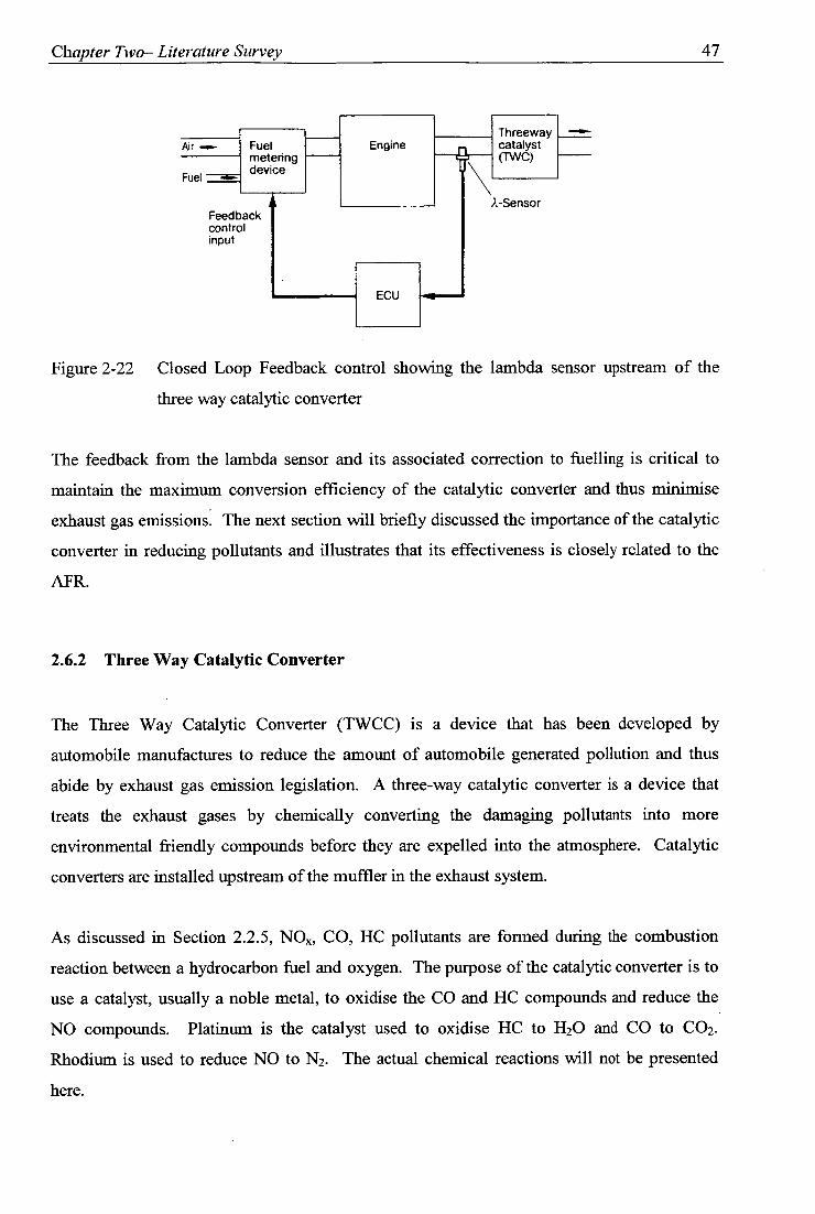
Chapter Two— Literature Survey 47
Threeway catalyst (TVVC)
■••111.-
Engine Fuel metering device
Fuel
A.-Sensor Feedback control input
ECU
Figure 2-22 Closed Loop Feedback control showing the lambda sensor upstream of the
three way catalytic converter
The feedback from the lambda sensor and its associated correction to fuelling is critical to
maintain the maximum conversion efficiency of the catalytic converter and thus minimise
exhaust gas emissions. The next section will briefly discussed the importance of the catalytic
converter in reducing pollutants and illustrates that its effectiveness is closely related to the
MR.
2.6.2 Three Way Catalytic Converter
The Three Way Catalytic Converter (TWCC) is a device that has been developed by
automobile manufactures to reduce the amount of automobile generated pollution and thus
abide by exhaust gas emission legislation. A three-way catalytic converter is a device that
treats the exhaust gases by chemically converting the damaging pollutants into more
environmental friendly compounds before they are expelled into the atmosphere. Catalytic
converters are installed upstream of the muffler in the exhaust system.
As discussed in Section 2.2.5, NON, CO, HC pollutants are formed during the combustion
reaction between a hydrocarbon fuel and oxygen. The purpose of the catalytic converter is to
use a catalyst, usually a noble metal, to oxidise the CO and HC compounds and reduce the
NO compounds. Platinum is the catalyst used to oxidise HC to 1120 and CO to CO 2 .
Rhodium is used to reduce NO to N2. The actual chemical reactions will not be presented
here.

it-Control Range (Catalytic Converter Window)
N 0 x
N 0
--- Prior to Catalyst — After Catalyst
CO
HC
Chapter Two— Literature Survey 48
The conversion efficiency of the TWCC is dependant upon two factors, the AFR and the
TWCC temperature. The ideal operating temperature of the TVVCC is about 400-800 °C [23].
During times of engine cold start, electrical heating elements are used to bring the TWCC to
the optimum temperature range and minimise the heating delay.
In order for the catalytic converter to operate at its highest efficiency for conversion of all the
three gases (HC, CO, NO,) the average AFR must be maintained within less than 1 percent of
stoichiometry [38]. This small operating range is known as the lambda operating window or
catalytic converter operating window [38]. This lambda window is usually defined for when
the catalytic converter is operating at an efficiency above 80 % [17]. Figure 2-23 below is a
graph of lambda (A) verses the exhaust gas emissions both before and after the catalytic
converter.
0,9 0,95 1,0 1,05 1,1 Lambda X
Figure 2-23 Lambda effect on exhaust- gas emissions prior to and after catalyst treatment
[38]
When the lambda ratio is equal to one the conversion efficiency is approximately 90%, which
represents the point at which the conversion of the three pollutants is maximum. Figure 2-23,
above illustrates that the conversion efficiency of the catalytic converter is highly dependent
upon the AFR. Research [3] has shown that even small deviations around the stoichiometric
value can result in a severe loss in the efficiency of the catalytic converter. Even a 1%

Chapter Two— Literature Survey 49
variation of the AFR may cause up to a 50% reduction in catalytic converter efficiency [3],
[4]. The next section reviews some of the reasons as to why conventual engine control
systems are unable to prevent deviations in the AFR around the stoichiometric value,
especially during transient engine operation, thus limiting the effectiveness of the catalytic
converter.
2.7 Deviations in the Air Fuel Ratio Using Conventional Engine Control
Conventional engine control technologies such as feedback loop control strategies are unable
to avoid large AFR excursions during transient engine operation, that is during periods of
engine acceleration, deceleration, and engine load variations [32]. Conventional AFR control
algorithms perform poorly during transient conditions as they are based on look up tables,
which are, developed by stationary or non-dynamic modelling techniques. Many researchers
have examined why AFR variations occur during transient driving conditions [26] [8], [9],
[10]. The main reason for MR deviations is due to the fact it is very difficult to accurately
estimate the airflow at the engine cylinder ports, especially during transient operating
conditions [11]. It is also difficult to place the fuel in the intake manifold at the necessary
location and at that instant [12]. This is because during transient conditions the fuel injected
does not equal the fuel flow into the cylinders of the engine and the air mass flow either
calculated or measured upstream of the throttle does not correspond to the actual air mass
flow inducted into the engine.
These two effects have been known for a long time and are called the wall-wetting
phenomenon and the manifold-filling phenomenon [32] respectively. The wall-wetting
phenomenon occurs when some of the injected fuel becomes deposited on the manifold wall
instead of entering the engine cylinders immediately. The manifold filling phenomenon
occurs during transient conditions when the port air mass flow and throttle air mass flow are
different because of the filling and emptying of the intake manifold volume. A number of
researchers have developed and revised mathematical models to try and compensate for these
two effects and these will be looked at in the next chapter.
Chapter Two— Literature Survey 50
Other factors that make it difficult to obtain tight control of the AFR in transient driving
conditions include engine pumping fluctuations, poor engine sensor response time and ECU
computational time delays. These factors will be briefly described below.
In the intake manifold, pressures and flows oscillate because of the periodic motion of the
piston and valves and these resulting variations are often referred to as pumping fluctuations
[42], [43]. The pumping fluctuations introduce noise into the Air Mass Flow Related signals
(AMFR) encompassing manifold air pressure sensors and mass air flow sensors. This sensor
noise is undesirable in the control of the AFR. Current fuelling strategies ignore this problem
and fail to condition the signals in an attempt to remove the fluctuating noisy component of
the sensor measurements [32]. Serious aliasing problems should be expected if no special
measures are taken during the sampling/processing of the AMFR measurements [32]. Some
researchers have proposed step moving average filters and extended Kalman Filters which
have built into them a priori dynamic description of the mean AMFR signals as well as a
statistical description of the noise in an attempt to remove the noise from AMFR sensor
signals [44].
Sensor response time also has a significant impact on the performance of AFR controllers
[32]. Hot wire Mass air flow meters (MAF) which are the most popular choice with
automotive companies can have a response time anywhere between 30 ms and 0.5 sec. This
is a relatively large response time in comparison to manifold absolute pressure sensors (MAP)
which has a response time of 1 ms [45]. Another problem associated with mass airflow
sensors is that they are unable to determine the air flow direction and therefore they can give
a false reading when engine back flow or flow reversal occurs. Engine back flow is caused
by engine pulsations due to the periodic motion of the pistons.
There is a significant transport delay associated with the readings from the Lambda sensor in
feedback AFR control strategies. This transport delay is known as the lambda feedback
control transport delay and exists because it takes time for the exhaust gases to travel from the
exhaust valve to the position of the oxygen sensor mounted in the exhaust manifold. Thus,
the readings from the lambda sensor actually provide delayed AFR information on previous
engine events rather than the current engine event. This phenomenon severely limits the
response time of the ECU controller [32]. It takes about 3 1/2 engine strokes before the burnt

Chapter Two— Literature Survey 51
exhaust gases enter the exhaust manifold and a further 2 to 20 ms before they reach the
lambda sensor [32].
AFR excursions are also apparent due to the time delay associated with the fuelling
calculation and the subsequent time needed to delivery the fuel into the engine cylinders.
This involves three separate time delays, computation duration, injection duration and start of
injection delay. Computation time delay is the time it takes for the ECU to determine the
appropriate amount of fuel that should be injected with the calculated or measured air mass
flow. This time delay is usually about 15 ms long [46]. Injection duration is the delay
associated with the injector actuation. This delay is usually between 2-15 ms long [32].
Start of injection delay (SOT) is the time that is required to wait until the the inlet valves are
fully closed before injection is initiated. The ECU delays injection until the hot inlet valves
are closed as this is the optimal moment for fuel injection as a greater proportion of the fuel
evaporates and enters the combustion chamber directly than in comparison to open valve
injection. The SOT delay varies continuously and can be equal in the worst case to 15 ms
[32].
The cumulative sum of all the time delays associated with fuel delivery described above can
total in the worst case over 100 ms or 0.1 sec [32]. Conventional AFR feedback control
strategies are adequate during steady state engine operation, however during transient
operation the time delays mentioned above result in large AFR excursions and poor TWC
efficiency. The time delays associated with fuel delivery become critical during transient
conditions, as during these periods there are two types of disturbances possible on the engine
which can not be immediately detected and which move the actual air mass flow inducted
into the engine away from the ECU estimated value. These disturbances are driver derived
and are observed as fast changes on the external load (torque) on the crankshaft (and
consequently a change in engine speed) and a change of throttle position (and consequently a
change in mass air flow) [32].
During realistic transient driving conditions, such as during peak hour traffic, the accelerator
(throttle angle) can be changed on a time scale as low as 50 ms to 100 ms [40]. This suggests
that in the worst case there can be as many as two movements of the accelerator pedal before
the injection of fuel. The ECU bases its fuel calculation on delayed sensor measurements and
delivers fuel based on previous engine events. During steady state, engine operation control

Chapter Two— Literature Survey 52
of the AFR is adequate, as there are no imposed changes on engine operation. However
during highly transient-driving conditions, the engine controller is always trying to "catch up"
to the drivers wishes and with the current technology this can only be achieved a short period
after the driver engages steady state engine operation. This is most evident in a tip in tip out
throttle actions. The value of the AFR as a result of this fast throttle action leans out and then
becomes rich due to the time delays associated with the controllers measurement, estimation
and delivery of the fuel. Conventual AFR controllers at present do not have the required
control bandwidth to be able to immediately detect and control the fuel delivery during the
minimum throttle rise time (50 ms) [32].
2.8 Summary
The above chapter has provided a comprehensive overview of the reciprocating SI engine. In
particular the review concentrated on the significance of the AFR and its effect on a number
of engine operating and performance characteristics. As highlighted above, current AFR
control strategies and additional components are unable to avoid deviations in the AFR during
transient conditions. As a result this has prompted a great deal of research into engine
modelling in order to develop mathematical descriptions of the physical fuelling problems.
The purpose of such analytical models is to compensate for dynamic air and fuelling effects
and thus maintain better control of the AFR. The purpose of the next chapter is to provide a
review of some of these models in particular describe the Mean Value Engine Model which
has become the prominent nonlinear engine model used extensively throughout automotive
research.

Chapter Three — Mean Value Engine Modelling & Neural Network Models 53
3 MEAN VALUE ENGINE MODELLING & NEURAL NETWORK MODELS
This chapter reviews the research that has been undertaken in the field of conventional
analytical engine modelling and describes the Mean Value Engine Model's (MVEM's) in
mathematical detail. The aim of analytical engine modelling is to represent the entire engine
plant in terms of mathematical expressions so that a better understanding of the processes
involved can be established and thus a greater degree of control can be gained over critical
engine operating variables such as the AFR. Linear engine models were the first to be
developed, however such models were too basic and idealistic in representing the complex
nonlinear nature of practical engine operation. Subsequently nonlinear models began to
emerge that were better suited to cope with the complexities and relationships involved in
'real world' engine operation.
Of these models one has become very popular with automotive researchers due to the high
accuracy in which it can characterise engine parameters. This is Hendrick's et a; [1] MVEM,
and is discussed in some detail below. The complexities associated with the implementation
of the MVEM's to real world conditions are raised, also the need for an alternative control
strategy to replace the shortly to be inadequate conventional models currently in use. A
review of recent research into the application of Artificial Neural Networks to SI engines is
also presented in this chapter. A detail description of the MVEM's is deemed necessary as a
large amount of Artificial Neural Network engine related research, is inspired by MVEM's
with a significant number of papers incorporating specific relationships directly into their
research.
3.1 Engine Modelling
(a ) In the 1970's, Hazell and Flower [47], were among the first to develop discrete engine models
[48] and since then there has been a large amount of research interest shown in the modelling
of engine processes. IC engines are highly nonlinear systems and as a result engine
modelling is a very complicated and difficult task involving a number of interrelated and
interdependent variables. In the late 1970's and early 1980's nonlinear dynamic engine
models started to emerge that were accurate over wide speed and load engine operating

Chapter Three — Mean Value Engine Modelling & Neural Network Models 54
ranges. At present there is one nonlinear dynamic engine model that has gained wide
accepted in literature, has proven accuracy and to be a good basis for engine design and
control [49]. This model was first presented by Hendricks and Sorenson in 1990 [1] and is
referred to as the Mean Value Engine Model (MVEM). Over the past decade this model has
been revised and optimised, increasing its accuracy in the prediction of engine parameters and
its capacity to be applied to a wider range of engine configurations. This model will be
described in some detail below and is based on the equations and description presented in [1],
[50], [51].
3.2 Mean Value Engine Modelling (MVEM) of SI Engines
The Mean Value Engine Models (MVEM's) are simplified dynamic engine models, which
are based on collections of physical models of the most important engine subsystems [1].
The MVEM developed by Hendricks and Sorenson [1] has been strongly influenced by work
presented by other researchers such as Rasmussen [52], Aquino [53], Hires and Overington ftl) n
[54], and Fozo [55]. MVEM's are intended to operate as predictors of the averages rather (S-. than cycle to cycle values of the most important engine states and variables [1].
The MVEM's consists of mathematical expressions of the three most important dynamic
subsystems, which describe the behaviour of the fuel mass flow, the intake manifold filling
dynamics and the acceleration of the crankshaft [48]. MVEM does not allow a distinction
between single cylinders or positions of the crankshaft, but a display of the dynamic
behaviour of interesting states [47]. Each of the engine subsytems, namely the fuel flow
evaporation model, the manifold filling dynamics model and the crankshaft dynamics model
will be individually described below on a mathematical basis.
3.2.1 MVEM Time Scaling Relationships and State Variables
MVEM's are composed of instantaneous and time developing analytical relationships.
Instantaneous relationships only take one or two engine cycles for equilibrium to be reached.
For time developing relationships, equilibrium is attained in 10 to 1000 engine cycles.
Instantaneous relationships are expressed as time independent algebraic equations while time

Chapter Three — Mean Value Engine Modelling &Neural Network Models 55
based differential equations are used to describe time developing relationships. State
variables are those which are determined by integrating the differential equations, which are
used to describe time developing relationships of the engine [1].
3.2.2 Fuel Flow Evaporation Dynamic Submodel
This model describes the path of the fuel from the injector into the combustion chamber. As
mentioned briefly in Section 2.7 not all of the injected fuel directly enters the combustion
chamber when the intake valve opens, this due to the wall wetting phenomena. When fuel is
injected into an engine, a fraction of the fuel vaporises (1 — ), mixes with the inducted air
and enters the combustion chamber directly. The remaining portion of the injected fuel (xi )
is deposited on the walls of the intake runners. This deposited fuel is referred to as the fuel
film. Mathematical expressions have been developed to describe the wall wetting
phenomena. The expressions below are based on monitoring the fuel mass entering the
cylinders and are based on the assumption that only fuel vapour enters the combustion
chamber, that is no liquid fuel directly enters the combustion chamber. The total mass of fuel
entering the engine is therefore equal to the fraction of the injected fuel that vaporises and
mixes with the air and the quantity of fuel that evaporates from the fuel film.
(
1 Mff = -
f
Xf Mfi Equation 3-1
Equation 3-2
Equation 3-3
M ft = - X f )111 fi
Mf = Mfr+ M ff
where, = is the fuel vapour mass flow
Mff = is the rate of change of the evaporating fuel film mass flow
Mf = is the total fuel mass flow that enters the combustion chambers
X,. = is the portion of fuel that is deposited on the walls of the intake runners
rf = is the evaporation time constant for the fuel film

Chapter Three — Mean Value Engine Modelling & Neural Network Models 56
The parameters rf , X are operating point dependent and thus the model is nonlinear in spite
of its linear form [49]. The parameters rf ,Xf can not be measured directly by any means
and are highly dependent upon the temperature of the inlet air, the temperature of the fuel and
the temperature of the manifold walls [56]. The variables r f , Xf are normally mapped for a
specific engine as a polynomial function of engine speed and the intake manifold pressure
over a wide range of operating temperatures and engine conditions. The parameter r1 has a
value generally in the range of 0.25-0.75 seconds while X1 has values within the range of
0.1 — 0.5 seconds, [57], [47], [48].
Other models have been developed that describe the wall wetting phenomenon. One of these
is the Aquino model [51], which is based on monitoring the fuel film mass deposited on the
intake rather than the mass of fuel. The Aquino model is also uses the parameters rf , Xf
which have the same physical meaning and function as in Hendricks' et al [1] model
presented above. With the correct mapping strategy for the parameters, Hendricks' et al [1]
MI/EM and the Aquino model provides more or less an equally good description of the fuel
flow dynamics [48].
The mathematical expressions that describe the fuel flow submodel are rarely used directly in
conventional engine control systems [49]. Transient Fuel Compensation (TFC) has been
developed which is based on the above expressions, with the aim to take into consideration
the wall-wetting phenomenon and adjust the fuel injected accordingly. That is fuel is either
added or subtracted from the base amount determined by the ECU in an attempt to cancel out
the dynamic effects of the fuel evaporating from and being deposited onto the intake manifold
runners. As a result of this compensation the fuel mass that actually enters the engine is
closer to the amount of fuel requested rather than a quantity less than or greater than the
desired amount.
The TFC mathematical expressions for Hendricks' et al [1] model for the fuel flow dynamics
are presented below.

Chapter Three — Mean Value Engine Modelling & Neural Network Models 57
t 1 Mfi = - Mff 1-1- Xf Mfi
f
1
Mfi (1- xf)(
mfi'
— mff
Equation 3-4
Equation 3-5
where, mfi = is the second rate of change of the projected fuel film mass
flow.
mff = is the rate of change of the projected fuel film mass flow
f = have the same meaning as above
A transient method of mapping the above parameters of the compensators is suggested in
[49].
3.2.3 Manifold Filling Dynamics Submodel
This model mathematically describes the path of air that is inducted into the engine. During
transient engine operation the mass flow rate at the throttle, which is normally used to
calculate the amount of fuel to inject, is not equivalent to the mass of air that actually enters
the engine cylinders known as the port air mass flow rate. This is because of the manifold
filling phenomena, which was introduced in Section 2.7 above. Figure 3-1 shows the effect
of the manifold filling phenomena for a tip in tip out throttle action, illustrating the difference
between the throttle air mass flow rate and the port air mass flow rate.
XI

Chapter Three — Mean Value Engine Modelling & Neural Network Models 58
70
air f
low
- k
g/s
0.06 —
0.05 —
0.04
0.03
0.02
0.01 -
port throttle
55 a§ 40 a 25 0 co
0 10
0 .
0.75 -0.5 5
0.25 f'3, 0 3
0 0.25 0.5 0.75 1 1.25 1.5 1.75 2 time - s
Figure 3-1
Tip in tip out throttle action and its effect on the throttle air mass flow rate and
the port air mass flow rate [2].
The mathematical model of the port air mass flow rate will be described below.
If the conservation of mass is applied to the intake manifold that is the volume of space
between the throttle plate and the engine valves one obtains,
Mat = Map+ Mam ±MEGR Equation 3-6
where, Mat =
m ap =
Manz =
M EGR =
air mass flow rate passed the throttle plate
air mass flow rate at the engine, which represents the actual
mass flow rate inducted into the engine
rate of change of the mass inside the intake manifold
exhaust gas recirculation mass flow rate
Assuming the contents inside the intake manifold obey the Perfect Gas Law and assuming the
pressure inside the manifold is uniform we can apply,

Chapter Three – Mean Value Engine Modelling & Neural Network Models 59
PM - PM RT m
p„, V„, =
Equation 3-7
as p —
V Equation 3-8
where, = Intake manifold air pressure
V„, = Volume of intake manifold
ma„, = Mass of air in intake manifold
R = Universal gas constant
Tm = Intake manifold air temperature
Taking derivative of Equation 3-8 with respect to time and assuming that the time derivative
Tm is negligible in comparison to the time derivative of p„„ one obtains
p mV„, —d
m dt dt amRT m
Equation 3-9
Equation 3-9 can be rearranged into the following form
• V m man, = p m
RT„, Equation 3-10
Equation 3-10 can be substituted into Equation 3-6 to obtain.
• • Vm • !nth = M ap p„,—+MEGR Equation 3-11
Equation 3-11 above is often expressed in the following form.
RTm m = , Mth 171 M EGR
V m aP
Equation 3-12
Thus the port air mass flow is a function of the following parameters.

Chapter Three — Mean Value Engine Modelling & Neural Network Models 60
m = f n aP a,T„„n, pm , M EGR Mth
The expression in equation 3-12 is referred to as the isothermal port air mass flow model and
has been derived on the basis of mass conservation assuming that the intake manifold
temperature is known instantaneously and is equal to the ambient and the EGR temperatures
[58]. It is assumed in the derivation of this equation that there is no heat transfer to the
surroundings and that the intake manifold temperature is uniform and constant [56]. In
practice the ambient, intake manifold and EGR temperatures are not equal. The EGR
temperature can easily approach 200 °C and the EGR flow can compose 25 % of the total
fluid flow entering an engine [48].
3.2.4 Determination of the Air Mass Flow Rate through the Throttle
The mass flow rate through the throttle into the intake manifold can be determined in one of
two ways. It can be measured directly using a mass air flow meter placed upstream of the
throttle plate to within an accuracy of less than or equal to 3 % or calculated assuming that
that the flow of the air through the throttle plate can be described as the flow of compressible
medium through a converging diverging nozzle or an orifice. The equations describing a
compressible medium through a converging diverging nozzle are presented below.
2 in at = C d Ath 1-0 1-1// Equation 3-13
RT0
where, C d = Discharge coefficient
Ath = Area at the throttle, which is expressed as nonlinear function of throttle
plate angle
The term C d Am is a nonlinear function of the throttle angle [58]

Equation 3-16
converging diverging nozzle
the mass airflow at the throttle
which have to be determined
• (a- p ) = in„,, m„, 1 (a) 102(P, ) 1- mai° Equation 3-17
Equation 3-18
Equation 3-19
Pa
= /-a 1 cos(a)-a I
Chapter Three— Mean Value Engine Modelling & Neural Network Models 61
( where, w = w /-2 is described by Po
k —1 Equation 3-14
( For pressure ratios below the critical pressure the ratio 11T-. is described by Po
A
P 2 rPo k +1 0.528 when k = 1.4 for air Equation 3-15
For choked flow max is described by
co max 2 )4+1 11 k k+1) k+1
Hendricks' et al [55] has modified the expressions of the
approach and proposes an alternative method for determining
plate. Hendricks' model is based on a number of constants,
experimentally and are specific to the experimental engin
presented below.
e. The model equations are

Chapter Three — Mean Value Engine Modelling & Neural Network Models 62
r il y
fl2( pr)= 1 Pr- P` 1 - p c
fl2( 1), ) = 1
II' Pr PC Equation 3-20
H' P r < pc. Equation 3-21
where man , mato , a l , ao , pc are constants and pc = 0.4125
Look up tables are employed for the expressions in equations 3-17, 3-18 in model based
engine controllers [50]
The modified isentropic converging diverging nozzle model presented above is too inaccurate
for actual use [32]. The reason for this is that the flow of the air splits along two paths across
the plate (one large dominant flow and one residual flow) [32]. Chevalier et al [59] has
presented a more accurate model to determine the mass air flow at the throttle plate, which
takes these factors into consideration, but will not be presented here.
Chevalier's model was shown to calculate the air mass flow rate to within an accuracy of less
than 3 % the actual flow over the entire operating range upto a p r 1 [32]. However errors
of 50 % where encountered at throttle angles above 77 degrees and unavoidable at wide-open
throttle operation or when p r approached 1. Errors in excess of 10 % of the actual air mass
flow rate were encountered at throttle angles of 40-60 degrees (p, 0.95-0.98) [32]. The
model presented by Chevalier is inappropriate for MVEM for conditions when pr is close to
1 [32]. This limits the application of the model to real world engine operating conditions as
throttle angles of and exceeding 40-60 degrees are commonly encountered during normal
driving conditions.
3.2.5 Determination of the Port Air Mass Flow Rate
The speed density equation, mathematically, presented in Equation 3-24, is used to calculate
the port air mass flow in many engine management systems. The speed density equation
(3s)

P,n
Chapter Three — Mean Value Engine Modelling & Neural Network Models 63
assumes the engine acts as an air pump and therefore is a function of the engine speed, engine
displacement and the engines volumetric efficiency, which is nonlinear parameter.
Volumetric efficiency is defined as the volume flow rate of air into the intake system divided
by the rate at which volume is displaced by the piston [17]. Engine cylinders do not get
completely charged or filled by air during the induction process due to dynamic losses in the
intake manifold, ports and the valve system [60].
120 m, 17= pV d n
Equation 3-22
where, map = is the port air mass flow rate which is actually inducted into the engine
Vd = is the displacement of the engine
n = is the engine speed (rpm)
p = is either the density of atmospheric air or the density of the air inside
the intake manifold
The volumetric efficiency of an engine is a dimensionless parameter, which measures the
effectiveness of the induction process of a specific engine [17].
The density of the air inside the intake manifold can be determined by applying the Perfect
Gas Equation, assuming the pressure inside the manifold is uniform.
Equation 3-23
Substituting Equation 3-23 into Equation 3-22 and rearranging for map one obtains the speed
density equation.
m . Vd n pm 17 al' 120 RT„,
Equation 3-24

Chapter Three— Mean Value Engine Modelling & Neural Network Models 64
Conventionally the nonlinear volumetric efficiency term in the speed density equation is
determined through extensive stationary engine testing over a wide range of engine speeds
and load conditions. Conventional engine controllers employ look up tables to determine the
volumetric efficiency usually in terms of engine speed and load information provided by
sensors.
Hendricks' et al prefers not to model the volumetric efficiency (77) directly but rather the
quantity ti p,.
P, = s,(0 P,+ Y,00 Equation 3-25
where si (n) and y, (n) are positive, weak functions of the crank shaft speed and y, » s i [48].
This expression holds for many engines and was derived physically in [48], [55].
3.2.6 Crankshaft Speed State Equation
The final MVEM describes the crankshaft dynamics. This model is derived using the
conservation of rotational energy on the crankshaft. Energy is transferred to the crankshaft by
the torque produced from the air fuel combustion reaction.
The rate of change of rotational kinetic energy of the crankshaft is equal to the actual power
that is available to accelerate the crankshaft [1]. The actual power that rotates the crankshaft
is equal to the torque (power) generated by the combustion reaction minus any frictional
torque losses that are present in mechanical couplings of the piston cylinder arrangement.
Pumping and friction losses dissipate the rotational kinetic energy and some of the available
energy goes into the load [I].
d ( — —In = in +p p + pl,)+ H„ • (t-A rd ) dt 2
1 2 , Equation 3-26
where, PI, Pp ,P1, = friction, pumping and load power losses
H,, fuel heating value

Chapter Three— Mean Value Engine Modelling & Neural Network Models 65
17, = indicated efficiency, a function of ( p,,n , A)
cylinder port fuel mass flow
t =
rd =
1 =
n =
time
mean injection/torque time delay
scaled moment of inertia of the engine
engine speed (rpm)
time rate of change of engine speed
Equation 3-29 can be arranged in terms of ii to obtain the Crankshaft Speed State Equation
/ 11= -
111
/ • r
p. id+ pp[pi . 1- 1d + pb[ n1/ 11;lpi , a A] — A ) I n n .
Equation 3-27
The rate of change of engine speed is a function of the following parameters.
n= "(p 11,,n,0,A,m f ) Equation 3-28
The frictional, pumping and load powers are given by regression equations derived from
well-known physical arguments as functions of p, ,n [56]. These equations along with the
functions developed for indicated efficiency can be found in [55]. The quantities
I,A T(,,ni f are given by the following expressions.
1 = 60 Equation 3-29
where, is the actual moment of inertia for a port injected engine
The mean injection/torque time delay can be approximated as the mean time delay between
mixture ignitions [I] and for a four cycle SI engine this is expressed as.

Chapter Three— Mean Value Engine Modelling & Neural Network Models 66
60 = — , ,)
A rd + — n
Equation 3-30
where, = is the number of engine cylinders
The rate of change of the crankshaft is governed by the amount of torque that is generated
which is dependant upon the fuel flow to the engine, which in turn is dependant upon the
desired operational air fuel ratio. By rearranging the lambda ratio equation, an expression can
be developed for the cylinder port fuel mass flow, ie.
Ades = ill lip Equation 3-31
l4.64 m1
Map
14.642.des Equation 3-32
Equation 3-32 assumes that there is ideal fuelling, assuming no transient fuel film
compensation. Ades is the desired operating lambda ratio for those particular operating
conditions. The cylinder port mass airflow in Equation 3-32, is calculated by rearranging
Equation 3- I .
The MVEM mathematical expressions presented above provide a good theoretical means to
describe and analyse the physical processes that occur during engine operation. However,
some of the mathematical functions of the MVEM are quite complex, as they are dependent
upon nonlinear parameters. The values of these nonlinear parameters can only be determined
by applying curve fitting techniques to highly accurate experimental engine data over a wide
range of engine operating conditions. The overall accuracy of the MVEM and the
complexities associated with their application to real world engine control implementation
will be the focus of the next section.

Chapter Three — Mean Value Engine Modelling & Neural Nehvork Models 67
3.3 Complexities with Conventional Mean Value Engine Models
The MVEM's presented by Hendricks' et al [1], use a number of differential equations to
describe the three major engine subsystems. The overall engine model has been validated
experimentally on a test bed comprising of a 1.1 Litre Ford Central Fuel Injection (CFI) SI
Engine in both static and transient engine testing conditions over the engines entire speed and
load ranges. The model has shown to estimate various engine state variables to within an
accuracy of 2 %, during both static and transient engine testing, which is comparable to the
accuracy of a typical engine dynamometer [1].
Although the model is very accurate, there are a number complexities involved with
MVEM's which have prevented them from totally replacing current look up table based
control strategies. One reason is because the many of the equations of the MVEM's are a
function of a number of nonlinear "fitting constants". In order to determine values for these
parameters and hence develop a valid MVEM, comprehensive engine testing and data
acquisition is required and thorough data analysis needs to be conducted involving regression
fitting. After this the model then has to undergo subsequent validation to see if the regression
fitting process is adequate and the model meets a desired level of estimation accuracy. If this
is not met, further engine testing is required to fully define conditions where estimation
accuracy is poor. This process must occur over a wide range of engine speeds, load
conditions and engine temperatures.
The estimation accuracy of Hendricks' MVEM's relies on extensive and time consuming
engine testing and detailed processing of the collected data, which often makes the approach
difficult to implement in some instances [6]. The equations of the various subsystems of the
MVEM are physically based and thus the model has to be "calibrated" to the specific engine
under investigation. The amount of engine testing which is used to calibrate or match/map
the MVEM to a specific engine greatly effects the performance of the model in terms of its
estimation accuracy. Using all the MVEM in a production engine controller would require a
human intensive, laborious and an exhaustive calibration process similar or greater than what
is currently required in the development of conventional engine fuel maps. The dominant
reason an extensive amount of engine testing is required is because the MVEM differential

Chapter Three — Mean Value Engine Modelling &Neural Network Models 68
equations are functions of nonlinear variables that vary strongly with engine operating
conditions.
Hendricks' intended to develop mathematical expressions of the MVEM that were based on
the least number of fitting constants where possible, while still ensuring a model that fully
described the engine subsystems and possessed high accuracy in the estimation of the engine
variables. The advantage of developing expressions based on minimum number of fitting
constants is that it reduces the complexity of the model calibration process. However, the
complex nature of the modelling problem requires the use of some fitting constants to
adequately describe the engine subsystems. Both the fuel flow evaporation dynamic
submodel and the crankshaft dynamic subsystem are strongly dependent upon fitting
constants.
The fuel flow evaporation dynamic submodel, which describes the path of fuel to the engine
combustion chamber is a function of a number of fitting constants, variables that can not be
measured or quantified directly. These nonlinear fitting constants include the parameter X
and the time constant r, which are described above in Section 3.2.2.
Practically it is not possible to directly measure the fuel film flow or the fuel vapour flow and
therefore the total amount of fuel that actually enters the engine cylinders. The parameters
X, r unlike many other nonlinear parameters such as volumetric efficiency of the model can
not be determined from steady state engine measurements. This means that the parameters
X, r can only be found using optimum fitting procedures by applying classical and advanced
statistical identification techniques based on the maximum likelihood [1]. Values for the
X ,r have to be determined over a wide range of engine operating conditions and are both
dependant on engine operating temperature. The X parameter is represented as a function of
the throttle position (X (a)) for a series of different operating points and specific engine
temperature using curve-fitting techniques.
Algebraic functions for the crankshaft dynamic submodel parameters, p f , Pp , Pb , 77, and for the
manifold filling dynamics parameters q„b„ma, are developed in terms of the engine state
variables from data collected from steady state engine measurements [1]. These parameters
are approximated as polynomial functions of one or more of the following variables, engine

Chapter Three — Mean Value Engine Modelling & Neural Network Models 69
speed, manifold and exhaust pressure and lambda ratio and rely on correction terms to
account for certain physical occurrences, such as engine pumping losses. The polynomial
coefficients are estimated by employing advanced curve fitting techniques using regression
analysis on data collected from engine measurements. A great effort is expended in finding
the physically correct regression variables before even attempting to make a regression fit [1].
Even once a regression fit has been obtained, more effort is necessary in testing the statistical
hypothesis that the correct and optimum number of regression terms are used and that the
functional representation used is minimal [1].
This fitting process and subsequent validation is time consuming as it is based on a model
optimisation process that seeks the most accurate model using "educated trial and error".
This process can become difficult, as there are a large number of parameters that have the
potential to be changed. Changing the degree or power of the curve fitted polynomial can
have a significant effect to the fitting performance of the mathematical function to the
collected experimental data. In addition, the polynomial expressions developed by the curve
fitting process can only be regarded as an approximation or an estimate of the modelled
engine parameters to within a certain accuracy range. The accuracy of these models will vary
over time due to engine wear and aging and model performance will also differ due to engine
manufacturing tolerances. The only way to update the algebraic functions over time is to
compensate for aging effects and this would require a similar engine testing and model
calibration process that was necessary in the development of the model in the first place.
It is unlikely that MVEM's will be implemented in their entire mathematical forms in modern
engine management systems. As a result it is unlikely that MVEM's will be able to
completely fill the void needed to meet the exhaust gas emission targets of the next decade.
Consequently, there is a need to find alternatives to the MVEM's or better ways of
representing them. Alternatives MVEM's should have the potential to accurately estimate
engine variables with a reduced amount of development time. The following section
highlights the inadequacies of convention AFR control systems and demonstrates a need for
research into potential alternative engine modelling techniques.

Chapter Three — Mean Value Engine Modelling & Neural Network Models 70
3.4 Need for Intelligent Engine Modelling Techniques
Precise control of the AFR is critical in modern engine operation for optimum engine
performance and for minium engine emissions [61]. If the automotive industry does not
develop additional methods and or strategies to improve AFR control it may encounter
problems meeting future exhaust gas emission legislation. Automotive manufactures must
not only abide by tightening government emission legislation but at the same time satisfy
consumer demands in providing a reliable engine that runs smoothly, has low fuel
consumption and delivers sufficient power [6].
Currently feedforward look up table control algorithms with a feedback signal provided by a
lambda sensor is used together with a catalytic converter in the control of the AFR and
automotive emissions. This technology is only able to obtain tight control of the AFR during
steady state engine operation as described in detail in Section 2.7. The aim of future fuel
injection control systems is to maintain tight control of the AFR ratio in all driving
conditions, both in steady state and transient engine operation. This is particularly important,
as the use of catalytic converters is compulsory in today's modern automobiles due to
successive amendments to the emission legislation. The catalytic converter is widely
regarded as the critical device that until now has maintained and regulated exhaust gas
emission levels below the targets set out in legislation.
The maximum efficiency of a catalytic converter is achieved only when the engine is
constantly operating at the stoichiometric AFR value as described in Section 2.6.2 (14.64) [3],
[4], [62]. The conversion efficiency is also very sensitive to changes in the AFR, as a ± 1 %
deviation from the stoichiometric AFR value may result in up to a 50 % reduction of the
efficiency of the catalytic converter in reducing pollutants [3], [4]. To minimise automotive
generated pollution it is therefore paramount that future fuel injection control systems can
precisely determine the correct amount of air entering the engine and hence be able to inject
the correct amount of fuel, in order to maintain the AFR to within this ± 1 % boundary of the
stoichiometric AFR in all driving conditions.
Until now the existing fuel injection systems have been able to control the AFR to a sufficient
level to meet current emission legislation and satisfy the demands of the consumer. Further

Chapter Three — Mean Value Engine Modelling & Neural Network Models 71
amendments to the exhaust gas emission legislation over the next few years will significantly
stretch the capabilities of the conventional control strategies in maintaining sufficient control
of the AFR. As an example the state of California in the USA, which has the strictest
emission legislation in the world, in 2003 will introduce legislation requiring 10 % of all
production vehicles to be zero emission vehicles [13], [60]. The remaining 90% of vehicles
manufactured will need to reduce their allowable levels of exhaust pollution by as much as
60-84% of current legislative values [13] [60].
The first signs of the inadequacy of conventional fuel injection systems in the control of the
AFR are already apparent with standard engine control technologies unable to avoid large
AFR excursions during transient operation as described in Section 2.7. Conventional AFR
control algorithms perform poorly during transient conditions as they are based on look up
tables, that are developed by non-dynamic modelling techniques.
To meet tightening emission legislation automotive manufactures have so far primarily
focussed on improving the hardware side of the fuel injection control system, by developing
more advance sensors of higher accuracy and lower response times, more precise fuel
injectors and implementing ECU's with faster microprocessors. Very little progress has
actually been made by automobile manufactures in developing and implementing totally new
techniques or algorithms of controlling the hardware of the fuel injection system. More
advanced AFR control systems have been published in literature, however automotive
manufactures as yet have not implemented these methods in full scale ECU production.
This is evident, as the control of most modern fuel injection systems are still based or rely
heavily on feedforward look up tables, the operating principals of which have basically
remained unchanged over the past decade or more. Hybrid engine controllers are now
emerging which are partially based on simplified MVEM's subsystems and look up tables.
This development has taken approximately a decade since the complete MVEM was first
published. However there are a number complexities involved with the MVEM's which
prevent them from being implemented in an engine management system in their entire form,
as the sole engine control algorithm. These were as described above in Section 3.2.
Until now, the increasing demands of emission legislation have been met simply by
approaching the control problem in a more comprehensive and detailed manner through the

Chapter Three — Mean Value Engine Modelling & Neural Network Models 72
introduction of a larger number of compensation factors that attempt to improve the poor
performance of modem engine controllers during transient engine operation. Additional
looks up tables are employed to reduce the effect of cold start operation, and different types
of transient throttle operation. The outcomes of this approach has resulted in a significant
increase in the amount of engine testing, tuning and calibration work necessary in the
development of additional compensation maps and as a result a large rise in the cost of engine
model development.
Legislation is also being introduced requiring maintenance of low emission levels over the
lifetime of a vehicle [59]. This is an additional challenge, as fuel injection systems are
developed for new engines and most are unable to adapt to the changing engine
characteristics over time [59]. Over the life of the engine the control system becomes
outdated as a result of engine wearing. Currently feedback control from a lambda sensor
compensates for age and wearing effects and for variations in engine to engine manufacturing
tolerances. However, feedback control is unable to correct AFR excursions during transient
operation due to the large time delay associated with its signal, as described in Section 2.6.1.
In order to achieve precise control of the AFR in all driving conditions a new "smarter"
control strategy is required, that is not simply a variation on the feedforward look up table
based strategy and thus is removed from the problems associated with such a control
algorithm. A more sophisticated approach is needed that is easily adaptable over the life of
the engine, the accuracy of which does not rely upon extensive and laborious engine testing
and which can provide accurate control during transient engine operation.
Artificial Intelligence, in the form of Artificial Neural Networks is one suitable alternative
that has the potential to totally replace the conventional look up table fuel injection control
systems and perhaps revolutionise AFR control. Neural Networks are ideally suited to such
an application due to their proven ability in capturing complex highly nonlinear relationships.
The major advantages of neural networks will be discussed below highlighting their
significant advantages over alternative control strategies.

Chapter Three — Mean Value Engine Modelling & Neural Network Models 73
3.5 The Advantages & Strengths of ANN
ANN have a number of significant advantages over conventional modelling techniques and
are ideally suited to engine modelling and control due to their proven ability to characterise
complex highly nonlinear systems with a high degree of accuracy. Neural networks offer a
different way to analyse data and to recognise patterns within data, than traditional computing
methods [63]. ANN have also been used in problem solving situations which were found to
be to difficult to handle by conventional control techniques, especially those which are hard
to characterise [64]
The main advantages of ANN over conventional modelling techniques, is in their capacity to
model nonlinear systems without relying on existing analytical relations between input and
output variables. Hence, the input variables to neural networks are not restricted to those for
which mathematical relationships already exist. Below is a summary of the major
characteristics of ANN's. The information presented here is primarily based on the ideas
presented in [62], where the advantages and strengths of ANN are discussed under the
following headings in some detail.
3.5.1 Generality
Neural networks are learning systems and their ability to model a process is dependent upon
the training data. A major strength of ANN's is their flexibility to be applied to a variety of
different problems without the need to change the way they operate. Another benefit of
ANN's is that it is easy to implement such models in both hardware and software. This is
mainly due to ANN being simple in all aspects of their design and configuration. ANN are
composed of a number of simple processing elements called neurones. The architecture of
ANN's is relatively simple, and communication between various components is
uncomplicated, communicating through a rich set of interconnections with variable weights
or strengths [65].

Chapter Three — Mean Value Engine Modelling & Neural Network Models 74
3.5.2 Adaptively
Neural networks learn to reproduce a response for a given input [62]. When an ANN receives
new or unseen inputs they have the potential to adapt to produce the right output for the given
input. Likewise if certain inputs are no longer received by the model and hence no longer
acted upon the ANN over time will forget the relationships between the outdated input and
output creating more room for the learning of new patterns. ANN's are taught a number of
basic skills or instincts regarding the system it will model. Once these basic skills have been
established the model can be placed in the control environment where it has the potential to
develop and update its skills in real time by relearning the relationship that exists between the
input and output from feedback provided by sensors. Such a capability is advantageous in
complex changing environments where it is impractical or too expensive to reprogram the
control systems.
3.5.3 Feature Selection
Neural networks have the ability to detect correlations and recognise trends between input
data and a specific output. A major advantage of neural networks is that decisions are made
on the basis of identifying relevant trends in data. Consequently irrelevant information such
as noise, which is a random distortion and has no recognisable pattern or association with the
desired output is ignored and hence has no bearing on the ANN solution. Computers on the
other hand are not capable of recognising even simple patterns and the accuracy of the control
response is dependent upon the quality of information presented [61]. That is ANN can
detect and pick out those features or trends in data that influence the response of certain
outputs [62].
3.5.4 Tolerance
Neural networks are tolerant against damage, because each component of the network
contributes a small part to the output, which reduces the importance of individual components
[62]. This means if part of the neural network becomes damaged the network will not
immediately fail, but will continue to operate using its available processing power. Also
ANN's have the ability to operate with missing input information, which may arise due to
possible sensor failure. In such circumstances the ANN produces the optimal or best results it

Chapter Three — Mean Value Engine Modelling & Neural Network Models 75
can, based on the information made available to it. As expected the output of ANN models is
less accurate and of a lower quality during operating conditions involving network damage or
missing input data. As mentioned above ANN's are also tolerant against noisy input data.
3.5.5 Imprecision
In the real world it is not possible to find exact or perfect solutions to many problems due to
financing, time constraints or the complexity of the problem at hand. In practical applications
ANN's are becoming very attractive and popular as they can provide good solutions to
difficult problems quickly and with small development times, reducing implementation costs
which is a crucial factor in industrial applications.
3.5.6 Self Programming
NN are not programmed how to do things, they are taught what to do [62]. This makes
system development easier, if there is little knowledge about the actual complexities involved
with the problem and hence if an accurate analytical model is difficult to develop. As a result
ANN have been likened to "black boxes" as the actual system model which the network
utilises in arriving at a solution is unknown. ANN have been successfully implemented in
situations where conventional techniques have failed due to programmers over complicating
the control problem [62].
The advantages of neural network modelling are evident from the information presented
above. The next section reviews some of the recent research that has been conducted using
neural networks in the control of the AFR and the prediction of other engine parameters. The
review demonstrates some of the advantages of using neural networks in the modelling and
control of various engine parameters.
3.6 ANN Applied to Engine Modelling & Engine Management Systems
Applying neural network models to vehicle engine management systems is not novel and a
significant amount of research has already demonstrated the advantages of using neural
networks models over convention look up table based engine management systems [66]. This

Chapter Three — Mean Value Engine Modelling & Neural Network Models 76
is clearly illustrated by [6], [67] who replaced conventional engine lookup tables with a
Neural Network model equivalent and demonstrated an increase level in performance when
the Neural Network model was used, due to their nonlinear interpolation capabilities.
However there have not been many papers published using neural networks directly as
controllers of engines [56].
Research into the application and viability of neural networks in the modelling of SI engines
first appeared in the early 1990's. Since then a large amount of research has been published
on the application of neural networks into engine fault diagnosis, such as [14] and the
possible replacement of specific sections of the engine control strategy software with neural
network based systems [64].
Many researchers have attempted to represent the physical subsystems of the MVEM's using
neural network modelling [56]. Thus, the description of the MVEM provided above is
considered essential for the thorough understanding of current research that will be reviewed
below. Presented below is a review of research that has been published in the area of neural
network IC SI engine modelling and control over the past decade. The literature review has
shown that neural network engine related research can be distinguished into two main groups,
on the basis of the types of sensors used in the research. Research based on conventional
automotive sensors is considered a group while research based on unconventional sensors is
considered a seperate group. Unconventional sensors encompass cylinder pressure sensors,
for example [68], [69] and using the spark plug as a "sensor" to analyse the ionisation current
[70], [71].
The focus of this review is on research undertaken into the application of neural network
modelling to the prediction and control of engine management parameters, using only
conventional sensors, currently used in engine management systems. The review is primarily
concerned with research dealing with the control of the AFR of IC SI engines using neural
networks.
Alippi et al [4] investigated the use of recurrent neural networks in the prediction and control
of the air fuel ratio. The recurrent neural network consisted of 15 inputs and a single output.
The inputs to the neural network included two delays for the manifold pressure, engine speed,
and throttle position at times t, t-1, t-2 and three delays of output dynamic, the predicted AFR

Chapter Three — Mean Value Engine Modelling &Neural Network Models 77
at time t-1, t-2, t-3. Training data consisted of simulated and real data obtained from an Alfa
Romeo 1.3 L engine decimated at 30 Hz. Simulated data was corrupted by a white noise with
an intensity 3 % of the amplitude of the signal.
The neural network architecture was optimised by varying the number of hidden layers and
the number of neurons per layer. Selection of the optimum neural network architecture was
based on the prediction accuracy of the models, defined in terms of the mean percentage
error. The final model predicted the AFR to within a mean percentage error accuracy of 1.27
% and its architecture consisted of a single hidden layer with 15 neurons.
Control of the AFR is achieved by using a neural network model, which receives inputs of
manifold air pressure at time t, t-1, engine speed at time t, throttle position at t and t-1 and the
integrated error between the desired AFR and the a neural network predicted AFR at time t, t-
1,t-2 to estimate the fuel injector opening time. The neural network control structure was
validated using simulated and real transient engine data consisting of tip in tip out movements
of the throttle. Four different AFR control validation experiments were conducted on the test
engine and it was found that the neural network model based controller outperformed the
conventional controller in maintaining the AFR to the optimum stoichiometric value.
The comparison between the two controllers was made, by recording the number of times the
controlled AFR deviated from the desired AFR by 3 %. Averages of the four experiments
show that the conventional controller was found to be outside the desired AFR operating
range 3.46% of the testing time while the neural network control structure was outside the
this zone on average 0.83% of the testing time. This demonstrates the obvious potential of
neural network based control schemes in AFR control.
73 Dov4 Dong et al [72] demonstrated the application of neural/network modelling to detect soft
failures of sensors and actuators automobile engines. Wong developed a dynamic two layer
feedback neural network to predict manifold pressure, using three feed forward inputs and a
single feedback input. The three feed forward input variables consisted of the mass air flow
rate, EGR valve position and engine speed and the predicted manifold pressure value was
used as the feedback input to the network. The architecture of the neural network consisted
of four input neurons, sixteen hidden layer neurons and a single output layer neuron. The
neural network was trained using the back propagation technique.

Chapter Three — Mean Value Engine Modelling & Neural Network Models 78
The neural network training and testing data was collected on an experimental testing vehicle
under normal city and highway driving conditions. A fault was introduced into the data by
using a fault generator. Two separate data sets were collected one with a simulated manifold
pressure sensor reading 80 % of the true value. A second set of data was collected using a
fault of the same nature introduced into the EGR reading, which had the effect of increasing
the manifold air pressure by approximately 5 %.
After training the neural network model was able to identify a normal vehicle sensor output
from a faulty output and thus be able to diagnose a fault. The performance of the network
was validated using a separate data set. The authors of the paper suggest the neural network
can predict the manifold pressure accurately, however fail to provide any information
regarding the actual error margin in network prediction.
For fault diagnosis the authors believe the best method, especially for small changes in the
manifold pressure output, with the EGR fault generated data is to use the residual variance,
the variance of the difference between the predicted and measured manifold air pressure
values. The authors confirm this by providing graphical evidence illustrating that the
variance from the EGR faulty data is significantly greater than the variance of the normal data
set. The authors also confirm the accuracy of their model on data collected with different
drivers at the wheel. The authors claim that the network is still able to detect faults when
different driver are at the wheel. The research demonstrates the usefulness of applying neural
network technology for engine modelling and diagnosis purposes.
Hodgson et al [2] developed a neural network model to predict the transient air mass flow at
the engine intake ports. The authors of the paper applied the MVEM manifold filling
emptying model relationship to describe the manifold filling dynamics and characterise the
engines transient port air mass flow. The MVEM was implemented and calibrated on a 1.8 L
port injected engine.
The air flow at the throttle in this research was estimated using the standard equations for the
flow of a compressible fluid past an orifice. Two neural network architectures were
employed for prediction purposes, namely a multilayer feedforward network that predicts the
mass air flow and manifold pressure under steady state operation and a recurrent Elman
network which predicts the transient port mass air flow at the engine ports. Backpropagation
Chapter Three — Mean Value Engine Modelling & Neural Network Models 79
was used to train the Elman network architecture and the Lavenberg Marquardt was used to
train the feedforward network.
Real engine data acquired from dynamometer testing was used to train the neural network.
The neural network training data set consisted of 48 static engine-operating points collected at
various constant throttle and constant engine speeds by varying the load on the engine.
Throttle position and engine speed were used as inputs to the feedforward neural network for
the prediction of air mass flow. The architecture of the neural network consisted of two input
neurons, two hidden layers of four neurons each and two output layer neurons, a 2:4:4:2
structure. The neural network was trained for a 1000 epochs and the model possessed a RMS
error of 623 Pa in the prediction of the manifold air pressure and a RMS error of 4.7 x 10 -4
kg/s in the prediction of the air mass flow.
The training data for the Elman network consisted of several tip in tip out examples generated
from the air flow model [2]. There were three inputs to the neural network model, namely
throttle angle, engine speed and mass air flow for the prediction of the transient port air mass
flow. The RMS error for the prediction of the transient port air mass flow was not provided
in the paper. However the authors detail that a more comprehensive set of data is required to
adequately train the model during transient tip in tip out operations as the prediction accuracy
of the model deteriorates when the unseen validating data differs from the training data set.
f -74-3 Asik et al [73] developed a neural network model to estimate the AFR and used the output of
the model in a conventional closed loop AFR control system as the replacement for the
feedback signal normally provided by an exhaust gas oxygen sensor. The authors believe that
the estimator would be especially useful during cold start engine operation, as the feedback
control signal from the lambda sensor is unavailable until it reaches a certain operating
temperature and as a result the engine management systems operate in open loop control.
The neural network AFR estimator could also be used as contingency feedback signal to the
engine management system if the lambda sensor was not functioning due to failure.
Data was collected from the first 40 seconds of the standard Federal Test Procedure 1975 and
used to validate the performance of the neural network model. Testing was conducted on a
4.6 L V8 engine mounted in a test car. The developed neural network architecture consisted
of eight inputs, two hidden layers and one output the estimated APR. The input parameters

Chapter Three — Mean Value Engine Modelling & Neural Network Models 80
consisted of engine speed, cylinder air charge, spark advance, engine coolant temperature,
automatic transmission speed ratio and a metric derived from the crankshaft fluctuations
induced by rapidly altering the fuel ijection pulse width. These inputs were selected based on
prior system identification [71].
The neural network model was trained on data gathered during lean, rich and stoichiometric
engine operation. The neural network estimator is more accurate in predicting the AFR than
a regression estimator the authors developed previously and also shows better correlation
with the actual AFR measured by a Universal Exhaust Gas Oxygen Sensor (UEGO). The
neural network estimator has a tendency to underpredict the AFR generated by the UEGO
sensor during lean and rich engine operation.
The AFR control structure was achieved by implementing a conventional PD controller and
using the neural network estimated AFR signal to replace as the feedback signal provided by
an UEGO sensor. The results indicate that the neural network PD control system has slightly
improved performance in comparison to a similar control structure based on a previously
developed AFR regression estimator.
Shayler et al [74] demonstrates the use of a back-propagation neural networks in the
development and implementation of an open loop control of the AFR during transient engine
operating conditions. A Transient Fuel Compensation model, based on Aquino's approached
is replaced by a neural network model in this investigation.
The developed back-propagation neural network consisted of three inputs and a single output,
the transient fuel compensation required. The inputs to the network included the engine
airflow rate, the engine temperature and the fuel film mass deposited on the intake manifold
runners. The fuel film mass was determined by considering the fuel injected during the last
cycle and solving the differential equations based on the Aquino model. TFC is supplied
until the calculated fuel film mass reaches the value for which the network learned to supply
zero fuel for that air flow and temperature [54].
Training data consisted of nine transient data sets collected on a 1.8 L Zetec engine mounted
on an engine dynamometer. Transient driving conditions were simulated by a tip in tip out
movement of the throttle expressed in terms of change in normalised airflow.rate.

Chapter Three — Mean Value Engine Modelling & Neural Network Models 81
An optimisation technique was used to determine the final architecture of the network. The
network architecture that provided the least AFR deviation from the stoichiometric value
during training was selected as the final model. The final 3:5:1 architecture is able to model
the training data to within 0.1 AFR units.
The authors also present an alternative training method for the model without the need of
prior knowledge of the intake port characteristics [54]. The architecture inputs, are the same,
however the fuel film mass is determined by deriving a quadratic expression as a function of
airflow rate. This trained neural network is able to reduce AFR excursions to below 1.2 AFR
units for a range of validation transients. Results indicated acceptable performance with the
benefit of vastly simpler calibration procedures the elimination of a number of look up tables
and fast development time.
Beaumont and Frith [59] demonstrate the potential viability of using neural networks for
adaptive transient AFR control. The inputs to the neural network model consisted of delayed
and filtered engine measurements and the fuel pulse width, the output of the model is the
AFR. The actual architecture of the developed model is not discussed. Information on the
actual "relevant engine measurement" inputs to the model are also not presented. The model
was trained using back-propagation to give six AFR predictions ranging from 0.13 to 0.23
seconds ahead of the current time [59]. The ahead of time prediction considers the time delay
associated with the exhaust gas oxygen sensor measurement, which is dependent upon engine
speed.
Unworn and worn simulated engine data was used in this research to train and validate the
neural network model. The authors generated the simulated data from a Simulink simulation
of the air, fuelling and exhaust dynamic engine processes, which had previously been
validated, with experimental data. Transient engine data was generated in the simulation
software by applying step changes to the throttle position. Eight sets of worn and unworn
data were generated, at a sampling rate of 100 Hz, for 100 seconds. Before training
commenced the "a realistic level of noise" was added to the simulated data. Four data sets
were used for network training, two sets for intermediate network validation and the final two
sets were kept as "unseen" for final network validation.

Chapter Three — Mean Value Engine Modelling & Neural Network Models 82
The author's definition of the AFR error is vague and the paper does not discuss the actual
prediction accuracy of the developed neural network model. Graphical plots of the AFR error
suggest it is less than 1 %. The authors suggest that the developed neural network models
provide an accurate prediction of the AFR. The authors propose an AFR control strategy
using the predicted AFR as an input to a nonlinear equivalent of a Generalised Minimum
Variance (GMV) control law. The authors believe that ANN's are potentially a viable
technology in adaptive AFR control.
(g 3) Shiraishi et al [60] used a cerebellar model articulation controller (CMAC) neural network to
maintain the AFR at its stoichiometric value. The CMAC model developed, is based on the
speed density method of estimating the mass flow rate at the intake valves. The CMAC
neural network consists of two inputs, engine speed and manifold air pressure to predict the
air mass flow at the intake valves. The authors assume that the manifold temperature is
almost constant and changes in its signal are slow enough for the CMAC algorithm to adjust
to the changes in its learning mechanism.
The initial weights for the CMAC model are based on values derived from previous research.
The weights of the model are updated with feedback information from a switching exhaust
gas oxygen sensor using a learning gain. The learning gain is set small enough for the
weights to converge to the desired value to maintain the a stoichiometric AFR.
Training and validation was conducted on a 1988 Oldsmobile Cutlass Calais with a Quad-4
DOHC four cylinder engine. A toggle was mounted in the testing vehicle to switch the
injector control signal between the vehicles standard ECU based controller with the
developed CMAC controller. This was required in order to make a *comparison between the
effectiveness of the two different control strategies.
AFR control was achieved by using the mass airflow predicted by the CMAC model and
calculating the injector opening. Transient engine operation was used to train and validate the
AFR controller. This comprised of a number of tip in tip out throttle movements, ranging
from a change in throttle position from 0 to 50 degrees in approximately ten seconds. This
was achieved using a throttle position controller. The results indicate that the CMAC
controller is comparable with the ECM under most operating conditions with as little as

Chapter Three — Mean Value Engine Modelling & Neural Network Models 83
thirty-minutes training and believe controller improvement can be achieved with additional
training.
rt33 Majors et al [75] continued the initial work presented by Shiraishi et al [60]. The exact same
experimental test rig was used to train and validate the controller with the exception that the
switching exhaust gas sensor was replaced with a linear exhaust gas sensor. The weight
adjustment learning algorithm used in [73] has been replaced. The new adjustment algorithm
is based on a learning gain applied to the difference between the fuel required to maintain
stoichiometric operation and the previous amount of fuel injected.
Experimental results based on tip in tip out operation indicate an improved performance in
maintaining the AFR to the stoichiometric value. During one transient, the CMAC controller
maintains the AFR to within the 1 % AFR operating window which is required to maintain
catalytic converter efficiency above 80 %. With sufficient network training, the AFR
deviation is lower with the CMAC control strategy than those experienced with the standard
production ECU controller on the same transient data sets. The authors believe "the results
demonstrate that the CMAC controller has excellent potential for good emission
performance" [76]. The research illustrated that a neural network is capable of improving
upon the AFR control performance of traditional fuelling control strategies under certain load
and engine speed conditions.
Recent research using ANN's in automotive applications was presented above highlighting
the advantages of using neural networks in the modelling and control of various engine
parameters. The next section reviews the Neural Network Algorithms that will be used in this
research, providing a description of the network's structure and learning algorithms.
3.7 Review of the Neural Network Algorithms Used in this Research —
Back Propagation Network and Optimised Layer By Layer Network
Two types of multilayer perception feedforward neural network paradigms will be used in
this investigation. These are the Backpropagation Neural Network and the Optimised Layer
by Layer Neural Network. In this section, the important characteristics and features of

Chapter Three — Mean Value Engine Modelling & Neural Network Models 84
feedforward neural networks will be described and the particularities of each of the above
networks will be discussed in terms of network structure and the learning algorithm used in
network development.
3.7.1 Feedforward Networks
In a feedforward network, input activity signals propagate in one direction only, from the
input stage through intermediate neurons to an output stage. This type of neural network has
one input layer, one output layer, and any number of hidden layers in between [76], [77]. The
basic architecture of a feedforward network is shown in Figure 3-2 with the main features
labelled.
Inter-Connects
Input (xi)
Input (x2)
Input (xi)
Output (outi)
Output (o ut2)
Output (out)
Input Hidden Output Layer Layer Layer
Figure 3-2 Basic Structure of a Multi-Layer Feedforward Network [77]
Each layer in the network contains neurons, which receive any number of inputs, process
those inputs and send a single output to other neurons in the subsequent layer. The neurons in
the input layer receive information from a knowledge base while the output layer neurons
send information to the surrounding environment. The neurons in the hidden layer are the
processing units of the network.

Chapter Three — Mean Value Engine Modelling & Neural Network Models 85
3.7.2 Backpropagation Network
Backpropagation is the most widely used of the neural network paradigms and has been
applied successfully in applications studies in a broad range of areas. Backpropagation
networks are multi-layered feedforward neural networks that are trained using the error
backpropagation procedure, a supervised mode of training. Backpropagation is a systematic
method for training multi-layered artificial neural networks and is a form of supervised
training [78].
3.7.3 Architecture
The architecture of a backpropagation network, shown in Figure 3-3, consists of an input
layer, one or more hidden layers and an output layer. There are i input nodes, ] hidden nodes
and k output nodes. All input nodes are connected to all hidden nodes through weighted
connections, wii, and all hidden nodes are connected to all output nodes through weighted
connections, ivkj .
xl
X2 -31.
Y1
Y2
Yk
Input Hidden Output Layer Layer Layer
Figure 3 -3 Basic Structure of a Backpropagation Network [77]
The sole function of the input neurons is to pass forward input patterns to neurons in the
hidden layer. In this type of feedforward network there are no connections leading from a unit
to units in previous layers, nor to other units in the same layer, nor to units more than one
layer ahead [79]. Hence, every neuron in each layer communicates only with neurons in the

Chapter Three — Mean Value Engine Modelling & Neural Network Models 86
immediate following layer. Only the hidden layer and output layer neurons complete any type
of processing. The neurons in these layers perform three functions; an input function, an
activation function and an output function. The input function performs a summing of the
inputs and synaptic weights. It is a linear function and is given by the equation:
net . = E x,w,„ Equation 3-33
where, neti = weighted summed input to neuron j,
x i = input to input node i to neuron j
wii = weight connecting input neuron i to hidden layer
neuron j,
The most common activation function used in backpropagation networks is the logistic
function, which is a nonlinear sigmoidal function given by the following equation:
1 y k = f(net j)= 1+ e (-net' )
Equation 3-34
Hence, the input function summation is used in the processing performed by activation
fiuiction. The purpose of the output function is to pass forward the output of the activation
function. Hence, the output function is a linear function, and is equal to the output of the
activation function.
3.7.4 Backpropagation Learning Procedure
Each training pattern presented to a backpropagation network is processed in two stages. In
the first stage, the input pattern presented to the network generates a forward flow of
activation from the input to the output layer. In the second stage, errors in the network's
output generate a flow of information from the output layer backward to the input layer [77].
The error backpropagation procedure uses a gradient descent method which adjusts the
network weights by an amount proportional to the derivative of the error function, this will be
explained below [80]. The calculation of associated error for a given input pattern is

Negative slope
Positive slope
Chapter Three — Mean Value Engine Modelling & Neural Network Models 87
determined only after the forward propagation of the pattern is complete. That is, for each
neuron in the output layer of the backpropagation network a single real number is output,
which is compared to a target value presented with each input pattern. The error associated
with this comparison is then used to update the weights for all interconnections from the
output layer through to the hidden layers. Similarly, an error value is calculated for all
neurons in the hidden layer immediately prior to the output layer, and subsequently, all
weights are updated for interconnections that form inputs to this hidden layer. This process is
completed until the all the weights between neurones have been updated in this manner
3.7.4.1 Output Layer Weight Adjustment
Network connection weights are adjusted on the basis of minimising the error function, that is
the error between the desired or target output and the actual output of the neural network.
This is achieved by calculating the derivative (or slope) of the error function using the chain
rule and finding where this curve is minimum. This is done by adjusting the network weights
using an iterative process in the direction, which provides the greatest rate of decrease of the
error until the minimum is found. Figure 3-4 below shows a representative error curve
showing the nature of the iterative solution. In order to decrease the predictive error, positive
and negative step adjustments are made to the value of the weights until the direction of the
gradient becomes negative and ideally with sufficient weight adjustment converges to zero.
Slope of E positive decrease W
Slope of E negative =)- increase W
W
Figure 3-4 The effect of increasing or decreasing the network weights on error
minimisation [81]
The error function is displayed below.
E(w) = (t Yk)
Equation 3-35

dy = f' (net) dw
dE where — = – tk dy
Equation 3-37
Equation 3-38
Chapter Three – Mean Value Engine Modelling & Neural Network Models 88
Applying the chain rule
dE(w) _ dE x dy dw dy dw
Equation 3-36
The gradient of the error function using the chain rule is often represented by 6, and is simple
to compute for the output layer and somewhat more complicated for the hidden layers [82].
Considering firstly the output layer, for neuron j in the output layer, the error gradient is [79]:
8k = k —tk)f l (netk) Equation 3-39
where, Yk f(netk) output value for unit k
tk target value for unit k
f (x)
derivative of the sigmoid function, and
netk EZ j Wkj weighted sum of inputs to k
Hence, the quantity (y k – tk ) represents the difference between the network prediction and the
target output while the derivative of the sigmoid function is used to scale the error. For the
commonly used sigmoid function, the maximum value of the derivative corresponds to the
point of maximum slope on the function curve. It is useful to reproduce a graph of the
logistic function here along with a graph of the derivative of this function in order to highlight
this important relationship, as shown below in Figure 3-5 (a), (b). It can be seen that by
including the derivative term in the error value calculation, the error is scaled to make a larger
correction when the weighted sum of the inputs is small, close to zero, and a smaller
correction when the absolute value of the weighted sum of the inputs is large.

Chapter Three — Mean Value Engine Modelling & Neural Network Models 89
(a)
(b)
Figure 3-5 (a) Logistic Function (b) Derivative of the Logistic Function
3.7.4.2 Hidden Layer Weight Adjustment
For hidden layer neurons, the associated input and output weighted connections are shown
below in Figure 3-6 to illustrate the weights that are to be considered in the weight update for
hidden layer neurons.
1 > 8 1
2 >2
k >6k
Input to Hidden Layer Output of Neuron Neuron Neuron
Figure 3-6 Hidden Layer Processing Neuron [79]
For neuron j in the hidden layer the error value calculation considers the weighted sum of the
8 values of all neurons that receive output from neuron j. Hence, the error value calculation
for the hidden layer is written as [79]:
[Lbiwkilft (net)
Equation 3-40

Chapter Three — Mean Value Engine Modelling & Neural Network Models 90
where wkj = weight connection to neuron k from neuron/
The weight adjustment for the interconnections of the output and hidden layer neurons is now
calculated using the respective 6 values. Therefore, each interconnection weight is adjusted
by considering the 6 value of the neuron that receives input from that interconnection. Hence,
the interconnection weight adjustment for wk is written as [79]:
Awkj= T1 8k zj Equation 3-41
Likewise for w11
Awkj 11 oj Xi
where, wii = weight connection to neuron/ from neuron i,
zi = f(neti) output of hidden layer node j
Xi = input to input node i
1 = learning rate constant, 0 <11 < 1
It can be seen from Equation 3-42 that updating of interconnection weights is primarily based
on three parameters, 60, and zi , x1 . As Awii is proportional to 6j then it follows that a large
error value from neuron j will result in a large adjustment to its incoming weights. Similarly,
large output values, x 1, will result in larger weight adjustments. The learning rate, 11, in the
weight adjustment equation is selected to reflect the desired convergence speed of the neural
network. However, very large values of 11 lead to instability in the network and
unsatisfactory learning while very small values of 11 give rise to an excessively slow learning
rate. Sometimes the learning rate is varied in an attempt to produce a more efficient learning
rate for the network; for example, allowing the value of ri to begin at a high value and to
decrease during the learning session can sometimes produce better learning performance [79].
One of the most popular ways to improve the convergence of the weight update is the
introduction of a momentum term. The weight adjustment at each iteration is shown in the
following equation and is referred to as the 'generalised delta rule' [83]:

Chapter Three — Mean Value Engine Modelling & Neural Network Models 91
Awiik =11 xi
± otAwiik-1 Equation 3-42
where, momentum term constant, 0 a < 1
Awiik = weight update at iteration k
Awiik-i = weight update at iteration (k-/)
Through addition of the momentum term a portion of the weight update is not applied until
the following iteration, resulting in dampening of oscillations in weight changes and
improved convergence [84].
The weights of the network to be trained are typically initialised at small random values [85].
A well known initialisation heuristic for a feedforward network with sigmoidal units is to
select its weights with uniform probability from an interval (-a, a) [86]. A common
procedure is to initialise weights to random values between -0.5 and 0.5, or between -1 and 1,
or some other suitable interval [87]. Weight initialisation is an important procedure as it has
substantial influence over network convergence. If all weights start out with equal values,
and if the solution requires that unequal weight values be developed, the network may not
train properly. Unless random factors, or the random character of input patterns during
training, disturb the network, the internal representation may continuously result in symmetric
weights. In particular, because the network weight update procedure incorporates the
difference between a neuron output and the target output, if each neuron output within the
network is the same value, due to equal valued weights, each weight change within the
network will be identical and hence, the network weights will never differ. This is not
desirable however, as most applications require uneven weights within the network, hence, a
network with even weights will not produce accurate results.
3.7.5 Backpropagation Training Algorithm
The training procedure for a backpropagation network is as follows [78]:
Step 1. Initialise the weights of the network at small random values.
Step 2. Start the learning cycle by exposing the network to a certain input pattern, paired with
the desired output.

Chapter Three — Mean Value Engine Modelling & Neural Network Models 92
Step 3. Compute the network's output, Equations 3-34 and 3-35, and compare it with the
desired output so that the error can be calculated, Equations 3-40 and 3-41 for the
output and hidden layers, respectively.
Step 4. Adjust the weights of the network using the error backpropagation algorithm
so that a certain amount of the detected error is removed, Equation 3-42, or 3-43 if a
momentum term is used.
Step 5. Repeat Steps 2 to 4 with all the input patterns and their correspondent desired
outputs (training examples), until the RNIS error is within a tolerable range. Compute
the cumulative error.
3.7.6 Optimised Layer by Layer Neural Network Learning Algorithm
The Optimised Layer by Layer (OLL) multilayer perception neural network, like the
backpropagation network described above is a feedforward neural network. However, there
are two significant differences between the OLL neural network and the backpropagation
network. The architecture of the OLL and the learning algorithm used to update the network
weights of the OLL network are considerably different to the architecture and training
procedure used with backpropagation networks. Below an overview of the architecture and
learning algorithm of the OLL network is presented. A more detailed and mathematically
comprehensive description is provided in [88].
The architecture of the OLL network, shown below in Figure 3-7, consists of an input layer,
one or more hidden layers and an output layer. There are M, input nodes (equivalent to the ith
input node of the backpropagtion network), H, (equivalent to the j th input node of the
backpropagtion network) hidden nodes and k scalar output nodes. All input nodes are
connected to all hidden nodes through weighted connections, W I, and all hidden nodes are
connected to all output nodes through weighted connections Vki.

Chapter Three — Mean Value Engine Modelling & Neural Network Models 93
Figure 3-7 Basic Structure of the OLL Network [85]
Unlike the network architecture of the backpropagation paradigm the architecture of the OLL
network is not symmetric about the hidden layer in terms of activation functions, as can be
seen above in Figure 3-6. The architecture can be split into two different sections a nonlinear
part and a linear part. This is achieved by employing two different types of activation
functions. It uses a sigmoidal function in the non linear region between the input neurons and
the hidden layer neurons and a linear function between the hidden neurons and the output
neurones. The two activation functions are displayed below
1 f(net .)=
1+
f(net)= net
In order to describe the thresholds of the hidden layer and the output nodes in the same
manner as the wights the node xo with fixed value 1.0 is added to the input layer and the
node o 0 with fixed value 1.0 is added to the hidden layer [85].

Chapter Three — Mean Value Engine Modelling & Neural Network Models 94
3.7.7 Advantages of the OLL Network
The standard backpropagation algorithm presented above suffers from the typical handicaps
of all steepest descent approaches, that is very slow convergence rate and the need for
predetermined learning parameters limit the practical use of the algorithm [85]. The OLL
network has been developed to overcome these problems. The OLL learning algorithm does
this by reducing the optimisation of each layer, output, hidden and input to a linear problem,
which can be solved exactly [85]. There are also no learning parameters, which have to be
tuned by the user, such as the learning rate constant associated with backpropagation training
[85]. Another major advantage is that the weights of each layer are modified dependant on
each other but separately from all other layers [85].
3.7.8 OLL Learning Procedure
The network weights for the OLL network are also adjusted on basis of minimising the error
function, the between the desired or target output and the actual output of the neural network.
3.7.8.1 Output Layer Weight Adjustment
For the output layer the error function is derived and set to zero and solved for v in order to
find VP', the optimum values for the scalar weighted connection v at which error is minimum.
From Section 3.7.4.1 the general form of the derivative of the error function for the output
layer for unit k of the of the backpropagation network is:
(5.k (Yk — tk)f i (netk)
For the OLL network, this is
dE T. k ,k )0 k O k =-=
( V 0 = 0 •
dv
Comparing coefficients between Equation 3-43 and Equation 3-44
tk is equivalent to the target output of BP
Equation 3-43
Equation 3-44

Chapter Three — Mean Value Engine Modelling & Neural Network Models 95
H k V 0= is equivalent to the network output ie yk of BP
0k is equivalent to (net k) of BP and is the scalar transformation function
of the hidden layer of the OLL network
Equation 3-45 is a linear equation that can be solved exactly using matrix representation to
find the optimum weight values for v which correspond to the minium error. As a result the
iterative procedure used in the backpropagation is eliminated which reduces network training
and development time. The matrix representation of this procedure is presented below.
Av = b
vopt _ A -ib Equation 3-45
where
k k A =1(2.1= a.. = 0, 0 Y Y
k=1
b={b,}=b; =It k o, k=1
Equation 3-46
3.7.8.2 Hidden Layer Weight Adjustment
The optimum weights for the hidden layer, the nonlinear section of the network architecture,
are determined, by using a similar approach as that presented above. In order to achieve this,
the nonlinear sigmoidal activation functions between the input neurons and the hidden layer
neurons need to be transformed into a set of linear equations. Linearisation errors are
introduced during the linear transformation of the sigmoidal activation function. As a result
of the linearisation errors network optimisation can not be carried out in a single step [85].
An iterative procedure which alternatively optimises the output layer and the hidden layer has
to be incorporated to compute the weights v* and W* which minimise the error function [85]
[89]. The Taylor series expansion is used to transform the nonlinear sigmoidal activation
functions into a set of linear equations, resulting in a linearised network structure depicted
below in Figure 3-8.

Chapter Three – Mean Value Engine Modelling & Neural Network Models 96
Figure 3-8 The linearised network structure of the hidden layer of the OLL network [85]
The modified cost function for the optimisation of the hidden layer is given by equation 3-47
and is composed of two separate error functions as seen below in Equation 3-48.
E hidden = E linear + PE pen Equation 3-47
Ehidden= Overall Error function for the hidden layer
Elinear = Error function for the linearised sigmoidal functions
EPrn Penalty term to account for the linearisation error
11= is a weighting factor which determines the influence of the
penalty term against the linear cost function
The optimiurn weight change, 6, irP f, is found by taking the partial derivatives of Elmear, Epm
of Equation 3-48 with respect to A W°P by using the chain rule and solving for when the above
error functions are equal to zero. The result of this process is depicted below.
SE hidden = 15E linear + ii6E pen
= 0 hni gwhmSlVhm
Equation 3-48
SEhidden M H M 1-`
••Aw •• —Ech,,,,Awhi – bh„, = 0 nM,JI JI
(5Whm i=0 j=1 i=o
Equation 3-49

Chapter Three — Mean Value Engine Modelling & Neural Network Models 97
Equation 3-50 is a set of (M +1)• H linear equations expressed in terms of the individual
weight changes Awh for the hidden layer connections. These sets of linear equations can be
solved exactly using matrix notation, as for the output layer, to yield the optimum weight
changes required for minimum network predictive error.
AA W = b
AFV"P` =
Equation 3-50
The to hidden layer weights are then updated according to Equation 3-51.
Ffinew = Wom W Equation 3-51
m = 0,...,M h=1,...,H
Below is a summary of the OLL training procedure.
3.7.9 Optimised Layer By Layer Network Training Algorithm
6r17 The training procedure for the optimised layer by layer network is as follows [85]:
Step 1. Initialise the weights of the network (W, v) at small random values and choose
an initial value for the penalty term ,u in Equation 3-49
Step 2. Start the learning cycle by exposing the network to a certain input pattern
paired with the desired output.
Step 3. Compute the network's output, RMS error, and compute the optimum output
layer weights v°Pt from Equation 3-46. Update the output layer weights, v = vopt, and re-calculate the RMS prediction error from Equation 3-45.
Step 4. Compute the optimum weight changes for the hidden layer by minimising
Equation 3-49 and using Equation 3-51. Re-calculate the RMS error (E)
according to Equation 3-49 with the updated weight changes.

Chapter Three — Mean Value Engine Modelling & Neural Netvvork Models 98
Step 5.
(a) Determine if Etest < E then update the hidden layer connections using Equation
3-52, set E = Etest and decrease the influence of the penalty term, ie p = tesr
where 0 < fi <1. Continue to step 6.
(b) If Etest E, increase the influence of the penalty term, ie p = Y tesr
where y > 1, and repeat step 5 (a)
Step 6. Repeat Steps 2 to 5 with all input patterns and their corresponding desired
outputs (training examples) above until until the RMS error is within a
tolerable range.
3.8 Summary
This chapter has provided an insight into Hendricks' [1] Mean Value Engine Models
(MVEM) and presented some of the potential advantages of applying Artificial Neural
Networks to nonlinear engine modelling. A review of recent research that has been published
in the field of engine modelling using ANN's was also presented. The basic structure,
features and operating principals of the Backpropagation and Optimised Layer by Layer
Network algorithms were also provided. The next chapter provides an explanation of the
rationale behind this investigation, describing the overall objectives of this research.

Chapter Four — Research Rationale 99
4 RESEARCH RATIONALE
The purpose of this investigation is to develop an Artificial Neural Network (ANN) model-
based observer that represents the manifold filling dynamics and furthermore can estimate the
port air mass flow into an engine during steady state and transient engine operating
conditions. A simplified MVEM based on Hendricks' et al [1] analytical description of the
manifold filling dynamics, as presented in Section 3.1.3, is used in this research.
The main reason for the presence of transient AFR deviations is due to the fact it is very
difficult to accurately estimate the air flow at the actual engine cylinder ports especially
during transient operating conditions. It is hoped the developed ANN model will have the
capacity to accurately estimate the mass airflow at the intake ports of the engine in both
steady state and transient conditions, which is essential in order to determine the correct
amount of fuel to inject and hence maintain the desired AFR.
The objective of this research is not to simply replace conventional engine look up functions
and tables, based on static experimental engine testing, with an equivalent ANN model. Nor
does it rely solely on the superior nonlinear interpolation abilities of ANN in comparison to
conventional look up. table linear interpolation.
The aim of this research is to begin to develop a single complete static and dynamic engine
model observer for the estimation of the port air mass flow. The two current conventional
methods for determining the mass airflow in modern automobiles is to use either an air mass
flow sensor or to employ a speed density system, these systems were outlined in Chapter 2.
Mass flow sensors directly measure the air mass flow at the throttle however are unable• to
determine the port air mass flow. Speed density systems calculate an engine airflow that
approximates the flow rate at the intake ports. This calculation is based on static engine
measurements and consequently is unable to determine the port air mass flow during transient
driving conditions. As highlighted in previous chapters there is a strong need for a system
that can determine the port air mass flow in both static and dynamic operating conditions if
automotive manufactures are to reduce transient AFR excursions and hence meet exhaust gas
emission legislation targets of the decade.

Chapter Four — Research Rationale 100
Two types of Feedforward ANN paradigms are used in this investigation, namely the
Backpropagation Neural Network and the fast converging Optimised Layer by Layer Neural
Network. The Backpropagation algorithm is an established ANN, which has been used,
extensively in a wide range of nonlinear modelling applications. The Optimise Layer by
Layer network is a more recent network, which has been specifically designed and developed
to overcome the short comings of the backpropagation network that primarily being its large
convergence time. To the authors knowledge this is the first time the Optimise Layer by
Layer Network has been applied to nonlinear engine modelling.
The performance of the individual ANN architectures in the estimation of the port air mass
flow will be discussed and compared in this research. The overall goal is to find an optimum
model, by altering the network architecture, that is the number of nodes and hidden layers and
the inputs to each model. The optimum model will be selected on the basis of minimising the
Root Mean Square percentage error between the model prediction2 and target output3 , and
also considering model computational time4. Model computation time is also considered in
order to prevent solely maximising model accuracy.
4.1.1 Model Input Selection
The intention of this research is to develop an ANN model that has the future potential to be
easily implemented and integrated into the control system of a modem vehicle. Therefore,
inputs to the ANN models were limited to those engine parameters that are conventionally
used in engine management systems and thus those for which affordable sensors are produced
on a large scale. A modelling exercise is required to identify the main engine parameters that
affect the ANN model output the port air mass flow. Such an analysis has already been
undertaken by Hendricks' et al [1], who highlighted that the port air mass flow rate is a
function of the following commonly measured engine parameters, as discussed in Section
3.1.3.
2 that is the mass airflow at the intake ports 3 target output is calculated from a MVEM relationship, based on the conservation of mass airflow in the engine man ifold
the time in seconds it takes the model to complete the total learning and testing cycle

Chapter Four — Research Rationale 101
vv. = fn aP
(
a,T„,,n, pm , M EGR M th
Accordingly the inputs to the ANN models are based on those presented above, excluding the
exhaust gas recirculation flow rate, as this is not available on the experimental testing engine
and the throttle mass air flow rate for reasons that are presented below in Section 4.1.2.
Figure 4-1 below shows the inputs to the ANN model.
Throttle Position
Time Derivative of Throttle Position
Manifold Temperature
Engine Speed
Manifold Pressure
Throttle Air Density
Artificial Neural
Network Model
Port Air Mass Flow Rate
Figure 4-1 Inputs to the ANN model for the estimation of the port air mass flow rate
e, The inputs depicted above can are directly measurable by sensors or can be evaluated from
sensor data. Throttle air density is a function of both atmospheric pressure and temperature
and is included to compensate for variations in air density and hence the throttle mass airflow
rate. A suitable look up table could be used to replace this input of the ANN model, in a
similar fashion as that employed to compensate for such effects in modern automobiles.
The selection of time derivative of throttle position as an input to the ANN model was
inspired by specific speed density systems that use this parameter for acceleration enrichment
and deceleration enleanment compensation purposes. However, in this model it is simply
used to represent if the engine is operating in a steady state or a transient driving condition. It

Chapter Four — Research Rationale 102
was also inspired by the Shayler et al [54] research who believes that engine mass air flow
prediction might be possible by using throttle position as an input to a suitable ANN.
"The throttle clearly moves a finite time before changes in the manifold pressure
occur, so using throttle movement as an indication of immanent changes in MAP
may be possible and an air flow anticipation scheme might be possible on this
basis" [54]
In this research, the time differential of throttle position is included to provide an indication
of changes in the time differential of manifold pressure.
Conventional control systems usually have difficulties dealing with the time differential of
noisy or low resolution sensor readings as differentiation amplifies any error already present
in the measurement [90]. As highlighted in Section 3.4 ANN's have the ability to cope with
noisy sensor readings as decisions are made on the basis of identifying relevant trends in data.
Any noise or errors introduced with the time differential of the throttle position will be
uniform across all calculations and therefore the ANN will still be able to recognise patterns
associated with its input.
When the time derivative of the throttle position is non-zero, the manifold pressure is also
non-zero and hence the mass airflow at the engine ports is not equal to the mass airflow at the
throttle. The movement in the throttle position represents a changing driver derived input to
the system, which directly effects the behaviour of the manifold absolute pressure and hence
the air mass flow rate.
The time derivative of the throttle position is a critical input to the ANN model. Without this
input the ANN model would be unable to distinguish between steady state engine operation
(when the flow at the throttle is equal to the flow at the engine ports) and transient engine
operation (when the flow at the throttle and the flow at the ports differ due to the manifold
filling phenomenon). Selecting such an input enables the model to be able to identify the
appropriate time to apply compensation for the manifold filling dynamics based on the
isothermal model developed by Hendricks' et al [1].

V. RT,
Equation 4-2
Equation 4-3
map = in at — man,
where m. = Pm
Chapter Four — Research Rationale 103
However even during periods of constant throttle operation there are small fluctuations in the
manifold pressure. These small fluctuations can be considered insignificant in comparison to
the large manifold pressure excursions that occur during fast throttle transients. It is hoped
that the ANN model will be able to correlate the magnitude of the throttle position derivative
to the magnitude of p and hence compensate the effect this parameter has in the calculation
of the port air mass flow equation. The effectiveness of this parameter in establishing this
correlation will be assessed by conducting a predictive importance analysis of the developed
ANN models to determine if the rate of change of throttle position contributes to model
prediction. Predictive importance analysis is concerned with investigating the increase in
generalisation error when a variable is omitted from the training set [91].
4.1.2 Port Air Mass Flow Calculation
The port air mass flow can be described using Hendricks' [1] isothermal MVEM relationship,
which is based on the conservation of mass principal, as described in Section 3.1.3. It
assumes the pressure and temperature inside the manifold are constant at any particular time.
171 ap = mat — m an, — 111 EGR Equation 4-1
A simplified version of the MVEM is used in this research. The rn EGR term is removed, as
the experimental testing engine does not have EGR, thus eliminating some of the
complexities involved with large variations in the manifold temperature. The revised MVEM
used in this research is provided below.
The complete port air mass flow relationship to be used in this research is provided below.

Chapter Four — Research Rationale 104
V,,, I"' =mat—Pm RT,,,
Equation 4-4
When the throttle position remains constant, representing a steady state engine operation, the
time derivative of the throttle position is equal to zero and the time derivative of the manifold
pressure is also approximately zero. During such operating conditions the port air mass flow
model observer will simply be predicting the throttle mass airflow rate as the manifold flow
rate is insignificant. This can be illustrated by examining Equation 4-4 above, noting that
when a = 0, p 0 therefore Equation 4-4 reduces to.
m ap -= mat Equation 4-5
Therefore it is irrational to use the mass air flow rate as a model input as during instances of
constant throttle operation the model will simply be outputting an input which is pointless.
However when the time derivative of the throttle position is non-zero, it is hoped the model
will be able to recognise that the engine is in transient operation and apply suitable
compensation for the manifold air mass flow of Equation 4-3.
4.1.3 Significance of the Research in Enhancing AIR Control
This research attempts to explore the feasibility of using ANN for the estimation of the port
air mass flow as means to enhance AFR control. If the port air mass flow rate can be
accurately predicted over a wide range of engine operating conditions the fuel pulse width
(injector opening time t,o ) can be determined from the lambda relationship presented in
Section 2.2.3, assuming the desired operating lambda value is known in advance. Typically,
for minimum exhaust gas emissions, the optimum AFR occurs at stoichiometry or when the X. = 1 as this represents the point at which the conversion efficiency of the catalytic converter is
( NN
maximum. Therefore, if the port air mass flow output from the ANN model map can be
integrated with respect to time for when the intake valves are open, as suggested in [47], then

Chapter Four — Research Rationale 105
apAqv 1 . one can obtain the actual amount of air that enters the combustion chamber (m ) This is
shown mathematically below.
(
NN M = di
mat — Mam dt Equation 4-6
If maN: is known it is possible to determine the correct amount of fuel to inject (m fi ) and thus
calculate the ideal fuel injection opening time (t 0 ) in order to sustain the desired AFR during
transient operating conditions. This calculation does not include any compensation for the
fuel film developing on the intake runners.
m NN ap
n = ' 14.642
Equation 4-7
mfi tio = Equation 4-8
4.2 Summary
This chapter has provided the reader with the objecti'ves of this research, the inputs paramters
that will be used in the developed ANN models and how the port air mass flow will be
calculated. The next chapter provides a description of the experimental setup that will be
used to collect the necessary data required to train and test the developed ANN model.

Chapter Five — Design & Development of Experimental Test Rig 106
5 DESIGN & DEVELOPMENT OF EXPERIMENTAL TEST RIG
In developing an ANN model, extensive testing must be undertaken to compile a
comprehensive collection of experimental data. This is necessary as it is the experimental
data gathered on the dynamic response of the automotive engine during different operational
testing conditions that forms the foundation for the training and testing of the ANN models.
In this research the ANN model must be presented sufficient engine data so that it can
accurately estimate the port air mass flow over a wide range of engine operating conditions.
The accuracy and reliability of any developed ANN model is therefore dependent upon the
accuracy, relevance and correctness of the data collected during experimental testing. The
correctness of the data is conditional to the establishment of an appropriate, reliable and
accurate measuring system. With this in mind careful consideration was given to the
selection of appropriate automotive sensors and the precision of the data acquisition system
for this project.
This chapter describes the experimental setup that is used to obtain the associated engine data
that is necessary to adequately train and test the ANN models. This chapter provides a
description of:
(i) The experimental engine
(ii) The custom made engine intake manifold
(iii) The engine management & fuel injection system
(iv) The Data Acquisition System
(v) Engine Sensors &
(vi) Testing dynamometer
5.1 Experimental Engine
A 2000 Kawasaki Ninja ZX6, was used as the experimental test bed for this investigation.
Figure 5-1 shows the experimental testing engine.

Chapter Five — Design & Development of Experimental Test Rig 107
(a)
(b)
Figure 5-1 (a) Experimental test engine mounted in a Kawaski ZX6 Ninja motorbike
(b) The separate Kawaski ZX6 Ninja engine
An overview of the engine specifications are displayed in the Table 5-1 below. The full
engine specifications, along with drawings are presented in Appendix D.
Kawaski Ninja ZX6 Engine Specifications
Serial Number ZX600 FE071487
Type 4 stroke, 4-cylinders inline
Cooling System Liquid cooled
Bore & Stroke 66 x 43.88 mm
Displacement 599 cc
Compression Ratio 12.8:1
Maximum Horsepower 81.6 kW
Maximum Torque 65.6 Nm @ 10,000 rpm
Valve Train 4 valves per cylinder, DOHC, Chain
drive to camshafts
Firing Order 1-2-4-3
Lubrication System Forced lubrication (wet sump)
Spark Plug NGK CR9E
Table 5-1 2000 Kawaski ZX6 Ninja Engine Specifications [92]

Chapter Five — Design & Development of Experimental Test Rig 108
This engine is the power plant for the 2001/2002 University of Tasmania's FSAE Race Car.
Figure 5-2 shows the research engine installed and mounted in the 2002 Race Car.
Figure 5-2 Picture of the 2001-2002 FSAE Race Car
Experimental engine data will be collected with the engine mounted to the Race Car. Engine
data will be gathered using a chassis dynamometer, the details of which are described below
in Section 5.4. Fuel is normally delivered to such a motorbike engine by a bank of four
carburettors, one for each cylinder. For this research a fuel injection system is necessary and
this required a custom made intake manifold to be designed and manufactured.
5.1.1 Custom Built Intake Manifold
The intake manifold consists of four straight runners, 50 mm in length and 36.5 mm in
diameter. The plenum chamber is rectangular in shape, fabricated by folding 3-mm
aluminium sheet. A multi-point fuel injection system is used by mounting four Bosch (Part
Number 0280 150 790) injectors directly above each intake runner so that they sprayed
directly down the intake runner at the back of each intake valve. This greatly reduces the
likelihood of a fuel film developing on the intake runners. Figure 5-3 shows the custom-built
intake manifold that will be used in this investigation. The exact manifold volume, defined
from throttle plate to intake valves, is 2.98 Litres measured by filling the intake manifold with
water. The volume of the entire intake system is approximately five times the size of the

Chapter Five — Design & Development of Experimental Test Rig 109
research engines total displacement. The engine is throttled upstream of the plenum chamber
with a 50 mm diameter butterfly style throttle body.
(a)
(b)
Figure 5-3 The custom built intake manifold mounted to the engine (a) top view, (b) side
view
5.1.2 Engine Management & Fuel Injection System
A MoTeC engine management system was selected as being the most appropriate engine
management system for this research as it possessed all the major operating characteristics of
a conventional automotive manufacturer produced electronic fuel injection system. A

ZoFoig) Nuanced 32 hit Engine Management Systems
Ness Arn ,
Chapter Five — Design & Development of Experimental Test Rig 110
MoTeC M4-Pro system, shown below in Figure 5-4, was selected, as this system provided
sequential injection and 3-D fuelling and ignition look up tables that were fully
programmable.
Figure 5-4 MoTeC M4 Pro Engine Management System
The MoTeC system also provided the additional option of either operating in open loop
lambda control or closed loop lambda control using feedback information provided by a
lambda sensor. The MoTeC ECU is manufactured to ISO 9001 quality control standards. The
main inputs and outputs of the engine management system are shown below in Figure 5-5.
Crank Angle Sensor
Camshaft Sensor
Throttle Position Sensor
Manifold Pressure Sensor
Air Temperature Sensor
Engine Temperature Sensor
Lambda Sensor
Engine Ignition Output
Fuel Injector Timing
MoTeC ECU
Figure 5-5 Inputs & Outputs of the MoTeC M4 Pro Engine Management System

Chapter Five — Design & Development of Experimental Test Rig 111
Additional inputs and outputs are available on the MoTeC engine management system,
however these have no effect in controlling the engine injection/ignition timing.
A MoTeC engine management system like conventional engine management systems
determines the amount of fuel to inject by calculating the engine speed and load then
extracting the corresponding fuel injection time from a 3D look up table [93]. Two different
sensor inputs can be used to characterise the engine load, a manifold air pressure sensor, or a
throttle position sensor. In this research the throttle position sensor input was selected to
represent engine load and was used together with engine speed in the development of the
fuelling and ignition maps. The ECU comes with its own software for fuel injection
configuration purposes and the associated development of the 3D engine fuelling and ignition
maps. The specifications of the MoTeC M4 Pro ECU are provided in Appendix E.
5.2 Data Acquisition System
A MoTeC Advanced Dash Logger (ADL) was selected as the Data Acquisition System
(DAS) for this investigation as any ECU generated engine data could be directly obtained via
an RS232 serial link between the two devices. The unit, shown below in Figure 5-6, is a
compact DAS suitable to manage the on-board acquisition of data from the selected
automobile sensors.
Figure 5-6 The Research DAS, MoTeC Advance dash Logger (ADL)

ANN Model Dala,Set
Real Time Vj#Will2 of
ADL :ILogged :Data
Sensor Data
Remote Computer
CAN Cnble
Chapter Five — Design & Development of Experimental Test Rig 112
The layout of the complete DAS is also shown below in Figure 5-7
Figure 5-7 Diagram of the complete DAS
The ADL also serves as a programmable dash display unit for the test vehicle and supports 14
analog inputs, 10 digital inputs, one RS232 serial input and 4 auxiliary outputs in its current
configuration. ECU based engine data is received by the ADL through the RS232 input and
all other sensor inputs for this investigation use the available analog ADL inputs. The ADL
incorporates a high speed 32-bit microprocessor and has 1Mb storage capacity. Logged ADL
data files are downloaded to a PC via the computer's parallel port using a high speed CAN
communication cable at a rate of 19 sec/MB. The MoTeC ADL is manufactured to ISO 9001
quality standards.
The ADL comes with two windows based programs, these are the Dash Manager Software
Package and the Interpreter Analysis Software Package. The Dash Manager Software
primarily deals with the configuration of the ADL and is used to retrieve any data stored on
the ADL memory. This program allows sensor channel properties to be selected, enables
sensor calibration, and all other ADL configuration features.

Chapter Five — Design & Development of Experimental Test Rig 113
The Interpreter Software Package, is used to analyse the collected data. This program allows
the graphical representation of the collected data, and has many additional features, including
a number of mathematical functions, which can be used for parameter conditioning, the
development of mathematical formulas and for providing statistical information. This
program also has the ability to export acquired ADL data files into Microsoft Excel, using a
comma separated (*.csv), format. The specifications of the MoTeC ADL are provided in
Appendix F.
5.3 Sensors
The engine parameters listed below have either been identified as ANN model inputs or are
required to be measured as they are needed in the calculation of the model output, the port air
mass flow.
• Throttle Position
• Manifold Pressure & Temperature
• Atmospheric Pressure
• Throttle Air Mass Flow Rate & Throttle Air Temperature
• Engine Speed
Sensor selection was limited to conventional automotive sensors that are currently used in
modern engine management systems. Sensors were selected on the basis of resolution,
accuracy, response time and the availability of a manufacturer produced sensor calibration
characteristic curves. The availability of sensor calibration curves was considered important,
as any effort to calibrate the sensors with the equipment available at hand would significant
reduce the accuracy of the sensors. This section is not intended to give detailed information
on how the sensor operates, its purpose is to give a brief overview of some of the technical
specifications of each sensor. Bosch produces all sensors that have been selected for this
research.

Chapter Five — Design & Development of Experimental Test Rig 114
5.3.1 Throttle Position Sensor
An analog Bosch Throttle-valve angular position sensor Part Number 0 280 122 001 was
chosen for the measurement of the throttle position. The throttle valve angular position
sensor is a potentiometric sensor, which has a linear characteristic curve. The rotor of the
sensor is attached to the throttle valve shaft and is mounted on the throttle valve housing. As
the throttle valve rotates it generates a voltage proportion to the throttle valves angle of
rotation [94]. The sensor specification brochure is presented in Appendix G-1. This
particular type of throttle position sensor has an accuracy of ± 3 % and a typical response
time in the order of 0.1 ms [90], [95].
This sensor is required as an input to the MoTeC engine management system and as such
must be calibrated using the associated ECU software. The procedure involved simply taking
a voltage reading of the sensor when it was at 0 degrees (no depression of the throttle pedal)
and then repeating the process when the butterfly was at wide-open throttle position
(complete depression of the throttle pedal).
5.3.2 Manifold Air Pressure (MAP) & Manifold Temperature Sensors
An analog Bosch micromechanical hybrid design absolute-pressure sensor, Part Number 0
261 230 030, was selected to measure the manifold absolute pressure. This sensor has been
specifically designed for measuring manifold absolute pressure. This sensor also has the
advantage of an in built temperature sensor, which means that the manifold pressure and
temperature can be measured, by the same measuring device at the same location in the intake
manifold. The temperature sensor measures the temperature of the air that is drawn into the
sensor for pressure measurement purposes [90].
A piezoresistive pressure sensor element and suitable electronic circuitry for signal
amplification are used in the determination of the intake manifold pressure. . The MAP
sensor has a manifold absolute pressure measuring range between 10 — 115 KPa. The sensor
has been mounted on the top of the intake manifold. The pressure fitting and the temperature
sensor extend into the manifold and are sealed of to atmosphere by 0-rings [90]. The
pressure sensor has an accuracy of ± 1% and a typical response time of 1 ms [91].

Chapter Five — Design & Development of Experimental Test Rig 115
A Negative Temperature Coefficient (NTC) thermistor temperature sensor is integrated into
the MAP sensor. The manifold temperature sensor has an air temperature measuring range
between —40 —130 °C. The sensing element of the NTC temperature sensor is a resistor
comprised of metal oxides and oxidised mixed crystals [90]. If the sensor is exposed to a
shift in temperature the resistance of the sensor element changes dramatically and the input
current increases, so long as the input voltage remains constant. This temperature sensor has
a measurement accuracy of ± 2 % and a thermal time constant of 10 seconds [91]. The
specification brochure for both these sensors is presented in Appendix G-2.
A calibration curve for the MAP sensor is provided in the specification brochure, presented in
Appendix G-2. The characteristic curve for the MAP sensor is linear. The characteristic
curve was inserted in the MoTeC dash manager software in a look up table format.
Information regarding the NTC temperature calibration curve was obtained directly from
Bosch, this is also presented in Appendix G-2. The characteristic curve for the temperature
sensor was also inserted into the MoTeC Dash Manager software in a look up table format.
5.3.3 Atmospheric Pressure Sensor
An analog Bosch absolute pressure sensor designed especially for the measurement of
atmospheric pressure, Part Number 0 273 300 030 was selected for this purpose. It has an
atmospheric pressure measuring range between 60 to 115 kPa. The pressure sensor has a
measurement accuracy of 1% and a typical response time of 1 ms [91].
The linear calibration characteristic curve for the atmospheric pressure sensor is provided in
specification brochure, presented in Appendix G-3. The characteristic curve was inserted into
the MoTeC dash manager software.
5.3.4 Throttle Air Mass Flow Rate & Throttle Temperature
An analog Bosch hot-film air mass flow meter, Type HFM 5, Part Number 0 280 218 019
was selected to measure the mass airflow rate at the throttle. This sensor also comes with a

Chapter Five — Design & Development of Experimental Test Rig 116
temperature sensor, which in this investigation will be used to measure the throttle air
temperature before the throttle (approximately equivalent to atmospheric temperature). This
mass air flow sensor has return flow detection which eliminates measurement errors
associated with air flow reversible caused by the reciprocating motion of the pistons.
The sensor incorporates a heated element and as air is drawn into the engine the heated
element dissipates its heat to the incoming air. As the airflow increases, the heated element
dissipates a larger amount of heat to the inducted air. The resulting temperature differential is
used as a basis to determine the air mass flowing past the sensor and hence entering the
engine. This sensor has a mass airflow measuring range between 8 to 480 kg/h. and has a
measurement accuracy of less than ± 3% and a typical response time of less than 30 ms [90],
[91].
An NTC thermistor temperature sensor similar to the one used to measure the manifold
temperature is used to measure the air temperature at the throttle. The temperature sensor has
an air temperature measuring range between —40 — +130 °C. This temperature sensor has a
measurement accuracy of ± 2 % and a thermal time constant of 10 seconds [91]. The
specification brochure for both sensors is presented in Appendix G-4.
This mass air flow sensor has been calibrated to measure the volumetric flow rate rather than
the mass airflow rate as the volumetric flow rate is independent of air density and therefore
independent of the experimental testing pressure and temperature conditions. An mass
airflow rate calibration curve for the sensor is provided in specification brochure, presented in
Appendix G 4. The information presented in the specification brochure has been modified to
develop a volumetric flow calibration curve for the sensor. The testing conditions at which
the mass airflow rate calibration characteristic curve was developed were obtained from
Bosch directly [96]. From this information and using perfect gas relationships the associated
volumetric flow calibration curve can be directly calculated. This process is shown below.
m. = Equation 5-1
mai Throttle mass airflow rate (kg/s)
Qat Throttle volumetric airflow (m3/s)

Chapter Five — Design & Development of Experimental Test Rig 117
p, Throttle air density
Rearranging Equation 5-1 above in terms of ah m t n h
th
Pth
Using the perfect gas relationship, pth can be expressed as:
Pth
Pat RTII,
Equation 5-2
Equation 5-3
In this research it is assumed Ph • Pa,m is measured by the atmospheric pressure
sensor, described above and will be used in Equation 5-3.
The air mass flow calibration characteristic curve for this sensor was developed under the
following atmospheric testing conditions.
Pressure 101.30 l(Pa
Temperature 20.00 °C (293.15 K)
With this information the calibration air density can be determined from Equation 5-3.
101.30 Pat 1.204 kg/m3
0.287 x 293.15
Using Equation 5-2, Q,h can be calculated from the sensors' mass air flow characteristic
curve. The volumetric calibration table is shown below in Table 5-2.

Chapter Five — Design & Development of Experimental Test Rig 118
Mass Airflow
Rate
(kg/hr)
Volumetric Airflow
(m3/hr)
Voltage
(V)
0 0 1.0000
8 6.6444 1.2390
10 8.3054 1.3644
15 12.4582 1.5241
30 24.9163 1.8748
60 49.8326 2.3710
120 99.6652 2.9998
250 207.6359 3.7494
370 307.3011 4.1695
480 398.6609 4.4578
Table 5-2 Volumetric flow rate calibration Data
Using the developed volumetric airflow rate calibration characteristic curve the sensor is now
operating as a volumetric flow rate sensor rather than a mass air flow sensor.
5.3.4.1 Calculation of Compensated Air Mass Flow Rate
The experimental throttle air mass flow rate is calculated from Equation 5-1 by compensating
for experimental ambient testing conditions. This involves using the volumetric flow rate
output from the sensor and multiplying this value by the experimental testing density
calculated from Equation 5-3. The experimental testing air density is determined by using the
pressure and temperature information collected by the atmospheric temperature sensor and
the throttle temperature sensor (assuming Pat -= P

Chapter Five — Design & Development of Experimental Test Rig 119
5.3.5 Engine Speed
Engine Speed is determined from the standard motorbike crankshaft angle sensor. This
sensor is an inductive sensor, which is mounted above the teeth of the crankshaft. The
crankshaft wheel is composed of eleven teeth. When the crank-angle sensor generates eleven
pulses the MoTeC engine management system identifies that the crankshaft has undergone
one revolution. This information is then converted into an engine speed in revolutions per
minute by the MoTeC ECU. The crankshaft sensor has a an accuracy of less than 1 % and a
response between 0.3 ms [91]
5.4 Testing Dynamometer
As the experimental engine is mounted to a Formulae SAE Race Car, all testing was
conducted on a Chassis Dynamometer. An engine/chassis dynamometer is designed to apply
a variable load to an engine and measure the resultant engine torque and power output. The
chassis dynamometer used in this investigation is produced by DynoDynamics, model
Dynomax 450 4WD. This specific chassis dynamometer has a power measuring limit of 450
kW (600 Hp), which is many times greater than the maximum power output of the
experimental engine. The dynamometer uses a load cell to measure engine torque and has a
power resolution of 0.1 kW. The full specifications of the experimental testing dynamometer
is presented in Appendix H. The dynamometer testing facility is less than a year old, is not
used excessively and hence the dynamometers operational accuracy is considered reliable and
its repeatability good. Figure 5-8 shows a picture of the dynamometer testing facility used in
this investigation.

Chapter Five — Design & Development of Experimental Test Rig 120
Figure 5-8 Dynamometer control panel
Figure 5-9 Race car mounted on the chassis dynamometer
This particular dynamometer uses an eddy current or absorber or a "brake" to apply load on
the engine. When the current supplied to the coils of the absorber is increased the magnetic
field increases which in turn increases the resistance to the rotor spinning inside the armature.
This has the effect of reducing engine speed, equivalent to driving a vehicle up an incline.
Eddy current brakes have the advantage varying engine load rapidly.

Chapter Five — Design & Development of Experimental Test Rig 121
5.5 Summary
This chapter provided a description of the experimental setup, which will be used to collect
the necessary steady state and transient engine data required for the development of the ANN
models. Details regarding the data collection procedures and the experimental data testing
range, are addressed in the following chapter.

Chapter Six — Evaluation of Developed ANN Models 122
6 CHAPTER 6
6.1 Experimental Testing Matrix
ANN transient engine modelling research, to date, has relied on some or all of the training or
validation data sourced from engine simulation programs [59]. Other research simply present
theoretical models or approaches without providing sufficient evidence through experimental
validation to support their ideas or rationale [47], [97]. In this research it is considered
paramount to use only real valid engine data, acquired through chassis dynamometer engine
testing.
In this research the feasibility of developing an ANN engine model that has the capacity to
adequately estimate the port air mass flow during periods of steady state and transient driving
conditions is to be illustrated. In order to achieve this, two different forms of engine
information must be collected, steady state and transient engine data, for network training and
validation purposes. Consequently the experimental testing data matrix has been divided
into, steady state engine data collection and transient engine data collection.
6.1.1 Sampling Rate
It is not possible to choose a sampling rate in the crank-angle domain with the current
experimental setup and as a result data is to be decimated in the time domain. Selecting the
optimum sampling rate is of importance as a low sampling rate of a highly variable data set
can result in a loss of information, as the true variation is not presented in the sample. In
selecting the rate of data decimation one must consider the correct sampling period that is
sufficient to adequately distinguish all dynamic variations in the parameters under
investigation while still maintaining measurement accuracy. Higher sampling rates than this
optimum does not improve measurement accuracy, repeated sensor measurements are
recorded.

Chapter Six — Evaluation of Developed ANN Models 123
In this study there are two distinctly different types of engine operational modes at which data
is to be collected. In steady state engine operation there is only small fluctuations in the
parameters of interest. However in transient engine operation the engine parameter vary on
much smaller time scales. As a result two different sampling rates were chosen for the
different engine testing modes. Data was decimated at 20 Hz in steady state testing, while
data was decimated at 50 Hz in transient engine testing. The sampling rate for the transient
case was selected on the basis of identifying the parameter with the highest frequency of
change (varies on the smallest time scale) which is the manifold absolute air pressure.
MoTeC recommends a sampling rate of 50 Hz when logging manifold pressure. The
sampling rate of all data can be adjusted in the Dash Manager Software.
6.1.2 Calculation of the Port Air Mass Flow
The calculations required for the determination of the port air mass flow using Hendricks' [1]
MVEM manifold filling equations and all associated parameter conditioning was conducted
using Microsoft Excel. The time derivative of the throttle position and manifold absolute
pressure were determined by developing differential mathematical functions in Microsoft
Excel using numerical differentiation based on the accepted forward, backward and central
difference formula. Details of which are provided in Appendix I.
Before model training commences it is necessary to consider the inherent accuracy of the port
air mass flow calculation.
6.1.3 Consideration of Accuracy in Port Air Mass flow Calculation
Consideration must be given to the overall accuracy in the calculation of the port air mass
flow. This is calculated based on the propagation of error in a function of several variables.
Table 6-1, depicts the measurement error that is assigned to each variable involved in the port
air mass flow calculation. The error limits for each parameter are based on the published
accuracy of the associated sensors, presented in Chapter 5.

Chapter Six – Evaluation of Developed ANN Models 124
Equation Variable Associated
Measurement Error (0/0 )
M t h 3 %
P711 1%
dPm 3% dt T. 2% V. 5 %
R Literature value used
0.287 kj kgK
Table 6-1 Variable assigned measurement error
The isentropic MVEM port air mass flow equation used in this investigation is:
map = m am Equation 6-1
• • V„, map = mat P.
V. Error associated with man, = p, term is;
RTm
( \2
Equation 6-2
= (0 . 03 2 + 0 . 05 2 + 0 . 02 2 )
E = 0.0616 or 6.16%
Vm Total error of m – — is therefore; RTm

Chapter Six — Evaluation of Developed ANN Models 125
=0.032 + 0.0616 2 ) incq,
= 0.0685 or 6.85 % mm
The above calculation suggests that the calculated port air mass flow is accurate to within +
6.85 %. With the port air mass flow error margins established it is now possible to proceed
with a description of the ANN model training and testing software and provide a definition of
the errors used to evaluate and analyse the performance of the individual networks.
6.1.4 ANN Training & Testing Software
The University of Tasmania has developed Microsoft ® Excel based ANN training and testing
software primarily for manufacturing applications, as covered in [88]. This software was
used in this investigation. The software operates in Microsoft Excel by first requesting the
number of inputs and outputs of the ANN and how many lines of data encompass the training
and testing data set. The software then generates a table based on this information and the
associated data is then inserted into the worksheet. The software then proceeds to normalise
the data. The program then presents a number of training options - such as ANN type,
transfer function, number of neurons (nodes), and the percentage of training data that is to be
withheld and used as testing data. Network training then commences. At the conclusion of
network training there a number of analysing options available to the user, such as testing the
network with new data, plotting graphs to compare network accuracy with testing data,
evaluating RIVIS percentage errors, conducting model input importance analysis and
evaluating total model training time.
6.1.5 Definition of Error Evaluation Criteria Used in this Investigation
In order to analyse and compare the performance of two or more ANN models it is necessary
to define the errors that will be used to evaluate the prediction accuracy of the developed
models. Three different error measures are used to analyse and evaluate the performance of
the different ANN algorithms. These are the average RMS error, the average RMS
'\ 2
E

Chapter Six – Evaluation of Developed ANN Models 126
percentage error and the model percentage error. The mathematical definitions of the three
types of error are provided below:
11 N AverageRMSERRoR = —1 1(y(n)– t(n) ) 2 Equation 6-3
111 " Ty(n)– t(n) AverageRNISPercentage ERRoR = -E
N n=1 \ t(n)
Equation 6-4
PercentageError = y(n)– t(n) \ t(n)
x100 Equation 6-5
where y(n) ANN model output
t(n) = Actual target output
N = Number of data patterns
The average RMS error is used to determine the optimum number of training iterations and
the optimum model architecture. It is calculated using the normalised data set values. The
average RMS percentage error and model percentage error both use the original experimental
data values in their calculation. The average RMS percentage error is used to compare how
accurate the model output is relative to the measured target output. Model percentage error is
employed to investigate the overall model error distribution for the optimum model. As can
be seen the average percentage RMS error calculation is different from the average RMS
error as it replaces the deviation between model output and actual output with the model
percentage error. A description of the network training process will be provided below.
6.1.6 Process of Selecting Optimum ANN Architecture
The optimum ANN model for both steady state and transient conditions was determined
through an iterative (trial error) procedure, by manipulating the architecture of the model in
an effort to find the model that best estimated the input data.

Chapter Six — Evaluation of Developed ANN Models 127
The identification of the five input parameters and the single output of the ANN model, as
discussed in Chapter Four has fixed the number of nodes at five on the input side and one on
the output side of the developed ANN. Hence manipulating the model architecture involved
adjusting the number of nodes and number of hidden layers of the network, over a suitable
interval, until a configuration was arrived at which minimised the RMS prediction error.
Below, the prediction performance of the two different ANN paradigms, namely BP and
OLL, will be discussed. The steady state port air mass flow engine models will be analysed
first, followed by the transient engine port air mass flow models.
6.2 Steady State Engine Port Air Mass Flow Prediction
This section individually appraises the steady state engine port air mass flow prediction
performance of the two ANN models, namely BP and OLL. During periods of steady state
engine operation the port air mass flow is a strong function of the throttle air mass flow rate,
as there are only small changes in the manifold pressure. However, there still exists some
deviation in the manifold pressure due to the reciprocating motion of the pistons. Below the
steady state data collection procedure and any parameter, conditioning is explained. The
selection of the optimum ANN architecture and the effect of the number of training iterations
on the RMS error are also discussed. The BP network will be analysed first followed by the
OLL network.
6.2.1 Steady State Engine Data Collection
Table 6-2 illustrates the steady state experimental testing sites, expressed as a function of
engine speed and throttle position, used to train and validate the neural network models.

Chapter Six — Evaluation of Developed ANN Models 128
Throttle
Position (%)
RPM
4000 5000 6000 70000 8000 9000 10000
20 X X X X 0 0 0
40 X X X X X X X
50 X X X X X X X
60 X X X X X X X
80 X X X X X X X
100 X X X X X X X
Table 6-2 Table illustrating the steady state testing sites, represented by X, at which data
was collected.
For each data point, the engines throttle angle was fixed and the dynamometer load was
adjusted accordingly so the engine was operating at the desired speed for data collection to
commence. At 20 % throttle position it was not possible for the engine speed to exceed 7000
rpm no matter what dynamometer load was applied. Once steady state engine operation had
been reached, determined by observing when the real time output of the engine sensors
provided relatively constant readings, data logging was initiated, by switching a toggle
located on the dash of the race car.
The sampling rate during steady state conditions was set at 20 Hz for all logging parameters.
At each testing site, data was recorded for fifteen seconds, which is equivalent to 300 patterns
of data.
6.2.2 Steady State Data Parameter Conditioning
In order to reduce the training data size and hence the ANN model training time, a moving
average taken over three was introduced into the raw collected data to generate the static back
propagation data training and testing sets. This resulted in 100 data points for each testing
site and a complete training data set of 3900 data points. An additional twenty point moving
average was introduced into the back propagation training data set to generate the Optimise

Chapter Six — Evaluation of Developed ANN Models 129
Layer by Layer training and testing data set. This provided five data points for each testing
site.
Two different training sets were deemed necessary, as a preliminary investigation based on
the three point moving average data for both the BP and OLL ANN models disclosed that BP
presented significantly better prediction results. As a result a smaller set of data was
generated and used to train both models and in this case the prediction of the OLL model
improved significantly, however the prediction of the BP model deteriorated. To be fair to
both models and to eliminate any bias in the training methodology, separate sized training
data sets, both based on the same set of data (the OLL data set being an average of the BP
data set) were used in an attempt to enhanced the individual models prediction.
The testing data for both models was identical, so that a valid prediction comparison between
the models could be made. The testing data was formed by selecting one of the five data
points of the OLL training set, resulted in 39 testing validation data points. This data was
withheld during the training process. This subsequently reduced the training OLL data set to
four data points at each testing site 156 training data points in total.
6.2.3 Prediction Using the Back Propagation Algorithm
The number of training epochs was selected by using the standard approach, by undertaking
an investigation in to how the RMS model output error varies with the number of training
epochs. As expected this error reduces until it converges to a specific RMS error value after a
certain number of training epochs. Further training past this particular epoch number does
not improve the accuracy of the model it actually has a detrimental effect of increasing model
training time. A common way to observe and determine the optimum training epoch number
is to construct a graph of RMS model output error against training epoch/iteration number.
The Figure 6-1 shows the variation of RMS output error with increasing training epoch
number.

Number of iterations selected for training
purposes
Chapter Six — Evaluation of Developed ANN Models 130
RMS Error with Number of Training Epochs/Iterations
02
0.18
0.16
0.14
8 0.12
Iri 0.1 co 2 re 0.08
0.06
0.04
0 02
0
0 50 100 150 200 250 300 350 400 450 500 550 600 650 700 750 800 850 900 950 1000
Number of Training Epochs/Iterations
— Training Testing
Figure 6-1 The effect the number of training iterations has on RMS error
The RMS error as shown above in Figure 6-1, is calculated from the normalised data set. The
RMS error calculated from the normalised data set and the RMS error based on the real actual
values are proportional to each other and hence either one can be used for the purpose of this
investigation. When selecting the appropriate training epoch number one must take into
consideration that a model can become over trained and when this occurs the model can lose
its ability to generalise from the data it was trained on. With this in mind, the number of BP
model training epochs was chosen based on minimising model training time, maximising the
models generalisation abilities and minimising the RMS model output error. The above three
selection criteria all carried equal importance in the decision making process. For the BP
network, 250 training iterations were selected as the number training epochs that provided the
best compromise between all three selection criteria. This is the number of training epochs at
which the RMS error starts to converge to its steady state error value as identified in Figure 6-
1.
Figure 6-1, is typical of most curves of this nature, depicting a rapid decline in model output
error during the initial stages of training (first fifty iterations). With increasing training
iterations prediction accuracy slowly improves until the accuracy reaches almost steady state

Chapter Six — Evaluation of Developed ANN Models 131
with only very small improvements in accuracy with increasing training after this point. In
Figure 6-1 this is at approximately 250 training iterations.
6.2.4 Selection of Optimum Network Architecture
Both single layer and two layer Back Propagation models were investigated in this study and
their associated architectures manipulated in an endeavour to find the overall optimum
configuration which minimised the RMS percentage error. For the single layer BP network
only the number of nodes in the first layer could be manipulated. However, the number of
nodes in both layers of the two layer BP model could be adjusted independently of each other.
The hidden layer nodes were adjusted between the range of 2-10 nodes for both layers of the
two-layer BP model and between 2-10 for the single layer BP model. These node boundaries
were chosen as it is generally accepted that with increasing network size the generalisation
abilities of the ANN model deteriorates, conversely generalisation is enhanced if the smallest
number of neurones are used in the model architecture [54]. A sigmoid transfer function was
selected for training purposes, as it is widely known that the port air mass flow is a highly
non-linear function. Table 6-3, below, summarises the range of nodes investigated and other
parameters involved in model training.
Model BP 1 Layer BP 2 Layers
Inputs 5 5
Output 1 1
Training Epochs 250 250
Transfer Function Sigmoid Sigmoid
Number Nodes 1 st Layer 2-10 2-10
Number Nodes 2nd Layer - 2-10
Table 6-3 Summary of model parameters investigated
The best way to present the results of the above investigation is through graphical means.
Figure 6-2, below shows the RMS error calculated from the normalised data for different BP
architectures, based solely on the training data and Figure 6-3, below based solely on testing
data.

0.3
Number Nodes 1st
Hidden Layer
6 41111Ww'— 4
0 2 4
2
0.25
0.2
0.15 RMS Error
0.1
0.05
0
Number Nodes 2nd Hidden Layer
Number Nodes 1st
Hidden Layer
10 8
6 -411" 2 4
0.3
-
0.25
0.2
0.15 RMS Error
1
0.1
0.05
0
10 8
6
Number Nodes 2nd Hidden Layer
4
• 0-0.05 110.05-0.1 00.1-0.15 00.15-0.2 •0.2-0.25 00.25-0.3
Chapter Six — Evaluation of Developed ANN Models 132
Train RMS Error with Changing BP Architecture
• 0-0.05 M0.05-0.1 00.1-0.15 00.15-0.2 •0.2-0.25 00.25-0.3
Figure 6-2 Training RMS error with changing BP architecture
Test RMS Error with Changing BP Architecture
Figure 6-3 Testing/validation RMS error with changing BP architecture
Figure 6-2 and Figure 6-3, show the effect of varying network architecture on the RMS error.
The general shape of the two Figures is quite similar, however the magnitude of the error

Chapter Six — Evaluation of Developed ANN Models 133
does not correlate in all positions. This is especially clear in comparing the error magnitude
of the middle region of the two figures.
The above investigation revealed that the same network architecture produced the minimum
RMS error for both the training and testing data. The optimum network architecture is
composed of eight first layer nodes and four second layer nodes, resulting in a final model
architecture of 5:8:4:1. The model's prediction performance in terms of average RMS
percentage error based the original data values was calculated to be 2.87 % and 1.79 % for the
training and testing data respectively. It is interesting to note that the testing percentage error
is less than the training error. Intuitively one would expect this to be the other way round.
The network prediction accuracy will be analysed in greater detail below.
6.2.4.1 Back Propagation Prediction Accuracy
The steady state port air mass flow prediction accuracy of the optimum 5:8:4:1 BP network
will be analysed in this section only in terms of how well the network estimates the training
data set. Section 6.2.5 will analyse the performance of each model, by comparing the
accuracy to which the BP and OLL network models can predict the testing data set, which is
identical for both models. Such a comparison can not be undertaken on the training data set
as the training data is not identical for both models as explained above in Section 6.2.2 and
hence a direct comparison can not be justified.
The accuracy of each network is evaluated both qualitatively and quantitatively. The
qualitative analysis involves graphing the actual port air mass flow target output together with
the ANN model output. How well the two curves correlate to one another can be determined
in this manner. The quantitative analysis involves statistically analysing the actual and
predicted data by developing percentage error deviation histograms to observe model error
bias. The BP training results are provided below.

Chapter Six — Evaluation of Developed ANN Models 134
BP Port Air Mass Flow Prediction of Training Data
80%
404 20 %
60 % TP
ask
In!
014;44r'.
41,4 L pr.! 0 01
••■■••
0 06
005
AC 004
40% TP
50 °,0 TP
100 % TP
483
54 43
460 434
368
271
210
1 01
45 19 17
5 6 35
Data Pattern — Port Air Mass Flow Port Air Mass Flow
NN Output
Figure 6-4 BP Training data results comparing actual port air mass flow with the ANN
output. TP refers to Throttle Position
BP Training Percentage Error Histogram
-8% _7% -6% -5% -4% -3% -2% -1% 0% 1% 2% 3% 4% 5% 6% 7% 8% More
Percentage Error Distribution
• Frequency
600
500
400
C.)
a) cr
300
U. 200
100
Figure 6-5 BP Training data percentage error deviation histogram

Chapter Six — Evaluation of Developed ANN Models 135
In Figure 6-4, the stepwise behaviour of the curve, represents each different testing site, that
is a change in engine load at a specific throttle position, producing the desired experimental
testing engine speed. At each throttle position there are seven steps, 20 % being an exception,
corresponding to the seven testing engine speeds investigated, ranging from 4000 to 10000
rpm, increasing in increments of 1000 rpm.
Observing Figure 6-4 it can be clearly seen that the developed network predicted the actual
calculated port air mass flow rate values at each testing site quite well. The network in most
instances predicts approximately the average flow rate at each particular tested engine speed
and throttle position, with only very small fluctuations in the model output signal in
comparison to the calculated port air mass flow.
The percentage error histogram, shown in Figure 6-5 approximates a normal distribution,
with a slight positive bias. This suggests that the model more frequently estimates values
higher than the actual port air mass flow rates based on the training data. 52 % of all training
data is estimated to be greater than the actual port air mass flow rate, 33% of the training data
is under estimated by the model, leaving 15 % of the time when the model predicts zero (0-
0.49 %) port air mass flow rate error. The developed ANN model can predict the training
data to within a ± 3 % error band, approximately 81 % of the time.
An engine would run richer a greater proportion of the time than leaner, if this model was
used in a online control situation, which is advantageous for engine power requirements but
detrimental to engine fuel economy and engine emission production. Ideally it would be
more advantageous to produce a model that slightly under predicts the port air mass flow
rather than over predicts while still maintaining vehicle driveability as this would increase
engine fuel economy and potentially reduce emissions 5 .
6.2.5 Prediction Using OLL Algorithm
The procedure used to determine the optimum number of training iterations for the BP
network was also employed to determine the required number of training epochs for the OLL
5 . . Emissions are minimised when the engine is operating at a lambda value of 1 as this is the point at which the catalytic converter efficiency is maximum.

Number of iterations selected for training
purposes
Chapter Six — Evaluation of Developed ANN Models 136
network. Figure 6-6 shows the variation of RMS output error with increasing training
iterations for the OLL network.
RMS Error with Number of Training Epochs/Iterations
0 08
0 07
006
0.05
0.04 co 2 re
0.03
002
0 01
0
5
10 15 20 25 30 35
40
45
50
Number of Training Epochs/Iterations
—0—Training -0- Testing
Figure 6-6 The effect the number of training iterations has on RMS error
Previous experience with the OLL model at the University of Tasmania has found that the
number of training epochs should not exceed fifteen as further training above this number
causes the network to quickly loose its generalisation capabilities. With this in mind and
considering the selection criteria highlighted in Section 6.2.3 above, 10 training epochs were
selected for training purposes, as highlighted in Figure 6-6. This initial investigation also
illustrates the fast convergence rate of the OLL algorithm, (only taking approximately 15
epochs) in comparison to the BP paradigm (taking approximately 250 iterations) before the
model converges to a steady state error value. The OLL network has a fast convergence due
to the method used to calculate the optimum weight connections between each layer of the
model. The OLL model solves for the weight connections by linearising the transfer function
rather than relying on an iterative, trial an error approach as used by the BP algorithm. The
training methodologies for each network are discussed in more detail in Chapter 3, Section
3.6.

Chapter Six — Evaluation of Developed ANN Models 137
6.2.6 Selection of Optimum Network Architecture
In this study only single layer OLL models were investigated and their associated
architectures manipulated in an endeavour to find the overall optimum configuration, which
minimised the RMS percentage error. The following results were obtained by adjusting the
first layer nodes over the range of 2-20 nodes. As above for the BP training a sigmoid
transfer function was selected for training purposes. Table 6-4, below summarises the range
of nodes investigated and other parameters of interest, which are related to model training.
Model OLL 1 Layer
Inputs 5
Output 1
Training Epochs 10
Transfer Function Sigmoid
Number Nodes 1 st Layer 2-20
Table 6-4 Summary of model parameters investigated
The best way to present the results of the above investigation is through graphical means.
Figure 6-7, below shows the RMS prediction error for different BP architectures, based solely
on the training data set and Figure 6-3, below based solely on testing data set.

Chapter Six — Evaluation of Developed ANN Models 138
OLL Static Port Mass Air Flow Prediction Error Vs Number of Nodes in Hidden Layer
20
006
18
i
I
0.01
2 I
o
--
o
2 4 8 10 12 14 16 18 20
Number of Nodes in Hidden Layer
MTraining RMS Percentage Error MTesting RMS Percentage Error Training RMS Error — Testing RMS Error
Figure 6-7 Training/testing data RMS based on normalised data / Percentage RMS error
based on original magnitude with changing OLL architecture
Figure 6-7 illustrates that increasing the number of hidden layer nodes decreases the training
and testing RMS error. Minimum RMS error for both the training and testing data sets occurs
with a model architecture of 5:20:1. One would expect that further increasing the number of
nodes in the hidden layer would further reduce the prediction error. It was decided to limit
the investigation to this number of nodes in an attempt to maximise the generalisation
capabilities of the developed network model and to minimise the associated training time.
The resultant RMS percentage error calculated on the original data values rather than on the
normalised values is quite small at 3.37 % and 3.62 % for the training and testing data
respectively. The network prediction accuracy will be analysed in greater detail below.

0.06
0.05
Ca
0 04
LL
003 cn
002
0 01
0
Data Pattern
Figure 6-8 Training data results comparing actual port air mass flow with the ANN output
OLL Training percentage Error Devaition Histogram
51
60
0
1 1 1
50
40
C.)
c 30 a- E12
20
1 0
-- Port Mass Air Flow —Port Mass Air Flow NN Output
Chapter Six — Evaluation of Developed ANN Models 139
6.2.6.1 Optimised Layer by Layer Prediction Accuracy
Port Air Mass Flow Prediction of Training Data
-8% -7% -6% -5% -4% -3% - 2% - 1% 0% 1% 2% 3% 4% 5% 6% 7% 8% More
Percentage Error Distribution
•Frequency
Figure 6-9 Training data percentage error deviation histogram

Chapter Six — Evaluation of Developed ANN Models 140
As before in Figure 6-4 shown above, the stepwise behaviour of Figure 6-8, represents the
different engine throttle and load sites used for training and testing purposes. The training
data for the OLL network is an average of the BP training data as explained above.
Observing Figure 6-8 it can be clearly seen that the developed network predicted the actual
port air mass flow values reasonably well. The percentage error deviation histogram, as
shown above in Figure 6-9, shows that the error distribution approximates a normal
distribution, with a positive bias. This suggests that the OLL model more frequently
estimates values higher than the actual port air mass flow rate. 58 % of all training data is
estimated to be greater than the actual port air mass flow rate, 24 % of the training data is
under estimated by OLL model, leaving 15 % of the time when the model predicts zero
percentage error deviation. The developed ANN model can predict the training data to within
a ± 3 % error band, approximately 91 % of the time.
6.2.7 Comparison of the Established BP & Developed OLL Steady State Models
As mentioned above it was not possible to directly compare the steady state BP and OLL
models based on their training data set, as it was not exactly the same. However the unseen
testing data for each model is identical and thus the testing prediction performance of each
model can be compared directly. The results of this comparison are displayed below using
the same graphical techniques employed above.

?I
50% &
9000 rpm
Pe
rce
nta
ge
Err
or
-10%
20%
15%
10%
-5%
0%
5%
Chapter Six — Evaluation of Developed ANN Models 141
Comparison Between Developed Models & Actual Port Air Mass Flow
0 060
0.050
15) -1g 0 040
ul U-
0030
0.020
ca.
0 0 1 0
0 000
Testing Pattern
• Actual Port Air Mass Flow Rate BP Model Output OLL Model Output
Figure 6-10 Actual Port Air Mass Flow and BP/OLL Model Predicted Port Air Mass Flow
BP & OLL Percentage Error Vs Testing Pattern
Testing Pattern
—0—BP Percentage Error --e— OLL Percentage Error
Figure 6-11 Percentage error against training pattern

4
22 2
o 000
Chapter Six — Evaluation of Developed ANN Models 142
Testing Data Percentage Error Deviation Histogram for BP & OLL Models
lo
12
10
8
4
2
o _8% -7% _8% -5% _4% -3% -2% -1% 0% 1% 2% 3% 4% 5% 6% 7% 8% Other
Percenatge Error Deviation
• BP Model MOLL Model
Figure 6-12 BP and OLL static Models, testing data percentage error deviation histogram
Above in Figure 6-10, the testing data is composed of a single point at each experimental
throttle and load condition. This data remained unseen during the model training process.
Generally, both the BP and OLL developed models can predict the unseen testing data quite
well. The BP model has an average RMS percentage error calculated from the original data
values of 1.79 %, compared to 3.62 % for the OLL model. On this basis alone it is clear that
the BP network is more accurate at predicting the steady state port air mass flow rate. Figures
6-10 and 6-11 also illustrating that the BP model provides a more precise prediction.
Based on the worst case scenario the BP model predicts the target output to within ± 5 %,
while the OLL model can only predict the testing data to within approximately ± 16 % (+
16% / -8%). The OLL model has a greater tendency for large percentage error excursions, in
comparison to the BP model and hence the reason for its greater RMS error value in
comparison to the BP model. To illustrate this the worst absolute percentage error excursion,
for the BP model is 4.55 % compared to 16.15 % for the OLL model. One interesting
validation point, highlighted in Figure 6-10 above, is at 50 % throttle position with the engine
operating at 9000 rpm. Both models find it difficult to adequately predict the port air mass

Chapter Six — Evaluation of Developed ANN Models 143
flow rate at this particular operating condition with both models over estimating the target
value.
Figure 6-12 compares the percentage error distribution of each model. As can be seen the
OLL model's percentage error is greater than ± 5 % on three occasions. With the exception
of these three points, the OLL model's percentage error distribution is comparable to the BP
models percentage error distribution. Two of these excursions occur at the beginning of a
new throttle position value experimental testing sites. The percentage error deviation
distribution of both models approximately represents a normal distribution, with the BP &
OLL networks both exhibiting a slight positive bias. The BP model is able to predict
approximately 26 % of all the testing data to within zero percentage error, while the OLL
model can only predict 21 % of the testing data to within zero percentage error. The BP
model can predict the testing data to within a ± 3 % error band, approximately 95 % of the
time, which is an increase of 14 % in comparison to the value calculated based on the training
data. In comparison, the OLL model can predict the testing data to within a + 3 % error band,
approximately 82 % of the time, which is a decrease of 9 % in comparison to the training data
value.
The results above clearly indicate that the most accurate and precise model in predicting the
stationary port air mass flow (throttle air mass flow) is the BP network. The accuracy of the
results suggests that ANN can adequately represent steady state engine mass airflow maps
and thus confirms what Hodgson et al [2] found in the same field of study. The results also
support Blomqvist et al [6] rationale in comparing steady state developed ANN based engine
fuelling strategies to conventional ECU look up table algorithms under certain transient
testing conditions.
6.3 Transient Engine Operation Port Air Mass Flow Prediction
It was shown above that ANN's can adequately predict the steady state port air mass flow rate
to within a reasonable accuracy. This section appraises the potential of the Backpropagation
and Optimised Layer by Layer neural networks in predicting the transient port air mass flow
which is a more challenging task due to the time changing characteristics of model input and

Chapter Six — Evaluation of Developed ANN Models 144
output variables. During periods of highly transient engine operation the changes in the
manifold pressure are large and the manifold filling phenomena becomes significant and
consequently effects the amount of airflow at the engine ports.
The transient data collection procedure and the any conditioning that was performed on the
collected experimental data will be explained in the following section. The selection of the
optimum ANN architecture will then be appraised followed by the effect of the number of
iterations on the RMS error. The investigation will conclude by analysing the prediction
accuracy of the separate ANN models. The BP network will be analysed first followed by the
OLL network.
6.3.1 Transient State Engine Data Collection
Transient state engine data was collected at a constant dynamometer load. The dynamometer
load chosen limited the engine speed to 10,000 rpm at 100 % throttle position, which is 2500
rpm below the speed limiter for the engine. This load condition was chosen mainly to prevent
damaging the engine during the long periods of experimental testing. Transient data
collection was composed of a number of tip in tip out throttle angle scenarios at various
throttle position magnitudes. It was decided that a random excitation on the accelerator pedal
would represent more closely a real valid driving condition and eliminate any preconceived
knowledge in being able to set a throttle transient schedule that could enhance ANN model
training and hence improve prediction performance. The innovation in making the
experimental test rig suitable for both static and transient conditions has enabled the testing to
be carried out over a large range of driving conditions. Realistic driving behaviour was
simulated by varying the dynamic engine parameters in such a manner to best represent
transient engine operation. Using such a transient schedule is a much more difficult in terms
of model training than using idealised repetitive square wave tip in tip out scenarios that other
authors have based similar research upon [4], [59], [60], [73]. Transient data was measured at
a sampling rate of 50 Hz.
Transient data collection in this instance does not solely refer to repetitive throttle
movements, but also periods at which the throttle is constant for a small period of time. With
this in mind periods of constant throttle operation can be considered a special case of transient

I ?
i
J ■ \
Chapter Six — Evaluation of Developed ANN Models 145
engine operation, represented when the derivative of the throttle position is equivalent to zero.
As a result transient engine operation covers the whole spectrum of potential throttle positions
available as inputs to the system. The diagram below shows the testing and training transient
throttle position movement at which the ANN models were trained and validated on.
Throttle Position (/0) Vs Time
0 10 20 30 40 50 60 70 80 90 100 110
Time (sec)
Figure 6-13 Transient Throttle Position Training/Testing Schedule
Figure 6-14 shows a comparison between the calculated port air mass flow and the actual
throttle air mass flow for the highlighted throttle movement of Figure 6-13 above.
Thro
ttle
Pos
itio
n (%
)
80
70
60
50
40
30
20
10
0

45
40
35
-7! 30
20
25 ie 0 0.
15 2 .c
10
5
0 0250
0 0200
0 0150
0.0100
0,0050
0.0000
Chapter Six — Evaluation of Developed ANN Models 146
Air Mass flow Vs Throttle Position
0 10 20 30 40 50 60
70 80 90 100
110
Data Pattern
— Throttle Mass Air Flow Rate Port Air Mass Flow Rate Throttle Position
Figure 6-14 Air Mass Flow Vs Throttle Position
It can be seen above in Figure 6-13, that there are no obvious identifiable trends or repetitive
throttle excitation movements, which could improve model predictive performance due to
associated trends in the training and testing data. Zero throttle positions are also included in
the training and testing data sets as they encompass normal driving throttle conditions. Such
throttle positions are common during periods of braking and engine coasting. The variation
of the port air mass flow in Figure 6-14 is typical of a tip in tip out throttle action and the
profile of Figure 6-14 compares favourably with the idealised profile of Figure 3-1.
The throttle transients used to train and test the ANN models are more severe than the largest
throttle transients of the EPA's US Federal Test Procedure (FTP75) drive cycle. This is a
realistic test schedule that simulates stop and go urban driving conditions. All automobiles
driving in the USA must comply to the exhaust gas emission regulations based on this driving
cycle. The first sixty seconds of FTP Cycle 2 are shown below for comparative purposes and
according to Weeks et al [87] the largest throttle transients of the FTP 75 drive cycle occur in
this period.

170 1'75 180 135 190 195 2530 2i-15 FTP 76 lel Bine (sec)
166 210 215
Chapter Six — Evaluation of Developed ANN Models 147
Figure 6- 15 First 60 seconds of Cycle 2 FTP 75 driving cycle [87]
The training data and testing data was developed from two different transient logged files
combined together with a complete time duration of approximately 110 seconds. The throttle
was adjusted between the ranges of 0 and approximately 80 % of full throttle.
6.3.2 Transient Data Parameter Conditioning
The only parameter conditioning conducted on the raw data was that long periods of constant
throttle operation were removed to reduce the training and testing data set in an effort to
maximise the frequency of transient data present within the training and testing data set.
Apart from removing large periods of steady state data, no parameter conditioning was
conducted on the experimental data. Only the raw non-manipulated data was used in the
ANN model training and testing process. The total size of the training and testing data set
was 5507 data sets of experimental conditions.
Five percent of the training data (276 data points) was chosen to make up the testing data.
The software randomly extracts the testing data points from the training data sets and this data
is withheld from the training process. The training data set is randomly presented during the
training process to reduce the likelihood of the network learning any trends within the data.
Unlike the steady state training process both the BP and OLL network models have been
trained and tested on the exact same experimental data. As a result there is no need to analyse
each model separately. Analysing and presenting the results of each model together enhances
model comparison. The proceeding model analysis also introduces an additional assessment
criterion, the model computational time, which will be used in the selection of the optimum
network architecture.
Chapter Six — Evaluation of Developed ANN Models 148
Model computation time is the actual time it takes for the model to complete the total learning
and testing cycle and is measured in seconds. The model achieving minimum RMS
percentage error with a realistic computation time is ranked as the most suitable for this
specific application. That is the optimum model architecture will be chosen on the basis of
which model produces the least RMS error, with a suitable model computational time.
Computational time has been incorporated into the selection criteria as it is the aim of this
investigation to find the most suitable network for future online modelling purposes. An
online model requires a high level of accuracy and must also have fast processing and
learning times.
As with the steady state port air mass flow prediction, an investigation into determining the
required number of training epochs and the selection of the optimum network architecture is
necessary. The same techniques used to determine the number of training epochs and the
optimum architecture for the steady state port air mass flow model have also been used below
to determine these characteristics for the transient data set. To avoid repetition, the results
and outcomes of each investigation will be presented only. It is necessary to determine the
significance of the throttle derivative as an input to the transient engine model and decide
wether this input contributes to the prediction of the port air mass flow.
6.3.3 Throttle Position Derivative Model Importance Investigation
An analysis is required to determine if the derivative of the throttle position is a contributing
parameter in the prediction of the port air mass flow for each model. This involves
undertaking a predictive importance analysis for each model. Predictive importance is
concerned with the increase in generalisation error when a variable is omitted from the
training set [88]. The result of this investigation for both the BP and OLL models is
presented below in Table 6-5.

Chapter Six — Evaluation of Developed ANN Models 149
PREDITIVE IMPORTANCE RESULTS
Ranking Parameter Contribution Percentage (%)
BP OLL
1 Throttle Position
(TP) 81.70 81.70
2 RPM 10.10 10.10
3 Air Density 2.90 2.90
4 Derivative TP 2.60 2.60
5 Manifold Temp 2.60 2.60
Table 6-5 Contribution of models input parameters on prediction
There are no non-contributing parameters in either of the developed models. This is to be
expected as all the model input parameters for the exception of the derivative of the throttle
position are identical to those engine parameters identified by Hendricks' et al [1] in
modelling the mass air flow rate inducted into an engine.
As can be seen from Table 6-5 the throttle position and the engine speed are the two most
important factors governing the engine port air mass flow. This was anticipated as the
throttle mass air flow which is the dominate term in the port air mass flow equation is a
stronger function of throttle position and engine speed in comparison to the other terms. For
the same reason atmospheric air density is weighted slightly ahead of both the throttle
position derivative and the manifold temperature as it directly effects the throttle air mass
flow rate ( Mat = Pat a ---- 0at ) The derivative of the throttle position and manifold temperature are •
ranked lowest, as both are variables of the manifold mass airflow rate equation which is a
variation of the perfect gas relationship. The impact of this term in the overall port air mass
flow expression is small in comparison to the throttle air mass flow.
The above investigation confirms that the throttle position derivative is not a redundant input
for the port air mass flow model. This is because if the throttle derivative input is excluded
the RMS prediction percentage error of the model increases.
Number of iterations selected
for training purposes
" . 1^'IrroroonnnfOr•I wrnior ortirri ro-rirovrinwIr rviy, •
Chapter Six — Evaluation of Developed ANN Models 150
6.3.4 Number of Epochs Selected for Training
The graphs of RMS error against increasing epoch/iteration number for both the BP and OLL
networks are provided below in Figures 6-16 and 6-17 respectively. The RMS error shown in
these graphs is calculated from the normalised data set. As identified in the figures below,
250 iterations were selected for the BP model and 10 iterations were chosen for the OLL
network for training purposes. The chosen number of training iterations for both models
occurs after model RMS error convergence has been reached. As low as five training
iterations could have been selected for the OLL network as it is at this point at which the
RMS error converges. The same number of training iterations have been selected for both the
steady state and transient testing scenarios. It is interesting to note that both models converge
to approximately the same RMS error value of 0.025. However as is clearly evident in
Figures 6-16 and 6-17 the OLL network converges to this value at a much faster rate in
comparison to the BP network. The reasons for the fast convergence of the OLL algorithm is
discussed above in Section 6.2.5.
BP RMS Error with Increasing Training Epoch/Iterations
0 50 100 150 200 250 300 350 400 450 500 550 600 650 700 750 800 850 900 950 1000
Training Epoch/iteration Number
—Training RMS Error Testing RMS Error
0.08
0.07
0 06
005 2
0.04 co re 0.03
0.02
0,01
Figure 6-16 The effect increasing the number of training iterations has on the BP networks
average RMS error

Number of iterations
selected for training
Chapter Six — Evaluation of Developed ANN Models 151
OLL RMS Error with Increasing Number of Training Epochs/Iterations
0.08
0.07
0 06
0 05
uJ 0 04
2 0 03
0 02
0 01
5 10 15 20 25 30 35 40 45 50
Training Epoch/Iteration Number
Training RMS Error -6- TestingRMS Error
Figure 6-17 The effect increasing the number of training iterations has on the OLL
networks average RMS error
6.3.5 Selection of Optimum Network Architecture
Manipulation of the individual model's network architecture was conducted in the same
manner as described above in Section 6.2.4, for the BP network and Section 6.2.6, for the
OLL network.
Table 6-6, below summarises the range of nodes investigated for each model and other
parameters important to model training.

10 Number of
Nodes in First Hidden Layer
Number of Nodes in Second Hidden Layer
0.35
0.3
0.25
0.2 RMS Error
0.15
0.1
------ 0.05
0
r
Chapter Six — Evaluation of Developed ANN Models 152
Model BP 1 Layer BP 2 Layers OLL
Inputs 5 5 5
Output 1 1 1
Training Epochs 250 250 10
Transfer Function Sigmoid Sigmoid Sigmoid
Number Nodes 1st
Layer 2-10 2-10 2-20
Number Nodes
2nd Layer - 2-10 -
Table 6-6 Summary of transient model parameters investigated
6.3.5.1 BP Training & Testing
Figures 6-18 & 6-19, below show the training and testing RMS error calculated from the
normalised data values for the different BP architectures.
Training RMS Error VS ANN Architecture
•0-0.05 •0.05-0.1 00.1-0.15 00.15-0.2 •0.2-0.25 •0.25-0.3 •0.3-0.35
Figure 6-18 Training RMS error with changing BP architecture

"Rh
10 Number of 8
6 Nodes in First 4 0 Hidden Layer 2
0.35
0.3
025
0.2 RMS Error
0.15
0.1
0.05
8 10
Number of Nodes in Second Hidden Layer
IN 0-0.05 1110.05-0.1 00.1-0.15 00.15-0.2 •0.2-0.25 •0.25-0.3 M0.3-0.35
Chapter Six — Evaluation of Developed ANN Models 153
Testing RMS Error Vs. ANN Architecture
Figure 6-19 Testing RMS error with changing BP architecture
The general shape and error magnitude profiles of Figures 6-18 & 6-19 are almost identical.
The above investigation revealed that the same network architecture produced the minimum
RMS error for both the training and testing data. The optimum network architecture is
composed of six first layer nodes and zero second layer nodes, resulting in a final model
architecture of 5:6:1. The model's prediction performance in terms of RMS percentage error
based on the original data values was calculated to be 8.86 % for training and 7.56 % for the
testing data. Model computational time was determined to be approximately 23 seconds.
6.3.5.2 OLL Training & Testing
Figure 6-20 depicts the training and testing RMS error with changing OLL network
architecture.

0 06
0 05
0.04
.6.
co 003
0.02
0.01
Chapter Six — Evaluation of Developed ANN Models 154
OLL Transient Port Air Mass Flow Prediction Error Vs Number of Nodes in Hidden Layer
0
2
4
6 8 10 12 14
16
18
20
Number of Nodes in Hidden Layer
RMS Error Train • RMS Error Test
Figure 6-20 Training/Testing RMS error with changing BP architecture
The optimum network architecture based on RMS error alone is composed of fourteen first
layer nodes resulting in a 5:14:1 model. However, based on minimising both RMS error and
computational time the 5:5:1 model is the more appropriate model. The 5:5:1 model is
slightly more inaccurate in terms of RMS error with training and testing RMS errors of
0.02583 and 0.02546 compared with 0.02547 and 0.02528 for the 5:14:1 model. However,
the 5:5:1 model in terms of computation time is over seven times faster than the 5:14:1
model, (5.74 s compared to 42.29 s).
The model's prediction performance in terms of RMS percentage error based on original
values was calculated to be 177.52 % and 11.10 % for the training and testing data
respectively.
Below in Table 6-7, is a summary of major outcomes of the investigation.

Chapter Six — Evaluation of Developed ANN Models 155
Model Parameter BP OLL
Architecture 5 : 6: 1 5 : 5 : 1
RMS Error Training Set (%) 8.86 177.52
RMS Error Testing Set (%) 7.56 11.10
Computation Time (s) 23.01 5.74
Table 6-7 Summary of results for investigation into optimum BP and OLL model
architecture
The information presented above in Table 6-7 suggests that the BP model is able to predict
the target output to a higher level of accuracy in comparison to the OLL network. However,
the computational time of the BP network is significantly larger than that of the OLL model.
Although the OLL training error is large in comparison to the BP model training error, a
closer investigation into the error distribution of each model, reveals that the error margins of
the above two models are much closure than the raw RMS error values shown above indicate.
6.3.6 Training Error Comparison of the Developed BP & OLL Transient Models
As with the steady state port air mass flow analysis, transient model accuracy is evaluated
both qualitatively and quantitatively. Figure 6-21 is a graph comparing the BP & OLL model
outputs to the training port air mass flow data values. Individual graphs of the BP model
output and the OLL model output compared to actual training port air mass flow are provided
in Appendix A.

FTE'01 IF ,
ft . ,
•,_,__1_,- i I
i A '1 I I ,
1 i 1 1 ,
,
, , k I
4 1
1—
i _L tA
1 ,,,._ a' ,
, ' .1 ' -7, 1 1 . ,. ,1--1,--k--,%- -
I—P , I,,i t lif
,1 i . 1 t i___1, ,, .,,,,,:
r ,
.. ,
kt Si; 1 Vicik-.,I.li
4 1 t, I I
I 1 . 1
V ', —i 1.
1 .
0.055
0.05
0.045
:€ 0 . 04
0.035
LI- 0.03 a is 0.025
0.02
0 0.015 a.
0.01
0.005
0
Chapter Six — Evaluation of Developed ANN Models 156
Comparison Between Developed Models & Actual Port Air Mass Flow (Training Data)
Data Pattern
— Port Air Mass Flow OLL Port Air Mass Flow NN Output BP Port Air Mass Flow NN Output
Figure 6-21 Comparison between developed models & actual port air mass flow based on
the training data
Figure 6-21 illustrates that there is no significant qualitative difference between the individual
model output and the actual port air mass flow output, as both curves correlate well to the
actual port air mass flow output. This is also confirmed from observing the individual model
prediction to actual output curves shown in Appendix A. The OLL model has a tendency to
over predict large port air mass flow values and under predict low port air mass flow values in
comparison to the BP models output. Both models during periods resembling steady state
engine operation predict the average port air mass flow value. This is most clearly evident
during the initial period after the second throttle transient, highlighted by a red circle in
Figure 6-21. The training percentage error histograms for both models is provided below in
Figures 6-22, 6-23.
1842
74180
73 68 37 25 33 20 8 9 3 3 0_ 4 0
0\0 0\0 0\0 • 45\o o o\o ;4' 0 0
2000
1800
1600
1400
>. 1200 c.)
1000 Cr
ut 800
600
400
200
0
43\° ;3, e < ,43`° 14,3\° 43\`' e Percentage Error Deviation
BP Train • OLL Train
464
III
342 11111111111011101
345 327
31 3
387
Chapter Six — Evaluation of Developed ANN Models 157
Training Data Percentage Error Deviation Histogram for BP & OLL Model
Figure 6-22 BP and OLL models, training data percentage error histogram at 5%
increments between ± 50 %
Training Data percentage Error Deviation Histogram for BP & OLL Models
500
450
400
350
>% 300
a) 250
cr
u_ 200
150
100
50
.53\o 5eo Ao \o 4o":oy, e e \ e e e .00 s
Percentage Error Deviation
• BP Train • OLL Train
Figure 6-23 BP and OLL models, training data percentage error histogram at 1 %
increments between ± 10 %.

Chapter Six — Evaluation of Developed ANN Models 158
Figures 6-22 and 6-23 compare the percentage error deviation distribution of each model
between + 50 % at increments of 5 % and ± 10 % at increments of 1 %. The error boundary
range of both the transient BP and OLL models are significantly larger in comparison to the
error ranges of the steady state engine data models. The error data scatter is within a training
error range of ± 8 % for the steady state engine data, while the transient data requires a range
of ± 40 % to adequately display the approximately the same proportion of data. This
discrepancy is to be expected as transient engine operation is significantly more complex than
steady state engine operation and as a result model prediction accuracy would intuitively be
higher.
From Figure 6-22 the shapes of both the BP and OLL algorithms are quite similar
approximately resembling a normal distribution. Both the deviation histograms for the BP
and OLL models have a negative bias. Approximately 48 % of all the training data is located
in the negative region of the percentage error histogram for the BP model while 49 % of all
training data is located in the negative region of the OLL histogram. Additional information
regarding the distribution of the training data is provided below in Table 6-8. This
information has been calculated using the data presented in Figure 6-23.
Percentage Error BP OLL
Percentage of Training Data (%)
0 % 8.87 7.67
51.80 49.59
0 - ± 5 % 69.58 67.33
0 - + 10 % 93.75 93.40
Table 6-8 Training data categorised into certain percentage error boundaries
Table 6-8 shows that the BP model is approximately 1-2 % more accurate than the OLL
model over the first three error boundaries investigated, however between the range of 0 - ±
10 % both models are of similar accuracy in terms of what proportion of data falls within this
percentage error range. Both transient models require an error margin between ± 0-10 %,
which is three times the size of what is needed for the steady state case (± 0-3%) to
encompass approximately 90 percent of the training data. The profile of Figure 6-23, the

Chapter Six — Evaluation of Developed ANN Models 159
percentage error histogram between the range of 0 - ± 10 % approximates a normal
distribution. From the results provided above in Table 6-8, the training errors of the BP and
OLL models do not appear to be significantly different which is in disagreement with what
the training RMS error values indicate.
The reason for this is not obvious from looking at Figure 6-22. However in Figure 6-23 there
are a number of data points that are labelled under the heading "More". These data points all
fall outside the 50 % percentage error margin. An investigation into the magnitude of these
data points for both models yields some interesting results.
It was found that the average RMS percentage error for these data points for the BP network
was 76 % compared to 1832 % for the OLL network. This clearly explains the large
discrepancy between the overall training RMS error of both models. It was also observed that
in both instances these large percentage errors occur when predicting data points of very
small throttle positions, predominantly of magnitudes less than 2 %. Based on the RMS error
results it can be said that the OLL model is inadequate in predicting the port air mass flow
during periods of small throttle operation.
With this in mind a new average RMS percentage error value was calculated for both models.
Data composed of throttle angles of less than 2 degrees was eliminated from this calculation.
The new RMS error for the BP was calculated to be 7.88 %, which in comparison to the
original RMS value of 8.86 % represents a reduction of 0.98 %. The new RMS error value
for the OLL model was calculated to be 9.26 %, which is nineteen times smaller than the
original RMS value of 177.52 %. This illustrates the enormous impact this small amount of
training data, composing approximately 2 % of the total training data set has on the RMS
error calculation for this particular model. This phenomenon will be further discussed below
in light of its significance in an online engine prediction application.
6.3.7 Testing Error Comparison of the Developed BP & OLL Transient Models
Only the testing BP qualitative graph is shown below as the BP model graph is representative
of the OLL model and thus it is believed that this single graph is sufficient in conveying the
prediction trend of both models. Both graphs can be viewed in Appendix B.

Por
t Air
Mas
s Fl
ow
0.055
0.050
0.045
0.040
0.035
0.030
0.025
0.020
0.015
0.010
0.005
0.000
i 111111N1111 111111111=.111FEN iii • 111111 11111111L 1•1111/1•11=11111111WEillidliilli 1111111111111111{ 111111111M111132,1111I' 11•11111N1111112111•111 '
If
Chapter Six — Evaluation of Developed ANN Models 160
Comparison Between Developed BP Model & Actual Port Air Mass Flow (Testing Data)
Data Pattern
Port Air Mass Flow • Port Air Mass Flow NN Output
Figure 6-24 Comparison between developed models & actual port air mass flow based on
the testing data
It is believed that displaying the results in such a manner above is more correct way of
illustrating how close the model's prediction is to each testing data point in comparison to
convention line based charts. Prediction of both models is quite good based on this type of
evaluation, however a quantitative analysis needs to be undertaken to gain a better
understanding of how accurate the prediction of the BP and OLL models are relative to the
actual port air mass flow. Percentage error deviation histograms have been developed for both
models and are provided below.

10 9 9
2 1 0 0 1 0 0 0 0 0 0
41
93
821
87
13
3 33 0 0 1 0 0 0 1 0 0 11111 1 0
23E!
35
30
25
U 2C
CD 3 cr 112 15 4
U.
10
0
32
77
5
8
4
13
7
17 —17 18
22
19
:5
26
16
29
24
20 21
Chapter Six — Evaluation of Developed ANN Models 161
Testing Data Percentage Error Deviation Histogram for BP & OLL Model
e, 0. )4e. o ,no. 0. 0. 0. 6A. 4;4 0. 00. 0 4 e <0 0 6 (,)
Percentage Error Deviation
• BP Test • OLL Test
Figure 6-25 BP and OLL models, testing data percentage error histogram at 5% increments
between ± 50 %
Training Data Percentage Error Deviation Histogram for BP & OLL Models
-10% -9% -8% -7% -6% -5% -4% -3% -2% -1% 0% 1% 2% 3% 4% 5k
Percentage Error Deviation
• BP Test MOLL Test
6% 7% 8% 9% 10% More
100
90
80
70
>. 60
50 cr
u. 40
30
20
10
Figure 6-26 BP and OLL models, testing data percentage error histogram at 1 %
increments between ± 10 %

Chapter Six — Evaluation of Developed ANN Models 162
Figures 6-25 and 6-26, compare the percentage error deviation distribution of each model
between ± 50 % at increments of 5 % and ± 10 % at increments of 1 %. The error boundary
range of both the transient BP and OLL models is less than the training error boundaries.
This is to be expected as the testing RMS error is less than the training RIVIS error for both
models. Intuitively one would not expect the RMS error for the testing data to be less than
the training data. It is interesting to note that there is only a small difference between the
transient testing RMS percentage errors of the BP and OLL models in comparison to the
difference that exists between the training RMS percentage error values. The reason for this
is due to the testing data being composed of only two points at which the throttle position is
less than 2 %6 where the OLL model prediction is highly inaccurate. Although there were
only two such points in the testing data at each point the OLL model as expected predicted a
value with a significantly larger percentage error than the BP model. The average difference
between the models percentage errors at these two points was 37.9 %.
Once again the profile of Figure 6-25 resembles a normal distribution. The BP model has a
very slight negative bias while the OLL model has a very slight positive bias. The frequency
values of Figure 6-26 are scattered in a more random fashion in comparison to the other error
histograms constructed in this study. Although there is no obvious most frequently occurring
value to which the error distribution is maximum, the subsequently trend in both the above
BP and OLL model profiles do loosely resemble normal distributions. The correlation though
is not as well defined in comparison to other histograms developed above. Figure 6-26 does
illustrate that the OLL model has a greater tendency to predict values with larger percentage
error deviations in comparison to the BP model, as seen by comparing the frequency of
occurrence between the two models at —10 %.
Table 6-7, below illustrates what percentage of the training data that lies within the
percentage error ranges of 0 %, 0 to ± 3 %, 0 to ± 5 % and 0 to ± 10 %, calculated from
information presented in Figure 6-26.
6 The ANN software randomly choses the training and testing software and the author did not arrange the data to improve model accuracy.

Chapter Six — Evaluation of Developed ANN Models 163
Percentage Error BP OLL
Percentage of Training Data (%)
0% 5.44 9.42
0 - ± 3 % 49.28 48.19
0 - ± 5 % 68.11 64.49
0 - ± 10 % 93.12 92.39
Table 6-9 Testing data categorised into certain percentage error boundaries
Although the testing RMS values for both models are lower in comparison to the training
RMS values the proportional of data falling within the above percentage error margins is
slightly smaller in comparison to the training data. There is little separating the different
models in terms of the proportion of data that lies in the above error boundaries, as can be
seen by comparing the values in Table 6-7. However comparing the testing and training
RMS percentage errors of both models clearly indicates that the BP model is more accurate
than the OLL model.
The next section reviews the developed port air mass flow ANN models for online training
and prediction purposes. The poor prediction accuracy of the models at low throttle
predictions is analysed and the possible practical consequences of this phenomenon
discussed. An investigation is also undertaken to determine the most appropriate model for
transient online training and prediction.
6.4 Evaluation of the Developed Dynamic Models
6.4.1 Prediction Accuracy at Low Throttle Positions a
An investigation is necessary to find the cause as why both the models, but in particular the
OLL model, are inaccurate in predicting small throttle position data. This is to be
investigated by analysing the percentage error and absolute error over the entire throttle
position range. This is to be conducted by developing the appropriate graphs of percentage

Chapter Six — Evaluation of Developed ANN Models 164
error against throttle position and difference in prediction 7 against throttle position for both
models. These graphs can be viewed in Appendix C, and indicate that the ANN predicted
output to actual target output deviation increases with increasing throttle position opening,
however the percentage error increases with decreasing throttle position. The reason for this
is due to the fact that at small throttle position openings the actual port air mass flow value
approaches zero (ie its value is close to zero). Although the prediction difference is small at
small throttle positions, relative to the actual port air mass flow value the percentage error
becomes significantly large. As expected the largest percentage error excursions occur at
throttle position of zero percent. It can be seen from Appendix C, graphs C-1, C-2, that the
BP model at low throttle positions overpredicts the actual port air mass flow, while the OLL
model has a tendency to underpredict the port air mass flow model at low throttle positions.
It is difficult to assess the significance of such a deviation on engine operation without
implementing the model online in a non control scenario and observing the deviation between
model and actual port air mass flow results. The majority of the time the BP network over-
predicts the port air mass flow at low throttle position values. This would increase the fuel
consumption of the engine. The OLL model underpredicts the port air mass flow at low
throttle positions, which would decrease engine fuel consumption. Low throttle position
engine operation can not be ignored as it frequently occurs throughout normal driving
conditions. These include during times of coasting where the throttle position is small or zero
and during normal braking periods.
Current engine management systems during phases of deceleration and coasting actually
employ what is known as fuel cut off. This occurs when the throttle is closed and the engine
speed is above a threshold value usually 1500 rpm [23]. When the engine speed falls to about
1000 rpm injection recommences according to the speed and load conditions of the engine.
Figure 6-27 illustrates the strategy, which is used to control injection cut-out and
reinstatement.
7 Prediction difference is the difference between model full scale output and actual target output

Chapter Six — Evaluation of Developed ANN Models 165
Cutout speed
Reinstatement
Time
Decrease to avoid jerk I
Idle advance
Time control
Enrichment at
reinstatement
Cut out • •
Progressive re-increase
Rapid
Slow !increase
increase
Figure 6-27 Strategy used to control injection cut-out and reinstatement [23]
If the network model was integrated into a conventional engine management system, fuel cut
off would be employed in during potential throttle situations, overriding the signal from the
ANN model.
An online investigation may demonstrate the need for an additional algorithm used in
conjunction with the one of the above network models, for small throttle operating conditions.
The hybrid system could either be composed of an additional ANN trained at only low
throttle openings or use an existing conventional look up table based control algorithm to
compensate for the port air mass flow estimation during.
6.4.2 Incorporating an Intelligent Model for Online Monitoring
Conventional engine modelling is based only on steady state experimental engine data and
transient driving conditions are compensated for by correction factors. The above networks
are a preliminary investigation into developing a single model that can adequately estimate
the port air mass flow during steady state and transient driving conditions.

Chapter Six — Evaluation of Developed ANN Models 166
This is a more complex engine-modelling task in comparison to what is presently done and
consequently the training data for such a model must be more extensive. For control
purposes, such an ANN model would require an extensive representation of all possible
driving conditions. This would include what is already required presently for conventional
model development but also would need to incorporate training data concerned with the rate
of change of throttle position and the effect of dynamic load changes on the port air mass
flow or other engine parameters of interest. Some transient engine testing is conducted
currently as it is required to develop the transient compensation factors.
With this in mind the online model must not only be accurate but also have minimum
computation time. Model computational time is particular important in this application as
engine modelling is renowned for being a laborious human intensive task.
Both steady state and transient port air mass flow models were developed in this research.
The BP model was slightly more accurate in predicting the port air mass flow in both cases.
However, the OLL network has a significantly smaller computational time in comparison to
the BP transient engine model. Model-training time is proportional to the cost associated
with engine model development. Thus from an economic point of view the OLL model,
which has the lowest training time, would be considered the more attractive prospect. This
would be true if there was no significant statistical difference between the mean percentage
errors of the BP and OLL networks.
This can be determined by undertaking a t-test on the percentage errors of the testing data of
both the BP and OLL models, encompassing 276 data points. A t-test assesses wether the
means of two populations with unknown means and unknown variances are statistically
different from each other. The t-test is based on comparing a test statistic, t with a critical t
value at a particular confidence level. More information regarding this statistical technique
can be found in [98]. The results of this investigation are shown below in Table 6-10 and are
based on a 95 % confidence level, which means that five times out of one hundred a
statistically significant difference between means would be found if there was none [88].

Chapter Six — Evaluation of Developed ANN Models 167
Population BP Model OLL Model
Mean -0.000935953 -0.01
Variance 0.005740157 0.012269
T calculated 1.559017899
T critical 1.645
Table 6-10 t-test statistical results
The above results indicate that the null hypothesis should be accepted (ie that is that there is
no significant difference between the three population means) as the t value is less than the t
critical value at a 95 % confidence level. This suggests that the two models exhibit
statistically equivalent mean error. On this basis it can be strongly argued that the OLL
should be incorporated for online monitoring, however further assessment needs to be
undertaken to determine the accuracy of the OLL model at low throttle positions.
6.4.3 Practical Application of the Transient Neural Network Model 0-)
The main motivation in developing a/model centred around the throttle position and its
derivative is inspired by Strivender's [99] idea of not only controlling the path of fuel but also
the path of air as an alternative solution to the AFR control problem [32].
The driver of an automobile has direct mechanical control of the accelerator pedal and moves
it in such a manner corresponding to the engine load requirements deemed necessary by the
driver. Consequently, it is not possible to predict future throttle positions unless the load
requirements are known in advance, which they are not. Therefore there is always a
computation and injection delay associated with current AFR control systems as described in
Section 2.7.
A solution to this problem has been suggested by many authors [9] [32] [54] who described a
system involving the use of electronic throttle control. It is believed it may be possible to
delay the requested throttle motion for a short period time equal to the computation and
injection delay. The result of doing this means that the throttle position is known some time
in advance providing sufficient time for a suitable feedforward engine model to estimate the

Chapter Six — Evaluation of Developed ANN Models 168
amount of air being inducted at future engine operating conditions and fuelling adjusted
accordingly [32] [54].
The ANN model developed above would be ideal for such an application, as the critical input
to the model is the throttle position and its derivative. The other inputs of the developed port
air mass flow models namely, engine speed and air density are time developing variables that
reach equilibrium in 10 or more engine cycles at times [1]. Thus using the current values of
the engine speed and air density would be insignificant in the estimation of the future port air
mass flow. This is because there would be only small changes in the engine speed and air
density over the time scales associated in the calculation of the future port air mass flow
estimation.
6.5 Concluding Remarks
Two different ANN's, namely the BP and OLL models were trained to estimate the port air
mass flow in both steady state and transient engine operating conditions. In each case
extensive analysis was undertaken in an attempt to find the optimum architecture for both
models. The models were compared both qualitatively relying on graphical analysis and
quantitatively involving histograms and statistical techniques for comparing population
means. Both models predicted the actual values well, however the BP model in both steady
state and transient engine operating conditions performed slightly better in comparison to the
OLL network. A t-test determined that there was no statistical difference between the mean
error of both models based on the transient testing data at a 95 % confidence level. However,
the computational time of the fast converging OLL model was significantly smaller than the
BP network based on the transient data.
It was determined that the rate of change of throttle position is a contributing parameter to the
transient model and its inclusion improves prediction. Both models had difficulty in
predicting low throttle position data (low port air mass flow values) in terms of percentage
error. In terms of deciding which model is best suited for online prediction implementation
further investigation is required to assess the potential of both models. However, the fast
convergence OLL model would significantly decrease training and testing time in comparison

Chapter Six — Evaluation of Developed ANN Models 169
to the BP model and on this basis from an economic viewpoint it is the more attractive model
at this stage.

Chapter Seven — Final Concluding Remarks & Proposed Future Work 170
7 FINAL CONCLUDING REMARKS & PROPOSED FUTURE WORK
The literature survey has highlighted that there is a critical need for new algorithms that can
offer more precise control of the AFR in all engine operating conditions. Conventional AFR
control techniques in the near future will be unable to meet exhaust gas emission regulations,
because they are reaching their optimisation limits and further improvements to such models
is becoming harder to achieve. Current AFR technologies, involve feedforward look up
tables, supplemented by feedback control supplied by a signal from a lambda sensor and the
use of catalytic converters. However, such systems are unable to provide tight control of the
AFR during transient engine operation. The aim of future fuel injection control systems is to
maintain tight control of the AFR ratio not only in steady state engine operation but also in
transient engine operation, where large AFR excursions are most prevalent. Conventional
AFR control algorithms perform poorly during transient conditions as they are based on look
up tables, that are developed through non-dynamic experimental testing.
This study has presented a preliminary investigation into the development of Artificial Neural
Networks Models in the prediction of both the steady state and transient port air mass flow.
The main aim was to assess the potential of using Artificial Neural Networks for the
development of a complete engine model that could accurately predict the port air mass flow
during both steady state and transient engine operation. Two different ANN models have
been investigated for this purpose namely the Backpropagation algorithm, both single and
two layer models and the fast converging Optimise Layer by Layer algorithm.
The objective of the research has been to determine the most suitable ANN for online
prediction purposes. Therefore, the most appropriate model was not selected solely on the
basis of minimum RMS percentage error alone. The most suitable model was the one, which
achieved the optimum combination of minimum error and minimum computation time. The
model input parameters have been limited to those engine parameters that are conventionally
measured in the control of the AFR. The inputs to the ANN models were selected from those
engine parameters previously identified by Hendricks' et al [1] to model air mass flow
inducted into an engine. A comprehensive investigation has been carried out in both the
steady state and transient engine operating conditions in an attempt to determine the optimum

Chapter Seven — Final Concluding Remarks & Proposed Future Work 171
ANN architecture. This involved determining the ideal number of training iterations for each
model and the optimum number of nodes in the hidden layer for each model.
The optimum BP and OLL models exhibit high prediction accuracy when exposed to the
nonlinear complex and discontinuous mathematical function that is the port air mass flow,
either in steady state or transient engine operating conditions. The training data in all cases
has been presented to each network in a manner, which minimised the training error.
The optimum architectures for the BP and OLL models for the steady state port air mass flow
prediction were found to be 5:8:4:1 and 5:20:1 respectively. The BP model was found to be
approximately twice as accurate as the OLL model based on the testing RMS percentage
error. The BP model had an average testing RMS percentage error of ± 1.79 % while the
OLL model had an average testing RMS percentage error of ± 3.62. The computation time of
both models could not be directly compared, as both models did not have exactly the same
amount of training data. The steady state port air mass flow ANN prediction results are very
promising and indicate the feasibility of potentially replacing convention look up tables with
ANN model equivalents.
It has been determined through a predictive importance analysis that the rate of change of
throttle position is a contributing model parameter for the prediction of the transient port air
mass flow. The accuracy of the transient port air mass flow prediction is generally poorer
than the steady state case but this is to be expected, as it is a more complex modelling
problem. The transient throttle schedule used to train and test the developed models appears
to be more demanding than the throttle positions used in the FTP 75 driving cycle.
The optimum architectures for the BP and OLL models for the transient port air mass flow
prediction were found to be 5:6:1 and 5:5:1 respectively. The BP model had an average
testing RMS percentage error of ± 7.56 % while the OLL model had an average testing RMS
error of ± 11.10. However, the computation time of the BP model is four times larger than
the OLL model. A t-test has been undertaken to determine if the mean testing percentage
errors of the developed BP and OLL models were significantly different. The results of this
statistical analysis indicate that there is no significant difference between the mean percentage
errors of the two models based on a 95 % confidence level. Hence, this suggests that the

Chapter Seven — Final Concluding Remarks & Proposed Future Work 172
OLL model is more suitable for online implementation due to its superior computation time
in comparison to the BP model.
Both models exhibit large percentage errors at low throttle positions. Although the predicted
to actual deviation is small during periods of small throttle operation, relative to the actual
port air mass flow value (which is very close to zero) the percentage error becomes
significantly large. It is encouraging that the poor performance of the developed ANN
models at low throttle positions may not be significantly detrimental to engine operation due
to the fuel cut off phenomena which occurs at zero throttle operation. However too fully
assess these effects an online model investigation is required.
At this stage, the level of accuracy of the developed transient models is outside the range
required for the precise AFR control that is needed to maximise catalytic converter efficiency
and hence minimise exhaust gas emissions. If the developed models were incorporated for
transient AFR control at best they could control the AFR ratio to within approximately ± 10
%, which is far greater than the ± 1 % accuracy required for optimum catalytic converter
efficiency. However, the developed transient models illustrate great potential for automotive
engine fault diagnosis applications. There is also the potential to use such models as virtual
sensors that are activated if automotive sensor failure occurs. The redundant virtual sensing
system would provide sufficient time for the driver to undertake an appropriate set of evasive
actions to deal with the automotive fault and reduce the chances of disturbing additional
traffic. The need for such an automotive redundant sensor system has been identified by
Atkinson et al [14] who suggests that an ultra low emissions vehicle operating with an engine
sensor failure for one day may produce more emissions than a fully functional system does in
a year.
The use of artificial neural networks as engine modelling tools was found to be extremely
promising with both the developed BP and OLL port air mass flow neural networks models
providing good quantitative predictive capabilities given the preliminary nature of this
investigation. This preliminary investigation suggests the developed transient models in their
current form do not have the required accuracy to completely replace conventional engine
control systems with transient correction factors. The steady state models results are very
promising and could be regarded as potential candidates for replacing engine look up tables.

Chapter Seven — Final Concluding Remarks & Proposed Future Work 173
It is believed with the development of more advanced artificial neural network algorithms the
accuracy of transient ANN engine models will improve considerably.
7.1 Future Work
Future work in this area would encompass developing offline ANN engine models for a
standard automobile engine with a factory developed engine control unit, complete with
exhaust gas recirculation (EGR) control. The adiabatic port air mass flow equation could be
applied to such an experimental engine and the full effect of EGR could be accurately
modelled. However, additional engine inputs would be required for model development
including EGR valve position, which would give an indication of the mass air flow of EGR
entering the intake manifold and the EGR temperature. Future work may also encompass
applying other ANN algorithms for transient engine modelling. This may possibly include
appropriate recurrent ANN algorithms that may be better suited to model the transient
behaviour of the modelling problem.
It is recommended that research should also commence into developing ANN models with the
intention of predicting the manifold air pressure and or its derivative. The output of such
ANN model could be used to compensate for dynamic manifold filling effects by correcting
the signal of a mass air flow sensor or speed density system. Achleitner et al [100] and
Gerhardt et al [.101] have undertaken similar research by using conventional feedforward (to.:
observer based techniques to correct for the manifold filling phenomena.
The future experimental test field would require a programmable stepper motor (or electronic
throttle control) so that the rate of change of the throttle position could be adjusted and
controlled in a more accurate manner at set increments over a predefined range. Xu [8] used
such an arrangement and varied the rotational speed of the throttle plate between 50 to 150
degree/s through a gear box. It is proposed that future data collection process would involve
exciting both the rate of change of throttle position and the engine load. This could be done
by dividing the engine map up into various load and engine speed sites, as done in this
research, and at these experimental testing sites undertaking a wide range of throttle transients
at various rotational throttle speeds.
o .1

References 174
REFERENCES
[1] E Hendricks, S. C. Sorenson, "Mean Value Engine Modelling of Spark Ignition Engines", SAE Technical Paper 900616, 1990
[2] J Hodgson, Dr H R M Sadek, Professor A D Hope, "Neural Networks in Engine Management", Southhampton Institute UK, 95ME022, 1995
[3] C D Falck, J J Money, "Three Way conversion catalyst: effect of closed loop feedback control and other parameters on catalyst efficiency", SAE paper No. 800462, 1980
[4] C Alippi, C De Russis, V Piuri, "A Fine Control of the Air fuel Ratio with Recurrent Neural Networks", IEEE Instrumentation & Measurement Technology conference St Paul Minnesota , USA, May 18-21 1998
[5] N Anderson, "More Emissions than the manufactures report", Ny Teknik 1999 (46) : 20-21, 1999. See http://www.rototest.com/Rotonews/
[6] D Blomqvist, S Byttner, U Holmberg, T Rognvaldson, "Different Strategies for Transient Control of the Air-Fuel Ratio in a SI Engine", SAE Technical Paper 200 1- 01-2835, 2000
[7] R C Turin and H. P. Geering, "On-line Identification of Air Fuel Dynamics in a Sequentially Injected Engine", SAE 930857, 1993
[8] Hongming Xu, "Control of A/F Ratio During Engine Transients", SAE paper 1999- 01-1484, 1999
[9] N.F. Benninger, G Plapp, "Requirements and Performance of Engine Management Systems Under Transient Conditions", SAE paper 910083, 1991
[10] H S Braun, G Kramer, M Thiessen, "Engine Dynamic Response — A New Goal in Engine Control Application", SAE Paper 881155, 1988
[11] T Sekzawa, S Takahashi, M Shioya, T Ishii, S Asano, "Development of a Highly Accurate Air Fuel Ratio Control Method Based on Internal State Estimation", SAE paper 920290, 1992
[12] E Hendricks, M Jenson, P Kaidantzis, P Rasmussen, T Vesterholm, "Transient A/F Ratio Errors in Conventional SI Engine Controllers", SAE paper no 930856, 1993
[13] T Y Chang, D P Chock et al, "Urban and Regional Ozone Air Quality: Issuers Relevant to Automobile Industry", Critical Review Environmental Control, Vol 22, 1992
[14] C M Atkinson, T W Long, E L Hanzevack, "Virtual Sensing: a Neural Network-based Intelligent Performance and Emissions Prediction System for On-board Diagnositics and Engine Control", SAE paper 980516, 1998

References 175
[15] D Butler, "Traction Control Using Artificial Neural Networks", Masters Thesis, University of Tasmania, 2002
[16] G Heron, "Estimation of Brake Force on an Open Wheel Racing Car Using Artificial Neural Networks", Masters Thesis, University of Tasmania, 2002
[17] H Cunningham, "Roll Over Parameters Prediction Using Neural Networks", Masters Thesis, University of Tasmania, 2002
[18] How Stuff Works, Internal Combustion Engines,http://www.howstuffworks.com/, Jan 17 2003
[19] V. L. Maleev, "Internal Combustion Engines Theory and Design", McGraw-Hill, 1945
[20] J. B. Heywood, "Internal Combustion Engine Fundamentals", McGraw-Hill Series in Mechanical Engineering, 1988
[21] M. J. Moran, H. N. Shapiro, "Fundamentals of Engineering Thermodynamics", John Wiley & Sons New York, 1998
[22] R. S. Benson, N. D. Whitehouse, "Internal Combustion Engines", Vol 1,2, Pergamon Press, 1979
[23] R. S. Benson, Edited by J. H. Horlock, D. E. Winterbone, "Thermodynamics and Gas Dynamics of Internal Combustion Engines", Vol 1, Oxford University Press, 1982
[24] R Stone, "Introduction to the Internal Combustion Engines", The Macmillian Press Ltd, 1992
[25] Supervising Editor R. B. Bucat, "Elements of Chemistry Earth Fire and Water" Vol 2, Australian Academy of Science, 1987
[26] T Denton, "Automotive Electrical and Electronic Systems", Arnold Publishers, 2000
[27] McGraw-Hill, "Encyclopaedia of Science and Technology", 8 th Edition, Combustion, Vol 4 p 202-205, 1997
[28] L Eriksson, 'Spark Advance for Optimium Efficiency," SAE paper No. 1999-01- 0548, 1999
[29] P Berggren, A Perkovic, "Cylinder Individual Lambda Feedback Control in an SI Engine", Examination Degree Performed at University of Technology Linkoping Sweden, 1996
[30] R Morrison, R Boyd, "Organic Chemistry', Prentice Hall Inc, New Jersey, 1992
[31] E Hendricks, M . Jenson, P Kaidantzis, P Rasmussen, T Vesterholm, "Transient AJF Ratio Errors in Conventional Engine Controllers", SAE Technical Paper No. 930856, 1993

References 176
[32] How Stuff Works, Carburettor, http://www.howstuffworks.com/, Nov 2002
[33] How Stuff Works, Fuel injection Systems, http://www.howstuffworks.com/, Nov 2002
[34] Press Release, Delphi Energy & Engine Management Systems, Presentation to SAE, 1998
[35] A Chevalier, C Vigild, E Hendricks, "Predicting Port Mass Flow of SI Engines in Air/Fuel Ratio Control Applications", SAE paper No. 2000-01-260, 2000
[36] H. Holzmann, Ch Halfmann, R Isermann, "Representation of 3D Mappings for Automotive Control applications using Neural Networks and Fuzzy Logic", Proceedings of the 1997 IEEE International conference on Control Applications Hartford, CT October 5-7 1997
[37] R Sauer, "Hot Film Air Mass Meter — Low Cost Approach to Intake Measurement", SAE Technical Paper No. 880560, 1988
[38] W C Follmer, "Frequency Domain Characterisation of Mass Air Flow Sensors", SAE Technical Paper No. 880561, in SP-737, 1988
[39] Robert Bosch GmbH, "Automotive Handbook", Dusseldorf, Germany, VDI, 1993
[40] A Amstutz N Fekete and D Powell, "Model-Based Air Fuel ratio Control in SI Engines with a Switch Type EGO Sensor", SAE 940972, 1994
[41] G F Franklin, J D Powell and A Emami-Naeimi, "Feedback Control of Dynamic Systems", Addison Wesley Pub Co 1987 p 495
[42] R K Jurgen, "Automotive Electronics Handbook", 2 1'd Edition, Society of Automotive Engineers, 1999
[43] E Hendricks, M Jenson, A Chevalier, and T Vesterholm, "Conventional Event Based Engine Control", SAE 940377
[44] E Hendricks, A Chevalier, M Jenson, "Conventional Event Based Engine Control", Practical Problems and Solutions, SAE 950008
[45] E Hendricks and A Chevelier, "Emerging Engine Control Technologies, 29 th ISATA Conference on Automotive Electronics", June 1996, Florence Italy
[46] E Hendricks, "Errors in Hot Wire MAF Measurement Systems", Revised Interim Report, the Technical University of Denmark 1992
[47] L. Trajkovski, "Computer Controlled Engine Management System", Masters Thesis, the Technical University of Denmark, Institute of Automation 1997

References 177
[48] P A Haze11, J 0 Flower, "Discrete Modelling of Spark Ignition Engines for Control Purposes", Int. J. Control, vol 13 no 4 pp 609-623, 1971
[49] J A Cook, B K Powell, "Modelling of an Internal Combustion Engine", IEEE Control Systems Magazine, 1988
[50] U Lenz, D Schroeder, "Transient Air Fuel Ratio Control Using Artificial Intelligence", SAE paper 970618. 1997
[51] E Hendricks, D Engler, M Fam, "A Generic Mean Value Engine Model for Spark Ignition Engines", Institute for Automation, DTU, 2001
[52] E Hendricks, T Vesterholm, Kaidantzis, P Rasmussen et al, "Nonlinear Transient Fuel Compensation", SAE Technical Paper No. 930767
[53] I Rasmussen, "Emissions from Cars", PhD Dissertation, The Laboratory for Energetic, The Technical University of Denmark, Lyngby, Denmark, 1971
[54] C F Aquino, "Transient A/F Control Characteristics of the 5 Litre Central Fuel Injection Engine", SAE Technical Paper 810494, 1981
[55] S D Hires, and M T Overington, "Transient Mixture Strength Excursions — An investigation of their Causes and the Development of a Constant Mixture Strength Fuelling Strategy", SAE Technical Paper 810495,1981
[56] S R Fozo and C F Aquino, "A Transient A/F Characteristics for Cold Operation of a 1.6 litre Engine with Sequential Fuel Injection", SAE Technical Paper 880691, 1988
[57] P J Shayler, M S Goodman, T Ma, "Transient AFR Control of an SI Engine Using Neural Networks", SAE Technical Paper 960326, 1996
[58] E Hendricks and S. C Sorenson, Modelling of the Intake Manifold Filling Dynamics, SAE technical paper No. 960037
[59] E Hendricks, J B Luther, Model and Observer Based Control of Internal Combustion Engines, Institute for Automation Technical University of Denmark (MU) DK-2800 Kongens Lyngby, Densmark, 2000
[60] A Chevalier and M Muller, On the Validity of Mean Value Engine Models During Transient Operation, SAE paper no 2000-01-1261, 2000
[61] J B Burl, "A State Model for the Air Fuel Ratio", http://www.ece.mtu.edu/faculty/burl/kut/Engine%20Controls/FuelControl.doc, Jan 2003
[62] A.J. Beaumont, "A.M. Frith, Adaptive Control of Transient Air Fuel Ratio Using Neural Networks", 94EN001, Isata Conference, 1994
[63] H Shiraishi, S Ipri, D Cho, "CMAC Neural Network for Fuel Injection Control", American Control Conference San Fransisco June, 1993

References 178
[64] D Anderson, G McNeill, "Artificial Neural Networks Technology, Kaman Sciences Corporation", 258 Genesse Street Utica, New York 13502-4627, 1992
[65] J Stader, "Applying Neural Networks, Artificial Intelligence Applications Institute", University of Edinburgh 80 South Bridge Edinburgh EH1 1I1N UK, August 1992
[66] M Caudill, C Butler, 'Understanding Neural Networks — Computer Explorations", Vol 1: Basic Neural Networks, MIT, 1992
[67] D Lowe, C Zapart, "Point-Wise Confidence Interval Estimation by Neural Networks: A Comparitive Study based on Automotive Engine Calibration", Neural Computing & Applications77-85, Springer-Verlag London Ltd, 1999
[68] R Isermann, N Muller, "Modelling and Adaptive Control of Combustion Engines with Fast Neural Networks", Darmstadt University of Technology Institute of Autoatic Control Laboratory of Control Systems and Process Automation Landgraf-Georg-Str. 4, D-64283 Darmstadt Germany Tel: 49/6151-162114, fax 49/6151-293445, RIsermann, [email protected] , 2000
[69] M L Traver, R J Atkinson, C M Atkinson, "Neural Network-Based Diesel Engine Emission Prediction Using In-cylinder Combustion Pressure", SAE paper 1999-0 1- 1532, 1999
[70] M C Sellnau, F A Matekunas, P A Battiston, C F Chang et al, "Cylinder Pressure Based Engine Control Using Pressure Ratio Management and Low Cost Non-Intrusive Cylinder Pressure Sensors", SAE Paper200-01-0932, 2000
[71] M Hellring, T Munther, T Rognvaldsson, N Wicksrom et al, "Spark Advance Control Using the Ion current and Neural Soft Sensors", SAE Technical Paper 1999-01-1162, 1999
[72] A Linde, M Tavenilcu, B Svensson, "Using Neural Networks for Air Fuel Ratio Estimation in Two-Stroke Combustion Engines", Chalmers University of Technology Goteborg Sweden and Halmstad University, Halmstad Sweden, 1998
[73] D W Dong, J J Hopefield, K P Unnikrishnan, "Neural Network for Engine Fault Diagnosis", Computation and Neural Systems California Institute of Technology, Pasadena CA 91125, 1998
[74] J. R.Asik, J M Peters, G M Meyer and D X Tang, "Transient A/F Estimation and Control Using a Neural Network", SAE Technical Paper 970619, 1997
[75] P J Shayler, M S Goodman, T Ma, "Transient AFR Control of an SI Engine Using Neural Networks", SAE Technical Paper 960326, 1996
[76] M Majors, J Stori, D Cho, "CMAC Neural Network for Fuel Injection Control", IEEE Control Systems June 0272-1708/94, 1994

References 179
[77] R P Lippman, "An Introduction to Computing with Neural Nets", IEEE ASSP Magazine, April 1987
[78] M J Willis, G A Montague, C Peel, "On the Application of Artificial Neural Networks for Process Control", Kluwer Academic Publishers London, 1995
[79] D H Rao, M M Gupta, H C Wood, "Neural Networks in Control Systems, Neural Networks: Theory, Technology and Applications", IEEE, 1996
[80] A J Weijters, G A Hoppenbrouwes, "Backpropagation Networks for Grapheme-Phoneme Conversion: A Non-Technical Introduction", Artificial Neural Networks, Springer-Verlag Berlin Heidelberg, 1995
[81] D E Rumelhart, J L McClelland, "Parallel Distributed Processing", Vol 2, MIT Press, Cambridge MA,1986
[82] G Orr, N Schroudolph, F Cummins, "Neural Network Lecture Notes", Willianette University, USA, 1999
[83] C R Jones, C P Tsang, "On the Convergence of Feed Forward Neural Networks Incorporating Terminal Attractors", IEEE, New York, 1996
[84] R Brunelli, "Training Neural Nets Through Stochastic Minimisation Neural Networks", Vol 7, No 9, pp 1405-1412, 1994
[85] H Ritter, T Martinetz, K Schulten, "Neural Computation and Self Organising Maps: An Introduction", Addison-Wesley Publishing Company, 1992
[86] J A Freeman, D M Skapura, "Neural Networks: Algorithms, Applications and Programming Techniques", Addison-Wesley Publishing Company Inc, 1992
[87] F Rosenblatt, "The Perceptron: A Probabilistic Model for Information Storage and Organisation in the Brain", Psychological Review, Vol 65, 1960 pp 386-408
[88] L Fausett, "Fundamentals of Neural Networks: Architectures, Algorithms and Applications", Prentice Hall International, Inc.,1994
[89] S Ergezinger, E Thomsen, "An Accelerated Learning Algorithm for Multilayer Perceptrons": Optimised Layer by Layer, IEE Transactions on Neural Networks, Vol 6, No 1 Jan 1995
[90] P Grassberger, I Procaccia, "Measuring the Strangeness of Strange Attractors", Physicia D, Vol 9 pp 189-208, 1983
[91] R W Weeks, J J Moskwa, "Transient Air Flow Rate Estimation in a Natural Gas Engine Using a Nonlinear Observer", SAE Technical Paper 940759, 1994
[92] F Frost, "Neural Network Applications to Aluminium Manufacturing", PhD Thesis, University of Tasmania, 2000

References 180
[93] "Kawasaki Ninja ZX-6R Motor Cycle Service Manual", Kawaski Heavy Industries Ltd cionsumer Products & Machinery group, Part No 99924-1254-01, 2000
[94] MoTeC M4 & M48 Engine Management User's Manual, Electronic Performance Systems Pty Ltd, 2001
[95] Bosch Sensors Product Program 2001/2002, Robert Bosch GmbH Automotive Aftermarket Postfach 410960 D-76225 Karsruhe, htp://www.bosch.de/aad, 2001
[96] M H Westbrook, J D Turner, "Automotive Sensors," Institute of Physics Publishing, Bristol and Philadelphia, 1994
[97] Technical Customer Information Y 280 K16 892 E, Hot-film mass air flow meter, HEMS - 4.7 with temperature sensor Part Number 0 280 218 019, Robert Bosch GmbH, 1999
[98] U Lenz, D Schroder, "Air Fuel Ratio Control for direct Injecting Combustion Engines Using Neural Networks", SAE Technical Paper 981060, 1998
[99] D C Montgomery, "Introduction to Statistical Quality Control", Sixth Edition, John Wiley and Son's Inc, 1991
[100] DL Stivender, "Engine Control — Basis of a Vehicular Systems Control Heirachy", SAE Technical Paper no. 780346, 1978
[101] E Achleitner, W Hosp, A Koch, W Schurz, "Electronic Engine Control System for Gasoline Engines for LEV and ULEV Standnrds", SAE Technical Paper No. 950479, 1995
[102] Gerhardt J, Benninger N, Wess W, "Torque Based System Structure of an Electronic engine Management System as a New Base for Drive Train Systems", (Bosch ME7 System) Aachener Kolloqium, Fahrzeug and Motorentech nik, Aachen Germany 20- 22 October 1997

4
Appendix A 181
APPENDIX A TRAINING BP & OLL MODEL OUTPUTS
BP Model Output & Actual Port Air Mass Flow (Training Data)
0 055
0 050
0 045
0 040 cn
0 035
17-
•
0 030
g
•
0 025
• 0.020
O 0 015 a_ 0.010
0.005
0.000
Data Pattern
—Port Air Mass Flow — BP Port Air Mass Flow NN Output
Figure A-1: Training BP model output Vs. actual port air mass flow
OLL Model Output & Actual Port Air Mass Flow (Training Data)
0.055
0.050
0.045
in — 0 040
0 035
0 030 in g 0.025
0,020
0 010
0 005
0 000
Data Pattern —Port Air Mass Flow — Port Air Mass Flow
NN Output
Figure A-2: Training OLL model output Vs. actual port air mass flow

Por
t Air M
ass
Flow
0 055
0.050
0.045
0.040
0.035
0.030
0 025
0 020
0 015
0.010
0 005
0 000
Port
Air
Mas
s Fl
ow (
kgis
)
0 055
0 050
0 045
0.040
0.035
0.030
0 025
0.020
0.015
0.010
0.005
0.000
INN Ni1 d 1/111P11 11111111fil1ill1tIATI 1111111111E1E111-1
1111111111WILIWAIIIII IrRITMKOLI 1111111111Eksr2 rr
Appendix B
APPENDIX B
182
TESTING BP & OLL MODEL OUTPUTS
Comparison Between Developed BP Model & Actual Port Air Mass Flow (Testing Data)
IH 111111111WIE 1111111 1111E11111-11m! 11111111 11111111•1111111=1111111111s11111M 111111111111.3ilmnimumil IMINI1110111 11111111E1 ii II ii Ta1lILKFM1 I
1 P Data Pattern
Port Air Mass Flow • Port Air Mass Flow NN Output
Figure BI: Testing BP model output Vs. actual port air mass flow
Comparison Between Developed BP Model & Actual Port Air Mass Flow (Testing Data)
Data Pattern
Port Air Mass Flow • Port Air Mass Flow NN Output
Figure B2: Testing OLL model output Vs. actual port air mass flow

Pe
rce
ntag
e E
rro
r
-20%
-40%
-60%
-80%
-100%
-120%
120%
100%
80%
60%
40%
20%
0%
Appendix C 183
APPENDIX C BP & OLL MODELS PERCENTAGE ERROR AND DEVIATION VS THROTTLE POSITION GRAPHS
BP Model Percentage Error Vs Throttle Position (Training Data)
Per
cen
tag
e E
rro
r
120%
100%
80%
60%
40%
20%
0%
-20%
-40%
-60%
-80%
-100%
-120%
Throttle Position (%)
Figure C-1: Training BP model percentage error Vs throttle position
OLL Model Percentage Error Vs Throttle Position
Throttle Position (%)
Figure C-2: Training OLL model percentage error Vs throttle position

•*48.. • •• • ..l• •e8•:
% •• 1
! , 0 • •8 80
8 • •
• ,* •• • •
• • • • • •. • so • j 0 • • • • • • to**
•
.
• • • *
• • • •
•• t .
• • • # • • • . • ..••t .. . •
•• • .
.
.
• .
•
Appendix C 184
BP Model Deviation Vs Throttle Position (Training Data)
0.020
0.015 . . .
0.010
:E.' ....) 0 005 CO
-le
c 0 0.000
1.7. ea > a) a -0.005
-0.010
-0.015
-0.020
• •
Throttle Position (A)
Figure C-3: Training BP model error deviation Vs throttle position
OLL Model Deviation Vs. Throttle Position
Throttle Position (%)
Figure C-4: Training OLL error deviation Vs throttle position
Dev i
atio
n (k
g/s )
0 020
0 015
0 010
0 005
0.000
-0 005
-0010
-0 015

Appendix D
APPENDIX D
185
ENGINE SPECIFICATIONS
D-1: Engine specifications
D-2: Engine top end exploded view
D-3: Engine crankshaft exploded view
D-1: Engine specifications
Engine: Type Cooling system Bore and stroke Displacement Compression ratio Maximum horsepower
Maximum torque
Carburetion system Starting system Ignition system Timing advance Ignition timing
Spark plug Cylinder numbering method Firing order Valve timing:
Inlet Open Close Duration
Exhaust Open Close Duration
Lubrication system Engine oil:
Grade Viscosity Capacity
4-stroke, DOHC, 4-cylinder Liquid-cooled 66 x 43.8 mm 599 mL 12.8 81.6 kW (111 PS) 012 500 r/min (rpm), (AS) 80.6 kW (109.6 PS) 012 500 r/min (rpm), (PR) 78.2 kW (106.3 PS) 012 500 r/min' (rpm), (US) - - - 65.6 N•m (6.7 kg.m, 48 ft.lb) 010 000 r/min (rpm), (AS) 64.6 N.m (6.6 kg.m, 48 tt.lb ) 010 000 r/min (rpm) (FR)(US) - - - Carburetors, Mikuni BDSR 36R x 4 Electric starter Battery and coil (transistorized) Electronically advanced(digital igniter) From 12.5° BTDC 01 300 r/min (rpm) to 42.5° BTDC 05 000 r/min (rpm) NGK CR9E Lett to right, 1-2-3-4 1-2-4-3
56° BTDC 80° ABDC 316° 61 ° BBDC 33° ATDC 274° Forced lubrication (wet sump with cooler)
SE, SF or SG class SAE10W-40, 10W-50, 20W-40, or 20W-50 3.8 L
172
173
174

Appendix D 186
D-2: Engine top end exploded view
Ti: 9.8 N-m (1.0 kg-m, 87 in-lb) 12: 11 N.rt1 (1.1 kg-m, 95 in-lb) 13: 12 1‘14t1 (1.2 kg-m, 104 in-lb) T4: 13 hl.m (1.3 kg-m, 113 in-lb) T5: 15 Nin (1.5 kg-m, 11.0 ft-lb) T6: 25 INI.m (2.5 kg-m, 18.0 ft-lb) 17: 20 N.m (2.0 kg-m, 14.5 ft.lb) T8: 49 1‘1411 (5.0 kg.m, 36 ft-lb) T9: 5.9 N.m (0.60 kg-m, 52 in-lb)
T10: 7.8 N-m (0.8 kg-m, 69 in-lb)
1. Closed coil end faces downward. L: Apply a non-permanent locking agent.
M: Apply molybdenum disulfide grease. EO: Apply engine oil. SS: Apply silicone sealant.
R: Replacement Parts S: Follow the specific tightening sequence.

•1020103114 C
Appendix D 187
D-3: Engine crankshaft exploded view
Ti: 5.4 INI-rn (0.55 kg.m, 48 in.lb) T2: 9.8 N-rn (1.0 kg-m, 87 'nib) T3: 12 N•rn (1.2 kg.m, 104 in-lb) T4: 15 tst-m (1.5 kg•m, 11.0 ft•lb) T5: 20 N•rn (2.0 kg-rn, 14.5 ft.lb) T6: 28 N•rn (2.9 kg-rn, 21 ft-lb) 17: 40 INI•nt (4.0 kg•m, 29 ft-lb)
T8: 30 N.m (3.0 kg-rn, 22 ft.lb) T9: 18 N.m (1.8 kg.m, 13.0 ft-lb)
T10: 13 14-m (1.3 kg.m, 113 in-lb) T11: 11 NI-rti (1.1 kg , m, 95 in-lb) T12: 6.9 14•rn (0.70 kg-m, 61 in-lb) T13: See the text.

Appendix E
APPENDIX E
188
MOTEC M4 ECU SPECIFICATIONS
175-178
179 E-1: ECU specifications
E-2: ECU installation
E-1: ECU specifications
General • Microprocessor 32 Bit 33 MHz with Time CO Processor • Quality Standard ISO 9001 • Manufacturing Standard IPC-S-815-A Class 3 High Reliability • Warranty 1 year Parts & Labour • Bum In -50 to 70°C for 32 His • ECU Control Software stored in updatable FLASH memory • High RFI Immunity • Low heat generation • Battery transient protection • Environmentally sealed electronics • Water proof connector with gold plated contacts • Case Size 120 x 100 x 36 mm (4.7 x 3.9 x 1.4 inches) • Weight 0.4 kg (14 oz) • Cylinders 1,2,3,4,6,8,12 • Engines 2 stroke, 4 stroke, Rotary (1-4), Odd or Even fire • Maximum RPM >15,000 RPM
Fuel Calibration • Accuracy 0.00001 seconds • All RPM & Load sites are user programmable • Main Table (3D) 40 RPM sites x 21 Load sites (840 points) • End of Injection (3D) 20 RPM sites x 6 Load sites • Overall Trim ±99 % • Individual Cylinder Trim ±99 % • Individual Cylinder Tables (3D) 20 RPM sites x 11 Load sites • Hi / Lo Injector Balance (3D) 20 RPM sites x 11 Load sites • Hi / Lo End of Injection (3D) 20 RPM sites x 11 Load sites • Eng Temp & Air Temp comps • MAP modifier compensation • Two Auxiliary compensation • Injector Dead Time Compensation • Accel Clamp, Decay & Sensitivity • Deccel Clamp, Decay & Sensitivity • Cold Start

Appendix E 189
Injection • 4 group sequential • User programmable injector current 0.5-12 Amps peak • Battery Comp to suit any injector
Boost Control Calibration • Main Table (3D) 20 RPM sites x 10 Throttle sites or 10 Gear sites • Overall Trim • Engine Temp & Air Temp comps • One Auxiliary compensation
Ignition Outputs • Up to 4 Ignition Outputs • One output may drive up to 8 coils using the MoTeC Ignition Expander • Versatile Ignition Interface allows connection to most OEM ignition systems
including: • Nissan Multi Coil modules • GM EST DFI systems • FORD EDIS DFI systems • Mazda Rotary DFI modules • Many Others
Ignition Calibration • Accuracy 0.25 degrees • All RPM & Load sites are user programmable • Main Table (3D) 40 RPM sites x 21 Load sites (840 points) • Overall Trim ±99 % • Individual Cylinder Trim ±99 % • Individual Cylinder Tables (3D) 20 RPM sites x 11 Load sites • Rotary Split 20 RPM x 11 Load • Eng Temp & Air Temp comps • MAP compensation • Two Auxiliary compensations • Dwell Time 20 RPM x11 Battery • Odd fire engine capability Each Top Dead Centre angle may be specified Resolution
0.5 degree
Trigger Sensors • Directly compatible with most OEM trigger systems including :
• HALL, Magnetic and Optical types • Multi Tooth (eg Mazda and Toyota) • 1 or 2 Missing Teeth (eg Porsche) • Many other special types, eg. Ford Narrow Tooth, Nissan Optical, Harley
Davidson
Data Logging • Optional Logging memory allows logging of all ECU parameters • Memory Size 512 KByte

Appendix E 190
• Logging Rate 1-20 sets / sec • Logging Time 38 minutes at 5 sets / sec (28 Parameters+Diags) PC Software is
available for analysis of the logged data.
Air Fuel Ratio Sensor • High accuracy Wide Band Air Fuel Ratio Sensor Input (Optional) • Range 0.75 to 1.20 Lambda • Resolution 0.01 Lambda
Other Sensors • Throttle Position, Manifold Pressure, Engine Temp & Air Temp • 2 Auxiliary Sensor inputs • 2 Digital / Speed Inputs
Special Functions • Traction Control & Launch Control (2 wheel speed sensors) (or 4 sensors using the
MoTeC TC Mux) • Gear Change Ignition Cut • Wide Band or Narrow Band Air Fuel Ratio Control (3D mapped) • Over Run Boost Enhancement • Warning Alarms (Sensor HI / LO) • Gear Detection Ground Speed Limiting • Dual RPM Limit • Nitrous Oxide Enrich / Retard • Air Conditioner Request • Over Run Fuel Cut • Sensor Calibration Tables RPM Limit Hard or Soft Cut Fuel and / or Ignition Cut
Auxiliary Outputs • Four general purpose outputs (3 shared with ignition outputs) • The outputs may be used for :
• Turbo Wastegate Control • Idle Speed Control • Fuel Used Pulse • Tacho Output • Shift Light (Gear Dependent) • Driver Warning Alarm • RPM / Load dependant device • User Defined Table (20x11) with defmable axis parameters • Slip Warning • Fuel Pump Relay • Thermatic Fan • Air Conditioner Fan or Clutch
Diagnostics • Injectors Open Circuit, Short Circuit, Peak Current Not Reached • Sensors Open & Short circuit

Appendix E 191
• Operating Errors RPM Limit Exceeded, Injector Overduty, Over Boost, Low Battery, REF Error etc.
Operating Conditions • Internal Temp Range -10-85°C • Ambient Temp -10-70°C (Depending on load & ventilation) • Operating Voltage 6-22V DC • Operating Current 0.4 A max • Reverse Battery External Fuse
Calibration • PC Software is available for calibration
Telemetry Link Optional Telemetry Link allows real time monitoring and data

Engine Sensors Fuel Injectors
Connect in firing sequence for sequential operation
4
White White / Black I 1st 16
Red
Green
Black 27
Open
Closed
White White 7 Red
1
Throttle Position Sensor
Pressure Sensor
4 2nd I 17
8 27
Red Orange Black
1 28 3rd
4th
27 Purple Black
Engine Temp Sensor
White White / Green
Not uteri on 2 cyl engines 29
Grey Black
Air Temp Sensor
White White / Yellow
14
1 13 White
Brown 36
Note 3
3 Core Shielded 5,6 27
REF and SYNC Senso s Refer to the detailed drawings for the particular trigger system
+8 Volts — Red REF Sensor — White
0 Volts — Black
Aux Valve XNote 4
Fuel Pump Note 5
+8 Volts — Red _26 7 8
SYNC Sensor — White 27
0 Volts — Black
Note All wires except those marked "Heavy" are 18# (0.85 mm2)
Note 1 To avoid the ECU fuse blowing due to reverse battery polarity use a diode activated relay Bosch 0 332 014 112
3 Core Shielded
36
87
Fuse 20 A
Blue
White
Heavy Red
87
85
Relay 30A Note 2
87
87 30 0 0
30 —0-
86
85 0
86 o
Relay 30A Bosch 0 332 014 112
Note 1
Battery
0 Ignition Switch
MoTeC Title M4 Loom 4 CYLINDER Date 1910212001
Drawn ST API, At) Products ECU
Sheet No
1 of 1 Drawing No
LO3
Appendix E
192
E-2: ECU installation
Note 3
Note 2 The Ignition System power should be suplied by the Fuel Pump relay to ensure that the Ignition System power is off when the engine is stopped. This also provides reverse battery protection for the Ignition System
Note 3 Remove the Foil and drain wire DO NOT connect the foil or drain wire to the sensor or to ground
Note 4 The Aux Valve wire is connected to ECU Aux Output 1.
33 Yellow
25 Heavy Black
Ignition System
(See Detailed Drawings)
->c Earth at Engine Block
Chassis
Note 5 The Fuel Pump wire is connected to ECU Aux Output 4
Note 6 (Refer to the detailed drawings for the particular trigger system)
Looking Into connector on ECU
ECU Fuse 20A
REF -.White (Note 61
SYNC - Green (Note 6)
MoTeC 13 24
25 36 Connector to PC

Appendix F 193
APPENDIX F MoTEC ADL SPECIFICATIONS
F-1: ADL specifications 180-178
General • Microprocessor: 32 Bit High Performance • Manufacturing Quality standard to IS09001 • Field updateable Operating System • Non-volatile FLASH memory for data & operating system • High RFI Immunity • Rugged Aluminium Housing (113-55, NEMA 4) • 79 pin Autosport connector • Operating Temperature: -10 to 70 DegC • Operating Voltage: 7 to 22 VDC • Operating Current: 0.3 A max. • Weight: 385 gms (0.85 lbs) • Size: 180mm x 91mm x 18mm (excluding connector) • Reverse Battery and Transient Protection • Warranty: 2 years Parts and Labour
Measurement Inputs
• 28 Analog Inputs (10 Standard): • 20 Analog Voltage (6 Standard) • 8 Analog Temperature (4 Standard) • 12 bit resolution, 0 to 15 VDC range • Update rate (Max. 8 channels): up to 1000 times/sec • Other inputs: up to 500 times/sec
• 4 Digital Inputs (2 Standard) • 4 Speed Inputs (2 Standard)
Digital & Speed • Switch to OV, logic signal, open collector (Hall Effect), or Magnetic • State & Counting (1MHz) • Period (1 micro sec) • Pulse width (1 micro sec)
• 4 Switch Inputs (4 Standard • User definable sensor calibrations
Auxiliary Outputs • 8 Digital Outputs (4 standard)
• Open Collector (drives to ground) with pullup (10k ohms) to battery positive • On/Off or Pulse Width Modulation with variable Frequency and Duty Cycle
Air Fuel Ratio Measurement (Optional) • 2 high accuracy Wideband LambdilAir/Fuel ratio) inputs

Appendix F 194
• Resolution: 0.01 Lambda • Temperature compensated • Range: 0.75 to 1.2 Lambda
Data Logging • Memory: 384k, 1MB, 2MB, 4MB, 8MB • Non-volatile FLASH, field upgradeable • Logging of any Analog, Digital, Serial, CAN bus or Calculated channel • Maximum Logging throughput: 20k/sec • 2 Burst Logging buffers with pre triggering (Large logging option only) • Typical Unload Speed: 19 sec/MB, using parallel port of PC to CAN bus RS232
unload rates dependent on baud rate
Calculations • Timers (0.01s, 0.1s, & is resolution) • 2D and 3D Tables • User conditions • Math Functions: Differentiate, Integrate, Absolute, Min/Max • Lap Time and Number • Lap Gain/Loss • Speed and Distance • Gear Detection • Fuel Prediction • Tell-tales • Running Min/Max
Display • Custom LCD, High Contrast, High Temperature, Reflective • Display any Analog, Digital, Serial, CAN bus channel or Calculated channel • 3 Display Modes • 70 Segment Bar graph:
• Defmable Range • Programmable Setpoint and Peak Hold point
• 4 Numeric Display Items • 13 Digit Alpha Numeric Display area, 1,2 or 3 channels per line • (20 scrollable lines per display mode) • Alarm messages • Channel display • Descriptive text
Communication • Serial RS232 Corns. (1200 to 115k baud) • CAN data link (250Kbit to 1Mbit) • Telemetry Link output (RS232)
Host Software 1. Dash Manager Software 2. Interpreter Analysis Software

Appendix F 195
3. Telemetry Software (Optional)
Computer Requirements • IBM PC compatible running Windows 95/98 or NT4.0 • Pentium (Min.) 90MHz, 16MB RAM

Appendix G 196
APPENDIX G SENSOR SPECIFICATIONS
G1 Throttle position Sensor 186-187
G2 Manifold Pressure & Temperature Sensor 188-191
G3 Atmospheric Temperature Sensor 192-193
G4 Throttle Mass Air Flow & Temperature Sensor 194-195

Characteristic curve 1. A Internal stop, L Positional tolerance of the wiper when fitted, N Nominal characteristic curve. T Tolerance limit, Tw Electrically usable angular range.
Characteristic curves 2 and 3. A Internal stop,
Electrically usable angular range.
Technical data / Range
Part number Diagram Useful electrical angular range Useful mechanical angular range Angle between the internal stops
(must not be contacted when sensor installed)
Direction of rotation Total resistance (Terms. 1-2) Wiper protective resistor (wiper
in zero setting, Terms. 2-3) Operating voltage Uv V Electrical loading Permissible wiper current pA Voltage ratio from stop to stop
Chars, curve 1 0.046 USN 5 0.96 - Voltage ratio in area 0.-88 °C
Chara. curve 2 Chara. curve 3
Slope of the nominal characteristic curve deg -, 0.00927 Operating temperature °C -40...+130 -40...+85 Guide value for permissible vibration
acceleration m • s-2 5 700 5 300 Service life (operating cycles) Mio 2
1.2
0.056 UA211/5 5 0.985 0.05 5 Umniv 5 0.970
0 280 122 001 1; 2
Degree 5 86 Degree 5 86
0 280 122 201 3 5 88 5 92
Degree 95 Optional 2 ±20%
- Counterclockwise
710...1380 5 Ohmic resistance 618
5 Ohmic resistance 5 20
Appendix G 197
G-1 Throttle Position Sensor
8 Angular-position sensors
BOSCH
Throttle-valve angular-position sensor Measurement of angles up to 88°
• Potentiometic angular-position sensor with linear characteristic curve. • Sturdy construction for extreme loading. • Very compact.
Application These sensors are used in automotive applications for measuring the angle of rotation of the throttle valve. Since these sensors are directly attached to the throttle-valve housing at the end of the throttle-shaft extension, they are subject to ex-tremely hostile underhood operating con-ditions. To remain fully operational, they must be resistant to fuels, oils, saline fog, and industrial climate.
Design and function The throttle-valve angular-position sensor is a potentiometric sensor with a linear characteristic curve. In electronic fuel injec-tion (EFI) engines it generates a voltage ratio which is proportional to the throttle valve's angle of rotation. The sensor's rotor is attached to the throttle-valve shaft, and when the throttle valve moves, the sensor's special wipers move over their resistance tracks so that the throttle's angular position is transformed into a voltage ratio. The throttle-valve angular-position sensor's are not provided with return springs.
Design The position sensor 0 280 122 001 has one linear characteristic curve. The position sensor 0 280 122 201 has
.Mo linear characteristic curves. This permits particularly good resolution in the angular range
Explanation of symbols UA Output voltage Uy Supply voltage cp Angle of rotation UA2 Output voltage, characteristic curve 2 1.43 Output voltage, characteristic curve 3
Accessories for 0 280 122 001 Connector 1 237 000 039
Accessories for 0 280 122 201 Plug housing 1 284 485 118 Receptacles, 5 per pack, Qty. required: 4 1 284 477 121 Protective cap, 5 per pack, Qty. required: 1 1 280 703 023

Angular-position sensors 9 BOSCH 0
Sc I / S1 4 32 1
Diagram 3. Throttle valve in idle setting.
Dimension drawings. A Plug-in connection, B 0-ring 14.66 x 2 mm, C Fixing dimensions for throttle-valve housing, D Clockwise rotation '), E Counterclockwise rotation .), Direction of throttle-valve opening. ') Throttle valve in idle setting.
0 280 122 001
F 0-ring 16.5 x 2.5 mm, 02 ribs, 2.5 mm thick, H Plug-in connection, I Blade terminal, K This mounting position is only permissible when the throttle-valve shaft is sealed against oil, gasoline, etc., D Direction of throttle-valve opening, L Fixing dimensions for throttle-valve potentiometer.
0 280 122 201
'
Appendix G 198

Appendix G 199
G-2 Manifold Pressure & Temperature Sensor
34 Pressure sensors C BOSCH
Absolute-pressure sensors in micromechanical hybrid design Measurement of pressures in gases up to 400 kPa
• High accuracy. • EMC protection better than 100V m -1 . • Temperature-compensated. • Version with additional integral temperature sensor.
Applications This sensor is used to measure the absolute intake-manifold pressure. On the version with integral temperature sensor, the temperature of the drawn-in air flow is also measured.
Design and function The piezoresistive pressure-sensor element and suitable electronic circuitry for signal. amplification and temperature compensa-tion are mounted on a silicon chip. The measured pressure is applied from aboVe to the diaphragm's active surface. A reference vacuum is enclosed between the rear side and the glass base. Thanks to a special coating, both pressure sensor and temperature sensor are insensitive to the gases and liquids which are present in the intake manifold.
Installation information The sensor is designed for mounting on a horizontal surface of the vehicle's intake manifold. The pressure fitting together with the temperature sensor extend into the manifold and are sealed-off to atmosphere by 0-rings. By correct mounting in the vehicle (pressure-monitoring point on the top at the intake manifold, pressure fitting pointing downwards etc.) it is to be en-sured that condensate does not collect in the pressure cell.
Range
Pressure range kPa (oi••.O2)
Character- istic curve')
Features Dimension Order No. drawing 2)
10...115 1 1 B 261 260 136 3) 10...115 1 2 0 261 230 052 20...250 1 1 0 281 002 487 10...115 1 Integral temperature sensor 3 0 261 230 030 20...250 1 Integral temperature sensor 3 0 261 230 042 20...300 1 Integral temperature sensor 3 0 281 002 437 50...350 2 Integral temperature sensor 3 0 281 002 456 50...400 2 Integral temperature sensor 3 8 261 260 508 3)
The characteristic-curve tolerance and the tolerance expansion factor apply for all versions, see Page 36
2) See Page 37 3) Provisional draft number, order number available upon enquiry. Available as from about
the end of 2001
Accessories
Plug housing Qty. required: 1') 1 928 403 966 Plug housing Qty. required: 1 5) 1 928 403 736 Contact pin Qty. required: 3 or 4 6) 1 928 498 060 Individual gasket Qty. required: 3 or 4 6) 1 928 300 599 4) Plug housing for sensors without integral temperature sensor 5) Plug housing for sensors with integral temperature sensor 6) Sensors without temperature sensor each need 3 contacts and gaskets. Sensors with
integral temperature sensor each need 4 contacts and gaskets

Pressure sensor ECIJ
Signal evaluation: Recommendation. R Reference
Pressure.signal T Temperature signal
Appendix G
200
BOSCH 4l Pressure sensors 35
Technical data
max. 0 ratin tern ature "C -40 +130 Supply voltage Uv V 4.5 5.0 5.5 Current consumption at Uv = 5 V mA 6.0 9.0 12.5 Load current at output ii mA -1.0 - 0.5 Load resistance to Uv or ground Rro_„„ kO 5 680
kL2 10.0 100 Response time ri woo ms 1.0 Voltage limitation at Uv = 5 V
Lower limit Up rnrc, V 0.25 0.3 0.35 Upper limit V 4.75 4.8 4.85
Limit data Supply voltage V +16 Storage temperature °C -40 +130
Temperature sensor Measuring range °C -40 +130 Measured current IM mA 1 1) Nominal resistance at +20 °C 2.5±5% Thermal time constant 183 10 2 ) 1)Operation at 5 V with 1 Ica series resistor 2) In air with a flow rate of 6 m s- 1
Section through the sensor cell. 1 Protective gel, 2 Pressure, 3 Sensor chip, 4 Bonded connection, 5 Ceramic substrate. 6 Glass base.
Section through the pressure sensor. 1 Bonded connection, 2 Cover, 3 Sensor chip, 4 Ceramic substrate, 5 Housing with pressure-sensor fitting, 6 Gasket, 7 NTC element.
Signal evaluation: Recommendation. The pressure sensor's electrical output is so designed that malfunctions caused by cable open-circuits or short circuits can be detected by a suitable circuit in the following electronic circuitry. The diagnosis areas situated outside the characteristic- curve limits are provided for fault diagnosis. The circuit diagram shows an example for detection of all malfunctions via signal outside the characteristic-curve limitation.

P2 kPa PI Pressure p
5
4.50
4
3 -
5
0 1 -
0,50
0 P2 kPa
Pressure p
Characteristic curve 1 (Uv = 5.0 V).
Characteristic curve (LA, = 5.0 V).
V
5 4.65
4 -2
3
5 2
8 0,40
0
Characteristic-curve tolerance.
P2
Absolute pressure p
Tolerance-expansion factor.
\
-40 10 110 130 7C Temperature 19
1.5 Co
-15
5
1
1 U-
0.5
Appendix G 201
36 Pressure sensors
BOSCH
Absolute-pressure sensors in micromechanical hybrid design (contd.) Measurement of pressures in gases up to 400 kPa
Explanation of symbols. VA Output voltage Uv Supply voltage k Tolerance multiplier D After continuous operation N As-new state

Pressure sensors 37 BOSCH C)
Connector-pin assignment Pin 1 Ground Pin 2 NTC resistor Pin 3 +5 V Pin 4 Output signal
Connector-pin assignment Pint +5V Pin 2 Ground Pin 3 Output signal
Dimensions drawings.
0 Connector-pin assignment Pin t +5V Pin 2 Ground Pin 3 Output signal
72
Appendix G 202

.... „... ..... . .....
1
y:4769 . 0.1546
0.2685 0,2063 0.1606 kg 0.1262 a
_
Appendix G
203
G-2 Manifold Temperature Sensor characteristic curve
eratur-e. sensor-._
2t 111 'with )-:easut"ing. e, 1 mA aftQr > 10 nin the r.e .:7,peratures -10) and 'C. Tes7,11
the. fOloving
.
• • )). M.‘0:•) r) i). •••••:
LYP.
1 5 fi.,' ,, ,:-.Z.44 27,00
1 15.6 .7 9.4s,
I() •!) .1 3.39. 1,79 2.0 ±.• j 2_2'; 2.500
1.692
• 1,059 0,74.8
1,170
0..2.917
• 0,2902
90 t 1 0).2171
Ir.g) ± I 0.1641•
.1 ...1 ,) • ± .. 0,1254
129 4-1 0,0970 .
:._...,,.. .„,.
0,4J43 0.3224 0,2426 0.1852 Q.1410 . 0.111.6
• • f..: ,:'17.1m;:n! ,q".prIV:.i.-1,1:•••,, '
. • • •• • . •••

1>-
E, K, 0
Un kP a
V 45
± 4 - 4
3.5
± 3 - 3
2.5
Characteristic curves.
± 2 -
± 1 -
2
1.5
1
0.5
N
0 60 80 100 115 kPa
Absolute pressure
2
-40 0 40 80 125 °C Temperature .
Block diagram. E sensitivity, 0 Offset, K Compensation circuit, S Sensor bridge, V Amplifier.
Appendix G
204
G-3 Atmospheric Pressure Sensor
30 Pressure sensors BOSCH
Absolute-pressure sensor for measuring atmospheric pressure Measurement of temperatures from 60 kPa to 115 kPa
i/u
• SMD assembly. • Low-profile micromechanics. • Temperature-compensation. • Integral signal amplification.
Design and function This sensor comprises a temperature-compensated measuring element for deter-mining the barometric absolute pressure. In this monolithic integrated silicon pres-sure sensor, the sensor element, and the respective evaluation circuitry with calibra-tion elements are all united on a single silicon chip. The silicon chip is glued onto a hybrid substrate to facilitate automatic SMD assembly.
Explanation of symbols IA. Supply voltage 14., Output voltage (signal voltage) k Temperature-error multiplier 13 Temperature pa. Absolute pressure D Following endurance test N Nominal status

Appendix G 205
BOSCH 0, Pressure sensors 31
Technical data / Range
Part number 0 273 300 030 min. typ. max.
Pressure-measuring range pab, kPa 60 - 115 Operating temperature range 19s °C -40 - +125 Supply voltage Uv V 4.75 5.0 5.25 Supply current at /Iv = 5 V iv mA 6.0 9.0 12.5 Load current at output ii. mA -1.0 - 0.5 Signal voltage (ix V 2.37 - 4.54 Voltage limitation at Uv = 5 V
Lower limit U p min V 0.25 0.3 0.35 Upper limit Upm. V 4.75 4.8 4.85
Response time t10/90 MS — — 1 Load capacity Ci nF - - 12
.. Signal evaluation: Recommendation Load resistance to Uy or ground R.,,,o-un kil 5 680
kil 10.0 100
Limit data Supply voltage, 1 min Uv rn. V 16 Pressure Prnu kPa - 160 Storage temperature 191. °C -40 130
Connector-pin assignment For operation, only the following pins are needed: Pin 1 OUT output signal Pin 2 GND (ground) Pin 3 tiv supply voltage

Technical data / range
Nominal sup* voltage UN Supply-voltage range Us, Output voltage Input current Iv Permissible vibration acceleration Time constant 763 ')
Time constant r', 2) Temperature range
•
14 V 8...17 V 0...5 V <0.1 A 5 150 ms-2 5 15 ms 530 ms —40...+120 °C
Part number 0 280 217 123 Measuring range a, 8...370 kci/h Accuracy') 5 3% Fitting length Le Fitting length LA
Installation length L Connection diam. 0 Venturi ID 1-res. in drop at nominal air mass 5) < 20 hPa < 15 hPa < 15 hPa < 15 hPa < 15 hPa Temperature sensor Yes Yes Yes No Yes Version 1 2 3 4 5
In case of sudden increase of the air-mass flow from 10 kg • h - auf 0.7 Q,n„,r„,„j, time required to reach 63% of the final value of the air-mass signal.
9 Period of time in case of a throughf low jump of the air mass I A /Win I 5 5%. 5) For a short period up to +130 C. °) The measurement deviation AQ„, from the exact value, referred to the measured value (/„. 5) Measured between input and output 9 Inflow/outflow end
Accessories for connector
Plug housing Contact pins Individual gaskets For conductor cross-section 1 928 403 836 1 987 280 103 1 987 280 106 0.5...1 mm 2
1 987 280 105 1 987 280 107 1.5...2.5 min , Note: Each 5-pole plug reguires ,1 plug housing, 5 contact pins, and 5 individual gaskets. For automotive applications, original AMP crimping tools must be used.
22 mm 20 mm 96 mm 60 mm 50 mm
0 280 218 019 0 280 217 531 0 280 218 008 0 281 002 421 10..480 kg/h 12...640 kg/h 12...850 kg/h 15...1000 kg/h 53% 53% 53% 53% 22 mm 22 mm 16 mm 22 mm 20 mm 20 mm 16 mm 20 mm 96 mm 130 mm 100 mm 130 mm 70 mm 80 mm 86/84 mm 6) 92 mm 62 mm 71 mm 78 mm 82 mm
Appendix G 206
G-4 Throttle Air Mass Flow & Temperature Sensor
56 Air-mass meters
BOSCH
Hot-film air-mass meter, Type HFM 5 Measurement of air-mass throughflow up to 1000 kg/h
• Compact design. • Low weight. • Rapid response. • Low power input. • Return-flow detection.
Application In order to comply with the vehicle emission limits demanded by law, it is necessary to maintain a given air/fuel ratio exactly. This requires sensors which precisely register the actual air-mass flow and output a corresponding electrical signal to the open and closed-loop control electronics.
Design The micromechanical sensor element is located in the plug-in sensor's flow pas-sage. This plug-in sensor is suitable for incorporating in the air filter or, using a measurement venturi, in the air-intake pas-sages. There are different sizes of mea-surement venturi available depending upon the air throughflow. The micromechanical measuring system uses a hybrid ci.cuit, and by evaluating the measuring data is able to detect when return flow takes place during air-flow pulsation.
Operating principle The heated sensor element in the air-mass meter dissipates heat to the ii :corning air. The higher the air flow, the more heat is dissipated. The resulting temperature differ-ential is a measure for the air mass flowing past the sensor. An electronic hybrid circuit evaluates this measuring data so that the sir-flow quantity can be measured precisely, and its direc-tion of flow. Only part of the air-mass flow is registered by the sensor element. The total air mass flowing through the measuring tube is determined by means of calibration, known as the characteristic-curve definition.
Application In internal-combustion engines, this sensor is used for measuring the air-mass flow so that the injected fuel quantity can be adapted to the presently required power, to the air pressure, and to the air temperature.
Explanation of symbols Q,,, Air-mass flow rate AQ„, Absolute accuracy AQIQ„, Relative accuracy ra Time until measuring error is
5% T63 Time until measured-value change
63%

Function diagram with connector-pin assignment 1 Additional temperature sensor a, (not on version 4, Part number 0 280 218 008), 2 Supply voltage Uv, 3 Signal ground, 4 Reference voltage 5 V, 5 Measurement signal 0 Temperature-dependence of the resistor, RH Heater resistor, UK Constant cottage
. . . . . . . . . .
HFM 5 plug-in sensor design. 1 Measuring-passage cover, 2 Sensor, 3 Mounting plate, 4 Hybrid-circuit cover, 5 Hybrid, 6 Plug-in sensor, 7 0-ring, 8 Auxiliary temperature sensor.
Output voltage UA = f(0,) of the air-mass meter Part number 0 280 217 123 0 280 218 019 0 280 217 531 0 280 218 008 0 280 002 421 Characteristic curve 1 2 3 4 5
U,r,N U AN UN U AN U AN 8 1.4837 1.2390 - -
10 1.5819 1.3644 1.2695 - 15 1.7898 1.5241 - 1.4060 1.3395 1.2315 30 2.2739 1.8748 1.7100 1.6251 1.4758 60 2.8868 2.3710 2.1563 2.0109 1.8310
120 3.6255 2.9998 2.7522 2.5564 2.3074 250 4.4727 3.7494 3.5070 3.2655 2.9212 370 4.9406 4.1695 3.9393 3.6717 3.2874 480 - 4.4578 4.2349 3.9490 3.5461 640 - - 4.5669 4.2600 3.8432 850 - - 4.5727. 4.1499
1000 - - 4.3312-
Temperature-dependence Re = f(0) of the temperature sensor Temperature 0 °C -40 -30 -20 -10 ±0 10 20 30 40 Resistance Re 39.26 22.96 13.85 8.609 5.499 3.604 2.420 1.662 1.166 Temperature 0 °C 50 60 70 80 90 100 110 120 130 Resistance Re 0 835 609 452 340 261 202 159 127 102
Dimensions overview of the HFPA 5. 1 Plug-in sensor, 2 Throughflow direction, 3 Measurement venturi.
Appendix G 207
BOSCH 0 Air-mass meters 57
Temperature-resistance diagram of the temperature sensor.
Nominal resistance Reno...at 25 °C: 2.00 MI ± 5% 1:0
30 -
20
10 -
01 -40 -20 ±0 20 40 60 80 103
Temperature 8

Appendix H
APPENDIX H
208
DYNOMAX 450 4WD SPECIFICATION
DESCRIPTION & CAPACITY
• Maximum Power (per axle) 450 kW (600 HP)
• Maximum Power (combined) 900 kW (1200 HP)
• Power Resolution - 0.1 Kw
• Maximum Tractive Effort (per axle) - 11,000 (N) 2500 (lb)
• Maximum Tractive Effort (combined) - 22,000 (N) 5000 (lb)
• Maximum Roller Torque (per axle) - 1200 Nm (880 ft. lb)
• Maximum Roller Torque (combined) - 2400 Nm (1760 ft. lb)
• Force measurement - load Cell
• Maximum Speed - 200km/h
• Speed Accuracy - 0.3km/h
• Speed Sensing - Electronic
• Odometer Resolution - 0.1 Kilometre
• Dynamically Balanced - Retarders & Rollers
• Rollers - Knurled Drive Rollers (Square Cut)
• Roller Diameter: 218 mm
• Maximum Axle Weight - 4.5 Tonne
• Track Maximum - 2180 mm
• Track Minimum - 820 mm
• Wheelbase Ajustment - Hydraulic
• Maximum Wheel Base - 3300mm
• Minimum Wheel Base - 2100mm
• Tie-Down Points - 8
• Bi-Directional - Yes
• Compensated Readings (Automatically) - Inlet Temp.
• Comp. Readings (Manually) - Humidity & Barometric.
• Graph Live to Screen - Yes

Appendix H 209
• (Optional) Control Cabinet - W900 x 111460 x D680
• (Optional) Weight of Control Cabinet - 60kg
• Electrical Supply - AC 110/240V 50/60HZ
FULL COLOUR COMPUTER DISPLAY
• High Quality Computer and Colour Monitor
• Colour Inkjet Printer
Main Screen Displays:
• Customer Details
• Inlet Air Temperature
• Test Details
• Distance Travelled
• Transmission Type
• Vehicle Details
• Dynamometer Status
Metric or Imperial Display of:
• Power
• Speed
• Tractive Effort
Large Bar Graphs and Digital Displays of:
• Power
• Tractive Effort
• Speed
• Front to Rear Load Balance
Graph Screen Display:
• Customer Details
• Test Details
• Vehicle Details
Graph Details:

Appendix H 210
• Speed x Power
• Speed x Tractive Effort
• Speed x Power & T. Effort
• 40 Preset Scales available
• Temporary Scales available, make your own scales to suit (Zoom In or Zoom Out)
• Live, see-as-you-go Graphing
• Full Auto Colour Graphs
• Multiple Graph
• Overlay/Comparison
• Recall - Overlay Previous Graphs
Computer Storage: of performance Graphs is automatically stored and may be displayed as:
• Speed x Tractive Effort
• Speed x Power
• Speed x Power & Tractive Effort
'Snapshot' of performance may be recorded displaying:
• Vehicle Repair History
• Speed
• Power
• Tractive Effort
• Inlet Air Temperature
COMMAND MODULE
• Lightweight Hand-held
• Use from within Vehicle
Displays:
• Desired Speed and Load
• Retarder Over Temp
Controls:

Appendix H 211
• Vehicle Speed
• Vehicle Load
• Wheelbase
• Screen Selection
• Snapshots
• Odometer Reset
• Roller Brake
• Balance Front to Rear
• Manual/ Auto load
• (Optional) Wheel Stabilisers
• Graph Acceleration Rate
• Graph Start
• Graph Finish

Appendix I 212
APPENDIX I NUMERICAL DIFFERENTIATION
(a) Differentiation using Difference Formulae
Differentiation => slope of the curve at a point
Derivative at xo Difference Type dY Yi — Yo = Forward cbc h dY Yo — Y-1 Backward dx h dY Yi — Y-1 = Central dx 2h
d 2y y2 — 2yi + yo Forward dx2 h2
d 2y _ yo — 2y_ i + y_, Backward dx2 — h2 d2 y _ yi -2yo + y_ i Central dx2 — h2
where h is the separation along the x axis