
"Heat Transfer and Fuel Transport in the Intake Port of a Spark ...
186
"Heat Transfer and Fuel Transport in the Intake Port of a Spark Ignition Engine" Michael John Farrelly Colechin BEng CEng MIMechE Thesis submitted to the University of Nottingham for the degree of Doctor of Philosophy, October, 1996 "'"'-- ,': . .-; ..:
-
Upload
khangminh22 -
Category
Documents
-
view
1 -
download
0
Transcript of "Heat Transfer and Fuel Transport in the Intake Port of a Spark ...
"Heat Transfer and Fuel Transport
in the Intake Port of a Spark Ignition Engine"
Michael John Farrelly Colechin BEng CEng MIMechE
Thesis submitted to the University of Nottingham
for the degree of Doctor of Philosophy, October, 1996
~ "'"'--
,~ ~ ,': ~,~i' . .-; .'4'~h'" ..:
'~'~'~
Contents
Chapter 1
Chapter 2
2.1
2.2
2.3
2.4
Chapter 3
3.1
3.2
3.3
3.4
Chapter 4
INTRODUCTION
LITERATURE SURVEY
Introduction
Port Fuel Injection
Detailed Investigations of Mixture Preparation
2.3.1 Production of a Homogeneous Mixture
2.3.2 Formation of Fuel Films & Droplet Behaviour
2.3.3 Fuel Transfer from the Fuel Film
Summary and Conclusions
TEST FACILITIES
Introduction
The Single-Cylinder Rig
3.2.1 Construction
3.2.2 Engine Management
3.2.3 Engine Services and Connections
General Instrumentation
Heat Flux Sensors
FUEL SPRAY AND MIXTURE PREPARATION
CHARACTERISTICS
4.1 Introduction
4.2 Photographic Technique
4.3 Description of Spray Characteristics
4.3.1 Pencil Beam Injector (Figure 4.5)
4.3.2 Single-Pintle, Single-Spray Injector (Figure 4.6)
1
6
6
7
8
11
15
17
18
19
19
19
20
20
21
24
26
26
26
27
4.3.3 Single-Pintle, Twin-Spray Injector (Figure 4.7) 27
4.3.4 Four-Hole, Diffuser Plate Injector (Figures 4.8-4.9) 27
(ii)
M J F CoJechin 1996 - Contents (iii)
4.4
4.5
Measurement of Fuel Transfer Model Parameters
Variations of Fuel Transfer Characteristics with Injector Type
4.5.1 't'Values
4.5.2 X Values
4.5.3 The Effects on Transient Compensation of Differences
28
29
30
31
in't' and X Values Between Injectors 32
4.6 Discussion
Chapter 5 HEAT FLUX SENSOR DYNAMICS
5.1 Introduction
5.2 Heat Flux Sensor Construction
5.3 Modelling of Sensor Dynamics
33
39
39
41
5.3.1 Response to a Step in Surface Heat Flux 43
5.3.2 Response to a Steady Harmonic Variation
in Surface Heat Flux 44
5.4 Measurement of Sensor Dynamics 46
5.5 Compensation for Sensor Dynamics in Measurements
from Heat Flux Sensors 48
5.6 Discussion 50
Chapter 6 HEAT TRANSFER FOR DRY-PORT CONDITIONS
6.1 Introduction 53
6.2 The Effects of Different Gas Flow Regimes on
Measured Heat Fluxes 55
6.3 Spatial Variations in "Dry-Port" Heat Transfers 57
6.4 Variation of "Dry-Port" Heat Transfers During a Warm-Up 57
6.5 Correlation between Heat Transfer and Gas Flow through
the Inlet Port 59
6.6 Discussion 60
M J FColechin 1996 - Contents (iv)
Chapter 7 HEAT TRANSFER UNDER WETTED-PORT CONDITIONS
7.1 Introduction 63
7.2 The Effects of Fuel Deposition on Inlet Port Heat Transfer 65
7.3 Intra-Cycle Variations in Heat Flux to the Fuel 66
7.4 Heat Transfer Variations Caused by Changing Operating
Conditions and Injector Type 68
7.5 The Response of Heat Transfer to a Step Change in Fuel Supply 72
7.6 Discussion 74
Chapter 8 HEAT TRANSFER TO ISOOCTANE
8.1 Introduction 79
8.2 Variations in Heat Flux Around Engine Cycle 80
8.3 Variations in Integrated Heat Transfer During Engine Warm-Up 82
8.4 Modelling of Heat Transfer and the Fuel Film Vaporisation Process 83
8.5 Discussion 89
Chapter 9 SUMMARY AND DISCUSSION
9.1 Introduction 93
9.2 Crank-Angle Resolved Heat Flux Variations 93
9.3 Variations in Cycle-Averaged Heat Transfer Rates 95
9.4 Theoretical Interpretation of Heat Transfer Variations 98
Chapter 10 CONCLUSIONS 101
References 103
Figures llS
ABSTRACT
"Heat Transfer and Fuel Transport in the Intake
Port of a Spark Ignition Engine"
Michael John Farrelly Colechin
Surface-mounted heat flux sensors have been used in the intake port of a fuel injected,
spark ignition engine to investigate heat transfer between the surface, the gas flows
through the port, and fuel deposited in surface films. This investigation has been carried
out with a single-cylinder engine on which the cylinder head is from a production four
valve per cylinder engine with a bifurcated intake port. The objective has been to establish
how engine operating conditions affect trends in surface heat transfer rates both with and
without fuel deposition on the surfaces, and to relate these to the mechanisms involved
in the transport offuel into the engine. The effects on these mechanisms of injector type
and fuel characteristics have also been studied.
Fuel transport has been characterised using the 't and X parameters, and experimental
studies have been carried out to examine these for fully-warm and warm-up engine
operating conditions, with a range of injector types representative of those currently used
in service. This data has been compared to the results of a photographic study of the fuel
distribution pattern produced by each injector type, and these combined results used to
decide upon suitable positions within the inlet port for the heat flux sensors.
The dynamic response characteristics of the surface-mounted heat flux sensors have been
determined, and measured heat flux data corrected accordingly to account for these
characteristics. Details of the model and data processing technique used, are described.
Corrected intra-cycle variations of heat transfer to fuel deposited have been derived for
engine operating conditions at 1000 RPM covering a range of manifold pressures, fuel
supply rates, port surface temperatures, and fuel injection timings. Both pump-grade
(v)
M J F Colechin 1996 - Abstract (vi)
gasoline and isooctane fuel have been used. The influence on heat transfer rates of the
deposited fuel and its subsequent behaviour has been examined by comparing fuel-wetted
and dry-surface heat transfer measurements. With both fuel types, the heat transfer rate
to the fuel reaches peak values up to around 50 kW/m2 during the engine cycle, and is
typically 5 kW/m2 on average in regions of heavy fuel deposition. The effects of operating
conditions on the magnitude and features of the heat flux variations are described.
Integration of this heat flux data has provided values of heat transfer per cycle, allowing
direct comparisons of operating condition and injector type effects to be made. For dry
port conditions heat transfer per cycle varies between 0 and 300 11m2 depending on
location, towards the surface at low temperatures and away from the surface at fully-warm
conditions. During warm-ups with fuel deposition, as coolant temperature increases from
o to 90°C, values of heat transfer to the fuel typically increase from 300 11m2 to
1000 11m2• For a given coolant temperature, heat transfer values generally increase as
manifold absolute pressure (MAP) is lowered or fuel flow rate increases. The effect of
fuel deposition on heat transfer has been characterised by a function of MAP, fuel flow
rate and coolant temperature.
When running on isooctane fuel the heat transfer measurements were made using a heat
flux gauge bonded to the intake port surface in the region where highest rates of fuel
deposition occur. Heat transfer changes are consistent with trends predicted by
convective mass transfer over much of the range of surface temperatures from 20°C to
100°C. Towards the upper temperature limit, heat transfer reaches a maximum limited
by the rate and distribution of fuel deposition. The inferences drawn from the isooctane
results are discussed and related to characteristics observed when gasoline is used.

Acknowledgements
My thanks are due to Professor P I Shayler whose guidance has helped me to carry out
the research reported here, making the writing of this thesis so much easier, and to
Professor B R Clayton for providing the facilities I have used within the Department of
Mechanical Engineering at the University of Nottingham. The generous support of the
Ford Motor Company must also be acknowledged, particularly that of Mr A Scarisbrick
and the staff at their Research and Engineering Centre in Dunton.
In the practical work I have undertaken I have received assistance from the technical staff
in the L4 Laboratory and I would like to thank them, especially John McGhee and Brian
Webster whose skills and experience have been invaluable.
Other sources of inspiration and support have been Ion Dixon and the other Research
Assistants with whom I have worked over the past four years; my family; and friends,
particularly David Abbott, David Dadswell and Simon Read. To all of these I offer my
appreciation.
Finally, I must thank Clare to whom lowe so much more than just my third name.
(vii)
Nomenclature
a
A
B
d
g
g*
hlg
k
( .") m dep
( .") m vap
Nu
p
Pr
q"
q" . "
Q
q". q. Re
t
tcyc
T
x
Thickness of protective layer on heat flux sensor (m)
Area over which the heat flux measured through the sensor is assumed to
apply (m2)
Convective mass transfer driving force
Specific heat capacity (J/kg K)
Hydraulic diameter of port at specified location (m)
or Thickness of thermal barrier in heat flux sensor (m)
Adhesive layer thickness (m)
Mass conductance (kg/m2 s)
Latent heat of vaporisation of fuel (J/kg)
Thermal conductivity 0V 1m K)
Air flow rate (kg/s)
Fuel flow rate (kg/s)
Mass transferred per cycle under convective conditions (kg/m2)
Mass of fuel deposited per cycle (kg/m2)
Mass of fuel vaporised per cycle (kg/m2)
. " Nusselt number = Q d I 8k
Manifold absolute pressure (bar)
Prandtl number = ~cp I k
Integrated heat transfer per cycle (J/m2)
Heat flux (W/m2)
Heat transfer rate, q" Itcyc (W/m2)
Heat flux measured through heat flux sensor 0V 1m2)
Heat flux applied to surface of heat flux sensor 0N 1m2)
Reynolds number = 41110 I J.l1td
Time (s)
Time for one engine cycle (8)
Temperature eC)
Distance through heat flux sensor (m)
(viii)
M J F Colechin 1996 - Nomenclature (ix)
X Fuel deposition constant
Y Proportion of fuel film deposited on heat flux sensor
ex Thermal diffusivity = klpc (m2/s)
A T Change in fuel temperature (K)
e Port gas to surface temperature difference (K)
~ Viscosity (kg/m s)
p Density (kg/m3)
't Time constant (s)
(a) Frequency (rad/s)
Abbreviations
AFR Air Fuel Ratio
ATDC After Top Dead Centre of the Firing Stroke
BDC Bottom Dead Centre
CA Crank Angle (0 ATDC)
CO Carbon Monoxide
COV Coefficient of Variance
EEC Electronic Engine Control
EGR Exhaust Gas Recirculation
EOI End ofInjection e ATDC)
EVC Exhaust Valve Closing (0 ATDC)
FFT Fast Fourier Transform
FID Flame Ionisation Detector
HC Hydrocarbon
IMEP Indicated Mean Effective Pressure (bar)
IVC Inlet Valve Closing e ATDC)
IVO Inlet Valve Opening (0 AIDC)
MAP Manifold Absolute Pressure (bar)
MOSFET Metal Oxide Semiconductor Field Effect Transistor
MPI Multi-Point Injection
NO" Oxides of Nitrogen
O2 Oxygen
PC Personal Computer
PID Proportional, Integral and Differential
PRBS Pseudo-Random Binary Sequence
RMS Root Mean Square
RPM Revolutions Per Minute
SI Spark Ignition
SPI Single-Point Injection
TC Thermocouple
(x)

TDC
UEGO
M J F Colechin 1996 - Abbreviations (xi)
Top Dead Centre
Universal Exhaust Gas Oxygen [Sensor]
Chapter 1
Introduction
In recent years, some of the most important changes in the design of spark-ignition
engines have been concerned with fuel supply and mixture preparation improvements.
Manufacturers have now moved from almost exclusive use of carburettors to using fuel
injection throughout their product ranges. In most applications these systems are of the
multi-point injection (MPI) type, with individual injectors mounted near the intake port
entrance of each cylinder and oriented to direct fuel towards the intake valves. These
introduce carefully controlled quantities of fuel to the engine close to the point at which
it enters the cylinder, helping to ensure that the induced mixture ratio is appropriate to the
engine operating conditions.
Although rviPI systems are now essentially standard equipment on spark ignition engines,
they are indirect injection systems that reduce but still do not eliminate the deposition of
fuel on the walls of the intake passages. The injectors deliver fuel as an atomised spray
into the intake port of each cylinder, but a significant proportion of the fuel is still
deposited on the port and valve surfaces, particularly when the engine is cold.
Furthermore, mixture control requirements have become more stringent. Consequently,
there is still a need to understand the mechanisms involved in the transport of fuel to the
cylinder and the way these influence mixture preparation and control.
MPI systems create an additional problem, in that the proximity of the injectors to the
intake valves means that the period during which mixture preparation can take place is
short. There is, therefore, a tendency for MPI systems to produce a less homogeneous
induced mixture than earlier centrally supplied systems, which increases the engine-out
and tailpipe emissions of pollutants. A variety offuel injector types have been developed
for MPI systems, since choice of injector type and targeting of injector spray influence
mixture preparation and the dynamics of fuel transport in the intake port. The extent of
this influence is rarely clear because of other effects such as fuel control strategy and fuel
1
M J FColechin 1996 - Chapter 1 2
quality variations. An aim of the work reported in this thesis has been to compare data
obtained from engines tests carried out for a number of injector types at operating
conditions which are likely to reveal any significant differences specifically due to these.
This was initially achieved through the photographic investigation described in Chapter 4,
which established the fuel distribution patterns and spray characteristics created by a
selection offour different fuel injectors. Further quantitative comparisons were also made
using the heat transfer measurement techniques described later in the thesis. The fuel
injectors examined cover the range of types currently used in-service.
Because MPI systems do not totally eliminate fuel deposition, there has been considerable
interest in understanding how this deposited fuel is subsequently transported into the
cylinder, since this will affect mixture homogeneity, emissions and drivability. Fuel
transport and mixture preparation in the intake systems of port-injected spark ignition
engines have, therefore, been the subject of numerous investigations. The characteristics
of fuel transport in the intake port are principally of interest in connection with the control
of induced fuel flow under transient operating conditions. Unless the injected fuel supply
is adjusted to provide compensation, the behaviour of deposited fuel can produce
significant excursions in induced mixture ratio. Poor control causes mixture ratio
excursions which adversely affect the performance of 3-way catalytic converters. The
efficiency of NO x reduction is poor when lean excursions occur, and HC and CO oxidation
is poor when rich mixture excursions arise. Minimising the proportion of injected fuel
which is deposited on the intake port and valve surfaces reduces the need for
compensating fuel supply adjustments to maintain a target induced mixture ratio during
transients. For the remaining fuel film a phenomenological modelling approach is often
used to describe fuel transfer, and the 'r-X model proposed by Hires and Overington [1.1]
for single-point injection (SPI) systems has been successfully used to define fuel
compensation schemes which minimise mixture excursions in :MPI systems (1.2]. In
addition to the photographic work, Chapter 4 of this thesis presents and compares values
for the parameters or and X produced by the different injectors during warm-up conditions.
Various attempts have been made at identifying the mechanisms inherent in this fuel
transport process, although very little work on firing engine conditions has been reported
M J F Colechin 1996 - Chapter 1 3
in the literature, and the lack of understanding of which factors most influence 1; and X
remains a limitation on the ability to predict fuel transfer behaviour.
The mechanisms by which fuel leaves the films on the inlet port surfaces not only affect
the rate at which it is transferred, but also determine the quality of mixture preparation.
The short time available for mixture preparation when MPI systems are used, and the
potentially adverse effects this has on the homogeneity of the induced mixture, have
already been mentioned. It is well known that raising the surface temperature of the
intake port ameliorates these problems, purportedly by raising heat transfer to fuel
deposited on the surfaces and thereby promoting evaporation. Most attempts to
understand the processes involved have been based on experiments carried out on non
firing engines or bench rigs [1.3, 1.4, 1.5], or on computational model predictions [1.6,
1.7, 1.8], and there is little direct experimental evidence from work on firing engines to
support the inferences drawn. The direction and magnitude of heat exchange between
fuel, the port surface, and air and any combustion products entering the intake port during
periods of reversed flow from the cylinder depend upon a number of factors. The
investigation of these processes and their relative importance in a firing engine has been
the main aim of the studies described throughout the rest of this thesis. The focus of the
experimental work has been the measurement of heat exchange phenomena at the surface
of the intake port, using heat flux sensors bonded to this surface.
Heat transfer measurements were made around the inlet port surfaces of a firing, four
valve, port-injected engine, using Rhopoint "Micro-Foil" heat flux sensors. The fuel
distribution patterns established by the photographic investigation were used to identify
areas where fuel deposition occurred. Heat flux sensors were then fitted inside the port
to measure heat transfer through the port walls at points within and around these areas.
The surface heat flux sensors used have a response time constant which is too slow to
accurately resolve heat transfer variations within an engine cycle. However, using data
from dynamic calibration experiments together with a model of the sensor, the raw output
signal characteristics can be processed to derive instantaneous heat transfer information.
This has enabled details of variations in these instantaneous heat transfer values to be
M J F Colechin 1996 - Chapter 1 4
determined and related to events occurring within an engine cycle. Later in this thesis, the
signal processing technique is described and results for intra-cycle heat transfer variations
are presented. To separate the effects of fuel deposition and gas flow on heat transfer,
complementary tests were carried out with fuel injection into one branch of the bifurcated
port, while heat transfer measurements were made in the second. The dry-surface heat
transfer rates were subtracted from values measured when the sensors were wetted by fuel
to determine the effect of the latter. The effects of both gas flows and fuel deposition
depend upon engine operating conditions and fuel injection details, and the importance of
the results to improving mixture preparation and fuel transfer processes are described.
Besides the intra-cycle variations, values of heat transfer per cycle to deposited fuel have
been derived by integrating intra-cycle heat flux variations around the cycle. Since the
heat flux data were essentially periodic with a period of one engine cycle, the integrated
values were independent of sensor dynamic response characteristics. These heat transfer
measurements were processed for a range of engine operating conditions covering warm
up and fully-warm engine states. During warm-up, increases in coolant temperature led
to corresponding increases in heat transfer, and for a given coolant temperature heat
transfer values generally increased when manifold absolute pressure (MAP) was lowered
or as the supplied fuel flow rate increased. In general, the effect of fuel deposition on heat
transfer rate, when running on pump-grade unleaded gasoline, could be characterized as
a function of injected fuel flow rate, MAP, and engine coolant temperature or surface
temperature. This function reflects the underlying mechanisms of vaporisation and
convective mass transfer from the surface film. However, the extent to which these
characteristics were dependent on the properties of the fuel used was less clear, and to
clarify this further work was undertaken using a single-component fuel, 2-2-4
trimethylpentane (isooctane), for which thermodynamic property values are known.
The heat transfer measurements with pump-grade unleaded gasoline were made using a
similar range of injector types to that used in the photographic work, allowing the
distribution patterns of these to be compared. The isooctane test work was carried out
with a single-spray, single-pintle injector fitted. The photographic work had shown that
M J F Colechin J 996 - Chapter I 5
this injector type delivered fuel in a cone which impinged on the central bifurcation of the
intake port. This deflected the spray partly on to the lower surface of the intake port and
partly on to the back of the two intake valves. Of the fuel deflected down on to the port
surface, the highest proportion was invariably deposited onto a sensor located close to the
intake valves, which is why the single-spray injector was selected for the isooctane tests.
In the work with isooctane the analysis has been based on results taken from this sensor.
2.1 Introduction
Chapter 2
Literature Survey
In Chapter 1 it was noted that the introduction of port fuel injection systems, the
requirement to reduce emissions of pollutants, and the demand for improved engine
drivability have stimulated much research into fuel transport and mixture preparation in
the intake port. Much of the research has concentrated on characterising the fuel
transport process for mixture control purposes, without looking at the detailed aspects of
the physical mechanisms involved. Generally, the more detailed investigations carried out
have also used modelling approaches, based on assumptions drawn from observing how
an engine responds to changes in operating conditions. Very little of the research has
concentrated on measurements of events within the inlet port of a running engine.
This chapter provides some background on the most recent ofthese developments in the
study of fuel injection and mixture preparation in S.I. engines.
2.2 Port Fuel Injection
Aquino [2.1], Hires and Overington [2.2] and Boam et al [2.3] describe studies of fuel
transport in the intake manifold of engines fitted with single-point injection (SPI) systems.
Such systems consist of one, centrally located injector to meter fuel into the intake in
place of the carburettor, and provide micro-processor control of the fuel supply, which
reduces but does not remove engine response delays during throttle transients.
Aquino [2.1] identified these delays as being due to fuel lag caused by wall wetting,
manifold air charging, injector phasing, and sensor and calculation delays. During
transient operation these delays cause AFR excursions away from the desired operating
conditions. In the worst case, such excursions cause misfires and poor vehicle drivability,
but they also have consequences for the use of 3-way catalytic convertors: during an
6
M J F Colechin J 996 - Chapter 2 7
excursion the catalyst will not operate at its most efficient and may even be damaged.
Servati and Herman [2.4] identify the deposition of fuel on induction system walls as
creating the main contribution to non-steady-state AFR control problems, even when
multi-point injection (MPI) systems are used. :MIll systems, like those discussed by Boam
et al [2.5] and Nogi et at [2.6], aim to minimise the size of the deposited fuel films by
using a set of injectors, one situated close to the intake valves on each cylinder. Of
course, increasing the number of injectors within the system increases its cost, but as
noted by Shayler et al [2.7] this is offset by the performance and control advantages;
besides which, efforts on the part of manufacturers to reduce these costs mean that multi
point injector systems now dominate the market place. MPI systems offered the further
advantage identified by NeuBer et at [2.8], of allowing design possibilities in the intake
system geometry not available with SPI systems; in SPI systems the design of the intake
manifold is still constrained by the need to deliver a balanced mixture to every cylinder
from a central supply point.
2.3 Detailed Investigations of Mixture Preparation
Rose et at [2.9] describe how, under steady-state conditions, a stable fuel film is produced
in the inlet port by an :MIll system, as a balance is set up between the amount of fuel
impinging on the surfaces and the amount leaving. The size of this stable film depends on
engine load, with higher loads resulting in thicker films because of the increased fuel flow
required to maintain stoichiometric in-cylinder AFR's. Servati and Herman [2.4] note that
this fuel film acts as a sink during accelerations, as increasing load leads to an increasing
film mass, and as a fuel source during decelerations, when the fuel film mass decreases.
These film mass variations result in the characteristic lean and rich AFR excursions
observed during accelerations and decelerations respectively. Development of effective
fuel control strategies, such as that described by Shayler et al [2.10], requires further
information on the processes involved in these dynamics.
M J F Colechin J 996 - Chapter 2 8
Boam and Finlay [2.11] highlight the complexity of these mixture preparation processes
when considering fuel evaporation in the intake system of a carburetted engine. In
developing a computer model of this evaporation, they identify the processes involved as
simultaneous heat, mass and momentum transfer between highly turbulent pulsating air
flows and liquid fuel. They model liquid fuel existing in two states within the system: as
droplets entrained in the air flow and as a multicomponent liquid film flowing on the walls.
A similar approach was taken by Servati and Yuen [2.12] and Maroteaux and
Thelliez [2.13], who describe the flows through the inlet port as a mixture of phases: a
gaseous phase of air and fuel vapour, a dispersed phase containing the fuel droplet
population, and a continuous phase in the flowing fuel film. Chen et al [2.14] apply these
ideas to mixture preparation with an MPI system, where the AFR excursions are explained
by the difference in the response times of the three phases to a change in air flow rate.
2.3.1 Production of a Homogeneous Mixture
:Minimisation of fuel films within the inlet manifold is not the only concern for designers
of modern fuel supply systems. Other requirements, indicated by several authors [2.7 t
2.15,2.16,2.17,2.18], include the need to reduce raw emissions; reduce cyclic variations;
improve start-ups and warm-ups; conserve catalyst life; and minimise emission levels prior
to catalyst light-off. Realisation of all these aims is aided by the production of a
homogeneous air and fuel mixture within the cylinder at the time of combustion. Nogi et
al [2.6] and Shayler et al [2.7] note, however, that the reduced distance between injectors
and intake valves in an MPI system means that there is only a short period during which
mixture preparation can take place. Often, this leads to fuel entering the cylinder in liquid
form and causing non-uniform mixing. Shayler et al [2.7] and Takemura et al [2.19]
characterise this heterogeneity as a combination of well mixed fuel vapour and air, which
has an AFR lean of the overall value, with zones of rich mixture around vaporising fuel
and liquid droplets. Several different approaches have been adopted in trying to quantify
the extent to which this division of the mixture occurs, and to establish how the mixture
quality is affected by changes in various engine parameters.

M J FColechin 1996 - Chapter 2 9
Miller and Nightingale [2.20] developed two "air-flow simulation)' rigs that allowed
measurements to be made of the mixture preparation characteristics of an :MPI fuelling
system, whilst avoiding some of the problems encountered with engine based
measurements. These rigs allowed them to measure the size of suspended fuel droplets
in the intake system and the proportion of the injected fuel which entered the cylinder as
a wall-film, over a range of conditions. By making comparisons between an :MPI system
and a carburetted system they found that at high loads comparable fuel droplet sizes were
produced by both. As the load was decreased the carburettor produced finer fuel
atomization than port-injection and this led to reduced proportions of fuel being induced
as a wall-film, leading them to conclude that drastic improvements can be made to the in
cylinder mixture quality by providing good mixture preparation upstream of the valves.
Their tests were only carried out at ambient temperatures providing no indication of how
the effects vary with temperature, although they argue that this provides useful
information about cold-start conditions when the problems associated with mixture
inhomogeneity are greatest. Unfortunately, the use of bench-rig rather than engine-based
measurements meant that the port thermal environment would not be that of a running
engine, where the effects of backflows from the cylinder are significant [2.15].
One of the problems with making engine-based measurements of mixture preparation,
identified by Miller and Nightingale [2.20], is that often the instrumentation techniques
will disturb flow phenomena important to the process. A solution is offered by taking
non-invasive measurements of the engine emissions and inferring the quality of mixture
preparation from these (2.7, 2.17, 2.19]. Shayler et at [2.7] compared the effects on
emissions of varying injector type and orientation under fully-warm operating conditions.
They found that the effects of these variations on emissions were secondary to the effects
of mixture ratio and this made the results difficult to interpret, although they were able to
establish a link between emissions levels and mixture inhomogeneity. Similar
measurements were undertaken by Takemura et al (2.19], again under fully-warm
operating conditions, when looking at the effects of intake port turbulence on fuel/air
mixing. They developed two theoretical models to help explain their results in terms of
mixture preparation quality: a "Zone Separation Model" and a "Statistical Distribution
M J F Colechin 1996 - Chapter 2 10
Model". In the Zone Separation Model, the above description of in-cylinder heterogeneity
was simplified and applied directly by assuming that the mixture could be considered as
a series of separated zones of air, fuel and mixture. They set-up combustion equations
accordingly to predict the resultant emissions levels and compared these with results from
the, perhaps more realistic, Statistical Distribution Model, where varying AFR's
throughout the mixture were accounted for by considering the local AFR to be distributed
statistically with spatial continuity. They found that both models produced similar results
and, therefore, adopted the simpler Zone Separation Model to define an index
representing the mixing uniformity, based on measurements of emissions levels.
The test technique used by Daniels and Evers [2.17] combined careful control of mixture
preparation in the intake system with measurements of the resultant emissions levels and
combustion characteristics. They evaluated the individual effects of fuel vapour, droplets
and liquid streams on steady-state performance and emissions, finding that IMEP, COV,
He and O2 were affected most significantly. Generally, engine performance was
diminished and He emissions were increased by increasing the amount of fuel in liquid
streams, adding credence to the hypothesis that it is important to maximise in-cylinder
homogeneity and minimise the amount of fuel induced as a liquid.
Another unique approach was adopted by Takeda et al [2.18], using the test equipment
described by Saito et al [2.21). For this, an engine was specially adapted to have
electronically controlled, hydraulically driven intake and exhaust valves, with an additional
"intake shutter" valve in the port upstream of the injector. Using these valves, they were
able to instantaneously stop the engine and isolate the intake port and combustion
chamber at various times during firing operation, hence containing the fuel remaining in
these two parts of the system. They then used heated purge air to completely vaporise the
trapped fuel and measured the resultant He concentrations with a Flame Ionisation
Detector (FID) to ascertain the quantities of fuel involved. By making these
measurements at various points around the engine cycle they were able to build up
quantitative data for the proportions of injected fuel involved in the various processes
occurring: port-wall wetting, cylinder-wall wetting, combustion and exhausted He's.
M J F Colechin 1996 - Chapter 2 11
Takeda et al [2.18] collected this data at different points throughout a warm-up, but
. concentrated on the first few cycles after start-up where the problems of mixture
inhomogeneity have already been identified as acute [2.20]. They found that during a
cold-start most of the injected fuel adheres to the intake port and cylinder walls and is
carried over to the next cycle, making AFR control difficult and resulting in high engine
out He emissions. Intake port wall-wetting continued to increase, rising to a peak at
around the 300th cycle, after which it decreased gradually as the engine warmed up,
whereas cylinder wall-wetting decreased gradually after start-up, engine out HC emissions
being more closely related to the latter. Injection timing, fuel quality and injector spray
characteristics were all found to influence these observed trends. Adjusting injection
timing during the first cycle affected the relative proportions of fuel adhering to the inlet
port and cylinder walls. Injecting while the valves were open increased cylinder wall
wetting, while closed-valve injection increased port wall-wetting. They examined the
effects of fuel quality by comparing results from fuels with different 50% distillation
temperatures. Reducing the fuel's volatility increased the amount required for stable
combustion, created greater wetting of all walls, and increased engine-out HC emissions
throughout the warm-up. Conversely, increasing the atomization in the injector spray
reduced all these parameters.
2.3.2 Formation of Fuel Films & Droplet Behaviour
It is clear from the work reviewed so far that there are two requirements in the design of
a fuel injection system: minimisation of inlet port fuel films and vaporisation of injected
fuel to create a homogeneous in-cylinder mixture at the time of combustion. At first,
these two requirements appear to be mutually exclusive in an MPI system, since, as noted
by Shayler et al [2.7] and Miller and Nightingale [2.20], complete vaporisation of the fuel
requires extended port residence time, which in tum implies increased inlet port fuel films
with associated transient response problems. Various strategies have been suggested for
avoiding this conflict, but they can be summarised in two basic categories: targeting of the
injector spray and increasing injector atomization.
M J FCo/echin 1996 - Chapter 2 12
Targeting the spray of fuel from the injectors onto specific areas within the port helps in
the realisation of both requirements for a fuel delivery system [2.20, 2.22, 2.23]. It helps
to minimise the port fuel film by ensuring that the area over which fuel lands is small,
particularly avoiding the bifurcation web in a 4-valve engine [2.5, 2.23]. Martins and
Finlay [2.22] and Iwata et al [2.23] also found that directing fuel at the hottest part of the
port, the back of the valves, improved in-cylinder homogeneity by increasing the rate at
which the fuel is vaporised. Iwata et al [2.23] describe the development of a twin-spray
injector designed to avoid the bifurcation web and produce good targeting of the fuel on
the back of the valves, simply by attaching a two-hole adaptor to a "hole-type" injector.
Ford Motor Company now use a similar twin-spray injector, constructed by fitting a two
hole adaptor to a single-pintle single-spray injector, in many of their current production
instalments of the Zetec engine.
Iwata et al [2.23] suggest that minimisation of wall-wetting is the most important
consideration in the design of a port fuel injector, since better AFR control means that a
three-way catalytic convertor can be used at its most efficient, removing the engine-out
emissions and thereby compensating for any loss in mixture preparation quality.
Unfortunately, however, this conclusion is based upon evidence from fully-warm tests,
whereas it is in the first few seconds before catalyst light-up when the most significant
emissions levels occur. Both NeuBer et al [2.8] and Miller and Nightingale [2.20],
therefore, highlight the importance of optimising injector spray atomization in the design
of :MIll systems. Although:Mlll systems provide better cylinder-to-cylinder control of
mixture strength, they tend to produce a less well mixed charge than their SPI forerunners.
SPI systems utilised the high flow velocities and low pressures within the throttle body,
where the injector was generally situated, to break the supplied fuel into a very fine spray.
This improved in-cylinder homogeneity by providing for fuel that entered the cylinder
without being deposited on the port walls to be in a form that was easily vaporised. With
an :MIll system there is a lower relative velocity between the injection spray and the air
flow, and the shorter distances in which atomization can occur mean that the fuel must be
broken up through careful injector design. In pursuit of this, four-hole injectors have been
developed, such as those described by Zhao et al [2.24], which use a "director-plate"
M J F Catechin J 996 - Chapter 2 13
assembly in the injector tip to break the spray up before passing it through four holes
arranged in such a way as to produce two separate sprays. A direct comparison between
this and two other types of injector (a single-pintle single-spray and a single-pintle twin
spray) was offered by Shayler et al [2.25). Using the variation ofHC and CO during a
warm-up as an indicator, they found that of these injector types the four-hole injector gave
the best mixture preparation, followed by the twin-spray, the lowest quality being given
by the single-spray injector despite apparently producing greater atomization of the fuel
than the twin-spray. A similar ranking occurred in the results of transient response tests
with the three injector types. By modelling the interaction between fuel droplets and the
air flow, Nogi et a1 [2.6] found that improved fuel spray atomization also had some effect
on fuel deposition. Small droplets, they inferred, are more likely to be vaporised before
deposition, and when deposited will evaporate from the port surface more quickly, a
conclusion which they support with experimental data. Further reductions in fuel film
deposition can be achieved by injecting during the period when the valves are open [2.6,
2.26], when the injected fuel will be carried straight into the cylinder by the air flow.
When using this strategy good atomization is very important; not only do the fuel droplets
need to be small to ensure that they can be carried around the valve heads [2.6], but they
also need to be vaporised quickly within the cylinder if HC emissions are not to be
increased through poor mixture homogeneity. Harada et al [2.26] found that this level of
atomization could be achieved using an air-assisted twin-spray injector, although their
reported tests are for coolant temperatures of 40°C, well above the cold-start
temperatures at which problems of in-cylinder heterogeneity are greatest. This type of
injector is also less attractive to manufacturers, since it requires an air-supply to the
injectors which increases the cost of the fuel supply system.
In addition to the effects of injector design and targeting, fuel film formation and droplet
behaviour are likely to be influenced by injector location and engine operating conditions,
effects which have been investigated by several authors. When they looked at the effects
of injector type, location and orientation on mixture preparation, Shayler et al [2.7] found
that the influence of improvements in fuel spray atomization were more noticeable when
the injector was situated closer to valves. They suggest, however, that the effects of these
M J FColechin 1996 - Chapter 2 14
parameters were not as important as obtaining the correct calibration for the engine, since
calibration changes of 1 AFR had a greater effect on emissions than installation detail
changes within the range of options available. In their analysis of fuel sprays, N ogi et al
[2.6] found that manifold pressure affected the spray pattern from injectors; as pressure
was reduced the inferred spray angle decreased until low pressures, around 0.2 bar, when
the increased production of vapour around the spray caused it to spread out. They also
found that MAP affected the experimentally measured HC levels, which decreased at
lower MAP's, and they attributed this to the lower fuel flow rates as well as the lower
pressures making vaporisation easier. The inferred effect of increasing speed on mixture
preparation was to enhance the atomization of fuel that had adhered to the intake valve
surface and could not be completely vaporised. Saito et al [2.21] used video and
photographic techniques to make inlet port observations of injected fuel behaviour from
twin-spray and air-assisted twin-spray injectors in a 4-valve engine. They used two
manifold pressures (0.47 bar and 0.95 bar) and two coolant temperatures (30°C and
80 0 C) to provide comparisons at different operating conditions. At the lower manifold
pressure and coolant temperature the twin-spray injector produced a narrow "pencil
stream", and fuel spray hitting the walls formed a liquid stream which flowed into
combustion chamber as the valves opened. At the higher temperature fuel landing on the
walls vaporised and could be seen as "white smoke" (sic) above the valves, again flowing
into the combustion chamber when the valves opened. Using valve-open injection at these
conditions the fuel apparently flowed directly into the combustion chamber without
vaporisation. Running at the higher MAP condition, with a coolant temperature of 30°C
and closed-valve injection, fuel droplets in the spray were smaller, which, they suggest,
is due to them being crushed by the higher air density. The air-assisted injectors atomised
the spray and spread it out. Too much spreading would increase wall-wetting and,
therefore, they concluded that it is important to optimise injection timing, spray spread,
spray direction and the shape of the intake ports when using such injectors. Iwata et
at [2.23] and Harada et al [2.26] also used photographic techniques to establish the spray
characteristics of different injector types. Harada et at [2.26], like Saito et al [2.21], took
pictures of the wall-wetting effects of twin-spray and air-assisted twin-spray injectors in
situ, while Iwata et al [2.23] used an evacuated bench-rig to provide conditions replicating

M J F Colechin 1996 - Chapter 2 15
the lower manifold pressures whilst making it easier to photograph injector spray patterns
directly. The work of Iwata et al [2.23] included measurements of the droplet diameters
within the spray, measurements which were also taken by Miller and Nightingale [2.20]
who were fairly sceptical about the results being used as anything other than a
comparative tool.
2.3.3 Fuel Transfer from the Fuel Film
Acknowledging that it is very difficult to totally eliminate deposited fuel films from the
inlet port walls has created a great deal of interest in the mechanisms by which fuel is
transferred from these films into the engine cylinder. The views of Martins and
Finlay [2.22] and Iwata et al [2.23] have already been noted on the need to ensure that
fuel deposition occurs in hot areas of the port where vaporisation of the fuel will be
quicker. Miller and Nightingale [2.20] point out, that it is difficult to achieve the sort of
vaporisation necessary within the inlet port when the engine is cold. Strategic heating of
affected parts of the intake system, as suggested by NeuBer et al [2.8], can be used to
improve this but may lead to some loss of volumetric efficiency as the engine warms up.
Vaporisation is not, however, the only mechanism by which fuel transfer can occur.
Aquino [2.1] identifies two other possible mechanisms: wall film-flow and re-entrainment
of fuel as droplets seeded from the film surface by turbulence in the port gas flows, as
described by Takemura et al [2.19). Aquino [2.1] concludes that, in an engine fitted with
an SPI system, at low temperatures a significant proportion of the deposited fuel will be
transferred by wall film-flow, but this proportion decreases as coolant temperature
increases. He also highlights the mUlti-component nature of gasoline fuel and the
influence this will have on fuel vaporisation, with events within the intake system being
too quick for equilibrium vaporisation to occur. This theme is developed by Servati and
Herman [2.4) who, when looking at a port-injected engine, further subdivide the
vaporisation process into "conductive vaporisation" of the lighter fuel fractions through
heat transfer from the higher temperature port walls, and "convective vaporisation" of the
heavier fractions as the induced air flows over the film.
M J F Colechin ] 996 - Chapter 2 16
Cheng et al [2.15) emphasise the importance of the thermal environment within the inlet
port on these vaporisation processes, and highlight the need to understand the influence
of the flow phenomena which form a large part of this thermal environment: overlap
backflow during the valve-overlap period; forward induction flow while the inlet valves
are open; and displacement backflow after the piston has passed BDC and before Ive. Their measurements of these phenomena show that they are particularly significant at part
load when combustion and emissions issues are critical. Using Fast FID measurements
within the inlet port, they found that injection timing influences fuel vaporisation and
mixing and used 4 different injection timings to study these effects:
(a) Injection when the inlet valves are closed, stopping shortly before the valves
open: this gave a short fuel residence time before the overlap backflow broke-up
and vaporised the liquid film around the valve seat pushing fuel vapour into the
inlet port. The forward induction flow then swept this vaporised fuel into the
cylinder, after which the displacement backflow pushed some of the in-cylinder
mixture back into the inlet port. While the inlet valves were closed He levels
within the inlet port steadily increased as fuel still in the surface film evaporated
and diffused through the port.
Cb) Injection shortly after inlet valve closes: this gave a relatively long fuel residence
time in the port allowing more vaporization to take place before the valves
opened, creating a build up of fuel vapour.
( c) Injection during the inlet valve-open period: with this injection timing backflows
of in-cylinder gas would have minimum impact on fuel behaviour.
Correspondingly, less fuel vapour was detected in the port during the valve-closed
period.
Cd) Injection during displacement backflaw period: from the results with this injection
timing they were able to infer that more fuel was deposited on the walls than in
case (c) but less than in case (a).
M J F Colechin 1996 - Chapter 2 17
2.4 Summary and Conclusions
Interest in fuel transport and mixture preparation in port-injected spark ignition engines
is reflected in the body of literature published on the subject in recent years. This survey
provides a representative picture of contemporary research, the theories that have been
developed around the subject, and the hardware developments these have led to. The
development offuel delivery systems can be traced from the original carburetted systems,
through single, central-point injection to the modem multi-point, port-injected systems.
Some of the detailed investigations of mixture preparation using MP! systems have then
been reviewed, looking particularly at the influence of fuel delivery system parameters on
transient response and in-cylinder mixture quality. These have included consideration of
fuel spray quality, fuel deposition and fuel transfer from these deposited films.
Generally, the main qualities looked for in an MPI system are the ability to minimise wall
wetting, which reduces transient response problems, while creating a homogenous in
cylinder mixture of air and fuel, to create the conditions necessary for good combustion
and low engine-out emissions. Most of the literature seems to concur with the idea that
this is best achieved by targeting well-atomised fuel sprays at the back of the inlet valves
where any fuel that is deposited will be vaporised quickly by the higher temperatures on
the valve surfaces. This is the ideal, however, and in reality it is recognised that the design
of injection systems requires a compromise between fuel atomization, which tends to
create a more diffuse spray, and targeting the spray on the required part of the intake port.
This compromise is affected by changes in operating conditions, particularly engine
temperature and load, the effects of the latter being through changes in both manifold
pressure and fuel flow rate. In addition, the cost of systems and their practicality are
issues for manufacturers who are keen to gain competitive advantage by minimising the
unit cost of vehicles. The injection system cannot, therefore, be considered in isolation:
decisions about injector design must be taken in conjunction with decisions about fuelling
strategy, particularly injection timing; intake system design; and the strategies used for
removing engine-out emissions such as 3 -way catalytic convertors.
3.1 Introduction
Chapter 3
Test Facilities
Investigations of heat transfer and fuel transport in the inlet port of a standard, four
cylinder, spark-ignition engine are fraught with problems: access to the ports for
instrumentation is difficult, as are making changes to the engine configuration, while
events in the other inlet ports may affect conditions in the port being studied, adding
complexity to the results. For these reasons, the work for this thesis, like the similar study
of intake port phenomena made by Cheng et al [3.1], has been carried out on a single
cylinder research engine. This chapter describes the single-cylinder rig which has been
developed at Nottingham. Based around a Ricardo "Hydra" engine, it is mated to a
McClure motor regenerator unit providing power absorption and motoring facilities which
allow the engine to be run at a constant speed. It also has facilities for cooling the engine
to below ambient temperatures.
Initially instrumented with various general engine monitoring equipment, as the work on
the engine progressed, more specific instrumentation was fitted for measuring heat fluxes
and temperatures within the inlet port. The set-up of the rig, its monitoring, and the data
acquisition systems used reflect the objectives for the rig, both in the work described in
this thesis and in future research projects: detailed studies of cycle-by-cycJe events and
general operating condition trends with different engine configurations.
18

M J F Colechin J 996 - Chapter 3 19
3.2 The Single-Cylinder Rig
The engine is a Ricardo "Hydra" Research Engine, a single-cylinder engine, "capable of
operating at conditions representative of modern automobile and light commercial vehicle
engines" [3.2]. Like its mythical namesake [3.3], the Hydra has many heads, being
designed to accommodate a variety of cylinder head configurations. In this particular
case, the piston and cylinder head from a 1.8 litre, high output, Ford Zetec engine were
used. Figure 3.1 shows a diagram of the engine and its control systems.
3.2.1 Construction
The main problem with a single-cylinder rig is the high aural noise levels it produces in
comparison with a four-cylinder engine. These result from two main sources:
(i) Harmonics set up, particularly within the exhaust system, by the pulsating gas
flows. To minimise the noise created within the exhaust system various silencer
configurations were tested. The arrangement that was finally adopted, consisted
of a spark arrestor and light truck silencer coupled in series and mounted on
vibration absorbing rubber mounts. The exhaust gases are passed to atmosphere
through a fan assisted extraction system.
(ii) Having only one cylinder makes the engine less balanced when running creating
vibrational problems, especially at the engine's resonant frequencies. To minimise
the vibrational effects the engine is fitted to an anti-vibration bed; this consists of
a seismic mass attached to a base pedestal by rubber mounts, which are designed
to absorb the vibrations.
3.2.2 Engine Management
To control the spark and fuel injection timing the standard Ford engine control system is
used, with suitable modifications made to the control strategy for single-cylinder
M J F Colechin 1996 - Chapter 3 20
operation. This system does not, however, control the fuelling level successfully. Instead,
the injector firing pulses produced by the engine management system trigger a PC-based
timer/counter board. This creates an injector firing signal, with its length set by the PC,
which fires the injectors through a MOSFET injector driver circuit.
3.2.3 Engine Services and Connections
Temperature control of oil and coolant passing through the engine is obtained using heat
exchangers in the respective circuits. The cold sides of both exchangers are connected in
parallel either to a total loss cooling system, for warm running, or to a chiller, allowing
forced cooling of the engine to temperatures below the ambient temperature. Flow from
these cooling sources is controlled by solenoid valves linked to PID (proportional, integral
and differential) temperature controllers~ these monitor the temperatures of engine oil and
coolant through thermocouples fitted in the sump and coolant header tank. One of the
benefits realised from the use of a single-cylinder engine is its greater thermal inertia,
resulting in a much slower warm up. This is useful when observing changes of inlet port
characteristics with engine temperature, but it means that as the Hydra reaches higher
temperatures the warm-up becomes very slow, so an oil heater is fitted in the sump to
increase the warm-up rate under these conditions. A stepper motor connected to the
engine throttle controls air flow into the engine. A calibrated measurement of MAP
rec,?rds the rate of this air flow at a given throttle position and engine speed.
3.3 General Instrumentation
In addition to the instrumentation fitted to the engine as part of its control systems,
supplementary instrumentation was provided to give further engine monitoring
information and data for experimental work. K-type thermocouples were fitted in the air
intake manifold, the fuel rail, the engine coolant passages and the exhaust system. The
operating AFR was monitored using a Universal Exhaust Gas Oxygen (UEGO) Sensor
fitted in the exhaust pipe and connected to a Horiba Mexa-ll 0 l meter. Cylinder pressure
was measured using a piezoelectric pressure transducer connected to a Kistler charge
M J F Colechin 1996 - Chapter 3 21
amplifier. During initial tests with the engine to establish that it was performing correctly
through comparison with results produced by a four-cylinder Ford Zetec engine of the
same type, data was collected from the sensors using a PC based data acquisition system
capable of recording crank-angle resolved data. Later tests required measurements of
higher sensitivity than were possible with this PC based system, for which an alternative,
self-contained data-logger was used.
3.4. Heat Flux Sensors
Initial tests with the engine used the same methods as Shayler et al [3.4] to measure the
parameters for the 't and X model of the fuel transport process (this model was introduced
in Chapter 1, and is described in more detail in Chapter 4). To study the mechanisms by
which this process takes place in more detail, Rhopoint 'Micro-Foil' sensors were used
to measure heat flux at various locations around the intake port surfaces. These sensors
consist of two arrays of thermocouple junctions either side of a thermal barrier (see
Figure 3.2). Heat transfer through the surface to which the sensor is attached sets up a
temperature difference across the barrier producing a voltage difference between the two
thermocouple arrays. This voltage difference is calibrated for heat flux at the temperature
measured by a 'T' type thermocouple also incorporated in the sensor, with positive heat
fluxes indicating a flow out of the port walls and vice versa for negative values.
Figure 3.3 shows the positioning of the sensors around the port surfaces. The locations
of the sensors were chosen on the evidence of preliminary tests to provide information on
the variety of conditions that arise. The number and arrangement of sensors was limited
by the space available within the port and the desire to minimise changes to the port
surface conditions. Sensors 1, 2 and 3 were positioned at points which remain dry under
most conditions; Sensors 4 and 7 were on the floor of the port where most fuel deposition
occurs; Sensor 5 detected any fuel deposition on the web; Sensors 6 and 8 were
positioned near the valves where the effects of residual gas backflows are greatest. In
each case, the leads from the sensors were laid in grooves cut in the port surface and
covered in epoxy resin to restore the port profile. The injector was located in the aperture
M J FColechin 1996 - Chapter 3 22
through the manifold flange shown in Figure 3.3. The position of the injector tip is
indicated.
Along with the heat flux sensors, four fast-response, "K" type thermocouples were fitted
around the inlet port, to measure cycle-averaged gas and surface temperatures.
Figure 3.4(a) shows the positioning of these. Like the heat flux sensor leads, the sheath
of each thermocouple was buried beneath the port surface to minimise variations in the
port profile. The tips ofTC 1 and TC 2 were bent away from the side of the port (see
Figure 3.4(b)) to provide the gas temperature measurements. TC 3 and TC 4 were
embedded into epoxy resin to provide surface temperature measurements in the same
region as Sensors 6 and 7 measured heat fluxes. At all conditions, these two
thermocouples recorded higher temperatures than the thermocouples incorporated into
Sensors 6 and 7; therefore, they were used for the surface temperature measurements
associated with these two sensors. In earlier tests, more thermocouples were arrayed
around the port surface but these had shown that for the other sensors the spatial variation
of surface temperature was not as great, and the thermocouple incorporated in the sensor
was sufficient to measure local surface temperature. Once the heat flux sensors and
thermocouples were fitted, repeat tests were carried out to establish 't" and X parameters
for the port with this new configuration They showed that the fuel transfer characteristics
had not been altered significantly.
A Campbell Scientific 21X Data-Logger was used to record the J.1V signal levels produced
by both the heat flux sensors and the thermocouples at data acquisition rates of up to 1
kHz; this provided crank-angle resolution in the heat flux data. Once recorded, the data
was down-loaded to a PC through an RS-232 connection. The measured sensor
temperatures remained effectively constant around the cycle and Figures 3.5(a) and (b)
show typical traces derived from J.1 V measurements with two of the heat flux sensors, the
values quoted being based on the mean of ten consecutive cycles. Each set of traces
includes mean, maximum, minimum and standard deviation results. The heat flux data
shown in Figure 3.5(a), for Sensor 7, are far more variable than those shown in
Figure 3.5(b), for Sensor 5. This has been attributed to the higher concentration offuel

M J FColechin 1996 - Chapter 3 23
landing on Sensor 7, a trend repeated throughout measurements from other sensors , greater variability being found in data from those sensors most affected by fuel.
After processing the data to give crank-angle resolved heat fluxes it could be integrated
around each cycle to give a value for the total heat transfer per cycle in J/m2• In this way
the data could be presented in a more compact form, allowing comparisons to be made
between the heat transfers recorded from the different positions within the port over a
range of operating conditions.
The conventions adopted throughout the rest of this thesis are that heat transfer from the
surface towards the gas stream is positive, heat flux denotes the heat transfer rate per unit
area, and heat transfer per cycle values are also referred to unit area of surface.
Chapter 4
Fuel Spray and Mixture Preparation
Characteristics
4.1 Introduction
Stringent regulations on the emission of pollutants [4.1] and the demand from consumers
for good vehicle drivability and fuel economy have stimulated research into mixture
preparation in spark ignition engines. Much of this research has concentrated upon the
fuel transfer process and the associated response of the engine during transient operating
conditions, although the mixture preparation quality also directly influences engine
performance, efficiency and emissions levels. These effects are not only governed by
engine operating conditions but also, in engines with port fuel injection, by the fuel
distribution pattern that the injector produces, the behaviour of fuel on the inlet port
surfaces, and the resultant quality of mixture preparation as the charge is induced. A
study of the relative merits of various injector types must be undertaken as part of the
design process for an engine, particularly since there are many variables involved in the
design of an engine's induction system of which injector selection is only one.
Figure 4.1 shows a typical interpretation of what happens to fuel between injection and
its entry into the combustion chamber [4.2]. It is generally accepted that to achieve the
best engine performance and efficiency, and the lowest emissions levels, a homogeneous
in-cylinder fuel and air mixture is needed for good combustion characteristics, with a
minimum of fuel deposition in the inlet port to improve transient response. However, it
is not easy to satisfy these two requirements in the design of a single injector. To
minimise fuel deposition requires an injector with a narrow cone angle (see Figure 4.2)
which targets fuel at the inlet valves [4.3, 4.4, 4.5], while production of a homogeneous
in-cylinder mixture needs a finely atomised injection spray [4.6, 4.7, 4.8]. A solution
suggested by many authors [4.9, 4.10, 4.11] is to use an air-assisted injector, which
combines fine spray atomization for mixture homogeneity with higher forward momentum
24
M J F Colechin J 996 - Chapter 4 25
to minimise deposition; however, the increased complexity and unit costs of such a system
make this expensive and the accruing performance improvements are not always large.
This chapter describes some photographic work undertaken to establish the fuel-spray
characteristics offour different injector types, when used in conjunction with the cylinder
head of the Ford, Zetec engine. The injector types, chosen to give a range of
characteristics, were: a pencil beam injector, a single-pintle, single-spray injector; a single
pintle, twin-spray injector; and a four-hole, diffuser-plate injector. The photographs
recorded fuel injection into the intake port for each injector type, with the engine running.
From these, a series of diagrams of the observed spray patterns was produced.
In addition to the photographic work, measurements were made of the AFR response of
the system to fuel perturbations using the same injector types. By processing these data,
values can be found for parameters in a well-established model of the fuel transfer process.
The model was first proposed by Hires and Overington [4.12] and Aquino [4.13], to
model fuel transfer in central-point injection systems. This was based on observations
[4.14, 4.15] that some of the fuel entering the inlet manifold creates a fuel film on the
manifold and port surfaces, delaying its induction into the engine. Two parameters, 't and
X, are defined in the model; X represents the fraction of injected fuel initially deposited on
the surfaces of the intake port and valves creating a first-order lag in the system, and 't is
the time constant for fuel transfer from this deposited film. The rate of transfer from the
film is assumed to be proportional to the film mass and inversely proportional to 't. In
mUlti-point injection systems, the proximity of the injectors to the inlet valves means that
these films are less extensive. F or control purposes, though, Hires, Overington and
Aquino's model is also widely accepted as a good representation of these systems [4.16-
4.21] (see Figure 4.3).
Calibration of this parametric model requires a large amount of experimental testing.
Much recent work has, therefore, been focused upon defining the best ways of carrying
out this testing and building up empirical relationships for 't and X over a range of engine
operating conditions. Such work has been carried out at Nottingham University, on a four
cylinder engine, by Shayler et al [4.16]. The measurements described in this chapter are
M J F Colechin J 996 - Chapter 4 26
an extension to their work, carried out on the single-cylinder rig, in which values for the
parameters were established over a range of operating conditions with each injector type.
The results of these tests are compared with the visualisation of the injection process
produced by the photographic study, and they provide a basis for the heat transfer study
described in later chapters.
4.2 Photographic Technique
The photographic work used the flash photography set-up shown in Figure 4.4. The
engine was run without the inlet manifold, and therefore effectively at wide-open-throttle
conditions, to expose the port area. In most cases it was also run fully-warm, the one
exception being a test where the coolant was force cooled to a temperature of 30°C, to
allow the effects of colder port walls to be observed. Mixture settings were lean of
stoichiometric, to prevent fuel from spraying back out of the ports, and engine speed was
maintained nominally at 1000 RPM. The flash trigger point was varied through the engine
cycle to produce a sequence of photographic records of injection and deposition
conditions covering the main phases of the cycle. Diagrammatic summaries of these
records are provided in Figures 4.5-4.9 and the main spray characteristics associated with
each of the four injector types investigated are described below.
4.3 Description of Spray Characteristics
4.3.1 Pencil Beam Injector (Figure 4.5)
This injector was originally designed for auxiliary injection into a plenum chamber and
produces a poorly atomised, narrow jet of fuel, which is not normally associated with
good mixture preparation. However, the jet impinges on the bifurcation web of the port,
breaking down into a much finer spray which is deflected onto the port walls.
Consequently, the fuel arrives at the valves relatively late in the cycle, when compared to
the other injectors. This is evidenced by observations of fuel vapour condensing above
M J F Colechin 1996 - Chapter 4 27
the valves after fuel injection has been completed; for the other injectors this appeared
during the injection period.
4.3.2 Single-Pintle, Single-Spray Injector (Figure 4.6)
This injector produced a single spray broken into a conical pattern, with a core of medium
sized droplets surrounded by an outer layer offine droplets. The fine droplets penetrated
directly into the ports, while the medium sized droplets hit the bifurcation web, where they
were broken into a very fine spray before also travelling on towards the valves.
4.3.3 Single-Pintle, Twin-Spray Injector (Figure 4.7)
A development of the single-spray injector, this injector has a "splitter-cap" fitted to the
end, which divides the spray in two. This directed the spray both sides of the intake-port
bifurcation. The photographs suggested that it produced the least well atomized spray of
the four injector types. The splitter-cap tended to re-coagulate the fuel into larger
droplets which it then directed towards the back of the valves. These were not broken up
in any way before reaching their destination, producing an accumulation of fuel around
the valves as a mixture of droplets, liquid and vapour, a mixture that appears to be far less
homogeneous than that created by the other injectors. However, the direction and narrow
cone angle of the spray directs fuel deeper into the port.
4.3.4 Four-Hole, Diffuser Plate Injector (Figures 4.8-4.9)
This design, also based on the single-pintle injector, has a four-hole diffuser plate fitted
to the end. °As for the twin-spray injector, a high proportion of the injected fuel penetrates
directly onto the valves, with improved atomization, but also with a wider cone angle
which is likely to create greater fuel deposition. Force cooling the engine with this
injector fitted (Figure 4.9), resulted in the port filling with condensed vapour. This
cleared as the valves went down, although droplets of fuel were seen to break off the
valve edges and spray upwards as the valves shut. This phenomenon was not seen under
M J F Colechin 1996 - Chapter 4 28
fully-wann conditions with any injector. It indicates a collection of liquid fuel around the
edge of the valve seat, suggesting fuel transfer through a film flow mechanism at lower
engine temperatures.
4.4 Measurement of Fuel Transfer Model Parameten
Fuel perturbation and throttle perturbation test procedures are methods of producing AFR
measurements from which values of't' and X can be established. Teo [4.22] investigated
the application of these methods based on the processing of AFR measurements made
using a UEGO sensor. He found that the fuel perturbation method was the most effective
of the two, so this method was adopted for the work described here. A fuel perturbation
is simply a step between two steady state fuelling levels, created by changing the length
of time for which each fuel injector is held open during an engine cycle. If these
perturbations are carried out whilst keeping all other operating conditions constant, the
effect is that of giving a step input to the system. By measuring the response of the engine
to such step inputs, it is possible to derive values for the parameters 't' and X
In the tests run for this study, the fuel perturbations used stepped the mixture strength one
AFR unit either side of a mean value; at each test point, sufficient repetitions of these
steps were made to produce three switches from lean to rich of the mean value, the
resultant AFR trace being measured with a UEGO sensor. The data were then processed
to give the mean AFR variation produced by the lean-to-rich perturbation. Lean-to-rich
fuelling level switches most closely represent the conditions of increasing fuel mass flow
rate which occur within the port during an acceleration. They were considered separately
from the rich-to-Iean perturbations since initial tests indicated that steps in the two
directions produced different responses. Accelerations are of greater interest, since
suitable fuelling strategies can be developed to add fuel and compensate for the resultant
lag in fuel supply; during decelerations the best that can be achieved is to tum off the fuel
when the film begins to act as a fuel source. By adjusting the values of't' and X used in
the parametric model, modelled AFR traces, which also took account of the UEGO
sensor's response characteristics, were fitted to the experimental traces.
M J F Cole chin 1996 - Chapter 4 29
The experimental traces were recorded at 10 deg. C steps in coolant temperature during
engine warm-ups between 30°C and 80°C, at a speed of 1000 RPM, MAP of 0.79 bar
and with a stoichiometric mean AFR. These tests were carried out twice with each of the
four injector types used in the photographic study to give an indication of the test
repeatability and allow the comparisons between injector types to be made.
Figures 4.10-4.12 summarise the results of these tests. Further tests were carried out with
the single-spray and twin-spray injectors, over a range of MAP's and mean AFR's. Trends
observed in these data have, however, been shown to be inaccurate by recent tests using
new techniques for finding values of t and X [4.23]. These inaccuracies are apparently
caused by errors in the AFR measurements from the UEGO sensor at extreme operating
conditions. At the conditions tested for Figures 4.10-4.12 the effect of these errors is
minimal.
Figures 4.l0(a)-(d) and 4.11(a)-(d) show the values oft and X recorded in the initial tests
for each of the injectors. Each graph (a)-(d) displays two plots of the mean values from
the repeated warm-ups. The mean 't' and X values determined for all the injectors are
summarised alongside one another in Figures 4. 12(a)-(b), where the effects of changing
the injector are clearly visible. The low temperature variations in t and high temperature
variations in X with injector type are larger than the variations with most injectors across
a warm-up.
4.5 Variations of Fuel Transfer Characteristics with Injector Type
The photographic work and the measurement of the parameters 't' and X has shown that
there are differences between the fuel transfer characteristics of the four injector types
considered. Most of the photographic work could only be carried out under fully warm
conditions; direct comparison can, therefore, only be made with the t and X values
derived from data recorded at a coolant temperature of 80°C. Some additional
photographs, taken with a force cooled engine, provide possible explanations of the trends
apparent in the t and X values at lower temperatures.
M J F Colechin 1996 - Chapter 4 30
4.5.1 or Values
Figure 4.12(a) shows that with the engine fully warm, the 't' values for most of the
injectors are the same. Under these conditions, the main fuel transport mechanism,
measured by 't', is normally considered to be evaporation [4.13, 4.24]. Accepting this
gives an explanation for the convergence of the t values at higher temperatures, since, if
the port surface temperature is uniform, the fuel will evaporate at the same rate regardless
of the spray pattern produced by the injector. The slightly higher 't' values produced by
the pencil beam injector were probably due to the fuel being deflected onto the port walls
closer to the injector, which are colder than around the valve seat. Taking this hypothesis
further one would expect to find higher 't' values from all injectors at lower coolant
temperatures, when all of the port surfaces will be colder. Figure 4. 12(a) shows this
happening, but the values for the different injectors are also seen to diverge. To an extent
this will be due to non-uniformity in the port wall surface temperatures interacting with
the different spray patterns. This does not, however, give an explanation for the way in
which the four hole injector gives by far the highest 't values, or the way the two hole and
single pintle values stay so low. To explain this anomaly one needs to look again at the
assumptions made about the transfer mechanism.
Monden and Kataoka [4.25] found that with a single-point injection system or consists of
two components. These were or 1, associated with fuel film transfer into the cylinder, and
t Y' due to vaporisation of the fuel film. They are related to t by the equation:
1 1 1 -+ - (4.1)
which is analogous to the equation for calculating the total resistance of two electrical
resistors connected in parallel. The photographic work indicated that with a force cooled
engine some fuel film transfer occurred; this suggested that a similar approach of splitting
t into evaporative and film flow components at lower temperatures might also be adopted
with a multi-point injection system. When the engine is fully warm, the discrete nature of
the system results in the film flow component of't being minimised when using closed
valve injection. As observed by Martins and Finlay [4.5], any liquid fuel flowing down to
MJFCoiechin 1996 -Chapter 4 31
the valve seat at these conditions evaporates before the induction stage of the engine
cycle. At lower coolant temperatures, however, the film flow component becomes far
more significant, and acts to reduce the total value of 't recorded, in the same way that
connecting one electrical resistor in parallel with another acts to reduce a circuit's total
resistance. The extent to which this reduction occurs is dependant upon the injector spray
pattern. Indeed, a correlation can be seen between the spray patterns observed in the fully
warmed up engine and the 't values recorded at lower temperatures. The two hole
injector sprays fuel towards the back of the valves where liquid fuel will collect in a cold
engine, making fuel film transfer very quick. All of the other injectors to a greater or
lesser extent spray onto the walls, from where fuel film transfer will be slower. The single
pintle and pencil beam injectors create sprays that appear to make contact with the walls
in quite specific areas, probably leading to a concentrated fuel film. The large cone angle
and smaller droplets from the four hole injector, on the other hand, result in the fuel hitting
more of the port surfaces. This is likely to create a more wide spread film from which
liquid transfer will be much slower.
4.5.2 X Values
At a coolant temperature of 80°C, each injector produced a different X value (see
Figure 4. 12(b)). The pencil beam injector gave the highest values, followed by the four
hole and the single-spray, with the lowest value being produced by the twin-spray injector.
There is a correlation between this ranking and the spray patterns deduced from the
photographic work. Martins and Finlay [4.5] found that fuel landing on the hot backs of
the valves evaporates very quickly, leading Martins et al [4.24] to conclude that with
closed valve injection it will evaporate before the valves open, leading to its exclusion
from the deposition fraction measured by the parameter X. Therefore, an injector that
directs fuel towards the back of the valves will produce lower X values than one directing
fuel onto the walls. The photographs indicated that of the four injector types, it was the
twin-spray injector that produced the most coherent targeting of fuel on the backs of the
valves, explaining its result as the injector that gave the lowest X value. At the other
extreme, the pencil beam injector appeared to direct fuel only onto the port walls, hence
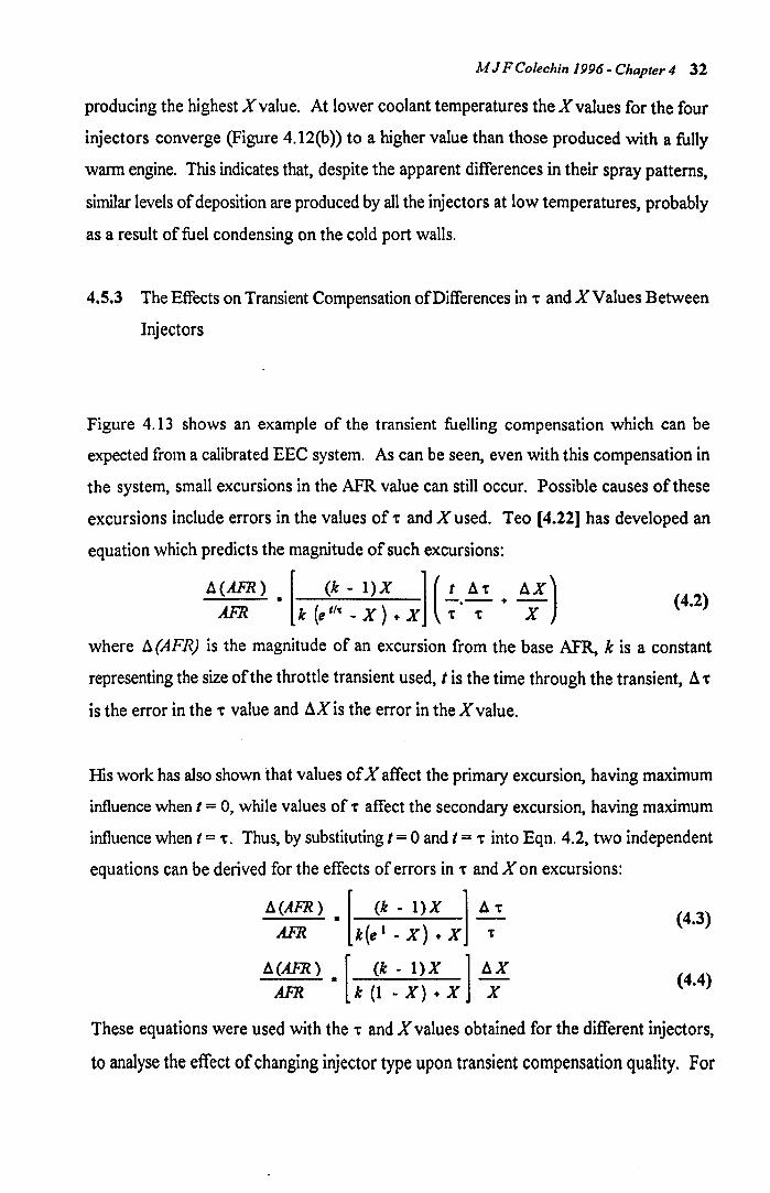
M J F Colechin J 996 - Chapter 4 32
producing the highest X value. At lower coolant temperatures the X values for the four
injectors converge (Figure 4. 12(b)) to a higher value than those produced with a fully
wann engine. This indicates that, despite the apparent differences in their spray patterns,
similar levels of deposition are produced by all the injectors at low temperatures, probably
as a result of fuel condensing on the cold port walls.
4.5.3 The Effects on Transient Compensation of Differences in l' and X Values Between
Injectors
Figure 4.13 shows an example of the transient fuelling compensation which can be
expected from a calibrated EEC system. As can be seen, even with this compensation in
the system, small excursions in the AFR value can still occur. Possible causes of these
excursions include errors in the values of l' and X used. Teo [4.22] has developed an
equation which predicts the magnitude of such excursions:
A(AFR) • [ (k - I)X 1 (!.... A't + AX) AFR k (e tIt - X ) + X l' l' X
(4.2)
where A (AFR) is the magnitude of an excursion from the base AFR, k is a constant
representing the size of the throttle transient used, t is the time through the transient, A l'
is the error in the l' value and AX is the error in the X value.
His work has also shown that values of X affect the primary excursion, having maximum
influence when t = 0, while values of l' affect the secondary excursion, having maximum
influence when t = 1'. Thus, by substituting t = 0 and t = l' into Eqn. 4.2, two independent
equations can be derived for the effects of errors in l' and X on excursions:
A (An.) • [ (k - I) X 1 A l' (4.3) AFR k(e I _ X) + X l'
A(AFR) • [ (k - I)X 1 AX (4.4) AFR k (I - X) + X X
These equations were used with the l' and X values obtained for the different injectors,
to analyse the effect of changing injector type upon transient compensation quality. For
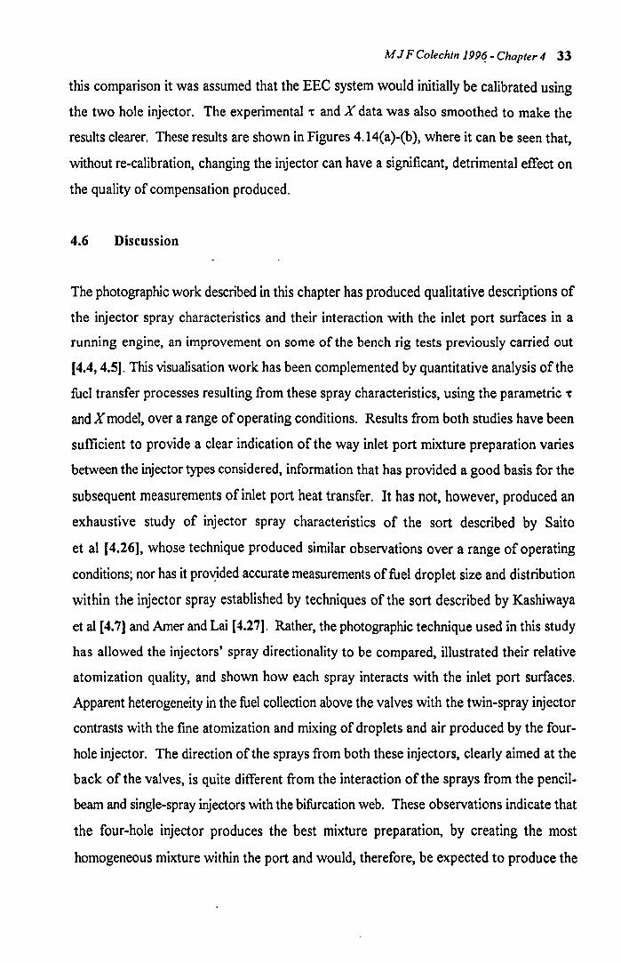
M J F Colechin J 99~ - Chapter 4 33
this comparison it was assumed that the EEe system would initially be calibrated using
the two hole injector. The experimental 't and X data was also smoothed to make the
results clearer. These results are shown in Figures 4 .14( a )-(b), where it can be seen that,
without re-calibration, changing the injector can have a significant, detrimental effect on
the quality of compensation produced.
4.6 Discussion
The photographic work described in this chapter has produced qualitative descriptions of
the injector spray characteristics and their interaction with the inlet port surfaces in a
running engine, an improvement on some of the bench rig tests previously carried out
[4.4,4.5]. This visualisation work has been complemented by quantitative analysis of the
fuel transfer processes resulting from these spray characteristics, using the parametric 't
and X model, over a range of operating conditions. Results from both studies have been
sufficient to provide a clear indication of the way inlet port mixture preparation varies
between the injector types considered, information that has provided a good basis for the
subsequent measurements of inlet port heat transfer. It has not, however, produced an
exhaustive study of injector spray characteristics of the sort described by Saito
et al [4.26], whose technique produced similar observations over a range of operating
conditions; nor has it pro-0ded accurate measurements of fuel droplet size and distribution
within the injector spray established by techniques of the sort described by Kashiwaya
et al [4.7] and Amer and Lai [4.27]. Rather, the photographic technique used in this study
has allowed the injectors' spray directionality to be compared, illustrated their relative
atomization quality, and shown how each spray interacts with the inlet port surfaces.
Apparent heterogeneity in the fuel collection above the valves with the twin-spray injector
contrasts with the fine atomization and mixing of droplets and air produced by the four
hole injector. The direction of the sprays from both these injectors, clearly aimed at the
back of the valves, is quite different from the interaction of the sprays from the pencil
beam and single-spray injectors with the bifurcation web. These observations indicate that
the four-hole injector produces the best mixture preparation, by creating the most
homogeneous mixture within the port and would, therefore, be expected to produce the
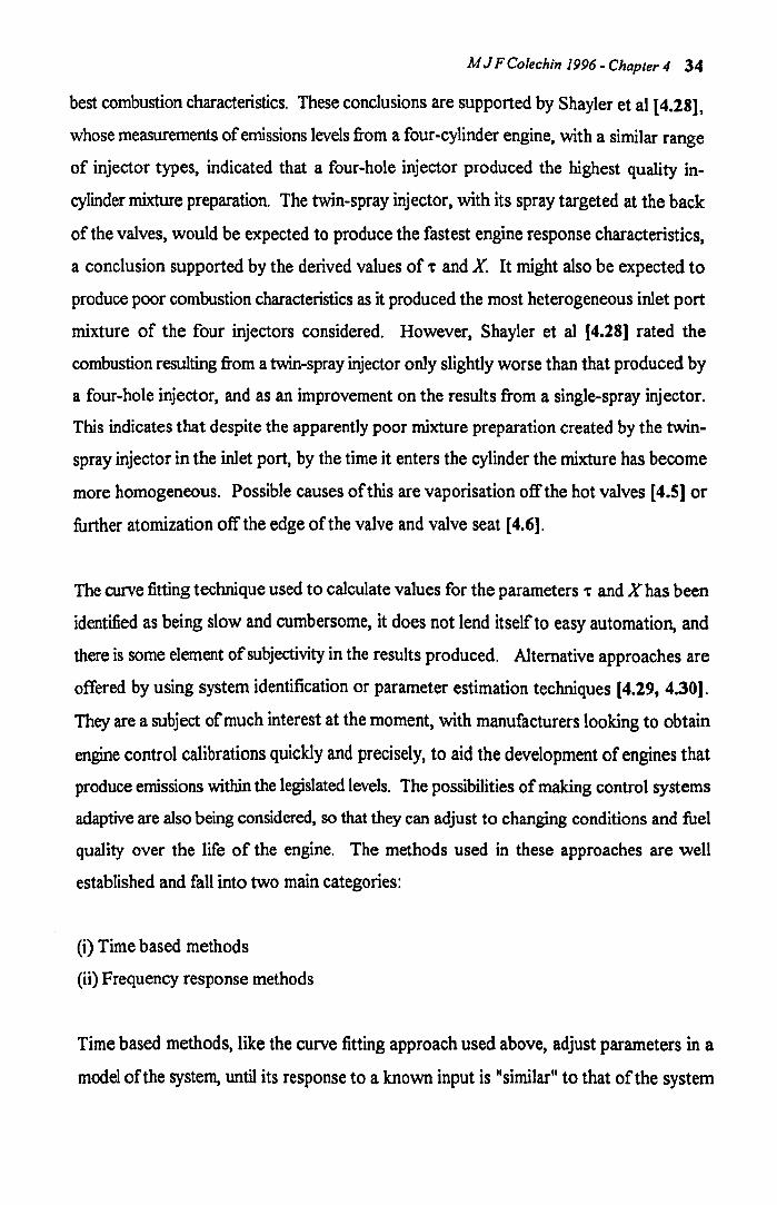
M J F Colechin 1996 - Chapter 4 34
best combustion characteristics. These conclusions are supported by Shayler et al [4.28],
whose measurements of emissions levels from a four-cylinder engine. with a similar range
of injector types, indicated that a four-hole injector produced the highest quality in
cylinder mixture preparation The twin-spray injector, with its spray targeted at the back
of the valves, would be expected to produce the fastest engine response characteristics.
a conclusion supported by the derived values of't and X. It might also be expected to
produce poor combustion characteristics as it produced the most heterogeneous inlet port
mixture of the four injectors considered. However, Shayler et at [4.28] rated the
combustion resulting from a twin-spray injector only slightly worse than that produced by
a four-hole injector, and as an improvement on the results from a single-spray injector.
This indicates that despite the apparently poor mixture preparation created by the twin
spray injector in the inlet port, by the time it enters the cylinder the mixture has become
more homogeneous. Possible causes of this are vaporisation off the hot valves [4.5] or
further atomization off the edge of the valve and valve seat [4.6].
The curve fitting technique used to calculate values for the parameters 't and X has been
identified as being slow and cumbersome, it does not lend itself to easy automation, and
there is some element of subjectivity in the results produced. Alternative approaches are
offered by using system identification or parameter estimation techniques [4.29, 4.30].
They are a subject of much interest at the moment, with manufacturers looking to obtain
engine control calibrations quickly and precisely, to aid the development of engines that
produce emissions within the legislated levels. The possibilities of making control systems
adaptive are also being considered. so that they can adjust to changing conditions and fuel
quality over the life of the engine. The methods used in these approaches are well
established and fall into two main categories:
(i) Time based methods
(ii) Frequency response methods
Time based methods, like the curve fitting approach used above, adjust parameters in a
model of the system, until its response to a known input is "similar" to that of the system
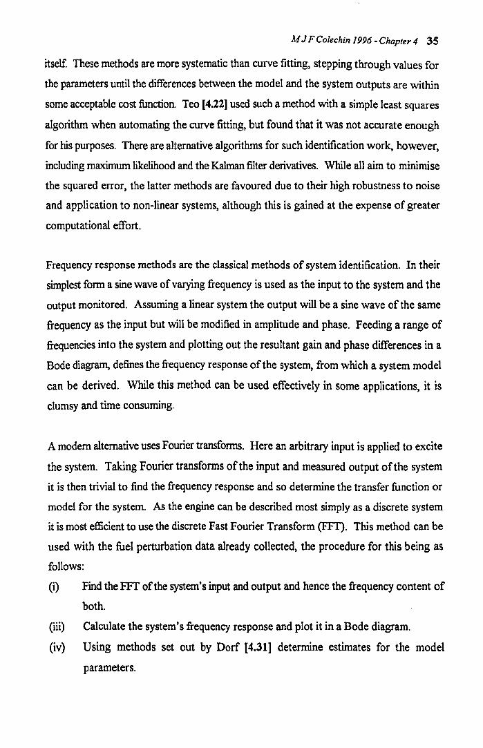
M J F Colechin J 996 - Chapter 4 35
itself These methods are more systematic than curve fitting, stepping through values for
the parameters until the differences between the model and the system outputs are within
some acceptable cost function. Teo [4.22] used such a method with a simple least squares
algorithm when automating the curve fitting, hut found that it was not accurate enough
for his purposes. There are alternative algorithms for such identification work, however,
including maximum likelihood and the Kalman filter derivatives. While all aim to minimise
the squared error, the latter methods are favoured due to their high robustness to noise
and application to non-linear systems, although this is gained at the expense of greater
computational effort.
Frequency response methods are the classical methods of system identification. In their
simplest form a sine wave of varying frequency is used as the input to the system and the
output monitored. Assuming a linear system the output will be a sine wave of the same
frequency as the input but will be modified in amplitude and phase. Feeding a range of
frequencies into the system and plotting out the resultant gain and phase differences in a
Bode diagram, defines the frequency response of the system, from which a system model
can be derived. While this method can be used effectively in some applications, it is
clumsy and time consuming.
A modern alternative uses Fourier transforms. Here an arbitrary input is applied to excite
the system. Taking Fourier transforms of the input and measured output of the system
it is then trivial to find the frequency response and so determine the transfer function or
model for the system. As the engine can be described most simply as a discrete system
it is most efficient to use the discrete Fast Fourier Transform (FFT). This method can be
used with the fuel perturbation data already collected, the procedure for this being as
follows:
(i) Find the FFT of the system's input and output and hence the frequency content of
both.
(iii) Calculate the system's frequency response and plot it in a Bode diagram.
(iv) Using methods set out by Dorf [4.31] determine estimates for the model
parameters.
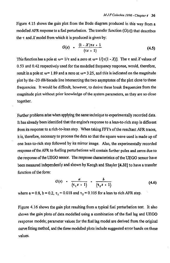
M J F Colechin J 996 - Chapter 4 36
Figure 4.15 shows the gain plot from the Bode diagram produced in this way from a
modelled APR response to a fuel perturbation. The transfer function (G(s)) that describes
the 't and X model from which it is produced is given by:
G(s) .. (1 - X)'tS + 1 (ts + 1)
(4.5)
This function has a pole at w= 1/ 't and a zero at w= 1/[ 't' (1 - X)]. The 't and X values of
0.53 and 0.42 respectively used for the modelled frequency response, would, therefore,
result in a pole at w= 1.89 and a zero at w= 3.25, and this is indicated on the magnitude
plot by the -20 dB/decade line intersecting the two asymptotes of the plot close to these
frequencies. It would be difficult, however, to derive these break frequencies from the
magnitude plot without prior knowledge of the system parameters, as they are so close
together.
Further problems arise when applying the same technique to experimentally recorded data.
It has already been identified that the engine's response to a lean-to-rich step is different
from its response to a rich-to-Iean step. When taking FFT's of the resultant AFR traces,
it is, therefore, necessary to process the data so that the square wave used is made up of
one lean-to-rich step followed by its mirror image. Also, the experimentally recorded
response of the AFR to fuelling perturbations will contain further poles and zeros due to
the response of the UEGO sensor. The response characteristics of the UEGO sensor have
been measured independently and shown by Keogh and Shayler [4.32] to have a transfer
function of the form:
b + (4.6)
where a = 0.8, b = 0.2, 't'l = 0.018 and 't'2 = 0.105 for a lean to rich AFR step.
Figure 4.16 shows the gain plot resulting from a typical fuel perturbation test. It also
shows the gain plots of data modelled using a combination of the fuel lag and UEGO
response models; parameter values for the fuel lag model are derived from the original
curve fitting method, and the three modelled plots include suggested error bands on these
values.
M J F Cole chin 1996 - Chapter 4 37
The data in Figure 4.16 shows fairly good agreement between the gain plots from the
Bode diagrams of the modelled and the experimental data, indicating that the 't' and X
model is a fair representation of the system being considered. However, it does not offer
an alternative approach to establishing values, since attributing system parameters to the
Bode diagram produced by the experimental data would be as subjective as using a curve
fitting method with the raw AFR data. The problem with using the Bode diagram is a lack
of data in the middle of the frequency range being considered. To overcome this the tests
would have to be re-designed to provide a wider range of input frequencies to the system.
This could be done by providing random white noise as an input to the system, or more
practically by providing fuel perturbations in the pseudo-random binary sequence (PRBS)
suggested by several authors [4.20,4.30,4.33]. Such methods would not, however, take
account of the differences in response between accelerations and decelerations, and may
be difficult to use during a warm up when there is only limited time available to carry out
perturbations before the engine conditions change significantly. The solution, therefore,
probably lies in the use of improved time based methods for establishing values of't' and
X, such as those being developed by Durrant [4.23).
This study has been limited in its scope by the problems encountered with errors in the
AFR measurements and the limited temperature range over which it was undertaken.
Some of the trends observed in this work are, however, further supported by the later heat
transfer work. This heat transfer work has also allowed the mechanisms behind fuel
transport to be studied in more detail. The aim of this work is to provide information to
allow the mixture preparation and fuel transport for an engine to be optimised through
correct injector choice; improved port geometries, providing localised heating to aid fuel
vaporisation; and ensuring that the injector open periods are controlled in the most
suitable way. From the work described in this chapter it is evident that the selection of
the injector in the design of a port-injected, 4-valve engine involves a compromise. An
injector that improves combustion by giving good mixture preparation, has important
consequences for power output, fuel consumption, emissions levels and cold starting;
equally, though, an injector which improves fuel transfer has important consequences for

M J F Cotechin 1996 - Chapter 4 38
engine transient response and control, with further benefits to be had for emissions by
more efficient operation of the catalytic convertor.
Chapter 5
Heat Flux Sensor Dynamics
5.1 Introduction
The study described in Chapter 4 established that even for port fuel injected engines, a
significant proportion of the injected fuel is deposited on the intake port and valve
surfaces, with potentially adverse effects on mixture preparation and control, particularly
when mixture demand changes. It is also well known that raising the surface temperature
of the intake port ameliorates these problems, purportedly by raising heat transfer to fuel
deposited on the surfaces and thereby promoting evaporation (see Figure 5.1). These
fundamental mechanisms have been investigated either by modelling the flows within the
inlet port [5.1, 5.2, 5.3], or through experimentation with bench rigs [5.4,5.5,5.6], but
there is little direct experimental evidence from work on firing engines to support the
inferences drawn. The measurements of inlet port heat transfers described in the next four
chapters were designed to produce such evidence from a four-valve, port-injected engine.
This chapter describes the construction and mounting of the sensors used and presents an
investigation of their dynamic response characteristics. This showed that the response
characteristics of the sensors were inadequate to accurately resolve instantaneous heat
transfer rates without post-processing the data. A method of reconstructing instantaneous
variations from the recorded sensor output has been developed, using Fourier transforms.
The method is described in this chapter and the results justified using finite difference
analysis techniques.
5.2 Heat Flux Sensor Construction
Figure 5.2 illustrates the construction of the Micro-Foil Heat Flow Sensors manufactured
by Rhopoint and used to measure heat transfer through the inlet port walls. Each sensor
consists of two arrays ofK-type thermocouple junctions either side of a thin polyimide
(Kapton) film, which acts as a thermal barrier. Also mounted on the top surface of this
39
M J F Colechin 1996 - Chapter 5 40
film is aT-type thermocouple junction, used to measure the temperature of the sensor for
calibration purposes. Under steady state conditions, the heat flux through the sensor is
given by measuring the potential difference between the two thermocouple arrays, which
is calibrated for heat flux against the sensor's temperature by applying the calibration
factor provided by the manufacturer. To protect the thermocouple junctions two further
layers of Kapton (Figure 5.3) are laminated over the top and bottom surfaces of the
sensor. The sensors were attached to the port wall surfaces using a high temperature
epoxy resin, "Araldite 2014" (see Figure 5.3). Rhopoint quote a response time of 60 ms
for the output from the sensors to rise to 62% of a step input [5.7]. This is of the same
order as the period of an engine cycle, 120 ms at 1000 RPM, and indicates that there will
be some attenuation of signals arising from variations in heat fluxes around the cycle.
Epstein et al [5.8] developed a theoretical approach to assessing the significance of this
attenuation, which requires knowledge of the dimensions and thermal characteristics of
the various layers highlighted in Figure 5.3.
To establish the adhesive film thickness, a sample sensor was attached to a piece of
aluminium plate using the technique developed for fixing the sensors around the inlet port
surfaces, and the thickness of the adhesive layer was measured using a dial indicator on
a surface table. This measurement was dependent upon finding the relative distance
between the sensor's top surface and the surface table at various points before and after
applying the layer of adhesive between the sensor and the aluminium plate. It was,
therefore, unsuitable for making measurements within the inlet port. To measure the
thickness of the two protective laminae and the central lamina between the arrays of
thermocouple junctions, an example sensor was first set in a resin block and sections of
the block removed with a surface grinder until the visible section passed through the
centre of the thermocouple arrays. Magnified images of this section were then captured
using a PC in conjunction with a video camera and a microscope (see Figure 5.4), which
could then be scaled against the overall thickness of the sensor, previously measured with
a micrometer. Values for the dimensions and thermal characteristics of each layer
highlighted in Figure 5.3 are listed in Table 5.1. The thermal property values for the port
wall material are most uncertain because factors such as casting porosity can have a
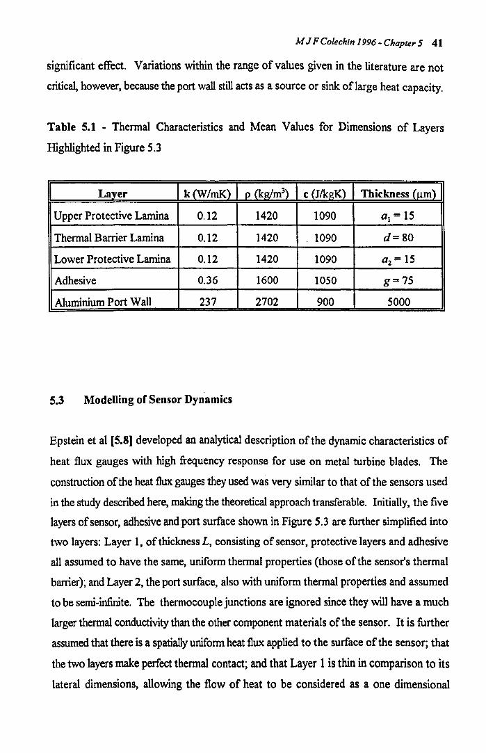
M J F Colechin 1996 - Chapter 5 41
significant effect. Variations within the range of values given in the literature are not
critical, however, because the port wall still acts as a source or sink oflarge heat capacity.
Table 5.1 - Thermal Characteristics and Mean Values for Dimensions of Layers
Highlighted in Figure 5.3
Layer k(W/mK) p (kg/m3) c (J/kgK) Thickness (J,lm)
Upper Protective Lamina 0.12 1420 1090 a1 == 15
Thermal Barrier Lamina 0.12 1420 1090 d== 80
Lower Protective Lamina 0.12 1420 1090 a2 = 15
Adhesive 0.36 1600 1050 g=75
Aluminium Port Wall 237 2702 900 5000
5.3 Modelling of Sensor Dynamics
Epstein et al [5.8] developed an analytical description of the dynamic characteristics of
heat flux gauges with high frequency response for use on metal turbine blades. The
construction of the heat flux gauges they used was very similar to that of the sensors used
in the study described here, making the theoretical approach transferable. Initially, the five
layers of sensor, adhesive and port surface shown in Figure 5.3 are further simplified into
two layers: Layer 1, of thickness L, consisting of sensor, protective layers and adhesive
all assumed to have the same, uniform thermal properties (those of the sensor's thermal
barrier)~ and Layer 2, the port surface, also with uniform thermal properties and assumed
to be semi-infinite. The thermocouple junctions are ignored since they will have a much
larger thermal conductivity than the other component materials of the sensor. It is further
assumed that there is a spatially uniform heat flux applied to the surface of the sensor; that
the two layers make perfect thermal contact; and that Layer 1 is thin in comparison to its
lateral dimensions, allowing the flow of heat to be considered as a one dimensional
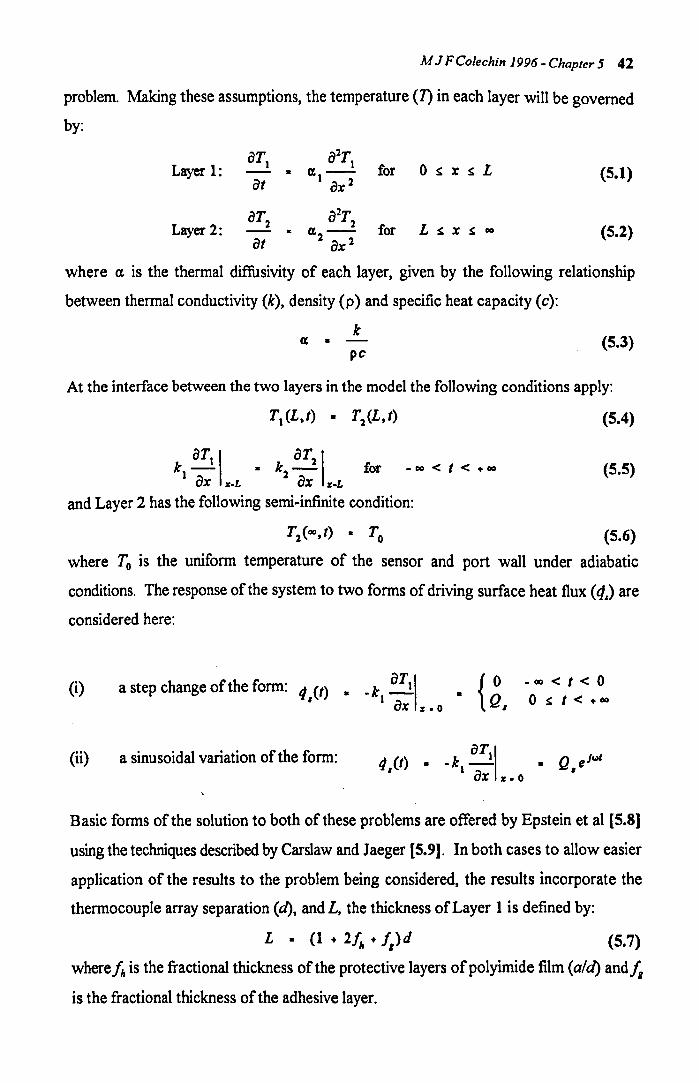
M J F Colechin 1996 - Chapter 5 42
problem. Making these assumptions, the temperature (1) in each layer will be governed
by:
Layer 1: for o s: x s: L (5.1)
Layer 2: for (5.2)
where a is the thermal diffusivity of each layer, given by the following relationship
between thermal conductivity (k), density (p) and specific heat capacity (c):
k « • -pc
(5.3)
At the interface between the two layers in the model the following conditions apply:
(5.4)
k- . k- for -00<1< .. 00 oTt \ OT2 \
1 ax It.L 2 ax It.L (5.5)
and Layer 2 has the following semi-infinite condition:
T2(oo,t) • To (5.6)
where To is the uniform temperature of the sensor and port wall under adiabatic
conditions. The response of the system to two forms of driving surface heat flux (46) are
considered here:
(i) a step change of the form: ",(/) • _ k aTt \ • { QO - 00 < t < 0 'f 'a Os:/< .. oo x It. 0 I
(ii) a sinusoidal variation of the form: OTt \ wi 4,(t) • -kl - • Q,el ax It.O
Basic forms of the solution to both of these problems are offered by Epstein et al [5.8]
using the techniques described by Carslaw and Jaeger [5.9]. In both cases to allow easier
application of the results to the problem being considered, the results incorporate the
thermocouple array separation (d), and L, the thickness of Layer 1 is defined by:
L • (1 .. 2J;. .. i,)d (5.7)
wherej;, is the fractional thickness of the protective layers of poly imide film (aId) and!,
is the fractional thickness of the adhesive layer.
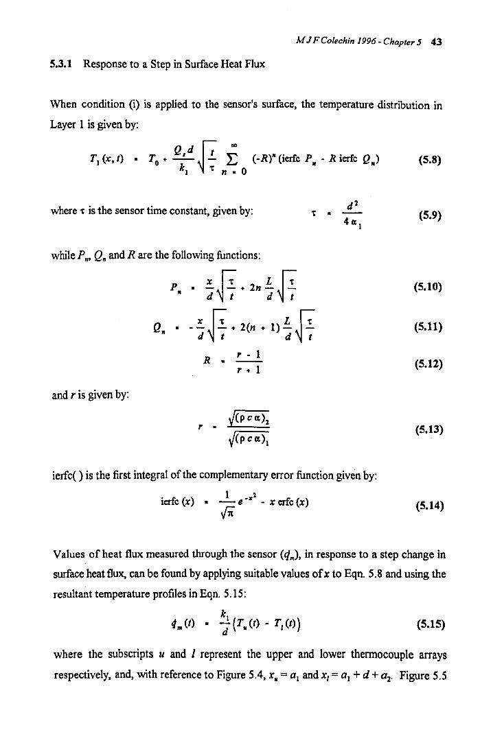
M J F Colechin 1996 - Chapter 5 43
5.3.1 Response to a Step in Surface Heat Flux
When condition (i) is applied to the sensor's surface, the temperature distribution in
Layer 1 is given by:
T, (:<, t) • To' Q. d ~ t i (-R)· (ierfe p. - R ierfc Q.) (5.8) kl or n • 0
where or is the sensor time constant, given by: t •
while P n' Qn and R are the following functions:
p. • .!. ~ T >2n ~ ~ 1 d t d t
Q. • _.!. r:;- • 2(n • 1) L ~ T d~t d t
R •
and r is given by:
r •
r - 1 r + 1
y(p C cr.)2
J(PCcr.)l
ierfc( ) is the first integral of the complementary error function given by:
ierfe (x) • ~ e _¥2 - x erfe (x)
fi
(5.9)
(5.10)
(5.11)
(5.12)
(5.13)
(5.14)
Values of heat flux measured through the sensor (g",), in response to a step change in
surface heat flux, can be found by applying suitable values of x to Eqn. 5.8 and using the
resultant temperature profiles in Eqn. 5.15:
k 4 lit (I) • ~ (Til (I) - T, (I) ) (5.15)
where the subscripts u and I represent the upper and lower thermocouple arrays
respectively, and, with reference to Figure 5.4, Xu = 01 and XI = 01 + d + 02. Figure 5.5

M J F Colechin J 996 - Chapter 5 44
shows typical step responses calculated in this way for three values of adhesive thickness
(g) and three values for the thickness of the upper protective lamina defined by XII'
Variations in values of g were considered to provide an indication of the effects of errors
introduced by assuming that the adhesive had the same thermal properties as the polyimide
film, and to allow for variations introduced during attachment; variations in XII were
apparent in the magnified cross-sectional images of the sensors arising from variations in
the thickness of the interstitial glue layers (see Figure 5.4). Both variations have an effect
in the time domain, although it is the variations in the thickness of the adhesive layer
which are most significant. In Figure 5.S(b), where the time scale is expanded to show
the initial response of the sensor, it can be seen that the dimension variations considered
give rise to a range of 50-90 ms in values of time for the measured heat flux to rise to 62%
of the steady state value. This is in agreement with the "typical" value of 60 ms quoted
by Rhopoint [5.7].
5.3.2 Response to a Steady Harmonic Variation in Surface Heat Flux
When condition (ii) is applied at the sensor's surface for all time, the temperature
distribution in Layer 1 is given by:
Tl (x, t) • To + Q; d G e 1(II)t - +) 1
a harmonic function in which G describes the magnitude variation with x:
G •
(5.16)
(5.17)
and 4> describes the difference in phase between the temperature variation at x and the
applied surface heat flux:
4> • .!..=. G + .!:. _ tan· 1 (BC -AD) 2 d ~ (a) t: 4 AC + BD
(5.18)
where:
(5.19a)
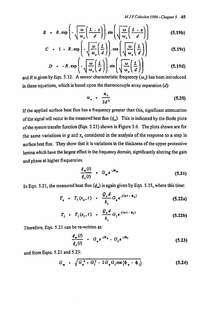
M J F Colechin 1996 - Chapter 5 45
(5.19b)
(5.19c)
(5.19d)
and R is given by Eqn. 5.12. A sensor characteristic frequency «&) c) has been introduced
in these equations, which is based upon the thermocouple array separation (d):
(5.20)
If the applied surface heat flux has a frequency greater than this, significant attenuation
of the signal will occur in the measured heat flux (4m). This is indicated by the Bode plots
of the system transfer function (Eqn. 5.21) shown in Figure 5.6. The plots shown are for
the same variations in g and XII considered in the analysis of the response to a step in
surface heat flux. They show that it is variations in the thickness of the upper protective
lamina which have the largest effect in the frequency domain, significantly altering the gain
and phase at higher frequencies.
4", (t)
4. (I) • G e -f+.
III (5.21)
In Eqn. 5.21, the measured heat flux (lim) is again given by Eqn. 5.15, where this time:
Til • T1(xlI,l) •
T, • Tl (x" 1 ) •
Q.dG
f(",t-.,,} - e k .,
1
Q.d G J(w'-+,) -- e k I
1
Therefore, Eqn. 5.21 can be re-written as:
4", (I)
4, (I)
and from Eqns. 5.21 and 5.23:
• G e -f." _ G e -J+, II ,
Gill • VGII'l·G,'l-2GIIG,COS(cIJlI-cIJ,)
(5.22a)
(5.22b)
(5.23)
(5.24)
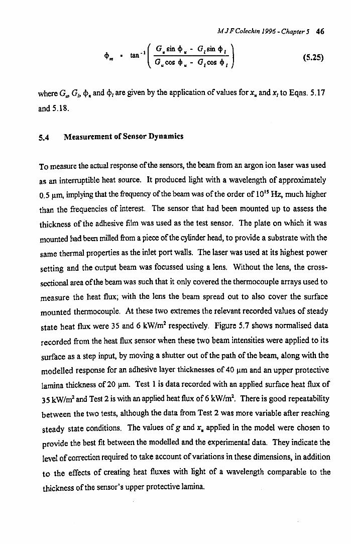
M J F Colechin 1996 - Chapter 5 46
<1>," • tan 01 ( G"sin<l>" - G,sin<l>, ) G"cos <1>" - G,COS <1>,
(5.25)
where G", GI, <1>" and <1>1 are given by the application of values for x" and XI to Eqns. 5.17
and 5.18.
5.4 Measurement of Sensor Dynamics
To measure the actual response of the sensors, the beam from an argon ion laser was used
as an interruptible heat source. It produced light with a wavelength of approximately
0.5 ~m, implying that the frequency of the beam was of the order of 1015 Hz, much higher
than the frequencies of interest. The sensor that had been mounted up to assess the
thickness of the adhesive film was used as the test sensor. The plate on which it was
mounted had been milled from a piece of the cylinder head, to provide a substrate with the
same thermal properties as the inlet port walls. The laser was used at its highest power
setting and the output beam was focussed using a lens. Without the lens, the cross
sectional area of the beam was such that it only covered the thermocouple arrays used to
measure the heat flux; with the lens the beam spread out to also cover the surface
mounted thermocouple. At these two extremes the relevant recorded values of steady
state heat flux were 35 and 6 kW/m2 respectively. Figure 5.7 shows normalised data
recorded from the heat flux sensor when these two beam intensities were applied to its
surface as a step input, by moving a shutter out of the path of the beam, along with the
modelled response for an adhesive layer thicknesses of 40 J.1m and an upper protective
lamina thickness of 20 J.1m. Test 1 is data recorded with an applied surface heat flux of
35 kW/m2 and Test 2 is with an applied heat flux of6 kW/ml. There is good repeatability
between the two tests, although the data from Test 2 was more variable after reaching
steady state conditions. The values of g and x" applied in the model were chosen to
provide the best fit between the modelled and the experimental data. They indicate the
level of correction required to take account of variations in these dimensions, in addition
to the effects of creating heat fluxes with light of a wavelength comparable to the
thickness of the sensor's upper protective lamina.
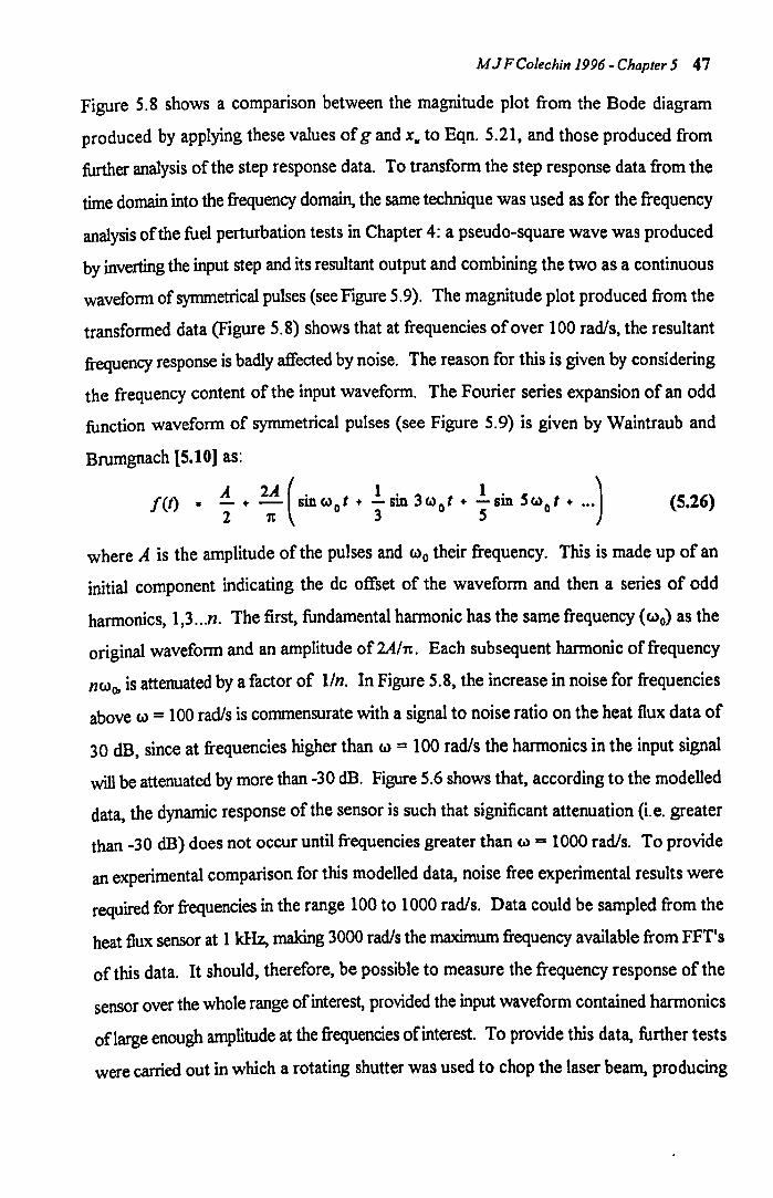
M J FCo/ecJlin 1996 - Chapter 5 47
Figure 5.8 shows a comparison between the magnitude plot from the Bode diagram
produced by applying these values of g and XII to Eqn. 5.21, and those produced from
further analysis of the step response data. To transform the step response data from the
time domain into the frequency domain, the same technique was used as for the frequency
analysis of the fuel perturbation tests in Chapter 4: a pseudo-square wave was produced
by inverting the input step and its resultant output and combining the two as a continuous
waveform of symmetrical pulses (see Figure 5.9). The magnitude plot produced from the
transformed data (Figure 5.8) shows that at frequencies of over 100 rad/s, the resultant
frequency response is badly affected by noise. The reason for this is given by considering
the frequency content of the input waveform. The Fourier series expansion of an odd
function waveform of symmetrical pulses (see Figure 5.9) is given by Waintraub and
Brumgnach [5.10] as:
f(t) • A + 2A (Sinc.>ot + .!.sin 3c..> ot + .!.sin Sc.>ot + ... ) (5.26) 2 ~ 3 S
where A is the amplitude of the pulses and (&)0 their frequency. This is made up of an
initial component indicating the de offset of the waveform and then a series of odd
harmonics, 1,3 .. . n. The first, fundamental harmonic has the same frequency (wo) as the
original waveform and an amplitude of 2Aht. Each subsequent harmonic of frequency
nW()J is attenuated by a factor of lin. In Figure 5.8, the increase in noise for frequencies
above (&) = 100 radls is conunensurate with a signal to noise ratio on the heat flux data of
30 dB, since at frequencies higher than ll) = 100 radls the harmonics in the input signal
will be attenuated by more than -30 dB. Figure 5.6 shows that, according to the modelled
data, the dynamic response of the sensor is such that significant attenuation (i.e. greater
than -30 dB) does not occur until frequencies greater than W = 1000 rad/s. To provide
an experimental comparison for this modelled data, noise free experimental results were
required for frequencies in the range 100 to 1000 rad/s. Data could be sampled from the
heat flux sensor at 1 kHz, making 3000 radls the maximum frequency available from FFT's
of this data. It should, therefore, be possible to measure the frequency response of the
sensor over the whole range of interest, provided the input waveform contained harmonics
oflarge enough amplitude at the frequencies of interest. To provide this data, further tests
were carried out in which a rotating shutter was used to chop the laser beam, producing
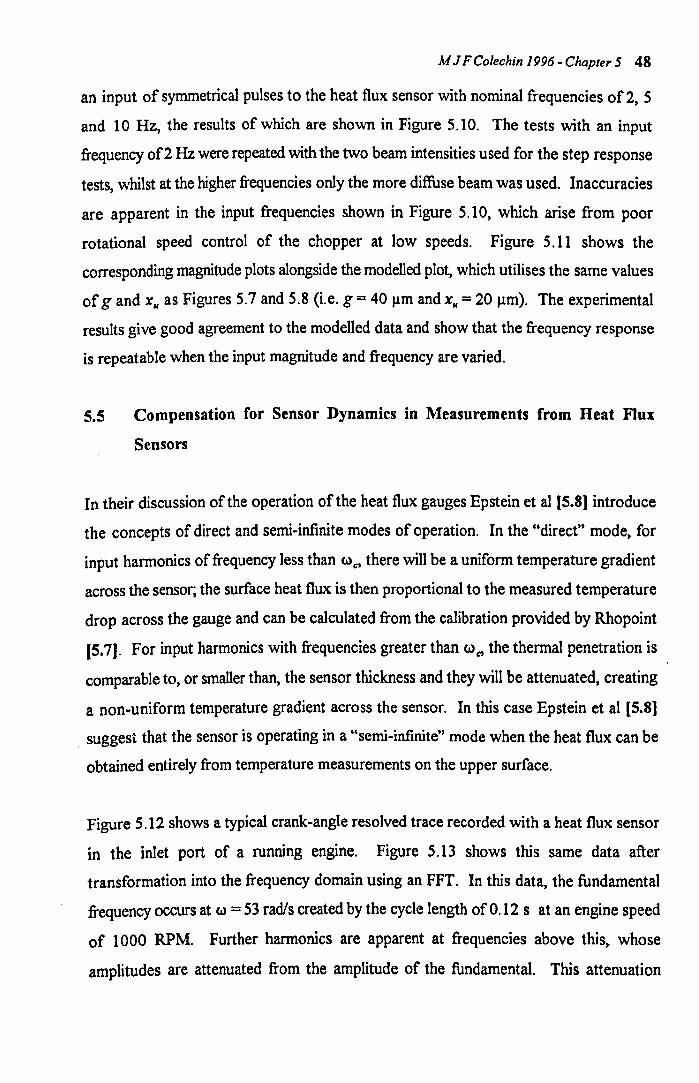
M J F Colechin J 996 - Chapter 5 48
an input of symmetrical pulses to the heat flux sensor with nominal frequencies of 2, 5
and 10Hz, the results of which are shown in Figure 5.1 o. The tests with an input
frequency of2 Hz were repeated with the two beam intensities used for the step response
tests, whilst at the higher frequencies only the more diffuse beam was used. Inaccuracies
are apparent in the input frequencies shown in Figure 5.10, which arise from poor
rotational speed control of the chopper at low speeds. Figure 5.11 shows the
corresponding magnitude plots alongside the modelled plot, which utilises the same values
of g and XII as Figures 5.7 and 5.8 (i.e. g = 40 Jlm and X" = 20 ~m). The experimental
results give good agreement to the modelled data and show that the frequency response
is repeatable when the input magnitude and frequency are varied.
5.5 Compensation for Sensor Dynamics in Measurements from Heat Flux
Sensors
In their discussion of the operation of the heat flux gauges Epstein et al (5.8] introduce
the concepts of direct and semi-infinite modes of operation. In the "direct" mode, for
input harmonics of frequency less than (&)co there will be a uniform temperature gradient
across the sensor; the surface heat flux is then proportional to the measured temperature
drop across the gauge and can be calculated from the calibration provided by Rhopoint
[5.7]. For input harmonics with frequencies greater than Wet the thermal penetration is
comparable to, or smaller than, the sensor thickness and they will be attenuated, creating
a non-uniform temperature gradient across the sensor. In this case Epstein et al [5.8]
. suggest that the sensor is operating in a "semi-infinite" mode when the heat flux can be
obtained entirely from temperature measurements on the upper surface.
Figure 5.12 shows a typical crank-angle resolved trace recorded with a heat flux sensor
in the inlet port of a running engine. Figure 5.13 shows this same data after
transformation into the frequency domain using an FFT. In this data, the fundamental
frequency occurs at (&) = 53 rad/s created by the cycle length of 0.12 s at an engine speed
of 1000 RPM. Further harmonics are apparent at frequencies above this, whose
amplitudes are attenuated from the amplitude of the fundamental. This attenuation
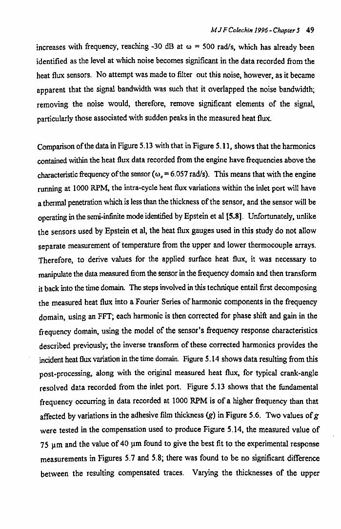
M J FColechin 1996 - Chapter 5 49
increases with frequency, reaching -30 dB at <..> = 500 rad/s, which has already been
identified as the level at which noise becomes significant in the data recorded from the
heat flux sensors. No attempt was made to filter out this noise, however, as it became
apparent that the signal bandwidth was such that it overlapped the noise bandwidth~
removing the noise would, therefore, remove significant elements of the signal,
particularly those associated with sudden peaks in the measured heat flux.
Comparison of the data in Figure 5.13 with that in Figure 5. 11, shows that the harmonics
contained within the heat flux data recorded from the engine have frequencies above the
characteristic frequency of the sensor (<">0 = 6.057 rad/s). This means that with the engine
running at 1000 RPM, the intra-cycle heat flux variations within the inlet port will have
a thermal penetration which is less than the thickness of the sensor, and the sensor will be
operating in the semi-infinite mode identified by Epstein et al [5.8]. Unfortunately, unlike
the sensors used by Epstein et aI, the heat flux gauges used in this study do not allow
separate measurement of temperature from the upper and lower thermocouple arrays.
Therefore, to derive values for the applied surface heat flux, it was necessary to
manipulate the data measured from the sensor in the frequency domain and then transform
it back into the time domain. The steps involved in this technique entail first decomposing
the measured heat flux into a Fourier Series of harmonic components in the frequency
domain, using an FFT; each harmonic is then corrected for phase shift and gain in the
frequency domain, using the model of the sensor's frequency response characteristics
described previously~ the inverse transform of these corrected harmonics provides the
incident heat flux variation in the time domain. Figure 5.14 shows data resulting from this
post-processing, along with the original measured heat flux, for typical crank-angle
resolved data recorded from the inlet port. Figure 5.13 shows that the fundamental
frequency occurring in data recorded at 1000 RPM is of a higher frequency than that
affected by variations in the adhesive film thickness (g) in Figure 5.6. Two values of g
were tested in the compensation used to produce Figure 5.14, the measured value of
75 Ilm and the value of 40 Ilm found to give the best fit to the experimental response
measurements in Figures 5.7 and 5.8; there was found to be no significant difference
between the resulting compensated traces. Varying the thicknesses of the upper
M J FColechin 1996 - Chapter 5 50
protective layer (xU> in the compensation model did make a difference, however.
Figure 5.14 provides a comparison between the compensated data produced when the
measured value of 15 p,m is used for XII' and that produced when XII is given a value of
20 p,m, the "best fit" value in Figures 5.7 and 5.8.
5.6 Discussion
The analysis and experimental work described in this chapter has shown that the heat flux
sensors have a response time comparable with the period of an engine cycle.
Compensation for this dynamic response can be made to infer instantaneous variations in
heat transfer using spectral analysis. Limitations are placed on the quality of this
compensation by the sensitivity of the sensors, the quality of the signal they produce, and
the frequency at which the data can be sampled. The maximum sampling rate is 1 kHz
(6380 rad/s) and, therefore, only harmonics of frequency less than 500 Hz (3140 rad/s)
can be analysed using the FFT methods applied, any higher frequency harmonics being
effectively filtered out of the signal. However, Figure 5.13 shows that at these frequencies
the amplitude of the harmonics in typical crank-angle resolved data is attenuated by more
than -60 dB from that of the fundamental frequency, suggesting that they are not a
significant component of the original signal. The aliasing effects of FFT analysis,
discussed by Newland [5.11), must also he considered in such cases. These will lead to
distortion of the signal in the frequency domain ifthere are significant components of the
signal at frequencies approaching half the sampling frequency. In this case, the data in
Figure 5.13 shows that the components of the original signal are heavily attenuated at
frequencies below this and, therefore, the aliasing effects will be minimal. Figure 5.13 also
shows that there are noise harmonics in the signal at frequencies above about 500 rad/s
(80 Hz), these overlap with significant components of the signal and cannot be filtered
out. They arise from a combination of cycle-by-cycle variability in the data, signal noise
and the limitations of the data acquisition system, which itself produces a noise level with
anRMS value of3 ~Vequivalent to a signal to noise ratio of between 40 and 50 dB on
typical recorded signals.
M J F Colechin J 996 - Chapter 5 51
Some effort was made to reduce the effects of noise on the measured data by taking the
mean of ten consecutive cycles before carrying out the spectral analysis. Figure 5.14
shows that this has been fairly successful. The effects of random noise on the
compensated data are limited, being most apparent in the data recorded through Sensor 1
(Figure 5.14(a)), which also displayed the lowest overall values of heat flux. More
significant, are the effects of the parameter Xu on the quality of compensation produced.
A high frequency component is apparent in each of the compensated traces in Figure 5 .14
when Xu is set to 20 11m, the value indicated by results of frequency response
measurements using a laser. This is not apparent when a value of 15 ~m is used in the
compensation model. It leads to a variation of up to 30% in the inferred peak heat flux
values and illustrates the level of uncertainty surrounding which value of Xu to use when
compensating for the dynamic response of these sensors. The sensor used for the
response experiments was purchased at a different time from the sensors used within the
inlet port or the one sectioned to provide the measurements in Figure 5.4 and Table 5.1.
The calibration factors provided by Rhopoint for the "direct" mode operation of these
sensors indicate that significant variations can occur between sensors, particularly when
they are purchased from different batches. Also, the conditions for the sensor response
tests were somewhat different to those found within the inlet port. It has been excepted,
therefore, that the response characteristics of the sensor used in the frequency response
tests, when excited by a beam oflaser light, are best characterised by a model in which XII
is taken as 20 11m, whereas the response characteristics of the sensors positioned around
the inlet port are better characterised by taking XII as 15 11m.
In Figure 5.14(c) additional high frequency spikes appear in the data at the two ends of
the compensated traces. These arise because spectral analysis using FFT's relies upon the
assumption that in the time domain the original function is periodic and continuous for
..00 < t < +00. Figure 5.12 shows a magnified form of the data from which the compensated
traces in Figure 5.14(c) are produced, where it can be seen that in this case there is a slight
discontinuity between the heat flux values for crank-angles of 0 0 and 720 0, due to cycle
by-cycle variations in the crank-angle resolved data. The effect of these discontinuities
M J FColechin 1996 - Chapter 5 52
is to produce the high frequency spikes observed at the same points in the compensated
data.
To provide further confirmation of the compensated results, a finite difference model of
the sensor was developed. Inferred SUlface heat flux data were applied to this model, and
corresponding values of measured heat flux were calculated to see if they matched the
uncompensated data recorded from the sensors. In this finite difference model it was
assumed that the thermal capacity and conductivity of the aluminium port surface were
such that the interface between the adhesive and the port surface remained at a constant
temperature, that of the coolant passing through the engine. Above this interface the four
layers shown in Figure 5.3 were modelled as two layers with independent thermal
properties: the top layer, consisting of the two protective layers and the central thermal
barrier of the sensor, was modelled as polyimide film, with the relevant thermal properties
from Table 5.1; the bottom layer was modelled using the thermal properties for the
adhesive given in Table 5.1. In this finite difference model the thickness of the adhesive
layer was taken as the measured value of 75 Ilm, since it has already been identified that
the correction to 40 Ilm required in the model of the sensor's step response was at least
partly due to the error introduced by the assumption of constant thermal properties
throughout the sensor and adhesive layers. Figure 5.15 shows that there is good
agreement between the measured data from Figure 5. 14 and the output from the finite
difference model when the compensated traces for Xu = 15 Jlm are applied.
Chapter 6
Heat Transfer for Dry-Port Conditions
6.1 Introduction
In this Chapter, an investigation of heat transfer between the inlet port surfaces and the
gas flow in the port is described. Cheng et al [6.1] identified four distinct gas flow
regimes which occur during various periods of an engine cycle. The timing of these
periods is shown in Figure 6.1. When the intake valves are closed, no bulk motion of the
gas occurs. During the intake and exhaust valve overlap period, hot combustion products
can flow from the cylinder back into the intake port, described as overlap backflow. As
induction progresses, a forward induction flow develops. Finally, towards the time of inlet
valve closure, a displacement backflow of gas may occur. To differing degrees, each of
these stages will affect the heat exchange between the gas mixture and the port walls.
(i) Period of no bulk gas flow:
During this period, although there is no net movement of gas through the port,
there is likely to be some movement within the port as a result of eddy currents set
up by turbulent flows during previous bulk gas movements. These movements
will produce convective heat transfer effects, with heat transfer being further
driven by the temperature difference between the port gases and the port walls.
(ii) Overlap backflow:
Valve overlap, between inlet valve opening (IVO) and exhaust valve closing
(EVC), improves volumetric efficiency particularly at higher speeds and loads, by
increasing the efficiency with which exhaust gas residuals are "scavenged" from
the cylinder. At part load conditions it results in a reverse flow blowdown, as the
pressure in the cylinder, which is close to atmospheric at the end of the exhaust
stroke, equalises with that in the inlet manifold. The resultant overlap backflow
of hot residual gases from the cylinder will affect inlet port heat transfer both
through convection and through the changes such an influx of hot gas will have
53
M J F Colechin 1996 - Chapter 6 54
on the thermal environment. It is also likely to displace any liquid fuel that has
collected around the valve seats during the previous period of valve closure.
(ii) Forward induction flow:
With the inlet valves open there will be aforward induction flaw of air through the
inlet port. This mixes with the burnt gases from the overlap backflow and flows
into the cylinder. Like the overlap backflow it will affect heat transfer by
increasing convection and changing the thermal environment, this time, however,
by inducing colder fresh charge through the port.
(iii) Displacement backflow:
Inlet valve closing (IVC) is timed after bottom dead centre (BOC) of the
compression stroke to improve volumetric efficiency at high engine speeds and
loads, when the momentum of the air maintains a forward flow into the engine
until IVe. However, at lower speeds fresh fueVair mixture and residual gases
from the previous combustion stroke will be displaced back into the inlet port as
the piston starts to move back up the compression stroke before IVe. This
displacement backjlow will be warmer than the fresh charge air left in the port and
since it will be present for the whole of the valve closed period it may exert an
extended influence on the port's thermal environment. Its composition is a
mixture of fresh charge and in-cylinder residual gases, which may also affect the
vaporisation of fuel from deposited fuel films.
At the present time, there is very little information on the effects of these various gas flow
regimes on surface heat transfer. Turin et al [6.2] took some account of the effect of
displacement backflow on the mass of fuel returned to the port in their model, but
otherwise assumed that the flow of gas through the port was steady. The bench rig work
of both Martins and Finlay [6.3, 6.4] and Ladommatos [6.5] simulated unsteady flows
using pulsating gas motion to represent periods of forward induction flow between
periods of no bulk gas flow; they did not, however, consider the effect of overlap and
displacement backflows.
M J F Colechin 1996 - Chapter 6 55
6.2 The Effects of Different Gas Flow Regimes on Measured Heat Fluxes
To establish how each gas flow regime within the port affected heat transfer between the
gases and the port walls, tests were carried out with fuel injection restricted to one side
of the intake port bifurcation. A twin-spray injector was modified to achieve this, by
sealing one hole in the injector splitter cap (see Figure 6.2). By rotating the cap, fuel
injection could be directed into either branch of the port leaving either Sensors 3, 4 and 5,
or Sensors 6, 7 and 8 dry. Sensors 1 and 2 were outside the region wetted during tests
with an unmodified twin-spray injector, the results from which are used as measurements
of the dry-port conditions for these two sensors. Engine operating conditions were
chosen to cover a range of MAP (0.53, 0.79 and 0.95 bar) with the engine running fully
warm; at a speed of 1000 RPM; a nominally constant, stoichiometric mixture ratio; and
with the injection timed to end at 270 0 ATDC, during the exhaust stroke of the cycle.
Figure 6.3 shows summaries of crank-angle resolved heat flux variations recorded from
all the sensors over ten consecutive cycles, with a MAP of 0.79 bar. These results are far
less variable than those recorded when fuel deposition occurred, which increased the
standard deviation by a factor of up to 10. Figure 6.3 also illustrates the effects on the
heat fluxes of variations in gas flow due to overlap backflow, forward induction flow and
displacement backflow. As has already been discussed in Chapter S, the transient
response of the heat flux sensors will have reduced the apparent effects of these flows.
Inferred data for the actual heat fluxes occurring at the surface of the sensor, after
removing the sensor response from the mean results in Figure 6.3, are presented in
Figure 6.4 The timings, ATDC of the firing stroke, of the various valve events that
produce these inlet port phenomena are: IVO at 350°, EVe at 370° and Ive at 598°.
For the two sensors furthest upstream (Sensors 1 and 2), the dominant influence is the
forward flow of air during induction, which gives rise to high heat fluxes from the surface
to the colder fresh charge passing into the intake port (see Figure 6.4(a». No obvious
discontinuity in heat transfer rate occurs at the end of the induction period. The heat flux
continues to decay monotonically to negligible levels at the start of the next induction
period, as fresh charge and gases from displacement backflow mix and the mixture motion
M J F Colechin 1996 - Chapter 6 56
decays. The locations of Sensors 3 and 4 are further downstream, in the vicinity of the
port bifurcation. Here, the variations of heat flux during the induction period are similar
to those for Sensors 1 and 2 (see Figure 6.4(b», but after inlet valve closing the heat flux
drops more rapidly, probably because displacement backflow raises the temperature of the
gas within the port to values close to that of the port surface. During the valve overlap
period, Sensor 3 records the effects of overlap backflow gases passing back into the port
as a large negative spike in heat flux. The variations recorded by Sensors 5 and 7
(Figure 6.4(c» show a similar response, most obviously in the variation recorded by
Sensor 5.
The negative heat flux spikes recorded by Sensors 3 and 5 are substantially larger than
that recorded by Sensor 7 and the spike is absent in the variation recorded by Sensor 4.
Sensors 3 and 5 were bonded to the side walls of the intake port and Sensors 4 and 7 to
the floor. This suggests that the overlap backflow passes up the port as far as these
sensors, but is directed into the upper section of the intake port. The heat flux variations
for Sensors 6 and 8, which are nearest to the intake valves, are shown in Figure 6.4(d).
For these, the overlap backflow produces a negative heat flux spike which is an order of
magnitude greater than the positive values during the remainder of the induction period.
Collectively Figures 6.4(a)-(d) show that heat transfer to the gas during the main phase
of induction has a similar magnitude at each location in the intake port and that the main
difference between locations is the magnitude of the heat flux spike associated with
overlap backflow gases. At low manifold pressures, these spikes can more than offset the
positive heat transfer to the fresh charge during induction giving a net heat transfer to the
surface over the cycle. The effect of manifold absolute pressure is more clear in the data
given in Figure 6.5, which shows how crank-angle resolved surface heat fluxes varied with
MAP for Sensors 1,4 and 8. For a MAP of 0.53 bar, the overlap backflow spike in heat
flux occurs at all locations including that of Sensor 1, although here the magnitude of the
spike is relatively small. At a MAP of 0.79 bar or higher, the spike no longer occurs in
the data for Sensors 1 or 4, reflecting the more limited extent of the backflow into the
intake port, and at a MAP of 0.95 bar there is no evidence of overlap backflow occurring
M J F Colechin J 996 - Chapter 6 57
even in the data recorded by Sensor 8. At around inlet valve closing, the effects of the
displacement backflow can be seen in the data for Sensor 4, and less obviously for
Sensor 8, to produce a rapid drop in heat transfer to the gas independent of manifold
pressure.
6.3 Spatial Variations in "Dry-Port" Heat Transfers
The crank-angle resolved data described above indicated that the variations in inlet port
heat transfer were affected both by engine operating conditions and the spatial positioning
of the sensors used to detect the heat fluxes. To provide a clearer representation of these
effects, Figure 6.7 shows how integrated results, giving heat transfer per cycle to the port
gases, vary with MAP and sensor position. As MAP decreases, the heat transfer
decreases from positive to, in some cases, increasingly negative values due to the effect
of increasing overlap backflow on gas temperatures in the port. Figure 6.8 shows a
simulation of the regions occupied by backflow gas at the two lower MAP values,
calculated assuming an adiabatic expansion from the combustion chamber at atmospheric
pressure as the valves open. As might be anticipated from this, Figure 6.7 shows that heat
transfer at locations near to the valves is most affected by the backflow. Heat transfer
from side and bottom surfaces of the port display differing sensitivity to MAP. Only
Sensors 3, 5, 6 and 8, which are on the side walls, record large negative values of heat
transfer per cycle at low MAP. These sensors appear to be exposed to higher gas
temperatures, indicating that the majority of the backflow gases pass through the upper
part of the port cross section.
6.4 Variation of "Dry-Port" Heat Transfers During a Warm-Up
To examine the effects of temperature on the "dry-port" heat transfers, each test condition
was repeated to cover engine warm-ups from a coolant temperature ofOoe through to
fully-warm running conditions. The variation and magnitude of the crank-angle resolved
heat fluxes change quite significantly during warm-up as illustrated by the results
presented in Figure 6.6 for Sensors 4 and 7. These results were recorded during a warm-
M J F Colechin J 996 - Chapter 6 58
up test following a cold-start from a temperature below O°C. The air intake temperature
was approximately 20°C throughout the warm-up. For both Sensors 4 and 7 the heat flux
during induction increases as engine coolant temperature increases, reflecting the growing
differential between surface temperature and air charge temperature. During the quiescent
part of the cycle, heat fluxes were generally negative at temperatures less than fully-warm,
indicating that gas temperatures were generally higher than the surface temperature except
for the latter condition. The test data shown is for a manifold pressure of 0.79 bar, for
which the effects of overlap backflow are significant. During the early period of engine
warm-up the negative heat flux spike peaks at a coolant temperature between 10 and
20°C, beyond which it reduces to a smaller, almost negligible value at fully-warm
operating conditions. The observed maximum suggests the temperature of the backflow
gases is changing rapidly during the early stages of warm-up. This is probably due to a
combination of low cylinder wall and valve temperatures and poor combustion quality.
The observation that the spike diminishes at higher temperatures suggests that some
restructuring (rather than diminution) of the flow back into the port occurs, since
Sensors 3 and 5 continue to record large negative heat flux spikes even at the fully-warm
operating conditions, and these two sensors are located at a similar distance from the
intake valves as Sensors 4 and 7.
Generally, the temperature of each heat flux sensor, as measured by the T -type
thermocouple incorporated in the sensor, varied linearly with coolant temperature during
warm-up tests, with a typical spread of 10-ISOC at a given coolant temperature. In most
cases, the temperature of the sensor followed the coolant temperature so closely that it
was assumed that this gave a good indication of the port surface temperature under the
sensor. Sensor 1, located upstream of the cylinder head flange face, provided an
exception to this. The surface upon which this sensor was mounted was insulated from
the cylinder head by a gasket and there were no coolant passages running underneath it.
Therefore, the temperature of this sensor was generally lower than the coolant
temperature and did not follow a linear variation with coolant temperature. It was still
assumed to provide a good indication of the local surface temperature, though. For
Sensors 6 and 7, however, the surface temperatures were measured with the additional
M J F Colechin 1996 - Chapter 6 59
K-type thermocouples, TC3 and TC4, to allow for the greater spatial variation in port
surface temperatures around these two sensors mentioned in Chapter 3. There was no
significant variation with MAP in any of these measured temperatures, and Figure 6.9
shows the surface temperature variation with coolant temperature used in the fonowing
for each sensor.
The heat transfer per cycle recorded by the sensors during engine warm-up varied linearly
with local surface temperature at the higher MAP conditions (0.95 and 0.79 bar), with
different offsets. At the lower MAP setting (0.53 bar) the dependence on surface
temperature is more complex, reflecting the influence of high levels of overlap bacldlow
on effective gas temperatures in the port. Illustrative data sets for 1000 RPM and
stoichiometric running conditions are given in Figures 6.10(a)-(c). At first sight, the linear
relationship between heat transfer values and surface temperature is surprising since the
former depends on the surface-to-gas temperature difference rather than surface
temperature alone. However, the cycle-averaged. gas temperatures measured by
thermocouples TCI and TC2 (see Figure 6.11) varied in a way that indicates the
temperature difference is also varying linearly with surface temperature, illustrated in
Figure 6.12 by data from Sensors 3 and 5 and thermocouple TC2. Measured gas
temperatures generally increased during a warm-up test. The adiabatic surface
temperature, at which the heat transfer per cycle was zero, was highest at locations nearer
to the intake valves, as can be inferred from the data in Figure 6.10.
6.S Correlation between Heat Transfer and Gas Flow through the Inlet Port
The convective effects of steady gas flows in various situations have been widely
investigated in the past. In most cases, the results have been summarised in the form of
a correlation between a series of non-dimensional groups: Nu representing the heat
transfer from the surface over which the convection is occurring; Re representing the flow
characteristics; and Pr representing the properties of the gas. In the case of turbulent flow
of gas at or below 5S.S oC through a tube, Burghardt [6.6] gives this relationship as:
Nu • 0.023 (Re)o., (Pr)" (6.1)
M J F Colee/lin 1996· Chapter 6 60
where n is 0.4 when the gas is being heated and 0.3 when the gas is being cooled. For
steady flow through an inlet port, where the gas is being heated and Pr can be considered
invariant, Martins and Finlay [6.3] deduced the correlation between Nu and Re given in
Eqn. 6.2; they showed that this gave good agreement to a similar correlation developed
by Ede et al [6.7] for a heated tube immediately downstream ofa 90° radiused bend.
Nu • 0.0675 Re 0.713 (6.2)
In the current work, uncertainties in deducing the effective temperature difference
between the gas and the port surface have limited the data which can be used to make
comparisons with Eqn. 6.2. The data plotted in Figure 6.13, however, has been derived
from measurements with thermocouple TC 1 and Sensors 1 and 2 with a fully-warm
engine. Here the values of Re are calculated using a mean value of air flow rate into the
engine. The adjusted correlation line through this data, given by Eqn. 6.3, uses the same
Re index as Eqn. 6.2 with the scaling constant increased by a factor of2:
Nu • 0.135 Re 0.713 (6.3)
This indicates that heat transfer rates arising upstream of the port bifurcation from the
unsteady port gas flows caused by a firing engine are approximately double those
predicted from the steady flow result. This is at least partly because the turbulence
created by the pulsation of the flow continues to cause convection during the period of
no bulk flow.
6.6 Discussion
principally, these measurements of "dry-port" heat transfer were made for comparison
with convective heat transfer data produced by Martins and Finlay (6.3] and presented in
the form ofa correlation between values of Nu and Re. This would provide confirmation
of the experimental apparatus and test procedure used here. Comparable data was,
however, only produced from Heat Flux Sensors 1 and 2, with a correlation which
indicated heat transfer rates from a firing engine are double those produced with steady
flow through an inlet port. For the other sensors the effects ofbackflow gases on the
thermal environment made the temperature differences between the gases and the port

M J F Colechin J 996 - Chapter 6 61
surfaces difficult to assess, and where they could be assessed they were often too small
to allow for reliable calculation of Nu values.
Although it was only Sensors 1 and 2 that produced data comparable with previous
convective heat transfer measurements, the data recorded through the other sensors was
not without corroboration. The increasing effects ofbackflow with proximity to the inlet
valves, was also observed by Cheng et al [6.1] in measurements ofHC concentration and
gas temperature using a Fast FID and a platinum-iridium hot-wire sensor. Their results
indicated similar variations with MAP in the penetration of overlap backflow effects up
the inlet port, and the high gas temperatures they found to be associated with overlap
backflow are commensurate with the large negative spike observed in the heat flux data.
The pressure wave associated with this overlap backflow, particularly at low MAP levels,
would be expected to set up oscillations in the flow through the inlet port, similar to those
found by Cheng et al [6.1] in predictions of mass flow rate through the intake valves.
Since these oscillations are of a relatively high frequency, however, their effects on the
"dry-port" heat fluxes will be damped out by the response characteristics of the heat flux
sensors. Compensation for these response characteristics, as shown in Figures 6.4
and 6.S, will re-amplify these oscillations but amplification of signal noise in the data
makes these oscillatory effects difficult to discern.
An indication of the effect the presence of the heat flux sensors has on the heat transfer
between the port walls and the gases is given in Figure 6.14. Here, the temperature at the
surface of Sensors 2 and S is plotted around the cycle, from calculations using the finite
difference model of the sensor, glue and port surface described in Chapter 5. For these
calculations the port walls are assumed to have a very large thermal mass in comparison
with the gas, such that the port surface temperature remains constant. In this case a value
ofSO°C was used for the port wall temperature below both sensors. Figure 6.14 shows
that variations in the temperature difference between the sensor surface and the port wall
are insignificant around the cycle in comparison with suggested gas temperature
variations. The largest variation occurs across Sensor S during overlap backflow, with
a peak temperature difference across the sensor of6 deg. C. However, Cheng et al [6.1]

M J F Colechin 1996 - Chapter 6 62
measured port gas temperatures of the order of 300°C during this backflow period. The
presence of the heat flux sensors will, therefore, have little effect on the heat transfer
between the port walls and the port gases.

Chapter 7
Heat Transfer Under Wetted-Port Conditions
7.1 Introduction
When the surfaces of the inlet port are being "wetted" by fuel. the heat transfer varies
significantly from that recorded under "dry-port"conditions. This has been attributed not
only to the cooling affects of the fuel. which is generally at a lower temperature than the
port surfaces, but also to the processes by which fuel is transferred from the fuel film.
So far in this thesis, a phenomenological modelling approach has been used to describe
fuel transfer in the intake port, based on the or-X model proposed by Hires and
Overington [7.1]. This approach is only a macroscopic description, however, of a
combination of various mechanisms by which fuel is transferred from the fuel film.
possible mechanisms were identified by Aquino [7.2] as film flow along the port surface,
vaporisation, and re-entrainment as droplets back into the air flow. Although liquid film
flow might account for some of the transfer, particularly at low temperatures, Aquino
suggests that a greater proportion is transferred by the other two methods. Aquino and
Plensdorf [7.3] identified the effects of air flow over the fuel as promoting the
vaporisation process, in SPI or carburetted engines, through convective mass transfer.
They used an analogy between heat and mass transfer to predict the evaporation rates of
single component fuels with local heating of the manifold. Sindano [7.4] applied this
convective mass transfer approach to port injected systems, considering it to be the only
mechanism for evaporation of fuel from the film, even with multi-component fuels. This
assumes that the more volatile fuel components vaporise in the air stream, or on contact
with the port walls and that the fuel film temperature is well below the boiling temperature
of the remaining components. Conversely. predictions made by Chen et al [7.5] suggest
the short flight-time of droplets limits vaporisation prior to deposition. They highlight the
importance of convective mass transfer from the film on the port walls, and indicate that
film vaporisation rates depend on fuel composition and engine speed more than manifold
63
M J FColechin 1996 - Chapter 7 64
pressure. The effects offuel composition identified by both Chen et al [7.5] and Turin et
al [7.6) are that lighter components with boiling points lower than the film temperature
will boil off, while heavier components will evaporate through convective mass transfer
or, particularly at low temperatures, flow into the cylinder as a film.
The bench-rig studies carried out by Martins and Finlay [7.7, 7.8) and Ladommatos [7.9)
were concerned with heat transfer and fuel vaporisation from the port and valve surfaces.
Ladommatos used water as the injected medium, with which he found that vaporisation
only accounted for a small fraction of the injected fluid, re-entrainment and film flow being
the main transport mechanisms. Martins and Finlay [7.8], injecting gasoline at simulated
light load conditions, observed that almost all the injected fluid was vaporised when
targeted at the centre of the valve and injected when the valves were closed. At other
operating conditions and with different targeting they found that the proportion vaporised
decreased. Martins et al [7.10] interpreted this as evidence that fuel evaporates more
quickly from the back of the valves than from other port surfaces. It is, therefore, fuel
transfer from these other port surfaces which they considered to be the main cause of
delays in engine transient response. Although Martins and Finlay [7.7) made some
measurements of heat transfer in a section of the inlet port, their measurements were
limited and used methanol and ethanol rather than gasoline as the injected fuel.
All of these models and bench-rig studies have clarified further aspects of the interaction
between heat transfer, gas flow and fuel deposition in the intake port. However, the
limited amount of work on firing engine conditions reported in the literature creates a lack
of understanding of which factors most influence 't and X This remains a limitation on
the ability to predict fuel transfer behaviour. To aid this understanding, this chapter and
Chapter 8 present measurements of inlet port heat transfers with the engine running on
both pump-grade unleaded and isooctane fuels, along with discussions of the results and
a model of the processes that occur.
M J F Colechin J 996 - Chapter 7 65
7.2 The Effects of Fuel Deposition on Inlet Port Heat Transfer
To ascertain the effects offuel on the heat fluxes, data were recorded with the normal fuel
injection arrangement, with fuel delivery split equally between the two intake port
branches. Sensor 1, which is upstream of the plane ofinjection, remained dry. The other
sensors were wetted by deposited fuel to an extent which varied with sensor location,
injector type and operating conditions. The injector types used were a single-spray, a
twin-spray and a four-hole. Initially, heat transfer rates were recorded at the same running
conditions used to determine the "dry-port" heat fluxes in Chapter 6. Figure 7. 1 (a) shows
typical results for Sensor 7 from these tests, with the engine fully-warm, using a single
spray injector. Figure 7.1(b) shows "dry-port" heat flux data recorded at the same
conditions, while Figure 7. 1 (c) shows the "net" results obtained by subtracting the "dry
port" data from the raw "wetted-port" data. As with all the following crank-angle
resolved data, these data are the mean of ten, consecutive, measured cycles, and have been
post-processed to compensate for the dynamic response characteristics of the heat flux
sensors. The sign convention described in Chapter 3 has been retained, with positive heat
fluxes indicating a flow out of the port walls and vice versa for negative values. If the
"dry-port" value is negative and the ''wetted-port'' value is positive, both contribute to the
implied net heat flux to the fuel on the film surface. It is these "net" results which are used
in the following discussion of heat transfer to the fuel. Figure 7.1 shows that the heat
fluxes recorded when the port is ''wetted'' are typically much larger than those for a "dry
port". This is particularly the case in regions of the port where fuel deposition is heaviest.
With few exceptions, the inferred "net" values for heat transfer to deposited fuel are
insensitive to changes at the interface with the gas stream when the surface is "wetted".
Inferred heat flux to the fuel varies substantially from sensor to sensor, primarily because
of spatial variations in deposition rate. The prime area of deposition is the floor of the
intake port around the locations of Sensors 4 and 7. This is reflected in the data presented
in Figure 7.2 for injection with a single-spray injector. With injection timed to end at
270 0 ATDe, the variation in heat flux recorded by Sensor 7 exhibits a sharp rise at or
shortly after the end of fuel injection to an initial peak value near to the time when inlet
M J FCoJechin 1996 - Chapter 7 66
valve opening occurs. A second peak occurs at around 360 0 ATDC, due to the effect of
overlap backflow on fuel vaporisation. The fall in heat flux after the valve overlap period
is arrested by the influence of the forward induction flow on mass transfer conditions and
the lower temperature of the, fresh mixture passing through the intake port. Throughout
the remaining part of the engine cycle the heat flux falls monotonically but remains
measurable, indicating the continued presence of fuel on the sensor. For Sensors 4 and 5,
each of which record peak heat flux values of more than 5 kW/m2, the heat flux is near to
o for over % of the cycle suggesting that deposited fuel either fully vaporises or reaches
an eqUilibrium condition. The variation of heat flux recorded by Sensor 4 after the end
offuel injection and throughout the period up to the inlet valve closing point has similar
features to the variation recorded by Sensor 7, with the exception of a faster decay in the
heat flux during the induction stroke. Sensor 3, which is mounted on the side wall of the
port, is unlikely to receive fuel by direct deposition and the small heat flux spike which
occurs during the valve overlap period tends to support this. Sensors 6 and 8, which are
mounted near the intake valve on the side walls of the port, are again only lightly wetted
by fuel deposition. This appears to be vaporised by the backflow of gases during the
overlap period, which produces a short but large magnitude (50 kW/m2) spike in heat flux
to the fuel. No data is shown for Sensors 1 and 2, since with the single-spray injector
fitted there was no difference between the "wetted-port" and "dry-port" heat flux data at
these operating conditions.
7.3 Intra-Cycle Variations in Heat Flux to the Fuel
With EOr timed at 270 0, the close proximity of fuel injection to the timing of IVO made
it difficult to distinguish independent effects of the two events. By varying the injection
timing, an insight into the relative importance of these effects on heat flux to the fuel can
be obtained. Figure 7.3 shows variations over the cycle for five injection timings with a
single-spray injector, as measured through Sensor 7. For EOI at 450 0 AIDC, fuel is
injected when the forward induction flow is fully developed. This appears likely to have
modified the deposition pattern within the intake port slightly, reducing the proportion of
the injected fuel deposited on Sensor 7. An indication that this has occurred is given by
M J F Colechin J 996 - Chapter 7 67
values for the integrated heat transfer over the cycle (see Figure 7.4): the value for the
EOl = 450 0 ATDC case is lower than for the other injection timings, each of which give
similar values. For this reason the following has focused on the remaining four injection
timing cases. In general, the variations show similar peaks in heat flux shortly after the
end offuel injection, followed by a decay until the valve overlap period when a spike in
heat flux occurs, and then by a more extended hump in the variation associated with the
forward induction and displacement backflow periods.
Excluding the inlet-valve-open period and overlaying the crank angle variations such that
the positions of peak heat flux after the end ofinjection are aligned, gives the result shown
in Figure 7.5(a). The variations for each injection timing are very similar. In each case
there is an underlying heat transfer rate of3.7 kW/ml throughout the cycle, associated
with equilibrium diffusive mass transfer from the fuel film under the relatively quiescent
conditions which pertain Qver most of the engine cycle. Departures from this underlying
value arise as newly injected fuel is heated to the film temperature and lighter fractions
vaporise, again through a diffusive mass transfer mechanism. Realigning and then
subtracting the mean variation given by Figure 7.S(a) from the data in Figure 7.3, gives
a heat flux "remainder". This has a variation over the cycle which is, to a good
approximation, independent of injection timing. Figure 7.S(b) shows the results for EOI
at 0, 90, 270 and 630 0 AIDC. The "remainder" is associated with enhanced heat transfer
due to the high temperature ofbackflow residuals and the convective effects of gas flows
generated during the inlet-valve-open period. The first spike in the variation is associated
with the overlap backflow, the second period of enhancement is associated with the
forward induction flow, and the third extended period is associated with the displacement
backflow effects and the decay of the subsequent gas motion. For this particular engine
running condition, and Sensor 7 location, the relative importance of the various effects can
be estimated by integrating each contribution over the appropriate crank-angle period.
To discriminate between the effect of the overlap backflow and the forward induction
flow, the boundary is taken arbitrarily to be at the crank angle where the enhanced effect
is a minimum (labelled A in Figure 7.S(b». Likewise, the boundary between the effects
of the forward induction flow and the displacement backflow is taken to be at the crank
M J F Colechin 1996 - Chapter 7 68
angle labelled B. Adopting these assumptions, heat transfer associated with fuel warming
and diffusion accounts for 76% of the total, the enhancement due to convective mass
transfer during the forward induction period accounts for 13%, the effects of displacement
backflow and the decay of gas motion account for 10%, and the overlap backflow
produces an enhancement accounting for the residual 1 %. Of the heat transfer associated
with fuel warming and diffusive mass transfer, knowledge of the fuel deposition
characteristics indicates that 51 % (38% of the total heat transferred) is associated with
equilibrium mass transfer of the established fuel film, 25% (I9% of the total) with
warming the deposited fuel to the film temperature, and 24% (18% of the total) with
vaporisation of the lighter fuel fractions within the engine cycle.
7.4 Heat Transfer Variations Caused by Changing Operating Conditions and
Injector Type
To investigate in more detail the effects of injector type, MAP, fuel flow rate and coolant
temperature on the heat transferred to the fuel per cycle, a further series of tests was
undertaken in which each of these parameters was varied independently. The MAP and
fuel flow rate variations were undertaken with the engine running fully-warm, at a speed
of 1000 RPM and with EOI timed at 270 0 AIDe of the firing stroke~ the range of MAP
and AFR values used is shown in Table 7.1, and the results of these tests for each injector
type are summarised in Figures 7.6(a)-(c), which show estimated values for the total heat
transfer to the fuel film. Values oflocal heat transfer per unit area vary substantially over
the surface of the port, and the total area covered by the sensors is a small fraction of the
total port surface area. As a consequence, any estimate of the total heat transfer to the
fuel film will be subject to large uncertainties. However, such estimates provide a useful
indication of the effects of changes in operating conditions. The values plotted in
Figures 7.6(a)-(c) were obtained from the average "wetted-port" heat flux over Sensors 2
to 8 multiplied by an estimate of the total area of the port downstream of the manifold
flange face. No surface area weightings have been applied to individual sensors and the
"dry-port" heat transfer contributions have been subtracted before plotting the data. From
these data it can be seen that at a given MAP increasing fuel flow rate increases the rate
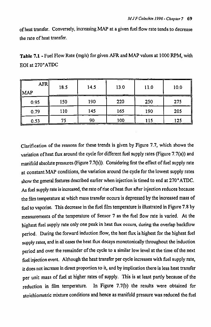
M J F Colechin 1996 - Chapter 7 69
of heat transfer. Conversely, increasing MAP at a given fuel flow rate tends to decrease
the rate of heat transfer.
Table 7.1 - Fuel Flow Rate (mgls) for given APR and MAP values at 1000 RPM, with
EOI at 270 0 ATDC
AFR 18.5 14.5 . 13.0 11.0 10.0
MAP
0.95 150 190 220 250 275
0.79 110 145 165 190 205
0.53 75 90 100 115 125
Clarification of the reasons for these trends is given by Figure 7.7, which shows the
variation of heat flux around the cycle for different fuel supply rates (Figure 7.7(a» and
manifold absolute pressures (Figure 7.7(b». Considering first the effect of fuel supply rate
at constant MAP conditions, the variation around the cycle for the lowest supply rates
show the general features described earlier when injection is timed to end at 270 0 ATDC.
As fuel supply rate is increased, the rate of rise of heat flux after injection reduces because
the film temperature at which mass transfer occurs is depressed by the increased mass of
fuel to vaporise. This decrease in the fuel film temperature is illustrated in Figure 7.8 by
measurements of the temperature of Sensor 7 as the fuel flow rate is varied. At the
highest fuel supply rate only one peak in heat flux occurs, during the overlap backflow
period. During the forward induction flow, the heat flux is highest for the highest fuel
supply rates, and in all cases the heat flux decays monotonically throughout the induction
period and over the remainder of the cycle to a similar low level at the time of the next
fuel injection event. Although the heat transfer per cycle increases with fuel supply rate,
it does not increase in direct proportion to it, and by implication there is less heat transfer
per unit mass of fuel at higher rates of supply. This is at least partly because of the
reduction in film temperature. In Figure 7.7(b) the results were obtained for
stoichiometric mixture conditions and hence as manifold pressure was reduced the fuel
M J FColechin 1996 - Chapter 7 70
supply rate was also reduced to maintain this ratio. The effect of reducing MAP is to
promote an increasing heat flux soon after the end of injection associated with fuel
vaporisation at lower temperatures and partial pressures. It is this improved vaporisation
at lower MAP's which produces the observed increase in heat transfer with decreasing
MAP in Figure 7.6.
To examine the effects of coolant temperature, warm-ups were carried out at each of the
MAP levels (0.95, 0.79 and 0.53 bar) using a stoichiometric mixture setting with the
engine again running at 1000 RPM and EOI timed at 270° AIDe of the firing stroke. For
each warm-up the engine was cold soaked to a uniform temperature below ooe while the
fuel and inlet air were kept at laboratory ambient temperatures. This resulted in a nominal
fuel temperature of 20°C at the start of each test, typically increasing to 30°C at fully
warm conditions, as the spill-back flow was returned to the supply tank.
Figures 7.9(a)-(c) show the variation in local rates of heat transfer to the fuel during these
warm-ups with a twin-spray injector fitted. Although even at the lowest coolant
temperatures apparently significant heat transfer rates were recorded, values less than
50 J/m2 have been deemed to be within levels of measurement uncertainty and neglected.
The injected fuel is generally warmer than the port walls at the low end of the coolant
temperature range (see Figure 7.10), so the positive heat transfer from the surface must
result from fuel evaporation and indicates the importance of convective mass transfer in
the vaporisation process at these conditions. Further evidence for this is given in
Figure 7.11, which shows the variation with coolant temperature of crank-angle resolved
heat fluxes for the single-spray injector. Here, at low coolant temperatures (0-30°C) very
little heat transfer occurs outside of the inlet valve open period, when mass transfer is
driven by the increased temperature of the overlap backflow and the convective effects
of all the gas flows. By the time the coolant temperature reaches 60°C, heat flux peaks
are apparent both immediately after fuel injection and during the inlet valve open period.
Finally, at fully-warm operating conditions (90°C) the comparative effects of the events
around the cycle are as described for Figure 7.5.
M J F Colechin J 996 - Chapter 7 71
The results presented in Figure 7.9 show that fuel distribution varies with MAP. For a
MAP of 0.95 bar, most deposition occurs around Sensor 7 and Figure 7.9(a) shows that
heat transfer levels measured through Sensors 4, S, 6 and 8 are relatively low. This was
supported by the photographic evidence, recorded at high MAP values, showing that the
twin-spray injector produces two sprays of large droplets directed towards the backs of
the valves, close to the position of Sensor 7. A redistribution of deposition around
Sensor 4 and Sensor 7 occurs when MAP is lowered, as indicated by comparing
Figure 7.9(a) and Figure 7.9(c). The heat transfers recorded through Sensor 4 at a MAP
of 0.53 bar are the highest recorded for any sensor across the test range, even though the
rate of fuel injection is low. This apparent redistribution of fuel was most obvious with
the twin-spray injector and could be due to changes in spray characteristics as MAP is
lowered, like those observed by Nogi et al [7.11], or fuel redistribution, as suggested by
Curtis et al [7.12]. The same occurred with the four-hole injectors at the low MAP
condition, to a lesser extent, when heat transfer rates recorded by Sensors 6, 7 and 8 had
similar magnitudes. With the single-spray injector the fuel appeared to centre around
Sensor 7 at all MAPs.
In Figures 7.12(a)-(c) the effects of injector type on the warm-up data are compared.
These three figures show how the estimated total heat transfer per cycle in Joules for each
injector type varies with coolant temperature, after subtracting the "dry-port" heat transfer
contributions, at three different fuel flow rate and MAP levels. The increase in heat
transfer with increasing coolant temperature is similar for each injector, despite marked
differences between their deposition patterns. This is coincidence and somewhat
misleading. The four-hole injector data is the average of results from two, nominally
identical injectors, and the individual sets of data diverge from similar values at O°C to
differ by a factor of two at fully-warm conditions. Some explanation of these inter
injector variations was offered by fully-warm tests carried out with the twin-spray injector
in which the splitter cap was rotated through a series of known points and the effects on
inlet port heat transfer measured. Figure 7.13 shows the results of these tests, where it
can be seen that the orientation of the injector sprays is at least as important as the spray
characteristics in determining the heat transfer to the fuel.
M J F Colechin 1996 - Chapter 7 72
The effect of increasing fuel flow rate at a given coolant temperature systematically
increased heat transfer per cycle, seen in Figure 7.12, for both the single-spray and four
hole injectors. For the twin-spray injector, at the lowest fuel flow rate, the heat transfer
showed an increase over values at the higher fuel flow cases due to the changes in spray
characteristics and deposition patterns with MAP. Since AFR was maintained nominally
constant at stoichiometric settings for all these tests, the higher fuel flow rates correspond
to higher MAP settings, which also influence heat transfer due to the relationship between
partial pressure and vaporisation rates. The effect of fuel flow rate and MAP are not
separated in Figure 7.12; it has already been shown in Figures 7.6(a)-(c), however, that
increasing fuel flow rate increases heat transfer and this is the dominant effect, while
increasing MAP tends to reduce the heat transferred.
7.5 The Response of Heat Transfer to a Step Change in Fuel Supply
A step change in fuel supply rate at otherwise steady state engine operating conditions
represents an important special case in the study of fuel transport. The rate at which the
induced fuel flow changes to match the new fuel supply rate has implications for the
control of induced mixture ratio to within a narrow target range. The initial and final
quantities of fuel stored in surface films in the intake port are different, according to
predictions based upon the phenomenological T-Xmodel [7.2,7.13], and the rate at which
the film mass adjusts to a new equilibrium condition will depend upon heat transfer to the
fuel film. By implication, heat transfer during cycles after the fuelling level change should
reflect the changes in fuel deposition rate and the rate of mass transfer from the fuel film
which occur.
To examine this, a test was carried out whereby the fuel injection rate was increased in a
single step and the variation of the heat transfer measured by Sensor 7 was recorded until
a new steady-state condition was established. The engine was run fully-warm at
1000 RPM and 0.79 bar MAP. The fuel supply rate was increased from 112 mg/s to
206 mg/s. The variation of induced mixture AFR was monitored using a UEGO sensor
in the exhaust gas stream. The results for heat transfer per cycle and AFR variations are

M J F Colechin J 9~6 - Chapter 7 73
given in Figure 7.14. The repeatability of the heat transfer variation between initial and
final conditions is indicated by the upper and lower bounds on experimental data taken
over eight repeated tests. The final to initial ratio of heat transfer values is in agreement
with the dependence upon fuel supply rate established previously during steady-state tests.
Figure 7.15(a) shows the variation of instantaneous "wetted" heat transfer rate over
twelve cycles spanning conditions before and after the change in fuel supply rate, which
occurred after cycle zero. Prior to the change, heat flux peaks at around 20 kW/m2
shortly after the end offuel injection, and a second peak of between 11 and 15 kW/m2
occurs during the induction period. After the change in fuel supply rate, the peak heat
flux increases to 40 kW/m2 but declines to less than 30 kW/m2 over the first six cycles,
despite the increasing value for heat transfer rate per cycle. This declining maximum is
associated with changes in fuel film composition as well as quantity. Immediately after
the change in fuel supply rate the fuel film will contain a higher proportion of lighter fuel
fractions. This proportion will diminish, as the new equilibrium film mass and composition
is approached.
For the same engine operating condition the dry surface heat transfer rate is relatively
small. Subtracting this from the measured "wetted" port heat transfer variation gives the
net heat transfer to the fuel shown in Figure 7.I5(b) for cycles 0, 1, 5, 10 and 15. An
overlay of these cycles on a crank angle base is shown in Figure 7 .15( c). The changes in
heat transfer variation which occur over these cycles are consistent with the inferences
drawn from the steady state results. On the first cycle with the higher fuel injection rate,
the early evaporation of higher quantities of light fractions produces the high peak heat
flux, but as the cycle progresses the heat flux decays to levels reflecting mass transfer of
the residual heavier fractions from a film mass similar to that prior to the change in fuel
flow rate. Over the ensuing cycles the film mass builds up and the initial rate of rise and
peak heat flux after injection both diminish, whilst heat transfer in the tail of the variation
increases.
M J F Colechin 1996 - Chapter 7 74
These characteristics suggest that the initial response of induced fuel flow rate to changes
in supply is strongly influenced by the proportion of lighter fuel fractions in the fuel being
deposited and the initial fuel film mass. The response is therefore likely to be more rapid
if the initial film mass is relatively small. As the new equilibrium condition is approached,
the effect of the lighter fuel fractions is diminished by dilution with the more persistent
heavier fractions building up in the fuel film. For the tests carried out, this takes more
than 15 engine cycles. The effects of a perturbation in the opposite direction, a decrease
in fuel supply rate, are shown in Figure 7.16. Here, on the first cycle with the lower fuel
injection rate, the early evaporation of light fractions is immediately diminished by dilution
with the more persistent heavier fractions in the residual film from the higher fuel flow rate
condition. Over the ensuing cycles the film mass diminishes, reducing heat transfer in the
tail of the variation, and the initial rate of rise and peak heat flux after injection both
increase. The time to establish new equilibrium conditions for perturbations in both
directions is a strong function of surface temperature. This is affected by fuel
composition, particularly the relative proportions of light to heavy fractions in the fuel,
which dictates the temperature at which the lighter fuel components are transferred from
the film. The time required will also be influenced by the persistence of the heavier fuel
fractions, which dictates the equilibrium film mass.
7.6 Discussion
The changes in surface heat transfer rates associated with fuel deposition exhibit complex
characteristics dependent upon engine running conditions. No attempt has been made in
this Chapter to model the fundamental processes of convective mass transfer and
evaporation which give rise to these characteristics. As a step towards rationalising the
data, however, the functional dependence of heat transfer on fuel flow rate, MAP and
coolant temperature has been examined using the data obtained from Sensor 7 (see
Figure 7.17), which was "wetted" consistently by deposition over the range of running
conditions tested. The results are for the single-spray injector and the "dry-port" heat
transfer rate has been subtracted from the measured rate. For a given MAP, the sensitivity
of heat transfer rate to fuel supply rate can be approximated to:
M J FColechin 1996 - Chapler 7 75
aQ II
- • exp (a + b p 2) am 1 1 /
(7.1)
where a1 and bl are constants. Integrating Eqn. 7.1 yields:
(7.2)
where the constant of integration is assumed to be a linear function of MAP, with
constants a2 and b2 consistent with the values of (2' for zero fuel mass flow rate inferred
by extrapolation of the results given in Figure 7. 17.
Data showing how Q' varies with coolant temperature is shown in Figure 7.18. To
account for this dependence, Eqn. 7.2 was modified to the form:
(7.3)
Although there are alternatives which would give an equally good fit to the data, the
functionf(1J was chosen as:
f(T). ! [1. cos ( ;; · n) 1 (7.4)
and the constant c determined from the data taken at a coolant temperature of O°C.
Figure 7.19 shows that the variation given by Eqn. 7.3 compares reasonably well with the
raw data in Figure 7.18. By inspection this equation is of the form:
(7.5)
The function/t, deduced from Figure 7.17, accounts for the effects of fuel supply rate and
MAP on fuel warming and diffusive mass transfer. Variations in the fuel supply rate affect
the heat transfer required to warm newly deposited fuel to the film temperature, but they
also particularly affect the heat transfer to those fractions of the fuel for which the mass
available is the limiting factor in the vaporisation process. Variations in MAP also have
an effect. through};, on those fractions for which the limiting factor is the mass vaporised
with the aid of convection. Functioniz relates,h to the temperature of the port. At lower
temperatures the evaporation of more components will be limited by convective mass
transfer than by the film mass available, until at the lowest temperature recorded
M J F CoJechin J 996 - Chapter 7 76
convective mass transfer dominates: the heat transfer becomes dependant on MAP alone,
1. becomes 0 and the heat transfer is given by J;. A similar description could be attached
to data recorded with each of the other injectors as borne out by Figure 7.12 where similar
trends are apparent in all the data, although the constants implicit in Eqn. 7.5 will differ.
The prospects of producing a general correlation for the total heat transfer to the fuel
appear to be poor, however, because such large local variations arise. Nevertheless, the
description given by Eqn. 7.5 should be characteristic of the regions of the port near to
the valves where deposition rates are high. Combining Eqn. 7.5 and Eqn. 6.2 gives a
value for heat flux as measured with the heat flux sensors under "wetted-port" conditions,
which includes the surface-to-gas contribution:
(7.6)
Evaluating the surface-to-gas contribution in Eqn. 7.6 requires knowledge of the
magnitude and sense (positive or negative) of the surface-to-gas temperature difference
from Chapter 6. Figure 6.12 illustrated how temperature differences vary as the engine
warms up. For high MAP, low surface temperature conditions, the direction of heat
transfer is towards the surface. As the surface temperature increases, the temperature
difference becomes progressively less negative and, at most locations, eventually positive
by the time fully-warm conditions are established, giving rise to heat transfer from the
surface to the gas. The effects of backflow at low MAP values raise the effective gas
temperatures and over much of the region downstream of the port bifurcation, heat is
transferred from the gas towards the surface throughout the warm-up.
Sensor 7 was located in the region where most fuel deposition occurs. At this position,
for fully-warm conditions, the direction of heat transfer was always from the surface
towards the gas when the port was dry. Comparing the results shown in Figures 6.10
and 7.9 indicates that at fully-warm conditions, the inferred heat transfer to the fuel film
has been reduced by heat transfer to the gas stream. When the surface temperature is
below typically 40°C during a warm-up, the heat transfer to the fuel film is increased by
heat transfer from the gas stream. It must be emphasised, however, that these inferences
are based on the assumption that heat transfer to or from the gas stream is the same for
M J F Colechin J 996 - Chapter 7 77
"dry" and "wetted" surface conditions. More accurately, these changes in heat transfer
rate should be described as being associated with fuel deposition.
Unlike the "dry-port" conditions discussed in Chapter 6, the temperature of the sensors
when "wetted" was lower than the assumed surface temperature, particularly in areas of
heavy fuel deposition. As fuel flow rate and hence fuel film mass increased the sensor
temperature decreased further (see Figure 7.8), reflecting a drop in the fuel film
temperature. This will be at least partly due to the insulating effect of the heat flux sensor
creating a temperature drop between the port-wall and the fuel film, because of the
relatively high rates of local heat transfer in areas of heavy deposition. Figure 6.14
showed crank-angle resolved sensor surface temperatures calculated using a finite
difference model of the sensor from the inferred "dry-port" surface heat fluxes. Using the
same finite difference model, crank-angle resolved temperatures were calculated for a
"wetted" Sensor 7 at the surface and at the position of the incorporated T -type
thermocouple used to measure sensor temperature. Typical results are shown in
Figure 7.20. Figure 7.21 shows mean cycle temperatures calculated from these data over
a range of fuel flow rates, along with experimentally measured sensor temperatures for the
same operating conditions. The experimental data indicates that the sensor is at a lower
temperature than can be explained purely by the insulating effects of the sensor. Other
factors in this temperature drop will be the contribution the sensible internal energy ofthe
fuel film makes in providing the required heat of vaporisation for the mass transfer which
is occurring, and the effect of newly deposited fuel from the colder injection spray.
For "dry-port" conditions heat transfer per cycle varies between 0 and 300 J/m2 depending
on location, towards the surface at low temperatures and away from the surface at fully
warm conditions. The changes in measured heat transfer per cycle associated with fuel
deposition are invariably positive (from the surface). These changes vary with location
but, in the vicinity of highest deposition, are in the range 1000 to 1500 J/m2 at fully-warm
operating conditions. During the early period of engine running after start-up, when both
surface temperatures and the temperature of the fuel supply are around 20°C, the change
is typically 300 J/m2• The effect of fuel supply temperature has not been examined
M J F Colechin J 996 - Chapter 7 78
systematically in the current work, but a supplementary test was carried out with the fuel
supply cooled to an initial temperature ofOoe. Figure 7.22 shows results from this test
along with results from the equivalent test with fuel at ambient laboratory temperature,
while Figure 7.23 shows the difference in fuel temperatures between the two tests.
Comparing the results produced by tests at different fuel temperatures, it is clear that
lowering the fuel temperature from 20 0 e to O°C gives rise to increases of up to 100 11m2
in heat transfer per cycle during the early period of engine running, in areas of the port
where fuel deposition is most concentrated.
Chapter 8
Heat Transfer to Isooctane
8.1 Introduction
The work described in this chapter extends the study of inlet port heat transfer presented
in Chapters 6 and 7 to cases when the engine is running on a single-component fuel, 2-2-4
trimethylpentane (isooctane). The results obtained for isooctane are of particular interest
in connection with the development of a model to describe mass transfer from the fuel film
produced by deposition. As for the tests with pump-grade unleaded fuel, the dry-surface
heat transfer rates found in Chapter 6 were subtracted from values measured when the
sensors were wetted by fuel, to determine the effect of the latter. With both fuel types,
the heat transfer rate to the fuel reaches peak values up to around 50 kW/m2 during the
engine cycle, and is typically 5 kW/m2 on average in regions of heavy fuel deposition. The
heat transferred per cycle depends upon engine operating conditions: during warm-up, as
coolant temperature increased from ooe to 90°C, this increased from typically 300 J/m2
to 1000 J/m2; for a given coolant temperature, heat transfer values generally increased
when MAP was lowered or as supplied fuel flow rate was increased. In general, the effect
offuel deposition on heat transfer rate, when running on pump-grade unleaded gasoline,
could be characterized as a function of injected fuel flow rate, MAP, and engine coolant
temperature or surface temperature. This function reflects the underlying mechanisms of
diffusive and convective mass transfer from the surface film. However, the extent to
which these characteristics were dependent on the properties of the fuel used was less
clear and to clarify this the work described here, using isooctane fuel which has known
thermodynamic properties, was undertaken. The characteristics of isooctane are
summarised in Table 8.1 [8.1].
79
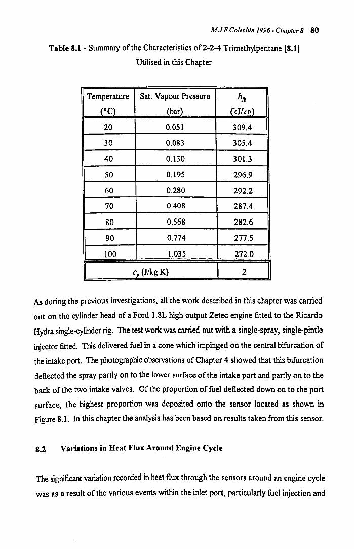
M J F Colechin 1996 - Chapter 8 80
Table 8.1 - Summary of the Characteristics of2-2-4 Trimethylpentane [8.1)
Utilised in this Chapter
Temperature Sat. Vapour Pressure h!6
(DC) (bar) (kJ/kg)
20 0.051 309.4
30 0.083 305.4
40 0.130 301.3
50 0.195 296.9
60 0.280 292.2
70 0.408 287.4
80 0.568 282.6
90 0.774 277.5
100 1.035 272.0
I cp (J/kg K) I 2 I As during the previous investigations, all the work described in this chapter was carried
out on the cylinder head of a Ford 1.8L high output Zetec engine fitted to the Ricardo
Hydra single-cylinder rig. The test work was carried out with a single-spray, single-pintle
injector fitted. This delivered fuel in a cone which impinge~ on the central bifurcation of
the intake port. The photographic observations of Chapter 4 showed that this bifurcation
deflected the spray partly on to the lower surface of the intake port and partly on to the
back of the two intake valves. Of the proportion of fuel deflected down on to the port
surface, the highest proportion was deposited onto the sensor located as shown in
Figure 8.1. In this chapter the analysis has been based on results taken from this sensor.
8.2 Variations in Heat Flux Around Engine Cycle
The significant variation recorded in heat flux through the sensors around an engine cycle
was as a result of the various events within the inlet port, particularly fuel injection and
M J F Colechin J 996 - Chapter 8 81
forward induction flow. To investigate these measured variations further and establish
their underlying phenomenological causes, a warm-up test was undertaken with the engine
running on isooctane and EOI timed to occur at TDC of the firing stroke. Tests with
pump-grade unleaded fuel showed that injecting at this point in the cycle clearly separated
the effects offuel injection from those of the forward induction flow (see Figure 7.3). The
other operating conditions used for the isooctane fuelled warm-up were an engine speed
of 1000 RPM, a MAP of 0.53 bar, and a fuel flow rate of90mgls, such that the AFR was
stoichiometric once the engine was fully-warm. Data were recorded during an engine
warm-up between O°C and 90°C, after cold soaking to a uniform temperature below O°C
with the fuel supply at laboratory ambient temperature. Figure 8.2 shows the resultant
crank-angle resolved heat flux variations. These are "net" values obtained, after
compensating for heat flux sensor response, by subtracting the values recorded previously
in the absence of fuel deposition. Depending on whether these "dry-surface" values
indicate heat transfer towards the surface (a negative value) or from the surface, the net
heat transfer to the fuel is increased or decreased respectively relative to the raw data
values.
Injection timing was phased to end at 00 A TOC, which is earlier than the standard EOI at
270 0 AIDC but was selected because it separates two distinct features of the heat transfer
variation. Generally, shortly after the fuel injection event, heat transfer rates peak; this is
associated with the arrival of fuel on the sensor. Heat is transferred to this fuel as its
temperature is raised to that of the port wall and as vaporisation occurs raising the partial
pressure of fuel vapour above the film. The rate of heat transfer then decreases
monotonically until the forward induction period of the engine cycle, when a second peak
occurs due to an increased rate of convective mass transfer from the film. At lower
temperatures this peak corresponds to the maximum heat flux arising during the cycle.
At these low coolant temperatures the difference between the fuel and surface
temperatures is small, as is the partial pressure of the fuel vapour, requiring relatively little
heat transfer to raise the film temperature to the surface temperature. This temperature
difference and the partial pressure above the film both increase as the engine warms-up,
giving rise to the increasing magnitude of heat flux shortly after fuel injection has taken
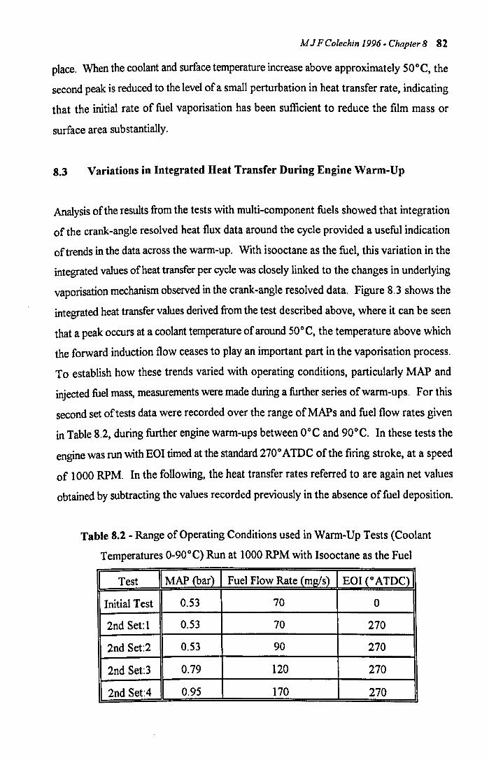
M J F Colechin 1996 - Chapter 8 82
place. When the coolant and surface temperature increase above approximately 50°C, the
second peak is reduced to the level of a small perturbation in heat transfer rate, indicating
that the initial rate of fuel vaporisation has been sufficient to reduce the film mass or
surface area substantially.
8.3 Variations in Integrated Heat Transfer During Engine Warm-Up
Analysis of the results from the tests with multi-component fuels showed that integration
of the crank-angle resolved heat flux data around the cycle provided a useful indication
of trends in the data across the warm-up. With isooctane as the fuel, this variation in the
integrated values of heat transfer per cycle was closely linked to the changes in underlying
vaporisation mechanism observed in the crank-angle resolved data. Figure 8.3 shows the
integrated heat transfer values derived from the test described above, where it can be seen
that a peak occurs at a coolant temperature of around 50°C, the temperature above which
the forward induction flow ceases to play an important part in the vaporisation process.
To establish how these trends varied with operating conditions, particularly MAP and
injected fuel mass, measurements were made during a further series of warm-ups. For this
second set of tests data were recorded over the range of MAPs and fuel flow rates given
in Table 8.2, during further engine warm-ups between O°C and 90°C. In these tests the
engine was run with EOI timed at the standard 270° ATDC of the firing stroke, at a speed
of 1000 RPM. In the following, the heat transfer rates referred to are again net values
obtained by subtracting the values recorded previously in the absence of fuel deposition.
Table 8.2 - Range of Operating Conditions used in Warm-Up Tests (Coolant
Temperatures 0-90°C) Run at 1000 RPM with Isooctane as the Fuel
Test MAP (bar) Fuel Flow Rate (mg/s) EOI (OATDC)
Initial Test 0.53 70 0
2nd Setl 0.53 70 270
2nd Set2 0.53 90 270
2nd Set3 0.79 120 270
2nd Set:4 0.95 170 270
M J F Colechin J 996 - Chapter 8 83
Figures 8.3 and 8.4 show that when the crank-angle resolved data is integrated up to give
values of heat transfer per cycle, there is relatively little difference between data recorded
with the end of injection (EOI) occurring at 00 AIDe and that recorded with the E01 at
270 0 ATDC. Values of heat transfer per cycle recorded with the latter injection timing
over the range of operating conditions tested are shown in Figures 8.5 and 8.6. Figure 8.5
shows the effect of changing load whilst running at stoichiometric mixture settings,
indicating that increasing load increases both the peak value of heat transfer per cycle and
also the coolant temperature at which this occurs. Although both MAP and fuel flow rate
change over the three test conditions, fuel flow rate is the dominant variable; this is
evident in the results presented in Figure 8.6, which shows two data sets obtained at a
constant MAP with fuel flow rate varying. In both Figures 8.5 and 8.6, for a given
coolant temperature below that at which the heat transfer per cycle peaks, the heat
transferred is relatively independent of fuel flow rate and, in this case, MAP.
8.4 Modelling or Heat Transfer and the Fuel Film Vaporisation Process
In the previous analysis of the measured heat transfer rates, resulting when isooctane is
used as a fuel, it has been inferred that there are three basic processes that give rise to this
transfer of heat between the port walls and the injected fuel:
(i) raising the sensible heat of the injected fuel to increase its temperature from
injection temperature to the fuel film temperature;
(ii) diffusive mass transfer of the fuel film, requiring latent heat of vaporisation and
dependent upon the vapour concentration gradient above the film;
(iii) convective mass transfer of the fuel film, also requiring latent heat of vaporisation,
associated with the convective effects of the various gas flows through the port,
particularly the forward induction flow.
M J FColechin 1996 - Chapter 8 84
An energy balance for the fuel film suggests that the net rate of heat transfer to the fuel
deposited on the sensor should be equal to the increase in sensible internal energy of the
fuel as its temperature is raised from an initial value to some film temperature, plus the
latent heat required to vaporise a proportion of the deposited fuel. This is given by
Eqn.8.1:
q " • t [(m" ) c 11 T + (m" ) h ] ')Ie Up P WIp I, (8.1)
Eqn. 8.1 cannot be evaluated, however, without knowledge of the rate of vaporisation
produced by diffusion and convective mass transfer and limitations on this imposed by the
availability of fuel.
The relative importance of diffusive and convective contributions to mass transfer rates
depends on the timing of fuel injection within the cycle, port surface temperature, and gas
flow conditions. For the conditions pertaining to Figure 8.2, when injection occurred
during the compression stroke, mixture motion in the port will be relatively quiescent, and
the high heat flux, arising soon after fuel is deposited at the higher coolant temperatures,
is associated with mass transfer by diffusion. In such cases, diffusion and convection
appear to be of similar importance to the total mass transfer occurring over the cycle, with
convection dominating at low temperatures and diffusion dominating at high temperatures.
Both mechanisms depend on vapour concentration gradients in a similar way. For
diffusion ofa volatile liquid through stagnant air Stefan's Law can be used. This is quoted
by Kay and Nedderman [8.2] as:
N · :T In(p ~p...) (8.2)
where Nis the molar flux (moVm2s), D is the diffusivity of vapour from the volatile liquid
through the surrounding gas (m2/s), R is the universal gas constant (J/mol K) and all the
other variables are defined in Figure 8.7, a diagram of Stefan's experiment used to
establish rates of diffusion. Eqn. 8.2 has been applied in the following way to diffusive
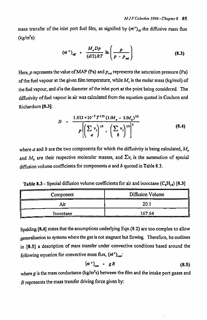
M J F Colechin 1996· Chapter 8 85
mass transfer of the inlet port fuel film, as signified by (ni")dif the diffusive mass flux
(kg/m2s):
m" " In P M Dp ( ) ( }Jtf. (d/2}RT p - p MIt
(8.3)
Here,p represents the value of MAP (pa) and PIal represents the saturation pressure (Pa)
ofthe fuel vapour at the given film temperature, while My is the molar mass (kg/mol) of
the fuel vapour, and dis the diameter of the inlet port at the point being considered. The
diffusivity of fuel vapour in air was calculated from the equation quoted in Coulson and
Richardson [8.3]:
D • 1.013 x 10.7 T1.7S (11M. + lIM6)11l
p[(EaVf· (~vrr (8.4)
where a and b are the two components for which the diffusivity is being calculated, Ma
and Mb are their respective molecular masses, and Ev, is the summation of special
diffusion volume coefficients for components a and b quoted in Table S.3.
Table 8.3 - Special diffusion volume coefficients for air and isooctane (C.H1.) [8.3)
Component Diffusion Volume
Air 20.1
Isooctane 167.64
Spalding [8.4] states that the assumptions underlying Eqn.(S.2) are too complex to allow
generalisation to systems where the gas is not stagnant but flowing. Therefore, he outlines
in [8.5] a description of mass transfer under convective conditions based around the
following equation for convective mass flux, (ni")COII:
(m Nt •• gB (8.5)
where g is the mass conductance (kglm2s) between the film and the intake port gases and
B represents the mass transfer driving force given by:
M J F Colechin J 996 - Chapter 8 86
(8.6)
In Eqn. 8.6, mris the vapour mass fraction within the fuel film, assumed to be 1; ms is the
fraction immediately above the fuel film surface, and is determined from the partial
pressures of the vapour and air and their respective molecular weights. The vapour in this
area is assumed to be saturated at the fuel film temperature. Finally, the mass fraction ma
offuel vapour in the main flow is small and assumed to be O.
The value of mass conductance can be found from knowledge of the Stanton number (St):
Sf • g - . G
Sh (8.7)
(Re. Sc)
where G is the bulk gas velocity along the centre line of the port (m/s), and Sh, Re and Sc
are the Sherwood, Reynolds and Schmidt numbers respectively. There is, however,
insufficient information in the measurements of heat transfer made with the heat flux
sensors to allow Sh to be calculated directly. Instead, the Reynolds Analogy between
momentum, heat and mass transfer can be utilised:
c, Sf • St· •
2 (8.8)
where c, is the skin friction factor and St· is a modified form of the Stanton number
derived from heat transfer measurements when no mass transfer is occurring. This uses
a relationship which is analogous to Eqn. 8.7, but with Sh and Sc replaced by Nu (Nusselt
number) and Pr (prandtl number):
Sf· • Nu
(Re. Pr) (8.9)
Kay and Nedderman [8.2] suggest that an improvement on Reynolds Analogy is offered
by the I·Factor Analogy, in which:
M J F Colechin 1996 - Chapter 8 87
which leads to the definition of mass conductance given by Spalding [8.5]:
g' ,. St'G( Dp )i kl(c ,),.
(8.10)
(8.11)
in which the * again indicates values derived from heat transfer measurements when no
mass transfer is occurring, p is the density (kg/ml) of the mixture above the film, while
k and {cp)gQl are, respectively, the thermal conductivity (W/m K) and specific heat capacity
(Ilkg K) of the inlet port gases. Spalding [8.5] adds that when utilising this derivation of
mass conductance Eqn. 8.5 should be modified to:
(m "t.. · g' In (1 + B) (8.12)
There are clear similarities between Eqns. 8.3 and 8.12, particularly in the form of the In
function, which in both cases will tend to infinity as P.at approaches MAP. Spalding [8.4]
reflects this by offering a form of Eqn. 8.12 for a situation in which no convection is
occurring and the mass transfer will be purely diffusive:
(m")djf • Dp In(l + B) dl2
(8.13)
Although less accurate than Eqn. 8.3, Eqn. 8.13 is useful for making an estimate of the
ratio between the values of mass flux given by Eqn. 8.12 and those for diffusive mass
transfer when no convection is occurring. For temperatures below those at which the
function In(1 + B) tends to infinity, Eqns. 8.11, 8.12 and 8.13 can be combined to give the
proportion of the mass transfer that is diffusive when convection is also occurring:
(m II tOrI • d/2. St. G • ( D p ) 213
(m ")djf D p kl(c ,),. (8.14)
M J F Colechin 1996 - Chapter 8 88
This gives values representative of Sh, which, being directly analogous to Nu [8.6], is the
ratio of mass transfer by convection to that by diffusion across a characteristic dimension.
Based on this interpretation, the value of Sh is unity when there is no convection and the
mass transfer is purely by diffusion. Typical values derived from Eqn. 8.14 are between
10 and 20 for temperatures below those at which the In function tends to infinity. These
are of the same order of magnitude as the values of Nu derived for gas flows through a
"dry-port". At higher temperatures, when the mass transfer driving force becomes
infinite, fuel vaporises even during the quiescent period of the cycle (see Figure 8.2).
Under these conditions, the dominant mechanism for vaporisation is diffusive mass
transfer.
In principle, therefore, over most of the temperature range, values of (ni")vap for Eqn. 8.1
can be derived by calculating (ni ")con from knowledge of flow conditions and the
thermodynamic properties of the gas and fuel. However, the complexity of conditions in
the port and measurement limitations give rise to large uncertainties in the calculation of
g*, required for the derivation of (ni ")con. In view of this, g* has been deduced to best fit
the experimental data for the heat transfer characteristics, making use of Eqns. 8.1
and 8.12 to obtain:
g. • Q" - ~")dlpcp~T
1n(l + B) • hll (8.15)
Here, the value of g* reflects the influence of both diffusive and convective mass transfer
mechanisms. When evaluating this, measured values of heat transfer rate q" have been
used together with values of (ni")dep inferred using Eqn. 8.16, described later. Figure 8.8
shows the derived variation of g* with surface temperature, for three MAP values. In
general, across the range of temperatures from 30°C to 80°C, the mass conductance value
is weakly dependent on MAP and effectively constant. Values for g* at surface
temperatures less than 30°C are more variable. It is not clear if this is a real effect or a
consequence of uncertainty in the experimental data. In the following the mass
conductance has been taken as a constant independent of surface temperature throughout
the whole range of surface temperatures examined.
M J F Colechin 1996 - Chapter 8 89
U sing the deduced value of mass conductance, the predicted rate of vaporisation is as
shown in Figure 8.9, for three operating conditions. As surface temperature increases, the
mass flux increases monotonically towards infinity as the equilibrium saturation vapour
pressure approaches the manifold absolute pressure. The heat flux measurements indicate,
however, that before this condition is reached the rate of mass transfer becomes limited
by some other factor associated with the mass of fuel available for vaporisation in the film.
In this case, the rate of fuel vaporisation is assumed to be proportional to the rate at which
fuel is deposited on the sensor as given by:
(8.16)
and the value of YIA at a given surface temperature is determined to be consistent with the
measured rate of heat transfer. At temperatures below the range when this supply-limit
exceeds the predicted rate of vaporisation by convective mass transfer, the excess fuel
deposited is assumed to be transferred from the sensor surface by film flow. For these
lower temperatures, the value of YIA has been determined by extrapolating the variation
with temperature to give the trend shown in Figure 8.10. This variation is independent
of engine operating conditions. Using this, together with the constant value of g*
determined earlier, gives good agreement between the model predictions and measured
values of heat flux per cycle over the range of engine operating conditions examined, as
illustrated in Figure 8.11. The higher fuel flow rates used at higher MAPs lead to a
greater mass of fuel being deposited each cycle; this requires greater heat transfer to
increase its sensible internal energy, thus obscuring the effects of the mass flux variations
with MAP observed in Figure 8.9. A breakdown of the constituent contributions to the
total heat transfer per cycle is given in Figure 8.12, for one operating condition.
8.5 Discussion
The measured rates of heat transfer associated with fuel deposition, and its variation with
operating conditions and events within the engine cycle, are consistent with the following
interpretation. The injected fuel temperature is generally lower than the surface
M J F Colechin J 996 - Chapter 8 90
temperature of the intake port and the sensor and, once deposited, heat transfer raises the
sensible internal energy of the fuel. Depending on the surface temperature a portion of
the fuel is vaporised, establishing a partial vapour pressure above the film commensurate
with the film temperature. The rate of vaporisation varies with operating conditions and
with variations in intake port conditions around the cycle. The rate of vaporisation is
affected both by the manifold absolute pressure and the flow conditions in the intake port
thus giving rise to relatively high rates at low manifold pressures and during the induction
interval of the cycle when charge velocities in the intake port are highest. As surface
temperature increases so does the rate of heat transfer up to a maximum value that is
dependent on engine operating conditions and fuel flow rate. The measured trends in heat
transfer rate suggest that at higher temperatures, the rate of heat transfer is limited by the
availability of fuel to vaporise.
The trends observed are well characterised using a relatively simple model for mass
transfer together with information on how fuel deposition varies with temperature and
engine operating condition. Although two parameters in the model have been calibrated
empirically, the inferred value of g* (i.e. 0.012) is of a similar magnitude to the values
estimated for convective mass transfer using Eqn. 8.11 ~ similarly the magnitude and
variation of Y are in accord with knowledge of deposition rates determined using the fuel
perturbation technique described in [8.7]. The values of g* estimated from Eqn. 8.11
varied from 0.014 to 0.022 across the temperature range tested. They were based on the
dry-port heat transfer measurements made through Sensor 7 in conjunction with gas
temperatures measured by Te 1, all at a MAP of 0.95 bar when the backflow effects
would be minimised. At these conditions with this sensor, the calculated values ofNu
were closer to the Martins and Finlay correlation in Figure 6.13 than to the correlation for
Sensors 1 and 2. Values of Y were compared with the fraction X of isooctane supplied
which is deposited overall, rather than locally. By looking at the temperature variation
inX (see Figure 8.13) and values of Y determined from Figure 8.10, using a value for A
of 1.3xl0-3 m2 (chosen arbitrarily to be ten times the sensor area and representing about
1h of the wetted surface area of the port), the inferred proportion of deposited fuel landing
on and immediately around the sensor was found to account for typically 40% of the total
MJ FColechin 1996 - Chapter 8 91
fraction deposited. This is not unreasonable and, by implication, indicates that the
remaining 60% is distributed around the other parts of the intake port surface and on the
back of the valve. To maintain simplicity in the model the temperature of the fuel film was
assumed to be the same as the port surface temperature. It was shown in Chapter 7,
however, that the fuel film above Sensor 7 was generally at a lower temperature, creating
a temperature difference of over 20 deg. C at higher fuel flow rates. This will
undoubtedly lead to errors in the modelled data and may explain the mismatch between
the modelled and experimental data in Figure 8.11.
At fully warm conditions the data suggests that a high proportion of the fuel deposited on
the sensor is vaporised and that the rate of vaporisation is limited by the availability offuel
in the film. During warm up this is not the case and Figure 8.14 shows how the
proportion offuel vaporised varies with port surface temperature at each MAP level. At
a port surface temperature of 20°C and a MAP of 0.95 bar only 5% of the deposited fuel
is vaporised, indicating that the remainder is re-entrained as liquid droplets into the
airstream or is displaced from the sensor by the flow of liquid in the film.
One of the objectives of the current work was to examine the effect offuel properties by
comparing data obtained using single-component and multi-component fuels. In both
cases, the trends in the heat transfer data are associated with the variation of saturation
pressure with temperature and conditions in the intake port. Generally the results
obtained with pump-grade unleaded gasoline show higher heat transfer rates at lower
temperatures, and these rise continuously across the temperature range without evidence
of a maximum point (see Figure 7.18). The higher heat transfer rates at lower
temperatures indicate that a larger proportion of the deposited fuel is vaporised as a
consequence of the lighter components in the multi-component fuel. Conversely the
heavier fractions do not vaporise to the same extent as isooctane until higher surface
temperatures are reached. These heavier fractions persist in the fuel film and hence the
heat transfer rate does not become supply-limited. One consequence of this was the
reduction in heat transfer rate with increasing MAP at fully-warm conditions, shown in
Figure 7.17. Data recorded under the same conditions with isooctane as the fuel (see

M J F Colechin 1996 - Chapter 8 92
Figure 8.15) did not show the same dependence on MAP, but did maintain a general heat
transfer increase in proportion to injected fuel flow rate. The modelled data also shown
in Figure 8.15 uses the supply-limitation assumption to predict this trend quite accurately.
Chapter 9
Summary and Discussion
9.1 Introduction
The processes of mixture preparation and fuel transport in the intake systems of spark
ignition engines are receiving much attention, as manufacturers strive to meet emissions
regulations with vehicles which fulfill the performance and economy requirements of their
customers. The widespread adoption of port fuel injection systems has prompted detailed
investigations of the mixture preparation quality these produce. Investigations of inj ector
spray characteristics do not provide sufficient information, in isolation, to characterise fuel
transport from the injector to the combustion chamber. More commonly. investigations
have sought to define parameters in models of these fuel transfer properties. based on
exhaust measurements of combusted AFR. This approach has been utilised in the work
for the first part of this thesis. where comparisons were made between the mixture
preparation properties of different injector types. These involved photographing the spray
patterns they produced in a firing engine. and measuring the response of the combusted
AFR to fuelling perturbations with each injector type. Although useful in characterising
the fuel transfer processes for control purposes, such approaches do not provide in-depth
analysis of the mechanisms by which mixture preparation occurs. A better understanding
of these mechanisms is required if mixture preparation is to be optimised through
hardware design and selection of the most appropriate control strategies. To this end the
majority of this thesis concentrated on the measurement of heat transfer in the inlet port
of a spark ignition engine. using these measurements to infer detailed information about
the vaporisation of fuel deposited on the intake port walls.
9.2 Crank-Angle Resolved Heat Flux Variations
Surface heat fluxes have been measured in the intake port directly. using heat flux sensors.
for the first time in a firing engine. Although the response of these sensors was relatively
93
M J FCoJechin /996 - Chapter 9 94
slow, experiments to determine their response characteristics, together with an analytical
model of the sensors, have enabled measured heat flux data to be processed to derive
variations within the period of an engine cycle. The likely temperature reduction at the
surface of sensors, due to the insulating effects of their construction, has also been
analysed. This analysis has shown that the cycle-averaged temperature at the surface of
sensor can vary by up to IS deg. C from the temperature at the port surface when there
is a high local cycle-averaged heat transfer rate, generally associated with heavy fuel
deposition. This compares with a measured local temperature difference of 20 deg. C for
the same operating conditions, which will also be partly due to a reduction in the sensible
internal energy of the film as fuel is vaporised.
In the absence of fuel deposition, heat exchange between the surface and gases within the
intake port at fully-warm operating conditions takes place predominantly during the inlet
valve-open period. The direction of this heat flow is towards the surface during the valve
overlap interval, due to the influence of hot backflow gases, and from the surface over the
major part of the induction period. Valve-overlap backflow results in heat flux spikes of
up to 60 kW/m2 at low manifold pressures, while the forward induction flow gives rise to
heat fluxes of up to 6 kW/m2• After inlet-valve-closing, the heat flux falls monotonically
to a small value, generally within Yl a crank angle revolution, as displacement backflow
and the subsequent gas motion decay. The influence of overlap backflow varies with
manifold pressure. At low pressures, this backflow both extends further upstream in the
intake port and gives rise to higher heat transfer rates to the surface. The overlap
backflow also appears to be unmixed in the intake port to an extent which can change
during engine warm-up, as evidenced by the development and eventual disappearance of
the associated heat transfer spike at some locations over the warm-up period.
Deposition of fuel on the port surfaces invariably produced a heat transfer contribution
which was positive (from the surface), at all the test conditions examined. Tests with a
single-component fuel (isooctane) indicated that the influence of this contribution on intra
cycle heat flux variations was dependent on the thermal properties of the fuel. The multi
component nature of pump-grade gasoline, therefore, makes the results with this fuel most
M J F Colechin J 996 - Chapter 9 95
difficult to interpret, although the following will generally apply. When surface
temperature is low, vaporisation of even the lighter fuel fractions is limited and convective
mass transfer during the period of gas motion is important. As surface temperature rises,
the influence of the gas flows diminishes. At fully-warm engine running conditions, heat
transfer to fuel deposited upon the intake port surface is not substantially enhanced by
either the overlap backflow, forward induction flow or decaying gas motion effects.
Typically these enhancements contribute 1%, 13% and 10%, respectively, to the total over
the cycle. More significant is the heat transfer associated with raising the sensible internal
energy of the fuel and vaporising, particularly the lighter fuel fractions, through diffusive
mass transfer. Consequently, heat transfer rates increase very rapidly after each injection
event, more so at low fuel supply and low manifold pressures. Under these conditions,
the effect on the total heat transfer per cycle is partially offset by lower heat transfer rates
later in the cycle.
9.3 Variations in Cycle-Averaged Heat Transfer Rates
When the surface is dry and backflow effects are minimal, measured rates of cycle
averaged heat exchange between the gas flow and the surface vary linearly with surface
temperature at a given location and charge flow rate. Such data that can be processed to
relate Nu and Re, which has been limited by the difficulty of determining the effective gas
to-surface temperature difference, produces a similar correlation to that derived by
Martins and Finlay [9.1] from steady-flow experiments.
Strong spatial variations occur in both "dry-port" heat transfer and in heat transfer to the
fuel under ''wetted-port'' conditions. Without fuel deposition, these reflect the domain of
influence of reversed gas flows back into the manifold, whereas when the port is "wetted"
they reflect variations in local rates of fuel deposition. At fully-warm conditions the
positive heat transfer contribution created by fuel deposition increased the heat transfer
from the surface. At low surface temperatures, it produced a reduction in the heat transfer
to the surface. The magnitUde of the contribution depended on manifold pressure, fuel
injection rate, and coolant temperature. Increasing coolant temperature or fuel injection
M J F Colechin 1996 - Chapter 9 96
rate gives rise to an increase in heat transfer, as does a reduction in MAP. These
variations, both spatially within the port and with operating conditions, provide an
indication of the deposition pattern for the injector types examined, which can be
compared with the results of the photographic study in Chapter 4. Values of heat transfer
per cycle to the fuel deposited under fully-warm conditions at 1000 RPM and three
manifold pressure settings are presented in Table 9.1. Only sensors which record values
greater than 50 kJ/m2 at one or more operating conditions have been included in the table.
The values given were recorded for a mixture AFR of 14.7 and two other settings at the
same manifold pressure. Each case gave similar distributions of values across the set of
sensors, although magnitudes changed by up to a factor of 3 in some cases. With few
exceptions highest heat transfers were recorded by Sensors 7 and 4, which are located on
the floor of the intake port. In most cases Sensor 7 records the highest value. For the
single-spray injector, significant levels of heat transfer were recorded for all but Sensor 1
at one or more of the manifold pressures examined, suggesting this injector produced the
widest distribution of fuel deposition to the port surface. The greatest spread occurred
at the lowest manifold pressure when 66% of the total measured across all sensors was
recorded by Sensor 7, a decrease from around 80% at the higher manifold pressures. The
most dramatic redistribution of fuel deposition appears to occur with the twin-spray
injector. Here, when manifold pressure is lowered, the highest heat transfer per cycle
recorded is by Sensor 4 rather than Sensor 7. However, only a small movement of the
fuel spray in the upstream direction is required to account for this. At the same time it
appears that fuel wetting of the central bifurcation is reduced as evidenced by the fall in
heat transfer recorded by Sensor 5. The results obtained for the four-hole injector suggest
fuel deposition occurs primarily on Sensors 4, 6, 7 and 8. As manifold pressure is lowered
the deposition pattern appears to shift downstream towards the intake valves with nearly
equal values of heat transfer per cycle recorded by Sensors 6, 7 and 8.
The photographic studies together with the heat transfer measurements indicated that the
most significant differences between the injector types are as follows. The single-spray
injector appears to deposit fuel over the widest area of the port. This and the pencil beam
injector each direct fuel onto the bifurcation web which deflects the spray and produces
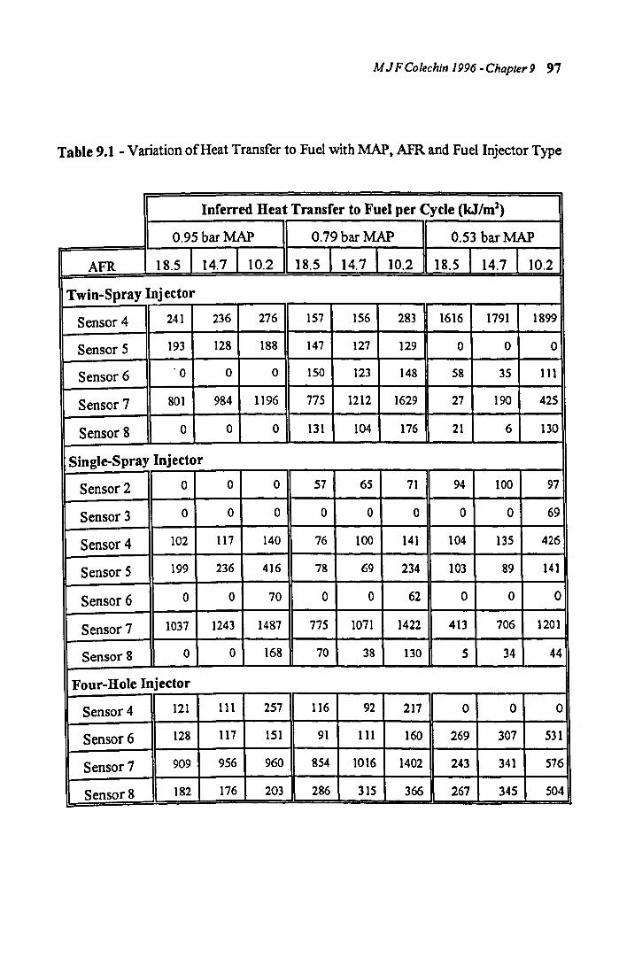
M J F CoJechin J 996 - Chapter 9 97
Table 9.1 - Variation of Heat Transfer to Fuel with MAP, AFR and Fuel Injector Type
Inferred Heat Transfer to Fuel per Cycle (kJ/m2)
0.95 bar MAP 0.79 bar MAP 0.53 bar MAP
AFR 18.5 14.7 10.2 18.5 14.7 10.2 18.S 14.7 10.2
Twin-Spray Inj ector
Sensor 4 241 236 276 157 156 283 1616 1791 1899
Sensor 5 193 128 188 147 127 129 0 0 0
Sensor 6 '0 0 0 150 123 148 58 35 111
Sensor 7 801 984 1196 775 1212 1629 27 190 425
Sensor 8 0 0 0 131 104 176 21 6 130
Single-Spray Injector
Sensor 2 0 0 0 57 65 71 94 100 97
Sensor 3 0 0 0 0 0 0 0 0 69
Sensor 4 102 117 140 76 100 141 104 135 426
Sensor 5 199 236 416 78 69 234 103 89 141
Sensor 6 0 0 70 0 0 62 0 0 0
Sensor 7 1037 1243 1487 775 1071 1422 413 706 1201
Sensor 8 0 0 168 70 38 130 5 34 44
Four-Hole Injector
Sensor 4 121 111 257 116 92 217 0 0 0
Sensor 6 128 117 151 91 111 160 269 307 531
Sensor 7 909 956 960 854 1016 1402 243 341 576
Sensor 8 182 176 203 286 315 366 267 345 504
M J F Colechin 1996 - Chapter 9 98
secondary atomization. Sensor 5 records a significant level of heat transfer to the fuel for
the single-spray injector, but this value is always relatively small compared to that
recorded by Sensor 7 on the port floor. The twin-spray injector also appears to give rise
to wetting of the bifurcation surface, but most fuel deposition appears to occur directly
on the port floor around Sensors 4 and 7, with the possibility of some small shift of floor
deposition upstream at low manifold pressures. The four-hole injector, although
producing a wider cone angle than that of the single-pintle twin-spray injector, appears
to give the best penetration of fuel into the intake port. This gives a reasonably uniform
distribution of heat flux to fuel over Sensors 6, 7 and 8 at low manifold pressures and a
more focused pattern around Sensor 7 at higher manifold pressures, but in each case
without evidence of appreciable wetting of the side wall or bifurcation web in the vicinity
of Sensors 3 and 5.
When fuel supply rate is step-increased, heat transfer per cycle to deposited fuel adjusts
at a similar rate as the induced mixture ratio. This is shown in Figure 9.1, where
normalised heat transfer data is plotted alongside inverted and normalised AFR data for
the same test conditions. The peak instantaneous heat transfer rate is highest for the first
cycle after the change. On subsequent cycles the peak diminishes and levels in the tail of
the variation increase. If the fuel supply rate is step-decreased, the peak instantaneous
heat transfer rate is lowest for the first cycle after the change with higher rates in the tail
of the variation. In this case, the peak increases and levels in the tail decrease during
subsequent cycles. These features reflect the changing quantity and composition of fuel
in the surface film. It is the time taken for these changes to take place and a new steady
state to be established which produce the engine response delay characterised by 't in the
parametric 't and X model of fuel transport.
9.4 Theoretical Interpretation of Heat Transfer Variations
When considering a single-component fuel, which avoids the complexities inherent in
multi-component pump-grade fuel, the mechanisms by which heat transfer occurs can be
modelled. In this way it was found that trends in the heat transfer data, particularly the
M J F Colechin J 996 - Chapter 9 99
changes with port surface temperature, were consistent with the following interpretation
of fuel behaviour:
(i) Fuel deposited on the surface is heated to a film temperature with an associated
change in sensible internal energy.
(ii) The rate of vaporisation from the fuel film is controlled by the variation of
saturation pressure with temperature through both convective and diffusive mass
transfer. The rate of vaporisation increases with increasing surface temperature
and is promoted by the forward induction flow during the intake stroke.
(iii) At high surface temperatures the rate of vaporisation may be limited by the
availability offuel supplied to the film by deposition. In this case, a maximum heat
transfer rate to the fuel is reached at a temperature dependent upon fuel
characteristics. The rate of heat transfer can decrease with subsequently
increasing surface temperature, due to a decreasing fraction of fuel supply being
deposited on the port surfaces.
These effects are also apparent in results taken with multi-component fuels, although the
temperature at which the heat transfer rate becomes supply limited is different for each
component, and the heavier components never reach such a point under normal engine
operating conditions. Therefore, whereas warm-up results with isooctane rise to a
maximum value which is dependent on engine operating conditions and fuel flow rate,
multi-component results rise continuously across the temperature range without evidence
of a maximum. Modelled data for isooctane fuelling sweeps at different temperatures
show the effects of this "supply-limiting" as fuel flow rate changes at different manifold
pressures (see Figure 9.2). At low temperatures (Figure 9.2(a», there is no supply
limiting and the heat transfer rates vary with both MAP and fuel flow rate. With the
engine fully-warm (Figure 9.2(c» the heat transfer rates become supply-limited across the
range of conditions considered and they are, therefore, only dependent on fuel flow rate.
When an intermediate temperature is considered (Figure 9.2(b», it is only at lower MAP's
and fuel flow that the heat transfer becomes supply limited. The trends in the data at this
temperature condition begin to replicate the trends in experimental data recorded under
M J F Colechin J 996 - Chapter 9 100
fully-warm conditions with multi-component fuels (Figure 7.17), where a proportion of
the components are supply-limited at lower MAP's and fuel flow rates.
Chapter 10
Conclusions
* Measurements of heat transfer in the intake port of a spark-ignition engine, using
surface mounted heat flux sensors, provide a good indication of factors affecting the
thermal environment of the port. Under "dry-port" conditions it is the port gas flows
which create these effects, while under "wetted-port" conditions they are also affected by
the mechanisms involved in mixture preparation.
* U sing an analytical model of the heat flux sensors together with experimentally
measured response characteristics, it is possible to resolve the heat flux data on a crank
angle basis. This allows the significance of events within an engine cycle to be
determined.
* When the port is dry the effects of overlap backflow, forward induction flow and
displacement backflow are apparent. The relative significance of these effects vary with
manifold pressure and engine coolant temperature.
* Deposition offuel on the port surfaces generally increases the heat transfer rates
by an order of magnitude. The effects of the gas flows are still apparent in the crank-angle
resolved data, even in inferred "heat flux to fuel" data, since they enhance fuel
vaporisation through convection. Particularly at high temperatures, though, this data is
dominated by heat transfer associated with increasing the temperature of newly injected
fuel and vaporising fuel from the film by diffusive mass transfer, with the lighter fuel
fractions evaporating most quickly. Again the relative significance of the different heat
transfer mechanisms is dependent upon engine operating conditions.
* Integrated values of heat transfer per cycle provide a useful indication of variations
due to the positioning of sensors within the port and changes in operating conditions.
When the port is dry, both spatial and operating condition variations arise from differences
101
M J F Colechin J 996 - Chapter J 0 102
in the penetration of the gas flows, particularly the overlap backflow. With a "wetted"
port, the inferred values of "heat transfer to the fuel" are associated with the distribution
of the fuel around the port surfaces. These provide a relative comparison between the
deposition patterns produced by the different injector types and how these vary with
operating conditions.
* When running on isooctane fuel a good correlation with the experimental data has
been produced using a model of heat transfer to the fuel. In addition to the heat transfer
required to raise the sensible internal energy of newly injected fuel, this model accounts
for the heat used in the vaporisation of fuel in one of two ways. At high temperatures
where the fuel is vaporised very quickly through diffusive mass transfer, it is assumed that
the heat transfer is limited by the availability of fuel supplied to the film by deposition. At
lower temperatures the mass transfer is dominated by convection and heat transfer is not
limited by fuel availability. The temperature at which the vaporisation mechanism
switches from convective to purely diffusive mass transfer is dependent upon MAP and
fuel supply rate. This interpretation is also consistent with data from multi-component
fuel tests although the picture is far more complex, since each component in the fuel has
a different vaporisation characteristic.
References
1.1 S D Hires and M T Overington, "Transient Mixture Strength Excursions - An
Investigation of Their Causes and the Development of a Constant Mixture
Strength Fuelling Strategy", SAE Paper No. 810495, 1981
1.2 P J Shayler, Y C Teo, A Scarisbrick, "Fuel Transport Characteristics of Spark
Ignition Engines for Transient Fuel Compensation", SAE Paper No. 950067, 1995
1.3 J J G Martins and I C Finlay, "Heat Transfer to Air-Ethanol and Air Methanol
Sprays Flowing in Heated Ducts and Across Heated Intake Valves", SAE Paper
No. 900583, 1990
1.4 J J G Martins and I C Finlay, "Fuel Preparation in Port Injected Engines", SAE
Paper No. 920518, 1992
1.5 N Ladommatos, "Mechanisms of Heat Transfer to Liquid Films in the Manifold
of Port-Injected Petrol Engines", Proc Instn Mech Engrs, Vol 207 pgs 211-221,
1993
1.6 H Sindano, "Phenomenological Transient Fuelling Model for Port Injected
Engines",I.Mech.E. Seminar on Engine Transient Performance, 7th Nov. 1990
1.7 G Chen, M Vmcent and T Gutermuth, "The Behaviour of Multi phase Fuel-Flow
in the Intake Port", SAE PaperNo. 940445, 1994
1.8 R C Turin, E G B Casartelli and H P Geering, "A New Model for Fuel Supply
Dynamics in an SI Engine", SAE Paper No. 940208, 1994
2.1 C F Aquino, "Transient AIF Control of the 5 Litre Central Fuel Injection Engine"
SAE Paper No. 810494, 1981
103
M J FColechin 1996 -References 104
2.2 S D Hires, M T Overington, "Transient Mixture' Strength Excursions - An
Investigation of Their Causes and the Development of a Constant Mixture
Strength Fuelling Strategy" SAE Paper No. 810495, 1981
2.3 D J Boam, I C Finlay and G S Fairhead, "The Optimization of Fuel Enrichment
Patterns with Throttle Body Injection", Pree Instn Meeh Engrs Vol 202 No DI,
1988
2.4 H B Servati, E W Herman, "SpraylWall Interactions Simulation" SAE Paper
No. 890566, 1989
2.5 D J Boam, I C Finlay and J J G Martins, "A Model for Predicting Engine Torque
Response During Rapid Throttle Transients in Port-Injected Spark-Ignition
Engines", SAE Paper No. 890565, 1989
2.6 T Nogi, Y Ohyama, T Yamauchi and H Kuroiwa, "Mixture Formation of Fuel
Injection Systems in Gasoline Engines", SAE Paper No. 880558, 1988
2.7 P J Shayler, W D P Marshall, J Turner and K Ford, "Exhaust Emissions: the
Influence of Fuel Injection System Details", I Mech E Paper No. C394/0 1 5, 1990
2.8 H J NeuBer, H Endres and M Breuer, "New Variable Intake and Mixture
Formation System for Multi-Valve SI Engines", SAE Paper No. 940449, 1994
2.9 D Rose, N Ladommatos, R Stone, "In-Cylinder Mixture Excursions in a Port
Injected During Fast Throttle Opening" SAE PaperNo. SP-I029, 1994
2.10 P J Shayler, Y C Teo and A Scarisbriek, "Fuel Transport Characteristics of Spark
Ignition Engines for Transient Fuel Compensation", SAE Paper No. 950067, 1995
M J F Colechin J 996 - References 105
2.11 D J Boam and I C Finlay, "A Computer Model of Fuel Evaporation in the Intake
System of a Carburetted Petrol Engine", I Mech E Paper No. C89/79, 1979
2.12 H B Servati, W W Yuen, "Deposition of Fuel Droplets in Horizontal Intake
Manifolds and the Behaivour of Fuel Film Flow on Its Walls", SAE Paper
No. 840239, 1984
2.13 F Maroteaux and M Thelliez, "Modeling of Unsteady Multiphase Flow in the
Intake Manifold of Spark Igniton Engines", SAE Paper No. 910392, 1991
2.14 G Chen, M T Vincent and T R Gutermuth, "The Behaviour of Multiphase Fuel
Flow in the Intake Port", SAE Paper No. 940445, 1994
2.15 C Cheng, W K Cheng, J B Heywood, D Maroteaux and N Collings, "Intake Port
Phenomena in a Spark-Ignition Engine at Part Load", SAE Paper No. 912401,
1991
2.16 M C Bourke and L W Evers, "Fuel Film Dynamics in the Intake Port of a Fuel
Injected Engine", SAE Paper No. 940446, 1994
2.17 C H Daniels and L W Evers, "The Influence of Mixture Preparation on a Warm
1.9L Ford Engine", SAE Paper No. 940444, 1994
2.18 K Takeda, T Yaegashi, K Sekiguchi, K Saito and N Imatake, "Mixture
Preparation and HC Emissions of a 4-Valve Engine with Port Fuel Injection
During Cold Starting and Warm-up", SAE Paper No. 950074, 1995
2.19 J Takemura, D Sabuyashi and H Ando, "Effect of Turbulence in Intake Port of
MPI Engine on Fuel Transport Phenomena and Nonuniformity of FueV Air Mixing
in Cylinder", SAE PaperNo. 900162, 1990

M J F Colechin J 996 - References 106
2.20 M J Miller and C J E Nightingale, "Measurement of the Changes in Mixture
Preparation that Occur During Flow Past the Inlet Valve of a Spark-Ignition
Engine", IMechE Paper No. C394/004, 1990
2.21 K Saito, K Sekiguchi, N Irnatake (Nippon Soken), K Takeda and T Yaegashi, "A
New Method to Analyze Fuel Behaviour in a Spark Ignition Engine", SAE Paper
No. 950044, 1995
2.22 J J G Martins and I C Finlay, "Fuel Preparaton in Port Injected Engines", SAE
PaperNo. 920518, 1992
2.23 M Iwata, M Furuhashi and M Ujihashi, "Two Hole Injector Improves Transient
Perfonnance and Exhaust Emissions of 4-valve Engines", SAE Paper No. 870125,
1987
2.24 F Zhao, M Lai and D L Harrington, "The Spray Characteristics of Automotive
Port Fuel Injection - A Critical Review", SAE Paper No. 950506, 1995
2.25 P J Shayler, M T Davies, M J F Colechin and A Scarisbrick "Intake Port Fuel
Transport and Emissions: the Influence of Injector Type and Fuel Composition",
SAE Paper No. 961996, 1996
2.26 K Harada, R Shimizu, K Kurita, M Muramatsu, M Ohashi and T Makimura,
"Development of Air-Assisted Injector System", SAE Paper No. 920294, 1992
3.1 C Cheng, W K Cheng, J B Heywood, D Maroteaux and N Collings, "Intake Port
Phenomena in a Spark-Ignition Engine at Part Load", SAE Paper No. 912401,
1991
3.2 Operator's Manual for the Ricardo Hydra Research Engine, Ricardo
Consulting Engineers Ltd., 1985
M J F Colechin /996 - Reference! 107
3.3 The Oxford English Reference Dictionary, Edited by J Pearsall and B Trumble,
Oxford University Press, Oxford, 1995
3.4 P J Shayler, Y C Teo and A Scarisbrick, "Fuel Transport Characteristics of Spark
Ignition Engines for Transient Fuel Compensation", SAE Paper No. 950067, 1995
4.1 0 Hadded, J Stokes and 0 W Grigg, "Low Emission Vehicle Technology for
Ultra Low Emissions Vehicle and European Stage 3 Emissions Standards", Proc
Instn Mech Engrs, Vol 209, Part D, pgs 159-170, 1995
4.2 C Cheng, W Cheng, J Heywood, D Maroteaux and N Collings, "Intake Port
Phenomena in a Spark-Ignition Engine at Part Load", SAE Paper No. 912401,
1991
4.3 M Greiner, P Romann and U Steinbrenner, "BOSCH Fuel Injectors - New
Developments", SAEPaperNo. 870124, 1987
4.4 M Iwata, M Furuhashi and M Ujihashi, "Two-Hole Injector Improves Transient
Performance and Exhaust Emissions of 4-Valve Engines", SAE Paper
No. 870125, 1987
4.5 J J G Martins and I C Finlay, "Fuel Preparation in Port Injected Engines", SAE
PaperNo. 920518, 1992
4.6 T Nogi, Y Ohyama, T Yamauchi and H Kuroiwa, "Mixture Formation of Fuel
Injection Systems in Gasoline Engines", SAE Paper No. 880558, 1988
4.7 M Kashiwaya, T Kosuge, K Nakagawa and Y Okamoto, " The Effect of
Atomization of Fuel Injectors on Engine Performance", SAE PaperNo. 900261,
1990
M J F Colechin J 996 - References 108
4.8 K Takeda, T Yaegashi, K Sekiguchi, K Saito and N Imatake, "Mixture
Preparation and HC Emissions of a 4-Valve Engine with Port Fuel Injection
During Cold Starting and Warm-Up", SAE Paper No. 950074, 1995
4.9 H Manger, "Electronic FuelInjection", SAE Paper No. 820903, 1982
4.10 K Harada, R Shimizu, K Kurita, M Muramatsu, T Makimura and M Ohashi,
"Development of Air-Assisted Injector System", SAE Paper No. 920294, 1992
4.11 F Zhao, M Lai and D L Harrington, "The Spray Characteristics of Automotive
Port Fuel Injection - A Critical Review", SAE Paper No. 950506, 1995
4.12 S D Hires and M T Overington, "Transient Mixture Strength Excursions - An
Investigation of Their Causes and the Development of a Constant Mixture
Strength Fuelling Strategy", SAE PaperNo. 810495, 1981
4.13 C F Aquino, "Transient NF Control of the 5 Litre Central Fuel Injection Engine",
SAE Paper No. 810494, 1981
4.14 W S James, H C Dickinson and S W Sparrow, "Intake Manifold Temperatures
and Fuel Economy", SAE Transactions V. IS, Part II, 1920
4.15 J 0 Eisinger, "Engine Acceleration Tests", SAE Transactions V. 22, Part II, 1927
4.16 P J Shayler, Y C Teo, A Scarisbrick, "Fuel Transport Characteristics of Spark
Ignition Engines for Transient Fuel Compensation", SAE Paper No. 950067, 1995
4.17 S R Fozo and C F Aquino, "Transient NF Characteristics for Cold Operation of
a 1.6 Litre Engine with Sequential Fuel Injection", SAE Paper No. 880691, 1988
M J FColechin 1996 -References 109
4.18 H B Servati and E W Hennan, "Spray/Wall Interactions Simulation", SAE Paper
No. 890566, 1989
4.19 D J Boam, I C Finlay and J J G Martins, "A Model for Predicting Engine Torque
Response During Rapid Throttle Transients in Port-Injected Spark-Ignition
Engines", SAE Paper No. 890565, 1989
4.20 A J Beaumont, A D Noble and A Scarisbrick, "Adaptive Transient Air-Fuel Ratio
Control to Minimize Gasoline Engine Emissions", Paper Presented at the FISIT A
Congress, London, Iune 1992
4.21 E Hendricks and S C Sorensen, "Mean Value Modelling of Spark Ignition
Engines", SAE Paper No. 900616, 1990
4.22 Y C Teo, "Mixture Ratio Control of a Spark Ignition Engine During Transient
Operations", Ph.D. Thesis, University of Nottingham, 1994
4.23 A J Durrant, "Closed Loop UEGO Probe Feedback Engine Control", Progress
Report 2, University of Nottingham, 1996
4.24 J J G Martins, D J Boam and J F Bingham, "A Computer Model for the
Assessment of Engine Control System Parameters", SAE Paper No. 940484, 1994
4.25 H Monden and R Kataoka, "Practical Measuring Method of Deposited Fuel and
Evaporated Fuel in the Induction System", SAE Paper No. 905042, 1990
4.26 K Saito, K Sekiguchi, N Imatake, K Takeda and T Yaegashi, "A New Method to
Analyze Fuel Behaviour in a Spark Ignition Engine", SAE Paper No. 950044,
1995
M J F Colechin J 996 - Reference3 110
4.27 A A Amer and M Lai, "Time-Resolved Measurements in Transient Port Injector
Sprays", SAE Paper No. 950509, 1995
4.28 P J Shayler, M T Davies, M J F Colechin and A Scarisbrick "Intake Port Fuel
Transport and Emissions: the Influence of Injector Type and Fuel Composition",
SAE PaperNo. 961996, 1996
4.29 K J Bush, N J Adams, S Dua and C R Markyvech, "Automatic Control of
Cylinder by Cylinder Air-Fuel Mixture Using a Proportional Exhaust Gas Sensor",
SAEPaperNo. 940149, 1994
4.30 G V Stuuart, "A System Identification Approach to the Modelling of Engine
Transients", SAE PaperNo. 900237, 1990
4.31 R C Dort: Modem Control Systems, Fifth Edition, Addison-Wesley, California,
1989
4.32 P R Keogh, P J Shayler, "Transient Fuel Compensation", Progress Report 3,
University of Nottingham, 1994
4.33 H Melgaardt, E Hendricks and H Madsen, "Continuous Identification of a Four
Stroke Engine", 1990 American Control Conference, Paper No. TP-I0, 5:30, San
Diego CA, 1990
5.1 H Sindano, "Phenomenological Transient Fuelling Model for Port Injected
Engines", I.Mech.E. Seminar on Engine Transient Performance, 7th Nov. 1990
5.2 G Chen, M Vincent and T Gutermuth, "The Behaviour of Multiphase Fuel-Flow
in the Intake Port", SAE Paper No. 940445, 1994
MJ FColechin 1996 -References 111
5.3 R C Turin, E G B Casartelli and H P Geering, "A New Model for Fuel Supply
Dynamics in an SI Engine", SAE Paper No. 940208, 1994
5.4 J J G Martins and I C Finlay, "Heat Transfer to Air-Ethanol and Air Methanol
Sprays Flowing in Heated Ducts and Across Heated Intake Valves", SAE Paper
No. 900583, 1990
5.5 J J G Martins and I C Finlay, "Fuel Preparation in Port Injected Engines", SAE
PaperNo. 920518, 1992
5.6 N Ladomrnatos, "Mechanisms of Heat Transfer to Liquid Films in the Manifold
of Port-Injected Petrol Engines", Proc lnstn Mech Engrs, Vol 207 pgs 211-221,
1993
5.7 RdF Corporation, "Micro-Foil Heat Flow Sensor Calibration Sheet", Hudson,
1994
5.8 A H Epstein, G R Guenette, R J G Norton and C Yuzhang, "High Frequency
Response Heat Flux Gauge for Metal Blades", AGARD Conference Proceedings
No. 390 - Heat Transfer and Cooling in Gas Turbines, pgs 30-1 to 30-16, May
1985
5.9 H S Carslaw and J C Jaeger, Conduction of Heat in Solids, 2nd Edition, Oxford
University Press, Oxford, 1959
5.10 J L Waintraub and E Brumgnach, "Electric Circuits for Technologists", West
Publishing Company, St Paul, 1989
5.11 DE Newland. An Introduction to Random Vibrations, Spectral Analysis and
Wavelet Analysis, 3rd Edition, Longman, Harlow, 1993
M J FColechin 1996 -References 112
6.1 C Cheng, W Cheng, J Heywood, D Maroteaux and N Collings, "Intake Port
Phenomena in a Spark-Ignition Engine at Part Load", SAE Paper No. 912401,
1991
6.2 R C Turin, E G B Casartelli and H P Geering, "A New Model for Fuel Supply
Dynamics in an SI Engine", SAE Paper No. 940208, 1994
6.3 J J G Martins and I C Finlay, "Heat Transfer to Air-Ethanol and Air Methanol
Sprays Flowing in Heated Ducts and Across Heated Intake Valves", SAE Paper
No. 900583, 1990
6.4 J J G Martins and I C Finlay, "Fuel Preparation in Port Injected Engines", SAE
PaperNo. 920518, 1992
6.5 N Ladommatos, "Mechanisms of Heat Transfer to Liquid Films in the Manifold
of Port-Injected Petrol Engines", Proc Instn Mech Engrs, Vol 207 pgs 211-221,
1993
6.6 M D Burghardt, Engineering Thermodynamics with Applications, 3rd Edition,
Harper and Row, New York, 1986
6.7 A J Ede and E J Febre, "The Effect on the Heat Transfer from a Pipe to a Fluid
Flowing Through it of a Bend in the Pipe", Prog. 9th Int. Congress on
Refrigeration, 1955, Vol. 1, pp 2127-2132
7.1 S D Hires and M T Overington, "Transient Mixture Strength Excursions - An
Investigation of Their Causes and the Development of a Constant Mixture
Strength Fuelling Strategy", SAE Paper No. 810495, 1981
7.2 C F Aquino, "Transient NF Control of the 5 Litre Central Fuel Injection Engine",
SAE PaperNo. 810494,1981
MJ FColechin 1996 -References 113
7.3 C Aquino and W D Plensdorf, "An Evaluation of Local Heating as a Means of
Fuel Evaporation for Gasoline Engines", SAE Paper No. 860246, 1986
7.4 H Sindano, "Phenomenological Transient Fuelling Model for Port Injected
Engines", I.Mech.E. Seminar on Engine Transient Performance, 7th Nov. 1990
7.5 G Chen, M Vmcent and T Gutermuth, "The Behaviour of Multi phase Fuel-Flow
in the Intake Port", SAB Paper No. 940445, 1994
7.6 R C Turin, E G B Casartelli and H P Geering, "A New Model for Fuel Supply
Dynamics in an SI Engine", SAE Paper No. 940208, 1994
7.7 J J G Martins and I C Finlay, "Heat Transfer to Air-Ethanol and Air Methanol
Sprays Flowing in Heated Ducts and Across Heated Intake Valves", SAB Paper
No. 900583, 1990
7.8 J J G Martins and I C Finlay, "Fuel Preparation in Port Injected Engines", SAE
Paper~0.920518, 1992
7.9 ~ Ladomrnatos, "Mechanisms of Heat Transfer to Liquid Films in the Manifold
of Port-Injected Petrol Engines", Proc lnstn Mech Engrs, Vol 207 pgs 211-221,
1993
7.10 J J G Martins, D J Boam and J F Bingham, "A Computer Model for the
Assessment of Engine Control System Parameters", SAE Paper ~o. 940484, 1994
7.11 T Nogi, Y Ohyama, T Yamauchi and H Kuroiwa, "Mixture Formation of Fuel
Injection Systems in Gasoline Engines", SAE PaperNo. 880558, 1988
M J F Colechin J 996 - References 114
7.12 E W Curtis, C F Aquino, D K Trumpy and G C Davis, "A New Port and Cylinder
Wall Wetting Model to Predict Transient AirlFuel Excursions in a Port Fuel
Injected Engine", SAE Paper No. 961186, 1996
7.13 P J Shayler, Y C Teo and A Scarisbrick, "Fuel Transport Characteristics of Spark
Ignition Engines for Transient Fuel Compensation", SAE Paper No. 950067, 1995
8.1 N B Vargaftik, Tables on the Thermophysical Properties of Liquids and
Gases, Second Edition, Hemisphere Publishing Corp., London, 1975
8.2 J M Kay and R M Nedderman, Fluid Mechanics and Transfer Processes,
Cambridge University Press, Cambridge, 1985
8.3 J M Coulson and J F Richardson, Chemical Engineering Vol. 6: An
Introduction to Chemical Engineering Design by R K Sinnott, 2nd Edition,
Pergamon, Oxford, 1993.
8.4 D B Spalding, Some Fundamentals of Combustion, Butterworths Scientific
Publications, London, 1955
8.5 DB Spalding, Convective Mass Transfer, An Introducion, Edward Arnold Ltd,
London, 1963
8.6 M N ()~ik, Heat Transfer, A Basic Approach, McGraw-Hill, Singapore, 1985
8.7 P J Shayler, Y C Teo and A Scarisbrick, "Fuel Transport Characteristics of Spark
Ignition Engines for Transient Fuel Compensation", SAE Paper No. 950067, 1995
9.1 J J G Martins and I C Finlay, "Heat Transfer to Air-Ethanol and Air-Methanol
Sprays Flowing in Heated Ducts and Across Heated Intake Valves", SAE Paper
No. 900583, 1990
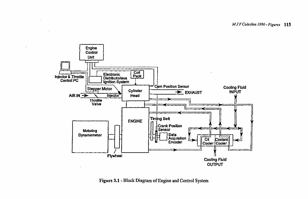
Engine Control Unit
0 II
Injectl r . I Coil I {
Electronic Pack . & Throttle II Oistributorfess I Ilrol PC Ignition System
~r Motor "'. Cylinder AlRIN. " Irnector Head
Throttle T
ENGINE r--
Motoring Dynamometer r-
I--
L..-
/ Flywheel
I
p!c jam Position Sensor
+ ext
II 1
Tim ng Belt
Crank Position F-c= Sensor
I- fDoata r;:::::::::=: ~ I- Acquisition l!:::)c Oil !coolant
Encoder Cooler Cooler
t Cooling Fluid
OUTPUT
Figure 3.1 - Block Diagram of Engine and Control System
M J F Colechin 1996 - Figures 115
~
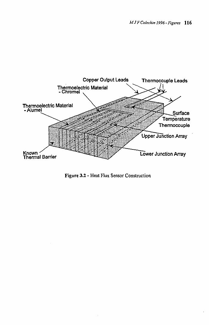
Copper Output Leads
Thermoelectric Material -Chromel
Thermoelectric Material -Alumel
Known . Thermal Barner
M J FColechin 1996 - Figures 116
Thermocouple Leads
.:.:.:.:.:,r-__ Surface Temperature
Thennocouple
Lower Junction Array
Figure 3.2 - Heat Flux Sensor Construction
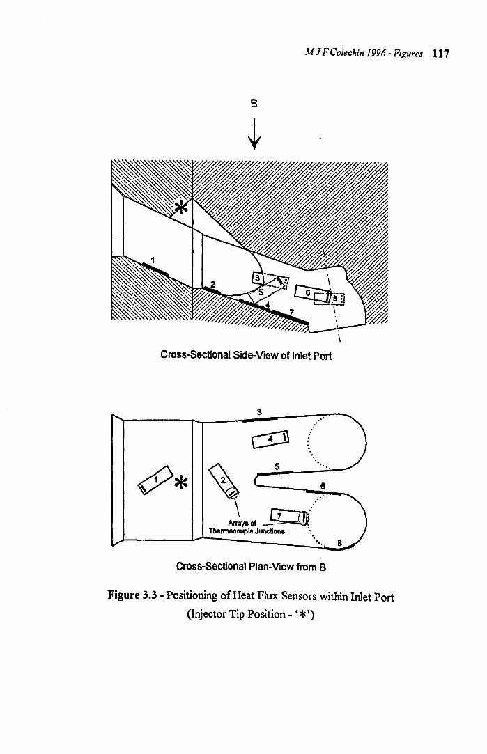
M J F Colechin 1996 - Figures 117
B
Cross-Sectional Side-View of Inlet Port
3
c:D1 . '.
&* ~ 5 ".
6
. Q l1i Arrayaof _
Thermocouple Junctions
8
Cross-Sectional Plan-View from B
Figure 3.3 - Positioning of Heat Flux Sensors within Inlet Port
(Injector Tip Position - '* ')
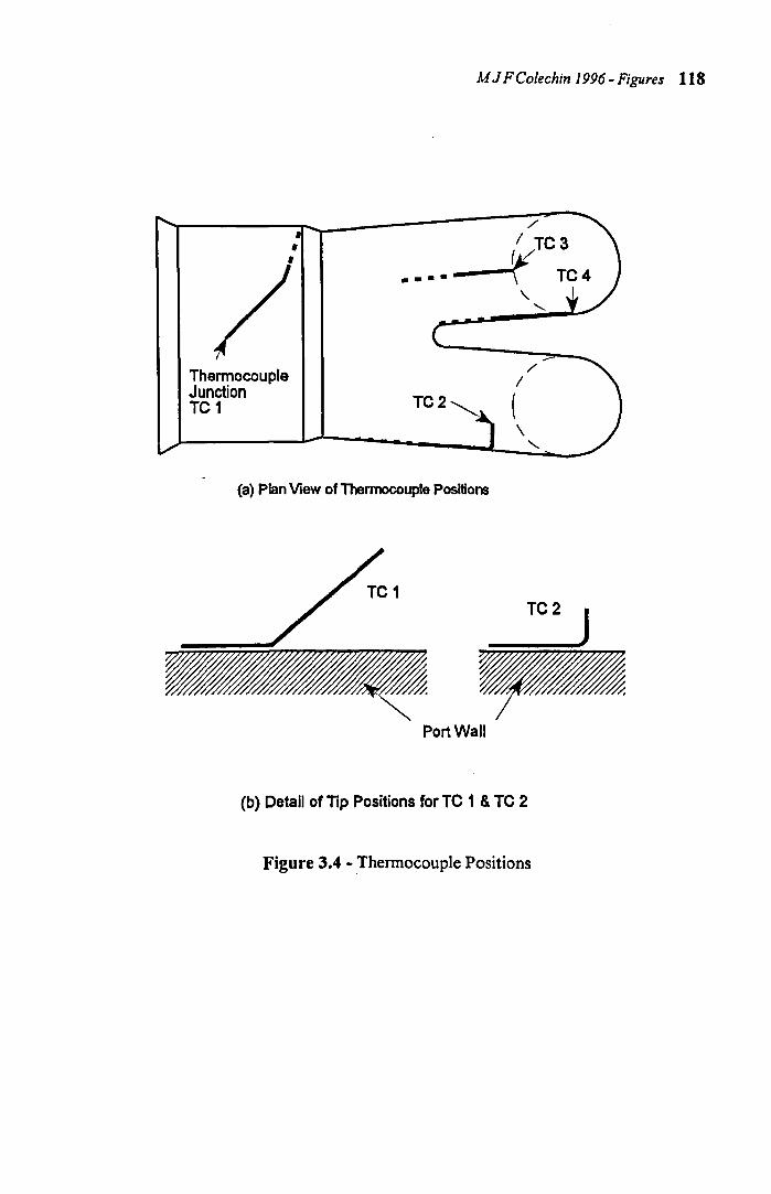
M J F Colechin 1996 - Figures 118
/
I TC3
•••• -------ri{ Te 4 "
'-
Thermocouple Junction
TC2 (
/ I
TC 1
(a) Plan View of Thermocouple Positions
\ '-
TC2 J
~ Port Wall
(b) Detail of Tip Positions for TC 1 & TC 2
Figure 3.4 - Thermocouple Positions
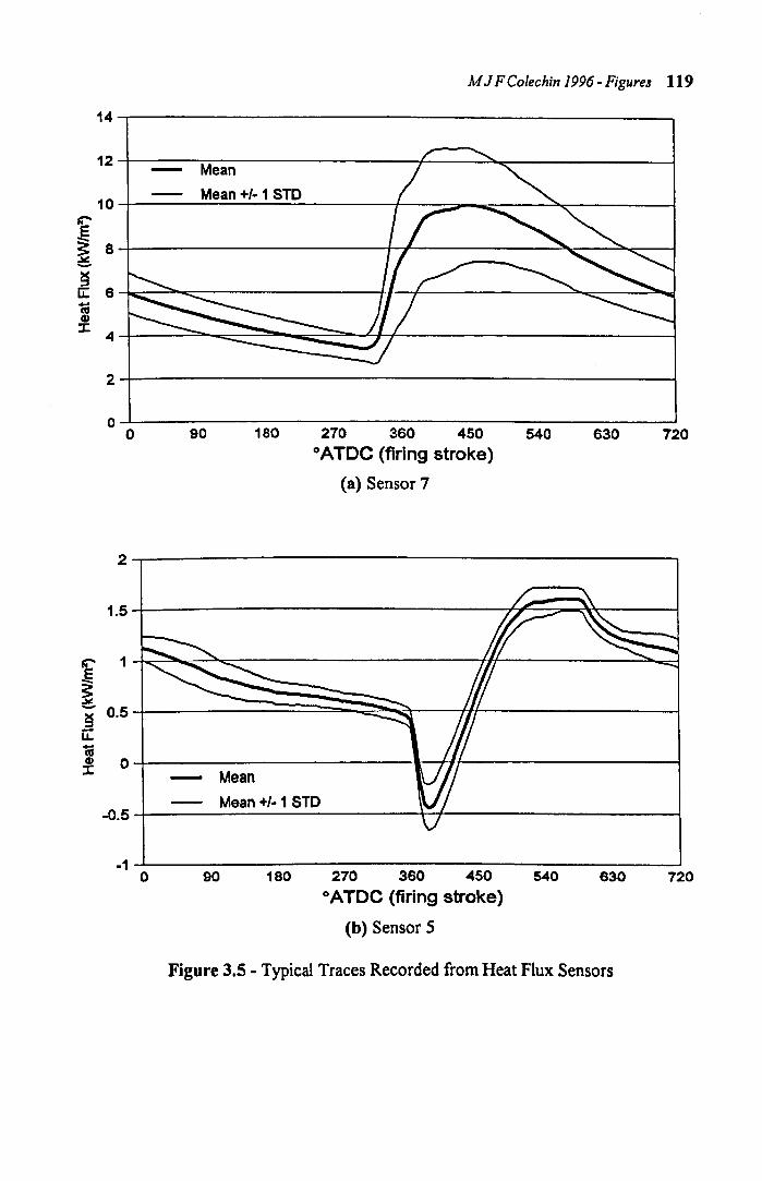
14
12
10 t:' ,E ~ 8 ->< ::s u:: 6 1;j CI) ~
4
2
0 0
2
1.5
'f 1
~ - 0.5 ~ u: 1;j CI) 0 J:
-0.5
-1 0
M J FColechin 1996 - Figures 119
Mean
Mean +/- 1 STO
90 180 270 360 450 540 °ATDC (firing stroke)
(a) Sensor 7
Mean
Mean +/- 1 STO
90 180 270 360 450 540 ° ATDC (firing stroke)
(b) Sensor 5
630
630
Figure 3.5 - Typical Traces Recorded from Heat Flux Sensors
720
720
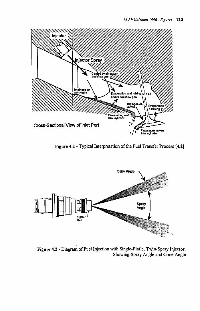
MJ FColechin 1996 -Figures 120
Cross-Sectional View of Inlet Port
Figure 4.1 - Typical Interpretation of the Fuel Transfer Process [4.2]
Cone Angle
Figure 4.2 - Diagram of Fuel Injection with Single-Pintle, Twin-Spray Injector, Showing Spray Angle and Cone Angle
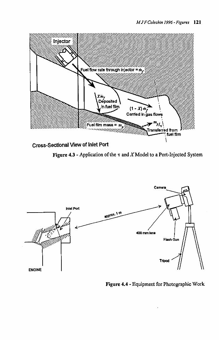
MJ FColechin /996 -Figures 121
Cross-Sectional View of Inlet Port
Figure 4.3 - Application of the 't' and X Model to a Port-Injected System
Inlet Port
FlashGun
ENGINE
Figure 4.4 - Equipment for Photographic Work
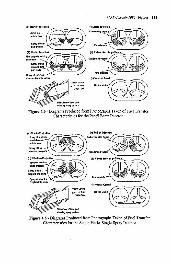
(.) Start orInjection
Jet of fuel --t--f--I-I~-4I onto bridge
Spray of very fine droplets
(b) Ead 01 Injeetioa
Spray of very fine dropleta toward. valve.
OTHERVlEWS
~ INlHlS DIRECTION
Side-V'- of Inlet port _howlng _pray pattern
MJ FColechin 1996 -Figures 122
(c) Arter Injection
Fine
(d) Valves Start to 10 Down --",,--_,-/--
(e) Valves CIo.ee1
Figure 4.5 - Diagrams Produced from Photographs Taken of Fuel Transfer Characteristics for the Pencil Beam Injector
(.) Start oflDjeetioD
Spray of medium .Ized droplets onto bridge
(b) Middle orlDjeetioD --"'--.-'"--
Spray of very fin. droplets Into porta
OTHERVIEWI
~ INlHlS DIRECTION
Side-VIew of inlet port ~g -lOY pattern
(e) End ofInjectiOD
End of Injection
Condenaad vapour
Fine droplets
(e) Valves CIo.ed
No fuel vi.ible
Figure 4.6 - Diagrams Produced from Photographs Taken of Fuel Transfer Characteristics for the Single-Pintle, Single-Spray Injector
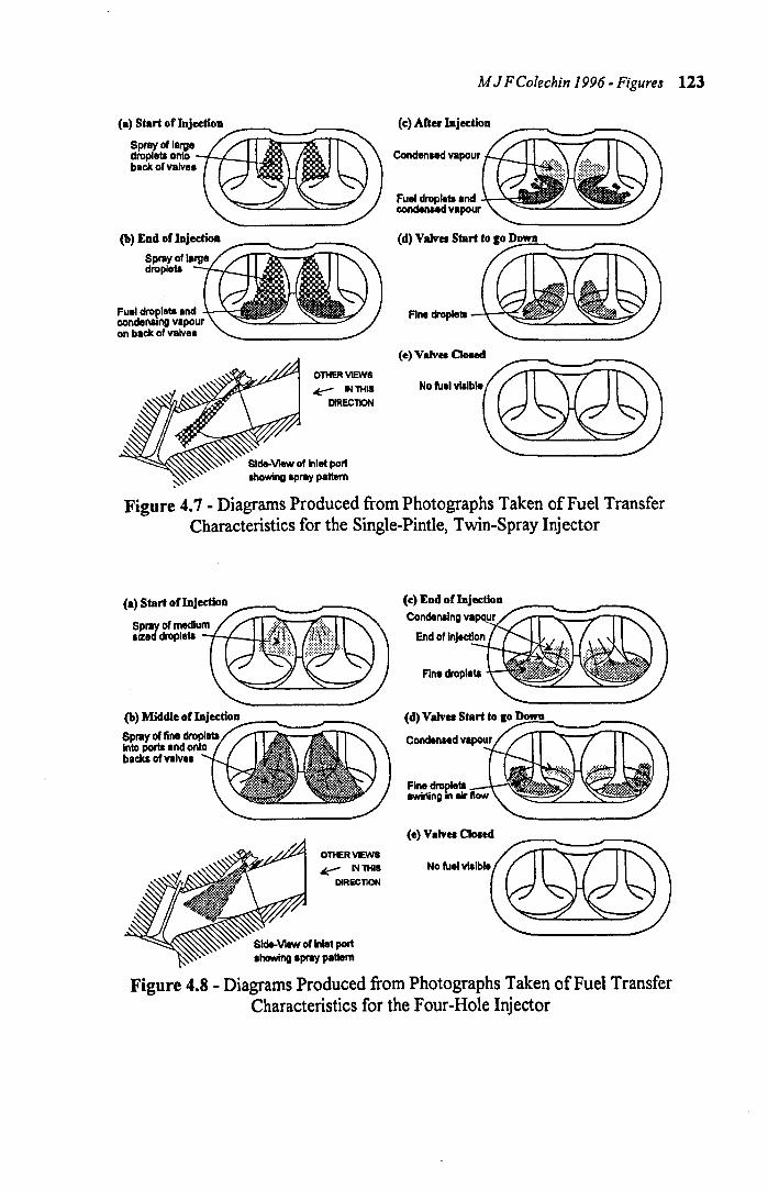
(a) Start oflnjection --"'----"'--Spray of large dropretl onto "/--r--I-.w!lI~ back of valvlII
(b) End of Injection
Spray of largl dropletl
Fuel droplets and conden.lng vapour on back of valve.
OTHERV1EW8
~ INlHlS DIRECTION
Side-VIew of Inlet port Ihowing &pray pattern
M J F Colechin 1996 - Figures 123
(c) Arter Injection
Condenaed vapour
Fuel dropleta and ..J,-..>o.c:~ condenaed vapour -=:..:....::;,._--:::.....:::;:;;;;.--
(e) Valvs Clond
No fuel visible
Figure 4.7 - Diagrams Produced from Photographs Taken of Fuel Transfer Characteristics for the Single-Pintle, Twin-Spray Injector
(a) Start oflDjection _-"'-_--"'-
Spray of medium aizld dropletl -r--f---LU;;t:
Spray of fine Into porta and backa of valve.
OTHER VIEWS ~ INlHl8
DIRECTION
Slde-View of Inlet port allowing Ipray pattem
(e) End orInJection
(4) Valvs Start to IO,Down_ .......... __ /"_-....
Fine dropIetl twining In air now
(e) Valvs OGled
No fuel vl&ibl.
Figure 4.8 - Diagrams Produced from Photographs Taken of Fuel Transfer Characteristics for the Four-Hole Injector
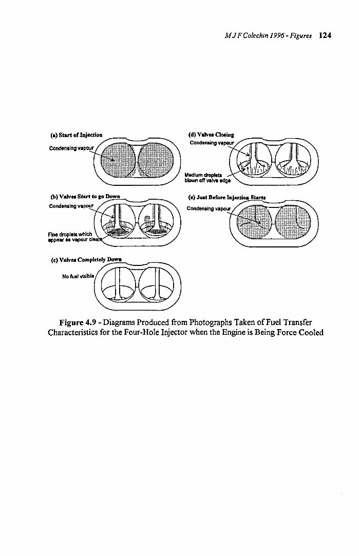
<a> Start Or InjedioD ,---~ ____ r---~
(b) Valvel Start to ,0 Dowa --""---,----..... Condensing vapour
Fine drop leta which appear I. vapour
(e) Valvel Completely.,...D_OWIl_ ........ ___ r-_ ......
No fuel visible
M J FColechin 1996 - Figures 124
(d) Valvel OOling
(e) Ju.t Before IDjltC~~~~ ___ ,..-_ .....
Condensing vapour
Figure 4.9 - Diagrams Produced from Photographs Taken of Fuel Transfer Characteristics for the Four-Hole Injector when the Engine is Being Force Cooled

1.4,--------------, 1.2 +-------------l
" .... --- ... -.. g 0.8 _~::---....ot-----_ .......... ... ' ...... ------ ... -.-----~~:::;?-..... -- ............. -........
0.8-t------------.....:..:r
0.4+------------~
0.2+------------~
O-t--~---r--_.I--~-~
30 40 50 80 70 Coolant Temperature (OC)
(a) Pencil-Beam Injector
80
1.4.,-------------, 1.2 +--------------1
$ 0.8 -1:-::.=: •• ::-.-.-_-----..... -:--------1 ... ........ ~.,..-.,.-- '''', 0.8 --- __ ---" ....... "
................. _---'.!'"*"S...----' 0.4+-------....:::t:==.:....~-~
0.2+-------------l
O+---T--~-_.--~-~
30 40 50 80 70
Coolant Temperature (OC)
(c) Twin-Spray Injector
80
M J F Colechin 1996 - Figures 125
u-r------------~
1.2 -1---------------1
14---------------1 ' .........
~ 0.8 -1--..:...0:--------------1 ... .. ,.'::::.,. -_ .. -
~ ...
0.8 -I-------=.;-~~~ .. + !::!-... .-;..-----_='~' -=------,,~ ... ...,~-.-::. 0.4 -1---------------1
0.2 -1---------------1
0+---.--~1---~--T-~
1.4
1.2
0.8
0.8
0.4
0.2
30 40 50 60 70 Coolant Temperature (OC)
(b) Single-Spray Injector
.. ..
'-" " ----....... ..... ...... -......
' . "
.............. -----
80
O+---'r--~--'--,~-~
30 40 50 80 70
Coolant Temperature (OC)
(d) 4-Hole Injector
80
Figure 4.10 - Variations in 't' Produced by Each Injector
During Repeated Warm-Up Tests at an Engine Speed of 1000 RPM,
MAP of 0.79 bar and with a Stoichiometric Mean AFR
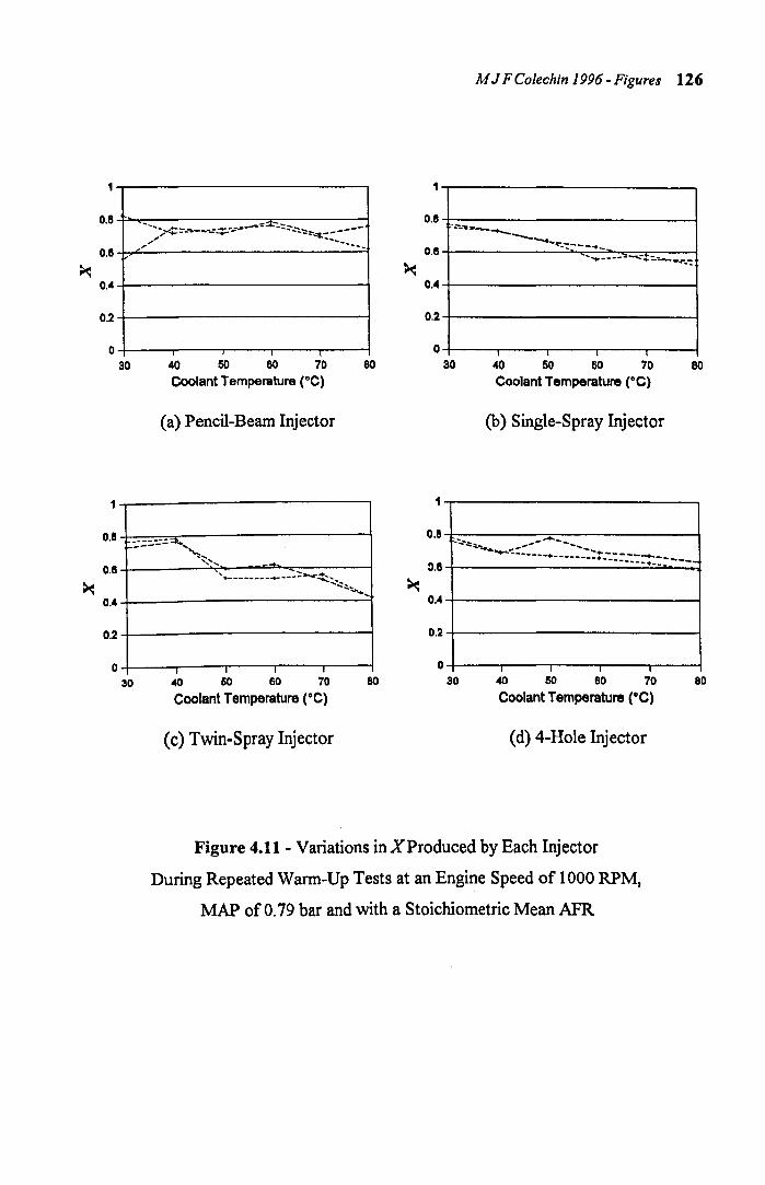
><
1
O.B
0.8
0."
0.2
0 30 40 50 60 70
Coolant Temperature (OC)
(a) Pencil-Beam Injector
O.B -.:.::.-:=.:;~ .... ~,
... ,......... --4
80
M J F Colechin J 996 - Figures 126
1.------------~
O.B+------------~ .::.-= .. --~--...
........... ~ ... "':---~-0.8 -+------..:..::.........,...::.:::.:........,..,...~-___l ... ~-- .. --~ .. ~":..-_.r:.":
0.4-+------------___l
0.24----------------1
O-+--~--~-~r_-~-___l
30 40 50 60 70 Coolant Temperature (OC)
(b) Single-Spray Injector
80
1~-----------~
0.6 -l-___ ~,...'._-_-__ -__ a..: __ ""'_-------..... ::-----:-~-':.--..:::::.-_--I
>< ......... 0.4.+-------------=t 0.4 -±--------------I
0.2 +--------------1 0.24------------__1
o-l--~---._-_.--._-~ O-+--~--'I--'T--~---I 30 40 50 60 70
Coolant Temperature (GC)
(c) Twin-Spray Injector
BO 30 40 50 80 70
Coolant Temperature (GC)
(d) 4-Hole Injector
Figure 4.11 - Variations in X Produced by Each Injector
During Repeated Warm-Up Tests at an Engine Speed of 1000 RPM,
MAP of 0.79 bar and with a Stoichiometric Mean AFR
80
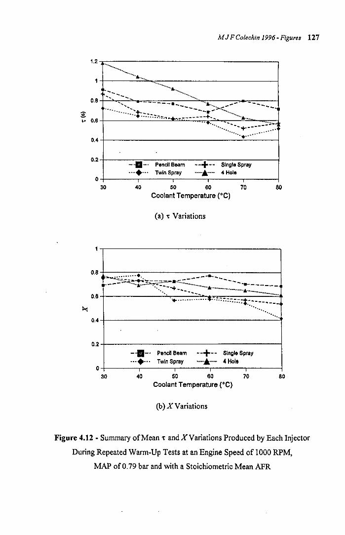
M J F Colechin 1996 - Figures 127
1.2 -x-----------------------, ........................•......
1~----=-~------------~ .~ .. ---- .................................. .
0.8 .. -- __ ......... --. --- ...... - ............ --,"" ---.. o..... - ..... - ".>-t: --""1
Jii ............... :+-•. :-.--- ... ___ & ::+ .. ..". ...................... ""--- .................. ------..... . ..... . ... 0.8 -+-_______ ..31::..:. ......... _ ..... -:-: •• ..-••• """"-.,... ..... :---=-=-.."" ... ::::: .... :-i_"1
.......... ~ ........ ----~~:. ... ................
0.4-!---------------------I
0.2 -+----=---------=+:----------1 -.-. Pencil Beam -- -- Single Spray ••••••• Twin Spray ........ --. 4 Hole
04----~,----.,----.,----.,---~
~ ~ ~ ~ ro 80 Coolant Temperature (OC)
(a) or Variations
1,--------------------~
0.8 I.:................. ___ ...... ... I- _ :.::S".;;.~~.::.;:~~:~:~~-.:.~~~.:.:= ... -........ ~-~=-:.=.~.=.=:.:.:.:.
0.8 ................. ~::=-:::-::::7:::_i.---------~ ............... .
0.4 -+---------------------'1'
0.24---------------------1 - .-. Pencil Beam ••••••• Twin Spray
--+ -- Single Spray -••.•.••.• 4 Hole
04----~1----.r----.1r------,r---~
30 40 50 80 70 80 Coolant Temperature (OC)
(b) X Variations
Figure 4.12 - Summary of Mean or and X Variations Produced by Each Injector
During Repeated Warm-Up Tests at an Engine Speed of 1000 RPM,
MAP of 0.79 bar and with a Stoichiometric Mean AFR
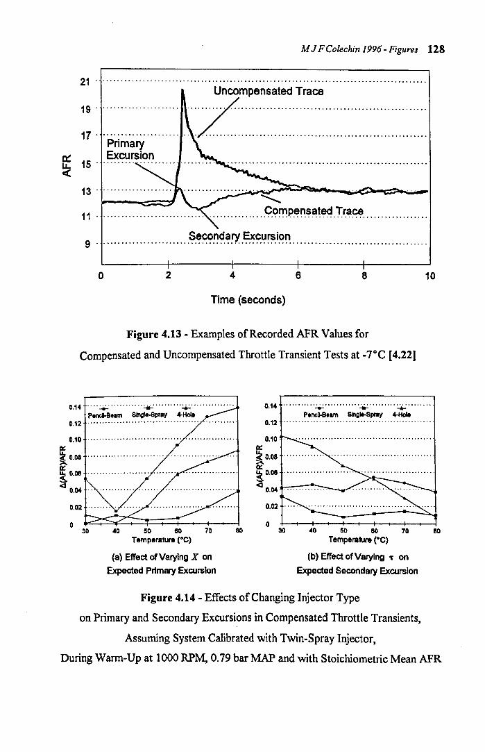
M J F Colechin 1996 - Figure.! 128
21 ....................................... , ................................................. . Uncompensated Trace
:: :::: .. :.:··L::.:·:: .. :.: .... ::.:.:: .. ·::::.::: .. :·:.:.: Primary
~ Excursion 15 ................... . ~
13 .................. .. "-..... Compensated Trace 11 ........................................................................................ .
Secondary Excursion 9 ......................................................................................... .
o 2 4 6 8
Time (seconds)
Figure 4.13 - Examples of Recorded AFR Values for
Compensated and Uncompensated Throttle Transient Tests at _7°C [4.22]
10
0.14 .... : ... : ........... + .......... .:.;,.:. ............... . 0.14 ........... ..,: ............ + .......... + ........ . Pencl-B.am Single-Spray 4-HoIe p.nclJ..B.am SlngJt.Spray 4-MoIe
0.12 0.12 .................................................. .
0.10
i 0.08
~ 0.08
0.04
0.02
o 30 40 60 80 70
Temperature CDC)
(a) Effect of Varying X on
Expected Primary Excursion
80
0.10 Q!
~ 0.08
~ 0.08
<30.04~---
0.02
o 30 40 60 80 70
Temperature (DC)
(b) Effect of Varying "C on
Expected Secondary Excursion
Figure 4.14 - Effects of Changing Injector Type
on Primary and Secondary Excursions in Compensated Throttle Transients,
Assuming System Calibrated with Twin-Spray Injector,
80
During Warm-Up at 1 000 RPM, 0.79 bar MAP and with Stoichiometric Mean AFR
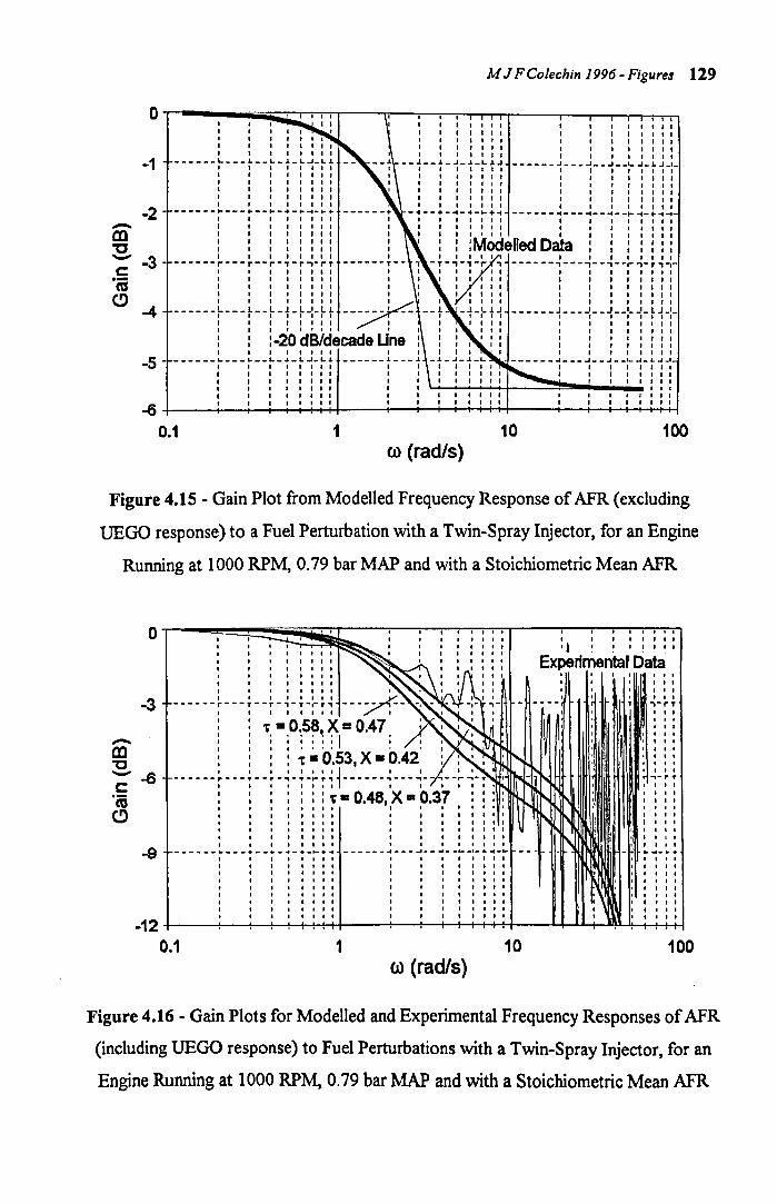
M J FColechin 1996 - Figures 129
0 I I I I
-1
-2 -en "C
1 1 1 I I I I I I I I I I I I I
I I I I I I I I I I I I I I I I I I I I I I I I ______ L ___ L __ L_~_L~_L~ __ ~ ___ ~ __ ~_~_~_L~~ ---- __ ~ ___ ~ __ ~ __ ~~_L~~_ I 1 I I I I I I I I I I I I I I I I I I I I I I I I I I I I I I I I I , I I I I I I I I I I I I I I I I I I I I I I t I , I I r I I I I I It I I I I I I I I I f I I I • I I I I • I I I I t I I I I I I I f I I I I I I I I " I I I I I I I I I I I I I I I I I I I I I I I I I I
------~---~--~-+-~~-~+ -~--.-~-~-~+~ ------~---~--~--~~-+~~-, • I I I I I I I I I I I I I I I I I I , I I I I I I I I I I I I I I I I I I I • I I I I I I I I I I I I I I I I I f I I I I I I
: : : : : : : : : ; : ModeDed Data : : : : : - -3 c::: I I I I I I I I I I I I I I I t I I I I I
------r---r--r-T-r'-rT , -T-~-~-r , ------,---'--'--r'-T'~-I I I I. I I I I I I I I • I I " I
'm C)
-4
I I I • I I I I I I I I I I I I I I I I I I I I I I I I I I I I I I I I I I
I I I I I I I I I I I I I I I I • I I I IIIIIIII~IIIIIII 11""1'
------~---t--~-t-H-H ------' -- --f l-t-:-+1 ------1---~--1--:--:-H-:-I I • , I I I I I I I I I I I I I I I I I I I I I ' • , , I I I I I I I I I I I I I I I
: : : -20 dB/decade Una I : : ::: : : : ! : I I I I I I I I I I I I • I I I I I
-5 ______ L ___ L __ L_~_L~_LL ______ ~ ___ ~ ______ J ___ ~ __ J __ ~~_~~~_
I I I I I I I I I I I I I I , t I I I I I I I I I I I I I I I I I I I I I I I I I I I I I I I , , I I I I I I I I I f I I I I " , I I I , I "1 I I I I I I , I I I I I I " f I I
~+---~~~-+~~~--~-+~~~M+----~~~~~
0.1 1 10 100 CI) (rad/s)
Figure 4.15 - Gain Plot from Modelled Frequency Response of AFR (excluding
UEGO response) to a Fuel Perturbation with a Twin-Spray Injector, for an Engine
Running at 1000 RPM, 0.79 bar MAP and with a Stoichiometric Mean AFR
-(Xl "C -c: 'm C)
o lI~--"~~~~~~~~~~~~;;::~--:----:---:--:-:I-:I-:I-lrl--------:I~--::--:--:I-:I::'::'-:1' : I 1 . I ~ I ! •
-3
-9
I I I I
t I I I • I I I I I I I I __ ~
-----r---T--r-'-~-r~~ ---~ ;--t, =,0 .. 5~1 ~ II 0.47.
I I • I I I I I I I • • • • ••
1 1 : : 't. 0.53. X • 0.42 I , I I ••• '1 1 1
-----,..---~--r-~-y-~r~ ------~---~-, • I I • 1'1 I I
1 1 : : : : : t. 0.48. X • 0,37 , t I I I I
, I I' II II
1
I I • I
------~---.--.-~-.-~ ... ~ ------~---~--~--~~- ... ~ I I I I
II.
I I I I II
III 1 1 1
, I "
Experimental Data .. 1 1 1 II 1 II -.-r T 1 II
1
1 1
1 1 II 1 • .. II ..,-,.. ,. III
I I I I I I I I
I. II 1 II
I I I I 1 1 • 1 II
~ ~-~ ... , I " I • I I I • I I
1 II 1 II
I , I I
-12+----~~~--+~++~--~--+--+~~~--~~~~~~~
0.1 1 10 100 00 (radls)
Figure 4.16 - Gain Plots for Modelled and Experimental Frequency Responses of AFR
(including UEGO response) to Fuel Perturbations with a Twin-Spray Injector, for an
Engine Running at 1000 RPM, 0.79 bar MAP and with a Stoichiometric Mean AFR
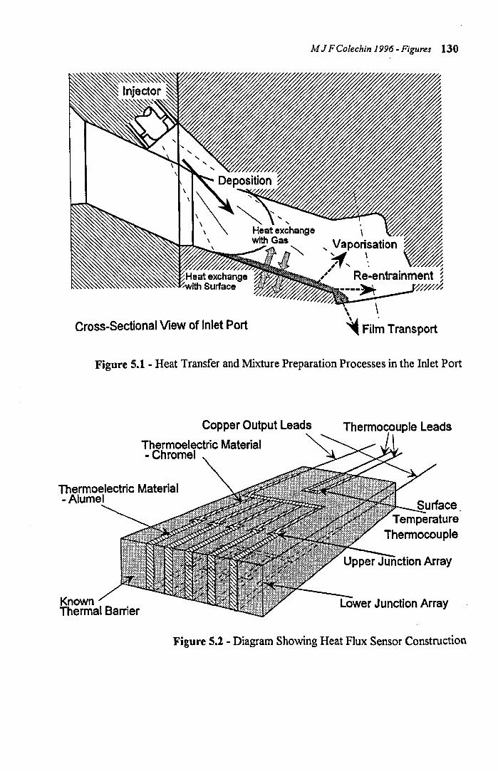
M J F Colechin 1996 - Figures 130
Cross-Sectional View of Inlet Port Film Transport
Figure 5.1 - Heat Transfer and Mixture Preparation Processes in the Inlet Port
Copper Output Leads
Thermoelectric Material ·Chromel
Thermoelectric Material -Alumel
Thermocouple Leads
Figure 5.2 - Diagram Showing Heat Flux Sensor Construction
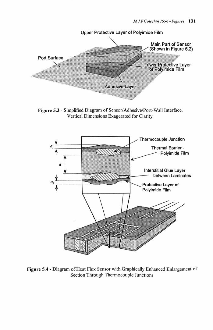
M J FColechin 1996 - Figures 131
Upper Protective Layer of Polyimide Film
Main Part of Sensor (Shown in Figure 5.2)
Figure 5.3 - Simplified Diagram of SensorlAdhesivelPort-Wall Interface.
d
Vertical Dimensions Exagerated for Clarity.
Thermocouple Junction
Thermal Barrier -Polyimide Film
Interstitial Glue Layer between Laminates
Protective Layer of Polylmlde Film
Figure 5.4 - Diagram of Heat Flux Sensor with Graphically Enhanced Enlargement of Section Through Thermocouple Junctions

MJ FColechin /996 -Figures 132
1 .... -._, -- I ............. ....... , ".' -- """",,"
/' """,--- .",'······· .. • .. 1 I I
./ // ... 1········ I II 'I I / ••.•• , ,
0.8 --[~'" .. ·····---I------------j------------,-----------I------------
~!--------i------------l-----------i------------~------------0.6
0.4
0.2
o o
1
0.8
0.6
0.4
---------+----------1------ =:: ~:~: ~: ~~ : .------I I --g = 75 ~m xu= 1 0 ~m
-----------r--------r---- ~:::: ~:ompm ~:::~: .------
0.2 0.4 0.6 0.8 1
time (8)
1.2 1.4 1.6
(a) Full Response to Steady State Conditions
1.8 2
'I I -'-'-'-'-'-'-',_._._._._._.-.... _._, _ ... ------------~------------ ---~~~-----I------------.:IJ c::_-==-_
, j......... L ------ .. " I
. - .... ,","",,,,""." '*' I -".- ""1'"
."'· ... ~ ... r "''''--'.' .. " J ----------~j;;~;'~~~ -I -~--------- ----------- 1------------
//7 ,_ g = 75 ~m xu= 15 ~m
-- g= 75 ~m xu= 10 ~m --I-II-I-/~/ . --il------------l----- - g. 75 ~m xu· 20 ~m -------
- .. g·OJ.lm xu·15J,1m 0.2 --------r-----------r----- "". g = 150 J.lm xu. 15 J.lm-------
I I I I o
o 0.02 0.04 0.06 0.08 0.1 0.12 0.14 0.16 0.18 0.2
time (8)
(b) Magnified Time-Scale, Showing Rise to 62% of Steady State Value
Figure 5.5 - Variation with Adhesive Film Thickness in Modelled Response of
Heat Flux Sensor to a Step Change in Surface Heat Flux
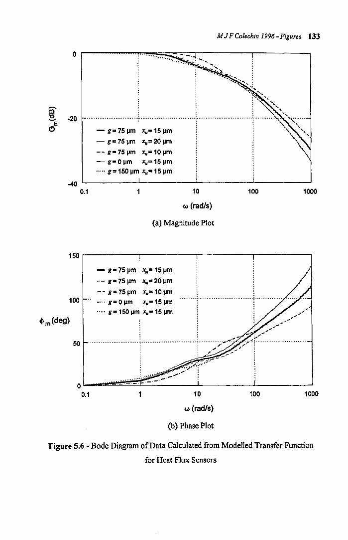
o
-co
M J F Colechin J 996· Figures 133
" .... ......... , : , .. :, . ... . ...
" " .. .. "
:g. ·20 .......................................................... \ ............................... \ .............. '~.", .... .. E
C)
-40 0.1
- g= 75 ~m x.,= 15IJm
- g. 75 \Jm Xu· 20 IJm
-- g= 75 \Jm Xu= 10 J.lm _ .. g- 0 J.lm Xu= 15 \Jm
..... g= 150 IJm x,,-15 J.lm
1 10
(j) (rad/s)
(a) Magnitude Plot
'~ "
100
" "
1000
150~--------~~----------~--------~~--------~
- g= 75 ~m x,,= 15IJm
- g= 75 ~m x.,= 20 IJm
-- g=75\Jm x,,=10J.lm 100 .. _ .. g= 0 IJm x,,= 15 J.lm
..... g- 150 \Jm Xu· 15 \Jm
., ....... ~ ............................... ~ .............. . ; . . . : :
~m{deg) ~~ ... ......
... ' ",,-,''/ ,
..... .,., .. ",,,, '" 50 ............................ ; ...................................................... .. y<'.: ........................... .
: : ,,' .J"': ~ ',," ~ . .
oL-~~·-~·-~·-~·-~·~~----~-------L------~ 0.1 1 10 100 1000
(,.) (rad/s)
(b) Phase Plot
Figure 5.6 - Bode Diagram of Data Calculated from Modelled Transfer Function
for Heat Flux Sensors
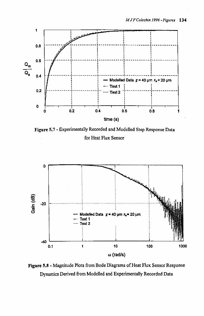
M J F Cotechin 1996 - Figures 134
1
0.8
0.6
0.4
0.2
o o
I I I , .. of!.
I ""' ~~. I I , ..... ' I I I ~------------+------------~-----------4------------I I I I I I I I I I I I I I I I I I I I
"I I I I ___ · _______ J ____________ ! ____________ L ___________ J ___________ _
• I I I I I I I I I I I I I I I I I I I I I I I I
---------~------------t------------~-----------~------------I I - Modelled Data g = 40 IJm XII = 20 IJm I I . .
I I _ .. Test 1 I I I I I I ----- -- --- -1- -- -- -- -- ---T -...... Test 2 -r -- ---------1- -- -- ---- - --I I I I I I I I I I I I I I I I I I I I
0.2 0.4 0.6 0.8
time (s)
Figure 5.7 - Experimentally Recorded and Modelled Step Response Data
for Heat Flux Sensor
o
m "C - -20
- Modelled Data g. 40 IJm Xu· 20 IJm -" Test 1 ... " Test 2
1
~o L-_______________ ~ ____________ ~~ ____________ ~~ _________ ~~
0.1 1 10 100 1000
(a) (rad/s)
Figure 5.8 - Magnitude Plots from Bode Diagrams of Heat Flux Sensor Response
Dynamics Derived from Modelled and Experimentally Recorded Data
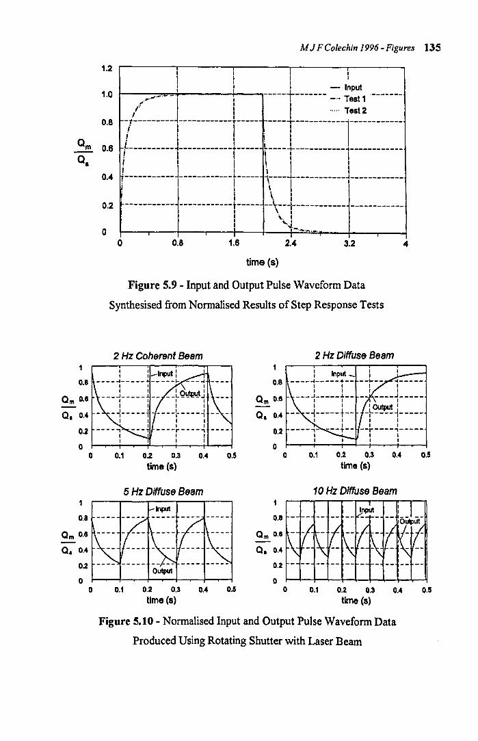
Qm
Q.
0.8
Qm O.S -Q.
0.2
0 0
1
0.8
Qm 0.8
Q. 0.4
0.2
0 0
M J F Colechin 1996 - Figures 135
1.2 i
1.0
0.8
0.6
0.4
0.2
0
I - Input
/~'.".-' -I j -----T------- ~:~ ~::!! .-------1'---------1------------[----- r----~-----------1------------~----------~------------~----- ~----~-----------~------------! I I! I I ! I I \ I I I I I I '-----------~------------~----- \----~-----------~------ ----, i i· I I - -, I I \ I I
i \. i i -----------J------------t----- --\--i------------ ------------
I \.. I I "-L
j--... -. I I
o 0.8 1.6 2.4 3.2 4
time (s)
Figure 5.9 - Input and Output Pulse Waveform Data
Synthesised from Normalised Results of Step Response Tests
2 Hz Coherent Beam 2 Hz Diffuse Beam I I
0.8 --1---I I I
Qm 0.8 -- ----.1-----I - I Output I
Q. 0.4 -~----1-----I I I I
0.2 --r-----,-----I I I I
0 0.1 0.2 0.3 0.4 0.5 0 0.1 0.2 0.3 0.4 0.5
time (s) time (s)
5 Hz Diffuse Beam 10Hz Diffuse Beam
Qm 0.8
Q. 0.4
0.2 - -- --Output
0 0.1 0.2 0.3 0.4 0.5 0 0.1 0.2 0.3 0.4 0.5
time (s) time (s)
Figure 5.10 - Normalised Input and Output Pulse Waveform Data
Produced Using Rotating Shutter with Laser Beam
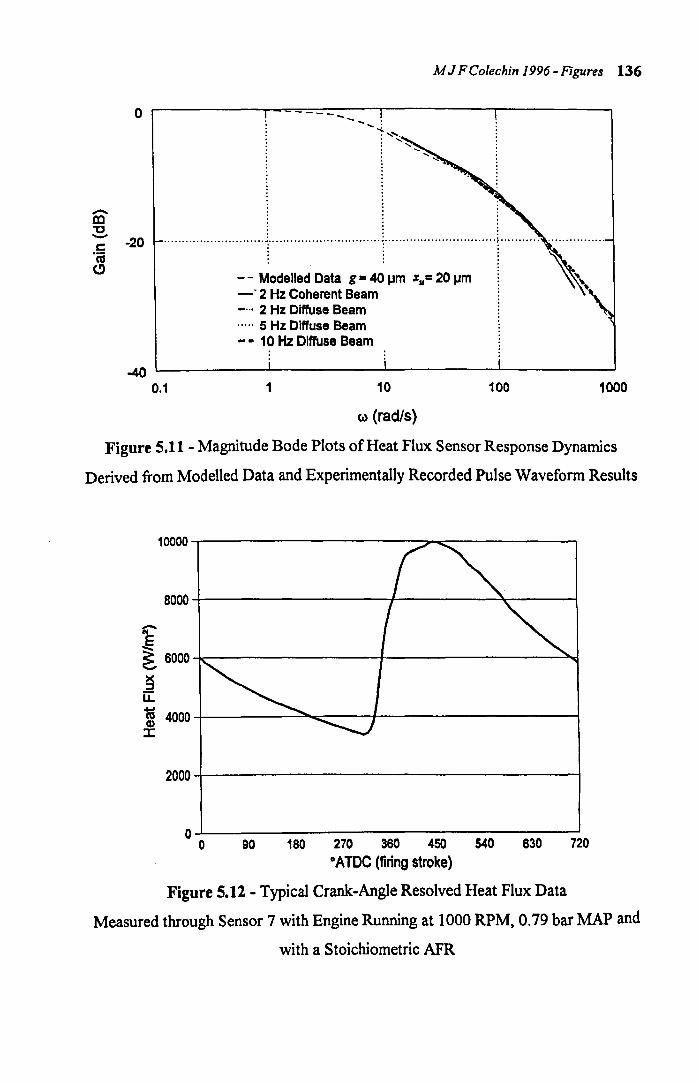
M J FColechin 1996 - Figures 136
o r-----------~~_~_~_-_-----.----------~----------~
-m "'C "; -20 'cu
.......................................................... ; ............................... } .......... . ~ ~ . :
C!) - - Modelled Data g = 40 \Jm xlI= 20 \Jm -- 2 Hz Coherent Beam _ ... 2 Hz Diffuse Beam ..... 5 Hz Diffuse Beam _. 10Hz Diffuse Beam
~o L-__________ L-__________ L-__________ L-________ ~
0.1 1 10 100 1000
c.> (radls)
Figure 5.11 - Magnitude Bode Plots of Heat Flux Sensor Response Dynamics
Derived from Modelled Data and Experimentally Recorded Pulse Waveform Results
10000~----------------------~~------------
8000+----------J-----~---~
~ ~ 6000 -k---------1---------~
~ u::: ~ 4000~---------3~----~------------------~ Q)
J:
2000 -t-------------------I
o~------------------------------------~ o 90 180 270 360 450 540 630 720
°ATDe (firing stroke)
Figure 5.12 - Typical Crank-Angle Resolved Heat Flux Data
Measured through Sensor 7 with Engine Running at 1000 RPM, 0.79 bar MAP and
with a Stoichiometric AFR

M J F Colechin 1996 - Figures 137
o r-----------~--_r----------------r_--------------~
CD "C
I I I I I .a - -20 . - m
•••.••••••.••••••••••..•••• 1" •••.•.••••••..••.••.•••..•••••..••.••••••••••..•••.••.•..••••••.••••••••..••.••..•••.••••
C"C ~:!:! E 5i ~ E -40
- cu C"C o C :ai ::l :::Ju.. c '5 -60 CD
~
-80 10
I I I I I ........................... ~ .......... . I I I I I
........•.................. J. ....•............•...........................•.•... : ....... . I : I : I : I : I : I
Fundamental 100 Frequency 1000
(a) (radls)
Figure 5.13 - Frequency Content of Crank-Angle Resolved Data
Shown in Figure 5.12
10000
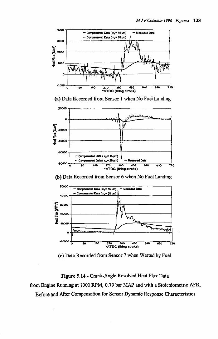
M J F Colechin 1996 - Figures 138
4oo0,-----------------------------------------~ - Compenlllled Oata ( :r. - 15 11m) - Meuured om _. Comperuted Data ( :r •• 20 11m)
3OO0+-------------------------~,_------------~
~ ~2~~----------------------~--~r-----------~
a! I 1~+----~._------------~~~~~~~
-1000 ...L.. ____________________________________ ...I
o 110 180 270 380 460 640 830 720 -ATDC (firing stroke)
(a) Data Recorded from Sensor 1 when No Fuel Landing
20000
o
.eoooo
-800000
I A --- ~ _!\n ,-p .......
"q v-! i \.
- CoInpenIated Data ( :r •• 15 11m) \! i
_. Compelllllllld Oata ( :r.. 20 11m) -MMMndData
eo 1 ao 270 380 4150 640 e30 720 -ATDC (firing stroke)
(b) Data Recorded from Sensor 6 when No Fuel Landing
60000
40000
~30000 ~ ~ 20000
1 10000
o
-10000
- Compenuted Data (:r. -15 JIM) 1 - Meulftd Olla - compenuted Data ( :r. - 20 \l1li) ,.
P j~ ! .
lJV~ ! ',"~ i . I·
,/ \>"~ II
lil, \y ... 71J ... " " . 'r'<1/ .... I
o 180 270 380 460 640 830 720 -ATDC (firing stroke)
(c) Data Recorded from Sensor 7 when Wetted by Fuel
Figure 5.14 - Crank-Angle Resolved Heat Flux Data
from Engine Running at 1000 RPM, 0.79 bar MAP and with a Stoichiometric AFR,
Before and After Compensation for Sensor Dynamic Response Characteristics
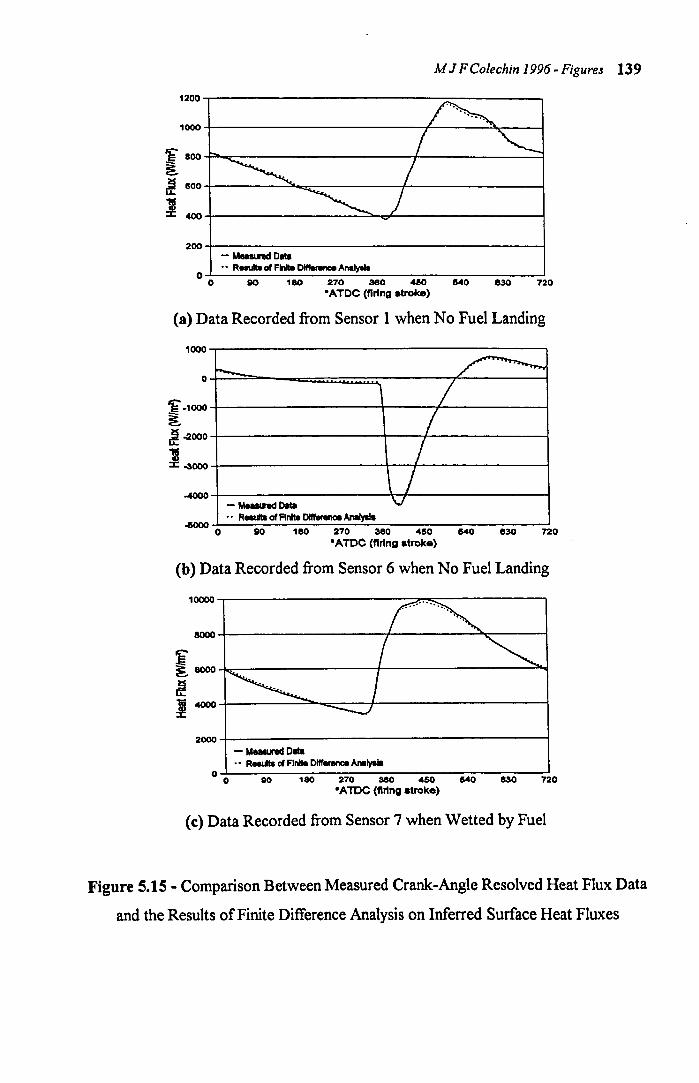
M J F Colechin J 996 - Figures 139
120o,.---------------::--------,
1000+------------~~--~~-~
~ aoo~~------------------~----------~ ~ ~ 800+----~:co:::_---~f_-----__l
I 400+--------=~~---------~ 200+-------------------~ -MeaalndData
•• RwuIIB of FInftII DItfere_ Analyala
o 0 80 180 270 380 460
°ATDC (firing atroke) 540 830 720
(a) Data Recorded from Sensor 1 when No Fuel Landing
1000
o
~ -1000
~ ~ -2000
1-3000
~o
r-- ~
o
1 / I
/ \/
-M-.dData v •• Reeulta of Finite DII'IInnce AnIiIyIIs
90 180 270 380 4150 540 830 °ATDC (firing atroke)
720
(b) Data Recorded from Sensor 6 when No Fuel Landing
10000~----------~~-----~
aooo+---------~-----~--~
i8000~------------~------------~ ~ f 4000
2000+------------------~ -MIIaII.I1IdData .• R ... at FI,.. DItferenca Analyala
0~O---8~0-~1!o~~2~7~0-~3~!o~-4ao~-54~0--8-30--~no °ATDC (tiring stroke)
(e) Data Recorded from Sensor 7 when Wetted by Fuel
Figure 5.15 - Comparison Between Measured Crank-Angle Resolved Heat Flux Data
and the Results of Finite Difference Analysis on Inferred Surface Heat Fluxes
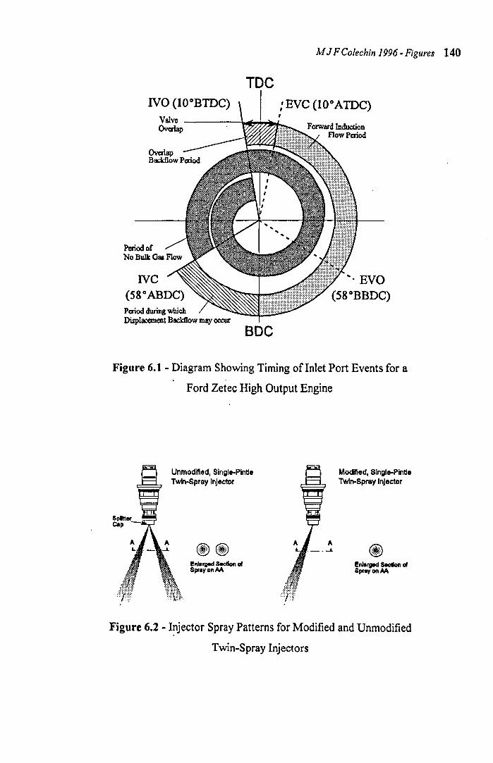
M J F Colechin 1996 - Figures 140
TDe : EVe (10 0 AIDe) ,
Valve -----\o~~W_ Overlap
Period during which Displacement Bacl:flow may occur
BOC
Figure 6.1 - Diagram Showing Timing of Inlet Port Events for a
Ford Zetec High Output Engine
Unmodified, Single-PinUe Twin-Spray Injector
~@ enlarged s.cdon III SprayonAA
Modified, Single-PinUe TwIn-Spray Injector
~ enlarged SeoIIon III Spray on AA
Figure 6.2 - Injector Spray Patterns for Modified and Unmodified
Twin-Spray Injectors
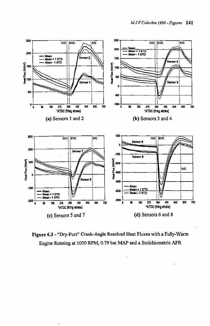
M J F Colechin 1996 - Figures 141
2500 IVO: :EVC
2500 IVO' 'EVC :IVC
" , , ,
2000 , - MelIn + 1 STO
2000 ,
-Mean - Mean -1 8TD
-Mean+1 STD 1500
~ 1500
-Mean-18TD
{1(XX1
!i !i Ii: Ii: 500
1'000 I 0
500 -600
" " " " 0 ·1000 0 SO 180 270 360 450 540 S30 no 0 eo 180 270 360 450 540 S30
°ATDC (firing stroke) tAlDC (firing stroke)
(a) Sensors 1 and 2 (b) Sensors 3 and 4
3000 IVO' :EVC :IVC !(XXI IVO: :EVC ,
SenIor 8 " , " ,
0 I, , , ,
2000 ' , , , , .!(XXI
SenlOl' 8
~,(XX1 I~ ~ I
~ ~.3OQO :IVC Ii:
,
I 0 I -4000
·1000 -Mean .6OOQ
-M ..... +1STD -M ..... ·1Sm
.mI 0 90 180 270 360 450 540 630 no
.6OOQ 0 SO 180 270 360 450 540 S30
'ATDC (firing stroke) t A TDC (firing stroke)
(c) Sensors 5 and 7 (d) Sensors 6 and 8
Figure 6.3 - "Dry-Port" Crank-Angle Resolved Heat Fluxes with a Fully-Warm
Engine Running at 1000 RPM, 0.79 bar MAP and a Stoichiometric AFR
720
no

M J F Colechin 1996 - Figures 142
7000 IVO: :eve :lVe ~ IVO: :eve
II
8000 ~ II II
5000 2000
~~ i D ~ I
~3000 ~.2OQO : S_or3 u.. I
12000 I II II II II
1000 -4000 I
II II II
.«lQD II
0
·1000 D 80 180 270 380 450 540 830 720
.aooo a 80 180 270 360 450 540 e30 720
°ATDC (firing stroke) °ATDC (firing stroke)
(a) Sensors 1 and 2 (b) Sensors 3 and 4
10000 IVO: :EVe :lVe II I II I II Seneor1 I II I
"~ II I II I II II
~: ( I
5000
10000 IVO: : eve -. _ :IVe
Sensors : I tI --...l. Sensor 8 :f
I I
I I
o
·10000
I
I
: Sensors I
I I I I I I I I I I I I I I I I I
·15000 I I I
I I I I I I
I I I I I II I
.8OOQO -20000 D 80 180 270 360 45D 540 830 no D 80 ~ 270 360 450 540 830 72D
°ATDC (firing stroke) • AiDe (firing stroke)
(c) Sensors 5 and 7 (d) Sensors 6 and 8
Figure 6.4 - "Dry-Port" Crank-Angle Resolved Heat Fluxes with a Fully-Warm
Engine Running at 1000 RPM, 0.79 bar MAP and a Stoichiometric AFR,
After Compensating for the Effects of Sensor Response
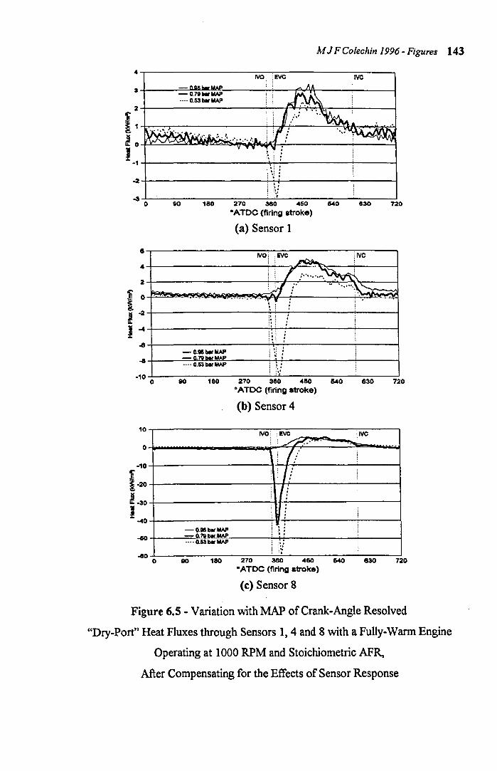
M J F Colechin J 996 - Figures 143
4~------------------------------------'--~ IVO EVC IVC
24-------------------~~~r+~~--~----~
11~~------------------~~------~~~~~~ ~o~~~~~~~~~~---------~~~ I -14-------------------~~----------~----~ ; ~~ i ~4_------------------~+_----------~----~ : \1 ~~~----------------~~----------~----~ o
8
4
2
f 0 .....
i..,2 ~ I -4
~
... -10
0
10
0
-10
r ! -20
~ -30
! -40
-60
-80 0
90 180 270 360 450 640 830
DATDC (firing stroke)
(a) Sensor 1
IVO: ,EVe ~ IVC
" .. ~ ~ : .,: .
····O.A_MAP j ~,: ~ ~ , .
80 180 270 380 460 540 630
---- 0.53 b8r WIP
DATDC (firing stroke)
(b) Sensor 4
IVO: . EVe ; IVC i \ ../""/'., ~
: /:' ~ :
:7! ; . Ii
: . : , . ; J. . ~.
: '. I !V
.
80 180 270 380 460 540 630 DATDC (firing stroke)
(C) Sensor 8
720
720
720
Figure 6.5 - Variation with MAP of Crank-Angle Resolved
"Dry-Port" Heat Fluxes through Sensors 1,4 and 8 with a Fully-Warm Engine
Operating at 1000 RPM and Stoichiometric AFR,
After Compensating for the Effects of Sensor Response
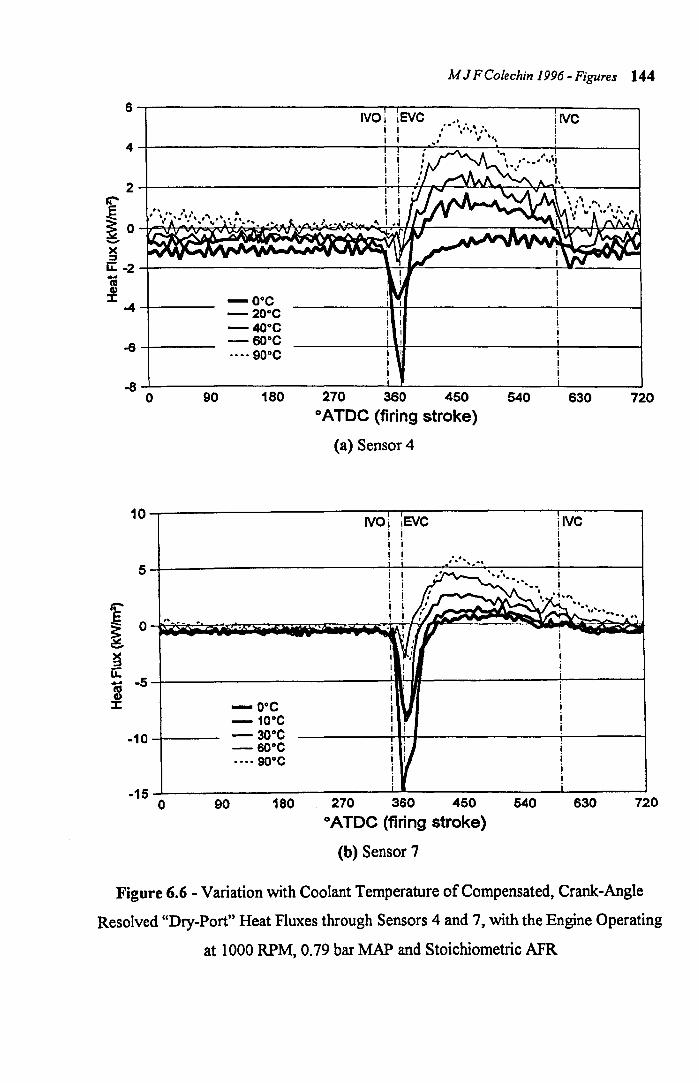
6
4
2
'f ~ 0 -)( :s Li: -2 ... as 41
:J: -4
-6
-8 0 90
-O°C -20°C -40°C -60°C ····90°C
180
M J FColechin 1996 - Figures 144
IVO' EVC
270 360 450 o ATDC (firing stroke)
(a) Sensor 4
540
jlVC i i
630 720
10~-----------rT--------r---~ IVO IEVC i IVC
i
~ ~ -~ u: (G Q) J:
5
0
-5
-10
_O°C _10°C -30°C -60°C •••. 900 e
i !
_15-L------------LL----------~------~ 180 270 360 450 540 630 720 o 90
o ATDC (firing stroke)
(b) Sensor 7
Figure 6.6 - Variation with Coolant Temperature of Compensated, Crank-Angle
Resolved "Dry-Port" Heat Fluxes through Sensors 4 and 7, with the Engine Operating
at 1000 RPM, 0.79 bar MAP and Stoichiometric AFR
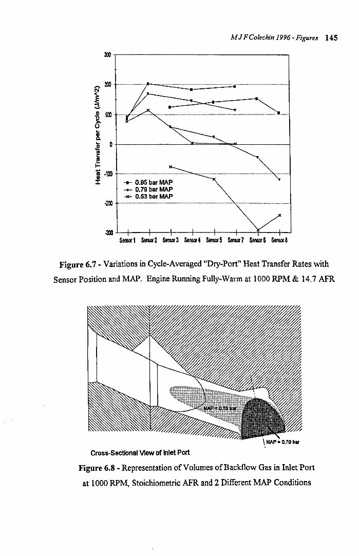
M J F Cole chin 1996 - Figures 145
...... 200 .............................................•...................................................................................
~ ~ ~ Cl 100 ............................................................................................................................................................. .
~ ~
8. ~ O~------------~~====~~--------~ III
~ m .100 Q) J: __ 0.95 bar MAP
__ 0.79 bar MAP -K- 0.53 bar MAP
-200 ...................................................................................................................................................................... .
~L-+---~---+---4----~--+---~---+~ Sensor 1 Sensor 2 Sensor 3 Sensor 4 Sensor 5 Sensor 7 Sensor 6 Sensor a
Figure 6.7 - Variations in Cycle-Averaged "Dry-Port" Heat Transfer Rates with
Sensor Position and MAP. Engine Running Fully-Warm at 1000 RPM & 14.7 AFR
Cross-Sectional View of Inlet Port
Figure 6.8 - Representation of Volumes ofBackflow Gas in Inlet Port
at 1000 RPM, Stoichiometric AFR and 2 Different MAP Conditions
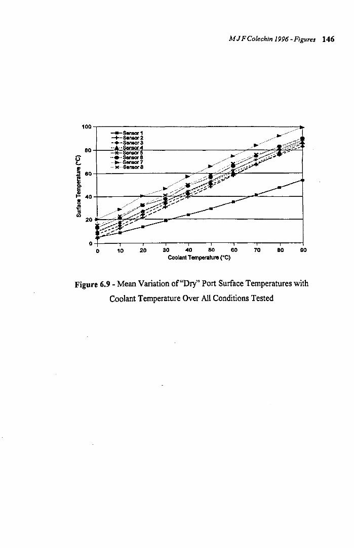
M J FCo/echin /996 -Figures 146
100,---------------------------------------------~ ---Sensor 1 -+-Sensor2 .............. -. - Se/'llOr 3
20~~~~~~~--~~~--------------------------~
04-----r----,-----r----~--~~--~----~----T_--~
o 10 20 30 40 50 60 Coolant Temperature COC)
70 80 90
Figure 6.9 - Mean Variation of "Dry" Port Surface Temperatures with
Coolant Temperature Over All Conditions Tested
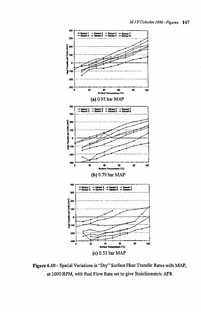
M J F Colechin 1996 - Figures 147
4OOr-----------------------------~ -Stntor 1 --Stntor:l ... SeNor 5 -- SenIor 7 -8enecr2-Stntor4+-SeNore-Seniore
300· ...... --.--......... ---._ ........ - ............. --. . ........ - ....... --....... -.. -.... .
[200 --....... _ ... --- -..... -... -_ ... -.. -....... --.. -.... _ ..... -.---......... -..... -.. -......... . ! 100 . --.-.----- .. ---.-- .... -.--.
1 ~~~~~-
I 0 I-
1-100
-200 ... _ .... ---.... -.. -.......... --.......... -_ ... _.... -_.-..... _ ...... --.. -.-.--.-..... --.... - ........ --..... - ... - ...... - ..
~~-+--+--+--+-~--+-~--~~~~ o 20 eo eo 100 ._Tem ......... rC)
(a) 0.95 bar MAP
~T-----------------------------~ -s.necr 1 --Senecr:l .... StnIor 5 - SeNor 7 -SenIor 2 .... s...- 4 +- StnIor. - SeNor.
300 .--... -----.. ---.. ---... -... --.-..... - ... --.--.--.-... ---.---..... _--... ---..... --.. -.
(b) 0.79 bar MAP
~.~----------------------------~ .... SenIcir 1 --Stntor:l - StntorS - 5ereor7 ..... se'*ll'2 -Senecr4 +StntorO ... s.r-a
300 .. -..... - .. _--..... -_ .... _--._--.--.-...... _ ...... _-.-.-.. -.. -.-.... ---.... ------.... -.-.... --..... .
-200
~~~~~~~~--~-+--+-~~ o 20 eo 100
(c) 0.53 bar MAP
Figure 6.10 - Spatial Variations in "Dry" Surface Heat Transfer Rates with MAP,
at 1000 RPM, with Fuel Flow Rate set to give Stoichiometric AFR
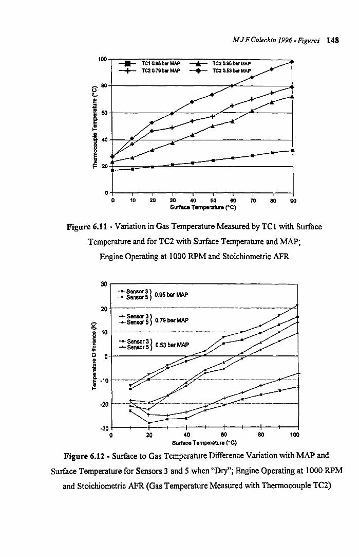
M J F Colechin J 996 - Figures 148
100,--. __ -=~~~~--~--~~~~--------~ -II- TC1 0.95 bar MAP ~ TC2 0.95 bar MAP
-+- TC2 0.79 bar MAP --+-~~~----------------------~~----------~ o o ..... ! t 6O-I------.,.,L-----"7'C---.,,,.........----I
~ \I)
I :~--=-====::!:::~~ O~--,_---r--~--~--~----~--~--~~
o 10 20 30 40 50 60 Surface Temperature (OC)
70 80 90
Figure 6.11 - Variation in Gas Temperature Measured by TCI with Surface
Temperature and for TC2 with Surface Temperature and MAP;
Engine Operating at 1000 RPM and Stoichiometric AFR
30 .r-----------------------------------. ..... SensorS) ........ Sensor 5) 0.95 bar MAP
20 -.--.-.. -----.--.. -.---.--------.------.-----.- ... ..... Sensor3) ....... Sensor 5) 0.79 bar MAP g
8 10 ! ..... Sensor3) ~ -+- Sensor 5) 0.53 bar MAP
c O+------------~~~L---~~~~------~ ! ~ !. ~ -10'· .. --.--... --..... . .....
I-
·20
.so .t---+----If.---tr----t----t----i----+---+----+----I
o 20 40 60 80 100 Surface Temperature (OC)
Figure 6.12 - Surface to Gas Temperature Difference Variation with MAP and
Surface Temperature for Sensors 3 and 5 when "Dry"; Engine Operating at 1000 RPM
and Stoichiometric AFR (Gas Temperature Measured with Thermocouple TC2)
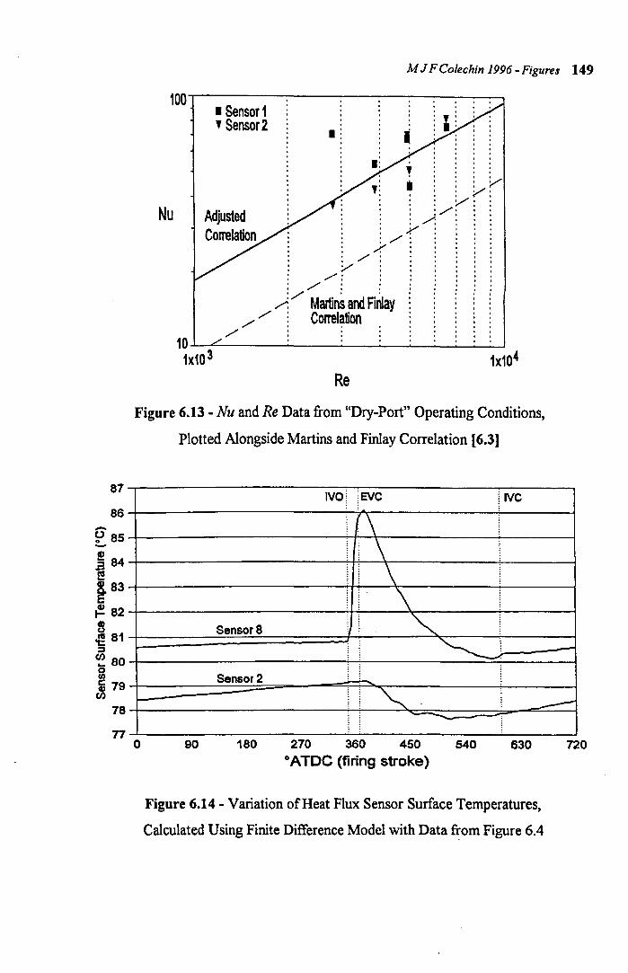
M J F Colechin 1996 - Figures 149
100...-------:------------------. • Sensor 1 , Sensor2
Nu
• .V
. y' V· . :/"' .. . /: . . ;,.... . . /"'. /. .
. ,,/: /
/: . /"': . '''/ . ,
/. Martins and Finlay /'" /'" ~ Correlation
/'" : 10~~----~------------~ __ ~ __ -J
ixi0 3 ix104
Re
Figure 6.13 - Nu and Re Data from "Dry-Port" Operating Conditions,
Plotted Alongside Martins and Finlay Correlation [6.3]
87~---------------------IV-O::':'EV-C-------------;l-w-c------,
_86~----------------~:~ {:~~---------+----~
~::~~=======================:=: :\::===================: ~ ~ ~S3+---------------~~~~-------~---~
~82~------------------~r.----.~~~--------~-----1 o SensorS """" ~ 81i:====================~~--------~~~=---~L jj-_-_-_-----=---~ ~ 80~----------------------~~-------~----~~------~ ~ Sensor 2 ~79t_====~~~--~fF~~~-_----~--___ ~ 78i--------------------~:_--~~~~~~--~--~
--~ n~----------------------~--------------~------~ o 90 180 270 360 450 540 630
o ATDC (firing stroke)
Figure 6.14 - Variation of Heat Flux Sensor Surface Temperatures,
Calculated Using Finite Difference Model with Data from Figure 6.4
720
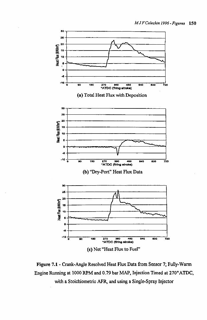
30
25
:€ 20
~ 115
~ 10
I II
o
-10
30
215
:f 20
~ 15
~ 10
I II
o
-10
30
25
:€ 20
liS ~ 10
I II
o
-10
r-...
o
o
--
o
M J FColechin 1996 - Figures 150
1\ .-IV :'\. f ~ I ~ I
180 270 380 460 640 830 720 -ATOC (flnng atroke)
(a) Total Heat Flux with Deposition
110
/ ~ ,/
v
180 270 380 460 640 IS30 720 -ATDC (tlrtng atroke)
(b) "Dry-Port" Heat Flux Data
I
1\1\ I . '---. I .. ~ L "'---..-~
_I
180 270 380 460 640 830 720 -ATOC (firing atroke)
(c) Net "Heat Flux to Fuel"
Figure 7.1- Crank-Angle Resolved Heat Flux Data from Sensor 7; Fully-Warm
Engine Running at 1000 RPM and 0.79 bar MAP, Injection Timed at 270 0 ATDe,
with a Stoichiometric AFR, and using a Single-Spray Injector
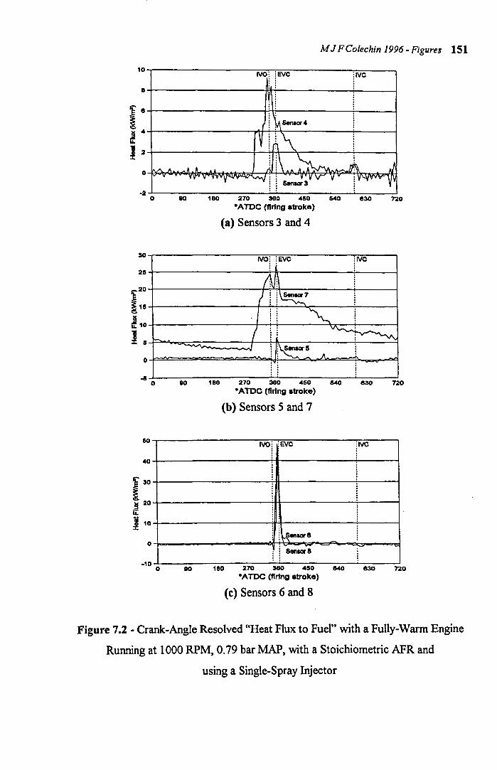
M J FCo/echin 1996 -Figures 151
1o.-----------------~~~~--------~----~ IVO l EVe \ IVC
a~------------------~~----------~----~
~e+---------------~----------~--~ ~ ~ 44-----------------~~4.----------~----~ ii:
12+-----------+-~~------~--~
~JO-----~-----,8-0----2-ro--~H~0----4-50----540--~~e-~----~no °ATDC (ftring stroke)
(a) Sensors 3 and 4
30.-----------------~IV~O~\~l~EV~C~--------~tlV~C~--~
254-------------------~r_----------~----~
$20
~154---------------~~~~------~--~
~,0~----------------+-~--------~r-~----~ I s~~==~----~_+~--------~--~ o~~==~~~~~~~~~~~~~~~~ __ ~
~JO-----~-----,8-0----27~0--~~~~----4-60----~--0--~e-~----~no °ATDC (firing stroke)
(b) Sensors 5 and 7
~,-----------------71VO~1~:EV~C----------~IVC~--~
~4_------------------~------------~----~
~304---------------~*-----------~----
~204_----------------~----------~----~ ~ I 104-------------------~r_----------4-----~
i ihSenaor8 04-________________ ~~,~~y~~~~~-----d i ~ SenlOr8
_10...L.------------------..:.....;,.------------.l--------l o 1M) 1eo 270 HO 450 540 830 720
°ATDC (firing stroke)
(C) Sensors 6 and 8
Figure 7.2 - Crank-Angle Resolved "Heat Flux to Fuel" with a Fully-Warm Engine
Running at 1000 RPM, 0.79 bar MAP, with a Stoichiometric AFR and
using a Single-Spray Injector
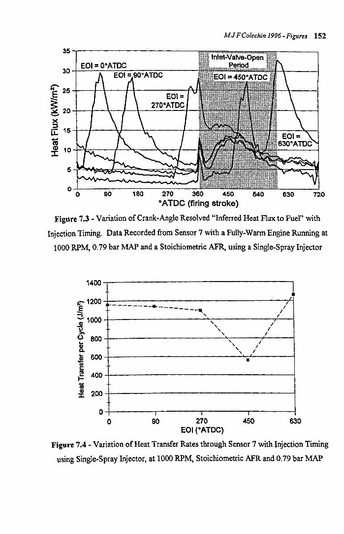
MJ FColechin 1996 -Figures 152
35,-------------------------
30~~---------------------
-~ 254---~+_--~+_--------_PH
.E ~ 204--4--4--+~~------~->< :::J ~ 154--+----~----~------~-
m J: 10
OJ-----------------------~ o 90 180 270 360 450 540 o ATDC (firing stroke)
630 720
Figure 7.3 - Variation of Crank-Angle Resolved "Inferred Heat Flux to Fuel" with
Injection Timing. Data Recorded from Sensor 7 with a Fully-Warm Engine Running at
1000 RPM, 0.79 bar MAP and a Stoichiometric AFR, using a Single-Spray Injector
1400
~ 1200 .E ;-1000
l (,) 800 '-
8. '- 600 ~ c:: t! 400 .... 1;; ~ 200
a
--.---------.. --------.. , , , , ,
I I
o 90 270 EOI (GATDe)
} /
/ /
/
/' /
I , I ,
/ , , / •
I
450 630
Figure 7.4 - Variation of Heat Transfer Rates through Sensor 7 with Injection Timing
using Single-Spray Injector, at 1000 RPM, Stoichiometric AFR and 0.79 bar MAP

M J FColechin 1996 - Figures 153
30
25
- Mean Variation -E 20
~ ~ '-" >< 15 ::J u:: -as
10 (I)
::I:
5
0 630 0 90 180 270 360 450 540 630
° Crank-Rotation
Figure 7.5(a) - Aligned Variations of Heat Flux given in Figure 7.3, Excluding Data
for the Inlet-Valve-Open Period, for Injection Timings (EOI) of 0, 90, 270 and
12
10
8 -N
E 6
~ '-"
>< 4 ::J u: 1;; 2 CD :r:
0
-2
-4
- Mean Variation
630 0 AIDC
IVO :EVC , , , IVC
i / -+-____ -L _____ --\-HJ~------l-· Data or __ --I ; EOI =: 630 0 ATDC I ,
0 90 180 270 360 450 540 630 720 o ATDC (firing stroke)
Figure 7.5(b) - Heat Flux "Remainder" After Subtracting the Mean Variation given in
Figure 7.s(a) from the data given in Figure 7.3, for Injection Timings (E01) oro, 90,
270 and 6300 ATDC

M J FColechin 1996 - Figures 154
5 I
s: ! 4
I I I I I I -----V --~ ------:------~ ------
... !. 3 --~------l-- --~------l------... ..! II) c l! 2 ~
1i ~----j------~---1 1 1 1
1 1 I , II J: 1
! 1 1 --- 0.95 bar MAP -----,------r----" 1 ...,... 0.79 bar MAP 1 -+- U3 bar MAP . .
0 50 100 150 200 250 300
Fuel Flow Rate (mgts)
(a) Twin-Spray Injector 5T------.------~1~----~------~----~
I 3 1 1 1 1 I ! 4 -----l------r-----l------r------I I 1 13 --+--i----}----- ,--- --t------
~ 2 - - - - - : - - - - : - - - - - -1- -----t ------~ I 1 I I iii I I . :! _____ -: ______ ~----.--- O.85barMAP ____ _
- I I ...,... D.NbarMAP
~ : : ~ O.63bar~
s: ~
~ 8. l! l! l! ~
I ~ ~
0+---~_+---r--4_--+_--~~--_+--_r--~
50
5
4
3
2
1
0 50
100 150 200 250
Fuel Flow Rate (mgls)
(b) Single-Spray Injector
I I I
1 1 1 I
300
-----~------~-----~------.------1 1 1 I 1 1 I I I I I I , I 1 -----,------r--- -,------r------
I I I I I . . I. .--
----~-----~------.------I I I I I I
I I . 1 I --- 0.85 bar MAP ---,------r----· I I ...,... 0.70 bar MAP I I -+- 0.63 bar MAP I I • •
100 150 2DD 250 300
Fuel Flow Rate (mg/a)
(e) Four-Hole Injector
Figure 7.6 - Variation in Estimated Total Heat Transfer Rates with Injector Type,
MAP and Fuel Flow Rate with the Engine Fully-Warm and Running at 1000 RPM
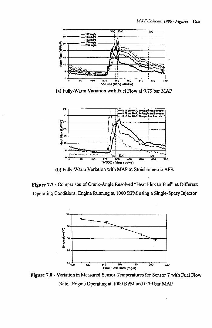
M J F Cotechin 1996 - Figures 155
35 IVO :EVC ,
30
r a5
~20 ~ 15 u..
110
5
0 0 10 180 270 380 460 640 830 720
-ATDC (ftring atroke)
(a) Fully-Warm Variation with Fuel Flow at 0.79 bar MAP
35
30
f25
~20 )( ~ u:: 15
110
II
0
:-O.IIS _ MAP. 180 mgIS tuelliow rata . . ,!- 0.79 _ MAP. 145 mgfs tuelliow rata -+--------~-HI ! ..... 0.53_MAP.90mgJar'ftow ....
, t
··,··· .. • •• •• .......... • ........ n .......... • it
IVO' 'EVe: 0 110 180 270 380 460 640 720
-ATDC (ftring atroke)
(b) Fully-Warm Variation with MAP at Stoichiometric AFR
Figure 7.7 - Comparison of Crank-Angle Resolved "Heat Flux to Fuel" at Different
Operating Conditions. Engine Running at 1000 RPM using a Single-Spray Injector
70
115
E
I~ ....
65
80 100 12 «0 180 180 200 220
Fuel Flow Rate ems'a)
Figure 7.8 - Variation in Measured Sensor Temperatures for Sensor 7 with Fuel Flow
Rate. Engine Operating at 1000 RPM and 0.79 bar MAP
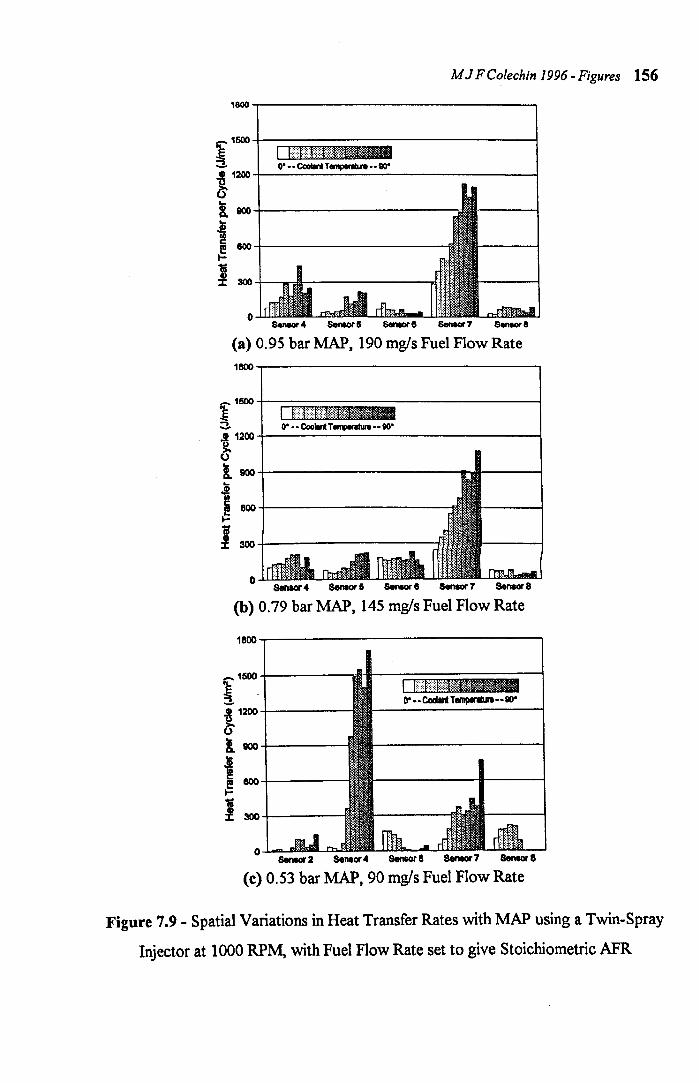
M J F Colechin J 996 - Figures 156
1~,-------------------------------~
~1~1--[]illiEiiiiiiiil--------------~ .e I 1:lrftlffN¥** ~ 0··· CooIInI Ternpnhn •• 90" ~1200+-------~--------------------~
is i 800+---------------------I &004---------------------
I 3004-__ ~------------~. o
SenIorS 6ene«7 S_ 8
(a) 0.95 bar MAP, 190 mgls Fuel Flow Rate
1&oo,-------------------------------~
~1500t-rl~I:~<I~t)~M~%~i®~~~~~~-------------------l :J. o· •. Coolant Temper.tur.·· eo· t 1200
o 1 9oo+-----------------------------1~------~
J 800+---------------------
I 3OO-l--------f
o SenIor 4 se",or6 Seneor7
(b) 0.79 bar MAP, 145 mgls Fuel Flow Rate
1800 -r-------------------------------..,
~ 1200
is l 800 +-----------
I ~800
I 300-+----
Sensor 7 Sensors
(c) 0.53 bar MAP, 90 mg/s Fuel Flow Rate
Figure 7.9 - Spatial Variations in Heat Transfer Rates with MAP using a Twin-Spray
Injector at 1000 RPM, with Fuel Flow Rate set to give Stoichiometric AFR
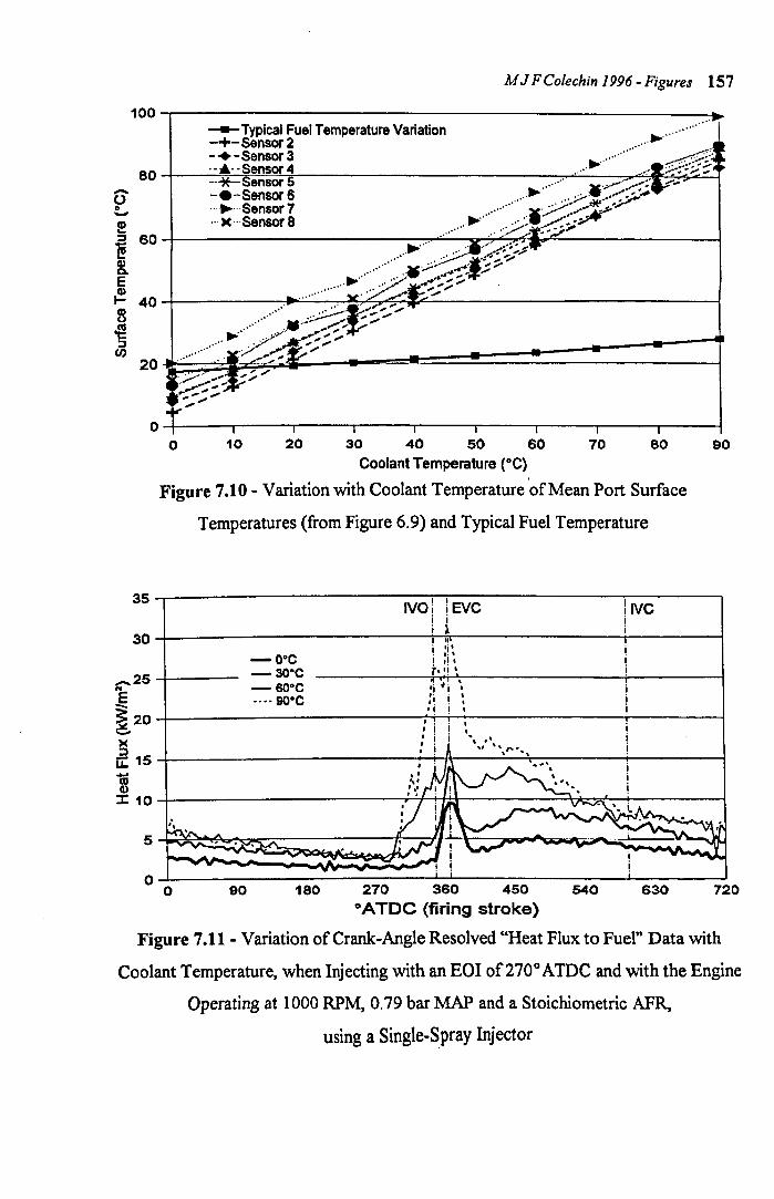
M J F Colechin J 996 - Figures 157
100-r----------------------------------------------------~ --Typical Fuel Temperature Variation -+-Sensor2
.. ' ....
,."
-+-Sensor3 .~ ...... . 80-r ___ ·_-·~·-~S~M=S~or~4~------------------------~~.~.----~ .. ~:.~~~ _.*-Sensor 5 ......... .v~>:.:·;·
6 o -! ~ 60
8. E
-.-Sensor 6 ..... ,:.:.:.-- ".~" ". ""Sensor 7 ........... I' .. :;;.:~ .. ~ ... '*:;..r
S 8 ......... ".~ ...
,,)(.. ensor ............... ..' ... ~:. ;.:...:: ~.
~ 40~----------~~·-··~~~~~~--------------------------~ ~ ~ :s en
O~----_r----_r----_r----_.----~----_,----~~----~--~
35
30
,,25
..e ~20 )( ::l u::: 15 as Q)
::J: 10
5
0
o 10 20 30 40 50 60 70 80 90 Coolant Temperature (OC)
Figure 7.10 - Variation with Coolant Temperature 'ofMean Port Surface
. "
0
Temperatures (from Figure 6.9) and Typical Fuel Temperature
-O·C -3O·C -60·C ····90·C
90 180
lVol : EVC i i i •
:! ~ ,I, t, '! ' 'i f i " :, ! ' '1 I
270 360 450 °ATDC (firing stroke)
540
live i i
630 720
Figure 7.11 - Variation of Crank-Angle Resolved "Heat Flux to Fuel" Data with
Coolant Temperature, when Injecting with an EOI of 270° AIDe and with the Engine
Operating at 1000 RPM, 0.79 bar MAP and a Stoichiometric AFR,
using a Single-Spray Injector
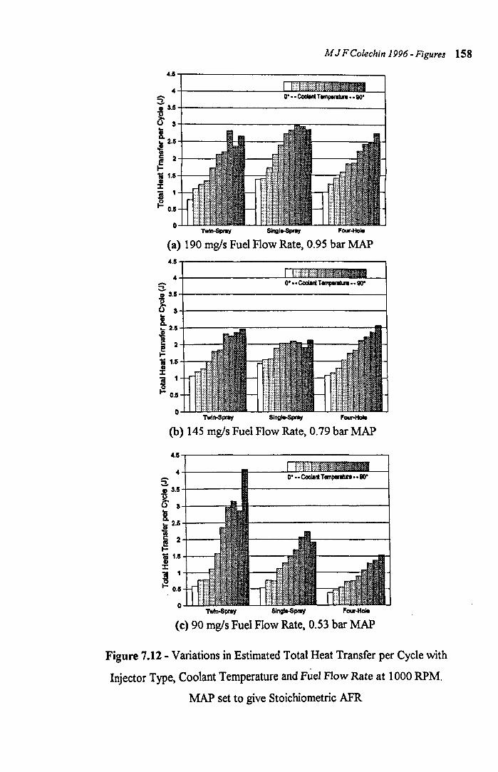
M J F Colechin 1996 - Figures 158
4.5-r-----------------. ...... :::!. ~305-t----------------l
?i' 3+--------1l1li(;;'"------1 l .. 2.54----
i e 2+---I-11.5 J: ~ , F 0.5
O...w...J= ~ Slngl..spray Four-Hole
(a) 190 mg/s Fuel Flow Rate, 0.95 bar MAP
4.5,..------------------, ..... o· •• CooIIrt TIIIIpIII\UrW •• 110" :::!. III 305-+----------------1
~ 3+-----------------------~ l .. 2.5-1-----;;:------------1l1l-I
i I! 2 I-
11.5 J: ~ , F 0.5
o
(b) 145 mg/s Fuel Flow Rate, 0.79 bar MAP
u..,.-----------------. 4L---I1I---PEP_ ... -J o· •• CooIatt Tempet'IIurI •• 80' .-
:::!. -8 3.5
l5' 34.---
l ... 2.5-1---.e ~ 2-1---li U+---f.:3 J:
~ 1
F 0.5
o Twln-SpIay SlngIt-SpnIy Four-Hole
(c) 90 mg/s Fuel Flow Rate, 0.53 bar MAP
Figure 7.12 - Variations in Estimated Total Heat Transfer per Cycle with
Injector Type, Coolant Temperature and Fuel Flow Rate at 1000 RPM.
MAP set to give Stoichiometric AFR
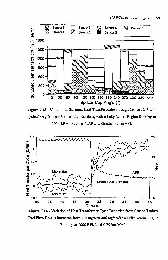
-l§ ..., -m SensorS
ill] Sensor 4
D Sensor7
~ Sensor3
M J F Colechin J 996 - Figures 159
~ SensorS
• Sensor2 ~ Sensor5
~ 1800.-----------------------------------------------------------------------------------------------------~ ~
~ 1500;-----------~~~--------------------------r~ CD c. ~ 1200 -+---I~~ tJ) C
~ 900 I-m CD 600 J:
i 300~~ E § oJlliilll~!!D en o 30 60 90 120 150 180 210 240 270 300 330 360
Splitter-Cap Angle (0)
Figure 7.13 - Variation in Summed Heat Transfer Rates through Sensors 2-8 with
Twin-Spray Injector Splitter-Cap Rotation, with a Fully-Warm Engine Running at
1000 RPM, 0.79 bar MAP and Stoichiometric AFR
1.6-.----------:------------------,-20
-:g ~ 1.4 -CD "0 0 1.2 LCD C.
~ 1.0 ~ c: ! I- 0.8 10 CD :J:
15
AFR
Mean Heat Transfer
0.6 -+---I----+---+---+---I---t-----+---+--__+_ 5 0.0 0.5 1.0 1.5 2.0 2.5 3.0 3.5 4.0 4.5
Time (s) Figure 7.14 - Variation of Heat Transfer per Cycle Recorded from Sensor 7 when
Fuel Flow Rate is Increased from 112 rog/s to 206 mg/s with a Fully-Warm Engine
Running at 1000 RPM and 0.79 bar MAP

M J F Colechin J 996 - Figures 160
50.-------------------------------____ ~
o~~~~----~--~~----~----------~ 1600 1760 2000 2260 2600 2760 3000
Time (ms)
(a) Recorded Cycles of "Wetted" Data 60
40
10 1\ \ \ \ ~ ~~~~ ~
o Cycle 0 Cycle 1 Cycle II Cycle 10 Cycle 16
(b) Progressive Cycles of "Heat Flux to Fuel" Data
IIO~--------------~~~--------~~--~ IVO: :EVC :IVC
i -CycleD i
40 -f---- Cyd., _______ ~---------......;I'_-~ -CycleS
'j; ~30
-Cycle 10 •••• CycIe1S
!! ~20+_--------,M~~~~--_+--~
I 10i:--------~~~~~~~~~~~~
o~~~JlI !_=:::::±~ o 1eo 380 540 720
-ATDC (firing stroke)
(c) Overlayed Cycles of "Heat Flux to Fuel" Data
Figure 7.15 - Variation of Crank-Angle Resolved Heat Flux Data when Fuel Flow is
Increased from 112mg/s to 206 mg/s between Cycles 0 and 1. Data Recorded from
Sensor 7 with a Fully-Warm Engine Running at 1000 RPM and 0.79 bar MAP, using a
Single-Spray Injector
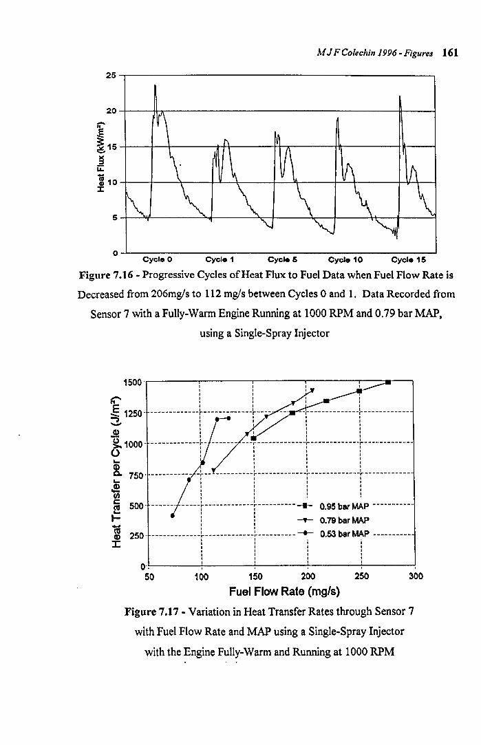
M J F Colechin J 996 - Figures 161
25,------------------------------------------------,
20~--~hr------------------------------------~--~
" ,E ~15~--~-4-------+~------+r~----~~------~~--~ ~ u: m10~--~--~----~--+_----~~----~~~----~~~~ J:
o~----------------------------------------------~ Cycle 0 Cycle 1 Cycle 5 Cycle 10 Cycle 15
Figure 7.16 - Progressive Cycles of Heat Flux to Fuel Data when Fuel Flow Rate is
Decreased from 206mg/s to 112 mg/s between Cycles 0 and 1. Data Recorded from
Sensor 7 with a Fully-Warm Engine Running at 1000 RPM and 0.79 bar MAP,
using a Single-Spray Injector
1500 .r---------r-------,-, -------,--------,-----:11.---, , ,
(4' I: : E ll I
- 1250' -------------f-----------··f---- --;-------------r------------3 : : : :
I " Jl : ::
(So 1000' -------------r- ------- --·T-------------r·-------------r------------I I I I I I I t .... I:::
CD I I I
~ 750' ----------- -~-------------r-------------r-------------r------------. .... I I I
.! ::: o I:!! c 500' ------. -----~, ------------+---------- -w- 0.95 bar MAP ----------~ "
.... :: -'t'- 0.79 bar MAP I I
l 250· -------------~-------------~---------- -e- 0.53 bar MAP ----------.,.. :: i .... I I I
I I I , I , I I I
o·~. -------+'------~'--------~' ------~------~ 50 100 150 200 250 300
Fuel Flow Rate (mg/s)
Figure 7.17 - Variation in Heat Transfer Rates through Sensor 7
with Fuel Flow Rate and MAP using a Single-Spray Injector
with the Engine Fully-Warm and Running at 1000 RPM
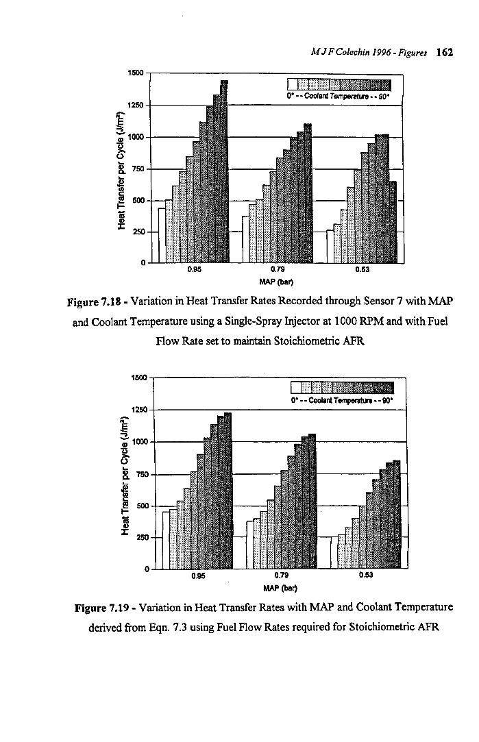
1500
1250
""" ~ ';' 1000
~ ~
8. 750 ~
oS! II) &::
~ 500
i J:
250
0 0.95
M J F Colechin J 996 - Figures 162
o· _. Coolant TemperatLn· - so·
0.79
MAP (bar)
0.53
Figure 7.18 - Variation in Heat Transfer Rates Recorded through Sensor 7 with MAP
and Coolant Temperature using a Single-Spray Injector at 1000 RPM and with Fuel
Flow Rate set to maintain Stoichiometric AFR
1500~---------------------------------------------~~;;~======~
o· -. Coolant Temperature -·90· 1250-+---------------------1
t;"" .§ .., ';' 1000 4----1
~ 8. 7504---
~ &:: ~ 500 4--t":::
i J: 250
o 0.95 0.79
MAP (bar)
0.53
Figure 7.19 - Variation in Heat Transfer Rates with MAP and Coolant Temperature
derived from Eqn. 7.3 using Fuel Flow Rates required for Stoichiometric AFR
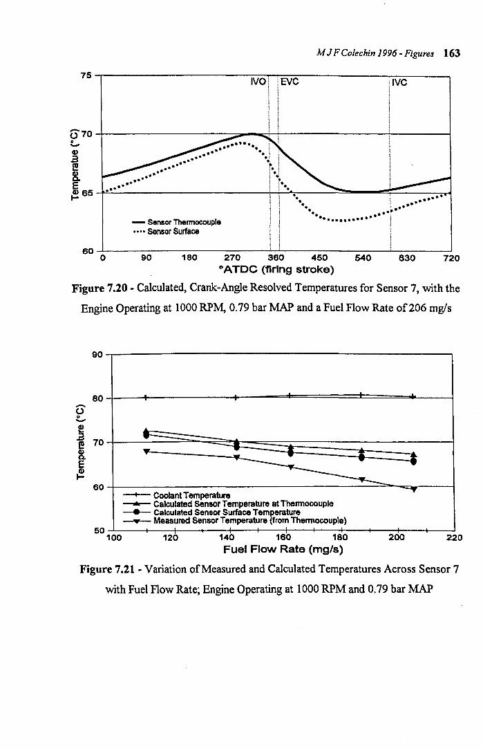
M J F Colechin 1996 - Figures 163
75.---------------------~~"=EV~C=-------------~IV~C----~
()70~--------------------~--~~----------------~--------~ t, ..... ..... .... ~ •••• -.1 l! •.•..• •• : 8. •.••••••• l··J .. - : ~. E •••• • ; ~ •• ~65~~------------------------~~ ••• ----~~----~~~-.-•• -.-•• ~.~ .. : ....
- Sensor Thermocouple •••• Sensor Surface
-. ..-.••••.........••••
60-L--------------------------~----------------~--------~ o 90 180 270 360 450 540 830 720
o A Toe (firing stroke)
Figure 7.20 - Calculated, Crank-Angle Resolved Temperatures for Sensor 7, with the
Engine Operating at 1000 RPM, 0.79 bar MAP and a Fuel Flow Rate of206 mg/s
-0 0 -! ~ 8. E CD I-
90
80
70
60
50 100
.
~ -'"
... -- ... .~
-. ... --+-- Coolant Temperature
"'"T
--..- Calculated Sensor Temperature at Thennocouple ____ Calculated Sensor Surface Temperature --.- Measured Sensor Temperature (from Thennocouple)
120 140 160 180 200 220 Fuel Flow Rate (mg/s)
Figure 7.21 - Variation of Measured and Calculated Temperatures Across Sensor 7
with Fuel Flow Rate; Engine Operating at 1000 RPM and 0.79 bar MAP
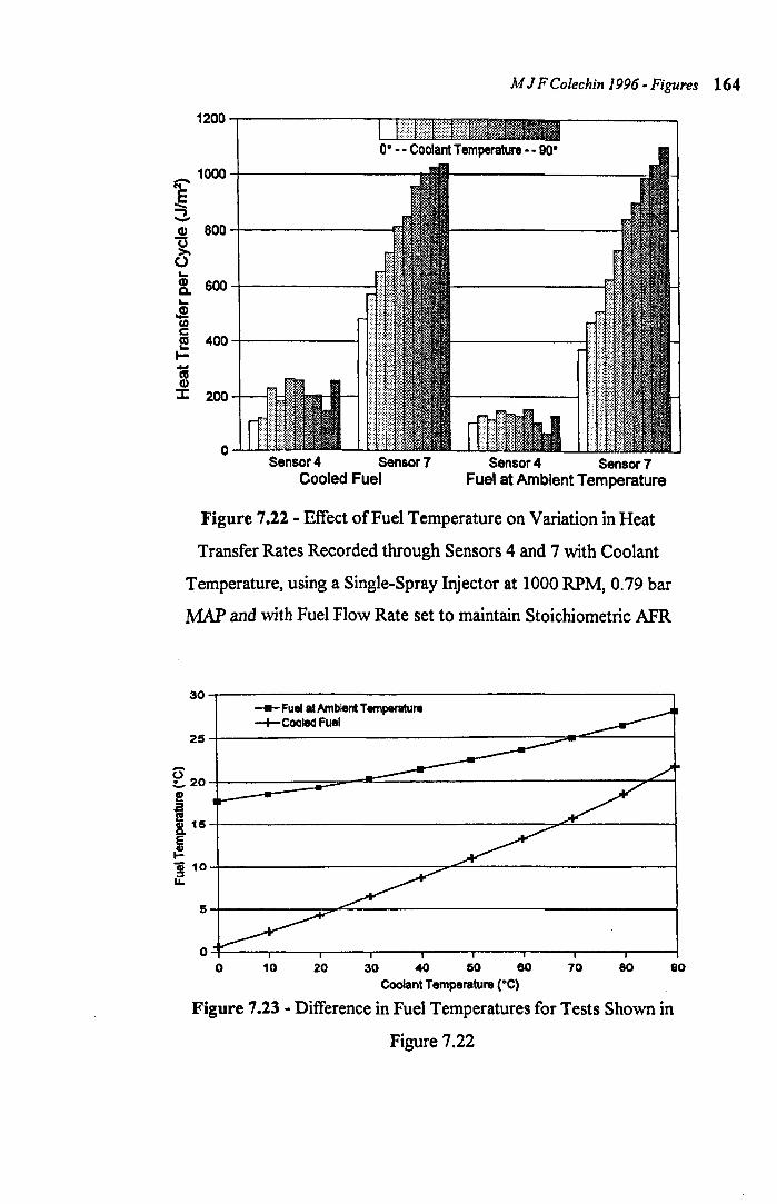
M J F Colechin 1996 - Figures 164
1200,--------------r~~=
~ 1000
:3-CD 800 -1-------------g. o '-8. 600 -1---------'-.! (D c e 400 -+--------1 ... .... m :I: 200 -+---1;;,'1-
o Sensor 4 Sensor 7 Sensor 4 Sensor 7
Cooled Fuel Fuel at Ambient Temperature
Figure 7.22 - Effect of Fuel Temperature on Variation in Heat
Transfer Rates Recorded through Sensors 4 and 7 with Coolant
Temperature, using a Single-Spray Injector at 1000 RPM, 0.79 bar
MAP and with Fuel Flow Rate set to maintain Stoichiometric AFR
30~-------------------------------------------, ---Fuel at Ambient Temperature -+-Cooled Fuel
25~--------------------------------~--=-------~
E20~--------~=--d~------------------------~~~ ~ i 15-1--------------------------------~~--------~ ~ ~ 10-l---------------------~~--------------------~ u..
5-1----------=~--------------------------------~
O~--~r_---r----r_--_r----._--~----,_--_,----~
o 10 20 30 40 50 60 70 80 90 Coolant Temperature (Oc)
Figure 7.23 - Difference in Fuel Temperatures for Tests Shown in
Figure 7.22
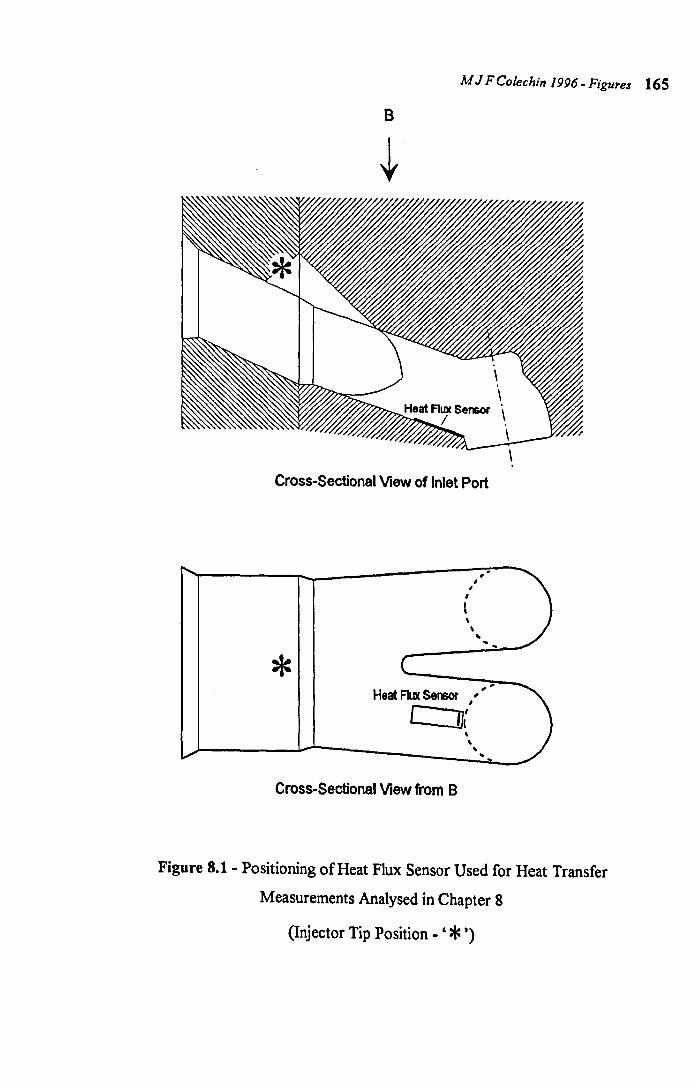
M J F Co/echin J 996 - Figures 165
B
Cross-Sectional View of Inlet Port
*
, , , , I , \
\ .. ..
Heat Flux Sensor ,,"
C ]: \ \ .. ..
Cross-Sectional View from B
Figure 8.1 - Positioning of Heat Flux Sensor Used for Heat Transfer
Measurements Analysed in Chapter 8
(Injector Tip Position - ' * ')
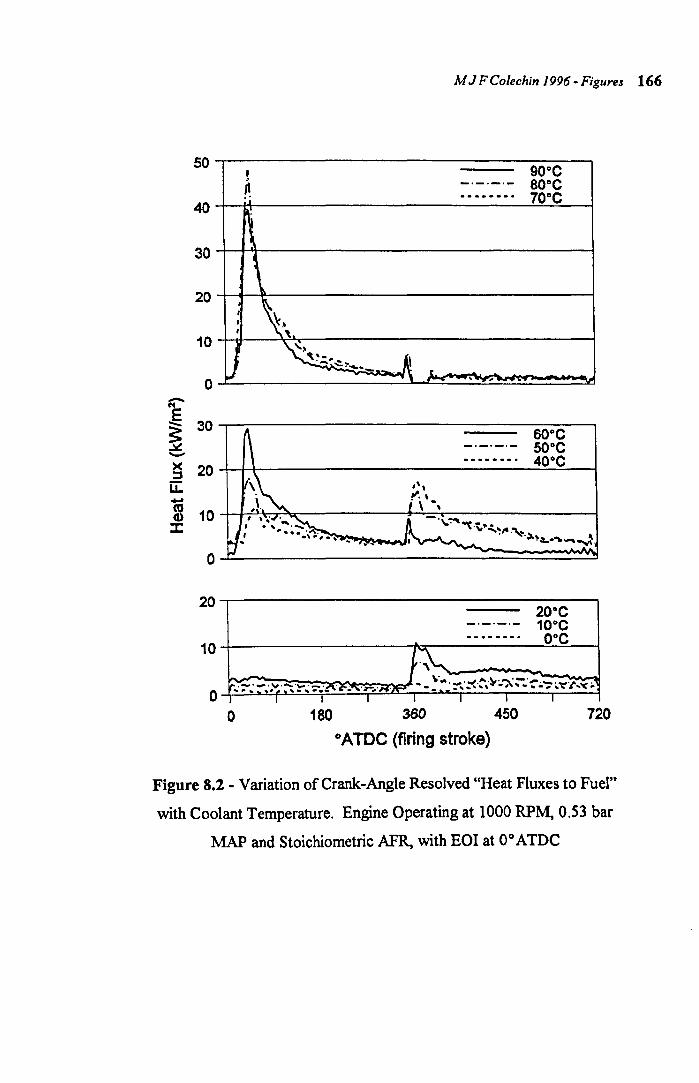
M J F Colechin 1996 - Figures 166
50 90°C ,
40
,
" ----_.- 80°C
.' ------.- 70°C
30 ~ j
20
10
0
\ , \, , ,
~ ~ '\~"::'''~l' ~ ~~.-. 1:, .... .. --.. , ,
t:' E ;: ~
30
-)( 20 ::::s u:: .... as 10 CD J:
0
20
10
o 180 380 450 720
°ATDC (firing stroke)
Figure 8.2 - Variation of Crank-Angle Resolved "Heat Fluxes to Fuel"
with Coolant Temperature. Engine Operating at 1000 RPM, 0.53 bar
MAP and Stoichiometric APR, with EOl at 00 ATDC
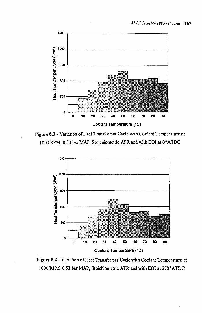
M J F Colechin J 996 - Figure! 167
1500.-------------------,
;;"" 1200 .§ .., -CD
~ 900 t-CD Q. t-
oe! en 600 c I! t-'t;i CD 300 J:
o 10 20 30 40 50 80 70 80 90
Coolant Temperature (OC)
Figure 8.3 - Variation of Heat Transfer per Cycle with Coolant Temperature at
1000 RPM, 0.53 bar MAP, Stoichiometric AFR and with EO! at 00 ATDC
1500...,...--------------------,
~12oo+------------------~
.§ ~ .9! ~ 900+---------------------------1 t-
8. ... ~ ~ 600+_-------
~ 1 ::I: 300 +-------'
0-'---==== o 10 20 30 40 50 60 70 80 90
Coolant Temperature (OC)
Figure 8.4 - Variation of Heat Transfer per Cycle with Coolant Temperature at
1000 RPM, 0.53 bar MAP, Stoichiometric AFR and with EO! at 2700 ATDe
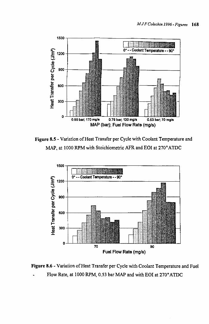
M J F Colechin 1996 - Figures 168
1500~----------------------------__________ -,
f:'" -E 1200 -+-----3 Q)
~ 900-+----&.. Q) c.. &..
~ 600-+----th c: I! I-m 300-+---r:;
J:
O.....L....J'---"""= 0.95 bar; 170 mg/s 0.79 bar; 120 mg/s 0.53 bar; 70 mg/s
MAP (bar); Fuel Flow Rate (mgts)
Figure 8.5 - Variation of Heat Transfer per Cycle with Coolant Temperature and
MAP, at 1000 RPM with Stoichiometric AFR and EOI at 270 0 ATDC
1500
f:'" 0° •• Coolant Temperature •• goo j§ 1200 ..., -Q)
'0 >- 900 (.) &.. Q) c.. &..
J!! th
600 c: ~ I-'to 300 Q) :I:
0 70 90
Fuel Flow Rate (mgts)
Figure 8.6 - Variation of Heat Transfer per Cycle with Coolant Temperature and Fuel
Flow Rate, at 1000 RPM, 0.53 bar MAP and with EOI at 270 0 ATDC
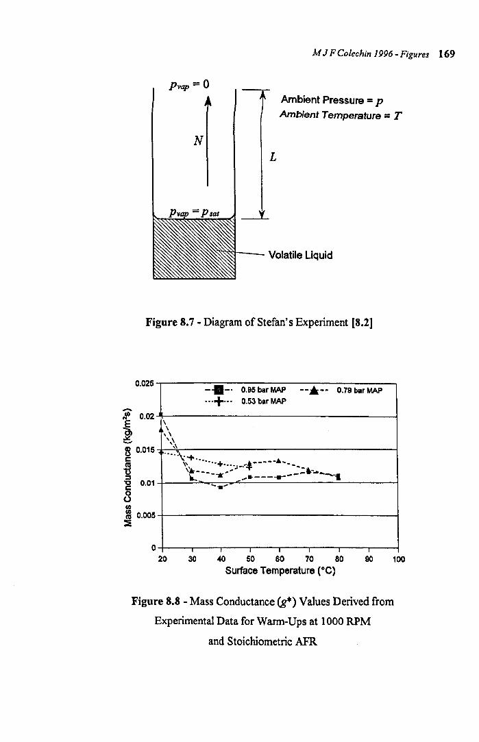
pvap = 0
N L
M J F CoJechin J 996 - Figures 169
Ambient Pressure = p Ambient Temperature = T
Volatile Liquid
Figure 8.7 - Diagram of Stefan's Experiment [8.2]
0.025
-/P 0.02
i -8 0.015 c::
~ '2 0.01 o o II)
~ 0.005 ::i
o
-.-. 0.95 bar MAP --*-- 0.79 bar MAP ... + ... 0.53 bar MAP
\ \ ,\ '\ ',\ .... \. .....
\' .... + ~-----."
20
\'Ic- ___ ~.~: . .:.... "";;. ___ -. ~ ,.---~-
30
-.. '
, , , , I
40 50 60 70 80 Surface Temperature (OC)
90 100
Figure 8.8 - Mass Conductance (g*) Values Derived from
Experimental Data for Warm-Ups at 1000 RPM
and Stoichiometric AFR
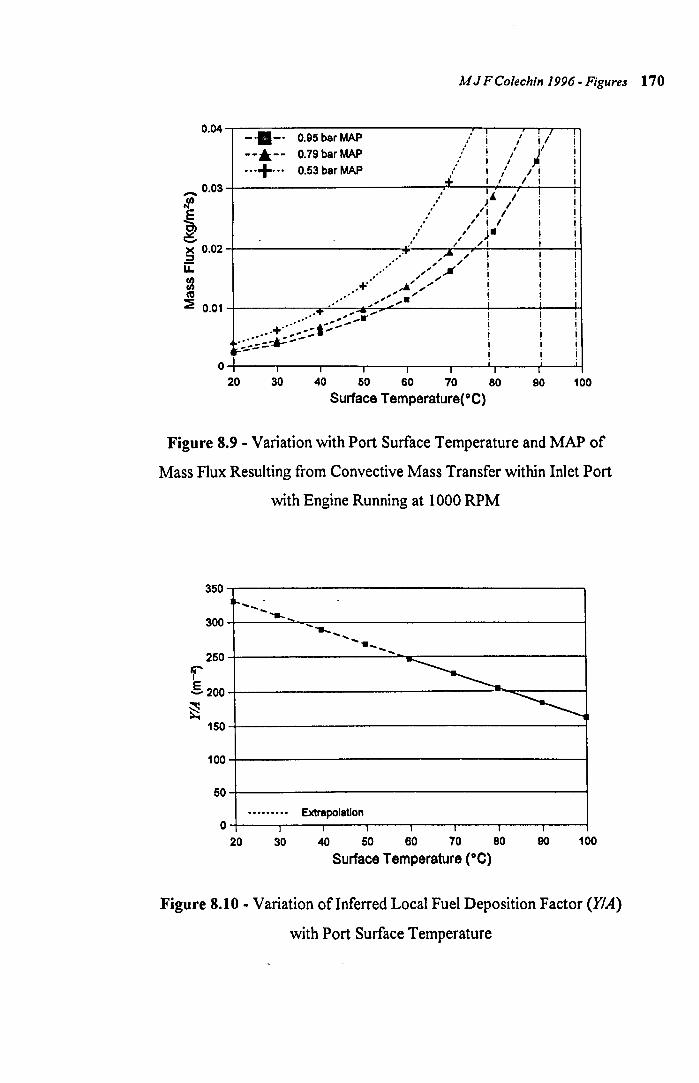
0.04
_ 0.03
If E ) -)( 0.02 :::J u:: :2 «J
::! 0.01
-.-. 0.95 bar MAP
--*-- 0.79 bar MAP ... + ... 0.53 bar MAP
.+. . .. '
M J FColechin 1996 - Figures 170
i I it' i I . i I l i i I i I i I I I i .i. I I I I i i . I~ I
I ! . ) I I I . 'I I i ! . , . i . . , I I I ,
j.. . , I I , i i I "
,oA " I ! , " i " ... i , .;
,.&' .; I , .;.; i ",,,, ...... i i i I ........ ,. ,':-' .............. i .+ .. , ,'t' ...... i ....... :t:-=:..":.- ....
';';:'.::~'
o 20 30
I I I I
40 50 60 70 80
Surface Temperature(OC)
i ! I
I
90 100
Figure 8.9 - Variation with Port Surface Temperature and MAP of
Mass Flux Resulting from Convective Mass Transfer within Inlet Port
with Engine Running at 1000 RPM
350
300
250
r .§. 200 ;S ~
150
100
50
o
.......... ...........
......... I
20 30
........ ...... ...... -.... ...
~
extrapolation I I I I I
40 50 60 70 80 Surface Temperature (OC)
~
I
90 100
Figure 8.10 - Variation ofInferred Local Fuel Deposition Factor (YIA)
with Port Surface Temperature
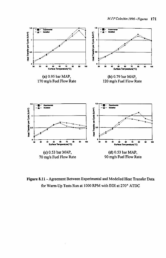
1.1 _._ ~
- -. _. MocIoIIod
~ ~ ~ M ~ ~ ~ ~ ~
Surface Temperatln(°C)
(a) 0.95 bar MAP, 170 mg/s Fuel Flow Rate
1.1 _._ ~
- -. _. MocIoIIod
o+-~--.--,--.--.--,,--.-~ ~ ~ ~ M ~ ~ M ~ ~
Surface Temperatl.n(·C)
(c) 0.53 bar MAP, 70 mg/s Fuel Flow Rate
M J F Colechin 1996 - Figure! 171
~ M ~ M ~ ~ M ~ ~
SII'faaI Temperatln(·C)
(b) 0.79 bar MAP, 120 mg/s Fuel Flow Rate
1.1 _. ____
- - • _. MocIoIIod
O+--.--~-,--.-~~,,--~~ ~ ~ ~ M M ~ M ~ ~
Surface Temperatl.n(·C)
(d) 0.53 bar MAP, 90 mg/s Fuel Flow Rate
Figure 8.11 - Agreement Between Experimental and Modelled Heat Transfer Data
for Warm-Up Tests Run at 1000 RPM with EOI at 270 0 ATDe
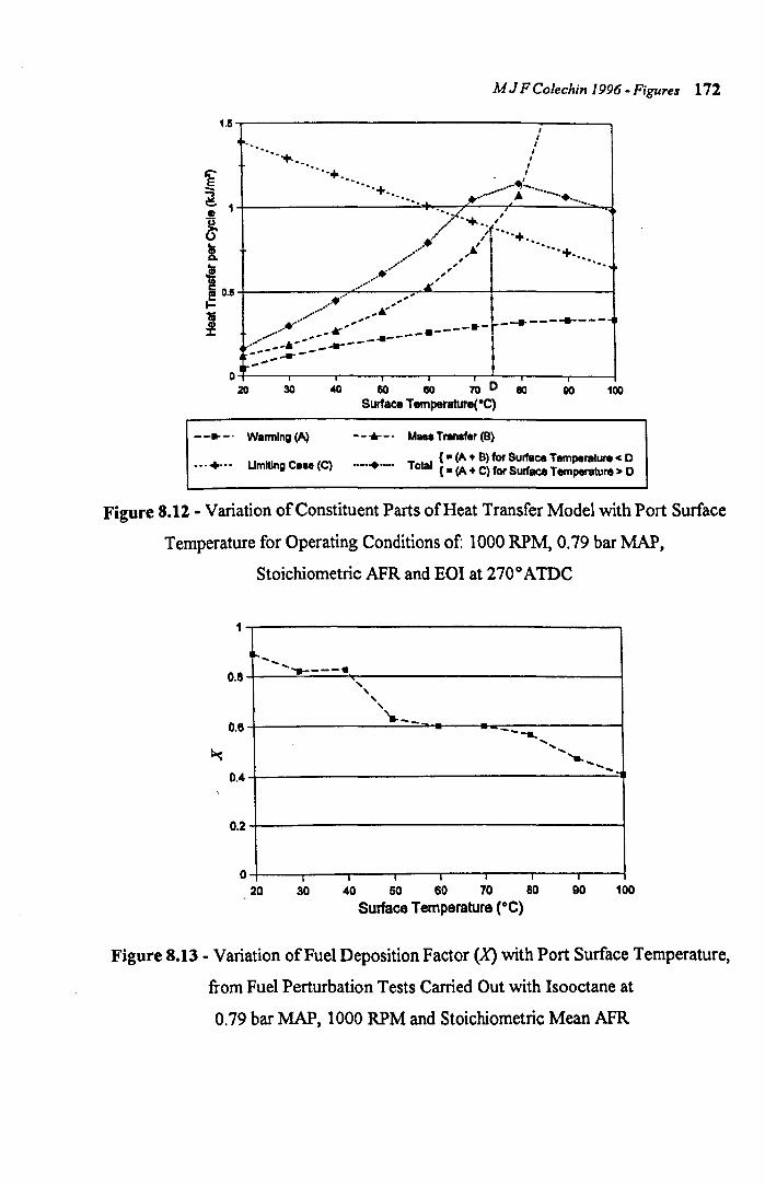
M J F Colechin 1996 - Figures 172
1.5-r---------------~--__.. I I
". I
•••• -+. " r:L" ••••••• + " E ••••••• + . ,.~~.~ ~ ....... .,..--~ . ~ ... -... ~ .... . I. / .... '-+. •• (' U . ,', •••• + .. II ....• ~ .••.. is. ......" + .... ~ ... / ", ". c ...... .~' I! 0.5 +-------..-'~ ... --.....,.......----+------~ I- ...•... "" I "I ...... '. "j{'
:I: .~...... ~", ----·-r'-------..... ---....... ..-- .. -----...... ....-- .,.-------=~-----
O+---.--r--,--~--r-~~-~-~ ~ ~ ~ ~ ~ ~D ~ 100
.. , +-.. Umltlng Ca .. (C)
Surface Temperature(°C)
- - .. -. Mass T...,.fer (8)
{ • (A + B) for Surface Temperature c 0 - .. - Total {. (A + C) for Surface Temperature :. 0
Figure 8.12 - Variation of Constituent Parts of Heat Transfer Model with Port Surface
Temperature for Operating Conditions of: 1000 RPM, 0.79 bar MAP,
Stoichiometric AFR and EOI at 270 0 AIDe
1
1'- .. ..... .... ---. , 0.8 , , , '---- --..... 0.6 ... ...... ........ ..... ,
0.4
0.2
o 1 -I -. 20 30 40 50 60 70 80 90 100
Surface Temperature (Oe)
Figure 8.13 - Variation of Fuel Deposition Factor (X) with Port Surface Temperature,
from Fuel Perturbation Tests Carried Out with Isooctane at
0.79 bar MAP, 1000 RPM and Stoichiometric Mean AFR
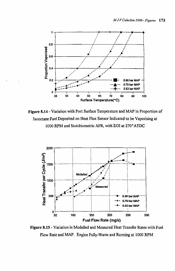
M J F Colechin 1996 - Figures 173
~ o ·c
1
0.8
8. 0.6
~ c ~ 0.4 o Q. e D.
,+
,,,,' , ,'"
,"
:
,
, , I
~ , ~
~ ~ ,
'" ..
,r ,-I
, I ,
I , , , , I , , ,
~ , I • ,
/ , , / ,
/ / ./
'" '" '" ,.- ....... .-".1{' .,. .. "
0,95 bar MAP -0.2
... -A'" _ .. ..,..,." --lr-- 0.79 bar MAP f-::..:----- ... + ... 0.53 bar MAP
o I I I I I I
20 30 40 50 60 70 80 90 100 Surface Temperature(OC)
Figure 8.14 - Variation with Port Surface Temperature and MAP in Proportion of
Isooctane Fuel Deposited on Heat Flux Sensor Indicated to be Vaporising at
1000 RPM and Stoichiometric AFR, with EO! at 270 0 ATDC
2000 .,..------;,------;,------;,-----r, -----, I I I I
Ii:' \ ; \ L.l; t: I I I I
?5 ::: -----: "a;' 1500· ······· .. ·············· .. ·f····· .. ··········· ........ ·l·· .. ·· ...... ····7[~·· ........ ············~::-··.,.··· .. ···· ...... ·· 13 :: / I' : ~ : : / I: : U : Modelled , l': : 8. ' '/ I , ,
: : /: : 1000· ......................... ~.............. . ........ -: ..... ,. ................. -: .......................... ~ ......................... . ... 'I ~ I I
Je : /If : : en ,/' Measured: : c: I / I •
t'I'I _.-1--- J( , , ~ • //: I ~ I- 500· ... > ................ ~¥"L ................... ~ .......................... ~ ...... ___ 0.95 bar MAP ....... .
I · \ l ' -.- 0.79 bar MAP
--- 0.53 bar MAP
o!-, ---~---~----+-----:----~ 50 100 150 200 250 300
Fuel Flow Rate (mgls)
Figure 8.15 - Variation in Modelled and Measured Heat Transfer Rates with Fuel
Flow Rate and MAP. Engine Fully-Warm and Running at 1000 RPM
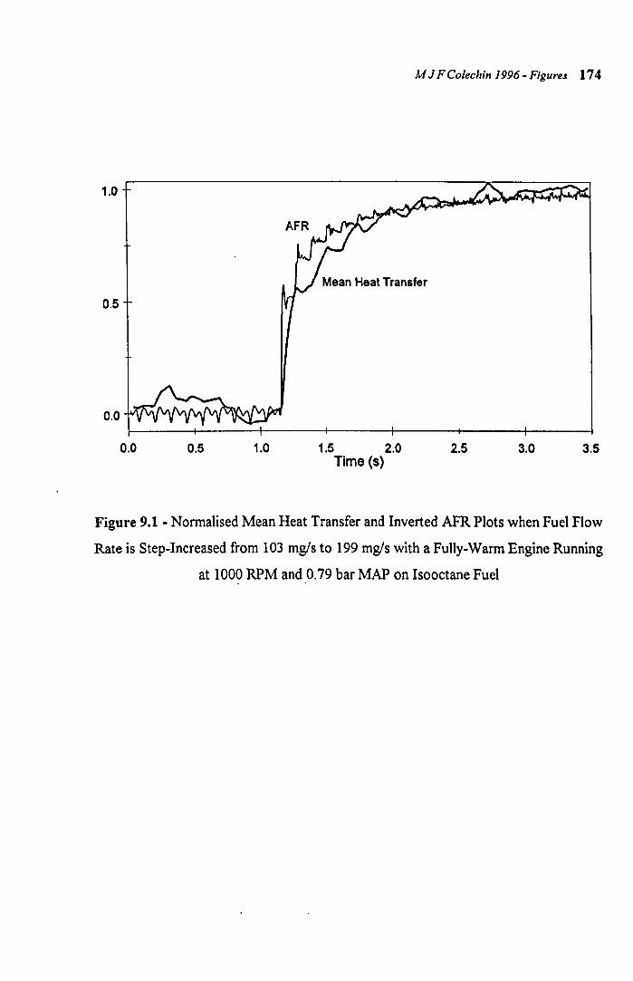
M J F Colechin J 996 - Figures 174
1.0
Mean Heat Transfer
0.5
0.0
0.0 0.5 1.0 1.5 2.0 2.5 3.0 3.5 Time (s)
Figure 9.1 - Normalised Mean Heat Transfer and Inverted AFR Plots when Fuel Flow
Rate is Step-Increased from 103 mgls to 199 mgls with a Fully-Warm Engine Running
at 1000 RPM and 0.79 bar MAP on Isooctane Fuel . .
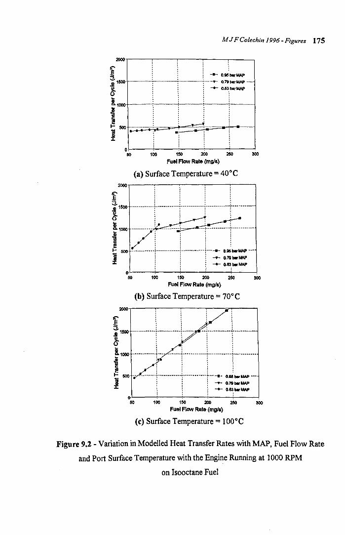
M J FColechin 1996 - Figures 175
~r-----~----~----~----~--~
f . j . ___ 0"'''. "aft ::s ::: . ..., ... r....,.-:; 1500- ................ --.... -+ .................. -... -+--...................... : ...... ~ 0.79 bar MAP ...... .
~ i i \ -- O.53;barMAP U .., I
8. 1000 ........... ----........ + ....... --......... --.--t-... ------------.... -.. --\-........................ \ ........................ . .! ... . Ii! ... . I! ~ ~ ~ ~ i 500 ; .. ;· ......... i ... ;~ .. ~ ...... · ~ •. -........... .
I: :::~
O. 50
. . 100 150 200 250
Fuel Flow Rate (mg/a)
(a) Surface Temperature = 40 0 e
300
2ooo~----~----~----~----~--~
if ?; :!:: --: 1500 --- -- ---- -- -~- -- --- --- ---i ------------i ------------+ -----------Q ;::
~1ooo ----------- --------~-------e ,:: 'lZ ::: c .:: I! : ~ : I- 500 - ------------;------------~------------~--- --- 0.815 _ MAP ---
i ::: -+- o.n_MAP
:f i i l -- 0.53: bar MAP OL.----~----~. ----~. ----~----~ 50 100 150 200 250 300
Fuel Flow Rate (mg/6)
(b) Surface Temperature = 70 0 e
f - .. ., ., i 1SOO ------------t-----------1------
ls l \ \ \ 8. 1000 -.............. ----t- .... - -.. --..... -t----.. --- .. ---~---- .... -.... --.. "'l .... --...... - ...... -t : l j \ .. ::; ~ : 1 : : I- 500 -- ---------r-----------1'--------·--r-- --- 0.85 bar MAP ---J ::: -+- 0.79_"",
1 ~ ! -- 0.53_"", O-L.----~----~----~----~----~ 50 100 150 200 250 300
Fuel Flow Rate (mg/6)
(C) Surface Temperature = 1000e
Figure 9.2 - Variation in Modelled Heat Transfer Rates with MAP, Fuel Flow Rate
and Port Surface Temperature with the Engine Running at 1000 RPM
on Isooctane Fuel