i n t e r n a t i o n a l j o u r n a l o f h y d r o g e n e n e r g y 3 4 ( 2 0 0 9 ) 9 2 4 8 – 9 2 5 7

Avai lab le at www.sc iencedi rect .com

journa l homepage : www.e lsev ie r . com/ loca te /he

Incorporating in-cylinder pressure data to predict NOx

emissions from spark-ignition engines fueled with landfillgas/hydrogen mixtures

Kurt Kornbluth, Zach McCaffrey, Paul A. Erickson*

Department of Mechanical and Aerospace Engineering, University of California, One Shields Avenue, Davis, CA 95616, USA

a r t i c l e i n f o

Article history:

Received 3 August 2009

Received in revised form

9 September 2009

Accepted 9 September 2009

Available online 8 October 2009

Keywords:

Hydrogen

Engine modeling

NOx

Spark-ignition

Landfill gas

Natural gas

* Corresponding author. Tel.: þ530 752 5360;E-mail addresses: kkorn@ucdavis.edu

(P.A. Erickson).0360-3199/$ – see front matter ª 2009 Profesdoi:10.1016/j.ijhydene.2009.09.020

a b s t r a c t

A 0.745 L 2-cylinder spark-ignition engine was operated with compressed natural gas and

with simulated landfill gas (60% CH4 and 40% CO2 by volume) containing hydrogen

concentrations of 0, 30%, 40%, and 50% (by volume of the CH4 in the fuel) at constant rpm.

This empirical data was compared with predictions from three existing semi-empirical

engine models, using a first-law-based finite heat release model to correlate measured in-

cylinder pressure data and burn rate for each fuel mixture. Of the three models only a two

zone model incorporating thermal and prompt NOx came within 25% of predicting the

measured NOx emissions.

ª 2009 Professor T. Nejat Veziroglu. Published by Elsevier Ltd. All rights reserved.

1. Main section combustion characteristics which can enhance flame stabili-

1.1. Introduction

Landfill gas (LFG) is a product of the decomposition of munic-

ipal waste, and is composed of approximately sixty-percent

methane and forty-percent CO2. Landfill operators capture and

burn this gas in internal-combustion reciprocating engine-

based generators, but tightening NOx emission are major

barriers to new Landfill Gas-to-Energy (LFGTE) projects [1].

Hydrogen-enrichment of compressed natural gas (HCNG)

is a technology currently being used to lower engine-out NOx

in internal combustion (IC) engines and has been proposed for

landfill gas-fueled engines [2,3]. Hydrogen has favorable

fax: þ530 752 4158.(K. Kornbluth), zmc

sor T. Nejat Veziroglu. Pu

zation when mixed with other fuels in small percentages.

Thus, in natural gas engines, hydrogen-enrichment allows the

use of lean-burn or high charge-dilution strategies to cool

combustion, drastically reducing engine-out NOx levels [4]. In

a strategy analogous to HCNG, hydrogen-enrichment of

landfill gas (HLFG) allows high air/fuel ratios previously

unattainable in landfill gas engines without misfire, allowing

for significant reductions in engine-out NOx while retaining

low CO, and HC emissions [5].

The ability to predict the effect of these ultra-lean mixtures

on NOx emissions is critical for engine designers. NOx emis-

sions in SI engines are largely a thermal phenomena thus

cylinder pressure and temperature are keys to making

caffrey@ucdavis.edu (Z. McCaffrey), paerickson@ucdavis.edu

blished by Elsevier Ltd. All rights reserved.

Nomenclature

ATDC after top dead center

BACT best available control technology

BTDC before top dead center

CH4 methane

CO carbon monoxide

CO2 carbon dioxide

CNG compressed natural gas

EGR exhaust gas recirculation

ER equivalence ratio

H2 hydrogen

HCNG hydrogen-enriched compressed natural gas

HLFG hydrogen-enriched landfill gas

LFG landfill gas

LFGTE landfill gas-to-energy

LOL lean operating limit

MBT maximum brake torque

NG natural gas

NOx nitrogen oxides

ppm parts per million

RT reference timing

SCR selective catalytic reduction

SMR steam methane reforming

SNCR selective non-catalytic reduction

VOC volatile organic compounds

WOT wide open throttle

Xb mass fraction burned

i n t e r n a t i o n a l j o u r n a l o f h y d r o g e n e n e r g y 3 4 ( 2 0 0 9 ) 9 2 4 8 – 9 2 5 7 9249

accurate predictions. If cylinder pressure data is available the

heat release during combustion can be modeled, and thus

NOx, can be more accurately simulated [6].

Current semi-empirical engine models incorporate some

form of heat release model but do not account for equivalence

ratios ranging from near stoichiometric to near the lean

operating limit [7]. For hydrogen-enriched systems this is

critical because as the mixture is leaned, combustion duration

is increased and ignition begins at an earlier crank angle (due

to advanced spark timing). Thus for each fuel mixture a cor-

responding heat release model must be created to reflect

these altered fuel burn rates. This study, by combining recent

experimental data and mixture-specific heat release models

(using associated in-cylinder pressure measurements) yields

more accurate NOx emission predictions for hydrogen-

enriched landfill gas engines.

Table 1 – Inputs for CHEMWORK_6.

Input Typical values

Polytropic compression coefficient 1.35–1.40

Polytropic expansion coefficient 1.27

Displacement 0.745 L

Engine rpm 2600

Maximum cylinder pressure 18–29 atm

Species (mole fraction) CH4, H2, N2, O2, CO2

Inlet Pressure 0.95 atm

Exhaust pressure 1.05 atm

Inlet Temperature 300–320 �C

L/a ratio 3.25

Compression ratio 9.0:1

Cycle type Mixed

Fraction burned

at constant volume

0.10–0.20

2. Theory

2.1. Background

2.1.1. Hydrogen enrichmentFor this study hydrogen content is expressed as a volume

fraction of the fuel (not including the volume of CO2 for LFG

mixtures). Thus, with enrichment of nH2 moles of hydrogen

the combustion equation becomes:

CH4 þ nCO2CO2 þ nH2

H2 þ�2þ 0:5nH2

�ðO2 þ 3:77N2Þ

/�Iþ nCO2

�CO2 þ

�2þ nH2

�H2Oþ

�2þ 0:5nH2

�ð3:77N2Þ ð1Þ

where hydrogen enrichment ðby volumeÞ ¼ ½nH2=ðnCH4

þnH2Þ �100%� .

2.1.2. Ignition timingProper spark timing places the combustion event for optimum

work transfer from the gases to the piston which is the location

for maximum power. If the combustion event is too early the

pressure works against the piston, if the combustion event is

too late the pressure is not effectively transferred. Based on

empirical data, Heywood has related the optimum timing

setting (MBT) to the cylinder pressure and burn rate of fuel [8].

Heywood suggests that since there is considerable uncertainty

in NOx emissions at MBT timing, NOx measurements are best

taken at reference timing [8]. Reference timing (RT) is deter-

mined by reducing MBT advance timing until there is a small

decrease in torque, usually a reduction of 2–3 degrees of

timing, representing less than 5% reduction in brake torque.

Thus all the baseline lean-limit and emissions measurements

were taken under reference timing.

2.1.3. Brake specific NOx emissionsNOx emissions are typically measured as a volume concen-

tration but are often expressed as a mass in relation to the

mechanical energy output. Thus, brake specific NOx emissions

(BSNOx) are defined as the mass of NOx emissions divided by

the engine output and are expressed in units of g/kWh. While

NO and NO2 are grouped together, NO is the main oxide of

nitrogen produced inside an IC engine, with NO2 on the order

of 1% to 2% of total NOx [9]. The measurements given in this

study include both NO and NO2 and are reported as equivalent

NO2 per standard emission reporting procedures.

2.2. Modeling

Three different computer simulation models designed to

predict NOx production from IC engines were compared in the

present study. Model I is ‘‘CHEM_WORK6’’ which simulates

i n t e r n a t i o n a l j o u r n a l o f h y d r o g e n e n e r g y 3 4 ( 2 0 0 9 ) 9 2 4 8 – 9 2 5 79250

gas processes under the assumption of chemical equilibrium.

Model II is a mechanistic 4-part semi-empirical model repor-

ted by Dwyer in 2004 [10] which incorporates a detailed flame

structure and Gas Research Institute (GRI) chemical kinetics.

Model III is ‘‘WAVE’’, which incorporates a limited chemical

mechanism incorporating Fenimore and Zeldovich NOx

kinetics. A first-law-based finite heat release model was

developed and incorporated to predict the fraction of mass

burned vs. crank angle for Model II and Model III.

2.2.1. CHEM_WORK6- model description (Model I)CHEM_WORK6 [11] makes direct use of the equilibrium program

STANJAN [12], and an ideal internal combustion engine cycle

analysis which can predict species, cylinder pressure and

temperature, and finite-rate NOx emissions. In addition to fuel

type and equivalence ratio, CHEM_WORK6 variable user inputs

include the percentages of the P¼ const, and V¼ const process

that are assumed during mixed-cycle combustion, as well as

independent polytropic coefficients, g, for the PVg¼ const

compression and expansion processes, as well as inlet and

outlet pressures and temperatures [5]. Table 1 summarizes the

inputs for CHEMWORK_6 used in this study.

CHEMWORK_6 uses finite-rate NOx production based on the

extended Zeldovich mechanism and uses finite rates for N and

NO, and equilibrium values for H, OH, O, O2, N2, and other

species. Although CHEMWORK_6 can predict trends in NOx

production with respect to fuel type, diluent concentration, and

equivalence ratio, there are two major drawbacks in estimating

NOx production: 1) The mixed cycle assumption does not

capture the true pressure-volume relationship near maximum

pressure, and 2) the model does not allow for the further

compression of gases due to temperature rise after top dead

center (TDC). This compression effect is known to significantly

increase thermal NO production [11].

2.2.2. Semi-empirical model description (Model II)Model II is a software program previously developed at UC

Davis based on the methane GRI mechanism [10]. This model

uses 2-zones separating the burned gases from the unburned

gases. A flame structure model is used to predict NOx forma-

tion during the engine cycle with the use of GRI chemical

reaction mechanism, and a chemical model predicts the

influence of compression and expansion on the evolution of

the burned gas parcels in the engine [10].

Model II incorporates measured in-cylinder pressure data

with a time-dependent flame model and a post-combustion

equilibrium bomb model. Assuming the unburned gas is

initially uniform and undergoes isentropic compression with

constant specific heat, theunburned gas temperatureprofile,Tu,

is determined from the pressure curve using the isentropic ideal

gas relation [8].

Tu

To¼�

ppo

�ðgu�1Þ=gu

(2)

where To and po are standard reference values, p is the

instantaneous pressure, and gu is the specific heat ratio for the

unburned mixture.

The flame model predicts the burning of the fuel mixture at

a given crank angle in the engine. This code solves the equa-

tions of continuity, energy, and species transport that are

appropriate for the GRI 3.0 reaction mechanism [12] for 53

species. Using the unmixed model assumption, the cylinder

charge is separated into homogenous control volumes of

‘‘packets or parcels’’, each corresponding to 5 degrees of crank

angle, from approximately�30 toþ50 degrees relative to TDC.

In order to model the influences of compression of the

unburned mixture in the engine, each flame packet is given

the instantaneous pressure and temperature of the unburned

mixture as a function of crank angle.

The post-combustion equilibrium bomb model takes the

flame products that have been created during the combustion

process, and expands and compresses them based on the

variation of cylinder pressure. In this model it is assumed that

there is no mixing between the burned and unburned cylinder

charges. Chemical equilibrium data from the STANJAN model

[12] are supplemented by finite-rate kinetics from the CHEM-

KIN II model [13] to predict NOx emissions.

2.2.3. WAVE (Model III) descriptionThe internal combustion engine combustion simulation soft-

ware, Ricardo� WAVE, was used in conjunction with a finite

heat release model to predict NOx emissions. WAVE includes

engine-specific inputs such as geometry and displacement as

well as the specific operating conditions including inlet pres-

sures, temperatures, fuel type, and equivalence ratio.

WAVE predicts NOx production during combustion and

exhaust for a series of control volumes, each originating at

a discrete crank angle with the starting at ignition and ending

after the fuel is fully burned. The relationship of pressure and

temperature to crank angle are predicted according to

a method analogous to that described in Model II. WAVE

separates the combustion chamber into two zones: burned

and unburned gases. At any instant during the combustion

process, there is mass flux into the burned zone associated

with the instantaneous fuel burning rate and the stoichiom-

etry of the incremental burned mass of intake charge. In each

zone, the mixture is assumed to be fully mixed and

homogenous.

The NOx model in WAVE assigns an initial NOx concen-

tration to each packet representing the prompt and residual

NOx formed during initial combustion, prior to thermal NOx

formation. After combustion, the packets which burn early in

the cycle are compressed for a longer period, thus attaining

a higher temperature and contributing more NOx than those

which burn later. The WAVE NOx model accounts for the

‘‘prompt’’ or ‘‘flame-formed’’ NO, due to the over-equilibrium

of oxygen atoms and hydroxyl radicals in the flame region.

The value of the prompt NO is obtained from correlation of the

data reported by Fenimore [14], which gives the ratio of

prompt NO to equilibrium NO as a function of equivalence

ratio.

In the burned zone, further NOx formation takes place

depending on the equivalence ratio of the burned packet, as

well as the temperature and pressure at a given crank angle.

Thermodynamic equilibrium values are used for the species

O2, O, H, and OH, and the steady-state assumption is used for

highly reactive N atoms. The concentration of NO vs. time is

solved using an open system in which the above elementary

reactions are used with those rate constants reported by

Heywood [8]. The calculation is terminated when the

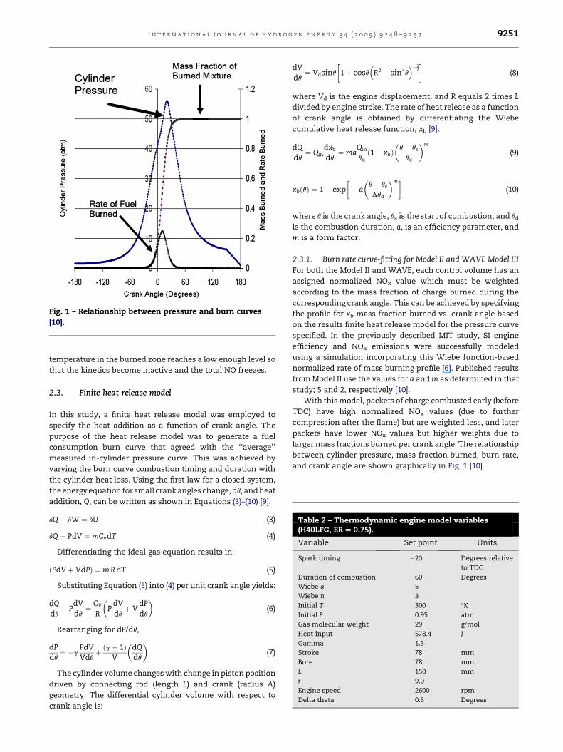
Fig. 1 – Relationship between pressure and burn curves

[10].

Table 2 – Thermodynamic engine model variables(H40LFG, ER [ 0.75).

Variable Set point Units

i n t e r n a t i o n a l j o u r n a l o f h y d r o g e n e n e r g y 3 4 ( 2 0 0 9 ) 9 2 4 8 – 9 2 5 7 9251

temperature in the burned zone reaches a low enough level so

that the kinetics become inactive and the total NO freezes.

2.3. Finite heat release model

In this study, a finite heat release model was employed to

specify the heat addition as a function of crank angle. The

purpose of the heat release model was to generate a fuel

consumption burn curve that agreed with the ‘‘average’’

measured in-cylinder pressure curve. This was achieved by

varying the burn curve combustion timing and duration with

the cylinder heat loss. Using the first law for a closed system,

the energy equation for small crank angles change, dq, and heat

addition, Q, can be written as shown in Equations (3)–(10) [9].

dQ � dW ¼ dU (3)

dQ � PdV ¼ mCvdT (4)

Spark timing �20 Degrees relative

to TDC

Duration of combustion 60 Degrees

Wiebe a 5

Wiebe n 3

Initial T 300 �K

Initial P 0.95 atm

Gas molecular weight 29 g/mol

Heat input 578.4 J

Gamma 1.3

Stroke 78 mm

Bore 78 mm

L 150 mm

r 9.0

Engine speed 2600 rpm

Delta theta 0.5 Degrees

Differentiating the ideal gas equation results in:

ðPdV þ VdPÞ ¼ m R dT (5)

Substituting Equation (5) into (4) per unit crank angle yields:

dQdq� P

dVdq¼ CV

R

�P

dVdqþ V

dPdq

�(6)

Rearranging for dP/dq,

dPdq¼ �g

PdVVdq

þ ðg� 1ÞV

�dQdq

�(7)

The cylinder volume changes with change in piston position

driven by connecting rod (length L) and crank (radius A)

geometry. The differential cylinder volume with respect to

crank angle is:

dVdq¼ Vdsinq

�1þ cosq

�R2 � sin2

q��1

2

(8)

where Vd is the engine displacement, and R equals 2 times L

divided by engine stroke. The rate of heat release as a function

of crank angle is obtained by differentiating the Wiebe

cumulative heat release function, xb [9].

dQdq¼ Qin

dxb

dq¼ ma

Qin

qdð1� xbÞ

�q� qs

qd

�m

(9)

xbðqÞ ¼ 1� exp

�� a

�q� qs

Dqd

�m(10)

where q is the crank angle, qs is the start of combustion, and qd

is the combustion duration, a, is an efficiency parameter, and

m is a form factor.

2.3.1. Burn rate curve-fitting for Model II and WAVE Model IIIFor both the Model II and WAVE, each control volume has an

assigned normalized NOx value which must be weighted

according to the mass fraction of charge burned during the

corresponding crank angle. This can be achieved by specifying

the profile for xb mass fraction burned vs. crank angle based

on the results finite heat release model for the pressure curve

specified. In the previously described MIT study, SI engine

efficiency and NOx emissions were successfully modeled

using a simulation incorporating this Wiebe function-based

normalized rate of mass burning profile [6]. Published results

from Model II use the values for a and m as determined in that

study; 5 and 2, respectively [10].

With this model, packets of charge combusted early (before

TDC) have high normalized NOx values (due to further

compression after the flame) but are weighted less, and later

packets have lower NOx values but higher weights due to

larger mass fractions burned per crank angle. The relationship

between cylinder pressure, mass fraction burned, burn rate,

and crank angle are shown graphically in Fig. 1 [10].

Fig. 2 – Engine test set up [5].

i n t e r n a t i o n a l j o u r n a l o f h y d r o g e n e n e r g y 3 4 ( 2 0 0 9 ) 9 2 4 8 – 9 2 5 79252

2.3.2. Implementation of finite heat release modelA discrete numerical approximation for (6) and (9) was devel-

oped using spreadsheet software to generate the relationship

between crank angle, in-cylinder pressure, and mass fraction of

burned mixture (xb) and rate of fuel burned (x0b). This allows

proper fitting of the burn curve with the pressure data for each

run. From the pressure curve other characteristics such as

temperature, torque, work-per-cycle, thermal efficiency, and

volumetric efficiency can then be calculated.

The required inputs are shown in Table 2. Spark timing,

duration of combustion, Wiebe a, and Wiebe n describe the burn

curve, xb. The burn curve plays a critical role in determining the

cylinder pressurecurve, and therefore overall power, emissions,

and efficiency of the engine. To achieve maximum torque, a good

rule of thumb is to position the burn curve with 50% fuel burnt at

about 15 degrees after TDC (the normal location of peak pres-

sure). In contrast, reference timing refers to retarding maximum

torque timing by a 2–3 degrees and this was incorporated in the

model. Ignition delay was not modeled specifically.

Input parameters initial T and initial P are the assumed

intake temperature and pressure within the combustion

cylinder in this example 30 �C, 0.95 atm respectively. Gas

molecular weight is the molecular weight of the mixture of fuel

and air within the cylinder. Heat input represents the amount

of heat in joules added by combustion. This variable allows for

modeling of the thermodynamic processes within the cylinder

to be calculated independent of fuel type. External to the

model, lower heating values, fuel mass, charge burn

percentage of specific fuels can be calculated. For an isen-

tropic process Gamma is the ratio of specific heats. For non-

isentropic processes Gamma is the polytropic coefficient.

Stroke, bore, and L are geometric parameters of the engine

cylinder. The compression ratio, r, is the ratio of the volume in

the cylinder when the piston allows maximum cylinder

volume at bottom dead center (BDC) to minimum cylinder

volume at top dead center (TDC). Engine speed is the rate of

rotation, in revolutions per minute.

2.3.3. Heat transferEquation (9) does not include heat transfer to the cylinder

walls. Without accounting for this heat transfer, cylinder

pressure (and thus IMEP) will be over-predicted by 10–15% [9].

The heat loss to the cylinder walls is a function of exposed

area, heat transfer rate coefficient, and the temperature

differences between the hot gases and cylinder walls. At

constant rpm, however, this is primarily a function of the

temperature difference. An additional term, Qw/dq, can be

included for heat loss to the cylinder walls. Thus the finite

heat release model can be modified to include heat transfer to

the cylinder walls as shown in Equation (11).

dPdq¼ g� 1

V

�Qin

dxb

dq� dQw

dq

�� g

PV

dVdq

(11)

The heat transfer is determined by applying Newtonian

convection as shown in equations (12)–(14). This development

follows that shown in reference [9].

dQw

dq¼

hgðqÞAwðqÞ�TgðqÞ � Tw

�N

(12)

where Tw is area-weighted average temperature over the

exposed cylinder wall, head and piston crown. Aw is the

exposed cylinder area.

AwðqÞ ¼ Awall þAhead þApiston ¼ pbyðqÞ þ p

2b2 (13)

y(q) is the exposed cylinder wall height.

yðqÞ ¼ aþ l�h�

l2 � a2sin2q�1=2

þacosqi

(14)

‘a’ is the crank radius. ‘l’ is the connecting rod length and

‘‘hg(q)’’ is the cylinder instantaneous average heat transfer

coefficient. For the present study Woschni’s heat transfer

correlation, Equation (15), which incorporates variable char-

acteristic gas velocities, was used [9], (16):

hg ¼ 3:26P0:8U0:8b�0:2T�0:55 (15)

Where hg has units of W/m2K, P is in kPa, U is in m/s, b in

meters, T in Kelvin.

The average cylinder gas velocity, U, can be expressed as

shown in Equation (16).

U ¼ 2:28Up þ 0:00324ToVd

Vo

DPc

Po(16)

where,

Up¼mean piston speed (m/s)

To¼ temperature at intake valve closing (K)

Vo¼ cylinder volume at intake valve closing (m3)

Vd¼ displacement volume (m3)

DPc¼ instantaneous pressure rise due to combustion (kPa)

Po¼ pressure at intake valve closing (kPa)

2.3.4. The effect of combustion burn durationCombustion duration is longer with leaner mixtures due to

lower flame speed so the start of combustion (from the initia-

tion of spark) varies depending on equivalence ratio and fuel.

The shift in the start of combustion, qs, however, is offset by the

need for increased timing advance to achieve MBT at lean

mixtures (and visa-versa for richermixtures). This is confirmed

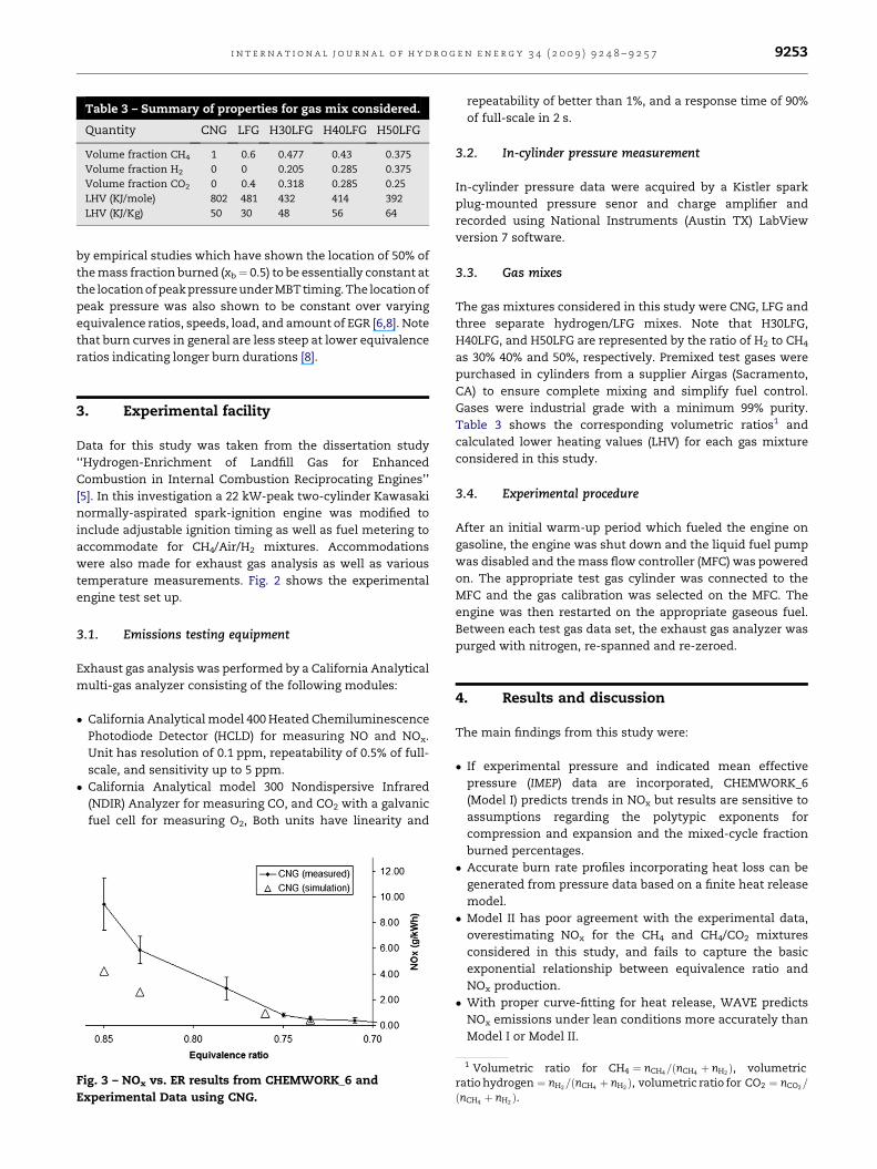
Table 3 – Summary of properties for gas mix considered.

Quantity CNG LFG H30LFG H40LFG H50LFG

Volume fraction CH4 1 0.6 0.477 0.43 0.375

Volume fraction H2 0 0 0.205 0.285 0.375

Volume fraction CO2 0 0.4 0.318 0.285 0.25

LHV (KJ/mole) 802 481 432 414 392

LHV (KJ/Kg) 50 30 48 56 64

i n t e r n a t i o n a l j o u r n a l o f h y d r o g e n e n e r g y 3 4 ( 2 0 0 9 ) 9 2 4 8 – 9 2 5 7 9253

by empirical studies which have shown the location of 50% of

the mass fraction burned (xb¼ 0.5) to be essentially constant at

the location of peak pressureunder MBT timing. The location of

peak pressure was also shown to be constant over varying

equivalence ratios, speeds, load, and amount of EGR [6,8]. Note

that burn curves in general are less steep at lower equivalence

ratios indicating longer burn durations [8].

3. Experimental facility

Data for this study was taken from the dissertation study

‘‘Hydrogen-Enrichment of Landfill Gas for Enhanced

Combustion in Internal Combustion Reciprocating Engines’’

[5]. In this investigation a 22 kW-peak two-cylinder Kawasaki

normally-aspirated spark-ignition engine was modified to

include adjustable ignition timing as well as fuel metering to

accommodate for CH4/Air/H2 mixtures. Accommodations

were also made for exhaust gas analysis as well as various

temperature measurements. Fig. 2 shows the experimental

engine test set up.

3.1. Emissions testing equipment

Exhaust gas analysis was performed by a California Analytical

multi-gas analyzer consisting of the following modules:

� California Analytical model 400 Heated Chemiluminescence

Photodiode Detector (HCLD) for measuring NO and NOx.

Unit has resolution of 0.1 ppm, repeatability of 0.5% of full-

scale, and sensitivity up to 5 ppm.

� California Analytical model 300 Nondispersive Infrared

(NDIR) Analyzer for measuring CO, and CO2 with a galvanic

fuel cell for measuring O2, Both units have linearity and

Fig. 3 – NOx vs. ER results from CHEMWORK_6 and

Experimental Data using CNG.

repeatability of better than 1%, and a response time of 90%

of full-scale in 2 s.

3.2. In-cylinder pressure measurement

In-cylinder pressure data were acquired by a Kistler spark

plug-mounted pressure senor and charge amplifier and

recorded using National Instruments (Austin TX) LabView

version 7 software.

3.3. Gas mixes

The gas mixtures considered in this study were CNG, LFG and

three separate hydrogen/LFG mixes. Note that H30LFG,

H40LFG, and H50LFG are represented by the ratio of H2 to CH4

as 30% 40% and 50%, respectively. Premixed test gases were

purchased in cylinders from a supplier Airgas (Sacramento,

CA) to ensure complete mixing and simplify fuel control.

Gases were industrial grade with a minimum 99% purity.

Table 3 shows the corresponding volumetric ratios1 and

calculated lower heating values (LHV) for each gas mixture

considered in this study.

3.4. Experimental procedure

After an initial warm-up period which fueled the engine on

gasoline, the engine was shut down and the liquid fuel pump

was disabled and the mass flow controller (MFC) was powered

on. The appropriate test gas cylinder was connected to the

MFC and the gas calibration was selected on the MFC. The

engine was then restarted on the appropriate gaseous fuel.

Between each test gas data set, the exhaust gas analyzer was

purged with nitrogen, re-spanned and re-zeroed.

4. Results and discussion

The main findings from this study were:

� If experimental pressure and indicated mean effective

pressure (IMEP) data are incorporated, CHEMWORK_6

(Model I) predicts trends in NOx but results are sensitive to

assumptions regarding the polytypic exponents for

compression and expansion and the mixed-cycle fraction

burned percentages.

� Accurate burn rate profiles incorporating heat loss can be

generated from pressure data based on a finite heat release

model.

� Model II has poor agreement with the experimental data,

overestimating NOx for the CH4 and CH4/CO2 mixtures

considered in this study, and fails to capture the basic

exponential relationship between equivalence ratio and

NOx production.

� With proper curve-fitting for heat release, WAVE predicts

NOx emissions under lean conditions more accurately than

Model I or Model II.

1 Volumetric ratio for CH4 ¼ nCH4=ðnCH4 þ nH2 Þ, volumetricratio hydrogen ¼ nH2=ðnCH4 þ nH2 Þ, volumetric ratio for CO2 ¼ nCO2=

ðnCH4 þ nH2 Þ.

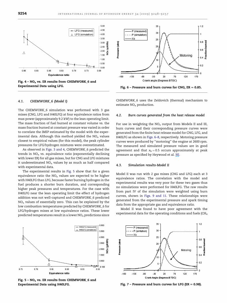
Fig. 6 – Pressure and burn curves for CNG, ER [ 0.85.

Fig. 4 – NOx vs. ER results from CHEMWORK_6 and

Experimental Data using LFG.

i n t e r n a t i o n a l j o u r n a l o f h y d r o g e n e n e r g y 3 4 ( 2 0 0 9 ) 9 2 4 8 – 9 2 5 79254

4.1. CHEMWORK_6 (Model I)

The CHEMWORK_6 simulation was performed with 3 gas

mixes (CNG, LFG and H40LFG) at four equivalence ratios from

max power (approximately 9.2 kW) to the lean operating limit.

The mass fraction of fuel burned at constant volume vs. the

mass fraction burned at constant pressure was varied in order

to correlate the IMEP estimated by the model with the exper-

imental data. Although this method yielded the NOx values

closest to empirical values (for this model), the peak cylinder

pressures for LFG/hydrogen mixtures were overestimated.

As observed in Figs. 3 and 4, CHEMWORK_6 predicted the

trends in NOx vs. equivalence ratio (exponentially declining

with lower ER) for all gas mixes, but for CNG and LFG mixtures

it underestimated NOx values by as much as half compared

with experimental data.

The experimental results in Fig. 5 show that for a given

equivalence ratio the NOx values are expected to be higher

with H40LFG than LFG, because faster burning hydrogen in the

fuel produces a shorter burn duration, and corresponding

higher peak pressures and temperatures. For the case with

H40LFG near the lean operating limit the effect of hydrogen

addition was not well-captured and CHEMWORK_6 predicted

NOx values of essentially zero. This can be explained by the

low combustion temperatures predicted by CHEMWORK_6 for

LFG/hydrogen mixes at low equivalence ratios. These lower

predicted temperatures result in a lower NOx predictions since

Fig. 5 – NOx vs. ER results from CHEMWORK_6 and

Experimental Data using H40LFG.

CHEMWORK_6 uses the Zeldovich (thermal) mechanism to

estimate NOx production.

4.2. Burn curves generated from the heat release model

For use in weighting the NOx output from Models II and III,

burn curves and their corresponding pressure curves were

generated from the finite heat release model for CNG, LFG, and

H40LFG as shown in Figs. 6–8, respectively. Motoring pressure

curves were produced by ‘‘motoring’’ the engine at 2600 rpm.

The measured and simulated pressure values are in good

agreement and that xb¼ 0.5 occurs approximately at peak

pressure as specified by Heywood et al. [6].

4.3. Simulation results-Model II

Model II was run with 2 gas mixes (CNG and LFG) each at 3

equivalence ratios. The correlation with the model and

experimental results was very poor for these two gases thus

no simulations were performed for H40LFG. The raw results

from part IV of the simulation were weighted using burn

curves, shown in Figs. 9 and 11. These relationships were

generated from the experimental pressure and spark timing

data from the appropriate gas and equivalence ratio.

Model II was found to have poor agreement with the

experimental data for the operating conditions and fuels (CH4

Fig. 7 – Pressure and burn curves for LFG (ER [ 0.98).

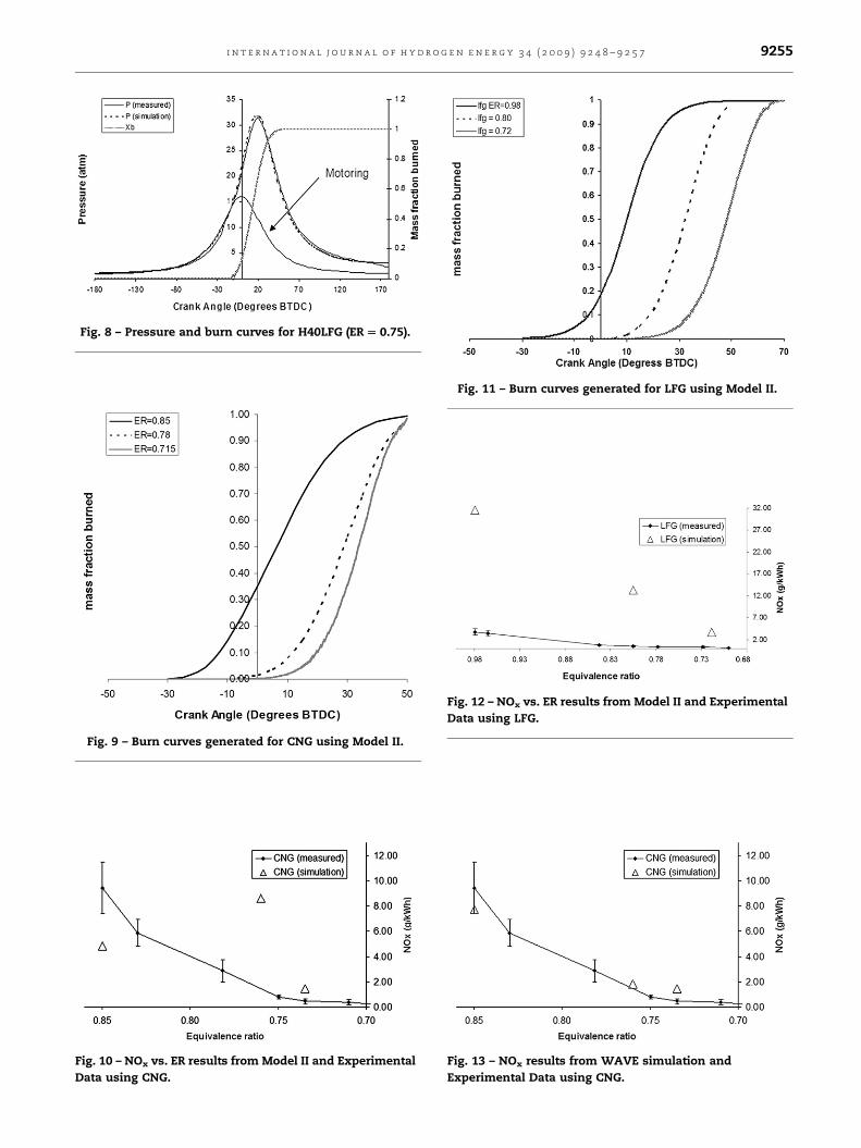
Fig. 8 – Pressure and burn curves for H40LFG (ER [ 0.75).

Fig. 9 – Burn curves generated for CNG using Model II.

Fig. 10 – NOx vs. ER results from Model II and Experimental

Data using CNG.

Fig. 11 – Burn curves generated for LFG using Model II.

Fig. 12 – NOx vs. ER results from Model II and Experimental

Data using LFG.

Fig. 13 – NOx results from WAVE simulation and

Experimental Data using CNG.

i n t e r n a t i o n a l j o u r n a l o f h y d r o g e n e n e r g y 3 4 ( 2 0 0 9 ) 9 2 4 8 – 9 2 5 7 9255

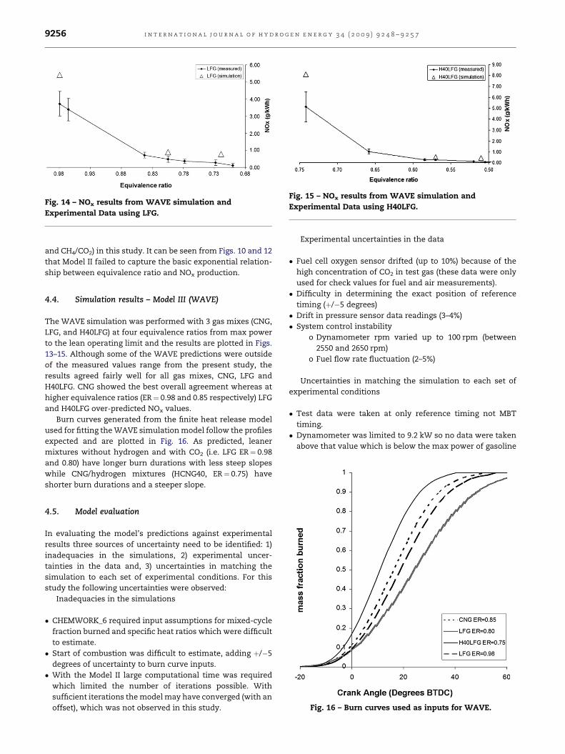
Fig. 14 – NOx results from WAVE simulation and

Experimental Data using LFG.

Fig. 15 – NOx results from WAVE simulation and

Experimental Data using H40LFG.

i n t e r n a t i o n a l j o u r n a l o f h y d r o g e n e n e r g y 3 4 ( 2 0 0 9 ) 9 2 4 8 – 9 2 5 79256

and CH4/CO2) in this study. It can be seen from Figs. 10 and 12

that Model II failed to capture the basic exponential relation-

ship between equivalence ratio and NOx production.

4.4. Simulation results – Model III (WAVE)

The WAVE simulation was performed with 3 gas mixes (CNG,

LFG, and H40LFG) at four equivalence ratios from max power

to the lean operating limit and the results are plotted in Figs.

13–15. Although some of the WAVE predictions were outside

of the measured values range from the present study, the

results agreed fairly well for all gas mixes, CNG, LFG and

H40LFG. CNG showed the best overall agreement whereas at

higher equivalence ratios (ER¼ 0.98 and 0.85 respectively) LFG

and H40LFG over-predicted NOx values.

Burn curves generated from the finite heat release model

used for fitting the WAVE simulation model follow the profiles

expected and are plotted in Fig. 16. As predicted, leaner

mixtures without hydrogen and with CO2 (i.e. LFG ER¼ 0.98

and 0.80) have longer burn durations with less steep slopes

while CNG/hydrogen mixtures (HCNG40, ER¼ 0.75) have

shorter burn durations and a steeper slope.

Fig. 16 – Burn curves used as inputs for WAVE.

4.5. Model evaluation

In evaluating the model’s predictions against experimental

results three sources of uncertainty need to be identified: 1)

inadequacies in the simulations, 2) experimental uncer-

tainties in the data and, 3) uncertainties in matching the

simulation to each set of experimental conditions. For this

study the following uncertainties were observed:

Inadequacies in the simulations

� CHEMWORK_6 required input assumptions for mixed-cycle

fraction burned and specific heat ratios which were difficult

to estimate.

� Start of combustion was difficult to estimate, adding þ/�5

degrees of uncertainty to burn curve inputs.

� With the Model II large computational time was required

which limited the number of iterations possible. With

sufficient iterations the model may have converged (with an

offset), which was not observed in this study.

Experimental uncertainties in the data

� Fuel cell oxygen sensor drifted (up to 10%) because of the

high concentration of CO2 in test gas (these data were only

used for check values for fuel and air measurements).

� Difficulty in determining the exact position of reference

timing (þ/�5 degrees)

� Drift in pressure sensor data readings (3–4%)

� System control instability

o Dynamometer rpm varied up to 100 rpm (between

2550 and 2650 rpm)

o Fuel flow rate fluctuation (2–5%)

Uncertainties in matching the simulation to each set of

experimental conditions

� Test data were taken at only reference timing not MBT

timing.

� Dynamometer was limited to 9.2 kW so no data were taken

above that value which is below the max power of gasoline

i n t e r n a t i o n a l j o u r n a l o f h y d r o g e n e n e r g y 3 4 ( 2 0 0 9 ) 9 2 4 8 – 9 2 5 7 9257

and CNG for the test engine. This only affected data at

equivalence ratios near 1.0 but not at lean conditions.

5. Conclusion

This study lays the foundation for predicting the effects on NOx

emissions of hydrogen-enriched LFG by addressing the ques-

tion: Can these effects be predicted accurately with current models?

Cylinder pressure and NOx data for landfill gas and landfill

gas and hydrogen mixtures under a range of operating condi-

tions from stoichiometric to ultra-lean were essential in evalu-

ating the models examined in this study. Results from the finite

heat release model will help future efforts to effectively model

the effects of hydrogen enrichment on LFG combustion. The

burn curves are crucial in understanding the effect on efficiency

as well as NOx produced, especially for semi-empirical models.

Accurate trends for NOx production for LFG under a range

of operating conditions can be generated quickly from

CHEM_WORK6 (Model I) if cylinder pressure data are available,

but for hydrogen/LFG mixes the results are less accurate.

Using the experimental data generated in this study it was

possible to test the ability of Model II to predict NOx produc-

tion for CH4 and CH4/CO2 fuel mixtures under lean conditions.

Model II was shown to have had poor agreement with the

experimental data, overestimating NOx, and failing to capture

the basic exponential relationship between equivalence ratio

and NOx production. Thus although the model has a sound

theoretical basis, this study suggests it requires better cali-

bration before it can be a useful tool for NOx prediction.

Burn rate profiles generated from the finite heat release

model in the present study can be utilized with current 2-zone

combustion models such as Model II and II. For example, this

study has shown that with proper curve-fitting for heat release,

the WAVE simulation (Model III) can predict NOx emissions with

reasonable accuracy for ultra-lean CH4/CO2/hydrogen mixes.

Acknowledgements

The authors would like to thank the researchers at the Univer-

sity of California, Davis Institute of Transportation Studies (ITS)

and the Hydrogen Production and Utilization Laboratory

(HYPAUL) for supporting this work. This research project was

partially funded by the California Energy Commission Public

Interest Energy Research by EISG grant# 54678A/05-17. The

views and opinions of the authors expressed herein do not

necessarily state or reflect those of the United States Govern-

ment or any agency thereof.

r e f e r e n c e s

[1] Kornbluth K, Erickson P, Williams R. Workshop on the role ofhydrogen in landfill gas utilization summary report.Sacramento, CA: California Integrated Waste ManagementBoard; 2006.

[2] Richards GA, McMillian MM, Gemmen RS, Rogers WA,Cully SR. Issues for low-emission, fuel-flexible powersystems. Progress in Energy and Combustion Science 2001;27(2):141–69.

[3] TIAX. Application of hydrogen assisted lean operation tobiogas-fueled reciprocating engines (Bio-HALO). Sacramento,CA: California Energy Commission; 2002.

[4] Erickson PA, Vernon DR, Jordan EA, Collier K, Mulligan N. LowNOx operation and recuperation of thermal and chemical energythrough hydrogen in internal combustion engines. In:Proceedings of the 16th annual hydrogen conference of thenational hydrogen association; 2005.

[5] Kornbluth K. Hydrogen-enrichment of landfill gas forenhanced combustion in internal-combustion reciprocatingengines, dissertation in mechanical and aeronauticalengineering. Davis, CA: University of California; 2008. p. 156.

[6] Heywood JB, Higgins JM, Watts PA, Tabaczynski RJ.Development and use of a cycle simulation to predict SIengine efficiency and NOx emissions. SAE International 1979:790291.

[7] Shiao Y, Moskwa JJ. Cylinder pressure and combustion heatrelease estimation for SI engine diagnostics using nonlinearsliding observers. IEE Transactions on Control Technology1995:3.

[8] Heywood JB. Internal combustion engine fundamentals. ,New York: McGraw-Hill; 1988.

[9] Ferguson CR, Kirkpatrick AT. In: Hayton J, editor. Internalcombustion engines. New York: Johen Wiley & Sons; 2001.

[10] Dwyer HA, McCaffrey Z, Miller M. Analysis and prediction ofin cylinder NOx emissions for lean burn CNG/H2 transit busengines. SAE International 2004. 2004-01-1994.

[11] Dwyer HA. CHEM_WORK6-A personal PC program for idealgas equilibrium calculations with IC engine applications.Davis, CA: University of California, Davis; 2005.

[12] Reynolds WC. STANJAN: version 3.8C. Stanford University;1988.

[13] Kee RJ, Rupley FM, Miller JA. CHEMKIN II. Sandia NationalLaboratory Report; 1989.

[14] Turns. An introduction to combustion. 2nd ed. , Boston:McGraw-Hill; 2000.