Impact of present and future aircraft NOx and aerosol ...

1

Impact of present and future aircraft NOx and aerosol emissions on atmospheric composition and associated direct radiative forcing of climate Etienne Terrenoire1,2, Didier A. Hauglustaine1, Yann Cohen1, Anne Cozic1, Richard Valorso3, Franck Lefèvre4, and Sigrun Matthes5 51Laboratoire des Sciences du Climat et de l’Environnement (LSCE), UMR 8212, Gif-sur-Yvette, France. 2Now at Office National d’Etudes et de Recherches Aérospatiales (ONERA), DMPE, Université Paris-Saclay, Palaiseau, France. 3Univ. Paris-Est-Créteil and Université de Paris, CNRS, LISA, F-94010 Créteil, France. 4Laboratoire Atmosphères, Milieux, Observations Spatiales (LATMOS), UMR 8190, Paris, France. 105Deutsches Zentrum für Luft-und Raumfahrt e.V., DLR Institut für Physik der Atmosphäre, Oberpfaffenhofen, 82334 Wessling, Germany

Correspondence to: D. A. Hauglustaine ([email protected])

Abstract. 15Aviation NOx emissions have not only an impact on global climate by changing ozone and methane levels but also contribute to deteriorate local air quality. In order to properly assess the co-benefit with air quality improvement and the trade-off with the climate change associated with CO2, it appears essential to better quantify the climate impact of aircraft NOx emissions. A new version of the LMDZ-INCA global model, including both tropospheric and stratospheric chemistry and the sulfate-nitrate-ammonium cycle, is applied to re-evaluate the impact of aircraft 20NOx and aerosol emissions on climate. The results confirm that the efficiency of NOx to produce ozone is very much dependent on the injection height. For the baseline simulation and reference scenario this efficiency is 6.6 TgO3/TgN. The efficiency increases with the background methane and NOx concentrations and with decreasing aircraft NOx emissions. The same findings translate to the associated ozone radiative forcing which exhibits a fairly constant value per ozone mass change of 3.4 mW/m2/TgO3. The methane lifetime variation is less sensitive 25to the aircraft NOx emission location than the ozone change. The change in CH4 mixing ratio itself represents 75% of the total methane forcing. The indirect changes through long-term tropospheric ozone, stratospheric water vapour and methane oxidation to CO2 contribute for 19%, 4% and 1%, respectively. The net NOx radiative forcing (O3 + CH4) is largely affected by the revised CH4 radiative forcing formula which increases the total CH4 negative

forcing by 15%. As a consequence, the ozone positive forcing and the methane negative forcing largely offset each 30other resulting in a slightly positive forcing for the present-day. However, in the future, the net forcing turns to negative due essentially to higher methane background concentrations. Additional radiative forcings involving particle formation arise from aircraft NOx emissions since the increased OH concentrations are responsible for an enhanced conversion of SO2 to sulfate particles. Aircraft NOx emissions also increase the formation of nitrate particles in the lower troposphere. However, in the upper-troposphere, increased sulfate concentrations favor the 35titration of ammonia leading to lower ammonium nitrate concentrations. The total forcing from sulfate and nitrate aerosols associated with NOx emissions is negative and is estimated to -3.0 mW/m2/TgN for the present-day. When these aerosol radiative forcings are considered, the total NOx forcing turns from a positive value to a negative value even for present-day conditions. Hence, total radiative forcing from aircraft emissions associated with changes in atmospheric chemistry and direct aerosols forcings is negative for both present-day and future (2050) 40conditions. NOx emissions only cause a negative forcing representing about 45% of the total forcing. The negative forcing associated with sulfates largely dominates the effect of the other particles. The sulfate direct radiative forcing is estimated to be associated for about 50% with the direct SO2 and SO4 aircraft emissions and for about 50% with the increased conversion of SO2 to SO4 at higher OH concentrations, and hence related to the NOx emissions. The net effect of decreasing (resp. increasing) the flight altitude by 2000 ft (about 610 m) is to increase 45(resp. decrease) the total negative forcing by 57% (resp. 65%). The variation of the total forcing with flight altitude is dominated by the high sensitivity of the ozone positive forcing to the altitude of the perturbation. Several mitigation options involving flight aircraft operation and cruise altitude changes, traffic growth, engine technology, and fuel type, exist to reduce the climate impact of aircraft NOx emissions. However, the climate forcing of aircraft NOx emissions is likely to be small or even switch to negative (cooling) depending on 50atmospheric NOx or CH4 future background concentrations or when the NOx impact on sulfate and nitrate particles is considered. There remain large uncertainties on the NOx net impact on climate effect calculation. Nevertheless, the results suggest that reducing aircraft NOx emissions is primarily beneficial for improving air quality. For climate consideration, one option to reduce uncertainties in mitigation strategies might be to prioritize the reduction of CO2 aircraft emissions which have a well-established and long-term impact on climate, however this 55reduces the overall mitigation potential.

https://doi.org/10.5194/acp-2022-222Preprint. Discussion started: 19 April 2022c© Author(s) 2022. CC BY 4.0 License.

2

1 Introduction Air traffic emissions represent a sizeable contribution to global anthropogenic climate change (Lee et al., 2021) 60and also to regional surface air pollution, in particular around airports (Yim et al., 2015). Aircraft release in the atmosphere not only gaseous compounds such as carbon dioxide (CO2), nitrogen oxides (NOx), hydrocarbons (HC), sulfur dioxide (SO2) and water vapour (H2O), but also particulate material composed of ice crystals, soot particles (Black Carbon, BC) and sulfates (SO4) (e.g., Kärcher, 2018; Lee et al., 2021). There is a wide range of spatial and temporal scales associated with atmospheric perturbations due to aircraft emissions. It ranges from the 65local and plume scales for chemical species, aerosols, and contrail-cirrus formation to the global scale for methane and carbon dioxide perturbations; and from a few minutes after emission up to several decades (Brasseur et al., 2016). Evaluating the global chemical and climate perturbations associated with aircraft emissions therefore appears as a complex issue. 70Due to this range of scales and also to the different nature of the perturbations of the climate system involved, a distinction is usually made between the CO2 and the non-CO2 climate impacts of aviation. These climate forcings were recently reassessed by Lee et al. (2021). For 2018, the net aviation Effective Radiative Forcing (ERF) of historic aviation emissions until 2018 was estimated in this recent study to 101 mW/m2 with major contributions from contrail cirrus (57.4 mW/m2 or 57% of the total forcing), CO2 (34.3 mW/m2, 34%), and NOx (17.5 mW/m2, 7517%). Non-CO2 terms represent a net positive forcing that accounts for more than half (66%) of the aviation total radiative forcing of climate. In contrast to the CO2 forcing which is relatively well determined except for some methodological issues (Terrenoire et al., 2019; Boucher et al., 2021), non-CO2 forcing terms contribute about 8 times more than CO2 to the uncertainty in the aviation total forcing (Lee et al., 2021). 80From these non-CO2 climate forcings associated with aircraft emissions, nitrogen oxides (NOx) play a particular role. Indeed, not only do they affect climate by changing the atmospheric concentration of ozone (O3) and methane (CH4) (e.g., Hauglustaine et al., 1994; Brasseur et al., 1998; Holmes et al; 2011; Myhre et al., 2011), two important greenhouse gases, but they also have an impact on local air quality and human health, both through emissions in and around airports and from emissions at higher altitude affecting near-ground background concentrations (e.g., 85Barrett et al., 2010; Hauglustaine and Koffi, 2012; Cameron et al., 2017). For this reason, it has been assumed that emissions standards for NOx emissions set since the 1980s by the International Civil Aviation Organization (ICAO) were not only protecting local air quality but also had co-benefits for climate change mitigation (Skowron et al., 2021). A technological difficulty faced by aircraft industry today is that reducing NOx emissions tends to increase fuel burn, hence resulting in increased CO2 emissions and a climate penalty. There is however a possibility 90that technological development could lead simultanesously to CO2 and NOx emissions reduction. Hence, a better quantification of the aircraft NOx effect on climate is needed to determinate if the climate effect of CO2 increase linked to new technology could be compensated by the associated NOx reduction. Emissions of NOx into the troposphere result in a short-term increased photochemical ozone production (resulting 95in a positive climate forcing or warming), and a long-term increased oxidation of atmospheric methane through reaction with the hydroxyl radical (OH) (resulting in a negative climate forcing or cooling) (Fuglestvedt et al., 1999; Naik et al., 2022). In addition, the aforementioned methane reduction results in a long-term reduction in tropospheric O3 (cooling) and a long-term reduction in H2O in the stratosphere (cooling). In the lower troposphere, the net effect of NOx emissions is dominated by the increased methane destruction and a negative forcing is 100predicted. In the upper-troposphere, at aircraft cruise altitudes, the ozone production is about 5 times more efficient per molecule of NOx emitted (e.g., Hauglustaine et al., 1994; Derwent et al., 2001; Hoor et al., 2009; Dahlmann et al., 2011) and a positive net radiative forcing of climate is generally associated with aircraft NOx emissions (e.g., Holmes et al., 2011; Myhre et al., 2011; Hoor et al., 2009; Søvde et al., 2014; Brasseur et al., 2016; Lee et al., 2021). Based on an in-depth literature assessment, Lee et al. (2021) provided the most recent estimate of these 105forcings and derived a net NOx radiative forcing from all emissions released by aviation of 17.5 (0.6, 28.5) mW/m2 in 2018, decomposed into a positive short-term tropospheric ozone forcing of 49.3 (32, 76) mW/m2 and a negative methane forcing of -34.9 (-65, -25.5) mW/m2. The aircraft NOx net radiative forcing of climate is positive but this net effect is the sum of two forcings of opposite sign, distinct geographic distributions and each of them associated with large uncertainties. 110 Recently, Skowron et al. (2021) reinvestigated the aircraft NOx climate forcing based on various future scenarios for both surface and aircraft NOx emissions using the MOZART-3 global chemistry-climate model (Kinnison et al., 2007). They found that in all their future (2050) simulations and even for “present-day” (2006) simulations under certain conditions, the net radiative forcing from aircraft NOx could turn negative. This finding is essentially 115associated with the revised expression for methane direct radiative forcing from Etminan et al. (2016) which increases, for instance, the methane forcing by 24.5 % for a halving of its atmospheric concentration compared to previous formulationss. However, another major uncertainty associated with the impact of NOx emissions on atmospheric composition arises from the non-linear character of the tropospheric chemistry. This feature makes the impact of aircraft NOx dependent on the background atmospheric concentrations and hence sensitive to 120anthropogenic surface emissions of NOx, CO and hydrocarbons or even to natural emissions such as lightning NOx (Holmes et al., 2011; Skowron et al., 2021). It also makes the impact of aircraft NOx very dependent on the location of the emission and on the season (Stevenson et al., 2004; Stevenson and Derwent, 2009; Gilmore et al., 2013;


3

Skowron et al., 2013; Søvde et al., 2014). Since the ozone production sensitivity differs from the methane destruction sensitivity, the positive short-term ozone forcing associated with aircraft NOx can be overwhelmed by 125the methane negative forcing, providing a negative net radiative forcing of climate (Stevenson and Derwent, 2009; Skowron et al., 2021). Other effects of aircraft NOx emissions, less accounted for in earlier studies, include the role played by tropospheric aerosols and in particular the impact on secondary inorganic aerosols such as nitrates and sulfates (Unger, 2011; 130Pitari et al., 2015; Brasseur et al., 2016). Increased NOx emissions from aircraft have indeed the potential to form ammonium nitrates particles. However, the changes in oxidants and the direct emission of SO2 by aircraft also increase the formation of sulfate particles with possible implications on nitrate concentrations (Unger et al., 2013; Righi et al., 2013; 2016). These indirect forcings associated with aircraft NOx emissions are however complex and need further investigation since they can provide additional negative direct forcings of climate. In order to account 135for the role played by secondary inorganic aerosols and other interactions involving gas-phase and aerosols chemistry, the global models used to asses the impact of aircraft NOx emissions need to include both gas phase chemistry, tropospheric aerosols and in particular the role played by the sulfate-nitrate-ammonium cycle. The aim of the present study is to provide a comprehensive and updated model-based analysis of the impact of 140aircraft NOx emissions on atmospheric composition and associated radiative forcing of climate. The LMDZ-INCA global model, including both tropospheric and stratospheric chemistry as well as tropospheric aerosols, is applied. An earlier and less mature version of this model has been precedently used by Koffi et al. (2010) and Hauglustaine and Koffi (2012), or in several model intercomparisons (Hoor et al., 2009; Hodnebrog et al., 2011; 2012; Myhre et al., 2011) in order to investigate the impact of NOx transport emissions on atmospheric composition and climate. 145This earlier version of the model only included tropospheric gas phase chemistry and used a coarser vertical resolution. The new version of LMDZ-INCA used in this study allows to revisit the impact of aircraft NOx on ozone production, changes in oxidants and methane destruction but also the impact on the secondary inorganic aerosol distributions. These earlier studies will provide a point of comparison for this new assessment. This study focuses on the effect of aircraft NOx emissions but also includes aircraft SO2 and aerosols emissions in order to 150account for the effect of the sulfate-nitrate-ammonium cycle and consider the potential effect linked to heterogeneous chemistry. Similarly, the direct water vapour aircraft emission is also included in order to account for the role of stratospheric water vapour on atmospheric oxidants and in link also with the methane indirect effect on H2O. 155Moreover, another aim of this paper is to investigate the sensivivity of the aircraft NOx net radiative forcing of climate to various mitigation options. Motivated by earlier work (e.g., Unger, 2011; Hodnebrog et al., 2012; Matthes et al., 2021; Skowron et al., 2021) we assess in particular the sensivity of the NOx forcing to a variation of the aircraft emission injection height and to background (present versus future) atmospheric concentrations. In the future, several scenarios are considered in order to investigate low and high assumptions in air-traffic growth 160and fuel burn efficiencies. Other scenarios will also illustrate more specifically the impact of desulfurized jet fuel as a mitigation option or engines with ultra-low NOx combustor technology. For all these “present-day” and future (2050) scenarios, the changes in atmospheric composition are illustrated and the radiative forcings of climate associated with NOx emissions (O3 and CH4 direct and indirect forcings) and with aerosol direct effects are calculated. 165 The remainder of this paper is organized as follows. In Section 2, we present the aircraft emission inventories prepared and introduced in the global chemistry-climate model for both the “present-day” baseline simulation and for the future (2050) baseline and mitigation scenarios. In Section 3, we provide a description of the LMDZ-INCA chemistry-climate model used in this study along with a description of the radiative forcing calculations and 170modelling set-up. In addition, in Section 3, we also summarize the model performance comparing the model results with ozone soundings and with the IAGOS (In-service Aircraft for a Global Observing System) measurements of ozone and carbon monoxide concentrations in the upper-troposphere and lower-stratosphere. In Section 4, we present the atmospheric composition perturbations associated with the “present-day” aircraft emissions and in Section 5 the perturbations associated with future aircraft emissions under different scenarios. 175We then present the radiative forcings of climate associated with the changes in atmospheric composition in Section 6. Finally, in Section 7, we discuss conclusions drawn from this study. 2 Aircraft emissions 180The global three-dimensional and time varying aircraft emission inventories used in this study are essentially based on the previous Reducing Emissions from Aviation by Changing Trajectories for the benefit of Climate (REACT4C) (Matthes et al., 2012) and Quantifying the Climate Impact of Global and European Transport Systems (QUANTIFY) (Lee et al., 2010) European Union (EU) projects. These inventories are based on the fuel-flow model PIANO (Project Interactive Analysis and Optimization model) and the global emission model FAST (Future 185Aviation Scenario Tool) with air traffic movements coming from radar data for flights for Europe and North America and the the Official Airline Guide (OAG) database for the remaining global flight movements (Lee et al., 2009; Owen et al., 2010). For this specific study, the methodology used to derive emissions for the global


4

chemistry-transport model LMDZ-INCA is futher described in the following Section 2.1 for “present-day” baseline emissions and in Section 2.2 for the future (2050) emission scenarios. 190 2.1 “Present-day” baseline emissions The aircraft emission inventory used for “present-day” baseline emissions is based on the EU project REACT4C (Matthes et al., 2012, 2021; Søvde et al., 2014; Grewe et al., 2014) and is representative of the year 2006. This 195inventory will be refered to as REACT4C_2006 in this paper. The REACT4C_2006 data includes three-dimensional gridded distributions of travelled-km, fuel consumption, as well as CO2, NO2, and BC (Black Carbon, soot) emissions. Flight data are derived from CAEP8 data using the “great circle distance” method corrected with the CAEP8 formula. This dataset is available on a latitude-longitude-altitude grid for 12 months with a horizontal resolution of 1°x1° and a 610 m vertical resolution. In this inventory, the global mean NOx Emission Index (EI) is 20012.1 gNO2/kg fuel (12.7 gNO2/kg below 1800 m and 12.3 gNO2/kg above 8400 m). For BC, the mean EI is 0.023 gBC/kg fuel (0.046 gBC/kg below 1800 m and 0.015 gBC/kg above 8400 m). Additional species are needed to run the global chemistry-transport model. For H2O, carbon monoxide (CO) and total non-methane hydrocarbons (HC), we use the three-dimensional emissions from the AERO2K project inventory (Eyers et al, 2005). The EIs for these species are derived for the AERO2K vertical levels (500 feet vertical resolution) and interpolated onto 205the REACT4C vertical levels. Based on the REACT4C fuel burn we then derive the H2O, CO and HC three-dimensional and monthly emissions representative of the year 2006. For HC we use the speciation given by FAA (2009) in order to derive the emissions of the LMDZ-INCA model individual hydrocarbons. For Organic Carbon (OC), SO2 and SO4, we use the mean EIs reported by Lee et al. (2010). For OC, Lee et al. (2010) provide a range of 0.0065-0.05 g/kg. As was done by Balkanski et al. (2010) and Righi et al. (2016), we choose the highest EI 210value of 0.05 g/kg fuel and determine a maximum value for organic carbon produced from aircraft. For SO2 and SO4, the mean EIs are respectively 0.8 and 0.04 g/kg fuel. From REACT4C_2006, we derive global EIs of 3.15 kgCO2/kg fuel, 1.23 kgH2O/kg fuel, 3.25 gCO/kg fuel, and 0.405 gHC/kg fuel, which compares well to the EICO2 and EIH2O used in Lee et al. (2021) recent review. They are somewhat lower than the EIs used in Lee et al. (2021) for BC (EIBC=0.03 gBC/kg fuel), NOx (EINOx=14.12 gNO2/kg fuel) and SO2 (EISO2=1.2 g/kgfuel). Table 1 215summarizes the total emissions for the baseline REACT4C_2006 inventory. The REACT4C_2006 inventory is chosen for the “present-day” baseline simulation since this inventory provides, in addition to the baseline emissions, two additional mitigation inventories. These motigation scenarios based on the original REACT4C_2006 emissions were used in this study in order to investigate the sensitivity of the 220chemical perturbations and associated radiative forcings to a cruise altitude variation (Søvde et al., 2014, Matthes et al., 2021). REACT4C_PLUS corresponds to the original REACT4C_2006 inventory with flight altitude increased by 2000 feet (610 m) while in REACT4C_MINUS the flight altitudes been decreased by 2000 feet. While the total distance flown is approximately equal in all REACT4C inventories, as fuel efficiency increases with altitude, the fuel use is 178, 177 and 181 Tg/yr in the baseline, REACT4C_PLUS and REACT4C_MINUS 225inventories, respectively. As a consequence, the total NOx emissions are respectively 0.71, 0.72 and 0.71 TgN/yr. In order to compare the future perturbations based on the QUANTIFY project emissions (see next section) to the “present-day” perturbations, another reference inventory has been used in this paper. This inventory labelled QUANTIFY_2000 is based on the QUANTIFY assumptions as described in Owen et al. (2010). In particular, this 230QUANTIFY_2000 reference is scaled based on IEA sales justifying the higher fuel burn compared to REACT4C_2006. The QUANTIFY emission inventory has been extended to the additional species needed in the global chemistry-transport model as described above. As a consequence of the 20% higher fuel consumption and different assumptions for EIs (for BC and NOx) in this inventory, the total emissions of primary species are higher by 18-25% than those provided for REACT4C_2006 (Table 1). This inventory is only used for the sake of 235comparison with the more recent REACT4C_2006 inventory and as baseline for the future perturbations for which 2050 QUANTIFY inventories are used. Table S1 gives the total global emissions for the REACT4C_2006 and QUANTIFY_2000 inventories used in this study and compares to the Aviation Climate Change Research Initiative (ACCRI) 2006 Aviation Environmental 240Tool (AEDT) (Brasseur et al., 2016) and Community Emissions Data System (CEDS) 2006 (Hoesly et al., 2018) inventories. The AEDT and CEDS inventories use the US governmental’s Volpe National Transportation Systems Centre data. It should be noted that these inventories not only differ in terms of total fuel use and global emissions but also in terms of vertical distributions as described in Skowron et al. (2013). 2452.2 Future 2050 emission scenarios In this study, the future aircraft emission inventories prepared during the QUANTIFY EU project, and representative of the year 2050 are used (Owen et al., 2010). These scenarios were developed more than 10 years ago based on earlier economic assumptions regarding future Gross Domestic Product (GDP) growth and aviation 250demands in various regions according to the former IPCC Special Report on Emission Scenarios (SRES) storylines (Nakicenovic and Swart, 2000). These scenarios are still used in this study since they can be considered as benchmark scenarios, used in numerous former model simulations and intercomparisons (e.g., Koffi et al., 2010; Hodnebrog et al., 2011; 2012; Righi et al., 2016). These scenarios compare fairly well in terms of total future


5

aircraft emissions to the more recent inventories. Three different aircraft emission inventories are selected in this 255study: the A1B (labelled QUANTIFY_A1 in the following), B1 (QUANTIFY_B1) and B1_ACARE (QUANTIFY_B1_ACARE) scenarios. These scenarios are described in details in Owen et al. (2010) and are only briefly summarized in the following. The scenario A1B is representative of an intense growth of the aviation sector during the first part of the century where global demand is driven by growth of the global economy. Due to technological improvements and introduction of new and less polluting airplanes within the overall fleet, the fuel 260efficiency improvement is assumed to be approximately 1% yr−1 over the period 2000-2050. In constrast, the scenario B1 is a mitigation scenario in which the propensity to travel is reduced due to a goal to limit the environmental impact of aviation and to improve local air quality in particular. The fuel efficiency improves by 1% yr−1 over the 2000-2020 period and increases by 1.3 % yr−1 after 2020. This leads to a significant reduction of NOx, SO2 and BC global emissions in 2050 for this scenario. Finally, assuming the technology targets of the 265Advisory Council for Aeronautical Research in Europe (ACARE) in 2010, the alternative scenario B1_ACARE is an ambitious mitigation scenario which main goal is to limit the environmental impact of aviation. In this scenario the fuel efficiency assumptions are further tightened and the efficiency improves by 2.1% yr−1 after 2020. As a result, the fuel consumption is divided by more than a factor 2 compared to the A1B scenario in 2050. The reduction hypotheses behind this extreme goal are the ACARE 2050 goals, which for example aim at a 40% 270improvement in aircraft fuel efficiency (with a further 10% improvement from air traffic management) compared to an equivalent new aircraft introduced in 2000. The variables available from the QUANTIFY three-dimensional inventories are the fuel burn, NOx and BC emissions. The highest NOx EIs derived from these inventories are for the A1B scenario and reaches 15.2 gNO2/kg fuel (20 gNO2/kg below 1800 m and 13.3 gNO2/kg above 8400 m). For the mitigation scenarios B1 and B1_ACARE, the technology improvement strongly impacts the NOx emissions 275and the EIs decrease by about a factor of 2 (i.e., 7.9 gNO2/kg fuel and 7.3 gNO2/kg fuel for B1 and B1_ACARE, respectively). For BC, the EI remains fairly constant in the various QUANTIFY future scenarios (0.022, 0.021 and 0.019 gBC/kg fuel for A1B, B1 and B1_ACARE, respectively). The EIs for other species (i.e. H2O, CO, HC, OC, SO2, SO4) are assumed to be similar to those used for the REACT4C emission inventory. 280In addition to the QUANTIFY A1, B1 and B1_ACARE scenarios, two other mitigation scenarios are used for the perturbation simulations. The QUANTIFY_LowNOx scenario is identical to the A1 scenario with the NO2 emission index divided by a factor of 2. This scenario is intended to illustrate one of the ACARE objectives of reducing NOx emissions by the 2050 time-horizon compared to 2000. Similarly, the A1_Desulfurized scenario corresponds to the QUANTIFY_A1 scenario, with SO2 and sulfate emissions imposed to 0 to illustrate the impact 285of desulfurized fuels on the chemical composition perturbations and climate. Table 2 summarizes the total global emissions in 2050 for the different considered species and for the QUANTIFY_A1, QUANTIFY_B1 and QUANTIFY_B1_ACARE scenarios. As expected, for the QUANTIFY_A1 scenario, an increase in overall fuel consumption compared to the QUANTIFY_2000 of a factor of 3 is obtained and a factor 4 for NOx. For the QUANTIFY_B1 and QUANTIFY_B1_ACARE scenarios the NOx emissions are reduced by a factor of 3.3 and 2904.8, respectively, compared to the A1B scenario. The BC emissions are reduced by a factor of 1.8 and 2.5, respectively, and the SO2 emissions by a factor of 1.7 and 2.3 respectively. The total emissions from the QUANTIFY inventories are compared for 2050 to the recent Shared Socioeconomic Pathways (SSP) scenarios (Hoesly et al., 2018) and to the ACCRI AEDT scenarios (Brasseur et al., 2016) at Table 295S2. The ACCRI 2050-Base scenario is a high emission scenario providing emissions even higher than the QUANTIFY_A1 scenario, in particular in terms of BC emissions (81% higher emissions), SO2 (87% higher) and to a lesser extent for NOx (20% higher). We also note for comparison that Skowron et al. (2021) recently assumed a high air-traffic growth and low technology development reaching a high NOx emission of 5.59 TgN yr-1 in 2050 in their “high scenario” and a low air-traffic growth and optimistic technology development reaching 2.17 TgN yr-3001 in 2050 for the “low scenario”, intermediate between the A1B and B1 scenarios in terms of NOx emissions. The ACCRI 2050-S1 scenario also provides emissions intermediate between the A1B and B1 scenarios in terms of global NOx and BC emissions. The SSP3-7.0 scenario, used as a reference in the AerChemMIP model intercomparison (Collins et al., 2017), also provides NOx emissions intermediate between the QUANTIFY_A1 and QUANTIFY_B1 and BC and SO2 emissions close to QUANTIFY_A1. The mitigation scenario SSP1-2.6, 305also used as a mitigation option for the AerChemMIP simulations, is close to the QUANTIFY_B1_ACARE in terms of global emissions. This comparison suggests that the benchmark QUANTIFY scenarios used in this study are generally consistent with more recent aircraft scenarios in terms of global mean emissions and provide a reasonable estimate for both baseline and mitigation scenarios. 3103 The LMDZ-INCA model 3.1 Model description The LMDZ-INCA global chemistry-aerosol-climate model couples on-line the LMDZ (Laboratoire de 315Météorologie Dynamique, version 6) General Circulation Model (Hourdin et al., 2020) and the INCA (INteraction with Chemistry and Aerosols, version 5) model (Hauglustaine et al., 2004; 2014). The interaction between the atmosphere and the land surface is ensured through the coupling of LMDZ with the ORCHIDEE (ORganizing Carbon and Hydrology In Dynamic Ecosystems, version 1.9) dynamical vegetation model (Krinner et al., 2005). In the present configuration, we use the “Standard Physics” parameterization of the GCM (Boucher et al., 2020). 320


6

The model includes 39 hybrid vertical levels extending up to 70 km. The horizontal resolution is 1.9° in latitude and 3.75° in longitude. The primitive equations in the GCM are solved with a 3 min time-step, large-scale transport of tracers is carried out every 15 min, and physical and chemical processes are calculated at a 30 min time interval. For a more detailed description and an extended evaluation of the GCM we refer to Hourdin et al. (2020). The large-scale advection of tracers is calculated based on a monotonic finite-volume second-order scheme (Van Leer, 3251977; Hourdin and Armengaud 1999). Deep convection is parameterized according to the scheme of Emanuel (1991). The turbulent mixing in the planetary boundary layer is based on a local second-order closure formalism. The transport and mixing of tracers in the LMDZ GCM have been investigated and evaluated against observations for both inert tracers and radioactive tracers (e.g., Hourdin and Issartel, 2000; Hauglustaine et al., 2004) and in the framework of inverse modelling studies (e.g., Bousquet et al., 2010; Zhao et al., 2019). 330 INCA initially included a state-of-the-art CH4-NOx-CO-NMHC-O3 tropospheric photochemistry (Hauglustaine et al., 2004; Folberth et al., 2006). The tropospheric photochemistry and aerosols scheme used in this model version is described through a total of 123 tracers including 22 tracers to represent aerosols. The model includes 234 homogeneous chemical reactions, 43 photolytic reactions and 30 heterogeneous reactions. Please refer to 335Hauglustaine et al. (2004) and Folberth et al. (2006) for the list of reactions included in the tropospheric chemistry scheme. The gas-phase version of the model has been extensively compared to observations in the lower troposphere and in the upper troposphere. For aerosols, the INCA model simulates the distribution of aerosols with anthropogenic sources such as sulfates, nitrates, black carbon (BC), organic carbon (OC), as well as natural aerosols such as sea salt and dust. The heterogeneous reactions on both natural and anthropogenic tropospheric 340aerosols are included in the model (Bauer et al., 2004; Hauglustaine et al., 2004; 2014). The aerosol model keeps track of both the number and the mass of aerosols using a modal approach to treat the size distribution, which is described by a superposition of 5 log-normal modes (Schulz, 2007), each with a fixed spread. To treat the optically relevant aerosol size diversity, particle modes exist for three ranges: sub-micronic (diameter < 1µm) corresponding to the accumulation mode, micronic (diameter between 1 and 10µm) corresponding to coarse particles, and super-345micronic or super coarse particles (diameter > 10µm). This treatment in modes is computationally much more efficient compared to a bin-scheme (Schulz et al., 1998). Furthermore, to account for the diversity in chemical composition, hygroscopicity, and mixing state, we distinguish between soluble and insoluble modes. In both sub-micron and micron size, soluble and insoluble aerosols are treated separately. Sea-salt, SO4, NO3, and methane sulfonic acid (MSA) are treated as soluble components of the aerosol, dust is treated as insoluble, whereas black 350carbon (BC) and organic carbon (OC) appear both in the soluble and insoluble fractions. The ageing of primary insoluble carbonaceous particles transfers insoluble aerosol number and mass to soluble with a half-life of 1.1 day. Ammonia and nitrates aerosols are considered as described by Hauglustaine et al. (2014). The aerosol component of the LMDZ-INCA model has been extensively evaluated during the various phases of AEROCOM (e.g., Gliß et al., 2021; Bian et al., 2017). 355 Earlier versions of the LMDZ-INCA model only including gas-phase tropospheric chemistry have been previously used to assess the impact of subsonic aircraft on tropospheric ozone (Koffi et al., 2010; Hauglustaine and Koffi, 2012). These previous versions of the LMDZ-INCA model were prescribing the ozone distribution to satellite observations above a potential temperature of 380K, providing a strong constraint on the ozone perturbation at 360aircraft flight altitudes. In order to assess the impact of aircraft emissions on atmospheric composition, the model has been extended to include an interactive chemistry in the stratosphere and mesosphere. Chemical species and reactions specific to the middle atmosphere have been included. A total of 31 species were added to the standard chemical scheme, mostly belonging to the chlorine and bromine chemistry, and 66 gas phase reactions and 26 photolytic reactions. Water vapour is now affected by both physical processes in LMDZ and, in the stratosphere, 365an additional H2O tracer is introduced in INCA in order to account for photochemical production and destruction. In addition, heterogeneous processes on Polar Stratospheric Clouds (PSCs) and stratospheric aerosols are parameterized in INCA following the scheme implemented in Lefèvre et al. (1994). PSCs are first predicted as a function of H2O and HNO3 local partial pressures, using the saturation vapour pressures for type I PSC (nitric acid trihydrate crystals) and for type II water-ice PSC (Hanson et al. 1988, Carslaw et al. 1995). The excess of H2O and 370HNO3 is removed from the gas phase when saturation occurs and is used to compute the surface area concentration in the PSC region. Heterogeneous reaction rates are calculated explicitly, as a function of the surface area available, mean molecular velocity, and the reaction probabilities. Furthermore, the PSC scheme includes sedimentation of the cloud material. The fallout of PSC particles affects the vertical distribution of H2O, HNO3, and HCl. Condensed species are returned to the gas phase when clouds evapourate. In the presence of PSCs, the heterogeneous reactions 375convert bromine and chlorine reservoirs (HCl, HBr, ClONO2, BrONO2) into reactive species (Cl2, ClNO2, HOCl, Br2, BrNO2, HOBr) based on 9 additional heterogeneous reactions introduced in the chemical scheme. The distribution of stratospheric aerosols is prescribed according to the CCMI exercise (Thomason et al., 2018). 3.2 Model evaluation 380 We refer to previous publications for a general evaluation of the LMDZ-INCA model performances and comparison against observations for both gas phase chemistry and aerosols (e.g., Brunner et al., 2003, 2005; Hauglustaine et al., 2004; Folberth et al., 2006; Myhre et al., 2013; Hauglustaine et al., 2014; Koffi et al. 2016). The version of the LMDZ-INCA model used in this study and extended to the stratosphere has been evaluated by 385comparing model outputs with observations, in particular in the upper-troposphere and lower-stratosphere, before


7

the model has been applied to investigate the impact of aircraft emissions. In this study, we summarize this evaluation for two key observational datasets. Figure 1 synthetizes the assessment of the modelled ozone seasonal cycles against ozonesondes as compiled by 390Tilmes et al. (2012) and with respect to the latitude and pressure domains. We present Taylor diagrams to summarize the model biases and correlations with the dataset. The model results are interpolated on both the horizontal and vertical to mimic the 42 ozonesonde stations observations over the 1995-2011 observational period. In matter of yearly mean biases, we distinguish two distribution modes for the three geographical domains, although it is less visible in the tropics: the 100 – 200 hPa domain (corresponding to the lower stratosphere in the 395middle and high latitudes), and the other pressure intervals throughout the troposhere. On one hand, the 200 – 1000 hPa mean values show a tendency towards negative biases, especially at high-latitudes where the modelled yearly averages spread from about 60% to 100% with respect to the observations, contrasting with the 80 to 110 % interval elsewhere. On the other hand, most of 100 – 200 hPa yearly mean values are positively biased. In the middle and high latitudes, almost all the significant positive biases concern this pressure domain. 400 In matter of correlation between observed and modelled seasonal cycles, Pearson’s r coefficient mainly spreads from 0.60 up to 0.95, and is mostly greater than 0.8. Outside the tropics, this metric also shows distinct distribution modes between the same pressure domains. Higher correlations are reported in the 100 – 200 hPa interval where most r values are greater than 0.9 and part of them even reach the 0.99 value. Note that the six high-latitude points 405showing a poor correlation and a strong positive bias correspond to the only three stations located in the southern polar region (Marambio, 64°S; Syowa, 69°S; Neumayer, 70°S). Consequently, although the simulation tends to overestimate lower-stratospheric ozone in the middle and high latitudes, it reproduces the seasonality particularly well outside the southern pole. 410Figure 2 provides, again as Taylor diagrams, the assessment of the modelled geographical distribution against IAGOS observations for ozone and CO, averaged over the periods December 1994 – November 2017 and December 2001 – November 2017 respectively (Cohen et al., 2018). The IAGOS (In-service Aircraft for a Global Observing System, www.iagos.org) is a European research infrastructure performing in situ measurements on board several passenger aircraft (Petzold et al., 2015). Amongst the observed variables, ozone and CO have been 415monitored so far since August 1994 and December 2001, respectively. Information on the instruments is available in Thouret et al. (1998) and Marenco et al. (1998) for ozone and in Nédélec et al. (2003, 2015) for CO. The model assessment against the aircraft-based measurements is performed using the Interpol-IAGOS software (Cohen et al., 2021) that consists in projecting the IAGOS data onto the model grid and to derive monthly means for each sampled grid cell. The model monthly averages are then derived from the daily output by applying a mask with 420respect to the IAGOS sampling. Last, for each data set, these monthly outputs are used to derive seasonal and annual climatologies. For this comparison we apply the methodology for comparison with the global model described in Cohen et al. (2021). Since all the four cruise-altitude levels are regularly crossed by the tropopause, each of them will contain both high-ozone (low-CO) and low-ozone (high-CO) grid cells. In order to account for these discrepancies while deriving a mean bias, thus to avoid absolute biases in high values to govern the results, 425the normalized mean value shown in these graphics is derived from the Modified Normalized Mean Bias (MNMB). In yearly means, the normalized mean value for ozone spreads from about 70% up to 125% and increases with the altitude, consistently with Fig. 1. It is also the case with the dependence on the season, represented by a 10% difference at 300 hPa and a 30% difference at 180 hPa. The same scheme is reproduced between the three highest 430levels, i.e. a lower summertime value and a greater wintertime value, likely depending on the distance from the tropopause. It suggests that the vertical ozone gradient in the lower stratosphere is overestimated by the model. However, the ozone geographical distribution is remarkably well correlated between the simulation and the observations, with all the yearly r coefficients greater than 0.92. It is especially the case at the highest levels. One possible reason is a good representation of tropopause motions at northern mid-latitudes, which ensures a realistic 435proportion between stratospheric and tropospheric air masses in most grid cells. Carbon monoxide is characterized by relatively small biases at the IAGOS-coverage scale, showing a balance between regional positive and negative biases. As for ozone, the correlation increases with altitude. However, the poor correlation reported at the lowest level highlights the difficulties to simulate the upward transport of pollutants in the troposphere. 4403.3 Model set-up In this study, meteorological data from the European Centre for Medium-Range Weather Forecasts (ECMWF) ERA-Interim reanalysis have been used. The relaxation of the GCM winds towards ECMWF meteorology is performed by applying at each time step a correction term to the GCM u and v wind components with a relaxation 445time of 2.5 hours (Hourdin and Issartel, 2000; Hauglustaine et al., 2004). The ECMWF fields are provided every 6 hours and interpolated onto the LMDZ grid. We focus this work on the impact of aircraft emissions on atmospheric composition, its future evolution, and its direct radiative forcing of climate. In order to isolate the impact of aircraft emissions, all snapshot simulations are performed under present-day climate conditions and run for a period of ten years after a two-year spin-up. Therefore, ECMWF meteorological data for 2000-2009 are used. 450The perturbations are averaged over the last 3 years of the simulations.


8

For the baseline simulations, the anthropogenic emissions compiled by Lamarque et al. (2010), are added to the natural fluxes used in the INCA model. The ORCHIDEE vegetation model has been used to calculate off-line the biogenic surface fluxes of isoprene, terpenes, acetone and methanol as well as NO soil emissions as described by 455Lathière et al. (2005). NH3 emissions from natural soils and ocean are taken from Bouwman et al. (1997). Natural emissions of dust and sea salt are computed using the 10m wind components from the the ECMWF reanalysis. For the future simulations (2050), the Representative Concentration Pathways (RCP) 6.0 anthropogenic and biomass burning emissions provided by Lamarque et al. (2011) are used. Natural emissions for both gaseous species and particles are kept to their present-day level. Lightning is an important source of NOx in the upper-460troposphere at aircraft cruise altitudes. The lightning NOx emissions are parameterized in the model based on convective cloud heights as described in Jourdain et al. (2001). Based on this parameterization, the total lightning NOx emissions for the baseline simulation is 5.5 TgN/yr. The methane surface mixing ratio used for both chemistry simulations and radiative forcing calculations is fixed to 1769 and 1895 ppbv for the “present-day” (2004) and 2050 baseline simulations, respectively. For N2O, the surface mixing ratio is fixed to 323 and 355 ppbv for 2004 465and 2050, respectively. The impact of aviation emissions on atmospheric composition is calculated based on a 100% perturbation methodology, comparing the results of the simulations with aircraft emissions to a reference simulation with zero aircraft emissions. As discussed by Søvde et al. (2014), in previous work, both 5% perturbations (e.g. Hoor et al., 4702009; Hodnebrog et al., 2012) and 100% perturbations (e.g., Gauss et al., 2006, Søvde et al., 2014) have been applied. The latter gives the overall effect of aircraft, without considering compensating effects from other emission sectors due to chemical non-linearity (Grewe et al., 2019). This non-linear chemistry depends mostly on the background of NOx and hydrocarbons, and increases with larger perturbations in NOx. In this study we focus on aircraft emissions solely in contrast to other studies which compared impact of emissions from different 475transport modes (e.g., Hoor et al., 2009; Koffi et al., 2010; Hodnebrog et al., 2012). Sensitivity analysis (as we envisaged our simulations) aims at characterizing the concentration change resulting from a given emissions change (Clappier et al., 2017). On the other hand, source apportionment approaches aim to quantify contributions by attributing a fraction of the pollutant concentration to each emission source (e.g., tagged species approach) (Grewe et al., 2010; Clappier et al., 2017; Grewe et al., 2019; Matthes et al., 2021). The two methods provide 480different results but also different information. The source apportionment accounts for non-linearities and is used to retrieve information on the source contribution to the concentration of one pollutant (e.g., contributions of different transport modes to ozone). Sensitivity or impact methods are used to determine the impact of abatement strategies. In this study which focuses on aircraft impact solely, we adopt the 100% perturbation, keeping in mind this may mask some mild non-linearities. 485 3.4 Radiative forcing calculations Several radiative forcings associated with atmospheric composition changes due to aircraft emissions are computed on-line during the LMDZ-INCA simulations. This is in particular the case for the various components 490of the direct aerosol forcing. The radiative calculations in the GCM are based on an improved version of the ECMWF scheme developed by Fouquart and Bonnel [1980] in the solar part of the spectrum and by Morcrette [1991] in the thermal infrared. The shortwave spectrum is divided into two intervals: 0.25–0.68 µm and 0.68–4.00 µm. The model accounts for the diurnal cycle of solar radiation and allows fractional cloudiness to form in a grid box. These radiative forcings are calculated as instantaneous, clear-sky and all-sky forcings at the surface and at 495the top of the atmosphere. In section 6 the all-sky forcings at the top of the atmosphere will be presented for aerosols as was done for instance by Hauglustaine et al. (2014). For ozone and stratospheric water vapour, a different protocol is used. For these two species, the radiative forcings at the tropopause are calculated with an off-line version of the LMDZ GCM radiative transfer model described 500above. In this off-line version, the forcings are calculated on a monthly mean basis using the temperature, water vapour, cloud distributions and optical properties, surface albedo, and ozone fields stored from the GCM simulations and read from pre-established history files. The fixed-dynamical heating approximation is then applied to the calculations with a thermal adjustment of the stratosphere. The radiative code iterates until the forcings at the top of the atmosphere converges with the forcings at the tropopause. The iterations are performed with a one-505day timestep over 200 days. This radiative transfer model off-line of the LMDZ-INCA model has for instance already been used to calculate the tropospheric ozone radiative forcings in Berntsen et al. (2005) or more recently in Li et al. (2016). 4 “Present-day” baseline perturbations 510 4.1 Aviation impact on atmospheric composition Figure 3 presents the daily changes in concentration associated with the base REACT4C_2006 aircraft emission inventory for several key species at 250 hPa (i.e. cruise altitude). For NOx, a strong seasonal cycle is calculated 515with a fall-winter maximum reaching 39 pptv and a summer minimum of 15-20 pptv located at 30°-60°N and corresponding mostly to the transatlantic flight corridors. A northward transport of NOx, associated with the transport of mid-latitude air masses to the polar regions is visible. During spring, the NOx mixing ratio increases


9

by up to 20 pptv at high latitudes. The geographical distribution depicted in Fig. 4 shows that NOx increases by up to 60 pptv in regions with high aircraft emissions over Europe, Northern America. It also extends to North-East 520Asia and Japan, reaching more than 40 pptv. As a consequence of this increase in NOx concentrations, ozone increases by 3-6 ppbv at flight altitude at northern mid-latitudes. A marked seasonal cycle (Fig. 3), associated with the NOx increase and higher photochemical activity, is calculated at mid-high northern latitudes and peaks in May. A maximum zonal mean ozone increase reaching almost 7 ppbv is calculated in polar regions where photochemistry is active and where mid-latitude ozone is transported and accumulates. Due to its longer lifetime, 525the change in ozone at 250 hPa reaches 2-4 ppbv over most of the northern hemisphere above 30°N (Fig. 4). The zonal mean distributions of the NOx and O3 perturbations are shown in Fig. 5 for January and May. The NOx increase reaches a maximum of about 45 pptv at 250 hPa and at 40°N-60°N during both seasons. In May, the mixing of air masses towards higher latitudes is visible with increased mixing ratios reaching about 25 pptv at the 530pole. The induced ozone perturbation ranges from a maximum of 3 ppbv in January to a maximum of 6-7 ppbv in May. These results agree with the model intercomparison of Søvde et al. (2014) who calculated, with the same aircraft emission inventory, a maximum ozone increase ranging from 4.8 to 8.8 ppbv during summer, and a lower impact in winter associated with less photochemical activity, and ranging from 3.4 to 4.4 ppbv. They are also in agreement in terms of distribution and ozone increase with the earlier model intercomparison results by Hoor et 535al. (2009) obtained with the QUANTIFY_2000 emission inventory, and with the peak absolute ozone increase of 5 to 8 ppbv calculated by Olsen et al. (2013). The calculated maximum ozone perturbation occurs between 300 and 200 hPa in both seasons. A downward transport of the ozone produced is visible down to 800 hPa at 30°N-40°N. Due to higher photochemical activity at high latitudes (>60°N), and mixing and accumulation of air masses around the pole, the ozone increase is centered in polar regions in May. In winter, this maximum is located at 540lower latitudes between 40°N and 60°N, as illustrated in Fig. 4. The maximum perturbation associated with aircraft emissions appears just above the tropopause at high latitudes showing the need to account for both chemistry in the troposphere and in the stratosphere (Gauss et al., 2006; Søvde et al., 2014; Khodayari et al., 2014a). As a result of the NOx and hence ozone increases, an increase of OH located between 30°N and 50°N, depending on the solar radiation seasonal cycle, and reaching 14-20 10-3 pptv is calculated (Fig. 3). 545 The increase in water vapour associated with H2O aircraft emissions shows a strong seasonal cycle and reaches a maximum of 3.5 ppbv in spring at 250 hPa (Fig. 3). The zonal mean distribution (Fig. 5) shows that the maximum is located in the stratosphere where the water vapour lifetime is longer. The increase in stratospheric water vapour reaches 19 ppbv at 200 hPa in January at 60°N. In May the increase reaches about 10 ppbv at this latitude. This is 550significantly lower than the 64 ppbv annual mean maximum increase calculated by Wilcox et al. (2012) with a Lagrangian model and considering water vapour as a passive tracer. With a Lagrangian model Morris et al. (2003) also calculated an increase of water vapour due to aircraft emissions of more than 150 ppbv just above the tropopause and of less than 2 ppbv in the stratosphere. In our model set-up, the increase of water vapour is reset to zero below the model tropopause at each time-step, strictly limiting the aircraft perturbation to a stratospheric 555perturbation. For BC (Fig. 3), the seasonal cycle is well marked with a maximum reaching 0.16 ng/m3 in winter-spring and a minimum in summer of 0.01 ng/m3. This aerosol accumulates at cruise altitude during winter leading to a marked maximum. In summer, due to more intense atmospheric mixing, these high concentrations are mixed to lower 560altitudes. Meridional and poleward transport is also visible for these particles and higher concentrations are reached from 40°N to the pole, in agreement with the transport of NOx discussed earlier. The change in SO2 concentration (not shown) exhibits a similar feature with a winter maximum reaching more than 6 pptv. For this aerosol precursor, despite direct aircraft emissions, a decrease is calculated in summer reaching 3.5 pptv, and corresponding to the SO2 oxidation by OH forming sulfate particles. As a consequence of this enhanced 565production, a maximum increase in SO4 is calculated from May to September and reaches 8-12 ng/m3 (Fig. 3). Figure 6 shows the geographical distribution of the BC perturbation at 250 hPa. In January, the maximum reaching 0.17 ng/m3 is located over source regions in Northern America, Europe and Eastern Asia with zonal transport over the Pacific and Atlantic flight corridors. The distribution in May clearly shows transport and accumulation of BC 570in polar regions. The zonal mean distribution of the BC perturbation is shown in Fig. 7 and exhibits a maximum of 0.15 ng/m3 between 300 and 200 hPa at 40°N-70°N. A redistribution of these flight altitude emissions through subsidence is visible with a secondary maximum of about 0.08 ng/m3 calculated in the lower troposphere around 30°N. These results are in line with the perturbations calculated by Righi et al. (2016) and ranging from 0.05-0.1 ng/m3 in annual mean at cruise altitude in the northern hemisphere. In the lower troposphere, Righi et al. (2016) 575calculated a somewhat higher BC concentration increase reaching up to 0.5 ng/m3 near the surface. The geographical distribution of sulfates at 250 hPa (Fig. 6), clearly shows a strong seasonal cycle associated with increased oxidation of SO2 in spring, reaching 14 µg/m3 in May over a large part of Europe and Asia. In Fig. 7, the zonal mean SO2 perturbation varies between 8 ppt in January and 5 ppt in May at 200 hPa between 40°N and 58090°N. The associated sulfate perturbation reaches a maximum of 10 ng/m3 in May with a minimum of 5 ng/m3 simulated in January and localized, as for BC, between 300 and 200 hPa at the latitude band between 30°N-50°N and with a clear poleward transport in May. As seen for BC, a significant subsidence of the sulfate perturbation is calculated between 30 and 40°N. Again, these results agree with the perturbations calculated by Righi et al. (2016)


10

with the EMAC model and reaching 2-5 ng/m3 in annual mean at cruise altitude in the northern hemisphere. In the 585lower troposphere, Righi et al. (2016) calculated higher SO4 concentration increase reaching up to 10 ng/m3 near the surface. Since similar emission indexes are used in both studies, this points towards a more efficient removal of aerosols in LMDZ-INCA than in EMAC. Nitrates are not emitted by aviation but their distribution is affected by two competing processes. On one hand, 590the increase of SO4 reduces the amount of NH3 available for ammonium nitrate formation and on the other hand the increase of NOx enhances the production of nitrates. At cruise altitudes, the strong increase in SO4 dominates and an overall decrease in nitrates of up to -7 µg/m3 is calculated in May over Europe and Asia, collocated with the increase in sulfates (Fig. 6). In regions characterized with high NH3 concentrations, in India or south-east Asia, enough ammonia is still present after ammonium sulfate production to increase the production ammonium nitrate 595when more NOx associated with aircraft emissions are present. This is in particular the case in January around 30°N in the lower troposphere (Fig. 7), but also at cruise altitudes in localized areas in India and South-East Asia (Fig. 6). In these regions an increase of nitrates reaching more than 9 ng/m3 is calculated. Righi et al. (2016) calculated a very similar zonal mean pattern for the nitrate concentration perturbation, decreasing in the upper troposphere by up to 1 µg/m3 in annual mean and increasing by 5-10 ng/m3 in the lower troposphere. Similarly, 600the zonal mean perturbation pattern for nitrate aerosols agrees with the results presented by Unger (2011). 4.2 Impact of flight altitude changes The atmospheric lifetime of pollutants emitted by aviation is highly dependent on the altitude at which they are 605injected into the atmosphere (Grewe et al., 2002; Gauss et al., 2006; Fröming et al., 2012; Søvde et al., 2014; Matthes et al., 2017). The sensitivity of the calculated perturbations to the flight altitude is illustrated in this section based on the REACT4C_PLUS and REACT4C_MINUS emissions corresponding, respectively, to an increase or decrease of the flight cruise altitude by 2000 feet compared to the REACT4C_2006 baseline inventory. 610Figure 8 shows the impact of the flight altitude variation on the zonal mean distribution of key species compared to the baseline scenario. These variations are illustrated for May conditions when the maximum impact of aircraft emissions is calculated by the model, as illustrated in the previous section. As expected as a consequence of the chemical lifetime increase with altitude, a higher (resp. lower) flight cruise altitude increases (resp. decreases) the change in ozone mixing ratio by 1.7 ppbv (resp. -1.6 ppbv) between 150 and 250 hPa compared to the baseline 615scenario. The impact on ozone is comparable to the results obtained by Søvde et al. (2014) and Matthes et al. (2017; 2021) (1-2 ppb in summer and 0.4-1 ppb in winter). Similarly, the BC concentration increases by 0.031 ng/m3 when the flight altitude is increased and, in contrast, decreases by 0.032 ng/m3 with a lowered flight altitude. Directly related to the response of SO2 to flight altitude changes, the concentration of sulfates shows a behavior 620similar to the primary aerosol BC, and increases by a maximum of 2.3 ng/m3 between 250 and 150 hPa at 40°-90°N in the REACT4C_PLUS case and decreases by 2.3 ng/m3 in the REACT4C_MINUS simulation. In contrast, the variation of nitrate aerosols shows an opposite behavior associated to the change in sulfates. An increase in sulfates reduces the NH3 available for forming ammonium nitrates particles in favour of ammonium sulfates and NO3 decreases by 0.84 ng/m3 at flight altitude in the REACT4C_PLUS simulation. On the other hand, the decrease 625in sulfate concentration calculated in the REACT4C_MINUS scenario induces an increase of ammonium nitrate particles of 0.83 ng/m3 at 200 hPa. These sensitivity simulations show that changing the aircraft flight altitude has a marked impact on the ozone and aerosol responses to emissions (of about 25% compared to the baseline simulation in May) and hence on the associated radiative forcings, as will be analyzed in the section 6. 6305 Future impact of aviation 5.1 Future baseline scenario In addition to these simulations using the REACT4C_2006 emission inventory, a set of future simulations using 635the QUANTIFY emission inventories have been carried out for the year 2050. The corresponding distributions of the baseline perturbations for the QUANTIFY_2000 inventory are in line with the results obtained for REACT4C_2006 (Fig. S1). However, in the case of the QUANTIFY_2000 emissions, due in particular to the higher fuel consumption, the maximum perturbations are generally slightly higher. In zonal mean, these perturbations reach 6.8 ppbv for ozone in May between 250 hPa and 350 hPa, 0.16 ng/m3 for BC, 11.3 ng/m3 for 640SO4, and -3.95 ng/m3 for NO3, to be compared with 6.4 ppbv, 0.15 ng/m3, 10.2 ng/m3 and -3.71 ng/m3, respectively, in the case of REACT4C_2006 (see Section 4). For future simulations (2050), the baseline simulation corresponds to the aviation emissions from the QUANTIFY_A1 inventory. Figure 9 illustrates the perturbation associated with aircraft emissions for this 645scenario for key constituents (May as the seasonal maximum of the perturbation). The NOx mixing ratio increases in the upper troposphere by up to 194 pptv in January at 200 hPa and 170 pptv in May (not shown). As a consequence, ozone increases from 9.2 ppbv in January to up to 19.6 ppbv in May at flight altitude. These values are comparable to the values calculated by Søvde et al. (2007) (7 to 18 ppbv for monthly averages in January and May respectively) but higher than the ozone increase calculated by Koffi et al (2010) (10 ppbv in July) and the 650


11

model mean given by Hodnebrog et al. (2012) for the same emission inventory. We note however that only a few models used in Hodnebrog et al. (2012) included an interactive chemisty in the stratosphere, hence imposing ozone to climatologies or calculated with simplified parameterizations in this region. This could have the consequence to dampen the response of ozone in the upper-troposphere. This finding is confirmed by the higher tropospheric ozone increase associated with aircraft NOx emissions calculated by global models including both interactive 655chemistry in the troposphere and in the stratosphere (Olsen et al., 2013; Khodayari et al., 2014a; Brasseur et al., 2016; Skowron et al., 2021). The increase in BC is also significant and reaches 0.6 ng/m3 in January and 0.55 ng/m3 in May, a factor of 3 larger than the QUANTIFY_2000 perturbation. As noted earlier, in addition to the maximum increase at flight altitude, a secondary maximum reaching 0.3 ng/m3 and associated with the downward redistribution of aircraft emissions is also calculated at ground level. The increase in SO4 for this scenario reaches 66015.6 ng/m3 in January and 32.8 ng/m3 in May. The marked increase in SO4 concentrations at cruise altitude is responsible for a subsequent decrease in NO3 reaching -9.4 ng/m3 and -21 ng/m3 in May. Below about 500 hPa, an increase in NO3 concentrations reaching 14 ng/m3 in May and as much as 47 ng/m3 in January is simulated. These increased surface concentrations in 2050 are mostly associated with much higher NH3 background concentrations at the surface in the future (in particular in South East Asia) (Hauglustaine et al., 2014), and 665subsequent enhanced NO3 formation due to redistribution of aircraft NOx emissions to lower levels forming ammonium nitrates. This result agrees with the findings of Righi et al. (2016) and Unger (2011) who calculated a decrease of nitrate particles in the NH3-limited mid-upper troposphere due to aircraft emissions and an increase in the lower troposphere and at surface. This is however in contrast to the results of Unger et al. (2013) who calculated an increase of NO3 associated with aircraft emissions in most of the troposphere with a moderate 2-3% decrease 670in the upper-troposphere and lower-stratosphere, and consequently derived a strong negative forcing by nitrate particles as reported also by Brasseur et al. (2016). 5.2 Mitigation scenarios 675Two alternative future scenarios are derived from the future scenario QUANTIFY_A1. As described in Section 2, the QUANTIFY_LowNOx scenario simulates the impact of NOx emissions reduced by a factor 2, mimicking a significant improvement of the engine combustion technology with respect to NOx emission index. The QUANTIFY_A1_Desulfurized scenario simulates the impact of a desulfurized fuel. In addition, two alternative scenarios representing two aircraft emission mitigation trajectories are used, these are the QUANTIFY_B1 and 680QUANTIFY_B1_ACARE scenarios described by Owen et al. (2010) and summarized in Section 2. Figure 10 shows the impact of the LowNOx and Desulfurized future emission scenarios on the zonal mean distribution of key atmospheric species. The low NOx emissions have a significant impact on the ozone increase. In this case, the zonal mean ozone increase reaches a maximum of 5.9 ppbv in January (not shown) and 12 ppbv 685in May at 200 hPa. This corresponds to a reduction of 3 ppbv in January and 7 ppbv in May compared to the QUANTIFY_A1 scenario (Fig. 9). In this scenario, SO4 is only moderately affected at flight altitude and the maximum SO4 increase in May remains close to 33 ng/m3. However, in the lower troposphere, less sulfates are produced in the aqueous phase at lower O3 concentrations especially in subsidence regions. The increase in SO4 at the surface is significantly reduced and decrease from about 17 ng/m3 at 30°N in the QUANTIFY_A1 scenario 690to less than 10 ng/m3 in the QUANTIFY_LowNOx simulation. In addition, as shown in Fig. 10, the impact on NO3 is very limited at the flight cruise altitude. However, in the lower troposphere, the formation of nitrates through the reaction with NH3 is decreased at lower NOx emissions and the NO3 concentration increase at the surface reaches 7 ng/m3 to be compared with the 14 ng/m3 calculated in the QUANTIFY_A1 simulation (Fig. 9). This is a factor of 2 reduction, linear with the decrease in total NOx aircraft emissions in this scenario. This 695LowNOx scenario has a significant impact on air quality reducing both tropospheric ozone but also the concentration of sulfates and nitrates in the lower troposphere. In comparison to the QUANTIFY_A1 baseline scenario, the QUANTIFY_A1_Desulfurized simulation has, as expected, a significant impact on the SO2 aircraft perturbation and consequently on the formation of SO4. As seen 700from Fig. 10, since no emission of SO2 and SO4 are considered in this simulation, the SO4 increase reaching 13 ng/m3 in May aroung 30°N and at 300-200 hPa is only associated with the increased production from SO2 oxidation at higher ozone and OH concentrations. As a consequence of the reduced change in SO4, a very moderate decrease in nitrates reaching only -6 ng/m3 is calculated at flight altitude. In the lower troposphere, the increase in NO3 associated with production of ammonium nitrate from surface NH3 emissions and aircraft NOx reaches 14 ng/m3 705as also calculated in the QUANTIFY_A1_Desulfurized scenario. These results agree with Unger (2011) and Kapadia et al. (2016) who calculated a similar impact of desulfurized fuel, a much lower increase of sulfates and nitrates at flight altitude and a significant increase in nitrates in the lower troposphere. As in Unger (2011), but in contrast to earlier work by Pitari et al. (2002), little effect of sulfate aerosols on ozone via heterogeneous chemistry is predicted in the upper troposphere. The impact of aircraft desulfurized fuel is close to the regular fuel ozone 710perturbation. The results for the alternative economic and technological scenarios QUANTIFY_B1 and QUANTIFY_B1_ACARE (Owen et al., 2010) are illustrated in Fig. 11. QUANTIFY_B1 is a mitigation scenario for which improving air quality is a primary objective and therefore the reduction of NOx, SO2 and BC emissions 715are relatively important compared to the base case future scenario QUANTIFY_A1. In this case, as a consequence


12

of lower NOx emissions, the O3 perturbation is reduced by more than a factor of 2 compared to QUANTIFY_A1 and the ozone zonal mean increase reaches a maximum of 4.5 ppbv in January (not shown) and of 8.6 ppbv in May compared to 9.2 ppbv and 19.6 ppbv in January and May, respectively, for the QUANTIFY_A1 simulation. For this mitigation scenario Hodnebrog et al. (2011) derived a model mean ozone increase at cruise altitude of 3 720ppbv in January and about 5 ppbv in July, somewhat lower than our results. Again, it should be kept in mind that none of the models used in Hodnebrog et al. (2012) included an interactive chemisty in the stratosphere. The BC perturbation reaches a maximum of 0.35 ng/m3 at flight altitude, to be compared with 0.55 ng/m3 in the QUANTIFY_A1 simulation. The sulfate concentrations increase in May by up to 22 ng/m3 and as a consequence of this SO4 increase, NO3 are reduced by -14 ng/m3 at flight altitude, compared to 33 ng/m3 and -22 ng/m3, 725respectively, for the QUANTIFY_A1 scenario. The alternative scenario QUANTIFY_B1_ACARE is the most ambitious mitigation future scenario used in this study with very strong emission reductions. This scenario is an “extreme” scenario to limit the environmental impact of aviation. In this scenario, the NOx emissions are reduced by almost a factor of 5 and the ozone increase reaches in May a maximum of 6.2 ppbv, a value even lower that the ozone increase calculated under the QUANTIFY_2000 (6.8 ppbv) and REACT4C_2006 (6.4 ppbv) simulations. 730A significantly attenuated aerosol increase is also calculated for the QUANTIFY_B1_ACARE scenario, and BC and SO4 increase by up to 0.25 ng/m3 and 16 ng/m3 at flight altitude respectively. The nitrate concentration decreases by 10 ng/m3 at flight altitude and increases by up to 3.8 ng/m3 in the lower troposphere (Fig. 11). 6 Radiative forcing of climate 735 6.1 Changes in ozone burden and methane lifetime Table 3 summarizes the impact of aircraft emissions on the global burden of ozone and on the methane lifetime. Ozone increases by 4.7 Tg (0.430 DU) for the REACT4C_2006 reference scenario and an ozone production 740efficiency of 6.6 TgO3/TgN is derived. The ozone sensitivity to aircraft NOx emissions (0.6 DU/TgN) is similar to the adopted mean value reported by Holmes et al. (2011) (Table S4) and in the higher range of the 0.39-0.63 DU/TgN model range provided by Myhre et al. (2011). A somewhat higher values (0.79 DU/TgN for present-day conditions) was derived by Khodayari et al. (2014b) with the AEDT inventory. We note however that the ozone burden calculated by Koffi et al. (2010), presented in a model intercomparison by Hoor et al. (2009) (model mean 745of 5.6 TgO3/TgN) and by Myrhe et al. (2011) were for global models including tropospheric chemistry solely. In most of these earlier models (and in particular in an earlier 19 level version of LMDZ-INCA) the stratospheric chemistry was not included and ozone constrained to climatogies above a potential temperature of 380 K. This neglects the ozone change above the tropopause, as seen from Fig. 5. Olsen et al. (2013) derived a high model spread for the ozone burden change per emitted NOx of 2.5-11 TgO3/TgN with some linearity of the model 750responses to the NOx emission. At higher flight altitudes (REACT4C_PLUS), the increase in ozone is about 15% higher than for the reference case and at lower cruise altitude (REACT4C_MINUS) the increase in ozone is 11% lower, reflecting longer NOx residence time at higher altitude. This results in an increase in ozone production efficiency reaching 7.5 at higher flight altitudes and a decrease to 5.8 at lower flight cruise altitude. In the case of QUANTIFY_2000, the ozone burden increases by 5.0 Tg (0.457 DU) and the ozone production efficiency is 755slightly lower (6.0) than for the REACT4C_2006 inventory, reflecting aircraft emissions deposited at somewhat lower flight altitudes (Skowron et al., 2013). The reference present-day methane chemical lifetime calculated with this model version is 10.6 yr, close to the present-day (2000) value reported by Voulgarakis et al. (2012) for a previous version of the LMDZ-INCA model. Due to the increase in OH concentration when NOx aircraft emissions are considered, based on the REACT4C_2006 emission scenario, the methane chemical lifetime decreases by -7601.0% (-1.15% for the QUANTIFY_2000 aircraft emissions). A somewhat higher values (-1.65%/TgN for present-day conditions) was derived by Khodayari et al. (2014b) with the AEDT inventory. For the 2050 scenarios, ozone increases by up to 20.3 Tg (1.86 DU) for the QUANTIFY_A1 scenario and by 7-8 Tg (0.64-0.73 DU) for the B1 and B1_ACARE scenarios. Despite the very different atmospheric background in 7652050, the derived ozone production efficiency for the A1 scenario (6.14) is rather close to the QUANTIFY_2000 reference value (6.0). A higher ozone production efficiency of respectively 7.7 and 7.9 is derived in the case of the B1 and B1_ACARE scenarios. A similar feature was derived by Hodnebrog et al. (2011; 2012) for the QUANTIFY inventories in 2050, with ozone production efficiencies averaged among several models (and for different background conditions) of respectively 5.7, 7.4, 7.9 for the A1, B1 and B1_ACARE scenarios. For the 770A1_LowNOx scenario (future NOx emissions reduced by 50%), the ozone burden decreases by 56% compared to the A1 scenario, showing a very slight non-linearity. We calculate a methane reference lifetime in 2050 of 11.4 yr. Due to aircraft emissions, the future methane lifetime decreases by 4.7% for the QUANTIFY_A1 scenario and by 1.8% and 1.2% for the B1 and B1_ACARE scenarios respectively. The calculated future ozone changes can also be compared with more recent estimates involving global models including both tropospheric and 775stratospheric chemistry. With the ACCRI_2050_Base and 2050-S1 emissions (Table S2), Olsen et al. (2013) derived a global ozone burden increase ranging from 10.3 to 18.6 Tg (2.6-7.24 TgO3/TgN) and from 4.5 to 13.8 Tg (2.9-8.8 TgO3/TgN), respectively. More recently, Skowron et al. (2021) calculated with the MOZART-3 model and based on a high (5.59 TgN) and a low (2.17 TgN) future (2050) aircraft emission scenarios, global ozone increases of respectively 31 Tg and 15.4 Tg with some variation depending on the surface emission scenario, 780providing respectively 5.5 TgO3/TgN and 7.1 TgO3/TgN. Our results agree with the ozone sensitivity to NOx and all these future simulations point to a decreasing ozone production efficiency at higher NOx emissions.


13

6.2 Radiative forcing from NOx emissions 785The calculated radiative forcing of climate for the different scenarios are summarized in Table 4. The increase in tropospheric ozone due to the aircraft NOx emissions is responsible for a positive radiative forcing FO3 of 15.9 mW/m2 in the case of the reference scenario REACT4C_2006. This forcing increases by 1.85 mW/m2 (12%) when the flight altitude is increased in the case REACT4C_PLUS and decreases by 1.59 mW/m2 (10%) when the flight altitude is decreased in the case REACT4C_MINUS. In the case of QUANTIFY_2000 the calculated ozone 790forcing is 17.2 mW/m2, a value somewhat higher than REACT4C_2006 due to higher NOx emissions. This value agrees with the ozone forcings calculated by Hoor et al. (2009) in a multi-model study who derived a mean forcing of 16.3 mW/m2 for the QUANTIFY_2000 scenario. The calculated ozone forcing provides a forcing relative to the NOx emissions of 22.35 mW/m2/TgN. This value is in good agreement with Myhre et al. (2011) who calculated a range for five models of 16-25 mW/m2/TgN and Holmes et al. (2011) who calculated based on factor 795decomposition a forcing of 21.6 ± 7.2 mW/m2/TgN. As noted by Skowron et al. (2013), the ozone forcing is very much dependent on the NOx emission vertical profile with normalized forcings ranging from 16.5 to 20.5 mW/m2/TgN in their MOZART-3 simulations depending on the aircraft emission inventory considered. More recently, Lee et al. (2021) derived a best estimate value of 25.1±7.2 mW/m2/TgN. As obtained by Holmes et al. (2011), we derive an ozone forcing per DU of 37.1 mW/m2/DU, in agreement with this previous work (Table S4). 800With different emission inventories, Olsen et al. (2013) reported an even wider range for the normalized ozone forcing of 6-37 mW/m2/TgN. For the future scenarios, the tropospheric ozone forcing reaches 70.6 mW/m2 for the QUANTIFY_A1 scenario and 27.6 and 18.7 mW/m2 in the case of the B1 and B1_ACARE mitigation scenarios, respectively. These values agree with the ozone forcings calculated by Hodnebrog et al. (2011; 2012) in a multi-model study who derived forcings of 61.3±14.0 mW/m2, 24.1±7.7 mW/m2 and 18.9±6.6 mW/m2 for the 805QUANTIFY_A1, QUANTIFY_B1 and B1_ACARE, respectively. For the reduced NOx emission scenario (A1_LowNOx), the ozone forcing is 55% of the A1 scenario value, in line with the change in ozone burden. The total methane forcing FCH4 can be broken down into four distinct forcings (Table 5). As described in previous work (e.g., Fuglestvedt et al., 1999; Skowron et al., 2013), the methane decrease associated with enhanced 810oxidation by OH, is responsible for a long-term methane direct radiative forcing that we calculate at equilibrium based on the change in the methane photochemical lifetime, and including the methane feedback on its own lifetime. According to this methodology the steady-state methane mixing ratio decrease due to aircraft emissions is given by (Prather, 1994; Fiore et al., 2009; Holmes, 2018): 815𝑞"#$ = 𝑞"#$' (1 + 𝑓∆𝜏"#$) (1) where qCH4 is the new steady-state methane mixing ratio, q0CH4 is the reference methane mixing ratio (taken as 1769 ppbv for the “present-day” and 1985 ppbv in 2050), f denotes the methane feedback on its own lifetime (Prather et al., 2001; Holmes et al., 2011), and ∆τCH4 (%) is the change in the methane lifetime due to aircraft 820emissions and subsequent OH perturbation (Table 3). The associated direct radiative forcing of climate of this change in methane is calculated using the simple formula revised by Etminan et al. (2016). The inclusion of the shortwave contribution in this revised expression results, for instance, in an increase by 24.5% of the methane forcing associated with a halving of its concentration, compared to the previous literature (Myhre et al., 1998). For the methane feedback factor, f, Prather et al. (2001) derived a best estimate value of 1.4 based on a multimodel 825range of 1.33–1.45. A similar best estimate value was recommended by Holmes et al. (2011). Fiore et al. (2009) derived a multimodel ensemble mean of 1.33 and a range of 1.25-1.43, including a value of 1.31 contributed with an earlier version of the LMDZ-INCA model. The feedback factor has been recalculated in this study for the current version of our model based on a reference simulation and a 10% perturbation in methane surface mixing ratio simulation. Based on this set of simulations and the methodology described in Fiore et al. (2009), we 830recalculated a methane feedback factor f of 1.36, in agreement with the previous estimates. This factor is then used in (1) in order to derive the change in methane mixing ratio due to aircraft emissions and the associated radiative forcing of climate. It should be noted that this estimate of the methane feedback is based on fixed surface CH4 concentrations. Other methodologies have also been proposed to evaluate this feedback and in particular the use of methane surface fluxes (Khodayari et al., 2015; Pitari et al., 2016). The fixed surface concentration perturbation 835method has been widely used in previous work and was found to be accurate to within 10% by Khodayari et al. (2015). We calculate a direct radiative forcing at equilibrium associated with this methane decrease FCH4-OH of -11.0 mW/m2 for the “present-day” REACT4C_2006 simulation (-12.5 mW/m2 for the QUANTIFY_2000 simulation). For future conditions, the direct methane forcing ranges from -13.3 mW/m2 for the QUANTIFY_B1_ACARE to -52.8 mW/m2 for the QUANTIFY_A1 scenario (Table 5). 840 The indirect forcings associated with this change in methane mixing ratio through long-term tropospheric ozone and stratospheric water-vapour ajustments were recalculated with the LMDZ-INCA global model. This was done by imposing the new methane steady-state surface mixing ratio qCH4 (1744 ppbv) calculated from (1) for the REACT4C_2006 simulation in the 3D model and running for a period of 10 years in order to determine the 845associated change in ozone and stratospheric water vapour by comparing to a reference simulation using q0CH4

(1769 ppbv) as methane surface mixing ratio. In this case, we calculated a change in ozone after 10 years of -0.93 Tg (0.085 DU) and a change in stratospheric water vapour of -2.12 Tg. We then calculated for these perturbations,


14

an ozone radiative forcing of -2.82 mW/m2 and a stratospheric water vapour radiative forcing of -0.65 mW/m2 (Table 5). This provides an indirect long-term ozone forcing of 116 mW/m2/ppmv of CH4 and an indirect long-850term stratospheric water vapour forcing of 27 mW/m2/ppmv of CH4. These numbers were then used to derive the indirect long-term ozone and water vapour forcings for the other aircraft emission scenarios based on a simple scaling with the methane mixing ratio change calculated with Eq. (1) for all simulations. For the future simulations we calculated an ozone long-term forcings FCH4-O3 ranging from -3.6 mW/m2 (B1_ACARE) to -13.96 mW/m2 (A1) and a stratospheric water vapour forcings FCH4-SWV ranging from -0.82 mW/m2 (B1_ACARE) to -3.22 mW/m2 855(A1). Carbon dioxide is the end-product of the methane atmospheric oxidation. The production of CO2 is hence an indirect radiative forcing resulting from the change in methane mixing ratio due to increased oxidation by OH resulting from aviation NOx emissions. Since intermediate carbon containing methane oxidation products are 860subject to dry and wet deposition, not every oxidized methane molecule results in a produced CO2 molecule. In this study, we assume that 1 mole of change in CH4 oxidation leads to 0.6 mole of CO2 produced (Folberth et al., 2005; Boucher et al., 2009). The decrease in CH4 due to enhanced oxidation is then translated into a change in CO2 and converted to a radiative forcing based on the simple formula from Myhre et al. (1998). Based on the REACT4C_2006 change in methane mixing ratio we derive an indirect CO2 forcing FCH4-CO2 of 8.25 mW/m2/ppmv 865of CH4. This normalized number is used to calculate the forcings for the other simulations. These forcings are -0.20 mW/m2 and -0.23 mW/m2 for the “present-day” simulations REACT4C_2006 and QUANTIFY_2000, respectively, and range from -0.21 mW/m2 (B1_ACARE) to -0.81 mW/m2 (A1) in 2050 (Table 5). The sum of these four components provides FCH4 the total methane radiative forcing associated with aircraft NOx 870emissions. This total forcing is -14.7 mW/m2 and -16.7 mW/m2 for the “present-day” REACT4C_2004 and QUANTIFY_2000 inventories, respectively. In 2050, the total methane forcing ranges from -17.9 mW/m2 for QUANTIFY_B1_ACARE to -70.8 mW/m2 for the A1 scenario (Table 5). The change in CH4 mixing ratio itself represents 75% of this total methane forcing. The indirect changes through long-term tropospheric ozone, stratospheric water vapour and oxidation to CO2 contribute for 19%, 4% and 1%, respectively. 875 As seen in Table 4, the NOx forcing components resulting from the tropospheric ozone positive forcing and the methane negative forcing largely offset each other resulting in a slightly positive forcing of 1.2 and 0.5 mW/m2 for the REACT4C_2006 and QUANTIFY_2000 “present-day” simulations. In 2050, a net negative forcing of -0.28 mW/m2 is calculated for the QUANTIFY_A1 scenario. For the alternative scenarios B1 and B1_ACARE we 880still derive positive forcings of 1.14 and 0.84 mW/m2. This partial compensation and the resulting positive or negative NOx net forcing depends on the level of NOx present in the background atmosphere and the location of emissions (Stevenson and Derwent, 2009; Gilmore et al., 2013; Skowron et al., 2021). Thus, for the future, higher concentrations of NOx increase the OH response and the effect of methane so that total NOx forcings even become negative. Table S3 compares the methane forcings calculated with the revised CH4 radiative forcing 885parameterization proposed by Etminan et al. (2016) and by the former parameterization (Myhre et al., 1998). The net NOx negative forcings calculated for future conditions in this study are largely affected by this methane forcing parameterization, since the methane total forcing is higher by about 15% when Etminan et al. (2016) parameterization is used. In the case of the methane forcing former parameterization (Myhre et al., 1998), positive NOx net forcings ranging from 3.3-5.0 mW/m2 for “present-day” conditions to 3.3-9.7 mW/m2 in 2050 are 890calculated. A similar conclusion regarding the possibility to have negative NOx net forcings has been reached by Skowron et al. (2021). The radiative forcings associated with NOx emissions are decomposed into its various factors following Holmes et al. (2011) methodology, and compared to previous estimates at Table S4. A good agreement is found for the various components or sensivities of the chemistry and of the radiative forcings with the previous estimate provided by Holmes et al. (2011). The major difference arises from the methane forcing 895calculation based on Etminan et al. (2016) in our study. Similary, the forcings normalized by emissions are also generally in agreement with Lee et al. (2021). Including the forcings associated with particles (SO4 and NO3) is found to change the sign of the next NOx radiative forcings compared to these earlier studies. The sensitivity of the NOx associated forcings with aircraft flight altitude has been investigated in earlier studies 900(Gauss et al., 2006; Frömming et al., 2012; Søvde et al., 2014). In particular, based on the REACT4C emission inventories, Søvde et al. (2014) derived, in a multi-model study, an increase of the total NOx forcing of 2±1 mW/m2

for aircraft cruising at higher altitudes and a decrease of the forcing by the same value for aircraft cruising at lower altitudes with a change essentially due to the ozone forcing. In this study, the NOx net forcing is increased by 1.74 mW/m2 for aircraft cruising at higher altitudes and decreased by 1.58 mW/m2 at lower altitudes. These values agree 905with this previous estimate. It should be noticed that based the Etminan et al. (2016) parameterization, the NOx net forcing turns from positive to negative when the aircraft cruise altitude is reduced (Table S3). As illustrated by the REACT4C_2006_NOx_Only simulation results (only the NOx emissions are perturbed by aviation without including the other chemical and aerosol emissions) shown in Table 4 and Tables S4, additional 910forcings arise from aircraft NOx emissions. This sensitivity simulation shows that the change in OH associated with NOx emissions is responsible for an increased formation of sulfate particles and a negative forcing from these aerosols of -2.0 mW/m2. Similarly, NOx emissions and concentrations increase the formation of nitrate particles, also responsible for an additional negative forcing of -0.12 mW/m2. The nitrate forcing calculated by Pitari et al.


15

(2016) is much higher (-1.7 mW/m2) but the role played by ammonia was not considered in this earlier study. The 915ammonium cycle is important to consider since we discussed earlier that in the lower troposphere increased NOx from aircraft emissions increase nitrates particles. However, in the upper troposphere, increased sulfate concentrations will favor the titration of ammonia to form ammonium sulfates leading to lower ammonium nitrate concentrations despite the increased NOx and HNO3 concentrations. The total indirect forcing of sulfate and nitrate aerosols associated with NOx emissions is -2.12 mW/m2. When these aerosol direct radiative forcings are 920considered, the total net NOx forcing switches from a positive value of 1.19 mW/m2 from tropospheric ozone plus methane to -0.93 mW/m2. When these indirect terms are accounted for, we derive a negative net NOx radiative forcing per TgN emitted by aviation as summarized in Table S4. It should also be noted that these two forcings from ozone and methane represent perturbations at steady-state. 925This assumption is correct for tropospheric ozone which has an averaged of a few weeks but is not for methane which has lifetime of 10.6 years in our model. For methane, the response does not reach a steady-state in any given year and the response in a particular year depends on the historical time-evolving emissions. This limitation was for instance discussed and illustrated by Khodayari et al. (2014b), Grewe et al. (2019), Lee et al. (2021) and Matthes et al. (2021). For this reason, a transient correction factor was applied to the total methane forcing by 930Myhre et al. (2011), Hodnebrog et al. (2011; 2012), Matthes et al. (2021) and in the best estimate provided by Lee et al. (2021). However, this factor has not been considered in Brasseur et al. (2016) or, more recently, in Skowron et al. (2021). The major difficulty with this non-steady state factor is that its determination is strongly model dependent. Due to the long time-integration needed to investigate the methane response, complex models have not been used so far and the non-steady state factor has been determined based on simplified or parameterized 935chemistry-climate models (Grewe and Stenke, 2008; Lee et al., 2021). Another difficulty in determining this factor, and in particular for future scenarios, arises from its dependency on the considered year or on the assumed future emission pathway. For the QUANTIFY_2000 emissions, Myhre et al. (2011) derived, based on Grewe and Stenke (2008) methodology, a non-steady state correction factor of 0.65. A similar factor has been used by Matthes et al. (2021). This factor has been recently reassessed by Lee et al. (2021) with a two-dimensional model and a factor 940of 0.73 and 0.79 were determined for 2000 and 2018, respectively. For the future 2050 scenarios, Hodnebrog et al. (2011; 2012) derived factors of 0.74, 1.0, and 1.15 for the QUANTIFY A1B, B1 and B1_ACARE, respectively. Considering the uncertainty associated with this factor, the forcings calculated in this study assumed a steady-state methane perturbation, as was done by Skowron et al. (2021). However, for sake of completeness, Table S5 compares the standard steady-state forcings and the forcings with non-steady factors applied. The factors provided 945by Lee et al. (2021) for the 2000 and 2004 simulations and by Hodnebrog et al. (2011; 2012) for the 2050 scenarios have been used. When these non-steady methane forcings are considered, the future NOx net forcings are generally higher and even switch back to positive in 2050. We note however the high uncertainty on these factors and the need for future work in order to provide a more robust estimate of this non-steady state correction and overall methodology. 950 6.3 Direct radiative forcing from SO2 and particulate carbon emissions The concentrations of several types of particles are perturbed by aircraft emissions and hence provide direct radiative forcings (Table 4). Direct emissions of soot particles induce a positive radiative forcing of 0.46 mW/m2 955in the case of the REACT4C_2006 inventory and 0.54 mW/m2 for the QUANTIFY_2000 inventory. With the REACT4C inventory, Pitari et al. (2015) calculated a higher direct soot forcing of 0.78 mW/m2. We note however that the soot radiative forcing is subject to large uncertainties. In 2050, this forcing reaches 1.88 mW/m2 for the QUANTIFY_A1 scenario. For these particles we derive a normalized forcing of 108-115 mW/m2/Tg for present-day conditions, in the range provided by Balkanski et al. (2010) of 8-140 mW/m2/Tg and calculated based on the 960QUANTIFY emissions. The calculated normalized forcing is also in good agreement with the recent study of Brasseur et al. (2016) providing a range of 101-168 mW/m2/Tg. Sulfates particle concentrations are also perturbed by the aviation SO2 emissions and by the direct SO4 emissions. The negative forcing associated with an increase of these particles largely dominates the effect of the other particles 965and ranges from -3.87 mW/m2 and -4.33 mW/m2 for the REACT4C_2006 and QUANTIFY_2000 “present-day” simulations to -13.7 mW/m2 in 2050 under the QUANTIFY_A1 scenario. With the REACT4C inventory, Pitari et al. (2015) calculated a direct sulfate forcing of -3.5 mW/m2, a value close to this study. For these particles we derive a normalized direct forcing of -52.8 (REACT4C_2006) and -49.3 (QUANTIFY_2000) mW/m2/TgS for “present-day” conditions, in the range provided by Unger (2011) of -56 mW/m2/TgS and Brasseur et al. (2016) of 970-27/-62 mW/m2/TgS. The atmospheric distribution of ammonium nitrate particles is indirectly affected by aviation emissions and dominated by the increase in sulfates favoring the formation of ammonium sulfates over ammonium nitrates. The decrease in nitrate particles is responsible for a positive forcing ranging from 0.07 mW/m2 for the “present-day” to 1.3 mW/m2 in 2050 for the A1 scenario. The impact of aircraft emissions on nitrates very much depends on the NH3 and SO2 levels in the upper troposphere as discussed by Unger et al. (2013) who calculated a 975much larger nitrate forcing from aircraft in their future simulations. The results of LMDZ-INCA showed a good comparison with other models as illustrated by the model intercomparison presented by Bian et al. (2017). A slight negative forcing reaching -0.16 mW/m2 in 2050 is associated with the emission of organic carbon by aviation. In total, aerosols are responsible for a negative direct forcing largely dominated by sulfate particles and ranging from -3.4 mW/m2 in the case of REACT4C_2006 to -10.6 mW/m2 in 2050 for the A1 scenario. 980


16

The variation of aircraft flight altitude modifies the residence time of particles in the atmosphere. A longer life time is associated with a higher injection altitude and therefore influences concentration changes and the radiative forcing associated with these particles. The forcing associated with soot particles increases from 0.46 mW/m2 in the case of the REACT4C_2006 scenario to 0.49 mW/m2 at higher flight altitudes and decreases to 0.44 mW/m2 985at lower altitudes. The dominant forcing from aviation-induced particles remains the negative forcing from sulfates. This forcing decreases from -3.87 mW/m2 to -4.38 mW/m2 at higher flight altitudes and increases to -3.40 mW/m2 at lower altitudes. The total aerosol forcing is dominated by sulfates and its variation with flight altitude reflects the variation of the sulfate negative forcing. The total aerosol direct forcing decreases by to -3.0 mW/m2 (-12%) at lower flight altitudes (REACT4C_MINUS) and increases to -3.8 mW/m2 (+13%) at higher flight 990altitudes (REACT4C_PLUS). For the future QUANTIFY_A1 simulation, the use of desulfurized fuel reduces the sulfate direct forcing by 55%. The remaining sulfate forcing is associated with changes in OH and increased sulfate formation. However, the reduced direct SO2 (and SO4) emissions have the consequence to decrease the sulfate forcing to -6.5 mW/m2. The 995use of desulfurized fuel also has an impact on nitrates particles. In this case, the nitrates are essentially affected by increased NOx concentrations and a negative forcing of -0.8 mW/m2 is calculated. In total, the use of desulfurized fuel decreases the forcing of particles from -12.4 mW/m2 to -5.6 mW/m2. The ozone forcing is only slightly affected by the removal of SO2 aircraft emissions in agreement with Unger (2011). 10006.4 Radiative forcing from water vapour emissions The radiative forcing associated with water vapour increase in the stratosphere due to direct aircraft emissions and calculated with the LMDZ-INCA model is 0.13-0.16 mW/m2 for “present-day” conditions (REACT4C_2006 and QUANTIFY_2000) and increases to 0.52 mW/m2 in 2050 under the QUANTIFY_A1 scenario (Table 4). Based 1005on earlier literature, Lee et al. (2009) reported a best estimate for this forcing of 2.8 mW/m2 with a range of 0.39-20.3 mW/m2. More recently Lee et al. (2021) reported values ranging from 0.4 mW/m2 (Wilcox et al., 2012) to 1.5 mW/m2 (Fromming et al., 2012; Lim et al., 2015) and even to 3.0 mW/m2 (Penner et al., 2009), and derived a best estimate for this forcing of 2.0 (0.8, 3.2) mW/m2. The forcing recalculated with the LMDZ-INCA chemistry-transport model is at the lower range of this previous literature. 1010 Myhre et al. (2009) performed an intercomparaison of stratospheric water vapour radiative forcings in several models imposing idealized stratospheric H2O perturbations. In particular a simulation imposing an increase of water vapour in the stratosphere from 3 to 3.7 ppmv has been performed. In this case, based on 6 different models the calculated net radiative forcings at the tropopause range from 0.16 to 0.38 W/m2 with a mean at 0.25 W/m2. 1015The longwave forcings range from 0.19 to 0.40 W/m2 and the shotwave forcings range from -0.020 to -0.058 W/m2. In order to evaluate our radiative transfer model, we have performed this benchmark simulation with the LMDZ-INCA model version used in the present study. We calculate a net radiative forcing at the tropopause of 0.18 W/m2 (longwave: 0.22 W/m2; shortwave: -0.038 W/m2). These forcings agree with the model ranges provided by Myhre et al. (2009) for both forcing components. 1020 The water vapour forcing associated with aircraft emissions calculated in this study is based on a detailed calculation involving stratospheric chemistry and transport and includes only the water vapour change above the tropopause. This forcing is at the lower range of previous estimates. It should be noted that these previous estimates are based on different model set-up. For instance, Wilcox et al. (2012) used a Lagrangian model for transport 1025imposing a water vapour lifetime and Froming et al. (2012) provided a water vapour forcing including both the H2O change in the stratosphere and upper troposphere. In Brasseur et al. (2016), the reported stratospheric water vapour forcings by two models (1.3 and 2.0 mW/m2) did account for both direct H2O emissions and photochemical production by methane. A more detailed evaluation of this stratospheric water vapour forcing associated with direct aircraft emissions is still needed based on various models using the same protocol for calculation. 1030 6.5 Total direct radiative forcing from atmospheric composition changes The total radiative forcing from aircraft emissions and associated with changes in atmospheric chemistry and direct aerosols forcings are given in Table 4. The total forcing calculated with the LMDZ-INCA model are negative for 1035both the “present-day” and future (2050) simulations. The total forcing ranges from -2.1 mW/m2 for the “present-day” inventory REACT4C_2006 (-3.1 mW/m2 in the case of the QUANTIFY_2000 inventory) to -2.5 mW/m2 in 2050 for the QUANTIFY_B1_ACARE scenario and to -10.4 mW/m2 for the QUANTIFY_A1 scenario. A total negative forcing from reactive species and aerosol direct forcings was also calculated by Unger et al. (2013) for both present and future conitions based on the AEDT emission inventories. The total forcing associated with NOx 1040only emissions (REACT4C_2006_NOx_Only) also becomes negative (-0.93 mW/m2) when the indirect forcings from sulfates and nitrates particles are considered. The comparison with the baseline simulation (REACT4C_2006) indicates that the climate effect of NOx emissions amounts to about 45% of the total perturbation. In the future simulations, this translates into a decrease of the total forcing by about 30% when the NOx emissions are reduced by 50%. Since sulfates dominate the particulate radiative forcing from aircraft, 1045


17

lowering the fuel sulfur contain is another potential mitigation option to reduce the total forcing. For the future QUANTIFY_A1 simulation, the use of desulfurized fuel reduces the total forcing by more than 45%. The net effect of decreasing the flight cruise altitude by 2000 ft is to increase the total negative forcing from -2 mW/m2 to -3.2 mW/m2 (+57%). Increasing the flight altitude by 2000 ft decreases the negative forcing to -0.7 1050mW/m2 (-65%). The variation of the total forcing with flight altitude is dominated by the high sensitivity of the ozone positive forcing to the altitude of the perturbation, with the variation of the negative sulfate forcing of secondary importance for these sensitivity simulations. The radiative forcings from aircraft emissions calculated in this study are compared to the recent review by Lee et 1055al. (2021) at Table 6. For this comparison the forcings are scaled to the 2018 aircraft fuel and the ERF/RF ratios provided by Lee et al. (2021) are applied. For the methane forcing, we also apply the transient correction factor (see Section 6.2) recalculated and applied by Lee et al. (2021) for the best estimates (0.79). Overall the agreement for the total forcing between this study and the best estimate from Lee et al. (2021) and based on the previous literature is reasonable. However, a detailed comparison shows that both the ozone positive and methane negative 1060forcings are lower in LMDZ-INCA compared to the Lee et al. (2021) assessment. The ozone forcing calculed in this study is in better agreement with the Holmes et al. (2011) best estimate as discussed earlier (see also Table S4). As indicated above the stratospheric water vapour forcing is also significantly lower and requires further attention. It is also important to note that the total ERF is now positive and equal to 8.9 mW/m2 while the total radiative forcing calculated in Table 4 was negative (-2.06 mW/m2). This is due to the increase, in Lee et al. 1065(2021), of the ozone ERF by almost 40% compared to the radiative forcing while keeping the aerosol forcings unchanged (ERF/RF = 1). Considering the uncertainty on the determination of the ERF/RF ratio for the different forcing agents, which depends on the climate model used, this feature also clearly requires further investigation. A similar conclusion applies to the methane transient factor estimate. 10707 Summary and conclusion Aviation NOx emissions have not only an impact on global climate by changing ozone and methane levels in the atmosphere but also contribute to deteriorate local air quality. Improved combustor performance from future aircraft can therefore contribute to reduce the impact of aircraft on climate but also provide a co-beneficial 1075improvement of air quality. However, historically, reductions in aircraft NOx emissions have tended to increase fuel burn and hence CO2 emissions. Thus, a trade-off generally arises between reducing aircraft NOx and CO2 emissions. In order to properly assess the co-benefit with air quality improvement and the trade-off with climate change due to CO2 emissions, it appears essential to better quantify the climate impact of aircraft NOx emissions and its future evolution. 1080 In this paper, a new version of the LMDZ-INCA global model is applied to reevaluate the impact of aircraft NOx and aerosol emissions on climate. This version of the model is better designed to investigate the role played by aircraft emissions in the upper-troposphere and lower-stratosphere and includes both the gas phase chemistry in the troposphere and in the stratosphere. The model results have been compared to ozone soundings and to IAGOS 1085data for O3 and CO in the upper-troposphere and lower-stratosphere. In addition, tropospheric aerosols are also considered including the sulfate-nitrate-ammonium cycle and heterogeneous reactions between gas phase chemistry and aerosols. With this model, we investigate the impact of “present-day” baseline and future (2050) aircraft emissions on atmospheric composition and the associated radiative forcings of climate of ozone, methane and the aerosol direct forcings. 1090 A major uncertainty regarding the future impact of aircraft NOx emissions arises from the scenarios that are used for the evolution of air traffic, aircraft operations, fuel used and assumptions on emission indices. In this study, we use a set of scenarios prepared in the framework of the previous projects QUANTIFY and REACT4C as they can be considered as benchmark scenarios, used in numerous former model simulations and intercomparisons. 1095They are augmented by several scenarios designed to investigate selected mitigation options. This set of scenarios is generally consistent with more recent aircraft scenarios in terms of global mean emissions and provide a reasonable estimate for both baseline and mitigation scenarios. The results from the various simulations performed in this study confirm that the efficiency of NOx to produce 1100ozone is very much dependent on the injection height. For the baseline “present-day” REACT4C_2006 simulation, this efficiency is 6.6 TgO3/TgN compared to an averaged efficiency of 1.1 TgO3/TgN derived for instance by Hoor et al. (2009) for road transport emissions. The ozone response to aircraft emissions is therefore very much dependent on the cruise altitude and confirms the need for a fine vertical resolution in the models in the region of the upper-troposphere and higher-stratosphere in order to represent more accurately the aircraft emission vertical 1105distribution. For instance, in the case of the QUANTIFY_2000 baseline “present-day” emissions this ozone production efficiency is slightly reduced to 6.0 TgO3/TgN as a consequence of emissions injected at slightly lower cruise altitudes than REACT4C_2006 (Skowron et al., 2013). It implies that flying higher increases the impact of NOx on ozone (efficiency increased to 7.5 TgO3/TgN when the altitude is increased by 2000 ft, 610 m) and flying lower reduces the impact on ozone (efficiency reduced to 5.8 TgO3/TgN when the altitude is decreased by 2000 1110ft). In the future, an ozone production four times higher than for the “present-day” and reaching more than 20


18

TgO3/TgN is calculated for the QUANTIFY_A1 scenario. An increase which is roughly linear with the increase in NOx emissions. The future evolution of the ozone production efficiency indicates that: 1) The efficiency increases with the background methane and NOx concentrations. In the case of the QUANTIFY_B1 and QUANTIFY_B1_ACARE scenarios, the efficiency increases to 7.7 and 7.9 TgO3/TgN, respectively, for aircraft 1115NOx emissions close to the baseline “present-day” values; 2) The efficiency increases with decreasing aircraft NOx emissions: 6.1, 6.8, 7.7 and 7.9 TgO3/TgN for the A1, A1_LowNOx, B1 and B1_ACARE, respectively. These variations in ozone efficiency translate to the ozone radiative forcings as they exhibit, for both “present-day” and future scenarios, a fairly constant value per ozone change of 3.4 mW/m2/TgO3 (37.7 mW/m2/DU). 1120As a result of NOx aircraft emissions, the atmospheric methane sink is decreased by about 1% for the “present-day” simulations and by up to 4.7% in 2050 for the QUANTIFY_A1 scenario. We found the methane lifetime variation is less sensitive to the aircraft NOx emission location than the ozone change. Similarly, the methane sink appears slightly less sensitive than the ozone production to the amount of aircraft NOx emitted. This agrees with Holmes et al. (2011) and Skowron et al. (2021) who found ozone more responsive to aircraft emissions than 1125methane. The change in CH4 mixing ratio itself represents 75% of the total methane forcing. The indirect changes through long-term tropospheric ozone, stratospheric water vapour and oxidation to CO2 contribute for 19%, 4% and 1%, respectively. The net NOx forcing (O3 + CH4) is largely affected by the revised CH4 radiative forcing formula provided by Etminan et al. (2016) which increases by 15% the total CH4 negative forcing. As a consequence, the ozone positive forcing and the methane negative forcing largely offset each other resulting in a 1130slightly positive forcing for “present-day” simulations (1-3 mW/m2). In 2050, the net forcing even turns negative (-0.28 mW/m2 for the QUANTIFY_A1 scenario) due essentially to higher methane background concentrations. Since the methane sink appears slightly less sensitive than the ozone production to the amount of aircraft NOx emitted, the total NOx forcing switches back to a slight positive value for the mitigation scenarios B1 and B1_ACARE. Skowron et al. (2021) also reached the similar conclusion that the revision of the methane radiative 1135forcing significantly reduced the aircraft NOx forcing and that, in the future, this forcing could even turn negative, providing a different perspective on the aircraft NOx emissions impact on climate. Additional radiative forcings involving particle formation arise from aircraft NOx emissions. The increased OH concentrations associated with NOx emissions are responsible for an enhanced conversion of SO2 to sulfate 1140particles and an associated negative forcing. Similarly, NOx emissions are expected to increase the formation of nitrate particles, also responsible for an additional negative forcing. The sulfate-nitrate-ammonium cycle is however important to consider since the increased NOx emissions from aircraft indeed increase nitrates particles in the lower troposphere where ammonia concentration are higher. However, in the upper troposphere, increased sulfate concentrations favor the titration of ammonia to form ammonium sulfates leading to lower ammonium 1145nitrate concentrations (despite the increased NOx and HNO3 concentrations). Overall, the indirect forcings of sulfate and nitrate aerosols associated with NOx emissions is negative and is estimated to -3.0 mW/m2/TgN for the baseline “present-day” simulation. When these aerosol radiative forcings are considered, the net NOx forcing, due to O3 and CH4, and estimated to +2 mW/m2/TgN for the baseline simulation, turns from a positive value to a negative value even for present-day conditions. These indirect forcings need further investigation and are sensitive 1150to the model sulfate-ammonium-nitrate scheme (Unger et al., 2011; Righi et al., 2013; Pitari et al., 2016; Brasseur et al., 2016). However, they suggest that, in addition to the increased methane negative forcing discussed above, indirect forcing from sulfate and nitrate particles could turn the aircraft NOx radiative forcing from positive to negative even for present-day conditions and not only under future scenarios. 1155The concentrations of several types of particles are perturbed by aircraft emissions and hence provide direct radiative forcings of climate. Emissions of soot particles induce a positive radiative forcing of 0.46 mW/m2 for the “present-day” baseline simulation increasing to 1.9 mW/m2 in 2050. Sulfates particles are also significantly affected by the aviation SO2 emissions but also by the increased conversion of SO2 to sulfates as discussed above. The negative forcing associated with sulfates, -3.9 mW/m2 for the “present-day” baseline simulation and increasing 1160up to -13.7 mW/m2 in 2050, largely dominates the effect of the other particles. The sulfate direct radiative forcing is estimated to be associated for about 50% to the direct SO2 and SO4 aircraft emissions and for about 50% to the increased conversion of SO2 to SO4 at higher OH concentrations, and hence related to the NOx emissions. Since the residence time of particles is longer at higher altitudes, the total aerosol direct forcing, dominated by the sulfates negative forcing, decreases by 12% at lower flight altitudes and increases by 13% at higher flight altitudes. For 1165the future simulation, the use of desulfurized fuel reduces the sulfate direct forcing and also has an impact on nitrates particles. In total, the use of desulfurized fuel decreases the forcing of particles (makes it less negative) from -12.4 mW/m2 to -5.6 mW/m2 in 2050 under the QUANTIFY_A1 scenario. We found the ozone forcing only slightly affected by heterogeneous chemistry in the upper-troposphere. 1170The radiative forcing associated with direct aircraft emissions of water vapour in the stratosphere is 0.13-0.16 mW/m2 for “present-day” conditions and increases up to 0.52 mW/m2 in 2050 under the QUANTIFY_A1 scenario. The water vapour forcing associated with aircraft emissions calculated in this study is based on a detailed calculation involving stratospheric chemistry and transport and include only the water vapour change above the tropopause. This forcing is at the lower range of previous estimates. It should be noted that these previous estimates 1175are based on very different model set-up. This forcing is likely to be small, however, a more detailed evaluation


19

of this stratospheric water vapour forcing associated with direct aircraft emissions is still needed based on several models using the same protocol for calculation. The total radiative forcing from aircraft emissions associated with changes in atmospheric chemistry and direct 1180aerosols forcings is negative for both the “present-day” and future (2050) simulations. The total forcing ranges from -2.1 mW/m2 for the “present-day” inventory REACT4C_2006 (-3.1 mW/m2 in the case of the QUANTIFY_2000 inventory) to -2.5 mW/m2 in 2050 for the QUANTIFY_B1_ACARE scenario and to -10.4 mW/m2 for the QUANTIFY_A1 scenario. NOx emissions cause about 45% of the total forcing for the “present-day”. Since sulfates dominate the aerosol direct radiative forcing from aircraft, lowering the fuel sulfur content is 1185a potential mitigation option to reduce this total negative forcing. For the future QUANTIFY_A1 simulation, the use of desulfurized fuel reduces the total forcing by more than 45%. The net effect of decreasing the flight cruise altitude by 2000 ft is to increase the total negative forcing from -2 mW/m2 to -3.2 mW/m2 (+57%). Increasing the flight altitude by 2000 ft decreases the negative forcing to -0.7 mW/m2 (-65%). The variation of the total radiative forcing with flight altitude is dominated by the high sensitivity of the ozone positive forcing to the altitude of the 1190emissions and hence the aviation-induced perturbation, with the variation of the negative sulfate forcing being of secondary importance. Overall the agreement for the non-CO2 total forcing between this study and the best estimate from Lee et al. (2021) is reasonable. However, a detailed comparison reveals several key differences and points to the key uncertainties 1195associated with the NOx and aerosol direct forcings. Both the ozone positive and methane negative forcings are lower in LMDZ-INCA compared to the Lee et al. (2021) assessment. This is mostly due to the increase, in Lee et al. (2021), of the ozone ERF by almost 40% compared to the radiative forcing while keeping the aerosol forcings unchanged (ERF/RF = 1). Considering the uncertainty on the determination of the ERF/RF ratio for the different forcing agents, which depends on the climate model used, this feature clearly requires further investigation. A 1200similar conclusion applies to the methane transient factor estimate which can flip the sign of the total NOx forcing. The stratospheric water vapour forcing due to direct aircraft emissions is also significantly lower in this study. This forcing, although quite small for subsonic aircraft emissions, also requires further attention. The role played by nitrates particles has not been assessed in Lee et al. (2021). This indirect term associated with NOx emissions is also a topic for further studies. 1205 Several previous studies have suggested that cruise emissions could be a significant or even dominant contribution to aviation-attributable surface level particulate matter and ozone (e.g., Barrett et al., 2010; Unger, 2011; Hauglustaine and Koffi, 2012; Lee et al., 2013; Eastham and Barrett, 2016). Our results confirm this important subsidence of ozone produced in the free troposphere by cruise altitude NOx emissions, down to the lower 1210troposphere and surface. A similar downward transport of black carbon and sulfates is also simulated by the global model with a significant increase of particulate matter levels at the surface. We further find that aircraft NOx emissions are responsible, in the lower troposphere, for an important formation of ammonium nitrate particles, in particular in regions of high ammonia concentrations. Since ammonia concentrations are predicted to increase in the future (Hauglustaine et al., 2014), the aircraft NOx emissions could become a significant source of nitrate 1215particles near the ground, in addition to contributing already significantly to ground-level sulfates and ozone concentrations. These results show that several mitigation options involving aircraft flight operation and cruise altitude changes, traffic growth, engine technology, and fuel type, exist to reduce the climate impact of aircraft NOx emissions. 1220However, our results, based on a current state-of-the-art global model, also show that the climate forcing of aircraft NOx emissions is likely to be small or even turn to negative (cooling) depending on atmospheric NOx or CH4 future background concentrations and when the aircraft NOx impact on sulfate and nitrate particles is considered. There are still large uncertainties on the estimate of the aircraft NOx net impact on climate. In particular the use of Effective Radiative Forcings (ERFs) or accounting for the methane transient forcing varies among the different 1225models. These methodological concepts require further investigation in order to determine the best appropriate metric to express the climate impact of aircraft NOx. Nevertheless, the results suggest that reducing aircraft NOx emissions is primarily beneficial for improving air quality and reducing O3 and Particulate Matter (PM) ground-level concentrations. In line with the recent findings of Skowron et al. (2021), for climate consideration, one option to reduce uncertainties in mitigation strategies might be to prioritize the reduction of CO2 aircraft emissions which 1230have a well-established and long-term impact on climate (Terrenoire et al., 2019), however this reduces the overall mitigation potential. New technologies in combustor design, which could help to reduce simultaneously NOx and CO2 emissions, do not appear essential for aircraft non-CO2 climate mitigation but rather as being co-beneficial for climate change mitigation from CO2 emission reduction and for air quality improvement from reduced aviation NOx emissions. 1235 Acknowledgements. This study was partly funded by the Direction Générale de l’Aviation Civile (DGAC) under the IMPACT and CLIMAVIATION projects and by the European Union Horizon 2020 research and innovation programme under the ACACIA project (Grant Agreement No 875036). The simulations were performed using HPC resources from GENCI (Grand Equipement National de Calcul Intensif). 1240


20

References Balkanski, Y., Myhre, G., Gauss, M., Rädel, G., Highwood, E. J., and Shine, K. P.: Direct radiative effect of

aerosols emitted by transport: from road, shipping and aviation, Atmos. Chem. Phys., 10, 4477-4489, 1245doi:10.5194/acp-10-4477-2010, 2010.

Barrett, S.R.H. Rex E. Britter and Ian A. Waitz, Global mortality attributable to aircraft cruise emissions. Environmental Science and Technology 44 (19), pp. 7736-7742. DOI: 10.1021/es101325r, 2010.

Bauer, S., Y. Balkanski, M. Schulz, D. A. Hauglustaine, et F. Dentener, Heterogeneous chemistry on mineral 1250aerosol surfaces: a global modelling study on the influence on tropospheric ozone chemistry and comparison to observations, J. Geophys. Res., 109, D02304, doi:10.1029/2003JD003868, 2004.

Berntsen, T. K., J. S. Fuglestvedt, M. Joshi, K. P. Shine, N. Stuber, M. Ponater, R. Sausen, D. A. Hauglustaine, and L. Li, Climate response to regional emissions of ozone precursors; sensitivities and warming potentials, Tellus B, 57, 283-304, 2005. 1255

Bian, H., Chin, M., Hauglustaine, D. A., Schulz, M., Myhre, G., Bauer, S. E., Lund, M. T., Karydis, V. A., Kucsera, T. L., Pan, X., Pozzer, A., Skeie, R. B., Steenrod, S. D., Sudo, K., Tsigaridis, K., Tsimpidi, A. P., and Tsyro, S. G.: Investigation of global particulate nitrate from the AeroCom phase III experiment, Atmos. Chem. Phys., 17, 12911–12940, https://doi.org/10.5194/acp-17-12911-2017, 2017.

Boucher, O., P. Friedlingstein, B. Collins, and K. P. Shine, The indirect global warming potential and global 1260temperature change potential due to methane oxidation, Environmental Research Letters, 4, 4, 2009.

Boucher, O., Servonnat, J., Albright, A. L., Aumont, O., Balkanski, Y., & Bastrikov, V. et al. (2020). Presentation and evaluation of the IPSL‐CM6A‐LR climate model. Journal of Advances in Modeling Earth Systems, 12, e2019MS002010. https://doi.org/10.1029/2019MS002010, 2020.

Boucher, O., A. Borella, T. Gasser and D. Hauglustaine, On the contribution of global aviation to the CO2 radiative 1265forcing of climate, Atmos. Environ., 267, 2021. Bousquet, P., C. Yver, I. Pison, Y. S. Li, A. Fortems, D. Hauglustaine, S. Szopa, P. J. Rayner, P. Novelli, R.

Langenfelds, P. Steele, M. Ramonet, M. Schmidt, P. Foster, C. Morfopulos, et P. Ciais, A 3D synthesis inversion of the molecular hydrogen cycle: sources and sinks budget implications for the soil uptake, J. Geophys. Res., 116, D01302, 2010. 1270

Bouwman, A. F., D. S. Lee, W. A. H. Asman, F. J. Dentener, K. W. Van Der Hoek, and J. G. J. Olivier, A global high-resolution emission inventory for ammonia, Global Biogeochem. Cycles, 11, 561-587, 1997.

Brasseur G. P., R. A. Cox, D. A. Hauglustaine, I. Isaksen, J. Lelieveld, D. H. Lister, R. Sausen, U. Schumann, A. Wahner et P. Wiesen, European scientific assessment of the atmospheric effects of aircraft emissions, Atmos. Environ., 32, 2329-2418, 1998. 1275

Brasseur, G. P., et al., Impact of aviation on climate, Bulletin of the American Meteorological Society, 97(4), 561-583, 2016.

Brunner, D., J. Staehelin, H. L. Rogers, M. O. Köhler, J. A. Pyle, D. A. Hauglustaine, L. Jourdain, T. K. Berntsen, M. Gauss, I. S. A. Isaksen, E. Meijer, P. van Velthoven, G. Pitari, E. Mancini, V. Grewe, et R. Sausen, An evaluation of the performance of chemistry transport models by comparison with research aircraft 1280observations. Part 1: concepts and overall model performance, Atmos. Chem. Phys., 3, 1606-1631, 2003.

Brunner, D., J. Staehelin, H. L. Rodgers, M. O. Kohler, J. A. Pyle, D. A. Hauglustaine, L. Jourdain, T. K. Berntsen, M. Gauss, I. S. A. Isaksen, E. Meijer, P. van Velthoven, G. Pitari, E. Mancini, V. Grewe, et R. Sausen, An evaluation of the performance of chemistry transport models. Part 2: detailed comparison with two selected campaigns, Atmos. Chem. Phys., 5, 107-129, 2005. 1285

Cameron, M.A., Jacobson, M.Z., Barrett, S.R.H., Bian, H., Chen, C.C., Eastham, S.D., Gettelman, A., Khodayari, A., Liang, Q., Selkirk, H.B., Unger, N., Wuebbles, D.J., Yue, X., An intercomparative study of the effects of aircraft emissions on surface air quality. J. Geophys. Res. 122, 8325–8344. doi:10.1002/2016JD025594, 2017.

Carslaw, K., Luo, B., and Peter, T.: An analytic expression for the composite of aqueous HNO3 -H2SO4 1290stratospheric aerosols including gas phase removal of HNO3, Geophys. Res. Lett., 22, 18771880, 1995.

Clappier, A., Belis, C. A., Pernigotti, D., and Thunis, P.: Source apportionment and sensitivity analysis: two methodologies with two different purposes, Geosci. Model Dev., 10, 4245–4256, https://doi.org/10.5194/gmd-10-4245-2017, 2017.

Cohen, Y., Petetin, H., Thouret, V., Marécal, V., Josse, B., Clark, H., Sauvage, B., Fontaine, A., Athier, G., Blot, 1295R., Boulanger, D., Cousin, J.-M., and Nédélec, P.: Climatology and long-term evolution of ozone and carbon monoxide in the upper troposphere–lower stratosphere (UTLS) at northern midlatitudes, as seen by IAGOS from 1995 to 2013, Atmos. Chem. Phys., 18, 5415–5453, https://doi.org/10.5194/acp-18-5415-2018, 2018.

Cohen, Y., Marécal, V., Josse, B., and Thouret, V.: Interpol-IAGOS: a new method for assessing long-term 1300chemistry–climate simulations in the UTLS based on IAGOS data, and its application to the MOCAGE CCMI REF-C1SD simulation, Geosci. Model Dev., 14, 2659–2689, doi:10.5194/gmd-14-2659-2021, 2021.

Collins, W. J., Lamarque, J.-F., Schulz, M., Boucher, O., Eyring, V., Hegglin, M. I., Maycock, A., Myhre, G., Prather, M., Shindell, D., and Smith, S. J.: AerChemMIP: quantifying the effects of chemistry and aerosols 1305in CMIP6, Geosci. Model Dev., 10, 585–607, https://doi.org/10.5194/gmd-10-585-2017, 2017.


21

Dahlmann, K, Grewe, V., Ponater, M., Matthes, S., Quantifying the contributions of individual NOx sources to the trend in ozone radiative forcing, Atmos. Environ. 45 (17), 2860-2868, DOI: 10.1016/j.atmosenv.2011.02.071, 2011

Derwent, R. G., W. J. Collins, C. E. Johnson, D. S. Stevenson, Transient behaviour of tropospheric ozone 1310precursors in a global 3-D CTM and their indirect greenhouse effects. Climatic Change 49, 463–487, https://doi.org/10.1023/A:1010648913655, 2001.

Eastham, Sebastian D., and Steven R. H. Barrett. 2016. “Aviation-Attributable Ozone as a Driver for Changes in Mortality Related to Air Quality and Skin Cancer.” Atmospheric Environment. https://doi.org/10.1016/j.atmosenv.2016.08.040, 2016. 1315

Emanuel, K. A., A scheme for representing cumulus convection in large-scale models, J Atmos. Sci., 48, 2313–2335, 1991.

Etminan, M., G. Myhre, E. J. Highwood, K. P. Shine, Radiative forcing of carbon dioxide, methane, and nitrous oxide: A significant revision of the methane radiative forcing. Geophysical Research Letters 43,12,614–12,623 https://doi.org/10.1002/2016GL071930, 2016. 1320

Eyers, C.J., Addleton, D., Atkinson, K., Broomhead, M.J., Christou, R., Elliff, T., Falk, R., Gee, I., Lee, D.S., Marizy, C., Michot, S., Middel, J., Newton, P., Norman, P., Plohr, M., Raper, D., Stanciou, N., AERO2k Global Aviation Emissions Inventories for 2002 and 2025 QINETIQ/04/01113, Farnborough, Hants, UK., 2005.

Federal Aviation Administration (FAA), Recommended best practice for quantifying speciated organic gas 1325emissions from aircraft equipped with turbofan, turbojet and turboprop engines, 2009.

Fiore, A. M., Dentener, F. J., Wild, O., Cuvelier, C., Schultz, M. G., Hess, P., et al. Multimodel estimates of intercontinental source‐receptor relationships for ozone pollution. Journal of Geophysical Research, 114, D04301. https://doi.org/10.1029/2008JD010816, 2009.

Folberth, G. A., D. A. Hauglustaine, P. Ciais, et J. Lathière, On the role of atmospheric chemistry in the global 1330CO2 budget, Geophys. Res. Lett, 32, L08801, doi:10.1029/2004GL021812, 2005.

Folberth, G. A., D. A. Hauglustaine, J. Lathière, and F. Brocheton, Interactive chemistry in the Laboratoire de Météorologie Dynamique general circulation model: model description and impact analysis of biogenic hydrocarbons on tropospheric chemistry, Atmos. Chem. Phys., 6, 2273–2319, 2006.

Fouquart, Y., and B. Bonel, Computations of solar heating of the earth's atmosphere: a new parameterization, 1335Beitr. Phys. Atmos., 53, 35-62, 1980.

Fromming, C., Ponater, M., Dahlmann, K., Grewe, V., Lee, D.S., Sausen, R., Aviation-induced radiative forcing and surface temperature change in dependency of the emission altitude. J. Geophys. Res. 117 (D19), D19104, 2012.

Fuglestvedt, J. S., T. K. Berntsen, I. S. A. Isaksen, H. T. Mao, X. Z. Liang, W. C. Wang, Climatic forcing of 1340nitrogen oxides through changes in tropospheric ozone and methane; global 3D model studies. Atmospheric Environment 33, 961–977, 1999.

Fuglestvedt, J. S., K. P. Shine, T. Berntsen, J. Cook, D. S. Lee, A. Stenke, R. B., Skeie, G. J. M. Velders, et I. A. Waitz, Transport impacts on atmosphere and climate: metrics, Atmos. Environ., 44, 4648-4677, 2010.

Gauss, M., Isaksen, I.S.A., Lee, D.S., Søvde, O.A., Impact of aircraft NOx emissions on the atmosphere and 1345tradeoffs to reduce the impact, Atmos. Chem. Phys. 6., 2006.

Gidden, M. J., Riahi, K., Smith, S. J., Fujimori, S., Luderer, G., Kriegler, E., van Vuuren, D. P., van den Berg, M., Feng, L., Klein, D., Calvin, K., Doelman, J. C., Frank, S., Fricko, O., Harmsen, M., Hasegawa, T., Havlik, P., Hilaire, J., Hoesly, R., Horing, J., Popp, A., Stehfest, E., and Takahashi, K.: Global emissions pathways under different socioeconomic scenarios for use in CMIP6: a dataset of harmonized emissions trajectories 1350through the end of the century, Geosci. Model Dev., 12, 1443–1475, https://doi.org/10.5194/gmd-12-1443-2019, 2019.

Gilmore, C. K., S. R H Barrett, J. Koo and Q. Wang, Temporal and spatial variability in the aviation NOx-related O3 impact, Environ. Res. Lett. 8 034027, 2013.

Gliß, J., Mortier, A., Schulz, M., Andrews, E., Balkanski, Y., Bauer, S. E., Benedictow, A. M. K., Bian, H., Checa-1355Garcia, R., Chin, M., Ginoux, P., Griesfeller, J. J., Heckel, A., Kipling, Z., Kirkevåg, A., Kokkola, H., Laj, P., Le Sager, P., Lund, M. T., Lund Myhre, C., Matsui, H., Myhre, G., Neubauer, D., van Noije, T., North, P., Olivié, D. J. L., Rémy, S., Sogacheva, L., Takemura, T., Tsigaridis, K., and Tsyro, S. G.: AeroCom phase III multi-model evaluation of the aerosol life cycle and optical properties using ground- and space-based remote sensing as well as surface in situ observations, Atmos. Chem. Phys., 21, 87–128, 1360https://doi.org/10.5194/acp-21-87-2021, 2021.

Grewe, V., M. Dameris, C. Fichter, D. Lee, Impact of aircraft NOx emissions. Part 2: Effects of lowering the flight altitude, Meteorol. Z. 3, 197-205, 2002.

Grewe, V., and A. Stenke, AirClim: an efficient tool for climate evaluation of aircraft technology. Atmospheric Chemistry and Physics 8, 4621–4639, https://doi.org/10.5194/acp-8-4621-2008, 2008. 1365

Grewe, V., Frömming, C., Matthes, S., Brinkop, S., Ponater, M., Dietmüller, S., Jöckel, P., Garny, H., Tsati, E., Dahlmann, K., Søvde, O. A., Fuglestvedt, J., Berntsen, T. K., Shine, K. P., Irvine, E. A., Champougny, T., and Hullah, P.: Aircraft routing with minimal climate impact: the REACT4C climate cost function modelling approach (V1.0), Geosci. Model Dev., 7, 175-201, doi:10.5194/gmd-7-175-2014, 2014.

Grewe V., Matthes S., Dahlmann K. The contribution of aviation NOx to climate change: are we ignoring 1370methodological flaws? Environmental Research Letters 14, 121003 (2019).


22

Hanson, D., Ravishankara, A. R., and Solomon, S.: Heterogeneous reactions in sulfuric acid aerosols: A framework for model calculations, J. Geophys. Res., 99, 36153629, 1988.

Hauglustaine D. A., C. Granier, G. P. Brasseur et G. Mégie, Impact of present aircraft emissions of nitrogen oxides on tropospheric ozone and climate forcing, Geophys. Res. Lett., 21, 2031-2034, 1994. 1375

Hauglustaine, D. A., Hourdin, F., Jourdain, L., Filiberti, M. A., Walters, S., Lamarque, J. F., and Holland, E. A.: Interactive chemistry in the Laboratoire de Meteorologie Dynamique general circulation model: Description and background tropospheric chemistry evaluation, J. Geophys. Res., 109, D04314, doi:10.1029/2003JD003957, 2004.

Hauglustaine, D.A. and B. Koffi, Boundary layer ozone pollution caused by future aircraft emissions, Geophys. 1380Res. Lett., 39, L13808, 2012.

Hauglustaine, D. A., Balkanski, Y., and Schulz, M.: A global model simulation of present and future nitrate aerosols and their direct radiative forcing of climate, Atmos. Chem. Phys., 14, 11031-11063, doi:10.5194/acp-14-11031-2014, 2014.

Hodnebrog, Ø., Berntsen, T. K., Dessens, O., Gauss, M., Grewe, V., Isaksen, I. S. A., Koffi, B., Myhre, G., Olivié, 1385D., Prather, M. J., Pyle, J. A., Stordal, F., Szopa, S., Tang, Q., van Velthoven, P., Williams, J. E., and Ødemark, K.: Future impact of non-land based traffic emissions on atmospheric ozone and OH – an optimistic scenario and a possible mitigation strategy, Atmos. Chem. Phys., 11, 11293-11317, doi:10.5194/acp-11-11293-2011, 2011.

Hodnebrog, Ø., T. K. Berntsen, O. Dessens, M. Gauss, V. Grewe, I. S. A. Isaksen, B. Koffi, G. Myhre, D. Olivié, 1390M. J. Prather, F. Stordal, S. Szopa, Q. Tang, P. van Velthoven, J. E. Williams, Future impact of traffic emissions on atmospheric ozone and OH based on two scenarios. Atmospheric Chemistry and Physics 12, 12,211–12,225, https://doi.org/10.5194/acp-12-12211-2012, 2012.

Hoesly, R. M., Smith, S. J., Feng, L., Klimont, Z., Janssens-Maenhout, G., Pitkanen, T., Seibert, J. J., Vu, L., Andres, R. J., Bolt, R. M., Bond, T. C., Dawidowski, L., Kholod, N., Kurokawa, J.-I., Li, M., Liu, L., Lu, 1395Z., Moura, M. C. P., O'Rourke, P. R., and Zhang, Q.: Historical (1750–2014) anthropogenic emissions of reactive gases and aerosols from the Community Emissions Data System (CEDS), Geosci. Model Dev., 11, 369–408, https://doi.org/10.5194/gmd-11-369-2018, 2018.

Holmes, C. D., Methane feedback on atmospheric chemistry: Methods, models, and mechanisms. Journal of Advances in Modeling Earth Systems, 10, 1087–1099. https://doi.org/10.1002/2017MS001196, 2018. 1400

Holmes, C. D., Q. Tang, et M. Prather, Uncertainties in climate assessment for the case of aviation NO, Proceedings of the National Academy of Sci., 108, 10997-11002, 2011.

Hoor, P., Borken-Kleefeld, J., Caro, D., Dessens, O., Endresen, O., Gauss, M., Grewe, V., Hauglustaine, D., Isaksen, I. S. A., Jöckel, P., Lelieveld, J., Myhre, G., Meijer, E., Olivie, D., Prather, M., Schnadt Poberaj, C., Shine, K. P., Staehelin, J., Tang, Q., van Aardenne, J., van Velthoven, P., and Sausen, R.: The impact 1405of traffic emissions on atmospheric ozone and OH: results from QUANTIFY, Atmos. Chem. Phys., 9, 3113–3136, doi:10.5194/acp-9-3113-2009, 2009.

Hourdin, F. and A. Armengaud, The use of finite-volume methods for atmospheric advection of trace species 1. Test of various formulations in a general circulation model, Month. Weather Rev., 127, 822-837, 1999

Hourdin, F. and J. P. Issartel, Sub-surface nuclear tests monitoring through the CTBT xenon network, Geophys. 1410Res. Lett., 27, 2245-2248, 2000.

Hourdin, F., C. R., Grandpeix, J.-Y., Madeleine, J.-B., Chéruy, F., Rochetin, N., Musat, I., Idelkadi, A., Fairhead, L., Foujols, M.-A., Mellul, L., Traore, A.-K., Dufresne, J.-L., Boucher, O., Lefebvre, M.-P., Millour, E., Vignon, E., Jouaud, J., Diallo, F. B., Lott, F., Caubel, A., Meurdesoif, Y., and Ghattas, J.: LMDZ6A: the atmospheric component of the IPSL climate model with improved and better tuned physics, J. Adv. Model. 1415Earth Syst., https://doi.org/10.1029/2019MS001892, 2020.

Penner, J.E., D.H. Lister, D.J. Griggs, D.J. Dokken, and M. McFarland (Eds.), Aviation and the global atmosphere, Intergovernmental Panel on Climate Change (IPCC), Cambridge University Press, 1999.

Jourdain, L. et D. A. Hauglustaine, The global distribution of lightning NOx simulated on-line in a general circulation model, Phys. Chem. Earth, 26, 585-591, 2001. 1420

Kapadia, Z. A., et al., Impacts of aviation fuel sulfur content on climate and human health, Atmos. Chem. Phys., 16, 10521-10541, 2016.

Kärcher, B. Formation and radiative forcing of contrail cirrus. Nature Communications 9:1824, https://doi.org/10.1038/s41467-018-04068-0, 2018.

Khodayari, A., S. Tilmes, S. C. Olsen, D. B. Phoenix, D. J. Wuebbles, J.-F. Lamarque, C.-C. Chen, Aviation 2006 1425NOx-induced effects on atmospheric ozone and HOx in Community Earth System Model (CESM). Atmospheric Chemistry and Physics 14, 9925–9939, https://doi.org/10.5194/acp-14-9925-2014, 2014a.

Khodayari, A., S. C. Olsen, D. J. Wuebbles, Evaluation of aviation NOx-induced radiative forcings for 2005 and 2050. Atmospheric Environment 91, 95–103, https://doi.org/10.1016/j.atmosenv.2014.03.044, 2014b.

Khodayari, A., S. C. Olsen, D. J. Wuebbles, and D. B. Phoenix, Aviation NOx-induced CH4 effect: fixed mixing 1430ratio boundary conditions versus flux boundary conditions, Atmos. Environ., 113, 135-139, 2015.

Kinnison, D. E. et al. Sensitivity of chemical tracers to meteorological parameters in the MOZART-3 chemical transport model. J. Geophys. Res. 112, D20302, 2007.

Koffi, B., S. Szopa, A. Cozic, D. Hauglustaine and P. VanVelthoven, Present and future impact of aircraft, road traffic and shipping emissions on global tropospheric ozone, Atmos. Chem. Phys., 10, 11681-11705, 2010. 1435

Koffi, B., M. Schulz, F.-M. Bréon, F. Dentener, B. M. Steensen, J. Griesfeller, D. Winker, Y. Balkanski, S. Bauer, N. Bellouin, T. Berntsen, H. Bian, M. Chin, T. Diehl, R. Easter, S. Ghan, D. A. Hauglustaine, T. Iversen,


23

A. Kirkevag, X. Liu, U. Lohmann, G. Myhre, P. Rasch, O. Seland, R. B. Skeie, S. D. Steenrod, P. Stier, T. Takemura, K. Tsigaridis, M. R. Vuolo, J. Yoon, K. Zhang, Evaluation of the aerosol vertical distribution in global transport models through comparison against CALIOP measurements: update based on the 1440AeroCom phase II simulations, J. Geophys. Res., 121, 7254–7283, doi:10.1002/2015JD024639, 2016.

Krinner, G., N. Viovy, N. de Noblet-Ducoudre, J. Ogee, J. Polcher, P. Friedlingstein, P. Ciais, S. Sitch, and I. C. Prentice, A dynamic global vegetation model for studies of the coupled atmosphere- biosphere system, Global Biogeochem. Cycles, 19, GB1015, doi: 10.1029/2003GB002199, 2005.

Lamarque J.-F., T. C. Bond, V. Eyring, C. Granier, A. Heil, Z. Klimont, D. Lee, C. Liousse, A. Mieville, B. Owen, 1445M. G. Schultz, D. Shindell, S. J. Smith, E. Stehfest, J. Van Aardenne, O. R. Cooper, M. Kainuma, N. Mahowald, J. R. McConnell, V. Naik, K. Riahi, and D. P. van Vuuren, Historical (1850–2000) gridded anthropogenic and biomass burning emissions of reactive gases and aerosols: methodology and application, Atmos. Chem. Phys., 10, 7017-7039, 2010.

Lamarque, J.-F., G. P. Kyle, M. Meinshausen, K. Riahi, S. J. Smith, D. P. van Vuuren, A. J. Conley, and F. Vitt, 1450Global and regional evolution of short-lived radiatively-active gases and aerosols in the Representative Concentration Pathways, Climatic Change, 109:191–212 doi :10.1007/s10584-011-0155-0, 2011.

Lathière, J., D. A. Hauglustaine, N. De Noblet-Ducoudré, G. Krinner, et G. A. Folberth, Past and future changes in biogenic volatile organic compound emissions simulated with a global dynamic vegetation model, Geophys. Res. Lett., 32, L20818, doi:10.1029/2005GL024164, 2005. 1455

Lee D. S., Fahey, D. W., Forster, P. M., et al.: Aviation and global climate change in the 21st century, Atmos. Environ., 43, 3520–3537, 2009.

Lee, D. S., Pitari, G., Grewe, V., Gierens, K., Penner, J. E., Pet- zold, A., Prather, M. J., Schumann, U., Bais, A., Berntsen, T., Iachetti, D., Lim, L. L., and Sausen, R.: Transport impacts on atmosphere and climate: Aviation, Atmos. Environ., 44, 4678–4734, doi:10.1016/j.atmosenv.2009.06.005, 2010. 1460

Lee, D. S., Fahey, D. W., Skowron, A., Allen, M. R., Burkhardt, U., Chen, Q., Doherty, S. J., Freeman, S., Forster, P. M., Fuglestvedt, J., Gettelman, A., De Léon, R. R., Lim, L. L., Lund, M. T., Millar, R. J., Owen, B., Penner, J. E., Pitari, G., Prather, M. J., Sausen, R., Wilcox, L. J. The contribution of global aviation to anthropogenic climate forcing for 2000 to 2018. Atmos. Environ., 244, 117834, 2021.

Lee, H., Olsen, S.C., Wuebbles, D.J., Youn, D., Impacts of aircraft emissions on the air quality near the ground. 1465Atmos. Chem. Phys. 13, 5505–5522. doi:10.5194/acp-13-5505-2013, 2013.

Lefèvre, F., G. P. Brasseur, I. Folkins, A. K. Smith, and P. Simon, Chemistry of the 1991-1992 stratospheric winter: threedimensional model simulations, J. Geophys. Res., 99, 8183, 1994.

Li B., T. Gasser, P. Ciais, S. Piao, S. Tao, Y. Balkanski, D. Hauglustaine, J.-P. Boisier, Z. Chen, L. Z. Li, Y. Li, H. Liu, J. Liu, S. Peng, Z. Sun, R. Wang, T. Wang, G. Yin, Y. Yin, Z. Zeng, and F. Zhou, The contribution 1470of China’s emissions to global climate forcing, Nature, 531, 357-362, 2016.

Lim, L. L., D. S. Lee, B. Owen, A. Skowron, S. Matthes, U. Burkhardt, S. Dietmuller, G. Pitari, G. Di Genova, D. Iachetti, I. Isaksen, O. A. Søvde, REACT4C: Simplified mitigation study. TAC-4 Proceedings, June 22nd to 25th, 2015, Bad Kohlgrub, 181-185, 2015.

Marenco, A., Thouret, V., Nédélec, P., Smit, H., Helten, M., Kley, D., Karsher, F., Simon, P., Law, K., Pyle, J., 1475Poschmann, G., Von Wrede, R., Hume, C., and Cook, T.: Measurement of ozone and water vapour by Airbus in-service aircraft: The MOZAIC airborne programme, an overview, J. Geophys. Res., 103, 25 631–25 642, doi:10.1029/98JD00977, 1998.

Matthes, S., Schumann, U., Grewe, V., Frömming, C., Dahlmann, K., Koch, A., and Mannstein, H.: Climate Op- timized Air Transport, edited by: Schumann, U., ISBN 978-3-642-30182-7, ISBN 978-3-642-30183-4 1480(eBook), doi:10.1007/978-3-642-30183-4, Springer, Heidelberg, New York, 2012.

Matthes, S., Grewe, V., Dahlmann, K., Frömming, C., Irvine, E., Lim, L., Linke, F., Lührs, B., Owen, B., Shine, K., Stromatas, S., Yamashita, H., Yin, F., A concept for multi-dimensional environmental assessment of aircraft trajectories, Aerospace 4(3), 42; doi:10.3390/aerospace4030042, 2017.

Matthes., S, Lim, L., Burkhardt, U., Dahlmann, K., Dietmüller, S., Grewe, V. Haslerud, A.S., Hendricks, J., Owen, 1485B., Pitari, G., Righi, M., Skowron, A. Mitigation of non-CO2 aviation’s climate impact by changing cruise altitudes. Aerospace, 8(2), 36., 2021

Morcrette, J.-J., Radiation and cloud radiative properties in the European Centre for Medium Range Weather Forecasts foirecasting system, J. Geophys. Res., 96, 9121-9132, 1991.

Morris, G.A., Rosenfield, J.E., Schoeberl, M.R., Jackman, C.H., Potential impact of subsonic and supersonic 1490aircraft exhaust on water vapour in the lower stratosphere assessed via a trajectory model. Journal of Geophysical Research, 108, 4103, 2003.

Myhre, G., M. Kvalevåg, G. Rädel, J. Cook, K. P. Shine, H. Clark, F. Karcher, K. Markowicz, A. Kardas, P. Wolkenberg, Y. Balkanski, M. Ponater, P. Forster, A. Rap, R. R. de Leon, Intercomparison of radiative forcing calculations of stratospheric water vapour and contrails. Meteorologische Zeitschrift 18, 585–596, 1495https://doi.org/10.1127/0941-2948/2009/0411, 2009.

Myhre, G., K. P. Shine, G. Rädel, M. Gauss, I. S. A. Isaksen, Q. Tang, M. J. Prather, J. E. Williams, P. van Velthoven, O. Dessens, B. Koffi, S. Szopa, P. Hoor, V. Grewe, J. Borken-Kleefeld, T. K. Berntsen, J. S. Fuglestvedt, Radiative forcing due to changes in ozone and methane caused by the transport sector. Atmospheric Environment 45, 387–394, https://doi.org/10.1016/j.atmosenv.2010.10.001, 2011. 1500

Myhre, G., and 40 co-authors, Radiative forcing of the direct aerosol effect from AEROCOM Phase II simulations, Atmos. Chem. Phys., 13, 1853-1877, 2013.


24

Naik, V., S. Szopa, B. Adhikary, P. Artaxo, T. Berntsen, W. D. Collins, S. Fuzzi, L. Gallardo, A. Kiendler Scharr, Z. Klimont, H. Liao, N. Unger, P. Zanis, Short-Lived Climate Forcers. In: Climate Change 2021: The Physical Science Basis. Contribution of Working Group I to the Sixth Assessment Report of the 1505Intergovernmental Panel on Climate Change [Masson-Delmotte, V., P. Zhai, A. Pirani, S. L. Connors, C. Péan, S. Berger, N. Caud, Y. Chen, L. Goldfarb, M. I. Gomis, M. Huang, K. Leitzell, E. Lonnoy, J. B. R. Matthews, T. K. Maycock, T. Waterfield, O. Yelekçi, R. Yu and B. Zhou (eds.)], Cambridge University Press. 2022.

Nakicenovic, N., and R. Swart (eds), IPCC special report on emissions scenarios, Cambridge University Press, 1510Cambridge, 2000.

Nédélec, P., Cammas, J.-P., Thouret, V., Athier, G., Cousin, J.-M., Legrand, C., Abonnel, C., Lecoeur, F., Cayez, G., and Marizy, C.: An improved infrared carbon monoxide analyser for routine measurements aboard commercial Airbus aircraft: technical validation and first scientific results of the MOZAIC III programme, Atmos. Chem. Phys., 3, 1551–1564, doi:10.5194/acp-3-1551-2003, 2003. 1515

Nédélec, P., Blot, R., Boulanger, D., Athier, G., Cousin, J.-M., Gautron, B., Petzold, A., Volz-Thomas, A., and Thouret, V.: Instrumentation on commercial aircraft for monitoring the atmospheric composition on a global scale: the IAGOS system, technical overview of ozone and carbon monoxide measurements, Tellus B, 67, 27 791, doi:10.3402/tellusb.v67.27791, 2015.

Olsen, S.C., G.P. Brasseur, D.J. Wuebbles, S.R.H. Barrett, H. Dang, S.D. Eastham, M.Z. Jacobson, A. Khodayari, 1520H. Selkirk, A. Sokolov, N. Unger et al., Comparison of model estimates of the effects of aviation emissions on atmospheric ozone and methane, Geophys. Res. Lett., 40, 6004-6009, 2013.

Owen, B., Lee, D. S., and Lim, L., Flying into the future: aviation emissions scenarios to 2050, Environmental Science and Technology, 44(7), 2255-2260, doi: 10.1021/es902530z, 2010.

Petzold, A., Thouret, V., Gerbig, C., Zahn, A., Brenninkmeijer, C., Gallagher, M., Hermann, M., Pontaud, M., 1525Ziereis, H., Boulanger, D., Marshall, J., Nédélec, P., Smit, H., Friess, U., Flaud, J.-M., Wahner, A., Cammas, J.-P., and Volz-Thomas, A.: Global-scale atmosphere monitoring by in-service aircraft - current achievements and future prospects of the European Research Infrastructure IAGOS, Tellus B, 67, doi:10.3402/tellusb.v67.28452, 2015.

Pitari G., D. Iachetti, G. Di Genova, N. De Luca, O.A. Søvde, Ø. Hodnebrog, D.S. Lee, L. Lim, Impact of coupled 1530NOx/aerosol aircraft emissions on ozone photochemistry and radiative forcing. Atmosphere, 6, 751–782; 2015.

Pitari, G., E. Mancini, and A. Bregman, Climate forcing of subsonic aviation: Indirect role of sulfate particles via heterogeneous chemistry, Geophys. Res. Lett., 29(22), 2057, doi:10.1029/2002GL015705, 2002.

Pitari, G., I. Cionni, G. Di Genova, O. Søvde, and Ling Lim, Radiative forcing from aircraft emissions of NOx : 1535model calculations with CH4 surface flux boundary condition, Meteorol. Zeitschrift, 2016.

Prather, M. J., Lifetimes and eigenstates in atmospheric chemistry. Geophysical Research Letters 21, 801–804, https://doi.org/10.1029/94GL00840, 1994.

Prather, M., D. Ehhalt, F. Dentener, R. Derwent, E. Dlugokencky E, “Atmospheric chemistry and greenhouse gases”, in Climate Change 2001: The Scientific Basis, Contribution of Working Group I to the Third 1540Assessment Report of the Intergovernmental Panel on Climate Change, J. T. Houghton ed. (Cambridge University Press, Cambridge, United Kingdom and New York, NY, USA, 2001) pp. 239–287, 2001.

Righi, M., Hendricks, J., and Sausen, R.: The global impact of the transport sectors on atmospheric aerosol: simulations for year 2000 emissions, Atmos. Chem. Phys., 13, 9939-9970, doi:10.5194/acp-13-9939-2013, 2013. 1545

Righi, M., Hendricks, J., & Sausen, R. (2016). The global impact of the transport sectors on atmospheric aerosol in 2030; Part 2 : Aviation. Atmos. Chem. Phys., 16(7), 4481-4495. https://doi.org/10.5194/acp-16-4481-2016.

Schulz, M., Constraining Model Estimates of the Aerosol Radiative Forcing, Thèse d’Habilitation à Diriger des Recherches, Université Pierre et Marie Curie, Paris VI, 2007. 1550

Schulz, M., Y. Balkanski, F. Dulac, and W. Guelle, Role of aerosol size distribution and source location in a three-dimensional simulation of a Saharan dust episode tested against satellite-derived optical thickness, J. Geophys. Res., 103, 10,579–10,592, 1998.

Skowron, A., D. S. Lee, R. R., De Leon, The assessment of the impact of aviation NOx on ozone and other radiative forcing responses – The importance of representing cruise altitude accurately, Atmos. Environ., 74, 159-1555168, 2013.

Skowron, A., D. S. Lee, R. R. De León, L. L. Lim, B. Owen, Greater fuel efficiency is potentially preferable to reducing NOx emissions for aviation’s climate impacts. Nature Communications. 12, 2021.

Søvde, O. A., Gauss, M., Isaksen, I. S. A., Pitari, G., and Marizy, C.: Aircraft pollution – a futuristic view, Atmos. Chem. Phys., 7, 3621–3632, https://doi.org/10.5194/acp-7-3621-2007, 2007. 1560

Søvde, O.A., S. Matthes, A. Skowron, D. Iachetti, L. Lim, L., Ø. Hodnebrog, G. Di Genova, G. Pitari, D.S. Lee, G. Myhre, I.S.A. Isaksen, Aircraft emission mitigation by changing route altitude: A multi-model estimate of aircraft NOx emission impact on O3 photochemistry, Atmospheric Environment, 95, 468-479, 2014.

Stevenson, D. S., R. M. Doherty, M. G. Sanderson, W. J. Collins, C. E. Johnson, R. G. Derwent, Radiative forcing from aircraft NOx emissions: mechanisms and seasonal dependence Journal of Geophysical Research 1565Atmospheres 109, D17307, https://doi.org/10.1029/2004JD004759, 2004.

Stevenson, D.S. and R.G. Derwent: How does the location of aircraft nitrogen oxide emissions affect their climate impact? Geophys. Res. Lett., 36, L17810, doi:10.1029/2009GL039422, 2009.


25

Terrenoire, E., D. A. Hauglustaine, T. Gasser and O. Penanhoat, The contribution of carbon dioxide emissions from the aviation sector to future climate change, Environ. Res. Lett. 14 084019, 2019. 1570

Thomason, L. W., Ernest, N., Millán, L., Rieger, L., Bourassa, A., Vernier, J.-P., Manney, G., Luo, B., Arfeuille, F., and Peter, T.: A global space-based stratospheric aerosol climatology: 1979–2016, Earth Syst. Sci. Data, 10, 469–492, https://doi.org/10.5194/essd-10-469-2018, 2018.

Thouret, V., Marenco, A., Logan, J. A., Nédélec, P., and Grouhel, C.: Comparisons of ozone measurements from the MOZAIC airborne program and the ozone sounding network at eight locations, J. Geophys. Res., 103, 157525 695–25 720, doi:10.1029/98JD02243, 1998.

Tilmes, S., J.-F. Lamarque, L. K. Emmons, A. Conley, M. G. Schultz, M. Saunois, V. Thouret, A. M. Thompson, S. J. Oltmans, B. Johnson, and D. Tarasick. Technical Note: Ozonesonde climatology between 1995 and 2011: description, evaluation and applications. Atmos. Chem. Phys., 12, 7475-7497, 2012.

Unger, N.: Global climate impact of civil aviation for standard and desulfurized jet fuel, Geophys. Res. Lett., 38, 15801–6, doi:10.1029/2011GL049289, 2011.

Unger, N., Zhao, Y., and Dang, H.: Mid-21st century chemical forcing of climate by the civil aviation sector, Geophys. Res. Lett., 40, 641–645, doi:10.1002/grl.50161, 2013.

Van Leer, B., Towards the ultimate conservative difference scheme. Part IV: a new approach to numerical convection, J. Comput. Phys., 23, 276-299, 1977. 1585

Voulgarakis, A., V. Naik, J.-F. Lamarque, D. T. Shindell, P. J. Young, M. J. Prather, O. Wild, R. D. Field, 1259 D. Bergmann, P. Cameron-Smith, I. Cionni, W. J. Collins, S. B. Dalsøren, R. M. Doherty, V. Eyring, G. 1260 Faluvegi, G. A. Folberth, L. W. Horowitz, B. Josse, I. A. McKenzie, T. Nagashima, D. A. Plummer, M. Righi, S. T. Rumbold, D. S. Stevenson, S. A. Strode, K. Sudo, S. Szopa, G. Zeng, Analysis of present-day 1262 and future OH and methane lifetime in the ACCMIP simulations. Atmospheric Chemistry and 1590Physics 13, 2563–2587, https://doi.org/10.5194/acp-13-2563-2013, 2013.

Wilcox, L., K. P. Shine, B. J. Hoskins, Radiative forcing due to aviation water vapour emissions. Atmospheric Environment 63, 1–13, https://doi.org/10.1016/j.atmosenv.2012.08.072, 2012.

Yim, S. H. L., G. L. Lee, I. H. Lee, F. Allroggen, A. Ashok, F. Caiazzo, S. D. Eastham, R. Malina and S. R. H. Barrett, Global, regional and local health impacts of civil aviation emissions, Environ. Res. Lett., 1, 034001, 15952015.


26

1600 Table 1. Total global aircraft emissions corresponding to the baseline REACT4C_2006 and QUANTIFY_2000 1605inventories.

Species Units REACT4C_2006 QUANTIFY_2000 Fuel Tg yr-1 178 214 CO2 Tg yr-1 560 672 NOx TgN yr-1 0.71 0.84 BC Gg yr-1 4.0 5.0 SO2 GgS yr-1 71 85 HC Gg yr-1 63 91 OC Gg yr-1 8.8 10.0 SO4 GgS yr-1 2.3 2.8 H2O Tg yr-1 220 264 CO Tg yr-1 0.51 0.72

1610 Table 2. Total global aircraft emissions for future 2050 baseline scenario QUANTIFY_A1 and for the two 1615mitigation scenarios QUANTIFY_B1 and QUANTIFY_B1_ACARE.

Species Units A1 B1 B1_ACARE Fuel Tg yr-1 716 434 313 CO2 Tg yr-1 2257 1367 986 NOx TgN yr-1 3.3 1.0 0.69 BC Gg yr-1 16.0 8.9 6.4 SO2 GgS yr-1 280 170 120 HC Gg yr-1 280 150 110 OC Gg yr-1 35.0 21.0 15.0 SO4 GgS yr-1 9.3 5.5 4.1 H2O Tg yr-1 886 537 387 CO Tg yr-1 2.3 1.3 0.93


27

1620 1625 Table 3. Annual aircraft NOx emissions (ENOx, TgN), ozone burden variation (∆O3, TgO3), ozone to NOx sensitivity (∆O3/ENOx , TgO3/TgN), methane lifetime variation (∆τCH4, %) and methane lifetime to NOx sensitivity (∆τCH4/ENOx , %/TgN), for the various simulations.

Scenario ENOx ∆O3 ∆O3/ENOx ∆τCH4 ∆τCH4/ENOx REACT4C_2006 0.71 4.67 6.58 -1.01 -1.43 QUANTIFY_2000 0.84 5.05 6.01 -1.15 -1.37 REACT4C_PLUS 0.72 5.35 7.47 -1.02 -1.41 REACT4C_MINUS 0.71 4.15 5.84 -1.01 -1.42 QUANTIFY_A1 3.31 20.33 6.14 -4.67 -1.41 QUANTIFY_A1_LowNOx 1.66 11.34 6.83 -2.62 -1.58 QUANTIFY_A1_Desulfurized 3.31 20.18 6.09 -4.66 -1.41 QUANTIFY_B1 1.04 7.95 7.67 -1.76 -1.69 QUANTIFY_B1_ACARE 0.69 5.46 7.91 -1.19 -1.73

1630 1635 Table 4. Radiative forcings of ozone, methane, black carbon (BC), sulfates, nitrates, organic carbon (OC) and stratospheric water vapour calculated for the different simulations (mW/m2). The radiative forcing of methane is the sum of 4 terms as depicted in Table 5. 1640

Scenario FO3 FCH4 FBC FSO4 FNO3 FOC FH2O Total REACT4C_2006 15.87 -14.69 0.46 -3.87 0.07 -0.03 0.13 -2.06 REACT4C_2006_NOx_Only 15.90 -14.72 0.00 -2.00 -0.12 0.00 0.00 -0.93 QUANTIFY_2000 17.19 -16.69 0.54 -4.33 0.06 -0.04 0.16 -3.12 REACT4C_PLUS 17.72 -14.80 0.49 -4.38 0.12 -0.04 0.17 -0.72 REACT4C_MINUS 14.28 -14.68 0.44 -3.40 0.03 -0.03 0.10 -3.24 QUANTIFY_A1 70.56 -70.84 1.88 -13.66 1.29 -0.16 0.52 -10.40 QUANTIFY_A1_LowNOx 39.29 -39.45 1.86 -10.88 1.69 -0.15 0.52 -7.11 QUANTIFY_A1_Desulfurized 70.08 -70.65 1.89 -6.47 -0.84 -0.16 0.52 -5.63 QUANTIFY_B1 27.57 -26.43 1.12 -7.38 1.17 -0.10 0.32 -3.73 QUANTIFY_B1_ACARE 18.74 -17.90 0.84 -5.20 0.85 -0.07 0.23 -2.52


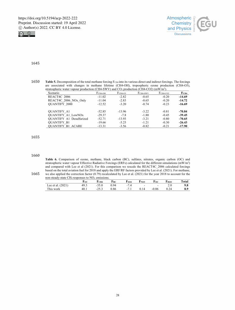
28

1645 Table 5. Decomposition of the total methane forcing FCH4 into its various direct and indirect forcings. The forcings 1650are associated with changes in methane lifetime (CH4-OH), tropospheric ozone production (CH4-O3), stratospheric water vapour production (CH4-SWV) and CO2 production (CH4-CO2) (mW/m2).

Scenario FCH4-OH FCH4-O3 FCH4-SWV FCH4-CO2 FCH4 REACT4C_2006 -11.02 -2.82 -0.65 -0.20 -14.69 REACT4C_2006_NOx_Only -11.04 -2.83 -0.65 -0.20 -14.72 QUANTIFY_2000 -12.52 -3.20 -0.74 -0.23 -16.69 QUANTIFY_A1 -52.85 -13.96 -3.22 -0.81 -70.84 QUANTIFY_A1_LowNOx -29.37 -7.8 -1.80 -0.45 -39.45 QUANTIFY_A1_Desulfurized -52.71 -13.93 -3.21 -0.80 -70.65 QUANTIFY_B1 -19.66 -5.25 -1.21 -0.30 -26.43 QUANTIFY_B1_ACARE -13.31 -3.56 -0.82 -0.21 -17.90

1655 1660Table 6. Comparison of ozone, methane, black carbon (BC), sulfates, nitrates, organic carbon (OC) and stratospheric water vapour Effective Radiative Forcings (ERFs) calculated for the different simulations (mW/m2) and compared with Lee et al (2021). For this comparison we rescale the REACT4C_2006 calculated forcings based on the total aviation fuel for 2018 and apply the ERF/RF factors provided by Lee et al. (2021). For methane, we also applied the correction factor (0.79) recalculated by Lee et al. (2021) for the year 2018 to account for the 1665non-steady-state CH4 responses to NOx emissions.

FO3 FCH4 FBC FSO4 FNO3 FOC FH2O Total Lee et al. (2021) 49.3 -35.0 0.94 -7.4 - - 2.0 9.8 This work 40.1 -25.3 0.86 -7.1 0.14 -0.06 0.24 8.9


1

Figure 1. Taylor diagram comparing the mean and temporal correlation of ozone volume mixing ratio between ozonesonde climatology over the 1995-2011 period (Tilmes et al., 2012) and LMDZ-INCA model results, interpolated to the sample locations and interpolated on six pressure levels for high-latitudes, mid-latitudes and tropical stations.


2

Figure 2. Taylor diagram comparing the mean and geographical correlation of ozone (left) and carbon monoxide (right) volume mixing ratio between the IAGOS data base (Cohen et al., 2018; 2021) and the LMDZ-INCA model results. The error bars denote the 1st and 3rd quartiles of the model to IAGOS biases for a given vertical level and season.

Stan

dard

dev

iatio

n

MNMB

O3

−0.4 −0.2 0.0 0.2 0.4●

0.1 0.2 0.30.4

0.50.6

0.7

0.8

0.9

0.95

0.99

Correlation coefficientSt

anda

rd d

evia

tion

MNMB

CO

−0.4 −0.2 0.0 0.2 0.4●

0.1 0.2 0.30.4

0.50.6

0.7

0.8

0.9

0.95

0.99

Correlation coefficient

SeasonVertical grid level

DJF~180 hPa

MAM~210 hPa

JJA~250 hPa

SON~305 hPa

ANN

Taylor diagrams: INCA−M vs IAGOS−DM (UTLS)


3

Figure 3. Daily and zonally averaged perturbation due to aircraft emissions at 250 hPa of NOx (pptv), O3 (ppbv), OH (10-3 pptv), H2O (ppbv), BC (ng/m3) and SO4 (ng/m3) for the REACT4C_2006 inventory.


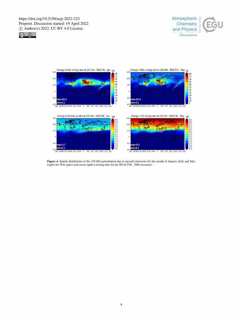
4

Figure 4. Spatial distribution of the 250 hPa perturbation due to aircraft emissions for the month of January (left) and May (right) for NOx (pptv) and ozone (ppbv) mixing ratio for the REACT4C_2006 inventory.


5

Figure 5. Zonal mean perturbation due to aircraft emissions for January (left) and May (right) of NOx (pptv), O3 (ppbv), and H2O (ppbv) for the REACT4C_2006 inventory. The solid line represents the model tropopause pressure.


6

Figure 6. Spatial distributions of the 250 hPa perturbation due to aircraft emissions for January (left) and May (right) for BC, SO4 and NO3 (ng/m3) for the REACT4C_2006 inventory.


7

Figure 7. Zonal mean perturbation due to aircraft emissions for January (left) and May (right) of BC (ng/m3), SO2 (pptv), SO4 (ng/m3) and NO3 (ng/m3) for the REACT4C_2006 inventory. The solid line represents the tropopause pressure.


8

Figure 8. Zonal mean difference for the months of May for O3 (ppbv), BC (ng/m3), SO4 (ng/m3) and NO3 (ng/m3) between the REACT4C_PLUS (left) and REACT4C_MINUS (right) simulations and REACT4C_2004 as the reference. The solid line represents the tropopause pressure.


9

Figure 9. Zonal mean perturbation due to aircraft emissions for the months of January (left) and May (right) for O3 (ppbv), BC (ng/m3), SO4 (ng/m3) and NO3 (ng/m3) averaged for the future scenario QUANTIFY A1 2050. The solid line represents the tropopause pressure.


10

Figure 10. Zonal mean perturbation due to aircraft emissions for May of O3 (ppbv), SO4 and NO3 (ng/m3) for the LowNOx (left) and Desulfurized (right) scenarios. The solid line represents the tropopause pressure.


11

Figure 11. Zonal mean perturbation due to aircraft emissions for May of O3 (ppbv), BC, SO4, and NO3 (ng/m3) for the QUANTIFY 2050 B1 (left) and B1 ACARE (right) scenarios. The solid line represents the tropopause pressure.


Impact of present and future aircraft NOx and aerosol ...

Documents

Transcript of Impact of present and future aircraft NOx and aerosol ...