Copula representation of bivariate L-moments : A new estimation method for multiparameter...

arX

iv:1

106.

2887

v2 [

stat

.ME

] 1

7 Ju

n 20

11

Copula representation of bivariate L-moments:

A new estimation method for multiparameter2-dimentional copula models

Brahim Brahimia, Fateh Chebanab, and Abdelhakim Necira,∗

aLaboratory of Applied Mathematics, Mohamed Khider University of Biskra,

Biskra 07000, Algeria

bCanada Research Chair on the Estimation of Hydrometeorological Variables,

INRS-ETE, 490, rue de la Couronne, G1K 9A9 Quebec (QC), Canada

Abstract.

Recently, Serfling and Xiao (2007) extended the L-moment theory (Hosking, 1990) to the multi-

variate setting. In the present paper, we focus on the two-dimension random vectors to establish

a link between the bivariate L-moments (BLM) and the underlying bivariate copula functions.

This connection provides a new estimate of dependence parameters of bivariate statistical data.

Consistency and asymptotic normality of the proposed estimator are established. Extensive simu-

lation study is carried out to compare estimators based on the BLM, the maximum likelihood, the

minimum distance and rank approximate Z -estimation. The obtained results show that, when the

sample size increases, BLM-based estimation performs better as far as the bias and computation

time are concerned. Moreover, the root mean squared error (RMSE) is quite reasonable and less

sensitive in general to outliers than those of the above cited methods. Further, we expect that

the BLM method is an easy-to-use tool for the estimation of multiparameter copula models.

MSC classification: Primary 62G05; Secondary 62G20.

Keywords: Copulas; Dependence; Multivariate L-moments; Parametric estimation; FGM copu-

las; Archimedean copulas.

*Corresponding author: (A. Necir): [email protected]

[email protected] (B. Brahimi),

[email protected] (F. Chebana)1

http://arxiv.org/abs/1106.2887v2

2

1. Introduction and motivation

The copula method is a tool to construct multivariate distributions and describe the dependence

structure in multivariate data sets (e.g., Joe, 1997 or Nelsen, 2006). Modelling dependence struc-

tures by copulas is a topic of current research and of recent use in several areas, such as financial

assessments (e.g., Malevergne and Sornette, 2003), insurance (e.g., Drees and Muller, 2008) and

hydrology (e.g., Dupuis, 2007). For the sake of simplicity, throughout the paper, we restrict

ourself to the two-dimensional case. Let(X(1),X(2)

)be a bivariate random variable with joint

distribution function (df)

F (x1, x2) = P

(X(1) ≤ x1,X

(2) ≤ x2

), (x1, x2) ∈ R

2,

and marginal df Fj (xj) = P(X(j) ≤ xj

)for xj ∈ R and j = 1, 2. If not stated otherwise, we

assume that the Fj are continuous functions. According to Sklar’s theorem (Sklar, 1959) there

exists a unique copula C : I2 → I, with I = [0, 1] , such that

F (x1, x2) = C (F1 (x1) , F2 (x2)) , for (x1, x2) ∈ R2.

The copula C is the joint df of the uniform random variables (r.v.’s) Uj = Fj

(X(j)

), j = 1, 2,

defined for (u1, u2) ∈ I2, by

C (u1, u2) = F(F−11 (u1) , F

−12 (u2)

),

where G−1 is the generalized inverse function (or the quantile function) of a df G.

A parametric copula model arises for(X(1),X(2)

)when C is unknown but assumed to belong to

a class C := {Cθ, θ ∈ O} , where O is an open subset of Rr for some integer r ≥ 1. Statistical

inference on the dependence parameter θ is one of the main topics in multivariate statistical

analysis. Several methods of copula parameter estimation have been developed, including the

pseudo maximum likelihood (PML), inference of margins, minimum distance and others, see for

instance Genest et al. (2009). All these methods use constrained some optimization techniques,

and may require substantial computational time. In this paper, we present a new estimation

method of θ based on the bivariate L-moments that serves as alternative in front of computation’s

time issue and produces results leads to reasonable estimation performances. The multivariate

L-moments have been introduced by Serfling and Xiao (2007) as an extension of the univariate

L-moments introduced by Hosking (1990). The L-comoments have interpretations similar to the

classical central moment covariance, coskewness, and cokurtosis that also possess the features of

the L-moments. This extension is useful to solve some problems in connection with multivariate

heavy-tailed distributions and small samples. As mentioned, for instance, in Hosking (1990) and

recently in Delicado and Goria (2008), the main advantage of L-moments vis-a-vis of classical

estimation methods (e.g. least squares, moments and maximum likelihood) is their relative slight

sensitivity to outlying data and their performance in statistical inference with small samples.

In this paper we establish a functional representation of bivariate L-moments (BLM) by the

underlying copula function and propose a new estimation method for parametric copula models.

By considering multiparameter Farlie-Gumbel-Morgenstern (FGM) and Archimedean copulas,

3

simulation studies are carried out to compare the performance of this method with those of the

PML, minimum distance (MD) and rank approximate Z -estimation.

The L-moment approach is of interest for multiparameter distributions. In the case of one parame-

ter distributions, it is equivalent to the classical method of moments (see e.g. Hosking, 1990)(since

the first L-moment corresponds to the expected value). Next we see, that this property applies

also in the case of multivariate setting for multiparameter copulas.

The rest of the paper is organized as follows. In Section 2, we briefly introduce the univariate

and bivariate L-moment approaches. We present, in Section 3, functional representations of the

bivariate L-moments by copula functions and give some examples. A new estimator of copula

parameter and its asymptotic behavior are given in Sections 4. In Section 5, a simulation study

evaluates the BLM performance is given.

2. Bivariate L-moments

First we begin with a brief introduction on the univariate L-moments. Hosking (1990) introduced

L-moments λk as an alternative to the classical central moments µk = E

[(Y − µ)k

]determined

by the df FY of the underlying r.v. Y. An L-moment λk is defined as a specific linear combination

of the expectations of the order statistics Y1:k ≤ ... ≤ Yk:k. More precisely, the kth L-moment is

defined by

λk =1

k

k−1∑

ℓ=0

(−1)ℓ (k − 1)!

ℓ! (k − 1− ℓ)!E [Yk−ℓ:k] , k = 1, 2, ...

By analogy with the classical moments, the first four L-moments λ1, λ2, λ3 and λ4 measure

location, scale, skewness and kurtosis features respectively. The L-functional representation of λk

is terms of the quantile function F−1Y is given by (see Hosking, 1998):

λk =

∫

I

F−1Y (u)Pk−1 (u) du, (2.1)

where Pk (u) :=k∑

ℓ=0

pk,ℓuℓ, with pk,ℓ = (−1)k+ℓ (k + ℓ)!/

[(ℓ2)! (k − ℓ)!

]is the shifted Legendre

polynomials (SLP). In the sequel, we will make use of the three first SLP

P0 (u) = 1, P1 (u) = 2u− 1, P2 (u) = 6u2 − 6u+ 1.

A straightforward transformation in (2.1) using P0 ≡ 1 and the orthogonality of Pk−1 leads to a

representation in terms of covariance, that is

λk =

E [Y ] k = 1;

Cov (Y, Pk−1 (FY (Y ))) k = 2, 3, ...(2.2)

L-moments may be used as summary statistics for data samples, to identify probability distri-

butions and fit them to data. A brief description of these methods is given in Hosking (1998).

L-moments are now widely used in water sciences especially in flood frequency analysis. Recent

studies include Kjeldsen et al. (2002), Kroll and Vogel (2002), Lim and Lye (2003), Chebana and

Ouarda (2007) and Chebana et al. (2009). In other recent work, Karvanen et al. (2002) used

L-moments for fitting distributions in independent component analysis in signal processing, and

4

Jones and Balakrishnan (2002) pointed out some relationships between integrals occurring in the

definition of moments and L-moments. Hosking (2006) showed that, for a wide range of distribu-

tions, the characterization of a distribution by its L-moments is non-redundant. That is, if one

L-moment is dropped, the remaining L-moments no longer suffice to determine the entire distri-

bution. Recently, Serfling and Xiao (2007) extended this approach to the multivariate case, this

has already begun to be developed and applied in statistical hydrology by Chebana and Ouarda

(2007) and Chebana et al. (2009).

Next we present basic notations and definitions of the bivariate L-moments. Let X(1) and X(2)

be two r.v.’s with finite means, margins F1 and F2 and L-moments sequences λ(1)k and λ

(2)k ,

respectively. By analogy with the covariance representation (2.2) for L-moments, and the central

comoments, Serfling and Xiao (2007) defined the kth L-comoment of X(1) with respect to X(2)

by the covariance of the couple of r.v.’s X(1) and Pk−1(F2(X(2))), for every k ≥ 2, as

λk[12] = Cov(X(1), Pk−1

(F2

(X(2)

))).

Thus, the kth L-comoment of X(2) with respect to X(1) is defined by

λk[21] = Cov(X(2), Pk−1

(F1

(X(1)

))).

If we suppose that F belongs to a parametric family of df’s, then the kth L-comoment λk[12]

depends on the parameters relies the margins and the dependence structure between X(1) and

X(2). Since we focus only on the estimation of copula parameters, then it is convenient to use the

kth L-comoment of F1

(X(1)

)with respect to X(2) instead of λk[12], that is

λ∗

k[12] := Cov(F1

(X(1)

), Pk−1

(F2

(X(2)

))), k = 2, 3, ...

Similarly the kth L-comoment of F2

(X(2)

)with respect to X(1) is given by

λ∗

k[21] = Cov(F2

(X(2)

), Pk−1

(F1

(X(1)

))), k = 2, 3, ...

For the sake of notation simplicity, we set

δk[12] = λ∗

(k+1)[12] and δk[21] = λ∗

(k+1)[21], for k = 1, 2, ... (2.3)

If the copula C is symmetric in the sense that C (u, v) = C (v, u) , then δk[12] = δk[21], for each

k = 1, 2... We call the coefficient δk[12] by ”the kth bivariate copula L-moment” of X(1) with

respect to X(2), similarly we call δk[21] by the kth copula L-moment of X(2) with respect to X(1).

In application, we will often make use of the three first bivariate copula L-moments, that is:

δ1[12] = 2Cov(F1

(X(1)

), F2

(X(2)

))

δ2[12] = −6Cov(F1

(X(1)

), F2

(X(2)

) (1− F2

(X(2)

)))

δ3[12] = Cov(F1

(X(1)

), 20F 3

2

(X(2)

)− 30F 2

2

(X(2)

)+ 12F2

(X(2)

)− 1).

5

3. Bivariate copula representation of kth copula L-moment

Theorem 3.1 below gives a representation of the kth bivariate L-moment in terms of the underlying

copula function. This result provides a new estimate of bivariate copula parameters.

Theorem 3.1. The kth bivariate copula L-moment of X(1) with respect to X(2) may be rewritten,

for each k ≥ 1, as

δk[12] =

∫

I2

(C (u1, u2)− u1u2) du1dPk (u2) , (3.4)

or

δk[12] =

∫

I2

u1Pk (u2) dC (u1, u2) .

Observe that δ1[12] = δ1[21] = ρ/6 where ρ is the Spearman rho ρ, coefficient defined in term of

copula C by

ρ = 12

∫

I2

u1u2dC (u1, u2)− 3, (3.5)

(see Nelsen, 2006, page 167).

In view of Theorem 3.1, according to our needs, we can construct a system of equations that will

serve to the estimation of multiparameter copula models. For this reason, the proposed estimator

is more likely to be used for the multiparameter copulas. In the case of the one-parameter copulas,

it is equivalent to the rho-inversion method (see (4.22) below). Indeed, suppose that we are dealing

with the estimation of one dimension parameter of a copula model, then it suffices to use one of

the kth bivariate copula L-moment, says δ1[12]. In the case of r−dimension parameters we have to

take the r first bivariate copula L-moment, so we obtain a system of r equations with r unknown

parameters. Then, by replacing the coefficients δk[12], k = 1, ..., r by their empirical counterparts,

we obtain estimators of the r parameters. Indeed, suppose that r = 3 and C = Cθ, θ = (θ1, θ2, θ3) ,

then from Theorem 3.1, the first three bivariate copula L-moments of X(1) with respect to X(2)

are

δ1[12] = 2

∫

I2

Cθ (u1, u2) du1du2 −1

2

δ2[12] = 6

∫

I2

(2u2 − 1)Cθ (u1, u2) du1du2 −1

2

δ3[12] =

∫

I2

(60u22 − 60u2 + 12

)Cθ (u1, u2) du1du2 −

1

2.

Since, in general the copula of (X(1),X(2)) is not the same as of (X(2),X(1)), the corresponding

parameters could be estimated accordingly to δk[12] or δk[21].

Next we present applications of Theorem 3.1 to parameter estimation of two popular families of

copula, namely the FGM and Archimedean copulas.

3.1. FGM families. One of the most popular parametric family of copulas is the FGM family

defined for |α| ≤ 1 by

Cα (u1, u2) = u1u2 + αu1u2u1u2, 0 ≤ u1, u2 ≤ 1, (3.6)

6

with uj := 1 − uj , j = 1, 2. The model is useful for the moderate correlation which occurs

in engineering and medical applications (see, e.g., Blischke and Prabhaker Murthy, 2000 and

Chalabian and Dunnington, 1998). The Pearson correlation coefficient ρ corresponds to the model

(3.6) can never exceed 1/3, (see, e.g., Huang and Kotz, 1984). In order to increase the dependence

between two random variables obeying the type of FGM distribution, Johnson and Kotz (1977)

introduced the (r − 1)-iterated FGM family with r-dimensional parameter α =(α1, ..., αr) :

Cα (u1, u2) = u1u2 +

r∑

j=1

αj (u1u2)[j/2]+1 (u1u2)

[j/2+1/2] ,

where [z] denotes the greatest integer less than or equal to z. For example, the one-iterated FGM

family (Huang and Kotz, 1984) is a two-parameter copula model:

Cα1,α2 (u1, u2) = u1u2 {1 + α1u1u2 + α2u1u2u1u2} . (3.7)

The range of parameters (α1, α2) is given by the region

R :=

{(α1, α2) , |α1| ≤ 1, α1 + α2 ≥ −1, α2 ≤

1

2

[3− α1 +

(9− 6α1 − 3α2

1

)1/2]}. (3.8)

The maximal reached correlation for this family is

ρmaxFGM = 0.42721, for (α1, α2) =

(−1 + 7/

√13, 2− 2/

√13), (3.9)

and the minimal correlation is ρminFGM = −1/3 for (α1, α2) = (−1, 0) . The two-iterated FGM family

is given by

Cα1,α2,α3 (u1, u2) = u1u2

{1 + α1u1u2 + α2u1u2u1u2 + α3u1u2 (u1u2)

2},

and it has been discussed by Lin (1987).

According to Theorem 3.1, we may give explicit formulas of bivariate copula L-moments for the

FGM, the one-iterated FGM and the two-iterated FGM. Since the number of parameters equals

k ∈ {1, ..., r} , then we are dealing with first k bivariate copula L-moments that will provide a

system of k equations and therefore a tool for the estimation of the parameters of the copulas.

We have :

• The first bivariate copula L-moment of FGM family Cα is

δ1[12] = α/18

• The two first bivariate copula L-moments of one-iterated FGM copula Cα1,α2 are:

δ1[12] = α1/18 + α2/72

δ2[12] = α2/120(3.10)

• The three first bivariate copula L-moments of two-iterated FGM copula Cα1,α2,α3 are:

δ1[12] = α1/18 + α2/72 + α3/450

δ2[12] = α2/120

δ3[12] = −α3/1050

7

3.2. Archimedean copula families. The Archimedean copula family is one of important class

of copula models that contains the Gumbel, Clayton, Frank, ... (see, Table 4.1 in Nelsen, 2006,

page 116). In the bivariate case, an Archimedean copula is defined by

C(u, v) = ϕ−1 (ϕ(u) + ϕ(v)) ,

where ϕ : I → R is a twice differentiable function called the generator, satisfying: ϕ (1) = 0,

ϕ′ (x) < 0, ϕ′′ (x) ≥ 0 for any x ∈ I/ {0, 1} . The notation ϕ−1 stands for the inverse function

of ϕ. For examples, the three generators ϕθ (t) = (− ln ((1− θ (1− t)) /t)) , ϕα (t) = (t−α − 1) /α

and ϕβ (t) = (− ln t)β define, respectively, the one parameter Frank, Clayton and Gumbel copula

families. For example, the Gumbel family is defined by

Cβ(u, v) = exp

(−[(− lnu)β + (− ln v)β

]1/β), β ≥ 1. (3.11)

For more flexibility in fitting data, it is better to use the multi-parameters copula models than those

of one parameter. To have a copula with more one parameter, we use, for instance, the distorted

copula defined by CΓ (u, v) = Γ−1 (C (Γ (u) ,Γ (v))) , where Γ : I → I is a continuous, concave

and strictly increasing function with Γ (0) = 0 and Γ (1) = 1. Note that if C is an Archimedean

copula with generator ϕ, then CΓ is also Archimedean copula with generator generator ϕ ◦Γ. Formore details see Nelsen (2006), page 96 . As example, suppose that Γ = Γβ2 , with Γβ2 (t) =

exp(t−β2 − 1

), β2 > 0 and consider a Gumbel copula Cβ1 with generator ϕβ1 (t) = (− ln t)β1 ,

β1 ≥ 1. Then the copula Cβ1,β2 (u, v) = Γ−1β2

(Cβ1 (Γβ2 (u) ,Γβ2 (v))) given by

Cβ1,β2 (u, v) :=

(((u−β2 − 1

)β1

+(v−β2 − 1

)β1)1/β1

+ 1

)1/β2

, (3.12)

which is a two-parameter Archimedean copula with generator ϕβ1,β2 (t) :=(t−β2 − 1

)β1 . (see

Nelsen 2006, page 96).

To have the two first bivariate copula L-moments correspond to Cβ1,β2 , we apply Theorem 3.1 to

get the following system of equations:

δ1[12] = 2∫ 10

∫ 10 (Cβ1,β2 (u, v) − uv) dudv,

δ2[12] = 6∫ 10

∫ 10 (2v − 1) (Cβ1,β2 (u, v)− uv) dudv.

(3.13)

In this case we cannot give explicit formulas, in terms of{δ1[12], δ2[12]

}, for the parameters {β1, β2} ,

however for given values of the bivariate copula L-moments, we can obtain the corresponding values

of {β1, β2} by solving the previous system by numerical methods.

Remark 3.1. The previous system provides estimators for copula parameters by replacing the bi-

variate copula L-moments by their sample counterparts. This is similar to the method of moments

(see Section 4).

4. Semi-parametric BLM-based estimation

The aim of the present section is to provide a semi-parametric estimation for bivariate copula

parameters on the basis of results of Section 3. Suppose that the underlying copula C belongs to

8

a parametric family Cθ with θ = (θ1, · · · , θr) ∈ O an open subset of Rr satisfies the concordance

ordering condition of copulas (see, Nelsen, 2006, page 135), that is:

for every θ(1), θ(2) ∈ O : θ(1) 6= θ(2) =⇒ Cθ(1) (> or <)Cθ(2) . (4.14)

The above inequalities mean that for any (u, v) ∈ I2, Cθ(1) (u, v) (> or <)Cθ(2) (u, v) . It is clear

that condition (4.14) implies the well known identifiability condition of copulas:

for every θ(1), θ(2) ∈ O : θ(1) 6= θ(2) =⇒ Cθ(1) 6= Cθ(2) . (4.15)

Identifiability is a natural and even a necessary condition: if the parameter is note identifiable

then consistent estimator cannot exist (see, e.g., van der Vaart, 1998, page 62). A wide class of

copula families satisfy condition (4.14), and therefore (4.15), including the iterated FGM and the

archimedean models. Indeed, the iterated FGM family is linear with respect to their parameters,

then by a little algebra we easily verify this condition. For two-parameter Gumbel family, the

condition (4.14) is already checked in Nelsen (2006), page 144, example 4.22. Consider now a

random sample(X

(1)i ,X

(2)i

)i=1,n

from the bivariate r.v.(X(1),X(2)

). For each j = 1, 2, let

F+j:n := nFj:n/ (n+ 1) denotes the rescaled empirical df corresponds to the empirical df

Fn:j (xj) = n−1n∑

i=1

1{X

(j)i ≤ xj

}.

We are now in position to present, in three steps, the semi-parametric BLM-based estimation:

• Step 1: For each k = 1, ..., r, compute

δk[12] = n−1n∑

i=1

F+1:n

(X

(1)i

)Pk

(F+2:n

(X

(2)i

)). (4.16)

given in equation (2.3).

• Step 2 : Using Theorem 3.1 to generate a system of r equations given by equation (3.4),

for k = 1, ..., r.

• Step 3: Solve the system

δ1[12] (θ1, ..., θr) = δ1[12]δ2[12] (θ1, ..., θr) = δ2[12]...

δr[12] (θ1, ..., θr) = δr[12].

(4.17)

The obtained solution θBLM :=(θ1, ..., θr

)is called a BLM estimator for θ = (θ1, ..., θr) .

The existence and the convergence of a solution of the previous system are established in Theorem

4.1, (see Section 4.2).

As an application of the BLM based estimation, we choose the one-iterated FGM copula Cα1,α2

given in (3.7) and propose estimators for the parameters (α1, α2) noted (α1, α2) . For this family,

using (3.10), system (4.17) becomes

α1/18 + α2/72 = δ1[12],

α2/120 = δ2[12],

9

where δk[12], k = 1, 2 are given in (4.16). Therefore

α1 = 18δ1[12] − 30δ2[12],

α2 = 120δ2[12].

4.1. BLM as a rank approximate Z -estimation. Tsukahara (2005) introduced a new estima-

tion method for copula models called the rank approximate Z-estimation (RAZ) that generalizes

the PML one. The BLM method may be interpreted as a RAZ estimation. Let Ψ (·; θ) be an

Rr-valued function on I

2, called ”score function”, whose components Ψj (·; θ) satisfy the condition∫

I2

Ψj (u1, u2; θ) dC (u1, u2) = 0, for j = 1, ..., r.

Any solution θRAZ in θ of the following equation

n∑

i=1

Ψ(F+1:n

(X

(1)i

), F+

2:n

(X

(2)i

); θ)= 0, (4.18)

is called a RAZ estimator. There may not be an exact solution to equation (4.18) in general,

so in practice, we should choose θRAZ to be any value of θ for which the absolute value of the

left-hand side of equation (4.18) is close to zero. It is worth mentioning that if the copula Cθ is

absolutely continuous with density cθ, then the function Ψ =•cθ/cθ, with

•cθ = (∂cθ/∂θk)j=1,...,r ,

leads the PML based estimation (see for instance Genest et al., 1995). The existence of a sequence

of consistent roots of Z-estimation in this context is discussed in Theorem 1 in Tsukahara (2005).

One of the main question of RAZ-estimation is the choice of the score function Ψ producing, in

a certain sense, the best estimator. In Section (5), we show that the the copula L-moment score

(CLS) functions (4.19) improve the concordance score functions in terms of bias and root mean

square error (RMSE).

The univariate L-moments are a special case of the L-statistics with a specific choice of the weight

coefficients. This fact makes the L-moments interpretable and popular. In a similar way, the

BLM-based estimator represents an important special case of the RAZ one. In our case, the

score function Ψ (u1, u2; θ) corresponds to the function Lk given in (4.19) below. Recall that from

Theorem 3.1 we have

δk[12] (θ) =

∫

I2

u1Pk (u2) dCθ (u1, u2) , k = 1, 2...,

and define the CLS functions by

Lk (u1, u2; θ) := u1Pk (u2)− δk[12] (θ) , k = 1, ..., r, (4.19)

satisfying∫I2Lk (u1, u2; θ) dCθ (u1, u2) = 0, k = 1, ..., r. Then the RAZ estimator corresponding to

the CLS function L =(L1, ..., Lr) is a solution in θ of the system

n∑

i=1

L(F+1:n

(X

(1)i

), F+

2:n

(X

(2)i

); θ)= 0, (4.20)

that isn∑

i=1

F+1:n

(X

(1)i

)Pk

(F+2:n

(X

(2)i

))− nδk[12] (θ) = 0, k = 1, ..., r, (4.21)

10

therefore δk[12] (θ) = δk[12], k = 1, ..., r, which in fact the system of bivariate copula L-moments

given in system (4.17).

On the other hand, the measures of concordance produce also a Z-estimation for copula models.

Indeed, the most popular measures of concordance (see, Nelsen, 2006, page 182) are Kendall’s tau

(τ), Spearman’s rho (ρ) , Gini’s gamma (γ) and Spearman’s foot-rule phi (ϕ) , given respectively

by

τ (θ) = 4

∫

I2

Cθ (u1, u2) dCθ (u1, u2)− 1,

ρ (θ) = 12

∫

I2

u1u2dCθ (u1, u2)− 3,

γ (θ) = 4

∫

I

Cθ (u1, 1− u1) du1 −∫

I

(u1 − Cθ (u1, u1)) du1,

ϕ (θ) = 1− 3

∫

I2

|u1 − u2| dCθ (u1, u2) .

It follows that the concordance score (CS) functions associated to τ, ρ, γ and ϕ respectively are

Ψ1 (u1, u2; θ) := 4Cθ (u1, u2)− τ (θ) ,

Ψ2 (u1, u2; θ) := 12u1u2 − 3− ρ (θ) ,

Ψ3 (u1, u2; θ) := 4Cθ (u1, 1− u1)− u1 +Cθ (u1, u1)− γ (θ) ,

Ψ4 (u1, u2; θ) := 1− 3 |u1 − u2| − ϕ (θ) .

It is clear that∫I2Ψj (u1, u2; θ) dCθ (u1, u2) = 0, j = 1, ..., 4, then whenever the dimension of

parameters r = 4, the function Ψ = (Ψ1, ...,Ψ4) provides Z-estimators for copula models. If the

dimension of parameters r < 4, then we may choose any r functions from Ψ1, ...,Ψ4 to have a

system of r equations that provides estimators of the r parameters.

Tsukahara (2005) also discussed the RAZ-estimators based on Kendall’s tau (τ) and Spearman’s

rho (ρ) , called τ -score and ρ-score RAZ-estimators. Suppose that r = 1 and let τn and ρn be

the sample versions of Kendall’s tau (τ) and Spearman’s rho (ρ) . By using the same idea as the

method of moments, the τ -inversion θτ estimator and the ρ-inversion θρ estimator of θ are defined

by

θτ = τ−1 (τn) and θρ = ρ−1 (ρn) . (4.22)

In the case when r = 2, we may also estimate θ =(θ1, θ2) by solving the system

τ (θ1, θ2) = τn

ρ (θ1, θ2) = ρn.(4.23)

We call, the obtaining solution of the previous system, by (τ, ρ)−inversion estimator of θ. Suppose

that we are dealing with the estimation of parameters (α1, α2) of the one-iterated FGM copula

11

Cα1,α2 in (3.7). Then, the associated Kendall’s tau (τ) and Spearman’s rho (ρ) are

τ (α1, α2) = 2α1/9 + α2/18 + α1α2/450

ρ (α1, α2) = α1/3 + α2/12.(4.24)

The (τ, ρ)-inversion estimator of parameters (α1, α2) is the solution of the system

τ (α1, α2) = τn

ρ (α1, α2) = ρn.

Similarly, if we consider the FGM family Cα1,α2,α3 we have to add γ−score and ϕ−score to have

a system of four equations, we omit details.

4.2. Asymptotic behavior of the BLM estimator. By considering BLM’s estimator as a

RAZ-estimator, a straight application of Theorem 1 in Tsukahara (2005) leads to the consistency

and asymptotic normality of the considered estimator. Let θ0 be the true value of θ and assume

that the assumptions [H.1] − [H.3] listed below are fulfilled.

• [H.1] θ0 ∈ O ⊂ Rr is the unique zero of the mapping θ →

∫I2L (u1, u2; θ) dCθ0 (u1, u2) that

is defined from O to Rr.

• [H.2] L (·; θ) is differentiable with respect to θ with the Jacobian matrix denoted by

•

L (u1, u2; θ) :=

[∂Lk (u1, u2; θ)

∂θℓ

]

r×r

,

•

L (u1, u2; θ) is continuous both in (u1, u2) and θ, and the Euclidian norm

∣∣∣∣•

L (u1, u2; θ)

∣∣∣∣ isdominated by a dCθ-integrable function h (u1, u2) .

• [H.3] The r × r matrix A0 :=∫I2

•

L (u1, u2; θ0) dCθ0 (u1, u2) is nonsingular.

Theorem 4.1. Assume that the assumptions [H.1] − [H.3] hold. Then with probability tending

to one as n → ∞, there exists a solution θBLM to the equation (4.21) which converges to θ0.

Moreover√n(θBLM − θ0

)D→ N

(0Rr , A−1

0

∑0

(A−1

0

)T), as n → ∞,

with

∑0 := var

L (ξ1, ξ2; θ0) +

2∑

j=1

∫

I2

Mj (u1, u2) (1 {ξj ≤ uj} − uj) dCθ0 (u1, u2)

, (4.25)

where (ξ1, ξ2) is a bivariate r.v. with joint distribution function Cθ0 ,

M1 (u1, u2) := {Pk (u2)}k=1,r and M2 (u1, u2) := {u1dPk (u2) /du2}k=1,r .

The proof of Theorem 4.1 is given in the Appendix.

Note that the assumptions [H.1]− [H.3] correspond to A2, A4 and A5 in Tsukahara (2005). The

score function L meets the remaining assumptions A1 and A3.

12

4.3. A discussion on Theorem 4.1. Notice that assumption [H.1] is verified for any parametric

copula Cθ satisfying the concordance ordering condition of copulas (4.14) . Indeed, suppose that

there exists θ1 6= θ0, such that∫

I2

Lk (u1, u2; θ1) dCθ0 (u1, u2) = 0, for every k ∈ {1, ..., r} . (4.26)

Recall that δk[12] (θ0) =∫I2u1Pk (u2) dCθ0 (u1, u2) and δk[12] (θ1) =

∫I2u1Pk (u2) dCθ1 (u1, u2) and,

from assumption (4.14) , Cθ0 (> or <)Cθ1 . It follows, by monotonicity of the integral, that

δk[12] (θ1) (> or <) δk[12] (θ0) , this implies that δk[12] (θ1) − δk[12] (θ0) 6= 0, for every k ∈ {1, ..., r} .Observe that

∫I2dCθ0 (u1, u2) = 1 then δk[12] (θ1) =

∫I2δk[12] (θ1) dCθ0 (u1, u2) , consequently, since

Lk (u1, u2; θ1) = u1Pk (u2)− δk[12] (θ1) , that

∫

I2

Lk (u1, u2; θ1) dCθ0 (u1, u2) =

∫

I2

u1Pk (u2) dCθ0 (u1, u2)−∫

I2

δk[12] (θ1) dCθ0 (u1, u2)

= δk[12] (θ0)− δk[12] (θ1) 6= 0, for every k ∈ {1, ..., r} ,

which is a contradiction with equation (4.26) , as sought. Let’s now discuss the rest of assumptions. In

[H.2] , the continuity and the differentiability with respect to θ and (u1, u2) of L (·; θ) and•

L (·; θ)are lie with that of copula Cθ, which are natural assumptions in parametric copula models. Some

examples on this issue are illustrated in Fredricks et al. (2007). The second part of [H.2] and

[H.3] may be checked for a given copula model. For example, if we consider the FGM family

(see (3.6)) we get L1 (u1, u2;α) = u1 (2u2 − 1) − α/18 and Lk (u1, u2;α) = 0, for k = 2, 3...Then

dL1 (u1, u2;α) /dα = −1/18 and dLk (u1, u2;α) /dα = 0, for k = 2, ... Let α0 denote the true value

of parameter α. It is clear that each compound of•

L is continuous with respect to α and (u1, u2) ,∣∣∣∣•

L (u1, u2;α)

∣∣∣∣ = 1/18, which is Cα−integrable function and, A0 =∫I2

•

L (u1, u2;α0) dCα0 = −1/18

which is nonsingular matrix, then the assumptions [H.2] and [H.3] are well verified. By a little

algebra we get to the corresponding value of∑

0 that is defined in (4.25) , and by Theorem 4.1 we

get √n(αBLM − α0

) D→ N(0, α2

0/270 + 1/5), as n → ∞.

For the one-iterated FGM family (see (3.7)), by letting α1 = α and α2 = β, it is readily to verify

that

L1 (u1, u2;α, β) = u1 (2u2 − 1)− α/18 − β/72,

L2 (u1, u2;α, β) = u1(6u22 − 6u2 + 1

)− β/120,

which, obviously, are continuous with respect to (α, β) and (u1, u2) and Cα,β−integrable function,

and•

L (u1, u2;α, β) =

[−1/18 −1/72

0 −1/120

].

Let (α0, β0) denote the true value of parameter (α, β) and by calculating the elements of the

matrix

A0 :=

∫

I2

•

L (u1, u2;α0, β0) dCα0,β0 ,

13

we get

A0 =

[−1/18 1/72

0 −1/120

],

which is nonsingular because its determinant equals 1/2160 6= 0, therefore [H.2] and [H.3] are also

verified. Then, in view of Theorem 4.1, we have

√n

{(αBLM

βBLM

)−(

α0

β0

)}D→ N

((0

0

),∑2

), as n → ∞,

where∑2 := A−1

0

∑0

(A−1

0

)T. After a tedious computation we get

∑0 =

α20

270+

α0β0540

+β20

3780+

1

5

β20

8640+

α0β02160

β20

8640+

α0β02160

α20

105+

α0β0252

+17β2

0

21000+

1

15

,

it follows that

∑2 =

342α20

35+

327α0β070

+263β2

0

280+

624

5

240α20

7+

107α0β07

+443β2

0

140+ 240

240α20

7+

107α0β07

+443β2

0

140+ 240

960α20

7+

400α0β07

+408β2

0

35+ 960

.

Finally, we note that assumptions [H.1] − [H.3] may be also verified for one and two parameters

copula families given in (3.11) and (3.12), respectively, but that requires tedious calculations which

would get us out of the context of the paper.

5. Simulation study

To evaluate and compare the performance of BLM’s estimator with other estimators a simulation

study is carried out with r = 2 by considering Cα1,α2 (the one iterated FGM family) and Cβ1,β2

(the two parameters Gumbel family) given in (3.10) and (3.12) respectively. The evaluation of the

performance is based on the bias and the RMSE defined as follows:

Bias =1

N

N∑

i=1

(θi − θ

), RMSE =

(1

N

N∑

i=1

(θi − θ

)2)1/2

, (5.27)

where θi is an estimator (from the considered method) of θ from the ith samples for N generated

samples from the underlying copula. In both parts, we selected N = 1000. We compare the BLM

estimator with the PML, (τ, ρ)−inversion (4.23) and MD estimators (see the Appendix). The

procedure outlined in Section (4) is repeated for different sample sizes n with n = 30, 50, 100, 500

to assess the improvement in the bias and RMSE of the estimators with increasing sample size.

Furthermore, the simulation procedure is repeated for a large set of parameters of the true copulas

Cα1,α2 and Cβ1,β2 . For each sample, we solve systems (3.10) and (3.13) to obtain, respectively,

14

the BLM-estimators (α1,i, α2,i) and(β1,i, β2,i

)of (α1, α2) and (β1, β2) for i = 1, ..., N, and the

estimators αk, βk for k = 1, 2 are given by αk = 1N

∑Ni=1 αk,i and βk = 1

N

∑Ni=1 βk,i.

5.1. Performance of the BLM-based estimation. We first select parameters, as the true

values of the parameters, of Gumbel and FGM copula models. The choice of the parameters

have to be meaningful, in the sense that each couple of parameters assigns a value of one of the

dependence measure, that is weak, moderate and strong dependence. In other words, if we consider

Spearman’s rho ρ as a dependence measure, then we should select values for copula parameters

that correspond to specified values of ρ by using equation (3.5). Recall that for the FGM family

Cα1,α2 , the dependence reaches the maximum ρmaxFGM = 0.42721 in α1 = −1 + 7/

√13 ≈ 0.941

and α2 = 2 − 2/√13 ≈ 1.445 (see (3.9)). So, we may chose (α1, α2) = (0.941, 1.445) as the

true parameters of FGM family that correspond to the strong dependence. For the true values

of (α1, α2) corresponding to the weak and the moderate dependence, we proceed as follows. We

assign a value to the couple (ρ, α1) such that |α1| ≤ 1, then we solve by numerical methods the

equation (3.5) in the region (3.8) and get the corresponding value to α2. We summarize the results

in the following table:

ρ α1 α2

0.001 0.100 0

0.208 0.400 0.900

0.427 0.941 1.445

Table 5.1. The true parameters of FGM copula used for the simulation study .

By the same procedure, we select the true parameters (β1, β2) of the Gumbel copula Cβ1,β2 and

get:

ρ β1 β2

0.001 1 0.001

0.500 1.400 0.200

0.900 2.500 1

Table 5.2. The true parameters of Gumbel copula used for the simulation study.

To evaluate the performance of the BLM estimators, we proceed as follows:

(1) By using the Algorithm in Nelsen 2006 page 41 and Theorem 4.3.7 in Nelsen 2006 page

129, respectively, we generate twice N samples of size n from each one the considered

copulas Cα1,α2 and Cβ1,β2 .

(2) Obtain the BLM estimators (α1, α2) of (α1, α2) and(β1, β2

)of (β1, β2) .

(3) By computing, for each estimator, the appropriate Bias and RMSE, we compare (α1, α2)

and(β1, β2

), respectively, with the true parameters (α1, α2) and (β1, β2) .

All computations were performed in the R Software version 2.10.1. The results of the simulation

study are summarized in Tables 7.3 and 7.4. We observed that BLM’s method provides, in terms

15

of bias and RMSE, reasonable results, notably when the sample size increases. However, in the

case of strong dependence for FGM’s family when the sample size is small and less than 30, the

estimation of the first parameter α1 is better that of the second one α2. However, for the sample

sizes greater than 100 the results become reasonable and more better for sample sizes greater than

n = 500. For Gumbel family the performance of BLM’s method looks good even for small samples.

5.2. Comparative study: BLM, (τ, ρ)−inversion, MD and PML. As the previous Subsec-

tion, we consider the bivariate two-parameter FGM and Gumbel copula families with the trues

parameters those given in Tables 5.1 and 5.2 respectively. The simulation study proceeds as

follows:

(1) Generate N samples of size n = 30, 50, 100, 500 from the copula Cθ.

(2) Assess the performances of the BLM, (τ, ρ)−inversion, MD and PML estimators.

(3) Compare the BLM, (τ, ρ)−inversion, MD and PML estimators with the true parameter θ

by computing, for each estimator, the appropriate criteria given by (5.27) .

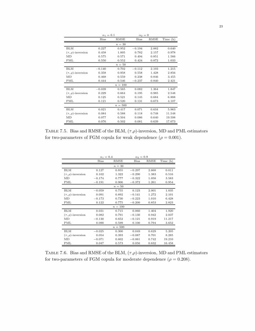
It is clear, from Tables 7.5 to 7.10, that the BLM estimate preforms better than the (τ, ρ)−inversion,

MD and PML ones as far as the Bias is concerned. On the other hand, in the case of small sam-

ples the (τ, ρ)−inversion, MD and PLM methods give better RMSE than the BLM one. However,

when the sample size increases, the RMSE of the BLM estimator becomes reasonable. Moreover,

for the computation time point of view, we observed that the (τ, ρ)−inversion, MD and PLM

estimates require hours to be obtained, notably when the sample size becomes large, whereas the

BLM estimate execution time is in terms of minutes. This is a natural conclusion, because the

(τ, ρ)−inversion, MD and PLM methods use the optimization problem under constraints, while

the BLM method uses systems of equations.

5.3. Comparative robustness study: BLM, (τ, ρ)−inversion, MD and PML. In this

subsection we study the sensitivity to outliers of BLM’s estimator and compare with those of the

(τ, ρ)−inversion, MD and PML ones. We consider an ǫ−contaminated model for two-parameters

FGM familly by means of a copula from the same family. In other terms, we are dealing with the

following mixture copula model:

Cα1,α2 (ǫ) := (1− ǫ)Cα1,α2 + ǫCα∗

1,α∗

2, (5.28)

where 0 < ǫ < 1 is the amount of contamination. For the implementation of mixtures models to

the study outliers one refers, for instance, to Barnett and Lewis (1994), page 43. In this context,

we proceed our study as follows. First, we select (α1, α2) = (0.4, 0.9) corresponds to Spearman’s

Rho ρ = 0.208 (see Table 5.1) and chose (α∗1, α

∗2) = (0, 0) to have the contamination model as the

product copula that is Cα∗

1 ,α∗

2(u, v) = uv. Then we consider four contamination scenarios according

to ǫ = 5%, 10%, 20%, 30%. For each value ǫ, we generate 1000 samples of size n = 40 from the

copula Cα1,α2 (ǫ) . Finally, we compare the BLM, (τ, ρ)−inversion, MD and PML estimators with

the true parameter (α1, α2) by computing, for each estimator, the appropriate Bias and RMSE

and summarize the results in Table 7.11. We observed that, for example, in 0% contamination

the (Bias, RMSE) of α1 equals (0.044, 0.832) , while for 30% contamination is (−0.165, 0.835) . We

may conclude that the RMSE of BLM’s estimation in less sensitive (or robust) to outliers, however

the Bias is not. The same conclusion is for the (τ, ρ)−inversion method but the BLM one is better.

16

For PLM’s estimation both the Bias and the RMSE are sensitive, indeed for 0% contamination the

(Bias, RMSE) of α1 equals (−0.238, 0.440) , while for 30% contamination is (−0.328, 0.589) . Both

the bias and the RMSE of MD’s estimation are note sensitive to outliers, then we may conclude

that is the better among the four estimation methods. However, the computation time cost in

MD’s method is important which is considered as an handicap from practitioners.

6. Conclusions

In this paper, a formula of the bivariate L-moments in terms of copulas is given. This formula

leads to introduce a new estimation method for bivariate copula parameters, that we called the

BLM based estimation. The limiting distribution of the estimators given by the BLM method are

established. Moreover, we compared by simulations the BLM method with the (τ, ρ)-inversion,

the minimum distance (MD) and the pseudo maximum likelihood (PML) estimators by focusing

on the Bias and the RMSE. We conclude that the BLM based estimation performs well the Bias

and reasonably the RMSE. However, BLM’s method may be an alternative robust method as far

as the RMSE is concerned. As final conclusion, it is worth noting that computation’s time of the

proposed method is quite small compared to MD and PML ones.

Acknowledgements

The authors are grateful to Professor Taha B.M.J. Ouarda from INRS-ETE for his valuable

comments and suggestions that helped to improve the quality of this paper.

References

[1] Barnett, V., Lewis, T., 1995. Outliers in statistical data, Third ed. John Willey & Sons, . New York.

[2] Biau, G., Wegkamp, M., 2005. A note on minimum distance estimation of copula densities. Statist. Probab.

Lett. 73, 105-114.

[3] Bickel, J., Klaassen, C. A. J., Ritov, Y., Wellner, J. A., 1993. Efficient and Adaptive Estimation for Semipara-

metric Models. Johns Hopkins University Press, Baltimore.

[4] Blischke, W.R., Prabhakar Murthy, D.N., 2000. Reliability modeling, prediction, and optimization, Wiley, New

York.

[5] Chalabian, J., Dunnington, G., 1998. Do our current assessments assure competency in clinical breast evaluation

results? The American Journal of Surgery, 175, 6, pp. 497- 502.

[6] Chebana, F., Ouarda, T.B.M.J., 2007. Multivariate L-moment homogeneity test. Water resources research 43:

W08406. DOI: 10-1029/2006WR005639.

[7] Chebana, F., Ouarda, T.B.M.J., Bruneau, B., Barbet, M., El Adlouni, S. Latraverse, M., 2009. Multivariate

homogeneity testing in a northern case study in the province of Quebec, Hydrological Processes, 23, 1690-1700,

DOI: 10.1002/hyp.7304.

[8] Deheuvels, P., 1979. La fonction de dependance empirique et ses proprietes. Acad. Roy. Belg. Bull. Cl. Sci. 65,

274-292.

[9] Delicado, P., Goria, M.N., 2008. A small sample comparison of maximum likelihood, moments and L-moments

methods for the asymmetric exponential power distribution. Comput. Statist. Data Anal. 52, 1661-1673.

[10] Drees, H., Muller, P., 2008. Fitting and validation of a bivariate model for large claims. Insurance Math.

Econom. 42, 638-650.

[11] Dupuis, D.J., 2007. Using copulas in hydrology: Benefits, cautions, and issues. Journal of Hydrologic Engineer-

ing, 12, 381-393.

[12] Fredricks, G. A.; Nelsen, R. B., 2007. On the relationship between Spearman’s rho and Kendall’s tau for pairs

of continuous random variables. J. Statist. Plann. Inference 137, 2143-2150.

17

[13] Genest, C., Remillard, B., 2008. Validity of the parametric bootstrap for goodness-of-fit testing in semipara-

metric models. Ann. Inst. Henri Poincare Probab. Stat. 44, 1096-1127.

[14] Genest, C., Remillard, B., Beaudoin, D., 2009. Goodness-of-fit tests for copulas: a review and a power study.

Insurance Math. Econom. 44, 199-213.

[15] Hosking, J.R.M., 1990. L-moments: analysis and estimation of distributions using linear combinations of order

statistics. J. Royal Statist. Soc. Sev. B 52, 105-124.

[16] Hosking, J.R.M., 1998. L-moments. in:Kotz, S., Read, C., Banks, D.L. (Eds.), Encyclopedia of Statistical

Sciences, vol. 2. Wiley, NewYork, 357-362.

[17] Hosking, J.R.M., 2006. On the characterization of distributions by their L-moments. J. Statist. Plann. Inference

136, 193-198.

[18] Huang, J.S., Kotz, S., 1984. Correlation structure in iterated Farlie-Gumbel-Morgenstern distributions.

Biometrika 71, 633-636.

[19] Joe, H., 1997. Multivariate Models and Dependence Concepts, Chapman & Hall, London.

[20] Johnson, N. L., Kotz, S., 1977. On some generalized Farlie- Gumbel-Morgenstern distributions-II: Regression,

correlation and further generalizations, Communications in Statistics. Theor. Meth., 6,pp. 485-496.

[21] Jones, M.C., Balakrishnan, N., 2002. How are moments and moments of spacings related to distribution

functions? J. Statist. Plann. Inference 103, 377-390.

[22] Karvanen, J., Eriksson, J., Koivunen, V., 2002. Adaptive score functions for maximum likelihood ICA. J. VLSI

Signal Process. 32, 83-92.

[23] Kjeldsen, T.R., Smithers, J.C., Schulze, R.E., 2002. Regional flood frequency analysis in the KwaZulu-Natal

province, South Africa, using the index-flood method. J. Hydrol. 255, 194-211.

[24] Kroll, C.N., Vogel, R.M., 2002. Probability distribution of low streamflow series in the United States. J. Hydrol.

Eng. 7, 137-146.

[25] Lim,Y.H., Lye, L.M., 2003. Regional flood estimation for ungauged basins in Sarawak, Malaysia. Hydrol. Sci.

J. 48, 79-94.

[26] Lin, G.D., 1987. Relationships between two extensions of Farlie–Gumbel–Morgenstern distribution. Annals of

the Institute of Statistical Mathematics 39, 129-140.

[27] Malevergne, Y., Sornette, D., 2003. Testing the Gaussian copula hypothesis for financial assets dependences.

Quant. Finance 3, 231-250.

[28] Nelsen, R.B., 2006. An Introduction to Copulas, second ed. Springer, New York.

[29] Serfling, R., Xiao, P., 2007. A Contribution to Multivariate L-moments, L-comoment Matrices. J. Multivariate

Anal. 98, 1765-1781.

[30] Sklar, A., 1959. Fonctions de repartition a n dimensions et leurs marges, Publ. Inst. Statist. Univ. Paris 8,

229-231.

[31] Tsukahara, H., 2005. Semiparametric estimation in copula models. Canad. J. Statist. 33, 357-375.

[32] van der Vaart, A. W., Wellner, J. A., 1996. Weak Convergence and Empirical Processes: With applications to

Statistics. Springer, New York.

[33] van der Vaart, A.W., 1998. Asymptotic Statistics, Cambridge University Press.

7. Appendix

7.1. Proof of Theorem 3.1. The proof is straightforward and based on elementary calculation.

Indeed, since(F2(X

(2)))is (0, 1)−uniform r.v., then copula’s representation of the joint df of the

pair of r.v.’s(X(1),

(F2(X

(2)))ℓ)

is

D(u, v) := C(F1 (u) , v

1/ℓ), ℓ = 1, 2, ..., k,

then, the covariance of(X(1),

(F2(X

(2)))ℓ)

equals

18

Cov

(X(1),

(F2

(X(2)

))ℓ)=

∫

R

∫

I

(D(u, v)− v1/ℓF1(u)

)dvdu

=

∫

R

∫

I

(C(F1(u), v

1/ℓ)− v1/ℓF1(u)

)dvdu

=

∫

I2

(C (u, v) − uv) dvℓdF−11 (u),

it follows that

Cov(X(1), Pk

(F2

(X(2)

)))=

k∑

ℓ=1

pℓ,kCov

(X(1),

(F2

(X(2)

))ℓ).

Since

δk[12] = Cov(X(1), Pk

(F2

(X(2)

)))=

k∑

ℓ=1

pℓ,kCov

(F1

(X(1)

),(F2

(X(2)

))ℓ)

=k∑

ℓ=1

pℓ,k

∫

I2

(C (u, v)− uv) dvℓdu

=

∫

I2

(C (u, v)− uv) dPk (v) du,

as sought. �

7.2. Proof of Theorem 4.1. The existence of a sequence of consistent roots θBLM to (4.17) or

(4.21), may be checked by using a similar argument as the proof of Theorem 1 in Tsukahara

(2005). Indeed, we have only to check the conditions in Theorem A.10.2 in Bickel et al. (1993).

Since we are dealing with an asymptotic result, we may consider that, for all large n, without

loss of generality, that the empirical df Fj:n and their rescaled version F+j:n have a same effect.

Therefore throughout the proof, we will make use of Fj:n instead of F+j:n. For convenience we set

Φn (θ) :=1

n

n∑

i=1

L(F1:n

(X

(1)i

), F2:n

(X

(2)i

); θ)

and Φ (θ) :=

∫

I2

L (u1, u2; θ) dCθ0 (u1, u2) .

By assumption [H.2] , it is clear that the following derivatives exist:

•

Φn (θ) =∂Φn (θ)

∂θ=

1

n

n∑

i=1

•

L(F1:n

(X

(1)i

), F2:n

(X

(2)i

); θ),

•

Φ (θ) =∂Φ (θ)

∂θ=

∫

I2

•

L (u1, u2; θ) dCθ0 (u1, u2) .

Next, we verify that

sup

{∣∣∣∣•

Φn (θ)−•

Φ (θ)

∣∣∣∣ : |θ − θ0| < ǫn

}P→ 0, as n → ∞, (7.29)

19

for any real sequence ǫn → 0. By using the triangular inequality we get

∣∣∣∣•

Φn (θ)−•

Φn (θ0)

∣∣∣∣ ≤1

n

n∑

i=1

∣∣∣∣•

L(F1:n

(X

(1)i

), F2:n

(X

(2)i

); θ)−

•

L(F1:n

(X

(1)i

), F2:n

(X

(2)i

); θ0

)∣∣∣∣ .

Since•

L is continuous in θ, then

sup

{∣∣∣∣•

L(F1:n

(X

(1)i

), F2:n

(X

(2)i

); θ)−

•

L(F1:n

(X

(1)i

), F2:n

(X

(2)i

); θ0

)∣∣∣∣ : |θ − θ0| < ǫn

}= oP (1) ,

therefore

sup

{∣∣∣∣•

Φn (θ)−•

Φn (θ0)

∣∣∣∣ : |θ − θ0| < ǫn

}P→ 0, as n → ∞. (7.30)

On the other hand, from the law of the large number, we infer that

1

n

n∑

i=1

•

L(F1

(X

(1)i

), F2

(X

(2)i

); θ0

)P→

•

Φ(θ0) , as n → ∞.

Moreover, in view of the continuity of•

L in u and since supx(j)

∣∣Fi:n

(x(j))− Fi

(x(j))∣∣→ 0, j = 1, 2,

almost surely, n → ∞ (Glivenko-Cantelli theorem), we have

1

n

n∑

i=1

∣∣∣∣•

L(F1:n

(X

(1)i

), F2:n

(X

(2)i

); θ0

)−

•

L(F1

(X

(1)i

), F2

(X

(2)i

); θ0

)∣∣∣∣P→ 0.

It follows that

∣∣∣∣•

Φn (θ0)−•

Φ (θ0)

∣∣∣∣P→ 0, which together with (7.30), implies (7.29).

Conditions (MG0) and (MG3) in Theorem A.10.2 in Bickel et al. (1993) are trivially satisfied by

our assumptions [H1]− [H3] . In view of the general theorem for Z-estimators (see, van der Vaart

and Wellner, 1996, Th. 3.3.1), it remains to prove that√n

(•

Φn −•

Φ

)(θ0) converges in law to the

appropriate limit. But this follows from Proposition 3 in Tsukahara (2005), which achieves the

proof of Theorem 4.1. �

7.3. Minimum distance based estimation. We briefly present the minimum distance (MD)

base estimation for copula models that possesses a qualitative robustness (Genest and Remillard,

2008), this will be compared with the BLM method (see Subsection 5.2). Let C be the true

copula associated to the df of(X(1),X(2)

)and suppose that we have a given parametric family

of copula C := {Cθ, θ ∈ O} to fit data. Let us define the minimum distance functional T on the

space of the copula by

T (C) := argminθ∈O

µ (C,Cθ) .

Here µ is a distance between probabilities on I2. In the present paper, we consider the Cramer-von

Mises distance defined by

µCVM (C,Cθ) :=

∫

I2

{C (u1, u2)−Cθ (u1, u2)}2 dC (u1, u2) .

20

Consider now a random sample(X

(1)i ,X

(2)i

)i=1,n

, from the bivariate random variables(X(1),X(2)

).

The joint empirical distribution functions is given by

Fn (x1, x2) =1

n

n∑

i=1

1{X

(1)i ≤ x1,X

(2)i ≤ x2

}.

Following Deheuvels (1979), we define the empirical copula by

Cn (u1, u2) := Fn

(F−1n:1 (u1) , F

−1n:2 (u2)

), 0 ≤ u1, u2 ≤ 1.

The corresponding Cramer-von Mises statistics is

µCVM (Cn, Cθ) =

∫

I2

{Cn (u1, u2)− Cθ (u1, u2)}2 dCn (u1, u2) .

This may be rewritten into

µCVM (Cn, Cθ) = n−1n∑

i=1

(Cn

(U

(1)i , U

(2)i

)− Cθ

(U

(1)i , U

(2)i

))2,

where U(j)i := F ∗

j:n

(X

(j)i

), i = 1, ..., n, for each j = 1, 2 (see, Genest and Remillard, 2008, eq.

31). The MD estimator of the parameter θ is defined by

θ = T (Cn) := argminθ∈O

µCVM (Cn, Cθ) .

Note that we may also use the Kolmogorov-Smirnov distance but this is awkward in practice due

to the supremum norm uses. Also since the Hellinger distance is defined by copula densities, other

nonparametric estimators of the underling copula are needed (see, Biau and Begkamp, 2005) and

therefore non-standard computational procedures are required.

Suppose now that we are dealing with the estimation of parameters of one iterated FGM copula

family Cα1,α2 in (3.7) by means of the MD method. The MD estimator for α =(α1, α2) noted

αMD results by minimizing the function (α1, α2) → ρ (Cn, Cα1,α2) over the region R given in

(3.8) . Then to solve the previous optimization problem, we will introduce the Lagrange multiplier

principle, that is we have to rewrite the region R into

R = {(α1, α2) , ℓj (α1, α2) ≥ 0, j = 1, 2, 3} ,

where ℓ1 (α1, α2) := 1− α21, ℓ2 (α1, α2) := α1 + α2 + 1 and

ℓ3 (α1, α2) :=1

2

[3− α1 +

(9− 6α1 − 3α2

1

)1/2]− α2,

and then minimize the function

Kn (α, ν) := ρ (Cn, Cα1,α2)−3∑

j=1

νjℓj (α1, α2) ,

over the whole R5, with α =(α1, α2) ∈ R

2 and ν =(ν1, ν2, ν3) ∈ R3. So, the new formulation of

the MD estimator of parameter α is

αMD = arg min(α,ν)∈R5

Kn (α, ν) .

21

We note here that it is difficult, in general, to have an explicit form for αMD, then only the

numerical computation can solve this issue. This is observed for the one-iterated FGM family,

that the optimization problem requires tedious tools.

22

ρ = 0.001 ρ = 0.208 ρ = 0.427

α1 = 0.1 α2 = 0 α1 = 0.4 α2 = 0.9 α1 = 0.941 α2 = 1.445

n Bias RMSE Bias RMSE Bias RMSE Bias RMSE Bias RMSE Bias RMSE

30 0.197 0.882 −0.089 2.417 0.113 0.931 −0.210 2.804 0.098 0.823 −0.312 2.861

50 0.133 0.672 −0.050 1.781 0.042 0.703 −0.065 2.074 −0.051 0.712 0.276 2.197

100 0.065 0.456 −0.040 1.105 0.026 0.498 0.048 1.408 0.041 0.513 −0.055 1.572

500 −0.017 0.206 0.041 0.639 0.021 0.215 0.031 0.659 −0.020 0.308 −0.031 0.692

Table 7.3. Bias and RMSE of BLM’s estimator of two-parameters FGM copula.

ρ = 0.001 ρ = 0.5 ρ = 0.9

β1 = 1 β2 = 0.001 β1 = 1.4 β2 = 0.2 β1 = 2.5 β2 = 1

n Bias RMSE Bias RMSE Bias RMSE Bias RMSE Bias RMSE Bias RMSE

30 0.162 0.994 0.428 1.945 0.214 1.002 0.549 1.421 0.404 0.920 −0.653 1.109

50 0.134 0.725 0.294 1.107 0.187 0.695 0.498 0.999 0.350 0.854 −0.550 0.835

100 −0.094 0.697 0.219 0.804 −0.136 0.619 0.287 0.665 0.183 0.597 −0.536 0.526

500 −0.071 0.597 0.107 0.358 −0.081 0.489 0.148 0.477 −0.096 0.395 −0.340 0.480

Table 7.4. Bias and RMSE of BLM’s estimator of two-parameters FGM copula.

23

α1 = 0.1 α2 = 0

Bias RMSE Bias RMSE Time (h)

n = 30

BLM 0.227 0.952 −0.194 2.882 0.640

(τ, ρ)-inversion 0.458 1.005 0.782 2.157 0.978

MD 0.575 0.571 0.494 0.851 1.566

PML 0.550 0.552 0.424 0.872 1.033

n = 50

BLM −0.140 0.702 −0.112 2.193 1.215

(τ, ρ)-inversion 0.358 0.958 0.558 1.428 2.856

MD 0.468 0.559 0.238 0.846 3.455

PML 0.444 0.546 −0.237 0.840 2.421

n = 100

BLM −0.039 0.565 0.082 1.364 1.847

(τ, ρ)-inversion 0.229 0.664 0.195 0.985 2.548

MD 0.125 0.521 0.145 0.684 6.888

PML 0.121 0.520 0.131 0.673 4.107

n = 500

BLM 0.021 0.417 0.071 0.634 5.963

(τ, ρ)-inversion 0.084 0.588 0.118 0.748 11.548

MD 0.077 0.504 0.086 0.640 19.598

PML 0.076 0.502 0.081 0.639 17.073

Table 7.5. Bias and RMSE of the BLM, (τ ,ρ)-inversion, MD and PML estimators

for two-parameters of FGM copula for weak dependence (ρ = 0.001).

α1 = 0.4 α2 = 0.9


n = 30

BLM 0.127 0.855 −0.297 2.668 0.011

(τ, ρ)-inversion 0.102 1.322 −0.290 1.383 0.516

MD −0.174 0.777 −0.322 1.058 3.583

PML −0.191 0.906 −0.372 1.261 0.954

n = 50

BLM −0.059 0.755 0.123 2.001 1.035

(τ, ρ)-inversion 0.091 0.892 −0.141 1.272 2.101

MD −0.173 0.730 −0.223 1.010 6.428

PML 0.122 0.775 −0.200 0.853 2.823

n = 100

BLM 0.031 0.715 0.060 1.404 1.920

(τ, ρ)-inversion 0.082 0.791 −0.130 0.942 2.037

MD −0.130 0.652 −0.121 0.919 11.217

PML 0.090 0.599 0.100 0.794 3.652

n = 500

BLM −0.025 0.300 0.049 0.629 5.205

(τ, ρ)-inversion 0.054 0.393 −0.087 0.701 8.285

MD −0.071 0.602 −0.061 0.742 19.210

PML 0.047 0.573 0.056 0.632 16.458


for two-parameters of FGM copula for moderate dependence (ρ = 0.208).

24

α1 = 0.941 α2 = 1.445


n = 30

BLM 0.091 0.832 0.402 2.715 0.017

(τ, ρ)-inversion 0.171 1.142 −0.471 1.229 0.757

MD −0.142 0.871 −0.420 1.025 2.083

PML −0.121 0.927 −0.415 1.061 1.781

n = 50

BLM 0.054 0.641 0.300 1.982 1.020

(τ, ρ)-inversion 0.157 0.997 −0.321 1.120 2.021

MD −0.135 0.753 0.351 0.940 6.633

PML 0.092 0.892 −0.307 1.150 2.754

n = 100

BLM 0.030 0.449 0.090 1.391 1.620

(τ, ρ)-inversion 0.081 0.463 −0.153 0.931 3.037

MD 0.070 0.743 −0.114 0.904 9.217

PML 0.050 0.712 0.102 0.800 3.652

n = 500

BLM 0.021 0.315 0.046 0.602 5.205

(τ, ρ)-inversion 0.071 0.357 −0.098 0.765 8.285

MD −0.064 0.541 −0.054 0.782 19.210

PML 0.052 0.472 0.076 0.699 17.458


for two-parameters of FGM copula for strong dependence (ρ = 0.427).

β1 = 1 β2 = 0.001


n = 30

BLM 0.174 0.941 0.453 1.854 1.121

(τ, ρ)-inversion 0.181 0.782 0.532 1.186 2.021

MD −0.274 0.546 −0.698 1.243 4.691

PML 0.310 0.335 −0.593 0.910 2.065

n = 50

BLM −0.157 0.897 0.289 0.977 1.026

(τ, ρ)-inversion 0.184 0.539 0.476 0.629 2.265

MD 0.262 0.448 −0.310 0.759 5.633

PML 0.250 0.303 −0.302 0.815 2.754

n = 100

BLM −0.126 0.530 0.193 0.824 1.920

(τ, ρ)-inversion −0.177 0.523 0.250 0.619 2.248

MD −0.161 0.420 −0.201 0.521 6.285

PML 0.151 0.272 −0.197 0.810 4.153

n = 500

BLM −0.098 0.411 0.114 0.324 5.010

(τ, ρ)-inversion −0.235 0.502 0.136 0.503 7.149

MD −0.181 0.409 0.116 0.376 14.984

PML 0.170 0.205 −0.115 0.619 13.147


for two-parameters of Gumbel copula for weak dependence (ρ = 0.001).

25

β1 = 1.4 β2 = 0.2


n = 30

BLM −0.182 0.989 0.593 1.317 1.024

(τ, ρ)-inversion 0.191 0.885 0.655 1.215 2.042

MD 0.214 0.985 −0.525 1.056 4.485

PML 0.195 0.524 −0.423 1.051 2.125

n = 50

BLM −0.134 0.594 0.526 0.994 1.058

(τ, ρ)-inversion 0.187 0.512 0.555 0.972 2.212

MD 0.181 0.423 −0.461 0.853 5.588

PML 0.177 0.318 −0.413 0.916 2.859

n = 100

BLM −0.122 0.482 0.272 0.492 2.247

(τ, ρ)-inversion −0.150 0.421 0.291 0.712 3.153

MD −0.170 0.439 −0.269 0.474 6.256

PML 0.152 0.293 −0.275 0.471 5.254

n = 500

BLM −0.101 0.223 0.135 0.312 6.587

(τ, ρ)-inversion −0.149 0.400 0.221 0.655 9.145

MD −0.106 0.306 −0.212 0.355 14.445

PML 0.102 0.221 −0.200 0.317 13.157


for two-parameters of Gumbel copula for moderate dependence (ρ = 0.5).

β1 = 2.5 β2 = 1


n = 30

BLM 0.422 0.954 −0.740 1.119 0.755

(τ, ρ)-inversion 0.786 1.125 0.782 1.175 1.254

MD 0.546 0.546 0.592 0.563 1.545

PML 0.553 0.551 0.723 0.522 1.765

n = 50

BLM 0.329 0.817 −0.635 0.852 1.021

(τ, ρ)-inversion 0.586 0.983 0.745 0.972 2.045

MD 0.321 0.522 0.582 0.552 2.265

PML 0.292 0.512 0.551 0.514 2.255

n = 100

BLM 0.107 0.584 −0.592 0.713 1.920

(τ, ρ)-inversion 0.425 0.812 0.611 0.902 2.153

MD −0.181 0.501 −0.578 0.488 5.544

PML 0.172 0.482 −0.545 0.472 5.458

n = 500

BLM −0.066 0.456 −0.367 0.478 5.205

(τ, ρ)-inversion 0.123 0.757 0.501 0.694 9.789

MD 0.094 0.469 0.408 0.495 14.565

PML 0.084 0.465 0.375 0.482 13.425

Table 7.10. Bias and RMSE of the BLM, (τ ,ρ)-inversion, MD and PML estima-

tors for two parameters of Gumbel copula for strong dependence (ρ = 0.9).

26

α1 = 0.4 α2 = 0.9

0% contamination

Bias RMSE Bias RMSE

BLM 0.044 0.832 −0.141 2.650

(τ, ρ)-inversion 0.053 0.432 −0.440 0.711

MD 0.267 0.270 −0.456 0.461

PML −0.238 0.440 −0.472 0.627

5% contamination

BLM 0.046 0.833 −0.137 2.662

(τ, ρ)-inversion −0.069 0.431 −0.479 0.738

MD 0.254 0.257 −0.472 0.475

PML −0.274 0.407 0.432 0.613

10% contamination

BLM −0.082 0.811 −0.155 2.641

(τ, ρ)-inversion −0.090 0.393 −0.461 0.695

MD 0.279 0.281 −0.464 0.468

PML −0.267 0.506 −0.429 0.637

20% contamination

BLM −0.100 0.802 −0.188 2.585

(τ, ρ)-inversion −0.130 0.423 −0.537 0.786

MD 0.280 0.282 −0.472 0.477

PML −0.268 0.524 −0.500 0.639

30% contamination

BLM −0.165 0.835 −0.280 2.627

(τ, ρ)-inversion −0.179 0.480 −0.619 0.909

MD 0.293 0.266 −0.458 0.465

PML −0.328 0.589 −0.515 0.641

Table 7.11. Bias and RMSE of the BLM, (τ ,ρ)-inversion, MD and PML estima-

tors for ǫ-contaminated two-parameters of FGM copula by product copula.

Copula representation of bivariate L-moments : A new estimation method for multiparameter...

Documents

Transcript of Copula representation of bivariate L-moments : A new estimation method for multiparameter...