Copula-Based Factor Models for Multivariate Asset Returns

econometrics

Article

Copula-Based Factor Models for MultivariateAsset Returns

Eugen Ivanov 1,*, Aleksey Min 2 and Franz Ramsauer 2

1 Department of Economics, University of Augsburg, Universitätsstr. 16, 86159 Augsburg, Germany2 Department of Mathematics, Technical University of Munich, Boltzmannstr. 3, 85748 Garching, Germany;

[email protected] (A.M.); [email protected] (F.R.)* Correspondence: [email protected]; Tel.: +49-821-598-4027

Academic Editor: Jean-David FermanianReceived: 29 September 2016; Accepted: 3 May 2017; Published: 17 May 2017

Abstract: Recently, several copula-based approaches have been proposed for modeling stationarymultivariate time series. All of them are based on vine copulas, and they differ in the choice of theregular vine structure. In this article, we consider a copula autoregressive (COPAR) approach tomodel the dependence of unobserved multivariate factors resulting from two dynamic factor models.However, the proposed methodology is general and applicable to several factor models as well asto other copula models for stationary multivariate time series. An empirical study illustrates theforecasting superiority of our approach for constructing an optimal portfolio of U.S. industrial stocksin the mean-variance framework.

Keywords: COPAR model; dynamic factor model; multivariate time series; optimal mean-varianceportfolio; vine copula

JEL Classification: C58; C53; C10; G10

1. Introduction

It took almost four decades before the statistical usefulness and attractiveness of copulas was widelyrecognized after the seminal papers by Frees and Valdez (1998), Li (2000), and Embrechts et al. (2002).Copulas are now a standard tool for modeling a dependence structure of multivariate identicallyand independently distributed (iid) data in applied science. The foundation of the copula theory waslaid by the famous Sklar’s theorem (see Sklar 1959), which states that any multivariate distributioncan be represented through its copula and marginal distributions. If marginal distributions arecontinuous, then the copula of a multivariate distribution is unique. This approach is particularlyflexible, since margins and the dependence structure—which is dictated by the copula—can bemodeled independently.

To our knowledge, Darsow et al. (1992) initiated a theoretical application of copulas to specifyunivariate Markov processes of first order. Thus, conditional independence can be stated in termsof copulas, and this results in a copula counterpart of the Chapman–Kolmogorov equations for thetransition probabilities of a Markov process. Ibragimov (2009) generalized their approach for univariateMarkov processes of higher order as well as for non-Markov processes. Furthermore, he introduced newclasses of copulas for modeling univariate time series. Estimation of copula-based stationary time seriesmodels can still be pursued in the classical framework as for iid data. For example, Chen and Fan (2006)investigated theoretical aspects of the two-step estimation when marginal distributions are fittednon-parametrically in the first step and copula parameters are then estimated by maximum likelihood.

The first non-Gaussian Vector Autoregression (VAR) models were introduced by Biller andNelson (2003), where smartly chosen Gaussian VAR time series were transformed to achieve

Econometrics 2017, 5, 20; doi:10.3390/econometrics5020020 www.mdpi.com/journal/econometrics

http://www.mdpi.com/journal/econometrics

http://www.mdpi.com

http://dx.doi.org/10.3390/econometrics5020020

http://www.mdpi.com/journal/econometrics

Econometrics 2017, 5, 20 2 of 24

desired autocorrelation structure and marginal distributions. Recently, Brechmann and Czado (2015),Beare and Seo (2015), and Smith (2015) simultaneously developed copula-based models for stationarymultivariate time series. Although these models differ from each other, their generality consists of anunderlying R-vine pair-copula construction (see Aas et al. 2009) to describe the cross-sectional andtemporal dependence jointly. To capture the cross-sectional dependence, Brechmann and Czado (2015)employ C-Vine, while Beare and Seo (2015) and Smith (2015) consider D-vine. Further, Brechmann andCzado (2015) and Beare and Seo (2015) assume the existence of a key variable, whose temporaldependence was explicitly modeled, and this assumption combined with C- or D-vine for thecross-sectional dependence results in a corresponding R-vine for a multivariate time series. In contrast,Smith (2015) explicitly modeled the temporal dependence between multivariate observations andconstructed a general D-vine for them consisting of D-vines for the cross-sectional dependence.

In the time of big data, factor models offer an elegant solution to describe a high-dimensional paneldata with a few unobservable (latent) variables, called factors. The idea behind factor models is thatobservable variables are driven by two orthogonal, hidden processes: one captures their co-movementsand arises from a linear combination of the latent factors, whereas the other covers their individualnature in the form of idiosyncratic shocks. The dimension of the observed data usually significantlyexceeds the number of factors, and so a reduction in dimension takes place.

In the seminal works of Stock and Watson (1999, 2002a, 2002b), factor models supported theforecasting of univariate time series. It was shown for large panel data that the unobserved factorscan be consistently estimated, and this served for a consistent forecasting framework. In particular,Stock and Watson (2002a) illustrated that the forecasting of several macroeconomic variables based onfactor models can outperform those obtained from competing models such as autoregression (AR),VAR, and leading indicators. In the literature, factor models are classified as static or dynamic withrespect to the stochastic dynamics of the unobserved factors. Static factor models suppose iid normallydistributed factors, while dynamic factor models assume that the factor obeys a VAR model of orderp ≥ 1.

In this paper, we apply the copula autoregressive (COPAR) model of Brechmann and Czado (2015)to quantify the dependence structure of estimated unobserved factors in dynamic factor models.More precisely, we consider two dynamic factor models and estimate them separately with themaximum likelihood by employing the Kalman filter and smoother. The estimated factors are thencombined with a COPAR model, from which latent factors are simulated for a forecasting purpose.Thus, our approach allows several estimated dynamic factor models to be coupled with a copula andadmits a non-Gaussian dependence structure of simulated latent factors. To gain information from theestimated factors, a forecasted variable of each market is regressed on the corresponding simulatedfactors and its previous value.

It should be noted that our modeling approach is different from the factor copula modeling ofKrupskii and Joe (2013) and Oh and Patton (2017). We first estimate unobserved factors and then fitcopula for them as for observable data. With factor models, we reduce the data dimension, and usingautoregressive structure of factors we decrease the number of copula parameters essentially. In contrast,Krupskii and Joe (2013) and Oh and Patton (2017) treat iid data and reduce the dimension of copulaparameters by considering conditional independence with respect to unobserved factors. Numericallyintegrating the unobserved factors, a copula with low dimensional parameters for observed iid data isobtained. For multivariate time series, Oh and Patton (2016) extended the factor copula models withtime-varying parametric copulas.

In the empirical application, we consider monthly U.S. financial and macroeconomic panel data tofilter driving factors later employed for a mean-variance portfolio optimization. Our main contributionis a new method to improve portfolio performance using factor predictions sampled from the COPARmodel. In contrast to dynamic factor models, we explicitly allow for non-Gaussian cross-sectional andtemporal dependence between factors. The forecasted factors with non-linear dependence structureare used to assess the future variability of multivariate asset returns. This allows us to construct


an optimal portfolio in the mean-variance framework. For comparison, three benchmark portfoliosare constructed using dynamic factor models as well as empirical moments of observed asset returns.Thus, our optimal portfolio outperforms the benchmark portfolios according to several risk-adjustedperformance measures.

The rest of the paper is organized as follows. Section 2 outlines dynamic factor models andtheir estimation in the maximum likelihood framework. Section 3 briefly considers vine copulas.Section 4 reviews COPAR models and discusses an algorithm to extend COPAR(1) model for anothermultivariate observation. Section 5 presents our proposed methodology for an optimal asset allocationof 35 industrial stocks from S&P500 listed in Appendix A and compares it with three benchmarkportfolios. Finally, we conclude and discuss further research. Appendix B gives an overview on theconsidered monthly panel data. Appendix C presents bivariate pair-copulas considered in a modelselection procedure for cross-sectional dependence. Appendices D and E contain detailed numericalresults for portfolio comparisons. Appendix F summarizes testing results of Granger causality betweenestimated factors.

2. Factor Models

In our application, we deal only with dynamic factor models (DFMs). Further, we restrict ourexposition to the simplest factor dynamics of order 1, since any VAR(p) can be written in VAR(1) form(see Lütkepohl 2005, p. 15).

Definition 1. (Dynamic Factor Model) For any point in time t, let Xt ∈ Rm be a stationary vector processwith zero mean. Let Ft ∈ Rq, q ≤ m, denote the multivariate factor at time t, and let the vector εt ∈ Rm collectall idiosyncratic shocks. Then, a dynamic factor model of order 1 is given by

Xt = ΛFt + εt,

Ft = AFt−1 + ut,

with constant matrices Λ ∈ Rm×q and A ∈ Rq×q. The idiosyncratic shocks εt are iid Gaussian with zeromean and covariance matrix R ∈ Rm×m and the error vectors ut ∈ Rq are iid Gaussian with zero mean andcovariance matrix Q ∈ Rq×q.

Since Xt is a stationary process, Definition 1 implicitly assumes that unobserved factor processFt is also stationary. The stationarity of Ft can be ensured if the roots of the characteristic polynomial∣∣Iq − Az

∣∣ lie outside of the complex unit circle. In this case, the moving average representation for Ft

yields its stationary q−dimensional zero-mean Gaussian distribution (see Lütkepohl 2005, pp. 18–21)given by

Nq(0, ΣF) with ΣF =∞

∑i=1

AiQ(

Ai)′

. (1)

For known or estimated Q and A, the factors can be drawn from (1) by truncating the infinite sum fora pre-specified error tolerance of 10−5 for all entries of ΣF.

Parameters Λ, A, R, and Q of the dynamic factor model in Definition 1 can be estimated inthe maximum likelihood framework with Expectation-Maximization Algorithm (EM-Algorithm) ofDempster et al. (1977). This was first done by Shumway and Stoffer (1982) and Watson and Engle (1983),though Shumway and Stoffer (1982) assumed a known Λ, and Watson and Engle (1983) did notdirectly maximize the log-likelihood of dynamic factor models. Recently, Bork (2009) and Banbura andModugno (2014) derived the EM-Algorithm for the dynamic factor models in Definition 1, on whichwe rely in our empirical application. Note that the convergence properties of the EM-Algorithm hasbeen theoretically shown for an exponential family by Wu (1983).

For the convenience of the reader, we outline the estimation procedure of Bork (2009) andBanbura and Modugno (2014) and refer to the original works for further details. Ignoring the


unobservability of the factors, the log-likelihood function of the model in Definition 1 for a datasample of length T can be derived by iterative conditioning on observations (e.g., in Bork 2009, p. 45or Banbura and Modugno 2014, p. 156). However, the factors Ft are unobservable, and therefore thelog-likelihood is integrated out with respect to the factor distribution. This results in the expectedlog-likelihood conditioned on the observed panel data, which constitutes the expectation step of theEM-Algorithm. In contrast to the unconditioned log-likelihood, here factors are replaced by theircorresponding conditional moments of first and second order, which a single run of the Kalman filterand smoother given in (Bork 2009, p. 43) can provide.

In the maximization step of the EM-Algorithm, Bork (2009) and Banbura and Modugno (2014)treat the conditional factor moments as constants, when the partial derivatives of the conditionalexpectation of the log-likelihood with respect to the model parameters are computed. Next, they searchfor the zeros of the arising system of linear equations to determine the maximum of the expectedlog-likelihood function. The iterative parameter updates of the EM-Algorithm from Bork (2009) andBanbura and Modugno (2014) is summarized in Theorem 1.

Theorem 1. (EM-Algorithm as in Bork (2009) and Banbura and Modugno (2014)) Assume the dynamicfactor model in Definition 1 and let the matrix X = [X1, . . . , XT ] ∈ Rm×T collect all panel data. Let the indexl ≥ 0 indicate the current loop of the EM-Algorithm and let E

[·∣∣∣X, θ(l)

]denote the expectation conditioned

on the panel data and the parameters estimated in loop l. Then, the parameter updates in loop (l + 1) are givenas follows:

Λ(l+1) =

(T

∑t=1

XtE[

F ′t∣∣∣X, θ(l)

])( T

∑t=1E

[FtF ′t

∣∣∣X, θ(l)

])−1

,

A(l+1) =

(T

∑t=1E

[FtF ′t−1

∣∣∣X, θ(l)

])( T

∑t=1E

[Ft−1F ′t−1

∣∣∣X, θ(l)

])−1

,

R(l+1) =1T

(T

∑t=1

XtX ′t −Λ(l+1)

T

∑t=1E

[Ft

∣∣∣X, θ(l)

]X ′t

),

Q(l+1) =1T

(T

∑t=1E

[FtF ′t

∣∣∣X, θ(l)

]− A(l+1)

T

∑t=1E

[Ft−1F ′t

∣∣∣X, θ(l)

]),

where Z−1 stands for the inverse matrix and conditional factor moments are computed using the Kalman filterand smoother for each loop l.

The iterative estimation procedure in Theorem 1 requires a termination criterion. In ourapplication, we terminate the above EM-Algorithm as soon as the change in log-likelihood is smallerthan 10−8. Finally, note that the estimated factors are unique up to rotation with orthogonal matrices.For forecasting purposes, one can ignore this fact, since estimated parameters of factors in forecastingequations will then be transformed correspondingly with no effect on forecasting variable. We illustratethis point later in our application.

3. Vine Copulas

Since the statistical applicability of vine copulas with non-Gaussian building bivariate copulaswas recognized by Aas et al. (2009), vine copulas became a standard tool to describe the dependencestructure of multivariate data (see Aas 2016 for a recent review). Moreover, Brechmann and Czado (2015),Beare and Seo (2015), and Smith (2015) have applied vine copulas to model temporal dependence ofmultivariate time series as well as the cross-sectional dependence between univariate time series. In thissection, we review the COPAR model of Brechmann and Czado (2015), which is used to describe thestochastic dynamics and the dependence structure of the estimated factors from Section 2. We start


with the concept of regular vines from Kurowicka and Cooke (2006). We do not consider illustratingexamples on pair-copula constructions, and refer instead to Aas (2016) or Czado (2010) for moreintuition on them.

Definition 2. (Regular vine) A collection of trees V = (T1, . . . , Td−1) is a regular vine on d elements if

1. T1 is a tree with nodes N1 = {1, . . . , d} connected by a set of non-looping edges E1.2. For i = 2, . . . , d − 1, Ti is a connected tree with edge set Ei and node set Ni = Ei−1, where

|Ni| = d− (i− 1) and |Ei| = d− i are the number of edges and nodes, respectively.3. For i = 2, . . . , d− 1, ∀e = {a, b} ∈ Ei: |a ∩ b| = 1 (two nodes a, b ∈ Ni are connected by an edge e in

Ti if the corresponding edges a and b in Ti−1 share one node (proximity condition)).

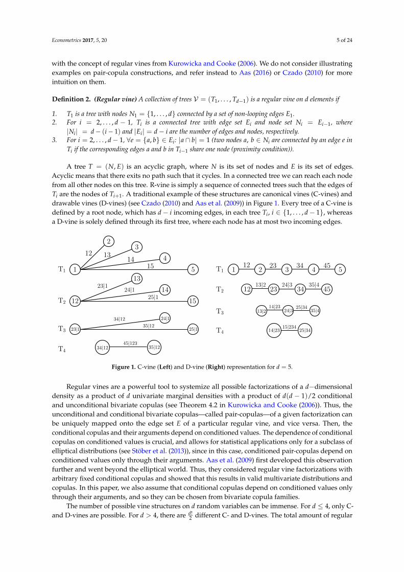
A tree T = (N, E) is an acyclic graph, where N is its set of nodes and E is its set of edges.Acyclic means that there exits no path such that it cycles. In a connected tree we can reach each nodefrom all other nodes on this tree. R-vine is simply a sequence of connected trees such that the edges ofTi are the nodes of Ti+1. A traditional example of these structures are canonical vines (C-vines) anddrawable vines (D-vines) (see Czado (2010) and Aas et al. (2009)) in Figure 1. Every tree of a C-vine isdefined by a root node, which has d− i incoming edges, in each tree Ti, i ∈ {1, . . . , d− 1}, whereasa D-vine is solely defined through its first tree, where each node has at most two incoming edges.

1

23

4

5

12

13

14

15

12 1314

15

23|1

24|1

25|1

23|124|1

25|1

34|1235|12

34|12 35|1245|123

1 2 3 4 512 23 34 45

12 23 34 4513|2 24|3 35|4

13|2 24|3 35|414|23 25|34

14|23 25|3415|234

T1

T2

T3

T4

T1

T2

T3

T4

Figure 1. C-vine (Left) and D-vine (Right) representation for d = 5.

Regular vines are a powerful tool to systemize all possible factorizations of a d−dimensionaldensity as a product of d univariate marginal densities with a product of d(d − 1)/2 conditionaland unconditional bivariate copulas (see Theorem 4.2 in Kurowicka and Cooke (2006)). Thus, theunconditional and conditional bivariate copulas—called pair-copulas—of a given factorization canbe uniquely mapped onto the edge set E of a particular regular vine, and vice versa. Then, theconditional copulas and their arguments depend on conditioned values. The dependence of conditionalcopulas on conditioned values is crucial, and allows for statistical applications only for a subclass ofelliptical distributions (see Stöber et al. (2013)), since in this case, conditioned pair-copulas depend onconditioned values only through their arguments. Aas et al. (2009) first developed this observationfurther and went beyond the elliptical world. Thus, they considered regular vine factorizations witharbitrary fixed conditional copulas and showed that this results in valid multivariate distributions andcopulas. In this paper, we also assume that conditional copulas depend on conditioned values onlythrough their arguments, and so they can be chosen from bivariate copula families.

The number of possible vine structures on d random variables can be immense. For d ≤ 4, only C-and D-vines are possible. For d > 4, there are d!

2 different C- and D-vines. The total amount of regular


vine structures has been computed by Morales-Nápoles et al. (2010), and is equal to d!2 · 2(

d−22 ). To select

conditional copulas on these graphical structures, we define the following sets as in Czado (2010).

Definition 3. (Conditioned and conditioning sets) For any edge e = {a, b} ∈ Ei of a regular vine V , thecomplete union of e is the subset

Ae ={

v ∈ N1 : ∀m = 1, . . . , i− 1, ∃ejm ∈ Em s.t. v ∈ ej1 ∈ · · · ∈ eji−1 ∈ e}

.

The conditioning set associated with e isDe = Aa ∩ Ab.

The conditioned sets associated with e are

i(e) = Aa \ De

j(e) = Ab \ De.

The copula for this edge will be denoted by

Ce := Ci(e),j(e)|D(e).

Given a regular vine, we specify a regular vine copula by assigning a (conditional) pair copula(with parameters) to each edge of the regular vine. In doing so, we follow Czado et al. (2012).

Definition 4. (Regular vine copula). A regular vine copula C = (V , B (V), θ (B (V))) in d dimensions is amultivariate distribution function such that for a random vector U = (U1, . . . , Ud)

′ ∼ C with uniform margins

1. V is a regular vine on d elements,2. B (V) = {Ce | e ∈ Em, m = 1, . . . , d− 1} is a set of d (d− 1) /2 copula families identifying the

unconditional distributions of Ui(e),j(e) as well as the conditional distributions of Ui(e),j(e) | UD(e),3. θ (B (V)) = {θe | e ∈ Em, m = 1, . . . , d− 1} is the set of parameter vectors corresponding to the copulas

in B (V).

To facilitate statistical inference, a matrix representation of R-vines was proposed byMorales-Nápoles et al. (2010) and further developed by Dissmann et al. (2013). To specify a d-dimensionalR-vine in matrix form, one needs several lower triangular d× d matrices: one that stores the structure ofthe R-vine, one with copula families, and another two with the first and second parameters.

For a d-dimensional R-vine, the matrix with the structure has the following form

M =

m1,1

.... . .

md−1,1 · · · md−1,d−1md,1 · · · md,d−1 md,d

,

where mi,j ∈ (1, . . . , d). The rules for reading from this matrix are as follows. The conditioned set foran entry mi,j is the entry itself and the diagonal entry of the column mj,j, whereas the conditioningset is composed of variables under the entry; i.e., for mi,j, the conditioned set will be

(mi,j, mj,j

), the

conditioning set is(

mi+1,j, . . . , md,j

). Thus, mi,j denotes the node

(mj,j, mi,j | mi+1,j, . . . , md,j

). We will

assume that the diagonal of M is sorted in descending order, which can always be achieved byreordering the node labels, so that we have mi,i = n− i + 1. To illustrate the R-vine matrix notation,we consider the C-vine from Figure 1 and give below its R-vine matrix representation.


54 43 3 32 2 2 21 1 1 1 1

The first column encodes the following nodes

1. Node 54 | 321 is saved through m1,1, m2,1 given m3,1, m4,1 and m5,1;2. Node 53 | 21 is saved through m1,1, m3,1 given m4,1 and m5,1;3. Node 52 | 1 is saved through m1,1, m4,1 given m5,1;4. Node 51 is saved through m1,1, m5,1.

In the sequel, we utilize C-vines to capture the cross-sectional dependence of a multivariate timeseries at any time point t. To capture the dependence between multivariate observations, the firsttree of the C-vine for multivariate observation at time point t is connected to the first trees of theC-vines for existing neighboring multivariate observations at time points t− 1 and t + 1 with one edge,correspondingly. This results in the first tree of an R-vine for all multivariate observations treated asone huge sample point. Depending on the choice of C-vines and the connection of the first trees, thecopula autoregressive model of Brechmann and Czado (2015) from the next section can be obtained.

Finally, note that the information on copula families and their parameters is similarly storedin lower triangular d× d matrices. Each element of the R-vine matrix below the diagonal specifiesa conditional or unconditional pair-copula depending on the diagonal entry above it. The familyand parameters of this pair-copula are now entered at the same entry place of matrices for copulafamilies and parameters. Since the diagonal entries of the R-vine matrix alone do not determineany pair-copulas, no entries for copula family and parameters matrices are needed on the diagonal.To avoid confusion with space character, we fill the main diagonal with ∗ sign.

4. Copula Autoregressive Model

R-vines have been mostly used to model contemporaneous dependence. We now present a specialR-vine structure called copula autoregressive (COPAR) model from Brechmann and Czado (2015)which is designed to capture cross-sectional, serial, and cross-serial dependence in multivariatetime series, and allows a general Markovian structure. Let {Ft, Gt}t=1,...,T be an observable bivariatestationary time series. To illustrate how the two individual time series are interdependent, considerthe mapping of dependencies for T = 4 in Figure 2. Vertical solid lines represent the cross-sectionaldependence, horizontal solid lines and curved lines represent the serial dependence for each timeseries, and dotted and dashed lines represent the cross-serial dependence.

F1 F2 F3 F4

G1 G2 G3 G4

Figure 2. Dependencies of a simultaneous bivariate time series for T = 4. Vertical solid lines:cross-sectional dependence; horizontal solid lines and curved lines: serial dependence for each timeseries; dotted and dashed lines: cross-serial dependence.

Traditionally, R-vines were used to model only the cross-sectional dependence (pictured by thevertical solid lines in Figure 2), but under the assumption that other dependencies are absent (i.e., data


is iid). The COPAR model is designed to additionally capture serial and cross-serial dependence.The following definition of a COPAR model without Markovian structure for two time series adoptedto our notation is taken from Brechmann and Czado (2015). The vectors (Fs, . . . , Ft) and (Gs, . . . , Gt)

are denoted as Fs:t and Gs:t, respectively.

Definition 5. (COPAR model for the bivariate case) The COPAR model for stationary continuous timeseries {Ft}t=1,...,T and {Gt}t=1,...,T has the following components.

(i) Unconditional marginal distributions of each time series are independent of time.(ii) An R-vine for the serial and between-series dependence of {Ft}t=1,...,T and {Gt}t=1,...,T , where the following

pairs are selected.

1. Serial dependence of {Ft}t=1,...,T : The pairs of serial D-vine copula for F1, . . . , FT ; that is,

Fs, Ft | F(s+1):(t−1), 1 ≤ s < t ≤ T. (2)

2. Between-series dependence:Fs, Gt | F(s+1):t, 1 ≤ s ≤ t ≤ T, (3)

andGs, Ft | F1:(t−1), G(s+1):(t−1), 1 ≤ s < t ≤ T. (4)

3. Conditional serial dependence of {Gt}t=1,...,T : The pairs of a serial D-vine copula for G1, . . . , GTconditioned on all previous values of {Ft}t=1,...,T ; that is,

Gs, Gt | F1:t, G(s+1):(t−1), 1 ≤ s < t ≤ T. (5)

Pair copulas of the same lag length t− s, t ≥ s, are identical. We associate

1. copula CFt−s := CFs ,Ft |F(s+1):(t−1)

with (2),2. copulas CFG

t−s := CFs ,Gt |F(s+1):tand CGF

t−s := CGs ,Ft |F1:(t−1),G(s+1):(t−1)with (3) and (4), respectively, and

3. copula CGt−s := CGs ,Gt |F1:t ,G(s+1):(t−1)

with (5).

Let us explain the above definition on an example of a bivariate time series {Ft, Gt}t=1,...,4 withfour observations. Using a D-vine, Equation (2) captures the dependence structure of F1, F2, F3, and F4

expressed by the top lines connecting them in Figure 2. For s = 1 and t = 4, Equation (3) describesthe conditional dependence between F1 and G4 conditioned on F2, F3, and F4. Thus, Equation (3)captures the conditional dependence between Fs and Gt for s < t reflected by the dashed lines inFigure 2. For s = t, Equation (3) models the unconditional dependence between Ft and Gt expressedby the vertical lines. Similarly, Equation (4) describes the conditional serial dependence betweenunivariate time series illustrated by the dotted lines in Figure 2. However, Equations (3) and (4) are notsymmetric with respect to conditioned sets. In particular, the conditional distribution of Fs and Gt fors < t is independent of G1, . . . , Gt−1. This already indicates that the first time series {Ft}t=1,...,T playsa key role in the stochastic dynamics of the time series, since it is sufficient to describe the conditionaldependence between Fs and Gt for s < t. Therefore, the univariate time series are not interchangeable.Using a D-vine, Equation (5) finally describes the dependence structure of G1, G2, . . . , GT (connectingbottom lines in Figure 2) conditioned on F1, F2, . . . , FT . Due to the property that copulas of same laglength are identical, the COPAR model defines a stationary bivariate time series.

Now, we expand the COPAR model to an arbitrary number of variables with Markov structure.We consider q univariate time series observed at T time points; that is, {F1,t}t=1,...,T , . . . ,

{Fq,t}

t=1,...,T .

We denote a random vector of q variables observed at times t = 1, . . . , T as Ft =(

F1,t, . . . , Fq,t)′, time

series of individual variables for i = 1, . . . , q as F(i) = (Fi,1, . . . , Fi,T), and also introduce a vectorFl:q,s:t =

(Fl,s, . . . , Fl,t, . . . , Fq,s, . . . , Fq,t

). Finally, we define a COPAR(k) model, which is COPAR model

for a multivariate time series with a Markovian structure of the k-th order. Since unobservable factors


in Section 2 are also denoted by Ft, our notation above should not lead to a confusion. Our modelingapproach utilizes estimated factors even if they are not observed. Therefore, for reader convenience,we denote here multivariate time series with Ft and present COPAR models in terms of Ft.

Definition 6. (COPAR(k) model for q time series of length T) The COPAR(k) model for a q-dimensionalstationary time series Ft ∈ Rq×1, t = 1, . . . , T has the following components.

(i) Unconditional marginal distributions of each time series are independent of time.(ii) An R-vine for the serial and between-series dependence of Ft ∈ Rq×1, t = 1, . . . , T, where the following

pairs are selected.

1. Serial dependence of F(1): The pairs of serial D-vine copula for F1,1, . . . , F1,T ; that is,

F1,s, F1,t | F1,(s+1):(t−1), 1 ≤ s < t ≤ T.

2. Between-series dependence of F(i) and F(j) for i < j, i, j = 1, . . . , q:

Fi,s, Fj,t | F1:(i−1),1:t, Fi,(s+1):t 1 ≤ s ≤ t ≤ T,

andFj,s, Fi,t | F1:(i−1),1:t, Fi:(j−1),1:(t−1), Fj,(s+1):(t−1) 1 ≤ s < t ≤ T,

3. Conditional serial dependence of F(i) for 2 ≤ i ≤ q:

Fi,s, Fi,t | F1:(i−1),1:t, Fi,(s+1):(t−1), 1 ≤ s < t ≤ T,

whereas

(a) copulas ∀i and for lag length t− s > k are independent copulas,(b) copulas for i, j = 1, . . . , q for the same lag length t− s, t ≥ s are identical.

Definition 6 introduces the COPAR model, if a) is neglected. The dependence of F(i) is modeledconditioned on F(1), . . . , F(i−1), and consequently, the order of variables cannot be simply interchanged.The number of pair copulas in COPAR models for time series with Markovian structure does notdepend on T, and is less than the number needed for a general R-vine. With respect to the number ofpair-copulas, the following result from Brechmann and Czado (2015) holds.

Lemma 1. The number of copulas needed for a COPAR(k) model of q univariate time series is q2k + q(q−1)2 .

Note, the number of parameters in a VAR(k) for the between-series dependence of q timeseries—not counting parameters for marginal distributions—is equal to the number of pair-copulasin a COPAR(k) model. Therefore, the number of parameters in a COPAR(k) model is bounded bya multiple of the number of VAR parameters, depending on the number of parameters of the involvedcopula families. In contrast, a general R-vine requires qT(qT−1)

2 pair-copulas, resulting in a huge numberof parameters.

Figure 3 illustrates the first 4 trees of a COPAR model for three univariate time series Ft, Gt, andHt with T = 4 (i.e., for four observations). Examining the first tree, we observe that it is a sequence ofconnected C-vines, where the central nodes are the time points of the first factor Ft. Thus, unconditionalcontemporaneous dependence is modeled with a C-vine.


F1

F1,F3|F2

F1,H1

F1,G2|F2

F1,G1

F1,F2 F2,F3

F2,G2 F2,H2

F3,F4

F3,G3 F3,H3

F4,G4 F4,H4

F1,H2|F2

G1,H1|F1

F2,G1|F1

F2,G3|F3 F2,H3|F3

F2,F4|F3

F3,G4|F4 F3,H4|F4

G2,H2|F1:2 F3,G2|F1:2

F2,H1|F1,G1 G1,G2|F1:2

F1,F4|F2:3

F1,G3|F2:3 F1,H3|F2:3

F2,G4|F3:4

F2,H4|F3:4

G1 H1

F2 F3 F4

G2 H2

G3 H3

G4 H4

Figure 3. R-vine structure of three-dimensional time series for T = 4.

The matrix representation of the R-vine structure of this COPAR model is given by

H4

H1 G4

H2 H1 F4

H3 H2 H1 H3

G1 H3 H2 H1 G3

G2 G1 H3 H2 H1 F3

G3 G2 G1 G1 H2 H1 H2

G4 G3 G2 G2 G1 H2 H1 G2

F1 F1 G3 G3 G2 G1 G1 H1 F2

F2 F2 F1 F1 F1 G2 G2 G1 H1 H1

F3 F3 F2 F2 F2 F1 F1 F1 G1 G1 G1

F4 F4 F3 F3 F3 F2 F2 F2 F1 F1 F1 F1

and the matrix of copulas for three-dimensional COPAR model is given by

∗CH

3 ∗CH

2 CHG3 ∗

CH1 CHG

2 CHF3 ∗

CGH3 CHG

1 CHF2 CH

2 ∗CGH

2 CG3 CHF

1 CH1 CGH

2 ∗CGH

1 CG2 CGF

3 CGH2 CGH

1 CHF2 ∗

CGH CG1 CGF

2 CGH1 CG

2 CHF1 CH

1 ∗CFH

3 CFG3 CGF

1 CGH CG1 CGF

2 CGH1 CGH

1 ∗CFH

2 CFG2 CF

3 CFH2 CFG

2 CGF1 CGH CG

1 CHF1 ∗

CFH1 CFG

1 CF2 CFH

1 CFG1 CF

2 CFH1 CFG

1 CGF1 CGH ∗

CFH CFG CF1 CFH CFG CF

1 CFH CFG CF1 CFH CFG ∗

.

If a COPAR(k) model is estimated based on the first T multivariate observations, then it can easilybe extended to T + 1 observations. This allows us to sample the (T + 1)-th observation according tothe estimated dependence structure between the k−th subsequent multivariate observations. Let us


illustrate this point for a COPAR(1) model and the above example with three univariate time series.The matrix representation of the R-vine structure of this COPAR(1) model remains unchanged, andthe matrix of copulas for three-dimensional COPAR(1) model is now simplified to the matrix in (6),where 0 stands for independence copula

∗0 ∗0 0 ∗

CH1 0 0 ∗0 CHG

1 0 0 ∗0 0 CHF

1 CH1 0 ∗

CGH1 0 0 0 CGH

1 0 ∗CGH CG

1 0 CGH1 0 CHF

1 CH1 ∗

0 0 CGF1 CGH CG

1 0 CGH1 CGH

1 ∗0 0 0 0 0 CGF

1 CGH CG1 CHF

1 ∗CFH

1 CFG1 0 CFH

1 CFG1 0 CFH

1 CFG1 CGF

1 CGH ∗CFH CFG CF

1 CFH CFG CF1 CFH CFG CF

1 CFH CFG ∗

. (6)

Now, if we want to expand this COPAR(1) model by adding a new time point (i.e., T → T + 1—inour case, 4→ 5), the matrix representation will be changed as follows

1. Add three blank columns to the left of the matrix and add (HT+1, GT+1, FT+1) to the diagonal;2. Under FT+1 comes (H1, . . . , HT)

′, then (G1, . . . , GT)′ and (F1, . . . , FT)

′;3. Under GT+1 comes (H1, . . . , HT)

′, then (G1, . . . , GT)′ and (F1, . . . , FT+1)

′;4. Under HT+1 comes (H1, . . . , HT)

′, then (G1, . . . , GT+1)′ and (F1, . . . , FT+1)

′.

The expanded matrix representation is as follows, where the new columns are marked in bold:

H5

H1 G5

H2 H1 F5

H3 H2 H1 H4

H4 H3 H2 H1 G4

G1 H4 H3 H2 H1 F4

G2 G1 H4 H3 H2 H1 H3

G3 G2 G1 G1 H3 H2 H1 G3

G4 G3 G2 G2 G1 H3 H2 H1 F3

G5 G4 G3 G3 G2 G1 G1 H2 H1 H2

F1 F1 G4 G4 G3 G2 G2 G1 H2 H1 G2

F2 F2 F1 F1 F1 G3 G3 G2 G1 G1 H1 F2

F3 F3 F2 F2 F2 F1 F1 F1 G2 G2 G1 H1 H1

F4 F4 F3 F3 F3 F2 F2 F2 F1 F1 F1 G1 G1 G1

F5 F5 F4 F4 F4 F3 F3 F3 F2 F2 F2 F1 F1 F1 F1

.

We also expand the matrix of copulas by adding three columns to the left of (6), as follows:


∗0 ∗0 0 ∗0 0 0 ∗

CH1 0 0 0 ∗

0 CHG1 0 0 0 ∗

0 0 CHF1 CH

1 0 0 ∗0 0 0 0 CHG

1 0 0 ∗CGH

1 0 0 0 0 CHF1 CH

1 0 ∗CGH CG

1 0 CGH1 0 0 0 CGH

1 0 ∗0 0 CGF

1 CGH CG1 0 CGH

1 0 CHF1 CH

1 ∗0 0 0 0 0 CGF

1 CGH CG1 0 CGH

1 CGH1 ∗

0 0 0 0 0 0 0 0 CGF1 CGH CG

1 CHF1 ∗

CFH1 CFG

1 0 CFH1 CFG

1 0 CFH1 CFG

1 0 CFH1 CFG

1 CGF1 CGH ∗

CFH CFG CF1 CFH CFG CF

1 CFH CFG CF1 CFH CFG CF

1 CFH CFG ∗

.

Thus, the three new columns are just replications of the previous three columns by expanding theuninterrupted sequences of zeros with an additional zero.

5. Empirical Application

The idea to model asset returns with factors arising from some observed data and idiosyncraticcomponents is quite popular in modern finance theory. The most prominent example is the capitalasset-pricing model (CAPM) of Sharpe (1964), Litner (1965), Mossin (1966), and Treynor (2012), which isa one-factor model with the market return as the only common driver of asset prices. Another well-knownapproach is the arbitrage pricing theory (APT) of Ross (1976). In this case, a multi-factor model describesthe return of an asset as the sum of an asset-specific return, an exposure to systematic risk factors, and anerror term. A third example is Stock and Watson (2002a), who extracted factors from a large number ofpredictors to forecast the log-returns of the Federal Reserve Board’s Index of Industrial Production.Ando and Bai (2014) provide further empirical evidence that stock returns are related to macro- andmicroeconomic factors. In this section, latent factors from U.S. macroeconomic data are extractedand then used for portfolio optimization. We consider 35 assets from S&P 500, which are classifiedas “Industrials” according to Global Industry Classification Standard. We assume that the estimatedfactors have the most prediction power for these assets.

The U.S. panel data includes such economic indicators as government bond yields along the curve,currency index, main commodity prices, indicators of money stock, inflation, consumer consumption,and industrial production gauges. Altogether, we have 22 time series listed in Appendix B. Each seriescontains monthly data from 31 January 1986 to 30 November 2016, 371 data points in total. Next, we splitthe panel data into financial and macroeconomic groups according to Tables A2 and A3 in Appendix B.In the sequel, each time series is transformed in order to eliminate trends and achieve its stationarity.Tables A2 and A3 in Appendix B also contain information on considered data transformations. Further,we consider three factor models: separately for the two groups of the panel data, and one joint modelfor all monthly indicators. Thereby, we aim to illustrate that modeling nonlinear dependence betweenestimated factors of different groups of panel data with COPAR may lead to a better asset allocation.

We consider the following three DFMs for i = f in, macro, all:

X(i)t = Λ(i)F(i)

t + ε(i)t (7)

F(i)t = A(i)F(i)

t−1 + u(i)t , (8)


where X(i)t ∈ Rmi×1 collects observed macroeconomic data and F(i)

t ∈ Rqi×1 is the vector of factors.The dimension mi of the panel data for i = f in, macro and all is equal to 9, 13 and 22, respectively.

In the first step, we estimate three DFMs—one for each group (macro and financial) and for the fullpanel data. The starting time frame is from January 1986 to December 2005, and expands successivelyby one month until November 2016 is reached. For the three DFMs, we apply the EM-Algorithmfrom Section 2 to the panel data from each expanding time window and obtain a monthly sequenceof estimated factors for each month of the considered time period. For i = f in, macro, and all, theEM-Algorithm requires the factor dimension qi, which is not known. In what follows, we perform themodel selection for the factor dimension.

The dimension of factors is selected using principal components analysis (see Jolliffe 2002).We choose the number of principal components (PCs) such that we capture more than 95% of theempirical data variance, based on the initial time frame from January 1986 to December 2005. Figure 4illustrates the fraction of variance captured by eight or fewer PCs for the considered time window.Thus, two factors are sufficient for the financial group to capture 95.4% of the corresponding datavariability. For macroeconomic indicators, we need three factors (96.5% of variability), while fourfactors are enough for the whole panel data (96.2% of variability).

●

●

●

● ● ● ● ●

●

●●

● ● ● ● ●

0.7

0.8

0.9

1.0

2 4 6 8

Number of PCs

Per

cent

age

of e

xpla

ined

var

ianc

e

group●● fin

joint

macro

Figure 4. Amount of principal components (PCs) vs. captured variance for three dynamic factormodels (DFMs) considered up to December 2005.

In general, the latent factors of DFMs may follow a VAR model of order p. Initiated by a referee’scomment, we also consider autoregressive order p = 2 for the joint DFM with all monthly indicatorsand compare its forecasting performance for p = 1 and p = 2. Our decision criterion is based on theroot-mean-square error (RMSE) of point predictions defined for univariate observations x1, . . . , xT∗ as

RMSE =

√∑T∗

t=1 (xt − xt)2

T∗,

where x1, . . . , xT∗ are predicted values. Thus, we compute the RMSE for each time series and take theiraverage value. Thereby, our first prediction is done for January 2006 and ends in November 2016,resulting in 131 point forecasts. The averaged values of the RMSE for p = 1 and for p = 2 are 0.0302and 0.0306, respectively. Therefore, our initial choice of p = 1 is justified.

Figure 5 illustrates the correlation coefficients of the financial and macro factors filtered from dataup to October 2010. The estimated factors show some moderate linear dependence within groups anda weak linear dependence between groups. Note that dynamic factor models assume factors to bemultivariate normally distributed. Nevertheless, the estimated factors could exhibit non-Gaussiandependence, which we aim to capture using the COPAR model.


Fin1

Fin2

Macro1

Macro2

Macro3

Fin1 Fin2 Macro1 Macro2 Macro3

−1.0

−0.5

0.0

0.5

1.0value

2010−10−31

Figure 5. Correlations heatmap as of October 2010.

To improve the joint forecasting of asset returns at month t, for a subsequent month, we link thetwo factor models; namely, we capture the dependence structure of the estimated factors with a COPARmodel. Thereby, we combine the estimated factors from two groups as a single five-dimensional vectorfor each data time window. We put the financial factors first, then the macroeconomic. Using fittedmarginal normal distribution functions, the filtered factors are translated to copula data.

We consider a COPAR(1) model, since the transition equation of the DFMs is supposed to be a VAR(1).Further, Brechmann and Czado (2015) discuss a sophisticated copula family selection procedure for twotime series. Here, we follow a more simple approach consisting of three steps. In the first step, theselection of copulas for contemporaneous cross-sectional dependence of the filtered factors is done byneglecting serial dependence. Note that the cross-sectional dependence is described by a C-vine withfixed order of variables. Therefore, we only have to select copula families of pair-copulas. Thus, weconsider the estimated five-dimensional factors as iid data and perform sequential selection of copulafamilies for each pair-copula using Akaike information criterion. Copula families for the pair-copulasassociated with the first tree of the C-vine are selected first, then with the second tree, and so on.For more details on model selection for C-vines, we refer to Czado et al. (2012). Equation (9) presentsthe selected copula families for cross-sectional dependence in R-vine matrix notation until December2005 (for copula families in (9), see Appendix C):

Families =

∗2 ∗5 2 ∗

16 3 2 ∗16 2 36 2 ∗

. (9)

It is remarkable that none of the selected copula families in (9) is Gaussian. Moreover, only 0.5%of families selected for cross-sectional dependence for all expending time windows are theGaussian copula.

In the second step, we use the Gaussian copulas as conditional pair-copulas to model thetemporal dependence of the filtered factors. Note that this simple approach does not imply thatthe joint distribution of the time-shifted factors is Gaussian except for the first component of F( f in)

t ;

i.e., F( f in)1,t1

, F( f in)1,t2

, . . . , F( f in)1,tk

. Non-Gaussian pair-copulas for cross-sectional dependence destroy the

Gaussianity of the time-shifted factors, and only the joint distribution of the first component of F( f in)t

remains Gaussian. In the third step, the R-vine matrix of the COPAR(1) model for the estimated factors


(F( f in)′

t , F(macro)′

t

)′is constructed, and the maximum likelihood estimation is performed. Copula

selection and parameter estimation of the COPAR model for the factors is done for every expandingwindow of data; that is, as soon as the DFMs for both groups are estimated and the latent factors arefiltered out. Finally, note that we also test Granger causality between components of the multivariate

time series(

F( f in)′

t , F(macro)′

t

)′in the whole time period, and can confirm it. For this, we regress

univariate series of(

F( f in)′

t , F(macro)′

t

)′on the lagged values of

(F( f in)′

t−1 , F(macro)′

t−1

)′. Table A11 in

Appendix F summarizes all five linear regressions. For example, the first component of{

F( f in)t

}t=1,...,T

Granger causes almost all other univariate time series at least at 10% of significance level with theexception of the second component of

{F(macro)

t

}t=1,...,T

.

Next, we present a conditional method for forecasting using COPAR, which follows Brechmannand Czado (2015) with a small modification. For a prediction time point, we simulate factors from theestimated COPAR model, but conditioned on the past values of the factors. The sampled factors arefurther used to forecast assets returns and to construct an optimal mean-variance portfolio. Since weassume an autoregressive order of one, it is enough to condition only on the last value of factors; i.e., we

condition only on FT( f in) and FT

(macro) to make a forecast for time point T + 1. The full algorithm forboth markets is given in Algorithm 1, employing notation F1:0,t = ∅.

Algorithm 1: Conditional method of forecasting using COPAR.

1. Estimate COPAR model based on the first T observations and get factor estimates

Ft =

(Ft

( f in)′ , Ft(macro)′

)′;

2. Set j = 1;3. Repeat the following steps

(a) If j = q + 1 then Stop;(b) Determine the estimated conditional density of Fj,T+1 | F1:q,T , F1:(j−1),T+1 on the

equidistant grid on (0, 1) with step ∆ = 10−4, i.e., for u = n10000 , n = 1, . . . , 9999;

c(Φ1 (F1,T+1) , . . . , Φj−1

(Fj−1,T+1

), u, Φ1

(F1,T

), . . . , Φq

(Fq,T

))f(

F1,T+1, . . . , Fj−1,T+1, F1,T , . . . , Fq,T)

·j−1

∏k=1

φk (Fk,T+1) · φj

(Φ−1

j (u))·

q

∏k=1

φk(

Fk,T)

,

where φk and Φk are the estimated Gaussian density and distribution function of latentfactor F(i)

k,t ;(c) Determine the estimated conditional cumulative distribution function on the above grid;(d) Simulate 10,000 Fj,T+1 from the estimated conditional cumulative distribution function

and set forecast Fj,T+1 to their empirical mean;(e) Set j = j + 1 and go to (a);

To illustrate the idea behind this method, we consider a small-scale example of two variables Gt

and Ht. Let us assume that we observe some values of these two random variables at time point t;i.e., Gt = Gt, Ht = Ht. We want to find the distribution of Gt+1 and Ht+1 conditioned on the observedvalues that we have observed. For this purpose, we consider the decomposition of the conditionaldistribution of Gt+1, Ht+1 | Gt = Gt, Ht = Ht given by


F(Gt+1, Ht+1 | Gt = Gt, Ht = Ht

)= F

(Gt+1 | Gt = Gt, Ht = Ht

)F(

Ht+1 | Gt = Gt, Ht = Ht, Gt+1 = Gt+1)

,

where Gt+1 is some forecast. One has a free choice for forecast methods for Gt+1. As Brechmann andCzado (2015), we opt for the conditional mean estimated by the sample mean. Next, we first estimatethe conditional density, and then, the conditional distribution function. For this simple case of twovariables Gt and Ht, the estimated density f of Gt+1 | Gt = Gt, Ht = Ht on a grid from 0 to 1 with step0.0001 is estimated. Then, we search for the estimated distribution function F. With f and F, one canestimate the mean.

In the next step, we use the estimated factors to model the asset returns of 35 industrial stocks fromS&P 500 and the sampled factors to construct an optimal portfolio in the mean-variance frameworkfor each expanding time window starting from January 2006 up to November 2016. We consider andestimate the following model for each asset return j = 1, . . . , 35:

rj,t = αj,0 + αj,1rj,t−1 + Γ′j Ft + vj,t, (10)

where the constants αj,0, αj,1, and the vector Γj constitute unknown regression parameters and theerrors vj,t are assumed to be iid Gaussian with respect to t. The error terms vj,t are assumed to beindependent across j due to the dimensionality of the error covariance matrix. Moreover, we treat alllinear regression separately for each asset j due to the dimensionality of regression parameters andcouple them with the common estimated factors. In Section 2, we have pointed out that the estimatedfactors are unique up to a rotation with an orthogonal matrix R; i.e., RR′ = R′R is an identity matrix.Since Γ′j Ft = Γ′jR

′RFt holds, the impact of the rotated and unrotated estimated factors together withtheir regression coefficients on asset returns remains the same.

To construct an optimal portfolio in the mean-variance framework, we determine portfolio weightsw at month t by solving the following optimization problem with respect to w:

max w′ ·E [rt+1]

s.t.

1T ·w = 1, w ≥ 0,

w′ ·Var [rt+1] ·w ≤ σ2monthly,

where rt = (r1,t, . . . , r35,t)′ is a vector of asset returns at t, E [rt+1] and Var [rt+1] are the expectation

and covariance matrix of rt+1. Thus, our optimal portfolio does not allow short-selling.Since E [rt+1] and Var [rt+1] are unknown at month t, we estimate them with four different

methods, resulting in four portfolios. The first portfolio is the COPAR portfolio, which is constructedusing asset returns modeled with (10). In this case, E [rt+1] and Var [rt+1] are empirically estimatedat time point t based on 10,000 sampled factors from the COPAR model and 10,000 sampled errorsfrom the estimated univariate Gaussian distribution. The second portfolio is the DFM portfoliosimilarly constructed with sampled factors from the estimated stationary distribution (1) for (7)–(8)and i = all (i.e., the DFM for the full panel data). The third portfolio—called independent DFM—usessampled factors from the estimated stationary distribution (1) for (7)–(8) and i = f in, macro; i.e.,

assets returns are driven by(

F( f in)′

t , F(macro)′

t

)′. The fourth portfolio is the historical portfolio, which

employs the empirical mean and covariance matrix based on the data up to time t. We consider thehistorical portfolio as a benchmark. Finally note that the comparison of these four portfolios enablesthe assessment of the economic relevance of factors.

For the above mean-variance optimization problem, we choose three monthly volatilitiesσmonthly = 2.89%, 3.75%, 4.62%, which correspond to annual volatilities of σ = 10%, 13%, 16%.These choices of σ’s are practically reasonable, and the optimizer diversifies the portfolio for them. For


higher values of σ, the optimal portfolio consists of only one stock, if no constraints on maximal weightsare imposed. We start to determine an optimal portfolio for the panel data up to January 2006. Then, wesequentially expand the time window by one month and find optimal weights for the considered fourportfolios and chosen level of volatilities. The performance of the four portfolios with initial investmentof 1 USD during the out-of-sample time period up to November 2016 is illustrated in Figure 6.

1.0

1.5

2.0

2.5

1

2

3

1

2

3

2005

−12

−31

2006

−06

−30

2006

−12

−31

2007

−06

−30

2007

−12

−31

2008

−06

−30

2008

−12

−31

2009

−06

−30

2009

−12

−31

2010

−06

−30

2010

−12

−31

2011

−06

−30

2011

−12

−31

2012

−06

−30

2012

−12

−31

2013

−06

−30

2013

−12

−31

2014

−06

−30

2014

−12

−31

2015

−06

−30

2015

−12

−31

2016

−06

−30

2016

−11

−30

Portfolio COPAR DFM Hist Ind

10%

13%

16%

Figure 6. Performance of four portfolios with initial investment of 1 USD over the out-of-sample timeperiod from January 2006 to November 2016 for σ = 10%, 13%, 16%. COPAR: copula autoregressive;Hist: historical; Ind: independent DFM.


We observe that the COPAR portfolio outperforms the DFM, independent DFM, and historicalportfolios. Further, two portfolios based on DFMs deliver a higher overall return than the historicalportfolio, and the independent DFM (abbreviated in Figures and Tables as ind) is preferred over theDFM portfolio.

To compare the four portfolios, we consider several portfolio performance and risk measuressummarized in Appendix D. First, note that observed standard deviations of portfolio returns arehigher than prespecified ones. This is natural due to the prediction error. According to the Sharpe andOmega ratio, the COPAR portfolio is preferred over all remaining portfolios. For both risk measures, theindependent DFM portfolio outperforms the DFM portfolio. We explain this finding with a fortunatesplit of the panel data. Further, if we consider 95% Value at Risk (VaR) and 95% Conditional Value atRisk (CVaR), then the historical portfolio outperforms the others except for one case. For σ = 16% and95% VaR, the COPAR portfolio is slightly superior.

To statistically assess the differences in the Sharpe ratios, we perform the Jobson–Korkie Testfrom Jobson and Korkie (1981). The null hypothesis of this test is that the Sharpe ratios of the twoconsidered portfolios are equal. The normalized and centered test statistics are asymptotically Gaussiandistributed with mean 0 and variance 1 under the null hypothesis. If the null hypothesis is rejected,then there is significant statistical evidence for different Sharpe ratios. Appendix E presents resultsof the Jobson–Korkie Test for all pairs of portfolios and σ = 10%, 13%, 16%. The COPAR portfoliosignificantly outperforms the independent DFM portfolio, and this advocates our approach to modelestimated factors with a COPAR model. For σ = 10% and σ = 13%, we do not see a statisticallysignificant difference in Sharpe ratios for historical and COPAR portfolios. We explain this findingwith lower standard deviations of the historical portfolio returns.

6. Conclusions and Final Remarks

This paper applies copulas to capture the dependence structure of estimated latent factors fromdynamic factor models. The proposed modeling approach is especially convenient when several factormodels under consideration are estimated separately. In this context, we combine the filtered latentfactors with the COPAR model of Brechmann and Czado (2015), which results in a non-Gaussiandependence between the factors. The gained flexibility of the factor dependence is then used formodeling asset returns and building optimal mean-variance portfolios.

In our empirical study, we consider U.S. panel data consisting of 9 financial and 13 macroeconomicmonthly observable indicators. The nature of indicators suggests the consideration of two separatedynamic factor models. We also treat a joint dynamic factor model for all indicators. Estimated factorsfrom the considered DFMs are used to model returns of 35 industrial stocks from S&P500. Then, factors’predictions from different models spanning almost 11 years are employed for portfolio optimization inthe mean-variance framework.

Our main contribution is a performance improvement of portfolios based on DFMs. For this,we propose to capture the dependence structure of filtered factors from DFMs with a COPAR model.This allows us to sample factor forecasts from the estimated COPAR model conditionally on past valuesof estimated factors. The gained factor predictions are then utilized to construct an optimal mean-varianceportfolio. Thus, we compare the COPAR-based portfolio with two portfolios derived from DFMs, as wellas with the classical mean-variance approach utilizing empirical means and covariance matrices. For theconsidered panel data and industrial stocks, we observe the outperformance of the COPAR portfolio interms of the total return, the Sharpe and Omega ratio. The superiority of the COPAR-portfolio in termsof the Sharpe ratio is even statistically significant for several portfolio comparisons.

A possible improvement of the proposed approach is its extension with a model selectioncriterion for a general R-vine, which best captures the cross-sectional and temporal dependence.Thus, one departs from the COPAR model and generalizes it as well as the copula based multivariatetime series models of Beare and Seo (2015) and Smith (2015). In general, one can completely reviseour approach and alternatively develop dynamic versions of copula factor models as proposed by


Krupskii and Joe (2013) and Oh and Patton (2017) for iid data. The first methodology in this direction isprovided by Oh and Patton (2016), who capture cross-sectional dependence with time-varying copulas.These points are the subject of further research.

Acknowledgments: The authors want to thank the editor and the anonymous reviewers for their very helpfulsuggestions, which contributed essentially to the improvement of our manuscript. We are also obliged toEike Brechmann, who kindly provided R-code for COPAR model, which served as an inspiration for computerimplementation of this paper. Franz Ramsauer gratefully acknowledges the support of Pioneer Investments duringhis doctoral phase. Eugen Ivanov gratefully acknowledges the support of Deutsche Forschungsgemeinschaft duringhis doctoral phase. The authors also express gratitude to Leibniz-Rechenzentrum for providing computationalresources and assistance.

Author Contributions: Eugen Ivanov, Aleksey Min and Franz Ramsauer analyzed the data, constructed themodel and designed the estimation procedure. Asset allocation procedure based on dynamical factor modelsis proposed by Franz Ramsauer. Eugen Ivanov and Franz Ramsauer performed the complete computationalimplementation. All three authors wrote the paper.

Conflicts of Interest: The authors declare no conflict of interest. The sponsors had no role in the design of thestudy, in the collection, analyses, or interpretation of data, in the writing of the manuscript, and in the decision topublish the results.

Appendix A. Assets for Portfolio Optimization

Table A1. Assets used for portfolio construction.

Ticker Name GICS Sub Industry

CMI Cummins Inc. Industrial MachineryEMR Emerson Electric Company Industrial ConglomeratesCSX CSX Corp. Railroads

MMM 3M Company Industrial ConglomeratesBA Boeing Company Aerospace & Defense

CHRW C. H. Robinson Worldwide Air Freight & LogisticsCAT Caterpillar Inc. Construction & Farm Machinery & Heavy Trucks

CTAS Cintas Corporation Diversified Support ServicesDHR Danaher Corp. Industrial ConglomeratesDE Deere & Co. Construction & Farm Machinery & Heavy Trucks

ETN Eaton Corporation Industrial ConglomeratesEFX Equifax Inc. Research & Consulting ServicesGD General Dynamics Aerospace & DefenseGE General Electric Industrial ConglomeratesLLL L-3 Communications Holdings Industrial ConglomeratesLEG Leggett & Platt Industrial ConglomeratesNSC Norfolk Southern Corp. RailroadsPBI Pitney-Bowes Technology, Hardware, Software and Supplies

RTN Raytheon Co. Aerospace & DefenseRHI Robert Half International Human Resource & Employment ServicesROK Rockwell Automation Inc. Industrial ConglomeratesCOL Rockwell Collins Industrial ConglomeratesUNP Union Pacific RailroadsUPS United Parcel Service Air Freight & LogisticsUTX United Technologies Industrial ConglomeratesWM Waste Management Inc. Environmental ServicesTXT Textron Inc. Industrial ConglomeratesFLR Fluor Corp. Diversified Commercial ServicesFDX FedEx Corporation Air Freight & Logistics

PCAR PACCAR Inc. Construction & Farm Machinery & Heavy TrucksGWW Grainger (W.W.) Inc. Industrial MaterialsMAS Masco Corp. Building Products

R Ryder System Industrial ConglomeratesLMT Lockheed Martin Corp. Aerospace & DefenseNOC Northrop Grumman Corp. Aerospace & Defense


Appendix B. Underlying Panel Data

In the following tables, FRED stands for Federal Reserve Bank of St. Louis.

Table A2. U.S. financial indicators.

Indicator Description Transformation Source

USA Treasury 3 m Yield of U.S. government bonds with maturity of3 months

Monthly change FRED

USA Treasury 1y Yield of U.S. government bonds with maturity of 1 year Monthly change FRED

USA Treasury 2y Yield of U.S. government bonds with maturity of 2 years Monthly change FRED





Gold Gold Fixing Price 10:30 A.M. (London time) inLondon Bullion Market, based in U.S. Dollars. Return FRED

WTI Crude Crude Oil Prices: West Texas Intermediate(WTI)—Cushing, Oklahoma. Return FRED

Table A3. U.S. macroeconomical indicators.

Indicator Description Transformation Source

M1 U.S.

Narrow money (M1) includes currency, i.e., banknotes andcoins, as well as balances which can immediately be

converted into currency or used for cashless payments, i.e.,overnight deposits.

Return FRED

M2 U.S.

“Intermediate” money (M2) comprises narrow money (M1)and, in addition, deposits with a maturity of up to two years

and deposits redeemable at a period of notice of up tothree months.

Return FRED

Unemployment Unemployment rate Return FRED

CPIConsumer Price Index (CPI) measures changes in the price

level of a market basket of consumer goods and servicespurchased by households.

Return FRED

PPI Producer Price Index (PPI) measures the average changes inprices received by domestic producers for their output Return FRED

PCE Measures goods and services purchased by U.S. residents Return FRED

Personal saving ratePersonal saving as a percentage of disposable personal

income (DPI), frequently referred to as “the personal savingrate,” is calculated as the ratio of personal saving to DPI.

Return FRED

Payrolls All Employees: Total Nonfarm Payrolls. Return FRED

Unemployment Unemployment Return FRED

Initial claims Initial claims Return FRED

Housing Starts Housing Starts Return FRED

Capacity utilization Capacity utilization Return FRED

Dollar Index Trade Weighted U.S. Dollar Index Return FRED


Appendix C. Copula Families

Table A4. Copula families as numbered in the R-package VineCopula.

Number Family

0 Independence copula1 Gaussian copula2 Student’s t copula3 Clayton copula4 Gumbel copula5 Frank copula6 Joe copula13 Rotated Clayton copula (180 degrees; “survival Clayton”)14 Rotated Gumbel copula (180 degrees; “survival Gumbel”)16 Rotated Joe copula (180 degrees; “survival Joe”)23 Rotated Clayton copula (90 degrees)24 Rotated Gumbel copula (90 degrees)26 Rotated Joe copula (90 degrees)33 Rotated Clayton copula (270 degrees)34 Rotated Gumbel copula (270 degrees)36 Rotated Joe copula (270 degrees)

Appendix D. Portfolio Characteristics

Table A5. Portfolio characteristics for annual volatility σ = 10%.

COPAR DFM ind DFM hist

Log-return (Total) 1.0578 0.9592 0.9661 0.6982Log-return (Monthly) 0.0079 0.0072 0.0072 0.0050Std. deviation (Annual) 0.1775 0.1808 0.1799 0.1571Sharpe Ratio (Monthly) 0.1816 0.1665 0.1668 0.1354Omega Ratio (Monthly) 1.6389 1.5617 1.5696 1.442095% VaR −0.1930 −0.1916 −0.1993 −0.189995% CVaR −0.1965 −0.1956 −0.20373 −0.1924








Appendix E. Significance Tests for Sharpe Ratios

Table A8. Test statistics of the Jobson–Korkie Test for pairwise comparison of Sharpe ratios for fourportfolios from the mean-variance optimization problem with σ = 10%.

COPAR DFM ind DFM

COPARDFM 1.02ind DFM 1.89 * 0.03hist 1.04 0.66 0.70

Note: * p-value < 0.1, ** p-value < 0.05, *** p-value < 0.01.


COPAR DFM ind DFM

COPARDFM 1.62ind DFM 2.20 ** 0.42hist 1.30 0.71 0.82



COPAR DFM ind DFM

COPARDFM 2.03 **ind DFM 2.27 ** 0.95hist 1.95 * 1.39 1.60


Appendix F. Testing for Granger Causality

Table A11. Summary of linear regressions for testing Granger causality. Columns contain estimate ofregression coefficients, and their standard errors are given in brackets.

Dependent Variable:

yF f in

1,t F f in2,t Fmacro

1,t Fmacro2,t Fmacro

3,t

(1) (2) (3) (4) (5)

F f in1,t−1

0.216 *** 0.655 *** −0.189 *** 0.076 −0.094 *(0.054) (0.060) (0.053) (0.056) (0.055)

F f in2,t−1

0.086 ** 0.214 *** 0.052 −0.056 0.048(0.041) (0.045) (0.040) (0.042) (0.042)

Fmacro1,t−1

0.076 0.009 −0.385 *** 0.037 −0.104 **(0.047) (0.052) (0.046) (0.048) (0.048)

Fmacro2,t−1

0.077 * −0.006 0.020 −0.456 *** 0.024(0.046) (0.051) (0.045) (0.047) (0.047)

Fmacro3,t−1

−0.009 0.065 0.192 *** −0.045 −0.554 ***(0.043) (0.047) (0.042) (0.044) (0.044)

Constant 0.003 0.002 −0.0005 0.003 0.0002(0.052) (0.058) (0.051) (0.054) (0.053)

Observations 369 369 369 369 369R2 0.093 0.369 0.236 0.215 0.315Adjusted R2 0.080 0.360 0.225 0.204 0.305Residual Std. Error (df = 363) 1.003 1.109 0.981 1.030 1.026F Statistic (df = 5; 363) 7.428 *** 42.464 *** 22.408 *** 19.893 *** 33.339 ***

Note: * p-value < 0.1; ** p-value < 0.05; *** p-value < 0.01.


References

Aas, Kjersti. 2016. Pair-copula constructions for financial applications: A review. Econometrics 4: 43.Aas, Kjersti, Claudia Czado, Arnoldo Frigessi, Henrik Bakken. 2009. Pair-copula constructions of multiple

dependence. Insurance: Mathematics and economics 44: 182–98.Ando, Tomohiro, and Jushan Bai. 2014. Asset pricing with a general multifactor structure. Journal of Financial

Econometrics 13: 556–604.Banbura, Marta, and Michele Modugno. 2014. Maximum likelihood estimation of factor models on data sets with

arbitrary pattern of missing data. Journal of Applied Econometrics 29: 133–60.Beare, Brendan K., and Juwon Seo. 2015. Vine copula specifications for stationary multivariate markov chains.

Journal of Time Series Analysis 36: 228–46.Biller, Bahar, and Barry L. Nelson. 2003. Modeling and generating multivariate time-series input processes using

a vector autoregressive technique. ACM Transactions on Modeling and Computer Simulation 13: 211–37.Bork, Lasse. 2009. Estimating US Monetary Policy Shocks Using a Factor-Augmented Vector Autoregression:

An EM Algorithm Approach. CREATES Research Paper 2009-11, Department of Economics and BusinessEconomics, Aarhus University, Denmark.

Brechmann, Eike Christian, and Claudia Czado. 2015. COPAR—Multivariate time series modeling using thecopula autoregressive model. Applied Stochastic Models in Business and Industry 31: 495–514.

Chena, Xiaohong, and Yanqin Fan. 2006. Estimation of copula-based semiparametric time series models. Journal ofEconometrics 130: 307–35.

Czado, Claudia. 2010. Pair-copula constructions of multivariate copulas. In Copula Theory and Its Applications.Edited by Wolfgang Härdle, Piotr Jaworski and Tomasz Rychlik. New York: Springer, pp. 93–109.

Czado, Claudia, Eike Christian Brechmann, and Lutz Gruber. 2012. Selection of vine copulas. In Copulae inMathematical and Quantitative Finance. Edited by Fabrizio Durante and Piotr Jaworski. New York: Springer,pp. 17–37.

Czado, Claudia, Ulf Schepsmeier, and Aleksey Min. 2012. Maximum likelihood estimation of mixed C-vines withapplication to exchange rates. Statistical Modelling 12: 229–55.

Darsow, William F., Bao Nguyen, and Elwood T. Olsen. 1992. Copulas and Markov processes. Illinois Journal ofMathematics 36: 600–642.

Dempster, Arthur P., Nan M. Laird, and Donald B. Rubin. 1977. Maximum likelihood from incomplete data viathe EM algorithm. Journal of the Royal Statistical Society. Series B (Methodological) 39: 1–38.

Dissmann, Jeffrey, Eike Christian Brechmann, Claudia Czado, and Dorota Kurowicka. 2013. Selecting andestimating regular vine copulae and application to financial returns. Computational Statistics & Data Analysis59: 52–69.

Embrechts, Paul, Alexander McNeil, and Daniel Straumann. 2002. Correlation and dependency in risk management:Properties and pitfalls. In Risk Management: Value at Risk and Beyond. Edited by Michael Dempster andHenry Moffat. Cambridge: Cambridge University Press, pp. 176–223.

Frees, Edward W., and Emiliano A. Valdez. 1998. Understanding relationships using copulas. North AmericanActuarial Journal 2: 1–25.

Ibragimov, Rustam. 2009. Copula-based characterizations for higher order Markov processes. Econometric Theory25: 819–46.

Jolliffe, Ian. 2002. Principal Component Analysis. New York: Springer.Jobson, John, and Bob Korkie. 1981. Performance hypothesis testing with the Sharpe and Treynor measures.

The Journal of Finance 36: 889–908.Krupskii, Pavel, and Harry Joe. 2013. Factor copula models for multivariate data. Journal of Multivariate Analysis

120: 85–101.Kurowicka, Dorota, and Roger Cooke. 2006. Uncertainty Analysis with High Dimensional Dependence Modelling.

New York: John Wiley & Sons.Li, David X. 2000. On default correlation: A copula function approach. Journal of Fixed Income 9: 43–54.Litner, John. 1965. The valuation of risk assets and the selection of risky investments in stock portfolios and

capital budgets. Review of Economics and Statistics 47: 13–37.Lütkepohl, Helmut. 2005. New Introduction to Multiple Time Series Analysis. New York: Springer.Mossin, Jan. 1966. Equilibrium in a Capital Asset Market. Econometrica 34: 768–83.


Morales-Nápoles, Oswaldo, Roger Cooke and Dorota Kurowicka. 2010. About the number of vines and regularvines on n nodes. doi:10.13140/RG.2.1.4400.8083.

Oh, Dong Hwan, and Andrew J. Patton. 2017. Modelling dependence in high dimensions with factor copulas.Journal of Business & Economic Statistics 35: 139–154.

Oh, Dong Hwan, and Andrew J. Patton. 2016. Time-varying systemic risk: Evidence from a dynamic copulamodel of CDS spreads. Journal of Business & Economic Statistics. doi:10.1080/07350015.2016.1177535.

Ross, Stephen. 1976. The arbitrage theory of capital asset pricing. Journal of Economic Theory 13: 341–60.Shumway, Robert, and David Stoffer. 1982. An approach to time series smoothing and forecasting using the EM

algorithm. Journal of Time Series Analysis 3: 253–64.Sklar, Abe. 1959. Fonctions de répartition à n dimensions et leurs marges. Publications de l’Institut Statistique de

l’Université de Paris 8: 229–31.Smith, Michael Stanley. 2015. Copula modelling of dependence in multivariate time series. International Journal of

Forecasting 31: 815–33.Stock, James, and Mark Watson. 1999. Diffusion indices. Working Paper No. 6702, National Bureau of Economic

Research, Cambridge, MA, USA.Stock, James, and Mark Watson. 2002. Forecasting using principal components from a large number of predictors.

Journal of the American Statistical Association 97: 1167–79.Stock, James, and Mark Watson. 2002. Macroeconomic forecasting using diffusion indexes. Journal of Business &

Economic Statistics 20: 147–62.Stöber, Jakob, Harry Joe, and Claudia Czado. 2013. Simplified pair copula constructions—Limitations and

extensions. Journal of Multivariate Analysis 119: 101–18.Sharpe, William F. 1964. Capital asset prices: A theory of market equilibrium under conditions of risk. The Journal

of Finance 19: 425–42.Treynor, Jack L. 2012. Toward a Theory of Market Value of Risky Assets. In Treynor on Institutional Investing.

Edited by Jack L. Treynor. Hoboken: John Wiley & Sons. doi:10.1002/9781119196679.ch6.Watson, Mark and Robert Engle. 1983. Alternative algorithms for the estimation of dynamic factor, mimic and

varying coefficient regression models. Journal of Econometrics 23: 385–400.Wu, Jeff. 1983. On the convergence properties of the EM algorithm. The Annals of Statistics 11: 95–103.

© 2017 by the authors. Licensee MDPI, Basel, Switzerland. This article is an open accessarticle distributed under the terms and conditions of the Creative Commons Attribution(CC BY) license (http://creativecommons.org/licenses/by/4.0/).

http://creativecommons.org/

http://creativecommons.org/licenses/by/4.0/.

Copula-Based Factor Models for Multivariate Asset Returns

Documents

Transcript of Copula-Based Factor Models for Multivariate Asset Returns