Estimation of bivariate excess probabilities for elliptical models

arX

iv:m

ath/

0611

914v

4 [

mat

h.ST

] 1

7 N

ov 2

008

Bernoulli 14(4), 2008, 1065–1088DOI: 10.3150/08-BEJ140

Estimation of bivariate excess probabilities for

elliptical models

BELKACEM ABDOUS1 , ANNE-LAURE FOUGERES2,* ,KILANI GHOUDI3 and PHILIPPE SOULIER2,**

1Departement de medecine sociale et preventive, Universite Laval, Quebec, Canada G1K 7P4.

E-mail: [email protected] Paris Ouest-Nanterre, Equipe MODAL’X, 92000 Nanterre, France.

E-mail: *[email protected]; **[email protected] of Statistics, United Arab Emirates University, P.O Box 17555 Al-Ain, United

Arab Emirates. E-mail: [email protected]

Let (X,Y ) be a random vector whose conditional excess probability θ(x, y) := P (Y ≤ y |X >x)is of interest. Estimating this kind of probability is a delicate problem as soon as x tends to belarge, since the conditioning event becomes an extreme set. Assume that (X,Y ) is ellipticallydistributed, with a rapidly varying radial component. In this paper, three statistical proceduresare proposed to estimate θ(x, y) for fixed x, y, with x large. They respectively make use of anapproximation result of Abdous et al. (cf. Canad. J. Statist. 33 (2005) 317–334, Theorem 1), anew second order refinement of Abdous et al.’s Theorem 1, and a non-approximating method.The estimation of the conditional quantile function θ(x, ·)← for large fixed x is also addressedand these methods are compared via simulations. An illustration in the financial context is alsogiven.

Keywords: asymptotic independence; conditional excess probability; elliptic law; financialcontagion; rapidly varying tails

1. Introduction

Consider two positively dependent market returns, X and Y . It is of practical importanceto assess the possible contagion between X and Y . Contagion formalizes the fact thatfor large values x, the probability P (Y > y |X > x) is greater than P (Y > y): see, forexample, Abdous et al. [1] or Bradley and Taqqu [9, 10], among others. Besides, thisconditional probability is also related to the tail dependence coefficient which has beenwidely investigated in the financial risk management context: see, for instance, Frahmet al. [22]. Therefore, the behavior of the conditional excess probability θ(x, y) := P (Y ≤y |X > x) is of practical interest, especially for large values of x. Estimating this kind of

This is an electronic reprint of the original article published by the ISI/BS in Bernoulli,2008, Vol. 14, No. 4, 1065–1088. This reprint differs from the original in pagination andtypographic detail.

1350-7265 c© 2008 ISI/BS

http://arXiv.org/abs/math/0611914v4

http://isi.cbs.nl/bernoulli/

http://dx.doi.org/10.3150/08-BEJ140

mailto:[email protected]




http://isi.cbs.nl/BS/bshome.htm

http://isi.cbs.nl/bernoulli/

http://dx.doi.org/10.3150/08-BEJ140

1066 B. Abdous et al.

probability is a delicate problem as soon as x tends to be large, since the conditioningevent becomes an extreme set. “Large” here essentially means that x is beyond the largestvalue of the X observations so that the conditional empirical distribution function thenfails to be of any use, even if the probability θ(x, y) in itself is not a small probability,nor close to 1. Alternative methods have to be considered.

A classical approach is to call on multivariate extreme value theory. Many refinedinference procedures have been developed, making use of the structure of multivariatemax-stable distributions introduced by De Haan and Resnick [15], Pickands [37] and DeHaan [14]. These procedures are successful in the rather general situation where (X,Y )are asymptotically dependent (for the maxima), which means heuristically that X and Ycan be simultaneously large (see, e.g., Resnick [38] or Beirlant et al. [5] for more details).

Efforts have recently been made to address the problem in the opposite case of asymp-totic independence. In some papers, attempts are made to provide models for joint tails(see, e.g., Ledford and Tawn [33, 34], Draisma et al. [18], Resnick [39], Maulik and Resnick[36]). In a parallel way, Heffernan and Tawn [28] explored modeling for multivariate tailregions which are not necessarily joint tails, and Heffernan and Resnick [27] provided acomplementary mathematical framework in the bivariate case.

In these papers, the key assumption is that there exists a limit for the conditionaldistribution of Y , suitably centered and renormalized, given that X tends to infinity.This assumption was first checked for bivariate spherical distributions by Eddy andGale [19] and Berman [8], Theorem 12.4.1. Abdous et al. [1] obtained it for bivariateelliptical distributions, Hashorva [25] for multivariate elliptical distributions, Balkemaand Embrechts [3] for generalized multivariate elliptical distributions and Hashorva etal. [26] for Dirichlet multivariate distributions.

Elliptical distributions form a large family of multivariate laws which have receivedconsiderable attention, especially in the financial risk context; see Artzner et al. [2],Embrechts et al. [20], Hult and Lindskog [30], among others. Assume from now on that(X,Y ) is elliptically distributed; Theorem 1 of Abdous et al. [1] exhibits the asymptoticbehavior of θ(x, y) when x→∞ for such an elliptical pair. The appropriate rate y = y(x)is made explicit to get a non-degenerate behavior of limx→∞ θ(x, y). This rate dependson the tail behavior of the radial random variable R defined by the relation R2 = (X2 −2ρXY + Y 2)/(1 − ρ2), where ρ is the Pearson correlation coefficient between X and Y .The only parameters involved in y(x) and in the limiting distribution are the Pearsoncorrelation coefficient ρ and the index of regular variation of R (say α) or an auxiliaryfunction of R (say ψ), depending on whether R has a regularly or rapidly varying uppertail.

In financial applications, the regularly varying behavior of the upper tails is commonlyencountered. Abdous et al. [1] provided a simulation study in the specific case whereR has a regularly varying tail. Existing estimators of ρ and α were used therein toobtain a practical way to estimate excess probabilities. However, this assumption fails tohold in some situations, as shown by Levy and Duchin [35] who compared the fit of 11distributions on a wide range of stock returns and investment horizons. They concludedthat the logistic distribution, which has a rapidly varying tail, gives the best fit in mostof the cases for weekly and monthly returns.

Estimating excess probabilities 1067

The aim of this paper is to focus on the case where the radial component R asso-ciated with the elliptical pair (X,Y ) has a rapidly varying upper tail. A second orderapproximation result is obtained, which refines Theorem 1 of Abdous et al. in the caseof rapid variation of R. As we mentioned earlier, under the rapidly varying upper tailassumption, the obtained approximation involves an auxiliary function ψ which has tobe estimated. To the best of our knowledge, estimation of the auxiliary function hasnever been considered in the literature. We propose three statistical procedures for theestimation of θ(x, y) for fixed x, y with x large. They respectively make use of Abdous etal.’s approximation result, its second order refinement and an alternative method whichdoes not rely on an analytic approximation result.

The conditional quantiles – also called regression quantiles – of a response Y given acovariate X have received significant attention; see, for example, Koenker and Bassett[32] or Koenker [31]. More specifically, extremal conditional quantiles have proven to beuseful in economics and financial applications (see, e.g., Chernozhukov [11]). In the samespirit, one might be interested in estimating the conditional quantile function θ(x, ·)←when x is fixed and large. This problem is also addressed in detail in the present paperand the simulation study performed is presented in terms of estimation of both θ andθ(x, ·)←.

The paper is organized as follows. The second order approximation result is presentedin Section 2, as well as some remarks and examples illustrating the theorem. The sta-tistical procedures are described in Section 3, where a semi-parametric estimator of ψ isproposed. Section 4 deals with a comparative simulation study, while Section 5 providesan application to the financial context, revisiting data studied by Levy and Duchin [35].Some concluding comments are given in Section 6. Proofs are deferred to the Appendix.

2. Asymptotic approximation

Consider a bivariate elliptical random vector (X,Y ). General background on ellipticaldistributions can be found in, for example, Fang et al. [21]. One can focus, without loss oftheoretical generality, on the standard case where EX = EY = 0 and VarX = VarY = 1.A convenient representation is then the following (see, e.g., Hult and Lindskog [30]):(X,Y ) has a standard elliptical distribution with radial positive distribution function Hand Pearson correlation coefficient ρ if it can be expressed as

(X,Y ) =R(cosU,ρ cosU +√

1− ρ2 sinU),

where R and U are independent, R has distribution function H with ER2 = 2 and U isuniformly distributed on [−π/2,3π/2]. Hereafter, to avoid trivialities, we assume |ρ|< 1.

Let Φ denote the normal distribution function and ϕ its density, that is,

ϕ(t) =e−t

2/2

√2π

, Φ(x) =

∫ x

−∞

ϕ(t)dt.

This paper deals with elliptical distributions with rapidly varying marginal upper tailsor, equivalently, with a rapidly varying radial component. More precisely, the radial


component R associated with (X,Y ) is assumed to be such that there exists an auxiliaryfunction ψ for which one gets, for any positive t,

limx→∞

P{R> x+ tψ(x)}P (R> x)

= e−t. (1)

Such a condition implies that R belongs to the max-domain of attraction of the Gumbeldistribution; see Resnick [38], page 26 for more details. De Haan [13] introduced this classof distributions as the Γ-varying class. The function ψ is positive, absolutely continuousand satisfies limt→∞ψ

′(t) = 0, limt→∞ ψ(t)/t= 0 and limt→∞ψ{t+ xψ(t)}/ψ(t) = 1 foreach positive x. It is only unique up to asymptotic equivalence.

Let us recall Abdous et al. [1]’s result in this rapidly varying context (see Theorem1(ii)).

Theorem 1. Let (X,Y ) be a bivariate standardized elliptical random variable with Pear-son correlation coefficient ρ and radial component satisfying (1). Then, for each z ∈ R,one has

limx→∞

P (Y ≤ ρx+ z√

1− ρ2√

xψ(x) |X >x) = Φ(z).

In the following subsection, a rate of convergence is provided for the approximationresult stated in Theorem 1, as well as a second order correction. Note that if (X,Y )has an elliptic distribution with correlation coefficient ρ, then the couple (X,−Y ) hasan elliptic distribution with correlation coefficient −ρ. Therefore, one can focus on non-negative ρ. From now on, assume that ρ ≥ 0. As a consequence, one can assume thatboth x> 0 and y > 0.

2.1. Main result

For each distribution function H , denote by H the survival function H = 1 −H . Thefollowing assumption will be sufficient to obtain the main result. It is a strengthening of(1).

Assumption 1. Let H be a rapidly varying distribution function such that

∣

∣

∣

∣

H{x+ tψ(x)}H(x)

− e−t∣

∣

∣

∣

≤ χ(x)Θ(t) (2)

for all t≥ 0 and x large enough, where limx→∞ χ(x) = 0, ψ satisfies

limx→∞

ψ(x)

x= 0 (3)

and Θ is locally bounded and integrable over [0,∞).


The following result is a second order approximation for conditional excess probabilitiesin the elliptical case with rapidly varying radial component.

Theorem 2. Let (X,Y ) be a bivariate elliptical vector with Pearson correlation coeffi-cient ρ ∈ [0,1) and radial distribution H that satisfies Hypothesis 1. Then, for all x > 0and z ∈ R,

P(Y ≤ ρx+ z√

1− ρ2√

xψ(x) |X > x)(4)

= Φ(z)−√

ψ(x)

x

ρϕ(z)√

1− ρ2+O

(

χ(x) +ψ(x)

x

)

,

P(Y ≤ ρx+ z√

1− ρ2√

xψ(x) + ρψ(x) |X > x)(5)

= Φ(z) +O

(

χ(x) +ψ(x)

x

)

.

All the terms O( ) are locally uniform with respect to z.

Remark 1. This result provides a rate of convergence in the approximation result ofAbdous et al. [1] Theorem 1, and a second order correction. This correction is useful onlyif χ(x) = o(

√

ψ(x)/x).

Remark 2. Theorem 2 and the formula

P(X ≤ x′; Y ≤ y |X > x)

= P(Y ≤ y |X > x)− P(X > x′ |X > x)P(Y ≤ y |X > x′)

yield (with some extra calculations) the asymptotic joint distribution (and the rate ofconvergence) of (X,Y ) given that X >x when x is large: for all x > 0 and z ∈ R,

P(X ≤ x+ tψ(x); Y ≤ ρx+ z√

1− ρ2√

xψ(x) |X > x)

= (1− e−t)Φ(z) +O

(

χ(x) +

√

ψ(x)

x

)

, (6)

where all the terms O( ) are locally uniform with respect to z.

Remark 3. Hashorva [25] obtained that the conditional limit distribution of Y , giventhat X = x for multivariate elliptical vectors with rapidly varying radial component, isalso the Gaussian distribution. The equality of these two asymptotic distributions is nottrue in general. In the elliptical context, this is only true if the radial variable is rapidlyvarying. The conditional distribution of Y given that X = x is of course related to thejoint distribution of (X,Y ) given that X >x via the formula

P(X ≤ x′; Y ≤ y |X > x) =

∫ x′

x

P(Y ≤ y |X = u)PX(du),


where PX is the distribution of X . However, the limiting behavior of the integrand is notsufficient to obtain the limit of the integral, so (6) is not a straightforward consequenceof Hashorva’s result.

2.2. Remarks and examples

Hypothesis 1 gives a rate of convergence in the conditional excess probability approxima-tion. To the best of our knowledge, the literature deals more classically with second orderconditions providing limits (see, e.g., Beirlant et al. [5], Section 3.3) or with pointwise oruniform rates of convergence (cf. De Haan and Stadtmuller [16] or Beirlant et al. [6]). Theneed here is to have a non-uniform bound that can be used for dominated convergencearguments. However, in the examples given below, the non-uniform rates χ(x) that weexhibit are the same as the optimal uniform rates provided by De Haan and Stadtmuller[16].

One can, however, check that Hypothesis 1 holds for the usual rapidly varying func-tions, in particular, for most of the so-called Von Mises distribution functions, whichsatisfy (see, e.g., Resnick [38], page 40)

H(x) = d exp

{

−∫ x

x0

ds

ψH(s)

}

(7)

for x greater than some x0 ≥ 0, where d > 0 and ψH is positive, absolutely continuousand limx→∞ψ

′

H(x) = 0. Note that under this assumption, ψH = H/H ′ and ψH is anauxiliary function in the sense of (1). In the sequel, auxiliary functions ψH satisfying (7)will be called Von Mises auxiliary functions.

The following lemma provides sufficient conditions for Hypothesis 1, which could beweakened at the price of additional technicalities.

Lemma 1. Let H be a Von Mises distribution function and assume that

(i) ψH is ultimately monotone, differentiable and |ψ′H | is ultimately decreasing;(ii) if ψH is decreasing, then either limx→∞ψH(x)> 0 or there exist positive constants

c1 and c2 such that for all x≥ 0 and u≥ 0,

ψH(x)

ψH(x+ u)≤ c1e

c2u. (8)

Then Hypothesis 1 holds the for ψH :∣

∣

∣

∣

H{x+ tψH(x)}H(x)

− e−t∣

∣

∣

∣

≤ χ(x)Θ(t),

with χ(x) =O(|ψ′H(x)|) and Θ(t) =O((1 + t)−κ) for an arbitrary κ > 0.

Remark 4. Assumption (8) holds if ψH is regularly varying with index γ < 0. It alsoholds if ψH(x) = e−cx for some c > 0.


Remark 5. If ψH is regularly varying with index γ < 1 and ψ′H ultimately decreasing,

then ψ′H(x) = o(√

ψH(x)/x) and hence the second order correction is useful.

Remark 6. This bound corresponds to a worst-case scenario. In many particularcases, a much faster rate of convergence can be obtained. For instance, if H(x) =e−t, then (2) holds with ψH ≡ 1, whence χ(x) = 1/x, but for any positive x andt, H{x + tψH(x)}/H(x) = e−t. The rate of convergence is infinite here. If H is theGumbel distribution, then ψH ≡ 1 and the rate of convergence in (2) is exponential:|H(x+ t)/H(x)− e−t| ≤ 2e−xe−t.

Some examples of continuous distributions satisfying Hypothesis 2 are given for thepurposes of illustration in Section 4, Table 1. The following example illustrates a discretesituation.

Example 1 (Discrete distribution in the domain of attraction of the Gum-bel law). Let ψ be a concave increasing function such that limx→∞ψ(x) = +∞ andlimx→∞ψ

′(x) = 0, and define

H#(x) = exp

{

−∫ x

x0

ds

ψ(s)

}

, H(x) = H#([x]),

where [x] is the integer part of x. H is then a discrete distribution function and Hbelongs to the domain of attraction of the Gumbel distribution, but does not satisfycondition (7). Nevertheless, following the lines of the proof of Lemma 1, one can checkthat condition (2) holds with

χ(x) =O(ψ′([x]) + 1/ψ(x)), Θ(t) =O((1 + t)−κ)

for any arbitrary κ > 0.

One can deduce from Lemma 1 that Theorem 2 holds for ψ = ψH . The following lemmaconcerns what happens if one uses an asymptotically equivalent auxiliary function ψinstead of ψH in Theorem 2.

Lemma 2. Under the assumption of Lemma 1, let ψ be equivalent to ψH at infinity anddefine ξ(x) = |ψ(x)− ψH(x)|/ψH(x). Then

∣

∣

∣

∣

H(x+ tψ(x))

H(x)− e−t

∣

∣

∣

∣

≤O{|ψ′H(x)|+ ξ(x)}Θ(t). (9)

Remark 7. A consequence of Lemma 2 is that if an auxiliary function ψ is used insteadof ψH in Theorem 2, then the second order correction is relevant, provided that ξ(x) =o(

√

ψH(x)/x ). This is the case in the examples given on line 1 and line 3 of Table 1(‘Normal’ and ‘Logis’) if one takes ψ(x) = 1/x or ψ(x) = 1/(2x), respectively, and in theexample given on line 5 of Table 1 (‘Lognor’) when using ψ(x) = x/ log(x).


3. Statistical procedure

For given large positive x and y, consider the problems of estimating θ(x, y) = P(Y ≤ y |X > x) and the conditional quantile function θ(x, ·)←. Note, in passing, that in a practicalsituation, x is neither a threshold nor a parameter of the statistical procedure, but a valueimposed by the practical problem (e.g., a high quantile of the marginal distribution ofX). The empirical distribution function is useless since there might be no observationsin the considered range. We suggest estimating these quantities by means of Theorem 2.

Assume that a sample (X1, Y1), . . . , (Xn, Yn) is available, drawn from an elliptical dis-tribution with radial component satisfying Hypothesis 2. Note that in this section, wedo not assume that the distribution is standardized, so a preliminary standardization isrequired.

3.1. Definition of the estimators

The estimation of θ(x, y) and the conditional quantile function requires estimates of µX ,

µY , σX , σY , ρ and ψ. Let µX , µY , σX , σY , ρn and ψn denote such estimates. For fixedx, y > 0, define

θn,1(x, y) = Φ

(

y− ρnx√

1− ρ2n

√

xψn(x)

)

(10)

and

θn,2(x, y) = Φ

(

y− ρnx− ρnψn(x)√

1− ρ2n

√

xψn(x)

)

, (11)

where x= (x− µX)/σX and y = (y− µY )/σY .In order to estimate the conditional quantile function θ(x, ·)←, define, for fixed θ ∈

(0,1),

yn,1 = µY + σY {ρnx+√

1− ρ2n

√

xψn(x)Φ−1(θ)}, (12)

yn,2 = µY + σY {ρnx+ ρnψn(x) +√

1− ρ2n

√

xψn(x)Φ−1(θ)}. (13)

Estimating µX , µY , σX , σY and ρ is a classical topic and the empirical version of eachquantity can easily be used. Under the assumption of elliptical distributions, however,one can observe better stability when the Pearson correlation coefficient is estimated byρn = sin(πτn/2), where τn is the empirical Kendall’s tau (see, e.g., Hult and Lindskog[30] for more details). This estimator is

√n-consistent and asymptotically normal.

Consider now the problem of the estimation of ψ. Since auxiliary functions are definedup to asymptotic equivalence, a particular representantive must be a priori chosen inorder to define the estimator. We assume that an admissible auxiliary function is


ψ(x) =1

cβx1−β (14)

for some constants c > 0 and β > 0. Under this assumption, estimation of ψ reduces toestimating c and β.

An extensive body of literature exists on estimators of β (see, e.g., Beirlant et al. [4],Gardes and Girard [23], Dierckx et al. [17], among others). The method chosen here is theone proposed in Beirlant et al. [7]. Let kn be a user-chosen threshold and Rj,n, 1 ≤ j ≤ n,be the order statistics of the sample R1, . . . ,Rn. The estimator of β is obtained as theslope of the Weibull quantile plot at the point (log log(n/kn), log(Rn−kn,n)):

βn =k−1n

∑kn

i=1 log log(n/i)− log log(n/kn)

k−1n

∑kn

i=1 log(Rn−i+1,n)− log(Rn−kn,n). (15)

An estimator of c is then naturally given by

cn =1

kn

kn∑

i=1

log(n/i)

Rβn

n−i+1,n

. (16)

Actually, in our context, the radial component is not observed. We estimate the Ri’s by

R2i = X2

i + (Yi − ρnXi)2/(1− ρ2

n),

where Xi = (Xi − µX)/σX and Yi = (Yi − µY )/σY , and we plug these values into (15)and (16). We then define ψn(x) = x1−βn/(cnβn).

3.2. Discussion of the estimation error versus approximation

error

Let

zn,1 =y− ρnx

√

1− ρ2n

√

xψn(x), zn,2 =

y− ρnx− ρnψn(x)√

1− ρ2n

√

xψn(x),

z1 =y− ρx

√

(1− ρ2)√

x2−β/(cβ), z2 =

y− ρx− ρx1−β/(cβ)√

(1− ρ2)√

x2−β/(cβ).

Then, for i= 1,2,

θn,i(x, y)− θ(x, y) = Φ(zn,i)−Φ(zi) + Φ(zi)− θ(x, y).

This shows that the estimators defined in (10) and (11) have two sources of error: thefirst one, Φ(zn,i) − Φ(zi), comes from the estimation of ρ, µ, σ and ψ, and the secondone, Φ(zi)− θ(x, y), from the asymptotic nature of the approximations (4) and (5).


The order of magnitude of the estimation error can be measured by the rate of con-vergence of the estimators. In order to obtain a rate of convergence for the estimatorsβn and cn, we assume that H is a Von Mises distribution function with

ψH(x) =1

cβx1−β{1 + t(x)}, (17)

where t is a regularly varying function1 with index ηβ for some η < 0. This implies thatH(x) = exp{−cxβ [1+ s(x)]}, where s is also regularly varying with index ηβ. Under thisassumption, the function ψ defined in (14) is an admissible auxiliary function and Girard

[24] has shown that βn is k1/2n -consistent, for any sequence kn such that

kn→∞, k1/2n log−1(n/kn)→ 0, k1/2

n b(log(n/kn)) → 0,

where b is regularly varying with index η; see Girard [24], Theorem 2 for details. Similarly,

it can be shown that k1/2n (cn − c) =OP (1) under the same assumptions on the sequence

kn. Thus, for any x, ψn(x) is a k1/2n -consistent estimator of ψ(x). Besides, ρn, µn and σn

are√n-consistent, so the estimation error Φ(zn,i)−Φ(zi) is of order k

−1/2n in probability.

If ψH satisfies (17), then Hypothesis 1 holds, and Theorem 2 and Lemma 2 provide abound for the deterministic approximation error Φ(zi)− θ(x, y). Some easy computationshows that the second order correction is useful only if η <−1/2.

3.3. Discussion of an alternative method

The method described previously makes use of the asymptotic approximations of Theo-rem 2. It could be thought that a direct method, making use of (19) and an estimator ofH , would yield a better estimate of θ(x, y) since it would avoid this approximation step.Recall, however, that we specifically need to estimate the tail of the radial distributionso that a nonparametric estimator of H cannot be considered. The traditional solutiongiven by extreme value theory consists of fitting a parametric model for the tail. Thiswill always induce an approximation error.

Nevertheless, there exists a situation in which the approximation error can be canceled:if the radial component is exactly Weibull distributed, that is, H(x) = exp{−cxβ}, thenψH satisfies (14), so for any x,u > 0, (7) implies that

H(xu)

H(x)= exp

{∫ xu

x

ds

ψ(s)

}

.

Therefore, in this specific case, a consistent estimator of θ(x, y), say θn,3(x, y), can beintroduced which does not make use of any asymptotic expansion as in Theorem 2. Via

1A function f is regularly varying at infinity with index α if for all t > 0, limx→∞ f(tx)/f(x) = tα.


Table 1. Bivariate elliptical distributions used for the simulations, together with elliptical gen-erator g, Von Mises auxiliary function ψH (or equivalent), the function χ defined in Hypothesis 1and the values of the parameters used (in addition to ρ ∈ {0.5,0.9})

Bivariate law Generator g(u) ψH(x) χ(x) Parameters

Normal e−u/2 1

x+O

(

1

x3

)

O(x−2)

Kotz uβ/2−1e−uβ/2

x1−β/β O(x−β) β ∈ {1,4}

Logis∗e−u

(1 + e−u)21 + e−x2

2xO(x−2)

Modified Kotz g⋆(u)‡ x1−β

1 + β logxO

(

x−β

logx

)

β = 3/2

Lognor∗∗1

ue−(log2 u)/8 x

logx+O

(

x

log3 x

)

O(

1

logx

)

Student(

1 +u

ν

)−(ν+2)/2

− − ν ∈ {3,20}

∗“Logis” and “Lognor” refer to the elliptical distributions with logistic and lognormal generator, respec-tively.∗∗g⋆(u) = {(3/8) log u + 1/2}u−1/4 exp{−(1/2)u3/4 logu}.

(19), we get, explicitly,

θn,3(x, y) = 1−∫

π/2

arctan(t0)K(x, x, cos(u))du+

∫ arctan(t0)

−U0

K(x, y, sin(u+ U0))du

2∫

π/2

0K(x, x, cos(u))du

, (18)

where

K(x, y, v) = exp

{∫ y/v

x

ds

ψn(s)

}

,

t0 = (y/x− ρn)/√

1− ρ2n, U0 = arctan(ρn/

√

1− ρ2n),

x = (x− µX)/σX , y = (y− µY )/σY .

We included this estimator in the simulation study as a benchmark when looking atelliptical Kotz-distributed observations (see Table 1).

4. Simulation study

To assess the performance of the proposed estimators, we simulated several families ofbivariate standard elliptical distributions. Recall that a standardized bivariate ellipticaldensity function can be written as f(x, y) = Cg{(x2 − 2ρxy + y2)/(1 − ρ2)}, where gis called the generator, ρ is the Pearson correlation coefficient and C is a normalizing


constant. The density of the radial component R is given by H ′(r) =Krg(r2), where Kis a normalizing constant (see, e.g., Fang et al. [21]).

The distributions used are presented in Table 1. The Pearson correlation coefficientwill be either ρ = 0.5 or ρ = 0.9. Three of them (Normal, Kotz and Logis) are VonMises distributions which satisfy both Hypothesis 1 and (17); in addition, the Von Misesauxiliary function of the Kotz distribution satisfies (14). The Lognor and the modifiedKotz distributions satisfy Hypothesis 1 but not (14) and, finally, the bivariate Studentdistribution has a regularly varying radial component, so it does not satisfy any of theassumptions. These three distributions are used to explore the robustness of the proposedestimation method.

In each case, 200 samples of size 500 were simulated. Several values of x were cho-sen, corresponding to the (1 − p)-quantile of the marginal distribution of X , withp = 10−3, p = 10−4 and p = 10−5. For each value of x, we computed (by numeri-cal integration) the theoretical values of y corresponding to the probability θ(x, y) =0.05,0.1,0.2, . . . ,0.8,0.9,0.95. We then estimated θ(x, y) via the three proposed methods(cf. Section 3). For the estimation of the auxiliary function ψ, the threshold chosen cor-responds to the highest 10% of the estimated Ri’s. It must be noted that this choice isindependent of x. For each fixed x, we also estimated the conditional quantile functionθ(x, ·)← by both methods (12) and (13). We did not compute the estimated quantilefunction for Method 3 since it would involve the numerical inversion of the integralswhich appear in (19). This is one advantage of Methods 1 and 2 over Method 3.

Some general features can be observed which conform to theoretical expectations. (i)First, in the given range of x and y, there were hardly any observations, so the empiricalconditional distribution function is useless. (ii) For a given probability θ, the variabilityof the estimators slightly increases with x for all underlying distributions. For a given x,the variability of the estimators is greater for medium values of θ. (iii) The results for theStudent distribution are as expected: if the degree of freedom ν is large, the estimationshows a high variability but moderate bias, while if ν is small, then the estimation isclearly inconsistent. (iv) The results for the Logis and modified Kotz distributions aresimilar to those for Gaussian distribution. (v) As described in Section 3.3, Method 3 ismarkedly better for the Kotz distribution only.

Hence, we have chosen to report only the results for the largest value of x (correspond-ing to the 10−5-quantile of the marginal distribution of X) and the Normal, Kotz (withparameter β = 1 and β = 4) and Lognor distributions, for ρ= 0.5 and ρ= 0.9. Figures 1–4 illustrate the behavior of the estimators of the probability θ: median, 2.5% and 97.5%quantiles of the estimation error θn,i(x, y) − θ(x, y) (i= 1,2,3) are shown as a functionof the estimated probability. Figure 5 shows the estimated conditional quantile functionsyn,i(x, y) (i= 1,2) and the theoretical conditional quantile function y = θ(x, ·)← for onlythree distributions and ρ= 0.9 because the results are much more stable as the correlationor the distribution vary. Median, 2.5% and 97.5% quantiles of the estimated conditionalquantile function yn,i(x, y) (i= 1,2) are given as a function of the probability.

From these simulation results, one can see that the estimator of θ by Method 1 presentsa systematic positive bias which, of course, induces an underestimation of the conditionalquantile function. As expected, Method 2 corrects this systematic bias; the correction is


Figure 1. Median, 2.5% and 97.5% quantiles of the estimation error θn,i(x, y) − θ(x, y)(i= 1,2,3) as a function of the estimated probability. Gaussian distribution. First row: ρ= 0.9;second row: ρ= 0.5.

better when ρ is large. This is also true for the Lognormal generator, though to a lesserextent.

As already mentioned, the Lognor and modified Kotz distributions do not satisfy theassumption (17). In both cases the radial component belongs to an extended Weibull-typefamily, with auxiliary function ψ of the form

ψ(x) = cx1−β(logx)−δ{1 + o(1)}

with c > 0, β ≥ 0 and δ > 0 if β = 0. The modified Kotz distribution corresponds toβ = 3/2 and δ = 1 and Lognor corresponds to β = 0 and δ = 1. The simulation results are


Figure 2. Median, 2.5% and 97.5% quantiles of the estimation error θn,i(x, y) − θ(x, y)(i= 1,2,3) as a function of the estimated probability. Kotz distribution, β = 1. First row: ρ= 0.9;second row: ρ= 0.5.

much better for the modified Kotz than for the Lognor distribution. This tends to provethat the method is not severely affected by the logarithmic factor, as long as β > 0.

5. Financial application

In this section, the practical usefulness of our estimation procedure is illustrated in thecontext of financial contagion, for which an estimation of the conditional excess proba-bility is needed. Data used by Levy and Duchin [35] are here revisited. More precisely,we consider the series of monthly returns for the 3M stock and the Dow Jones Industrial


Figure 3. Median, 2.5% and 97.5% quantiles of the estimation error θn,i(x, y) − θ(x, y)(i= 1,2,3) as a function of the estimated probability. Kotz distribution, β = 4. First row: ρ= 0.9;second row: ρ= 0.5.

Average for the period ranging from January 1970 to January 2008. In the sequel, wearbitrarily investigate the conditional behavior of the 3M stock monthly returns, givensome extreme values of the Dow Jones Industrial Average.

According to Levy and Duchin [35], these two series can be marginally fitted by alogistic distribution. Indeed, a Kolmogorov–Smirnov goodness-of-fit test of the logisticdistribution gave us a P-value of 0.48 for the 3M returns and 0.49 for the Dow JonesIndustrial Average returns. These P-values were obtained via a Monte Carlo simulation,following the procedure outlined by Stephens [40]. Moreover, the test of elliptical sym-metry of Huffer and Park [29] was used to show that the data fit the bivariate elliptical


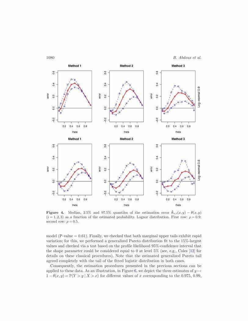
Figure 4. Median, 2.5% and 97.5% quantiles of the estimation error θn,i(x, y) − θ(x, y)(i= 1,2,3) as a function of the estimated probability. Lognor distribution. First row: ρ = 0.9;second row: ρ= 0.5.

model (P-value = 0.61). Finally, we checked that both marginal upper tails exhibit rapidvariation; for this, we performed a generalized Pareto distribution fit to the 15%-largestvalues and checked via a test based on the profile likelihood 95%-confidence interval thatthe shape parameter could be considered equal to 0 at level 5% (see, e.g., Coles [12] fordetails on these classical procedures). Note that the estimated generalized Pareto tailagreed completely with the tail of the fitted logistic distribution in both cases.

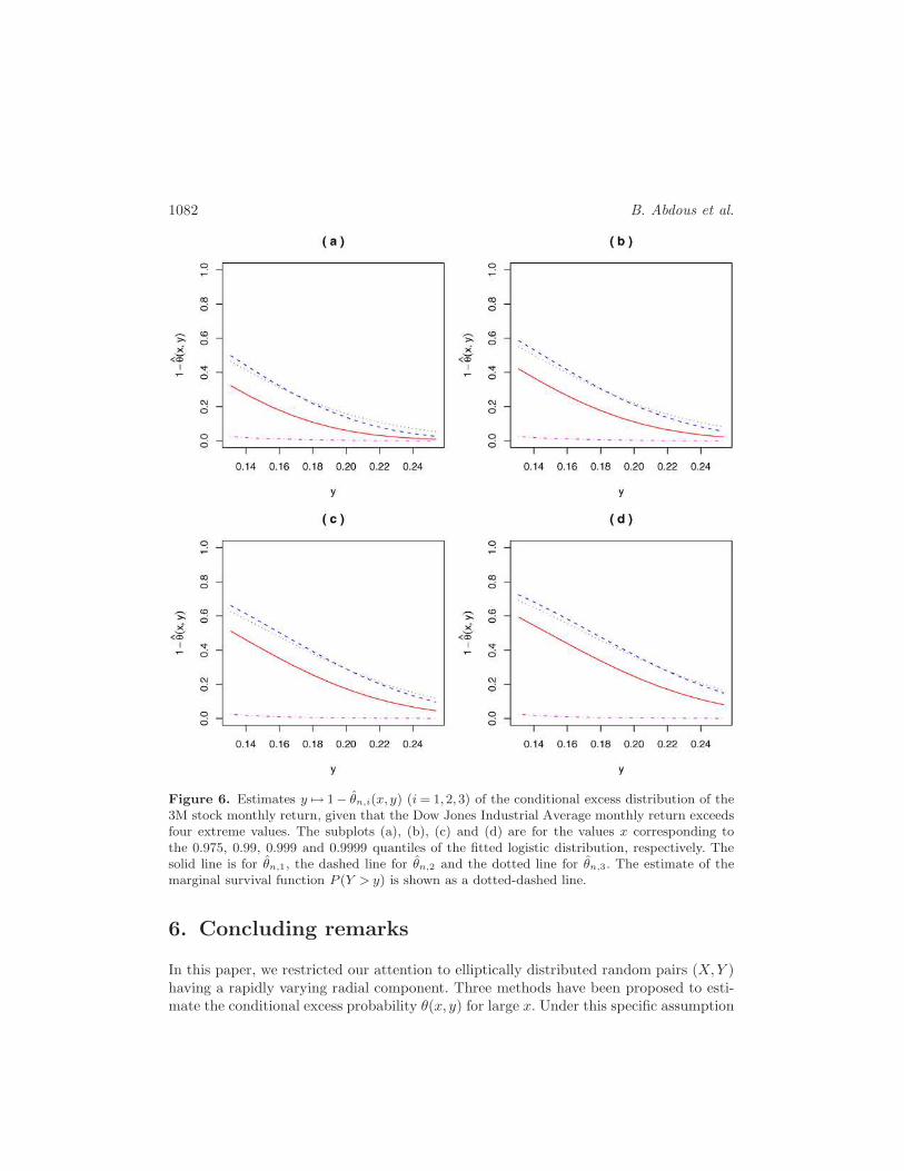
Consequently, the estimation procedures presented in the previous sections can beapplied to these data. As an illustration, in Figure 6, we depict the three estimates of y 7→1− θ(x, y) = P(Y > y |X > x) for different values of x corresponding to the 0.975, 0.99,


Figure 5. Median (solid line), 2.5% and 97.5% quantiles (dashed lines) of the estimated con-ditional quantile function yn,i (i = 1,2) defined in (12) and (13) and theoretical conditionalquantile function y (dotted line) as a function of the probability θ. First row: Normal distri-bution; second row: Kotz distribution, β = 4; third row: Lognor distribution. For each of these,ρ= 0.9.

0.999 and 0.9999 quantiles of the fitted logistic distribution, together with the estimated

marginal survival function P(Y > y). This last probability was estimated via the logistic

distribution fitted to the Yi’s. It is clearly evident from these graphics that 1− θn,2 and

1− θn,3 provide very similar estimates, whereas 1− θn,1 gives uniformly smaller values.

All these estimates are uniformly greater than the marginal survival function of Y . This

allows us to conclude that the data exhibit contagion from the Dow Jones Industrial

Average to the 3M stock.


Figure 6. Estimates y 7→ 1− θn,i(x, y) (i= 1,2,3) of the conditional excess distribution of the3M stock monthly return, given that the Dow Jones Industrial Average monthly return exceedsfour extreme values. The subplots (a), (b), (c) and (d) are for the values x corresponding tothe 0.975, 0.99, 0.999 and 0.9999 quantiles of the fitted logistic distribution, respectively. Thesolid line is for θn,1, the dashed line for θn,2 and the dotted line for θn,3. The estimate of themarginal survival function P (Y > y) is shown as a dotted-dashed line.

6. Concluding remarks

In this paper, we restricted our attention to elliptically distributed random pairs (X,Y )having a rapidly varying radial component. Three methods have been proposed to esti-mate the conditional excess probability θ(x, y) for large x. Under this specific assumption


of elliptical distributions, Methods 2 and 3 revealed comparable results and outperformedMethod 1.

Methods 1 and 2 make use of an asymptotic approximation of the conditional excessdistribution function by the Gaussian distribution function. As shown by Balkema andEmbrechts [3], this approximation remains valid outside the family of elliptical distri-butions, under geometric assumptions on the level curves of the joint density functionof (X,Y ). This suggests that these methods may be useful outside the elliptical family.This is an ongoing research project.

Appendix

Proof of Theorem 2. Define U0 = arctan(ρ/√

1− ρ2). For x > 0 and y ∈ (0, x), wehave

P(X >x,Y > y)

= P

(

R>x

cosU∨ y

ρ cosU +√

1− ρ2 sinU; −U0 ≤ U ≤ π

2

)

Let t0 = (y/x − ρ)/√

1− ρ2. Then −U0 < arctan(t0), and x/ cosu > y/(ρ cosu +√

1− ρ2 sinu) if and only if u > arctan(t0). Hence,

P(X > x,Y > y)

=

∫

π/2

arctan(t0)

H

{

x

cosu

}

du

2π

+

∫ arctan(t0)

−U0

H

{

y

sin(u+U0)

}

du

2π

,

P(Y > y |X > x)

=

∫

π/2

arctan(t0)H(x/ cos(u))du+

∫ arctan(t0)

−U0

H(y/ sin(u+U0))du

2∫

π/2

0 H(x/ cos(u))du. (19)

If t0 ≥ 0, that is, y− ρx≥ 0, the changes of variables v = 1/ cos(u) and v = 1/ sin(u+U0)yield

P(Y > y |X > x) =I1 + I2I3

(20)

with

I1 =

∫

∞

w1

H(vx)

H(x)

dv

v√v2 − 1

,

I2 =

∫

∞

w2

H(vy)

H(x)

dv

v√v2 − 1

,


I3 = 2

∫

∞

1

H(vx)

H(x)

dv

v√v2 − 1

,

w1 =√

1 + t20 =√

1 + (y/x− ρ)2/(1− ρ2) ,

w2 = xw1/y.

If t0 < 0, then

P(Y > y |X > x) =I3 − I1 + I2

I3. (21)

Denote w0 = x(w1 − 1)/ψ(x). In I1 and I3, the change of variable v = 1 + ψ(x)x t yields

I1 =

√

ψ(x)

x

∫

∞

w0

H(x+ tψ(x))

H(x)

dt

(1 + t(ψ(x)/x))√

1 + (t/2)(ψ(x)/x)√

2t,

I3 = 2

√

ψ(x)

x

∫

∞

0

H(x+ tψ(x))

H(x)

dt

(1 + t(ψ(x)/x))√

1 + (t/2)(ψ(x)/x)√

2t.

In I2, the change of variable vy = x+ tψ(x) yields

I2 =ψ(x)

x

∫

∞

w0

H(x+ tψ(x))

H(x)

(y/x)dt

(1 + t(ψ(x)/x))√

1− (y/x)2 + 2t(ψ(x)/x) + (ψ2(x)/x2)t2.

Let Ji =√

x/ψ(x)Ii, i= 1,3, and J2 = (x/ψ(x))I2 . We start with I1 and I3. We will usethe bound, valid for all B,C > 0,

0 ≤ 1− 1

(1 +C)√

1 +B≤B/2 +C, (22)

which follows from straightforward algebra and the concavity of the function x 7→√

1 + x.

Applying this bound with B = ψ(x)x

t2 and C = ψ(x)

x t yields

0≤ 1− 1

(1 + t(ψ(x)/x))√

1 + (t/2)(ψ(x)/x)≤ 5

4

ψ(x)

xt.

We thus have

|J1 −√

2πΦ(√

2w0)|+ |J3 −√

2π|

≤ 3χ(x)

∫

∞

0

Θ(t)dt√2t

+15

16

√2π

ψ(x)

x.


Hence,

I1I3

= Φ(√

2w0) +O

(

χ(x) +ψ(x)

x

)

. (23)

Now consider J2. Applying the bound (22) with C = tψ(x)/x and

B =

{

2tψ(x)

x+ψ2(x)

x2t2

}

/

√

1− (y/x)2,

and making use of Hypothesis 1, we obtain

∣

∣

∣

∣

J2 −(y/x)

√2πϕ(

√2w0)

√

1− (y/x)2

∣

∣

∣

∣

≤ y/x√

1− (y/x)2χ(x)

∫

∞

0

Θ(t)dt+y/x

1− (y/x)2ψ(x)

x

(

√

1−(y

x

)2

+ 1 +ψ(x)

x

)

.

Choose y = ρx+√

1− ρ2√

xψ(x)z for some fixed z ∈ R. Then, for large enough x, wehave 0< y < x and

y/x√

1− (y/x)2=

ρ√

1− ρ2+O(

√

ψ(x)/x).

Thus,

I2I3

=ρ

√

1− ρ2

√

ψ(x)

xϕ(

√2w0) +O

(

χ(x) +ψ(x)

x

)

. (24)

For z ≥ 0 and large enough x, plugging (23) and (24) into (20) yields

θ(x, y) = Φ(√

2w0)−ρ

√

1− ρ2

√

ψ(x)

xϕ(

√2w0) + O

(

χ(x) +ψ(x)

x

)

.

For z < 0 and large enough x, plugging (23) and (24) into (21) yields

θ(x, y) = Φ(√

2w0)−ρ

√

1− ρ2

√

ψ(x)

xϕ(

√2w0) + O

(

χ(x) +ψ(x)

x

)

.

Now note that w0 = z2/2+O(ψ(x)/x), hence√

2w0 = |z|+O(ψ(x)/x). Thus, in both the

cases z ≥ 0 and z < 0, (4) holds. Let z = z′ + ρ√

ψ(x)/x/√

1− ρ2. A Taylor expansionof Φ and ϕ around z′ yields (5). �


Proof of Lemma 1.

H{x+ tψ(x)}H(x)

− e−t = exp

{

−∫ x+tψ(x)

x

ds

ψ(s)

}

− e−t

= exp

[

−∫ t

0

ψ(x)

ψ{x+ sψ(x)} ds

]

− e−t.

Applying the inequality |e−a − e−b| ≤ |a− b|e−a∧b valid for all a, b≥ 0 yields

∣

∣

∣

∣

H{x+ tψ(x)}H(x)

− e−t∣

∣

∣

∣

≤∣

∣

∣

∣

∫ t

0

ψ{x+ sψ(x)} − ψ(x)

ψ{x+ sψ(x)} ds

∣

∣

∣

∣

exp

[

−t∧∫ t

0

ψ(x)

ψ{x+ sψ(x)} ds

]

.

Let∫ t

0

|ψ{x+ sψ(x)} − ψ(x)|ψ{x+ sψ(x)} ds= I(x, t)

and

exp

[

−t∧∫ t

0

ψ(x)

ψ{x+ sψ(x)} ds

]

=E(x, t).

Case ψ increasing. If ψ is non-decreasing, then ψ′ ≥ 0 and ψ′ is decreasing. Thus, forany δ > 0 and large enough x, ψ′(x) ≤ δ and

∫ t

0

ψ(x)

ψ{x+ sψ(x)} ds ≥∫ t

0

ψ(x)

ψ(x) + sψ′(x)ψ(x)ds

=

∫ t

0

ds

1 + sψ′(x)≥

∫ t

0

ds

1 + sδ=

1

δlog(1 + δt).

This implies that E(x, t) ≤ (1 + δt)−1/δ for large enough x. Since ψ is increasing and ψ′

is decreasing, we also have

I(x, t) ≤ ψ′(x)

∫ t

0

sψ(x)

ψ{x+ sψ(x)} ds≤ ψ′(x)t2

2.

Thus, for any δ > 0, I(x, t)E(x, t) =O(|ψ′(x)|t2(1 + δt)−1/δ).Case ψ decreasing. If ψ is monotone non-increasing, then

∫ t

0

ψ(x)

ψ{x+ sψ(x)} ds≥ t


and E(x, t) ≤ e−t. Also, since |ψ′| is decreasing,

I(x, t)≤ |ψ′(x)|∫ t

0

sψ(x)

ψ{x+ sψ(x)} ds.

If ψ has a positive limit at infinity, then I(x, t) =O(ψ′(x)t2). Otherwise, limx→∞ψ(x) = 0and (8) holds. This yields, for large enough x,

I(x, t) ≤ |ψ′(x)|∫ t

0

sψ(x)

ψ{x+ sψ(x)} ds

≤ c1|ψ′(x)|∫ t

0

sec2sψ(x) ds≤ c1|ψ′(x)|∫ t

0

ses/2 ds.

Thus, I(x, t) =O(|ψ′(x)|t2et/2) and I(x, t)E(x, t) =O(|ψ′(x)|t2e−t/2). This concludes theproof. �

Proof of Lemma 2. Write∣

∣

∣

∣

H{x+ tψ(x)}H(x)

− e−t∣

∣

∣

∣

≤∣

∣

∣

∣

H{x+ tψ(x)}H{x+ tψH(x)} − 1

∣

∣

∣

∣

e−t

(25)

+H{x+ tψ(x)}H{x+ tψH(x)}

∣

∣

∣

∣

H{x+ tψH(x)}H(x)

− e−t∣

∣

∣

∣

,

H{x+ tψ(x)}H{x+ tψH(x)} = exp

[

−∫ tψ(x)/ψH(x)

t

ψH(x)

ψ{x+ sψH(x)} ds

]

. (26)

If ψH is increasing, then

∣

∣

∣

∣

∫ tψ(x)/ψH(x)

t

ψH(x)

ψH{x+ sψH(x)} ds

∣

∣

∣

∣

≤ tξ(x), (27)

exp

[

−∫ tψ(x)/ψH(x)

t

ψH(x)

ψH{x+ sψH(x)} ds

]

≤ etξ(x). (28)

Since ξ(x) → 0, gathering (27) and (28) yields, for large enough x,∣

∣

∣

∣

H{x+ tψ(x)}H{x+ tψH(x)} − 1

∣

∣

∣

∣

e−t ≤ tξ(x)e−t/2. (29)

If ψH is decreasing and limx→∞ψH(x) > 0, then the ratio ψH(x)/ψH{x + sψ(x)} isbounded above and away from 0, so

∣

∣

∣

∣

∫ tψ(x)/ψH(x)

t

ψH(x)

ψ{x+ sψH(x)} ds

∣

∣

∣

∣

≤Ctξ(x),

and (29) still holds.If ψH is decreasing and limx→∞ψH(x) = 0, then applying (8) gives that the left-hand


side of the previous equation is bounded by Ctξ(x) exp{2c2ψ(x)t}. Thus, for large enoughx, (29) still holds.

This provides a bound for the right-hand side of (25). The term (26) is bounded byLemma 1. �

Acknowledgements

We would like to thank two anonymous refereesfor useful remarks. We also acknowledgeFree Software R. The first author gratefully acknowledges the support of the NaturalSciences and Engineering Research Council of Canada.

References

[1] Abdous, B., Fougeres, A.-L. and Ghoudi, K. (2005).Extreme behaviour for bivariate elliptical distributions.Canad. J. Statist. 33 317–334. MR2193978

[2] Artzner, Ph., Delbaen, F., Eber, J.-M. and Heath, D. (1999).Coherent measures of risk.Math. Finance 9 203–228. MR1850791

[3] Balkema, G. and Embrechts, P. (2007).High Risk Scenarios and Extremes. A Geometric Approach. Zurich: EMS. MR2372552

[4] Beirlant, J., Dierckx, G., Goegebeur, Y. and Matthys, G. (1999).Tail index estimation and an exponential regression model.Extremes 2 177–200. MR1771132

[5] Beirlant, J., Goegebeur, Y., Teugels, J. and Segers, J. (2004).Statistics of Extremes. Chichester: Wiley. MR2108013

[6] Beirlant, J., Raoult, J.-P. and Worms, R. (2003).On the relative approximation error of the generalized Pareto approximation for a high

quantile.Extremes 6 335–360. MR2125497

[7] Beirlant, J., Vynckier, P. and Teugels, J.L. (1996).Practical Analysis of Extreme Values.Leuwen Univ. Press.

[8] Berman, S. M. (1992).Sojourns and Extremes of Stochastic Processes. Pacific Grove, CA: Wadsworth and

Brooks/Cole Advanced Books and Software. MR1126464[9] Bradley, B.O. and Taqqu, M. (2004).

Framework for analyzing spatial contagion between financial markets.Finance Lett. 2 8–16.

[10] Bradley, B.O. and Taqqu, M. (2005).Empirical evidence on spatial contagion between financial markets.Finance Lett. 3 77–86.

[11] Chernozhukov, V. (2005).Extremal quantile regression.Ann. Statist. 33 806–839. MR2163160

http://www.ams.org/mathscinet-getitem?mr=2193978









[12] Coles, S. (2001).An Introduction to Statistical Modeling of Extreme Values. London: Springer. MR1932132

[13] de Haan, L. (1970).On Regular Variation and Its Application to the Weak Convergence of Sample Extremes.

Amsterdam: Mathematisch Centrum. MR0286156[14] de Haan, L. (1985).

Extremes in higher dimensions: The model and some statistics. In Proceedings of the 45th

Session of the International Statistical Institute 4 (Amsterdam, 1985).Bull. Inst. Internat. Statist. 51 1–15; V 185–192. MR0886266

[15] de Haan, L. and Resnick, S.I. (1977).Limit theory for multivariate sample extremes.Z. Wahrsch. Verw. Gebiete 40 317–337. MR0478290

[16] de Haan, L. and Stadtmuller, U. (1996).Generalized regular variation of second order.J. Austral. Math. Soc. Ser. A 61 381–395. MR1420345

[17] Dierckx, G., Beirlant, J., de Waal, D.J. and Guillou, A. (2007).A new estimation method for Weibull-type tails. Preprint.

[18] Draisma, G., Drees, H., Ferreira, A. and de Haan, L. (2004).Bivariate tail estimation: Dependence in asymptotic independence.Bernoulli 10 251–280. MR2046774

[19] Eddy, W.F. and Gale, J.D. (1981).The convex hull of a spherically symmetric sample.Adv. in Appl. Probab. 13 751–763. MR0632960

[20] Embrechts, P., Lindskog, F. and McNeil, A. (2003).Modelling dependence with copulas and applications to risk management. In Handbook of

Heavy Tailed Distributions in Finance (S. Rachev ed.) Chapter 8 329–384. Elsevier.[21] Fang, K.T., Kotz, S. and Ng, K.W. (1990).

Symmetric Multivariate and Related Distributions Monographs on Statistics and Applied

Probability.London: Chapman and Hall Ltd. MR1071174

[22] Frahm, G., Junker, M. and Schmidt, R. (2005).Estimating the tail-dependence coefficient: Properties and pitfalls.Insurance Math. Econom. 37 80–100. MR2156598

[23] Gardes, L. and Girard, S. (2006).Comparison of Weibull tail-coefficient estimators.REVSTAT 4 163–188. MR2259371

[24] Girard, S. (2004).A Hill type estimator of the Weibull tail-coefficient.Comm. Statist. Theory Methods 33 205–234. MR2045313

[25] Hashorva, E. (2006).Gaussian approximation of elliptical random vectors.Stoch. Models 22 441–457. MR2247592

[26] Hashorva, E., Kotz, S. and Kume, A. (2007).Lp-norm generalised symmetrised Dirichlet distributions.Albanian J. Math. 1 31–56 (electronic). MR2304265

[27] Heffernan, J.E. and Resnick, S.I. (2007).Limit laws for random vectors with an extreme component.Ann. Appl. Probab. 17 537–571. MR2308335
















[28] Heffernan, J.E. and Tawn, J.A. (2004).A conditional approach for multivariate extreme values.J. Roy. Statist. Soc. Ser. B 66 497–546. MR2088289

[29] Huffer, F. and Park, C. (2007).A test for elliptical symmetry.J. Multivariate Anal. 98 256–281. MR2301752

[30] Hult, H. and Lindskog, F. (2002).Multivariate extremes, aggregation and dependence in elliptical distributions.Adv. in Appl. Probab. 34 587–608. MR1929599

[31] Koenker, R. (2005).Quantile Regression Econometric Society Monographs.Cambridge: Cambridge Univ. Press. MR2268657

[32] Koenker, R. and Bassett, Jr., G. (1978).Regression quantiles.Econometrica 46 33–50. MR0474644

[33] Ledford, A.W. and Tawn, J.A. (1996).Statistics for near independence in multivariate extreme values.Biometrika 83 169–187. MR1399163

[34] Ledford, A.W. and Tawn, J.A. (1997).Modelling dependence within joint tail regions.J. Roy. Statist. Soc. Ser. B 59 475–499. MR1440592

[35] Levy, H. and Duchin, R. (2004).Asset return distributions and the investment horizon.J. Portfolio Management 30 47–62.

[36] Maulik, K. and Resnick, S.I. (2004).Characterizations and examples of hidden regular variation.Extremes 7 31–67. MR2201191

[37] Pickands, J., III (1981).Multivariate extreme value distributions. In Proceedings of the 43rd session of the Interna-

tional Statistical Institute 2 (Buenos Aires, 1981).Bull. Inst. Internat. Statist. 49 859–878, 894–902. MR0820979

[38] Resnick, S.I. (1987).Extreme Values, Regular Variation, and Point Processes.New York: Springer. MR0900810

[39] Resnick, S.I. (2002).Hidden regular variation, second order regular variation and asymptotic independence.Extremes 5 303–336. MR2002121

[40] Stephens, M. (1979).Tests of fit for the logistic distribution based on the empirical distribution function.Biometrika 66 591–595.

Received June 2007 and revised April 2008












Estimation of bivariate excess probabilities for elliptical models

Documents

Transcript of Estimation of bivariate excess probabilities for elliptical models