Concomitants of generalized order statistics from bivariate Lomax distribution

ProbStat Forum, Volume 06, October 2013, Pages 73–88ISSN 0974-3235

ProbStat Forum is an e-journal.For details please visit www.probstat.org.in

Concomitants of generalized order statistics frombivariate Lomax distribution

Nayabuddin

Abstract. In this paper probability density function (pdf ) for rth, 1 ≤ r ≤ n and the joint (pdf) of rthand sth, 1 ≤ r < s ≤ n, concomitants of generalized order statistics from bivariate Lomax distribution isobtained. Also single and product moments are derived. Further the results are deduced for moments ofkth upper record values and order statistics. Also their means and product moments are tabulated.

1. Introduction

The Lomax distribution introduced and studied by Lomax (1954). He used this distribution to analyzebusiness failure data. Lomax distribution has been studied by several authors in literature. Balkemaand de Haan (1974) showed that the (df) of Lomax distribution arises as a limit distribution of residuallifetime at great age. According to Arnold (1983), the Lomax distribution is well adapted for modelingreliability problems. Nayak (1987) used multivariate Lomax distribution in reliability theory. Balakrishnanand Ahsanullah (1994) derived the relations for single and product moments of record values from Lomaxdistribution. The Lomax distribution is also known as the Pareto distribution of second kind.

In this paper, we consider the bivariate Lomax distribution (Sankaran and Nair, 1993) with probabilitydistribution function (pdf)

f(x, y) = α1α2c(c+ 1)(1 + α1x+ α2y)−(c+2), x, y, c, α1, α2 > 0, (1)

and corresponding df

F (x, y) = 1− (1 + α1x+ α2y)−c, x, y, c, α1, α2 > 0.

The conditional pdf of Y given X is

f(y|x) =α2(c+ 1)(1 + α1x)(c+1)

(1 + α1x+ α2y)(c+2), y > 0. (2)

The marginal pdf of X is

f(x) =cα1

(1 + α1x)(c+1), x > 0, (3)

Keywords. Generalized order statistics, concomitants of generalized order statistics, order statistics, record values, bivariateLomax distribution, single and product moments

Received: 09 August 2012; Revised: 30 May 2013; Re-revised: 12 September 2013; Accepted: 17 September 2013Email address: [email protected] (Nayabuddin)

Nayabuddin / ProbStat Forum, Volume 06, October 2013, Pages 73–88 74

and the marginal df of X is

F (x) = 1− (1 + α1x)−c, x > 0. (4)

The concept of generalized order statistics (gos) was given by Kamps (1995). Several authors utilized theconcept of (gos) in their work for detailed survey one may refer to Khan et al. (2006), Ahsanullah and beg(2006), Anwar et al. (2007), Beg and Ahsanullah (2008), Faizan and Athar (2008), Tavangar and Asadi(2008), Khan et al. (2009), Tahmasebi and Behboodian (2012), Athar et al. (2012), Athar et al. (2013),Athar and Nayabuddin (2013), Athar and Nayabuddin (2013), among others.

Let n ∈ N , n ≥ 2, k > 0, m = (m1,m2, . . . ,mn−1) ∈ <n−1, Mr =∑n−1j=r mj , such that γr = k + n− r +

Mr > 0 for all r ∈ {1, 2, . . . , n − 1}. Then X(r, n, m, k), r ∈ {1, 2, . . . , n} are called gos if their joint pdf isgiven by

k( n−1∏j=1

γj

)( n−1∏i=1

[1− F (xi)

]mif(xi)

)[1− F (xn)

]k−1f(xn) (5)

on the cone F−1(0) < x1 ≤ x2 ≤ . . . ≤ xn < F−1(1) of <n.Choosing the parameters appropriately, models such as ordinary order statistics (γi = n − i + 1; i =

1, 2, . . . , n, i.e. m1 = m2 = . . . = mn−1 = 0, k = 1), kth record values (γi = k, i.e. m1 = m2 . . . =mn−1 = −1, k ∈ N), sequential order statistics (γi = (n− i+ 1)αi;α1, α2, . . . , αn > 0), order statistics withnon-integral sample size (γi = (α − i + 1);α > 0), Pfeifers record values (γi = βi;β1, β2, . . . , βn > 0) andprogressive type II censored order statistics (mi ∈ N0, k ∈ N) are obtained (Kamps, 1995, 2001).

In view of (5) with mi = m; i = 1, 2, . . . , n− 1, the pdf of rth gos, X(r, n,m, k) is

fX(r,n,m,k) =Cr−1

(r − 1)![F (x)]γr−1f(x)gr−1

m (F (x)) (6)

and joint pdf of X(s, n,m, k) and X(r, n,m, k), 1 ≤ r < s ≤ n, is

fX(r,s,n,m,k)(x, y) =Cs−1

(r − 1)!(s− r − 1)![F (x)]mf(x)gr−1

m

(F (x)

)[hm

(F (y)

)− hm

(F (x)

)]s−r−1

×[F (y)]γs−1f(y), α ≤ x < y ≤ β, (7)

where

Cr−1 =

r∏i=1

γi, γi = k + (n− i)(m+ 1),

hm(x) =

−1

m+ 1(1− x)m+1 , m 6= −1

− log(1− x) , m = −1

and

gm(x) = hm(x)− hm(0), x ∈ (0, 1).

Let (Xi, Yi), i = 1, 2, . . . , n, be n pairs of independent random variables from some bivariate populationwith distribution function F (x, y). If we arrange the X variates in ascending order as X(1, n,m, k) ≤X(2, n,m, k) ≤ · · · ≤ X(n, n,m, k), then Y variates paired (not necessarily in ascending order) with thesegeneralized ordered statistics are called the concomitants of generalized order statistics and are denoted byY[1,n,m,k], Y[2,n,m,k], . . . , Y[n,n,m,k]. The pdf of Y[r,n,m,k], the rth concomitant of generalized order statisticsis given as

g[r,n,m,k] =

∫ ∞−∞

fY |X(y|x)fX(r,n,m,k)(x)dx (8)


and the joint pdf of Y[r,n,m,k] and Y[s,n,m,k] is

g[r,s,n,m,k](y1, y2) =

∫ ∞−∞

∫ x2

−∞fY |X(y1|x1)fY |X(y2|x2)fX(r,s,n,m,k)(x1, x2)dx1dx2. (9)

It is well known that the distribution function of order statistics are connected by the relations (David,1981)

Fr:n(x) =

n∑i=n−r+1

(−1)i−n+r−1

(i− 1

n− r

)(n

i

)F1:i(x)

where Fr:n(x) is the df of rth order statistics.Thus the pdf of rth concomitants of order statistics Y[r:n] is

g[r:n](y) =

n∑i=n−r+1

(−1)i−n+r−1

(i− 1

n− r

)(n

i

)g[1:i](y)

and the kth moments of Y[r:n] is

µk[r:n](y) =

n∑i=n−r+1

(−1)i−n+r−1

(i− 1

n− r

)(n

i

)µ

(k)[1:i](y). (10)

Here some important transformation and formulas are presented, which will be used in the subsequentsections (Prudnikov et al., 1986; Srivastava and Karlsson, 1985)

(λ)−n =(−1)n

(1− λ)n, n = 1, 2, 3, . . . , λ 6= 0,±1,±2, . . . , (11)

(1 + z)−a =

∞∑p=0

(−1)p(a)pzp

p!, (12)

(λ+m) =λ(λ+ 1)m

(λ)m, (13)

where (λ)m = Γ(λ+m)Γ(λ) , λ 6= 0,−1,−2, . . .

(λ+m+ n) =λ(λ+ 1)m+n

(λ)m+n, (14)

(λ)m+n = (λ)m(λ+m)n. (15)

Important identities/result in hypergeometric function are

2F1

a, b; −z

c

=

∞∑p=0

(a)p(b)p(c)p

(−z)p

p!(16)

is conditionally convergent for |z| = 1, z 6= −1 if −1 < Re(ω) ≤ 0,

2F1

a, b; 1

c

=Γ(c)Γ(c− a− b)Γ(c− a)Γ(c− b)

, Re(c− a− b) > 0, c 6=, 0,−1,−2, . . . , (17)

∫ ∞0

xp−12F1

a, b; −mx

c

dx =(m)−pΓ(c)Γ(p)Γ(a− p)Γ(b− p)

Γ(a)Γ(b)Γ(c− p), (18)


if 0 < Re p < a, Re b; |arg m| < π

∫ ∞0

xs−13F2

(a1), (a2), (a3); −x

(b1), (b2)

dx =Γ(b1)Γ(b2)Γ(s)Γ(a1 − s)Γ(a2 − s)Γ(a3 − s)

Γ(a1)Γ(a2)Γ(a3)Γ(b1 − s)Γ(b2 − s), (19)

if 0 < Re < s < Re aj ; j = 1, 2, 3

3F2

−N, 1, a, 1

b, a−m,

=(b− 1)(a−m− 1)

(b+N − 1)(a− 1) 3

F2

−m, 1, 2− b, 1

2− b−N, 2− a,

(20)

3F2

−N, 1, 1, 1

l, m

=(l − 1)

(N + l − 1) 3

F2

−N, m− 1, 1, 1

m, 2−N − l

, (21)

for m = 1, 2, . . . , l = −N,−N − 1,−N − 1, . . .For real positive k, c and a positive integer b

b∑a=0

(−1)a(b

a

)B(a+ k, c) = B(k, c+ b). (22)

Note that (Erdelyi et al., 1954)∫ ∞y

x−λ(x− y)µ−1dx =Γ(λ− µ)Γµ

Γλy(µ−λ), 0 < Reµ < Re < λ (23)

∫ ∞0

xv−1(a+ x)−µ(x+ y)−ρdx =ΓvΓ(µ− v + ρ)

Γ(µ+ ρ)aµy(v−%)

2F1

µ, v; 1− y

aµ+ ρ

(24)

if |arg a| < Π, Rev > 0, |arg y| < Π, Reρ > Re(v − µ).Note that (Srivastava and Karlsson, 1985)

F p:q;kl:m;n

(ap); (bq); (ck); x, y

(αl); (βm); (γn);

=

∞∑r=0

∞∑s=0

∏pj=1(aj)r+s

∏qj=1(bj)r

∏kj=1(cj)s∏l

j=1(αj)r+s∏mj=1(βj)r

∏nj=1(γj)s

xr

r!

ys

s!(25)

is known as Kampe de Feriet’s series.Note that (Prudnikov et al., 1986)

pFq

α1, α2, ..., αp; z

β1 β2, ..., βq

=

∞∑k=0

(α1)k(α2)k...(αp)k(β1)k(β2)k...(βq)k

(z)k

k!(26)

is known as generalized hypergeometric series.

2. Probability density function of Y[r,n,m,k]

For the bivariate Lomax distribution as given in (1), using (2), (3), (4) and (6) in (8), the pdf of rthconcomitants of gos Y[r,n,m,k] is given as

g[r,n,m,k](y) =α2Cr−1c(c+ 1)

(r − 1)!(m+ 1)r−1

r−1∑i=0

(−1)i(r − 1

i

)∫ ∞0

α1

(1 + α1x+ α2y)c+2

1

(1 + α1x)c(γr−i−1)dx . (27)


Let t = α1x, then the R.H.S. of (27) reduces to

=α2Cr−1

(r − 1)!(m+ 1)r−1 c(c+ 1)

r−1∑i=0

(−1)i(r − 1

i

)∫ ∞0

(1 + t+ α2y)−(c+2)

(1 + t)−c(γr−i−1)dt. (28)

Using relation (24) in (28), we get

g[r,n,m,k](y) =Cr−1

(r − 1)!(m+ 1)r−1 c(c+ 1)

(α2)

(1 + α2y)(c+1)

r−1∑i=0

(−1)i

×(r − 1

i

)1

(cγr−i + 1)2F1

(cγr−i − c), 1; −α2y

(cγr−i + 2)

. (29)

We now prove that∫g[r,n,m,k](y)dy = 1. We have,∫ ∞

0

g[r,n,m,k](y)dy =Cr−1

(r − 1)!(m+ 1)r−1 c(c+ 1)

r−1∑i=0

(−1)i(r − 1

i

)1

cγr−i + 1

×∫ ∞

0

α2

(1 + α2y)(c+1) 2F1

(cγr−i − c), 1; −α2y

(cγr−i + 2)

dy. (30)


=α2Cr−1c(c+ 1)

(r − 1)!(m+ 1)r−1

r−1∑i=0

(r − 1

i

)(−1)i

cγr−i + 1

∞∑p=0

(cγr−i − c)p(1)p(−1)p

(cγr−i + 2)p p!

∫ ∞0

1

(1 + α2y)(c+1)(α2y)pdy. (31)

Let t = 1 + α2y, then R.H.S. of (31) becomes

=Cr−1c(c+ 1)

(r − 1)!(m+ 1)r−1

r−1∑i=0

(−1)i(r − 1

i

)1

cγr−i + 1

∞∑p=0

(cγr−i − c)p(1)p(−1)p

(cγr−i + 2)p p!

∫ ∞1

t−(c+1)(t− 1)pdt. (32)

Now using relation (23) in (32), we get

=Cr−1

(r − 1)!(m+ 1)r−1 c(c+ 1)

r−1∑i=0

(−1)i(r − 1

i

)1

cγr−i + 1

∞∑p=0

(cγr−i − c)p(1)p(−1)pΓ(c− p)(cγr−i + 2)pΓ(c+ 1)

.

In view of (11), we have

=Cr−1

(r − 1)!(m+ 1)r−1 (c+ 1)

r−1∑i=0

(−1)i(r − 1

i

)1

cγr−i + 13F2

(cγr−i − c), 1, 1, 1

(cγr−i + 2), (1− c)

. (33)


=Cr−1

(r − 1)!(m+ 1)r−1

r−1∑i=0

(−1)i(r − 1

i

)2F1

(cγr−i − c), 1; 1

(1− c)

. (34)

Now in view of (17) in (34), we have∫ ∞0

g[r,n,m,k](y)dy =Cr−1

(r − 1)!(m+ 1)r

r−1∑i=0

(−1)i(r − 1

i

)B( k

m+ 1+ (n− r) + i, 1

)= 1

in view of (22).


3. Moment of Y[r,n,m,k]

In view of (29), we have

E(Y

(a)[r,n,m,k]

)=

∫yag[r,n,m,k](y)dy

=Cr−1

(r − 1)!(m+ 1)r−1 c(c+ 1)

r−1∑i=0

(−1)i(r − 1

i

)1

cγr−i + 1

×∫ ∞

0

yaα2

(1 + α2y)(c+1) 2F1

(cγr−i − c), 1; −α2y

(cγr−i + 2)

dy=

Cr−1

(r − 1)!(m+ 1)r−1 c(c+ 1)

r−1∑i=0

(−1)i(r − 1

i

)1

cγr−i + 1

×∞∑p=0

(cγr−i − c)p(1)p(cγr−i + 2)p!

∫ ∞0

ya(α2)

(1 + α2y)(c+1)(−α2y)p dy. (35)

Letting t = 1 + α2y in (35) we have

=1

(α2)aCr−1c(c+ 1)

(r − 1)!(m+ 1)r−1

r−1∑i=0

(r − 1

i

)(−1)i

cγr−i + 1

∞∑p=0

(cγr−i − c)p(1)p(−1)p

(cγr−i + 2)p!

∞∫1

t−(c+1)(1− t)(p+a)dt. (36)

In view of relation (23), (36), becomes

=(α2)−aCr−1c(c+ 1)

(r − 1)!(m+ 1)r−1

r−1∑i=0

(r − 1

i

)(−1)i

cγr−i + 1

∞∑p=0

(cγr−i − c)p(1)p(−1)p

(cγr−i + 2)pp!

Γ(c− a− p)Γ(p+ 1 + a)

Γ(c+ 1). (37)

Now on using (11) in (37), we get after simplification

=α−a2 Cr−1c(c+ 1)

(r − 1)!(m+ 1)r−1

r−1∑i=0

(r−1i

)(−1)i

cγr−i + 1

Γ(c− a)Γ(1 + a)

Γ(c+ 1)3F2

(cγr−i − c), 1, (1 + a), 1

(cγr−i + 2), (1− c+ a)

. (38)

After application of (20) in (38), we have

=cα−a2 Cr−1

(r − 1)!(m+ 1)r−1

(c− a)Γ(c− a)

Γ(c+ 1)

Γ(1 + a)

a

r−1∑i=0

(−1)i(r − 1

i

)2F1

1, (−cγr−i); 1

(1− a)

. (39)

Applying (17) in (39), we get

=1

(α2)aCr−1

(r − 1)!(m+ 1)r−1

Γ(c+ 1− a)Γ(1 + a)

cΓ(c)

r−1∑i=0

(−1)i(r − 1

i

)1

γr−i − ac

=α−a2 Cr−1

(r − 1)!(m+ 1)r

Γ(c+ 1− a)Γ(1 + a)

Γ(c+ 1)

r−1∑i=0

(−1)i(r − 1

i

)sB( k

m+ 1+ (n− r) + i− a

c(m+ 1), 1),

which after application of (22), yields

E(y

(a)[r,n,m,k]

)=

1

(α2)aCr−1

(m+ 1)r

Γ(c+ 1− a) Γ(1 + a)

cΓ(c)

Γ(k+(n−r)(m+1)− a

c

m+1 )

Γ(k+n(m+1)− a

c

m+1 )(40)

=1

(α2)a

Γ(c+ 1− a) Γ(1 + a)

cΓ(c)

1∏ri=1(1− a

cγi)

(41)


Remark 3.1. Set m = 0, k = 1 in (40), to get moments of concomitants of order statistics from bivariateLomax distribution

E(y

(a)[r:n]

)=

1

(α2)an!

(n− r)!Γ(c+ 1− a) Γ(1 + a)

cΓ(c)

Γ(n− r + 1− ac )

Γ(n+ 1− ac )

and at r = 1, we get

E(y

(a)[1:n]

)=

1

(α2)an

(nc− a)

Γ(c+ 1− a) Γ(1 + a)

Γ(c). (42)

Further, in view of (10), (42) becomes

E(y

(a)[r:n]

)=

n∑i=n−r+1

(−1)i−n+r−1

(i− 1

n− r

)(n

i

)i

(ic− a)(α2)aΓ(c+ 1− a) Γ(1 + a)

Γ(c).

Remark 3.2. At m = −1 in (41), we get moment of concomitants of kth upper record value from bivariateLomax distribution

E(y

(a)[r,n,−1,k]

)=

1

(α2)a

Γ(c+ 1− a) Γ(1 + a)

cΓ(c)

1

(1− ack )r

.

Here in Table 3, it may be noted that the well known property of order statistics∑ni=1E(Xi:n) = nE(X)

(David and Nagaraja, 2003) is satisfied.

4. Joint probability density function of Y[r,n,m,k] and Y[s,n,m,k]

For the bivariate Lomax distribution as given in (1), using (2), (3), (4) and (7) in (9), the joint pdf ofrth and sth concomitants of gos Y[r,n,m,k] and Y[s,n,m,k] is given as

g[r,s,n,m,k](y1, y2) =Cs−1c

2(c+ 1)2(α1)(α2)2

(r − 1)!(s− r − 1)!(m+ 1)s−2

r−1∑i=0

s−r−1∑j=0

(−1)i+j

(r − 1

i

)(s− r − 1

j

)×∫ ∞

0

1

(1 + α1x2)c(γs−j−1)

1

(1 + α1x2 + α2y2)c+2I(x2, y1)dx2 (43)

where

I(x2, y1) =

∫ x2

0

α1

(1 + α1x1)c(s−r+i−j)(m+1)−c1

(1 + α1x1 + α2y1)c+2dx1. (44)

Let t1 = (1 + α1x1), then the R.H.S. of (44) reduces to

I(x2, y1) = (λ)−β∫ 1+α1x2

1

t−α1 (1 +t1λ

)−βdt1, (45)

where α = c(s− r+ i− j)(m+ 1)− c, β = (c+ 2) and λ = α2y1. Now on using (12) in (45), and simplifying,we get

I(x2, y1) = (λ)−β∞∑p=0

(−1)p(β)p(

1λ )p

p!

1

(−α+ p+ 1)

[(1 + α1x2)−(α−p−1) − 1

].


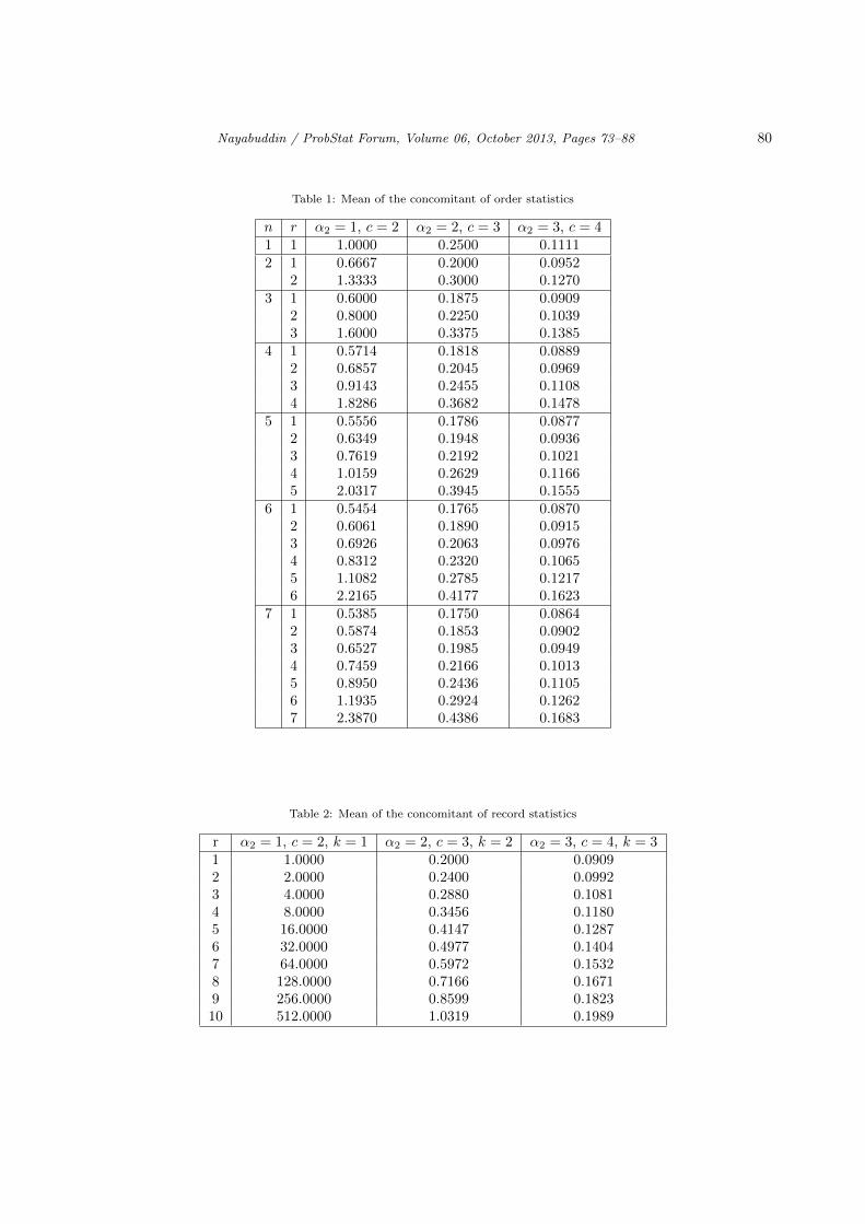
Table 1: Mean of the concomitant of order statistics

n r α2 = 1, c = 2 α2 = 2, c = 3 α2 = 3, c = 41 1 1.0000 0.2500 0.11112 1 0.6667 0.2000 0.0952

2 1.3333 0.3000 0.12703 1 0.6000 0.1875 0.0909

2 0.8000 0.2250 0.10393 1.6000 0.3375 0.1385

4 1 0.5714 0.1818 0.08892 0.6857 0.2045 0.09693 0.9143 0.2455 0.11084 1.8286 0.3682 0.1478

5 1 0.5556 0.1786 0.08772 0.6349 0.1948 0.09363 0.7619 0.2192 0.10214 1.0159 0.2629 0.11665 2.0317 0.3945 0.1555

6 1 0.5454 0.1765 0.08702 0.6061 0.1890 0.09153 0.6926 0.2063 0.09764 0.8312 0.2320 0.10655 1.1082 0.2785 0.12176 2.2165 0.4177 0.1623

7 1 0.5385 0.1750 0.08642 0.5874 0.1853 0.09023 0.6527 0.1985 0.09494 0.7459 0.2166 0.10135 0.8950 0.2436 0.11056 1.1935 0.2924 0.12627 2.3870 0.4386 0.1683

Table 2: Mean of the concomitant of record statistics

r α2 = 1, c = 2, k = 1 α2 = 2, c = 3, k = 2 α2 = 3, c = 4, k = 31 1.0000 0.2000 0.09092 2.0000 0.2400 0.09923 4.0000 0.2880 0.10814 8.0000 0.3456 0.11805 16.0000 0.4147 0.12876 32.0000 0.4977 0.14047 64.0000 0.5972 0.15328 128.0000 0.7166 0.16719 256.0000 0.8599 0.182310 512.0000 1.0319 0.1989


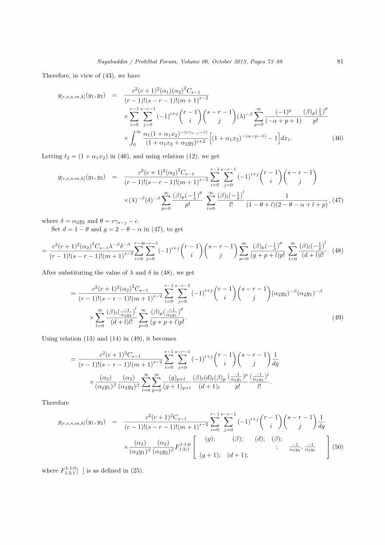
Therefore, in view of (43), we have

g[r,s,n,m,k](y1, y2) =c2(c+ 1)2(α1)(α2)

2Cs−1

(r − 1)!(s− r − 1)!(m+ 1)s−2

×r−1∑i=0

s−r−1∑j=0

(−1)i+j

(r − 1

i

)(s− r − 1

j

)(λ)−β

∞∑p=0

(−1)p

(−α+ p+ 1)

(β)p(1λ )p

p!

×∫ ∞

0

α1(1 + α1x2)−(cγs−j−c)

(1 + α1x2 + α2y2)c+2

[(1 + α1x2)−(α−p−1) − 1

]dx1. (46)

Letting t2 = (1 + α1x2) in (46), and using relation (12), we get

g[r,s,n,m,k](y1, y2) =c2(c+ 1)2(α2)

2Cs−1

(r − 1)!(s− r − 1)!(m+ 1)s−2

r−1∑i=0

s−r−1∑j=0

(−1)i+j

(r − 1

i

)(s− r − 1

j

)

×(λ)−β(δ)−β∞∑p=0

(β)p(− 1λ )p

p!

∞∑l=0

(β)l(− 1δ )l

l!

1

(1− θ + l)(2− θ − α+ l + p), (47)

where δ = α2y2 and θ = cγs−j − c.Set d = 1− θ and g = 2− θ − α in (47), to get

=c2(c+ 1)2(α2)

2Cs−1λ

−βδ−β

(r − 1)!(s− r − 1)!(m+ 1)s−2

r−1∑i=0

s−r−1∑j=0

(−1)i+j

(r − 1

i

)(s− r − 1

j

) ∞∑p=0

(β)p(− 1λ )p

(g + p+ l)p!

∞∑l=0

(β)l(− 1δ )l

(d+ l)l!. (48)

After substituting the value of λ and δ in (48), we get

=c2(c+ 1)2(α2)

2Cs−1

(r − 1)!(s− r − 1)!(m+ 1)s−2

r−1∑i=0

s−r−1∑j=0

(−1)i+j

(r − 1

i

)(s− r − 1

j

)(α2y2)−β(α2y1)−β

×∞∑l=0

(β)l(−1α2y2

)l

(d+ l)l!

∞∑p=0

(β)p(−1α2y1

)p

(g + p+ l)p!. (49)

Using relation (13) and (14) in (49), it becomes

=c2(c+ 1)2Cs−1

(r − 1)!(s− r − 1)!(m+ 1)s−2

r−1∑i=0

s−r−1∑j=0

(−1)i+j

(r − 1

i

)(s− r − 1

j

)1

dg

× (α2)

(α2y1)β(α2)

(α2y2)β

∞∑l=0

∞∑p=0

(g)p+l(g + 1)p+l

(β)l(d)l(β)p(d+ 1)l

( −1α2y1

)p

p!

( −1α2y2

)l

l!.

Therefore

g[r,s,n,m,k](y1, y2) =c2(c+ 1)2Cs−1

(r − 1)!(s− r − 1)!(m+ 1)s−2

r−1∑i=0

s−r−1∑j=0

(−1)i+j

(r − 1

i

)(s− r − 1

j

)1

dg

× (α2)

(α2y1)β(α2)

(α2y2)βF 1:1;0

1:2;1

(g); (β); (d); (β);; −1

α2y2, −1α2y1

(g + 1); (d+ 1);

(50)

where F 1:1;01:2;1 [ ] is as defined in (25).


We now prove that∫∞

0

∫∞0g[r,s,n,m,k](y1, y2)dy1dy2 = 1. We have∫ ∞

0

∫ ∞0

g[r,s,n,m,k](y1, y2)dy1dy2 = A

∫ ∞0

∫ ∞0

(α2)

(α2y1)β(α2)

(α2y2)β

×F 1:1;01:2;1

(g); (β); (d); (β);; −1

α2y2, −1α2y1

(g + 1); (d+ 1);

dy1dy2

where

A =c2(c+ 1)2Cs−1

(r − 1)!(s− r − 1)!(m+ 1)s−2

r−1∑i=0

s−r−1∑j=0

(−1)i+j

(r − 1

i

)(s− r − 1

j

)1

dg.

Then,∫ ∞0

∫ ∞0

g[r,s,n,m,k](y1, y2)dy1dy2 = A

∫ ∞0

∫ ∞0

(α2)

(α2y1)β(α2)

(α2y2)β

×∞∑p=0

∞∑l=0

(g)l+p(g + 1)l+p


( −1α2y1

)p

p!

( −1α2y2

)l

l!dy1dy2. (51)

On applying (15) in (51), we can write

= A

∫ ∞0

(α2)

(α2y2)β

∞∑l=0

(g)l(β)l(d)l(g + 1)l(d+ 1)l

( −1α2y2

)l

l!

{∫ ∞0

(α2)

(α2y1)β

∞∑p=0

(g + l)p(β)p(g + l + 1)p

( −1α2y1

)p

p!dy1

}dy2. (52)

Now using relation (26) in (52), we have

= A

∫ ∞0

α2

(α2y2)β

∞∑l=0

(g)l(β)l(d)l(g + 1)l(d+ 1)l

( −1α2y2

)l

l!

∞∫0

(α2)

(α2y1)β2F1

(β); (g + l); −1

α2y1

(g + 1 + l)

dy1dy2. (53)

Now letting t1 = 1α2y1

in (53), to get

= A

∫ ∞0

(α2y2)

(α2y2)β

∞∑l=0

(g)l(β)l(d)l(g + 1)l(d+ 1)l

( −1α2y2

)l

l!

∫ ∞0

t(β−1)−12F1

(β); (g + l); −t1

(g + 1 + l)

dt1dy2.

Now in view of relation (18), we have

= A

∫ ∞0

(α2)

(α2y2)β

∞∑l=0

(g)l(β)l(d)l(g + 1)l(d+ 1)l

( −1α2y2

)l

l!

(g + l)

(β − 1)(g + l + 1− β)dy2. (54)

Further, using relation (13) in (54), to get

=gA

(g − β + 1)

∫ ∞0

(α2)

(α2y2)β

∞∑l=0

(g − β + 1)l(β)l(d)l(g − β + 2)l(d+ 1)l

( −1α2y2

)l

l!dy2. (55)

Now using relation (26) in (55), we have

=gA

(g − β + 1)

∫ ∞0

(α2)

(α2y2)β3F2

(g + 1− β); (β); (d); − 1

α2y2

(g + 2− β); (d+ 1)

dy2. (56)


Set t2 = 1α2y2

in (56), to get

=gA

(g − β + 1)

∫ ∞0

(t2)(β−1)−1

3F2

(g + 1− β); (β); (d); −t2

(g + 2− β); (d+ 1)

dt2. (57)

Now on using relation (19) in (57), we have

=Agd

(β − 1)2(g + 2− 2β)(d+ 1− β). (58)

Now after putting the value of g, d, β, A in (58), we get

=Cs−1

(r − 1)!(s− r − 1)!(m+ 1)s

r−1∑i=0

s−r−1∑j=0

(−1)i+j

(r − 1

i

)(s− r − 1

j

)[ km+1 + (n− s) + j]−1

[ km+1 + (n− r) + i]

.

Therefore,∫ ∞0

∫ ∞0

g[r,s,n,m,k](y1, y2)dy1dy2 =Cs−1

(r − 1)!(s− r − 1)!(m+ 1)s

r−1∑i=0

(s− r − 1

j

)

×s−r−1∑j=0

(−1)i+j

(r − 1

i

)B( k

m+ 1+ (n− r + i), 1

)B( k

m+ 1+ (n− s+ j), 1

)= 1.

in view of (22).

5. Product moments of two concomitants Y[r,n,m,k] and Y[s,n,m,k]

The product moments of two concomitants Y[r,n,m,k] and Y[s,n,m,k] is given by

E(Y

(a)[r,n,m,k]Y

(b)[s,n,m,k]

)=

∫ ∞0

∫ ∞0

ya1yb2 g[r,s,n,m,k](y1, y2)dy1dy2. (59)

In view of (50) and (59), we have

E(Y

(a)[r,n,m,k]Y

(b)[s,n,m,k]

)=

= A

∫ ∞0

∫ ∞0

ya1yb2

(α2)

(α2y1)β(α2)

(α2y2)βF 1:1;0

1:2;1

(g); (β); (d); (β);; −1

α2y2, −1α2y1

(g + 1); (d+ 1);

dy1dy2.

= A

∫ ∞0

∫ ∞0

ya1yb2

(α2)

(α2y1)β(α2)

(α2y2)β

∞∑p=0

∞∑l=0

(g)l+p(g + 1)l+p


( −1α2y1

)p

p!

( −1α2y2

)l

l!dy1dy2. (60)

On applying (15) in (60), we have

= A

∫ ∞0

yb2(α2)

(α2y2)β

∞∑l=0

(g)l(g + 1)l

(β)l(d)l(d+ 1)l

( −1α2y2

)l

l!

{∫ ∞0

ya1(α2)

(α2y1)β

∞∑p=0

(β)p(g + l)p(g + 1 + l)p

( −1α2y1

)p

p!dy1

}dy2. (61)

Using relation (26) in (6), we have

= A

∫ ∞0

yb2(α2)

(α2y2)β

∞∑l=0

(g)l(g + 1)l

(β)l(d)l(d+ 1)l

( −1α2y2

)l

l!

×∫ ∞

0

ya1(α2)

(α2y1)β2F1

(β); (g + l); −1

α2y1 1(g + l + 1)

dy1dy2. (62)


Setting t1 = 1α2y1

in (62), to get

=A

(α2)a

∫ ∞0

yb2(α2)

(α2y2)β

∞∑l=0

(g)l(g + 1)l

(β)l(d)l(d+ 1)l

( −1α2y2

)l

l!

×∫ ∞

0

t(β−a−1)−12F1

(β); (g + l); −t1

(g + l + 1)

dt1dy2. (63)

On using relation (18) in (63), we have

=A

(α2)a(g + l)Γ(β − a− 1)Γ(a+ 1)

Γ(β)(g + l + 1− β + a)

∫ ∞0

yb2(α2)

(α2y2)β

∞∑l=0

(g)l(g + 1)l

(β)l(d)l(d+ 1)l

( −1α2y2

)l

l!dy2.

Now in view of relation (13) and (26), we have

=A

(α2)ag

(g + 1− β + a)

Γ(β − a− 1)Γ(a+ 1)

Γ(β)

∫ ∞0

yb2(α2)

(α2y2)β

×3F2

(d); (g + 1− β + a); (β); − 1

α2y2

(d+ 1); (g + 2− β + a)

dy2. (64)

Let t2 = 1α2y2

in (64), we have

=A

(α2)a+b

g

(g + 1− β + a)

Γ(β − a− 1)Γ(a+ 1)

Γ(β)

∫ ∞0

t(β−b−1)−12

×3F2

(d); (g + 1− β + a); (β); −t2

(d+ 1); (g + 2− β + a)

dt2. (65)

Using relation (19) in (65), to get

=A

(α2)a+b

Γ(β − a− 1)Γ(a+ 1)

Γ(β)

Γ(β − b− 1)Γ(b+ 1)

Γ(β)

dg

(d− β + b+ 1)(g − 2β + a+ b+ 2). (66)

Now putting the value of A, d, g and β in (66), we have

E(Y

(a)[r,n,m,k]Y

(b)[s,n,m,k]

)=

1

(α2)(a+b)

c2(c+ 1)2Cs−1

(r − 1)!(s− r − 1)!(m+ 1)s−2

Γ(c− a+ 1)Γ(a+ 1)

Γ(c+ 2)

×Γ(c− b+ 1)Γ(b+ 1)

Γ(c+ 2)

r−1∑i=0

s−r−1∑j=0

(−1)i+j(r − 1

i

)(s− r − 1

j

)× 1

[c{k + (n− s+ j)(m+ 1)} − b]1

[c{k + (n− r + i)(m+ 1)} − a− b](67)

=1

(α2)(a+b)

(c+ 1)2Cs−1

(r − 1)!(s− r − 1)!(m+ 1)s−2

Γ(c− a+ 1)Γ(a+ 1)

Γ(c+ 2)

×Γ(c− b+ 1)Γ(b+ 1)

Γ(c+ 2)

r−1∑i=0

(−1)i(r − 1

i

)B( k

m+ 1+ (n− r + i)− a+ b

c(m+ 1), 1)

×s−r−1∑j=0

(−1)j(s− r − 1

j

)B( k

m+ 1+ (n− s+ j)− b

c(m+ 1), 1).


In view of relation (22), we get

=1

(α2)(a+b)

(c+ 1)2Cs−1

(r − 1)!(s− r − 1)!(m+ 1)s−2

Γ(c− a+ 1)Γ(a+ 1)

Γ(c+ 2)

Γ(c− b+ 1)Γ(b+ 1)

Γ(c+ 2)

×B( k

m+ 1+ (n− r)− a+ b

c(m+ 1), r)B( k

m+ 1+ (n− s)− b

c(m+ 1), s− r

),

which after simplification yields

E(Y

(a)[r,n,m,k]Y

(b)[s,n,m,k]

)=

1

(α2)(a+b)

Cs−1

(m+ 1)s−2

Γ(c− a+ 1)Γ(a+ 1)

Γ(c+ 1)

Γ(c− b+ 1)Γ(b+ 1)

Γ(c+ 1)

×Γ( k

(m+1) + (n− r)− a+bc(m+1) )

Γ( k(m+1) + n− a+b

c(m+1) )

Γ( k(m+1) + (n− s)− b

c(m+1) )

Γ( k(m+1) + (n− r)− b

c(m+1) ).

E(Y

(a)[r,n,m,k]Y

(b)[s,n,m,k]

)=

1

(α2)(a+b)

Γ(c− a+ 1)Γ(a+ 1)

Γ(c+ 1)

Γ(c− b+ 1)Γ(b+ 1)

Γ(c+ 1)

× 1∏ri=1(1− a+b

cγi)∏sj=r+1(1− b

cγi). (68)

Remark 5.1. Set m = 0, k = 1 in (67), to get product moments of concomitants of order statistics frombivariate Lomax distribution

E(Y

(a)[r:n]Y

(b)[s:n]

)=

Cr,s:n(α2)(a+b)

Γ(c− a+ 1)Γ(a+ 1)

Γ(c)

Γ(c− b+ 1)Γ(b+ 1)

Γ(c)

×r−1∑i=0

s−r−1∑j=0

(−1)i+j(r − 1

i

)(s− r − 1

j

)1

[sc− nc− jc− c+ b]

1

[rc− nc− ic− c+ a+ b].

E(Y

(a)[r:n]Y

(b)[s:n]

)=

1

(α2)(a+b)

n!

(n− s)!Γ(c− a+ 1)Γ(a+ 1)

Γ(c+ 1)

Γ(c− b+ 1)Γ(b+ 1)

Γ(c+ 1)

×Γ(n− r + 1− a+b

c )

Γ(n+ 1− a+bc )

Γ(n− s+ 1− bc )

Γ(n− r + 1− bc ).

Remark 5.2. If m = −1, in (68), then we get product moment of concomitants of kth upper record valuefrom bivariate Lomax distribution as

E(Y

(a)[r,n,−1,k]Y

(b)[s,n,−1,k]

)=

1

(α2)(a+b)

Γ(c− a+ 1)Γ(a+ 1)

Γ(c+ 1)

Γ(c− b+ 1)Γ(b+ 1)

Γ(c+ 1)

1

(1− a+bck )r(1− b

ck )(s−r).

Acknowledgement

Authors are grateful to Dr. Haseeb Athar, Aligarh Muslim University, Aligarh, India, for his help andsuggestions throughout the preparation of this manuscript. The authors are also thankful to learned refereefor his/her comments which led improvement in the manuscript.


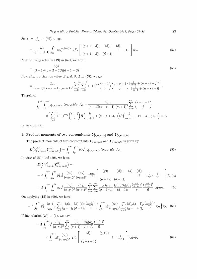
Table 3: Product moments between the concomitants of order statistics:

α2 = 1 c = 3n s \ r 1 2 3 4 51 1 -0.08212 1 0.1231

2 -0.0615 -0.12313 1 -0.0633

2 0.1266 0.15823 -0.0633 -0.0791 -0.1582

4 1 0.53172 0.3323 0.37983 0.1329 0.1519 0.18994 -0.0665 -0.0759 -0.0949 -0.1898

5 1 0.76692 0.5577 0.61353 0.3486 0.3834 0.43824 0.1394 0.1534 0.1753 0.21915 -0.0697 -0.0767 -0.0876 -0.1096 -0.2191


α2 = 2 c = 4n s \ r 1 2 3 4 51 1 -0.00642 1 0.0170

2 -0.0057 -0.00853 1 0.0408

2 0.0175 0.02043 -0.0058 -0.0068 -0.0102

4 1 0.06662 0.0424 0.04663 0.0182 0.0199 0.02334 -0.0061 -0.0067 0.0078 -0.0117

5 1 0.09422 0.0691 0.07403 0.0439 0.0471 0.05184 0.0188 0.0202 0.0222 0.02595 -0.0063 -0.0067 -0.0074 -0.0086 -0.0129



α2 = 3 c = 5n s \ r 1 2 3 4 51 1 -0.00132 1 0.0048

2 -0.0012 -0.00163 1 0.0110

2 0.0049 0.00553 -0.0012 -0.0014 -0.0018

4 1 0.01772 0.0114 0.01223 0.0050 0.0054 0.00614 -0.0013 -0.0014 -0.0015 -0.0020

5 1 0.02462 0.0182 0.01923 0.0117 0.0123 0.01334 0.0052 0.0055 0.0059 0.00665 -0.0013 -0.0014 -0.0015 -0.0017 -0.0022

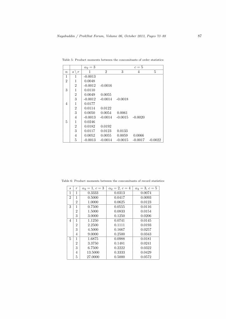
Table 6: Product moments between the concomitants of record statistics:

s r α2 = 1, c = 3 α2 = 2, c = 4 α2 = 3, c = 51 1 0.3333 0.0313 0.00742 1 0.5000 0.0417 0.0093

2 1.0000 0.0625 0.01233 1 0.7500 0.0555 0.0116

2 1.5000 0.0833 0.01543 3.0000 0.1250 0.0206

4 1 1.1250 0.0741 0.01452 2.2500 0.1111 0.01933 4.5000 0.1667 0.02574 9.0000 0.2500 0.0343

5 1 1.6875 0.0988 0.01812 3.3750 0.1481 0.02413 6.7500 0.2222 0.03224 13.5000 0.3333 0.04295 27.0000 0.5000 0.0572


References

Ahsanullah, M., Beg, M.I. (2006) Concomitant of generalized order statistics in Gumbel’s bivariate exponential distribution,Journal of Statistical Theory and Applications 6, 118–132.

Anwar Z., Athar H., Khan R.U. (2007) Expectation identities based on recurrence relations of function of generalized orderstatistics, J. Statist. Res. 41(2), 93–102.

Arnold, B.C. (1983) Pareto Distributions, International Cooperative Publishing House, Fairland, Maryland.Athar H., Nayabuddin (2012) On moment generating function of generalized order statistics from extended generalized half

logistic distribution and its characterization, South Pacific Journal of Pure and Applied Mathematics 1(1), 1–11.Athar H., Nayabuddin (2013) Recurrence relations for single and product moments of generalized order statistics from Marshall-

Olkin extended general class of distributions, J. Stat. Appl. Prob. 2(2), 63–72.Athar H., Nayabuddin, Saba Khalid Khwaja (2013) Relations for moments of generalized order statistics from Marshall-Olkin

extended Weibull distribution and its characterization, ProbStat Forum 5, 127–132.Athar H., Saba Khalid Khwaja, Nayabuddin (2012) Expectation identities of Pareto distribution based on generalized order

statistics and its characterization, AJAMMS 1(1), 23-29.Balakrishnan, N., Ahsanullah, M. (1994) Relations for single and product moments of record values from Lomax distribution,

Sankhya B(56), 140–146.Balkema, A.A., de Haan, L. (1974) Residual life time at great age, Ann. Probab. 2, 792–804.Beg, M.I., Ahsanullah, M. (2008) Concomitants of generalized order statistics from Farlie-Gumbel-Morgenstern distributions,

Statistical Methodology 5, 1–20.David, H.A. (1981) Order Statistics, 2nd edn, John Wiley and Sons, New York.David, H.A., Nagaraja, H.N. (2003) Order Statistics, John Wiley, New York.Erdelyi, A., Magnus, W., Oberhetinger, F., Tricomi, F.G. (1954) Tables of Integral Transforms Vol. I and Vol. II, MC Graw-Hill,

New York.Faizan M., Athar H. (2008) Moments of generalized order statistics from a general class of distributions, Journal of Statistics

15, 36–43.Kamps, U. (1995) A concept of generalized order statistics, B.G. Teubner Stuttgart, Germany (Ph. D. Thesis).Kamps, U., Cramer, E. (2001) On distribution of generalized order statistics, Statistics 35, 269–280.Khan, A.H., Khan R.U., Yaqub, M. (2006) Characterization of continuous distributions through conditional expectation of

generalized order statistics, J. Appl. Prob. Statist 1, 15–131.Khan A.H., Anwar Z., Athar, H. (2009) Exact moments of generalized and dual generalized order statistics from a general form

of distributions, J. Statist. Sci 1(1), 27–44.Lomax, K.S. (1954) Business failures. Another example of the analysis of failure data, J. Amer. Statist. Assoc. 49, 847–852.Nayak, T.K. (1987) Multivariate Lomax distribution: Properties and usefulness in reliability theory, J. Appl. Prob. 24, 170–177.Prudnikov, A.P., Brychkov, Y.A., Marichev, I. (1986) Integral and series Vol. 3, More Special Functions, Gordon and Breach

Science Publisher, New York.Sankaran, P.G., Nair, N.U. (1993) A bivariate Pareto model and its applications to reliability, Naval Research Logistics 40,

1013–1020.Srivastava, H.M., Karlsson, P.W. (1985) Multiple Gaussian Hypergeometric series, John Wiley and Sons, New York.Tahmasebi, S., Behboodian, J. (2012) Shannon information for concomitants of generalized order statistics in Farlie-Gumbel-

Morgenstern (FGM) family, Bull. Malays. Math. Sci. Soc. 34(4), 975–981.Tavangar M., Asadi M. (2008) On a characterization of generalized Pareto distribution based on generalized order statistics,

Commun. Statist. Theory Meth. 37, 1347–1352.

Concomitants of generalized order statistics from bivariate Lomax distribution

Documents

Transcript of Concomitants of generalized order statistics from bivariate Lomax distribution