Guidelines Activity-4: Univariate and Bivariate analysis Epi ...

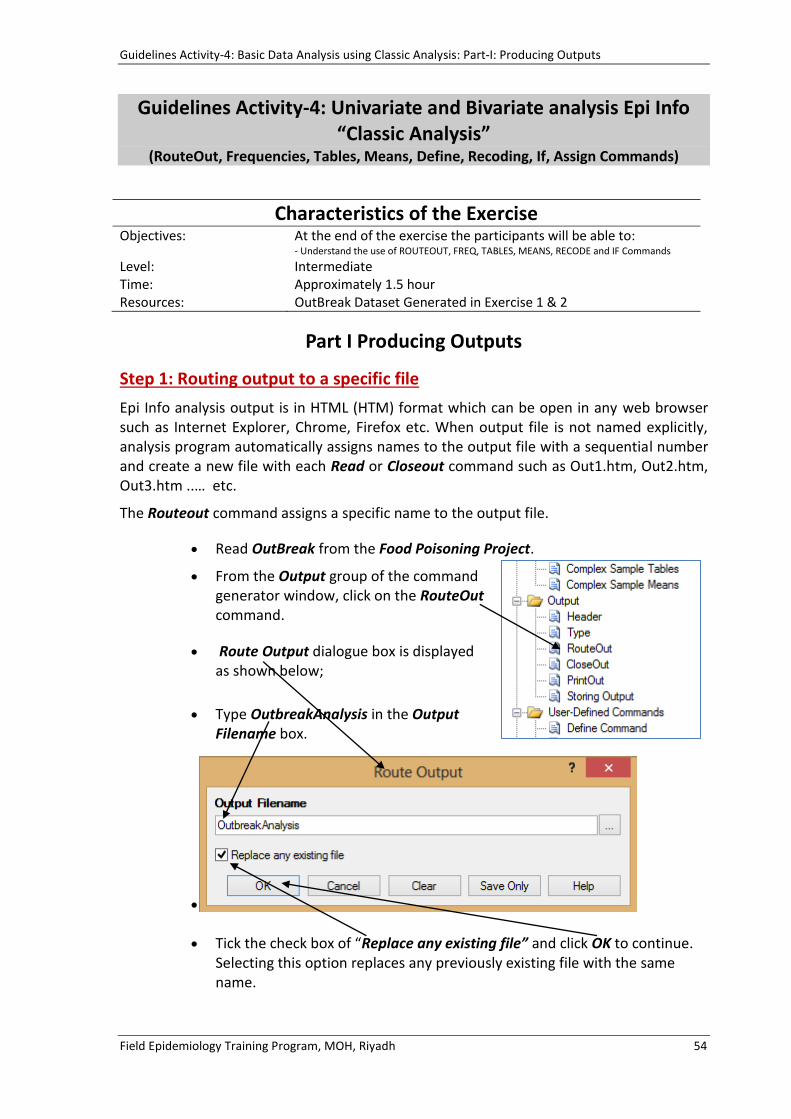
Guidelines Activity-4: Basic Data Analysis using Classic Analysis: Part-I: Producing Outputs

Field Epidemiology Training Program, MOH, Riyadh 54

Guidelines Activity-4: Univariate and Bivariate analysis Epi Info “Classic Analysis”

(RouteOut, Frequencies, Tables, Means, Define, Recoding, If, Assign Commands)

Characteristics of the Exercise

Objectives: At the end of the exercise the participants will be able to: - Understand the use of ROUTEOUT, FREQ, TABLES, MEANS, RECODE and IF Commands

Level: Intermediate Time: Approximately 1.5 hour Resources: OutBreak Dataset Generated in Exercise 1 & 2

Part I Producing Outputs

Step 1: Routing output to a specific file

Epi Info analysis output is in HTML (HTM) format which can be open in any web browser such as Internet Explorer, Chrome, Firefox etc. When output file is not named explicitly, analysis program automatically assigns names to the output file with a sequential number and create a new file with each Read or Closeout command such as Out1.htm, Out2.htm, Out3.htm ..… etc.

The Routeout command assigns a specific name to the output file.

Read OutBreak from the Food Poisoning Project.

From the Output group of the command generator window, click on the RouteOut command.

Route Output dialogue box is displayed as shown below;

Type OutbreakAnalysis in the Output Filename box.

Tick the check box of “Replace any existing file” and click OK to continue.

Selecting this option replaces any previously existing file with the same name.

Guidelines Activity-4: Univariate and Bivariate Analysis using Classic Analysis: Part-I: Producing Outputs


Step 2: Frequencies

A) Simple Frequency From the command tree, click the command Frequencies.

Frequencies dialogue box is displayed as shown below;

Click the drop down arrow of the “Frequency of” box, a list of all available variables in the data table is visible in an alphabetic order.

From the drop down list of the variables, select variables Sex. This appears in the box below. Next click OK button to continue.

The frequency distribution table of the sex variable is generated in the analysis output window as shown below in the illustration.

Similarly other variables can be selected to compute frequency. More than one variable can also be selected at the same time. Selecting (*) from the drop list of the variables compute frequency tables for all variables of the dataset.



B) Frequency Distribution with Stratification

From the command explorer panel, click the command Frequencies again.

Select variable Sex from the drop-down box labeled “Frequency of” and select

variable ILL from “stratify by” box. Click OK.

Two frequency distribution Tables are generated for sex variable. One for “ILL=Yes” and second “ILL=No” as shown below in the illustration.



Step 3: Means

A) Simple Means

Means command only works with numeric variables.

Click Means command from the command window. When Means dialogue box is displayed as shown below, Select Age variable from the drop-down box labeled “Means of”.

Click OK button to continue.

Output window shows frequency table for numeric variable along with Number of observations, Mean, Std Deviation, Minimum, Maximum, Mode etc as shown below.



B) Means Command with Stratification

Means with stratification compute the mean value of numeric variable for each strata of the stratification variable.

Click on the Means command again. Select Age variable again from the drop-down box labeled “Means of”, select Sex from “Stratify by” and click OK button to continue.

Output window shoes Number of Observation, Mean, Std Deviation, Minimum, Maximum, Mode etc for Age variable separately for Female and Males as shown below in the illustration.



C) Means Command with Cross Tabulation

Means with cross tabulation compare the mean value of numeric variable for each strata of stratification variable also apply statistical test.

Click on the Means command again.

Select Age from the drop-down box labeled Means of and select ILL from “Cross tabulate by Value of”.

Click OK button to continue. Observe the output.

Output window shows comparison of mean value of Age with the ILL=Yes and ILL=No. Please note that t-test is also computed for the comparison of mean ages as shown in below illustrations.



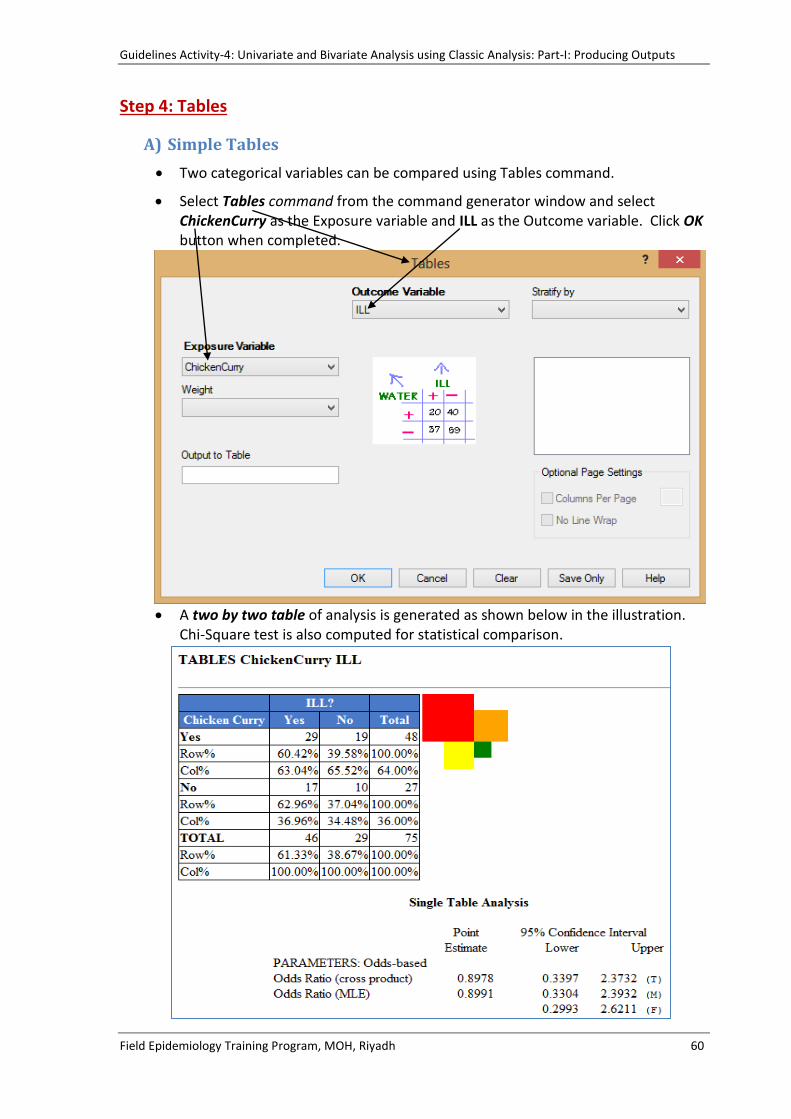
Step 4: Tables

A) Simple Tables

Two categorical variables can be compared using Tables command.

Select Tables command from the command generator window and select ChickenCurry as the Exposure variable and ILL as the Outcome variable. Click OK button when completed.

A two by two table of analysis is generated as shown below in the illustration. Chi-Square test is also computed for statistical comparison.



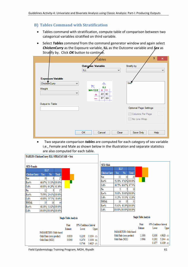
B) Tables Command with Stratification

Tables command with stratification, compute table of comparison between two categorical variables stratified on third variable.

Select Tables command from the command generator window and again select ChickenCurry as the Exposure variable, ILL as the Outcome variable and Sex as Stratify by. Click OK button to continue.

Two separate comparison tables are computed for each category of sex variable i.e., Female and Male as shown below in the illustration and separate statistics are also computed for each table.



Step 5: Defining a new variable

New variables can be defined in the Analysis Program. These variables hold the results of calculations or conditional statements. Three types of variables can be defined. These are standard, Global and Permanent. Standard variable is temporary variable and is lost at the next Read command. For this exercise we will define the Standard Variable which is the default setting in Define command.

To define a new variable, click on Define command in the command explorer window. DefineVariable dialogue box appears. Type AgeGrp as the name of the new variable in the variable name text box. Click OK button to continue.

A new variable AgeGrp is created.

Use Display variable command to view the newly created variable as shown below in the illustration.

Please note that new Defined variable AgeGrp is listed down in the variable list. New value can be assigned to this variable using Recode or If Command.

Please also note that in naming a variable, no space is allowed between the words.



Step 6: Assigning values to a variable using “Recode” Command

In this step, Recode command of the analysis will be used to assign values to the new variable AgeGrp which was defined in previous step.

Age variable of the dataset will be grouped into new variable AgeGrp based on following age ranges.

a) < 15 years b) 15-29 years c) 30-44 years d) 45 and above

Following are the steps to recode the Age variable into AgeGrp variable.

Select Recode command from the command generator window. Recode Dialogue box is visible.

Select Age variable from the drop down list of the From and AgeGrp from the To Text box

Click in the text box Value and type 1. Press Enter key.

Type 14 In the text box of To Value. Press Enter Key.

In the Box of Recoded Value and type 1) < 15 Years. Press Enter Key

A new blank row will be created. Add the remaining categories in the similar

way to complete the recode statement as illustrated above.

On completion of all categories, Press OK button to continue.



Use Frequency command to generate the frequency distribution of the newly created variable AgeGrp which appears as shown below in the illustration.

Please note the Analysis Codes or Command Syntax is also displayed in the program

editor window as shown below. These codes can be saved in the program file and

can be used later.



Step 7: Assigning values to a variable using “If” Command

There are three types of beverages in the dataset ie., Milk, softdrink and Water. We can group these 3 variables into a new variable (Beverage) which means that if a person has taken any of the three items then Beverage variable is Yes(true) and else Beverage is No (False).

If order to do so, first a new variable Beverage is to be defined and then If command is used to assign value to new variable. The steps are as below;

Define a new variable Beverage.

To assign the value to new variable Beverage, click on the If command in command explorer window.

IF dialogue box is displayed on the screen as shown below.

There are three sections of If dialogue box.

If Condition

Then

Else

From the Available Variables drop-down box, select the variable Juice and build the following expression Juice= (+) OR SoftDrink= (+) OR Water= (+) Please note that (+) means “Yes”. On clicking “Yes”, (+) is displayed in the expression box.



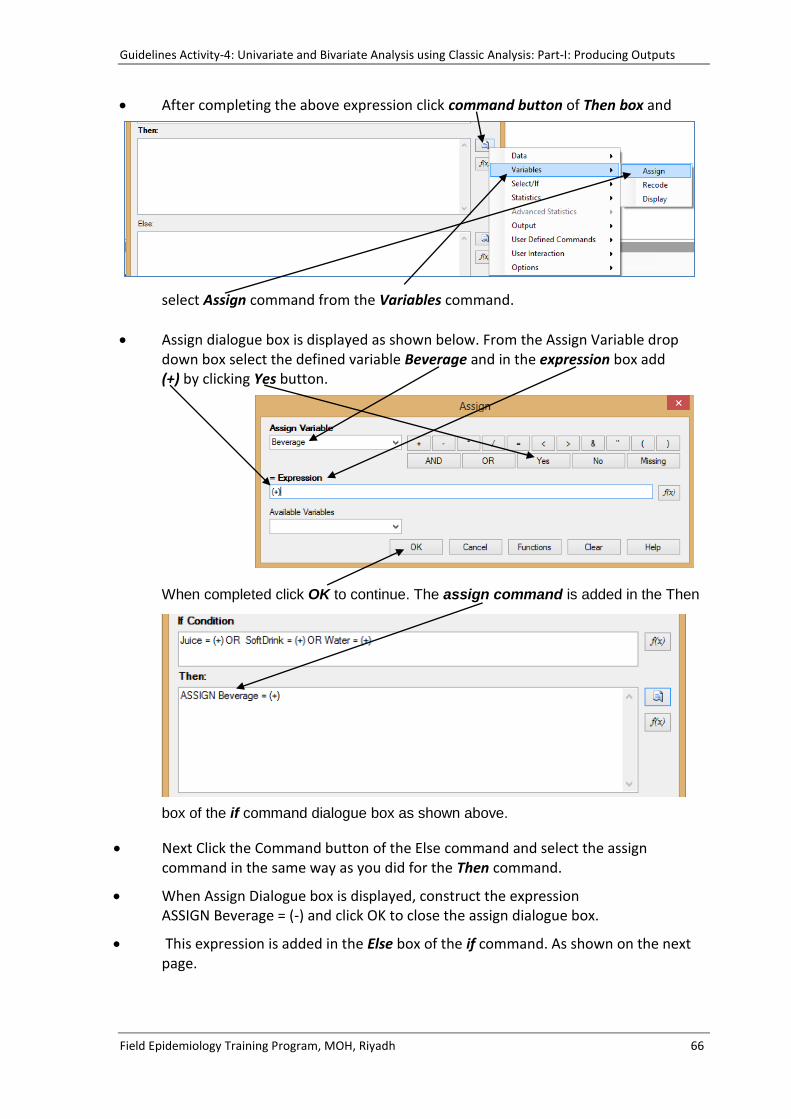
After completing the above expression click command button of Then box and

select Assign command from the Variables command.

Assign dialogue box is displayed as shown below. From the Assign Variable drop down box select the defined variable Beverage and in the expression box add (+) by clicking Yes button.

When completed click OK to continue. The assign command is added in the Then

box of the if command dialogue box as shown above.

Next Click the Command button of the Else command and select the assign command in the same way as you did for the Then command.

When Assign Dialogue box is displayed, construct the expression ASSIGN Beverage = (-) and click OK to close the assign dialogue box.

This expression is added in the Else box of the if command. As shown on the next page.



When all steps are completed, the If dialogue box should be look like as shown above. Click OK to complete the If command.

Use Frequency command to generate frequency distribution of the Beverage variable.

Please note the corresponding syntax is also displayed in the Program editor window.

Guidelines Activity-4: Univariate and Bivariate Analysis using Classic Analysis: Part-II: Creating Graphs


Guidelines Activity-4: Univariate and Bivariate Analysis using Classic Analysis

Part II: Creating Graphs


Objectives: At the end of the exercise the participants will be able to: - Understand the use of Graph command to generate various types of Graph such as Pie, Bar, Stacked bar

Level: Intermediate Time: Approximately 1/2 hour Resources: Outbreak Dataset Generated in Activity 1 & 2

Part II Creating Graphs Epi Info Analysis program can also create various types of graphs (Pie, bar, line etc) to make visual representation of the data.

Step 8: Creating Pie Diagram

To create pie diagram of the Sex variable in the Food poisoning outbreak dataset do

following steps;

Click on the Graph command in the command generator window

A GRAPH dialog box appears with various options appears as shown on the next page.

Guidelines Activity-4: Univariate and Bivariate Analysis: Part-II: Creating Charts


From the drop down arrow of the Graph Type select Pie. From the drop down arrow of the Main variable(s) text box select Sex variable and Type the Title as

mentioned above. From the drop down box of show value of select Count

After completing the above options click OK to generate Pie graph as show.

Step 9: Creating Bar Diagram

To create Bar diagram of the Time Duration variable in the Food poisoning outbreak dataset do the following steps;

Click on the Graph command in the command generator window as shown

in the previous step.

GRAPH dialog box appears on the screen as shown below

Guidelines Activity-4: Univariate and Bivariate Analysis: Part-II: Creating Charts


Select Bar from the Graph Type.

Add X-Axis, Y-Axis Labels and Title as shown above

Click Ok to generate the graph as shown below.

Guidelines Activity-4: Univariate and Bivariate Analysis using Classic Analysis: Part-III: Working with Syntax


Guidelines Activity-4: Univariate and Bivariate Analysis using Classic Analysis

Part III: Working with Analysis Syntax


Objectives: At the end of the exercise the student will be able to: - Understand the analysis program codes, saving codes in the program file and running and executing the analysis program

Level: Intermediate Time: Approximately 1/2 hour Resources: Outbreak Dataset Generated in Activity 1 & 2

Part III Working with Analysis Syntax

Step 10: Saving a program file (.PGM) Note that with each command execution, one or more lines of program codes are generated in the Program Editor windows at the bottom of the analysis screen.

These program codes can be saved in the program file and can be reloaded and Run from the program editor window.

Program codes can be saved internally within the project file or externally as a text file with .pgm file extension.

a) Saving a Analysis Code Internally

Internally, the codes written in the program editor are saved in a special table in the Epi Info Project file called as metaPrograms.

So the internally saved program becomes part of the project file. It can be opened in the program editor window and can be run by using the Run command of the program Editor.

Guidelines Activity-4: Univariate and Bivariate Analysis: Part-III: Working with Analysis Syntax


To save the codes, click the Save button of the program editor window. A Save Program dialogue box appears as shown on next page.

In the Save Program dialogue box, type OutBreak Analysis in the program text box, and then type your name in the Author box. Before you save, you may type a brief description of the program in the comments box. When this is completed, click OK button to save program file.

Saving a Analysis Code Externally (.Pgm)

To save the codes externally, click the Text File button in the save program dialogue box. This brings the Save As dialogue box, Type Outbreak Analysis in file name box and click save button. The program codes are now saved as external file with the

extension of pgm. This is similar to program file for Epi Info 6 for DOS.



Please note that Closing and opening Analysis program removes the analysis codes from the program editor window.

Step 11: Opening an existing program

In the Program Editor, click the Open Pgm button.

On clicking the open button of program editor window, Read Program dialogue box is displayed. From the drop down arrow of the program Box select the Outbreak Analysis.



Check that your name and your comments are displayed along with the Date Created and Date Updated. Click OK button to load the program is in the Program Editor Window. To run the program, click on the Run command of the program editor window.

To open a program that was saved externally, click Open button from the

program editor window to display Read Program dialogue box as before.

Next click the Text File button to display Read Text dialogue box containing list of available .PGM files.

Click on Outbreak Analysis.pgm7 file and click open button.



The file is loaded in the content box of the Open Program dialogue box. Clicking Ok button of the open program loads the analysis code in the program editor window.

Step 12: Running the program

After the program is loaded in the program editor, it is ready to be executed. Click the Run Commands button to execute all the analysis codes. The analysis codes can also be edited if desired.

A single command can also be run by placing the cursor on the command line and clicking the Run Commands or highlighting group of commands and Clicking this button again.

If more analysis is performed, the more codes are added in the program editor windows, these changes can be saved to the program by clicking Save button

Guidelines Activity-4: Univariate and Bivariate analysis Epi ...

Documents

Transcript of Guidelines Activity-4: Univariate and Bivariate analysis Epi ...