Alain Hecq, Sébastien Laurent and Franz C. Palm

On the Univariate Representation

of BEKK Models with Common Factors

RM/12/018

On the Univariate Representation of BEKK

Models with Common Factors

Alain Hecq, Sébastien Laurent and Franz C. Palm �

Department of Quantitative Economics

Maastricht University

The Netherlands

March 27, 2012

Abstract

First, we investigate the minimal order univariate representation of some well known n�dimensionalconditional volatility models. Even simple low order systems (e.g. a multivariate GARCH(0,1)) for

the joint behavior of several variables imply individual processes with a lot of persistence in the form

of high order lags. However, we show that in the presence of common GARCH factors, parsimonious

univariate representations (e.g. GARCH(1,1)) can result from large multivariate models generat-

ing the conditional variances and conditional covariances/correlations. The trivial diagonal model

without any contagion e¤ects in conditional volatilities gives rise to the same conclusions though.

Consequently, we then propose an approach to detect the presence of these commonalities in

multivariate GARCH process. The factor we extract is the volatility of a portfolio made up by the

original assets whose weights are determined by the reduced rank analysis.

We compare the small sample performances of two strategies. First, extending Engle and Mar-

cucci (2006), we use reduced rank regressions in a multivariate system for squared returns and

cross-returns. Second we investigate a likelihood ratio approach, where under the null the matrix

parameters of the BEKK have a reduced rank structure (Lin, 1992). It emerged that the latter

approach has quite good properties enabling us to discriminate between a system with seemingly

unrelated assets (e.g. a diagonal model) and a model with few common sources of volatility.

JEL: C10, C32

Keywords: Common GARCH, factor models, BEKK, Final equations.

�Corresponding author: Franz Palm, Department of Quantitative Economics, Maastricht University, P.O.Box 616, 6200

MD Maastricht, The Netherlands. E-mail: f.palm@maastrichtuniversity.nl. This paper is a revised version of our 2011

METEOR discussion paper "On the Univariate Representation of Multivariate Volatility Models with Common Factors".

We would like to thank two anonymous referees for their comments on the previous version. The usual disclaimer applies.

1

1 Motivation

This paper proposes an alternative view to interpret and investigate the presence of common volatility

in multivariate asset return models. Indeed, we start with the observation that parsimonious univariate

volatility models (e.g. GARCH(1,1)) are often detected in empirical works. We show that this can be

seen as an indication of the presence of few factors generating the volatility of asset returns. We get

this result using the �nal equation representation of multivariate models, tools ushered from Zellner and

Palm (see inter alia 1974, 1975, 2004) for VARMA and extended to reduced rank models by Cubadda et

al. (2009). This framework allows us to derive the marginal GARCH representation for the conditional

variances and conditional covariances of the multivariate GARCH model (e.g. Nijman and Sentana

(1996) in the unrestricted case) but in the presence of common GARCH factors.

Given that both independent volatility models (e.g. a diagonal model) and a highly dependent struc-

ture with few factors generating the conditional second moments deliver similar parsimonious marginal

representations, we propose a new framework for detecting the presence of common volatility. Our set-

ting is di¤erent from two types of modeling commonly found in this literature. First, contrary to the

usual factor models in �nance, our approach does not assume any ad hoc idiosyncratic component to be

added to the common factor representation. Second, with the volatility being unobservable, we do not

directly test for potential combinations of hereroskedastic series that are conditionally homoskedastic

(see Engle and Susmel, 1993; Engle and Kozicki 1993). Instead we translate the task to detect the

presence of common volatility in asset returns into an analysis of common cyclical features (Vahid and

Engle, 1993) in the dynamics of the squared returns and cross-returns. To some extent our framework

can be seen as a generalization of the Engle and Marcucci (2006) pure variance model although they do

not consider the covariances in their analysis. Moreover, they tailor the dynamics of the logarithms of

squared returns to exactly match their theoretical assumptions and they do not consider the presence

of non-i.i.d. disturbances.

The common volatility factors extracted by our strategy are quite intuitive since they represent

the conditional variance of a portfolio composed by the series involved in the analysis. Applying our

common cycle approach and hence testing for the presence of commonalities in the vech or the vecd of

the conditional covariance matrix is hazardous however. Indeed, even under the null, the combination

that annihilates the temporal dependence in squared returns and cross-returns is a martingale di¤erence

sequence. We show that this leads to large size distortions if one uses canonical correlation test statistics

as in Engle and Marcucci (2006). Moreover, accounting for the presence of hereroskedasticity using a

robusti�ed version of those reduced rank tests (Hecq and Issler, 2012) does not help to get rid of the

e¤ect of non-normality. It turns out that, although the representation of multivariate systems in terms of

squared returns and cross-returns is crucial to obtain the orders of the marginal models, only a maximum

likelihood strategy consisting in estimating a multivariate GARCH for the returns under the reduced

2

rank null hypothesis enables us to draw some conclusions. Also note that our goal is not to provide

a glossary of marginal representations obtained from every multivariate systems1 but to provide tools

to understand the underlying behavior of a parsimonious block of assets. As an example, among the

bunch of �fty daily stock returns that we analyze in this paper, six of them are rather better described as

GARCH(1,1) than as long memory processes. Then we will investigate whether there is a factor structure

behind this feature or simply an absence of causality from the past covariances to the variances.

The rest of this paper is as follows. Section 2 sets up the notations and derives the general results for

the �nal equation representation of multivariate GARCH models. We propose in Section 3 some multi-

variate models accounting for co-movements in volatility and show that the implied marginal volatility

processes are of low order. We introduce the pure portfolio common GARCH volatility model based on

the factor GARCH speci�cation proposed by Lin (1992) for the BEKK. Section 4 extends the previous

results to the multiple factor cases. This will be important for our approach because the dimension of

the system for k > 1 factors is not k but some ~k > k. We develop in Section 5 several testing strategies

that we evaluate in Section 6 using a Monte Carlo exercise. In Section 7 we apply our preferred test to

six US stock return series. In particular we are able to discriminate between a diagonal model and a

general multivariate framework, with correlated conditional variances and contagion e¤ects, driven by a

small number of common factors in volatility. The �nal section concludes.

2 The �nal equation representation of multivariate GARCH

models

2.1 De�nition of common volatility features

To state the notation for univariate excess returns2 , "1t is such that "1t = u1tph11t, where u1t has

any centered parametric distribution with unitary variance and the conditional variance of "1t follows

a GARCH(p; q) with h11t = !1 +Pp

j=1 �1;jh11t�j +Pq

i=1 �1;i"21t�i: Consequently here, p refers to the

GARCH terms and q is the order of the moving average ARCH term. The error in the squared returns is

obtained as usual using �1t = "21t�h11t. As an example a GARCH(1; 2) can be rearranged for the squaredreturns such that "21t = !1 + (�1;1 + �1;1)"

21t�1 + �1;2"

21t�2 + �1t � �1;1�1t�1 (see inter alia Bollerslev,

1Let us just name the diagonal model, the constant conditional correlation (CCC), the dynamic conditional correlation

(DCC), the dynamic equicorrelation (DECO, see Engle and Kelly, 2008), the approach by Baba, Engle, Kraft and Kroner

(1999, hereafter BEKK), the orthogonal GARCH, the factor GARCH, as well as some of their block versions such as the

BLOCK-DCC (Billio, Caporin and Gobbo, 2003) and BLOCK-DECO (Engle and Kelly, 2008) as examples proposed in

the literature to restrict the multivariate setting towards a manageable size as well as to impose the positive de�nitiveness

of the covariance matrix (see inter alia the surveys by Bauwens, Laurent and Rombouts, 2006 and Silvennoinen and

Terasvirta, 2009).2By excess return we mean that the conditional mean (a constant or an ARMA model for instance) has been substracted

from the returns rt, say "t = rt � E(rtjt�1); where t�1 denotes the information set up to and including t� 1.

3

1996). Thus, the squared returns follow a heteroskedastic weak GARCH univariate ARMA(2; 1) process.

In general a GARCH(p; q) has got an ARMA(max(p; q); p) representation for the squared returns. In

most of the examples we have considered, we take q � p:For multivariate modeling, we denote by "t = H

1=2t zt; t = 1; : : : ; T; the n� 1 vector of excess returns

of �nancial assets observed at the time period t: T is the number of observations and zt � i:i:d:(0; In):Consequently we have "tjt�1 � D(0;Ht) with t�1 the past information set and Ht the conditional

covariance matrix of the n assets that is measurable with respect to t�1; D(:; :) is some arbitrary

multivariate distribution. Let us also denote without loss of generality Ht = H + ~Ht as the sum of a

constant part and a time-varying part.

In this multivariate setting, testing for common GARCH (in the sense of Engle and Kozicki, 1993)

amounts to look towards s directions �0"t such that the �0"t combinations of asset returns are conditionally

homoskedastic, namely such that �0"tjt�1 � D(0; C) where C does not depend on t. To be more explicitlet us de�ne the following partitioned matrix � spanning Rn

� =

Is ��0s�(n�s)

0(n�s)�s In�s

!;

where we have normalized the cofeature space �0 = (Is : ��0s�(n�s)) for the sake of notation. We de�ne a

common volatility feature model i¤ for

�"tjt�1 � D(0;�Ht�0);

and hence in

�"tjt�1 � D(0;�H�0 + � ~Ht�0);

we have

rank(� ~Ht�0) = n� s

instead of n: Clearly this de�nition splits in a natural way, i.e. without referring to an ad hoc factor

structure, the volatility feature of the n�dimensional process as the sum of two parts. There exists s

combinations of the asset returns that have a common volatility component. Consequently there exist

s linear combinations of "t that have time-invariant conditional distributions. The remaining n � scombinations generate the time-varying volatility of the system.

This approach, although not formulated in this way can be seen as a generalization of Engle and

Kozicki (1993) and Engle and Susmel (1993). Indeed, it is a generalization because both papers only look

at bivariate processes (i.e. n = 2) with potentially the presence of a single factor, namely k = n� s = 1:Our paper goes beyond these aforementioned papers because we propose a multivariate framework for

n � 2 and k � 1: The limitations of the previous papers come also from the fact that a grid search is

used to �nd a combination of series such that this combination minimizes the LM test of no ARCH. Not

only is this strategy computationally ine¢ cient but it is tedious to extend to more than two series. This

4

explains why bivariate analyses are usually considered in Ruiz (2009) or in Arshanapalli et al. (1997)

for instance. Note also that our approach might look like a factor model in volatility with a constant

idiosyncratic component, namely when only the factor generates time-varying volatility. This is very

di¤erent to the usual approach proposed in the literature (e.g. King and Wadhwani, 1990) in which the

distribution of the idiosyncratic part can also be time-varying. In this sense we are closer to Diebold

and Nerlove (1989) although in our framework the number of factors is going to be tested. Finally, our

approach improves upon Engle and Marcucci (2006) in three respects. First we investigate the theoretical

impact of the addition of the cross-products to their pure variance model. Second, we do not assume a

particular form such as an exponential model. Third we evaluate di¤erent testing strategies in a Monte

Carlo experiment.

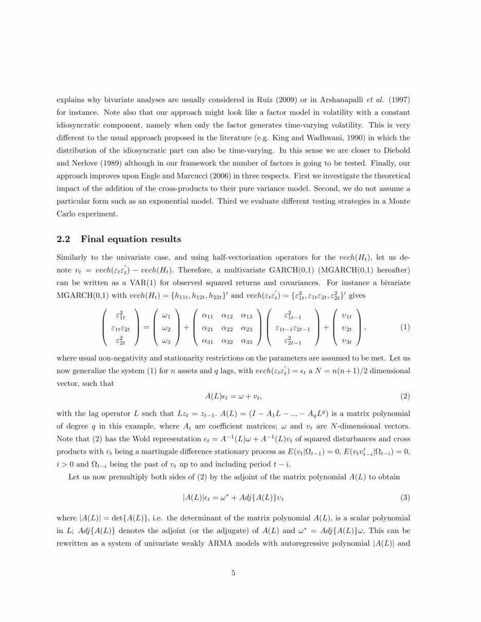
2.2 Final equation results

Similarly to the univariate case, and using half-vectorization operators for the vech(Ht); let us de-

note vt = vech("t"0

t) � vech(Ht): Therefore, a multivariate GARCH(0,1) (MGARCH(0,1) hereafter)can be written as a VAR(1) for observed squared returns and covariances. For instance a bivariate

MGARCH(0,1) with vech(Ht) = fh11t; h12t; h22tg0 and vech("t"0

t) = f"21t; "1t"2t; "22tg0 gives0BB@"21t

"1t"2t

"22t

1CCA =

0BB@!1

!2

!3

1CCA+0BB@�11 �12 �13

�21 �22 �23

�31 �32 �33

1CCA0BB@

"21t�1

"1t�1"2t�1

"22t�1

1CCA+0BB@�1t

�2t

�3t

1CCA ; (1)

where usual non-negativity and stationarity restrictions on the parameters are assumed to be met. Let us

now generalize the system (1) for n assets and q lags, with vech("t"0

t) = �t a N = n(n+1)=2 dimensional

vector, such that

A(L)�t = ! + vt; (2)

with the lag operator L such that Lzt = zt�1: A(L) = (I � A1L � ::: � AqLq) is a matrix polynomialof degree q in this example, where Ai are coe¢ cient matrices; ! and vt are N -dimensional vectors.

Note that (2) has the Wold representation �t = A�1(L)! +A�1(L)vt of squared disturbances and cross

products with vt being a martingale di¤erence stationary process as E(vtjt�1) = 0; E(vtv0t�ijt�i) = 0;i > 0 and t�i being the past of vt up to and including period t� i:Let us now premultiply both sides of (2) by the adjoint of the matrix polynomial A(L) to obtain

jA(L)j�t = !� +AdjfA(L)g�t (3)

where jA(L)j = detfA(L)g; i.e. the determinant of the matrix polynomial A(L); is a scalar polynomialin L; AdjfA(L)g denotes the adjoint (or the adjugate) of A(L) and !� = AdjfA(L)g!: This can berewritten as a system of univariate weakly ARMA models with autoregressive polynomial jA(L)j and

5

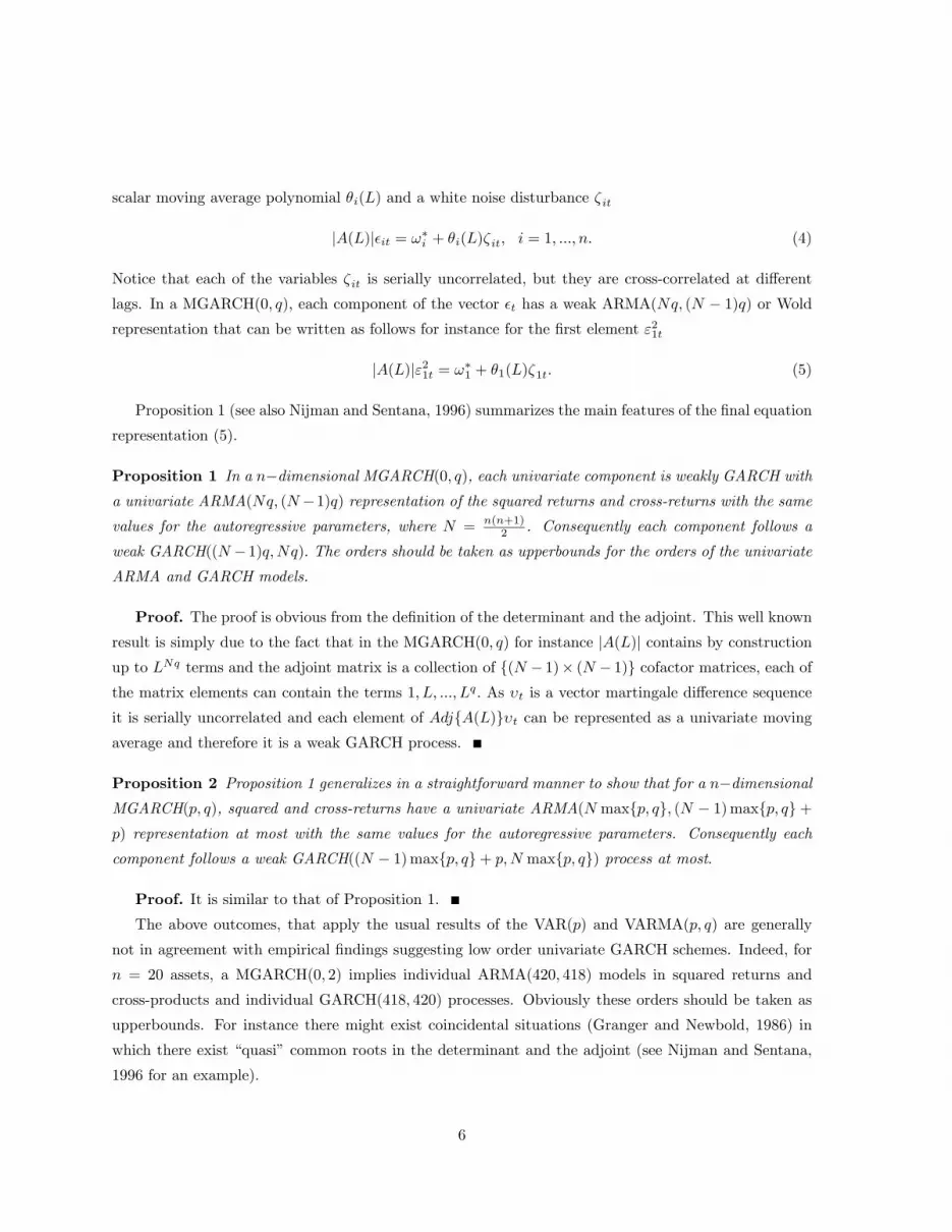
scalar moving average polynomial �i(L) and a white noise disturbance �it

jA(L)j�it = !�i + �i(L)�it; i = 1; :::; n: (4)

Notice that each of the variables �it is serially uncorrelated, but they are cross-correlated at di¤erent

lags. In a MGARCH(0; q); each component of the vector �t has a weak ARMA(Nq; (N � 1)q) or Woldrepresentation that can be written as follows for instance for the �rst element "21t

jA(L)j"21t = !�1 + �1(L)�1t: (5)

Proposition 1 (see also Nijman and Sentana, 1996) summarizes the main features of the �nal equation

representation (5).

Proposition 1 In a n�dimensional MGARCH(0; q), each univariate component is weakly GARCH witha univariate ARMA(Nq; (N�1)q) representation of the squared returns and cross-returns with the samevalues for the autoregressive parameters, where N = n(n+1)

2 . Consequently each component follows a

weak GARCH((N �1)q;Nq): The orders should be taken as upperbounds for the orders of the univariateARMA and GARCH models.

Proof. The proof is obvious from the de�nition of the determinant and the adjoint. This well known

result is simply due to the fact that in the MGARCH(0; q) for instance jA(L)j contains by constructionup to LNq terms and the adjoint matrix is a collection of f(N � 1)� (N � 1)g cofactor matrices, each ofthe matrix elements can contain the terms 1; L; :::; Lq: As �t is a vector martingale di¤erence sequence

it is serially uncorrelated and each element of AdjfA(L)g�t can be represented as a univariate movingaverage and therefore it is a weak GARCH process.

Proposition 2 Proposition 1 generalizes in a straightforward manner to show that for a n�dimensionalMGARCH(p; q), squared and cross-returns have a univariate ARMA(N maxfp; qg; (N � 1)maxfp; qg+p) representation at most with the same values for the autoregressive parameters. Consequently each

component follows a weak GARCH((N � 1)maxfp; qg+ p;N maxfp; qg) process at most:

Proof. It is similar to that of Proposition 1.

The above outcomes, that apply the usual results of the VAR(p) and VARMA(p; q) are generally

not in agreement with empirical �ndings suggesting low order univariate GARCH schemes. Indeed, for

n = 20 assets, a MGARCH(0; 2) implies individual ARMA(420; 418) models in squared returns and

cross-products and individual GARCH(418; 420) processes. Obviously these orders should be taken as

upperbounds. For instance there might exist coincidental situations (Granger and Newbold, 1986) in

which there exist �quasi�common roots in the determinant and the adjoint (see Nijman and Sentana,

1996 for an example).

6

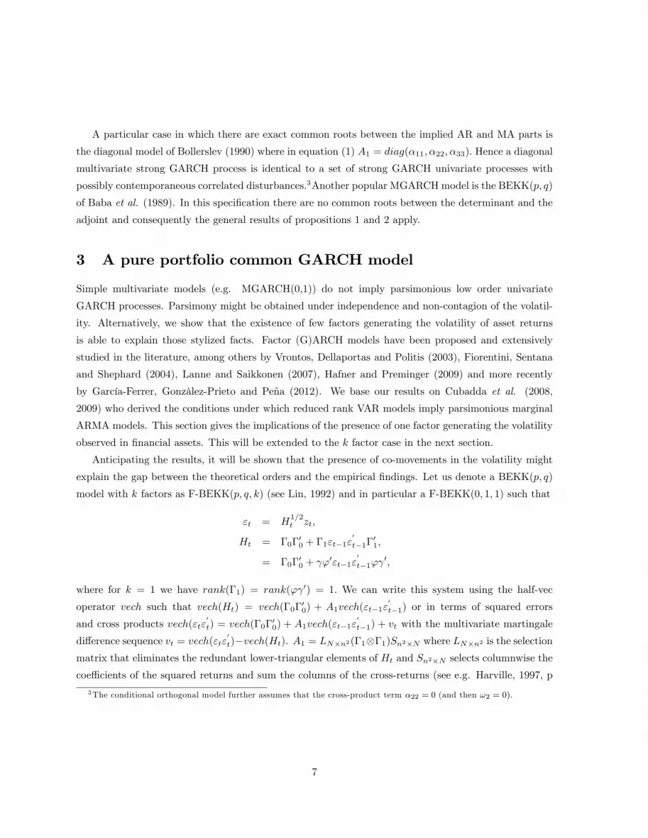
A particular case in which there are exact common roots between the implied AR and MA parts is

the diagonal model of Bollerslev (1990) where in equation (1) A1 = diag(�11; �22; �33): Hence a diagonal

multivariate strong GARCH process is identical to a set of strong GARCH univariate processes with

possibly contemporaneous correlated disturbances.3Another popular MGARCH model is the BEKK(p; q)

of Baba et al. (1989). In this speci�cation there are no common roots between the determinant and the

adjoint and consequently the general results of propositions 1 and 2 apply.

3 A pure portfolio common GARCH model

Simple multivariate models (e.g. MGARCH(0,1)) do not imply parsimonious low order univariate

GARCH processes. Parsimony might be obtained under independence and non-contagion of the volatil-

ity. Alternatively, we show that the existence of few factors generating the volatility of asset returns

is able to explain those stylized facts. Factor (G)ARCH models have been proposed and extensively

studied in the literature, among others by Vrontos, Dellaportas and Politis (2003), Fiorentini, Sentana

and Shephard (2004), Lanne and Saikkonen (2007), Hafner and Preminger (2009) and more recently

by García-Ferrer, Gonzàlez-Prieto and Peña (2012). We base our results on Cubadda et al. (2008,

2009) who derived the conditions under which reduced rank VAR models imply parsimonious marginal

ARMA models. This section gives the implications of the presence of one factor generating the volatility

observed in �nancial assets. This will be extended to the k factor case in the next section.

Anticipating the results, it will be shown that the presence of co-movements in the volatility might

explain the gap between the theoretical orders and the empirical �ndings. Let us denote a BEKK(p; q)

model with k factors as F-BEKK(p; q; k) (see Lin, 1992) and in particular a F-BEKK(0; 1; 1) such that

"t = H1=2t zt;

Ht = �0�00 + �1"t�1"

0

t�1�01;

= �0�00 + '

0"t�1"0

t�1' 0;

where for k = 1 we have rank(�1) = rank(' 0) = 1: We can write this system using the half-vec

operator vech such that vech(Ht) = vech(�0�00) + A1vech("t�1"

0

t�1) or in terms of squared errors

and cross products vech("t"0

t) = vech(�0�00) + A1vech("t�1"

0

t�1) + vt with the multivariate martingale

di¤erence sequence vt = vech("t"0

t)�vech(Ht). A1 = LN�n2(�1�1)Sn2�N where LN�n2 is the selectionmatrix that eliminates the redundant lower-triangular elements of Ht and Sn2�N selects columnwise the

coe¢ cients of the squared returns and sum the columns of the cross-returns (see e.g. Harville, 1997, p

3The conditional orthogonal model further assumes that the cross-product term �22 = 0 (and then !2 = 0):

7

357).4 A1 can be written in a reduced form with

A1 =

0BB@ 21'

21 2 21'1'2 21'

22

1 2'21 2 1 2'1'2 1 2'

22

22'21 2 22'1'2 22'

22

1CCA =

0BB@1 2 1

( 2 1)2

1CCA� 21'21 2 21'1'2 21'22

�;

such that there exists a normalized cofeature matrix

� =

0BB@� 2 1

� 22 21

1 0

0 1

1CCA ;with �

0A = 02�3: From the determinant det(I�AL) = 1�( 1'1 + 2'2)

2L and the adjoint (which is not

reported to save space) it emerges that all squared returns and their cross-products are ARMA(1; 1) and

hence we have GARCH(1,1) speci�cations for the conditional variances and covariances. Importantly

enough the combination of the series representing the factor, i.e. 21'21"21t�1 + 2

21'1'2"1t�1"2t�1 +

21'22"22t�1

P 2t�1 = ( 1'1"1t�1 + 1'2"2t�1)2;

has the same variance as a portfolio made up by the series whose weights are determined by the reduced

rank analysis and the factor structure.

Therefore, each volatility and cross-correlation in such a system only depend on that portfolio. This is

the reason why we call this model a pure portfolio common GARCH model given in terms of unobserved

volatilities 0BB@h11t

h12t

h22t

1CCA =

0BB@$1

$2

$3

1CCA+0BB@�1

�2

�3

1CCAP 2t�1; (6)

where the �0is measure the impact of the volatility of the portfolio on the volatilities and covariances

of the underlying assets. Moreover there exist combinations of series such that �0?vech(Ht) does not

depend on the volatility of the portfolio. This approach is also di¤erent from the GO-GARCH where

the direction for the combination is such that the variance of the returns is maximized using a principal

combination analysis. In our case we look at the combinations that are the most correlated with the

volatility and covariances of the assets.

Note that this interpretation is made easier using the factor BEKK than from an unrestricted

MGARCH with a reduced rank in squared returns and cross-returns. Finding a reduced rank in the

general model (1) for instance does not ensure that the coe¢ cient of the cross-correlation is numerically

two times the coe¢ cients in front of the returns.4Note that in the one-factor case, A1 can also be obtained using ''0( 0"t�1)2 = '0"t�1"

0t�1'

0: Therefore, the matrix

''0 is of rank one as well as the coe¢ cient matrix A1.

8

Our �ndings about the parsimony of the implied series generalize as follows in the s factor case.

Note however (see the next section for details) that for k > 1 we do not have rank(A1) = k anymore:

Propositions and proofs are given for N but the results are derived in the same manner for n if one does

not consider the covariances in the analysis.

Proposition 3 In a n�dimensional F-BEKK(0; q; k), the squared returns and cross-returns have a uni-variate ARMA(p�; q�) representation with the same values for the autoregressive parameters. The orders

of p� and q� are at most (N �s)q: When k = 1 and hence s = N �1; the orders of p� and q� are at mostq and hence do not depend on N . As a special case, each component of a multivariate F-BEKK(0; 1; 1)

follows a weak GARCH(1; 1) whatever the number of assets jointly considered.

The propositions and the proofs are applications of the results obtained in Cubadda et al. (2009) for

the VAR(p). We provide the proof for the (N�s) factor MGARCH(0; q); i.e. the F-BEKK(0; q; (N�s)).In this case there exists an (N�s) full column rank matrix � (with N = n(n+1)

2 ) such that �0vech("t"

0

t) =

�0vt:

Proof. Let us rewrite the F-BEKK(0; q; k) as follows

Q(L)xt = et;

where xt = Mvech("t"0t), et = Mvt, Q(L) = M�(L)M�1, M 0 � [� : �?], �? is the orthogonal

complement of � with span( �?) = span('). Given that xt is a non-singular linear transformation

of vech("t"0t), the maximum AR and MA orders of the univariate representation of the elements of

vech("t"0t) must be the same as those of the elements of xt. Since M

�1 = [� : �?], where � = �(�0�)�1,

and �? = �?(�0?�?)

�1, we have

Q(L) =

"Is 0s�(N�s)

�0?�(L)� �0?�(L)�?

#;

from which it easily follows that det[Q(L)] = det[�0?�(L)�?] is a polynomial of order (N � s)q. Hence,the univariate AR order of each element of vech("t"0t) are at most q when s = N � 1. To prove theorder of the MA component, let P (L) denote a submatrix of Q(L) that is formed by deleting one of the

�rst s rows and one of the �rst s columns of Q(L). We can partition P (L) as follows

P (L) =

"P11 P12

P21(L) P22(L)

#: (7)

Now, P11 is a (s� 1)� (s� 1) identity matrix, P12 is a (s� 1)� (N � s) matrix of zeros, P21(L) is a(N � s)� (s� 1) polynomial matrix of order q, and P22(L) is a (N � s)� (N � s) polynomial matrix oforder q. Hence, det[P (L)] = det[P11] det[P22(L)], and therefore det[P (L)] is of order (N � s)q. Sincecofactors associated with the blocks of Q(L) di¤erent from P11 are polynomials of degree not larger than

9

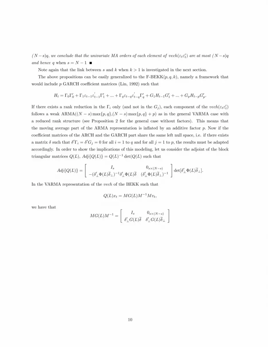
(N�s)q, we conclude that the univariate MA orders of each element of vech("t"0t) are at most (N�s)qand hence q when s = N � 1Note again that the link between s and k when k > 1 is investigated in the next section.

The above propositions can be easily generalized to the F-BEKK(p; q; k); namely a framework that

would include p GARCH coe¢ cient matrices (Lin, 1992) such that

Ht = �0�00 + �1"t�1"

0

t�1�01 + :::+ �q"t�q"

0

t�q�0q +G1Ht�1G

01 + :::+GpHt�pG

0p:

If there exists a rank reduction in the �i only (and not in the Gj), each component of the vech("t"0t)

follows a weak ARMA((N � s)maxfp; qg,(N � s)maxfp; qg + p) as in the general VARMA case with

a reduced rank structure (see Proposition 2 for the general case without factors). This means that

the moving average part of the ARMA representation is in�ated by an additive factor p: Now if the

coe¢ cient matrices of the ARCH and the GARCH part share the same left null space, i.e. if there exists

a matrix � such that �0�i = �0Gj = 0 for all i = 1 to q and for all j = 1 to p; the results must be adapted

accordingly. In order to show the implications of this modeling, let us consider the adjoint of the block

triangular matrices Q(L), AdjfQ(L)g = Q(L)�1 det(Q(L) such that

AdjfQ(L)g ="

Is 0s�(N�s)

�(�0?�(L)�?)�1�0?�(L)� (�0?�(L)�?)�1

#det[�0?�(L)�?]:

In the VARMA representation of the vech of the BEKK such that

Q(L)xt =MG(L)M�1Mvt;

we have that

MG(L)M�1 =

"Is 0s�(N�s)

�0?G(L)� �0?G(L)�?

#

10

and consequently

AdjfQ(L)gMG(L)M�1

= det[�0?�(L)�?]

"Is 0s�(N�s)

�(�0?�(L)�?)�1�0?�(L)� (�0?�(L)�?)�1

#"Is 0s�(N�s)

�0?G(L)� �0?G(L)�?

#

= det[�0?�(L)�?]

"Is 0s�(N�s)

�(�0?�(L)�?)�1�0?�(L)� + (�0?�(L)�?)�1�0?G(L)� (�0?�(L)�?)�1�0?G(L)�?

#

= det[�0?�(L)�?]| {z }(N�s)max(q;p)

�

2664 Is

� (�0?�(L)�?)�1| {z }

(N�s�1)max(q;p)�(N�s)max(q;p)

�0?�(L)�| {z }max(q;p)

+ (�0?�(L)�?)�1| {z }

(N�s�1)max(q;p)�(N�s)max(q;p)

�0?G(L)�| {z }p

0s�(N�s)

(�0?�(L)�?)�1| {z }

(N�s�1)max(q;p)�(N�s)max(q;p)

�0?G(L)�?| {z }p

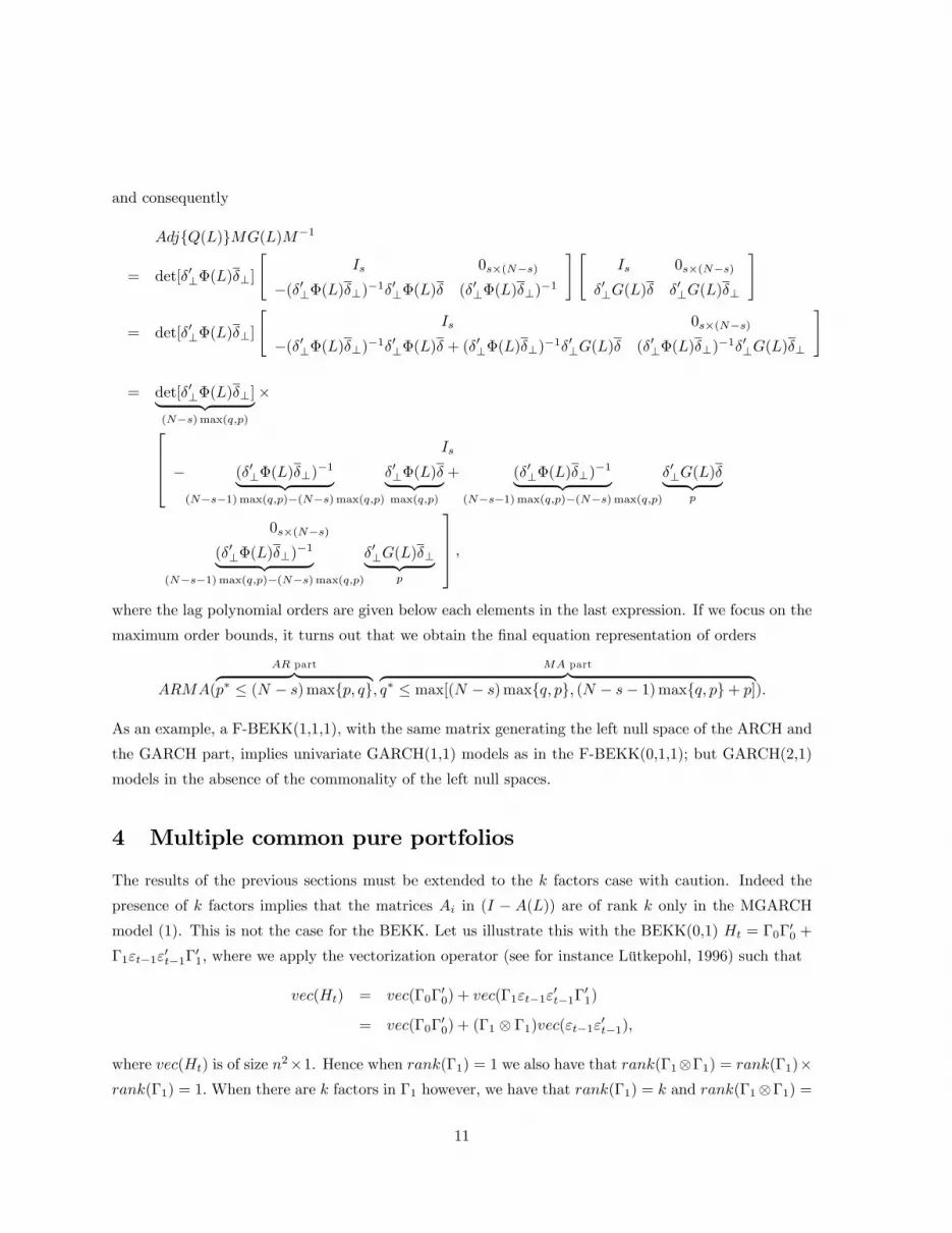
3775 ;where the lag polynomial orders are given below each elements in the last expression. If we focus on the

maximum order bounds, it turns out that we obtain the �nal equation representation of orders

ARMA(

AR partz }| {p� � (N � s)maxfp; qg;

MA partz }| {q� � max[(N � s)maxfq; pg; (N � s� 1)maxfq; pg+ p]):

As an example, a F-BEKK(1,1,1), with the same matrix generating the left null space of the ARCH and

the GARCH part, implies univariate GARCH(1,1) models as in the F-BEKK(0,1,1); but GARCH(2,1)

models in the absence of the commonality of the left null spaces.

4 Multiple common pure portfolios

The results of the previous sections must be extended to the k factors case with caution. Indeed the

presence of k factors implies that the matrices Ai in (I � A(L)) are of rank k only in the MGARCHmodel (1). This is not the case for the BEKK. Let us illustrate this with the BEKK(0,1) Ht = �0�00 +

�1"t�1"0t�1�

01; where we apply the vectorization operator (see for instance Lütkepohl, 1996) such that

vec(Ht) = vec(�0�00) + vec(�1"t�1"

0t�1�

01)

= vec(�0�00) + (�1 �1)vec("t�1"0t�1);

where vec(Ht) is of size n2�1. Hence when rank(�1) = 1 we also have that rank(�1�1) = rank(�1)�rank(�1) = 1:When there are k factors in �1 however, we have that rank(�1) = k and rank(�1�1) =

11

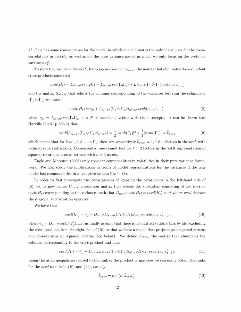
k2: This has some consequences for the model in which one eliminates the redundant lines for the cross-

correlations in vec(Ht) as well as for the pure variance model in which we only focus on the vector of

variances "2t :

To show the results on the vech; let us again consider LN�n2 the matrix that eliminates the redundant

cross-products such that

vech(Ht) = LN�n2vec(Ht) = LN�n2vec(�0�00) + LN�n2(�1 �1)vec("t�1"0t�1)

and the matrix Sn2�N that selects the columns corresponding to the variances but sum the columns of

(�1 �1) we obtain

vech(Ht) = 0 + LN�n2(�1 �1)Sn2�Nvech("t�1"0t�1); (8)

where 0 = LN�n2vec(�0�00) is a N�dimensional vector with the intercepts. It can be shown (see

Harville (1997, p 358-9) that

rank[LN�n2(�1 �1)Sn2�N ] =1

2[rank(�1)]

2 +1

2[rank(�1)] = ~kvech (9)

which means that for k = 1; 2; 3; ::: in �1, there are respectively ~kvech = 1; 3; 6; :::factors in the vech with

reduced rank restrictions. Consequently, one cannot test for k = 2 factors in the VAR representation of

squared returns and cross-returns with n = 3 assets.

Engle and Marcucci (2006) only consider commonalities in volatilities in their pure variance frame-

work. We now study the implications in terms of model representations for the variances if the true

model has commonalities in a complete system like in (8).

In order to �rst investigate the consequences of ignoring the covariances in the left-hand side of

(8), let us now de�ne Dn�N a selection matrix that selects the subsystem consisting of the rows of

vech(Ht) corresponding to the variances such that Dn�Nvech(Ht) = vecd(Ht) = "2t where vecd denotes

the diagonal vectorization operator.

We have that

vecd(Ht) = ~ 0 +Dn�NLN�n2(�1 �1)Sn2�Nvech("t�1"0t�1); (10)

where ~ 0 = Dn�Nvec(�0�00): Let us �nally assume that there is no omitted variable bias by also excluding

the cross-products from the right-side of (10) or that we have a model that projects past squared returns

and cross-returns on squared returns (see below). We de�ne KN�n the matrix that eliminates the

columns corresponding to the cross product and have

vecd(Ht) = � 0 +Dn�NLN�n2(�1 �1)Sn2�NKN�nvecd("t�1"0t�1): (11)

Using the usual inequalities related to the rank of the product of matrices we can easily obtain the ranks

for the vecd models in (10) and (11), namely

~kvecd = min(n; ~kvech): (12)

12

Our previous results on the implied univariate models must be adapted using ~kvech or ~kvecd instead

of k (and therefore (N � ~kvech) and (n� ~kvecd) are now the number of common volatility vectors). Forinstance, using the same type of proof that we have proposed for the more general model it emerges that

in an n-dimensional stationary GARCH(0; q), the individual ARMA processes for the squared excess

returns have both AR and MA orders not larger than ~kvechq:

The previous results also show that results obtained by Engle and Marcucci (2006) might be mis-

leading for getting the number of factors k: Indeed, they assume a pure variance speci�cation in which

the covariances do not play any role. In practice they consider an exponential form and thus take the

log-transform to ensure strictly positive squared returns. However, whether this is a good model de-

scription of the data or not, they test for the presence of reduced rank between the squared returns and

the past such that

"2t = 0 + ' 0"2t�1 + vt;

for "2t = ("21t; :::; "2nt)

0: Consequently if the DGP has a BEKK representation, the numbers that one

obtains (~kvecd = min(n; ~kvech))must be translated to get back to k: Finally note that Engle and Marcucci

(2006) take the log of the elements of "2t : Furthermore, to avoid taking the log of zero squared returns,

they add a tiny constant � to the squared returns, (i.e. ln("2t + �)) with the undesirable consequence of

introducing large negative values and hence arti�cially making ln("2t + �) closer to an i:i:d: process.

Engle and Marcucci (2006) explicitly ignore the cross-products. In our explanation of the model above

we have used a matrix KN�n to get rid of the columns corresponding to the cross-product, assuming

that the remaining parameters are unchanged. This can be di¤erent when we estimate such a model

however. Let us �rst develop the theoretical model representation of such a misspeci�ed model. We can

indeed write the N�dimensional MGARCH(0; q) with N = n(n+ 1)=2 such that

ht = ! +Aq(L)

"2t

xt

!

with xt the vector ofn(n�1)

2 = N � n cross-product elements "it"jt; i 6= j: In terms of observable serieswe have

fI �Aq(L)g "2t

xt

!= ! + �t; �t = ht �

"2t

xt

!;

or more explicitly �11 �12

�21 �22

! "2t

xt

!=

!1

!2

!+

�1t

�2t

!; (13)

where to simplify notation �ij = �ij(L) are polynomial matrices of degree q in L: Similarly we denote

by j�iij and �aij respectively the determinant and the adjoint of �ij(L): We now marginalize (13) withrespect to xt: This can be done by �rst computing the �nal equation representation of the second row

13

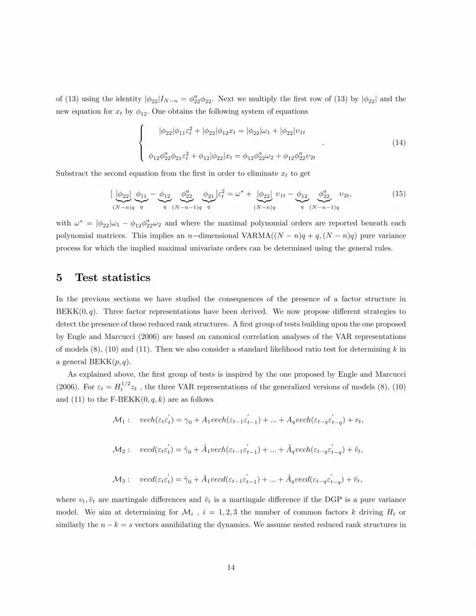
of (13) using the identity j�22jIN�n = �a22�22. Next we multiply the �rst row of (13) by j�22j and thenew equation for xt by �12: One obtains the following system of equations8>><>>:

j�22j�11"2t + j�22j�12xt = j�22j!1 + j�22j�1t

�12�a22�21"

2t + �12j�22jxt = �12�a22!2 + �12�a22�2t

: (14)

Substract the second equation from the �rst in order to eliminate xt to get

[ j�22j|{z}(N�n)q

�11|{z}q

� �12|{z}q

�a22|{z}(N�n�1)q

�21|{z}q

]"2t = !� + j�22j|{z}

(N�n)q

�1t � �12|{z}q

�a22|{z}(N�n�1)q

�2t; (15)

with !� = j�22j!1 � �12�a22!2 and where the maximal polynomial orders are reported beneath eachpolynomial matrices. This implies an n�dimensional VARMA((N � n)q + q; (N � n)q) pure varianceprocess for which the implied maximal univariate orders can be determined using the general rules.

5 Test statistics

In the previous sections we have studied the consequences of the presence of a factor structure in

BEKK(0; q). Three factor representations have been derived. We now propose di¤erent strategies to

detect the presence of these reduced rank structures. A �rst group of tests building upon the one proposed

by Engle and Marcucci (2006) are based on canonical correlation analyses of the VAR representations

of models (8), (10) and (11). Then we also consider a standard likelihood ratio test for determining k in

a general BEKK(p; q):

As explained above, the �rst group of tests is inspired by the one proposed by Engle and Marcucci

(2006). For "t = H1=2t zt , the three VAR representations of the generalized versions of models (8), (10)

and (11) to the F-BEKK(0; q; k) are as follows

M1 : vech("t"0

t) = 0 +A1vech("t�1"0

t�1) + :::+Aqvech("t�q"0

t�q) + vt;

M2 : vecd("t"0

t) = ~ 0 +~A1vech("t�1"

0

t�1) + :::+~Aqvech("t�q"

0

t�q) + ~vt;

M3 : vecd("t"0

t) = � 0 + �A1vecd("t�1"0

t�1) + :::+ �Aqvecd("t�q"0

t�q) + �vt;

where vt; ~vt are martingale di¤erences and �vt is a martingale di¤erence if the DGP is a pure variance

model. We aim at determining for Mi , i = 1; 2; 3 the number of common factors k driving Ht or

similarly the n� k = s vectors annihilating the dynamics: We assume nested reduced rank structures in

14

the A matrices.5 In order to determine the rank ~kvech or ~kvecd corresponding to the number of factors

k we �rst rely on the canonical correlation analysis (as suggested by Engle and Marcucci, 2006 for a

speci�cation similar toM3), i.e. an analysis of the eigenvalues and the eigenvectors of

��1Y Y �YW ��1WW �WY ; (16)

or similarly in the symmetric matrix

��1=2Y Y �YW �

�1WW �WY �

�1=2Y Y : (17)

�ij are the empirical covariance matrices, Y is the left hand-side variable of one of the three system

Mi and W the right hand-side explanatory variables. For iid normally distributed disturbances, the

likelihood ratio test statistic for the null hypothesis that there exist at least s linear combinations that

annihilate ~kvecd = (n� s) or ~kvech = (N � s) features in common to these random variables is given by

�LR(s) = �TsXj=1

ln(1� �j) s = 1; : : : ; n or N; (18)

where �j is the j-th smallest eigenvalue of the estimated matrix (16).6 In VAR models with Gaussian

errors, (18) is the usual likelihood ratio statistics and follows asymptotically a �2(dfi) distribution under

the null for Mi , i = 1; 2; 3 where respectively df1 = sNq � s(N � s); df2 = snq � s(N � s) anddf3 = snq � s(n� s). However in our setting, the errors vt; ~vt and �vt are neither i:i:d: nor Gaussian buthighly skewed and at best martingale di¤erence sequences. Consequently �LR(s) is likely not to be �

2(df)

distributed under the null. Nevertheless, we consider this case because it is a direct extension of Engle

and Marcucci (2006). Note that in their theoretical framework of an exponential pure variance model,

the log transformation of the squared residuals �rst renders the residuals normally distributed (justifying

the use (18)) and attenuates the heteroskedasticity of the error term. Whether this test is accurate in

a F-BEKK(0; q; k) framework (not imposing an exponential structure and allowing for cross-returns in

the factor structure), is an open question that we investigate in the next section by means of a Monte

Carlo analysis.

In order to �nd a multivariate robust counterpart to the canonical correlation approach7 , we propose

to modify �LR(s) in two respects. First we use a Wald approach �W (s); asymptotically equivalent to �LR(s)5We have also investigated a variant ofM2 with a factor representation on the variances only. To do so, we concentrate

out the e¤ect of the covariances before applying M3 on residuals. The behavior of this test was poor and consequently

the results are not reported to save space.6Canonical correlation based tests have been extensively used in economics to test for the presence of common factors

and to determine their number (see e.g. Anderson and Vahid, 2007, who proposed a version of this test that is robust to

the presence of jumps in the observed series).7 In the context of testing for common cyclical features, Candelon et al. (2005) have illustrated in a Monte Carlo exercise

that �LR(s) has indeed large size distortions in the presence of GARCH disturbances. The solution proposed by the authors

was to use a GMM approach in which the covariance matrix is the robust HCSE covariance matrix proposed by White

(1982). We do not whish to apply this technique in our paper because it is suited for a single equation approach.

15

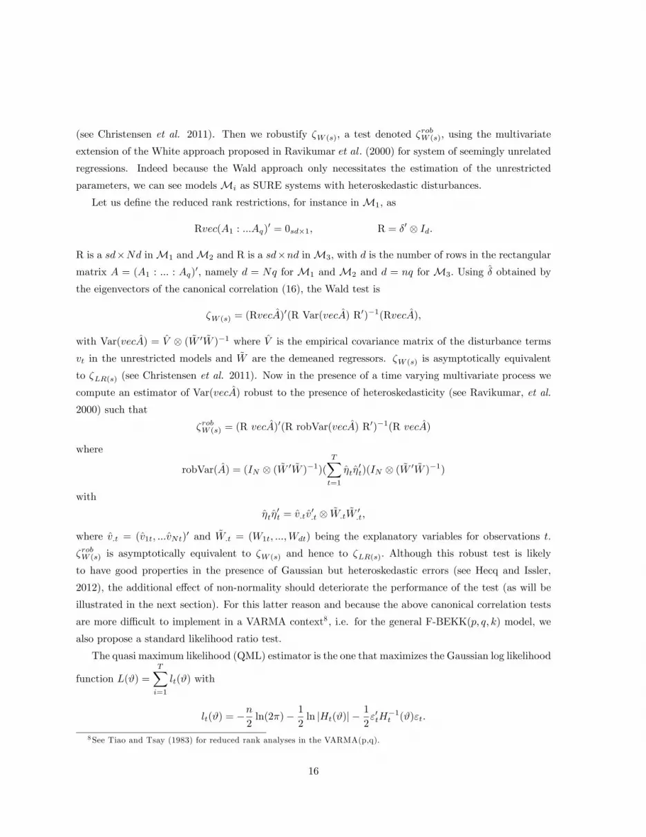
(see Christensen et al. 2011). Then we robustify �W (s), a test denoted �robW (s); using the multivariate

extension of the White approach proposed in Ravikumar et al: (2000) for system of seemingly unrelated

regressions. Indeed because the Wald approach only necessitates the estimation of the unrestricted

parameters, we can see modelsMi as SURE systems with heteroskedastic disturbances.

Let us de�ne the reduced rank restrictions, for instance inM1; as

Rvec(A1 : :::Aq)0 = 0sd�1; R = �0 Id:

R is a sd�Nd inM1 andM2 and R is a sd�nd inM3; with d is the number of rows in the rectangular

matrix A = (A1 : ::: : Aq)0; namely d = Nq for M1 and M2 and d = nq for M3: Using � obtained by

the eigenvectors of the canonical correlation (16), the Wald test is

�W (s) = (RvecA)0(R Var(vecA) R0)�1(RvecA);

with Var(vecA) = V ( ~W 0 ~W )�1 where V is the empirical covariance matrix of the disturbance terms

vt in the unrestricted models and ~W are the demeaned regressors. �W (s) is asymptotically equivalent

to �LR(s) (see Christensen et al. 2011). Now in the presence of a time varying multivariate process we

compute an estimator of Var(vecA) robust to the presence of heteroskedasticity (see Ravikumar, et al.

2000) such that

�robW (s) = (R vecA)0(R robVar(vecA) R0)�1(R vecA)

where

robVar(A) = (IN ( ~W 0 ~W )�1)(

TXt=1

�t�0t)(IN ( ~W 0 ~W )�1)

with

�t�0t = v:tv

0:t ~W:t

~W 0:t;

where v:t = (v1t; :::vNt)0 and ~W:t = (W1t; :::;Wdt) being the explanatory variables for observations t:

�robW (s) is asymptotically equivalent to �W (s) and hence to �LR(s): Although this robust test is likely

to have good properties in the presence of Gaussian but heteroskedastic errors (see Hecq and Issler,

2012), the additional e¤ect of non-normality should deteriorate the performance of the test (as will be

illustrated in the next section). For this latter reason and because the above canonical correlation tests

are more di¢ cult to implement in a VARMA context8 , i.e. for the general F-BEKK(p; q; k) model, we

also propose a standard likelihood ratio test.

The quasi maximum likelihood (QML) estimator is the one that maximizes the Gaussian log likelihood

function L(#) =TXi=1

lt(#) with

lt(#) = �n

2ln(2�)� 1

2ln jHt(#)j �

1

2"0tH

�1t (#)"t:

8See Tiao and Tsay (1983) for reduced rank analyses in the VARMA(p,q).

16

Let us denote by respectively L(#un) and L(#res) the likelihood values for the unrestricted full-BEKK

and the reduced rank BEKK with k factors. For instance in a BEKK(0; 1); the unrestricted model

is Ht = �0�00 + �1"t�1"

0t�1�

01 and the restricted one Ht = �0�

00 + ��

01"t�1"

0t�1�1�

0: Then the quasi-

likelihood ratio is

QLR = 2fL(#un)� L(#res)g � �2(df)

where the number of degrees of freedom is the di¤erence between the number of estimated parameters

of the unrestricted and restricted models. As an example, in a BEKK(0; q) this di¤erence is df =

n2q|{z}unrestricted

� (nk + nkq � k2)| {z }restricted

: The advantage of this QML approach over the canonical correlation is

that it can be easily generalized to F-BEKK(p; q; k): From the discussion in Section 3 we favor a model

with a same left null space for the ARCH and the GARCH matrix parameters. For instance Ht =

�0�00 + ��

01"t�1"

0t�1�1�

0 + ��01"t�1"0t�1�1�

0 in a BEKK(1,1,k): The number of degrees of freedom is

computed in the same manner. The main drawback of this approach might be the di¢ culty to estimate

the model for large n.

6 Monte Carlo results

We investigate in this section the small sample behavior of �LR(s) and �RobW (s) forM1;M2 andM3 and of

QLR. The DGP is a factor BEKK(0; 1; k) Ht = �0�00 + �1"t�1"0t�1�

01 with k = rank(�1) = 1; 2 factors

for n = 5 returns.9 We take T = 1000 and 2000 observations (sample sizes typically encountered with

�nancial time series) and compute the rejection frequencies when testing the null hypothesis at a 5%

signi�cance level in 1000 replications. The parameters of the factor BEKK models have been "calibrated"

on estimations obtained from some daily observations of stocks used in the empirical application but

here we forced the model to have successively k = 1 or 2 factors. Table 1 shows that the strategy that

consists in estimating directly the unrestricted and the restricted BEKK models, i.e. QLR; is preferred.

Indeed, the rejection frequencies for QLR are close to the nominal 5% level.

On the other hand the behavior of the tests statistics �LR(s) and �robW (s) is not coherent. For instance

the canonical correlation approach proposed by Engle and Marcucci (2006) seems to diverge when T

increases. While the robust Wald test appears to be adequate with two factors present, it is oversized

when testing for one factor; hence numbers around 5% may be accurate but non robust estimates of the

true size of the test and therefore only hold for speci�c DGPs (this has been con�rmed on alternative

DGPs).

9Fewer size distorsions are obtained for smaller n and hence it was less obvious to discriminate between the di¤erent

approaches: Also note that many alternative strategies have been investigated but are not reported due to their bad

performance. For instance a partial least square approach, similar to the one proposed by Cubadda and Hecq (2011) for

the VAR, underestimates the number of factors and concludes to multivariate white noise process in most cases. Also,

taking the log of the covariance matrix seems to work for some particular cases but not in general.

17

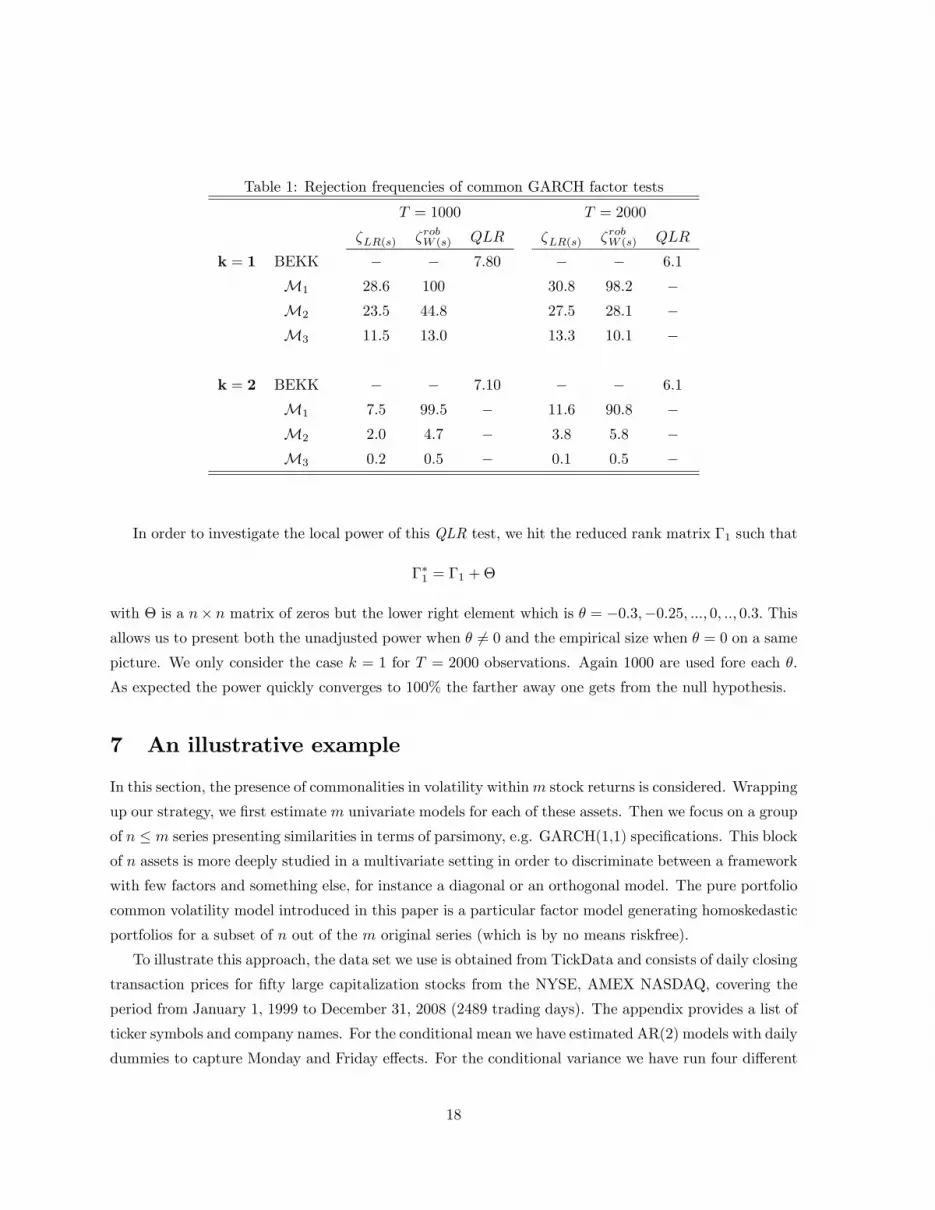
Table 1: Rejection frequencies of common GARCH factor tests

T = 1000 T = 2000

�LR(s) �robW (s) QLR �LR(s) �robW (s) QLR

k = 1 BEKK � � 7:80 � � 6:1

M1 28:6 100 30:8 98:2 �M2 23:5 44:8 27:5 28:1 �M3 11:5 13:0 13:3 10:1 �

k = 2 BEKK � � 7:10 � � 6:1

M1 7:5 99:5 � 11:6 90:8 �M2 2:0 4:7 � 3:8 5:8 �M3 0:2 0:5 � 0:1 0:5 �

In order to investigate the local power of this QLR test, we hit the reduced rank matrix �1 such that

��1 = �1 +�

with � is a n� n matrix of zeros but the lower right element which is � = �0:3;�0:25; :::; 0; ::; 0:3: Thisallows us to present both the unadjusted power when � 6= 0 and the empirical size when � = 0 on a samepicture. We only consider the case k = 1 for T = 2000 observations. Again 1000 are used fore each �.

As expected the power quickly converges to 100% the farther away one gets from the null hypothesis.

7 An illustrative example

In this section, the presence of commonalities in volatility withinm stock returns is considered. Wrapping

up our strategy, we �rst estimate m univariate models for each of these assets. Then we focus on a group

of n � m series presenting similarities in terms of parsimony, e.g. GARCH(1,1) speci�cations. This block

of n assets is more deeply studied in a multivariate setting in order to discriminate between a framework

with few factors and something else, for instance a diagonal or an orthogonal model. The pure portfolio

common volatility model introduced in this paper is a particular factor model generating homoskedastic

portfolios for a subset of n out of the m original series (which is by no means riskfree).

To illustrate this approach, the data set we use is obtained from TickData and consists of daily closing

transaction prices for �fty large capitalization stocks from the NYSE, AMEX NASDAQ, covering the

period from January 1, 1999 to December 31, 2008 (2489 trading days). The appendix provides a list of

ticker symbols and company names. For the conditional mean we have estimated AR(2) models with daily

dummies to capture Monday and Friday e¤ects. For the conditional variance we have run four di¤erent

18

Figure 1: Power of the quasi-likelihood ratio test

­0.30 ­0.25 ­0.20 ­0.15 ­0.10 ­0.05 0.00 0.05 0.10 0.15 0.20 0.25 0.30

10

20

30

40

50

60

70

80

90

100Po

wer

θ

speci�cations. These are the GARCH(1,1), the GARCH(1,2) and two long memory models, namely

FIGARCH(1; d; 0) and FIGARCH(1; d; 1). Out of the 50 series, the GARCH(1,1) model is favoured in

six cases using both formal likelihood ratio tests and the Hannan-Quinn information criterion. The six

returns with no indication of long memory are (and using their acronyms, see Appendix) ABT, BMY,

GE, SLB, XOM, XRX. Table 2 reports the value of the estimated parameters in the conditional variance

equation, the results on the conditional mean equations being not reported to save space.

Therefore we consider these six series and we apply our proposed tests. On the six series we consider

both a BEKK(0,1) and a BEKK(1,1) where for the latter we impose the same left null space generating

the ARCH and the GARCH parts. For these two models we compute the likelihood of the full-BEKK

as well as the factor BEKK for k = 0; 1; 2; 3; 4; 5; the F-BEKK with k = 6 being the unrestricted full-

BEKK. Using the QLR test statistics we reject the null of any rank reduction (p-values are all smaller

than 0.001 and are therefore not reported to save space). Consequently, the parsimony observed for

these six returns is more likely due to independent behavior (diagonal or orthogonal model) than to the

presence of factors. We also estimated diagonal BEKK(0,1) and a BEKK(1,1) and found that on these

6 series, likelihood ratio tests favour the diagonal models compared to the full-BEKK ones. A diagonal

BEKK(1,1) is therefore retained for these series.

Interestingly, we also applied the two reduced rank tests �LR(s) and �robW (s) in the VAR representation

for the squared returns and cross-returns, i.e. M1;M2 andM3: Unlike the QLR test, these tests point

out the presence of commonalities in volatility which is very likely due to the strong size distortion of

19

Table 2: QMLE of GARCH(1,1) on the 6 retained series

ABT BMY GE SLB XOM XRX

!0:0139

(0:0036)

0:0076

(0:0027)

0:0028

(0:0015)

0:0284

(0:0115)

0:0253

(0:0071)

0:0162

(0:0060)

�10:0439

(0:0048)

0:0617

(0:0058)

0:0433

(0:0049)

0:0428

(0:0051)

0:0726

(0:0067)

0:0612

(0:0053)

�10:9512

(0:0054)

0:9405

(0:0046)

0:9580

(0:0046)

0:9515

(0:0065)

0:9180

(0:0082)

0:9413

(0:0054)

Q2(20) 0:72 0.96 0.38 0.50 0.28 0.98

Note: Robust standard errors are reported in brackets. Q2(20) is the p-value of the Ljung-Box test on

squared standardized residuals with 20 lags.

these tests highlighted in the previous section.

8 Conclusions

This paper studies the orders of the univariate weak GARCH processes implied by multivariate GARCH

models. We recall that except in some coincidental situations, the marginal models are generally non-

parsimonious. However, the presence of common features in volatility leads to a large decrease of these

implied theoretical orders. We emphasize two radically di¤erent structures that may give rise to similar

parsimonious univariate representations. These are diagonal models on the one hand, e.g. diagonal-

BEKK, and models with reduced rank matrices resulting from the presence of common factors on the

other hand, e.g. the F-BEKK.

Consequently we propose di¤erent strategies to detect the presence of such GARCH co-movements in

a multivariate setting. We believe that this is better than either assuming non-contagion of asset returns

from the outset or imposing a factor framework when it is not present. We �nd that reduced rank

test statistics in squared returns (and cross-returns) display severe size distortions while our proposed

likelihood ratio test is correctly sized and has good power properties.

Our results plead for looking at individual series prior to a multivariate modelling. For instance,

this would help to discover and estimate separately blocks of assets sharing the same sort of dynamic

behavior. We won�t be able to see it on the whole set of series.

In our application, we detected six series following GARCH(1,1) speci�cations. We applied our

20

proposed likelihood ratio test and did not �nd any evidence of commonalities in volatility.

Extensions of this paper are numerous. For instance one could have used bootstrapped versions

of some of the tests statistics presented in this paper. This approach has been used by Hafner and

Herwartz (2004) to test for causality in the full-BEKK model but with little improvement compared to

the asymptotic versions of their test. Next we can further decompose the set of m assets into K blocks

with m = n1 + ::: + nK : There might exist a group of series with long memory having similarities in

their dynamics.

9 References

Anderson, H.M., and F. Vahid (2007), Forecasting the Volatility of Australian Stock Returns: Do

Common Factors Help?, Journal of Business and Economic Statistics 25, 76-90.

Arshanapalli, B, Doukas, J. and L. Lang (1997), Common volatility in the industrial structure

of global capital markets, Journal of International Money and Finance 16, 189-209.

Baba, Y., R.F. Engle, D.F. Kraft, and K.F. Kroner (1989), Multivariate Simultaneous

Generalized ARCH, DP 89-57 San Diego.

Bauwens, L., S. Laurent and J.V.K. Rombouts (2006), Multivariate GARCH Models: a

Survey, Journal of Applied Econometrics 21, 79�109.

Billio M., M. Caporin and M. Gobbo (2003), Block Dynamic Conditional Correlation Multi-

variate GARCH Models, Working paper 0303 GRETA, Venice.

Candelon, B., Hecq, A. and W. Verschoor (2005), Measuring Common Cyclical Features

During Financial Turmoil, Journal of International Money and Finance 24, 1317-1334

Christensen, T., Hurn, S. and A. Pagan (2011), Detecting Common Dynamics in Transitory

Components, Journal of Time Series Econometrics 3, issue 1.

García-Ferrer, A., Gonzàlez-Prieto, E. and D. Peña (2012), A conditionally heteroskedas-

tic independent factor model with an application to dinancial stock returns, International Journal of

Forecasting 28, 70-93.

Cubadda, G., Hecq A. and F.C. Palm .(2008), Macro-panels and Reality, Economics Letters

99, 537-540.

Cubadda, G., Hecq A. and F.C. Palm (2009), Studying Interactions without Multivariate

Modeling, Journal of Econometrics 148, 25-35.

Cubadda, G. and A. Hecq (2011), Testing for Common Autocorrelation in Data Rich Environ-

ments, Journal of Forecasting 30, 325-335 .

Drost, F.C. and T.E. Nijman (1993), Temporal Aggregation of GARCH Processes, Econometrica

61, 909-927.

21

Engle, R. F., V. Ng and M. Rothschild (1990), Asset Pricing With a Factor ARCH Covariance

Structure: Empirical Estimates of Treasury Bills, Journal of Econometrics 45, 213-238.

Engle, R. F. and B. Kelly (2008), Dynamic Equicorrelation, Stern School of Business, WP

NYU.

Engle, R. F. and S. Kozicki (1993), Testing for Common Features (with Comments), Journal

of Business and Economic Statistics 11, 369-395.

Engle, R. F. and J. Marcucci (2006), A Long-run Pure Variance Common Features Model for

the Common Volatilities of the Dow Jones, Journal of Econometrics 132, 7-42.

Engle, R. F. and R. Susmel (1993), Common Volatility in International Equity Markets, Journal

of Business and Economic Statistics 11, 167-176.

Fiorentini, G., E. Sentana and N. Shephard (2004), Likelihood-Based Estimation of Latent

Generalized ARCH Structures, Econometrica 72, 1481-1517.

Francq, C. and J.-M. Zakoian (2007), HAC Estimation and Strong Linearity Testing in Weak

ARMA Models, Journal of Multivariate Analysis 98, 114-144.

Hafner, C.M. and H. Herwartz (2004), Testing for causality in variance using multivariate

GARCH models. Econometric Institute Report 20, Erasmus University Rotterdam.

Hafner, C.M. and A. Preminger (2009), Asymptotic theory for a factor GARCH model, Econo-

metric Theory 25, 336-363.

Hecq, A. and J.V. Issler (2012), A Common-Feature Approach for Testing Present-Value Re-

strictions with Financial Data, Maastricht University, METEOR RM/12/006.

Lanne, M. and P. Saikkonen (2007), A Multivariate Generalized Orthogonal Factor GARCH

Model, Journal of Business and Economic Statistics 25, 61-75.

Lin, W.-L. (1992), Alternative Estimators for Factor GARCHModels - A Monte Carlo Comparison,

Journal of applied Econometrics 7, 259-279.

Nijman, T. and E. Sentana (1996), Marginalization and Contemporaneous Aggregation in Mul-

tivariate GARCH Processes, Journal of Econometrics 71, 71-87.

Ravikumar, B., Ray, S. and E. Saving (2000), Robust Wald tests in Sur systems with adding-up

restrictions, Econometrica 68, 715-720.

Ruiz, I.(2009), Common volatility across Latin American foreign echange markets, Applied Finan-

cial Economics 19, 1197-1211.

Silvennoinen, A. and T. Terasvirta (2009), Multivariate GARCH Models, Handbook of Finan-

cial Time Series, Ed. Andersen, T.G. and Davis, R.A. and Kreiss, J.P. and T. Mikosch, Springer.

Tiao, G. C. and R. S. Tsay (1989), Model Speci�cation in Multivariate Time Series (with Com-

ments), Journal of Royal Statistical Society, Series B 51, 157-213.

Zellner, A. and F.C. Palm (1974), Time Series Analysis and Simultaneous Equation Econometric

Models, Journal of Econometrics 2, 17-54.

22

Zellner, A. and F.C. Palm (1975), Time Series and Structural Analysis of Monetary Models of

the US Economy, Sanhya: The Indian Journal of Statistics, Series C 37, 12-56.

Zellner, A. and F.C. Palm (2004), The Structural Econometric Time Series Analysis Approach,

Cambridge University Press.

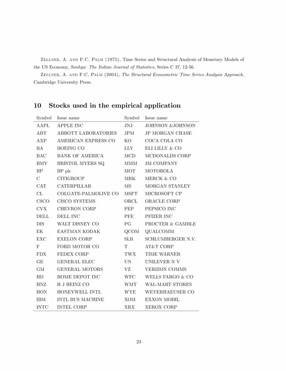
10 Stocks used in the empirical application

Symbol Issue name Symbol Issue name

AAPL APPLE INC JNJ JOHNSON &JOHNSON

ABT ABBOTT LABORATORIES JPM JP MORGAN CHASE

AXP AMERICAN EXPRESS CO KO COCA COLA CO

BA BOEING CO LLY ELI LILLY & CO

BAC BANK OF AMERICA MCD MCDONALDS CORP

BMY BRISTOL MYERS SQ MMM 3M COMPANY

BP BP plc MOT MOTOROLA

C CITIGROUP MRK MERCK & CO

CAT CATERPILLAR MS MORGAN STANLEY

CL COLGATE-PALMOLIVE CO MSFT MICROSOFT CP

CSCO CISCO SYSTEMS ORCL ORACLE CORP

CVX CHEVRON CORP PEP PEPSICO INC

DELL DELL INC PFE PFIZER INC

DIS WALT DISNEY CO PG PROCTER & GAMBLE

EK EASTMAN KODAK QCOM QUALCOMM

EXC EXELON CORP SLB SCHLUMBERGER N.V.

F FORD MOTOR CO T AT&T CORP

FDX FEDEX CORP TWX TIME WARNER

GE GENERAL ELEC UN UNILEVER N V

GM GENERAL MOTORS VZ VERIZON COMMS

HD HOME DEPOT INC WFC WELLS FARGO & CO

HNZ H J HEINZ CO WMT WAL-MART STORES

HON HONEYWELL INTL WYE WEYERHAEUSER CO

IBM INTL BUS MACHINE XOM EXXON MOBIL

INTC INTEL CORP XRX XEROX CORP

23