Forecasting spot prices in bulk shipping using multivariate and univariate models
37
Page 1 of 37 RESEARCH ARTICLE Forecasting spot prices in bulk shipping using multivariate and univariate models N.D. Geomelos and E. Xideas Cogent Economics & Finance (2014), 2: 932701
Transcript of Forecasting spot prices in bulk shipping using multivariate and univariate models

Page 1 of 37
ReseaRch aRticle
Forecasting spot prices in bulk shipping using multivariate and univariate modelsN.D. Geomelos and E. Xideas
Cogent Economics & Finance (2014), 2: 932701

Geomelos & Xideas, Cogent Economics & Finance (2014), 2: 932701http://dx.doi.org/10.1080/23322039.2014.932701
ReseaRch aRticle
Forecasting spot prices in bulk shipping using multivariate and univariate modelsN.D. Geomelos1* and E. Xideas1
abstract: This paper employs an applied econometric study concerning forecasting spot prices in bulk shipping in both markets of tankers and bulk carriers in a disag-gregated level. This research is essential, as spot market is one of the most volatile markets and there is a great uncertainty about the future development of spot prices. This uncertainty could be reduced by using estimates of ex-post and ex-ante fore-casts. Econometric analysis focuses in the comparison of different econometric mod-els from two important categories of econometrics: (1) multivariate models (VAR and VECM) and (2) univariate time series models (ARIMA, GARCH and E-GARCH) in order to derive the best predicting model for each ship type. Also, forecasts can be modified to yield an improved performance of forecasting accuracy via the theory of combining methods. Ex-post and ex-ante forecasts are estimated on the basis of best predicting model’s performance. Results show that the combining methodology can reduce even more the forecasting errors. The results of empirical analysis could also be useful from the specialization, identification, estimation, and evaluation of previous econometric models’ point of view. Also, ex-ante forecasts, which are taking into consideration the present economic crisis, can be used for the formation of efficient economic policy from decision-makers of shipping industry reducing even more spot markets’ risk.
Keywords: c32—time-series models, c0—general, a—general economics and teaching, c52—model evaluation and testing
*Corresponding author: N.D. Geomelos, Department of Shipping, Trade and Transport, University of the Aegean, G. Veriti 84, Chios 82100, Greece E-mail: [email protected]
Reviewing Editor: David McMillan, University of Stirling
Further author and article information is available at the end of the article
AuTHoR BIoGRApHyN.D. Geomelos Economist, Applied Econometrician—Researcher (Department of Shipping, Trade and Transport, university of the Aegean, Greece). His dissertation on Applied Economics and Econometrics has as a topic “Applied Techniques of Econometric Forecasting in Shipping Markets”. His researching interests extend to applied econometrics, macroeconomics analysis, and international trade. He has been awarded grants for his studies from the National Foundation of Scholarships in Greece. He has graduated from the National School of Artillery with the rank of Second Lieutenant.
puBLIC INTEREST STATEMENTThis paper examines analytically two categories of applied econometrics’ models, multivariate and univariate time-series models. The research realizes a systematic econometric analysis to compare and to propose specific quantitative economic relations, which are developed among the spot market of shipping industry. Analysis also uses the estimates and the results of models to generate ex-post and ex-ante forecasts, so much in the sample as beyond the original estimation period. The estimation sample includes monthly observations from the beginning of 1970s until the beginning of 2011. The generated forecasts are not limited in one vessel type, but they extend according to a disaggregated analysis in both tanker (five vessel types) and dry bulk markets (three vessel types). The results show that multivariate models give more precise forecasts revealing the relation of interdependence and feedback, which exists among the shipping markets. Combining forecasting methodology provide lower forecasting errors in spot market.
Received: 14 November 2013Accepted: 01 June 2014Published: 08 July 2014
© 2014 The Author(s). This open access article is distributed under a Creative Commons Attribution (CC-BY) 3.0 license.
Page 2 of 37
Dow
nloa
ded
by [
94.6
5.25
.105
] at
10:
53 0
7 D
ecem
ber
2014
Page 3 of 37
Geomelos & Xideas, Cogent Economics & Finance (2014), 2: 932701http://dx.doi.org/10.1080/23322039.2014.932701
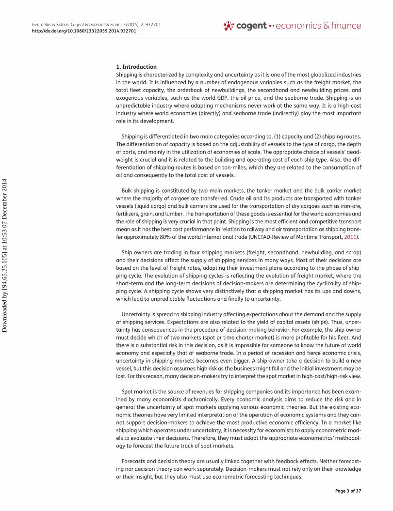
1. introductionShipping is characterized by complexity and uncertainty as it is one of the most globalized industries in the world. It is influenced by a number of endogenous variables such as the freight market, the total fleet capacity, the orderbook of newbuildings, the secondhand and newbuilding prices, and exogenous variables, such as the world GDp, the oil price, and the seaborne trade. Shipping is an unpredictable industry where adapting mechanisms never work at the same way. It is a high-cost industry where world economies (directly) and seaborne trade (indirectly) play the most important role in its development.
Shipping is differentiated in two main categories according to, (1) capacity and (2) shipping routes. The differentiation of capacity is based on the adjustability of vessels to the type of cargo, the depth of ports, and mainly in the utilization of economies of scale. The appropriate choice of vessels’ dead-weight is crucial and it is related to the building and operating cost of each ship type. Also, the dif-ferentiation of shipping routes is based on ton-miles, which they are related to the consumption of oil and consequently to the total cost of vessels.
Bulk shipping is constituted by two main markets, the tanker market and the bulk carrier market where the majority of cargoes are transferred. Crude oil and its products are transported with tanker vessels (liquid cargo) and bulk carriers are used for the transportation of dry cargoes such as iron-ore, fertilizers, grain, and lumber. The transportation of these goods is essential for the world economies and the role of shipping is very crucial in that point. Shipping is the most efficient and competitive transport mean as it has the best cost performance in relation to railway and air transportation as shipping trans-fer approximately 80% of the world international trade (uNCTAD-Review of Maritime Transport, 2011).
Ship owners are trading in four shipping markets (freight, secondhand, newbuilding, and scrap) and their decisions affect the supply of shipping services in many ways. Most of their decisions are based on the level of freight rates, adapting their investment plans according to the phase of ship-ping cycle. The evolution of shipping cycles is reflecting the evolution of freight market, where the short-term and the long-term decisions of decision-makers are determining the cyclicality of ship-ping cycle. A shipping cycle shows very distinctively that a shipping market has its ups and downs, which lead to unpredictable fluctuations and finally to uncertainty.
uncertainty is spread to shipping industry affecting expectations about the demand and the supply of shipping services. Expectations are also related to the yield of capital assets (ships). Thus, uncer-tainty has consequences in the procedure of decision-making behavior. For example, the ship owner must decide which of two markets (spot or time charter market) is more profitable for his fleet. And there is a substantial risk in this decision, as it is impossible for someone to know the future of world economy and especially that of seaborne trade. In a period of recession and fierce economic crisis, uncertainty in shipping markets becomes even bigger. A ship-owner take a decision to build a new vessel, but this decision assumes high risk as the business might fail and the initial investment may be lost. For this reason, many decision-makers try to interpret the spot market in high-cost/high-risk view.
Spot market is the source of revenues for shipping companies and its importance has been exam-ined by many economists diachronically. Every economic analysis aims to reduce the risk and in general the uncertainty of spot markets applying various economic theories. But the existing eco-nomic theories have very limited interpretation of the operation of economic systems and they can-not support decision-makers to achieve the most productive economic efficiency. In a market like shipping which operates under uncertainty, it is necessity for economists to apply econometric mod-els to evaluate their decisions. Therefore, they must adopt the appropriate econometrics’ methodol-ogy to forecast the future track of spot markets.
Forecasts and decision theory are usually linked together with feedback effects. Neither forecast-ing nor decision theory can work separately. Decision-makers must not rely only on their knowledge or their insight, but they also must use econometric forecasting techniques.
Dow
nloa
ded
by [
94.6
5.25
.105
] at
10:
53 0
7 D
ecem
ber
2014

Page 4 of 37
Geomelos & Xideas, Cogent Economics & Finance (2014), 2: 932701http://dx.doi.org/10.1080/23322039.2014.932701
Forecasting is even more difficult in case of shipping industry as it is one of the most stochastic economic environments. This paper is based on the hypothesis of stochastic properties of shipping markets and analyzes different methodologies of econometric forecasting and especially analyzes the following models: (1) Vector AutoRegressive (VAR), (2) Vector Error Correction Model (VECM), (3) AutoRegressive Integrated Moving Average Models (ARIMA), (4) Generalized AutoRegressive Conditional Heteroskedasticity (GARCH), and (5) Exponential GARCH (E-GARCH).
The aim of this paper is to create econometric models which are adapted to the complicated real-ity of shipping industry. Econometric research concerns both tankers and bulk carriers markets in a disaggregated analysis with eight different vessel types (Tankers: uLCC-VLCC, Suezmax, Aframax, panamax, Handysize—Bulk carriers: Capesize, panamax Bulk, Handymax). Models are focused on dynamic properties of shipping system taking into account the cyclical fluctuations of economic and shipping cycles using dynamic multipliers and dynamic elasticities.
2. literature reviewThe essay about the mechanism of freight rates is one of the most crucial points in the shipping industry. In fact, the nature of the industry raises a point to carry out a number of researches and studies. uncertainty and implied volatility of freight prices are the main motives, which lead the researchers to discover more appropriate quantitative methods to decipher the market.
It is important to be noticed that the majority of economists have been studied, in most cases, the equilibrium of shipping markets during the last two decades (Beenstock & Vergottis, 1993; Tsolakis, 2005). They analyzed the shipping markets as a static mechanism where a system of variables must link together supply and demand into balance. Most theories, which were dedicated in market’s equilibrium, come from this static notion about shipping economy. However, this concept about equilibrium can be used only as a very simple explanatory tool in contrast to a very complicated real-ity which underlies disharmony fluctuations and lack of balance.
New studies are focused on dynamic systems which exploit the development of econometrics. The dynamic nature of models interprets shipping markets in better way and it helps to understand the mechanism of markets by producing more accurate forecasts (Hawdon, 1978). Many modern econo-mists lay the foundation of dynamic analysis of shipping markets and especially that of spot market combining the traditional view of equilibrium with the new techniques of econometric analysis.
Veenstra and Franses (1997) produce forecasts for panamax dry bulk carrier using the issue of cointegration relation among spot rates of six different shipping routes. Their methodology is based on the existence of cointegration relations and spot market’s efficiency using a VAR model. This model doesn’t include other endogenous or exogenous variables, because the authors consider the spot market as efficient. This hypothesis leads to large forecast errors, because of the existence of common stochastic trend among the six different time series of routes.
Randers and Göluke (2007) create an aggregate model of interpretation of tanker market without any discrimination in vessel size or shipping routes. Their model is focused on the total fleet capacity and the way of utilization of that capacity. Cyclicality and volatility of spot market are not exogenous variables, because they are not influencing from the economic changes but from the market itself and hence they have been treated as endogenous. Many researchers and academics support that the disturbances of volatility of shipping markets are largely due to events, which occur outside the shipping sector such as wars, canal closings, oil prices, and legislation (Stopford, 1997). They also claim that the shipping community creates the cyclicality and especially its own investment deci-sions create the volatility of shipping environment. This phenomenon is known as self-infliction view. Authors’ forecasts are based on the shipping cycle’s analysis and they believe that the long-term forecasts are possible mainly from 1 to 4 years. For shorter periods of time there is too much noise from the changes of exogenous variables where the forecasts are inaccurate.
Dow
nloa
ded
by [
94.6
5.25
.105
] at
10:
53 0
7 D
ecem
ber
2014

Page 5 of 37
Geomelos & Xideas, Cogent Economics & Finance (2014), 2: 932701http://dx.doi.org/10.1080/23322039.2014.932701
Scarsi (2007) underlines the unstable nature of dry bulk market because of the economic and geo-political changes. He supports that when the economy grows, then the demand of cargoes is in-creased following the definition of derived demand. It is obvious that according to shipping cycle, ship owner must take into account two very serious decisions. The first is related to the operation of ships and the second with the asset play. Scarsi believes that it is difficult to produce reliable fore-casts because the volatility of shipping is depended on exogenous factors like the delivery of a ship after two or four years. During this time period, the conditions of freight market have already changed.
Except the previous studies, a different approach of freight market analysis is realized using the Forward Freight Agreement (FFA) market. The forward freight market determines the equilibrium prices in spot market during the price discovery process. According to price discovery, efficient infor-mation about the future price of asset can be obtained through future markets. In shipping industry, price discovery is used for the determination and the forecasting of spot rates using only one variable that of forward rates. Kavussanos and Nomikos (1999) use four forecasting models (VECM, ARIMA, Exponential Smoothing, and Random Walk) in the freight futures market. They also examine the short-run dynamic properties of spot and futures prices in order to specify the speed which responds to deviations from their long-run relationship. They propose VECM model as the best forecasting mod-el in the contrary of Cullinane (1992) who proposes ARIMA models. The final conclusion is that the hypothesis of unbiasedness is based on the unbiasedness of future contract’s price in relation to the realized spot price. This confirms the significance of future rates to spot prices. Their final conclusion is that the future prices react more quickly in the changes of market in relation to the spot prices.
Kavussanos and Visvikis (2004) re-examine the price discovery and especially the lead–lag rela-tionship between current spot rates and FFA. They use a multivariate model VECM combined with a GARCH model. Variances and covariances of time series are varied from time to time allowing the spill-over effect between spot and derivatives markets. According to authors, this methodology gives better forecasting performance and market analysis is improved.
Batchelor, Alizadeh, and Visvikis (2007), in a similar methodology, show that ARIMA or VAR models forecast the future prices with smaller forecast errors, but using different samples from the study of Kavussanos and Nomikos. The differentiation of results is obviously based on different samples.
A new methodology for the prediction of spot prices is the Artificial Neural Network (Lyridis, Zacharioudakis, Mitrou, & Mylonas, 2004). This technique follows the multivariate analysis with exogenous variables which affect the level of spot prices. Authors support that in an industry as dynamic as shipping, multivariable models interpret more precisely the freight markets in relation to univariate models.
3. MethodologyFirstly, the issues of stationarity and seasonality are considered in order to investigate the forecast-ing performance of univariate and multivariate models of spot prices in bulk shipping.
3.1. StationarityStationarity implies that the distribution of the variable under consideration does not depend upon time or in other words the variances and autocovariances are finite and independent of time.
It is of great importance for the analysis to test the order of integration of spot prices. For univariate time-series models, spot prices must be stationary or integrated of order zero—I(0,0).1 This analysis implements the three most used statistical tests according to Lutkepohl and Kratzig (2004). The first test is Augmented Dickey-Fuller (ADF) where tests the pair of hypotheses H0: φ = 0 and β = 0 (stochastic trend) versus H1:φ < 0 and β ≠ 0 (deterministic trend) and estimates the following regression:
(1)Δyt =�yt−1+�t+
p−1∑
j=1
�∗
j Δyt−j+�t
Dow
nloa
ded
by [
94.6
5.25
.105
] at
10:
53 0
7 D
ecem
ber
2014

Page 6 of 37
Geomelos & Xideas, Cogent Economics & Finance (2014), 2: 932701http://dx.doi.org/10.1080/23322039.2014.932701
where φ = −α(1) and �∗
j = −(αj + 1+ ··· + αp). ADF test is based on t-statistic and critical values have been obtained by Davidson and MacKinnon (1993).
The second test known as philips–perron (pp) is an alternative to the ADF test. The adoption of pp test from the current paper lays to the fact that the test covers the case of series which have struc-tural breaks (perron, 1989).
For ADF and pp tests, it is checked the hypothesis H0: β = ρ = 0 for the following model according to F-statistic:
The econometric analysis of this research is also examines a third test known as Kwiatkowski–philips–Schmidt–Shin (KpSS) test. This test examines as null hypothesis that the data generating process is stationary [H0: yt − I(0)] against the alternative that it is [H1: yt − I(1)]. KpSS test is not appropriate for large samples and its application is questioned in models with a large number of observations as Caner and Kilian (2001) and Kuo and Tsong (2004) notice. However, this paper applies this test in order to test the accuracy of previous results in shipping data.
The paper also takes into consideration the significance of constant term considering the exist-ence of unit root. The null hypothesis is that H0: φ = ρ = 0 and F-statistic and t-statistic critical values are included in Table 1.
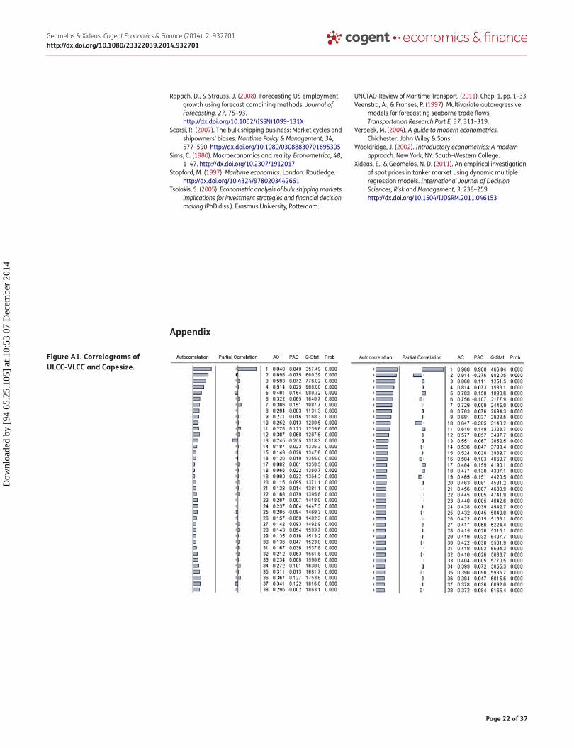
3.2. SeasonalityAnother important parameter for univariate models is the examination of seasonality. Seasonality can be identified by observing regular peaks in the sample autocorrelation function (SACF). Also, the partial autocorrelation function (pACF) provides additional information about the seasonality of time-series. More specifically, the SACF exhibits peaks in lags 12, 24, 36, 48, etc. and the pACF exhibits a strong positive peak in first lag and negative peak in lag 13 (Figure A1-Appendix, u-VLCC market shows seasonality in contrary to Capesize market which hasn’t shown any form of seasonality).
After the confirmation of seasonality, it is important to follow a deseasonalized procedure. This paper follows the seasonal adjustment estimating the seasonal indices by removing the seasonal variations.2 This method has the advantage that eliminates the seasonal variation, while the long-run trend and short-run irregular fluctuations remain.
3.3. Multivariate model VAR—VAR-XVAR model implies univariate ARMA models for each of its components and simultaneous estima-tion of variables with their lags may lead to more parsimonious and fewer lags in relation to ARMA models. This simultaneity will produce better forecasts at least in short-term period (Verbeek, 2004). Also, VAR models impose linearity, which is not required in structural models (Boero, 1990).
(2)Yt=�+
�∑
�
�iΔYt−1+�t
table 1. critical values of unit root test (time trend and constant term)Model with time trend and constant term
test equation: 𝚫Yt=�+�
t+�Y
t−1+∑�
���𝚫Y
t−1+u
t
sample size F-test critical values 5% level (t-statistic)50 6.73 −3.49
100 6.49 −3.45
[500] [6.30] [–3.42]
∞ 6.25 −3.41
Source: Author (adaptation from Heij, De Boer, Franses, Kloek, and Van Dijk [2004]).
Dow
nloa
ded
by [
94.6
5.25
.105
] at
10:
53 0
7 D
ecem
ber
2014

Page 7 of 37
Geomelos & Xideas, Cogent Economics & Finance (2014), 2: 932701http://dx.doi.org/10.1080/23322039.2014.932701
With a VAR, it is necessary to specify only two things, (1) endogenous and exogenous3 variables and (2) the number of lags in order to capture the interdependence among the variables (Litterman, 1984).
An extensive research must be done in order to characterize the estimated variables as endoge-nous or exogenous during the construction of VAR models. This research is based on Hausman test for endogeneity (Hausman, 1983), and has as a final aim to reduce the Akaike Information Criterion (AIC) and Schwarz Information Criterion (SIC) criteria of VAR models. The differentiation of variables according to Hausman test leads to more accurate ex-post forecasts with smaller forecasting errors. The results of Hausman test is presented in Appendix (Table A2).
The lag structure implies an important aspect of model specification and testing. The largest num-ber of lags needed to VAR or VECM models must capture most of the effects that the variables have on each other. With monthly data, lags up to 6 or 12 months are likely to be sufficient according to pindyck and Rubinfeld (1998). Also, it is widely acceptable that the choice of time lag must be based on SIC and Hannan–Quinn Criterion and less to AIC. on the contrary, AIC seems to be more reliable to infinite orders autocorrelations, Kilian (2001).
Also, another proposed method of VAR–VECM specification and selection of lag orders is by mini-mizing AIC or SIC (Heij et al., 2004). In practice, the lag order of VAR model is chosen relatively small, as otherwise the previous criteria become large. one method to reduce the number of parameters is by considering the possible exogeneity of some of the variables, as described by Hausman test. This method of model specification is followed by this paper.
In this paper, VAR-X models are estimated for all ship types. VAR-X models are a special case of VAR models as apart from endogenous variables they also include exogenous variables. The VAR-X models can be expressed as:
where αi are p × p matrices of endogenous variables and γj are 1 × q matrices for exogenous variables. More specifically, for each ship type, an extensive empirical research have been conducted into dif-ferent combinations of variables in order to minimize the Theil’s inequality coefficient according to SIC criterions and Hausman exogeneity test.
3.4. Multivariate models VECMWhen the variables in VAR models are integrated of first or higher order, then estimation faces the problem of multiple regressions models known as spurious regression problem. The presence of non-stationary variables increases the possibilities to specify cointegration relations. The existence of cointegration relations creates the VECM models (Lutkepohl & Kratzig, 2004).
This paper uses the cointegration test as developed by Johansen (1991).
The VECM model is expressed as:
The deviations of Yt − 1 from the equilibrium value μ are corrected by the multiplier matrix −Φ(1). If the variables deviate from the long-run equilibrium, the error correction term will be non-zero. In this case, the variables adjust to a new equilibrium relation. Model specification follows the method of VAR models as described in previous part.
(3)ΔYt=�+
p∑
i=1
aiΔyt−i+
q∑
j=1
�jXt−j+�t
(4)ΔYt=−Φ(1)(Yt−1−�)+
p−1∑
j=1
ΓjΔYt−j+�t
Dow
nloa
ded
by [
94.6
5.25
.105
] at
10:
53 0
7 D
ecem
ber
2014

Page 8 of 37
Geomelos & Xideas, Cogent Economics & Finance (2014), 2: 932701http://dx.doi.org/10.1080/23322039.2014.932701
3.5. Univariate modelsBibliography in econometrics separates the univariate models in two categories. The first category includes ARMA models where the variance of residuals is constant and the second includes GARCH models where the residuals have variable variance. univariate time series models try to interpret the various economic phenomena using only the past behavior of dependent variable.
Newbold (1983) refers very distinctively about times series models:
“Time series models’ building is not an attempt to make the data fit a particular number, but rather to make a model that fits the data.”
In other words, the data process in time continuity is the crucial factor in order to choose the ap-propriate univariate time series model.
3.5.1. ARMA modelsIn this paper, Box–Jenkins methodology is followed (Box & Jenkins, 1976). Model specification and especially the determination of AR and MA orders are based on the principles of parsimony and over-fitting.
The quantitative form of an ARIMA model is:
where p and q are the orders of AR and MA terms respectively and φi and θj the fixed coefficients. The order of homogeneity is zero as spot rates are stationary for all markets.
Many time-series which are estimated in monthly basis as in this paper may present seasonality. In this case, seasonal autoregressive (SAR) and seasonal moving average (SMA) terms are used. The results of estimations are presented using the lag operator L according to the following equation:
where the parameters φ and θ are associated with the seasonal part of the process and α and β are the orders of AR and MA terms, respectively.
3.5.1.1. Diagnostic Testsonce apparent stationarity has been tested (all spot series have been tested and they are stationary at their level), the next step is to identify the orders of the ARIMA process. Cuthbertson, Hall, and Taylor (1992, pp. 95–96) propose to test the correlograms of SACF and the pACF which help to recog-nize the orders of AR and MA by the spikes and the exponential decay or damped sine-wave behav-ior. For high-order ARIMA process, the specification of AR and MA orders becomes more difficult and requires close inspection of the full and pACFs. The diagnostic checking via Q-statistic calculates the autocorrelation function of the estimated ARMA model and determines whether those residuals ap-pear to be white noise. paper follows this procedure but also is taking into consideration the thoughts of pindyck and Rubinfeld (1998). They support that when two or more specifications pass the diag-nostic checks, it is better to compare the forecasted series with the actual series. The specification that yields the smallest forecasted errors will be retained.
Diagnostic checking for the examination of the goodness of fit of ARMA models uses Ljung–Box (LB) Q-statistic and Breusch–Godfrey (BG) statistic. LB statistic tests if the residuals are white noise and BG statistic tests the serial correlation of residuals. All tankers satisfy both LB and BG tests and they do not present any autocorrelation. Bulk carriers only show a small autocorrelation in residuals in panamax Bulk but according to Q-statistic the residuals are white noise. (Appendix-Tables A5 and A6).
(5)Yt=
p∑
t=1
�iYt−1+�t+
q∑
j=1
�j�t−j
(6)(1−�1L−�
2L2−⋯−�iL
i)(1−�L12)= (1−�1L−�
2L2−⋯−�jL
j)(1−�L12)�t
Dow
nloa
ded
by [
94.6
5.25
.105
] at
10:
53 0
7 D
ecem
ber
2014

Page 9 of 37
Geomelos & Xideas, Cogent Economics & Finance (2014), 2: 932701http://dx.doi.org/10.1080/23322039.2014.932701
3.5.2. ARCH–GARCH modelsThe models where residuals have variable variance are known as ARCH and GARCH and it is neces-sary to examine the implication of these models in spot markets which are characterized by intense volatility.
In general, an ARCH model is expressed as:
where α0 = constant term and εt/Yt − 1 ~ Ν(0,�
2
t
).
GARCH models have a more general form, as apart from the time lags of disturbance’s term vari-ance; time lags of variance are also examined. A simple GARCH (1,1) is written as:
where α0 is the constant term, α1 is the last’s period volatility (ARCH term), and λ1 is the last’s period variance (GARCH term).
E-GARCH models have two important advantages in relation to GARCH models. The first is that it is possible, the examination of asymmetric innovations and the second is that the disturbance error cannot have negative variance as the variance is expressed by logarithms.
An EGARCH (1,1) model is written as:
If γ < 0, the negative shocks (bad news) generate more volatility than positive shocks (good news) and vice versa.
Also, financial theory supports that certain sources of risk are assessed by the market. Assets with more risk may provide higher average returns. If �2t is an appropriate measure of risk, the conditional variance may enter the conditional mean function of GARCH models (Verbeek, 2004). This estimated model is known as ARCH-in Mean or ARCH-M model and it is specified as:
where θ is the regression coefficient.
3.5.2.1. Diagnostic TestingIn this paper, three very important hypotheses are used to determine if the time series have the properties of variable variance (ARCH effect) according to Heij et al. (2004):
(1) Residuals are white noise.
(2) Time-varying variance (clustered volatility).
(3) Distributions with excess kurtosis (fat tails) > 3.
Also, the test take into consideration Breusch–pagan test where residuals εt have been estimated from the mean equation. Then an auxiliary regression of the squared residuals (�2t) is estimated upon the lagged squared terms (�2t−1,… , �
2
t−q) and compute R2 times T (Asteriou & Hall, 2007, pp. 252–253). When the models have ARCH effect, then the Maximum Likelihood is the most appropriate estimation method in relation to least squares. The latter is an improper estimation method, because the estimations are consistent but they are also biased and inefficient.
(7)�2t =�0+�1�
2t−1+�2�
2t−2+�p�
2t−p
(8)�2t =�0+�1�
2t−1+�1�
2t−1
(9)log �2t =a0+a1 log �2t−1+�
�t−1
��−1
+�|�t−1|�t−1
(10)Yt=xt�+��
2t +�tD
ownl
oade
d by
[94
.65.
25.1
05]
at 1
0:53
07
Dec
embe
r 20
14

Page 10 of 37
Geomelos & Xideas, Cogent Economics & Finance (2014), 2: 932701http://dx.doi.org/10.1080/23322039.2014.932701
Identification of the lag selection of ARCH process can be achieved by observing the autocor-relation function of the squared residuals of the estimated model. The appropriate lag structure for the conditional variance is resulted by examination of the SACF of the squared residuals and by AIC and SIC criteria in a series of ARCH models. Also, the comparison of forecasted series with actual series from models with different lags of ARCH and GARCH terms shows that the models with the lowest SIC and AIC generate the best static ex-post forecasts. This method of ARCH speci-fication is followed by this research. (The autocorrelations functions can be provided by the authors).
3.6. Combining methodologyThe theory of combining forecasts is also used in order to minimize the forecasting errors. The meth-odology which is used in this paper is the simple average of individual forecasts of VAR or VECM, ARMA and GARCH models, a combining procedure that has been worked well in practice by Clemen (1989).4 The methodology is based on the estimation of ex-post forecasts of previous individual models and then calculating the average value of these forecasts. By adopting this methodology, it is proved that the forecasting errors can be reduced in relation to forecasts of individual models.
The weighting according to average is used by Clemen (1989), palm and Zellner (1992), Aiolfi and Timmermann (2006), and Rapach and Strauss (2008). The mathematical form of combining fore-casts with simple average weight can be expressed as:
where Yc,t+h�t is the combined forecast, w is the weight average, and Yi,t+h�t are the individual fore-casts of models. The number of models i for the current research is three, (1) VAR or VECM, (2) ARMA, and (3) GARCH. More specifically, the methodology of combining forecasts in this research is referred to forecasts from each category of econometric model, one from the multivariate models (VAR or VECM—the best forecast of them), one from the univariate models with constant variance (ARMA), and one from the univariate models with time-varying variance (GARCH or EGARCH—the best forecast of two). The choice of three models is based on the occasion that models from the same category (VAR–VECM and GARCH–EGARCH) have very close forecasted values, and for this reason, the selection of one model from each category is more appropriate.
4. DataThe sample period of research is based on monthly time series of 494 observations from January 1970 to February 2011. It is worth pointing out that it’s the first paper which adopts such a large sample in order to examine and to compare the multivariate systems with the univariate models. Data obtained from Clarksons and especially from the Shipping Intelligent Network internet database.
The categorization of vessels is become according to their deadweight and is separated in eight types, five for tankers and three for bulk carriers. In particular, the eight categories are (Table 2):
(11)Yc,t+h�t =
n∑
i=1
wi,tYi,t+h�t
table 2. categorization of vessels according to their deadweighttankers Bulk carriers1. ULCC-VLCC (200,000 dwt+) 1. Capesize (80,000 dtw+)
2. Suezmax (120,000–199,999 dwt) 2. Panamax Bulk (50,000–79,999 dwt)
3. Aframax (80,000–119,999 dwt) 3. Handymax (15,000–49,999 dwt)
4. Panamax (50,000–79,999 dwt)
5. Handysize (18,000–35,000 dwt)
Dow
nloa
ded
by [
94.6
5.25
.105
] at
10:
53 0
7 D
ecem
ber
2014
Page 11 of 37
Geomelos & Xideas, Cogent Economics & Finance (2014), 2: 932701http://dx.doi.org/10.1080/23322039.2014.932701
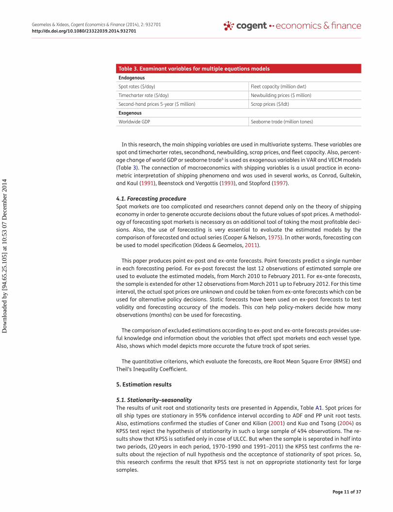
In this research, the main shipping variables are used in multivariate systems. These variables are spot and timecharter rates, secondhand, newbuilding, scrap prices, and fleet capacity. Also, percent-age change of world GDp or seaborne trade5 is used as exogenous variables in VAR and VECM models (Table 3). The connection of macroeconomics with shipping variables is a usual practice in econo-metric interpretation of shipping phenomena and was used in several works, as Conrad, Gultekin, and Kaul (1991), Beenstock and Vergottis (1993), and Stopford (1997).
4.1. Forecasting procedureSpot markets are too complicated and researchers cannot depend only on the theory of shipping economy in order to generate accurate decisions about the future values of spot prices. A methodol-ogy of forecasting spot markets is necessary as an additional tool of taking the most profitable deci-sions. Also, the use of forecasting is very essential to evaluate the estimated models by the comparison of forecasted and actual series (Cooper & Nelson, 1975). In other words, forecasting can be used to model specification (Xideas & Geomelos, 2011).
This paper produces point ex-post and ex-ante forecasts. point forecasts predict a single number in each forecasting period. For ex-post forecast the last 12 observations of estimated sample are used to evaluate the estimated models, from March 2010 to February 2011. For ex-ante forecasts, the sample is extended for other 12 observations from March 2011 up to February 2012. For this time interval, the actual spot prices are unknown and could be taken from ex-ante forecasts which can be used for alternative policy decisions. Static forecasts have been used on ex-post forecasts to test validity and forecasting accuracy of the models. This can help policy-makers decide how many observations (months) can be used for forecasting.
The comparison of excluded estimations according to ex-post and ex-ante forecasts provides use-ful knowledge and information about the variables that affect spot markets and each vessel type. Also, shows which model depicts more accurate the future track of spot series.
The quantitative criterions, which evaluate the forecasts, are Root Mean Square Error (RMSE) and Theil’s Inequality Coefficient.
5. estimation results
5.1. Stationarity–seasonalityThe results of unit root and stationarity tests are presented in Appendix, Table A1. Spot prices for all ship types are stationary in 95% confidence interval according to ADF and pp unit root tests. Also, estimations confirmed the studies of Caner and Kilian (2001) and Kuo and Tsong (2004) as KpSS test reject the hypothesis of stationarity in such a large sample of 494 observations. The re-sults show that KpSS is satisfied only in case of uLCC. But when the sample is separated in half into two periods, (20 years in each period, 1970–1990 and 1991–2011) the KpSS test confirms the re-sults about the rejection of null hypothesis and the acceptance of stationarity of spot prices. So, this research confirms the result that KpSS test is not an appropriate stationarity test for large samples.
table 3. examinant variables for multiple equations modelsendogenous
Spot rates ($/day) Fleet capacity (million dwt)
Timecharter rate ($/day) Newbuilding prices ($ million)
Second-hand prices 5-year ($ million) Scrap prices ($/ldt)
exogenous
Worldwide GDP Seaborne trade (million tones)
Dow
nloa
ded
by [
94.6
5.25
.105
] at
10:
53 0
7 D
ecem
ber
2014

Page 12 of 37
Geomelos & Xideas, Cogent Economics & Finance (2014), 2: 932701http://dx.doi.org/10.1080/23322039.2014.932701
In similar way, timecharter rates are stationary time-series for all vessel types except for panamax in tanker market. As spot and timecharter prices are stationary, they haven’t any trend which is confirmed by the estimations and the critical value of F-statistic (6.30) in Table A1.
The SACF and pACF show a sine wave for all tankers which means that they present seasonality. A characteristic correlogram of this sine wave is presented in Appendix (Figure A1) which is the same for all tankers. on the contrary, bulk carriers don’t present any form of seasonality according to their correlogram (Figure A1-Capesize). The deseasonalize procedure for spot prices of tankers follows the estimation of seasonal indices which are presented in Table 4. As table shows there is higher season-ality in June and from August to December where the consumption of oil is higher for the countries of north hemisphere.
5.2. Multivariate models
5.2.1. VARThe use of VAR-X models by the current research was adopted because there was a significant de-crease of forecasting errors. The number of lags is restricted to 4 or 6 and especially in u-VLCC, Suezmax and Handysize, VAR model has 4 lags and for all other markets 6 lags. This lag structure minimizes the SIC criterion. A close relationship between the freight markets and the newbuilding market is confirmed by the estimations of models, as newbuilding prices is endogenous variable in most vessel types (except Suezmax and Aframax). The current conditions in one market affect di-rectly the other providing important information for their development. Also, if freight market is considered as the potential income market for ship owners and the newbuilding market as the po-tential market of higher investments and profit then it is comprehensible why these two markets are crucial for shipping companies. A shipping company without income and new investments is math-ematically clear that will be constrained and finally will leave the shipping industry. From the rest variables, fleet capacity plays a more important role in tanker market and secondhand prices in bulk carrier. More specifically, second-hand prices affect more the panamax Bulk and Handymax mar-kets, because in these markets exist higher sales volume according to historical data. The results of VAR models and SIC criterion are presented in Appendix Table A7.
5.2.2. VECMVECM models are based on the existence of cointegration relations. The purpose of the Johansen cointegration test is to determine whether a group of non-stationary series is cointegrated or not. The numbers of lags for each vessel market are: u-VLCC 6 lags, Suezmax 4 lags, Aframax 6 lags, panamax 4 lags, Handysize 6 lags, Capesize 6 lags, panamax Bulk 4 lags, and Handymax 6 lags (Table A8-Appendix).
table 4. seasonal indices for each month for each vessel type in tanker marketseasonal indices
January February March April May June
ULCC .939060 .888217 .894972 .851429 .92064 1.064014
Suezmax 1.00158 .903644 .944425 .911301 .95627 1.029373
Aframax .97613 .925980 .928886 .911263 .96454 1.045815
Panamax .98709 .920305 .883262 .847791 .91934 1.046102
Handysize 1.01565 .984155 .978709 .906427 .93486 1.015049
July August September October November December
ULCC 1.03521 1.101264 1.095930 1.112983 1.05030 1.045960
Suezmax .99753 1.023298 .978473 1.049508 1.08220 1.122382
Aframax .99748 1.042561 1.027438 1.104286 1.01731 1.058288
Panamax 1.02038 1.124750 1.110881 1.108793 1.00778 1.023505
Handysize .98760 1.048781 1.063103 1.059473 .96075 1.045417
Dow
nloa
ded
by [
94.6
5.25
.105
] at
10:
53 0
7 D
ecem
ber
2014

Page 13 of 37
Geomelos & Xideas, Cogent Economics & Finance (2014), 2: 932701http://dx.doi.org/10.1080/23322039.2014.932701
The determination of endogenous variables in VECM models has been done according to their cointegration relation to spot rates. There are five endogenous variables with at least one cointegra-tion relation in uLCC-VLCC and Suezmax vessels. In Aframax and panamax, there are three endogenous variables with at least two cointegration relations. In Handysize, there are also three endogenous variables with one cointegration relation. In bulk carriers, Capesize presents two endogenous variables with one cointegration relation, panamax Bulk presents five endogenous variables with four cointegration relations, and Handymax presents three endogenous variables with three cointegration relations (Table 5).
VECM models suppose that the endogenous variables have cointegration relations analyzing at the same time the adjustment coefficients of ECM. These coefficients describe how fast the param-eters are adjusted if the variables are in disequilibrium. Also, the adjustment coefficients show the trend of new adjustment (downward or upward) and the speed of this adjustment.
In both markets, tanker and bulk carrier, shipping markets are linked together with cointegration relations presenting common stochastic trend. In regard to dynamic adjustment, the larger the ca-pacity (uLCC-VLCC = 1.14%, Suezmax = 5.21%, panamax = 21.85%) the slower the speed of adjust-ment in tanker market. This is due to that vessels with larger capacity have higher volatility which affects the speed of dynamic adjustment. In bulk carriers, panamax Bulk has the fastest adjustment (10.14%) and Handymax the slowest (3.60%). The long-run equilibrium relations and adjustment coefficients (Dynamic Multipliers) are presented in following Table 6.
5.3. Univariate models
5.3.1. ARMAAccording to Box–Jenkins methodology, AR models are of third order for Suezmax, panamax, and panamax Bulk. For larger capacity vessels (uLCC-VLCC, Capesize), AR models are of fifth order and for smaller capacity the order is increased (sixth order for Handysize and Handymax). So, the vessels of larger and smaller capacity seem to have higher order of AR, which is interpreted as more time lags of past values affect the current values of spot rates. Finally, Aframax market is expressed by AR(4) (Table 7).
For MA models, the orders are as follows: Suezmax and panamax MA(2), Aframax, Handysize, and Capesize MA(3). Also, the results show MA(4), MA(5), MA(6) for uLCC-VLCC, panamax Bulk and Handymax respectively. In conclusion, the orders of ARMA models determine the dynamic relation-ship of past values of spot rates from 3 to 6 months. Analytical estimations of ARMA models are presented in Appendix-Table A9.
5.3.2. GARCHHigh volatility of spot markets means that it is necessary to examine GARCH models. According to Breusch–pagan LM test, there is an ARCH effect for all vessel types in tanker and bulk carriers market as the variance of disturbance term is not constant but changes over time (Appendix Tables A3 and A4).
The research about the orders of ARCH and GARCH terms gives quite similar results. The best GARCH model for each vessel type is: uLCC-VLCC-GARCH-M (3,3), Suezmax-GARCH (3,3), Aframax-GARCH (4,4), panamax-GARCH (4,4), Handysize-GARCH-M (4,4), Capesize-GARCH-M (3,3), panamax Bulk-GARCH-M (3,3), Handymax-GARCH (1,3). For uLCC-VLCC, Handysize, Capesize and panamax Bulk vessels, there is higher volatility as ARCH-M model is used, which means that the conditional variance is introduced into the mean equation to measure the expected risk of spot rates.
In tanker market, the largest intensity of outside shocks on spot market’s volatility is in uLCC-VLCC market (1.174) and the smallest is in Suezmax market (.489). Spot rates for uLCC-VLCC present more intense response because they are affected by number of factors in relation to other vessels. For example, the vessels of large capacity are entering in fewer ports and their commercial activity is
Dow
nloa
ded
by [
94.6
5.25
.105
] at
10:
53 0
7 D
ecem
ber
2014

Page 14 of 37
Geomelos & Xideas, Cogent Economics & Finance (2014), 2: 932701http://dx.doi.org/10.1080/23322039.2014.932701
table 5. cointegration relations among endogenous variablesJohansen cointegration test
Unrestricted cointegration rank test (trace)
hypothesized No. of ce(s) eigenvalue trace statistic .05 critical value Prob.**ULCC-VLCC: Endogenous variables: spot, fleet, secondhand, newbuilding, scrap
None* .089433 84.16515 69.81889 .0023
At most 1 .041545 38.53912 47.85613 .2790
At most 2 .022285 17.87441 29.79707 .5754
At most 3 .010409 6.898775 15.49471 .5895
At most 4 .003695 1.802831 3.841466 .1794
Suezmax: Endogenous variables: spot, fleet, secondhand, newbuilding, scrap
None* .108392 89.76766 69.81889 .0006
At most 1 .042983 33.66543 47.85613 .5202
At most 2 .016981 12.18178 29.79707 .9254
At most 3 .007374 3.806977 15.49471 .9185
At most 4 .000384 .187889 3.841466 .6647
Aframax: Endogenous variables: spot, secondhand, fleet
None* .078535 56.15922 29.79707 .0000
At most 1* .031398 16.32725 15.49471 .0374
At most 2 .001623 .791223 3.841466 .3737
Panamax: Endogenous variables: spot, newbuilding, fleet
None* .133653 102.1103 29.79707 .0000
At most 1* .060149 31.95356 15.49471 .0001
At most 2 .003306 1.619169 3.841466 .2032
Handysize: Endogenous variables: spot, newbuilding, scrap
None* .090231 54.63725 29.79707 .0000
At most 1 .011086 8.584316 15.49471 .4052
At most 2 .006458 3.155381 3.841466 .0757
Capesize: Endogenous variables: spot, newbuilding
None* .042562 28.31457 15.49471 .0004
At most 1* .014540 7.133080 3.841466 .0076
Panamax Bulk: Endogenous variables: spot, fleet, secondhand, newbuilding, scrap
None* .096678 129.9755 69.81889 .0000
At most 1* .070618 80.25565 47.85613 .0000
At most 2* .040165 44.44341 29.79707 .0005
At most 3* .029025 24.39738 15.49471 .0018
At most 4* .020230 9.994036 3.841466 .0016
Handymax: Endogenous variables: spot, fleet, secondhand, newbuilding
None* .072522 78.95723 47.85613 .0000
At most 1* .045369 42.29303 29.79707 .0011
At most 2* .023572 19.68147 15.49471 .0110
At most 3* .016423 8.064460 3.841466 .0045
Note: Trace test indicates one cointegrating equation(s) at the .05 level.
*Rejection of the hypothesis at the .05 level.
**MacKinnon–Haug–Michelis (1999) p-values.
Dow
nloa
ded
by [
94.6
5.25
.105
] at
10:
53 0
7 D
ecem
ber
2014

Page 15 of 37
Geomelos & Xideas, Cogent Economics & Finance (2014), 2: 932701http://dx.doi.org/10.1080/23322039.2014.932701
limited in periods of oil or economic crisis, like present crisis. Suezmax market is more flexible and it is not affected so intensely by exterior factors. one reason is the limited number of ships, which trade in relation to uLCC-VLCC (31% less number of ships, 158% less fleet capacity6). The rest three markets, Aframax (.854), panamax (.966), and Handysize (.852) have quite the same high response in outside shocks. The memory of volatility for tankers is u-VLCC (.170), Suezmax (.596), Aframax (.283), panamax (.052), and Handysize (.165). It is obvious that panamax market has the smallest memory of volatility. This is linked to the fact that panamax vessels are more flexible to adjust to market conditions (ports, cargoes, etc.) The volatility lasts less, as many factors alter the managerial conditions of this specific market. The sum of ARCH and GARCH terms, in other words GARCH process is non-stationary for all tankers (u-VLCC 1.344, Suezmax 1.085, Aframax 1.137, panamax 1.018, and Handysize 1.017). This result is expected, as there are very sharp increase and decrease in spot rates’ volatility in all markets. Spot rates’ volatility of tanker market can be characterized as non-regular according to GARCH model.
In bulk carrier market, Handymax market has the largest intensity of outside shocks for the bulk carrier market (.340) and panamax Bulk market has the smallest (.146). This result confirms the results of Jing, Marlow, and Hui (2008). The intense of outside shocks is larger in Handymax because the number of ships is double in relation to Capesize market (Fleet Number-Capesize: 1400 ships, Handymax: 2540 ships). Handymax market is characterized by flexibility and adaptability in shipping routes, ports and cargoes. GARCH coefficients for Capesize, panamax Bulk and Handymax are .749, .861, and .708 respectively. Handymax market has the smallest memory of volatility because the intense activity of ships leads to many changes in spot rates. The respective values of Jing, Marlow, and Hui (2008) are .726, .763, and .497 where the row of numbers is confirmed by the current
table 6. long-run equilibrium relations and adjustment coefficientsULCC-VLCC
Spott = −1.54 Secondhandt + 5.64 Newbuildingt − 27.96 Scrapt + .58 Fleett − 180.48
(−.3%) (.2%) (.4%) (−.06%) (.18%) = 1.14%
Suezmax
Spott = +2.98 Secondhandt + .81 Newbuildingt − 30.88 Scrapt + 1.52 Fleett − 32.46
(−4.8%) (−.04%) (.2%) (−.13%) (.04%) = 5.21%
Aframax
Spott = 3.06 Secondhandt + 26.34
(−9.2%) (−.38%) Fleet (.06%) = 9.64%
Panamax
Spott = −5.26 Fleett + 237.75
(−21.70%) (.03%) Newbuilding (.12%) = 21.85%
Handysize
Spott = 9.07 Newbuildingt − 53.99 Scrapt + 34.49
(−14.70%) (.24%) (−.04%) = 14.98%
Capesize
Spott = .97 Newbuildingt − 31.27
(−2.57%) (2.26%) = 4.83%
Panamax Bulk
Spott = 21.55 Scrapt − 25.35
(−8.35%) (.33%) Secondhand (1.08%) Newbuilding (.38%) = 10.14%
Handymax
Spott = −3.24 Fleett + 148.81
(−2.01%) (.33%) Secondhand (.4%) Newbuilding (.86%) = 3.60%Note: Long-run multipliers in italics and adjustment coefficients in bold.
Dow
nloa
ded
by [
94.6
5.25
.105
] at
10:
53 0
7 D
ecem
ber
2014
Page 16 of 37
Geomelos & Xideas, Cogent Economics & Finance (2014), 2: 932701http://dx.doi.org/10.1080/23322039.2014.932701
research. The sum of ARCH and GARCH terms is very close to unity. More specifically, the values are 1.064, 1.007, and 1.048 for Capesize, panamax Bulk, and Handymax, respectively. GARCH processes are non-stationary and this is due to the high volatility of spot rates from 2003 until the end of the current sample (2011). Analytical estimations of GARCH models are presented in Appendix-Table A10.
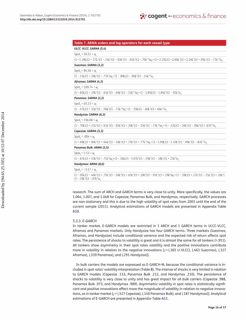
5.3.3. E-GARCHIn tanker market, E-GARCH models are restricted in 1 ARCH and 1 GARCH terms in uLCC-VLCC, Aframax and panamax markets. only Handysize has four GARCH terms. Three markets (Suezmax, Aframax, and Handysize) include conditional variance and the expected risk of return affects spot rates. The persistence of shocks to volatility is great and it is almost the same for all tankers (>.951). All tankers show asymmetry in their spot rates volatility and the positive innovations contribute more in volatility in relation to the negative innovations [γ = (.365 u-VLCC), (.463 Suezmax), (.327 Aframax), (.339 panamax), and (.291 Handysize)].
In bulk carriers the models are expressed as E-GARCH-M, because the conditional variance is in-cluded in spot rates’ volatility interpretation (Table 8). The intense of shocks is very limited in relation to GARCH models (Capesize .133, panamax Bulk .212, and Handymax .210). The persistence of shocks to volatility is very close to unity and has great impact for all bulk carriers (Capesize .988, panamax Bulk .973, and Handymax .989). Asymmetric volatility in spot rates is statistically signifi-cant and positive innovations affect more the magnitude of volatility in relation to negative innova-tions, as in tanker market [γ = (.527 Capesize), (.140 panamax Bulk), and (.187 Handymax)]. Analytical estimations of E-GARCH are presented in Appendix-Table A11.
table 7. aRMa orders and lag operators for each vessel typeULCC-VLCC: SARMA (5,4)
Spott = 50.51 + ut
(1 + 1.28L)(1 + .57L2)(1 − .14L3)(1 − .93L4)(1 − .82L5)(1 − .70L12)ut = (1 + 2.25L)(1 + 2.60L2)(1 + 2.16L3)(1 + .95L4)(1 − .71L12)εt
Suezmax: SARMA (3,2)
Spott = 84.36 + ut
(1 − .11L)(1 + .18L2)(1 − .77L3)ut = (1 − .89L)(1 − .90L2)(1 − .14L12)εt
Aframax: SARMA (4,3)
Spott = 109.74 + ut
(1 + .83L)(1 + .19L2)(1 − .61L3)(1 − .66L4)(1 − .33L12)ut = (1 − 1.85L)(1 − 1.84L2)(1 − .92L3)εt
Panamax: SARMA (3,2)
Spott = 65.13 + ut
(1 − .47L)(1 + .33L2)(1 − .56L3)(1 − .72L12)ut = (1 − .59L)(1 − .60L2)(1 + .66L12)εt
Handysize: SARMA (6,3)
Spott = 196.08 + ut
(1 − .70L)(1 + .21L2)(1 + .61L3)(1 − .92L4)(1 + .20L5)(1 − .15L6)(1 − .73L12)ut = (1 − .22L)(1 − .20L2)(1 − .96L3)(1 + .67L12)εt
Capesize: SARMA (5,3)
Spott = .004 + ut
(1 + .68L)(1 + .86L2)(1 + .64L3)(1 − .10L4)(1 + .15L5)(1 + .77L12)ut = (1 − 1.09L)(1 − 1.10L2)(1 − .89L3)(1 − .82L12)εt
Panamax Bulk: ARMA (3,5)
Spott = 2.53 + ut
(1 − .67L)(1 + .53L2)(1 − .71L3)ut = (1 − .56L)(1 − 1.07L2)(1 − .19L3)(1 − .18L4)(1 + .22L5)εt
Handymax: ARMA (8,6)
Spott = −3.57 + ut
(1 − .95L)(1 − .40L2)(1 + .75L3)(1 − .56L4)(1 + .65L5)(1 + .28L6)(1 − .97L7)(1 + .29L8)ut = (1 − .39L)(1 + .27L2)(1 − .25L3)(1 + .26L4)(1 − .39L5)(1 − .97L6)εt
Dow
nloa
ded
by [
94.6
5.25
.105
] at
10:
53 0
7 D
ecem
ber
2014

Page 17 of 37
Geomelos & Xideas, Cogent Economics & Finance (2014), 2: 932701http://dx.doi.org/10.1080/23322039.2014.932701
table 8. GaRch and e-GaRch models in bulk shipping
5.4. Ex-post forecasting resultsThe forecasting accuracy of VAR models is very high with very low RMSE and Theil values. This means that spot prices are affected by the interaction with other endogenous variables such as newbuilding and second-hand prices.
VECM models have very low forecasting errors and they give the best forecasts in five out of eight ship types according to Table 9. More specifically, VECM produce the best forecasts in Aframax and panamax and in all bulk carriers. It seems that the bulk carriers are affected more by other endog-enous variables and especially the second-hand and newbuilding prices and not by the past behav-ior of spot prices.
According to Table 9, ARMA models give better forecasting results only in case of Handysize mar-ket. Consequently, in bulk shipping the past values of spot prices cannot produce accurate forecasts and it seems that the current values of spot prices are moving independently from the past behavior of its values.
GARCH models give better forecasts in relation to other univariate models (ARMA, E-GARCH) for all vessel types (except Suezmax, Handysize). This result points out that spot prices seem to be affected more from their volatility than from their past values. This conclusion agrees with the fact that the vessels with larger capacity show larger volatility in their spot prices.
Forecasting accuracy of EGARCH models is worse in relation to GARCH models for all ship types except the Suezmax market. Also, EGARCH models seem to have better predictions compared to ARMA models.
ModelsVessels GaRch model specification e-GaRch model specification
ULCC-VLCC GARCH-M (3,3) E-GARCH (1,1)
Suezmax GARCH (3,3) E-GARCH-M (0,1)
Aframax GARCH (4,4) E-GARCH-M (1,1)
Panamax GARCH (4,4) E-GARCH (1,1)
Handysize GARCH-M (4,4) E-GARCH-M (1,4)
Capesize GARCH-M (3,3) E-GARCH-M (1,3)
Panamax Bulk GARCH-M (3,3) E-GARCH-M (1,6)
Handymax GARCH (1,3) E-GARCH-M (1,6)
table 9. Forecasting results (ex-post static forecast)—theil and RMse criterionsModels
Vessels aRMa GaRch eGaRch VaR VecMtheil RMse theil RMse theil RMse theil RMse theil RMse
ULCC-VLCC .093 9.041 .086 8.326 .087 8.467 .071 6.757 .075 7.101
Suezmax .091 17.11 .090 17.05 .089 16.73 .101 19.32 .099 18.86
Aframax .109 26.20 .096 23.09 .097 23.15 .089 21.45 .088 21.33
Panamax .084 19.90 .066 17.56 .066 18.01 .061 15.76 .054 14.40
Handysize .072 2.80 .078 22.08 .079 22.40 .091 25.84 .088 25.39
Capesize .095 4.736 .089 4.379 .088 4.402 .055 2.734 .055 2.716
PanamaxB .081 9.478 .078 9.145 .082 9.743 .059 6.848 .056 6.499
Handymax .062 7.898 .048 6.060 .048 6.074 .038 4.771 .032 4.117Note: Numbers in bold show the model with the smallest forecasting errors (Read table horizontally).
Dow
nloa
ded
by [
94.6
5.25
.105
] at
10:
53 0
7 D
ecem
ber
2014
Page 18 of 37
Geomelos & Xideas, Cogent Economics & Finance (2014), 2: 932701http://dx.doi.org/10.1080/23322039.2014.932701
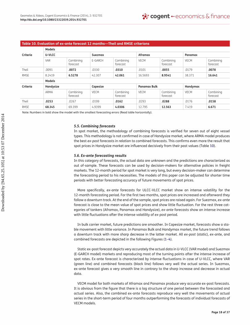
5.5. Combining forecastsIn spot market, the methodology of combining forecasts is verified for seven out of eight vessel types. This methodology is not confirmed in case of Handysize market, where ARMA model produces the best ex-post forecasts in relation to combined forecasts. This confirms even more the result that spot prices in Handysize market are influenced decisively from their past values (Table 10).
5.6. Ex-ante forecasting resultsIn this category of forecasts, the actual data are unknown and the predictions are characterized as out of-sample. These forecasts can be used by decision-makers for alternative policies in freight markets. The 12-month period for spot market is very long, but every decision-maker can determine the forecasting period to his necessities. The models of this paper can be adjusted for shorter time periods with better forecasting accuracy of future movements of spot prices.
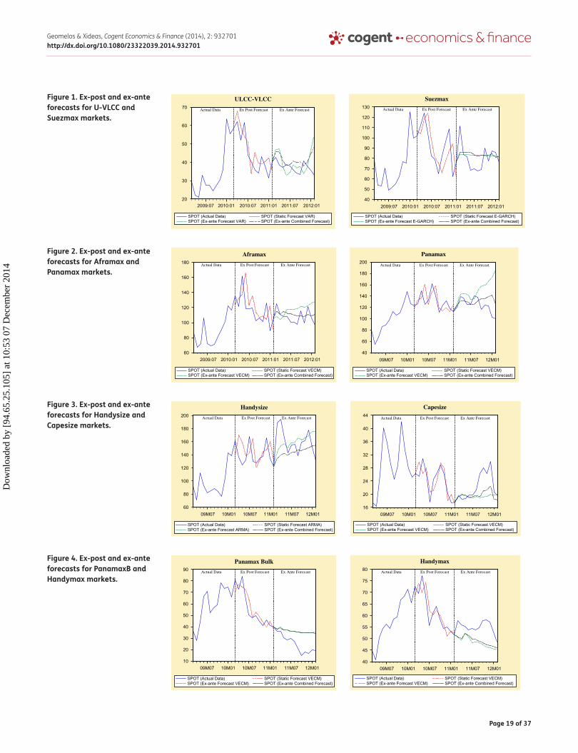
More specifically, ex-ante forecasts for uLCC-VLCC market show an intense volatility for the 12-month forecasting period. For the first two months, spot prices are increased and afterward they follow a downturn track. At the end of the sample, spot prices are raised again. For Suezmax, ex-ante forecast is close to the mean value of spot prices and show little fluctuation. For the rest three cat-egories of tankers (Aframax, panamax and Handysize), ex-ante forecasts show an intense increase with little fluctuations after the intense volatility of ex-post period.
In bulk carrier market, future predictions are smoother. In Capesize market, forecasts show a sta-ble movement with little variance. In panamax Bulk and Handymax market, the future trend follows a downturn track with more sharp decrease in the latter market. All ex-post (static), ex-ante, and combined forecasts are depicted in the following Figures (1–4).
Static ex-post forecast depicts very accurately the actual data in u-VLCC (VAR model) and Suezmax (E-GARCH model) markets and reproducing most of the turning points after the intense increase of spot rates. Ex-ante forecast is characterized by intense fluctuations in case of u-VLCC, where VAR (green line) and combined forecasts (black line) follows very well the actual series. In Suezmax, ex-ante forecast gives a very smooth line in contrary to the sharp increase and decrease in actual data.
VECM model for both markets of Aframax and panamax produce very accurate ex-post forecasts. It is obvious from the figure that there is a lag structure of one period between the forecasted and actual series. Also, the combined ex-ante forecasts reproduce very well the movements of actual series in the short-term period of four months outperforming the forecasts of individual forecasts of VECM models.
table 10. evaluation of ex-ante forecast 12 months—theil and RMse criterionsModels
criteria U-Vlcc suezmax aframax Panamax
VAR Combining forecast
E-GARCH Combining forecast
VECM Combining forecast
VECM Combining forecast
Theil .0091 .0072 .0330 .0310 .0101 .0055 .0179 .0078
RMSE 8.2419 6.5278 42.307 42.061 16.5693 8.9541 38.371 16.641
Models
criteria handysize capesize Panamax Bulk handymax
ARMA Combining forecast
VECM Combining forecast
VECM Combining forecast
VECM Combining forecast
Theil .0253 .0267 .0199 .0162 .0293 .0288 .0176 .0158
RMSE 68.345 69.399 4.9399 4.0306 12.795 12.563 7.419 6.671Note: Numbers in bold show the model with the smallest forecasting errors (Read table horizontally).
Dow
nloa
ded
by [
94.6
5.25
.105
] at
10:
53 0
7 D
ecem
ber
2014
Page 19 of 37
Geomelos & Xideas, Cogent Economics & Finance (2014), 2: 932701http://dx.doi.org/10.1080/23322039.2014.932701
Figure 2. ex-post and ex-ante forecasts for aframax and Panamax markets.
40
60
80
100
120
140
160
180
200
09M07 10M01 10M07 11M01 11M07 12M01
SPOT (Actual Data) SPOT (Static Forecast VECM)SPOT (Ex-ante Forecast VECM) SPOT (Ex-ante Combined Forecast)
Panamax
Actual Data Ex Post Forecast Ex Ante Forecast
60
80
100
120
140
160
180
2009:07 2010:01 2010:07 2011:01 2011:07 2012:01
SPOT (Actual Data) SPOT (Static Forecast VECM)SPOT (Ex-ante Forecast VECM) SPOT (Ex-ante Combined Forecast)
Aframax
Actual Data Ex Post Forecast Ex Ante Forecast
Figure 1. ex-post and ex-ante forecasts for U-Vlcc and suezmax markets.
20
30
40
50
60
70
2009:07 2010:01 2010:07 2011:01 2011:07 2012:01
SPOT (Actual Data) SPOT (Static Forecast VAR)SPOT (Ex-ante Forecast VAR) SPOT (Ex-ante Combined Forecast)
ULCC-VLCC
Actual Data Ex Post Forecast Ex Ante Forecast
40
50
60
70
80
90
100
110
120
130
2009:07 2010:01 2010:07 2011:01 2011:07 2012:01
SPOT (Actual Data) SPOT (Static Forecast E-GARCH)SPOT (Ex-ante Forecast E-GARCH) SPOT (Ex-ante Combined Forecast)
Suezmax
Actual Data Ex Post Forecast Ex Ante Forecast
Figure 3. ex-post and ex-ante forecasts for handysize and capesize markets.
60
80
100
120
140
160
180
200
09M07 10M01 10M07 11M01 11M07 12M01
SPOT (Actual Data) SPOT (Static Forecast ARMA)SPOT (Ex-ante Forecast ARMA) SPOT (Ex-ante Combined Forecast)
Handysize
Actual Data Ex Post Forecast Ex Ante Forecast
16
20
24
28
32
36
40
44
09M07 10M01 10M07 11M01 11M07 12M01
SPOT (Actual Data) SPOT (Static Forecast VECM)SPOT (Ex-ante Forecast VECM) SPOT (Ex-ante Combined Forecast)
Capesize
Actual Data Ex Post Forecast Ex Ante Forecast
Figure 4. ex-post and ex-ante forecasts for PanamaxB and handymax markets.
40
45
50
55
60
65
70
75
80
09M07 10M01 10M07 11M01 11M07 12M01
SPOT (Actual Data) SPOT (Static Forecast VECM)SPOT (Ex-ante Forecast VECM) SPOT (Ex-ante Combined Forecast)
Handymax
Actual Data Ex Post Forecast Ex Ante Forecast
10
20
30
40
50
60
70
80
90
09M07 10M01 10M07 11M01 11M07 12M01
SPOT (Actual Data) SPOT (Static Forecast VECM)SPOT (Ex-ante Forecast VECM) SPOT (Ex-ante Combined Forecast)
Panamax Bulk
Actual Data Ex Post Forecast Ex Ante Forecast
Dow
nloa
ded
by [
94.6
5.25
.105
] at
10:
53 0
7 D
ecem
ber
2014

Page 20 of 37
Geomelos & Xideas, Cogent Economics & Finance (2014), 2: 932701http://dx.doi.org/10.1080/23322039.2014.932701
ARMA model’s ex-post forecast for Handysize market follows the changing trends of actual data missing only the first turning point. on the contrary, VECM model in Capesize market can generate very accurate ex-post forecasts. Combined ex-ante forecasting is following the sharp increase and decrease in actual data only in case of Capesize. Handysize market is the only market where com-bined forecasting cannot generate forecasts with lower forecasting errors.
VECM ex-post forecasts for the last 12 observations (red line), for both panamax Bulk and Handymax markets, is quite close to the actual data (blue line) and reproduces most the sharp de-crease of actual data. Ex-ante forecasts can produce only the decreasing trend of actual series and they have a very smooth decay especially in panamax Bulk market.
6. conclusionsThe extensive analysis of different econometric models and from different econometric methodolo-gies results a number of important conclusions. First of all, spot prices for all tankers and bulk carri-ers are stationary confirming the classical economic theory which supports the stationarity of freight rates in a perfect competitive market. Also, tankers present seasonality and particularly in the sec-ond semester of the year as the consumption of oil is increased. The volatility of spot prices is asym-metric for both tanker and bulk carrier markets with the characteristic volatility of positive innovations to be larger than that of negative. GARCH processes are non-stationary for all ship types of tanker and bulk carrier markets confirming the result that spot prices have irregular volatility.
More specifically, in uLCC vessels, the past values of spot prices affect the present values in a pe-riod of five or six months. Spot prices are adapted more slowly in a case of disequilibrium of market presenting a higher risk. Cointegration relations prove the existence of common stochastic trend among spot, newbuilding and second-hand prices. VAR models can produce more accurate fore-casts in relation to other models.
The influence of past values to current spot prices in Suezmax market is limited to a quarter of year. The univariate models and especially the examination of volatility according to E-GARCH mod-els give the best ex-post forecasts in relation to multivariate models.
In Aframax market, the effect of past values concerns a four-month period and in panamax con-cerns a quarter. Forecasting evaluation shows that VECM models and especially the close relation between spot and second-hand prices for Aframax and spot and newbuilding prices for panamax simulates the actual spot prices more precisely in relation to all examinant models.
ARMA model plays a decisive role in the formation of Handysize spot prices. Firstly, past behavior of spot prices affects current prices in a period of six-month and produces more accurate forecasts.
In bulk carriers, the influence of past values of spot price concerns five-month, three-month, and four-month lags for Capesize, panamax Bulk, and Handymax, respectively. Also, VECM model pro-duces more accurate forecasts for all three categories of ships showing homogeneity in the fore-casting procedure indicating that the spot prices are affected from other endogenous variables and not only from the past values of spot rates.
Finally, the combining methodology of previous univariate and multivariate models provide lower forecasting errors in seven out of eight categories (except Handysize) of ships using the simple aver-age of forecasts instead of the forecasts of each individual model. A future research can compare more econometric models such as simultaneous equations models or multiple regressions and can use more complicate combining methods in order to minimize, as possible, the forecasting errors in spot markets.
Dow
nloa
ded
by [
94.6
5.25
.105
] at
10:
53 0
7 D
ecem
ber
2014

Page 21 of 37
Geomelos & Xideas, Cogent Economics & Finance (2014), 2: 932701http://dx.doi.org/10.1080/23322039.2014.932701
acknowledgmentThe authors wish to thank two anonymous referees for their useful comments and their constructive suggestions.
author detailsN.D. Geomelos1
E-mail: [email protected]. Xideas1
E-mail: [email protected] Department of Shipping, Trade and Transport, University of
the Aegean, G. Veriti 84, Chios 82100, Greece.
article informationCite this article as: Forecasting spot prices in bulk shipping using multivariate and univariate models, N.D. Geomelos & E. Xideas, Cogent Economics & Finance (2014), 2: 932701.
cover imageSource: Author
Notes1. A unit root process is a highly persistent time
series process where the current value equals last period’s value, plus a weakly dependent disturbance (Wooldridge, 2002).
2. The method of estimation of seasonal indices is referred in detail in Pindyck and Rubinfeld (1998, pp. 482–484).
3. As Sims (1980) noticed, the specification of some of variables as exogenous introduces restrictions on the model, because they affect the endogenous variables directly through feedback procedure.
4. For the advantages of simple average, see the paper of Palm and Zellner (1992, pp. 699–700).
5. In VAR and VECM models, it is used only one variable of them (GDP [%] or seaborne trade [%]) in order to avoid any correlation problems.
6. Authors estimations based on Clarksons SIN database.
ReferencesAiolfi, M., & Timmermann, A. (2006). persistence in forecasting
performance and conditional combination strategies. Journal of Econometrics, 135, 31–53. http://dx.doi.org/10.1016/j.jeconom.2005.07.015
Asteriou, D., & Hall, S. (2007). Applied econometrics. New york, Ny: palgrave MacMillan.
Batchelor, R., Alizadeh, A., & Visvikis, I. (2007). Forecasting spot and forward prices in the international freight market. International Journal of Forecasting, 23, 101–114. http://dx.doi.org/10.1016/j.ijforecast.2006.07.004
Beenstock, M., & Vergottis, A. (1993). Econometric modelling of world shipping. London: Chapman and Hall.
Boero, G. (1990). Comparing ex-ante forecasts from a SEM and VAR model: An application to the Italian economy. Journal of Forecasting, 9, 13–24. http://dx.doi.org/10.1002/(ISSN)1099-131X
Box, G. E. p., & Jenkins, G. M. (1976). Time series analysis: Forecasting and control (Revised ed.). San Francisco, CA: Holden-Day.
Caner, M., & Kilian, L. (2001). Size distortions of tests of the null hypothesis of stationarity: Evidence and implications for the ppp debate. Journal of International Money and Finance, 20, 639–657. http://dx.doi.org/10.1016/S0261-5606(01)00011-0
Clemen, R. T. (1989). Combining forecasts: A review and annotated bibliography. International Journal of Forecasting, 5, 559–583. http://dx.doi.org/10.1016/0169-2070(89)90012-5
Conrad, J., Gultekin, M., & Kaul, G. (1991). Asymmetric predictability of conditional variances. Review of Financial Studies, 4, 597–622. http://dx.doi.org/10.1093/rfs/4.4.597
Cooper, J. p., & Nelson, C. R. (1975). The ex-ante prediction performance of the St. Louis and FRB-MIT-pENN econometric models and some results on composite predictors. Journal of Money, Credit and Banking, 7, 1–32. http://dx.doi.org/10.2307/1991250
Cullinane, K. (1992). A short-term adaptive forecasting model for BIFFEX speculation, a Box–Jenkins approach. Maritime Policy and Management, 19, 1–114.
Cuthbertson, K., Hall, S., & Taylor, M. (1992). Applied econometric techniques. London: Harvester Wheatsheaf.
Davidson, R., & MacKinnon, G. J. (1993). Estimation and inference in econometrics. oxford: oxford university press.
Hausman, J. (1983). Specification and estimation of simultaneous equations models. Handbook of Econometrics, 1, 391–448. http://dx.doi.org/10.1016/S1573-4412(83)01011-9
Hawdon, D. (1978). Tanker freight rates in the short and long run. Applied Economics, 10, 203–218. http://dx.doi.org/10.1080/758527274
Heij, C., De Boer, p., Franses, p., Kloek, T., & Van Dijk, H. (2004). Econometric methods with application in business and economics. New york, Ny: oxford university press.
Jing, L., Marlow, p., & Hui, W. (2008). An analysis of freight rate volatility in dry bulk shipping markets. Maritime Policy & Management, 35, 237–251. http://dx.doi.org/10.1080/03088830802079987
Johansen, S. (1991). Estimation and hypothesis testing of cointegration vectors in Gaussian vector autoregressive models. Econometrica, 59, 1551–1580. http://dx.doi.org/10.2307/2938278
Kavussanos, M. G., & Nomikos, N. (1999). The forward pricing function of the shipping freight futures market. Journal of Futures Markets, 19, 353–376. http://dx.doi.org/10.1002/(ISSN)1096-9934
Kavussanos, M. G., & Visvikis, I. (2004). Market interactions in returns and volatilities between spot and forward shipping freight markets. Journal of Banking & Finance, 28, 2015–2049. http://dx.doi.org/10.1016/j.jbankfin.2003.07.004
Kilian, L. (2001). Impulse response analysis in vector autoregressions with unknown lag order. Journal of Forecasting, 20, 161–179. http://dx.doi.org/10.1002/(ISSN)1099-131X
Kuo, B. S., & Tsong, C. C. (2004). Bootstrap inference for stationarity. Manuscript National Chengchi university.
Litterman, R. (1984). Forecasting and policy analysis with Bayesian vector autoregression models. Federal Reserve Bank of Minneapolis Quarterly Review, 8, 30–41.
Lutkepohl, H., & Kratzig, M. (2004). Applied time series econometrics. New york, Ny: Cambridge university press. http://dx.doi.org/10.1017/CBo9780511606885
Lyridis, D. V., Zacharioudakis, p. G., Mitrou, p., & Mylonas, A. (2004). Forecasting tanker market using artificial neural networks. Maritime Economics and Logistics, 6, 93–108. http://dx.doi.org/10.1057/palgrave.mel.9100097
Newbold, p. (1983). ARIMA model building and the time series analysis approach to forecasting. Journal of Forecasting, 2, 23–35. http://dx.doi.org/10.1002/(ISSN)1099-131X
palm, F., & Zellner, A. (1992). To combine or not to combine? Issues of combining forecasts. Journal of Forecasting, 11, 687–701. http://dx.doi.org/10.1002/(ISSN)1099-131X
perron, p. (1989). The great crash, the oil price shock, and the unit root hypothesis. Econometrica, 57, 1361–1401. http://dx.doi.org/10.2307/1913712
pindyck, R., & Rubinfeld, D. (1998). Econometric models and economic forecasts. Boston, MA: Irwin McGraw-Hill.
Randers, J., & Göluke, u. (2007). Forecasting turning points in shipping freight rates: Lessons from 30 years of practical effort. System Dynamics Review, 23, 253–284. http://dx.doi.org/10.1002/(ISSN)1099-1727
Dow
nloa
ded
by [
94.6
5.25
.105
] at
10:
53 0
7 D
ecem
ber
2014
Page 22 of 37
Geomelos & Xideas, Cogent Economics & Finance (2014), 2: 932701http://dx.doi.org/10.1080/23322039.2014.932701
Rapach, D., & Strauss, J. (2008). Forecasting uS employment growth using forecast combining methods. Journal of Forecasting, 27, 75–93. http://dx.doi.org/10.1002/(ISSN)1099-131X
Scarsi, R. (2007). The bulk shipping business: Market cycles and shipowners’ biases. Maritime Policy & Management, 34, 577–590. http://dx.doi.org/10.1080/03088830701695305
Sims, C. (1980). Macroeconomics and reality. Econometrica, 48, 1–47. http://dx.doi.org/10.2307/1912017
Stopford, M. (1997). Maritime economics. London: Routledge. http://dx.doi.org/10.4324/9780203442661
Tsolakis, S. (2005). Econometric analysis of bulk shipping markets, implications for investment strategies and financial decision making (phD diss.). Erasmus university, Rotterdam.
uNCTAD-Review of Maritime Transport. (2011). Chap. 1, pp. 1–33.Veenstra, A., & Franses, p. (1997). Multivariate autoregressive
models for forecasting seaborne trade flows. Transportation Research Part E, 37, 311–319.
Verbeek, M. (2004). A guide to modern econometrics. Chichester: John Wiley & Sons.
Wooldridge, J. (2002). Introductory econometrics: A modern approach. New york, Ny: South-Western College.
Xideas, E., & Geomelos, N. D. (2011). An empirical investigation of spot prices in tanker market using dynamic multiple regression models. International Journal of Decision Sciences, Risk and Management, 3, 238–259. http://dx.doi.org/10.1504/IJDSRM.2011.046153
Figure a1. correlograms of Ulcc-Vlcc and capesize.
appendix
Dow
nloa
ded
by [
94.6
5.25
.105
] at
10:
53 0
7 D
ecem
ber
2014

Page 23 of 37
Geomelos & Xideas, Cogent Economics & Finance (2014), 2: 932701http://dx.doi.org/10.1080/23322039.2014.932701ta
ble
a1. t
est r
esul
ts o
f uni
t roo
t and
sta
tiona
rity
test
s in
tank
er a
nd b
ulk
carr
ier m
arke
t (aD
F, PP
, KPs
s)ta
nker
sUn
it ro
ot te
sts
ship
s va
riabl
esUn
it ro
ot te
st
(con
stan
t)—
aDF
Unit
root
test
(con
stan
t and
tr
end)
—aD
FUn
it ro
ot te
st
(con
stan
t)—
PPUn
it ro
ot te
st (c
onst
ant
and
tren
d)—
PPKP
ss
ship
ping
var
iabl
esco
nsta
ntla
gsF-
stat
istic
cons
tant
an
d tr
end
lags
F-st
atist
icin
terc
ept
lags
inte
rcep
t and
tr
end
lags
inte
rcep
tla
gs
ULCC
-VLC
C
SPOT
−4.3
4976
314
7.15
−4.4
8563
215
.63
−6.5
1701
61
−6.5
3593
61
.378
429
15
LogS
POT
−5.0
4185
21
5.69
−5.2
7180
11
1.13
−5.1
4378
71
−5.3
8338
61
.682
676
16
Tim
echa
rter
_Rat
e−4
.299
262
146.
79−4
.372
307
15.3
3−5
.550
506
3−5
.554
937
3.3
2635
516
LogT
imec
hart
er_R
ate
−3.4
0036
812
5.55
−3.5
5681
512
.59
−3.5
2480
83
−3.6
1434
73
.537
454
17
Suez
max
SPOT
−5.4
2257
32
9.98
−5.9
7761
63
3.04
−5.3
6367
12
−5.9
4807
52
.681
236
30
LogS
POT
−4.0
2957
41
7.81
−4.8
1039
01
3.41
−3.6
8176
36
−4.5
8240
95
.776
276
30
Tim
echa
rter
_Rat
e−3
.195
757
144.
03−3
.812
497
152.
19−4
.292
573
3−4
.922
830
2.6
5428
630
LogT
imec
hart
er_R
ate
−2.9
9274
77
4.10
−4.0
3874
17
3.85
−2.9
6922
31
−3.7
0381
91
.781
599
30
Afra
max
SPOT
−3.4
1120
214
5.00
−4.2
1120
715
3.07
−5.7
2380
43
−6.3
9446
13
.676
344
36
LogS
POT
−3.0
8448
512
4.87
−4.0
7713
712
3.59
−4.8
9659
13
−5.8
7905
64
.796
458
36
Tim
echa
rter
_Rat
e−3
.341
314
144.
90−3
.980
898
152.
37−4
.823
215
2−5
.346
847
2.7
0864
230
LogT
imec
hart
er_R
ate
−3.1
3824
612
4.97
−3.9
0033
012
2.72
−3.5
6178
43
−4.3
0058
84
.811
075
30
Pana
max
SPOT
−3.8
3593
38
6.26
−4.5
9926
19
3.18
−5.8
7779
05
−6.6
3707
64
.880
332
30
LogS
POT
−3.1
8386
312
5.26
−4.0
7243
912
3.31
−5.7
8619
41
−6.7
0493
61
.945
241
30
Tim
echa
rter
_Rat
e−2
.413
106
32.
33−2
.962
882
41.
67−2
.381
216
5−2
.903
565
51.
1143
0830
LogT
imec
hart
er_R
ate
−3.6
4874
012
7.24
−4.6
1742
512
4.76
−3.2
1051
85
−4.5
6492
01
1.15
1128
30
Hand
ysize
SPOT
−4.8
4187
14
10.0
3−5
.426
465
52.
95−5
.746
835
4−6
.563
017
5.8
1492
430
LogS
POT
−2.9
5472
412
4.57
−3.3
7345
612
1.52
−5.4
1044
54
−6.3
0146
05
.862
364
30
Tim
echa
rter
_Rat
e−3
.421
291
155.
16−4
.057
274
162.
41−4
.989
460
13−5
.020
977
13.3
3383
820
LogT
imec
hart
er_R
ate
−3.3
2365
313
5.49
−4.2
5677
313
3.63
−3.3
0732
18
−3.7
4447
48
.676
813
20
(Con
tinue
d)
Dow
nloa
ded
by [
94.6
5.25
.105
] at
10:
53 0
7 D
ecem
ber
2014

Page 24 of 37
Geomelos & Xideas, Cogent Economics & Finance (2014), 2: 932701http://dx.doi.org/10.1080/23322039.2014.932701
Criti
cal v
alue
s F-
stat
istic
4.61
Criti
cal v
alue
s F-
stat
istic
6.30
Mac
Kinn
on c
ritica
l val
ues
Criti
cal v
alue
s 1%
−3.4
4371
9−3
.977
251
−3.4
4338
8−3
.976
781
.739
000
Criti
cal v
alue
s 5%
−2.8
6732
9−3
.419
191
−2.8
6718
3−3
.418
962
.463
000
Criti
cal v
alue
s 10
%−2
.569
916
−3.1
3216
5−2
.569
837
−3.1
3203
0.3
4700
0
Bulk
car
riers
ship
ping
va
riabl
esco
nsta
ntla
gsF- sta-
tistic
cons
t./tr
end
lags
F-st
atist
icin
terc
ept
lags
inte
rc./t
rend
lags
inte
rc./t
rend
lags
Cape
size
SPOT
−3.0
0939
812
2.83
−3.9
3429
113
3.24
−3.0
1866
115
−3.8
0643
814
.191
327
30
LogS
pot
−2.3
7217
92
2.70
−3.6
2590
52
3.25
−2.5
3875
26
−3.6
9909
97
.135
861
18
Tim
echa
r-te
r_Ra
te−3
.569
842
33.
88−4
.682
310
1229
.44
−3.2
1552
05
−3.6
0372
05
.109
682
16
Log-
Tim
echa
r-te
r_Ra
te
−2.9
5191
13.
96−3
.505
408
11.
80−3
.024
795
10−3
.483
413
10.0
4869
517
Pana
max
-Bu
lk
SPOT
−3.1
0639
17
3.51
−4.9
4626
98
1.37
−2.9
0984
71
−3.8
1936
31
.204
703
30
Log
Spot
−2.5
7421
54
3.12
−3.9
9109
75
1.65
−2.4
8119
63
−3.8
0806
14
.111
303
18
Tim
echa
r-te
r_Ra
te−4
.049
112
44.
72−4
.712
969
52.
86−3
.381
721
1−3
.837
920
1.1
1762
116
Log-
Tim
echa
r-te
r_Ra
te
−3.2
1527
11
4.83
−4.3
4985
81
4.22
−3.0
5010
57
−3.9
5918
88
.057
740
16
Hand
ymax
SPOT
−2.9
5127
51
2.78
−4.1
3990
61
4.19
−2.5
6701
33
−3.5
8662
83
.215
300
35
LogS
pot_
Bulk
−2.0
5583
21
2.21
−3.6
0290
51
4.44
−2.0
8119
97
−3.4
1014
67
.173
846
17
Tim
echa
r-te
r_Ra
te−3
.696
674
114.
20−4
.883
746
125.
07−3
.027
410
5−3
.738
123
5.1
6058
930
tabl
e a1
. (Co
ntin
ued)
(Con
tinue
d)
tank
ers
Unit
root
test
ssh
ips
varia
bles
Unit
root
test
(c
onst
ant)
—aD
FUn
it ro
ot te
st (c
onst
ant a
nd
tren
d)—
aDF
Unit
root
test
(c
onst
ant)
—PP
Unit
root
test
(con
stan
t an
d tr
end)
—PP
KPss
ship
ping
var
iabl
esco
nsta
ntla
gsF-
stat
istic
cons
tant
an
d tr
end
lags
F-st
atis
ticin
terc
ept
lags
inte
rcep
t and
tr
end
lags
inte
rcep
tla
gs
Dow
nloa
ded
by [
94.6
5.25
.105
] at
10:
53 0
7 D
ecem
ber
2014

Page 25 of 37
Geomelos & Xideas, Cogent Economics & Finance (2014), 2: 932701http://dx.doi.org/10.1080/23322039.2014.932701
Log-
Tim
echa
r-te
r_Ra
te
−2.8
8471
08
4.68
−4.6
0512
69
4.98
−2.5
6398
79
−3.7
3733
79
.077
196
17
Criti
cal v
alue
s F-
stat
istic
4.
61Cr
itica
l val
ues
F-st
atist
ic6.
30Kw
iatk
owsk
i–Ph
ilips–
Schm
idt–
Shin
(199
2)M
acKi
nnon
crit
ical v
alue
s
Criti
cal v
alue
s 1%
−3.4
4371
9−3
.977
251
−3.4
4338
8−3
.976
781
.216
00
Criti
cal v
alue
s 5%
−2.8
6732
9−3
.419
191
−2.8
6718
3−3
.418
962
.146
00
Criti
cal v
alue
s 10
%−2
.569
916
−3.1
3216
5−2
.569
837
−3.1
3203
0.1
1900
tabl
e a1
. (Co
ntin
ued)
Not
es: N
umbe
rs in
bol
d sh
ow th
e st
atio
narit
y in
95%
con
fiden
ce in
terv
al.
Lag
s fo
r ADF
are
est
imat
ed a
ccor
ding
to S
IC c
riter
ion
Lags
for p
p an
d Kp
SS a
re e
stim
ated
acc
ordi
ng to
New
ey–W
est b
andw
idth
.
Bulk
car
riers
Unit
root
test
ssh
ips
varia
bles
Unit
root
test
(c
onst
ant)
—aD
FUn
it ro
ot te
st (c
onst
ant a
nd
tren
d)—
aDF
Unit
root
test
(c
onst
ant)
—PP
Unit
root
test
(con
stan
t an
d tr
end)
—PP
KPss
ship
ping
var
iabl
esco
nsta
ntla
gsF-
stat
istic
cons
t./tr
end
lags
F-st
atis
ticin
terc
ept
lags
inte
rc./t
rend
lags
inte
rc./
tren
dla
gs
tren
d
Dow
nloa
ded
by [
94.6
5.25
.105
] at
10:
53 0
7 D
ecem
ber
2014

Page 26 of 37
Geomelos & Xideas, Cogent Economics & Finance (2014), 2: 932701http://dx.doi.org/10.1080/23322039.2014.932701
table a2. endogenous and exogenous variables for each vessel type in bulk shippingtankersVessels
Variables Ulcc suezmax aframax Panamax handysizeSpot Endogenous Endogenous Endogenous Endogenous Endogenous
Timecharter Exogenous Exogenous Exogenous Exogenous Exogenous
Secondhand Pr. Endogenous Endogenous Endogenous Exogenous Exogenous
Newbuilding Pr. Endogenous Endogenous Exogenous Endogenous Endogenous
Scrap value Endogenous Endogenous Exogenous Exogenous Endogenous
Fleet capacity Endogenous Endogenous Endogenous Endogenous Exogenous
% Change of GDP Exogenous Exogenous Exogenous – –
% Change of seaborne trade – – – Exogenous Exogenous
Bulk carriers
capesize Panamax Bulk handymax
Spot Endogenous Endogenous Endogenous
Timecharter Exogenous Exogenous Exogenous
Secondhand Pr. Exogenous Endogenous Endogenous
Newbuilding Pr. Endogenous Endogenous Endogenous
Scrap value Exogenous Endogenous Exogenous
Fleet capacity Exogenous Endogenous Endogenous
% Change of GDP – – –
% Change of seaborne trade Exogenous Exogenous Exogenous
table a3. estimation of aRch effect (tankers)Dependent variable: DeseasON_sPOt
Method: least squares-sample (adjusted): 1970M02 2011M02
included observations: 493 after adjustments-convergence achieved after three iterations
Ulcc-Vlcc suezmax aframax Panamax handysizeVariable C AR(1) C AR(1) C AR(1) C AR(1) C AR(1)
Coefficient 55.69 .862 83.80 .900 111.11 .881 149.10 .883 190.14 .8718
Std. Error 6.646 .022 10.45 .019 10.779 10.30 12.92 .021 14.797 12.849
t-Statistic 8.378 37.78 8.018 46.67 .0212 41.39 11.53 41.76 .0220 39.488
Prob. .0000 .0000 .0000 .0000 .0000 .0000 .0000 .0000 .0000 .0000
ARCH effect
lags X2-statistic (critical value)
Ulcc-Vlcc suezmax aframax Panamax handysize
T × R2
1 3.84 3.45 9.90 3.45 1.95 .47
2 5.99 17.58 28.98 21.14 21.90 14.87
3 7.81 41.69 43.70 28.58 24.23 19.38
4 9.49 41.68 44.12 29.15 24.24 19.91
5 11.07 57.40 52.88 38.55 35.31 29.02
6 12.59 59.54 53.13 40.18 37.30 31.59
Dow
nloa
ded
by [
94.6
5.25
.105
] at
10:
53 0
7 D
ecem
ber
2014

Page 27 of 37
Geomelos & Xideas, Cogent Economics & Finance (2014), 2: 932701http://dx.doi.org/10.1080/23322039.2014.932701
table a4. estimation of aRch effect (Bulk carriers)Dependent variable: sPOt_BUlK
Method: least squares-sample (adjusted): 1970M02 2011M02
included observations: 493 after adjustments-convergence achieved after three iterations
capesize Panamax Bulk handymax
Variable C AR(1) C AR(1) C AR(1)
Coeffi-cient
14.28 .968 28.63 .971 28.55 .983
Std. Error 4.799 .011 7.804 .010 11.54 .008
t-statistic 2.977 86.69 3.669 91.91 2.473 116.3
Prob. .0031 .0000 .0003 .0000 .0137 .0000
ARCH effect
lags X2-statistic (criti-cal value)
capesize Panamax Bulk handymax
T × R2
1 3.84 88.98 127.99 70.96
2 5.99 89.57 127.99 72.23
3 7.81 97.15 160.50 74.43
4 9.49 206.12 175.20 89.77
5 11.07 205.75 175.44 99.52
6 12.59 206.49 178.13 102.91
table a5. Diagnostic tests aRMa model—tankersVessel size Q-statistic Breusch–Godfrey lM testtankers QlB (36) X2 serial correlation (2 lags) X2
ULCC-VLCC 29.97 50.99 .71 5.99
Suezmax 39.65 50.99 2.69 5.99
Aframax 30.32 50.99 3.44 5.99
Panamax 42.56 50.99 1.69 5.99
Handysize 35.28 50.99 .03 5.99
table a6. Diagnostic tests aRMa model—Bulk carriersBulk carriers QlB (36) X2 serial correlation (2 lags) X2
Capesize 57.47 50.99 2.19 5.99
Panamax Bulk 60.39 50.99 7.50 5.99
Handymax 65.14 50.99 1.00 5.99
Dow
nloa
ded
by [
94.6
5.25
.105
] at
10:
53 0
7 D
ecem
ber
2014

Page 28 of 37
Geomelos & Xideas, Cogent Economics & Finance (2014), 2: 932701http://dx.doi.org/10.1080/23322039.2014.932701
table a7. VaR estimations (tanker—Bulk carriers)Vector autoregression estimates for D(sPOt) Ulcc-Vlcc (tankers)
sample (adjusted): 1970M06 2011M02—included observations: 489 after adjustments
Variables coeff. t-statistic Variables coeff. t-statisticD(SPOT(-1)) −.0522 [−2.452] D(Secondhand_Pr.(-3)) −.3579 [−1.653]
D(SPOT(-2)) −.0498 [−2.344] D(Secondhand_Pr.(-4)) .0913 [.424]
D(SPOT(-3)) −.0008 [−.039] D(Scrap_Value(-1)) .2268 [.274]
D(SPOT(-4)) −.0410 [−1.888] D(Scrap_Value(-2)) 2.6092 [3.052]
D(Newbuilding_Pr.(−1)) .3316 [1.208] D(Scrap_Value(-3)) 2.6489 [3.079]
D(Newbuilding_Pr.(−2)) .1248 [.463] D(Scrap_Value(-4)) −1.6244 [−1.915]
D(Newbuilding_Pr.(−3)) −.2546 [−.950] C −.3343 [−.589]
D(Newbuilding_Pr.(−4)) −.2235 [−.857] Percentage_Gdp .9234 [1.865]
D(Secondhand_Pr.(−1)) −.6511 [−3.066] D(Fleet_Dwt) −.1700 [−.395]
D(Secondhand_Pr.(−2)) −.4834 [−2.212] D(Timecharter_Rate) 3.2070 [41.46]
R2 .798381 Akaike information criterion 18.348
S.E. equation 10.60739 Schwarz criterion 19.034
Log likelihood −4406.19
Vector autoregression estimates of D(sPOt) sUeZMaX (tankers)
sample (adjusted): 1970M06 2011M02—included observations: 489 after adjustments
Variables coeff. t-statistic Variables coeff. t-statisticD(SPOT(−1)) −.1166 [−3.776] D(Scrap_Value(−3)) 4.4420 [2.598]
D(SPOT(−2)) −.0699 [−2.259] D(Scrap_Value(−4)) −.7684 [−.454]
D(SPOT(−3)) −.0366 [−1.167] D(Fleet_Dwt(−1)) 6.7747 [2.260]
D(SPOT(−4)) −.0607 [−1.920] D(Fleet_Dwt(−2)) .7851 [.267]
D(Secondhand_Pr.(−1)) −1.2100 −2.480] D(Fleet_Dwt(−3)) −1.0906 [−.371]
D(Secondhand_Pr.(−2)) −1.2898 [−2.671] D(Fleet_Dwt(−4)) −7.0020 [−2.327]
D(Secondhand_Pr.(−3)) −.3355 [−.705] C −.8035 [−.866]
D(Secondhand_Pr.(−4)) .7383 [1.561] D(Timecharter) 4.9022 [24.32]
D(Scrap_Value(−1)) 3.6943 [2.209] D(Newbuilding_Pr.) .6445 [1.014]
D(Scrap_Value(−2)) 3.5168 [2.106] Percentage_Gdp 1.3652 [1.790]
R2 .5920 Akaike information criterion 13.74413
S.E. equation 16.370 Schwarz criterion 14.43000
Log likelihood −3280.4
Vector autoregression estimates of D(sPOt) aFRaMaX (tankers)
sample (adjusted): 1970M08 2011M02—included observations: 487 after adjustments
Variables coeff. t-statistic Variables coeff. t-statisticD(SPOT(−1)) −.0978 [−3.104] D(Fleet_Dwt(−4)) 6.8323 [1.621]
D(SPOT(−2)) −.0925 [−3.029] D(Fleet_Dwt(−5)) −6.6016 [−1.532]
D(SPOT(−3)) −.0822 [−2.613] D(Fleet_Dwt(−6)) −1.7867 [−.413]
D(SPOT(−4)) −.0765 [−2.477] C −.6412 [−.498]
D(SPOT(−5)) −.0319 [−1.042] D(Timecharter_Rate) 7.1652 [22.26]
D(SPOT(−6)) −.0703 [−2.247] D(Secondhand_Pr.) .1497 [.208]
D(Fleet_Dwt(−1)) 5.1680 [1.234] D(Newbuilding_Pr.) 2.5377 [2.913]
D(Fleet_Dwt(−2)) −7.7321 [−1.794] D(Scrap_Value) 1.6467 [.592]
(Continued)
Dow
nloa
ded
by [
94.6
5.25
.105
] at
10:
53 0
7 D
ecem
ber
2014

Page 29 of 37
Geomelos & Xideas, Cogent Economics & Finance (2014), 2: 932701http://dx.doi.org/10.1080/23322039.2014.932701
Vector autoregression estimates of D(sPOt) aFRaMaX (tankers)
sample (adjusted): 1970M08 2011M02—included observations: 487 after adjustments
Variables coeff. t-statistic Variables coeff. t-statisticD(Fleet_Dwt(−3)) 2.8582 [.663] Percentage_Gdp 1.0135 [1.082]
R2 .5839 Akaike information criterion 8.721014
S.E. equation 20.185 Schwarz criterion 9.030618
Log likelihood −2087.5
Vector autoregression estimates of D(sPOt) PaNaMaX (tankers)
sample (adjusted): 1970M08 2011M02—included observations: 487 after adjustments
Variables coeff. t-statistic Variables coeff. t-statisticD(SPOT(−1)) −.050619 [−1.278] D(Newbuilding_Pr.(−4)) .706997 [.398]
D(SPOT(−2)) −.250836 [−6.613] D(Newbuilding_Pr.(−5)) −1.010416 [−.567]
D(SPOT(−3)) −.083357 [−2.151] D(Newbuilding_Pr.(−6)) −.088206 [−.051]
D(SPOT(−4)) −.041316 [−1.059] C −.214986 [−.151]
D(SPOT(−5)) −.138809 [−3.683] D(Fleet_Dwt) −11.11909 [−1.075]
D(SPOT(−6)) −.202798 [−5.287] D(Timecharter_Rate) 15.05347 [11.93]
D(Newbuilding_Pr.(−1)) −1.806370 [−1.033] D(Secondhand_Pr.) 3.098490 [2.227]
D(Newbuilding_Pr.(−2)) 1.238302 [.693] D(Scrap_Value) −4.115325 [−.798]
D(Newbuilding_Pr.(−3)) −2.471770 [−1.397] Percentage_Seaborne .545972 [.278]
R2 .375099 Akaike information criterion 11.96602
S.E. equation 29.16946 Schwarz criterion 12.27562
Log likelihood −2877.725
Vector autoregression estimates of D(sPOt) haNDYsiZe (tankers)
sample (adjusted): 1970M06 2011M02—included observations: 489 after adjustments
Variables coeff. t-statistic Variables coeff. t-statisticD(SPOT(−1)) −.0516 [−1.254] D(Scrap_Value(−3)) −.5800 [−.057]
D(SPOT(−2)) −.2518 [−6.121] D(Scrap_Value(−4)) 11.105 [1.099]
D(SPOT(−3)) −.0654 [−1.578] D(Fleet_Dwt(−1)) 14.650 [1.293]
D(SPOT(−4)) −.0087 [−.208] D(Fleet_Dwt(−2)) −13.105 [−1.183]
D(Newbuilding_Pr.(−1)) 2.8106 [1.025] D(Fleet_Dwt(−3)) −.5467 [−.048]
D(Newbuilding_Pr.(−2)) 2.4843 [.897] D(Fleet_Dwt(−4)) −5.6595 [−.496]
D(Newbuilding_Pr.(−3)) −3.4757 [−1.262] C −.2310 [−.120]
D(Newbuilding_Pr.(−4)) −3.3492 [−1.248] D(Timecharter) 5.5870 [10.77]
D(Scrap_Value(−1)) 25.806 [2.635] PercentageSeaborne 2.1800 [.843]
D(Scrap_Value(−2)) 2.1378 [.213] D(Secondhand_Pr.) −1.2349 [−.706]
R2 .2762 Akaike information criterion 10.85258
S.E. equation 38.854 Schwarz criterion 11.53844
Log likelihood −2573.4
Vector autoregression estimates of D(spot_Bulk) caPesiZe (Bulk carriers)
sample (adjusted): 1970M08 2011M02—included observations: 487 after adjustments
Variables coeff. t-statistic Variables coeff. t-statisticD(Spot_Bulk(−1)) −.0591 [−1.851] D(Newbuilding_Pr.(−4)) −.0856 [−1.295]
D(Spot_Bulk(−2)) −.1363 [−4.794] D(Newbuilding_Pr.(−5)) −.0676 [−1.014]
table a7. (Continued)
(Continued)
Dow
nloa
ded
by [
94.6
5.25
.105
] at
10:
53 0
7 D
ecem
ber
2014

Page 30 of 37
Geomelos & Xideas, Cogent Economics & Finance (2014), 2: 932701http://dx.doi.org/10.1080/23322039.2014.932701
Vector autoregression estimates of D(spot_Bulk) caPesiZe (Bulk carriers)
sample (adjusted): 1970M08 2011M02—included observations: 487 after adjustments
Variables coeff. t-statistic Variables coeff. t-statisticD(Spot_Bulk(−3)) −.0328 [−1.158] D(Newbuilding_Pr.(−6)) .1603 [2.480]
D(Spot_Bulk(−4)) −.2717 [−9.486] C .0776 [.803]
D(Spot_Bulk(−5)) .1583 [5.462] D(Fleet_Dwt) −.0727 [−.650]
D(Spot_Bulk(−6)) −.0253 [−.926] D(Timecharter_Rate) .7755 [19.83]
D(Newbuilding_Pr.(−1)) .0099 [.148] Percentage_Seaborne −.1163 [−1.012]
D(Newbuilding_Pr.(−2)) −.0206 [−.302] D(Scrap_Value) .1098 [.480]
D(Newbuilding_Pr.(−3)) −.0454 [−.682] D(Secondhand_Pr.) .4164 [10.02]
R2 .7498 Akaike information criterion 7.173799
S.E. equation 1.7253 Schwarz criterion 7.483404
Log likelihood −1710.8
Vector autoregression estimates of D(spot_Bulk) PaNaMaX (Bulk carriers)
sample (adjusted): 1970M08 2011M02—included observations: 487 after adjustments
Variables coeff. t-statistic Variables coeff. t-statisticD(Spot_Bulk(−1)) −.0553 [−1.217] D(Secondhand_Pr.(−6)) .2392 [2.089]
D(Spot_Bulk(−2)) −.0426 [−.866] D(Fleet_Dwt(−1)) −.1697 [−.213]
D(Spot_Bulk(−3)) −.1719 [−3.513] D(Fleet_Dwt(−2)) −.3166 [−.397]
D(Spot_Bulk(−4)) .1427 [2.877] D(Fleet_Dwt(−3)) .0710 [.084]
D(Spot_Bulk(−5)) −.0458 [−.890] D(Fleet_Dwt(−4)) −1.4265 [−1.694]
D(Spot_Bulk(−6)) .0278 [.539] D(Fleet_Dwt(−5)) .0154 [.018]
D(Newbuilding_Pr.(−1)) .5330 [2.047] D(Fleet_Dwt(−6)) .6425 [.794]
D(Newbuilding_Pr.(−2)) −.0184 [−.069] D(Scrap_Value(−1)) 2.6716 [3.167]
D(Newbuilding_Pr.(−3)) −.3299 [−1.232] D(Scrap_Value(−2)) −.1743 [−.203]
D(Newbuilding_Pr.(−4)) −.6005 [−2.350] D(Scrap_Value(−3)) .6515 [.765]
D(Newbuilding_Pr.(−5)) −.1179 [−.473] D(Scrap_Value(−4)) .0929 [.109]
D(Newbuilding_Pr.(−6)) −.1061 [−.440] D(Scrap_Value(−5)) −.8632 [−1.029]
D(Secondhand_Pr.(−1)) .0480 [.393] D(Scrap_Value(−6)) −1.2110 [−1.511]
D(Secondhand_Pr.(−2)) .2172 [1.746] C .3625 [1.399]
D(Secondhand_Pr.(−3)) .0688 [.547] PercentageSeaborne −.0839 [−.343]
D(Secondhand_Pr.(−4)) −.3391 [−2.646] D(Timecharter) 1.1785 [15.64]
D(Secondhand_Pr.(−5)) .1745 [1.374]
R2 .4941 Akaike information criterion 10.46120
S.E. equation 3.5973 Schwarz criterion 11.88023
Log likelihood −2382.3
Vector autoregression estimates of D(spot_Bulk) haNDYMaX (Bulk carriers)
sample (adjusted): 1970M08 2011M02—included observations: 487 after adjustments
Variables coeff. t-statistic Variables coeff. t-statisticD(Spot_Bulk(−1)) .0222 [.547] D(Secondhand_Pr.(−1)) .0948 [.873]
D(Spot_Bulk(−2)) −.1853 [−4.447] D(Secondhand_Pr.(−2)) .3268 [3.047]
D(Spot_Bulk(−3)) −.0583 [−1.373] D(Secondhand_Pr.(−3)) .3851 [3.625]
D(Spot_Bulk(−4)) −.1600 [−3.891] D(Secondhand_Pr.(−4)) −.1831 [−1.726]
table a7. (Continued)
Dow
nloa
ded
by [
94.6
5.25
.105
] at
10:
53 0
7 D
ecem
ber
2014

Page 31 of 37
Geomelos & Xideas, Cogent Economics & Finance (2014), 2: 932701http://dx.doi.org/10.1080/23322039.2014.932701
Vector autoregression estimates of D(spot_Bulk) haNDYMaX (Bulk carriers)
sample (adjusted): 1970M08 2011M02—included observations: 487 after adjustments
Variables coeff. t-statistic Variables coeff. t-statisticD(Spot_Bulk(−5)) .0776 [1.874] D(Secondhand_Pr.(−5)) .0612 [.572]
D(Spot_Bulk(−6)) −.0900 [−2.176] D(Secondhand_Pr.(−6)) .0799 [.790]
D(Newbuilding_Pr.(−1)) .1567 [.662] C .1889 [1.291]
D(Newbuilding_Pr.(−2)) −.2538 [−1.061] Percentage_Seaborne −.0477 [−.279]
D(Newbuilding_Pr.(−3)) −.4324 [−1.823] D(Timecharter_Rate) 1.7836 [18.26]
D(Newbuilding_Pr.(−4)) .3287 [1.394] D(Scrap_Value) −.0944 [−.136]
D(Newbuilding_Pr.(−5)) −.1095 [−.469] D(Fleet_Dwt) −.55133 [−1.405]
D(Newbuilding_Pr.(−6)) −.2725 [−1.233]
R2 .6335 Akaike information criterion 9.032675
S.E. equation 2.5583 Schwarz criterion 9.626084
Log likelihood −2130.4
table a8. VecM estimations (tankers—Bulk carriers)Vector error correction estimates (U-Vlcc–tankers)
sample (adjusted): 1970M08 2011M02—included observations: 487 after adjustments, t-statistics in [ ]
cointegrating eq: coint. eq1SPOT(−1) 1.000000
Secondhand_Pr.(−1) 1.540622 [1.34216]
Newbuilding_Pr.(−1) −5.644820 [−3.87671]
Scrap_Value(−1) 27.95869 [3.57976]
Fleet_Dwt(−1) −.573406 [−1.39674]
C 180.4849
Error Correction: D(SPOT) D(Secondhand_Prices) D(Newbuilding_Prices) D(Scrap Value) D(Fleet_Dwt)
Coint. Eq1 −.003354 .002087 .004285 −.000558 .001798
[−.46361] [1.12219] [3.43981] [−1.20114] [3.64057]
R2 .801158 .262991 .312918 .218149 .636380
S.E. equation 10.41086 2.675403 1.792557 .668337 .710465
Log likelihood Akaike information criterion Schwarz criterion
−4825.421 20.53561 22.04063
Vector error correction estimates (suezmax–tankers)
sample (adjusted): 1970M06 2011M02—included observations: 489 after adjustments, t-statistics in [ ]
cointegrating eq: coint. eq1SPOT(−1) 1.000000
Secondhand_Pr.(−1) −2.978870 [−2.29751]
Newbuilding_Pr.(−1) −.808660 [−.54569]
Scrap_Value(−1) 30.88417 [3.69128]
Fleet_Dwt(−1) −1.515290 [−1.05679]
C −32.46050
Error Correction: D(SPOT) D(Secondhand_Prices) D(Newbuilding_Prices) D(Scrap Value) D(Fleet_Dwt)
table a7. (Continued)
(Continued)
Dow
nloa
ded
by [
94.6
5.25
.105
] at
10:
53 0
7 D
ecem
ber
2014
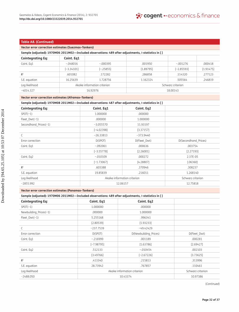
Page 32 of 37
Geomelos & Xideas, Cogent Economics & Finance (2014), 2: 932701http://dx.doi.org/10.1080/23322039.2014.932701
Vector error correction estimates (suezmax–tankers)
sample (adjusted): 1970M06 2011M02—included observations: 489 after adjustments, t-statistics in [ ]
cointegrating eq: coint. eq1Coint. Eq1 −.048016 −.000395 .001950 −.001276 .000418
[−3.34101] [−.25855] [1.89795] [−2.85593] [1.91475]
R2 .601082 .172282 .286858 .114320 .277123
S.E. equation 16.25639 1.728756 1.162324 .505564 .246819
Log likelihood Akaike information criterion Schwarz criterion
−4014.327 16.92976 18.00143
Vector error correction estimates (aframax–tankers)
sample (adjusted): 1970M08 2011M02—included observations: 487 after adjustments, t-statistics in [ ]
cointegrating eq: coint. eq1 coint. eq2SPOT(−1) 1.000000 .000000
Fleet_Dwt(−1) .000000 1.000000
Secondhand_Prices(−1) −3.055570 11.93197
[−4.02398] [3.37157]
C −26.33813 −373.9440
Error correction D(SPOT) D(Fleet_Dwt) D(Secondhand_Prices)
Coint. Eq1 −.092061 .000636 .003754
[−3.55778] [2.26001] [2.27193]
Coint. Eq2 −.010109 .000272 2.37E-05
[−1.73067] [4.28807] [.06360]
R2 .603388 .370946 .308237
S.E. equation 19.85839 .216011 1.268140
Log likelihood Akaike information criterion Schwarz criterion
−2855.992 12.06157 12.75818
Vector error correction estimates (Panamax–tankers)
sample (adjusted): 1970M06 2011M02—included observations: 489 after adjustments, t-statistics in [ ]
cointegrating eq: coint. eq1 coint. eq2SPOT(−1) 1.000000 .000000
Newbuilding_Prices(−1) .000000 1.000000
Fleet_Dwt(−1) 5.255168 .996341
[2.80539] [1.93233]
C −237.7539 −49.42429
Error correction D(SPOT) D(Newbuilding_Prices) D(Fleet_Dwt)
Coint. Eq1 −.216999 .001189 .000281
[−7.98795] [1.63786] [2.69427]
Coint. Eq2 .512133 −.010454 .002103
[3.49766] [−2.67226] [3.73625]
R2 .413340 .215813 .313996
S.E. equation 28.73942 .767857 .110461
Log likelihood Akaike information criterion Schwarz criterion
−2488.050 10.43374 10.97386
table a8. (Continued)
(Continued)
Dow
nloa
ded
by [
94.6
5.25
.105
] at
10:
53 0
7 D
ecem
ber
2014

Page 33 of 37
Geomelos & Xideas, Cogent Economics & Finance (2014), 2: 932701http://dx.doi.org/10.1080/23322039.2014.932701
Vector error correction estimates (handysize–tankers)
sample (adjusted): 1970M08 2011M02—included observations: 487 after adjustments, t-statistics in [ ]
cointegrating eq: coint. eq1SPOT(−1) 1.000000
Newbuilding_Prices(−1) −9.065271
[−5.80248]
Scrap_Value(−1) 53.99123
[3.31459]
C −34.48705
Error correction: D(SPOT) D(Newbuilding_Prices) D(Scrap_Value)
Coint. Eq1 −.147034 .002438 −.000357
[−4.42416] [4.34322] [−2.17613]
R2 .316044 .230622 .056724
S.E. equation 37.48530 .633099 .185136
Log likelihood Akaike information criterion Schwarz criterion
−2756.459 11.62817 12.27318
Vector error correction estimates (capesize–Bulk carriers)
sample (adjusted): 1970M08 2011M02—included observations: 487 after adjustments, t-statistics in [ ]
cointegrating eq: coint. eq1Spot_Bulk(−1) 1.000000
Newbuilding_Prices(−1) −.970013
[−6.40975]
C 31.27048
Error correction D(Spot_Bulk) D(Newbuilding_Prices)
Coint. Eq1 −.025728 .022566
[−2.45942] [3.16150]
R2 .752692 .305278
S.E. equation 1.717535 1.171876
Log likelihood Akaike information criterion Schwarz criterion
−1703.287 7.159291 7.503296
Vector error correction estimates (PanamaxB–Bulk carriers)
sample (adjusted): 1970M06 2011M02—included observations: 489 after adjustments, t-statistics in [ ]
cointegrating eq: coint. eq1 coint. eq2 coint. eq3 coint. eq4Spot_Bulk(−1) 1.000000 .000000 .000000 .000000
Secondhand_Pr.(−1) .000000 1.000000 .000000 .000000
Newbuilding_Pr. (−1) .000000 .000000 1.000000 .000000
Fleet_Dwt(−1) .000000 .000000 .000000 1.000000
Scrap_Value(−1) −21.55242 −15.85086 −10.33899 10.98117
[−7.76574] [−9.72067] [−7.42110] [1.42054]
C 25.35444 18.41539 −.368095 −76.77063
Error correction: D(Spot_Bulk) D(Secondhand_Prices) D(Newbuilding_Prices) D(Fleet_Dwt) D(Scrap_Value)
Coint. Eq1 −.083451 .010823 .003753 .003252 .005962
[−2.86145] [.88385] [.70622] [1.91473] [3.25534]
Coint. Eq2 .059989 −.079856 .004048 −.006101 −.003896
table a8. (Continued)
(Continued)
Dow
nloa
ded
by [
94.6
5.25
.105
] at
10:
53 0
7 D
ecem
ber
2014

Page 34 of 37
Geomelos & Xideas, Cogent Economics & Finance (2014), 2: 932701http://dx.doi.org/10.1080/23322039.2014.932701
Vector error correction estimates (PanamaxB–Bulk carriers)
sample (adjusted): 1970M06 2011M02—included observations: 489 after adjustments, t-statistics in [ ]
cointegrating eq: coint. eq1 coint. eq2 coint. eq3 coint. eq4[1.12293] [−3.56003] [.41582] [−1.96109] [−1.16120]
Coint. Eq3 .131376 .052994 −.038739 .003048 −.004132
[2.10746] [2.02456] [−3.41006] [.83974] [−1.05545]
Coint. Eq4 .012148 −.004285 −.003120 .001291 .000112
[1.65662] [−1.39167] [−2.33473] [3.02216] [.24233]
R2 .500445 .660719 .405204 .594102 .408980
S.E. equation 3.544036 1.488113 .645845 .206384 .222560
Log likelihood Akaike information criterion
Schwarz criterion
−2404.526 10.46841 11.79728
Vector error correction estimates (handymax–Bulk carriers)
sample (adjusted): 1970M08 2011M02—included observations: 487 after adjustments, t-statistics in [ ]
cointegrating eq: coint. eq1 coint. eq2 coint. eq3Spot_Bulk(−1) 1.000000 .000000 .000000
Secondhand_Prices(−1) .000000 1.000000 .000000
Newbuilding_Prices(−1) .000000 .000000 1.000000
Fleet_Dwt(−1) 3.235324 1.582158 1.384436
[2.55074] [2.24684] [2.74668]
C −148.8089 −78.34988 −77.46503
Error Correction: D(Spot_Bulk) D(Secondhand_Prices) D(Newbuilding_Prices) D(Fleet_Dwt)
Coint. Eq1 −.020136 .004040 .008559 .003310
[−1.22390] [.65037] [2.62953] [3.48403]
Coint. Eq2 .036944 −.030550 −.006100 −.008376
[1.00147] [−2.19343] [−.83573] [−3.93235]
Coint. Eq3 .013774 .029477 −.013489 .003913
[.40493] [2.29525] [−2.00429] [1.99238]
R2 .646993 .734067 .438884 .777903
S.E. equation 2.532805 .956279 .501127 .146245
Log likelihood Akaike information criterion Schwarz criterion
−1842.059 8.123444 9.293062
table a8. (Continued)
Dow
nloa
ded
by [
94.6
5.25
.105
] at
10:
53 0
7 D
ecem
ber
2014
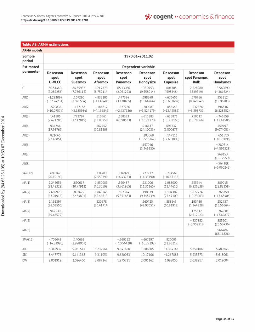
Page 35 of 37
Geomelos & Xideas, Cogent Economics & Finance (2014), 2: 932701http://dx.doi.org/10.1080/23322039.2014.932701
table a9. aRMa estimationsaRMa models
sample period
1970:01–2011:02
estimated parameter
Dependent variableDeseason
spot U-Vlcc
Deseason spot
suezmax
Deseason spot
aframax
Deseason spot
Panamax
Deseason spot
handysize
Deseason spot
capesize
Deseason spot Panamax
Bulk
Deseason spot
handymaxC 50.51440
(7.289256)84.35932
(7.766115)109.7379
(8.757114)65.13086
(2.061293)196.0753
(9.558014).004305
(.598348)2.528280 (.339349)
−3.569690 (−.381624)
AR(1) −1.283094 (−37.74231)
.107290 (2.071504)
−.832105 (−12.48406)
.477334 (3.120405)
.698240 (13.64264)
−.676455 (−6.633687)
.670766 (8.249042)
.953212 (19.96283)
AR(2) −.570836 (−10.07574)
−.177158 (−3.585934)
−.186717 (−4.195845)
−.327766 (−2.437536)
−.209087 (−3.524179)
−.856443 (−12.42586)
−.537376 (−6.298731)
.396836 (6.828252)
AR(3) .141185 (2.421285)
.772797 (17.12819)
.610561 (13.03950)
.558373 (6.590533)
−.611883 (−16.21170)
−.635871 (−5.302165)
.710012 (10.78866)
−.746559 (−12.41586)
AR(4) .934746 (17.95769)
.662752 (10.81503)
.916437 (24.10023)
.096732 (1.500675)
.559497 (9.074051)
AR(5) .821065 (27.48851)
−.203068 (−3.516742)
−.147111 (−2.651800)
−.651510 (−10.73098)
AR(6) .157016 (3.245630)
−.280714 (−4.599328)
AR(7) .969153 (16.12959)
AR(8) −.294555 (−6.060243)
SAR(12) .699167 (20.19190)
.334203 (7.550390)
.716029 (14.43753)
.727717 (14.33190)
−.774569 (−10.67135)
MA(1) 2.246656 (82.48329)
.890617 (20.77912)
1.850083 (40.35599)
.590487 (3.761955)
.221006 (11.31165)
1.088000 (12.44610)
.555944 (6.226538)
.389015 (23.83258)
MA(2) 2.602970 (43.01914)
.897622 (22.64891)
1.843245 (42.44613)
.597314 (5.351663)
.198839 (9.345439)
1.104382 (25.47100)
1.072724 (10.79403)
−.266350 (−17.68404)
MA(3) 2.161397 (38.09550)
.920578 (20.41714)
.960425 (49.97051)
.888543 (10.81919)
.195430 (1.944928)
.252737 (15.56664)
MA(4) .947539 (39.66572)
.175612 (2.517423)
−.262681 (−17.69877)
MA(5) −.227382 (−3.952912)
.385901 (26.58436)
MA(6) .966484 (63.16826)
SMA(12) −.706648 (−14.83996)
.140662 (2.998067)
−.660152 (−10.56428)
−.667197 (−10.27292)
.820005 (11.83217)
AIC 8.342932 9.081541 9.232544 9.541650 10.06605 −1.364143 5.850106 5.480243
SIC 8.447776 9.141368 9.311051 9.620033 10.17106 −1.267883 5.935573 5.618061
DW 2.001919 2.096460 2.087147 1.975731 2.001162 1.998050 2.038217 2.019004
Dow
nloa
ded
by [
94.6
5.25
.105
] at
10:
53 0
7 D
ecem
ber
2014

Page 36 of 37
Geomelos & Xideas, Cogent Economics & Finance (2014), 2: 932701http://dx.doi.org/10.1080/23322039.2014.932701
table a11. e-GaRch estimationse-GaRch models
sample period
1970:01–2011:02
estimated parameter
Dependent variableDeseason
spot U-Vlcc
Deseason spot
suezmax
Deseason spot
aframax
Deseason spot
Panamax
Deseason spot
handysize
Deseason spot
capesize
Deseason spot Panamax
Bulk
Deseason spot
handymaxC .080997
(1.154514).189936
(2.655860).174026
(2.254872).122143
(1.537955).210860
(2.895870)−.112579
(−2.516638)−.113772
(−3.472137)−.144885
(−3.930217)
ARCH (1) .173842 (2.711991)
.079576 (1.292355)
.131530 (2.105265)
−.055893 (−2.990198)
.132892 (2.607516)
.211706 (4.574413)
.209561 (4.354164)
GARCH (1) .949529 (85.63437)
.950800 (70.29388)
.952892 (84.38945)
.963147 (80.57513)
1.153938 (439.2297)
.468422 (5.440948)
1.030720 (18.77174)
.697731 (9.252560)
GARCH (2) −.517418 (−26.98499)
.393596 (5.374048)
−.167527 (−2.810100)
.851964 (10.64576)
GARCH (3) .779859 (38.02508)
.125720 (1.530027)
.181747 (4.066184)
−1.198651 (−8.040732)
GARCH (4) −.446274 (−128.7171)
−.328864 (−6.964393)
.661886 (5.539970)
table a10. GaRch estimationsGaRch models
sample period
1970:01–2011:02
estimated parameter
Dependent variableDeseason
spot U-Vlcc
Deseason spot
suezmax
Deseason spot
aframax
Deseason spot
Panamax
Deseason spot
handysize
Deseason spot
capesize
Deseason spot Panamax Bulk
Deseason spot
handymaxC 5.691304
(2.213809)6.466746
(2.867686)17.89197
(2.199346)108.3865
(3.505629)139.9965
(3.156653).028021
(3.400383).106843
(3.561445).102673
(3.375823)
ARCH (1) .392118 (12.32730)
.455110 (9.027228)
.211607 (8.028785)
.245802 (6.067745)
.241939 (12.68916)
.462388 (7.730518)
.184306 (3.519282)
.340177 (7.806101)
ARCH (2) .444280 (10.53461)
−.262658 (−4.535314)
.210654 (8.342708)
.237916 (6.516534)
.224924 (7.449137)
−.360060 (−3.151224)
−.172317 (−2.215324)
ARCH (3) .337734 (9.539731)
.296729 (6.757749)
.205676 (7.318297)
.235949 (6.312831)
.182055 (9.840213)
.212833 (3.373868)
.134430 (2.810678)
ARCH (4) .225983 (8.842686)
.246055 (6.054769)
.202829 (91.19500)
GARCH (1) −.195273 (−3.900444)
.731743 (25.29878)
−.082794 (−2.620347)
−.128263 (−2.849323)
−.328229 (−9.388411)
1.563985 (23.15183)
2.024000 (135.6112)
.992152 (7.109913)
GARCH (2) −.127651 (−3.358435)
−.629088 (−19.46479)
−.248008 (−7.881385)
−.180311 (−5.838934)
−.141188 (−4.193502)
−1.321975 (−21.73843)
−1.881301 (−470.8925)
−.581392 (−3.200924)
GARCH (3) .493274 (10.55966)
.493006 (22.84013)
−.197958 (−7.981229)
−.335436 (−11.11069)
−.096629 (−4.260191)
.506914 (20.39618)
.717883 (41.94791)
.297335 (3.182537)
GARCH (4) .811815 (30.57328)
.696045 (19.24948)
.731271 (31.20748)
AIC 7.810066 8.277758 8.835272 9.417321 9.995540 3.102276 4.625304 4.098563
SIC 7.895269 8.354441 8.928995 9.511044 10.09778 3.187479 4.710507 4.158205
DW 1.967438 2.024944 1.936013 1.782192 1.913008 1.270328 1.561924 1.268188
(Continued)
Dow
nloa
ded
by [
94.6
5.25
.105
] at
10:
53 0
7 D
ecem
ber
2014
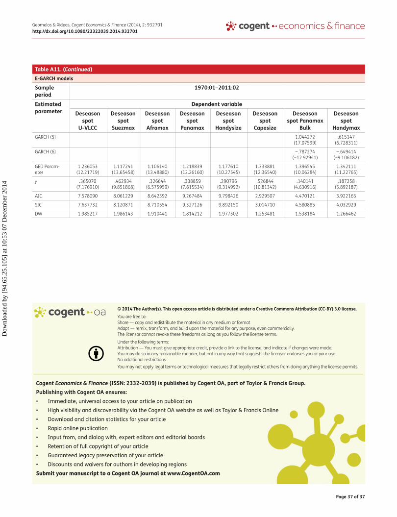
Page 37 of 37
Geomelos & Xideas, Cogent Economics & Finance (2014), 2: 932701http://dx.doi.org/10.1080/23322039.2014.932701
e-GaRch models
sample period
1970:01–2011:02
estimated parameter
Dependent variableDeseason
spot U-Vlcc
Deseason spot
suezmax
Deseason spot
aframax
Deseason spot
Panamax
Deseason spot
handysize
Deseason spot
capesize
Deseason spot Panamax
Bulk
Deseason spot
handymaxGARCH (5) 1.044272
(17.07599).615147
(6.728311)
GARCH (6) −.787274 (−12.92941)
−.649414 (−9.106182)
GED Param-eter
1.236053 (12.21719)
1.117241 (13.65458)
1.106140 (13.48880)
1.218839 (12.26160)
1.177610 (10.27545)
1.333881 (12.36540)
1.396545 (10.06284)
1.342111 (11.22765)
γ .365070 (7.176910)
.462934 (9.851868)
.326644 (6.575959)
.338859 (7.615534)
.290796 (9.314992)
.526844 (10.81342)
.140141 (4.630916)
.187258 (5.892187)
AIC 7.578090 8.061229 8.642392 9.267484 9.798426 2.929507 4.470121 3.922165
SIC 7.637732 8.120871 8.710554 9.327126 9.892150 3.014710 4.580885 4.032929
DW 1.985217 1.986143 1.910441 1.814212 1.977502 1.253481 1.538184 1.266462
table a11. (Continued)
© 2014 The Author(s). This open access article is distributed under a Creative Commons Attribution (CC-BY) 3.0 license.You are free to: Share — copy and redistribute the material in any medium or format Adapt — remix, transform, and build upon the material for any purpose, even commercially.The licensor cannot revoke these freedoms as long as you follow the license terms.
Under the following terms:Attribution — You must give appropriate credit, provide a link to the license, and indicate if changes were made. You may do so in any reasonable manner, but not in any way that suggests the licensor endorses you or your use. No additional restrictions You may not apply legal terms or technological measures that legally restrict others from doing anything the license permits.
Cogent Economics & Finance (ISSN: 2332-2039) is published by Cogent OA, part of Taylor & Francis Group. Publishing with Cogent OA ensures:• Immediate, universal access to your article on publication• High visibility and discoverability via the Cogent OA website as well as Taylor & Francis Online• Download and citation statistics for your article• Rapid online publication• Input from, and dialog with, expert editors and editorial boards• Retention of full copyright of your article• Guaranteed legacy preservation of your article• Discounts and waivers for authors in developing regionsSubmit your manuscript to a Cogent OA journal at www.CogentOA.com
Dow
nloa
ded
by [
94.6
5.25
.105
] at
10:
53 0
7 D
ecem
ber
2014