Geomorphology 134 (2011) 297–308

Contents lists available at ScienceDirect

Geomorphology

j ourna l homepage: www.e lsev ie r.com/ locate /geomorph

Comparison of GIS-based gullying susceptibility mapping using bivariate andmultivariate statistics: Northern Calabria, South Italy

Federica Lucà, Massimo Conforti, Gaetano Robustelli ⁎Earth Science Department, University of Calabria, Via P. Bucci, 87036 Arcavacata di Rende (CS), Italy

⁎ Corresponding author. Tel.: +39 0984 493546; fax:E-mail address: robustelli@unical.it (G. Robustelli).

0169-555X/$ – see front matter © 2011 Elsevier B.V. Adoi:10.1016/j.geomorph.2011.07.006

a b s t r a c t

a r t i c l e i n f o

Article history:Received 26 July 2010Received in revised form 30 May 2011Accepted 19 July 2011Available online 24 July 2011

Keywords:Gullying susceptibilityStatisticsBivariate methodLogistic regressionCalabria

This paper presents GIS-aided procedures for the evaluation of gullying susceptibility on a statistical basis.Field surveys and air-photo interpretation allowed us to identify gullies, geology and land use, while somepredisposing factors were derived from a 7.5 m cell-size DEM. In order to investigate the role of eachinstability factor in controlling the spatial distribution of gullies, we implemented four models that differ inthe types of method (bivariate vs. multivariate), training set sampling (polygon or point-based) and variables(continuous or categorical). The models were applied to the Turbolo river catchment, a tributary of the CratiRiver, Northern Calabria, Italy. The susceptibility values were classified into five categories. Modelperformance was evaluated using prediction rate curves and by comparing the proportion of eachsusceptibility class with gully distribution in the validation set. Although all models showed relatively goodperformances, the bivariate method overestimated the extent of the high susceptibility classes. Themultivariate logistic regression model using continuous variables was found to be the best model inpredicting gullying susceptibility of the study area. The area classified as stable increased with DEM cell size,meaning that a reasonably fine DEM should be used.

+39 0984 493601.

ll rights reserved.

© 2011 Elsevier B.V. All rights reserved.

1. Introduction

Gullies are major soil–water erosion features in various places ofthe world (e.g., Bufalo and Nahon, 1992; DeRose et al., 1998; Poesen etal., 1998; Vandekerckhove et al., 2000; Vanwalleghem et al., 2005;Bou Kheir et al., 2007; Whitford et al., 2010). Gullying may result in(i) high sediment yields that cause downstream sedimentation(Prosser and Winchester, 1996; Erskine, 2005), (ii) a significant lossof productive land (Starr, 1989; Erskine, 2005) and (iii) the damageand loss of structures and a transport routes (Erskine, 2005; Valentinet al., 2005). In the last decade, more attention has been paid toevaluate debris flow occurrence in gullies due both to a large volumeof readily entrainable sediment (Bovis and Jakob, 1999; Glade, 2005;Jakob et al., 2005; Brayshaw and Hassan, 2009) and to landslidesaffecting gully headcuts and banks steeper than the adjacent slopes(May, 2002; VanDine and Bovis, 2002). Globally, recent studies havereported that the proportion of landslides that result in a debris flowappears to be variable from 14% to 56%, potentially controlled byclimate, lithology, and vegetation (Crosta et al., 2003; Gabet andMudd, 2006; Imaizumi et al., 2007).

Although models developed for gully erosion commonly deal withthe estimation of erosion rates (Knisel, 1980; Merkel et al., 1988;

Knisel, 1993; Flanagan and Nearing, 1995; Sidorchuk, 1999), only afew authors focused on gully erosion susceptibility (Meyers andMartínez-Casasnovas, 1999; Bou Kheir et al., 2007; Conoscenti et al.,2008; Fernández et al., 2008; Gómez Gutiérrez et al., 2009; KrishnaBahadur, 2009; Pike et al., 2009; Conforti et al., 2011). Conversely, it ispossible to find many studies in literature for landslide susceptibilityand hazard mapping. Susceptibility is defined as the probability ofspatial occurrence of a phenomenon on the basis of the relationshipsbetween the distribution of the events in the past and a set ofpredisposing factors. The numerous methods developed to detectsusceptibility fall into twomain categories: direct mapping or indirectmapping techniques. Each of them has some advantages anddrawbacks and, in the literature, there is no agreement either onthe methods or on the scope of producing hazard maps (Brabb, 1984).Direct susceptibility mapping is dependent on the experience of ageomorphologist and on his knowledge of the terrain conditions. Onthe other hand, indirect mapping, which includes a deterministic orstatistical model, focuses on the relationships between landscapefactors and event (e.g. landslides and gullies) distribution (vanWesten et al., 2006). Deterministic methods are based on soundphysical models and geotechnical parameters and are capable ofidentifying the triggering threshold (Montgomery and Dietrich, 1994;Dietrich and Montgomery, 1998; Bathurst, 2002; Guimarães et al.,2003; Wilcock et al., 2003), but their limitations are related to the useof simple instability models and the availability of a few inputparameters with high accuracy.

298 F. Lucà et al. / Geomorphology 134 (2011) 297–308

To detect quantitative estimates on the locations of future events,statistical methods are undoubtedly suitable since susceptibilityevaluation should be as objective as possible. After the estimation ofthe contribution of each predisposing factors, the area is divided inzones characterized by different susceptibilities (Soeters and vanWesten, 1996; Aleotti and Chowdhury, 1999; Guzzetti et al., 1999).These statistical techniques, not common in gully erosion research(Gómez Gutiérrez et al., 2009), can be grouped into bivariate andmultivariate methods. In bivariate statistics, each parameter isanalyzed individually and the calculation and application arestraightforward and efficient (Suzen and Doyuran, 2004). On theother hand, a multivariate statistical method analyses the interactionof all parameters in controlling the occurrence of a phenomenon.Among the existing methods for quantitative susceptibility assess-ment, the logistic regression model is one of the most commonlyapplied statistical methods (Atkinson and Massari, 1998; Lee, 2005;Yesilnacar and Topal, 2005; Pike et al., 2009). The main advantage ofthis technique is that the dependent variable is dichotomic (i.e.,presence or absence of a characteristic) and that predicted values canbe interpreted as a probability (Kleinbaum, 1991). Furthermore, thevariables may be either continuous or discrete, or any combination ofboth types, and they do not necessarily have normal distributions.

Calabria (South Italy) is a typical Mediterranean region very proneto shallow landslides (Gullà et al., 2008 and references therein) thatmay initiate debris flows; similarly, gullies are very widespreadthroughout the region, affecting different lithologies and soil types(Pulice, 2008; Conforti, 2009). This study aims to assess gullyingsusceptibility in a river catchment of Northern Calabria. We illustrateand compare bivariate and multivariate statistical models in order toassess gullying susceptibility. In addition, we focus on the applicationof thesemodels using different terrain units (polygon or cell size), anddiscuss the use of continuous or categorical variables in logisticregression. We further test the ability of these models and comparethem in order to find the most suitable model for land use planning.Because most of the variables were derived from a DEM, we alsoexperimented with the control of DEM resolution, i.e. spatial scale, onthe resulting maps.

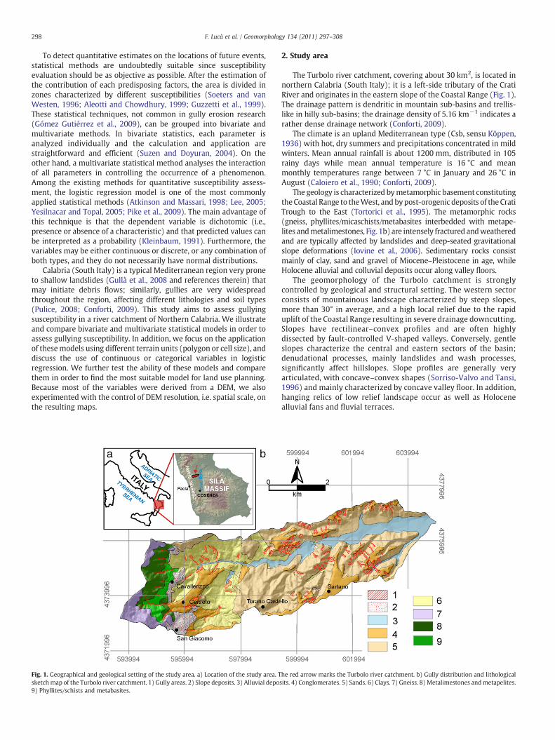
Fig. 1. Geographical and geological setting of the study area. a) Location of the study area. Tsketch map of the Turbolo river catchment. 1) Gully areas. 2) Slope deposits. 3) Alluvial depo9) Phyllites/schists and metabasites.

2. Study area

The Turbolo river catchment, covering about 30 km2, is located innorthern Calabria (South Italy); it is a left-side tributary of the CratiRiver and originates in the eastern slope of the Coastal Range (Fig. 1).The drainage pattern is dendritic in mountain sub-basins and trellis-like in hilly sub-basins; the drainage density of 5.16 km−1 indicates arather dense drainage network (Conforti, 2009).

The climate is an upland Mediterranean type (Csb, sensu Köppen,1936) with hot, dry summers and precipitations concentrated in mildwinters. Mean annual rainfall is about 1200 mm, distributed in 105rainy days while mean annual temperature is 16 °C and meanmonthly temperatures range between 7 °C in January and 26 °C inAugust (Caloiero et al., 1990; Conforti, 2009).

The geology is characterized bymetamorphic basement constitutingtheCoastal Range to theWest, andbypost-orogenic deposits of theCratiTrough to the East (Tortorici et al., 1995). The metamorphic rocks(gneiss, phyllites/micaschists/metabasites interbedded with metape-lites andmetalimestones, Fig. 1b) are intensely fractured andweatheredand are typically affected by landslides and deep-seated gravitationalslope deformations (Iovine et al., 2006). Sedimentary rocks consistmainly of clay, sand and gravel of Miocene–Pleistocene in age, whileHolocene alluvial and colluvial deposits occur along valley floors.

The geomorphology of the Turbolo catchment is stronglycontrolled by geological and structural setting. The western sectorconsists of mountainous landscape characterized by steep slopes,more than 30° in average, and a high local relief due to the rapiduplift of the Coastal Range resulting in severe drainage downcutting.Slopes have rectilinear–convex profiles and are often highlydissected by fault-controlled V-shaped valleys. Conversely, gentleslopes characterize the central and eastern sectors of the basin;denudational processes, mainly landslides and wash processes,significantly affect hillslopes. Slope profiles are generally veryarticulated, with concave–convex shapes (Sorriso-Valvo and Tansi,1996) and mainly characterized by concave valley floor. In addition,hanging relics of low relief landscape occur as well as Holocenealluvial fans and fluvial terraces.

he red arrow marks the Turbolo river catchment. b) Gully distribution and lithologicalsits. 4) Conglomerates. 5) Sands. 6) Clays. 7) Gneiss. 8) Metalimestones andmetapelites.

Fig. 2. Overview of gully landforms. a) Gully heads retreat affecting permanent gully onthe left side of the study area. b) Gully developed during the extremely rainy 2008–2009 winter in olive groves. c) “Calanco” landform on clayey slope close to the Turbolovalley floor.

299F. Lucà et al. / Geomorphology 134 (2011) 297–308

The study area is also characterized by high variability of soils,ranging from highly evolved soils (Alfisols) to poorly evolved soils(Inceptisols and Entisols, sensu USDA, 2006), with soil profiles oftencharacterized by erosive truncation. From the land use standpoint, thehalf of the study area is characterized by agricultural activities (mainlycrops and olive groves), whereas more than 20% has a shrubby andherbaceous cover often left to pasture. The remaining land coverconsists of woodland, which dominates in the western part of thebasin on the slopes dropping down from the Coastal Range.

Recently, Conforti et al. (2011) indicate mass movement and watererosion processes as the main denudational processes acting in theTurbolo catchment. Clayey, steep and weathered slopes experiencemainly landsliding, whereas sheet, rill erosion and gully incisionparticularly affect areas without vegetation cover, in cultivated fieldsand pasture lands. In the study area, many permanent, large gullies(Fig. 2a) consist of deep incisions with subvertical sidewalls and depthoften more than 8 m (Conforti, 2009). Where sands and conglomeratesoutcrop, gully channels are narrow and usually V-shaped, with almostbare side slopes indicating an active stage of dissection (Fig. 1b). Duringheavy rainfall events,manygullies alsoundergoheadcut and valley-sideretreat processes causing their lengthening and widening. Gullydevelopment increases from November to February, the rainy season,when cultivated fields are unprotected because of seeding practices(Fig. 2b). The most evident and spectacular landforms related to gullyerosion in the study area are represented by calanchi landforms, mainlydeveloped into clay deposits (Fig. 2c); they locally developed fromslopes affected by landslide scars, promoting concentration of runningwater (Morgan, 2005).

3. Data collection

Air-photo interpretation and field surveys allowed mapping theareas affected by gullies (Fig. 1b), which consist of slope units(microbasins) widely affected by gully erosion. In the study area, 101gully areas weremapped; they occupy 1.45 km2 and correspond to 5%of the whole study area.

Because of gullying is a threshold-dependent process controlled byseveral factors, the choice of a number of predisposing factors isneeded to assess gullying susceptibility (Valentin et al., 2005). Thepredisposing factors used in this work are reported in Table 1. Theyare lithology, land use and a series of topographic factors: slope,aspect, plan curvature, stream power index (SPI), topographicwetness index (TWI) and length-slope factor (LSF). The topographicfeatures were directly extracted from a detailed digital elevationmodel (DEM) using ESRI ArcView 3.2. The DEM, with a resolution of7.5×7.5 m pixel size, was created from stereo aerial photos of 2003 byusing the Z-map software.

The lithology is considered one of the main factors influencingslope processes, including gully development. By integrating thegeological map of Calabria (1:25,000 scale sheet map, Cassa delMezzogiorno; CASMEZ, 1971), air photo interpretation and fieldsurvey data, a lithological map was produced.

Land use types significantly influence soil erosion processes.Generally barren and sparsely vegetated areas experience fastererosion than forests where plant cover strongly reduces the erosiveaction of surface runoff (Dai et al., 2001; Cevik and Topal, 2003). Landuse map was derived from color orthophoto interpretation and fieldsurveys. The steepness of slopes is a factor of primary importance thatpromotes high runoff velocity, resulting in rill and gully initiation(Valentin et al., 2005). Aspect is also considered an important factor ingeomorphological instability analysis because it controls someclimatic parameters such as exposure to sunlight and winds (dry orwet), rainfall intensity and soil moisture (Carrara et al., 1991; Guzzettiet al., 1999; Nagarajan et al., 2000; Conforti, 2009).

TWI indicates the effect of topography on the location and size ofsaturated source areas of runoff generation; it is based on the

assumption of steady state conditions and uniform soil properties (i.e.transmissivity is constant throughout the catchment and equal tounity; Moore et al., 1991). It is defined as:

TWI = ln As= tanσð Þ ð1Þ

where As is the specific catchment area (m) and σ is the slope gradient(degs.).

Table 1Weight values of bivariate statistics.

B_POL B_POI

LITHOLOGYGneiss −2.365 −2.813Alluvial deposits −2.226 −2.262Slope deposits −1.100 −1.691Metalimestones and metapelites −0.122 −0.099Clays −0.020 −0.05Conglomerates 0.172 0.097Sands 0.293 0.286Phyllites/schists and metabasites 0.333 0.330

LAND USEUrban −6.848 −2.625Orchard and/or vineyard −2.057 −2.237River beds and flooding areas −3.505 −2.134Olive groves −1.082 −1.185Crops −0.854 −0.825Grass −0.250 −0.243Wood 0.298 0.219Scrub and herbaceous 0.836 0.911Barren land 1.726 1.567

SLOPE0–5 −1.767 −1.2255–10 −1.039 −0.83410–15 −0.642 −0.47115–20 −0.128 −0.01020–30 0.617 0.528N30 0.924 0.783

ASPECTFlat −0.130 −3.203N −0.282 −0.759NE −0.130 −0.616E −0.299 −0.524NW −0.168 −0.260SE −0.016 0.005S 0.320 0.623W 0.648 0.802SW 1.010 1.139

TWI10–24 −2.000 −2.2338–10 −1.153 −1.2976–8 −0.202 −0.3514–6 0.336 0.385

SPI0–1 −0.370 −0.6361–2 0.831 0.1642–3 0.998 0.6463–4 1.383 1.2914–5 1.571 1.597

LSF0–2 −1.311 −1.3902–4 −0.449 −0.4014–8 0.288 0.2908–12 0.899 0.816N12 1.133 1.040

CURVATUREPlanar −0.466 −0.545Convex −0.165 −0.052Concave 1.425 1.359

300 F. Lucà et al. / Geomorphology 134 (2011) 297–308

SPI is a measure of the erosive power of water flow based on theassumption that discharge is proportional to the specific catchmentarea (Moore et al., 1991). It is calculated as:

SPI = As tanσ : ð2Þ

The LSF factor, also used in the RUSLE equation, is a parameter thatconsiders the effect of topography on erosion (Renard et al., 1997). Itdepends on the slope steepness factor (S) and the slope length factor(L), influences surface runoff speed and is considered as a sedimenttransport capacity index. There are different approaches in literaturefor determining LSF in a grid-based DEM. One of them is based on the

upslope contributing area of each cell, which can be calculated withthe equation described by Moore and Bruch (1986):

LSF = f a×cellsize=22:13ð Þ0:4 × sinσ =0:0896ð Þ1:3 ð3Þ

where fa is flow accumulation (Lee, 2004).The plan curvature, which represents the morphology of topog-

raphy, plays also an important role in determining terrain instabilitybecause it may control the surface and subsurface hydrologicalregimes of the slope. A positive curvature is an externally convexcell, and a negative curvature is upwardly concave; zero indicates aflat surface.

4. Gullying susceptibility assessment

To detect gullying susceptibility, bivariate and logistic regressionanalyses were implemented, using the inventory of mapped gullyareas to understand and weigh the role of each factor in controllingsoil erosion. Through a statistical software package, the gully areaswere split into two groups: training and validation sets using arandom partition. The occurrence of gullies in relation to the terrainconditions was analyzed using the training set and the resultantmodel was applied to the whole study area. The validation set wasalso used to evaluate the prediction performance of the model.

The training set used should be representative of the variability ofthe whole gully areas. Considering this, we developed two bivariatemodels based on a polygon (B_POL) and a point (B_POI) sampling(Fig. 3). The first partitioning strategy selected 70% of gully areas astraining set and the remnant 30% as validation set. In the secondstrategy, gully areas were converted to points and some points in eachgully area were used for constructing the model while the others forvalidating it. There were 23,491 seed cells: among them, we used arandom population of 16,444 (70%) for calibrating the model; theremaining cells were then used as the validation set.

In order to carry out the logistic regression, the training set for theB_POI analysis was used; moreover, an equal number (16,444) ofrandom sample points were selected from the gully free areas, andmerged to the randomly selected gully data (Dillon and Goldstein,1986). Then to each point, the relative factors were associated. Todetermine if the type of variables influenced the resulting map, twologistic regression models were derived: one uses original dataincluding continuous ones (M_CON), and the other uses categorizedvariables (M_CAT). Consequently we developed four models, and theresultant maps were divided into five susceptibility classes usingnatural breaks.

To test the effect of DEM resolution on gullying susceptibilitymapping, the original 7.5 m DEM was resampled by using bilinearinterpolation and the M_CON model was applied to 10, 15 and 20 mgrid DEMs (M_10, M_15, and M_20 respectively).

4.1. Bivariate statistics

The bivariate statistical procedure used in this study is known asthe Information Value Method, outlined and considered by manyworks as the simplest and quantitatively suitable method insusceptibility mapping (Yin and Yan, 1988; Zézere, 2002; Cevik andTopal, 2003; Yalcin, 2008).

This approach is based on the observed relationships betweeneach predisposing factor and the distribution of gully areas. For eachpredisposing factor, the density of the gullies of the training set ineach class was evaluated. The weighting values for each class werecomputed through the formula of van Westen (1993):

Wi = lnDensClassDensMap

= lnNpixXi =NpixNi

∑NpixXi =∑NpixNið4Þ

Fig. 4. Gullying susceptibility maps in the Turbolo river catchment developed through:a) polygon-based bivariate statistics; b) point-based bivariate statistics; c) logisticregression with categorical variables; and d) logistic regression with continuousvariables. 1) Very low susceptibility. 2) Low susceptibility. 3) Moderate susceptibility.4) High susceptibility. 5) Very high susceptibility.

Fig. 3. Random partitioning of the training set (red color) based on a) polygons andb) points. Blue polygons were used for the validation set.

301F. Lucà et al. / Geomorphology 134 (2011) 297–308

where Wì = weighting value of the class i; DensClass = density ofthe gullies of the training set in the class i; DensMap = density ofthe gullies of the training set in the whole study area; NpixXi =number of pixels that contains the gullies of the training set in theclass i; NpixNi = number of pixels within the class i; ΣNpixXi = totalnumber of pixels that contains the gullies of the training set in thewhole study area; and ΣNpixNi = total number of pixels of the whole

study area. On the basis of these weighting values, each predisposingfactor map was reclassified and then summed up by means of overlayprocedures to yield the final scores for the susceptibility map. Thisprocedure was applied to the B_POL and B_POI training data todevelop two bivariate maps (Fig. 4a,b).

4.2. Multivariate statistics (logistic regression)

Among multivariate methods, when the variables do not satisfythe assumptions of normality, linearity, and homogeneity of variance,logistic regression is generally considered as an effective statisticalprocedure. The goal of logistic regression is to find the best fittingmodel to describe the relationship between the presence or absenceof gullies (dependent variable) and a set of independent parameters(predisposing factors). Logistic regression estimates the probability(P) of the occurrence of a certain event (Atkinson and Massari, 1998;Dai et al., 2001; Lee and Min, 2001) through the formulas:

P =1

1 + exp−zð Þ ð5Þ

z = b0 + b1x1 + b2x2 + … + bnxn ð6Þ

Table 3Ranks derived from bivariate statistic and significant b coefficients for variables inlogistic regression analyses.

Rank M_CON M_CAT M_10 M_15 M_20

LITHOLOGYGneiss 1 −3.882 −3.842 −3.880 −3.855 −3.865Alluvial deposits 2 −1.662 −1.579 −1.645 −1.593 −1.640Slope deposits 3 −1.656 −1.663 −1.592 −1.576 −1.634Metalimestones andmetapelites

4 −2.297 −2.014 −2.285 −2.140 −2.234

Clays 5 −0.279 −0.319 −0.268 −0.261 −0.264Conglomerates 6 0.154 0.397 0.151 0.148 0.156Sands 7 a a a a a

Phyllites/schists andmetabasites

8 −1.631 −1.491 −1.600 −1.502 −1.551

LAND USEUrban 1 −2.043 −2.280 −2.060 −2.000 −2.070Orchard and/orvineyard

2 −2.329 −2.374 −2.346 −2.329 −2.384

River beds and floodingareas

3 −0.996 −1.307 −1.016 −1.093 −1.042

Olive groves 4 −1.402 −1.593 −1.444 −1.383 −1.422Crops 5 −0.519 −0.714 −0.572 −0.510 −0.569Grass 6 0.228 −0.479 −0.252 −0.215 −0.242Wood 7 a a a a a

Scrub and herbaceous 8 0.709 0.516 0.665 0.744 0.684Barren land 9 2.461 2.220 3.200 3.229 3.189

SLOPE 0.018 0.019 0.020 0.0190–5 1 −0.3205–10 2 −0.67910–15 3 −0.80615–20 4 −0.40020–30 5 a

N30 6 0.076ASPECT 0 0 0 0

Flat 1 −0.672N 2 −0.833NE 3 −0.072E 4 −0.163NW 5 −0.721SE 6 a

S 7 0.421W 8 0.622SW 9 0.892

TWI 0.035 0.034 0.018 0.03010–24 1 0.4678–10 2 0.7246–8 3 0.5714–6 4 a

SPI −0.111 −0.118 −0.114 −0.1140–1 1 −0.1741–2 2 a

2–3 3 0.0553–4 4 0.9324–5 5 0.935

LSF 0.185 0.180 0.180 0.1780–2 1 −0.8652–4 2 −0.3574–8 3 a

8–12 4 0.594N12 5 1.305

CURVATURE −0.361 −0.349 −0.308 −0.316Planar 1 −1.041Convex 2 −0.773Concave 3 a

INTERCEPT −1.078 1.332 −1.096 −0.876 −1.030

a Not computed.

302 F. Lucà et al. / Geomorphology 134 (2011) 297–308

where z represents a combination of the variables, b0 is the interceptof the model, n is the number of independent variables, bi (i=1, 2,…n) is the coefficient of the model and xi (i=1, 2,…n) is theindependent variable.

The algorithm of logistic regression, through the maximumlikelihood iterative procedure, assigns coefficients to the independentvariables; subsequently, z is transformed by means of Eq. (5) into alogit variable (the natural log of the odds of presence or absence).Coefficients are expressed in log units; if a coefficient is positive, itstransformed log value will be greater than one, meaning that themodeled event is more likely to occur. If a coefficient is negative, theodds of the event occurrence decrease; a coefficient of zero (0) has atransformed log value of 1, meaning that this coefficient does notchange the odds of the event one way or the other. Although a goodstatistical background is required to understand this analysis, theapplication is quite simple. The advantage of the logistic regressionover simple multiple regression is that the variables may be eithercontinuous or categorical, or any combination of both types (Lee,2005) and that predicted values can be interpreted as probabilitybecause they are constrained to fall into an intervlal between 0 and 1(Kleinbaum, 1991).

We developed two stepwise logistic regression models. In ordernot to alter the state and information in the parameters, we first usedM_CON; the nominal variables lithology and land use were rankedbased on the gully density of the training set computed by bivariatestatistical analyses. A low rank value was assigned to the first class ofeach parameter.

Afterwards, all continuous parameters were converted to M_CATand corresponding rank was assigned to each class based on gullydensity, as previously done for lithology and land use. The two logisticregression models were applied to the same data set.

4.3. Map validation and comparison

In order to detect the prediction rate performance of the models,we validated the four gullying susceptibility maps based on the 7.5-mDEM using the gullies in the validation data set, creating the ratecurves for each map. Validation curves represent the cumulativepercentage of gullies in the validation set (y axis) with respect to thepercentage of area classified as unstable (x axis) for increasing valuesof the selected susceptibility index. The area under the ROC curve(AUC) characterizes the quality of the model in predicting theoccurrence or non-occurrence of a gully; the most ideal modelshows a curve that has the largest AUC. For a better comparison ofmodels, weweighted the areas of susceptibility classes with respect tothe corresponding densities of gullies in the validation set, using theso-called “modified Seed Cell Area Index” (mSCAI):

mSCAI = Areal extent of susceptibility classes %ð Þ=Gully of the validation set in each susceptibility class %ð Þ

ð7Þ

revising the SCAI index introduced by Suzen and Doyuran (2004).According to mSCAI, the best model should be able to detect gullyingwithout classifying large areas of the map as unstable, in order toreflect the typically low density of the event; moreover, it should havethe highest percentage of gullies in areas classified as highly and veryhighly susceptible.

Table 2Percentage of susceptibility classes from the four models.

Very low Low Moderate High Very high

Model B_POL 8.82 14.57 22.32 27.61 26.68B_POI 6.66 19.21 27.62 27.81 18.70M_CON 30.11 26.36 18.07 14.72 10.74M_CAT 33.60 23.70 17.60 13.64 11.47

5. Results and discussion

5.1. Role of predisposing factors in gullying

The results of the bivariate analysis are reported in Table 1;negative weighting values indicate a low influence of the classes ofeach predisposing factors in gully development while positive valuesimply a strong control on gully occurrence (Zézere, 2002). The Wivalues of the B_POL and B_POI models show a very similar trend. For

Table 4Final classification based on logistic regression models. Value of 1 refers to gullyoccurrence, and value of 0 to non-occurrence cells.

Predicted

Gully Percentagecorrect

0 1

M_CAT Step 1 Observed Gully 0 18,205 5286 77.5%1 5051 18,440 78.5%

Overall percentage 78.0%M_CON Step 1 Observed Gully 0 17,735 5756 75.5%

1 5754 17,737 75.5%Overall percentage 75.5%

Fig. 5. Sketches of gullying susceptibility maps with spatial resolutions of a) 7.5, b) 10, c) 15where sands and conglomerates outcrop. 1) Very low susceptibility. 2) Low susceptibility.

303F. Lucà et al. / Geomorphology 134 (2011) 297–308

instance, areas with “Sands”, “Conglomerates” and “Phyllites/schistsand metabasites” are susceptible to gully development, while thecontrary occurs where “Gneiss” and “Alluvial deposits” crop out. TheB_POL andB_POImodels also indicate a strong slope control on the gullydistribution. These weights were then added up to create the finalsusceptibilitymaps (Fig. 4a,b); they classify nearly 50% of the area in thehigh and very high susceptibility classes (Table 2).

Regarding logistic regression, the presence of a relationshipbetween the dependent variable and the combination of predisposingfactors is based on the statistical significance of the model chi-squareat step 1, after the independent variables have been added to theanalysis. In this analysis, the probability of the model chi-square(99.120 for M_CON and 131.021 for M_CAT) was b0.001, less than orequal to the level of significance of 0.05, supporting the existence of arelationship between the independent and dependent variables. Noneof the independent variables in this analysis had a standard error

, and d) 20 m. e) Location of the maps in the middle part of the Turbolo river catchment3) Moderate susceptibility. 4) High susceptibility. 5) Very high susceptibility.

Fig. 6. Percentages of susceptibility classes for different cell-size DEMs. 1) Very lowsusceptibility. 2) Low susceptibility. 3) Moderate susceptibility. 4) High susceptibility.5) Very high susceptibility.

304 F. Lucà et al. / Geomorphology 134 (2011) 297–308

larger than 2, avoiding problems related to multi-collinearity amongthe independent variables.

The results of the two logistic regression analyses are listed inTable 3; as reported, they show the coefficients calibrated for theindependent variables that significantly (i.e. Pb0.05) influence thelocation of gullies. On the basis of these coefficients, concrete forms ofEq. (6) were derived:

M CONz = LITHOLOGYb + LANDUSEb + 0:018SLOPE

+ 0:035TWI−0:111SPI + 0:185LSF−0:361CURVATURE−1:078ð8Þ

M CATz = LITHOLOGYb + LAND USEb + SLOPEb + ASPECTb + TWIb

+ SPIb + LSFb + CURVATUREb + 1:332ð9Þ

where the subscript b indicates the coefficients listed in Table 3.The success of the two models can be assessed on the correct and

incorrect classification results as shown in Table 4. TransformingEqs. (8) and (9) into their logit value through Eq. (5), we created twogullying susceptibility maps (Fig. 4c,d).

Table 3 also shows the coefficients of the logistic regressionanalyses based on continuous variables and on the DEMs withresolutions of 10, 15 and 20 m. Although the role of each predisposingfactor is quite similar in all models, the resulting maps are quitedifferent (Fig. 5); by increasing DEM cell size, the extent of low andvery low susceptibility classes increases from 56.5% to 97.5% (Fig. 6).

Despite the regression coefficients of the logistic models arenumerically different from the weights of the bivariate models, thesign of the values (coefficients or weights) indicates whether thevariable is positively or negatively correlated to gullying. Most of the

Table 5Percentage of susceptibility classes from the four models based on the validation set.

Very low Low Moderate High Very high

Model B_POL 0.03 1.26 4.36 16.58 77.77B_POI 0.08 3.31 9.75 26.38 60.48M_CON 1.98 8.98 14.53 24.39 50.11M_CAT 2.45 7.17 12.62 24.46 53.30

variables with large absolute coefficient values are common to all themodels, indicating the validity of the developed methodologies(Table 5).

The strong negative coefficients of “Gneiss”, “Alluvial deposits” and“Slope deposits” indicate that the areas where these lithologies cropout are more stable. The areas close to “River beds and flooding areas”,“Urban” and “Orchard and/or vineyard” are also less susceptible togullying. On the other hand, large positive coefficients for “BarrenLand” suggest it facilitates gullying. Many authors highlighted thepredisposition of abandoned lands to gullying because of a slowvegetation recovery, soil crusting, quick concentration of runoff,reduced surface storage capacity and absence of appropriate man-agement strategies (Lasanta et al., 2000; Valentin et al., 2005;Lesschen et al., 2007; Kakembo et al., 2009). Actually, even thoughthese processes enhance gully development, we think that thiscorrelation could be partly overestimated because statistical methodsare data-driven and gully detection in non-vegetated land is easier,both from aerial photographs and in the field.

Gullies could occur in almost every slope aspect according tomultivariate statistics, while bivariate analysis suggests that slopesfacing southwest seem to be more susceptible to their development.With respect to the slope curvature, concave zones (hollows andvalley heads) appear to characterize slopes more prone to gullydevelopment. Under this condition, in fact, the concentration of flowdownslope and the possible saturation of soil due to surface and sub-surface water enhance erosion. In bivariate models, the steeper theslope, the higher SPI and LSF, and the higher the probability ofgullying. This effect is greater in B_POL than in B_POI.

Despite some similarities, significant differences between the distri-butions of the susceptibility classes are shown in Fig. 4, especially inhighly sloping areas. Since slope is part of the SPI and LSFparameters, thehigher gradient, the greater the values of these indices for the samecatchment area. Therefore, the bivariatemodels overestimate the role ofslope in gully development. In fact, in the study area, gullies not onlyoccur on very steep slopes but also onhillslopeswithmoderate gradient(Fig. 2b).

5.2. Validating and comparing the models

Although the ROC curves of all these models are closely located toeach other (Fig. 7), the enlargement of the lowermost part of the plot(corresponding to very high and high susceptibility classes) shows agreater gradient of the multivariate models than the bivariate models(Fig. 7b), and thus a greater predictive capability. The four maps haveAUC values between 0.78 and 0.86 (Fig. 7c), with M_CON yielding thebest results for distinguishing between gullied and gully-free cells(Swets, 1988). The degree ofmodel fit is not necessarily a goodmeasureof the model forecasting skill (Chung and Fabbri, 2003; Fabbri et al.,2003; Guzzetti et al., 2006); it does not supply the geographical locationand areal extent of susceptibility classes either. Models with similarperformancemay result in differentmaps; in fact, considerable portionsof the maps in Fig. 4 are differently classified.

The obtained mSCAI values (Fig. 8) indicate that the susceptibilitymaps developed through logistic regression are more accurate thanthe bivariate ones; they correctly locate around 70% of gullies in zoneswith very high and high susceptibility, even though their cumulativeareal extent is only about 25% of the maps. Among the bivariate maps,B_POI is better than B_POL because it delineated as prone to gullying asmaller area. Even though B_POL has a higher AUC value, the mSCAIvalue suggests that B_POI more correctly classify gullies into the mostsusceptible classes.

To compare the susceptibility models based on the location of maindifferences, two of the obtained maps were overlaid. When the twomaps classified a pixel to the same susceptibility class, the spatialagreement was considered “correct”. When the classification of a pixelin the twomaps differed by only one susceptibility class, the agreement

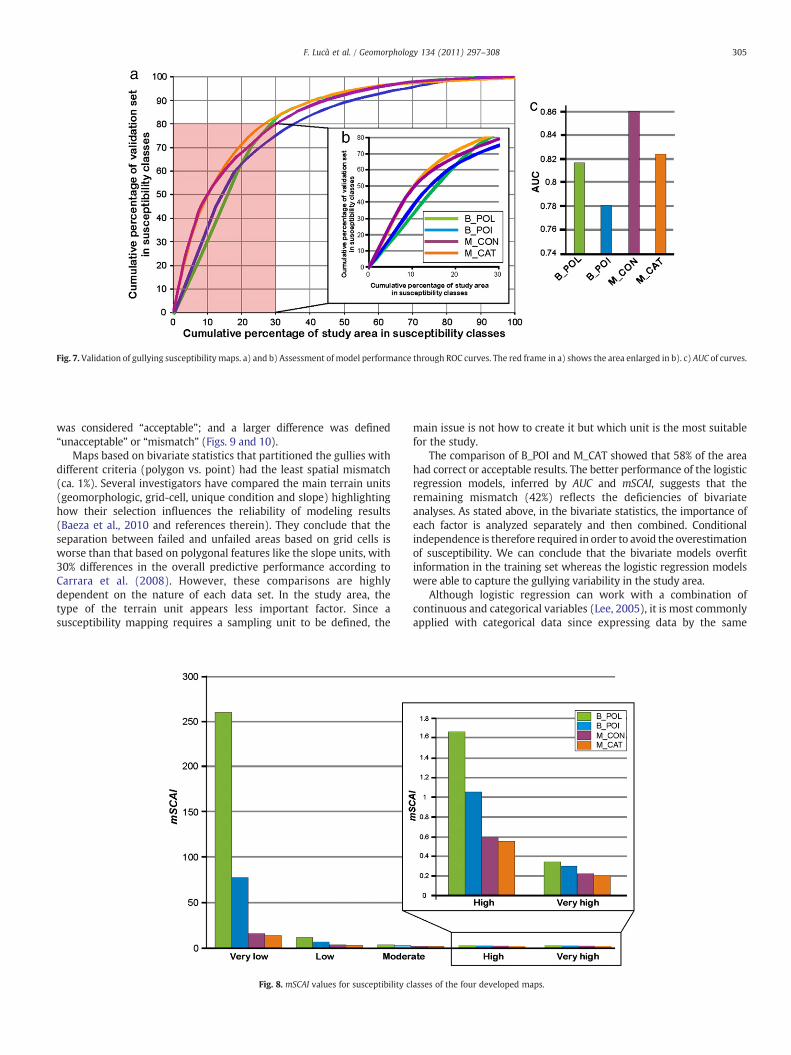
Fig. 7. Validation of gullying susceptibility maps. a) and b) Assessment of model performance through ROC curves. The red frame in a) shows the area enlarged in b). c) AUC of curves.

305F. Lucà et al. / Geomorphology 134 (2011) 297–308

was considered “acceptable”; and a larger difference was defined“unacceptable” or “mismatch” (Figs. 9 and 10).

Maps based on bivariate statistics that partitioned the gullies withdifferent criteria (polygon vs. point) had the least spatial mismatch(ca. 1%). Several investigators have compared the main terrain units(geomorphologic, grid-cell, unique condition and slope) highlightinghow their selection influences the reliability of modeling results(Baeza et al., 2010 and references therein). They conclude that theseparation between failed and unfailed areas based on grid cells isworse than that based on polygonal features like the slope units, with30% differences in the overall predictive performance according toCarrara et al. (2008). However, these comparisons are highlydependent on the nature of each data set. In the study area, thetype of the terrain unit appears less important factor. Since asusceptibility mapping requires a sampling unit to be defined, the

Fig. 8. mSCAI values for susceptibility c

main issue is not how to create it but which unit is the most suitablefor the study.

The comparison of B_POI and M_CAT showed that 58% of the areahad correct or acceptable results. The better performance of the logisticregression models, inferred by AUC and mSCAI, suggests that theremaining mismatch (42%) reflects the deficiencies of bivariateanalyses. As stated above, in the bivariate statistics, the importance ofeach factor is analyzed separately and then combined. Conditionalindependence is therefore required in order to avoid the overestimationof susceptibility. We can conclude that the bivariate models overfitinformation in the training set whereas the logistic regression modelswere able to capture the gullying variability in the study area.

Although logistic regression can work with a combination ofcontinuous and categorical variables (Lee, 2005), it is most commonlyapplied with categorical data since expressing data by the same

lasses of the four developed maps.

Fig. 9. Degree of spatial agreement between the four susceptibility maps.

Fig. 10. Locations of the correctly classified, acceptable, and unacceptable pixels for a)polygon-based bivariate and point-based bivariate maps; b) logistic regression mapswith continuous and categorical variables; and c) point-based bivariate and logisticregression maps with categorical variables. 1) Correct. 2) Acceptable. 3) Unacceptable.

306 F. Lucà et al. / Geomorphology 134 (2011) 297–308

measuring scales could lead to a better model performance (Ayalewand Yamagishi, 2005; Greco et al., 2007). Even though the approachesused to transform continuous variables are different (Guzzetti et al.,1999; Dai et al., 2001; Lee and Min, 2001; Suzen and Doyuran, 2004;Ayalew and Yamagishi, 2005; Greco et al., 2007), they usually do notanalyze the effect of discretization on the quality of a susceptibilitymap.

In the study area, the spatial agreement between M_CAT andM_CON revealed that the two maps differ only in 3% of the total areawith evenly distributed differences over the catchment. The ROCcurves and AUC indicate that the predictive capability of M_CAT islower than that of M_CON; at the same time, mSCAI suggests thatM_CON is able to allocate minimum areas for high susceptibilityzones, while covering most of the mapped gully areas. For thesereasons, we can conclude that the best model to predict gullying in theTurbolo river catchment is the logistic regression based on continuousvariables. The conversion of variables into categorical ones couldcreate some problems.

Some considerations on the effect of the DEM resolution on thegullying susceptibility map can also be made. Previous studies usedDEMs with cell sizes from 20 m to 1 km to extract topographicvariables related to gullying (Bou Kheir et al., 2007; Lesschen et al.,2007; Conoscenti et al., 2008; Kakembo et al., 2009; Ndomba et al.,2009). In the study area, even though the coefficients of the logisticregression models were quite similar for different DEM resolutions,the size of DEM cells clearly affected the extent of each susceptibilityclass: the larger the spatial resolution, the smaller the extent of themost susceptible classes and the accuracy of the map. The optimalDEM cell size DEM may be related to the mean size of gullied areas.

6. Conclusions

In this paper, four statistical models for gullying susceptibilityassessment were developed and compared in the 30 km² Turboloriver catchment (northern Calabria, South Italy) based on a 7.5-mDEM. The produced maps differed in the types of model (bivariate vs.multivariate), data sampling (polygon or point based) and variables(continuous or categorical). GIS-based map overlay, ROC curves andmSCAI allowed us to compare the constructed models. Each one hadadvantages and limitations in terms of complexity of modeldevelopment, performance of the ROC curves, percentage of gullies

falling in the most susceptible areas, and extent of susceptibilityclasses. The influence of DEM resolution on the susceptibility mapswere also discussed.

The results from the two bivariate statistical models with differentsampling methods (polygon vs. point) differed only by 1%. AlthoughAUC of the polygon-based bivariate model was higher, mSCAIsuggested that point-based models better places gullies in the mostsusceptible classes. The multivariate susceptibility maps from differ-ent types of variables (continuous vs. categorical) differ only by 3.6%.Instead, spatial mismatch larger than 40% occurred between themodels based on the bivariate and multivariate approaches, mostly atsteep slopes. The twomultivariate models had higher AUC values thanbivariate ones and better discriminated the gully areas with very highand high susceptibility classes.

For these reasons we can affirm that the best method for mappinggullying susceptibility is logistic regression. In particular, AUC=0.86testifies a better performance of multivariate analysis based oncontinuous variables. The main limit of the bivariate models is theassumption that the predisposing factors are independent and theresultant too much weight to slope.

The size of grid cells affects the accuracy of gullying susceptibilitymaps which are dependent on both DEM accuracy and the scale ofgullied areas. Because susceptibility maps may be used by managersfor land use planning, the effect of different statistical techniques,mapping units and spatial scale on the maps should be considered inorder to find the most suitable approach for a study area.

Acknowledgments

We are grateful to T. Oguchi and to two anonymous reviewers fortheir useful suggestions and comments.

We also thank W. Spataro for the improvement of English.

307F. Lucà et al. / Geomorphology 134 (2011) 297–308

References

Aleotti, P., Chowdhury, R., 1999. Landslide hazard assessment: summary review andnew perspectives. Bulletin of Engineering Geology and the Environment 58,21–44.

Atkinson, P.M., Massari, R., 1998. Generalised linear modelling of susceptibility tolandsliding in the Central Apennines. Computers and Geosciences 24, 373–385.

Ayalew, L., Yamagishi, H., 2005. The application of GIS-based logistic regression forlandslidesusceptibility mapping in the Kakuda-Yahiko Mountains, Central Japan.Geomorphology 65, 15–31.

Baeza, C., Lantada, N., Mova, J., 2010. Influence of sample and terrain unit on landslidesusceptibility assessment at La Pobla de Lillet, Eastern Pyrenees, Spain. Environ-mental Earth Sciences 60, 155–167.

Bathurst, J.C., 2002. Physically-based erosion and sediment yield modelling: theSHETRAN concept. In: Summer, W., Walling, D.E. (Eds.), Modelling Erosion,Sediment Transport and Sediment Yield: IHP-VI Technical Documents inHydrology, 60, pp. 47–68.

Bou Kheir, R.B., Wilson, J., Deng, Y., 2007. Use of terrain variables for mapping gullyerosion susceptibility in Lebanon. Earth Surface Processes and Landforms 32,1770–1782.

Bovis, M.J., Jakob, M., 1999. The role of debris supply conditions in predicting debrisflow activity. Earth Surface Processes and Landforms 24, 1039–1054.

Brabb, E.E., 1984. Innovative approaches to landslide hazard and risk mapping.Proc. 4th Int. Symp. on Landslides, 1. Canadian Geotechnical Society, Toronto,pp. 307–324.

Brayshaw, D., Hassan, M.A., 2009. Debris flow initiation and sediment recharge ingullies. Geomorphology 109, 122–131.

Bufalo, M., Nahon, D., 1992. Erosional processes of Mediterranean badlands: a newerosivity index for predicting sediment yield from gully erosion. Geoderma 52,133–147.

Caloiero, D., Niccoli, R., Reali, C., 1990. Le precipitazioni in Calabria (1921–1980).Geodata 36, Consiglio Nazionale delle Ricerche-Istituto di Ricerca per la ProtezioneIdrogeologica, Cosenza, p. 53.

Carrara, A., Cardinali, M., Detti, R., Guzzetti, F., Pasqui, V., Reichenbach, P., 1991. GIStechniques and statistical models in evaluating landslide hazard. Earth SurfaceProcesses and Landforms 16, 427–445.

Carrara, A., Crosta, G., Frattini, P., 2008. Comparing models of debris-flow susceptibilityin the alpine environment. Geomorphology 94, 353–378.

CASMEZ, 1971. Carta Geologica della Calabria. Volume II, Fogli 237, 238. Legge specialeper la Calabria 26, 11, 1955, n. 1177.

Cevik, E., Topal, T., 2003. GIS-based landslide susceptibility mapping for a problematicsegment of the natural gas pipeline, Hendek (Turkey). Environmental Geology 44,949–962.

Chung, C.J.F., Fabbri, A.G., 2003. Validation of spatial prediction models for landslidehazard mapping. Natural Hazards 30, 451–472.

Conforti, M., 2009. Studio geomorfopedologico dei processi erosivi nel bacino del T.Turbolo (Calabria settentrionale) con il contributo della spettrometria dellariflettenza. PhD Thesis, Università della Calabria, pp. 310.

Conforti, M., Aucelli, P.P.C., Robustelli, G., Scarciglia, F., 2011. Geomorphology and GISanalysis for mapping gully erosion susceptibility in the Turbolo Stream catchment(Northern Calabria, Italy). Natural Hazards 56, 881–898.

Conoscenti, C., Di Maggio, C., Rotigliano, E., 2008. Soil erosion susceptibility assessmentand validation using a geostatistical multivariate approach: a test in SouthernSicily. Natural Hazards 46, 287–305.

Crosta, G.B., Dal Negro, P., Frattini, P., 2003. Soil slips and debris flows on terracedslopes. Natural Hazards and Earth System Sciences 3, 31–42.

Dai, F.C., Lee, C.F., Xu, Z.W., 2001. Assessment of landslide susceptibility on the naturalterrain of Lantau Island, Hong Kong. Environmental Geology 40, 381–391.

DeRose, R.C., Gomez, B., Marden, M., Trustrum, N.A., 1998. Gully erosion in Mangatuforest, New Zealand, estimated from digital elevation models. Earth SurfaceProcesses and Landforms 23, 1045–1053.

Dietrich, W.E., Montgomery, D.R., 1998. SHALSTAB: a digital terrain model for mappingshallow landslide potential. National Council of the Paper Industry for Air andStream Improvement: Technical Report, 29.

Dillon, W.R., Goldstein, M., 1986. Multivariate analysis. In: John Wiley and Sons (Ed.),Methods and applications, p. 565.

Erskine, W., 2005. Gully erosion. In: Lehr, J., Keeley, J. (Eds.), Water Encyclopaedia:Surface and Agricultural Water. Wiley-Interscience, Hoboken, pp. 183–188.

Fabbri, A.G., Chung, C.J.F., Cendrero, C., Remondo, J., 2003. Is prediction of futurelandslides possible with a GIS? Natural Hazards 30, 487–503.

Fernández, S., Marquínez, J., Menéndez-Duarte, R., 2008. A sapping erosion suscepti-bility model for the southern Cantabrian Range, North Spain. Geomorphology 95,145–157.

Flanagan, D.C., Nearing, M., 1995. USDA-water erosion prediction project hillslopeprofile and watershed model documentation. National Soil Erosion ResearchLaboratory, West Lafayette, Indiana Report No. 10.

Gabet, E.J., Mudd, S.M., 2006. The mobilization of debris flows from shallow landslides.Geomorphology 74, 207–218.

Glade, T., 2005. Linking debris-flow hazard assessments with geomorphology.Geomorphology 66, 189–213.

Gómez Gutiérrez, Á., Schnabel, S., Contador, F.J.L., 2009. Using and comparing twononparametric methods (CART and MARS) to model the potential distribution ofgullies. Ecological Modelling 220, 3630–3637.

Greco, R., Sorriso-Valvo, M., Catalano, E., 2007. Logistic Regression analysis in theevaluation of mass movements susceptibility: The Aspromonte case study,Calabria, Italy. Engineering Geology 89, 47–66.

Guimarães, R.F., Fernandes, N.F., Gomes, R.A.T., Greenberg, H.M., Montgomery, D.R.,Carvalho Jr., O.A., 2003. Parameterization of soil parameters for a model of thetopographic controls on shallow landsliding. Engineering Geology 69, 99–108.

Gullà, G., Antronico, L., Iaquinta, P., Terranova, O., 2008. Susceptibility andtriggering scenarios at a regional scale for shallow landslides. Geomorphology99, 39–58.

Guzzetti, F., Carrara, A., Cardinali, M., Reichenbach, P., 1999. Landslide hazardevaluation: a review of current techniques and their application in a multi-scalestudy, Central Italy. Geomorphology 31, 181–216.

Guzzetti, F., Reichenbach, P., Ardizzone, F., Cardinali, M., Galli, M., 2006. Estimating thequality of landslide susceptibility models. Geomorphology 81, 166–184.

Imaizumi, F., Sidle, R.C., Kamei, R., 2007. Effects of forest harvesting on the occurrence oflandslides and debris flows in steep terrain of central Japan. Earth Surface Processesand Landforms 33, 827–840.

Iovine, G., Petrucci, O., Rizzo, V., Tansi, C., 2006. The March 7th 2005 Cavallerizzo(Cerzeto) landslide in Calabria—Southern Italy. Engineering geology for tomor-row's cities—the 10th IAEG Congress, Nottingham (UK), The Geological Society ofLondon, Paper number 785.

Jakob, M., Bovis, M.J., Oden, M., 2005. The significance of channel recharge rates forestimating debris-flow magnitude and frequency. Earth Surface Processes andLandforms 30, 755–766.

Kakembo, V., Xanga, W.W., Rowntree, K., 2009. Topographic thresholds in gullydevelopment on the hillslopes of communal areas in Ngqushwa Local Municipality,Eastern Cape, South Africa. Geomorphology 110, 188–194.

Kleinbaum, D.G., 1991. Logistic Regression: A Self-learning Text. Springer, BerlinHeidelberg New York.

Knisel, W.G., 1980. CREAMS: A Field-scale Model for Chemicals Runoff and Erosion fromAgricultural Management Systems. U.S. Department of Agriculture.

Knisel, W.G., 1993. GLEAMS: Groundwater Loading Effects of Agricultural ManagementSystems, University of Georgia Coastal Plains Experiment Station. Biological andAgricultural Engineering Department Publication.

Köppen, W., 1936. Das geographische System der Klimate. In: Köppen, W., Geiger, R.(Eds.), Handbuch der Klimatologie. Band 5, Teil C. Gebrüder Bornträger, Berlin,pp. 1–46.

Krishna Bahadur, K.C., 2009. Mapping soil erosion susceptibility using remote sensingand GIS: a case of the Upper Nam Wa Watershed, Nan Province, Thailand.Environmental Geology 57, 695–705.

Lasanta, T., García-Ruiz, J.M., Perez-Rontome, C., Sancho-Marcen, C., 2000. Runoff andsediment yield in a semi-arid environment: the effect of land management afterfarmland abandonment. Catena 38, 265–278.

Lee, S., 2004. Soil erosion assessment and its verification using the Universal Soil LossEquation and geographic information system: a case study at Boun, Korea.Environmental Geology 45, 457–465.

Lee, S., 2005. Application and cross-validation of spatial logistic multiple regression forlandslide susceptibility analysis. Geosciences 9 (1), 63–71.

Lee, S., Min, K., 2001. Statistical analysis of landslide susceptibility at Yongin, Korea.Environmental Geology 40, 1095–1113.

Lesschen, J.P., Kok, K., Verburg, P.H., Cammeraat, L.H., 2007. Identification of vulnerableareas for gully erosion under different scenarios of land abandonment in SoutheastSpain. Catena 71, 110–121.

May, C.L., 2002. Debris flows through different forest age classes in the centralOregon Coast Range. Journal of the American Water Resources Association 38,1097–1113.

Merkel, W.H., Woodward, D.E., Clarke, C.D., 1988. Ephemeral gully erosion model(EGEM). Modelling Agricultural, Forest, and Rangeland Hydrology. AmericanSociety of Agricultural Engineers Publication 7, 315–323.

Meyers, J.A., Martínez-Casasnovas, J.A., 1999. Prediction of existing gully erosion invineyard parcels of the NE Spain: a logistic modelling approach. Soil and TillageResearch 50, 319–331.

Montgomery, D.R., Dietrich, W.E., 1994. A physically based model for the topographiccontrol on shallow landsliding. Water Resources Research 30, 1153–1171.

Moore, I.D., Bruch, G.J., 1986. Physical basis of the length-slope factor in the universalsoil loss equation. Soil Science Society of America Journal 50, 1294–1298.

Moore, I.D., Grayson, R.B., Ladson, A.R., 1991. Digital terrain modelling: a reviewof hydrological, geomorphological, and biological applications. HydrologicalProcesses 5, 3–30.

Morgan, R.P.C., 2005. Soil Erosion and Conservation, 3rd ed. Blackwell Publishing,Oxford, UK, p. 303.

Nagarajan, R., Roy, A., Vinod Kumar, R., Mukherjee, A., Khire, M.V., 2000. Landslidehazard susceptibility mapping based on terrain and climatic factors for tropicalmonsoon regions. Bulletin of Engineering Geology and the Environment 58,275–287.

Ndomba, P.M., Mtalo, F., Killingtveit, A., 2009. Estimating gully erosion contribution tolarge catchment sediment yield rate in Tanzania. Physics and Chemistry of theEarth 34, 741–748.

Pike, A.C., Mueller, T.G., Schörgendorfer, A., Shearer, S.A., Karathanasis, A.D., 2009.Erosion index derived from terrain attributes using logistic regression and neuralnetworks. Agronomy Journal 101, 1068–1079.

Poesen, J., Vandaele, K., van Wesemael, B., 1998. Gully erosion: importance and modelimplications. In: Boardman, J., Favis-Mortlock, D. (Eds.), Modelling Soil Erosion byWater. Springer, Berlin, pp. 285–311.

Prosser, I., Winchester, S., 1996. History and processes of gully initiation anddevelopment in eastern Australia. Zeitschrift für Geomorphologie N.F. SupplementBand 105, 91–109.

Pulice, I., 2008. Studio geomorfologico, geochimico e mineralogico delle formecalanchive in Calabria. PhD Thesis, Università della Calabria, pp. 164.

308 F. Lucà et al. / Geomorphology 134 (2011) 297–308

Renard, K.G., Foster, G.R., Weesies, G.A., Mccool, D.K., Yoder, D.C., 1997. Predicting SoilErosion by Water: A Guide to Conservation Planning with the Revised Soil LossEquation (RUSLE). U.S. Dept. of Agriculture. Agric. Handbook, 703, p. 404.

Sidorchuk, A., 1999. Dynamic and static models of gully erosion. Catena 37, 401–414.Soeters, R., van Westen, C.J., 1996. Slope stability recognition analysis and zonation. In:

Turner, A.K., Schuster, R.L. (Eds.), Landslides: Investigation and Mitigation.Transportation Research Board Special Report, 247. National Academy Press,Washington D.C., pp. 129–177.

Sorriso-Valvo, M., Tansi, C., 1996. Relazioni tra frane, forme del rilievo e strutturetettoniche nella media Valle del Fiume Crati (Calabria). Geografia Fisica e DinamicaQuaternaria 19, 107–117.

Starr, B.J., 1989. Anecdotal and relic evidence of the history of gully erosion andsediment movement in the Michelago Creek catchment area, NSW. AustralianJournal of Soil and Water Conservation 2 (3), 26–31.

Suzen, L.M., Doyuran, V., 2004. A comparison of the GIS based landslide susceptibilityassessment methods: multivariate versus bivariate. Environmental Geology 45,665–679.

Swets, J.A., 1988. Measuring the accuracy of diagnostic systems. Science 240,1285–1293.

Tortorici, L., Monaco, C., Tansi, C., Cocina, O., 1995. Recent and active tectonics in theCalabrian Arc (south Italy). Tectonophysics 243, 37–55.

USDA, 2006. Keys to Soil Taxonomy. USDA (United States Department of Agriculture),Soil Survey Staff, 10th ed. Natural Resources Conservation Service, Washington D.C.333 pp.

Valentin, C., Poesen, J., Li, Y., 2005. Gully erosion: impacts, factors and control. Catena63, 132–153.

van Westen, C.J., 1993. Application of geographic information systems to landslidehazard zonation. ITC publ. no. 15, Int. Ins. for Aerospace and Earth Res. Surv.,Enschede, The Netherlands, p. 245.

vanWesten, C.J., van Asch, T.W.J., Soeters, R., 2006. Landslide hazard and risk zonation—whyis it still so difficult? Bulletin of Engineering Geology and the Environment 65, 167–184.

Vandekerckhove, L., Poesen, J., Oostwoudwijdenes, D.J., Gyssels, G., Beuselinck, L., DeLuna, E., 2000. Characteristics and controlling factors of bank gullies in two semiarid Mediterranean environments. Geomorphology 33, 37–58.

VanDine, D.F., Bovis, M.J., 2002. History and goals of Canadian debris flow research, areview. Natural Hazards 26, 69–82.

Vanwalleghem, T., Poesen, J., Nachtergaele, J., Verstraeten, G., 2005. Characteristics,controlling factors and importance of deep gullies under cropland on loess.derivedsoils. Geomorphology 69, 76–91.

Whitford, J.A., Newham, L.T.H., Vigiak, O., Melland, A.R., Roberts, A.M., 2010. Rapidassessment of gully sidewall erosion rates in data-poor catchments: a case study inAustralia. Geomorphology 118, 330–338.

Wilcock, P.R., Schmidt, J.C.,Wolman, M.G., Dietrich,W.E., DeWitt, D., Doyle, M.W., Grant, G.E.,Iverson, R.M., Montgomery, D.R., Pierson, T.C., Schilling, S.P., Wilson, R.C., 2003. Whenmodels meet managers: examples from geomorphology. In: Wilcock, P.R., Iverson, R.M.(Eds.), Prediction in Geomorphology. AGU, Washington, pp. 27–40.

Yalcin, A., 2008. GIS-based landslide susceptibility mapping using analytical hierarchyprocess and bivariate statistics in Ardesen (Turkey): comparisons of results andconfirmations. Catena 72, 1–12.

Yesilnacar, E., Topal, T., 2005. Landslide susceptibility mapping: a comparison of logisticregression and neural networks methods in a medium scale study, Hendek region(Turkey). Engineering Geology 79, 251–266.

Yin, K.L., Yan, T.Z., 1988. Statistical prediction model for slope instability ofmetamorphosed rocks. In: Bonnard, C. (Ed.), Proc. 5th Int. Symp. on Landslides 2,Lausanne, pp. 1269–1272.

Zézere, J.L., 2002. Landslide susceptibility assessment considering landslide typology.A case study in the area north of Lisbon (Portugal). Natural Hazards and Earth SystemSciences 2, 73–82.