A Comparative Assessment Between Three MachineLearning Models and Their Performance Comparisonby Bivariate and Multivariate Statistical Methodsin Groundwater Potential Mapping

Seyed Amir Naghibi1 & Hamid Reza Pourghasemi2

Received: 31 October 2014 /Accepted: 4 August 2015# Springer Science+Business Media Dordrecht 2015

Abstract As demand for fresh groundwater in the worldwide is increasing, delineation ofgroundwater spring potential zones become an increasingly important tool for implementing asuccessful groundwater determination, protection, and management programs. Therefore, theobjective of current study is to evaluate the capability of three machine learning models suchas boosted regression tree (BRT), classification and regression tree (CART), and random forest(RF), and comparison of their performance by bivariate (evidential belief function (EBF)), andmultivariate (general linear model (GLM)) statistical methods in the groundwater potentialmapping. This study was carried out in the Beheshtabad Watershed, Chaharmahal-e-BakhtiariProvince, Iran. In total, 1425 spring locations were detected in the study area. Seventy percentof the spring locations were used for model training, and 30 % for validation purposes.Fourteen conditioning-factors were considered in this investigation, including slope angle,slope aspect, altitude, plan curvature, profile curvature, slope length (LS), stream power index(SPI), topographic wetness index (TWI), distance from rivers, distance from faults, riverdensity, fault density, lithology, and land use. Using the above conditioning factors anddifferent algorithms, groundwater potential maps were generated, and the results were plottedin ArcGIS 9.3. According to the results of success rate curves (SRC), values of area under thecurve (AUC) for the five models vary from 0.692 to 0.975. In contrast, the AUC for predictionrate curves (PRC) ranges from 77.26 to 86.39 %. The CART, BRT, and RF machine learningtechniques showed very good performance in groundwater potential mapping with the AUC

Water Resour ManageDOI 10.1007/s11269-015-1114-8

* Hamid Reza Pourghasemihr.pourghasemi@shirazu.ac.ir; hamidreza.pourghasemi@yahoo.com

Seyed Amir Naghibiamirnaghibi2010@yahoo.com

1 Department of Watershed Management Engineering, College of Natural Resources, Tarbiat ModaresUniversity, Noor, Mazandaran, Iran

2 Department of Natural Resources and Environmental Engineering, College of Agriculture, ShirazUniversity, Shiraz, Iran

values of 86.39, 86.12, and 86.05 %, respectively. By the way, The GLM and EBF models incomparison by machine learning models showed weaker performance in spring groundwaterpotential mapping by the AUC values of 77.26, and 67.72 %, respectively. The proposedmethods provided rapid, accurate, and cost effective results. Furthermore, the analysis may betransferable to other watersheds with similar topographic and hydro-geological characteristics.

Keywords Groundwater potential mapping . Boosted regression tree . Classification andregression tree . Random forest . General linear model . Evidential belief function . GIS

1 Introduction

Groundwater is known as one of the most important natural resources in the worldwide, and ismajor source in industries and agricultural purposes (Nampak et al. 2014). As demand for freshgroundwater in the worldwide is increasing, delineation of groundwater spring potential zonesbecome an increasingly important tool for implementing a successful groundwater determina-tion, protection, and management programs. In the last decade, some researchers haveemployed several statistical models such as frequency ratio (Oh et al. 2011; Manap et al.2012; Pourtaghi and Pourghasemi 2014; Davoodi Moghaddam et al. 2015; Naghibi et al.2015), weights-of-evidence (Ozdemir 2011a; Pourtaghi and Pourghasemi 2014), logisticregression (Ozdemir 2011a; Pourtaghi and Pourghasemi 2014), index of entropy (Naghibiet al. 2015), artificial neural network (Lee et al. 2012), analytical hierarchy process (Rahmatiet al. 2014; Razandi et al. 2015) and evidential belief function (Pourghasemi and Beheshtirad2014) models in the groundwater potential mapping.

Also, other researchers have used fuzzy clustering (Moradi Dashtpagerdi et al. 2013) forflood spreading, spatial optimization techniques (Durga Rao 2014) for planning groundwatersupply scheme, distributed hydrogeological budget (Mazza et al. 2014) for evaluating theavailable regional groundwater resources, multi-criteria analysis (Esquivel et al. 2015) forgroundwater level monitoring, an optimization-simulation approach (Zekri et al. 2015) forgroundwater abstraction under recharge uncertainty, and spatial multi-criteria evaluation(Chezgi et al. 2015) for underground dam site selection.

Meanwhile, according to the literature, the BRT, CART, and RF models haven’t been usedin the groundwater potential mapping, but several studies have been applied to assess accuracyof the mentioned machine learning models in different cases such as landslide susceptibilityand hazard mapping (Stumpf and Kernel 2011; Vorpahl et al. 2012; Lee et al. 2013; Trigilaet al. 2013), ground subsidence hazard mapping (Oh and Lee 2010), wildfire (Oliveira et al.2012; Leuenberger et al. 2013), gully susceptibility mapping (Gutiérrez et al. 2009a, 2009b),ecology (Elith et al. 2008; Aertsen et al. 2010, 2011), environmental modeling (Bachmair andWeiler 2012; Catani et al. 2013). According to the aforementioned literature, machine learningmodels had better performance than bivariate and multivariate models in different studies.Thus, the aim of current study is to evaluate the capability of BRT, CART, RF, EBF, andGLM models in the groundwater potential mapping and comparison of their perfor-mance. The main difference between this research and the approaches described in theaforementioned publications is that three machine learning models were applied, andthe result is compared with bivariate and multivariate models in the study area. So,application of the BRT, CART, and RF models in groundwater potential mappingbelongs originally to the current study.

S.A. Naghibi, H.R. Pourghasemi

2 The Study Area

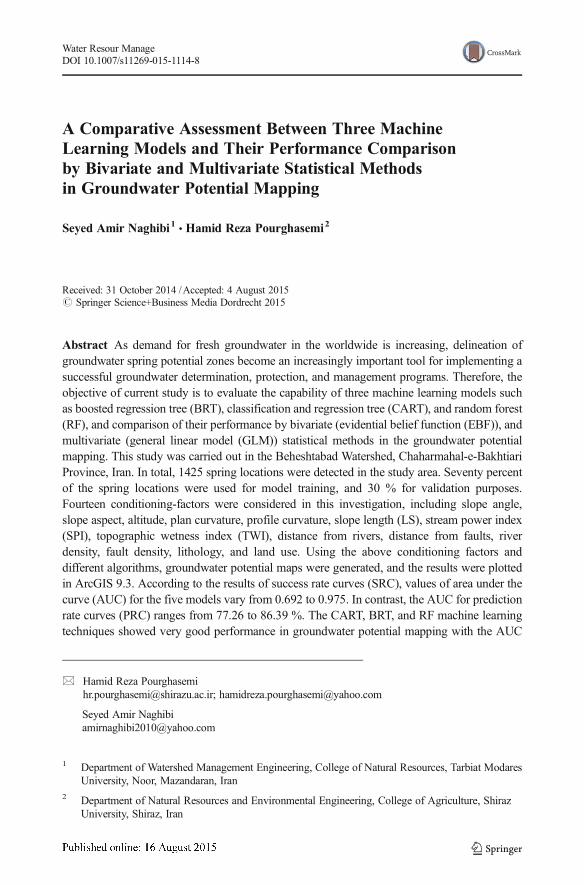
The Beheshtabad Watershed is located in the Chaharmahal-e-Bakhtiari Province, Iran,between 31° 50′ 36″N and 32° 34′ 16″ N latitude and 51°26′ 57″ E and 59° 21′ 51″E longitude (Fig. 1). It covers an area of approximately 2321 km2. The topographicalelevation of the study area varies between 1660 m and 3560 m above sea level(a.s.l.). The mean annual point precipitation is recorded as 618.8 mm in the weatherstation (Mojiri and Zarei 2006). Based on the geological survey of Iran (GSI 1997),49 % of the lithology covering the study area falls within the units described as Aincluding low level pediment fan and valley terraces deposit. Most of the area(66.26 %) is covered by rangeland/pasture land use types. Exploitation of groundwaterresources in this area includes use of qanats, springs, and deep and semi-deep wells.The average spring discharge is approximately 4 gal per second in the study area. Thegeneral trend of groundwater flow is from the north of the basin to the south of theplain, and the general topographic gradient of the plain is north to south.

3 Methods

3.1 Spring Characteristics

In total, 1425 springs were detected in Beheshtabad Watershed and was mapped at 1:50,000-scale (Fig. 1). By randomly partition (Oh et al. 2011; Ozdemir 2011a), 998 (70 %) of the springlocations were used for groundwater potential mapping and 427 (30 %) cases were used forvalidation aims.

3.2 Groundwater Conditioning Factors

Various thematic data layers such as slope angle, slope aspect, altitude, plan curvature,profile curvature, LS, SPI, TWI, distance from rivers, distance from faults, riverdensity, fault density, lithology, and land use were prepared in GIS environment andapplied for this study.

The digital elevation model (DEM) was created from the 1:50,000-scale topograph-ic maps in 20 m resolution. Groundwater conditioning-factors such as slope angle,slope aspect, and altitude were prepared using DEM in ArcGIS 9.3 and represented inFig. 2a–c.

Plan curvature can be used to describe the divergence and convergence of flow and to bediscriminate between watersheds, and hollows channelized by a 0th order hydraulic network(Fig. 2d). Profile curvature represents the rate at which the slope gradient changes in thedirection of maximum slope (Catani et al. 2013) (Fig. 2e).

Slope-length (Eq. 1) is the combination of the slope steepness (S) and slope length (L)which is calculated by Moore and Burch (1986) (Fig. 2f).

LS ¼ Bs

22:13

� �0:6 sin α0:0896

� �1:3

ð1Þ

where,α is the local slope gradient measured in degree and Bs is the specific catchment area (m2).

A Comparative Assessment Between Three Machine Learning Models

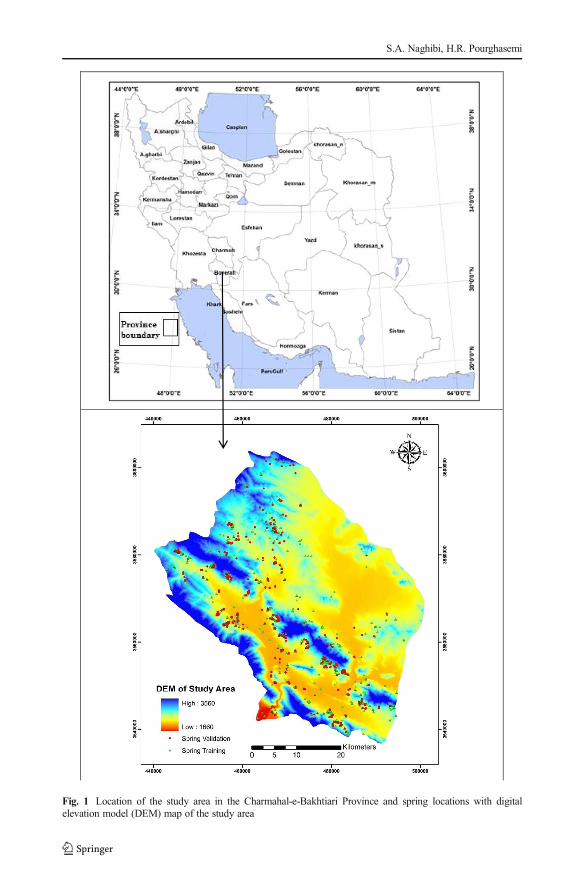
Fig. 1 Location of the study area in the Charmahal-e-Bakhtiari Province and spring locations with digitalelevation model (DEM) map of the study area

S.A. Naghibi, H.R. Pourghasemi

The SPI (Fig. 2g) is defined by Moore et al. (1991) as:

SPI ¼ Bs*tanα ð2ÞThe TWI (Fig. 2h) is defined as ln (A/tanβ), where A is upslope contributing area (or flow

accumulation) and β is the slope angle (Beven and Kirkby 1979).

Fig. 2 Groundwater effective factors maps of the study area; a slope degree, b slope aspect, c altitude, d plancurvature, e profile curvature, f slope length, g stream power index, h topographic wetness index, i distance fromrivers, j distance from faults, k drainage density, l fault density, m landuse, n lithology

A Comparative Assessment Between Three Machine Learning Models

Distance from rivers and drainage density maps were created using topographic maps,whereas, distance from faults and fault density maps were calculated using a geological map.Distance from rivers and faults layers were classified into five classes with 100 and 250 mintervals, respectively (Fig. 2i–j). But drainage density and fault density maps (Fig. 2k–l) wereclassified using the natural break method into four classes.

The landuse map was prepared using Landsat 7/ETM+ images for 2010 based on thesupervised classification method and maximum likelihood algorithm. These landuse types areagriculture, residential area, orchard, and rangeland types (Fig. 2m).

Fig. 2 (continued)

S.A. Naghibi, H.R. Pourghasemi

The lithology map was digitized using a 1:100,000-scale geological map in the ArcGIS 9.3.The study area is covered by various types of lithological formations and was classified intothirteen classes such as: A to M, respectively. The low-level piedmont fan and valley terracesdeposit (A) covers about 45.83 % of the study area. The general geological setting of the areais shown in Fig. 2n. Class B represents Low weathering grey marls alternating with bands ofmore resistant shelly limestone. Class C refers to Pale-red, polygenic conglomerate, andsandstone. Class D is undifferentiated metamorphic rocks, including phillite, meta-volcanics,

Fig. 2 (continued)

A Comparative Assessment Between Three Machine Learning Models

calcschist and crystalized limestone. Class E represents cream to brown-weathering, feature-forming, well- jointed limestone with intercalations of shale. Class F is grey, thick-bedded,o’olitic, fetid limestone. Class G represents grey, thick-bedded to massive orbitolina limestone.Class H is high level piedmont fan and valley terraces deposits and class I is marl andcalcareous shale with intercalations of limestone. Class J refers to polymictic conglomerateand sandstone. Class K is undivided Bangestan Group, mainly limestone and shale, Albian toCompanian. Class L represents undivided Eocene rock and class M is unconsolidated wind-blown sand deposits and back shore sand dunes.

3.3 Application of Models

3.3.1 Boosted Regression Tree (BRT)

BRT, also called stochastic gradient boosting (Elith et al. 2006), combines classification andregression trees with the gradient boosting algorithm (Friedman 2001). Boosting is a machinelearning technique similar to model averaging, where the results of several competing modelsare combined. Unlike model averaging, boosting uses a forward, stage-wise procedure, wheretree models are fitted interactively to a subset of the training data. Subsets of the training datawere implemented at each iteration of the model fitting are randomly selected withoutreplacement, where the proportion of the training data used is determined by the modeler,the “bag fraction” parameter. This procedure introduces an element of stochastic that improvesmodel accuracy and reduces over fitting (Elith et al. 2008).

3.3.2 Classification and Regression Tree (CART)

CART is a popular machine learning and non-parametric regression technique (Breiman et al.1984). The CART grows a decision tree based on a binary partitioning algorithm, that

Fig. 2 (continued)

S.A. Naghibi, H.R. Pourghasemi

recursively splits the data until groups is either homogeneous or contained fewer observationsthan a user-defined threshold (Aertsen et al. 2010). Regression trees are insensitive to outliers,and can accommodate missing data in predictor factors using surrogates (Breiman et al. 1984).

3.3.3 Random Forest (RF)

RFs are very powerful and flexible ensemble classifiers based upon decision trees, the firstdeveloped by Breiman (2001) (Catani et al. 2013; Micheletti et al. 2014). RF consists of acombination of many trees, where each tree is generated by boot-strap samples, leaving about athird of the overall sample for validation (the out-of-bag predictions- OOB) (Oliveira et al.2012). The algorithm estimates the importance of a variable by looking at how much theprediction error goes up when OOB data for that variable is permuted while all others are leftunchanged (Liaw and Wiener 2002; Catani et al. 2013).

RFs need two parameters to be tuned by the user: (1) the number of trees T, (2) the numberof variables m, to be stochastically chosen from the available set of features. Also, two types oferror were calculated: mean decrease in accuracy and mean decrease in node impurity (meandecrease Gini). These different importance measures can be used for ranking variables andvariable selection (Calle and Urrea 2010).

3.3.4 Generalized Linear Model (GLM)

Regression approaches comprising of linear regression, log-linear regression, and logisticregression (LR) have been used commonly. The primary goal of the LR is to find the bestmodel to represent the relationship between a dependent variable and multiple independentvariables (Ozdemir and Altural 2013). The logistic regression model can be expressed in itssimplest form as:

P ¼ 1=1þ e2 ð4Þwhere, P is the estimated probability of an event occurring. Because Z can vary from -∞ to+∞,the probability varies from 0 to 1 as an S-shaped curve. Parameter Z is defined as:

Z ¼ B0 þ B1X 1 þ B2X 2 þ…þ BnX n ð5Þ

where, B0 is the intercept and n is the number of independent variables. Values of Bi (i=0, 1, 2,…, n) are the slope coefficients, and Xi (i=0, 1, 2, …, n) are the independent variables. Basedon Eqs. 4 and 5, the logistic regression can be written in the following extended form:

Logit Pð Þ ¼ 1=1þ e−B0þB1X 1þB2X 2þ…þBnX n ð6Þ

3.3.5 Evidential Belief Function (EBF)

The Dempster–Shafer theory of evidence belief (Dempster 1968; Shafer 1976), is amathematical-based model with a bivariate statistically methodology, used to find the spatialintegration based on the rule of combination. The main advantage of the EBF is that it has arelative flexibility to accept uncertainty and the ability to combine beliefs from multiplesources of evidence (Thiam 2005). The EBFs are Bel (degree of belief), Dis (degree ofdisbelief), Unc (degree of uncertainty) and Pls (degree of plausibility). The Bel and Pls be,

A Comparative Assessment Between Three Machine Learning Models

respectively, lower and upper degrees of belief that the proposition is true based on givenevidence. The difference between Pls and Bel is uncertainty (Unc), which represents ignorancethat the evidence supports a proposition. Disbelief (Dis) is the belief of the false propositionbased on given evidential data; it is equal to 1−Pls (or 1−Unc−Bel). Therefore, the sum ofBel, Unc, and Dis is always 1.

The details of the mentioned algorithm (EBF) can be found in Carranza et al. (2008), andNampak et al. (2014).

3.3.6 Validation and Comparison of the GPMs

Validation of predictive groundwater potential maps (GPMs) is an essential component inmodeling process. Using the success-rate and prediction -rate curves, the five GPMs werevalidated with known spring locations.

The success-rate results were obtained based on training dataset (998 spring grid cells) foreach of the five GPMs, separately.

Since the success-rate measures the goodness of fit for the five models to the trainingdataset, it isn’t a suitable method for measuring the prediction capability of the spring models(Tien Bui et al. 2012). The prediction-rate curve can provide the validation and explainshow well the model and groundwater conditioning factors predict the existing springs(Lee 2007).

4 Results

4.1 BRT Model

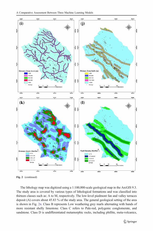
Main effects for the BRT model, where learning rate=0.005, tree complexity=5 and bagfraction=0.005, the optimal number of trees was reached at trees=900. The BRT final modelincluded 71.93 % of the mean total deviance (1-mean residual deviance / mean total devi-ance=1 - (0.49/1.38)=0.64) (Abeare 2009). An index of relative influence calculated insumming the contribution of each variable, which is equivalent to summing the branch lengthfor each variable in the regression tree (Abeare 2009). The measures are based on the numberof times a variable is selected for splitting, weighted by the squared improvement to the modelas a result of each split, and averaged over all trees (Friedman and Meulman 2003). For themain effects BRT model fitted here, the five most influential variables were altitude (20.24 %),distance from faults (19.56 %), SPI (12.98 %), distance from rivers (10.67 %) and fault density(10.33 %), respectively (Table 1). Furthermore, it was seen that six factors, including profilecurvature, plan curvature, river density, landuse, slope aspect, and lithology were removed inthe final analysis.

4.2 CART Model

The results of variables importance in CART model are represented in Table 1. According tothe results, from the 14 independent factors, CART used only six factors to generate theoptimal model, including distance from faults, fault density, altitude, SPI, TWI, and distancefrom rivers, which had high variable importance values of 25, 18, 16, 8, 7, and 7 %,respectively. Also it can be concluded from the results that landuse, profile curvature, slope

S.A. Naghibi, H.R. Pourghasemi

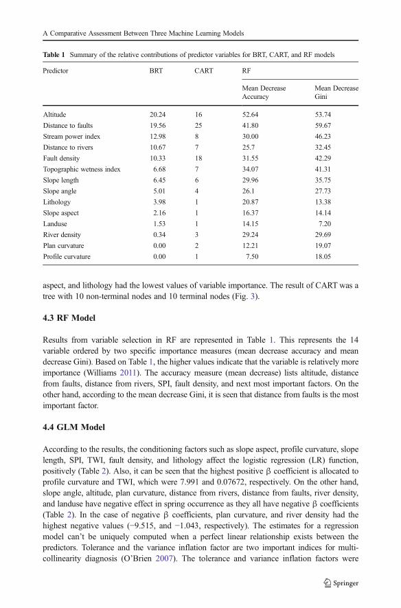
aspect, and lithology had the lowest values of variable importance. The result of CART was atree with 10 non-terminal nodes and 10 terminal nodes (Fig. 3).

4.3 RF Model

Results from variable selection in RF are represented in Table 1. This represents the 14variable ordered by two specific importance measures (mean decrease accuracy and meandecrease Gini). Based on Table 1, the higher values indicate that the variable is relatively moreimportance (Williams 2011). The accuracy measure (mean decrease) lists altitude, distancefrom faults, distance from rivers, SPI, fault density, and next most important factors. On theother hand, according to the mean decrease Gini, it is seen that distance from faults is the mostimportant factor.

4.4 GLM Model

According to the results, the conditioning factors such as slope aspect, profile curvature, slopelength, SPI, TWI, fault density, and lithology affect the logistic regression (LR) function,positively (Table 2). Also, it can be seen that the highest positive β coefficient is allocated toprofile curvature and TWI, which were 7.991 and 0.07672, respectively. On the other hand,slope angle, altitude, plan curvature, distance from rivers, distance from faults, river density,and landuse have negative effect in spring occurrence as they all have negative β coefficients(Table 2). In the case of negative β coefficients, plan curvature, and river density had thehighest negative values (−9.515, and −1.043, respectively). The estimates for a regressionmodel can’t be uniquely computed when a perfect linear relationship exists between thepredictors. Tolerance and the variance inflation factor are two important indices for multi-collinearity diagnosis (O’Brien 2007). The tolerance and variance inflation factors were

Table 1 Summary of the relative contributions of predictor variables for BRT, CART, and RF models

Predictor BRT CART RF

Mean DecreaseAccuracy

Mean DecreaseGini

Altitude 20.24 16 52.64 53.74

Distance to faults 19.56 25 41.80 59.67

Stream power index 12.98 8 30.00 46.23

Distance to rivers 10.67 7 25.7 32.45

Fault density 10.33 18 31.55 42.29

Topographic wetness index 6.68 7 34.07 41.31

Slope length 6.45 6 29.96 35.75

Slope angle 5.01 4 26.1 27.73

Lithology 3.98 1 20.87 13.38

Slope aspect 2.16 1 16.37 14.14

Landuse 1.53 1 14.15 7.20

River density 0.34 3 29.24 29.69

Plan curvature 0.00 2 12.21 19.07

Profile curvature 0.00 1 7.50 18.05

A Comparative Assessment Between Three Machine Learning Models

calculated for this study, and variables with VIF>5 and TOL<0.1 should be excluded from theLR analysis, but there was not any multi-collinearity problem in used factors in this study.

4.5 EBF Model

The spatial factor datasets were evaluated using EBFs to reveal the correlation between theexisting springs and the individual spatial factors in the study area. Table 2 shows the estimatedEBFs (belief, disbelief, uncertainty, Plausibility). According to Table 2, each class of theeffective factors has a belief value which a higher belief value shows that the class has highereffect on the groundwater potential. For example, in the case of slope angle, 5–15° and 15–30°classes had the highest belief values (0.45, and 0.27).

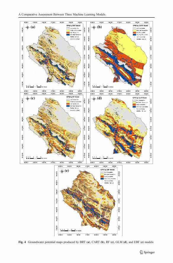
4.6 Groundwater Potential Mapping (GPM)

The obtained cell values were then classified based on the natural break classification scheme(Pourghasemi and Beheshtirad 2014; Naghibi et al. 2015) into low, moderate, high, and veryhigh potential groups (Fig. 4a–e) and Table 3).

Fig. 3 Optimal tree obtained by CARTwith terminal nodes resulting in spring (highlighted) and non-spring (grey)

S.A. Naghibi, H.R. Pourghasemi

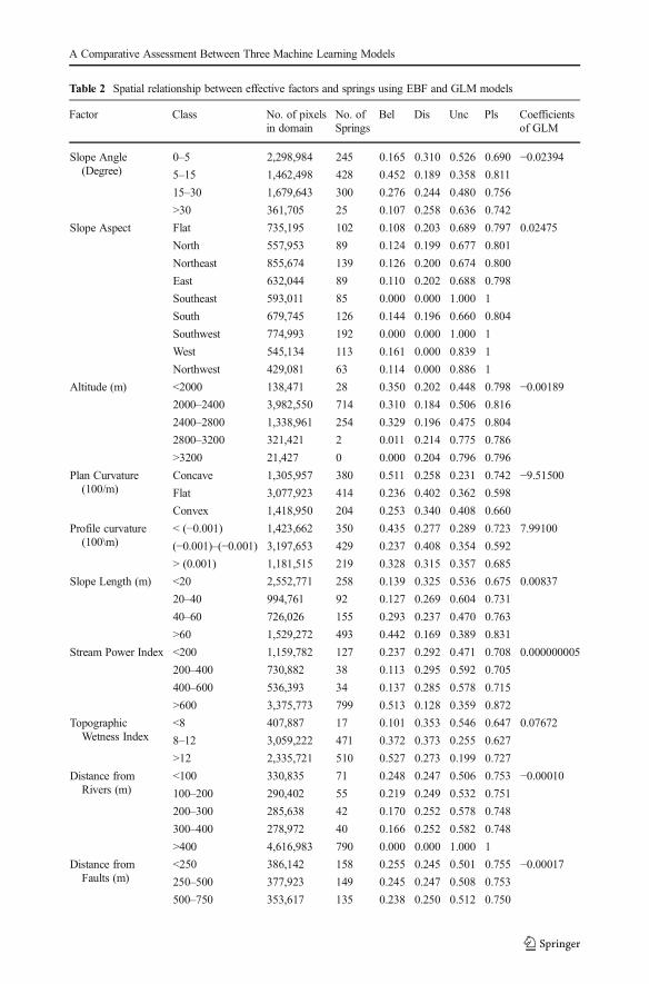
Table 2 Spatial relationship between effective factors and springs using EBF and GLM models

Factor Class No. of pixelsin domain

No. ofSprings

Bel Dis Unc Pls Coefficientsof GLM

Slope Angle(Degree)

0–5 2,298,984 245 0.165 0.310 0.526 0.690 −0.023945–15 1,462,498 428 0.452 0.189 0.358 0.811

15–30 1,679,643 300 0.276 0.244 0.480 0.756

>30 361,705 25 0.107 0.258 0.636 0.742

Slope Aspect Flat 735,195 102 0.108 0.203 0.689 0.797 0.02475

North 557,953 89 0.124 0.199 0.677 0.801

Northeast 855,674 139 0.126 0.200 0.674 0.800

East 632,044 89 0.110 0.202 0.688 0.798

Southeast 593,011 85 0.000 0.000 1.000 1

South 679,745 126 0.144 0.196 0.660 0.804

Southwest 774,993 192 0.000 0.000 1.000 1

West 545,134 113 0.161 0.000 0.839 1

Northwest 429,081 63 0.114 0.000 0.886 1

Altitude (m) <2000 138,471 28 0.350 0.202 0.448 0.798 −0.001892000–2400 3,982,550 714 0.310 0.184 0.506 0.816

2400–2800 1,338,961 254 0.329 0.196 0.475 0.804

2800–3200 321,421 2 0.011 0.214 0.775 0.786

>3200 21,427 0 0.000 0.204 0.796 0.796

Plan Curvature(100/m)

Concave 1,305,957 380 0.511 0.258 0.231 0.742 −9.51500Flat 3,077,923 414 0.236 0.402 0.362 0.598

Convex 1,418,950 204 0.253 0.340 0.408 0.660

Profile curvature(100\m)

< (−0.001) 1,423,662 350 0.435 0.277 0.289 0.723 7.99100

(−0.001)–(−0.001) 3,197,653 429 0.237 0.408 0.354 0.592

> (0.001) 1,181,515 219 0.328 0.315 0.357 0.685

Slope Length (m) <20 2,552,771 258 0.139 0.325 0.536 0.675 0.00837

20–40 994,761 92 0.127 0.269 0.604 0.731

40–60 726,026 155 0.293 0.237 0.470 0.763

>60 1,529,272 493 0.442 0.169 0.389 0.831

Stream Power Index <200 1,159,782 127 0.237 0.292 0.471 0.708 0.000000005

200–400 730,882 38 0.113 0.295 0.592 0.705

400–600 536,393 34 0.137 0.285 0.578 0.715

>600 3,375,773 799 0.513 0.128 0.359 0.872

TopographicWetness Index

<8 407,887 17 0.101 0.353 0.546 0.647 0.07672

8–12 3,059,222 471 0.372 0.373 0.255 0.627

>12 2,335,721 510 0.527 0.273 0.199 0.727

Distance fromRivers (m)

<100 330,835 71 0.248 0.247 0.506 0.753 −0.00010100–200 290,402 55 0.219 0.249 0.532 0.751

200–300 285,638 42 0.170 0.252 0.578 0.748

300–400 278,972 40 0.166 0.252 0.582 0.748

>400 4,616,983 790 0.000 0.000 1.000 1

Distance fromFaults (m)

<250 386,142 158 0.255 0.245 0.501 0.755 −0.00017250–500 377,923 149 0.245 0.247 0.508 0.753

500–750 353,617 135 0.238 0.250 0.512 0.750

A Comparative Assessment Between Three Machine Learning Models

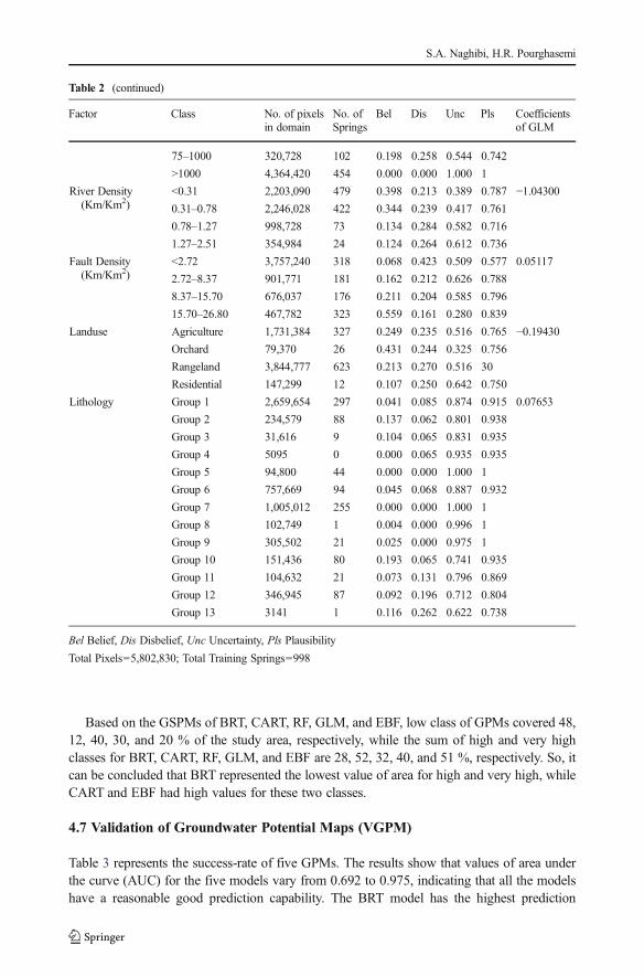
Based on the GSPMs of BRT, CART, RF, GLM, and EBF, low class of GPMs covered 48,12, 40, 30, and 20 % of the study area, respectively, while the sum of high and very highclasses for BRT, CART, RF, GLM, and EBF are 28, 52, 32, 40, and 51 %, respectively. So, itcan be concluded that BRT represented the lowest value of area for high and very high, whileCART and EBF had high values for these two classes.

4.7 Validation of Groundwater Potential Maps (VGPM)

Table 3 represents the success-rate of five GPMs. The results show that values of area underthe curve (AUC) for the five models vary from 0.692 to 0.975, indicating that all the modelshave a reasonable good prediction capability. The BRT model has the highest prediction

Table 2 (continued)

Factor Class No. of pixelsin domain

No. ofSprings

Bel Dis Unc Pls Coefficientsof GLM

75–1000 320,728 102 0.198 0.258 0.544 0.742

>1000 4,364,420 454 0.000 0.000 1.000 1

River Density(Km/Km2)

<0.31 2,203,090 479 0.398 0.213 0.389 0.787 −1.043000.31–0.78 2,246,028 422 0.344 0.239 0.417 0.761

0.78–1.27 998,728 73 0.134 0.284 0.582 0.716

1.27–2.51 354,984 24 0.124 0.264 0.612 0.736

Fault Density(Km/Km2)

<2.72 3,757,240 318 0.068 0.423 0.509 0.577 0.05117

2.72–8.37 901,771 181 0.162 0.212 0.626 0.788

8.37–15.70 676,037 176 0.211 0.204 0.585 0.796

15.70–26.80 467,782 323 0.559 0.161 0.280 0.839

Landuse Agriculture 1,731,384 327 0.249 0.235 0.516 0.765 −0.19430Orchard 79,370 26 0.431 0.244 0.325 0.756

Rangeland 3,844,777 623 0.213 0.270 0.516 30

Residential 147,299 12 0.107 0.250 0.642 0.750

Lithology Group 1 2,659,654 297 0.041 0.085 0.874 0.915 0.07653

Group 2 234,579 88 0.137 0.062 0.801 0.938

Group 3 31,616 9 0.104 0.065 0.831 0.935

Group 4 5095 0 0.000 0.065 0.935 0.935

Group 5 94,800 44 0.000 0.000 1.000 1

Group 6 757,669 94 0.045 0.068 0.887 0.932

Group 7 1,005,012 255 0.000 0.000 1.000 1

Group 8 102,749 1 0.004 0.000 0.996 1

Group 9 305,502 21 0.025 0.000 0.975 1

Group 10 151,436 80 0.193 0.065 0.741 0.935

Group 11 104,632 21 0.073 0.131 0.796 0.869

Group 12 346,945 87 0.092 0.196 0.712 0.804

Group 13 3141 1 0.116 0.262 0.622 0.738

Bel Belief, Dis Disbelief, Unc Uncertainty, Pls Plausibility

Total Pixels=5,802,830; Total Training Springs=998

S.A. Naghibi, H.R. Pourghasemi

(a) (b)

(c) (d)

(e)

Fig. 4 Groundwater potential maps produced by BRT (a), CART (b), RF (c), GLM (d), and EBF (e) models

A Comparative Assessment Between Three Machine Learning Models

capability (97.50 %), while the EBF model has lowest prediction capability (69.20 %). Theother models with almost equal prediction capabilities are intermediate between the BRT andEBF models.

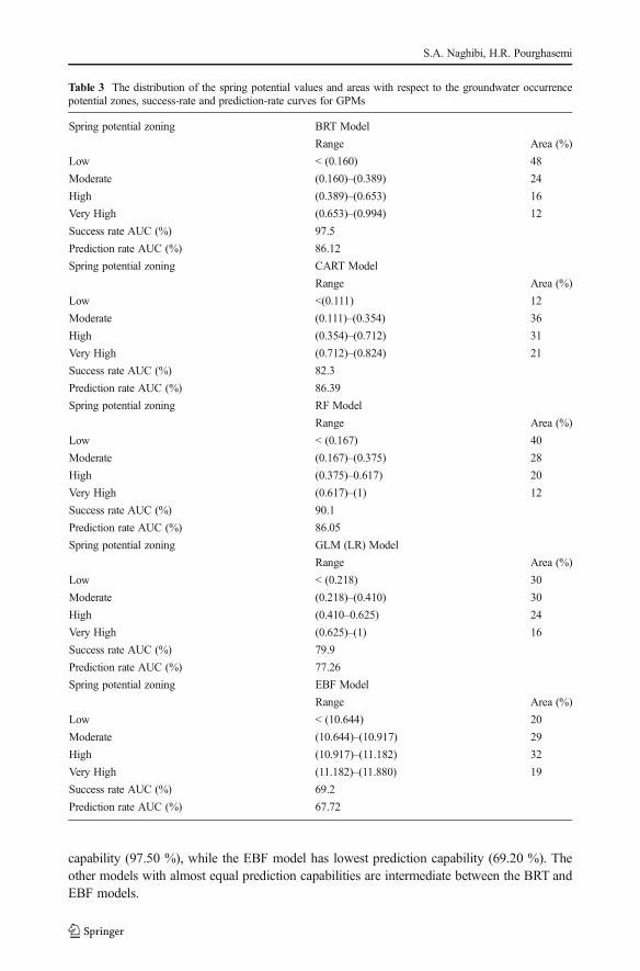
Table 3 The distribution of the spring potential values and areas with respect to the groundwater occurrencepotential zones, success-rate and prediction-rate curves for GPMs

Spring potential zoning BRT Model

Range Area (%)

Low < (0.160) 48

Moderate (0.160)–(0.389) 24

High (0.389)–(0.653) 16

Very High (0.653)–(0.994) 12

Success rate AUC (%) 97.5

Prediction rate AUC (%) 86.12

Spring potential zoning CART Model

Range Area (%)

Low <(0.111) 12

Moderate (0.111)–(0.354) 36

High (0.354)–(0.712) 31

Very High (0.712)–(0.824) 21

Success rate AUC (%) 82.3

Prediction rate AUC (%) 86.39

Spring potential zoning RF Model

Range Area (%)

Low < (0.167) 40

Moderate (0.167)–(0.375) 28

High (0.375)–0.617) 20

Very High (0.617)–(1) 12

Success rate AUC (%) 90.1

Prediction rate AUC (%) 86.05

Spring potential zoning GLM (LR) Model

Range Area (%)

Low < (0.218) 30

Moderate (0.218)–(0.410) 30

High (0.410–0.625) 24

Very High (0.625)–(1) 16

Success rate AUC (%) 79.9

Prediction rate AUC (%) 77.26

Spring potential zoning EBF Model

Range Area (%)

Low < (10.644) 20

Moderate (10.644)–(10.917) 29

High (10.917)–(11.182) 32

Very High (11.182)–(11.880) 19

Success rate AUC (%) 69.2

Prediction rate AUC (%) 67.72

S.A. Naghibi, H.R. Pourghasemi

Table 3 depicts the results of prediction-rate for the implemented methods in groundwaterpotential mapping. According to the results, the AUC for prediction-rate ranges from 77.26 to86.39 %. The CART, BRT, and RF techniques showed very good performance in groundwaterpotential mapping with the values of 86.39, 86.12, and 86.05 %, respectively, which showsclose performance of these models. In contrast, The EBF and GLM models showed weakperformance by the AUC values of 67.72, and 77.26 %, respectively.

5 Discussion

In this section, the results are discussed by two parts: (1) the performance of models and theircharacteristics, (2) the importance of variables in groundwater potential mapping and theirrelationship in each used model in the current study.

5.1 The Performance of Models and Their Comparison

BRT models are able to select relevant variables, fit accurate functions and automaticallyidentify and model interactions, giving sometimes substantial predictive advantage overmethods such as GLM and GAM (Generalized Additive Models). A growing body ofliterature quantifies this difference in performance (Elith et al. 2006; Leathwick et al. 2006;Moisen et al. 2006; Vorpahl et al. 2012). Efficient variable selection means that large suites ofcandidate variables will be handled well than in GLM or GAM developed with stepwiseselection.

According to the results, RF method had better performance than a GLM which is commonwith some researches in other fields, including wildfire, landslide susceptibility mapping, andecology studies (Peters et al. 2007; Oliveira et al. 2012; Vorpahl et al. 2013). According toOzdemir (2011b), GLM or LR showed poor estimator for groundwater potential mapping.Also, the results of Nampak et al. (2014) showed that EBF model had better results than GLMbut both, they had prediction rates of less than 78 %.

In their final form, BRT model included a smaller number of variables selected from theoriginal dataset of 14 (eight variables), while CART, EBF, GLM, and RF included all 14variables. Other authors also stated that a parsimonious model would be more stable and easierto generalize (Catry et al. 2009; Vilar et al. 2010), particularly at a broad spatial scale.

5.2 The Importance of Variables in GPMs and Their Relationship

According to the results of three machine learning methods, altitude, distance from faults, SPI,and fault density had the highest importance in groundwater potential mapping. However, theresults of Pourtaghi and Pourghasemi (2014) showed that the conditioning factors such asslope aspect, altitude, plan curvature, and lithology affect the LR function positively. So, theimportance of variables in groundwater potential mapping is considerably affected by themethod used in a research and properties of study area. In other words, different geological,topographical, and climatic conditions of an area change the priority of the effective factors ingroundwater potential mapping. For example, in a semi-flat watershed, altitude may not be asimportant as in a mountainous watershed. Also, precision of the models and their accuracyaffect the importance of effective factors in groundwater potential mapping which is seenaccording to the current studies’ results.

A Comparative Assessment Between Three Machine Learning Models

According to the results, there was direct relationship between LS, TWI, and fault density anddegree of belief that means groundwater potential increase when the value of these factorsincreased. On the other hand, results showed inverse relationship between altitude, distance fromrivers, distance from faults, and river density and degree of belief. A growing body of literaturedetermines the relationship between groundwater conditioning factors and potential (Oh et al.2011; Naghibi et al. 2015). The result of Ozdemir (2011b) showed that the elevation and slope-related factors had a negative correlation with groundwater potential, whereas other factors (TWI,river density, and lineament-related factors) show a positive correlation. The results of Naghibiet al. (2015) showed that TWI had direct relationship, while altitude, slope angle, distance tofaults, and profile curvature had inverse relationship with groundwater potential.

6 Conclusions

This study presented an application of three different machine learning models, bivariate, andmultivariate models in groundwater potential mapping in BeheshtabadWatershed, Chaharmahal-e-Bakhtiari Province, Iran. According to results, three machine learning techniques used in thecurrent study had very good results in groundwater potential mapping. The AUC of prediction-rates for machine learning techniques were approximately 86 %. But, bivariate and multivariatemodels used in this study had weaker performance in groundwater potential mapping with AUCvalues of 67, and 77 %, respectively. The GPMs produced from this study could therefore assistplanners and engineers during development and water resource planning. The results of suchstudies determine areas with high groundwater potential which can be used for exploitation. Onthe other hand, susceptible areas with low groundwater potential are determined. Planners canapply conservation plans such as flood spreading in these areas. In the final form of models, BRTincluded a smaller number of variables selected from the original set of 14 (8 variables), whileCART, EBF, GLM, and RF included all 14 variables and can be generalized easier. Also, it wasconcluded from the results that altitude, distance from faults, SPI, and fault density had the highestimportance in groundwater potential mapping.

The result obtained in this study may provide technical support to government agencies, aswell as private sectors for groundwater exploration and assessment in Iran. The proposedmethods provided rapid, accurate, and cost effective results. Furthermore, the analysis may betransferable to other watersheds with similar topographic and hydro-geological characteristics.

Acknowledgments The authors would like to thank of editorial comments and the anonymous reviewers fortheir helpful comments on the previous version of the manuscript.

References

Abeare SM (2009) Comparisons of boosted regression tree, GLM and GAM performance in the standardizationof yellowfin tuna catch-rate data from the Gulf of Mexico Lonline Fishery. Master’s Thesis, Louisiana StateUniversity

Aertsen W, Kint V, Van Orshoven J, Özkan K, Muys B (2010) Comparison and ranking of different modelingtechniques for prediction of site index in Mediterranean mountain forests. Ecol Model 221:1119–1130

Aertsen W, Kint V, Van Orshoven J, Muys B (2011) Evaluation of modelling techniques for forest siteproductivity prediction in contrasting eco-regions using stochastic multi-criteria acceptability analysis(SMAA). Environ Model Softw 26(7):929–937

S.A. Naghibi, H.R. Pourghasemi

Bachmair S, Weiler M (2012) Hillslope characteristics as controls of subsurface flow variability. Hydrol EarthSyst Sci 16:3699–3715

Beven KJ, Kirkby MJ (1979) A physically based, variable contributing area model of basin hydrology. HydrolSci Bull 24:43–69

Breiman L, Friedman JH, Olshen R, Stone CJ (1984) Classification and regression trees. Wadsworth, BelmontBreiman L (2001) Random forests. Mach Learn 45:5–32Calle ML, Urrea V (2010) Letter to the Editor: stability of random forest importance measures. Brief Bioinform

12(1):86–89Catani F, Lagomarsino D, Segoni S, Tofani V (2013) Landslide susceptibility estimation by random forests

technique: sensitivity and scaling issues. Nat Hazards Earth Syst Sci 13:2815–2831Carranza EJM, Van Ruitenbeek F, Hecker C et al (2008) Knowledge-guided data-driven evidential belief

modeling of mineral prospectivity in Cabo de Gata, SE Spain. Int J Appl Earth Obs 10:374–387Catry FX, Rego FC, Bação FL, Moreira F (2009) Modelling and mapping the occurrence of wildfire ignitions in

Portugal. Int J Wildland Fire 18:921–931Chezgi J, Pourghasemi HR, Naghibi SA, Moradi HR, Kheirkhah Zarkesh M (2015) Assessment of a spatial

multi-criteria evaluation to site selection underground dam in the Alborz Province, Iran. Geocarto Int. doi:10.1080/10106049.2015.1073366

Davoodi Moghaddam D, Rezaei M, Pourghasemi HR, Pourtaghie ZS, Pradhan B (2015) Groundwater springpotential mapping using bivariate statistical model and GIS in the Taleghan watershed, Iran. Arab J Geosci8(2):913–929

Dempster AP (1968) A generalization of Bayesian inference. J R Stat Soc 30:205–247Durga Rao KHV (2014) Spatial optimization technique for planning groundwater supply schemes in a rapid

growing urban environment. Water Resour Manag 28(3):731–747Elith J, Graham CH, Anderson RP et al (2006) Novel methods improve prediction of species’ distributions from

occurrence data. Ecography 29:129–151Elith J, Leathwick JR, Hastie T (2008) A working guide to boosted regression trees. J Anim Ecol 77:802–813Esquivel JM, Morales GP, Esteller MV (2015) Groundwater monitoring network design using GIS and multi-

criteria analysis. Water Resour Manag 29(9):3157–3194Friedman JH (2001) Greedy function approximation: a gradient boosting machine. Ann Stat 29:1189–1232Friedman JH, Meulman JJ (2003) Multiple additive regression trees with application in epidemiology. Stat Med

22:1365–1381Geology Survey of Iran (GSI) (1997) Geology map of the Chaharmahal-e-Bakhtiari Province. http://www.gsi.ir/

Main/Lang_en/index.html. Accessed September 2000Gutiérrez ÁG, Schnabel S, Felicisimo AM (2009a) Modelling the occurrence of gullies in rangelands of

southwest Spain. Earth Surf Process Landf 34:1894–1902Gutiérrez ÁG, Schnabel S, Lavado Contador JF (2009b) Using and comparing two nonparametric methods

(CART and MARS) to model the potential distribution of gullies. Ecol Model 220(24):3630–3637Leathwick JR, Elith J, Francis MP et al (2006) Variation in demersal fish species richness in the oceans

surrounding New Zealand: an analysis using boosted regression trees. Mar Ecol Prog Ser 321:267–281Lee S (2007) Application and verification of fuzzy algebraic operators to landslide susceptibility mapping.

Environ Geol 52:615–623Lee S, Song KY, Kim Y et al (2012) Regional groundwater productivity potential mapping using a geographic

information system (GIS) based artificial neural network model. Hydrogeol J 20:1511–1527Lee S, Hwang J, Park I (2013) Application of data-driven evidential belief functions to landslide susceptibility

mapping in Jinbu, Korea. Catena 100:15–30Leuenberger M, Kanevski M, Orozco CDV (2013) Forest fires in a random forest. EGU General Assembly, AustriaLiaw A, Wiener M (2002) Classification and regression by random forest. R News 2:18–22ManapMA,NampakH, PradhanB et al (2012)Application of probabilistic-based frequency ratiomodel in groundwater

potential mapping using remote sensing data and GIS. Arab J Geosci. doi:10.1007/s12517-012-0795-zMazza R, La Vigna F, Alimonti C (2014) Evaluating the available regional groundwater resources using the

distributed hydrogeological budget. Water Resour Manag 28(3):749–765Micheletti N, Foresti L, Robert S (2014) Machine learning feature selection methods for landslide susceptibility

mapping. Math Geosci 46:33–57Moisen GG, Freeman EA, Blackard JA et al (2006) Predicting tree species presence and basal area in Utah: a

comparison of stochastic gradient boosting, generalized additive models, and tree-based methods. EcolModel 199:176–187

Mojiri HR, Zarei AR (2006) The investigation of precipitation condition in the Zagros area and its effects on thecentral plateau of Iran. The 2nd Conference of Water Resource Management. Tehran, Iran

Moore ID, Burch GJ (1986) Sediment transport capacity of sheet and rill flow: application of unit stream powertheory. Water Resour Res 22(8):1350–1360

A Comparative Assessment Between Three Machine Learning Models

Moore ID, Grayson RB, Ladson AR (1991) Digital terrain modelling: a review of hydrological, geomorpholog-ical, and biological applications. Hydrol Process 4:3–30

Moradi Dashtpagerdi M, Nohegar A, Vagharfard H, Honarbakhsh A, Mahmoodinejad V, Noroozi A,Ghonchehpoor D (2013) Application of spatial analysis techniques to select the most suitable areas forflood spreading. Water Resour Manag 27:3071–3084

Naghibi SA, Pourghasemi HR, Pourtaghi ZS et al (2015) Groundwater qanat potential mapping using frequencyratio and Shannon’s entropy models in the Moghan watershed, Iran. Earth Sci Inf 8(1):171–186

Nampak H, Pradhan B, ManapMA (2014) Application of GIS based data driven evidential belief function modelto predict groundwater potential zonation. J Hydrol. doi:10.1016/j.jhydrol.2014.02.053

O’Brien RM (2007) A caution regarding rules of thumb for variance inflation factors. Qual Quant 41(5):673–690Oh HJ, Lee S (2010) Assessment of ground subsidence using GIS and the weights-of-evidence model. Eng Geol

115(1–2):36–48Oh HJ, Kim YS, Choi JK et al (2011) GIS mapping of regional probabilistic groundwater potential in the area of

Pohang City, Korea. J Hydrol 399:158–172Oliveira S, Oehler F, San-Miguel-Ayanz J (2012) Modeling spatial patterns of fire occurrence in Mediterranean

Europeusing Multiple Regression and Random Forest. Forest Ecol Manag 275:117–129Ozdemir A (2011a) GIS-based groundwater spring potential mapping in the Sultan Mountains (Konya, Turkey)

using frequency ratio, weights of evidence and logistic regression methods and their comparison. J Hydrol411:290–308

Ozdemir A (2011b) Using a binary logistic regression method and GIS for evaluating and mapping thegroundwater spring potential in the Sultan Mountains (Aksehir, Turkey). J Hydrol 405:123–136

Ozdemir A, Altural T (2013) A comparative study of frequency ratio, weights of evidence and logistic regressionmethods for landslide susceptibility mapping: Sultan Mountains, SW Turkey. J Asian Earth Sci 64:180–197

Peters J, De Baets B, Verhoest NEC, Samson R, Degroeve S, De Becker P, Huybrechts W (2007) Random forestsas a tool for ecohydrological distribution modelling. Ecol Model 207:304–318

Pourghasemi HR, Beheshtirad M (2014) Assessment of a data-driven evidential belief function model and GISfor groundwater potential mapping in the Koohrang Watershed, Iran. Geocarto Int. doi:10.1080/10106049.2014.966161

Pourtaghi ZS, Pourghasemi HR (2014) GIS-based groundwater spring potential assessment and mapping in theBirjand Township, southern Khorasan Province, Iran. Hydrogeol J 22(3):643–662

Rahmati O, Nazari Samani A, Mahdavi M, Pourghasemi HR, Zeinivand H (2014) Groundwater potentialmapping at Kurdistan region of Iran using analytic hierarchy process and GIS. Arab J Geosci. doi:10.1007/s12517-014-1668-4

Razandi Y, Pourghasemi HR, Samani Neisani N, Rahmati O (2015) Application of analytical hierarchy process,frequency ratio, and certainty factor models for groundwater potential mapping using GIS. Earth Sci Inf. doi:10.1007/s12145-015-0220-8

Shafer G (1976) A mathematical theory of evidence. Princetown University Press, New JerseyStumpf A, Kernel N (2011) Object-oriented mapping of landslides using random forests. Remote Sens Environ

115(10):2564–2577Tien Bui D, Pradhan B, Lofman O et al (2012) Spatial prediction of landslide hazards in Hoa Binh province

(Vietnam): a comparative assessment of the efficacy of evidential belief functions and fuzzy logic models.Catena 96:28–40

Thiam AK (2005) An evidential reasoning approach to land degradation evaluation: Dempster-Shafer theory ofevidence. Trans GIS 9:507–520

Trigila A, Frattini P, Casagli N et al (2013) Landslide susceptibility mapping at national scale: the Italian casestudy. Landslide Sci Prac 1:287–295

Vilar L, Woolford DG, Martell DL et al (2010) A model for predicting human-caused wildfire occurrence in theregion of Madrid, Spain. Int J Wildland Fire 19(3):325–337

Vorpahl P, Elsenbeer H, Märker M et al (2012) How can statistical models help to determine driving factors oflandslides? Ecol Model 239:27–39

Williams G (2011) Data mining with rattle and R (The art of excavating data for knowledge discovery series)Zekri S, Triki C, Al-Maktoumi A, Bazargan-Lari MR (2015) An optimization-simulation approach for ground-

water abstraction under recharge uncertainty. Water Resour Manag 29(10):3681–3695

S.A. Naghibi, H.R. Pourghasemi