Bivariate Flood Frequency Analysis of Upper Godavari River Flows Using Archimedean Copulas

Bivariate Flood Frequency Analysis of Upper GodavariRiver Flows Using Archimedean Copulas

M. Janga Reddy & Poulomi Ganguli

Received: 1 November 2010 /Accepted: 27 August 2012 /Published online: 11 September 2012# Springer Science+Business Media B.V. 2012

Abstract In this paper, a copula based methodology is presented for flood frequencyanalysis of Upper Godavari River flows in India. By using the specific advantages of copulamethod in modeling the joint dependence structure of uncertain variables, this study appliesArchimedean copulas for frequency analysis of flood characteristics annual peak flow, floodvolume and flood duration. To determine the best fit marginal distributions for floodvariables, few parametric and nonparametric probability distributions are examined andthe best fit model is adopted for copula modeling. Four Archimedean family of copulas,namely Ali-Mikhail-Haq, Clayton, Gumbel-Hougaard and Frank copulas are evaluated formodeling the joint dependence of annual peak flow-volume, and flood volume-durationpairs. The performance of two parameter estimation methods, namely method-of-moments-like estimator based on inversion of Kendall’s tau and maximum pseudo-likelihood estima-tor for copulas are investigated. On performing Monte Carlo simulation to assess theperformance of copula distributions in modeling the joint dependence structure of floodvariables, it is found that the developed copula models are well representing the observedflood characteristics. From standard statistical tests, Frank copula has been identified as thebest fitted copula for both bivariate models. The Frank copula function is used for obtainingjoint and conditional return periods of flood characteristics, which can be useful for riskbased design of water resources projects.

Keywords Archimedean copulas . Flood flows . Frequency analysis . Multivariateprobability distributions . Return period

1 Introduction

The flood frequency analysis is one of the most important and widely studied subjects in thefield of hydrology and water resources. Since, floods have become most common naturalhazards, increasingly posing a significant risk to human life and environment. At the

Water Resour Manage (2012) 26:3995–4018DOI 10.1007/s11269-012-0124-z

M. J. Reddy (*) : P. GanguliDepartment of Civil Engineering, Indian Institute of Technology Bombay, Powai, Mumbai 400076, Indiae-mail: [email protected]

drainage basin scale, consideration of flood risk plays an important role in planning of waterinfrastructure projects, for example in design of hydraulic structures (e.g., dam spillways,diversion canals, dikes and river channels), urban drainage systems, cross drainage struc-tures (e.g., culverts and bridges), reservoir management, flood hazard mapping etc.

In general, a flood means inundation caused by rivers overflowing their banks on accountof heavy rainfall and/or melting of large amounts of snow (Rakhecha and Singh 2009). Theoccurrence of hydrological extreme event, flood, involves lot of uncertainty, and its prop-erties being stochastic in nature, are characterized by mutually correlated random variablessuch as flood peak, volume and duration of the flood hydrograph. Since flood is amultivariate stochastic phenomenon, so risk analysis of flood flows has to be modeled byan effective multivariate probabilistic approach.

Although single variable flood frequency analysis has been widely used in the past(Cunnane 1987; Bobée and Rasmussen 1994), it may not provide effective risk analysesto handle the associated risks of correlated flood properties. By recognizing the limitationsof single variable flood frequency analysis, the multivariate frequency analysis wasaddressed by several researchers using conventional probability distributions. For example,bivariate generalized extreme value distribution (Raynal and Salas 1987; Yue et al. 1999;Yue and Wang 2004; Nadarajah and Shiau 2005; Escalante 2007), bivariate gamma distri-bution (Yue 2001), bivariate normal distribution (Goel et al. 1998; Yue 1999), bivariatelognormal distribution (Yue 2000), bivariate exponential distribution (Choulakian et al.1990) etc. Most of these studies applied the bivariate probability distributions to obtainjoint and conditional distribution of flood peak and volume. Some of these studies haveconsidered the dependence among flood variables, but with restrictive assumptions, such as,assuming all flood properties were well represented by a single probability distribution (e.g.,normal distribution). But in practice, the flood variables may follow different distributionsand needs to be modeled separately. Also other issue is applying data transformations, suchas taking natural logarithms or applying Box-Cox transformations to the flood variables,with an assumption of the transformed series will be invariant. But this may not be case allthe time, as transformed marginals may deviate from original distributions. Moreover,several conventional multivariate distributions do not allow full coverage of dependencestructure between the variables and they can represent only a very limited range ofdistributional shapes.

For modeling point of view, lower the dimensionality of the model, higher the reliabilityof the estimates. In this respect, any modeling approach that could decompose the multi-variate estimation procedure into separate marginal distributions and functional form ofdependence between the variables can effectively increase the reliability of the estimationprocess (Ané and Kharoubi 2003). Also, sometimes conventional methods are mathemati-cally complicated and multivariate models may require linking to Pearson’s linear correla-tion coefficient as the dependence parameter. However, Pearson’s correlation coefficient isnot an efficient measure of association when the dependence between the variables isnonlinear. Another classical approach to model joint distribution of random variables isthe product of marginal and conditional distributions (Clemen and Reilly 1999). But thecomplexity of estimation process grows as the number of random variables increases. Thusconventional multivariate distributions are not flexible enough, and there is a greaternecessity of sophisticated methods for flood frequency analysis.

In recent times, the use of copulas have become popular for multivariate analysis invarious fields, viz., in financial studies (Frees and Valdez 1998; Cherubini et al. 2004), inhydrology and water resources for rainfall analysis (De Michele and Salvadori 2003; Shiauet al. 2006), for flood flow analysis (Favre et al. 2004; De Michele et al. 2005; Zhang and

3996 M.J. Reddy, P. Ganguli

Singh 2006; Grimaldi and Serinaldi 2006; Genest and Favre 2007; Karmakar and Simonovic2009; Wang et al. 2009; Klein et al. 2010; Chowdhary et al. 2011), for drought analysis (Kaoand Govindaraju 2010; Song and Singh 2010; Janga Reddy and Ganguli 2012a), forgroundwater analysis (Bárdossy 2006; Janga Reddy and Ganguli 2012b), and hydro-climatic variable analysis (Maity and Kumar 2008; Janga Reddy and Ganguli 2012b) etc.In the following, brief details of copula applications with relevance to the present study arediscussed.

One of the early applications of copulas in hydrology is for rainfall analysis by DeMichele and Salvadori (2003). They applied for a case study in Bisagno drainage basin,Italy, and modeled different combinations of negatively associated average storm intensityand duration using Frank Archimedean copula with heavy tailed Generalized Pareto as themarginal distribution for both storm duration and intensity data. Favre et al. (2004) inves-tigated applicability of Clayton, Gumbel-Hougaard and Frank copulas for flood flowanalysis for case studies in Québec, Canada. They found that Frank copula as the bestmodel to capture dependence between flood variables. De Michele et al. (2005) employedGumbel-Hougaard copula to model joint distribution of annual maximum flood peak andvolume in Anza catchment, Northern Italy. They generated large number of syntheticobservations with GEV marginals to check the behavior of reservoir during its expecteddesign life and tested adequacy of dam spillways. Shiau et al. (2006) analyzed bivariatedistribution of flood peak and volume in Jhuoshuei River basin, Taiwan using Ali-Mikhail-Haq, Clayton, Frank, Galambos, Gumbel-Hougaard and Plackett copulas. A comparativestudy is carried out between joint return period and univariate return period, and stressed thenecessity of copulas for estimation of joint return periods.

Zhang and Singh (2006) modeled bivariate joint distributions of flood peak-volume, andflood volume-duration combinations using Archimedean copulas and applied to flood datafrom two different gauging stations, Ashuapmushuan River at Saguenay in Canada andAmite River at Denham springs in US, with marginal distribution as Extreme Value Type Iand Log-Pearson Type III distributions. They found that Gumbel-Hougaard copula providesbetter fit to the both combinations of flood variables. Also the copula derived distributionswere compared with Gumbel mixed model and Box-Cox transformed normal distributions,and found that copula derived distributions were much efficient to that of conventionalmultivariate distributions. Genest and Favre (2007) presented a comprehensive review ofcopula with their parameter estimation and inference procedures, with an application to acase study in Harricana watershed, Québec, Canada. Among various copula models con-sidered in their study, they found that extreme value class of copulas—Gumbel-Hougaard,Galambos, Husler-Reiss, BB1 and BB5 as the plausible models for modeling flood peak andvolume data. Karmakar and Simonovic (2009) applied three Archimedean copulas namely,Ali-Mikhal-Haq, Clayton and Gumbel-Hougaard for bivariate flood frequency analysis offlood flows of Red River at Grand Forks, Dakota, and found that Gumbel-Hougaard copulaas the best model for representing flood properties.

Wang et al. (2009) presented copula method to estimate flood quantiles for a river at thedownstream confluence point considering flood flows at two upstream tributaries, anddemonstrated through an application to a case study in Des Moines River basin, Iowa andhinted that Frank copula performed satisfactorily. Klein et al. (2010) presented copula basedbivariate probability analyses of flood flows in Unstrut River basin, Germany. In firstapplication the spatial distribution of flood events within river basin is analyzed by jointprobability of inflow peaks at two reservoirs located at the downstream of the main tributary.In second application copulas are used to obtain joint distribution of flood peak and volumein Unstrut catchment for risk assessment of individual flood detention structures.

Flood Frequency Analysis using Copulas 3997

Chowdhary et al. (2011) employed Archimedean families of copulas namely Ali-Mikhail-Haq, Clayton, Farlie-Gumbel-Morgenstern, Frank, Galambos and Gumbel-Hougaard cop-ulas to obtain joint distribution of flood peak and volume of Greenbrier River basin atAlderson, West Virginia, and found that Clayton copula was the best model for representingthe flood properties.

Flood is a common phenomenon in many parts of India and studies have conducted forflood frequency analysis (FFA) using conventional probabilistic approaches in differentparts of India. For example, L-moments based regional flood frequency analysis for devel-oping flood frequency relationship for both gauged and ungauged catchments (Parida et al.1998; Kumar et al. 2003; Kumar and Chatterjee 2005), LH-moments approach (Bhuyan etal. 2010). Most of these studies analyzed regional flood frequency relationship taking intoaccount only annual maximum peak flow of the flood. Few studies considered bivariateanalysis, for example bivarate FFA using bivariate normal distribution (Goel et al. 1998). Asdiscussed in the above paragraphs regarding the limitations of conventional approaches,there is a greater necessity to adopt effective multivariate probabilistic approaches toproperly assess the risks associated with the floods.

To overcome the problems associated with univariate probability analysis, which maylead to over and under estimation of associated hydrological risks, in this study, bivariatecopula approach is presented for frequency analysis of floods in upper Godavari River basinin Maharashtra, India. The study aims to address the following issues: (i) evaluating theperformance of parametric and non-parametric probability distributions for representingflood characteristics; (ii) Evaluating the performance of two types of parameter estimationmethods for copula models; (iii) Testing the performance of four Archimedean copulas forflood frequency analysis by applying to a case study, and estimating joint return periods andconditional return periods of flood characteristics.

In the following, first brief details on theoretical aspects of copulas, procedure forestimation of copula parameter, and goodness-of-fit test and performance measuresused for selection of best copula are presented. Afterward, copula methodology isapplied to a case study and the obtained results are presented in a systematic way,which includes analysis of dependence structure of flood characteristics, selection ofmarginal distributions, fitting copulas, determining joint and conditional distribution offlood characteristics at various return periods. Finally a brief summary and conclusionis presented.

2 Theoretical Aspects of Copula

Copula is a function for capturing the dependence of two or more random variables. TheSklar’s theorem (Sklar 1959) states that the joint behavior of random variables (X, Y) withcontinuous marginals u 0 FX(x) 0 P(X ≤ x) and v 0 FY(y) 0 P(Y ≤ y) can be characterizeduniquely by its associated dependence function or copula C. For 2-dimensional case, for all(u, v) 2 [0,1]2 the relationship can be written as,

FX ;Y x; yð Þ ¼ C FX ðxÞ;FY ðyÞ½ � ¼ C u; vð Þ; 8x; y 2 < ð1Þwhere FX,Y(x,y) is joint cumulative distribution function (CDF) of random variables X and Y.

Let I0[0,1]. A bivariate copula is distribution function C 0 I2 → I, which normallysatisfies the following basic properties:

& the boundary conditions: C(t, 0) 0 C(0, t) 0 0 and C(t, 1) 0 C(1, t) 0 t, 8t 2 I


& 2-increasing property: C u2; v2ð Þ � C u2; v1ð Þ � C u1; v2ð Þ þ C u1; v1ð Þ � 0 , 8u1; u2; v1; v2;2 I such that u1 ≤ u2 and v1 ≤ v2

The bivariate copula density c(u, v) is the double derivative of C with respect to its

marginals and can be written as, c u; vð Þ ¼ @2C u;vð Þ@u@v .

2.1 Archimedean Copulas

The copula function C: [0, 1]2→ [0, 1] is called bivariate Archimedean copula, if it holds therepresentation (Nelsen 2006),

C u; vð Þ ¼ f�1 fðuÞ þ fðvÞð Þ u; v 2 0; 1½ � ð2Þwhere ϕ(•) is known as generator function of the copula and ϕ−1 is the inverse of ϕ(•). Thegenerator f : I ! <þ is a continuous, decreasing, convex function such that ϕ(1)00 andfð0Þ ¼ 1 .

In this study, four Archimedean families of copula functions are applied, namely, Ali-Mikhail-Haq, Clayton, Gumbel-Hougaard and Frank copula. The expressions for thesecopula families, generator functions, and other properties are given in Table 1 (Nelsen2006). The applicability of each copula family is constrained by the association of the floodvariables (e.g., by using the Kendall’s rank correlation (t) dependence measure).

& The Ali-Mikhail-Haq family of copula is applicable for both negative and positivedependence, but has limitation that the copula parameter θ does not cover the entirerange [−1, 1] of association measures, the dependence parameter is restricted forKendall’s tau, tθ 2 [−0.1817, 0.3333].

& Clayton copula and Gumbel-Hougaard copula are applicable only for positive depen-dence between random variables, tθ≥0.

& Frank copula can model both negative and positive dependence structure for entire rangeof association measures, tθ 2 [−1, 1].

2.2 Estimation of Copula Parameter

The estimation of copula parameters is performed using two procedures: (1) method-of-moments-like (MOM) estimator based on inversion of Kendall’s t (Genest and Rivest 1993)and (2) maximum pseudo likelihood (MPL) estimator (Genest et al. 1995).

Table 1 Copula function, parameter space, generating function ϕ(t) and functional relationship of Kendall’stθ with copula parameter for various Archimedean copulas

Copula family Cθ(u, v) Generatorϕ(t)

Parameterθ 2

Kendall’s tθ

Clayton max u�θ þ v�θ � 1� ��1

θ ; 0� �

1θ t�θ � 1� � �1;1½ Þ% 0f g θ/(θ+2)

Gumbel-Hougaard exp � � ln uð Þθ þ � ln vð Þθh i1

θ

� (−ln t)θ 1;1½ Þ (θ−1)/θ

Ali-Mikhail-Haq uv1�θ 1�uð Þ 1�vð Þ ln 1�θ 1�tð Þ

t �1; 1½ Þ 3θ�23θ � 2 1�θð Þ2

3θ2ln 1� θð Þ

Frank � 1θ ln 1þ e�θu�1ð Þ e�θv�1ð Þ

e�θ�1ð Þ

� � ln e�θt�1

e�θ�1 �1;1ð Þ% 0f g 1þ 4θ

*D1 θð Þ � 1� �

*DkðxÞ is the Debye function, for any positive integer k, DkðxÞ ¼ kxk

R x0

tk

et�1 dt


2.2.1 Estimation Based on Inversion of Kendall’s t

In MOM estimation, the relationship between sample rank correlation and the copula

parameter θ is used. If there exists one-to-one correspondence between copula parameter bθand rank correlation, then by substituting the empirical values of the rank correlation into the

relation bθ ¼ f btð Þ will yield the estimate of copula parameter.For Archimedean family of copulas, the following relationships between Kendall’s t,

copula and the generator function holds (Nelsen 2006),

t ¼ 4R0;1½ �2 C u; vð Þ dC u; vð Þ � 1; and t ¼ 1þ 4

R10

fðtÞf 0ðtÞ dt ð3Þ

Where ϕ (•) is the generator function of Archimedean family of copula; ϕ′ (•) is firstderivative of the generator function. For Archimedean family of copulas, there exists explicit

expressions for Kendall’s t as a function of copula parameter bθ , which are given in Table 1(Nelsen 2006).

The Kendall’s t is defined as the difference between the probability of concordance andthe probability of discordance. Let n paired samples (x1, y1), …, (xn, yn) be observations of

independent identically distributed random variables X and Y. Among then

2

!distinct

paired samples, two paired samples (xi, yi) and (xj, yj) are concordant if [(xi-xj)(yi-yj)>0] and

otherwise those are discordant. The sample version of Kendall’s t is defined as, t ¼

c� dð Þ n

2

!,, where n is sample size; c and d denote the number of concordant and

discordant pairs respectively. The range of t is [−1, 1], where 1 represents total concordance,−1 represents total discordance, and 0 represents zero concordance. Thus, the copula

parameter bθ can be estimated by using the given Kendall’s t functional relation with θfor Archimedean family of copulas (Table 1).

2.2.2 Maximum Pseudo-Likelihood (MPL) Method

The MPL estimation method does not require any prior assumptions regarding marginaldistributions of the dependent variables. The procedure consists of transforming the mar-ginal variables into uniformly distributed vectors using its empirical distribution function.Then the copula parameters are estimated using maximization of pseudo log-likelihoodfunction.

Let X1 0 (X1,1, X1,2), …, Xn 0 (Xn,1, Xn,2)be n sample of observations in 2-dimensionalspace. The empirical CDF of variable Xk, for k 2 {1,2} can be computed by,

Fk Xi;k

� � ¼ Ri;k

nþ1; i 2 1; . . . ; nf g; k 2 1; 2f g ð4Þ

where Ri,k is rank, which is given by Ri;k ¼Pnj¼1

I Xj;k � Xi;k

� �. Here I(A) is a logical indicator

function results in either 1 (if A is true) or 0 (if A is false).


The empirical distribution function is used as a surrogate for the unknown marginals.Substituting empirical CDFs into copula density and applying logarithm to the likelihoodfunction of the copula yields the following form,

‘ θð Þ ¼Xni¼1

log cθ F1 Xi;1

� �;F2 Xi;2

� � �� ð5Þ

Then the copula parameter bθ can be obtained by maximizing this pseudo log-likelihoodfunction ‘ θð Þ .

From a computational perspective, estimation based on inversion of Kendall’s t isgenerally faster than MPL method. However, in recent studies, it was noted that for theasymptotic relative efficiency point of view with finite samples, the MPL estimation methodis more efficient (Kojadinovic and Yan 2010).

2.3 Selection of Appropriate Copula Family

Generally, there are more than one copula families that can model the dependence structurebetween the random variables. To identify the most appropriate copula family (amongdifferent copulas) for joint distribution of the flood variables, graphical methods as well asanalytical goodness-of-fit tests are adopted in this study.

2.3.1 Graphical Methods

Graphical plots or comparison of the superimposed scatter plots of observed and simulateddata (from copula) is a qualitative approach to assess the suitability of the assumed copulas.This method is more appropriate for bivaraite cases only, as visual inspection may becomedifficult for higher dimensional cases. The data generation is performed as Monte Carlosimulation, where it involves employing the conditional distributions for simulating fairlylarge number of samples (Nelsen 2006). The procedures for simulating random samples forchosen family of copulas are given in appendix A.

2.3.2 Statistical Test

Apart from graphical plots, an analytical goodness-of-fit (GOF) test is employed to formallytest the adequacy of the hypothesized copulas. The test is based on parametric bootstrappingprocedure and makes use of the Cramer-von Mises statistic Sn:

Sn ¼Z

0;1½ �2n Cn u; vð Þ � Cθn u; vð Þf g2dCn u; vð Þ ð6Þ

Where Cn is the empirical copula calculated using n observational data, and Cθn is theparametric copula (estimation under the null hypothesis). Genest et al. (2009) carried out apower study to evaluate the effectiveness of various GOF tests and recommended it forArchimedean copulas.

The GOF test helps to examine whether the unknown copula C actually belongs to thechosen parametric copula family Cθ or not. It involves testing null hypothesis H0:C 2 C0, C0 0{Cθ:θ 2 O}; against H1 : C=2C0 . Where O is an open subset of <q for some integer q≥1.

The step-by-step procedure for parametric bootstrap based GOF test is given below.

1. Compute empirical copula Cn from the pseudo-observations (U1,n, V1,n),…, (Un,n, Vn,n),


Cn u; vð Þ ¼ 1n

Pni¼1

1 Ui;n � u;Vi;n � v� �

; u; vð Þ 2 0; 1½ �

Where 1(•) is a logical indicator function; and (Ui,n, Vi,n) are pseudo-observations from Ccomputed from the data (X1, Y1), …, (Xn, Yn),

Ui;n ¼ 1nþ1

Pnj¼1

1 Xj � Xi

� �; Vi;n ¼ 1

nþ1

Pnj¼1

1 Yj � Yi� �

; i 2 1; . . . ; nf g;

and estimate dependence parameter θ using suitable estimator

2. Compute the Cramer-von Mises statistic

Sn ¼Z

0;1½ �2n Cn u; vð Þ � Cθn u; vð Þf g2dCn u; vð Þ

¼Xni¼1

Cn Ui;n;Vi;n

� �� Cθn Ui;n;Vi;n

� � �2 ð7Þ

3. For some large integer N, repeat the following steps for every k 2 {1,…,N}:(a) Generate a random sample Uk

1 ;Vk1

� �; . . . ; Uk

n ;Vkn

� �from copula Cθn and deduce the

associated pseudo-observations Uk1;n;V

k1;n

� �; . . . ; Uk

n;n;Vkn;n

� �(b) Let CðkÞ

n and θðkÞn stand for the versions of Cn and θn derived from the pseudo

observations Uk1;n;V

k1;n

� �; . . . ; Uk

n;n;Vkn;n

� �.

(c) Form an approximate realization of the test statistic under null hypothesis H0 as

SðkÞn ¼Xni¼1

CðkÞn U ðkÞ

i;n ;Vki;n

� �� C

θðkÞnU ðkÞ

i;n ;Vki;n

� �n o2ð8Þ

4. An approximate p-value for the test is finally given by p ¼ 1N

PNk¼1

1 SðkÞn � Sn� �

If the p-value is larger than a particular significance level (α), then the null hypothesis isaccepted; otherwise, it is rejected. The larger the p-value, the more strongly the test acceptsthe null hypothesis.

2.4 Estimation of Return Periods

The return period of flood events is usually associated with a certain exceedance probability.For univariate case, the return period (T) is expressed as

TX ¼ 1

P X � xð Þ ¼1

1� FX ðxÞð Þ ð9Þ


2.4.1 Joint Return Period

For bivariate case, the joint return period can be characterized in two ways: (i) return periodfor X ≥ x AND Y ≥ y, let the corresponding return period represented by TX,Y; (ii) returnperiod for X ≥ x OR Y ≥ y, let the corresponding return period represented by T

0X ;Y .

Accordingly the joint return periods for copula based flood events can expressed (Shiau etal. 2006) as:

TX ;Y ¼ 1P X�x ANDY�yð Þ ¼ 1

1�FX ðxÞ�FY ðyÞþFX ;Y x;yð Þ¼ 1

1�FX ðxÞ�FY ðyÞþC FX ðxÞ;FY ðyÞ½ �ð10Þ

T0X ;Y ¼ 1

P X � xORY � yð Þ ¼1

1� FX ;Y x; yð Þ ¼1

1� C FX ðxÞ;FY ðyÞ½ � ð11Þ

2.4.2 Conditional Return Period

The concern in flood risk analysis is not only just to determine whether flood peak flow,volume, and/or duration simultaneously exceed certain thresholds. But also to determine theprobability of flood peak (or volume) given flood duration exceeding a certain threshold isvital, which can be estimated by copula modeling. The conditional probability for bivariatemodels can be expressed as:

P X � xjY � yð Þ ¼ P X � x; Y � yð ÞP Y � yð Þ ¼ FX ;Y x; yð Þ

FY ðyÞ ¼ C FX ðxÞ;FY ðyÞð ÞFY ðyÞ ð12Þ

PðX � xjY � yÞ ¼ PðX � x; Y � yÞPðY � yÞ ¼ FX ðxÞ � FX ;Y ðx; yÞ

1� FY ðyÞ

¼ FX ðxÞ � CðFX ðxÞ;FY ðyÞÞ1� FY ðyÞ

ð13Þ

By using above conditional distributions the corresponding return periods can beobtained (for given flood characteristics) by using the standard convention for return period(Eq. 10). In present study the capability of copula function to model joint dependencebetween annual flood peak flow, volume and/or duration has been evaluated for GodavariRiver basin near Nasik in India. By using copula based joint distributions of correlated floodvariables, the joint and conditional return periods of flood events are computed, which canbe useful for hydrologic design of water infrastructure.

3 Application

3.1 Study Area Details

The River Godavari ranks 34th and 32nd in terms of catchment area and water dischargerespectively, amongst the 60 major rivers of the world. Figure 1 presents location map of the


study region upper Godavari River basin. The River originates near Nasik at an elevationof 1,065 m in the Western Ghat, about 80 Km from the Arabian Sea. After descendingfrom Western Ghats, it takes a South-Easterly course across the Southern part of IndianPeninsula and flows through 1,230 Km and falls into Bay of Bengal. The catchment areadrained by the river is over an area of 31.3 Mha, which is nearly 9.5 % of the totalgeographical area of the country. Godavari basin is located between the latitudes of 16°16′ N and 22°36′N; longitudes of 73°26′E and 83°07′ E. The principal tributaries of theRiver are Manjara, Pranhita, Indravati, and Sabri. The Godavari basin receives anaverage rainfall of about 92.3 cm during monsoon season (June to September), whichis about 85 % of the total annual rainfall (Rao 2001). The mean annual water dischargeof Godavari River is 1.1×105Mm3, of which 93–96 % occurs during monsoon season.The flow in the river is mainly ephemeral in nature with high stream flow in monsoonseason due to heavy rainfall. In non-monsoon season, there is low stream flow in theRiver and remains almost in dry state. Floods in Godavari are mostly associated withheavy rain in monsoon season.

Geographical location of Nasik is 20°01′–20°02′ N and 73°30′–73°50′ E. Due to heavyrains, Nasik is frequently affected by floods in the monsoon season. In present study, streamgauge station located near Nasik City is considered, which is one of the heavy flood affectedarea in Nasik district. Daily stream flow data is collected from Hydrology Project Circle,Nasik for the period of 22 years (1987–2008). Due to sampling problem no measurementswere available for the year 1995, 1998, 2000 and 2001. Hence those years are not consideredand a total of 18 years daily stream flow record is available for the present analysis. Theaverage monthly discharge data for monsoon period shows that stream flow is highest duringthe month of August (1255.65 m3/s).

Fig. 1 Location map of upper Godavari River basin


3.2 Flood Characteristics

The flood characteristics such as flood peak (Q), flood volume (V) and flood duration(D) are obtained from daily stream flow data. The flood peak is defined as themaximum daily flow during the flood event; flood duration is defined as the totalnumber of days the flood event occurred; while the flood volume is defined as thecumulative flow volume during the flood period. These are obtained for annual scale,which means that for each year there will be one flood characteristic. Other issue,which needs proper attention, is base flow consideration. The start of the surface runoffis marked by the sharp rise of the hydrograph and end of the flood runoff is identifiedby the inflection point on the receding limb of the hydrograph. If time of rise of theflood hydrograph is denoted by SD (day) and fall by ED (day), the flood volume (V) ofeach flood event is estimated as (Yue 2001):

Vi ¼ V totali � Vbaseflow

i

� �¼ZEDSD

qijdt � Di

2� qis þ qieð Þ

¼XEDj¼SD

qij � Di

2qis þ qieð Þ 8i ¼ 1; 2; . . . ; n ð14Þ

where, qij is the jth day observed stream flow value for ith year, qis and qie are observeddaily stream flow values on start and end day of the flood hydrograph for ith year.

The annual flood peak series is constructed by:

Qi ¼ max qij; j ¼ SDi; SDi þ 1; . . . ;EDi

�i ¼ 1; 2; . . . ; n ð15Þ

where SDi and EDi are start and end day of a flood event during the ith year.The flood duration series is given by:

Di ¼ EDi � SDi; i ¼ 1; 2; . . . ; n ð16ÞOnce the flood characteristics are obtained from daily stream flow data, which can be

used for flood frequency analysis.

3.3 Step-Wise Procedure for Copula Based Flood Frequency Analysis

The steps involved in copula-based flood frequency analysis are given below:

1. Quantify the strength of dependence between the flood variables using standard depen-dence measures. Test whether the dependence is statistically significant using standardtwo-tailed t-test.

2. Fitting marginal (univariate) distribution of each variable using suitable probabilitydistribution function.

3. Select copula families based on strength of dependence between flood variables.4. Fitting copula, which requires estimating copula parameter using methods described

above.5. Identify appropriate copula model by using graphical plots, performance measures and

statistical goodness-of-fit tests.6. After selecting suitable copula family, the copula-based joint distribution can be used to

estimate the joint and conditional return periods of flood events.


Table 2 Pair-wise association between flood characteristics flood peak, volume and duration

Dependence measure Flood peak -volume Volume-duration Flood peak -duration

Pearson’s correlation, r 0.81 (5.3333e-005) 0.29 (0.23) 0.23 (0.36)

Kendall’s t 0.76 (8.0418e-007) 0.46 (0.01) 0.29 (0.11)

Spearman’s rank correlation, ρ 0.91 (0.000) 0.62 (0.006) 0.45 (0.06)

p-values of the estimate is shown in bracket

1985 1990 1995 2000 2005 20100

50

100

Pea

k flo

w (

Mm

3 /da

y)

Year

20100

200

400

Vol

ume

(Mm

3 )

Peak flow(Mm3/day)

Volume (Mm3)

1985 1990 1995 2000 2005 20100

200

400

Vol

ume

(Mm

3 )

Year

0

20

40

Dur

atio

n (d

ays)

Volume (Mm3)

Duration (days)

(a)

(b)

Fig. 2 Characteristics of observed bivariate annual flood flows: a peak flow and volume, b flood volume andduration pairs


4 Results and Discussion

4.1 Dependence of Flood Variables

To measure the statistical dependence between random variables, the Pearson’s linearcorrelation (r), and two non-parametric dependence measures (rank correlations) such asSpearman’s rho (ρ) and Kendall’s tau (t) are used. The Pearson’s linear correlation, measuresthe linear dependence between two random variables, but assumes that the underlyingdistribution is normal, and it is not invariant under monotonic non-linear transforma-tion. The Spearman’s rho, and Kendall’s tau are calculated using ranking of variablevalues rather than actual values, so they are invariant under monotonic non-linear

Table 3 Probability density function and parameters of marginal distribution

Marginal distribution Probability Density Function (PDF) Parameters

Log-normal fX ðxÞ ¼ 1xffiffiffiffiffiffiffi2pσ2y

p exp � lnðxÞ�μyð Þ22σ2y

� μy and σy are mean and standarddeviations of Y;

x>0, μy ¼P

yin

Y 0 ln (X), �1 < μy < 1 σ2y ¼P

y2i �ny2

n�1

Gamma fX ðxÞ ¼ abxb�1e�ax

.ðbÞ ; x � 0; a; b > 0; α 0 scale parameter,

β 0 shape parameter

. bð Þ ¼ R10 tb�1e�tdt for β>0 A ¼ ln xð Þ �P

lnðxÞn

b ¼ 14A 1þ

ffiffiffiffiffiffiffiffiffiffiffiffi1þ 4A

3

qh i;a ¼ b

x

Kernel density bfkðxÞ ¼ 1nh

Pni¼1

K x�xih

� �n 0 total length of data,

h 0 the bandwidth of kernel,

Normal kernel: KðxÞ ¼ 1ffiffiffiffi2p

p exp �x2

2

n o;�1 < x < 1 hopt ¼ 4

3n

� �1 5=σ

Quadratic kernel: KðxÞ ¼ 34 1� x2ð Þ;�1 < x < 1 σ is the standard deviation

Table 4 Performance of various parametric and non-parametric methods for fitting marginal distributions offlood variables

Flood variables Distribution MSE AIC K-S test statistic dmax

Peak flow Parametric Gamma 0.009 −80.29 0.164

Log normal 0.007 −83.27 0.153

Nonparametric Normal kernel 0.003 −106.63 0.134

Quadratic kernel 0.003 −105.11 0.141

Volume Parametric Gamma 0.004 −93.30 0.135

Log normal 0.004 −94.61 0.116



Duration Parametric Gamma 0.011 −77.71 0.177

Log normal 0.009 −81.29 0.171



best estimate is marked as bold


transformations; also there is no assumption on underlying distributions. Hence, theseare more preferred and often used as effective dependence measures for the nonlinearmodeling in hydrology.

Table 2 presents pair-wise association among flood variables—annual flood peak, volumeand duration, along with their corresponding p-values of the estimate. It can be observed that the

Table 5 Copula dependence parameter estimates based on the inversion of Kendall’s tau (MOM) andcorresponding goodness-of-fit statistics. N 0 number of bootstrap sampling

Copula family bθ Sn N0500 N01000

Scritical p-value Scritical p-value

Flood peak -volume

Clayton 6.5 0.043 0.047 0.094 0.047 0.091

Gumbel-Hougaard 4.25 0.031 0.044 0.592 0.045 0.569

Frank 15.15 0.031 0.052 0.616 0.051 0.624

Flood volume -duration

Clayton 1.70 0.042 0.061 0.442 0.061 0.444

Gumbel-Hougaard 1.85 0.039 0.061 0.516 0.060 0.564

Frank 5.04 0.038 0.062 0.666 0.062 0.676

0 50 1000

0.02

0.04

0.06

Q (m3/day)

f Q(q

)

0 50 1000

0.5

1

Q (m3/day)

FQ

(q)

0 0.5 10

0.5

1

Empirical CDF

Nor

mal

Ker

nel C

DF

0 100 200 300 4000

0.01

0.02

0.03

V (m3)

f V(v

)

0 100 200 300 4000

0.5

1

V (m3)

FV (

v)

0 0.5 10

0.5

1

Empirical CDF

Qua

d. K

erne

l CD

F

0 10 20 300

0.1

0.2

0.3

0.4

D (days)

f D(d

)

0 10 20 300

0.5

1

D (days)

FD

(d)

0 0.5 10

0.5

1

Empirical CDF

Nor

mal

Ker

nel C

DF

Histogram

Gamma

Log NormalNormal Ker

Quadratic Ker

Empirical

Gamma

Log-normalNormal Ker

Quadratic Ker

Fig. 3 Illustration of fitted marginal distributions for flood characteristics: annual peak flow Q (first row),flood volume V (second row), and flood duration D (third row). First and second columns show the PDF andCDF of fitted distributions. Third column show the results for best fits models only


rank correlations for peak flow-volume and volume-duration pairs are statistically significant at5 % significance level. The time series plots for flood characteristics are shown Fig. 2. TheFig. 2a and b give the visual or qualitative illustration of the dependence between annual floodpeak-volume, and volume-duration pairs respectively. But the correlation between peak flow-duration pair is small and the estimate of corresponding Kendall’s t and Spearman’s ρ is notstatistically significant as confirmed by larger p-value of the estimate. Therefore, the nullhypothesis of there is no dependence may be accepted and concluded that the correspondingflood variables are uncorrelated. So, in this study the dependence modeling is carried out forflood peak-volume, and volume-duration combinations only.

4.2 Marginal Distribution of Flood Variables

For fitting marginal distributions to flood variables, two parametric and two nonparametricprobability distribution functions are tested. For parametric distributions, 2-parameter Gam-ma and 2-parameter Log-normal are used; whereas for nonparametric distributions, kerneldensity estimator with kernel type—Normal and Quadratic kernel functions are used. Theexpressions for probability density functions (PDFs) with their associated parameters ofmarginal distributions are presented in Table 3. The maximum likelihood estimation (MLE)method is applied to estimate the parameters of the distributions.

In parametric methods for estimating density function, it is assumed that the samplecomes from a population with a given probability density function; whereas nonparametricmethod is developed directly from the data and it can reproduce attributes represented by thesample (Moon and Lall 1994). For validation, rank based Weibull plotting position formulaP X � xið Þ ¼ i nþ 1ð Þ= is used as an estimate of empirical cumulative probability distribu-tion. Where ‘i’ is the rank in ascending order, and xi is the i

th largest variate in a data series ofsize n.

The performance of each marginal distribution is evaluated against the empirical non-exceedance probability (i.e.,Weibull plotting position formula) using AIC criteria (meansquare error form). The results are presented in Table 4, which provides a comparison ofperformances for various marginal distributions. From Table 4, the model results indicatethat normal kernel is the best fit model for peak flow and duration, while quadratic kernelperformed well for volume. Although the difference between relative performances ofNormal and Quadratic kernel is very small, Normal kernel is chosen due to its lower AIC

Table 6 Copula dependence parameter estimates based on the Maximum Pseudo Likelihood (MPL) methodand corresponding goodness-of-fit statistics

Copula family bθ LL Sn N0500 N01000

Scritical p-value Scritical p-value

Flood peak -volume

Clayton 3.94 12.75 0.072 0.106 0.002 0.015 0.001

Gumbel-Hougaard 3.16 11.85 0.048 0.051 0.072 0.052 0.079

Frank 13.56 14.61 0.035 0.053 0.580 0.054 0.582

Flood volume -duration

Clayton 1.71 4.55 0.042 0.050 0.002 0.104 0.003

Gumbel-Hougaard 1.69 2.91 0.049 0.057 0.118 0.055 0.094

Frank 4.78 3.85 0.040 0.063 0.480 0.063 0.463


value for fitting flood duration data. The Kolmogorov-Smirnov (KS) goodness-of-fit test isused to detect whether the proposed models can be used to represent the observeddata. The critical value of KS test statistic for sample size of 18, at 5 % significancelevel is dcritical 00.31. The maximum deviations (dmax) between observed data and thecorresponding distributions are also reported in Table 5, which indicates that all thedeviations are less than the critical value. Thus all the distributions are satisfactory.Figure 3 illustrates the fitted marginal distributions for the three flood variables. Forempirical CDF, weibull plotting position formula is used. The PDFs, CDFs andcorresponding probability (P-P) plots for the marginal distributions of flood variables(in Fig. 3) show good agreement between theoretical distributions and the empiricaldistributions. It can be noticed that normal kernel is the best fitted model for floodvariables—peak flow and duration; whereas quadratic kernel is the best fitted modelfor flood volume.

0 20 40 60 800

100

200

300

Clayton

Peak flow (Mm3/day)

Vol

ume

(Mm

3 ) MOM = 6.5 Kendall's = 0.76

0 20 40 60 800

100

200

300

Peak flow (Mm3/day)

Vol

ume

(Mm

3 ) MPL = 3.94 Kendall's = 0.66

0 20 40 60 800

100

200

300

Gumbel-Hougaard

Peak flow (Mm3/day)

Vol

ume

(Mm

3 ) MOM = 4.25 Kendall's = 0.76

0 20 40 60 800

100

200

300

Peak flow (Mm3/day)

Vol

ume

(Mm

3 ) MPL = 3.16 Kendall's = 0.69

0 20 40 60 800

100

200

300

Frank

Peak flow (Mm3/day)

Vol

ume

(Mm

3 ) MOM = 15.15 Kendall's = 0.76

0 20 40 60 800

100

200

300

Peak flow (Mm3/day)

Vol

ume

(Mm

3 ) MPL = 13.56 Kendall's = 0.75

MOM method MPL method(a)

(b)

(c)

Fig. 4 Scatter plots of flood peak and volume, shows comparison of observed data with sets of 1,000generated random samples based on dependence parameters obtained by MOM and MPL methods fordifferent copula families: a Clayton, b Gumbel- Hougaard, c Frank copula. Solid circles in black color areobserved data, and gray dots are simulated samples from copula models


4.3 Joint Dependence Structure of Flood Variables Using Copulas

Four Archimedean families of copulas, viz., Ali-Mikhail-Haq, Clayton, Gumbel-Hougaardand Frank are chosen to model flood characteristics. To apply Ali-Mikhail-Haq copula fordependence modeling, the Kendall’s τ should be within the range of [−0.18, 0.33]. But forthe present case study, the kendall’s τ of the flood variable pairs under consideration fordependence modeling i.e., flood peak-volume and volume-duration pairs, are found to be0.76 and 0.46 respectively. Therefore, the Ali-Mikhail-Haq copula may not be applicable,and is not considered for further analysis.

The dependence parameter of copula families is estimated by method-of-moments-like(MOM) estimator based on inversion of Kendall’s tau, and maximum-pseudo likelihood(MPL) method. The copula dependence parameters estimated by MOM and MPL methodare given in Tables 5 and 6 respectively. First observed flood data are compared with large

0 100 200 300 4000

10

20

30

Clayton

Volume (Mm3)

Dur

atio

n (d

ay)

MOM = 1.70 Kendall's = 0.47

Simulated Observed

0 100 200 300 4000

10

20

30

Volume (Mm3)

Dur

atio

n (d

ay)

MPL = 1.71 Kendall's = 0.48

0 100 200 300 4000

10

20

30

Volume (Mm3)

Dur

atio

n (d

ay)

Gumbel-Hougaard


0 100 200 300 4000

10

20

30

Volume (Mm3)

Dur

atio

n (d

ay)


0 100 200 300 4000

10

20

30

Volume (Mm3)

Dur

atio

n (d

ays)

Frank


0 100 200 300 4000

10

20

30

Volume (Mm3)

Dur

atio

n (d

ays)


(a)

(b)

(c)

Fig. 5 Scatter plots of flood volume and duration, shows comparison of observed data with sets of 1,000generated random samples based on dependence parameters obtained by MOM and MPL methods fordifferent copula families: a Clayton, b Gumbel- Hougaard, c Frank copula


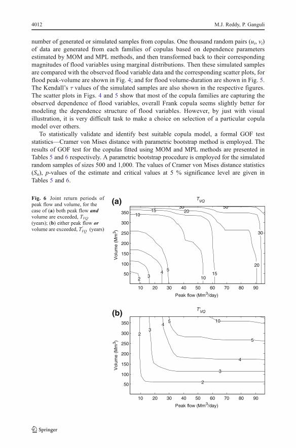
number of generated or simulated samples from copulas. One thousand random pairs (ui, vi)of data are generated from each families of copulas based on dependence parametersestimated by MOM and MPL methods, and then transformed back to their correspondingmagnitudes of flood variables using marginal distributions. Then these simulated samplesare compared with the observed flood variable data and the corresponding scatter plots, forflood peak-volume are shown in Fig. 4; and for flood volume-duration are shown in Fig. 5.The Kendall’s τ values of the simulated samples are also shown in the respective figures.The scatter plots in Figs. 4 and 5 show that most of the copula families are capturing theobserved dependence of flood variables, overall Frank copula seems slightly better formodeling the dependence structure of flood variables. However, by just with visualillustration, it is very difficult task to make a choice on selection of a particular copulamodel over others.

To statistically validate and identify best suitable copula model, a formal GOF teststatistics—Cramer von Mises distance with parametric bootstrap method is employed. Theresults of GOF test for the copulas fitted using MOM and MPL methods are presented inTables 5 and 6 respectively. A parametric bootstrap procedure is employed for the simulatedrandom samples of sizes 500 and 1,000. The values of Cramer von Mises distance statistics(Sn), p-values of the estimate and critical values at 5 % significance level are given inTables 5 and 6.

23

4 5

10

10

15

15

20

2030

30

50

Peak flow (Mm3/day)

Vol

ume

(Mm

3 )

TVQ

10 20 30 40 50 60 70 80 90

50

100

150

200

250

300

350

2

2

3

3

4

4

5

5

10

Peak flow (Mm3/day)

Vol

ume

(Mm

3 )

T'VQ

10 20 30 40 50 60 70 80 90

50

100

150

200

250

300

350

(a)

(b)

Fig. 6 Joint return periods ofpeak flow and volume, for thecase of (a) both peak flow andvolume are exceeded, TVQ(years); (b) either peak flow orvolume are exceeded, T

0VQ (years)


From Table 5 (results of MOM based copula models), it can be seen that the GOF testresulted in significantly higher p-values for Frank copula model as compared to othermodels. From Table 6 (results of MPL based copula models), it can be noted that the smallerp-values of GOF test for Clayton copula lead to rejection of Clayton copula at 5 %significance level for flood variable pairs; whereas for Frank copula model the test resultedin significantly higher p-values for peak flow-volume and volume-duration pairs (for bothN0500 and N01,000 bootstrapped samples). Hence Frank copula is found to be best copulamodel for dependence modeling of bivariate flood data.

Further to evaluate the performance of parameter estimation methods (MOM andMPL), the performance is evaluated in terms of root mean square error (RMSE)between the Frank copula CDF and the empirical non-exceedance probability orempirical CDF (ECDF) of flood variables. The ECDF is computed using Gringorten’splotting position formula (Zhang and Singh 2006). For flood peak-volume, the resultingRMSE are 0.0441 and 0.0436 for MOM and MPL methods respectively; whereas forflood volume-duration dependence modeling, the resulting RMSE are 0.063 and 0.062for MOM and MPL methods respectively. This shows that MPL based estimator givesslightly better performance over MOM method. Therefore, Frank copula model and thecopula parameters obtained using MPL method are adopted for further analysis of floodcharacteristics.

23 4 5

10

10

20

20

25

25

30

30

50

50

Volume (Mm3)

Dur

atio

n (d

ays)

TVD

50 100 150 200 250 300 350

5

10

15

20

25

2

2

3

3

4

4

5

10

Volume (Mm3)

Dur

atio

n (d

ays)

T'VD

50 100 150 200 250 300 350

5

10

15

20

25

a

b

Fig. 7 Joint return periods offlood volume and duration, forthe case of (a) both volume andduration are exceeded, TVD(years); (b) either volume orduration are exceeded,T

0VD (years)


4.4 Joint Return Periods

The joint return period of flood variables of interest, such as flood peak flow-volume pair(TV,Q and T

0V ;Q ), flood volume –duration pair (TV,D and T

0V ;D ) can be obtained using Eqs. 10

and 11. Here it should be noted that for a given joint probability (or return period), there mayexist more than one possible flood variable combinations (e.g., flood volume and duration).Hence, the contour line of each particular return period is illustrated in Figs. 6 and 7. Thecontour plots of bivariate joint return periods associated with Eqs. 10 and 11 for floodcharacteristics are shown in separate figures. Figure 6a and b show the joint return periods ofpeak flow-volume pair for ‘AND’ and ‘OR’ cases respectively. Similarly, Fig. 7a and b showthe joint return periods of flood volume-duration pair for ‘AND’ and ‘OR’ cases respective-ly. The contour lines for specific joint return periods, in which both peak flow and volumeexceeded (TVQ), has inward bounds (Fig. 6a), whereas the joint return period, in which eitherpeak flow or volume exceeded (T

0VQ ) has outward bounds (Fig. 6b). Similar inferences can

be made from Fig. 7 for joint return periods of flood volume and duration pair.From Fig. 6, it can be noticed that for the same values of peak flow and volume, the joint

return period of TVQ is much greater than that of T0VQ. For example, in the year 1997, for

annual peak flow of 39.523 Mm3/day the corresponding flood volume was 107.2 Mm3. Thejoint return periods for this flood event TVQ estimated using Eq. 10 and T

0VQ using Eq. 11 are

5.36 and 3.38 years respectively. Similar results are observed for joint return periods of

0 50 100 150 200 250 300 350

101

102

Volume (Mm3)

TV

|Q

q (

year

s)

Q = 40 Mm3/day

Q = 60 Mm3/day

Q = 80 Mm3/day

Q = 90 Mm3/day

0 10 20 30 40 50 60 70 80 90

101

102

Peak flow (Mm3/day)

TQ

|V

v (

year

s)

V = 50 Mm3

V = 100 Mm3

V = 200 Mm3

V = 300 Mm3

(a)

(b)

Fig. 8 Conditional return periods of flood characteristics: a return period of the flood volume given the floodpeak (TV|Q≤q); b return period of the flood peak given flood volume (TV|D≤d)


volume and duration (i.e., TV,D is greater than that of T0V ;D ). These results can be very useful

for decision making in hydrologic design of water resource projects.

4.5 Conditional Return Periods

The conditional return periods of the flood volume V given the flood peak Q (TV|Q≤q), andreturn period of the flood peak Q given the flood volume V (TQ|V≤v) are computed by usingthe conditional probabilities estimated from Eq. 12, and the resultant conditional returnperiods are presented in Figs. 8 and 9. From Fig. 8(a-b), it is easy to know about returnperiods of the flood volume (flood peak) for a given value of flood peak (flood volume).Similarly, from Fig. 9(a-b), it is easy to determine return periods of the flood volume (floodduration) for a given value of flood duration (flood volume).

From Fig. 8a(b), it can be noticed that the curves indicate smaller conditional returnperiod of flood events at higher conditional peak flow values (volume) as compared to thelower conditional peak flows (volume) for the same specified value of flood volume (floodpeak). At the same time, higher the flood volume (flood peak), higher is the return period offlood event. Similar kind of trend can be seen from Fig. 9, which shows conditional returnperiod plots for flood volume and duration.

0 50 100 150 200 250 300 350

101

102

Duration (days)

TV

|D

d (

year

s)

V = 50 Mm3

V = 100 Mm3

V = 200 Mm3

V = 300 Mm3

0 5 10 15 20 25

101

102

Volume (Mm3)

TD

|V

v (

year

s)

D = 10 days

D = 15 days

D = 20 days

D = 25 days

(a)

(b)

Fig. 9 Conditional return periods of flood characteristics: a return period of the flood duration given the floodvolume (TD|V≤v); b return period of the flood volume given flood duration (TV|D≤d)


These results can be useful in hydrological risk assessment and design of hydraulicstructures, such as design of spill way and construction of flood protection structures suchas, levees, flood walls, diversion works and taking non- structural safety measures to controlflood damage and developing flood mitigation strategies. Thus, the copula based method-ology can be used as a potential tool for frequency analysis of flood flows.

5 Summary and Conclusions

In this study, a copula based methodology is presented for frequency analysis of flood flows andapplied for a case study of Upper Godavari River flows in India. For bivariate frequencyanalysis, the flood flow characteristics such as annual flood peak flow (Q), flood volume (V)and flood duration (D) are considered. The correlation for flood peak flow-flood volume pair,and flood volume—duration pair are found to be statistically significant and considered forflood frequency analysis. Parametric and nonparametric methods are evaluated for fittingmarginal distributions to flood variables and the best fit model is selected for copula modeling.Four Archimedean families of copulas namely, Ali-Mikhail-Haq (AMH), Clayton, Gumbel-Hougaard (GH), and Frank copula have been evaluated to model the joint distributions ofcorrelated flood variables. The estimation of copula parameters is carried out using method-of-moments-like (MOM) estimator based on inversion of Kendall’s t, and maximum pseudolikelihood (MPL) method. Based on dependence measures of flood data, it is noticed that Ali-Mikhail-Haq copula is not applicable for the data (as the correlation of flood variable pairsexceeded its allowable Kendall’s t range). The remaining three copulas (Clayton, GH, Frank)are fitted for flood variables and evaluated their performances using graphical methods andgoodness-of-fit (GOF) tests. Then, the best fit copula model is employed to obtain the joint andconditional return periods of flood characteristics.

The following specific conclusions can be drawn from the present study:

& The nonparametric kernel density functions are found to be best fit marginal distribu-tions for flood variables.

& On performing standard goodness-of-fit tests for the Clayton, GH, Frank copula models,it is found that Frank copula is the best fitted copula for flood peak flow-volume, andflood volume-duration pairs.

& While comparing the copula parameter estimation methods, it is found that MPL methodprovided better estimates as compared to MOM method.

& The copula based joint distribution is found to be effective in preserving the dependencestructure of flood variables and helping in better estimates of joint and conditional returnperiods of flood characteristics, which can be very useful for decision making inhydrologic design of water resource projects.

Appendix

A1 Simulation of Random Samples from Bivariate Archimedean Copulas

The generation of random variates (u, v) from Clayton and Frank copulas involves thefollowing steps:

1. Generate two independent uniform U(0,1) random variates u and q.


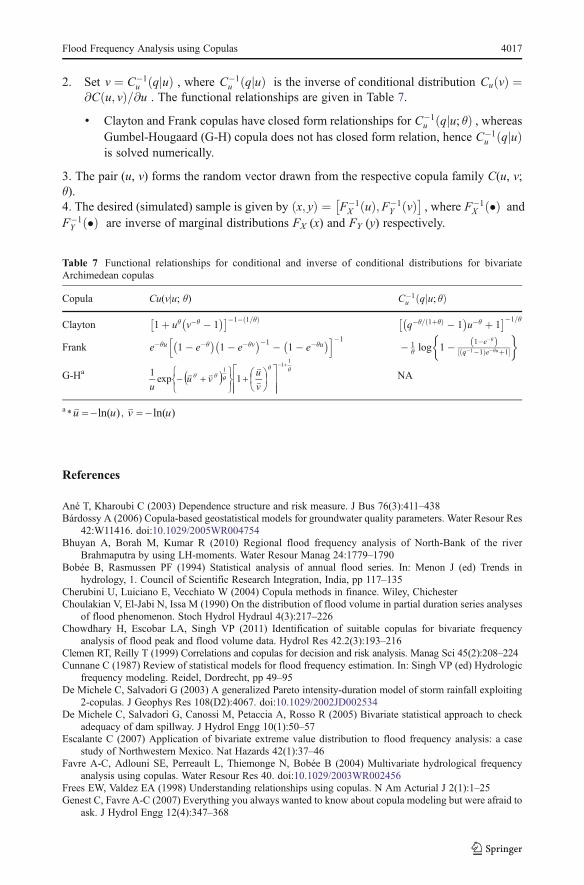
2. Set v ¼ C�1u qjuð Þ , where C�1

u qjuð Þ is the inverse of conditional distribution CuðvÞ ¼@C u; vð Þ @u= . The functional relationships are given in Table 7.

& Clayton and Frank copulas have closed form relationships for C�1u qju; θð Þ , whereas

Gumbel-Hougaard (G-H) copula does not has closed form relation, hence C�1u qjuð Þ

is solved numerically.

3. The pair (u, v) forms the random vector drawn from the respective copula family C(u, v;θ).4. The desired (simulated) sample is given by x; yð Þ ¼ F�1

X ðuÞ;F�1Y ðvÞ� �

, where F�1X �ð Þ and

F�1Y �ð Þ are inverse of marginal distributions FX (x) and FY (y) respectively.

References

Ané T, Kharoubi C (2003) Dependence structure and risk measure. J Bus 76(3):411–438Bárdossy A (2006) Copula-based geostatistical models for groundwater quality parameters. Water Resour Res

42:W11416. doi:10.1029/2005WR004754Bhuyan A, Borah M, Kumar R (2010) Regional flood frequency analysis of North-Bank of the river

Brahmaputra by using LH-moments. Water Resour Manag 24:1779–1790Bobée B, Rasmussen PF (1994) Statistical analysis of annual flood series. In: Menon J (ed) Trends in

hydrology, 1. Council of Scientific Research Integration, India, pp 117–135Cherubini U, Luiciano E, Vecchiato W (2004) Copula methods in finance. Wiley, ChichesterChoulakian V, El-Jabi N, Issa M (1990) On the distribution of flood volume in partial duration series analyses

of flood phenomenon. Stoch Hydrol Hydraul 4(3):217–226Chowdhary H, Escobar LA, Singh VP (2011) Identification of suitable copulas for bivariate frequency

analysis of flood peak and flood volume data. Hydrol Res 42.2(3):193–216Clemen RT, Reilly T (1999) Correlations and copulas for decision and risk analysis. Manag Sci 45(2):208–224Cunnane C (1987) Review of statistical models for flood frequency estimation. In: Singh VP (ed) Hydrologic

frequency modeling. Reidel, Dordrecht, pp 49–95De Michele C, Salvadori G (2003) A generalized Pareto intensity-duration model of storm rainfall exploiting

2-copulas. J Geophys Res 108(D2):4067. doi:10.1029/2002JD002534De Michele C, Salvadori G, Canossi M, Petaccia A, Rosso R (2005) Bivariate statistical approach to check

adequacy of dam spillway. J Hydrol Engg 10(1):50–57Escalante C (2007) Application of bivariate extreme value distribution to flood frequency analysis: a case

study of Northwestern Mexico. Nat Hazards 42(1):37–46Favre A-C, Adlouni SE, Perreault L, Thiemonge N, Bobée B (2004) Multivariate hydrological frequency

analysis using copulas. Water Resour Res 40. doi:10.1029/2003WR002456Frees EW, Valdez EA (1998) Understanding relationships using copulas. N Am Acturial J 2(1):1–25Genest C, Favre A-C (2007) Everything you always wanted to know about copula modeling but were afraid to

ask. J Hydrol Engg 12(4):347–368

Table 7 Functional relationships for conditional and inverse of conditional distributions for bivariateArchimedean copulas

Copula Cu(v|u; θ) C�1u qju; θð Þ

Clayton 1þ uθ v�θ � 1� �� 1� 1 θ=ð Þ

q�θ 1þθð Þ= � 1� �

u�θ þ 1� ��1 θ=

Frank e�θu 1� e�θ� �

1� e�θv� ��1 � 1� e�θu

� �h i�1� 1

θ log 1� 1�e�θð Þq�1�1ð Þe�θuþ1½ �

�G-Ha NA

a


http://dx.doi.org/10.1029/2005WR004754

http://dx.doi.org/10.1029/2002JD002534

http://dx.doi.org/10.1029/2003WR002456

Genest C, Rivest L-P (1993) Statistical inference procedures for bivariate Archimedean copulas. J Am StatAssoc 88(423):1034–1043

Genest C, Ghoudi K, Rivest LP (1995) A semiparametric estimation procedure of dependence parameters inmultivariate families of distributions. Biometrika 82(3):543–552

Genest C, Rémillard B, Beaudoin D (2009) Goodness-of-fit tests for copulas: a review and a power study.Insur Math Econ 44:199–213

Goel NK, Seth SM, Chandra S (1998) Multivariate modeling of flood flows. J Hydraul Engg 124(2):146–155Grimaldi S, Serinaldi F (2006) Asymmetric copula in multivariate flood frequency analysis. Adv Water

Resour 29(8):1155–1167Janga Reddy M, Ganguli P (2012a) Application of copulas for derivation of drought severity–duration–

frequency curves. Hydrol Process 26:1672–1685. doi:10.1002/hyp. 8287Janga Reddy M, Ganguli P (2012b) Risk assessment of hydro-climatic variability on groundwater levels in the

Manjara basin aquifer in India using Archimedean copulas. J Hydrol Engg. doi:10.1061/(ASCE)HE.1943-5584.0000564

Kao SC, Govindaraju RS (2010) A copula-based joint deficit index for droughts. J Hydrol 380(1–2):121–134Karmakar S, Simonovic SP (2009) Bivariate flood frequency analysis. Part 2: a copula-based approach with

mixed marginal distributions. J Flood Risk Manag 2(1):32–44Klein B, Pahlow M, Hundecha Y, Schumann A (2010) Probability analysis of hydrological loads for the

design of flood control systems using copulas. J Hydrol Engg 15(5):360–369Kojadinovic I, Yan J (2010) Comparison of three semiparametric methods for estimating dependence

parameters in copula models. Insur Math Econ 47:52–63Kumar R, Chatterjee C (2005) Regional flood frequency analysis using L-moments for North Brahmaputra

region of India. J Hydrol Engg 10(1):1–7Kumar R, Chatterjee C, Kumar S, Lohani AK, Singh RD (2003) Development of regional flood frequency

relationships using L-moments for middle Ganga plains subzone 1(f) of India. Water Resour Manag17:243–257

Maity R, Kumar DN (2008) Probabilistic prediction of hydroclimatic variables with nonparametric quantifi-cation of uncertainty. J Geophys Res 113:D14105. doi:10.1029/2008JD009856

Moon Y-I, Lall U (1994) Kernel quantile function estimator for flood frequency analysis. Water Resour Res 30(11):3095–3103

Nadarajah S, Shiau J (2005) Analysis of extreme flood events for the Pachang River, Taiwan. Water ResourManag 19:363–374

Nelsen RB (2006) An introduction to copulas. Springer, New YorkParida BP, Kachroo RK, Shrestha DB (1998) Regional flood frequency analysis of Mahi-Sabarmati basin

(Subzone 3-a) using index flood procedure with L-moments. Water Resour Manag 12:1–12Rakhecha PR, Singh VP (2009) Applied hydrometeorology. Capital Publishing Company, New DelhiRao NG (2001) Occurrences of heavy rainfall around the confluence line in monsoon disturbances and its

importance in causing floods. Proc Indian Acad Sci (Earth Planet Sci) 110:87–94Raynal JA, Salas JD (1987) A probabilistic model for flooding downstream of the junction of two rivers. In:

Singh VP (ed) Hydrologic frequency modeling. Reidel, Dordrecht, pp 595–602Shiau JT, Wang HY, Tsai CT (2006) Bivariate frequency analysis of floods using copulas. J Am Water Resour

Assoc 42(6):1549–1564Sklar A (1959) Functions de repartition a n dimensions et leurs marges. Publ Inst Stat Univ Paris 8:229–231Song S, Singh VP (2010) Meta-elliptical copulas for drought frequency analysis of periodic hydrologic data.

Stoch Env Res Risk A 24(3):425–434Wang C, Chang N-B, Yeh G-T (2009) Copula-based flood frequency (COFF) analysis at the confluences of

river systems. Hydrol Process 23:1471–1486Yue S (1999) Applying the bivariate normal distribution to flood frequency analysis. Water Int 24(3):248–252Yue S (2000) The bivariate lognormal distribution to model a multivariate flood episode. Hydrol Process

14:2575–2588Yue S (2001) A bivariate gamma distribution for use in multivariate flood frequency analysis. Hydrol Process

15:1033–1045Yue S, Wang CY (2004) A comparison of two bivariate extreme value distributions. Stoch Env Res Risk A

18:61–66Yue S, Ouarda TBMJ, Bobée B, Legendre P, Bruneau P (1999) The Gumbel mixed model for flood frequency

analysis. J Hydrol 226(1–2):88–100Zhang L, Singh VP (2006) Bivariate flood frequency analysis using copula method. J Hydrol Engg 11

(2):150–164


http://dx.doi.org/10.1002/hyp. 8287

http://dx.doi.org/10.1029/2008JD009856

http://dx.doi.org/10.1029/2008JD009856

http://dx.doi.org/10.1029/2008JD009856

Bivariate Flood Frequency Analysis of Upper Godavari River Flows Using Archimedean Copulas

Documents

Transcript of Bivariate Flood Frequency Analysis of Upper Godavari River Flows Using Archimedean Copulas