Value at Risk trade-off and capital allocationwith copulas

U. CherubiniUniversity of Bolognaand ICER, Turin

E. LucianoUniversity of Turin

First version: September 30, 2000,this version: November 13, 2000∗

Abstract

This paper uses copula functions in order to evaluate tail probabilitiesand market risk trade-offs at a given confidence level, dropping the jointnormality assumption on returns. Copulas enable to represent distribu-tion functions separating the marginal distributions from the associationstructure. We present an application to two stock market indices: for eachmarket we recover the marginal probability distribution. We then calibratecopula functions and recover the joint distribution. The estimated copulasdirectly give the joint probabilities of extreme losses. Their level curvesmeasure the trade-off between losses over different desks. This trade offcan be exploited for capital allocation and is shown to depend on fat-tails.

∗Part of the material in this paper was presented at the Conference ”Managing credit andmarket risk”, Verona, May 25-26, 2000.

1. Introduction

Value-at-Risk (VaR) techniques are the state of the art tools used both to mea-sure risk and to allocate capital among the different business units of a financialinstitution. As a firmwide measure of risk, VaR is a percentile of the profit andloss distribution of the financial intermediary as a whole. As a capital allocationcriterion, VaR is computed for the different business units of the firm, and for thedifferent desks within each business unit, in order to set the appropriate tradinglimits. The relationship between these two ways of using VaR is far from clear.In principle, we may think of two alternative approaches. The first one, that

is widely used in real applications, may be deemed “bottom-up”: VaR figures arecomputed for each and every single desk and then aggregated both on a diversi-fied and undiversified basis. The aggregate VaR figure is computed using linearcorrelation, which means relying on the assumption of multivariate normality ofreturns. As this assumption has been widely criticized both on empirical andtheoretical grounds, one should support the analysis with some other device tocheck the accuracy of the VaR figures: for example, RiskMetrics proposes to takea look at the joint distribution of losses on the different markets involved, and tocompare the empirical one with the multivariate normal used in their approach.This leads us to a second approach to allocate capital among the business

units, that we may call “top-down”: capital could be allocated in such a way asto grant a given joint probability of exceeding the loss limits. This approach usesless capital than the previous one, as the joint probability of exceeding the losslimits is lower than the probability that a single unit experiences a loss higherthan the capital.The complexity of the problem increases if we drop the assumption of joint

normality of returns. A subtle point here is that normality of losses of each singledesk, which may also be questioned, is not even sufficient for the joint distributionto be normal: in other terms, it may well be the case that the losses of each deskare normally distributed while their joint probability is far from Gaussian. Noticethat no matter which approach is used to allocate capital, one is interested in theanalysis of the joint probability distribution of losses. In the case of a bottom upapproach one would like to check the joint probability that the desks run out oftheir capital endowment. In the alternative top down approach one is interestedin the trade-off between the capital allocated: in other words, one would liketo know how much capital should be allocated to the different desks in order tomaintain the same joint probability target. In both cases, the answer relies on the

2

dependence structure of losses between different desks. Intuitively, if the lossesof two desks are perfectly positively dependent, one would expect that the jointprobability of running out of capital would be the same as that chosen for eachsingle desk. On the contrary, if the losses exhibit perfect negative dependence,the two desks provide a “perfect hedge” for each other and one would expect zerojoint probability of loss. In the reality, however, as common wisdom suggests,“no perfect hedge exists”, and one is left with the problem of modelling imperfectdependence among losses.The purpose of this paper is to suggest the use of copula functions to perform

a pairwise analysis of the dependence structure of losses of desks. Copulas, oncecomputed at the marginal distribution values, provide a useful tool to representany joint distribution function. Opposite to traditional joint distributions howeverthey separate the effect of the marginal distribution from the one of associationor dependence between returns. The same separation applies when it comes tostatistical estimation: for both reasons, they seem to be particularly well suitedfor financial applications1.The approach is applied to both problems discussed above: on one side, we

address the issue of the joint non-normality of returns in a VaR context, providinga measure of joint tail probability. On the other, endowed with the concepts de-veloped for non-normality, we explore the issue of VaR trade-offs between differentdesks or markets.The paper is structured as follows. Section 2 introduces some mathematical

background, namely the concept of copula and its properties. Section 3 intro-duces non parametric measures of association, which enable us to drop the jointnormality hypothesis. It also presents some one-parameter families of copulas —belonging to the so-called Archimedean class — whose relationship with the as-sociation measure is particularly simple and amenable to statistical estimation.Section 4 formalizes the use of copula functions both for the validation of jointprobability of losses over different desks and for the analysis of their trade-off. Sec-tion 5 presents an application of joint losses estimation and trade-off evaluationto a couple of stock market indices (FTSE100 and S&P100). Section 6 concludesand outlines further research.

1Frees and Valdez (1998) mention a number of additional advantages of copulas with respectto joint distribution functions.

3

2. Mathematical background: copula functions

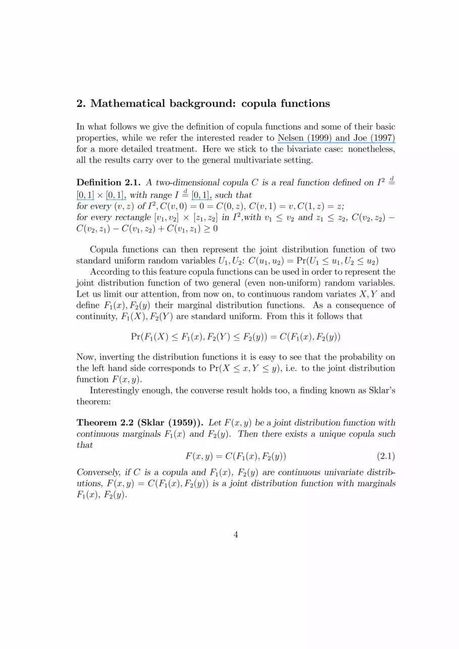
In what follows we give the definition of copula functions and some of their basicproperties, while we refer the interested reader to Nelsen (1999) and Joe (1997)for a more detailed treatment. Here we stick to the bivariate case: nonetheless,all the results carry over to the general multivariate setting.

Definition 2.1. A two-dimensional copula C is a real function defined on I2 d=

[0, 1]× [0, 1], with range I d= [0, 1], such that

for every (v, z) of I2, C(v, 0) = 0 = C(0, z), C(v, 1) = v, C(1, z) = z;for every rectangle [v1, v2] × [z1, z2] in I2,with v1 ≤ v2 and z1 ≤ z2, C(v2, z2) −C(v2, z1)− C(v1, z2) + C(v1, z1) ≥ 0

Copula functions can then represent the joint distribution function of twostandard uniform random variables U1, U2: C(u1, u2) = Pr(U1 ≤ u1, U2 ≤ u2)According to this feature copula functions can be used in order to represent the

joint distribution function of two general (even non-uniform) random variables.Let us limit our attention, from now on, to continuous random variates X, Y anddefine F1(x), F2(y) their marginal distribution functions. As a consequence ofcontinuity, F1(X), F2(Y ) are standard uniform. From this it follows that

Pr(F1(X) ≤ F1(x), F2(Y ) ≤ F2(y)) = C(F1(x), F2(y))

Now, inverting the distribution functions it is easy to see that the probability onthe left hand side corresponds to Pr(X ≤ x, Y ≤ y), i.e. to the joint distributionfunction F (x, y).Interestingly enough, the converse result holds too, a finding known as Sklar’s

theorem:

Theorem 2.2 (Sklar (1959)). Let F (x, y) be a joint distribution function withcontinuous marginals F1(x) and F2(y). Then there exists a unique copula suchthat

F (x, y) = C(F1(x), F2(y)) (2.1)

Conversely, if C is a copula and F1(x), F2(y) are continuous univariate distrib-utions, F (x, y) = C(F1(x), F2(y)) is a joint distribution function with marginalsF1(x), F2(y).

4

The main advantage of copulas consists in representing the joint probabilityditribution by separating the impact of the marginals from the association struc-ture, explained by the copula functional form.Three particular copulas are worth mentioning: the product copula, the min-

imum and the maximum copulas. As for the first, the copula representation ofa distribution F degenerates into the so-called product copula, C(v, z) = v · z, ifand only if X and Y are independent. As for the others, they derive from thewell-known Fréchet-Hoeffding result in probability theory, stating that every jointdistribution function is constrained between the bounds

Fl(x, y) ≤ F (x, y) ≤ Fu(x, y)where the lower and upper limits Fl(x, y) and Fl(x, y) are defined as

Fl(x, y)d= max(F1(x) + F2(y)− 1, 0) (2.2)

Fu(x, y)d= min(F1(x), F2(y))

As a consequence of Sklar’s theorem, the Fréchet-Hoeffding bounds exist for cop-ulas too:

Cl(v, z) ≤ C(v, z) ≤ Cu(v, z)where the lower bound or minimum copula and the upper bound or maximumcopula are:

Cl(v, z)d= max(v + z − 1, 0) (2.3)

Cu(v, z)d= min(v, z)

The following proposition in Embrechts, McNeil and Straumann (1999) high-lights the meaning of the maximum and minimum copulas:

Theorem 2.3 (Hoeffding (1940), Frechet (1957)). If the continuous randomvariables X and Y have the copula Cu, then there exists a monotonically increas-ing function U such that

Y = U(X) U = F−12 (F1))

where F−12 is the generalized inverse of F2. If instead they have the copula Cl,then there exists a monotonically decreasing function L such that

Y = L(X) L = F−12 (1− F1))The converse of the previous results holds too.

In the first case, X and Y are called comonotonic, while in the second theyare deemed countermonotonic.

5

3. Association measures and copula functions

In order to extract the dependence structure from financial data we need a measureof association: in what follows we review some widely known measures of thistype and focus on their relationships with copulas. We first show why, as ageneral rule, the use of linear correlation without the normality assumption maybe problematic. We then introduce the standard non-parametric measures ofassociation, such as Kendall’s tau and Spearman’s rho (see for instance Gibbons1988). Finally, we are going to relate them with some copula families.

3.1. Association measures

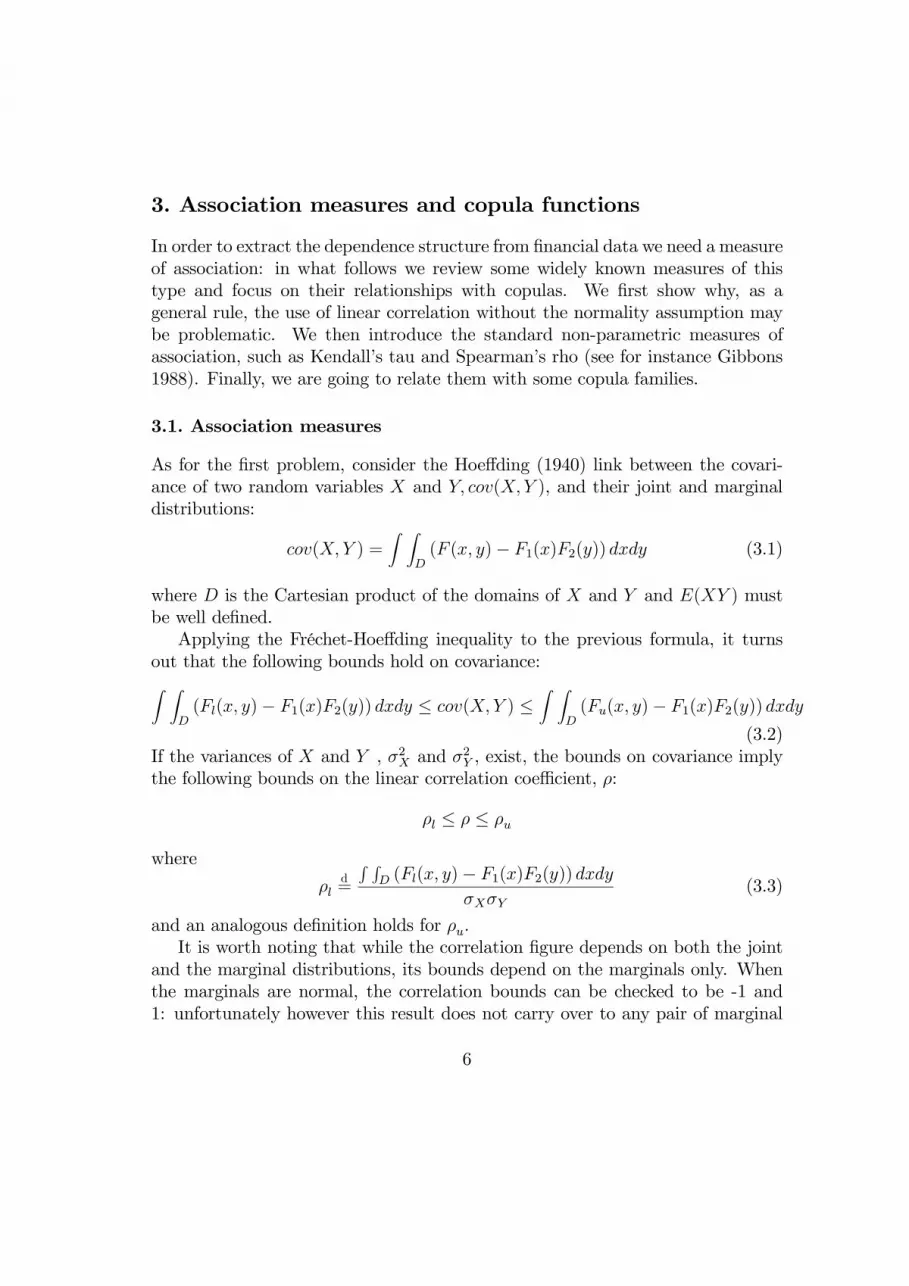
As for the first problem, consider the Hoeffding (1940) link between the covari-ance of two random variables X and Y, cov(X,Y ), and their joint and marginaldistributions:

cov(X, Y ) =Z Z

D(F (x, y)− F1(x)F2(y)) dxdy (3.1)

where D is the Cartesian product of the domains of X and Y and E(XY ) mustbe well defined.Applying the Fréchet-Hoeffding inequality to the previous formula, it turns

out that the following bounds hold on covariance:Z ZD(Fl(x, y)− F1(x)F2(y)) dxdy ≤ cov(X, Y ) ≤

Z ZD(Fu(x, y)− F1(x)F2(y)) dxdy

(3.2)If the variances of X and Y , σ2X and σ2Y , exist, the bounds on covariance implythe following bounds on the linear correlation coefficient, ρ:

ρl ≤ ρ ≤ ρu

where

ρld=

R RD (Fl(x, y)− F1(x)F2(y)) dxdy

σXσY(3.3)

and an analogous definition holds for ρu.It is worth noting that while the correlation figure depends on both the joint

and the marginal distributions, its bounds depend on the marginals only. Whenthe marginals are normal, the correlation bounds can be checked to be -1 and1: unfortunately however this result does not carry over to any pair of marginal

6

distributions. Indeed, it may be proved, along Fréchet (1957), that the correlationbounds can be smaller than one in absolute value and that they differ over differentdistributions.This shortcoming adds to the fact that ρ captures the linear dependence only.

Fortunately, it does not extend to other measures of association, such as Kendall’stau and Spearman’s rho, for which we recall the definitions:

Definition 3.1 (Kruskal (1958)). Let (Xa, Ya), (Xb, Yb) be iid random vectors,with distribution function F (x, y) and common margins F1 and F2 :

(Xa ∼ F1, Xb ∼ F1, Ya ∼ F2, Yb ∼ F2)The Kendall’s tau τ is defined as

τd= Pr ((Xa −Xb)(Ya − Yb) > 0)− Pr ((Xa −Xb)(Ya − Yb) < 0)

Definition 3.2 (Kruskal (1958)). Let (Xa, Ya), (Xb, Yb), (Xc, Yc) be iid randomvectors, with distribution function F (x, y) and common margins F1 and F2

(Xa ∼ F1, Xb ∼ F1,Xc ∼ F1, Ya ∼ F2, Yb ∼ F2, Yc ∼ F2)The Spearman’ s rho R is defined as

Rd= 3 [Pr ((Xa −Xb)(Ya − Yc) > 0)− Pr ((Xa −Xb)(Ya − Yc) < 0)]

The relationship of τ and R with copula parameters can be traced back to thefollowing theorems:

Theorem 3.3 (Nelsen (1999)). If (X,Y ) are continuous random variables withcopula C, the following representation holds for τ :

τ = 4Z Z

I2C(v, z)dC(v, z)− 1

Theorem 3.4 (Nelsen (1999)). If (X,Y ) are continuous random variables withcopula C, the following representation holds for R:

R = 12Z Z

I2C(v, z)dvdz − 3 (3.4)

Unlike the linear correlation coefficient ρ, both τ and R only depend on thecopulas, and not on the marginals; in addition, it can be proved that their boundsare always -1 and +1. This makes the two non parametric measures ideal instru-ments for the joint study of non-normality and association.

7

3.2. Families of copulas

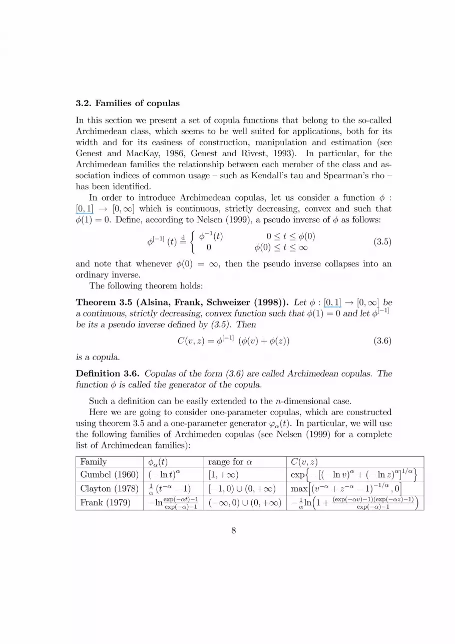
In this section we present a set of copula functions that belong to the so-calledArchimedean class, which seems to be well suited for applications, both for itswidth and for its easiness of construction, manipulation and estimation (seeGenest and MacKay, 1986, Genest and Rivest, 1993). In particular, for theArchimedean families the relationship between each member of the class and as-sociation indices of common usage — such as Kendall’s tau and Spearman’s rho —has been identified.In order to introduce Archimedean copulas, let us consider a function φ :

[0, 1] → [0,∞] which is continuous, strictly decreasing, convex and such thatφ(1) = 0. Define, according to Nelsen (1999), a pseudo inverse of φ as follows:

φ[−1] (t) d=

(φ−1(t) 0 ≤ t ≤ φ(0)0 φ(0) ≤ t ≤ ∞ (3.5)

and note that whenever φ(0) = ∞, then the pseudo inverse collapses into anordinary inverse.The following theorem holds:

Theorem 3.5 (Alsina, Frank, Schweizer (1998)). Let φ : [0, 1] → [0,∞] bea continuous, strictly decreasing, convex function such that φ(1) = 0 and let φ[−1]

be its a pseudo inverse defined by (3.5). Then

C(v, z) = φ[−1] (φ(v) + φ(z)) (3.6)

is a copula.

Definition 3.6. Copulas of the form (3.6) are called Archimedean copulas. Thefunction φ is called the generator of the copula.

Such a definition can be easily extended to the n-dimensional case.Here we are going to consider one-parameter copulas, which are constructed

using theorem 3.5 and a one-parameter generator ϕα(t). In particular, we will usethe following families of Archimeden copulas (see Nelsen (1999) for a completelist of Archimedean families):

Family φα(t) range for α C(v, z)

Gumbel (1960) (− ln t)α [1,+∞) expn− [(− ln v)α + (− ln z)α]1/α

oClayton (1978) 1

α(t−α − 1) [−1, 0) ∪ (0,+∞) max

h(v−α + z−α − 1)−1/α , 0

iFrank (1979) −lnexp(−αt)−1

exp(−α)−1 (−∞, 0) ∪ (0,+∞) − 1αln³1 + (exp(−αv)−1)(exp(−αz)−1)

exp(−α)−1´

8

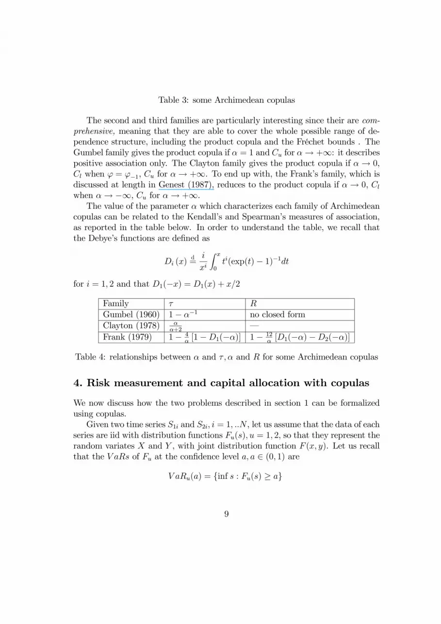
Table 3: some Archimedean copulas

The second and third families are particularly interesting since their are com-prehensive, meaning that they are able to cover the whole possible range of de-pendence structure, including the product copula and the Fréchet bounds . TheGumbel family gives the product copula if α = 1 and Cu for α→ +∞: it describespositive association only. The Clayton family gives the product copula if α→ 0,Cl when ϕ = ϕ−1, Cu for α→ +∞. To end up with, the Frank’s family, which isdiscussed at length in Genest (1987), reduces to the product copula if α→ 0, Clwhen α→ −∞, Cu for α→ +∞.The value of the parameter α which characterizes each family of Archimedean

copulas can be related to the Kendall’s and Spearman’s measures of association,as reported in the table below. In order to understand the table, we recall thatthe Debye’s functions are defined as

Di (x)d=i

xi

Z x

0ti(exp(t)− 1)−1dt

for i = 1, 2 and that D1(−x) = D1(x) + x/2

Family τ RGumbel (1960) 1− α−1 no closed formClayton (1978) α

α+2–

Frank (1979) 1− 4α[1−D1(−α)] 1− 12

α[D1(−α)−D2(−α)]

Table 4: relationships between α and τ ,α and R for some Archimedean copulas

4. Risk measurement and capital allocation with copulas

We now discuss how the two problems described in section 1 can be formalizedusing copulas.Given two time series S1i and S2i, i = 1, ..N , let us assume that the data of each

series are iid with distribution functions Fu(s), u = 1, 2, so that they represent therandom variates X and Y , with joint distribution function F (x, y). Let us recallthat the V aRs of Fu at the confidence level a, a ∈ (0, 1) are

V aRu(a) = {inf s : Fu(s) ≥ a}

9

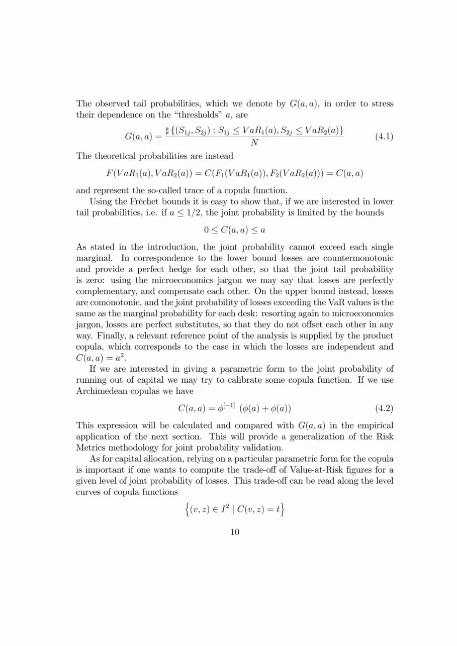
The observed tail probabilities, which we denote by G(a, a), in order to stresstheir dependence on the “thresholds” a, are

G(a, a) =] {(S1j, S2j) : S1j ≤ V aR1(a), S2j ≤ V aR2(a)}

N(4.1)

The theoretical probabilities are instead

F (V aR1(a), V aR2(a)) = C(F1(V aR1(a)), F2(V aR2(a))) = C(a, a)

and represent the so-called trace of a copula function.Using the Fréchet bounds it is easy to show that, if we are interested in lower

tail probabilities, i.e. if a ≤ 1/2, the joint probability is limited by the bounds0 ≤ C(a, a) ≤ a

As stated in the introduction, the joint probability cannot exceed each singlemarginal. In correspondence to the lower bound losses are countermonotonicand provide a perfect hedge for each other, so that the joint tail probabilityis zero: using the microeconomics jargon we may say that losses are perfectlycomplementary, and compensate each other. On the upper bound instead, lossesare comonotonic, and the joint probability of losses exceeding the VaR values is thesame as the marginal probability for each desk: resorting again to microeconomicsjargon, losses are perfect substitutes, so that they do not offset each other in anyway. Finally, a relevant reference point of the analysis is supplied by the productcopula, which corresponds to the case in which the losses are independent andC(a, a) = a2.If we are interested in giving a parametric form to the joint probability of

running out of capital we may try to calibrate some copula function. If we useArchimedean copulas we have

C(a, a) = φ[−1] (φ(a) + φ(a)) (4.2)

This expression will be calculated and compared with G(a, a) in the empiricalapplication of the next section. This will provide a generalization of the RiskMetrics methodology for joint probability validation.As for capital allocation, relying on a particular parametric form for the copula

is important if one wants to compute the trade-off of Value-at-Risk figures for agiven level of joint probability of losses. This trade-off can be read along the levelcurves of copula functions n

(v, z) ∈ I2 | C(v, z) = to

10

In the Archimedean case the level curves explicitly give an argument of the copulaas a function of the other according to the relationship

z = ϕ[−1] (ϕ(t)− ϕ(v)) (4.3)

which is defined (consistently with the Fréchet bounds) for t ≤ v. One can easilyargue, at least when the generator has an ordinary inverse, that, along a levelcurve, z is a decreasing function of v, with derivative

dz

dv= − ϕ0(v)

ϕ0 (z)

(since ϕ0(u) < 0 for u ∈ [0, 1]). In addition, since ϕ ∈ C2 and ϕ00(u) > 0, thesecond derivative of z

d2z

dv2= −ϕ

00(v)

ϕ0 (z)

exists, is positive, and z is a convex function of v.For the Clayton copula for instance the level curves reduce to

z =³t−α − v−α + 1

´−1/αObviously, the level curves can be written also in terms of the original variates Xand Y , whenever F2 has an inverse, as

y = F−12³ϕ[−1] (ϕ(t)− ϕ(F1(x)))

´(4.4)

Due to the monotonicity properties of univariate distribution functions, y is adecreasing function of x along the level curve. However, concavity cannot bediscussed without further assumptions on the marginals.Both the expressions (4.3) and (4.4) will be used and commented in the em-

pirical application.

5. An Empirical Application

In this section we apply copulas to the estimation of the joint probability dis-tributions of daily returns on the English and U.S. stock markets. The task isto provide an estimate of the joint probability of losses on these markets andto design a schedule of VaR allocation between them for any given level of joint

11

probability. The data refer to the FTSE100 and S&P 100 indices from Janu-ary 3rd 1995 through April 20th 2000. They are closing values downloaded fromBloomberg.We first use a standard non-parametric technique to derive the marginal den-

sity function of each index. For comparison, we also compute the correspondingGaussian marginals, i.e. the normals with the same mean and variance of the em-pirical distribution. Then, we use a non-parametric technique based on Kendall’sτ to estimate copula functions and use them to compute the tail joint probabil-ities; the evaluation of the latter will provide us with a criterion to select themost appropriate copula within the Archimedean family. To end up with, we willcompute level curves at the 1% level of confidence for the two indices at hand.We will also compare the level curves obtained with empirical marginals with theones corresponding to Gaussian ones.

5.1. Non-parametric estimation of marginal distributions

We estimate the marginal probability distributions of the two indices involved(S&P and FTSE) using a standard historical simulation technique, i.e. the em-pirical distribution of past returns. It is well-known that historical simulation isa powerful tool to address the issue of non-normality of returns2.Figures 6.1 and 6.2 report the empirical density function of the two indexes,

together with the corresponding normal densities. Even a simple visual inspectionof the frequencies suggests evidence of leptokurtosis in both cases, in particular forthe American index. This feeling is confirmed both by the excess kurtosis figures,that read 3.68 and 1.45 for S&P and FTSE respectively, and by the 1% VaRfigures which turn out to be 2.9% for both the empirical distributions, comparedwith 2.4% and 2.3% for the Gaussian one.

Insert here figures 6.1 and 6.2

2It is also true that resorting to some more parsimonious technique, such as a Garch filter(Barone-Adesi and Giannopoulos, 1999), rather than directly using the histogram of yieldsmay enhance the robustness of the analysis. We however chose to stick to the most standardapplication of historical simulation simply because it is widely used in concrete risk managementapplications and because the focus of our analysis is in the estimation of the joint probabilitydistribution, for any given pair of marginals. It should be clear that the same analysis carriesover to cases in which the marginal distribution is estimated with far more sophisticated tools.

12

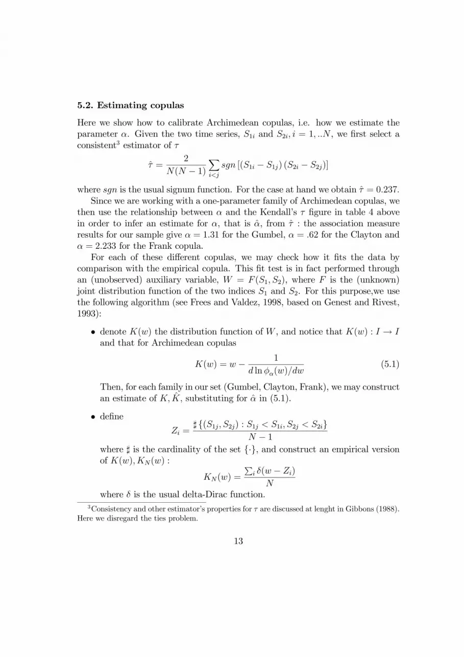
5.2. Estimating copulas

Here we show how to calibrate Archimedean copulas, i.e. how we estimate theparameter α. Given the two time series, S1i and S2i, i = 1, ..N , we first select aconsistent3 estimator of τ

τ̂ =2

N(N − 1)Xi<j

sgn [(S1i − S1j) (S2i − S2j)]

where sgn is the usual signum function. For the case at hand we obtain τ̂ = 0.237.Since we are working with a one-parameter family of Archimedean copulas, we

then use the relationship between α and the Kendall’s τ figure in table 4 abovein order to infer an estimate for α, that is α̂, from τ̂ : the association measureresults for our sample give α = 1.31 for the Gumbel, α = .62 for the Clayton andα = 2.233 for the Frank copula.For each of these different copulas, we may check how it fits the data by

comparison with the empirical copula. This fit test is in fact performed throughan (unobserved) auxiliary variable, W = F (S1, S2), where F is the (unknown)joint distribution function of the two indices S1 and S2. For this purpose,we usethe following algorithm (see Frees and Valdez, 1998, based on Genest and Rivest,1993):

• denote K(w) the distribution function of W , and notice that K(w) : I → Iand that for Archimedean copulas

K(w) = w − 1

d lnφα(w)/dw(5.1)

Then, for each family in our set (Gumbel, Clayton, Frank), we may constructan estimate of K, K̂, substituting for α̂ in (5.1).

• defineZi =

] {(S1j , S2j) : S1j < S1i, S2j < S2i}N − 1

where ] is the cardinality of the set {·}, and construct an empirical versionof K(w),KN(w) :

KN(w) =

Pi δ(w − Zi)N

where δ is the usual delta-Dirac function.3Consistency and other estimator’s properties for τ are discussed at lenght in Gibbons (1988).

Here we disregard the ties problem.

13

• compare KN(w) and K̂(w) graphically and via mean-square error.

The plots of the empirical versions ofK and those from the fitted Archimedeancopulas are presented in figure 6.3 below. The corresponding mean square errorsare .15%0 for the Gumbel, .47%0 for the Clayton and .25%0 for the Frank copulas.

Insert here figure 6.3

It is evident both from the figure and the errors that, overall, the best-fit isprovided by the Gumbel copula: however, we disregard it in the ensuing analysisboth because it can represent non-negative association only, which seems to be ingeneral quite a restrictive condition in VaR studies, and because its K function isnot the closest to the empirical one in the low quantiles region (for low values ofw). At the opposite, the Clayton’s copula is generally dominated by the others;nonetheless, we can see from the figure 6.2 and we will verify in the next sectionthat the Clayton is much more conservative and appropriate in representing theindices behavior in the tails, where the other two copulas are quite similar and atodds with the empirical behavior.

5.3. Multivariate Value-at-Risk validation

We are now in a position to evaluate the joint distribution of losses, or tail prob-ability, for any pair of choice of VaR figures, by computing the traces of theempirical and estimated copulas, which are represented in eq. (4.1) and (4.2)above respectively.In figures 6.4 and 6.5 we report these copulas, computed respectively with the

estimated parameters and with the parameter values which “maximize” the fit:in figure 6.4 we report, within the triangle that defines the Fréchet bounds, theempirical copula, along with the Frank’s, the Clayton’s and the product copula.We omit the Gumbel case because of its similarity in the queues with respect tothe Frank. In figure 6.5 we focus on the estimated Frank and Clayton’s copulas,and use the parameter values (around 8 for the former, 5 for the latter) whichmake them closest to the empirical one

Insert here figures 6.4 and 6.5

A brief inspection of the former graph highlights that the Frank copula un-derestimates the joint probability of losses in the tail, since it underestimates

14

dependence. From the second figure we also notice that in order to provide agood fit at the 5% probability level the dependence parameter α for the Frankmust be increased substantially. Moreover, one can verify that this is not enoughto provide a good fit at the 1% level, for which the parameter of the copulafunction should be raised to a value of about 25.The Clayton copula seems to provide a better fit, both when evaluated at the

estimated parameter value (figure 6.4) and at the “best-fit” one (figure 6.5), 0.5,which is also pretty close to the figure estimated for the whole distribution, 0.62.As a result of this validation step, the Clayton’s copula, while quite inappro-

priate when we consider the whole distribution, will be used in the next sectionto represent tail behavior.

5.4. Value-at-Risk trade-offs

As we pointed out above, using a parametric form for the copula function, such asone of the Archimedean family, is not only useful but definitely necessary if onewants to design a trade-off between the capital allocated to the different businessunits in such a way as to preserve the same joint probability of losses: in fact, itwould not be possible to perform this task using empirical copulas.Figure 6.6 below describes the trade-off at the 1% level of confidence, in terms

of the underlying risks, according to (4.4) and using the empirical marginals tocompute the percentiles on the axes. The irregular shape of the curve is due toexactly to the fact that we use the percentiles of the empirical distributions. Asreference instances, we again report the trade-off in the case of perfect positiveand negative dependence as well as that of independence.

Insert here figure 6.6

The instances of perfect positive and negative dependence design a triangle-shaped area. The closer the trade-off line to lower region of the triangle, thehigher the correlation between losses: in this case, the joint probability cannot beaffected by moving capital from a desk to the other. On the contrary, if the trade-off line is close to the upper region of the triangle, we have negative dependence,and the losses of the two business units tend to offset each other. Finally, if thetrade-off schedule is close to the independence line, trading-off capital for one deskto the other is made possible by diversification. The case of our application is infact close to the independence schedule.

15

We may ask what is the effect of leptokurtosis of the marginal distributionson the capital trade off. For this purpose, we compare the trade-off in figure 6.6,i.e. the one obtained using the empirical distribution, with that obtained usingthe corresponding Gaussian marginals. In figures 6.7. and 6.8, the comparisonis reported for the extreme correlation hypotheses and for the copula estimatedfrom the sample respectively.

Insert here figures 6.7 and 6.8

Inspection of the former graph shows that the fat-tail problem makes thetriangle-shaped trade-off region bigger: indeed, the more dependent the losses, thecloser the joint probability is to the Fréchet bounds. At the upper bound, the jointprobability coincides with one of the marginals, which, because of leptokurtosis,calls for higher VaR figures in the empirical than in the Gaussian case.Inspection of the latter figure confirms the result in the former: again the

trade-off schedule referred to the empirical marginal distributions is at the leftof that computed with Gaussian marginals, since for the same joint probabilityfat-tails provide bigger percentiles in the marginals.

6. Conclusions

In this paper we adopt copula functions in order to validate VaR figures andallocate capital. The adoption of copulas presents a number of advantages withrespect to direct estimation or smoothing of multivariate distributions: mainly,copulas separate marginal behavior from association and are easily amenable tostatistical estimation, at least in the bivariate case needed for validation à laRiskmetrics. In addition, we suggest the use of Archimeden copulas, which canbe estimated starting from a non parametric measure of association and for whichselection procedures exist or can be envisaged.After having developed reliable multivariate models of returns, we explore

the existence of trade-offs of VaRs — and consequently of capital allocated forsafety reasons — between different desks or markets: in the limit, between a deskand the rest of the trading book. We are able to quantify this trade-off and tobuild indifference curves between desks or units. These curves tend to a rightangle when the units returns are perfectly, positively dependent, and get closerto a straight line when they move from perfect dependence to independence andperfectly negative dependence. For any joint probability of losses for the whole

16

firm and for a given loss on one desk, the trade-off determines the unique VaRfigure for the rest of the book. So, the level curve gives the capital to be allocatedto one desk and to the rest of the portfolio to maintain a given joint probabilityof losses.We have performed the trade-off analysis on more than five years of daily

data on FTSE100 and S&P100. The empirical analysis has been conducted usingboth empirical and Gaussian marginals: this has allowed us to study the effectof fat-tailedness of the returns on the VaR trade-off. We show that the trade-offschedule is shifted downwards by fat tails. In this sense, a correct estimation ofthe marginals is important, even if the trade-off exists because of the associationstructure only, as represented by copulas.

17

References

[1] Alsina, C., Frank, M.J. and Schweizer, B., 1998, On the characterization ofa class of binary operations on distribution functions, Statist. Probab. Lett.,17, 85-89

[2] Barone-Adesi, G., Giannopoulos, K., and Vosper, L., 1999, VaR withoutcorrelations for non-linear portfolios, Journal of Futures Markets, 19, 583-602.

[3] Embrechts, P., McNeil, A. and Straumann, D., 1999, Correlation and depen-dence in risk management: properties and pitfalls, ETHZ working paper.

[4] Fréchet, M., Les tableaux de corrélations dont les marges sont données, An-nales de l’Université de Lyon, Sciences Mathématiques at Astronomie, SérieA, 4, 13-31.

[5] Frees, E.,W. and Valdez, E., 1998, Understanding relationships using copulas,North American Actuarial Journal, 2, 1-25.

[6] Genest, C., 1987, Frank’s family of bivariate distributions, Biometrika, 74,549-555.

[7] Genest, C. and MacKay, J., 1986, The joy of copulas: bivariate distributionswith uniform marginals, The American Statistician, 40, 280-283.

[8] Genest, C. and Rivest, L.P., 1993, Statistical inference procedures for bivari-ate Archimedian copulas, Journal of Amer. Statist. Assoc., 88, 423, 1034-1043.

[9] Gibbons, J.D., 1988, Nonparametric statistical inference, Dekker, New York.

[10] Hoeffding, W., 1940, Massstabinvariante Korrelationstheorie, Schriften desMathematischen Seminars und des Instituts fur Angewandte Mathematik derUniversitat Berlin, 5, 181-233.

[11] Joe, H., 1997, Multivariate models and dependence concepts, Chapman andHall, London.

[12] Klugman, S.A. and Parsa, R., 1999, Fitting bivariate loss distributions withcopulas, Insurance: mathematics and economics, 24, 139-148.

18

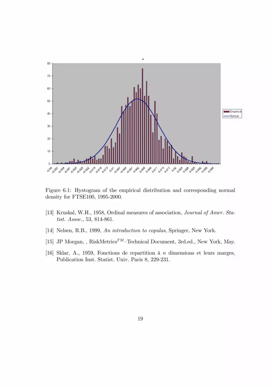
Figure 6.1: Hystogram of the empirical distribution and corresponding normaldensity for FTSE100, 1995-2000.

[13] Kruskal, W.H., 1958, Ordinal measures of association, Journal of Amer. Sta-tist. Assoc., 53, 814-861.

[14] Nelsen, R.B., 1999, An introduction to copulas, Springer, New York.

[15] JP Morgan, , RiskMetricsTM—Technical Document, 3rd.ed., New York, May.

[16] Sklar, A., 1959, Fonctions de repartition à n dimensions et leurs marges,Publication Inst. Statist. Univ. Paris 8, 229-231.

19

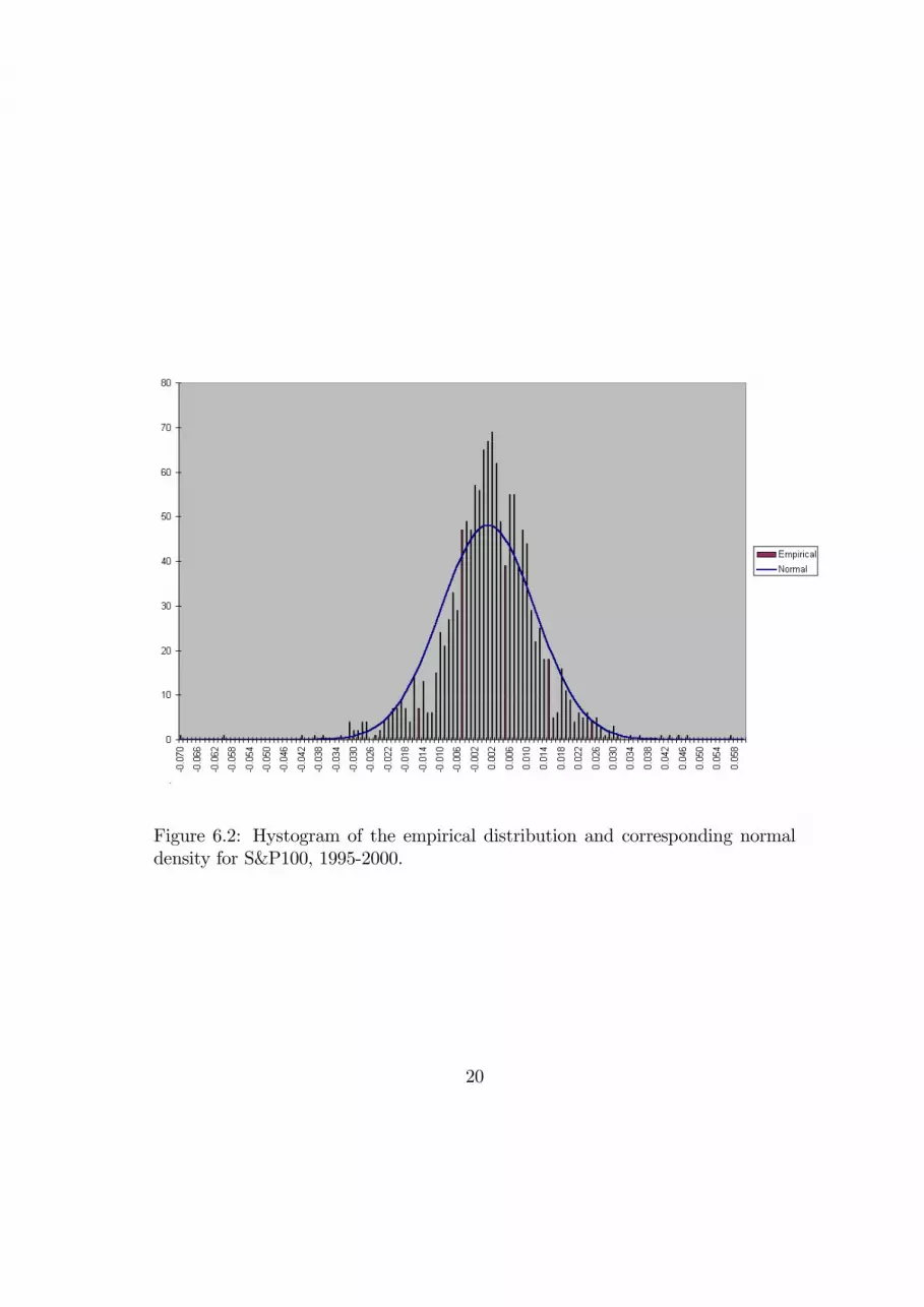
Figure 6.2: Hystogram of the empirical distribution and corresponding normaldensity for S&P100, 1995-2000.

20

Figure 6.3: KN(w) empirical and K(w) for different copula choices.

21

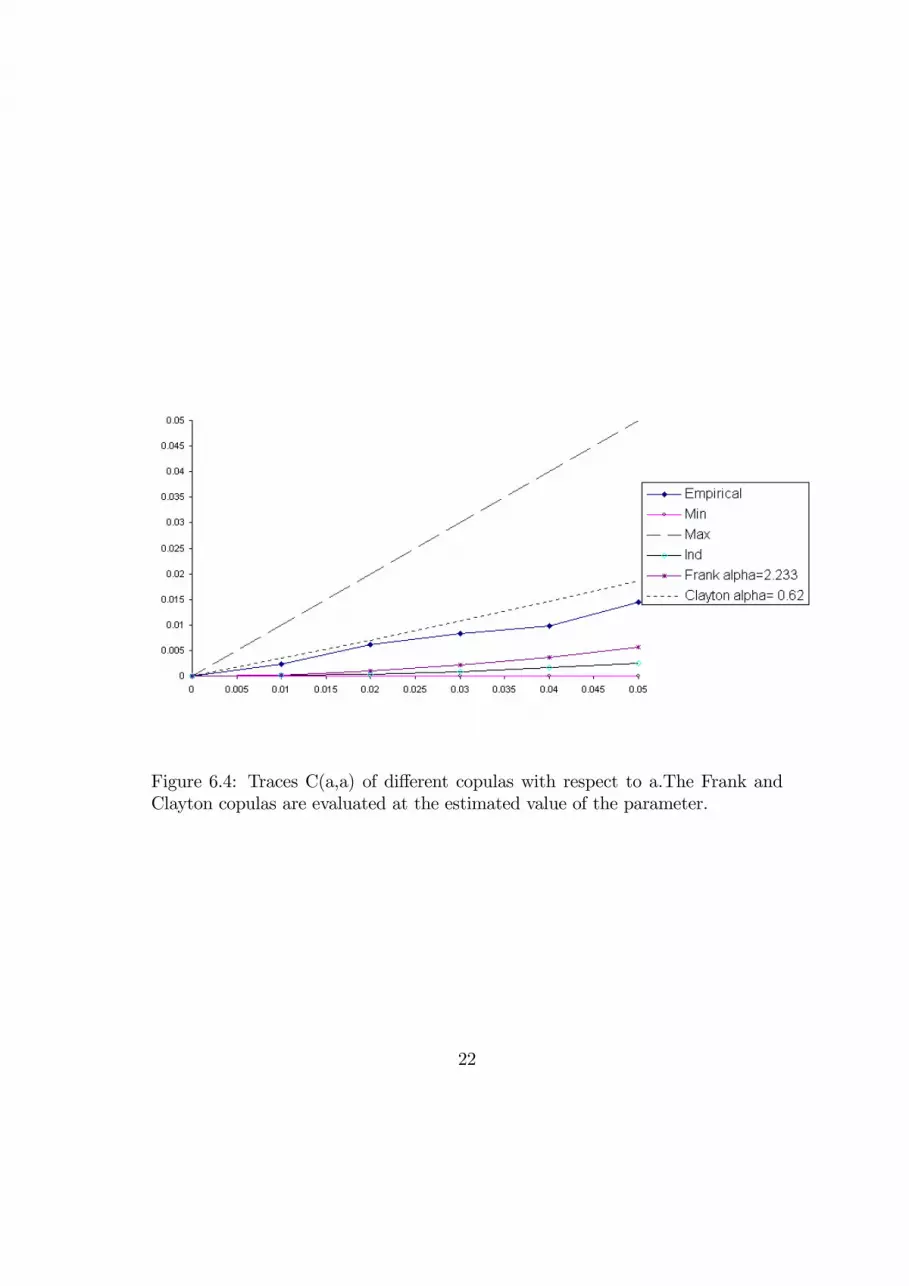
Figure 6.4: Traces C(a,a) of different copulas with respect to a.The Frank andClayton copulas are evaluated at the estimated value of the parameter.

22

Figure 6.5: Traces C(a,a) of different copulas with respect to a. The Frank andClayton copulas are evaluated at the ”best-fit” value of the parameter alpha.

23

Figure 6.6: VaR trade-off FTSE100-S&P100, with different copulas and the em-pirical marginals.

24

Figure 6.7: Upper (+) and Lower (-) Bounds for the VaR trade-off betweenFTSE100 and S&P100, with the empirical marginals and with the Gaussian (G)ones.

25

Figure 6.8: Comparison between the VaR trade-off FTSE100 & S&P100 in cor-respondence to the estimated association, using the empirical and the Gaussianmarginal.

26