
Trace Register Allocation - System Software
179
Submied by DI Josef Eisl, BSc. Submied at Institute for System Soſtware Supervisor and First Examiner o.Univ.-Prof. DI Dr.Dr.h.c. Hanspeter Mössenböck Second Examiner Ao.Univ.-Prof. DI Dr. Andreas Krall October 2018 JOHANNES KEPLER UNIVERSITY LINZ Altenbergerstraße 69 4040 Linz, Österreich www.jku.at DVR 0093696 Trace Register Allocation Doctoral Thesis to obtain the academic degree of Doktor der technischen Wissenschaſten in the Doctoral Program Technische Wissenschaſten
-
Upload
khangminh22 -
Category
Documents
-
view
1 -
download
0
Transcript of Trace Register Allocation - System Software
Submitted byDI Josef Eisl, BSc.
Submitted atInstitute for SystemSoftware
Supervisor andFirst Examinero.Univ.-Prof. DIDr.Dr.h.c. HanspeterMössenböck
Second ExaminerAo.Univ.-Prof. DIDr. Andreas Krall
October 2018
JOHANNES KEPLERUNIVERSITY LINZAltenbergerstraße 694040 Linz, Österreichwww.jku.atDVR 0093696
Trace Register Allocation
Doctoral Thesisto obtain the academic degree of
Doktor der technischen Wissenschaften
in the Doctoral Program
Technische Wissenschaften

Oracle, Java, HotSpot, and all Java-based trademarks are trademarks or registered trademarksof Oracle in the United States and other countries. All other product names mentioned herein
are trademarks or registered trademarks of their respective owners.

In memory of my brother.(Wolfgang Eisl, 1973–2016)


v
Abstract
Register allocation, i.e., mapping the variables of a programming language to the physical reg-isters of a processor, is a mandatory task for almost every compiler and consumes a significantportion of the compile time. In a just-in-time compiler, compile time is a particular issue becausecompilation happens during program execution and contributes to the overall application runtime. Compilers often use global register allocation approaches, such as graph coloring or linearscan, which only have limited potential for improving compile time since they process a wholemethod at once. With growing methods sizes, these approaches are reaching their scalabilityboundary due to their limited flexibility.
We developed a novel trace register allocation framework, which competeswith global approachesin both, compile time and code quality. Instead of processing a whole method at once, our al-locator processes linear code segments (traces) independently and is therefore able to (1) selectdifferent allocation strategies based on the characteristics of a trace in order to control the trade-off between compile time and peak performance, and (2) to allocate traces in parallel in order toreduce compilation latency, i.e., the time until the result of a compilation is available.
We implemented our approach in GraalVM, a production-quality Java Virtual Machine devel-oped by Oracle. Our experiments verify that, although our allocator works on a non-globalscope, it performs equally well (or even better) than a state-of-the-art global allocator. This re-sult is already remarkable, since it refutes the common believe that global register allocation is anecessity for good allocation quality. Furthermore, to demonstrate the flexibility of trace registerallocation, we seamlessly reduce register allocation time in a range from 0 to 40%, depending onhow much peak performance penalty we are willing to sacrifice (from 0–12% on average). Asan extra benefit, we present parallel trace register allocation, a mode where traces are allocatedconcurrently by multiple threads. In our experiments, this reduces the register allocation latencyby up to 30% when using 4 threads compared to a single allocation thread.
Our work adds a new class of register allocators to the list of state-of-the-art approaches. Itsflexibility opens manifold opportunities for future research and optimization, and enriches thelandscape of compiler construction.


vii
Kurzfassung
Eine der wesentlichen Aufgaben eines Compilers ist es die potentiell unbegrenzte Anzahl vonVariablen eines Programms auf die physisch vorhandenen Maschinenregister eines Prozessorsabzubilden. Dieser Vorgang – die sogenannte Registerallokation – trägt erheblich zur Überset-zungszeit eines Programms bei. Die Optimierung solcher Registerallokatoren spielt besondersfür dynamische Übersetzer (Just-In-Time Compiler ), in denen die Übersetzung erst zur Laufzeitstattfindet, eine wichtige Rolle, da die Allokationszeit hier maßgeblich zur Gesamtlaufzeit desProgramms beiträgt. Viele Übersetzer verwenden globale Registerallokatoren, zum Beispiel nachdem Graph Coloring oder Linear Scan Verfahren, in denen das Optimierungspotential aufgrunddesmethoden-basierten Ansatzes eingeschränkt ist. Mit zunehmenderMethodengröße erreichendiese bestehenden Ansätze die Grenzen ihrer Skalierbarkeit.
Um dieses Problem zu lösen, haben wir im Zuge dieser Arbeit einen neuartigen Trace-basierten
Registerallokator entwickelt, der eineMethode nicht als Ganzes verarbeitet, sondern sie in lineareCodesegmente (Traces) zerlegt, die dann unabhängig voneinander bearbeitet werden. Zum einenkönnen so abhängig von den Eigenschaften der Codesegmente unterschiedliche Strategien an-gewendet werden, die uns beispielsweise erlauben, für kritische Teile mehr Zeit aufzuwendenals für weniger kritische Teile. Zum anderen können die einzelnen Segmente parallel verarbeitetwerden, was die Latenzzeit einer Übersetzung verringert.
Die Implementierung unseres Registerallokators erfolgte in GraalVM, einer von Oracle entwi-ckelten hochoptimierenden virtuellen Maschine für Java. Unsere Experimente haben gezeigt,dass unser lokaler Ansatz mindestens gleich gut – und in einigen Fällen sogar besser – als glo-bale State-of-the-Art-Allokatoren arbeitet. Diese Erkenntnis widerlegt somit die weit verbreiteteAnnahme, dass für gute Ergebnisse globale Allokationsverfahren benötigt werden. Aufgrundder Flexibilität unseres Ansatzes konnte, abhängig von den tolerierten Performance-Einbußen(durchschnittlich zwischen 0–12%), die Registerallokationszeit um bis zu 40% reduziert werden.Zusätzlich erlaubt unser Allokator eine parallele Abarbeitung, die beispielsweise bei der Verwen-dung von vier Threads anstelle von einem, die Allokationslatenz um bis zu 30% verringert.

viii
Unser hier vorgestellter Registerallokator fügt sich nahtlos in die Liste der State-of-the-Art-Ansätze ein. Die zusätzliche Flexibilität eröffnet eine Vielzahl an zukünftigen Forschungsmög-lichkeiten und bereichert die bestehende Übersetzerbau-Landschaft.

ix
Acknowledgement
First, I thank my advisor Hanspeter Mössenböck for his continuous support and for encouragingme to pursue my ideas. Thanks for numerous discussions and thorough feedback on all of mywork, even if the schedule was sometimes tight due to my commitment to the just-in-time prin-ciple. Although we might never agree on the usage of the terms variable, value and temporary,I learned a lot, especially about the importance of presenting complex topics in a simple andapproachable way.
I am very grateful to Oracle Labs for funding my position and providing me with a productiveenvironment for exploring my vision. Special thanks to Thomas Würthinger without whomthis work would not exist. I thank Doug Simon for being an amazing manager and for makingworking within the Graal compiler team a delightful experience. Also, for finding every singleof my JavaDoc typos. Thanks to the other members of the team, especially to Roland Schatz,Gilles Duboscq, Tom Rodriguez, Lukas Stadler, and Stefan Anzinger, who received me with openarms when I joined the ride. Your reviews and suggestions made my code do something useful.Thanks also to Christian Wimmer for enlightening discussions about register allocation and forthe C1Visualizer.
I want to thank two former colleagues from the Institute for System Software, Matthias Grimmerand Stefan Marr, who taught me a lot about paper writing and academia in general. Ask Stefanabout the 3× 3 rule for a successful conference poster if you happen to run into him. Definitelyworked for me.
Special shout-out to my office buddies (and fellow ACM Student Research Award Winners!)David Leopoldseder and Manuel Rigger. Although the atmosphere in the office was occasion-ally a bit heated—partially due to an undersized air condition, partially because of me trying tofinish my thesis on time—the overall experience was very joyful and fun. All the best for yourupcoming endeavors. Ach ja?
I am grateful to my friends for their continuous friendship, even when the intervals between ourget-togethers are often longer than I want them to be. Special thanks to Bernhard Urban, whoconvinced me to come to Linz to join the Graal team. See you all soon.

x
I thankmy family for their everlasting support and for always believing in me. Especially, I thankmy parents for supporting all of my wild ideas. It seems like some of them really worked out.
Most importantly, I want to thank my wonderful wife Marianne, who not only moved with me toLinz for my studies, but also supported me in every possible way over the last years. Thank youfor encouraging me to continue when I was in doubt and for giving me critical feedback when Ineeded it. And thank you for every once in a while reminding me that there is more to life thancompilers and virtual machines. It was utterly important for keeping my mental health. I loveyou!
Pursuing a Ph.D. is not a one-person show. In fact, it involves a lot of people, institutions andlucky coincidences. In honor of those who were making this work possible, I include them inevery “we” inhere.

Contents xi
Contents
1 Introduction 11.1 Background on Register Allocation . . . . . . . . . . . . . . . . . . . . . . . . . 21.2 Graph Coloring . . . . . . . . . . . . . . . . . . . . . . . . . . . . . . . . . . . . 6
1.2.1 Chaitin’s Allocator . . . . . . . . . . . . . . . . . . . . . . . . . . . . . . 61.2.2 Other Graph Coloring Approaches . . . . . . . . . . . . . . . . . . . . . 8
1.3 Linear Scan . . . . . . . . . . . . . . . . . . . . . . . . . . . . . . . . . . . . . . . 101.3.1 Lifetime Holes and Interval Splitting . . . . . . . . . . . . . . . . . . . . 11
1.4 Problems of Existing Register Allocation Approaches . . . . . . . . . . . . . . . 141.5 Our Approach . . . . . . . . . . . . . . . . . . . . . . . . . . . . . . . . . . . . . 171.6 Contributions . . . . . . . . . . . . . . . . . . . . . . . . . . . . . . . . . . . . . 191.7 Outline . . . . . . . . . . . . . . . . . . . . . . . . . . . . . . . . . . . . . . . . . 21
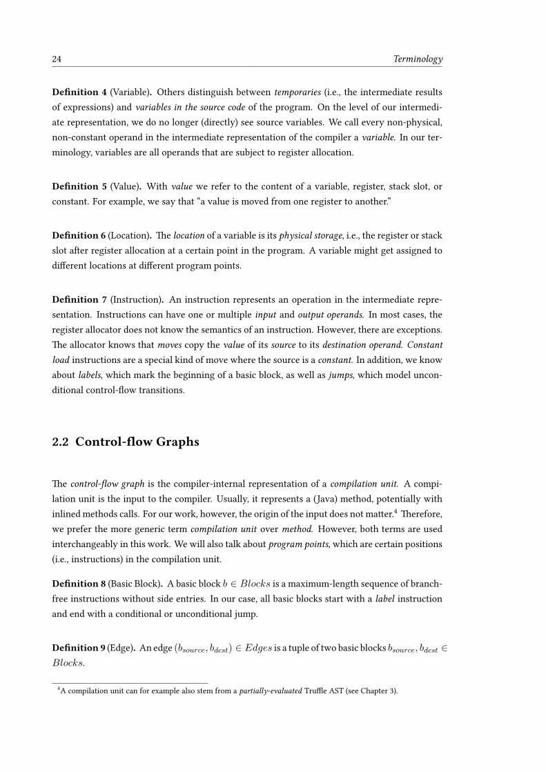
2 Terminology 232.1 Instructions, Values, Locations . . . . . . . . . . . . . . . . . . . . . . . . . . . . 232.2 Control-flow Graphs . . . . . . . . . . . . . . . . . . . . . . . . . . . . . . . . . 24
2.2.1 Dominance . . . . . . . . . . . . . . . . . . . . . . . . . . . . . . . . . . 262.2.2 Loops . . . . . . . . . . . . . . . . . . . . . . . . . . . . . . . . . . . . . 27
2.3 Liveness and Lifetime Intervals . . . . . . . . . . . . . . . . . . . . . . . . . . . . 282.4 Static Single Assignment Form . . . . . . . . . . . . . . . . . . . . . . . . . . . . 30
2.4.1 ϕ-notation . . . . . . . . . . . . . . . . . . . . . . . . . . . . . . . . . . . 322.4.2 SSA destruction . . . . . . . . . . . . . . . . . . . . . . . . . . . . . . . . 33
3 The Graal Virtual Machine 353.1 The Java Virtual Machine . . . . . . . . . . . . . . . . . . . . . . . . . . . . . . . 363.2 The HotSpot VM . . . . . . . . . . . . . . . . . . . . . . . . . . . . . . . . . . . . 36
3.2.1 Graal on the HotSpot VM . . . . . . . . . . . . . . . . . . . . . . . . . . 383.3 The Graal Compiler . . . . . . . . . . . . . . . . . . . . . . . . . . . . . . . . . . 39
4 Trace Register Allocation 434.1 Trace Building . . . . . . . . . . . . . . . . . . . . . . . . . . . . . . . . . . . . . 44
4.1.1 Unidirectional Trace Building . . . . . . . . . . . . . . . . . . . . . . . . 454.1.2 Bidirectional Trace Building . . . . . . . . . . . . . . . . . . . . . . . . . 48

xii Contents
4.2 Trace Properties . . . . . . . . . . . . . . . . . . . . . . . . . . . . . . . . . . . . 504.2.1 Greedy Trace Properties . . . . . . . . . . . . . . . . . . . . . . . . . . . 504.2.2 Dominance Properties of Traces . . . . . . . . . . . . . . . . . . . . . . . 51
4.3 Global Liveness Analysis . . . . . . . . . . . . . . . . . . . . . . . . . . . . . . . 534.3.1 Liveness Analysis . . . . . . . . . . . . . . . . . . . . . . . . . . . . . . . 544.3.2 Representation of Global Liveness . . . . . . . . . . . . . . . . . . . . . 55
4.4 Allocating Registers . . . . . . . . . . . . . . . . . . . . . . . . . . . . . . . . . . 564.5 Global Data-flow Resolution . . . . . . . . . . . . . . . . . . . . . . . . . . . . . 57
5 Register Allocation Strategies 615.1 Linear Scan Allocator . . . . . . . . . . . . . . . . . . . . . . . . . . . . . . . . . 61
5.1.1 Interval Building . . . . . . . . . . . . . . . . . . . . . . . . . . . . . . . 625.1.2 Register Allocation on Intervals . . . . . . . . . . . . . . . . . . . . . . . 635.1.3 Local Data-flow Resolution . . . . . . . . . . . . . . . . . . . . . . . . . 655.1.4 Register Assignment on LIR . . . . . . . . . . . . . . . . . . . . . . . . . 66
5.2 Trivial Trace Allocator . . . . . . . . . . . . . . . . . . . . . . . . . . . . . . . . 665.3 Bottom-Up Allocator . . . . . . . . . . . . . . . . . . . . . . . . . . . . . . . . . 68
5.3.1 Tracking Liveness Information . . . . . . . . . . . . . . . . . . . . . . . 685.3.2 Register Allocation . . . . . . . . . . . . . . . . . . . . . . . . . . . . . . 695.3.3 Phi-resolution . . . . . . . . . . . . . . . . . . . . . . . . . . . . . . . . . 735.3.4 Loop Back-Edge . . . . . . . . . . . . . . . . . . . . . . . . . . . . . . . . 745.3.5 Example . . . . . . . . . . . . . . . . . . . . . . . . . . . . . . . . . . . . 745.3.6 Ideas that did not Work Out . . . . . . . . . . . . . . . . . . . . . . . . . 75
6 Inter-trace Optimizations 776.1 Inter-trace Hints . . . . . . . . . . . . . . . . . . . . . . . . . . . . . . . . . . . . 786.2 Spill Information Sharing . . . . . . . . . . . . . . . . . . . . . . . . . . . . . . . 796.3 Known Issue: Spilling in Loop Side-Traces . . . . . . . . . . . . . . . . . . . . . 796.4 Stack Intervals . . . . . . . . . . . . . . . . . . . . . . . . . . . . . . . . . . . . . 81
7 Evaluation 837.1 Benchmarks . . . . . . . . . . . . . . . . . . . . . . . . . . . . . . . . . . . . . . 84
7.1.1 SPECjvm2008 . . . . . . . . . . . . . . . . . . . . . . . . . . . . . . . . . 847.1.2 SPECjbb2015 . . . . . . . . . . . . . . . . . . . . . . . . . . . . . . . . . 847.1.3 DaCapo . . . . . . . . . . . . . . . . . . . . . . . . . . . . . . . . . . . . 857.1.4 Scala-DaCapo . . . . . . . . . . . . . . . . . . . . . . . . . . . . . . . . . 85
7.2 Configurations . . . . . . . . . . . . . . . . . . . . . . . . . . . . . . . . . . . . . 867.3 Peak Performance/Allocation Quality . . . . . . . . . . . . . . . . . . . . . . . . 86
7.3.1 DaCapo and Scala-DaCapo . . . . . . . . . . . . . . . . . . . . . . . . . 867.3.2 SPECjvm2008 . . . . . . . . . . . . . . . . . . . . . . . . . . . . . . . . . 897.3.3 SPECjbb2015 . . . . . . . . . . . . . . . . . . . . . . . . . . . . . . . . . 89

Contents xiii
7.3.4 Answering RQ1 . . . . . . . . . . . . . . . . . . . . . . . . . . . . . . . 897.4 Compile Time . . . . . . . . . . . . . . . . . . . . . . . . . . . . . . . . . . . . . 90
7.4.1 Compile Time per Method . . . . . . . . . . . . . . . . . . . . . . . . . . 937.4.2 Overall Compile Time . . . . . . . . . . . . . . . . . . . . . . . . . . . . 947.4.3 Answering RQ2 . . . . . . . . . . . . . . . . . . . . . . . . . . . . . . . 94
7.5 Inter-trace Optimizations . . . . . . . . . . . . . . . . . . . . . . . . . . . . . . . 957.6 Trace Builder Evaluation . . . . . . . . . . . . . . . . . . . . . . . . . . . . . . . 97
8 Trace Register Allocation Policies 998.1 Properties . . . . . . . . . . . . . . . . . . . . . . . . . . . . . . . . . . . . . . . 99
8.1.1 Block Properties . . . . . . . . . . . . . . . . . . . . . . . . . . . . . . . 1008.1.2 Trace Properties . . . . . . . . . . . . . . . . . . . . . . . . . . . . . . . 1008.1.3 Compilation Unit Properties . . . . . . . . . . . . . . . . . . . . . . . . . 1018.1.4 Aggregation of Properties . . . . . . . . . . . . . . . . . . . . . . . . . . 101
8.2 Policies . . . . . . . . . . . . . . . . . . . . . . . . . . . . . . . . . . . . . . . . . 1018.3 Evaluation . . . . . . . . . . . . . . . . . . . . . . . . . . . . . . . . . . . . . . . 104
8.3.1 Discussion . . . . . . . . . . . . . . . . . . . . . . . . . . . . . . . . . . . 1078.3.2 Answering RQ3 . . . . . . . . . . . . . . . . . . . . . . . . . . . . . . . 107
9 Parallel Trace Register Allocation 1099.1 Concurrency Potential . . . . . . . . . . . . . . . . . . . . . . . . . . . . . . . . 109
9.1.1 Example . . . . . . . . . . . . . . . . . . . . . . . . . . . . . . . . . . . . 1109.2 Evaluation . . . . . . . . . . . . . . . . . . . . . . . . . . . . . . . . . . . . . . . 112
9.2.1 Answering RQ4 . . . . . . . . . . . . . . . . . . . . . . . . . . . . . . . 1149.3 Future Directions . . . . . . . . . . . . . . . . . . . . . . . . . . . . . . . . . . . 114
10 Related Work 11510.1 Register Allocation . . . . . . . . . . . . . . . . . . . . . . . . . . . . . . . . . . 115
10.1.1 Local Register Allocation . . . . . . . . . . . . . . . . . . . . . . . . . . . 11610.1.2 Non-Global Register Allocation . . . . . . . . . . . . . . . . . . . . . . . 11710.1.3 Decoupled Register Allocation . . . . . . . . . . . . . . . . . . . . . . . 11910.1.4 Mathematical Programming Register Allocation Approaches . . . . . . . 12110.1.5 Register Allocation in Virtual Machines . . . . . . . . . . . . . . . . . . 123
10.2 Non-global Code Units . . . . . . . . . . . . . . . . . . . . . . . . . . . . . . . . 12410.3 Trace Compilation . . . . . . . . . . . . . . . . . . . . . . . . . . . . . . . . . . . 12510.4 Liveness and Intermediate Representations . . . . . . . . . . . . . . . . . . . . . 12710.5 Compile-time Trade-offs and Concurrent Compilation . . . . . . . . . . . . . . . 129
11 Conclusion and Future Work 131
A Additional Sources 135

xiv Contents
B Graal Backends 137B.1 AMD64 on HotSpot . . . . . . . . . . . . . . . . . . . . . . . . . . . . . . . . . . 137B.2 SPARC on HotSpot . . . . . . . . . . . . . . . . . . . . . . . . . . . . . . . . . . 138
C Hardware Environment 139C.1 Sun Server X3-2 . . . . . . . . . . . . . . . . . . . . . . . . . . . . . . . . . . . . 139C.2 Sun Server X5-2 . . . . . . . . . . . . . . . . . . . . . . . . . . . . . . . . . . . . 139C.3 SPARC T7-2 Server . . . . . . . . . . . . . . . . . . . . . . . . . . . . . . . . . . 141
Index 145
Publications 147
Bibliography 149

1
Chapter 1
Introduction
Teaser
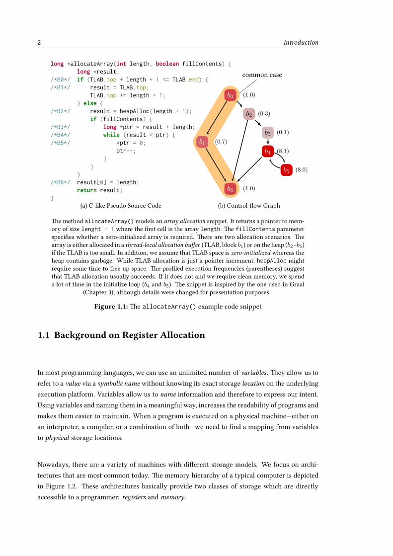
Most optimizing compilers use global register allocation approaches, such as graph coloring orlinear scan, which process a whole method at once. Compiler optimizations such as inlining orcode duplication cause methods to become large. This poses two problems. First, register alloca-tion time increases with method complexity, often in a non-linear fashion [Poletto and Sarkar,1999]. Second, different regions contribute differently to the overall performance of the compiledcode [Bala et al., 2000]. Global allocators do not adjust the allocation strategy based on the ex-pected execution frequency of the code region. Important and unimportant parts of a method areallocated with the same algorithm, i.e., they contribute equally to the overall allocation time.
Let us have a look at the allocateArray() example in Figure 1.1. A global allocator spendsabout the same amount of time for the uncommon cases (b2–b5) as for the common case (b0, b1and b6). However, we want to spend our time budget more wisely, e.g., by spending 80% on themost likely case, and only 20% for the rest.
In addition to compile time, i.e., the time required to compile a method, compilation latency, i.e.,the duration until the result of a compilation is ready, is an important metric, especially for just-in-time compilers. In contrast to the former, latency can be tackled with parallelization, in casemultiple threads are available to the compiler. Because global register allocators process a wholemethod at once, they offer only few opportunities to do work concurrently.
We propose a novel non-global register allocation approach, called trace register allocation, thattackles both issues of traditionally global allocators, namely to control the compile time on afine-granular level, and to reduce compilation latency using parallelization.
2 Introduction
long *allocateArray(int length, boolean fillContents) {long *result;
/*B0*/ if (TLAB.top + length + 1 <= TLAB.end) {/*B1*/ result = TLAB.top;
TLAB.top += length + 1;} else {
/*B2*/ result = heapAlloc(length + 1);if (fillContents) {
/*B3*/ long *ptr = result + length;/*B4*/ while (result < ptr) {/*B5*/ *ptr = 0;
ptr--;}
}}
/*B6*/ result[0] = length;return result;
}(a) C-like Pseudo Source Code
common case
b0
b1
b6
b2
b3
b4
b5
(0.3)
(0.1)
(8.1)
(8.0)
(1.0)
(0.7)
(1.0)
(b) Control-flow Graph
The method allocateArray()models an array allocation snippet. It returns a pointer to mem-ory of size lenght + 1 where the first cell is the array length. The fillContents parameterspecifies whether a zero-initialized array is required. There are two allocation scenarios. Thearray is either allocated in a thread-local allocation buffer (TLAB, block b1) or on the heap (b2–b5)if the TLAB is too small. In addition, we assume that TLAB space is zero-initialized whereas theheap contains garbage. While TLAB allocation is just a pointer increment, heapAlloc mightrequire some time to free up space. The profiled execution frequencies (parentheses) suggestthat TLAB allocation usually succeeds. If it does not and we require clean memory, we spenda lot of time in the initialize loop (b4 and b5). The snippet is inspired by the one used in Graal
(Chapter 3), although details were changed for presentation purposes.
Figure 1.1: The allocateArray() example code snippet
1.1 Background on Register Allocation
In most programming languages, we can use an unlimited number of variables. They allow us torefer to a value via a symbolic name without knowing its exact storage location on the underlyingexecution platform. Variables allow us to name information and therefore to express our intent.Using variables and naming them in a meaningful way, increases the readability of programs andmakes them easier to maintain. When a program is executed on a physical machine—either onan interpreter, a compiler, or a combination of both—we need to find a mapping from variablesto physical storage locations.
Nowadays, there are a variety of machines with different storage models. We focus on archi-tectures that are most common today. The memory hierarchy of a typical computer is depictedin Figure 1.2. These architectures basically provide two classes of storage which are directlyaccessible to a programmer: registers and memory.

1.1 Background on Register Allocation 3
Register
Cache
Main memory
Hard disk
Available storage
Decreasingaccess
time
Increasing
storagesize
250 ps
1 ns
100 ns
10 ms
500 bytes
64 KiB
1 GiB
1 TiB
The pyramid representation is inspired by Pereira [2008, Figure 2.1]. The numbers are takenfrom Hennessy and Patterson [2003, Figure 5.1].
Figure 1.2: Typical memory hierarchy of a computer
Registers are located in the processor and are the fastest type of storage. Depending on the pro-cessor, their size is usually in the range of 16 to 512-bits. Their number is limited to supportefficient encoding. For example, the AMD64 architecture features only 16 general purpose reg-isters1 in 64-bit mode. A SPARC processor provides a register set of 32 registers2 for generalusage.
With memory we refer to non-persistent, random-access storage. The number of storage loca-tions available in memory is significantly higher than the number of registers. For the course ofthis work, it is safe to assume that it is unlimited. Regarding access time, memory is orders ofmagnitudes slower than registers [Hennessy and Patterson, 2003]. To speed up memory access,most computers use one or multiple levels of caches. A cache basically mirrors parts of recentlyused data from the main memory for faster consecutive access. Caches are transparent to theprogrammer.3 A downside of memory is that processors only have limited support for accessingit directly. Many machine instructions require their operands to reside in registers.
In this work, we will focus mainly onmethod-based compilers. Method-based compilers translatea method (function) from a source language to a target language, in our case to machine code. Weuse a control-flow graph (CFG) to represent methods. The nodes of this graph are basic blocks,i.e., a sequence on branch-free instructions. Figure 1.1 shows a method in C-like pseudo code andits corresponding control-flow graph.
Given the options above, the simplest solution is to map every variable to exactly one memorylocation. Since memory is virtually unlimited, finding this mapping is trivial. Whenever a valueneeds to reside in a register we can load it from memory into a register and store the result back
1Intel® 64 and IA-32 Architectures Software Developer’s Manual — Volume 1 Basic Architecture by Intel [2013a] Section3.4.1.1
2Oracle SPARC Architecture 2011 by Oracle Corporation [2012] Section 5.23However, many processors provide instructions to manipulate the cache, for example for loading specific memorylocations into the cache or flushing it.

4 Introduction
int length; bool fillContents;
long *result;
if (TLAB.top + length + 1 <= TLAB.end)
result = TLAB.top;
TLAB.top += length + 1;
result = heapAlloc(length + 1);
if (fillContents)
long *ptr = result + length;
while (result < ptr)
*ptr = 0;
ptr--;
result[0] = length;
return result;
b0(1.0)
b1(0.7)
b2(0.3)
b3(0.1)
b4(8.1)
b5(8.0)
b6(1.0)
false
false
leng
th
fill
C.re
sult
ptr
(a) Lifetime intervals
length
fillC. ptr
result
(b) Interference graph
The numbers in parentheses on the left are execution frequencies. The lifetime intervals for theallocateArray() method are shown on the left. The bullet symbol ( ) marks the definition(write) of the value, a square ( ) depicts a usage (read). The interference graph is shown onthe right. Vertices represent variables, edges interference between them. See also Figure 1.1 for
more context.
Figure 1.3: Lifetime intervals and interference graph for allocateArray()
to memory. However, repeatedly moving values back and forth between registers and memory isnot efficient. Therefore, optimizing compilers try to keep values in registers whenever possible.This optimization is known as register allocation. For programs where there are more variablesthan registers the decision whether to keep a value in a register is non-trivial. In this case,multiple variables need to share a register. To do so, we need to find variables that are not liveat same time, i.e., they do not interfere.
Example Let us have a look at our recurring example in Figure 1.1. In total, there are 4 vari-ables, length, fillContents, result, and ptr. Figure 1.3a depicts the lifetime intervals of thesevariables. The interference relation can be visualized as a graph, the so-called interference graph
(see Section 2.3). The vertices of the graph represent the variables. An edge between two verticesmeans that the variables are live at the same time. Figure 1.3b shows the interference graph forour example. While length and result interfere with all other variables, the lifetime intervals forfillContents and ptr do not overlap. Therefore, they can use the same register.

1.1 Background on Register Allocation 5
This leads to the basic definition of the register allocation problem:
The Register Allocation Problem
Allocate a finite number of machine registers to an unbounded number of variables suchthat variables with interfering live ranges are assigned to different registers.
It is not always possible to find a solution for this problem. For example, in cases where thenumber of registers is smaller than the number of live values at any instruction. In that case weneed to store one or more variables in memory, usually on the stack of the method. There aretwo concepts that are closely related to register allocation. Live Range Splitting: Given the liveranges of a variable, split them in such a way that the variable can reside in different locations(register or stack) at different points of the method. Spilling: Move a variable to the stack, so thata register becomes free and can be used for some other variable. This brings us to the problemthat is by far more interesting—and also more complicated—than the basic register allocationproblem:
The Splitting and Spilling Problem
In case the register pressure (the number of live variables) is higher than the numberof available registers, decide which variables to split and/or spill to reduce the registerpressure.
Splitting and spilling is often formulated as an optimization problem, i.e., to make decisions tominimize a cost function. The cost function might be based on a static property such as thenumber of added spill moves, a dynamic property such as the number of executed spill moves, orsomething more abstract such as system performance. It is often the structure of the cost functionthat causes the problem to get difficult.
There are different approaches to register allocation. Most register allocators in a method-basedcompiler can be categorized into local and global approaches, based on the scope they work on.Local register allocators work on the scope of a single basic block. Due to their limited scopethey are fast and simple to implement but have limited optimization potential. On the otherhand, global allocators process the whole method at once. While this offers opportunities foroptimization it also makes the problem more difficult to solve. Most optimizing compiler use anallocator that follows the global principle. Two kinds of global register allocation are commonlyused today. The first one is register allocation based on graph coloring, which was proposedby Chaitin et al. [1981]. The other approach is linear scan register allocation, first described byPoletto and Sarkar [1999].

6 Introduction
1.2 Graph Coloring
Graph coloring is used in many compilers today, for example in WebKit,4 the HotSpot servercompiler,5 or in GCC.6 The idea is to solve the register allocation problem via coloring [Aho etal., 1974, Chapter 10.4] of the interference graph. Each color represents a machine register. Sincegraph coloring with more than two colors is NP-complete [Karp, 1972], it is intractable to findthe optimal solution in polynomial time. Therefore, Chaitin et al. [1981] and others [Briggs et al.,1994; Chow and Hennessy, 1990] proposed heuristics to approximate solutions in polynomialtime.
1.2.1 Chaitin’s Allocator
Chaitin et al. [1981] first showed a practical application of graph coloring for register alloca-tion. Figure 1.4 shows an overview of the original Chaitin allocator. It operates in seven phases.Renumber calculates lifetime intervals for each variable definition. Build constructs the interfer-ence graph. Coalesce combines live ranges which are connected via a move instruction and donot interfere. Spill costs computes the estimated cost of spilling a variable based on its definitionand use positions and the expected execution frequency of its live ranges. Simplify removes allnodes from the graph where the number of neighbors (degree) is smaller than the number ofavailable registers (k) until the graph is empty; the removed nodes are put onto a stack. Then,the removed nodes are added back to the graph in reverse order. Every re-added node is guaran-teed to have less than k neighbors, so it can be colored. If during node removal we get to a pointwhere there are only nodes with k or more neighbors, one is selected for spilling based on itsspill costs. In the worst case all neighbors have a different color. However, there is still at leastone color left for the current node. From the nodes with higher degree, one is selected for spillingbased on its spill costs. Spill code inserts spill and reload code for spilled nodes. Select assignscolors to the nodes in the reverse order they were removed from the graph by simplify. Eachnode gets a color different to all its neighbors. Note the feedback loop from simplify to renumber
via spill code. Whenever simplify decides to spill a node the algorithm is restarted. This is one ofthe main sources of time complexity of this approach.
4Graph Coloring Register Allocator in WebKit by WebKit [2017a]5Chaitin Allocator in C2 by OpenJDK [2017a]6Integrated Register Allocator in GCC by GCC [2017]

1.2 Graph Coloring 7
renumber build coalesce spill cost simplify select
spill code
Figure adapted from [Briggs et al., 1994, Figure 1].
Figure 1.4: Chaitin’s allocator
length
fillC. ptr
result
2 2
3
3 (empty)stack
length
fillC. ptr
result
2
2
2 fill
stack
length
fillC. ptr
result
1
1ptr
fill
stack
length
fillC. ptr
result 0
length
ptr
fill
stack
result
length
ptr
fill
stack
The simplify phase removes nodes with a degree (right of the nodes) less than 3 and pushesthem onto the stack. This decreases the degree of the neighbors. The procedure is continued
until there are no more nodes, or all nodes have a degree greater than 2.
(a) Simplify phase
length
fillC. ptr
result
length
ptr
fill
stack
length
fillC. ptr
resultptr
fill
stack
length
fillC. ptr
result fill
stack
length
fillC. ptr
result (empty)stack
The selection phase assigns colors (registers) to the nodes. The nodes are processed in the reverseorder they where removed from the graph in the simplify phase. In the example there are three
registers available, reg1 , reg2 , and reg3 .
(b) Select phase
Figure 1.5: Graph coloring of allocArray using three registers
Example without Spilling
To demonstrate the approach, let us refer to our example in Figure 1.1. Let us assume that we havethree registers available, reg1 , reg2 , and reg3 . First, the algorithm builds an interferencegraph (Figure 1.5a). Next, we simplify the graph by removing nodes with a degree of less thank = 3. The removed nodes are pushed onto the stack. Once all nodes have been removed fromthe graph, we can continue with the select phase. We pop a node from the stack and assign it acolor that is different from the colors of its neighbors. Due to the construction of the stack in thesimplify phase this is always possible (see Figure 1.5b).

8 Introduction
length
fillC. ptr
result
2 2
3
3
(a) Interferencegraph
Name def/use frequencies cost (∑
) degree cost/degree
length 1.0+1.0+0.7+0.3+0.1+1.0
4.1 3 1.4
fillC. 1.0 + 0.3 1.3 2 0.6result 0.7+0.3+0.1+8.1+1.0+
1.011.2 3 3.7
ptr 0.1 + 8.1 + 8.0 + 8.0 24.2 2 12.1
(b) Spill costs for allocateArray()
The spill costs are the sum of definitions and usages weighted by their estimated executioncount [Chaitin, 1982]. The nodewith the lowest cost divided by its degree is selected for spilling,in this case fillContents. Execution frequencies for the blocks of allocArray are given in
Figure 1.7a.
Figure 1.6: Graph coloring of allocArray using two registers (interference before spilling)
Example with Spilling
Let us redo the example with only two registers, reg1 and reg2 . As can be seen in Figure 1.6a,there is no nodewith a degree lower than 2. Therefore, we need to select a node for spilling. To doso, we calculate the spill costs. The result is shown in Figure 1.6b. We first select fillContents forspilling because it has the lowest spill cost. We therefore split the interval and reload it at everyusage of the variable. However, this does not change the degrees in the interference graph. Wecontinuewith the next best candidate, length. This time the register pressure reduces as shown inFigure 1.7. We can simplify the graph and push the variables onto the stack (Figure 1.8). Finally,the select phase colors the nodes by popping them from the stack and assigning colors, as shownin Figure 1.9.
1.2.2 Other Graph Coloring Approaches
Following the work of Chaitin et al., many refinements have been proposed to improve the resultof the original approach. While the underlying idea was retained, the details of the spillingheuristics or the interaction of the various phases changed.
Chaitin’s allocator is rather pessimistic regarding spilling. It spills whenever it cannot prove thatthere is a valid coloring, i.e., that every node has a degree lower than the number of registers.However, in many cases it is possible to color the graph also in such situations. See Figure 1.10for an example. Although all nodes have a degree of 2, the graph is 2-colorable. To overcomethis issue, Briggs et al. [1994] proposed the optimistic graph coloring allocator. As shown inFigure 1.11, the main difference to the original algorithm is that instead of eagerly spilling nodes,Briggs et al. try to select a color also for potentially spilled nodes. Only when this fails, a node

1.2 Graph Coloring 9
int length; bool fillContents;
long *result;
if (TLAB.top + length + 1 <= TLAB.end)
result = TLAB.top;
TLAB.top += length + 1;
result = heapAlloc(length + 1);
if (fillContents)
long *ptr = result + length;
while (result < ptr)
*ptr = 0;
ptr--;
result[0] = length;
return result;
b0(1.0)
b1(0.7)
b2(0.3)
b3(0.1)
b4(8.1)
b5(8.0)
b6(1.0)
false
false
length
fillC.
result
ptr
(a) Lifetime Intervals
length0
fillC. ptr
result
length1
length2
length3
5
1 1
0
1
1
1
(b) Interference Graph
Spilled interval in orange ( ).
Figure 1.7: Graph coloring of allocArray using two registers (interference after spilling)
is actually spilled. Another difference to Chaitin et al. is their conservative coalescing approach.Instead of combining all nodes which are connected with a move instruction, only those areconsidered that will provably not introduce spilling.
Building on the results of Chaitin et al. and Briggs et al., George and Appel [1996] proposediterative register coalescing. As the name suggests, they iteratively perform coalescing in a loopwith the simplification phase. This way, they are able to coalesce more nodes but still guaranteethat they do not introduce spilling. Investigations by Pereira and Palsberg [2005] suggest thatGeorge and Appel’s approach is among the best performing polynomial-time register allocatorswith respect to register allocation quality.
Time Complexity Giving a definite asymptotic time complexity measure for graph coloringallocators is difficult as it strongly depends on the concrete implementation, e.g., optimistic vs.pessimistic coloring or conservative vs. iterative coalescing. Building the interference graphrepeatedly whenever spill code is inserted is considered the most expensive part of the ap-proach [Cooper and Torczon, 2011, Chapter 13]. Also, the size of the graph can gets quadratic inthe number of live ranges [Poletto and Sarkar, 1999]. Experiments conducted by Briggs [1992]suggest that in practice the allocator behaves quadratic in terms of its “input size.”

10 Introduction
length0
fillC. ptr
result
length1
length2
length3
5
1 1
1
1
1
length0
stack
(a) Removed length0
length0
fillC. ptr
result
length1
length2
length3
5
1 1
length3
length2
length1
length0
stack
(b) Removedlength1–length3
result
ptr
fillContents
length3
length2
length1
length0
stack
(c) Empty Graph
Figure 1.8: Graph coloring of allocArray using two colors (simplify)
Compile time is an important metric for all compilers. For static compilation, i.e., where theprogram is compiled once ahead-of-time (AOT), long compilation times are often set off as anunfavorable but necessary condition.7,8,9 The picture changes when talking about dynamic orjust-in-time (JIT) compilation systems. Since compilation happens at application run time, it isan integral part of the performance of a system. No matter how good the quality of the compiledcode is, if the code is not ready quickly enough, the user will be unsatisfied. Therefore, JITcompilation always has to consider a compile-time/code-quality trade-off.
1.3 Linear Scan
Poletto and Sarkar [1999] proposed the linear scan approach as a fast register allocator that pro-duces reasonable results for the code generation system tcc [Poletto et al., 1997]. Instead ofcoloring an interference graph, linear scan performs a linear pass over the lifetime intervals ofthe method. First, the basic blocks of the control-flow graph are organized in a linear mannerand instructions are numbered in ascending order.10 Lifetime intervals are defined by a start andend position which represent the first and last occurrence of the respective variable in the linearstream of instructions. To allocate registers, the intervals are visited in the order of increasingstart positions. The visited interval is moved into an active list, which is sorted by increasingend positions. Whenever a new interval is activated, intervals with an end position less thanthe new interval’s start position are removed from the active list. In case the active list is longerthan the number of registers, intervals need to be spilled. In Poletto and Sarkar’s implementa-
7Exhibit A: https://gcc.gnu.org/bugzilla/show_bug.cgi?id=271408Exhibit B: https://www.rust-lang.org/en-US/faq.html#why-is-rustc-slow9Exhibit C: https://lists.llvm.org/pipermail/llvm-dev/2016-March/096488.html
10For the algorithm, the block order does not matter. However, it has a big impact on code quality [Wimmer andMössenböck, 2005].

1.3 Linear Scan 11
length0
fillC. ptr
result
length1
length2
length3
result
ptr
fillContents
length3
length2
length1
length0
stack
length0
fillC. ptr
result
length1
length2
length3
result
ptr
fillContents
length3
length2
length1
length0
stack
length0
fillC. ptr
result
length1
length2
length3
result
ptr
fillContents
length3
length2
length1
length0
stack
Figure 1.9: Graph coloring of allocArray using two colors (select)
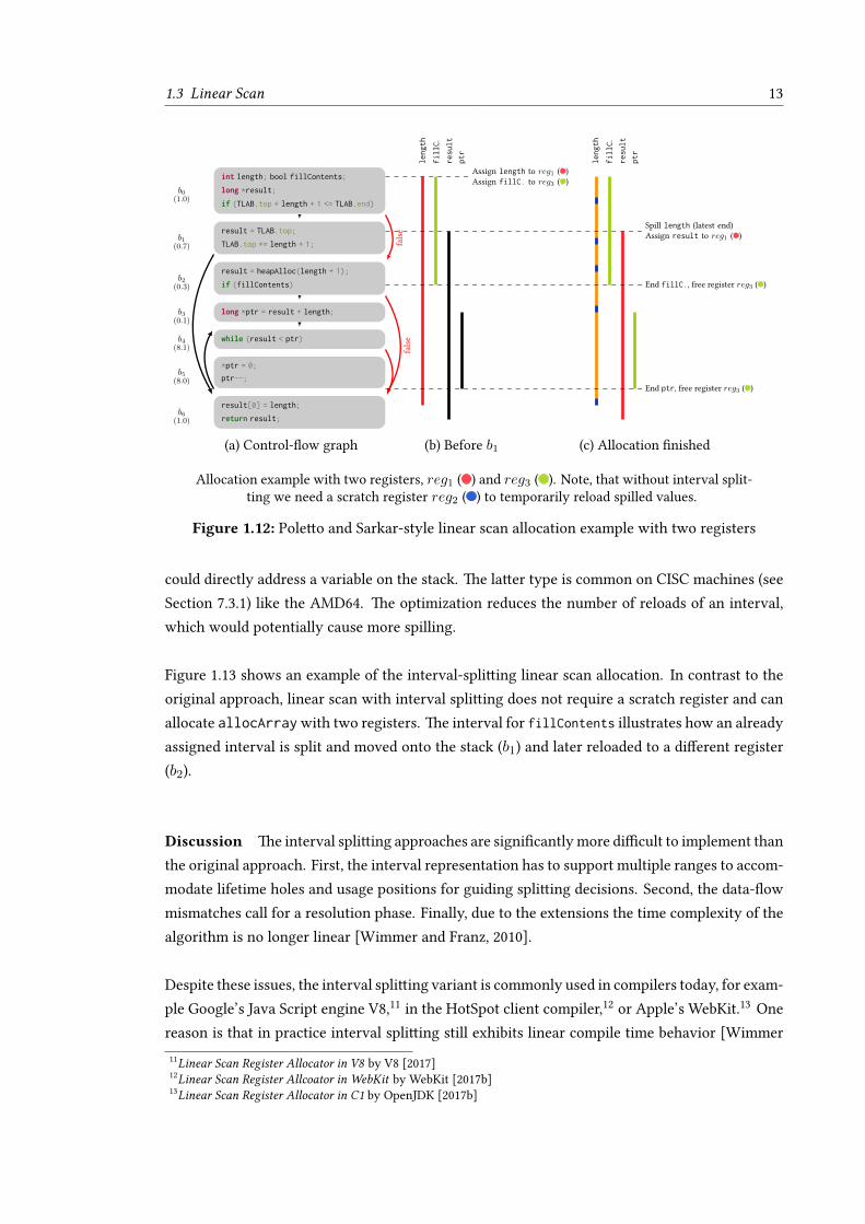
tion, they choose the interval with the highest end position. When an interval is spilled, it iscompletely kept on the stack throughout its lifetime, also if it was previously selected to residein a register.
Figure 1.12 illustrates how the linear scan algorithm would allocate our running example. Werestricted the set of available registers to two. However, since some instructions require a registeroperand and cannot deal with stack slots directly, we need an additional scratch register.
1.3.1 Lifetime Holes and Interval Splitting
Two shortcomings of Poletto and Sarkar’s linear scan approach are eye-catching. First, it alwaysspills the whole interval, whereas it would be sufficient to split the interval at the position wherethe register pressure is too high. Also, there might be a register available later, so spilling itindefinitely is overly conservative. The second issue is about liveness. When linearizing theblocks of a control-flow graph, the liveness of a variable is not a continuous range, but a list ofranges. This means that intervals have lifetime holes (see Section 2.3) where the variable is notneeded.

12 Introduction
x
w z
y
Figure adapted from [Briggs et al., 1994, Figure 2].
Figure 1.10: Diamond-shaped interference graph diamond which is 2-colorable
renumber build coalesce spill cost simplify select
spill code
Figure adapted from [Briggs et al., 1994, Figure 4].
Figure 1.11: Briggs’ optimistic allocator
Traub et al. [1998] introduced both improvements shortly after the first disclosure of linear scanby Poletto et al. [1997]. They proposed modeling liveness of a variable in linear scan as a list oflive ranges. The emerging lifetime holes reduce the register pressure and therefore the need forspilling. If there is still need for spilling, the interval that is selected for spilling is split just beforethe register pressure exceeds the number of available registers. The first part of the interval staysin a register. The remaining part of the interval is allocated to a stack slot. In addition to that,the interval is split again just before the next usage of the variable and is inserted into the list ofunhandled intervals. In other words, the interval gets a second chance of getting into a register.Thus the name of the approach, second-chance binpacking. Due to the splitting technique, Traubet al.’s allocator selects the spill candidate based on the next use position of the interval. Intervalsplitting also leads to data-flowmismatches because a variable might reside in different locations(i.e., in different registers or in a register and in a stack slot) at both ends of a control-flowedge. Therefore, a resolution phase iterates the edges and fixes mismatches by inserting moveinstructions.
Wimmer and Mössenböck [2005] extended the second-chance binpacking approach to further im-prove the allocation quality. The optimal split position optimization moves the split position (i.e.,the position where a value is moved from a register to a stack slot) out of loops. If this succeeds,the spill move is executed less often, which has a positive impact on the performance of the gen-erated code. Wimmer and Mössenböck also proposed register hints as a light-weight alternativeto coalescing. If two intervals are linked via a move instruction, the destination interval tries toreuse the register of the source interval, if it is available, i.e., if the interval ends at the move. Fur-thermore, they distinguish between usages of a variable that require a register and those which
1.3 Linear Scan 13
int length; bool fillContents;
long *result;
if (TLAB.top + length + 1 <= TLAB.end)
result = TLAB.top;
TLAB.top += length + 1;
result = heapAlloc(length + 1);
if (fillContents)
long *ptr = result + length;
while (result < ptr)
*ptr = 0;
ptr--;
result[0] = length;
return result;
b0(1.0)
b1(0.7)
b2(0.3)
b3(0.1)
b4(8.1)
b5(8.0)
b6(1.0)
false
false
length
fillC.
result
ptr
Assign length to reg1 ( )Assign fillC. to reg3 ( )
length
fillC.
result
ptr
Spill length (latest end)Assign result to reg1 ( )
End fillC., free register reg3 ( )
End ptr, free register reg3 ( )
(a) Control-flow graph (b) Before b1 (c) Allocation finished
Allocation example with two registers, reg1 ( ) and reg3 ( ). Note, that without interval split-ting we need a scratch register reg2 ( ) to temporarily reload spilled values.
Figure 1.12: Poletto and Sarkar-style linear scan allocation example with two registers
could directly address a variable on the stack. The latter type is common on CISC machines (seeSection 7.3.1) like the AMD64. The optimization reduces the number of reloads of an interval,which would potentially cause more spilling.
Figure 1.13 shows an example of the interval-splitting linear scan allocation. In contrast to theoriginal approach, linear scan with interval splitting does not require a scratch register and canallocate allocArraywith two registers. The interval for fillContents illustrates how an alreadyassigned interval is split and moved onto the stack (b1) and later reloaded to a different register(b2).
Discussion The interval splitting approaches are significantlymore difficult to implement thanthe original approach. First, the interval representation has to support multiple ranges to accom-modate lifetime holes and usage positions for guiding splitting decisions. Second, the data-flowmismatches call for a resolution phase. Finally, due to the extensions the time complexity of thealgorithm is no longer linear [Wimmer and Franz, 2010].
Despite these issues, the interval splitting variant is commonly used in compilers today, for exam-ple Google’s Java Script engine V8,11 in the HotSpot client compiler,12 or Apple’s WebKit.13 Onereason is that in practice interval splitting still exhibits linear compile time behavior [Wimmer11Linear Scan Register Allocator in V8 by V8 [2017]12Linear Scan Register Allcoator in WebKit by WebKit [2017b]13Linear Scan Register Allocator in C1 by OpenJDK [2017b]

14 Introduction
int length; bool fillContents;
long *result;
if (TLAB.top + length + 1 <= TLAB.end)
result = TLAB.top;
TLAB.top += length + 1;
result = heapAlloc(length + 1);
if (fillContents)
long *ptr = result + length;
while (result < ptr)
*ptr = 0;
ptr--;
result[0] = length;
return result;
b0(1.0)
b1(0.7)
b2(0.3)
b3(0.1)
b4(8.1)
b5(8.0)
b6(1.0)
false
false
length
fillC.
result
ptr
Assign length to reg1 ( )Assign fillC. to reg2 ( )
Split fillC. before next usageAssign result to reg2 ( )
length
fillC.
result
ptr
Split length before next usageAssign fillC. to reg1 ( )
Assign length to reg1 ( )Split length before next usageAssign ptr to reg1 ( )
Assign length to reg1 ( )
(a) Control-flow Graph (b) After Activating result in b1 (c) Allocation Finished
Allocating allocArray with an interval splitting linear scan allocator as described by Traubet al. [1998] or Wimmer and Mössenböck [2005] with two registers, reg1 ( ) and reg2 ( ).
Interval activations (dashed line) occur from top to bottom.
Figure 1.13: Interval-splitting linear scan allocation of allocateArray with two registers
and Mössenböck, 2005]. The other, more compelling reason is that spilling the whole intervalleads to worse allocation results, especially with increasing numbers of variables and lengthsof intervals. For the rest of this work, unless otherwise noted, we refer to the Wimmer andMössenböck approach when talking about linear scan.
1.4 Problems of Existing Register Allocation Approaches
Figure 1.14 visualizes the graph coloring and the linear scan allocation examples with two regis-ters side-by-side. Both approaches introduce spilling in the common case (b0, b1 and b6). Graphcoloring spills fillContents and length in b0 and reloads length in b6. Linear scan performs bet-ter in this example and only reloads length before its usage in b6. Of course, we have carefullyselected this example tomake our case. Our graph coloring example uses a rather simple splittingheuristic (reload at every usage). An advanced approach, for example as described by Bergneret al. [1997], would improve the result. Also linear scan would perform better if the block or-der were different, for example if the important blocks come first. However, these workaroundsjust underline our criticism of the approaches. They use “tricks” to such as block orderings topush the algorithm into the right direction or heuristics to reduce obvious deficiencies. But theunderlying problem—distinguishing between common and uncommon cases—is not modeled ap-

1.4 Problems of Existing Register Allocation Approaches 15
int length; bool fillContents;
long *result;
if (TLAB.top + length + 1 <= TLAB.end)
result = TLAB.top;
TLAB.top += length + 1;
result = heapAlloc(length + 1);
if (fillContents)
long *ptr = result + length;
while (result < ptr)
*ptr = 0;
ptr--;
result[0] = length;
return result;
b0(1.0)
b1(0.7)
b2(0.3)
b3(0.1)
b4(8.1)
b5(8.0)
b6(1.0)
false
false
length
fillC.
result
ptr
length
fillC.
result
ptr
(a) Control-flow graph (b) Graph coloring (c) Interval-splitting linear scan
Comparison of graph coloring and linear scan allocation with two registers, reg1 ( ) andreg2 ( ). See Figure 1.9 and Figure 1.13 for the full allocation example.
Figure 1.14: Graph coloring vs. linear scan of allocateArray with two registers
propriately. For small compilation units, like our example, most well-tuned approaches wouldprobably come up with equally good results. When the method size increases, however, theshortcomings become more evident.
The issues are especially problematic in JIT compilers. First, there are compile time constraintsdue to compilation at run time. In addition, many JIT compilers perform speculative optimiza-
tions [Duboscq et al., 2013], based on profiling information (e.g., inlining a specific call targetof a virtual call, although there might be multiple candidates). This allows the compiler to per-form optimizations aggressively, which is not possible in a static compiler. The compiled codecontains checks to verify that the assumptions on which the optimizations were based still hold.If not, deoptimization takes place, i.e., execution is continued in an unoptimized version or inan interpreter [Hölzle et al., 1992; Wimmer et al., 2017]. In order to do so, the system needs toreconstruct the unoptimized (interpreter) state. Therefore, all local variables in the current stackframe need to be kept alive, although they are not needed by the optimized code [Duboscq et al.,2014]. Multiple levels of inlining means that multiple frames need to be reconstructed. Due tothis, compilation units in JIT compilers often consists of tens of thousands of instructions (seeFigure 7.7) and variables [Chen et al., 2018]. This poses a challenge for register allocation.

16 Introduction
Issues
Let us summarize the issues we have uncovered so far with graph coloring, linear scan and theglobal approach in general.
Graph Coloring The inference graph used by graph coloring models register requirementson the level of variables, nicely. However, due to the quadratic worst-case graph size, the ap-plicability of this approach to huge compilation units is limited [Sarkar and Barik, 2007]. Also,the graph coloring model loses a lot of its appeal when it comes to spilling and splitting, sincethe information that is necessary for doing it is not an inherent part of the graph. However, forthe performance of the generated code, making good spilling and splitting decisions is highlyimportant [Braun and Hack, 2009; Lozano et al., 2014]. Finally, the non-linear time complexityrules out graph coloring for most JIT compilers.
Linear Scan In linear scan, interference is only implicit in the entries of the active list, whichrepresents a local snapshot of live variables currently stored in registers. Due to this local view,the scope for decisions is also limited. For example, spilling an interval might render a previousspilling decision unnecessary. On the other hand, splitting the lifetime of a variable is morenatural in linear scan than in a graph coloring allocator. There is a closer connection betweenthe instructions and the liveness representation. However, the linearization of the control flow isanother issue of linear scan. Consecutive blocks might not have a control-flow dependency, eventhough they are processed as if they were executed sequentially. Lifetime holes are an incarnationof this dilemma.
Global Scope With increasing problem sizes, dealing with the whole compilation unit in a(global) register allocator becomes a problem. The allocation time depends on the size of theinput, often in a non-linear way. Optimizations target the complete compilation unit. However,as already stated, not all parts are equally important. A bad global decision (i.e., spilling due tohigh register pressure in an infrequently executed part of the method) may cause degradationfor the common case, as we have seen in our example in Figure 1.14. When compile time isscarce, we want to be more clever about where to spend it. We would like to invest more timeon important parts of the compilation unit and less time on others. The global view makes thisdifficult.

1.5 Our Approach 17
1.5 Our Approach
The deficiencies outlined in the previous section motivated our investigations for finding a newregister allocation approach that solves these problems. More specifically we envisioned thefollowing goals.
Register Allocation for JIT Compilers. Striving for optimal register allocation is easier if compiletime is not an issue. We explicitly target just-in-time compilerswhere the compile-time/peak-performance trade-off is a challenge.
Non-global approach. Instead of dealing with the whole compilation unit at once, we want todivide the input into sub-problems and solve them independently. This would allow us todeal with bigger problem sizes, provide more flexibility and enables concurrent allocation.
“Focus on the Common Case” is an often heard suggestion [Hennessy and Patterson, 2003, p. 38].We want to concentrate on those parts which will contribute most to the overall perfor-mance of the generated code and find a good solution for those. The quality of infrequentlyexecuted parts of a method is of low interest. Since we target virtual machines that provideprofiling information, we want to exploit this knowledge.
Natural liveness model. Liveness is the key information for a register allocator. Wewant a simpleliveness model which is easy to reason about. In particular, wewant to avoid lifetime holes.Therefore, the control flow of our sub-problems should to be linear.
Same or better allocation quality. Although we push for a simpler model, we still want to be ableto achieve the same allocation quality as global approaches.
Same or better compile-time behavior for the same allocation quality. Compile time is our majorconcern. The minimum goal is to compete with linear scan with respect to allocation timefor comparable allocation quality.
Better scaling for large compilation units. A main challenge is to cope with increasing sizes ofcompilation units. We want an allocator that scales well as the problem grows. It is espe-cially important to work towards a linear or almost linear compile time with respect to theinput size.

18 Introduction
T0 T1 T2
int length;
↪→ boolean fillContents;
long *result;
if (TLAB.top + length + 1)
↪→ <= TLAB.end)
result = TLAB.top;
TLAB.top += length + 1;
result[0] = length;
return result;
result = heapAlloc(length + 1);
if (fillContents)
long *ptr = result + length;
while (result < ptr)
*ptr = 0;
ptr--;
b0
b1
b2
b3
b4
b5
b6
true
false
false
length
length
length
fillC.
result
fillC.
result
result
ptr
Allocating allocArraywith trace register allocation using two registers, reg1 ( ) and reg2 ( ).Each trace (dashed rectangles) is allocated independently. Note that the locations of the vari-ables at the trace boundaries do not always match. A resolution phase inserts moves to fix the
data-flow.
Figure 1.15: Trace register allocation of allocArray() with 2 registers
More flexibility to control the trade-off between compile time and allocation quality. We wantmeans to trade-off allocation quality for compile time on a fine-grained level. In particular,we want to be able to decide which parts of a method are particularly important for peakperformance and where we thus want to spend more compile time.
Idea The requirements outlined above led a novel register allocation framework which weentitled trace register allocation. In contrast to global register allocation, which processes a wholemethod at once, trace register allocation divides the problem into smaller sub-problems, so-calledtraces, for which register allocation can be done independently. A trace is a list of basic blocks,which might be executed sequentially. Traces are non-empty and non-overlapping, and everybasic block is contained in exactly one trace. We use profiling information provided by the virtualmachine to construct long and important traces first.
For each trace, the algorithm selects an allocation strategy. Due to the explicit global livenessinformation, allocating a trace is completely decoupled from the allocation of other traces. Thelinear structure of traces makes the implementation of strategies significantly simpler than ina global algorithm. Most importantly, there are no lifetime holes. Since some traces are moreimportant than others, we use different allocation algorithms (strategies), depending on the trace.For infrequently executed traces we use a strategy that is fast but produces sub-optimal code. Forimportant traces, on the other hand, we want the best allocation quality and are willing to investmore compile time.

1.6 Contributions 19
Example Figure 1.15 shows the control-flow graph of allocArray divided into traces. Eachtrace has been allocated independently with two available registers. In contrast to the graph col-oring and linear scan example, there are no spill moves or reloads in the common case (b0, b1, b6).At some inter-trace edges variables are stored in different locations. For example, length resideson the stack at the end of block b2 but in register reg1 at the beginning of b6. The resolutionphase inserts moves to correct the data-flow.
1.6 Contributions
In the course of this thesis, we contributed the following scientific results:
1. The Trace Register Allocation Framework. It is implemented in GraalVM, a production-quality Java virtual machine developed by Oracle. The code is open source and is publiclyavailable for everyone.14 As of version 9, the Graal compiler is an experimental part of theJDK. Therefore, our trace register allocation approach is now part of the most widely usedJava environment (although it is not enabled by default).15, 16 The implementation includesthree register allocation strategies for processing individual traces.
Linear Scan The trace-based linear scan strategy is an adaption of the global approachby Wimmer and Mössenböck [2005] and Wimmer and Franz [2010] to the propertiesof a trace. The main difference of our approach is that there is no need to maintain alist of live ranges for each lifetime interval, since there are no lifetime holes in traceintervals [Eisl et al., 2016].
Bottom-Up To decrease compilation time, we implemented the bottom-up allocator [Eislet al., 2017]. Its goal is to allocate a trace as fast as possible, potentially sacrificingcode quality. Our experiments show that it is about 40% faster than the linear scanstrategy.
Trivial Trace The trivial trace allocator is a special-purpose allocator for traces which havea specific structure. They consist of a single basic block which contains only a sin-gle jump instruction. Such blocks are introduced by splitting critical edges (see Sec-tion 2.2), and are quite common. For the DaCapo benchmark suite about 40% of alltraces are trivial [Eisl et al., 2016]. A trivial trace can be allocated by mapping thevariable locations at the beginning of the trace to the locations at the end of the trace.
14https://github.com/oracle/graal15On Java 10 and later:
java -XX:+UnlockExperimentalVMOptions -XX:+UseJVMCICompiler -Dgraal.TraceRA=true ...16On Java 9 an additional -XX:+EnableJVMCI is required.

20 Introduction
2. We showed that our trace register allocation approach achieves similar allocation qualityas a state-of-the-art global linear scan allocator for common Java benchmarks on bothAMD64 and SPARC processors [Eisl et al., 2016]. This suggests that high-quality registerallocation can be achieved without a global approach.
3. We showed that we are on par with global linear scan with respect to allocation speed forthe same allocation quality [Eisl et al., 2017].
4. Furthermore, we demonstrated the flexibility of using different strategies for allocatingindividual traces, which allows us to control the trade-off between allocation quality andcompile time [Eisl et al., 2017]. We can, for example, save over 10% of register allocationtime with a (geometric) mean performance degradation of only 1.5%. On the other end ofthe spectrum, we get over 40% faster allocation time at a mean slowdown of 11%. Depend-ing on the requirements, all trade-offs between those two boundaries can be achieved viasimple parameter settings. This flexibility is not possible with other approaches.
5. We prototyped an extension that enables parallel allocation of traces by multiple threadswithout a negative impact on allocation quality [Eisl et al., 2018]. This can reduce theregister allocation latency, i.e., the duration until the register allocation result is ready. Inour experiments, we decreased latency by up to 30% when using four threads instead ofone. This is yet another showcase for the flexibility of the trace register allocation approach.To the best of our knowledge, it is the first time that parallelism was exploited for registerallocation.
The trace register allocation results were published in the proceedings of multiple peer-reviewedvenues. We presented a vision paper at the Doctoral Symposium of SPLASH 2015, where wemotivated the trace register allocation idea [Eisl, 2015]. In 2016, we presented a full paper onallocation quality of a trace-based register allocator at the International Conference on Principles
and Practices of Programming on the Java Platform (PPPJ) [Eisl et al., 2016]. At ManLang 2017,the International Conference on Managed Languages & Runtimes, we demonstrated the flexibil-ity of our approach with a full paper on Trace Policies. We successfully submitted an extendedabstract on trace register allocation to the ACM Student Research Competition at CGO 2018 (Sym-
posium on Code Generation and Optimization), where our poster and presentation won the firstprice in the graduate category [Eisl, 2018a]. The award made us eligible to compete in the 2018Student Research Competition Grand Finals, where we submitted a summary paper [Eisl, 2018b].In 2018, a work-in-progress paper on parallel trace register allocation was accepted for the Inter-national Conference on Managed Languages & Runtimes (ManLang 2018) where we reported ourexperience with allocating traces by multiple threads [Eisl et al., 2018].

1.7 Outline 21
1.7 Outline
The rest of this thesis is organized as follows. In Chapter 2 “Terminology” we introduce notationsused throughout this work. All terms are commonly used in related literature, so feel free to skipit. Chapter 3 “The Graal Virtual Machine” discusses GraalVM, the Java Virtual Machine in whichwe implemented our trace register allocation approach. Chapter 4 “Trace Register Allocation”introduces the core of our allocator in detail. It also describes notations, definitions and prop-erties of traces which might not be commonly known. Chapter 5 “Register Allocation Strategies”outlines three allocation strategies, a linear-scan-based, a bottom-up and a trivial trace strategy.In Chapter 6 “Inter-trace Optimizations” we discuss three inter-trace optimizations needed forreaching peak performance. Chapter 7 “Evaluation” evaluates our implementation in GraalVMand argues why it solves the problems discussed in this introduction. In Chapter 8 “Trace Reg-ister Allocation Policies” we use various policies to control the trade-off between compile timeand peak performance. It showcases the flexibility and uniqueness of our trace register alloca-tion approach. Chapter 9 “Parallel Trace Register Allocation” describes how parallelization canreduce the compilation latency by allocating traces concurrently. In Chapter 11 “Conclusion and
Future Work” we finally reiterate the main contributions, discuss future work, and conclude thethesis.

23
Chapter 2
Terminology
Before we get into the details of this thesis we need to agree on the terminology and notation usedin this work. All terms are commonly used in the compiler construction community, so feel freeto skip this chapter if you are familiar with them. However, some terms are used ambiguouslyin literature. Therefore, we give here a proper definition.
2.1 Instructions, Values, Locations
First we describe the atomic building blocks of our intermediate representation and how theyinteract to produce new results.
Definition 1 (Register). For our work, we assume that registers are unique and do not alias [Leeet al., 2007], i.e., that modifying one register will leave the contents of all other registers un-touched.1
Definition 2 (Stack Slot). In our model we have an infinite number of stack slots for spilling.Assumptions are similar to registers. Stack slots do not overlap and there are no aliasing effects.2
Definition 3 (Constants). Constants are fixed numeric values that never change.3 We can usethem for rematerialization, i.e., for reloading the constant instead of spilling and reloading it froma stack slot.
1Register aliasing is a truly interesting and hard problem [Lee et al., 2007]. However, since there is no—or only verylimited—support for describing aliases in our implementation platform Graal, respectively HotSpot, we did noresearch into this direction.
2In practice this is not entirely true. It is possible to get the address of a stack slot. However, these cases are handledvery carefully by the compiler and they do not affect register allocation.
3Again, this is not always true. There are Java Object constants, i.e., the address of an object in memory. However,garbage collection might move the object and therefore change the address. Therefore, the compiler notifies thevirtual machine about usages of object constants. If the object is moved, the machine code is patched accordingly.
24 Terminology
Definition 4 (Variable). Others distinguish between temporaries (i.e., the intermediate resultsof expressions) and variables in the source code of the program. On the level of our intermedi-ate representation, we do no longer (directly) see source variables. We call every non-physical,non-constant operand in the intermediate representation of the compiler a variable. In our ter-minology, variables are all operands that are subject to register allocation.
Definition 5 (Value). With value we refer to the content of a variable, register, stack slot, orconstant. For example, we say that “a value is moved from one register to another.”
Definition 6 (Location). The location of a variable is its physical storage, i.e., the register or stackslot after register allocation at a certain point in the program. A variable might get assigned todifferent locations at different program points.
Definition 7 (Instruction). An instruction represents an operation in the intermediate repre-sentation. Instructions can have one or multiple input and output operands. In most cases, theregister allocator does not know the semantics of an instruction. However, there are exceptions.The allocator knows that moves copy the value of its source to its destination operand. Constantload instructions are a special kind of move where the source is a constant. In addition, we knowabout labels, which mark the beginning of a basic block, as well as jumps, which model uncon-ditional control-flow transitions.
2.2 Control-flow Graphs
The control-flow graph is the compiler-internal representation of a compilation unit. A compi-lation unit is the input to the compiler. Usually, it represents a (Java) method, potentially withinlined methods calls. For our work, however, the origin of the input does not matter.4 Therefore,we prefer the more generic term compilation unit over method. However, both terms are usedinterchangeably in this work. We will also talk about program points, which are certain positions(i.e., instructions) in the compilation unit.
Definition 8 (Basic Block). A basic block b ∈ Blocks is a maximum-length sequence of branch-free instructions without side entries. In our case, all basic blocks start with a label instructionand end with a conditional or unconditional jump.
Definition 9 (Edge). An edge (bsource, bdest) ∈ Edges is a tuple of two basic blocks bsource, bdest ∈Blocks.
4A compilation unit can for example also stem from a partially-evaluated Truffle AST (see Chapter 3).

2.2 Control-flow Graphs 25
b1
b2
b3 critica
ledg
e
(a) Critical edge (b1, b3)
b1
b2 bc
b3
(b) After splitting: new block bc
Figure 2.1: Critical edge splitting
Definition 10 (Predecessors). pred(b) is a list of predecessor blocks of b, i.e., pred(b) = [bp ∈Blocks | (bp, b) ∈ Edges].
Definition 11 (Successors). succ(b) is a list of successor blocks of b, i .e., succ(b) = [bs ∈Blocks | (b, bs) ∈ Edges].
Definition 12 (Path). A path ⟨b0, . . . , bn⟩ is a sequence of blocks where bi+1 is a successor of bifor i = 0, . . . , n− 1. A path may consist of a single block, i.e., ⟨b⟩ for b ∈ Blocks.
Definition 13 (Reachability). A block by ∈ Blocks is reachable from a block bx ∈ Blocks if andonly if there is a path ⟨bx, . . . , by⟩. We write bx ⇝ by .
Definition 14 (Control-Flow Graph). A control-flow graph is a tuple CFG = (Blocks,Edges)
consisting of a set of basic blocks and a set of edges. By definition, there is only one block inBlocks without a predecessor which we call the entry block bentry . In addition, every block b isreachable from the entry block, i.e., there is a path ⟨bentry, . . . , b⟩ for all b ∈ Blocks.
An example of the source code of allocateArray and the corresponding control-flow graph isshown in Figure 2.2.
Definition 15 (Critical Edge). An edge e = (bsource, bdest) is critical if and only if |succ(bsource)| >1 and |pred(bdest)| > 1. In other words, the source block of e has multiple successors and thedestination block of e has multiple predecessors.
See Figure 2.1a for an example of a critical edge. Critical edges can be removed by introducingnew (empty) blocks (Figure 2.1b). For data-flow resolution, critical edge splitting is of vast im-portance. The newly introduced blocks provide a place for compensation code, i.e., moves fromone location to another.
Our introductory example in Figure 1.1 contains two critical edges, from b2 to b6 and from b4 tob6. Figure 2.2 shows the example after critical edge splitting. Assume that there is a data-flowmismatch between b2 and b6. If the compensation code were placed at the end of b2 it would alsoaffect b3. If it were placed at the beginning of b6 it would also be executed for paths from b1 andb4. Therefore, the new block b8 is required.

26 Terminology
long *allocateArray(int length, boolean fillContents) {long *result;
/*B0*/ if (TLAB.top + length + 1 <= TLAB.end) {/*B1*/ result = TLAB.top;
TLAB.top += length + 1;} else {
/*B2*/ result = heapAlloc(length + 1);if (fillContents) {
/*B3*/ long *ptr = result + length;/*B4*/ while (result < ptr) {/*B5*/ *ptr = 0;
ptr--;}
/*B7*/ // critical edge} else {
/*B8*/ // critical edge}
}/*B6*/ result[0] = length;
return result;}
(a) C-like pseudo source code
common case
b0
b1
b6
b2
b3
b4
b5
b8
b7
(0.3)
(0.1)
(8.1)
(8.0)(0.1)
(0.2)
(1.0)
(0.7)
(1.0)
(b) Corresponding control-flow graph
The method allocateArray() after critical edge splitting which introduced b7 between b4 andb6, and b8 between b2 and b6. See Figure 1.1 for more information about the code snippet.
Figure 2.2: The allocateArray() sample code snippet (without critical edges)
For the rest of this thesis, we assume that all critical edges in the CFG have been split, so thatthere are no more critical edges.
2.2.1 Dominance
Definition 16 (Dominator). A block bd ∈ Blocks is a dominator of a block b ∈ Blocks if everypath ⟨bentry, . . . , b⟩ includes bd. We say that bd dominates b and define dom(b) as the set of allblocks that dominate b. Per definition, a block b dominates itself. It is easy to see that dominance
is a transitive relation.
Definition 17 (Strict Dominator). The strict dominators of a block b are the dominators of bwithout b itself, i.e., sdom(b) = dom(b) \ b.
Definition 18 (Immediate Dominator). The immediate dominator of b, denoted as idom(b), isthe strict dominator of b that is dominated by all other strict dominators of b. In other words, itis the strict dominator that is closest to b. Every node except the entry node bentry has exactlyone immediate dominator.

2.2 Control-flow Graphs 27
b0
b1
b6
b2
b3
b4
b5
b8
b7
(0.3)
(0.1)
(8.1)
(8.0)(0.1)
(0.2)
(1.0)
(0.7)
(1.0)
(a) Control-flow Graph
b0
b1 b6b2
b3
b4
b5
b8
b7
(b) Dominator Tree
On the left the control-flow graph of allocateArray(), on the right the dominator tree of thatmethod. The dominator tree is a visualization of the immediate dominator relation. Source code
in Figure 2.2a.
Figure 2.3: Dominator tree for allocateArray()
Figure 2.3b shows the dominator tree for the control-flow graph of allocateArray in Figure 2.3a.The edges represent the immediate dominator relation.
Definition 19 (Dominance Order). In dominance order, a block is visited only after all its dom-inators have been visited.
2.2.2 Loops
Definition 20 (General Loops). A loop is a set of basic blocks L ⊂ Blocks so that there is apath of at least length 2 from every block bx ∈ L to every other block by ∈ L, i.e., ∀bx, by ∈ L ||⟨bx, . . . , by⟩| ≥ 2.
Definition 21 (Reducible Loops). A reducible loopL is a loopwhere there is a loop header bh ∈ L
which dominates all blocks bi ∈ L. As a result, bh is the only block in L that can be targeted byan edge from a block outside of the loop. Edges from a block be in the loop to the loop headerare called back edges. Any such block be is called a loop end. An edge from a block in the loop L
to a block not in L is called a loop exit.
In this work we only deal with reducible graphs, i.e., with CFGs that only contain reducible
loops.
Theorem 1. Every path ⟨bx, . . . , bd⟩ from a block bx to a strict dominator bd ∈ sdom(bx) con-tains a loop header and therefore a back edge.

28 Terminology
Proof. Since bx ⇝ bd and bd ⇝ bx, there is a loop L which contains bx and bd. Therefore theremust be a loop header bh which dominates both and is on every path from bx to bd.
Theorem 2. Every loop has at least one back edge.
Proof. By definition, there is a path from every block b in a loop to every other block in this loop;in particular, there must be a path ⟨b, . . . , be, bh⟩ from b to the loop header bh. By definition, theedge (be, bh) is a back edge.
Theorem 3. Every loop header has at least one predecessor from outside the loop, which iscalled the loop entry.
Proof. By Definition 14, bentry has no predecessor, so it cannot be a loop header. Since everyblock is reachable from the entry block bentry , there must be a path ⟨bentry, . . . , b, bh⟩ of at leastlength 2 where b /∈ L, otherwise bh would not be the header of L. Thus, there is an edge (b, bh)that is not a back edge.
Corollary 1. Let us assume that a CFG has no critical edges, every predecessor of a loop headerhas a single successor, namely the loop header.
Proof. FromTheorem 2 (at least one back edge) andTheorem 3 (at least one loop entry) we knowthat a loop header has at least two predecessors. Therefore, all predecessors must have a singlesuccessor otherwise there would be a critical edge.
Definition 22 (Reverse Postorder). In reverse postorder, a block is visited before any of its suc-cessor blocks are visited unless the successor is a loop header. Reverse postorder implies domi-nance order.
2.3 Liveness and Lifetime Intervals
Liveness is the most important concept for register allocation. The liveness of the variables inthe compilation unit determines whether the problem is hard or simple to solve.
Definition 23 (Instruction Path). An instruction path is a list of instructions that occur betweena start instruction is in block bs and an end instruction ie in block be. If both instructions arein the same block, the instruction path consists of all instructions between the two instructions(inclusive). If there is no (basic block) path between bs and be, then the instruction path is empty.

2.3 Liveness and Lifetime Intervals 29
Otherwise, the instruction path contains all instructions from is to the end of bs, all instructionsfrom the blocks along the path ⟨bs, . . . , be⟩ excluding bs and be, and all instructions from thebeginning of be to ie.
Definition 24 (Liveness). A variable is live at every instruction that is part of an instructionpath between any definition of the variable and any usages of the variable, for all instructionpaths that do not contain another definition of that variable. Note that we exclude the defininginstruction itself from the instruction path, i.e., a variable is live right after its definition.
Figure 1.3a in the introduction already showed lifetime intervals, which are a representation ofliveness.
Definition 25 (Interference). Two variables interfere, it they are live at the same instruction.Since we exclude the defining instruction from liveness, a usage of variable x in instruction i
does not interfere with the variables defined by i, unless x is live after i.
Definition 26 (Interference Graph). An interference graph is a graph where the nodes representvariables and an edge between two nodes indicates that the variables of these nodes interfere.5
In Figure 1.3b in the introduction, we saw an example of an interference graph for the methodallocateArray.
Definition 27 (Lifetime Hole). A lifetime hole, a term proposed by Traub et al. [1998], is a con-sequence of the linearization of the basic blocks of the control-flow graph. It occurs whenevera variable is not live in a block bh, but live in a block bb before bh and live in a block ba after bh,with respect to the linear block order [. . . , bb, bh, ba, . . . ].
Figure 2.4 demonstrates an example for an inevitable lifetime hole. For every possible block order,there is at least one lifetime hole.
Definition 28 (Live Range). In a linear list of instructions, a (live) range denotes a subset of theinstructions where a variable is continuously live, i.e., there is no lifetime hole. A range can bedescribed by a from and to position.
Definition 29 (Lifetime Interval). The term (lifetime) interval denotes a collection of one ormoreunconnected and non-overlapping live ranges.
We introduced the notions of liveness in terms of variables. However, the same definitions canbe applied to registers and stack slots.
5To be more precise we should add that they also need to belong to the same register class, i.e., they compete for thesame set of registers. For readability reasons, we assume that there is only a single register class.
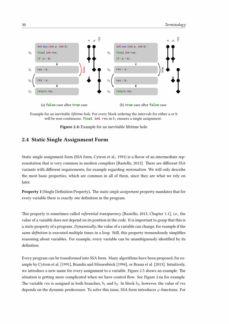
30 Terminology
int max(int a, int b)
final int res;
if (a < b)
res = b;
res = a;
return res;
b0
b1
b2
b3
false
a b res
(a) false case after true case
int max(int a, int b)
final int res;
if (a < b)
res = a;
res = b;
return res;
b0
b1
b2
b3
true
a b res
(b) true case after false case
Example for an inevitable lifetime hole. For every block ordering the intervals for either a or bwill be non-continuous. final int res in b1 ensures a single assignment.
Figure 2.4: Example for an inevitable lifetime hole
2.4 Static Single Assignment Form
Static single assignment form (SSA form, Cytron et al., 1991) is a flavor of an intermediate rep-resentation that is very common in modern compilers [Rastello, 2013]. There are different SSAvariants with different requirements, for example regarding minimalism. We will only describethe most basic properties, which are common in all of them, since they are what we rely onlater.
Property 1 (Single Definition Property). The static single assignment property mandates that forevery variable there is exactly one definition in the program.
This property is sometimes called referential transparency [Rastello, 2013, Chapter 1.1], i.e., thevalue of a variable does not depend on its position in the code. It is important to grasp that this isa static property of a program. Dynamically, the value of a variable can change, for example if thesame definition is executed multiple times in a loop. Still, this property tremendously simplifiesreasoning about variables. For example, every variable can be unambiguously identified by itsdefinition.
Every program can be transformed into SSA form. Many algorithms have been proposed, for ex-ample by Cytron et al. [1991], Brandis and Mössenböck [1994], or Braun et al. [2013]. Intuitively,we introduce a new name for every assignment to a variable. Figure 2.5 shows an example. Thesituation is getting more complicated when we have control flow. See Figure 2.6a for example.The variable res is assigned in both branches, b1 and b2. In block b3, however, the value of resdepends on the dynamic predecessor. To solve this issue, SSA form introduces ϕ-functions. For

2.4 Static Single Assignment Form 31
x = 1;y = x + 1;x = 2;z = x + 1;
(a) Before SSA
x1 = 1;y = x1 + 1;x2 = 2;z = x2 + 1;
(b) After SSA
Without SSA form one might assume that both occurrence of x + 1 calculate the same valueand that therefore y equals z. After renaming, it is clear that this is not the case. Example taken
from Rastello [2013].
Figure 2.5: Variable renaming in Static Single Assignment form
int max(int a, int b)
final int res;
if (a < b)
res = b;
res = a;
return res;
b0
b1
b2
b3
false
(a) Before SSA
int max(int a, int b)
if (a < b)
int res1 = b;
int res2 = a;
int res3 = ϕ(res1, res2);
return res;
(b) With ϕ-functions
int max(int a, int b)
if (a < b)
int res1 = b;
ϕout = (res1)
int res2 = a;
ϕout = (res2)
(int res3) = ϕin
return res3;
(c) With ϕ-splitting
Figure 2.6: ϕ-function in Static Single Assignment form
every variable that has different values in different branches, a ϕ-function is introduced at themerge block. It defines a new unique name for the variable. Its value depends on the actualpredecessor. In Figure 2.6b, res3 has the value res1 if b3 is reached via b1, or res2 if reached viab2.
Property 2 (Dominance Property). The dominance property requires the (single) definition ofa variable to dominate all its usages. If the definition and the usages are in the same block,the definition must occur before the usage in the instruction list of the block. If the blocks aredifferent, the definition block must dominate the block of the usage.
The dominance property simplifies liveness analysis significantly, since we know that a variablecan only be live in blocks after its definition, if visited in dominance order. This allows build-ing lifetime intervals in a linear pass over the blocks, as demonstrated by Wimmer and Franz[2010].

32 Terminology
void foo(int[] a)
int i = 1;
int j = 0;
while(i < a.length)
a[j] = a[i];
j = i;
i = i + 1;
return;
(a) Before SSA
void foo(int[] a)
int i1 = 1;
int j1 = 0;
int j2 = ϕ(i1, i2 )
int i2 = ϕ(j1, i2 + 1 )
while(i2 < a.length)
a[j2] = a[i2];
return;
(b) With ϕ-function
void foo(int[] a)
int i1 = 1;
int j1 = 0;
ϕout = (i1, j1)
(int i2, int j2) = ϕin
while(i2 < a.length)
a[j2] = a[i2];
ϕout = (i2 + 1, i2)
return;
(c) With ϕ-splitting
void foo(int[] a)
ϕout = (1, 0)
(int i, int j) = ϕin
while(i < a.length)
a[j] = a[i];
ϕout = (i + 1, i)
return;
(d) Copy propagation
Figure 2.7: Parallel ϕ-copies
2.4.1 ϕ-notation
There are multiple ways of notating ϕs. The most common way is the use of ϕ-functions, i.e., apseudo instruction at the beginning of a merge block that defines a new variable and has exactlyone input from every predecessor block. Figure 2.7b shows an example. This notation suffersfrom two problems. First, it seems like the inputs to the ϕ are live in the merge block andtherefore interfere. Second, one might assume that the ϕ-variable definition order is fixed. Bothobservations are not true. The inputs of a ϕ-function are live until the end of the predecessorblock and all ϕ-variables are defined in parallel.
To make this more explicit, we use a notation that was, for example, described by Hack [2007,see Chapter 2.3.1]. As shown in Figure 2.7c, we split the ϕs into two parts. In the merge block wehave a ϕin instruction, that defines all ϕ-variables atomically. At the end of every predecessorthere is a ϕout instruction that has as many inputs as there are ϕ-variables. This notation solvesboth problems. First, the definitions occur in parallel. Second, the pseudo usages in ϕout keepthe values live until the end of the block. In contrast to the conventional notation, the livenessanalysis does not need modifications compared to a non-SSA variant.
The ϕin/ϕout notation allows us to see ϕs from a different perspective, namely as parameters ofa basic block, a mental model that was also suggested by Appel [1998]. The variables defined byϕin of a block can be seen as the formal parameters6 of a block. The values in ϕout are the actualparameters when “calling” a block. Since this model conceptionally decouples the outgoing and
6See Cooper and Torczon [2011] for more information about formal and actual parameter.

2.4 Static Single Assignment Form 33
incoming values, the renaming of variables is often not necessary. Therefore, we sometimes omitthe newly introduced variables and use values directly in ϕout, i.e., we perform a kind of copypropagation [Aho et al., 2006]. Figure 2.7d depicts an example.
2.4.2 SSA destruction
Before emitting machine code, ϕ-instructions need to be deconstructed. This means, they arereplaced by move instructions in the respective predecessor block. SSA destruction can be doneexplicitly, as for example described by Sreedhar et al. [1999]. However, register allocators thatwork on SSA form often perform SSA destruction as part of the data-flow resolution (e.g., theSSA-based linear scan allocator by Wimmer and Franz [2010]).


35
Chapter 3
The Graal Virtual Machine
We used GraalVM, a Java Virtual Machine, as a platform to experiment with our register allo-cation approach. GraalVM is a project done at Oracle Labs, in cooperation with academic col-laborators, with the goal of developing a polyglot runtime based on the JVM. We implementedour register allocator in the Graal compiler (or simply Graal), the just-in-time compiler that isthe core of the virtual machine. In addition to the compiler, GraalVM includes Truffle, a lan-guage implementation framework [Würthinger et al., 2017]. Truffle allows developers to createan execution system for a certain programming language by implementing an abstract-syntax-
tree (AST) interpreter for that language. During interpretation, the AST specializes to the ob-served input (e.g., to the observed variable types). When the execution frequency of a methodexceeds a certain threshold, the Graal compiler uses partial evaluation [Würthinger et al., 2012]to compile the specialized AST into high-performancemachine code. In addition, Truffle featureshigh-performance cross-language interoperability. The GraalVM can be executed in two differ-ent modes. The first mode is in the context of the HotSpot VM, the Java Virtual Machine (JVM)maintained by Oracle. The second deployment mode is via Substrate VM [Wimmer et al., 2017],which allows ahead-of-time (AOT) compilation of a restricted Java application—for example aTruffle interpreter and the Graal compiler—into a native image. Figure 3.1 gives an overview ofthe GraalVM ecosystem.
Since we evaluated our approach mainly with Java and Scala workloads on GraalVM on top ofHotSpot VM, we will not go into the details of Truffle and Substrate VM, although they are inter-esting projects on there own. All the core components of GraalVM, including the implementationof our approach, are open source.1 In addition, there is a pre-built enterprise edition bundle avail-able from the GraalVM website.2 It includes optional compiler optimizations, for example codeduplication [Leopoldseder et al., 2018], that are not open source. We, however, evaluated ourapproach with the open source parts.
1https://github.com/oracle/graal2https://www.graalvm.org

36 The Graal Virtual Machine
Graal Compiler
JVMCI
HotSpot VM SubstrateVM
TruffleJavaScalaKotlin
FastRGraalJS TruffleRuby Sulong (LLVM)GraalPython
C FortranC++JavaScript Node.js R RubyPython
Java
(Java) API
C++
Truffle Implementations
Languages
Figure 3.1: The GraalVM ecosystem
3.1 The Java Virtual Machine
The Java Virtual Machine Specification [Lindholm et al., 2015] defines an abstract machine thatexecutes Java bytecodes [Lindholm et al., 2015, Chapter 6]. Bytecodes are deployed in so-calledclass files, a format which is also specified in the JVM specification [Lindholm et al., 2015, Chapter4]. Class files and bytecodes are machine-independent and can be executed on every host wherethere exists an implementation of the JVM. The JVM does not only deal with the execution ofbytecodes but also offers support for threading, garbage collection and reflection.
Although the JVM is designed in close ties with the specification of the Java programming lan-
guage [Gosling et al., 2015], the JVM can execute all languages that are compiled to bytecodes.Examples include Scala,3 Clojure4 and Kotlin,5 which are ahead-of-time compiled to Java classfiles. Other languages, especially dynamically typed ones, generate bytecodes on-the-fly duringexecution of the program, for example JRuby6 or Jython.7
3.2 The HotSpotVM
The HotSpot VM [Oracle Corporation, 2016] is an implementation of the JVM specification orig-inally developed by Sun Microsystems and now maintained by Oracle. It executes bytecodesusing an interpreter, or it just-in-time compiles them to native machine code. The bytecodes arefirst executed in the interpreter. The VM tracks the number of invocations and loop iterations
3http://www.scala-lang.org/4https://clojure.org/5https://kotlinlang.org/6http://www.jruby.org/7http://www.jython.org/

3.2 The HotSpot VM 37
Interpreter
OptimizationDeoptimization
Client Compiler
Optimization
Server Compiler
(a) HotSpot VM
Interpreter
OptimizationDeoptimization
Client Compiler
Optimization
Server CompilerGraal
(b) GraalVM on HotSpot
Figure 3.2: Tiered-compilation on the JVM
of a method. Once a threshold is reached, the method is queued for JIT compilation.8 We saythe method is hot. The compiled code is orders of magnitude faster than the interpreter. Mostmethods are only executed rarely and will thus never be compiled. During the execution of byte-codes, the interpreter collects profiling information including branch probabilities or the types ofreceiver objects at a virtual call. The compiler exploits this knowledge about the run-time be-havior of the program to optimize the machine code for the (expected) use case. Many of theseoptimizations speculate that the program will exhibit the same behavior in the future [Duboscqet al., 2013]. For instance, if the profile shows that a branch was never taken, the compiler mightnot produce code for the branch target. Another example are virtual call sites which might beinlined if they were always called with the same receiver types. Since the program might changeits behavior, e.g., take an untaken branch or call a method with a different receiver type, thecompiled code is not valid in such a case. To ensure the semantic correctness of the machinecode, the compiler inserts checks to verify that the assumptions still hold. In case they do not,the compiled code triggers a so-called deoptimization, which means that execution is continuedin the interpreter [Hölzle et al., 1992; Wimmer et al., 2017]. Since interpreted code has a differ-ent stack and register layout than compiled code, the VM has to create an interpreter frame andpopulate it with the contents of machine registers and stack slots.
The HotSpot VM includes two compilers, the client compiler (C1) [Kotzmann et al., 2008] andthe server compiler (C2) [Paleczny et al., 2001]. The goal of the client compiler is to provide fastcompilation speed and rapid start-up. The server compiler, in contrast, aims at good code qualityat the cost of a higher compilation time. To combine the advantages of both, the HotSpot VMuses an approach called tiered compilation [Oracle Corporation, 2017], which utilizes both com-pilers. Execution starts in the interpreter, which collects profiling information. Hot methodsare then compiled using the client compiler, which continues to collect profiling information. Ifthe method execution count exceeds another threshold, the method is scheduled for compila-tion with the server compiler. Figure 3.2a illustrates the system. The client-compiled code withprofiling is still a lot faster than the interpreter. Therefore, more information is collected beforethe method is processed by the server compiler, which can therefore produce better optimizedcode.
8The default threshold is 10000 [Oracle Corporation, 2018].

38 The Graal Virtual Machine
JVM and Application Warmup When the JVM starts executing an application, all methodsare interpreted in the beginning. Eventually, the hot parts are compiled and executed via nativemachine code. That means the execution of the application gains speed after a while. We say theapplication warms up. For deterministic programs, especially benchmarks, it is often assumedthat after the warmup phase the application will reach a steady state of peak performance. In real-ity, however, determining if an application has reached its steady state is hard or even impossible,as demonstrated by Barrett et al. [2017].
3.2.1 Graal on the HotSpotVM
In theGraal-on-HotSpot deployment model, the server compiler is replaced by the Graal compileras the second-tier compiler, as depicted Figure 3.2b. The Graal compiler is itself written in Java,which enables a fast development cycle and allows us to use advanced debugging techniquessuch as hot code replacement.9 It is implemented in a modular way so that its components, e.g.the register allocator, can be easily replaced with a different implementation. This makes it apractical environment for (dynamic) compiler research. The Graal compiler communicates withthe HotSpot VM, which is implemented in C++, via the JVM Compiler Interface [JVMCI, 2014].JVMCI is part of Java 9 and later releases, however, all results presented in this work are basedon a JVMCI enabled development version of Java 8.10,11
A Note on Graal and Meta-circularity
The fact that Graal on the HotSpot VM is a meta-circular system—meaning that Graal is itselfimplemented in Java—has some interesting consequences.
Like any other Java code, the source code of the compiler is compiled to bytecodes which are thenexecuted by the JVM. If the JVM decides that a method should be compiled with the second-tiercompiler, Graal is invoked. Like other bytecodes, Graal is first executed by the interpreter. Thehot parts of Graal are scheduled for compilation and might even be compiled by Graal itself.Therefore, Graal starts slow (interpreted) and gets faster over time (JIT compiled). But Graalalso competes with the application for compiler threads and might delay the warmup of theapplication. The situation is two-fold. On the one hand, the application is what we are actu-ally interested in, so we should compile it early. On the other hand, if Graal gets compiled thecompilation of application code will be faster. The current trade-off is that compilation of Graalmethods will stop after the first compiler tier. This means that Graal will only be compiled by the
9https://wiki.eclipse.org/FAQ_What_is_hot_code_replace%3F10http://hg.openjdk.java.net/graal/graal-jvmci-8/11http://www.oracle.com/technetwork/oracle-labs/program-languages/downloads/index.html

3.3 The Graal Compiler 39
client compiler. Therefore, the Graal coding style favors patterns that are easy to optimize. Forexample, it prefers virtual calls over interface calls and avoids the use of lambda expressions12 orstreams.13
Another unfavorable effect of meta-circularity is profile pollution. Graal makes use of featuresfrom the Java standard library, for example, collections or sorting. Since profiling in HotSpot isnot context sensitive, the profile of the shared code includes information from the application aswell as about Graal. This might misguide the compiler and produce code that is not optimal forthe application. For example, an application always calls Arrays.sort(T[], Comparator<T>)
with the same comparator, Due to the profiling information the JIT compiler can inline thecompare() method of that comparator. Unfortunately, Graal also uses this function, so the pro-file will show two receiver types and the compiler refuses to optimize the call.14 However, Graalreduces the effect of profile pollution by using custom data structures.
For both problems there are proper solutions. One would be to run Graal in a different JVMcontext with a separate compilation queue and distinct profiling information. Another solutionwould be to compile Graal ahead-of-time. Substrate VM already applies the second solution, i.e.,it contains a pre-compiled version of Graal. Project Metropolis aspires towards the same for theHotSpot VM [OpenJDK, 2018].
3.3 The Graal Compiler
To translate Java bytecodes to machine code, the Graal compiler involves two transformation andthree translation stages. During the process, the compilation unit is represented in four differentshapes, as shown in Figure 3.3.
Bytecode Parser First, the bytecode parser translates the bytecodes into a high-level interme-
diate representation (HIR), which is graph-based [Duboscq et al., 2013; Click and Paleczny, 1995]and in static single assignment form (SSA, see Section 2.4). Many of the instructions, called nodesin HIR, are floating, which means that they are not bound to a specific basic block. Their posi-tion is only defined by their inputs (dependencies) and users (dependants). Figure 3.4 shows anexample of the high-level IR. Although Java bytecode can describe irreducible programs, Graal
12https://docs.oracle.com/javase/tutorial/java/javaOO/lambdaexpressions.html13http://www.oracle.com/technetwork/articles/java/ma14-java-se-8-streams-2177646.html14Note that static methods such as Arrays.sort() are often inlined into the caller, where we might have precise
receiver type knowledge and could optimize the comparator call after all.

40 The Graal Virtual Machine
Bytecode Parser
Front End
LIR Generator
Back End
Code Generator
(a) Phases
Bytecode
HIR
HIR
LIR
LIR
Machine Code
(b) Program representations
Translate Java bytecodes tothe graph-based high-levelIR.Perform optimizations on thegraph.
Translate the high-levelgraph to the low-level IR.
Perform register allocation.
Emit machine code for LIRinstructions.
(c) Responsibility
Figure 3.3: Graal compiler pipeline
handles only reducible control flow (Section 2.2.2). This assumption simplifies all control-flow-sensitive phases. Since Java programs are always reducible [Appel and Palsberg, 2003, Chapter18], this restriction is not an issue in practice.15
Front End The front end16 performs a number of optimizations [Stadler et al., 2013; Prokopecet al., 2017], including polymorphic inlining [Deutsch and Schiffman, 1984], partial escape analy-sis and scalar replacement [Stadler et al., 2014], loop unrolling [Stadler et al., 2013], global valuenumbering [Click and Paleczny, 1995], strength reduction, constant folding, branch and dead-code
elimination [Cooper and Torczon, 2011] as well as speculative JVM-specific optimizations [Du-boscq, 2016]. In addition, the front end transforms the HIR from JVM-specific concepts (e.g., aninstruction representing a getfield bytecode) to machine-level constructs (a null-check and araw memory access). The scheduler is the final phase of the front end. All remaining floatingnodes are assigned to basic blocks and the order of the nodes within the blocks is finalized. Referto Click [1995, Chapter 6.3] for more details on this procedure.
LIR Generation The scheduled graph is then translated to a low-level intermediate repre-sentation (LIR ) before entering the back end. The LIR uses a conventional CFG representationwith basic blocks (see Section 2.2). Critical edges are split (see Definition 15). Every block isassociated with a list of LIR instructions, which are close to the actual machine instructions.15Note, however, that it is possible to create irreducible loops in Java bytecode.16 The use of the term front end might seem strange in this context since it is often associated with the component
that deals with the programming language. Clang [2018] for example is the C/C++ front end for the LLVM com-piler [Lattner and Adve, 2004]. Following the definition of Cooper and Torczon [2011] “the front end focuses onunderstanding the source-language program.” In the case of Graal, the source-language is Java bytecode and thefront end deals with the semantics of bytecodes. Therefore, the term front end is indeed appropriate.

3.3 The Graal Compiler 41
int foo(int value0, int value1,boolean cond) {
final int result;if (cond) {
result = value0 + value1;} else {
result = value1;}return result;
}
(a) Source code
Start
If
Begin Begin
End End
Merge
Return
==
P(2) Const(0)
Phi
+
P(0) P(1)
false true
(b) HIR
The Java code snippet (left) and the corresponding high-level graph (right). Example borrowedfrom Duboscq et al. [2013]. A downwards facing edge (red) represents a control-flow successorof a node. For example, the true and the false successors of the If node. Upwards facing edgesare dependencies and come in two forms: They are either input edges (blue), which representdata dependencies. For example, the + node calculates the sum of the two inputs, the parameternodes P(0) and P(1). In addition, there are association edges (black). They represent non-datadependencies. For example, a Phi node is always attached to a Merge node. Duboscq et al.
[2013] give more details on this IR.
Figure 3.4: Graal High-level Intermediate Representation (HIR)
Although they are specific to the target architecture, the back end phases are implemented ina machine-independent manner. LIR instructions may define (output) or use (input) operands.These operands can be variables, registers, virtual or physical stack slots, or constants. All operandsare associated with a type, called LIR kind, which determines the register class that can hold thecontent. In addition, LIR kinds store reference information, that is, whether the operand is apointer to a heap object. This is information needed for the garbage collector, in order to find allreferenced objects. The LIR generator also features a simple DAG17 matcher for common patterns.Nodes that are not processed by the matcher are translated to one or several LIR instructions.Figure 3.5 shows an example of the LIR.
Back End The main responsibility of the back end is register allocation. Before register allo-cation, the LIR still adheres to the SSA form, so every variable has a single definition. For ϕs, theLIR uses the representation described in Section 2.4.1. The ϕin variables are defined by the labelinstruction, which can be found at the beginning of every block. The ϕout values are attached asusages of the unconditional jump instruction at the end of the predecessors of the merge block.For fixed register constraints, for example as required by calling conventions, the LIR instructionsuse register operands directly. These usages do not adhere to the single definition property of theSSA form. However, a fixed register is never live across a basic block boundary, so these require-ments can be handled locally. The register allocator replaces variables with machine registers17Directed Acyclic Graph.

42 The Graal Virtual Machine
B0 -> B1,B2[rsi|DWORD, rdx|DWORD, rcx|DWORD, rbp|QWORD] = LABELv5|QWORD = MOVE rbp|QWORDv0|DWORD = MOVE rsi|DWORDv1|DWORD = MOVE rdx|DWORDv2|DWORD = MOVE rcx|DWORDTEST (x: v2|DWORD, y: v2|DWORD)BRANCH condition: =0 trueDest: B1 falseDest: B2
B2 <- B0 -> B3[] = LABEL numbPhis: 0v3|DWORD = ADD (x: v0|DWORD, y: v1|DWORD)JUMP ~[v3|DWORD] destination: B3
B3 <- B2,B1[v4|DWORD] = LABEL numbPhis: 1rax|DWORD = MOVE v4|DWORDRETURN (savedRbp: v5|QWORD, value: rax|DWORD)
B1 <- B0 -> B3[] = LABEL numbPhis: 0JUMP ~[v1|DWORD] destination: B3
(a) Before register allocation
B0 -> B3,B2[rsi|DWORD, rdx|DWORD, rcx|DWORD, rbp|QWORD] = LABELTEST (x: rcx|DWORD, y: rcx|DWORD)BRANCH condition: =0 trueDest: B3 falseDest: B2
B2 <- B0 -> B3[] = LABEL numbPhis: 0rsi|DWORD = ADD (x: rsi|DWORD, y: rdx|DWORD)rdx|DWORD = MOVE rsi|DWORD // phi resolverJUMP ~[] destination: B3
B3 <- B2,B0[] = LABEL numbPhis: 1rax|DWORD = MOVE rdx|DWORDRETURN (savedRbp: rbp|QWORD, value: rax|DWORD)
(b) After register allocation
The low-level intermediate representation (LIR) of the foo() method from Figure 3.4 forAMD64. Representation as shown by the Client Compiler Visualizer [Wimmer, 2007]. Operandshave the form v1|DWORD, where the first part is the variable or register name and the secondthe kind, i.e., the width and register class. On the left, the LIR after LIR generation. Note therepresentation of ϕin/ϕout as operands of the LABEL and JUMP instructions in the blocks B3, B2and B1. The right figure shows the LIR after register allocation. The block B1was empty and has
therefore been deleted. The ϕ has been replaced by a move in block B2.
Figure 3.5: Graal Low-level Intermediate Representation (LIR)
or stack slots and also destructs the SSA form. Machine instructions in modern architecturescan often directly address memory. Therefore, a LIR instruction differentiates between usagesthat must have a register and those that could also use a memory operand. The register allo-cator uses this information to reduce the register pressure. After register allocation, the backend performs simple peephole optimizations such as removing empty blocks (introduced by crit-ical edges splitting) or eliminating redundant explicit null-checks. Figure 3.5b shows the LIRexample after register allocation.
Code Generation Code generation is the last phase in the compiler pipeline. Every LIR in-struction has an emit() method that writes machine instructions into a code buffer. Usually, aLIR instruction will emit a single machine instruction, although it could also produce more thanone. The machine instructions are directly emitted to a byte array in their binary representation.In addition to the code array, the code generator collects meta-information needed by the virtualmachine, for example, the frame layout for deoptimization or embedded object constants whichmight be moved by the garbage collector.

43
Chapter 4
Trace Register Allocation
Trace register allocation relinquishes the idea that register allocation needs to be done globally,i.e., for the whole compilation unit at once, using the same allocation algorithm. Instead, theidea is to focus on those parts of the compilation unit which are considered the most important.For those parts we invest compile time to find a good allocation. For the remaining parts of thecompilation unit, any valid allocation is fine. To achieve this, we partition the control-flow graphinto lists of sequentially executed basic blocks, based on their execution frequency. We call thoselists traces. We allocate each of these traces independently, potentially using different allocationstrategies, i.e., allocation algorithms. Due to their simple structure, traces are easy to allocate, sothe strategies are simpler to implement than a global allocation approach. The allocation resultsof all traces are later combined to a valid global allocation.
Why are they called Traces? Many research directions in the field of programming lan-guage implementations utilize the term trace. Examples from our research group include com-piling traces of executed bytecodes [Häubl and Mössenböck, 2011], tracing the execution of pro-grams [Schatz and Prähofer, 2013], or tracking memory allocations via memory traces [Lengaueret al., 2016]. Although some of these works relate to our approach, we use the term trace inthe legacy of trace scheduling, for example by Fisher [1981], Ellis [1985] or Lowney et al. [1993],which operates on the same structure as our approach.
The remainder of this section gives an overview of the main components of our trace registerallocation approach. Figure 4.1 shows the components of the trace register allocation framework.We will first give a brief overview of the whole picture before going in to the details in thefollowing sections and chapters.
Trace Building The trace builder takes a control-flow graph and partitions it into distinct traces.See Figure 4.2 for an example. It uses profiling information gathered by the VM to find longhot traces with high execution frequencies.
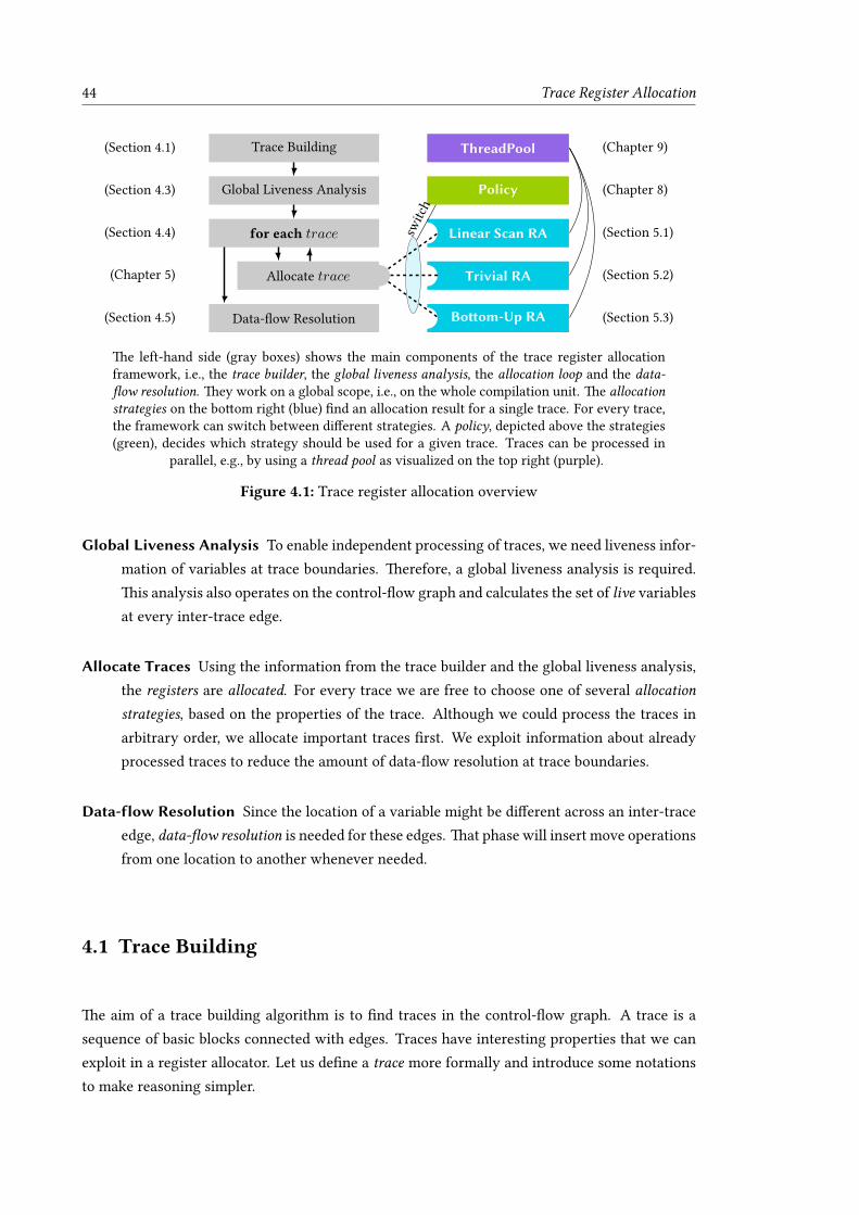
44 Trace Register Allocation
Trivial RA (Section 5.2)
Bottom-Up RA (Section 5.3)
Linear Scan RA (Section 5.1)
Policy (Chapter 8)
ThreadPool (Chapter 9)
(Chapter 5)
for each trace(Section 4.4)
Global Liveness Analysis(Section 4.3)
Trace Building(Section 4.1)
Data-flow Resolution(Section 4.5)
Allocate trace
switc
h
The left-hand side (gray boxes) shows the main components of the trace register allocationframework, i.e., the trace builder, the global liveness analysis, the allocation loop and the data-flow resolution. They work on a global scope, i.e., on the whole compilation unit. The allocationstrategies on the bottom right (blue) find an allocation result for a single trace. For every trace,the framework can switch between different strategies. A policy, depicted above the strategies(green), decides which strategy should be used for a given trace. Traces can be processed in
parallel, e.g., by using a thread pool as visualized on the top right (purple).
Figure 4.1: Trace register allocation overview
Global Liveness Analysis To enable independent processing of traces, we need liveness infor-mation of variables at trace boundaries. Therefore, a global liveness analysis is required.This analysis also operates on the control-flow graph and calculates the set of live variablesat every inter-trace edge.
Allocate Traces Using the information from the trace builder and the global liveness analysis,the registers are allocated. For every trace we are free to choose one of several allocationstrategies, based on the properties of the trace. Although we could process the traces inarbitrary order, we allocate important traces first. We exploit information about alreadyprocessed traces to reduce the amount of data-flow resolution at trace boundaries.
Data-flow Resolution Since the location of a variable might be different across an inter-traceedge, data-flow resolution is needed for these edges. That phase will insert move operationsfrom one location to another whenever needed.
4.1 Trace Building
The aim of a trace building algorithm is to find traces in the control-flow graph. A trace is asequence of basic blocks connected with edges. Traces have interesting properties that we canexploit in a register allocator. Let us define a trace more formally and introduce some notationsto make reasoning simpler.

4.1 Trace Building 45
Definition 30 (Trace). A trace T is a sequence of basic blocks ⟨b0, . . . , bn⟩. The trace length |T |denotes the number of blocks in a trace. We use the notation T [i] to refer to the ith block in atrace with i ranging from 0 to |T |−1. We call the first block T [0] in a trace the trace head. Thereis an edge between two consecutive blocks in a trace, T [i] ∈ succ(T [i− 1]) for i > 0. Therefore,the blocks might be executed sequentially. We also define that the edge (T [i− 1], T [i])must notbe a back edge. This implies that all blocks of a trace T are distinct, so T [i] ̸= T [j] for i ̸= j.
The set of Traces is a partition of the blocks of a CFG. Every block is in exactly one trace, soT ∩ T ′ = ∅ for T, T ′ ∈ Traces and T ̸= T ′. We write T = traceOf(b) if T is the tracethat contains block b and b ∈ T if T = traceOf(b). Traces are non-empty, i.e., |T | > 0 forT ∈ Traces.
We call an edge (ba, bb) between two blocks of the same trace an intra-trace edge, i.e., if ba, bb ∈ T .If not, i.e., traceOf(ba) ̸= traceOf(bb), it is an inter-trace edge. Any block in a trace can be thesource or the target of an inter-trace edge. In other words, a trace can have multiple entries andexits.
There are many possible ways of finding trace partitions in the CFG.1 In the simplest case, everyblock can be treated as a separate trace. In this case trace register allocation would be equivalentto local register allocation. However, longer traces offer more opportunities for optimization,for example, by moving spill code out of loops, and thus to improve the quality of the registerallocation. Therefore, we need more sophisticated trace building strategies. In the following, wepropose two trace building strategies that utilize the run-time feedback provided by the executionenvironment.
4.1.1 Unidirectional Trace Building
The unidirectional trace builder tries to minimize the trace exit probability. The algorithm, asshown in Algorithm 1, starts a new trace by selecting a block where all predecessors are alreadypart of some other trace. If there are multiple candidates, we choose the block with the highestexecution frequency. At the beginning, the only eligible block is the method entry. The blockis selected as the header of the new trace. Next, we select the block with highest executionfrequency from the set of successors that are not yet in any trace and add it to the current trace.We continue adding blocks in this way as long as possible. If there are no more successors thetrace is complete andwe proceed with the next trace. This is repeated until all blocks are assignedto a trace. Figure 4.2c depicts the result of the algorithm for the code in Figure 4.2a.
1 The number of possible partitions of a set is called the Bell number [Flajolet and Sedgewick, 2009]. However, onlysome of them fulfill all the properties we require for a trace partition.

46 Trace Register Allocation
long *allocateArray(int length, boolean fillContents) {/*B0*/ if (TLAB.top + length + 1 <= TLAB.end) {/*B1*/ result = TLAB.top;
TLAB.top += length + 1;} else {
/*B2*/ result = heapAlloc(length + 1);if (fillContents) {
/*B3*/ long *ptr = result + length;/*B4*/ while (result < ptr) {/*B5*/ *ptr = 0; ptr--;
} /* critical edge B7*/} else { /* critical edge B8*/ }
}/*B6*/ result[0] = length;
return result;}
(a) C-like source code
b0
b1
b6
b2
b3
b4
b5
b8
b7
(0.3)
(0.1)
(8.1)
(8.0)(0.1)
(0.2)
(1.0)
(0.7)
(1.0)
(b) Control-flow graph
T0 T1 T2 T3
b0
b1
b6
b2
b3
b8
b4
b5 b7
(1.0)
(0.7)
(0.3)
(0.1)
(8.1)
(8.0)
(1.0)
(0.1)
(0.2)
[1]
[2]
[3]
[4]
[5]
[6]
[7]
[8] [9]
(c) Unidirectional trace builder
T0 T1T2 T3
b0
b2
b3
b4
b5
b8
b7
b1
b6
(1.0)
(0.7)
(0.3)
(0.1)
(8.1)
(8.0) (1.0)
(0.1)
(0.2)
[1]
[2]
[3]
[4]
[5] [6]
[7]
[8]
[9]
(d) Bidirectional trace builder
Source code, control-flow graph and trace-building results of allocateArray. The values inparentheses (e.g. (0.8)) denote relative execution frequencies. The numbers in square brackets
(e.g. [2]) denote the order in which the trace builder processed the block.
Figure 4.2: Trace-building example for allocateArray
Although the algorithm is simple, it is not trivial to see that it terminates under all circumstances.Let us therefore analyze it in more depth.
Theorem 4. The unidirectional trace builder described in Algorithm 1 terminates for every (re-ducible) CFG without critical edges.
Proof. Let us first discuss the termination condition of Algorithm 1. The inner loop on line 9continues until the eligible set E is empty. In the loop, E is redefined on line 13. It is easy to seethat its size is bound by B. The size of B, however, is reduced by one in every iteration of theinner loop due to line 12. Therefore, the inner loop will eventually terminate.

4.1 Trace Building 47
Algorithm 1 Pseudocode for the Unidirectional Trace Builder1: procedure UnidirectionalTraceBuilder(CFG)2: (Blocks,Edges)← CFG3: Traces← {}4: B ← Blocks ▷ Block not yet in a trace5: while |B| > 0 do ▷ There are blocks not yet in a trace6: T ← ⟨⟩ ▷ New trace7: E ← {b ∈ B | pred(b) ∩B = ∅}8: ▷ Eligible blocks where all predecessors are in a trace9: while E ̸= ∅ do
10: b← bmax ∈ E where freq(bmax) is maximal ▷ Block with highest frequency11: T ← T + ⟨b⟩ ▷ Add block to trace12: B ← B \ b ▷ Block in a trace13: E ← succ(b) ∩B ▷ Eligible blocks, successor not in a trace14: end while15: Traces← Traces ∪ T ▷ Add T to the set of traces16: end while17: return Traces18: end procedure
How about the outer loop? Due to the condition on line 5, the loop terminates if all blocks are in atrace, so thatB is empty. For termination we need to ensure that the size ofB is reduced in everyiteration. We have already seen that the inner loop, if entered, will always terminate and reduceB in every iteration. It remains to show that we will enter the inner loop at least once in everyouter-loop iteration. In other words, we have to show that the set {b ∈ B | pred(b)∩B = ∅} online 7 is never empty. In the first iteration of the outer loop all blocks are inB, so pred(b)∩B willbe non-empty for every block unless pred(b) is empty. Per definition, the only block withoutpredecessors is the method entry block bentry . This means that we will find at least one tracecontaining bentry . In the general case, B is a proper subset of the blocks (B ⊂ Blocks). So someblocks are already in a trace (Blocks \ B) and some are not (B). Let us now assume that E online 7 is empty. Since we know that bentry /∈ B and all blocks are per definition reachable bybentry , there must be an inter-trace edge from a block b1 /∈ B to a block b2 ∈ B. Also, for E tobe empty, b2 must have another predecessor b3 ∈ B. See Figure 4.3a for an illustration. Note,that the building algorithm is greedy, which means that it will extend a trace as long as possible.If block b2 would be the single successor of b1, it would have been added to the trace due to theconstruction of the eligible set on line 13. Therefore, since b1 /∈ B, there must be another blockb4 /∈ B and an edge (b1, b4). However, as we can see in Figure 4.3b, this would mean that theedge (b1, b2) is critical which would violate our assumption that there are no such edges inCFG.Since b4 must exist, b2 can have only a single predecessor b1. More specifically, b3 cannot existas shown in Figure 4.3c. Thus, no predecessor of b2 is inB and the setE is not empty (it includesat least b2) which violates our assumption.

48 Trace Register Allocation
b1
b2
Blocks \B B
b3
(a) Non-greedy
b1
b2
Blocks \B B
b3
b4
critical edge
(b) Greedy with Critical Edge
b1
b2
Blocks \B B
b4
(c) Conclusion
Attempt to construct a non-terminating example for Algorithm 1. Blocks are all block of theCFG. The blocks inB are not yet assigned to a trace. Due to the greedy nature of the algorithmthe situation in sub-figure (a) cannot occur since b2 would be appended to the trace containingb1. So there must be a block b4 as shown in sub-figure b. This, however, violates our assumption
that there are no critical edges. Thus, b3 cannot exist c and b2 is eligible.
Figure 4.3: Termination of the unidirectional trace building algorithm
4.1.2 Bidirectional Trace Building
The bidirectional trace builder creates traces in decreasing order of their maximum block exe-cution frequency. Algorithm 2 outlines the idea in pseudocode. It first selects the block withthe highest execution frequency from all blocks that are not yet part of a trace. From this initialblock, it first grows the trace upwards. Among all predecessors from the candidate set we selectthe one with the highest execution frequency and prepend it to the trace. Note that we excludepredecessors that are the source of a loop back-edge. This means that after we processed a loopheader we always continue with the block entering the loop, never with the loop end block. Oncethere is no candidate left we start the downwards pass, again starting at the initial block. We pro-ceed in a way that is similar to the unidirectional trace builder. Bidirectional trace building hasalready been described by Ellis [1985] and Lowney et al. [1993]. Figure 4.2d shows the tracesformed by the bidirectional trace builder. The example illustrates that both strategies potentiallylead to different results.
Since the bidirectional trace builder imposes less restrictions for starting a new trace, the termi-nation of the algorithm is easier to see.
Theorem 5. The bidirectional trace builder (Algorithm 2) terminates for every CFG that is re-ducible and has no critical edge.
Proof. Both inner loops of Algorithm 2 terminate if the respective eligible set E becomes empty.Both sets are bound by B (line 11 and line 20). In every inner loop, B is decreased by one sothe inner loops terminate eventually. The outer loop terminates if B is empty. Since we pick anew s ∈ B for every iteration and remove s from B in line 8 the outer loop is also guaranteedto terminate.

4.1 Trace Building 49
Algorithm 2 Pseudocode for the Bidirectional Trace Builder1: procedure BidirectionalTraceBuilder(CFG)2: (Blocks,Edges)← CFG3: Traces← {}4: B ← Blocks ▷ Block not yet in a trace5: while |B| > 0 do ▷ There are blocks not yet in a trace6: s← bmax ∈ B where freq(bmax) is maximal ▷ Block with highest frequency7: T ← ⟨s⟩ ▷ New trace with s8: B ← B \ s ▷ Block s in a trace9: b← s ▷ Start with block s
10: loop ▷ Go upwards11: E ← {b′ ∈ (pred(b) ∩B) | (b′, b) ∈ Edges not a backedge}12: ▷ Eligible blocks, predecessors that do not form a loop and are not in a trace13: if E = ∅ break ▷ No more eligible blocks, leave loop14: b← bmax ∈ E where freq(bmax) is maximal ▷ Block with highest frequency15: T ← ⟨b⟩+ T ▷ Prepend block to trace16: B ← B \ b ▷ Block in a trace17: end loop18: b← s ▷ Reset current block to s19: loop ▷ Go downwards20: E ← succ(b) ∩B ▷ Eligible blocks, successor not in a trace21: if E = ∅ break ▷ No more eligible blocks, leave loop22: b← bmax ∈ E where freq(bmax) is maximal ▷ Block with highest frequency23: T ← T + ⟨b⟩ ▷ Append block to trace24: B ← B \ b ▷ Block in a trace25: end loop26: Traces← Traces ∪ T ▷ Add T to the set of traces27: end while28: return Traces29: end procedure

50 Trace Register Allocation
Discussion
Figure 4.2 shows that the traces formed by the two trace building algorithmsmay differ. While theunidirectional algorithm favors the execution paths that aremore likely, for example the commoncase b0, b1 and b6, the bidirectional trace builder creates traces where most time is spent. In theallocateArray example, this is the initialize loop of the heap allocation case. Both methods leadto interesting results. Since our goal is to focus on the common case, the unidirectional tracebuilder is our algorithm of choice. We evaluated both approaches and came to the conclusionthat the unidirectional trace builder is not only simpler but also achieves slightly better resultsthan its bidirectional counterpart (see Figure 7.12).
4.2 Trace Properties
Although it seems intuitive that register allocation for a trace is simpler than for a general control-flow graph, traces have properties that are not self-evident. Some originate from the generaldefinition of traces (Definition 30), others are due to our trace building strategies. Many of theseproperties can be exploited by a register allocation strategy to simplify its algorithmic complexity.In the following, we summarize these observations. Keep in mind that we assume that the CFGis reducible and does not contain critical edges.
Definition 31 (Greedy Trace Builder). A trace builder is upwards (downwards) greedy if itprepends (appends) blocks to a trace until there is no more predecessor (successor) that is notalready in a trace.
Theorem 6. The unidirectional and bidirectional trace builders are greedy.
Proof: Unidirectional. This directly follows from the calculation of the eligible sets on line 7 andline 13 of Algorithm 1.
Proof: Bidirectional. This directly follows from the calculation of the eligible sets on line 11 andline 20 of Algorithm 2.
4.2.1 Greedy Trace Properties
The following properties hold for all greedy trace builders.
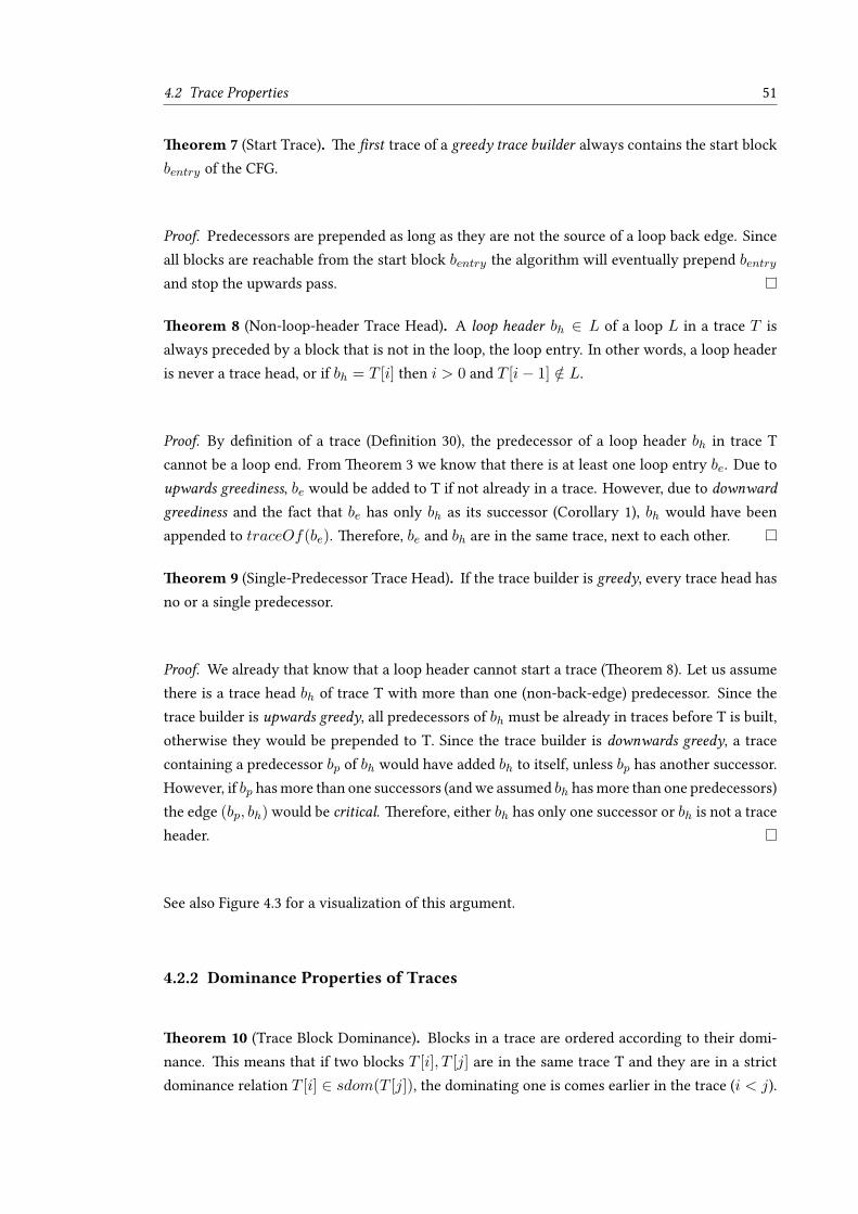
4.2 Trace Properties 51
Theorem 7 (Start Trace). The first trace of a greedy trace builder always contains the start blockbentry of the CFG.
Proof. Predecessors are prepended as long as they are not the source of a loop back edge. Sinceall blocks are reachable from the start block bentry the algorithm will eventually prepend bentry
and stop the upwards pass.
Theorem 8 (Non-loop-header Trace Head). A loop header bh ∈ L of a loop L in a trace T isalways preceded by a block that is not in the loop, the loop entry. In other words, a loop headeris never a trace head, or if bh = T [i] then i > 0 and T [i− 1] /∈ L.
Proof. By definition of a trace (Definition 30), the predecessor of a loop header bh in trace Tcannot be a loop end. From Theorem 3 we know that there is at least one loop entry be. Due toupwards greediness, be would be added to T if not already in a trace. However, due to downward
greediness and the fact that be has only bh as its successor (Corollary 1), bh would have beenappended to traceOf(be). Therefore, be and bh are in the same trace, next to each other.
Theorem 9 (Single-Predecessor Trace Head). If the trace builder is greedy, every trace head hasno or a single predecessor.
Proof. We already that know that a loop header cannot start a trace (Theorem 8). Let us assumethere is a trace head bh of trace T with more than one (non-back-edge) predecessor. Since thetrace builder is upwards greedy, all predecessors of bh must be already in traces before T is built,otherwise they would be prepended to T. Since the trace builder is downwards greedy, a tracecontaining a predecessor bp of bh would have added bh to itself, unless bp has another successor.However, if bp hasmore than one successors (andwe assumed bh hasmore than one predecessors)the edge (bp, bh)would be critical. Therefore, either bh has only one successor or bh is not a traceheader.
See also Figure 4.3 for a visualization of this argument.
4.2.2 Dominance Properties of Traces
Theorem 10 (Trace Block Dominance). Blocks in a trace are ordered according to their domi-nance. This means that if two blocks T [i], T [j] are in the same trace T and they are in a strictdominance relation T [i] ∈ sdom(T [j]), the dominating one is comes earlier in the trace (i < j).

52 Trace Register Allocation
b1
b2
b3 critica
ledg
e
Figure 4.4: Non-sequential forward edges are critical edge
Proof. By contradiction. Let T [i], T [j], i < j and T [j] ∈ sdom(T [i]). From Theorem 1 weknow that every path from a block to its strict dominator contains a back edge. So the path⟨T [i], T [i+1], . . . , T [j]⟩, which is a subset of the trace T contains a back edge which is prohibitedby the definition of a trace (Definition 30).
Theorem 11 (Consecutive Intra-trace Edges). If a control-flow graph does not contain criticaledges, an intra-trace edge either connects two blocks that are next to each other in the trace, orit is a back edge.
Proof. By contradiction. Due to Definition 30 we know that every block in a trace T [i], withexception of the last one, has at least one successor, namely the next block in the trace T [i+ 1].Analogously, every block T [i], that is not the trace head, has at least one predecessor, namely theprevious block in the trace T [i−1]. Without loss of generality we assume that the trace consistsof three blocks ⟨b1, b2, b3⟩. Figure 4.4 illustrates such a trace. Now, let there be a forward edge(b1, b3). However, this means that the source block b1 has two successor, namely b2 and b3, andthe target block b3 has more than one predecessor, namely b1 and b2. Therefore, the edge (b1, b3)is a critical edge, which contradicts our assumption that there are no critical edges.
Corollary 2 (Loop End/Trace End). If a control-flow graph does not contain critical edges, aback edge can only occur at the end of a trace.
Proof. From Corollary 1 we know that a loop end has only one successor, the loop header. How-ever, by Definition 30, the trace builder does not follow a back edge. Therefore, there is no eligiblesuccessor and the trace must end at a loop end.
Theorem12 (TraceHeadDominator). Let bi be a block of trace T. Every dominator bd ∈ dom(bi)
is either in T or bd also dominates the trace head bh of T.
Proof. Assume that bd ∈ dom(bi), bd /∈ T and bd /∈ dom(bh) where bh is the trace head. Thiswould mean that there is a path ⟨bentry, . . . , bh⟩ which does not include bd. Since bh ⇝ bi,there would also have to be a path ⟨bentry, . . . , bi⟩ that does not include bd. Therefore, bd cannotdominate bi.

4.3 Global Liveness Analysis 53
Theorem 13 (Trace Head Liveness). Assuming SSA form, a value which is live at a certain pointin a trace T is either defined in T or live at the beginning of the trace head of T.
Proof. Due to the dominance property (Property 2) of the SSA form we know that a value v thatis used in block bi is defined in a dominator bd of bi. If v is not defined in T then there is a pathfrom the definition in bd to the usage that goes through the trace head bh. Therefore, v must belive at the beginning bh.
Theorem 14 (No Lifetime Holes in Traces). The lifetime interval for a variable in a trace doesnot contain lifetime holes.
Proof. By Definition 27, a lifetime hole can only occur if there are non-consecutive blocks in thelinearized form of the CFG. By Definition 30, this does not hold for a trace.
Definition 32 (Interval Graph). Following Brisk and Sarrafzadeh [2007, Definition 1], whichoriginates from Lekkeikerker and Boland [1962], a graph is an interval graph if it is the interfer-ence graph of some set of live ranges.
Corollary 3 (The Interference Graph of a Trace is an Interval Graph). By the definition of aninterference graph and Theorem 14, the interference graph of a trace is an interval graph.
Theorem 15 (Trace Domination). Assume that a greedy trace builder builds traces in the orderT0, T1, . . . , Tn. Then we know that for a block b in trace Tk all dominators dom(b) of b are intraces T0, . . . , Tk.
Proof. Due to upwards greediness, the single predecessor bp (Theorem 9) of trace header bh ofa trace Tk is already in a trace T0, . . . , Tk−1. Since bentry ∈ T0 (Theorem 7) there is a path⟨bentry, . . . , bp, bh⟩ which contains all dominators of bh. So, due to Theorem 12, all dominatorsof all blocks in Tk are either in Tk or in dom(bh).
4.3 Global Liveness Analysis
A core feature of our trace register allocation approach is that traces can be processed indepen-dently by the allocator, potentially with different strategies. However, a trace in general does nothave enough information about the liveness of variables.
Let’s have a look at Figure 4.5. There is no usage of totalFS in T1, so we could conclude thatwe do not need a register for storing its value. In trace T2, on the other hand, it seems thatonly totalFS is live. However, when looking at the whole method, it becomes clear, that this is
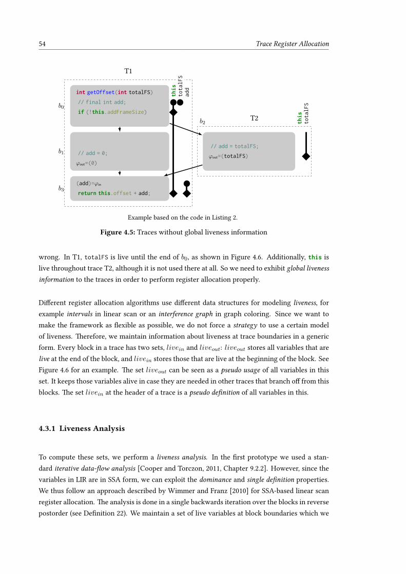
54 Trace Register Allocation
T1
T2
int getOffset(int totalFS)
// final int add;
if (!this.addFrameSize)
// add = 0;
ϕout=(0)
(add)=ϕin
return this.offset + add;
// add = totalFS;
ϕout=(totalFS)
b0
b1
b2
b3
this
tota
lFS
add
this
tota
lFS
Example based on the code in Listing 2.
Figure 4.5: Traces without global liveness information
wrong. In T1, totalFS is live until the end of b0, as shown in Figure 4.6. Additionally, this islive throughout trace T2, although it is not used there at all. So we need to exhibit global livenessinformation to the traces in order to perform register allocation properly.
Different register allocation algorithms use different data structures for modeling liveness, forexample intervals in linear scan or an interference graph in graph coloring. Since we want tomake the framework as flexible as possible, we do not force a strategy to use a certain modelof liveness. Therefore, we maintain information about liveness at trace boundaries in a genericform. Every block in a trace has two sets, livein and liveout: liveout stores all variables that arelive at the end of the block, and livein stores those that are live at the beginning of the block. SeeFigure 4.6 for an example. The set liveout can be seen as a pseudo usage of all variables in thisset. It keeps those variables alive in case they are needed in other traces that branch off from thisblocks. The set livein at the header of a trace is a pseudo definition of all variables in this.
4.3.1 Liveness Analysis
To compute these sets, we perform a liveness analysis. In the first prototype we used a stan-dard iterative data-flow analysis [Cooper and Torczon, 2011, Chapter 9.2.2]. However, since thevariables in LIR are in SSA form, we can exploit the dominance and single definition properties.We thus follow an approach described by Wimmer and Franz [2010] for SSA-based linear scanregister allocation. The analysis is done in a single backwards iteration over the blocks in reversepostorder (see Definition 22). We maintain a set of live variables at block boundaries which we

4.3 Global Liveness Analysis 55
T1
T2
int getOffset(int totalFS)
// final int add;
if (!this.addFrameSize)
liveout =(this,totalFS)
(this,-)= livein
// add = 0;
ϕout=(0), liveout =(this)
(this)= livein, (add)=ϕin
return this.offset + add;
(this,totalFS)= livein
// add = totalFS;
ϕout=(totalFS),
liveout =(this)
b0
b1
b2
b3
this
tota
lFS
add
this
tota
lFS
Figure 4.6: Traces with global liveness information
later use for the livein and liveout sets. For loop headers, the live sets in the loop need to be up-dated, as proposed by Wimmer and Franz [2010]. Nevertheless, this approach offers significantspeedup over the iterative approach.
4.3.2 Representation of Global Liveness
The most convenient way to represent liveness information is to add pseudo usages and defini-tions directly to the LIR, as shown in Figure 4.6. The representation is similar to the notion ofϕs. The advantage is that phases can process the pseudo usages just as any other usage withoutspecial handling. Pseudo usages will be picked up by (trace-local) liveness analysis and the regis-ter allocator will assign locations to them. These locations are then used by the global data-flowresolution (see Section 4.5). The downside is that the in-LIR variant poses overhead in terms ofspace, because the livein and liveout sets at both ends of an edge are redundant, and in terms oftime, since the iteration of LIR instructions gets slower due to the increased number of operandreferences. In addition, it increases the number of indirections, since all operands in LIR areobjects (of class Variable in this case), although a primitive integer value would be sufficient forencoding variables.
Therefore, we decided to use an external data structure to capture only the required information.Our first observation was, that for every control-flowmerge, the liveness information is the sameat the end of all predecessors. This is only true because there are no critical edges. Also notethat ϕs are still represented in the LIR. Therefore, it is sufficient to store only livein at the merge,and use this set also for all predecessors. We can use a similar optimization for control-flow

56 Trace Register Allocation
T1
T2
int getOffset(int totalFS)
// final int add;
if (!this.addFrameSize)
// add = 0;
ϕout=(0)
(add)=ϕin
return this.offset + add;
// add = totalFS;
ϕout=(totalFS)
b0
b1
b2
b3
this
tota
lFS
add
this
tota
lFS
liveB0out = (this, totalFS)
liveB3in = (this)
The set liveout is stored at the end of split blocks and the set livein at the beginning of mergeblocks.
Figure 4.7: Representation of liveness
splits, although a variable that is live at the end of a branching block might not be needed in allsuccessors. The edge (b0, b1) in T1 of Figure 4.6 demonstrates the situation. The variable totalFSis live at the end of b0 but not at the beginning of b2. However, this is usually not a problem.During trace-local liveness analysis—assuming that we do it via a backwards pass—we wouldsee a pseudo definition without usage, which we can simply ignore. Thus, it is sufficient to storeliveout at the end of splitting blocks, and livein at the beginning of merge blocks, which reducesthe memory requirement to at least a third.2 Figure 4.7 shows the improved global livenessinformation for the previous example.
4.4 Allocating Registers
The allocation step is the core of the framework and the basis for its flexibility. Essentially, aslong as there is an unprocessed trace, the framework selects one and allocates registers for it.How registers are allocated is not relevant to the framework. We implemented three differentallocation strategies for different purposes. The details of them are described in Chapter 5. Forevery trace, the framework can use a different strategy. The decisionwhich strategy ismost suitedis based on heuristics, which are discussed in Chapter 8. Note that traces could be processed in
2Also, we can use an int[] instead of a Variable[] array. Thismeans that in addition to removing one indirection,only half of the memory is needed assuming that int requires 32 bits and a reference 64 bits.

4.5 Global Data-flow Resolution 57
T1
T2
int getOffset(int totalFS)
// final int add;
if (!this.addFrameSize)
// add = 0;
ϕout=(0)
(add)=ϕin
return this.offset + add;
// add = totalFS;
ϕout=(totalFS)
b0
b1
b2
b3
this
tota
lFS
add
this
tota
lFS
liveb0out = (this, totalFS)
locb0out = (reg1 , reg2 )
locb2in = (reg2 , reg1 )
liveb3in = (this)
locb2out = (reg2 )
locb3in = (reg1 )
Figure 4.8: Representation of the locin/locout sets
arbitrary order, even in parallel as demonstrated in Chapter 9. However, traces that are processedlater can exploit information about already processed traces. Therefore, traces are processed inorder of their importance.
In addition to allocating registers in the trace, the allocation strategy needs to record the locationof variables at inter-trace edges. This information is stored in locin and locout sets. In contrast tothe livein/liveout sets, the location sets are needed for both ends of an edge, since variables mightbe in different locations in different traces. Figure 4.8 shows the location sets for the getOffsetexample.
4.5 Global Data-flow Resolution
Since traces are processed independently, the location of a variable might differ at the two ends ofan inter-trace edge. See the edge (b0, b2) in Figure 4.8, for example. In b0 of T1, this is stored inreg1. However, in b2 the value is in reg2. Therefore, when crossing the edge, we need to adjustthe locations to get a valid allocation. To do so, we need to insert moves which are executedwhen following the edge. For our example this means that we have to insert the moves at thebeginning of b2. This global data-flow resolution is done for every inter-trace edge. Figure 4.9shows the example with the inserted move instructions.

58 Trace Register Allocation
T1
T2int getOffset(reg1 ,reg2 )
// final int add;
if (!reg1 .addFrameSize)
// add = 0;
reg2 = 0;
return reg1 .offset + reg2 ;
st1 = reg1 ; // tmp this
reg1 = reg2 ; // totalFrameSize
reg2 = st1 ; // this
// add = totalFrameSize;
st2 = reg2 ; // tmp this
reg2 = reg1 ; // add
reg1 = st2 ; // this
b0
b1b2
b3
locB0out = (reg1 , reg2 )
locB2in = (reg2 , reg1 )
locB2out = (reg2 )
locB3in = (reg1 )
Result of data-flow resolution for the allocation of addOffset in Figure 4.8. There are two inter-trace edges that need data-flow resolution, namely (b0, b2) and (b2, b3). For the first edge weneed to insert moves from reg1 to reg2 for this and from reg2 to reg1 for totalFS. Since themoves are cyclic we introduce a temporary stack slot st1 to break the cycle. The moves areinserted at the beginning of b2. For the edge (b2, b3) we need to fix the data-flow mismatch forthis with a move from reg2 to reg1. In addition, we need to destruct the ϕ which assigns addto totalFS. To do so we insert a move from reg1 to reg2. As this example demonstrates, ϕsand data-flow mismatches need to be resolved simultaneously since they may also introduce acycle. We therefore introduce another temporary stack slot st2. The resolution code is inserted
at the end of b2.
Figure 4.9: Inserted move instructions for global data-flow resolution
Where should the phase place the resolution code? As suggested in the above example, we wouldwant to insert it along a control-flow edge. Since there are no critical edges, this is easy. Eitherthe source of an edge has only a single successor, then we can insert the code at the end of thesource block. Otherwise, the target must have only a single predecessor. Therefore, we can placethe code in the target block.
Conceptionally, all resolution moves are done in parallel. In reality, however, most processorsforce us to place the moves in sequential order.3 Since there might be write-after-read depen-dencies (also called anti-dependencies) [Cooper and Torczon, 2011, Chapter 12.2] between moveinstructions, we need to be careful with the order in which we insert the moves. In the worstcase, those dependencies are cyclic, that means that we cannot find an order so that all dependen-cies are satisfied. The edge (b0, b2) in Figure 4.8 shows such an example. To resolve the locationmismatch for this we need to insert a move from reg1 to reg2. However, to fix the data flowtotalFS, a move from reg2 to reg1 is required. No matter how we place the moves, we would
3Mohr et al. [2013] proposed special hardware to speed up the shuffle code. While this would avoid the move emis-sion, compiler support is still required [Buchwald et al., 2015].

4.5 Global Data-flow Resolution 59
overwrite one of the two values. Note, that the cycle can consist of an arbitrary number of moveinstructions. To break such a cycle, we introduce a new temporary stack slot. Figure 4.9 showsthe result for the example.
In addition to a location mismatch, there might be ϕin/ϕout pairs that need to be resolved. Weneed to handle them in parallel to the locations, since they might have interdependencies. Theedge (b2, b3) in Figure 4.8 shows an example. Due to the location mapping for this, we need amove from reg2 to reg1. To resolve the ϕ for add, the content of reg1 should be copied to reg2.Again, this forms a cycle and requires a temporary stack slot to break it.


61
Chapter 5
Register Allocation Strategies
The task of a register allocation strategy is to solve the register allocation problem, i.e., to replacevariables with registers, for a single trace. Since a trace is a list of sequential blocks, allocatingregisters for a trace is significantly simpler than for a method with arbitrary control-flow. First,there are no holes in the lifetime intervals of variables (see Theorem 14). Since variables adhereto the SSA form, we know that a variable is live from its definition in the trace (either the explicitdefinition, or the livein set of the trace header, see Theorem 13) to the last usage in the trace,which might be a real usage or an entry in the liveout set. In addition, a strategy must resolveϕ-functions for the predecessor that is in the same trace as the merge block. (Inter-trace edgeswith ϕs are handled by the global data-flow resolver, which was discussed in Section 4.5.)
In the course of this work, we implemented three strategies, a linear scan allocator (Section 5.1),a special trivial trace allocator (Section 5.2) and a fast bottom-up allocator (Section 5.3).
5.1 Linear Scan Allocator
The trace-based linear scan algorithmoriginated from an adaption of the global approach byWim-mer andMössenböck [2005] andWimmer and Franz [2010], which is the default register allocatorin Graal. However, due to the straightforward structure of traces, the implementation could besignificantly simplified. As a result, large parts of the code have been rewritten. In this section,we given an overview of our trace-based linear scan strategy with a focus on the differences tothe global variant.
Figure 5.1 shows the phases of the trace-based linear scan strategy. The general idea is that firstan interval representation of liveness is created. These intervals capture all information neces-sary to perform the actual allocation. Working with intervals as an intermediate data structureis more efficient than modifying the LIR directly. This is especially important, since decisions

62 Register Allocation Strategies
Interval Building
Register Allocation on Intervals
Local Data-flow Resolution
Register Assignment on LIR
LIR of Trace with Variables
LIR of Trace without Variables
Figure 5.1: Trace-based linear scan
during allocation are not final in general. For example, the spill position, i.e., the position wherea variable is spilled to the stack, might change during allocation. After the allocation pass isfinished, a data-flow resolution phase handles data-flow mismatches and ϕs across intra-traceedges, which might have been introduced by interval splitting. Last but not least, the variablesin the LIR are replaced by the locations stored in the corresponding intervals.
5.1.1 Interval Building
First, we number the instructions of the traces. For technical reasons we only use even numbers,and start at 2. The interval builder performs a backwards liveness analysis. It creates an intervalfor every variable and every register in the LIR instructions of the trace. Variable intervals areused to perform register allocation. Since they have no lifetime holes (see Theorem 14) theirrepresentation is simple. For every interval, we store the variable, the (allocated) location, thespill slot, a from and a to position, as well as a list of usages. Listing 1 in the appendix showsthe relevant parts of the class TraceInterval. Register intervals are used to track fixed register
constraints, which are imposed by calling conventions,1 instruction set restrictions,2 or specialpurpose registers used by the virtual machine.3 The allocator needs to respect these requirementswhile it allocates registers for variables. Fixed registers do not adhere to SSA form, since aregister might be defined multiple times. This implies that register intervals can have lifetimeholes. Therefore, they are represented as a list of live ranges, each with a from and to position.These ranges are usually short, spanning only very few instructions, and are never live across ablock boundary.
1Calling conventions specify, for example, parameter or return registers.2For example, the result of the idiv instruction on AMD64 is implicitly stored in rax and rdx [Intel, 2013b].3On HotSpot, register rbp is used as the frame pointer register on AMD64.
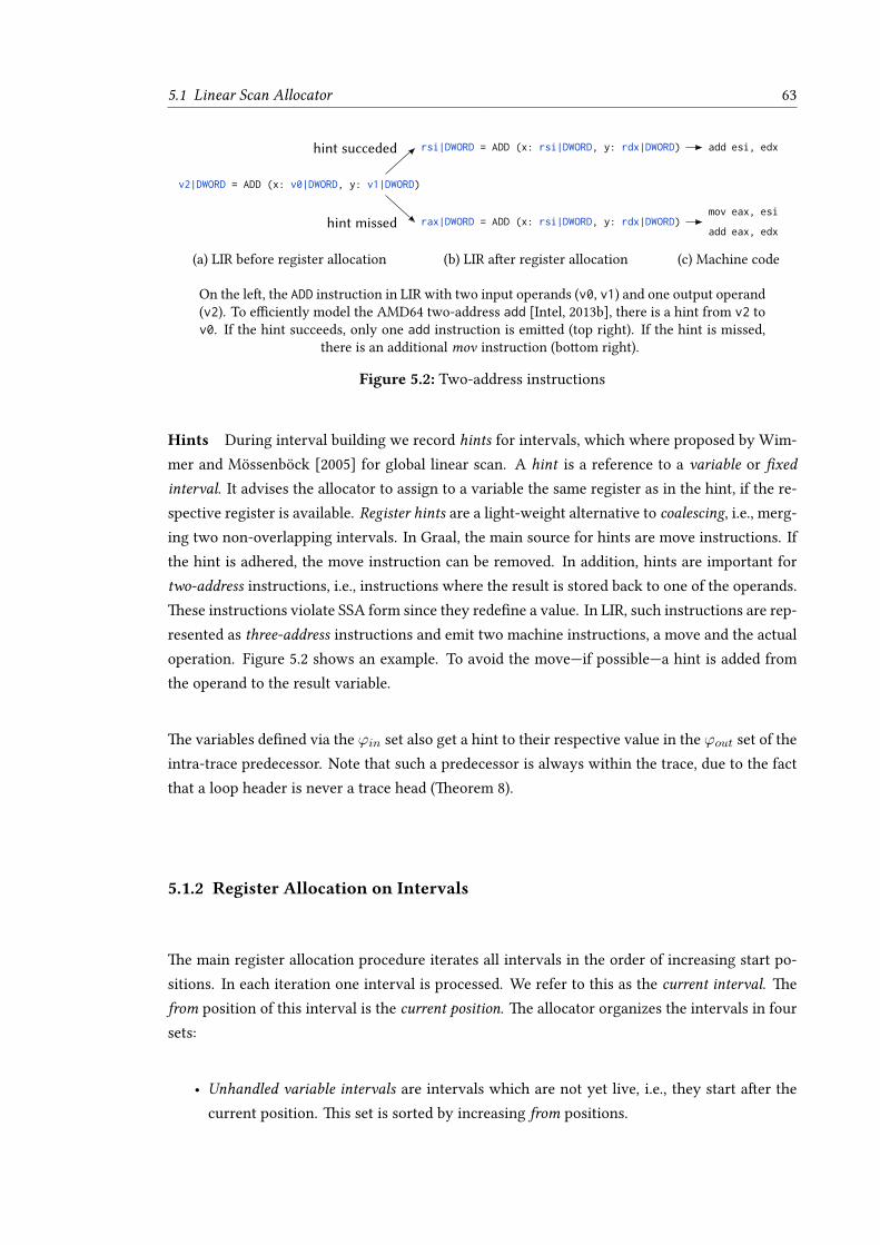
5.1 Linear Scan Allocator 63
v2|DWORD = ADD (x: v0|DWORD, y: v1|DWORD)
rsi|DWORD = ADD (x: rsi|DWORD, y: rdx|DWORD)
rax|DWORD = ADD (x: rsi|DWORD, y: rdx|DWORD)
add esi, edx
mov eax, esi
add eax, edx
hint succeded
hint missed
(a) LIR before register allocation (b) LIR after register allocation (c) Machine code
On the left, the ADD instruction in LIR with two input operands (v0, v1) and one output operand(v2). To efficiently model the AMD64 two-address add [Intel, 2013b], there is a hint from v2 tov0. If the hint succeeds, only one add instruction is emitted (top right). If the hint is missed,
there is an additional mov instruction (bottom right).
Figure 5.2: Two-address instructions
Hints During interval building we record hints for intervals, which where proposed by Wim-mer and Mössenböck [2005] for global linear scan. A hint is a reference to a variable or fixedinterval. It advises the allocator to assign to a variable the same register as in the hint, if the re-spective register is available. Register hints are a light-weight alternative to coalescing, i.e., merg-ing two non-overlapping intervals. In Graal, the main source for hints are move instructions. Ifthe hint is adhered, the move instruction can be removed. In addition, hints are important fortwo-address instructions, i.e., instructions where the result is stored back to one of the operands.These instructions violate SSA form since they redefine a value. In LIR, such instructions are rep-resented as three-address instructions and emit two machine instructions, a move and the actualoperation. Figure 5.2 shows an example. To avoid the move—if possible—a hint is added fromthe operand to the result variable.
The variables defined via the ϕin set also get a hint to their respective value in the ϕout set of theintra-trace predecessor. Note that such a predecessor is always within the trace, due to the factthat a loop header is never a trace head (Theorem 8).
5.1.2 Register Allocation on Intervals
The main register allocation procedure iterates all intervals in the order of increasing start po-sitions. In each iteration one interval is processed. We refer to this as the current interval. Thefrom position of this interval is the current position. The allocator organizes the intervals in foursets:
• Unhandled variable intervals are intervals which are not yet live, i.e., they start after thecurrent position. This set is sorted by increasing from positions.

64 Register Allocation Strategies
• Active variable intervals are live at the current position and have a register assigned. Theyare sorted by increasing to positions.
• Active register intervals are fixed register intervals that have a range that covers the currentposition. They are also sorted by increasing to position of their current ranges.
• Inactive register intervals do not have a range covering the current position. They are sortedby increasing from positions of their next range.
The allocator continues as long as there are intervals in the unhandled set. The interval withthe lowest from position is removed from the set and is processed. First, the other interval setsare adjusted. Variable intervals with a to position smaller than the current position are removedfrom the active set. The register intervals in the active (inactive) set are removed if the to (from)position of their current range is smaller than the current position. The removed register intervalsmight be readded to the active or inactive set if there is another range with ends after the currentposition.
Next, the allocator tries to assign a free register to the current interval. To do so, it builds a mapfrom registers to free-until positions, i.e., to the position when the registers become available.All entries are initialized with infinity. The registers assigned to variable and fixed intervals inthe active sets are removed. Finally, for all inactive register intervals we record the from positionof the next range. From this set of feasible registers, the allocator selects the register with thesmallest free-until position that is still bigger than the current interval’s to position. If there issuch a register the allocation succeeded. However, due to fixed register constrains, there mightbe no register available for the full interval. In that case, we select the register with the biggestfree-until position, split the current interval at this position and assign the register to the partialinterval. The split child is added to the unhandled list. In addition, we insert a move from theparent interval to the child interval at the split position. In case the current interval has a hint,we favor the hint register by ignoring the free-until position. However, a partially available hintwill never overrule a fully available register.
If we fail to find a register that is either fully or partially free, we need to spill. The goal is to selecta register which is not accessed until the next usage of the current interval. Again, we collectinformation about the feasible registers. In case the register is occupied by a variable interval,we record the next usage of this interval, which is where the interval needs to be reloaded. Weremove active fixed intervals from the list since we cannot spill them. The from position of thenext range of inactive fixed intervals also contributes to the next usage of a register. With thisinformation at hand, we select the register with the highest next usage position. If two registers

5.1 Linear Scan Allocator 65
have the same position, we favor the one where the corresponding variable interval has alreadybeen spilled in the past. That way, we can avoid to insert a spill move. If we do not find a register,we bailout and abort compilation.4 Otherwise, the candidate register is occupied by a variable.
We split the interval which currently occupies the register at the current position, as well asbefore the next usage. The parent interval has already a register assigned and will not be touched,other than setting the to position. The first split child is located on the stack. The last split childis unassigned and inserted into the unhandled list. Finally, we set the location of the currentinterval to the freed register and are finished.
However, an inactive register interval might restrict the period for which a register candidate isavailable. If the start of the next range of the fixed interval is greater than the to position of thecurrent interval, we can use the register for the entire interval. Otherwise, the register is onlypartially available and we perform the same actions as in the allocate free register scenario, i.e.,split the current interval and add the split child to the unhandled list.
Splitting and Spilling When an interval needs to be split, the algorithm computes the latestpossible split position. However, we can split the interval anywhere between the last usage andthe latest position. If both positions are in the same block, no optimization is possible. Otherwise,we split the interval in the block with the lowest execution frequency between both positions.Therefore, the corresponding move instruction is executed less often. Since we need to ensurethat moves which are inserted at a particular position are properly ordered, we split the intervalsat block boundaries and let the local data-flow resolution phase deal with it. Since we are in SSAform, we only need to spill a value once. The spill position is independent from the split positions,as long as the spill happens between the definition of the value and the first stack interval. Similarto the split position we choose the block with the lowest execution frequency.
5.1.3 Local Data-flow Resolution
Due to interval splitting, the location of a value might be different at both ends of an intra-traceedge. Similar to the global data-flow resolution, which we described in Section 4.5, we performa local resolution phase. It also takes care of ϕ-instructions. The only difference to its globalcounterpart is that the local resolution operates on intervals instead of on the global liveness
information. It is worth noting that due to the placement of the resolution moves, the local andthe global data-flow resolution phases do not interfere.
4Usually, this is an evidence for a compiler bug, since the number of registers required at the current position—thatare active fixed register intervals and registers required by the current instruction—is higher than the number ofavailable registers. In production this should never happen.

66 Register Allocation Strategies
b1
b2
b3
b4
critical edge
(a) Critical edge
b1
b2
b3
b4
bhbe
(b) Link trace
b1
b2
b3
b4
bt
(c) Trivial link trace
Figure 5.3: Link traces
5.1.4 Register Assignment on LIR
Since the algorithm splits already assigned intervals, the final location of a variable at a giveninstruction is only known when all intervals are processed. Therefore, we conclude linear scanallocation with an assignment phase, which iterates all instructions and replaces all variableswith the location recorded in the corresponding interval.
5.2 Trivial Trace Allocator
As already mentioned, control-flow can exit and enter a trace at any block. Let us consider theexample in Figure 5.3a. If an edge would lead from inside a trace (i.e., not from the last block)to the middle of another trace, this edge would be critical. Therefore, there must be (at least) atrace in between which is entered at the head and left via the last block, as shown in Figure 5.3b.Often, this trace consists of a single block. Figure 5.3c depicts an example. We call such tracestrivial traces.
Definition 33 (Trivial Trace). A trivial trace is a special kind of trace with a single basic blockwhich contains only a single jump instruction.
Trivial traces are very common. For the DaCapo benchmark suite, about 40% of the traces aretrivial (see Figure 8.2). The unidirectional trace-building example in Figure 4.2c contains onetrivial trace (T3). In the bidirectional case (Figure 4.2d) two out of four traces are trivial (T2 andT3).

5.2 Trivial Trace Allocator 67
ϕout = (v6, v0, v6)
bp
…
bt
locbtin=locbpout
livebtin = (v0, v1, v4, v6)
locbpout = (reg2 , reg3 , st0 , reg1 )
locbtout = (reg2 )
livebtout = (v0)
(a) Before allocation
ϕout = (reg1 , reg2 , reg1 )
bp
…
bt
locbtin=locbpout
livebtin = (v0, v1, v4, v6)
locbpout = (reg2 , reg3 , st0 , reg1 )
locbtout = (reg2 )
livebtout = (v0)
(b) After allocation
Example allocation of a trivial trace consisting of block bt. A trivial trace is a trace consistingof a block without any instruction (except a jump). There are several interesting observationsto make. First, the live sets are ordered w.r.t. the variable indices. Second, the liveout set is asubset of livein. Third, the values in ϕout are ordered w.r.t. to their respective ϕin and there
might be duplicates and variables not in liveout.
Figure 5.4: Example of a trivial trace allocation
Due to their simple structure, trivial traces are significantly easier to allocate than general traces.But why do we even have to allocate them? Like for every other trace, we need to populate thelocin and locout locations according to their respective livein and liveout sets. In addition, theremay be outgoing values in ϕout, which need to be replaced with a register or stack slot. However,both requirements are easy to fulfil.5
Figure 5.4a shows a typical example of a trivial trace. The variables in the livein and liveout setsare sorted by construction. Also, since there cannot be a variable definition in a trivial trace,liveout is a subset of livein. In which case is liveout a proper subset of livein? As described inSection 4.3.2, the live sets are shared between a split block and its successors. So a variable v
might be live in a sibling of a trivial trace block, but in or after the trivial trace. Therefore, v isin livein but not in liveout of the trivial trace. The outgoing ϕout variables can only referencevariables in livein. However, the order in which variables occur in ϕout is arbitrary. There mighteven be duplicates.
Algorithm 3 shows the allocator in pseudo code. It assumes that the live sets are ordered ac-cording to their variable index.6 First, on line 2, the locin is set to the locout of the predecessor.Next, the algorithm iterates over all incoming variables (line 5). In case the variables occur inthe liveout set of the trivial trace, the locout location is set to the current locin location (loop 6).Afterwards, the allocator resolves ϕ values for the ϕout list on line 11. Since the livein set issorted, we can binary search for the index of the respective location in the locin set. Note that we
5One might say trivially…6In our implementation this is true by construction of the sets by the global liveness analysis (Section 4.3.2).

68 Register Allocation Strategies
Algorithm 3 Trivial Trace Allocation Strategy1: procedure TrivialTraceAllocator( locpredout , livein, liveout, ϕout )2: locin ← locpredout ▷ Incoming locations are the outgoing of the predecessor3: locout ← new list of size |liveout|x] ▷ Reserve space for outgoing locations4: idxout ← 0 ▷ Incoming and outgoing indices might diverge5: for idxin ∈ {0, . . . , |locin| − 1} do6: if liveout[idxout] = livein[idxin] then ▷ The incoming variable is also in liveout7: locout[idxout]← locin[idxin] ▷ Set outgoing location8: idxout ← idxout + 1 ▷ Increment outgoing index9: end if
10: end for11: for idxϕ ∈ {0, . . . , |ϕout| − 1} do12: val← ϕout[idxϕ] ▷ Get ϕout value13: if val is variable then14: idxin ← binarySearch(val, livein) ▷ Find location index for val using binary search15: ϕout[idxϕ]← locin[idxin] ▷ Update ϕout
16: end if17: end for18: return (locin, locout)19: end procedure
also experimented with a version that used a variable-to-location map to avoid repetitive search-ing. However, empirical experiments suggest that the binary search variant outperforms themapapproach by 40%. We account this to the reduced number of allocations.
5.3 Bottom-Up Allocator
Not all traces of a method are equally important for peak performance. As already said, we donot want to spend too much time on traces that are infrequently executed. Although the linearscan strategy outlined in Section 5.1 exhibits a linear time behavior with respect to the numberof instructions [Eisl et al., 2016], it is relatively complex and requires multiple passes over theinstructions of a trace. The constant factors are relevant in practice. Therefore, we aim for a fast,general-purpose allocation strategy that sacrifices peak performance for allocation time. Theidea is to perform (local) liveness analysis, register selection and LIR modification in a singlebackwards pass over the instructions. Therefore, we call this strategy bottom-up allocator.
5.3.1 Tracking Liveness Information
In the bottom-up allocator, liveness information is never maintained for the whole trace butis only known locally for the current instruction. This information is tracked using two datastructures. The register content map stores the current contents of every register. The entry for

5.3 Bottom-Up Allocator 69
Algorithm 4 Bottom-up allocator: allocateTrace1: procedure allocateTrace(T)2: blast ← null3: variable location, register content← preinitFromSuccessor(T)4: for b ∈ reverse(T) do ▷ Iterate blocks in reverse order5: if blast ̸= null then6: resolvePhis(b, blast) ▷ Handle ϕs in Trace, see Algorithm 127: end if8: for all inst ∈ reverse(instructions(b)) do ▷ Iterate instructions in reverse order9: allocateInstruction(inst, b) ▷ See Algorithm 5
10: end for11: blast ← b12: end for13: resolveLoopBackEdge(T) ▷ Handle loop intra-trace back-edge14: end procedure
a register points to a variable if the variable is currently stored in this register. It can also pointto a register itself, which indicates that there is a fixed register constraint, e.g., due to callingconvention requirements. An entry in the register content map might be empty in case theregister is currently unused. The second data structure is the variable location map. It tracksthe current location of every variable, which is either a register, a stack slot, or empty if thevariable is not live. We also trackwhich registers are used in the current instruction. Thememoryrequirement is therefore linear in the number of registers and the number of variables. Only thesize of the second map depends on the compilation unit while the size of the first one is fixed fora given architecture.
Note that the bottom-up approach does not require the SSA-property and can deal with lifetimeholes without modification. In fact, it does so for fixed register constraints, which do not adhereto the SSA properties.
5.3.2 Register Allocation
Register allocation is done in a single backward pass over the instructions of a trace (see Algo-rithm 4). If the last block of the trace has a successor that has already been allocated, we use theallocation information from this successor to initialize the variable location and register content
maps.
An instruction is processed in two phases, as outlined in Algorithm 5. We start with the valuesthat are defined (inst.output()) by the instruction before dealing with the values that are usedby it (inst.input()). When visiting the values, we first process fixed register usages to markthem as used in the register content map (see Algorithm 6). Next, we iterate the operands of theinstruction. We start with those variables whichmust reside in a register (see Algorithm 7). Such

70 Register Allocation Strategies
Algorithm 5 Bottom-up allocator: allocateInstruction1: procedure allocateInstruction(inst)2: if inst.isCall() then3: spillCallerSavedRegisters(inst)4: end if5: allocateOps(inst.output()) ▷ Allocate output operands6: freeRegisters(inst.output()) ▷ Free register in output operands7: allocateOps(inst.input()) ▷ Allocate input operands8: end procedure
9: procedure allocateOps(ops)10: for all op ∈ ops if isF ixedRegister(op) do ▷ Fixed-register operands11: allocFixedRegister(op) ▷ No need to reassign, see Algorithm 612: end for13: for all op ∈ ops if requireRegister(op) do ▷ Variables which require a register14: op← allocRegister(op) ▷ See Algorithm 715: end for16: for all op ∈ ops if mayBeOnStack(op) do ▷ Variables which might be on stack17: op← allocStackOrRegister(op) ▷ See Algorithm 818: end for19: end procedure
20: procedure freeRegisters(ops)21: for all reg ∈ ops if isRegister(reg) do ▷ Free registers that have been defined22: variable location[register content[reg]]← null ▷ Clear variable location23: register content[reg]← null ▷ Clear register content24: end for25: end procedure
Algorithm 6 Bottom-up allocator: allocFixedRegister1: procedure allocFixedRegister(reg)2: evacuateRegisterAndSpill(reg) ▷ Spill reg if occupied, see Algorithm 113: setLastRegisterUsage(reg) ▷ Mark register as used in the current instruction4: end procedure

5.3 Bottom-Up Allocator 71
Algorithm 7 Bottom-up allocator: allocRegister1: function allocRegister(var)2: loc← variable location[var]3: if isRegister(loc) then ▷ Variable is already in a register4: setLastRegisterUsage(loc) ▷ Mark register as used in the current instruction5: return loc6: end if
▷ Variable on the stack or not allocated, need new register7: reg ←findFreeRegister(var) ▷ See Algorithm 98: if no reg avaiable then9: reg ←findRegisterToSpill(var) ▷ See Algorithm 10
10: end if
11: variable location[var]← reg ▷ Update variable location12: register content[reg]← var ▷ Update register content13: setLastRegisterUsage(reg) ▷ Mark register as used in the current instruction
14: if isStack(loc) then ▷ Variable was on the stack, need spill move from reg to stack15: if var is an input operand then ▷ Input operand, is live before the instruction16: insertMoveBefore(loc, reg) ▷ Might be destroyed by an output operand17: else ▷ Output operand, is live after the instruction18: insertMoveAfter(loc, reg)19: end if20: end if
21: return reg22: end function
Algorithm 8 Bottom-up allocator: allocStackOrRegister1: function allocStackOrRegister(var)2: loc← variable location[var]3: if loc ̸= null then ▷ Variable is already in a stack slot or a register4: setLastRegisterUsage(loc) ▷ Mark register as used in the current instruction5: return loc6: end if
▷ Variable not allocated, find register or stack slot7: loc←findFreeRegister(var) ▷ Try first to get a register, see Algorithm 98: if loc ̸= null then ▷ Register available9: setLastRegisterUsage(loc) ▷ Mark register as used in the current instruction
10: register content[loc]← var ▷ Update register content11: else ▷ No register available, use stack slot12: loc←allocateSpillSlot(var) ▷ Get a spill slot for the variable13: end if
14: variable location[var]← loc ▷ Update variable location15: return loc16: end function

72 Register Allocation Strategies
Algorithm 9 Bottom-up allocator: findFreeRegister1: function findFreeRegister(var)2: for all reg ∈ allocatableRegisters(var) do3: if register content[reg] = null then4: return reg ▷ Free register found5: end if6: end for7: return null ▷ No free register found8: end function
Algorithm 10 Bottom-up allocator: findRegisterToSpill1: function findRegisterToSpill(var)2: for all reg ∈ allocatableRegisters(var) do3: if ¬isUsedInCurrentInstruction(reg) then ▷ Register which is not used currently4: evacuateRegisterAndSpill(reg) ▷ Spill reg, see Algorithm 115: return reg6: end if7: end for8: error No register found for spilling9: end function
Algorithm 11 Bottom-up allocator: evacuateRegisterAndSpill1: procedure evacuateRegisterAndSpill(reg)2: var ← register content[reg] ▷ Get current register content3: register content[reg]← null ▷ Clear register content4: stack ←allocateSpillSlot(var) ▷ Get a spill slot for the variable5: variable location[var]← stack ▷ Update variable location6: insertMoveAfter(reg, stack) ▷ Insert reload from stack to register7: end procedure
Algorithm 12 Bottom-up allocator: resolvePhis1: procedure resolvePhis(bsrc, bdest)2: for i ∈ {0, . . . , |ϕbsrc
out |} do3: out← ϕbsrc
out [i]4: in← ϕbdest
in [i]5: loc← variable location[out]6: if loc ̸= null then ▷ Outgoing variable already in a location7: insertMoveAfter(in, loc) ▷ Insert move from out to in8: else ▷ Outgoing variable not yet assign, reuse incoming9: variable location[out]← in ▷ Update predecessor location
10: if isRegister(in) then11: register content[in]← out ▷ Update register content12: end if13: end if14: end for15: end procedure

5.3 Bottom-Up Allocator 73
a variable might already be in a register. In this case we only need to replace its occurrence inthe instruction with the register and are done. If the location of the variable is not yet defined,i.e., if it is the last usage of the variable, or if it is currently stored on the stack, we need to finda free register for it (see Algorithm 9). To do so, we iterate the list of registers and look up theirregister content entry. If we find a register that is unused, i.e., its entry is empty, we can assignit to the current variable. If there is no free register, we need to free one by spilling one of theregisters. This is shown in Algorithm 10. We heuristically choose the first register which is notused in the current instruction and is not a fixed register. We spill the variable in this register andinsert a move from the spill slot to the register (i.e., a reload) right after the current instruction(Algorithm 11). If the variable that is to be loaded into this register was previously on the stack,we also insert a move from the stack slot to the register before the current instruction.
After all strict register requirements are fulfilled, we process the variables which might either bein a register or on the stack (see Algorithm 8). If the variable is already in a location, we are done.Otherwise we try to allocate a free register (Algorithm 9). If no register is available, we allocatethe variable to a stack slot.
5.3.3 ϕ-resolution
At block boundaries the allocator needs to take care of ϕ-instructions. As explained in Sec-tion 2.4.1, ϕ-instructions are basically parallel moves from the locations in the predecessor block(ϕout) to the locations in the successor block (ϕin). At the beginning of a basic block, all variablesin the ϕin set have already been assigned to a location. Due to the single definition property ofthe SSA form (Property 1), we know that these variables are not live in any predecessor, i.e., theyare defined at the beginning of the merge block. Therefore, we can directly reuse their locationsfor those variables in the ϕout set which are not yet mapped to a location. This way we canavoid unnecessary move operations. For the variables that are already assigned to a differentlocation, we need to insert moves to satisfy the data-flow requirements. Algorithm 12 showsthis resolution step.
Figure 5.5 shows an example for ϕ-resolution. Figure 5.5a shows a trace consisting of two blocksb1 and b2. Block b2 is a merge that contains two ϕ-variables, c and d. In the predecessor b1, thesevariables are matched to a and b, respectively. After allocation of b2 (Figure 5.5b) we allocatedb to reg2, c to reg0 and d to reg1. Before we continue with b1, we need to resolve the dataflow between ϕout and ϕin. Namely, we want to map a to reg0 and b to reg1. Since a is notyet assigned to a location, we can simple replace it with reg0. Variable b, on the other hand isalready stored in reg2. To resolve this data-flow mismatch, we need to insert a move from reg2
to reg1. Figure 5.5c shows the result of the resolution step.

74 Register Allocation Strategies
…
ϕout(a, b)
ϕin(c, d)
use(b)
…
b1
b2
(a) Before b2
…
ϕout(a, b)
ϕin(reg0,reg1)
use(reg2)
…
b1
b2
(b) After b2
…
reg1 ← reg2
ϕout(reg0,reg2)
ϕin(reg0, reg1)
use(reg2)
…
b1
b2
(c) After b1Figure 5.5: ϕ-resolution in the Bottom-Up allocator
5.3.4 Loop Back-Edge
A loop back-edge can only occur at the end of a trace (Corollary 2). Once again, we need aresolution step for this edge to fix the data-flow. This is handled in a similar fashion as done inthe global data-flow resolution.
5.3.5 Example
Figure 5.6 depicts bottom-up allocation of a simple trace T1 with two blocks, b1 and b2. Forreadability, we omitted the details of the instructions and only show the operand modes use,def and usestack, where the last one represents a usage which can directly access the stack. Tothe right of the blocks, we visualize the live intervals of the variables. This information is neverexplicitly stored. Next to the intervals, we describe the action that is performed when processingthe corresponding instruction. Actions are numbered from (0) to (9) in processing order. Onthe right-hand side of Figure 5.6, we display the contents of the variable location and the registercontent maps after the instruction has been processed.
The allocator starts with the outgoing values at line L6 at the end of block b2. The successortrace T0 has already been allocated, so the algorithm can match the incoming variable locationlivein(reg0) of block b0 with the outgoing variable locations liveout(a) in b2. This initializes thevariable location entry of a to reg0 and the register content of reg0 to a. Also, a is replaced withreg0 in the instruction at L6 (0). We continue with the instruction in line L5. Variable b hasno location assigned to it so we query the register content map for the next free register whichis reg1 (1). The next instruction to be processed is the usage of c in line L4. All registers arecurrently occupied so the allocator arbitrarily selects reg0 for spilling (2). Since the location ofa changes from a register to a stack slot, we insert a move from the stack slot sta to reg0 right
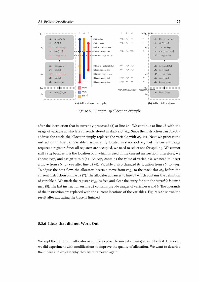
5.3 Bottom-Up Allocator 75
T0
T1
L0: livein(a, b)
L1: def{c}
L2−: sta ← reg1
L2: use{a, c}
L2+: reg1 ← stb
L3: usestack{a}
L4: use{c}
L4+: reg0 ← sta
L5: use{b}
L6: liveout(a)
Lx: livein(reg0)
. . .
b1
b2
b0
a b c a b c reg0 reg1
reg0
reg1
stack
variable location register content
(0) assign reg0 to a reg0 — — a —
(1) assign reg1 to b reg0 reg1 — a b
(2) assign reg0 to c sta reg1 reg0 c b
(3) insert reg0 ← sta
(4) use a on stack (sta) sta reg1 reg0 c b
(5) assign reg1 to a reg1 stb reg0 c a
(6) insert reg1 ← stb
(7) insert sta ← reg1
(8) free reg0 reg1 stb — — a
(9) finished reg1 stb — — a
(a) Allocation Example
T0
T1
L0: livein(reg1, stb)
L1: def{reg0}
L2−: sta ← reg1
L2: use{reg1, reg0}
L2+: reg1 ← stb
L3: usestack{sta}
L4: use{reg0}
L4+: reg0 ← sta
L5: use{reg1}
L6: liveout(reg0)
Lx: livein(reg0)
. . .
b1
b2
b0
(b) After Allocation
Figure 5.6: Bottom-Up allocation example
after the instruction that is currently processed (3) at line L4. We continue at line L3 with theusage of variable a, which is currently stored in stack slot sta. Since the instruction can directlyaddress the stack, the allocator simply replaces the variable with sta (4). Next we process theinstruction in line L2. Variable a is currently located in stack slot sta, but the current usagerequires a register. Since all registers are occupied, we need to select one for spilling. We cannotspill reg0 because it is the location of c, which is used in the current instruction. Therefore, wechoose reg1 and assign it to a (5). As reg1 contains the value of variable b, we need to inserta move from stb to reg1 after line L2 (6). Variable a also changed its location from sta to reg1.To adjust the data-flow, the allocator inserts a move from reg1 to the stack slot sta before thecurrent instruction on line L2 (7). The allocator advances to line L1which contains the definitionof variable c. We mark the register reg0 as free and clear the entry for c in the variable locationmap (8). The last instruction on line L0 contains pseudo usages of variables a and b. The operandsof the instruction are replaced with the current locations of the variables. Figure 5.6b shows theresult after allocating the trace is finished.
5.3.6 Ideas that did not Work Out
We kept the bottom-up allocator as simple as possible since its main goal is to be fast. However,we did experiment with modifications to improve the quality of allocation. We want to describethem here and explain why they were removed again.

76 Register Allocation Strategies
Reduce Spill Moves The placement of spill moves is suboptimal. Due to SSA form, it is suffi-cient to spill a variable only once since it never changes. Still, the bottom-up allocatorwill happilyupdate the stack-slot every time a variable’s location changes from a register to the stack. Weimplemented a mode where spilling is delayed and the move is inserted only after the definitionof the variable is reached. Although, this reduces the number of moves significantly, it did alsoincrease compile time.
Better Spilling Heuristics The bottom-up allocator always spills the first non-blocked reg-ister. We experimented with the furthest-first strategy [Guo et al., 2003], i.e., we selected theregister whose next usage was farthest away. However, it had again a negative influence oncompile time, so we abandoned the idea.
Round Robin Selection Due to our spilling and selection strategy, registers which come firstin the set of available registers, are used more frequently than those at the end of the set. Onlyrecently, Chen et al. [2018] proposed using a round-robin-style register set. In theory, this woulddistribute the register usage better. In addition, the spilling heuristic could easily select a reg-ister which has not been allocated recently. In practice, it did not make a difference, neitherin terms of peak performance nor in compile time. In favor of simplicity, we kept the originalimplementation.
Summing it up Although, the described modifications did not work out for our use case,they might be worth revisiting if the focus shifts. We also want to remark that our main targetwas AMD64, which performs hardware optimizations such as register renaming [Hennessy andPatterson, 2003]. Simpler architectures might be more sensible to the optimizations above.
77
Chapter 6
Inter-trace Optimizations
We have already argued that traces can be processed independently of each other. The data-flow resolution guarantees the correctness of trace register allocation. It does so by insertingmoves whenever the location of a variable is different across an inter-trace edge. If we manageto assign the same location, we can avoid the moves and therefore improve the allocation quality.We implemented three optimizations to reduce the number of moves introduced during data-flowresolution and thus to avoid unnecessary spill moves. They all follow the same idea.
All optimizations provide allocation strategies with information from already processed traces toguide the allocation of an unprocessed trace. Therefore, the order in which we process traces hasan influence on the allocation quality. As a basic principle of trace register allocation, we strivefor the best allocation of a trace, ignoring the rest of the compilation unit. Using information fromother traces violates this principle, since it restricts the freedom of the current trace. To keep theinfluence on peak performance low, we allocate traces in decreasing order of importance. In ourcase, importance is basically defined by the order the trace builder finds traces (see Section 4.1).The only exceptions are trivial traces. We allocate them right after their preceding trace.1 Forinstance, in the bidirectional trace-builder example in Figure 4.2d, we would allocate T2 and T3before T1.
Also, the optimizations work on the scope of inter-trace edges. This retains the non-global char-acter of the approach and keeps the complexity limited. In addition, we communicate all infor-mation that is needed for the optimizations via the global liveness information (see Section 4.3.2).Using this canonical representation decouples the optimizations from the details of the allocationstrategies. For instance, there is no need to keep the intervals of the linear scan strategy live.
1As we have argued in Theorem 9, the trace head has at most one predecessor.

78 Inter-trace Optimizations
T1
T2
int getOffset(int reg2 ( ) )
// final int add;
if (!reg1 ( ) .addFrameSize)
// add = 0;
ϕout=(0)
( reg2 ( ) )=ϕin
return reg1 ( ) .offset + reg2 ( );
// add = totalFS;
ϕout=(totalFS)
b0
b1
b2
b3
this
tota
lFS
add
this
tota
lFS
liveb0out = (this, totalFS)
locb0out = (reg1 , reg2 )
liveb3in = (this)
locb3in = (reg1 )
hints
hint
hint
Inter-trace hint (orange) for trace T2 from the allocation result in T1. Note that the liveout andlivein sets, as well as the ϕin sets, are considered. Full source code for the getOffset method
is depicted in Listing 2.
Figure 6.1: Inter-trace hints example (getOffset)
6.1 Inter-trace Hints
Inter-trace hints are themost straight forward optimization. We use use livein/liveout andϕin/ϕout
of an already allocated predecessor trace as a hint for the current trace. Figure 6.1 depicts an ex-ample. Trace T1 has already been allocated. When allocating T2, the liveb0out advises the strategyto allocate this to reg1 and totalFS to reg2. Also the ϕin set in b3 suggests to allocate totalFS
to reg2. Note, however, that two inter-trace hints may disagree. The final decision which hint isfollowed—if any—is made by the allocation strategy.
Every strategy has a different way of handling inter-trace hints. In the linear scan strategy (Sec-tion 5.1), the inter-trace hints are an addition to the already existing (intra-trace) hints. Only thelocout of the (single) predecessor of the trace head is considered. This offers several advantages.First, if we allocate traces in trace building order, the predecessor has already been allocated.This is due to the greediness of the trace building algorithms (Definition 31). Second, as shownin Theorem 13, all variables that are entering a trace are live at the beginning of the trace head.Processing the trace head is therefore sufficient to get hints for all variables. We explicitly donot use inter-trace hints for variables defined by ϕs because we favor the hint coming from thepredecessor that is part of the current trace.
6.2 Spill Information Sharing 79
The trivial trace allocator (Section 5.2) simply forwards the hinting information to make it avail-able to its successor. That is why trivial traces are handled as soon as possible.
The bottom-up strategy (Section 5.3) uses the locout and ϕout information from an already allo-cated successor of the last block in the trace to initialize the current mapping of variables. Notethat not all variables must be live until the end of a trace. Therefore, we might miss hints forsome variables. We experimented with better hinting strategies for the bottom-up allocator, butdiscarded the idea in favor of faster allocation.
6.2 Spill Information Sharing
Since LIR is in SSA form, the value of a variable can be inferred from its single definition point.Due to spilling and spill-position optimization a value might be available in two locations atthe same time, i.e., in a register and in a stack-slot. If this is the case at the source of an inter-trace edge, we can exploit it to avoid redundant spill moves. To do so, we inform the allocationstrategies that the value is not only available in a register but that there is also a copy on thestack. The linear scan strategy treats intervals with this information as preferred candidatesfor spilling, since their value is already available in memory so the spill move can be omitted.Similar to inter-trace hints, the trivial trace allocator simply forwards the spill information toits successor. Due to its greedy fashion, the bottom-up strategy does not incorporate enoughknowledge to provide spill information. While the allocator could be extended to provide theinformation, we refrained from doing so.
6.3 Known Issue: Spilling in Loop Side-Traces
The non-global scope of trace register allocation is a natural boundary for optimizations. How-ever, in the evaluation of our benchmarks, we did not encounter a situation where this was anissue, except for one benchmark. The issue can occur when spill moves are introduced in a side-trace of a loop for variables that were not spilled in themain-trace, i.e., in the trace with the loopheader. Figure 6.2 shows an example: In trace T1 the allocator is able to move the spill code forx out of the loop (i.e., from b4 to b1). In trace T2, when spilling y, we cannot hoist the spill moveout of the loop, since the block entering the loop (b1) is not part of T2. This means that we needto execute the spill move inside the loop, every time we enter b6. Doing the spill also in b1 wouldbe preferable, but since register allocation of traces is decoupled, this is not possible. Note thatin any case, we cannot remove the load of y at the end of b6.

80 Inter-trace Optimizations
T1 T2
x← · · ·
y ← · · ·
spill(x)
· · ·
· · ·
spill(x)
. . .
. . .
spill(y)
. . .
load(y)
· · ·
b1
b2
b3
b4
b5
b6
mov
esp
illou
tofloo
px y
x y
Spilled ranges are highlighted in orange.
Figure 6.2: Spilling in side-traces of a loop
The effect of this issue can be seen in the results of the sunflow benchmark in Figure 7.11a.The hot loop of the benchmark contains a switch statement where in every branch the registerpressure is higher than the number of available registers. The trace allocator creates one longtrace containing the loop header and the most likely branch of the switch. In this trace the spillscan be moved out of the loop. For the other branches, separate traces are created where the spillmoves cannot be hoisted out of the loop. Our investigation showed that in this benchmark thenumber of executed spill moves is higher with our trace allocator than with the global linear scanallocator.
There aremultiple potential solutions to the general problem. We could conservatively insert spillmoves for variables that are only used in side traces into the main-trace and try to hoist them outof the loop. Later, we could delete them, if they turn out to be unnecessary. However, this wouldsacrifice non-globalness of trace register allocation. Another possibility is to apply the decoupledregister allocation idea, proposed for example by Braun and Hack [2009], Tavares et al. [2011], orBarik et al. [2013]. Their allocator is split into two independent phases. First, spilling decisionsare made based on the register demands. The result is a compilation unit for which registers canbe allocated without spilling. A similar approach could be applied to trace register allocation. Apre-phase could compute the spill decisions of traces and propagate this information to precedingtraces. See Section 10.1.3 for more details on decoupled register allocation.
In our specific case, the stack interval optimization, which we will describe next, mitigates theabove problem. Note, however, it does not solve the problem in general.
6.4 Stack Intervals 81
6.4 Stack Intervals
While further investigating the benchmark that uncovered the loop side-trace spilling problem,we noticed that there were many variables that were spilled in the main-trace and not used inthe side-trace. Although those variables were first-class spill candidates due to spill information
sharing, the linear scan strategy first tries to allocate a register for them. To some extent thisseems reasonable. The variable is live because there is a path to a usage. If the register pressureis low, storing the variable in a register is favorable for its future usage. However, we haveto move it from the stack slot to the register. If this happens in a hot loop it has a significantperformance overhead. Based on this observation, we decided not to allocate registers for stackintervals, i.e., intervals that are in a stack slot at the beginning of the trace and have no usagein the current trace. It turned out that this heuristic mitigates the issues we were seeing in ourearly evaluation and no other benchmark is negatively affected by it.
Note that this optimization was explicitly added to the linear scan strategy. After interval build-ing, we remove intervals that are allocated on the stack and have no usages in the current tracefrom the unhandled list and take the stack slot as their location. The bottom-up strategy allo-cates registers on demand, so it will never try to allocate a register for a variable without a usage,assuming it is in a stack slot at the end of the trace. Also for the trivial trace allocator, this is anon-issue.


83
Chapter 7
Evaluation
In this chapter, we want to verify that our implementation of trace register allocation solvesthe problems as well as reaches the goals we described in the introduction (Section 1.4 and Sec-tion 1.5). To validate our approach, we want to answer the following questions positively.
Can the trace register allocation approach …
RQ1 …reach the same code quality as a state-of-the-art global allocator? [Eisl et al., 2016]
RQ2 …be as fast as a global allocator for the same quality of allocation? [Eisl et al., 2017]
RQ3 …enable fine-grained trade-offs between compile time and allocation quality? [Eisl et al.,2017]
RQ4 …reduce the compilation latency, i.e., the duration until the result of a compilation is avail-able? [Eisl et al., 2018]
In this chapter we present results and show that the trace register allocation approach can pos-itively answer RQ1 and RQ2. To give more insights on code quality, we also give a detailedevaluation of the inter-trace optimizations, which were presented in Chapter 6.
In the following two chapters on register allocation policies (Chapter 8) and parallel trace registerallocation (Chapter 9), we present how we approached RQ3 and RQ4.
All experiments were performed on GraalVM on top of HotSpot (Section 3.2.1). We start witha discussion of the benchmark suites. Afterwards, we compare our trace register allocation ap-proach with the global linear scan approach in terms of allocation quality and compile time.

84 Evaluation
7.1 Benchmarks
To ensure that our approach is applicable to a broad area of workloads we used a variety ofcommon Java benchmark suites. In the following, we provide details about their structure andhow we collected the results.
7.1.1 SPECjvm2008
The SPECjvm20081 benchmark suite consists of a collection of real-world Java applications. Itsgoal is to benchmark core functionality of a Java Runtime Environment, including the processorand memory subsystems but excluding disk I/O and inter-machine networking. The result met-ric is throughput-based, i.e., an operation is executed repeatedly for a fixed amount of time. Thenumber of performed operations during this time is the score. Therefore, higher numbers reflecta better performance of the system. The harness first warms up the benchmark for 120 secondsto trigger JIT compilation. The warmup is followed by a 240 second interval for the actual mea-surement. Usually, all benchmarks of SPECjvm2008 are executed in the same JVM instance. Thismeans that the order in which the benchmarks are executed is important since profiling data isshared for all benchmarks. However, different applications exhibit different profiling patterns, sothis leads to what we call profile pollution, i.e., that the profile does not represent the current—andexpected future—behavior of the application. Therefore, we start a new JVM instance for everybenchmark. We believe that this is a more realistic methodology.
The SPECjvm2008 suite also incorporates a startup mode. Its goal is—according to the vendor—tobenchmark the “user experience of Java.” In this mode, the benchmark workloads are only ex-ecuted once without any warmup. The duration of this run is used to calculate a throughputvalue. For most benchmarks, this interval is too short to even trigger JIT compilation, so the sig-nificance of this mode for evaluating our approach is very limited. We therefore do not presentstartup numbers.
7.1.2 SPECjbb2015
SPECjbb20152 is a server benchmark suite for Java. In contrast to the SPECjvm2008, it doesnot consist of multiple independent benchmarks but executes a single business application. Thebenchmark models the components of the IT infrastructure of a sales company. The different
1https://www.spec.org/jvm2008/2https://www.spec.org/jbb2015/

7.1 Benchmarks 85
components (controller, backend, transactors) can either be executed on a single JVM or on mul-tiple instances to test outbound communication performance [SPEC, 2017]. Since we are onlyinterested in compiler performance, we are only evaluating the single-JVM mode. The harnessprovides two metrics: the critical score, which relates to response time, and the max value,which measures throughput.
7.1.3 DaCapo
The DaCapo benchmark suite was proposed by Blackburn et al. [2006] to tackle certain short-comings of the SPEC suites such as more complex code patterns, a more diverse object behavior,and more demanding memory requirements.3 We used the 9.12 version of DaCapo for our exper-iments. Similar to SPECjvm2008, DaCapo consists of a set of real-world applications. The bench-marks are iteration-based, meaning that they run the same workload for a predefined numberof times in order to warm up the virtual machine. We chose this number high enough to makesure that all important methods are compiled. Since the work performed in one iteration variesconsiderably from benchmark to benchmark, the iteration numbers range from 5 to 120. Forgetting more stable results, the final performance result for a benchmark is the average of thetime for the last n iteration, where n is a number between 5 and 10, depending on the total num-ber of iterations. Since the result is a time value, lower numbers mean better performance (incontrast to the SPEC suites). As for SPECjvm2008, every benchmark is executed in a fresh virtualmachine.
Note that, due to Java 8 compatibility issues, we excluded the eclipse, tomcat,4 tradebeans,and tradesoap benchmarks. To minimize the effect of disk I/O, we executed the benchmarks ina fresh directory on a ram disk. For some benchmarks, for instance lusearch, luindex, h2, orbatik, this is necessary to get stable results.
7.1.4 Scala-DaCapo
There is a multitude of programming languages that are compiled to Java Bytecode and executedon JVMs. Examples include Clojure, Groovy, JRuby, Jython, and Scala. However, with the excep-tion of the jython benchmark in DaCapo, those languages are not represented by the benchmarksuites described above. To cope with this, at least with respect to Scala, Sewe et al. [2011] pro-posed the Scala-DaCapo benchmark suite. They show that Scala workloads differ significantly
3Note that they compared against older versions of the SPEC benchmark suites, so some points of criticismmight nolonger be valid. Also, we are using a newer version of DaCapo than the one analyzed in the paper by Blackburnet al. [2006].
4https://bugs.openjdk.java.net/browse/JDK-8155588

86 Evaluation
from Java, for example in term of call site polymorphism or the number of boxed values. Thisposes different challenges to the JVM and especially to the JIT compiler, as for example shownby Stadler et al. [2013] in the case of Graal. Scala-DaCapo uses the same benchmarking harnessas DaCapo, which is why we often present the results together.
7.2 Configurations
To answer RQ1 and RQ2, we compared our approach against the global linear scan allocation(GlobalLSRA) that is the default in Graal. We used the TraceLSRA configuration, i.e., only usingthe linear scan and the trivial trace strategy, since this is the configuration that achieves the bestallocation quality. In order to positively answer RQ1 and RQ2, the TraceLSRA configurationneeds to perform at least as good as GlobalLSRA. For some benchmarks we also included theBottomUp configuration, where we only used the bottom-up and the trivial trace strategy.
7.3 Peak Performance/Allocation Quality
Let us first focus on RQ1, i.e., whether the trace register allocator can compete with a state-of-the-art global register allocator in terms of allocation quality.
7.3.1 DaCapo and Scala-DaCapo
AMD64 The top half of Figure 7.1 depicts the composite performance results for DaCapo andScala-DaCapo on AMD64. The experiments were performed on our X3-2 cluster. The detailsof the machine are given in Section C.1 in the appendix. For every experiment, we randomlyselected a node from the cluster to execute a benchmark suite (DaCapo or Scala-DaCapo) witha single configuration. For every benchmark, we started a new Java VM with an initial andmaximum heap size of 8GB. To avoid distortion due to node switching, we fixed the CPU and thememory of the JVM to a single NUMA node using the hwloc-bind5 utility. Figure 7.1 shows thecomposite results for the benchmark suites, i.e., every observation in the box plot [Tukey, 1977](e.g., a dot) represents the mean result of a single benchmark (e.g., the mean of all lusearch runswith the TraceLSRA configuration). A per-benchmark evaluation is given in Figure 7.2, wherean observation represents a single benchmark run. The results are all relative to TraceLSRA. Weused the git6 revision b398d21c7c21 of Graal for this evaluation.7
5hwloc-bind(1) — Linux man page: https://linux.die.net/man/1/hwloc-bind6git(1) — Linux man page: https://linux.die.net/man/1/git7https://github.com/zapster/graal
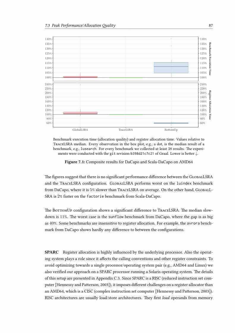
7.3 Peak Performance/Allocation Quality 87Benchm
arkExecution
Tim
eRegister
Allocation
Tim
e
GlobalLSRA TraceLSRA BottomUp
100%105%110%115%120%125%130%135%140%
60%80%100%120%140%160%180%200%220%240%
100%105%110%115%120%125%130%135%140%
60%80%100%120%140%160%180%200%220%240%
Benchmark execution time (allocation quality) and register allocation time. Values relative toTraceLSRA median. Every observation in the box plot, e.g., a dot, is the median result of abenchmark, e.g., lusearch. For every benchmark we collected at least 38 results. The experi-
ments were conducted with the git revision b398d21c7c21 of Graal. Lower is better ↓.
Figure 7.1: Composite results for DaCapo and Scala-DaCapo on AMD64
The figures suggest that there is no significant performance difference between the GlobalLSRAand the TraceLSRA configuration. GlobalLSRA performs worst on the luindex benchmarkfrom DaCapo, where it is 5% slower than TraceLSRA on average. On the other hand, GlobalL-SRA is 2% faster on the factorie benchmark from Scala-DaCapo.
The BottomUp configuration shows a significant difference to TraceLSRA. The median slow-down is 11%. The worst case is the sunflow benchmark from DaCapo, where the gap is as bigas 40%. Some benchmarks are insensitive to register allocation. For example, the avrora bench-mark from DaCapo shows hardly any difference to between the configurations.
SPARC Register allocation is highly influenced by the underlying processor. Also the operat-ing system plays a role since it affects the calling conventions and other register constraints. Toavoid optimizing towards a single processor/operating system pair (e.g., AMD64 and Linux) wealso verified our approach on a SPARC processor running a Solaris operating system. The detailsof this setup are presented in Appendix C.3. Since SPARC is a RISC (reduced instruction set com-puter [Hennessy and Patterson, 2003]), it imposes different challenges on a register allocator thanan AMD64, which is a CISC (complex instruction set computer [Hennessy and Patterson, 2003]).RISC architectures are usually load/store architectures. They first load operands from memory

88 Evaluation
avrora batik fop h2 jython luindex lusearch pmd sunflow xalan
DaC
apo
90%95%
100%105%110%115%120%125%130%135%140%145%
90%95%100%105%110%115%120%125%130%135%140%145%GlobalLSRA
TraceLSRA
BottomUp
actors apparat factorie kiama scalac scaladoc scalap scalariform scalatest scalaxb specs tmt
Scala-DaC
apo
90%95%100%105%110%115%120%125%130%135%140%145%
90%95%100%105%110%115%120%125%130%135%140%145%
Same data as in Figure 7.1. Values relative to TraceLSRA median. Lower is better ↓.
Figure 7.2: Peak performance of individual benchmarks from (Scala-)DaCapo on AMD64
to a register, perform an operation on them, and then store the results back. CISC, in contrast,allow direct addressing of memory in many operations. Consequently, RISCs usually have moreregisters than CISCs, which makes spilling less likely. On the other hand, on a CISC, reloading aspilled value is often not necessary, because instructions can directly use it from memory.
Figure 7.3 shows the results for DaCapo and Scala-DaCapo on SPARC. The conclusion is thesame as on AMD64. Trace register allocation achieves the same performance as GlobalLSRA. Itis worth noting, that the linear scan implementation (and also our trace-base linear scan imple-mentation) was tuned for AMD64 [Wimmer and Mössenböck, 2005]. We think that an investi-gation on whether RISC architectures offer further opportunities for trace register allocation isinteresting future work.

7.3 Peak Performance/Allocation Quality 89Benchm
arkExecution
Tim
e
GlobalLSRA TraceLSRA97.5%98.0%98.5%99.0%99.5%100.0%100.5%101.0%101.5%102.0%102.5%103.0%
97.5%98.0%98.5%99.0%99.5%100.0%100.5%101.0%101.5%102.0%102.5%103.0%
Values relative to TraceLSRA median. Same methodology as in Figure 7.1. For every bench-mark we collected at least 15 results. The experiments were conducted with the git revision
3e8cb34059d2 of Graal. Lower is better ↓.
Figure 7.3: Composite peak performance results for DaCapo and Scala-DaCapo on SPARC
7.3.2 SPECjvm2008
The AMD64 results for SPECjvm2008 are summarized in Figure 7.4. The experiments were per-formed on our X5-2 cluster (see Appendix C.2). Again, the results for GlobalLSRA are in thesame range as for the TraceLSRA configuration. They span from 1.2% slower to 5% faster com-pared to TraceLSRA.One interesting observation is that the difference on the crypto.signverifyis significant in favor of GlobalLSRA. It seems that the trace register allocator always choosesa less optimal allocation than the global linear scan approach.
7.3.3 SPECjbb2015
The results for SPECjbb2015 in Figure 7.5 show no significant difference between GlobalLSRAand TraceLSRA (again on X5-2). In our experiments, it appeared as if GlobalLSRA performsbetter on the criticalmetric (responsiveness) and TraceLSRA on max (throughput). However,the results vary too much to draw a definite conclusion.
7.3.4 Answering RQ1
The benchmark results let us conclude that RQ1 can be answered positively, i.e., that trace reg-ister allocation can achieve the same allocation quality as a state-of-the-art global allocator.

90 Evaluation
com
posite
com
piler.c
ompi
ler
com
pres
s
cryp
to.aes
cryp
to.rsa
cryp
to.signv
erify
derb
y
mpe
gaud
io
scim
ark.fft.l
arge
scim
ark.fft.s
mall
scim
ark.lu
.larg
e
scim
ark.lu
.sm
all
scim
ark.m
onte_c
arlo
scim
ark.so
r.lar
ge
scim
ark.so
r.sm
all
scim
ark.sp
arse
.larg
e
scim
ark.sp
arse
.sm
all
serial
sunfl
ow
xml.t
rans
form
xml.v
alid
atio
n
70%
80%
90%
100%
110%
GlobalLSRA
TraceLSRA
Composite result on the very left. Values relative to TraceLSRA median. For every bench-mark we collected at least 20 results. The experiments were conducted with the git revision
5e7a1574d37b of Graal. Higher is better ↑
Figure 7.4: Peak performance results for SPECjvm2008 on AMD64
7.4 Compile Time
Defining ameaningful compile timemetric is inherently more difficult for a dynamic compilationsystem than for a static compiler. On the one hand, the compilation and the execution of everybenchmark are intertwined. Compile time is an integral part of the run time. On the other hand,experiments are harder to reproduce, since the executed machine code can be different for everyrun after recompilation and depends on non-deterministic factors such as the order in whichcompilation happens.
The meta-circular aspect of the GraalVM adds another layer of challenges to the problem. Sincethe compiler itself is subject to compilation, as it is implemented in Java, changes in the compilerinfluence not only the generated machine code, but also the time it takes to translate the com-piler itself (compiler compile time). To minimize this effect, Graal avoids self-compilation, i.e.,all methods in the Java packages jdk.vm.ci and org.graalvm.compiler are compiled by theHotSpot client compiler and not by the Graal compiler. This on the other hand means that Graalcode is less optimized which again affects compile time.

7.4 Compile Time 91
critical max
GlobalLSRA TraceLSRA GlobalLSRA TraceLSRA90%
95%
100%
105%
110%
We collected at least 20 results for every configuration. The experiments were conducted withthe git revision 5e7a1574d37b of Graal. Higher is better ↑.
Figure 7.5: Peak performance results for SPECjbb2015 on AMD64
We need to accept that compile time results in our system are influenced by the surroundingcontext and that not all differences are necessarily caused by a change in the register allocator.Not all effects that we see in the evaluation of a specific implementation must also happen ina different context. Project Metropolis [OpenJDK, 2018] could mitigate these shortcomings. Itsgoal is to ahead-of-time compile the Graal compiler into a shared library so that it is not compiledduring application run time. Unfortunately, at the time of writing, the project was just started.Repeating the compile time experiments in this deployment is highly interesting future work.
For our compile time metric we measure the CPU time spend on register allocation. We also referto it as register allocation time. CPU time is the time the compiler thread did actual work and wasnot waiting, for example, because of preemption. Ignoring wait time is fair, since compilation ofa method is single threaded,8 so there is no waiting for resources. In the case of trace registerallocation, register allocation time includes all phases of the framework: trace building, globalliveness analysis, global data-flow analysis and the actual processing of the traces.
We only present compile time results for DaCapo and Scala-DaCapo since, due to the harness,the results of (most) DaCapo-style benchmarks are more stable than the results of the SPECbenchmarks. Also, we present only results for AMD64. We did experiments on SPARC, but thenumber of machines is limited (Appendix C.3). Anyhow, since SPARC offers more registers, thepressure on the register allocator is lower than on AMD64.
The lower half of Figure 7.1 depicts the composite register allocation time results for DaCapoand Scala-DaCapo on AMD64. Figure 7.6 shows the results for the individual benchmarks. Insummary (Figure 7.1), GlobalLSRA and TraceLSRA operate in the same range, although ourimplementation seems to be faster by a median difference of 4%. Figure 7.6 indeed shows that
8Except when it is not, see Chapter 9.

92 Evaluation
avrora batik fop h2 jython luindex lusearch pmd sunflow xalan
DaC
apo
40%60%80%
100%120%140%160%180%200%220%240%260%
40%60%80%100%120%140%160%180%200%220%240%260%GlobalLSRA
TraceLSRA
BottomUp
actors apparat factorie kiama scalac scaladoc scalap scalariform scalatest scalaxb specs tmt
Scala-DaC
apo
40%60%80%100%120%140%160%180%200%220%240%260%
40%60%80%100%120%140%160%180%200%220%240%260%
Same data as in Figure 7.1. Values relative to TraceLSRA median. Lower is better ↓
Figure 7.6: Register allocation time of individual benchmarks from (Scala-)DaCapo
trace register allocation outperforms GlobalLSRA on a number of benchmarks. Most notable isjython, where GlobalLSRA takes more than twice as long as TraceLSRA. The jython bench-mark produces Java bytecodes dynamically and the generated methods tend to become signifi-cantly larger than typical Java or Scala methods. As we will show in Section 7.4.1, trace registerallocation performs especially well on large methods. It is only fair to note that there are alsocases where GlobalLSRA is faster than TraceLSRA. On the actors benchmark from Scala-DaCapo, for example, GlobalLSRA is 7% faster.
The BottomUp configuration is significantly faster than TraceLSRA in all cases. The medianspeedup is 41%. Again, jython stands out. On this benchmark, the BottomUp configuration is50% faster than TraceLSRA.

7.4 Compile Time 93
0
200
400
600
0 10000 20000 30000Number of LIR Instructions
Register
Allo
catio
nTime[m
s]1
10
100
1000
10000
GlobalLSRA
TraceLSRA
BottomUp
Register allocation time in milliseconds vs. number of LIR instructions for DaCapo and Scala-DaCapo on AMD64. Each dots denotes a bucket of 800 instruction each. The y-value is themedian register allocation time. The size of the dot indicates the number of methods in the
bucket. The error bars represent the lower and upper quartiles. Lower is better ↓.
Figure 7.7: Register allocation time vs. LIR instructions for DaCapo and Scala-DaCapo
7.4.1 Compile Time per Method
To gain more insight on the compile-time behavior of the various register allocation approaches,we investigated the register allocation time on a per-method basis. Figure 7.7 shows the relation-ship between of the number of LIR instructions of a method and its register allocation time. Notethat the figure represents the results of all DaCapo and Scala-DaCapo benchmarks. Plotting all79155 compilations is not feasible, so we group the method sizes into buckets of 800 instructionsand print a circle for the median register allocation time of this group. The size of the circles indi-cates the number of methods in a bucket (logarithmic scale). The plot suggests that TraceLSRAperforms particularly well for large method, compared to GlobalLSRA. As expected, BottomUpis faster than the other configurations.
Since the method sizes are not evenly distributed, we show the results for small methods inFigure 7.8. In this case, the TraceLSRA has no advantage over the GlobalLSRA configuration.The BottomUp allocator, however, continues to outperform the other approaches in terms ofregister allocation time.

94 Evaluation
0
2
4
0 250 500 750 1000Number of LIR Instructions
Register
Allo
catio
nTime[m
s]
GlobalLSRA
TraceLSRA
BottomUp
100
1000
Register allocation time vs. number of LIR instructions for methods with less than 1000 LIRinstructions. Same methodology as in Figure 7.7. Bucket width is 40. Lower is better ↓.
Figure 7.8: Register allocation time vs. LIR instructions for (Scala-)DaCapo (small methods)
7.4.2 Overall Compile Time
The compile time results that we presented so far only show register allocation time. The ultimategoal, however, is to reduce the overall compile time, i.e., the time required for all phases, not onlyfor the register allocator.
The Graal compiler is currently tuned for peak performance. The majority of the compile time isspent in the front end on code optimizations. Figure 7.9 shows how much of the overall compiletime can be accounted to register allocation. With TraceLSRA, 7% of the time is spend on registerallocation, while in the BottomUp configuration this number goes down to 4%. Repeating thisexperiments with a Graal configuration that is tuned towards compile time rather than towardspeak performance, would showmore potential for saving compile time by optimizing the registerallocation.
7.4.3 Answering RQ2
As for peak performance, the trace register allocation approach can compete with state-of-theart global register allocators. Thus we can affirm RQ2.

7.5 Inter-trace Optimizations 95
2%
4%
6%
8%
10%
12%
14%
16%
2%
4%
6%
8%
10%
12%
14%
16%
GlobalLSRA TraceLSRA BottomUp
Register
Allo
catio
n/Co
mpile
Time
Overall compile time on AMD64. Same methodology as in Figure 7.1. Lower is better ↓.
Figure 7.9: Share of register allocation time in the overall compile time for (Scala-)DaCapo
com
posite
avro
ra
batik
fop
h2 jyth
on
luin
dex
luse
arch
pmd
sunfl
ow
tom
cat
trad
ebea
ns
trad
esoa
p
xalan
95%
100%
105%
110%
115%
120%
125%
95%
100%
105%
110%
115%
120%
125%TraceRA (spill info sharing and inter-trace hints)
TraceRA (inter-trace hints)
TraceRA (without optimization)
Performance impact of inter-trace hints and spill information sharing on DaCapo on AMD64.Numbers relative to the performance of TraceLSRAwith inter-trace hints and spill information
sharing. Lower is better ↓.
Figure 7.10: Influence of inter-trace hints and spill information sharing on peak performance
7.5 Inter-trace Optimizations
Since the time we did our original experiments on inter-trace optimizations as described in Chap-ter 6 [Eisl et al., 2016], the trace register allocation implementation was further improved. Mostoptimizations where algorithmic improvements, i.e., doing the same work in less time. However,results for the stack interval optimization described in Section 6.4 where not yet published. Yet,we decided to use the original measurements [Eisl et al., 2016] in order to be consistent to thispaper and because the results did not change much. Also, some optimizations are now manda-tory and can no longer be deactivated easily. The new changes do not invalidate the argumentspresented in the above-mentioned chapters but only the relation to global linear scan. Therefore,the numbers presented in this chapter are taken from [Eisl et al., 2016]. We used the git revisiona563a1d51507 of Graal for our evaluation.

96 Evaluation
avrora batik fop h2 jython luindex lusearch pmd sunflow xalan
80%
85%
90%
95%
100%
105%
110%
115%
120%
80%
85%
90%
95%
100%
105%
110%
115%
120%GlobalLSRA
TraceLSRA
(a) Without stack interval optimization
avrora batik fop h2 jython luindex lusearch pmd sunflow xalan
80%
85%
90%
95%
100%
105%
110%
115%
120%
80%
85%
90%
95%
100%
105%
110%
115%
120%GlobalLSRA
TraceLSRA
(b) With stack interval optimization
The influence of stack interval optimization on DaCapo. Same methodology as in Figure 7.2.Note the impact on the sunflow benchmark. Lower is better ↓.
Figure 7.11: Peak performance impact of the stack interval optimization on DaCapo
Figure 7.10 shows our evaluation of the inter-trace optimizations of DaCapo on AMD64.9 Thefigure clearly shows that inter-trace hints are the most influential optimization. The most signifi-cant change is on sunflowwith about 10% improvement when enabled. The core of the sunflowbenchmark is a hot loop with multiple equally hot branches (see also Section 6.3). Since everybranch will be allocated in a different trace, sharing allocation information is utterly important.Also jython is highly affected by inter-trace hints: Turning them off, results in a 5% degrada-tion.
The influence of spill information sharing is less significant. The luindex and the sunflow bench-marks seem to be the most influenced. However, spill information sharing is important for ex-panding the applicability of the stack intervals optimization.
9 Note that this evaluation was performed on an older version of the HotSpot VMwhere tradesoap and tradebeansstill worked.

7.6 Trace Builder Evaluation 97
com
posite
avro
ra
batik
fop
h2 jyth
on
luin
dex
luse
arch
pmd
sunfl
ow
tom
cat
trad
ebea
ns
trad
esoa
p
xalan
95%
100%
105%
110%
115%
120%
125%
95%
100%
105%
110%
115%
120%
125%TraceRA (unidirectional)
TraceRA (bidirectional)
Results for AMD64. Same methodology as in Figure 7.2. Lower is better ↓.
Figure 7.12: Unidirectional vs. bidirectional trace builder w.r.t. peak performance of DaCapo
The stack interval optimization was added after the other inter-trace optimizations. Figure 7.11shows its impact on the peak performance of DaCapo. In the version without the optimization(Figure 7.11a) there is an outlier in terms of peak performance, namely sunflow where Glob-alLSRA is about 9% faster than TraceLSRA. The benchmark in running into the loop spillingproblem that was discussed in Section 6.3. In Figure 7.11a, which includes the stack intervalsoptimization, this outlier is gone. The other benchmarks (including Scala-DaCapo) are not sig-nificantly affected. However, note that the issue is not directly solved by the optimization butonly mitigated.
7.6 Trace Builder Evaluation
Figure 7.12 compares the unidirectional and the bidirectional trace building algorithms. The re-sults were again conducted for our first evaluation [Eisl et al., 2016]. The numbers suggest thatthey both perform about equally well. We decided to use the unidirectional trace builder by de-fault, since it is the simpler algorithm and it follows our focus on the common case philosophymore closely.


99
Chapter 8
Trace Register Allocation Policies
In Chapter 5 we proposed three allocation strategies: The linear scan strategy (Section 5.1) toproduce good code, the bottom-up strategy (Section 5.3) for fast allocation, and the trivial tracestrategy (Section 5.2) for special traces. In this chapter we focus on the question when to usewhich strategy. The goal is to gain a fine-grained control over the trade-off between compile-time and peak-performance. Doing so allows us to answer RQ3 (Chapter 7).
Intuitively, we want to use linear scan for the important traces and bottom-up for the others andthus, reduce allocation time. Of course, trivial traces should be processed by the trivial traceallocator unconditionally, since it is fast and optimal. To apply this in practice, we need to defineour notion of importance. We evaluated a case study of 8 decision heuristics, so-called allocationpolicies [Eisl et al., 2017].
First, we identified properties, which allow us to characterize a trace. Based on these properties,we developed policies to select either the linear scan, the bottom-up, or the trivial allocator. Thelist of properties and policies is non-exhaustive.
8.1 Properties
Our allocation policies are based on properties of basic blocks, traces, the complete compilationunit, or a combination of them.
100 Trace Register Allocation Policies
8.1.1 Block Properties
A trace consists of a sequence of basic blocks. For every block b we know its relative executionfrequency, which we denote as freq(b). It is a real number estimating how frequently this blockis executed per invocation of the enclosing method. A value of 0.5 means that the block isexecuted in 50% of all invocations. For blocks inside of loops this value can be larger than 1.For example, if a loop header is entered with a probability of 1, a frequency of 10 indicates aloop iteration count of 10. Note that these numbers are relative to the invocation count of theenclosing method. Therefore, the frequency of the method entry block is always 1. We cannotinfer absolute execution counts from these numbers. The block frequencies are calculated frombranch profiles collected by the virtual machine in previous executions of the compilation unit.
Another blockmetric is the loop nesting level, or loopDepth(b). It indicates onwhich loop nestinglevel this block occurs. However, this metric can be misleading since not all branches inside aloop are equally likely. It should be used as a structural indicator only.
Due to the Global Liveness Analysis, described in Section 4.3, we can also consider the livein andliveout sets as block properties, i.e., the variables that are live at the beginning and the end of theblock. More live variables increase the likelihood of spilling.
8.1.2 Trace Properties
The properties of the blocks in a trace can be aggregated to define properties for the trace. Forexample, the frequency of a trace can be defined as the maximum frequency of the blocks in thetrace.
Another important property of a trace is its triviality, i.e., the fact that a trace consists of a singleblock containing just a jump instruction. It determines whether or not the framework can usethe trivial trace allocator.
We also consider the trace building order, denoted by id(trace), as a trace property. The tracebuilding algorithms, as described in Section 4.1, construct important traces first. That meansthat a trace with a lower number is generally more performance-critical than one with a highernumber.

8.2 Policies 101
8.1.3 Compilation Unit Properties
For compilation units we can apply the same aggregation techniques as for traces. We use com-pilation unit properties to set trace properties into relation. For example, the maximum blockfrequency of a trace vs. the maximum block frequency of the whole compilation unit. We alsoexploit structural properties of a compilation unit to switch between different sub-policies. Forinstance, if a method contains a loop we might want to choose a different decision model thanfor methods without loops.
8.1.4 Aggregation of Properties
As outlined above, we aggregate the block properties to calculate new metrics for traces of thecompilation unit. We consider different aggregation functions including maximum, minimum,sum, average, and count.
8.2 Policies
Wedeveloped a set of 8 allocation policies, based on the identified properties. A policy is a decisionfunction that selects an allocation strategy for a given trace.
For trivial traces, we always use the trivial trace allocator. For non-trivial traces, we have todecide whether to use the trace-based linear scan or the bottom-up approach. We describe thisdecision as a hotness condition. If the condition is true the trace is considered important, i.e., weuse the linear scan approach for it.
In the remainder of this section, trace refers to the trace for which we want to choose a strategy.We use the term method to describe the set of all blocks of the method (compilation unit).
TraceLSRA This policy uses the linear scan strategy for all traces that are not trivial.

102 Trace Register Allocation Policies
BottomUp TheBottomUp policy uses the bottom-up strategy for all traces that are not trivial.1
Ratio The Ratio policy uses linear scan for a fixed fraction p of the traces.
id(trace) ≤ |traces| × p
Since traces are processed in trace-building order (i.e., in the order of their importance), afraction of p = 0.5means that the first 50% of the created traces (i.e., those with an id lessor equal to |traces| × 0.5) is allocated with linear scan (or the trivial allocator).
Budget The Budget policy is a budget-based approach. The idea is to allocate traces with thelinear scan strategy in trace-building order until we run out of budget.⎛⎜⎝ ∑
t∈tracesid(t)<id(trace)
∑b∈t
freq(b)
⎞⎟⎠ <
( ∑b∈method
freq(b)
)× p
The cost function is the sum of the block frequencies of all traces that have already been al-located. The budget is a fraction of the total sum of the block frequencies in the compilationunit.
Loop The Loop policy uses the linear scan strategy for all traces that contain at least one blockthat is in a loop.
HasLoop(trace) ∨ ¬HasLoop(method)
where HasLoop(blocks) is defined as:
∃ b ∈ blocks where loopDepth(b) > 0
1Due to implementation reasons, there is one exception to this rule, namely traces with edges to compiled exceptionhandlers. These edges require slightly different handling. Graal assumes that the framestate at the instructionthat causes the exception, e.g., a call, is the same as at the beginning of the exception handler. In other words,we are not allowed to insert moves between the throwing instruction and the end of the block. The linear scanimplementation in Graal guarantees this by design. The bottom-up allocator, however, does not. It could be easilyimplemented in the bottom-up allocator, but it would make the algorithm more complicated. Since exceptionsin Graal are usually handled via deoptimization, this case is uncommon. To keep the implementation simple, wedecided to ignore this special case and fall back to the linear scan strategy if it occurs. The entry for the BottomUppolicy in Figure 8.2 shows that the fraction of linear-scan-compiled traces is indeed marginal (∼0.3% as depictedin Table 8.1 in the evaluation).

8.2 Policies 103
The idea is that we consider loops to be performance-critical, so we want to find a goodallocation for them. In addition to that, linear scan is used if the whole compilation unitdoes not contain a loop at all. The rationale behind this is that the virtual machine com-piles only methods which either exceed a certain invocation threshold or a loop back edgethreshold. If a method without a loop is queued for compilation, the runtime did so dueto the invocation count only. This means that the method was called often enough to beconsidered important.
LoopBudget This policy combines the Loop policy with the Budget policy. Instead of usinglinear scan for all compilation units without loops, we apply the MaxFreq condition.
HasLoop(trace) ∨(¬HasLoop(method) ∧ Budget(trace)
)
The resulting policy can decrease compile time compared to the Loop policy since fewertraces are allocated with linear scan. Nevertheless, loop traces are still prioritized.
MaxFreq The MaxFreq policy considers a trace important if the maximum execution fre-quency of the blocks in the trace is greater than a fraction p of the maximum frequency ofthe blocks in the compilation unit.
maxbt∈trace
freq(bt) > maxbm∈method
freq(bm)× p
Only traces with high-frequency blocks are allocated with the linear scan strategy sincethese traces are most critical for performance. For example, if p = 0.8, a trace is compiledwith the linear scan allocator if its frequency is larger than 0.8× the frequency of the mostfrequent block of the method.
NumVars The NumVars policy uses linear scan for all traces where the maximum number oflive variables at block boundaries exceeds a certain threshold p.
maxb∈trace
(max
(|livein(b)|, |liveout(b)|
))> p
The idea is that traces with a higher number of live variables are more likely to requirespilling. The spilling mechanism in the linear scan strategy leads to better code than thespilling mechanism in the bottom-up allocator. On the other hand, if no spilling is neededthe bottom-up allocator produces code of similar quality as the linear scan allocator but inshorter time.

104 Trace Register Allocation Policies
Benchm
arkExecution
Tim
eRegister
Allocation
Tim
e
Trac
eLSR
A
Ratio
-0.8
Budg
et-0.999
995
Ratio
-0.5
Loop
Num
Vars-8
Budg
et-0.98
Max
Freq
-0.1
Loop
Budg
et-0.5
Ratio
-0.3
Num
Vars-15
Max
Freq
-0.8
Budg
et-0.5
Botto
mUp
100%
105%
110%
115%
120%
125%
130%
45%50%55%60%65%70%75%80%85%90%95%100%105%
100%
105%
110%
115%
120%
125%
130%
45%50%55%60%65%70%75%80%85%90%95%100%105%
Evaluation of register allocation policies for DaCapo and Scala-DaCapo on AMD64. Valuesrelative to TraceLSRA median. Same methodology as in Figure 7.2. Lower is better ↓.
Figure 8.1: Peak performance and register allocation time of various allocation policies
8.3 Evaluation
The goal of this evaluation is to answer RQ3 and to support our claim that selective trace-basedregister allocation is an appropriate approach for controlling the trade-off between compile timeand peak performance on a fine-grained level. To this end, we study the impact of the 8 allo-cation policies discussed in the last section. For policies with parameters we compare multiplevalues to further highlight the flexibility of our approach. In total, we selected 14 configura-tions as case study to supports our claim. Our experiments were performed using git revisionf5cad2eda111.
We performed the experiments on the X3-2 cluster (see Appendix C.1) with at least 30 repetitions.The baseline is again the trace-based linear scan allocator, denoted by TraceLSRA. We show thenumbers relative to the baseline of a given benchmark.
Figure 8.1 shows the total peak performance and the register allocation time for various allocationpolicies relative to the trace-based linear scan. For measuring the register allocation time, weincluded all compilations of the benchmarks, including those in warm-up iterations, since the

8.3 Evaluation 105
Bottom-Up Strategy
Linear Scan Strategy
Trivial Strategy
0%
10%
20%
30%
40%
50%
60%
70%
80%
90%
100%
0%
10%
20%
30%
40%
50%
60%
70%
80%
90%
100%
Trac
eLSR
A
Ratio
-0.8
Budg
et-0.999
995
Ratio
-0.5
Loop
Num
Vars-8
Budg
et-0.98
Max
Freq
-0.1
Loop
Budg
et-0.5
Ratio
-0.3
Num
Vars-15
Max
Freq
-0.8
Budg
et-0.5
Botto
mUp
The distribution is calculated per benchmark. The figure shows the mean over all benchmarks.
Figure 8.2: Distribution of the allocation strategy per policy
peak performance of the last iteration depends on all these compilations. Figure 8.2 depicts thedistribution of the allocation strategies for the various policies. Not surprisingly, the numberssuggest that there is a correlation between the percentage of linear-scan-compiled traces and theregister allocation time in Figure 8.1. Unless otherwise noted, the numbers mentioned in thissection represent the geometric mean of the averaged benchmark results relative to TraceLSRA.All results are summarized in Table 8.1.
TraceLSRA TraceLSRA is the policy that performs best with respect to peak performance. Itis the upper bound in terms of register allocation time but also produces the best code. Inthis baseline configuration, linear scan is used for 61% of the traces. The other traces aretrivial and are therefore allocated by the trivial trace allocator.
BottomUp The BottomUp policy, on the other hand, is the lower bound with respect to allo-cation time. It requires only about 57% of the time used by TraceLSRA. In terms of peakperformance, this policy is the slowest with an average performance decrease of about 11%.For the sunflow benchmark from the DaCapo suite, however, the performance penalty is30%.
Ratio In our experiments, we evaluated the Ratio policy with the parameters 0.8, 0.5, and0.3. Although the number of linear-scan-allocated traces decreased by 17% for p = 0.8,this is hardly noticeable in the allocation time and the peak performance. Setting p = 0.5
106 Trace Register Allocation Policies
decreases the time for allocation to 87%. The performance slowdown is about 1% relativeto TraceLSRA. With p = 0.3 allocation time is further reduced to 80% with a performancedegradation of 4%. In this configuration, only 13% of the traces are allocated with thelinear scan strategy. The results suggest that the Ratio policy allows a fine-grained tuningof compile time vs. peak performance.
Budget The Budget policy exhibits a non-linear behavior with respect to the parameter p. Forp = 0.99995, we see a performance degradation of only 1% while the register allocationtime goes down to 93%. Only 33% of the traces use the linear scan strategy. Setting p =
0.98 reduces the allocation time to 77% with a performance decrease of 3%. For p = 0.5,allocation time drops to 62%. The linear scan strategy is used for only 1% of the traces. Inthis configuration, basically, only the first trace of a method is considered important. Theperformance decrease is 10%, which is almost at the level of the BottomUp policy (11%).
Loop The Loop policy triggers for 26% of the traces, which is slightly less than half of the non-trivial traces (61%). Performance-wise this policy is about 2% slower than TraceLSRA. Onthe other hand, it requires only 86% of the time for register allocation.
LoopBudget The LoopBudget policy (p = 0.5) combines the advantages of Loop, i.e. goodand stable peak performance, with the fast allocation time of the Budget policy. About11% of the traces use the linear scan strategy. The allocation time therefore drops to 79%compared to TraceLSRA. With respect to peak performance this policy is 3% slower.
MaxFreq We evaluated the MaxFreq policy with p = 0.1 and p = 0.8. Compared to theTraceLSRA policy, MaxFreq with p = 0.1 is about 3% slower regarding peak perfor-mance. Again, sunflow exhibits the worst behavior with a performance decrease of 20%.Allocation time, on the other hand, is only about 77% of the time used by TraceLSRA.With p = 0.8 the allocation time drops to 71%. However, the impact on peak performanceis significant. On average, the generated code is 7% slower than with TraceLSRA (max.31%).
NumVars The evaluation of the NumVars policy shows that 32% of the traces have at most 8live variables at their block boundaries (and are not trivial). Allocating these traces withthe bottom-up strategy reduces the allocation time to 92%. Performance decreases by 3%.Extending the scope to 15 variables increases the fraction of bottom-up-allocated tracesto 51% and reduces performance by 5% compared to TraceLSRA. However, the registerallocation time goes down to 76%.

8.3 Evaluation 107
8.3.1 Discussion
Some of the evaluated policies are more appealing than others. The Ratio policy convinces dueto its simplicity and scalability. There is no need to calculate metrics and the parameter correlateswith the register allocation time saving. The Budget policy seems to offer the best trade-off, i.e.,most compile time savings for the lowest performance penalty. However, it requires summingup the frequencies of all blocks. Loop is interesting because it solely depends on the structureof the trace, not on profiled frequencies. Therefore, this policy is an option even if profiling isnot available or inaccurate. The NumVars policy is disappointing, especially for lower numberswhere it achieves little compile time improvement for relatively high performance degradation.
8.3.2 Answering RQ3
Our trace-based register allocation approach offers the flexibility to switch between allocationalgorithmswithin the same compilation unit. This gives us fine-grained control over the trade-offbetween compile time vs. peak performance, which is not supported in other register allocationapproaches. Most policies can be parameterized, which allows adjusting the trade-off betweencompile time and peak performance on a fine-grained level. Our results confirm that our traceregister allocation policy framework offers unique flexibility not seen in other approaches. Thus,trace policies answer RQ3 positively.

108Trace
RegisterAllocation
Policies
Register Allocation Time (∆%) Peak Performance (∆%) Strategy (%)
Policy mean median min min max max mean median min min max max LS BU TT
TraceLSRA 0.0 0.0 0.0 avrora 0.0 avrora 0.0 0.0 0.0 avrora 0.0 avrora 61.2 38.8Ratio-0.8 −1.3 −0.6 −10.7 jython 3.0 avrora 0.7 0.4 −0.8 kiama 6.5 apparat 43.9 17.3 38.8Budget-0.999995 −7.5 −4.9 −33.4 jython −0.1 avrora 0.7 0.5 −0.2 sunflow 2.0 scalaxb 32.6 28.7 38.7Ratio-0.5 −12.6 −11.0 −30.6 jython −2.8 avrora 1.5 1.1 0.1 scalatest 9.2 sunflow 22.4 38.8 38.8Loop −14.0 −13.1 −27.4 jython −4.8 avrora 2.2 1.8 0.3 scalaxb 5.5 xalan 26.4 34.8 38.7NumVars-8 −7.9 −8.3 −14.2 scalatest −2.3 luindex 2.6 2.2 0.2 sunflow 8.7 apparat 29.2 32.0 38.7Budget-0.98 −23.2 −21.5 −44.9 jython −11.3 avrora 3.3 2.9 0.6 scalatest 9.0 luindex 11.4 49.9 38.7MaxFreq-0.1 −23.5 −21.9 −47.0 jython −7.7 avrora 3.4 2.7 0.1 avrora 19.6 sunflow 11.3 50.0 38.7LoopBudget-0.5 −21.0 −20.5 −34.9 scalac −10.9 lusearch 3.5 3.8 0.2 scalatest 6.7 apparat 11.2 50.0 38.7Ratio-0.3 −20.3 −19.2 −42.4 jython −8.1 avrora 3.6 3.0 0.7 scalatest 17.2 sunflow 12.6 48.6 38.8NumVars-15 −23.9 −25.1 −34.0 scalac −6.4 sunflow 5.4 5.1 0.6 avrora 13.3 scalaxb 10.2 51.2 38.7MaxFreq-0.8 −29.2 −28.5 −49.1 jython −16.5 avrora 7.2 5.5 0.6 avrora 30.5 sunflow 4.8 56.6 38.6Budget-0.5 −37.5 −37.0 −52.9 jython −29.5 avrora 9.7 9.2 0.5 scalatest 30.6 sunflow 1.4 60.0 38.6BottomUp −43.0 −42.3 −54.6 jython −36.0 factorie 10.6 9.6 0.8 scalatest 31.7 luindex 0.3 61.2 38.4
For every configuration, we show the (geometric) mean, the median, the min and max values of the benchmark results for both the register allocationtime as well as the peak performance (lower is better). For min and max we also show the corresponding benchmark. The given numbers are thedifferences relative to TraceLSRA in %. The last three columns depict the distribution between the allocation strategies, Linear Scan Allocator (LS),Bottom-Up Allocator and Trivial Trace Allocator (TT).
Table 8.1: Experimental results for trace register allocation policies
109
Chapter 9
Parallel Trace Register Allocation
In this chapter, we focus on RQ4, i.e., whether trace register allocation can reduce compilationlatency. Compilation latency is the duration required to compile a given method. If compilationhappens on the main thread, latency has a significant impact on response time, since the execu-tion of the application is delayed. But also for systems with one or more background compilationthreads [Krintz et al., 2001], short latencies mean that the compiled code is available earlier andcan therefore be executed earlier.
We exploit the flexibility of trace register allocation to reduce compilation latency without im-pacting peak performance. The idea is to use multiple threads to allocate traces concurrently. Thetrace register allocation framework allows traces to be allocated in arbitrary order. However, asdiscussed in Chapter 6, traces that are processed later can profit from decisions in already allo-cated traces. Optimizations based on this principle can improve the peak performance for someDaCapo benchmarks by up to 10%, as shown in Figure 7.10. We want to ensure that concurrentallocation does not influence the allocation quality. Therefore, we define dependencies in a waythat all the information available in the serial mode is also available in the parallel mode.
We prototyped parallel trace register allocation and summarized our findings in awork-in-progresspaper, which is currently under review [Eisl et al., 2018]. However, the current implementationis only a proof-of-concept and is not used by default.
9.1 Concurrency Potential
Before investing time on an implementation, we wanted to gain more insight into whether thereis enough potential for parallelization. Therefore, we simulated the speedups when using 2, 4and 8 threads for register allocation of the DaCapo and Scala-DaCapo benchmarks.

110 Parallel Trace Register Allocation
Not all traces require the same time for allocation. We use the number of instructions as a compiletime estimator since it correlates with the time required for register allocation, as depicted inFigure 7.7. The lower bound for compile time is the length of the critical path in the dependencygraph. Our experiments show that the (geometric) mean of the critical path length is 51% (min =
44%,max = 57%) of the number of instructions in the compilation unit. That means that ideally,with an infinite number of threads and ignoring all overheads, the register allocation step couldbe done in about half the time.
To simulate the concurrency potential with a given number of threads, we need to find a sched-ule that satisfies the dependencies. Finding an optimal schedule with minimal duration is NP-hard [Pinedo, 2016]. Therefore, we apply a simple heuristic for finding a schedule. Whenever athread is idle, we assign it to the longest trace in terms of instructions, whose predecessor traceshave already been processed. For 2 threads, the simulated register allocation time goes down by68% (64%, 71%). This is already an interesting result, since adding only a single thread to the sys-tem can potentially improve register allocation time by about 30%. Another noteworthymetric isthe utilization of the threads, that is the ratio between work and idle time. For 2 threads this ratiois 74% (70%, 78%), which means that allocation threads are idle only one fourth of their run time.If 4 threads are used, the simulated allocation time is 56% (50%, 61%) of the single-threaded case.However, the utilization also decreases to 45% (41%, 50%). The threads are idle more than halfof the time. With 8 allocation threads the allocation time is 52% (45%, 58%), which is almost thebest that can be achieved given a mean critical path length of 51% of all instruction. As expected,the thread utilization further decreases to 24% (22%, 28%).
9.1.1 Example
Let’s illustrate the simulation with an example. We chose the method PrintStream.write()1
from the Java standard library, since it is small enough to be understandable, yet long enoughto exhibit scheduling potential. After high-level optimizations (e.g., inlining) there are 19 traces.Their dependencies are depicted in Figure 9.1. The values in parentheses are the trace lengths ininstructions. The compilation unit consists of 168 instructions in total, which is also the lengthof the single threaded schedule. Figure 9.2 shows the calculated schedule as a Gantt chart [Gantt,1913] for 2, 4 and 8 threads (top, middle, bottom, respectively). Each rectangle represents a tracewith its number. The horizontal axis depicts the length in terms of instructions. The length ofthe schedule with 2 threads is 104 instructions with a thread utilization of 81%. With 4 threadsthe utilization decreases to 50%. However, the length of 84 is already optimal, i.e., the critical
path length. Therefore, increasing the number of threads to 8 cannot yield any improvementsand utilization drops to 25%. Figure 9.2 also shows that although 8 threads are available, only 5
are used.1Full descriptor: java.io.PrintStream.write(byte[], int, int)void

9.1 Concurrency Potential 111
T0
T1 T3 T18
T4 T8 T10T2 T5 T14
T6 T7 T12 T9 T11
T15 T16T13
T17
(36)
(16)
(2)
(19)
(14)(15)
(2) (5)
(10)
(2)
(7)
(2)(6)
(2)
(5)
(7) (7)
(7)
(4)
Dependency graph for the method PrintStream.write(). The values in parentheses are thelength of the traces, i.e., the number of instructions. The critical path (T0–T17, orange edges)
is 84 instructions long.
Figure 9.1: Trace dependency graph for PrintStream.write()
01 23 4
56
78910
1112
131415 16
1718
01
2
3 45
67
8 910 11
12 13
1415
1617
18
01
2
3 45 6
78 9
10 11
12 13
1415
16
17
18
2Th
reads4Th
reads8Th
reads
0 10 20 30 40 50 60 70 80 90 100
01234
01234
01234
Gantt chart [Gantt, 1913] for 2, 4 and 8 threads. The horizontal axis denotes the number ofinstructions. The compilation unit consists of 168 instructions in total. The critical path (red
vertical line) is 84 instructions long.
Figure 9.2: Trace allocation scheduling for PrintStream.write()

112 Parallel Trace Register Allocation
9.2 Evaluation
To verify that the theoretic results presented in Section 9.1 also apply in practice, we prototypeda parallel version of our trace register allocator. More specifically, we wanted to ensure thatparallel register allocation (1) can improve register allocation latency, and (2) does not impairallocation quality. We used a standard Java thread pool2 with a fixed pool size for the allocationthreads. Idle threads are kept alive to avoid the overhead for starting a new thread. Once atrace is allocated, its successors are added to the work queue, if all traces on which they dependhave already been processed. We use a priority queue,3 where traces are ordered by decreasinginstruction count, so that longer traces are allocated first.
From the register allocation point of view, synchronization is only needed for the queue and fortracking dependencies on finished traces. Accessing and modifying traces is safe by design ofthe trace register allocator if the dependencies are respected. However, Graal assumes that everymethod is compiled by just a single thread and therefore uses unsynchronized data structures. Forexample, the map from the register class to the set of available registers, which is lazily initialized.For our concurrent allocation approach, this is a problem. We worked around this issue, forexample, by pre-populating cached maps, duplicating data-structures or simply recalculatingresults. These workarounds cause allocation time overheads which we are willing to accept forour prototype. We are confident that most of them could be mitigated by a more advancedimplementation.
By default, GraalVM uses multiple compiler threads to concurrently compile different methods.Compilation happens in the background, that means the application continues to execute while amethod is compiled. The compiler threads compete with the application threads. Adding threadsfor register allocation makes the situation even more challenging. To keep this interference low,we suppressed the parallel compilation of different methods and rather used the threads for theparallel allocation of registers. To measure register allocation time, we take a timestamp4 beforeand after register allocation and report the difference, i.e., the duration. In other words, theduration is the time elapsed from the beginning of register allocation until it is finished and theresult is available. Of course, the numbers are influenced by the scheduling of threads by thevirtual machine. For example, if the VM decides to preempt the register allocation threads infavor of an application thread, the duration increases although the compiler or allocator did notperform more work. More precisely, the duration does not represent CPU time. However, themetric of duration is what we are interested in, since the goal is not to reduce the work that isdone by the allocator but to have the result available earlier.
2See ThreadPoolExecutor:https://docs.oracle.com/javase/8/docs/api/java/util/concurrent/ThreadPoolExecutor.html
3See PriorityBlockingQueue:https://docs.oracle.com/javase/8/docs/api/java/util/concurrent/PriorityBlockingQueue.html
4See System.nanoTime(): https://docs.oracle.com/javase/8/docs/api/java/lang/System.html

9.2 Evaluation 113
40%50%60%70%80%90%100%110%120%
40%50%60%70%80%90%100%110%120%
NoThreads
1Thread
2Threads
4Threads
8Threads
DaCapo and Scala-DaCapo on AMD64. Values are relative to 1 allocation thread. Lower isbetter ↓.
Figure 9.3: Concurrent register allocation time
We evaluated our approach using (Scala-)DaCapo on the X3-2 cluster (see Appendix C.1). Foreach configuration, we collected at least 10 results. The experimental results are summarizedin Figure 9.3. Note that the reported values are the durations of register allocation, includingall necessary phases. This includes trace building, global liveness analysis and global data-flow
resolution. Note that the potential analysis in the previous section only reasons about the registerallocation allocation itself, not about the global phases. All numbers are relative to the 1 Threadconfiguration, which uses the priority queue and the other synchronization mechanisms, but thethread pool only consists of a single thread. To see the overhead imposed by our prototype, wealso compare it against the No Threads configuration, i.e., the trace register allocation where allwork is done by the single compiler thread. The mean overhead of 23% might seem high at firstsight. However, as already mentioned before, our implementation is an initial proof-of-conceptprototype. We are confident that this gap can be reduced by a more advanced implementation.
To answer the question whether we can reduce allocation latency, we evaluated the prototypewith 2, 4, and 8 allocation threads. Using 2 threads instead of one decreases the latency by 21%(4%, 37%). Using 4 threads instead of one decreases the latency by 30% (7%, 53%). As we alreadyexpected from the potential analysis, using 8 threads does not give any further advantages. Infact, the result is slightly worse than with 4 threads. This is due to the additional synchronizationeffort and the fact that we are close to the number of hardware threads.
The second assumption we wanted to verify in this evaluation is that parallel register allocationdoes not affect allocation quality. To do so, we report steady-state performance in Figure 9.4. Theresults suggest that parallel register allocation has no negative impact on allocation quality.
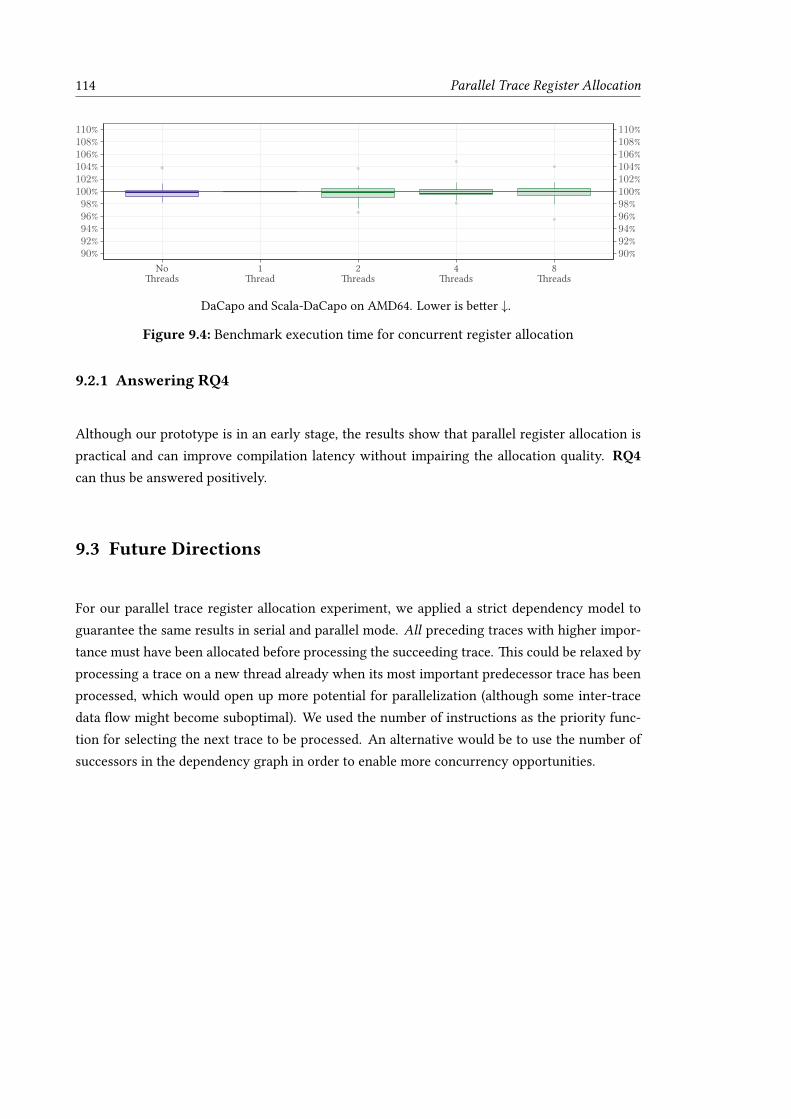
114 Parallel Trace Register Allocation
90%92%94%96%98%100%102%104%106%108%110%
90%92%94%96%98%100%102%104%106%108%110%
NoThreads
1Thread
2Threads
4Threads
8Threads
DaCapo and Scala-DaCapo on AMD64. Lower is better ↓.
Figure 9.4: Benchmark execution time for concurrent register allocation
9.2.1 Answering RQ4
Although our prototype is in an early stage, the results show that parallel register allocation ispractical and can improve compilation latency without impairing the allocation quality. RQ4can thus be answered positively.
9.3 Future Directions
For our parallel trace register allocation experiment, we applied a strict dependency model toguarantee the same results in serial and parallel mode. All preceding traces with higher impor-tance must have been allocated before processing the succeeding trace. This could be relaxed byprocessing a trace on a new thread already when its most important predecessor trace has beenprocessed, which would open up more potential for parallelization (although some inter-tracedata flow might become suboptimal). We used the number of instructions as the priority func-tion for selecting the next trace to be processed. An alternative would be to use the number ofsuccessors in the dependency graph in order to enable more concurrency opportunities.
115
Chapter 10
Related Work
Trace register allocation relates to a variety of research areas in the field of compilers and virtualmachines. The diverse field of register allocation is of course highly relevant for our work. Thus,we first look at common register allocation approaches and discuss their complexity and optimal-ity results. Optimizations that work on non-global code units, such as traces or regions, are oftenmotivated by similar considerations as in our approach. We also look at trace scheduling, sincethis class of optimizations did not only influence the name of our approach, but also uses thevery same unit of scope. Another related area is trace compilation, which follows a very differentapproach for compiling code than our method-based compilation does. However, there are areaswhere trace compilation and trace register allocation can learn from each other. Liveness is thecore information of register allocation. Our global liveness information relates to other repre-sentations of liveness used for register allocation and compilation in general. Our main focus ison the improvement of compile-time characteristics by either trading-off peak performance, ordoing work in parallel. In the last section of this chapter we discuss other trade-off techniquesused in virtual machines.
10.1 Register Allocation
In our introduction in Chapter 1, we have already discussed two well established register allo-cation approaches, graph coloring and linear scan. Register allocation is a very active area ofresearch in compiler construction for at least six decades. There are literally hundreds of pa-pers on register allocation proposing dozens of different approaches. In this section we focus onfurther work that either directly relates to trace register allocation, provides pointers for futureimprovements, or is for other reasons interesting in this context.

116 Related Work
10.1.1 Local Register Allocation
Local register allocation, where registers are allocated just for a single basic block, is particularlyinteresting for trace register allocation. Like a single basic block, traces consist of straight-linecode, which simplifies the allocation problem. Approaches that were proposed for local regis-ter allocation can also be used for traces. Other results, for example, regarding complexity oroptimality, might apply as well, although the prerequisites must be considered carefully. If rea-soning, for example, builds upon branch-free code, then it does not hold for traces because thereare control-flow joins and merges.
Approaches similar to our bottom-up allocation strategy have been described previously for lo-cal register allocation, which is not surprising given its simple and straight-forward idea. Cooperand Torczon discuss a bottom-up allocator in their book Engineering a compiler [2011, Chapter13]. However, there are a few minor differences in our implementation. We initialize our vari-able/location map to match the successor trace to avoid data-flow mismatches, which usually isnot done in local register allocators. Another difference is how we select spill candidates. Thebottom-up allocator described by Cooper and Torczon spills the register with the longest distanceto the next usage (furthest-first). While this improves the allocation quality, it also requires morework to maintain this information. We experimented with similar heuristics, but they all have asignificant negative impact on allocation time. Since fast allocation time is the main goal of ourbottom up approach, we refrained from such optimizations.
Farach-Colton and Liberatore [2000] showed that local register allocation is NP-hard with re-spect to minimal spill loads and stores. Since local register allocation can be trivially reduced
[Cook, 1971] to trace register allocation,1 the hardness result also applies to allocating a trace.However, other results by Farach-Colton and Liberatore do not. The 2-approximation algorithm,for example, assumes that the cost of a spill is the same for all program points. For traces this isnot true because of splits and joins. Whether the algorithm can be extended to traces is left forfuture research.
The furthest-first heuristic is often used for selecting a spill candidate in local register allocators,but also in global approaches such as linear scan. Facing the problem that no register is availableat a certain instruction, the furthest-first strategy selects the register whose next usage is thefurthest in the future. The heuristic is often contributed to Belady [1966] and Horwitz et al.[1966], but apparently it dates back to FORTRAN compilers from the 1950s [Farach-Colton andLiberatore, 2000]. It is optimal for basic blocks if a variable is never written, e.g., there is no needto move its value from a register to memory [Farach-Colton and Liberatore, 2000]. We havealready seen that minimizing the spill costs is NP-hard.
1Every block is considered a trace.

10.1 Register Allocation 117
Although the furthest-first strategy is not optimal for realistic cost models, the heuristic hassuccessfully been applied in practice. Guo et al. [2003] evaluated the furthest-first strategy onlarge basic blocks (300–5000 instructions). The blocks are the result of unrolling loop bodiesof number crunching libraries such as Fast-Fourier-Transformation or Matrix Multiplication. Onthe MIPS architecture their compiler using a furthest-first strategy outperformed GCC and theMIPSpro compiler by up to 33%. Especially in cases where the register pressure is high, theheuristic seems toworkwell.2 Avariant of this heuristic is also used in our linear scan strategy.
10.1.2 Non-Global Register Allocation
In contrast to global approaches such as graph coloring or linear scan, there are register allocatorsthat operate on subparts of the method and merge the intermediate results for a final solution,just like our trace register allocation approach. However, most of them do not strictly separatethe allocation of the subparts, or they force a particular allocation order, for example, from innerloops to outer loops.
Callahan and Koblenz [1991] proposed hierarchical graph coloring as a technique to minimizethe number of dynamically executed spills by moving them to infrequently executed code parts.They also divide the control-flow graph into what they call tiles and (partially) solve the registerallocation problem for each of them. Tiles are sets of basic blocks. Two tiles are either non-overlapping or one is a proper subset of the other. Callahan and Koblenz use loop-nesting aswell as branches for their tile hierarchy. The difference to our approach is that tiles are notindependent but organized in a hierarchical tree. Allocation starts at the innermost tile (the leafof the tree). Once all children are processed, the parent tile uses the information of its children tocontinue. It is also worth noting that the algorithm does not assign registers in the first pass butuses pseudo registers to record the requirements of a tile. In a second top-down pass, physicalregister are assigned and spill code is inserted if needed. Callahan and Koblenz use graph coloringfor allocating a tile. Also, the interference graph is used to communicate allocation decisionsfrom a sub-tile to its parent. This rules out the use of algorithms for tiles that do not work oninterference graphs, for example linear scan. The hierarchical graph coloring allocator featurespreferencing as an alternative to coalescing. It supports local preferencing, which is similar tothe hints we use in our linear scan strategy, as well as inter-tile preferencing, which relates toour inter-trace hints (Section 6.1). It is noteworthy that sub-tiles do not deal with variableswhich are live but not used in the tile. This is somehow related to our handling of stack intervals(Section 6.4). However, our approach basically works in top-down direction. Therefore, we stillmaintain stack intervals to keep them in registers if possible, or inform successor traces thatthese intervals are already spilled.
2However, no details are given about the allocation algorithms used in the reference compilers, nor whether theyapply global or local approaches. This makes is difficult to assess the results in more detail.

118 Related Work
The motivation for register allocation based on graph-fusion by Lueh et al. is similar to Calla-han and Koblenz. Its goal is to minimize the number of dynamically executed spill instructions.Their allocator works on regions of the control-flow graph, where a region can be a basic block,a loop-nest, a superblock [Hwu et al., 1993], or some other combination of basic blocks. Theybuild the interference graph for each region and ensure that it is colorable by potentially spillinglive ranges, as it is done in the global graph coloring approach. However, registers are not yet as-signed. Connected regions are then fused to build up the graph for larger parts of the compilationunit. The key property of fusing is that it ensures that the graph stays colorable. If fused regionswould yield an uncolorable result, live ranges are split at the edge that connects the two regionsand shuffle code is inserted. This way, the interference graph for the whole compilation unit isincrementally constructed. Due to the invariant that the graph is always colorable, the registerassignment phase can simply perform a Chaitin-style simplify and coloring. No more spill deci-sions need to be made. Although, the fusion-based allocator starts with local spilling decisions,the decisions are getting more global incrementally. Also, the actual register allocation is delayeduntil a global view on the problem is available. In contrast to that, we solve the problem locallyand independently for each trace. In addition, the graph fusion approach uses the interferencegraph as the single model for liveness. The complex fusion operation and the global assignment
phase limit the potential for doing work concurrently. In contrast to that, in our trace registerallocation approach the tasks are independent and are only connected via livein/liveout set attrace boundaries. Once a trace has been processed, its result is final and will not be changedapart from inserting resolution code.
Koes andGoldstein [2006b] proposed a global progressive register allocator usingmulti-commodity
network flow (MCNF).Their flow formulation explicitlymodels spill cost, register hints, live rangesplitting and constant rematerialization. They first create a network for the local problem (i.e. fora basic block) and then extend it to the global case. To find an initial solution, Koes and Goldsteinfirst use a heuristic approach (second-chance binpacking [Traub et al., 1998] or a simple graphcoloring) which yields a valid, but potentially suboptimal solution. Then their progressive solveriteratively improves this result towards the optimal solution with respect to the overall costs.The progressive model allows them to control the compile-time vs. peak-performance trade-offswhich relates to our allocation policies (Chapter 8). Note, however, that their decision whether tocontinue optimizing or stop is global, i.e., on the whole method, while we distinguish betweenimportant and unimportant traces. Later, Koes and Goldstein [2006a] proposed an extension totheir idea where they used traces instead of basic blocks as the scope for the local problem, whichfurther improved the quality and the speed of their approach. We find the idea of progressivelyimproving the allocation result very appealing. Applying their approach (or earlier work on alocal progressive allocator [Koes and Goldstein, 2005]) to traces could perfectly fit into our policymodel and poses an interesting future research direction.

10.1 Register Allocation 119
a b
cd
(a) chordal
a b
cd
(b) non-chordal
a b
cd
e
(c) non-chordal
A graph is chordal if every cycle with four or more edges has an edge which is not part of thecycle but which connects two vertices on the cycle. Cycles of length four without a chord are
highlighted in red. Example taken from Pereira and Palsberg [2005].
Figure 10.1: Examples for chordal and non-chordal graphs
10.1.3 Decoupled Register Allocation
Decoupled register allocation is an interesting class of allocation approaches that got a lot of atten-tion over the last years. Basically, the idea is to split the spilling and the actual register allocationinto two separate phases. Since the first phase guarantees that the register allocation will suc-ceed, the second phase is very simple. Actually, the graph fusion approach by Lueh et al. [1997]already follows a similar principle. However, most recent decoupled approaches exploit graph-theoretic properties of chordal graphs.
Definition 34 (Chordal Graph). A graph is chordal if every cycle with four or more edges has achord. A chord is an edge which is not part of the cycle but which connects two vertices on thecycle.
Figure 10.1 depicts examples for chordal and non-chordal graphs. In 2005, several research groupshave independently proven [Brisk et al., 2005; Hack, 2005; Bouchez et al., 2005] that interferencegraphs for programs in SSA form are chordal.3 Hack et al. [2006] have motivated that chordalgraphs have two properties that are utterly relevant for register allocation:
1. Their chromatic number, i.e., the smallest number of colors needed to color a graph, is equalto the size of the largest clique (see below).
2. They can be optimally colored in quadratic time with respect to the number of nodes.
Interference graph cliques are the set of variables that are live at the same time, i.e., the register
pressure. Consequently, if we can reduce the register pressure at every program point to be atmost the number of available registers, coloring will succeed. Optimal coloring means that wecan color a graph with as few colors as possible. In register allocation, however, we are only
3Those results eventually ended up in the PhD theses “Advances in Static Single Assignment Form and RegisterAllocation” by Brisk [2006], “Register Allocation for Programs in SSA Form” by Hack [2007], and “A Study ofSpilling and Coalescing in Register Allocation as Two Separate Phases” by Bouchez [2009].

120 Related Work
interested in any coloring which does not exceed the number of registers. We can find such acoloring in linear time, for example, by iterating the lifetime intervals in a linear scan fashion, assuggested by Rong [2009]. Since this renders allocation a non-issue, it allows us to concentratesolely on spilling. Braun and Hack [2009] discussed a spilling technique based on the furthest-
first heuristic. In its traditional form, all variables that are not used in the block itself but are liveafterwards have the same distance (∞). Braun and Hack [2009] extended this to control-flowgraphs. During the liveness analysis they collected the use-distance at basic block boundaries.The minimum of the distances of the successors plus the distance to the block end is then usedas the furthest-first estimator. Another issue with decoupled spilling is that reloading a variablefrom the stack destroys SSA form since it redefines a variable. Braun and Hack [2009] solved thisby introducing a new variable and placing ϕs in successor blocks to merge the original and thereloaded version.4 See Braun et al. [2013] for more details on SSA form reconstruction.
Decoupled register allocation is interesting for trace register allocation formultiple reasons. First,the interference graph of variables in a trace is an interval graph (Corollary 3), which is—inthe case of SSA form—a subclass of chordal graphs (see also Rong [2009]). Therefore, we candecouple spilling and allocating registers for a single trace. However, we could extend this to aset of traces, for example, the most important ones. This would allow us to systematically solvethe issue presented in Section 6.3. The question remains, how to deal with the loss of the singledefinition property of SSA form due to the reloads from the stack? The good news is that theseviolations are local to a trace. The overall framework does not care as long as the locin/locout setsare preserved.5 We only need to ensure that our allocation strategies can deal with pre-spilled
variables. As already argued in Section 5.3, the bottom-up strategy does not strictly require SSAform. We only need to ensure that whenever a variable is defined by a reload instruction, thevariable location is updated to the stack slot, since we need this information for updating thelocin/locout sets at trace boundaries. Also for the linear scan strategy (Section 5.1), dealing withthis special form of redefinition is possible. In the interval building step we create a new lifetimeinterval for every definition of a variable. Whether there are multiple intervals for the samevariable does not matter since all the required moves have already been added. Since the linearscan does no longer introduce new spills, this cannot interfere with the linear scan allocationprocedure.
Rong [2009] made some interesting observations regarding variable liveness and chordal inter-ference graphs. First, he reformulated a theorem by Gavril [1974] saying that if and only if theinterference graph is chordal, the lifetime of the variables span a subtree in a tree of basic blocks.Based on this formulation he proposed the class of tree register allocation. Moreover, he arguesthat this model subsumes previous approaches such as linear scan or local register allocation.Rong evaluated different tree structures such as a single basic block (local register allocation),
4However, the new ϕ defines yet another variable!5In fact, register allocation in a trace always destroys SSA form!

10.1 Register Allocation 121
the dominator tree, extended basic blocks, and the maximal spanning tree. Clearly, traces fitperfectly into this model, so trace register allocation belongs to the same class. For every tree,Rong performs a decoupled spilling and allocation phase. A data-flow resolution phase fixesmismatches on control-flow edges that are not part of a tree.
As Brisk and Sarrafzadeh [2007] showed, interference graphs which are interval graphs (Defini-tion 32) have interesting properties for register allocation. One property is that the k-colorablesubgraph problem can be solved in polynomial time [Yannakakis and Gavril, 1987]. That meansthat given an (interval) interference graph, we can get the largest subgraph (with respect tonodes) which is k-colorable. The subgraph represents the variables that are kept in registers,the others are spilled.6 Since interference graphs of traces are interval graphs (Corollary 3), thisalso holds for trace register allocation. Note, however, that this is orthogonal to minimizing spillcosts which is NP-hard, as we have argued above.
The k-colorable subgraph problem can be solved in polynomial time for chordal graphs if k isfixed [Yannakakis and Gavril, 1987]. In register allocation, k is the number of registers, which isusually a constant for a given architecture. However, it is polynomial in the order of nk whichis for realistic cases still unpractical [Brisk and Sarrafzadeh, 2007].
10.1.4 Mathematical Programming Register Allocation Approaches
We have already seen several ways to model register allocation. However, most of them onlycover parts of the overall problem. Graph coloring nicely describes interference but fails whenspilling is involved. Linear scan precisely models live ranges and allows simple splitting, but in-formation about control flow is mostly lost. The furthest-first spilling heuristic optimally handlesthe selection of a register to be spilled, but does not model the cost of spill code. Also, architec-tural irregularities like register aliasing [Lee et al., 2007] or fixed register constraints are oftenignored or handled heuristically. Unifying all requirements into a single model is appealing if anoptimal or near-optimal solution is the goal.
We have already discussed Koes and Goldstein’s MCNF model for register allocation. There area wide variety of register allocation approaches that apply different mathematical programmingmodels for solving the problem.
Goodwin and Wilken [1996] described an optimal register allocator as a 0-1 integer program-ming problem. It incorporates coalescing, splitting, rematerialization, fixed registers, and spillcode placement. The input program is modeled as a function of boolean decision variables, each
6Note, however, that this ignores the fact that not all usages of a variable can directly access the stack. An interme-diate register is needed. In practice, scratch registers could solve this issue.

122 Related Work
of which represents a certain allocation action, for example, inserting a spill move. Afterwards,their allocator uses the CPLEX solver7 to find a solution. Once there is one, the actions asso-ciated with variables that are assigned to 1 are performed. Since 0-1 integer programming isNP-complete [Karp, 1972], the solver has exponential worst-case run time, so they use time lim-its in their experiments. Since the high compile time overhead is not always practical nor needed,they proposed a hybrid allocation approach. Based on profiling, they distinguish between critical
and non-critical regions in a function. Critical regions are allocated optimally, while others use astandard graph coloring approach. Resolution code is inserted at region boundaries. This drasti-cally reduces allocation time while the result is still near-optimal. The hybrid approach is similarto our policies, which we use to switch between the linear scan and the bottom-up allocator. Asalready remarked, adding an optimal allocation strategy would further enrich our system.
Scholz and Eckstein [2002] formulated register allocation as a partitioned boolean quadratic opti-
mization problem (PBQP). They specifically focused on irregularities of non-RISC architectures,as for example used in digital signal processing (DSP). One of the main issues with comparableapproaches, for example, Goodwin and Wilken [1996], is the exponential solving time. To over-come this issue, they developed a heuristic PBQP solver that exhibits nearly linear run time. Theallocator with the heuristic solver outperforms graph coloring in all but one of their (limited setof) benchmarks (with a speedup of 1.9–10%) while showing a similar allocation time behavior.The speedup of the optimal solution is in the range of 1.3 to 13.6%.
Later, Hames and Scholz [2006] presented a new branch-and-bound solver for PBQP to circum-vent poor performance of the initial heuristic on SPEC2000 benchmarks on Intel’s IA-32 archi-tecture. With this new solver, they were able to be within 3% of the optimal solution regardingspill costs. Graph coloring, which is about 4× faster, the spill costs were never worse than 7%above the optimum. However, overall results suggest that both, graph coloring and branch-and-bound-based PBQP, are very close to the optimal solution and that there is only little room forimprovement (at least for IA-32).
Ebner et al. [2009] combined the decoupled register allocation idea with a mathematical model.Since the actual allocation is a non-issue, their formulation deals with spill code placement. Forevery variable, their allocator produces a network where the nodes represent positions at whichthe variable is live, and the weighted edges denote the cost of reloading a variable between thesepositions.8 Thenetworks for the individual variables are combined to correctly represent the reg-ister demand by every program point. By searching for the minimum-cut in the combined net-work, they get a solution to the reload placement problem. The comparison with the linear scanimplementation that was used by LLVM at that time [Lattner and Adve, 2004] showed that theirapproach speeds up the execution of the compiled code for a selected set of benchmarks from
7https://www.ibm.com/products/ilog-cplex-optimization-studio8In addition, a node representing the spill move is added. An interesting extension would be to support with multiplespill moves.

10.1 Register Allocation 123
the MiBench suite by up to 30% on a Very Long Instruction Word (VLIW) architecture. Especiallywhen register pressure is high, they achieve significant improvements. For the SPECint 2000benchmark on an ARM Thumb their speedup is 6% on average. In addition, they present a La-
grangian relaxation algorithm that finds a valid solution fast and progressively improves it. Thisallows them to trade-off compile time for code quality.
Lozano et al. [2012] modeled register allocation using constraint programming [Mayoh et al.,2013]. One interesting property of their approach is the use of Linear SSA (LSSA). This is similarto our global liveness information. Every block explicitly denotes livein and liveout variables.They model every block independently. The blocks are only connected via their liveout/liveinrelations. There are analogies to the way we allocate traces independently. We can think of twopotential crossover areas of their approach and ours. First, the constraints model could be appliedto traces instead of basic blocks to increase the scope for optimization. This is especially inter-esting since their approach also integrates instruction scheduling, which could benefit from longstraight-line code. Second, we could integrate their local constraints model into our frameworkto solve individual traces and combine this with our policies and existing strategies.
10.1.5 Register Allocation in Virtual Machines
Many of the register allocation approaches we already described, were developed for—or evalu-ated on—virtual machines. There are, however, approaches that are interesting not only becauseof their allocation algorithm, but because they explicitly integrate with a virtual machine.
Cavazos et al. [2006] proposed a hybrid optimizationmechanism to switch between a graph color-ing and a linear scan allocator in the Jikes RVM.They use an offlinemachine learning algorithm tofind a decision heuristic. Their induced heuristic reduces the total time (compile time plus bench-mark execution time) by 9% on average over graph coloring for a selected set of benchmarks fromthe SPECjvm98 suite. To classify a method, they use properties which are similar to those we areusing in our policies in Chapter 8. However, we can change the allocation algorithm for eachtrace even within a method. This allows a more fine-grained control over the compile-time vs.peak-performance trade-off. Nevertheless, deducing parameters for our policies using machinelearning techniques seems like an interesting experiment to us.
Also related to our proposed bottom-up allocator is the work by Yang et al. [1999]. They de-scribed LaTTe, a compile-only Java VM that focuses on compilation speed, including a fast, non-local register allocator. Register allocation is performed on tree regions, which are trees of basicblocks with a single entry and potentially multiple exits. The allocator does a backward pass tocollect register preferences based on the requirements at the exits of the allocation region. After

124 Related Work
collecting the references, a forward pass performs the actual register allocation. Their spillingtechnique is similar to the approach used by our bottom-up allocation strategy. However, we per-form allocation on traces instead of trees and require only a single pass over the instructions.
The (baseline) compiler of the CACAOVM uses a simple yet efficient register allocation scheme[Krall, 1998]. It is tailored for allocation of an intermediate representation that is based on Javabytecodes, as well as for RISC architectures like the Alpha processor, where there are many reg-isters available. The first observation Krall [1998] made is that the Java-to-Bytecode compilerjavac already performs pre-coloring. Non-interfering local variables are assigned to the sameslot. Second, the live range of stack variables is implicitly encoded in the push and pop opera-tions of the values.9 Therefore, no complex lifetime analysis is required, which enables a simplefirst-come-first-serve allocation scheme. Another observation is that the expression stack at ba-sic block boundaries is mostly empty (93%) or very small (< 7). This allows efficient interfacingbetween basic blocks. The CACAO allocator first allocates these interface variables. Next, tem-poral variables used only in a basic block are processed. Finally, local variables are assignedon a global scope. Therefore, local variables are most likely to be spilled. While this approachperforms well if the register set is large and the method is small, it tends to be suboptimal forarchitectures with only few registers, and if method size increases, for example, due to inlining,as discussed by Steiner et al. [2007] and Steiner [2007].
10.2 Non-global Code Units
As we showed in this thesis, the global scope of a method is not always the adequate unit foroptimizations. In literature, alternative approaches were proposed.
Fisher [1981] introduced traces as compilation units for instruction scheduling on VLIW archi-tectures. The goal is to reorder instructions so that instruction level parallelism (ILP) can beincreased. The Bulldog compiler by Ellis [1985] and later the Multiflow compiler by Lowneyet al. [1993] are popular implementations of this approach. Their definition of a trace is similarto our use of the term. However, their traces do not span across loop headers. Although themain focus of the approach is on scheduling, they treat registers as a scheduling resource in theprocess [Lowney et al., 1993]. Freudenberger and Ruttenberg [1992] presented a detailed descrip-tion of the interaction of those two optimizations. Whenever a trace is processed, they record theregister assignment decisions at trace exits and entries in a so-called value-location-map (VLM).This is basically the same as our locin/locout sets. Subsequent traces need to adhere to the VLMsof neighboring traces, i.e., the freedom of later traces is incrementally reduced. This relates to
9This also includes implicit pushing and popping, for example, by arithmetic instructions. Also, stack manipulationinstructions like dup and swap need special care.

10.3 Trace Compilation 125
our inter-trace hinting (Chapter 6). However, since we use a dedicated data-flow resolution tofix mismatches, an allocation strategy is free to ignore hints. In Multiflow, values that are livethroughout a trace but never referenced are not immediately assigned to a register, but the deci-sion is delayed until they are referenced in a later trace. There are similarities to stack intervals
in our approach.
For most of this thesis, we assumed methods to be the input to the compiler. However, a pro-grammer usually (hopefully) partitions the code into methods based on software engineeringprinciples, which do not take into account what is important to be optimized by the compiler.Outsourcing code into subroutines is mostly due to modularity or maintainability concerns, notdue to performance considerations. Method-based compilers “undo” this restructuring by ag-gressively inlining methods. However, this can lead to big compilation units which increase thepressure on the optimizations.
As an alternative, Hank et al. [1995] suggested region-based compilation which allows for aggres-sive optimization while keeping the compilation unit size small. First, they perform aggressiveinlining to enlarge the scope. Afterwards, the basic blocks are partitioned into smaller regionswhich are then compiled independently. Their region building algorithm starts similar to ourbidirectional trace builder. They use profiling data to select a start block and then append suc-cessors before going upwards. They always add the most frequently executed successor or pre-decessor. In contrast to our approach, they use a threshold value to limit the size of the region.After there is an initial trace, the algorithm continues to append successors to the blocks as longas their execution frequency exceeds the threshold.
Hank et al.’s analysis revealed, that programs exhibit different performance-critical interactionsbetween functions. Some benchmarks spend over 90% of the time in regions of one or twofunctions. Other benchmarks, however, spend 70% of their time in regions consisting of blocksfrom 10 or more functions. Their region-based approach is able to cope with all of them in auniform manner.
10.3 Trace Compilation
Hank et al. already pointed out that methods are not always the right unit of compilation. Nev-ertheless, they still perform inlining before determining their units of operation. However, insome cases this detour is not necessary or not even possible, for example, in the case of dynamicmachine code optimization. Although call and return instructions can still give a hint aboutthe original structure, determining which code segment belongs to which method is impractical.Therefore, other approaches are required.

126 Related Work
Dynamo by Bala et al. [2000] was the first widely known system using an approach called trace
compilation for dynamic translation of compiled binaries. Their system executes machine code inan interpreter. For every backward branch, they increment a counter associated with the branchtarget. Once this counter exceeds a certain limit, their interpreter enters a recording mode, i.e.,it appends every executed instruction to a trace buffer. Calls and returns are handled just as ifthey would be jumps, i.e., functions are opaque to the trace. Recording continues as long as nobackward branch is taken.10 Once trace recording has finished, the machine code is transformedinto an IR and is optimized. Since traces are straight-line code, the optimizing compiler is sim-ple and efficient. The optimized code is installed into a so-called fragment cache. Whenever theinterpreter would branch to the location that triggered trace recording, the compiled fragmentis invoked instead of interpreting the original machine instructions. Branches that exit the com-piled code return to the interpreter, potentially through compensation code to fix the executionstate. To avoid switching to the interpreter, traces can be linked together.
Gal et al. [2006] showed that this approach perfectly fits the needs of resource-constrained de-vices. Their light-weight implementation of a trace-based JIT compiler for a JVM reached aperformance that is comparable with full-fledged production quality systems. The traces arerecorded on bytecode level using an interpreter. Gal et al. use an SSA-based representation fortheir compiler. Because only the relevant basic blocks are considered, bytecode parsing overheadis avoided for uncommon parts. Similar to Dynamo, the HotPathVM performs trace merging
where different traces are stitched together. When compiling the child trace, they initialize thestate of the variables to the mapping present at the end of the parent trace. The idea is similarto our inter-trace hints. For register allocation inside a trace, they use a bottom-up approachwhich also emits machine code. As we do in our allocation strategies, ϕin and ϕout operands arecoalesced, if possible.
The trace-based approach is also suitable for dynamically typed languages as shown by Gal et al.[2009]. The empirical study by Garret et al. [1994] suggests that dynamic types in the hot regionsof a program are relatively stable. Based on this assumption, Gal et al. generate type-specializednative code for hot traces. They implemented this idea in TraceMonkey, a tracing JavaScriptvirtual machine that was used in Mozilla’s Firefox browser.
Häubl and Mössenböck [2011] modified the HotSpot client compiler in order to perform trace-based compilation. A difference to other tracing approaches is that when a call is encountered, anew trace is started and linked to the current one. This keeps the exact call information, which isimportant for a system like the HotSpot VM, that is tuned for method based compilation. Theirapproach provided speedups of the compiled code compared to themethod-based client compiler,although less code was compiled. They use the linear scan implementation for register allocationthat is used by default in the client compiler [Wimmer and Mössenböck, 2005].
10Or branches to already compiled segments, as we will see shortly.

10.4 Liveness and Intermediate Representations 127
Bolz et al. [2009] used trace compilation for obtaining an efficient JIT compiler for bytecodeinterpreters that were implemented in the PyPy language implementation framework. Theyapplied the tracing compiler not to the user program but to the bytecode interpreter that waswritten by the language implementer. This approach is also referred to as meta-tracing. Themeta-level imposes some challenges compared to traditional trace compilation. Usually, tracingassumes that the path through a hot loop is the same inmost iterations. For bytecode interpreters,the inner loop is the dispatch loop, where each iteration represents one interpreted bytecode.Since usually a different bytecode is executed in every iteration, the original assumption doesnot hold. To solve this problem, Bolz et al. proposed hints in the interpreter code to informthe trace recording mechanism about program counter information in the language interpreter.This information, in addition to the interpreter code, is used to refine trace-start and trace-endconditions. In other words, a trace is an unrolled version of the dispatch loop that represents aloop in the user program. The advantage of the meta-tracing approach is similar to Truffle (seeChapter 3). A language implementer only needs to implement an annotated bytecode interpreterand the meta-trace framework enables JIT compilation automatically.
There are some similarities between trace compilation and the traces we use for register alloca-tion. Both work on straight-line code, which simplifies optimizations and analysis, for example,when calculating lifetimes. One difference, however, is that in general, traces have no side en-tries, i.e., a trace is always entered through its head.11 In the context of trace compilation, codepieces (e.g. a basic-block or an instruction) can usually occur in multiple traces, i.e., there is somekind of code duplication. This is not the case in our implementation. Although register allocationis not the focus of trace compilation, allocation strategies used in this area can also be applied totrace register allocation and vice versa.
10.4 Liveness and Intermediate Representations
A proper and easy-to-use notion of liveness is utterly important for register allocation. In ourapproach, we use what we call global liveness information to decouple trace-local liveness fromliveness in other traces. Several related approaches have been proposed in literature.
Pereira and Palsberg’s paper on register allocation via puzzle-solving [Pereira and Palsberg, 2008]sparked our interest in Static Single Information (SSI) form. SSI form, which was proposed byAnanian [1999] and later refined by others [Singer, 2006; Boissinot et al., 2012], is an extensionto the SSA form. In addition to the ϕ functions at control-flow joins, SSI also has σ-functions12 atcontrol-flow splits. Basically, in SSI form, every usage of a variable post-dominates its definition.
11Although there are exceptions like in the approach by Häubl and Mössenböck [2011].12Sometimes called π-functions.

128 Related Work
T1
T2
int getOffset(int totalFS_0)
// final int add;
if (!this.addFrameSize)
σout=(totalFS_0)
(totalFS_1)=σin
// add = 0;
ϕout=(0)
(add)=ϕin
return this.offset + add;
(totalFS_2)=σin
// add = totalFS;
ϕout=(totalFS_2),
b0
b1
b2
b3
this
totalFS_0
add
this
totalFS_2
The example from Figure 4.5 in SSI form. Note the σout in b0, which renames totalFS inthe successor branches b1 and b2. While SSI form is sufficient to keep totalFS live until theend of b2, the liveness of this in b2 is not represented properly, due to single-entry-single-exit region bypassing [Singer, 2006]. See Figure 4.6 for our representation, which captures this
information.
Figure 10.2: Example for a program in SSI form
See Figure 10.2 for an example. SSI form has several interesting properties. Most importantfor register allocation, the interference graph is an interval graph (Definition 32) [Boissinot etal., 2012]. As we have already mentioned above, interval graphs allow solving the k-colorable
subgraph problem in polynomial time.
Pereira and Palsberg [2008] exploited a further extension to SSI form, namely elementary pro-
grams, in their register allocator based on puzzle-solving. In addition to ϕ- and σ-functions, theyinsert parallel copies of all live variables in-between two instructions of a basic block to renamevariables. That way not only definitions and usages are unique, but also liveness of a variable atevery program point.
Although we borrowed ideas from the SSI representation and elementary programs, our IR doesnot adhere to their definitions. First, SSI form might not provide all the liveness information thatwe need. A σ-function (and the corresponding ϕ-function) might be omitted for variables thatare defined before a split, but only used after the corresponding control-flow join. Singer [2006]calls this property single-entry-single-exit region bypassing. See the variable this in Figure 10.2.This defeats the purpose of our liveness representation, since we need exact liveness informationin every trace. Also, we avoid excessive renaming of variables for the sake of fewer instruction
10.5 Compile-time Trade-offs and Concurrent Compilation 129
redefinitions. Still, our global liveness model (Section 4.3.2) provides properties to make regis-ter allocation simpler, including interval interference graphs (Corollary 3) and the independentallocation of traces.
Lozano et al. [2012] introduced Linear Static Single Assignment (LSSA) form as an intermediaterepresentation for their constraint-based register allocation and instruction selection approach. Thein- and out-delimiters in LSSA form are related to our representation. In our approach, however,we distinguish between livein/liveout and ϕin/ϕout sets. While the latter are a proper part of theIR, global liveness information is stored off-site.
10.5 Compile-time Trade-offs and Concurrent Compilation
The trade-off between time spent for executing application code and time spent in the runtimeis an important design parameter for a virtual machine. For many virtual machines, such asthe early Java VMs, portability was the main focus. The deployed code, e.g. Java bytecode,is executed by an interpreter. Although optimization techniques were proposed, for exampleby [Ertl and Gregg, 2003], the execution speed is limited. Many modern virtual machines usedynamic compilation to produce efficient native machine code. However, for such systems thetime constraints for the compiler are very strict.
Some virtual machines, e.g., the CACAOVM [Krall, 1998] or the JalapeñoVM [Arnold et al.,2000], follow a compile-only approach. This means that there is no interpreter but a baseline
compiler. Since every method needs to be compiled before it is executed, this compiler mustbe fast. The CACAO baseline compiler therefore performs optimizations only on a local scope.Systems such as the JalapeñoVM [Arnold et al., 2000] or the HotSpot VM [Paleczny et al., 2001],introduce adaptive compilation, i.e., dynamic compilation and optimization of the most relevantparts based on the current execution profile. They use multiple optimization stages that are in-voked for performance-critical parts only. While Jalapeño uses a baseline compiler, HotSpot VMfeatures an interpreter for the initial execution. Methods are usually selected for optimizationbased on profiling information, for instance invocation and loop counters, or stack sampling.Although, these systems can select thresholds to control the compile time, they can do so onlyon a per-method basis. Our trace register allocation policy approach is orthogonal to that. For acompilation that is considered hot by the virtual machine, we can make a fine-grained compiletime vs. peak performance decision.
Just-in-time compilers often apply concurrency techniques to improve compilation performance.The HotSpot VM, for example, executes the compilers in background threads [Kotzmann et al.,2008]. So does V8, Googles JavaScript engine [McIlroy, 2018]. The advantage of this approach is

130 Related Work
that the main thread can continue executing the program, for example, in an interpreter, whilea method is compiled. HotSpot also uses multiple compiler threads [Oracle Corporation, 2015].The synchronization overhead is low. Compilation threads need to synchronize at the beginningwhen taking a method from the compilation queue and at the end when installing the code. Thecompiler itself can be single-threaded. Also, adding more compiler threads scales well, as long asthere are enough methods in the queue. Background compilation on multiple threads improvesthroughput, i.e., the number of units compiled in a given time frame. However, it cannot improvecompilation latency, i.e., the time that is required to compile a given method. This is in contrastto our parallel register allocation approach where multiple threads can reduce the time requiredfor compiling a single method. However, the scaling potential is bound by the number and thedependencies of traces.

131
Chapter 11
Conclusion and Future Work
Register allocation is a task that almost every compiler writer has to deal with. Most registerallocation approaches fall into one of two categories, local register allocation or global registerallocation. Local register allocators solve the problem for a single basic block. The absence ofcontrol flow guarantees liveness properties, most importantly the absence of lifetime holes, whichrenders the problem easy to tackle. However, the narrow scope limits the opportunities for op-timizations. Especially spill decisions and spill placement suffer from this constraint. Globalregister allocators, on the other hand, deal with the whole method at once. Their omniscientview allows them to optimize decisions in a way that improves the quality of the allocation. Thiscomes at a cost. First, these optimizations require a lot of contextual information which needsto be computed and/or stored. Second, a global allocator has to deal with control flow, which inturn complicates the maintenance of the liveness, which is the central piece of information theallocator deals with. Consequently, global register allocators are slower in terms of compilationtime and more complex in terms of implementation, compared to a local approach. Usually, acompiler creator needs to choose. Either use a fast and simple-to-implement local register alloca-tor and accept suboptimal allocation quality, or implement a complex and slower global allocatorto achieve better allocation results. Existing approaches did not offer a middle ground.
We wanted to gain the advantages of both worlds. The simplicity of a local allocator and theallocation quality of a global approach. In this thesis, we presented the trace register allocation
framework, a novel, flexible, non-global and extensible register allocation approach, that com-bines the advantages of local and global allocators. The approach works in two phases. A global
pre- and post-processing phase that deals with control flow and liveness, and the actual allocationphase. Instead of processing a whole method at once, the framework divides the control-flowgraph into traces, i.e., lists of sequentially executed basic blocks. The allocator then handles onetrace at a time. From the allocator’s perspective, a trace is no different than a basic block. Thereis no need to deal with control flow and the liveness behaves nicely. Therefore, we can applysimple algorithms used for local register allocation. This is possible due to the information theframework collects in the pre-processing phase. Register allocation can be done independently

132 Conclusion and Future Work
for each trace. This flexibility offers novel opportunities. First, we can choose different alloca-tion algorithms for each trace. This allows us to invest more time on the important traces of themethods and reduce the time spent on insignificant parts. We can make this decision based onthe structure of the trace, its expected execution frequency, or due to the compile-time budget.Second, since traces can be processed independently, they can be allocated in parallel by multiplethreads and thus, compilation latency can be reduced without a negative impact on allocationquality.
Although the simplicity and flexibility of our trace register allocation approach is compelling, wewanted to convince ourselves that the idea can be successfully applied in practice. To quantifysuccess, we posed four research questions: RQ1: Can trace register allocation produce the samecode quality as state-of-the-art global allocators, despite the limited scope of traces? RQ2: Canthe result be found in the same amount of time? Once these two questions were answered, wecould focus on exploiting the unique flexibility of trace register allocation. Thus we stated RQ3:Can different allocation strategies help us to better control the trade-off between compile timeand peak performance? Finally, we posed RQ4: Can the compilation latency, i.e., the durationrequired to compile a given method, be reduced by allocating traces concurrently by multiplethreads without impacting allocation quality?
All four research questions could be answered positively. We implemented trace register allo-cation in GraalVM, a production-quality Java Virtual Machine, and compared it to the existingregister allocator of Graal, a global linear scan implementation. In Section 7.3 we showed thatfor common benchmarks there is virtually no difference in terms of allocation quality (RQ1).This result is remarkable, because it suggests that a global view on the problem is not neces-sary to achieve good performance. We also showed that trace register allocation is at least asfast as global linear scan, sometimes even slightly faster (RQ2, Section 7.4). Especially for largecompilation units, traces offer a compile time advantage over the existing allocator. Section 8.3demonstrates how the careful selection of trace register allocation strategies allows us to grad-ually reduce register allocation time from 0 to 40%, depending on how much peak performancewe are willing to sacrifice (ranging from 0–12%, on average) (RQ3). Finally, in Section 9.2, weshowed that register allocation can be parallelizedwithout a negative effect on peak performance.With our early prototype we were able to reduce register allocation time by 30% when using 4
threads compared to a single allocation thread (RQ4).
In our research, we focused primarily on achieving better compile-time behavior than existingglobal approaches. In terms of allocation quality, we were satisfied with reaching the same re-sults as the global linear scan allocator. We think that exploring further improvements of theallocation quality a highly interesting research direction. From our perspective, this poses thefollowing challenges. First, the question is whether there is even potential for improvement. Webelieve that this question should be answered before investing resources on this topic. Ideally, the

133
experimentation platform, be it Graal or any other system, should be equipped with an allocatorthat finds an optimal or near-optimal allocation. Only if this uncovers missed opportunities thatreally make a difference, working towards improving the allocation quality of the trace registerallocator makes sense. The absence of this upper bound on allocation quality is one of the reasonswhy we focused on compile time first. This brings us to the second challenge. One of the keyprinciples of trace register allocation is to reduce the allocation scope and to divide the probleminto smaller sub-problems that are easier to solve than the whole problem. While this simplifiesthe problem we need to solve, it also reduces the amount of information that is available. In thisrespect, a global allocator has an immanent advantage over the trace-based approach (whetherthis advantage is exploited or not). We think that one of most the promising ideas to improveallocation quality of a trace register allocator is to apply methods, that are too costly for theglobal scope, to a single trace, or a set of important traces. We envision strategies that computethe optimal allocation for a few traces, while the rest of the method uses the heuristic methodsthat we described here.
The idea of trace-based processing does not end with register allocation. In fact, similar ideaswere already applied to instruction scheduling decades ago. We are confident that other opti-mizations can also profit from the approaches we developed for trace register allocation. Webelieve that our results lay the foundation for future research in the area of trace-based opti-mizations, and in particular to trace register allocation. We are convinced that the flexibility ofour approach can push the boundaries of current register allocation and optimization techniquesand can have an impact on both, research and production compilers.


135
Appendix A
Additional Sources

136 Additional Sources
Listing 1 Fields of the TraceInterval Classclass TraceInterval {
/** The variable for this interval prior. */final Variable operand;
/** The start of the range, inclusive. */int intFrom = Integer.MAX_VALUE;
/** The end of the range, exclusive. */int intTo = Integer.MAX_VALUE;
/** List of (use-positions, register-priorities) pairs, sorted by use-positions. */int[] usePosListArray;
/** The register or spill slot assigned to this interval. */AllocatableValue location;
/** The stack slot to which all splits of this interval are spilled if necessary. */AllocatableValue spillSlot;
/* ... */}
Listing 2 Java Source of StackSlot.getOffset()class StackSlot {
int offset;boolean addFrameSize;
int getOffset(int totalFrameSize) {final int add;if (!this.addFrameSize) {
add = 0;} else {
add = totalFrameSize;}return this.offset + add;
}
/* ... */}

137
Appendix B
Graal Backends
Thebasic parameters for register allocation in GraalVMdepends on three factors: the architecture(processor), the virtual machine, and the operating system. We evaluated Graal on top of theHotSpot VM, with AMD64 on Linux and SPARC on Solaris.
B.1 AMD64 on HotSpot
For AMD64 on HotSpot, the configuration is done by the AMD64HotSpotRegisterConfig class,which is part of JVMCI [2014]. There are 14 general purpose registers, namely rax, rcx, rdx,rbx, rbp, rsi, rdi, and r8–r14. The register rsp is used as the frame pointer, r15 is the threadregister which contains a pointer to the current thread storage (e.g., to access ThreadLoacals). Ifcompressed object pointers [Oracle Corporation, 2018] are enabled, r12 is used as the heap base
register. HotSpot uses 16 floating point registers, xmm0–xmm15. If the processor supports AVX512,there are 16 additional registers xmm16–xmm31.
The calling convention for Java methods uses 6 general purpose registers (rsi, rdx, rcx, r8, r9,rdi) for integers and reference types, and 8 floating point registers (xmm0–xmm7). Additionalparameters are passed via the stack. The rbp register is an implicit parameter, which containsthe frame pointer of the calling method. However, it can be reassigned, just like other parameterregisters.
Integer values are returned via rax, floating point values via xmm0. All allocatable registers arecaller-saved, i.e., they need to be spilled before every call.

138 Graal Backends
B.2 SPARC on HotSpot
The register set on SPARC is slightly more complex. There are 23 general purpose register, g1,g4 and g5, o0–o5, l0–l7, and i0–i5. The frame pointer is in o6, g0 is always zero, and otherregisters are system-reserved. The register g6 is the optional heap base register. SPARC hasseparate registers for single precision (float, f8–31) and double precision (double, register pairsd32_d33–d62_d63) floating point values.
Integer parameters are passed via i0–i5 (callee side), single precision floats via f0–f7, doubleprecision floating point values via d0_d1–d6_d7. The return register is either i0, f0, or d0_d1.
The SPARC architecture features a register window. At every procedure call the registers i0–i7and l0–l7 are automatically stored in a predefined location on the stack. In addition, the registerso0–o7 of the caller are mapped to the i0–i7 of the callee (that includes the parameter registers).The compiler does not need to spill those registers across a call.

139
Appendix C
Hardware Environment
The experiments on AMD64 were performed on two kinds of machines, the Sun Server X3-2 andSun Server X5-2. The machines were running an Oracle Linux Server 6.8 operating system withLinux Kernel version 4.1.12. For the experiments we disabled all frequency scaling modes (e.g.scaling governors or Intel Turbo Boost).
C.1 Sun Server X3-2
The X3-2 cluster consists of 64 identical Sun Server X3-2 machines,1 equipped with two Intel“Sandy Bridge” Xeon E5-2660 at 2.20GHz with 8 real cores per processor, and 256GB of DDR3-1600 memory. Each core has 2 threads. The cache sizes are 32KB for L1, 265KB for L2 and 20MBL3. Figure C.1 shows the hardware topology of the machine.
C.2 Sun Server X5-2
The X5-2 cluster consists of 36 identical Sun Server X5-2 machines,2 equipped with two Intel“Haswell” Xeon E5-2699 v3 at 2.30GHz with 18 real cores per processor, and 384GB of mainmemory. Each core features 2 threads. The cache sizes are 32KB for L1, 265KB for L2 and 45MBL3. Figure C.2 shows the hardware topology of the machine.
1Sun Server X3-2: http://www.oracle.com/goto/x3-2/docs2Sun Server X5-2: http://www.oracle.com/goto/x5-2/docs

140 Hardware Environment
Machine (252GB)
NUMANode P#0 (126GB)
Socket P#0
L3 (20MB)
L2 (256KB)
L1d (32KB)
L1i (32KB)
Core P#0
PU P#0
PU P#16
L2 (256KB)
L1d (32KB)
L1i (32KB)
Core P#1
PU P#1
PU P#17
L2 (256KB)
L1d (32KB)
L1i (32KB)
Core P#2
PU P#2
PU P#18
L2 (256KB)
L1d (32KB)
L1i (32KB)
Core P#3
PU P#3
PU P#19
L2 (256KB)
L1d (32KB)
L1i (32KB)
Core P#4
PU P#4
PU P#20
L2 (256KB)
L1d (32KB)
L1i (32KB)
Core P#5
PU P#5
PU P#21
L2 (256KB)
L1d (32KB)
L1i (32KB)
Core P#6
PU P#6
PU P#22
L2 (256KB)
L1d (32KB)
L1i (32KB)
Core P#7
PU P#7
PU P#23
PCI 8086:1528
eth0
PCI 8086:1528
eth1
PCI 1000:0079
sda sdb
sdc
PCI 1a03:2000
PCI 8086:1d02
NUMANode P#1 (126GB)
Socket P#1
L3 (20MB)
L2 (256KB)
L1d (32KB)
L1i (32KB)
Core P#0
PU P#8
PU P#24
L2 (256KB)
L1d (32KB)
L1i (32KB)
Core P#1
PU P#9
PU P#25
L2 (256KB)
L1d (32KB)
L1i (32KB)
Core P#2
PU P#10
PU P#26
L2 (256KB)
L1d (32KB)
L1i (32KB)
Core P#3
PU P#11
PU P#27
L2 (256KB)
L1d (32KB)
L1i (32KB)
Core P#4
PU P#12
PU P#28
L2 (256KB)
L1d (32KB)
L1i (32KB)
Core P#5
PU P#13
PU P#29
L2 (256KB)
L1d (32KB)
L1i (32KB)
Core P#6
PU P#14
PU P#30
L2 (256KB)
L1d (32KB)
L1i (32KB)
Core P#7
PU P#15
PU P#31
PCI 8086:1528
eth2
PCI 8086:1528
eth3
PCI 15b3:1011
ib0 ib1
mlx5_0
Host: bunch036
Indexes: physical
Date: Thu 03 May 2018 01:43:35 PDT
Topology of the X3-2 system collected with the lstopoa utility.
alstopo(1) — Linux man page: https://linux.die.net/man/1/lstopo
Figure C.1: Sun Server X3-2 topology

C.3 SPARC T7-2 Server 141
Machine (378GB)
NUMANode P#0 (189GB)
Socket P#0
L3 (45MB)
L2 (256KB)
L1d (32KB)
L1i (32KB)
Core P#0
PU P#0
PU P#36
L2 (256KB)
L1d (32KB)
L1i (32KB)
Core P#1
PU P#1
PU P#37
L2 (256KB)
L1d (32KB)
L1i (32KB)
Core P#2
PU P#2
PU P#38
L2 (256KB)
L1d (32KB)
L1i (32KB)
Core P#3
PU P#3
PU P#39
L2 (256KB)
L1d (32KB)
L1i (32KB)
Core P#4
PU P#4
PU P#40
L2 (256KB)
L1d (32KB)
L1i (32KB)
Core P#8
PU P#5
PU P#41
L2 (256KB)
L1d (32KB)
L1i (32KB)
Core P#9
PU P#6
PU P#42
L2 (256KB)
L1d (32KB)
L1i (32KB)
Core P#10
PU P#7
PU P#43
L2 (256KB)
L1d (32KB)
L1i (32KB)
Core P#11
PU P#8
PU P#44
L2 (256KB)
L1d (32KB)
L1i (32KB)
Core P#16
PU P#9
PU P#45
L2 (256KB)
L1d (32KB)
L1i (32KB)
Core P#17
PU P#10
PU P#46
L2 (256KB)
L1d (32KB)
L1i (32KB)
Core P#18
PU P#11
PU P#47
L2 (256KB)
L1d (32KB)
L1i (32KB)
Core P#19
PU P#12
PU P#48
L2 (256KB)
L1d (32KB)
L1i (32KB)
Core P#20
PU P#13
PU P#49
L2 (256KB)
L1d (32KB)
L1i (32KB)
Core P#24
PU P#14
PU P#50
L2 (256KB)
L1d (32KB)
L1i (32KB)
Core P#25
PU P#15
PU P#51
L2 (256KB)
L1d (32KB)
L1i (32KB)
Core P#26
PU P#16
PU P#52
L2 (256KB)
L1d (32KB)
L1i (32KB)
Core P#27
PU P#17
PU P#53
PCI 15b3:1011
ib0 ib1
mlx5_0
PCI 1000:005d
sda
PCI 8086:1528
eth0
PCI 8086:1528
eth1
PCI 102b:0522
PCI 8086:8d02
sr0
NUMANode P#1 (189GB)
Socket P#1
L3 (45MB)
L2 (256KB)
L1d (32KB)
L1i (32KB)
Core P#0
PU P#18
PU P#54
L2 (256KB)
L1d (32KB)
L1i (32KB)
Core P#1
PU P#19
PU P#55
L2 (256KB)
L1d (32KB)
L1i (32KB)
Core P#2
PU P#20
PU P#56
L2 (256KB)
L1d (32KB)
L1i (32KB)
Core P#3
PU P#21
PU P#57
L2 (256KB)
L1d (32KB)
L1i (32KB)
Core P#4
PU P#22
PU P#58
L2 (256KB)
L1d (32KB)
L1i (32KB)
Core P#8
PU P#23
PU P#59
L2 (256KB)
L1d (32KB)
L1i (32KB)
Core P#9
PU P#24
PU P#60
L2 (256KB)
L1d (32KB)
L1i (32KB)
Core P#10
PU P#25
PU P#61
L2 (256KB)
L1d (32KB)
L1i (32KB)
Core P#11
PU P#26
PU P#62
L2 (256KB)
L1d (32KB)
L1i (32KB)
Core P#16
PU P#27
PU P#63
L2 (256KB)
L1d (32KB)
L1i (32KB)
Core P#17
PU P#28
PU P#64
L2 (256KB)
L1d (32KB)
L1i (32KB)
Core P#18
PU P#29
PU P#65
L2 (256KB)
L1d (32KB)
L1i (32KB)
Core P#19
PU P#30
PU P#66
L2 (256KB)
L1d (32KB)
L1i (32KB)
Core P#20
PU P#31
PU P#67
L2 (256KB)
L1d (32KB)
L1i (32KB)
Core P#24
PU P#32
PU P#68
L2 (256KB)
L1d (32KB)
L1i (32KB)
Core P#25
PU P#33
PU P#69
L2 (256KB)
L1d (32KB)
L1i (32KB)
Core P#26
PU P#34
PU P#70
L2 (256KB)
L1d (32KB)
L1i (32KB)
Core P#27
PU P#35
PU P#71
PCI 8086:1528
eth2
PCI 8086:1528
eth3
Host: clutter029
Indexes: physical
Date: Thu 03 May 2018 01:27:19 PDT
Topology of the X5-2 system collected with lstopo.
Figure C.2: Sun Server X5-2 topology
C.3 SPARC T7-2 Server
For our SPARC/Solaris experiments we used a SPARC T7-2 Server3 running the Solaris 11.3 oper-ating system.4 It is equipped with two SPARCM7 processors, which are SPARC V9 architectures[Weaver and Germond, 1994]. A single M7 is running at 4.13 GHz and features 32 cores with 8threads each. Consequently, the T7-2 machine has 64 cores and 512 threads, respectively. Eachcore has 16KB L1 cache, 256KB of L2 per core pair, and 64MB per chip. Our system features2×500GB of main memory, one for each processor. We use Solaris Kernel Zones5 to divide theT7-2 into 8 isolated zones. Each zone can use 4 dedicated cores and has access to 96GB ofmemory.The remaining cores and memory are left for the root zone.
3SPARC T7-2 Server: http://www.oracle.com/goto/t7-2/docs4Solaris 11.3 https://www.oracle.com/solaris/oracle-solaris-11-3.html5Solaris Kernel Zones: http://docs.oracle.com/cd/E36784_01/pdf/E36848.pdf

142 List of Figures
List of Figures
1.1 The allocateArray() example code snippet . . . . . . . . . . . . . . . . . . . . 21.2 Typical memory hierarchy of a computer . . . . . . . . . . . . . . . . . . . . . . 31.3 Lifetime intervals and interference graph for allocateArray() . . . . . . . . . 41.4 Chaitin’s allocator . . . . . . . . . . . . . . . . . . . . . . . . . . . . . . . . . . . 71.5 Graph coloring of allocArray using three registers . . . . . . . . . . . . . . . . 71.6 Graph coloring of allocArray using two registers (interference before spilling) 81.7 Graph coloring of allocArray using two registers (interference after spilling) . 91.8 Graph coloring of allocArray using two colors (simplify) . . . . . . . . . . . . 101.9 Graph coloring of allocArray using two colors (select) . . . . . . . . . . . . . . 111.10 Diamond-shaped interference graph diamond which is 2-colorable . . . . . . . . 121.11 Briggs’ optimistic allocator . . . . . . . . . . . . . . . . . . . . . . . . . . . . . . 121.12 Poletto and Sarkar-style linear scan allocation example with two registers . . . 131.13 Interval-splitting linear scan allocation of allocateArray with two registers . . 141.14 Graph coloring vs. linear scan of allocateArray with two registers . . . . . . . 151.15 Trace register allocation of allocArray() with 2 registers . . . . . . . . . . . . 18
2.1 Critical edge splitting . . . . . . . . . . . . . . . . . . . . . . . . . . . . . . . . . 252.2 The allocateArray() sample code snippet (without critical edges) . . . . . . . 262.3 Dominator tree for allocateArray() . . . . . . . . . . . . . . . . . . . . . . . . 272.4 Example for an inevitable lifetime hole . . . . . . . . . . . . . . . . . . . . . . . 302.5 Variable renaming in Static Single Assignment form . . . . . . . . . . . . . . . . 312.6 ϕ-function in Static Single Assignment form . . . . . . . . . . . . . . . . . . . . 312.7 Parallel ϕ-copies . . . . . . . . . . . . . . . . . . . . . . . . . . . . . . . . . . . . 32
3.1 The GraalVM ecosystem . . . . . . . . . . . . . . . . . . . . . . . . . . . . . . . 363.2 Tiered-compilation on the JVM . . . . . . . . . . . . . . . . . . . . . . . . . . . . 373.3 Graal compiler pipeline . . . . . . . . . . . . . . . . . . . . . . . . . . . . . . . . 403.4 Graal High-level Intermediate Representation (HIR) . . . . . . . . . . . . . . . . 413.5 Graal Low-level Intermediate Representation (LIR) . . . . . . . . . . . . . . . . . 42
4.1 Trace register allocation overview . . . . . . . . . . . . . . . . . . . . . . . . . . 444.2 Trace-building example for allocateArray . . . . . . . . . . . . . . . . . . . . 46

List of Figures 143
4.3 Termination of the unidirectional trace building algorithm . . . . . . . . . . . . 484.4 Non-sequential forward edges are critical edge . . . . . . . . . . . . . . . . . . . 524.5 Traces without global liveness information . . . . . . . . . . . . . . . . . . . . . 544.6 Traces with global liveness information . . . . . . . . . . . . . . . . . . . . . . . 554.7 Representation of liveness . . . . . . . . . . . . . . . . . . . . . . . . . . . . . . 564.8 Representation of the locin/locout sets . . . . . . . . . . . . . . . . . . . . . . . . 574.9 Inserted move instructions for global data-flow resolution . . . . . . . . . . . . 58
5.1 Trace-based linear scan . . . . . . . . . . . . . . . . . . . . . . . . . . . . . . . . 625.2 Two-address instructions . . . . . . . . . . . . . . . . . . . . . . . . . . . . . . . 635.3 Link traces . . . . . . . . . . . . . . . . . . . . . . . . . . . . . . . . . . . . . . . 665.4 Example of a trivial trace allocation . . . . . . . . . . . . . . . . . . . . . . . . . 675.5 ϕ-resolution in the Bottom-Up allocator . . . . . . . . . . . . . . . . . . . . . . . 745.6 Bottom-Up allocation example . . . . . . . . . . . . . . . . . . . . . . . . . . . . 75
6.1 Inter-trace hints example (getOffset) . . . . . . . . . . . . . . . . . . . . . . . 786.2 Spilling in side-traces of a loop . . . . . . . . . . . . . . . . . . . . . . . . . . . . 80
7.1 Composite results for DaCapo and Scala-DaCapo on AMD64 . . . . . . . . . . 877.2 Peak performance of individual benchmarks from (Scala-)DaCapo on AMD64 . 887.3 Composite peak performance results for DaCapo and Scala-DaCapo on SPARC 897.4 Peak performance results for SPECjvm2008 on AMD64 . . . . . . . . . . . . . . 907.5 Peak performance results for SPECjbb2015 on AMD64 . . . . . . . . . . . . . . 917.6 Register allocation time of individual benchmarks from (Scala-)DaCapo . . . . 927.7 Register allocation time vs. LIR instructions for DaCapo and Scala-DaCapo . . 937.8 Register allocation time vs. LIR instructions for (Scala-)DaCapo (small methods) 947.9 Share of register allocation time in the overall compile time for (Scala-)DaCapo 957.10 Influence of inter-trace hints and spill information sharing on peak performance 957.11 Peak performance impact of the stack interval optimization on DaCapo . . . . 967.12 Unidirectional vs. bidirectional trace builder w.r.t. peak performance of DaCapo 97
8.1 Peak performance and register allocation time of various allocation policies . . 1048.2 Distribution of the allocation strategy per policy . . . . . . . . . . . . . . . . . . 105
9.1 Trace dependency graph for PrintStream.write() . . . . . . . . . . . . . . . . 1119.2 Trace allocation scheduling for PrintStream.write() . . . . . . . . . . . . . . 1119.3 Concurrent register allocation time . . . . . . . . . . . . . . . . . . . . . . . . . 1139.4 Benchmark execution time for concurrent register allocation . . . . . . . . . . . 114
10.1 Examples for chordal and non-chordal graphs . . . . . . . . . . . . . . . . . . . . 11910.2 Example for a program in SSI form . . . . . . . . . . . . . . . . . . . . . . . . . 128
C.1 Sun Server X3-2 topology . . . . . . . . . . . . . . . . . . . . . . . . . . . . . . . 140

144 List of Tables
C.2 Sun Server X5-2 topology . . . . . . . . . . . . . . . . . . . . . . . . . . . . . . . 141
List of Algorithms
1 Pseudocode for the Unidirectional Trace Builder . . . . . . . . . . . . . . . . . . 472 Pseudocode for the Bidirectional Trace Builder . . . . . . . . . . . . . . . . . . . 493 Trivial Trace Allocation Strategy . . . . . . . . . . . . . . . . . . . . . . . . . . . 684 Bottom-up allocator: allocateTrace . . . . . . . . . . . . . . . . . . . . . . . . . 695 Bottom-up allocator: allocateInstruction . . . . . . . . . . . . . . . . . . . . . 706 Bottom-up allocator: allocFixedRegister . . . . . . . . . . . . . . . . . . . . . . 707 Bottom-up allocator: allocRegister . . . . . . . . . . . . . . . . . . . . . . . . . 718 Bottom-up allocator: allocStackOrRegister . . . . . . . . . . . . . . . . . . . . 719 Bottom-up allocator: findFreeRegister . . . . . . . . . . . . . . . . . . . . . . . 7210 Bottom-up allocator: findRegisterToSpill . . . . . . . . . . . . . . . . . . . . . 7211 Bottom-up allocator: evacuateRegisterAndSpill . . . . . . . . . . . . . . . . . . 7212 Bottom-up allocator: resolvePhis . . . . . . . . . . . . . . . . . . . . . . . . . . 72
List of Tables
8.1 Experimental results for trace register allocation policies . . . . . . . . . . . . . 108

Index
HotSpot VM, 36
abstract-syntax-tree, see ASTahead-of-time, see AOTalive, see livenessanti-dependency, 58AOT, 35assumptions, 37AST, 35
back edge, 27back end, 40basic block, 24bidirectional trace builder, 48bytecode, 36bytecode parser, 39
C1, see client compilerC2, see server compilerCISC, 87class file, 36client compiler, 37coalescing, 63compilation unit, 24constant, 23control-flow graph, 25critical edge, 25
deoptimization, 37dominance order, 27dominator, 26
edge, 24entry block, 25
front end, 40
general loop, 27global data-flow resolution, 57global liveness information, 54GraalVM, 35
high-level intermediate representation, seeHIR
hint, 63HIR, 39hot method, 37
immediate dominator, 26instruction, 24instruction path, 28inter-trace edge, 45interference, 29interference graph, 29intra-trace edge, 45
Java programming language, 36Java Virtual Machine, see JVMJava-Level JVM Compiler Interface, see
JVMCIJVM, 36JVMCI, 38
lifetime hole, 29lifetime interval, see liveness, 29LIR, 40LIR kind, 41live range, 29live variable, see liveness
146 INDEX
liveness, 29location, 24loop, 27
end, 27entry, 28exit, 27header, 27
low-level intermediate representation, seeLIR
meta-circularity, 38
partial evaluation, 35path, 25peak performance, 38predecessor, 24profile, see profiling informationprofile pollution, 39profiling information, 37program points, 24
reachability, 25reducible graph, 27register, 23register allocation, 4reverse postorder, 28RISC, 87
server compiler, 37SSA form, 30
dominance property, 31
ϕ-function, 30stack slot, 23static single assignment form, see SSA
formsteady state, 38strict dominator, 26Substrate VM, 35successor, 25SVM, see Substrate VM
temporary, see variabletiered compilation, 37trace, 44
entries, 45exits, 45greedy, 50head, 45length, 45partition, 45trivial, see trivial trace
trivial trace, 66
unidirectional trace builder, 45
value, 24variable, 23
warmup, 38write-after-read dependency, see
anti-dependencies
147
Publications
Eisl, Josef (2015). “Trace Register Allocation”. In: SPLASH Companion 2015. ACM. doi: 10.1145/2814189.2814199. (SPLASH 2015 Doctoral Symposium Vision Paper)
Eisl, Josef (2018a). “Divide and Allocate: The Trace Register Allocation Framework”. In: CGO’18.ACM. preprint: http://ssw.jku.at/General/Staff/Eisl/papers/CGO_SRC2018.pdf(Peer Reviewed Extended Abstract, Winner CGO ACM Student Research Competition Graduate
Category)
Eisl, Josef (2018b). “Divide and Allocate: The Trace Register Allocation Framework (ExtendedGrand Finals Version)”. In: SRC’18. ACM. url: https://src.acm.org/binaries/content/assets/src/2018/josef-eisl.pdf. (Submitted to the ACM Student Research Competition
Grand Finals 2018)
Eisl, Josef, Matthias Grimmer, Doug Simon, Thomas Würthinger, and Hanspeter Mössenböck(2016). “Trace-based Register Allocation in a JIT Compiler”. In: PPPJ’16. ACM. doi: 10.1145/2972206.2972211.
Eisl, Josef, David Leopoldseder, and Hanspeter Mössenböck (2018). “Parallel Trace Register Allo-cation”. In: ManLang 2018. ACM. doi: 10.1145/3237009.3237010.
Eisl, Josef, Stefan Marr, Thomas Würthinger, and Hanspeter Mössenböck (2017). “Trace RegisterAllocation Policies: Compile-time vs. Performance Trade-offs”. In: ManLang 2017. ACM. doi:10.1145/3132190.3132209.
Leopoldseder, David, Lukas Stadler, Thomas Würthinger, Josef Eisl, Doug Simon, and HanspeterMössenböck (2018). “Dominance-based Duplication Simulation (DBDS) – Code Duplicationto Enable Compiler Optimizations”. In: CGO’18. ACM. doi: 10.1145/3168811. (best paper
finalist)


149
Bibliography
Aho, Alfred V., John E. Hopcroft, and Jeffrey D. Ullman (1974). The Design and Analysis of Com-
puter Algorithms. Addison-Wesley. isbn: 9780201000290.
Aho, Alfred V., Monica S. Lam, Ravi Sethi, and Jeffrey D. Ullman (2006). Compilers: Princi-
ples, Techniques, and Tools (2nd Edition). Addison-Wesley Longman Publishing Co., Inc. isbn:0321486811. url: http://dragonbook.stanford.edu/.
Ananian, C. Scott (1999). “The Static Single Information Form”. MA thesis. Princeton University.url: http://publications.csail.mit.edu/lcs/pubs/pdf/MIT-LCS-TR-801.pdf.
Appel, Andrew W. (1998). SSA is Functional Programming.
Appel, AndrewW. and Jens Palsberg (2003).Modern Compiler Implementation in Java. 2nd. Cam-bridge University Press. isbn: 052182060X.
Arnold, Matthew, Stephen Fink, David Grove, Michael Hind, and Peter F. Sweeney (2000). “Adap-tive Optimization in the Jalapeño JVM”. In: OOPSLA ’00. ACM. doi: 10.1145/353171.353175.
Bala, Vasanth, Evelyn Duesterwald, and Sanjeev Banerjia (2000). “Dynamo: A Transparent Dy-namic Optimization System”. In: PLDI’00. ACM. doi: 10.1145/349299.349303.
Barik, Rajkishore, Jisheng Zhao, and Vivek Sarkar (2013). “A Decoupled non-SSA Global RegisterAllocation Using Bipartite Liveness Graphs”. In: TACO’13. doi: 10.1145/2544101.
Barrett, Edd, Carl Friedrich Bolz-Tereick, Rebecca Killick, SarahMount, and Laurence Tratt (2017).“Virtual Machine Warmup Blows Hot and Cold”. In: Proc. ACM Program. Lang. doi: 10.1145/3133876.
Belady, L. A. (1966). “A study of replacement algorithms for a virtual-storage computer”. In: IBMSystems Journal. doi: 10.1147/sj.52.0078.
Bergner, Peter, Peter Dahl, David Engebretsen, and Matthew O’Keefe (1997). “Spill Code Mini-mization via Interference Region Spilling”. In: PLDI’97. ACM. doi: 10.1145/258915.258941.

150 Bibliography
Blackburn, S. M., R. Garner, C. Hoffman, A. M. Khan, K. S. McKinley, R. Bentzur, A. Diwan, D.Feinberg, D. Frampton, S. Z. Guyer, M. Hirzel, A. Hosking, M. Jump, H. Lee, J. E. B. Moss, A.Phansalkar, D. Stefanović, T. VanDrunen, D. von Dincklage, and B. Wiedermann (2006). “TheDaCapo Benchmarks: Java Benchmarking Development and Analysis”. In: OOPSLA’06. ACMPress. doi: 10.1145/1167473.1167488.
Boissinot, Benoit, Philip Brisk, Alain Darte, and Fabrice Rastello (2012). “SSI Properties Revisited”.In: ACM Trans. Embed. Comput. Syst. doi: 10.1145/2180887.2180898.
Bolz, Carl Friedrich, Antonio Cuni,Maciej Fijalkowski, andArmin Rigo (2009). “Tracing themeta-level”. In: ICOOOLPS’09. doi: 10.1145/1565824.1565827.
Bouchez, Florent (2009). “A Study of Spilling and Coalescing in Register Allocation as Two Sep-arate Phases”. Theses. Ecole normale supérieure de lyon - ENS LYON. url: https://tel.archives-ouvertes.fr/tel-00403504.
Bouchez, Florent, Alain Darte, Christophe Guillon, and Fabrice Rastello (2005). Register allocationand spill complexity under SSA. Tech. rep. École Normale Supérieure de Lyon.
Brandis, Marc M. and Hanspeter Mössenböck (1994). “Single-pass Generation of Static Single-assignment Form for Structured Languages”. In: TOPLAS’94. doi: 10.1145/197320.197331.
Braun, Matthias, Sebastian Buchwald, Sebastian Hack, Roland Leißa, Christoph Mallon, and An-dreas Zwinkau (2013). “Simple and Efficient Construction of Static Single Assignment Form”.In: CC 2013. Springer-Verlag. doi: 10.1007/978-3-642-37051-9_6.
Braun, Matthias and Sebastian Hack (2009). “Register Spilling and Live-Range Splitting for SSA-Form Programs”. In: CC 2009. Springer-Verlag. doi: 10.1007/978-3-642-00722-4_13.
Briggs, Preston (1992). “Register Allocation via Graph Coloring”. PhD thesis. Rice University.
Briggs, Preston, Keith D. Cooper, and Linda Torczon (1994). “Improvements to graph coloringregister allocation”. In: TOPLAS’94. doi: 10.1145/177492.177575.
Brisk, Philip (2006). “Advances in Static Single Assignment Form and Register Allocation”. PhDthesis.
Brisk, Philip, Foad Dabiri, Jamie Macbeth, and Majid Sarrafzadeh (2005). “Polynomial time graphcoloring register allocation”. In:
Brisk, Philip and Majid Sarrafzadeh (2007). “Interference graphs for procedures in static singleinformation form are interval graphs”. In: SCOPES’07. ACM. doi: 10.1145/1269843.1269858.
Buchwald, Sebastian, Manuel Mohr, and Ignaz Rutter (2015). “Optimal Shuffle Code with Permu-tation Instructions”. In: Springer International Publishing. doi: 10.1007/978-3-319-21840-3_44.

Bibliography 151
Callahan, David and Brian Koblenz (1991). “Register Allocation via Hierarchical Graph Coloring”.In: SIGPLAN Not. doi: 10.1145/113446.113462.
Cavazos, John, J. Eliot B. Moss, and Michael F. P. O’Boyle (2006). “Hybrid Optimizations: WhichOptimization Algorithm to Use?” In: CC 2000. Springer Berlin Heidelberg. doi: 10 . 1007 /11688839_12.
Chaitin, Gregory J. (1982). “Register Allocation & Spilling via Graph Coloring”. In: SIGPLAN Not.
doi: 10.1145/872726.806984.
Chaitin, Gregory J., Marc A. Auslander, Ashok K. Chandra, John Cocke, Martin E. Hopkins, andPeter W. Markstein (1981). “Register Allocation via Coloring”. In: Computer languages. doi:10.1016/0096-0551(81)90048-5.
Chen, Wei-Yu, Guei-Yuan Lueh, Pratik Ashar, Kaiyu Chen, and Buqi Cheng (2018). “Register Al-location for Intel Processor Graphics”. In: CGO’18. ACM. doi: 10.1145/3168806.
Chow, Fred C. and John L. Hennessy (1990). “The priority-based coloring approach to registerallocation”. In: ACM Trans. Program. Lang. Syst. doi: 10.1145/88616.88621.
Clang (2018). clang: a C language family frontend for LLVM. url: https://clang.llvm.org/(visited on 01/12/2018).
Click, Cliff and Michael Paleczny (1995). “A simple graph-based intermediate representation”. In:IR’95. ACM. doi: 10.1145/202529.202534.
Click, Clifford Noel (1995). “Combining Analyses, Combining Optimizations”. PhD thesis. RiceUniversity.
Cook, Stephen A. (1971). “The complexity of theorem-proving procedures”. In: STOC’71. ACM.doi: 10.1145/800157.805047.
Cooper, Keith and Linda Torczon (2011). Engineering a compiler. 2nd ed. Elsevier. isbn:9780120884780.
Cytron, Ron, Jeanne Ferrante, Barry K. Rosen, Mark N. Wegman, and F. Kenneth Zadeck (1991).“Efficiently Computing Static Single Assignment Form and the Control Dependence Graph”.In: TOPLAS’91. doi: 10.1145/115372.115320.
Deutsch, L. Peter and Allan M. Schiffman (1984). “Efficient Implementation of the Smalltalk-80System”. In: POPL ’84. ACM. doi: 10.1145/800017.800542.
Duboscq, Gilles (2016). “Combining Speculative Optimizations with Flexible Scheduling of Side-effects”. PhD thesis. Johannes Kepler University Linz. url: http://resolver.obvsg.at/urn:nbn:at:at-ubl:1-9708.
Duboscq, Gilles, Thomas Würthinger, and Hanspeter Mössenböck (2014). “Speculation withoutregret”. In: PPPJ’14. doi: 10.1145/2647508.2647521.

152 Bibliography
Duboscq, Gilles, Thomas Würthinger, Lukas Stadler, Christian Wimmer, Doug Simon, andHanspeterMössenböck (2013). “An Intermediate Representation for Speculative Optimizationsin a Dynamic Compiler”. In: VMIL’13. doi: 10.1145/2542142.2542143.
Ebner, Dietmar, Bernhard Scholz, and Andreas Krall (2009). “Progressive Spill Code Placement”.In: CASES ’09. ACM. doi: 10.1145/1629395.1629408.
Eisl, Josef (2015). “Trace Register Allocation”. In: SPLASH Companion 2015. ACM. doi: 10.1145/2814189.2814199. (SPLASH 2015 Doctoral Symposium Vision Paper)
Eisl, Josef (2018a). “Divide and Allocate: The Trace Register Allocation Framework”. In: CGO’18.ACM. preprint: http://ssw.jku.at/General/Staff/Eisl/papers/CGO_SRC2018.pdf(Peer Reviewed Extended Abstract, Winner CGO ACM Student Research Competition Graduate
Category)
Eisl, Josef (2018b). “Divide and Allocate: The Trace Register Allocation Framework (ExtendedGrand Finals Version)”. In: SRC’18. ACM. url: https://src.acm.org/binaries/content/assets/src/2018/josef-eisl.pdf. (Submitted to the ACM Student Research Competition
Grand Finals 2018)
Eisl, Josef, Matthias Grimmer, Doug Simon, Thomas Würthinger, and Hanspeter Mössenböck(2016). “Trace-based Register Allocation in a JIT Compiler”. In: PPPJ’16. ACM. doi: 10.1145/2972206.2972211.
Eisl, Josef, David Leopoldseder, and Hanspeter Mössenböck (2018). “Parallel Trace Register Allo-cation”. In: ManLang 2018. ACM. doi: 10.1145/3237009.3237010.
Eisl, Josef, Stefan Marr, Thomas Würthinger, and Hanspeter Mössenböck (2017). “Trace RegisterAllocation Policies: Compile-time vs. Performance Trade-offs”. In: ManLang 2017. ACM. doi:10.1145/3132190.3132209.
Ellis, John R. (1985). “Bulldog: A Compiler for VLIW Architectures”. PhD thesis. Yale University.
Ertl, M. Anton and David Gregg (2003). “The Structure and Performance of Efficient Interpreters”.In: The Journal of Instruction-Level Parallelism. url: http://www.complang.tuwien.ac.at/papers/ertl%26gregg03jilp.ps.gz.
Farach-Colton,Martin andVincenzo Liberatore (2000). “On Local Register Allocation”. In: Journalof Algorithms. doi: 10.1006/jagm.2000.1095.
Fisher, Joseph Allen (1981). “Trace Scheduling: A Technique for Global Microcode Compaction”.In: Computers, IEEE Transactions on Computers. doi: 10.1109/TC.1981.1675827.
Flajolet, Philippe and Robert Sedgewick (2009). Analytic Combinatorics. Cambridge UniversityPress.

Bibliography 153
Freudenberger, Stefan M. and John C. Ruttenberg (1992). “Phase Ordering of Register Allocationand Instruction Scheduling”. In: Workshops in Computing. Springer London. doi: 10.1007/978-1-4471-3501-2_9.
Gal, Andreas, Brendan Eich, Mike Shaver, David Anderson, David Mandelin, Mohammad R.Haghighat, Blake Kaplan, Graydon Hoare, Boris Zbarsky, Jason Orendorff, Jesse Ruderman,Edwin W. Smith, Rick Reitmaier, Michael Bebenita, Mason Chang, and Michael Franz (2009).“Trace-based Just-in-Time Type Specialization for Dynamic Languages”. In: PLDI’09. ACM.doi: 10.1145/1542476.1542528.
Gal, Andreas, ChristianW. Probst, andMichael Franz (2006). “HotpathVM: An Effective JIT Com-piler for Resource-constrained Devices”. In: VEE’06. ACM. doi: 10.1145/1134760.1134780.
Gantt, Henry Laurence (1913). Work, Wages, and Profits. Second Edition. The Engineering Maga-zine Co.
Garret, Charles D, Jeffrey Dean, David Grove, and Craig Chambers (1994). Measurement and Ap-
plication of Dynamic Receiver Class Distributions. University of Washington.
Gavril, Fǎnicǎ (1974). “The intersection graphs of subtrees in trees are exactly the chordal graphs”.In: Journal of Combinatorial Theory, Series B. doi: 10.1016/0095-8956(74)90094-X.
GCC (2017). Integrated Register Allocator in GCC. url: https://github.com/gcc-mirror/gcc/blob/216fc1bb7d9184/gcc/ira.c.
George, Lal and Andrew W. Appel (1996). “Iterated register coalescing”. In: TOPLAS’96. doi: 10.1145/229542.229546.
Goodwin, David W. and Kent D. Wilken (1996). “Optimal and Near-optimal Global Register Allo-cation Using 0–1 Integer Programming”. In: Software: Practice and Experience. doi: 10.1002/(SICI)1097-024X(199608)26:8<929::AID-SPE40>3.0.CO;2-T.
Gosling, James, Bill Joy, Guy Steele, Gilad Bracha, and Alex Buckley (2015). The Java Language
Specification: Java SE 8 Edition. url: https://docs.oracle.com/javase/specs/jls/se8/html/.
Guo, Jia, Maria Jesus Garzaran, and David Padua (2003). “The Power of Belady’s Algorithm inRegister Allocation for Long Basic Blocks”. In: LCPC’03. doi: 10.1007/978-3-540-24644-2_24.
Hack, Sebastian (2005). Interference Graphs of Programs in SSA-form. Tech. rep. Universität Karl-sruhe. url: http://compilers.cs.uni-saarland.de/papers/ifg_ssa.pdf.
Hack, Sebastian (2007). “Register Allocation for Programs in SSA Form”. PhD thesis. Univer-sität Karlsruhe. isbn: 978-3-86644-180-4. url: http://digbib.ubka.uni-karlsruhe.de/volltexte/documents/6532.

154 Bibliography
Hack, Sebastian, Daniel Grund, and Gerhard Goos (2006). “Register Allocation for Programs inSSA-Form”. In: CC’06. Springer Berlin Heidelberg. doi: 10.1007/11688839_20.
Hames, Lang and Bernhard Scholz (2006). “Nearly Optimal Register Allocation with PBQP”. In:Springer Berlin Heidelberg. doi: 10.1007/11860990_21.
Hank, R.E., W.W. Hwu, and B.R. Rau (1995). “Region-based compilation: an introduction andmotivation”. In: MICRO’95. IEEE Comput. Soc. Press. doi: 10.1109/micro.1995.476823.
Häubl, Christian and Hanspeter Mössenböck (2011). “Trace-based compilation for the JavaHotSpot virtual machine”. In: PPPJ’11. doi: 10.1145/2093157.2093176.
Hennessy, John L. andDavid A. Patterson (2003).Computer Architecture: AQuantitative Approach.3rd ed. Morgan Kaufmann Publishers Inc. isbn: 1558607242.
Hölzle, Urs, Craig Chambers, and David Ungar (1992). “Debugging Optimized Code with Dy-namic Deoptimization”. In: SIGPLAN Not. doi: 10.1145/143103.143114.
Horwitz, L. P., R. M. Karp, R. E. Miller, and S. Winograd (1966). “Index Register Allocation”. In: J.ACM. doi: 10.1145/321312.321317.
Hwu,Wen -MeiW., Scott A. Mahlke, William Y. Chen, Pohua P. Chang, Nancy J. Warter, Roger A.Bringmann, Roland G. Ouellette, Richard E. Hank, Tokuzo Kiyohara, Grant E. Haab, and et al.(1993). “The superblock: An effective technique for VLIW and superscalar compilation”. In:The
Journal of Supercomputing. doi: 10.1007/bf01205185.
Intel (2013a). Intel® 64 and IA-32 Architectures Software Developer’s Manual — Volume 1 Ba-
sic Architecture. url: http : / / www . intel . com / content / www / us / en / processors /architectures-software-developer-manuals.html.
Intel (2013b). Intel® 64 and IA-32 Architectures Software Developer’s Manual — Volume 2 Instruc-
tion Set Reference. url: http : / / www . intel . com / content / www / us / en / processors /architectures-software-developer-manuals.html.
JVMCI (2014). JEP 243: Java-Level JVM Compiler Interface. url: http://openjdk.java.net/jeps/243 (visited on 05/06/2016).
Karp, Richard M (1972). Reducibility among Combinatorial Problems. Springer.
Koes, David Ryan and Seth Copen Goldstein (2006a). A better global progressive register allocator.url: http://www.cs.cmu.edu/~dkoes/research/lctes06_tracealloc.pdf. (Poster at
LCTES 2006)
Koes, David Ryan and Seth Copen Goldstein (2006b). “A global progressive register allocator”.In: PLDI’06. doi: 10.1145/1133981.1134006.
Koes, David and Seth Copen Goldstein (2005). “A Progressive Register Allocator for IrregularArchitectures”. In: CGO ’05. IEEE Computer Society. doi: 10.1109/CGO.2005.4.

Bibliography 155
Kotzmann, Thomas, Christian Wimmer, Hanspeter Mössenböck, Thomas Rodriguez, KennethRussell, and David Cox (2008). “Design of the Java HotSpot™ client compiler for Java 6”. In:TACO’08. doi: 10.1145/1369396.1370017.
Krall, Andreas (1998). “Efficient JavaVM Just-in-Time Compilation”. In: PACT’98. IEEE ComputerSociety. doi: 10.1109/PACT.1998.727250.
Krintz, Chandra J., David Grove, Vivek Sarkar, and Brad Calder (2001). “Reducing the overheadof dynamic compilation”. In: Software: Practice and Experience. doi: 10.1002/spe.384.
Lattner, Chris and Vikram Adve (2004). “LLVM: A Compilation Framework for Lifelong ProgramAnalysis & Transformation”. In: CGO’04. IEEE Computer Society. doi: 10.1109/CGO.2004.1281665.
Lee, Jonathan K., Jens Palsberg, and Fernando Magno Quintão Pereira (2007). “Aliased RegisterAllocation for Straight-Line Programs Is NP-Complete”. In: doi: 10.1007/978-3-540-73420-8_59.
Lekkeikerker, C. and J. Boland (1962). “Representation of a finite graph by a set of intervals onthe real line”. In: Fundamenta Mathematicae. url: http://eudml.org/doc/213681.
Lengauer, Philipp, Verena Bitto, Stefan Fitzek, Markus Weninger, and Hanspeter Mössenböck(2016). “Efficient Memory Traces with Full Pointer Information”. In: PPPJ ’16. ACM. doi: 10.1145/2972206.2972220.
Leopoldseder, David, Lukas Stadler, Thomas Würthinger, Josef Eisl, Doug Simon, and HanspeterMössenböck (2018). “Dominance-based Duplication Simulation (DBDS) – Code Duplicationto Enable Compiler Optimizations”. In: CGO’18. ACM. doi: 10.1145/3168811. (best paper
finalist)
Lindholm, T., F. Yellin, G. Bracha, and A. Buckley (2015). The Java Virtual Machine Specification:
Java SE 8 Edition. url: http://docs.oracle.com/javase/specs/jvms/se8/html/.
Lowney, P. Geoffrey, Stefan M. Freudenberger, Thomas J. Karzes, W. D. Lichtenstein, Robert P.Nix, John S. O’donnell, and John C. Ruttenberg (1993). “The Multiflow Trace Scheduling Com-piler”. In: Journal of Supercomputing. doi: 10.1007/BF01205182.
Lozano, Roberto Castañeda, Mats Carlsson, Frej Drejhammar, and Christian Schulte (2012).“Constraint-Based Register Allocation and Instruction Scheduling”. In: Principles and Practice
of Constraint Programming. doi: 10.1007/978-3-642-33558-7_54.
Lozano, Roberto Castañeda, Mats Carlsson, Gabriel Hjort Blindell, and Christian Schulte (2014).“Combinatorial spill code optimization and ultimate coalescing”. In: LCTES’14. ACM. doi: 10.1145/2597809.2597815.

156 Bibliography
Lueh, Guei-Yuan, Thomas Gross, and Ali-Reza Adl-Tabatabai (1997). “Global register allocationbased on graph fusion”. In: Lecture Notes in Computer Science. Springer Berlin Heidelberg. doi:10.1007/BFb0017257.
Mayoh, B., E. Tyugu, and J. Penjam (2013).Constraint Programming.Nato ASI Subseries F: SpringerBerlin Heidelberg. isbn: 9783642859830.
McIlroy, Ross (2018). V8 JavaScript Engine: Background compilation. url: https://v8project.blogspot.co.at/2018/03/background-compilation.html (visited on 03/28/2018).
Mohr, M., A. Grudnitsky, T. Modschiedler, L. Bauer, S. Hack, and J. Henkel (2013). “Hardwareacceleration for programs in SSA form”. In: doi: 10.1109/CASES.2013.6662518.
OpenJDK (2017a). Chaitin Allocator in C2. url: http://hg.openjdk.java.net/jdk/hs/file/5caa1d5f74c1/src/hotspot/share/opto/chaitin.hpp.
OpenJDK (2017b). Linear Scan Register Allocator in C1. url: http://hg.openjdk.java.net/jdk/hs/file/5caa1d5f74c1/src/hotspot/share/c1/c1_LinearScan.hpp.
OpenJDK (2018). OpenJDK: Project Metropolis. url: http://openjdk.java.net/projects/metropolis/ (visited on 05/28/2018).
Oracle Corporation (2016). Java SE HotSpot at a Glance. url: http : / / www . oracle . com /technetwork/articles/javase/index-jsp-136373.html (visited on 05/06/2016).
Oracle Corporation (2012). Oracle SPARC Architecture 2011. Draft D0.9.5d.
Oracle Corporation (2014). Introduction to Oracle Solaris Zones. url: http://docs.oracle.com/cd/E36784_01/pdf/E36848.pdf (visited on 05/26/2016).
Oracle Corporation (2015). JRockit to HotSpot Migration Guide: Compilation Optimization. url:https://docs.oracle.com/javacomponents/jrockit-hotspot/migration-guide/
comp-opt.htm (visited on 03/28/2018).
Oracle Corporation (2017). Java HotSpot™ Virtual Machine Performance Enhancements. url:https://docs.oracle.com/javase/8/docs/technotes/guides/vm/performance-
enhancements-7.html (visited on 01/09/2018).
Oracle Corporation (2018). Java Platform, Standard Edition Tools Reference – java. url: https://docs.oracle.com/javase/8/docs/technotes/tools/unix/java.html (visited on05/28/2018).
Paleczny, Michael, Christopher Vick, and Cliff Click (2001). “The Java HotSpot™ Server Com-piler”. In: JVM’01. USENIX Association. url: https://www.usenix.org/events/jvm01/full_papers/paleczny/paleczny.pdf.
Pereira, Fernando Magno Quintão (2008). “Register Allocation by Puzzle Solving”. PhD thesis.University of California Los Angeles.

Bibliography 157
Pereira, Fernando Magno Quintão and Jens Palsberg (2005). “Register allocation via coloring ofchordal graphs”. In:
Pereira, Fernando Magno Quintão and Jens Palsberg (2008). “Register allocation by puzzle solv-ing”. In: PLDI’08. doi: 10.1145/1375581.1375609.
Pinedo, Michael L. (2016). Scheduling: Theory, Algorithms, and Systems. 5th ed. Springer Interna-tional Publishing. doi: 10.1007/978-3-319-26580-3.
Poletto, Massimiliano, Dawson R. Engler, and M. Frans Kaashoek (1997). “tcc: A System for Fast,Flexible, and High-level Dynamic Code Generation”. In: PLDI’97. ACM. doi: 10.1145/258915.258926.
Poletto, Massimiliano and Vivek Sarkar (1999). “Linear Scan Register Allocation”. In: TOPLAS’99.doi: 10.1145/330249.330250.
Prokopec, Aleksandar, David Leopoldseder, Gilles Duboscq, and Thomas Würthinger (2017).“Making Collection Operations Optimal with Aggressive JIT Compilation”. In: SCALA 2017.ACM. doi: 10.1145/3136000.3136002.
Rastello, Fabrice, ed. (2013). SSA-based Compiler Design. Springer. url: ssabook.gforge.inria.fr/latest/book.pdf. (Not Yet Published)
Rong, Hongbo (2009). “Tree Register Allocation”. In: MICRO 42. ACM. doi: 10.1145/1669112.1669123.
Sarkar, Vivek and Rajkishore Barik (2007). “Extended Linear Scan: An Alternate Foundation forGlobal Register Allocation”. In: CC’07. Springer-Verlag. doi: 1759937.1759950.
Schatz, R. and H. Prähofer (2013). “Trace-Guided Synthesis of Reactive Behavior Models of Pro-grammable Logic Controllers”. In: doi: 10.1109/SEAA.2013.37.
Scholz, Bernhard and Erik Eckstein (2002). “Register Allocation for Irregular Architectures”. In:SIGPLAN Not. doi: 10.1145/566225.513854.
Sewe, Andreas, Mira Mezini, Aibek Sarimbekov, and Walter Binder (2011). “Da capo con scala”.In: OOPSLA’11. doi: 10.1145/2048066.2048118.
Singer, Jeremy (2006). Static program analysis based on virtual register renaming. Tech. rep. Uni-versity of Cambridge. url: https://www.cl.cam.ac.uk/techreports/UCAM-CL-TR-660.pdf.
SPEC (2017). SPECjbb2015 Benchmark Design Document. url: https://www.spec.org/jbb2015/docs/designdocument.pdf.
SPECjbb2015: Java Server Benchmark (2016). url: https://www.spec.org/jbb2015/ (visited on05/25/2016).

158 Bibliography
SPECjvm2008: Java Virtual Machine Benchmark (2015). url: https://www.spec.org/jvm2008/(visited on 06/15/2015).
Sreedhar, Vugranam C., Roy Dz-Ching Ju, David M. Gillies, and Vatsa Santhanam (1999). “Trans-lating Out of Static Single Assignment Form”. In: Lecture Notes in Computer Science. SpringerBerlin Heidelberg. doi: 10.1007/3-540-48294-6_13.
Stadler, Lukas, Gilles Duboscq, Hanspeter Mössenböck, Thomas Würthinger, and Doug Simon(2013). “An Experimental Study of the Influence of Dynamic Compiler Optimizations on ScalaPerformance”. In: SCALA’13. ACM. doi: 10.1145/2489837.2489846.
Stadler, Lukas, Thomas Würthinger, and Hanspeter Mössenböck (2014). “Partial Escape Analysisand Scalar Replacement for Java”. In: CGO ’14. ACM. doi: 10.1145/2544137.2544157.
Steiner, Edwin (2007). “Adaptive Inlining and On-Stack Replacement in a Java Virtual Machine”.MA thesis. Vienna University of Technology.
Steiner, Edwin, Andreas Krall, and Christian Thalinger (2007). “Adaptive Inlining and On-StackReplacement in the CACAO Virtual Machine”. In: PPPJ’07. ACM. doi: 10.1145/1294325.1294356.
Tavares, André L. C., Quentin Colombet, Mariza A. S. Bigonha, Christophe Guillon, FernandoM. Q. Pereira, and Fabrice Rastello (2011). “Decoupled graph-coloring register allocation withhierarchical aliasing”. In: Proceedings of the 14th International Workshop on Software and Com-
pilers for Embedded Systems - SCOPES ’11. doi: 10.1145/1988932.1988934.
Traub, Omri, Glenn Holloway, and Michael D. Smith (1998). “Quality and Speed in Linear-scanRegister Allocation”. In: PLDI’98. ACM. doi: 10.1145/277650.277714.
Tukey, John W. (1977). Exploratory data analysis. Reading, Mass.
V8 (2017). Linear Scan Register Allocator in V8. url: https://github.com/v8/v8/blob/d16b45ebf8bf/src/compiler/register-allocator.h.
Weaver, David L. and Tom Germond (1994). The SPARC Architecture Manual – Version 9. Version9. Prentice Hall. isbn: 0-13-825001-4.
WebKit (2017a). Graph Coloring Register Allocator in WebKit. url: https : / / github .
com / WebKit / webkit / blob / 5277f6fb92b0 / Source / JavaScriptCore / b3 / air /
AirAllocateRegistersByGraphColoring.h.
WebKit (2017b). Linear Scan Register Allcoator in WebKit. url: https : / / github . com /
WebKit / webkit / blob / 5277f6fb92b0 / Source / JavaScriptCore / b3 / air /
AirAllocateRegistersAndStackByLinearScan.h.
Wimmer, Christian (2007). C1visualizer. url: https://java.net/projects/c1visualizer(visited on 01/06/2015).

Bibliography 159
Wimmer, Christian and Michael Franz (2010). “Linear Scan Register Allocation on SSA Form”. In:CGO’10. ACM. doi: 10.1145/1772954.1772979.
Wimmer, Christian, Vojin Jovanovic, Erik Eckstein, and Thomas Würthinger (2017). “One Com-piler: Deoptimization to Optimized Code”. In:CC 2017. ACM. doi: 10.1145/3033019.3033025.
Wimmer, Christian and Hanspeter Mössenböck (2005). “Optimized Interval Splitting in a LinearScan Register Allocator”. In: VEE’05. ACM. doi: 10.1145/1064979.1064998.
Würthinger, Thomas, Christian Wimmer, Christian Humer, Andreas Wöß, Lukas Stadler, ChrisSeaton, Gilles Duboscq, Doug Simon, and Matthias Grimmer (2017). “Practical Partial Evalua-tion for High-performance Dynamic Language Runtimes”. In: PLDI 2017. ACM. doi: 10.1145/3062341.3062381.
Würthinger, Thomas, Andreas Wöß, Lukas Stadler, Gilles Duboscq, Doug Simon, and ChristianWimmer (2012). “Self-optimizing AST interpreters”. In:DLS’12. ACM. doi: 10.1145/2384577.2384587.
Yang, Byung-Sun, Soo-Mook Moon, Seongbae Park, Junpyo Lee, SeungIl Lee, Jinpyo Park, Y.C.Chung, Suhyun Kim, K. Ebcioglu, and E. Altman (1999). “LaTTe: a Java VM just-in-time com-piler with fast and efficient register allocation”. In: PACT’99. doi: 10.1109/pact.1999.807503.
Yannakakis, Mihalis and Fanica Gavril (1987). “The Maximum K-colorable Subgraph Problem forChordal Graphs”. In: Inf. Process. Lett. doi: 10.1016/0020-0190(87)90107-4.


Josef EislCompilers and Virtual Machines
CONTACT
[email protected] (mailto:[email protected])
zapster.cc (https://zapster.cc)
linkedin.com/in/zapster (https://linkedin.com/in/zapster)
github.com/zapster (https://github.com/zapster)
@zapstercc (https://twitter.com/zapstercc)
LANGUAGES
German (Native) , English (Professional)
INTERESTS
Crafting , Traveling , Cycling , Bass and Trombone , Cooking
Hi, I am Josef. I am doing research at Oracle Labs (https://labs.oracle.com/pls/apex/f?p=labs:bio:0:2667). My main interests include
programming languages, compilers, register allocation, and virtual machines. Since 2014, I am working on GraalVM (https://www.graalvm.org/), a
high-performance polyglot virtual machine. At Oracle Labs, my current focus is on Sulong (https://github.com/graalvm/sulong), the LLVM bitcode
interpreter of GraalVM.
I am about to finish my PhD at the Johannes Kepler University Linz (http://jku.at), Austria. My research topic is on register allocation for just-in-
time compilers. More precisely, I proposed a novel approach called Trace Register Allocation (#publications). The allocator was implemented in
the Graal compiler (https://github.com/oracle/graal/blob/master/compiler) within the GraalVM project. My research was carried out as part of a
collaboration between the Institute for System Software (http://ssw.jku.at) at the Johannes Kepler University and Oracle Labs.
Oracle Labs, Austria
I am a researcher at Oracle Labs (https://labs.oracle.com/) working on GraalVM (https://www.graalvm.org/). My current focus is on Sulong
(https://github.com/graalvm/sulong), the LLVM bitcode interpreter.
Johannes Kepler University Linz, Austria
Until 2018 I was a university and research assistant at the Institute for System Software (http://ssw.jku.at) of the Johannes Kepler University Linz
(https://www.jku.at).
As part of my university assistant duties, I helt the practical classes in compiler construction and data structures. In addition, I supervised term
projects, Bachelor's and Master's theses.
My research work was done in course of a collaboration with Oracle Labs (http://ssw.jku.at/Research/Projects/JVM/). The collaboration covers
around 12 PhD, Master and Bachelor students who work in close ties with Oracle Labs employees in Linz and around the globe. The research
focus is on compilers and virtual machines, more specifically the GraalVM (https://www.graalvm.org). See the Projects (#projects) section for
more details.
TU Wien, Austria
During my Bachelor's and Master's studies at the TU Wien (https://tuwien.ac.at), I worked as a student teaching assistant (tutor).
At the Algorithms and Data Structures Group, I was a tutor for the course algorithms and data structures. The duties include giving exercise
lectures and organizing the programming assignments.
For the Compilers and Languages Group, I offered tutorial lessons to support students solving the compiler construction programming exercise.
CAREER PROFILE
EXPERIENCES
Senior Researcher 2018–Present
University and Research Assistant 2014–2018
Student Teaching Assistant 2008–2012
Curriculum Vitae 161

Sony DADC, Salzburg/Austria
At the beginning of my studies, I worked remotely as a part-time technical support employee for Sony DADC (https://www.sonydadc.com/) in
Salzburg, Austria. The employment followed three years of summer internship as outlined below.
Sony DADC, Salzburg/Austria
During my senior classes at school, I repeatedly worked as a summer intern at Sony DADC (https://www.sonydadc.com/). I mainly worked on
technical end-user support for copy control solutions. Other tasks included assembling of optical disc encryption control hardware as well as
hardware compatibility testing.
SKIDATA, Salzburg/Austria
During the internship at SKIDATA (https://www.skidata.com), I serviced components of parking management solutions, including disassembling,
repairing and reassembling of mechanical and electronic devices.
Johannes Kepler University Linz, Austria
I am about to finish my PhD in computer science at the Johannes Kepler University Linz (https://www.jku.at). My research focus is on improving
compilation in virtual machines. More precisely, most of my work is about Trace Register Allocation, a novel register allocation approach for just-
in-time compilation. The idea was awarded with the first place (https://src.acm.org/winners/2018) in the graduate category of the ACM Student
Research Competition (https://src.acm.org/) at the International Symposium on Code Generation and Optimization (CGO) 2018 (http://cgo.org/
cgo2018/). The thesis is supervised by Prof. Hanspeter Mössenböck (http://ssw.jku.at/General/Staff/HM/).
TU Wien, Austria
I received a Master's degree in Computational Intelligence from the TU Wien (https://tuwien.ac.at) in January 2014. The core fields of the program
were algorithms and complexity, knowledge representation and artificial intelligence, logic, mathematics and theoretical computer science, and
programming languages and verification. My personal focus was on the last topic, specifically on compilation and virtual machines. I wrote my
Master's thesis about an "Optimization Framework for the CACAO VM (#publications)", a virtual machine for Java Bytecode. The thesis was
supervised by Prof. Andreas Krall (http://www.complang.tuwien.ac.at/andi/).
TU Wien, Austria
In 2010 I got my Bachelor's degree in Computer Engineering from the TU Wien (https://tuwien.ac.at). In addition to the fundamental topics in
computer science, the program focused on computer architecture, embedded systems engineering as well as physics and compiler construction.
I wrote a Bachelor's thesis discussing "RFID-based Event Tracking".
HTBLA Salzburg, Austria
I attended the HTBLA Salzburg (http://www.htl-salzburg.ac.at) (secondary technical collage) at the department of Electronics and Computer
Engineering with a focus on electronics, embedded systems and programming.
GraalVM is an Oracle Labs (https://labs.oracle.com) project developing a new just-in-time compiler and polyglot runtime for the Java Virtual
Machine. The project, led by Thomas Würthinger (https://labs.oracle.com/pls/apex/f?p=labs:bio:0:137), mainly consists of the Graal (https://
github.com/oracle/graal/blob/master/compiler) just-in-time compiler, the Truffle (https://github.com/oracle/graal/blob/master/truffle) language
implementation framework and Substrate VM (https://github.com/oracle/graal/blob/master/substratevm), an ahead-of-time compilation system.
Most parts of the system are open source and available on GitHub (https://github.com/oracle/graal).
I am currently working on Sulong (https://github.com/graalvm/sulong), the LLVM bitcode interpreter.
During my PhD, I worked on the Graal compiler where my key area coincided with my research topic, namely register allocation. I implemented the
novel Trace Register Allocation (#publications) approach on top of Graal where it has proven production quality as it is tested and benchmarked
as part of Graal continuous integration pipeline since 2015. All parts of the implementation are in Graal and publicly available (https://
github.com/oracle/graal).
Technical Support (part-time) 2007–2009
Technical Support (internship) Summer 2004, 2005, 2006
Technical Support (internship) Summer 2002
EDUCATION
PhD in Computer Science 2014–2018 (expected)
MSc in Computer Science 2010–2014
BSc in Computer Science 2006–2010
Matura (A-level) 1999–2005
PROJECTS
GraalVM (https://www.graalvm.org) — Just-in-time compiler and polyglot runtime. 2014–Present
162 Curriculum Vitae
I also participate in the development of GraalVMs build system mx (https://github.com/graalvm/mx), as well as the benchmarking and
continuous integration systems, which are used throughout the project.
During my involvement, Graal has grown from a research project into a production quality system. Many core artifacts of the project are now part
of mainstream Java, such as Java-level Compiler Interface (JDK9) (http://openjdk.java.net/jeps/243), the Graal Compiler (JDK10) (http://
openjdk.java.net/jeps/317), and more are about to come (http://openjdk.java.net/projects/metropolis/).
CACAO was among the first Java virtual machines that followed a compile-only approach. That means all code is compiled to native code prior
execution. Therefore, CACAO features a baseline compiler for fast compilation.
In course of my Master's thesis, I implemented a second stage compilation framework, to improve the performance of the VM by adaptively
compiling important methods with a higher degree of optimizations, compared to the baseline compiler. The work laid the foundation for further
improvements (https://doi.org/10.1145/3178372.3179501) of CACAO.
While working on the project, I established a continuous integration infrastructure, organized the transition from a legacy code hosting model to
Bitbucket (https://bitbucket.org/cacaovm/cacao-staging), and implemented code quality measures such as coverage reports, unit testing and
source code documentation.
JorthVM was implemented as a term project for the course stack-based languages, together with two colleagues. The motivation was to map the
execution of the stack-based Java Bytecodes to Forth (https://www.gnu.org/software/gforth/), a stack-based programming language. Although
JorthVM was at the end only able to execute the most basic snippets of Bytecodes, we learned a lot about JVM internals and the Classfile
formats, as well as about untyped stack-based languages. The project sparked my interest in virtual machine design and implementation.
Since Graal (https://github.com/oracle/graal) is written in Java, this was my main programming language over the last years, although writing a
compiler for Java in Java is not the most idiomatic use of the language. The build tool mx (https://github.com/graalvm/mx) and a lot of the
benchmarking infrastructure is written in Python, so this is a close second.
In the course of publishing my research results, I learned to master R for data preparation and LaTeX as a scientific typesetting system.
When I was working on CACAO VM (http://www.cacaojvm.org), I gained profound experience with C and C++. However, the C++ language
underwent drastic improvements since then so my know-how might be a bit dated.
I am a happy GNU/Linux user for 15+ years.
I am a member of a brass band where I play the trombone. In the past, I played bass in several bands. I was a mentor at JugendHackt.at (https://
jugendhackt.org/), a youth hackathon for 12-18 year olds. In 2006, I completed my mandatory military service. I hold a driving license for the
categories A, B, and C.
CACAO VM (http://www.cacaojvm.org) — JIT-only Java virtual machine. 2012–2014
JorthVM (https://github.com/JorthVM/JorthVM) — A (minimal) Java virtual machine written in Forth. 2011–2012
SKILLS & PROFICIENCY
Compiler Construction, Java, Linux & Unix, Bash, LaTeX, Python, R & Tidyverse, C & C++, HTML & CSS, JavaScript
ADDITIONAL INFORMATION
Curriculum Vitae 163

Eidesstattliche Erklärung 165
Eidesstattliche Erklärung
Ich erkläre an Eides statt, dass ich die vorliegende Dissertation selbstständig und ohne fremdeHilfe verfasst, andere als die angegebenenQuellen undHilfsmittel nicht benutzt bzw. die wörtlichoder sinngemäß entnommenen Stellen als solche kenntlich gemacht habe.
Die vorliegende Dissertation ist mit dem elektronisch übermittelten Textdokument identisch.
Statutory Declaration
I hereby declare that the thesis submitted ismy own unaidedwork, that I have not used other thanthe sources indicated, and that all direct and indirect sources are acknowledged as references.
This printed thesis is identical with the electronic version submitted.
Linz, October 16, 2018
Josef Eisl