ORI GIN AL PA PER

An assessment of multivariate and bivariate approachesin landslide susceptibility mapping: a case studyof Duzkoy district

Taskin Kavzoglu • Emrehan Kutlug Sahin • Ismail Colkesen

Received: 8 April 2013 / Accepted: 1 November 2014 / Published online: 9 November 2014� Springer Science+Business Media Dordrecht 2014

Abstract Landslide susceptibility maps are valuable sources for disaster mitigation works

and future investments of local authorities in unstable hazard-prone areas. However, there are

limitations and uncertainties inherent in landslide susceptibility assessment. For this purpose,

many methods have been suggested and applied in the literature, which are generally cate-

gorized as bivariate and multivariate. Here, in this paper, the most popular and widely used

multivariate [support vector regression (SVR), logistic regression (LR) and decision tree

(DT)] and bivariate methods [frequency ratio (FR), weight of evidence (WOE) and statistical

index (SI)] were compared with respect to their performances in landslide susceptibility

modeling problem. Duzkoy district of Trabzon Province was selected due to its unique

topographical and lithological characteristics, magnifying shallow landslide risk potential.

Slope, lithology, land cover, aspect, normalized difference vegetation index, soil thickness,

drainage density, topographical wetness index and elevation were employed as landslide

occurrence factors. Accuracy measures based on confusion matrix (i.e., overall accuracy and

Kappa coefficient) and receiver operating characteristic (ROC) curve were employed to

compare the performances of the methods. Furthermore, McNemar’s test was employed to

analyze the statistical significance of differences in method performances. The results indi-

cated that multivariate approaches (i.e., SVR, LR and DT) outperformed the bivariate

methods (i.e., FR, SI and WOE) by about 13 %. Within the multivariate approaches, SVR

method performed the best with the highest accuracy, while FR method was the most

effective and accurate bivariate method. Interpretation of AUC values and the McNemar’s

statistical test results revealed that the SVR method was superior in modeling landslide

susceptibility compared with the other multivariate and bivariate methods.

Keywords Landslide Susceptibility mapping � Support vector machine � Decision tree �Weight of evidence � Logistic regression � Frequency ratio

T. Kavzoglu (&) � E. Kutlug Sahin � I. ColkesenDepartment of Geodetic and Photogrammetric Engineering, Gebze Institute of Technology, CayirovaCampus, Gebze 41400, Kocaeli, Turkeye-mail: kavzoglu@gyte.edu.tr

123

Nat Hazards (2015) 76:471–496DOI 10.1007/s11069-014-1506-8

1 Introduction

Landslides are destructive natural disasters affecting a large number of people and prop-

erties. Production of landslide susceptibility map is an important task for decision making

to help citizens, planners and engineers to reduce loss of life and property that landslide

cause in these places in the future. The results of the landslide susceptibility assessment

can help to identify the degree of susceptibility areas best suited for potential risk zones.

Production of accurate, up-to-date and reliable landslide susceptibility maps has been a hot

topic for landslide-related studies. In recent years, many methods have been applied and

evaluated in the literature for producing landslide susceptibility maps. These methods have

been commonly classified as qualitative and quantitative approaches. According to Guz-

zetti et al. (1999), qualitative approaches are subjective and portray the hazard zoning in

descriptive terms. These approaches can be divided into two groups, namely geomor-

phologic analysis and map combination. In the first group, the landslide susceptibility is

determined directly either in the field or by the interpretation of images trough geomor-

phologic analysis (Rupke et al. 1988; Aleotti and Chowdhury 1999; Guzzetti et al. 1999;

Fall et al. 2006; Kouli et al. 2010; Bui et al. 2011). In the second group, map combination

is based on combining a number of landslide influence factor maps (Saaty 1980; Soeters

and Van Westen 1996; Ayalew et al. 2004; Kavzoglu et al. 2014).

Landslide susceptibility assessment is usually performed using two common approa-

ches; namely qualitative and quantitative approaches. Generally, qualitative approaches are

based on expert opinions. On the other hand, the quantitative approaches, such as statistical

and probabilistic approaches, can be considered as more objective due to their data-

dependent characteristics (Kanungo et al. 2009). Quantitative methods can be generally

categorized into bivariate and multivariate methods that focus on the analysis of numerical

data and statistics expressing the relationship between instability factors and landslides

(Bui et al. 2011). In bivariate analysis, each factor map is combined with the landslide

distribution map, and weighting values based on landslide densities are calculated for each

factor. There are several methods [e.g., frequency ratio (FR), SI analyses and weight of

evidence (WOE)] in the literature using bivariate statistics for the assessment of landslide

susceptibility. Recently, the Bayesian probability model, using the WOE approach, has

been applied for landslide susceptibility assessment (Nandi and Shakoor 2009; Regmi et al.

2010; Schicker and Moon 2012). Also, SI, another bivariate statistic algorithm, has been

employed to determine landslide susceptibility (Van Westen 1997; Yalcin 2008; Bui et al.

2011; Yilmaz et al. 2012). Another bivariate method is the FR analysis that calculates the

probabilistic relationship between dependent (i.e., landslides) and independent variables

(e.g., slope, aspect and lithology) (Sarkar et al. 1995; Akgun et al. 2008; Yilmaz 2009;

Demir et al. 2013). A main drawback of the statistical methods is their dependence to data

structure. Statistical methods require assumptions about underlying sampling distributions

and statistical properties of samples (e.g., normal distribution). In addition, the size of the

training data set is also very important if statistical estimates are to be reasonable. In the

case of limited training set size, for example, it is difficult to define decision boundaries in

the feature space. Therefore, effectiveness of statistical methods highly depends on the data

set size and its characteristics. Distribution-free multivariate approaches should be pre-

ferred particularly when the data are not in the form of normal distribution. Lately, some

distribution-free multivariate methods including artificial neural networks (Gomez and

Kavzoglu 2005; Yilmaz 2009; Pradhan and Lee 2010), support vector machines (SVMs)

(Yao et al. 2008; Yilmaz 2010; Kavzoglu et al. 2014), decision trees (DTs) (Hwang et al.

2009; Abdallah 2010; Bui et al. 2012) and logistic regression (LR) (Ayalew and Yamagishi

472 Nat Hazards (2015) 76:471–496

123

2005; Yao et al. 2008; Pradhan and Lee 2010) have been utilized to produce landslide

susceptibility maps. In recent years, several studies were reported related to the comparison

of bivariate and multivariate methods. For example, Akgun (2012) compared the perfor-

mances of LR with two bivariate methods, multi-criteria decision and likelihood ratio.

Schicker and Moon (2012) analyzed the landslide susceptibility maps produced by weights

of evidence and LR in a landslide susceptibility assessment. Devkota et al. (2013) applied

certainty factor and index of entropy as bivariate methods and compared their perfor-

mances with LR method. Althuwaynee et al. (2014) investigated the performance of

Dempster–Shafer-based evidential belief function and analytical hierarchy process, and

modeling performances were compared with the traditional LR method.

In this paper, multivariate (SVM, logical regression and DT) and bivariate (FR, WOE

and SI) methods were utilized for landslide susceptibility process, and their modeling

performances were analyzed with statistical measures. For this purpose, nine thematic

maps representing with slope, lithology, land cover, aspect, soil thickness/slope, NDVI,

drainage density, topographical wetness index (TWI) and elevation were employed for

landslide susceptibility mapping of a region experiencing severe landslides in the past.

Method performances were then analyzed using contingency matrices, ROC curves and

significance test of differences (i.e., McNemar’s test).

2 Study area

Duzkoy district of Trabzon Province located in the Black Sea region of Turkey was chosen

as a study area, covering about 171 km2 land located north of the 41st parallel and east of

the 39th meridian (Fig. 1a). Historical landslide activities in the region have had a serious

impact on many villages, superstructure, substructure, roads, agricultural lands and other

infrastructural developments. Climatic conditions and geological structure of the study area

make it suitable for landslide activity. Its topographical features also play an important role

in landslide occurrence. The elevations in the study area range between 230 and 2,286 m,

and the slope angles range between 0� and 62�. Geological units of the study area are

mainly formed by Lias–Dogger (Jlh,), Upper Jurassic–Lower Cretaceous (Jcr), Upper

Cretaceous–Paleocene (Cru1, Cru2, Cru3, Cru4 and Cru5c) and Eocene (c2, c3, Ev) epochs

(Fig. 1b). Landslide susceptibility mapping using statistical techniques is based on a well-

defined inventory of all known landslides in an area. Thus, an important step is the

production of landslide inventory map of the study area, indicating the locations of the past

landslides and potential non-landslide sites. Landslides occurred lands, published by the

General Directorate of Mineral Research as 1:25,000 scale maps, were defined as vector

polygons. Almost all landslides in the study area can be recognized as shallow landslides

because of the region’s geological and topographical conditions. As reported by Yalcin

et al. (2011), high-intensity rainfalls produce flash floods that cause shallow landslides with

translational characteristics. It should be noted that landslide polygons in the inventory

map depict recent shallow translational landslides zones. Landslides in the study area

primarily lie along the northeast and southwest direction. Non-landslide fields were

obtained from an approach proposed by Gomez and Kavzoglu (2005) that is based on two

basic facts: landslide activity is not likely to happen on river channels and on terrains with

slope angles lower than 5�. All polygons consisting of landslide and non-landslide areas

were converted to 30-m resolution rasterized thematic map to be used in modeling pro-

cesses. Thematic maps of the study area were prepared at a scale of 1:25,000 with posi-

tional accuracy of ±12.5 m. Landslide inventory map and all factor maps were stored in

Nat Hazards (2015) 76:471–496 473

123

raster format into a 30 m 9 30 m pixel size grid, which contains 364,080 pixels, laid out in

555 columns and 656 rows. The inventory map contains 25 distinct landslide events

covered by 833 pixels with an average per-event area of 4.5 ha and a total area of 75 ha.

The inventory map also includes 14 non-landslide areas (totally 1,251 pixels) with an

average area of 10 ha and a total area of 113 ha.

3 Landslide-related parameters

Determination of landslide-related factors and preparing corresponding data sets are cru-

cial steps in the production of landslide susceptibility maps. The topographic and mete-

orological characteristics of the study area were major landslide-conditioning factors. For

this study, nine factors including slope, lithology, land cover, aspect, soil thickness/slope,

NDVI (normalized vegetation index), drainage density, TWI and elevation were utilized

for landslide susceptibility mapping. It should be mentioned that recent studies conducted

in the Black Sea region also considered similar conditioning factors (Yalcin et al. 2011;

Akgun et al. 2008; Nefeslioglu et al. 2008). In the reclassification of factor maps, natural

breaks strategy was employed for all data sets except for the DEM data. As highlighted by

Grozavu et al. (2013), this strategy identifies significant changes in the histogram distri-

bution and sets class breaks which best group similar values and maximize the differences

between the classes. For the DEM data, there was no need for natural breaks as the

histogram shows normal distribution curve characteristics.

One of the most important contributing factors of landslides can be given as the slope of

the terrain. In general, the causes of landslides are associated with the slope angle.

Therefore, it can be stated that landslide risk increases as the slope angle increases.

Fig. 1 a Study area containing landslide and non-landslide areas and b geological map of the study areas

474 Nat Hazards (2015) 76:471–496

123

Because of this consideration, most researchers have used slope angle as a major factor in

landslide occurrence (Cevik and Topal 2003; Bui et al. 2011; Costanzo et al. 2012). A

digital elevation model (DEM) produced from 1:25,000-scale topographic maps was used

to estimate the slope angles that ranged from 0� to 62�. They were reclassified into eight

natural break intervals expressed in decimal degrees (1) 0�–8.6�, (2) 8.6�–14.2�, (3) 14,2�–19.3�, (4) 19.3�–24.2�, (5) 24.2�–28.8�, (6) 28.8�–33.7�, (7) 33.7�–40.1� and (8) 40.1�–62.0�.

Lithology of the terrain is one of the main factors having direct impact on mass

movement (Dai et al. 2001; Yesilnacar and Topal 2005). Landslide activities can be

directly affected by the rock mass properties of the land surface. The lithological map of

the study area published by the General Directorate of Mineral Research and Exploration

of Turkey in 1998 was used after grouping lithological units into ten classes (Fig. 1b).

These classes corresponded to (1) c3 (granite, granodiorite), (2) Ev (pyroclastics, greenish-

gray basalt and andesite, sandy limestone, and tuff), (3) c2 (granite, granodiorite, quartz

diorite and diorite), (4) Cru5a (gray marl, gray-white clayey, micritic/sandy limestone and

tuff), (5) Cru4 (rhyolite, rhyodacitic lava and pyroclastics), (6) Cur3 (basalt, andesite, lava

and pyroclastics), (7) Cru2 (rhyodacite, dacitic lava and pyroclastics), (8) Cru1 (basalt,

andesite, lava and pyroclastics (sandstone, sandy/clayey limestone)), (9) JCr (sandy and

cherty reef limestone and dolomite limestone, clayey and sandy limestone) and (10) Jlh

(basalt, andesite, dacitic lava and pyroclastics). It should be pointed out that preliminary

analysis on the study area showed that landslides mainly occurred in Cru2 and Cru1

formations.

Land use/cover type is another factor associated with landslide. This factor is used to

take into consideration the natural and man-made environmental impacts on land surface.

Environmental and human-induced impacts on land surface, such as deforestation, con-

struction activities, road cuts, exploitation of natural resources, may contribute to landslide

occurrence. For inclusion of land use/cover information, 30-m resolution Landsat

ETM? imagery was selected to produce land use/cover map of the study area. After a

detailed analysis of forest maps and aerial photographs, it was decided that the study area

mainly covered by nine land use/cover types, namely green tea, hazelnut, deciduous,

coniferous, pasture, rocky areas, water (i.e., pond), agricultural lands (including corn,

potato and green bean) and urban lands (including roads, buildings and concrete surfaces).

Maximum likelihood classifier, a traditional supervised classification method, was used to

produce thematic maps of the study area.

Slope aspect is measured in degrees clockwise from 0 to 360, where 0 is north-facing,

90 is east-facing, 180 is south-facing, and 270 is west-facing. Aspect-associated parameters

such as exposure to sunlight, drying winds, rainfall (degree of saturation) and disconti-

nuities are important factors for landslides (Dai et al. 2001). Aspect map derived from the

DEM data was reclassified into ten categories as flat (-1�), north (0�–22.5�, 337.5�–360�),

northeast (22.5�–67.5�), east (67.5�–112.5�), southeast (112.5�–157.5�), south (157.5�–

202.5�), southwest (202.5�–247.5�), west (247.5�–292.5�), northwest (292.5�–337.5�).

Soil thickness is one of the most important predisposing factors in shallow landslides

(Santacana et al. 2003; Alparslan 2011; Segoni et al. 2012). Slope movements, such as

translation or rotational slope failures, occur when sheer stress exceeds sheer strength of the

materials forming the slope (Gray and Leiser 1982). The soil thickness on a hillslope, which

coincides with the failure depth, is a critical parameter in performing a slope-instability

analysis (Ho et al. 2012). In this paper, soil thickness map classified into 9 classes considering

the relation between slope terrain (�) and soil depth (cm) was produced by the General

Directorate of Rural Services. In the construction of soil thickness map, both soil depth and

Nat Hazards (2015) 76:471–496 475

123

slope angle were taken into consideration as a common strategy reported in the literature.

Totally, nine classes were formed by considering various soil depth and slope angle com-

binations (see Table 2). For example, Class I in soil thickness map represents areas with

slopes bigger than 30 degrees and the soil depth ranging from 0 to 20 cm. Vegetation plays an

important role in controlling soil erosion and can help to stabilize the slope by providing

mechanical strength to the subsoil (Singhal and Srivastava 2004). NDVI is a measure about

the green vegetation amount and condition. In landslide susceptibility assessment, NDVI can

be utilized as one of the important indicator of possible vegetation stress such as landslide

events. Chang et al. (2007) point out that the loss of vegetative cover is one of the major causes

of landslides. In the literature, it is reported that landslide-prone areas were usually located in

grassland, afforested area and bare soils (Ercanoglu 2005; Yilmaz 2010). In this study, NDVI

values were obtained by the combination of visible bands (red) and near-infrared band of the

Landsat ETM ? data. NDVI map was classified to produce eight classes using natural break

intervals, from -0.08 to 0.74.

The concept of topographic wetness index (TWI) was introduced by Beven and

Kirkby (1979) through a terrain analysis-based hydrologic model (TOPMODEL). TWI

can be thought of as an abstract parameter used as a basis for estimating the local soil

moisture status and, thus, landslide areas due to surface topographic effect on hydrology

response (Gomez and Kavzoglu 2005). Soil moisture can have strong relation with slope

stability. For this reason, TWI data were reclassified into six classes from 0.58 to 17.2 m

and used in this study.

Drainage density is the total length of all streams and rivers in a drainage basin divided

by the total area of the drainage basin. Drainage density is often used for susceptibility

mapping by many researchers (Sarkar and Kanungo 2004; Suzen and Doyuran 2004;

Yalcin 2008). In the study, a kernel density algorithm was used for drainage density

evaluations. The factor map was reclassified into eight classes with natural break intervals

ranging from 0 to 4.66 km-1.

Lastly, different elevation levels cause varying temperature and rainfall conditions that

are suitable for different plant types to grow. Vivas (1992) indicates that these conditions

are likely to affect slope stability for the data sets considered in this study. For the study

area, topographical elevation maps were produced from the DEM (30 9 30 m2). Eleva-

tions ranging from 230 to 2,286 m were then reclassified into 10 elevation classes based on

equal interval strategy.

4 Methods for landslide susceptibility modeling

Two groups of methods (bivariate and multivariate methods) were compared in a landslide

susceptibility problem. SVMs, LR and DTs were applied as examples of multivariate

approach, while FR, WOE and SI analysis were applied as bivariate methods. Perfor-

mances of the methods were compared with each other in terms of several accuracy

measures. To apply multivariate methods (SVR, LR and DT), training and test data sets

including landslide and non-landslide zones were created using a landslide inventory map.

Training and testing data sets were created with equal numbers of samples for landslide

and non-landslide class using random pixel selection method. As a result, 900 pixels were

selected as training data (i.e., 450 pixels for landslide and 450 pixels for non-landslide) and

700 pixels were selected as testing data (i.e., 350 pixels for landslide and 350 pixels for

non-landslide). Method performances in relation to the ground reference map were ana-

lyzed using both ROC curves and confusion matrices. In addition to these metrics,

476 Nat Hazards (2015) 76:471–496

123

McNemar’s test was utilized to determine the significance of differences in method

performances.

4.1 Multivariate methods

In multivariate models, all independent variables and landslide-occurred lands were treated

together to determine the landslide susceptibility analysis. The multivariate model, unlike

the bivariate model, evaluates the relative contribution of each variable by putting more

emphasis on the variables known to contribute to landslide occurrence (Nandi and Shakoor

2009). Several methods based on multivariate theory were suggested and applied in the

literature for landslide susceptibility assessment. In this study, the most popular multi-

variate methods, namely SVMs, LR and DTs analysis, were chosen to test the robustness of

the multivariate approaches.

4.1.1 Support vector machine regression

SVM, a kernel-based advanced learning algorithm, has lately become one of the most

popular methods for solving classification and regression problems. In recent years, SVMs

have been successfully applied to many problems including landslide susceptibility map-

ping (Pourghasemi et al. 2013; Pradhan 2013; Kavzoglu et al. 2014; Peng et al. 2014). The

basic idea behind the SVM for a given binary classification problem is to find an optimal

separating hyperplane that maximizes the margin to the nearest training data points

(Vapnik 2000; Scholkopf and Smola 2002).

In susceptibility assessment, most regression techniques (e.g., LR) are based on linear

functions. In support vector regression (SVR), the hyperplane is derived from the values

calculated through the dot product. For nonlinear data sets as in landslide susceptibility

modeling, it is not possible to separate landslide and non-landslide classes using a linear

function in feature space. To overcome this problem, the data set is projected into a high-

dimensional space through the use of kernel functions (e.g., linear, polynomial or radial

basis functions), making it possible to separate the two classes with a plane (Ballabio and

Sterlacchini 2012).

In SVR, the main goal is to estimate an unknown continuous-valued function based on a

finite number of noisy samples (Burges and Scholkopf 1997; Durbha et al. 2007). A

regression problem is learned from the training patterns and used to predict the target values

of unseen input vectors. SVR tries to locate a regression hyperplane with small risk in high-

dimensional feature space. Among the various types of SVR, the most popular one is e-intensive loss function that tries to find an optimum hyperplane, from which the distance to all

data points is minimum (Cristianini and Shawe-Taylor 2000; Yeh et al. 2011).

In SVR theory, considering a regression problem with training samples xi; yið Þf gni¼1

where xi is ith sample value of the input vector, yi is the corresponding output and n is the

number of training samples. The SVR approximates the relationship between the input and

output data points in the following form:

F xið Þ ¼ w � / xið Þ þ b ð1Þ

where w is a vector in the feature space, /(xi) is a mapping from the input space to the

feature space F, b is the bias term and �h i denotes the inner product in F. When the e-insensitive loss function is used, the SVR can be expressed in an optimization form

(Vapnik 2000).

Nat Hazards (2015) 76:471–496 477

123

minw;b;n;n�

1

2w2 þ C

Xn

i¼1

ni; n�i

� �s:t:

yi � w/ xið Þh i � bi� eþ ni

w � / xið Þh i þ bi � yi� eþ ni

ni; n�i � 0; i ¼ 1; . . .; n

8<

: ð2Þ

where C [ 0 is the regular constant; under an e- intensive loss function, the slack variables

ni and ni* are described as:

n �ð Þ���

��� ¼0 if n �ð Þ

������� e

n �ð Þ���

���� e otherwise

8<

: ð3Þ

In SVR, several parameters including regularization or penalty parameter (C), threshold

value (e) and kernel function parameter (e.g., c value for radial basis function) must be

defined by the users for a given problem. Basic steps of SVR were summarized by Smola

and Scholkopf (2004) and are shown in Fig. 2. The input pattern for which a prediction is

to be made is mapped into feature space by mapping function (U). Then, dot products are

computed with the training pixels under the map U. This corresponding to evaluating

kernel functions k(x, xi). Finally, the dot products are added up using the weights vi = -

ai - ai*. This plus the constant term b yields a final prediction output. For landslide

susceptibility estimation, each pixel in the image represented by a vector is fed into the

model, and susceptibility level is, thus, estimated.

4.1.2 Logistic Regression

LR is a statistical method for analyzing factor sets in which there are one or more inde-

pendent variables. The outcome is measured with a dichotomous variable such as 0 or 1 or

true and false (Menard 2001). The main objective of LR is to find the best-fitting (yet

reasonable) model to describe the relationship between the presence or absence of land-

slides (dependent variable) and a set of independent parameters such as slope, lithology,

aspect and elevation. LR model is based on the generalized linear model that can be

calculated by the following formula:

Fig. 2 General architecture of support vector regression algorithm

478 Nat Hazards (2015) 76:471–496

123

P ¼ 1

1þ eZð Þ ð4Þ

where P is the probability of an event, Z is a value from -? to ??, defined by the linear

form,

Z ¼ B0 þ B1X1 þ B2X2 þ . . .þ BnXn ð5Þ

where B0 is the intercept of the regression function, n is the number of independent

variables and coefficients (B1, B2, …, Bn) are representative of the contribution of single

independent variables Xi, which measure the contribution of independent set of geo-

graphical variables (X1, X2, …, Xn) (Ayalew and Yamagishi 2005). In the LR model, the

dependent variable can be expressed as:

Logit pð Þ ¼ ln p= 1� pð Þð Þ ¼ 1=1þ e�B0þB1X1þB2X2þ���þBnXn ð6Þ

where p is the probability that the dependent variable has values of only 0 and 1, p/(1 - p)

is the so-called odds or likelihood ratio. Probabilities vary between 0 and 1. As a proba-

bility gets closer to 1, the numerator of the odds becomes larger relative to the denomi-

nator, and the odds become an increasingly large number. On the contrary, if a probability

gets closer to 0, the numerator of the odds becomes smaller relative to the denominator

(Ayalew and Yamagishi 2005).

4.1.3 Decision trees

DTs, a nonparametric supervised learning method, have long been popular in machine

learning arena for the solution of a variety of classification and regression problems

(Breiman et al. 1984; Quinlan 1993; Niuniu and Yuxun 2010; Bui et al. 2012). A DT is a

flow-chart-like structure consisting of a root node (containing all the data), a set of internal

nodes (splits) and a set of terminal nodes (leaves). Each node of the tree structure makes a

binary decision that separates either one class or some of the classes from the remaining

classes (Xu et al. 2005). DT construction involves the recursive partitioning of a set of

training data, which is split into increasingly homogenous subsets on the basis of test

applied to one or more of the feature values (Pal and Mather 2003). When the target

variables are continuous, a DT constructs a regression tree with respect to relationship

between features (i.e., landslide factors) and target value (i.e., landslide-related suscepti-

bility). The construction of a regression tree is based on binary recursive partitioning,

which is an iterative process that splits the data into partitions. Initially, all the training

samples are used to determine the structure of the tree. Then, the algorithm breaks the data

(using every possible binary split and selects the split that partitions the data) into two parts

such that it minimizes the sum of the squared deviations from the mean in the separate

parts. The splitting process is then applied to each of the new branches. The process

continues until each node reaches a user-specified minimum node size (i.e., the number of

training samples at the node) (Xu et al. 2005).

Up to now, many techniques have been developed for DT induction (e.g., ID3, CART

and C4.5). General idea of the DT induction is identical to other type of DT models. Each

induction method employs a learning algorithm to identify a model that best fits the

relationships between the continuous features and target of input data (Nefeslioglu et al.

2010). In this study, classification and regression trees (CART) algorithm introduced by

Breiman et al. (1984) was applied to construct a regression tree for determining landslide

Nat Hazards (2015) 76:471–496 479

123

susceptibility of the study area. CART constructs binary trees, and splits are selected using

the Twoing index given by the formula in Eq. 7. In this equation, L and R refer to the left

and right sides of a given split, respectively, and P(i|t) is the relative frequency of class i at

node t (Breiman 1996). In case of regression, CART tries to find splits that minimize the

prediction-squared error. The prediction in each leaf is based on the weighted mean for

node (Rokach and Maimon 2008).

Twoing tð Þ ¼ PLPR

4

X

i

PðijtLÞ � PðijtRÞj jð Þ2 !

ð7Þ

4.2 Bivariate methods

In bivariate statistical analysis, each factor map is combined with the landslide distribution

map, and weighting values based on landslide densities are calculated for each parameter

class (Suzen and Doyuran 2004). Bivariate approaches are considered robust and flexible

for landslide susceptibility assessment (Van Westen et al. 2003; Suzen and Doyuran 2004;

Thiery et al. 2007). However, several restrictions were reported including model

requirement of categorical/reclassified input data sets, the large sensitivity to the accuracy

of the thematic data and loss of data sensitivity in forced individual analysis of causative

factors (Thiery et al. 2007; Schicker and Moon 2012). In the literature, there are several

bivariate statistical methods that have been used for landslide susceptibility mapping. In

this study, the FR, weights of evidence and SI methods were evaluated for the particular

problem under consideration.

4.2.1 Weight of evidence

Bayesian probability model, known as the weights of evidence (WOE), is an objective

approach for the definition and selection of parameter weights in prediction modeling

(Bonham-Carter 1994). The method is applied where sufficient data are available to

estimate the relative importance of the evidence by statistical means. The basic principle of

WOE is the concept of prior and conditional/posterior probability. The prior probability of

landslide occurrence is estimated from all existing evidences based on the density of

landslide-affected areas in the study site. Posterior probability takes into account other

evidences modifying the initial estimate of landslides occurrence. It is obtained according

to the density of known landslide locations in each class of the variables, addressed as

‘‘evidence’’ such as slope, lithology and aspect (Armas 2012). Detailed information about

WOE method can be found in Regmi et al. (2010) and Van Westen et al. (2003). A pair of

weights, W? and W-, is calculated for the classes of landslide-affected factors using the

following equations (Regmi et al. 2010).

Wþ ¼ ln

w1

w1þw2

w3

w3þw4

" #¼ ln

Landslide area in the considered classTotal landslide area

Stable area in the considered class

Total stable area

" #ð8Þ

W� ¼ ln

w2

w1þw2

w4

w3þw4

" #ð9Þ

where w1 is the number of landslide pixels present in a given factor class, w2 is the number

of landslide pixels not present in the same given factor class, w3 is the number of pixels in

480 Nat Hazards (2015) 76:471–496

123

the given factor class in which no landslide pixels are present and w4 is the number of

pixels in the given factor class when neither a landslide nor the given factor is present.

A positive weight (W?) indicates that the causative factor is present at the landslide

location and this weight is an indication of the positive correlation between presence of the

causative factor and landslides. The negative weights (W-) indicate an absence of the

causative factor and show the negative correlation (Dahal et al. 2008). The difference

between W? and W- weights is known as the weights contrast (C) that reflects the overall

spatial association between a predictable variable and landslide occurrence.

4.2.2 Frequency ratio

FR calculates the probabilistic relationship between dependent (landslides) and indepen-

dent (slope, aspect, lithology, etc.) variables. FR analysis is used to estimate the densities

of landslide occurrence within each parameter classes and factor weights based on class

distribution and the landslide density. FR results give the relative susceptibility to landslide

occurrence. The greater result in the index represents the higher landslide risk, and the

lower value in the index shows the lower risk. After calculation of the rates, parameters are

normalized and aggregated to create landslide susceptibility map. To obtain the landslide

susceptibility index (LSI), below equation is applied.

LSI ¼XðFRÞi i ¼ 1; 2; . . .nð Þ ð10Þ

where FR is the FR of a factor and n is the total number of the input factors.

4.2.3 Statistical index

SI method, proposed by Van Westen (1997), was employed in this study under a GIS

environment to produce landslide susceptibility map. In this method, weights for each

parameter class (lithology, slope, aspect, etc.) are defined as the natural logarithm of the

landslide density class and divided by the landslide density in the entire map. The weights

of natural algorithms values will be negative when the landslide density is lower than

normal and positive when it is higher than normal. This method is based upon the formula

given below.

wi ¼ lndensClass

densMap

� �¼ ln

NpixðSiÞNpixðNiÞ

� �� PNpixðSiÞPNpixðNiÞ

� �� ð11Þ

where wi is the weight given to the parameter class, densClass is the landslide density within

the parameter class and densMap is the landslide density within the entire map. Npix (Si) is

the number of landslide pixels in parameter class i, and Npix (Ni) is the total number of pixels

in the same parameter class. The SI method is based on statistical correlation of the landslide

inventory map with the illustrative attributes of the parameter maps. It means that the wi is

only calculated for landslide-occurred classes. If the parameter class contains no landslide

occurrence, it will have no correlation with the landslide inventory (Bui et al. 2011).

5 Result and discussion

Performances of the multivariate and bivariate methods were analyzed in this study for a

landslide susceptibility mapping problem of Duzkoy district of Trabzon province, Turkey.

Nat Hazards (2015) 76:471–496 481

123

While SVR, LR and DTs were applied as the multivariate methods, FR, SI and WOE were

evaluated as bivariate methods. It should be noted that produced landslide susceptibility

maps were reclassified as very high, high, moderate, low and very low susceptibility

classes using natural break approach in ArcGIS software.

5.1 Multivariate methods

SVR process was carried out using radial basis function kernel with e-insensitive loss

function to produce landslide susceptibility map of the study area (Fig. 4a). Regularization

parameter C, threshold value e and the radial basis function parameter known as kernel

width c were selected by employing the cross-validation strategy which divides training

data randomly into k folds (subsets) of equal size. Each set is used as the validation data

once, while the remaining data are used as the training data. The training process is

repeated k times so that all folds are used for testing, and the generalization performance is

evaluated using the root-mean-square error (RMSE). Finally, the average validation rate is

used to determine the requested parameter combination (Ito and Nakano 2003; Wu and

Wang 2009). After applying tenfold cross-validation, the optimum parameters of C, e and cwere determined as 125, 0.001 and 0.05, respectively. RMSE was calculated as 0.15 when

the trained SVR model was applied to the test data set. It should be noted that the final SVR

model consisted of 560 support vectors. When the SVR model was analyzed, it was

observed that slope, lithology and NDVI were the most effective factors while TWI and

aspect were the least effective factors. The developed regression model was applied to the

entire data set including nine landslide factor layers to calculate the susceptibilities of each

pixel. It can be seen from the figure that high and very high susceptible areas were mainly

located in the center of the study area. On the other hand, the northwest and southeast sides

of the study area were found to be less susceptible for landslide.

In performing LR analysis, the independent variables were slope, lithology, land cover,

aspect, soil thickness, drainage density, TWI and elevation, while the dependent variable

was landslide areas in the inventory map. The ground reference map comprising 833

landslide pixels and 1,251 non-landslide pixels was used to produce a dependent variable.

The coefficients obtained by MATLAB software for the final LR model are shown in

Table 1. While the positive regression coefficient indicates a positive relationship between

the landslide occurrences, negative values of the coefficients have negative relationship

with the landslide occurrence. When the coefficient values given in the table were ana-

lyzed, it was found that slope was the most contributing factor related to landslide

occurrence. Among the other parameters, NDVI and elevation were detected as other

effective factors. Also, the coefficients estimated for TWI and aspect were close to 0,

indicating minor impacts compared to the other factors. This finding coincides with the

results of SVR model. Landslide susceptibility map produced by LR was reclassified into

five susceptibility classes as very low, low, moderate, high and very high (Fig. 4b). It was

observed that high landslide susceptibility zones were generally situated in the central and

northeast part of the study area. On the other hand, the northeast of the study area was

generally covered by low susceptibility zones.

In this study, CART algorithm was applied to construct regression trees for determining

landslide susceptibility of the study area. Twoing index was used to construct CART tree

structure. Tenfold cross-validation strategy was used to define optimal regression tree

structure. Minimum number of observations per tree leaf was set to three, and all variables

were considered for each decision split in this study. Root-mean-square error was esti-

mated as 0.12 when the optimal regression tree model (Fig. 3) was applied to the test data

482 Nat Hazards (2015) 76:471–496

123

set. The regression tree structure was composed of 18 variables and 19 leaves representing

susceptibility level. The top-down induction of the DT indicates that variables in the higher

order of the tree structure were more important for analyzing the landslide susceptibility.

The tree structure showed that important factors related to landslide susceptibility were

ordered as follows: slope, lithology, NDVI, aspect, soil thickness, drainage density, TWI,

elevation and land cover. Among the other landslide-related factors, the slope was selected

as a root node by the algorithm. This finding could be a good indicator about the effec-

tiveness of the slope factor for the data set considered in this study.

Final regression model was applied to the whole data set to produce landslide sus-

ceptibility map (Fig. 4c). It can be easily seen from the figure that landslide susceptible

regions were mainly located in the center, also low and very low susceptible zones in the

northwest and southeast of the study area.

5.2 Bivariate methods

The application of FR method consists of three steps. First, ratio for landslide occurrence

and non-occurrence is calculated for each factor’s class. Second, ratio of each factor’s class

to the total area of the factor is determined, and, finally, FRs for each factor are calculated

by dividing the landslide occurrence ratio by the area ratio. Applying the main steps of the

method, FRs were estimated (Table 2). The FRs of each factor’s subclasses were evaluated

to determine the LSI, computed from the ratings of each factor’s type or range. Suscep-

tibility map was reclassified using natural break approach (Fig. 5a). As a result, the

southwest and central of the study area were mostly identified as very high and high

susceptible zones, while the northwest and southeast of the study area were largely

described as low and very low susceptibility zones.

To perform SI method, landslide density was determined using the landslide-occurred

areas (totally 833 pixels) for each parameter (Table 2). Then, weight of each value was

calculated, and all weighted factor maps were aggregated to produce landslide suscepti-

bility map. Resulting map was reclassified into five susceptibility class using natural breaks

(Fig. 5b). Similar to the previous susceptibility maps, central part of the study area was

generally identified as highly susceptible to landslides, while the north was determined as

low susceptible to landslides.

Table 1 Logistic regression coefficients estimated for landslide-conditioning factors

Factor Logistic regressioncoefficients

Wald Collinearity statistics

Tolerance VIF

Slope 1.7803 138.113 0.536 1.865

Lithology 0.4356 43.401 0.658 1.519

Land cover 0.5064 15.293 0.861 1.161

Aspect -0.0678 1.004 0.950 1.052

Soil thickness -0.1334 1.589 0.928 1.077

NDVI 1.2454 104.670 0.546 1.831

Drainage density 0.2648 3.776 0.686 1.458

TWI 0.0519 0.190 0.770 1.299

Elevation -0.6757 45.525 0.538 1.859

Intercept -14.5517 80.657

Nat Hazards (2015) 76:471–496 483

123

To construct a regression model using WOE algorithm, weight and contrast values were

calculated for each landslide-related factor (Table 2). Contrast value of C is positive for a

positive spatial association, and negative for a negative spatial association (Pradhan et al.

2010). If the C value is positive, the factor is favorable for the occurrence of landslides,

whereas if it is negative, it is unfavorable. Otherwise, C values close to zero indicate the

little relation to the occurrence of landslides. Some examples of relationships between

landslide and landslide-related factor are given (see Table 2). The contrast value is high in

Cru2 and Jlh formation, whereas c3, Cru1 and Cru4 are less vulnerable for lithology. In the

case of TWI, some classes in contrast to other factors are less vulnerable. It means that

TWI factor plays insignificant role in the WOE modeling process. Resulting susceptibility

map was reclassified to show five levels of susceptibility using natural break approach

(Fig. 5c).

Fig. 3 Decision tree model forlandslide susceptibilityassessment for the study area

484 Nat Hazards (2015) 76:471–496

123

Fig

.4

Lan

dsl

ide

susc

epti

bil

ity

map

pro

duce

db

ya

SV

R,

bL

Ran

dc

DT

Nat Hazards (2015) 76:471–496 485

123

Ta

ble

2W

eigh

tses

tim

ated

for

dat

ala

yer

sb

ased

on

lan

dsl

ide-

occ

urr

edla

nd

s

Cla

ssN

o.

of

pix

els

Per

cen

tag

eo

fcl

ass

(a)

No

.o

fla

nd

slid

eP

erce

nta

ge

of

lan

dsl

ide

(b)

FR

SI

W?

W-

C

Slo

pe

(�)

0.0

1–

8.5

63

5,3

09

9.7

02

02

.40

0.2

5-

1.4

0-

1.4

00

.08

-1

.47

8.5

6–

14

.17

61

,83

41

6.9

83

94

.68

0.2

8-

1.2

9-

1.2

90

.14

-1

.43

14

.17

–1

9.3

06

5,2

97

17

.93

91

10

.92

0.6

1-

0.5

0-

0.5

00

.08

-0

.58

19

.30

–2

4.1

96

1,2

45

16

.82

11

01

3.2

10

.79

-0

.24

-0

.24

0.0

4-

0.2

8

24

.19

–2

8.8

35

8,2

17

15

.99

18

92

2.6

91

.42

0.3

50

.35

-0

.08

0.4

3

28

.83

–3

3.7

14

8,1

14

13

.22

23

52

8.2

12

.13

0.7

60

.76

-0

.19

0.9

5

33

.71

–4

0.0

72

7,3

38

7.5

11

28

15

.37

2.0

50

.72

0.7

2-

0.0

90

.80

40

.07

–6

2.0

56

,72

31

.85

21

2.5

21

.37

0.3

10

.31

-0

.01

0.3

2

Lit

holo

gy

Gam

a38

23

0.2

30

0.0

00

.00

0.0

00

.00

0.0

00

.00

Ev

10

2,2

07

28

.07

10

.12

0.0

0-

5.4

5-

5.4

50

.33

-5

.78

Gam

a2a

19

,28

95

.30

00

.00

0.0

00

.00

0.0

00

.05

-0

.05

Kru

5c

19

,28

05

.30

35

4.2

00

.79

-0

.23

-0

.23

0.0

1-

0.2

4

Cru

47

,69

02

.11

00

.00

0.0

00

.00

0.0

00

.02

-0

.02

Cru

35

9,2

61

16

.28

44

5.2

80

.32

-1

.13

-1

.13

0.1

2-

1.2

5

Cru

24

6,6

10

12

.80

43

05

1.6

24

.03

1.3

91

.39

-0

.59

1.9

8

Cru

18

3,0

88

22

.82

18

92

2.6

90

.99

-0

.01

-0

.01

0.0

0-

0.0

1

Jcr

13

,52

93

.72

59

7.0

81

.91

0.6

50

.65

-0

.04

0.6

8

Jlh

12

,30

33

.38

75

9.0

02

.66

0.9

80

.98

-0

.06

1.0

4

486 Nat Hazards (2015) 76:471–496

123

Ta

ble

2co

nti

nued

Cla

ssN

o.

of

pix

els

Per

cen

tag

eo

fcl

ass

(a)

No

.o

fla

nd

slid

eP

erce

nta

ge

of

lan

dsl

ide

(b)

FR

SI

W?

W-

C

Lan

dco

ver

Gre

ente

a6

84

0.1

90

0.0

00

.00

0.0

00

.00

0.0

00

.00

Haz

eln

ut

5,9

91

1.6

52

12

.52

1.5

31

.00

0.4

3-

0.0

10

.44

Dec

iduo

us

97

,68

32

6.8

32

00

24

.01

0.8

9-

0.1

1-

0.1

10

.04

-0

.15

Co

nif

ero

us

76

,59

02

1.0

48

81

0.5

60

.50

1.0

0-

0.6

90

.12

-0

.81

Pas

ture

13

1,2

55

36

.05

27

63

3.1

30

.92

-0

.08

-0

.08

0.0

4-

0.1

3

Ro

cky

lan

ds

13

,47

13

.70

47

5.6

41

.52

0.4

20

.42

-0

.02

0.4

4

Wat

er1

1,9

24

3.2

85

66

.72

2.0

50

.72

0.7

2-

0.0

40

.76

Agri

cult

ura

lla

nds

26,2

85

7.2

2144

17.2

92.3

90.8

70.8

7-

0.1

10

.99

Urb

anla

nd

s1

97

0.0

51

0.1

22

.22

0.8

00

.80

0.0

00

.80

Asp

ect

Fla

t7

30

0.2

00

0.0

00

.00

0.0

00

.00

0.0

00

.00

N5

0,4

24

13

.85

11

51

3.8

11

.00

2.0

00

.00

0.0

00

.00

NE

43

,21

71

1.8

71

10

13

.21

1.1

10

.11

0.1

1-

0.0

20

.12

E4

6,3

22

12

.72

20

92

5.0

91

.97

2.0

00

.68

-0

.15

0.8

3

SE

43

,79

91

2.0

35

97

.08

0.5

9-

0.5

3-

0.5

30

.05

-0

.58

S3

4,8

21

9.5

62

22

.64

0.2

8-

1.2

9-

1.2

90

.07

-1

.36

SW

37

,15

41

0.2

01

72

.04

0.2

0-

1.6

1-

1.6

10

.09

-1

.70

W5

0,1

24

13

.77

95

11

.40

0.8

3-

0.1

9-

0.1

90

.03

-0

.22

NW

57

,48

71

5.7

92

06

24

.73

1.5

70

.45

0.4

5-

0.1

10

.56

Nat Hazards (2015) 76:471–496 487

123

Ta

ble

2co

nti

nued

Cla

ssN

o.

of

pix

els

Per

cen

tag

eo

fcl

ass

(a)

No

.o

fla

nd

slid

eP

erce

nta

ge

of

lan

dsl

ide

(b)

FR

SI

W?

W-

C

So

ilth

ick

nes

s(c

m)/

Slo

pe

(�)

0–

2/[

30

52

,69

81

4.4

71

67

20

.05

1.3

90

.33

0.3

3-

0.0

70

.39

0–

20

/[3

09

,49

32

.61

00

.00

0.0

00

.00

0.0

00

.03

-0

.03

20

–5

0/1

2–

20

16

,71

64

.59

98

11

.76

2.5

60

.94

0.9

4-

0.0

81

.02

20

–5

0/2

0–

30

1,1

65

0.3

20

0.0

00

.00

0.0

00

.00

0.0

00

.00

20

–5

0/[

30

17

9,3

85

49

.27

38

54

6.2

20

.94

3.0

0-

0.0

60

.06

-0

.12

50

–9

0/6

–1

21

,64

80

.45

96

11

.52

25

.46

3.2

43

.24

-0

.12

3.3

6

50

–9

0/1

2–

20

12

,55

83

.45

00

.00

0.0

00

.00

0.0

00

.04

-0

.04

50

–9

0/2

0–

30

65

,81

61

8.0

88

71

0.4

40

.58

3.0

0-

0.5

50

.09

-0

.64

50

–9

0/[

30

24

,60

16

.76

00

.00

0.0

00

.00

0.0

00

.07

-0

.07

ND

VI

-0

.08–

0.2

83

,62

00

.99

10

.12

0.1

2-

2.1

1-

2.1

10

.01

-2

.12

0.2

8–

0.3

51

2,1

48

3.3

49

1.0

80

.32

4.0

0-

1.1

30

.02

-1

.15

0.3

8–

0.4

12

4,3

27

6.6

81

72

.04

0.3

1-

1.1

9-

1.1

90

.05

-1

.23

0.4

1–

0.4

64

5,8

23

12

.59

52

6.2

40

.50

4.0

0-

0.7

00

.07

-0

.77

0.4

6–

0.5

26

2,5

89

17

.19

86

10

.32

0.6

0-

0.5

1-

0.5

10

.08

-0

.59

0.5

2–

0.5

77

5,9

41

20

.86

15

41

8.4

90

.89

-0

.12

-0

.12

0.0

3-

0.1

5

0.5

7–

0.6

37

9,4

66

21

.83

20

12

4.1

31

.11

0.1

00

.10

-0

.03

0.1

3

0.6

3–

0.7

46

0,1

65

16

.53

31

33

7.5

82

.27

0.8

20

.82

-0

.29

1.1

1

Dra

inag

eD

en.

(km

-1)

0.0

–0

.33

20

4,3

14

56

.12

25

03

0.0

10

.53

5.0

0-

0.6

3-

0.9

50

.33

0.3

3–

0.9

74

9,2

37

13

.52

99

11

.88

0.8

8-

0.1

3-

0.1

3-

0.9

30

.80

0.9

7–

1.6

34

2,5

96

11

.70

14

71

7.6

51

.51

0.4

10

.41

-1

.01

1.4

2

1.6

3–

2.4

55

1,9

00

14

.26

33

74

0.4

62

.84

1.0

41

.04

-1

.32

2.3

6

2.4

5–

4.6

61

6,0

33

4.4

00

0.0

00

.00

0.0

00

.00

-0

.85

0.8

5

488 Nat Hazards (2015) 76:471–496

123

Ta

ble

2co

nti

nued

Cla

ssN

o.

of

pix

els

Per

cen

tag

eo

fcl

ass

(a)

No

.o

fla

nd

slid

eP

erce

nta

ge

of

lan

dsl

ide

(b)

FR

SI

W?

W-

C

TW

I-

0.4

2to

-0

.16

15

40

.05

00

.00

0.0

06

.00

0.0

00

.00

0.0

0

-0

.16–

1.7

89

2,8

39

32

.62

22

32

6.7

70

.82

-0

.20

0.0

50

.08

-0

.03

1.7

8–

3.7

11

37

,01

14

8.1

43

41

40

.94

0.8

56

.00

0.0

80

.13

-0

.05

3.7

1–

5.6

43

3,5

53

11

.79

72

8.6

40

.73

-0

.31

-0

.06

0.0

4-

0.1

0

5.6

4–

7.5

71

1,3

66

3.9

92

42

.88

0.7

26

.00

-0

.08

0.0

1-

0.0

9

7.5

7–

17

.18

9,7

05

3.4

13

64

.32

1.2

70

.24

0.4

8-

0.0

10

.49

Ele

vat

ion

(m)

23

0–

50

07

,32

12

.01

00

.00

0.0

00

.00

0.0

00

.02

-0

.02

50

0–

70

01

3,0

59

3.5

98

91

0.6

82

.98

1.0

91

.09

0.1

50

.94

70

0–

90

02

0,8

14

5.7

23

13

.72

0.6

5-

0.4

3-

0.4

30

.10

-0

.53

90

0–

11

00

36

,97

21

0.1

52

93

.48

0.3

47

.00

-1

.07

0.1

4-

1.2

1

1,1

00

–1

,30

04

7,1

14

12

.94

24

32

9.1

72

.25

0.8

10

.81

0.4

80

.33

1,3

00

–1

,50

05

4,9

68

15

.10

17

22

0.6

51

.37

7.0

00

.31

0.3

9-

0.0

8

1,5

00

–1

,70

06

2,8

36

17

.26

24

12

8.9

31

.68

0.5

20

.52

0.5

3-

0.0

1

1,7

00

–1

,90

06

8,6

16

18

.85

28

3.3

60

.18

7.0

0-

1.7

20

.24

-1

.97

1,9

00

–2

,10

04

7,4

73

13

.04

00

.00

0.0

00

.00

0.0

00

.14

-0

.14

2,1

00

–2

,28

64

,90

51

.35

00

.00

0.0

00

.00

0.0

00

.01

-0

.01

Nat Hazards (2015) 76:471–496 489

123

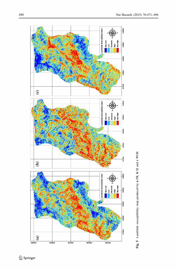
Fig

.5

Lan

dsl

ide

susc

epti

bil

ity

map

pro

duce

db

ya

FR

,b

SI

and

cW

OE

490 Nat Hazards (2015) 76:471–496

123

Accuracy statistics (i.e., overall accuracy and kappa coefficient) and ROC curves were

calculated using the test data sets to analyze the results produced by the bivariate and

multivariate methods considered in this study. All landslide susceptibility maps were

categorized into five susceptibility levels as: very low, low, moderate, high and very high.

It should be noted that the lands classified as very high, high and moderate were considered

as landslide zones and the rest (i.e., low and very low) was considered as non-landslide

zones in accuracy assessment stage. The overall accuracy values were calculated as 94.434,

93.858, 89.827, 85.077, 82.486 and 81.833 % for SVR, DT, LR, FR, SI and WOE,

respectively (Table 3). It can be seen that multivariate approaches (i.e., SVR, LR and DT)

produced significantly higher accuracies than the bivariate ones (i.e., FR, SI and WOE) for

all cases. Considering the overall accuracies and kappa coefficients, SVR and LR methods

produced similar performances, but outperforming other methods (i.e., DT, FR, SI and

WOE).

For the validation of the results, area under the ROC curve or simply AUC was also

applied. In the ROC analysis, a susceptibility map is compared with a data set showing the

landslide/non-landslide of occurrences in the same area. While AUC values between 0.7

and 0.9 indicate reasonable discrimination ability, values higher than 0.9 show typical of

highly accurate classification models (Swets 1988). AUC values \0.5 indicate that per-

formance of the methods has no power to discriminate. In this study, the ROC curves were

plotted based on the number of correctly classified pixels (true-positive) and the number of

the incorrectly identified pixels (false-positive). The AUC values of the ROC curve for

SVR, LR, DT, FR, SI and WOE methods were estimated as 0.985, 0.984, 0.980, 0.921,

0.911 and 0.893, respectively (Fig. 6). These results indicated that SVR, LR and DT

methods were effective for determining landslide susceptibility in the study area, but SVR

produced the best score within the multivariate analysis methods. When comparing

bivariate methods to each other based on AUC values, the FR method was found to be the

most effective one.

In addition to the assessments of modeling performances using standard accuracy

metrics (i.e., overall accuracy, kappa coefficient and AUC values), McNemar’s test was

employed to analyze statistical significance of differences in modeling performances of

multivariate and bivariate methods. The McNemar’s Chi-squared statistic (Eq. 12) is a

nonparametric test applied to 2 9 2 contingency table.

v2 ¼nij � nji

�� ��� 1� �2

nij þ nji

ð12Þ

where nij denotes the number of pixels that are misclassified by method i, but correctly

classified by method j and nji denotes the number of pixels that are misclassified by method

j, but correctly classified by method i. (Japkowicz and Shah 2011). If the observed statistic

Table 3 Susceptibility mappingresults in terms of overall accu-racy and kappa coefficient values

Methods Overall accuracy (%) Kappa

Support vector regression 94.434 0.882

Logistic regression 93.858 0.869

Decision trees 89.827 0.784

Frequency ratio 85.077 0.687

Statistical index 82.486 0.635

Weight of evidence 81.883 0.612

Nat Hazards (2015) 76:471–496 491

123

value estimated with Eq. 12 is larger than v21;0:05 ¼ 3:84, the null hypothesis can be

rejected with 95 % confidence level. In other words, methods i and j differ in their per-

formances, so the difference in accuracy is said to be statistically significant.

McNemar’s Chi-squared test was applied to susceptibility maps, and statistical results as

a symmetric matrix are given in Table 4. It should be noted that the calculated statistics

greater than the critical Chi-squared table value (v21;0:05 ¼ 3:84) are shown in bold in the

table. When the performances of SVR and LR were compared, they found to be producing

statistically similar performances (1.04 \ 3.84). When the performances of bivariate

approaches were analyzed with each other, it was found that the SI method showed

statistically similar performance with FR and WOE methods.

Fig. 6 ROC statistics for the methods used in landslide susceptibility assessment

Table 4 McNemar’s statistic test results for the multivariate and bivariate approaches

SVR LR DT FR SI WOE

SVR – 1.04 10.20 9.00 11.35 13.05

LR – 7.50 6.93 10.58 12.43

DT – 37.44 6.32 11.19

FR – 2.54 7.78

SI – 0.54

WOE –

Please note that calculated statistics greater than the critical value v21;0:05 ¼ 3:84

�, indicating statistical

significance, are shown in bold

492 Nat Hazards (2015) 76:471–496

123

6 Conclusions

Landslide susceptibility assessment is a complex and multi-step process that has been

investigated by many researchers in the literature. Up to now, a variety of methods have

been suggested for estimation of landslide susceptibility and their performances were

analyzed based on various statistical measures. In this study, performances of bivariate and

multivariate approaches were evaluated for the determination of landslide susceptibility of

Duzkoy district of Trabzon province, Turkey. These approaches were assessed using slope,

lithology, land cover, aspect, soil thickness, drainage density, TWI and elevation factors.

SVR, LR and DT methods were applied as multivariate approaches, while FR, SI and

WOE methods were used as bivariate approaches. Overall accuracy, kappa coefficient and

ROC curves were employed in the stage of performance evaluation. In addition to these

performance evaluation measures, McNemar’s test statistic was applied to assess the

statistical significance of the differences in method performances.

When the results of multivariate and bivariate methods were analyzed, some important

findings were deduced. Firstly, the multivariate methods (i.e., SVR, LR, DT) clearly

outperformed bivariate methods for all cases, reaching up to 13 % overall accuracy. The

results of the ROC curves also confirmed this finding. Also, McNemar’s statistical test

showed that the accuracy level reached by the multivariate methods compared with the

bivariate methods was statistically significant. Secondly, results showed that the FR

method produced the best performance (85.1 %) among the bivariate methods. When the

statistical significance of differences in performances of bivariate methods was analyzed, it

was found that the FR method was superior to the WOE method, whereas performance

difference with the SI method was statistically insignificant. Thirdly, it was seen that the

SVR and LR methods showed similar performances (94.4 and 93.9 %, respectively),

significantly higher than the DT method. Also, the statistical test results supported the

finding that difference in performances of SVR and LR methods was statistically insig-

nificant. It should be noted that while the LR method has a simple mathematical structure

that can be easily programmed, the SVR method requires user defined parameters

depending on the selected kernel function that highly affects its performance. Finally,

when the produced landslide susceptibility maps were analyzed, it was observed that high

susceptibility sites were mostly situated in the region between northeast and southwest of

the study area. When the susceptibility maps were analyzed in detail, it was found that

landslide susceptible sites were mainly located on the lithological units of Cru2 and Cru1

and the slope angles between 20� and 35�, which points out the latest landslide events in

the study area. In addition, it was observed that the northwestern-facing and north-facing

parts of the study area located at elevations of between 800 and 1,400 m carry the highest

hazard potential. When the susceptibility maps were analyzed in terms of land cover types,

it was observed that landslides in the region generally occurred in pasture and deciduous

lands. In addition, it was found that high susceptibility areas were mainly observed on the

land having characteristics [20� slope terrain and 20–50 cm soil depth.

Landslide susceptibility information is most commonly required at the local government

level for planning urban development particularly in developing countries. This informa-

tion is also vital for disaster management planning made by state agencies. Findings in this

study showed that the most of the urban lands and main roads in the region were located in

very high and high susceptibility zones. Therefore, future landslide activities may cause

major damages or casualties in the study area. Landslide susceptibility maps produced in

this study provide invaluable information in developing strategies for disaster mitigation

works and future investigation for provincial authorities.

Nat Hazards (2015) 76:471–496 493

123

References

Abdallah C (2010) Spatial distribution of block falls using volumetric GIS-decision-tree models. Int J ApplEarth Obs 12:393–403

Akgun A (2012) A comparison of landslide susceptibility maps produced by logistic regression, multi-criteria decision, and likelihood ratio methods: a case study at Izmir. Turkey. Landslides 9(1):93–106

Akgun A, Dag S, Bulut F (2008) Landslide susceptibility mapping for a landslide-prone area (Findikli, NEof Turkey) by likelihood-frequency ratio and weighted linear combination models. Environ Geol54:1127–1143

Aleotti P, Chowdhury R (1999) Landslide hazard assessment: summary review and new perspectives. BullEng Geol Env 58:21–44

Alparslan E (2011) Landslide susceptibility mapping in Yalova, Turkey, by remote sensing and GIS.Environ Eng Geosci 17:255–265

Althuwaynee OF, Pradhan B, Park HJ, Lee JH (2014) A novel ensemble bivariate statistical evidential belieffunction with knowledge-based analytical hierarchy process and multivariate statistical logisticregression for landslide susceptibility mapping. Catena 114:21–36

Armas I (2012) Weights of evidence method for landslide susceptibility mapping. Prahova Subcarpathians.Romania. Nat Hazards 60:937–950

Ayalew L, Yamagishi H (2005) The application of GIS-based logistic regression for landslide susceptibilitymapping in the Kakuda-Yahiko Mountains, Central Japan. Geomorphology 65:15–31

Ayalew L, Yamagishi H, Ugawa N (2004) Landslide susceptibility mapping using GIS-based weightedlinear combination, the case in Tsugawa area of Agano River, Niigata Prefecture, Japan. Landslides1:73–81

Ballabio C, Sterlacchini S (2012) Support vector machines for landslide susceptibility mapping: the StafforaRiver Basin case study, Italy. Math Geosci 44:47–70

Beven KJ, Kirkby MJ (1979) A physically based, variable contributing area model of basin hydrology.Hydrol Sci Bull 24:43–69

Bonham-Carter GF (1994) Geographic information systems for geoscientists: modelling with GIS. Perg-amon, Oxford

Breiman L (1996) Bagging predictors. Mach Learn 24:123–140Breiman L, Friedman JH, Olshen RA, Stone CJ (1984) Classification and regression trees. Wadsworth,

BelmontBui DT, Lofman O, Revhaug I, Dick O (2011) Landslide susceptibility analysis in the Hoa Binh province of

Vietnam using statistical index and logistic regression. Nat Hazards 59:1413–1444Bui DT, Pradhan B, Lofman O, Revhaug I (2012) Landslide susceptibility assessment in Vietnam using

support vector machines, decision tree, and naive Bayes models. Math Probl Eng. vol. 2012, Article ID974638, doi:10.1155/2012/974638

Burges CJC, Scholkopf B (1997) Improving the accuracy and speed of support vector learning machine. In:Mozer MC, Jordan MI, Petsche T (ed) Advances in neural information processing systems 9. Cam-bridge, MIT Press, pp 375–381

Cevik E, Topal T (2003) GIS-based landslide susceptibility mapping for a problematic segment of thenatural gas pipeline, Hendek (Turkey). Environ Geol 44:949–962

Chang YL, Liang LS, Han CC, Fang JP, Liang WY, Chen KS (2007) Multisource data fusion for landslideclassification using generalized positive Boolean functions. IEEE T Geosci Remote 45(6):1697–1708

Costanzo D, Rotigliano E, Irigaray C, Jimenez-Peralvarez JD, Chacon J (2012) Factors selection in landslidesusceptibility modelling on large scale following the GIS matrix method: application to the river Beirobasin (Spain). Nat Hazard Earth Sys 12:327–340

Cristianini N, Shawe-Taylor J (2000) An introduction to support vector machines. Cambridge UniversityPress, Cambridge

Dahal RK, Hasegawa S, Nonomura A, Yamanaka M, Masuda T, Nishino K (2008) GIS-based weights-of-evidence modelling of rainfall-induced landslides in small catchments for landslide susceptibilitymapping. Environ Geol 54:311–324

Dai FC, Lee CF, Li J, Xu ZW (2001) Assessment of landslide susceptibility on the natural terrain of LantauIsland, Hong Kong. Environ Geol 40:381–391

Demir G, Aytekin M, Akgun A, Ikizler SB, Tatar O (2013) A comparison of landslide susceptibilitymapping of the eastern part of the North Anatolian Fault Zone (Turkey) by likelihood-frequency ratioand analytic hierarchy process methods. Nat Hazards 65:1481–1506

Devkota KC, Regmi AD, Pourghasemi HR, Yoshida K, Pradhan B, Ryu IC, Dhital MR, Althuwaynee OF(2013) Landslide susceptibility mapping using certainty factor, index of entropy and logistic regression

494 Nat Hazards (2015) 76:471–496

123

models in GIS and their comparison at Mugling-Narayanghat road section in Nepal Himalaya. NatHazards 65(1):135–165

Durbha SS, King RL, Younan NH (2007) Support vector machines regression for retrieval of leaf area indexfrom multiangle imaging spectroradiometer. Remote Sens Environ 107:348–361

Ercanoglu M (2005) Landslide susceptibility assessment of SE Bartin (West Black Sea region, Turkey) byartificial neural networks. Nat Hazard Earth Sys 5(6):979–992

Fall M, Azzam R, Noubactep C (2006) A multi-method approach to study the stability of natural slopes andlandslide susceptibility mapping. Eng Geol 82:241–263

Gomez H, Kavzoglu T (2005) Assessment of shallow landslide susceptibility using artificial neural networksin Jabonosa River Basin, Venezuela. Eng Geol 78:11–27

Gray DH, Leiser AT (1982) Biotechnical slope protection and erosion control. Van Nostrand ReinholdCompany, New York

Grozavu A, Plescan S, Patriche CV, Margarint MC, Rosca B (2013) Landslide susceptibility assessment:GIS application to a complex mountainous environment. In: Kozak J et al (eds) The carpathians:integrating nature and society towards sustainability, environmental science and engineering. Springer,Berlin, pp 31–44

Guzzetti F, Carrara A, Cardinali M, Reichenbach P (1999) Landslide hazard evaluation: a review of currenttechniques and their application in a multi-scale study, Central Italy. Geomorphology 31:181–216

Ho JY, Lee KT, Chang TC, Wang ZY, Liao YH (2012) Influences of spatial distribution of soil thickness onshallow landslide prediction. Eng Geol 124:38–46

Hwang S, Guevarra IF, Yu B (2009) Slope failure prediction using a decision tree: a case of engineeredslopes in South Korea. Eng Geol 104:126–134

Ito K, Nakano R (2003) Optimizing Support Vector regression hyperparameters based on cross-validation.Proceedings of the International Joint Conference on Neural Networks 1–4:2077–2082

Japkowicz N, Shah M (2011) Evaluating learning algorithms: a classification perspective. CambridgeUniversity Press, New York

Kanungo DP, Arora MK, Sarkar S, Gupta RP (2009) Landslide susceptibility zonation (LSZ) mapping: areview. J South Asia Disaster Stud 2:81–105

Kavzoglu T, Sahin EK, Colkesen I (2014) Landslide susceptibility mapping using GIS-based multi-criteriadecision analysis, support vector machines, and logistic regression. Landslides 11:425–439

Kouli M, Loupasakis C, Soupios P, Vallianatos F (2010) Landslide hazard zonation in high risk areas ofRethymno Prefecture, Crete Island, Greece. Nat Hazards 52:599–621

Menard S (2001) Applied logistic regression analysis, 2nd edn. Sage Publication, Thousand OaksNandi A, Shakoor A (2009) A GIS based landslide susceptibility evaluation using bivariate and multivariate

statistical analyses. Eng Geol 110:11–20Nefeslioglu HA, Duman TY, Durmaz S (2008) Landslide susceptibility mapping for a part of tectonic Kelkit

Valley (Eastern Black Sea region of Turkey). Geomorphology 94(3–4):401–418Nefeslioglu HA, Sezer E, Gokceoglu C, Bozkir AS, Duman TY (2010) Assessment of landslide suscepti-

bility by decision trees in the metropolitan area of Istanbul. Math Probl Eng, TurkeyNiuniu X, Yuxun L (2010) Review of decision trees. Computer science and information technology

(ICCSIT), 2010 3rd IEEE International Conference, pp. 105–109Pal M, Mather PM (2003) An assessment of the effectiveness of decision tree methods for land cover

classification. Remote Sens Environ 86:554–565Peng L, Niu RQ, Huang B, Wu XL, Zhao YN, Ye RQ (2014) Landslide susceptibility mapping based on

rough set theory and support vector machines: a case of the Three Gorges area, China. Geomorphology204:287–301

Pourghasemi HR, Jirandeh AG, Pradhan B, Xu C, Gokceoglu C (2013) Landslide susceptibility mappingusing support vector machine and GIS at the Golestan Province, Iran. J Earth SystSci 122(2):349–369

Pradhan B (2013) A comparative study on the predictive ability of the decision tree, support vector machineand neuro-fuzzy models in landslide susceptibility mapping using GIS. Comput Geosci 51:350–365

Pradhan B, Lee S (2010) Landslide susceptibility assessment and factor effect analysis: backpropagationartificial neural networks and their comparison with frequency ratio and bivariate logistic regressionmodelling. Environ Modell Softw 25:747–759

Pradhan B, Oh HJ, Buchroithner M (2010) Weights-of-evidence model applied to landslide susceptibilitymapping in a tropical hilly area. Geomat Nat Hazards Risk 3:199–223

Quinlan JR (1993) C4.5: programs for machine learning. Kaufmann Publishers, San MateoRegmi NR, Giardino JR, Vitek JD (2010) Modeling susceptibility to landslides using the weight of evidence

approach: western Colorado, USA. Geomorphology 115:172–187Rokach L, Maimon O (2008) Data mining with decision trees: theory and applications. World Scientific

Publishing, Singapore, Series in Machine Perception and Artificial Intelligence

Nat Hazards (2015) 76:471–496 495

123

Rupke J, Cammeraat E, Seijmonsbergen AC, Vanwesten CJ (1988) Engineering geomorphology of thewidentobel catchment, appenzell and sankt-gallen, gallen, Switzerland: a geomorphological inventorysystem applied to geotechnical appraisal of slope stability. Eng Geol 26:33–68

Saaty TL (1980) The analytic hierarchy process: planning, priority setting. Resource allocation, McGraw-Hill

Santacana N, Baeza B, Corominas J, De Paz A, Marturia J (2003) A GIS-based multivariate statisticalanalysis for shallow landslide susceptibility mapping in La Pobla de Lillet area (Eastern Pyrenees,Spain). Nat Hazards 30:281–295

Sarkar S, Kanungo DP (2004) An integrated approach for landslide susceptibility mapping using remotesensing and GIS. Photogramm Eng Rem S 70:617–625

Sarkar S, Kanungo DP, Mehrotra GS (1995) Landslide Hazard Zonation: a case Study in Garhwal Himalaya.India, Mountain Research and Development 15:301–309

Schicker R, Moon V (2012) Comparison of bivariate and multivariate statistical approaches in landslidesusceptibility mapping at a regional scale. Geomorphology 161:40–57

Scholkopf B, Smola AJ (2002) Learning with kernels: support vector machines, regularization, optimizationand beyond. MIT Press, Cambridge

Segoni S, Rossi G, Catani F (2012) Improving basin-scale shallow landslides modelling using reliable soilthickness maps. Nat Hazards 61:85–101

Singhal PK, Srivastava P (2004) Challenges in sustainable development. Anmol publication, IndiaSmola AJ, Scholkopf B (2004) A tutorial on support vector regression. Stat Comput 14(3):199–222Soeters R, Van Westen CJ (1996) Slope instability recognition analysis and zonation. In: Turner KT,

Schuster RL, editors. Landslides: investigation and mitigation. Transportation Research BoardNational Research Council, Special Report No 247, Washington, DC, pp. 129–177

Suzen ML, Doyuran V (2004) Data driven bivariate landslide susceptibility assessment using geographicalinformation systems: a method and application to Asarsuyu catchment, Turkey. Eng Geol 71:303–321

Swets JA (1988) Measuring the accuracy of diagnostic systems. Science 240:1285–1293Thiery Y, Malet JP, Sterlacchini S, Puissant A, Maquaire O (2007) Landslide susceptibility assessment by

bivariate methods at large scales: application to a complex mountainous environment. Geomorphology92:38–59

Van Westen CJ (1997) Statistical landslide hazard analysis ILWIS 2.1 for windows application guide. ITCPublication, Enschede

Van Westen CJ, Rengers N, Soeters R (2003) Use of geomorphological information in indirect landslidesusceptibility assessment. Nat Hazards 30:399–419

Vapnik VN (2000) The nature of statistical learning theory, 2nd edn. Springer-Verlag, New YorkVivas L (1992) Los andes venezolanos. Academia Nacional de la Historia, CaracasWu KP, Wang SD (2009) Choosing the kernel parameters for support vector machines by the inter-cluster

distance in the feature space. Pattern Recogn 42(5):710–717Xu M, Watanachaturaporn P, Varshney PK, Arora MK (2005) Decision tree regression for soft classification

of remote sensing data. Remote Sens Environ 97:322–336Yalcin A (2008) GIS-based landslide susceptibility mapping using analytical hierarchy process and bivariate

statistics in Ardesen (Turkey): comparisons of results and confirmations. Catena 72:1–12Yalcin A, Reis S, Aydinoglu AC, Yomralioglu T (2011) A GIS-based comparative study of frequency ratio,

analytical hierarchy process, bivariate statistics and logistics regression methods for landslide sus-ceptibility mapping in Trabzon. NE Turkey. Catena 85(3):274–287

Yao X, Tham LG, Dai FC (2008) Landslide susceptibility mapping based on support vector machine: a casestudy on natural slopes of Hong Kong, China. Geomorphology 101:572–582

Yeh CY, Huang CW, Lee SJ (2011) A multiple-kernel support vector regression approach for stock marketprice forecasting. Expert Syst Appl 38:2177–2186

Yesilnacar E, Topal T (2005) Landslide susceptibility mapping: a comparison of logistic regression andneural networks methods in a medium scale study, Hendek region (Turkey). Eng Geol 79:251–266

Yilmaz I (2009) Landslide susceptibility mapping using frequency ratio, logistic regression, artificial neuralnetworks and their comparison: a case study from Kat landslides (Tokat-Turkey). Comput Geosci35:1125–1138

Yilmaz I (2010) Comparison of landslide susceptibility mapping methodologies for Koyulhisar, Turkey:conditional probability, logistic regression, artificial neural networks, and support vector machine.Environ Earth Sci 61:821–836

Yilmaz C, Topal T, Suzen ML (2012) GIS-based landslide susceptibility mapping using bivariate statisticalanalysis in Devrek (Zonguldak-Turkey). Environ Earth Sci 65:2161–2178

496 Nat Hazards (2015) 76:471–496

123