
Controlling a Hydraulic System using Reinforcement Learning
78
Linköpings universitet SE– Linköping + , www.liu.se Linköping University | Department of Management and Engineering Master’s thesis, 30 ECTS | Mechanical Engineering - Mechatronics 2021 | LIU-IEI-TEK-A--21/04015–SE Controlling a Hydraulic System using Reinforcement Learning – Implementation and validation of a DQN-agent on a hydraulic Multi-Chamber cylinder system David Berglund Niklas Larsson Supervisor : Henrique Raduenz Examiner : Liselott Ericson External supervisor : Kim Heybroek (Volvo CE)
-
Upload
khangminh22 -
Category
Documents
-
view
4 -
download
0
Transcript of Controlling a Hydraulic System using Reinforcement Learning
Linköpings universitetSE–581 83 Linköping+46 13 28 10 00 , www.liu.se
Linköping University | Department of Management and EngineeringMaster’s thesis, 30 ECTS | Mechanical Engineering - Mechatronics
2021 | LIU-IEI-TEK-A--21/04015–SE
Controlling a Hydraulic Systemusing Reinforcement Learning– Implementation and validation of a DQN-agent on a hydraulicMulti-Chamber cylinder system
David BerglundNiklas Larsson
Supervisor : Henrique RaduenzExaminer : Liselott Ericson
External supervisor : Kim Heybroek (Volvo CE)

Upphovsrätt
Detta dokument hålls tillgängligt på Internet - eller dess framtida ersättare - under 25 år från publicer-ingsdatum under förutsättning att inga extraordinära omständigheter uppstår.Tillgång till dokumentet innebär tillstånd för var och en att läsa, ladda ner, skriva ut enstaka ko-pior för enskilt bruk och att använda det oförändrat för ickekommersiell forskning och för undervis-ning. Överföring av upphovsrätten vid en senare tidpunkt kan inte upphäva detta tillstånd. All annananvändning av dokumentet kräver upphovsmannens medgivande. För att garantera äktheten, säker-heten och tillgängligheten finns lösningar av teknisk och administrativ art.Upphovsmannens ideella rätt innefattar rätt att bli nämnd som upphovsman i den omfattning somgod sed kräver vid användning av dokumentet på ovan beskrivna sätt samt skydd mot att dokumentetändras eller presenteras i sådan form eller i sådant sammanhang som är kränkande för upphovsman-nens litterära eller konstnärliga anseende eller egenart.För ytterligare information om Linköping University Electronic Press se förlagets hemsidahttp://www.ep.liu.se/.
Copyright
The publishers will keep this document online on the Internet - or its possible replacement - for aperiod of 25 years starting from the date of publication barring exceptional circumstances.The online availability of the document implies permanent permission for anyone to read, to down-load, or to print out single copies for his/hers own use and to use it unchanged for non-commercialresearch and educational purpose. Subsequent transfers of copyright cannot revoke this permission.All other uses of the document are conditional upon the consent of the copyright owner. The publisherhas taken technical and administrative measures to assure authenticity, security and accessibility.According to intellectual property law the author has the right to bementionedwhen his/her workis accessed as described above and to be protected against infringement.For additional information about the Linköping University Electronic Press and its proceduresfor publication and for assurance of document integrity, please refer to its www home page:http://www.ep.liu.se/.
©David BerglundNiklas Larsson
Abstract
One of the largest energy losses in an excavator is the compensation loss. In a hy-draulic load sensing system where one pump supplies multiple actuators, these compen-sation losses are inevitable. To minimize the compensation losses the use of a multi cham-ber cylinder can be used, which can control the load pressure by activate its chambers indifferent combinations and in turn minimize the compensation losses.
For this proposed architecture, the control of the multi chamber cylinder systems isnot trivial. The possible states of the system, due to the number of combinations, makesconventional control, like a rule based strategy, unfeasible. Therefore, is the reinforcementlearning a promising approach to find an optimal control.
A hydraulic system was modeled and validated against a physical one, as a base forthe reinforcement learning to learn in simulation environment. A satisfactory model wasachieved, accurately modeled the static behavior of the system but lacks some dynamics.
A Deep Q-Network agent was used which successfully managed to select optimal com-binations for given loads when implemented in the physical test rig, even though the sim-ulation model was not perfect.
Acknowledgments
First we would like to thank Martin Hochwallner for all theexplanations and time he put down to realise the real time implementation,and Samuel Kärnell for sharing his hydraulic knowledge in the lab.
Our fellow student colleagues Chester, Andy and Keyvan, for thecooperation in the early stages in the work, and the Mathworkspersonell Chris, Juan & Gaspar for their assistance with matlabstruggels and technical inputs.
We would also thank our examiner and supervisors. LiselottEricson for quick response for administrative quest, good tips andguidance for hardware. Kim Heybroek from Volvo CE for good inputsand insights. Finally a special thanks to our supervisor, HenriqueRaduenz, for all the long conversations, inputs and technicalsupport making this project possible.
iv
Contents
Abstract iii
Acknowledgments iv
Contents v
List of Figures vii
List of Tables ix
List of Abbreviations x
List of Symbols xi
1 Introduction 11.1 Background . . . . . . . . . . . . . . . . . . . . . . . . . . . . . . . . . . . . . . . 11.2 Aim . . . . . . . . . . . . . . . . . . . . . . . . . . . . . . . . . . . . . . . . . . . . 21.3 Research Questions . . . . . . . . . . . . . . . . . . . . . . . . . . . . . . . . . . . 21.4 Delimitations . . . . . . . . . . . . . . . . . . . . . . . . . . . . . . . . . . . . . . 2
2 Method 32.1 Validation of System . . . . . . . . . . . . . . . . . . . . . . . . . . . . . . . . . . 32.2 Select, Train and Implement Reinforcement Learning . . . . . . . . . . . . . . . 32.3 Simulations . . . . . . . . . . . . . . . . . . . . . . . . . . . . . . . . . . . . . . . 4
3 System Description 53.1 Excavator Arm . . . . . . . . . . . . . . . . . . . . . . . . . . . . . . . . . . . . . 53.2 Hydraulics . . . . . . . . . . . . . . . . . . . . . . . . . . . . . . . . . . . . . . . . 5
3.2.1 Multi Chamber Cylinder . . . . . . . . . . . . . . . . . . . . . . . . . . . . 73.3 Connection . . . . . . . . . . . . . . . . . . . . . . . . . . . . . . . . . . . . . . . . 93.4 Control Flow . . . . . . . . . . . . . . . . . . . . . . . . . . . . . . . . . . . . . . . 103.5 Derivations of Calculated Signals . . . . . . . . . . . . . . . . . . . . . . . . . . . 11
4 Related Research 124.1 Pressure Compensation . . . . . . . . . . . . . . . . . . . . . . . . . . . . . . . . 124.2 Digital Hydraulics . . . . . . . . . . . . . . . . . . . . . . . . . . . . . . . . . . . 134.3 Reinforcement Learning . . . . . . . . . . . . . . . . . . . . . . . . . . . . . . . . 13
4.3.1 Neural Networks . . . . . . . . . . . . . . . . . . . . . . . . . . . . . . . . 154.3.2 Agents . . . . . . . . . . . . . . . . . . . . . . . . . . . . . . . . . . . . . . 15
4.4 Reinforcement Learning used with Hydraulics . . . . . . . . . . . . . . . . . . . 17
5 Model Validation 185.1 Models . . . . . . . . . . . . . . . . . . . . . . . . . . . . . . . . . . . . . . . . . . 18
5.1.1 Proportional Valve . . . . . . . . . . . . . . . . . . . . . . . . . . . . . . . 18
v
5.1.2 Pressure Dynamics of Digital Valve Block . . . . . . . . . . . . . . . . . . 195.1.3 Digital Valves and Multi Chamber Cylinder . . . . . . . . . . . . . . . . 215.1.4 Single Chamber Cylinder . . . . . . . . . . . . . . . . . . . . . . . . . . . 225.1.5 Load Function . . . . . . . . . . . . . . . . . . . . . . . . . . . . . . . . . . 22
5.2 Validation Results . . . . . . . . . . . . . . . . . . . . . . . . . . . . . . . . . . . . 235.2.1 Proportional Valve . . . . . . . . . . . . . . . . . . . . . . . . . . . . . . . 235.2.2 Pressure Dynamics of Digital Valve Block . . . . . . . . . . . . . . . . . . 255.2.3 Digital Valves and Multi Chamber Cylinder . . . . . . . . . . . . . . . . 265.2.4 Single Chamber Cylinder . . . . . . . . . . . . . . . . . . . . . . . . . . . 295.2.5 Load Function . . . . . . . . . . . . . . . . . . . . . . . . . . . . . . . . . . 32
6 Development of Reinforcement Learning Controller 356.1 Position Control . . . . . . . . . . . . . . . . . . . . . . . . . . . . . . . . . . . . . 35
6.1.1 Training Setup . . . . . . . . . . . . . . . . . . . . . . . . . . . . . . . . . 356.1.2 Observations . . . . . . . . . . . . . . . . . . . . . . . . . . . . . . . . . . 366.1.3 Reward Function . . . . . . . . . . . . . . . . . . . . . . . . . . . . . . . . 366.1.4 Environment . . . . . . . . . . . . . . . . . . . . . . . . . . . . . . . . . . 376.1.5 Hyperparameters . . . . . . . . . . . . . . . . . . . . . . . . . . . . . . . . 376.1.6 Training . . . . . . . . . . . . . . . . . . . . . . . . . . . . . . . . . . . . . 376.1.7 Deployment . . . . . . . . . . . . . . . . . . . . . . . . . . . . . . . . . . . 38
6.2 Enabling Control . . . . . . . . . . . . . . . . . . . . . . . . . . . . . . . . . . . . 396.2.1 Training Setup . . . . . . . . . . . . . . . . . . . . . . . . . . . . . . . . . 396.2.2 Observations . . . . . . . . . . . . . . . . . . . . . . . . . . . . . . . . . . 406.2.3 Reward Function . . . . . . . . . . . . . . . . . . . . . . . . . . . . . . . . 406.2.4 Environment . . . . . . . . . . . . . . . . . . . . . . . . . . . . . . . . . . 416.2.5 Hyperparameters . . . . . . . . . . . . . . . . . . . . . . . . . . . . . . . . 416.2.6 Training . . . . . . . . . . . . . . . . . . . . . . . . . . . . . . . . . . . . . 426.2.7 Deployment . . . . . . . . . . . . . . . . . . . . . . . . . . . . . . . . . . . 44
6.3 Area Compensation . . . . . . . . . . . . . . . . . . . . . . . . . . . . . . . . . . . 44
7 Results 467.1 Position Control . . . . . . . . . . . . . . . . . . . . . . . . . . . . . . . . . . . . . 467.2 Enabling Control . . . . . . . . . . . . . . . . . . . . . . . . . . . . . . . . . . . . 49
7.2.1 Load Case 80 kg . . . . . . . . . . . . . . . . . . . . . . . . . . . . . . . . . 497.2.2 Load Case 200 kg . . . . . . . . . . . . . . . . . . . . . . . . . . . . . . . . 52
7.3 Energy Consumption . . . . . . . . . . . . . . . . . . . . . . . . . . . . . . . . . . 547.4 Area Compensation . . . . . . . . . . . . . . . . . . . . . . . . . . . . . . . . . . . 56
8 Discussion 588.1 Validation . . . . . . . . . . . . . . . . . . . . . . . . . . . . . . . . . . . . . . . . 588.2 Position Control . . . . . . . . . . . . . . . . . . . . . . . . . . . . . . . . . . . . . 588.3 Enabling Control . . . . . . . . . . . . . . . . . . . . . . . . . . . . . . . . . . . . 598.4 Agent Settings . . . . . . . . . . . . . . . . . . . . . . . . . . . . . . . . . . . . . . 618.5 Energy Consumption Comparison . . . . . . . . . . . . . . . . . . . . . . . . . . 618.6 Area Compensation . . . . . . . . . . . . . . . . . . . . . . . . . . . . . . . . . . . 618.7 Gear Selection . . . . . . . . . . . . . . . . . . . . . . . . . . . . . . . . . . . . . . 628.8 Unsuccessful Tries . . . . . . . . . . . . . . . . . . . . . . . . . . . . . . . . . . . . 638.9 Multi-Agent Application . . . . . . . . . . . . . . . . . . . . . . . . . . . . . . . . 63
9 Conclusion 649.1 Research Questions . . . . . . . . . . . . . . . . . . . . . . . . . . . . . . . . . . . 649.2 Future Work . . . . . . . . . . . . . . . . . . . . . . . . . . . . . . . . . . . . . . . 65
Bibliography 66
vi
List of Figures
2.1 Reinforcement Learning controller development process. . . . . . . . . . . . . . . . 4
3.1 The excavator arm. . . . . . . . . . . . . . . . . . . . . . . . . . . . . . . . . . . . . . 63.2 A pq-diagram showing losses for different gears while SC is controlling the system
pressure. . . . . . . . . . . . . . . . . . . . . . . . . . . . . . . . . . . . . . . . . . . . 63.3 The hydraulic system which will be used in this thesis. Digital valve block is
marked with the dashed box. Credit [Multi-chamber-system]. . . . . . . . . . . . . 73.4 Cross section area of the MC. Green is MCA, red is MCB, blue is MCC and orange
is MCD. Credit [Digital-hydraulic-system]. . . . . . . . . . . . . . . . . . . . . . . . 73.5 Possible forces at system pressure 100 bar. . . . . . . . . . . . . . . . . . . . . . . . . 93.6 The control cycle of the physical system where MATLAB’s Simulink is used as HMI. 93.7 Control flow of the system. . . . . . . . . . . . . . . . . . . . . . . . . . . . . . . . . 10
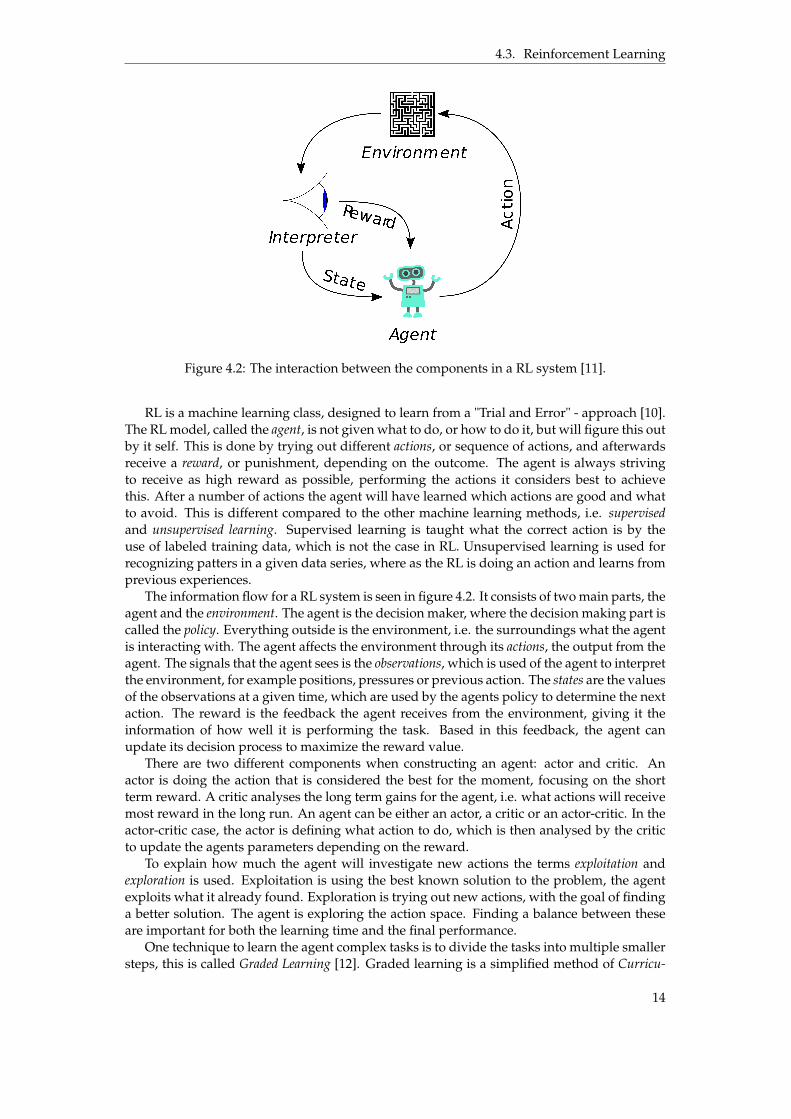
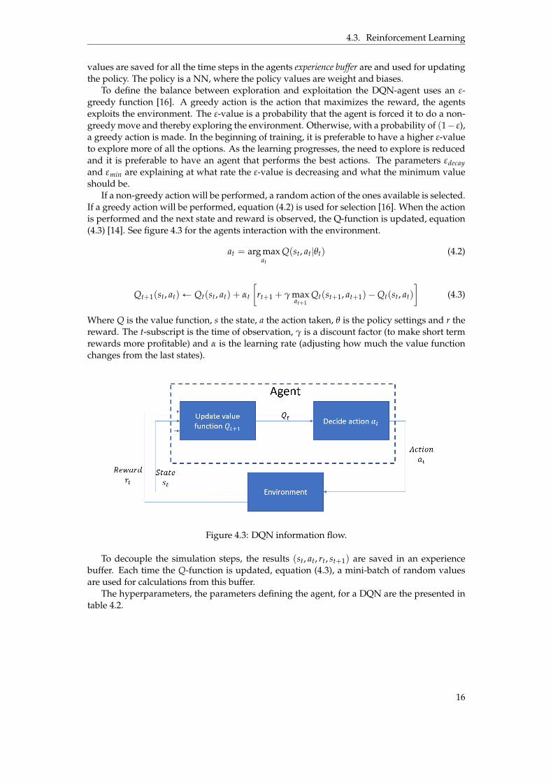
4.1 Location of hydraulic losses in a system using load sensing and MC. . . . . . . . . 124.2 The interaction between the components in a RL system [RL-picture]. . . . . . . . 144.3 DQN information flow. . . . . . . . . . . . . . . . . . . . . . . . . . . . . . . . . . . . 16
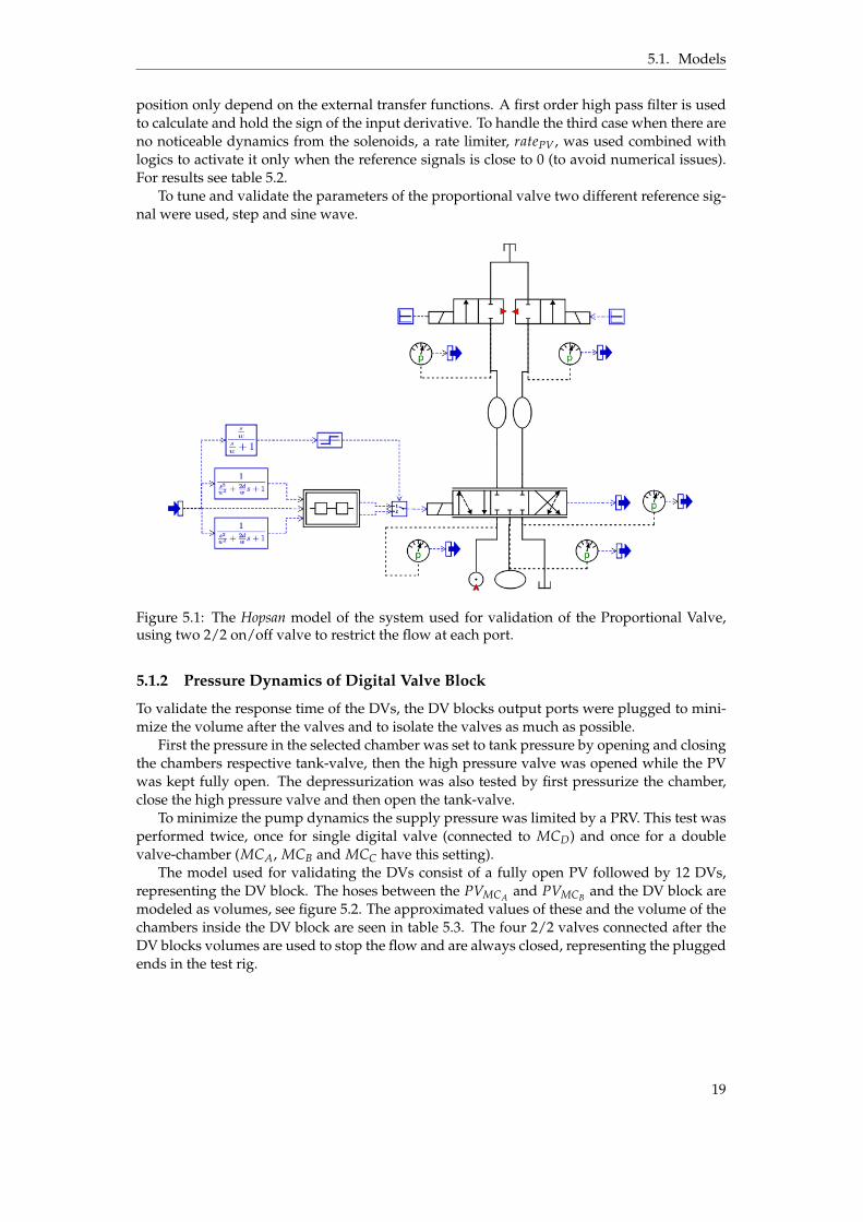
5.1 The Hopsan model of the system used for validation of the Proportional Valve,using two 2/2 on/off valve to restrict the flow at each port. . . . . . . . . . . . . . . 19
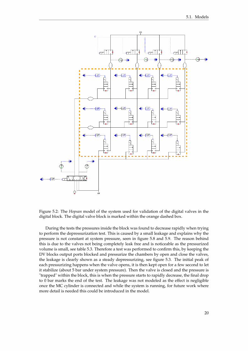
5.2 The Hopsan model of the system used for validation of the digital valves in thedigital block. The digital valve block is marked within the orange dashed box. . . 20
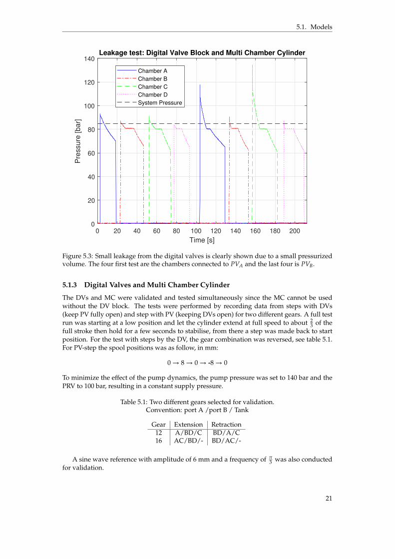
5.3 Small leakage from the digital valves is clearly shown due to a small pressurizedvolume. The four first test are the chambers connected to PVA and the last four isPVB. . . . . . . . . . . . . . . . . . . . . . . . . . . . . . . . . . . . . . . . . . . . . . . 21
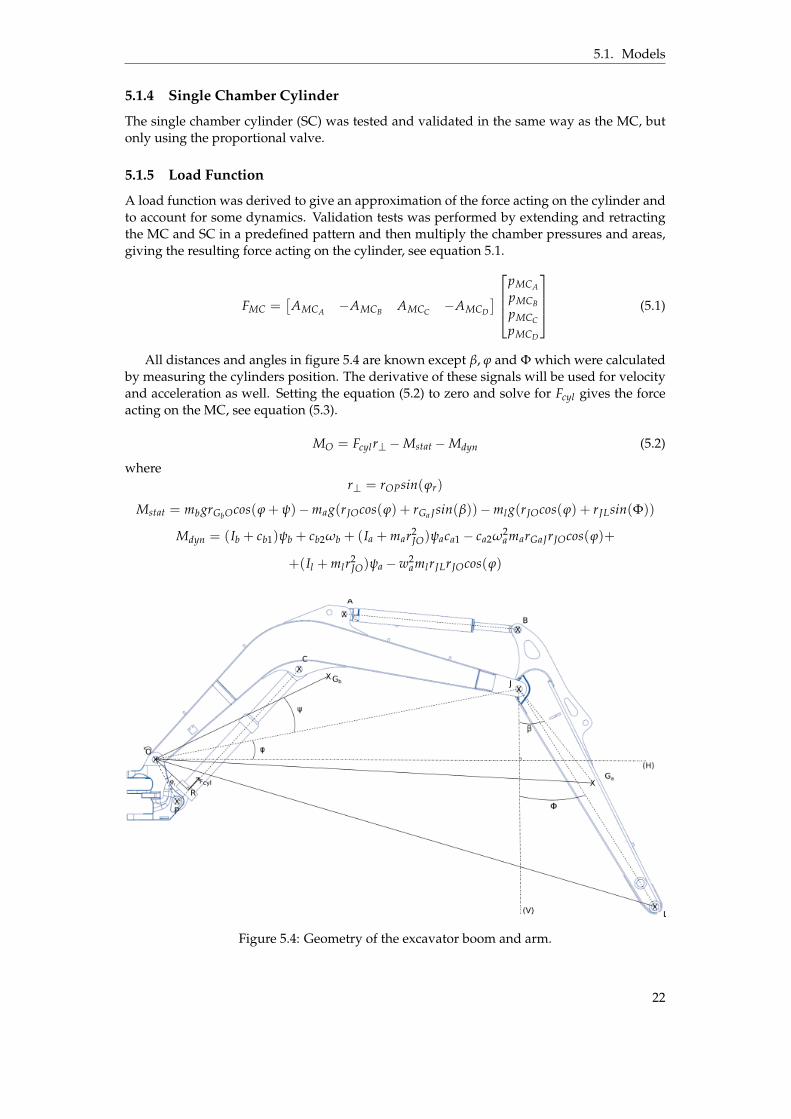
5.4 Geometry of the excavator boom and arm. . . . . . . . . . . . . . . . . . . . . . . . 225.5 Step responses for different system pressures . . . . . . . . . . . . . . . . . . . . . . 235.6 Step response for test data and tuned simulation model of proportional valve. . . . 245.7 Sine wave response for test data and tuned simulation model, showing only the
positive spool displacement due to limitations of measuring devices. . . . . . . . . 255.8 Validation results from testing and simulation of double connected digital valves. . 265.9 Validation results from testing and simulation of a single digital valve. . . . . . . . 265.10 Position response for MC, step with PV. . . . . . . . . . . . . . . . . . . . . . . . . . 275.11 Pressure response for MC, step with PV. . . . . . . . . . . . . . . . . . . . . . . . . . 285.12 Position response for MC, sine wave reference. . . . . . . . . . . . . . . . . . . . . . 285.13 Pressure response for MC, sine wave reference. . . . . . . . . . . . . . . . . . . . . . 295.14 Position response for SC, step with PV. . . . . . . . . . . . . . . . . . . . . . . . . . . 305.15 Pressure response for SC, step with PV. . . . . . . . . . . . . . . . . . . . . . . . . . 315.16 Position response for SC, sine wave reference. The spike at 10 sec. is due to faulty
sensor. . . . . . . . . . . . . . . . . . . . . . . . . . . . . . . . . . . . . . . . . . . . . 315.17 Pressure response for SC, sine wave reference. . . . . . . . . . . . . . . . . . . . . . 325.18 Force acting on multi chamber cylinder as a function of the two cylinders position,
with 3kg external load, constant velocity at 0.03 m/s and no acceleration. . . . . . 33
vii
5.19 Test data and load function compared. The SC is set at a fixed position and MCextends or retracts. . . . . . . . . . . . . . . . . . . . . . . . . . . . . . . . . . . . . . 33
5.20 Test data and load function compared. The MC is set at a fixed position and SCextends or retracts. The gap around 0.15 m is due to faulty sensor. . . . . . . . . . . 34
6.1 Information flow of the agent as a controller. . . . . . . . . . . . . . . . . . . . . . . 356.2 Reward the RL agent received during training for position control. The black
dashed vertical line separates first and second training session. . . . . . . . . . . . 386.3 Information flow of the agent as an enabler. . . . . . . . . . . . . . . . . . . . . . . . 396.4 Training progress from first iteration. . . . . . . . . . . . . . . . . . . . . . . . . . . . 426.5 Training progress from second iteration. . . . . . . . . . . . . . . . . . . . . . . . . . 436.6 Training progress from third iteration. . . . . . . . . . . . . . . . . . . . . . . . . . . 44
7.1 Test data from physical rig and from simulation, using 100% open PV. . . . . . . . 477.2 Test data from physical rig and from simulation, using 50% open PV. . . . . . . . . 477.3 Simulation results when using reversed direction of PV. Integrated error is shown
to explain the time for the final adjustment. . . . . . . . . . . . . . . . . . . . . . . . 487.4 Simulation results when following a sine wave reference. . . . . . . . . . . . . . . . 487.5 Performance for load case 80 kg. . . . . . . . . . . . . . . . . . . . . . . . . . . . . . 507.6 Normalized observations for load case 80 kg. . . . . . . . . . . . . . . . . . . . . . . 507.7 Performance for load case 80 kg, sine wave reference. . . . . . . . . . . . . . . . . . 517.8 Observations for load case 80 kg, sine wave reference. . . . . . . . . . . . . . . . . . 517.9 Performance for load case 200 kg. . . . . . . . . . . . . . . . . . . . . . . . . . . . . . 527.10 Observations for load case 200 kg. . . . . . . . . . . . . . . . . . . . . . . . . . . . . 537.11 Performance for load case 200 kg, sine wave reference. . . . . . . . . . . . . . . . . 537.12 Observations for load case 200 kg, sine wave reference. . . . . . . . . . . . . . . . . 547.13 Energy and performance comparison between using gear 16 and the agents policy
at load case 260 kg. . . . . . . . . . . . . . . . . . . . . . . . . . . . . . . . . . . . . . 557.14 Energy and performance comparison between using gear 16 and the agents policy
at load case 110 kg. . . . . . . . . . . . . . . . . . . . . . . . . . . . . . . . . . . . . . 567.15 Position and velocity of the gears 9, 11, 14 and 16, with and without the area
compensation parameter KA. . . . . . . . . . . . . . . . . . . . . . . . . . . . . . . . 57
viii
List of Tables
3.1 Areas of the chambers in the Multi Chamber Cylinder. . . . . . . . . . . . . . . . . 83.2 Different gears of the MC, sorted in ascending resulting force, system pressure at
100 bar. Starting at gear 4 by convention from previous project, where gears 1-3generate negative forces. . . . . . . . . . . . . . . . . . . . . . . . . . . . . . . . . . . 8
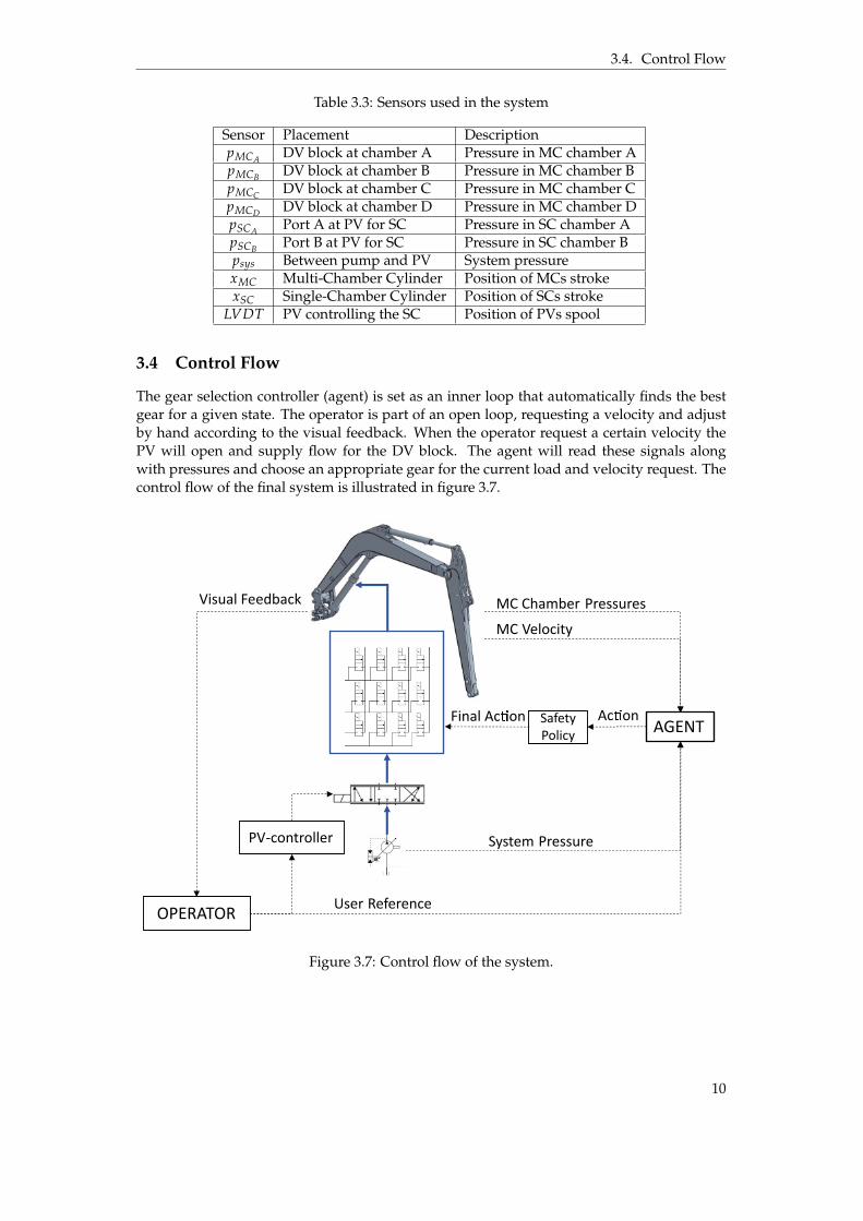
3.3 Sensors used in the system . . . . . . . . . . . . . . . . . . . . . . . . . . . . . . . . . 10
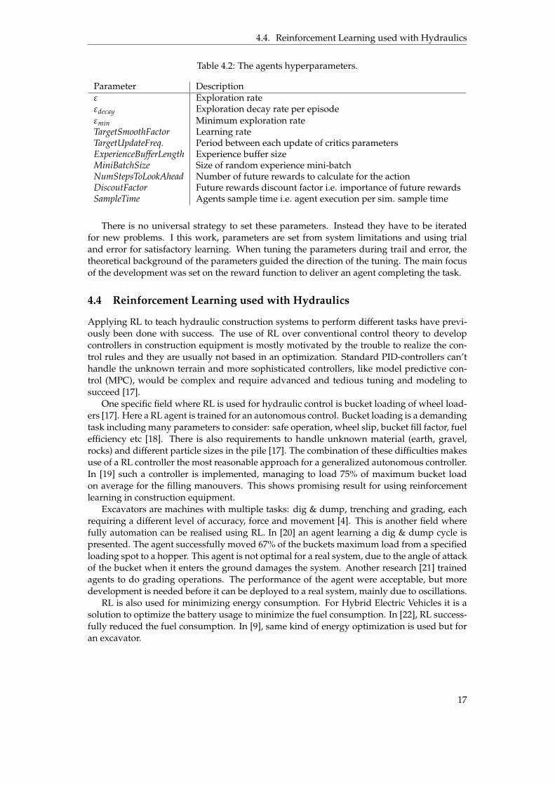
4.1 Mathworks agents and recommended using. . . . . . . . . . . . . . . . . . . . . . . 154.2 The agents hyperparameters. . . . . . . . . . . . . . . . . . . . . . . . . . . . . . . . 17
5.1 Two different gears selected for validation. Convention: port A /port B / Tank . . 215.2 Tuned parameters for the proportional valve. . . . . . . . . . . . . . . . . . . . . . . 235.3 Digital valve simulation parameters in left table, volumes are seen in the right table 255.4 Tuned parameters for MC, PV and PCV . . . . . . . . . . . . . . . . . . . . . . . . . 275.5 Tuned parameters for SC, PV and PCV . . . . . . . . . . . . . . . . . . . . . . . . . . 30
6.1 Gear selection for position control. Chamber convention: PV port A / PV port B /Tank . . . . . . . . . . . . . . . . . . . . . . . . . . . . . . . . . . . . . . . . . . . . . . 36
6.2 The agents observations of the environment. . . . . . . . . . . . . . . . . . . . . . . 366.3 The agents hyperparameters. . . . . . . . . . . . . . . . . . . . . . . . . . . . . . . . 376.4 The agents critic (neural network). . . . . . . . . . . . . . . . . . . . . . . . . . . . . 376.5 Gears and loads used for gear selection training . . . . . . . . . . . . . . . . . . . . 406.6 Observations used for gear selection. . . . . . . . . . . . . . . . . . . . . . . . . . . . 406.7 The agents hyperparameters. . . . . . . . . . . . . . . . . . . . . . . . . . . . . . . . 416.8 The agents critic (neural network). . . . . . . . . . . . . . . . . . . . . . . . . . . . . 426.9 PV spool displacement for different gears with the area compensator. . . . . . . . . 456.10 PV reference position depending on operator signal and each gear. . . . . . . . . . 45
7.1 Gears and loads used during training and test. The Load Rig column shows thephysical systems equivalent loads to the simulation. . . . . . . . . . . . . . . . . . . 49
7.2 Comparison of compensation energy losses over the PV for the cases. . . . . . . . . 55
8.1 Effects of KA when using gear 5 as the reference gear. . . . . . . . . . . . . . . . . . 62
ix

List of Abbreviations
DQN Deep Q-Network
DV Digital Valve
HMI Human Machine Interface
LVDT Linear Variable Differential Transformer
MC Multi Chamber Cylinder
MCA´D Multi Chamber Cylinder chambers A to D
MPC Model Predictive Control
NN Neural Networks
PCV Pressure Compensating Valve
PPO Proximal Policy Optimization
PRV Pressure Relief Valve
PV Proportional Valve
ReLU Rectified Linear Unit
RL Reinforcement Learning
SC Single Chamber Cylinder
x
List of Symbols
Quantity Description Unit
β Angle radδ Damping ´
γ Discount factor ´
ωa Angular acceleration of body a m/s2
ωPV Resonance Frequency rad/sΦ Angle radψ Angle radρ Density kg/m3
τ Time delay sθ Reinforcement Learning Policy parameters ´
ε Reinforcement Learning Exploration Rate ´
ϕ Angle radA Area m2
a Reinforcement Learning Action ´
Cq Flow coefficient ´
F Force Ng Gravitational acceleration m/s2
gear Combination of active chambers ´
Ia Moment of inertia kgm2
L Circumference mM Torque Nmm Mass kgP Power Wp Pressures PaQ Reinforcement Learning Value Function ´
q Flow m3/sr Reinforcement Learning Reward ´
rAB Distance between points A and B mrate Rate limit ´
s Reinforcement Learning State ´
Ts Sample time sV Volume m3
v Velocity m/sx Position m
xi
1 Introduction
Advancements in hydraulics and machine learning opens up for opportunities to developoptimized and sophisticated control strategies for complex problems. This could help in-crease the energy efficiency and performance of construction equipment which are knownfor low efficiency. Because of global warming and increasing oil prices, new technology forexcavators are required to improve fuel economy and reduce emission.
1.1 Background
Load sensing systems are a widely used system in modern construction machines. Theirability to adjust the system pressure enables energy savings and the proportional valves (PV)allows for smooth control at low velocities. To maintain a constant pressure drop over theproportional valve a pressure compensating valve (PCV) is used, which gives same velocityfor the same valve displacement despite the external load. Using multiple actuators and asingle pump will cause different pressure drops between the pump and actuators. In combi-nation with pressure compensation valves, this pressure drops creates compensation losseswhen actuated. These losses are known to be one of the largest hydraulic losses in suchhydraulic architectures.
A multi chamber cylinder (MC) system can change the resulting load pressure for a givenload through the combination of different areas. This system can be seen as a hydraulic forcegearbox, where each chamber combination corresponds to a specific gear. However, bothposition- and velocity control of this type of system are difficult to design. Especially at lowloads and low velocity.
If a MC is used in a load sensing architecture it opens up the opportunity to adjust thepressure drop between the pump- and the load pressure and thereby minimize the compen-sation losses. In cooperation with Volvo Construction Equipment (Volvo CE), a hydraulicsystem combining these architecture is designed. The idea is to control the velocity by a PVand the pressure drop adjusted by a MC. The problem with this system is to select the optimalgear for each given state during load cycles, like dig & dump or trenching. In this thesis theusage of machine learning to control such system is explored. More specifically, reinforce-ment learning (RL) will be used to develop an optimised gear selection for the hydraulic forcegearbox.
1
1.2. Aim
1.2 Aim
The aim of this thesis is to develop an optimization-based controller for a hydraulic force gear-box using reinforcement learning. This will be developed in a simulation environment andimplemented on a test rig.
1.3 Research Questions
1. How can reinforcement learning be used for gear selection to improve the energy effi-ciency while maintaining the performance of a hydraulic system with a hydraulic forcegearbox?
2. How shall the training process of a reinforcement learning model be performed for ahydraulic force gearbox system?
3. What changes are needed for the control of the proportional valve to maintain the samesystem performance?
1.4 Delimitations
Delimitation of this thesis is presented in the list below:
• Focus will be on development of controller for finding optimal gear, not an optimalswitch sequence between gears.
• The validation of the system will not be performed in a real application environment.
• No component selection is carried out, all of the components are selected in advance.
• Different reinforcement learning approaches will not be tested. One will be chosen andcarried out. The alternatives to chose from are the ones included in the ReinforcementLearning Toolbox™ from Mathworks.
2
2 Method
To find out however or not the reinforcement learning (RL) is a suitable option for the hy-draulic force gearbox, the work was divided into two major parts: validation of the simulationenvironment and implementation of the RL controller. The validation is an important part asa model representing the real world is crucial for the learning algorithm to actually learn howto behave in the final application. Along with the validation of the model, a literature studyof RL was carried out. This provided theoretical knowledge for the selection of a suitablealgorithm, setting up the training and testing procedures, and finally for the deployment onthe real platform.
2.1 Validation of System
The used simulation tools are Hopsan, for the modelling of the physical system, and MAT-LAB/Simulink for control development. The physical models is first validated on a componentlevel followed by system level.
The components for validation are the proportional valve (PV) and digital valves (DV).This was carried out by isolating the components as much as possible and measure represen-tative quantities. The main component, the MC, was validation at a system level due to theneed of the PV and DVs for control. A more detailed explanation of the procedure is foundin Chapter 5.
2.2 Select, Train and Implement Reinforcement Learning
The literature study about RL gave a wide perspective of possible algorithms and techniquessuitable for this thesis. For the development of the RL model a reward function was designed,including both how and when a reward is generated. The training of the model was carriedout using the validated system model with representative loads. Once the RL model wastrained to satisfactory performance in the simulation environment it was implemented in thetest rig for validation.
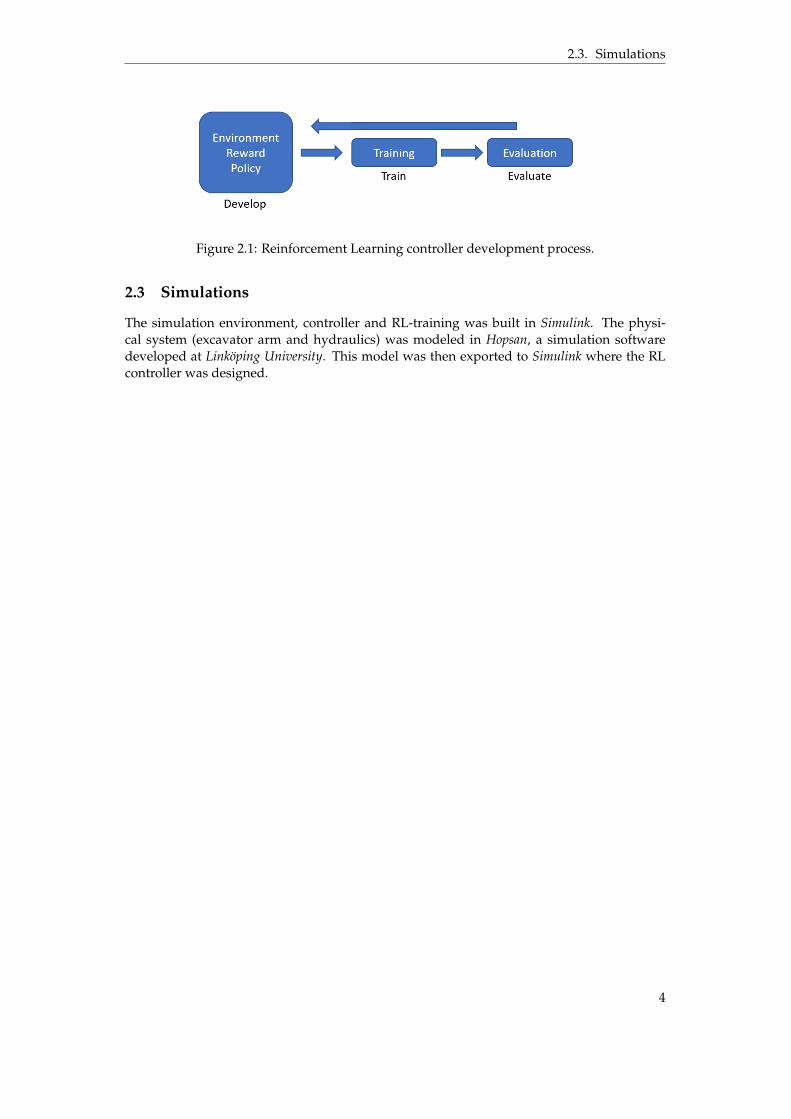
The development of the RL controller was an iterative process. First a basic environment,reward and policy was used and a simple task. Once the RL model learned to handle the task,the complexity of the task and environment increased. This cycle was then repeated until thefinal RL model was trained. See figure 2.1.
3
2.3. Simulations
Figure 2.1: Reinforcement Learning controller development process.
2.3 Simulations
The simulation environment, controller and RL-training was built in Simulink. The physi-cal system (excavator arm and hydraulics) was modeled in Hopsan, a simulation softwaredeveloped at Linköping University. This model was then exported to Simulink where the RLcontroller was designed.
4
3 System Description
The system consists of an excavator boom and arm, hydraulics with a multi chamber cylinder(MC) and electronics.
3.1 Excavator Arm
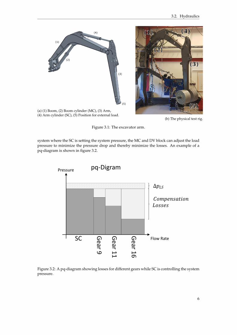
The test rig is an excavator arm from Volvo CE. It consists of a boom, arm, MC cylinderand a conventional single chamber cylinder (SC). A CAD-model of the excavator arm is seenin figure 3.1a, the physical rig and its surrounding structure is seen in figure 3.1b. Due tothe area ratios of the MC, it can handle high loads for extension movements but is weak inretraction, described more in Section 3.2.1. Because of this, it is more suitable as the boomcylinder.
3.2 Hydraulics
The MC system used in this thesis is described by Raduenz et.al in [1]. The physical systemhydraulic schematic diagram is seen in figure 3.3. A pump is connected to two 4/3 loadsensing proportional valves (PV) for controlling the SC and MC, which are connected to thearm and boom, respectively, of the excavator.
To control the MC, a block containing a set of 2/2 on-off digital valves (DV) is controllingthe flow to each chamber, represented by the valves in the dashed box in figure 3.3. Thereare three inputs to this block: high and low pressure port from the PV and a port directlyconnected to tank. Each of these are connected to four digital valves, one for each of the MCchambers (MCA´D). If the DV connected to PV high pressure and the DV valve to MCAchamber is opened, high pressure is supplied to the MCA, see figure 3.3 for a detailed view.The opening areas of the DVs connected to MCA, MCB and MCC have twice the area of theones connected to MCD, due to different flow rate requirements. A more elaborate descrip-tion of the DV block, MC and the connection between is found in [2]. The other componentsare discussed in Chapter 5.
The idea of the concept is to use the DV block to control the MC by activate or deactivatechambers (i.e. pressurize), effecting the resulting load pressure and thereby minimize thepressure drop. The flow rate and direction is controlled by the PV. In the case of a load sensing
5
3.2. Hydraulics
(a) (1) Boom, (2) Boom cylinder (MC), (3) Arm,(4) Arm cylinder (SC), (5) Position for external load.
(1)
(2)
(3)
(4)
(5)
(b) The physical test rig.
Figure 3.1: The excavator arm.
system where the SC is setting the system pressure, the MC and DV block can adjust the loadpressure to minimize the pressure drop and thereby minimize the losses. An example of apq-diagram is shown in figure 3.2.
Flow Rate
Pressure
���
������� �
���
SC
Ge
ar
9
Ge
ar
11
Ge
ar
16
pq-Digram
Figure 3.2: A pq-diagram showing losses for different gears while SC is controlling the systempressure.
6

3.2. Hydraulics
SCMC
DV
MCA MCB MCC MCD
PVA
PVB
Tank
Figure 3.3: The hydraulic system which will be used in this thesis. Digital valve block ismarked with the dashed box. Credit [1].
Note: This is a simplified view of the DV block used for a simplified simulation. In thephysical rig there is a total of 27 valves, four for each connection to chamber MCA, two forMCB and MCC each, and one for MCD, i.e. 3 ˚ (4 + 2 + 2 + 1) = 27.
3.2.1 Multi Chamber Cylinder
A cross section view of the MC is seen in figure 3.4. Pressurizing chambers MCA or MCCresults in an extension movement of the piston and the opposite are true for the MCB andMCD chamber. The area ratio difference between the chambers are significant, MCA beingthe largest and MCD the smallest. Since the MC is used for the boom this is not an issue dueto the load acts mostly in the same direction as the gravity. See table 3.1 for the areas, arearatios and movement direction.
MCB
MCD
MCA
MCC
Figure 3.4: Cross section area of the MC. Green is MCA, red is MCB, blue is MCC and orangeis MCD. Credit [2].
7
3.2. Hydraulics
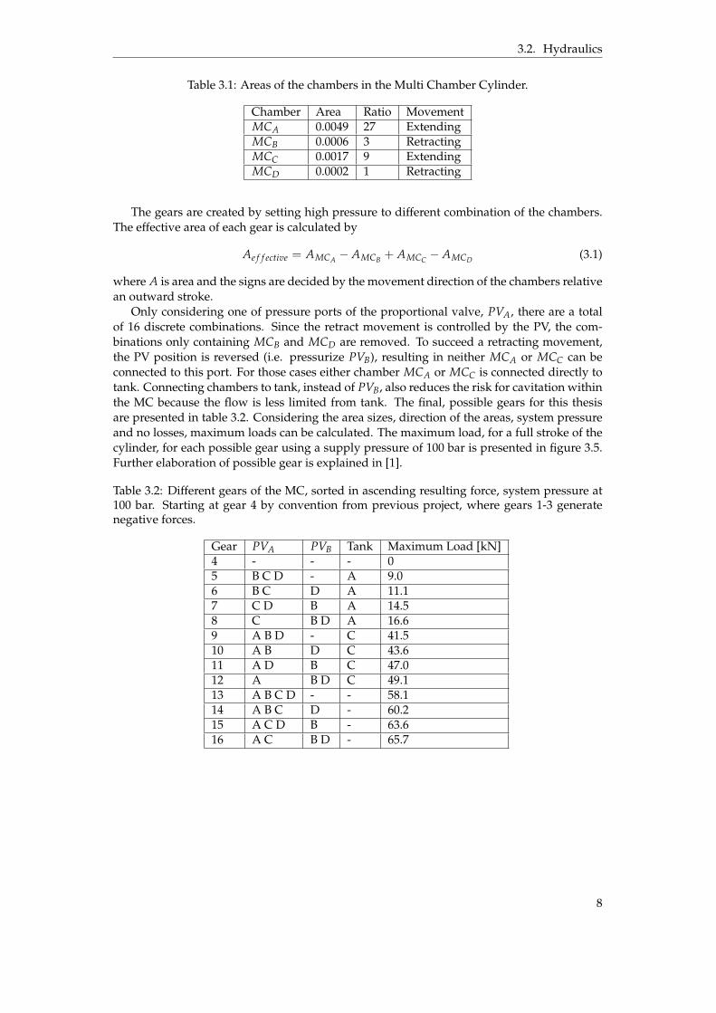
Table 3.1: Areas of the chambers in the Multi Chamber Cylinder.
Chamber Area Ratio MovementMCA 0.0049 27 ExtendingMCB 0.0006 3 RetractingMCC 0.0017 9 ExtendingMCD 0.0002 1 Retracting
The gears are created by setting high pressure to different combination of the chambers.The effective area of each gear is calculated by
Ae f f ective = AMCA ´ AMCB + AMCC ´ AMCD (3.1)
where A is area and the signs are decided by the movement direction of the chambers relativean outward stroke.
Only considering one of pressure ports of the proportional valve, PVA, there are a totalof 16 discrete combinations. Since the retract movement is controlled by the PV, the com-binations only containing MCB and MCD are removed. To succeed a retracting movement,the PV position is reversed (i.e. pressurize PVB), resulting in neither MCA or MCC can beconnected to this port. For those cases either chamber MCA or MCC is connected directly totank. Connecting chambers to tank, instead of PVB, also reduces the risk for cavitation withinthe MC because the flow is less limited from tank. The final, possible gears for this thesisare presented in table 3.2. Considering the area sizes, direction of the areas, system pressureand no losses, maximum loads can be calculated. The maximum load, for a full stroke of thecylinder, for each possible gear using a supply pressure of 100 bar is presented in figure 3.5.Further elaboration of possible gear is explained in [1].
Table 3.2: Different gears of the MC, sorted in ascending resulting force, system pressure at100 bar. Starting at gear 4 by convention from previous project, where gears 1-3 generatenegative forces.
Gear PVA PVB Tank Maximum Load [kN]4 - - - 05 B C D - A 9.06 B C D A 11.17 C D B A 14.58 C B D A 16.69 A B D - C 41.510 A B D C 43.611 A D B C 47.012 A B D C 49.113 A B C D - - 58.114 A B C D - 60.215 A C D B - 63.616 A C B D - 65.7
8

3.3. Connection
Resulting Forces
100 bar System Pressure
4 5 6 7 8 9 10 11 12 13 14 15 16
Time [s]
0
10
20
30
40
50
60
70
Fo
rce
[kN
]
Figure 3.5: Possible forces at system pressure 100 bar.
3.3 Connection
The information flow for controlling the system is shown in figure 3.6. The Human MachineInterface (HMI), used for controlling the system, is located in a MATLAB/Simulink environ-ment. To convert these commands to the hardware, the program B&R’s Automation Studio isused. This program transfers the commands to electrical signals via B&R’s PLC (x20-series).These signals controls the valves, which in turn controls the flow in the hydraulic system.The measurements from the sensors follows the same chain of communication but in oppo-site direction.
Figure 3.6: The control cycle of the physical system where MATLAB’s Simulink is used asHMI.
Measurements of the rig is made by pressure sensors, linear transducers and a linear vari-able differential transformer (LVDT). The pressures are measured in all chambers for bothcylinders as well as the system pressure. The position of both cylinders are measured by lin-ear transducers and the spool position of the PV is measured by the LVDT. The sensors usedin the rig are presented in table 3.3.
9
3.4. Control Flow
Table 3.3: Sensors used in the system
Sensor Placement DescriptionpMCA DV block at chamber A Pressure in MC chamber ApMCB DV block at chamber B Pressure in MC chamber BpMCC DV block at chamber C Pressure in MC chamber CpMCD DV block at chamber D Pressure in MC chamber DpSCA Port A at PV for SC Pressure in SC chamber ApSCB Port B at PV for SC Pressure in SC chamber Bpsys Between pump and PV System pressurexMC Multi-Chamber Cylinder Position of MCs strokexSC Single-Chamber Cylinder Position of SCs stroke
LVDT PV controlling the SC Position of PVs spool
3.4 Control Flow
The gear selection controller (agent) is set as an inner loop that automatically finds the bestgear for a given state. The operator is part of an open loop, requesting a velocity and adjustby hand according to the visual feedback. When the operator request a certain velocity thePV will open and supply flow for the DV block. The agent will read these signals alongwith pressures and choose an appropriate gear for the current load and velocity request. Thecontrol flow of the final system is illustrated in figure 3.7.
AGENTAc�on
MC Chamber Pressures
System Pressure
MC Velocity
OPERATORUser Reference
Visual Feedback
Safety
Policy
Final Ac�on
PV-controller
Figure 3.7: Control flow of the system.
10
3.5. Derivations of Calculated Signals
3.5 Derivations of Calculated Signals
Not all the signals needed by the agent can be measured. Some needs to be calculated. Con-sidering the signals from the sensors, table 3.3, and the system constants, the velocity, flow,pressure drop and power loss can be calculated.
To calculate the velocity, six time steps of the position is sampled and the derivative nu-merically calculated, presented in [3].
v =5xt + 3xt´1 + xt´2 ´ xt´3 ´ 3xt´4 ´ 5xt´5
35Ts(3.2)
where x is the measured position, indexing the number of time steps ago the position wasmeasured, and Ts is the sample time.
To calculate the flow through the PV, the calculated velocity, known chamber areas andactive gear is used to approximate the value.
qPV = AMCvMC =[AMCA ´AMCB AMCC ´AMCD
]˚ gearT ˚ vMC (3.3)
Where qPV is the flow, A is areas for the chambers, gear is a [1x4] -vector of the combinationof chambers according to table 3.2 and vMC the velocity.
To calculate the pressure drop over the PV, the pressure directly after it is needed. Sincethis is not measured, it is approximated to be the same as the highest pressure of the activechambers, assuming no pressure losses between PV and DV. The system pressure is mea-sured, and the pressure drop over the PV is calculated by equation (3.4).
∆pPV = psys ´max([pA, pB, pC, pD]. ˚ gear)) (3.4)
where " .* " indicates element-wise multiplication.The power loss over the PV is calulated by equation (3.5), only the hydraulic losses are
included.
PPV = ∆pPVqPV (3.5)
This power loss considers both the pressure compensating valve and the PV itself.
11
4 Related Research
Related research regards previous work of the multi chamber cylinder (MC) and how this canreduce energy consumption, reinforcement learning (RL) theory and RL applied to hydraulicapplications.
4.1 Pressure Compensation
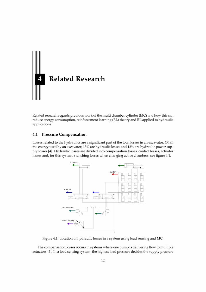
Losses related to the hydraulics are a significant part of the total losses in an excavator. Of allthe energy used by an excavator, 13% are hydraulic losses and 12% are hydraulic power sup-ply losses [4]. Hydraulic losses are divided into compensation losses, control losses, actuatorlosses and, for this system, switching losses when changing active chambers, see figure 4.1.
Actuator
Switch
Control
Compensation
Power Supply
Figure 4.1: Location of hydraulic losses in a system using load sensing and MC.
The compensation losses occurs in systems where one pump is delivering flow to multipleactuators [5]. In a load sensing system, the highest load pressure decides the supply pressure
12
4.2. Digital Hydraulics
for the entire system. For actuators with lower load pressure, this creates a pressure drop overthe components between pump and actuator i.e. the PV in this case. The hydraulic powerlosses, Ploss, is calculated by
Ploss = ∆pq (4.1)
where ∆p is the pressure drop over the PV and q is the flow though it. A third of the totalhydraulic energy consumed by an excavator in a digging cycle are related to these losses [6],which gives reason for improvement.
4.2 Digital Hydraulics
Digital hydraulics have gained attention latest decade and its systems architecture differsfrom conventional hydraulic systems for construction equipment (e.g. excavators). The mainbenefits compared to traditional systems are the use of simple and reliable components, po-tential for improved performance due to the fast dynamics of on/off valves and the flexibilityof the system. The control strategy defines the system characteristics instead of using com-plex components for specific tasks [5].
Using a MC, discrete force levels can be achieved from the combination of pressuresources and cylinder chambers [7]. In [2], three supply pressures are used with a MC cre-ating 81 possible forces, linearly distributed. This was to be used for secondary force controlof the cylinder. This architecture can be seen as a force gearbox, where each combinationcorresponds to one gear. This approach have been seen to reduce the energy consumption by60% compared to the convectional load sensing system [8], which shows the potential of thistype of cylinder.
One of the main drawbacks of using digital hydraulics is the increased complexity ofthe controller. Partly because of possible gears and lower controllability when switchinggear, as oscillations occur when pressurized and non-pressurized chambers are connected.Also velocity control is hard to achieve with force control, especially for lower velocities [1].Introducing a PV, as described in Chapter 3, velocity control can be improved while keepingthe reduced energy consumption.
Finding the optimal gear to switch to from a certain gear while aiming to increase theoverall efficiency, keep the controllability and follow the reference set by the operator is acomplex control task. Combined with the complexity of digital controls the gear selectiongets even more difficult. This raise enough reason to try out machine learning and deeplearning to develop a controller for the MC.
4.3 Reinforcement Learning
There are different kinds of numerical optimal control. In [9] different options are analysedfor real time control. A solution, not applicable as a real time controller, is the Dynamic Pro-gramming (DP) approach. DP will generate a global optimum within its discretization rangeand the given load cycle. This can be considered the possible optimum, used as referencewhile developing other controllers. For real time implementation, alternatives are EquivalentConsumption Minimization Strategy (ECMS) or a rule-based strategy. The ECMS only worksat a given load cycle, due to the equivalence factor. The final output can differ a lot evenat small deviations of this factor, making it load dependent. A rule-based strategy requiresunreasonably amounts of rules to always do the optimal control in all possible situations.
To solve this issue, having a long term, optimal controller that is working for more thanone cycle, Reinforcement Leaning (RL) is applicable. This approach almost reaches the sameoptimality as DP, since both are using the same concept for calculating the optimality [9]. Themain difference is that RL isn’t as computational heavy, and is therefore an alternative as areal-time controller.
13
4.3. Reinforcement Learning
Figure 4.2: The interaction between the components in a RL system [11].
RL is a machine learning class, designed to learn from a "Trial and Error" - approach [10].The RL model, called the agent, is not given what to do, or how to do it, but will figure this outby it self. This is done by trying out different actions, or sequence of actions, and afterwardsreceive a reward, or punishment, depending on the outcome. The agent is always strivingto receive as high reward as possible, performing the actions it considers best to achievethis. After a number of actions the agent will have learned which actions are good and whatto avoid. This is different compared to the other machine learning methods, i.e. supervisedand unsupervised learning. Supervised learning is taught what the correct action is by theuse of labeled training data, which is not the case in RL. Unsupervised learning is used forrecognizing patters in a given data series, where as the RL is doing an action and learns fromprevious experiences.
The information flow for a RL system is seen in figure 4.2. It consists of two main parts, theagent and the environment. The agent is the decision maker, where the decision making part iscalled the policy. Everything outside is the environment, i.e. the surroundings what the agentis interacting with. The agent affects the environment through its actions, the output from theagent. The signals that the agent sees is the observations, which is used of the agent to interpretthe environment, for example positions, pressures or previous action. The states are the valuesof the observations at a given time, which are used by the agents policy to determine the nextaction. The reward is the feedback the agent receives from the environment, giving it theinformation of how well it is performing the task. Based in this feedback, the agent canupdate its decision process to maximize the reward value.
There are two different components when constructing an agent: actor and critic. Anactor is doing the action that is considered the best for the moment, focusing on the shortterm reward. A critic analyses the long term gains for the agent, i.e. what actions will receivemost reward in the long run. An agent can be either an actor, a critic or an actor-critic. In theactor-critic case, the actor is defining what action to do, which is then analysed by the criticto update the agents parameters depending on the reward.
To explain how much the agent will investigate new actions the terms exploitation andexploration is used. Exploitation is using the best known solution to the problem, the agentexploits what it already found. Exploration is trying out new actions, with the goal of findinga better solution. The agent is exploring the action space. Finding a balance between theseare important for both the learning time and the final performance.
One technique to learn the agent complex tasks is to divide the tasks into multiple smallersteps, this is called Graded Learning [12]. Graded learning is a simplified method of Curricu-
14
4.3. Reinforcement Learning
lum Learning which normally requires design of algorithms and implementation of complexframework. Graded learning can be implemented just by simplifying the task or environmentand let the agent train for a set number of episodes or until convergence, then complexity isadded to the task or environment. The trained weights and biases are then transferred to thenew agent and the process repeats. Transferring weights and biases from a previously trainedagent is called transfer learning [12].
4.3.1 Neural Networks
Due to the curse of dimensions a Neural Network (NN) is used, to make it possible to mapobservations to actions. A NN works as a universal function approximator, giving the proba-bilities of doing an action depending on the observed states. Due to the flexible structure andsize of the NN, it is possible to map large and complex structures. In the RL application, thisis used to calculate the next action, whether it is the next action directly, the probability foran action or expected reward for the actions [10].
The structure and computations within a neural network is simple, layers that are madeup of neurons (nodes) that are connected, and information is sent between the layers. Theinformation is multiplied by weights and a bias is added, the values of these weights andbiases are what the learning algorithms tries to optimize. Each layer also have a so calledactivation function which helps to capture non-linearity’s of the data [10]. One such activationfunction is the rectified linear unit (ReLU) that returns zero for negative values and the inputvalue for all positive, i.e. ReLU(x) = max(x, 0).
4.3.2 Agents
The action of the agent, in this work, is an integer value, representing a selected gear. Eachvalue represents a unique set of which DVs to open. All the observations are continuousmeasurements from the system or reference signals to the system, made in real time. Becauseof this the agent needs to be designed to deliver actions in discrete space and observe incontinuous space. The agents delivered by Mathworks with the action and observation spaceare presented in table 4.1. There are two alternatives, Deep Q-Network (DQN) and ProximalPolicy Optimization (PPO) [13]. DQN is an agent consisting of a critic, while the PPO is anactor-critic. Because DQN is a simpler agent, this was selected.
Table 4.1: Mathworks agents and recommended using.
Agent Action ObservationQ-learning Discrete DiscreteDeep Q-Network Discrete ContinuousSARSA Discrete DiscreteProximal Policy Optimization Discrete ContinuousDeep Deterministic Policy Gradient Continuous ContinuousTwin-Delayed Deep Deterministic Policy Gradient Continuous ContinuousSoft Actor-Critic Continuous Continuous
Deep Q-Network
A DQN agent consists of a critic value function, Q-function, trying to estimate future returnsfor given actions [14]. The return is the sum of all future discounted rewards. The discountfactor, γ in equation (4.3), makes more distant rewards less valuable. During training, theagent gathers the current state st, the action taken at, the reward rt it received and the state itcame to st+1, creating a quadruple of saved values for each update (st, at, rt, st+1) [15]. These
15
4.3. Reinforcement Learning
values are saved for all the time steps in the agents experience buffer are and used for updatingthe policy. The policy is a NN, where the policy values are weight and biases.
To define the balance between exploration and exploitation the DQN-agent uses an ε-greedy function [16]. A greedy action is the action that maximizes the reward, the agentsexploits the environment. The ε-value is a probability that the agent is forced it to do a non-greedy move and thereby exploring the environment. Otherwise, with a probability of (1´ ε),a greedy action is made. In the beginning of training, it is preferable to have a higher ε-valueto explore more of all the options. As the learning progresses, the need to explore is reducedand it is preferable to have an agent that performs the best actions. The parameters εdecayand εmin are explaining at what rate the ε-value is decreasing and what the minimum valueshould be.
If a non-greedy action will be performed, a random action of the ones available is selected.If a greedy action will be performed, equation (4.2) is used for selection [16]. When the actionis performed and the next state and reward is observed, the Q-function is updated, equation(4.3) [14]. See figure 4.3 for the agents interaction with the environment.
at = arg maxat
Q(st, at|θt) (4.2)
Qt+1(st, at)Ð Qt(st, at) + αt
[rt+1 + γ max
at+1Qt(st+1, at+1)´Qt(st, at)
](4.3)
Where Q is the value function, s the state, a the action taken, θ is the policy settings and r thereward. The t-subscript is the time of observation, γ is a discount factor (to make short termrewards more profitable) and α is the learning rate (adjusting how much the value functionchanges from the last states).
Figure 4.3: DQN information flow.
To decouple the simulation steps, the results (st, at, rt, st+1) are saved in an experiencebuffer. Each time the Q-function is updated, equation (4.3), a mini-batch of random valuesare used for calculations from this buffer.
The hyperparameters, the parameters defining the agent, for a DQN are the presented intable 4.2.
16
4.4. Reinforcement Learning used with Hydraulics
Table 4.2: The agents hyperparameters.
Parameter Descriptionε Exploration rateεdecay Exploration decay rate per episodeεmin Minimum exploration rateTargetSmoothFactor Learning rateTargetUpdateFreq. Period between each update of critics parametersExperienceBufferLength Experience buffer sizeMiniBatchSize Size of random experience mini-batchNumStepsToLookAhead Number of future rewards to calculate for the actionDiscoutFactor Future rewards discount factor i.e. importance of future rewardsSampleTime Agents sample time i.e. agent execution per sim. sample time
There is no universal strategy to set these parameters. Instead they have to be iteratedfor new problems. I this work, parameters are set from system limitations and using trialand error for satisfactory learning. When tuning the parameters during trail and error, thetheoretical background of the parameters guided the direction of the tuning. The main focusof the development was set on the reward function to deliver an agent completing the task.
4.4 Reinforcement Learning used with Hydraulics
Applying RL to teach hydraulic construction systems to perform different tasks have previ-ously been done with success. The use of RL over conventional control theory to developcontrollers in construction equipment is mostly motivated by the trouble to realize the con-trol rules and they are usually not based in an optimization. Standard PID-controllers can’thandle the unknown terrain and more sophisticated controllers, like model predictive con-trol (MPC), would be complex and require advanced and tedious tuning and modeling tosucceed [17].
One specific field where RL is used for hydraulic control is bucket loading of wheel load-ers [17]. Here a RL agent is trained for an autonomous control. Bucket loading is a demandingtask including many parameters to consider: safe operation, wheel slip, bucket fill factor, fuelefficiency etc [18]. There is also requirements to handle unknown material (earth, gravel,rocks) and different particle sizes in the pile [17]. The combination of these difficulties makesuse of a RL controller the most reasonable approach for a generalized autonomous controller.In [19] such a controller is implemented, managing to load 75% of maximum bucket loadon average for the filling manouvers. This shows promising result for using reinforcementlearning in construction equipment.
Excavators are machines with multiple tasks: dig & dump, trenching and grading, eachrequiring a different level of accuracy, force and movement [4]. This is another field wherefully automation can be realised using RL. In [20] an agent learning a dig & dump cycle ispresented. The agent successfully moved 67% of the buckets maximum load from a specifiedloading spot to a hopper. This agent is not optimal for a real system, due to the angle of attackof the bucket when it enters the ground damages the system. Another research [21] trainedagents to do grading operations. The performance of the agent were acceptable, but moredevelopment is needed before it can be deployed to a real system, mainly due to oscillations.
RL is also used for minimizing energy consumption. For Hybrid Electric Vehicles it is asolution to optimize the battery usage to minimize the fuel consumption. In [22], RL success-fully reduced the fuel consumption. In [9], same kind of energy optimization is used but foran excavator.
17

5 Model Validation
The components in the simulation models were validated with recorded measurements fromtests performed on the test rig. The tests were performed in such a way to try to isolate thetested component as much as possible, without disassemble the system more than necessary.A load equation was created to give an indication of the load feedback for different positionsof the cylinders.
5.1 Models
In this section the models, tests, tuning and validation are explained.
5.1.1 Proportional Valve
The position of the spool was measured to validate the model of the proportional valve (PV),a linear variable differential transformer (LVDT) was used to measure the spool position. Thesensor had a span of +/- 4 mm, giving it 8 mm total stroke, the same length as the valvesspool displacement in one direction. The pressure is measured at three different locations,the PVA and PVB ports as well as the system pressure (before the PV).
To keep the system pressure constant, and to reduce the influence of the pump dynamics,a pressure relief valve (PRV) was used to control the supply pressure to the PV and thereforea constant pressure source could be used in the validation model seen in figure 5.1. The twovolumes represents the hoses of the real system and two 2/2 directional valves to stop theflow (always closed while validating).
The dynamics of the spool is different depending if a positive or negative stroke is madewhile the spool is centered or not (in position 0). At a positive stroke, the spool dynamicsdepends on the force produced by the solenoid and on a counter acting force from a spring,when changing direction while the spring is contracted the spring force will act in the samedirection as the reference and solenoid, giving it a different behaviour. A third case happenswhen the spool is positioned off centre and the reference is set to zero, at this moment thespring force is the main contributor to the dynamic which can be seen as a linear motion infigure 5.6. Because of this, different spool dynamics needed to be modeled and validated. Byusing two second order transfer functions as the input to the proportional valve componentin Hopsan. The dynamics of the valve itself is therefore set at high frequency to let the spool
18
5.1. Models
position only depend on the external transfer functions. A first order high pass filter is usedto calculate and hold the sign of the input derivative. To handle the third case when there areno noticeable dynamics from the solenoids, a rate limiter, ratePV , was used combined withlogics to activate it only when the reference signals is close to 0 (to avoid numerical issues).For results see table 5.2.
To tune and validate the parameters of the proportional valve two different reference sig-nal were used, step and sine wave.
Figure 5.1: The Hopsan model of the system used for validation of the Proportional Valve,using two 2/2 on/off valve to restrict the flow at each port.
5.1.2 Pressure Dynamics of Digital Valve Block
To validate the response time of the DVs, the DV blocks output ports were plugged to mini-mize the volume after the valves and to isolate the valves as much as possible.
First the pressure in the selected chamber was set to tank pressure by opening and closingthe chambers respective tank-valve, then the high pressure valve was opened while the PVwas kept fully open. The depressurization was also tested by first pressurize the chamber,close the high pressure valve and then open the tank-valve.
To minimize the pump dynamics the supply pressure was limited by a PRV. This test wasperformed twice, once for single digital valve (connected to MCD) and once for a doublevalve-chamber (MCA, MCB and MCC have this setting).
The model used for validating the DVs consist of a fully open PV followed by 12 DVs,representing the DV block. The hoses between the PVMCA and PVMCB and the DV block aremodeled as volumes, see figure 5.2. The approximated values of these and the volume of thechambers inside the DV block are seen in table 5.3. The four 2/2 valves connected after theDV blocks volumes are used to stop the flow and are always closed, representing the pluggedends in the test rig.
19
5.1. Models
Figure 5.2: The Hopsan model of the system used for validation of the digital valves in thedigital block. The digital valve block is marked within the orange dashed box.
During the tests the pressures inside the block was found to decrease rapidly when tryingto perform the depressurization test. This is caused by a small leakage and explains why thepressure is not constant at system pressure, seen in figure 5.8 and 5.9. The reason behindthis is due to the valves not being completely leak free and is noticeable as the pressurizedvolume is small, see table 5.3. Therefore a test was performed to confirm this, by keeping theDV blocks output ports blocked and pressurize the chambers by open and close the valves,the leakage is clearly shown as a steady depressurizing, see figure 5.3. The initial peak ofeach pressurizing happens when the valve opens, it is then kept open for a few second to letit stabilize (about 5 bar under system pressure). Then the valve is closed and the pressure is"trapped" within the block, this is when the pressure starts to rapidly decrease, the final dropto 0 bar marks the end of the test. The leakage was not modeled as the effect is negligibleonce the MC cylinder is connected and while the system is running, for future work wheremore detail is needed this could be introduced in the model.
20
5.1. Models
0 20 40 60 80 100 120 140 160 180 200
Time [s]
0
20
40
60
80
100
120
140
Pre
ssu
re [
ba
r]
Leakage test: Digital Valve Block and Multi Chamber Cylinder
Chamber A
Chamber B
Chamber C
Chamber D
System Pressure
Figure 5.3: Small leakage from the digital valves is clearly shown due to a small pressurizedvolume. The four first test are the chambers connected to PVA and the last four is PVB.
5.1.3 Digital Valves and Multi Chamber Cylinder
The DVs and MC were validated and tested simultaneously since the MC cannot be usedwithout the DV block. The tests were performed by recording data from steps with DVs(keep PV fully open) and step with PV (keeping DVs open) for two different gears. A full testrun was starting at a low position and let the cylinder extend at full speed to about 2
3 of thefull stroke then hold for a few seconds to stabilise, from there a step was made back to startposition. For the test with steps by the DV, the gear combination was reversed, see table 5.1.For PV-step the spool positions was as follow, in mm:
0 ÝÑ 8 ÝÑ 0 ÝÑ -8 ÝÑ 0
To minimize the effect of the pump dynamics, the pump pressure was set to 140 bar and thePRV to 100 bar, resulting in a constant supply pressure.
Table 5.1: Two different gears selected for validation.Convention: port A /port B / Tank
Gear Extension Retraction12 A/BD/C BD/A/C16 AC/BD/- BD/AC/-
A sine wave reference with amplitude of 6 mm and a frequency of π3 was also conducted
for validation.
21
5.1. Models
5.1.4 Single Chamber Cylinder
The single chamber cylinder (SC) was tested and validated in the same way as the MC, butonly using the proportional valve.
5.1.5 Load Function
A load function was derived to give an approximation of the force acting on the cylinder andto account for some dynamics. Validation tests was performed by extending and retractingthe MC and SC in a predefined pattern and then multiply the chamber pressures and areas,giving the resulting force acting on the cylinder, see equation 5.1.
FMC =[AMCA ´AMCB AMCC ´AMCD
] pMCApMCBpMCCpMCD
(5.1)
All distances and angles in figure 5.4 are known except β, ϕ and Φ which were calculatedby measuring the cylinders position. The derivative of these signals will be used for velocityand acceleration as well. Setting the equation (5.2) to zero and solve for Fcyl gives the forceacting on the MC, see equation (5.3).
MO = FcylrK ´Mstat ´Mdyn (5.2)
whererK = rOPsin(ϕr)
Mstat = mbgrGbOcos(ϕ + ψ)´mag(rJOcos(ϕ) + rGa Jsin(β))´ml g(rJOcos(ϕ) + rJLsin(Φ))
Mdyn = (Ib + cb1)ψb + cb2ωb + (Ia + mar2JO)ψaca1 ´ ca2ω2
amarGaJrJOcos(ϕ)+
+(Il + mlr2JO)ψa ´w2
amlrJLrJOcos(ϕ)
Figure 5.4: Geometry of the excavator boom and arm.
22
5.2. Validation Results
5.2 Validation Results
In this section the results for the validation of the model are presented.
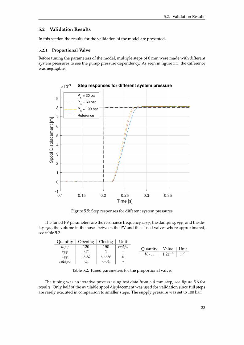
5.2.1 Proportional Valve
Before tuning the parameters of the model, multiple steps of 8 mm were made with differentsystem pressures to see the pump pressure dependency. As seen in figure 5.5, the differencewas negligible.
0.1 0.15 0.2 0.25 0.3 0.35
Time [s]
-1
0
1
2
3
4
5
6
7
8
9
Sp
oo
l D
isp
lace
me
nt
[m]
10-3 Step responses for different system pressure
Ps = 30 bar
Ps = 60 bar
Ps = 100 bar
Reference
Figure 5.5: Step responses for different system pressures
The tuned PV parameters are the resonance frequency, ωPV , the damping, δPV , and the de-lay τPV , the volume in the hoses between the PV and the closed valves where approximated,see table 5.2.
Quantity Opening Closing UnitωPV 120 150 rad/sδPV 0.74 1 ´
τPV 0.02 0.009 sratePV 8 0.04 -
Quantity Value UnitVHose 1.2e´4 m3
Table 5.2: Tuned parameters for the proportional valve.
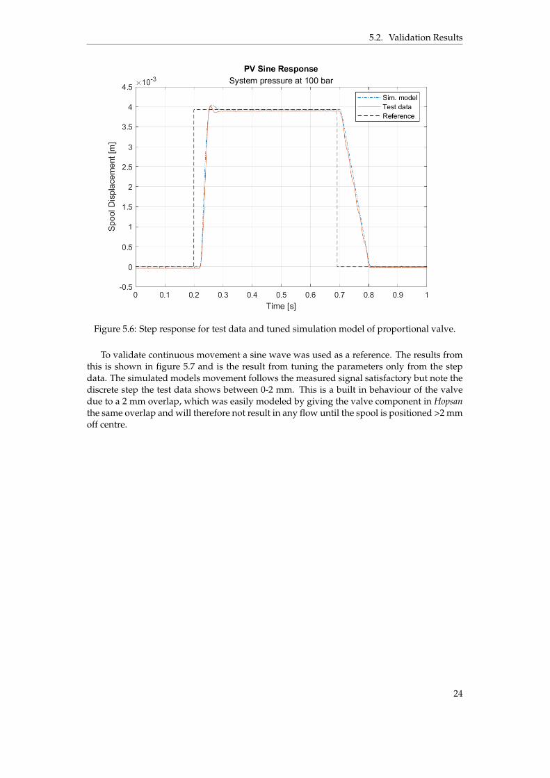
The tuning was an iterative process using test data from a 4 mm step, see figure 5.6 forresults. Only half of the available spool displacement was used for validation since full stepsare rarely executed in comparison to smaller steps. The supply pressure was set to 100 bar.
23
5.2. Validation Results
Figure 5.6: Step response for test data and tuned simulation model of proportional valve.
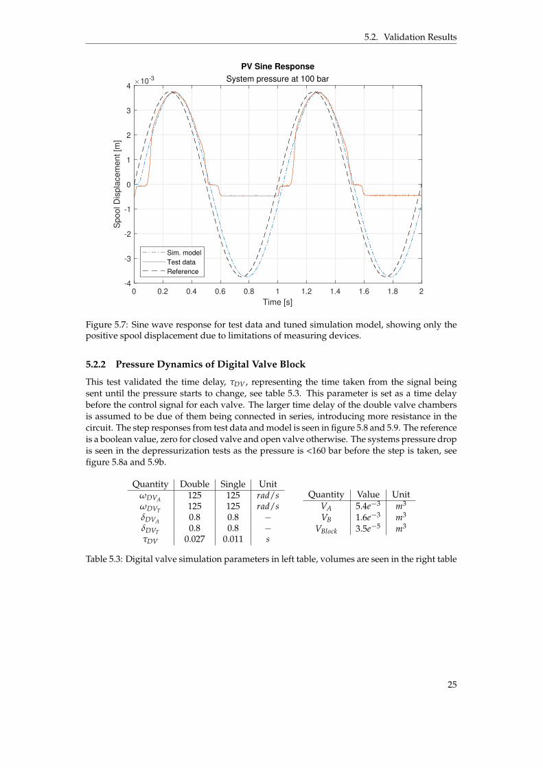
To validate continuous movement a sine wave was used as a reference. The results fromthis is shown in figure 5.7 and is the result from tuning the parameters only from the stepdata. The simulated models movement follows the measured signal satisfactory but note thediscrete step the test data shows between 0-2 mm. This is a built in behaviour of the valvedue to a 2 mm overlap, which was easily modeled by giving the valve component in Hopsanthe same overlap and will therefore not result in any flow until the spool is positioned >2 mmoff centre.
24
5.2. Validation Results
0 0.2 0.4 0.6 0.8 1 1.2 1.4 1.6 1.8 2
Time [s]
-4
-3
-2
-1
0
1
2
3
4
Sp
oo
l D
isp
lace
me
nt
[m]
10-3
PV Sine Response
System pressure at 100 bar
Sim. model
Test data
Reference
Figure 5.7: Sine wave response for test data and tuned simulation model, showing only thepositive spool displacement due to limitations of measuring devices.
5.2.2 Pressure Dynamics of Digital Valve Block
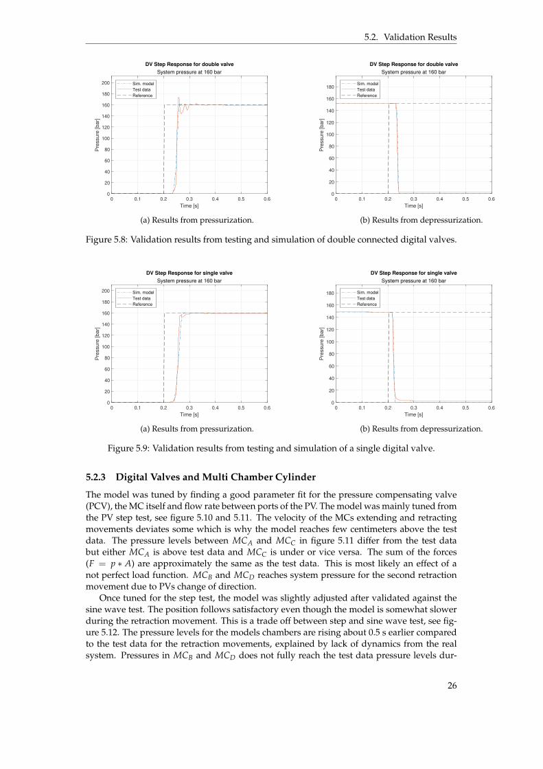
This test validated the time delay, τDV , representing the time taken from the signal beingsent until the pressure starts to change, see table 5.3. This parameter is set as a time delaybefore the control signal for each valve. The larger time delay of the double valve chambersis assumed to be due of them being connected in series, introducing more resistance in thecircuit. The step responses from test data and model is seen in figure 5.8 and 5.9. The referenceis a boolean value, zero for closed valve and open valve otherwise. The systems pressure dropis seen in the depressurization tests as the pressure is <160 bar before the step is taken, seefigure 5.8a and 5.9b.
Quantity Double Single UnitωDVA 125 125 rad/sωDVT 125 125 rad/sδDVA 0.8 0.8 ´
δDVT 0.8 0.8 ´
τDV 0.027 0.011 s
Quantity Value UnitVA 5.4e´3 m3
VB 1.6e´3 m3
VBlock 3.5e´5 m3
Table 5.3: Digital valve simulation parameters in left table, volumes are seen in the right table
25
5.2. Validation Results
0 0.1 0.2 0.3 0.4 0.5 0.6
Time [s]
0
20
40
60
80
100
120
140
160
180
200
Pre
ssu
re [
ba
r]
DV Step Response for double valve
System pressure at 160 bar
Sim. model
Test data
Reference
(a) Results from pressurization.
0 0.1 0.2 0.3 0.4 0.5 0.6
Time [s]
0
20
40
60
80
100
120
140
160
180
Pre
ssu
re [
ba
r]
DV Step Response for double valve
System pressure at 160 bar
Sim. model
Test data
Reference
(b) Results from depressurization.
Figure 5.8: Validation results from testing and simulation of double connected digital valves.
0 0.1 0.2 0.3 0.4 0.5 0.6
Time [s]
0
20
40
60
80
100
120
140
160
180
200
Pre
ssu
re [
ba
r]
DV Step Response for single valve
System pressure at 160 bar
Sim. model
Test data
Reference
(a) Results from pressurization.
0 0.1 0.2 0.3 0.4 0.5 0.6
Time [s]
0
20
40
60
80
100
120
140
160
180
Pre
ssu
re [
ba
r]
DV Step Response for single valve
System pressure at 160 bar
Sim. model
Test data
Reference
(b) Results from depressurization.
Figure 5.9: Validation results from testing and simulation of a single digital valve.
5.2.3 Digital Valves and Multi Chamber Cylinder
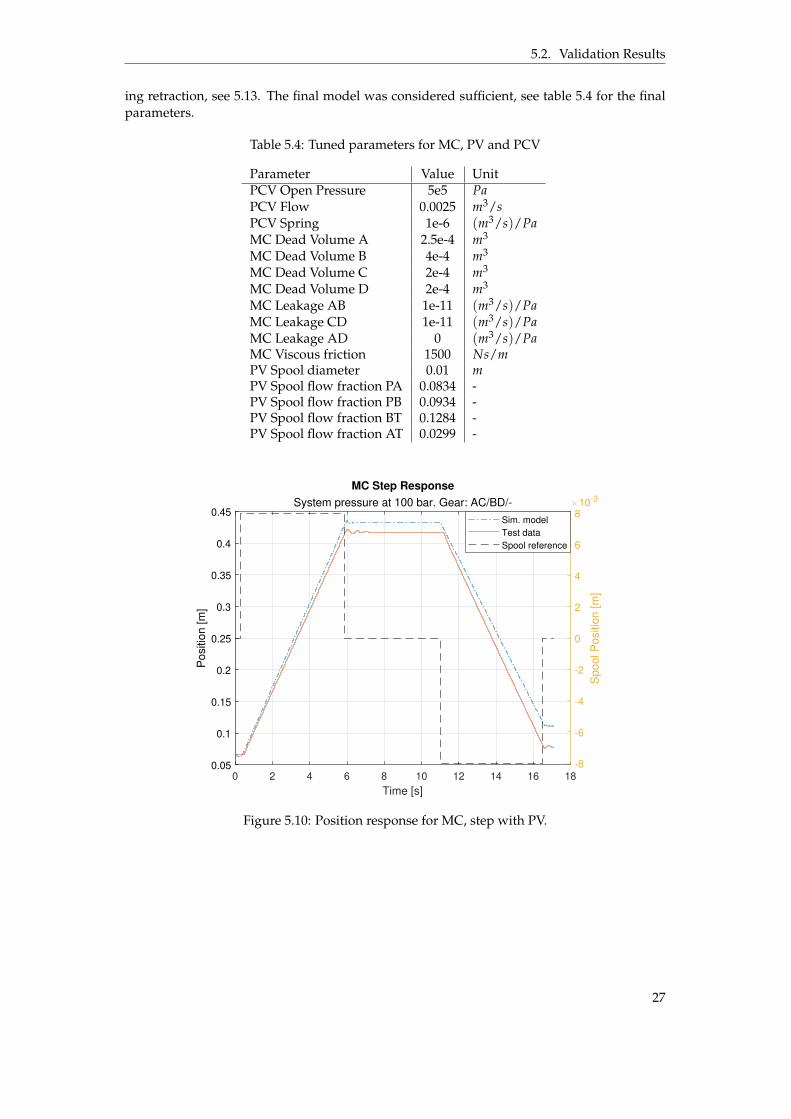
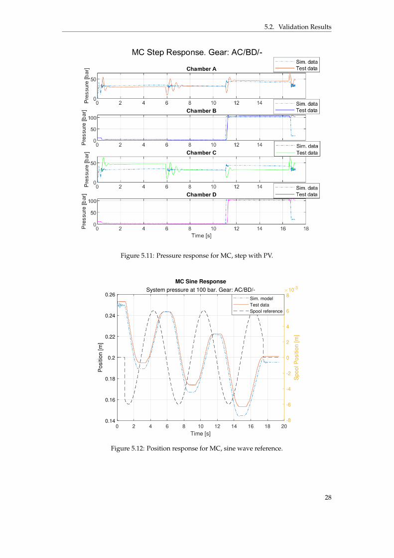
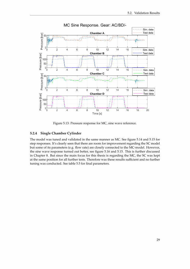
The model was tuned by finding a good parameter fit for the pressure compensating valve(PCV), the MC itself and flow rate between ports of the PV. The model was mainly tuned fromthe PV step test, see figure 5.10 and 5.11. The velocity of the MCs extending and retractingmovements deviates some which is why the model reaches few centimeters above the testdata. The pressure levels between MCA and MCC in figure 5.11 differ from the test databut either MCA is above test data and MCC is under or vice versa. The sum of the forces(F = p ˚ A) are approximately the same as the test data. This is most likely an effect of anot perfect load function. MCB and MCD reaches system pressure for the second retractionmovement due to PVs change of direction.
Once tuned for the step test, the model was slightly adjusted after validated against thesine wave test. The position follows satisfactory even though the model is somewhat slowerduring the retraction movement. This is a trade off between step and sine wave test, see fig-ure 5.12. The pressure levels for the models chambers are rising about 0.5 s earlier comparedto the test data for the retraction movements, explained by lack of dynamics from the realsystem. Pressures in MCB and MCD does not fully reach the test data pressure levels dur-
26
5.2. Validation Results
ing retraction, see 5.13. The final model was considered sufficient, see table 5.4 for the finalparameters.
Table 5.4: Tuned parameters for MC, PV and PCV
Parameter Value UnitPCV Open Pressure 5e5 PaPCV Flow 0.0025 m3/sPCV Spring 1e-6 (m3/s)/PaMC Dead Volume A 2.5e-4 m3
MC Dead Volume B 4e-4 m3
MC Dead Volume C 2e-4 m3
MC Dead Volume D 2e-4 m3
MC Leakage AB 1e-11 (m3/s)/PaMC Leakage CD 1e-11 (m3/s)/PaMC Leakage AD 0 (m3/s)/PaMC Viscous friction 1500 Ns/mPV Spool diameter 0.01 mPV Spool flow fraction PA 0.0834 -PV Spool flow fraction PB 0.0934 -PV Spool flow fraction BT 0.1284 -PV Spool flow fraction AT 0.0299 -
0 2 4 6 8 10 12 14 16 18
Time [s]
0.05
0.1
0.15
0.2
0.25
0.3
0.35
0.4
0.45
Po
sitio
n [
m]
-8
-6
-4
-2
0
2
4
6
8
Sp
oo
l P
ositio
n [
m]
10-3
MC Step Response
System pressure at 100 bar. Gear: AC/BD/-
Sim. model
Test data
Spool reference
Figure 5.10: Position response for MC, step with PV.
27
5.2. Validation Results
Figure 5.11: Pressure response for MC, step with PV.
0 2 4 6 8 10 12 14 16 18 20
Time [s]
0.14
0.16
0.18
0.2
0.22
0.24
0.26
Po
sitio
n [
m]
-8
-6
-4
-2
0
2
4
6
8S
po
ol P
ositio
n [
m]
10-3
MC Sine Response
System pressure at 100 bar. Gear: AC/BD/-
Sim. model
Test data
Spool reference
Figure 5.12: Position response for MC, sine wave reference.
28
5.2. Validation Results
Figure 5.13: Pressure response for MC, sine wave reference.
5.2.4 Single Chamber Cylinder
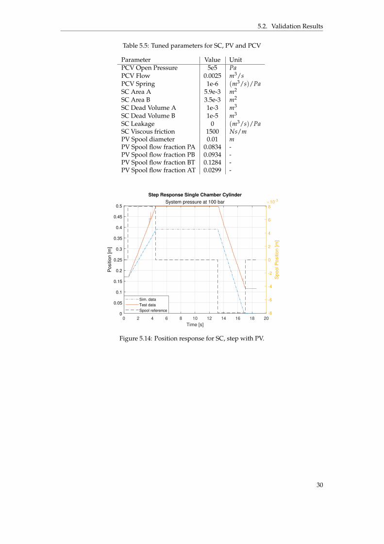
The model was tuned and validated in the same manner as MC. See figure 5.14 and 5.15 forstep responses. It’s clearly seen that there are room for improvement regarding the SC modelbut some of its parameters (e.g. flow rate) are closely connected to the MC-model. However,the sine wave response turned out better, see figure 5.16 and 5.15. This is further discussedin Chapter 8. But since the main focus for this thesis is regarding the MC, the SC was keptat the same position for all further tests. Therefore was these results sufficient and no furthertuning was conducted. See table 5.5 for final parameters.
29
5.2. Validation Results
Table 5.5: Tuned parameters for SC, PV and PCV
Parameter Value UnitPCV Open Pressure 5e5 PaPCV Flow 0.0025 m3/sPCV Spring 1e-6 (m3/s)/PaSC Area A 5.9e-3 m2
SC Area B 3.5e-3 m2
SC Dead Volume A 1e-3 m3
SC Dead Volume B 1e-5 m3
SC Leakage 0 (m3/s)/PaSC Viscous friction 1500 Ns/mPV Spool diameter 0.01 mPV Spool flow fraction PA 0.0834 -PV Spool flow fraction PB 0.0934 -PV Spool flow fraction BT 0.1284 -PV Spool flow fraction AT 0.0299 -
0 2 4 6 8 10 12 14 16 18 20
Time [s]
0
0.05
0.1
0.15
0.2
0.25
0.3
0.35
0.4
0.45
0.5
Po
sitio
n [
m]
-8
-6
-4
-2
0
2
4
6
8
Sp
oo
l P
ositio
n [
m]
10-3
Step Response Single Chamber Cylinder
System pressure at 100 bar
Sim. data
Test data
Spool reference
Figure 5.14: Position response for SC, step with PV.
30

5.2. Validation Results
2 4 6 8 10 12 14 16 180
20
40
60
80
Pre
ssu
re [
ba
r]
Chamber A
Sim. data
Test data
2 4 6 8 10 12 14 16 18
Time [s]
0
50
100
Pre
ssu
re [
ba
r]
Chamber B
Sim. data
Test data
Pressure in Single Chamber Cylinder
Figure 5.15: Pressure response for SC, step with PV.
0 2 4 6 8 10 12 14 16 18 20
Time [s]
0.15
0.2
0.25
0.3
0.35
0.4
0.45
0.5
0.55
0.6
Po
sitio
n [
m]
-8
-6
-4
-2
0
2
4
6
8
Sp
oo
l P
ositio
n [
m]
10-3
Sine Response Single Chamber Cylinder
System pressure at 100 bar
Sim. data
Test data
Spool reference
Figure 5.16: Position response for SC, sine wave reference. The spike at 10 sec. is due to faultysensor.
31
5.2. Validation Results
2 4 6 8 10 12 14 16 18 200
20
40
60
80
Pre
ssu
re [
ba
r]
Chamber A
Sim. data
Test data
2 4 6 8 10 12 14 16 18 20
Time [s]
0
50
100
150
Pre
ssu
re [
ba
r]
Chamber B
Sim. data
Test data
Pressure in Single Chamber Cylinder
Figure 5.17: Pressure response for SC, sine wave reference.
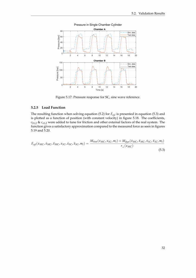
5.2.5 Load Function
The resulting function when solving equation (5.2) for Fcyl is presented in equation (5.3) andis plotted as a function of position (with constant velocity) in figure 5.18. The coefficients,cb1,2 & ca1,2 were added to tune for friction and other external factors of the real system. Thefunction gives a satisfactory approximation compared to the measured force as seen in figures5.19 and 5.20.
Fcyl(xMC, xMC, xMC, xSC, xSC, xSC, ml) =Mstat(xMC, xSC, ml) + Mdyn(xMC, xMC, xSC, xSC, ml)
rK(xMC)(5.3)
32

5.2. Validation Results
Figure 5.18: Force acting on multi chamber cylinder as a function of the two cylinders posi-tion, with 3kg external load, constant velocity at 0.03 m/s and no acceleration.
Figure 5.19: Test data and load function compared. The SC is set at a fixed position and MCextends or retracts.
33

5.2. Validation Results
Figure 5.20: Test data and load function compared. The MC is set at a fixed position and SCextends or retracts. The gap around 0.15 m is due to faulty sensor.
34
6 Development of ReinforcementLearning Controller
The procedure of setting up training environment, validation and deployment are describedin this chapter.
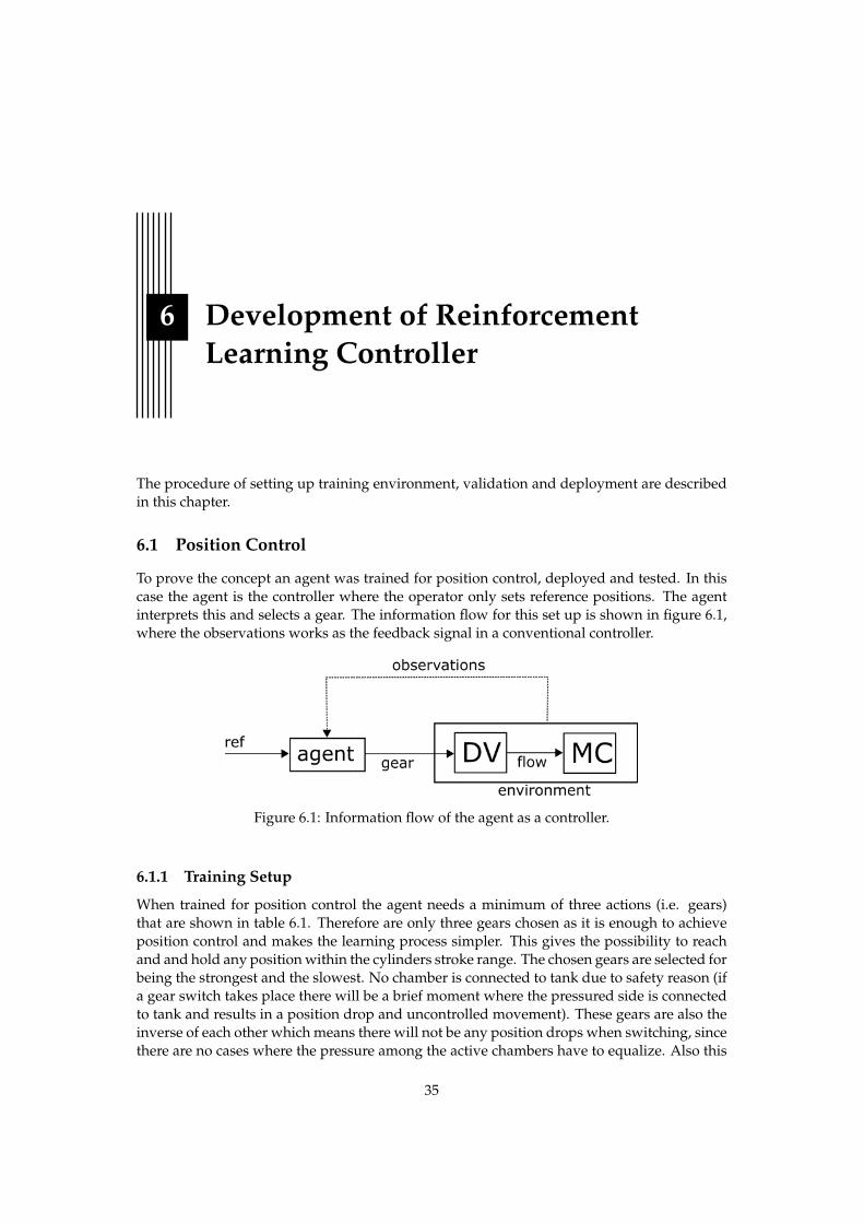
6.1 Position Control
To prove the concept an agent was trained for position control, deployed and tested. In thiscase the agent is the controller where the operator only sets reference positions. The agentinterprets this and selects a gear. The information flow for this set up is shown in figure 6.1,where the observations works as the feedback signal in a conventional controller.
Figure 6.1: Information flow of the agent as a controller.
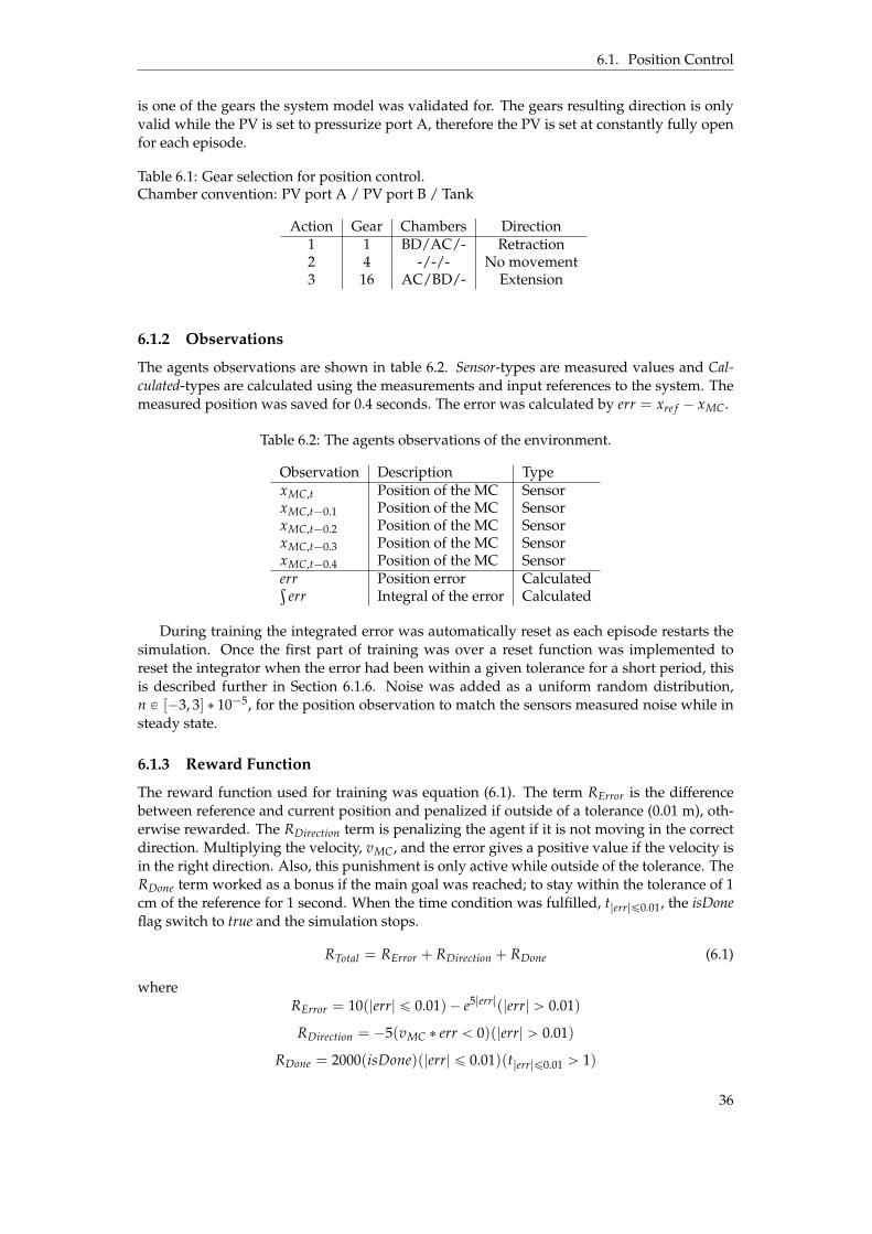
6.1.1 Training Setup
When trained for position control the agent needs a minimum of three actions (i.e. gears)that are shown in table 6.1. Therefore are only three gears chosen as it is enough to achieveposition control and makes the learning process simpler. This gives the possibility to reachand and hold any position within the cylinders stroke range. The chosen gears are selected forbeing the strongest and the slowest. No chamber is connected to tank due to safety reason (ifa gear switch takes place there will be a brief moment where the pressured side is connectedto tank and results in a position drop and uncontrolled movement). These gears are also theinverse of each other which means there will not be any position drops when switching, sincethere are no cases where the pressure among the active chambers have to equalize. Also this
35
6.1. Position Control
is one of the gears the system model was validated for. The gears resulting direction is onlyvalid while the PV is set to pressurize port A, therefore the PV is set at constantly fully openfor each episode.
Table 6.1: Gear selection for position control.Chamber convention: PV port A / PV port B / Tank
Action Gear Chambers Direction1 1 BD/AC/- Retraction2 4 -/-/- No movement3 16 AC/BD/- Extension
6.1.2 Observations
The agents observations are shown in table 6.2. Sensor-types are measured values and Cal-culated-types are calculated using the measurements and input references to the system. Themeasured position was saved for 0.4 seconds. The error was calculated by err = xre f ´ xMC.
Table 6.2: The agents observations of the environment.
Observation Description TypexMC,t Position of the MC SensorxMC,t´0.1 Position of the MC SensorxMC,t´0.2 Position of the MC SensorxMC,t´0.3 Position of the MC SensorxMC,t´0.4 Position of the MC Sensorerr Position error Calculatedş
err Integral of the error Calculated
During training the integrated error was automatically reset as each episode restarts thesimulation. Once the first part of training was over a reset function was implemented toreset the integrator when the error had been within a given tolerance for a short period, thisis described further in Section 6.1.6. Noise was added as a uniform random distribution,n P [´3, 3] ˚ 10´5, for the position observation to match the sensors measured noise while insteady state.
6.1.3 Reward Function
The reward function used for training was equation (6.1). The term RError is the differencebetween reference and current position and penalized if outside of a tolerance (0.01 m), oth-erwise rewarded. The RDirection term is penalizing the agent if it is not moving in the correctdirection. Multiplying the velocity, vMC, and the error gives a positive value if the velocity isin the right direction. Also, this punishment is only active while outside of the tolerance. TheRDone term worked as a bonus if the main goal was reached; to stay within the tolerance of 1cm of the reference for 1 second. When the time condition was fulfilled, t|err|ď0.01, the isDoneflag switch to true and the simulation stops.
RTotal = RError + RDirection + RDone (6.1)
whereRError = 10(|err| ď 0.01)´ e5|err|(|err| ą 0.01)
RDirection = ´5(vMC ˚ err ă 0)(|err| ą 0.01)
RDone = 2000(isDone)(|err| ď 0.01)(t|err|ď0.01 ą 1)
36
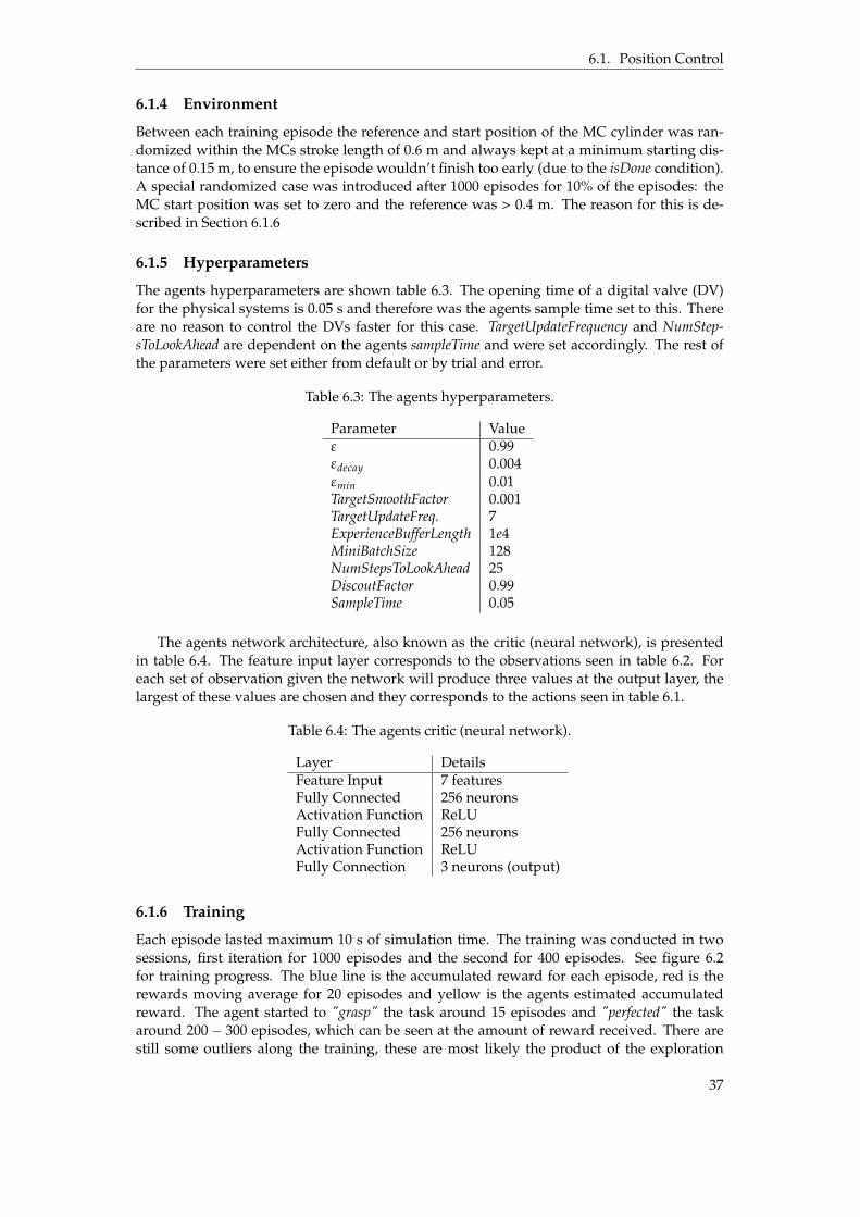
6.1. Position Control
6.1.4 Environment
Between each training episode the reference and start position of the MC cylinder was ran-domized within the MCs stroke length of 0.6 m and always kept at a minimum starting dis-tance of 0.15 m, to ensure the episode wouldn’t finish too early (due to the isDone condition).A special randomized case was introduced after 1000 episodes for 10% of the episodes: theMC start position was set to zero and the reference was > 0.4 m. The reason for this is de-scribed in Section 6.1.6
6.1.5 Hyperparameters
The agents hyperparameters are shown table 6.3. The opening time of a digital valve (DV)for the physical systems is 0.05 s and therefore was the agents sample time set to this. Thereare no reason to control the DVs faster for this case. TargetUpdateFrequency and NumStep-sToLookAhead are dependent on the agents sampleTime and were set accordingly. The rest ofthe parameters were set either from default or by trial and error.
Table 6.3: The agents hyperparameters.
Parameter Valueε 0.99εdecay 0.004εmin 0.01TargetSmoothFactor 0.001TargetUpdateFreq. 7ExperienceBufferLength 1e4MiniBatchSize 128NumStepsToLookAhead 25DiscoutFactor 0.99SampleTime 0.05
The agents network architecture, also known as the critic (neural network), is presentedin table 6.4. The feature input layer corresponds to the observations seen in table 6.2. Foreach set of observation given the network will produce three values at the output layer, thelargest of these values are chosen and they corresponds to the actions seen in table 6.1.
Table 6.4: The agents critic (neural network).
Layer DetailsFeature Input 7 featuresFully Connected 256 neuronsActivation Function ReLUFully Connected 256 neuronsActivation Function ReLUFully Connection 3 neurons (output)
6.1.6 Training
Each episode lasted maximum 10 s of simulation time. The training was conducted in twosessions, first iteration for 1000 episodes and the second for 400 episodes. See figure 6.2for training progress. The blue line is the accumulated reward for each episode, red is therewards moving average for 20 episodes and yellow is the agents estimated accumulatedreward. The agent started to "grasp" the task around 15 episodes and "perfected" the taskaround 200´ 300 episodes, which can be seen at the amount of reward received. There arestill some outliers along the training, these are most likely the product of the exploration
37
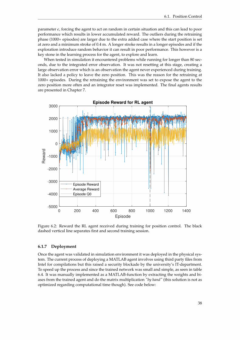
6.1. Position Control
parameter ε, forcing the agent to act on random in certain situation and this can lead to poorperformance which results in lower accumulated reward. The outliers during the retrainingphase (1000+ episodes) are larger due to the extra added case where the start position is setat zero and a minimum stroke of 0.4 m. A longer stroke results in a longer episodes and if theexploration introduce random behavior it can result in poor performance. This however is akey stone in the learning process for the agent, to explore and learn.
When tested in simulation it encountered problems while running for longer than 80 sec-onds, due to the integrated error observation. It was not resetting at this stage, creating alarge observation error which is an observation the agent never experienced during training.It also lacked a policy to leave the zero position. This was the reason for the retraining at1000+ episodes. During the retraining the environment was set to expose the agent to thezero position more often and an integrator reset was implemented. The final agents resultsare presented in Chapter 7.
0 200 400 600 800 1000 1200 1400
Episode
-5000
-4000
-3000
-2000
-1000
0
1000
2000
3000
Re
wa
rd
Episode Reward for RL agent
Episode Reward
Average Reward
Episode Q0
Figure 6.2: Reward the RL agent received during training for position control. The blackdashed vertical line separates first and second training session.
6.1.7 Deployment
Once the agent was validated in simulation environment it was deployed in the physical sys-tem. The current process of deploying a MATLAB agent involves using third party files fromIntel for compilations but this raised a security blockade by the university’s IT-department.To speed up the process and since the trained network was small and simple, as seen in table6.4. It was manually implemented as a MATLAB-function by extracting the weights and bi-ases from the trained agent and do the matrix multiplication "by hand" (this solution is not asoptimized regarding computational time though). See code below:
38
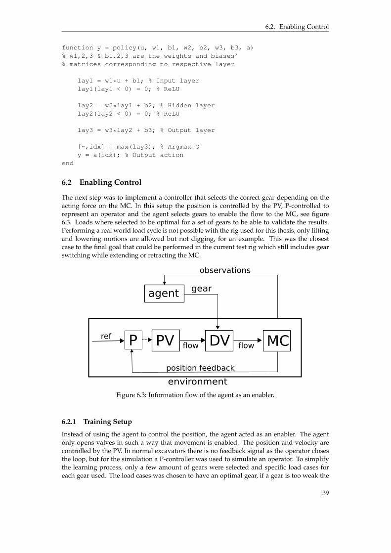
6.2. Enabling Control
function y = policy(u, w1, b1, w2, b2, w3, b3, a)% w1,2,3 & b1,2,3 are the weights and biases’% matrices corresponding to respective layer
lay1 = w1*u + b1; % Input layerlay1(lay1 < 0) = 0; % ReLU
lay2 = w2*lay1 + b2; % Hidden layerlay2(lay2 < 0) = 0; % ReLU
lay3 = w3*lay2 + b3; % Output layer
[~,idx] = max(lay3); % Argmax Qy = a(idx); % Output action
end
6.2 Enabling Control
The next step was to implement a controller that selects the correct gear depending on theacting force on the MC. In this setup the position is controlled by the PV, P-controlled torepresent an operator and the agent selects gears to enable the flow to the MC, see figure6.3. Loads where selected to be optimal for a set of gears to be able to validate the results.Performing a real world load cycle is not possible with the rig used for this thesis, only liftingand lowering motions are allowed but not digging, for an example. This was the closestcase to the final goal that could be performed in the current test rig which still includes gearswitching while extending or retracting the MC.
PV DV
agent
refMC
position feedback
observations
flow flow
gear
P
environment
Figure 6.3: Information flow of the agent as an enabler.
6.2.1 Training Setup
Instead of using the agent to control the position, the agent acted as an enabler. The agentonly opens valves in such a way that movement is enabled. The position and velocity arecontrolled by the PV. In normal excavators there is no feedback signal as the operator closesthe loop, but for the simulation a P-controller was used to simulate an operator. To simplifythe learning process, only a few amount of gears were selected and specific load cases foreach gear used. The load cases was chosen to have an optimal gear, if a gear is too weak the
39

6.2. Enabling Control
cylinder would not be able to extend the cylinder fully but if too strong gear the power losswill increase. During training the external load was randomized from these load cases. Thegears and loads used are presented in table 6.5.
Table 6.5: Gears and loads used for gear selection training
Gear Chambers Load [kg]9 ABD / - / C 110
11 AD / B / C 17014 ABC / D / - 23016 AC / BC / - 260
6.2.2 Observations
The observations are presented in table 6.6. Signal types are control signals of the system,Measured are measured signals from sensors and Calculated are signals calculated from signalsand measurements.
Table 6.6: Observations used for gear selection.
Observation Description Typegear The active gear Signalxre f ,PVMC Reference signal to the PV SignalpMC,A Pressure in chamber A MeasuredpMC,B Pressure in chamber B MeasuredpMC,C Pressure in chamber C MeasuredpMC,D Pressure in chamber D Measuredpsys System pressure MeasuredvMC Velocity of the MC Calculated
All observations are normalized, by division of respectively maximum value or scaled tobe close to the interval of [´1, 1]. The reason behind the velocity and the PV reference signalwhere to give the agent information of what the operator asks for and how it performs. Alarger magnitude of reference signal means higher asked velocity. The pressures are meantto select an appropriate gear and the action mean to simplify the learning process by un-derstanding what each gear is representing and how it change the other observations. Allobservations are part of the reward function.
6.2.3 Reward Function
For this case the reward function is designed to only give negative rewards, to encouragethe agent to finish each episode as quick as possible, see equation (6.2). The idea for RPower,equation (6.4), is to use as weak gear as possible since it is known to be more efficient. Aweaker gear results in a smaller volume, resulting in less flow for the same velocity. Since theP-controller will be fully open for the most part of the episode this made it preferable to finishthe simulation as quick as possible. A downside of this is when there is no flow, then thereare no losses. This term was calculated using equation (3.3), (3.4) and scaled by the maximumflow and system pressures as well as weighted by a scalar.
Using a too weak gear the MC will not reach the reference and make it come to a halt. Theterm RVelocity was introduced to penalize if the MC was not keeping a set minimum velocity.In equation (6.3) the respective coefficient and constant kre f ,vel and mre f ,vel is transforming thePVs reference position to a minimum accepted velocity of the MC. The minimum acceptedvelocity is refereed to the slowest gear (16). The velocity, vMC, is calculated by equation (3.2).
40

6.2. Enabling Control
The combination of RPower and RVelocity will force the agent to find gears where the lossesare as low as possible and at the same time keep the minimum velocity.
A counter, RSwitchCounter, was used to penalize unnecessary switching. A negative rewardis received, depending on the number of time steps the new gear was different compared tothe previous ones, see equation (6.5).
RTotal = RVelocity + RPower + RSwitchCounter (6.2)
where
RVelocity =
#
´8, if vMC ă (kre f ,vel xre f ,PVMC + mre f ,vel ˚ sign(vMC)) &vMC ą 0´8, if vMC ą (kre f ,vel xre f ,PVMC + mre f ,vel ˚ sign(vMC)) &vMC ă 0
(6.3)
RPower = ´100|qPV∆pPV |
qPump,max pSys,max(6.4)
RSwitchCounter =T
ÿ
t=1
´1(Actiont ‰ Actiont´1) (6.5)
6.2.4 Environment
The same model was used for this case as in the position control case. Every episode startswith a random selection of an external load which corresponds to one of the four gears. A20% bias towards choosing the lowest load was implemented to let the agent experiencemore of those cases. The reason is that as the training runs the agents experience buffer getsfilled with states and actions which is used for updating the network policy. Lower loadsand weaker gears results in higher velocity, for a successful episode, and will therefore cometo an end faster. This results in an experience buffer biased towards the longer simulations,i.e. high loads that require stronger gears. For the first part of the training the start andreference position was always constant, going from zero to full stroke. The complexity of theenvironment increased as the training progressed, this is described in more detail in Section6.2.6.
6.2.5 Hyperparameters
The agents hyperparameters and network are shown table 6.7 and 6.8. When switching gearsthe system oscillated more or less depending on the number of chamber changing pressure.To handle that the agents sample time is set to 0.4s to give time for the oscillations to set-tle. This also decreased the computational time significantly. The NumStepsToLookAhead andTargetUpdateFreq parameters are affected by this and are set accordingly. The rest of the pa-rameters are set either from default or by trial and error.
Table 6.7: The agents hyperparameters.
Parameter Valueε 0.99εdecay 0.003εmin 0.01TargetSmoothFactor 0.002TargetUpdateFreq. 1ExperienceBufferLength 1e4MiniBatchSize 128NumStepsToLookAhead 10DiscoutFactor 0.99SampleTime 0.4
41
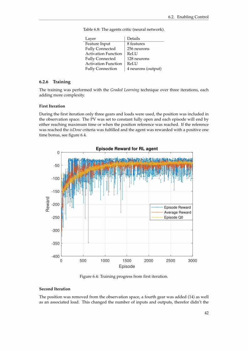
6.2. Enabling Control
Table 6.8: The agents critic (neural network).
Layer DetailsFeature Input 8 featuresFully Connected 256 neuronsActivation Function ReLUFully Connected 128 neuronsActivation Function ReLUFully Connection 4 neurons (output)
6.2.6 Training
The training was performed with the Graded Learning technique over three iterations, eachadding more complexity.
First Iteration
During the first iteration only three gears and loads were used, the position was included inthe observation space. The PV was set to constant fully open and each episode will end byeither reaching maximum time or when the position reference was reached. If the referencewas reached the isDone criteria was fulfilled and the agent was rewarded with a positive onetime bonus, see figure 6.4.
0 500 1000 1500 2000 2500 3000
Episode
-400
-350
-300
-250
-200
-150
-100
-50
0
Re
wa
rd
Episode Reward for RL agent
Episode Reward
Average Reward
Episode Q0
Figure 6.4: Training progress from first iteration.
Second Iteration
The position was removed from the observation space, a fourth gear was added (14) as wellas an associated load. This changed the number of inputs and outputs, therefor didn’t the
42
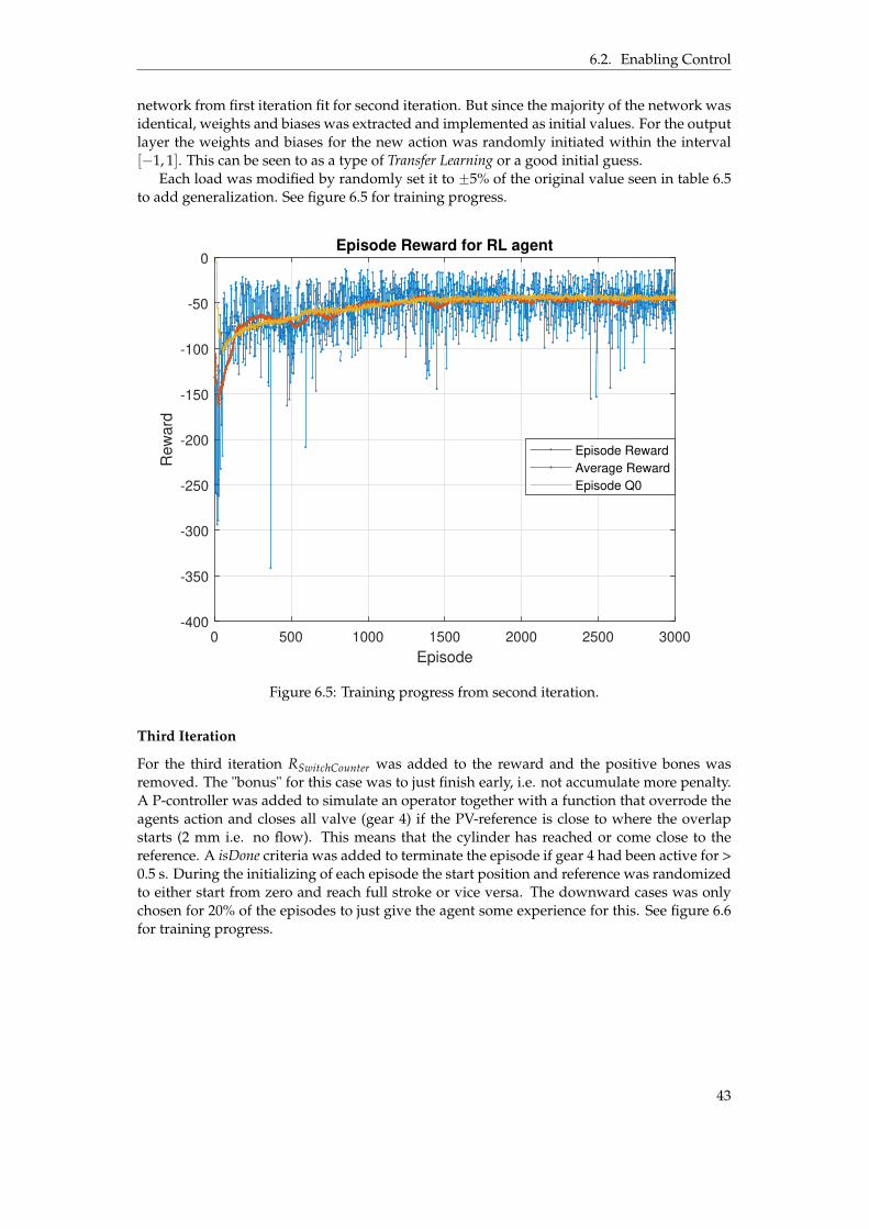
6.2. Enabling Control
network from first iteration fit for second iteration. But since the majority of the network wasidentical, weights and biases was extracted and implemented as initial values. For the outputlayer the weights and biases for the new action was randomly initiated within the interval[´1, 1]. This can be seen to as a type of Transfer Learning or a good initial guess.
Each load was modified by randomly set it to ˘5% of the original value seen in table 6.5to add generalization. See figure 6.5 for training progress.
0 500 1000 1500 2000 2500 3000
Episode
-400
-350
-300
-250
-200
-150
-100
-50
0
Re
wa
rd
Episode Reward for RL agent
Episode Reward
Average Reward
Episode Q0
Figure 6.5: Training progress from second iteration.
Third Iteration
For the third iteration RSwitchCounter was added to the reward and the positive bones wasremoved. The "bonus" for this case was to just finish early, i.e. not accumulate more penalty.A P-controller was added to simulate an operator together with a function that overrode theagents action and closes all valve (gear 4) if the PV-reference is close to where the overlapstarts (2 mm i.e. no flow). This means that the cylinder has reached or come close to thereference. A isDone criteria was added to terminate the episode if gear 4 had been active for >0.5 s. During the initializing of each episode the start position and reference was randomizedto either start from zero and reach full stroke or vice versa. The downward cases was onlychosen for 20% of the episodes to just give the agent some experience for this. See figure 6.6for training progress.
43
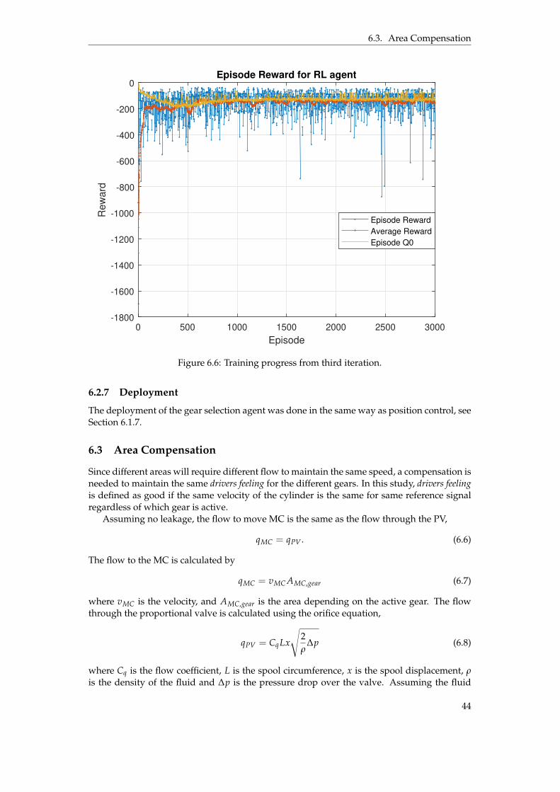
6.3. Area Compensation
0 500 1000 1500 2000 2500 3000
Episode
-1800
-1600
-1400
-1200
-1000
-800
-600
-400
-200
0
Re
wa
rd
Episode Reward for RL agent
Episode Reward
Average Reward
Episode Q0
Figure 6.6: Training progress from third iteration.
6.2.7 Deployment
The deployment of the gear selection agent was done in the same way as position control, seeSection 6.1.7.
6.3 Area Compensation
Since different areas will require different flow to maintain the same speed, a compensation isneeded to maintain the same drivers feeling for the different gears. In this study, drivers feelingis defined as good if the same velocity of the cylinder is the same for same reference signalregardless of which gear is active.
Assuming no leakage, the flow to move MC is the same as the flow through the PV,
qMC = qPV . (6.6)
The flow to the MC is calculated by
qMC = vMC AMC,gear (6.7)
where vMC is the velocity, and AMC,gear is the area depending on the active gear. The flowthrough the proportional valve is calculated using the orifice equation,
qPV = CqLx
d
2ρ
∆p (6.8)
where Cq is the flow coefficient, L is the spool circumference, x is the spool displacement, ρis the density of the fluid and ∆p is the pressure drop over the valve. Assuming the fluid
44
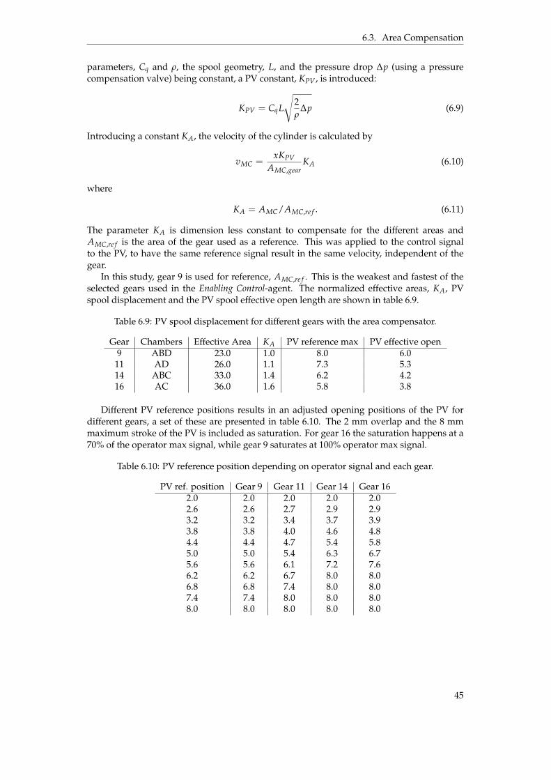
6.3. Area Compensation
parameters, Cq and ρ, the spool geometry, L, and the pressure drop ∆p (using a pressurecompensation valve) being constant, a PV constant, KPV , is introduced:
KPV = CqL
d
2ρ
∆p (6.9)
Introducing a constant KA, the velocity of the cylinder is calculated by
vMC =xKPV
AMC,gearKA (6.10)
where
KA = AMC/AMC,re f . (6.11)
The parameter KA is dimension less constant to compensate for the different areas andAMC,re f is the area of the gear used as a reference. This was applied to the control signalto the PV, to have the same reference signal result in the same velocity, independent of thegear.
In this study, gear 9 is used for reference, AMC,re f . This is the weakest and fastest of theselected gears used in the Enabling Control-agent. The normalized effective areas, KA, PVspool displacement and the PV spool effective open length are shown in table 6.9.
Table 6.9: PV spool displacement for different gears with the area compensator.
Gear Chambers Effective Area KA PV reference max PV effective open9 ABD 23.0 1.0 8.0 6.011 AD 26.0 1.1 7.3 5.314 ABC 33.0 1.4 6.2 4.216 AC 36.0 1.6 5.8 3.8
Different PV reference positions results in an adjusted opening positions of the PV fordifferent gears, a set of these are presented in table 6.10. The 2 mm overlap and the 8 mmmaximum stroke of the PV is included as saturation. For gear 16 the saturation happens at a70% of the operator max signal, while gear 9 saturates at 100% operator max signal.
Table 6.10: PV reference position depending on operator signal and each gear.
PV ref. position Gear 9 Gear 11 Gear 14 Gear 162.0 2.0 2.0 2.0 2.02.6 2.6 2.7 2.9 2.93.2 3.2 3.4 3.7 3.93.8 3.8 4.0 4.6 4.84.4 4.4 4.7 5.4 5.85.0 5.0 5.4 6.3 6.75.6 5.6 6.1 7.2 7.66.2 6.2 6.7 8.0 8.06.8 6.8 7.4 8.0 8.07.4 7.4 8.0 8.0 8.08.0 8.0 8.0 8.0 8.0
45
7 Results
The results from position control, enabling control and area compensation are presented inthis chapter.
7.1 Position Control
Two tests were performed, one with the PV fully open, figure 7.1, and one with the PV 50%open, figure 7.2. The second test was conducted to see how well the agent performed tochanges of the environment that it had never experienced previously, this could been testedmore thoroughly but the simple approach was chosen due to safety and time constraints.
The top plot in figures 7.1 and 7.2 shows the selected action, both from simulation andphysical tests. Gear 1 results in retraction of the cylinder, gear 4 stand still and gear 16 ex-tension. The lower plots show the positions, including the reference signals. The fully openPV managed to control the position accurately while the 50% open-case had a small positionerror. This is discussed further in Chapter 8.
46

7.1. Position Control
0 5 10 15 20 25 30 35 40 45 50
1
4
16
Gear
[-]
PV 100%
Sim. data
Test data
0 5 10 15 20 25 30 35 40 45 50
Time [s]
0.1
0.2
0.3
0.4
Positio
n [m
]
Sim. data
Test data
Reference
RL position control
Figure 7.1: Test data from physical rig and from simulation, using 100% open PV.
0 5 10 15 20 25 30 35 40 45 50 55 60
1
4
16
Gear
[-]
PV 50%
Sim. data
Test data
0 5 10 15 20 25 30 35 40 45 50 55 60
Time [s]
0.1
0.2
0.3
0.4
Positio
n [m
]
Sim. data
Test data
Reference
RL position control
Figure 7.2: Test data from physical rig and from simulation, using 50% open PV.
In the simulation environment the direction of the PV was reversed to test the generaliza-tion of the agent further. This reverses the resulting direction of the gears, turning everything"up side down" in comparison to what the agent have been trained for. It can handle this,even thought far from perfect, see figure 7.3. This test was only carried out in simulationenvironment due to safety reasons.
47

7.1. Position Control
0 50 100 150
1
4
16
Ge
ar
[-]
PV reversed at 100%
0 50 100 150
0
0.2
0.4
0.6
Po
sitio
n [
m]
MC position
Reference
0 50 100 150
Time [s]
0
5
10
Inte
gra
ted
Err
or
[-]
RL position control
Figure 7.3: Simulation results when using reversed direction of PV. Integrated error is shownto explain the time for the final adjustment.
A sine wave reference test was performed in simulation environment to validate if theagent learnt the task, i.e. to follow a reference. There are a significant amount of gear switchesbut that was expected since the controller is discrete and the reference continuously changing,see figure 7.4. The agent was only trained on constant references and had never experiencedsuch case before.
RL position control
0 10 20 30 40 50
1
4
16
Ge
ar
[-]
Sine wave, PV 100%
0 10 20 30 40 50 60
0
0.2
0.4
Po
sitio
n [
m]
MC position
Reference
0 10 20 30 40 50 60
Time [s]
0
0.2
0.4
Inte
gra
ted
Err
or
[-]
Figure 7.4: Simulation results when following a sine wave reference.
48
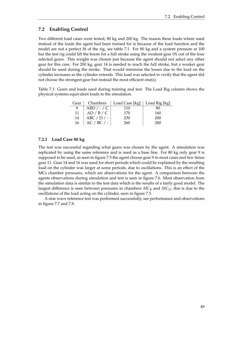
7.2. Enabling Control
7.2 Enabling Control
Two different load cases were tested, 80 kg and 200 kg. The reason these loads where usedinstead of the loads the agent had been trained for is because of the load function and themodel are not a perfect fit of the rig, see table 7.1. For 80 kg and a system pressure at 100bar the test rig could lift the boom for a full stroke using the weakest gear (9) out of the fourselected gears. This weight was chosen just because the agent should not select any othergear for this case. For 200 kg, gear 14 is needed to reach the full stroke, but a weaker gearshould be used during the stroke. That would minimize the losses due to the load on thecylinder increases as the cylinder extends. This load was selected to verify that the agent didnot choose the strongest gear but instead the most efficient one(s).
Table 7.1: Gears and loads used during training and test. The Load Rig column shows thephysical systems equivalent loads to the simulation.
Gear Chambers Load Case [kg] Load Rig [kg]9 ABD / - / C 110 80
11 AD / B / C 170 16014 ABC / D / - 230 20016 AC / BC / - 260 280
7.2.1 Load Case 80 kg
The test was successful regarding what gears was chosen by the agent. A simulation wasreplicated by using the same reference and is used as a base line. For 80 kg only gear 9 issupposed to be used, as seen in figure 7.5 the agent choose gear 9 in most cases and few timesgear 11. Gear 14 and 16 was used for short periods which could be explained by the resultingload on the cylinder was larger at some periods, due to oscillations. This is an effect of theMCs chamber pressures, which are observations for the agent. A comparison between theagents observations during simulation and test is seen in figure 7.6. Most observation fromthe simulation data is similar to the test data which is the results of a fairly good model. Thelargest difference is seen between pressures in chambers MCB and MCD, this is due to theoscillations of the load acting on the cylinder, seen in figure 7.5.
A sine wave reference test was performed successfully, see performance and observationsin figure 7.7 and 7.8.
49
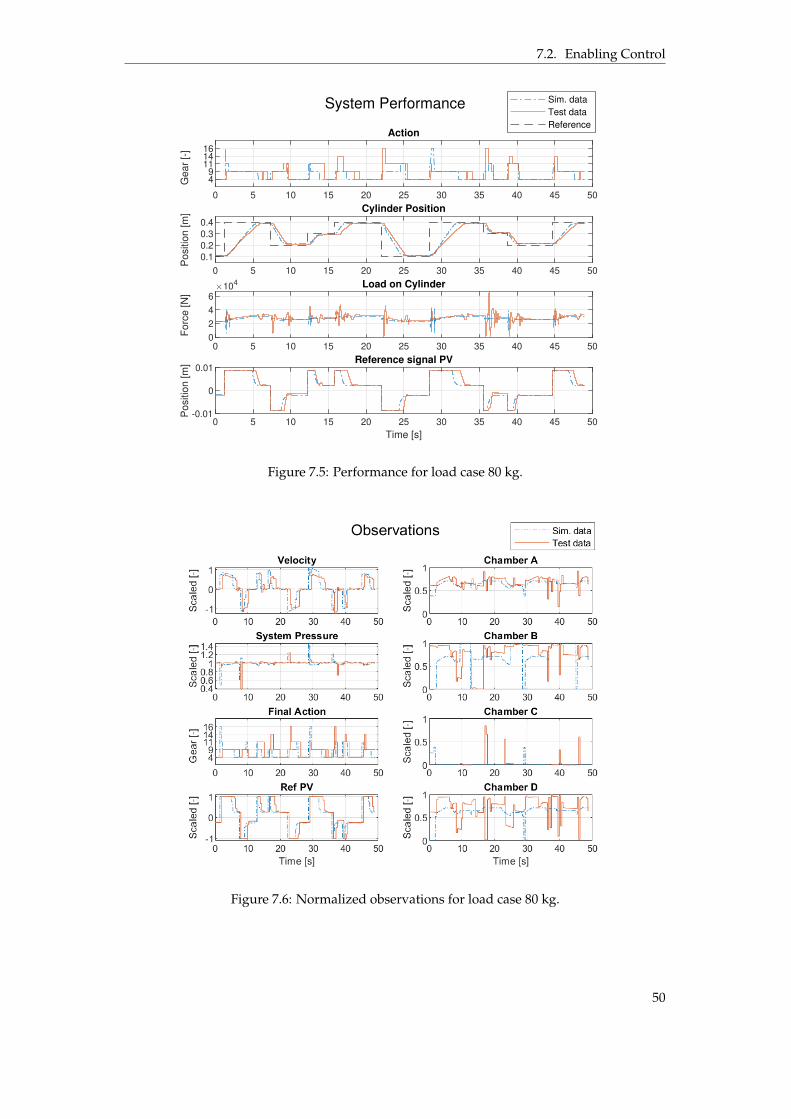
7.2. Enabling Control
System Performance
0 5 10 15 20 25 30 35 40 45 50
49
111416
Gear
[-]
Action
0 5 10 15 20 25 30 35 40 45 50
0.1
0.2
0.3
0.4
Positio
n [m
] Cylinder Position
Sim. data
Test data
Reference
0 5 10 15 20 25 30 35 40 45 500
2
4
6
Forc
e [N
]
104 Load on Cylinder
0 5 10 15 20 25 30 35 40 45 50
Time [s]
-0.01
0
0.01
Positio
n [m
] Reference signal PV
Figure 7.5: Performance for load case 80 kg.
Figure 7.6: Normalized observations for load case 80 kg.
50
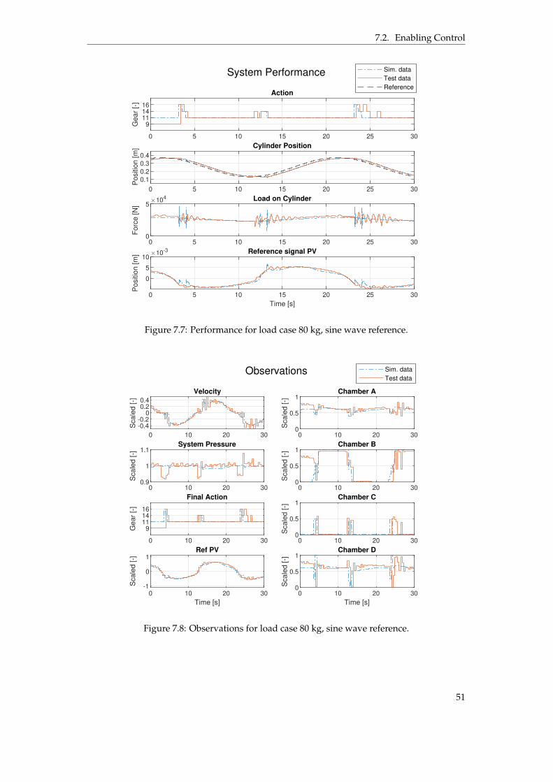
7.2. Enabling Control
System Performance
0 5 10 15 20 25 30
9111416
Gear
[-]
Action
0 5 10 15 20 25 30
0.1
0.2
0.3
0.4
Positio
n [m
] Cylinder Position
Sim. data
Test data
Reference
0 5 10 15 20 25 300
5
Forc
e [N
]
104 Load on Cylinder
0 5 10 15 20 25 30
Time [s]
0
5
10
Positio
n [m
] 10-3 Reference signal PV
Figure 7.7: Performance for load case 80 kg, sine wave reference.
0 10 20 30
-0.4-0.2
00.20.4
Scale
d [-]
Velocity
Sim. data
Test data
0 10 20 300.9
1
1.1
Scale
d [-]
System Pressure
0 10 20 30
9111416
Gear
[-]
Final Action
0 10 20 30
Time [s]
-1
0
1
Scale
d [-]
Ref PV
0 10 20 300
0.5
1
Scale
d [-]
Chamber A
0 10 20 300
0.5
1
Scale
d [-]
Chamber B
0 10 20 300
0.5
1
Scale
d [-]
Chamber C
0 10 20 30
Time [s]
0
0.5
1
Scale
d [-]
Chamber D
Observations
Figure 7.8: Observations for load case 80 kg, sine wave reference.
51
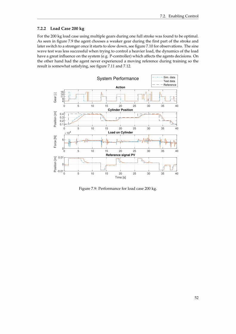
7.2. Enabling Control
7.2.2 Load Case 200 kg
For the 200 kg load case using multiple gears during one full stroke was found to be optimal.As seen in figure 7.9 the agent chooses a weaker gear during the first part of the stroke andlater switch to a stronger once it starts to slow down, see figure 7.10 for observations. The sinewave test was less successful when trying to control a heavier load, the dynamics of the loadhave a great influence on the system (e.g. P-controller) which affects the agents decisions. Onthe other hand had the agent never experienced a moving reference during training so theresult is somewhat satisfying, see figure 7.11 and 7.12.
System Performance
0 5 10 15 20 25 30 35 40
49
111416
Gear
[-]
Action
0 5 10 15 20 25 30 35 40
0.1
0.2
0.3
0.4
Positio
n [m
] Cylinder Position
Sim. data
Test data
Reference
0 5 10 15 20 25 30 35 400
5
Forc
e [N
]
104 Load on Cylinder
0 5 10 15 20 25 30 35 40
Time [s]
-0.01
0
0.01
Positio
n [m
] Reference signal PV
Figure 7.9: Performance for load case 200 kg.
52
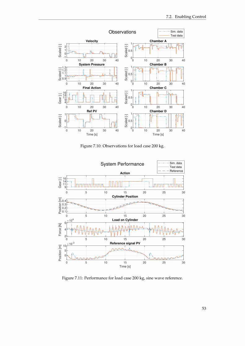
7.2. Enabling Control
0 10 20 30 40-1
0
1
2
Scale
d [-]
Velocity
Sim. data
Test data
0 10 20 30 40
0.91
1.11.21.3
Scale
d [-]
System Pressure
0 10 20 30 40
49
111416
Gear
[-]
Final Action
0 10 20 30 40
Time [s]
-1
0
1
Scale
d [-]
Ref PV
0 10 20 30 400
0.5
1
Scale
d [-]
Chamber A
0 10 20 30 400
0.5
1
Scale
d [-]
Chamber B
0 10 20 30 400
0.5
1
Scale
d [-]
Chamber C
0 10 20 30 40
Time [s]
0
0.5
1
Scale
d [-]
Chamber D
Observations
Figure 7.10: Observations for load case 200 kg.
System Performance
0 5 10 15 20 25 30
9111416
Gear
[-]
Action
0 5 10 15 20 25 30
0.1
0.2
0.3
0.4
Positio
n [m
] Cylinder Position
Sim. data
Test data
Reference
0 5 10 15 20 25 302
4
6
Forc
e [N
]
104 Load on Cylinder
0 5 10 15 20 25 30
Time [s]
0
5
10
Positio
n [m
] 10-3 Reference signal PV
Figure 7.11: Performance for load case 200 kg, sine wave reference.
53
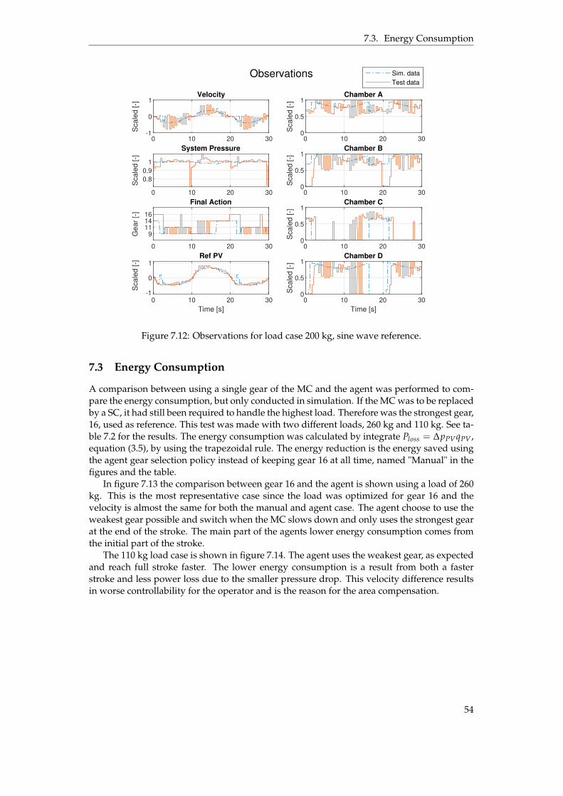
7.3. Energy Consumption
0 10 20 30-1
0
1
Scale
d [-]
Velocity
Sim. data
Test data
0 10 20 30
0.8
0.9
1
Scale
d [-]
System Pressure
0 10 20 30
9111416
Gear
[-]
Final Action
0 10 20 30
Time [s]
-1
0
1
Scale
d [-]
Ref PV
0 10 20 300
0.5
1
Scale
d [-]
Chamber A
0 10 20 300
0.5
1
Scale
d [-]
Chamber B
0 10 20 300
0.5
1
Scale
d [-]
Chamber C
0 10 20 30
Time [s]
0
0.5
1
Scale
d [-]
Chamber D
Observations
Figure 7.12: Observations for load case 200 kg, sine wave reference.
7.3 Energy Consumption
A comparison between using a single gear of the MC and the agent was performed to com-pare the energy consumption, but only conducted in simulation. If the MC was to be replacedby a SC, it had still been required to handle the highest load. Therefore was the strongest gear,16, used as reference. This test was made with two different loads, 260 kg and 110 kg. See ta-ble 7.2 for the results. The energy consumption was calculated by integrate Ploss = ∆pPVqPV ,equation (3.5), by using the trapezoidal rule. The energy reduction is the energy saved usingthe agent gear selection policy instead of keeping gear 16 at all time, named "Manual" in thefigures and the table.
In figure 7.13 the comparison between gear 16 and the agent is shown using a load of 260kg. This is the most representative case since the load was optimized for gear 16 and thevelocity is almost the same for both the manual and agent case. The agent choose to use theweakest gear possible and switch when the MC slows down and only uses the strongest gearat the end of the stroke. The main part of the agents lower energy consumption comes fromthe initial part of the stroke.
The 110 kg load case is shown in figure 7.14. The agent uses the weakest gear, as expectedand reach full stroke faster. The lower energy consumption is a result from both a fasterstroke and less power loss due to the smaller pressure drop. This velocity difference resultsin worse controllability for the operator and is the reason for the area compensation.
54
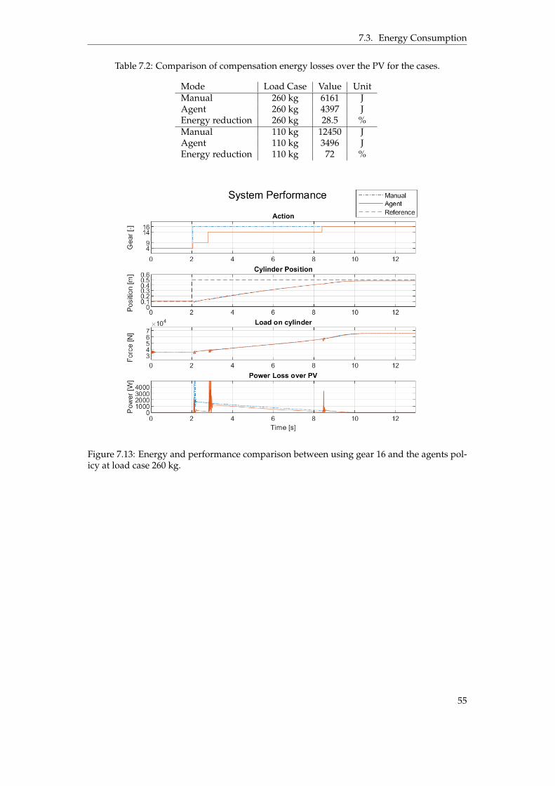
7.3. Energy Consumption
Table 7.2: Comparison of compensation energy losses over the PV for the cases.
Mode Load Case Value UnitManual 260 kg 6161 JAgent 260 kg 4397 JEnergy reduction 260 kg 28.5 %Manual 110 kg 12450 JAgent 110 kg 3496 JEnergy reduction 110 kg 72 %
Figure 7.13: Energy and performance comparison between using gear 16 and the agents pol-icy at load case 260 kg.
55
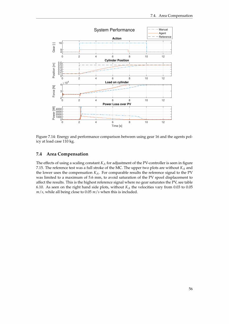
7.4. Area Compensation
System Performance
0 2 4 6 8 10 12
49
16
Gear
[-]
Action
0 2 4 6 8 10 120
0.10.20.30.40.50.6
Positio
n [m
]
Cylinder Position
Manual
Agent
Reference
0 2 4 6 8 10 122
3
4
Forc
e [N
]
104 Load on cylinder
0 2 4 6 8 10 12
Time [s]
01000200030004000
Pow
er
[W]
Power Loss over PV
Figure 7.14: Energy and performance comparison between using gear 16 and the agents pol-icy at load case 110 kg.
7.4 Area Compensation
The effects of using a scaling constant KA for adjustment of the PV-controller is seen in figure7.15. The reference test was a full stroke of the MC. The upper two plots are without KA andthe lower uses the compensation KA. For comparable results the reference signal to the PVwas limited to a maximum of 5.6 mm, to avoid saturation of the PV spool displacement toaffect the results. This is the highest reference signal where no gear saturates the PV, see table6.10. As seen on the right hand side plots, without KA the velocities vary from 0.03 to 0.05m/s, while all being close to 0.05 m/s when this is included.
56
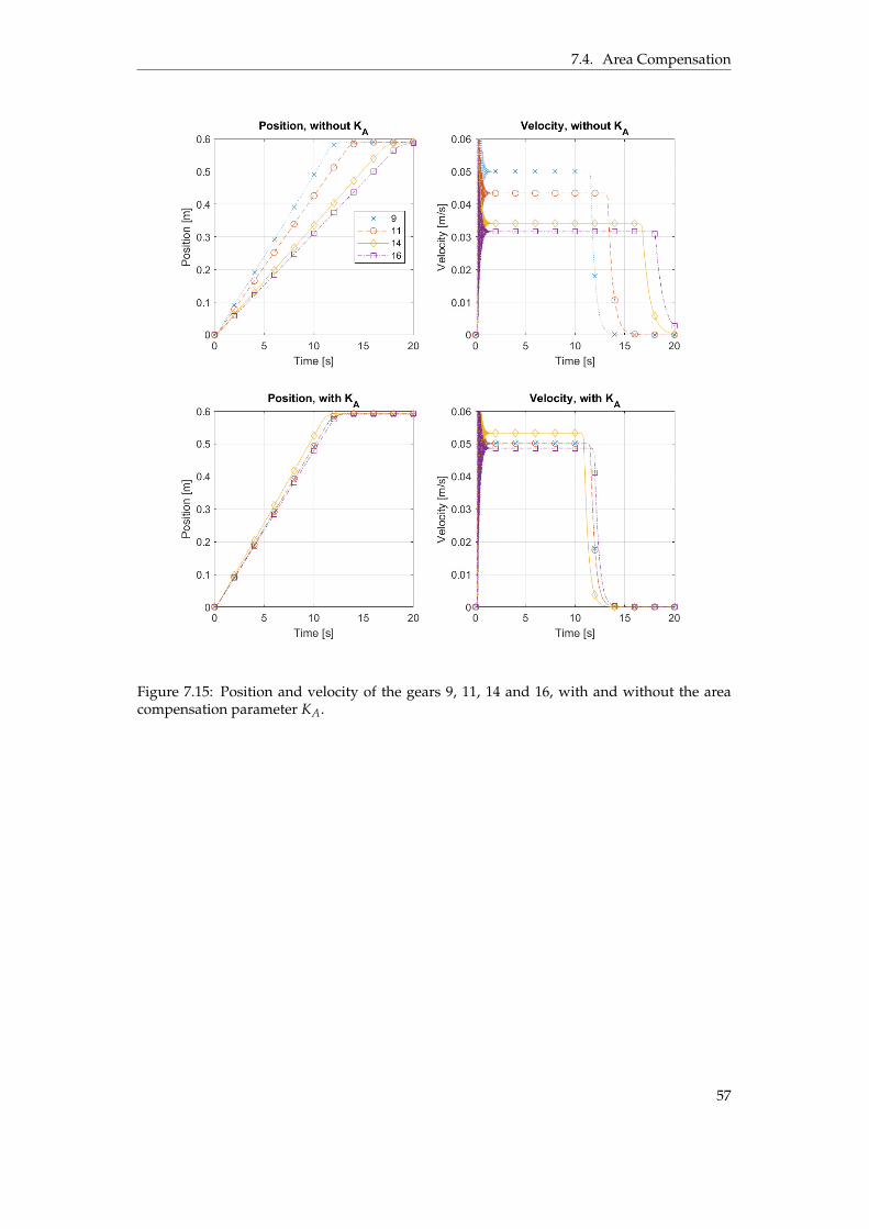
7.4. Area Compensation
Figure 7.15: Position and velocity of the gears 9, 11, 14 and 16, with and without the areacompensation parameter KA.
57
8 Discussion
Discussion of the validation of system model, the Reinforcement Learning method, resultsand the PV controller adjustments is treated in this chapter.
8.1 Validation
The validations gave a model that follows the physical system good. The deviation betweenthe simulation and the measurement remained small for all test cases except from SC steptest.
The PV was validated with closed ends and therefore the flow forces was easily neglected.This showed to be a problem when validating the cylinders as they are dependant of the flowfrom the PV and the flow did differ between small and large steps with the spool. Especiallywhen testing against a sine wave where the spool moves all the time. In hindsight it wouldbeen better to test steps/sines of the actuators and at the same time record the spool move-ment. That might be harder to validate as there are more parameters to tune but with theknowledge of them separately validated (which we now have) it should be possible. Mainlythe flow rate from the different ports should be tuned. Leakage between the ports within thePV have been seen to have an impact in the test data which was only accounted for betweenport A and B of the PV. There are still the P-T, A-T, B-T, P-A and P-B ports to consider.
SC was closely connected to MCs parameters since they were sharing the same spoolfraction parameters. These could been separated but was not for two reasons; The PV for SCand the PV for MC are identical and the dynamics of the SC model did only have a fractionof impact for this thesis and was therefore not prioritized. As mentioned above, if a secondround of model validation should be conducted where the flow over the PV is accounted forthis could greatly increase its precision.
8.2 Position Control
In both figure 7.1 and 7.2 the simulation model and the real system doesn’t corresponds thatgood. For an extension movement is it quite close, but not for retraction. This is becausethe models parameters are tuned to match a step of the PV (i.e. using the same gear butchanging direction of the PV). The PV have different flow rates for different ports, causing
58
8.3. Enabling Control
this difference in movement depending on PV position. On the other side, this means thatthe agent could still learn even though the model isn’t perfect and therefore it has managedto generalize, which can be seen in both real test cases. The agent performs rather good andreaches the reference in each case. For the case when the PV is held 50% open, it closes thevalves too early in some cases but adjusts by open and close quickly a brief moment later,seen in 7.2.
Setting the PV at 50% open, resulted in some fast spike gear selection for the physicalsystem, which fine-tuned the position to be closer to the reference signal. This did not happenfor the simulated version. Probably because of the integrated error: since the real systemmoved slower the integrated error increased faster which indicated that it needed to movefurther. Running the simulation longer would give time build up this value and eventuallydo the adjustment.
The position control when the PV is set at opposite direction reverses the direction for thegears. From the simulation, figure 7.3, the agent still manage to follow the reference signal.The expected results was to select action 3 at all times. This was true initially, but after a fewseconds the agent reverses the actions and followed the reference. One possible explanationto this is the integrated error. When the agent observes a positive integrated error, the bestaction is to select action 1, and a negative observation select action 3. This value is to becompared to the position error. Initially the error was large, resulting in some time before theintegrated error was large enough to overrule this decision. The tuning spikes later in thesimulation did not have to wind up for too long since the position error was small (the dropof the integrated value to zero is because of the included reset function).
The sine wave simulation test behaved as one could expect. The agent works as a discretecontroller, three discrete actions, it would be hard to follow a continuously changing refer-ence. Although it switched extremely often it shows that it "understands" what it is supposedto do even thought it has never experienced a moving reference, not even a simple step.
Reward function
During the development of the reward function for the position control, the RDirection func-tion, equation (6.1), contributed the most for an efficient training. This condition penalizesthe agent while it is not actively moving towards the reference by comparing the sign of theerror and velocity. This gave the agent an instant feedback and it quickly learned whetherit was choosing the right action. Once this condition was implemented the agent started tograsp the task after 15 instead of 150´ 200 episodes witch were the case before, the resultingagent also performed noticeably better.
The RDirection in position control was a good example of how direct feedback makes iteasier for agents to learn. Using some direct feedback to learn the basics and then delayedrewards for more sophisticate tasks.
8.3 Enabling Control
During the 80 kg tests the agent choose more or less the same action in simulation environ-ment and test. Comparing the observations from tests and simulations one can see that theyare much more similar than for the heavier load case. This might be the load function not ac-counting for heavier loads good enough. The pressures are similar but the largest differenceis seen when changing the flow rate from the PV, which affects the velocity and accelerationwhich in turn is the input for the load function. This does of course affect the system as awhole too, which makes it hard to define the root of the problem.
The reason why the agent takes different actions compared to the simulation test is thatthe decision taken depends on the observation at that time step, and there are differencesbetween the simulation environment and the test rig. A safety function is used where allDVs are closed once the reference is reached. This will result in a trapped pressure inside
59
8.3. Enabling Control
the previously active chambers of the MC. Since the pressures are observed, this trappedpressure will affect the next decision. This could explain why different gears are chosen.For an example could there be 70 bar pressure in chamber B in simulation while there is nopressure during the test. This difference in observation is large, which could result in differentactions.
Dynamics from the load plays an important role as it affects the behaviour of the systemsignificantly. It induces more oscillations which changes the pressures in active chambersas well as changes the P-controller to oscillate if the position is close to reference. The loaddynamics difference is clearly shown in figure 7.5 and 7.9.
In figure 7.9 and 7.10 there are some unnecessary/uncontrolled switching taking place ataround 30 seconds. It is hard to say exactly what trigger those decision since the pressuresare dependant on the active gear and the oscillations that started due to the gear switch. Ifthe cylinder position changes, the P-controller will try to compensate for that, which in turnchanges the observations as well.
The agent perform well on the sine wave test for the 80 kg load case, almost identical to thesimulation, see figure 7.7 and 7.8. For the 200 kg load case it didn’t perform as well, it seemsto be a combination of a heavier load which gives higher inertia along with a poorly tunedP-controller. These two in combination seems to start the oscillations. If a PI-controller wouldbe implemented the issue might been avoided but it wasn’t prioritized due to the simulationtests gave good results when tested. The over-all performance is good, considering that theagent had never experienced a moving references during a training episodes.
An agent was tested to be trained on sine waves but with worse result than the agentused for these tests. Most likely was it hard to grasp how to cooperate with the P-controller.The reward function as well as the P-controller could need some development for such case.Alternative for a more successful training could be to only observe the P-controllers signalbefore is compensated (due to velocity and gears). Or use a PI-controller which would softenthe movement.
Reward Function
The velocity penalty is a discrete function which activates if the cylinder is moving too slowdepending on how much the PV is open. This function and the power loss function formeda good combination where the agent had to move fast enough but at the same time use thelowest possible gear. The velocity function was only tuned by measuring the velocity of theslowest gear (16), for simplicity.
The power loss function only accounts for the pressure drop and flow over the PV. How-ever, when using gears that have a direct connection to tank there are losses due to suction ofoil from tank. For a more realistic power loss function these needs to be included.
The switch counter penalty are accumulating for each gear switch that takes place, tellingthe agent to switch as few times as possible during training. The back side of this approachis that lots of switching in the beginning of an episode will result in a higher accumulatedpenalty than for lots of switches towards the end of the episode. An alternative is to give afinal reward at the end of the simulation based on the total number of switches. The backsideof this could result in a training where the agent doesn’t want finalize the episode, if it onlyconsider ending the simulation with a penalty instead of associating it with the actual reason;the amount of switches. Another approach would be to use the switch counter as it is butimplement a decay rate that reduced the penalty gradually after a set time, this would evenout the penalty and it might be easier to grasp for the agent.
Implementing our knowledge can guide the agent to learn quicker. For instance, knowingthat a lower gear is better and faster. There is no point in letting the agent figure that out. Animportant difference is to tell the agent what to do and not how to do it. Already known factscould most likely be implement manually as a rule based controller.
60
8.4. Agent Settings
The reward function is how you as a developer communicates with the agent and to dothat you have to understand how the algorithms works, how good it is to exploit poorly de-fined reward function etc. At the same time the reward function should not be too detailed,as said before, how to solve the task is what the agent should learn, in that way we canlearn from it. More difficult problems of gear switching are when the system (environment)have multiple actuators and controllers, varying system pressure which is not included inthis work. It seems to work well by using Graded Learning so this technique would be recom-mended when trying to tackle a more complex environment and task. Also how the actualswitching sequence between two gears could be optimized to minimize the drop that occursdue to gravity and connecting depressurized chambers to pressurized ones.
8.4 Agent Settings
There are many parameters to consider for tuning: all hyperparameters in the DQN-agent,construction and size of the neural network and reward function. Since the goal was to de-velop an agent that worked, details in these parts was not analyzed, instead parts that workedwere built upon. A structured analysis was not carried out, but could be a way of optimizingthe agent. The size of the network (the agents critic) is also an important aspect for the realtime implementation, where a smaller one requires less computational power.
We used a rather large network for the position control which worked good(7x256x256x3). This network was later diminished for the gear switch case to 8x256x128x4and could most likely be reduced further but due to lack of experience, lots of differentsettings to try out and time it wasn’t researched further.
8.5 Energy Consumption Comparison
As mentioned earlier, the most representative case is the heavier case, figure 7.13, wherethe cylinders velocity is almost the same during the full stroke. Most of the performance isthe same but with some smaller position drops due to gear switching. The result of almost30% efficiency is promising result for the MC and digital hydraulics-systems, however thetest case was conduced as a constant pressure system and not a load sensing system. For asystem with one actuator, a load sensing architecture is enough for a high efficiency. Used ina system with multiple actuators, where the MC doesn’t affect the system pressure, is wherethe large energy savings can be made.
The smaller load case, figure 7.14, has about 70% better efficiency which is impressive.It is partly due to the fact that it finishes the stroke earlier, but even if the two cases wouldreach the reference at the same time the agents case would be more efficient. The power lossover the PV for the agents case is always about half of the manual case. It might not be afair comparison since it’s obvious that a smaller area for a small gear will result in a betterefficiency compared to an oversized one. But if a system would been designed one wouldneed to design it to handle the heaviest case, which justifies these results some.
This comparison does only account for the pressure drop and flow through the PV con-nected to the DV block. Other losses for a DV-block/MC like switching and leakages are notaccounted for. But since the comparison is made for the same component it should be seen asrepresentative since the efficiency is notable!
8.6 Area Compensation
The parameter KA to adjust the proportional gain works good. Without this the velocitiesdiffers from 0.04 m/s for the weakest gear to 0.025 m/s for the strongest. The compensationmade the velocities differs between 0.05 m/s and 0.03 m/s. For the same input reference the
61
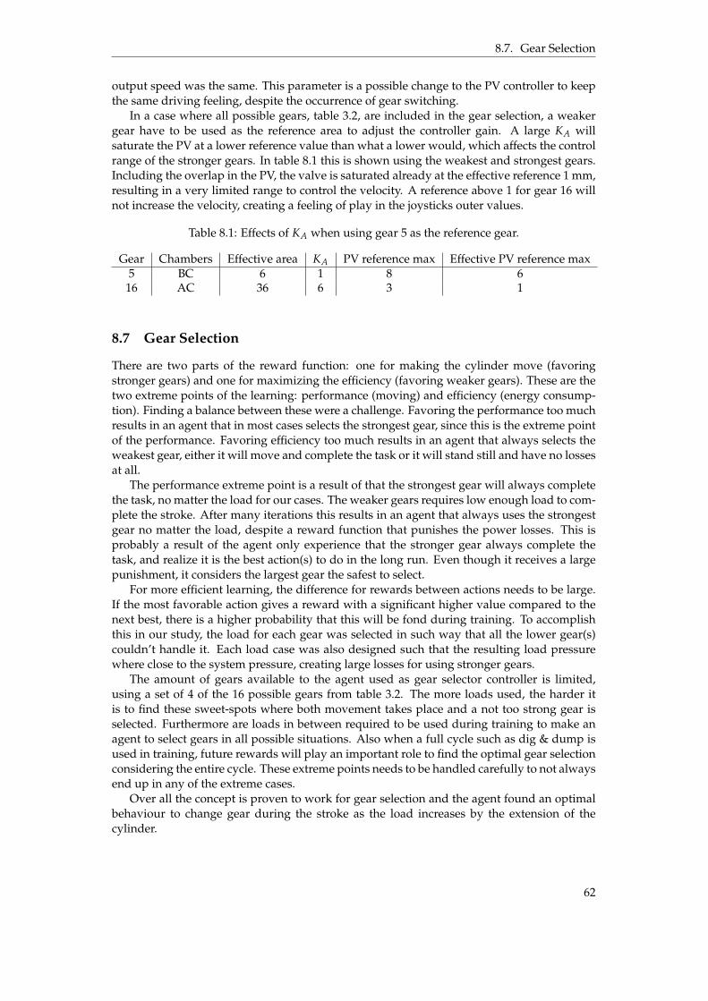
8.7. Gear Selection
output speed was the same. This parameter is a possible change to the PV controller to keepthe same driving feeling, despite the occurrence of gear switching.
In a case where all possible gears, table 3.2, are included in the gear selection, a weakergear have to be used as the reference area to adjust the controller gain. A large KA willsaturate the PV at a lower reference value than what a lower would, which affects the controlrange of the stronger gears. In table 8.1 this is shown using the weakest and strongest gears.Including the overlap in the PV, the valve is saturated already at the effective reference 1 mm,resulting in a very limited range to control the velocity. A reference above 1 for gear 16 willnot increase the velocity, creating a feeling of play in the joysticks outer values.
Table 8.1: Effects of KA when using gear 5 as the reference gear.
Gear Chambers Effective area KA PV reference max Effective PV reference max5 BC 6 1 8 6
16 AC 36 6 3 1
8.7 Gear Selection
There are two parts of the reward function: one for making the cylinder move (favoringstronger gears) and one for maximizing the efficiency (favoring weaker gears). These are thetwo extreme points of the learning: performance (moving) and efficiency (energy consump-tion). Finding a balance between these were a challenge. Favoring the performance too muchresults in an agent that in most cases selects the strongest gear, since this is the extreme pointof the performance. Favoring efficiency too much results in an agent that always selects theweakest gear, either it will move and complete the task or it will stand still and have no lossesat all.
The performance extreme point is a result of that the strongest gear will always completethe task, no matter the load for our cases. The weaker gears requires low enough load to com-plete the stroke. After many iterations this results in an agent that always uses the strongestgear no matter the load, despite a reward function that punishes the power losses. This isprobably a result of the agent only experience that the stronger gear always complete thetask, and realize it is the best action(s) to do in the long run. Even though it receives a largepunishment, it considers the largest gear the safest to select.
For more efficient learning, the difference for rewards between actions needs to be large.If the most favorable action gives a reward with a significant higher value compared to thenext best, there is a higher probability that this will be fond during training. To accomplishthis in our study, the load for each gear was selected in such way that all the lower gear(s)couldn’t handle it. Each load case was also designed such that the resulting load pressurewhere close to the system pressure, creating large losses for using stronger gears.
The amount of gears available to the agent used as gear selector controller is limited,using a set of 4 of the 16 possible gears from table 3.2. The more loads used, the harder itis to find these sweet-spots where both movement takes place and a not too strong gear isselected. Furthermore are loads in between required to be used during training to make anagent to select gears in all possible situations. Also when a full cycle such as dig & dump isused in training, future rewards will play an important role to find the optimal gear selectionconsidering the entire cycle. These extreme points needs to be handled carefully to not alwaysend up in any of the extreme cases.
Over all the concept is proven to work for gear selection and the agent found an optimalbehaviour to change gear during the stroke as the load increases by the extension of thecylinder.
62
8.8. Unsuccessful Tries
8.8 Unsuccessful Tries
Originally the position controller was intended to include multiple extension gears andtrained using different loads, to learn it to select an optimal gear for the given load. Dueto unsuccessful tries in simulation this idea were abandoned, in favor for the work of usingthe agent as the enabler together with an P-controller.
A problem we faced were that the agent always favored the stringest gear, no matter theexternal load. By averaging the reward and learning it most likely realized that no matter thecase, the strongest gear would complete the task. When the power loss reward function wassuccessfully implemented this was finally solved.
Power losses during gear switch is a known problem for MCs. The gear switching pro-cedure is not in the scope of this thesis, but different reward functions have been used tominimize the number of switching, i.e. reduce unnecessary switching. One way is to use atime constraint, the agent have to keep the same gear for some time before it receives rewardsfor a positive actions.
8.9 Multi-Agent Application
As mentioned earlier, the gear switching was not investigated in this study. As this is adifficult task, where the number of possible ways of changing gear are large as well as includedifferent opening timings between valves to keep the switching losses to a minimum. Thismight be a task for another agent, where the agent in this work controls which valves to openand close in between a gear switch.
In [20] an agent was trained to do the full movement of an excavator. Using this in com-bination with this agent could result in even better efficiency. This would mean that a pre-defined path is calculated, and possibility to optimize the gear selection depending on that(instead of just consider the current load). This combination gives the possibility to plan thegear selection, both what gear and when to do the switch.
63
9 Conclusion
Reinforcement learning is easy to play around with and is a completely different approachto develop control systems compared to conventional methods. But time and experience areneeded to create well defined reward functions, choose correct observations and setting upthe simulation for each episode. Knowledge of how the algorithm works such as experiencebuffer, back propagation for the neural network and much more is needed for more sophisti-cated problems. This technique offers another take on control problems that are hard to defineor solve, and could be used as a compliment in a larger control system where the agent con-trols specific hard parts while known control theory is used for their specific problems. Anagents decision should be constrained by some safety measurements since it’s hard to predictwhat the decision will be for all cases.
9.1 Research Questions
• How can Reinforcement Learning be used for gear selection to improve the energyefficiency while maintain the performance of a hydraulic system with a hydraulicforce gearbox?By training a DQN Agent in simulation environment, it managed to learn which gear touse depending on the load. Selection of a gear that is strong enough keeps the systemperformance while allowing weaker gears reduces the losses. Due to the DQN Agentsgeneralization it was possible to implement this in the real world test rig with similarperformance as the simulation.
• How shall the training process of a Reinforcement Learning model be performed fora hydraulic force gearbox system?The Agent was successfully trained by using Graded Learning, where the complexity ofthe environment and the task was increased step wise. This also included the rewardfunction which is an important aspect to find the balance between performance andefficiency. The reward function and task should explain what to do, not how to do it.
• What changes are needed for the control of the proportional valve to maintain thesame system performance?The control of the proportional valve needs some adjustment to maintain a good drivers
64
9.2. Future Work
feeling. As the different gears have different areas which will result in different veloc-ities for the same flow. Therefore are different flow rates needed to keep the same ve-locity. Introducing a scaling factor, KA, can make the the same reference signal result inthe same velocities for the different gears.
9.2 Future Work
This thesis have showed that the concept works: a Reinforcement Learning agent can learnto select the right gear for a given load and be implemented in a real system. The number ofgears used have been limited to four. For a wider operation range, more of the 16 gears needsto be included in the training process. Also continue the training with more advanced loadcycles, based on real world operations, needs to be made. This will make the decision makingeven closer to the global optimum. This can also be validated using a Dynamic Programmingsimulation.
A thorough sensitivity analysis of the agents observations should be conducted to gainmore knowledge of how they affect its decisions. Some observations might be unnecessaryand therefor could either be removed or replaced. This would also be a good approach tovalidate the agents robustness.
The switch between two gears could need some improvement since there will be positiondrop when switching, especially when activate or deactivate chamber MA or MC. Using arule based controller or train an agent to find a suitable gear switch sequence could improvethe performance and controllability.
The agent have not been introduced to a load sensing system, different constant pressureshave been used during training. However, the agent have not experienced situations wherethe system pressure depends on the selected gear. The agent will in this case experiencetwo different scenarios: constant system pressure when the single chamber cylinder sets thesystem pressure, or the system pressure depends in the gear when the multi chamber cylindersets the system pressure.
The adjustable gain for the control of the proportional valve also needs to be validatedusing as real system. In simulations the velocities are kept the same for the same reference,but if this will achieve a good drivers feeling for the physical system is not validated. Usinga real joystick and an experienced driver are needed for validation as drivers feeling is hardto measure.
65
Bibliography
[1] Henrique Raduenz, Liselott Ericson, Kim Heybroek, Victor J. De Negri, and Petter Krus.“Improving the efficiency of valve-controlled systems by using multi-chamber actua-tors”. In: The 17th Scandinavian International Conference on Fluid Power (2021). Sweden,Linköping.
[2] Alessandro Dell’Amico, Marcus Carlsson, Erik Norlin, and Magnus Sethson. “Inves-tigation of a Digital Hydraulic Actuation System on an Excavator Arm”. In: The 13thScandinavian International Conference on Fluid Power (2013). Sweden, Linköping.
[3] A. Harrison and D. Stoten. “Generalized finite difference methods for optimal esti-mation of derivatives in real-time control problems”. In: Journal of systems and control(1995).
[4] M. Vukovic, R. Leifeld, and H. Murrenhoff. “Reducing Fuel Consumption in HydraulicExcavators - A Comprehensive Analysis”. In: Energies 2017, 10, 687 (2017).
[5] Damiano Padovani, Massimo Rundo, and Gabriele Altare. “The Working Hydraulics ofValve-Controlled Mobile Machines: Classification and Review”. In: Journal of DynamicSystems, Measurement, and Control. July Vol. 142 (2020).
[6] Zimmerman J. D., M. Pelosi, C. A. Williamson, and S. Anwar. “Energy Consumption ofan LS Excavator Hydraulic System”. In: ASME Paper No. IMECE2007-42267 (2007).
[7] V.H. Donkov, T.O. Andersen, M Linjama, and M.K. Ebbesen. “Digital Hydraulic Tech-nology for Linear Actuation: A State of the Art Review”. In: International Journal of FluidPower, Vol 21_2 (2020).
[8] Linjama M, Vihtanen H-P, Sipola A, and Vilenius M. “Secondary Controlled Multi-Chamber Hydraulic Cylinder”. In: The 11th Scandinavian International Conference onFluid Power (June 2009). Sweden, Linköping.
[9] Qian Zhu and Qing-feng Wang. “Real-time energy management controller design fora hybrid excavator using reinforcement learning”. In: Journal of Zhejiang University-SCIENCE A (Applied Physics & Engineering) (2017).
[10] Richard.S. Sutton and Andrew.G. Barto. Reinforcement Learning, An Introduction - secondedition. The MIT Press, 2018.
[11] Wikimedia Commons. Reinforcement Learning Diagram. 2021-03-24. URL: https://en.wikipedia.org/wiki/Reinforcement%5C_learning.
66
Bibliography
[12] Rajesh Siraskar. Reinforcement Learning for Control of Valves. 2021.
[13] MathWorks. Reinforcement Learning Agents. URL: https://se.mathworks.com/help/reinforcement-learning/ug/create-agents-for-reinforcement-learning.html. (accessed: 03.19.2021).
[14] Melrose Roderick, James MacGlashan, and Stefanie Tellex. “Implementing the DeepQ-Network”. In: 30th Conference on Neural Information Processing Systems (2016). Spain,Barcelone.
[15] Volodymyr Mnih, Koray Kavukcuoglu, David Silver, Alex Graves, Ioannis Antonoglou,Daan Wierstra, and Martin Riedmiller. “Playing Atari with Deep Reinforcement Learn-ing”. In: DeepMind Technologies (2013).
[16] MathWorks. Deep Q-Network Agents. URL: https://se.mathworks.com/help/reinforcement-learning/ug/dqn-agents.html. (accessed: 03.22.2021).
[17] S. Dadhich, U. Bodin, F. Sandin, and U. Andersson. “Machine Learning approach toAutomatic Bucket Loading”. In: 24th Mediterranean Conference on Control and Automation(MED) (2016).
[18] S. Dadhich, U. Bodin, and U. Andersson. “Key challenges in automation of earth-moving machines”. In: Automation on Construction 68 (2016).
[19] S. Backman, D. Lindmark, K. Bodin, M. Servin, J. Mörk, and H. Löfgren. “Continuouscontrol of an underground loader using deep reinforcement learning”. In: (2021).
[20] H. Kurinov, G. Orzechowski, P. Hämäläinen, and A. Mikkola. “Automated ExcavtorBased on Reinforcement Learning and Multibody System Dynamics”. In: IEEE Access2020 Vol 8 (2020).
[21] B.J. Hodel. “Learning to Operate an Excavator via Policy Optimization”. In: ComplexAdaptive Systems Conference with Theme: Cyber Physical Systems and Deep Learning (2018).
[22] T. Li, Y. Zou, D. Liu, and F. Sun. “Reinforcement Learning of Adaptive Energy Manage-ment With Transition Probability for a Hybrid Electric Tracked Vehicle”. In: Transactionson Industrial Electronics (2015).
67