
Do Intermittent Renewables Threaten the Electricity Supply ...
Upload
khangminh22Category
view
0download
0
Thès
e de
doc
tora
tNNT:2020UPA
SG011
Control of AC/DC Microgridswith Renewables in the Context
of Smart GridsIncluding Ancillary Services and Electric Mobility
Thèse de doctorat de l’Université Paris-Saclay etUNIFEI
École doctorale n 580, Sciences and Technologies ofInformation and Communication (STIC)
Spécialité de doctorat: AutomatiqueUnité de recherche: Université Paris-Saclay, CNRS, CentraleSupélec,Laboratoire des signaux et systèmes, 91190, Gif-sur-Yvette, France
Référent: CentraleSupélec
Thèse présentée et soutenue en visioconférence totale, le 28septembre 2020, par
Filipe PEREZ
Composition du jury:
Antonio Carlos Zambroni de Souza PrésidentProfesseur, Université Fédérale d’ItajubáDidier Georges Rapporteur & ExaminateurProfesseur, Grenoble INP Institut d’ingénierie (GIPSA)Glauco Nery Taranto Rapporteur & ExaminateurProfesseur, Université Fédérale de Rio de Janeiro (COPPE)William Pasillas-Lépine ExaminateurChercheur (HDR), CNRS, Université Paris-Saclay (L2S)Pedro Machado de Almeida ExaminateurProfesseur, Université Fédérale de Juiz de ForaBenedito Donizeti Bonatto InvitéProfesseur, Université Fédérale d’Itajubá
Françoise Lamnabhi-Laguarrigue DirectriceDirecteur de recherche, Université Paris-Saclay (L2S)Paulo Fernando Ribeiro DirecteurProfesseur, Université Fédérale d’ItajubáGilney Damm CoencadranteMaître de conférences, Université Paris-Saclay (IBISC)


AcknowledgmentsFirst, I would like to thank God for giving me life, good experiences, and for
giving me the ability to do this work.
I would like to thank my supervisors Dr. Françoise Lamnabhi-Lagarrigue, Dr.Gilney Damm and Dr. Paulo Ribeiro for the guidance and learning during thethesis period. Françoise, thank you for the opportunity to be part of this excellentteam. Gilney, thank you for the excellent guidance in technical issues and personalfriendship. Paulo, thank you again for helping me improve.
Thank you, the members of the jury for accepting this mission and spendingyour time to make this thesis much better, providing detailed and consistentrecommendations, suggestions and corrections.
I want to thank L2S Laboratory for the thesis subject and for the peoplecompany during the first two years of the thesis, especially Paulo, Hidayet, Fernando,Abdelkrim, João, Janailson, Juan, Sabah, João Neto, Kuba, Raul and Maryvonne.Thank you Guacira for your friendship in the laboratory during working and restingdays, and for your help with softwares and simulations.
I would like to thank Efficacity for the partnership during the thesis progression,specially to Alessio for the fruitful discussions and for mentoring in control area, andto Lilia for the support. I also would like to thank Erasmus Mundus Programme onSMART2 Project for the scholarship.
I want to thank the friendships I made in Paris and for being with me in momentsof relaxation. I also thank the power systems team from Lactec Institute for thesupport in the last years of the thesis.
Finally, to my wife Rafaela, I cannot describe how your support was importantto me. Thank you for being there for me in all bad and great moments of my life.Also, I want to thank my family, especially my father Ulisses, my mother Ivani andmy sister Talita, for the love and support, for helping me even with the distanceand difficulties of life.
Filipe PEREZSeptember, 2020
i


ContentsAcknowledgments i
Contents iii
List of Tables vii
List of Figures ix
Abstract xix
Résumé xxi
Resumo xxiii
1 General Introduction 11.1 Context . . . . . . . . . . . . . . . . . . . . . . . . . . . . . . . . . . . . . . . . . 1
1.1.1 Renewable energy sources . . . . . . . . . . . . . . . . . . . . . . . . . . 21.1.2 Energy storage systems . . . . . . . . . . . . . . . . . . . . . . . . . . . . 4
1.2 Microgrids . . . . . . . . . . . . . . . . . . . . . . . . . . . . . . . . . . . . . . . . 51.2.1 Hierarchical structure . . . . . . . . . . . . . . . . . . . . . . . . . . . . . 8
1.3 Ancillary Services . . . . . . . . . . . . . . . . . . . . . . . . . . . . . . . . . . . . 101.4 Thesis Contribution . . . . . . . . . . . . . . . . . . . . . . . . . . . . . . . . . . 131.5 Thesis Outcomes . . . . . . . . . . . . . . . . . . . . . . . . . . . . . . . . . . . . 15
2 Microgrid Overview 172.1 Introduction . . . . . . . . . . . . . . . . . . . . . . . . . . . . . . . . . . . . . . . 17
2.1.1 General review . . . . . . . . . . . . . . . . . . . . . . . . . . . . . . . . . 172.1.2 Supervision and optimal operation . . . . . . . . . . . . . . . . . . . . . 192.1.3 Microgrid examples . . . . . . . . . . . . . . . . . . . . . . . . . . . . . . 22
2.2 Classification and Stability . . . . . . . . . . . . . . . . . . . . . . . . . . . . . . . 252.3 DC Microgrids . . . . . . . . . . . . . . . . . . . . . . . . . . . . . . . . . . . . . 31
2.3.1 Droop control strategies . . . . . . . . . . . . . . . . . . . . . . . . . . . 342.4 AC Microgrids . . . . . . . . . . . . . . . . . . . . . . . . . . . . . . . . . . . . . 362.5 Conclusions . . . . . . . . . . . . . . . . . . . . . . . . . . . . . . . . . . . . . . . 43
3 The Microgrid Components 453.1 Introduction . . . . . . . . . . . . . . . . . . . . . . . . . . . . . . . . . . . . . . . 453.2 Microgrid Components . . . . . . . . . . . . . . . . . . . . . . . . . . . . . . . . . 46
3.2.1 Photovoltaic panels . . . . . . . . . . . . . . . . . . . . . . . . . . . . . . 46
iii

Contents
3.2.2 Energy storage systems . . . . . . . . . . . . . . . . . . . . . . . . . . . . 523.2.3 Braking energy recovery system . . . . . . . . . . . . . . . . . . . . . . . 633.2.4 Local loads . . . . . . . . . . . . . . . . . . . . . . . . . . . . . . . . . . . 673.2.5 Grid-connection . . . . . . . . . . . . . . . . . . . . . . . . . . . . . . . . 68
3.3 Proposed Microgrid Design . . . . . . . . . . . . . . . . . . . . . . . . . . . . . . 683.3.1 Power converters configuration . . . . . . . . . . . . . . . . . . . . . . . . 713.3.2 Sizing of DC/DC converters . . . . . . . . . . . . . . . . . . . . . . . . . 73
3.4 Conclusions . . . . . . . . . . . . . . . . . . . . . . . . . . . . . . . . . . . . . . . 74
4 Control Strategy 774.1 Introduction . . . . . . . . . . . . . . . . . . . . . . . . . . . . . . . . . . . . . . . 77
4.1.1 Model introduction . . . . . . . . . . . . . . . . . . . . . . . . . . . . . . 784.2 Supercapacitor Subsystem . . . . . . . . . . . . . . . . . . . . . . . . . . . . . . . 79
4.2.1 Supercapacitor model . . . . . . . . . . . . . . . . . . . . . . . . . . . . . 804.2.2 Non-minimum phase problem . . . . . . . . . . . . . . . . . . . . . . . . 804.2.3 Control induced time-scale separation . . . . . . . . . . . . . . . . . . . . 824.2.4 Supercapacitor control application . . . . . . . . . . . . . . . . . . . . . . 864.2.5 Zero dynamics analysis . . . . . . . . . . . . . . . . . . . . . . . . . . . . 874.2.6 Reference calculation . . . . . . . . . . . . . . . . . . . . . . . . . . . . . 89
4.3 Battery Subsystem . . . . . . . . . . . . . . . . . . . . . . . . . . . . . . . . . . . 914.3.1 Battery model . . . . . . . . . . . . . . . . . . . . . . . . . . . . . . . . . 924.3.2 Feedback linearization . . . . . . . . . . . . . . . . . . . . . . . . . . . . 934.3.3 Zero dynamics analysis . . . . . . . . . . . . . . . . . . . . . . . . . . . . 94
4.4 PV Array Subsystem . . . . . . . . . . . . . . . . . . . . . . . . . . . . . . . . . . 954.4.1 PV array model . . . . . . . . . . . . . . . . . . . . . . . . . . . . . . . . 964.4.2 Feedback linearization . . . . . . . . . . . . . . . . . . . . . . . . . . . . 964.4.3 Zero dynamics analysis . . . . . . . . . . . . . . . . . . . . . . . . . . . . 97
4.5 DC Load Subsystem . . . . . . . . . . . . . . . . . . . . . . . . . . . . . . . . . . 984.5.1 DC load model . . . . . . . . . . . . . . . . . . . . . . . . . . . . . . . . 984.5.2 Backstepping control . . . . . . . . . . . . . . . . . . . . . . . . . . . . . 994.5.3 Zero dynamics analysis . . . . . . . . . . . . . . . . . . . . . . . . . . . . 101
4.6 Regenerative Braking Subsystem . . . . . . . . . . . . . . . . . . . . . . . . . . . 1024.6.1 Regenerative braking model . . . . . . . . . . . . . . . . . . . . . . . . . 1034.6.2 Regenerative braking control application . . . . . . . . . . . . . . . . . . 1044.6.3 Zero dynamics analysis . . . . . . . . . . . . . . . . . . . . . . . . . . . . 1054.6.4 Reference calculation . . . . . . . . . . . . . . . . . . . . . . . . . . . . . 106
4.7 AC Grid-Connection . . . . . . . . . . . . . . . . . . . . . . . . . . . . . . . . . . 1074.7.1 AC grid model . . . . . . . . . . . . . . . . . . . . . . . . . . . . . . . . . 1074.7.2 Feedback linearization . . . . . . . . . . . . . . . . . . . . . . . . . . . . 1094.7.3 Zero dynamics analysis . . . . . . . . . . . . . . . . . . . . . . . . . . . . 1094.7.4 PLL synchronization . . . . . . . . . . . . . . . . . . . . . . . . . . . . . 110
4.8 System Interconnection . . . . . . . . . . . . . . . . . . . . . . . . . . . . . . . . . 1114.8.1 The DC bus . . . . . . . . . . . . . . . . . . . . . . . . . . . . . . . . . . 1114.8.2 Hierarchical control structure . . . . . . . . . . . . . . . . . . . . . . . . 1124.8.3 Preliminaries . . . . . . . . . . . . . . . . . . . . . . . . . . . . . . . . . . 1134.8.4 Stability analysis . . . . . . . . . . . . . . . . . . . . . . . . . . . . . . . 113
iv

Contents
4.9 Simulation Results . . . . . . . . . . . . . . . . . . . . . . . . . . . . . . . . . . . 1204.9.1 The proposed nonlinear control . . . . . . . . . . . . . . . . . . . . . . . 1214.9.2 A control comparison: Linear vs Nonlinear . . . . . . . . . . . . . . . . . 1294.9.3 Robustness . . . . . . . . . . . . . . . . . . . . . . . . . . . . . . . . . . . 133
4.10 Different Approaches for DC Bus Control . . . . . . . . . . . . . . . . . . . . . . 1354.10.1 Fixed reference for VC2 . . . . . . . . . . . . . . . . . . . . . . . . . . . . 1354.10.2 Simplification on C2 dynamics . . . . . . . . . . . . . . . . . . . . . . . . 1424.10.3 DC bus generalization: Thévenin equivalent . . . . . . . . . . . . . . . . 143
4.11 Conclusions . . . . . . . . . . . . . . . . . . . . . . . . . . . . . . . . . . . . . . . 148
5 Ancillary Services for AC Microgrids 1515.1 Chapter Introduction . . . . . . . . . . . . . . . . . . . . . . . . . . . . . . . . . . 1515.2 Power System Stability . . . . . . . . . . . . . . . . . . . . . . . . . . . . . . . . . 151
5.2.1 Frequency stability and control . . . . . . . . . . . . . . . . . . . . . . . 1535.2.2 Voltage stability and control . . . . . . . . . . . . . . . . . . . . . . . . . 160
5.3 Ancillary Services in Brazil . . . . . . . . . . . . . . . . . . . . . . . . . . . . . . 1645.4 Power Converters Issues . . . . . . . . . . . . . . . . . . . . . . . . . . . . . . . . 168
5.4.1 Inertial response and low inertia issues . . . . . . . . . . . . . . . . . . . 1715.4.2 Frequency problems in weak power systems . . . . . . . . . . . . . . . . 172
5.5 Virtual Inertia . . . . . . . . . . . . . . . . . . . . . . . . . . . . . . . . . . . . . . 1735.5.1 Virtual inertia topologies . . . . . . . . . . . . . . . . . . . . . . . . . . . 1765.5.2 Weak grid modelling . . . . . . . . . . . . . . . . . . . . . . . . . . . . . 1825.5.3 Proposed virtual inertia . . . . . . . . . . . . . . . . . . . . . . . . . . . 1835.5.4 Droop control strategy . . . . . . . . . . . . . . . . . . . . . . . . . . . . 1845.5.5 Stability analysis . . . . . . . . . . . . . . . . . . . . . . . . . . . . . . . 1855.5.6 Simulation results . . . . . . . . . . . . . . . . . . . . . . . . . . . . . . . 1875.5.7 Isolated operation . . . . . . . . . . . . . . . . . . . . . . . . . . . . . . . 1895.5.8 Dynamics of the DC Microgrid . . . . . . . . . . . . . . . . . . . . . . . 193
5.6 Adaptive Virtual Inertia Formulation . . . . . . . . . . . . . . . . . . . . . . . . . 1955.6.1 Stability analysis . . . . . . . . . . . . . . . . . . . . . . . . . . . . . . . 1965.6.2 Simulation results . . . . . . . . . . . . . . . . . . . . . . . . . . . . . . . 1985.6.3 Comparison with droop control . . . . . . . . . . . . . . . . . . . . . . . 2015.6.4 Comparison of different inertia coefficients . . . . . . . . . . . . . . . . . 2035.6.5 Additional simulation results . . . . . . . . . . . . . . . . . . . . . . . . . 204
5.7 VSM with Voltage and Current Control . . . . . . . . . . . . . . . . . . . . . . . 2065.7.1 Active and reactive power control . . . . . . . . . . . . . . . . . . . . . . 2085.7.2 Virtual impedance . . . . . . . . . . . . . . . . . . . . . . . . . . . . . . 2085.7.3 Voltage and current control . . . . . . . . . . . . . . . . . . . . . . . . . 2095.7.4 Simulation results . . . . . . . . . . . . . . . . . . . . . . . . . . . . . . . 2115.7.5 Fixed voltage reference . . . . . . . . . . . . . . . . . . . . . . . . . . . . 2145.7.6 Parameters variation . . . . . . . . . . . . . . . . . . . . . . . . . . . . . 2155.7.7 Control strategy comparison . . . . . . . . . . . . . . . . . . . . . . . . . 216
5.8 Conclusions . . . . . . . . . . . . . . . . . . . . . . . . . . . . . . . . . . . . . . . 218
6 General Conclusions 2196.1 Main Results . . . . . . . . . . . . . . . . . . . . . . . . . . . . . . . . . . . . . . 222
v

Contents
6.2 Future Works . . . . . . . . . . . . . . . . . . . . . . . . . . . . . . . . . . . . . . 223
Bibliography 225
Appendix
G Appendix I 251G.1 Proportional Integral (PI) Controller . . . . . . . . . . . . . . . . . . . . . . . . . 251G.2 Park Transformation . . . . . . . . . . . . . . . . . . . . . . . . . . . . . . . . . . 256G.3 Input-to-State Stability . . . . . . . . . . . . . . . . . . . . . . . . . . . . . . . . . 257
H Appendix II - Résumé en Français 261H.1 Introduction . . . . . . . . . . . . . . . . . . . . . . . . . . . . . . . . . . . . . . . 261
H.1.1 Sources d’énergie renouvelables . . . . . . . . . . . . . . . . . . . . . . . 262H.2 Microgrids . . . . . . . . . . . . . . . . . . . . . . . . . . . . . . . . . . . . . . . . 263H.3 Services Système . . . . . . . . . . . . . . . . . . . . . . . . . . . . . . . . . . . . 267H.4 Contribution de la Thèse . . . . . . . . . . . . . . . . . . . . . . . . . . . . . . . . 269H.5 Conclusions Générales . . . . . . . . . . . . . . . . . . . . . . . . . . . . . . . . . 271H.6 Résultats Principaux . . . . . . . . . . . . . . . . . . . . . . . . . . . . . . . . . . 275H.7 Travaux Futurs . . . . . . . . . . . . . . . . . . . . . . . . . . . . . . . . . . . . . 276
vi

List of Tables1.1 Electric grid energy storage services. . . . . . . . . . . . . . . . . . . . . . . . . . . . 4
2.1 Categories of Microgrid control from communication perspective. . . . . . . . . . . . 262.2 Main issues in Control System Stability of Microgrids. . . . . . . . . . . . . . . . . . 292.3 Main issues in Power Supply and Balance Stability of Microgrids. . . . . . . . . . . . 302.4 Control techniques feature in DC Microgrids. . . . . . . . . . . . . . . . . . . . . . . . 372.5 Different application of power converters for AC Microgrids. . . . . . . . . . . . . . . 38
3.1 Different topologies of grid-connected photovoltaic systems. . . . . . . . . . . . . . . . 513.2 Energy storage systems classification according to the form of store energy. . . . . . . 533.3 Power converters configuration in the Microgrid. . . . . . . . . . . . . . . . . . . . . . 74
4.1 Microgrid parameters . . . . . . . . . . . . . . . . . . . . . . . . . . . . . . . . . . . . 1224.2 Gains’ parameters for the nonlinear controller. . . . . . . . . . . . . . . . . . . . . . . 123
5.1 Microgrid operation standard for frequency levels. . . . . . . . . . . . . . . . . . . . . 1735.2 Microgrid parameters . . . . . . . . . . . . . . . . . . . . . . . . . . . . . . . . . . . . 1875.3 The AC load power demand. . . . . . . . . . . . . . . . . . . . . . . . . . . . . . . . . 1885.4 The AC load power demand in isolated operation. . . . . . . . . . . . . . . . . . . . . 1905.5 The power demand in the AC load, considering the DC Microgrid dynamics. . . . . . 1935.6 The AC load power demand for two synchronous machines scenario. . . . . . . . . . . 204
G.1 Parameter gains of the linear Proportional-Integral (PI) controller. . . . . . . . . . . 256
vii


List of Figures1.1 The transformation of the distribution grid from a centralized generation to a
heterogeneous grid. . . . . . . . . . . . . . . . . . . . . . . . . . . . . . . . . . . . . . 31.2 Relation between energy density and power density for different ESS. . . . . . . . . . 51.3 A general DC Microgrid scheme. . . . . . . . . . . . . . . . . . . . . . . . . . . . . . . 81.4 The traditional hierarchical control structure for a Microgrid. The local and primary
control generate the references for lower level power converters, while the secondarycontrol deals with power flow regulation and the tertiary control covers the energydispatch and energy market. . . . . . . . . . . . . . . . . . . . . . . . . . . . . . . . . 9
1.5 The effect of the inertia reduction according to the renewable integration levels in thenetwork. . . . . . . . . . . . . . . . . . . . . . . . . . . . . . . . . . . . . . . . . . . . 11
1.6 Network evolution towards power converters’ systems. . . . . . . . . . . . . . . . . . . 11
2.1 A Microgrid composed of central control with hierarchical structure. . . . . . . . . . . 212.2 The classification of stability in Microgrids. . . . . . . . . . . . . . . . . . . . . . . . . 282.3 Conventional droop control scheme for multiple generations units in a DC Microgrid. 352.4 Local control loop in a Microgrid using VSC converter. . . . . . . . . . . . . . . . . . 392.5 Power converter control of a Microgrid applying virtual output impedance loop. . . . 41
3.1 Simplified model of photovoltaic panel. . . . . . . . . . . . . . . . . . . . . . . . . . . 473.2 Characteristic curve of PV, and curves for different irradiance and temperature values. 483.3 Control scheme of the MPPT algorithm. . . . . . . . . . . . . . . . . . . . . . . . . . 493.4 Incremental conductance scheme. . . . . . . . . . . . . . . . . . . . . . . . . . . . . . 493.5 Parallel and series arrangement of PV arrays. . . . . . . . . . . . . . . . . . . . . . . 503.6 Characteristic curve of the entire PV system considering different irradiation and
temperature levels. . . . . . . . . . . . . . . . . . . . . . . . . . . . . . . . . . . . . . 523.7 Battery electrical model based on internal resistance. . . . . . . . . . . . . . . . . . . 563.8 Different HESS configurations among passive, active, cascaded and multi-level appli-
cations. . . . . . . . . . . . . . . . . . . . . . . . . . . . . . . . . . . . . . . . . . . . . 603.9 Power sharing of passive HESS where supercapacitor and battery time constant is
highlighted. . . . . . . . . . . . . . . . . . . . . . . . . . . . . . . . . . . . . . . . . . 613.10 Discharge curve of the Lithium-ion battery from Simulink model. . . . . . . . . . . . 633.11 Supercapacitor charge characteristic. . . . . . . . . . . . . . . . . . . . . . . . . . . . 633.12 The power and speed variation of a urban train between two stations. . . . . . . . . . 643.13 Sankey diagram for DC railway station extracted from. . . . . . . . . . . . . . . . . . 653.14 a) Traditional braking energy recovery. b) Braking energy recovery with energy storage
system. . . . . . . . . . . . . . . . . . . . . . . . . . . . . . . . . . . . . . . . . . . . . 663.15 The general AC/DC hybrid Microgrid scheme. . . . . . . . . . . . . . . . . . . . . . . 70
4.1 The considered Microgrid framework. . . . . . . . . . . . . . . . . . . . . . . . . . . . 78
ix

List of Figures
4.2 The bidirectional boost converter of the supercapacitor subsystem. . . . . . . . . . . 804.3 The bidirectional boost converter of the battery subsystem. . . . . . . . . . . . . . . 924.4 The boost converter of the PV array subsystem. . . . . . . . . . . . . . . . . . . . . . 964.5 The buck converter of the DC load subsystem. . . . . . . . . . . . . . . . . . . . . . . 994.6 The buck converter of the train (regenerative braking) subsystem. . . . . . . . . . . . 1034.7 Voltage Source Converter (VSC) to AC grid-connection. . . . . . . . . . . . . . . . . 1084.8 Block diagram of SRF-PLL. . . . . . . . . . . . . . . . . . . . . . . . . . . . . . . . . 1114.9 The PV incident irradiance and the demanded DC load current, respectively. . . . . . 1224.10 The power demand in the DC load in kW . . . . . . . . . . . . . . . . . . . . . . . . . 1224.11 The voltages VS , VB , VPV , VT , of the supercapacitor, battery, PV array, and train,
respectively. . . . . . . . . . . . . . . . . . . . . . . . . . . . . . . . . . . . . . . . . . 1234.12 The currents IL3 , IL6 , IL9 and their references IeL3
, I∗L6, I∗L9
. . . . . . . . . . . . . . . 1244.13 The voltage VC2
and its nominal reference V eC2
. . . . . . . . . . . . . . . . . . . . . . 1244.14 A zoom on VC2
voltage dynamics, showing its convergence and settling times. . . . . 1254.15 The DC bus voltage Vdc and its reference V ∗
dc. . . . . . . . . . . . . . . . . . . . . . . 1254.16 The DC load voltage VC11 and its reference V ∗
C11. . . . . . . . . . . . . . . . . . . . . 125
4.17 The currents IL13, IL16
and IR17with their respective references IeL13
and IeL16. . . . . 126
4.18 The voltage VC14and its reference V ∗
C14ensuring the injection of power from the
regenerative braking system. . . . . . . . . . . . . . . . . . . . . . . . . . . . . . . . . 1264.19 The direct and quadrature currents Ild and Ilq with their references I∗ld and I∗lq,
respectively. . . . . . . . . . . . . . . . . . . . . . . . . . . . . . . . . . . . . . . . . . 1274.20 The AC bus voltage and the injected current into AC grid in [p.u.]. . . . . . . . . . . 1274.21 The dynamics of VC1 , VC4 and VC7 , respectively. . . . . . . . . . . . . . . . . . . . . . 1284.22 The output voltages VC5
, VC8, VC12
, VC15and VC17
on the Microgrid converters (zerodynamics). . . . . . . . . . . . . . . . . . . . . . . . . . . . . . . . . . . . . . . . . . . 128
4.23 The computed (in red) and simulated (in blue) voltages VC2 and VC14 with a zoom inthe respective variables. . . . . . . . . . . . . . . . . . . . . . . . . . . . . . . . . . . . 129
4.24 A comparison of the DC bus dynamics when the whole system is controlled by simplePI (blue curve) and by the introduced nonlinear technique (red curve). . . . . . . . . 130
4.25 A zoom on Vdc to compare PI and nonlinear control in the most critical transients. . 1314.26 The controlled variables in the Microgrid, comparing the PI controller in red and the
nonlinear controller in blue. . . . . . . . . . . . . . . . . . . . . . . . . . . . . . . . . 1314.27 The stronger variations in the battery current. . . . . . . . . . . . . . . . . . . . . . . 1324.28 The supercapacitor current variation to regulate the power mismatch in the DC bus. 1324.29 The behavior of the DC bus voltage for the PI controller in red and nonlinear controller
in blue, when strong variations takes place. . . . . . . . . . . . . . . . . . . . . . . . . 1334.30 A zoom on Vdc to highlight the PI controller diverging towards the power imbalance
caused by the battery. . . . . . . . . . . . . . . . . . . . . . . . . . . . . . . . . . . . . 1334.31 The voltage Vdc when comparing PI and nonlinear control with parametric errors of
+20% and −20%. . . . . . . . . . . . . . . . . . . . . . . . . . . . . . . . . . . . . . . 1344.32 A zoom on Vdc of Figure 4.31 to compare PI and nonlinear control in the most critical
transients. . . . . . . . . . . . . . . . . . . . . . . . . . . . . . . . . . . . . . . . . . . 1344.33 The voltage Vdc in case of +25% higher parametric error than the nominal value. . . 1354.34 A zoom of Figure 4.33 in the highest transients, showing the unstable behavior of PI
control after the high peak transient due to the regenerative braking. . . . . . . . . . 135
x

List of Figures
4.35 The considered DC Microgrid. . . . . . . . . . . . . . . . . . . . . . . . . . . . . . . . 1364.36 VC2
voltage behavior for different values of R2. . . . . . . . . . . . . . . . . . . . . . . 1384.37 Calculated voltage VC2
from equation (4.45) for different values of R2. . . . . . . . . 1384.38 Voltage VC2 with the calculated value from equation (4.45) and the error between those
variables. . . . . . . . . . . . . . . . . . . . . . . . . . . . . . . . . . . . . . . . . . . . 1384.39 DC bus voltage (Vdc) profile for different values of R2. . . . . . . . . . . . . . . . . . 1394.40 Controlled current IL3 on the supercapacitor subsystem for different values of R2. . . 1394.41 Voltage VC2
with parameters uncertainties 10% and 20%. . . . . . . . . . . . . . . . . 1404.42 Voltage on the DC bus with parameters uncertainties 10% and 20%. . . . . . . . . . 1404.43 Voltage VC2 controlled by nonlinear control (in blue) and linear control (in red). . . . 1414.44 A comparison on the DC bus voltage (Vdc) between the proposed nonlinear and linear
control. . . . . . . . . . . . . . . . . . . . . . . . . . . . . . . . . . . . . . . . . . . . . 1414.45 The controlled currents IL3
, IL6, IL9
and IL12. . . . . . . . . . . . . . . . . . . . . . . 144
4.46 The controlled voltages VC11 and Vdc. . . . . . . . . . . . . . . . . . . . . . . . . . . . 1444.47 Zero dynamics VC2
, VC5, VC8
, and VC12. . . . . . . . . . . . . . . . . . . . . . . . . . . 145
4.48 Thévenin equivalent circuit for the DC Microgrid. . . . . . . . . . . . . . . . . . . . . 1464.49 The simplified electrical model of the DC Microgrid. . . . . . . . . . . . . . . . . . . 1464.50 The equivalent Thévenin voltage (Vth) for the Microgrid part (battery, PV and DC
load). . . . . . . . . . . . . . . . . . . . . . . . . . . . . . . . . . . . . . . . . . . . . . 1474.51 The controlled currents IL3 , IL6 , IL9 and IL13 in the equivalent Thévenin approach. . 1484.52 The controlled voltages VC2
, Vdc and VC11. . . . . . . . . . . . . . . . . . . . . . . . . 149
4.53 Zero dynmics VC5, VC8
, and VC12. . . . . . . . . . . . . . . . . . . . . . . . . . . . . . 149
5.1 Power system stability classification. . . . . . . . . . . . . . . . . . . . . . . . . . . . 1525.2 Isochronous governor block diagram. . . . . . . . . . . . . . . . . . . . . . . . . . . . 1565.3 Frequency response in the isochronous mode. . . . . . . . . . . . . . . . . . . . . . . . 1565.4 Droop governor block diagram. . . . . . . . . . . . . . . . . . . . . . . . . . . . . . . 1575.5 Power sharing scheme of droop control in steady-state. . . . . . . . . . . . . . . . . . 1575.6 Frequency response in the droop control mode. . . . . . . . . . . . . . . . . . . . . . . 1585.7 Block diagram of a droop governor with load reference setpoint. . . . . . . . . . . . . 1595.8 A generator connected to a load through a transmission line. . . . . . . . . . . . . . . 1605.9 P − V curve characteristics for different power factors. . . . . . . . . . . . . . . . . . 1615.10 Block diagram of the voltage regulator and exciter. . . . . . . . . . . . . . . . . . . . 1625.11 Different coefficients of the voltage droop control scheme. . . . . . . . . . . . . . . . . 1645.12 Time-scale separation of power system dynamics considering conventional synchronous
generators and power converters integration. . . . . . . . . . . . . . . . . . . . . . . . 1705.13 Inertial response scheme with a primary control. . . . . . . . . . . . . . . . . . . . . . 1725.14 The concept of virtual inertia. . . . . . . . . . . . . . . . . . . . . . . . . . . . . . . . 1745.15 Time range of frequency response stages. . . . . . . . . . . . . . . . . . . . . . . . . . 1755.16 Control diagram of a synchronverter. . . . . . . . . . . . . . . . . . . . . . . . . . . . 1775.17 General control scheme of ISE lab topology for virtual inertia. . . . . . . . . . . . . . 1785.18 General control scheme of Virtual Synchronous Generator (VSG) topology for virtual
inertia. . . . . . . . . . . . . . . . . . . . . . . . . . . . . . . . . . . . . . . . . . . . . 1805.19 Virtual Synchronous Machine (VSM) connected to an AC Microgrid based on diesel
generation. . . . . . . . . . . . . . . . . . . . . . . . . . . . . . . . . . . . . . . . . . . 1835.20 VSM general control scheme for a Microgrid integration. . . . . . . . . . . . . . . . . 184
xi

List of Figures
5.21 The controlled active and reactive power in the VSC converter of the Microgrid. . . . 1885.22 The active and reactive power supplied by the diesel generator. . . . . . . . . . . . . 1895.23 The voltage amplitude profile on the PCC. . . . . . . . . . . . . . . . . . . . . . . . . 1895.24 The controlled frequency from the VSM approach. . . . . . . . . . . . . . . . . . . . . 1895.25 The frequency deviation (∆w) and RoCoF. . . . . . . . . . . . . . . . . . . . . . . . . 1905.26 The active and reactive power from the VSM in the isolated operation. . . . . . . . . 1915.27 The voltage profile and the grid frequency in the isolated operation. . . . . . . . . . . 1915.28 Frequency deviation and RoCoF in isolated operation. . . . . . . . . . . . . . . . . . 1925.29 Voltage profile on PCC applying the integral term. . . . . . . . . . . . . . . . . . . . 1925.30 Frequency response with the integral term (secondary control). . . . . . . . . . . . . . 1925.31 Frequency deviation and RoCoF when the integral term is applied. . . . . . . . . . . 1935.32 Active and reactive power injected by the VSC converter from the DC side of the grid. 1945.33 The mechanical power in the diesel generator. . . . . . . . . . . . . . . . . . . . . . . 1945.34 The voltage on the PCC and the frequency of the grid. . . . . . . . . . . . . . . . . . 1945.35 The DC bus voltage of the Microgrid considering the virtual inertia approach. . . . . 1955.36 AC load profile in the Microgrid. . . . . . . . . . . . . . . . . . . . . . . . . . . . . . 1985.37 The injected power P into the grid and its desired power dispatch P ∗. . . . . . . . . 1995.38 The injected reactive power Q into the grid and its desired power dispatch Q∗. . . . . 1995.39 Voltage profile on the PCC. . . . . . . . . . . . . . . . . . . . . . . . . . . . . . . . . 1995.40 The Id,q currents of the VSM. . . . . . . . . . . . . . . . . . . . . . . . . . . . . . . . 2005.41 The mechanical power input of the synchronous machine. . . . . . . . . . . . . . . . . 2005.42 Grid frequency ωg with the angular speed on the VSM (ωvsm) and frequency reference
ω∗. . . . . . . . . . . . . . . . . . . . . . . . . . . . . . . . . . . . . . . . . . . . . . . 2005.43 Inertia coefficient behavior varying during frequency transients. . . . . . . . . . . . . 2015.44 Zoom in frequency deviation ω and in angular acceleration ˙ω during the largest transients.2015.45 Frequency of the grid considering different control approaches. . . . . . . . . . . . . . 2025.46 Zoom in the frequency tramsients to compare the control strategies. . . . . . . . . . . 2035.47 Grid frequency on left and frequency deviation on right for different variation in the
inertia coefficients. . . . . . . . . . . . . . . . . . . . . . . . . . . . . . . . . . . . . . . 2035.48 Inertia coefficient on the left and angular acceleration on the right over different values
of KM . . . . . . . . . . . . . . . . . . . . . . . . . . . . . . . . . . . . . . . . . . . . . 2045.49 Active and reactive power flow of the generator 1 (2MVA) and the inserted generator
2 (1MVA), respectively. . . . . . . . . . . . . . . . . . . . . . . . . . . . . . . . . . . 2055.50 Controlled active and reactive power in the VSM. . . . . . . . . . . . . . . . . . . . . 2055.51 Voltage on the PCC and grid frequency with two generators connected in the AC bus
of the Microgrid. . . . . . . . . . . . . . . . . . . . . . . . . . . . . . . . . . . . . . . . 2055.52 The comparison between fixed inertia and adaptive inertia approach for the system in
isolated operation. . . . . . . . . . . . . . . . . . . . . . . . . . . . . . . . . . . . . . . 2065.53 Proposed virtual inertia control scheme for the Microgrid using virtual impedance. . 2075.54 The controlled active and reactive power in the Voltage Source Converter (VSC)
converter of the Microgrid. . . . . . . . . . . . . . . . . . . . . . . . . . . . . . . . . . 2125.55 The controlled active and reactive power in the diesel generator to allow power balance.2125.56 The controlled voltage of the grid in the Point of Common Coupling (PCC). . . . . . 2125.57 The controlled currents of the VSC converter. . . . . . . . . . . . . . . . . . . . . . . 2135.58 Frequency of the grid and its reference. . . . . . . . . . . . . . . . . . . . . . . . . . . 213
xii

List of Figures
5.59 Inertia coefficient behavior varying during frequency transients. . . . . . . . . . . . . 2145.60 Zoom in frequency deviation ω and in angular acceleration ˙ω during the largest transients.2145.61 Zoom in frequency deviation ω and in angular acceleration ˙ω during the largest transients.2145.62 Comparison among different VSM parameters considering the response of the grid
frequency. . . . . . . . . . . . . . . . . . . . . . . . . . . . . . . . . . . . . . . . . . . 2165.63 Comparison among different Virtual Synchronous Machine (VSM) parameters consid-
ering the response of the grid frequency. . . . . . . . . . . . . . . . . . . . . . . . . . 2175.64 A comparison among different control approaches in the frequency behavior. . . . . . 2175.65 A zoom in the frequency for different control strategies. . . . . . . . . . . . . . . . . . 218
G.1 Block diagram of the DC bus voltage control. . . . . . . . . . . . . . . . . . . . . . . 251G.2 Block diagram of the current battery control. . . . . . . . . . . . . . . . . . . . . . . 252G.3 Block diagram of the current PV control. . . . . . . . . . . . . . . . . . . . . . . . . . 253G.4 Block diagram of the DC load voltage control. . . . . . . . . . . . . . . . . . . . . . . 254G.5 Block diagram of the DC load voltage control. . . . . . . . . . . . . . . . . . . . . . . 254G.6 Block diagram of Ild and Ilq current control, respectively. . . . . . . . . . . . . . . . . 255
xiii


AcronymsAC Alternating Current.AGC Automatic Generation Control.AVR Automatic Voltage Regulator.CPL Constant Power Load.DC Direct Current.DER Distributed Energy Resources.EMS Energy Management System.ESS Energy Storage System.FACTS Flexible AC Transmission Systems.HESS Hybrid Energy Storage System.HVDC High-Voltage Direct Current.ICT Information and Communication Technologies.IEEE Institute of Electrical and Electronics Engineers.ISS Input to State Stability.LPF Low Pass Filter.LQR Linear Quadratic Regulator.MMC Modular Multilevel Converter.MPC Model Predictive Control.MPP Maximum Power Point.MPPT Maximum Power Point Tracking.MTDC Multi-Terminal DC system.PCC Point of Common Coupling.PI Proportional-Integral.PID Proportional-Integral-Derivative.PLL Phase Locked Loop.PSP Pumped Storage Plants.PSS Power System Stabilizer.PV Photovoltaic Panel.PWM Pulse Width Modulation.rms root mean square.RoCoF Rate of Change of Frequency.SoC State of Charge.SRF Synchronous Reference Frame.TSO Transmission System Operator.UPS Uninterruptible Power Supply.VSC Voltage Source Converter.VSG Virtual Synchronous Generator.VSM Virtual Synchronous Machine.
xv


Nomenclatureδ Power angle
η Dynamics related to the DC bus interconnection
µ Controlled dynamics of the supercapacitor subsystem
ωg Grid frequency
ωvsm Frequency produced by the Virtual Synchronous Machine
θ Phase angle
ω Frequency deviation
ξ1 Dynamics controlled by feedback linearization
ξ2 Dynamics controlled by dynamical feedback linearization
ζ Zero dynamics
E Generator’s voltage magnitude
e Per unit voltage magnitude on the power converter
Ek Kinetic energy
Ek Potential energy
Ic,dq Synchronous reference frame currents in the output filter of the VSC converter
Il,dq Synchronous reference frame currents in the line of AC grid
ILmInductor current, m = 3, 6, 9, 13, 16
IL Current on DC load
Km.n Control gains
Lf,g Lie derivative
mdq Modulation indexes of the VSC converter
P Measured active power
Pm Active power input
PAC Power injected into AC grid
PB Battery power
Pload Active power demand from AC load
xvii

Acronyms
PL Power demand from DC load
PPV PV generated power
PS Supercapacitor power
PT Regenerative train braking power
Q Measured reactive power
Qload Reactive power demand from AC load
r Reference vector
Te Electric torque
ui Control input, i = 1, 2, 3, 4, 5, 6, 7
V Voltage magnitude on the load side terminal
vm Additional control inputs
VB Voltage on battery
Vc,dq Synchronous reference frame voltages in the output filter of the VSC converter
VCnVoltage on the capacitor Cn, where n = 1, 2, 4, 5, 7, 8, 11, 12, 14, 15, 17
Vdc Voltage on the DC bus
Vl,dq Synchronous reference frame voltages on AC grid
VL Voltage on DC load
VPV Voltage on PV array
VS Voltage on supercapacitor
VT Voltage on train system
W Lyapunov function
x Extended state variable
xe Equilibrium point of x
y Output control
z1,2 Variable transformation for VC14
xviii

AbstractMicrogrids are a very good solution for current problems raised by the constant growthof load demand and high penetration of renewable energy sources, that results in gridmodernization through “Smart-Grids” concept. The impact of distributed energy sourcesbased on power electronics is an important concern for power systems, where naturalfrequency regulation for the system is hindered because of inertia reduction. In this context,Direct Current (DC) grids are considered a relevant solution, since the DC nature of powerelectronic devices bring technological and economical advantages compared to AlternativeCurrent (AC). The thesis proposes the design and control of a hybrid AC/DC Microgridto integrate different renewable sources, including solar power and braking energy recoveryfrom trains, to energy storage systems as batteries and supercapacitors and to loads likeelectric vehicles or another grids (either AC or DC), for reliable operation and stability.The stabilization of the Microgrid buses’ voltages and the provision of ancillary servicesis assured by the proposed control strategy, where a rigorous stability study is made.A low-level distributed nonlinear controller, based on “System-of-Systems” approach isdeveloped for proper operation of the whole Microgrid. A supercapacitor is applied todeal with transients, balancing the DC bus of the Microgrid and absorbing the energyinjected by intermittent and possibly strong energy sources as energy recovery from thebraking of trains and subways, while the battery realizes the power flow in long term.Dynamical feedback control based on singular perturbation analysis is developed forsupercapacitor and train. A Lyapunov function is built considering the interconnecteddevices of the Microgrid to ensure the stability of the whole system. Simulations highlightthe performance of the proposed control with parametric robustness tests and a comparisonwith traditional linear controller. The Virtual Synchronous Machine (VSM) approach isimplemented in the Microgrid for power sharing and frequency stability improvement. Anadaptive virtual inertia is proposed, then the inertia constant becomes a system’s statevariable that can be designed to improve frequency stability and inertial support, wherestability analysis is carried out. Therefore, the VSM is the link between DC and AC sideof the Microgrid, regarding the available power in DC grid, applied for ancillary servicesin the AC Microgrid. Simulation results show the effectiveness of the proposed adaptiveinertia, where a comparison with droop and standard control techniques is conducted.
Index Terms: Microgrids, Nonlinear control, Power system stability, Voltage and
frequency regulation, Lyapunov methods, Virtual inertia, Ancillary services.
xix


RésuméLes Microgrids sont une excellente solution aux problèmes actuels soulevés par la croissanceconstante de la demande de charge et la forte pénétration des sources d’énergie renouvelables,qui se traduisent par une modernisation du réseau grâce au concept de “Smart-Grids”. L’impactdes sources d’énergie distribuées basées sur l’électronique de puissance est une préoccupationimportante pour les systèmes d’alimentation, où la régulation naturelle de la fréquence du systèmeest entravée en raison de la réduction de l’inertie. Dans ce contexte, les réseaux à courant continu(DC) sont considérés comme une solution pertinente, car la nature DC des appareils électroniquesde puissance apporte des avantages technologiques et économiques par rapport au courant alternatif(AC). La thèse propose la conception et le contrôle d’une Microgrid hybride AC/DC pour intégrerdifférentes sources renouvelables, y compris la récupération d’énergie solaire et de freinage destrains, aux systèmes de stockage d’énergie sous forme de batteries et de supercondensateurs et à descharges telles que les véhicules électriques ou d’autres réseaux (AC ou DC), pour un fonctionnementet une stabilité fiables. La stabilisation des tensions des bus du Microgrid et la fourniture deservices systèmes sont assurées par la stratégie de contrôle proposée, où une étude de stabilitérigoureuse est réalisée. Un contrôleur non linéaire distribué de bas niveau, basé sur une approche“System-of-Systems”, est développé pour un fonctionnement correct de l’ensemble du Microgrid.Un supercondensateur est appliqué pour faire face aux transitoires, équilibrant le bus DC duMicrogrid et absorbant l’énergie injectée par des sources d’énergie intermittentes et possiblementtrès fortes comme celle provenant du freinage régénératif de trains ou metros, tandis que la batterieréalise le flux de puissance à long terme. Un contrôle de linéarisation par bouclage dynamiquebasé sur une analyse par perturbation singulière est développé pour les supercondensateurs et lestrains. Des fonctions de Lyapunov sont construites en tenant compte des dispositifs interconnectésau Microgrid pour assurer la stabilité de l’ensemble du système. Les simulations mettent enévidence les performances du contrôle proposé avec des tests de robustesse paramétriques etune comparaison avec le contrôleur linéaire traditionnel. L’approche VSM (Virtual SynchronousMachine) est implémentée dans le Microgrid pour le partage de puissance et l’amélioration dela stabilité de fréquence. Une inertie virtuelle adaptative est proposée, puis la constante d’inertiedevient une variable d’état du système qui peut être conçue pour améliorer la stabilité de fréquenceet le support inertiel, où l’analyse de stabilité est effectuée. Par conséquent, le VSM est la connexionde liaison entre les côtés DC et AC du Microgrid, où la puissance disponible dans le réseau DC estutilisée pour les services système dans les Microgrids AC. Les résultats de la simulation montrentl’efficacité de l’inertie adaptative proposée, où une comparaison avec la solution de statisme et lecontrôle standard est effectuée.
Mot Clés: Microgrids, Contrôle non-linéaire, Stabilité du système électrique, Régulation de
tension et de fréquence, Méthodes de Lyapunov, Inertie virtuelle, Services système.
xxi


ResumoAs Microrredes são uma ótima solução para os problemas atuais gerados pelo constante crescimentoda demanda de carga e alta penetração de fontes de energia renováveis, que resulta na modernizaçãoda rede através do conceito “Smart-Grids”. O impacto das fontes de energia distribuídas baseadosem eletrônica de potência é uma preocupação importante para o sistemas de potência, onde aregulação natural da frequência do sistema é prejudicada devido à redução da inércia. Nessecontexto, as redes de corrente contínua (CC) são consideradas um progresso, já que a naturezaCC dos dispositivos eletrônicos traz vantagens tecnológicas e econômicas em comparação com acorrente alternada (CA). A tese propõe o controle de uma Microrrede híbrida CA/CC para integrardiferentes fontes renováveis, incluindo geração solar e frenagem regenerativa de trens, sistemas dearmazenamento de energia como baterias e supercapacitores e cargas como veículos elétricos ououtras (CA ou CC) para confiabilidade da operação e estabilidade. A regulação das tensões dosbarramentos da Microrrede e a prestação de serviços anciliares são garantidas pela estratégiade controle proposta, onde é realizado um rigoroso estudo de estabilidade. Um controlador nãolinear distribuído de baixo nível, baseado na abordagem “System-of-Systems”, é desenvolvido paraa operação adequada de toda a rede elétrica. Um supercapacitor é aplicado para lidar com ostransitórios, equilibrando o barramento CC da Microrrede, absorvendo a energia injetada por fontesde energia intermitentes e possivelmente fortes como recuperação de energia da frenagem de trense metrôs, enquanto a bateria realiza o fluxo de potência a longo prazo. O controle por dynamicalfeedback baseado numa análise de singular perturbation é desenvolvido para o supercapacitor eo trem. Funções de Lyapunov são construídas considerando os dispositivos interconectados daMicrorrede para garantir a estabilidade de todo o sistema. As simulações destacam o desempenhodo controle proposto com testes de robustez paramétricos e uma comparação com o controladorlinear tradicional. O esquema de máquina síncrona virtual (VSM) é implementado na Microrredepara compartilhamento de potência e melhoria da estabilidade de frequência. Então é proposto ouso de inércia virtual adaptativa, no qual a constante de inércia se torna variável de estado dosistema, projetada para melhorar a estabilidade da frequência e prover suporte inercial. Portanto,o VSM realiza a conexão entre lado CC e CA da Microrrede, onde a energia disponível na rede CCé usada para prestar serviços anciliares no lado CA da Microrrede. Os resultados da simulaçãomostram a eficácia da inércia adaptativa proposta, sendo realizada uma comparação entre ocontrole droop e outras técnicas de controle convencionais.
Index Terms: Microrredes, Controle não-linear, Estabilidade de sistemas de potência, Regulação
de tensão e frequência, Métodos de Lyapunov, Inércia virtual, Serviços ancilares.
xxiii


Ch
ap
te
r
1General Introduction
1.1. Context
The electrical grid is going through a revolution since the years 2000s. Suchrevolution is composed first by economic aspects as the liberalization of powermarkets and the unbundling and privatization of previously state-owned powercompanies, which brings new dynamics to the energy market. Next, because ofenvironmental and societal concerns, there has been a choice for reducing the useof fossil-based sources, and to some extent even nuclear power. This fundamentalchange of the power matrix has introduced ever-increasing shares of renewableenergy sources (renewables). Such changes, if continued in the future, will completelyreshape the way power grids operate, in particular because the two previous points(economic and environmental) are rather antagonistic. Also, renewables introducelarge variability in the electrical grid, which need a perfect equilibrium at all timeon the produced and consumed electric power [1]. The solution to attain stabilityin such time-varying production and consumption has been the introduction of newelements from Information and Communication Technologies (ICT). Such merge oftraditional power grids with ICT is now known as Smart-Grids [2–4].
The power system modernization is also related with the constant growthof energy demand and modern loads based on power electronics. Therefore,when modern loads and renewables interfaced by power converter reach highpenetration levels, the planning and operation of the system can become a verycomplex challenge. In this context, Smart-Grids are composed of several elementsthat use various new computational tools such as Big Data, Machine Learningand Optimization together with ICT to make feasible the interconnection ofheterogeneous technologies. So, the fast communication between elements with
1

Chapter 1. General Introduction
information processing build up self-healing philosophy, black-start capacity, smart-metering application, etc [5, 6].
1.1.1. Renewable energy sources
High penetration of Distributed Energy Resources (DER), characterized by smallgenerations close to consumers’ centers (connected to Distribution Systems) bringsome advantages like power loss reduction, supply cost reduction, transmission reliefand more. The biggest part of DER are composed by renewables. Renewables havesome characteristics that completely distinguish them from other power sources,like diesel generators that are dispatchable sources. The most prevalent feature isthat renewables are not controlled to dispatch energy. Wind, sun, tides, and othernatural phenomena are uncorrelated with the needs of consumers, which meansintermittent energy production. For this reason, it is not possible to have at all timethe production that matches the consumption; this intermittent generation is thelargest challenge renewables pose, and must be considered either in the frameworkof power and of energy. A second characteristic is that most renewables have largedispersion. For this reason, electric production by renewables is often distributed,and then much harder to be integrated. Thus, renewables are mostly integrated intolow and medium voltage levels, which is in complete antagonism with the way powersystems were designed [7–9].
The diversity of renewables also includes the possibility of integrating non-conventional kinds of energy sources, as for example railways’ braking energyrecovery systems that regenerates this energy by providing negative torque to thedriven wheels of trains, subway, tramways, etc. In that case, the engine’s motoract as a generator, injecting power into the grid. Since the generated energy inregenerative braking is free from pollutant emission and waste, it can be considereda renewable energy source [10–12]. In a railway station, the regenerated energy isusually transferred to the third rail in order to let nearby trains utilize it. In caseit cannot be used by other trains, it is dissipated on resistors. To improve systemefficiency, the energy available can be seized to be stored or used when needed [13].
In transportation context, electric vehicles and trains can be integrated intothe power system, which helps to reduce CO2 emissions, increasing the efficiencyin power conversion. But at the same time, electric vehicles considerably increasesthe demand for power in the distribution system, moreover, regenerative braking oftrain injects a big amount of power into the system in few seconds, which may bring
2

1.1. Context
G GTraditional grid Heterogeneous grid
Figure 1.1: The transformation of the distribution grid from a centralized generation to aheterogeneous grid.
instability problems. Therefore, a proper control strategy to integrate it is necessarybecause of the power bursts [14–16].
Renewables are mostly integrated into electrical grid by power converters, whichalso present specific features. The switching of their semiconductors, either by IGBT,MOSFET or thyristors generate synchronized waveform to properly inject powerto the grid created by a Pulse Width Modulation (PWM) signal. The switchingprocess generates harmonics in the voltage and current signals, which may harmpower quality indexes. Therefore, passive filters and multilevel converters have beenstudied to reduce the impact of harmonics and improve the controllability of theequipment. Power converters are also distinguished by their absence of inertia, sincethere is no rotating machine in the energy conversion, as a consequence the highpenetration of renewables are impacting the system inertia as a whole. Hence, lowinertia grids are becoming more common, directly affecting the stability of thesystem. In this context, isolated Microgrids represent a major challenge, since theymay be completely composed of interconnected power converters [17,18].
Figure 1.1 depicts the power system revolution representing the transitionfrom the traditional network composed of generation units supplying the load inunidirectional way to the future choice of network composed of multiple distributedgenerations, storage systems and smart devices [19].
3

Chapter 1. General Introduction
1.1.2. Energy storage systems
Energy Storage System (ESS) is one of the solutions to mitigate the impactof renewables, since a number of operation modes to manage ESS are wellknown and have been largely applied to other applications like transportationand Uninterruptible Power Supply (UPS) [8, 20]. Energy storage techniques canbe mechanical, electro-chemical, thermal, etc. The most popular are the hydraulicin pumped storage and stored fuel for thermal power plants. ESS has been widelyused to meet the energy generation with energy consumption, such as reservoirs forhydroelectric plants in Brazil, and Pumped Storage Plants (PSP) in France, beinga mature technology. Therefore, ESS have the ability to improve many aspects ofpower systems directly related to power quality and stability. The main benefits ofESS to power systems are summarized in Table 1.1 according with [8].
Table 1.1: Electric grid energy storage services.
Bulk energy services: Infrastructure services:Energy arbitrage Update deferralSupply capacity Congestion relief
Ancillary services: Customer energy management services:Regulation Power quality
Spinning reserves (inertia) Power reliabilityVoltage support Energy time-shift
Black start Demand charge management
However, new technologies such as supercapacitors and batteries have limitedpower and energy capacities. In the same way, concerning efficiency, some tech-nologies have yet to achieve high performance level. In particular when consideringhigh levels of energy storage, since power losses may become considerable high [8].All things considered, the major challenge for ESS is to find a tradeoff betweeninvestment and operational costs, while fulfilling economical constraints [20].
There is a very diverse range of ESS that are distinguished by their storagecapacities, technology, or the way they store energy. The different ESS technologiescan be seen in Figure 1.2 adapted from [9], exposing the relation between power andenergy capacity. Technologies such as batteries have been widely exploited, especiallyin renewables integration and Microgrids. However, the operational cost of batteriesbecomes harmful, since the unpredictable power generation, has a significant impacton batteries’ life-cycle. On the other hand, supercapacitors are devices capable ofhandling large variations of power within small time intervals compared to batteries.
4

1.2. Microgrids
1 10 100 1000101
102
103
104
105
106
107
108
Po
wer
[W
/kg]
Energy [Wh/kg]
SMES
Battery
Flywheel
Capacitor
Figure 1.2: Relation between energy density and power density for different ESS.
This is due to its high power density, so they can supply much more power for asudden demand.
At the same time, supercapacitors can inject/absorb power extremely quickly,which is a great advantage for applications with large spikes in power range.However, applications with large amounts of stored energy turn this equipmenteconomically less viable. For this reason, Hybrid Energy Storage System (HESS) maybe applied as optimized solution to store energy, putting together the advantages ofeach technology [21–24]. Since, each storage technology has a more suitable mean ofapplication, the combined operation of different energy storage technologies (HESS)can greatly improve their application in power systems. In this work it will beconsidered the application o HESS mainly combining electro-chemical batteries andsupercapacitors.
1.2. Microgrids
Among a number of elements, the concept of Microgrids has risen as aninteresting solution to integrate renewables, loads and ESS as an autonomoussystem. Microgrids are small portions of the electric grid that can, to some extent,balance itself with the production and consumption of electricity and can stabilize itsfundamental states. The United States Department of Energy Microgrids ExchangeGroup has defined Microgrid as [25]:
“A Microgrid is a group of interconnected loads and distributed energy resourceswithin clearly defined electrical boundaries that acts as a single controllable entitywith respect to the grid. A Microgrid can connect and disconnect from the grid toenable it to operate in both grid-connected or island-mode”.
5

Chapter 1. General Introduction
When the Microgrid is always connected to the main grid, thus importing andexporting arbitrary amounts of power, the Microgrid is said to be in grid-connectedmode. In this case, the Microgrid is kept synchronized to the main grid, and as aconsequence, frequency, angle, and inertia phenomena are dealt with by the maingrid. Then, the Microgrid only needs to ensure voltage stability and mitigation ofpower congestion in lines, and optimize some power consumption patterns. Thisoptimization may be regarding auto-consumption, renewables’ share, profit, amongothers, and will be obtained by managing its production, the amount of powerimported from the main grid, and possibly the use of storage [26–28].
But when the Microgrid may be disconnected (or at least not be synchronized)from the main grid, the Microgrid is said to be in island mode. In this case, theMicrogrid is responsible for keeping stability in all states that compose it, i.e.,frequency, angle (mainly inertia problems), voltage, power flow congestion, andprofit. This case is far more complicated than the first. Then, if there is at leastone large synchronous generator in the Microgrid, a diesel generator for example,that provides the largest share of the consumed power, then the system degeneratesto the standard isolated Microgrid one can find in remote locations. But whenlarger shares of renewables are present in such grids, the problem may become verycomplex [28–30].
Another important aspect is the significant number of people in remotecommunities living without access to electricity. These villages may never havegrid connection because of economic reasons and remoteness, therefore Microgridis a great solution for electricity supply. On the other hand, many of isolatedcommunities, such as African, Brazilian, Canadian or island communities, have greatpotential for solar radiation and wind, emphasizing the use of renewables. Electricitysupply can be seen as a contribution to social inclusion and improvement of life’squality where electricity is mainly used for household purposes such as lighting,heating, water management and others to meet local energy demand [31, 32]. Inaddition, the transition to an electricity based energy usage avoids consuming localcarbon-based resources like coal or wood, and helps to improve the conservation ofecosystems and mitigation of CO2 emissions.
The stand-alone grid application (island mode) requires a proper operation toprovide reliable, continuous, sustainable, and good-quality electricity to consumers,which brings several technical challenges for renewables application. The intermit-tent and non-dispatchable characteristic of renewables cause great impacts relatedto instability and fluctuations in their energy generation. In this context, the use ofESS coupled with renewables operating to supply a local load properly highlighted
6

1.2. Microgrids
the Microgrid concept, which is a powerful solution to accomplish the targets ofstand-alone grid operation, improving reliability, resilience, and availability of thewhole system [33–35].
Microgrids may indeed bring an important answer for most of these problemsand may represent in the future the new standard for power systems. Nevertheless,it is still a very difficult problem to guarantee reliable operation and attain stabilityof the system considering the grid requirements, thus much effort is necessary tomake such grids a widespread reality.
In Microgrid context, Direct Current (DC) Microgrids are seen as a majoradvantage, since renewables (Photovoltaic Panel (PV), Wind turbines, fuel cells),electronic loads, electric vehicles, and storage (batteries, supercapacitors) have DCnature. If they are connected through a DC grid, they would need a smaller numberof converters, and those converters would be simpler than if they are connectedthrough an Alternating Current (AC) grid. The result would be less expensivematerials, and better efficiency (fewer losses). Also, direct current can be moreefficient due to its simpler topology; the absence of reactive power and frequencyto be controlled; the harmonic distortion is not a problem anymore; and there isno need of synchronization with the network. The consequence is a simpler controlstructure based on the interaction of currents between the converters, being the DCbus voltage the main control priority, that is, the voltage is a natural indicator ofpower balance conditions [36–40]. At the same time, the DC Microgrid is a challengebecause the structure of the current power grid, power supplies, transformers, cables,and protection are designed for alternating current. For this reason, hybrid AC/DCMicrogrid is seen as a compromise between AC and DC to allow better integrationbetween these new devices and the classical electric grid components [41–43]. Figure1.3 depicts a general DC Microgrid composed of renewables generation, ESS, loadsand grid-connection.
Nowadays there exist several examples of small DC Microgrids, as in marine,aviation, automotive, and manufacturing industries. In all these examples, it isextremely important that the Microgrid is controlled in such a way to presentreliability and proper operation. To attain this goal, there are many control strategiesproposed for Microgrids. The linear technique is the most popular one, due itssimplicity and robustness; in addition linear control is well known for both academiaand industry. Linear control is based on a linearized model given by the electricalcircuit equations of the Microgrid, where the nonlinearities are not considered. Asa consequence, this simplified model is only valid in a small region around theoperation point where the linearization was made. There are several approaches to
7

Chapter 1. General Introduction
DC/DC
RENEWABLES
ENERGY STORAGE
DC LOADS
DC/AC
DC/DC
DC/DC
GRID
DC/AC
AC GENERATION
DC BUS
Figure 1.3: A general DC Microgrid scheme.
design linear control, for example, in frequency domain via transfer functions or bystate space modeling, where Proportional-Integral-Derivative (PID), state feedbackvia pole placement and Linear Quadratic Regulator (LQR) optimization are commonstrategies. The minor loop gain is another example of linear technique that relatessource and load impedance to determine stability in the grid and this strategymaintains the system dynamics even when connecting more devices like filters. Theimpedance-based approach provides a good perspective on dynamics like the well-known state space modeling [35,44,45].
Nonlinear control, on the other hand is based on a more detailed model of thesystem, in the sense that nonlinear dynamics and the whole operation space areconsidered. Then, the nonlinear theory allows for a more realistic grid modeling, amore effective stability analysis, and a broader range of operation. The utilizationof nonlinear control techniques may also improve power flow performances in theMicrogrid, since the system is not restricted to a specific operating point. Asa consequence, there is the possibility to work in a wider region of operation,considering just the physical limitations of the system as restrictions. A drawbackof the use of nonlinear control technique is the increased complexity of analysis andsometimes in the resulting control law, which is sometimes harder to be implemented[36,37,46,47].
1.2.1. Hierarchical structure
To provide proper operation of the system, it is necessary to implement a fullcontrol strategy involving different time scales, referring to a hierarchical controlstructure. The hierarchical control structure spans local, primary, secondary, andtertiary controllers, ranging from milliseconds to hours or a day. Figure 1.4 describesthe hierarchical control structure in a Microgrid.
8

1.2. Microgrids
Local control[milli seconds]
Tertiary control[hours - day]
Secondary control[minutes]
Primary control[seconds] Microgrid
V I*
E
P, *
*
*
IV,
E
P
measurements
Energy marketObjectives and constrains
Power dispatch
Optimal power lowSoC management
,SoC
Figure 1.4: The traditional hierarchical control structure for a Microgrid. The localand primary control generate the references for lower level power converters, while thesecondary control deals with power flow regulation and the tertiary control covers theenergy dispatch and energy market.
The local controllers are the mathematical algorithms that assure stabilityof the lower level variables and counteract disturbances with fast response,good transient and steady-state performances. Hence, local controllers ensure thetransient stability of the system in milliseconds to seconds, and currents and voltagesreferences are given by higher level controllers. The local control acts on the powerconverters of the Microgrids devices usually using their PWM modulation to controlthe converters’ dynamics [48, 49].
The primary control operates in a time range of a few seconds; its responsibilityis to adapt the grid operation points to a disturbance acting during the time intervalthe secondary controller needs to calculate new optimal operation set points. Forsmaller Microgrids, the primary can be integrated into the local controller, in amaster–slave approach. In this case, one converter is assumed to keep the grid’sstability (master).
The secondary control level carries out the power flow regulation of the systemtaking into account the State of Charge (SoC) of ESS (battery and supercapacitor),then an optimal power flow is generated. The power flow is calculated by sharingthe load demand in the system among the renewables generation and the storageelements also taking care of their SoC to allow for proper functioning and savebattery lifetime. The secondary control provides a reference of power to the gridassuring power balance in the system; it is also related to power quality requirementsand device operating limits where the constraints must be respected [50].
The tertiary control deals with the energy market, organizing the energydispatch schedule according to an economic point of view, taking into account nego-
9

Chapter 1. General Introduction
tiation between consumers and producers. This level also deals with human–machineinteraction and social aspects [48, 51].
1.3. Ancillary Services
Historically, power systems were based on synchronous machines rotating insynchronism, sharing power to suppply the load, and providing natural inertia (fre-quency response) following disturbances or simply changes on operating conditions.This classical scheme is less and less true, because of the large penetration of powerelectronic devices like power converters and modern loads.
Power converters are inherent to the interconnection of renewable energy sourcesand storage units as mentioned before, but also by the High-Voltage Direct Current(HVDC) lines that are being built to reinforce current transmission systems.For this reason, inertia is reducing fast, and in some situations, there are gridsmostly composed of power converters where the frequency reference is completelylost [52–54]. This situation is a change of paradigm from the classic electric grid,and power systems practitioners are struggling to keep the grid running. A recentexample of such situation is the 9 august 2019 black-out in the United Kingdon [55],where the main cause was the reduction of inertia, and its effect in several powerconverters interconnecting distributed generation.
DER are mostly formed by renewable energy sources, which have a powerelectronic interface. And so, the power converters do not have an inertial responsedue to the absence of a rotating mass, as conventional synchronous generators do.Power converters are unable to naturally respond to a load change. Consequently, thefrequency response worsens, causing oscillations and operating margins problems.Thus, the integration of renewables has a direct relationship with the reduction ofinertia in power systems.
The consequences on frequency response from the inertia reduction is depictedin Figure 1.5 [56]. The integration of renewables in power system induces a higherfrequency deviation from a load change. As the level of penetration of renewablesincreases, the inertia of the system decreases resulting in larger frequency variations.The effect of inertia reduction in frequency response is compared according withthe level of renewable participation (20%, 40% and 60%). The Rate of Change ofFrequency (RoCoF) indicates how fast the variations of frequency become as thelevel of renewables penetration increases.
The inherent features that systems mainly composed of power converters are:
10

1.3. Ancillary Services
Figure 1.5: The effect of the inertia reduction according to the renewable integration levelsin the network.
Renewables
Coal power
Hydro power Diesel power
High Inertia
PV systems
Coal power
Wind PowerEnergy storage
LowInertia
Rotating machine based power system
Power converter based power system
Figure 1.6: Network evolution towards power converters’ systems.
1. Fast response;2. Lack of inertia;3. Harmonic issues;4. Interaction between controls;5. Weak overload capacity.
The converter dominated grid is emerging from a traditional generator dom-inated grid, therefore the lack of inertia is becoming a main issue of concern.The grid modernization through power electronics advancements is illustrated inFigure 1.6, adapted from [57]. Therefore, energy storage is required to balancegeneration and consumption in this kind of system, specially for strong variationson load or generation, when compared to the case of rotating mass reserve (inertia)
11

Chapter 1. General Introduction
and damping winding in traditional synchronous machines that buffer the strongoscillations improving the system’s stability.
Many studies proposed different control strategies to maintain voltage andfrequency stability in weak/isolated grids. Indeed, such low-inertia power converterinterfaces tend to make the system sensitive to disturbances. The most relevantstrategy is the droop control, where Active Power and Frequency (P − f) relationtogether with Reactive Power and Voltage (Q − V ) are made to assure stableoperation of the system. This control technique has been widely applied enablingflexible operation of the connected distributed resources making possible to sharethe burden of keeping frequency and voltage stability in the network. Anyway, classicP−f and Q−V droop strategy act only in the steady state regime, and then the lackof effect in transients make droop control unsuitable to improve frequency stability.But we already have some variants of droop control that consider the transientresponse by inserting a frequency derivative term. Usually, droop control is appliedas the primary control in a hierarchical structure, where the secondary control isdesigned to mitigate frequency and voltage deviation in a slower time scale [58–62].
An interesting possibility for solving these problems, is represented by theconcept of synchronverters [63], called VSM1 in [64–67], or even VISMA in [68].These are composed of power converters that mimic synchronous machines. In thisway, it is much easier to integrate such systems to the power network, providing aframework that practitioners are well acquainted [57,69,70]. These synchronvertershave raised much interest in recent years. In this approach, it is proposed tomimic the steady state and the transient characteristics of synchronous machinesby inserting the swing equation to provide an inertial response improvement.
Many studies have been carried out concerning the application of virtualinertia in power converters, such as integration of distributed generation [70–72],improvements in Microgrids [73, 74] and isolated power systems [75]. In [76], acomparison on the dynamics between virtual inertia and droop control strategyis done, pointing out the similarities and the advantages of each control strategy,as well as the relevance of inertia properties. As the next step, new propositions ofvirtual inertia emerged, for example, in [67], the parameters of virtual synchronousmachines can be controlled, and then, VSM with alternating moment of inertia isdeveloped. The damping effect of the alternating inertia scheme is investigated bytransient energy analysis.
1Note that VSM is said as the VSC operating as a synchronous machine.
12

1.4. Thesis Contribution
In the following chapters it will be presented new results for these systems,but now acknowledging that if power converters act as synchronous machines, theyare not limited to this behaviour, and can provide extended support than physicalmachines do. In this way, it was studied the contribution that Virtual SynchronousMachines may bring to the overall inertia of a power grid, and how they can provideancillary services, considering frequency support and synthetic inertia. In particular,this approach can contribute to solve problems brought by renewables in modernpower systems, and allow much larger penetration of such intermittent energies.
1.4. Thesis Contribution
This thesis constitutes a step forward of hybrid AC/DC Microgrid control andintroduces rigorous stability analysis via Lyapunov techniques considering nonlineardynamical model of the studied system. In the same context, the behavior of multipleinterconnected devices are carried out considering a System-of-Systems approach,where different generations, loads and storage systems must properly operate.
The studied Microgrid is composed of renewables, such as PV arrays controlledto extract the maximum available power, and regenerative braking from subwaysor tramways where the generated energy from braking is harnessed and correctlystored to be used when needed.
A HESS composed of batteries and supercapacitors is applied. The battery isused to realize the power flow in long term, without harming its life cycle, and thesupercapacitor is used to regulate the DC bus of the grid assuring the power balanceof the system.
Different kinds of loads (AC, DC and Constant Power Load (CPL)) are insertedinto the Microgrid to understand the perturbations caused and how the systemreacts to these variations.
At last, connection with the main AC grid is done, where the DC side of the gridsupports the AC side with different control strategies. When there is a strong mainAC grid, the control target is to provide ancillary services by injecting/absorbingactive and reactive power for the main grid. When there is a weak grid, or evenin an isolated case (no synchronous machine case), the control target is to controlfrequency and voltage of the AC system, assuring proper operation and systemstability. Therefore, the voltage and frequency support highlight the ancillaryservices provision.
13

Chapter 1. General Introduction
In this last case of the interconnection with the AC weak grid, the is developeda virtual synchronous machine approach, where the swing equation of a traditionalsynchronous generator is introduced in the AC/DC converter to mimic the inertialbehavior of a synchronous machine. Therefore, the control strategy is designed toprovide inertial support, improving voltage and frequency stability. A next step istaken using the inertia value as a state variable to improve the frequency supportand robustness.
From the resulted Microgrid model, a distributed nonlinear control is developedconsidering the operation of each device of the system and the stability of the wholegrid. Therefore, the proposed nonlinear controller is able to integrate renewableswhile properly supplying the local loads. The control of the DC bus of the Microgrid,and the regenerative braking system from trains when that is the case, are designedbased on control induced singular perturbation and dynamic feedback linearization.The controllers for the Microgrid equipment are designed via feedback linearizationand backstepping control techniques while a Lyapunov function considering thewhole system is build to guarantee the stability of the system.
Therefore, disturbances to the system such as high energy peaks from trains’braking, intermittent nature of renewables, load variations and nonlinear dynamicsare considered in the evaluations of the nonlinear control strategy. The performanceof the proposed controller is highlighted by detailed simulations and the comparisonof classical linear control strategy is conducted to emphasize the improvements incontrol response and robustness properties of the nonlinear control in contrast withthe linear approach.
The contributions and proposed investigations of the thesis can be summarizedas follows:
• Design of a flexible hybrid AC/DC Microgrid capable of integrating a numberof distributed generators without affecting system stability.
• Integrating different ESSs into a HESS that can balance the whole grid intransients and steady state (long term stability).
• Study the perturbation caused by different loads connected into the Microgridand the intermittent behavior of the renewables.
• Design a control strategy to allow regenerative braking from trains, such thatthe burst of power is properly absorbed by the storage system.
• Modeling the system, and design a distributed nonlinear control strategy tothe entire Microgrid according to physical characteristics of their components,such that stability is guaranteed.
14

1.5. Thesis Outcomes
• Develop a complete and rigorous stability analysis, such that the stabilityproperties are demonstrated.
• Develop a control strategy via virtual inertia approach, such that the DCside of the grid is able to properly provide ancillary services to the AC grid,considering strong and weak grid.
• Proposition of variable virtual moment of inertia to improve the frequencystability and the inertial support.
1.5. Thesis Outcomes
Journal Articles
1. F. Perez, A. Iovine, G. Damm, L. Galai-Dol, and P. Ribeiro, “Stabilityanalysis of a DC Microgrid for a smart railway station integrating renewablesources,” IEEE Transactions on Control Systems Technology, 2019.
2. F. Perez, G. Damm, F. Lamnabhi-Lagarrigue, and P. Ribeiro, “Nonlinearcontrol for isolated DC Microgrid,” Revue Africaine de la Recherche enInformatique et Mathematiques Appliquees, vol. 30, 2019.
3. F. Perez, G. Damm, F. Lamnabhi-Lagarrigue, and P. Ribeiro, “StabilityAnalysis of a Hybrid AC/DC Microgrid based on Nonlinear Control includingAdaptive Virtual Inertia for Ancillary Services Provision”, IEEE Transactionson Smart Grid, 2020, submitted.
Book Chapters
1. F. Perez and G. Damm, “DC Microgrids,” in Microgrid Design and Imple-mentation. Springer, Cham, 2019, pp. 447–475.
Conference Articles
1. F. Perez, A. Iovine, G. Damm, and P. Ribeiro, “DC Microgrid VoltageStability by Dynamic Feedback Linearization,” in 2018 IEEE InternationalConference on Industrial Technology (ICIT). IEEE, 2018, pp.129–134.
2. F. Perez, A. Iovine, G. Damm, L. Galai-Dol, and P. Ribeiro, “RegenerativeBraking Control for Trains in a DC Microgrid Using Dynamic FeedbackLinearization Techniques,” in IFAC Workshop on Control of Smart Grid andRenewable Energy Systems CSGRES 2019, vol. 52, no. 4,pp. 401–406, 2019.
3. F. Perez, G. Damm, P. Ribeiro, F. Lamnabhi-Lagarrigue and L. Galai-Dol,“A Nonlinear Distributed Control Strategy for a DC Microgrid using HybridEnergy Storage for Voltage Stability,” IEEE Conference on Decision andControl, 2019.
15

Chapter 1. General Introduction
4. F. Perez, G. Damm, F. Lamnabhi-Lagarrigue, P. Ribeiro and R. Monaro,“Adaptive Variable Synthetic Inertia from a Virtual Synchronous MachineProviding Ancillary Services for an AC Microgrid,” IFAC world congress,2020.
5. F. Perez, G. Damm, F. Lamnabhi-Lagarrigue, P. Ribeiro and Guacira C.de Oliveira, “Voltage and Frequency Control of an Isolated Hybrid AC/DCMicrogrid using Virtual Synchronous Generator,” EPE’20 ECCE EuropeConference, 2020, accepted.
16

Ch
ap
te
r
2Microgrid Overview
2.1. Introduction
In this chapter, a review in Microgrid operation and control is developed, wherethe conventional management strategies are presented and real application examplesare cited. The standard control structures are discussed to understand the featuresand behavior of the system, regarding stability aspects. DC and AC Microgrids’design are also presented, considering the different control targets for grid-connectedand isolated systems. The chapter highlight the challenges for Microgrid operationto reduce the impact of renewable generation, improve system reliability and provideancillary services. The goal is to present the state of the art in Microgrids toemphasize its importance in modern power systems.
2.1.1. General review
Microgrids allow better integration of renewable sources, supply of local loadsregardless the network, i.e., operation in island mode, through the managementof the ESS. Thus, the benefits generated by the use of Microgrids bring greaterreliability and resilience to the distribution system with better energy efficiency.More benefits of using Microgrids and the possibilities of operating this system arecited in the following.
Microgrids may interconnect Distributed Energy Resources (DER) and loadswith a dedicated control strategy aiming at suitable operation of the system,considering the behavior and limitation of the DER while keeping the system’sstability and the required operational margins. In this regard, Microgrids can betterintegrate renewables, since the control strategy is designed considering the system asa whole, including loads and generations’ particular characteristics, which improves
17

Chapter 2. Microgrid Overview
the operation of DER in the Microgrid context. Among the control techniquesused in Microgrids, the droop control stands out. This is applied to coordinatethe different units of DER and to operate the converters connected in parallel forload sharing in the electrical network. A comparative analysis between the maindroop control methods and their variations is presented in [61]. In [77], a droopcontrol scheme for voltage and frequency is proposed, which allows multiple VSCconverters to operate in parallel in a Microgrid, sharing active and reactive power.Converters are needed to integrate renewable energy sources such as wind turbinesand fuel cells. The droop control scheme has its limitations, generally presenting aslow response in transients with small errors in steady state, however it is simple toimplement and allows good sharing of multiple distributed generators.
Power quality is a great issue in Microgrids, since the operation is limitedaccordingly with the technology and control scheme of the DER integrated intothe grid. The power converters used for DER connection have brought solutionsthat improved the operation of the system, but harmonic problems, and voltageand power fluctuations arrived as a consequence, which brings other powerquality problems. The main power quality problems and possible solutions forMicrogrid application is summarized in [78], where cooperative control is used toenhance voltage harmonics and unbalances in the grid. Then, Static SynchronousCompensator (STATCOM) is introduced to improve voltage sags and voltageswells, allowing multiple DER operating in parallel with acceptable voltage level.In conclusion, the coordination of power converters in Microgrids are capable ofenforcing rated proportional power sharing among the different sources, where windturbines and PV converters can be used to improve the power quality of the grid.
In view of the complexity of Microgrids, both DC and AC systems haveoperational challenges, when interconnecting multiple energy sources to properlysupply the loads. A comparison between AC and DC Microgrids is provided in[29] considering different equipment technologies based on economical, technicaland environmental benefits related to DER units. The feasibility of control andenergy management strategies is investigated, where real applications examples ofDC and AC Microgrids are given. The paper also presents a study over differentconfigurations of DER in low voltage distribution networks, considering distributionlines and protections schemes for AC and DC Microgrids. The importance of theDC Microgrids is highlighted in the future power system.
AC Microgrids present difficulties of frequency synchronization, voltage controlin islanding operation and control of reactive power flow, when compared to DCMicrogrids, however DC grids also have problems regarding stability. In [38], the
18

2.1. Introduction
stability problems of DC Microgrids are addressed together with control strategiestypically used in these systems. It is pointed out that the limitations of the proposedcontrol strategies are assessed by the complexity of implementation, operationperformance and verification of stability margins. In the exploited approach, thestability of the whole system can be defined by the relationship of the source and loadimpedances, referred to as the minor loop gain, that has the advantage of directlydefining the stability criteria for each individual subsystem. Another approach tosolve voltage stability issues in Microgrids is presented in [79], based on passivity-based control. The proposed control design is decentralized and allows the additionand removal of DER units in a “plug n’ play” manner.
In [80], an overview of the Microgrid control techniques for different hierarchicallevels is provided. An analysis of the main operation modes and control structuresis performed, for the converter control level, considering the power supply andsupport for the network. Also, the importance of the high-level control layer tooptimize the network efficiency and performance is highlighted. Therefore, theoptimal operation is met based on strategic criteria, such as operating cost andpower quality. Depending on the hierarchical control levels, it is possible to split thetime scales of the system for different control action and operation modes.
Concerning the challenge of coordinating Microgrid storage systems, a generalreview of the control strategies for this purpose is provided in [49]. A multi-agentcontrol is proposed as a direction for future research, as it presents the desirablemiddle ground between the decentralized control structure, which is not able tofully utilize the combined power and energy capacities of the storage system, andthe centralized one that raises concerns about the security and communicationresources required. This theme is also addressed in [81], where a control schemebased exclusively on local measurements is presented for isolated Microgrids. Thefocus is to perform frequency restoration and maintain the SoC of the storageelements, without the need of communication, which can impact the reliability ofthe Microgrid. Thus, it is possible to keep the system frequency within the desiredlevels using only local controllers.
2.1.2. Supervision and optimal operation
There are many challenges that need to be faced in controlling Microgrids. Unlikeconventional networks, Microgrids bring the integration of energy sources in theform of DER, which can cause bidirectional power flow complicating the protectionand control schemes of these systems. In addition, instability problems, due to the
19

Chapter 2. Microgrid Overview
interaction of controls and transitions to different operation modes (connected orisolated). The reduced inertia of the Microgrids due to the composition of loads andgenerators based on power electronics, bring problems in the system’s operatingmargin, reducing the system’s robustness in face of disturbances and load changes.There are various factors of uncertainty associated with load demand and especiallywith renewable energy sources, that have intermittent characteristics. Thus, reliableoperation of the system needs to involve load forecasting and weather forecastingmodels. Another important factor is the Microgrid’s electric models, where severalassumptions are made, as balanced three-phase systems, inductive lines and constantloads, which deviate traditional models from reality.
To address these challenges, control systems must ensure reliable systemoperation. Thus, currents and voltages must be properly controlled to reduceoscillations, frequency must be kept within the operating margins in both connectedand isolated operation. The power balance must be regulated to maintain the balancebetween demanded load and generated power, with smooth variations for differentoperating modes transition and fast fault detection. In addition, economic dispatchwith power sharing between generations can reduce operating costs and maintainsystem reliability. The optimization of operating costs can also include the provisionof ancillary services together with optimal management of the power flow for theentire network. Thus, an adequate control strategy guarantees the proper operationfor a Microgrid.
The main challenge in the operation of the Microgrids is to maintain a safeoperation of the system, balancing generation and demand, where the optimalmanagement of the system can be done through heuristic algorithms or intelligentcontrol. Model Predictive Control (MPC) is also widely applied in Microgrids toassure the optimal operation. MPC solves optimization problems in each samplingtime, in order to determine the operational minimum (economic or technical)considering the physical limits and technical restrictions of the grid. Thus, the MPCincludes a feedback feature in the optimization process to withstand uncertaintiesand disturbances, dealing with operational restrictions, such as the limits of storagecapacity or the rate of power variation. MPC can also incorporate generation andload demand forecasts, based on the future behavior of the system. It is possibleto obtain an optimal operation considering economic and technical criteria, whichmakes the MPC a very relevant control strategy for Microgrids [82–84].
The Microgrid operation address different energy scenarios, where generationexcess/deficit is minimized trough optimization methods composed of cost functions.However, the open-loop feature of optimization systems does not allow to com-
20

2.1. Introduction
Solar Panel
DC/DC
MicrogridCentral ControlCommunication
DC bus
DC/DC
Supercap
Battery
DC Load
DC/DCDC/DC
AC bus
Diesel Generator
AC Load
Wind Power
Main Grid
Tertiary Control-Optimal operation in grid-connectedand island mode-Power flow control in grid-tied mode
Secondary Control-Compensating the voltage deviationcaused by primary control-Compensating the frequency deviationcaused by primary control
Primary Control-Voltage stability provision-Frequency stability preserving-Plug n' play capability-Circulating current avoidanceEnergy forecast
Price prediction
Microgrid model
DC/AC
AC/AC
Figure 2.1: A Microgrid composed of central control with hierarchical structure.
pensate uncertainties and disturbances. Therefore, MPC closed-loop feature allowscorrective actions using measurements to update the optimization problem, whichensures the optimal operation of the system [82].
The hierarchical control structure of Microgrids perform the separation of thevariables according to time scale, therefore, variables with close time response arecontrolled in the same control level. Hierarchical control are typically composed ofthree different levels: primary, secondary and tertiary level. Primary control dealswith the stability of currents and voltages at the transient level, on a time scalefrom milliseconds to seconds. The secondary control performs the control of powerand energy of the system through optimization techniques in minutes to hours.The tertiary control deals with strategic dispatches, according to an energy marketor human factors, in the order of hours or days [85, 86]. A general scheme of aMicrogrid is presented in Figure 2.1, where the Microgrid central control containsthe hierarchical structure to optimal operation of the entire system.
In [87], a control strategy using MPC is proposed for the optimal power flowamong ESS in a Microgrid. The proposed control strategy solves the optimal powerflow problem considering line losses, voltage restrictions and current restrictionsin converters, as it does not assume that active and reactive power flows aredissociated. Nonlinear variations in efficiency of the batteries are also considered,
21

Chapter 2. Microgrid Overview
which contributes to improve the optimization result. The real time implementationis possible thanks to the reduced computational effort of the strategy.
In [88], a structure of control and supervision is designed for the managementof the optimal energy cost in a grid-connected DC Microgrid. The Microgrid iscomposed of PV generation, ESS and DC loads. The work combines power balanceregulation with real time optimization. The control structure of the Microgridis composed of four layers: human machine interface; the forecast layer, whichprovides load consumption and PV generation; energy management layer, where thepower flow optimization is realized; and operating layer that perform the balanceof instantaneous power. The multi-layer structure simplifies the implementation ofa complex control scheme, since each layer provides an independent function. Thus,the power balance optimization and control is carried out simultaneously withoutinterfering with each other.
2.1.3. Microgrid examples
In [89], the implementation of a Smart Village Microgrid is introduced, whichis applied to isolated communities of African villages that are not connected tothe main electricity grid. This concept was supported by the programs: Instituteof Electrical and Electronics Engineers (IEEE) Smart Village Program, OxfordUniversity Smart Villages and NREL’s International Sustainable Village PowerProgram for township electrification programs for informal settlements. The ideaof this kind of Microgrid, is to promote energy justice and quality of life, togetherwith sustainable employment and energy supply, to offer a new paradigm formodeling sustainable development capable of supporting isolated communities. Atthe same time, Microgrids can help accelerate the development of energy andentrepreneurship. The Smart Village approach provides an understanding of the realbarriers to access energy (technological, political and financial barriers) and how toovercome these barriers in remote communities in a practical way to provide accessto education, health, drinking water, technologies information and communication,entertainment and sustainable livelihoods.
The Microgrid at Gaidouromantra, in Kythnos, electrifies 12 residences in asmall valley located in the middle of the Aegean Sea, is introduced in [90]. Thesystem is built via an aerial distribution network and parallel communication cables.This valley is located 4 km from the nearest medium voltage network and, dueto access difficulties, the island’s isolated operation was chosen. The network ispowered by three converters connected in parallel, operating together in a master-
22

2.1. Introduction
slave configuration, allowing the use of more than one converter, only when poweris required. Each battery system has a maximum capacity of 3.6 kW and operatein droop control mode. This mode of operation distributes the duty to stabilizevoltage and frequency (active and reactive power control) in the network. The controlalso allows limiting the PV converters if the storage system is totally charged, andeven perform load shedding at critical moments (low generation and empty storagesystem).
The system consists of a 10 kWp photovoltaic module installed in the roof of thehouses, divided into smaller subsystems, a battery bank with a nominal capacityof 53 kWh, and a diesel generator set with 5 kV A nominal power. A second PVsystem with 2 kWp is connected to a 32 kWh battery bank to provide power forthe monitoring and communication system.
The objective of this Microgrid was to test centralized and decentralized controlstrategies in island mode and to test different communication configuration. Windturbine integration is proposed as future investments to reduce the use of thediesel generator and diversifying energy resources. Also is proposed, new monitoringsystem to allow remote connection via cell phone, check the system’s operating statusand transfer data.
In [91], a DC Microgrid is integrated into a train station, controlled by a lowlevel distributed nonlinear controller. A number of elements compose the Microgrid:a PV plant, a train line for power injection through regenerative braking, a batterysystem, a supercapacitor and a local load. The aim of the paper is to ensure voltagestability in the DC network and correctly supply the load while both the PV systemand the braking energy recovery system inject as much energy into the grid aspossible. As the braking energy recovery system introduces high current in a shortperiod of time, battery life could be reduced quickly. Therefore, the supercapacitoris the most suitable storage element to absorb the large peaks of power injection inthe network, since its lifespan is not affected by this kind of operation. The energyfrom the battery provides the stability in long term, considering the system powerflow and the SoC of the storage elements. The supercapacitor duty is to control thevoltage on the DC bus to meet the power imbalance in the whole system, assuringvoltage stability. In this way, the paper presents an interesting application of HESS,composed of battery and supercapacitor, for voltage stabilization in a DC Microgrid.
An isolated Microgrid project in Bella Coola, Canada, is presented in [92]. Theproject aims to reduce the use of diesel generators improving reliance on cost anddecrease emission of pollution. The idea is to replace the generators with cleanrenewable energy. The paper describes the technical challenges with emphasis on the
23

Chapter 2. Microgrid Overview
control and monitoring part, highlighting the lessons learned that can be inspiringfor future projects.
The Microgrid is composed by 8 diesel generators from 300 kV A to 2500 kV A,where the total capacity is about 7200 kV A. Also, two hydro plants with powerrate of 720 kV A and 1400 kV A are installed. The peak load values are 4.3 MW
during the winter and 2.3 MW during summer season. The diesel generator duty isto regulate the frequency and the hydro plants complement the load demand supply,according to the available power. However, during the summer due to the significantcontribution of hydro units, the larger hydro turbine is operated in isochronousmode. Therefore, the diesel consumption is reduced, but since the hydro turbine hasslower dynamics response, the diesel is occasionally used to maintain the desiredfrequency control.
To improve the system operation, a fuel cell of 100 kW , composed of electrolyzer,compressor and hydrogen storage cylinder is proposed as ESS. The fuel cell canbalance power mismatch between power generation and load demand in a properway, improving the system efficiency. The use of the diesel generator is reduced tofrequency regulation purposes. The monitoring system was proven to be an efficienttool for system operation, meeting the project expectations, which provides a goodexample of Microgrid operation.
There are many papers in literature that identify the technical challenges ofMicrogrids in order to maintain power quality. A transition from the connectedmode to the island mode and vice-versa must be accurate, as well as control strategyand protection schemes. The main regulatory barriers of Microgrids are related togrid-connection, bidirectional power flow restrictions and energy commercialization.Although many generation and storage technologies incorporated to Microgrids haveeconomic government incentives, renewable generation, batteries and other storagetechnologies still present relatively high costs, which is a great challenge for practicalimplementation of Microgrids. Thus, incentives and financial support from researchdevelopers are still the biggest investors in this technology considered innovative.
In [93], is pointed out the main necessary characteristics for a Microgrid tooperate within techno-commercial trends. These success factors can be describedas:
• Stable, reliable and economically viable energy sources, such as combined heatand power, hydro power, wind generation, diesel generators, among others,must be part of the Microgrid to provide stable electricity during outageperiods;
24

2.2. Classification and Stability
• Optimize the equipment size of the Microgrid to meet energy demands andmaintain power quality more efficiently when the Microgrid operates in islandmode;
• Backup equipment, especially energy storage, to ensure the power supplyduring peak demand and facilitate the transition between grid-connected andisland operation;
• Effective power quality and Energy Management System (EMS) communicatewith distributed generators and the main grid, therefore the consumption isoptimized and power quality is attained within grid requirements;
• Supportive regulatory and market framework, such that the energy commer-cialization between consumers is promoted, facilitates trading with the mainnetwork and between constituents, therefore an energy market is developed;
• Stakeholder involvement, building a cooperative relationship between the en-ergy provider and the consumer is especially important in isolated Microgridsto preserve equipment and its maintenance;
• Training of Microgrid operators, as well as an easy-to-use interface to facilitatemaintenance during unforeseen events, such as failures and natural disasters.
2.2. Classification and Stability
The Microgrid configuration goes from low voltage to medium voltage, normallythe voltage values are between 220V to 69kV . Their dimensions can be as variedas possible from a few units of kilowatts, supplying few consumers, even large andcomplex interconnected systems with dozens of Megawatts. The ability of Microgridto operate in island mode, with seamless transition towards grid-connection andthe capacity to provide a black start, improve the resiliency and the reliability ofdistribution systems against blackouts [94].
The required control scheme to operate a Microgrid can be centralized, decentral-ized and distributed. In centralized control, the measurements and grid informationis allocated in a Central Command trough a communication infrastructure. Indecentralized control, the communication remains locally, but the operation of thewhole system is assured. Decentralized control uses local metering to estimate theneighbor variables, which has a considerably lower installation cost, due to theabsence of communication cables, but its implementation complexity is much largerthan the centralized control.
The distributed scheme exchange information with neighbors to provide localactions. Distributed control allows independent operation of each device in the
25

Chapter 2. Microgrid Overview
Table 2.1: Categories of Microgrid control from communication perspective.
Category Definition Technical features
Centralized control
Data acquisition from distributed units,
central aggregators collect and store information,
processed and feedback commands are send
via digital communication links
Reliability is degraded,
high computational effort,
optimal decision assured,
plug n’ play is difficult
Distributed control
Digital communication link are
implemented among different generation units,
coordinated control strategies have local action
Reliability is maintained,
less communication effort,
optimal decision is possible,
plug ’n play is possible
Decentralized control
Digital communication link are
not implemented in this case,
The local controllers do not receive
information from higher control layers
Reliability is maintained,
least computational effort,
not guaranteed optimal decision,
easy to plug n’ play
system assuring greater flexibility and improving reliability, compared to thecentralized strategy where a communication fail can bring down the whole system[36, 95]. Indeed, the advantages of the distributed control for Microgrids is becausethe control laws are developed for each converter connected to the grid, in whichcoordinated strategies provides the operation of the whole system [27,51]. Table 2.1introduces the aspects of centralized and distributed control from the communicationpoint of view for Microgrids.
Typically, the Microgrid contains a communication structure and meteringdevices to provide information from primary control layer (local control) to highercontrol layers, such as the secondary and tertiary control layer. The control layers areorganized by the hierarchical control structure of the Microgrid1. The hierarchicalcontrol ensure operational stability, optimality and reliability.
According to [96,97], to maintain the proper operation of a Microgrid, the controlfunctions must include:
1. Regulate voltages, currents, angles and frequency inside the desired margins;2. Maintain the balance between power supply and load demand;3. Realize economic dispatch and demand side management;4. Acceptable transition between different operational modes.
The stability properties of a Microgrid relies on primary control, which pertainsfaster control actions, oriented to frequency and voltage control, island transitionand power sharing. When dealing with grid-forming synchronous machines, thepower and frequency control is done by governors and machine inertia, the
1The hierarchical control structure was detailed in Figure 1.4 from Chapter 1
26

2.2. Classification and Stability
exciters are used to control voltage and reactive power. Alternatively, the controlstrategy is distinguished for grid-forming converters, which have much faster controlresponse and are associated with Phase Locked Loop (PLL) to provide frequencymeasurement and grid synchronism. Therefore, grid-forming converters are moresusceptible to perturbations and black-outs, which bring voltage and frequencydeviations due the fast control action of these converters. This issue is the subjectof research for the development of new control strategies, such that grid-formingconverters are more resilient for operating Microgrids.
Considering the stability problem of Microgrids, the dynamics of this system iscompletely different from traditional power system. The Microgrid parameters havelower impedance with reduced short-circuit capacity, and therefore, the relationamong voltage, angle and power differs from conventional power system, withfaster dynamics, and higher uncertainty from the load demand and renewablesources. The variable feature of the local power demand and the intermittent natureof renewables is critical to balance power in these grids. Also, the bidirectionalpower flow caused by DER and prosumers is very common, resulting in protectionproblems. Power converter-interfaced systems pose challenges to stability, since thesystem is more sensitive to perturbations, and may lead to shut down an entiresystem. The imbalance between phases can also be cited as a common characteristicof Microgrids, since the distribution of loads is more difficult because they areheterogeneous.
Therefore, the most relevant feature of the Microgrids when compared totraditional power systems can be summarized below [98]:
• Reduced system size;• High integration of renewables;• Uncertainties and perturbations are more evident;• Lower X/R relation of the lines;• Reduced short-circuit capacity;• Power converter-interfaced.
The loads have influence over power stability, therefore, load shedding operationis possible to be realized, improving the stable operation of the system. In theMicrogrid case, the loads can participate actively to perform the stability of thesystem, where the operation follows a schedule, turning off during peak periods. Itis also possible to develop load disconnection criteria, prioritizing more importantloads. These control strategies concerning to load shedding and disconnectioncriteria are inserted within secondary control scheme.
27

Chapter 2. Microgrid Overview
Microgrid Stability
Control SystemStability
Electric MachineStability
Converter Stability
Power Supply andBalance Stability
Voltage Stability Frequency Stability
System Stability DC Link Stability
SmallDisturbance
Short Term Long Term
LargeDisturbance
SmallDisturbance
Short Term Long Term
LargeDisturbance
Figure 2.2: The classification of stability in Microgrids.
Considering the above features of Microgrids and its distinctions with theconventional power system, a classification of Microgrid stability is developed in [98].The scheme of this classification is presented in Figure 2.2 as proposed in [98]. Theclassification is originally divided into Power Supply and Balance Stability, andControl System Stability. The first refers to the system’s ability to maintain powerbalance and maintain the network within the desired operating requirements. Thispart deals with generation loss, power sharing between several generating units, andload tripping.
Subsequently, Power Supply and Balance Stability is divided into Voltagestability and Frequency Stability. Frequency Stability in the sense of Microgridsis a concern for isolated systems, which is greatly affected by low inertia and will bedetailed in Chapter 6. Voltage Stability is subdivided to also consider DC buses ofMicrogrids.
In voltage stability, the control is done locally, because the magnitude of voltagevaries at different points in the network, therefore, it is more difficult to carry outthe sharing of reactive power more adequately. The line impedance is reduced, beingmore resistive, compromises the relationship between reactive power and voltagemagnitude, where the active power also interfere in the voltage of the system.Thus, voltage regulation can become quite complex, a solution widely used forMicrogrids is the application of virtual impedance to improve voltage control. Therelationship between the voltage and reactive power consumption are determinedby the sensitivity to the load voltage, which is not linear in general. Finally, thevoltage on the capacitors on the DC side of power converters, maintained by DC/DCconverters that interface generators and the grid, also need to be properly controlled.
28

2.2. Classification and Stability
Table 2.2: Main issues in Control System Stability of Microgrids.
Category Control System StabilitySubcategory Electric Machine Stability Converter Stability
Main reasons Poor controller tuning
Poor controller tuning,PLL bandwidth,
synchronization failure,harmonic instability
EffectsUndamped oscillations,aperiodic voltage and/orfrequency deviations
Undamped oscillations,low steady-state voltages,high-frequency oscillations
Variations in the DC bus voltage of the converters can cause power fluctuations andunwanted ripples to the system [99].
Control System Stability is studied to guarantee the proper functioning of thecontrol scheme, related to harmonics compensation, adjustment of the controllers,considering output filters (L or LCL filters) and PLL adjustments. This is subdividedin Electric Machine Stability and Converter Stability. The first one is similar tothe traditional power system stability issues, concerning synchronization, dampingoscillations and torque control [100]. The particularity in Microgrids is associatedwith poor adjustments of exciters and governors, which need specific tuning forisland operation. The second one is the Converter stability, where the inner voltageand current control loops are the main concern. The tuning of the inner control loopsare a challenge in real applications and can affect the behavior of the whole system,which may cause blackouts and have influence in protection schemes. Also, the PLLmay introduce negative admittance, that directly affect system stability. In thiscase, low-bandwidth PLL can mitigate this problem according to [101]. Lastly, theoutput filter of the converters, when a Microgrid is composed mostly by convertersunits can cause resonance problems, therefore the control interactions makes thisproblem even more serious. Tuning the controllers to reduce this problem is oftenhighly complex.
Considering the mentioned instability issues, the knowledge of these issues allowsto identify the main causes and difficulties in the operation of Microgrids relatedto the system’s stability. Table 2.2 summarizes the main stability issues relatedto Control System Stability and Table 2.3 summarizes the issues related to PowerSupply and Balance Stability according to a study carried out in [98].
While the stability analysis of conventional power system are well establishedwith standard models of synchronous generators, loads and known perturbations, inMicrogrids, the stability study is made individually for each case, where a general
29

Chapter 2. Microgrid Overview
Table 2.3: Main issues in Power Supply and Balance Stability of Microgrids.
Category Power Supply and Balance StabilitySubcategory Voltage Stability Frequency Stability
Main reasons
Distributed generation limits,reactive power supply unbalance,
poor reactive power sharing,load voltage sensitive,
DC bus voltage (capacitor)
Distributed generation limits,active power supply unbalance,
poor active power sharing
EffectsLow steady-state voltages,
large power swings,DC bus voltage ripples
RoCoF increase,low steady-state frequency,
large power and frequency swings
stability analysis is hard to be achieved. This is due to the great variability ofcomponents and the wide power range of Microgrids, in which different technologiesand control schemes are applied. The dynamic behavior of Microgrids are mostlyinvestigated via small-signal stability analysis, where too slow and too fast dynamicsare neglected.
In these studies, linear state-space model is obtained, where eigenvalue analysis isperformed. Therefore, linear controllers are applied to result in closed-loop controlsystem. The small-signal model of each subsystem of the Microgrid is developed,and then the global model set up is inserted in different operating modes to indicatethe damping of the oscillatory terms and the effect of the perturbations over thesystem stability margin [97]. The model of the Microgrid components are detailedin Chapter 3.
The simplified models, such as transfer functions, can be employed for steadystate analysis and power/frequency control of Microgrids. A first order transferfunction is achieved to present the behavior of the system. Basically, to attainstable operation, the power generation meets the power demand, minimizing thepower imbalance (∆P ), which is given by:
∆P = ∆PL −∆Pg (2.1)
where the ∆PL is the deviation on power load demand and ∆Pg is the deviation onthe generated power. Therefore, the frequency deviation of a simplified Microgridmodel can be written as:
Ggrid(s) =∆f
∆P=
1
Kgrid(1 + sTgrid)(2.2)
where Kgrid is the Microgrid frequency constant and Tgrid is the Microgrid timeconstant associated to the time delay between power and frequency deviations.
30

2.3. DC Microgrids
Thus, an association with the system inertia (M) and damping constant (D) fromconventional power systems can be done. In this case, ∆Pg and ∆PL are disturbancesignals [102].
Ggrid(s) =1
D + sM(2.3)
The simplified dynamic model of the Microgrid components together with theobtained Microgrid model can be combined to compose a complete model of thesystem. The linearized state-space representation model is useful for linear controlapplications. But, the state-space representation may also include more dynamicdetails of the system, like converters’ output filters (L, LC, or LCL filter). Thedynamics of filters, transformers and other relevant disturbances can be included inthe Microgrid model [103].
Also, the nonlinearities of the converter’s model, such as the control inputmultiplied by a state variable, typical in DC/DC converters and VSC converterscreate a more detailed nonlinear state space model. This enables to develop amore specific control strategy, which results in a more rigorous stability analysisconsidering relevant details of the whole system, when compared with linear analysis,such as Nyquist diagram.
Indeed, due to the fact that they are well known among practitioners because oftheir simplicity, usually linear control techniques based on Proportional Integral (PI)strategies are used: with the drawbacks that they do not rely on the model and donot provide a rigorous stability analysis [27]. Unfortunately, linear control is limitedto a linearized model, which is restricted to only one operating point. When dealingwith strong perturbations, as the impact of regenerative energy in a Microgrid,linear techniques may not be enough to solve the question of general stability in apower system [42, 95, 104]. Thus, a nonlinear control approach is more suitable tothis purpose, due to the nonlinear nature of the electrical models [91,105,106].
2.3. DC Microgrids
Direct Current (DC) Microgrids are attracting interest thanks to their abilityto easily integrate modern loads, renewable sources and energy storage [44, 107].They also acknowledge the fact that most renewable energy sources and storagesystems use DC energy (as PV, batteries and even electric vehicles for example),and allow the reduction of the number of power converters in the grid with simplertopology. By doing this, they increase energy efficiency, and allow faster control ofthe grid [33,38,95,108–110].
31

Chapter 2. Microgrid Overview
DC Microgrids are generally fully composed of DC/DC or AC/DC convertersto adequate the voltage level of the system. Commonly, a DC bus operates as themain interconnection link, where power flow control is performed. The devices of theMicrogrid are integrated in the DC link to share power, where distributed generatorsinject the produced power, the load demand is supplied and the storage elements canabsorb the power mismatch. The main target here is to control the DC bus voltageto ensure proper operation of the system, since fluctuations, ripples and deviationin the voltage amplitude may cause a collapse, harming the overall operation ofthe system. Also, DC/DC converters are used to interconnect buses with differentvoltage levels, so the devices are inserted according to their voltage level. Therefore,sensitive loads can be properly supplied through a specific bus with multiple DClinks configuration [27,41,42,111].
On the other hand, the connection of a large number of power converters may leadto stability problems, since the converters can act as a Constant Power Load (CPL),which introduces negative impedance into the system. The effect of the negativeimpedance reduces significantly the stability margins and the operating region of theentire system. Therefore, standard control techniques, as droop controllers and linearPI controllers, are very limited to attain stability in this case, and different solutionsmust be achieved to improve the operation of this type of system. The nonlinearcontrol can be introduced as a powerful tool to develop improved controllers, thatare robust enough to keep safe operation in a wide operating region. Nonlinearcontrol technique can easily suppress the negative impedance term and insert astabilizing dynamic through feedback process, when the variables of the system areknown [43,51,111].
The most relevant feature of DC Microgrids are described as follows [103,112]:
1. The reduced number of converters between sources and loads improveefficiency and decrease losses.
2. A number of system variables are eliminated, such as frequency, reactivepower, power factor and synchronization.
3. The system is more robust against voltage sags and blackouts, since theyhave fault ride trough capability from voltage control of the power converterand the energy stored in the DC bus capacitor.
4. DC distribution is not the standard shape and need to be built in parallel tothe conventional AC distribution system.
5. The system protection is harmed, since zero cross detection is non-existent.
32

2.3. DC Microgrids
6. The power electronic loads and DC motors are easily integrated in DCsystems, but there are a number of loads that must be adapted for DC powersupply.
7. The absence of transformers reduces losses and inrush currents.8. Voltage stability is directly affected by power flow control.
Many studies have been conducted regarding the control of DC Microgrids, afew papers are highlighted next. For example, a complete nonlinear model of aDC distribution system driven by PI cascaded droop-based controllers includinga damping factor is developed in [113], where a valid nonlinear stability analysisis conducted using Lyapunov techniques. Also, small signal stability studies areintroduced as in [114], where different DC loads and a supercapacitor composethe DC networks of aircrafts. Then, a large-signal-stabilizing study is proposed,to ensure global stability by generating proper stabilizing power references for thewhole system. In [115], a simplified model of a small DC Microgrid under droopcontrol is addressed to reduce the complexity of the nonlinear stability analysis,which is based on the bifurcation theory, and a relation among grid parameters isprovided. Several strategies for stability analysis and stabilization techniques for DCMicrogrids are presented in [95] and in [42].
In [37], a nonlinear distributed local control is proposed to interconnect a numberof elements in a DC Microgrid. The Microgrid is composed of different time scale’sstorage elements, like batteries and supercapacitors that are used to improve thesystem operation. A stability analysis of the proposed control strategy is conductedconsidering the system as a whole and its physical limitations. The proposed schemecan easily be scalable to a much larger number of elements and a comparison withstandard linear controllers is also carried out. In this way, the control performanceof the system is presented towards interconnected disturbances from loads and PVvariations. The robustness of the proposed control is highlighted when comparedwith linear control. Subsequently, a power management controller to ensure powerbalance and grid stability of the DC Microgrid is designed in [116]. The secondarycontrol scheme, based on MPC, is developed to optimize the operation of the DCMicrogrid in long term, considering weather forecasts and load demand profile. Inthis case, the power balance and the DC bus voltage regulation are considered asconstraints.
Therefore, in [36], the connection with the main AC grid is carried out consideringthe stability of the Microgrid DC bus, still applying nonlinear control techniques.Afterwards, in [117], a more favorable power converter configuration is proposedto improve the electrical scheme of the DC Microgrid. The dynamical feedback
33

Chapter 2. Microgrid Overview
controller is designed to reduce the complexity of the stability analysis and simplifyprevious controller design keeping the stability properties. And finally, a nonlinearcontrol scheme to integrate regenerative braking from a train line is proposedin [118]. In this case, the DC bus stability is also taken into account, where thepower surges from braking periods are considered as disturbances. The proposedcontroller must be able to properly operate regarding various disturbances in thenetwork.
Ancillary services provision using DC Microgrid is carried out in [119,120], wherethe available power on the DC side of the Microgrid is used to supply the AC side ofthe grid appropriately, ensuring voltage limits within grid requirements. Therefore,the power quality of the main grid is improved.
Results are also obtained in [121], where design and control of a DC Microgridintegrated in a railway station is introduced. In this case, a HESS is used to takethe available energy from regenerative braking and reusing it to meet local energydemand. In [122], a signal decomposition block, used to filter low and high frequency,is applied in the nonlinear control scheme of hybrid storage system that perform thevoltage control of a DC Microgrid. Here, the fast changing components required toregulate the DC bus of the grid is handled by the supercapacitor while the batteryprovides the slow varying components to perform power flow balance in long term.This approach is verified by experimentation tests.
Relating the different applications of power electronics in power systems,HVDC transmission, Multi-Terminal DC system (MTDC) and Modular MultilevelConverter (MMC) [123–126] results can be adapted for DC Microgrids application,because of the following reasons: they have similar power converter configuration,differentiated only by their size and power value; the electrical model and dynamicsof the system are similar; the perturbations’ properties can be easily compared toeach other; the control schemes are compatible, besides the gain tuning.
2.3.1. Droop control strategies
Droop control strategy traditionally applied in AC Microgrids is also widelyapplied in DC Microgrids for power sharing purposes. This simple strategy is basedon the linearized behavior of the system power flow around a operation point. Theoutput power or output current can be used as the droop feedback. In the Power-based droop, the DC bus voltage reference is given by the power variation in thegrid according to the droop coefficient [38,61,115,127].
VDC,ref = V ∗DC −mpPout (2.4)
34

2.3. DC Microgrids
DC/DC
DC/DC
DC/DC
GD 1
GD 2
GD n
DC
bus
PWM
CurrentControl
VoltageControl Droop Controller
LPF
Powerbased droop
𝑃𝑜𝑢𝑡 𝐼𝑜𝑢𝑡
𝐼𝑖𝑛 𝑉𝐷𝐶
Currentbased droop
𝐼𝑖𝑛 ∗ ∗
measurements𝑉𝐷𝐶 𝐼𝑜𝑢𝑡 ,
Converter Control
𝑉𝐷𝐶
DC Microgrid
Figure 2.3: Conventional droop control scheme for multiple generations units in a DCMicrogrid.
where Vdc,ref is the voltage reference value for the given operation condition, V ∗DC isthe rated DC voltage value. mp is the droop coefficient and Pout is the power output.
In the Current-based droop, the DC bus voltage is the control output, given bythe droop coefficient and the current in the converter.
VDC,ref = V ∗DC −miIout (2.5)
here, Vdc,ref is given by the droop relation according to the current output Iout. mi
is the droop coefficient, which can be interpreted as a virtual internal resistance. Ageneral control scheme of the conventional droop control is introduced in Figure 2.3according with [38].
The droop strategy is associated as an adaptive voltage positioning and the droopcoefficients have a direct effect over system stability and power sharing accuracy.Higher droop coefficients may bring better sharing accuracy and damped response,but a commitment must be made not to cause major voltage deviations. Besidesthat, the droop coefficient can change the power sharing of the generation units.Detailed schemes of the conventional droop control will be developed in Chapter 5.
An extension of conventional droop control is to introduce adaptive featurefor droop control, where the droop coefficients become time varying (mp(t) andmi(t)), and can change according to a specific strategy. The adaptive calculationof droop control can consider the SoC of the energy storage elements or otherstrong perturbations related to power injection and load demand. With the dynamic
35

Chapter 2. Microgrid Overview
adjustment of the coefficients, the operation of the system and power sharing isimproved. This approach also reduces the effects of the line impedance and alsoreduce line losses, but the control parameterization is too complex [61].
In this sense, it may be proposed a quadratic droop control that can bringbenefits since the relationship between power and voltage is nonlinear (P = V 2/R).Therefore, the quadratic droop proposition has a physical motivation [128]. Thequadratic droop can be written as follows [61]:
V 2DC,ref = V ∗DCVDC,ref −mpPout (2.6)
Another well known approach is the virtual resistance-based droop control[61, 129], where a fast control loop that emulates the line resistance of the gridcan be inserted as follows:
VDC,ref = V ∗DC −RvIout (2.7)
where Rv is the virtual resistance considering the grid parameters and the operationmargin of the control structure.
The virtual resistance can be chosen via summation approach, when a numberof converters is connected to the DC bus. Therefore, the line resistance (Rl) is usedto calculate the needed coefficients. Therefore, considering two generation units asan example, the virtual droop strategy for multiple generators is written as follows:
Vdroop = (Rv1 +Rl1)Il1 = (Rv2 +Rl2)Il2 (2.8)
In this approach, the first virtual resistance is set to zero and the second is set toemulate the desired equivalent impedance. So, if Rl1 > Rl2, the virtual resistancescan be allocated as: Rv1 = 0 and Rv2 = Rl1 −Rl2 [61].
In [112], a comparison of the relevant control techniques in DC Microgrid isintroduced, and is presented here in Table 2.4. The table highlights the mainsadvantages and disadvantages of the mentioned control techniques.
2.4. AC Microgrids
ACMicrogrids are widely employed since conventional distribution feeders, loads,equipment and protections schemes are standardized on AC power, therefore, energyconversion is not required. AC Microgrids incorporates a number of variables,such as frequency, reactive power and angle synchronism, which makes AC gridmore complex than DC grids with more control loops. On the other hand, the
36

2.4. AC Microgrids
Table 2.4: Control techniques feature in DC Microgrids.
Control Scheme Advantages Disadvantages
Conventional droop Easy implementationPoor voltage regulation;
Poor power sharing accuracy
Virtual resistance droop Unaffected by line resistance Poor voltage regulation
Adaptive droopMinimizes circulating current,
Improve power sharing
The grid parameters
(resistances) must be known
Intelligent techniques
(fuzzy logic)
The better adjustment of virtual
resistance reduces voltage deviation,
proper load sharing
Time consuming process,
higher computational effort
Digital average
current sharing
Accurate voltage regulation and
load sharingSignal transmission delays
Distributed cooperative
controlRobust, extensive and flexible
Signal transmission delays,
Security issues in communication
standard control techniques in power systems can be adapted for AC Microgrids, aswell as the relation between active power with frequency and reactive power withvoltage, regarding the grid size. The main AC bus of the Microgrid is typically thePCC, where the distributed generators, ESS, loads and the main grid connection isdone [29,39,93,94].
Synchronous generators, such as diesel, hydro power and thermal power can bedirectly connected to the AC bus with no need of power converter interface, andthe voltage level adjustment is easily done trough transformers. But the naturalDC devices, such as PV panels, batteries, fuel cells and electronic loads require aDC/AC converter to be integrated in the AC Microgrid bus, where a decouplingbetween the AC and DC side can be advantageous. DC/AC converters can alsobring harmonic distortion and ripples to AC grid, where the use of passive filters isrequired to mitigate these problems [62,77,80,130].
Grid-connected operation mode for AC Microgrid requires simple controlstrategy to inject active and reactive power to the main grid and a PLL structure isused to guarantee synchronism with the main network. In this case, the frequencyand voltage output of the Microgrid converters are governed by the main network,which can be represented most of the time as an infinite bus. However, in theabsence of the network, the Microgrid operates in island mode. The operationof power converters in grid forming mode perform the control of frequency andvoltage of the system, which is challenging for traditional control structures. Asmentioned before, the outer voltage control loop cascaded with inner control currentloop in power converters have complex tuning and suffer interference from theexternal parameters of the network, output converter filters and PLL. Therefore,
37

Chapter 2. Microgrid Overview
Table 2.5: Different application of power converters for AC Microgrids.
Grid-forming Grid-feeding Grid-supporting
𝐶𝑣 𝜔∗
𝑉∗
𝑍 𝑉𝑟𝑒𝑓
AC bus
𝐶𝑝 𝑄∗
𝑃∗ 𝑍
𝐼𝑟𝑒𝑓
AC bus
𝐶𝑝
𝑄∗
𝑃∗
𝑍
𝐼𝑟𝑒𝑓
AC bus
𝜔∗
𝑉∗
𝐶𝜔
𝐶𝑣
𝑃𝑟𝑒𝑓
𝑄𝑟𝑒𝑓
+ +
+ +
Control inputs are voltage V ∗
and frequency ω∗ to assure
grid stability
References of P ∗ and Q∗
power are given, PLL is
needed for synchronization
Participation in the regulation
of frequency ω∗ and voltage
V ∗, by P ∗ and Q∗ control
robust control techniques are required to maintain suitable operation, regarding thecomplexity of Microgrid operation [38,60,62,62,77,131].
The classification of VSC converters is proposed in [132], based on theirdifferent application, such as grid-forming, grid-feeding and grid-supporting. Thegrid-forming converters are modelled as an ideal AC voltage source with low outputimpedance, where the amplitude voltage and frequency are controlled to maintainthe stable operation of the system. In this case, grid-forming converters need aaccurate synchronization to realize power sharing among other generators connectedin parallel. Grid-feeding converters are modelled as a current source, typicallyconnected to the grid with high impedance, they are designed to deliver power to thegrid, where active and reactive power are controlled for this purpose. In this case, thesynchronization with the grid is needed, where stand alone operation is not possible.Last, the grid-supporting converters are modelled as controlled current sources inparallel with a shunt impedance. They are also modelled as voltage source. In thiscase, the currents and voltages of the converters are controlled to improve frequencyand voltage levels of the connected grid. Extra ancillary services for grid-supportingmay be implemented locally, such as inertia emulation, damping power oscillationand unbalanced compensation. A general scheme of the three applications of powerconverters for AC Microgrids is presented in Table 2.5 according to [132].
Synchronization is needed for grid-connected applications and in isolatedoperation with multiple power converter units for power sharing. A precisesynchronization algorithm to estimate the grid parameters is required, such thatperform a suitable operation supporting connections/disconnection with the maingrid. The system must ensure proper behavior under distorted and unbalancedvoltage conditions. The PLL may apply the value of the rated frequency, which isincluded as a feedforward to improve the phase estimation, given by the integral offrequency. A smooth transition between grid-connected and island operation mode
38

2.4. AC Microgrids
Power Source
PWM
CurrentControl
VoltageControl
AC bus
Currentfeedforward
LPF
LPF
𝑍
𝑎𝑏𝑐
𝑑𝑞
PowerCalc.
𝑎𝑏𝑐
𝑑𝑞
𝜔∗
𝑉∗
𝑉𝑙 𝐼𝑙
𝑘𝑞 𝑘𝑝
𝜃
𝑢
𝑉𝑑𝑐 𝐿𝑓
𝐶𝑓 𝐼𝑓
𝐿𝑙
1
𝑠
𝑉𝑙
𝐼𝑙 𝐼𝑓
𝐼∗
𝑃 𝑄
Load
𝑉𝑟∗
Droop Control
Figure 2.4: Local control loop in a Microgrid using VSC converter.
must be considered to establish stable voltage in the Microgrid. In island mode, thePLL can work as an oscillator with fixed frequency, and can be used for frequencymeasurement purposes. In the re-connection with the main grid, the PLL slowlyvaries the phase angle to achieve the grid synchronization [132,133].
A typical local controller for an AC Microgrid operated by a VSC is introducedin Figure 2.4 adapted from [103], where a distributed generator operates asvoltage-controlled system. The voltage references are given by a conventional droopcontroller where kp and kq are the droop coefficients, and nested frequency andvoltage control loops are presented. A transfer function is used to feed the currentterm through a feedforward compensation to improve closed-loop performance. ALow Pass Filter (LPF) is used to provide active and reactive power measurements.PI controllers are implemented in the inner loop current and voltage control toassure proper operation and eliminate the steady state error, where they work in agiven operation point. The reference frames are transformed from natural abc frameto synchronous reference frame dq, which is associated with DC variables, allowingimplementation of linear controllers, such as PI controllers, to operate using constantreferences of currents and voltages [103].
Secondary control has the task of providing references for the inner control loopsof the primary control. They improve the parallel operation of the generation unitsand remove steady-state errors from lower control layers. In this way, the frequencyand voltage references are calculated by the secondary control, such that, the powersharing and the load supply are accurate [134]. A secondary control loop can be
39

Chapter 2. Microgrid Overview
implemented via linear techniques, such that, the frequency deviation is eliminated.Therefore, a proportional plus integral term (αω) is introduced to improve theconvergence speed of frequency and eliminate the steady state error. The controlcan be developed as follows:
αω = Kωp (ω∗ − ωg) +Kω
i
∫(ω∗ − ωg)dt (2.9)
where ωg is the grid frequency and ω∗ is the reference of frequency. Kωp and Kω
i arethe proportional and integral gains of a PI controller and can be allocated accordingto grid requirements. Therefore, frequency RoCoF and frequency deviation arelimited [81,135].
The secondary control term introduced in (2.9), is inserted in the frequencydroop equation as follows, assuring the elimination of deviations in steady state andimproving frequency RoCoF:
ωr = ω∗ −mp(Pm − P ∗) + αω (2.10)
where ωr is the frequency reference from droop scheme, mp is the droop coefficient,Pm is the measured active power and P ∗ is the active power reference.
The same consideration of the secondary control can be adopted for voltageregulation, where an integral term given by αv can be inserted in the voltage droop.Therefore, the voltage droop control considering αv from secondary control layercan be written as:
Vr = V ∗ −mq(Qm −Q∗) + αv (2.11)
where Vr is the voltage reference resulted from droop scheme, V ∗ is the rated voltagereference. Qm is the measured reactive power, Q∗ is the reactive power reference andαv is given by:
αv = Kvp (V ∗ − Vr) +Kω
i
∫(V ∗ − Vr)dt (2.12)
The gains Kvp and Kv
i are calculated according to the desired convergence speed ofthe secondary control layer [135].
The droop control strategy essentially depends on the impedance of theMicrogrid and the X/R ratio. In many cases, the impedance of the system variesaccording to the connection/disconnection of loads and generators, or when theoperation mode is changed from grid-connected to island mode, which harm gridimpedance estimation. Therefore, the virtual impedance approach can be applied,introducing a large inductor between the power converter and the AC bus to assure
40

2.4. AC Microgrids
Power Source
PWM
CurrentControl
VoltageControl
AC bus
Currentfeedforward
LPF
LPF
𝑍
𝑎𝑏𝑐
𝑑𝑞
PowerCalc.
𝑎𝑏𝑐
𝑑𝑞
𝜔∗
𝑉∗
𝑉𝑙 𝐼𝑙
𝑘𝑞 𝑘𝑝
𝜃
𝑢
𝑉𝑑𝑐 𝐿𝑓
𝐶𝑓 𝐼𝑓
𝐿𝑙
1
𝑠
𝑉𝑙
𝐼𝑙 𝐼𝑓
𝐼∗
𝑃 𝑄
𝐼𝑙
Load
VirtualImpedance
𝑉𝑟∗
Figure 2.5: Power converter control of a Microgrid applying virtual output impedance loop.
the X/R relation (X >> R) of conventional power systems, and then the activepower-frequency (P −f) and reactive power-voltage (Q−V ) relation is maintained.The virtual impedance improve power sharing, and limit over current during griddisturbances [103,129]. The virtual impedance is inserted in the reference of voltageof the grid (V ∗r ) as a voltage drop. The voltage reference of the virtual impedanceapproach can be expressed as follows:
V ∗r = Vref − ZvIg (2.13)
where Vref is the voltage reference from the droop control equation, Zv is the virtualimpedance selected according to the nominal power of the converter and Ig is thecurrent output in the grid, which generates a voltage drop in the voltage referenceV ∗r [103]. The Microgrid with virtual output impedance loop is introduced in Figure2.5 adapted from [103], where V ∗r is provided as the reference to the inner voltagecontrol loop.
In [136], a cooperative control for frequency and voltage regulation is proposed foran autonomous Microgrid composed of multiple distributed generators, consideringdelays and noises in fading channels. Then, based on the droop control equations in(2.10) and (2.11) and removing the integral terms, a dynamical model of the systemcan be obtained by feedback linearization. Therefore, the frequency and voltagedynamics in this case, can be written as follows.
ωr = ω∗ −mpPm = uω (2.14)
Vr = V ∗ −mqQm = uv (2.15)
41

Chapter 2. Microgrid Overview
where uω and uv are auxiliary control inputs. Therefore, (2.14) and (2.15) representthe system dynamics to calculate the control inputs ω∗ and V ∗. The voltageand frequency restoration of the Microgrid including N distributed generators isintroduced by a tracking synchronization problem:
ωr,i = uωi, i = 1, 2, ..., N (2.16)
Vr,i = uvi, i = 1, 2, ..., N (2.17)
Therefore, the voltage and frequency can be robustly restored to their referencevalues with accurate power sharing achieved.
A survey in control techniques of AC Microgrids is carried out in [112] andin [97]. A number of different control approaches are reviewed, such as, PI control,droop control, adaptive droop, angle droop, virtual impedance, adaptive control,optimal control, heuristic algorithms, virtual inertia, MPC, etc. The advantages anddrawbacks each control scheme is highlighted and the main applications’ scenarioproposed. Classical PI control is the most exploited technique, while detailedresearch on modern control techniques implementation is open [97]. Most of theapproached methods are based on small-signal dynamic model or linearized models,where relevant nonlinear dynamics are neglected. Only a few control approachesinclude the faster dynamics of the converters and other nonlinearities of thesesystems. Some examples of nonlinear controllers are presented next.
In [137], a nonlinear control scheme for parallel multiple generators in islandoperation mode is proposed. Due to poor power sharing performance of conventionaldroop schemes, the design of a nonlinear output feedback linearized droop controlis developed, where simulation results highlight the performance of control underload changes. In [138], a robust nonlinear controller is designed in order to maintainactive and reactive power balance in islanded Microgrids, where only local andneighbor measurements are required. The proposed controller is developed by partialfeedback linearization and robust properties are achieved including uncertainties inthe distributed generators and ESS. Simulation results indicates a superior controlperformance when compared with LQR approach.
The paper in [139] presents a large-signal based control designed for powerconverters to suitable operate in grid-connected and island mode operation withoutneed to reconfigure the system in transitions periods and without islandingdetection. The control structure is made by emulating inertia and damping functionsand then an adaptive backstepping technique is applied to guarantee large anglestability and robustness against unmodeled dynamics. The flexible control schemeensure high performance of the Microgrid during harsh transients, such as islanding
42

2.5. Conclusions
transition. Simulation results show the effectiveness of the proposed nonlinearcontroller.
A cooperative control for AC Microgrids composed of power converters isaddressed in [140], where a distributed feedforward approach based on multi-agents systems is applied in a distributed way. It is only requested local statemeasurement and reference signal from neighbors. Therefore, the nonlinear andheterogeneous dynamics of power converters are handled by input-output feedbacklinearization, assuring proper control response. The control gains tuning does notrely on the whole Microgrid dynamics. In [141], a nonlinear stability analysis of ACMicrogrids with Constant Power Loads (CPL) is carried out. The complete systemconsiders the AC Microgrid dynamics together with the CPL dynamics, then a setof nonlinear state space equations is resulted. The Lyapunov and Popov’s theoremsare utilized to analyze the stability conditions of the AC Microgrid. When the powerinjection/absorption in the CPL satisfies the proposal criteria, the AC Microgrid isabsolutely stable.
2.5. Conclusions
In this chapter a literature review in Microgrids structure and control wasdeveloped. It has addressed the main technologies of distributed level’s generators,renewables and ESS related to Microgrids. Standard control techniques were citedcomparing the advantages and the limitations in their application to Microgridoperation and stability. Operation and control of Microgrids is a topic of greatinterest in academic research and industry due to the development of technologies forSmart-Grids. The design of control strategies is a big challenge considering stabilitymargins, network requirements and power electronics.
43


Ch
ap
te
r
3The Microgrid Components
3.1. Introduction
In this chapter, the proposed Microgrid components are defined and detailed,where the mathematical model of the devices are introduced. The Microgrid iscomposed by a number of elements: two different types of renewable energy sources(regenerative braking energy recovery from the trains and photovoltaic panels), twokinds of storages acting at different time-scale (a battery and a supercapacitor), aDC load representing an aggregation of all loads in the Microgrid, and the connectionwith the main AC grid.
The thesis proposes the development of local distributed control structure for ahybrid AC/DC composed of a several components. A Microgrid for a Smart RailwayStation equipped with renewables, as Photovoltaic Panels (PV) and regenerativesystem, storage devices and loads is proposed, which is able to connect or disconnectto the AC main grid, and the low-level control laws needed to let the Microgridcorrectly operate are introduced, together with a complete stability analysis. In theconsidered framework, a device dedicated to train braking energy recovery is addedtogether with the conventional PV source: the targets are to merge regenerate energyfrom the trains (that can be very significant) to the one produced by photovoltaicand to keep a desired voltage level for the DC bus. The combination of the tworenewable sources stresses the system with respect to any kind of perturbation cantake place. As appropriate hypothesis of power availability for the DC Microgridare taken into account, the AC network does not contribute to the DC Microgridstability: it is seen as a controllable load to be fed selecting the needed amount ofactive and reactive power.
Stability of the Microgrid is ensured by different time scale storage devicesutilization (batteries and supercapacitors), in order to obtain a flexible and reliable
45

Chapter 3. The Microgrid Components
system in response to the intermittent nature of the renewables: the batteries havethe duty to provide energy when it is missing from the renewable sources, whilethe supercapacitors act to compensate the power transient variations in powerproduction or consumption [36,37,142]. In the following, the Microgrid componentsare introduced, and then the complete configuration of the system is assembled.
3.2. Microgrid Components
3.2.1. Photovoltaic panels
A photovoltaic panel (PV) converts solar energy into electricity trough the pho-toelectric effect. The energy is produced when a solar radiation hits a photovoltaiccell, and then produces an electric current. A group of cell compose a photovoltaicmodule and the set of solar modules produces the PV array. Photovoltaic systemshave been one of the most applied kind of renewable energy worldwide, because oftheir ease of installation and adaptation to facades and buildings. Also because oftheir wide range of power, from few Watts installed in homes and industries to MegaWatts, installed in solar power plants [143].
The growth in the number of PV modules installed is mainly due to the drasticreduction in the cost of PV modules over the years, costs fell about 20% with everydoubling of cumulative capacity since the 1970s. The improvements in the efficiencyof the panels contributed with 23% of the price reduction. The development ofprivate research and economies of scale also plays an important role in this costreduction [144]. For example, in [145] the price of polysilicon in U.S. dollars per Wattwas 1.55$/W in 2010, and a benchmark estimated cost for 2020 is 0.28$/W , whichrepresents a great price reduction compared with other renewable technologies. But,the efficiency of energy conversion depends on the different technologies (crystallineSilicon, amorphous silicon, organic cell, Thin-Film), being still a limitation for PVtechnologies. So, there are still many studies being carried out to improve thesetechnologies [143,146].
In Microgrids applications, there are many examples in stand alone application,especially in rural areas with hard access to the main grid and grid-connectedapplications in distribution systems of urban centers. In DC applications, the PVterminals can be directly connected to their loads, without any type of electronicconverter. Thus, this application has a very limited operation, and cannot adequatelymeet the load demand. But when a DC/DC converter is used, it is possible toimprove the load supply by controlling its voltage and current. For AC applications,
46

3.2. Microgrid Components
an AC/DC converter is necessary, usually a Voltage Source Converter (VSC), wherea large number of control possibilities can be chosen. In the case where powerelectronics are used, a Maximum Power Point Tracking (MPPT) algorithm canbe inserted to provide a more flexible coupling between systems and to optimizeenergy production in the PV system.
The electrical circuit of a photovoltaic panel is modeled as a DC current source(Ipv) generated by solar irradiance, representing the diode characteristic. The lossesby the reverse leakage current of the diode is represented by a parallel resistance (Rp)and the voltage drop is represented by a series resistance (Rs) [147]. The equivalentPV circuit is depicted in Figure 3.1 [148].
Figure 3.1: Simplified model of photovoltaic panel.
The output current of a PV array can be written as follows:
I = Ipv − ID − IRp (3.1)
where ID is the current of the diode and IRp is the current of the parallel resistance.The currents Ipv, ID and IRp are detailed next:
Ipv = (Ipv,nom +KG∆T )G
Gnom
(3.2)
ID = I0
[exp
(qV
akT
)](3.3)
IRp =1
Rp
(V +RsI) (3.4)
Ipv,nom is the nominal photoelectric current in the nominal irradiance Gnom, KG
is the constant that relates irradiance G with temperature T , with ∆T being thevariation of temperature in the PV. I0 is the reverse diode saturation current, q isthe elementary electron charge, a is the diode ideality constant, k is the Boltzmannconstant, and V is the output voltage on the PV.
From the electrical model, the characteristic curve of the PV can be generated,where the graphic of current versus voltage and power versus voltage is plotted in
47

Chapter 3. The Microgrid Components
Figure 3.2 [148]. The characteristic curve shows the Maximum Power Point (MPP)of the PV for each irradiance level, where different curves are generated accordingto the irradiance level. The curves are distinguished in short-circuit current (Isc),which is the current value when terminal voltage in the panel is zero, and in opencircuit voltage (Voc) given by the voltage value when the current in the panel is zero.
Figure 3.2: Characteristic curve of PV, and curves for different irradiance and temperaturevalues.
3.2.1.1. Maximum power point tracking
The MPP of a PV is the optimal operating point to extract the highest availablepower from sun. MPP varies according to solar irradiation and temperature. So, tomaintain the PV system in the MPP, a dedicate algorithm is necessary to handlewith the variations temperature and solar irradiation during the day. The variationson the power generated in the panel is also related with partial shading whichaffects the operational point of the system. The MPPT provides a current or voltagereference that is sent to the controller, where a power converter is able to maintainthe PV in proper operation [149]. Figure 3.3 introduces the MPPT scheme appliedto the converter of the PV system. In this case, the voltage and the current in thePV terminal are measured and the calculated reference is sent to the controller.
The Perturbation and Observation (P&O) method is the most simple and wellknown algorithm. P&O has reasonable performance for tracking, and accompaniedby its simplicity allows a low cost application. The method consists of producingdisturbances in the current and voltage of the panel, and observing the power. Ifthe power increases, the disturbance continues in the same direction as the previousdisturbance, if the power decreases, the disturbance occurs in the opposite directionto the previous direction [150,151].
48

3.2. Microgrid Components
DC
AC
MPPT control
Figure 3.3: Control scheme of the MPPT algorithm.
Many other methods are derived from P&O algorithm. For example, theincremental conductance algorithm, which has good tracking performance withsimple implementation and fast responses over irradiation changes. The incrementalconductance algorithm is based on the power curve of the panel, in which the powerderivative is calculated. When the power derivative is zero, the PV is at the MPPand when the derivative is different of zero, a voltage step is given to find a newoperating point. Incremental conductance algorithm can reduce steady state errorsand is more robust to perturbation than other methods [147]. Figure 3.4 depicts thescheme of the incremental conductance algorithm.
Figure 3.4: Incremental conductance scheme.
49

Chapter 3. The Microgrid Components
According to the flow chart described in Figure 3.4, the voltage step (∆V ) can bechanged to control the tracking speed of the algorithm. Therefore, when the systemis far from the MPP, ∆V value is increased, and to improve the tracking accuracy,the voltage increment is decreased with the operational point around MPP.
3.2.1.2. Photovoltaic structure
The PV panels are arranged to be composed in array structures, by theassociation of series and parallel modules. These groups are called photovoltaicstring and they are accompanied by crossover diodes to improve their performance inchain arrangements and blocking diode to prevent the circulation of reverse currentin the system. The strings are organized in series and parallel form according tothe desired level of terminal voltage and current of the system. Therefore, the PVsystem can be arranged to be directly connected to the power converter and theconverter topology can be determined [152]. A PV arrangement scheme is depictedin Figure 3.5 to exemplify the series and parallel modules connection.
Figure 3.5: Parallel and series arrangement of PV arrays.
To increase the terminal voltage (Vpv) of the PV system, the number of seriesconnection in the string is also increased, and the current level is determined by thenumber of parallel string connections, where each column of series panel is called asone string.
The power converters are the main devices to connect PV systems into anelectrical grid and there are a number of possibilities to connect PV through differentconverters. Basically, the converters can be single-phase, or three-phase accordingto the power level or desired application. Also, the converters can be structuredaccording to the number of conversion stages and series or parallel configuration[152]. Table 3.1 summarises the most common PV application in grid-connectedsystems.
50

3.2. Microgrid Components
Table 3.1: Different topologies of grid-connected photovoltaic systems.
Topology Figure Characteristics
One stageconverter
DCAC
gridPV array Converter
-simple installation;
-reduced number of components;
-poor isolation between panels and grid.
-simple modulation process.
Two stageconverter
DCAC
DCDC
-decoupling between panels and grid;
-wide voltage operation range on PV;
-better isolation properties.
-simple modulation process.
Multi converterindividual AC/DC
DCAC
DCDC
DCDC
DCDC
DCAC
DCAC
-better reliability in case of failure;
-higher efficiency of conversion;
-partial shading impact reduced;
-better individual operation of the array;
-simple modulation process.
Multi convertershared AC/DC
DCAC
DCDC
DCDC
DCDC
-reduced number of converters;
-complex modulation process;
-economic advantage compared
with individual AC/DC converter;
-multi-terminal DC link.
The PV is the main generation in the proposed Microgrid of this thesis, and itis obviously scaled according to the Microgrid’s load. The incremental conductancealgorithm is applied to track the reference for the PV array in the maximum powerpoint. The MPPT algorithm is chosen to be used as the reference to PV’s controlstrategy optimizing the power generation in the Microgrid. Then, the voltage stepis calculated according to the desired convergence speed of the MPPT. The PVarray model is composed of 15 modules in series (string), which results in total opencircuit voltage of Voc = 331.5 V and 100 strings in parallel, with total short circuitcurrent of Isc = 289 A. The system is composed of Kyocera SM48-KSM model,which generates 72 kW in nominal conditions (1000 W/m2 irradiation and 25C
temperature).
The characteristic curve of the PV subsystem (complete array) is presented inFigure 3.6, where the influence of irradiation and temperature variation is shown.The open circuit (Voc) voltage is directly affected by the temperature changes, whilethe short circuit current (Isc) is affected by irradiation profile.
51

Chapter 3. The Microgrid Components
0 50 100 150 200 250 300 350Voltage[V]
0
10
20
30
40
50
60
70
Pow
er [
kW]
25ºC50ºC75ºC
0 50 100 150 200 250 300 350Voltage [V]
0
50
100
150
200
250
300
Curr
ent
[A]
25ºC50ºC75ºC
0 50 100 150 200 250 300 350Voltage [V]
0
50
100
150
200
250
300Curr
ent
[A]
1000 W/m
800 W/m
600 W/m2
2
2
0 50 100 150 200 250 300 350Voltage[V]
0
10
20
30
40
50
60
70
Pow
er [
kW]
1000 W/m
800 W/m
600 W/m
2
2
2
Figure 3.6: Characteristic curve of the entire PV system considering different irradiationand temperature levels.
3.2.2. Energy storage systems
Energy Storage Systems (ESS) in the Microgrid context are elements that enablestrategic management of the generated energy, in order to optimize the power flow.ESS provides mitigation of the impact of renewable energy sources’ intermittency,and increase the reliability of the system in the event of a power supply failure.Smart Grid application of ESS can be seen as a management tool on the demandside, power flow control, load displacement, etc. The main advantages of ESS is toimprove stability, power quality and reliability of supply in power systems throughdifferent operation modes [9]. They have the ability to quickly vary power, becauseof the power converter characteristics without impacting the system power flow,when compared with typical synchronous generators.
In the design of ESS, important aspects must be taken into account, such as thelife cycle of the equipment, storage capacity, physical space, technology cost, loadingand unloading power, energy conversion technology, among others. Typically, theyare classified according to the way they store energy. In [20], the ESS technologiesare categorized in Table 3.2 according to the form of energy storage.
Solid-state storages includes electrochemical solutions, advanced chemical cellsand supercapacitors. Flow batteries store energy directly in the electrolytic solutionfor a longer life and fast response. Flywheels are mechanical devices that storeenergy in a rotational mechanism with the ability to deliver high values of
52

3.2. Microgrid Components
Table 3.2: Energy storage systems classification according to the form of store energy.
Mechanical Electrochemical Chemical ThermalPumped HydroStorage (PHS)
Solid-statebatteries
HydrogenStorage Sensible Heat
StorageCompressed AirStorage (CAES)
Superconducting MagneticEnergy Storage (SMES) Fuel Cells
Flow batteries Latent HeatStorageFlywheel SuperCapacitors Biofuels
instantaneous power. Compressed air storage uses underground spaces with hermeticcharacteristics to compress air for bulk energy reserve. Thermal storage capturesheat to meet energy needs of the load demand. And Pumped Hydro Storage(PHS) are large energy reservoirs through water deposits according to gravitationalpotential. The focus here are the solid-state storage that includes chemical batteries,especially, Lithium-ion batteries and supercapacitors [153].
To exemplify the wide application of ESS in power systems, the description ofthe main ESS application is done, according to [8]. Thus, the application of ESS canbring improvements for power quality, minimizing voltage and frequency variations,providing support to the network and improving system reliability and resilience.ESS applications are described next:
1. Ancillary services:
• Voltage and frequency regulation: minimizes the fluctuation impactsfrom generation, which can be caused by the imbalance between demandand generation or insertion of renewables, through active and reactivepower injection. Brings improvements in network stability.
• Spinning reserve: ability to respond to compensate a generation ortransmission contingency and maintain the system for as long as it isdetermined.
• Support voltage: maintains the voltage within the network operatinglimit requirements, mostly related to reactive power management forpower balance.
• Black start: ability to restore the network in cases of contingencies,where storage provides the power needed to restore the system.
2. Bulk storage:
• Arbitrage: during low cost energy period, the storage system absorbsenergy from the grid for later sale or use during expensive energy cost.
53

Chapter 3. The Microgrid Components
It can also be used to store energy with surplus of renewable energysources.
• Supply capacity: characterized by annual operating hours, frequency ofoperation and duration of operation for each use. For example, if priceis per hour, storage brings flexibility in supplementary hours. Supplycapacity can be used to peak shaving.
3. Infrastructure service (transmission and distribution):
• Update deferral: delay for improvements expenses, an example is theinstallation of storage systems close to the consumers relieving thetransmission, and providing capacity of supply without the need toinvest in transmission equipment.
• Line decongestion: with the natural growth of peak demand, the linemay lose the ability to deliver all the power demanded by the load, sothe storage systems are allocated to supply those peaks.
4. Energy management:
• Power quality: short-duration voltage variations, primary frequencyregulation, power factor control, harmonic reduction, and uninterruptedservice (UPS, for example).
• Reliability: greater guarantee of the energy supply, even in the face ofdisturbances and contingencies of the network.
Within the applications mentioned above, the supercapacitors and batteries havegreat potential for ancillary services, voltage and frequency regulation, and mainlyin applications for improving power quality, which require a fast response or greatamount of energy from the storage system.
3.2.2.1. Batteries
Batteries store energy electrochemically and are the most cost-effective tech-nology available, been widely applied in power systems, especially combined withrenewables and in Microgrids [154]. They have modular feature, that allows itsapplication in a wide range of power from few Watts to Megawatts, by combiningseries and parallel modules to reach the desired electrical characteristic. Key factorsfor batteries application are mentioned:
1. High energy density2. High energy capability3. Round trip efficiency4. Cycling capability
54

3.2. Microgrid Components
5. Viable initial cost
The impact of deep cycle in batteries is a current concern, since the operationmode can drastically affects the life cycle of a battery system. Researches to modelthe aging factor in batteries are also emphasized because they bring many impactsto the system operation in long term. Different batteries technologies have beendeveloped to improve their operation in deep charge/discharge operation modesand reduces the aging factors, but the main results are given by the strategies onthe operation mode and optimization techniques [154–156].
Lead–acid batteries are the most mature with lower cost options for mostlarge applications requirements, considering all the battery technologies available.They are considered a save technology, with relatively low maintenance (usuallyperiodic water maintenance), have high conversion efficiency (around 80% to 90%)and self discharge rate is also low. However, the poor performance at low and hightemperatures combined with short lifetime due to frequent deep charge/dischargeoperation and relatively low power density handicap the use of this technology forparticular applications like isolated Microgrids [153,157].
Lithium-ion batteries on the other hand, have grown as prominent technologywith longer life cycle, since the deep charge operation and aging factors doesn’t havemuch impact in this technology. Lithium-ion batteries also have a higher energyand power density, with higher conversion efficiency (around 95%) compared withother technologies. Other features are the lower self discharge and maintenance,and absence of memory effect. For these reasons, Lithium-ion technologies arebeing widely applied in Microgrid context [153]. The main concern in Lithium-ionapplications is the sensitivity to temperature variations, with the risk of explosion.Thus, it is necessary to use a dedicated unit for temperature control.
3.2.2.2. Batteries model
The studies of models of batteries depends on the approach and the desiredphysical characteristics to be obtained. If the studies consider temperature and agingeffects or even the chemical process inside of the battery, the parameters requiredare very specific. In the thesis, the focus is on the electrical behavior of the battery,therefore the electrical model is fundamental.
A simple way to model a battery is to use an internal ideal voltage source witha series resistance to compose the terminal voltage represented by Vbat. This is themost common battery model, that besides its simplicity, it provides a reasonableperformance for electrical studies. The electrical model of the battery is depicted in
55

Chapter 3. The Microgrid Components
Figure 3.7. The battery voltage equation can described as follows, according to theequivalent model.
Vbat = Vint −RintIbat (3.5)
In this case, the battery is seen as a variable voltage source where Vint is the idealopen-circuit voltage and Rint is the equivalent internal resistance where the outputvoltage Vbat varies according to the injected/absorbed current in the terminals ofthe battery. Ideal open-circuit voltage is obtained by open-circuit measurement andthe internal resistance is measured in fully charged condition by inserting a load inthe battery terminal while measuring both terminal voltage and current.
The internal resistance represents the charge/discharge losses associated withelectrolyte resistance, plate resistance and fluid resistance. Also, it can representself-discharge phenomena. However, this model is limited and does not consider thevariations in the internal resistance caused by temperature, SoC and electrolyticconcentration.
𝑉𝑖𝑛𝑡 𝑅𝑖𝑛𝑡
𝑉𝑏𝑎𝑡
𝐼𝑏𝑎𝑡
Figure 3.7: Battery electrical model based on internal resistance.
The battery model from Matlab/Simulink follows the same idea of the simplemodel presented in Figure 3.7. But a variable voltage source Vint is proposed basedon the equations developed in [158]. Also, temperature and aging effects can beconsidered in Simulink’s model following the propositions in [159] and [155]. Thelimitations of this model are:
• The internal resistance is assumed constant during charge/discharge cyclesand is not affected by current variations;
• The parameters derived from discharge model are considered the same forcharge model;
• The battery capacity is not changed by the level of current in the batteryoperation;
• The self-discharge is not considered.
The SoC is calculated according to the nominal capacity of the battery (Q) andthe measured current in the battery terminals (Ibat(t)). The SoC equation is written
56

3.2. Microgrid Components
as follows:
SoC = 100
[1− 1
Q
∫ t
0
Ibat(t)dt
](3.6)
where SoC is given in percentage and the limits are between 0 and 100%.
3.2.2.3. Supercapacitors
Capacitors store energy trough electrostatic field, by accumulating oppositecharges in parallel plates. The energy stored in the supercapacitor is proportionalto the voltage square value as expressed in (3.7):
Ecap =CV 2
cap
2(3.7)
where Ecap is the potential energy in the supercapacitor, C is the capacitance of thesupercapacitor, and Vcap is the voltage on the capacitor terminals.
Therefore, the capacitance value and the voltage level are key to improve theenergy storage capacity of a supercapacitor. This can be done by increasing thearea of the plates, or decreasing the distance between the plates, maintaining thedielectric feature to satisfy maximum voltage limits, since the capacitance is givenby:
C =εA
d(3.8)
where ε is the dielectric constant, A is the area of the plates and d is the distancebetween the plates.
The supercapacitors offer a higher surface area by using thin layers of electrolyteas a dielectric between them. The double layers capacitors used carbon electrodeswith a separator between the electrolyte. The energy capacity is improved due tolarge increase of surface area in the electrolyte.
The supercapacitors are still in development with few applications in powersystems, since they have high cost and limited energy density and large-scale energyapplications. They are mostly used in DC power applications and for high peakpower, low energy situations, because of the high power density of this technology.So, supercapacitors have a great potential in Microgrid systems, since they havea wide operation region, which can be completely discharged (unlike batteries)and operate effectively in several environments without damage (hot, cold andmoist) [9, 20].
Supercapacitors in power applications are made by modules, where series andparallel capacitors are combined to compose a supercapacitor module. The voltage
57

Chapter 3. The Microgrid Components
of the supercapacitor system is calculated by:
Vcap =1
Ctot
∫ t
0
Icap(t)dt+RtotIcap(t) (3.9)
where Ctot and Rtot are the equivalent capacitance and resistance of the combinedseries/parallel configuration of the supercapacitors cells. The product RtotCtot isthe time response on the module. In this case, the effective series resistance hassignificant impact on the charge/discharge efficiency and in the time response of thesupercapacitor.
The main characteristics of supercapacitors are: high charge/ discharge rates; lowdegradation over several hundred thousand cycles; good reversibility; less weightthan the others (higher specific energy); low toxicity in the materials used formanufacturing and high cycle efficiency, approximately 95%. However, the mainproblem presented is the lower energy density compared with other technologies.
The supercapacitor model on Matlab/Simulink is a double layer capacitor, whichis represented by a variable voltage source and an internal fixed resistance. Theproposed voltage equation is given in [160], where the self-discharge process is alsoconsidered. In this model, the input is the measured current in the supercapacitorIcap and the output is the measured voltage Vcap. The SoC of the supercapacitor iswritten as follows:
SoC =100
QT
[Qi −
∫ t
0
Icap(t)dt
](3.10)
where QT is the supecapacitor’s capacity and Qi is the initial capacity condition.SoC of the supercapacitor is given in percentage with 0 to 100% range.
The assumption made in the Simulink model are:
• Internal resistance is constant during charge and discharge operation;• The temperature effect is not considered in the electrolyte;• The aging effect and cell balancing are not modeled;• Charge redistribution is the same for all values of voltage;• The current is assumed to be continuous.
3.2.2.4. Hybrid energy storage systems
Hybrid Energy Storage Systems (HESS) are composed of two or more storagetechnologies aiming to optimally exploit the benefits of different ESS elements.Several management solutions of HESS have been proposed in the literaturethrough computational modeling and simulations, demonstrating their potential
58

3.2. Microgrid Components
and technical feasibility mainly related to Microgrids and isolated systems [161,162].These hybrid systems exploit the advantages of each type of storage combined tocompensate for the weaknesses of each one individually. The most common HESS usethe complement between the battery, which has the most predominant characteristicof energy density, and the supercapacitor, where high power density predominates.The supercapacitors when used with batteries demonstrates as advantages: highdurability (over 10,000 cycles); lower environmental impact, since they do notcontain harmful electrolytes; relieving peak loads and discharges in the batteries,promoting prolonged ESS lifetime [163,164].
Supercapacitors are devices capable of handling large variations of powercompared to batteries. This is due to its high power density, so it can supplymuch more power for a sudden demand. At the same time, supercapacitors caninject/absorb power extremely quickly, which is a great advantage for applicationswith large spikes in power range. However, applications with large amounts ofstored energy turn this equipment unfeasible, bringing the batteries in evidencefor this kind of application. Therefore, each storage technology has a more suitablemeans of application. The application of batteries for large-scale energy storageand the application of supercapacitors in the power peaks are highlighted in [161].The maximum instantaneous power that a supercapacitor can deliver is written asfollows:
Pcap,max =V 2cap
4Rtot
(3.11)
where the power delivered depends on the voltage level in the supercapacitor (Vcap)and the internal supercapacitor resistance Rtot.
When combined with the use of batteries and supercapacitors, the operation fieldof HESS becomes even more powerful, seen as the management unit of electricalsystems in Microgrids. Then, the hybrid storage becomes responsible for transientstability of the system, and also guarantees the long-term energy supply reducingdamage or degradation of the storage [165–167]. Batteries and supercapacitorshave been one of the most popular combinations to compose HESS structures.In this sense, HESS can be categorised based on the number of ESS elementsand converter configuration connected to the system. In [162] the classification ofbattery-supercapacitor HESS topologies is provided, and is depicted in Figure 3.8.
HESS can be configured in passive, active or parallel and series connections.The passive configuration is the most simple one, where the supercapacitor and thebattery are directly connected to the DC bus as depicted in Figure 3.8-(a). In thiscase, the system works according to the devices’ time constants to provide power
59

Chapter 3. The Microgrid Components
Batt Supercap
(a)
Batt
Supercap
(b)
DC
DC
DC
DC
Batt
Supercap
(d)
DC
DC
Batt
Supercap
(e)
DC
DC
Batt
DC
DC Supercap
DC
DC
(c)
Module 1
n Module
Module 1 n Module
(f)
DC
DC
or or
Battery-Supercapacitor HESSPassive Power Active Power
Fully Active Semi Active
Multi-level Elements Single Elements
Figure 3.8: Different HESS configurations among passive, active, cascaded and multi-levelapplications.
sharing in the DC bus. The capacity of the battery and the supercapacitor cannotbe fully used because the range of voltage in a DC bus is not flexible to preventvoltage fluctuations.
A example of passive HESS operation is depicted in Figure 3.9, where thepower sharing between the supercapacitor and the battery under a period pulsedload is presented. In this example, the supercapacitor has much faster response toimmediately provide the total amount of the power demand, then the power of thebattery slowly increases to reach the power demand while the supercapacitor reducesits contribution. Finally, in steady state, the battery supply the load demand andthe supercapacitor contributes only during the transients. The idea in the thesis isto use the supercapacitor feature to regulate the DC bus of the grid, therefore thehigh frequency variations will be handled by the supercapacitor, and the batterywill be controlled by the a secondary controller to regulate the power flow in longterm [161].
The active configuration uses a bidirectional DC/DC converter to control thepower flow in the ESS, which results in a more flexible operation of system. Theactive configuration of HESS can be done in parallel (Figure 3.8-(b)), or cascaded(Figure 3.8-(c)). In fully active HESS application, the ESS elements are independentsand can perform individual control targets allowing different control approachesat the same time, which results in much better system operation. Usually, thefaster storage elements (supercapacitors) are used to act in transients and fastperturbations and slower but higher energy density elements (batteries) are usedin power flow regulation in long term. Therefore, active configuration has the best
60

3.2. Microgrid Components
5 10 15 20 25 30Time [s]
-500
-250
0
250
500
Curr
ent
[A]
LoadBatterySupercap
Figure 3.9: Power sharing of passive HESS where supercapacitor and battery time constantis highlighted.
technical solution, but can be considered as a expensive and complex solution. Thecascaded configuration can be used for devices with different voltage rate operation,according to the construction of the element, but this configuration also increasesthe controller complexity.
Semi-active HESS topologies are explored as a good compromise betweenactive and passive configurations (Figure 3.8-(d)-(e)). For (d) configuration, theflexible operation of supercapacitor is assured, improving volumetric efficiency. Thesupercapacitor is controlled to absorb the high frequency fluctuations in the DC bus,while the battery passively maintains the voltage variation inside the limits, since thebattery presents stable electrical characteristics [161, 162]. In (e) configuration, thesystem is required to have a wider DC bus voltage range because of supercapacitorcharacteristics, which can be an issue for many applications.
In Figure 3.8-(f) is presented a multi-level HESS configuration, where thecombination of passive and active elements are configured to create a unique powersystem management. A example of multi-level configuration is presented in [163],where a more adaptable and sophisticated system can be obtained for complexenergy applications.
A common control strategy of parallel active HESS is to design Low-PassFilter (LPF) and Moving Average Smoothing Method (MASM) to decompose thefrequency in low and high component. Thus, the supercapacitor is allocated tohave fast response, dealing with high frequency perturbations, and the battery isallocated to deal with long term supply to mitigate the high frequency operationsimpacts. The bandwidth and the cut-off frequency of the LPF is chosen to smooththe battery current, while the supercapacitor is demanded according to its capacity(or the DC/DC converter capacity), then a trade-off between supercapacitor andbattery operation is necessary to assure proper operation of the HESS.
61

Chapter 3. The Microgrid Components
The decomposition approach is developed in [168] where the supercapacitorrespond to fast power variations and the battery respond to slower variations.According to the power reserve of the proposed Microgrid, the voltage variation(dV/dt) is decomposed in two components, a slower one to provide battery referenceand a faster component to the supercapacitor.
3.2.2.5. HESS structure
The Hybrid Energy Storage System (HESS) in the Microgrid is composed by abattery and a supercapacitor, with fully active configuration, which means that thereis an exclusive DC/DC converter for each technology. The configuration optimize thesystem operation allowing a different control target for each technology. Therefore,the energy stored in supercapacitor can be better used, and the battery is usedactively according to the control strategy in long term.
A proper sizing is mandatory for the battery to be able to inject or absorbthe needed amount of power. A piecewise constant power supply is demanded formaximizing its lifetime. In this case, a Lithium-ion battery is designed for theproposed function according to the Microgrid size. The battery is designed as theproposed model from Simulink, where the input is the measured current (Ibat) andthe output is voltage Vbat. The chosen battery has 380 V of nominal voltage, currentcapacity of 1000 Ah and nominal discharge current of 434.78 A, resulting in 380 kWh
of energy capacity and 165 kW of nominal power.
Figure 3.10 depicts the discharge curve of the Lithium-ion battery with differentcurrent rate. The discharge curve presents the nominal area where the batteryoperates. The limits of the nominal area are given by the nominal value of batteryvoltage (380 V ), which is the lower voltage limits, and the exponential zone is theupper voltage limit when the battery is fully charged. The discharge curve is givenby the complete discharge of the battery with nominal current (434.78 A).
The considered supercapacitor is composed of 4 parallel and 18 series cells with8.9 mΩ of equivalent DC series resistance, resulting in 50 F of total capacitance,420 V of nominal voltage and has 1.225 kWh of nominal energy capacity. Thenumber of layers is 1, with 1−9 m of molecular radius and 6.02−10 F/m permittivityof electrolyte material. The size of the supercapacitor is calculated according to thepeak power variations of the Microgrid, which in this thesis was in the case whenaddressing regenerative train braking. Therefore, the supercapacitor must be ableto absorb about 0.5 MW in few seconds.
62

3.2. Microgrid Components
0 0.5 1 1.5 2 2.5
Time [hours]
300
350
400
450
Vol
tage[
V]
Discharge curve
Nominal areaExponential area
0 2 4 6 8 10 12Time [hours]
300
350
400
450
Vol
tage[
V]
100 A200 A400 A
Time [hours]
Figure 3.10: Discharge curve of the Lithium-ion battery from Simulink model.
The charge curve of the supercapacitor is depicted in Figure 3.11 for differentconstant charge current levels. The curve shows the voltage variation in thesupercapacitor and the charge duration for a given constant current level.
0 50 100 150 200 250 300 350 400 450Time [s]
0
100
200
300
400
Vol
tage
[V]
100 A250 A500 A
Figure 3.11: Supercapacitor charge characteristic.
3.2.3. Braking energy recovery system
Microgrids are considered innovative solutions to be used also in transportationsystems to integrate the advantages of energy storage utilization [13–15, 169–171].Indeed, they can help to reach the target of increasing energy saving [172] and thecapability to compensate strong perturbations [173]. In urban railways, the powerconsumption is very high, therefore the optimization of energy consumption in thisfield means a great contribution for energy efficiency, specially when dealing withbraking energy recovery. The trains’ braking energy recovery system represents anew possibility of integrating a different kind of energy resource, in which since the
63

Chapter 3. The Microgrid Components
energy produced is free of any kind of pollution, regenerative energy braking fromtrains can be seen as a alternative energy source [10–12].
A train line can recover energy through regenerative braking when the trainmotor occasionally becomes a generator by producing a counter-torque in theelectrical motor, where negative torque is provided to the driven wheels [11]. Thebraking energy recovery system is a renewable energy source, and the perturbationit introduces is different with respect to the usually considered ones. Indeed, itintroduces a high level of current in a short time period [14–16] in a predictableway. However, this intermittent high power peak can cause instability in a Microgridcontext; to avoid it, the supercapacitor has the duty to absorb the transient peakof energy [173–176]. As a consequence, the battery is less stressed.
In a railway station, the regenerated energy is usually transferred to the thirdrail in order to let nearby trains utilize it. In case it cannot be used by other trains,it is dissipated on resistors. The purpose of this part of the thesis is to introduce amodel and related control methods for a Smart Railway Station able to store theregenerated energy in a battery, common to other renewable energy sources, allowingthe station to become a market participant and sell the energy (maybe providingalso ancillary services through a connection to the main AC grid) or simply to havethe energy available if needed [13].
Figure 3.12 introduces the power consumed during the acceleration process andthe absorbed power during the braking energy recovery process compared with thespeed of an urban train [170].
0
2
1
2
1
0 10 20 30 40 50 60 70 80 90 100
10 20
30
40
50
60
0
Time [s]
Spee
d [
km/h
]Po
wer
[M
W]
Acceleration Cruising Braking
23.7 kWh
4 kWh
10 kWh
Figure 3.12: The power and speed variation of a urban train between two stations.
64

3.2. Microgrid Components
The train departs from the station and starts the acceleration process until itreaches cruising speed, where the power consumed grows in the form of a ramp untilit reaches its nominal power value. Then, the power consumption decreases, as thetrain has already reached its rated speed, so only the losses (friction) need to beovercome to maintain the speed of the train. Finally, when the train approaches thenext station, braking begins, where energy is then recovered until the train reacheszero speed. Usually, the braking recovery period is combined with the departs ofother train to reduce the impacts caused by the spikes of power in the accelerationand braking process. In this combined operation, there are still some problems thatmay be minimized using ESS.
In this example, the energy recovered during braking is about 42% of the requiredenergy to accelerate the train and 36% of the total energy consumed, which meansthat the regenerative braking can save a considerable amount of energy in thisoperation. When the losses are considered, the total restored energy is not the sameas the energy produced during the braking recovery period. The rheostatic lossesare the most important of braking recovery process, since they are related to thereceptivity of the system due to regenerated energy excess [177]. A losses diagramof a DC railway system is presented in Figure 3.13 from [177].
Figure 3.13: Sankey diagram for DC railway station extracted from.
Trains are mostly supplied by DC systems, where a non-controlled rectifier isconnected between the catenary bus of the train and the grid. Therefore, there aretwo possibilities for regenerative braking systems. The first consists in connectingAC/DC converter in parallel with the existing substation to absorb the energy from
65

Chapter 3. The Microgrid Components
train braking. The second possibility, is to install a DC/DC converter that connectsthe train bus and the ESS to absorb the regenerated power. Figure 3.14 presentsthe two kinds of energy braking recovery introduced here.
DCAC
Catenary
GridBraking recoverysystem
DC
Catenary
ESS
Braking recoverysystem
DC
Grid
a) b)
Figure 3.14: a) Traditional braking energy recovery. b) Braking energy recovery with energystorage system.
In the traditional braking energy recovery, the energy absorbed by the AC/DCconverter is inserted in the main grid, which is seen as a strong perturbation andmay cause many impacts in the network as power and voltage fluctuations. Inthe case of weak grids, the impacts are stronger and they may cause instabilitiesissues. Therefore, a good solution is to use the energy storage system to absorbthe braking energy from the train, because the main grid is not impacted by thisoperation [13,171]. As consequence, the energy storage must be able to deal with thishigh peak of power in few seconds1. So, a supercapacitor fulfill this target becausefor batteries, the impact on their life cycle would be prohibitive. As seen earlier, acombination of the two technologies will optimize the use of ESS.
A step further is to insert the braking energy recovery system in a Microgrid,where energy management can be better provided and stronger DC bus stabilizationis assured. Hence in this thesis, the braking energy is inserted in the Microgrid suchas to perform the braking energy properly, without instability problems. Severalresults on EMS for optimal management of the regenerative energy can be cited[171, 178–180], but only few results focus on the physical systems’ interconnectionand on the overall stability analysis [13, 174, 181]. The target here is to propose aregenerative braking control strategy regarding the system stability.
In this thesis, the investigated railway station has nominal train line’s DC voltageVT = 750 V , which models the train DC bus. When the regenerative braking takesplace, the voltage of the train line increases to reach values around 900 V . A buck
1The time duration of braking energy recovery from trains are about 40 seconds, accordingwith RATP company from Paris’s metro.
66

3.2. Microgrid Components
converter is exclusively dedicated to the energy recovery, connecting the train lineto the DC Microgrid. The train load (energy demanded to accelerate and drive thetrain) is fed by one or more converters and they are independent: train’s load isnot included in the regenerative braking system. This system recovers the brakingenergy instead of wasting it, and also helps the train’s grid to keep its voltage insidedesired operational margins. The converter’s target is to keep rail voltage to itsconstant value, resulting in a power injection of approximately 0.5 − 1.0 MW in afew seconds when the regenerative energy is recovered.
To include the train as a load on the Microgrid, such that the train is completelyindependent of the main grid, a considerable increase in the power rating of theMicrogrid would be necessary. This would require a power generation in Megawatts,which may not be feasible for photovoltaic generation systems. A possible solutionwould be the use of hydro power or wind generators to meet the power demand froma train station.
3.2.4. Local loads
The DC load of the Microgrid is considered a combination of the load demandin the DC side of the grid and is composed of lights, heating systems, ventilation,escalators, electrical vehicles and more. Most of them are connected through a powerconverter, which are CPL, while others may be directly connected to the grid,and may be represented by a resistance. Therefore, the DC load is a time-varyingvariable, represented as a current source, where the voltage must be controlled. Inthis case, the usual voltage level in DC systems in France is 500 V .
The local AC load is supplied with 400V root mean square (rms) voltage and50Hz of nominal frequency, where piecewise constant variations are done to emulateload changes during the simulation period. The loads are designed as constantimpedance, where the load impedance is determined from the nominal voltage, thaneffective power varies proportionally to the square of the measured voltage; constantcurrent, where the power also varies according to the voltage level; and constant PQ,where the demanded power is kept constant independent of the voltage variationsin the network. This is implemented to diversify the types of loads included in theAC bus of the Microgrid. They may represent a number of different linear loads inthe AC side of the grid.
67

Chapter 3. The Microgrid Components
3.2.5. Grid-connection
The connection with the main grid is done through a three-phase AC bus of 400 V
rms and ωr = 50 Hz of fundamental frequency. The equivalent impedance of thegrid is Ll = 250 mH and Rl = 2 mΩ, and the short-circuit power is Psc = 50 MVA.The main grid is represented by an infinite bus, in which the voltage and frequencystability is assured. In other words, the Microgrid only inject/absorb active andreactive power to the main grid without voltage and frequency support.
The DC side of the Microgrid is connected with AC bus trough a VSC converter.The AC bus represents a weak grid, where the AC loads and a diesel generator isintegrated. The details of the weak grid will be presented in Chapter 5. In the caseof a weak grid, the frequency and voltage stability must be assured by the Microgridcontrol strategy, allowing the operation in island mode.
3.3. Proposed Microgrid Design
This thesis proposes the design of a hybrid AC/DC Microgrid composed by anumber of devices with the possibility of either grid-connection or island mode.
A HESS composed of a supercapacitor and a Lithium-ion battery is connectedto the DC bus as the energy storage of the system. A PV array is integrated asthe main generation of the system, where the PV is sized according to the loaddemand. A train braking recovery system is inserted in the system by connectingthe train terminal to inject power in the DC bus of the Microgrid. The train supply isrealized by the main grid, only the energy recovery from braking is injected into theMicrogrid system. A variable DC load is connected to the DC bus of the Microgrid,where DC load must be properly supplied meeting network requirements. The DCload represents the load demand in the DC side of the grid. Therefore, heating,motors and electrical vehicles are included here, containing the non-linearities ofthis kind of loads.
The DC bus of the Microgrid integrated all DC devices of the system, includingthe connection with the main grid and the AC side of the Microgrid. The DC bus isused to balance the power flow in the whole system and even provide support to theAC side. The main grid is seen as an infinite bus (strong grid) able to assure voltageand frequency stability, where only active and reactive power injection is controlled.The AC side of the Microgrid is composed by a diesel generator with an AutomaticVoltage Regulator (AVR) and a governor to maintain the AC Microgrid operation.This side of the grid is seen as a weak grid, where voltage and frequency support
68

3.3. Proposed Microgrid Design
is needed. A variable AC load is connected to the AC bus of the Microgrid, whereproper supply must be assured. The AC load is modelled as piecewise-constantactive and reactive power demands.
The Microgrid size must be designed in order to always supply the load requestedpower. Here, the DC side of the Microgrid is sized to be able to supply the wholesystem power demand. The PV array power (PPV ) is sized according to the energyconsumption of the load (AC and DC) during the full day as written in (3.12) wherePL is the total power load demand, therefore the energy produced by the PV meetthe energy demand. ∫ day
0
PPV dt ≥∫ day
0
PLdt (3.12)
To make the Microgrid independent of weather conditions, the battery shouldbe able of supply power to the load (in a worst case scenario) during an arbitraryperiod of time (T1), given according to the desired reliability of the grid as expressedin (3.13). ∫ T1
0
PBdt ≥∫ T1
0
PLdt (3.13)
where T1 is the considered time interval for battery reliability, considering theenvironmental and climatic characteristics of the installation region, in additionto the type of load to be applied to the microgrid.
Finally, the supercapacitor must provide power to the Microgrid during a specifictime interval (T2) as given in (3.14), dealing with the strongest power peak variationin the grid. Here, the power variations are a task of the supercapacitor, which needsto maintain the power balance in the order of seconds.∫ T2
0
PSdt ≥∫ T2
0
(∆PPV + ∆PL −∆PB −∆PT )dt (3.14)
T2 is the time step duration for the supercapacitor considering the transientvariations in the grid. ∆PPV and ∆PL are the worst case power variations the PV andthe load (AC and DC) can produce, ∆PB the allowed battery’s power variation, and∆PT is the power variation produced by the train during the regenerative brakingperiod [37,182,183].
It is important to highlight that the Microgrid is composed of two main buses(see Fig. 3.15): first the DC bus interconnecting the DC elements, where the voltagein DC bus is controlled to allow the correct operation of the equipment connectedto this link and to regulate the power flow in the system; second the AC bus that
69

Chapter 3. The Microgrid Components
Solar panel
DC/DC
Main grid
DC/DC
DC bus
DC/DC
Supercap
Battery
DC load
DC/DCDC/DC
DC/AC
AC bus
Train braking
Diesel generator
AC load
Figure 3.15: The general AC/DC hybrid Microgrid scheme.
interconnects the devices on the AC side of the grid with same voltage level andit is also controlled to attain stability of the AC grid. The AC bus is connected tothe DC one by an AC/DC converter, which can perform ancillary services to theAC side of the grid. The main grid is considered a medium voltage transmissionline, connected to the same point of coupling of the AC/DC Microgrid, where atransformer is applied to connect systems with same voltage level.
To analyze the operation of the proposed Microgrid, it may be disconnected fromthe main grid, then operating in island mode. Therefore, this critical operation ofthe system and the stability analysis of the system can be proved. Also, differentoperation profiles for the devices are performed to study the operation region ofthe system. The hierarchical control structured in different levels are assumed here,where the secondary and tertiary control are not detailed, since the focus is on thedevelopment of a distributed local nonlinear control. The references of the secondarycontroller are given to the local level in order to test the proposed controller. Acomparison with linear standard control will be realized to analyze the controlperformance.
The general scheme of the proposed AC/DC hybrid Microgrid is depicted inFigure 3.15, where the DC and the AC side of the grid are highlighted.
70

3.3. Proposed Microgrid Design
3.3.1. Power converters configuration
A voltage level study is necessary to implement the proposed Microgrid. The DCbus voltage level must be compatible with the other devices in the grid. In the sameway, the AC devices must be consistent with the voltage level in the AC bus. First,it is analyzed the voltage level of the Microgrid equipment and the grid requirementsto determine the power converters configuration and the voltage levels.
The DC devices of the Microgrid are mostly modular, which means thatthe equipment can be rearranged to obtain the desired configuration. But, thatconfiguration and the modular arrange can impact the costs of the system. The ESSis a clear example of modular devices, where smaller parts are integrated to eachother to compose the desired configuration. The supercapacitor and the Lithium-ionbattery can be structured to have the desired level of voltages by inserting seriesand parallel modules. The PV array also can be arranged according to the desiredlevel of voltage and current changing the number of series and parallel modulesconnection. Therefore, the critical criterion to determine the voltages in the busesare the grid requirements.
The proposed Microgrid was designed to be part of a Smart Train Station inParis, France, being part of a RATP train station. Therefore, the grid arrangementsare based on french grid’s standard. The AC voltage level in industrial distributionsystem is Vl,rms = 400 V phase-to-phase, which means that the AC bus of theMicrogrid is set to have rms voltage VAC,bus = 400 V three-phase with nominalfrequency of fg = 50 Hz. Therefore, the AC load and diesel generator in theMicrogrid have the same voltage as the AC bus voltage because of grid standard.
To connect the AC side of the grid with the DC side, a three level VSC converteris applied, where the AC voltage is well defined. Then, to allow current inversionDC to AC the following relation must be guaranteed [184]:
Vdc ≥√
2Vl,rms (3.15)
where Vdc is the DC bus voltage.
According to this relation, the minimum voltage for the DC bus is Vdc,min =
565.68 V . Considering that the DC bus voltage may have ±10% maximum variationaccording to grid general standard, Vdc,min is the smaller value of the DC busalready considering the maximum allowed variation. To keep stable operation, evenconsidering strong perturbations and the maximum allowed voltage variation, theDC bus voltage can be determined considering a 10% addition to the minimum DC
71

Chapter 3. The Microgrid Components
voltage value to give margin for adjustments during transients.
Vdc ≥ 1.1Vdc,min = 622.25 V (3.16)
Once defined the minimum value of the DC bus voltage, the cost aspect is takeninto account. From the economic point of view, higher is the DC bus voltage, moreexpensive is the converter. Because of technological reasons, the semiconductors(IGBT, MOSFET, Thyristor, etc) are more expensive for higher voltage levels.Also, the remaining equipment have this same feature, becoming more expensive forhigher voltages, since the insulation materials and protections need to be designedaccording to the voltage level. The DC bus voltage is designed to have the lowervoltage value according to these reasons. Therefore, the nominal value of DC busvoltage is Vdc = 630 V , making a good compromise between technical and economicreasons.
In a previous work [37], the supercapacitor voltage was adopted to have ahigher voltage than the DC bus voltage, where a bidirectional buck converter wasapplied. This is because a simpler control law can be developed, avoiding a non-minimal phase problem according to the chosen control target. But this schemealso presents drawbacks, mainly the fact that the supercapacitor must work in aeven higher voltage, what makes it more expensive and difficult to build. For thisreason, in this thesis the voltage level of the supercapacitor is considered also fromthe economical point of view and from the technological construction difficulty ofsuch devices. Indeed, the lower the voltage, the easier is the construction and lowerthe cost of the device. Then, in this case, a bidirectional boost converter for thesupercapacitor subsystem is chosen as a more reasonable solution. The rated voltagefor the supercapacitor subsystem is Vcap = 420 V , which maintains a good relation(Vdc/Vcap = 1.5) compared with the DC bus level, assuring proper operation of theboost converters.
As the supercapacitor injects energy in the system, its voltage Vcap dropsproportionally till reaching the converter’s limitation. Usually, considering technicalbounds in practical industry applications, a good relation between output (Vout) andinput (Vin) voltage for a boost converter is given by:
VoutVin
< 4 (3.17)
Gain limitation of boost converter due to the losses, mostly because of theinductor resistance. Therefore, the minimum value of supercapacitor’s voltage thatassures suitable converter’s operation is given by: Vcap,min = Vdc/4. As a consequence,
72

3.3. Proposed Microgrid Design
the minimal energy stored in the supercapacitor is:
Ecap,min = Ecap
(Vdc
4Vcap
)2
(3.18)
which means that 14, 06% of the energy stored in the supercapacitor is not usablebecause of the conversion limits of the boost converter.
The Lithium-ion battery system is structured to have nominal voltage of Vbat =
380 V , where a bidirectional boost converter is chosen to connect this system intothe DC bus. In the battery case, the voltage variation between complete charge anddischarge is not high enough to harm the converter operation and the voltage levelof the battery assures proper operation of the boost converter.
In the PV system, the maximum possible voltage is the open circuit voltage Voc,pvof the PV array, which is given by the open circuit voltage of each module multipliedby the number of series modules configuration. The result is Voc,pv = 285 V with aboost converter applied to the panel. In this case, the PV also doesn’t have significantvoltage variation to harm the system operation.
The transmission line connected to the Microgrid have nominal voltage of 34 kV ,where a step down transformer is applied to reduce the line voltage to the AC bus’voltage level, while the diesel generator and the AC load are directed connected tothe AC bus, since they have same nominal voltage as the AC bus Vl,rms = 400 V .
For the remaining devices of the Microgrid, as the DC load and the braking en-ergy recovery system, have their voltage defined previously by their manufacturers.The DC load is set to 500 V , which is a common value for the DC system of theSmart train Station in France (RATP Transports Parisiens). So a buck converter isused, since the current is flowing from the DC bus to the load. The nominal Trainvoltage is VT = 750 V , which is predefined by the railway. A buck converter ischosen for the braking energy recovery, since the DC bus voltage is smaller thanthe rail’s voltage. During the regenerative braking, the voltage in the train increasesup to 900 V , that despite being a considerably high value, does not hinder theconversion process of the buck converter. Table 3.3 summarizes the voltage level ofthe Microgrid and the chosen power converters.
3.3.2. Sizing of DC/DC converters
According to [184], the minimum inductance (L) to guarantee the desired currentripple value (∆IL) for the boost converter is given by:
L =VinD
∆ILfs(3.19)
73

Chapter 3. The Microgrid Components
Table 3.3: Power converters configuration in the Microgrid.
Device Voltage level Converter configuration Nominal powerDC bus 630 V - -
Supercapacitor 420 V Bidirectional boost 230 kWBattery 380 V Bidirectional boost 760kWPV array 285 V Boost converter 180kWDC load 500 V Buck converter 100kW
Train braking 750 V Buck converter 0.8MWAC bus 400 V VSC converter 1 MVAAC load 400 V - 2MVA
Diesel generator 400 V - 2 MVA
where D is the steady state value of the duty cycle on the converter in nominalconditions and fs is the switching frequency. In bidirectional converters, the powerswitches are controlled complementarily, i.e., D is applied for first switch and D forthe other switch. The bidirectional converters always operate in current continuousconduction mode, allowing the circulation of current in both directions.
The output capacitor of the boost converter is sized according to the voltageripple (∆Vout). This ripple is the result of the current variation in diode overcapacitor causing a load change, which is defined by ∆Qc = C∆Vout, where Cis the output capacitance. Therefore, the capacitance that assures the voltage to beinside of the ripple limits is given by [185]:
C =IoutD
∆Voutfs(3.20)
where Iout is the steady state output current on the converter in nominal operationconditions.
To improve life-time of the connected devices of the Microgrid, an input capacitoris inserted, acting as a capacitive filter to reduce high frequency oscillations from thepower electronic’s point of view, and at the same time introducing one more statevariable to the system from the control’s point of view. The input capacitance value(Cin) is obtained numerically, integrating its value till reaching the desired ripplelevel for the voltage input Vin [186]. The design of the buck converter is developedfollowing same idea.
3.4. Conclusions
In this chapter, the components of the proposed Microgrid is introduced,where the equipment model are detailed. Hybrid Energy Storage System (ESS)
74

3.4. Conclusions
was adopted because its advantages compared to other technologies. Regenerativebraking from trains was introduced, describing the way energy is recovered fromtrains’ braking and how to be integrated to smart train stations. The AC/DC hybridMicrogrid proposal is introduced here presenting the approach for modeling andcontrol of this Microgrid, and its form of operation.
75


Ch
ap
te
r
4Control Strategy
4.1. Introduction
In this chapter, the nonlinear model of the proposed Microgrid is developed as arealistic average model where the dynamics of the system are expressed by nonlineardifferential equations. A nonlinear distributed control strategy is developed basedon the Microgrid model, assuring the stability of the DC bus to guarantee theproper operation of each component of the Microgrid. In addition to standardrenewables, a regenerative train braking system is considered in the Microgrid.The ESS are separated according to their time-scale operation, where a fasterone (supercapacitor) controls voltage variations on the DC bus, and a slower one(battery) provides the power flow balance. The proposed nonlinear controller isanalysed in a rigorous way through Lyapunov theory. The operation of the gridis then analyzed by detailed simulations where the behavior of the interconnecteddevices are investigated as a whole system. The comparison with classical linearcontrollers is carried out in simulations to highlight the better performance of thenonlinear approach.
A System of Systems approach like the one introduced in [104] is utilized todevelop the controllers for letting each converter carry out its task at local level andfor performing whole system stability, similarly to [37,91,187]. Here the topology ofsome key converters has been reconsidered: since low voltage and high energy densityis desired for the fast storage device, due to usual standard and economical reasons,a bidirectional boost converter (presenting non-minimum phase characteristics inthe control target variables) is connected to the storage in charge of controlling theDC bus [113]. Also, according to the application, reconsiderations on the DC voltagebus value brought to the necessity of the utilization of buck converters for the loadsand the regenerative system. The emerging model results to be more complex to
77

Chapter 4. Control Strategy
VSC
BI. BOOST - BATTERY
BOOST - PV
BI. BOOST - SUPERCAP
BUCK - DC LOAD
BUCK - TRAIN
Figure 4.1: The considered Microgrid framework.
control with respect to the one in [91], and with the necessity to use together severalcontrol tools as feedback linearization [188], dynamic feedback linearization [189] andInput-to-Stable Stability (ISS) [190–192] to prove stability of the system as a whole.Furthermore, with respect to the stability analysis in [37], the property of Input toState Stability (ISS)-like Lyapunov function applied here produces less complexityto implement control laws. The proposed distributed nonlinear control technique isshown to ensure better performances of the interconnected nonlinear system withrespect to linear control techniques, impacting positively the power quality andallowing for the possibility to perform a system’s operating region analysis [42].
4.1.1. Model introduction
The considered DC Microgrid is depicted in Figure 4.1: it is composed by twodifferent types of renewable energy sources (braking energy recovery from the trainsand photovoltaic panels), two kinds of storage acting at different time-scales (abattery and a supercapacitor), a DC load and the connection with the main AC grid.The target is to assure voltage stability in the DC grid and correctly feed power tothe load while absorbing power from the SoC array and the braking energy recoverysystem. To each component of the Microgrid ( array, energy recovery system, battery,supercapacitor, load) a DC/DC converter is used, and a DC/AC one for the AC gridconnection. By applying Kirchhoff law in the Microgrid circuit in Figure 4.1, thedynamical equations for the state space modelling of the whole system are obtained,where development of each equipment model is detailed in the next sections.
78

4.2. Supercapacitor Subsystem
Another important target to be accomplished is to save the battery lifetime.Since the regenerative system introduces a very high peak current in a very shorttime period, the battery would be stressed if it is in charge of absorbing it and itslifetime would be significantly reduced. The supercapacitor is chosen to absorb thisamount of power; indeed, thanks to its different characteristics, its lifetime will notbe affected as the battery’s. Power coming from the battery will then be modifiedaccording to the new level of energy in the supercapacitor, and according to a desiredcharge/discharge rate [28,193].
The braking energy recovery is made by a reverse torque generated in the traindrive when the train brakes. So, when the train brakes, the energy produced isinjected into the system by a dedicated DC/DC converter, where the storage systemmanage the generated energy.
Finally, this DC grid is used to provide ancillary services of active and reactivepower to an AC grid. In the first case, a strong grid (infinite bus) is modeled,therefore there is a reference of active and reactive power to be provided, such asto procure ancillary services to that grid. Voltage and frequency control will beintroduced in next chapter when it will be considered a weak grid. Two assumptionsare made in this first step: a higher level controller is supposed to provide references1
to be accomplished by the local controllers [27,116]; the second one is about a propersizing of PV array, battery and supercapacitor in order to have feasible power balancewith respect to the sizing of the load and of the power coming from the brakingrecovery system.
4.2. Supercapacitor Subsystem
The supercapacitor is an energy storage device which is used to improve powerquality, due to its capability to provide fast response to grid oscillations. It has highpower density and an increased life-cycle while having a considerably low energydensity. The combination of such device with a slower one (like batteries) allowsto ensure proper control and management strategies of the power flow, dealingwith the multiple time-scale characteristic of DC Microgrids [43]. Indeed, combiningthe battery characteristics with the supercapacitor ones, it is possible to have thesupercapacitor acting to counteract grid’s transient variations, while the batterydeals with the power flow [175].
1The references are computed by a secondary control that considers the optimization of thegrid, aiming at physical characteristics as reducing losses, or aiming economical aspects as costreduction.
79

Chapter 4. Control Strategy
Figure 4.2: The bidirectional boost converter of the supercapacitor subsystem.
4.2.1. Supercapacitor model
A bidirectional-boost converter connects the supercapacitor to the DC link. Theboost configuration of the supercapacitor is depicted in Figure 4.2.
Using Kirchhoff’s circuit law, average state-space model is introduced as follows:
VC1 =1
R1C1
VS −1
R1C1
VC1 −1
C1
IL3 (4.1)
VC2 =1
R2C2
Vdc −1
R2C2
VC2 +1
C2
IL3(1− u1) (4.2)
IL3 =1
L3
VC1 −1
L3
VC2(1− u1)− R01
L3
IL3 (4.3)
where VS is the supercapacitor’s voltage, VC1 is the voltage of capacitor C1, VC2
is the voltage on capacitor C2 and IL3 is the current on inductor L3. R1 and R2
are the resistances representing the cable losses, while R01 and R02 represent thesemiconductor losses, where R01 = R02 when dealing with bidirectional converters.The inductor losses may be inserted as a series resistance with the converterinductor, or it can be merged with the semiconductor losses in R01 and R02. u1
is the duty cycle of the converter, where u1 ∈ [0, 1] for the average model. Vdc is thevoltage on the DC bus (its dynamics will be detailed later on).
The supercapacitor target is to regulate the voltage on the DC bus (Vdc) to assurepower balance in transients. Therefore the voltage VC2 is controlled such that, DCbus voltage Vdc is driven to V ∗dc. In this formulation, VC1 , VC2 and IL3 are the statevariables, u1 is the control input and voltages VS is seen as a disturbance.
4.2.2. Non-minimum phase problem
Then, taking u1 as the control input and VC2 as the control output in (4.2), onecan calculate a control law to steer VC2 → V e
C2.
u1 =1
IL3
[IL3 − C2v2 +
1
R2
(Vdc − VC2)
](4.4)
80

4.2. Supercapacitor Subsystem
where v2 is an additional control input to give the desired dynamics to VC2 as follows:
v2 = −K2(VC2 − V eC2
)−Kα2 α2 (4.5)
α2 = VC2 − V eC2
(4.6)
The closed-loop for the supercapacitor’s system using this control is presentedas:
VC2 = −K2(VC2 − V eC2
)−Kα2 α2
α2 = VC2 − V eC2
VC1 = 1R1C1
VS − 1R1C1
VC1 − 1C1IL3
IL3 = 1L3VC1 +
V eC2
R2L3IL3(Vdc − V e
C2)− R01
L3IL3
(4.7)
One may remark a problem because current IL3 can cross zero, assumingpositive values when the supercapacitor is discharging and negative values whenthe supercapacitor is charging, which generates a singularity in the calculation ofthe control input. This already illustrates a non-minimum phase phenomena thatwill be explicit in the following. Choosing VC2 as the considered output (or α2 if thisone is used), VC1 and IL3 compose the non-controlled dynamics, i.e., zero dynamicsof this system, that are expressed as follows:
VC1 =1
R1C1
VS −1
R1C1
VC1 −1
C1
IL3 (4.8)
IL3 =1
L3
VC1 +V eC2
R2L3IL3
(Vdc − V eC2
)− R01
L3
IL3 (4.9)
Based on (4.8) and (4.9), the equilibrium points are calculated as:
V eC1
= VS −R1IeL3
(4.10)
IeL3=
V eC1
2R01
± 1
2R01
√V eC1
2 + 4R01
R2
V eC2
(Vdc − V eC2
) (4.11)
which is well defined for R01 ≤ R2/4.
The local stability analysis of the zero dynamics is given by the Jacobian matrixas follows:
J0 =
− 1R1C1
− 1C1
1L3
− 1R2L3
V eC2
IeL3
2 (Vdc − V eC2
)− R01
L3
=
[a0 b0
c0 d0
]
and its eigenvalues are calculated as:
λ1,2 =a0 + d0
2± 1
2
√(a0 + d0)2 − 4(a0d0 − b0c0) (4.12)
81

Chapter 4. Control Strategy
Therefore, the region of stability can be defined by the inequalities a0 + d0 < 0
and a0d0 < 0, since b0c0 is always negative. The region of stability is given by theintersection of the above inequalities and can be written as:
− 1
R2L3
V eC2
IeL3
2 (Vdc − V eC2
)− R01
L3
< 0 (4.13)
and then:
VC2
(VC2 − Vdc)R2
< R01IL3
2 (4.14)
When IL3 < 0 (i.e. Vdc > VC2) the inequality is valid, but when IL3 > 0 (i.e.Vdc < VC2) the zero dynamics are unstable, i.e., there is a non-minimum phasecharacteristic for this choice of control output [188,194].
In the following, it is considered IL3 as the output of the subsystem (4.1)-(4.3)(relative degree equal to 1), and VC1 and VC2 the zero dynamics. The control targetwill be to properly let the voltage VC2 track a desired trajectory, which is V e
C2,
in order to accomplish the aforementioned duty of ensuring voltage stability. Thechoice of controlling directly the current is done according to a common practice inpower systems community and the physics of the device. Indeed, to directly controlthe voltage would bring several difficulties that come from the characteristics of thesystem. These difficulties can be dealt with by creating a multi-time scale behavioron the system by the control scheme, since the current dynamics can be designedto be faster than the voltage one [117, 125, 188, 195]. As showed, to directly controlthe voltage would result in an oscillating behavior, because of the non-minimumphase characteristics of the subsystem. Then, the dynamic feedback linearizationtechnique will be used (see [189,196]), as in [117].
4.2.3. Control induced time-scale separation
A common practice in power converter applications is to use the so calledvector control, an inner current loop with faster dynamics and a second slowerone for output capacitor voltage. It is empirically assumed that the outer voltageloop control can be designed independently from the inner current loop. But,mathematical explanation and validity of such hypothesis is seldom made. Thissubsection provides a formal analysis for control induced time-scale separation,where the control scheme is able to artificially induces two different closed-loopsubsystems. The time-scale separation is studied by means of singular perturbationtheory, in which the controller makes the full system to be split into a boundary layerand a reduced model [195, 197], providing a mathematical proof for this commonpractice of time-scale separation from power system community [198].
82

4.2. Supercapacitor Subsystem
Based on singular perturbation theory, lower-order subsystems in differenttime scales can be obtained to approximate the behavior of the original system.In this case two subsystems, i.e. the driving and the driven subsystems. Thedriving subsystem composes the fundamental control module (u) and the drivensubsystem constitutes the outer control module. In the present case, different fromthe traditional results on power system’s applications, the time-scale separation isinduced by the control input, which means that the system has no natural multitime scales, but the controller creates it. Therefore, the target here is to proposea control induced time scale separation for a DC/DC converter, such that a faster(inner) current control loop and a slower (outer) voltage control loop is createdcomparable with standard power converter’s control application [199].
The system (4.1)-(4.3) consists of two interconnected subsystems2, i.e., thecurrent IL3 is from subsystem 1 and the voltage VC2 is from subsystem 2. Therefore,one can develop a control such that the voltage VC2 is designed to have slowerdynamics than the current IL3 , resulting in a explicit time-scale separation, wherethe singular perturbation condition is created. With this consideration the controldesign can be developed separately for each subsystem. As VC1 is just a stable firstorder filter of IL3 , it is left out of the main analysis.
Defining x = VC2 and z = IL3 , the subsystems can be generically written as:
x = fx(x, z) + gx(z)u (4.15)
z = fz(x, z) + gz(x)u (4.16)
This system is a second order one with one control input: therefore, the uncontrolleddynamic should be brought to the equilibrium point by the controlled one. The ideais to develop a control law where u tracks a reference trajectory x∗, yet to be defined.In this case, V ∗C2
is designed aiming to obtain the DC bus stabilization developed inSection 4.8, but IeL3
is yet not available. Therefore, it is a crucial step to determineIeL3
, which is the desired trajectory of IL3 .
Suppose that there is a control law u = h(x, z) for the current subsystem, suchthat z in (4.16) converges to an equilibrium point z∗ as follows:
z = −a(z − z∗) + r(z, z∗) (4.17)
where a is a positive real number such that a = 1/ε, ε ∈ R∗+, and the nonlinearfunction r is chosen such that:
||r(z, z∗)||||z − z∗||
−→ 0 as ||z − z∗|| −→ 0 (4.18)
2The same analogy will be made for train subsystem in (4.100)-(4.102).
83

Chapter 4. Control Strategy
Assuming that for any γ > 0, there is a region Br which implies in the followinginequality:
||r(z, z∗)|| ≤ γ||(z − z∗)|| (4.19)
∀(z − z∗) ∈ Br.
The nonlinear part is dominated by the linear part in a small neighborhood ofthe equilibrium point. Consequently, one can impose faster dynamics on the currentsubsystem by designing dynamics given by constant a much faster than the voltagesubsystem. Then, the control input can be written as:
h(x, z) =1
gz[−a(z − z∗) + r(z, z∗)− fz] (4.20)
where gz must be non-singular.
The closed loop system then becomes:
x = fx(x, z) +gxgz
[−a(z − z∗) + r(z, z∗)− fz] (4.21)
εz = −(z − z∗) + εr(z, z∗) (4.22)
which is in the standard singular perturbation form. Following the standardprocedure from singular perturbation [188], one may take the current subsystemz already in its final manifold, z∗ driven by (4.20). Hence, the control input can bewritten as:
u′ = h(x, z∗) = −g−1z (x, z∗)fz(x, z
∗) (4.23)
Therefore, substituting z = z∗ and u = u′, one may obtain the reduced boundarylayer model:
x = fx(x, z∗)− gx(x, z∗)g−1
z (x, z∗)fz(x, z∗) (4.24)
The control target at this point is to make x steer x∗ exponentially, so in (4.24) itis used z∗ as a virtual control for this boundary layer x dynamic. It is then supposedthat there exists a control law z∗ = h2(x) where x can be exponentially stabilizedat x∗, in the form:
x = −b(x− x∗) + r2(z, z∗) (4.25)
where b is a design positive number, such that b << a and r2 is the nonlinear partas proceeded in (4.18):
||r2(z, z∗)||||z − z∗||
−→ 0 as ||z − z∗|| −→ 0 (4.26)
84

4.2. Supercapacitor Subsystem
or in another words:
||r2(x, x∗)|| ≤ γ2||z − z∗||
Now it is possible, by singular perturbation analysis, to assure that there existsε∗ > 0 such that for all ε < ε∗, the origin of the full system is exponentially stable.
Furthermore, the new closed loop system taking the boundary layer modelbecomes:
x = −b(x− x∗) + r2(z, z∗) (4.27)
z = −a(z − z∗) + r(z, z∗)
We may now estimate the region of convergence of this system by stating aLyapunov function:
Vsp =1
2(x− x∗)2 +
1
2(z − z∗)2
which derivative is:
Vsp = −b(x− x∗)2 + r2(x− x∗)(z − z∗)− a(z − z∗)2 + r(z − z∗)2
≤ −b||x− x∗||2 + γ2||x− x∗||||z − z∗|| − a||z − z∗||2 + γ||z − z∗||2
Applying Young’s inequality for the product
||x|| ||y|| ≤ 1
2m||x||2 +
m
2||z||2 (4.28)
where m is positive, the derivative of Vsp satisfies
Vsp ≤ −b||x− x∗||2 +γ2
2m||x− x∗||2 +
mγ2
2||z − z∗||2 − a||z − z∗||2 + γ||z − z∗||2
≤ −(b− γ2
2m)||x− x∗||2 − (a− γ − mγ2
2)||z − z∗||2
assuring exponential stability for the whole system. This Lyapunov function cannow be used for establishing the conditions on a and b gains that fulfill this result.
Remark 1. The singular perturbation analysis is the result of an explicit time-scaleseparation of two interconnected subsystems where a simpler control approach canbe developed.
85

Chapter 4. Control Strategy
Remark 2. The convergence speed of x and z are dominated by b and a respectively,in which by singular perturbation techniques, one can prove that if the convergencespeed of z is designed to be much faster, the error of the reduced model x becomessmall. In the following this approach will be used to design the controllers for theconverters that present non-minimum phase characteristics.
4.2.4. Supercapacitor control application
According to its multi-time scale characteristics, the system introduced in (4.1)-(4.3) consists of two interconnected sub-systems; i.e., subsystem 1 is composed onlyby the current IL3 , while the other one represents the three voltages VC1 , VC2 andVdc. To correctly address the desired actions, three steps need to be envisaged forperforming the control algorithm:
1. To introduce a stabilizing controller for the subsystem 1, representing thecurrent IL3 . Indeed, this subsystem is controllable and is designed to havefaster dynamics than the second one. The first target will be to steerthe controllable faster dynamics IL3 to bringing it to a desired manifoldIL3 → IeL3
, where IeL3is yet to be designed. To develop the controller for
the fast dynamics separately from the slow dynamics some mild conditionsconcerning singular perturbation are used and verified (see [188]).
2. To define the operating region where the controller introduced in step 1, isable to work with respect to the reference IeL3
. This operation region clearlydepends on the state of the system and on the tuning values.
3. To calculate the reference IeL3for the current dynamics, according to the
desired equilibrium point for voltage VC2 , i.e. V eC2. This reference is obtained
by considerations about singular perturbation analysis. Thus, IeL3will be
deduced from the desired equilibrium point of the output capacitor voltageV eC2.
With this methodology, it is possible to avoid the problems related to the non-minimum phase characteristics of the system that is due to the structure of theboost converter. The target will be to steer VC2 to a desired V e
C2, providing DC bus
voltage regulation.
The first step is to control the current IL3 in the supercapacitor’s converter,tracking its reference IeL3
, which is now supposed to be know, as well as its evolutionover the time. From singular perturbation analysis [125], one can consider the statesVdc, VC1 and VC2 , as constant in this part and then just study the subsystemdescribing the current. According to the control objective, the output is defined
86

4.2. Supercapacitor Subsystem
as y1 = IL3 . The system is a single-input single-output one:IL3 = f1(VC1 , VC2 , IL3) + g1u1
y1 = IL3
(4.29)
where f1 and g1 are defined in (4.1)-(4.3), and where the Lie derivative of the outputwith respect to g1 is calculated as:
Lg1(IL3) =VC2
L3
(4.30)
Since VC2 is always positive by technological reasons, Lie derivative in (4.30) isnon-singular and therefore a nonlinear feedback linearizing control for the controlinput u1 can be written as:
u1 = Lg1(IL3)−1
[v3 −
1
L3
(VC1 − VC2 −R01IL3)
](4.31)
u1 = 1 +1
VC2
[L3v3 − VC1 +R01IL3 ] (4.32)
where v3 is the additional input to be designed. It must to be noticed that VC1 andVC2 are considered constant because of the time-scale separation, where the voltagesare allocated to have much slower dynamics.
The additional input v3 is designed following linear theory in order to place polesand to bring the output IL3 to its desired trajectory IeL3
:
v3 = −K3(IL3 − IeL3)−Kα
3 α3 (4.33)
α3 = IL3 − IeL3(4.34)
where K3 and Kα3 are positive constants, chosen in a way such that the multi-time
scale nature of the dynamics of IL3 with respect to the voltages is preserved, or evenenlarged. By substituting (4.32), (4.33) and (4.34) in (4.29), the resulting dynamicsis linear and stable, where α3 is the auxiliary variable that can be interpreted as anauxiliary integral term. IeL3
is the desired current that has to be designed.
4.2.5. Zero dynamics analysis
The states VC1 and VC2 are the zero dynamics of the whole system with respectto output IL3 .
VC1 =1
R1C1
(VS − VC1)−1
C1
IeL3(4.35)
VC2 =1
R2C2
(Vdc − VC2 +1
C2
IeL3
VC2
(VC1 −R01IeL3
) (4.36)
87

Chapter 4. Control Strategy
A stability study is presented for this two variables. Based on (4.1) and (4.2),the calculated equilibrium points for VC1 and VC2 are:
V eC1
= VS −R1IeL3
(4.37)
V eC2
=Vdc2± 1
2
√V 2dc + 4R2IeL3
(VC1 −R01IeL3) (4.38)
As stated in (4.37), the variable VC1 has just one equilibrium point while VC2 hastwo equilibrium points (see (4.38)); the linearization technique will be used for localstability analysis in these equilibrium points. The resulting Jacobian linearizationmatrix JA is:
JA =
− 1R1C1
01
R2C2− 1R2C2
−IeL3
(V eC1−R01IeL3
)
C2V eC2
2
and its eigenvalues can be written as:
λ1,2 = −a1
2± 1
2
√a2
1 − 4b1 (4.39)
where:
a1 =1
R1C1
+1
R2C2
+IeL3
C2V eC2
2 (VC1 −R01IeL3
) (4.40)
b1 =1
R1C1
[1
R2C2
+IeL3
C2V eC2
2 (VC1 −R01IeL3
)
](4.41)
A stability region can then be established with respect to the values of a1 andb1; in the following, a dedicated analysis is introduced according to their signs:
1) For a1 > 0 and b1 > 0: the eigenvalues are such that Re[λ1,2 < 0],and consequently the equilibrium points of the zero dynamics are stable. Byconsiderations on the above inequalities, one can find out a region related to thevalue of IeL3
. The first region is given by a1 > 0:
VC1
2R01
− 1
2R01
√∆1 < IeL3
<VC1
2R01
+1
2R01
√∆1 (4.42)
where:
∆1 = VC1
2 + 4R01C2VeC2
2
[1
R1C1
+1
R2C2
]The second region is given considering b1 > 0, and it can be expressed as:
VC1
2R01
− 1
2R01
√∆2 < IeL3
<VC1
2R01
+1
2R01
√∆2 (4.43)
88

4.2. Supercapacitor Subsystem
with:
∆2 = VC1
2 +4R01
R2
V eC2
2
Since (4.43) is in (4.42), the intersection of (4.42) and (4.43) is given by (4.43),which is the region of stability for IeL3
.
2) For a1 ≥ 0 and b1 ≤ 0: at least one eigenvalue has a positive real partRe[λ1,2 ≥ 0], then the system is not stable.
3) For a1 ≤ 0: there is at least one eigenvalue with positive real part Re[λ1,2 ≥ 0]
where the zero dynamics are not stable.
The introduced analysis describes the operating regions where the control ofIL3 → IeL3
is stable, both for the charge and the discharge of the supercapacitor,and implicitly provides some bounds for the reference IeL3
. In fact, it is necessaryto realize that they reflect the physical limitations of the converter. So, the twozero dynamics are stable according to the aforementioned operating regions. In thefollowing, a reasonable assumption is made to not violate the bounds and then tooperate in the region of stability for the interconnected system.
4.2.6. Reference calculation
Now, the crucial step is to correctly compute the reference value IeL3used as a
control input such that VC2 → V eC2. It is necessary to design a slowly varying IeL3
,in order to respect the singular perturbation condition of being much slower thanthe imposed dynamic of IL3 . The induced time scale separation and its singularperturbation analysis boils down to formalize cascaded control loops, given bya faster inner current loop and a slower voltage loop, broadly applied in powerconverter controllers, usually composed of well known linear controllers such as PI.
From singular perturbation analysis, we can consider that IL3 has already reachedIeL3
on VC2 dynamics because of time-scale separation (IL3 is considered much fasterthan VC2 depending on the choice of a sufficient large K3 and Kα
3 in (4.33)).Therefore, we may replace VC2 dynamics as follows [189,196,200,201].
VC2 =1
R2C2
Vdc −1
R2C2
VC2 +1
C2
IeL3(1− u∗1) (4.44)
where:
u∗1 = 1− 1
VC2
[VC1 −R01IeL3
]
89

Chapter 4. Control Strategy
Therefore, the result is a boundary layer model of VC2 dynamics, which can bewritten as:
VC2 =1
R2C2
Vdc −1
R2C2
VC2 +IeL3
C2VC2
[VC1 −R01IeL3
] (4.45)
From this reduced model for VC2 , a good choice for the new control input isvd = IeL3
, such as obtain a dynamical feedback controller. The reason for this choiceis that if we chose IeL3
as the control input, it would result in non-minimum phaseproblems again, since IeL3
2 explicitly appears in (4.45). With IeL3as the new control
input, one has a full-state transformation with no zero dynamics, which yields ahigher order system. Besides that, one can easily find the control reference IeL3
byintegrating the new control input IeL3
=∫vddt. The dynamical feedback control
results to be a proper solution to deal with the non-minimal phase problem ofpower converters, allowing suitable calculation of reference current IeL3
with fullstate transformation.
Applying input/output feedback linearization theory and defining VC2 as thecontrol output, the relative degree is 2. Consequently, one may find vd in the secondtime-derivative of the simplified VC2 dynamics. The following Lie derivatives can bededuced as:
VC2 = L1f2
(VC2) (4.46)
VC2 =VdcR2C2
− VC2
[1
R2C2
+VC1I
eL3−R01I
eL3
2
C2VC2
2
]+
+1
C2VC2
IeL3VC1 +
1
C2VC2
(VC1 − 2R01IeL3
)IeL3(4.47)
Therefore, one have found the control input vd as follows:
VC2 = L2f2
(VC2) + Lg2L1f2
(VC2)vd (4.48)
By introducing a synthetic input θd to steer VC2 → V eC2, the input vd can be
designed as:
vd =1
Lg2L1f2
(VC2)[θd − L2
f2(VC2)] (4.49)
The synthetic input is chosen using linear techniques as pole placement to setnew desired dynamics for VC2 .
θd = −K2(VC2 − V eC2
) +Kα2 (VC2 − V e
C2) (4.50)
90

4.3. Battery Subsystem
where K2 and Kα2 are positive gains calculated by linear techniques.
By substituting (4.49) and (4.50) in (4.45) and (4.48), the resulted closed-loopis a linear second-order system.[
VC2
VC2
]=
[0 1
−Kα2 −K2
][VC2 − V e
C2
VC2 − V eC2
](4.51)
where it is defined the speed of convergence for VC2 using K2 and Kα2 by pole
placement to get slower voltage dynamics for the simplified model.
Theorem 1. System (4.1)-(4.3) is asymptotically stable at the desired equilibriumpoint under utilization of the control law (4.32) and of a reference trajectory for thecurrent given by (4.49) in (4.45). The gains K2, Kα
2 , K3 and Kα3 in (4.51) and
(4.33) have to be suitably chosen to define the proper control action.
The overall strategy may be seen as composed in two parts: at first, thecompensation of the nonlinearities takes places to enlarge the operating region, andthen the steering of the resulting system to its equilibrium point by pole placementprocedure, with the advantage to easily be able to chose the gains.
Remark 3. One of the tasks is to design a slowly varying IeL3whose derivative has
negligible effects on the current subsystem.
Remark 4. The use of singular perturbation to obtain the simplified model isvalid inside an operating region that is given by the time-scale ratio from the twosubsystems. As a consequence, the desired imposed dynamics should be chosen suchas to obtain a suitable operation region for the DC Microgrid.
Remark 5. In the proposed control law, the dynamical feedback linearizationapproach is chosen since one gets full state transformation achieving a linear second-order system.
4.3. Battery Subsystem
The battery is a storage device which is usually used as energy reservoir. Here, anion-lithium battery bank is considered. Compared to other battery technologies, thiskind of battery has a higher energy density, longer life cycle and absence of memoryeffect [8,107]. Battery storage systems can be used for many purposes, such as powerquality improvements, power supply and even ancillary services provision. A propersizing is mandatory for the battery to be able to inject or absorb the needed amountof power. In this work the battery is applied for power flow balance in long term,since the energy dispatch is given by the secondary control.
91

Chapter 4. Control Strategy
Figure 4.3: The bidirectional boost converter of the battery subsystem.
4.3.1. Battery model
A bidirectional-boost converter is also used to integrate the battery in theMicrogrid as depicted in Figure 4.3. The average state-space model of the batteryconverter is introduced in (4.52)-(4.54), where the equations are similar to thesupercapacitor subsystem in (4.1)-(4.3) because the same power converter is appliedhere.
VC4 =1
R4C4
VB −1
R4C4
VC4 −1
C4
IL6 (4.52)
VC5 =1
R5C5
Vdc −1
R5C5
VC5 +1
C5
IL6(1− u2) (4.53)
IL6 =1
L6
VC4 −1
L6
VC5(1− u2)− R04
L6
IL6 (4.54)
where VB is the battery’s voltage, VC4 and VC5 are the voltages on capacitorsC4 and C5, respectively, and IL6 is the current on the inductor L6. R4 and R5
are the resistances representing the cable losses, while R04 and R05 represent thesemiconductor losses plus the inductor losses, where R04 = R05. u2 is the duty cycleof the converter. Here, VC4 , VC5 and IL6 are the state variables of the system, u2 isthe input control and VB and Vdc are seen as perturbations.
The battery’s duty is to provide long term stability, by balancing the energy ofthe whole grid. Consequently, the battery subsystem supply the power imbalanceamong the Microgrid’s equipments, according to the power variation for each deviceof the Microgrid (PV, DC loads, AC grid, etc). Considering the proposed Microgridstructure, a power balance equation can be written, such that, the power referenceon the battery is obtained:
PB + PPV + PT + PDC + PAC = 0 (4.55)
where PB is the power supplied by the battery, PPV is the generated power in thePV array, PT is the regenerative braking power generated from train, PDC is thepower consumption on the DC load, PAC is the demanded power by the AC grid.
92

4.3. Battery Subsystem
Hence, the battery power reference is calculated as follows:
P ∗B = −PPV − PT − PDC − PAC (4.56)
P ∗B is the desired amount of power to balance the energy in the Microgrid.
The battery reference is given by a secondary control, that consider theenergy balance in the Microgrid, but also take into account the SoC level of thesupercapacitor to maintain this device properly working. In this case, battery behavewith piecewise constant variations according to second level control sampling rate tosave its lifetime. This can be a complex target for secondary control, and thereforethe supercapacitor can assume the target to respond in fast variation not consideredfor the battery.
4.3.2. Feedback linearization
Current IL6 is the chosen control output for the battery’s subsystem. Accordingto the control objective, let us define the considered output as y2 = IL6 . It isconsidered that the system has one output and one input, and thus the systemis shown in (4.57).
IL6 = f2(VC4 , VC5 , IL6) + g2u2
y2 = IL6
(4.57)
The Lie derivative of the output with respect to g2 is:
Lg2(IL6) = −VC5
L6
Lie derivative is non-singular since VC5 is always positive by technologicalreasons, and therefore a nonlinear feedback linearizing control input can be writtenas:
u2 = Lg2(IL6)−1
[v6 −
1
L6
(VC4 − VC5 −R04IL6)
](4.58)
Therefore:
u2 = 1 +1
VC5
[L6v6 − VC4 +R04IL6 ] (4.59)
where v6 is the additional input defined by linear techniques, such that IL6 → I∗L6.
Since I∗L6is the desired trajectory for IL6 , it is possible to design the additional
input v6 in a linear manner with respect to the output IL6 and hence a linear stable
93

Chapter 4. Control Strategy
subspace is generated.
v6 = −K6(IL6 − I∗L6)−Kα
6 α6
α6 = IL6 − I∗L6
where K6 and Kα6 are positive constants, that may be chosen by poles allocation.
4.3.3. Zero dynamics analysis
The same procedure made in subsection 4.2.5 is developed here. The states VC4
and VC5 are the zero dynamics in the battery subsystem.
VC4 =1
R4C4
(VB − VC4)−1
C4
I∗L6(4.60)
VC5 =1
R5C5
(Vdc − VC5) +1
C5
I∗L6
VC5
(V eC4−R04I
∗L6
) (4.61)
The calculated equilibrium points are given by:
V eC4
= VB −R4I∗L6
V eC5
=Vdc2± 1
2
√V 2dc + 4R5I∗L6
(V eC4−R04I∗L6
)
To analyze the zero dynamics local stability, the Jacobian linearization matrixJB is presented bellow:
JB =
− 1R4C4
01C5
I∗L6
V eC5
− 1R5C5
−I∗L6
(V eC4−R04I∗L6
)
C5V eC5
2
The eigenvalues of λ can be written as:
λ1,2 = −a2
2± 1
2
√a2
2 − 4b2
where:
a2 =1
R4C4
+1
R5C5
+I∗L6
C5V eC5
2 (VC4 −R04I∗L6
) (4.62)
b2 =1
R4C4
[1
R5C5
+I∗L6
C5V eC5
2 (VC4 −R04I∗L6
)
](4.63)
Stability of the equilibrium points will depend on the sign of a2 and b2, then thefollowing stability analysis is made.
94

4.4. PV Array Subsystem
1. For a2 > 0 and b2 > 0: the eigenvalues are Re[λ1,2 < 0]; consequently theequilibrium points of the zero dynamics are stable. Working on the aboveinequalities, we find out a region related to I∗L6
. The first region is given bya2 > 0:
VC4 −√
∆3
2R04
< I∗L6<VC4 +
√∆3
2R04
(4.64)
where:
∆3 = VC4
2 + 4R04C5VeC5
2
[1
R4C4
+1
R5C5
]The second region given by b2 > 0 can be expressed as:
VC4 −√
∆4
2R04
< I∗L6<VC4 +
√∆4
2R04
(4.65)
with:
∆4 = VC4
2 +4R04
R5
V eC5
2
The intersection of (4.64) and (4.65) is actually given by (4.65), which is theregion of stability for I∗L6
.2. For a2 ≥ 0 and b2 ≤ 0: at least one eigenvalue will have a positive real part
Re[λ1,2 ≥ 0], then the system is not stable.3. For a2 ≤ 0: there is also at least one eigenvalue with positive real part
Re[λ1,2 ≥ 0] where the zero dynamics are not stable.
The control of IL6 → I∗L6is stable to charge and discharge the battery as long
as the reference I∗L6is designed respecting condition (4.65).
4.4. PV Array Subsystem
The PV subsystem is a renewable energy source with non-dispatchable feature.Therefore, the target here is to provide the maximum power to the system accordingto power generated. The PV is the main generation in the considered Microgrid, andit is obviously scaled according to the Microgrid’s load. The incremental conductancealgorithm is applied to track the reference for the PV array in the maximum powerpoint. This method is one of the classical MPPT algorithms, and is characterizedby fast response and simple design [150,151]. The MPPT algorithm is chosen to beused as the reference to PV’s control strategy optimizing the power generation inthe Microgrid.
95

Chapter 4. Control Strategy
Figure 4.4: The boost converter of the PV array subsystem.
4.4.1. PV array model
Figure 4.4 depicts the converter configuration o the PV subsystem.
A boost converter connects the PV to the DC bus. The state-space model of thePV converter is presented in equations (4.66)-(4.68):
VC7 =1
R7C7
VPV −1
R7C7
VC7 −1
C7
IL9 (4.66)
VC8 =1
R8C8
Vdc −1
R8C8
VC8 +1
C8
IL9(1− u3) (4.67)
IL9 =1
L9
VC7 −1
L9
VC8(1− u3)− R08
L9
IL9 +1
L9
(R08 −R07)IL9u3 (4.68)
where, VPV is the panel’s voltage, VC7 is the voltage on capacitor C7, VC8 is thevoltage on capacitor C8, while IL9 is the current on the inductor L9. R7 and R8 arethe resistances representing the cable losses, and R07 and R08 are the semiconductorlosses plus the inductor losses. u3 is the duty cycle of the converter.
4.4.2. Feedback linearization
The secondary control contains a MPPT algorithm to track the maximumpower point for different weather conditions. The higher level controller providesthe current reference I∗L9
, then according to the control objective, let us define thecontrol output as y3 = IL9 . It is considered that the system has one output and oneinput, thus a square system is shown in (4.69).
IL9 = f3(VC7 , VC8 , IL9) + g3u3
y3 = IL9
(4.69)
The Lie derivative of the output with respect to g9 is:
Lg3(IL9) = −VC8 − (R08 −R07)IL9
L9
Lie derivative is non-singular since VC8 6= (R08−R07)IL9 because of technologicalreasons, the voltage drop in the semiconductors are always smaller than the output
96

4.4. PV Array Subsystem
of the converter.Therefore, a nonlinear feedback control input can be written as:
u3 = Lg3(IL9)−1
[v9 −
1
L9
(VC7 − VC8 −R08IL9)
](4.70)
u3 =L9v9 − VC7 + VC8 +R08IL9
VC8 − (R08 −R07)IL9
(4.71)
where u3 is the control input in (4.69) and v9 is the additional input.
Since I∗L9is the desired trajectory for IL3 , it is possible to design the additional
input v9 in a linear manner with respect to the output IL9 and hence a linear stablesubspace is generated.
v9 = −K9(IL9 − I∗L9)−Kα
9 α9 (4.72)
α9 = IL9 − I∗L9(4.73)
where K9 and Kα9 are positive constants.
4.4.3. Zero dynamics analysis
The states VC7 and VC8 are the zero dynamics in the PV system. The calculatedequilibrium points are given by:
V eC7
= VPV −R7I∗L9
(4.74)
V eC8
=Vdc2± 1
2
√V 2dc + 4R7I∗L9
(VC7 −R07I∗L9) (4.75)
To analyze the zero dynamics local stability, the Jacobian linearization matrixJC is presented:
JC =
− 1R7C7
0−I∗L9
V eC8−(R08−R07)I∗L9
− 1R8C8
−I∗L9
[VC7−(2R08−R07)I∗L9
]
C8[V eC8−(R08−R07)I∗L9
]2
In this case, one has that IL9 ≥ 0 is always positive, as a consequence VPV ≥ VC7 .
Therefore, there are only two possible cases in the matrix C parameters:
1. For VC7−(2R08−R07)I∗L9> 0, the eigenvalues of matrix C is always negative,
then the zero dynamics is locally stable.2. For VC7 − (2R08 − R07)I∗L9
< 0: this condition is not physically possible,therefore this case is not considered in the stability analysis.
97

Chapter 4. Control Strategy
4.5. DC Load Subsystem
The DC load is represented mostly by electronic devices, that have a DC nature.Therefore, to avoid energy conversion, these kind of loads can be directly suppliedin DC voltage. The general DC load in the Microgrid represents lights, ventilation,heating and electrical vehicles, as an aggregation of the power demand in the smarttrain station. The load shift power according to the required demand [202], wherevoltage deviation is not allowed to exceed the grid limits.
The DC load connected via a DC/DC converter is an adequate representation formodern DC distribution systems, since it represents a significant portion of the totalload in DC networks [113]. The main load requirement is to maintain its voltageinside of the grid requirements (normally ±5%).
4.5.1. DC load model
The load converter is a buck one as depicted in Figure 4.5. The state-space modelis introduced in (4.76)-(4.78):
VC11 =1
R11C11
VL −1
R11C11
VC11 +1
C11
IL13 (4.76)
VC12 =1
R12C12
(Vdc − VC12)−1
C12
IL13u4 (4.77)
IL13 = − 1
L13
VC11 −R011
L13
IL13 +1
L13
[VC12 − (R012 −R011)IL13
]u4 (4.78)
where VL is the load voltage, VC11 and VC12 are the voltages on capacitor C11 andC12, respectively, and IL13 is the current on the inductor L13. R11 and R12 are theresistances representing the cable losses, and R011 and R012 are the semiconductorlosses plus the inductor losses. u4 is the duty cycle of the converter. VC11 , VC12 andIL13 are the state variables, u4 is the control input and VL and Vdc are seen asperturbations.
The load is represented on the Microgrid model as a variable current sourceIL with a fixed resistance in parallel RL, where variations in the current sourcerepresent the load demand variations, and are related to the load voltage as follows:
IL =VLRL
+VL − VC11
R11
(4.79)
The current IL is unknown, because VL is the only measured variable from theload point of view. So, VL is measured on the PCC of the DC load system. Therefore,the DC load control strategy is to control the voltage VC11 on the DC/DC converter,such that, the voltage on VL is inside of the grid limits, since the cable losses (R11)create voltage drop on VL, which may overcome the grid limits.
98

4.5. DC Load Subsystem
Figure 4.5: The buck converter of the DC load subsystem.
4.5.2. Backstepping control
The target in DC load subsystem is to provide constant voltage supply, even ifthere are power variations. The DC load reference is given by V ∗C11
, which is thedesired value for VL, since VL is not directly controlled in this system. Here, one hasthe output control given by y4 = VC11 , then there is a square system where relativedegree is 2. The DC load model can be represented as follows:
VC11 = f11(VL, VC11) + g11IL13
IL13 = f13(VC11 , VC12 , Vdc) + g13(VC12 , IL13)u4
y4 = VC11
(4.80)
In this case, the backstepping control strategy have straight forward applicationaccording to the system model as can be seen in (4.80), the control input is appliedfor IL13 , which is used to control VC11 . This control scheme is the usual approach,since the control input (u4) appears in IL13 dynamics and and reference trajectoryI∗L13
is computed to control voltage VC11 . It is provided the desired linear dynamicsfor the output control VC11 called as the additional input v11:
v11 = −K11(VC11 − V ∗C11)−Kα
11α11 (4.81)
α11 = VC11 − V ∗C11(4.82)
where K11 and Kα11 are positive constants and α11 an auxiliary variable representing
an integral term.
It is needed to find a reference trajectory for IL13 , such that, one can obtainthe desired dynamics for VC11 as presented in (4.81). By feedback linearization inequation (4.76), results:
IeL13=
1
R11
(VC11 − VL)− C11
[K11(VC11 − V ∗C11
) +Kα11α11
](4.83)
With a desired trajectory IeL13designed to stabilize VC11 in V ∗C11
, a linear stablesubspace is generated. As next step, IeL13
is assigned as the feedback control law
99

Chapter 4. Control Strategy
ensuring closed-loop stability around the reference V ∗C11: furthermore, as before, there
is also a desired dynamic behaviour to impose:
v13 = −K13(IL13 − IeL13)−Kα
13α13 (4.84)
α13 = IL13 − IeL13(4.85)
where K13 and Kα13 are positive constants and α13 an auxiliary variable representing
an integral term. To select a proper control input, one can consider the followingLyapunov candidate:
W11,13 =1
2
(VC11 − V ∗C11
)2+Kα
11
2α2
11 +1
2
(IL13 − IeL13
)2+Kα
13
2α2
13 > 0 (4.86)
Therefore, the Lyapunov derivative can be developed as follows:
W11,13 =(VC11 − V ∗C11
)v11 +Kα
11α11 +(IL13 − IeL13
)(IL13 − IeL13
) +Kα13α13 (4.87)
W11,13 =(VC11 − V ∗C11
)[−K11(VC11 − V ∗C11
)−Kα11α11] +Kα
11(VC11 − V ∗C11) +
+(IL13 − IeL13
) [− 1L13VC11 − R011
L13IL13 + 1
L13
[VC12 − (R012 −R011)IL13
]u4
]+
−(IL13 − IeL13
)IeL13
+Kα13(IL13 − IeL13
) (4.88)
The time derivative of IeL13is calculated in order to solve equation (4.87):
IeL13=
[1
R11
− C11K11
]v11 − C11K
α11(VC11 − V ∗C11
) (4.89)
The derivative of the Lyapunov function is then used to obtain the proper controlinput, imposing the desired result for W11,13 as written next:
W11,13 = −K11
(VC11 − V ∗C11
)2 −K13(IL13 − IeL13)2 ≤ 0 (4.90)
by applying Barbalat’s lemma it is possible to establish that W11,13 → 0 as t→∞:ergo (VC11 − V ∗C11
)→ 0, (IL13 − I∗L13)→ 0, and by signal chasing, that α11 → 0 and
α13 → 0 [188].
Therefore, the proper control input u4 is calculated such that equation (4.90) issatisfied and asymptotic stability is assured. The control input u4 is written as:
u4 =L13v4 + VC11 +R011IL13
VC12 − (R012 −R011)IL13
(4.91)
where:
v4 = v13 +
(1
R11
− C11K11
)v11 − C11K
α11(VC11 − V ∗C11
) (4.92)
100

4.5. DC Load Subsystem
4.5.3. Zero dynamics analysis
The state VC12 is the zero dynamics here, where the local stability analysis isgiven.
VC12 =1
R12C12
Vdc −1
R12C12
VC12 −1
C12
IeL13u∗4 (4.93)
where IeL13= 1
R11(V ∗C11
− VL) and:
u∗4 =V ∗C11
+R011IeL13
VC12 − (R012 −R011)IeL13
(4.94)
To analyze the dynamics above, let us consider its linearization. The neededequilibrium points can be determined as follows:
V eC12
=−a12
2± 1
2
√a2
12 + 4∆12 (4.95)
where:
a12 = Vdc − (R012 −R011)IeL13
∆12 = IeL13
[(R012 −R011)Vdc +R12(VC11 +R011I
eL13
)]
The linearization of the VC12 dynamical equation is obtained with the eigenvalueof the linearized zero dynamics in (4.96).
J12 = − 1
R12C12
+IeL13
C12
[V ∗C11
+R011IeL13
[V eC12− (R012 −R011)IeL13
]2
](4.96)
In the DC load case, we have that current is always positive: IeL13≥ 0 (sense
adopted in modelling from Figure 4.1). As a consequence we can also state thatVL ≤ VC11 always. Given this physical considerations, let us now take into accountall possible cases for the stability analysis:
1. When V ∗C11+R011I
eL13
< 0, we may result in:
VL >R11 +R011
R011
V ∗C11∴ VL > VC11 (4.97)
which is not physically possible because VL ≤ VC11 , then this case is notconsidered.
101

Chapter 4. Control Strategy
2. When V ∗C11+R011I
eL13
> 0, we may result in:
VL <R11 +R011
R011
V ∗C11∴ VL < VC11 (4.98)
Which is feasible, then following inequality is required to obtain localstability:
− 1
R12C12
+IeL13
C12
[V ∗C11
+R011IeL13
[VC12 − (R012 −R011)IeL13]2
]< 0 (4.99)
Considering inequality (4.99), it is possible to find the region of stability forIeL13
, where eigenvalue of the linearized zero dynamics is negative assuringlocal stability for zero dynamics.
4.6. Regenerative Braking Subsystem
A train line can recover energy through regenerative braking when the trainmotor occasionally becomes a generator by producing a counter-torque in theelectrical motor [11]. The braking energy recovery system is a renewable energysource, and the perturbation it introduces is different with respect to the usuallyconsidered ones. Indeed, it introduces a high level of current in a short time period[14–16] in a predictable way. However, this intermittent high power peak can causeinstability in a Microgrid context; to avoid it, the supercapacitor has the duty toabsorb the transient peak of energy [173–176]. As a consequence, the system is ableto keep save operation and battery is less stressed.
A voltage source VT models the train DC bus3; when the regenerative brakingtakes place, the voltage of the train line in the Parisian metro system have incrementof 25% of the nominal value [14]. A buck converter is exclusively dedicated to theenergy recovery, connecting the train line to the DC Microgrid. The demandedpower of the train is fed by one or more others converters and they are independent:train’s power supply is not included in the regenerative braking system, only thegenerated energy from braking is then absorbed. This system recovers the brakingenergy instead of wasting it, and also helps the train’s grid to keep its voltage insidedesired operational margins. The target of the converter is to keep its voltage to theconstant value of the train line, resulting in a very high power injection in a fewseconds when the regenerative energy is recovered.
3Voltage VT represents the measured voltage on the train’s coupling point
102

4.6. Regenerative Braking Subsystem
Figure 4.6: The buck converter of the train (regenerative braking) subsystem.
4.6.1. Regenerative braking model
Figure 4.6 represents the energy recovery subsystem. The state-space modelof the regenerative energy subsystem including the buck converter is presented in(4.100)-(4.102):
VC14 =1
R14C14
VT −1
R14C14
VC14 −IL16
C14
u5 (4.100)
VC15 =1
R15C15
Vdc −1
R15C15
VC15 +1
C15
IL16 (4.101)
IL16 =1
L16
VC14u5 −1
L16
VC15 −R014
L16
IL16 (4.102)
here, VT is the train’s line voltage source, VC14 is the voltage on capacitor C14, VC15
is the voltage on capacitor C15, and IL16 is the current on inductor L16. R14 andR15 are the resistances representing the cable losses, and R014 and R015 are thesemiconductor losses plus the inductor losses. Here, the following consideration ismade: R014 = R015. u5 is the duty cycle of the converter. VC14 , VC15 and IL16 are thestate variables, u5 is the control input and VT and Vdc are seen as perturbations.
The control target in the regenerative braking system is to regulate the voltageVC14 in a constant reference V ∗C14
, such that, it is possible to inject the powergenerated by the train braking due to the different voltage created between VT
and VC14 . In this way, the generated current in the train can flow to the DC bus(which can be absorbed by the supercapacitor when needed). The straight forwardcontrol application for this subsystem is to define VC14 as the control control outputand then the control input is calculated as follows:
u5 =1
IL16
[C14v14 −
1
R14(VT − VC14)
](4.103)
where v4 is a additional control input to steer VC14 → V ∗C14by using linear techniques.
But, the control input calculated in (4.103) may result in a singularity whenIL16 is zero, and there is also a non-minimum phase problem with unstable zero
103

Chapter 4. Control Strategy
dynamics4. The buck converter has non-minimum phase feature when the inputvoltage converter is chosen as the control output.
Therefore, singular perturbation analysis applied to design a control inducedtime-scale separation, considering IL16 as the output of the subsystem (4.100)-(4.102), and the two voltages are the zero dynamics. Subsequently, the system isdivided into two lower order interconnected subsystems with different dynamics.Since the control target is to track a constant reference for VC14 , similar considera-tions for the case of the supercapacitor subsystem are done, and dynamic feedbacklinearization is used [117,118].
4.6.2. Regenerative braking control application
According to the control objective, it is defined the output as y5 = IL16 . It isconsidered that the system has one output and one input, thus the system can berepresented as follows:
IL16 = f16(VC14 , VC15 , IL16) + g16u5
y5 = IL16
(4.104)
Let Lg16(IL16) be a 1 × 1 matrix where the Lie derivative of the output withrespect to g16 is:
Lg16(IL16) = −VC15
L16
with Lg16(IL16) being non-singular since VC15 is always positive by technologicalreasons, therefore, a nonlinear feedback control input can be calculated as follows:
u5 =1
VC14
[L16v16 + VC15 +R015IL16 ] (4.105)
where v16 is the additional input to be designed.
The additional input v16 can be designed in a linear manner with respect to theoutput IL16 and hence a linear stable subspace is generated.
v16 = −K16(IL16 − IeL16)−Kα
16α16 (4.106)
˙α16 = IL16 − IeL16(4.107)
where K16 and Kα16 are positive constants calculated by pole allocation and α16 an
auxiliary variable.4Similar analysis as presented for the supercapacitor subsystem in subsection 4.2.2
104

4.6. Regenerative Braking Subsystem
4.6.3. Zero dynamics analysis
The states VC14 and VC15 presented in (4.100)-(4.102) are the zero dynamics inthe system, where a stability study is presented for these dynamics.
VC14 =1
R14C14
(VT − VC14)−I∗L16
C14VC14
(VC14 +R015I∗L16
) (4.108)
VC15 =1
R15C15
(Vdc − VC15) +1
C15
I∗L16(4.109)
The calculated equilibrium points are given by:
V eC14
=VT2± 1
2
√V 2T − 4R14IeL16
(V ∗C15+R05IeL16
) (4.110)
V eC15
= Vdc +R15IeL16
(4.111)
The stability analysis is made by linearization procedure, where the local stabilityof the zero dynamics is investigated. The matrix JD is the Jacobian linearizationmatrix:
JD =
− 1R14C14
+IeL16
(VC15+R015IeL16
)
C14V eC14
2 − 1C14
IeL16
VC14
0 − 1R15C15
The eigenvalues of λ from matrix D can be written as:
λ1,2 = −a3
2± 1
2
√a2
3 − 4b3 (4.112)
where:
a3 =1
R15C15
+1
R14C14
−IeL16
C14V eC14
2 (VC15 +R015IeL16
) (4.113)
b3 =1
R15C15
[1
R14C14
−IeL16
C14V eC14
2 (VC15 +R015IeL16
)
](4.114)
In this case, current IL16 is always positive (IL16 ≥ 0), because the regenerativebraking subsystem only injects energy into the Microgrid. Local stability can bedetermined when the eigenvalues are negative. Therefore, to assure local stability isassured when the following condition is satisfied:
1
R14C14
−IeL16
C14V eC14
2 (VC15 +R015IeL16
) > 0 (4.115)
From 4.115, the region of stability for current I∗L16can be determined as follows:
− VC15
2R015
−√
∆5
2R015
< IeL16< − VC15
2R015
+
√∆5
2R015
(4.116)
105

Chapter 4. Control Strategy
where:
∆5 = VC15
2 + 4R015
R14
V eC14
2
In conclusion, local stability for zero dynamics is assured when equations (4.116)is satisfied.
4.6.4. Reference calculation
The next procedure is to create the reference value IeL16, which must be deduced
from the desired V ∗C14. Following the theory presented in [125], it is designed the
controller such that IL16 quickly converges to IeL16and the dynamics of VC14 can be
replaced thanks to singular perturbation as by a simplified model considering theconvergence of IL16 :
VC14 =1
R14C14
VT −1
R14C14
VC14 −1
C14
IeL16u∗5 (4.117)
where:
u∗5 =1
VC14
[VC15 +R015IeL16
] (4.118)
One would like to develop a control strategy for IeL16such that VC14 is stabilized
at V ∗C14. With the above conditions and since (I∗L14
)2 explicitly appears in (4.119),one may apply the dynamical feedback strategy, choosing Ie16 as the control input.Therefore, it is added an integrator in IeL16
which yields a higher order system,resulting in full-state transformation with no zero dynamics:VC14 =
1
R14C14
(VT − VC14)−IeL16
[VC15 +R015IeL16
]
C14VC14
I∗L16= vt
(4.119)
The system above has the standard form (4.120), where vt is the input control.VC14 = f14(VC14 , VC15 , IL16) + g14vt
h14(x) = VC14
(4.120)
Defining VC14 as the output, the relative degree is 2, consequently there are noremaining dynamics in this part. The following Lie derivatives can be deduced as:
VC14 = L1f14
(VC14) (4.121)
106

4.7. AC Grid-Connection
VC14 =
[− 1
R14C14
+VC15I
eL16
+R015IeL16
2
C14VC14
2
]VC14 −
1
C14VC14
IeL16VC15 −
1
C14VC14
(VC15 + 2R015IeL16
)I∗L16(4.122)
VC14 = L2f14h14(x) + Lg14L1
f14(VC14)vt (4.123)
By introducing a synthetic input θt, the input vt can be designed as:
vt =1
Lg14L1f14
(VC14)[θt − L2
f14(VC14)] (4.124)
where the synthetic input is chosen using linear techniques to give the desireddynamics for VC14 .
θt = −K14(VC14 − V ∗C14) +Kα
14(VC14 − V ∗C14) (4.125)
The speed response of the voltage is defined by using the positive gains K14 andKα
14 by pole placement and IeL16can be easily determined by integrating the input∫
vtdt = IeL16.
4.7. AC Grid-Connection
A connection with a main AC grid is included in the considered Microgrid, withthe possibility to supply active and reactive power according with the grid demand.From the Microgrid point of view, it results as to supply an AC load, ensuring powersupply to the main network. The AC grid connection is done through a three-phaseAC bus connected with a VSC converter with output L-filter. In this case, the ACgrid is considered as an infinite bus, where voltage and frequency are not controlledby the Microgrid, and the power variations are supported by the main grid. Nextchapters will present a weak grid case5, where frequency and voltage are taken intoaccount for stability purposes.
4.7.1. AC grid model
The AC grid subsystem is depicted in Figure 4.7. The equations (4.126)-(4.128)represent the state-space model of the VSC interconnecting the Microgrid with the
5A weak grid can be composed of isolated system with low inertia properties.
107

Chapter 4. Control Strategy
Figure 4.7: Voltage Source Converter (VSC) to AC grid-connection.
main grid:
Ild = −Rl
LlIld + ωgIlq +
1
2LlVC17u6 −
VldLl
(4.126)
Ilq = −Rl
LlIlq − ωgIld +
1
2LlVC17u7 −
VlqLl
(4.127)
VC17 =1
R17C17
(Vdc − VC17)−3
2C17VC17
(IldVld + IlqVlq) (4.128)
Ild and Ilq are the direct and quadratic currents in the AC line, respectively, andVld and Vlq are the related direct and quadratic voltages on the AC grid using Park’stransformation [203]. VC17 is the voltage on capacitor C7, and R17 is the cable lossesin the VSC and ωg is the grid frequency. The modulation index u6 and u7 are thecontrol inputs: they are bounded by
√u2
6 + u27 ≤ 1. In this case, Ild, Ilq and VC17 are
the state variables, ωg and Vdc are seen as perturbations.
In the following, Ild and Ilq will be the outputs of the subsystems, and VC17 thezero dynamics. Feedback linearization is used to meet the control target, i.e., to letthe outputs reach two decoupled current references I∗ld and I∗lq. They are obtainedby given power references P ∗l and Q∗l , as in [125].
The synchronous dq reference frame is chosen such that the d-axis is fixed to theAC side of the grid, i.e., Vld = Vl, which is the voltage amplitude and Vlq = 0, thendecoupled control on Pl and Ql can be realized [125].
Pl =3
2VldIld (4.129)
Ql = −3
2VldIlq (4.130)
According to (4.129) and (4.130) it is possible to control Pl and Ql controllingIld and Ilq in the desired value. Therefore, one has the control objective explicit in(4.132) and (4.132).
I∗ld =2
3
P ∗lVld
(4.131)
I∗lq =2
3
Q∗lVld
(4.132)
108

4.7. AC Grid-Connection
4.7.2. Feedback linearization
According to the control objective, it is defined the control outputs as yd = Ild
and yq = Ilq. It is considered that the system has two outputs and two inputs, thusa square system is shown in (4.133).
Ild,q = fld,q(Ild,q, Vld,q, VC17) + gld,qu6,7
yd,q = Ild,q(4.133)
Let the Lie derivatives Lgld,q(Ild, Ilq) be a 2× 2 matrix where the Lie derivativeof the output with respect to gld,q is:
Lgld,q(Ild, Ilq) =VC17
2Ll
The Lie derivatives are non-singular since VC17 is always positive, therefore, anonlinear feedback control input can be written as:
u6 =2
VC17
[Llvid +RlIld − ωgLlIlq + Vld] , (4.134)
u7 =2
VC17
[Llviq +RlIlq + ωgLlIld + Vlq
], (4.135)
where u6,7 are the control input in (4.133) and vid,iq are the additional inputs.
Since I∗ld,q is the desired trajectory for Ild,q, it is possible to design the additionalinput vid,iq in a linear manner with respect to the output Ild,q and hence a linearstable subspace is generated.
vid,iq = −Kd,q(Ild,q − I∗ld,q)−Kαd,qαdq (4.136)
˙αdq = Ild,q − I∗ld,q (4.137)
where Kd,q and Kαd,q are positive constants calculated by pole allocation.
4.7.3. Zero dynamics analysis
The state VC17 is the zero dynamic in the VSC system.
VC17 =1
R17C17
(Vdc − V eC17
)− 3
2C17V eC17
(I∗ldVld + I∗lqVlq) (4.138)
where:
u∗6 =2
VC17
[RlI
∗ld − ωgLlI∗lq + Vld
](4.139)
u∗7 =2
VC17
[RlI
∗lq + ωgLlI
∗ld + Vlq
](4.140)
109

Chapter 4. Control Strategy
The calculated equilibrium point is given by:
V eC17
=Vdc2± 1
2
√V 2dc + 6R17[VldI∗ld + VlqI∗lq] (4.141)
The linearization of VC17 dynamic state is obtained by calculating the eigenvalueof the lineraized zero dynamics in (4.142).
J17 = − 1
R17C17
+3
2C17
1
V eC17
2 (VldI∗ld + VlqI
∗lq) (4.142)
As stated before Vlq = 0 from chosen reference frame, so I∗lq has no influence onlocal stability and the eigenvalue of the lineraized zero dynamics becomes:
J17 = − 1
R17C17
+3VldI
∗ld
2C17V eC17
2 (4.143)
One can easily see that J17 is always negative when I∗ld ≤ 0. Therefore, VC17 islocally stable when the Microgrid is absorbing active power from the AC grid.
When I∗ld > 0, one has to analyze the region where the Jacobian is negative(J17 < 0). From (4.143) results:
I∗ld <2V e
C17
2
3R17Vld(4.144)
Concluding, local stability is assured for zero dynamics VC17 for reactive powersupply and active power supply when current I∗ld respects equation (4.144).
4.7.4. PLL synchronization
The voltages in the AC side of the VSC converter can be written as follows:Vld = Vl cos(ωgt+ θ0 − ρ(t))
Vlq = Vl sin(ωgt+ θ0 − ρ(t))(4.145)
where Vl is the peak voltage value, ωg is the grid frequency, θ0 is the phase angleof the fundamental component and ρ(t) = ωt + ϕ is the angle of the synchronoussystem calculated by PLL.
The adopted reference frame implies Vld = V and Vlq = 0 when ρ(t) = ωgt+ θ0,which means that the converter is synchronized with the main grid. Thus, it ispossible to design a controller for ρ(t), such that Vlq = 0 in steady state [204, 205].The Synchronous Reference Frame (SRF) PLL structure is shown in Figure 4.8,
110

4.8. System Interconnection
with G(s) being a linear controller that cancels the quadrature component of thevoltage (Vlq = 0) by adjusting the value of ρ(t). The linear controller G(s) is writtenas follows:
G(s) = kp1 + sτisτi
(4.146)
where kp is the proportional gain and τi the time constant.
∗
𝑛
Figure 4.8: Block diagram of SRF-PLL.
The nonlinear dynamics of the synchronism structure is linearized around anoperating point (ρ = ωnt+ θ0, where ωn is the fundamental frequency), consideringsinµ ≈ µ when µ ≈ 0, and the grid frequency close enough to the fundamentalfrequency (ωg ≈ ωn) [205]. Thus, based on the block diagram of the PLL, thetracked frequency is given as:
ω = Vl(ωnt+ θ0 − ρ(t)) (4.147)
In this case, the PLL can be applied to synchronize the VSC with the mainAC grid. The PLL controller is not designed from nonlinear control strategies, buttraditional linearization is applied, since the focus here is the Microgrid as a whole.Therefore, no contribution on PLL synchronization is developed.
4.8. System Interconnection
4.8.1. The DC bus
The DC bus is the PCC among the devices, and it represents the interconnectionof the different subsystems. This node is represented by the capacitor C10 in Figure4.1. The cables inductance are not considered here, since for small distances as theproposed Microgrid, the inductance of the cables are not significant. Therefore, onlyresistance losses are considered. The dynamical behavior of Vdc is introduced asfollows.
Vdc =1
C10
[1
R2
(VC2 − Vdc) +1
R5
(VC5 − Vdc) +1
R8
(VC8 − Vdc) +
+1
R12
(VC12 − Vdc) +1
R15
(VC15 − Vdc) +1
R17
(VC17 − Vdc)]
(4.148)
111

Chapter 4. Control Strategy
Vdc is not directly controllable by any control inputs; then, it is considered it asa zero dynamics of the whole system. The control target is to fix a certain referencevoltage V ∗dc for the DC bus; the control law of the supercapacitor subsystem will bedeveloped for this purpose.
4.8.2. Hierarchical control structure
A hierarchical control structure is considered in this work [27, 95]. While thelow-level controllers for the converters are here introduced, they need referencessupposed to be provided by a higher secondary level controller, which developmentis out of the scope of this work. The references for the voltages of DC bus, DC loadand regenerative system are fixed and chosen a priori : they are V ∗dc, V ∗C11
and V ∗C14,
respectively.
The current reference I∗L9for the PV is given by the Incremental Conductance
MPPT algorithm, in order to address the maximum power point for the PV. Thereference of active and reactive powers to be provided to the AC grid are I∗ldand I∗lq, while the one for the battery is I∗L6
. These references are supposed to becalculated with an optimal power flow controller, considering grid codes, the physicalconstraints of the devices given by their sizes and the needs of the Microgrids, asin [116,123]. The reference vector is
r = [I∗L6I∗L9
V ∗dc V∗C11
V ∗C14I∗ld I
∗lq]. (4.149)
Part of the contribution of this work relies on the development of control laws forstabilizing the dynamics of the whole Microgrid system introduced previously withrespect to given references, introduced in (4.149). Furthermore, a complete rigorousanalysis of the DC Microgrid is implemented, proving stability of the whole systemand answering to the following Problem:
Problem 1. Given the equations of the system model (4.1), (4.2), (4.3), (4.52),(4.53),(4.54), (4.66), (4.67), (4.68), (4.76), (4.77), (4.78), (4.100), (4.101), (4.102),(4.126), (4.127), (4.128) and (4.148), and supposing the given references in (4.149)to fulfill the steady-state stability conditions (i.e., to correctly satisfy power balancein steady-state), the development of dedicated control law u1, u2, u3, u4, u5, u6 andu7 such to ensure grid stability is needed.
112

4.8. System Interconnection
4.8.3. Preliminaries
Consider the extended state x, the respective equilibrium point xe, the output yand the error x , x− xe:
x = [ ξ1 ξ2 η µ ζ ]T , (4.150)
xe = [ ξe1 ξe2 ηe µe ζe ]T , (4.151)
y = [ yµ yξ1 yξ2 ]T , (4.152)
where:
ξ1 = [ IL6 α6 IL9 α9 Ild αd Ilq αq ] , (4.153)
ξ2 =[VC11 α11 IL13α13 VC14 VC14 IL16 α16
], (4.154)
η = [ VC5 VC8 VC12 VC15 VC17 Vdc ] , (4.155)
µ =[VC2 VC2 IL3 α3
], ζ = [ VC1 VC4 VC7 ] , (4.156)
ξe1 =[I∗L6
0 I∗L90 I∗ld 0 I∗lq 0
], (4.157)
ξe2 =[V ∗C11
0 IeL130 V ∗C14
0 IeL160], (4.158)
ηe =[V ∗C5
V ∗C8V ∗C12
V ∗C15V ∗C17
V ∗dc], (4.159)
µe =[V eC2
0 IeL30], ζe =
[V ∗C1
V ∗C4V ∗C7
], (4.160)
yµ = [y1] = [IL3 ], yξ2 = [ y4 y5 ] = [ VC11 IL16 ] , (4.161)
yξ1 = [ y2 y3 yd yq ] = [ IL6 IL9 Ild Ilq ] . (4.162)
The equations of ILJ , with J = 3, 6, 9, 13, 16, d, q, and VCI , with I =
1, 2, 4, 5, 7, 8, 10, 11, 12, 14, 15, 17, are introduced in (4.1)-(4.148), while the termsαH , with H = 3, 6, 9, 11, 13, 16, d, q, are integral terms ensuring zero error insteady-state
4.8.4. Stability analysis
The values of the equilibrium point are either provided by the higher levelcontroller in (4.149), either obtained by solving the equations of the Microgrid (4.1)-(4.148), for VCI , I = 1, 4, 5, 7, 8, 12, 15, 17, and (4.34), (4.60), (4.73), (4.107) and(4.137) in steady-state, given (4.149). Finally, the trajectories V e
C2, IeL3
, IeL13and IeL16
are obtained by Lyapunov techniques considering the stability of the whole DC bus
113

Chapter 4. Control Strategy
connection (V eC2), backstepping (IeL13
) and dynamical feedback linearization (IeL3and
IeL16) techniques to meet the control purpose:
V eC2
=Vdc +K10
Vdc(V ∗dc
2 − V 2dc)−R2Ψdc+
− R2
Vdc[Ψ5 + Ψ8 + Ψ12 + Ψ15 + Ψ17 + ΨW ] , (4.163)
IeL3=
∫1
Lg2L1f2
(VC2)[θd − L2
f2(VC2)] dt, (4.164)
IeL13=VC11 − VL
R11
− C11
[K11(VC11 − V ∗C11
) +Kα11α11
], (4.165)
IeL16=
∫1
Lg14L1f14
(VC14)[θt − L2
f14(VC14)] dt, (4.166)
K10 is a positive constant calculated to improve the converge speed of the DC busvoltage. The η extended terms in (4.163) are expressed as follows, being part of thecomplete Lyapunov function detailed next.
Ψ5 =(VC5 − V eC5
)
[Vdc − VC5
R5
+ IL6(1− u2)
], (4.167)
Ψ8 =(VC8 − V eC8
)
[Vdc − VC8
R8
+ IL9(1− u3)
], (4.168)
Ψ12 =(VC12 − V eC12
)
[Vdc − VC12
R12
− IL13u4
], (4.169)
Ψ15 =(VC15 − V eC15
)
[Vdc − VC15
R15
+ IL16
], (4.170)
Ψ17 =(VC17 − V eC17
)
[Vdc − VC17
R17
− 3(IldVld + IlqVlq)
2VC17
], (4.171)
Ψdc =VC5 − Vdc
R5
+VC8 − Vdc
R8
+VC12 − Vdc
R12
+
+VC15 − Vdc
R15
+VC17 − Vdc
R17
, (4.172)
ΨW =−(VC5 − V e
C5)2
R5
−(VC8 − V e
C8)2
R8
−(VC12 − V e
C12)2
R12
−(VC15 − V e
C15)2
R15
−(VC17 − V e
C17)2
R17
(4.173)
where the Lie derivatives of the dynamical feedback approach (VC2 and VC14) canbe expressed as:
114

4.8. System Interconnection
Lg2L1f2
(VC2) =1
C2VC2
(VC1−2R01IeL3
), (4.174)
Lg14L1f14
(VC14) =1
C14VC14
(VC15 + 2R014IeL16
), (4.175)
and
L2f2
(VC2) =IeL3
C2VC2
VC1 +VdcR2C2
−[
1
R2C2
+VC1I
eL3−R01I
eL3
2
C2VC2
2
]VC2 , (4.176)
L2f14
(VC14) =IeL16
C14VC14
VC15 −[
1
R14C14
−VC15I
eL16
+R014IeL16
2
C14VC14
2
]VC14 , (4.177)
The synthetic inputs for dynamical feedback process are then written accordingto references V e
C2and V ∗C14
6:
θd = −K2(VC2 − V eC2
)−Kα2 (VC2 − V e
C2), (4.178)
θt = −K14(VC14)−Kα14(VC14 − V ∗C14
). (4.179)
The control inputs are bounded: ui ∈ [0, 1], i ∈ 1, 2, 3, 4, 5, and√u2
6 + u27 ≤ 1.
Consider the set Ωxe of all possible values of the equilibrium point xe and the setΩK of all possible positive values of the gains Ki, Kα
i , i ∈ 3, 6, 9, 10, 11, 13, 16, d, q,such that the physical constraints of the converters are not violate. Given xe ∈ Ωxe ,let us consider the set ΩVL of all the possible values of VL and IL such that thecondition of power balance is satisfied. Such condition can be expressed by:
V eC2− V e
dc
R2
+V eC5− V ∗dcR5
+V eC8− V ∗dcR8
+ (4.180)
+V eC12− V ∗dcR12
+V eC15− V ∗dcR15
+V eC17− V ∗dcR17
= 0.
Consider furthermore the set Ωx of any evolution of x satisfying for each t theconditions:
VC2 > 0 ; VC5 > 0 ; VC8 − (R08 −R07)IL9 > 0; (4.181)
VC14 > 0 ; VC17 > 0; VC12 − (R012 −R011)IL13 > 0.
The main result can now be formulated as:
6It should be noted that V eC2
is a time-varying reference to balance the DC bus according tosystem operation state and V ∗
C14is a constant reference, resulting in the calculated inputs (4.178)
and (4.179).
115

Chapter 4. Control Strategy
Theorem 2. Given xe ∈ Ωxe, VL, IL ∈ ΩVL, Ki, Kαi ∈ ΩK, the control laws u1, u2,
u3, u4, u5, u6, u7 introduced in (4.20), (4.59), (4.71), (4.91), (4.105), (4.134) and(4.135) solve the Problem 1, since there exist suitable functions ϑ ∈ KL and γ ∈ Ksuch that:
||x(t)|| ≤ ϑ(x(0), t) + γ(V ∗dc), (4.182)
provided that x ∈ Ωx.
Proof. The proof is based on the development of a Lyapunov function W for thewhole system x (see [104], [91], [37]). Such Lyapunov function is composed by severalLyapunov functions:
W (x(t)) = Wx = Wξ1+Wξ2
+Wη +Wµ +Wζ > 0. (4.183)
In the following, the proof is structured according to the introduction of theextended states ξ1, ξ2, η, µ and ζ. For each of them, a Lyapunov function isprovided, aiming at showing stability for the overall system. Wξ1
and Wξ2will be
the first pieces, since their dynamics are directly controllable with respect to a fixedgiven reference. The focus will move on the zero dynamics involved on the systems’interconnection, withWη, and how to control such interconnection, withWµ. Finally,stability analysis is provided for the remaining zero dynamics considered by Wζ .
Classical input-output feedback linearization technique is used to calculate thecontrol inputs in (4.59), (4.71), (4.134), (4.135), according to the output yξ1 (see[188]). Consequently, the following Lyapunov function Wξ1
can be used to provestability of ξ1:
Wξ1= W6 +W9 +Wd,q > 0, (4.184)
where:
Wj =1
2
(ILj − I∗Lj
)2
+Kαj
2α2j > 0, j ∈ 6, 9 (4.185)
Wd,q = 12
[(Ild − I∗ld)2 + (Ilq − I∗lq)2 +Kα
d α2d +Kα
q α2q
]> 0. (4.186)
Using the control inputs in (4.59), (4.71), (4.134), (4.135), the related timederivatives are calculated as:
Wj = −Kj
(ILj − I∗Lj
)2
≤ 0, j ∈ 6, 9 (4.187)
116

4.8. System Interconnection
Wd,q = −Kd (Ild − I∗ld)2 −Kq
(Ilq − I∗lq
)2 ≤ 0. (4.188)
From W6 ≤ 0, it results W6(t) ≤ W6(0), which implies that IL6 − I∗L6and α6
are bounded, thanks to Lyapunov theorem. Consequently, it can be shown that W6
is bounded as well. Then W6 is uniformly continuous in time. At this point, byapplying Barbalat’s lemma it is possible to establish that W6 → 0 as t → ∞: ergo(IL6 − I∗L6
) → 0 and α6 → 0 [188]. The same is valid for W9 and Wd,q with respectto W9 and Wd,q.
Asymptotic stability is then proved for the errors considered in (4.184), thanksto (4.187), (4.188) and Barbalat’s lemma. In a similar way, the solution is presentedfor the remaining Lyapunov functions.
We continue the analysis by focusing on Wξ2:
Wξ2= W11,13 +W14 +W16. (4.189)
First, classical input-output feedback linearization is used for obtaining thecontrol input in (4.91) that leads to a positive definite W11,13 with a negativesemidefinite W11,13, ensuring stability according to the same argumentations usedfor (4.185), (4.186), (4.187) and (4.188):
W11,13 = 12
(VC11 − V ∗C11
)2+
Kα11
2α2
11 + 12
(IL13 − IeL13
)2+
Kα13
2α2
13 > 0, (4.190)
W11,13 = −K11
(VC11 − V ∗C11
)2 −K13
(IL13 − IeL13
)2 ≤ 0. (4.191)
Next, dynamical feedback linearization is used to calculate the control input(4.105) based on (4.166); indeed, the reference IeL16
in (4.166) is calculated in a waysuch there exists W14 > 0 with a W14 < 0, where:
W14 =1
2Kα
14
(VC14 − V ∗C14
)2+
1
2V 2C14
> 0. (4.192)
This can be shown using a change of variable, where z1 = VC14 and z2 = VC14 .The resulting system would be:
z1 = z2,
z2 = L2f14
+ Lg14L1f14IeL16
,(4.193)
and, considering IeL16as a control input, the chosen value in (4.166) allows to obtain
a linear stable system with respect to the desired equilibrium;z1 = z2
z2 = −K14z2 −Kα14(z1 − z∗1).
(4.194)
117

Chapter 4. Control Strategy
From (4.194), it is possible to calculate the proper time derivative of theLyapunov function in (4.192) such that
W14 = −K14z22 < 0. (4.195)
Then, the control input in (4.105) correctly operates the tracking of thecalculated reference in (4.166), as it can be shown by calculating the time derivativeof the following Lyapunov function W16:
W16 =1
2
(IL16 − IeL16
)2+
1
2Kα
16α216 > 0, (4.196)
W16 = −K16
(IL16 − IeL16
)2 ≤ 0. (4.197)
In the same way as for (4.185) and (4.187), in the case of W16 asymptotic stabilitycan be proven by Barbalat’s lemma utilization with the calculation of W16.
Voltage V eC2
is seen as a control input that represents the remaining degreeof freedom of the system: it is then designed with the purpose to control theinterconnection of the whole system. To analyze the stability of such interconnection,the Lyapunov function Wη is introduced to perform calculations of the reference forVC2 to be applied by u1 in order to control the interconnections:
Wη =C10
2V 2dc +
C5
2(VC5 − V e
C5)2 +
C8
2(VC8 − V e
C8)2+ (4.198)
+C12
2(VC12 − V e
C12)2 +
C15
2(VC15 − V e
C15)2 +
C17
2(VC17 − V e
C17)2 > 0.
Voltages VC5 , VC8 , VC12 , VC15 and VC15 are the non-controlled dynamics thatinterconnect each device in the Microgrid DC bus, which are considered in theLyapunov equation to assure voltage stability on the DC bus. V e
C5, V e
C8, V e
C12, V e
C15and
V eC17
are their respective equilibrium points. The time derivative can be calculatedas:
Wη = Vdc
[1
R2
(VC2 − Vdc) + Ψdc
]+ Ψ5 + Ψ8 + Ψ12 + Ψ15 + Ψ17, (4.199)
where the term representing the available degree of freedom, i.e., VC2 , is clearlyindicated, and the others are defined in (4.167)-(4.172).
Then, by backstepping, supposing the dynamics of VC2 matches its referencecalculated in (4.163), the function Wη can be written as:
Wη =K10
R2
V ∗dc2 − K10
R2
V 2dc −
(VC5 − V ∗C5)2
R5
−(VC8 − V ∗C8
)2
R8
+
−(VC12 − V ∗C12
)2
R12
−(VC15 − V ∗C15
)2
R15
−(VC17 − V ∗C17
)2
R17
. (4.200)
118

4.8. System Interconnection
The Lyapunov function in (4.198) results to be an ISS-like Lyapunov function[119, 190, 206], therefore the system is proven to be input to state stable andconsequently it is robustly stable as explained at the end of the proof. Thecharacterization of Input-to-State Stability properties are defined in [207], whichis inserted in the Appendix.
Here, VC2 is considered as the control input, and by tracking its referencetrajectory V e
C2in (4.163) it can regulate Vdc and assure stability for the considered
dynamics. The extended state µ is studied to obtain convergence of VC2 to V eC2.
Then, using the control input in (4.20), the trajectory in (4.164) and defining aLyapunov function Wµ as:
Wµ = W2 +W3, (4.201)
where:
W2 =1
2
(VC2 − V e
C2
)2+
1
2
(dVC2
dt−dV e
C2
dt
)2
> 0, (4.202)
W3 =1
2
(IL3 −
∫dIeL3
dt
)2
+1
2Kα
3 α23 > 0. (4.203)
Stability is proven with arguments similar to the ones used for (4.192), (4.193),(4.194) and (4.195), considering a state-dependent trajectory and its time derivativesV eC2
and V eC2, obtaining:
W2 < 0 ; W3 = −(IL3 −
∫dIeL3
dt
)2
≤ 0. (4.204)
Finally, the focus on the states that represent the remaining zero dynamics of thesystem. To show their stability, the Lyapunov functionWζ is used and the controlleddynamics are considered already on their equilibrium point:
Wζ = W1 +W4 +W7, (4.205)
Wj =1
2Cj
(VCj − V ∗Cj
)2
> 0, j ∈ 1, 4, 7. (4.206)
Wj = − 1
Rj
(VCj − V ∗Cj
)2
< 0, j ∈ 1, 4, 7, (4.207)
assuring asymptotic stability for these zero dynamics.
From (4.184), (4.189), (4.198), (4.201), (4.205), we can state that there existfunctions α, α ∈ K∞ such that α(|x|) ≤ Wx(η) ≤ α(|x|) for Wx in (4.183). From(4.187), (4.188), (4.191), (4.195), (4.197), (4.200), (4.204), (4.207), we can state that:
Wx(x, V∗dc) ≤ −βx(|x|) + γx(|V ∗dc|), (4.208)
119

Chapter 4. Control Strategy
with βx, γx ∈ K∞ and V ∗dc playing the role of a virtual input [187, 190, 206]. From(4.208), inequality in (4.182) follows.
Remark 6. ISS stability is practically accepted for the proposed application domain[208, 209]. However, stronger stability results can be derived from the proposedanalysis by passivity based considerations, as in [113,210].
Remark 7. The domain of attraction and the convergence to the equilibrium canbe better defined as depending on the proposed Lyapunov function and the controlgains, according to [191, 192]. Numerical methods as the one proposed in [211] canbe used for computing the reachable set.
4.9. Simulation Results
The DC Microgrid model for the Microgrid proposed in Figure 4.1 has beenimplemented with the SimPowerSystems toolbox of Matlab/Simulink. Simulink’stoolbox SimPowerSystem allows to model a realist power system including powerelectronics devices7 like IGBT, MOSFET, and GTO, sources, loads, and basicelements like resistances, capacitors, and inductors providing a powerful simulationenvironment. Besides that, control algorithms can be easily developed on Simulinkenvironment, which makes Simulink environment the standard platform for simula-tion of complex systems like Microgrids.
The simulations are focused on showing the transient behavior of the systemand the proposed nonlinear control performance. The used parameters’ values areintroduced in table 4.1. In this simulation example, the DC bus is modeled ascapacitor with a small capacitance (representing fast voltage dynamics) and thedesired voltage on DC bus is V ∗dc = 630 V . The DC voltage reference value ischosen according to the devices architecture and grid standard. In the same way,the converters configuration were chosen according to voltage levels in each part ofthe grid.
The considered supercapacitor is composed of 4 parallel and 18 series cells with9 mΩ of equivalent DC series resistance, resulting in 50 F of total capacitance, 420 V
rated voltage and has 1.225 kWh of nominal energy capacity. The battery is an ion-lithium one with 380 kWh of energy capacity and 160 kW of power capacity withnominal voltage of 380 V . The current capacity is 1000 Ah and nominal dischargecurrent is 434 A, with 3.8 mΩ of internal resistance.
7Electronic devices are detailed modeled including the ripples generated by their switching.
120

4.9. Simulation Results
The PV array model is is a monocrystalline Kyocera KC60 composed by 15
modules in series and 100 modules in parallel of 60 W , which generates 90 kW innominal conditions (1000 W/m2 irradiation and 25C temperature) and the opencircuit voltage is 342 V . The MPPT algorithm used is the incremental conductanceone.
The main load requirement is to maintain its voltage inside of the gridrequirements (normally ±5%). The DC load reference voltage is V ∗C11
= 500 V ,the power demand is time-varying one with 62.5 kW of maximum consumption.The train line is modeled as a voltage source represented by VT with 750 V nominalvoltage. When the regenerative braking takes place the voltage increases up to 800 V ,injecting about 0.5MW with duration of 8 seconds in the Microgrid.
The VSC converter L-filter grid has an impedance of Ll = 0.5 mH andRl = 2mΩ. The AC grid has 10MVA short-circuit power and the nominal frequencyof the grid is fn = 50 Hz (ωn = 2πfn) and the rms voltage on the PCC is 400 V .The Microgrid provide active and reactive power supply to the AC grid, where themaximum power supplied to the AC side of the grid is 100 kV A, which is given bythe VSC nominal power. AC grid is not used to help the stabilization of the DCbus, but is supported by the DC grid.
The switching frequency of the DC/DC converters is 10 kHz, while the one ofthe VSC converter is 20 kHz. Here a simulation of the introduced nonlinear controllaws is presented, and a comparison with the classical linear technique is proposed.The simulation time is 30 s: during this time, both the conditions of having or nothaving regenerative energy from the braking recovery system is proposed.
4.9.1. The proposed nonlinear control
Here the proposed nonlinear control is shown to be capable to stabilize the DCMicrogrid. The gains of the nonlinear controllers are provided in Table 4.2, andare computed considering the pole placement of the linear controller (presentednext) provided in the Appendix, and are tuned experimentally so that the polesare allocated to present a good control performance with a time constant of 50ms
for current and 100ms for voltage variables. Figure 4.9 introduces the incidentirradiation on the PV system and the current variation in the DC load, respectively.They represent, in a realistic way, the time varying disturbances impacting thesystem. These variations are used to test the control system performance whenseveral nonlinearities characteristics take place. Panel temperature is kept constantduring the simulation time; the DC load current values are negative since the load
121

Chapter 4. Control Strategy
Table 4.1: Microgrid parameters
Supercap Battery PV Load Train ValueR1 R4 R7 R11 R14 0.1 ΩC1 C4 C7 C11 C14 10 mFR2 R5 R8 R12 R15 0.1 ΩC2 C5 C8 C12 C15 10 mFL3 L6 L9 L13 L16 3.3 mHR01 R04 R07 R011 R014 10 mΩR02 R05 R08 R012 R015 10 mΩ
VSC Value AC grid Value DC bus ValueR17 0.1 Ω Rl 2 mΩ C10 10 µFC17 50 mF Ll 0.5 mH
Figure 4.9: The PV incident irradiance and the demanded DC load current, respectively.
Figure 4.10: The power demand in the DC load in kW .
is absorbing power from the Microgrid and represents the power variations in DCload demand. The power variations in the DC load (in kW ) is depicted in Figure4.10.
The voltages VS, VB, VPV , VT , of supercapacitor, battery, PV array, and train,respectively, are depicted in Figure 4.11. While VS has important variations,highlighting the charge and discharge of the supercapacitor, VB is not affected bythe same problems as expected, since the references provided by the higher level
122

4.9. Simulation Results
Table 4.2: Gains’ parameters for the nonlinear controller.
Supercap. K3 = 3000 Kα3 = 50000 K2 = 500 Kα
2 = 10000Battery K6 = 1515.15 Kα
6 = 3030.30PV array K9 = 3030.30 Kα
9 = 6060.60DC load K13 = 3030.30 Kα
13 = 6060.60 K11 = 100 Kα11 = 1000
Train K16 = 1200 Kα16 = 200000 K14 = 1050 Kα
14 = 50000VSC Kd,q = 10000 Kα
d,q = 100000
Figure 4.11: The voltages VS , VB, VPV , VT , of the supercapacitor, battery, PV array, andtrain, respectively.
controller allow for a lower charge/discharge rate. The voltage VPV varies accordingto the incident irradiation in Figure 4.9. The voltage VT produces a high voltagepeak in a short time period due to the regenerative braking.
The currents IL3 , IL6 and IL9 , respectively related to the supercapacitor, batteryand PV array subsystem, are depicted in Figure 4.12. They are shown to correctlyfollow their references given by the higher level controller, as for I∗L6
from the powerflow model or I∗L9
by the MPPT algorithm, or calculated such that to keep DCbus voltage stability, as for IeL3
, which depends on the desired value of V eC2
for VC2
(see Figure 4.13). A zoom on VC2 voltage dynamics is introduced in Figure 4.14,where the fast convergence of voltage is highlighted with small overshoots, despitethe high variations in reference V e
C2during transients. So, even for fast disturbances,
introduced by the irradiation profile and the DC load power demand, depicted inFigure 4.9, the convergence of VC2 is guaranteed.The reference V e
C2is calculated
123

Chapter 4. Control Strategy
Figure 4.12: The currents IL3 , IL6 , IL9 and their references IeL3, I∗L6
, I∗L9.
Figure 4.13: The voltage VC2 and its nominal reference V eC2.
for having a proper regulation of the voltage in the DC bus, and it is a functionof several state variables, as shown in (4.163), and on the way it is controlled, asshown in (4.164).
Here, the derivative V eC2
is obtained by taking the time derivative of VC2
in (4.163) to be applied in the control input (4.178). It is not computed by anumerical derivative block. Therefore, the noise effects caused by derivatives blocksare eliminated, which improves the performance of control.
The obtained reference V eC2, together with the consequent dynamics of IL3 , is
shown to correctly being capable to perform DC bus voltage regulation to thedesired value V ∗dc in Figure 4.15. The effects of such fast control response to the
124

4.9. Simulation Results
Figure 4.14: A zoom on VC2 voltage dynamics, showing its convergence and settling times.
Figure 4.15: The DC bus voltage Vdc and its reference V ∗dc.
Figure 4.16: The DC load voltage VC11 and its reference V ∗C11.
grid variations are such that the transient peaks are lower than 2.4% of the nominalvalue.
To better highlight the quality of the proposed control action, a more detaileddescription of the involved power sources and power load are needed. The DCload profile has been introduced in Figure 4.9. Figure 4.16 shows the effectivenessof the proposed control action for DC load voltage regulation, resulting in therequested current IL13 depicted in Figure 4.17. It is calculated according to thecurrent demanded by DC load. The obtained load voltage successfully meets the gridcode requirements (±5%). Figure 4.17 also describes the renewable power profile ofthe braking regenerative system, IL16 , which has a high peak about 350 A duringa few seconds of energy recovery and the current flowing to the AC grid throughthe VSC, IR17 according the AC power demand given by the secondary control. Theprofiles of the current IL16 and its reference IeL16
are a consequence of the desired
125

Chapter 4. Control Strategy
Figure 4.17: The currents IL13 , IL16 and IR17 with their respective references IeL13and IeL16
.
Figure 4.18: The voltage VC14 and its reference V ∗C14ensuring the injection of power from
the regenerative braking system.
reference for VC14 , i.e., V ∗C14, and the proper control of such dynamics (see Figure
4.18). Indeed, since VT increases very fast during brake recovery peaks, to controlthe voltage VC14 to a constant reference V ∗C14
equal to the same value of VT whenthere is no regenerative energy means to absorb the whole injected power, obtaininga desired current profile as the one of IeL16
in Figure 4.17. To better understand thepossible risks of grid instability due to it, it is important to remark that the injectedregenerative power is much higher than the one normally provided by the PV array.
126

4.9. Simulation Results
Figure 4.19: The direct and quadrature currents Ild and Ilq with their references I∗ld andI∗lq, respectively.
Figure 4.20: The AC bus voltage and the injected current into AC grid in [p.u.].
The current IR17 in Figure 4.17 is given by the required direct (Ild) and quadratic(Ilq) current to supply the AC grid8. Figure 4.19 introduces the references I∗ld andI∗lq given by the second level controller, and shows how their are perfectly trackedby the related dynamics, these currents are shown in per unit (Sbase = 100kV A
and Vbase = 400V ). Figure 4.20 depicts rms voltage and current in the AC side ofthe main grid in per unit. The current injected in AC grid is directly related tothe desired active and reactive power injected in the grid as shown in (4.131) and(4.132) respectively. The AC voltage is kept constant since the AC bus is consideredto be a strong grid.
Finally, the zero dynamics are introduced to verify their stability. The voltagedynamics VC1 , VC4 and VC7 are depicted in Figure 4.21. Their variations are relatedto the dynamics of VS, VB, VPV and IL3 , IL6 , IL9 in Figure 4.11 and 4.12, accordingto the power injected/absorbed by the devices. The remaining zero dynamics aredepicted in Figure 4.22. They are the output voltages of the converters connectingthe devices (battery, PV, DC load, train and AC grid) into the Microgrid by theDC bus. As for the ones previously described, their dynamical behavior depends onthe ongoing power flow. Figure 4.22 characterizes their stable behavior.
8IR17is the current in the DC side of VSC converter to supply the AC grid
127

Chapter 4. Control Strategy
Figure 4.21: The dynamics of VC1 , VC4 and VC7 , respectively.
Figure 4.22: The output voltages VC5 , VC8 , VC12 , VC15 and VC17 on the Microgrid converters(zero dynamics).
Here, the boundary layer dynamics obtained from the singular perturbationanalysis are compared with the real voltage dynamics measured in simulationsto provide an evaluation of the limitations between the computed and measuredvalues. The Figure 4.23 shows the measured voltages VC2 and VC14 compared tothe computed voltages in (4.45) and (4.119), called in the figure as VC2n and VC14n ,respectively. One may concluded that the measured and computed variables aresimilar besides very small deviations, which makes feasible the application of thecomputed variables in the nonlinear control law. The zoom depicted in the lastpart of the figure highlights that the error between the measured variable and thecomputed one is irrelevant, showing that the boundary layer model can preciselydescribe the behavior of the controlled dynamics.
Once that the whole dynamics are introduced, and a full knowledge of thedisturbances acting on the Microgrid has been acquired, it is opportune to betterhighlight the success of the proposed control action. Indeed, Figure 4.15 shows howthe proposed nonlinear control performs voltage stability according to the grid codesand with a proper margin of error under the whole set of adverse circumstances,
128

4.9. Simulation Results
Figure 4.23: The computed (in red) and simulated (in blue) voltages VC2 and VC14 with azoom in the respective variables.
as the regenerate power input, AC and DC load power variations, PV and batteryoperating point variations. In the next, a further remark about the importance ofdealing with nonlinear control is proposed.
4.9.2. A control comparison: Linear vs Nonlinear
A very common control strategy applied to power converters and to Microgridsin general, both in academia and in industry, is the linear PI technique. However,in this work the importance of using nonlinear techniques is addressed. Thisbecause the PI technique works around a linearized operation point, which suffersof great limitations when compared to nonlinear control techniques. In this section,a comparison between the two control strategies is done to compare the controlperformance and the related limitations. The linear PI control law design is detailedin the Appendix, presenting the block diagrams of each converter and the tuning ofthe control gains according to the desired convergence speed.
Since DC bus voltage stability is the most important requirement, the com-parison in Figure 4.24 will focus on this dynamics, which is the key for thegood interconnection of the subsystems. Figure 4.24 compares the different voltage
129

Chapter 4. Control Strategy
Figure 4.24: A comparison of the DC bus dynamics when the whole system is controlledby simple PI (blue curve) and by the introduced nonlinear technique (red curve).
behavior in the DC bus when using the proposed nonlinear controller (in red) andthe classical PI controller (in blue). As it is possible to state, when implementingthe introduced nonlinear control, the DC bus dynamics presents smaller variationswith respect to the ones with the simpler PI control: indeed, the PI control hashigher overshoots. This is better highlighted in Figure 4.25, where a zoom of thecomparison for the two most critical transients is depicted. It is clearly shown thatthe nonlinear control has a smaller overshoot and a faster convergence rate than thePI control. Also, since the nonlinear control considers the different nonlinearities, ithas a larger operating region and there is no need to tune the gains continuouslyaccording to the different operating point.
Therefore, the proposed nonlinear control is shown to better perform whendealing with the system interconnection. A better controller is very importantfor improving energy efficiency, which is relevant for renewable energy systemsintegration in a Microgrid. But the most interesting point on this comparison isthe fact that in an extensive set of simulations carried out exploring the effectsof several disturbances, it was necessary to re-adjust the PI parameters for eachcase. While in the same simulations the nonlinear control has always kept the sametuning. In the same way, the nonlinear tuning is a easy pole placement problemfor all elements, where the tuning gains interaction are manifested on the DC buscontrol, while for the PI it is necessary to use one of the standard methods like rootlocus, but with complex interference between one controller setting to the others.Indeed, this much easier tuning procedure, and the fact that it is valid for the wholeoperation region are part of the most interesting advantages of the nonlinear control.
The behavior of the controlled dynamics in the Microgrid is introduced in Figure4.26. The comparison between the PI strategy and the proposed nonlinear controlfor the controlled variables highlight the performance of each controller. The PIcontroller has a slower behavior during the highest transients, due to the regenerative
130

4.9. Simulation Results
Figure 4.25: A zoom on Vdc to compare PI and nonlinear control in the most criticaltransients.
Figure 4.26: The controlled variables in the Microgrid, comparing the PI controller in redand the nonlinear controller in blue.
braking period, which is clearly seen in voltages VC2 , VC14 and in currents IL3 , IL16 .During this period, the nonlinear controller proves more to robust strong variations.
Figure 4.26 also shows that voltage VC11 have higher overshoots and slowerconvergence for the PI controller. The voltage VC14 is well controlled for bothstrategies, but the PI controller has slower convergence during transients. CurrentIL9 have different behavior for each control strategy, which indicate that the MPPTalgorithm influences the control strategy differently. Current IL6 present similarbehavior for each control strategy, but the nonlinear controller is slightly better, sincethe PI controller have small overshoots during transients. Currents Ild and Ilq alsohave similar behavior for both strategies, but PI controller presents higher ripples.Therefore, the nonlinear control presents a greater control response in general.
131
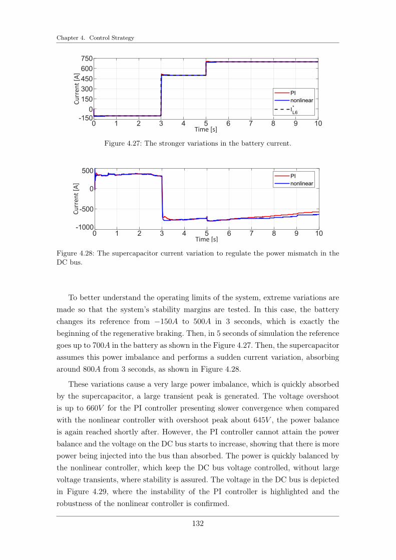
Chapter 4. Control Strategy
Figure 4.27: The stronger variations in the battery current.
Figure 4.28: The supercapacitor current variation to regulate the power mismatch in theDC bus.
To better understand the operating limits of the system, extreme variations aremade so that the system’s stability margins are tested. In this case, the batterychanges its reference from −150A to 500A in 3 seconds, which is exactly thebeginning of the regenerative braking. Then, in 5 seconds of simulation the referencegoes up to 700A in the battery as shown in the Figure 4.27. Then, the supercapacitorassumes this power imbalance and performs a sudden current variation, absorbingaround 800A from 3 seconds, as shown in Figure 4.28.
These variations cause a very large power imbalance, which is quickly absorbedby the supercapacitor, a large transient peak is generated. The voltage overshootis up to 660V for the PI controller presenting slower convergence when comparedwith the nonlinear controller with overshoot peak about 645V , the power balanceis again reached shortly after. However, the PI controller cannot attain the powerbalance and the voltage on the DC bus starts to increase, showing that there is morepower being injected into the bus than absorbed. The power is quickly balanced bythe nonlinear controller, which keep the DC bus voltage controlled, without largevoltage transients, where stability is assured. The voltage in the DC bus is depictedin Figure 4.29, where the instability of the PI controller is highlighted and therobustness of the nonlinear controller is confirmed.
132

4.9. Simulation Results
Figure 4.29: The behavior of the DC bus voltage for the PI controller in red and nonlinearcontroller in blue, when strong variations takes place.
Figure 4.30: A zoom on Vdc to highlight the PI controller diverging towards the powerimbalance caused by the battery.
Figure 4.30 present a zoom to show the impact of the power imbalance in theDC bus, where the stronger transients are introduced. The divergence of the PIcontroller is also emphasized in the second part of the figure, after the 5 seconds ofsimulation.
4.9.3. Robustness
Simulations to the purpose to test the robustness of the proposed control lawsare here introduced. The presence of errors for the value of the grid parametersas resistances, inductors and capacitors is treated. Two cases are described: in thefirst one, the parameters have a value of −20% smaller than nominal one, while inthe second case the value is +20% larger than the nominal value. The consideredgrid parameters are: R2, C1, C2, L3 for supercapacitor; R5, C4, C5, L6 for battery;R8, C7, C8, L9 for PV array; R12, C11, C12, L13 for DC load; R15, C14, C15, L16 for trainbraking; and R17, C17 for VSC converter.
The simulations are performed for both the PI and the proposed nonlinearcontrol, in order to better introduce a proper comparison. Figure 4.31 introducesthe behavior of the DC bus voltage Vdc considering the parametric errors: as it ispossible to state, the transients present higher peaks for both control techniques, but
133

Chapter 4. Control Strategy
Figure 4.31: The voltage Vdc when comparing PI and nonlinear control with parametricerrors of +20% and −20%.
Figure 4.32: A zoom on Vdc of Figure 4.31 to compare PI and nonlinear control in the mostcritical transients.
the nonlinear approach has better performances compared with the PI one becauseof the smaller overshoots.
A zoom on the highest transients in the proposed robustness test for bothcontrol strategies is depicted in Figure 4.32. It is clearly possible to see that theproposed nonlinear strategy presents smaller overshoots and a faster response thanthe traditional PI strategy even with considerable parametrical errors. One canconclude that the nonlinear controller shows good robustness properties in thesesimulations. The robust behavior of the proposed nonlinear control is a result fromthe ISS properties applied in this strategy, which assures good response even withstrong parametrical errors. However, PI control is also robust against parametricerrors.
The improvements of the nonlinear controller over the PI can be better remarkedin Figure 4.33, where the parametric errors are extended to be of +25% higher thanthe nominal value. As it is possible to see, in this case the voltage on the DC busfor the PI control diverges after the regenerative train braking takes place, whilethe nonlinear controller keeps a good performance. This behavior is highlightedin Figure 4.34, where a first zoom of Figure 4.33 in the most critical transient isproposed, still highlighting the better control performance of the nonlinear controlversus the PI, and with a second zoom on the beginning of the unstable behavior of
134

4.10. Different Approaches for DC Bus Control
Figure 4.33: The voltage Vdc in case of +25% higher parametric error than the nominalvalue.
Figure 4.34: A zoom of Figure 4.33 in the highest transients, showing the unstable behaviorof PI control after the high peak transient due to the regenerative braking.
the PI strategy. An interesting point to be addressed is the fact that the PI needsto re-adjust the control gains and parameters to keep following the grid referenceand to correctly perform stability, while the nonlinear gains can work in a broaderregion of attraction and consequently need less tuning. Therefore, it is possible toconclude that the nonlinear controller can stand larger disturbances, like the brakingenergy recovery, and that it is able to operate in a wider region with more robustperformances towards parametrical errors when compared with the standard PIcontrol.
4.10. Different Approaches for DC Bus Control
4.10.1. Fixed reference for VC2
Different from previous results, one may propose here a fixed reference value V ∗dcas desired reference for VC2 instead of a time-varying V e
C2used to exactly steer the
voltage of the DC grid. This will induce a small steady state error in Vdc, which isthe voltage drop in R2 (cable loss). This happens because the capacitor’s voltagewill not be driven to the desired bus voltage in a direct way. Nevertheless, the tradeoff between this small error (proportional to the resistance of the cables connectingVC2 and Vdc) and a greatly simplified control design is very convenient.
135

Chapter 4. Control Strategy
In this case, the regenerative braking from trains and the grid-connection arenot included in the stability proof and in simulations for simplification purposes.But, they can be easily inserted on the bus interconnection. The model of the DCMicrogrid for this approach is presented in Figure 4.35.
BI. BOOST - BATTERY
BOOST - PVBI. BOOST - SUPERCAP
BUCK - DC LOAD
Figure 4.35: The considered DC Microgrid.
DC bus voltage dynamic is rewritten according to Figure 4.35.
Vdc =1
C10
[1
R2
(VC2 − Vdc) +1
R5
(VC5 − Vdc) +
+1
R8
(VC8 − Vdc) +1
R12
(VC12 − Vdc)]
(4.209)
The behavior of Vdc dynamic must be analyzed to verify its convergence, whenVC2 is controlled to V ∗dc. Then, Vdc dynamic is not controlled by any control input,and this Vdc’s dynamic can be calculated as follows:
Vdc =1
C10
[1
R2
(V ∗dc − Vdc) +1
R5
(V eC5− Vdc) +
+1
R8
(V eC8− Vdc) +
1
R12
(V eC12− Vdc)
](4.210)
where V eC5, V e
C8and V e
C12were presented in (4.62), (4.75) and (4.95), respectively.
The equilibrium point of Vdc is calculated to provide steady-state value, whichvaries according to the other devices of the Microgrid (PV, battery and DC load).
V edc = Req
[V ∗dcR2
+V eC5
R5
+V eC8
R8
+V eC12
R12
](4.211)
where:
Req =R2R5R8R12
R5R8R12 +R2R8R12 +R2R5R12 +R2R5R8
(4.212)
It is clearly seen in (4.211) that the closer the voltages V eC5, V e
C8and V e
C12are to
reference V ∗dc the smaller DC bus error in steady-state. The reference V ∗dc given by
136

4.10. Different Approaches for DC Bus Control
controlling VC2 → V ∗dc in equation (4.211) implies that the error in steady state isaround this value.
To analyze the local convergence of Vdc dynamics, let us consider the eigenvalueof the linearization:
J10 = −[
1
R2
+1
R5
+1
R8
+1
R12
](4.213)
Indeed, the Jacobian J10 is always negative, then the equilibrium point of Vdc islocally stable around this equilibrium value V e
dc.
4.10.1.1. Simulation results
Simulations results using the same parameters configuration in Table (4.1) forthe DC Microgrid is provided here. Voltage VC2 from the supercapacitor subsystemis controlled in a fixed reference, which is the desired DC bus voltage V ∗C2
= V ∗dc.This approach simplifies the control design to regulate the DC bus in the Microgridand its stability analysis as previously presented. The following simulation resultsexpose the convenience and simplicity of this strategy, where the system can operatewith some limitations.
The voltage reference is V ∗C2= 630V . This approach does not control Vdc
directly, but it provides DC grid voltage regulation by maintaining Vdc in a grantedregion (with an error smaller than 5%) with smooth oscillations. To understandthe influence of the resistance between the supercapacitor subsystem and DC bus,the value of R2 is changed composing three different scenarios: 1) R2 = 0.1Ω, 2)R2 = 0.5Ω and 3) R2 = 0.05Ω.
Figure 4.36 introduces the dynamical behaviour of the voltage VC2 with respectto its reference V ∗C2
where the three proposed scenarios are shown. It is clear thatthe voltage remains with the same dynamics considering the variation of R2, but aslarger is R2, smaller is the overshoots and the ripples in VC2 . The voltage has somesmall transients according to variation on the other devices of the grid (PV, DCload and battery), with maximum error about 0.4%. The ripples are caused by theconverter switching; nevertheless, they can be considered moderate.
The calculated voltage VC2 in (4.45) is depicted in Figure 4.37. This is thesimplified dynamic for VC2 , considering IL3 already on its equilibrium point IeL3
, fromsingular perturbation analysis. This variable is used to design the control strategyof the DC bus voltage. As shown in Figure 4.37, the voltage is well controlled inV ∗dc, but for smaller values of R2, the voltage have higher overshoots with moreoscillation, which may bring instability to the grid.
137

Chapter 4. Control Strategy
Figure 4.36: VC2 voltage behavior for different values of R2.
Figure 4.37: Calculated voltage VC2 from equation (4.45) for different values of R2.
Figure 4.38: Voltage VC2 with the calculated value from equation (4.45) and the errorbetween those variables.
Figure 4.38 presents a comparison between the calculated9 (in red) and measured(in blue) voltage VC2 . The behavior of both signals are quite similar, since the error isvery small in transients (0.15% maximum). The error is zero in steady-state, besidesthe ripple in the measured voltage as depicted in the figure. Then, it is possible andreasonable to use the calculated VC2 instead of the measured one to calculate I∗L3
asmade in subsection 4.2.6.
The DC bus voltage is depicted in Figure 4.39, where the three scenariosare simulated to highlight the dynamical behavior of Vdc. As expected, the lowerthe value of R2, the smaller the steady-state error of Vdc, the more accurate thecontrol of the bus voltage, since VC2 approaches DC bus voltage. In the third case
9The proposed control strategy uses the calculated voltage VC2 , obtained in (4.45) instead ofthe measured value. This calculation is given by the obtained simplified dynamics of VC2 fromsingular perturbation analysis where IL3
is already considered in its equilibrium point.
138

4.10. Different Approaches for DC Bus Control
Figure 4.39: DC bus voltage (Vdc) profile for different values of R2.
Figure 4.40: Controlled current IL3 on the supercapacitor subsystem for different values ofR2.
scenario, where R2 = 0.5Ω, the behavior of Vdc conflicts with grid requirements. Gridrequirements generally allow voltage variations of a maximum of 5% relative to thenominal value. It is clearly seen that the value of resistor R2 must be considered inthis control approach to meet network requirements.
Figure 4.40 shows the behavior of IL3 current according to simulated variationsin Microgrid. The influence of resistance R2 is evident, because the lower the cablelosses between the supercapacitor and the DC bus, more current can be injected tokeep the DC bus controlled, reducing the error on voltage Vdc. However, in the casewhere resistance value is equal to R2 = 0.5Ω, the variations of current IL3 are muchsmaller, indicating that the supercapacitor is not varying enough to regulate busvoltage, resulting in poor control performance.
4.10.1.2. Control robustness test
The Input to State Stability (ISS) results from stability analysis assure robust-ness properties for the designed control law. Therefore, simulations with the purposeto test the robustness of the proposed control laws are performed in this subsection.The robustness is tested by introducing errors in the components parameters ofthe Microgrid grid, where the considered parameters are inductors, capacitors andresistors. In real Microgrid systems, it is very common to have uncertainties inthese parameters, therefore the proposed control strategy should be able to have
139

Chapter 4. Control Strategy
Figure 4.41: Voltage VC2 with parameters uncertainties 10% and 20%.
Figure 4.42: Voltage on the DC bus with parameters uncertainties 10% and 20%.
a good performance in the presence of this uncertainties. In simulations, 2 casesare described: the first case, the parameters are 10% smaller than the nominal one,and the second case the parameters are 20% smaller than the nominal value. Theparameters considered with uncertainties are presented in Table 4.1 and they are:R2, C1, C2, L3, R5, C4, C5, L6, R8, C7, C8, L9, R12, C11, C12 and L13.
The parametrical robustness test made for voltage VC2 is depicted in Figure 4.41.In this case, the transients present considerable higher peaks as the parametricalerrors increase. In the first scenario (10% error), the higher transient peaks are about2.1%, and the second scenario is the worse case, with transient peaks about 4.5% ofthe nominal.
The profile of the DC bus voltage Vdc is depicted in Figure 4.42 where theparametrical errors are analyzed. For voltage Vdc, the results with parametricalerrors are quite similar, which indicates that even in uncertainties problems, thevoltage profile remains stable. But, for the second scenario, the voltage has a peakthat exceeds the limits allowed by general grid requirements10.
The simulations highlight the robustness of the proposed control strategy,since the system remains stable even when high parametrical errors takes place(considered 20%). Concluding, the control have good robustness properties and great
10Usually, network regulation allows a maximum variation in steady-state of 5% in the voltageprofile. In Brazil, the voltage limits established by Prodist Module 8 are 5% above and 7% belowthe nominal for traditional distribution systems.
140

4.10. Different Approaches for DC Bus Control
Figure 4.43: Voltage VC2 controlled by nonlinear control (in blue) and linear control (inred).
Figure 4.44: A comparison on the DC bus voltage (Vdc) between the proposed nonlinearand linear control.
performance, but the level of uncertainties should be investigated to ensure that thevoltage is within the allowed limits.
4.10.1.3. Comparison with PI control
The proposed control strategy is also compared with standard control techniquesto highlight the benefits of the nonlinear strategy. Voltage VC2 profile is depictedin Figure 4.43, where the nonlinear control in blue line is compared with linear PIcontrol in red line. The PI control strategy have higher overshoots compared withthe nonlinear approach. The highest transient overshoot in the PI control is about2% error. Therefore, nonlinear control presents much better control performance.
Figure 4.44 introduces the comparison between nonlinear control and linear PIcontrol for DC bus voltage Vdc. Here, it is possible to notice that the voltage has thesame profile for both control strategies, but the linear control presents some peaksthat are very close to the allowed limits. The nonlinear control is able to work in awide operation region, with no need of gains re-adjustment. On the other hand, thelinear control strategy works only around one operation point, and then the controlgains must be redesigned to keep the stability of the system.
141

Chapter 4. Control Strategy
4.10.2. Simplification on C2 dynamics
As previously discussed, the DC bus Voltage dynamics is the sum of all currentsflowing trough the devices of the grid. The current flowing on the DC bus fromFigure 4.35 is written as follows:
Idc = IR2 + IR5 + IR8 + IR12 (4.214)
The currents that flows to the DC bus are composed of the voltage drop overthe output resistance as exemplified next:
IR2 =1
R2
(VC2 − Vdc) = IL3(1− u1)− C2VC2 (4.215)
The simplification of C2 dynamics eliminates the non-minimal phase featureof the DC/DC converter. In this case, the current IL3 is seen as the controlinput to control directly control the voltage Vdc. Therefore, ff we neglect theconverter switching and the transient current on capacitor C2, the current from thesupercapacitor subsystems becomes: IR2 = IL3 . In fact, this consideration despisessome terms of the equation, which is expressed as follows:
IR2 − IL3 = −u1IL3 − C2VC2 (4.216)
This may result in a very convenient simplification of Vdc dynamics, where currentIL3 explicity appears on voltage Vdc.
Vdc =1
C10
[IL3 +
1
R5
(VC5 − Vdc) +1
R8
(VC8 − Vdc) +1
R12
(VC12 − Vdc)]
(4.217)
With this simplification, one may propose a Lyapunov function candidate tocontrol Vdc → Vdc using IL3 as the degree of freedom that will result in a muchsimpler control strategy:
W =C10
2V 2dc +
C5
2(VC5 − V e
C5)2 +
C8
2(VC8 − V e
C8)2 +
C12
2(VC12 − V e
C12)2 > 0(4.218)
when its time derivative (W ) is investigated, IL3 is seen as the control input to bringstability for the whole grid.
W = Vdc
[IL3 +
1
R5
(VC5 − Vdc) +1
R8
(VC8 − Vdc) +
+1
R12
(VC12 − Vdc) + Ψ5 + Ψ8 + Ψ12
](4.219)
To obtain a stable grid-connection, it is analyzed the time derivative ofW wherethe desired expression for W is presented as follows:
W = − 1
R2
(V 2dc − V ∗dc
2) + ΨW1 (4.220)
142

4.10. Different Approaches for DC Bus Control
with:
ΨW1 = −(VC5 − V e
C5)2
R5
−(VC8 − V e
C8)2
R8
−(VC12 − V e
C12)2
R12
(4.221)
The Lyapunov function (4.218) then results to be an ISS-like Lyapunov functionwith equilibrium point in V ∗dc with same properties as the previous results [190,206].Here, IL3 is the control input that can regulate Vdc in the desired value and assureasymptotic stability for those dynamics. Therefore, the following control input isassigned to be the desired I∗L3
, such that one obtains (4.220) as the time-derivativeof the Lyapunov function.
I∗L3=
1
Vdc
[− 1
R2
(V 2dc − V ∗dc
2) + ΨW1 + Ψ5 + Ψ8 + Ψ12 +
−Vdc(
1
R5
(VC5 − Vdc) +1
R8
(VC8 − Vdc) +1
R12
(VC12 − Vdc))]
(4.222)
4.10.2.1. Simulation results
The simplification on C2 dynamics approach was tested in simulations using thesame parameters of Table 4.1, and the same inputs for irradiation profile and DCload demand from Figure 4.9.
The currents IL3 , IL6 , IL6 and IL12 are depicted in Figure 4.45. Currents IL6 , IL9
and IL12 from battery, PV and DC load present the same dynamics from previoussimulations, since they have the same inputs. But current IL3 is now following adifferent control reference I∗L3
to directly regulate the voltage Vdc.
The DC bus voltage is regulated with steady-state error from ISS results, butthe voltage profile can be considered satisfactory since, the DC grid remains stableover many grid perturbations. The DC load is properly supplied as the voltage VC11
is controlled in V ∗C11. Figure 4.46 presents the controlled voltages in the Microgrid.
In this control strategy, VC2 is considered a zero dynamics. The output voltageconverters present a stable behavior in simulations as depicted in Figure 4.47
4.10.3. DC bus generalization: Thévenin equivalent
For generalization purposes, one may consider that the voltage of the outputcapacitor of the PV array, the battery and the load are considered as piecewiseconstant plus a slowly time-varying disturbance. As the supercapacitor is allocatedexclusively to perform voltage stabilization in the DC bus, it will only act when thereis a power mismatch on power balance. The proposal is to design equivalent dynamicsfor the other devices of the Microgrid, when many different devices are integrated in
143

Chapter 4. Control Strategy
Figure 4.45: The controlled currents IL3 , IL6 , IL9 and IL12 .
Figure 4.46: The controlled voltages VC11 and Vdc.
the system. This generalization approach is to study the DC bus dynamics comparedwith many other devices in the Microgrid.
This because the battery is controlled in a time-scale of seconds according topower flow regulation, while the load is in general a sum of switching elements inaddition to slowly (seconds) varying ones. Finally, in the PV case, the disturbancescome from the solar radiance, where the solar variations is much slower than thevoltage control time-scale. The time varying disturbances will be neglected; theeffect of this will be an additive disturbance in a linear stable closed loop system,which will be compensated by the robustness of the controller. Nevertheless, there
144

4.10. Different Approaches for DC Bus Control
Figure 4.47: Zero dynamics VC2 , VC5 , VC8 , and VC12 .
will be an arbitrarily small slowly varying disturbance that will not bring the systemoutside of the operation margin defined around the desired equilibrium point.
From the hierarchical point of view, the secondary control target is to perform thepower flow trough the battery subsystem. In general, the DC bus is always balanced,unless there are errors in the power flow calculation, where the supercapacitor takeplace to act. The DC bus voltage can be considered always around the region theoperation point of the grid even under stronger power imbalance, then a equivalentapproach can be applied.
One can apply Thévenin theorem on those devices to obtain an equivalent circuit.The DC bus is the coupling point for the integrated devices in the system, modeledas a capacitance. The Thévenin equivalent circuit is used to substitute PV, batteryand load by a voltage source Vth and a resistance Rth.
Thévenin voltage Vth is calculated according to PV, battery and load system inopen circuit.
Vth = Rth
[VC5
R5
+VC8
R8
+VC12
R12
](4.223)
where VC5 , VC8 and VC12 are converters’ output voltage on PV, battery and load.They are considered according to generalization assumption; consequently, theresulting voltage Vth can be considered piecewise constant plus slowly time-varyingas well. In this approach, other devices included in the DC bus can be insertedthe equivalent circuit. Figure 4.48 depicts the Thévenin equivalent circuit on theMicrogrid.
The equivalent Thévenin resistance Rth is calculated as
Rth =R5R8R12
R5R8 +R5R12 +R8R12
(4.224)
where R5, R8 and R12 are the cable losses of the converters on PV, battery and DCload respectively.
Figure 4.49 depicts the Microgrid’s simplified electrical model due to theconsiderations done above. The system is composed by the converter that is
145

Chapter 4. Control Strategy
Figure 4.48: Thévenin equivalent circuit for the DC Microgrid.
Figure 4.49: The simplified electrical model of the DC Microgrid.
connected to the supercapacitor, a capacitor representing the DC bus and theThévenin equivalent circuit.
The equivalent circuit is expressed using state space average model as follows:
Vdc =1
C10R2
(VC2 − Vdc) +1
C10Rth
(Vth − Vdc) (4.225)
with this simplification, the control strategy to control the DC bus of the Microgridcan be easily developed even when many devices are inserted into the grid workingaround the operational point, but the stability analysis becomes limited due to theassumptions made.
One may proposed a Lyapunov function without considering the zero dynamics ofthe system, since they are proven to be locally stable in previous sections. EquivalentThévenin voltage is assumed to be piecewise constant where its dynamics are notconsidered. Therefore, a Lyapunov function candidate can be written as follows:
W10 =C10
2(Vdc − V ∗dc)2 +
Kα10
2α2
10 (4.226)
where α10 = Vdc − V ∗dc, is a auxiliary variable for a integral term.
146

4.10. Different Approaches for DC Bus Control
The derivative of W10 is written as follows, where VC2 is seen as the degree offreedom of this system.
W10 = (Vdc − V ∗dc)[
1
R2
(VC2 − Vdc) +1
Rth
(Vth − Vdc) +Kα10α10
](4.227)
hence, VC2 is calculated, such that, the system is asymptotically stable with thefollowing Lyapunov derivative:
W10 = −K10(Vdc − V ∗dc)2 (4.228)
The control input V ∗C2is given as follows.
V ∗C2= R2
[−K10(Vdc − V ∗dc)−Kα
10α10 −1
Rth
(Vth − Vdc) +VdcR2
](4.229)
Concluding, the system is asymptotically stable considering a region around theoperating point.
4.10.3.1. Simulation results
The Thévenin equivalent approach was tested in simulations using the sameparameters of Table 4.1, and the same inputs for irradiation profile and DC loaddemand from Figure 4.9. In this case, the Thévenin voltage is given in Figure4.50, where the behavior of the battery, PV array and the DC load subsystemsare expressed in the equivalent voltage Vth.
Figure 4.50: The equivalent Thévenin voltage (Vth) for the Microgrid part (battery, PVand DC load).
The currents IL3 , IL6 , IL6 and IL12 are depicted in Figure 4.51. Currents IL6 , IL9
and IL12 from battery, PV and DC load present the same dynamics from previoussimulations, since they have same inputs. But current IL3 follows the reference toregulate the voltage VC2 . Therefore the behavior of voltage VC2 → V ∗C2
is differentfrom last results as depicted in Figure 4.52.
The DC bus voltage is controlled in a fixed reference, with good transient per-formance, which means small overshoots and fast convergence. Reference computed
147

Chapter 4. Control Strategy
Figure 4.51: The controlled currents IL3 , IL6 , IL9 and IL13 in the equivalent Théveninapproach.
in (4.229) is well tracked and provides satisfactory DC bus regulation. Similarlyvoltage VC11 controlled assuring proper power supply for the DC load.
Finally, the zero dynamics voltages representing the grid interconnection isdepicted in Figure 4.53. Voltages remain stable towards the variations of the systemas expected from local stability analysis.
4.11. Conclusions
This chapter addresses the problem of controlling a Hybrid AC/DC Microgridwith grid-connection, renewables sources and different ESS. The proposed Microgridis used to absorb the train braking regenerative power, that constitutes a very largeand sudden peak of power that is difficult to address by classical linear controllers.This Microgrid is also used to integrate distributed generation as PV arrays. Theproposed system is based on two energy storages with different time-scale, i.e., abattery and a supercapacitor. The Microgrid is then completed with a variableDC load (that represents the aggregation of all DC loads as lights, heating andelectric vehicles) and a connection with the AC grid. The proposed DC Microgridis controlled by low-level distributed nonlinear controllers. For each subsystem
148

4.11. Conclusions
Figure 4.52: The controlled voltages VC2 , Vdc and VC11 .
Figure 4.53: Zero dynmics VC5 , VC8 , and VC12 .
composing the Microgrid and for each related target, a control strategy is providedaccording to a hierarchical control structure and a System of Systems approach.
The nonlinear control laws are developed according to a rigorous analysis basedon an ISS-like Lyapunov function, which provides the possibility to let the Microgridoperate under several adverse circumstances, as for example the high perturbationsbrought by the train’s braking recovery energy system or the load variations. Boththeoretical and numerical results show the capability of the proposed approach tohandle the complex scenarios given by the mix of different renewable sources, loadsand storage devices.
149


Ch
ap
te
r
5Ancillary Services for AC
Microgrids
5.1. Chapter Introduction
In this chapter it is presented a strategy for the interconnection of an ACand a DC Microgrids. In particular it is developed algorithms to provide inertial,frequency and voltage support (ancillary services) for an AC Microgrid (weakgrid) composed of diesel generators and loads. In addition, it is presented anadaptive variable synthetic inertia strategy for stabilizing this AC grid face tostrong variations on loads and productions, brought by electric vehicles and possiblyother renewable energy sources. In the proposed structure there is a DC Microgridconnected to the AC one by a Voltage Source Converter (VSC). The VSC converteris driven as a Virtual Synchronous Machine (VSM), where the control strategyfollows a swing equation such that the converter emulates a synchronous machine,including inertial support. A rigorous stability analysis is based on Lyapunovtechnique assuring proper stability conditions for the adaptive inertia, such thatfrequency stability is improved and power oscillations reduced. This strategy canbe exploited in low inertia systems like Microgrids or grids with high penetrationof renewables. Simulation results illustrate the performance of the proposed controland a comparison with classical droop control.
5.2. Power System Stability
Power system stability has been an important issue for proper system operation.Instability problems may cause oscillations and instability on the system states, oreven cause major problems as blackouts. The continuing growth and ramification of
151

Chapter 5. Ancillary Services for AC Microgrids
Power SystemStability
Rotor AngleStability
FrequencyStability
VoltageStability
Converter-drivenStability
LargeDisturbance
TransientStability
SmallDisturbance
DynamicStability
Short Term
FastInteraction
SlowInteraction
3 to 20s
few seconds 10s to severalminutes
severalseconds
severalminutes
Short Term Long Term
Short Term Long Term
LargeDisturbance
SmallDisturbance
few Herts<10Hz
hundreds of Hzto kHz
Figure 5.1: Power system stability classification.
power systems, the integration of distributed generation based on power convertersand electronic loads, and the highly stressed operation of the system has broughtdifferent forms of stability problems. For example, with the advance of Microgridstechnologies, voltage and frequency stability become important concerns. Thedefinition of power system stability is given in [104]:
“Power system stability is the ability of an electric power system, for a giveninitial operating condition, to regain a state of operating equilibrium after beingsubjected to a physical disturbance, with most system variables bounded so thatpractically the entire system remains intact.”
The definition can be extended to different interconnected power systems,because nowadays many systems have been interconnected to each other to improveits operation and reliability, like the Brazilian National System or the Europeansystem. But the complexity of a huge system like this brings thousands of variables todeal with, where the stability problem can not be easily addressed. The assessmentof power system stability is split according to different phenomena and variablesinvolved (angle, frequency or voltage), the scale of the perturbation (small or largesignal) and the time range (long and short term) as depicted in Figure 5.1 extractedfrom [104]. This definition has been updated for the new paradigms related to thelarge scale integration of high power’s converters in traditional power systems, whichdeal with fast and slow frequency-related interactions in [212].
Power systems are mainly composed by synchronous generators sharing power tofeed load demand. Rotor angle stability is related to synchronizing those generatorsin the power network, where dynamic stability deals with oscillations and controlinteraction among the generators and transient stability is the capacity of thosemachines to support large disturbances as partial disconnections of loads, black-outs or short-circuits. Transient stability is related to the robustness of the grid inface of large disturbances on the grid [213,214].
152

5.2. Power System Stability
Frequency stability is one of the most important issues of power systems, sinceit is related to the balance between the generation and the consumption of power inthe system. The power mismatch can cause excursions of frequency, accelerating orbraking the generators, since the synchronized machines works with the same speed.With current advances in power electronics, the physical interpretation of frequencyhas became a great issue, since for power converters the frequency is not a dynamicstate that respond to power balance, but it is a constant reference [215].
In the same way, voltage stability is the ability to maintain the equilibriumbetween load and supply, related to the ability to transfer the generated power tothe load. Low voltage conditions implies in large current responses to keep system’spower supply. Voltage stability is often a problem to be locally addressed accordingto power grid requirements (grid codes) [134].
Following the Power system Stability classification, this work is focused onvoltage and frequency stability, for Microgrids mainly composed of power convertersand the necessary ancillary services to maintain stability of the system, which arethe actions taken to assure this stability [216].
5.2.1. Frequency stability and control
Frequency stability is defined in [104] as:
“Frequency stability refers to the ability of a power system to maintain steadyfrequency following a severe system upset resulting in a significant imbalance betweengeneration and load. It depends on the ability to maintain/restore equilibriumbetween system generation and load, with minimum unintentional loss of load.”
The frequency in a traditional power system is given by the rotational speed ofthe synchronous generators that composes the system. Those machines transformsthe mechanical input power from a prime mover to electrical current injected inthe grid. A balanced system transmits the same amount of power generated bythe machine, otherwise it will be stored/supplied by the rotating masses of thegenerators. The Swing Equation1 describes the angular speed deviation caused bythe unbalance between the electrical power output and the mechanical power input.The Swing Equation is written as follows:
ω =1
2H(Pm − Pe) (5.1)
where ω is the rotating frequency of the generator (network), Pm is the mechanicalpower input and Pe is the electrical power output. H is the inertia constant of
1Also known as the equation of motion, it is primordial to power stability analysis.
153

Chapter 5. Ancillary Services for AC Microgrids
the network. The power unbalance generates a frequency deviation, changing theoperation point of the grid. Then, bring the frequency back to the desired operationalvalue can be one of the targets for ancillary services [213].
Frequency control reserve is the amount of active power kept available tocompensate a frequency drop, usually caused by a load shift. On the other hand, thenegative frequency control act to decreases the frequency. The frequency reserve isessential to maintain system stability even with sudden power load change, avoidinggreat excursions of frequency [134].
An interesting power system feature is the natural frequency regulation after apower unbalance. It comes from the self-regulating load and the stored energy inthe rotating mass (inertia) from the generation units and the loads (motors) [217].Concerning frequency stability, there are two types of power loads:
• Static load: are generally represented by algebraic equations, having suitablychosen power to voltage sensitivity, where the frequency dependency can beneglected. Then, the power output of the load is not changed for a frequencydeviation.
• Dynamic load: are modelled with algebraic and differential equations wherethe power output varies according to a frequency deviation [218]. They arecalled as self-regulating load, since they can attenuate a frequency deviationfrom a damping effect, given by the ratio between frequency deviation andactive power variation (DL).
The inertial contribution of rotating mass from (generators and motor loads) isvery important for frequency stability, since it can hold frequency deviation whilethe controllers from generation respond from a disturbance. The power stored in arotating mass is given by:
Pkinect = Jωdω
dt(5.2)
where J is the moment of inertia of the machine rotor and ω is the mechanicalspeed. From this equation it is seen that the inertial contribution is function ofthe derivative of frequency, called Rate of Change of Frequency (RoCoF), and themoment of inertia J . This concept of natural frequency response is part of an inertialresponse of a power system [213].
Grid’s evolution has brought large penetration of power converters in thenetwork, where the angular speed of the electrical machines are not coupled withthe frequency of the system. Then, the lack of inertia in this kind of grid maylead to higher Rate of Change of Frequency (RoCoF) than classical values. As
154

5.2. Power System Stability
a consequence, system’s operation and protection may suffer from poor inertialresponse. This important issue will be detailed in the virtual inertia subsection.
5.2.1.1. Primary control
Power system have a natural frequency response from the accumulated energyof rotating masses, but it is not enough to maintain frequency stability. The naturalresponse limits the frequency deviation, but when a bigger disturbance takes place,action is needed to decrease/increase the energy generation and keep stability.
Standard in frequency control adopt three levels of control to keep the balancebetween generation and load. The primary control is a local automatic controlto adjust the active power generation and the controllable loads to counteractfrequency variations, bringing the system to a new operation point within fewseconds. They are designed to react to large generation changing or load shifts. Thesmall deviations of frequency can be attenuated by the primary control, then largefrequency deviation (off-normal) is dealt by the secondary control to restore nominalfrequency. The speed governor performs this control in the region of synchronizationof the generation units. The prime mover has a speed regulator that uses themechanical power to maintain the rotating mass inside an operation range [102,214].
Demand side also contributes with frequency control by connecting or discon-necting a group of loads according to frequency thresholds, but they are not alwaystaken into account for primary control response. A distributed primary frequencycontrol can be advantageous since a generator unit can not surpass the active powersupply limits from a frequency drop, therefore other units must share the increaseon power demand.
There are many different approaches for speed governors, that can also be appliedin power converters for modern grid operation. The different strategies can be citedas isochronous regulation, droop control and virtual inertia.
5.2.1.2. Isochronous control
The isochronous regulation is featured by constant frequency, where the governoradjusts the input to eliminate the frequency deviation. Figure 5.2 presents theblock diagram of the isochronous governor, where the integral term guarantees theelimination of steady-state error in frequency by actuating the valve.
In the isochronous operation mode, a load increase will firstly cause a frequencydrop given by the generator’s inertia, and then, as response, the mechanical powerincrease to compensate the frequency deviation until the mechanical power reaches
155

Chapter 5. Ancillary Services for AC Microgrids
Turbine Generator
1
𝑠 𝐾
𝑃𝑚 𝑃
𝜔𝑔
𝜔∗ ∆𝜔
ValveWaterinput
Figure 5.2: Isochronous governor block diagram.
𝑃𝑚 𝜔∗
𝑃1
𝑃2
∆𝑃𝑚 = ∆𝑃𝐿
𝜔𝑔
Rotor speed
Mec. power
Time [s]
Figure 5.3: Frequency response in the isochronous mode.
the new load demand point. Finally, the frequency is back to its reference. Thisexample is illustrated in Figure 5.3 extracted from [213].
The operation of the isochronous control in an isolated system is consideredsatisfactory, but when two or more generators are sharing the same load, there iscontrol conflict and the system becomes unstable. Therefore in this case, only onegenerator is chosen to respond the load changes and perform frequency regulation,while the others are set to constant power supply [219].
5.2.1.3. Frequency droop control
A droop characteristic is obtained by inserting proportional gain in the rotationalspeed reference, causing a frequency deviation in steady-state. Figure 5.4 shows theblock diagram for droop strategy. The frequency-power curve is changed as a slopedline given by:
mp =∆f
∆P(5.3)
The droop control is better applied in multigenerator power sharing because theypresent a speed drop feature, i.e., a decrease of load will cause an increase of the speedand vice-versa. Therefore, they have a stable load share compared with isochronouscontrol. The frequency deviation rate is usually given in percentage, where the
156

5.2. Power System Stability
Turbine Generator
1
𝑠 𝐾
𝑃𝑚 𝑃
𝜔𝑔
𝜔∗ ∆𝜔
ValveWaterinput
𝑚𝑝
Figure 5.4: Droop governor block diagram.
𝜔1 = 𝜔2
𝜔𝑟1 = 𝜔𝑟2
𝑃1 𝑃2 𝑃𝑟1 𝑃𝑟2
𝑚𝑝2
𝑚𝑝1
∆𝑃1 ∆𝑃2
∆𝜔1 =∆𝜔2
𝜔
𝑃
Figure 5.5: Power sharing scheme of droop control in steady-state.
maximum power deviation2 is linked with the maximum frequency deviation bya proportional relation [131].
Droop control is able to allow the generators to contribute with power supplyin different levels, according to their power rate, to provide the balance of power inthe system. But, in this case, there will be always a non-zero frequency deviation.Because, there is only one operation point where the frequency is stabilized in itsnominal value. The power-frequency relation (P − ω) is seen in Figure 5.5. Thedroop coefficient (mp) provides the proportional contribution of each generator for agiven frequency deviation. This coefficient can be designed according to the nominalavailable power (Pnom) and the frequency deviation limits (∆ωmax) [135]. The droopcoefficient equation is written as follows:
mp =∆ωmaxPnom
(5.4)
with ∆ωmax = ωnl − ωfl, being ωnl the non-load frequency of the machine and ωflthe full-load frequency.
In a multigeneration example, the equivalent frequency characteristic of thewhole system (λ) will depend on the droop coefficient (mp) of each generator and
2Primary power reserve in nominal conditions.
157

Chapter 5. Ancillary Services for AC Microgrids
𝑃𝑚 𝜔∗
𝑃1
𝑃2
∆𝑃𝑚
𝜔𝑔
Rotor speed
Mec. power
Time [s]
∆𝜔
Figure 5.6: Frequency response in the droop control mode.
the variation of the load power output (DL).
λ = DL + 1mp1
+ 1mp2
+ ...+ 1mpn
(5.5)
λ = DL + 1meq
(5.6)
λ is the network frequency characteristic, DL is the natural response of frequencysensitive load and mpi is the droop coefficient of i− th generator of the system. Thesum of the inverse of each droop coefficients results in an equivalent droop given by1/meq [56].
Therefore, the steady state equation that relates frequency and active power isgiven as:
ωg = ω∗ −mp(Pm − P ∗) (5.7)
where ωg is the grid frequency, Pm is the power in the generator, P ∗ is the activepower set point and ω∗ is the grid frequency reference [129].
From equation (5.7), the behavior of the frequency in response to a load changecan be described as is shown in Figure 5.6 extracted from [213]. After a load increase,the frequency will drop and the mechanical power is increased as a response to thefrequency deviation, but in this case, the frequency end up with a steady-state errorgiven by ∆ω.
5.2.1.4. Load reference setpoint
The Automatic Generation Control (AGC) is used to eliminate the steady stateerror in frequency. In this case a load reference setpoint is inserted as input in theproportional gain of the droop control. The effect of the load reference set point isto distribute the proportion of load for each generation unit. Therefore, the outputpower of the generation unit can be shifted by changing the load reference. The load
158

5.2. Power System Stability
Turbine Generator
1
𝑠 𝐾
𝑃𝑚 𝑃
𝜔𝑔
𝜔∗ ∆𝜔
ValveWaterinput
𝑚𝑝 Loadreference
Figure 5.7: Block diagram of a droop governor with load reference setpoint.
reference is usually computed by a secondary centralized controller [213]. Figure 5.7shows the block diagram of this scheme.
The calculation of the load reference of AGC is necessary to bring frequency toits nominal value, as a consequence, the AGC is able to restores the power reservescaused by the droop control. Therefore, equation (5.8) can find the Load referenceby using an integral term in frequency assuring zero steady-state error.
∆PAGC = −∫
(ωg − ω∗)dt (5.8)
where ∆PAGC is the power variation of the load reference setpoint and ω∗ is thefrequency reference. Hence, frequency ωg can be computed as the average value offrequency in the generation units according to their power and inertia.
5.2.1.5. Secondary and tertiary control
The secondary frequency control is based on a centralized approach to meetthe power production of the generators units to restore the frequency to thenominal value and interacts with other systems to accomplish the balance target.While the primary level only avoids frequency excursion and reduces the frequencydeviation, the secondary brings the frequency back to the original equilibrium point,i.e., the nominal value of the frequency. This control scheme is mainly appliedin interconnected large systems, because a faster response is needed, and usuallydispensable in isolated systems. The AGC designates the combination of dispatchingand secondary control, where the time range of this level of control is few secondsto minutes [134].
Tertiary control refers to manual changes in the dispatching set of the generationsunits and application of optimization methods according to economical purposes.This level of control is applied to restore the primary and secondary reserves,managing the optimal operation of transmission lines.
159
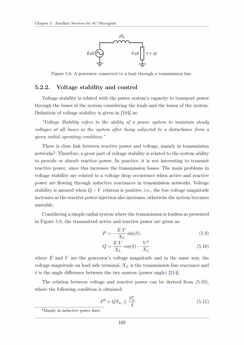
Chapter 5. Ancillary Services for AC Microgrids
𝐸∠0 𝑉∠𝛿
𝑗𝑋𝐿
𝑃 + 𝑗𝑄
Figure 5.8: A generator connected to a load through a transmission line.
5.2.2. Voltage stability and control
Voltage stability is related with the power system’s capacity to transport powerthrough the buses of the system considering the loads and the losses of the system.Definition of voltage stability is given in [104] as:
“Voltage Stability refers to the ability of a power system to maintain steadyvoltages at all buses in the system after being subjected to a disturbance from agiven initial operating condition.”
There is close link between reactive power and voltage, mainly in transmissionnetworks3. Therefore, a great part of voltage stability is related to the system abilityto provide or absorb reactive power. In practice, it is not interesting to transmitreactive power, since this increases the transmission losses. The main problems involtage stability are related to a voltage drop occurrence when active and reactivepower are flowing through inductive reactances in transmission networks. Voltagestability is assured when Q− V relation is positive, i.e., the bus voltage magnitudeincreases as the reactive power injection also increases, otherwise the system becomesunstable.
Considering a simple radial system where the transmission is lossless as presentedin Figure 5.8, the transmitted active and reactive power are given as:
P = −E.VXL
sin(δ); (5.9)
Q =E.V
XL
cos(δ)− V 2
XL
(5.10)
where E and V are the generator’s voltage magnitude and in the same way, thevoltage magnitude on load side terminal, XL is the transmission line reactance andδ is the angle difference between the two sources (power angle) [214].
The relation between voltage and reactive power can be derived from (5.10),where the following condition is obtained:
P 2 +QSsc ≤S2sc
4(5.11)
3Mainly in inductive power lines.
160

5.2. Power System Stability
0
0.2
0.4
0.6
0.8
1.0
𝑉/𝐸
𝑃/𝑃𝑚𝑎𝑥
0.9
0.95
1.0
0.9
0.95
0 0.2 0.4 0.6 0.8 1.0 1.2 1.4 1.6
lag
lag
lead
lead
Figure 5.9: P − V curve characteristics for different power factors.
The short-circuit power of the system is defined as: Ssc = E2/XL. The maximumpower transmission when power factor is one (Q = 0) is Pmax = Ssc/2 and themaximum reactive power transmission when power factor is zero (P = 0) is Qmax =
Ssc/4. So, the reactive power transmission is more restricted than active power.Also, the active power capacity is related with reactive power injection, for examplelooking again at equation (5.11), when the system is absorbing reactive power(negative value for Q), the active power maximum is increased. As a conclusion,there is a maximum value to transmit active power through an impedance from avoltage source (generation unit), which occurs when the voltage drop in the line isequal to load voltage (V ) [56].
For this reason, reactive power compensation is usually realized on the loadside using shunt and series capacitors, and tap changing transformers. Recently,the evolution in power electronics has brought Flexible AC Transmission Systems(FACTS), where voltage and reactive power control is improved. At the sametime, the grid evolution through power electronic devices, the reducing number ofsynchronous machines in the grid, together with the increasing load demand bringsome impacts to voltage stability [220].
A traditional way to illustrate the relation between voltage and power is to usethe P − V curve presented in Figure 5.9 adapted from [104]. Here, it is possible torelate the voltage drop according to active power transmission for different powerfactors. Pmax is the maximum power transfer with unity power factor.
The inflection point in the curves represent the critical operational points, wherethe voltage becomes unstable. Therefore, the satisfactory region of operation is abovethe critical point. As one can see, a sudden change in power factor (sudden variation
161
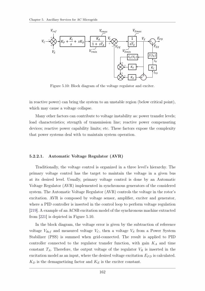
Chapter 5. Ancillary Services for AC Microgrids
𝐾𝑃 +𝐾𝐼
𝑠+ 𝑠𝐾𝐷
𝐾𝐴
1 + 𝑠𝑇𝐴 𝑉𝐶
𝑉𝑟𝑒𝑓
𝑉𝑆
𝑉𝑟𝑚𝑎𝑥
𝑉𝑟𝑚𝑖𝑛
𝑉𝑟
𝑉𝐹𝐸
𝑉𝐸𝑚𝑎𝑥
𝑉𝐸𝑚𝑖𝑛
1
𝑠𝑇𝐸
𝑉𝐸 𝐸𝐹𝐷
𝐹𝐸𝑋
𝐾𝐶 𝐾𝐸
𝐾𝐷
𝑆𝐸(𝑉𝐸) 𝑓(𝐼𝑁)
𝐼𝑁
𝐼𝐹𝐷
× ×
× ×
Figure 5.10: Block diagram of the voltage regulator and exciter.
in reactive power) can bring the system to an unstable region (below critical point),which may cause a voltage collapse.
Many other factors can contribute to voltage instability as: power transfer levels;load characteristics; strength of transmission line; reactive power compensatingdevices; reactive power capability limits; etc. These factors expose the complexitythat power systems deal with to maintain system operation.
5.2.2.1. Automatic Voltage Regulator (AVR)
Traditionally, the voltage control is organized in a three level’s hierarchy. Theprimary voltage control has the target to maintain the voltage in a given busat its desired level. Usually, primary voltage control is done by an AutomaticVoltage Regulator (AVR) implemented in synchronous generators of the consideredsystem. The Automatic Voltage Regulator (AVR) controls the voltage in the rotor’sexcitation. AVR is composed by voltage sensor, amplifier, exciter and generator,where a PID controller is inserted in the control loop to perform voltage regulation[219]. A example of an AC8B excitation model of the synchronous machine extractedfrom [221] is depicted in Figure 5.10.
In the block diagram, the voltage error is given by the subtraction of referencevoltage VRef and measured voltage VC , then a voltage VS from a Power SystemStabilizer (PSS) is summed when grid-connected. The result is applied to PIDcontroller connected to the regulator transfer function, with gain KA and timeconstant TA. Therefore, the output voltage of the regulator VR is inserted in theexcitation model as an input, where the desired voltage excitation EFD is calculated.KD is the demagnetizing factor and KE is the exciter constant.
162

5.2. Power System Stability
5.2.2.2. Voltage droop control
As presented in droop control subsection for frequency control, a relation betweenactive power and frequency (P − f) is built. Here, considering a power system withhigh value X/R relation, where the losses are negligible considering the systemreactance, a direct relation between reactive power and voltage magnitude (Q− V )can be shown. The coefficient that relates reactive power with voltage magnitude iswritten as:
mq =∆V
∆Q(5.12)
where the voltage droop coefficient (mq) provides a proportional contribution ofreactive power for a given voltage deviation [60]. In this case, the voltage droopfeature will cause a steady state error on the voltage level, since a change on reactivepower supply implies in a new operational point for the voltage, but will always bea non-zero voltage deviation. The coefficient mq can be designed according to thevoltage limits requirements (∆Vmax) and the nominal reactive power capacity (Qnom)as given next:
mq =∆VmaxQnom
(5.13)
where ∆Vmax = Vmax − Vmin according to the grid limits and Qnom is given by thecapability curve of the generator or power converter.
Therefore, the steady-state equation for voltage droop equation is written as:
V = V ∗ −mq(Qm −Q∗) (5.14)
where V is the grid voltage amplitude, V ∗ is the nominal voltage set, Qm is thefiltered reactive power, Q∗ is the reactive power set point. Figure 5.11 depictsthe behavior described in (5.13), exhibiting the voltage droop feature for differentcoefficients (mq) [135]. In island system operation, the reactive power reference isconsidered Q∗ = 0 [128].
As droop control has a better performance for power sharing, multiple units canshare the responsibility of reactive power supply to voltage regulation purposes.The generation units can contribute with reactive power supply in different levels,according to their capacity. Q − V droop control have been widely applied inpower converters that integrate renewable sources and ESS, since it allows thevoltage support by a simple relation with reactive power. Even in Microgrids mainlycomposed of power converters, the voltage control can be easily designed by droopcontrol approach [129,135].
163

Chapter 5. Ancillary Services for AC Microgrids
𝑉1 = 𝑉2
𝑉𝑟1 = 𝑉𝑟2
𝑄1 𝑄2
𝑄𝑟1
𝑄𝑟2
𝑚𝑞2
𝑚𝑞1
∆𝑄1
∆𝑄2
∆𝑉1 =∆𝑉2
𝑄
𝑉
Figure 5.11: Different coefficients of the voltage droop control scheme.
5.2.2.3. Secondary and tertiary control
Secondary control is based on a centralized automatic approach to manage thereactive power injection within a regional voltage zone by coordinating the action ofthe local controllers. This level of control is related to the capability of a generatorsupply an extra-mandatory quantity of reactive power, such that a group of busesin the grid is maintained at desired operation. The improvement of the voltageregulation can be done by the integral of the voltage error, which results in a reactivepower reference to the service provider. Tertiary control is based on optimizationtechniques to calculate the reactive power flow in the entire system [134].
5.3. Ancillary Services in Brazil
The main responsibility of a Transmission System Operator (TSO) is toprovide electric power from generators to the consumers through transmission linesmeeting the standardized network requirements (obligations of control areas andtransmitting utilities) to maintain the proper and reliable operation of the systeminterconnection. In this context, the specific services and functions provided tomaintain and support the power supply in the grid are called ancillary services. Theancillary services support the grid to maintain continuous and reliable operationof the system, properly supplying the loads while keeping stability and security.Traditionally, the ancillary services are provided by generators controlled by theTSO, however the integration of power electronic based equipment in the networkexpanded the possibility of ancillary services provision. Therefore, power electronicdevices and generators non-controlled by the TSO are now able to participate on thesupport to the grid in several operation modes, which has created a new opportunityin the energy market [222–224].
164

5.3. Ancillary Services in Brazil
The ancillary services provision in Brazil is still very limited because ofregulation aspects and restricted to the generation units controlled by the TSO(composed of hydroelectric and thermoelectric plants). There are some generationunits able to operate as synchronous compensators, which provide reactive powercompensation through a formal contract with the national TSO. These arecentralized thermoelectric plants used as operational power reserves. Therefore,power plants non-controlled by the TSO cannot perform ancillary services, whichgreatly restrict theses services in Brazil [225–227].
The normative resolution in [225] made in 2018 updates the version introducedin 2015 for ancillary services provision, where the TSO is in charge of identifyingthe generation units capable of carrying out the ancillary services related to powerreserve dispatch, opening the possibility for different generation units. The limitationof the prices offered for such services and the operating restrictions related to the loadcurve, operating time and minimum operating power were also discussed. Aspectsof fees and service unavailability, as well as forms of payment were also considered.
According to [226], the ancillary services’ provision in Brazil includes thefollowing supports: a) Primary frequency control, performed by all generating unitsintegrating the national electrical grid; b) Secondary frequency control, where onlythe plants that are part of the Automatic Generation Control, requested by the TSOare able to participate; c) Reactive power support, performed by generation unitsintegrating the network and by plants that operate as synchronous compensators,under prior authorization from the National Electrical Energy Agency (ANEEL);d) Black-start, performed by all generation units integrating the network and byplants in compliance with ANEEL and on demand from the TSO with the supportof previous studies; Special Protection System, performed by existing plants inoperation with the support of studies performed by operator with prior authorizationfrom ANEEL, in addition to proof of technical feasibility; and Complementary powerreserve dispatch, performed by centrally dispatched thermoelectric plants.
In this context, the report in [227] proposes a normative review for ancillaryservices provision based on the reduction of the regularization of the reservoirsof hydroelectric power plants and the high penetration of intermittent renewablesources. It addresses the need to adapt the spatial and temporal allocation ofenergy resources and the current load of the electrical system so that requirementscan be sized, equipment allocation made and guidelines of contracting servicescan be defined. The planning of the requirements of ancillary services identifiedby the planning and operation of the electrical system aims to encourage theprovision of services, identify costs in order to minimize the operational cost, and
165

Chapter 5. Ancillary Services for AC Microgrids
operate efficiently. It is also proposed to encourage the expansion of existing services(mentioned above) and the insertion of new services such as:
1. Development of new services for reactive power compensation using pho-tovoltaic plants, reactive power support for wind power plants and evenin the distribution system, which could be applied through tariffs alreadyestablished;
2. Inertia as an ancillary service through power electronics equipment, aimingat reducing the connection of thermal plants, but it may bring losses tothe system, or the use of thermal plants to increase inertia that avoids theinstallation of electronic equipment for this purpose;
3. Load modulation by distribution agents, performed through the dispatchingof power plants not operated by the national TSO, but by the localdistributor;
4. Paying for ancillary service provision: payment through system servicescharges using the principle of causality, where the TSO identifies the causersof the need to provide the service, which can bring improvements to theelectrical planning, or even the bilateral payment between consumer and theprovider, raising the need for the development of an ancillary services market.
Thus, in the Brazilian scenario, there are still many barriers to the diversificationof ancillary services provision, being restricted to large generation units controlledby the national TSO. In addition, the regulations updates presented are limitedto proposals and introduce possible advantages and disadvantages to be discussed,being distant from an imminent implementation. According to these reports, thegreatest barriers to the accomplishment of the rendering of ancillary services arepresented in the increase of complexity in the identification of costs, operation andverification of services.
Nowadays, ESS have the ability (according to their size and technology) toperform most kinds of ancillary services presented here according to their nominalpower limitation. Thus, ESS can be applied for primary frequency regulation (whichrepresents the most restricted ancillary service in ANEEL), in view of the availabilityof the power electronics equipment required for this purpose. However, due tothe lack of regulation in Brazil and the restriction of generation units authorizedby the national TSO, ESS are very restricted for ancillary services provision inBrazilian power grid. These limitations highlight the urgent need to develop newoperating strategies for the system, maintaining the operational requirements withthe installation of new equipment for this purpose. The adaptation of economic
166

5.3. Ancillary Services in Brazil
regulation tools must be considered, as well as carry out studies to identify costs(valuation of the service) for these services.
A crucial factor is the identification and verification of the service provision. Itis necessary to develop tools to validate these services, and to track the operatoror the local consumer that receives the service. Technological adaptation costs andequipment deterioration costs combined with massive insertion of power electronics’devices and ICT equipment make the valuation of ancillary service provision quitecomplex. Other aspects, such as cause and effect relationships are also widelydiscussed as in the case of harmonic mitigation and should be taken into account tocreate a new resolution for ancillary services. In addition, the size of the storagesystem limits its use for services requiring a large amount of energy, such assecondary (or even primary) reserve.
The development of a market for ancillary services in distribution is very relevantfrom a technical point of view for Brazil, considering that the main current powerquality problems are faced in the distribution system. The report in [225] proposesthat the modulation of loads can be carried out by distribution dealership for thedispatch of plants not operated by the national TSO, demonstrating the relevance ofthe high penetration of energy resources directly installed in the distribution system(mainly PV and ESS).
The distribution system has undergone a revolution in recent years, known asSmart-Grids, which results in a multitude of possibilities for ancillary services in thecontext of the distribution system. Therefore, consumers can also perform servicesto improve the network operation. This reflects in the creation of a new market thatbrings economic growth in the energy market, also improving the operation of thedistribution system as a whole. The use of renewable resources for ancillary servicesprovision enhances the effort to change the energy matrix, bringing more technicaland economic benefits for this type of generation, expanding the operation field ofrenewables to solve power quality issues.
Electric vehicles can also become an excellent contribution to the ancillaryservices through Vehicle to Grid (V2G) concept, since they bring a larger dispatchingcapacity. In conclusion, there is great technical feasibility for developing an ancillaryservices market in the context of distribution systems, which would further drive themodernization of the distribution system and the energy market economy, the mainchallenges being the development of regulations and valuation for ancillary servicesin Brazil.
167

Chapter 5. Ancillary Services for AC Microgrids
5.4. Power Converters Issues
Recent grid evolution has brought the integration of renewable energy sources,ESS and loads based on power electronics. Further, the HVDC advances and MTDCare more present in large interconnected grids. Those equipment are also based onpower converters. On the other hand, Microgrids like isolated systems, or smallindependent grids located in urban centers are composed mainly of power convertersto transform energy and operate the system [228,229].
In all of these cases, power converters are the key technology for grid compo-nents. But power converters have different behavior than synchronous machines.Synchronous machines have an inherent energy storage from their rotational mass4,being able to naturally respond to a load perturbation contributing to systemstability, while power converters are directly affected by their controllers with fastresponse and very low natural energy stored5. Therefore, power converters do nothave the natural ability to contribute to frequency stability in the active powersense [133,230].
In Microgrids context, power converters use the measured voltage of the networkto estimate the phase angle of the grid, being able to synchronize with the main gridto generate the voltage output, i.e., grid-following converters. The main issue relatedto power converters in Microgrids is the difficulty to implement isolated operationcalled as grid forming converters. Grid-forming converters are a great concern inacademia and industry, where numerous studies have been carried out to developuseful strategies to proper operate electrical grids only composed of power electronicstechnologies. In this context, droop control approach has been widely applied, sinceit allows power share among power converters with a distributed control approach.
A crucial issue in power electronics technology is the lack of inertia andinteractions between control as stated by the United Kingdom Transmission Systemin [231]. In fact, the high penetration of power electronics based technologies decreasethe inertia of the system, bringing frequency stability problems and reduction oftransient stability margins.
The AC/DC power converters like VSC are mostly controlled by Pulse WidthModulation (PWM) and traditional control schemes in grid-following operationmake these converters behave as current sources6. The Phased Locked Loop (PLL)
4Synchronous generators store kinetic energy proportional to moment of inertia J and theirangular speed, with time response of few seconds as seen in Section 5.2.1.
5The capacitors of power converters can store electrostatic energy in order of milliseconds.6Usually, VSC have outer voltage control loop and an inner control loop, which is the current
control loop
168

5.4. Power Converters Issues
is used to synchronize the converter with the grid by estimating the phase angleof the network, where the calculation of the voltage reference depends on thegrid impedance. Therefore, the control performance is affected by grid impedance,which makes these control schemes sensitive to grid condition. So, it is necessaryto design a good interaction between the PLL, voltage and current control loops,PWM switching frequency and the output filter. The match of bandwidth of thecontrollers can be a very complex task. Usually, current control loop bandwidthis twenty times smaller than the PWM frequency and filter frequency is designedaccordingly [232,233].
Other important issues can be related to power electronics in power systems,where countries in Europe are dealing as priorities [56]:
1. Decrease of inertia, related to frequency stability;2. Wrong participation of power converters devices in frequency regulation
(control errors);3. Reduction of transient stability margins due to decreased short-circuit
capacity of power converters4. Resonance and oscillations caused by power electronics;5. Power electronics controller interaction among the devices (active and
passive) in the grid.
In this scenario, new ancillary services and grid support are needed to fulfill thestability requirements for power system operation and reliability. A suitable solutionis to develop new control strategies for power converters changing the original featureof power converters to provide ancillary services to the network and reduce the powerelectronics impacts [234].
Traditional power systems composed of synchronous generators have a wellestablished time-scale separation considering the dynamics of the system. Usually,the time constant for frequency and voltage regulation are related to slow dynamicsof turbines (about 10s) and governors (about 1s), compared with faster dynamicsof the exciter (about 50ms), which can deal with the network line dynamics (timeconstants about 1 − 30ms). Besides that, the time constant of the swing equationand flux linkages will be given by the flux and swing dynamics. So, in conventionalsystems, the controllers are typically designed considering its operational marginsand can assure the stability of the whole system. However, in low inertia systems,the fast dynamics of power converter-based generation bring interactions amongdifferent controllers, affecting the time-scale separation and increasing complexity[235].
169

Chapter 5. Ancillary Services for AC Microgrids
PWM Harmonics
Fibre optic network
Signal Processing
Grid
Sync. gen.
VSC
Voltage dynamics Frequency dynamics
Network line dynamics
SRF inner control
AVR & PSS Flux GovernorTurbine
Swing dynamics
PLL
Active & reactivePower Control
current loop
transmissiondistribution
voltage loop
< 1 𝑚𝑠 1 𝑚𝑠 10 𝑚𝑠 100 𝑚𝑠 1 𝑠 10 𝑠 𝑡𝑖𝑚𝑒
Figure 5.12: Time-scale separation of power system dynamics considering conventionalsynchronous generators and power converters integration.
The time-scale separation of power systems including power converter-basedgeneration and the dynamics characteristics of low inertia are introduced in Figure5.12, adapted from [235]. It is presented the physical and control dynamics,considering three different time-scales: signal processing, voltage dynamics andfrequency dynamics. The voltage and frequency dynamics are related to thecontrollers designed for these purposes. First, the signal processing is associatedto the fastest interactions (< 1ms), which may include PWM signals and harmonicsfrom converters, and fibre optic network communication of the electrical grid.Then, the voltage dynamics are associated with large range time-scale interactions(> 1ms to < 100ms), which includes the network line dynamics, the AVR, PSS andlinkage flux dynamics of synchronous machines, and the SRF inner control loopsof converters. The frequency dynamics are associated with the slowest interactions(> 10ms to 10s), including the Active and reactive Power Control, PLL of powerconverters, and the Governor, Turbine and swing dynamics of synchronous machines[213,235,236].
In this sense, the controllers and LPF of power converters have faster dynamicsthan synchronous generator controllers, resulting in control interactions and causingstability issues, since they have different time constants as shown in Figure 5.12. So,power converters can potentially impact in the frequency regulation in low inertiasystems, affecting frequency dynamics and the associated fast transients. The resultis the deterioration of protection schemes that consider the limitation of frequencyNadir and RoCoF due to incompatible control strategies interacting with the maingrid under high penetration of power electronic-based generators. The transmissionline dynamics also interact with the dynamics of power converters’ controllers, wherethe fast behavior of these dynamics can amplify the interactions. Therefore, whenthe X/R impedance ratio is high enough, the time constant of the line is able tosuppress the gap between faster dynamics of power converters and slow dynamics ofsynchronous generators, acting as a buffer, improving the system stability. However,
170

5.4. Power Converters Issues
in distribution lines, the lower X/R relation restricts the operation and control ofvoltage and frequency, hindering system’s stability. In this case, virtual impedanceapplication may be a feasible solution for these stability issues.
5.4.1. Inertial response and low inertia issues
Since power converters based generations are not able to provide naturalfrequency response (primary control), the reliability of renewable generators andMicrogrids can be dramatically reduced. Consequently, the frequency response ofthe system as a whole can be affected, which is an European concern [233].
A reduced inertia may cause higher frequency excursions during and after acontingency and also increase the Rate of Change of Frequency (ROCOF). RoCoFis used to indicate load disconnections (Load Shed) and in protection schemes todetect the disconnection of generations units. Therefore, faster frequency ancillaryservices, inertial response emulation and increase the grid code requirements ofRoCoF were proposed by [237,238].
The power response of an inertial system (natural or virtual) depends on itsinertial time response (H) and the derivative of frequency as:
∆Pp.u. = −2H
f0
df
dt(5.15)
where f is the measured frequency and f0 is the nominal grid frequency.
The inertial power variation (∆Pp.u.) is proportional to the RoCoF, then itsmaximum is just after a frequency perturbation and it goes to zero when a newequilibrium point is reached. Considering a perturbation, as load increase or ageneration loss, in a power system with primary reserve to contain the frequencydrop. The behavior the frequency deviation and the inertial power variation aredepicted in Figure 5.13 from [56]. In this, case, the frequency Nadir is reduced whenthe inertial support takes place, which means that inertial power helps to improvefrequency variations.
This is a natural response of synchronous machines, but power electronic devicesmay apply this phenomenon as a virtual inertia approach. The synthetic inertialresponse after a contingency can be a great solution to lack of inertia due tointerfaced connection, since it results in an equivalent behavior of a synchronousmachine. The main difficulty in this process is to measure the frequency, when it isnot possible to use the angular velocity of a synchronous machine (Power convertersbased grids). Therefore, the PLL can be used for frequency measurement in thiscase.
171

Chapter 5. Ancillary Services for AC Microgrids
𝑃
Time
∆𝑓𝑛𝑎𝑑𝑖𝑟
∆𝑓
∆𝑓𝑠𝑡𝑒𝑎𝑑𝑦
𝑡𝑛𝑎𝑑𝑖𝑟 𝑡𝑠𝑡𝑒𝑎𝑑𝑦
without imertia servicewith imertia service
∆𝑃𝑖𝑛𝑒𝑟𝑡𝑖𝑎 ∝ 𝑑𝑓
𝑑𝑡
Figure 5.13: Inertial response scheme with a primary control.
5.4.2. Frequency problems in weak power systems
An important issue in weak grids and Microgrids is the severe effect on frequencystability caused by power converters when operating these systems. The reductionof system’s inertia affects the frequency deviation face to disturbances causingincrease in frequency changes even in strong grids, since the renewables has arrived.The Electricity Reliability Council of Texas (ERCOT) has reported a continuousdecline in the inertial response of its system and recommends additional inertialresponse [239]. Also, the European Network of Transmission System Operators forElectricity (ENTSO-E) has reported frequency violations growth related to largerenewable integration in the grid [240]. So, frequency problems have a straightrelation to renewable penetration and power converters based grids.
Frequency limits are imposed by TSO, and these limits are well defined in gridcodes. For example, the IEEE recommends a tight frequency operating standard of±0.036 Hz for grid-connected systems, but for off-grid operation in Microgrids andisolated systems, the limits are redefined to fit limitations of this kind of operation. Inthe North American Reliability Corporation (NERC) the recommendation is to startload shedding when the frequency drops bellow 59.3 Hz to re-balance the system7.For variations lower than 57 Hz or higher than 61.8 Hz, the NERC recommendationis to disconnect generators units. To highlight the regulatory differences betweengrid-connected and isolated modes, Table 5.1 is introduced from [57]. Generallyspeaking, the limits for the isolated mode are relaxed compared with grid-connectedmode, allowing variations of ±1.5Hz in frequency, and up to ±9 Hz for criticalperiods according to ISO 8528-5 standard, which provides a guideline for frequencyin off-grid context.
7Nominal frequency in this case is 60 Hz.
172

5.5. Virtual Inertia
Table 5.1: Microgrid operation standard for frequency levels.
Grid-connected Island modeFrequency: main grid task Freq. primary controller by VSC
Small number of critical deviation Low inertia with critical deviationsIEEE ISO 8528-5
Recommended range: ±0.036 Hz Nominal range: ±1.5 HzNERC Critical range: ±9 Hz
Freq. < 59.3 load shedding Recovery time: 10 sFreq. < 57 or > 61.8 disconnect generator Maximum RoCoF: 0.6 Hz/s
EN5016049.5 to 50.5 Hz for 95% of a week47 to 52 Hz for 100% of a week
A virtual inertia approach as a solution for power converters impacts related togrid integration and Microgrids solutions is presented in next section.
5.5. Virtual Inertia
Virtual or synthetic inertia consists in emulate the energy stored from rotationalmass (inertia) of synchronous generators in power electronic devices, such thatthe power converter is able to have natural frequency response. The definition ofSynthetic Inertia from ENTSO-E is [240]:
“A facility provided by a Power Park Module or HVDC System to replace theeffect of Inertia of a Synchronous Power Generating Module to a prescribed level ofperformance.”
The concept of virtual inertia implementation through power converters was firstappeared in [241]. Then, the concept of synchronverters has been developed [63],subsequently called as Virtual Synchronous Machine (VSM)8 in [242]. These arecomposed by power converters that mimic or behave like synchronous machines. Inthis way, it is much easier to integrate such systems to the power network, providing aframework that practitioners are well acquainted [57,69,70]. These VSM have raisedmuch interest in recent years and have been widely applied to improve frequencystability and to provide inertial support in weak grids and Microgrids [243–245].
Virtual inertia uses a combination of control strategies, DER (as renewablesand storage systems) and power converters to emulate the inertia of conventionalsynchronous machines. The control algorithm of virtual inertia approach can be
8Note that VSM is said as the VSC operating as a synchronous machine.
173

Chapter 5. Ancillary Services for AC Microgrids
Virtual InertiaControl
DC busconverterESS
PV
GD
𝑍 AC bus
Grid
PWM𝜔𝑔
𝑃 ,
Inner controlloops
Figure 5.14: The concept of virtual inertia.
inserted in the power converter, where the equations are written and the signal issent to the converter. Therefore, the power converter becomes the crucial device ableto emulate inertia based on a control scheme. PV’s and ESS with VSC converters(inverters), wind turbines with back-to-back converters and even HVDC links withmultilevel converters can apply the virtual inertia approach to contribute withinertial response for the grid. The key element to emulate inertia in this case isthe available energy from DER to proper inject power following inertial feature[57,133,246].
VSM reproduces the dynamic properties of a real synchronous generator in apower electronics unit, in order to achieve the inherent advantages of a synchronousmachine for stability improvement. It can be applied in strong grids on powerconverters based integration or in Microgrids. The idea of virtual inertia is illustratedin Figure 5.14 adapted from [57].
Many studies have been carried out concerning the application of virtual inertiain power converters, such as integration of DER [70], improvements in Microgrids [73]and isolated power systems [75]. In [76], a comparison on the dynamics betweenvirtual inertia and droop control strategy is done, pointing out the similarities andthe advantages of each control strategy, as well as the relevance of inertia properties.As the next step, new propositions on virtual inertia emerged, for example, in [67],where the parameters of VSM can be controlled, and then, VSM with alternatingmoment of inertia is developed. The damping effect of the alternating inertiascheme is investigated by transient energy analysis. In [247, 248], an improvementon frequency regulation is reached based on adaptive virtual inertia, where theinertia constant varies according to the frequency deviation. In this case, inertiaconstant and damping parameters become time-varying variables. As result, thefrequency nadir has great improvement, reducing frequency excursions, where thecontrol strategy matches the advantages of large inertia and small inertia properties.
174

5.5. Virtual Inertia
Figure 5.15: Time range of frequency response stages.
The time range of the hierarchical frequency response with virtual inertia isdepicted in Figure 5.15 extracted from [57]. Section AB is given by the inertialresponse, with less than ten seconds duration, where is clearly seen the maincontribution of virtual inertia. The frequency Nadir9 is greatly reduced along withhigh RoCoF thanks to inertial behavior created. Virtual inertia feature can alsoimprove the governor response, highlighting its contribution to primary control ingeneral. Therefore, virtual inertia must operate in a short time range in autonomousway like inertial response from synchronous generators. The advantage here is thatthe inertial time response (H) can be adjusted as needed10, and even can becomea state variable to behave such that frequency stability is improved. This approachgreatly enhance system stability, mainly in Microgrids context, where frequencystability is critical and then enable better penetration of power electronics in general.
The present section is dedicated to these systems, but now acknowledging thatif they act as synchronous machines, they are not limited to this behaviour, and canprovide extended support than a physical machine does. In this way, it was studiedthe contribution that VSM may bring to the overall inertia of a power grid, andhow they can provide ancillary services, in particular frequency support and inertialresponse.
9Frequency Nadir measures the minimum post contingency frequency.10The comparison can also be done with moment of inertia J .
175

Chapter 5. Ancillary Services for AC Microgrids
5.5.1. Virtual inertia topologies
The basic concepts of virtual inertia in the literature are quite similar, evenbecause as shown above, its definition is related to its effect and not by themeans to obtain it. Hence, there are various topologies distinguishing by theirmodel and application strategy. A topology may mimic the exact behavior ofa synchronous machine, by applying the mathematical model of such machine,while other approaches applies directly the swing equation of synchronous machinesto simplify the implementation on power converters, and yet others incorporatea responsive DER to respond to frequency changes. Next, the main topologiesdescribed in literature are discussed.
5.5.1.1. Synchronverters topology
Synchronverters developed in [63] are based on the dynamical equations ofsynchronous machines from the network point-of-view. Such control strategy allowsa traditional operation of the power system without major changes in the operationalinfrastructure. The electrical torque (Te), terminal voltage (e) and reactive power(Q) result from the equations written in the converter such that, a synchronousgenerator behavior is captured. A frequency droop strategy is applied to regulatethe output power from the converter. The equations to model the synchronverterare:
Te = Mf if ig sin θ (5.16)
e = θMf if sin θ (5.17)
Q = −θMf if ig cos θ (5.18)
where Mf is the magnitude of the mutual inductance between the field coil and thestator coil, if is the field excitation current, θ is the angle between the rotor axisand one of the phases of the stator winding, and ig is the stator current.
Figure 5.16 presents the block diagram of the proposed control scheme presentedin [63], where i and v are the current and voltage feedback to used to solve theequation within the controller. J is the moment of inertia and Dp is the dampingfactor, which are arbitrary control parameters used to impose desired behaviour.The design of these parameters is intrinsically related to the stability properties ofthe system and will dictate the RoCoF, frequency nadir and power injection limitsto keep the grid requirements.
The frequency and the voltage loops are used to generate the control inputs:mechanical torque Tm, given by the active power reference P ∗ from the swing
176

5.5. Virtual Inertia
ModelingEquations
1/𝜔𝑛 𝑃∗ 𝑇𝑚
𝑇𝑒
𝐷𝑝
1
𝑠
𝜃
𝑒
1/𝐽
𝑄 𝑄∗
𝐷𝑞
𝑀𝑓𝑖𝑓
𝑖
𝑉∗
𝑉 +
1
𝑠
𝑇𝑒
1
𝑠
Amplitudecalculation
1/𝐾𝑣 +
+
+
+
−
−
−
𝜔
Voltage loop
Frequency loop
To PWM
Feedback fromConverter
Figure 5.16: Control diagram of a synchronverter.
equation and excitation variableMf if , given by the desired voltage amplitude in theterminal v∗ and the reactive power reference Q∗ from the droop strategy. The voltageloop have a droop constant Dq, where the measured reactive power is compared toits reference (Q∗). The resulted signal is then integrated with a gain Kv to eliminatesteady-state error, resulting in Mf if . With Mf if , it is possible to generate e, whichis the first control output for the converter related to the modulation index (voltageamplitude regulation). A virtual angular frequency is generated (ω) from the swingequation loop, hence its integral θ can be calculated to be the reference for PWM,which is the second control output of the converter related to power injection.
In the synchronverter topology, PLL is only used for initial synchronization andfrequency measurement purposes, since the frequency loop from swing equationgenerates a natural ability to attain synchronism with the terminal voltage. A self-synchronized version of this approach is introduced in [249], greatly improvingthe stability performance, because PLL application may lead to instabilitiesin weak grids. In the synchronverter topology, the frequency derivative is notnecessary for the control implementation, which is a great advantage since frequencyderivative computation may bring noise and poor control performance. Anothergreat advantage is the fact that voltage source implementation allows grid-formingoperation for isolated systems. Synchronous motors can also be obtained when thistopology is applied to the power electronic based loads (rectifiers), helping withinertial response in the load side [250]. Concluding, synchronverters is seen as agreat solution for power converters based application in power systems to improvesystem’s stability.
177

Chapter 5. Ancillary Services for AC Microgrids
Virtual InertiaControl loop
Power andfrequencyCalculation
𝑃𝑖𝑛 𝑃𝑜𝑢𝑡 𝜔𝑔
𝑖 𝑉
𝜃
𝑒
PWMgenerator
,
𝑍 AC bus
Grid
DC bus
Converter
ISE inertia topology
Figure 5.17: General control scheme of ISE lab topology for virtual inertia.
5.5.1.2. ISE topology
The ISE lab topology is based on the swing equation of a synchronous machine,where the power-frequency relation is used to emulate the inertial response of thesystem [242]. In this strategy, the voltage v and current i on the output converteris measured to compute the grid frequency ωg (which can be done by the PLL) andthe active power output Pout. The swing equation of this approach is written asfollows, where the phase angle θ can be computed to generate the signal for PWM:
Pin − Pout = Jωmdωmdt
+Dp(ωm − ωg) (5.19)
where θ =∫ωmdt, Pin in the active power input given by the prime mover and ωm
is the virtual rotor speed.
A governor model is used in this case to control the grid frequency (ωg) to itsreference ω∗. The prime mover power input reference Pin is computed by a first ordersystem with gain K and time constant Td, where P0 is the active power referencereceived from a higher level controller. The prime mover equation is presented nextin frequency domain:
Pin(s) = P0(s) +K
1 + Tds(ω∗(s)− ωg(s)) (5.20)
The voltage reference (e), can be implemented via Q − V droop control togenerate the amplitude reference for the PWM. Similarly, P − f droop control maybe applied to generate the power reference Pin instead of a prime mover approach.The general scheme of ISE VSM is illustrated in Figure 5.17 from [57].
As in the synchronverter approach, frequency derivative is not required in thepresent case, what improves the control performance, avoids signal pollution andcan be applied for grid forming units. Nevertheless, a poor design of swing equationparameters (J and Dp) may result in oscillatory behavior and instability problems.
178

5.5. Virtual Inertia
5.5.1.3. Virtual synchronous generators
VSG is a Frequency-Power response based topology that emulates the inertialresponse feature of synchronous generators focused on frequency deviation im-provement. It is a simple way to insert inertial characteristics in power converterunits11, since it is not necessary to incorporate the detailed equation of synchronousgenerators. VSG can be easily compared with standard droop controllers, but here,they can also provide dynamic frequency control unlike droop controllers thatonly have steady-state performance. The dynamic frequency control is realized byfrequency derivative measurement, where the system reacts from a power imbalance[65,251]. So, VSG provides a power output (Pvsg) according to frequency deviation,which equation is written as follows:
Pvsg = KD∆ω +KId∆ω
dt(5.21)
where ∆ω is the frequency deviation and d∆ω/dt is the RoCoF. The gains KD andKI represents the damping factor and the inertial constant respectively, refereedfrom synchronous generator model.
The inertial constant (KI) impact the RoCoF improving the dynamic frequencyresponse, which is a suitable solution for isolated systems where the RoCoF mayhave high values, harming system stability. Therefore, this approach can be appliedto enhance RoCoF values, and the damping constant (KD) have the same effects of aP − f droop controller. In this topology, a PLL must be used to measure frequencydeviation and RoCoF, which can be challenging, since the harmonic distortionsand voltage variations may lead to poor control performance, while, in the othertopologies, PLL is not really necessary. The VSG scheme is depicted in Figure 5.18adapted from [57].
VSG can be seen as a dispatchable current source, where Pvsg is used to calculatethe current reference for power converter control loop. Equation (5.22) presents thecurrent reference I∗d related to active power injection:
I∗d =2
3
VdPvsg − VqQV 2d + V 2
q
(5.22)
where Vd and V q are the voltages in dq reference frame from Park transformation,Q is the measured reactive power.
11Power converter units can be understand as a generalization for DER integrated via powerconverters.
179

Chapter 5. Ancillary Services for AC Microgrids
PWMgenerator
𝑍 AC bus
Grid
DC bus
Converter
VSG topology
CurrentControl
PhaseLocked Loop𝐾𝐷∆𝜔 + 𝐾𝐼
𝑑∆𝜔
𝑑𝑡
∆𝜔
𝐼𝑑∗
𝐼𝑞∗
2
3
𝑉𝑑𝑃𝑠𝑣𝑔 − 𝑉𝑞𝑄
𝑉𝑑2 + 𝑉𝑞
2
𝑑∆𝜔/𝑑𝑡
𝑃𝑣𝑠𝑔
Figure 5.18: General control scheme of VSG topology for virtual inertia.
The reactive power can also be controlled by calculating current reference I∗qrelated to reactive power injection:
I∗q =2
3
VdQ∗ − VqP
V 2d + V 2
q
(5.23)
where Q∗ is the reactive power reference, which may be obtained by a droop controlstrategy, and P is the measured active power in the grid.
VSG topology is used by the European VSYNC group, because of the simplicityand effectiveness features of this approach. When applied as current sources asdescribed in equations (5.22) and (5.23), VSG approach is not able to operate asgrid-forming unit. Also, the inertia is not emulated during power input variations,but only in frequency variations. And the main problem of this approach is thecomplexity to compute and measure frequency deviations and RoCoF, since thederivative operation involves noise pollution and stability issues12. Stability problemscan also be noticed, when cascaded control loops are used, such as PI controllerswith an inner-current loop and an outer-voltage loop for converters. This happensbecause the tuning gains of these controllers may be complex to tune, which resultsin inaccurate control performance [253].
5.5.1.4. Droop based topology
The droop control is a well known approach used for power sharing both instrong grids or Microgrids without necessary communication among the distributedgeneration units, which contributes for an easy application. The designed controlloop is composed by P − f and Q − V droops considering an electrical grid withinductive impedance (X >> R) and large amount of inertia, which is the case
12PLL performance problems can also be cited here, since may bring steady state errors andinstability mainly in weak grids application. So, this approach requires robust PLL implementation[252].
180

5.5. Virtual Inertia
for conventional power system with high voltage transmission lines. In the classicalcase, equations (5.7) and (5.14) model the droop relation. But, when dealing withMicrogrids composed of medium and low voltage lines, in many cases the impedanceis not inductive (X ≈ R) and the active and reactive power decoupling is not true.Then, the traditional droop relation (P − f and Q− V ) is not applicable. In fact,in resistive lines, the reactive power will depends on the phase angle (or frequency)and the voltage is related to the real power exchange. Therefore, an opposite droopis addressed by P − V and Q− f droops [254].
As mentioned before, droop strategy has only steady state properties, with nodynamical contribution to frequency or voltage regulation, which results in slowtransient response with improper active power sharing. In addition, droop controlis not able to bring the system back to the original equilibrium point of thesystem [127,255].
Another approach to provide virtual inertia is to insert a delay in the active powerresponse, to emulate the inertial behavior of a synchronous machine [256, 257]. Indroop control applications, the measured output power is filtered to avoid noise andhigh frequency components from power converter switching. Usually, a low-pass filterwith a suitable time constant is applied, so the filter will induce a slower behaviorin active and reactive power that can be compared with the inertial behavior of asynchronous machine [74,258]. Consequently, the droop control with a well designedfilter may be used for virtual inertia purposes. A standard low-pass filter for activepower can be described as follows:
P ∗out(s) =1
1 + sTfPm(s) (5.24)
where P ∗out is the filtered output active power measured in the system, and Tf is thefilter time constant.
According to [259], applying the filter dynamics (5.24) in the frequency droopequation (5.7), we may result in the following expression that presents a virtualinertial component:
P ∗out − Pm =1
mp
(ω∗ − ωg) +Tfmp
dωgdt
(5.25)
where the derivative term is equivalent to the inertial response, which results in aLPF with analogous function of a virtual inertia approach. It is necessary to correctlytune the parameters of the droop regulator to obtain a small signal behavior of asynchronous machine [259].
181

Chapter 5. Ancillary Services for AC Microgrids
5.5.2. Weak grid modelling
A strong grid is generally modelled by an infinite bus that is capable to attainstability even in front of strong perturbations. The infinite bus is then modelled byan ideal AC voltage source with constant parameters, therefore, the terminal voltageand frequency can be always maintained at fixed values. For distributed generationintegration in strong grids using power converters, the converter is responsible onlyfor active and reactive power, while voltage and frequency stability is assured bythe main grid.
In weak grids, voltage and frequency stability is not assured, therefore the powerconverter connected to this grid must be able to provide voltage and frequencysupport for the system. The AC bus may be modelled as a capacitor, presentedin Figure 5.19, where Vc is the system’s terminal voltage, and represented by thecapacitor’s dynamics.
The electrical model used in this section was developed in two parts: TheMicrogrid with an output LC filter, and the VSM model. It is proposed a VSMusing an adaptive virtual inertia approach to improve frequency stability and reducepower oscillations in the grid. The variable inertia scheme is incorporated in a VSCconverter connected to an AC Microgrid composed by a diesel generator and loads.The DC side of the grid is formed by a DCMicrogrid able to provide energy (ancillaryservices) to the AC side of the grid. The DC side of the grid was detailed on ChapterIV, being summarized here as voltage Vdc. The electrical model of the system isdepicted in Figure 5.19.
The VSC converter has a LC filter, represented by Lc and Cc, connected to thePoint of Common Coupling (PCC) with the AC Microgrid. The line impedance isrepresented by Ll and the active losses are given by Rl. The state space model ofthe system can be written as:
Ic,d = −Rc
LcIc,d + ωgIc,q +
1
2LcVdcmd −
Vc,dLc
(5.26)
Ic,q = −Rc
LcIc,q − ωgIc,d +
1
2LcVdcmq −
Vc,qLc
(5.27)
Vc,d =Ic,dCc− Il,dCc
+ ωgVc,q (5.28)
Vc,q =Ic,qCc− Il,qCc− ωgVc,d (5.29)
Il,d = −Rl
LlIl,d + ωgIl,q +
Vc,dLl− Vl,d
Ll(5.30)
Il,q = −Rl
LlIl,q − ωgIl,d +
Vc,qLl− Vl,q
Ll(5.31)
182

5.5. Virtual Inertia
DCAC
VSC
DC Microgrid AC Microgrid
Load
LC filter
load P Q load
PCC
Figure 5.19: Virtual Synchronous Machine (VSM) connected to an AC Microgrid based ondiesel generation.
From Park transformation we have: Vc,dq the voltage on the LC filter capacitorCc, Ic,dq the current on the LC filter inductor Lc. Il,dq are the line current. TheDC/AC converter modulation indexes are md and mq. Vl is the voltage on the dieselgenerator and Pload and Qload are the active and reactive power of the load in theAC Microgrid respectively. The angular speed is given by ωg, where ωg = 2πfg.
5.5.3. Proposed virtual inertia
A VSM can act to provide transient power sharing and primary controlfrequency support independently, using only local measurements. VSM can alsobe implemented with no need of PLL, being used just for sensing the grid frequencyor during initial machine starting13. As result, VSM are conceptually simplethanks to intuitive interpretation as synchronous machines responses [57, 75]. TheVSM is implemented to provide voltage reference output where the power flow isrelated to inertia emulation and the angle from the swing equation, while voltageamplitude and reactive power control is made separately by the modulation indexin the converter. The VSM scheme is introduced in Figure 5.20, where the directapplication of VSM concept is built. The voltage amplitude and the phase angle aredirectly used to generate the PWM signal in the converter [259].
To develop a VSM it is necessary to implement the swing equation of aSynchronous Machine in the VSC control structure as detailed in [63]. In thefollowing, is presented the general swing equation of a synchronous machine appliedfor VSM implementation, where the inertia acceleration is represented by the powerbalance and a damping factor:
˙ω =1
H[Pref − P −Dp(ωvsm − ωg)] (5.32)
13The swing equation of VSM allows interactions with the grid frequency, influencing itsbehavior.
183

Chapter 5. Ancillary Services for AC Microgrids
Power Source
AC bus𝑍
𝑉𝑙
𝑉𝑑𝑐 𝑙
Grid
PWM
PowerCalc.
InertiaEmulation
VoltageRegulation
PLL
𝑃 𝑄
𝜔
𝜃
𝑒
VSC
𝐿𝑐
𝐶𝑐
Figure 5.20: VSM general control scheme for a Microgrid integration.
where ω = ωvsm − ωg is the frequency deviation, ωvsm is the VSM’s frequency, Hthe virtual inertia coefficient and Dp the damping factor. Pref is the active powerdroop reference and P is the measured power into the AC grid.
The inertia coefficient is defined in [213]:
H =Jω2
o
2Snom(5.33)
where Snom is the nominal apparent power of the VSC converter, ωo is nominal gridvalue and J is the emulated moment of inertia. In (5.33) it is evident the inverseratio between moment of inertia and its time constant. H unit is given in seconds,therefore, the larger the inertia coefficient, the lower the frequency deviation and thelonger the accommodation time, and vice-versa, the smaller the inertia coefficient,the higher the frequency deviation and the shorter the accommodation time. Thisidea is going to be used for variable inertia formulation.
5.5.4. Droop control strategy
Here, the droop control strategy is applied to implement the VSM on theMicrogrid’s VSC and the application of variable virtual inertia to provide ancillaryservices.
The power reference is calculated by an active power-frequency droop strategy,included in the swing equation (5.32), relating active power with angular speeddeviation as follows:
Pref = P ∗ −Kω[ωvsm − ω∗] (5.34)
where P ∗ is the desired active power to be injected/absorbed into the grid. Kω isthe P − f droop gain and ω∗ is the angular speed reference, i.e., ω∗ = ωo. In this
184

5.5. Virtual Inertia
case, the angular speed ωvsm computed in (5.32) can be integrated to obtain VSMangle δvsm =
∫ωvsmdt.
Voltage reference is also calculated by a reactive power-voltage droop strategy,where the voltage is controlled at the PCC (LC filter voltage on capacitor Cc). Fromsynchronous reference frame, voltage Vc,d reefers to the voltage module, and then toregulate the voltage amplitude, the following droop equation is presented:
Vc,dref = V ∗c,d −Kq[Q−Q∗] (5.35)
V ∗c,d is the desired voltage amplitude and Q∗ is the desired reactive powerinjected/absorbed into the grid, with Kq the droop gain for reactive power. Theconverter voltage Vc,d is controlled to reach Vc,dref using a PI controller, and thePLL is used to measure the grid frequency ωg, therefore one can consider Vc,q = 0.
Equations (5.34) and (5.35) are known as the droop reference for respectivelythe Active Power and Voltage, and represent primary ancillary services. They areseen as a higher level control for the overall power grid.
Here, the control system is used to directly generate the voltage references forPWM signals driving the power electronic conversion. Modulation indexes (md andmq) provides the signal reference to obtain the desired sinusoidal waveform forvoltage and current output (Vc and Ic) on the VSC converter, such that, controltargets like ancillary services are accomplished.
According to control target, frequency (ωvsm) and voltage (Vc,d) are chosenas the control output. Modulation indexes (md and mq) provide the reference togenerate the PWM signals, where md and mq are transformed into phasor signalwith amplitude m and phase θ, chosen as the control inputs. The angle is given byθvsm from the swing equation in (5.32) and voltage reference Vc,dref is given by thedroop strategy in (5.35):
Vdc2m∠θ = Vc,dref∠θvsm (5.36)
The signal obtained in (5.36) is the reference signal for the PMW modulation,making possible to emulate inertia in a VSC.
5.5.5. Stability analysis
The stability analysis of the virtual inertia can be compared with the con-ventional stability analysis of synchronous machines. The swing equation can be
185

Chapter 5. Ancillary Services for AC Microgrids
rewritten considering the total inertia of the system and defining ω = ωvsm − ωg:
M ˙ω = Pm − Pmax sin(δ)−Dω (5.37)
where δ is the power angle, Pmax = |Vvsm||Vg|/Xeq is the maximum power for thediesel and the VSC converter. D is the equivalent damping factor and M is theequivalent inertia coefficient given by [260]:
M =HvsmHdiesel
Hvsm +Hdisel
(5.38)
Hvsm and Hdiesel is the inertia coefficient of the VSM and the diesel generatorrespectively.
The equivalent input power is given by:
Pm =HdieselPvsm −HvsmPg
Hvsm +Hdiesel
(5.39)
If the damping term is neglected and the swing equation in (5.37) is multipliedby ω, the following equation is arranged [214]:
Mω ˙ω − (Pm − Pmax sin δ)ω = 0 (5.40)
To find a positive function, equation (5.40) is integrated from its equilibriumpoint (δe = δ, ωe = 0):
Wvi =
∫ ω
0
Mωdω −∫ δ
δ
(Pm − Pmax sin δ)dδ = C (5.41)
where C is a positive constant.
The Lyapunov function candidate is given by the the energy function of thesystem [214]:
Wvi = 12Mω2 − [Pm(δ − δ) + Pmax(cos δ − cos δ)] = (5.42)
Ek + Ep
where the kinetic energy is given by Ek = 12Mω2 and potential energy given by
Ep = −[Pm(δ − δ) + Pmax(cos δ − cos δ)], with respect to the equilibrium point(δe = δ, ωe = 0). The energy function is positive definite around the consideredequilibrium point.
The time derivative of the Lyapunov function can be calculated as follows:
Wvi =∂Ek∂ω
dω
dt+∂Ep∂δ
dδ
dt(5.43)
186

5.5. Virtual Inertia
Therefore,
Wvi = ωM ˙ω − (Pm − Pmax sin δ)ω −Dω2 (5.44)
The result is a negative definite function of the time derivative of the Lyapunovfunction [261].
Wvi = −Dω2 < 0 (5.45)
where is proven that the energy of the system is dissipated proportionally to thedamping factor and the frequency deviation. Therefore, the given equilibrium pointis asymptotically stable [213,214].
5.5.6. Simulation results
The proposed model was built on Matlab/Simulink using SimScape Electrical- SimPowerSystems toolbox. The converter that interfaces a DC Microgrid isconnected to an AC one composed of a diesel generator and loads as depicted inFigure 5.19. The diesel generator in the ACMicrogrid has a Governor (speed control)to control the frequency and active power. The control parameters of the governorare presented as follows: Regulator gain K = 150 and time constant Treg = 0.1s,actuator time constant Tact = 0.25s and engine time delay Td = 0.024s. The AVR isimplemented to control voltage and reactive power [262]. The AVR parameters arepresented as follows: Voltage regulator gain Kva = 400, time constant Tva = 0.02s
and low-pass filter time constant Tr = 0.02s.
The VSM and the AC grid parameters are presented in Table 5.2. The nominalfrequency of the grid is fn = 50Hz and the nominal power of the diesel generator isSdiesel = 2MVA with Vl = 400V rms nominal voltage, 2 pairs of poles and inertiacoefficient of Hdiesel = 3s. The Q-V droop coefficient is Kq = 0.3.
Table 5.2: Microgrid parameters
VSC Snom = 1MVA fs = 20kHz Vc,nom = 400VLC Filter Rc = 20mΩ Lc = 0.25mH Cc = 150µFVSM Kw = 20 Dp = 50 Ho = 2s
AC grid Rl = 0.1Ω Ll = 0.01mH Vl,nom = 400V
Here, the VSM has a nominal power of Svsm = 1MVA and same nominal rmsvoltage as the grid Vvsm = 400V , where these values are the base for per unittransformation. The active and reactive power load demand of the Microgrid isintroduced in Table 5.3.
187

Chapter 5. Ancillary Services for AC Microgrids
Table 5.3: The AC load power demand.
Time [s] 0 4 12 23 31Active power [MW ] 0.5 1 1.8 1.8 1.3Reactive Power [kW ] 50 100 200 150 100
Figure 5.21: The controlled active and reactive power in the VSC converter of theMicrogrid.
Active power (P ) and reactive power (Q) injected by the VSC converter arecontrolled in their references (P ∗ and Q∗), given by a higher control level, accordingto power dispatch schedule. The controlled active and reactive power are presentedin Figure 5.21. Active power is well controlled, following the reference with smallovershoots during the load changes. The reactive power is controlled to maintainthe voltage regulated in the desired value, and the reactive power reference is givenby a secondary control. The steady state errors are due to the droop control feature.
The active and reactive power supplied by the diesel generator is depicted inFigure 5.22, where the power variation are done to control the frequency given bythe machine governor. Voltage and machine excitation are regulated by the AVRcontrol. In the figure is clearly seen that the power response of the synchronousmachine is slower than the power variations in the VSM.
The voltage on the PCC is controlled according the P − V voltage droop. Thevoltage amplitude, given by Vc,d is introduced in Figure 5.23, where the overshootsare caused mainly during the load changes and the reactive power reference changes.But, even with deviations, the voltage operates within the established limits
The frequency of the VSM and its reference are depicted in Figure 5.24. Thediesel generator has a governor to track the frequency in the desired value, therefore,
188

5.5. Virtual Inertia
Figure 5.22: The active and reactive power supplied by the diesel generator.
Figure 5.23: The voltage amplitude profile on the PCC.
Figure 5.24: The controlled frequency from the VSM approach.
there is no error in steady state. The virtual inertia with the droop equation providethe power sharing with the VSM. As result, the frequency have some transientovershoots during load changes and when the active power injection dispatch changesin the VSM, but remains with good transitory behavior, and quick response todisturbances.
Next, the frequency deviation (∆w) and the frequency RoCoF is introducedin Figure 5.25, where the operational margins of the grid can be analyzed, as themaximum frequency deviation and the rate of change of frequency.
5.5.7. Isolated operation
In the context of Microgrid operation, errors and failures may exist. In the eventof a diesel generator failure, the Microgrid converter must be able to operate standalone, controlling the frequency and voltage in the network within the establishedgrid requirements. In this case, it is possible to use the concept of virtual inertia anddroop control to maintain the operation of the system. Here, the isolated operation
189

Chapter 5. Ancillary Services for AC Microgrids
Figure 5.25: The frequency deviation (∆w) and RoCoF.
Table 5.4: The AC load power demand in isolated operation.
Time [s] 0 4 12 23 31Active power [MW ] 0.5 1 1.8 1 0.5Reactive Power [kW ] 50 100 200 100 50
is called when only the VSM is supplying the AC loads from the DC side of theMicrogrid, i.e., no rotating machines are connected into the system.
In the isolated operation, considering the VSM, the P andQ dispatch is provided,such that the frequency and the voltage is controlled. Therefore, the reference valuesof the droop equations (5.34) and (5.35) are set to zero (P ∗ = 0 and Q∗ = 0). Theswing equation of the VSM becomes:
˙ω =1
H[Pref − P −Dp(ωvsm − ω∗)] (5.46)
where ω = ωvsm − ω∗. The swing equation in (5.46) can be applied for isolatedoperation of the Microgrid. And the droop equations can be expressed as follows:
Pref = −Kω[ωvsm − ω∗] (5.47)
Vc,dref = Kv[Vc,d − V ∗c,d]−KqQ (5.48)
where Kv is the voltage droop coefficient.
The simulation of the isolated operation is built considering the same Microgridparameters of previous simulations. Table 5.4 presents the load variation duringthese simulations. The power generated in the VSM is to attend the load demandedpower of the Microgrid, such that the frequency and the voltage are regulated. Theactive and reactive power injected by the VSM is introduced in Figure 5.26. Thepower response is slower than the traditional control of power converters, to emulatethe behavior of a synchronous machine.
The voltage on the PCC and the grid frequency are presented in Figure 5.27. Thevoltage and the frequency present steady state errors due to droop control behavior.
190

5.5. Virtual Inertia
Figure 5.26: The active and reactive power from the VSM in the isolated operation.
Figure 5.27: The voltage profile and the grid frequency in the isolated operation.
Therefore, when the load increase the power demand, the voltage and frequencystabilize below their references, which can be seen during 12 and 23 seconds ofsimulation. The transient overshoots are caused by the load change, with largervariations when compared to the system operating with the diesel generator, wherethe smallest value of frequency is 48.7 Hz. In this case, the voltage and the frequencyvaries according to the operating condition of the system.
The frequency deviation and the RoCoF are depicted in Figure 5.28. In this case,the frequency deviation are much larger than in previous simulations with the dieselgenerator in operation, and also has a steady state error. But the frequency RoCoFhave smaller peaks compared with the previous simulations.
A integral term from a secondary level control can be inserted in the systemto eliminate the steady state error of the frequency and the voltage of the system,improving the operating margins and power quality. Therefore, the droop equationsare written as follows:
Pref = −Kω[ωvsm − ω∗]−Kαωαω (5.49)
Vc,dref = Kv[Vc,d − V ∗c,d]−KqQ−Kαv αv (5.50)
191

Chapter 5. Ancillary Services for AC Microgrids
Figure 5.28: Frequency deviation and RoCoF in isolated operation.
Figure 5.29: Voltage profile on PCC applying the integral term.
Figure 5.30: Frequency response with the integral term (secondary control).
where the integral gains are Kαω and Kα
v , the integral terms are given as αω =∫(ωvsm − ω∗)dt and αv =
∫(Vc,d − V ∗c,d)dt.
The following simulations show the behavior of the system when the integralterms representing the secondary controller are employed. The Microgrid parametersare kept the same and the load variations are presented according to Table 5.4.
The voltage profile on the PCC is introduced in Figure 5.29, where the steadystate error is eliminated by the secondary control, improving the voltage profile.The same behavior is seen frequency, where the steady state error is eliminated,leaving only the transient overshoots during load changes. The transients levels canbe reduced according to the secondary control arrangement. The frequency behaviorwith the integral term is introduced in Figure 5.30.
The frequency deviation and the RoCoF are presented in Figure 5.31, wherefrequency deviation is reduced without steady state error.
192

5.5. Virtual Inertia
Figure 5.31: Frequency deviation and RoCoF when the integral term is applied.
Table 5.5: The power demand in the AC load, considering the DC Microgrid dynamics.
Time [s] 0 4 12 20 25Active power [kW ] 40 90 140 90 40Reactive Power [kW ] 5 15 20 15 5
5.5.8. Dynamics of the DC Microgrid
In this subsection the DC part of the Microgrid is analyzed, considering theproposed control strategy to the AC side of the grid. Therefore, the proposed virtualinertia approach applied in the VSC converter together with the AC side of theMicrogrid (AC load and diesel generator) is inserted in the DC bus of the DCMicrogrid, composing the complete system proposed in Figure 3.15. . Simulationsare carried out to show the operation of the whole system. The parameters of theVSC converter is sized according to the Microgrid power. The nominal power ofthe VSM and the diesel generator here is Pnom = 100kV A, the nominal voltageis Vnom = 400V , where the control gains are adapted for this configuration. Thevariation in the power load demand is introduced in Table 5.5.
The active and reactive power from the VSM are depicted in Figure 5.32. Thesteady state errors refers to the droop strategy feature, where the power is sharedwith the diesel generator. The mechanical power of the diesel is presented in Figure5.33, that complements the power injected from the DC side of the Microgrid toproperly supply the AC loads.
The voltage on the PCC and the grid frequency are depicted in Figure 5.34.The voltage and frequency are well controlled, with no steady state error, but withsome transient overshoots during load changes. The controlled DC bus voltage isintroduced in Figure 5.35. The DC bus is kept stable throughout the simulationperiod, where the largest transients in the voltage are caused by large load variationsin the AC grid. The stability of the DC bus is ensured by the supercapacitor in the
193

Chapter 5. Ancillary Services for AC Microgrids
Figure 5.32: Active and reactive power injected by the VSC converter from the DC side ofthe grid.
Figure 5.33: The mechanical power in the diesel generator.
DC side of the grid, dealing with all devices in the DC Microgrid bus (PV, battery,train braking and DC load) as seen in Chapter 4.
Figure 5.34: The voltage on the PCC and the frequency of the grid.
194

5.6. Adaptive Virtual Inertia Formulation
Figure 5.35: The DC bus voltage of the Microgrid considering the virtual inertia approach.
5.6. Adaptive Virtual Inertia Formulation
The inertia coefficient is the key to inertial support and the frequency regulationin the ancillary services provision context. The inertia coefficient indicates theamount of energy that can be stored in the rotating mass of synchronous machine.So, the higher the inertia coefficient, the smaller the frequency deviation, requiring alarge disturbance to generate a higher frequency deviation. Now, when the coefficientof inertia is small, the frequency is more susceptible to errors, easily leaving its pointof operation in face of disturbances.
Moving forward, the inertia emulated in power converters can be treated as atime varying variable, which can behave to favor the provision of ancillary services,such that, the operation of the system is improved [67, 242, 247]. The inertia isnot fixed according to the rotating mass value, but it varies strategically accordingto the frequency behavior. The idea is to minimize the frequency deviation whenthe frequency moves from a equilibrium point, by increasing the inertia coefficient.Then, when the frequency return to the equilibrium point, the inertia coefficient isdecreased to reach faster the new equilibrium point.
Based on [247], a variable inertia coefficient is given:
H ≈ Ho +KM ω ˙ω (5.51)
One may propose a proper time-varying inertia coefficient, from adaptive controltheory that precisely define the inertia variation:
H4= Ho +KM ω
1
H0
(Pref − Pmaxsin(δ)−Dpω) (5.52)
where Ho is a constant inertia coefficient, kept in steady-state and KM is interpretedas a positive gain that presents its influence during frequency transients. The inertiacoefficient is saturated in order to have Hmin ≤ H ≤ Hmax for suitable constantsHmin and Hmax assuring the desired behavior of the electric grid. The angular speeddeviation (ω) and its derivative ( ˙ω) play a important role to change significantly theinertia value during transients.
195

Chapter 5. Ancillary Services for AC Microgrids
The variable inertia coefficient proposed in (5.52) is replaced in the swingequation in (5.32). Therefore, an improved inertial support can be implementedin the VSC converter of the Microgrid [247].
To explain the action of the proposed variable inertia coefficient, one may remarkthat:
1. When ω > 0 and ˙ω > 0 or ω < 0 and ˙ω < 0, the machine is inaccelerating process, which means that angular speed is deviating from itsoriginal value. Therefore, the inertia should increase to minimize frequencydeviation (inertial support).
2. When ω < 0 and ˙ω > 0 or ω > 0 and ˙ω < 0, the machine is in deceleratingprocess, which means that angular speed is returning to its steady-statevalue. Therefore, the inertia should decrease to allow fast return to a newequilibrium point.
This way, it is possible to damp frequency and power oscillation more efficientlythan keeping constant inertia.
5.6.1. Stability analysis
Here, the stability analysis of the proposed adaptive virtual inertia is developed,where asymptotic stability of the system is proven. The swing equation of theproposed virtual inertia variation is restructured as a function of the power angle δ,remarking that δ = ωvsm − ωg. Equation (5.32) is rewritten as follows [261]:
Hδ = Pref − Pmaxsin(δ)−Dpδ (5.53)
where δ = δvsm − δg is the power angle difference between the diesel generatorand the VSC, Pmaxsin(δ) is the maximum available power14. Remembering thatω = ωvsm − ωg, and multiplying the last equation by ω, one may obtain:
ωH ˙ω − ωPref + ωPmax sin δ +Dpω2 = 0 (5.54)
The energy variation of the system from a given equilibrium point (δe = δ; ωe =
0) can be calculated by integrating equation (5.55) as:
H
∫ ω
0
ωdω − Pref∫ δ
δ
dδ + Pmax
∫ δ
δ
sin(δ)dδ = C (5.55)
where C is a positive constant.14The maximum available power is the nominal power of the VSC or the diesel generator,
depending on the power angle δ.
196

5.6. Adaptive Virtual Inertia Formulation
The dissipated energy (damping term) is not considered, obtaining then a wellknown Lyapunov candidate, considering just potential (Ep) and kinetic (Ek) energyintroduced in [214].
Wavi =1
2Hω2 − Pref (δ − δ)− Pmax[cos(δ)− cos(δ)] (5.56)
The time-derivative of the Lyapunov candidate is expressed in (5.57) from theenergy function of the system [213]:
Wavi =∂Ek∂ω
dω
dt+∂Ep∂δ
dδ
dt(5.57)
where Ek represents the kinetic energy and Ep is the potential energy.
Therefore, considering the inertia coefficient H as time varying, the time-derivative of the Lyapunov candidate can be computed as:
Wavi =1
2ω2dH
dt+Hω ˙ω − Pref δ + Pmax sin(δ)δ (5.58)
Substituting (5.53) in (5.58):
Wavi =1
2ω2dH
dt+ ω[Pref − Pmax sin δ −Dpω]− ωPref + ωPmax sin(δ) (5.59)
Therefore, it results:
Wavi =1
2ω2dH
dt−Dpω
2 (5.60)
The time derivative of the proposed adaptive inertia coefficient is investigated,since it explicitly appears in (5.60), where its computation is developed as follows:
H4=
KM
H20
[Pref − Pmax sin(δ)−Dpω]2
+KM ω
H0
[−ωPmax cos(δ) +
D2p
H0
ω − Dp
H0
[Pref − Pmax sin(δ)]
](5.61)
Developing equation (5.61), one may obtain:
H =KM
H20
[Pref − Pmax sin(δ)−Dpω]2 − KM
H0
ω2Pmax cos(δ) +KMD
2p
H20
ω2
−KMDp
H20
ω[Pref − Pmax sin(δ)] (5.62)
Therefore, considering the adaptive inertia coefficient in (5.62), the Lyapunov’sfunction time derivative becomes:
Wavi = −Dpω2 +
1
2ω2
[KM
H20
[Pref − Pmax sin(δ)−Dpω]2 (5.63)
−KM
H0
Pmax cos(δ)ω2 +KMD
2p
H20
ω2 − KMDp
H20
ω[Pref − Pmax sin(δ)]
]197

Chapter 5. Ancillary Services for AC Microgrids
and can be developed as:
Wavi = −Dpω2 +
KM
2H20
[Pref − Pmax sin(δ)−Dpω]2ω2 (5.64)
+
[KMD
2p
2H20
− KM
2H0
Pmax cos(δ)
]ω4 − KMDp
2H20
[Pref − Pmax sin(δ)]ω3
It is easy to see that inside a given operation region ‖ω‖ ≤ ωmax, ‖(δ−δ)‖ ≤ δmax,for KM properly chosen such that dH/dt is smaller than 2Dp, one obtains a negativesemi-definite function (ωmax, δmax and C1 suitable constants):
Wavi = −C1ω2 (5.65)
Indeed, for KM smaller than a limit value: dH/dt < 2Dp + C1, where KM canbe of several thousands of unities for typical values, equation (5.65) together with(5.56) assure boundedness of all states. From this, calling upon La Salle’s theorem,one may now conclude that the system is asymptotically stable inside the regionD = ω, δ | Wavi(ω, δ) ≤ 0.
5.6.2. Simulation results
The simulations are performed to present the effectiveness of the proposed controlstrategy. In this case, the load demand profile is depicted in Figure 5.36, where theactive and reactive power variation are shown. Large load variations were consideredin simulations, up to 50% of the total load, to analyze the virtual inertia responseunder large disturbances. The maximum power consumption is Pmax = 2.3MW andQmax = 0.25MVA.
Figure 5.36: AC load profile in the Microgrid.
The VSM is controlled to dispatch active power to assist the diesel generator onthe power supply. Figure 5.37 presents the desired power P ∗ to be injected into theMicrogrid by the VSM and measured active power P .
Next is presented the reactive power injected into the grid according to thedesired voltage and reactive power profile. The control of voltage and reactive power
198

5.6. Adaptive Virtual Inertia Formulation
5
Figure 5.37: The injected power P into the grid and its desired power dispatch P ∗.
is made by the droop control presented in (5.35). The reactive power behavior doesnot go exactly to the desired reactive power profile (Q∗), since the voltage has also tobe controlled to a desired value. Then, reactive supply changes to steer the voltageto its reference as depicted in Fig 5.38.
Figure 5.38: The injected reactive power Q into the grid and its desired power dispatchQ∗.
The voltage profile on the PCC (after LC filter) is depicted in Figure 5.39. Thevoltage is well controlled by the droop to its desired value, even with some transientand steady-state deviations. They are caused by the coupling between active powerand voltage, since in this Microgrid we have low X/R relation, which means thatthe grid is resistive (common in isolated systems).
Figure 5.39: Voltage profile on the PCC.
Once the active power was properly regulated by the VSM as shown in Figure5.37, the frequency of the grid should be controlled, such that system stabilityis attained. It means balance the injected power by the generator with the loaddemanded power. But, in this case, there is a low inertia system represented by thediesel generator, where the stability can be compromised by a large load change.Therefore, the VSM is used to assure frequency stability in the AC Microgrid, by
199

Chapter 5. Ancillary Services for AC Microgrids
using a virtual inertia. Moreover, a variable inertia is proposed here to improvefrequency stability and provide inertial support.
The Id,q currents of the VSM are depicted in Figure 5.40, where the current Il,dis varies according to the active power demand and current Il,q change such that thereactive power is controlled. The mechanical power of the synchronous machine isdepicted in Figure 5.41, which is the power input to supply the power demand.
Figure 5.40: The Id,q currents of the VSM.
Figure 5.41: The mechanical power input of the synchronous machine.
Figure 5.42 depicts the behavior of the grid frequency ωg, with the angularspeed ωvsm produced by the VSM and the angular speed reference (ω∗ = 1 p.u.).The transient variations outcome from load variations (in 4, 12, 23 and 31 secondsof simulation time) and active power reference changes (in 7, 16 and 27 seconds).As expected, the bigger the power change, the larger the frequency excursion in thegrid.
Figure 5.42: Grid frequency ωg with the angular speed on the VSM (ωvsm) and frequencyreference ω∗.
200

5.6. Adaptive Virtual Inertia Formulation
The variable inertia calculated in (5.52), is then applied in the VSM controllaw. Again, the main idea is to have an inertia coefficient H that varies accordingto frequency deviation ω and angular acceleration ˙ω. Therefore, when VSM isaccelerating, the inertia increases to minimize frequency deviation and when VSM isdecelerating, the inertia decreases to speed-up reaching steady-state. The behaviorof the variable inertia coefficient can be seen in Figure 5.43. The transient behaviorof the inertia is a consequence of ˙ω and ω as shown in Figure 5.44, where the zoompresents the largest transients in these variables.
Figure 5.43: Inertia coefficient behavior varying during frequency transients.
Figure 5.44: Zoom in frequency deviation ω and in angular acceleration ˙ω during the largesttransients.
5.6.3. Comparison with droop control
To perform a complete analysis of the proposed control strategy, a comparisonwith well know techniques is required. Droop control strategy is widely used inMicrogrids to share load demand among generators to balance the power and toassure frequency and voltage stability. Therefore, a comparison between virtualinertia strategy and droop control is developed here.
The droop control is developed as follows:
Pdroop = P ∗ −Kp(ωg − ω∗) (5.66)
where Pdroop is the resultant power reference in this strategy and Kp is the droopcoefficient that relates active power with frequency variation. The coefficient ischosen (Kp = 5) according to the limits of power and frequency.
201

Chapter 5. Ancillary Services for AC Microgrids
Figure 5.45: Frequency of the grid considering different control approaches.
To perform the comparison, the traditional Id,q control is also developed, wherethese currents are controlled, such that, active and reactive power are controlledon the desired values (P ∗ and Q∗). In this case, the only control target is to reachreferences, given by the following relations:
I∗c,d =P ∗
Vcd; I∗c,q =
Q∗
Vcd(5.67)
Figure 5.45 presents the behavior of the frequency for each control strategy.The frequency response for standard Id,q control is considered the worse case, sinceit has highest overshoots and more oscillations. The variable inertia presents besttransient response, which improves frequency stability and provides inertial support.The droop control presents a worse frequency behavior compared with virtual inertiastrategy, since the transient variations are larger and more oscillatory than thevirtual inertia approach. Also, the droop control is not able to perform inertiasupport, which may result in instability problems.
The main result here is the improvement in inertial support given by the virtualinertia approach, and not only improvement in frequency deviations. The virtualinertia approach may introduce robustness properties for frequency perturbations,therefore, the frequency remains stable in large load changes or shifts in thepower set-points. This approach may reduce the fast-control interference of powerconverters related to stability issues. One can see that, the frequency oscillationsare reduced for the virtual inertia when compared with the droop controller, and itis also possible to adjust the inertia coefficient of the system to provide a suitablefrequency behavior, reducing power oscillations, since the coefficient parameters(inertia coefficient and damping factor) from the swing equation of synchronousmachine can be tuned according to the system conditions. In this thesis, the inertiacoefficient and damping factor parameters are chosen according to classical valuesfrom synchronous machines, but a study to optimize the choice of these parameterscan be very interesting.
A zoom in the largest transient of frequency is depicted in Figure 5.46, whereis clearly seen that droop control and Id,q control present almost the same behavior
202

5.6. Adaptive Virtual Inertia Formulation
Figure 5.46: Zoom in the frequency tramsients to compare the control strategies.
Figure 5.47: Grid frequency on left and frequency deviation on right for different variationin the inertia coefficients.
with no inertial support while the virtual inertia approach reduces the frequencydeviation in the grid during load changes and power perturbations, improvingfrequency Nadir and RoCoF.
5.6.4. Comparison of different inertia coefficients
In this subsection, a comparison between constant inertia coefficient and avariable one is made. The idea is to compare how the frequency deviation changeswhen the inertia is fixed and how is the response for changing the coefficient KM
in the variable inertia approach. Four different scenarios are simulated, first withconstant inertia (which means KM = 0), second KM = 2e4, third KM = 1e5 andfourth KM = 5e5, where for the proposed values of KM , equation (5.65) is alwaysvalid.
As coefficient KM increases, the frequency deviation decreases, improving thetransient frequency response in the Microgrid. This is clearly shown in Figure 5.47,where the four scenarios are presented with a zoom.
Figure 5.48 presents how the moment of inertia changes according to thecoefficient KM , making possible larger inertia coefficients to reduce frequencydeviations, improving frequency Nadir and RoCoF. Also is presented how theangular acceleration behaves in these cases. All of these figures are zoomed in todepict the largest transient during simulations.
203

Chapter 5. Ancillary Services for AC Microgrids
Figure 5.48: Inertia coefficient on the left and angular acceleration on the right over differentvalues of KM .
Table 5.6: The AC load power demand for two synchronous machines scenario.
Time [s] 0 4 15 23 33Active power [MW ] 1.3 1.8 2.3 1.0 0.5Reactive Power [kW ] 100 150 250 100 50
5.6.5. Additional simulation results
The results of the proposed adaptive virtual inertia control can be diversified,creating different network configurations and analyzing their control performance.To do this, one more synchronous generator was inserted in the AC bus of Microgrid,to operate in parallel with the others already existed generators in the system. Theadditional synchronous machine have 1MVA and 400V of nominal voltage directlyconnected in the AC bus of the Microgrid. The power dispatch in the synchronousmachine is made according to the load demand supposing a secondary controller,and the local controller is given by droop scheme for power sharing. The voltagecontrol is made by the local AVR of the machine. The AC load demand for this caseis presented in Table 5.6.
Therefore, the power flow of the Microgrid can be seen trough the active andreactive power of each generator. The active and reactive power of both synchronousmachines is presented in Figure 5.49. The controlled active and reactive power ofthe VSM are depicted in Figure 5.50, where the active power assume negative valuesin few moments to absorb the energy from the other generators.
The voltage on the PCC and the frequency of the grid is depicted in Figure 5.51.The voltage and frequency have good control performance, with no steady stateerror. The Frequency deviation and the RoCoF is improved by the adaptive virtualinertia.
Finally, a comparison between the fixed coefficient of inertia and the proposedadaptive inertia is developed for the isolated operation, i.e., without the presenceof diesel generators. The comparison of the frequency behavior for both casesis depicted in Figure 5.52. The frequency transients in the adaptive inertia are
204

5.6. Adaptive Virtual Inertia Formulation
Figure 5.49: Active and reactive power flow of the generator 1 (2MVA) and the insertedgenerator 2 (1MVA), respectively.
Figure 5.50: Controlled active and reactive power in the VSM.
Figure 5.51: Voltage on the PCC and grid frequency with two generators connected in theAC bus of the Microgrid.
205

Chapter 5. Ancillary Services for AC Microgrids
Figure 5.52: The comparison between fixed inertia and adaptive inertia approach for thesystem in isolated operation.
considerably reduced when compared to the fixed inertia coefficient. The convergencespeed, in this case, are the same for both control strategies. Thus, the proposedadaptive inertia actually improves the inertial support.
5.7. VSM with Voltage and Current Control
Virtual Synchronous Machine application can be done through a reduced ordersynchronous machine model, where the active power balance is associated to thesystem inertia and the swing equation provides the power angle. Then, the voltageregulation is related with reactive power control from a droop equation independentof the inertia emulation [259]. The direct implementation of VSM concept isdeveloped in subsection 5.4.3, where voltage amplitude regulation and the phaseangle are straightly inserted as the PWM signal of the power converter. In this case,the voltage and current saturation, the over-current protection, and the interactionof the control loops are not included in this structure. Here, the voltage control loopis implemented following the reactive power control, with a inner current controlloop. This strategy allows a more flexible VSM implementation, which may includeprotection schemes with saturation in the control outputs, but a proper tuning ofthe controllers is required [259,263].
The proposed adaptive virtual inertia is implemented in this section consideringthe design of a nonlinear control strategy for voltage control loop and the innercurrent control loop, such that, the operation of the VSC converter is improved. Thevoltage control can enhance performance of the system assuring the stabilization ofother state variables of the system, i.e. voltage and current. A virtual impedanceis inserted to improve the controllability of the system, where the X/R ratio iscompared to classical power systems, and then the decoupling between active andreactive power is reached, accordingly the (P − f) and (Q − V ) relation can beapplied. A nonlinear control strategy based on singular perturbation analysis with
206

5.7. VSM with Voltage and Current Control
explicit time-scale separation is developed for voltage and current control 15, in thiscase the current is controlled, such that, the voltage tracks its reference, where asimplified controller is obtained. A rigorous stability analysis is conducted for theoverall control and the virtual inertia, assuring asymptotic stability.
The state space model of the AC Microgrid given in (5.26)-(5.31), where thecontrol induced time-scale separation based on singular perturbation for the voltageand current control loops are developed, followed by their stability analysis.
The scheme of the proposed control strategy is introduced in Figure 5.53, and iscomposed by the active and reactive power control, given by the droop controllers.The active power control provides the power reference for the swing equation of thevirtual inertia to generate the power angle of the converter. The virtual impedanceis inserted to provide the reference for the voltage control loop, improving damping,power sharing and decoupling of active and reactive power flows. The voltage controlloop provides the references for the current control loop, where the voltage isallocated to have slower dynamics than current control loop, such that, a controlinduced time-scale separation is created. The current control loop results in themodulation indexes, which is provided to the PWM signal.
Remark 8. In this case, the synchronism between the diesel generator and theVSC converter results from the virtual swing equation, similar to conventionalsynchronous machines in parallel, where the Phase-Looked Loop (PLL) is notnecessary. In any case, the PLL can be used for frequency measurement purposes.
PCC𝑍 𝑉𝑑𝑐 𝑙
Grid
𝑃
𝑄
VSC
𝐿𝑐
𝐶𝑐
∗
DCGrid
Reactive PowerControl
MeasurementsProcessing
Active PowerControl
VirtualImpedance
VoltageControl
CurrentControl
PWMVirtual Inertia
Equation
𝑉𝑙 𝑉𝑐
𝜔𝑣𝑠𝑚
𝑃 𝜔𝑔
𝜔∗
∗
,
∗
𝑄
𝑃𝑟𝑒𝑓
𝑉𝑙 ∗ 𝑉𝑐 ,𝑟𝑒𝑓 𝐼𝑐
∗
𝜔𝑣𝑠𝑚
𝑚
𝑉𝑐
𝜔𝑔 , 𝑉𝑙
𝑉𝑐
𝑉𝑑𝑐
𝛿𝑣𝑠𝑚
Figure 5.53: Proposed virtual inertia control scheme for the Microgrid using virtualimpedance.
15This is the similar development of the control strategy designed in subsection 4.2.3 fromChapter 4.
207

Chapter 5. Ancillary Services for AC Microgrids
5.7.1. Active and reactive power control
The power reference is calculated by an active power-frequency droop strategy,included in the swing equation (5.32), relating active power with angular speed devi-ation as given in (5.34) where P ∗ is the desired active power to be injected/absorbedinto the grid.
Voltage reference is computed by a reactive power-voltage droop strategy, wherethe voltage is controlled at the PCC (LC filter voltage on capacitor Cc). Fromsynchronous reference frame, voltage Vc,d refers to the voltage module, and then toregulate the voltage amplitude, the droop equation in (5.35) is applied, with V ∗c,d isthe desired voltage amplitude andQ∗ is the desired reactive power injected/absorbedinto the grid,
The converter’s voltage Vc,d is controlled to reach Vc,dref , and the PLL is used tomeasure the frequency of the grid ωg, therefore we may consider V ∗c,q = 0 from thesynchronous reference frame. Equations (5.34) and (5.35) are the droop reference forrespectively the Active Power and Voltage, and represent primary ancillary services.They are seen as a higher level control for the overall power grid.
5.7.2. Virtual impedance
The voltage amplitude reference from the droop equation in (5.35) is summedwith a virtual impedance, given by a virtual resistance (Rv) and a virtual inductance(Lv). The voltage reference including the virtual impedance is written as follows:
V ∗c,d = Vc,dref − (Rv − ωgLv)Il,q (5.68)
V ∗c,q = 0− (Rv + ωgLv)Il,d (5.69)
where the quadrature voltage reference is zero (Vc,qref = 0) from the synchronousreference frame.
The virtual impedance is used to modify the dynamics and steady-state featuresof the Virtual Synchronous Machine. The displacement of the phase angle betweenthe PCC voltage (Vl) and the converter output voltage (Vc) caused by the virtualpower flow, allows the VSM to improve voltage control in the converter insteadof the actual voltage in the PCC. It reduces the sensitivity to disturbances in thegrid and emulates the synchronous impedance quasi-stationary characteristics insynchronous generators [256,264,265].
208

5.7. VSM with Voltage and Current Control
5.7.3. Voltage and current control
The voltage control loop is designed via a control induced time-scale separation,to artificially make the currents’ dynamics much faster than the voltages’ dynamics,then we may create a singular perturbation condition. In this case, a reduced modelfor voltages Vcd and Vcq is obtained.
The first step is to design a current control loop, in which the currents Ic,d and Ic,qtrack their respective references I∗c,d and I∗c,q yet to be designed. Applying feedbacklinearization to currents Ic,d and Ic,q, the control inputs are calculated as follows:
md =2
Vdc[Lcvid +RcIc,d − ωgLcIc,q + Vc,d] (5.70)
mq =2
Vdc[Lcviq +RcIc,q + ωgLcIc,d + Vc,q] (5.71)
where the additional control inputs are chosen using linear techniques to give thedesired dynamics for Ic,dq:
vid = −Kid(Ic,d − I∗c,d)−Kαidαid
αid = Ic,d − I∗c,dviq = −Kiq(Ic,q − I∗c,q)−Kα
iqαiq
αiq = Ic,q − I∗c,q
Here, αdq are an auxiliary dynamics representing integral terms to ensure zeroerror in steady-state. The gains Kid and Kiq are positive constants calculated bypole placement to regulate the speed convergence of the current [36,117].
Now defining:
ξI =[(Ic,d − I∗c,d
)αid
(Ic,q − I∗c,q
)αiq]T
it is standard to define symmetric matrices PI , QI > 0 such that we obtain theLyapunov’s function and its derivative:
Wi = ξTI PIξI (5.72)
Wi = −ξTI QIξI (5.73)
that assure exponential stability for this subsystem.
209

Chapter 5. Ancillary Services for AC Microgrids
Then, applying control input (5.70)-(5.71) in (5.26)-(5.27) respectively, theboundary layer model for the voltages’ dynamics is obtained as:
Vc,d =I∗c,dCc− Il,dCc
+ ωgVc,q (5.74)
Vc,q =I∗c,qCc− Il,qCc− ωgVc,d (5.75)
where from singular perturbation analysis, we consider that Ic,dq has already reachedI∗c,dq on the voltages dynamics (the current is allocated to be much faster than thevoltages).
The dq currents’ references I∗c,d and I∗c,q will be used as virtual control inputs,such that, the voltages Vc,dq reach their references V ∗c,dq. This backstepping procedureis completed by feedback linearization, leading to:
I∗c,d = Ccvvd + Il,d − ωgCcVc,q (5.76)
I∗c,q = Ccvvq + Il,q + ωgCcVc,d (5.77)
with the additional control inputs vv,dq chosen to generate a linear stable subspaceexpressed as:
vvd = −Kvd(Vc,d − V ∗c,d)−Kαvdαvd
αvd = Vc,d − V ∗c,dvvq = −Kvq(Vc,q − V ∗c,q)−Kα
vqαvq
αvq = Vc,q − V ∗c,q
where Kvd and Kvq are positive gains computed by pole placement, such that theexplicit time-scale separation is ensured. αv,dq are the integral terms to eliminatesteady-state errors.
Therefore, by control inputs (5.70) and (5.71) based on (5.76) and (5.77), thesystem in (5.74)-(5.75) becomes linear. Now defining:
ξV =[(Vc,d − V ∗c,d
)αvd
(Vc,q − V ∗c,q
)αvq]T
it is standard to define symmetric matrices PV , QV > 0 such that we obtain theLyapunov’s function and its derivative:
Wv = ξTV PV ξV (5.78)
Wv = −ξTVQV ξV (5.79)
that assure exponential stability for this boundary layer subsystem. Now, usingsingular perturbation analysis [188], we can assure that the full system is alsoexponentially stable.
210

5.7. VSM with Voltage and Current Control
Therefore, there is a Lyapunov function for the whole system, composed of theprevious Lyapunov functions:
W = Wv +Wi +Wavi > 0 (5.80)
From (5.78), (5.72) and (5.65) we can state that:
W = Wv + Wi + Wavi ≤ 0 (5.81)
where, in conjunction with Barbalat’s Lemma, asymptotic stability is proven for allstates, but δ that is only kept stable. This last result is equivalent to the case ofstandard synchronous machines.
5.7.4. Simulation results
Active power (P ) and reactive power (Q) injected by the VSC converter arecontrolled to their references (P ∗ and Q∗), given by a higher control level, accordingto power dispatch schedule. Initially, the load demand in the simulation is 1MW
and 0.1MVA, where the VSC supplies 0.2MW and 0MVA and the diesel generatorcomplements the power supply. Therefore, a load increase of 1 MW and 0.1MVA
occurs after 5 seconds of simulation. In 10 seconds the active power reference of theVSC converter changes to 0.7MW and in 15 seconds the reactive power referencechanges to 0.2MVA. Then, in 20 seconds a load reduction of 1MW and 0.1MVA
takes place and finally in 25 seconds the active power reference changes to −0.5MW .
The controlled active and reactive power are presented in Figure 5.54. Activepower is controlled, following the reference with overshoots during the load changesand have fast response to reference changes. The reactive power is controlled tofollow its reference, with overshoots during load changes and changes in powerreference. The virtual impedance greatly improves the capacity of the system toprovide reactive power regulation in the grid by the VSC converter. The larger thevirtual impedance, the greater the amount of reactive power that can be controlled,assuring the decouple between active and reactive power. This is because, the virtualimpedance acts as a buffer to reduce the gap between the fast dynamics of powerconverters and synchronous machines. On the other hand, they impose bounds inthe droop feedback coefficients to guarantee the system stability.
The active and reactive power supplied by the diesel generator is depicted inFigure 5.55, where the power varies to stabilize the frequency following the machinegovernor, such that, the power balance is assured. Voltage and machine excitationare regulated by the AVR control. In the figure, it is clearly seen that the power
211

Chapter 5. Ancillary Services for AC Microgrids
Figure 5.54: The controlled active and reactive power in the VSC converter of theMicrogrid.
Figure 5.55: The controlled active and reactive power in the diesel generator to allow powerbalance.
Figure 5.56: The controlled voltage of the grid in the PCC.
response of the synchronous machine is slower than the power variations in the VSM.
The voltage profile is depicted in Figure 5.56, where voltage Vd shows thevoltage amplitude in the PCC, and the quadrature voltage Vq is set to zero forthe synchronous reference frame. The reference V ∗d is given by the droop controlin combination with the virtual impedance inserted to improve the controllabilityof the voltage and decouple the active and reactive power relation, resulting in ahigh X/R as traditional power systems. The voltages are well controlled with fasttransient response and very small overshoots, which results in a good voltage profile.The steady state errors are caused because of the droop feature.
212

5.7. VSM with Voltage and Current Control
Figure 5.57: The controlled currents of the VSC converter.
Figure 5.58: Frequency of the grid and its reference.
The direct and quadrature currents are presented in Figure 5.57, where thecurrents are controlled with fast response without overshoots. The references aregiven such that, the voltage Vd and Vq are controlled in the desired reference fromsingular perturbation analysis.
The frequency of the Microgrid is presented in Figure 5.42, where the proposedvirtual inertia is used to reduce frequency deviation and to improve frequencyRoCoF. The transient variations respond to load variations (in 5 and 20 secondsof simulation time) and power reference changes (in 10, 15 and 25 seconds). Asexpected, the bigger the power change, the larger the frequency excursion in thegrid. The droop control developed in the VSC converter would result in steady stateerror in frequency, but governor of the diesel generator manages to eliminate thesteady state error.
The adaptive inertia calculated in (5.52) is then applied in the VSM control law.The main idea is to have an inertia coefficient H that varies according to frequencydeviation ω and angular acceleration ˙ω. Therefore, when VSM is accelerating, theinertia increases to minimize frequency deviation and when VSM is decelerating, theinertia decreases to speed-up reaching steady-state. The behavior of the adaptiveinertia coefficient can be seen in Figure 5.59. The transient behavior of the inertiais a consequence of ˙ω and ω as shown in Figure 5.60, where the zoom presents thelargest transients in these variables.
213

Chapter 5. Ancillary Services for AC Microgrids
Figure 5.59: Inertia coefficient behavior varying during frequency transients.
Figure 5.60: Zoom in frequency deviation ω and in angular acceleration ˙ω during the largesttransients.
Figure 5.61: Zoom in frequency deviation ω and in angular acceleration ˙ω during the largesttransients.
5.7.5. Fixed voltage reference
To guarantee a fixed voltage level on the PCC, the voltage reference is set to1p.u., and it is removed the droop loop for sharing reactive power. Thus, the reactivepower is adjusted only by the synchronous machine, and the VSC converter is ableto maintain the voltage within a fixed reference value, which can improve the powerquality on the PCC.
The voltage profile with reference fixed to 1p.u. and the reactive power suppliedby the synchronous generator is introduced in Figure 5.61. It is possible to noticethat the voltage remains stable without deviations or overshoots, presenting goodcontrol performance. The reactive power has a slower behavior, because it is providedby the diesel generator, and one can see that the system is able to correctly fulfillthe load demand.
214

5.7. VSM with Voltage and Current Control
5.7.6. Parameters variation
To better understand the effect of parameters for the virtual inertia application,in this section there are tested several changes in the VSM parameters, in orderto analyze the difference in the frequency response of the network. The concernedparameters are the fixed inertia constant H0, the damping coefficient Dp, and thecoefficient droop Kw. Two cases are simulated, in the first case both parameters areincreased by 50% of the nominal value, and in the second case a reduction of 50%
of the parameters is made.
Figure 5.62 depicts the values of frequency, coefficient of inertia, frequencydeviation and frequency RoCoF respectively, where only the transient periods arepresented. It is clearly shown that in the first case (50% increase) the frequencyvariations are considerably reduced, that is, the frequency nadir is improved and thefrequency deviation together with the frequency RoCoF is also improved, howeverthe response speed is slightly reduced. This happens because the coefficient of inertiahas greater variations during transients, acting more to prevent frequency deviation.In the second case, the frequency variation increases and has some oscillations duringthe transient. The frequency deviation and RoCoF also increases, since the impactof adaptive inertia is reduced, however the convergence time is faster as shown inthe figure. In this way, it is possible to reach a compromise between the strengthof the VSM’s performance for different Microgrid applications, aiming to improveinertial support.
Another important comparison is in relation to constant KM referring to thetransient term of adaptive inertia during transients, which must be adjusted in orderto obtain an improvement in the frequency response and respecting the stabilitycondition in (5.65). Thus, variations were made in the constant KM for comparisonwith constant inertia coefficient (KM = 0). The idea is to compare how the frequencydeviation changes when the inertia is fixed and how is the response for coefficientKM in the adaptive inertia approach. Four different scenarios are simulated, firstwith constant inertia (which means KM = 0), second KM = 5e4, third KM = 5e5
and fourth KM = 5e6, where for the proposed values of KM , condition (5.65) isalways valid.
As coefficient KM increases, the frequency deviation decreases, improving thetransient frequency response in the Microgrid. This is clearly shown in Figure 5.63,where the four scenarios are presented in detail. The figure presents how the momentof inertia changes according to the coefficient KM , making possible larger inertia
215

Chapter 5. Ancillary Services for AC Microgrids
Figure 5.62: Comparison among different VSM parameters considering the response of thegrid frequency.
coefficients to reduce frequency deviations, improving frequency Nadir and RoCoF.Also it is presented how the angular acceleration behaves in these cases.
5.7.7. Control strategy comparison
One last way to analyze the performance of the proposed control using adaptivevirtual inertia is to compare with conventional control strategies. For this purpose,the conventional droop control was performed in the proposed Microgrid, where thevoltage droop equation is the same as in (5.35), and the frequency droop is presentedas follows:
ωdroop = ω∗ +Kp(P∗ − P ) (5.82)
where the active power droop coefficient is Kp = 0.1. The second strategy carriedout is the current control Idq, where the power references (P ∗ and Q∗) are associateddirectly with the direct and quadrature current as written:
I∗c,d =P ∗
Vcd; I∗c,q =
Q∗
Vcd(5.83)
The common parameters and gains of the controllers were kept the same forcomparison purposes.
216

5.7. VSM with Voltage and Current Control
Figure 5.63: Comparison among different VSM parameters considering the response of thegrid frequency.
Figure 5.64: A comparison among different control approaches in the frequency behavior.
The comparison among the proposed adaptive virtual inertia (VI), the droopcontrol and the current control is depicted in Figure 5.64, where the frequencyprofile is exhibited. A zoom showing the strongest transient variations is introducedin Figure 5.65. The droop control performs slightly better than current Idq control.The convergence time is similar for both control strategies, however the frequencyvariation is evidently reduced in the virtual inertia strategy. A reduction infrequency oscillation during the transient is also noticed. Therefore, the virtualinertia approach presents an improvement in the frequency RoCoF, providing aninertial support more suitable for the Microgrid.
217

Chapter 5. Ancillary Services for AC Microgrids
Figure 5.65: A zoom in the frequency for different control strategies.
5.8. Conclusions
This chapter proposes a variable virtual inertia scheme applied to a VSCconverter to improve frequency stability and reduce power oscillations in a lowinertia AC Microgrid. The AC Microgrid is composed by a diesel generator andloads, plus a VSC converter interfacing it to a DC Microgrid. The proposed schemeis analysed through a Lyapunov function that assures asymptotic stability for thewhole system under the proposed variable inertia.
This approach, in large part inspired by adaptive control, assures through aLyapunov function, asymptotic stability of the overall system. Simulation resultsillustrate the great contribution such Variable Synthetic Inertia can bring to a lowinertia system. In particular, this approach can contribute to solve the problemsbrought by renewables in modern power systems, and allow much larger penetrationof such intermittent energies.
The voltage and current control loop are designed based on a control inducedtime-scale separation, where singular perturbation analysis is applied, then in thiscase the tuning of controller parameters is much simpler than traditional linearcontrol with outer PI voltage loop cascaded with PI for inner current. This schemecan explicitly include flexible protection strategies and control saturations forvoltage and currents by saturating the regulators output, and in the same timeis not dependent of PLL tracking and has great capability for island operation.
Simulation results shows that VSM helps the system providing frequencyregulation and inertial support. This approach is compared to similar ones, and it isshown its improvement compared to classical droop control, since that one presentsno inertia support. In addition, the analysis of the variation of parameters allows tounderstand their influence on the system’s response in a more comprehensive way.Therefore, one can conclude that variable inertia of Virtual Synchronous Machine isa good strategy to provide ancillary services for low inertia systems like Microgrids.
218

Ch
ap
te
r
6General Conclusions
In the last decades, the development of Microgrids has become a very importantresearch topic, aiming to find a better way to integrate renewables and assure amore reliable operation of new power electronic devices in power systems. Microgridsprovide a great solution considering the constant growth of load demand and thegrid modernization through Smart Grid concepts. The impact of DER based onpower electronics is an important power system concern, since it affects manyaspects of power systems, breaking the radiality of distribution grids, the creationof bidirectional current flux in distribution feeders, and drastically reducing inertiaand thereby the natural regulation capacity of the system. Hence, DC grids areconsidered a relevant solution in power systems, since the DC nature of powerelectronic devices bring technological and economical advantages. For example itallows the reduction of converter stages in the grid, since many elements arenaturally DC, and allow an easier power flux control that is not dependent onphase angles or reactive power.
In this thesis it is introduced the design and control of a hybrid AC/DCMicrogridto integrate different renewable sources, energy storage systems and loads for reliableoperation and stability of the whole system. The stabilization of the Microgrid busesby power flow balance and the provision of ancillary services is assured by theproposed control strategy, where a rigorous stability study is made.
In Chapter 1, a brief introduction on Microgrids and energy transition challengesis introduced. There, it is mentioned the impacts of the high penetration of DERinto the network, the intermittent feature of renewables, the reduction of inertiabecause of power electronic technologies and the transformation of the grid fromcentralized generation to a heterogeneous distributed system. Furthermore, theimportance of energy storage system for power systems to reduce the impact ofrenewables balancing the power flow, to improve power quality and reliability, and
219

Chapter 6. General Conclusions
to provide grid support as many other services are exposed. Finally, the new trendsin Microgrids structures are presented to solve power system issues, where virtualinertia approach is highlighted.
In Chapter 2, it was presented an overview on Microgrid control, operationand stability aspects, where real application examples and management strategiesare introduced. Standard control structures related with island or grid-connectedoperation modes are developed to highlight the challenges for Microgrid operation.The main aspects of DC and AC Microgrids are compared, where the simplificationsand improvements that can be achieved through a DC network are introduced, aswell as the middle ground to be taking into account with the traditional AC systemsthat are already standardized in the distribution systems. The particular stabilityproblems in Microgrids are pointed out, such as control solutions that are developedto maintain the proper operation of the system, maintaining the power qualityindexes and system reliability. Also, the limitation of the conventional controllersare exposed, presenting the need to develop reliable control strategies suitable toassure the proper operation of the system facing the Microgrid challenges.
In Chapter 3, the Microgrid components are described: PV systems withintermittent feature where a MPPT algorithm allows the system to work in themaximum power point; different kind of energy storage systems as batteries andsupercapacitors to be composed into a Hybrid Energy Storage System to improvetheir operation in transients and long term stability. The rail regenerative brakingreview is also provided, motivated by industrial collaborations. Since these introducea large amount of power in short periods, the integration of this energy recoveredfrom trains is done based on more specific equipment that are able to withstand thispeculiar problem, and by a suited control strategy. In this work, a supercapacitorconnected through a bidirectional converter, is able to absorb this large amount ofpower during the breaking recovery, and reduce the strong power fluctuation. Lastpart of the chapter presents the proposed Microgrid where the voltage level andpower converters’ configuration is drawn.
In Chapter 4, the nonlinear dynamical model of the proposed Microgrid isintroduced, where the average state space model of the whole system is obtained. Anumber of elements are connected to the Microgrid: two different renewable energysources (photovoltaic panels and braking energy recovery from the trains), twokinds of storage acting at different time-scales (a battery and a supercapacitor),a DC load and the connection with the main AC grid. Then, a low-level distributednonlinear controller, based on System-of-Systems approach is developed for the DCMicrogrid integrated in a grid-connected Train Station. Feedback linearization and
220

Chapter 6. General Conclusions
backstepping approaches are employed in the Microgrid devices. For supercapacitorand train subsystems, the non-minimal phase problem of boost/buck converters,according to their chosen control output, is solved by a control induced explicittime scale separation, which is then addressed by a singular perturbation analysis.Therefore, a dynamical feedback linearization is applied using singular perturbationproperties, assuring the proper control of such subsystems. A Lyapunov functionfor the overall system, considering the interconnected devices of the Microgrid, isused to ensure the stability of the whole system. The stability analysis results inInput to State Stability properties for the Microgrid, therefore the system may haveproper operation inside the stability region and have good robustness propertiesfrom ISS results. The simulations highlight the performance of the proposed control,with parametric robustness tests and a comparison with traditional linear controller(PI), emphasizing the better performance of the proposed nonlinear controller. Thetransient behavior is much better and the control gains tuning much easier with thenonlinear control. Last, a not-static DC bus voltage is proposed to perform the gridstabilization, which results in a much simpler control law, besides the limitation ofthis approach. In addition, it was proposed a simplification on the DC bus current’sdynamic, neglecting small terms. In this way, it was possible to develop a simplerLyapunov function. Simulation tests of both propositions are made showing theperformance of the system.
In Chapter 5, the AC side of the Microgrid is better detailed, as well as ancillaryservices provision necessary to assure its stability. The dynamical model of theAC grid is developed including the connection of the DC Microgrid trough aVoltage Source Converter. A review on power system stability, focused on voltageand frequency stability is provided, pinpointing the stability issues brought by theincrease number of power converters in the grid and the energy transition in general.The lack of inertia in such systems is highlighted, where the virtual inertia approachis proposed here to improve system stability and power sharing. The virtual inertiais implemented in the Microgrid and the performance of the system is tested bysimulations, where voltage regulation is made by droop control. In this way, itis assured the provision of ancillary services for a weak grid, as AC Microgridsare. A comparison with droop control strategy is made, where the inertial supportand the dynamic frequency response for virtual inertia control is highlighted insimulations. Therefore, an adaptive virtual inertia is proposed where the inertiaconstant becomes a time varying control parameter of the system, which adaptationcan be designed to improve frequency stability and inertial support. A stabilityanalysis of the adaptive virtual inertia is carried out where asymptotic stability
221

Chapter 6. General Conclusions
is assured via La Salle theorem. Simulation results show the effectiveness of theproposed adaptive inertia, where a comparison with droop solution and standardcurrent control is conducted.
This thesis aims to study solutions for Microgrids, considering the current powersystems’ trends. The use of DC systems is proposed, highlighting several beneficialcharacteristics, as simpler converter topologies and control design, and the fact thatthere is no more complex variables as reactive power and frequency regulation.Also, current trends for AC grids are exposed, in particular virtual inertia toimprove power sharing in isolated systems, and improve frequency stability byproving support for inertial and primary control in Microgrids. In the same way,it is discussed new trends in ancillary services, such as inertial support, in responseto the high penetration of power electronics, providing a framework for Microgridevolution in the future SmartGrids solutions.
6.1. Main Results
The main contributions of this thesis can be summarized as:
1. Development of nonlinear control strategy for each converter of the Microgridbased on backstepping and feedback linearization.
2. Design a nonlinear control strategy to solve the non-minimal phase problemof DC/DC converters according to the chosen control output. The controlinduced time-scale separation design and dynamical feedback is used todevelop a controller for the boost converter for the supercapacitor and thebuck converter for the train braking recovery system.
3. Integration of regenerative braking system from trains, which is an originalrenewable energy source in a Microgrid, assuring proper operation of thesystem, considering the power fluctuations feature of braking energy recovery.
4. A rigorous stability analysis of the whole Microgrid considering all inter-connected devices, where Input to State Stability is obtained. The proofis formally done with constructive Lyapunov functions where stability ofthe whole system is assured under mild conditions. The stability analysisguarantee the dynamic performance of the system and operation.
5. Development of a control strategy for power sharing and frequency stabilityimprovement based on virtual inertia approach for AC Microgrids or weakgrids. The proposition of adaptive virtual inertia to improve inertial responseof Microgrids, where the inertia constant is variable. A stability analysis is
222

6.2. Future Works
conducted to prove the asymptotic stability of adaptive virtual inertia inpower converters application.
6. A comparison with traditional droop control strategy is performed viasimulations, where the enhanced response of the adaptive virtual inertia ishighlighted, since the droop control approach is not able to provide inertialsupport and have poor transient response features.
6.2. Future Works
The thesis approach brought several contributions related to Microgrid’s controland ancillary services’ provision for weak grids. However, there still exist many issuesto be investigated.
1. DC grids are not yet widespread in conventional distribution systems. Thereare still many research issues to be solved for their widespread use. Protectionschemes for DC grids are still difficult remaining technical challenge, as wellas voltage level issues and the lack of commercial solutions for DC/DC powerconverters to easily interconnect DC systems, opening up the possibility ofbuilding networks purely DC. A next step is to develop mixed protection andcontrol schemes in power converters to improve feasibility of DC systems.Also, the study of mixed AC/DC hybrid systems can be a good compromisebetween classical and DC grids.
2. Train station model can be more detailed to include real aspects ofregenerative train braking. In this work, the train impedance is fixed, butin real application, the losses vary according to the train position. Also, theelectric train drive could be included to match the braking of one train withthe acceleration of another as is generally done.
3. Different results can be derived from stability analysis by passivity based con-siderations and the implementation of adaptive control schemes consideringdifferent proposals from the one made in this thesis.
4. The inclusion of inductance characteristics in the cables of the DC sideof the Microgrid (not included in the thesis) will bring different dynamicsto the system, where a novel system design and control is required. Also,filtering aspects may result from this analysis and a Lyapunov function ofthe inductance current dynamics may be considered.
5. The adaptive virtual inertia may also be applied in the damping factor ofthe swing equation, where stronger results can be achieved. The parameterschoice for inertia coefficient and damping factor is an interesting topic of
223

Chapter 6. General Conclusions
study, where the optimization of these parameters can be achieved consideringthe operational margins of different power systems like weak grids orMicrogrids. The proper parameterization of virtual inertia can really improvethe stability properties of the system.
6. An experimental test bench of the proposed Microgrid system needs to beaddressed for practical validation of the control schemes and gain tuning. Inthe following they will be tested in a real subway station. Also, unbalancedvoltage networks and PLL issues may be addressed to consider a more realisticgrid.
7. Finally, future works on the development of a secondary and tertiary controllevel for the proposed Microgrid is required. It is important to understandthe behavior of the system and the interaction of the control hierarchy amongthe different layers. This will also allow the possibility of including economicaspects and to aim at sustainability in addition to reliability and powerquality.
224

Bibliography[1] T. Basso, S. Chakraborty, A. Hoke, and M. Coddington, “Ieee 1547 standards
advancing grid modernization,” in 2015 IEEE 42nd Photovoltaic SpecialistConference (PVSC), June 2015, pp. 1–5.
[2] M. E. El-Hawary, “The smart grid state-of-the-art and future trends,” ElectricPower Components and Systems, vol. 42, no. 3-4, pp. 239–250, 2014.
[3] V. C. Gungor, D. Sahin, T. Kocak, S. Ergut, C. Buccella, C. Cecati, andG. P. Hancke, “Smart grid technologies: Communication technologies andstandards,” IEEE Transactions on Industrial Informatics, vol. 7, no. 4, pp.529–539, Nov 2011.
[4] C. W. Potter, A. Archambault, and K. Westrick, “Building a smarter smartgrid through better renewable energy information,” in 2009 IEEE/PES PowerSystems Conference and Exposition, March 2009, pp. 1–5.
[5] J. Romero Aguero and A. Khodaei, “Grid modernization, der integration util-ity business models - trends challenges,” IEEE Power and Energy Magazine,vol. 16, no. 2, pp. 112–121, MARCH 2018.
[6] D. Tan and D. Novosel, “Energy challenge, power electronics amp; systems(peas) technology and grid modernization,” CPSS Transactions on PowerElectronics and Applications, vol. 2, no. 1, pp. 3–11, 2017.
[7] X. Li and S. Wang, “A review on energy management, operation control andapplication methods for grid battery energy storage systems,” CSEE Journalof Power and Energy Systems, pp. 1–15, 2019.
[8] A. A. Akhil, G. Huff, A. B. Currier, B. C. Kaun, D. M. Rastler, S. B.Chen, A. L. Cotter, D. T. Bradshaw, and W. D. Gauntlett, DOE/EPRI 2013electricity storage handbook in collaboration with NRECA. Sandia NationalLaboratories Albuquerque, NM, 2013.
[9] P. F. Ribeiro, B. K. Johnson, M. L. Crow, A. Arsoy, and Y. Liu, “Energystorage systems for advanced power applications,” Proceedings of the IEEE,vol. 89, no. 12, pp. 1744–1756, 2001.
225

Bibliography
[10] D. Cornic, “Efficient recovery of braking energy through a reversible DCsubstation,” in Electrical Systems for Aircraft, Railway and Ship Propulsion,Oct 2010, pp. 1–9.
[11] K. Itani, A. De Bernardinis, Z. Khatir, A. Jammal, and M. Oueidat, “Regen-erative braking modeling, control, and simulation of a hybrid energy storagesystem for an electric vehicle in extreme conditions,” IEEE Transactions onTransportation Electrification, vol. 2, no. 4, pp. 465–479, Dec 2016.
[12] J. W. Dixon and M. E. Ortuzar, “Ultracapacitors + dc-dc converters in regen-erative braking system,” IEEE Aerospace and Electronic Systems Magazine,vol. 17, no. 8, pp. 16–21, Aug 2002.
[13] Y. Yoshida, H. P. Figueroa, and R. A. Dougal, “Comparison of energy storageconfigurations in railway microgrids,” in 2017 IEEE Second InternationalConference on DC Microgrids (ICDCM), June 2017, pp. 133–138.
[14] L. Galaï-Dol, A. De Bernardinis, A. Nassiopoulos, A. Peny, and F. Bourquin,“On the use of train braking energy regarding the electrical consumptionoptimization in railway station,” in Transportation Research Procedia, vol. 14.Elsevier, 2016, pp. 655–664.
[15] L. Galaï-Dol and A. de Bernardinis, “AC or DC grid for railway stations?”in PCIM Europe 2016; International Exhibition and Conference for PowerElectronics, Intelligent Motion, Renewable Energy and Energy Management,May 2016, pp. 1–8.
[16] S. Nasr, M. Iordache, and M. Petit, “Smart micro-grid integration in DCrailway systems,” in IEEE PES Innovative Smart Grid Technologies, Europe,Oct 2014, pp. 1–6.
[17] P. Tielens and D. Van Hertem, “Grid inertia and frequency control inpower systems with high penetration of renewables,” in Young ResearchersSymposium in Electrical Power Engineering, Date: 2012/04/16-2012/04/17,Location: Delft, The Netherlands, 2012.
[18] F. Zare and D. Kumar, “Harmonics analysis of industrial and commercialdistribution networks with high penetration of power electronics converters,”in 2016 Australasian Universities Power Engineering Conference (AUPEC).IEEE, 2016, pp. 1–6.
[19] F. Kienle and C. de Schryver, “100% green computing at the wrong location?”2012.
226

Bibliography
[20] N. Khan, S. Dilshad, R. Khalid, A. R. Kalair, and N. Abas, “Review of energystorage and transportation of energy,” Energy Storage, p. e49, 2019.
[21] E. O. Ogunniyi and H. Pienaar, “Overview of battery energy storage systemadvancement for renewable (photovoltaic) energy applications,” in 2017International Conference on the Domestic Use of Energy (DUE), April 2017,pp. 233–239.
[22] J. C. Beardsall, C. A. Gould, and M. Al-Tai, “Energy storage systems: Areview of the technology and its application in power systems,” in 2015 50thInternational Universities Power Engineering Conference (UPEC), Sept 2015,pp. 1–6.
[23] S. Kotra and M. K. Mishra, “Energy management of hybrid microgrid withhybrid energy storage system,” in 2015 International Conference on RenewableEnergy Research and Applications (ICRERA), Nov 2015, pp. 856–860.
[24] K. Takeda, C. Takahashi, H. Arita, N. Kusumi, M. Amano, and A. Emori,“Design of hybrid energy storage system using dual batteries for renewableapplications,” in 2014 IEEE PES General Meeting | Conference Exposition,July 2014, pp. 1–5.
[25] U. Energy, “Doe microgrid workshop report,” 2018.
[26] T. Dragicevic, J. C. Vasquez, J. M. Guerrero, and D. Skrlec, “Advanced lvdcelectrical power architectures and microgrids: A step toward a new generationof power distribution networks.” IEEE Electrification Magazine, vol. 2, no. 1,pp. 54–65, March 2014.
[27] D. E. Olivares, A. Mehrizi-Sani, A. H. Etemadi, C. A. Cañizares, R. Ira-vani, M. Kazerani, A. H. Hajimiragha, O. Gomis-Bellmunt, M. Saeedifard,R. Palma-Behnke, G. A. Jiménez-Estévez, and N. D. Hatziargyriou, “Trendsin microgrid control,” IEEE Transactions on Smart Grid, vol. 5, no. 4, pp.1905–1919, July 2014.
[28] W. Jing, C. H. Lai, S. H. W. Wong, and M. L. D. Wong, “Battery-supercapacitor hybrid energy storage system in standalone dc microgrids:areview,” IET Renewable Power Generation, vol. 11, no. 4, pp. 461–469, 2017.
[29] J. J. Justo, F. Mwasilu, J. Lee, and J.-W. Jung, “Ac-microgrids versusdc-microgrids with distributed energy resources: A review,” Renewable andSustainable Energy Reviews, vol. 24, pp. 387–405, 2013.
227

Bibliography
[30] E. Unamuno and J. A. Barrena, “Hybrid ac/dc microgrids—part ii: Reviewand classification of control strategies,” Renewable and Sustainable EnergyReviews, vol. 52, pp. 1123–1134, 2015.
[31] J. G. de Matos, F. S. F. e Silva, and L. A. d. S. Ribeiro, “Power controlin ac isolated microgrids with renewable energy sources and energy storagesystems,” IEEE Transactions on Industrial Electronics, vol. 62, no. 6, pp.3490–3498, June 2015.
[32] L. A. de Souza Ribeiro, O. R. Saavedra, S. L. de Lima, and J. G. de Matos,“Isolated micro-grids with renewable hybrid generation: The case of lençóisisland,”,” IEEE Transactions on Sustainable Energy, vol. 2, no. 1, pp. 1–11,Jan 2011.
[33] L. E. Zubieta, “Are microgrids the future of energy?: Dc microgrids fromconcept to demonstration to deployment,” IEEE Electrification Magazine,vol. 4, no. 2, pp. 37–44, June 2016.
[34] L. A. d. S. Ribeiro, O. R. Saavedra, S. L. Lima, J. G. de Matos, and G. Bonan,“Making isolated renewable energy systems more reliable,” Renewable Energy,vol. 45, pp. 221–231, 2012.
[35] R. H. Lasseter, “Smart distribution: Coupled microgrids,” Proceedings of theIEEE, vol. 99, no. 6, pp. 1074–1082, 2011.
[36] A. Iovine, S. B. Siad, G. Damm, E. D. Santis, and M. D. D. Benedetto,“Nonlinear control of an ac-connected dc microgrid,” in IECON 2016 - 42ndAnnual Conference of the IEEE Industrial Electronics Society, Oct 2016, pp.4193–4198.
[37] ——, “Nonlinear control of a dc microgrid for the integration of photovoltaicpanels,” IEEE Transactions on Automation Science and Engineering, vol. 14,no. 2, pp. 524–535, April 2017.
[38] T. Dragičević, X. Lu, J. C. Vasquez, and J. M. Guerrero, “Dc microgrids—parti: A review of control strategies and stabilization techniques,” IEEE Transac-tions on power electronics, vol. 31, no. 7, pp. 4876–4891, 2015.
[39] L. Mariam, M. Basu, and M. F. Conlon, “Microgrid: Architecture, policy andfuture trends,” Renewable and Sustainable Energy Reviews, vol. 64, pp. 477–489, 2016.
228

Bibliography
[40] V. Nasirian, S. Moayedi, A. Davoudi, and F. L. Lewis, “Distributed cooperativecontrol of dc microgrids,” IEEE Transactions on Power Electronics, vol. 30,no. 4, pp. 2288–2303, April 2015.
[41] D. Kumar, F. Zare, and A. Ghosh, “Dc microgrid technology: System archi-tectures, ac grid interfaces, grounding schemes, power quality, communicationnetworks, applications, and standardizations aspects,” Ieee Access, vol. 5, pp.12 230–12 256, 2017.
[42] T. Dragičević, X. Lu, J. C. Vasquez, and J. M. Guerrero, “Dc microgrids—parti: A review of control strategies and stabilization techniques,” IEEE Transac-tions on power electronics, vol. 31, no. 7, pp. 4876–4891, 2016.
[43] N. Yang, B. Nahid-Mobarakeh, F. Gao, D. Paire, A. Miraoui, and W. Liu,“Modeling and stability analysis of multi-time scale dc microgrid,” ElectricPower Systems Research, vol. 140, pp. 906–916, 2016.
[44] S. M. Ashabani and Y. A. r. I. Mohamed, “New family of microgrid control andmanagement strategies in smart distribution grids; analysis, comparison andtesting,” IEEE Transactions on Power Systems, vol. 29, no. 5, pp. 2257–2269,Sept 2014.
[45] E. Rokrok, M. Shafie-Khah, and J. P. S. Catalão, “Comparison of two controlstrategies in an autonomous hybrid microgrid,” in 2017 IEEE PES InnovativeSmart Grid Technologies Conference Europe (ISGT-Europe), Sept 2017, pp.1–6.
[46] A. P. N. Tahim, D. J. Pagano, and E. Ponce, “Nonlinear control of dc-dcbidirectional converters in stand-alone dc microgrids,” in 2012 IEEE 51stIEEE Conference on Decision and Control (CDC), Dec 2012, pp. 3068–3073.
[47] C. Wang, X. Li, L. Guo, and Y. W. Li, “A nonlinear-disturbance-observer-based dc-bus voltage control for a hybrid ac/dc microgrid,” IEEE Transactionson Power Electronics, vol. 29, no. 11, pp. 6162–6177, 2014.
[48] S. Parhizi, H. Lotfi, A. Khodaei, and S. Bahramirad, “State of the art inresearch on microgrids: A review,” Ieee Access, vol. 3, pp. 890–925, 2015.
[49] T. Morstyn, B. Hredzak, and V. G. Agelidis, “Control strategies for microgridswith distributed energy storage systems: An overview,” IEEE Transactions onSmart Grid, vol. 9, no. 4, pp. 3652–3666, July 2018.
229

Bibliography
[50] J. M. Guerrero, J. C. Vasquez, J. Matas, L. G. De Vicuña, and M. Castilla,“Hierarchical control of droop-controlled ac and dc microgrids—a general ap-proach toward standardization,” IEEE Transactions on industrial electronics,vol. 58, no. 1, pp. 158–172, 2011.
[51] A. Bidram and A. Davoudi, “Hierarchical structure of microgrids controlsystem,” IEEE Transactions on Smart Grid, vol. 3, no. 4, pp. 1963–1976,2012.
[52] P. Tielens and D. Van Hertem, “The relevance of inertia in power systems,”Renewable and Sustainable Energy Reviews, vol. 55, pp. 999–1009, 2016.
[53] W. Winter, K. Elkington, G. Bareux, and J. Kostevc, “Pushing the limits:Europe’s new grid: Innovative tools to combat transmission bottlenecks andreduced inertia,” IEEE Power and Energy Magazine, vol. 13, no. 1, pp. 60–74,2014.
[54] F. Milano, F. Dörfler, G. Hug, D. J. Hill, and G. Verbič, “Foundationsand challenges of low-inertia systems,” in 2018 Power Systems ComputationConference (PSCC). IEEE, 2018, pp. 1–25.
[55] National Grid ESO, “Interim report into the low frequency demand disconnec-tion (lfdd) following generator trips and frequency excursion on 9 aug 2019,”in Technical report, 2019.
[56] J. Rodrigues Lima, “Variable speed pumped storage plants multi-time scalecontrol to allow its use to power system stability,” Ph.D. dissertation, ParisSaclay, 2017.
[57] U. Tamrakar, D. Shrestha, M. Maharjan, B. P. Bhattarai, T. M. Hansen, andR. Tonkoski, “Virtual inertia: Current trends and future directions,” AppliedSciences, vol. 7, no. 7, p. 654, 2017.
[58] E. Barklund, N. Pogaku, M. Prodanovic, C. Hernandez-Aramburo, andT. C. Green, “Energy management in autonomous microgrid using stability-constrained droop control of inverters,” IEEE Transactions on Power Elec-tronics, vol. 23, no. 5, pp. 2346–2352, 2008.
[59] A. Engler and N. Soultanis, “Droop control in lv-grids,” in 2005 InternationalConference on Future Power Systems. IEEE, 2005, pp. 6–pp.
230

Bibliography
[60] H. Han, X. Hou, J. Yang, J. Wu, M. Su, and J. M. Guerrero, “Review ofpower sharing control strategies for islanding operation of ac microgrids,”IEEE Transactions on Smart Grid, vol. 7, no. 1, pp. 200–215, 2015.
[61] U. B. Tayab, M. A. B. Roslan, L. J. Hwai, and M. Kashif, “A review of droopcontrol techniques for microgrid,” Renewable and Sustainable Energy Reviews,vol. 76, pp. 717–727, 2017.
[62] T. Vandoorn, J. De Kooning, B. Meersman, and L. Vandevelde, “Reviewof primary control strategies for islanded microgrids with power-electronicinterfaces,” Renewable and Sustainable Energy Reviews, vol. 19, pp. 613–628,2013.
[63] Q.-C. Zhong and G. Weiss, “Synchronverters: Inverters that mimic syn-chronous generators,” IEEE Transactions on Industrial Electronics, vol. 58,no. 4, pp. 1259–1267, 2010.
[64] J. Driesen and K. Visscher, “Virtual synchronous generators,” in 2008 IEEEPower and Energy Society General Meeting-Conversion and Delivery ofElectrical Energy in the 21st Century. IEEE, 2008, pp. 1–3.
[65] M. Torres and L. A. Lopes, “Virtual synchronous generator control inautonomous wind-diesel power systems,” in 2009 IEEE Electrical Power &Energy Conference (EPEC). IEEE, 2009, pp. 1–6.
[66] Y. Hirase, O. Noro, E. Yoshimura, H. Nakagawa, K. Sakimoto, and Y. Shindo,“Virtual synchronous generator control with double decoupled synchronousreference frame for single-phase inverter,” IEEJ Journal of Industry Applica-tions, vol. 4, no. 3, pp. 143–151, 2015.
[67] J. Alipoor, Y. Miura, and T. Ise, “Power system stabilization using virtualsynchronous generator with alternating moment of inertia,” IEEE journal ofEmerging and selected topics in power electronics, vol. 3, no. 2, pp. 451–458,2014.
[68] Y. Chen, R. Hesse, D. Turschner, and H.-P. Beck, “Improving the grid powerquality using virtual synchronous machines,” in 2011 international conferenceon power engineering, energy and electrical drives. IEEE, 2011, pp. 1–6.
[69] T. V. Van, K. Visscher, J. Diaz, V. Karapanos, A. Woyte, M. Albu, J. Bozelie,T. Loix, and D. Federenciuc, “Virtual synchronous generator: An elementof future grids,” in 2010 IEEE PES Innovative Smart Grid TechnologiesConference Europe (ISGT Europe). IEEE, 2010, pp. 1–7.
231

Bibliography
[70] S. D’Arco, J. A. Suul, and O. B. Fosso, “A virtual synchronous machineimplementation for distributed control of power converters in smartgrids,”Electric Power Systems Research, vol. 122, pp. 180–197, 2015.
[71] A. W. dos Santos Serra, J. G. de Matos, L. A. de Souza Ribeiro, and L. S.Pinheiro, “Implementation of a virtual synchronous machine to improve thedynamic response of inverters,” in IECON 2019-45th Annual Conference ofthe IEEE Industrial Electronics Society, vol. 1. IEEE, 2019, pp. 3912–3918.
[72] S. D’Arco, J. A. Suul, and O. B. Fosso, “Control system tuning and stabilityanalysis of virtual synchronous machines,” in 2013 IEEE Energy ConversionCongress and Exposition. IEEE, 2013, pp. 2664–2671.
[73] K. Shi, H. Ye, W. Song, and G. Zhou, “Virtual inertia control strategy inmicrogrid based on virtual synchronous generator technology,” IEEE Access,vol. 6, pp. 27 949–27 957, 2018.
[74] S. D’Arco and J. A. Suul, “Equivalence of virtual synchronous machinesand frequency-droops for converter-based microgrids,” IEEE Transactions onSmart Grid, vol. 5, no. 1, pp. 394–395, 2013.
[75] S. D’Arco, J. A. Suul, and O. B. Fosso, “Small-signal modeling and parametricsensitivity of a virtual synchronous machine in islanded operation,” Interna-tional Journal of Electrical Power & Energy Systems, vol. 72, pp. 3–15, 2015.
[76] J. Liu, Y. Miura, and T. Ise, “Comparison of dynamic characteristics betweenvirtual synchronous generator and droop control in inverter-based distributedgenerators,” IEEE Transactions on Power Electronics, vol. 31, no. 5, pp. 3600–3611, 2015.
[77] C. K. Sao and P. W. Lehn, “Control and power management of converter fedmicrogrids,” IEEE Transactions on Power Systems, vol. 23, no. 3, pp. 1088–1098, 2008.
[78] J. M. Guerrero, P. C. Loh, T.-L. Lee, and M. Chandorkar, “Advanced controlarchitectures for intelligent microgrids—part ii: Power quality, energy storage,and ac/dc microgrids,” IEEE Transactions on industrial electronics, vol. 60,no. 4, pp. 1263–1270, 2012.
[79] P. Nahata, R. Soloperto, M. Tucci, A. Martinelli, and G. Ferrari-Trecate, “Apassivity-based approach to voltage stabilization in dc microgrids with ziploads,” Automatica, vol. 113, p. 108770, 2020.
232

Bibliography
[80] R. Jadeja, A. Ved, T. Trivedi, and G. Khanduja, “Control of power electronicconverters in ac microgrid,” inMicrogrid Architectures, Control and ProtectionMethods. Springer, 2020, pp. 329–355.
[81] J.-O. Lee and Y.-S. Kim, “Frequency and state-of-charge restoration method ina secondary control of an islanded microgrid without communication,” AppliedSciences, vol. 10, no. 5, p. 1558, 2020.
[82] C. Bordons, F. Garcia-Torres, and M. A. Ridao, Model Predictive Control ofMicrogrids. Springer, 2020.
[83] A. Parisio, E. Rikos, and L. Glielmo, “A model predictive control approachto microgrid operation optimization,” IEEE Transactions on Control SystemsTechnology, vol. 22, no. 5, pp. 1813–1827, 2014.
[84] A. Parisio, E. Rikos, G. Tzamalis, and L. Glielmo, “Use of model predictivecontrol for experimental microgrid optimization,” Applied Energy, vol. 115,pp. 37–46, 2014.
[85] J. C. Vasquez, J. M. Guerrero, J. Miret, M. Castilla, and L. G. De Vicuna,“Hierarchical control of intelligent microgrids,” IEEE Industrial ElectronicsMagazine, vol. 4, no. 4, pp. 23–29, 2010.
[86] M. Arnold, R. R. Negenborn, G. Andersson, and B. De Schutter, “Model-based predictive control applied to multi-carrier energy systems,” in 2009IEEE Power & Energy Society General Meeting. IEEE, 2009, pp. 1–8.
[87] T. Morstyn, B. Hredzak, R. P. Aguilera, and V. G. Agelidis, “Model predictivecontrol for distributed microgrid battery energy storage systems,” IEEETransactions on Control Systems Technology, vol. 26, no. 3, pp. 1107–1114,2017.
[88] M. Sechilariu, B. C. Wang, and F. Locment, “Supervision control for optimalenergy cost management in dc microgrid: Design and simulation,” Interna-tional Journal of Electrical Power & Energy Systems, vol. 58, pp. 140–149,2014.
[89] G. J. Prinsloo, “Synthesis of an off-grid solar thermal cogeneration andintelligent smartgrid control system for rural applications,” Ph.D. dissertation,Stellenbosch: Stellenbosch University, 2018.
233

Bibliography
[90] S. Tselepis, “Greek experience with microgrids: Results from the gaidouro-mantra site, kythnos island,” in Vancouver 2010 Symposium on Microgrids,vol. 22, 2010.
[91] A. Iovine, L. Galai-Dol, E. De Santis, M. D. Di Benedetto, and G. Damm,“Distributed nonlinear control for a microgrid embedding renewables, train’senergy recovery system and storages,” in PCIM Europe 2017; InternationalExhibition and Conference for Power Electronics, Intelligent Motion, Renew-able Energy and Energy Management, May 2017, pp. 1–8.
[92] A. H. Hajimiragha and M. R. D. Zadeh, “Research and development of amicrogrid control and monitoring system for the remote community of bellacoola: Challenges, solutions, achievements and lessons learned,” in 2013 IEEEInternational Conference on Smart Energy Grid Engineering (SEGE), 2013,pp. 1–6.
[93] M. Soshinskaya, W. H. Crijns-Graus, J. M. Guerrero, and J. C. Vasquez, “Mi-crogrids: Experiences, barriers and success factors,” Renewable and SustainableEnergy Reviews, vol. 40, pp. 659–672, 2014.
[94] A. Hirsch, Y. Parag, and J. Guerrero, “Microgrids: A review of technologies,key drivers, and outstanding issues,” Renewable and sustainable Energyreviews, vol. 90, pp. 402–411, 2018.
[95] L. Meng, Q. Shafiee, G. F. Trecate, H. Karimi, D. Fulwani, X. Lu, and J. M.Guerrero, “Review on Control of DC Microgrids and Multiple Microgrid Clus-ters,” IEEE Journal of Emerging and Selected Topics in Power Electronics,vol. 5, no. 3, pp. 928–948, Sept 2017.
[96] “Ieee standard for the specification of microgrid controllers,” IEEE Std 2030.7-2017, pp. 1–43, 2018.
[97] S. Sen and V. Kumar, “Microgrid control: A comprehensive survey,” AnnualReviews in control, vol. 45, pp. 118–151, 2018.
[98] M. Farrokhabadi, C. A. Cañizares, J. W. Simpson-Porco, E. Nasr, L. Fan, P. A.Mendoza-Araya, R. Tonkoski, U. Tamrakar, N. Hatziargyriou, D. Lagos et al.,“Microgrid stability definitions, analysis, and examples,” IEEE Transactionson Power Systems, vol. 35, no. 1, pp. 13–29, 2019.
[99] M. Farrokhabadi, C. A. Cañizares, and K. Bhattacharya, “Frequency control inisolated/islanded microgrids through voltage regulation,” IEEE Transactionson Smart Grid, vol. 8, no. 3, pp. 1185–1194, 2015.
234

Bibliography
[100] X. Wang, F. Blaabjerg, M. Liserre, Z. Chen, J. He, and Y. Li, “Anactive damper for stabilizing power-electronics-based ac systems,” IEEETransactions on Power Electronics, vol. 29, no. 7, pp. 3318–3329, 2013.
[101] M. Cespedes and J. Sun, “Impedance modeling and analysis of grid-connectedvoltage-source converters,” IEEE Transactions on Power Electronics, vol. 29,no. 3, pp. 1254–1261, 2013.
[102] H. Bevrani, Robust power system frequency control. Springer, 2009, vol. 85.
[103] H. Bevrani, B. François, and T. Ise, Microgrid dynamics and control. JohnWiley & Sons, 2017.
[104] P. Kundur, J. Paserba, V. Ajjarapu, G. Andersson, A. Bose, C. Canizares,N. Hatziargyriou, D. Hill, A. Stankovic, C. Taylor, T. V. Cutsem, andV. Vittal, “Definition and classification of power system stability ieee/cigrejoint task force on stability terms and definitions,” IEEE Trans. on PowerSystems, vol. 19, no. 3, pp. 1387–1401, Aug 2004.
[105] A. Bindra, “Pulsewidth modulated controller integrated circuit: Four decadesof progress [a look back],” Power Electronics Magazine, IEEE, vol. 1, no. 3,pp. 10–44, Sept 2014.
[106] L. Hou and A. N. Michel, “Stability analysis of pulse-width-modulatedfeedback systems,” Automatica, vol. 37, no. 9, pp. 1335 – 1349, 2001.
[107] V. A. Boicea, “Energy storage technologies: The past and the present,”Proceedings of the IEEE, vol. 102, no. 11, pp. 1777–1794, Nov 2014.
[108] M. Tucci, S. Riverso, J. C. Vasquez, J. M. Guerrero, and G. Ferrari-Trecate, “Adecentralized scalable approach to voltage control of dc islanded microgrids,”IEEE Transactions on Control Systems Technology, vol. 24, no. 6, pp. 1965–1979, Nov 2016.
[109] M. Tucci, S. Riverso, and G. Ferrari-Trecate, “Line-independent plug-and-playcontrollers for voltage stabilization in dc microgrids,” IEEE Transactions onControl Systems Technology, vol. 26, no. 3, pp. 1115–1123, May 2018.
[110] M. Cucuzzella, S. Trip, C. De Persis, X. Cheng, A. Ferrara, and A. van derSchaft, “A robust consensus algorithm for current sharing and voltage regu-lation in dc microgrids,” IEEE Transactions on Control Systems Technology,pp. 1–13, 2018.
235

Bibliography
[111] E. Lenz, D. J. Pagano, and V. Stramosk, “Nonlinear control applied to a dc-dc power converter and the load sharing problem in a dc microgrid,” IFACProceedings Volumes, vol. 47, no. 3, pp. 534–539, 2014.
[112] S. K. Sahoo, A. K. Sinha, and N. Kishore, “Control techniques in ac, dc, andhybrid ac-dc microgrid: a review,” IEEE Journal of Emerging and SelectedTopics in Power Electronics, vol. 6, no. 2, pp. 738–759, 2017.
[113] D. I. Makrygiorgou and A. T. Alexandridis, “Stability analysis of dc distri-bution systems with droop-based charge sharing on energy storage devices,”Energies, vol. 10, no. 4, p. 433, 2017.
[114] P. Magne, B. Nahid-Mobarakeh, and S. Pierfederici, “General active globalstabilization of multiloads dc-power networks,” IEEE Transactions on PowerElectronics, vol. 27, no. 4, pp. 1788–1798, 2012.
[115] A. P. N. Tahim, D. J. Pagano, E. Lenz, and V. Stramosk, “Modeling andstability analysis of islanded dc microgrids under droop control,” IEEETransactions on Power Electronics, vol. 30, no. 8, pp. 4597–4607, 2015.
[116] A. Iovine, T. Rigaut, G. Damm, E. De Santis, and M. D. Di Benedetto, “Powermanagement for a dc microgrid integrating renewables and storages,” ControlEngineering Practice, vol. 85, pp. 59 – 79, 2019.
[117] F. Perez, A. Iovine, G. Damm, and P. Ribeiro, “DC microgrid voltage stabilityby dynamic feedback linearization,” in 2018 IEEE International Conferenceon Industrial Technology (ICIT), Feb 2018, pp. 129–134.
[118] F. Perez, A. Iovine, G. Damm, L. Galai-Dol, and P. Ribeiro, “Regenerativebraking control for trains in a dc microgrid using dynamic feedback lineariza-tion techniques,” IFAC-PapersOnLine, vol. 52, no. 4, pp. 401–406, 2019.
[119] A. Iovine, M. Jimenez Carrizosa, G. Damm, and P. Alou, “Nonlinear Controlfor DC MicroGrids enabling Efficient Renewable Power Integration andAncillary Services for AC grids,” IEEE Transactions on Power Systems, pp.1–1, 2018.
[120] F. Perez, G. Damm, P. Ribeiro, F. Lamnabhi-Lagarrigue, and L. Galai-Dol, “Anonlinear distributed control strategy for a dc microgrid using hybrid energystorage for voltage stability,” in 2019 IEEE 58th Conference on Decision andControl (CDC). IEEE, 2019, pp. 5168–5173.
236

Bibliography
[121] S. Siad, G. Damm, L. G. Dol, and A. d. Bernardinis, “Design and control of adc grid for railway stations,” in PCIM Europe 2017; International Exhibitionand Conference for Power Electronics, Intelligent Motion, Renewable Energyand Energy Management, 2017, pp. 1–8.
[122] S. B. Siad, A. Malkawi, G. Damm, L. Lopes, and L. G. Dol, “Nonlinearcontrol of a dc microgrid for the integration of distributed generation basedon different time scales,” International Journal of Electrical Power & EnergySystems, vol. 111, pp. 93–100, 2019.
[123] M. Jiménez Carrizosa, A. Arzandé, F. Dorado Navas, G. Damm, and J. C.Vannier, “A Control Strategy for Multiterminal DC Grids With RenewableProduction and Storage Devices,” IEEE Transactions on Sustainable Energy,vol. 9, no. 2, pp. 930–939, April 2018.
[124] J. C. Gonzalez-Torres, G. Damm, V. Costan, A. Benchaib, and F. Lamnabhi-Lagarrigue, “Transient stability of power systems withembedded vsc-hvdclinks: Stability margins analysis and control,” IET Generation, Transmission& Distribution, 2020.
[125] Y. Chen, G. Damm, A. Benchaib, and F. Lamnabhi-Lagarrigue, “Feedbacklinearization for the DC voltage control of a VSC-HVDC terminal,” inEuropean Control Conference (ECC), June 2014, pp. 1999–2004.
[126] Y. Chen, W. Huang, Y. Li, H. Rao, S. Xu, and G. Damm, “Nonlinear controldesign for multi-terminal voltage-sourced converter high voltage direct currentsystems with zero dynamics regulation,” in 2019 4th IEEE Workshop on theElectronic Grid (eGRID), 2019, pp. 1–8.
[127] K. De Brabandere, B. Bolsens, J. Van den Keybus, A. Woyte, J. Driesen,and R. Belmans, “A voltage and frequency droop control method for parallelinverters,” IEEE Transactions on power electronics, vol. 22, no. 4, pp. 1107–1115, 2007.
[128] J. W. Simpson-Porco, F. Dörfler, and F. Bullo, “Voltage stabilization inmicrogrids via quadratic droop control,” IEEE Transactions on AutomaticControl, vol. 62, no. 3, pp. 1239–1253, 2016.
[129] K. De Brabandere, B. Bolsens, J. Van den Keybus, A. Woyte, J. Driesen,and R. Belmans, “A voltage and frequency droop control method for parallelinverters,” IEEE Transactions on Power Electronics, vol. 22, no. 4, pp. 1107–1115, July 2007.
237

Bibliography
[130] M. Su, P. Pan, X. Long, Y. Sun, and J. Yang, “An active power-decouplingmethod for single-phase ac–dc converters,” IEEE Transactions on IndustrialInformatics, vol. 10, no. 1, pp. 461–468, 2013.
[131] F. Luo, Y. M. Lai, K. H. Loo, C. K. Tse, and X. Ruan, “A generalized droop-control scheme for decentralized control of inverter-interfaced microgrids,” in2013 IEEE International Symposium on Circuits and Systems (ISCAS), May2013, pp. 1320–1323.
[132] J. Rocabert, A. Luna, F. Blaabjerg, and P. Rodriguez, “Control of powerconverters in ac microgrids,” IEEE transactions on power electronics, vol. 27,no. 11, pp. 4734–4749, 2012.
[133] B. K. Poolla, D. Groß, and F. Dörfler, “Placement and implementation of grid-forming and grid-following virtual inertia and fast frequency response,” IEEETransactions on Power Systems, vol. 34, no. 4, pp. 3035–3046, July 2019.
[134] Y. G. Rebours, D. S. Kirschen, M. Trotignon, and S. Rossignol, “A survey offrequency and voltage control ancillary services—part i: Technical features,”IEEE Transactions on power systems, vol. 22, no. 1, pp. 350–357, 2007.
[135] J. S. Dohler, P. M. de Almeida, J. G. de Oliveira et al., “Droop control forpower sharing and voltage and frequency regulation in parallel distributedgenerations on ac microgrid,” in 2018 13th IEEE International Conference onIndustry Applications (INDUSCON). IEEE, 2018, pp. 1–6.
[136] N. Mahdian, A. Khorsandi, H. R. Baghaee, N. Sadati, S. S. Moghaddam,and J. M. Guerrero, “Voltage and frequency consensusability of autonomousmicrogrids over fading channels,” IEEE Transactions on Energy Conversion,2020.
[137] R. Mahmud, M. A. Hossain, and H. Pota, “Nonlinear output feedbackdroop control for parallel inverters in standalone microgrids,” in 2019 9thInternational Conference on Power and Energy Systems (ICPES). IEEE,2019, pp. 1–6.
[138] M. A. Mahmud, M. J. Hossain, H. R. Pota, and A. M. T. Oo, “Robust nonlineardistributed controller design for active and reactive power sharing in islandedmicrogrids,” IEEE Transactions on Energy Conversion, vol. 29, no. 4, pp.893–903, 2014.
238

Bibliography
[139] S. M. Ashabani and Y. A. I. Mohamed, “A flexible control strategy for grid-connected and islanded microgrids with enhanced stability using nonlinearmicrogrid stabilizer,” IEEE Transactions on Smart Grid, vol. 3, no. 3, pp.1291–1301, 2012.
[140] H. Cai, G. Hu, F. L. Lewis, and A. Davoudi, “A distributed feedforwardapproach to cooperative control of ac microgrids,” IEEE Transactions onPower Systems, vol. 31, no. 5, pp. 4057–4067, 2015.
[141] D. Karimipour and F. R. Salmasi, “Stability analysis of ac microgrids withconstant power loads based on popov’s absolute stability criterion,” IEEETransactions on Circuits and Systems II: Express Briefs, vol. 62, no. 7, pp.696–700, 2015.
[142] R. F. Bastos, T. Dragičević, J. M. Guerrero, and R. Q. Machado, “Decen-tralized control for renewable DC Microgrid with composite energy storagesystem and UC voltage restoration connected to the grid,” in IECON 2016 -42nd Annual Conference of the IEEE Industrial Electronics Society, Oct 2016,pp. 2016–2021.
[143] A. Jäger-Waldau, “Photovoltaics: Status and perspectives until 2020,” Green,vol. 1, no. 3, pp. 277–290, 2011.
[144] G. Kavlak, J. McNerney, and J. E. Trancik, “Evaluating the causes of costreduction in photovoltaic modules,” Energy policy, vol. 123, pp. 700–710, 2018.
[145] M. A. Woodhouse, B. Smith, A. Ramdas, and R. M. Margolis, “Crystallinesilicon photovoltaic module manufacturing costs and sustainable pricing: 1h2018 benchmark and cost reduction road map,” National Renewable EnergyLab.(NREL), Golden, CO (United States), Tech. Rep., 2019.
[146] A. H. Al-Waeli, K. Sopian, H. A. Kazem, and M. T. Chaichan, “Photo-voltaic/thermal (pv/t) systems: Status and future prospects,” Renewable andSustainable Energy Reviews, vol. 77, pp. 109–130, 2017.
[147] M. G. Villalva, J. R. Gazoli, and E. Ruppert Filho, “Comprehensive approachto modeling and simulation of photovoltaic arrays,” IEEE Transactions onpower electronics, vol. 24, no. 5, pp. 1198–1208, 2009.
[148] A. Cupertino, J. De Resende, H. Pereira, and S. S. Júnior, “A grid-connected photovoltaic system with a maximum power point tracker usingpassivity-based control applied in a boost converter,” in 2012 10th IEEE/IASInternational Conference on Industry Applications. IEEE, 2012, pp. 1–8.
239
Bibliography
[149] N. Drir, L. Barazane, and M. Loudini, “Comparative study of maximumpower point tracking methods of photovoltaic systems,” in 2014 InternationalConference on Electrical Sciences and Technologies in Maghreb (CISTEM).IEEE, 2014, pp. 1–5.
[150] D. Sera, L. Mathe, T. Kerekes, S. V. Spataru, and R. Teodorescu, “On thePerturb-and-Observe and Incremental Conductance MPPT Methods for PVSystems,” IEEE Journal of Photovoltaics, vol. 3, no. 3, pp. 1070–1078, July2013.
[151] D. C. Huynh and M. W. Dunnigan, “Development and Comparison of anImproved Incremental Conductance Algorithm for Tracking the MPP of aSolar PV Panel,” IEEE Transactions on Sustainable Energy, vol. 7, no. 4, pp.1421–1429, Oct 2016.
[152] M. G. Villalva et al., “Conversor eletrônico de potência trifásico para sistemafotovoltaico conectado à rede elétrica,” 2010.
[153] T. Kousksou, P. Bruel, A. Jamil, T. El Rhafiki, and Y. Zeraouli, “Energystorage: Applications and challenges,” Solar Energy Materials and Solar Cells,vol. 120, pp. 59–80, 2014.
[154] M. Aneke and M. Wang, “Energy storage technologies and real life applications- a state of the art review,” Applied Energy, vol. 179, pp. 350–377, 2016.
[155] N. Omar, M. A. Monem, Y. Firouz, J. Salminen, J. Smekens, O. Hegazy,H. Gaulous, G. Mulder, P. Van den Bossche, T. Coosemans et al., “Lithium ironphosphate based battery–assessment of the aging parameters and developmentof cycle life model,” Applied Energy, vol. 113, pp. 1575–1585, 2014.
[156] G. Sarre, P. Blanchard, and M. Broussely, “Aging of lithium-ion batteries,”Journal of power sources, vol. 127, no. 1-2, pp. 65–71, 2004.
[157] K. Divya and J. Østergaard, “Battery energy storage technology for powersystems—an overview,” Electric power systems research, vol. 79, no. 4, pp.511–520, 2009.
[158] O. Tremblay and L.-A. Dessaint, “Experimental validation of a batterydynamic model for ev applications,” World electric vehicle journal, vol. 3,no. 2, pp. 289–298, 2009.
240

Bibliography
[159] C. Zhu, X. Li, L. Song, and L. Xiang, “Development of a theoretically basedthermal model for lithium ion battery pack,” Journal of Power Sources, vol.223, pp. 155–164, 2013.
[160] N. Xu and J. Riley, “Nonlinear analysis of a classical system: The double-layercapacitor,” Electrochemistry Communications, vol. 13, no. 10, pp. 1077–1081,2011.
[161] W. Jing, C. H. Lai, W. S. Wong, and M. D. Wong, “Dynamic power allocationof battery-supercapacitor hybrid energy storage for standalone pv microgridapplications,” Sustainable Energy Technologies and Assessments, vol. 22, pp.55–64, 2017.
[162] ——, “A comprehensive study of battery-supercapacitor hybrid energy storagesystem for standalone pv power system in rural electrification,” AppliedEnergy, vol. 224, pp. 340–356, 2018.
[163] Y. Ye and K. W. E. Cheng, “Analysis and design of zero-currentswitching switched-capacitor cell balancing circuit for series-connected bat-tery/supercapacitor,” IEEE Transactions on Vehicular Technology, vol. 67,no. 2, pp. 948–955, 2017.
[164] A. Ostadi, M. Kazerani, and S.-K. Chen, “Hybrid energy storage system(hess) in vehicular applications: A review on interfacing battery and ultra-capacitor units,” in 2013 IEEE Transportation Electrification Conference andExpo (ITEC). IEEE, 2013, pp. 1–7.
[165] C. Abbey and G. Joos, “Supercapacitor energy storage for wind energyapplications,” IEEE Transactions on Industry Applications, vol. 43, no. 3,pp. 769–776, 2007.
[166] M. ud din Mufti, S. A. Lone, S. J. Iqbal, M. Ahmad, and M. Ismail, “Super-capacitor based energy storage system for improved load frequency control,”Electric Power Systems Research, vol. 79, no. 1, pp. 226–233, 2009.
[167] D. Casadei, G. Grandi, C. Rossi et al., “A supercapacitor-based powerconditioning system for power quality improvement and uninterruptiblepower supply,” in Proceedings of the 2002 IEEE International Symposium onIndustrial Electronics, ISIE, 2002.
[168] S. B. Siad, “Dc microgrids control for renewable energy integration,” Ph.D.dissertation, 2019.
241

Bibliography
[169] A. Verdicchio, P. Ladoux, H. Caron, and C. Courtois, “New medium-voltagedc railway electrification system,” IEEE Transactions on TransportationElectrification, vol. 4, no. 2, pp. 591–604, June 2018.
[170] R. R. Pecharromán, A. López-López, A. P. Cucala, and A. Fernández-Cardador, “Riding the Rails to DC Power Efficiency: Energy efficiency indc-electrified metropolitan railways.” IEEE Electrification Magazine, vol. 2,no. 3, pp. 32–38, Sept 2014.
[171] D. Roch-Dupré, Álvaro J. López-López, R. R. Pecharromán, A. P. Cucala,and A. Fernández-Cardador, “Analysis of the demand charge in dc railwaysystems and reduction of its economic impact with energy storage systems,”International Journal of Electrical Power and Energy Systems, vol. 93, pp.459 – 467, 2017.
[172] R. Barrero, J. V. Mierlo, and X. Tackoen, “Energy savings in public transport,”IEEE Vehicular Technology Magazine, vol. 3, no. 3, pp. 26–36, Sept 2008.
[173] A. Rufer, D. Hotellier, and P. Barrade, “A supercapacitor-based energy storagesubstation for voltage compensation in weak transportation networks,” IEEETransactions on Power Delivery, vol. 19, no. 2, pp. 629–636, April 2004.
[174] A. L. Allegre, A. Bouscayrol, P. Delarue, P. Barrade, E. Chattot, and S. El-Fassi, “Energy storage system with supercapacitor for an innovative subway,”IEEE Transactions on Industrial Electronics, vol. 57, no. 12, pp. 4001–4012,Dec 2010.
[175] F. A. Inthamoussou, J. Pegueroles-Queralt, and F. D. Bianchi, “Control ofa supercapacitor energy storage system for microgrid applications,” IEEETransactions on Energy Conversion, vol. 28, no. 3, pp. 690–697, Sept 2013.
[176] S. Nasr, M. Petit, M. Iordache, and O. Langlois, “Stability of DC micro-gridfor urban railway systems,” International Journal of Smart Grid and CleanEnergy, vol. 4, no. 3, pp. 261–268, 2015.
[177] A. J. López-López, R. R. Pecharromán, A. Fernández-Cardador, and A. P.Cucala, “Assessment of energy-saving techniques in direct-current-electrifiedmass transit systems,” Transportation Research Part C: Emerging Technolo-gies, vol. 38, pp. 85–100, 2014.
[178] A. González-Gil, R. Palacin, and P. Batty, “Sustainable urban rail systems:Strategies and technologies for optimal management of regenerative brakingenergy,” Energy Conversion and Management, vol. 75, pp. 374 – 388, 2013.
242

Bibliography
[179] S. Lu, P. Weston, S. Hillmansen, H. B. Gooi, and C. Roberts, “Increasing theregenerative braking energy for railway vehicles,” IEEE Trans. on IntelligentTransportation Systems, vol. 15, no. 6, pp. 2506–2515, Dec 2014.
[180] J. A. Aguado, A. J. S. Racero, and S. de la Torre, “Optimal operation ofelectric railways with renewable energy and electric storage systems,” IEEETrans. on Smart Grid, vol. 9, no. 2, pp. 993–1001, March 2018.
[181] C. Mayet, L. Horrein, A. Bouscayrol, P. Delarue, J. N. Verhille, E. Chattot,and B. Lemaire-Semail, “Comparison of different models and simulationapproaches for the energetic study of a subway,” IEEE Trans. on VehicularTechnology, vol. 63, no. 2, pp. 556–565, Feb 2014.
[182] F. Perez, G. Damm, F. Lamnabhi-Lagarrigue, and P. Ribeiro, “Nonlinearcontrol for isolated dc microgrids,” Revue Africaine de la Recherche enInformatique et Mathématiques Appliquées, vol. 30, 2019.
[183] S. Chen, H. B. Gooi, and M. Wang, “Sizing of energy storage for microgrids,”IEEE Transactions on Smart Grid, vol. 3, no. 1, pp. 142–151, 2011.
[184] N. Mohan, T. M. Undeland, and W. P. Robbins, Power electronics: converters,applications, and design. John wiley & sons, 2003.
[185] D. W. Hart, Eletrônica de potência: análise e projetos de circuitos. McGrawHill Brasil, 2016.
[186] M. J. Tiburski et al., “Técnicas para otimização de conversores da família boostcom alto ganho de tensão e alto rendimento aplicados à célula a combustível,”2019.
[187] K. F. Krommydas and A. T. Alexandridis, “Modular Control Design and Sta-bility Analysis of Isolated PV-Source/Battery-Storage Distributed GenerationSystems,” IEEE Journal on Emerging and Selected Topics in Circuits andSystems, vol. 5, no. 3, pp. 372–382, Sept 2015.
[188] H. K. Khalil, Nonlinear control. Prentice Hall, 2014.
[189] B. Charlet, J. Lévine, and R. Marino, “On dynamic feedback linearization,”Systems & Control Letters, vol. 13, no. 2, pp. 143–151, 1989.
[190] E. D. Sontag, “Input to state stability: Basic concepts and results,” inNonlinear and optimal control theory. Springer, 2008, pp. 163–220.
243

Bibliography
[191] E. D. Sontag, “Smooth stabilization implies coprime factorization,” IEEETransactions on Automatic Control, vol. 34, no. 4, pp. 435–443, April 1989.
[192] P. Pepe and H. Ito, “On Saturation, Discontinuities, and Delays, in iISS andISS Feedback Control Redesign,” IEEE Transactions on Automatic Control,vol. 57, no. 5, pp. 1125–1140, May 2012.
[193] Z. Chen, A. Iovine, G. Damm, and L. Galai-Dol, “Power Management for aDC MicroGrid in a Smart Train Station including Recovery Braking,” in ECC2019 - European Control Conference, Jun 2019.
[194] H. J. Sira Ramirez and R. Silva-Ortigoza, Control design techniques in powerelectronics devices. Springer, 2006.
[195] Y. Chen, G. Damm, A. Benchaib, M. Netto, and F. Lamnabhi-Lagarrigue,“Control induced explicit time-scale separation to attain dc voltage stabilityfor a vsc-hvdc terminal,” in IFAC Proceedings Volumes (IFAC-PapersOnline),vol. 19, 08 2014.
[196] P. Rouchon, “Necessary condition and genericity of dynamic feedback lin-earization,” J. Math. Systems Estim. Control, vol. 4, no. 2, pp. 257–260, 1994.
[197] Y. Chen, “Nonlinear control and stability analysis of multi-terminal highvoltage direct current networks,” Ph.D. dissertation, 2015.
[198] P. W. Sauer, S. Ahmed-Zaid, and P. Kokotovic, “An integral manifoldapproach to reduced order dynamic modeling of synchronous machines,” IEEEtransactions on Power Systems, vol. 3, no. 1, pp. 17–23, 1988.
[199] J. W. Kimball and P. T. Krein, “Singular perturbation theory for dc–dcconverters and application to pfc converters,” IEEE Transactions on PowerElectronics, vol. 23, no. 6, pp. 2970–2981, 2008.
[200] G. Oriolo, A. D. Luca, and M. Vendittelli, “Wmr control via dynamic feedbacklinearization: design, implementation, and experimental validation,” IEEETransactions on Control Systems Technology, vol. 10, no. 6, pp. 835–852, Nov2002.
[201] R. Marino, “Static and dynamic feedback linearization of nonlinear systems,”in Perspectives in control theory. Springer, 1990, pp. 249–260.
[202] F. Locment, M. Sechilariu, and I. Houssamo, “Dc load and batteries controllimitations for photovoltaic systems. experimental validation,” IEEE Trans-actions on Power Electronics, vol. 27, no. 9, pp. 4030–4038, Sept 2012.
244

Bibliography
[203] P. M. De Almeida, J. L. Duarte, P. F. Ribeiro, and P. G. Barbosa, “Repetitivecontroller for improving grid-connected photovoltaic systems,” IET PowerElectronics, vol. 7, no. 6, pp. 1466–1474, 2014.
[204] S. Golestan, M. Monfared, F. D. Freijedo, and J. M. Guerrero, “Performanceimprovement of a prefiltered synchronous-reference-frame pll by using a pid-type loop filter,” IEEE Transactions on Industrial Electronics, vol. 61, no. 7,pp. 3469–3479, 2013.
[205] H. A. Pereira, A. F. Cupertino, C. da SG Ribeiro, and S. Silva, “Influenceof pll in wind parks harmonic emissions,” in 2013 IEEE PES Conference onInnovative Smart Grid Technologies (ISGT Latin America). IEEE, 2013, pp.1–8.
[206] A. Iovine, G. Damm, E. De Santis, M. D. Di Benedetto, L. Galai-Dol, andP. Pepe, “Voltage Stabilization in a DC MicroGrid by an ISS-like LyapunovFunction implementing Droop Control,” in 2018 European Control Conference(ECC), June 2018, pp. 1130–1135.
[207] E. D. Sontag and Y. Wang, “On characterizations of the input-to-state stabilityproperty,” Systems and Control letters, vol. 24, no. 5, pp. 351–360, 1995.
[208] G. C. Konstantopoulos, Q. Zhong, B. Ren, and M. Krstic, “Bounded integralcontrol of input-to-state practically stable nonlinear systems to guaranteeclosed-loop stability,” IEEE Transactions on Automatic Control, vol. 61,no. 12, pp. 4196–4202, Dec 2016.
[209] A. Teel, L. Moreau, and D. Nešić, “Input to state set stability for pulse widthmodulated control systems with disturbances,” Systems & Control Letters,vol. 51, no. 1, pp. 23 – 32, 2004.
[210] G. C. Konstantopoulos and A. T. Alexandridis, “Generalized nonlinearstabilizing controllers for hamiltonian-passive systems with switching devices,”IEEE Transactions on Control Systems Technology, vol. 21, no. 4, pp. 1479–1488, July 2013.
[211] I. M. Mitchell, A. M. Bayen, and C. J. Tomlin, “A time-dependent hamilton-jacobi formulation of reachable sets for continuous dynamic games,” IEEETransactions on Automatic Control, vol. 50, no. 7, pp. 947–957, July 2005.
[212] N. Hatziargyriou, J. Milanović, C. Rahmann, V. Ajjarapu, C. Cañizares,I. Erlich, D. Hill, I. Hiskens, I. Kamwa, B. Pal et al., “Stability definitions
245

Bibliography
and characterization of dynamic behavior in systems with high penetration ofpower electronic interfaced technologies,” 2020.
[213] P. Kundur, N. J. Balu, and M. G. Lauby, Power system stability and control.McGraw-hill New York, 1994, vol. 7.
[214] J. Machowski, J. Bialek, and J. Bumby, Power system dynamics: stability andcontrol. John Wiley & Sons, 2011.
[215] J. A. Barnes, A. R. Chi, L. S. Cutler, D. J. Healey, D. B. Leeson, T. E.McGunigal, J. A. Mullen, W. L. Smith, R. L. Sydnor, R. F. Vessot et al.,“Characterization of frequency stability,” IEEE transactions on instrumenta-tion and measurement, no. 2, pp. 105–120, 1971.
[216] A. M. Pirbazari, “Ancillary services definitions, markets and practices in theworld,” in 2010 IEEE/PES Transmission and Distribution Conference andExposition: Latin America (T D-LA), Nov 2010, pp. 32–36.
[217] M. A. Pai, P. W. Sauer, and B. C. Lesieutre, “Static and dynamic nonlinearloads and structural stability in power systems,” Proceedings of the IEEE,vol. 83, no. 11, pp. 1562–1572, Nov 1995.
[218] D. Karlsson and D. J. Hill, “Modelling and identification of nonlinear dynamicloads in power systems,” IEEE Transactions on Power Systems, vol. 9, no. 1,pp. 157–166, Feb 1994.
[219] B. d. Almeida, “Análise da operação de sistemas de potência isolados paraplataformas flutuantes,” Ph.D. dissertation, Universidade de São Paulo, 2019.
[220] J. Dixon, L. Moran, J. Rodriguez, and R. Domke, “Reactive power compensa-tion technologies: State-of-the-art review,” Proceedings of the IEEE, vol. 93,no. 12, pp. 2144–2164, Dec 2005.
[221] D. Lee, “Ieee recommended practice for excitation system models for powersystem stability studies (ieee std 421.5-1992),” Energy Development and PowerGenerating Committee of the Power Engineering Society, vol. 95, no. 96, 1992.
[222] G. Joos, B. Ooi, D. McGillis, F. Galiana, and R. Marceau, “The potential ofdistributed generation to provide ancillary services,” in 2000 power engineeringsociety summer meeting (cat. no. 00ch37134), vol. 3. IEEE, 2000, pp. 1762–1767.
246

Bibliography
[223] T. Wu, M. Rothleder, Z. Alaywan, and A. D. Papalexopoulos, “Pricing energyand ancillary services in integrated market systems by an optimal power flow,”IEEE Transactions on power systems, vol. 19, no. 1, pp. 339–347, 2004.
[224] Y. G. Rebours, D. S. Kirschen, M. Trotignon, and S. Rossignol, “A survey offrequency and voltage control ancillary services—part ii: Economic features,”IEEE Transactions on power systems, vol. 22, no. 1, pp. 358–366, 2007.
[225] “Resolução normativa 822, de 26 de junho de 2018, que regulamenta aprestação e remuneração de serviços ancilares no sin,” National Agency ofElectrical Energy - ANEEL (Brazil), Tech. Rep., 2018.
[226] “Revisão da resolução normativa 697/2015, que regulamenta a prestação eremuneração de serviços ancilares no sin, relatório de análise de impactoregulatório 006/2019,” National Agency of Electrical Energy - ANEEL(Brazil), Tech. Rep., 2019.
[227] “Technical arrangements for ancillary services - submodule 14.2,” NationalAgency of Electrical Energy - ANEEL (Brazil), Tech. Rep., 2019.
[228] Y. V. Makarov, M. A. Elizondo, J. G. O’Brien, Q. Huang, H. Kirkham,Z. Huang, M. Chinthavali, D. Suman, N. Mohan, W. Hess et al., “Modelsand methods for assessing the value of hvdc and mvdc technologies in modernpower grids,” Pacific Northwest National Lab.(PNNL), Richland, WA (UnitedStates), Tech. Rep., 2017.
[229] X. . Zhang, L. Yao, B. Chong, C. Sasse, and K. R. Godfrey, “Facts andhvdc technologies for the development of future power systems,” in 2005International Conference on Future Power Systems, Nov 2005, pp. 6 pp.–6.
[230] D. Pattabiraman, R. H. Lasseter., and T. M. Jahns, “Comparison of gridfollowing and grid forming control for a high inverter penetration powersystem,” in 2018 IEEE Power Energy Society General Meeting (PESGM),Aug 2018, pp. 1–5.
[231] N. Grid, “Electricity ten year statement,” UK Electricity Transmission,London, 2014.
[232] L. Jessen, S. Günter, F. W. Fuchs, M. Gottschalk, and H.-J. Hinrichs,“Measurement results and performance analysis of the grid impedance indifferent low voltage grids for a wide frequency band to support gridintegration of renewables,” in 2015 IEEE Energy Conversion Congress andExposition (ECCE). IEEE, 2015, pp. 1960–1967.
247

Bibliography
[233] T. Breithaupt, B. Tuinema, D. Herwig, D. Wang, L. Hofmann, J. Rueda Tor-res, A. Mertens, S. Rüberg, R. Meyer, V. Sewdien et al., “Migrate deliverabled1. 1 report on systemic issues,” MIGRATE Project Consortium: Bayreuth,Germany, p. 137, 2016.
[234] G. Joos, B. T. Ooi, D. McGillis, F. D. Galiana, and R. Marceau, “Thepotential of distributed generation to provide ancillary services,” in 2000Power Engineering Society Summer Meeting (Cat. No.00CH37134), vol. 3,July 2000, pp. 1762–1767 vol. 3.
[235] U. Markovic, O. Stanojev, E. Vrettos, P. Aristidou, and G. Hug, “Understand-ing stability of low-inertia systems,” 2019.
[236] ENTSO-E, “Documentation on controller tests in test grid configurations,”European Network of Transmission System Operators for Electricity, Tech.Rep., 2013.
[237] N. Grid, “Enhanced frequency response: Invitation to tender for pre-qualifiedparties,” 2016.
[238] S. Eirgrid, “Ds3: System services consultation–new products and contractualarrangements,” 2012.
[239] E. R. C. of Texas (ERCOT), “Future ancillary services in ercot,” 2013.
[240] ENTSO-E, “High penetration of power electronic interfaced power sources(hpopeips),” Guidance document for national implementation for networkcodes on grid connection, Tech. Rep., 2017.
[241] H. Beck and R. Hesse, “Virtual synchronous machine,” in 2007 9th Interna-tional Conference on Electrical Power Quality and Utilisation, Oct 2007, pp.1–6.
[242] K. Sakimoto, Y. Miura, and T. Ise, “Stabilization of a power system witha distributed generator by a virtual synchronous generator function,” in 8thInternational Conference on Power Electronics-ECCE Asia. IEEE, 2011, pp.1498–1505.
[243] M. Torres and L. A. Lopes, “Virtual synchronous generator: A control strategyto improve dynamic frequency control in autonomous power systems,” 2013.
[244] D. Shrestha, U. Tamrakar, Z. Ni, and R. Tonkoski, “Experimental verificationof virtual inertia in diesel generator based microgrids,” in 2017 IEEE
248

Bibliography
International Conference on Industrial Technology (ICIT). IEEE, 2017, pp.95–100.
[245] Q.-C. Zhong, “Virtual synchronous machines: A unified interface for gridintegration,” IEEE Power Electronics Magazine, vol. 3, no. 4, pp. 18–27, 2016.
[246] H. Bevrani, T. Ise, and Y. Miura, “Virtual synchronous generators: A surveyand new perspectives,” International Journal of Electrical Power & EnergySystems, vol. 54, pp. 244–254, 2014.
[247] X. Hou, Y. Sun, X. Zhang, J. Lu, P. Wang, and J. M. Guerrero, “Improvementof frequency regulation in vsg-based ac microgrid via adaptive virtual inertia,”IEEE Transactions on Power Electronics, vol. 35, no. 2, pp. 1589–1602, 2019.
[248] X. Hou, H. Han, C. Zhong, W. Yuan, M. Yi, and Y. Chen, “Improvement oftransient stability in inverter-based ac microgrid via adaptive virtual inertia,”in 2016 IEEE Energy Conversion Congress and Exposition (ECCE). IEEE,2016, pp. 1–6.
[249] Q.-C. Zhong, P.-L. Nguyen, Z. Ma, and W. Sheng, “Self-synchronized syn-chronverters: Inverters without a dedicated synchronization unit,” IEEETransactions on power electronics, vol. 29, no. 2, pp. 617–630, 2013.
[250] Z. Ma, Q.-C. Zhong, and J. D. Yan, “Synchronverter-based control strategiesfor three-phase pwm rectifiers,” in 2012 7th IEEE conference on industrialelectronics and applications (ICIEA). IEEE, 2012, pp. 225–230.
[251] M. Van Wesenbeeck, S. De Haan, P. Varela, and K. Visscher, “Grid tiedconverter with virtual kinetic storage,” in 2009 IEEE Bucharest PowerTech.IEEE, 2009, pp. 1–7.
[252] J. Svensson, “Synchronisation methods for grid-connected voltage sourceconverters,” IEE Proceedings-Generation, Transmission and Distribution, vol.148, no. 3, pp. 229–235, 2001.
[253] T. Midtsund, J. Suul, and T. Undeland, “Evaluation of current controllerperformance and stability for voltage source converters connected to aweak grid,” in The 2nd International Symposium on Power Electronics forDistributed Generation Systems. IEEE, 2010, pp. 382–388.
[254] C. Chang, D. Gorinevsky, and S. Lall, “Stability analysis of distributed powergeneration with droop inverters,” IEEE Transactions on Power Systems,vol. 30, no. 6, pp. 3295–3303, Nov 2015.
249

Bibliography
[255] A. Mohd, E. Ortjohann, D. Morton, and O. Omari, “Review of controltechniques for inverters parallel operation,” Electric Power Systems Research,vol. 80, no. 12, pp. 1477–1487, 2010.
[256] O. Saborio Romano, “Small-signal modelling and stability analysis of atraditional generation unit and a virtual synchronous machine in grid-connected operation,” Master’s thesis, NTNU, 2015.
[257] M. F. M. Arani, Y. A.-R. I. Mohamed, and E. F. El-Saadany, “Analysis andmitigation of the impacts of asymmetrical virtual inertia,” IEEE Transactionson Power Systems, vol. 29, no. 6, pp. 2862–2874, 2014.
[258] N. Soni, S. Doolla, and M. C. Chandorkar, “Improvement of transient responsein microgrids using virtual inertia,” IEEE transactions on power delivery,vol. 28, no. 3, pp. 1830–1838, 2013.
[259] S. D’Arco and J. A. Suul, “Virtual synchronous machines—classificationof implementations and analysis of equivalence to droop controllers formicrogrids,” in 2013 IEEE Grenoble Conference. IEEE, 2013, pp. 1–7.
[260] J. C. Gonzalez-Torres, V. Costan, G. Damm, A. Benchaib, A. Bertinato,S. Poullain, B. Luscan, and F. Lamnabhi-Lagarrigue, “Hvdc protection criteriafor transient stability of ac systems with embedded hvdc links,” The Journalof Engineering, vol. 2018, no. 15, pp. 956–960, 2018.
[261] N. G. Bretas and L. F. Alberto, “Lyapunov function for power systemswith transfer conductances: extension of the invariance principle,” IEEETransactions on Power Systems, vol. 18, no. 2, pp. 769–777, 2003.
[262] D. Lee, “Ieee recommended practice for excitation system models for powersystem stability studies,” IEEE Std 421.5-2016, pp. 1–207, Aug 2016.
[263] H. A. Alsiraji and R. El-Shatshat, “Comprehensive assessment of virtualsynchronous machine based voltage source converter controllers,” IET Gener-ation, Transmission & Distribution, vol. 11, no. 7, pp. 1762–1769, 2017.
[264] X. Wang, Y. W. Li, F. Blaabjerg, and P. C. Loh, “Virtual-impedance-basedcontrol for voltage-source and current-source converters,” IEEE Transactionson Power Electronics, vol. 30, no. 12, pp. 7019–7037, 2014.
[265] J. He and Y. W. Li, “Analysis, design, and implementation of virtualimpedance for power electronics interfaced distributed generation,” IEEETransactions on Industry Applications, vol. 47, no. 6, pp. 2525–2538, 2011.
250

Ch
ap
te
r
GAppendix I
G.1. Proportional Integral (PI) Controller
The linear control of the DC Microgrid presented in Chapter 4 is designed viaPI controller, which is inserted in the control input of the power converters. Thecontrolled voltages (Vdc, VC11 and VC14) present a control structure with an outercontrol loop, that provides the reference for the inner control loop. The outer loop isdesigned to be slower than the inner one, where the difference between the dynamicsin this case is at least ten decades, according to classical PI cascade controllers. In theother devices of the system, the currents (IL6 , IL9 and Ild,q) are directly controlled.The block diagrams of the PI controllers in each converter of the system will beintroduced next.
First, the block diagram for the DC bus voltage is depicted in Figure G.1, whereIsum = IR5 + IR8 + IR12 + IR15 + IR17 . The PI controller is applied to the voltagecontrol loop and the current loop, which is inserted in a nonlinear plant.
𝐾𝑝1+𝐾𝑖1𝑠
𝐼𝐿3
𝑉𝑑𝑐
𝑉𝑑𝑐 ∗ ∗
𝐼𝐿3
𝐾𝑝2+𝐾𝑖2𝑠
𝑢1
𝑉𝐶2
𝑉𝐶1
1
𝑅01 + 𝑠𝐿3
𝐼𝑠𝑢𝑚
1
𝑠𝐶10𝑉𝐶2
𝑉𝑑𝑐
Figure G.1: Block diagram of the DC bus voltage control.
The Calculated control input for DC bus voltage control is presented in (G.1),where the current reference is provided by the voltage control loop in (G.2).
u1 = −Kp2(IL3 − I∗L3)−Ki2
∫(IL3 − I∗L3
)dt (G.1)
I∗L3= −Kp1(Vdc − V ∗dc)−Ki1
∫(Vdc − V ∗dc)dt (G.2)
251

Chapter G. Appendix I
Based on the block diagram in Figure G.1, considering the linearization of theplant and the PI controller, the closed-loop transfer function for DC bus voltage isobtained:
Vdc(s)
V ∗dc(s)=
Kp1s+Ki1
C10s2 +Kp1s+Ki1
(G.3)
Generally, the canonical form of the transfer function is expressed as:
F (s) =2ξs+ ω2
n
s2 + 2ξωns+ ω2n
(G.4)
where the damping coefficient ξ = Kp1/2ωnC10 and the natural frequency ωn =√Ki1/C10 can be adjusted to obtain the desired dynamical behavior with proper
filtering. The Wiener method defines ξ =√
2 and ωn is defined according to thecontroller bandwidth.
The gains of the PI controller can be calculated according to the chosen poles (p1
and p2) of the system, such that the voltage has the desired dynamics. Therefore,the gains of the controller are given as:
s2 +Kp1C10
s+Ki1C10
= (s+ p1)(s+ p2) = s2 + (p1 + p2)s+ p1p2 (G.5)
Kp1 = C10(p1 + p2) ; Ki1 = C10(p1p2) (G.6)
The transfer function of the current control loop is provided as:
IL3(s)
I∗L3(s)
=Kp2s+Ki2
L3s2 + (R01 +Kp1)s+Ki1
(G.7)
Considering the desired poles (p3 and p4) for the current dynamics, the gains of thecontrollers are calculated as:
Kp2 = L3(p3 + p4)−R01 ; Ki2 = L3p3p4 (G.8)
The block diagram of the battery control is depicted in Figure G.2. The PIcontroller is applied to the current control loop, which is inserted in a nonlinearplant.
∗
𝐾𝑝3+𝐾𝑖3𝑠
𝐼𝐿6
𝐼𝐿6 𝑢2
𝑉𝐶4
𝑉𝐶5
𝑉𝐶5
𝐼𝐿6 1
𝑅04 + 𝑠𝐿6
Figure G.2: Block diagram of the current battery control.
252

G.1. Proportional Integral (PI) Controller
The control law for the battery’s current is introduced in (G.9).
u2 = −Kp3(IL6 − I∗L6)−
∫Ki3(IL6 − I∗L6
)dt (G.9)
Based on the block diagram in Figure G.2, considering the linearization of theplant and the PI controller, the closed-loop transfer function for battery current isobtained:
IL6(s)
I∗L6(s)
=Kp3s+Ki3
L6s2 + (R04 +Kp3)s+Ki3
(G.10)
Considering the desired poles (p5 and p6) for the current dynamics, the gains of thecontrollers are calculated as:
Kp3 = L6(p5 + p6)−R04 ; Ki3 = L6p5p6 (G.11)
The block diagram of the PV array is depicted in Figure G.3.
∗
1
𝑅08 + 𝑠𝐿9 𝐼𝐿9
𝑉𝐶7
𝑉𝐶8
𝑉𝐶8
𝐼𝐿9
𝐼𝐿9
𝐾𝑝4+𝐾𝑖4𝑠
𝑢3
Figure G.3: Block diagram of the current PV control.
The control law of the PV array current is introduced in (G.12).
u3 = −Kp4(IL9 − I∗L9)−Ki4
∫(IL9 − I∗L9
)dt (G.12)
The closed-loop transfer function for PV array current is obtained:
IL9(s)
I∗L9(s)
=Kp4s+Ki4
L9s2 + (R08 +Kp4)s+Ki4
(G.13)
Considering the desired poles (p7 and p8) for the current dynamics, the gains of thecontrollers are calculated as:
Kp4 = L9(p7 + p8)−R08 ; Ki4 = L9p7p8 (G.14)
The block diagram of the DC Load is depicted in Figure G.4.
The control law of the DC load voltage is given in (G.15), where the currentreference is calculated in (G.16).
u4 = −Kp6(IL13 − I∗L13)−Ki6
∫(IL13 − I∗L13
)dt (G.15)
I∗L13= Kp5(VC11 − V ∗C11
) +Kp5
∫(VC11 − V ∗C11
)dt (G.16)
253

Chapter G. Appendix I
𝐾𝑝5+𝐾𝑖5𝑠
𝐼𝐿13
𝐾𝑝6
+𝐾𝑖6𝑠
𝑢4 𝑉𝐶11
∗ ∗
𝐼𝐿13 𝑉𝐶11
𝑉𝐶11
𝑉𝐶12
1
𝑅011 + 𝑠𝐿13 𝐼𝐿13
𝑉𝐿
𝑅11
1
1𝑅11
+ 𝑠𝐶11
𝑉𝐶11
Figure G.4: Block diagram of the DC load voltage control.
The closed-loop transfer function for DC load voltage is obtained:
VC11(s)
V ∗C11(s)
=Kp5s+Ki5
C11s2 + ( 1R11
+Kp5)s+Ki5
(G.17)
Considering the desired poles (p9 and p10) for voltage dynamics, the gains of thecontrollers are calculated as:
Kp5 = C11(p9 + p10)− 1
R11
; Ki5 = C11p9p10 (G.18)
The transfer function of the current control loop is provided as follows:
IL13(s)
I∗L13(s)
=Kp6s+Ki6
L13s2 + (R011 +Kp6)s+Ki6
(G.19)
Considering the desired poles (p11 and p12) for the current dynamics, the gains ofthe controllers are calculated as:
Kp6 = L13(p11 + p12)−R011 ; Ki6 = L13p11p12 (G.20)
The block diagram of the regenerative braking system is depicted in Figure G.5.
∗ ∗
1
1𝑅14
+ 𝑠𝐶14
𝑉𝐶14
𝑉𝐶14
𝐾𝑝7+𝐾𝑖7𝑠
𝐼𝐿16
𝐼𝐿16
𝐾𝑝8+𝐾𝑖8𝑠
𝑢5 1
𝑅014 + 𝑠𝐿16 𝐼𝐿16
𝑉𝑇
𝑅14
𝑉𝐶14
𝑉𝐶14
𝑉𝐶15
𝑅016
𝑢5
Figure G.5: Block diagram of the DC load voltage control.
In the same way, the control law of the train’s regenerative braking is given in(G.21), where the current reference is computed in (G.22).
u5 = −Kp8(IL16 − I∗L16)−Ki8
∫(IL16 − I∗L16
)dt (G.21)
I∗L16= Kp7(VC14 − V ∗C14
) +Ki7
∫(VC14 − V ∗C14
)dt (G.22)
254

G.1. Proportional Integral (PI) Controller
The closed-loop transfer function for train voltage is obtained:
VC14(s)
V ∗C14(s)
=Kp7s+Ki7
R14C14s2 + (1 +Kp7)s+Ki7
(G.23)
Considering the desired poles (p13 and p14) for voltage dynamics, the gains ofthe controllers are computed as:
Kp7 = R14C14(p13 + p14)− 1 ; Ki7 = R14C14p13p14 (G.24)
The transfer function for the current control loop is provided as follows:
IL16(s)
I∗L16(s)
=Kp8s+Ki8
L16s2 + (R014 +Kp8)s+Ki8
(G.25)
Considering the desired poles (p15 and p16) for the current dynamics, the gains ofthe controllers are computed as:
Kp8 = L16(p15 + p16)−R014 ; Ki8 = L16p15p16 (G.26)
The block diagram of the VSC control is depicted in Figure G.6. The PI controlleris applied to the current control loop, which is inserted in the nonlinear plant.
∗
1
𝑅𝑙 + 𝑠𝐿𝑙
𝑉𝐶17
2 𝐾𝑝𝑑 +
𝐾𝑖𝑑𝑠
𝐼𝑙𝑑
𝐼𝑙𝑑
𝑢6 𝐼𝑙𝑑
𝜔𝑔𝐿𝑙𝐼𝑙𝑞
𝑉𝑙𝑑
∗
1
𝑅𝑙 + 𝑠𝐿𝑙
𝑉𝐶17
2
𝜔𝑔𝐿𝑙
𝐼𝑙𝑞
𝐼𝑙𝑞
𝐼𝑙𝑞
𝑉𝑙𝑞
𝑢7
𝐼𝑙𝑑
𝐾𝑝𝑞 +𝐾𝑖𝑞𝑠
Figure G.6: Block diagram of Ild and Ilq current control, respectively.
Finally, the modulation index of the VSC converter to inject power in the ACside of the grid are computed in (G.27) and (G.28) respectively.
u6 = −Kpd(Ild − I∗ld)−Kid
∫(Ild − I∗ld)dt (G.27)
u7 = −Kpq(Ilq − I∗lq)−Kiq
∫(Ilq − I∗lq)dt (G.28)
The closed-loop transfer function for Ild,q currents is obtained:
Ild,q(s)
I∗ld,q(s)=
Kp9s+Ki9
Lls2 + (Rl +Kp9)s+Ki9
(G.29)
255

Chapter G. Appendix I
Considering the desired poles (p17 and p18) for the current dynamics, the gains ofthe controllers are calculated as:
Kp9 = Ll(p17 + p18)−Rl ; Ki9 = Llp17p18 (G.30)
The poles are chosen, such that the time-constant of the current dynamics isabout 50 ms and the time-constant for the voltage dynamics is about 100 ms. Theparameters for the linear controllers are presented in Table G.1 and these valuesare used to calculate the gains for the nonlinear controllers. The fine adjustmentof the control gains were made by simulation tests, in order to achieve a suitablecontrol performance, balancing convergence speed and overshoot signals for bothnonlinear and linear controllers. In practical applications and experimental tests,the tuning of gains and the parameters of the controllers may need to be readjusted,considering, unknown perturbations and deviations in the Microgrid parameters, forboth nonlinear and linear controllers.
Table G.1: Parameter gains of the linear PI controller.
Supercap. Kp1 = 25 Ki1 = 2000 Kp2 = 10 Ki2 = 1000Battery Kp3 = 10 Ki3 = 100PV array Kp4 = 10 Ki4 = 100DC load Kp5 = 20 Ki5 = 500 Kp6 = 10 Ki6 = 100Train Kp7 = 25 Ki7 = 500 Kp8 = 10 Ki8 = 100VSC Kp9 = 50 Ki9 = 100
G.2. Park Transformation
The currents of a balanced three-phase electrical system can be written as:
ia = I sin(ωgt) (G.31)
ib = I sin(ωgt−2π
3) (G.32)
ic = I sin(ωgt+2π
3) (G.33)
where I is the peak value of current and ωg is the grid frequency.
The Park transformation is a change of variables that implies obtaining a rotatingreference frame with direct (d), quadrature (q) and zero (0) components with DCvalues. This transformation greatly simplifies the complexity of solving AC powersystem equations. In this case, the grid frequency represents the rotational speed of
256

G.3. Input-to-State Stability
the phasor. The transformation from abc frame to dq0 is introduced the followingmatrix: id
iq
i0
=2
3
cos(θ) cos(θ − 2π3
) cos(θ + 2π3
)
− sin(θ) − sin(θ − 2π3
) − sin(θ + 2π3
)12
12
12
. ia
ib
ic
(G.34)
where the transformation is also applied for voltages, and the time-varying phaseangle is defined as θ =
∫ωg. The zero component of the Park transformation
is associated with symmetrical components, therefore under balanced circuits:ia + ib + ic = 0, which results in i0 = 0.
The inverse transformation can be written as follows: ia
ib
ic
=2
3
cos(θ) − sin(θ) 1
cos(θ − 2π3
) − sin(θ − 2π3
) 1
cos(θ + 2π3
) − sin(θ + 2π3
) 1
. id
iq
i0
(G.35)
The three phase complex power of a balanced system (i0 = 0) is given as:
S3φ =3
2V I∗ (G.36)
where V = vd + jvq is the voltage phasor and I∗ = id − jiq is the complex currentphasor, with S3φ = P + jQ.
Therefore, the active and reactive power expression using dq components aregiven as:
P =3
2(idvd + iqvq) (G.37)
Q =3
2(idvq − iqvd) (G.38)
G.3. Input-to-State Stability
The definition of input to state stability is provided in [207], which is applied inthis thesis to prove the stability of the DC Microgrid described in Chapter 4. TheISS definition and properties are introduced next.
Considering a nonlinear system:
x = f(x, u) (G.39)
where x is considered an extended state, f : Rn × Rm → Rn continuouslydifferentiable and u : R≥0 → Rm is a measurable locally bounded input control.
257

Chapter G. Appendix I
For each ξ ∈ Rn and u ∈ Lm∞ one may express the trajectory of the system (G.39)as x(t, ξ, u) where the initial condition is x(0) = ξ. Therefore, the definition is givenas follows:
Definition 1. The system (G.39) is input/state stable (ISS) if there exists a KL-function β : R≥0×R≥0 → R≥0 and a K-function γ : R≥0 → R≥0 such that, for eachinput u and for each ξ, the following inequality holds:
|x(t, ξ, u)| ≤ β(|ξ|, t) + γ(||u||) (G.40)
for each t ≥ 0.
This is seen as a generalization in a nonlinear way of the bound |x(t)| ≤|ξ|e−αt+c||u||, which holds for a linear system (x = Ax + Bu) when matrix A
is asymptotically stable. From this definition, one stated that a system can bestabilized by a smooth feedback if and only if it is feedback equivalent to an ISSsystem as shown in [207].
Definition 2. A smooth functionW : Rn → R≥0 is called an ISS-Lyapunov functionof system (G.39) if there exist K∞-functions α1, α2 and K-functions α3 and α4 suchthat:
α1(|ξ|) ≤ W (ξ) ≤ α2(|ξ|) (G.41)
for any ξ and
∇W (ξ).f(ξ, u) ≤ −α3(|ξ|) (G.42)
for any ξ and any µ such that |ξ| ≥ α4(|µ|).
Therefore W is an ISS-Lyapunov function for (G.39), which results that it isa Lyapunov function in the usual sense. System (G.39) is ISS if it admits an ISS-Lyapunov function.
A interesting connection between ISS stability and robust stability can be done.By a time-varying feedback for system (G.39) one will mean function k : R≥0×Rn →Rn for which the differential equation corresponding to using k as the feedback isgiven:
x = f(x, k(t, x)) (G.43)
Let ρ be a K∞-function, where a feedback law will be said to be bounded byρ if for each ξ, |k(t, ξ)| ≤ ρ(|ξ|) holds for almost all (recall that k is assumed to
258

G.3. Input-to-State Stability
be only measurable) t ≥ 0. So, the system (G.39) is robustly stable if there existsa K∞-function ρ, called as the stability margin, and KL-function β such that, forevery feedback law bounded by ρ it holds that:
|x(t)| ≤ β(|x(0)|, t) ∀t ≥ 0 (G.44)
for every solution of the system (G.43).
The main result is that the system (G.39) is ISS if and only if it is robustlystable.
One may remark from [207]:
Remark 9. Note that ISS is not a notion of local stability with respect to smallperturbations. It is a global notion, and perturbations can be arbitrarily large (sincefunction ρ is in class K∞). In some sense, this is analogous to exponential stabilityfor linear systems, where a perturbation of the spectrum preserves global asymptoticstability.
259


Ch
ap
te
r
HAppendix II - Résumé en Français
H.1. Introduction
Le réseau électrique traverse une révolution depuis les années 2000. Une tellerévolution se compose d’abord d’aspects économiques tels que la libéralisation desmarchés de l’électricité, le dégroupage et la privatisation de sociétés d’électricitéprécédemment détenues par l’État, ce qui apporte une nouvelle dynamique aumarché de l’énergie. Ensuite, pour des raisons environnementales et sociétales, ily a eu le choix de réduire l’utilisation des sources fossiles, et dans une certainemesure, même l’énergie nucléaire. Ce changement fondamental de la matricepanier énergétique a introduit des proportions toujours croissantes de sourcesd’énergie renouvelables. De tels changements, s’ils se poursuivent dans le futur, vontcomplètement remodeler le fonctionnement des réseaux électriques, en particulierparce que les deux points précédents (économique et environnemental) sont plutôtantagonistes. De plus, les énergies renouvelables introduisent une grande variabilitédans le réseau électrique, qui a besoin d’un équilibre parfait à tout moment surla puissance électrique produite et consommée [1]. La solution pour atteindre lastabilité dans une telle production et consommation variants dans le temps a étél’introduction de nouveaux éléments des Systèmes et Technologies de l’Informationet Télécommunication (ICT). Une telle intégration entre les réseaux électriquestraditionnels et les ICT est maintenant connue sous le nom de Smart-Grids [2–4].
La modernisation du système électrique est également liée à la croissance con-stante de la demande d’énergie, et des charges modernes basées sur l’électronique depuissance. Par conséquent, lorsque les charges modernes et les énergies renouvelablesinterfacées par un convertisseur de puissance atteignent des niveaux de pénétrationélevés, la planification et l’exploitation du système peuvent devenir un défi trèscomplexe. Dans ce contexte, les Smart-Grids sont composés de plusieurs éléments qui
261

Chapter H. Appendix II - Résumé en Français
utilisent divers nouveaux outils de calcul et des ICT tels que le Big Data, le MachineLearning et l’Optimisation pour rendre possible l’interconnexion de technologieshétérogènes. Ainsi, la communication rapide entre les éléments avec le traitementde l’information crée une philosophie d’auto-guérison, une capacité de black-start,une application de comptage intelligent, etc. [5, 6].
H.1.1. Sources d’énergie renouvelables
La forte Intégration de la géneration distribuée, caractérisée par de petitesunités de production à proximité des centres de consommation (connectés auxsystèmes de distribution), apporte certains avantages comme la réduction des pertesde puissance, la réduction des coûts d’approvisionnement, le soulagement de latransmission, etc. La plus grande partie de géneration distribuée est composéed’énergies renouvelables. Les énergies renouvelables ont certaines caractéristiquesqui les distinguent complètement des autres sources d’énergie, comme les générateursdiesel qui sont des sources dispatchables. La caractéristique la plus courante est queles énergies renouvelables ne sont pas contrôlées pour acheminer l’énergie. Le vent, lesoleil, les marées et d’autres phénomènes naturels ne sont pas corrélés aux besoins desconsommateurs, ce qui signifie une production d’énergie intermittente. Pour cetteraison, il n’est pas possible d’avoir à tout moment la production qui correspond àla consommation; cette production intermittente est le plus grand défi que posentles énergies renouvelables et doit être envisagée soit dans le cadre de l’électricité,soit dans le cadre de l’énergie. Une deuxième caractéristique est que la plupart desénergies renouvelables ont une grande dispersion. Pour cette raison, la productionélectrique par des énergies renouvelables est souvent distribuée, donc beaucoup plusdifficile à intégrer. Ainsi, les énergies renouvelables sont majoritairement intégréesdans des niveaux de basse et moyenne tension, ce qui est en totale contradictionavec la conception des systèmes électriques [7–9].
La diversité des énergies renouvelables comprend également la possibilitéd’intégrer des sources d’énergie non conventionnelles, comme par exemple lessystèmes de récupération d’énergie de freinage des chemins de fer qui régénèrentcette énergie en fournissant un couple négatif aux roues motrices des trains, desmétros, des tramways, etc. Dans ce cas, le moteur devient un générateur, injectantde l’énergie dans le réseau. Étant donné que l’énergie produite lors du freinagepar récupération est exempte d’émissions de polluants et de déchets, elle peutêtre considérée comme une source d’énergie renouvelable [10–12]. Dans une gareferroviaire, l’énergie régénérée est généralement transférée vers le troisième rail afinde permettre aux trains voisins de l’utiliser. Dans le cas où il ne peut pas être utilisé
262

H.2. Microgrids
par d’autres trains, il est dissipé sur des résistances. Pour améliorer l’efficacité dusystème, l’énergie disponible peut être saisie pour être stockée ou utilisée en cas debesoin [13].
Dans le contexte du transport, les véhicules électriques et les trains peuvent êtreintégrés au système électrique, ce qui contribue à réduire les émissions de CO2,augmentant ainsi l’efficacité de la conversion d’énergie. Mais dans le même temps,les véhicules électriques augmentent considérablement la demande de puissance dansle système de distribution. De plus, le freinage par récupération du train injecteune grande quantité de puissance dans le système en quelques secondes, ce quipeut entraîner des problèmes d’instabilité. Par conséquent, une stratégie de contrôleappropriée est nécessaire pour l’intégrer en raison des sursauts de puissance [14–16].
Les énergies renouvelables sont majoritairement intégrées au réseau électriquepar des convertisseurs de puissance, qui présentent également des spécificités. Lacommutation de leurs semi-conducteurs, soit par IGBT, MOSFET ou thyristors,génère une forme d’onde synchronisée pour injecter correctement la puissanceau réseau créé par un signal PWM. Le processus de commutation génère desharmoniques dans les signaux de tension et de courant, ce qui peut nuire auxindices de qualité de l’énergie. Par conséquent, des filtres passifs et des convertisseursmultiniveaux ont été étudiés pour réduire l’impact des harmoniques et améliorerla contrôlabilité de l’équipement. Les convertisseurs de puissance se distinguentégalement par leur absence d’inertie, car il n’y a pas de machine tournante dans laconversion d’énergie, en conséquence la forte pénétration des énergies renouvelablesa un impact sur l’inertie du système dans son ensemble. Par conséquent, les réseauxà faible inertie sont de plus en plus courants, affectant directement la stabilité dusystème. Dans ce contexte, les Microgrids isolés représentent un défi majeur, carils peuvent être entièrement composés de convertisseurs de puissance interconnectés[17,18].
H.2. Microgrids
Parmi un certain nombre d’éléments, le concept de Microgrids est devenu unesolution intéressante pour intégrer les énergies renouvelables, les charges et Systèmede Stockage d’Énergie (ESS) en tant que système autonome. Les Microgrids sontde petites portions du réseau électrique qui peuvent, dans une certaine mesure,s’équilibrer avec la production et la consommation d’électricité et peuvent stabiliserses principales variables d’état. Le groupe d’échange de Microgrids du départementaméricain de l’énergie a défini Microgrid comme [25]:
263

Chapter H. Appendix II - Résumé en Français
Un Microgrid est un groupe de charges interconnectées et de ressourcesénergétiques distribuées dans des limites électriques clairement définies qui agitcomme une seule entité contrôlable par rapport au réseau. Un Microgrid peut seconnecter et se déconnecter du réseau pour lui permettre de fonctionner à la fois enmode connecté au réseau ou en mode îloté.
Lorsque le Microgrid est toujours connecté au réseau principal, important etexportant ainsi des quantités d’énergie arbitraires, le Microgrid est dit en modeconnecté. Dans ce cas, le Microgrid est maintenu synchronisé avec le réseau principalet, par conséquent, les phénomènes de fréquence, d’angle et d’inertie sont traitéspar le réseau principal. Ensuite, le Microgrid doit uniquement assurer la stabilité dela tension et l’atténuation de la congestion électrique dans les lignes, et optimisercertains modèles de consommation d’énergie. Cette optimisation peut concernerl’autoconsommation, la part des énergies renouvelables, le profit, entre autres, etsera obtenue en pilotant sa production, la quantité d’énergie importée du réseauprincipal, et éventuellement l’utilisation du stockage [26–28].
Mais lorsque le Microgrid peut être déconnecté (ou du moins ne pas êtresynchronisé) au réseau principal, le Microgrid est dit en mode îloté. Dans cecas, le Microgrid est responsable du maintien de la stabilité dans tous les étatsqui le composent, c’est-à-dire la fréquence, l’angle (principalement des problèmesd’inertie), la tension, la congestion du flux d’énergie, ainsi que le profit. Ce cas estbien plus compliqué que le premier. Ensuite, s’il y a au moins un grand générateursynchrone dans le Microgrid, un générateur diesel par exemple, qui fournit la plusgrande partie de la puissance consommée, alors le système dégénère au Microgridisolé standard que l’on peut trouver dans des endroits éloignés. Mais lorsque de plusgrandes parts d’énergies renouvelables sont présentes dans ces réseaux, le problèmepeut devenir très complexe [28–30].
Un autre aspect important est le nombre important de personnes vivant dansdes communautés éloignées sans accès à l’électricité. Ces villages peuvent ne jamaisêtre connectés au réseau pour des raisons économiques et de leur éloignement,c’est pourquoi le Microgrid est une excellente solution pour l’approvisionnementen électricité. D’autre part, de nombreuses communautés isolées, telles que lescommunautés africaines, brésiliennes, canadiennes ou insulaires, ont un grandpotentiel pour le rayonnement solaire et le vent, mettant l’accent sur l’utilisationdes énergies renouvelables. L’approvisionnement en électricité peut être considérécomme une contribution à l’inclusion sociale et à l’amélioration de la qualité de vie,où l’électricité est principalement utilisée à des fins domestiques telles que l’éclairage,le chauffage, la gestion de l’eau et autres pour répondre à la demande d’énergie
264

H.2. Microgrids
locale [31, 32]. De plus, la transition vers une consommation d’énergie basée surl’électricité évite de consommer des ressources locales à base de carbone commele charbon ou le bois, et contribue à améliorer la conservation des écosystèmes etl’atténuation des émissions de CO2.
L’application de réseau autonome (mode îloté) nécessite un bon fonctionnementpour fournir une électricité fiable, continue, durable et de bonne qualité auxconsommateurs, ce qui pose plusieurs défis techniques pour l’application des énergiesrenouvelables. La caractéristique intermittente et non dispatchable des énergiesrenouvelables entraîne de grands impacts liés à l’instabilité et aux fluctuationsde leur production d’énergie. Dans ce contexte, l’utilisation de ESS couplée à desénergies renouvelables fonctionnant pour fournir une charge locale, a mis en évidencele concept de Microgrid, qui est une solution puissante pour atteindre les objectifsd’exploitation du réseau autonome, en améliorant la fiabilité, la résilience et ladisponibilité de tout le système [33–35].
Les Microgrids peuvent en effet apporter une réponse importante à la plupartde ces problèmes et peuvent représenter à l’avenir la nouvelle norme pour lessystèmes électriques. Néanmoins, il reste un problème très difficile pour garantirun fonctionnement fiable et d’atteindre la stabilité du système selon les grid codes.
Dans le contexte des Microgrids, ceux à Courant Continu (DC) sont con-sidérés avec grand intérêt, car les énergies renouvelables (PV, éoliennes, pilesà combustible), les charges électroniques, les véhicules électriques et le stockage(batteries, supercondensateurs) sont naturellement en DC. S’ils étaient connectésvia un réseau DC, ils auraient besoin d’un plus petit nombre de convertisseurs, etces convertisseurs seraient plus simples que s’ils étaient connectés via un réseaude Courant Alternatif (AC). Le résultat serait des matériaux moins chers et unemeilleure efficacité (moins de pertes). En outre, le courant continu peut être plusefficace en raison de sa topologie plus simple; l’absence de puissance réactive et defréquence à contrôler; la distorsion harmonique n’est plus un problème; et il n’y apas besoin de synchronisation avec le réseau. La conséquence est une structure decontrôle plus simple basée sur l’interaction des courants entre les convertisseurs, latension du bus DC étant la principale priorité de contrôle, c’est-à-dire que la tensionest un indicateur naturel des conditions d’équilibre de puissance [36–40]. Dans lemême temps, le Microgrid DC est un défi car la structure du réseau électriqueactuel, les alimentations, les transformateurs, les câbles et la protection sont conçuspour le courant alternatif. Pour cette raison, le Microgrid hybride AC/DC estconsidéré comme un compromis entre AC et DC pour permettre une meilleure
265

Chapter H. Appendix II - Résumé en Français
intégration entre ces nouveaux appareils et les composants classiques du réseauélectrique [41–43].
De nos jours, il existent plusieurs exemples de petits Microgrids DC, commedans l’industrie maritime, aéronautique, automobile et manufacturière. Dans tousces exemples, il est extrêmement important que le Microgrid soit contrôlé de manièreà présenter une fiabilité et un fonctionnement correct. Pour atteindre cet objectif, denombreuses stratégies de contrôle sont proposées pour les Microgrids. La commandelinéaire est la plus répandue, en raison de sa simplicité et de sa robustesse; enoutre, la commande linéaire est bien connue à la fois dans le milieu universitaireet dans l’industrie. Le contrôle linéaire est basé sur un modèle linéarisé donné parles équations du circuit électrique du Microgrid, où les non-linéarités ne sont pasprises en compte. En conséquence, ce modèle simplifié n’est valable que dans unepetite région autour du point d’opération où la linéarisation a été effectuée. Ilexistent plusieurs approches pour concevoir une commande linéaire, par exempledans le domaine fréquentiel via des fonctions de transfert ou par modèle par espaced’état, PID, retour d’état via le placement des pôles et l’optimisation LQR sont desstratégies courantes. Le minor loop gain est un autre exemple de technique linéairequi relie l’impédance de la source et de la charge pour déterminer la stabilité dans leréseau. Cette stratégie assure la stabilité du système même lors de la connexion deplusieurs appareils tels que des filtres. L’approche basée sur l’impédance fournit unebonne perspective sur la dynamique comme la modélisation bien connue de l’espaced’états [35, 44,45].
Le contrôle non linéaire quant à lui, est basé sur un modèle plus détaillédu système, dans le sens où la dynamique non linéaire et l’ensemble de l’espacede fonctionnement sont considérés. Ensuite, la théorie non linéaire permet unemodélisation de réseau plus réaliste, une analyse de stabilité plus efficace et une plagede fonctionnement plus large. L’utilisation de techniques de contrôle non linéairespeut également améliorer les performances de flux de puissance dans le Microgrid,puisque le système n’est pas limité à un point de fonctionnement spécifique. Enconséquence, il est possible de travailler dans une zone d’opération plus large, enconsidérant uniquement les limitations physiques du système. Un inconvénient del’utilisation de la technique de contrôle non linéaire est la complexité accrue del’analyse et parfois de la loi de contrôle résultante, qui est parfois plus difficile àmettre en oeuvre [36,37,46,47].
266

H.3. Services Système
H.3. Services Système
Historiquement, les systèmes électriques étaient basés sur des machines syn-chrones tournant en synchronisme, partageant la puissance pour alimenter la chargeet fournissant une inertie naturelle (réponse en fréquence) suite à des perturbationsou simplement à des changements des conditions de fonctionnement. Ce schémaclassique est de moins en moins vrai, en raison de la forte pénétration des appareilsde l’électroniques de puissance comme les convertisseurs de puissance et les chargesmodernes.
Les convertisseurs de puissance sont inhérents à l’interconnexion des sourcesd’énergie renouvelables et des unités de stockage comme mentionné précédemment,mais aussi par les lignes HVDC qui sont construites pour renforcer les systèmesde transport actuels. Pour cette raison, l’inertie diminue rapidement, et danscertaines situations, il existe des réseaux principalement composés de convertisseursde puissance où la référence de fréquence est complètement perdue [52–54]. Cettesituation est un changement de paradigme par rapport au réseau électrique classique,et les praticiens des systèmes électriques ont du mal à maintenir le réseau en marche.Un exemple récent d’une telle situation est le black-out du 9 août 2019 au Royaume-Uni [55], dont la cause principale était la réduction de l’inertie, et son effet surplusieurs convertisseurs de puissance interconnectant la génération distribuée.
Géneration distribuée sont principalement constitués de sources d’énergie renou-velables, qui ont une interface de l’électronique de puissance. Ainsi, les convertisseursn’ont pas de réponse inertielle en raison de l’absence de masse rotative, comme lefont les générateurs synchrones classiques. Les convertisseurs sont incapables derépondre naturellement à un changement de charge. Par conséquent, la réponse enfréquence s’aggrave, provoquant des oscillations et des problèmes de contraintes defonctionnement. Ainsi, l’intégration des énergies renouvelables a une relation directeavec la réduction de l’inertie dans les systèmes électriques.
Les caractéristiques inhérentes aux systèmes principalement composés de con-vertisseurs de puissance sont:
1. Réponse rapide;2. Manque d’inertie;3. Problèmes d’harmoniques;4. Interaction entre les les algorithmes de commande;5. Faible capacité de surcharge.
267

Chapter H. Appendix II - Résumé en Français
De nombreuses études ont proposé différentes stratégies de contrôle pourmaintenir la stabilité de la tension et de la fréquence dans les réseaux isolés. En effet,l’interfaçage de convertisseur de puissance à faible inertie ont tendance à rendre lesystème sensible aux perturbations. La stratégie la plus pertinente est la commandede statisme, où la relation entre la puissance active et la fréquence (P−f) ainsi que lapuissance réactive et la tension (Q−V ) sont établies pour assurer un fonctionnementstable du système. Cette technique de contrôle a été largement appliquée, permettantun fonctionnement flexible des ressources distribuées connectées, permettant departager la charge et de maintenir la stabilité de fréquence et de tension dans leréseau. Quoi qu’il en soit, la stratégie classique de statisme P−f etQ−V n’agit qu’enrégime stationnaire, puis le manque d’effet dans les transitoires rend le contrôle dustatisme inapproprié pour améliorer la stabilité de fréquence. Mais nous avons déjàquelques variantes de contrôle de statisme qui considèrent la réponse transitoire enrajoutant un terme avec la dérivé de la fréquence. Habituellement, la commande enstatisme est appliquée comme commande primaire dans une structure hiérarchique,où la commande secondaire est conçue pour atténuer les écarts de fréquence et detension dans une échelle de temps plus lente [58–62].
Une possibilité intéressante pour résoudre ces problèmes est représentée parle concept de synchronverters [63], appelé VSM1 dans [64–67], ou même VISMAdans [68]. Ceux-ci sont composés de convertisseurs de puissance qui imitent lesmachines synchrones. De cette façon, il est beaucoup plus facile d’intégrer de telssystèmes au réseau électrique, fournissant un cadre que les praticiens connaissentbien [57,69,70]. Ces convertisseurs à inertie virtuelle ont suscité beaucoup d’intérêtces dernières années. Dans cette approche, il est proposé d’imiter l’état stationnaireet les caractéristiques transitoires des machines synchrones en insérant l’équation derotation pour fournir une amélioration de la réponse inertielle.
De nombreuses études ont été menées concernant l’application de l’inertievirtuelle dans les convertisseurs de puissance, comme l’intégration de la généra-tion distribuée [70–72], les améliorations des Microgrids [73, 74] et des systèmesd’alimentation isolés [75]. Dans [76], une comparaison sur la dynamique entrel’inertie virtuelle et la stratégie de contrôle du statisme est effectuée, en soulignantles similitudes et les avantages de chaque stratégie de contrôle, ainsi que la pertinencedes propriétés d’inertie. Comme étape suivante, de nouvelles propositions d’inertievirtuelle ont émergé, par exemple dans [67], les paramètres des machines virtuellessynchrones peuvent être contrôlés, puis il est présenté une VSM avec un moment
1Notez que VSM est dit VSC fonctionnant comme une machine synchrone.
268

H.4. Contribution de la Thèse
d’inertie variant dans le temps. L’effet d’amortissement du schéma d’inertie varianteest étudié par une analyse d’énergie transitoire.
Dans les chapitres suivants, de nouveaux résultats seront présentés pour cessystèmes, mais en reconnaissant maintenant que si les convertisseurs de puissanceagissent comme des machines synchrones, ils ne sont pas limités à ce comportementet peuvent fournir un support plus étendu que les machines physiques. De cettemanière, il a été étudié la contribution que les machines synchrones virtuellespeuvent apporter à l’inertie globale d’un réseau électrique, et comment elles peuventfournir des services systèmes, compte tenu du support de fréquence et de l’inertiesynthétique. En particulier, cette approche peut contribuer à résoudre les problèmesposés par les énergies renouvelables dans les systèmes électriques modernes, etpermettre une pénétration beaucoup plus large de ces énergies intermittentes.
H.4. Contribution de la Thèse
Cette thèse constitue un pas en avant dans le contrôle des Microgrids hybridesAC/DC et introduit une analyse rigoureuse de leur stabilité via les techniques deLyapunov, en considérant le modèle dynamique non linéaire du système étudié.Dans ce même contexte, le comportement de plusieurs périphériques interconnectésest analysé en considérant une approche System-of-Systems, où différentes sources,charges et systèmes de stockage doivent fonctionner correctement.
Le Microgrid étudié est composé d’énergies renouvelables, telles que des pan-neaux PV contrôlés pour extraire la puissance maximale disponible, et la récupéra-tion de l’énergie de freinage des métros ou des tramways où l’énergie générée par lefreinage est exploitée et correctement stockée pour être utilisée en cas de besoin.
Un HESS composé de batteries et de supercondensateurs est appliqué. Labatterie est utilisée pour réaliser le flux de puissance à long terme, sans nuire àson cycle de vie, et le supercondensateur est utilisé pour réguler le bus DC duréseau assurant l’équilibre de puissance du système.
Différents types de charges (DC, AC et CPL) sont insérés dans le Microgridpour comprendre les perturbations provoquées et comment le système réagit à cesvariations.
Enfin, la connexion avec le réseau principal AC est établie, où le côté DC duréseau prend en charge le côté AC avec différentes stratégies de contrôle. Lorsqu’ilexiste un réseau principal AC puissant, l’objectif de contrôle est de fournir desservices système en injectant/absorbant de la puissance active et réactive pour le
269

Chapter H. Appendix II - Résumé en Français
réseau principal. Lorsqu’il y a un réseau faible, ou même dans un cas isolé (pas demachine synchrone), la cible de contrôle est de contrôler la fréquence et la tensiondu système AC, assurant un fonctionnement correct et la stabilité du système. Parconséquent, le support de tension et de fréquence met en évidence la fourniture deservices système.
Dans ce dernier cas d’interconnexion avec le réseau faible AC, on développe uneapproche de machine virtuelle synchrone, où l’équation différentielle d’un alternateursynchrone traditionnel est introduite dans le convertisseur AC/DC pour imiterle comportement inertiel d’une machine synchrone. Par conséquent, la stratégiede contrôle est conçue pour fournir un support inertiel, améliorant la stabilitéde la tension et de la fréquence. Une étape additionnelle a été l’utilisation de lavaleur d’inertie comme variable d’état pour améliorer le support de fréquence et larobustesse.
À partir du modèle Microgrid résultant, un contrôle non linéaire distribué estdéveloppé en tenant compte du fonctionnement de chaque appareil du systèmeet de la stabilité de l’ensemble du réseau. Par conséquent, le contrôleur nonlinéaire proposé est capable d’intégrer les énergies renouvelables tout en alimentantcorrectement les charges locales. La commande du bus DC du Microgrid, et lesystème de freinage régénératif des trains lorsque c’est le cas, sont conçus surla base d’une perturbation singulière induite par la commande et d’une dynamicfeedback linearization. Les contrôleurs de l’équipement Microgrid sont conçus viades techniques de feedback linearization et backstepping, tandis qu’une fonctionde Lyapunov considérant l’ensemble du système est construite pour garantir sonstabilité.
Par conséquent, les perturbations du système telles que les pics d’énergie élevésdus au freinage des trains, la nature intermittente des énergies renouvelables, lesvariations de charge et les dynamiques non linéaires sont prises en compte dansles évaluations de la stratégie de commande non linéaire. Les performances ducontrôleur proposé sont mises en évidence par des simulations détaillées et lacomparaison de la stratégie de contrôle linéaire classique est effectuée pour soulignerles améliorations de la réponse de contrôle et des propriétés de robustesse du contrôlenon linéaire par rapport à l’approche linéaire.
Les contributions de la thèse peuvent être résumées comme:
• Conception d’un Microgrid hybride AC/DC flexible capable d’intégrer uncertain nombre de générateurs distribués sans affecter la stabilité du système.
270

H.5. Conclusions Générales
• Intégration de différents ESS dans un HESS qui peut équilibrer l’ensemble duréseau en transitoires et en régime permanent (stabilité à long terme).
• Étudiez les perturbations causées par les différentes charges connectées auMicrogrid et le comportement intermittent des énergies renouvelables.
• Concevoir une stratégie de contrôle pour permettre le freinage régénératif destrains, de sorte que le sursaut de puissance soit correctement absorbé par lesystème de stockage.
• Modélisation du système et conception d’une stratégie de contrôle non linéairedistribuée à l’ensemble du Microgrid en fonction des caractéristiques physiquesde leurs composants, de sorte que la stabilité soit garantie.
• Développer une analyse de stabilité complète et rigoureuse, de sorte que lespropriétés de stabilité soient démontrées.
• Développer une stratégie de contrôle via une approche d’inertie virtuelle, desorte que le côté DC du réseau soit capable de fournir correctement des servicessystème au réseau AC, en considérant un réseau fort ou faible.
• Proposition d’un moment d’inertie virtuel variable pour améliorer la stabilitéen fréquence et le support inertiel.
H.5. Conclusions Générales
Au cours des dernières décennies, le développement des Microgrids est devenuun sujet de recherche très important, visant à trouver un meilleur moyen d’intégrerles énergies renouvelables et d’assurer un fonctionnement plus fiable des nouveauxdispositifs de l’électroniques de puissance dans les systèmes d’alimentation. LesMicrogrids fournissent une excellente solution compte tenu de la croissance constantede la demande de l’électricité et de la modernisation du réseau grâce aux conceptsde Smart-Grid. L’impact de la géneration distribuée basée sur l’électronique depuissance est une préoccupation importante du système d’alimentation, car il affectede nombreux aspects des systèmes d’alimentation, brisant la radialité des réseauxde distribution, la création de flux de courant bidirectionnel dans les départs dedistribution et réduisant considérablement l’inertie et ainsi la capacité de régulationnaturelle du système. Par conséquent, les réseaux DC sont considérés comme unesolution pertinente dans les systèmes d’alimentation, car la nature DC des appareilsde l’électroniques de puissance apporte des avantages technologiques et économiques.Par exemple, il permet de réduire les étages de conversion dans le réseau, puisquede nombreux éléments sont naturellement en courant continu, et permet un contrôle
271

Chapter H. Appendix II - Résumé en Français
plus facile du flux de puissance qui ne dépend pas de la phase ou de la puissanceréactive.
Dans cette thèse, il est introduit la conception et le contrôle d’un Microgridhybride DC/DC pour intégrer différentes sources renouvelables, des systèmes destockage d’énergie et des charges pour un fonctionnement fiable et la stabilité del’ensemble du système. La stabilisation des bus Microgrid par l’équilibre des flux depuissance et la fourniture de services système est assurée par la stratégie de contrôleproposée, où une analyse rigoureuse de la stabilité est réalisée.
Dans le chapitre 1, une brève introduction sur les Microgrids et les défis de latransition énergétique est présentée. Là, il est mentionné les impacts de la fortepénétration de géneration distribuée dans le réseau, la caractéristique intermittentedes énergies renouvelables, la réduction de l’inertie due aux technologies del’électroniques de puissance et la transformation du réseau de production centraliséeen un système distribué hétérogène. En outre, l’importance du système de stockaged’énergie pour les systèmes électriques afin de réduire l’impact des énergiesrenouvelables équilibrant le flux d’énergie, d’améliorer la qualité et la fiabilité del’énergie et de fournir un support au réseau sont exposés. Enfin, les nouvellestendances dans les structures Microgrids sont présentées pour résoudre les problèmesdu système électrique, où l’approche de l’inertie virtuelle est mise en évidence.
Au chapitre 2, il a été présenté une synthèse des aspects de contrôle, defonctionnement et de stabilité des Microgrids, où des exemples d’applicationet des stratégies de gestion réels sont introduits. Des structures de contrôlestandard liées aux modes de fonctionnement en îlotage ou connectés au réseau sontdéveloppées pour mettre en évidence les défis du fonctionnement des Microgrids. Lesprincipaux aspects des Microgrids DC et AC sont comparés, où les simplificationset améliorations pouvant être obtenues grâce à un réseau DC sont introduites. Lesproblèmes de stabilité particuliers aux Microgrids sont mis en évidence, tels queles solutions de contrôle développées pour maintenir le bon fonctionnement dusystème, maintenir les indices de qualité de puissance et la fiabilité du système.En outre, les limites des contrôleurs conventionnels sont exposées, présentant lanécessité de développer des stratégies de contrôle fiables appropriées pour assurer lebon fonctionnement du système face aux défis du Microgrid.
Dans le chapitre 3, les composants du Microgrid sont décrits: les systèmesPV avec fonction intermittente où un algorithme MPPT permet au système defonctionner au point de puissance maximum; différents types de systèmes de stockaged’énergie sous forme de batteries et de supercondensateurs à intégrer dans unsystème de stockage d’énergie hybride pour améliorer leur fonctionnement dans les
272

H.5. Conclusions Générales
transitoires et la stabilité à long terme. La synthèse du freinage régénératif ferroviaireest également proposée, motivée par des collaborations industrielles. Comme ceux-ciintroduisent une grande quantité de puissance sur de courtes périodes, l’intégrationde cette énergie récupérée des trains se fait sur la base d’équipements plus spécifiquescapables de résister à ce problème particulier, et par une stratégie de contrôleadaptée. Dans ce travail, un supercondensateur connecté via un convertisseurbidirectionnel, est capable d’absorber cette grande quantité de puissance lors de lareprise de coupure, et de réduire la forte fluctuation de puissance. La dernière partiedu chapitre présente le Microgrid proposé où le niveau de tension et la configurationdes convertisseurs de puissance sont dessinés.
Au chapitre 4, le modèle dynamique non linéaire du Microgrid est présenté,par un modèle dans l’espace d’état de l’ensemble du système. Un certain nombred’éléments sont connectés au Microgrid: deux sources d’énergie renouvelablesdifférentes (panneaux photovoltaïques et récupération de l’énergie de freinage destrains), deux types de stockage agissant à des échelles de temps différentes (unebatterie et un supercondensateur), une charge DC et la connexion avec le réseauAC principal. Ensuite, un contrôleur non linéaire distribué de bas niveau, basésur l’approche System-of-Systems, est développé pour le Microgrid DC intégrédans une gare connectée au réseau. Des approches de feedback linearisation etbackstepping sont utilisées dans les dispositifs Microgrid. Pour les sous-systèmesde supercondensateurs et de trains, le problème de phase non minimale desconvertisseurs boost/buck, en fonction de leur sortie de commande choisie, estrésolu par une séparation d’échelle de temps explicite induite par la commande,qui est ensuite traitée par une analyse de perturbation singulière. Par conséquent,une dynamic feedback linearisation est appliquée en utilisant des propriétés deperturbation singulières, assurant le bon contrôle de ces sous-systèmes. Une fonctionde Lyapunov pour l’ensemble du système, compte tenu des dispositifs interconnectésdu Microgrid, est utilisée pour assurer la stabilité de l’ensemble. L’analyse destabilité donne des propriétés de Input-to-State stability pour le Microgrid, parconséquent le système peut fonctionner correctement à l’intérieur de la région destabilité et avoir de bonnes propriétés de robustesse à partir des résultats de ISS.Les simulations mettent en évidence les performances du contrôle proposé, avec destests de robustesse paramétriques et une comparaison avec le contrôleur linéairetraditionnel (PI), soulignant les meilleures performances du contrôleur non linéaireproposé. Le comportement transitoire est bien meilleur et le réglage du contrôlebeaucoup plus facile avec le contrôle non linéaire. Enfin, une tension de bus DC nonstatique est proposée pour effectuer la stabilisation du réseau, ce qui se traduit
273

Chapter H. Appendix II - Résumé en Français
par une loi de commande beaucoup plus simple. De plus, il a été proposé unesimplification de la dynamique du courant du bus DC, en négligeant les petitstermes. De cette manière, il était possible de développer une fonction de Lyapunovplus simple. Des tests de simulation des deux propositions sont effectués montrantles performances du système.
Au chapitre 5, le côté AC du Microgrid est mieux détaillé, ainsi que la fourniturede services systèmes nécessaires pour assurer sa stabilité. Le modèle dynamique duréseau AC est développé, y compris la connexion du Microgrid DC à travers unconvertisseur de type VSC. Une analyse de la stabilité du réseau électrique, axé surla stabilité de la tension et de la fréquence est proposé, mettant en évidence lesproblèmes de stabilité induits par l’augmentation du nombre de convertisseurs depuissance dans le réseau et la transition énergétique en général. Le manque d’inertiedans de tels systèmes est mis en évidence, où l’approche par inertie virtuelle estproposée ici pour améliorer la stabilité et le partage des responsabilités. L’inertievirtuelle est implémentée dans le Microgrid et les performances du système sonttestées par des simulations, où la régulation de tension est effectuée par contrôlede statisme. De cette façon, il est assuré la fourniture de services système pourun réseau faible, comme le sont les Microgrids AC. Une comparaison avec lastratégie de contrôle de statisme est effectuée, où le support inertiel et la réponseen fréquence dynamique pour le contrôle d’inertie virtuelle sont mis en évidencedans les simulations. Par conséquent, une inertie virtuelle adaptative est proposéeoù la constante d’inertie devient un paramètre de commande variant dans le temps,laquelle adaptation peut être conçue pour améliorer la stabilité de fréquence etle support inertiel. Une analyse de stabilité de l’inertie virtuelle adaptative esteffectuée où la stabilité asymptotique est assurée via le théorème de La Salle. Lesrésultats de la simulation montrent l’efficacité de l’inertie adaptative proposée, oùune comparaison avec la solution de statisme et le contrôle de courant classique esteffectuée.
Cette thèse vise à étudier des solutions pour les Microgrids, en tenant comptedes tendances actuelles des systèmes électriques. L’utilisation de systèmes DC estproposée, mettant en évidence plusieurs caractéristiques bénéfiques, comme destopologies de convertisseur et une conception de commande plus simples, et le faitqu’il n’y a plus de variables complexes ni de régulation de la puissance réactive etde la fréquence. En outre, les tendances actuelles des réseaux AC sont exposées, enparticulier l’inertie virtuelle pour améliorer le partage de puissance dans les systèmesisolés, et améliorer la stabilité de fréquence en prouvant la prise en charge de l’inertieet du contrôle primaire dans les Microgrids. De la même manière, il est discuté des
274

H.6. Résultats Principaux
nouvelles tendances dans les services système, comme le support inertiel, en réponseà la forte pénétration de l’électronique de puissance, fournissant un cadre pourl’évolution du Microgrid dans les futures solutions Smart Grids.
H.6. Résultats Principaux
Les principales contributions de cette thèse peuvent être résumées comme suit:
1. Développement d’une stratégie de contrôle non linéaire pour chaque conver-tisseur du Microgrid basé sur le backstepping et feedback linearization.
2. Concevoir une stratégie de contrôle non linéaire pour résoudre le problèmede phase non minimale des convertisseurs DC/DC en fonction de la sortiede contrôle choisie. La conception de la séparation temporelle induite par lacommande et la dynamic feedback linearization sont utilisées pour développerun contrôleur pour le convertisseur élévateur pour le supercondensateur et leconvertisseur abaisseur pour le système de récupération de freinage de train.
3. Intégration du système de freinage régénératif des trains, qui est unesource d’énergie renouvelable originale dans un Microgrid, assurant le bonfonctionnement du système, compte tenu de la caractéristique de fluctuationsde puissance de la récupération d’énergie de freinage.
4. Une analyse rigoureuse de la stabilité de l’ensemble du Microgrid en tenantcompte de tous les dispositifs interconnectés, où la stabilité ISS. La preuveest formellement faite avec des fonctions constructives de Lyapunov où lastabilité de l’ensemble du système est assurée. L’analyse de stabilité garantitles performances dynamiques du système et de son exploitation.
5. Développement d’une stratégie de contrôle pour le partage de puissance etl’amélioration de la stabilité de fréquence basée sur une approche d’inertievirtuelle pour les Microgrids AC ou les réseaux faibles. La propositiond’inertie virtuelle adaptative pour améliorer la réponse inertielle des Micro-grids, où la constante d’inertie est variable. Une analyse de stabilité est menéepour prouver la stabilité asymptotique de l’inertie virtuelle adaptative dansl’application des convertisseurs de puissance.
6. Une comparaison avec la stratégie de contrôle de statisme traditionnelle esteffectuée via des simulations, où la réponse améliorée de l’inertie virtuelleadaptative est mise en évidence, puisque l’approche de contrôle de statismen’est pas en mesure de fournir un support inertiel et a de mauvaisescaractéristiques de réponse transitoire.
275

Chapter H. Appendix II - Résumé en Français
H.7. Travaux Futurs
Cette thèse a apporté plusieurs contributions liées à la commande et le supportde services système par un Microgrid pour les réseaux faibles. Cependant, il existeencore de nombreux problèmes à étudier.
1. Les réseaux DC ne sont pas encore répandus dans les réseaux de distributionconventionnels. Il reste encore de nombreux problèmes de recherche à résoudrepour leur utilisation généralisée. Les schémas de protection des réseaux DCsont encore un défi technique difficile, ainsi que les problèmes de niveau detension et le manque de solutions commerciales pour les convertisseurs depuissance DC/DC pour interconnecter facilement les systèmes DC, ouvrantla possibilité de construire des réseaux purement DC. Une étape suivanteconsiste à développer des schémas de protection et de contrôle mixtes dansles convertisseurs de puissance pour améliorer la faisabilité des systèmes DC.De plus, l’étude des systèmes hybrides mixtes AC/DC peut être un boncompromis entre les réseaux classiques et DC.
2. Le modèle de gare peut être plus détaillé pour inclure des aspects réels dufreinage régénératif des trains. Dans ce travail, l’impédance du train est fixe,mais en application réelle, les pertes varient en fonction de la position dutrain. De plus, l’entraînement électrique du train pourrait être inclus pourfaire correspondre le freinage d’un train avec l’accélération d’un autre commecela se fait généralement.
3. Différents résultats peuvent être dérivés de l’analyse de stabilité par desconsidérations basées sur la passivité et la mise en oeuvre de schémas decontrôle adaptatif en considérant des propositions différentes de celles faitedans cette thèse.
4. L’inclusion de caractéristiques d’inductance dans les câbles du côté DC duMicrogrid (non inclus dans la thèse) apportera une dynamique différenteau système, où une nouvelle conception et un contrôle du système sontnécessaires. De plus, des aspects de filtrage peuvent résulter de cette analyseet une fonction de Lyapunov de la dynamique du courant d’inductance peutêtre considérée.
5. L’inertie virtuelle adaptative peut également être appliquée au facteurd’amortissement de l’équation d’oscillation, où des résultats plus fortspeuvent être obtenus. Le choix des paramètres pour le coefficient d’inertie et lefacteur d’amortissement est un sujet d’étude intéressant, où l’optimisation deces paramètres peut être réalisée en tenant compte des marges opérationnellesde différents systèmes électriques comme les réseaux faibles ou les Microgrids.
276

H.7. Travaux Futurs
Le paramétrage approprié de l’inertie virtuelle peut vraiment améliorer lespropriétés de stabilité du système.
6. Un banc d’essai expérimental du système Microgrid proposé doit être mis enplace pour la validation pratique des schémas de contrôle et le réglage dugain. Dans ce qui suit, ils seront testés dans une vraie station de métro. Enoutre, les problèmes de réseaux à tension déséquilibrée et de PLL peuventêtre inclus pour envisager un réseau plus réaliste.
7. Enfin, des travaux futurs sur le développement d’un niveau de contrôlesecondaire et tertiaire pour le Microgrid proposé sont nécessaires. Il estimportant de comprendre le comportement du système et l’interaction de lahiérarchie de contrôle entre les différentes couches. Cela permettra égalementla possibilité d’inclure des aspects économiques et de viser la durabilité enplus de la fiabilité et de la qualité de l’énergie.
277


Titre: Contrôle des microgrid AC/DC avec des énergies renouvables dans le contexte dessmart grids inclus services système et la mobilité électrique
Mots clés: Microgrids, contrôle non-linéaire, stabilité du système électrique, Régulation detension et de fréquence, méthodes de Lyapunov, inertie virtuelle, services système
Résumé: Les Microgrids sont une excellentesolution aux problèmes actuels soulevés par lacroissance constante de la demande de chargeet la forte pénétration des sources d’énergie re-nouvelables, qui se traduisent par une moderni-sation du réseau grâce au concept de “Smart-Grids”. L’impact des sources d’énergie dis-tribuées basées sur l’électronique de puissanceest une préoccupation importante pour les sys-tèmes d’alimentation, où la régulation naturellede la fréquence du système est entravée en rai-son de la réduction de l’inertie. Dans ce con-texte, les réseaux à courant continu (CC) sontconsidérés comme une solution pertinente, car lanature CC des appareils électroniques de puis-sance apporte des avantages technologiques etéconomiques par rapport au courant alternatif(CA). La thèse propose la conception et le con-trôle d’une Microgrid hybride AC/DC pour inté-grer différentes sources renouvelables, y comprisla récupération d’énergie solaire et de freinagedes trains, aux systèmes de stockage d’énergiesous forme de batteries et de supercondensa-teurs et à des charges telles que les véhiculesélectriques ou d’autres réseaux (AC ou DC),pour un fonctionnement et une stabilité fiables.La stabilisation des tensions des bus du Micro-grid et la fourniture de services systèmes sontassurées par la stratégie de contrôle proposée,où une étude de stabilité rigoureuse est réal-isée. Un contrôleur non linéaire distribué debas niveau, basé sur une approche “System-of-Systems”, est développé pour un fonction-nement correct de l’ensemble du Microgrid. Un
supercondensateur est appliqué pour faire faceaux transitoires, équilibrant le bus CC du Mi-crogrid et absorbant l’énergie injectée par dessources d’énergie intermittentes et possiblementtrès fortes comme celle provenant du freinagerégénératif de trains ou metros, tandis que labatterie réalise le flux de puissance à long terme.Un contrôle de linéarisation par bouclage dy-namique basé sur une analyse par perturbationsingulière est développé pour les superconden-sateurs et les trains. Des fonctions de Lyapunovsont construites en tenant compte des disposi-tifs interconnectés au Microgrid pour assurer lastabilité de l’ensemble du système. Les sim-ulations mettent en évidence les performancesdu contrôle proposé avec des tests de robustesseparamétriques et une comparaison avec le con-trôleur linéaire traditionnel. L’approche VSM(Virtual Synchronous Machine) est implémentéedans le Microgrid pour le partage de puissance etl’amélioration de la stabilité de fréquence. Uneinertie virtuelle adaptative est proposée, puis laconstante d’inertie devient une variable d’étatdu système qui peut être conçue pour améliorerla stabilité de fréquence et le support inertiel,où l’analyse de stabilité est effectuée. Par con-séquent, le VSM est la connexion de liaison entreles côtés DC et AC du Microgrid, où la puissancedisponible dans le réseau DC est utilisée pour lesservices système dans les Microgrids AC. Les ré-sultats de la simulation montrent l’efficacité del’inertie adaptative proposée, où une compara-ison avec la solution de statisme et le contrôlestandard est effectuée.

Title: Control of AC/DC microgrids with renewables in the context of smart grids in-cluding ancillary services and electric mobility
Keywords: Microgrids, nonlinear control, power system stability, voltage and frequency regu-lation, Lyapunov methods, virtual inertia, ancillary services
Abstract: Microgrids are a very good solu-tion for current problems raised by the constantgrowth of load demand and high penetration ofrenewable energy sources, that results in gridmodernization through “Smart-Grids” concept.The impact of distributed energy sources basedon power electronics is an important concernfor power systems, where natural frequency reg-ulation for the system is hindered because ofinertia reduction. In this context, Direct Cur-rent (DC) grids are considered a relevant solu-tion, since the DC nature of power electronic de-vices bring technological and economical advan-tages compared to Alternative Current (AC).The thesis proposes the design and control ofa hybrid AC/DC Microgrid to integrate differ-ent renewable sources, including solar power andbraking energy recovery from trains, to energystorage systems as batteries and supercapaci-tors and to loads like electric vehicles or anothergrids (either AC or DC), for reliable operationand stability. The stabilization of the Micro-grid buses’ voltages and the provision of ancil-lary services is assured by the proposed con-trol strategy, where a rigorous stability studyis made. A low-level distributed nonlinear con-troller, based on “System-of-Systems” approachis developed for proper operation of the wholeMicrogrid. A supercapacitor is applied to deal
with transients, balancing the DC bus of the Mi-crogrid and absorbing the energy injected by in-termittent and possibly strong energy sources asenergy recovery from the braking of trains andsubways, while the battery realizes the powerflow in long term. Dynamical feedback controlbased on singular perturbation analysis is devel-oped for supercapacitor and train. A Lyapunovfunction is built considering the interconnecteddevices of the Microgrid to ensure the stabil-ity of the whole system. Simulations highlightthe performance of the proposed control withparametric robustness tests and a comparisonwith traditional linear controller. The VirtualSynchronous Machine (VSM) approach is im-plemented in the Microgrid for power sharingand frequency stability improvement. An adap-tive virtual inertia is proposed, then the iner-tia constant becomes a system’s state variablethat can be designed to improve frequency sta-bility and inertial support, where stability anal-ysis is carried out. Therefore, the VSM is thelink between DC and AC side of the Microgrid,regarding the available power in DC grid, ap-plied for ancillary services in the AC Microgrid.Simulation results show the effectiveness of theproposed adaptive inertia, where a comparisonwith droop and standard control techniques isconducted.
Université Paris-SaclayEspace Technologique / Immeuble DiscoveryRoute de l’Orme aux Merisiers RD 128 / 91190 Saint-Aubin, France
Copyright © 2022 FDOKUMEN