Deep Decarbonization in a High Renewables Future - Energy ...

Energy Research and Development Division

FINAL PROJECT REPORT

Deep Decarbonization in a High Renewables Future Updated Results from the California PATHWAYS Model

California Energy Commission Edmund G. Brown Jr., Governor

June 2018 | CEC-500-2018-012

PREPARED BY:

Primary Author(s):

Amber Mahone Dr. Zachary Subin

Jenya Kahn-Lang Douglas Allen

Vivian Li Gerrit De Moor

Dr. Nancy Ryan Snuller Price

Energy and Environmental Economics, Inc.

101 Montgomery Street, Suite 1600

San Francisco, CA 94104

Phone: 415-391-5100 | Fax: 415-391-6500

http://www.ethree.com

Contract Number: EPC-14-069

PREPARED FOR:

California Energy Commission

Guido Franco

Project Manager

Aleecia Gutierrez

Office Manager

Energy Generation Research Office

Laurie ten Hope

Deputy Director

Energy Research and Development Division

Drew Bohan

Executive Director

DISCLAIMER

This report was prepared as the result of work sponsored by the California Energy Commission. It does

not necessarily represent the views of the Energy Commission, its employees or the State of California.

The Energy Commission, the State of California, its employees, contractors and subcontractors make no

warranty, express or implied, and assume no legal liability for the information in this report; nor does any

party represent that the uses of this information will not infringe upon privately owned rights. This report

has not been approved or disapproved by the California Energy Commission nor has the California Energy

Commission passed upon the accuracy or adequacy of the information in this report.

i

ACKNOWLEDGEMENTS

The authors acknowledge those who helped develop the California PATHWAYS model since its

inception including Dr. Jim Williams, Ben Haley, Dr. Elaine Hart, Tory Clark, Hilary Staver, Jamil

Farbes, Katie Pickrell, and Dr. Sam Borgeson.

We are grateful to the California Energy Commission’s Electric Program Investment Charge for

the financial support that made this project possible, as well as to all those who provided

comments on the draft results and reviewed the report.

ii

PREFACE

The California Energy Commission’s Energy Research and Development Division supports

energy research and development programs to spur innovation in energy efficiency, renewable

energy and advanced clean generation, energy-related environmental protection, energy

transmission and distribution and transportation.

In 2012, the Electric Program Investment Charge (EPIC) was established by the California Public

Utilities Commission to fund public investments in research to create and advance new energy

solutions, foster regional innovation and bring ideas from the lab to the marketplace. The

California Energy Commission and the state’s three largest investor-owned utilities – Pacific Gas

and Electric Company, San Diego Gas & Electric Company and Southern California Edison

Company – were selected to administer the EPIC funds and advance novel technologies, tools,

and strategies that provide benefits to their electric ratepayers.

The Energy Commission is committed to ensuring public participation in its research and

development programs that promote greater reliability, lower costs, and increase safety for the

California electric ratepayer and include:

• Providing societal benefits.

• Reducing greenhouse gas emission in the electricity sector at the lowest possible cost.

• Supporting California’s loading order to meet energy needs first with energy efficiency

and demand response, next with renewable energy (distributed generation and utility

scale), and finally with clean, conventional electricity supply.

• Supporting low-emission vehicles and transportation.

• Providing economic development.

• Using ratepayer funds efficiently.

Deep Decarbonization in a High Renewables Future: Updated Results from the California

PATHWAYS Model is the final report for the Long-Term Energy Scenarios project (Contract

Number EPC-14-069) conducted by Energy and Environmental Economics, Inc. (E3). The

information from this project contributes to Energy Research and Development Division’s EPIC

Program.

For more information about the Energy Research and Development Division, please visit the

Energy Commission’s website at www.energy.ca.gov/research/ or contact the Energy

Commission at 916-327-1551.

iii

ABSTRACT

This project evaluates long-term energy scenarios in California through 2050 using the

California PATHWAYS model. These scenarios investigate options and costs to achieve a 40

percent reduction in greenhouse gas emissions by 2030 and an 80 percent reduction in

greenhouse gas emissions by 2050, relative to 1990 levels.

Ten mitigation scenarios are evaluated, each designed to achieve the state’s greenhouse gas

reduction goals subject to a changing California climate. All mitigation scenarios are

characterized by high levels of energy efficiency and conservation, renewable electricity

generation, and transportation electrification.

The mitigation scenarios differ in their assumptions about biofuels and building electrification,

among other variations. The High Electrification scenario is found to be one of the lower-cost

and lower-risk mitigation scenarios, subject to uncertainties in building retrofit costs as well as

implementation challenges.

This research highlights the pivotal role of the consumer in meeting the state’s climate goals.

To achieve high levels of adoption of electric vehicles, energy efficiency and electrification in

buildings, near-term action is necessary to avoid costly replacement of long-lived equipment in

10-15 years. Furthermore, market transformation is essential to reduce the capital cost of

electric vehicles and heat pumps.

Keywords: 2050 pathways, greenhouse gas emissions, climate change, California long-term

energy scenarios, electrification, energy efficiency, low-carbon biofuels, low-carbon electricity

Please use the following citation for this report:

Mahone, Amber, Zachary Subin, Jenya Kahn-Lang, Douglas Allen, Vivian Li, Gerrit De Moor,

Nancy Ryan, Snuller Price. 2018. Deep Decarbonization in a High Renewables Future:

Updated Results from the California PATHWAYS Model. California Energy Commission.

Publication Number: CEC-500-2018-012

iv

TABLE OF CONTENTS

Page

ACKNOWLEDGEMENTS ....................................................................................................................... i

PREFACE ................................................................................................................................................... ii

ABSTRACT .............................................................................................................................................. iii

TABLE OF CONTENTS ......................................................................................................................... iv

LIST OF FIGURES .................................................................................................................................. vi

LIST OF TABLES ................................................................................................................................... vii

EXECUTIVE SUMMARY ........................................................................................................................ 1

Introduction................................................................................................................................................ 1

Project Purpose .......................................................................................................................................... 1

Project Process ........................................................................................................................................... 1

Project Results ........................................................................................................................................... 3

Benefits of this Research to California ................................................................................................. 5

CHAPTER 1: Meeting California’s Long-term Climate Goals ......................................................... 7

Introduction ................................................................................................................................................... 7

Pillars of Decarbonization ....................................................................................................................... 7

Scenario Design Philosophy ........................................................................................................................ 9

Continued Economic and Population Growth .................................................................................. 10

Limited Reliance on Advanced, Sustainable Biofuels ..................................................................... 10

Research Questions ................................................................................................................................... 11

GHG Mitigation Strategies Tested ........................................................................................................... 11

Scenarios Evaluated ................................................................................................................................... 12

Reference Scenario ................................................................................................................................. 13

SB 350 Scenario....................................................................................................................................... 15

High Electrification Scenario ................................................................................................................ 16

Alternative Mitigation Scenarios and Sensitivities .......................................................................... 16

The Role of Carbon Pricing and Cap and Trade .............................................................................. 17

Report Organization .................................................................................................................................. 21

CHAPTER 2: Methods ............................................................................................................................ 22

The California PATHWAYS Model .......................................................................................................... 22

v

Cost Accounting Methodology and Technology Improvements Over Time .............................. 23

Uncertainty and Complexity in Scenario Analysis .......................................................................... 24

California PATHWAYS Model Enhancements ................................................................................... 24

Integrating Climate Change Impacts on Energy System ................................................................ 25

California RESOLVE Model for Electricity Sector Analysis ................................................................ 26

CHAPTER 3: Reference, SB 350 and High Electrification Scenario Results ................................ 28

Greenhouse Gas Emissions ...................................................................................................................... 28

Energy Demand Results ............................................................................................................................ 30

Decarbonization Strategies by Sector .................................................................................................... 31

Buildings................................................................................................................................................... 31

Transportation ........................................................................................................................................ 34

Industry and Agriculture ...................................................................................................................... 37

Electricity ................................................................................................................................................. 38

Biofuels ..................................................................................................................................................... 43

Non-Combustion Emissions ................................................................................................................. 49

Climate Change Impacts on the Energy System .................................................................................. 51

CHAPTER 4: Cost and Risk Analysis ................................................................................................. 54

Economy-wide High Electrification Scenario Costs ............................................................................ 54

Incremental Carbon Abatement Costs in the High Electrification Scenario ................................. 55

GHG Mitigation Risk and GHG Mitigation Cost in Alternative Mitigation Scenarios ................... 58

Discussion of Alternative Mitigation Scenario Costs and Uncertainties .................................... 61

CHAPTER 5: Conclusions ..................................................................................................................... 64

GLOSSARY .............................................................................................................................................. 69

REFERENCES .......................................................................................................................................... 71

APPENDIX A: Mitigation Scenario Assumptions and Abatement Curve Assumptions ........ A-1

APPENDIX B: PATHWAYS Model Input Assumptions ............................................................... B-1

Energy Demand ......................................................................................................................................... B-1

Energy Demand Equipment Financing Assumptions .................................................................... B-1

Residential Buildings and Commercial Buildings .......................................................................... B-2

Transportation ....................................................................................................................................... B-6

Industrial, Refining, and Oil and Gas .............................................................................................. B-11

vi

Agriculture and TCU (Transportation, Communication, and Utilities) ................................... B-13

Energy Supply .......................................................................................................................................... B-14

Electricity .............................................................................................................................................. B-14

Fossil Fuels ........................................................................................................................................... B-17

Pipeline Gas .......................................................................................................................................... B-18

Biomass and Biofuels ......................................................................................................................... B-18

Hydrogen Fuel ...................................................................................................................................... B-18

Synthetic Methane ............................................................................................................................... B-18

Non-Combustion Greenhouse Gases .................................................................................................. B-19

Data Sources and Assumptions ....................................................................................................... B-20

Appendix C: PATHWAYS Biofuels Module Methodology.......................................................... C-1

LIST OF FIGURES

Page

Figure 1: California Greenhouse Gas Emissions Goals ..................................................................... 7

Figure 2: Pillars of Decarbonization ...................................................................................................... 8

Figure 3: Progress is Required Under the Four Pillars ....................................................................... 9

Figure 4: Flow Diagram of California PATHWAYS Model ............................................................ 23

Figure 5: California Greenhouse Gas Emissions by Scenario ........................................................ 29

Figure 6: California Greenhouse Gas Emissions by Sector in the High Electrification Scenario .................................................................................................................................................................... 30

Figure 7: Final Energy Demand by Fuel Type in the High Electrification Scenario .................. 31

Figure 8: Percent of New Sales by Technology Type for Residential Space Heating and Water Heating in the High Electrification Case (2015–2050) ...................................................................... 32

Figure 9: Estimated Cost and Available Biomethane Supply to California in 2050 Compared with Non-Electric Natural Gas Demand............................................................................................. 34

Figure 10: Percent of New Sales of Light Duty Vehicles by Technology Type in the High Electrification Scenario .......................................................................................................................... 36

Figure 11: Percent of New Sales of Medium- and Heavy-Duty Vehicles by Technology Type in the High Electrification Scenario .................................................................................................... 36

Figure 12: Refining Sector Energy Consumption and Petroleum Product Consumption in the High Electrification Scenario ................................................................................................................ 38

vii

Figure 13: Electricity Demand by Sector in the High Electrification Scenario............................ 39

Figure 14: Electricity Generation by Fuel Type in the High Electrification Scenario ................ 40

Figure 15: 2050 Marginal Electricity Sector GHG Abatement Cost ............................................... 40

Figure 16: 2050 Capacity Additions and Cost Impacts of Electricity Sector Sensitivity Analysis .................................................................................................................................................................... 41

Figure 17: Assumed Biomass Use in California in 2050 in Three Mitigation Scenarios ........... 44

Figure 18: Assumed Feedstock Use in California in the High Electrification Scenario ............ 45

Figure 19: Estimated Biomass Primary Energy Use in 2050 ............................................................ 46

Figure 20: 2050 Biofuel Supply Curves ............................................................................................... 48

Figure 21: Non-combustion Emissions in 2030 and 2050 in the Reference and High Electrification Scenario .......................................................................................................................... 50

Figure 22: Changes in Building Electricity Demand Due to GHG Mitigation and Climate Change ...................................................................................................................................................... 53

Figure 23: Total 2030 Net Cost of the High Electrification Scenario Relative to Reference Scenario, Excluding Climate Benefits (2016$, Billions) ................................................................... 54

Figure 24: 2030 and 2050 Annual Net Present Value of the High Electrification Case, Including Climate Benefits (2016$, Billions) ..................................................................................... 55

Figure 25. 2030 Incremental Carbon Abatement Cost Curve (Total Resource Cost per Ton of GHG Reduction Measures, Net of Fuel Savings), in the High Electrification Scenario ........... 56

Figure 26: 2050 Incremental Carbon Abatement Cost Curve (Total Resource Cost per Ton of GHG Reduction Measures, Net of Fuel Savings), in the High Electrification Scenario ........... 57

Figure 27: Incremental Cost of All Mitigation Scenarios Relative to Reference ........................ 59

Figure 28: Cost Savings Associated with Each GHG Mitigation Strategy (2016$, Billions) ..... 61

LIST OF TABLES

Page

Table 1: Priority GHG Reduction Strategies ....................................................................................... 4

Table 2: Key Assumptions in the Reference Scenario ..................................................................... 14

Table 3: Key Policies and Assumptions in the SB 350 Scenario .................................................... 15

Table 4: Key 2030 Metrics for the High Electrification Scenario ................................................... 18

Table 5: Key 2050 Metrics for the High Electrification Scenario ................................................... 19

viii

Table 6: Alternative Mitigation Scenarios, Change in Measures Compared to the High Electrification Scenario .......................................................................................................................... 20

Table 7: Summary of Estimated Biomass Resources in California ............................................... 43

Table 8: Priority GHG Reduction Strategies ..................................................................................... 65

1

EXECUTIVE SUMMARY

Introduction

This project evaluates long-term energy scenarios through 2050 using a techno-economic

model known as the California PATHWAYS model. These scenarios investigate options and

costs for California in a changing climate to achieve a mandated 40 percent reduction in

greenhouse gas (GHGs) emissions by 2030, and an 80 percent reduction in GHGs by 2050,

relative to 1990 levels.

In 2017, California extended the state’s Cap-and-Trade Program through 2030 (Assembly Bill

398, Garcia. Chapter 135. Statutes of 2017). The carbon price resulting from the Cap-and-Trade

Program will help improve the economics of low-carbon alternatives, yet it is not clear whether

the carbon price on its own will be sufficient to close the gap between emissions reductions

achieved through current policies and the 2030 GHG target. The scenarios investigated in this

research suggest that additional upfront cost incentives or subsidies, technological

breakthroughs, and business and policy innovations may be required. While this research does

not specifically address the role of cap and trade in meeting the state’s climate goals, it

highlights the physical transformations of the state’s energy economy that is necessary and the

challenges in accomplishing that transformation for new equipment sales, megawatts of

renewable energy procured, and the production of zero-carbon fuels.

Project Purpose

This project advances the understanding of what is required for technology deployment and

other GHG mitigation strategies if California is to meet its long-term climate goals. This

research provides researchers and policy makers with information about key choices that could

lower the costs of meeting the state’s GHG reduction goals. Moreover, this analysis incorporates

and evaluates the implications of the expected impacts of climate change on the electricity

system through 2050 to inform California’s Fourth Climate Change Assessment.

This research addresses the key questions:

• What are the priority, near-term strategies in the areas of scaling-up deployment, market

transformation and reach technologies needed to achieve California’s 2030 and 2050

GHG reduction goals?

• What are the risks to, and potential cost implications of, meeting the state’s GHG goals

if key mitigation strategies are not as successful as hoped?

Project Process

Long-term energy scenarios through 2050 are analyzed using the California PATHWAYS model,

an economy wide, technology-specific scenario tool developed by Energy and Environmental

Economics (E3) from 2009 through the present. The PATHWAYS scenarios leverage prior

research and analysis from other state energy agencies and from E3, building upon and

expanding E3’s prior work.

These scenarios use the latest research from the University of California Irvine (EPC-14-074)

with results providing the expected impacts of climate change on the electricity sector through

2

2050. These results specifically show a lower average availability of hydroelectric generation

available to California and higher average temperatures, which result in lower heating demands

in buildings and higher air-conditioning demands.

In addition, researchers use a least-cost capacity expansion dispatch model, E3’s Renewable

Energy Solutions Model (RESOLVE), to test the impact of the PATHWAYS scenarios on the

California electricity grid. The RESOLVE model evaluates least-cost capacity expansion options

for the California electricity sector and generation dispatch solutions through 2050 using the

PATHWAYS scenario results of an electricity sector greenhouse gas constraint and a set of

electricity demands. The modeled geography represents the entire state (with simplified

assumptions in the rest of the Western Interconnection) through 2050.

Key changes to these scenarios, relative to E3’s prior work, include updated technology and fuel

cost assumptions, with lower cost trajectories for renewable electricity, energy storage and

electric vehicles, and updated cost assumptions for alternative fuel trucking technologies. The

analysis also includes a lower base case assumption about the consumer cost of capital. In

addition, most scenarios consider a biofuels-constrained future, whereby only biomass waste

and residues are available to produce biofuels from within the United States. Purpose-grown

crops are excluded from these scenarios because of the potential emissions from indirect land-

use change. In these scenarios, biofuel production efficiencies and costs do not change over

time, resulting in relatively limited and high-cost biofuels.

Scenarios Evaluated

Three types of California long-term energy scenarios are developed, including:

• A “Reference” or business-as-usual scenario, reflecting policies prior to the passage of

Senate Bill (SB) 350 (33 percent Renewables Portfolio Standard from 2030 through 2050

and historical levels of energy efficiency savings)

• A “Senate Bill 350” scenario, which reflects the impact of SB 350 (De León, Chapter 547,

Statutes 2015, which requires a 50 percent Renewables Portfolio Standard by 2030 and a

doubling of energy efficiency savings relative to historical goals), as well as other

policies that were in place as of 2016, including vehicle electrification and reductions in

short-lived climate pollutants by 2030

• “Mitigation” scenarios are evaluated which meet the state’s 2030 and 2050 GHG goals

using different combinations of greenhouse gas reduction strategies. The “High

Electrification” scenario is one of the ten mitigation scenarios evaluated, which meets

the state’s climate goals using a plausible combination of greenhouse mitigation

technologies.

Scenarios test the impact of over- or underperformance on key technology deployment

trajectories to assess potential cost risks, and to identify priority areas for near-term action for

deployment, market transformation, and “reach” technologies that may be required to meet the

2050 greenhouse gas target. A reach technology is a technology not widely commercialized

today but has been demonstrated outside of laboratory conditions and has the potential to

mitigate emissions from sectors that are currently difficult to address. Ten mitigation scenarios

are developed in total to help identify which strategies are most critical to meeting the state’s

3

2030 and 2050 greenhouse gas goals. These scenarios are used to identify key technology risks

and to evaluate the robustness of the state’s climate mitigation strategies if one strategy does

not deliver greenhouse gas reductions as expected.

The report focuses on the High Electrification scenario, which is one of the lower-cost, lower-

risk mitigation scenarios. This scenario includes high levels of energy efficiency and

conservation, renewable electricity, and electrification of buildings and transportation, with

reliance on biomethane in the pipeline to serve mainly industrial end uses. The High

Electrification scenario assumes a transition of the state’s buildings from using natural gas to

low-carbon electricity for heating demands. This transition presents a suite of implementation

challenges including uncertain feasibility and costs of retrofitting the state’s existing building

stock, equity and distributional cost impacts, as well as consumer acceptance.

Project Results

Achieving California’s climate goals will fundamentally transform the state’s energy economy,

requiring high levels of energy efficiency and conservation, electrification of vehicles, zero-

carbon fuels and reductions in non-combustion greenhouse gases. Meeting the state’s 2030

climate goals requires scaling up and using technologies already in the market such as energy

efficiency and renewables, while pursing aggressive market transformation of new technologies

that have not yet been utilized at scale in California (for example, zero-emission vehicles and

electric heat pumps). In addition, at least one “reach” technology that has not been

commercially proven will likely be necessary to help meet the 2050 greenhouse gas goal, and to

mitigate the risk of other greenhouse gas reduction solutions falling short.

To achieve high levels of consumer adoption of zero-carbon technologies, particularly of

electric vehicles and energy efficiency and electric heat in buildings, market transformation is

needed to bring down the capital cost and to increase the range of options available. Market

transformation can be facilitated by:

1. Higher carbon prices, such as those created by the state’s cap and trade and low-carbon

fuel standard programs, which reduce the cost differential between low-carbon fuels

and fossil fuels.

2. Codes and standards, regulations and direct incentives, to reduce the upfront cost to

the customer.

3. Business and policy innovations, to make zero-carbon technology options the cheaper,

preferred solution compared to the fossil fueled alternative.

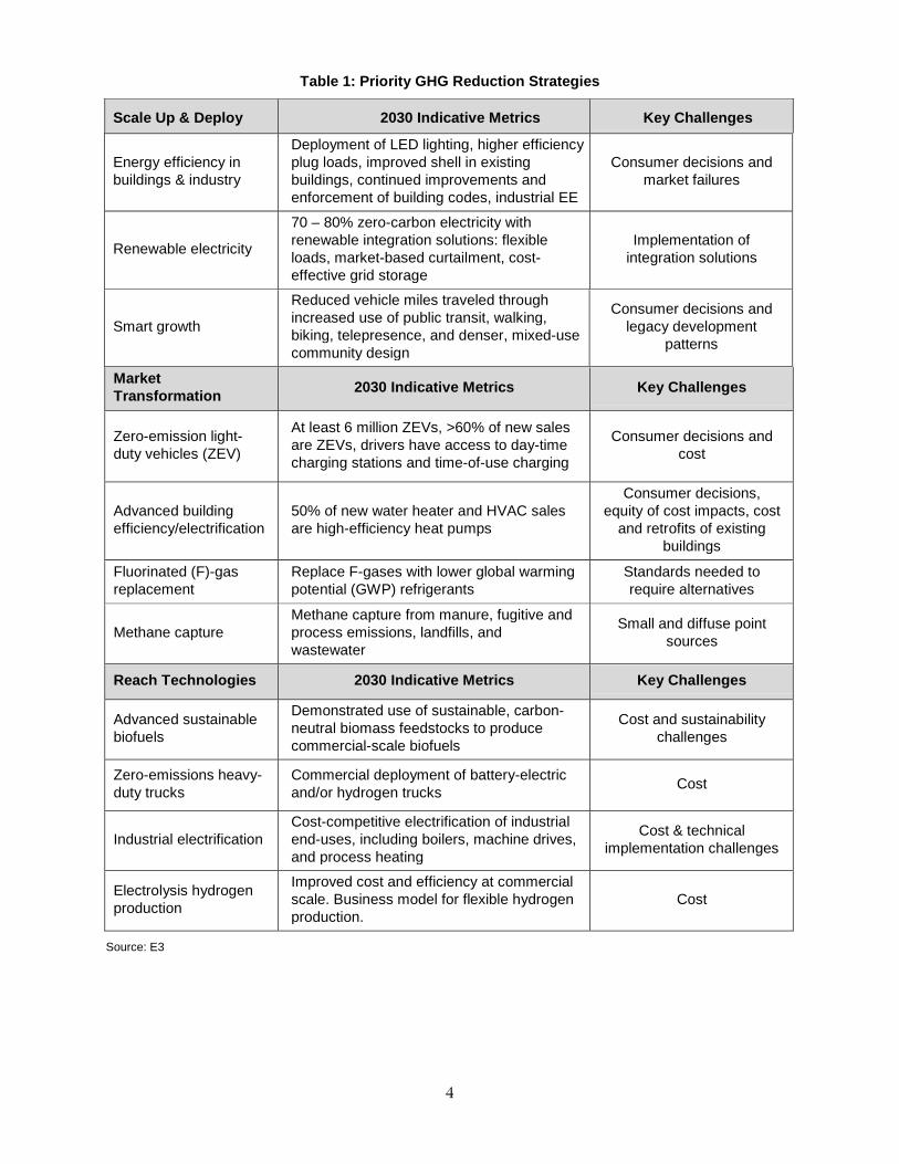
Table 1 summarizes the key strategies identified through this research that should be

prioritized for scaled-up use, market transformation, and as “reach” technologies that may be

crucial to meet the 2050 greenhouse gas target.

4

Table 1: Priority GHG Reduction Strategies

Scale Up & Deploy 2030 Indicative Metrics Key Challenges

Energy efficiency in buildings & industry

Deployment of LED lighting, higher efficiency plug loads, improved shell in existing buildings, continued improvements and enforcement of building codes, industrial EE

Consumer decisions and market failures

Renewable electricity 70 – 80% zero-carbon electricity with renewable integration solutions: flexible loads, market-based curtailment, cost-effective grid storage

Implementation of integration solutions

Smart growth Reduced vehicle miles traveled through increased use of public transit, walking, biking, telepresence, and denser, mixed-use community design

Consumer decisions and legacy development

patterns

Market Transformation 2030 Indicative Metrics Key Challenges

Zero-emission light-duty vehicles (ZEV)

At least 6 million ZEVs, >60% of new sales are ZEVs, drivers have access to day-time charging stations and time-of-use charging

Consumer decisions and cost

Advanced building efficiency/electrification

50% of new water heater and HVAC sales are high-efficiency heat pumps

Consumer decisions, equity of cost impacts, cost

and retrofits of existing buildings

Fluorinated (F)-gas replacement

Replace F-gases with lower global warming potential (GWP) refrigerants

Standards needed to require alternatives

Methane capture Methane capture from manure, fugitive and process emissions, landfills, and wastewater

Small and diffuse point sources

Reach Technologies 2030 Indicative Metrics Key Challenges

Advanced sustainable biofuels

Demonstrated use of sustainable, carbon-neutral biomass feedstocks to produce commercial-scale biofuels

Cost and sustainability challenges

Zero-emissions heavy-duty trucks

Commercial deployment of battery-electric and/or hydrogen trucks Cost

Industrial electrification Cost-competitive electrification of industrial end-uses, including boilers, machine drives, and process heating

Cost & technical implementation challenges

Electrolysis hydrogen production

Improved cost and efficiency at commercial scale. Business model for flexible hydrogen production.

Cost

Source: E3

5

High Electrification Scenario Direct Costs Compared to the Reference Scenario

The net cost of transforming the state’s energy economy to a low-carbon system is relatively

small. Fuel savings from reduced consumption of gasoline, diesel and natural gas help offset

the higher capital costs associated with low-carbon technologies. The estimated 2030 total

direct cost, (excluding health and climate benefits), to meet the state’s climate goals range from

a savings of $2 billion per year to net costs of $17 billion per year, with a base case result of $9

billion per year in 2030. This amount is less than the recovery costs associated with one large

natural disaster, such as the recent 2017 wildfires in Northern California. Put differently, the

estimated 2030 cost of reducing statewide greenhouse gas emissions by 40 percent is likely to

range from a savings of 0.1 percent to costs of 0.5 percent of California’s gross state product,

and the societal benefits of the GHG reductions achieved are likely to outweigh these costs. For

example, in other studies, the estimated health benefits associated with reducing GHG

emissions, and thus improving air quality, have been estimated to exceed these direct costs.

The upfront capital cost investment, however, is still significant, and is spread across both

businesses and households – some of which have better access to low-cost capital than others.

Long-term fuel savings, or even lifecycle cost savings, may not convince businesses and

households to make the switch to new technologies with which they have little experience. A

key challenge is convincing millions of households and businesses to adopt these technologies

and become the drivers of change to a low-carbon economy.

Finally, this study aggregates statewide costs and benefits, explicitly excluding the effect of

state incentives and in-state transfers, such as Cap-and-Trade, the Low Carbon Fuel Standard,

and utility energy efficiency programs. Costs borne by individual households will differ from

the average and will depend on policy implementation. Further research could investigate the

cost implications of specific state policies on individuals and businesses.

Uncertainty in Scenario Analysis

While these models produce numerically precise results, the long-term greenhouse gas

reduction scenarios resulting from the modeling are neither predictions nor forecasts of the

future. Several key assumptions, however, could change this study’s findings about the High

Electrification scenario as one of the lower-cost, lower-risk decarbonization pathways. First,

biofuels could be available at lower cost than modeled here, particularly if sustainability

concerns with purpose-grown crops are addressed, or if other jurisdictions continue to lag

California in decarbonizing their economies and so do not rely on advanced biofuels, resulting

in more of the global biofuel supply being available to California. Second, high costs associated

with retrofitting existing buildings for electric heating could significantly increase the cost of

the High Electrification scenario. This scenario assumes that building electrification could

proceed in California without requiring costly early retirement of end-use equipment, and

without creating cost equity impacts for natural gas customers which must be mitigated. These

assumptions deserve further research and inquiry.

Benefits of this Research to California

This research has evaluated options for meeting the state’s economywide climate goals,

including assessing the potential effects on and implications for the electricity sector. This

6

research provides decision-makers and researchers with information about the cost

implications and emissions tradeoffs between different greenhouse gas mitigation strategies

focusing on 2030 versus those focusing on 2050, and it highlights the pivotal role of the

consumer to help meet the state’s climate goals.

Furthermore, this research has helped fund the development of widely used energy and

electricity sector planning tools, including the California PATHWAYS model and the electricity

sector capacity expansion and dispatch RESOLVE model. These energy and electricity planning

tools have been, and continued to be, used by many California state agencies to provide unique

insights into how the electricity system may evolve during the next 15 to 30 years to achieve

state goals.

The benefits of this project and research will continue to expand as future projects build on

this work and through ongoing research and policy discussions within and outside California

on how to achieve deep reductions in greenhouse gas emissions.

7

CHAPTER 1: Meeting California’s Long-term Climate Goals

Introduction Climate change presents devastating risks to human health and welfare, the global economy

and ecosystems world-wide (IPCC, 2014). The impacts of climate change are already being

observed globally, and in California specifically, with increased temperatures, higher incidence

of wildfires, and changes to snowfall, snowmelt and precipitation patterns (CEC 2012, and

Kadir et al, 2013).

California is aiming to reduce its greenhouse gas emissions (GHG) while creating an energy

system that is resilient to climate risks, spurring innovation and a low-carbon transition

nationally and internationally. California’s climate goals are among the most ambitious in the

country. California’s Assembly Bill 32 (Nuñez, Chapter 488, Statutes of 2006) requires reducing

statewide GHG emissions to 1990 levels by 2020, while Senate Bill 32 (Pavley, Chapter 249,

Statutes of 2016) requires reducing statewide emissions to 40% below 1990 levels by 2030. The

state’s long-term climate commitment, laid out in Executive Order S-3-05, calls for an 80%

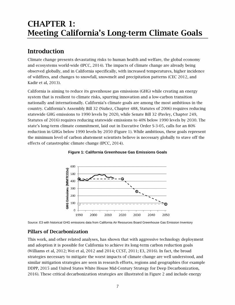
reduction in GHGs below 1990 levels by 2050 (Figure 1). While ambitious, these goals represent

the minimum level of carbon abatement scientists believe is necessary globally to stave off the

effects of catastrophic climate change (IPCC, 2014).

Figure 1: California Greenhouse Gas Emissions Goals

Source: E3 with historical GHG emissions data from California Air Resources Board Greenhouse Gas Emission Inventory

Pillars of Decarbonization

This work, and other related analyses, has shown that with aggressive technology deployment

and adoption it is possible for California to achieve its long-term carbon reduction goals

(Williams et al, 2012; Wei et al, 2012 and 2014; CCST, 2011; E3, 2016). In fact, the broad

strategies necessary to mitigate the worst impacts of climate change are well understood, and

similar mitigation strategies are seen in research efforts, regions and geographies (for example

DDPP, 2015 and United States White House Mid-Century Strategy for Deep Decarbonization,

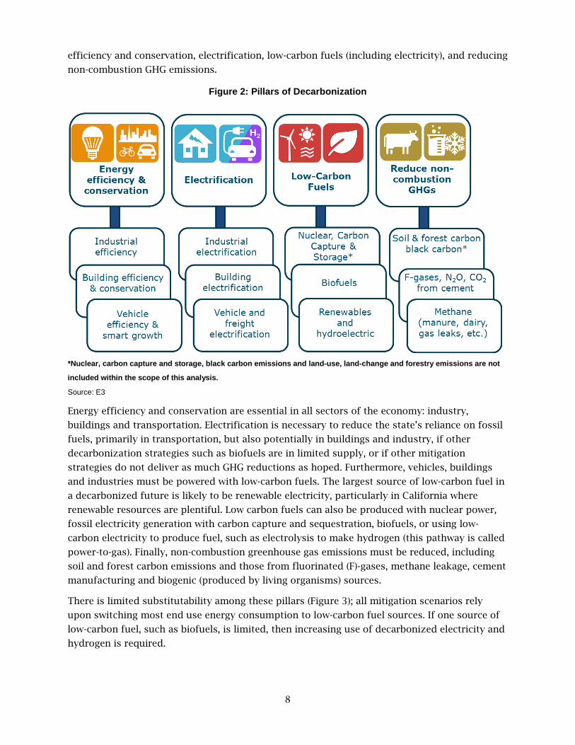
2016). These critical decarbonization strategies are illustrated in Figure 2 and include energy

8

efficiency and conservation, electrification, low-carbon fuels (including electricity), and reducing

non-combustion GHG emissions.

Figure 2: Pillars of Decarbonization

*Nuclear, carbon capture and storage, black carbon emissions and land-use, land-change and forestry emissions are not

included within the scope of this analysis.

Source: E3

Energy efficiency and conservation are essential in all sectors of the economy: industry,

buildings and transportation. Electrification is necessary to reduce the state’s reliance on fossil

fuels, primarily in transportation, but also potentially in buildings and industry, if other

decarbonization strategies such as biofuels are in limited supply, or if other mitigation

strategies do not deliver as much GHG reductions as hoped. Furthermore, vehicles, buildings

and industries must be powered with low-carbon fuels. The largest source of low-carbon fuel in

a decarbonized future is likely to be renewable electricity, particularly in California where

renewable resources are plentiful. Low carbon fuels can also be produced with nuclear power,

fossil electricity generation with carbon capture and sequestration, biofuels, or using low-

carbon electricity to produce fuel, such as electrolysis to make hydrogen (this pathway is called

power-to-gas). Finally, non-combustion greenhouse gas emissions must be reduced, including

soil and forest carbon emissions and those from fluorinated (F)-gases, methane leakage, cement

manufacturing and biogenic (produced by living organisms) sources.

There is limited substitutability among these pillars (Figure 3); all mitigation scenarios rely

upon switching most end use energy consumption to low-carbon fuel sources. If one source of

low-carbon fuel, such as biofuels, is limited, then increasing use of decarbonized electricity and

hydrogen is required.

9

Figure 3: Progress is Required Under the Four Pillars

Representative ranges of progress achieved in all four pillars in Mitigation Scenarios relative to the Reference Scenario

(scenarios defined below).

Source: E3

Scenario Design Philosophy This analysis does not evaluate the possibility of new nuclear power or generation with carbon

capture and storage, with or without using biomass, in California. These options are explored in

more detail elsewhere (for example Rhodes, 2015; Sanchez, 2015; Long, 2014). Instead, these

scenarios focus on the limits and implications of a high renewable electricity future, which is

the dominant strategy for low-carbon electricity in California today.

Furthermore, this analysis assumes that California’s natural and working lands emit net-zero

GHG emissions, which would require significant improvements over historical experience,

which has seen net positive emissions from natural and working lands, largely due to wildfires.

This assumption, that in the future California will be able to mitigate existing land-use

emissions, is consistent with California’s policy goal to turn the state’s natural and working

lands into a carbon sink, achieving at least net-zero GHG emissions, if not net negative GHG

emissions (CARB, 2017a). In this framework, sources and sinks from natural and working land

are not explicitly modeled, in large part because emissions from these sources and sinks are

not currently included in the state’s GHG emission inventory. New methods are being developed

for California creating improved retrospective and current estimates of GHG emissions from

natural and working lands. This on-going research may enable a better representation of

emissions from natural and working lands in this kind of scenario analysis in the future

(Battles, 2013; Gonzalez, 2015; Saah, 2016).

10

Continued Economic and Population Growth

These evaluated scenarios assume the current population and economic growth trends

continue through 2050.1 While these scenarios evaluate the impact of limited changes to

current energy consumption behaviors, such as the impact of smart growth policies and some

building energy savings from behavioral conservation, these changes are relatively minor

compared to what could be possible with major societal behavioral changes. For example, the

scenarios do not consider a major shift towards vegetarianism or widespread abandonment of

private vehicles to meet personal transportation needs.

Limited Reliance on Advanced, Sustainable Biofuels

Biofuels, (such as ethanol, biodiesel, wood, renewable diesel, renewable gasoline and

biomethane) represent a source of low-carbon energy to California. Even though the CO2

emissions from burning these biogenic fuels would have occurred anyway as the biomass

decayed, these fuels are considered net carbon neutral in the state’s greenhouse gas emission

inventory, which is based on the 2006 IPCC guidelines. As such, this study treats biofuels as net

carbon neutral fuels.

This study limits the supply of available biofuels in three important ways. First, most scenarios

exclude using purpose-grown crops or “energy crops” from the biofuel resource supply (the

exception is the “high biomass” scenario). The excluded energy crops include conventional food

crops such as corn and sugar cane, as well as plantation forestry and high-yielding perennial

grasses like miscanthus. This study’s primary data source for the biomass supply curves, the

U.S. DOE Billion Ton Update Study, includes purpose grown feedstocks that are estimated to

avoid indirect land-use change. However, other credible studies find that the risk of a net

increase in emissions from natural and working lands is large and poorly quantified (Plevin et

al, 2010; Melillo et al, 2009; Searchinger, 2008). As a result, most scenarios apply this more

restrictive biomass screen to avoid the risk that the cultivation of biomass for biofuels could

result in increased GHG emissions from natural or working lands.

Second, most scenarios assume that California has access to its in-state supply of waste

biomass feedstocks, and up to its population-weighted share of the United States supply of

sustainable biomass, based on Jaffe et al, 2017 and U.S. DOE, 2011 (with the exception of an in-

state only biomass scenario). This means that most scenarios limit total biomass resources to

equate to approximately 12% of the U.S. supply of waste feedstocks. None of the scenarios

assume that California imports biomass or biofuels from outside the U.S. or that California uses

more than its population-weighted share of the U.S. biomass supply. This assumption is based

on the scenario design philosophy that as California continues to decarbonize its energy

economy, the rest of the U.S. and the world will also do so, claiming access to their own

supplies of biomass and biofuels. By applying these assumptions of limited biomass, the

1 Population growth forecasts are based on the California Department of Finance projections

from 2014. Economic growth trends are implicitly included in PATHWAYS via benchmarking to

the California Energy Commission baseline forecast (CEC, 2016).

11

scenarios create decarbonization strategies for California that could be replicated in other

biomass-constrained parts of the world seeking to follow a similar decarbonization trajectory.

Finally, the scenarios do not assume breakthroughs in the cost or conversion efficiency

performance of biofuels technology over time. This leads to relatively conservative forecasts of

future costs of biofuels in all scenarios.

Research Questions While the broad pillars of decarbonization are generally well-understood, it is less well-

understood what the biggest deployment and technology risks are in achieving these long-term

plans, and how an understanding of those risks might shape polices and the research agenda

today. This research addresses that gap by asking the following research questions:

• What are priority, near-term areas for California to achieve 2030 and 2050 greenhouse

gas reduction goals? This question is evaluated for priorities in scaling-up deployment,

market transformation and “reach” technologies.

• What are the risks and potential cost implications of meeting the state’s GHG goals if

key mitigation strategies are not as successful as hoped?

Through a better understanding of the cost, climate, technology adoption, and technology

development risks, California, and other jurisdictions that are also seeking to reduce GHG

emissions, can develop new policies or focused research and development efforts to help

mitigate these risks.

GHG Mitigation Strategies Tested To guide the analysis, the study team synthesized key greenhouse gas mitigation strategies to

be modeled in PATHWAYS, testing their importance and associated risks. These strategies

include deploying new technologies and socially-coordinated actions such as smart growth to

reduce vehicle miles traveled. These strategies range from those with which the state has

extensive experience (for example, building energy efficiency) to nascent technologies that have

not been commercially developed (for example renewable hydrogen). However, the study team

excluded strategies that would require dramatic fundamental innovation before they could be

deployed, such as nuclear fusion, as well as uncertain events that could affect energy demand

and GHG emissions but are outside the control of California decision-makers, such as an

earthquake or a national or global economic shock.

The GHG mitigation strategies tested using the long-term energy scenarios include:

1. Building energy efficiency (EE), including conventional EE such as LED lightbulb

substitution and advanced EE including building retrofits and electrification.

2. Renewable electricity, including solar, wind, geothermal, and small hydropower.

Renewable integration solutions such as flexible building and vehicle loads, renewable

diversity including out-of-state renewables, energy storage, and flexible hydrogen

electrolysis are tested as well.

12

3. Smart growth that reduces light-duty vehicle miles traveled and increases the share of

higher-density new construction buildings, shifting towards more multi-family homes.

4. Mitigation of non-combustion emissions, including methane, CO2 from cement

production and many F-gases. Mitigation of black carbon was not evaluated.

5. Zero-emission light-duty vehicles, including plug-in hybrid (PHEVs), battery-electric

vehicles (BEVs) and hydrogen fuel-cell electric vehicles (FCEVs).

6. Heat pumps for buildings to replace natural gas heating in both HVAC and water

heating, as well as electrification of other building end uses, including cooking and

clothes drying.

7. Biofuels to replace liquid and gaseous fossil fuels. The focus is on advanced,

sustainable biofuels, excluding corn and sugarcane ethanol.

8. Industrial energy efficiency and electrification.

9. Solutions for trucking and freight including alternative-fuel trucks such as hybrid-

electric or compressed natural gas (CNG), along with zero-emission trucks including

battery-electric vehicles (BEVs) and fuel cell-electric vehicles (FCEVs).

10. Hydrogen as an energy carrier, modeled here as hydrogen produced from centralized,

grid-connected proton-exchange membrane (PEM) electrolysis for use in vehicles and, in

small volumes, as a natural gas replacement in the pipeline.

11. Production of climate-neutral fuels, modeled here as synthetic methane produced via

the reaction of CO2 captured from the atmosphere or seawater with renewably-produced

hydrogen. As an emerging technology, this option is only evaluated in one of the ten

scenarios.

Each of these greenhouse gas mitigation strategies are tested in different combinations with

different timing and levels of deployment in the scenarios and sensitivities, as discussed below.

Scenarios Evaluated Three types of California long-term energy scenarios are developed, including:

• A “Reference” or business-as-usual scenario, reflecting policies before the passage of

Senate Bill (SB) 350, specifically the 33 percent Renewable Portfolio Standard from 2030

through 2050 and historical levels of energy efficiency savings.

• An “SB 350” scenario, which reflects the impact of SB 350 (a 50 percent renewable

portfolio standard by 2030 and a doubling of energy efficiency savings relative to

historical goals) as well as other current policies as of 2016, including reductions in

short-lived climate pollutants by 2030.

• “Mitigation” scenarios are evaluated which meet the state’s 2030 and 2050 GHG goals

using different combinations of GHG reduction strategies. The “High Electrification”

scenario is one of the 10 mitigation scenarios evaluated, which meets the state’s climate

goals using a plausible low-cost, low-risk combination of GHG mitigation technologies.

13

Ten mitigation scenarios are developed to help identify which strategies are most critical to

meeting the state’s 2030 and 2050 GHG goals. These scenarios also isolate the estimated cost

and GHG implications of key uncertainties and are used to evaluate the robustness of the

state’s climate mitigation strategies if one strategy does not deliver GHG reductions as

expected.

Reference Scenario

The Reference scenario reflects a California GHG emissions trajectory based on energy policies

that were in place prior to 2015, including the 33% Renewables Portfolio Standard (RPS). The

Reference scenario excludes the impacts of SB 350, and other recent climate policies and

initiatives such as the short-lived climate pollutant strategy required by Senate Bill 1383 (Lara,

Chapter 395, Statutes of 2016). Key assumptions in the Reference scenario are summarized in

Table 2.

14

Table 2: Key Assumptions in the Reference Scenario

Pillar of GHG Reductions Sector & Strategy Reference Scenario assumptions

Efficiency

Building electric & natural gas efficiency

Approximately 26,000 GWh of electric efficiency, and 940 million therms of natural gas efficiency in buildings, relative to baseline load growth projections (approximately equal to the 2016 CEC IEPR additional achievable energy efficiency (AAEE) mid-scenario)

Transportation smart growth and fuel economy

Federal vehicle efficiency standards (new gasoline auto averages 40 mpg in 2030). Implementation of SB 375 (2% reduction in vehicle miles traveled (VMT) relative to 2015)

Industrial efficiency CEC IEPR 2016 AAEE mid-scenario

Electrification

Building electrification None

Zero-emission light-duty vehicles

Mobile Source Strategy from the Vision Model Current Control Program scenario: 3 million light-duty vehicle (LDV) zero-emission vehicles (ZEVs) by 2030, 5 million LDV ZEVs by 2050

Zero-emission and alternative fueled trucks

Mobile Source Strategy from the Vision Model Current Control Program scenario: 20,000 alternative-fueled trucks by 2030

Low carbon fuels

Zero-carbon electricity

Current RPS procurement achieves ~35% RPS by 2020, declining to 33% RPS with retirements post-2030. Includes current deployment of pumped storage and the energy storage mandate (1.3 GW by 2020). No additional storage after 2020.

Advanced biofuels 10% carbon-intensity reduction Low Carbon Fuel Standard including corn ethanol (1.2 billion GGE advanced biofuels in 2030 and 0.7 billion GGE corn ethanol in 2030)

Non-combustion GHGs

Reductions in methane and fluorinated gases

No mitigation: methane emissions constant after 2015, fluorinated gases increase by 56% in 2030 and 72% in 2050

Source: E3

15

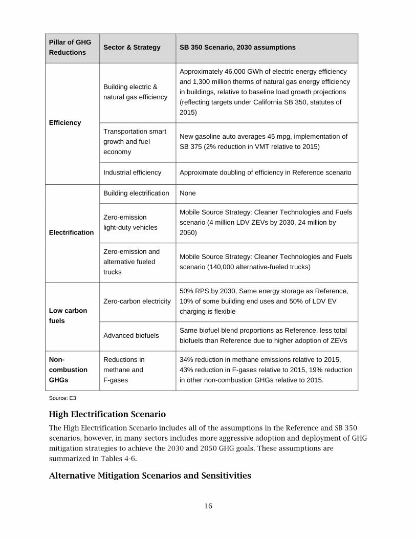
SB 350 Scenario

The SB 350 scenario includes all of the assumptions in the Reference scenario, but adds in the

estimated impacts of SB 350, the California Air Resources Board (ARB) Mobile Source Strategy

Cleaner Technologies and Fuels scenario and the Short-Lived Climate Pollutant Plan. These

impacts include a 50 percent RPS in 2030, a doubling of energy efficiency savings relative to the

“additional achievable energy efficiency” in the California Energy Commission’s 2016 Integrated

Energy Policy Report by 2026, higher adoption rates of ZEVs and reductions in non-combustion

GHG emissions.

Table 3: Key Policies and Assumptions in the SB 350 Scenario

16

Pillar of GHG Reductions

Sector & Strategy SB 350 Scenario, 2030 assumptions

Efficiency


Approximately 46,000 GWh of electric energy efficiency and 1,300 million therms of natural gas energy efficiency in buildings, relative to baseline load growth projections (reflecting targets under California SB 350, statutes of 2015)


New gasoline auto averages 45 mpg, implementation of SB 375 (2% reduction in VMT relative to 2015)

Industrial efficiency Approximate doubling of efficiency in Reference scenario

Electrification

Building electrification None


Mobile Source Strategy: Cleaner Technologies and Fuels scenario (4 million LDV ZEVs by 2030, 24 million by 2050)


Mobile Source Strategy: Cleaner Technologies and Fuels scenario (140,000 alternative-fueled trucks)

Low carbon fuels

Zero-carbon electricity 50% RPS by 2030, Same energy storage as Reference, 10% of some building end uses and 50% of LDV EV charging is flexible

Advanced biofuels Same biofuel blend proportions as Reference, less total biofuels than Reference due to higher adoption of ZEVs

Non-combustion GHGs

Reductions in methane and F-gases

34% reduction in methane emissions relative to 2015, 43% reduction in F-gases relative to 2015, 19% reduction in other non-combustion GHGs relative to 2015.

Source: E3

High Electrification Scenario

The High Electrification Scenario includes all of the assumptions in the Reference and SB 350

scenarios, however, in many sectors includes more aggressive adoption and deployment of GHG

mitigation strategies to achieve the 2030 and 2050 GHG goals. These assumptions are

summarized in Tables 4-6.

Alternative Mitigation Scenarios and Sensitivities

17

In addition to the High Electrification scenario, nine Alternative Mitigation scenarios are tested

which meet the state’s 2030 and 2050 GHG goals in PATHWAYS using different combinations of

mitigation technologies from the High Electrification scenario. These Alternative Mitigation

scenarios fall broadly into two categories: (1) reduced reliance on a key mitigation technology

choice within the state, with compensating GHG mitigation strategies used to meet the 2030

and 2050 climate goals; and (2) increased reliance on a key mitigation technology choice within

the state, with lower GHG mitigation in other sectors, to meet the 2030 and 2050 climate goals.

The costs of these alternative scenarios are then evaluated and compared to the High

Electrification scenario.

All of the scenarios include relatively high levels of electrification; some of the scenarios result

in higher electric loads than the “High Electrification” scenario. The distinguishing feature of

the “High Electrification” scenario is that nearly a full suite of GHG mitigation options is used,

including electric heat pumps in buildings. Each of the Alternative Mitigation scenarios is

described in Table 6.

In addition to these alternative technology scenarios, one additional scenario is tested. The “No

Climate Change” scenario tests the impacts of not including the climate change impacts on

hydroelectric availability and building energy demand in the scenario. All other scenarios

include the effects of climate change.

Cost sensitivities also probe uncertainties in economy-wide mitigation costs by changing key

cost inputs without changing energy or emissions assumptions. Cost sensitivities are not

comprehensive but rather emphasize a few key cost inputs whose effects may bracket the

overall cost uncertainty, including fossil fuel prices and demand-technology capital financing

rate.

The Role of Carbon Pricing and Cap and Trade

These scenarios do not attempt to directly model or predict the effect the state’s Cap-and-Trade

program (Assembly Bill 398, Garcia, Chapter 135, Statutes of 2017) will have on consumer

behavior or on business decisions through 2030 or beyond.

The cap and trade law requires the ARB to set a carbon price ceiling, price containment points,

and define other details of the cap and trade program. The impacts of cap and trade will

depend on the resulting carbon price, and the carbon price will depend on how far other

complementary policies reduce greenhouse gas emissions, and the costs of alternative GHG

mitigation options, including offsets and carbon permits from other linked jurisdictions, such

as Quebec, Canada or Ontario, Canada.

18

Table 4: Key 2030 Metrics for the High Electrification Scenario

Pillar of GHG Reductions

Sector & Strategy High Electrification Scenario, 2030 assumptions

Efficiency


10% reduction in total building energy demand relative to 2015. Same level of non-fuel substitution energy efficiency as the SB 350 Scenario in non-heating sub-sectors. Additional efficiency is achieved through electrification of space heating and water heating.


New gasoline ICE light-duty autos average 45 mpg, 12% reduction in light-duty vehicle miles traveled relative to 2015, 5-6% reduction in shipping, harbor-craft & aviation energy demand relative to Reference

Industrial efficiency 20% reduction in total industrial, non-petroleum sector energy demand relative to 2015, additional 14% reduction in refinery output relative to 2015

Electrification

Building electrification 50% new sales of water heaters and HVAC are electric heat pumps


6 million ZEVs (20% of total): 1.5 million BEVs, 3.6 million PHEVs, 0.8 million FCEVs, >60% of new sales are ZEVs


10% of trucks are hybrid & alternative fuel (4% are BEVs or FCEVs), 32% electrification of buses, 20% of rail, and 27% of ports; 26% electric or hybrid harbor craft

Low carbon fuels

Zero-carbon electricity

74% zero-carbon electricity, including large hydro and nuclear (70% RPS), Storage Mandate + 6 GW additional storage, 20% of key building end uses and 50% of LDV EV charging is flexible

Advanced biofuels

2.8 billion gallons of gasoline-equivalent (10% of gasoline, diesel, jet fuel and other non-electric energy demand); 49 million Bone Dry Tons of biomass: 57% of population-weighted share excluding purpose-grown crops

Non-combustion GHGs

Reductions in methane and F-gases

34% reduction in methane emissions relative to 2015, 43% reduction in F-gases relative to 2015, 19% reduction in other non-combustion CO2 & N2O

19

Source: E3

Table 5: Key 2050 Metrics for the High Electrification Scenario

Pillar of GHG Reductions Sector & Strategy High Electrification Scenario, 2050 assumptions

Efficiency Building electric & natural gas efficiency

34% reduction in total (natural gas and electric) building energy demand, relative to 2015. Savings are achieved via conventional efficiency and building electrification.


24% reduction in per capita light-duty vehicle miles traveled relative to 2015, plus shipping, harbor-craft & aviation energy demand 2030 measures

Industrial efficiency 20% reduction in total industrial, non-petroleum sector energy demand relative to 2015, 90% reduction in refinery and oil & gas extraction energy demand

Electrification Building electrification 100% new sales of water heaters and HVAC are electric heat pumps; 91% of building energy is electric (no building electrification is possible, but requires higher biofuels or power-to-gas), Moderate electrification of agriculture HVAC


35 million ZEVs (96% of total): 19 million BEVs, 11 million PHEVs, 5 million FCEVs, 100% of new sales are ZEVs


47% of trucks are BEVs or FCEVs (31% of trucks are hybrid & CNG); 88% electrification of buses, 75% of rail, 80% of ports; 77% of harbor craft electric or hybrid

Low carbon fuels Zero-carbon electricity

95% zero-carbon electricity (including large hydro), 84 GW of utility scale solar, 29 GW of rooftop solar, 52 GW out-of-state wind, 26 GW incremental storage above storage mandate, 80% of key building end-uses is flexible and 90% flexible EV charging; H2 production is flexible

Advanced biofuels 4.3 billion gallons of gasoline-equivalent (46% of gasoline, diesel, jet fuel and other non-electric energy demand); 64 million Bone Dry Tons of biomass: 66% of population-weighted share excluding purpose-grown crops

Non-combustion GHGs

Reductions in methane, F-gases and other non-combustion GHGs

42% reduction in methane emissions relative to 2015 83% reduction in F-gases relative to 2015 42% reduction in other non-combustion CO2 & N2O

Source: E3

20

Table 6: Alternative Mitigation Scenarios, Change in Measures Compared to the High Electrification Scenario

Scenario name (reduced reliance on key strategy)

Reduced reliance on key mitigation strategy

Increased, compensating reliance on mitigation strategies

No Hydrogen No fuel cell vehicles or hydrogen fuel

Industrial electrification, more BEV trucks & BEVs, renewables

Reference Smart Growth Less reduction in VMT Industrial electrification, more renewables

Reduced Methane Mitigation

Lower fugitive methane reductions (higher fugitive methane leakage)

Industrial electrification, more ZEV trucks, renewables

Reference Industry EE Less industrial efficiency More ZEV trucks, renewables

In-State Biomass Less biofuels, no out-of-state biomass used

Industrial electrification, more ZEV trucks, renewables

Reference Building EE Less building efficiency Industrial electrification, more renewables

No Building Electrification with Power-to-Gas

No heat pumps or building electrification

Climate-neutral power-to-gas (hydrogen and synthetic methane), industrial electrification, more ZEV trucks, renewables

Scenario name (increased reliance on key strategy)

Increased reliance on key mitigation strategy

Reduced, compensating reliance on mitigation strategies

High Biofuels Higher biofuels, including purpose grown crops

Less ZEVs, renewables

High Hydrogen More fuel cell trucks Less BEVs, renewables

Source: E3

If no additional energy or climate policies are passed between now and 2030, it seems likely

that the role of cap and trade in meeting the state’s climate goals will be significant, as can be

seen by the gap between greenhouse gas emission reductions achieved in the SB 350 Scenario

and the Mitigation Scenarios. If cap and trade is the primary policy mechanism to achieve

emission reductions between 2020 and 2030, then the carbon price would likely increase

towards the price ceiling, and greenhouse gas reductions would be achieved through consumer

21

price responses because of higher energy prices and longer-term investments in low-carbon

technologies, including energy efficiency, zero-emission vehicles and zero-emissions fuels.

The more aggressive zero-emission technology adoption assumptions included in the Mitigation

scenarios could be achieved, in part, through higher carbon prices. Carbon prices reduce

emissions by increasing the price of fossil fuels relative to lower carbon alternatives. In this

way, cap and trade is likely to help incentivize higher adoption rates of zero-emission vehicles

and energy efficiency, for example.

Carbon pricing, however, is not a panacea for zero-carbon technology adoption, because price

signals on their own cannot overcome a variety of market failures which may stand in the way

(for example, upfront capital cost barriers and principal-agent problems). For this reason, it is

expected that additional market transformation policies will be necessary for California to

achieve its 2030 and 2050 GHG goals. While the extension of cap and trade through 2030 will

certainly help to reduce GHG emissions, it may not be sufficient on its own.

Report Organization This report is organized as follows: Chapter 2 describes the research methods, including the

modeling tools used and key analytical improvements achieved through this research. Chapter

3 discusses the results for the main scenarios, including the Reference, SB 350 and High

Electrification scenario. Chapter 4 discusses the cost results and findings from the Alternative

Mitigation cases and additional scenario. Chapter 5 provides conclusions. Additional details

about key input assumptions and scenario results by sector are provided in the Appendices.

22

CHAPTER 2: Methods

The California PATHWAYS Model This analysis uses the California PATHWAYS model, an economy-wide energy and greenhouse

gas mitigation model, to identify priority GHG mitigation challenges in California through a

series of scenario and uncertainty analyses.

The PATHWAYS model is a long-horizon, technology-specific scenario model developed by

Energy and Environmental Economics, Inc. (E3). The model has been modified and improved on

over time, including through funding from this California Energy Commission Electric Program

Investment Charge grant. PATHWAYS includes detailed technology representation of the

buildings, industry, transportation and electricity sectors (including hourly electricity supply

and demand) and explicitly models stocks and replacement of buildings, building equipment

and appliances and vehicles. Demand for energy is driven by forecasts of population, building

square footage, and other energy service needs. The rate and type of technology adoption and

energy supply resources are all user-defined scenario inputs. PATHWAYS calculates energy

demand, greenhouse gas emissions, the portfolio of technology stock in selected sectors, as

well as capital costs and fuel costs and savings for each year between 2015 and 2050.

The final energy demand projections are used to project energy supply stocks and final

delivered energy prices and emissions. Electricity rates are calculated endogenously to the

model based on the scenario’s generation supply mix, hourly electricity demand and supply.

Likewise, delivered natural gas rates are calculated based on changes in annual demand and

fuel costs, including the calculated cost of biomethane, hydrogen or other synthetic fuels used

in the pipeline. Delivered costs of gasoline, diesel and other fuels include the blended costs of

the fossil fuel and biofuel. Fossil fuel price forecasts are exogenous inputs to the model, biofuel

prices are calculated endogenously to the model.

As a technology and energy-demand scenario model, the model does not explicitly model

macroeconomic changes to the economy, nor does it endogenously capture consumer price

responses, such as the impacts of carbon pricing or changes in energy prices. The model

evaluates greenhouse gas emissions based on the emissions accounting protocols used in the

Intergovernmental Panel on Climate Change (IPCC) Fourth Assessment Report, consistent with

the California Air Resources Board statewide emission inventory.

The model ultimately calculates a broad range of outputs, including energy demand by fuel

type and sector by year, greenhouse gas emissions by fuel type and sector, and annual changes

in incremental capital costs and fuel costs, relative to a Reference scenario (Figure 4). For more

detail about the PATHWAYS model methodology, see the Appendix B and E3, 2015.

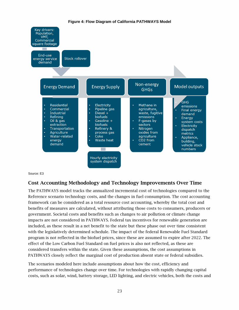
23

Figure 4: Flow Diagram of California PATHWAYS Model

Source: E3

Cost Accounting Methodology and Technology Improvements Over Time

The PATHWAYS model tracks the annualized incremental cost of technologies compared to the

Reference scenario technology costs, and the changes in fuel consumption. The cost accounting

framework can be considered as a total resource cost accounting, whereby the total cost and

benefits of measures are calculated, without attributing those costs to consumers, producers or

government. Societal costs and benefits such as changes to air pollution or climate change

impacts are not considered in PATHWAYS. Federal tax incentives for renewable generation are

included, as these result in a net benefit to the state but these phase out over time consistent

with the legislatively determined schedule. The impact of the federal Renewable Fuel Standard

program is not reflected in the biofuel prices, since these are assumed to expire after 2022. The

effect of the Low Carbon Fuel Standard on fuel prices is also not reflected, as these are

considered transfers within the state. Given these assumptions, the cost assumptions in

PATHWAYS closely reflect the marginal cost of production absent state or federal subsidies.

The scenarios modeled here include assumptions about how the cost, efficiency and

performance of technologies change over time. For technologies with rapidly changing capital

costs, such as solar, wind, battery storage, LED lighting, and electric vehicles, both the costs and

24

performance are assumed to improve over time, as economies of scale are assumed to be

achieved in manufacturing. In general, the researchers have relied on publicly available,

published projections for these cost assumptions. Other technologies do not include

assumptions about changing costs or performance over time, including many building and

industrial efficiency measures, although large-scale adoptions of these technologies could lead

to cost-declines and/or improvements in performance. In general, the cost and performance

assumptions applied in the PATHWAYS model tend to reflect conservative assumptions about

the potential for technological progress over time, to avoid overstating the potential benefits of

the Mitigation scenarios.

Uncertainty and Complexity in Scenario Analysis

To paraphrase the statistician George Box, “all models are wrong, but some are useful.” This

statement is certainly true of the PATHWAYS model, as it is true of any long-term scenario

analysis spanning decades into the future. This modeling effort was not to predict or forecast

the future. Rather, these scenarios ask, “what would be necessary to meet the state’s current

policy goals and future GHG mitigation goals, and what are the risks in meeting those goals?”

There are many sources of uncertainty in developing long-term scenarios including future

trajectories for technology capital costs, fuel costs, consumer behavior and preferences and the

future political and policy environment. Furthermore, key sources of complexity which cannot

be reflected in the PATHWAYS model include market dynamics, such as the interaction between

costs and prices, interactions between policies and technological change, and interactions

between actions taken in California and the rest of the world.

In this study design, the team attempted to capture many of these sources of uncertainty and

complexity through scenario and sensitivity analysis, while acknowledging that these tools are

not a crystal ball into the future.

Though less certain than a prediction, a scenario is more grounded in fact than mere

speculation. The scenarios were evaluated to provide useful information about what GHG

mitigation areas California should prioritize today, using the best information available about

technology costs, performance and the interactions between GHG mitigation strategies.

California PATHWAYS Model Enhancements

Since the initial California deep decarbonization scenario results were published in Williams, et

al, (2012), several improvements and enhancements have been made to the PATHWAYS model.

These include:

• Updated input data resulting in a lower Reference case forecast of greenhouse gas

emissions in California. This includes a revised, lower, population demand forecast

consistent with the California Department of Finance forecast, and revised, lower,

transportation vehicle stocks and transportation vehicle miles traveled from the

California Air Resources Board Mobile Source Emissions Inventory, EMFAC 2014

database.

• Calibrating the starting year energy consumption and emissions to the updated

California Emission Inventory–2016 Edition, covering GHG emissions through 2015. The

25

new inventory uses global warming potential (GWP) values from the IPCC Fourth

Assessment Report, consistent with current international and national GHG inventory

practices. This inventory practice excludes all biogenic emissions associated with

biofuels.

• Updated fossil price forecasts consistent with the Energy Information Agency (EIA) 2017

Annual Energy Outlook, incorporating the effect of lower expected petroleum and

natural gas prices on net economy-wide mitigation costs.

• Reflecting current California state legislation, policies and goals through 2030.

• Updated technology cost projections, particularly for solar, wind, batteries, and electric

vehicles, reflecting more rapid than expected cost reductions in these technologies.

• Updated assumptions on sustainable biomass resource limits, biofuel process

conversion efficiencies and costs, as well as an updated biofuel module which allows for

limited optimization of least-cost liquid and gaseous biofuel pathways.

• Reflecting the impacts of climate change on building energy demand and hydroelectric

generation.

• Updated assumptions for electricity resources serving California, including reduced

availability of in-state wind due to environmental restrictions and the planned

retirement of the Palo Verde nuclear plant by 2047.

• Technical enhancements and faster model run-time.

Integrating Climate Change Impacts on Energy System

This research grant was coordinated with three other research projects funded by the Energy

Commission: a team from Berkeley Economic Advising and Research, LLC (BEAR); a team and

Lawrence Berkeley National Laboratories (LBNL); and a team from the University of California,

Irvine (UCI). While each team’s work was funded separately, the teams worked together to share

data where possible and applicable. Analysis from this study was used as a key input into the

BEAR and LBNL studies. Analysis from the UCI study was used as input for this study, as

described below.

The UCI team (Tarroja, 2017) provided the E3 team with data on the likely long-term impacts of

climate change on electricity building demands and on hydroelectric generation through 2050.

These data were fed into the PATHWAYS model to create scenarios that reflect the potential

impacts of climate change on the electricity system.

Tarroja used global climate simulations that have been downscaled for California and the

Fourth Climate Assessment. The team used several model simulations based on representative

concentration pathway (RCP) 4.5 and RCP 8.5 scenarios to force a building energy model and a

regional hydrology model; these scenarios represent a modest mitigation trajectory and a high

climate change impacts trajectory, respectively.

Using the hydrology model, Tarroja estimated changes in annual hydroelectric energy

availability during the same time period relative to present-day. Changes in predicted

hydroelectric energy availability were relatively small in the annual average in each member of

the climate model ensemble, masking larger increases in inter-annual variability. As PATHWAYS

cannot incorporate inter-annual variability in hydroelectric energy availability, the model with

the largest average decrease (11%) in hydro-electric availability was used to estimate a worst-

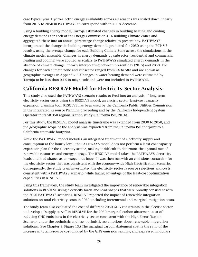
26

case typical year. Hydro-electric energy availability across all seasons was scaled down linearly

from 2015 to 2050 in PATHWAYS to correspond with this 11% decrease.

Using a building energy model, Tarroja estimated changes in building heating and cooling

energy demands for each of the Energy Commission’s 16 Building Climate Zones and

aggregated these into an annual percentage change relative to present-day. PATHWAYS

incorporated the changes in building energy demands predicted for 2050 using the RCP 8.5

results, using the average change for each Building Climate Zone across the simulations in the

climate model ensemble. Changes in energy demands by subsector (residential and commercial

heating and cooling) were applied as scalars to PATHWAYS simulated energy demands in the

absence of climate change, linearly interpolating between present-day (2015) and 2050. The

changes for each climate zone and subsector ranged from 9% to 58% and are shown as

geographic averages in Appendix B. Changes in water heating demand were estimated by

Tarroja to be less than 0.1% in magnitude and were not included in PATHWAYS.

California RESOLVE Model for Electricity Sector Analysis This study also used the PATHWAYS scenario results to feed into an analysis of long-term

electricity sector costs using the RESOLVE model, an electric sector least-cost capacity

expansion planning tool. RESOLVE has been used by the California Public Utilities Commission

in the Integrated Resource Planning proceeding and by the California Independent System

Operator in its SB 350 regionalization study (California ISO, 2016).

For this study, the RESOLVE model analysis timeframe was extended from 2030 to 2050, and

the geographic scope of the analysis was expanded from the California ISO footprint to a

California statewide footprint.

While the PATHWAYS model includes an integrated treatment of electricity supply and

consumption at the hourly level, the PATHWAYS model does not perform a least-cost capacity

expansion plan for the electricity sector, making it difficult to determine the optimal mix of

renewable resources and energy storage. The RESOLVE model takes the PATHWAYS electricity

loads and load shapes as an exogenous input. It was then run with an emissions constraint for

the electricity sector that was consistent with the economy-wide High Electrification Scenario.

Consequently, the study team investigated the electricity sector resource selections and costs,

consistent with a PATHWAYS scenario, while taking advantage of the least-cost optimization

capabilities in RESOLVE.

Using this framework, the study team investigated the importance of renewable integration

solutions in RESOLVE using electricity loads and load shapes that were broadly consistent with

the 2050 PATHWAYS scenarios. RESOLVE reported the impact of renewable integration

solutions on total electricity costs in 2050, including incremental and marginal mitigation costs.

The study team also evaluated the cost of different 2050 GHG constraints in the electric sector

to develop a “supply curve” in RESOLVE for the 2050 marginal carbon abatement cost of

reducing GHG emissions in the electricity sector consistent with the High Electrification

Scenario, under the optimistic and less-optimistic assumptions about renewable integration

solutions. (See Chapter 3, Figure 15.) The marginal carbon abatement cost is the ratio of the

increase in total resource cost divided by the GHG emission savings, and expressed in dollars

27

per ton, $/ton. This supply curve was compared to the incremental abatement costs for

mitigation options evaluated in other sectors in PATHWAYS.

28

CHAPTER 3: Reference, SB 350 and High Electrification Scenario Results

This chapter discusses the key results for the main long-term energy scenarios evaluated in

PATHWAYS: the Reference, SB 350 and High Electrification Scenarios. Results are shown for the

High Electrification scenario for greenhouse gas emissions, energy demand, and costs relative

to the Reference scenario.

Greenhouse Gas Emissions Greenhouse gas emissions in California peaked around 2004 and have been in decline since

then. If California succeeds in executing on its current policy commitments, California appears

likely to meet its 2020 goal of returning GHG emissions to 1990 levels, which requires keeping

emissions at or below 431 million metric tons. As of 2015, California greenhouse gas emissions

stood at 440 million metric tons of CO2-equivalent (ARB, 2017a).

In the Reference scenario, GHG emissions decline modestly between 2017 and about 2027, at

which point population and economic growth begin to push emissions higher through 2050. In

the Reference scenario, GHG emissions in 2050 are slightly higher than the projected 2020

level.

The SB 350 scenario, which reflects the impact of higher levels of renewables, energy efficiency,

and mitigation of non-combustion GHGs, results in a significant decrease in emissions between

present day and 2030 but does not entirely close the gap to meet the state’s 2030 GHG goal of

258.6 million metric tons of CO2e (equivalent). In the SB 350 scenario, the gap between the 2030

goal and the projected emissions is about 63 MMTCO2e. The gap to meet the 2050 goal, of 86

MMTCO2e, is much larger at nearly 190 MMTCO2e.

All of the Mitigation scenarios, including the High Electrification scenario, are designed to meet

the state’s 2030 and 2050 greenhouse gas mitigation goals (Figure 5).

29

Figure 5: California Greenhouse Gas Emissions by Scenario

Million metric tons of CO2-equivalent

Source: E3

In the High Electrification scenario, GHG emissions are reduced in all sectors by 2050. However,

the relative proportion of emissions reductions varies by sector, since the mitigation costs and

mitigation potential are not equal between sectors. By 2050, the single largest remaining source

of greenhouse gas emissions is from non-combustion emissions. Methane from agriculture and

waste (wastewater treatment, landfills and municipal solid waste) represent a large source of

remaining emissions; methane from waste and enteric fermentation in particular are expected

to be difficult to completely eliminate, although both are assumed to decline in absolute terms

through 2050.

In addition to non-combustion GHG emissions, the remaining 2050 emissions budget is

allocated between some remaining diesel and jet fuel use in the transportation sector (primarily

for off-road and long-haul, interstate trucking), the industrial sector, assuming that industrial

electrification will be relatively expensive compared to other mitigation alternatives, and the

electric power sector, which continues to use about 5% of generation from fossil natural gas for

resource balancing and resource sufficiency. Greenhouse gas emissions are not eliminated in

any sector by 2050 in the High Electrification scenario (Figure 6).

30

Figure 6: California Greenhouse Gas Emissions by Sector in the High Electrification Scenario

Greenhouse gas emissions in 2050 are 86 MMT CO2e, inclusive of non-combustion GHG emissions.

Source: E3

Transportation sector energy-related GHG emissions represent the largest source of greenhouse

gas emissions in California, currently about 39% of the statewide total2. In the High

Electrification scenario, this share declines over time to just over one-quarter of total statewide

greenhouse gas emissions. The industrial sector energy-related emissions represent the second

largest source of GHG emissions in California, with just over 20% of the total. Industrial sector

emissions are expected to be among the more difficult, and more expensive to mitigate. As a

result, the total share of GHG emissions from the industrial sector increases slightly over time,

even as total emissions are dramatically reduced. By 2050, the remaining non-combustion

emissions in agriculture and recycling and waste represent a far larger share of total GHG

emissions than today, illustrating that the challenging of reducing emissions beyond 2050 will

be somewhat different than the challenges of meeting the state’s 2050 GHG goal.

Energy Demand Results Final energy demand (i.e. non-electric generation energy consumption), shows that energy

consumption falls by 50% in the High Electrification scenario, from nearly 6 exajoules (EJ) today

to less than 3 EJ in 2050 (Figure 7). These energy savings are due to improved fuel economy

standards in vehicles, efficiency associated with electrification in transportation and buildings,

reductions in per capita VMT, and improved energy efficiency in buildings and industry. The

efficiency advantages of electric drive and heat pumps over internal combustion engines and

combustion heaters, respectively, result in dramatic reductions in final energy demand.

2 ARB Inventory (https://www.arb.ca.gov/cc/inventory/data/data.htm) accessed on May 18.

2018.

https://www.arb.ca.gov/cc/inventory/data/data.htm

31

Figure 7: Final Energy Demand by Fuel Type in the High Electrification Scenario

Source: E3

The High Electrification scenario shows a decline in fossil fuel demand across all fuel types,

with the greatest reductions in gasoline and natural gas, in-part due to a greater reliance on

biomethane blended into the pipeline. The High Electrification scenario biofuel assumptions are

based on a least net-cost analysis across all major fuel types (gasoline, diesel and natural gas).

Using these assumptions, the most efficient use of biomass is to produce renewable methane

(biogas), rather than liquid biofuels. This scenario does not model the impact of the Low

Carbon Fuel Standard policy which directs biofuel use towards the transportation sector. A

transportation-focused biofuel sensitivity would result in less overall biofuels used to displace

fossil natural gas and more biofuels used to displace diesel energy.

Decarbonization Strategies by Sector

Buildings

Energy efficiency in buildings is a central strategy to reducing the cost of greenhouse gas

mitigation in California. The state has already committed to doubling energy efficiency savings,

relative to an aggressive baseline of maintaining historical levels of efficiency savings through

SB 350, however, most experts agree that achieving a doubling of energy efficiency presents

many implementation challenges.

Deploying such a high level of energy efficiency will likely require substantial changes to

current efficiency deployment strategies. In addition to conventional energy efficiency, deep

decarbonization in buildings requires a combination of extensive building electrification,

featuring heat pumps for space conditioning and water heating, or replacing fossil natural gas

use with carbon-neutral renewable gas.

32

In the High Electrification scenario, higher levels of “conventional efficiency”, (i.e. non-fuel

substitution energy efficiency), are achieved through higher and faster adoption rates of LED

lighting, as well as more efficient refrigeration, plug-loads, water heating, air conditioning, and

space heating compared to the CEC’s 2016 IEPR additional achievable energy efficiency

potential metric. In addition, behavioral conservation measures are assumed to partially reduce

lighting and HVAC energy consumption, while “smart growth” measures encourage new

construction to include more high density, smaller and more efficient multi-family homes,

relative to historical trends. However, of all these measures in the High Electrification scenario,

it is fuel switching to high efficiency heat pumps in HVAC and water heating that achieves the

largest reductions in total building energy demand, factoring in both natural gas and electric

consumption. Greenhouse gas emissions decrease due to fuel-switching as well, due to the high

and increasing share of renewables on the grid.

To decarbonize heating demands in buildings through a transition to electric heat pumps,

without requiring early retirements of functional equipment, this transition must start by 2020

and achieve significant market share by 2030. In the High Electrification scenario, new heat

pump sales must represent no less than approximately 50% of new sales of HVAC and water

heating equipment by 2030 (Figure 8).

Figure 8: Percent of New Sales by Technology Type for Residential Space Heating and Water Heating in the High Electrification Case (2015–2050)

Source: E3

However, the electrification and renewable natural gas options still face large hurdles.

Widespread use of electric heat pumps would require market transformation, to make electric

heating a more attractive and cost-competitive option for households and businesses in

California. Many contractors in California do not have experience sizing and installing heat

pump equipment, and customers do not have experience using it. While heat pump adoption

has been increasing in the U.S. northeast and southeast and in Asia, heat pump technologies are

not common in California outside of some rural areas that lack access to natural gas.

Furthermore, the refrigerant F-gases used in heat pump technologies have a high global

warming potential and must be replaced with lower global warming potential gases in

accordance with the Montreal Protocol’s Kigali Amendment; state legislation is already moving

in this direction. Finally, current utility energy efficiency programs and tiered electricity retail

rates have not been designed with carbon savings, or fuel-switching from natural gas to electric

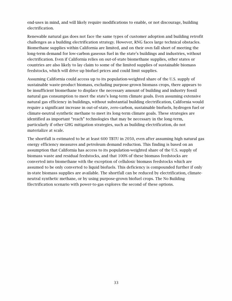
33

end-uses in mind, and will likely require modifications to enable, or not discourage, building

electrification.

Renewable natural gas does not face the same types of customer adoption and building retrofit

challenges as a building electrification strategy. However, RNG faces large technical obstacles.

Biomethane supplies within California are limited, and on their own fall short of meeting the

long-term demand for low-carbon gaseous fuel in the state’s buildings and industries, without

electrification. Even if California relies on out-of-state biomethane supplies, other states or

countries are also likely to lay claim to some of the limited supplies of sustainable biomass

feedstocks, which will drive up biofuel prices and could limit supplies.

Assuming California could access up to its population-weighted share of the U.S. supply of

sustainable waste-product biomass, excluding purpose-grown biomass crops, there appears to

be insufficient biomethane to displace the necessary amount of building and industry fossil

natural gas consumption to meet the state’s long-term climate goals. Even assuming extensive

natural gas efficiency in buildings, without substantial building electrification, California would

require a significant increase in out-of-state, zero-carbon, sustainable biofuels, hydrogen fuel or

climate-neutral synthetic methane to meet its long-term climate goals. These strategies are

identified as important “reach” technologies that may be necessary in the long-term,

particularly if other GHG mitigation strategies, such as building electrification, do not

materialize at scale.

The shortfall is estimated to be at least 600 TBTU in 2050, even after assuming high natural gas

energy efficiency measures and petroleum demand reduction. This finding is based on an

assumption that California has access to its population-weighted share of the U.S. supply of

biomass waste and residual feedstocks, and that 100% of these biomass feedstocks are

converted into biomethane with the exception of cellulosic biomass feedstocks which are

assumed to be only converted to liquid biofuels. This deficiency is compounded further if only

in-state biomass supplies are available. The shortfall can be reduced by electrification, climate-

neutral synthetic methane, or by using purpose-grown biofuel crops. The No Building

Electrification scenario with power-to-gas explores the second of these options.

34

Figure 9: Estimated Cost and Available Biomethane Supply to California in 2050 Compared with Non-Electric Natural Gas Demand

Note: Biomethane supply curves assume all available, non-cellulosic, biomass feedstocks are converted to biomethane.

Total supply is compared with non-electric gas demand in the No Building Electrification scenario in 2050 as well as non-

electric natural gas demand in 2015.

Source: E3

Transportation

Light duty vehicles (LDV) represent the largest source of greenhouse gas emissions in the state,

while transportation emissions as a whole, including trucking and off-road transportation, is

the largest source of emissions by sector. Reducing greenhouse gas emissions from the

transportation sector requires a multi-pronged strategy encompassing fuel economy standards

for conventional vehicles, reductions in vehicle miles traveled through smart growth strategies,

as well as low- and zero-emissions vehicles and biofuels.

Encouraging consumers to more rapidly switch to purchasing zero-emissions vehicles (ZEVs),

with perhaps as many as 6 million ZEVs required on the road by 2030, is a major market

transformation challenge. In the light-duty vehicle fleet, the commercial advantage seems to be

tilting in favor of battery electric (BEV) and plug-in hybrid electric vehicles (PHEVs), compared

to hydrogen fuel-cell vehicles. As a result, by 2030, 60% of new LDV sales are assumed to be

BEVs and PHEVs, while just over 10% of new sales of light-duty vehicles are assumed to be

hydrogen fuel cell vehicles. This reflects the possibility that the longer ranges and shorter

fueling times for fuel cell vehicles could be convincing to a portion of the market (

35

Figure 10). It is possible to meet the state’s climate goals with a wide range of zero-emission

vehicle types; the important part is achieving high volumes of ZEV sales before 2030.

36

Figure 10: Percent of New Sales of Light Duty Vehicles by Technology Type in the High Electrification Scenario

Source: E3

For light-duty ZEVs, the cost of fueling an electric vehicle is far lower than the cost of fueling a

conventional vehicle. The challenge is primarily in bringing down the capital cost of the electric

vehicles, ensuring that customers have a wide range of electric and plug-in hybrid vehicles to

choose from, and that they have confidence in the range and performance of those vehicles.

This analysis assumes that the capital cost of light duty electric vehicles will reach parity with

internal combustion engine vehicles by approximately 2030. This means that before 2030,

vehicle incentives may continue to be necessary to bridge the cost gap with conventional

vehicles. Coordination among electric utilities and local governments to facilitate widespread

deployment of vehicle charging stations is also critical.

In the medium- and heavy-duty trucking sectors, the zero-emission and alternative fueled

options are more diverse than in the light duty fleet. Solutions include conventional diesel

vehicles running on renewable diesel, compressed natural gas (CNG) trucks running on fossil

natural gas or compressed biomethane, hydrogen fuel cell trucks, battery electric, and hybrid

diesel-electric trucks. In the High Electrification case, a diverse, low-emissions trucking fleet is

envisioned encompassing all of these options, because of their diverse nature (Figure 11).

Figure 11: Percent of New Sales of Medium- and Heavy-Duty Vehicles by Technology Type in the High Electrification Scenario

37

In this analysis, the hydrogen fuel cell trucks appear to be the most expensive to purchase and

operate from among these options but they may be a competitive GHG mitigation option for a

limited number of long-haul, heavy duty applications. In general, costs for short-haul zero-

emission trucks are driven more by the total engine power requirements, while costs for long-

haul trucks are driven more by the total fuel storage requirements (Boer, 2013). Batteries tend

to be cheaper than fuel cells per unit of power but may be more expensive than hydrogen

storage per unit of energy. The mitigation scenarios here assume that battery trucks can

displace no more than 50% of truck vehicle miles (those used for shorter-haul distances), while

fuel-cell trucks are assumed to serve longer-haul heavy duty trucking. As a result, hydrogen

fuel cell heavy-duty trucks are a key “reach technology” in this scenario.

In other transportation sectors, (including buses, boats, aviation, ocean-going vessels, rail,

construction, and other recreational and industrial vehicles), GHG reductions are also required,

although the solutions, like in trucking, may be highly tailored to each application.

Electrification of buses, port equipment, and transportation vehicles at airports, for example,

represent a relatively easy GHG mitigation option, while reducing GHG emissions from aviation

and shipping may be more expensive.

In the High Electrification scenario, diesel and jet fuel use in off-road transportation (including

aviation, rail and shipping) represents 28% of total remaining GHG emissions in 2050, which is

the largest remaining source of fossil fuel use by 2050. While decarbonization options could be

developed for these sectors, including hydrogen-fueled, all-electric, or biofuel technologies,

these scenarios do not necessitate implementing these solutions to achieve the 2050 GHG goal.

Industry and Agriculture

California’s current industrial and agriculture GHG emissions from energy use are similar in

magnitude to those of the state’s electricity sector. The refining sector, oil and gas extraction,

and manufacturing, (notably cement, chemicals and food processing), represent the largest

sources of emissions in this category.

Reducing GHG emissions from these sectors will likely require significant increases in energy

efficiency, as well as, potentially, the use of biomethane to displace fossil natural gas. Carbon

pricing, through the cap and trade program, may help to achieve higher levels of energy

efficiency in industry, and could encourage the use of sustainable biofuels, although more

direct, industry-specific programs may also be required.

Industrial electrification is another GHG mitigation option, which is likely to be technically

feasible for nearly all end uses, but at potentially high cost. The high cost of many industrial

processes is due to the relative inefficiency of using a high-quality final energy carrier such as

electricity as a substitute for simple combustion to make heat. While heat pumps can offer

efficiency advantages for room temperature heating applications in buildings, they do not offer

the same advantage for high temperature industrial processes. Consequently, the High

Electrification scenario does not include any industrial electrification. Nevertheless, industrial

electrification is a key “reach technology” in this study, as it serves as a backstop mitigation

option in many of the alternative mitigation scenarios when cheaper options are not available.

38

The costs of high levels of industrial energy efficiency and electrification are not well

understood and this represents an area where additional research could be helpful.

Another key uncertainty in the industrial sector is what will happen to the state’s large

refineries, and to domestic oil and gas extraction, over time, as in-state demand for refined

petroleum products fall. This analysis assumes that, in addition to energy efficiency savings of

20 to 30% by 2030, the refining sector reduces its total production by an additional 14% by

2030.

The combined effect of energy efficiency and reduced production modeled in the refining

sector result in similar levels of energy reductions as seen in the total, in-state demand for

gasoline and diesel, which falls by 44% in 2030, relative to 2015, in the High Electrification

Scenario (Figure 12). It is not known how California’s refining sector will respond to a long-

term, structural shift towards lower demand for gasoline and diesel in California from vehicle

electrification. The sector could shift towards becoming a net-exporter of petroleum products,

or it could reduce in-state production, as modeled. However, if greenhouse gas emissions from

the refining sector do not decline significantly, it will make meeting the state’s long-term

climate goal very challenging. In the High Electrification Scenario, refining sector GHG

emissions fall 90% by 2050 relative to today, in line with the energy-related GHG emissions

reductions seen in other sectors.

Figure 12: Refining Sector Energy Consumption and Petroleum Product Consumption in the High Electrification Scenario

Source: E3

Electricity

California is well on its way to reducing greenhouse gas emissions from electricity. By 2025, the

state will have eliminated the small amounts of remaining in-state and imported coal-fired

generation. Currently, the state’s electricity generation mix is approximately 25% renewable,

10% nuclear and 10% hydroelectric, or about 45% zero-carbon. (Diablo Canyon, California’s only

remaining in-state nuclear generation facility will retire in 2024/25, leaving only a small portion

of imported nuclear power from Palo Verde through 2045, when that facility is likely to retire.

39

No new nuclear power is evaluated in this scenario.) This analysis suggests that a 70% - 85%

zero-carbon electricity mix could be necessary to meet the state’s 2030 climate goals. The range

of zero-carbon electricity needed for 2030 reflects the potential for slower progress in other

mitigation strategies than assumed in the High Electrification scenario. In this study, zero-

carbon electricity serves as the major backstop strategy in 2030, as technical obstacles to about

80% zero-carbon electricity appear to be more surmountable than the challenges associated

with scaling up GHG mitigation further in other sectors, and, unlike other sectors, consumer

adoption challenges are less of a concern for renewable energy deployment.

Energy efficiency savings could largely offset the increase of new electrification loads in the

2030 timeframe, but by 2050, electrification loads are expected to increase California’s

electricity demand by approximately 60% (Figure 13). This means that the electricity sector will

be providing the majority of the energy in the state, displacing fossil fuel use as the state’s

largest source of energy today.

Figure 13: Electricity Demand by Sector in the High Electrification Scenario

Source: E3

Renewable electricity generation is the largest single measure for reducing GHG emissions in

2050. This modeling suggests that approximately 95% zero-carbon generation and 5% gas

generation is needed by 2050 (Figure 14). This generation mix (including both in-state solar and

out-of-state wind to enhance resource diversity), plus aggressive deployment of flexible loads,

and energy storage appears to be a lower-cost means to reduce GHG emissions than other, non-

electricity sector GHG mitigation options. Achieving a 100% zero-carbon generation mix,

however, appears to be cost-prohibitive without reliance on nuclear, carbon capture and

sequestration (CCS), lower-cost, more abundant biofuels, or new forms of low-cost, long-

duration energy storage (Figure 15).

To achieve a 100% zero-carbon electricity system, affordable, zero-carbon and long-duration

dispatchable resources would be necessary to maintain resource sufficiency and reliability

during sequential days of low renewable energy availability. Low carbon electricity is critical for

achieving economy-wide decarbonization in concert with electrification of end-uses in other

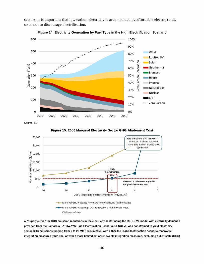
40

sectors; it is important that low-carbon electricity is accompanied by affordable electric rates,

so as not to discourage electrification.

Figure 14: Electricity Generation by Fuel Type in the High Electrification Scenario

Source: E3

Figure 15: 2050 Marginal Electricity Sector GHG Abatement Cost

A “supply curve” for GHG emission reductions in the electricity sector using the RESOLVE model with electricity demands

provided from the California PATHWAYS High Electrification Scenario. RESOLVE was constrained to yield electricity

sector GHG emissions ranging from 0 to 20 MMT CO2 in 2050, with either the High Electrification scenario renewable

integration measures (blue line) or with a more limited set of renewable integration measures, excluding out-of-state (OOS)

41

wind delivered to California from the other Western states, and flexible loads in buildings, hydrogen production, and

electric vehicle charging (gold line).

Source: E3

The annual cost savings in 2050, afforded by the diverse set of renewable integration solutions

in the High Electrification scenario is modeled to be large. Relying only on in-state solar

resources and renewable integration solutions, without the diversity provided by out-of-state

wind, adds about $19 billion per year in costs by 2050 to achieve the same level of

decarbonization (Figure 16). Moreover, if flexible loads in buildings, flexible electric vehicle

charging, and flexible hydrogen electrolysis are also not available and other sectoral strategies

are unchanged, the annual cost premium would reach $36 billion per year by 2050. This large

cost premium results from the expense of pairing solar generation with batteries so that

electricity can continue to serve demand at night, as well as overbuilding the solar generation

so that it can meet demands during cloudy and wintertime periods. Beyond the cost premium,

land use impacts could be significant: the land area required for new utility-scale solar in the

“In-state + Low Flexibility” scenario could exceed 1,700 square miles (about 1% of state land

area), versus only about 600 square miles in the High Electrification scenario.3

Figure 16: 2050 Capacity Additions and Cost Impacts of Electricity Sector Sensitivity Analysis

Results are based on RESOLVE modeling using electricity demands from the California PATHWAYS High Electrification

Scenario

Source: E3

This analysis underlines the critical importance of renewable integration strategies, including

diverse renewable generation sources, to affordably meeting the state’s climate goals. It also

raises many questions for additional research. These include how best to design electricity

markets to incentivize diverse renewable resources, flexible loads, and optimally dispatched

storage. Another question is how to compensate thermal generators whose value may

3 This assumes 8 acres per MW of installed solar including balance-of-system area (Ong et al., 2013).

42

increasingly be in providing capacity and resource sufficiency during periods of low-renewable

generation, rather than in providing regular energy services.

43

Biofuels

In addition to zero-carbon electricity (renewables, nuclear or carbon capture and storage),

biofuels represent the only other potential source of zero-emissions primary energy. This

analysis attempts to apply a conservative lens to estimate available biofuel supplies and costs.

Biofuel supply curves are developed based on estimates of the in-state supply of biomass

potential, as well as California’s population weighted share of the U.S. supply of biomass.

Biomass resources in California and the United States

Biomass resources are relatively limited in California. Estimates of in-state resources for

biomass vary from 20–40 million bone dry tons (Table 7). California currently imports

approximately 87% of its liquid biofuels from out-of-state to meet low-carbon fuel standard

regulations (ARB, 2016). In this analysis, the DOE Billion Ton Update (2011) is used to estimate

the U.S. supply of sustainable biomass resources, supplemented by Jaffe et al. (2016) for

estimates of in-state manure, landfill gas, and municipal solid waste, yielding about 30 million

bone dry tons of available in-state biomass in the scenarios. Full biomass module details are in

Appendix C.

Table 7: Summary of Estimated Biomass Resources in California

Source (Million bone dry tons)

Cellulose Wood Lipid

Manure and

Landfill Gas4

Misc. Total

Billion Ton Update (Perlack et al., 2011)

3.0 14.6 0.3 1.8 0.0 19.7

Horvath et al. (2016) 6.4 18.5 0.0 5.0 0.0 29.9 California Council on Science and Technology (2013)

6.6 16.7 5.5 0.0 11.8 40.6

California Biomass Collaborative (Williams, R.B. et al., 2015)

2.1 16.3 0.0 13.3 3.6 35.4

Resources are approximately mapped to PATHWAYS fuel conversion categories, Million Bone Dry Tons.

Source: E3

The Billion Ton Update (Perlack, 2011) estimated that about 1.3 billion tons of biomass

feedstock could be available nationally by 2030 for biofuel production, including wastes and

residues as well as purpose-grown crops and plantation forestry. About 0.5 billion tons of the

supply is associated with new cultivation of purpose-grown miscanthus, pine, eucalyptus, and

other grass and tree crops.

4 In this table, one ton of landfill gas is counted as one bone dry ton. Elsewhere in the document, a weighting factor of 6 is applied to landfill gas to account for the greater energy content of landfill gas as compared with crude biomass.

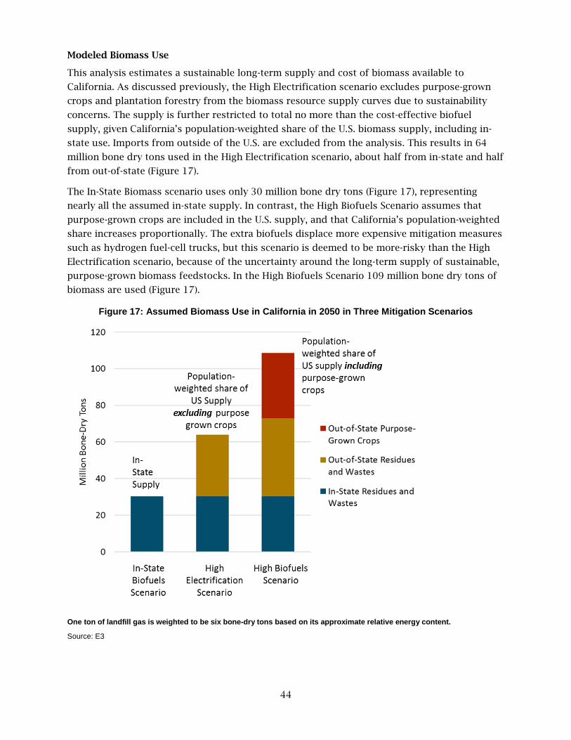
44

Modeled Biomass Use

This analysis estimates a sustainable long-term supply and cost of biomass available to

California. As discussed previously, the High Electrification scenario excludes purpose-grown

crops and plantation forestry from the biomass resource supply curves due to sustainability

concerns. The supply is further restricted to total no more than the cost-effective biofuel

supply, given California’s population-weighted share of the U.S. biomass supply, including in-

state use. Imports from outside of the U.S. are excluded from the analysis. This results in 64

million bone dry tons used in the High Electrification scenario, about half from in-state and half

from out-of-state (Figure 17).

The In-State Biomass scenario uses only 30 million bone dry tons (Figure 17), representing

nearly all the assumed in-state supply. In contrast, the High Biofuels Scenario assumes that

purpose-grown crops are included in the U.S. supply, and that California’s population-weighted

share increases proportionally. The extra biofuels displace more expensive mitigation measures

such as hydrogen fuel-cell trucks, but this scenario is deemed to be more-risky than the High

Electrification scenario, because of the uncertainty around the long-term supply of sustainable,

purpose-grown biomass feedstocks. In the High Biofuels Scenario 109 million bone dry tons of

biomass are used (Figure 17).

Figure 17: Assumed Biomass Use in California in 2050 in Three Mitigation Scenarios

One ton of landfill gas is weighted to be six bone-dry tons based on its approximate relative energy content.

Source: E3

45

The High Electrification scenario assumes a large transformation in the biomass supply chain

relative to today. Most of today’s biofuel consists of ethanol derived from out-of-state corn

from a conventional fermentation process that uses only the starch and simple sugars (Figure

18), but by 2050 the corn ethanol is assumed to be replaced with advanced biofuels dominated

by out-of-state wood and cellulose associated with agriculture and forestry residues. These

residues are converted to biofuels using hydrolysis, pyrolysis, and gasification. In-state

utilization includes a significant amount of landfill gas, based on the Jaffe et al. (2016) analysis.

Although manure could represent an important biomethane precursor, neither in-state, nor out-

of-state, manure is found to be cost-effective in the High Electrification scenario, using a total

resource cost perspective. The Low Carbon Fuel Standard (LCFS) incentivizes the production of

biomethane from manure because of the co-benefits of avoided methane emissions. In-state

economic transfers between producers and consumers, such as those that are created by LCFS

credits, are not modeled here, but could shift the feedstock supply of biomethane in California

relative to the estimates of the High Electrification scenario, albeit at a higher cost. Overall, the

model may be underestimating the cost of achieving manure methane reductions in the non-

combustion sector, which assumes that manure methane is used to produce biofuels.

Figure 18: Assumed Feedstock Use in California in the High Electrification Scenario

This scenario excludes purpose-grown crops in 2050. One ton of landfill gas is the equivalent of six bone dry tons based

on its approximate relative energy content.

Source: E3

Comparing Biomass Use to Previous Studies

Several previous studies of deep decarbonization in California and in other regions have

included biofuels as a source of net-zero carbon fuel. Eight of these analyses (Figure 19) are

46

reviewed including studies focused on Washington, the U.S., California, and the United

Kingdom. The previous PATHWAYS cases (E3, 2015) assumed a level of biomass availability

more comparable to the “High Biofuels” scenarios in the current analysis. Likewise, all of the

other deep decarbonization studies reviewed here, which evaluated economy-wide greenhouse

gas reductions of 80% by 2050, included a higher per capita biomass use than this study’s High


This literature review indicates the current High Electrification scenario is more conservative

regarding the role of biofuels in a low-carbon economy than previous deep decarbonization

literature. Exploring biofuel-constrained scenarios is an important contribution to the literature

given ongoing research into biofuel sustainability: even those produced from waste and residue

biomass could possibly have negative impacts on forest ecosystems or lead to net emissions of

CO2 from terrestrial stocks of carbon (US EPA, 2014). Moreover, recent progress in the

commercialization of advanced biofuels has been slower than anticipated, especially in

comparison with rapid technological progress in the commercialization of renewables and

electric vehicles. Consequently, reduced dependence on biofuels in the High Electrification

scenario is intended to reduce environmental risk, as well as cost risk.

Figure 19: Estimated Biomass Primary Energy Use in 2050

Estimated per capita biomass primary energy utilization in 2050 shown for selected deep decarbonization scenarios. The

comparison assumes 18 GJ per bone dry ton primary energy yield, corresponding to the average yield assumed in the US

analysis for the Deep Decarbonization PATHWAYS Project (Williams, 2014). References:

E3. 2015. California State Agencies’ PATHWAYS Project: Long-term GHG Reduction Scenarios;

California Council on Science and Technology (CCST). 2011. California's Energy Future - The View to 2050;

LBNL. 2013. Scenarios for Meeting California's 2050 Climate Goals (see cited reference Wei et al., 2014);

U.C. Davis: Yang et al. 2015. Achieving California's 80% Greenhouse Gas Reduction Target in 2050;

Washington State: Haley, et al. 2016. Deep Decarbonization Pathways Analysis for Washington State;

U.S. DDPP: Williams, J.H., et al. (2014). Pathways to deep decarbonization in the United States.

U.S. Mid-Century: The White House. 2016. United States Mid-Century Strategy for Deep Decarbonization;

U.K. Decarbonization: European Climate Foundation. 2010. Roadmap 2050

Source: E3

47

Biofuel Costs in 2050

Within each scenario, the biofuels module is used to select an array of feedstock and fuel

combinations that approximately maximizes the cost-effective CO2 abatement, within the

context of the marginal abatement costs in other sectors. The PATHWAYS model attempts to

capture the interactions between mitigation options: for instance, renewable ethanol as a

gasoline substitute is a relatively cheap biofuel that is not heavily utilized in most mitigation

scenarios because light-duty vehicles are assumed to be nearly all cost-effectively electrified by

2050. The impact of the federal Renewable Fuel Standard program is not reflected in the biofuel

prices, since these are assumed to expire after 2022. Consistent with the cost methodology

applied within the PATHWAYS model, the effect of the Low Carbon Fuel Standard on fuel prices

is also not reflected, as these are considered transfers within the state.

In all the scenarios, biofuels are estimated to carry a significant price premium over fossil fuels.

The team assumed there is a single market-clearing price for each biofuel type corresponding to

the all-in cost associated with the marginal feedstock increment, relatively large CO2 abatement

costs can result as inexpensive resources are exhausted. The total economy-wide net cost of

biofuels over their fossil fuel counterparts is estimated to be $17B in 2050 in the High

Electrification Scenario. This net cost in 2050 is highly uncertain and is based on a conservative

assumption excluding innovation in advanced biofuel conversion pathways.

In the High Biofuels Scenario, which includes the use of purpose-grown crops to produce

biofuels (Figure 20), the same complement of mitigation options is assumed to be available as

in the High Electrification Scenario. This means that the additional biofuels afforded by access

to imported purpose-grown crops can be used to lower overall scenario costs. The additional

biofuel displaces some vehicle electrification and hydrogen vehicles as well as displacing some

of the marginal renewable generation and battery storage.

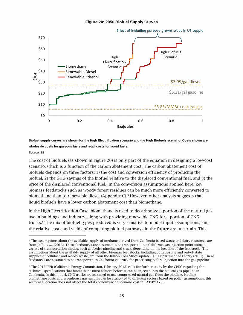
48

Figure 20: 2050 Biofuel Supply Curves

Biofuel supply curves are shown for the High Electrification scenario and the High Biofuels scenario. Costs shown are

wholesale costs for gaseous fuels and retail costs for liquid fuels.

Source: E3

The cost of biofuels (as shown in Figure 20) is only part of the equation in designing a low-cost

scenario, which is a function of the carbon abatement cost. The carbon abatement cost of

biofuels depends on three factors: 1) the cost and conversion efficiency of producing the

biofuel, 2) the GHG savings of the biofuel relative to the displaced conventional fuel, and 3) the

price of the displaced conventional fuel. In the conversion assumptions applied here, key

biomass feedstocks such as woody forest residues can be much more efficiently converted to

biomethane than to renewable diesel (Appendix C).5 However, other analysis suggests that

liquid biofuels have a lower carbon abatement cost than biomethane.

In the High Electrification Case, biomethane is used to decarbonize a portion of the natural gas

use in buildings and industry, along with providing renewable CNG for a portion of CNG

trucks.6 The mix of biofuel types produced is very sensitive to model input assumptions, and

the relative costs and yields of competing biofuel pathways in the future are uncertain. This

5 The assumptions about the available supply of methane derived from California-based waste and dairy resources are from Jaffe et al. (2016). These feedstocks are assumed to be transported to a California gas injection point using a variety of transportation modes, such as feeder pipeline and truck, depending on the location of the feedstock. The assumptions about the available supply of all other biomass feedstocks, including both in-state and out-of-state supplies of cellulose and woody waste, are from the Billion Tons Study update, U.S. Department of Energy (2011). These feedstocks are assumed to be transported to California via truck for processing before injection into the gas pipeline.

6 The 2017 IEPR (California Energy Commission, February 2018) calls for further study by the CPUC regarding the technical specifications that biomethane must achieve before it can be injected into the natural gas pipeline in California. In this model, CNG trucks are assumed to use compressed natural gas from the pipeline. Pipeline biomethane costs and greenhouse gas savings can be attributed to different sectors based on policy assumptions; this sectoral allocation does not affect the total economy-wide scenario cost in PATHWAYS.

49

uncertainty may not be reduced until more progress is made in expanding advanced biofuel

supply chains. This uncertainty underscores the necessity to encourage the most cost-effective

use of this valuable but limited net-zero-carbon resource.

Overall, this analysis finds that without additional innovation in advanced biofuel conversion

pathways, biofuels are expected to be a relatively expensive way to reduce GHG emissions but

can nevertheless help to reduce the cost of meeting the state’s climate goals relative to other

options. If California were restricted to using only in-state supplies of biofuels, which is

approximately the same quantity of biofuels used today (although today’s mix is more heavily

weighted towards corn-based ethanol) the 2030 total cost of GHG mitigation could increase by

about $4 billion/year relative to the High Electrification scenario.

Even though the High Electrification scenario is less reliant on biofuels than previous analyses,

it still requires a large expansion in the supply of advanced biofuels to California, from using

under 0.1 exajoules (EJ) in 2015, excluding conventional ethanol and biodiesel, to 0.340 EJ by

2030 and 0.56 EJ by 2050 (4.3 billion gallons of gasoline-equivalent).

To some extent, hydrogen can serve as a substitute for biofuels as a mitigation option: in the In-

State Biomass scenario, only 0.23 EJ of advanced biofuels are used in 2030 and 2050, but

hydrogen fuel utilization reaches 0.2 EJ, as compared with only 0.11 EJ in the High

Electrification scenario. If hydrogen fuel and vehicle costs are lower than expected, that could

further reduce the need for the state to rely on advanced biofuels.

Non-Combustion Emissions

Non-combustion greenhouse gas emissions include fluorinated gases (F-gases) used as

refrigerants, methane emissions from a variety of sources (including manure, waste water

treatment facilities, landfills, enteric fermentation in livestock, and methane leakage from

natural gas extraction, storage and pipelines), as well as carbon dioxide emissions from the

chemical conversion process for making cement and nitrogen oxide emissions from fertilizer

applications. This suite of non-combustion greenhouse gas emissions represented 16% of the

state’s total GHG emissions in 2015 and will increase significantly without mitigation efforts. Of

the non-combustion emissions, methane and many F-gases are considered to be short-lived

climate pollutants (SLCPs) with a disproportionate potential to add to near-term climate change,

and these SLCPs are targeted for a 40% reduction by 2030 as part of the ARB’s SLCP Strategy

(ARB, 2017b). Reducing non-combustion greenhouse gas emissions is critical to meeting the

state’s climate goals, and a diverse range of strategies are needed to reduce these emissions.

In the High Electrification scenario, an aggregate 33% reduction in non-combustion emissions is

achieved by 2030 relative to 2015, with a 37% reduction in SLCPs. The reduction increases to

52% in aggregate by 2050 relative to 2015, with a 54% reduction in SLCPs. Non-combustion

emissions are assumed to decline by a lower proportion than the economy-wide 80% relative to

1990 by 2050, requiring greater than 80% reductions in energy emissions by 2050 in all

mitigation scenarios (Figure 21). Strategies and challenges for major emission sectors are

further detailed below.

50

Figure 21: Non-combustion Emissions in 2030 and 2050 in the Reference and High Electrification Scenario

Source: E3

F-gases

F-gases consist primarily of hydrofluorocarbons (HFCs) that were introduced to replace ozone-

depleting chlorofluorocarbons (CFCs) that were used as refrigerants and propellants

subsequent to the Montreal Protocol phasing out CFCs.7 Thus, their emissions rose considerably

between 1990 and 2015. Reducing the emissions of these very high global warming potential

gases can be achieved by replacing current refrigerant gases with alternatives that are less

harmful to the climate, such as compressed CO2. The U.S. committed to reducing F-gases under

the Kigali Amendment to the Montreal Protocol in 2016. Whether the U.S. will follow through on

these commitments remains to be seen. Nevertheless, the Air Resources Board’s economic

analysis for the state’s SLCP Strategy found that these emissions can be avoided at relatively

low cost.

Methane from Livestock and Waste

Biogenic methane emissions from the decomposition of animal waste, food waste, and

wastewater represent a challenging source of GHG emissions, but if they are diverted for

anaerobic digestion or if their emitted methane is captured, they represent a potential source of

biomethane. Some of California’s renewable electricity generation includes direct combustion of

these resources today.

The ARB SLCP Strategy explores options for reducing these emissions while at the same time

producing biofuel in extensive detail. However, the large number of diffuse emission sources

remains a challenge. Manure that is not already centrally processed could be expensive to

collect, and enteric fermentation from cows cannot be readily captured.

7 A small proportion of F-gas emissions, such as SF6 used in transformers, represent long-lived

gases that are not explicitly addressed by the ARB SLCP Strategy.

51

Fugitive Methane Emissions

Fossil methane and other gases are lost as fugitive and process emissions associated with fossil

fuel extraction, processing, and transport. There is some uncertainty in estimating the scale of

these emissions, particularly for natural gas extraction and from pipelines. Some research

(Wunch et al., 2016) suggests that methane leakage from the pipeline gas system could be

several-fold higher than official state greenhouse gas inventory estimates. The team used the

high-end range of potential fugitive methane emission leaks in the state, estimating the cost of

meeting the state’s GHG emissions goals if methane leaks were 10 million tons higher than

assumed in the Reference case. This results in an increase in the cost of meeting the state’s

2030 climate goals of approximately $4 billion/year in 2030.

Other Industrial and Agricultural Sources

Remaining non-combustion GHG emissions include CO2 released during the production of

cement, nitrous oxide resulting from the application of fertilizer, and methane produced in

flooded fields associated with rice agriculture. Some options exist for mitigating these

emissions and are included in the High Electrification scenario, such as substituting fly ash for

Portland cement used in making concrete, and increased efficiency in fertilizer application.

However, the mitigation potential in these categories is expected to be relatively limited

compared to other GHG emission sectors.

Discussion

Reducing methane emissions and other non-combustion emissions requires bringing down the

cost and increasing the adoption rates of known strategies, such as covering landfills and

manure lagoons and fixing pipeline leaks, as well as R&D and innovation to reduce emissions

from enteric fermentation in cows and to reduce emissions from cement production.

Because of the high warming potential per molecule of methane and F-gases, some mitigation

options in these sectors can be cheap relative to reductions in CO2 combustion emissions, when

compared in $/ton CO2-equivalent. The average mitigation cost assumed in this study is near

zero, based on assumptions from the Short-Lived Climate Pollutant Reduction Strategy (CARB,

2017). Costs of biogenic methane mitigation are assumed to be associated with biofuel

production that is yielded as a co-benefit of mitigation.

Some sources of non-combustion emissions are likely very expensive to mitigate, such as

enteric fermentation in cows. Consequently, all mitigation scenarios assume that nearly 90%

reductions in combustion emissions by 2050 are needed to achieve California’s long-term

climate goals, since it is not realistic to assume that 80% reductions in non-combustion

emissions will be achieved by 2050.

Climate Change Impacts on the Energy System The climate impacts adapted for PATHWAYS from Tarroja (2017) were incorporated in

PATHWAYS for the Reference, SB 350, and Mitigation scenarios. They were compared for the

Reference and High Electrification Scenario with comparison scenarios that excluded these

impacts. In the High Electrification Scenario, resulting differences in emissions and costs were

52

very small in magnitude compared with the changes associated with climate mitigation: less

than $1B differences in costs and 1 MMT CO2e annually by 2050.

The relatively small direct impacts of climate change on the electricity system modeled in

PATHWAYS are partly the result of interactions with climate mitigation: moving to a very low-

carbon electricity system reduces its vulnerability to the impacts considered here. Higher total

loads due to electrification and the dominance of generation by solar, wind, and new energy

storage mean that the changes in hydroelectric availability and the shifts in building loads have

a proportionally smaller impact. In particular, the increase in heating loads due to

electrification is much larger than the increase in air conditioning loads due to climate change

(Figure 22). Also, while climate change will increase air conditioning demand more than it

decreases heating demand, causing a small net increase in load, the AC demand shape

coincides well with solar generation, the state’s most abundant renewable energy source. Space

heating demands, in contrast, peak at night and in the winter when solar availability is lowest,

requiring extensive use of out-of-state wind and/or storage to fully integrate these demands.

Climate change will also reduce the thermal efficiency of conventional thermal power plants

due to hotter temperatures. Other research suggests that power plant peak efficiency could

decline by 1-5% by mid-century in a conventional electricity grid (Bartos and Chester, 2015, and

Jaglom, 2014). However, this is inconsequential in the low-carbon electricity system considered

in the mitigation scenarios. Total gas generation is very small (less than 5% of annual

generation in the High Electrification Scenario) and is largely used as a backup resource when

solar and wind availability are low: with California’s abundant solar resources, this tends to

occur at night and in the winter, mitigating some of these effects of hotter temperatures on

thermal efficiency.

This analysis is limited to average, direct effects of climate change on the electricity system due

to climate change by mid-century. The effects of extreme events that damage infrastructure, as

well as the impacts of other changes in the California economy resulting from climate

adaptation or unavoidable damages, could be much larger in magnitude. Moreover, unabated

climate change would have much more severe effects later in the 21st century than by mid-

century.

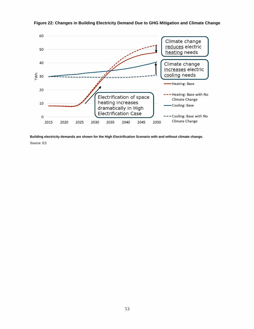
53

Figure 22: Changes in Building Electricity Demand Due to GHG Mitigation and Climate Change

Building electricity demands are shown for the High Electrification Scenario with and without climate change.

Source: E3

54

CHAPTER 4: Cost and Risk Analysis

Economy-wide High Electrification Scenario Costs This analysis estimates the upfront, annualized capital investments and expected fuel costs and

savings associated with the High Electrification Scenario.

In the High Electrification Scenario, which meets California’s climate goals in 2030 using a

reasonably likely, and relatively low-cost combination of strategies, the estimates range from

savings of $2 billion per year to net costs of $17 billion per year in 2030, depending on the fuel

price and financing assumptions. The base cost assumptions yield a net cost estimate of $9

billion per year in 2030, in today’s dollars (Figure 23). This net cost is equivalent to less than a

half a percent of California gross state product in 2030. Furthermore, the uncertainty range

around fossil fuel prices and financing costs results in a future net cost range that spans zero.

Figure 23: Total 2030 Net Cost of the High Electrification Scenario Relative to Reference Scenario, Excluding Climate Benefits (2016$, Billions)

Source: E3

The net present value of the costs of GHG mitigation is compared to the societal benefits

associated with reducing greenhouse gas emissions. Using two different estimates of the future

benefits of avoided GHG emissions, the climate benefits of avoided emissions are found to

likely be equal to, or much larger than the costs associated with reducing emissions (Figure

24).8

8 This assumes a 3% discount rate and uses the 2016 U.S. government social cost of carbon, which escalates as a function of emissions year. “Base climate benefits” is based on average social cost of carbon, corresponding to $58/tCO2 in 2030 and $79/tCO2 in 2050. “High climate benefits” is based on the 95th percentile in ensemble of modeled

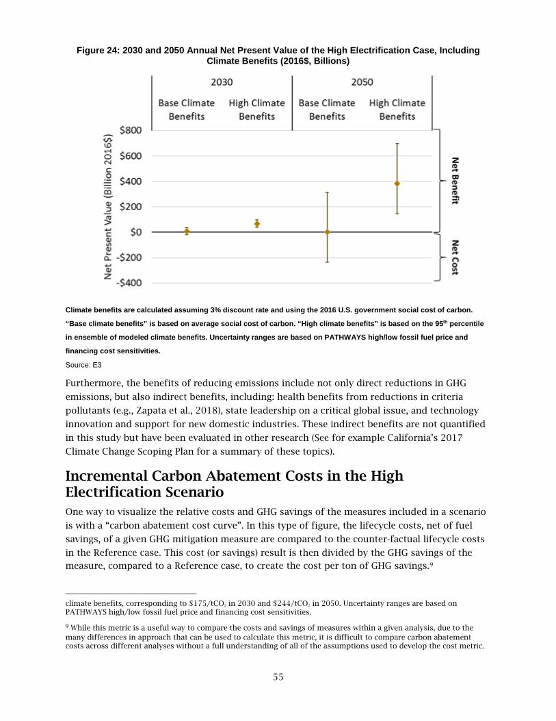
55

Figure 24: 2030 and 2050 Annual Net Present Value of the High Electrification Case, Including Climate Benefits (2016$, Billions)

Climate benefits are calculated assuming 3% discount rate and using the 2016 U.S. government social cost of carbon.

“Base climate benefits” is based on average social cost of carbon. “High climate benefits” is based on the 95th percentile

in ensemble of modeled climate benefits. Uncertainty ranges are based on PATHWAYS high/low fossil fuel price and

financing cost sensitivities.

Source: E3

Furthermore, the benefits of reducing emissions include not only direct reductions in GHG

emissions, but also indirect benefits, including: health benefits from reductions in criteria

pollutants (e.g., Zapata et al., 2018), state leadership on a critical global issue, and technology

innovation and support for new domestic industries. These indirect benefits are not quantified

in this study but have been evaluated in other research (See for example California’s 2017

Climate Change Scoping Plan for a summary of these topics).

Incremental Carbon Abatement Costs in the High Electrification Scenario One way to visualize the relative costs and GHG savings of the measures included in a scenario

is with a “carbon abatement cost curve”. In this type of figure, the lifecycle costs, net of fuel

savings, of a given GHG mitigation measure are compared to the counter-factual lifecycle costs

in the Reference case. This cost (or savings) result is then divided by the GHG savings of the

measure, compared to a Reference case, to create the cost per ton of GHG savings.9

climate benefits, corresponding to $175/tCO2 in 2030 and $244/tCO2 in 2050. Uncertainty ranges are based on PATHWAYS high/low fossil fuel price and financing cost sensitivities.

9 While this metric is a useful way to compare the costs and savings of measures within a given analysis, due to the many differences in approach that can be used to calculate this metric, it is difficult to compare carbon abatement costs across different analyses without a full understanding of all of the assumptions used to develop the cost metric.

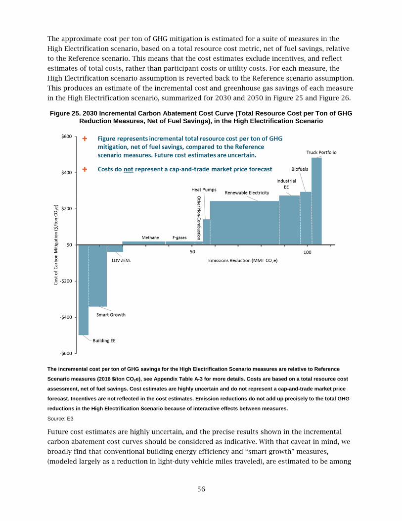
56

The approximate cost per ton of GHG mitigation is estimated for a suite of measures in the

High Electrification scenario, based on a total resource cost metric, net of fuel savings, relative

to the Reference scenario. This means that the cost estimates exclude incentives, and reflect

estimates of total costs, rather than participant costs or utility costs. For each measure, the

High Electrification scenario assumption is reverted back to the Reference scenario assumption.

This produces an estimate of the incremental cost and greenhouse gas savings of each measure

in the High Electrification scenario, summarized for 2030 and 2050 in Figure 25 and Figure 26.

Figure 25. 2030 Incremental Carbon Abatement Cost Curve (Total Resource Cost per Ton of GHG Reduction Measures, Net of Fuel Savings), in the High Electrification Scenario

The incremental cost per ton of GHG savings for the High Electrification Scenario measures are relative to Reference

Scenario measures (2016 $/ton CO2e), see Appendix Table A-3 for more details. Costs are based on a total resource cost

assessment, net of fuel savings. Cost estimates are highly uncertain and do not represent a cap-and-trade market price

forecast. Incentives are not reflected in the cost estimates. Emission reductions do not add up precisely to the total GHG

reductions in the High Electrification Scenario because of interactive effects between measures.

Source: E3

Future cost estimates are highly uncertain, and the precise results shown in the incremental

carbon abatement cost curves should be considered as indicative. With that caveat in mind, we

broadly find that conventional building energy efficiency and “smart growth” measures,

(modeled largely as a reduction in light-duty vehicle miles traveled), are estimated to be among

57

the lowest cost sources of carbon abatement in the 2030 timeframe. In the High Electrification

scenario, mitigation of methane, F-gasses and other non-combustion emissions save nearly as

much GHGs as fully-balanced and delivered renewable electricity, at a lower cost per ton. The

most expensive mitigation measures on a cost per ton basis in this scenario come from

additional GHG mitigation from the industrial sector, advanced biofuels and zero-emission

trucks.

The 2050 incremental carbon abatement cost curve for the High Electrification Scenario is

shown in Figure 26 below. In addition to the cost per ton of the measures included in the High

Electrification Scenario, Figure 26 also includes an estimate of the cost per ton of additional

mitigation measures that are not included in the High Electrification scenario, but which are

tested in the Alternative Mitigation scenarios. These measures (shown in grey) may be necessary

to meet the state’s 2050 GHG goal if the full mitigation potential of other GHG reduction

measures assumed in the High Electrification scenario is not realized.

Figure 26: 2050 Incremental Carbon Abatement Cost Curve (Total Resource Cost per Ton of GHG Reduction Measures, Net of Fuel Savings), in the High Electrification Scenario

The incremental cost per ton of GHG savings for the High Electrification Scenario measures are relative to Reference

Scenario measures (2016 $/ton CO2e), see Appendix Table A-4 for more details. Costs are based on a total resource cost

assessment, net of fuel savings. Cost estimates are highly uncertain and do not represent a cap-and-trade market price

forecast. Incentives are not reflected in the cost estimates. Emission reductions do not add up precisely to the total GHG

reductions in the High Electrification Scenario because of interactive effects between measures.

Source: E3

58

The incremental total resource cost estimates are even more uncertain in 2050 than in 2030,

and are intended to qualitatively illustrate three different cost regimes for long-term mitigation

strategies. The left-most tranche includes building energy efficiency and smart growth, which is

expected to be a large source of near-term GHG abatement and a long-term source of cost

savings, but which will deliver a relatively small amount of incremental GHG abatement by 2050

as fuels become decarbonized. The middle tranche includes most of the remaining strategies

used in the High Electrification scenario: electrification, renewable electricity, and non-

combustion emission reductions. Zero-emission vehicles and heat pumps are expected to be

relatively inexpensive by 2050 because of declining capital costs (for vehicles) and increasing

fuel savings (for both technologies). Renewable electricity makes up the largest single source of

GHG savings. The renewables bar shown above averages costs over an embedded renewable

supply curve that becomes steep as more and more renewable integration is needed. The third,

right-most tranche, including advanced biofuels as well as additional strategies unused in the

High Electrification scenario, consist of options for decarbonizing difficult-to-electrify end uses.

These cost estimates mask a great deal of uncertainty in future cost estimates and will likely

change as better information becomes available. Heat pump and zero-emission vehicle

incremental costs are highly sensitive to assumptions about equipment capital costs, financing

costs, and the costs of displaced fossil fuels. Methane mitigation costs are relatively low

because some of the costs of avoiding biogenic methane emissions are attributed to biofuel

costs here. Electricity and storage capital costs have been declining rapidly while future cost

declines remain uncertain. Costs of zero-emission trucks are poorly known as few models are

commercially available. Biofuel costs are high because supply is assumed to be limited relative

to demand, resulting in high market clearing prices; in addition, no innovation is assumed in

biofuel conversion pathways over time. These conservative biofuel conversion pathways

assumptions are being updated as part of on-going PATHWAYS analyses. Finally, hydrogen and

power-to-gas (synthetic methane) incremental costs depend on whether the production of these

energy carriers is from California-sourced grid electricity (as is assumed here), or from other

sources, and the extent to which they can provide a grid flexibility benefit that offsets more

expensive forms of energy storage. Because of limited commercial availability of hydrogen and

power-to-gas synthetic methane, the capital costs and performance of these technologies

remains uncertain.

GHG Mitigation Risk and GHG Mitigation Cost in Alternative Mitigation Scenarios The annual net costs resulting from the Alternative Mitigation scenarios are compared in Figure

27 mitigation measures are compared across all these scenarios in Appendix A. The High

Electrification scenario is among the lowest cost scenarios, however, the “No Hydrogen”

scenario and the “High Biofuels” scenarios are both slightly lower cost in 2050. All other

scenarios had higher costs than the High Electrification scenario.

59

Figure 27: Incremental Cost of All Mitigation Scenarios Relative to Reference

Costs are in 2016 billions of dollars

Source: E3

The “No Hydrogen” scenario relies on a highly electrified vehicle fleet as well as industrial

electrification in order to meet the 2050 GHG goal without the use of hydrogen fuel, which may

be slightly higher risk than the more diversified transportation strategy embedded in the High

Electrification scenario. The costs and resource potential for industrial electrification are

particularly uncertain, which is why industrial electrification is excluded from the High


The “High Biofuels” scenario is lower cost than the High Electrification scenario because it

assumes that purpose-grown biomass crops, such as miscanthus, are available at relatively low

cost as a zero-carbon fuel. This strategy may be lower cost than relying on higher adoption

rates of zero-emission vehicles and renewable generation, and using only sustainable biomass

waste products for biofuels, as is assumed in the High Electrification scenario. It could be

achieved at even lower costs than shown here with continued innovation and efficiency

enhancements for biomass conversion processes. However, the “High Biofuels” scenario is also

determined to be higher risk, due to concerns about the long-term availability and sustainability

of growing crops for biofuels.

The No Building Electrification with Power-to-Gas scenario is found to be among the most

expensive Mitigation scenario in 2050 due to the high expense of providing renewable natural

gas with relatively limited biofuels. This finding, however, could change if higher incremental

retrofit costs to install heat pumps in existing buildings were assumed in the other scenarios.

Also, producing hydrogen from renewable fuels and synthetic methane derived from a

renewable source of CO2 are reach technologies that have yet to be commercially deployed, so

cost estimates for this scenario are highly uncertain.

60

In terms of technology cost risk, the largest single contributor to keeping California’s GHG

mitigation costs reasonable is the wide scale use of renewable generation and zero-emissions

light duty vehicles. In fact, it does not appear to be possible to meet the state’s 2030 or 2050

GHG mitigation goals at current levels of renewable deployment. This makes sense given that

all Mitigation scenarios rely heavily on fuel-switching to low-carbon electricity as a central GHG

reduction strategy.

While it does appear to be possible to meet the state’s 2030 GHG mitigation goal with Reference

levels of ZEVs, it is not possible to meet the 2050 target without nearly complete deployment of

ZEVs. This makes sense given that today’s light duty vehicles represent the single largest source

of greenhouse gas emissions in the state. Other key strategies for reducing the cost of GHG

mitigation in the 2030 timeframe include smart growth (reducing vehicle miles traveled),

electric heat pumps in buildings, methane capture, and biofuels (Figure 28).

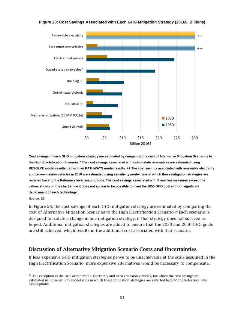
61

Figure 28: Cost Savings Associated with Each GHG Mitigation Strategy (2016$, Billions)

Cost savings of each GHG mitigation strategy are estimated by comparing the cost of Alternative Mitigation Scenarios to

the High Electrification Scenario. * The cost savings associated with out-of-state renewables are estimated using

RESOLVE model results, rather than PATHWAYS model results. ++ The cost savings associated with renewable electricity

and zero-emission vehicles in 2050 are estimated using sensitivity model runs in which these mitigation strategies are

reverted back to the Reference level assumptions. The cost savings associated with these two measures exceed the

values shown on the chart since it does not appear to be possible to meet the 2050 GHG goal without significant

deployment of each technology.

Source: E3

In Figure 28, the cost savings of each GHG mitigation strategy are estimated by comparing the

cost of Alternative Mitigation Scenarios to the High Electrification Scenario.10 Each scenario is

designed to isolate a change in one mitigation strategy, if that strategy does not succeed as

hoped. Additional mitigation strategies are added to ensure that the 2030 and 2050 GHG goals

are still achieved, which results in the additional cost associated with that scenario.

Discussion of Alternative Mitigation Scenario Costs and Uncertainties

If less expensive GHG mitigation strategies prove to be unachievable at the scale assumed in the

High Electrification Scenario, more expensive alternatives would be necessary to compensate.

10 The exception is the case of renewable electricity and zero emission vehicles, for which the cost savings are estimated using sensitivity model runs in which these mitigation strategies are reverted back to the Reference level assumptions.

62

Within the scenario design framework employed in this analysis, the effect of removing some

GHG mitigation strategies and compensating with others is tested in the Alternative Mitigation

scenarios, including the measures not found to be cost-effective in the High Electrification

Scenario. Available alternatives are selected sequentially from this limited and upward-sloping

supply curve, meaning that reducing or excluding GHG mitigation strategies from a scenario,

that are responsible for large quantities of CO2 abatement in the High Electrification scenario,

result in relatively expensive Alternative Mitigation Scenarios. Other studies (e.g., Yang et al.,

2016) have similarly found that marginal economy-wide mitigation costs could be much higher

than average costs. It is difficult to predict with confidence whether and where an “inflection

point” exists in the supply curve for decarbonization in 2050, underscoring the importance of

flexible policy implementation that can incorporate better information as it becomes available.

Two key alternative mitigation strategies are used in these scenarios when other mitigation

strategies fall short: hydrogen fuel cell trucks (fueled by hydrogen produced via grid

electrolysis) and industry electrification. These strategies are classified as “reach technologies”

in this study, meaning that they could be quite expensive but necessary to reach the 2050 goals.

If progress is made in commercializing these strategies and reducing costs, or if other

alternatives become available that are not modeled here, that could reduce the cost of

alternative mitigation scenarios relative to the High Electrification scenario.

Several other key assumptions could change the rank order of the scenario cost savings as

better information becomes available. Biofuels could be available at lower cost than modeled

here with progress in increasing biofuel conversion yields, or if sustainability concerns with

purpose-grown crops are addressed. Alternatively, other jurisdictions may continue to lag

California in decarbonizing their economies, making more of the global biofuel supply available

to California.

Finally, this analysis did not evaluate or include costs associated with retrofitting existing

buildings for electric heating, cooking, and clothes drying. More research is needed to

understand the costs of retrofitting existing buildings to electric alternatives. Including these

costs would reduce the relative cost of strategies that instead rely on decarbonizing the existing

gas pipeline. Likewise, this study did not include the costs of retrofitting natural gas pipelines

to accommodate a blend of hydrogen and methane (only applicable in the No Building

Electrification with Power to Gas Scenario). Future costs associated with producing hydrogen

and synthetic methane, as well as blending hydrogen into the natural gas pipeline are uncertain

and need further research. Building retrofit costs, as well as hydrogen, biomethane and

synthetic methane costs, are likely to decline over time with a market transformation effort.

Finally, this study emphasizes the total resource cost metric that aggregates statewide costs

and benefits, explicitly excluding the impact of state incentives and within-state transfers, such

as the impact of cap-and-trade, the LCFS, and utility energy efficiency programs. Costs borne by

individual households could differ markedly from the average, and these impacts could differ

for different mitigation strategies, as well as being dependent on policy implementation. The

Berkeley Economic Advising and Research (BEAR) team evaluated potential costs and benefits of

these deep decarbonization scenarios to low-income and disadvantaged communities in

California. Further research could investigate the specific cost implications of specific state

63

policies on individuals and businesses. Furthermore, developing better models to predict and

understand consumer behavior and consumer choices under different cost regimes could lead

to the development of different GHG mitigation scenarios.

64

CHAPTER 5: Conclusions

This research has evaluated long-term energy scenarios in California using a variety of

mitigation strategies and technologies. These findings highlight the important role that

consumer decisions, households and businesses, will play in meeting the state’s ambitious

near-term and long-term GHG goals.

Supply-side energy policies have been very successful at increasing the use of renewable

electricity and renewable fuels in California, however, these policies will not be sufficient.

Consumer decisions are important to improve the energy efficiency of the state’s existing

building stock, to reduce vehicle miles traveled, to purchase and drive zero-emission vehicles,

and potentially to switch to electric space heating and water heating options in their homes and

businesses.

To accomplish this low-carbon energy transition, carbon pricing, through the state’s cap and

trade program will play an important role. Likewise, additional market transformation efforts,

and regional policy initiatives, will be needed.

Through the evaluation of these ten scenarios, priority GHG mitigation strategies are identified

and grouped into three categories: 1) strategies requiring widespread scale-up of technology

deployment in the near-term; 2) strategies requiring market transformation to achieve

widespread deployment, and 3) “reach” technologies which are not yet widely commercialized,

but which may be required to achieve the state’s 2050 GHG goals, particularly if some

mitigation strategies fall short of expectations (Table 8).

High priority strategies for deployment include energy efficiency in buildings and industry,

renewable electricity and renewable integration solutions, and smart growth leading to near-

term reductions in light-duty vehicle miles traveled. By 2050, 85% to 95% zero-carbon electricity

is expected to be required; however, 100% zero-carbon electricity is likely to be cost prohibitive

compared to alternative GHG mitigation strategies.

High priority strategies that require additional market transformation include deployment of

zero-emission light duty vehicles, advanced energy efficiency in buildings, including building

electrification, replacement of fluorinated gases with less potent global warming potential

gases, and capture of methane emissions.

Finally, at least one reach technology is likely to be required to achieve the 2050 mitigation

goal. Examples of reach technologies that provide solutions in hard-to-electrify sectors include

advanced, sustainable biofuels, zero-emission heavy-duty long-haul trucks, industrial

electrification and hydrogen production using electrolysis. The priority strategies shown in

Table 8 are based on the costs and risks to achieving the state’s long-term 2050 climate goal

evaluated through this reach. The 2030 “indicative metrics” are provided as a near-term metric

to evaluate whether the state is on track to meet the long-term climate goals.

65

Table 8: Priority GHG Reduction Strategies

Scale-up & Deploy 2030 Indicative Metrics Key Challenges

Energy efficiency in buildings & industry

Deployment of LED lighting, higher efficiency plug loads, improved shell in existing buildings, continued improvements and enforcement of building codes, industrial EE

Consumer decisions and market failures

Renewable electricity

70 – 80% zero-carbon electricity with renewable integration solutions: flexible loads, market-based curtailment, cost-effective grid storage

Implementation of integration solutions

Smart growth Reduced vehicle miles traveled through increased use of public transit, walking, biking, tele-presence, and denser, mixed-use community design

Consumer decisions and legacy development

patterns

Market Transformation 2030 Indicative Metrics Key Challenges

Zero-emission light-duty vehicles (ZEV)

At least 6 million ZEVs, >60% of new sales are ZEVs, drivers have access to day-time charging stations and time-of-use charging

Consumer decisions and cost

Advanced building efficiency/ electrification

50% of new water heater and HVAC sales are high efficiency heat pumps

Consumer decisions, equity of cost impacts, cost and

retrofits of existing buildings

F-gas replacement Replace F-gases with lower global warming potential (GWP) refrigerants

Lack of standards to require alternatives

Methane capture Methane capture from manure, fugitive and process emissions, landfills and wastewater

Small and diffuse point sources

Reach Technologies 2030 Indicative Metrics Key Challenges

Advanced sustainable biofuels

Demonstrated use of sustainable, carbon-neutral biomass feedstocks to produce commercial-scale biofuels

Cost and sustainability challenges

Zero-emissions heavy-duty trucks

Commercial deployment of battery-electric and/or hydrogen trucks

Cost

Industrial electrification

Cost-competitive electrification of industrial end-uses, including boilers, machine drives, and process heating

Cost

Electrolysis hydrogen production

Improved cost and efficiency at commercial scale. Business model for flexible hydrogen production.

Cost

Source: E3

66

Scale-Up and Deploy

Within the category of scaling up the deployment of existing strategies this analysis indicates

the state must execute its ambitious building energy efficiency goals and exceed the current

renewable electricity goals to meet the GHG emission reduction goals for 2030 and 2050.

Examples include continued progress in using LED lighting across nearly all lighting

applications and continued improvements to the state’s adoption and enforcement of appliance

codes and building standards. California has a long history in using energy efficiency in

buildings. To meet the state’s energy efficiency goals of doubling energy efficiency

achievements, however, a new paradigm for energy efficiency program design is required which

is likely to require market transformation of advanced forms of energy efficiency and building

electrification.

Likewise, California also has a strong track record on renewable development. In the past

decade, renewables in the state have increased from 11% to over 25% of total generation (CEC,

2016). This research suggests that renewable generation requirements are expected to increase

to 60%–70% (equivalent to 70%–80% zero-carbon generation) by 2030, with 85%–95% zero-carbon

generation required by 2050. Achieving these high levels of renewable generation will require

policy coordination to ensure that renewable integration strategies are developed and deployed

in concert with higher levels of renewables.

However, achieving 100% zero-carbon generation appears to be cost prohibitive without major

advances in low-cost energy storage. In the High Electrification scenario, natural gas generation

provides the remaining 5% of energy requirements and helps ensure resource adequacy and

energy sufficiency during periods of low renewable generation. This 5% of natural gas

generation helps to contain the cost impacts of the scenario compared to a 100% zero-carbon

scenario.

For 2030 and 2050, key renewable integration solutions necessary to contain the costs of high

levels of renewable energy on the grid include: 1) increased reliance on flexible loads and

demand-shifting, particularly in electric vehicle charging, but also in buildings and industry; 2)

regional markets and regional procurement of renewable energy; 3) market-based renewable

curtailment, combined with using supervisory control and data acquisition (SCADA) systems, to

allow renewable curtailment as a low-cost strategy to manage variable renewables on the grid,

and 4) cost-effective grid storage including hydroelectric, battery, and chemical storage.

Finally, this analysis suggests California must achieve its ambitious smart growth and

sustainable community strategies as part of a suite of strategies to achieve 2030 and 2050

greenhouse gas emission reduction goals, entailing a per capita reduction in light duty vehicle

miles traveled through increased utilization of public transit, walking, biking, tele-presence and

denser, mixed-use community designs. Smart growth strategies are particularly important for

meeting the 2030 GHG goals while fossil-fueled transportation still represents the largest share

of the state’s total GHG emissions.

Without any one of these three priority deployment strategies – energy efficiency, renewable

generation, and smart growth - the cost of meeting the state’s climate goals is expected to be

much higher.

67

Market Transformation

Only scaling up known strategies will not be sufficient to meet the state’s 2030 goal, let alone

the 2050 goal. To meet the state’s 2030 climate goals, business and household decisions will

play a pivotal role: from vehicle purchases, to water heater and heating, ventilation and air

conditioning (HVAC) purchase and installation decisions, to vehicle driving behavior. Market

transformation is necessary to bring down the cost and improve the performance of customer-

facing zero-emissions technologies, primarily zero-emission vehicles and electric heat pumps in

buildings. Carbon pricing and other existing policies on their own are unlikely to be sufficient

to overcome some of the market barriers to adoption.

Furthermore, unlike in the transportation sector, California does not have a strong market or

policy framework to encourage decarbonization of buildings; a gap which the combination of

higher carbon prices and new market transformation programs could help fill. Market

transformation programs and incentives could be directed towards helping to bring down the

upfront capital cost of electric heat pump installations and retrofits, and training HVAC

professionals to gain more experience with their deployment.

The building construction, efficiency, and HVAC markets are more localized to California than

the vehicle or renewable generation markets because of the high reliance on local, skilled labor

for installation and construction. As a result, global markets may help reduce the equipment

cost and improve the performance of high efficiency appliances, but market transformation

may still be required at a local level to achieve higher levels of consumer adoption of these

technologies.

Another area where market transformation is needed is to reduce emissions of non-combustion

GHGs, principally fluorinated gasses (“F-gases”) used primarily as refrigerants, and methane

from agriculture, waste, and the extraction, production and conveyance of fossil fuels. Industry

standards and regulations are needed to phase out the use of F-gases. Such regulations are

under consideration at the U.S. EPA, and California legislation has been proposed to require

alternatives to F-gases. The Kigali Agreements, an amendment to the Montreal Protocol, call for

global reductions in F-gases, yet it remains to be seen to what degree these targets will be

adhered to and enforced. Meanwhile, achieving higher levels of methane capture will require a

diverse set of strategies that address the challenges posed, in particular, by the diffuse point

sources from waste and dairy methane.

Reach Technologies

In addition to scale-up and market transformation of existing GHG reduction strategies, at least

one, and potentially more than one, “reach” technology that has not yet been commercially

proven will likely be necessary to meet the 2050 GHG goal. Reach technologies can also help to

mitigate the risk that one or more “proven” GHG mitigation strategy could fall short of

expectations. A reach technology should ideally help to reduce greenhouse gas emissions in

otherwise difficult to electrify end-uses such as heavy-duty trucking (which currently represents

GHG emissions of about 30 MMT CO2e in California today), off-road transportation (including

aviation, rail, boats and other off-road equipment, and which represents about 15 MMT CO2e in

California today), or industry (including manufacturing, refining, and oil and gas, which

represents about 92 MMT CO2e in California today).

68

Examples of reach technologies include advanced, sustainable biofuels or hydrogen production

from electrolysis, both of which use proven manufacturing technologies, but neither of which

have achieved commercial scale. Industrial electrification and zero-emissions heavy duty trucks

are other examples of reach technology areas that could be useful to meeting the state’s 2050

GHG mitigation goals, but for which minimal cost and performance data are available.

Future Research Needs

These long-term energy scenarios show that natural gas electricity generation is likely to fall

dramatically relative to current levels, as higher levels of zero-carbon generation are brought

online. A key research question remains, however, regarding how much of the state’s existing

natural gas generation will still be required to support resource adequacy and ensure energy

sufficiency during periods of low renewable energy availability, or whether long-duration

energy storage technologies will be developed to replace this need.

Likewise, most of the scenarios evaluated in this analysis, including the High Electrification

scenario, show a dramatic reduction in natural gas demand at the distribution level. An area for

additional research and policy work surrounds the question of how the regulated natural gas

utilities will adapt to these changing demand conditions, and whether high building

electrification is practically, politically and economically feasible over this relatively short

timeframe.

California’s electric regulatory environment is not currently designed to prioritize low-carbon

solutions in buildings. Energy efficiency programs and electric retail rates may need to be

redesigned to enable greater building efficiency and electrification. Areas for additional

research include an assessment of the distribution level upgrades that would be needed to

enable building electrification, as well as the costs and market barriers to building

electrification.

This study assumes that California will succeed in reversing historical trends and will bring

GHG emissions from natural and working lands down to a zero net CO2 emissions impact by

2050. Achieving this goal will require large changes in ecosystem carbon storage, impacting

both land-use management and development practices. More research is needed to understand

both the likely changes in California ecosystems in response to climate change as well as the

potential for increasing carbon storage to offset other greenhouse gas emissions that are most

difficult to mitigate.

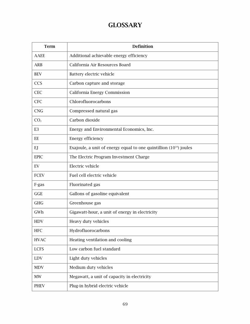
69

GLOSSARY

Term Definition

AAEE Additional achievable energy efficiency

ARB California Air Resources Board

BEV Battery electric vehicle

CCS Carbon capture and storage

CEC California Energy Commission

CFC Chlorofluorocarbons

CNG Compressed natural gas

CO2 Carbon dioxide

E3 Energy and Environmental Economics, Inc.

EE Energy efficiency

EJ Exajoule, a unit of energy equal to one quintillion (1018) joules

EPIC The Electric Program Investment Charge

EV Electric vehicle

FCEV Fuel cell electric vehicle

F-gas Fluorinated gas

GGE Gallons of gasoline equivalent

GHG Greenhouse gas

GWh Gigawatt-hour, a unit of energy in electricity

HDV Heavy duty vehicles

HFC Hydrofluorocarbons

HVAC Heating ventilation and cooling

LCFS Low carbon fuel standard

LDV Light duty vehicles

MDV Medium duty vehicles

MW Megawatt, a unit of capacity in electricity

PHEV Plug-in hybrid electric vehicle

70

PJ Petajoule, a unit of energy equal to one quadrillion (1015) joules

RPS Renewable portfolio standard

SB Senate Bill

SLCP Short-lived climate pollutant

VMT Vehicle miles traveled

ZEV Zero-emission vehicle

71

REFERENCES

Bartos, Matthew D. and Mikhail V. Chester. “Impacts of climate change on electric power supply in the Western United States.” Nature Climate Change 5, 2015, 748-751.

Battles, J. et al (2013). California Forest and Rangeland Greenhouse Gas Inventory Development. Final Report, ARB Contract 10-778.

Boer, Eelco den, Sanne Aarnik, Florian Kleiner, Johannes Pagenkopf (2013). Zero emission trucks: An Overview of state-of-the-art technologies and their potential. Delft, CE July 2013. Available at: http://www.cedelft.eu/publicatie/zero_emission_trucks/1399 Accessed January 16, 2018

California Air Resources Board. (2017a). The 2017 Climate Change Scoping Plan Update: The Proposed Strategy for Achieving California’s 2030 Greenhouse Gas Target (Sacramento, CA). Available at https://www.arb.ca.gov/cc/scopingplan/2030sp_pp_final.pdf. Accessed March 27, 2017.

California Air Resources Board. (2017b). Short-Lived Climate Pollutant Reduction Strategy. Available at https://www.arb.ca.gov/cc/shortlived/meetings/03142017/final_slcp_report.pdf. Accessed January 9, 2018.

California Air Resources Board. (2016). Low Carbon Fuel Standard Data Dashboard, Figure 10: Share of Liquid Biofuels Produced In-state by Volume, 2016. Available at https://www.arb.ca.gov/fuels/lcfs/dashboard/dashboard.htm. Accessed January 15, 2018.

California Council on Science and Technology. (2011). California’s Energy Future ‐ The View to 2050 (Sacramento, CA). Available at ccst.us/publications/2011/2011energy.pdf. Accessed March 27, 2017.

California Council on Science and Technology. (2013) California’s Energy Future - The potential for Biofuels. Available at: http://ccst.us/publications/2013/2013biofuels.pdf. Accessed January 9, 2018.

California Energy Commission. (2016). 2016 Total System Electric Generation. Retrieved from: http://www.energy.ca.gov/almanac/electricity_data/total_system_power.html.

California Energy Commission. (2016). California Energy Demand 2016-2026 Adopted Forecast, California Energy Commission, CEC-200-2016-001 (15-IEPR-03)

Deep Decarbonization Pathways Project. (DDPP), (2015). Pathways to deep decarbonization 2015 report, SDSN - IDDRI. Available at http://deepdecarbonization.org/wp-content/uploads/2016/03/DDPP_2015_REPORT.pdf. Accessed March 27, 2017.

E3 (2015). California PATHWAYS: GHG Scenario Results (San Francisco, CA). Available at http://www.ethree.com/wp-content/uploads/2017/02/E3_PATHWAYS_GHG_Scenarios_Updated_April2015.pdf. Accessed March 27, 2017.

European Climate Foundation. (2010). Roadmap 2050. doi: 10.2833/10759. Available at http://www.roadmap2050.eu/attachments/files/Volume1_fullreport_PressPack.pdf. Accessed January 9, 2018.

http://www.cedelft.eu/publicatie/zero_emission_trucks/1399

https://www.arb.ca.gov/fuels/lcfs/dashboard/dashboard.htm

http://ccst.us/publications/2013/2013biofuels.pdf

http://www.energy.ca.gov/almanac/electricity_data/total_system_power.html

http://www.roadmap2050.eu/attachments/files/Volume1_fullreport_PressPack.pdf

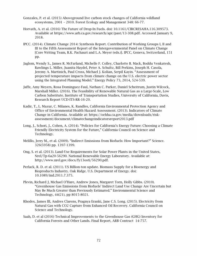
72

Gonzales, P. et al. (2015) Aboveground live carbon stock changes of California wildland ecosystems, 2001 – 2010. Forest Ecology and Management 348: 66-77.

Horvath, A. et al. (2016) The Future of Drop-In Fuels. doi: 10.1161/CIRCRESAHA.116.309573. Available at https://www.arb.ca.gov/research/apr/past/13-308.pdf. Accessed January 9, 2018.

IPCC. (2014). Climate Change 2014: Synthesis Report. Contribution of Working Groups I, II and III to the Fifth Assessment Report of the Intergovernmental Panel on Climate Change [Core Writing Team, R.K. Pachauri and L.A. Meyer (eds.)]. IPCC, Geneva, Switzerland, 151 pp.

Jaglom, Wendy S., James R. McFarland, Michelle F. Colley, Charlotte B. Mack, Boddu Venkatesh, Rawlings L. Miller, Juanita Haydel, Peter A. Schultz, Bill Perkins, Joseph H. Casola, Jeremy A. Martinich, Paul Cross, Michael J. Kolian, Serpil Kayin. “Assessment of projected temperature impacts from climate change on the U.S. electric power sector using the Integrated Planning Model.” Energy Policy 73, 2014, 524-539.

Jaffe, Amy Meyers, Rosa Dominguez-Faul, Nathan C. Parker, Daniel Scheitrum, Justin Wilcock, Marshall Miller. (2016). The Feasibility of Renewable Natural Gas as a Large-Scale, Low Carbon Substitute. Institute of Transportation Studies, University of California, Davis, Research Report UCD-ITS-RR-16-20.

Kadir, T., L. Mazur, C. Milanes, K. Randles, California Environmental Protection Agency and Office of Environmental Health Hazard Assessment. (2013). Indicators of Climate Change in California. Available at: https://oehha.ca.gov/media/downloads/risk-assessment/document/climatechangeindicatorsreport2013.pdf

Long, J., Schori, J., Cohen, A. (2014). “Policies for California’s Energy Future: Choosing a Climate Friendly Electricity System for the Future,” California Council on Science and Technology.

Melillo, Jerry M., et al. (2009). “Indirect Emissions from Biofuels: How Important?” Science. 326(5958) pp. 1397-1399.

Ong, S. et al. (2013). Land-Use Requirements for Solar Power Plants in the United States, Nrel/Tp-6a20-56290. National Renewable Energy Laboratory. Available at: http://www.nrel.gov/docs/fy13osti/56290.pdf.

Perlack, R. D. et al. (2011). US Billion-ton update. Biomass Supply for a Bioenergy and Bioproducts Industry. Oak Ridge. U.S. Department of Energy. doi: 10.1089/ind.2011.7.375.

Plevin, Richard J, Michael O’Hare, Andrew Jones, Margaret Torn, Holly Gibbs. (2010). “Greenhouse Gas Emissions from Biofuels’ Indirect Land Use Change Are Uncertain but May Be Much Greater than Previously Estimated.” Environmental Science and Technology, 44(21), pp 8015-8021.

Rhodes, James III, Andres Clarens, Pragnya Eranki, Jane C.S. Long. (2015). Electricity from Natural Gas with CO2 Capture from Enhanced Oil Recovery. California Council on Science and Technology.

Saah, D. et al (2016) Technical Improvements to the Greenhouse Gas (GHG) Inventory for California Forests and Other Lands. Final Report, ARB Contract 14-757.

73

Sanchez, Daniel L., James H. Nelson, Josiah Johnston, Ana Mileva, Daniel Kammen. (2015). Nature Climate Change, 5, pp. 230-234. Doi: 10.1038/nclimate2488

Searchinger, Timothy, et al. (2008). “Use of U.S. Croplands for Biofuels Increases Greenhouse Gases Through Emissions from Land-Use Change.” Science. 319(5867) pp. 1238-1240.

Tarroja, Brian with University of California Irvine, Advanced Power and Energy Program (2017). Personal communication as part of CEC EPIC research grant.

United States White House. (2016). United States Mid-Century Strategy for Deep Decarbonization. Available at http://unfccc.int/files/focus/long-term_strategies/application/pdf/mid_century_strategy_report-final_red.pdf . Accessed March 27, 2017.

U.S. Department of Energy. (2011). U.S. Billion-Ton Update, Biomass Supply for a Bioenergy and Bioproducts Industry. R.D. Perlack and B.J. Stokes (Leads), ORNL/TM-2011/224. Oak Ridge National Laboratory, Oak Ridge, TN. 227p.

U.S. Environmental Protection Agency. (2014). Framework for assessing biogenic CO2 emissions from stationary sources. Available at: http://saveourepa.com/sites/production/files/2016-08/documents/framework-for-assessing-biogenic-co2-emissions.pdf. Accessed January 9, 2018.

Wei, M., Nelson, J.H., Ting, M., Yang, C., Greenblatt, J.B., McMahon, J.E. (2012). “California’s Carbon Challenge: Scenarios for Meeting 80% Emissions Reduction in 2050,” Lawrence Berkeley National Laboratory Report LBNL‐5448E.

Wei, Max; Jeffery Greenblatt; Sally Donovan; James Nelson; Ana Mileva; Josiah Johnston; Daniel Kammen. (2014). Scenarios for Meeting California’s 2050 Climate Goals. (University of California, Berkeley and Lawrence Berkeley National Laboratory). California Energy Commission. Publication number: CEC‐500‐2014‐108.

Williams JH, DeBenedictis A, Ghanadan R, Mahone A, Moore J, Morrow WR III, Price S, Torn MS (2012). “The Technology Path to Deep Greenhouse Gas Emissions Cuts by 2050: The Pivotal Role of Electricity,” Science 335 53‐59.

Williams, R. B., Jenkins, B. M. and Kaffka, S. (2015). An Assessment of Biomass Resources in California, 2013 Data. California Biomass Collaborative. PIER Contract 500-11-020. doi: 500-11-020. Available at https://biomass.ucdavis.edu/files/2015/04/CA_Biomass_Resource_2013Data_CBC_Task3_DRAFT.pdf. Accessed January 9, 2018.

Williams, J. H. et al. (2015) Pathways to Deep Decarbonization in the United States. Available at: http://unsdsn.org/wp-content/uploads/2014/09/US-Deep-Decarbonization-Report.pdf. Accessed January 9, 2018.

Wunch, D. et al. (2016) “Quantifying the loss of processed natural gas within California’s South Coast Air Basin using long-term measurements of ethane and methane”, Atmospheric Chemistry and Physics, 16(22), pp. 14091–14105. doi: 10.5194/acp-16-14091-2016.

Yang, C. et al. (2015) “Achieving California’s 80% greenhouse gas reduction target in 2050: Technology, policy and scenario analysis using CA-TIMES energy economic systems model”, Energy Policy. Elsevier, 77, pp. 118–130. doi: 10.1016/J.ENPOL.2014.12.006.

Yeh, Sonia, et al. (2016). “A modeling comparison of deep greenhouse gas emissions reduction scenarios by 2030 in California,” Energy Strategy Reviews 13-14, pp 169-180.

74

Zapata, C. B. et al. (2018) ‘Low-carbon energy generates public health savings in California’, Atmospheric Chemistry and Physics, 18(7), pp. 4817–4830. doi: 10.5194/acp-18-4817-201

A-1

APPENDIX A: Mitigation Scenario Assumptions and Abatement Curve Assumptions

Table A-1: Scenario Measures Assumed in 2030, Highlighted Where Different Than the High Electrification Scenario

Hig

h El

ectri

ficat

ion

No

Hyd

roge

n

Hig

h B

iofu

els

Ref

eren

ce S

mar

t G

row

th

Red

uced

Met

hane

M

itiga

tion

Ref

eren

ce

Indu

stry

EE

In-S

tate

Bio

mas

s

Ref

eren

ce

Build

ing

EE

Hig

h H

ydro

gen

No

Bui

ldin

g El

ectri

ficat

ion

with

Po

wer

-to-G

as

Building efficiency (% reduction in total building energy demand relative to 2015) 10% 5% 9% Transportation VMT (% reduction in per capita light duty VMT relative to 2015) 12% 2% Industrial Efficiency (% reduction in total industrial energy demand relative to 2015 in non-petroleum industries) 22% 0% Building electrification (% of new sales of water heaters and HVAC that are electric heat pumps)* 50% 0% LDV electrification (Millions of ZEVs) 6 5 LDV electrification (ZEV % of total stock) 20% 17% LDV electrification (ZEV % of new sales) 64% 48% Trucking electrification (% of trucks that are BEVs or FCEVs) 4% Trucking - alternative fuels (% of trucks that are hybrid & CNG) 6% 9% 8% 8% Bus electrification (% of total) 32%

A-2

Hig

h El

ectri

ficat

ion

No

Hyd

roge

n

Hig

h B

iofu

els

Ref

eren

ce S

mar

t G

row

th

Red

uced

Met

hane

M

itiga

tion

Ref

eren

ce

Indu

stry

EE

In-S

tate

Bio

mas

s

Ref

eren

ce

Build

ing

EE

Hig

h H

ydro

gen

No

Bui

ldin

g El

ectri

ficat

ion

with

Po

wer

-to-G

as

Rail electrification (% of total) 20%

Port electrification (% of total) 27%

Industry electrification (% of non-petroleum industry end-use fossil replaced with electricity)

0%

Petroleum industry demand reduction 14%

Advanced biofuels (% of fossil end-uses replaced with advanced biofuels)**

10% 12% 7%

Advanced biofuels (Total EJ) 0.34 0.38 0.23

Power-to-gas (% of non-electric-generation pipeline gas supplied by hydrogen and renewable synthetic methane)

0% 8%

Hydrogen fuel for vehicles (Total EJ) 0.02 0.00 0.00

Reductions in methane (% reduction relative to 2015) 34% 10%

Reductions in F-gases (% reduction relative to 2015) 43%

% zero-carbon electricity, including large hydro and nuclear***

74% 74% 72% 80% 83% 82% 82% 76% 75% 76%

Approximate % RPS 70% 69% 67% 78% 83% 82% 80% 74% 71% 72% Total electricity demand (TWh) 295 293 290 298 294 301 292 316 294 327 Electric sector combustion emissions (MMT CO2e) 32 33 35 25 21 22 22 32 32 32 *Replacement of non-electric heaters; some electric resistance heating remains in the 2030 time period. **Excludes hydrogen and synthetic methane used for fuel-cell vehicles and in the pipeline. ***In-state nuclear is assumed to retire by 2025. Imports of nuclear from Palo Verde continue until retirement in 2047.

A-3

Table A-2: Scenario Measures Assumed in 2050, Highlighted Where Different Than the High Electrification Scenario

Hig

h E

lect

rific

atio

n

No

Hyd

roge

n

Hig

h B

iofu

els

Ref

eren

ce S

mar

t Gro

wth

Red

uced

Met

hane

M

itiga

tion

Ref

eren

ce In

dust

ry E

E

In-S

tate

Bio

mas

s

Ref

eren

ce B

uild

ing

EE

Hig

h H

ydro

gen

No

Bui

ldin

g El

ectri

ficat

ion

with

Pow

er-to

-Gas

Building efficiency (% reduction in total building energy demand relative to 2015)

34% 22% 10%

Transportation VMT (% reduction in per capita light duty VMT relative to 2015)

24% 3%

Industrial Efficiency (% reduction in total industrial energy demand relative to 2015 in non-petroleum industries)

22% 0%

Building electrification (% of new sales of water heaters and HVAC that are electric heat pumps)*

100% 0%

LDV electrification (Millions of ZEVs) 35 25

LDV electrification (ZEV % of total stock) 96% 69%

LDV electrification (ZEV % of new sales) 100% 81%

Trucking electrification (% of trucks that are BEVs or FCEVs)

47% 33% 27% 52% 69% 69% 65% 52%

Trucking - alternative fuels (% of trucks that are hybrid & CNG)

31% 55% 28% 19% 19% 16% 28%

Bus electrification (% of total) 88%

Rail electrification (% of total) 75%

Port electrification (% of total) 80%

A-4

Hig

h E

lect

rific

atio

n

No

Hyd

roge

n

Hig

h B

iofu

els

Ref

eren

ce S

mar

t Gro

wth

Red

uced

Met

hane

M

itiga

tion

Ref

eren

ce In

dust

ry E

E

In-S

tate

Bio

mas

s

Ref

eren

ce B

uild

ing

EE

Hig

h H

ydro

gen

No

Bui

ldin

g El

ectri

ficat

ion

with

Pow

er-to

-Gas

Industry electrification (% of non-petroleum industry end-use fossil replaced with electricity)

0% 26% 26% 37% 37% 26% 37%

Petroleum industry demand reduction 86%

Advanced biofuels (% of fossil end-uses replaced with advanced biofuels)**

46% 59% 27%

Advanced biofuels (Total EJ) 0.56 0.86 0.23

Power-to-gas (% of non-electric-generation pipeline gas supplied by hydrogen and renewable synthetic methane)

0% 32%

Hydrogen fuel for vehicles (Total EJ) 0.11 0.00 0.00 0.12 0.13 0.20 0.20 0.32 0.13 Reductions in methane (% reduction relative to 2015)

42% 18%

Reductions in F-gases (% reduction relative to 2015)

83%

% zero-carbon electricity, including large hydro

95% 93% 93% 94% 94% 94% 95% 94% 92% 97%

Approximate % RPS 103% 100% 100% 100% 101% 101% 101% 102% 97% 101% Total electricity demand (TWh) 456 449 403 502 512 525 545 533 525 592 Electric sector combustion emissions (MMT CO2e)

9 14 13 13 12 13 12 14 17 7

**Excludes hydrogen and synthetic methane used for fuel-cell vehicles and in the pipeline.

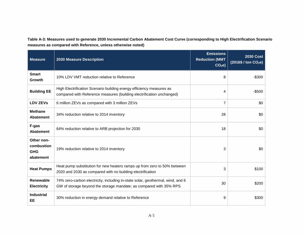
A-5

Table A-3: Measures used to generate 2030 Incremental Carbon Abatement Cost Curve (corresponding to High Electrification Scenario measures as compared with Reference, unless otherwise noted)

Measure 2030 Measure Description Emissions

Reduction (MMT CO2e)

2030 Cost (2016$ / ton CO2e)

Smart Growth

10% LDV VMT reduction relative to Reference 8 -$300

Building EE High Electrification Scenario building energy efficiency measures as compared with Reference measures (building electrification unchanged)

4 -$500

LDV ZEVs 6 million ZEVs as compared with 3 million ZEVs 7 $0

Methane Abatement

34% reduction relative to 2014 inventory 28 $0

F-gas Abatement

64% reduction relative to ARB projection for 2030 18 $0

Other non-combustion GHG abatement

19% reduction relative to 2014 inventory 3 $0

Heat Pumps Heat pump substitution for new heaters ramps up from zero to 50% between 2020 and 2030 as compared with no building electrification

3 $100

Renewable Electricity

74% zero-carbon electricity, including in-state solar, geothermal, wind, and 6 GW of storage beyond the storage mandate; as compared with 35% RPS

30 $200

Industrial EE

30% reduction in energy demand relative to Reference 9 $300

A-6



2030 Cost (2016$ / ton CO2e)

Biofuels 2.8 billion gallons gasoline-equivalent advanced biofuels as compared with 1.2 billion

5 $300

Truck Portfolio

10% of trucks are alternative compared with 5% (HDVs) and 0% (MDVs) 4 $500

Table A-4: Measures used to generate 2050 Incremental Carbon Abatement Cost Curve (corresponding to High Electrification Scenario measures as compared with Reference unless otherwise noted)



2050 Cost (2016$ / ton

CO2e)

Smart Growth 21% LDV VMT reduction relative to Reference 2 -$2500

Building EE High electrification building efficiency measures as compared with Reference measures (building electrification unchanged)

6 -$1000

LDV ZEVs 35 million ZEVs (96% of vehicle stock) as compared with 5 million ZEVs

57 $0

Heat Pumps Nearly 100% electrification of building heating as compared with no building fuel switching in Reference

27 $0

Non-combustion GHGs

59% reduction relative to Reference 51 $0

Industrial EE 30% reduction in energy demand relative to Reference, plus high additional electric efficiency

11 $100

A-7



2050 Cost (2016$ / ton

CO2e)

Renewable Electricity

95% zero-carbon including out-of-state wind and storage with high flexible loads; as compared with 33% RPS

103 $200

Truck Portfolio 78% of trucks are alternative-fuel as compared with 5% (HDVs) and 0% (MDVs) in Reference

23 $300

Biofuels 4.3 billion gallons gasoline-equivalent of advanced biofuels as compared 0.4 billion

21 $700

Industrial Electrification

35% of industrial non-electric end use energy is electrified in In-State Biofuels Only Scenario as compared with no industrial fuel-switching in Reference

6 $900

Additional Biofuels

Additional biofuels relative to biofuels in High Electrification Scenario 7 $1100

Power-to-Gas 7% of pipeline hydrogen and 25% of pipeline synthetic methane in No Building Electrification with Power-to-Gas Scenario as compared with no power-to-gas in Reference

19 $1100

Additional Hydrogen Trucks

58% hydrogen HDVs and 57% MDVs in the High Hydrogen Scenario as compared with 14% of HDVs and 7% of MDVs in the High Electrification Scenario

9 $1600

B-1

APPENDIX B: PATHWAYS Model Input Assumptions

For each sector, references to data sources are provided as well as highlighting key

assumptions.

Energy Demand

Energy Demand Equipment Financing Assumptions

The financing rate to annualize incremental equipment costs is 5% (real), with a range of 3% to

10% tested in sensitivities. Capital costs are annualized over the assumed useful lifetime of the

equipment. Lifetimes of selected equipment are listed below.

Subsector Technology Lifetime (yr)

Residential Water Heating

Reference Gas 9

High Efficiency Gas 9

Electric Heat Pump 16

Residential Space Heating

Reference Gas Furnace 18

Reference Gas Radiator 25

High Efficiency Gas Furnace 18

High Efficiency Gas Radiator 25

High Efficiency Electric Heat Pump 18

Residential Central Air Conditioning

Reference 14

High Efficiency 14

High Efficiency Electric Heat Pump (Cooling)

14

Commercial Water Heating

Reference Gas 12

High Efficiency Gas 12


Commercial Space Heating

Reference Gas Furnace 18

Reference Gas Boiler 25

High Efficiency Gas Furnace 18

B-2

Subsector Technology Lifetime (yr)

High Efficiency Gas Boiler 25


Commercial Air Conditioning

Reference 15

High Efficiency 15

High Efficiency Electric Heat Pump (Cooling)

15

Transportation: Light-Duty Vehicles Light-Duty Auto (all techs) 17

Light-Duty Truck (all techs) 17

Transportation: Medium-Duty Vehicles

Medium-Duty Truck (all techs) 17

Transportation: Heavy-Duty Vehicles

Heavy-Duty Truck (all techs) 16

Transportation: Buses Bus (all techs) 12

Residential Buildings and Commercial Buildings

Residential Data Sources

Description Reference

Calibration of sectoral electricity demand input data (GWh)

California Energy Demand 2016-2026 Adopted Forecast, California Energy Commission, January 2016, CEC-200-2016-001 (15-IEPR-03)

Calibration of sectoral pipeline gas demand input data (Mtherms)

2009 residential gas usage demand from CEC Energy Consumption database and KEMA, 2009. California RASS.

Reference technology shares (% of stock)

Kema, 2009. California RASS.

Percent of high efficiency clothes washers based on 2013 Navigant Potential Study.

Lighting based on 2010 DOE Lighting Market Characterization Report Tables

Technology inputs including useful life, energy type, and cost assumptions

Data used in support of AEO 2013 from the National Energy Modeling System: Input filenames “rsmlgt.txt” For lighting: Energy Savings Potential of Solid-State Lighting in General Illumination Applications (DOE, 2012)

B-3


Subsector energy or service demand consumption estimate used to calibrate total service demand (kWh/household)

KEMA, 2009. California RASS

Energy Star Program Requirements and Criteria for Dishwashers

Per-unit technology costs

Cost projections are taken from data used in support of AEO 2013 from the National Energy Modeling System: Input filenames “rsmlgt.txt” and Input filenames “rsmeqp.txt”. Lighting from the Energy Savings Potential of Solid-State Lighting in General Illumination Applications for LED lamps and luminaires. Heat pump water heater costs from Itron report to CPUC (2014; http://www.calmac.org/publications/2010-2012_WO017_Ex_Ante_Measure_Cost_Study_-_Final_Report.pdf ); see data below.

Technology efficiencies

Data used in support of AEO 2013 from the National Energy Modeling System: Input filename “rsmshl.txt” and Input filename “rsmeqp.txt”. Adjusted from UEC values taken from "rsuec.txt" and stock efficiencies from "rsstkeff.txt". DOE, 2012. Energy Savings Potential of Solid-State Lighting in General Illumination Applications.

Residential “Other” subsector efficiency capital cost

Assumed to be $0.03 / kWh (2012$).

Commercial Data Sources


Calibration of sectoral electricity demand input data (GWh)


Calibration of sectoral pipeline gas demand input data (Mtherms)

California Energy Demand IEPR 2014 - Mid Demand Case

http://www.calmac.org/publications/2010-2012_WO017_Ex_Ante_Measure_Cost_Study_-_Final_Report.pdf



B-4


Energy use by technology per square foot

CEUS, 2006. SCE values used for LADWP and "Other" electric service territories. Adjusted for square footage with no cooling. And for lighting: DOE Lighting Market Characterization Report, 2010.

Reference technology shares (% of stock)

Service demand share from National Energy Modeling System: Input filename “ktek.txt” adjusted for service saturation from 2006 CEUS, and for lighting: DOE Lighting Market Characterization Report, 2010.

Technology inputs including useful life, energy type, and cost assumptions

Data used in support of AEO 2013 from the National Energy Modeling System: Input filenames “ktek.txt”.

Subsector energy or service demand consumption estimate used to calibrate total service demand (kWh/sq ft)

CEUS, 2006 and data used in support of AEO 2013 from the National Energy Modeling System: Input filenames “ktek.txt”.

Per-unit technology costs

Data used in support of AEO 2013 from the National Energy Modeling System: Input filenames “ktek.txt”. Heat pump costs were updated to AEO 2014 data from National Energy Modeling System.

Technology efficiencies Data used in support of AEO 2013 from the National Energy Modeling System: Input filenames “ktek.txt”.

Water Heating and HVAC Selected Capital Cost and Efficiency Assumptions

Subsector Technology Efficiency for

Heating (COP) Efficiency for

Cooling (COP) Cost (2012$)

Residential Water Heating

Reference Gas 0.62 N/A $920/unit Electric Heat Pump 2.35 N/A $2630/unit

Residential HVAC (Heating and Cooling)

Reference Gas Furnace 0.81 N/A $2500/unit Reference Gas Radiator 0.82 N/A $3500/unit High Efficiency Gas Furnace

0.98 N/A $3750/unit

High Efficiency Gas Radiator

0.98 N/A $4000/unit

B-5

Subsector Technology Efficiency for

Heating (COP) Efficiency for

Cooling (COP) Cost (2012$)

Reference Central AC N/A 4.02 $3200/unit High Efficiency Central AC

N/A 7.03 $5750/unit

High Efficiency Electric Heat Pump (Heating & Cooling)

3.22 7.03 $4500/unit

Commercial Water Heating

Reference Gas 0.78 N/A $26/(kBTU/hr

) High Efficiency Electric Heat Pump

2.35 N/A $293/(kBTU/

hr)

Commercial HVAC (Heating and Cooling)

Reference Gas Furnace 0.78 N/A $10/(kBTU/hr

)

Reference Gas Boiler 0.80 N/A $25/(kBTU/hr

) High Efficiency Gas Furnace

0.89 N/A $12/(kBTU/hr

) High Efficiency Gas Boiler

0.97 N/A $38/(kBTU/hr

)

Reference Central AC N/A 3.37 $114/(kBTU/

hr) High Efficiency Central AC

N/A 4.07 $194/(kBTU/

hr) High Efficiency Electric Heat Pump (Heating & Cooling)

3.40 3.52 $112/(kBTU/

hr)

For new appliances sold in 2030 when values vary over time. Coefficient of performance (COP) is the ratio of heating or

cooling output to final fuel energy input. Capital costs for HVAC heat pumps are assumed to be split equally between

heating and cooling subsectors.

Climate Impacts on Building Heating and Cooling Demands

These demand changes were estimated based on building energy demand simulations

performed by the University of California, Irvine as part of a separately funded CEC EPIC grant

(PON-14-309). Demand changes for 2050 were forecast using Representative Concentration

Pathway 8.5 scenario changes, averaged over the climate models in California’s 4th State Climate

Assessment, for each of the CEC’s Building Climate Zones. These were mapped to PATHWAYS

energy geographies used for each demand subsector and linearly interpolated between 2015

and 2050. (Changes in water heating energy demands in building energy simulations were less

than 1% and were not included in PATHWAYS.) Resulting statewide average changes by

subsector are below.

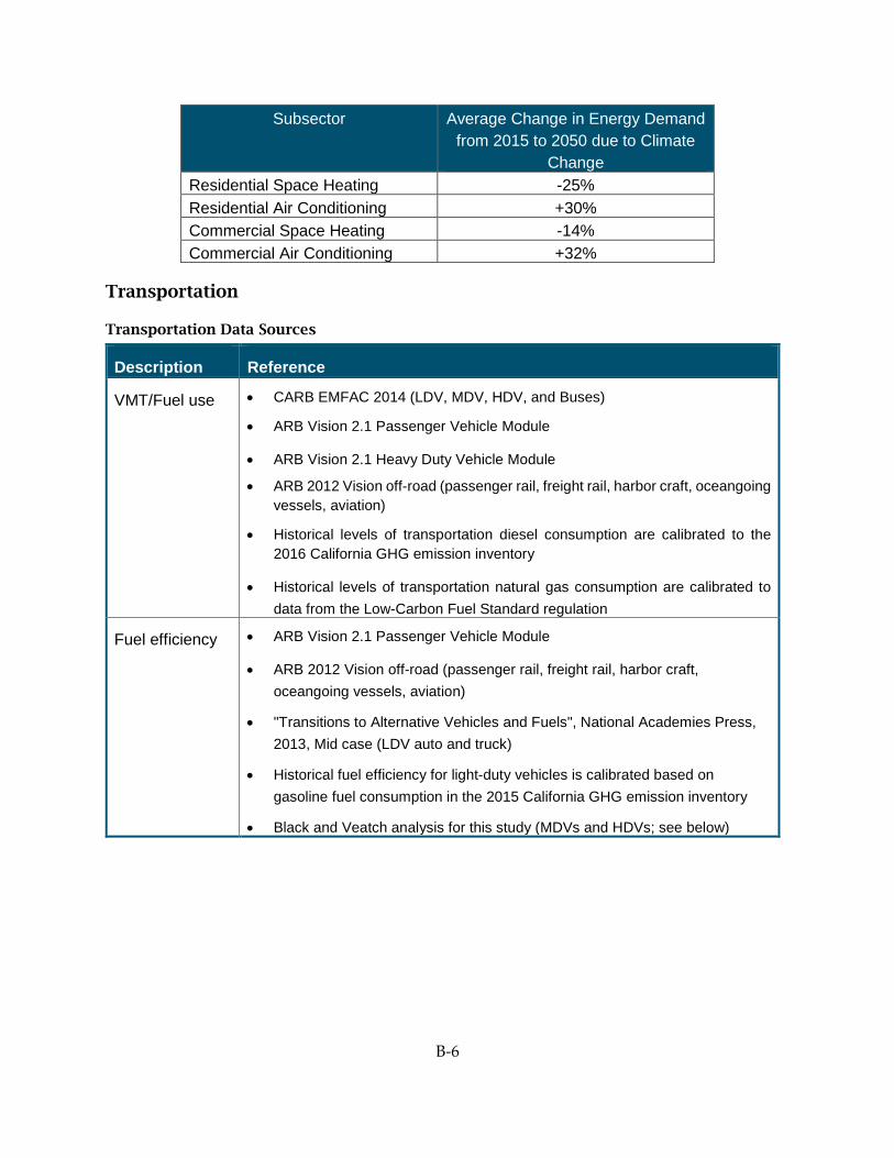
B-6

Subsector Average Change in Energy Demand from 2015 to 2050 due to Climate

Change Residential Space Heating -25% Residential Air Conditioning +30% Commercial Space Heating -14% Commercial Air Conditioning +32%

Transportation

Transportation Data Sources


VMT/Fuel use • CARB EMFAC 2014 (LDV, MDV, HDV, and Buses)

• ARB Vision 2.1 Passenger Vehicle Module

• ARB Vision 2.1 Heavy Duty Vehicle Module

• ARB 2012 Vision off-road (passenger rail, freight rail, harbor craft, oceangoing vessels, aviation)

• Historical levels of transportation diesel consumption are calibrated to the 2016 California GHG emission inventory

• Historical levels of transportation natural gas consumption are calibrated to data from the Low-Carbon Fuel Standard regulation

Fuel efficiency • ARB Vision 2.1 Passenger Vehicle Module

• ARB 2012 Vision off-road (passenger rail, freight rail, harbor craft, oceangoing vessels, aviation)

• "Transitions to Alternative Vehicles and Fuels", National Academies Press, 2013, Mid case (LDV auto and truck)

• Historical fuel efficiency for light-duty vehicles is calibrated based on gasoline fuel consumption in the 2015 California GHG emission inventory

• Black and Veatch analysis for this study (MDVs and HDVs; see below)

B-7


New Technology costs

• Electric bus costs data are from ARB, based on the 2013 CalSTART report.

• Black and Veatch analysis for this study (MDVs and HDVs; see below)

• Ricardo analysis of electric vehicle incremental costs for E3 used for the Pacific Gas & Electric Co EPIC report for 2016: “EPIC 1.25 – Develop a Tool to Map the Preferred Locations for DC Fast Charging, Based on Traffic Patterns and PG&E’s Distribution System, to Address EV Drivers’ Needs While Reducing the Impact on PG&E’s Distribution Grid”, available at https://www.pge.com/pge_global/common/pdfs/about-pge/environment/what-we-are-doing/electric-program-investment-charge/EPIC-1.25.pdf . Used for LDV auto and truck, PHEV and BEV costs and PHEV utility factors.

Reference technology shares

• Vehicle stocks are calibrated to the ARB Vision 2.1 “Current Control Programs” scenario

Workplace electric vehicle charger capital cost

• $4100 per vehicle in 2030 (2012$)

LDV costs and efficiencies

Efficiency (mi/GGE) Vehicle Technology 2020 2030 2050 Reference Gasoline ICE Light-Duty Auto 33 40 40 Efficient Gasoline ICE Light-Duty Auto 33 45 80 Battery-Electric Light-Duty Auto 131 155 202 Hydrogen Fuel-Cell Light-Duty Auto 83 101 138 Plug-in Hybrid Electric Light-Duty Auto 131 155 202 Reference Gasoline ICE Light-Duty Truck 23 30 30 Efficient Gasoline ICE Light-Duty Truck 23 34 54 Battery-Electric Light-Duty Truck 95 111 140 Hydrogen Fuel-Cell Light-Duty Truck 60 72 95 Plug-in Hybrid Electric Light-Duty Truck 95 111 140

Notes: Gallons of Gasoline-Equivalent (GGE) are used in PATHWAYS using the High Heating

Value: 129 MJ / GGE. The plug-in hybrid electric vehicles have a range of 40 mi in electric drive

mode, with 75% of miles assumed driven in electric drive mode.

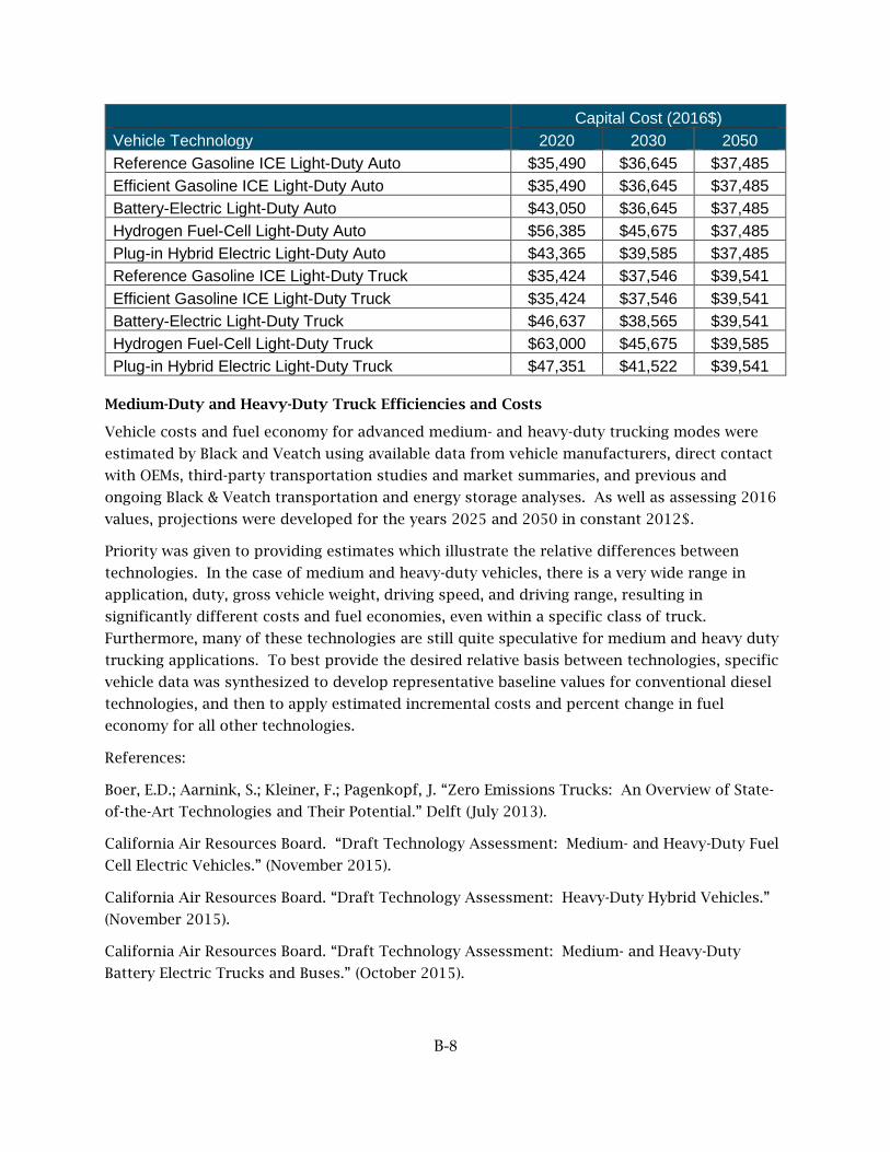
https://www.pge.com/pge_global/common/pdfs/about-pge/environment/what-we-are-doing/electric-program-investment-charge/EPIC-1.25.pdf



B-8

Capital Cost (2016$) Vehicle Technology 2020 2030 2050 Reference Gasoline ICE Light-Duty Auto $35,490 $36,645 $37,485 Efficient Gasoline ICE Light-Duty Auto $35,490 $36,645 $37,485 Battery-Electric Light-Duty Auto $43,050 $36,645 $37,485 Hydrogen Fuel-Cell Light-Duty Auto $56,385 $45,675 $37,485 Plug-in Hybrid Electric Light-Duty Auto $43,365 $39,585 $37,485 Reference Gasoline ICE Light-Duty Truck $35,424 $37,546 $39,541 Efficient Gasoline ICE Light-Duty Truck $35,424 $37,546 $39,541 Battery-Electric Light-Duty Truck $46,637 $38,565 $39,541 Hydrogen Fuel-Cell Light-Duty Truck $63,000 $45,675 $39,585 Plug-in Hybrid Electric Light-Duty Truck $47,351 $41,522 $39,541

Medium-Duty and Heavy-Duty Truck Efficiencies and Costs

Vehicle costs and fuel economy for advanced medium- and heavy-duty trucking modes were

estimated by Black and Veatch using available data from vehicle manufacturers, direct contact

with OEMs, third-party transportation studies and market summaries, and previous and

ongoing Black & Veatch transportation and energy storage analyses. As well as assessing 2016

values, projections were developed for the years 2025 and 2050 in constant 2012$.

Priority was given to providing estimates which illustrate the relative differences between

technologies. In the case of medium and heavy-duty vehicles, there is a very wide range in

application, duty, gross vehicle weight, driving speed, and driving range, resulting in

significantly different costs and fuel economies, even within a specific class of truck.

Furthermore, many of these technologies are still quite speculative for medium and heavy duty

trucking applications. To best provide the desired relative basis between technologies, specific

vehicle data was synthesized to develop representative baseline values for conventional diesel

technologies, and then to apply estimated incremental costs and percent change in fuel

economy for all other technologies.

References:

Boer, E.D.; Aarnink, S.; Kleiner, F.; Pagenkopf, J. “Zero Emissions Trucks: An Overview of State-

of-the-Art Technologies and Their Potential.” Delft (July 2013).

California Air Resources Board. “Draft Technology Assessment: Medium- and Heavy-Duty Fuel

Cell Electric Vehicles.” (November 2015).

California Air Resources Board. “Draft Technology Assessment: Heavy-Duty Hybrid Vehicles.”

(November 2015).

California Air Resources Board. “Draft Technology Assessment: Medium- and Heavy-Duty

Battery Electric Trucks and Buses.” (October 2015).

B-9

California Air Resource Board. “Medium- and Heavy-Duty Battery Electric Vehicles: Technology

Assessment.” Presented September 2, 2014, Sacramento, CA.

California Air Resources Board. “Medium- and Heavy-Duty Fuel Cell Electric Vehicles:

Technology Assessment.” Presented September 2, 2014, Sacramento, CA.

Ford Motor Company Website: http://www.ford.com/commercial-trucks/f650-f750/models/ ;

(accessed February 2016).

Freightliner Website: http://www.freightlinergreen.com/truck ; (accessed February 2016).

National Research Council. “Technologies and Approaches to Reducing the Fuel Consumption

of Medium- and Heavy-Duty Vehicles.” (2010).

U.S. Department of Energy. “Fuel Cell Technologies Program Record #12012.” (September 2012).

U.S. General Services Administration. “2012 Alternative Fuels Vehicle Guide.” (April 2012).

U.S. General Services Administration. “2013 Alternative Fuels Vehicle Guide.” (September 2012).

U.S. General Services Administration. “2016 Alternative Fuels Vehicle Guide.” (December 2015).

MDV Costs and Efficiencies

Efficiency (mi/GGE) Vehicle Technology 2020 2030 2050 Diesel ICE 14.0 13.5 13.2 Hybrid-Electric Diesel 16.0 20.0 22.4 Compressed Natural Gas 9.7 11.1 12.2 Battery-Electric 30.1 32.5 34.3 Hydrogen Fuel Cell 12.8 13.9 15.0 Gasoline ICE 9.7 10.4 10.9

Capital Cost (Thousand 2016$) Vehicle Technology 2020 2030 2050 Diesel ICE $85 $99 $99 Hybrid-Electric Diesel $110 $118 $113 Compressed Natural Gas $92 $106 $106 Battery-Electric $181 $145 $124 Hydrogen Fuel Cell $289 $247 $180 Gasoline ICE $75 $88 $88

B-10

HDV Costs and Efficiencies

Efficiency (mi/GGE) Vehicle Technology 2020 2030 2050 Reference Diesel ICE 7.6 7.7 7.7 Hybrid Diesel 9.2 11.8 12.7 Efficient Diesel ICE 8.2 9.4 10.2 Compressed Natural Gas 6.8 8.5 9.7 Hydrogen Fuel Cell 8.5 10.0 11.2 Battery-Electric 13.9 16.2 17.0

Capital Cost (Thousand 2016$) Vehicle Technology 2020 2030 2050 Reference Diesel ICE $197 $217 $217 Hybrid Diesel $250 $286 $277 Efficient Diesel ICE $220 $259 $259 Compressed Natural Gas $273 $307 $286 Hydrogen Fuel Cell $721 $636 $477 Battery-Electric $484 $372 $288

Bus Costs and Efficiencies

Efficiency (mi/GGE) Vehicle Technology 2020 2030 2050 Gasoline ICE 7 7 7 Diesel ICE 8 8 8 Compressed Natural Gas 6 6 6 Battery-Electric 20 18 23

Capital Cost (Thousand 2016$) Vehicle Technology 2020 2030 2050 Gasoline ICE $107 $107 $107 Diesel ICE $525 $525 $525 Compressed Natural Gas $609 $609 $609 Battery-Electric $731 $628 $628

Rail and Port Electrification Costs

Passenger and freight rail electrification is assumed to have a levelized capital cost of $0.73 per

gallon of diesel avoided, with a 45% energy efficiency improvement. Port electrification (shore

B-11

power for hoteling of ships) is assumed to have zero incremental capital cost, with a 45%

energy efficiency improvement.

Industrial, Refining, and Oil and Gas

Industrial Data Sources


Sectoral electricity demand input data CEC data used in support of http://uc-ciee.org/downloads/CALEB.Can.pdf

Sectoral pipeline gas demand input data

CEC data used in support of http://uc-ciee.org/downloads/CALEB.Can.pdf

Calibrated to CARB emissions inventory 2014 data

Sectoral "other" energy input data CARB emissions inventory historical data

End-use energy decomposition by subsector CPUC Navigant Potential Study, 2013.

Refining Data Sources


Sectoral electricity demand input data



CEC data used in support of http://uc-ciee.org/downloads/CALEB.Can.pdf. Allocated to gas utility service territories as a function of refinery electricity demand (broken out by electric service territory). Assumed that LADWP and SCE refining demand met by SCG.


Sectoral "other" energy input data

CARB GHG Emissions Inventory. Allocated to gas utility service territories as a function of refinery electricity demand (broken out by electric service territory). Assumed that LADWP and SCE refining demand met by SCG.

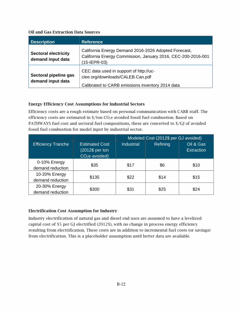
B-12

Oil and Gas Extraction Data Sources





CEC data used in support of http://uc-ciee.org/downloads/CALEB.Can.pdf


Energy Efficiency Cost Assumptions for Industrial Sectors

Efficiency costs are a rough estimate based on personal communication with CARB staff. The

efficiency costs are estimated in $/ton CO2e avoided fossil fuel combustion. Based on

PATHWAYS fuel cost and sectoral fuel compositions, these are converted to $/GJ of avoided

fossil fuel combustion for model input by industrial sector.

Modeled Cost (2012$ per GJ avoided) Efficiency Tranche Estimated Cost

(2012$ per ton CO2e avoided)

Industrial Refining Oil & Gas Extraction

0-10% Energy demand reduction

$35 $17 $6 $10


$135 $22 $14 $15


$300 $31 $25 $24

Electrification Cost Assumption for Industry

Industry electrification of natural gas and diesel end uses are assumed to have a levelized

capital cost of $5 per GJ electrified (2012$), with no change in process energy efficiency

resulting from electrification. These costs are in addition to incremental fuel costs (or savings)

from electrification. This is a placeholder assumption until better data are available.

http://uc-ciee.org/downloads/CALEB.Can.pdf

http://uc-ciee.org/downloads/CALEB.Can.pdf

B-13

Agriculture and TCU (Transportation, Communication, and Utilities)

Agriculture Data Sources






Sectoral "other" energy input data.

Diesel: EIA Adjusted Sales of Distillate Fuel Oil by End Use Gasoline: CARB GHG Emissions Inventory

End-use energy decomposition by subsector

CPUC Navigant Potential Study, 2013.

Energy efficiency cost assumptions

Efficiency costs are estimated at $0.37/kWh (2012$) based on estimated cost of switching to LED lighting.

TCU (Transportation, Communication, & Utilities) Data Sources






B-14

Energy Supply

Electricity

Electricity Data Sources

Category Data source

Hourly end-use electric load shapes

Residential & commercial: Primarily DEER 2008 and DEER 2011, BEopt for residential space heating, cooking and other, CEUS for commercial space heating, lighting and cooking. Agriculture & Industrial: PG&E 2010 load shape data

Hourly renewable generation shapes

Solar PV: simulated using System Advisor Model (SAM), PV Watts Concentrated solar power: simulated using System Advisor Model (SAM)

Wind: Western Wind Dataset by 3TIER for the first Western Wind and Solar Integration Study performed by NREL http://wind.nrel.gov/Web_nrel/

Hydroelectric characteristics

Monthly hydro energy production data from historical EIA data reported for generating units, www.eia.gov/electricity/data/eia923/ Daily minimum and maximum hydro generation limits based on CAISO daily renewable watch hydro generation data www.caiso.com/market/Pages/ReportsBulletins/DailyRenewablesWatch.aspx. Adjusted for climate change impacts based on simulated data from University of California, Irvine as part of a separately funded CEC EPIC grant (PON-14-309).

Import/export limits

Consistent with assumptions used in base case of CA electric utility/E3 study “Investigating a Higher RPS Study” (2013)

Existing generation & heat rates

TEPPC 2022 Common Case, and “Capital cost review of power generation technologies, recommendations for WECC’s 10- and 20-year studies” www.wecc.biz/committees/BOD/TEPPC/External/2014_TEPPC_Generation_CapCost_Report_E3.pdf

http://wind.nrel.gov/Web_nrel/

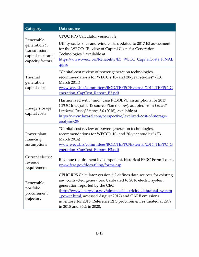
B-15


Renewable generation & transmission capital costs and capacity factors

CPUC RPS Calculator version 6.2

Utility-scale solar and wind costs updated to 2017 E3 assessment for the WECC: “Review of Capital Costs for Generation Technologies,” available at https://www.wecc.biz/Reliability/E3_WECC_CapitalCosts_FINAL.pptx

Thermal generation capital costs

“Capital cost review of power generation technologies, recommendations for WECC’s 10- and 20-year studies” (E3, March 2014) www.wecc.biz/committees/BOD/TEPPC/External/2014_TEPPC_Generation_CapCost_Report_E3.pdf

Energy storage capital costs

Harmonized with “mid” case RESOLVE assumptions for 2017 CPUC Integrated Resource Plan (below), adapted from Lazard’s Levelized Cost of Storage 2.0 (2016), available at https://www.lazard.com/perspective/levelized-cost-of-storage-analysis-20/

Power plant financing assumptions

“Capital cost review of power generation technologies, recommendations for WECC’s 10- and 20-year studies” (E3, March 2014) www.wecc.biz/committees/BOD/TEPPC/External/2014_TEPPC_Generation_CapCost_Report_E3.pdf

Current electric revenue requirement

Revenue requirement by component, historical FERC Form 1 data, www.ferc.gov/docs-filing/forms.asp

Renewable portfolio procurement trajectory

CPUC RPS Calculator version 6.2 defines data sources for existing and contracted generators. Calibrated to 2016 electric system generation reported by the CEC (http://www.energy.ca.gov/almanac/electricity_data/total_system_power.html, accessed August 2017) and CARB emissions inventory for 2015. Reference RPS procurement estimated at 29% in 2015 and 35% in 2020.

https://www.wecc.biz/Reliability/E3_WECC_CapitalCosts_FINAL.pptx

https://www.wecc.biz/Reliability/E3_WECC_CapitalCosts_FINAL.pptx

https://www.lazard.com/perspective/levelized-cost-of-storage-analysis-20/

https://www.lazard.com/perspective/levelized-cost-of-storage-analysis-20/



B-16


Renewable Portfolio Standard Compliance

Portfolio Content Category (PCC) 3 Renewable Energry Credits (RECs) harmonized with RESOLVE inputs for CPUC 2017 Integrated Resource Plan (see below). Water-pumping loads exempted from RPS compliance from the California Energy Demand 2016-2026 Adopted Forecast, California Energy Commission, January 2016, CEC-200-2016-001 (15-IEPR-03)

In-state renewable resource potential

Calibrated to RESOLVE simulations for 2030 for the CPUC 2017 Integrated Resource Plan (see below)

Customer-sited Solar PV capacity


Demand response potential

LBNL 2025 California Demand Response Potential Study (2017), available from the CPUC at http://www.cpuc.ca.gov/WorkArea/DownloadAsset.aspx?id=6442452698. A total of approximately 8 GW is available in PATHWAYS by 2031

Selected Resource Capital Costs

Levelized Capital Costs (2012$/kW-yr) Technology 2015 2030 2050

Wind $266 $162 $162 Utility-Scale PV $216 $176 $176 2-hr Batteries (Li-ion) $215 $127 $127 5-hr Batteries (Li-ion) $495 $294 $294 8-hr Batteries (Va Flow) $581 $360 $360

Miscellaneous Electricity Assumptions

Assumption Value

Reduction in annual hydroelectric energy budget due to climate change 11% between 2015 and 2050

Nuclear plant retirement years 2025 (Diablo Canyon) and 2047 (Palo Verde)

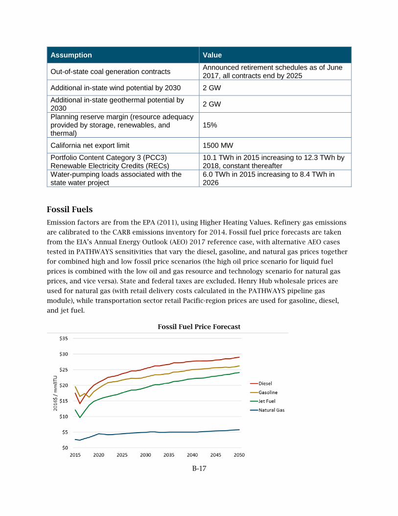
http://www.cpuc.ca.gov/WorkArea/DownloadAsset.aspx?id=6442452698

http://www.cpuc.ca.gov/WorkArea/DownloadAsset.aspx?id=6442452698

B-17

Assumption Value

Out-of-state coal generation contracts Announced retirement schedules as of June 2017, all contracts end by 2025

Additional in-state wind potential by 2030 2 GW

Additional in-state geothermal potential by 2030 2 GW

Planning reserve margin (resource adequacy provided by storage, renewables, and thermal)

15%

California net export limit 1500 MW

Portfolio Content Category 3 (PCC3) Renewable Electricity Credits (RECs)

10.1 TWh in 2015 increasing to 12.3 TWh by 2018, constant thereafter

Water-pumping loads associated with the state water project

6.0 TWh in 2015 increasing to 8.4 TWh in 2026

Fossil Fuels

Emission factors are from the EPA (2011), using Higher Heating Values. Refinery gas emissions

are calibrated to the CARB emissions inventory for 2014. Fossil fuel price forecasts are taken

from the EIA’s Annual Energy Outlook (AEO) 2017 reference case, with alternative AEO cases

tested in PATHWAYS sensitivities that vary the diesel, gasoline, and natural gas prices together

for combined high and low fossil price scenarios (the high oil price scenario for liquid fuel

prices is combined with the low oil and gas resource and technology scenario for natural gas

prices, and vice versa). State and federal taxes are excluded. Henry Hub wholesale prices are

used for natural gas (with retail delivery costs calculated in the PATHWAYS pipeline gas

module), while transportation sector retail Pacific-region prices are used for gasoline, diesel,

and jet fuel.

Fossil Fuel Price Forecast

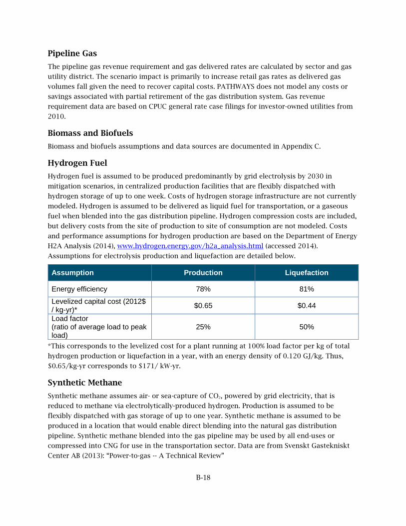
B-18

Pipeline Gas

The pipeline gas revenue requirement and gas delivered rates are calculated by sector and gas

utility district. The scenario impact is primarily to increase retail gas rates as delivered gas

volumes fall given the need to recover capital costs. PATHWAYS does not model any costs or

savings associated with partial retirement of the gas distribution system. Gas revenue

requirement data are based on CPUC general rate case filings for investor-owned utilities from

2010.

Biomass and Biofuels

Biomass and biofuels assumptions and data sources are documented in Appendix C.

Hydrogen Fuel

Hydrogen fuel is assumed to be produced predominantly by grid electrolysis by 2030 in

mitigation scenarios, in centralized production facilities that are flexibly dispatched with

hydrogen storage of up to one week. Costs of hydrogen storage infrastructure are not currently

modeled. Hydrogen is assumed to be delivered as liquid fuel for transportation, or a gaseous

fuel when blended into the gas distribution pipeline. Hydrogen compression costs are included,

but delivery costs from the site of production to site of consumption are not modeled. Costs

and performance assumptions for hydrogen production are based on the Department of Energy

H2A Analysis (2014), www.hydrogen.energy.gov/h2a_analysis.html (accessed 2014).

Assumptions for electrolysis production and liquefaction are detailed below.

Assumption Production Liquefaction

Energy efficiency 78% 81%

Levelized capital cost (2012$ / kg-yr)* $0.65 $0.44

Load factor (ratio of average load to peak load)

25% 50%

*This corresponds to the levelized cost for a plant running at 100% load factor per kg of total

hydrogen production or liquefaction in a year, with an energy density of 0.120 GJ/kg. Thus,

$0.65/kg-yr corresponds to $171/ kW-yr.

Synthetic Methane

Synthetic methane assumes air- or sea-capture of CO2, powered by grid electricity, that is

reduced to methane via electrolytically-produced hydrogen. Production is assumed to be

flexibly dispatched with gas storage of up to one year. Synthetic methane is assumed to be

produced in a location that would enable direct blending into the natural gas distribution

pipeline. Synthetic methane blended into the gas pipeline may be used by all end-uses or

compressed into CNG for use in the transportation sector. Data are from Svenskt Gastekniskt

Center AB (2013): “Power-to-gas -- A Technical Review”

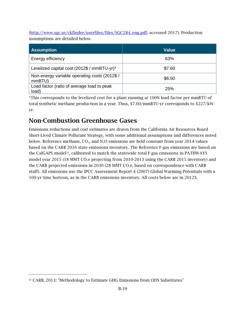
http://www.hydrogen.energy.gov/h2a_analysis.html

B-19

(http://www.sgc.se/ckfinder/userfiles/files/SGC284_eng.pdf, accessed 2017). Production

assumptions are detailed below.

Assumption Value

Energy efficiency 63%

Levelized capital cost (2012$ / mmBTU-yr)* $7.60

Non-energy variable operating costs (2012$ / mmBTU) $6.50

Load factor (ratio of average load to peak load) 25%

*This corresponds to the levelized cost for a plant running at 100% load factor per mmBTU of

total synthetic methane production in a year. Thus, $7.60/mmBTU-yr corresponds to $227/kW-

yr.

Non-Combustion Greenhouse Gases Emissions reductions and cost estimates are drawn from the California Air Resources Board

Short-Lived Climate Pollutant Strategy, with some additional assumptions and differences noted

below. Reference methane, CO2, and N2O emissions are held constant from year 2014 values

based on the CARB 2016 state emissions inventory. The Reference F-gas emissions are based on

the CalGAPS model11, calibrated to match the statewide total F-gas emissions in PATHWAYS

model year 2015 (18 MMT CO2e projecting from 2010-2013 using the CARB 2015 inventory) and

the CARB projected emissions in 2030 (28 MMT CO2e, based on correspondence with CARB

staff). All emissions use the IPCC Assessment Report 4 (2007) Global Warming Potentials with a

100-yr time horizon, as in the CARB emissions inventory. All costs below are in 2012$.

11 CARB, 2013: "Methodology to Estimate GHG Emissions from ODS Substitutes"

http://www.sgc.se/ckfinder/userfiles/files/SGC284_eng.pdf

B-20

Data Sources and Assumptions

Variable Description

Categories of

non-energy,

non-CO2

greenhouse

gases

Subsector GHG emissions data from CARB's emission inventory by IPCC

category:

• Agriculture: (IPCC Level I Agriculture)

• Cement: Clinker production

• Waste: (IPCC Level I Waste)

• Petroleum Refining: (IPCC Level I Energy/IPCC Level II Fugitive/Sector: Petroleum Refining)

• Industrial: (IPCC Level I Industrial) minus Cement

• Oil & gas Extraction: (IPCC Level I Energy/IPCC Level II Fugitive/Sector: Oil Extraction)

• Electricity Fugitive Emissions: (IPCC Level I Energy/IPCC Level II Fugitive/Sector: Anything related to electricity generation including CHP)

• Pipeline Fugitive Emissions: (IPCC Level I Energy/IPCC Level II Fugitive/Sector: Pipelines Natural Gas)

• F-gases are captured in the “High GWP” emissions sector in CARB’s emissions inventory by Scoping Plan category

Cement

(clinker

production)

$10/MTCO2e with a 9% reduction by 2030 from the Reference from fly ash

and other substitutes. Additional 11% reduction by 2050 assumed at the

same price.

Waste

$0/MTCO2e with a 14% reduction by 2030 from the Reference from organic

waste diversion. Based on estimates from the Short-Lived Climate Pollutant

Strategy and correspondence with California Air Resources Board staff.

This estimate excludes the cost of biogas production and any revenue from

electricity sales and LCFS credits. LCFS credits are not modeled in

PATHWAYS as these are assumed to be transfers within the state.

Additional 12% reduction from the Reference assumed by 2050.

Petroleum

Refining

fugitive and

non-energy

emissions

$33/ MTCO2e with a 45% reduction by 2030 from the Reference. Based on

estimates from the Short-Lived Climate Pollutant Strategy. Additional 35%

reduction from the Reference assumed by 2050 at the same price.

Oil Extraction

Fugitive

Emissions




B-21

Variable Description

Electricity

Generation

Fugitive &

Process

$50/MTCO2e with a 40% reduction by 2030 from the Reference. Costs

represent placeholder values as better cost data are needed. Additional 40%


Pipeline

Fugitive




Agriculture:

Enteric

fermentation

$100/ MTCO2e with a 16% reduction by 2030 from the Reference. Costs

represent placeholder values as better cost data are needed.

Agriculture:

Soil

$100/ MTCO2e with a 22% reduction by 2030 from the Reference based on

estimates from C.S. Snyder, T.W. Bruulsema, T.L. Jensen and P.E. Fixen

(2009) Review of greenhouse gas emissions from crop production systems

and fertilizer management effects. Agriculture, Ecosystems and

Environment 133: 247-266. And George Silva (2011) Slow release nitrogen

fertilizers. Available online

http://msue.anr.msu.edu/news/slow_release_nitrogen_fertilizers [Accessed

November 6, 2014]. Additional 30% reduction assumed by 2050 at the same

price.

Agriculture:

Manure

$0/MTCO2e. Based on estimates from the Short-Lived Climate Pollutant

Strategy and correspondence with California Air Resources Board staff.

This estimate assumes that manure collection costs are borne by biogas

production and captured within the biofuels module in PATHWAYS. LCFS

credits are not modeled in PATHWAYS as these are assumed to be transfers

within the state.

F-gases

$48/MTCO2e with a 63% reduction by 2030 from the Reference due to

coolant switching and leak mitigation. Based on correspondence with

California Air Resources Board staff. This estimate excludes the costs and

savings associated with energy efficiency appliance purchases as these are

captured in the equipment stocks costs in the residential, commercial and

transportation sectors. Additional 27% reduction assumed by 2050 at the

same price associated with full compliance with the Kigali agreement.

Land use/

land change Assumed to result in net-zero carbon dioxide emissions.

http://msue.anr.msu.edu/news/slow_release_nitrogen_fertilizers

C-1

Appendix C: PATHWAYS Biofuels Module Methodology

Table of Contents PATHWAYS Biofuels Overview ........................................................................................................ 2

Part 1: Technical Documentation ..................................................................................................... 3

Module Structure ........................................................................................................................................... 3

Input Data ....................................................................................................................................................... 5

Biomass Feedstock Supply ...................................................................................................................... 5

Biofuel Cost and Selection Drivers ........................................................................................................ 8

User-defined Scenario Inputs ..................................................................................................................... 3

Biofuel Energy Demand Targets................................................................................................................. 7

Biofuel Portfolio Selection ........................................................................................................................... 8

Step 1: Pre-optimization Screening ....................................................................................................... 8

Step 2: Portfolio Optimization ............................................................................................................... 9

Outputs ........................................................................................................................................................ 11

Glossary ................................................................................................................................................... 12

References .............................................................................................................................................. 13

C-2

PATHWAYS Biofuels Overview

The PATHWAYS biofuel module calculates the energy supply, delivered costs, and emissions

from the production of biomass-based liquid and gaseous energy products. These biofuels are

used as alternatives to fossil fuels.

In previous versions of the PATHWAYS model, including PATHWAYS 2.2, users selected

biomass resources and allocated them to specific conversion pathways (e.g., gasification) and

final fuel types (e.g., pipeline gas) by feedstock conversion category (e.g., woody cellulosic

feedstocks). Specifying these inputs was challenging, as the task required considerable

knowledge about the tradeoffs associated with each choice. At the same time, this approach

could easily result in suboptimal, overly expensive biofuel portfolios. This approach precluded

a selected biofuel pathway from changing over time, and it limited biofuel portfolio diversity by

allowing only one conversion pathway and final fuel type for all biomass within each

conversion category. To the extent that market conditions will determine dominant conversion

pathways, it seems likely that these optimal conversion pathways will be diverse and will

change over time.

PATHWAYS 2.5 addresses these issues by endogenously selecting optimal biofuel portfolios.

PATHWAYS creates optimized least-cost biofuel portfolios given user inputs on California’s

ability to access national biomass feedstocks and carbon costs. Users may also identify desired

biofuel penetration and optimization settings.

The remainder of this Appendix is organized as follows: Part 1 provides a detailed overview of

the new biofuel logic, and Part 2 demonstrates functionality and potential use cases through

illustrative modeling results. The glossary at the end of this section contains definitions of key

terminology.

C-3

Part 1: Technical Documentation

Module Structure The new biofuel cost minimization method optimally selects a least-cost portfolio of biomass

feedstocks and biofuel conversion pathways through either of two modes: 1) meeting user-

defined biofuel penetration targets (e.g., 80% renewable diesel by 2050); or 2) comparing biofuel

costs to the costs of their fossil fuel counterparts to determine the overall least-cost portfolio.

Under both modes, users may specify a carbon cost and an emission accounting method for

PATHWAYS to consider in cost comparisons. Biofuel portfolios are subject to U.S. biomass

feedstock availability and California’s access to this national feedstock. These feedstock

availability assumptions come from the 2011 Billion-Ton Update (BTS2011) (DOE 2011) and

user inputs on California access to national supply. PATHWAYS uses the resulting optimal

biofuel portfolios and associated costs in liquid and gaseous fuel supply, cost, and emission

calculations.

Figure C-1 illustrates the key inputs, outputs, and logic flow of the Cost Minimization biofuel

module.

C-4

Figure C-29: Cost Minimization Biofuel Module Flow Chart

PATHWAYS combines user inputs about biofuel demand, biomass supply, and biofuel selection

priorities with embedded model assumptions to calculate California biomass supply curves and

biofuel demand by final fuel. The model adds preparation, process, transportation, and delivery

costs to BTS2011 feedstock cost curves to achieve supply curves by feedstock and conversion

pathway. To obtain biofuel demand, PATHWAYS applies the percentage biofuel penetration

targets to aggregate calculated final energy demand.

C-5

The model uses these supply curves and carbon costs to find optimal biofuel portfolios by key

analysis year (2015, 2020, 2030, 4050, and 2050). The model has two modes for achieving this,

which can be selected by the user. In one mode, the model picks the least-cost portfolio that

achieves the biofuel demand, minimizing the total resource cost including any external

incentives. The biofuel demands here are driven by scenario assumptions. In the other mode,

unlimited biofuel demands may be requested, but the model restricts the optimization to only

select feedstocks and conversion pathways that are cost-effective relative to the fossil fuel

alternative, given the carbon price and other incentives. This second mode can be used to

determine the optimal final fuel portfolio, as well as the optimal feedstocks and conversion

pathways to meet that portfolio. Typically, this is used to establish the balance between liquid

fuels and biomethane that achieves the most cost-effective CO2 abatement for a given biomass

supply. A pre-screening of the cheapest pathway (per energy unit) by feedstock and biofuel

speeds up the optimization.

The biofuel module produces annual biofuel energy supply and costs by final fuel. By default,

PATHWAYS calculates delivered biofuel costs on a marginal basis to simulate market-driven

pricing, although users have the option to choose cost-based (average cost) pricing. Other

model results include total biomass bone dry tons used by year and the percent of this selected

biomass that is located within California.

The following sections describe the inputs, assumptions, and model logic in more detail. The

model details are divided into five sections: Input Data, User-defined Scenario Inputs, Biofuel

Energy Demand Targets, Biofuel Portfolio Selection, and Outputs.

Input Data

Biomass Feedstock Supply

Biomass supply curves (i.e. estimates of biomass resource supply potential by price) come from

BTS2011 and the Final Draft Report on The Feasibility of Renewable Natural Gas as a Large-

Scale, Low Carbon Substitute (Jaffe et al. 2016). The BTS2011 focuses on primary sources,

although it also provides estimates for secondary residue and tertiary waste. A review of the

literature found that the BTS2011 appears to underestimate biomethane feedstocks in

California. As a result, the team supplemented the BTS2011 data with more extensive estimates

of California landfill gas, manure, and municipal solid waste biomass using supply curves

produced by Jaffe et al. (2016).

The BTS2011 estimates continental U.S. biomass resource potential based on current and future

inventory, production capacity, availability, technology, and sustainability. Resource supply and

price estimates vary by U.S. county and feedstock type. The BTS2011 groups resources into

price bins of size $10 per bone dry ton (BDT) from $0-10/BDT through $90-100/BDT with an

additional $100-1,000/BDT price bin. PATHWAYS aggregates these data by state for cost

calculations.

C-6

The BTS2011 biomass supply curves are augmented with California landfill gas, manure, and municipal solid waste data from Jaffe et al. (2016). Additional quantities were added at a fixed all-in cost to the BTS2011 estimates from Fig. 30 in Jaffe et al. (2016)

Additional conversion efficiency and cost assumptions are required for the BTS2011 biomass

supply curves to yield all-in costs, described below.

For simplification, PATHWAYS groups feedstocks into five conversion categories: cellulosic,

woody cellulosic, lipid, manure, landfill gas, and starch. These categories share key

characteristics that impact conversion processes and costs. Table 2 displays the categorization

by feedstock.

Table C-9: California Biomethane Feedstocks from Jaffe et al. (2016)

Feedstock Type Quantity (PJ of biomethane) All-In Cost ($/GJ)

Landfill gas 43 $10

Manure 11 $47

Municipal solid waste 16 $19

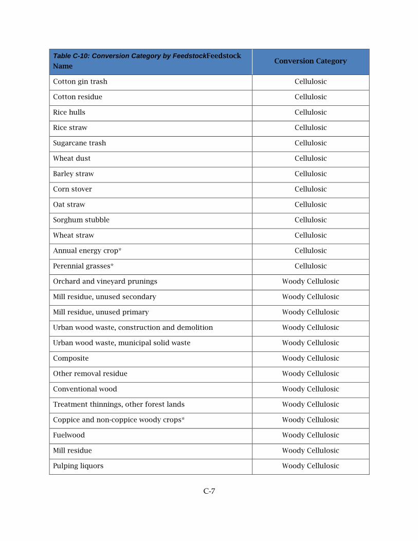
C-7

Table C-10: Conversion Category by FeedstockFeedstock

Name Conversion Category

Cotton gin trash Cellulosic

Cotton residue Cellulosic

Rice hulls Cellulosic

Rice straw Cellulosic

Sugarcane trash Cellulosic

Wheat dust Cellulosic

Barley straw Cellulosic

Corn stover Cellulosic

Oat straw Cellulosic

Sorghum stubble Cellulosic

Wheat straw Cellulosic

Annual energy crop* Cellulosic

Perennial grasses* Cellulosic

Orchard and vineyard prunings Woody Cellulosic

Mill residue, unused secondary Woody Cellulosic

Mill residue, unused primary Woody Cellulosic

Urban wood waste, construction and demolition Woody Cellulosic

Urban wood waste, municipal solid waste Woody Cellulosic

Composite Woody Cellulosic

Other removal residue Woody Cellulosic

Conventional wood Woody Cellulosic

Treatment thinnings, other forest lands Woody Cellulosic

Coppice and non-coppice woody crops* Woody Cellulosic

Fuelwood Woody Cellulosic

Mill residue Woody Cellulosic

Pulping liquors Woody Cellulosic

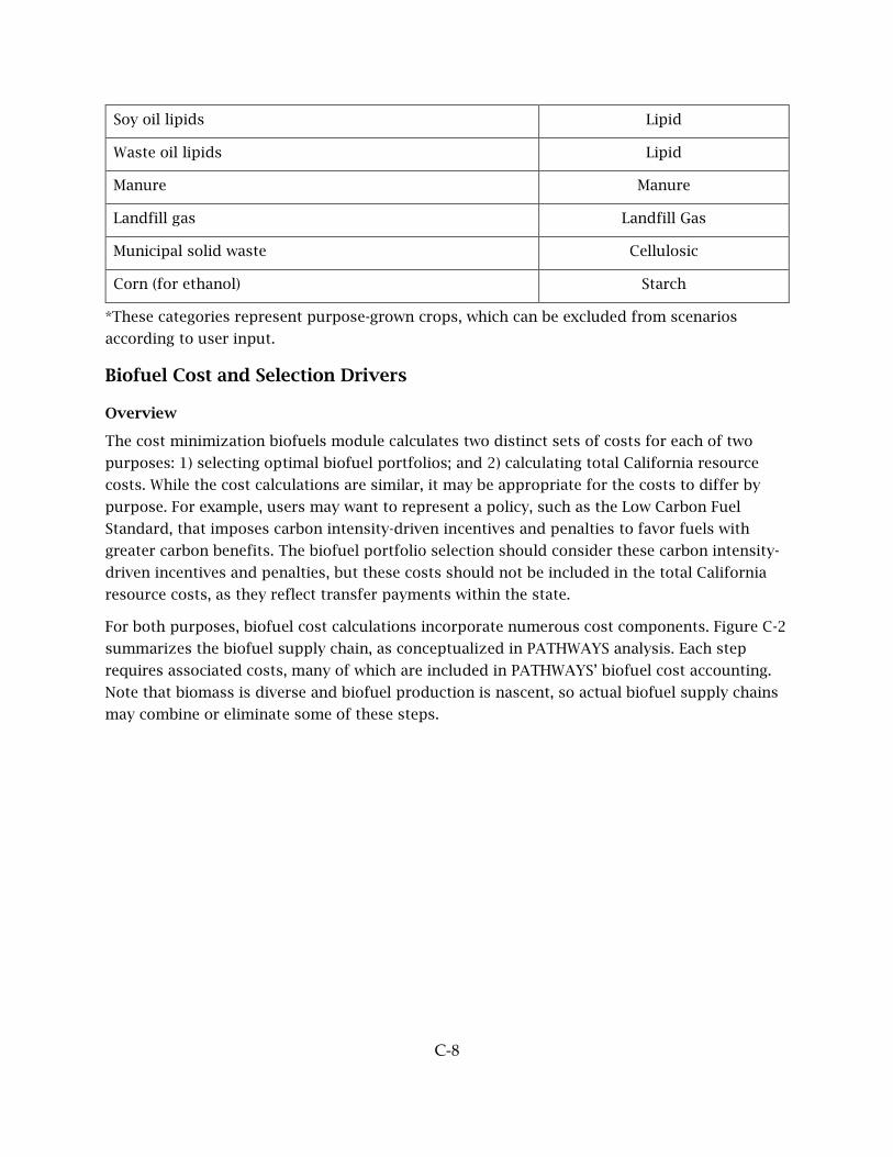
C-8

Soy oil lipids Lipid

Waste oil lipids Lipid

Manure Manure

Landfill gas Landfill Gas

Municipal solid waste Cellulosic

Corn (for ethanol) Starch

*These categories represent purpose-grown crops, which can be excluded from scenarios

according to user input.

Biofuel Cost and Selection Drivers

Overview

The cost minimization biofuels module calculates two distinct sets of costs for each of two

purposes: 1) selecting optimal biofuel portfolios; and 2) calculating total California resource

costs. While the cost calculations are similar, it may be appropriate for the costs to differ by

purpose. For example, users may want to represent a policy, such as the Low Carbon Fuel

Standard, that imposes carbon intensity-driven incentives and penalties to favor fuels with

greater carbon benefits. The biofuel portfolio selection should consider these carbon intensity-

driven incentives and penalties, but these costs should not be included in the total California

resource costs, as they reflect transfer payments within the state.

For both purposes, biofuel cost calculations incorporate numerous cost components. Figure C-2

summarizes the biofuel supply chain, as conceptualized in PATHWAYS analysis. Each step

requires associated costs, many of which are included in PATHWAYS’ biofuel cost accounting.

Note that biomass is diverse and biofuel production is nascent, so actual biofuel supply chains

may combine or eliminate some of these steps.

C-9

Figure C-30: Biofuel Supply Chain

Table C-3 summarizes the cost components and costing methods included in each of the two

cost calculation types.

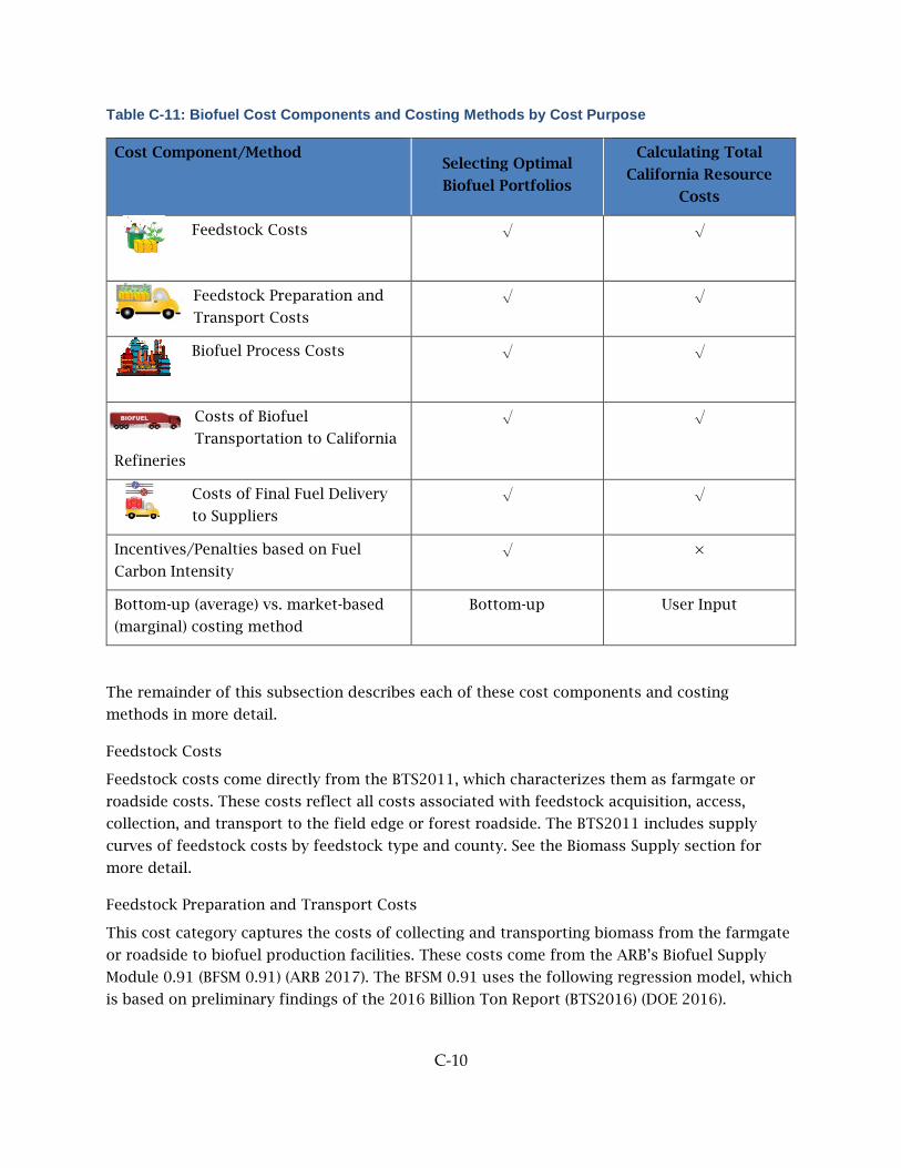
C-10

Table C-11: Biofuel Cost Components and Costing Methods by Cost Purpose

Cost Component/Method Selecting Optimal

Biofuel Portfolios

Calculating Total

California Resource

Costs

Feedstock Costs

√ √

Feedstock Preparation and

Transport Costs

√ √

Biofuel Process Costs

√ √

Costs of Biofuel

Transportation to California

Refineries

√ √

Costs of Final Fuel Delivery

to Suppliers

√ √

Incentives/Penalties based on Fuel

Carbon Intensity

√ ×

Bottom-up (average) vs. market-based

(marginal) costing method

Bottom-up User Input

The remainder of this subsection describes each of these cost components and costing

methods in more detail.

Feedstock Costs

Feedstock costs come directly from the BTS2011, which characterizes them as farmgate or

roadside costs. These costs reflect all costs associated with feedstock acquisition, access,

collection, and transport to the field edge or forest roadside. The BTS2011 includes supply

curves of feedstock costs by feedstock type and county. See the Biomass Supply section for

more detail.

Feedstock Preparation and Transport Costs

This cost category captures the costs of collecting and transporting biomass from the farmgate

or roadside to biofuel production facilities. These costs come from the ARB’s Biofuel Supply

Module 0.91 (BFSM 0.91) (ARB 2017). The BFSM 0.91 uses the following regression model, which

is based on preliminary findings of the 2016 Billion Ton Report (BTS2016) (DOE 2016).

C-11

Equation 1

𝐹𝐹𝑓𝑓𝑓𝑓 = 𝛼𝛼 + 𝛽𝛽1𝑃𝑃𝑓𝑓𝑓𝑓 + 𝛽𝛽2𝑊𝑊𝑓𝑓

Where

Ffp

Pfp

Wf

Feedstock preparation and transport costs in $/ton by feedstock type f and

price bin p

Resource price, estimated as the maximum price contained in the price bin

Boolean variable set to one for woody cellulosic feedstocks and to zero for all

other feedstocks

α Constant term of estimated value -14

Β1

Β2

Coefficient of estimated value 1.19

Coefficient of estimated value -12.47

Biofuel Process Costs and Efficiencies

Biofuel production process costs reflect the costs of producing biofuels from biomass at

biofuel production facilities. Biofuel production processes include pyrolysis, hydrolysis,

anaerobic digestion, gasification, and fatty acid methyl esterification (FAME). Biofuel process

efficiencies represent primary bioenergy losses associated with these processes.

Table C-4 and Table C-5 display the process cost and efficiency assumptions in PATHWAYS,

expressed per bone dry ton of biomass. Biofuel process costs vary by conversion category.

Process efficiencies vary by feedstock.

These process costs and efficiencies are harmonized with those assumed for the California Air

Resources Board Scoping Plan analysis and do not assume any innovation or improvement in

conversion over time. Cellulosic feedstock is only assumed to be available for conversion to

liquid fuels, while woody and other feedstocks can be converted to liquid fuels or biomethane.

C-12

Table C-12: Process Costs by Conversion Category

Feedstock

Conversion

Category

Biofuel Process Biofuel Process Cost

($/ton)

Cellulosic Pyrolysis

(thermochemical)

Renewable

Diesel

$145

Renewable

Gasoline

$145

Renewable Jet

Fuel

$145

Hydrolysis

(hydrotreating)

Renewable

Ethanol

$128

Woody

Cellulosic

Pyrolysis

(thermochemical)

Renewable

Diesel

$162

Renewable

Gasoline

$162

Renewable Jet

Fuel

$162

Hydrolysis

(hydrotreating)

Renewable

Ethanol

$128

Gasification Biomethane $143

Lipid Hydrolysis

(hydrotreating)

Renewable

Diesel

$314

FAME Biodiesel $345

Manure Anaerobic Digestion Biomethane $168

Landfill

Gas

Anaerobic Digestion Biomethane $2661

Municipal

Solid Waste

Gasification Biomethane $70

Starch Fermentation Conventional

Ethanol

$22

1Dollars per ton of raw gas

C-13

Sources: ARB BFSM (CARB 2017); Black and Veatch analysis for E3 (2016)12; Nathan Parker

analysis for E3 (2012)

12 Inputs aligned with other PATHWAYS assumptions. Assumes gas upgrading equipment to

meet SoCalGas Rule 30 specification. Assumes ~92% moisture content in the manure feedstock.

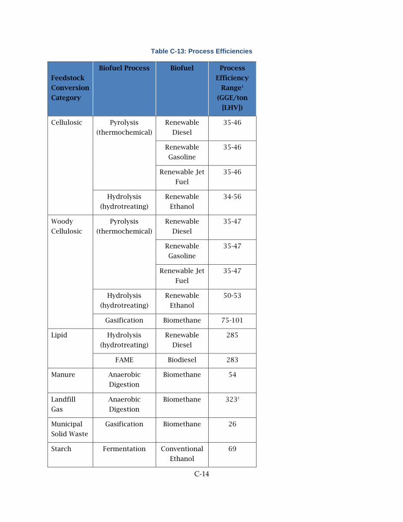
C-14

Table C-13: Process Efficiencies

Feedstock

Conversion

Category

Biofuel Process Biofuel Process

Efficiency

Range1

(GGE/ton

[LHV])

Cellulosic Pyrolysis

(thermochemical)

Renewable

Diesel

35-46

Renewable

Gasoline

35-46

Renewable Jet

Fuel

35-46

Hydrolysis

(hydrotreating)

Renewable

Ethanol

34-56

Woody

Cellulosic

Pyrolysis

(thermochemical)

Renewable

Diesel

35-47

Renewable

Gasoline

35-47

Renewable Jet

Fuel

35-47

Hydrolysis

(hydrotreating)

Renewable

Ethanol

50-53

Gasification Biomethane 75-101

Lipid Hydrolysis

(hydrotreating)

Renewable

Diesel

285

FAME Biodiesel 283

Manure Anaerobic

Digestion

Biomethane 54

Landfill

Gas

Anaerobic

Digestion

Biomethane 3232

Municipal

Solid Waste

Gasification Biomethane 26

Starch Fermentation Conventional

Ethanol

69

C-15

1Varies by feedstock type; GGE is in LHV in this table (115 MJ/GGE). Elsewhere in this document

and in PATHWAYS HHV is used. 2GGE per ton of raw gas

Same sources as for process conversion costs.

Biofuel Transportation to California Refineries

Because biofuels are often cheaper to transport than biomass, biofuel refining may occur in

locations relatively close to biomass production sites and relatively far from California biofuel

demand. Biofuel transportation costs reflect the costs to transport finished biofuel from biofuel

refineries to California refineries, where fuel blending occurs.

Biofuel transportation cost calculations mirror those of the BFSM 0.91, which uses a constant

cost of $0.0083 per ton-mile. This cost comes from a 2009 National Academies Press (NAP)

study and reflects gasoline transport costs. The transportation distances come from Google

Maps and denote centroid distances between U.S. states.

C-16

Table 14: Distances for Transportation to California Refineries

Resource Origin Distance (Miles)

AK 3179

AL 2166

AR 1805

AZ 737

CA 1

CO 1119

CT 2993

DE 2848

FL 2706

GA 2454

HI 2467

IA 1848

ID 908

IL 2085

IN 2231

KS 1539

KY 2311

LA 1906

MA 3097

MD 2782

ME 3243

MI 2406

MN 1993

MO 1845

MS 2010

Resource Origin Distance (Miles)

MT 1258

NC 2650

ND 1717

NE 1459

NH 3083

NJ 2888

NM 992

NV 543

NY 2915

OH 2390

OK 1504

OR 667

PA 2735

RI 3080

SC 2503

SD 1643

TN 2161

TX 1408

UT 794

VA 2648

VT 3082

WA 2794

WI 2178

WV 2548

WY 1156

C-1

Source: ARB Biofuel Supply Module: Technical Documentation for Version 0.91 Beta. Released

January 19, 2017.

Fuel Delivery Costs

PATHWAYS captures the costs to transport final (blended) fuels to suppliers, such as gasoline

fueling stations, within and outside of the biofuel module. The biofuels module includes per-

unit delivery costs for liquid biofuel. Fossil fuel price forecasts contain embedded per-unit fuel

delivery costs. A pipeline gas revenue requirement model determines pipeline gas delivery

costs.

Liquid biofuel delivery costs come from U.S. Energy Information Administration (EIA) data.

PATHWAYS uses the difference between wholesale and end use fuel prices, excluding taxes, as

delivery cost estimates for each of gasoline and diesel. The estimates are $0.32/gallon for

gasoline and $0.48/gallon for diesel.

Carbon Intensities

PATHWAYS may use two types of biofuel-related carbon emission accounting: net lifecycle

emission accounting and ARB Emission Inventory accounting. Users define which of these two

accounting methods to use for biofuel portfolio selection logic. PATHWAYS always adopts ARB

Emission Inventory accounting for scenario emission calculations.

The lifecycle carbon intensities come from the ARB CA-GREET 2.0 and BFSM 0.91 models. The

values typically include emissions associated with feedstock collection and extraction, biofuel

processing, and transport. When estimates exist, the carbon intensities also encompass

emissions from make-up nutrient application and land use change. Net lifecycle carbon

intensities equal biofuel lifecycle carbon intensities (Table C-7) less conventional fuel carbon

intensities (Table C-8).

Under ARB Emission Inventory accounting, biofuels are zero-emission resources. Hence, net

emission reductions exclusively depend on ARB Emission Inventory fossil fuel emission factors,

which are shown in Table C-8.

Table C-15: Biofuel Lifecycle Carbon Intensities

Feedstock Names Lifecycle CI

(gCO2e/MJ)

Cotton gin trash, rice hulls,

and annual energy crop

Pyrolysis &

Hydrolysis: 0

Cotton residue Pyrolysis: 25

Hydrolysis: 24

Rice straw Pyrolysis: 26

Hydrolysis: 19

C-2

Sugarcane trash Pyrolysis: 18

Hydrolysis: 12

Barley straw Pyrolysis: 25

Hydrolysis: 20

Corn stover Pyrolysis: 28

Hydrolysis: 22

Oat straw and sorghum

stubble

Pyrolysis: 23

Hydrolysis: 18

Wheat straw Pyrolysis: 24

Hydrolysis: 20

Annual energy crops Pyrolysis &

Hydrolysis: 0

Perennial grasses Pyrolysis: 38

Hydrolysis: 32

Orchard and vineyard

prunings, urban wood

waste, treatment thinnings,

composite, other forest

lands, and other removal

residue

Pyrolysis: 36

Hydrolysis: -2

Gasification: 25

Mill residue, unused Pyrolysis: 33

Hydrolysis: -4

Gasification: 24

Conventional wood,

fuelwood, mill residue, and

pulping liquors

Pyrolysis &

Hydrolysis: 0

Gasification: 25

Coppice and non-coppice

woody crops

Pyrolysis: 24

Hydrolysis: 19

Soy oil lipids Hydrolysis & FAME: 50

Waste oil lipids Hydrolysis & FAME: 30

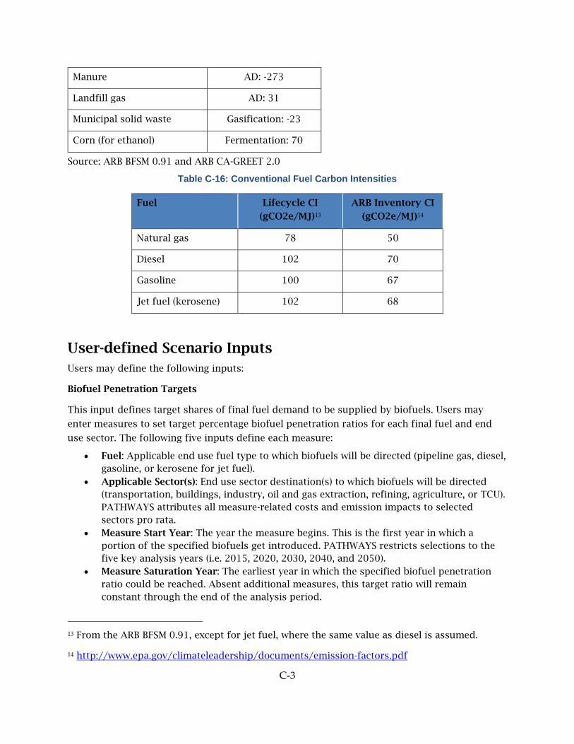
C-3

Manure AD: -273

Landfill gas AD: 31

Municipal solid waste Gasification: -23

Corn (for ethanol) Fermentation: 70

Source: ARB BFSM 0.91 and ARB CA-GREET 2.0

Table C-16: Conventional Fuel Carbon Intensities

Fuel Lifecycle CI

(gCO2e/MJ)13

ARB Inventory CI

(gCO2e/MJ)14

Natural gas 78 50

Diesel 102 70

Gasoline 100 67

Jet fuel (kerosene) 102 68

User-defined Scenario Inputs Users may define the following inputs:

Biofuel Penetration Targets

This input defines target shares of final fuel demand to be supplied by biofuels. Users may

enter measures to set target percentage biofuel penetration ratios for each final fuel and end

use sector. The following five inputs define each measure:

• Fuel: Applicable end use fuel type to which biofuels will be directed (pipeline gas, diesel, gasoline, or kerosene for jet fuel).

• Applicable Sector(s): End use sector destination(s) to which biofuels will be directed (transportation, buildings, industry, oil and gas extraction, refining, agriculture, or TCU). PATHWAYS attributes all measure-related costs and emission impacts to selected sectors pro rata.

• Measure Start Year: The year the measure begins. This is the first year in which a portion of the specified biofuels get introduced. PATHWAYS restricts selections to the five key analysis years (i.e. 2015, 2020, 2030, 2040, and 2050).

• Measure Saturation Year: The earliest year in which the specified biofuel penetration ratio could be reached. Absent additional measures, this target ratio will remain constant through the end of the analysis period.

13 From the ARB BFSM 0.91, except for jet fuel, where the same value as diesel is assumed.

14 http://www.epa.gov/climateleadership/documents/emission-factors.pdf

http://www.epa.gov/climateleadership/documents/emission-factors.pdf

C-4

• Saturation Ratio: The target ratio of biofuel energy to final fuel energy demand at the saturation year. Note that pipeline gas saturation ratios apply only to natural gas demand (i.e. total pipeline gas demand less hydrogen and other power-to-gas supply, if applicable). A gasoline biofuel target ratio should include conventional ethanol, if applicable. Conventional ethanol (e.g. ethanol produced with starch) penetrations can be specified explicitly in the separate Conventional Ethanol Share input.

For each measure, the model calculates a target penetration trajectory by linearly interpolating

the target penetration ratios between the start year and the saturation year. The target measure

penetration reaches the saturation ratio in the saturation year. Absent other measures, the

target penetration ratio stays at that level for the remainder of the analysis period.

Users may specify up to 20 biofuel measures. These measures are additive. Cumulative target

biofuel penetrations are limited to 100% by biofuel and end use sector.

These target biofuel ratios provide an upper bound for achieved biofuel penetrations. Achieved

biofuel penetrations may be further limited by feedstock availability or, in some cases, cost-

effectiveness.

CA Access to U.S. Biomass Supply:

Users define the portion of national biomass feedstock made available for California biofuel

production. Users may select one of the following five methods by which to allocate national

biomass feedstock to California:

• In-state Biomass: This option restricts California’s biomass use to feedstocks located within the state. This scenario assumes no biomass imports or exports.

• Population-weighted Share: This option allows California to use biomass from across the country, but it restricts the state’s biomass use to California’s share of the 2013 U.S. population. This results in California receiving access to about 12% of each type of biomass feedstock at each price point in each U.S. state

• User Input: This option provides users with the flexibility to explicitly specify biomass feedstock available to California as a percentage of total U.S. feedstock. Users must specify these percentages by key analysis year (i.e. 2015, 2020, 2030, 2040, and 2050), location (i.e. in-state vs. out-of-state), and conversion category (i.e. cellulosic, woody cellulosic, lipid, manure, landfill gas, municipal solid waste, and starch). The percentages apply to biomass supply pro rata across states. For example, a user could specify that California has access to 100% of in-state manure and 10% of out-of-state cellulose in 2030. Under this specification, California would receive access to 10% of each type of cellulosic feedstock at each price point in each of the other U.S. states.

In addition, users may select one or more feedstock types from Table 2 to exclude from

availability: for instance, purpose-grown crops have particular concerns about sustainability

associated with indirect land use GHG emissions and effects on food prices, so these are

excluded from most of the mitigation scenarios described in the main body of this report.

C-5

Carbon Cost and Emission Accounting for Biofuel Selection

Users may choose to include carbon-intensity driven incentives and penalties in the costs used

for least-cost biofuel portfolio selection. These incentives and penalties represent monetary

transfers (e.g., government tariff or tax) between parties within California to encourage

consideration of emission impacts in biofuel supply decisions.

Users specify two inputs related to emission accounting:

• Carbon Cost: Cost of carbon emissions in dollars per metric ton of carbon. Users specify a cost for each key analysis year.

• Emission Accounting Method for Biofuel Selection: This user input determines whether to apply the carbon costs to: 1) net lifecycle carbon intensity estimates, or 2) net ARB Emission Inventory accounting carbon intensity estimates. ARB Emission Inventory accounting captures anthropogenic GHG emissions within California and treats all biofuels as zero-emission resources.

Based on these two inputs, PATHWAYS calculates a $/GJ net incentive for each combination of

feedstock type, biofuel, and conversion pathway. This net incentive informs the optimal

selection of biomass and biofuels. Equation 2 illustrates the calculation method, which is based

on: the user-input carbon price trajectory, an estimate of the applicable biofuel carbon

intensity, and a carbon intensity estimate for the replaced fossil fuel. The Emission Accounting

Method for Biofuel Selection input determines whether these carbon intensities reflect lifecycle

emissions or ARB Emission Inventory accounting.

Equation 2

𝑁𝑁𝑁𝑁𝑁𝑁𝑓𝑓𝑓𝑓𝑓𝑓𝑦𝑦 = 𝑁𝑁𝑁𝑁𝑦𝑦 × (𝑁𝑁𝑁𝑁𝐹𝐹𝑓𝑓 − 𝑁𝑁𝑁𝑁𝑓𝑓𝑓𝑓𝑓𝑓)

Where

NCIfcby Net carbon intensity-driven incentive ($/GJ) for biofuel type f produced using

conversion pathway c and biomass feedstock type b in key analysis year y

CCy User-input carbon cost ($/metric ton) of carbon emissions in key analysis year

y

CIFf

CIFfcb

Carbon intensity (tons/GJ) of the fossil fuel counterpart of biofuel type f

Carbon intensity (tons/GJ) of biofuel type f produced using conversion

pathway c and biomass feedstock type b

Carbon intensity-driven incentives only impact biofuel portfolio selection. The final PATHWAYS

cost results do not reflect these carbon costs, as we assume carbon-related monetary transfers

remain within the state. The PATHWAYS emission results exclusively use ARB inventory

emission accounting.

C-6

Only Select cost-effective Biofuels:

The checkbox determines which of the two available modes to use for running the cost-

minimization biofuel module:

• Default Mode: Under the default (unchecked) mode, PATHWAYS selects the least-cost portfolio of biomass and conversion pathways that meet the biofuel targets. PATHWAYS considers carbon costs when selecting between feedstocks and conversion pathways. If the available biomass feedstock supply is insufficient to meet target biofuel energy demand, PATHWAYS prioritizes maximizing biofuel energy production over minimizing costs. In this situation, the model produces a warning to ensure that users are aware of this prioritization.

• Only Select Cost-effective Biofuels Mode: When the Only Select Cost-effective Biofuels input is checked, PATHWAYS only selects biomass feedstocks and conversion pathways that are cost-effective at the given carbon price. The model minimizes net fuel costs given that total selected biofuel energy supply can be no greater than the biofuel penetration targets.

Biofuel Costing Method

Users can choose one of two methods for calculating total California biofuel resource costs:

market-based (marginal) accounting or cost-based (average) accounting.

The market-based cost accounting method is the default method. Under this method, the cost

of biofuels is based on a single market clearing price for each fuel, while the model minimizes

the average total cost of the biofuels, excluding producer rents. The market clearing price

equals the all-in cost of the marginal unit of biofuel. PATHWAYS calculates one biofuel market

clearing price by key analysis year and final fuel. Equation 3 displays this calculation.

The cost-based accounting method produces a bottom-up calculation of all-in biofuel costs for

each unit of biofuel and key analysis year. The all-in costs include all of the cost components

outlined in Table 3, as applicable. Hence, under this method, PATHWAYS effectively calculates

the integral of the selected biofuel supply curve. Dividing by the total quantity of biofuel

produces the average biofuel cost by year and final fuel type (i.e. pipeline gas, diesel, gasoline,

conventional ethanol, and kerosene), as demonstrated in Equation 4.

C-7

Equation 3

𝐵𝐵𝐵𝐵𝑁𝑁𝑓𝑓𝑦𝑦 = max𝑓𝑓,𝑓𝑓,𝑓𝑓

𝑁𝑁𝑓𝑓𝑓𝑓𝑓𝑓𝑓𝑓𝑦𝑦

Equation 4

𝐵𝐵𝐵𝐵𝑁𝑁𝑓𝑓𝑦𝑦 =∑ ∑ ∑ ∑ 𝑁𝑁𝑓𝑓𝑓𝑓𝑓𝑓𝑐𝑐𝑓𝑓𝑦𝑦 × 𝐵𝐵𝑓𝑓𝑓𝑓𝑓𝑓𝑐𝑐𝑓𝑓𝑦𝑦𝑐𝑐𝑓𝑓𝑓𝑓𝑓𝑓

∑ ∑ ∑ ∑ 𝐵𝐵𝑓𝑓𝑓𝑓𝑓𝑓𝑐𝑐𝑓𝑓𝑦𝑦𝑐𝑐𝑓𝑓𝑓𝑓𝑓𝑓

Where

BACfy Average delivered bioenergy costs ($/GJ) for final fuel f in key analysis year y

Bcbplfy

Ccbplfy

Quantity (GJ) of final fuel f in key analysis year y produced using conversion

pathway c and biomass feedstock type b at price point p from location l

All-in cost ($/GJ) of final fuel f in key analysis year y produced using

conversion pathway c and biomass feedstock type b at price point p from

location l

BMCfy Marginal delivered bioenergy costs ($/GJ) for final fuel f in key analysis year y

Under both methods, PATHWAYS linearly interpolates costs between key analysis years to

obtain annual costs.

Note that cost accounting for selecting optimal biofuel portfolios exclusively uses the bottom-

up (average) accounting method, as described in the Biofuel Portfolio Selection section.

Biofuel Energy Demand Targets As described above, PATHWAYS uses the Biofuel Penetration Targets and Conventional Ethanol

Share inputs to define trajectories of biofuel demand as a percentage of final fuel demand by

end use sector. PATHWAYS defines an aggregate trajectory for each of the following final fuels:

pipeline gas, diesel, gasoline, conventional ethanol, and jet fuel. Table C-9 shows the mapping

of biofuels to each of these fuel categories.

C-8

Table C-17: Fuel Category Definitions

Final Fuel (incl. ethanol) Replaced Fuel Applicable Biofuels

Pipeline gas Natural gas Biomethane

Diesel Conventional diesel Renewable diesel, biodiesel

Gasoline Conventional gasoline Renewable gasoline, renewable

ethanol

Conventional ethanol Conventional gasoline Conventional ethanol

Jet fuel Kerosene Renewable jet fuel

As previously described, PATHWAYS calculates total fuel demand by sector. The biofuels

module applies the biofuel penetration trajectories to these total fuel demands to obtain

absolute biofuel energy demand by fuel category and end use sector.

Due to constraints on biomass supply and costs, these biofuel demands may not be met in a

given scenario. If conventional ethanol demand exceeds the attainable conventional ethanol

supply, the remaining demand is met with renewable ethanol or renewable gasoline. For all

other final fuels, conventional fuels replace any demand that cannot be met with biofuels. The

Biofuel Portfolio Selection section discusses these mechanics further.

Biofuel Portfolio Selection Given the biomass supply curves, biofuel demand, and lifecycle carbon costs, PATHWAYS

determines the least-cost biofuel portfolios via a two-step approach. The model first reduces

the dimensionality of the problem by performing a pre-optimization screen. It then uses a

linear optimization model to determine the least-cost viable portfolio of biomass and biofuels

for each of the five key analysis years.

PATHWAYS selects biofuel portfolios that minimize aggregate biofuel costs. For the purpose of

biofuel portfolio selection, biofuel costs include all cost components in the righthand column

of Table 3. As shown in the table, these costs may include carbon intensity-driven incentives

and penalties. The model uses the cost-based (average) accounting approach for biofuel

selection. The resulting portfolio may not minimize market-based (marginal) costs. Hence, the

portfolios may not minimize total scenario costs if users select market-based scenario cost

accounting.

Step 1: Pre-optimization Screening

The pre-optimization screening compares the $/GJ costs of competing conversion pathways for

each potential combination of feedstock type and final fuel. For each feedstock and final fuel,

PATHWAYS removes all but the lowest cost conversion pathway. For example, suppose a lipid

biomass feedstock could produce a gigajoule of biodiesel or a gigajoule of renewable diesel,

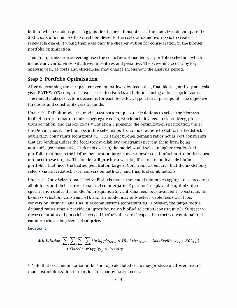
C-9

both of which would replace a gigajoule of conventional diesel. The model would compare the

$/GJ costs of using FAME to create biodiesel to the costs of using hydrolysis to create

renewable diesel. It would then pass only the cheaper option for consideration in the biofuel

portfolio optimization.

This pre-optimization screening uses the costs for optimal biofuel portfolio selection, which

include any carbon-intensity driven incentives and penalties. The screening occurs by key

analysis year, as costs and efficiencies may change throughout the analysis period.

Step 2: Portfolio Optimization

After determining the cheapest conversion pathway by feedstock, final biofuel, and key analysis

year, PATHWAYS compares costs across feedstocks and biofuels using a linear optimization.

The model makes selection decisions for each feedstock type at each price point. The objective

functions and constraints vary by mode.

Under the Default mode, the model uses bottom-up cost calculations to select the biomass-

biofuel portfolio that minimizes aggregate costs, which includes feedstock, delivery, process,

transportation, and carbon costs.15 Equation 5 presents the optimization specification under

the Default mode. The biomass in the selected portfolio must adhere to California feedstock

availability constraints (constraint #1). The target biofuel demand ratios act as soft constraints

that are binding unless the feedstock availability constraints prevent them from being

attainable (constraint #2). Under this set up, the model would select a higher-cost biofuel

portfolio that meets the biofuel penetration targets over a lower-cost biofuel portfolio that does

not meet these targets. The model will provide a warning if there are no feasible biofuel

portfolios that meet the biofuel penetration targets. Constraint #3 ensures that the model only

selects viable feedstock type, conversion pathway, and final fuel combinations.

Under the Only Select Cost-effective Biofuels mode, the model minimizes aggregate costs across

all biofuels and their conventional fuel counterparts. Equation 6 displays the optimization

specification under this mode. As in Equation 5, California feedstock availability constrains the

biomass selection (constraint #1), and the model may only select viable feedstock type,

conversion pathway, and final fuel combinations (constraint #3). However, the target biofuel

demand ratios simply provide an upper bound on biofuel selection (constraint #2). Subject to

these constraints, the model selects all biofuels that are cheaper than their conventional fuel

counterparts at the given carbon price.

Equation 5

𝑴𝑴𝒊𝒊𝒊𝒊𝒊𝒊𝒊𝒊𝒊𝒊𝒊𝒊𝒊𝒊𝒊𝒊𝒊𝒊 � � � �𝐵𝐵𝐵𝐵𝐵𝐵𝐵𝐵𝐵𝐵𝐵𝐵𝐵𝐵𝐵𝐵𝐵𝐵𝑓𝑓𝑓𝑓𝑓𝑓𝑐𝑐𝑦𝑦 × �𝐵𝐵𝐵𝐵𝐵𝐵𝑃𝑃𝐵𝐵𝐵𝐵𝐵𝐵𝐵𝐵𝑓𝑓𝑓𝑓𝑓𝑓𝑐𝑐𝑦𝑦 − 𝑁𝑁𝐵𝐵𝐶𝐶𝐶𝐶𝐹𝐹𝐵𝐵𝐵𝐵𝐵𝐵𝑃𝑃𝐵𝐵𝐵𝐵𝐵𝐵𝐵𝐵𝑓𝑓𝑦𝑦 + 𝑁𝑁𝑁𝑁𝑁𝑁𝑓𝑓𝑓𝑓𝑦𝑦 �𝑐𝑐𝑓𝑓𝑓𝑓𝑓𝑓

+ 𝐵𝐵𝐵𝐵𝑆𝑆𝐵𝐵𝑆𝑆𝑁𝑁𝐵𝐵𝐶𝐶𝐶𝐶𝐵𝐵𝐵𝐵𝐵𝐵𝐵𝐵𝐵𝐵𝐵𝐵𝑓𝑓𝑦𝑦 × 𝑃𝑃𝐵𝐵𝐶𝐶𝑆𝑆𝐵𝐵𝑃𝑃𝐵𝐵

15 Note that cost minimization of bottom-up calculated costs may produce a different result

than cost minimization of marginal, or market-based, costs.

C-10

𝒔𝒔. 𝒕𝒕. (1)∑ 𝐹𝐹𝐵𝐵𝐵𝐵𝐹𝐹𝐹𝐹𝑃𝑃𝐵𝐵𝐵𝐵𝑆𝑆𝑈𝑈𝐹𝐹𝐵𝐵𝑓𝑓𝑓𝑓𝑓𝑓𝑐𝑐𝑦𝑦 ≤ 𝑁𝑁𝐵𝐵𝐵𝐵𝐵𝐵𝐵𝐵𝐵𝐵𝐵𝐵𝐵𝐵𝐵𝐵𝐹𝐹𝐹𝐹𝑓𝑓𝑓𝑓𝑐𝑐𝑦𝑦𝑓𝑓

(2)� � � �𝐵𝐵𝐵𝐵𝐵𝐵𝐵𝐵𝐵𝐵𝐵𝐵𝐵𝐵𝐵𝐵𝐵𝐵𝑓𝑓𝑓𝑓𝑓𝑓𝑐𝑐𝑦𝑦 +𝑐𝑐𝑓𝑓𝑓𝑓𝑓𝑓

𝐵𝐵𝐵𝐵𝑆𝑆𝐵𝐵𝑆𝑆𝑁𝑁𝐵𝐵𝐶𝐶𝐶𝐶𝐵𝐵𝐵𝐵𝐵𝐵𝐵𝐵𝐵𝐵𝐵𝐵𝑓𝑓𝑦𝑦 = 𝐵𝐵𝐵𝐵𝐵𝐵𝐵𝐵𝐵𝐵𝐵𝐵𝑆𝑆𝐶𝐶𝐹𝐹𝑓𝑓𝑦𝑦

(3) 𝐹𝐹𝐵𝐵𝐵𝐵𝐹𝐹𝐹𝐹𝑃𝑃𝐵𝐵𝐵𝐵𝑆𝑆𝑈𝑈𝐹𝐹𝐵𝐵𝑓𝑓𝑓𝑓𝑓𝑓𝑐𝑐𝑦𝑦 ≤ 𝑁𝑁𝐵𝐵𝐵𝐵𝐵𝐵𝐵𝐵𝐵𝐵𝐵𝐵𝐵𝐵𝐵𝐵𝐹𝐹𝐹𝐹𝑓𝑓𝑓𝑓𝑐𝑐𝑦𝑦 × 𝑉𝑉𝐵𝐵𝑆𝑆𝑉𝑉𝐵𝐵𝐵𝐵𝑃𝑃𝑆𝑆𝑃𝑃ℎ𝑤𝑤𝑆𝑆𝐵𝐵𝑓𝑓𝑓𝑓

Equation 6

𝑴𝑴𝒊𝒊𝒊𝒊𝒊𝒊𝒊𝒊𝒊𝒊𝒊𝒊𝒊𝒊𝒊𝒊𝒊𝒊 � � � �𝐵𝐵𝐵𝐵𝐵𝐵𝐵𝐵𝐵𝐵𝐵𝐵𝐵𝐵𝐵𝐵𝐵𝐵𝑓𝑓𝑓𝑓𝑓𝑓𝑐𝑐𝑦𝑦 × �𝐵𝐵𝐵𝐵𝐵𝐵𝑃𝑃𝐵𝐵𝐵𝐵𝐵𝐵𝐵𝐵𝑓𝑓𝑓𝑓𝑓𝑓𝑐𝑐𝑦𝑦 − 𝑁𝑁𝐵𝐵𝐶𝐶𝐶𝐶𝐹𝐹𝐵𝐵𝐵𝐵𝐵𝐵𝑃𝑃𝐵𝐵𝐵𝐵𝐵𝐵𝐵𝐵𝑓𝑓𝑦𝑦 + 𝑁𝑁𝑁𝑁𝑁𝑁𝑓𝑓𝑓𝑓𝑦𝑦 �𝑐𝑐𝑓𝑓𝑓𝑓𝑓𝑓

𝒔𝒔. 𝒕𝒕. (1)∑ 𝐹𝐹𝐵𝐵𝐵𝐵𝐹𝐹𝐹𝐹𝑃𝑃𝐵𝐵𝐵𝐵𝑆𝑆𝑈𝑈𝐹𝐹𝐵𝐵𝑓𝑓𝑓𝑓𝑓𝑓𝑐𝑐𝑦𝑦 ≤ 𝑁𝑁𝐵𝐵𝐵𝐵𝐵𝐵𝐵𝐵𝐵𝐵𝐵𝐵𝐵𝐵𝐵𝐵𝐹𝐹𝐹𝐹𝑓𝑓𝑓𝑓𝑐𝑐𝑦𝑦𝑓𝑓

(2)� � � �𝐵𝐵𝐵𝐵𝐵𝐵𝐵𝐵𝐵𝐵𝐵𝐵𝐵𝐵𝐵𝐵𝐵𝐵𝑓𝑓𝑓𝑓𝑓𝑓𝑐𝑐𝑦𝑦𝑐𝑐𝑓𝑓𝑓𝑓𝑓𝑓

≤ 𝐵𝐵𝐵𝐵𝐵𝐵𝐵𝐵𝐵𝐵𝐵𝐵𝑆𝑆𝐶𝐶𝐹𝐹𝑓𝑓𝑦𝑦

(3) 𝐹𝐹𝐵𝐵𝐵𝐵𝐹𝐹𝐹𝐹𝑃𝑃𝐵𝐵𝐵𝐵𝑆𝑆𝑈𝑈𝐹𝐹𝐵𝐵𝑓𝑓𝑓𝑓𝑓𝑓𝑐𝑐𝑦𝑦 ≤ 𝑁𝑁𝐵𝐵𝐵𝐵𝐵𝐵𝐵𝐵𝐵𝐵𝐵𝐵𝐵𝐵𝐵𝐵𝐹𝐹𝐹𝐹𝑓𝑓𝑓𝑓𝑐𝑐𝑦𝑦 × 𝑉𝑉𝐵𝐵𝑆𝑆𝑉𝑉𝐵𝐵𝐵𝐵𝑃𝑃𝑆𝑆𝑃𝑃ℎ𝑤𝑤𝑆𝑆𝐵𝐵𝑓𝑓𝑓𝑓

Where

BioSupplyfbply Selected biofuel energy (GJ) for final fuel f produced from biomass

feedstock type b at price point p from location l in key analysis year y

BioPricefbply All-in cost ($/GJ) of final fuel f in key analysis year y produced using the

screened-in conversion pathway from biomass feedstock type b at price

point p from location l

ConvFuelPricefy All-in cost ($/GJ) of conventional fuel used for final fuel f in key

analysis year y

NCIfby Net carbon intensity-driven incentive ($/GJ) for biofuel type f produced

using the screened-in conversion pathway from biomass feedstock type

b in key analysis year y

SlackConvSupplyfy Decision variable representing conventional fuel demand used to meet

biofuel demand for final fuel f in key analysis year y

Penalty Large penalty for failing to meet biofuel demand

FeedstockUsefbply Decision variable representing selected biomass feedstock of type b at

price point p from location l used to produce final fuel f in key analysis

year y

CABioAccessbply California access to biomass feedstock of type b at price point p from

location l in key analysis year y

BioDemandfy Biofuel demand (GJ) by final fuel f in key analysis year y

ViablePathwayfb Boolean variable set to one if there is a viable conversion pathway

between biomass feedstock type b and final fuel f

C-11

Outputs PATHWAYS uses the optimized biofuel portfolio to inform liquid and gaseous blended fuel

prices and emission intensities. The biofuels module calculates annual biofuel energy supply by

sector and final fuel. The module achieves these annual estimates by linearly interpolating

biofuel supply between the five key analysis years. The module may adjust these trajectories to

ensure that the supply never exceeds the biofuel penetration targets. PATHWAYS also linearly

interpolates biofuel prices between key analysis years, as discussed previously.

PATHWAYS combines these annual biofuel supply trajectories with hydrogen and power to gas

supply trajectories to calculate annual fuel compositions of liquid and gaseous end use fuels

(i.e. pipeline gas, diesel, gasoline, or kerosene for jet fuel). The model uses these fuel

compositions along with the biofuel, fossil fuel, and other fuel price trajectories to calculate

weighted average annual prices by end use fuel. Similarly, the model calculates annual weighted

average carbon emission intensities by end use fuel based on annual fuel composition and

emission intensity trajectories.

The model also provides users with biofuel-specific diagnostic outputs. Users can explore the

total biomass quantity used, the portion of this biomass coming from outside of California, and

the resulting biofuel penetrations in liquid and gaseous fuels.

C-12

Glossary

• Biofuels: Biomass-derived liquid and gaseous fuels, including biomethane, renewable gasoline, renewable ethanol, conventional ethanol, renewable diesel, biodiesel, and renewable jet fuel.

• Conversion categories: Each biomass feedstock can be classified into one of the following conversion categories: cellulosic, woody cellulosic, lipid, manure, landfill gas, municipal solid waste, and starch. Feedstocks within each conversion category share key biofuel-related properties, including viable biofuel conversion pathways and costs.

• Conversion pathways: Processes for converting biomass into biofuel. PATHWAYS uses the following conversion pathways: anaerobic digestion, gasification, pyrolysis, hydrolysis, fermentation, and FAME. For conversions that require multiple conversion steps, PATHWAYS selects one primary process name to represent the entire conversion process (e.g., starch requires hydrolysis and fermentation for ethanol production, so this document refers to the combined process as “fermentation”).

• Final fuel types: Fuels delivered to end users. These may contain a blend of biofuels and conventional fossil-derived fuels. Final fuels include pipeline gas, gasoline, diesel, and kerosene for jet fuel. In some instances, PATHWAYS also considers conventional ethanol separately from other gasoline fuels.

• Key analysis years: The five years in which PATHWAYS performs biofuel portfolio optimization: 2015, 2020, 2030, 2040, and 2050.

C-13

References California Air Resources Board (2017). “Biofuel Supply Module: Technical Documentation for

Version 0.91 Beta.” Available at: https://www.arb.ca.gov/cc/scopingplan/bfsm_tech_doc.pdf

Kwiatkowski, Jason R., Andrew J. McAloon, Frank Taylor, and David B. Johnston (2006).

“Modeling the process and costs of fuel ethanol production by the corn dry-grind process.”

Industrial Crops and Products 2(3): 288-296.

The National Academies Press (NAP). Liquid Transportation Fuels from Coal and Biomass:

Technological Status, Costs, and Environmental Impacts. Washington, D.C. 2009. Web.

Available at: http://www.nap.edu

National Renewable Energy Laboratory (NREL) (2015). Jobs and Economic Development Impact

(JEDI) Fast Pyrolysis Model. Accessed Jan 2017. Available at:

https://www.nrel.gov/docs/fy15osti/62548.pdf

National Renewable Energy Laboratory (NREL) (2010). “Techno-Economic Analysis of

Biochemical Scenarios for Production of Cellulosic Ethanol.” Technical Report NREL/TP-6A2-

46588. Available at: http://www.nrel.gov/docs/fy10osti/46588.pdf

Oak Ridge National Laboratory (2011). “Billion-Ton Update.” U.S. Department of Energy.

Available at: https://bioenergykdf.net/content/billiontonupdate

Oak Ridge National Laboratory (2016). “2016 Billion-ton Report.” U.S. Department of Energy.

Available at: https://energy.gov/eere/bioenergy/2016-billion-ton-report

University of California, Davis (UC Davis) Institute of Transportation Studies (2016). “Final Draft

Report on The Feasibility of Renewable Natural Gas as a Large-Scale, Low Carbon Substitute.”

Prepared for the California Aire Resources Board and the California Environmental Protection

Agency. Available at: https://www.arb.ca.gov/research/apr/past/13-307.pdf

https://www.arb.ca.gov/cc/scopingplan/bfsm_tech_doc.pdf

http://www.nap.edu/

https://www.nrel.gov/docs/fy15osti/62548.pdf

http://www.nrel.gov/docs/fy10osti/46588.pdf

https://bioenergykdf.net/content/billiontonupdate

https://energy.gov/eere/bioenergy/2016-billion-ton-report

https://www.arb.ca.gov/research/apr/past/13-307.pdf

Deep Decarbonization in a High Renewables Future - Energy ...

Documents

Transcript of Deep Decarbonization in a High Renewables Future - Energy ...