Computation of consistent initial values for properly stated index 3 DAEs

BIT Numer Math (2009) 49: 161–175DOI 10.1007/s10543-009-0212-5

Computation of consistent initial values for properlystated index 3 DAEs

René Lamour · Francesca Mazzia

Received: 30 January 2008 / Accepted: 5 January 2009 / Published online: 7 February 2009© Springer Science + Business Media B.V. 2009

Abstract The computation of consistent initial values is one of the basic problemswhen solving initial or boundary value problems of DAEs. For a given DAE it is, infact, not obvious how to formulate the initial conditions that lead to a uniquely solv-able IVP. The existing algorithms for the solution of this problem are either designedfor fixed index, or they require a special structure of the DAE or they need more thanthe given data (e.g. additional differentiations). In this paper, combining the resultsconcerning the solvability of DAEs with properly stated leading terms with an ap-propriate method for the approximation of the derivative, we propose an algorithmthat provides the necessary data to formulate the initial conditions and which worksat least for nonlinear DAEs up to index 3. Illustrative examples are given.

Keywords DAE · Tractability index · Consistent initialization · Generalizedbackward differentiation formulas

Mathematics Subject Classification (2000) 65L80 · 65L05

1 Introduction

Consider the quasilinear DAEs of at most index 3

A(x(t), t)(D(t)x(t))′ + b(x(t), t) = 0, t ≥ t0, (1.1)

Communicated by Uri Ascher.

R. Lamour (�)Institut für Mathematik, Humboldt-Universität zu Berlin, 10099 Berlin, Germanye-mail: [email protected]

F. MazziaDipartimento di Matematica, Via Orabona 4, 70125 Bari, Italye-mail: [email protected]

mailto:[email protected]

mailto:[email protected]

162 R. Lamour, F. Mazzia

(A(x, t) ∈ Rm,n, D(t) ∈ R

n,m, b(x, t) ∈ Rm, x ∈ R

m, n ≤ m), which will have aunique solution if associated to a set of appropriate initial values defined by

DΠ(x(t0) − α) = 0, (1.2)

where α is a user provided vector. Condition (1.2) fixes a few of the componentsof the consistent initial value x(t0) we are looking for. It is well known that not allcomponents of the initial value can be chosen freely like in the ODE case (cf. [14]).The matrix Π is usually not known a priori, but should be defined in order to have aunique solution x∗ of (1.1), (1.2) at least in a neighborhood of t0 for t ≥ t0.

We consider a DAE with properly stated leading term which requires that

KerA(x, t) ⊕ ImD(t) = Rn

and both subspaces KerA and ImD are C1-subspaces. The representation of a DAEwith properly stated leading term:

– gives a clearer structure of the DAE,– has better numerical properties (cf. [8–10]),– has in the linear case adjoint DAEs of the same kind,– arises naturally in applications, e.g. in electrical circuit simulation using charge

oriented MNA.

The computation of consistent initial values, which corresponds to the computa-tion of Π in this case, is one of the basic problems of the numerical solution of initialor boundary value problems of DAEs. We find different ideas and algorithms in theliterature, e.g. in [2, 5, 6, 12, 13, 19]. All these proposals need either more than thegiven data of (1.1), (1.2) or a special structure of the DAE, or are designed for a lowerfixed index.

For a given DAE it is not obvious which matrix Π leads to a uniquely solvableIVP. This matrix has to describe those components of x which are (sometimes onlyin a restricted area) freely selectable.

In the present paper we combine the ideas of [1, 2] and [5, 13] using the tractabilityindex concept by [15]. The resulting algorithm is described in detail for a linear DAEof index 3 (index 1 and 2 are covered as a special case), obtained after a linearizationof (1.1) along a given sufficiently smooth function x∗:

A(x∗(t), t)(D(t)y(t))′ + B∗(t)y(t) = q(t), (1.3)

with B∗(t) = Ax(x∗(t), t)(Dx∗(t))′ + bx(x∗(t), t).To compute consistent initial values we determine a Π using the tractability index

and discretize the derivative of (1.1) by using the Generalized Backward Differentia-tion Formulas (GBDFs) on nonuniform meshes. The GBDFs are a class of BoundaryValue Methods (BVMs) described in [3], Chap. 5. Their use in block form with non-constant meshes is described in [3], Sects. 11.3–11.5, where the relation to classicalRunge-Kutta schemes is also discussed. Other interesting properties of block BVMscan be found in [11]. The resulting overdetermined nonlinear equations are solvedby Newton-like methods. The structure of the arising Jacobian matrix depends on the

Computation of consistent initial values 163

way of discretizing the derivative and on the structure of the linear DAE (1.3). InSect. 2 we describe how a linear DAE of index 3 is decomposed using the tractabilityindex concept. In Sect. 3 the approximation of the derivative is introduced, and inSect. 4 we illustrate the numerical scheme and its properties. Section 5 is devotedto numerical experiments that show the behavior of the proposed algorithm on testproblems of index 1, 2 and 3.

2 Decomposition of linear DAEs

We consider a linear regular DAE with tractability index 3

A(t)(D(t)x(t))′ + B(t)x(t) = q(t), t ≥ t0, (2.1)

with continuous matrix coefficients and, applying the tractability index notion(cf. [15–17]), we decompose (2.1) into three parts: the dynamic and the algebraicparts and the parts which have to be differentiated.

The tractability index is based on the construction of a matrix chain defined by

Gi+1 := Gi + BiQi, (2.2)

Bi+1 := BiPi − Gi+1D−(DP0 . . . Pi+1D

−)′DP0 . . . Pi (2.3)

where G0 := AD, B0 := B , Qj are admissible projector functions (see Definition 2.2of [17]) such that Q2

j = Qj , and ImQj = KerGj =: Nj , Pj = I − Qj , j = 0, . . . , i,and D− is a reflexive generalized inverse of D with D−D = P0. For regular DAEsa matrix chain element Gi becomes nonsingular and the first index μ, where Gμ

becomes nonsingular, is called the tractability index of the DAE (cf. Definition 2.1 of[17]).

For admissible projectors the following relation holds by definition

N0 ⊕ N1 ⊕ · · · ⊕ Ni−1 ⊆ KerQi

or, equivalently, QiQj = 0, j < i. This ensures that also compositions like P0P1P2and others are projectors, too.

Let Gi, i = 0, . . . ,3, be the matrices of the tractability index matrix chain (2.2),(2.3) and Qi, Pi := I − Qi , i = 0,1,2, related admissible projectors. Following thedecoupling procedure proposed in [15, 17] and [20] we realize the inherent struc-ture of the DAE by means of projections. In particular, we compute the componentsu := DP1P2x, v0 := Q0x, v1 := P0Q1x, and v2 := P0P1Q2x, which split the solu-tion into x = D−u+v0 +v1 +v2, where u is the dynamic part and the solution of theso-called inherent regular ODE, and vi, i = 0, . . . ,2, are successively determined inan explicit manner.

Scaling (2.1) by G−13 we obtain

P2P1D−(Dx)′ + G−1

3 BP0P1P2x + Q0x + Q1x + Q2x

+2∑

i=1

i∑

j=1

P2PjD−(DP1PjD

−)′DP0Pi−1Qix = G−13 q. (2.4)


Multiplying (2.4) by DP1P2 and taking into account that

DP1P2D−(Dx)′ = (DP1P2x)′ − (DP1P2D

−)′Dx, (2.5)

and

2∑

i=1

i∑

j=1

DP1P2P2PjD−(DP1PjD

−)′DP0Pi−1Qix

= (DP1P2D−)′(D − DP1P2)x, (2.6)

we obtain the inherent regular ODE

u′ − (DP1P2D−)′u + DP1P2G

−13 BD−u = DP1P2G

−13 q. (2.7)

It should be mentioned that the solution of (2.7) belongs to the invariant subspaceImDP1P2.

Multiplying (2.4) by P0P1Q2 we obtain

v2 + P0P1Q2G−13 BD−u = P0P1Q2G

−13 q, (2.8)

and multiplying (2.4) by P0Q1P2 and Q0P1P2 leads to

v1 = P0Q1P2G−13 q − K1D

−u + P0Q1Q2D−(Dv2)

′, (2.9)

v0 = Q0P1P2G−13 q − K0D

−u + Q0Q1D−(Dv1)

′

+ Q0P1Q2D−(Dv2)

′ + M02v2 (2.10)

with

K1 = P0Q1P2(G−13 BD− + P1D

−(DP1P2D−)′),

K0 = Q0P1P2(G−13 BD− − D−(DP1P2D

−)′), and

M02 = Q0(Q1 − P1)D−(DP1Q2D

−)′DP1Q2.

This decomposition makes clear what the matrix Π has to be. Only the initial valuesof the inherent ODE (2.7) can be chosen freely, i.e., with Π := Π2 := P0P1P2 wefilter exactly those components of x which belong to the inherent ODE. Now also theway the initial values (1.2) are written becomes clear, because u(t0) = DP1P2x(t0) =DΠx(t0) = DΠα is exactly fixed by (1.2).

The decomposition of a DAE into its components is given by the tractability indextheory for arbitrary index (cf. [15]). Our restriction to at most index 3 DAEs is basedon the numerical behavior, as we will see later on.

The presented decomposition (2.7)–(2.10) is also valid for DAEs with smallerindex (0 (ODE), 1 or 2). In those cases we have to specify the projectors Q2 = 0(index 2), Q1 = 0 (index 1) and Q0 = 0 (index 0), because of the nonsingularity ofG2, G1 or G0.


3 Approximation of the derivative

The approximation of the derivative on the grid t0 < t1 < · · · < ts of a sufficientlysmooth vector function y ∈ Cr(I,R

m), [t0, ts] ⊂ I , using the block k-step GBDFwith a nonuniform mesh is defined as:

⎧⎪⎪⎪⎪⎪⎪⎪⎪⎪⎪⎪⎨

⎪⎪⎪⎪⎪⎪⎪⎪⎪⎪⎪⎩

1

hn

k∑

i=0

α(n)i yi = y′(tn) + O(hk), n = 1, . . . , k1 − 1,

1

hn

k∑

i=0

α(n)i yn−k1+i = y′(tn) + O(hk), n = k1, . . . , s − k2,

1

hn

k∑

i=0

α(n)i ys−k+i = y′(tn) + O(hk), n = s − k2 + 1, . . . , s,

(3.1)

where k1 = k/2� + 1, k2 = k − k1, hi = ti − ti−1, i = 1, . . . , s, and h = ts − t0. Thecoefficients α

(n)i , n = 1, . . . , s and i = 0, . . . , k are computed by imposing that the

order of the method is p = k, using the algorithm described in [3], Sect. 5.2.Following [2] we consider one more initial method that approximates the deriva-

tive of y at t0:

1

h1

k∑

i=0

α(0)i yi = y′(t0) + O(hk). (3.2)

This method, which would not be necessary in the case of an ODE, is importantfor DAEs and useful to compute consistent initial values as explained in [1, 2] forproblems in Hessenberg form.

If we denote by

y :=⎡

⎢⎣y(t0)

...

y(ts)

⎤

⎥⎦ , As ∈ Rs+1,s+1,

the matrix that contains the coefficients α(n)i , and by Dh = diag (h1, h1, . . . , hs) a di-

agonal matrix with the stepsizes, we obtain in matrix form that:

(D−1h As ⊗ I )y =

⎡

⎢⎣y′(t0)

...

y′(ts)

⎤

⎥⎦ + O(hk)

(cf. [2]). We will denote such an approximation of the derivative by

[y]′ := (D−1

h As ⊗ I )y. (3.3)

We prove now a lemma that will be useful in the next section to show that it ispossible to decouple the numerical solution by means of projections, using the sameprocedure as applied for the continuous DAE.


Lemma 3.1 Let M be a matrix function M(t) ∈ C1(I,Rm,m), y and My sufficiently

smooth, and M := diag (M(t0), . . . ,M(ts)) ∈ Rm(s+1),m(s+1), then the discrete prod-

uct rule

M[y]′ = [My]′ − M ′y + O(hk) (3.4)

holds.

Proof

M[y]′ = My′ + O(hk) = My′ + O(hk)

= (My)′ − M ′y + O(hk)

= [My]′ − M ′y + O(hk). �

4 Application of the numerical scheme

We approximate the derivative of (1.3) by our scheme (3.3) and obtain the relation

A[Dy]′ + By = q + O(hk). (4.1)

If we now scale (4.1) by G−13 in the same way as in Sect. 1 and apply (3.4), where

we applied the (continuous) product rule, we obtain an equation similar to (2.4)

P2P1D−[Dy]′ + G−1

3 BP0P1P2y + Q0y + Q1y + Q2y

+2∑

i=1

i∑

j=1

P2Pj D−(DP1Pj D

−)′DP0Pi−1Qi y = G−13 q + O(hk) (4.2)

and the decomposition leads to

[u]′ − (DP1P2D−)′u + DP1P2G−13 BD−u = DP1P2G

−13 q + O(hk), (4.3)

v2 = P0P1Q2G−13 q − P0P1Q2G

−13 BP0P1P2DD−u + O(hk), (4.4)

v1 = P0Q1P2G−13 q − K1D−u + P0Q1Q2D−[Dv2]′ + O(hk−1), (4.5)

v0 = Q0P1P2G−13 q − K0D−u + Q0Q1D−[Dv1]′

+ Q0P1Q2D−[Dv2]′ + M02v2 + O(hk−2). (4.6)

It is obvious that we lose accuracy if we use an approximation of v2 to compute v1

because of the (numerical) differentiation and once more the same with v0. This isthe reason why the resulting coefficient matrix has a condition number O(h−2), aswe can see in the numerical experiments.


We consider (4.1) with the initial condition

DΠ2(y(t0) − α) = 0 (4.7)

with Π2 := P0P1P2.

Theorem 4.1 If the perturbation O(hk) is sufficiently small, the discrete IVP (4.1),(4.7) has a unique solution, and the resulting coefficient matrix has full column rank.

Proof Instead of (4.1) we consider (4.3)–(4.6) with the initial values (4.7). The initialvalues (4.7) operate only on the ODE (4.3).

The IVP (4.3), (4.7) has the structure

(D−1h As ⊗ I )u + Bu = q, (4.8)

DΠ2y(t0) = DΠ2α, (4.9)

with u = DΠ2z, As = (α

(0)0 α

(0)1 ... α

(0)s

as As

)and As nonsingular (cf. [2, 11]). If we com-

bine (4.8) and (4.9) as

⎛

⎜⎝(

1 00 D−1

h

)⎛

⎜⎝

1 0 . . . 0

α(0)0 α

(0)1 . . . α

(0)s

as As

⎞

⎟⎠ ⊗ I

⎞

⎟⎠ u +(

0B

)u =

(DΠ2α

q

), (4.10)

it is obvious that for small h the resulting Jacobian with respect to u has full rankand the least squares method applied to (4.10) has a unique solution. This conditionwill not change for small perturbations because of the continuous dependence of thesolution on the right-hand side. It is obvious that now also (4.4), (4.5) and (4.6) areuniquely solvable. The unique solvability of (4.1), (4.7) follows because of dimensionarguments to the full rank property of the resulting coefficient matrix. �

The computation of consistent initial values of nonlinear DAEs consists now inthe computation of the relevant matrix Π using the tractability matrix chain to makesure to have a locally uniquely solvable system and the application of the boundaryvalue method to approximate the derivative. The following corollary is true:

Corollary 4.1 The discrete DAE

A[Dy]′ + By = q (4.11)

associated with the initial condition (4.7) is convergent of order k − μ + 1, where μ

is the tractability index of the DAE.

The system (4.11) is solved by a Newton-like method. The least squares problem issolved by computing only the first ms columns of the matrix Q and the first ms rowsof the triangular factor R of the QR factorization of the matrix JS where JS = S1JS2is the Jacobian matrix scaled first by rows and then by columns with the maximum


absolute value of the row (column) entries, this allows to handle badly scaled matricesefficiently (for simplicity, we denote the computed matrices of the factorization by Q

and R in the following). The error estimation is made using a deferred correction-likeprocedure, by approximating the derivative with a higher order method in the sameclass and by solving one linear system with the already computed factorization. Ify0 is the approximate solution in t0 computed with the order p method and y0 isthe solution computed using the deferred correction procedure with the order p + 1method, the test for the error is:

1

m‖(y0 − y0)./(atol + rtol. ∗ |y0|)‖2 < τ, (4.12)

where atol and rtol are two input vectors with the absolute and relative tolerances,τ = 15 is a safety factor.

The grid t0 < t1 < · · · < ts is chosen as ti = t0 + 12 (1 + cos((s − i)π/s))h, which

are the so-called Chebyshev-Gauss-Lobatto points extended to the interval [t0, ts].Other choices of the grid are possible, we decide to use this particular grid becausefor s = k the corresponding numerical schemes are equivalent to the well-knownChebyshev spectral collocation methods (see [21], Sects. 5.2–5.5). We use s = k + 2to improve the stability properties of the methods. Moreover, this choice allows toconstruct, on the same mesh, the order p and the order p + 1 methods for approxi-mating the derivative.

5 Numerical experiments

We will present examples of index 1, 2 and 3 to illustrate the behavior of the algorithmcomputing initial values. For the index 1 and 2 we compare the computed consistentinitial conditions with those computed using the algorithm proposed in [13]. Theexamples are solved using different stepsizes h = ts − t0 to show the convergence ofthe numerical scheme and the behavior of the condition number (computed using the2-norm) κR of R and the infinity norm of the two scaling matrices S1 and S2. Theaccuracy of the scheme depends, in fact, on how these matrices change with respectto h. If the consistent initial values x0 and δ0, approximations of x(t0) and (Dx)′(t0),are known, we compute the following values to give an indication of the error:

ex = max1≤i≤m

(|(x0)i − (x0)i |)./(1 + |(x0)i |) and

eδ = max1≤i≤m

(|(δ0)i − (δ0)i |)./(1 + |(δ0)i |),

where x0 and δ0 are the approximations of x(t0) and (Dx)′(t0) computed using thenew algorithm.

Example 1 The first example is the linear index 3 problem proposed in [15] (Exam-ple 2.1), where:

A(t) =⎛

⎝1 0−t 10 0

⎞

⎠ , D(t) =(

0 1 00 0 1

),


Table 1 Example 2.1 of [15], p = 5

h κR(h) log2(κR(h)κR(2h)

) ‖S1(h)‖ ‖S2(h)‖ log2(‖S2(h)‖‖S2(2h)‖ ) r0

2 2.92 × 103 0.14 1.0 1.82 × 101 1.0 3.3 × 10−16

1 3.82 × 103 0.38 1.0 3.64 × 101 1.0 3.3 × 10−16

1/2 4.97 × 103 0.37 1.0 7.28 × 101 1.0 4.4 × 10−16

1/4 9.18 × 103 0.88 1.0 1.45 × 102 1.0 1.1 × 10−17

1/8 1.83 × 104 0.99 1.0 2.91 × 102 1.0 1.1 × 10−16

1/16 3.58 × 104 0.96 1.0 5.82 × 102 1.0 3.3 × 10−16

1/32 6.69 × 104 0.90 1.0 1.16 × 103 1.0 8.2 × 10−19

B(t) =⎛

⎝1 0 00 0 00 −t 1

⎞

⎠ , q =⎛

⎝0t

0

⎞

⎠ .

The exact solution of this index 3 problem is x(t) = (−1, t, t2)T and DΠ = 0.We solve this problem using the order p = 5 method as the numerical approxima-tion of the derivative. In Table 1 we present the condition number κR(h), the valuelog2(κR(h)/κR(2h)) to show how the condition number changes, the infinity normof the two scaling matrices S1 and S2, and the value

r0 = ‖A(x0, t0)[Dx]′0 + b(x0, t0)‖∞.

For this problem the error with respect to the exact solution is near the machineprecision. Both, the condition number of R and the norm of S2 grow like O(h−1) (thismeans that we lose accuracy to compute the numerical differentiation). The values ofr0 are near the machine precision, because the derivative is exactly computed by thenumerical scheme.

Example 2 The second example is the catalyst mixing problem [4, 7]; this problemhas index 1 or 3, depending on the initial data.

z′a = (10zb − za)F,

z′b = (za − 10zb)F − (1 − F)zb,

v′a = (va − vb)F,

v′b = 10(vb − va)F + (vb + 1)(1 − F),

0 = (za − 10zb)(va − vb) − za(vb + 1) + p−1 − p−

2 ,

0 = p+1 − F,

0 = p+2 − 1 + F,

with p+ := max(0,p) and p− := max(0,−p) and x = (za, zb, va, vb,F,p1,p2)T .

This DAE (and the next two examples, too) can be easily presented in the form (1.1)using constant matrices A and D, e.g. A = (

I0

)and D = ( I 0).


Table 2 Catalyst mixing problem index 1, p = 5 with R0 := log2(r0(2h)r0(h)

), Rx := log2(ex(2h)ex(h)

), Rδ :=log2(

eδ(2h)eδ(h)

)

h κR(h) r0(h) R0 ex(h) Rx eδ(h) Rδ

2 1.74 × 102 3.27 × 10−5 2.98 × 10−7 1.91 × 10−5

1 1.44 × 102 6.29 × 10−6 2.37 1.48 × 10−8 4.33 3.59 × 10−6 2.41

1/2 1.92 × 102 1.71 × 10−7 5.20 1.01 × 10−10 7.20 9.72 × 10−8 5.20

1/4 1.66 × 102 4.92 × 10−9 5.11 7.24 × 10−13 7.12 2.79 × 10−9 5.11

1/8 1.52 × 102 1.48 × 10−10 5.05 5.43 × 10−15 7.06 8.39 × 10−11 5.05

1/16 1.52 × 102 4.52 × 10−12 5.03 4.16 × 10−17 7.03 2.57 × 10−12 5.03

1/32 1.50 × 102 1.51 × 10−13 4.90 1.81 × 10−17 – 1.51 × 10−13 4.08

If we start at t0 = 1/2 and use

α = (0.9, 0.07, −0.002, −.24, 0.227, −0.227, 0.773)T

and x0 = α as the initial approximation, we obtain an index one problem.The used matrix of the initial condition is Π = (

I40

). In Table 2 we report the

condition number of R, the value of r0 and the relative errors ex and eδ using theapproximations of x(t0) and (Dx)′(t0) computed using the algorithm as presentedin [13] for x0 and δ0. We note that, since the problem is of index 1, the conditionnumber of R remains constant with h, and the same is true for the norm of the scalingmatrices, in this case we have ‖S1‖ = 1 and ‖S2‖ = 3.6. Moreover, as we use p = 5,we see that the derivative δ0 converges with order 5, as expected, and this is also truefor the value of the residual r0. For this problem the value of x0 converges with orderp + 2, it is not clear why we obtain this result.

If we start at t0 = 1/2 and use α = (0, 1, 1, −1, 1, 1, 1)T and x0 = α as theinitial approximation, we obtain an index 3 problem. The used matrix of the initialcondition is Π = (

M40

)with M4 = (M4,1,M4,2),

M4,1 =

⎛

⎜⎜⎝

4.729847009939550 × 10−1 4.991295839634978 × 10−1

4.991295839634932 × 10−1 5.267196614689953 × 10−1

−1.176637397366436 × 10−3 −1.241677655515170 × 10−3

1.176637397366799 × 10−2 1.241677655514866 × 10−2

⎞

⎟⎟⎠ ,

M4,2 =

⎛

⎜⎜⎝

−1.176637397370391 × 10−3 1.176637397370496 × 10−2

−1.241677655512309 × 10−3 1.241677655512216 × 10−2

9.901019370053175 × 10−1 9.898062994682633 × 10−2

9.898062994682692 × 10−2 1.019370053173017 × 10−2

⎞

⎟⎟⎠ .

Note that the rank of M4 is 2.In Table 3 we report the results. In this case the condition number of R grows like

h−2 and the scaling matrices have constant values (‖S1‖ = 10,‖S2‖ = 3.6). We notethat, even if the index is 3, the residual decreases with the same order of the methodused.


Table 3 Catmix problem index 3, p = 5


) r0(h) log2(r0(2h)r0(h)

)

8 6.92 × 102 1.12 × 10−08

4 1.60 × 103 1.20 3.43 × 10−10 5.03

2 4.89 × 103 1.61 1.04 × 10−11 5.03

1 1.72 × 104 1.81 3.23 × 10−13 5.03

1/2 7.34 × 104 2.09 6.25 × 10−15 5.97

1/4 2.68 × 105 1.87 8.90 × 10−15 –

Example 3 This is an academic index two problem.

x′1 + x1 = 0,

x′2 + x1 + x3 = 0,

x2 + x4 − 1 = 0,

x4 − (1 + sin t) = 0.

(5.1)

For this example x4 and x2 are fixed by the equations. The inherent ODE is given bythe first line of (5.1). The natural matrix Π would be

⎛

⎜⎜⎝

10

00

⎞

⎟⎟⎠ ,

which is also provided by the code.For the computation of consistent initial values it is not important to fix the free-

doms of the DAE by an equation of the form (1.2). We have to formulate the rightnumber of conditions. Example 3 has one degree of freedom, naturally assigned tothe first component x1. However, also an initial condition for x3 is possible. Becauseof the second equation, a given value for x3 fixes x1, which is used as the initial valueof the inherent ODE.

For practical applications it would be advantageous to check the possibility of suchinitial values and to put it into practice, as it is done in [13]. We plan to extend thealgorithm with that feature later on.

In Table 4 we report the numerical results with the natural matrix using α = x0 =(1,0,0,0)T . For approximating the derivative we use the method of order p = 9. Forthis example the ‖S2(h)‖ grows like O(h−1) and the error of δ0 decreases with orderp − 1.

Example 4 This is the classical pendulum problem of index 3:

x′1 − x3 = 0,

x′2 − x4 = 0,


Table 4 Problem of index 2, p = 9, with RS := log2(‖S2(h)‖‖S2(2h)‖ ), Rδ := log2(

eδ(2h)eδ(h)

)

h κR(h) ‖S2(h)‖ RS r0 ex(h) eδ(h) Rδ

8 6.94 × 101 1.18 × 101 9.45 × 10−05 4.58 × 10−11 4.72 × 10−05

4 6.85 × 101 2.38 × 101 1.00 7.32 × 10−07 1.49 × 10−15 3.65 × 10−07 7.01

2 7.24 × 101 4.74 × 101 1.00 3.02 × 10−09 8.33 × 10−16 1.51 × 10−09 7.92

1 1.00 × 102 9.52 × 101 0.99 8.76 × 10−12 2.55 × 10−15 4.38 × 10−12 8.43

1/2 1.23 × 102 1.90 × 102 1.00 2.87 × 10−14 8.33 × 10−16 1.37 × 10−14 8.32

1/4 1.38 × 102 3.78 × 102 1.00 3.33 × 10−15 2.33 × 10−15 4.38 × 10−15 –

Table 5 Pendulum problem index 3, p = 9


) ‖S2(h)‖ log2(‖S2(h)‖S2(2h)‖ ) r0

1/2 6.84 × 103 2.06 × 102 1.32 × 10−5

1/4 1.63 × 104 1.25 5.31 × 102 1.37 1.12 × 10−7

1/8 3.82 × 104 1.23 8.00 × 102 0.59 1.43 × 10−10

1/16 7.15 × 104 0.90 1.53 × 103 0.94 2.82 × 10−13

1/32 1.36 × 105 0.93 3.04 × 103 0.99 1.80 × 10−13

x′3 + x1x5 = 0,

x′4 + x2x5 − g = 0,

x21 + x2

2 − 1 = 0

with g = 9.81. The computed matrix Π is⎛

⎜⎜⎜⎜⎝

01

01

0

⎞

⎟⎟⎟⎟⎠.

We solve this problem using an approximation of the derivative of order p = 9 andα = x0 = (1,0,1,2,1)T . In Table 5 we report the results. The condition number of R

as well as the norm of ‖S2‖ grow like O(h−1), ‖S1(h)‖ = 1.

Example 5 The last set of examples are the DAEs problems taken from the Testset for IVP solvers [18], a collection of test problems arising from applications. Inthe Test set for IVP solvers it is explained how well-known solvers for IVP-DAEworks on the test problems. We note that all the solvers used in the IVP Test setneed consistent initial values as input parameters. These values have been previouslycomputed, in general using techniques based on differentiation. We report here theresults for the DAE problems called crank, pump, fekete and water, of index 2, and forthe problems andrews and caraxis, of index 3. All these problems are of the following


Table 6 Matrices A and D for the problems in the Test set for IVP solvers.

Problem m n A D

caraxis 10 8 I10,8 M(1 : 8, :)andrews 27 14 I27,14 M(1 : 14, :)pump 39 3 I39,3 M(1 : 3, :)fekete 160 120 I160,120 M(1 : 120, :)

water 49 20

⎛

⎜⎝

106I18 018,2018 018,2

02,18 I2011,18 011,2

⎞

⎟⎠(

10−6I18 018,202,18 I2

)M([1 : 18, 37 : 38], :)

crank 24 14 I24,14 M(1 : 14, :)

Table 7 Values of α for the problems in the Test set for IVP solvers

Problem α

caraxis α([1 : 4,6,8]) = x0([1 : 4,6,8]) α([5,7,9,10]) = 1

andrews α([1 : 14]) = x0([1 : 14]) α([14 : 27]) = 1

pump α([2 : 5]) = x0([2 : 5]) α([1,6 : 9]) = 1

fekete α([1 : 120]) = x0([1 : 120]) α([121 : 160]) = 1

water α([2 : 19,37 : 38]) = x0([2 : 19,37 : 38])α([1,19 : 36]) = 0.01 α([39 : 49]) = 1

crank α([1 : 14]) = x0([1 : 14]) α([14 : 24]) = 1

structure:

Mx(t)′ = f (x(t), t) (5.2)

with M ∈ Rm,m a constant matrix and f,x ∈ R

m. A complete description of the prob-lems is available in [18], in Table 6 we report the constant matrices A ∈ R

m,n andD ∈ R

n,m with AD = M that have been used to define the properly stated formula-tion

A(Dx(t))′ = f (x(t), t) (5.3)

used to run the numerical tests (we use a MATLAB notation).For all problems we use the consistent initial values available in [18] (x0, and δ0

in the following ) as approximation of x(t0), δ(t0) and we set only the components ofα that define the initial values of the inherent ODE equals to the corresponding onesof x0 (see Table 7). We use x0 = α as initial approximation.

We run these problems using the variable stepsize implementation that changesthe value of the initial stepsize h = h0 automatically until the relation for the estimateerror in (4.12) is satisfied. For each problem we use atoli = rtoli = tol, i = 1, . . . ,m.In Table 8 we report the initial value of h (h0), the value of tol, the output value ofh (hf ), the condition number of the factor R computed last, the value of r0, and therelative errors ex and eδ.


Table 8 Results for the problems in the Test set for IVP solvers, p = 9

Problem h0 rtol hf κR(hf ) r0 ex eδ

caraxis 10−2 10−10 10−2 6.3 × 105 1.2 × 10−12 7.2 × 10−13 1.0 × 10−12

andrews 10−3 10−6 10−3 5.8 × 108 7.8 × 10−12 2.3 × 10−6 2.3 × 10−6

pump 10−8 10−10 10−8 3.6 × 102 7.5 × 10−20 6.7 × 10−21 6.8 × 10−20

fekete 10−2 10−10 10−2 2.8 × 102 1.6 × 10−12 6.0 × 10−13 1.1 × 10−12

water 10−2 10−10 10−2 5.9 × 102 3.2 × 10−9 7.7 × 10−8 4.2 × 10−9

crank 10−4 10−8 10−4 8.6 × 109 5.7 × 10−10 1.3 × 10−7 2.2 × 10−7

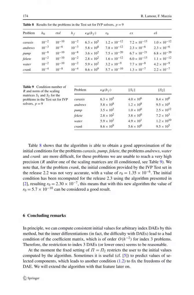
Table 9 Condition number ofR and norm of the scalingmatrices S1 and S2 for theproblems in the Test set for IVPsolvers, p = 9

Problem κR(hf ) ‖S1‖ ‖S2‖

caraxis 6.3 × 105 4.0 × 106 8.4 × 100

andrews 5.8 × 108 1.2 × 108 9.5 × 104

pump 3.5 × 102 1.0 × 100 2.5 × 1012

fekete 2.8 × 102 3.8 × 100 7.2 × 103

water 5.9 × 102 4.9 × 101 1.2 × 1010

crank 8.6 × 109 5.6 × 100 9.5 × 105

Table 8 shows that the algorithm is able to obtain a good approximation of theinitial conditions for the problems caraxis, pump, fekete, the problems andrews, waterand crank are more difficult, for these problems we are unable to reach a very highprecision (R and/or one of the scaling matrices are ill conditioned, see Table 9). Wenote that, for the problem crank, the initial condition provided by the IVP Test set inthe release 2.2 was not very accurate, with a value of r0 = 1.35 × 10−6. The initialcondition has been recomputed for the release 2.3 using the algorithm presented in[2], resulting r0 = 2.30 × 10−7, this means that with this new algorithm the value ofr0 = 5.7 × 10−10 can be considered a good result.

6 Concluding remarks

In principle, we can compute consistent initial values for arbitrary index DAEs by thismethod, but the inner differentiations (in fact, the difficulty with DAEs) lead to a badcondition of the coefficient matrix, which is of order O(h−2) for index 3 problems.Therefore, the restriction to index 3 DAEs (or lower ones) seems to be reasonable.

At the moment the fixed setting of Π = Π2 restricts the user to the initial valuescomputed by the algorithm. Sometimes it is useful (cf. [5]) to predict values of se-lected components, which leads to another condition (1.2) to fix the freedoms of theDAE. We will extend the algorithm with that feature later on.


References

1. Amodio, P., Mazzia, F.: Numerical solution of differential-algebraic equations and computation ofconsistent initial/boundary conditions. J. Comput. Appl. Math. 82(1–2), 299–311 (1997)

2. Amodio, P., Mazzia, F.: An algorithm for the computation of consistent initial values for differential-algebraic equations. Numer. Algorithms 19, 13–23 (1998)

3. Brugnano, L., Trigiante, D.: Solving Differential Problems by Multistep Initial and Boundary ValueMethods. Gordon & Breach, New York (1998)

4. England, R., Gómez, S., Lamour, R.: Expressing optimal control problems as differential-algebraicequations. Comput. Chem. Eng. 29(8), 1720–1730 (2005)

5. Estévez Schwarz, D., Lamour, R.: The computation of consistent initial values for nonlinear index-2differential-algebraic equations. Numer. Algorithms 26(1), 49–75 (2001)

6. Gear, C.W., Leimkuhler, B., Petzold, L.R.: Approximation methods for the consistent initialization ofdifferential-algebraic equations. SIAM J. Numer. Anal. 28, 205–226 (1991)

7. Gunn, D.J., Thomas, W.J.: Transport and chemical reaction in multifunctional catalyst systems. Chem.Eng. Sci. 20, 89–100 (1965)

8. Higueras, I., März, R.: Differential-algebraic equations with properly stated leading terms. Comput.Math. Appl. 48, 215–235 (2004)

9. Higueras, I., März, R., Tischendorf, C.: Stability preserving integration of index-1 DAE’s. APNUM45(2–3), 175–200 (2003)

10. Higueras, I., März, R., Tischendorf, C.: Stability preserving integration of index-2 DAEs. APNUM45(2–3), 201–229 (2003)

11. Iavernaro, F., Mazzia, F.: Block-boundary value methods for the solution of ordinary differential equa-tions. SIAM J. Sci. Comput. 21(1), 323–339 (1999) (electronic)

12. Kunkel, P., Mehrmann, V.: Differential-Algebraic Equations—Analysis and Numerical Solution. EMSPublishing House, Zürich (2006)

13. Lamour, R.: Index determination and calculation of consistent initial values for DAEs. Comput. Math.Appl. 50, 1125–1140 (2005)

14. März, R.: Numerical methods for differential-algebraic equations. Acta Numer. 1, 141–198 (1992)15. März, R.: The index of linear differential-algebraic equations with properly stated leading term. Re-

sults Math. 42, 308–338 (2002)16. März, R.: Fine decouplings of regular differential algebraic equations. Results Math. 46, 57–72 (2004)17. März, R.: Solvability of linear differential algebraic equations with properly stated leading terms.

Results Math. 45(1–2), 88–105 (2004)18. Mazzia, F., Magherini, C.: Test set for initial value problem solvers, release 2.4. Technical Report

4, Department of Mathematics, University of Bari, Italy, February 2008. Available at http://pitagora.dm.uniba.it/~testset

19. Pryce, J.D.: A simple structural analysis method for DAEs. BIT 41(2), 364–394 (2001)20. Riaza, R.: Differential-Algebraic Systems: Analytical Aspects and Circuit Applications. World Sci-

entific, Singapore (2008)21. van Lent, J.: Multigrid methods for time-dependent partial differential equations. Ph.D. Thesis,

Katholieke Universiteit Leuven, Faculteit Ingenieurswetenschappen, Departement Computerweten-schappen (2006)

http://pitagora.dm.uniba.it/~testset

http://pitagora.dm.uniba.it/~testset

Computation of consistent initial values for properly stated index 3 DAEs

Documents

Transcript of Computation of consistent initial values for properly stated index 3 DAEs