Long-run performance evaluation: Correlation and heteroskedasticity-consistent tests

Long-Run Performance Evaluation: Correlation and Heteroskedasticity-Consistent Tests

Narasimhan Jegadeesh

Goizueta Business School Emory Univeristy 1300 Clifton Road Atlanta, GA 30322

(404) 727-4821 [email protected]

and

Jason Karceski

Warrington College of Business University of Florida

P.O. Box 117168 Gainesville, FL 32611-7168

(352) 846-1059 [email protected]

April 19, 2004

Long-Run Performance Evaluation:

Correlation and Heteroskedasticity-Consistent Tests

Abstract

Although much work has been done on evaluating long-run equity abnormal returns, the statistical tests used in the literature are misspecified when event firms come from nonrandom samples. Specifically, industry clustering or overlapping returns in the sample contribute to test misspecification. We propose a new test of long-run performance that uses the average long-run abnormal return for each monthly cohort of event firms, but weights these average abnormal returns in a way that allows for heteroskedasticity and autocorrelation. Our tests work well in random samples and in samples with industry clustering and with overlapping returns, without a reduction in power compared to the methodologies of Lyon, Barber and Tsai (1999).

1

I. Introduction

One of the most significant challenges to the efficient market hypothesis comes from

studies of long-run performance following important corporate events. Several studies

document that stocks underperform their benchmarks in the long-run following new equity

issues, stock mergers, and dividend omissions. Other studies have found that stocks outperform

their benchmarks following repurchases, stock splits and dividend initiations.1 Although the

magnitudes of underperformance or outperformance that these papers document are non-trivial,

Barber and Lyons (1997), Kothari and Warner (1997) and others question the reliability of the

methods that these papers use for statistical inference. Specifically, they show that in

simulations, empirical rejection levels significantly exceed the theoretical levels of

significance.

Lyon, Barber and Tsai (1999) (henceforth LBT) evaluate various tests of long-run

abnormal returns. In a traditional event study framework, they recommend that researchers use

either a bootstrapped skewness-adjusted t-statistic, or the distribution of mean abnormal returns

of pseudoportfolios generated by simulation for statistical inference. Many recent papers on

long-run stock performance follow their recommendations. Their methods perform well in

random samples of firms. However, as LBT caution, for these methods the “misspecification in

nonrandom samples is pervasive.’’

An important reason for the misspecification is that the LBT approach assumes that

the observations are cross-sectionally uncorrelated. This assumption holds in random samples

of event firms, but is violated in nonrandom samples. In nonrandom samples where the returns

1 See Ritter (1991), Loughran and Ritter (1995) and Spiess and Affleck-Graves (1995) for evidence on new issues, Loughran and Vijh (1997), Michaely, Thaler and Womack (1995) for dividend initiations and omissions, and Ikenberry, Lakonishok and Varmaelen (1996) for repurchases.

2

for event firms are positively correlated, the variability of the test statistics is larger than in a

random sample. Therefore, if the empiricist calibrates the distribution of the test statistics in

random samples and uses the empirical cutoff points for nonrandom samples, the tests reject

the null hypothesis of no abnormal performance too often.

Such excess rejection is of major concern for event studies because the events tend to

occur within firms that share similar characteristics. For example, new equity issues were

concentrated among technology firms in certain years, and in oil and gas or other industries in

certain other years. Therefore, the applications of the tests that are currently used could result

in mistaken inferences in practical applications.

In this paper, we propose a methodology that is robust in nonrandom samples. We

recommend a t-statistic that is computed using a generalized version of the Hansen and

Hodrick (1980) standard error. Our generalization allows for heteroskedasticity,

autocorrelation, and for weights to differ across observations. These generalizations

accommodate samples that may contain different number of firms in different months and

where the variability of portfolio returns could depend on the number of stocks in the portfolios

and other factors.

We consider nonrandom samples that are concentrated in particular industries and

also nonrandom samples where event firms enter the sample on multiple occasions within the

holding period. These are the situations when LBT note pervasive misspecifications when their

test statistics are used. We examine the performance of our test statistics using bootstrap

experiments. We find that the distributions of the test statistics that we propose are similar in

both random and nonrandom samples. Therefore, we can reliably use the distribution of the test

https://www.researchgate.net/publication/24108042_Forward_Exchange_Rates_as_Optimal_Predictors_of_Future_Spot_Rates_An_Econometric_Analysis?el=1_x_8&enrichId=rgreq-ed641e3c38113faeedb1de212919a67a-XXX&enrichSource=Y292ZXJQYWdlOzIzNzc1Njk3O0FTOjEwMzI0OTM5NDc5ODU5NUAxNDAxNjI3OTgyMjEx


3

statistic in randomly generated samples to determine the critical values for samples that are not

selected at random.

Our approach is robust because we allow for correlation across observations.

Therefore, the standard error reflects the properties of the sample and will be larger if a sample

is concentrated in any particular industry, or if it is tilted towards any unobservable common

factors. As a result, the distributions of the test statistics we propose are the same in random nd

nonrandom samples.

We also examine the power of our tests using size and book-to-market matched firms,

and also size and book-to-market matched portfolios as benchmarks. For both of these cases,

the power of using our tests is about the same as that of the LBT tests. Therefore, the empiricist

does not have to sacrifice power to gain the robustness with our tests.

The rest of the paper is organized as follows. Section I presents the methodology that

we propose and Section II describes our simulation procedure. Section III presents the

simulations results in random samples and examines the robustness in nonrandom samples.

Section IV evaluates the power of the tests and Section V concludes the paper.

II. Data and test statistics

Many of the papers in the long horizon literature use the methodology advocated by

LBT.2 To facilitate direct comparison with the LBT methodology, we conduct our experiments

using the same data and sample period as LBT. We obtain monthly return data from CRSP

dataset. Our sample comprises NYSE, Amex, and Nasdaq stocks, and our sample period is July

1973 through December 1994. We exclude ADRs, closed-end funds, and REITs, and we keep

2 For example, see Mitchell and Stafford (2000), Eberhart and Siddique (2002), Boehme and Sorescu (2002), Gompers and Lerner (2003), and Byun and Rozeff (2003).

4

only stocks with a CRSP share class of 10 or 11. We also use book value of common equity

from Compustat (data item 60).

We follow LBT to construct 70 size and book-to-market reference portfolios.

Specifically, we first assign stocks to size deciles, based on the market value of equity at the

end of June each year. We compute firm size at the end of June each year using CRSP end-of-

month prices and total shares outstanding. For each year, we use NYSE size decile breakpoints

to assign firms to each of the size categories. We place Amex and Nasdaq stocks in the

appropriate NYSE size decile based on their end-of-June market capitalization. Because many

small firms listed on Nasdaq fall in the small firm decile, we further partition it into five

portfolios using size breakpoints based on all NYSE, Amex, and Nasdaq companies in this

decile. This procedure yields a total of 14 size categories. We further subdivide each size

category into book-to-market quintiles based on the book to market ratios of the stocks at the

end of the previous calendar year. We calculate the book-to-market (BM) ratio using the most

recent book value of equity at the end of December divided by the market value of equity at the

end of December. We evenly divide each of the 14 size-based portfolios into five portfolio

based on the previous December’s BM ratio. This procedure gives us a total of 70 size/book-

to-market reference portfolios.

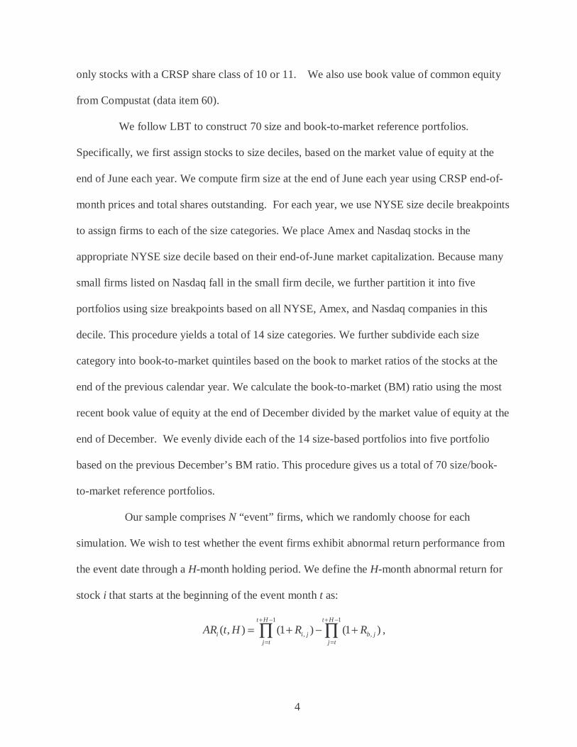
Our sample comprises N “event” firms, which we randomly choose for each

simulation. We wish to test whether the event firms exhibit abnormal return performance from

the event date through a H-month holding period. We define the H-month abnormal return for

stock i that starts at the beginning of the event month t as:

1 1

, ,( , ) (1 ) (1 )t H t H

i i j b jj t j t

AR t H R R+ − + −

= =

= + − +∏ ∏ ,

5

where Ri,t is the return for stock i in month t, and Rb,t is the return in month t for the firm’s

benchmark b. We consider three long-run performance horizons: one year, three years, and

five years. Therefore, in our simulation experiments, H equals 12, 36, or 60.

We use two types of benchmarks for each test statistic. The first benchmark is a buy-

and-hold size/BM-matched portfolio. Specifically, the size/BM portfolio that includes the

event firm on the event date serves as the benchmark. The second benchmark is a size/BM

matched individual control firm. We identify all firms with an equity market capitalization

between 70 percent and 130 percent of the event firm at the most recent end of June. From this

set of firms, we select the one with BM closest to the event firm in the previous December. If

a matching firm is delisted sometime during the H-month period, the next closest firm by BM

on the event date replaces the delisted firm. If the event firm is delisted prior to the conclusion

of the H-month period, we compute the abnormal return only during the time period when the

event firm has valid stock returns.

A. Conventional t-statistic

To test the null hypothesis that the average abnormal return for these N event firms

equals zero, the conventional t-statistic is

sample ( ),

standard error

AR Ht =

where sample

1

1( ) ( , )

N

ii

AR H AR t HN =

= ∑ and

2

sample

1

1( , ) ( )

N-1standard error =

N

ii

AR t H AR H

N=

− ∑. (1)

6

B. Test statistics based on monthly cohort average abnormal returns

Let Nt equal the number of stocks in the sample in month t, and let N be the total number of

stocks in the sample. Therefore,

∑=

=T

ttNN

1,

where T is the number of months in the sample.

Define the average abnormal return for each event month t across all stocks in the

sample that month (we refer to this group of firms as a monthly cohort) as

1

1( , ) if >0

( , )

0 , otherwise,

tN

i tit

AR t H NAR t H N =

=

∑

Let ( )AR H be a Tx1 column vector where the tth element equals ( , )AR t H . ( )AR H is the

average long-run abnormal return of each monthly cohort. For example, if there were three

stocks in the sample month t=10, then ( 10, 36)AR t H= = would be the average 36-month

abnormal return starting in month t=10 for these three event firms. If a month does not contain

any event, the abnormal return for that month is set equal to zero.

Define w as a Tx1 column vector of weights where the tth element is the ratio of the

number of events that occur in month t divided by N. Specifically,

( ) .tNw t

N=

Note that the sample average abnormal return is equal to the monthly weight vector

w times the average abnormal return of each monthly cohort

sample ( ) ' ( ).AR H w AR H=

7

The variance of sample ( )AR H is given by

samplevariance ( ) ' ,AR H w Vw =

where V is the TxT variance-covariance matrix of ( )AR H . Because holding periods overlap

for monthly cohorts that are closer than H months apart, we allow the first through H-1th serial

covariance of cohort returns to be non-zero, and we set all higher order serial covariances equal

to zero.

We consider two estimators for the variance-covariance matrix V. The first estimator

is the Hansen and Hodrick (1980) estimator. This estimator allows for serial correlation of

monthly returns, but assumes homoskedasticity. This estimator is denoted as SC_V, and the

ijth element of SC_V is

22

by month

1

0

, ,1,0

0

1( , ) ( ) , if

1sc_v ( , )* ( , ) , if 1 1 and 5

0 ,

t

t

t j

T

tNN

T

i j j N jtN j

N

N

AR t H AR H i jT

AR t H AR t j H i j H TT

σ

ρ

+

=>

=>>

= − =

= = + ≤ − ≤ − ≥

∑

∑

otherwise,

(2)

where TN,,j is the number of times where month t and month t+j both have at least one event

(i.e., Nt>0 and Nt+j>0). 2σ is the variance of monthly cohort H-period abnormal returns

including only months with at least one event. jρ is the estimator of jth -order serial

covariance. To reduce estimation error for this autocovariance, we require at least five cases

8

where month t and month t+j both have at least one event.3 If TN,,j <5, the covariance is set to

zero.

The autocorrelation consistent t-statistic that we propose is

sample ( )_ .

' _

AR HSC t

w SC Vw=

The second estimator for V that we consider allows for heteroskedasticity as well as

serial correlation and is denoted as HSC_V. Allowing for heteroskedasticity is important for at

least two reasons. First, stock return volatility varies over time. In addition, the number of

event firms each month and the types of stocks, particularly the industry composition of these

firms, typically varies substantially across sample months. For example, the hot-issue

phenomenon in the IPO market results in some time periods having a large number of new

issues while other periods experience very few firms going public. These factors may cause

the volatility of monthly cohort abnormal returns to change over time.

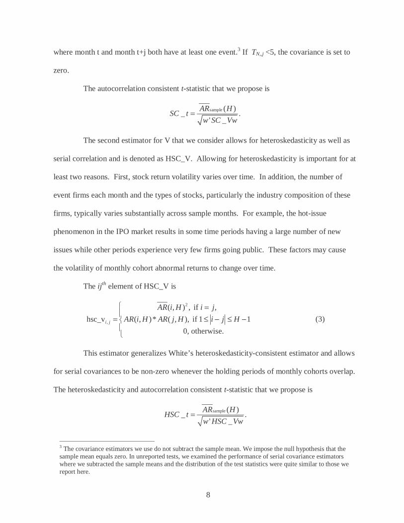
The ijth element of HSC_V is

2

,

( , ) , if ,

hsc_v ( , )* ( , ), if 1 1

0, otherwise. i j

AR i H i j

AR i H AR j H i j H

=

= ≤ − ≤ −

(3)

This estimator generalizes White’s heteroskedasticity-consistent estimator and allows

for serial covariances to be non-zero whenever the holding periods of monthly cohorts overlap.

The heteroskedasticity and autocorrelation consistent t-statistic that we propose is

sample ( )_ .

' _

AR HHSC t

w HSC Vw=

3 The covariance estimators we use do not subtract the sample mean. We impose the null hypothesis that the sample mean equals zero. In unreported tests, we examined the performance of serial covariance estimators where we subtracted the sample means and the distribution of the test statistics were quite similar to those we report here.

9

Our proposed test statistics follow a t-distribution in large samples. However, we do

not know the distribution of the test statistic in small samples. Therefore, in later sections, we

use bootstrap experiments to examine the small sample properties of our test statistics.

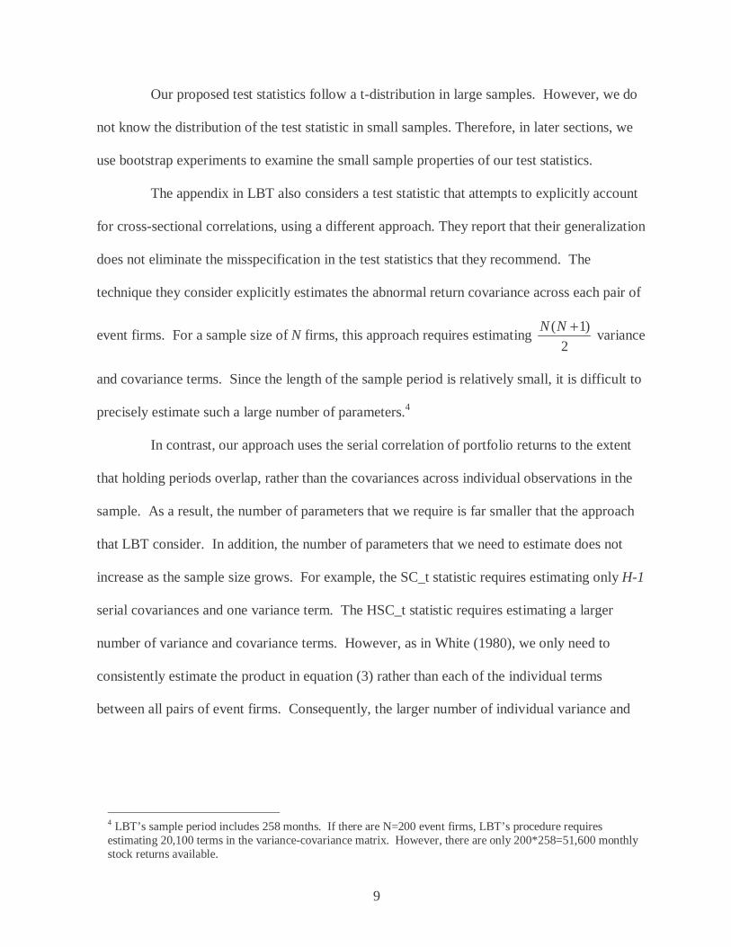
The appendix in LBT also considers a test statistic that attempts to explicitly account

for cross-sectional correlations, using a different approach. They report that their generalization

does not eliminate the misspecification in the test statistics that they recommend. The

technique they consider explicitly estimates the abnormal return covariance across each pair of

event firms. For a sample size of N firms, this approach requires estimating ( 1)

2

N N + variance

and covariance terms. Since the length of the sample period is relatively small, it is difficult to

precisely estimate such a large number of parameters.4

In contrast, our approach uses the serial correlation of portfolio returns to the extent

that holding periods overlap, rather than the covariances across individual observations in the

sample. As a result, the number of parameters that we require is far smaller that the approach

that LBT consider. In addition, the number of parameters that we need to estimate does not

increase as the sample size grows. For example, the SC_t statistic requires estimating only H-1

serial covariances and one variance term. The HSC_t statistic requires estimating a larger

number of variance and covariance terms. However, as in White (1980), we only need to

consistently estimate the product in equation (3) rather than each of the individual terms

between all pairs of event firms. Consequently, the larger number of individual variance and

4 LBT’s sample period includes 258 months. If there are N=200 event firms, LBT’s procedure requires estimating 20,100 terms in the variance-covariance matrix. However, there are only 200*258=51,600 monthly stock returns available.

10

covariance parameters that we need to estimate in HSC_V does not necessarily add to its

estimation error.5

Although the procedure that we illustrate here weights each monthly cohort

proportional to the number of stocks in the cohort, our approach can be adapted to any

weighting scheme that the empiricist chooses to use. The proportional weighting scheme that

we use is common in the literature (for example, see Loughran and Ritter (2000)). However,

Fama (1998) recommends a calendar time approach where each month is given equal weight,

regardless of the number of observations in each month. If the empiricist chooses to weight

each month equally, then the weight for each monthly cohort should be set equal to one over

the number of months in the sample period. Our results are not sensitive to the particular

weights assigned to each monthly cohort.

C. Critical values with pseudoportfolios

In addition to the t-statistics, we also examine the empirical distribution of long-run

abnormal returns under the null hypothesis for each of the test statistics that we study in this

paper. For each event firm in our sample with event month t, we randomly select with

replacement a firm that is in the same size/BM portfolio (one of the 70 portfolios) in that

month. We then estimate the long-run abnormal return test statistic based on the appropriate

methodology, and this yields one value of the test statistic.

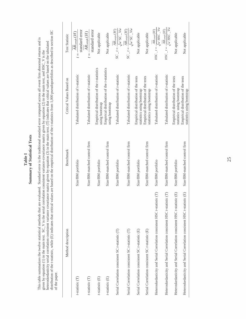
Table I summarizes the twelve statistical methods that we evaluate in this paper. The

first two methods use the conventional t-statistic, first with size/BM portfolio benchmarks and

then with size/BM individual firm benchmarks. The next two methods use the same

5 In fact, we cannot rely on the consistency of the estimate of any of the individual terms in the variance-covariance matrix in equation (3) because we use only one observation to compute each term. See White (1980) for a further discussion of this point in the context of his heteroskedasticity consistent standard error estimator.

https://www.researchgate.net/publication/4978464_Uniformly_Least_Powerful_Tests_of_Market?el=1_x_8&enrichId=rgreq-ed641e3c38113faeedb1de212919a67a-XXX&enrichSource=Y292ZXJQYWdlOzIzNzc1Njk3O0FTOjEwMzI0OTM5NDc5ODU5NUAxNDAxNjI3OTgyMjEx

11

conventional t-statistic and benchmarks, but utilize the critical values from the distribution of

the test statistics across the pseudoportfolios. We refer to these critical values as empirical

critical values.

LBT use the first three methods listed in Table I, and we present them here for direct

comparison. The next four methods use the autocorrelation-consistent test statistics that we

propose. The first two use the SC_t statistic with size/BM portfolio benchmarks and with

control firm benchmarks. The latter two methods use the same two benchmarks and the

empirical p values from pseudoportfolios. The last four statistical approaches are identical,

except they utilize the heteroskedasticity serial correlation consistent HSC_t statistic instead

the SC_t statistic.

D. Bootstrap experiment

To test the specification of the new test statistics that we propose, we conduct 1,000

simulations of N event firms. We first consider cases where both firm identity and event

month are randomly chosen. Later we allow for two types of nonrandomness in the sample. In

one case we constrain the firms to be clustered within industries. In the second nonrandom

case, we include the same firm in the sample on multiple occasions within an H-month holding

period. In our random sample and in our industry-clustered sample, we do not allow multiple

occurrences of the same firm within the H-month holding period. Therefore, both of these

samples do not include overlapping returns for the same event firms.

When testing a hypothesis at the α significance level, a well-specified test should

reject the null 1,000α times. The test is conservative (under-rejects) if the null is rejected

fewer than 1000α times, and the test over-rejects if the null is rejected more than 1000α times.

12

We examine the specification of each of our test statistics at the 1 percent, 5 percent, and 10

percent levels. In addition, we check the performance of each test methodology with nine

experiments using three event sample sizes (200 firms, 500 firms, and 1,000 firms) and three

long-run holding period horizons (1 year, 3 years, and 5 years).

III. Random Sample Results

A. Critical values

Before explicitly examining the sizes of our test statistics, we first consider the

critical values of the distribution of the t-statistics in random samples. We run 1,000

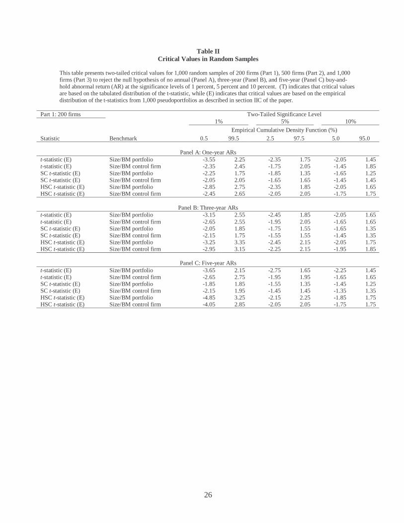
simulations and generate the tests statistics for each run. Table II reports the two-tailed critical

values for these 1,000 t-statistics using random samples. In large samples, the two-tail critical

values for the test statistics at the 1 percent, 5 percent, and 10 percent level would be 2.33,

1.96, and 1.65. However, we do not know the small sample distribution. The critical values in

Table II could be used to gauge the divergence of the small sample distribution from the large

sample limits. The critical values we tabulate here would also be useful to researchers who

wish to run the SC_t or HSC_t tests but who do not want to generate pseudoportfolios and the

corresponding empirical critical values.

The first pattern that is evident from Table II is that the left tail critical values for the

conventional t-statistic with benchmark portfolios are larger in absolute value than the right tail

critical values. For this test methodology, for a three-year holding period and 200 event firms,

Panel B of Part 1 gives the 5 percent two-tailed critical values of –2.45 and 1.85. This result

indicates that when benchmark portfolios are used, the resulting t-statistic is positively skewed,

because of the skewness of the abnormal return distribution.

13

The five percent critical values for the SC_t-statistic with 200 event firms (see Panel

B of Part 1) are –1.75 and 1.55. These values are smaller in absolute value than 1.96,

indicating that the sizes of the SC_t tests are smaller than the tabulated values. Consequently,

the SC_t test tends to under-reject when tabulated critical values are used. Out of these three

tests, the HSC t-statistic usually has the most extreme critical values. This indicates that the

sizes of the HSC_t tests are higher than they should be, if we were to use the tabulated

distribution of the test statistic. For example, for the HSC_t-statistic with benchmark

portfolios, a five-year holding period and 1,000 event firms, Panel C of Part 3 of Table II

reports 5 percent two-tailed critical values of –2.65 and 2.45. These are higher than the

standard 1.96 critical value.

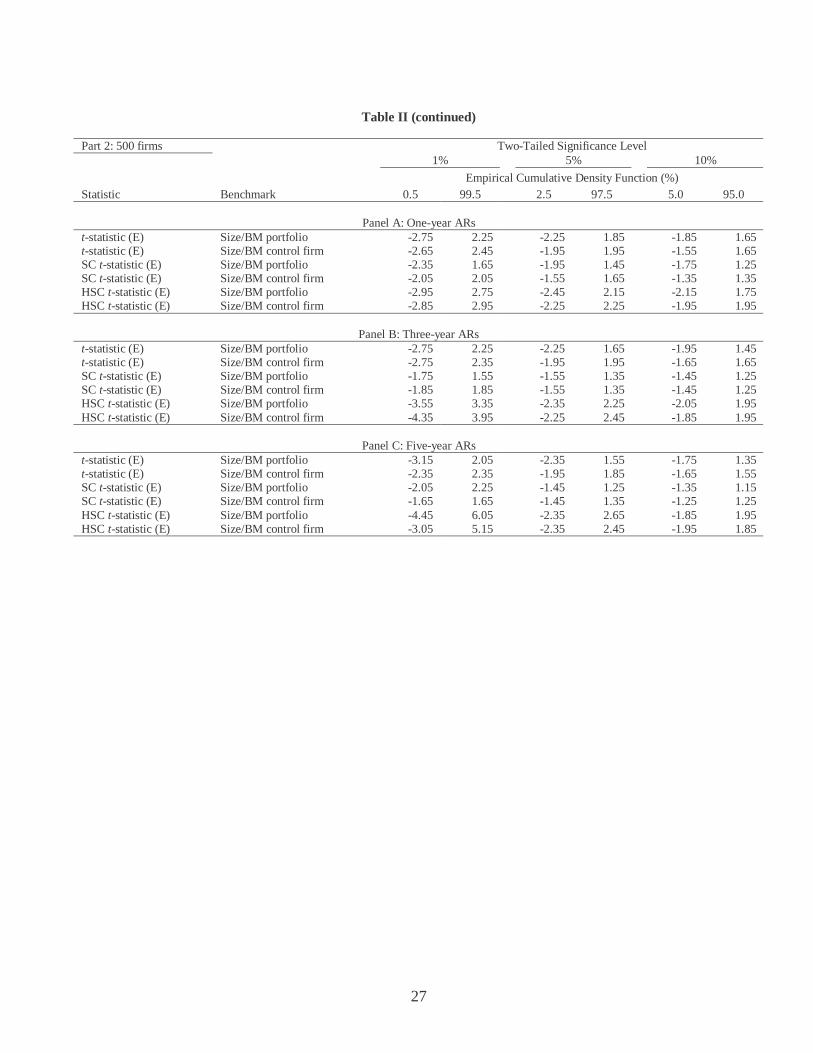
The distributions of the SC_t statistic and the HSC_t statistic present an interesting

contrast. The SC_t statistic has a tighter distribution than the standard normal distribution,

while the HSC_t statistic has a wider distribution. This difference is due to the fact that the

variance estimate under the SC procedure is on average larger than the variance estimate under

the HSC procedure. To understand the difference intuitively, note that the SC procedure

assigns equal weights to all observations to first get the sample estimate of variances and

covariances. Therefore, this procedure does not explicitly account for the fact that the monthly

cohorts with fewer event firms would have larger variances than the monthly cohorts with

larger numbers of event firms.

However, under the HSC procedure, the weight for each monthly cohort is inversely

proportional to square of the number of firms in each monthly cohort. Therefore, the return

variances of the smaller cohorts would have less of an effect on the estimate of the sample

14

mean standard error than the variances of larger cohorts. As a result, the variance estimate

under the HSC procedure is on average large than that under the SC procedure.

B. Specification tests in random samples

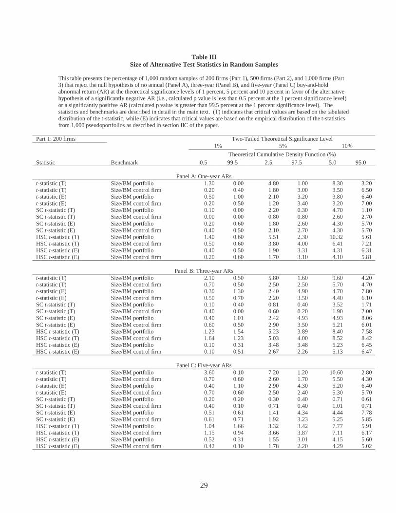
Table III presents the specification of our twelve statistical procedures. The results of

our first three statistical methods are fairly close to those reported in Table III of LBT. For

example, in Part 1 of Table III we report that the size of the conventional t-statistic with

benchmark portfolios and 200 event firms is 4.8 percent and 1.0 percent for a one-year holding

period, 5.8 percent and 1.6 percent for a three-year period, and 7.2 percent and 1.2 percent for a

five-year period. LBT find corresponding sizes of 4.9 percent and 0.9 percent for a one-year

period, 6.8 percent and 0.6 percent for a three-year period, and 6.1 percent and 0.5 percent for a

five-year period.

The first four test methodologies based on conventional t-statistics perform

reasonably well in random samples. There is some evidence of positive skewness in the first

two procedures. Of course, the empirical distribution reflects the skewness and hence the sizes

of the tests are fairly close to the theoretical significance level.

The rejection rates of the two SC_t tests using the tabulated t-distribution are

significantly lower than the theoretical significance levels.6 With 200 event firms and a five-

year holding period for the SC_t-statistic using benchmark firms, Panel C of Part 1 of Table III

reports rejection rates using a 5 percent significance level of 0.71 percent and 0.40 percent.

Low rejection rates are found for all three holding periods and all three event firm sizes.

However, when we use the empirical critical values for the SC_t-statistics, the tests appear

6 Our SC_t and HSC_t estimators do not guarantee positive definiteness of the variance-covariance matrix in small samples. In our experiments, the quadratic product of w and the sample variance-covariance matrix was negative in two to four percent of the simulation runs. We discarded these simulations.

15

reasonably well specified. For the same case as before but with empirical critical values, the

rejection rates are 1.92 percent and 3.23 percent, which add up very close to 5 percent.

In contrast to the first two SC_t tests, the first two HSC_t tests have significantly

higher sizes compared to theoretical significance levels. For 200 event firms, a five-year

holding period, and using the HSC_t-statistic with benchmark portfolios, Panel C of Part 1

gives rejection rates of 3.32 percent and 3.42 percent. Once again however, the HSC_t tests

appear reasonably well specified when we use the empirical critical values. In the same case as

before but using empirical p values, the rejection rates are 1.55 percent and 3.01 percent.

Overall, the specifications of the SC_t-statistic and HSC_t-statistic with empirical

critical value methodologies appear at least as good as LBT’s recommended procedures (the

bootstrapped version of a skewness-adjusted t-statistic and the empirical p value using

benchmark portfolios) in random samples.

C. Specification tests in nonrandom samples

C.1. Industry clustering

It should not be surprising that the distributions of the test statistics correspond to the

distribution in a random sample, as long as the event firms are selected at random. Under this

scenario, we calibrate the distribution of the test statistic in a random sample and examine the

test size using empirical cutoffs, also in a random sample. However, the test size becomes an

issue when we consider a more realistic scenario where the event firms come from a

nonrandom sample but the empirical distribution is calibrated using a random sample. For

instance, LBT find that the distribution of the test statistics that they recommend is severely

misspecified when the event firms are clustered within industries. This section examines the

16

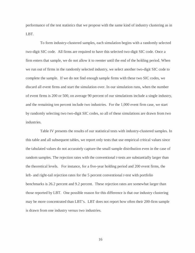
performance of the test statistics that we propose with the same kind of industry clustering as in

LBT.

To form industry-clustered samples, each simulation begins with a randomly selected

two-digit SIC code. All firms are required to have this selected two-digit SIC code. Once a

firm enters that sample, we do not allow it to reenter until the end of the holding period. When

we run out of firms in the randomly selected industry, we select another two-digit SIC code to

complete the sample. If we do not find enough sample firms with these two SIC codes, we

discard all event firms and start the simulation over. In our simulation runs, when the number

of event firms is 200 or 500, on average 90 percent of our simulations include a single industry,

and the remaining ten percent include two industries. For the 1,000 event firm case, we start

by randomly selecting two two-digit SIC codes, so all of these simulations are drawn from two

industries.

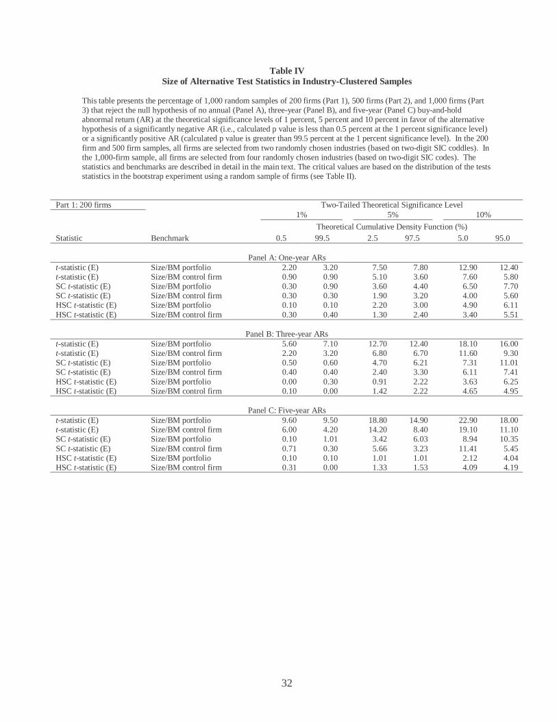
Table IV presents the results of our statistical tests with industry-clustered samples. In

this table and all subsequent tables, we report only tests that use empirical critical values since

the tabulated values do not accurately capture the small sample distribution even in the case of

random samples. The rejection rates with the conventional t-tests are substantially larger than

the theoretical levels. For instance, for a five-year holding period and 200 event firms, the

left- and right-tail rejection rates for the 5 percent conventional t-test with portfolio

benchmarks is 26.2 percent and 9.2 percent. These rejection rates are somewhat larger than

those reported by LBT. One possible reason for this difference is that our industry clustering

may be more concentrated than LBT’s. LBT does not report how often their 200-firm sample

is drawn from one industry versus two industries.

17

The level of misspecification generally increases as the holding period and the

number of event firms increase. This is illustrated by the rise in conventional t-test rejection

rates when going from the 200 event firm experiment (Part 1 of Table IV) to the 500 event firm

experiment (Part 2). For the 1000-firm experiment (Part 3), rejection rates are lower because

this sample is less industry concentrated than the 200-firm and 500-firm samples.

The rejections rates with the SC_t-statistics are far less than the rejection rates with

the conventional t-statistics, although the rates are greater than the theoretical levels. For

example, at the five percent significance level, Panel C of Part 1 of Table IV reports that the

SC_t test with control portfolios has rejection rates of 3.42 and 6.03 percent. The

specifications of these tests are also substantially better than the bootstrapped skewness

adjusted t-statistic that LBT recommend, which has rejection rates of 10.5 percent and 15.9

percent at the 5 percent significance level in the 200-firm, five-year holding period

experiment.7

The HSC_t tests tend to under-reject with empirical critical values. For example, the

rejection rates at the five percent significance level are 1.33 percent and 1.53 percent for the

200 firm sample and five-year holding period. The HSC_t test would be a conservative test for

the industry controlled sample while the other tests tend to reject in excess of the theoretical

levels.

Overall, the results here indicate that the actual sizes of both the SC_t test and the

HSC_t are closer to the theoretical levels than the conventional t-test. If one would prefer to

err on the conservative side, one should choose the HSC-t test.

Intuitively, the reason why the empirical critical values for the conventional t-

statistics are misspecified in industry clustered samples is because they do not account for the 7 See Table VII of LBT for rejection rates of all their tests in industry-clustered samples.

18

fact that the standard deviations are larger in these samples than in random samples. For

example, the empirical critical value methodology uses the critical value calibrated using

random samples, where the abnormal returns have a tighter distribution than in industry

clustered samples.

Our approach, on the other hand, is relatively robust because we allow for correlation

across observations. Therefore, the standard error reflects the properties of the sample and it

would be larger if a sample is concentrated in any particular industry, or if it is tilted towards

any unobservable common factors. As a result, the distributions of the test statistics we propose

are similar in random samples and nonrandom samples.

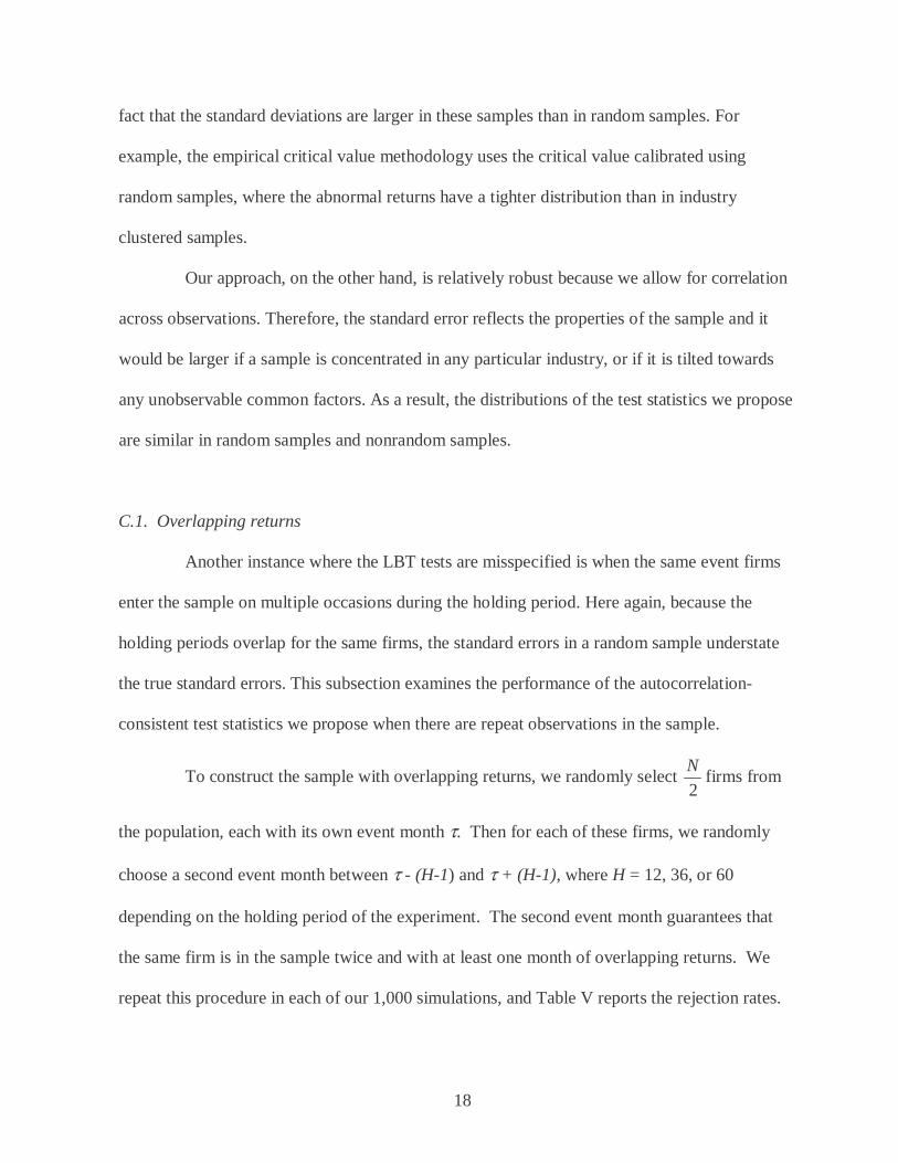
C.1. Overlapping returns

Another instance where the LBT tests are misspecified is when the same event firms

enter the sample on multiple occasions during the holding period. Here again, because the

holding periods overlap for the same firms, the standard errors in a random sample understate

the true standard errors. This subsection examines the performance of the autocorrelation-

consistent test statistics we propose when there are repeat observations in the sample.

To construct the sample with overlapping returns, we randomly select 2

Nfirms from

the population, each with its own event month τ. Then for each of these firms, we randomly

choose a second event month between τ - (H-1) and τ + (H-1), where H = 12, 36, or 60

depending on the holding period of the experiment. The second event month guarantees that

the same firm is in the sample twice and with at least one month of overlapping returns. We

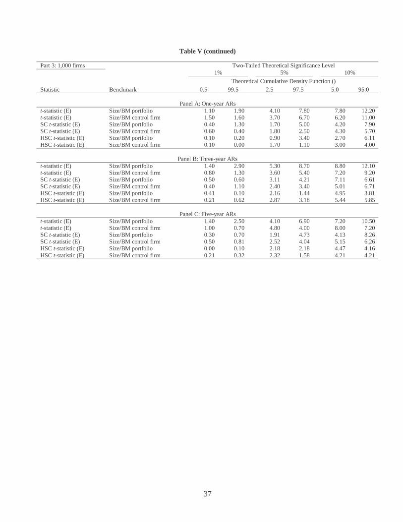
repeat this procedure in each of our 1,000 simulations, and Table V reports the rejection rates.

19

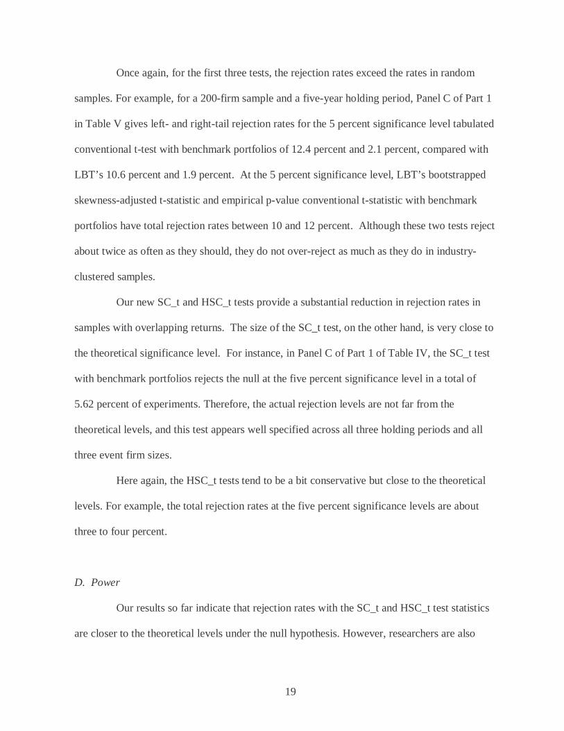
Once again, for the first three tests, the rejection rates exceed the rates in random

samples. For example, for a 200-firm sample and a five-year holding period, Panel C of Part 1

in Table V gives left- and right-tail rejection rates for the 5 percent significance level tabulated

conventional t-test with benchmark portfolios of 12.4 percent and 2.1 percent, compared with

LBT’s 10.6 percent and 1.9 percent. At the 5 percent significance level, LBT’s bootstrapped

skewness-adjusted t-statistic and empirical p-value conventional t-statistic with benchmark

portfolios have total rejection rates between 10 and 12 percent. Although these two tests reject

about twice as often as they should, they do not over-reject as much as they do in industry-

clustered samples.

Our new SC_t and HSC_t tests provide a substantial reduction in rejection rates in

samples with overlapping returns. The size of the SC_t test, on the other hand, is very close to

the theoretical significance level. For instance, in Panel C of Part 1 of Table IV, the SC_t test

with benchmark portfolios rejects the null at the five percent significance level in a total of

5.62 percent of experiments. Therefore, the actual rejection levels are not far from the

theoretical levels, and this test appears well specified across all three holding periods and all

three event firm sizes.

Here again, the HSC_t tests tend to be a bit conservative but close to the theoretical

levels. For example, the total rejection rates at the five percent significance levels are about

three to four percent.

D. Power

Our results so far indicate that rejection rates with the SC_t and HSC_t test statistics

are closer to the theoretical levels under the null hypothesis. However, researchers are also

20

interested in the power of the tests because even well specified tests would lose their appeal if

they are unable to detect violations of the null hypothesis. This subsection evaluates the power

of various tests. We confine our power analysis to the random sample case since we know that

the t-tests are misspecified in nonrandom samples.

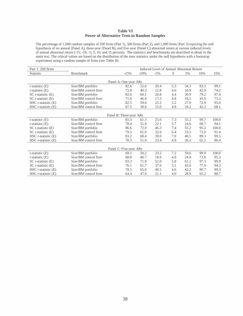
To evaluate power, we add a constant level of abnormal return to each of the event

firms in our random samples for all 1,000 simulations. Table VI reports the rejection rates at

the five percent theoretical significance level for three event firm sizes (200, 500, and 1,000

firms) and three holding periods (1, 3, and 5 years). The null hypothesis is that the mean

sample long-run abnormal return is zero across all 1,000 simulations, and the added level of

annual abnormal returns ranges from –15 percent to 15 percent in increments of 5 percent. The

power of all twelve tests generally increases as the number of firms and as the length of the

holding period increases.

When fixed amounts of abnormal returns are added to random samples, the rejection

rates of the conventional t-tests are generally close to those reported in LBT. With 200 event

firms and a one-year holding period, the conventional t-test with benchmark firms and

tabulated critical values has percentage rejection rates of 74.1, 42.0, 14.4, 4.8, 14.6, 39.5, and

71.5 (see Panel A of Part 1 of Table VI). By comparison, Figure 1 in LBT shows percentage

rejection rates for the same test that as approximately 72, 39, 16, 5, 14, 43, and 73.

The power of the SC_t and HSC_t tests is comparable to the power of the

conventional t-tests. For example, with 200 event firms, a five-year holding period, and an

induced level of annual abnormal return of –5 percent, Panel C of Part 1 of Table VI reports

that the rejection rates for the conventional t-tests ranges from 18.9 percent to 39.3 percent.

21

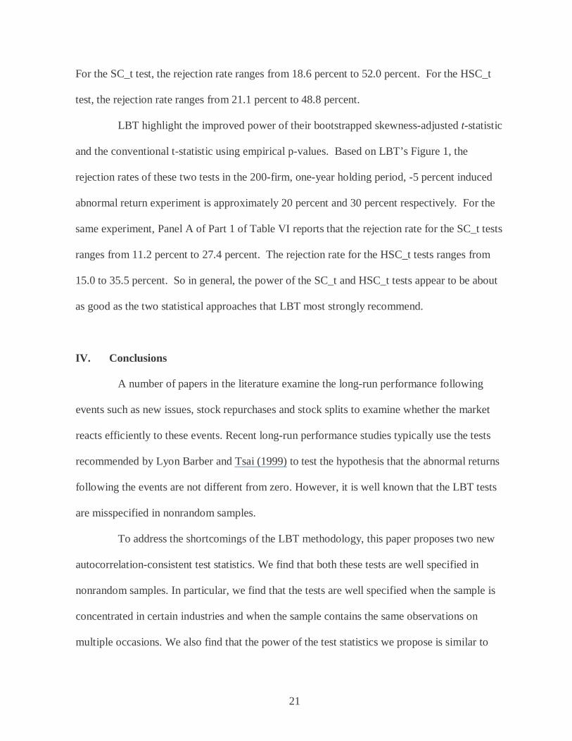
For the SC_t test, the rejection rate ranges from 18.6 percent to 52.0 percent. For the HSC_t

test, the rejection rate ranges from 21.1 percent to 48.8 percent.

LBT highlight the improved power of their bootstrapped skewness-adjusted t-statistic

and the conventional t-statistic using empirical p-values. Based on LBT’s Figure 1, the

rejection rates of these two tests in the 200-firm, one-year holding period, -5 percent induced

abnormal return experiment is approximately 20 percent and 30 percent respectively. For the

same experiment, Panel A of Part 1 of Table VI reports that the rejection rate for the SC_t tests

ranges from 11.2 percent to 27.4 percent. The rejection rate for the HSC_t tests ranges from

15.0 to 35.5 percent. So in general, the power of the SC_t and HSC_t tests appear to be about

as good as the two statistical approaches that LBT most strongly recommend.

IV. Conclusions

A number of papers in the literature examine the long-run performance following

events such as new issues, stock repurchases and stock splits to examine whether the market

reacts efficiently to these events. Recent long-run performance studies typically use the tests

recommended by Lyon Barber and Tsai (1999) to test the hypothesis that the abnormal returns

following the events are not different from zero. However, it is well known that the LBT tests

are misspecified in nonrandom samples.

To address the shortcomings of the LBT methodology, this paper proposes two new

autocorrelation-consistent test statistics. We find that both these tests are well specified in

nonrandom samples. In particular, we find that the tests are well specified when the sample is

concentrated in certain industries and when the sample contains the same observations on

multiple occasions. We also find that the power of the test statistics we propose is similar to

https://www.researchgate.net/publication/4992489_Improved_Methods_for_Tests_of_Long-Run_Abnormal_Stock_Returns?el=1_x_8&enrichId=rgreq-ed641e3c38113faeedb1de212919a67a-XXX&enrichSource=Y292ZXJQYWdlOzIzNzc1Njk3O0FTOjEwMzI0OTM5NDc5ODU5NUAxNDAxNjI3OTgyMjEx

22

that of the LBT tests. Therefore, in future work, we recommend our proposed SC_t and HSC_t

test methodologies when assessing long-run performance.

23

References

Barber, Brad M., and John D. Lyon, 1997, Detecting long-run abnormal stock returns: The

empirical power and specification of test statistics, Journal of Financial Economics 43, 341-372.

Boehme, Rodney D., and Sorin M. Sorescu, 2002, The long-run performance following

dividend initiations and resumptions: Underreaction or product of chance?, Journal of Finance 57, 871-900.

Brav, Alon, 2000, Inference in long-horizon event studies: A Bayesian approach with

application to initial public offerings, Journal of Finance 55, 1979-2016. Byun, Jinho, and Michael S. Rozeff, 2003, Long-run performance after stock splits: 1927 to

1996, Journal of Finance 58, 1063-1085. Eberhart, Allan C., and Akhtar Siddique, 2002, The long-term performance of corporate bonds

(and stocks) following seasoned equity offers, Review of Financial Studies 15, 1385-1406. Fama, Eugene F., 1998, Market efficiency, long-term returns, and behavioral finance, Journal

of Financial Economics 49, 285-306. Gompers, Paul A., and Josh Lerner, 2003, The really long-run performance of initial public

offerings: The pre-Nasdaq evidence, Journal of Finance 58, 1355-1392. Hansen, Lars Peter, and Robert J. Hodrick, 1980, Forward exchange rates as optimal predictors

of future spot rates: An econometric analysis, Journal of Political Economy 88, 829-853. Ikenberry, David, Josef Lakonishok, and Theo Vermaelen, 1995, Market underreaction to open

market share repurchases, Journal of Financial Economics 39, 181-208.

Kothari, S. P., and Jerold B. Warner, 1997, Measuring long-horizon security price performance, Journal of Financial Economics 43, 301-339.

Loughran, Tim, and Anand M. Vijh, 1997, Do long-term shareholders benefit from capital

acquisitions?, Journal of Finance 52, 1765-1790. Loughran, Tim, and Jay R. Ritter, 1995, The new issues puzzle, Journal of Finance 50, 23-51. Loughran, Tim, and Jay R. Ritter, 2000, Uniformly least powerful tests of market efficiency,

Journal of Financial Economics 55, 361-389. Lyon, John D., Brad M. Barber, and Chih-Ling Tsai, 1999, Improved methods for tests of

long-run abnormal stock returns, Journal of Finance 54, 165-201.

https://www.researchgate.net/publication/222460048_Detecting_Long-Run_Abnormal_Stock_Returns_The_Empirical_Power_and_Specification_of_Test_Statistics?el=1_x_8&enrichId=rgreq-ed641e3c38113faeedb1de212919a67a-XXX&enrichSource=Y292ZXJQYWdlOzIzNzc1Njk3O0FTOjEwMzI0OTM5NDc5ODU5NUAxNDAxNjI3OTgyMjEx



https://www.researchgate.net/publication/4992603_The_Long-Run_Performance_Following_Dividend_Initiations_and_Resumptions_Underreaction_or_Product_of_Chance?el=1_x_8&enrichId=rgreq-ed641e3c38113faeedb1de212919a67a-XXX&enrichSource=Y292ZXJQYWdlOzIzNzc1Njk3O0FTOjEwMzI0OTM5NDc5ODU5NUAxNDAxNjI3OTgyMjEx



https://www.researchgate.net/publication/4913290_The_Really_Long-Run_Performance_of_Initial_Public_Offerings_The_Pre-Nasdaq_Evidence?el=1_x_8&enrichId=rgreq-ed641e3c38113faeedb1de212919a67a-XXX&enrichSource=Y292ZXJQYWdlOzIzNzc1Njk3O0FTOjEwMzI0OTM5NDc5ODU5NUAxNDAxNjI3OTgyMjEx

https://www.researchgate.net/publication/4913290_The_Really_Long-Run_Performance_of_Initial_Public_Offerings_The_Pre-Nasdaq_Evidence?el=1_x_8&enrichId=rgreq-ed641e3c38113faeedb1de212919a67a-XXX&enrichSource=Y292ZXJQYWdlOzIzNzc1Njk3O0FTOjEwMzI0OTM5NDc5ODU5NUAxNDAxNjI3OTgyMjEx



https://www.researchgate.net/publication/4768479_The_New_Issues_Puzzle?el=1_x_8&enrichId=rgreq-ed641e3c38113faeedb1de212919a67a-XXX&enrichSource=Y292ZXJQYWdlOzIzNzc1Njk3O0FTOjEwMzI0OTM5NDc5ODU5NUAxNDAxNjI3OTgyMjEx

https://www.researchgate.net/publication/2312474_Inference_in_Long-Horizon_Event_Studies_A_Bayesian_Approach_with_Application_to_Initial_Public_Offerings?el=1_x_8&enrichId=rgreq-ed641e3c38113faeedb1de212919a67a-XXX&enrichSource=Y292ZXJQYWdlOzIzNzc1Njk3O0FTOjEwMzI0OTM5NDc5ODU5NUAxNDAxNjI3OTgyMjEx

https://www.researchgate.net/publication/2312474_Inference_in_Long-Horizon_Event_Studies_A_Bayesian_Approach_with_Application_to_Initial_Public_Offerings?el=1_x_8&enrichId=rgreq-ed641e3c38113faeedb1de212919a67a-XXX&enrichSource=Y292ZXJQYWdlOzIzNzc1Njk3O0FTOjEwMzI0OTM5NDc5ODU5NUAxNDAxNjI3OTgyMjEx



https://www.researchgate.net/publication/4992641_Long-Run_Performance_After_Stock_Splits_1927_to_1996?el=1_x_8&enrichId=rgreq-ed641e3c38113faeedb1de212919a67a-XXX&enrichSource=Y292ZXJQYWdlOzIzNzc1Njk3O0FTOjEwMzI0OTM5NDc5ODU5NUAxNDAxNjI3OTgyMjEx

https://www.researchgate.net/publication/4992641_Long-Run_Performance_After_Stock_Splits_1927_to_1996?el=1_x_8&enrichId=rgreq-ed641e3c38113faeedb1de212919a67a-XXX&enrichSource=Y292ZXJQYWdlOzIzNzc1Njk3O0FTOjEwMzI0OTM5NDc5ODU5NUAxNDAxNjI3OTgyMjEx

https://www.researchgate.net/publication/5216934_The_Long-Term_Performance_of_Corporate_Bonds_and_Stocks_Following_Seasoned_Equity_Offerings?el=1_x_8&enrichId=rgreq-ed641e3c38113faeedb1de212919a67a-XXX&enrichSource=Y292ZXJQYWdlOzIzNzc1Njk3O0FTOjEwMzI0OTM5NDc5ODU5NUAxNDAxNjI3OTgyMjEx

https://www.researchgate.net/publication/5216934_The_Long-Term_Performance_of_Corporate_Bonds_and_Stocks_Following_Seasoned_Equity_Offerings?el=1_x_8&enrichId=rgreq-ed641e3c38113faeedb1de212919a67a-XXX&enrichSource=Y292ZXJQYWdlOzIzNzc1Njk3O0FTOjEwMzI0OTM5NDc5ODU5NUAxNDAxNjI3OTgyMjEx



https://www.researchgate.net/publication/4978297_Measuring_Long-Horizon_Security_Price_Performance?el=1_x_8&enrichId=rgreq-ed641e3c38113faeedb1de212919a67a-XXX&enrichSource=Y292ZXJQYWdlOzIzNzc1Njk3O0FTOjEwMzI0OTM5NDc5ODU5NUAxNDAxNjI3OTgyMjEx

https://www.researchgate.net/publication/4978297_Measuring_Long-Horizon_Security_Price_Performance?el=1_x_8&enrichId=rgreq-ed641e3c38113faeedb1de212919a67a-XXX&enrichSource=Y292ZXJQYWdlOzIzNzc1Njk3O0FTOjEwMzI0OTM5NDc5ODU5NUAxNDAxNjI3OTgyMjEx

https://www.researchgate.net/publication/4992443_Do_Long-Term_Shareholders_Benefit_From_Corporate_Acquisitions?el=1_x_8&enrichId=rgreq-ed641e3c38113faeedb1de212919a67a-XXX&enrichSource=Y292ZXJQYWdlOzIzNzc1Njk3O0FTOjEwMzI0OTM5NDc5ODU5NUAxNDAxNjI3OTgyMjEx

https://www.researchgate.net/publication/4992443_Do_Long-Term_Shareholders_Benefit_From_Corporate_Acquisitions?el=1_x_8&enrichId=rgreq-ed641e3c38113faeedb1de212919a67a-XXX&enrichSource=Y292ZXJQYWdlOzIzNzc1Njk3O0FTOjEwMzI0OTM5NDc5ODU5NUAxNDAxNjI3OTgyMjEx

https://www.researchgate.net/publication/256557208_Market_Underreaction_to_Open_Market_Share_Repurchases?el=1_x_8&enrichId=rgreq-ed641e3c38113faeedb1de212919a67a-XXX&enrichSource=Y292ZXJQYWdlOzIzNzc1Njk3O0FTOjEwMzI0OTM5NDc5ODU5NUAxNDAxNjI3OTgyMjEx

https://www.researchgate.net/publication/256557208_Market_Underreaction_to_Open_Market_Share_Repurchases?el=1_x_8&enrichId=rgreq-ed641e3c38113faeedb1de212919a67a-XXX&enrichSource=Y292ZXJQYWdlOzIzNzc1Njk3O0FTOjEwMzI0OTM5NDc5ODU5NUAxNDAxNjI3OTgyMjEx

https://www.researchgate.net/publication/262908692_Market_Efficiency_Long-Term_Returns_and_Behavioral_Finance?el=1_x_8&enrichId=rgreq-ed641e3c38113faeedb1de212919a67a-XXX&enrichSource=Y292ZXJQYWdlOzIzNzc1Njk3O0FTOjEwMzI0OTM5NDc5ODU5NUAxNDAxNjI3OTgyMjEx

https://www.researchgate.net/publication/262908692_Market_Efficiency_Long-Term_Returns_and_Behavioral_Finance?el=1_x_8&enrichId=rgreq-ed641e3c38113faeedb1de212919a67a-XXX&enrichSource=Y292ZXJQYWdlOzIzNzc1Njk3O0FTOjEwMzI0OTM5NDc5ODU5NUAxNDAxNjI3OTgyMjEx

24

Michaely, Roni, Richard H. Thaler, and Kent L. Womack, 1995, Price reactions to dividend initiations and omissions: Overreaction or drift?, Journal of Finance 50, 573-608.

Mitchell, Mark L., and Erik Stafford, 2000, Managerial decisions and long-term stock price

performance, Journal of Business 73, 287-329. Ritter, Jay R., 1991, The long-run performance of initial public offerings, Journal of Finance

46, 3-28. Spiess, D. Katherine, and John Affleck-Graves, 1995, Underperformance in long-run stock

returns following seasoned equity offerings, Journal of Financial Economics 38, 243-267. White, Halbert, 1980, A heteroskedasticity-consistent covariance matrix estimator and a direct

test for heteroskedasticity, Econometrica 48, 817-838.

25

Tab

le I

Su

mm

ary

of S

tati

stic

al T

ests

Thi

s ta

ble

sum

mar

izes

the

twel

ve s

tatis

tical

met

hods

that

are

eva

luat

ed.

Stan

dard

err

or is

the

trad

ition

al s

tand

ard

erro

r co

mpu

ted

acro

ss a

ll ev

ent f

irm

abn

orm

al r

etur

ns a

nd is

gi

ven

by e

quat

ion

(1)

in th

e m

ain

text

. SC

_V is

the

seri

al c

orre

lati

on c

onsi

sten

t var

ianc

e-co

vari

ance

mat

rix

give

n by

equ

atio

n (2

) in

the

mai

n te

xt, a

nd H

SC_V

is th

e he

tero

sked

astic

ity

seri

al c

orre

lati

on c

onsi

sten

t var

ianc

e co

vari

ance

mat

rix

give

n by

equ

atio

n (3

) in

the

mai

n te

xt. (

T)

indi

cate

s th

at c

ritic

al v

alue

s ar

e ba

sed

on th

e ta

bula

ted

dist

ribu

tion

of th

e t-

stat

isti

c, w

hile

(E

) in

dica

tes

that

cri

tica

l val

ues

are

base

d on

the

empi

rica

l dis

trib

utio

n of

the

t-st

atis

tics

fro

m 1

,000

pse

udop

ortf

olio

s as

des

crib

ed in

sec

tion

IIC

of

the

pape

r.

Met

hod

desc

ript

ion

Ben

chm

ark

Cri

tica

l Val

ues

Bas

ed o

n T

est S

tatis

tic

t-st

atis

tic

(T)

Size

/BM

por

tfol

io

Tab

ulat

ed d

istr

ibut

ion

of t-

stat

istic

sa

mpl

e(

)

stan

dard

err

or

AR

Ht

=

t-st

atis

tic

(T)

Size

/BM

-mat

ched

con

trol

fir

m

Tab

ulat

ed d

istr

ibut

ion

of t-

stat

istic

sa

mpl

e(

)

stan

dard

err

or

AR

Ht

=

t-st

atis

tic

(E)

Size

/BM

por

tfol

io

Em

piri

cal d

istr

ibut

ion

of th

e t-

stat

istic

s us

ing

boot

stra

p N

ot a

ppli

cabl

e

t-st

atis

tic

(E)

Size

/BM

-mat

ched

con

trol

fir

m

Em

piri

cal d

istr

ibut

ion

of th

e t-

stat

istic

s us

ing

boot

stra

p N

ot a

ppli

cabl

e

Seri

al C

orre

latio

n co

nsis

tent

SC

t-st

atis

tic (

T)

Size

/BM

por

tfol

io

Tab

ulat

ed d

istr

ibut

ion

of t-

stat

istic

sa

mpl

e(

)_

'_

AR

HSC

tw

SCV

w=

Seri

al C

orre

latio

n co

nsis

tent

SC

t-st

atis

tic (

T)

Size

/BM

-mat

ched

con

trol

fir

m

Tab

ulat

ed d

istr

ibut

ion

of t-

stat

istic

sa

mpl

e(

)_

'_

AR

HSC

tw

SCV

w=

Seri

al C

orre

latio

n co

nsis

tent

SC

t-st

atis

tic (

E)

Size

/BM

por

tfol

io

Em

piri

cal d

istr

ibut

ion

of th

e te

sts

stat

isti

cs u

sing

boo

tstr

ap

Not

app

lica

ble

Seri

al C

orre

latio

n co

nsis

tent

SC

t-st

atis

tic (

E)

Size

/BM

-mat

ched

con

trol

fir

m

Em

piri

cal d

istr

ibut

ion

of th

e te

sts

stat

isti

cs u

sing

boo

tstr

ap

Not

app

lica

ble

Het

eros

keda

stic

ity a

nd S

eria

l Cor

rela

tion

cons

iste

nt H

SC t-

stat

istic

(T

) Si

ze/B

M p

ortf

olio

T

abul

ated

dis

trib

utio

n of

t-st

atis

tic

sam

ple(

)_

'_

AR

HH

SCt

wH

SCV

w=

Het

eros

keda

stic

ity a

nd S

eria

l Cor

rela

tion

cons

iste

nt H

SC t-

stat

istic

(T

) Si

ze/B

M-m

atch

ed c

ontr

ol f

irm

T

abul

ated

dis

trib

utio

n of

t-st

atis

tic

sam

ple(

)_

'_

AR

HH

SCt

wH

SCV

w=

Het

eros

keda

stic

ity a

nd S

eria

l Cor

rela

tion

cons

iste

nt H

SC t-

stat

istic

(E

) Si

ze/B

M p

ortf

olio

E

mpi

rica

l dis

trib

utio

n of

the

test

s st

atis

tics

usi

ng b

oots

trap

N

ot a

ppli

cabl

e

Het

eros

keda

stic

ity a

nd S

eria

l Cor

rela

tion

cons

iste

nt H

SC t-

stat

istic

(E

) Si

ze/B

M-m

atch

ed c

ontr

ol f

irm

E

mpi

rica

l dis

trib

utio

n of

the

test

s st

atis

tics

usi

ng b

oots

trap

N

ot a

ppli

cabl

e

26

Table II Critical Values in Random Samples

This table presents two-tailed critical values for 1,000 random samples of 200 firms (Part 1), 500 firms (Part 2), and 1,000 firms (Part 3) to reject the null hypothesis of no annual (Panel A), three-year (Panel B), and five-year (Panel C) buy-and-hold abnormal return (AR) at the significance levels of 1 percent, 5 percent and 10 percent. (T) indicates that critical values are based on the tabulated distribution of the t-statistic, while (E) indicates that critical values are based on the empirical distribution of the t-statistics from 1,000 pseudoportfolios as described in section IIC of the paper.

Part 1: 200 firms Two-Tailed Significance Level 1% 5% 10%

Empirical Cumulative Density Function (%) Statistic Benchmark 0.5 99.5 2.5 97.5 5.0 95.0

Panel A: One-year ARs

t-statistic (E) Size/BM portfolio -3.55 2.25 -2.35 1.75 -2.05 1.45 t-statistic (E) Size/BM control firm -2.35 2.45 -1.75 2.05 -1.45 1.85 SC t-statistic (E) Size/BM portfolio -2.25 1.75 -1.85 1.35 -1.65 1.25 SC t-statistic (E) Size/BM control firm -2.05 2.05 -1.65 1.65 -1.45 1.45 HSC t-statistic (E) Size/BM portfolio -2.85 2.75 -2.35 1.85 -2.05 1.65 HSC t-statistic (E) Size/BM control firm -2.45 2.65 -2.05 2.05 -1.75 1.75

Panel B: Three-year ARs t-statistic (E) Size/BM portfolio -3.15 2.55 -2.45 1.85 -2.05 1.65 t-statistic (E) Size/BM control firm -2.65 2.55 -1.95 2.05 -1.65 1.65 SC t-statistic (E) Size/BM portfolio -2.05 1.85 -1.75 1.55 -1.65 1.35 SC t-statistic (E) Size/BM control firm -2.15 1.75 -1.55 1.55 -1.45 1.35 HSC t-statistic (E) Size/BM portfolio -3.25 3.35 -2.45 2.15 -2.05 1.75 HSC t-statistic (E) Size/BM control firm -2.95 3.15 -2.25 2.15 -1.95 1.85

Panel C: Five-year ARs t-statistic (E) Size/BM portfolio -3.65 2.15 -2.75 1.65 -2.25 1.45 t-statistic (E) Size/BM control firm -2.65 2.75 -1.95 1.95 -1.65 1.65 SC t-statistic (E) Size/BM portfolio -1.85 1.85 -1.55 1.35 -1.45 1.25 SC t-statistic (E) Size/BM control firm -2.15 1.95 -1.45 1.45 -1.35 1.35 HSC t-statistic (E) Size/BM portfolio -4.85 3.25 -2.15 2.25 -1.85 1.75 HSC t-statistic (E) Size/BM control firm -4.05 2.85 -2.05 2.05 -1.75 1.75

27

Table II (continued)

Part 2: 500 firms Two-Tailed Significance Level 1% 5% 10%

Empirical Cumulative Density Function (%) Statistic Benchmark 0.5 99.5 2.5 97.5 5.0 95.0





28

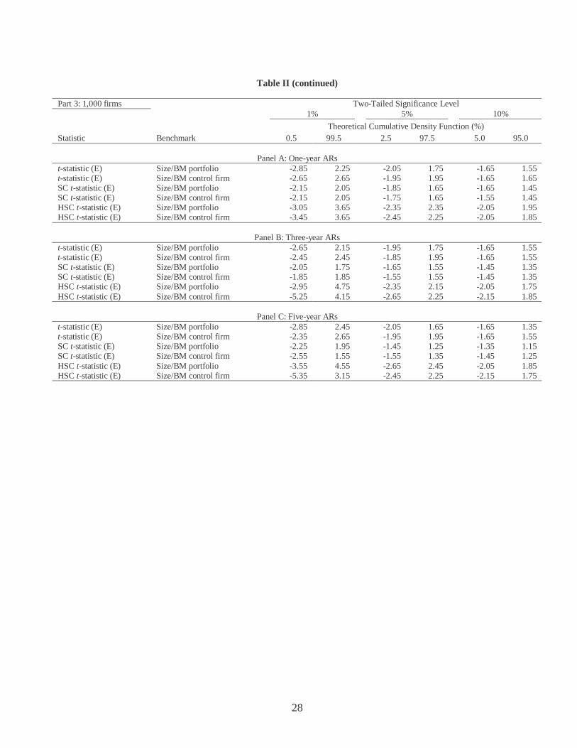
Table II (continued)

Part 3: 1,000 firms Two-Tailed Significance Level 1% 5% 10%

Theoretical Cumulative Density Function (%) Statistic Benchmark 0.5 99.5 2.5 97.5 5.0 95.0





29

Table III

Size of Alternative Test Statistics in Random Samples

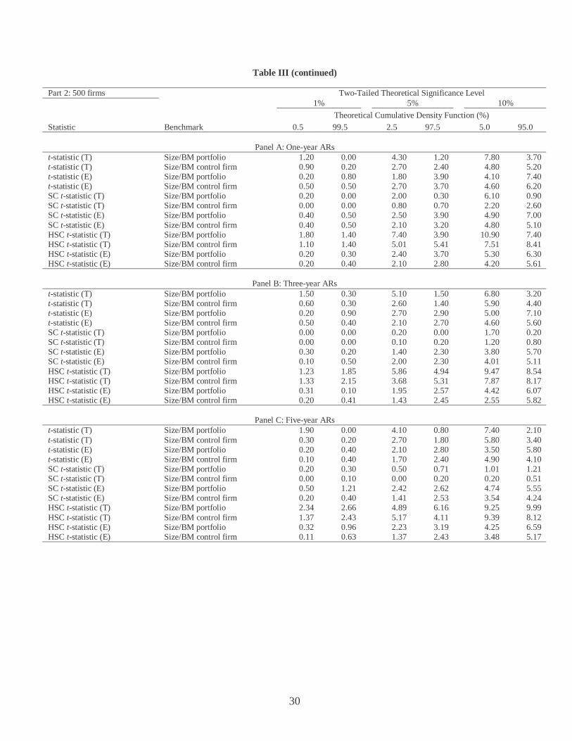
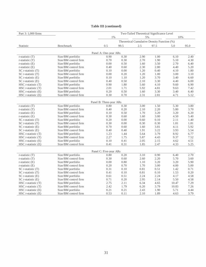
This table presents the percentage of 1,000 random samples of 200 firms (Part 1), 500 firms (Part 2), and 1,000 firms (Part 3) that reject the null hypothesis of no annual (Panel A), three-year (Panel B), and five-year (Panel C) buy-and-hold abnormal return (AR) at the theoretical significance levels of 1 percent, 5 percent and 10 percent in favor of the alternative hypothesis of a significantly negative AR (i.e., calculated p value is less than 0.5 percent at the 1 percent significance level) or a significantly positive AR (calculated p value is greater than 99.5 percent at the 1 percent significance level). The statistics and benchmarks are described in detail in the main text. (T) indicates that critical values are based on the tabulated distribution of the t-statistic, while (E) indicates that critical values are based on the empirical distribution of the t-statistics from 1,000 pseudoportfolios as described in section IIC of the paper.

Part 1: 200 firms Two-Tailed Theoretical Significance Level 1% 5% 10%



t-statistic (T) Size/BM portfolio 1.30 0.00 4.80 1.00 8.30 3.20 t-statistic (T) Size/BM control firm 0.20 0.40 1.80 3.00 3.50 6.50 t-statistic (E) Size/BM portfolio 0.50 1.00 2.10 3.20 3.80 6.40 t-statistic (E) Size/BM control firm 0.20 0.50 1.20 3.40 3.20 7.00 SC t-statistic (T) Size/BM portfolio 0.10 0.00 2.20 0.30 4.70 1.10 SC t-statistic (T) Size/BM control firm 0.00 0.00 0.80 0.80 2.60 2.70 SC t-statistic (E) Size/BM portfolio 0.20 0.60 1.80 2.60 4.30 5.70 SC t-statistic (E) Size/BM control firm 0.40 0.50 2.10 2.70 4.30 5.70 HSC t-statistic (T) Size/BM portfolio 1.40 0.60 5.51 2.30 10.32 5.61 HSC t-statistic (T) Size/BM control firm 0.50 0.60 3.80 4.00 6.41 7.21 HSC t-statistic (E) Size/BM portfolio 0.40 0.50 1.90 3.31 4.31 6.31 HSC t-statistic (E) Size/BM control firm 0.20 0.60 1.70 3.10 4.10 5.81

Panel B: Three-year ARs t-statistic (T) Size/BM portfolio 2.10 0.50 5.80 1.60 9.60 4.20 t-statistic (T) Size/BM control firm 0.70 0.50 2.50 2.50 5.70 4.70 t-statistic (E) Size/BM portfolio 0.30 1.30 2.40 4.90 4.70 7.80 t-statistic (E) Size/BM control firm 0.50 0.70 2.20 3.50 4.40 6.10 SC t-statistic (T) Size/BM portfolio 0.10 0.40 0.81 0.40 3.52 1.71 SC t-statistic (T) Size/BM control firm 0.40 0.00 0.60 0.20 1.90 2.00 SC t-statistic (E) Size/BM portfolio 0.40 1.01 2.42 4.93 4.93 8.06 SC t-statistic (E) Size/BM control firm 0.60 0.50 2.90 3.50 5.21 6.01 HSC t-statistic (T) Size/BM portfolio 1.23 1.54 5.23 3.89 8.40 7.58 HSC t-statistic (T) Size/BM control firm 1.64 1.23 5.03 4.00 8.52 8.42 HSC t-statistic (E) Size/BM portfolio 0.10 0.31 3.48 3.48 5.23 6.45 HSC t-statistic (E) Size/BM control firm 0.10 0.51 2.67 2.26 5.13 6.47

Panel C: Five-year ARs t-statistic (T) Size/BM portfolio 3.60 0.10 7.20 1.20 10.60 2.80 t-statistic (T) Size/BM control firm 0.70 0.60 2.60 1.70 5.50 4.30 t-statistic (E) Size/BM portfolio 0.40 1.10 2.90 4.30 5.20 6.40 t-statistic (E) Size/BM control firm 0.70 0.60 2.50 2.40 5.30 5.70 SC t-statistic (T) Size/BM portfolio 0.20 0.20 0.30 0.40 0.71 0.61 SC t-statistic (T) Size/BM control firm 0.40 0.10 0.71 0.40 1.01 0.71 SC t-statistic (E) Size/BM portfolio 0.51 0.61 1.41 4.34 4.44 7.78 SC t-statistic (E) Size/BM control firm 0.61 0.71 1.92 3.23 5.25 5.85 HSC t-statistic (T) Size/BM portfolio 1.04 1.66 3.32 3.42 7.77 5.91 HSC t-statistic (T) Size/BM control firm 1.15 0.94 3.66 3.87 7.11 6.17 HSC t-statistic (E) Size/BM portfolio 0.52 0.31 1.55 3.01 4.15 5.60 HSC t-statistic (E) Size/BM control firm 0.42 0.10 1.78 2.20 4.29 5.02

30

Table III (continued)







31

Table III (continued)

Part 3: 1,000 firms Two-Tailed Theoretical Significance Level 1% 5% 10%






32

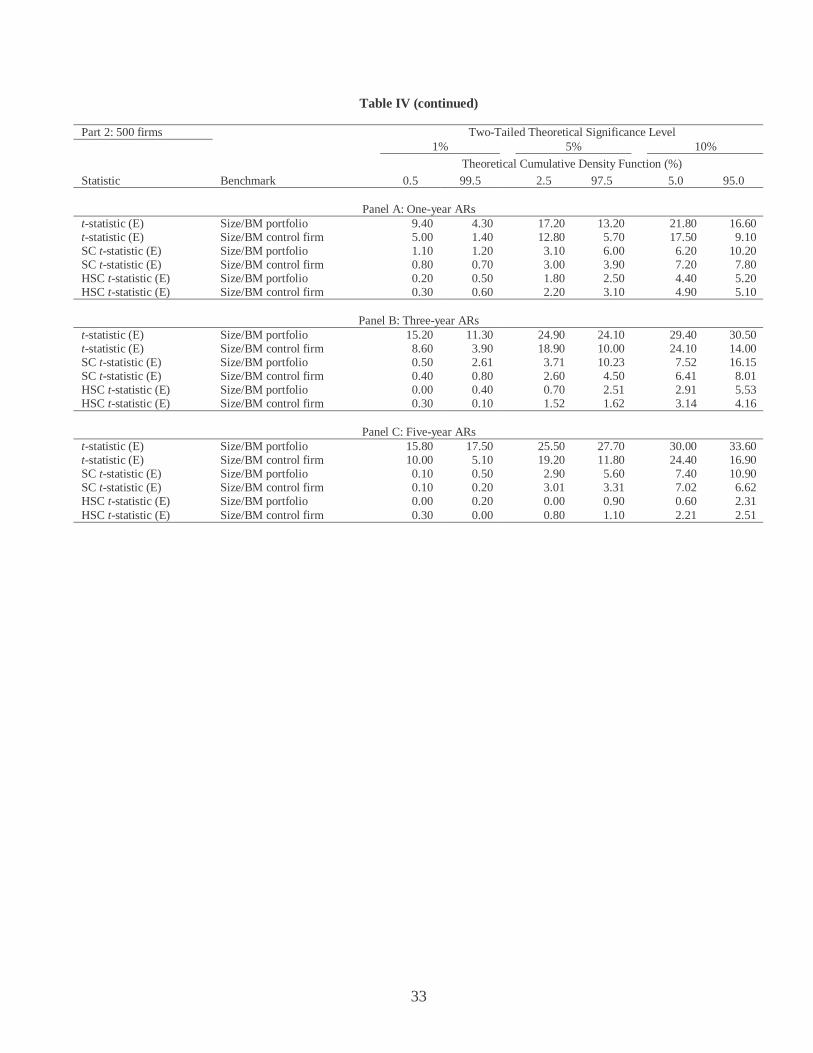
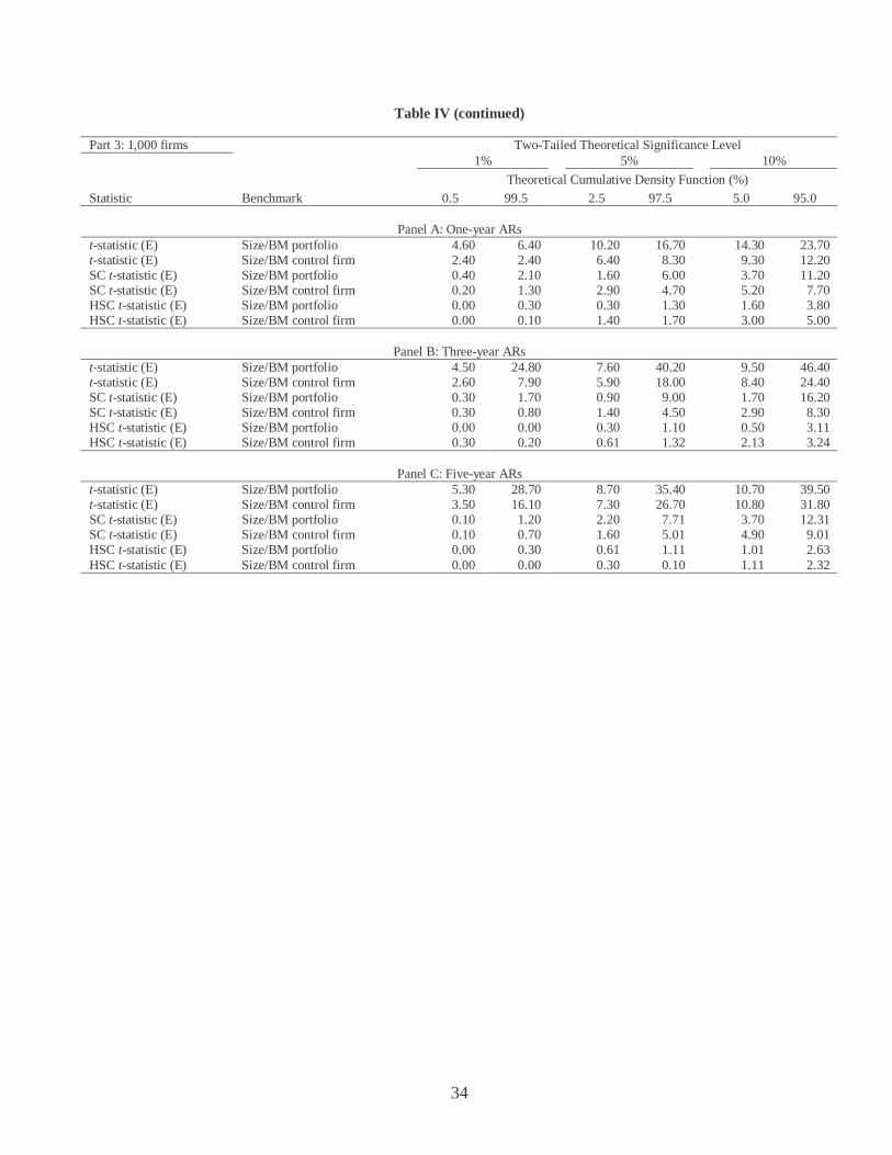
Table IV Size of Alternative Test Statistics in Industry-Clustered Samples

This table presents the percentage of 1,000 random samples of 200 firms (Part 1), 500 firms (Part 2), and 1,000 firms (Part 3) that reject the null hypothesis of no annual (Panel A), three-year (Panel B), and five-year (Panel C) buy-and-hold abnormal return (AR) at the theoretical significance levels of 1 percent, 5 percent and 10 percent in favor of the alternative hypothesis of a significantly negative AR (i.e., calculated p value is less than 0.5 percent at the 1 percent significance level) or a significantly positive AR (calculated p value is greater than 99.5 percent at the 1 percent significance level). In the 200 firm and 500 firm samples, all firms are selected from two randomly chosen industries (based on two-digit SIC coddles). In the 1,000-firm sample, all firms are selected from four randomly chosen industries (based on two-digit SIC codes). The statistics and benchmarks are described in detail in the main text. The critical values are based on the distribution of the tests statistics in the bootstrap experiment using a random sample of firms (see Table II).




t-statistic (E) Size/BM portfolio 2.20 3.20 7.50 7.80 12.90 12.40 t-statistic (E) Size/BM control firm 0.90 0.90 5.10 3.60 7.60 5.80 SC t-statistic (E) Size/BM portfolio 0.30 0.90 3.60 4.40 6.50 7.70 SC t-statistic (E) Size/BM control firm 0.30 0.30 1.90 3.20 4.00 5.60 HSC t-statistic (E) Size/BM portfolio 0.10 0.10 2.20 3.00 4.90 6.11 HSC t-statistic (E) Size/BM control firm 0.30 0.40 1.30 2.40 3.40 5.51

Panel B: Three-year ARs t-statistic (E) Size/BM portfolio 5.60 7.10 12.70 12.40 18.10 16.00 t-statistic (E) Size/BM control firm 2.20 3.20 6.80 6.70 11.60 9.30 SC t-statistic (E) Size/BM portfolio 0.50 0.60 4.70 6.21 7.31 11.01 SC t-statistic (E) Size/BM control firm 0.40 0.40 2.40 3.30 6.11 7.41 HSC t-statistic (E) Size/BM portfolio 0.00 0.30 0.91 2.22 3.63 6.25 HSC t-statistic (E) Size/BM control firm 0.10 0.00 1.42 2.22 4.65 4.95

Panel C: Five-year ARs t-statistic (E) Size/BM portfolio 9.60 9.50 18.80 14.90 22.90 18.00 t-statistic (E) Size/BM control firm 6.00 4.20 14.20 8.40 19.10 11.10 SC t-statistic (E) Size/BM portfolio 0.10 1.01 3.42 6.03 8.94 10.35 SC t-statistic (E) Size/BM control firm 0.71 0.30 5.66 3.23 11.41 5.45 HSC t-statistic (E) Size/BM portfolio 0.10 0.10 1.01 1.01 2.12 4.04 HSC t-statistic (E) Size/BM control firm 0.31 0.00 1.33 1.53 4.09 4.19

33

Table IV (continued)







34

Table IV (continued)







35

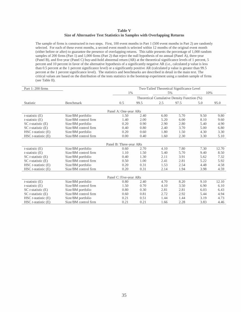
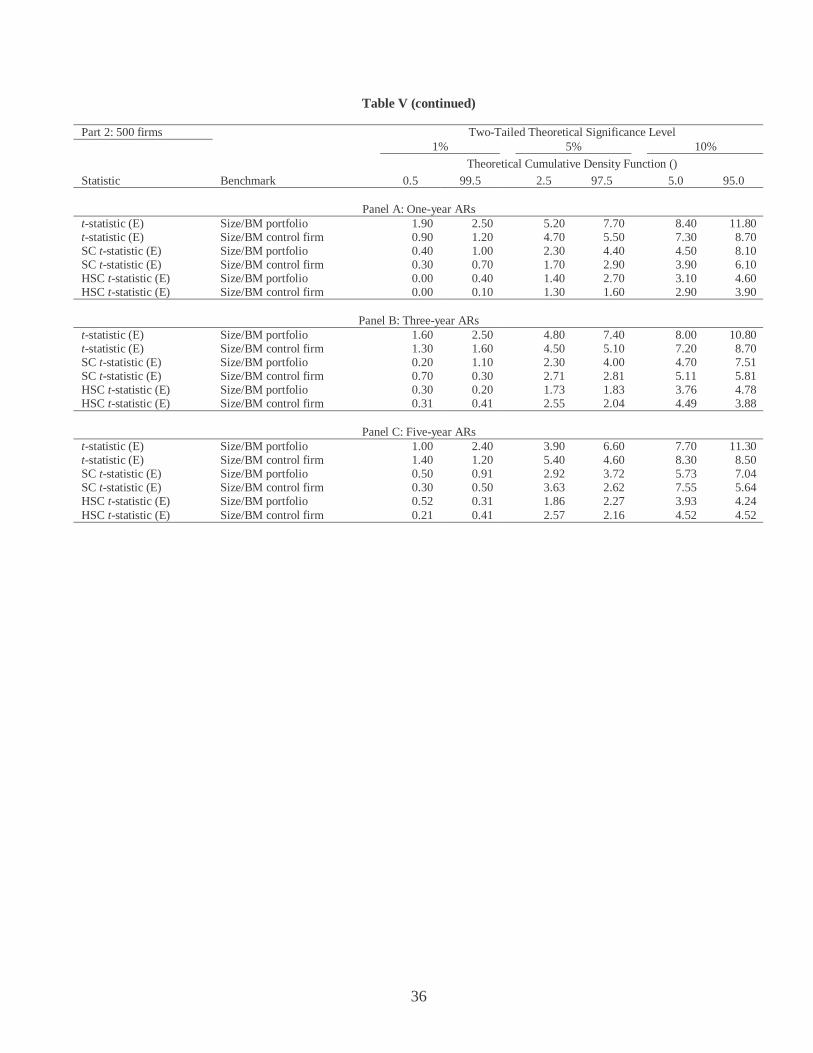
Table V Size of Alternative Test Statistics in Samples with Overlapping Returns

The sample of firms is constructed in two steps. First, 100 event months in Part 1 (500 event months in Part 2) are randomly selected. For each of these event months, a second event month is selected within 12 months of the original event month (either before or after) to guarantee the presence of overlapping returns. This table presents the percentage of 1,000 random samples of 200 firms (Part 1) and 1,000 firms (Part 2) that reject the null hypothesis of no annual (Panel A), three-year (Panel B), and five-year (Panel C) buy-and-hold abnormal return (AR) at the theoretical significance levels of 1 percent, 5 percent and 10 percent in favor of the alternative hypothesis of a significantly negative AR (i.e., calculated p value is less than 0.5 percent at the 1 percent significance level) or a significantly positive AR (calculated p value is greater than 99.5 percent at the 1 percent significance level). The statistics and benchmarks are described in detail in the main text. The critical values are based on the distribution of the tests statistics in the bootstrap experiment using a random sample of firms (see Table II).







36

Table V (continued)


Theoretical Cumulative Density Function () Statistic Benchmark 0.5 99.5 2.5 97.5 5.0 95.0





37

Table V (continued)


Theoretical Cumulative Density Function () Statistic Benchmark 0.5 99.5 2.5 97.5 5.0 95.0





38

Table VI Power of Alternative Tests in Random Samples

The percentage of 1,000 random samples of 200 firms (Part 1), 500 firms (Part 2), and 1,000 firms (Part 3) rejecting the null hypothesis of no annual (Panel A), three-year (Panel B), and five-year (Panel C) abnormal return at various induced levels of annual abnormal return (-15, -10, -5, 5, 10, and 15 percent). The statistics and benchmarks are described in detail in the main text. The critical values are based on the distribution of the tests statistics under the null hypothesis with a bootstrap experiment using a random sample of firms (see Table II).

Part 1: 200 firms Induced Level of Annual Abnormal Return Statistic Benchmark -15% -10% -5% 0 5% 10% 15%

Panel A: One-year ARs t-statistic (E) Size/BM portfolio 82.6 52.6 20.4 5.3 34.1 83.5 99.1 t-statistic (E) Size/BM control firm 72.8 40.3 12.8 4.6 16.9 42.9 74.2 SC t-statistic (E) Size/BM portfolio 82.6 60.1 26.8 4.4 30.9 79.2 97.4 SC t-statistic (E) Size/BM control firm 71.6 46.4 17.3 4.8 18.5 45.9 73.2 HSC t-statistic (E) Size/BM portfolio 82.5 59.6 25.2 5.2 27.0 72.9 95.0 HSC t-statistic (E) Size/BM control firm 67.5 39.6 15.0 4.8 16.2 42.2 68.1

Panel B: Three-year ARs t-statistic (E) Size/BM portfolio 81.3 61.3 25.6 7.3 55.2 99.7 100.0 t-statistic (E) Size/BM control firm 78.4 51.8 22.1 5.7 24.6 68.7 94.1 SC t-statistic (E) Size/BM portfolio 86.6 72.0 46.3 7.4 55.2 95.2 100.0 SC t-statistic (E) Size/BM control firm 79.5 61.0 32.6 6.4 33.5 72.0 91.4 HSC t-statistic (E) Size/BM portfolio 83.2 68.4 39.0 7.0 40.5 89.3 99.5 HSC t-statistic (E) Size/BM control firm 70.5 51.0 23.4 4.9 26.2 62.1 86.4

Panel C: Five-year ARs t-statistic (E) Size/BM portfolio 69.1 50.2 23.2 7.2 59.6 99.9 100.0 t-statistic (E) Size/BM control firm 68.8 46.7 18.9 4.9 24.9 73.6 95.3 SC t-statistic (E) Size/BM portfolio 83.3 71.8 52.0 5.8 61.1 97.3 99.9 SC t-statistic (E) Size/BM control firm 76.1 61.7 37.6 5.1 42.6 77.9 94.3 HSC t-statistic (E) Size/BM portfolio 78.5 65.6 40.5 4.6 42.2 90.7 99.3 HSC t-statistic (E) Size/BM control firm 64.4 47.9 21.1 4.0 28.9 65.2 88.7

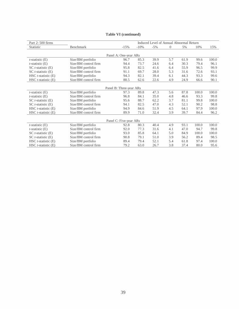
39

Table VI (continued)

Part 2: 500 firms Induced Level of Annual Abnormal Return Statistic Benchmark -15% -10% -5% 0 5% 10% 15%


Panel B: Three-year ARs t-statistic (E) Size/BM portfolio 97.3 89.8 47.3 5.6 87.8 100.0 100.0 t-statistic (E) Size/BM control firm 96.8 84.1 35.0 4.8 46.6 93.3 99.8 SC t-statistic (E) Size/BM portfolio 95.6 88.7 62.2 3.7 81.1 99.8 100.0 SC t-statistic (E) Size/BM control firm 94.1 82.5 47.0 4.3 52.1 90.2 98.8 HSC t-statistic (E) Size/BM portfolio 94.9 84.6 51.9 4.5 64.1 97.9 100.0 HSC t-statistic (E) Size/BM control firm 89.9 71.0 32.4 3.9 39.7 84.4 96.2


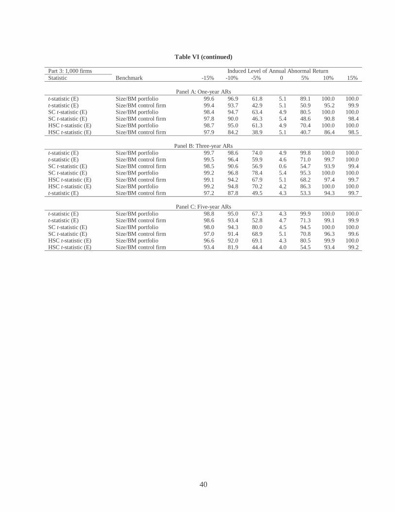
40

Table VI (continued)

Part 3: 1,000 firms Induced Level of Annual Abnormal Return Statistic Benchmark -15% -10% -5% 0 5% 10% 15%


Panel B: Three-year ARs t-statistic (E) Size/BM portfolio 99.7 98.6 74.0 4.9 99.8 100.0 100.0 t-statistic (E) Size/BM control firm 99.5 96.4 59.9 4.6 71.0 99.7 100.0 SC t-statistic (E) Size/BM control firm 98.5 90.6 56.9 0.6 54.7 93.9 99.4 SC t-statistic (E) Size/BM portfolio 99.2 96.8 78.4 5.4 95.3 100.0 100.0 HSC t-statistic (E) Size/BM control firm 99.1 94.2 67.9 5.1 68.2 97.4 99.7 HSC t-statistic (E) Size/BM portfolio 99.2 94.8 70.2 4.2 86.3 100.0 100.0 t-statistic (E) Size/BM control firm 97.2 87.8 49.5 4.3 53.3 94.3 99.7


Long-run performance evaluation: Correlation and heteroskedasticity-consistent tests

Documents

Transcript of Long-run performance evaluation: Correlation and heteroskedasticity-consistent tests