HAL Id: tel-01750538https://hal.univ-lorraine.fr/tel-01750538

Submitted on 29 Mar 2018

HAL is a multi-disciplinary open accessarchive for the deposit and dissemination of sci-entific research documents, whether they are pub-lished or not. The documents may come fromteaching and research institutions in France orabroad, or from public or private research centers.

L’archive ouverte pluridisciplinaire HAL, estdestinée au dépôt et à la diffusion de documentsscientifiques de niveau recherche, publiés ou non,émanant des établissements d’enseignement et derecherche français ou étrangers, des laboratoirespublics ou privés.

Self-consistent non-linear description of radio-frequencywave propagation and of the edge of a magnetized

plasmaJonathan Jacquot

To cite this version:Jonathan Jacquot. Self-consistent non-linear description of radio-frequency wave propagation and ofthe edge of a magnetized plasma. Other [cond-mat.other]. Université de Lorraine, 2013. English.NNT : 2013LORR0257. tel-01750538

AVERTISSEMENT

Ce document est le fruit d'un long travail approuvé par le jury de soutenance et mis à disposition de l'ensemble de la communauté universitaire élargie. Il est soumis à la propriété intellectuelle de l'auteur. Ceci implique une obligation de citation et de référencement lors de l’utilisation de ce document. D'autre part, toute contrefaçon, plagiat, reproduction illicite encourt une poursuite pénale. Contact : ddoc-theses-contact@univ-lorraine.fr

LIENS Code de la Propriété Intellectuelle. articles L 122. 4 Code de la Propriété Intellectuelle. articles L 335.2- L 335.10 http://www.cfcopies.com/V2/leg/leg_droi.php http://www.culture.gouv.fr/culture/infos-pratiques/droits/protection.htm

Collegium Sciences et Technologies École doctorale EMMA (n˚409)

THÈSE

pour l’obtention du titre de

Docteur de l’Université de Lorraine

Spécialité : Physique

présentée par :

Jonathan JACQUOT

Description non-linéaire auto-cohérentede la propagation d’ondes radiofréquenceset de la périphérie d’un plasma magnétisé

Thèse soutenue publiquement le 20 Novembre 2013 à Nancy devant le jury composé de:

Président du juryDr. Pascal Chabert Directeur de recherche,

Ecole Polytechnique, PalaiseauRapporteursDr. Steve Wukitch Directeur de Recherche,

MIT/PSFC (USA)Pr. Jean-Marie Noterdaeme Professeur des Universités,

Université de Gent (Belgique)ExaminateursDr. Kristel Crombe Chercheur,

Ecole Royale Militaire (Belgique)Dr. Xavier Litaudon Représentant CEA, HDR, Chef du service SCCP

IRFM, CadaracheDirecteur de thésePr. Stéphane Heuraux Professeur des Universités, Université de LorraineCo-directeur de théseDr. Laurent Colas Chercheur CEA, HDR, IRFM, CadaracheInvitésPr. Bruno Despres Professeur des Universités,

Université Paris VIDr. Patrick Joly Directeur de recherche,

INRIA, Palaiseau

Institut de Recherche sur la Fusion par confinement MagnétiqueCEA Cadarache 13108 Saint-Paul-lez-Durance, France

Université de Lorraine - Pôle M4: matière, matériaux, métallurgie, mécanique

“Une personne qui n’a jamais commis d’erreurs n’a jamais tenté d’innover.”“A person who never made a mistake never tried anything new.”

Albert Einstein, Theoretical Physicist (1879 - 1955).

Remerciements/Acknowledgments

Arrivé à la fin de cette thèse, il est de tradition de remercier les personnes, collègues, amisqui ont contribué à la réalisation de cette thèse par leur support, encouragement non seule-ment sur le plan scientifique mais aussi sur les plans humain, relationnel, psychologique.C’est avec une certaine émotion et fierté que j’écris cette dernière page de mon manuscrit(même si elle vient en premier) ainsi qu’avec une certaine nostalgie quand je pense au toutdébut de ma thèse en novembre 2010. Déjà 3 ans ont passé. Mais je sais que je continueraide travailler avec certains.

Tout d’abord, je tiens à sincèrement remercier Alain Bécoulet et Xavier Litaudon dem’avoir accueilli à l’IRFM malgré ma candidature tardive. Ils étaient à l’époque chef etchef-adjoint du SCCP. Merci aussi à Roland Magne, mon chef de groupe, le GCHF. Ils ontdepuis pris du galon. Les tâches et objectifs, qui m’avaient été confiées, ont été partiellementaccomplis. Pour le reste, beaucoup plus ardu, d’autres tâches sont apparues en cours deroute et une collaboration européenne (dont je fais partie dans le cadre de mon Post-Docà l’IPP Garching) se met en place. Je tiens également à remercier le SCCP de la confianceaccordée en proposant mon nom pour présenter au nom du service et de l’institut lesactivités autours des antennes ICRH lors de la conférence RF Topical 2013 à Sorrento.Ce papier invité englobait non seulement mon travail de modélisation mais également letravail en amont d’expérimentateurs. Cela m’a donné beaucoup de travail supplémentairequi ont été valorisé dans ma thèse, dans un papier en cours de publication. De nombreusesrépétitions ont aussi été nécessaires afin d’être prêt le jour J.

Je tiens aussi à remercier les secrétaires du SCCP, Valérie Icard, Stéphanie Villechavrollequi a été remplacée plus tard par Nathalie Borio. Leur aide en de multiples occasionspour les démarches administrative et autres soucis en tout genre a été très appréciée. Unexemple qui me vient à l’esprit est parmi les derniers. Il concerne l’organisation des moyensde transport du jury pour ma soutenance de thèse à Nancy.

A ce propos, je souhaiterais exprimer ma gratitude à mes deux rapporteurs, Jean-Marie Noterdaeme et Steve Wukitch. Je vous remercie de m’avoir fait l’honneur d’avoir toutd’abord accepté cette indispensable et lourde tâche que représente la lecture d’un manuscritde thèse et d’avoir ensuite évalué et jugé mon manuscrit de thèse. Merci pour l’intérêt quevous avez porté à ce manuscrit et pour le temps que vous y avez consacré. J’ai beaucoupapprécié vos commentaires. Je tiens aussi à remercier Jean-Marie de m’avoir accepté enPost-Doc dans son département à Garching afin de poursuivre mon travail dans la mêmethématique tout en me permettant de diversifier mes activités par une participation auxcampagnes expérimentales sur ASDEX-Upgrade. Cette dernière partie a été impossible àréaliser à Cadarache du fait d’éléments planifiés (travaux sur la ligne 400kV) et imprévus(incident sur le transformateur 400kV). I would like to thank Steve Wukitch for comingall the way from Boston to Nancy for my PhD defence and then to a visit in Cadarachethe next day. I hope the situation gets better at MIT for Alcator C-Mod and that you canstay in the field. I hope to see you at the next RF Topical Conference in the US.

i

ii REMERCIEMENTS/ACKNOWLEDGMENTS

Je voudrais également remercier les autres membres du jury. Je vais être amené àcollaborer de manière assez proche avec Kritel dans le cadre d’Ishtar à Garching dont elleest project leader. J’ai beaucoup apprécié la présence et les questions de nos collèguesmathématiciens, Bruno Després et Patrick Joly que j’ai perçu comme étant très intriguéspar la physique des plasmas et des gaines RF. J’espère qu’ils ont mieux compris la naturede nos problèmes et que cette collaboration sur les aspects d’implémentation des conditionsaux limites et de stabilité numérique et convergence pourra se réaliser dans un proche futur.Je tiens aussi à remercier Pascal Chabert d’avoir accepté l’invitation et de donner son avisd’expert en «plasma froids ». Je tiens également à le remercier d’avoir assumé au pied levéle rôle de président du jury qui aurait sinon été assumé par Xavier, selon mon opinion etd’après la composition du jury. Mais du fait des péripéties météorologiques (neige), l’aviondu Xavier n’a pas vu passer Lyon. Il a donc été contraint de rebrousser chemin. Il a quandmême pu assister à une rediffusion de ma soutenance lors de ma visite à Cadarache quelquessemaines plus tard.

Pour terminer le tour du jury, je tiens à exprimer ma plus grande gratitude et mesplus sincères remerciements à mon directeur de thèse, Stéphane Heuraux (ou $€ pourles intimes) et mon co-directeur de thèse Laurent Colas. Laurent m’a suivi au quotidien.Son bureau du 513 était juste à côté du mien. Il a maintenant déménagé au 508 pourrejoindre le reste du GCHF. Nous avons eu de très nombreux après-midi (et matinées) dediscussions sur la théorie, sur l’implémentation dans Comsol, sur la philosophie du code, surles résultats et leur interprétation physique. Son encadrement a été très réussi. Il a su fairepreuve d’une grande pédagogie afin de m’expliquer les choses que je ne comprenais pas.J’ai pu ensuite au fil de temps prendre plus d’initiatives. Je suis amené à continuer notrecollaboration (avec un éloignement géographique) durant mon Post-Doc. Les discussionstéléphoniques avec Stéphane ainsi que mes quelques visites (occasions de rentrer dans marégion natale) m’ont beaucoup aidé. Je le remercie beaucoup d’avoir fait l’interface avecl’Université de Lorraine et l’école doctorale du fait de l’éloignement géographique. Je leremercie aussi pour l’UE de physique stellaire en licence qui fut pour moi le cours le plusintéressant que j’ai suivi durant ma licence de physique aussi bien par le contenu que parl’évaluation par un travail personnel sur un sujet au choix. J’avais choisi l’évaluation dela datation du rayonnement cosmologique avec un modèle newtonien. Cela demandait desnotions de cosmologie, de thermodynamique, de mécanique quantique.

Je remercie également les Professeurs Michel Fabry et Gérard Bonhomme de m’avoirconvaincu de proposer ma candidature au master Erasmus Mundus Fusion EngineeringPhysics lors d’une porte ouverte. Je remercie de plus Gérard Bonhomme de s’être occupéde toutes les démarches administratives concernant les bourses Erasmus-Socrates puisque àl’époque les étudiants européens du master n’étaient pas financés par le master. De plus, lechoix définitif de Madrid pour le troisième semestre s’était fait après la limite de dépôt desdossiers. Nous avons malgré tout pu obtenir ces bourses. J’en profite également pour saluermes 3 autres comparses français et lorrains de la promotion 2010 : Guillaume Bousselin,Jordan Cavalier et Grégoire Hornung qui ont aussi terminé leur thèse. Je remercie égalementtous les enseignants du master pour la qualité de leurs cours.

Mes plus sincère remerciements à Marc Goniche qui a choisi de me suivre d’assez près àCadarache afin de me donner quelqu’un d’autre à qui parler de mes travaux. Sa spécialité estplutôt les ondes dans le domaine hybride, mais il a su me donner des remarques pertinenteset me faire bénéficier de toute son expérience.

Mes résultats de simulations numériques n’auraient pas grande valeurs dans le travailen amont des expérimentateurs : Martin Kubic, Yann Corre, Jamie Gunn, Frédéric Clairet,Gilles Lombard, Arnaud Argouarch et les autres. Je les remercie pour la qualité de leurs

REMERCIEMENTS/ACKNOWLEDGMENTS iii

mesures même si je leur demande en conclusion de mon manuscrit à l’avenir de repousserencore les limites.

Un grand merci à Daniele Milanesio et Riccardo Maggiora pour leur collaboration afind’interfacer SSWICH avec TOPICA. J’ai beaucoup apprécié travailler principalement avecDaniele.

Je tiens également à remercier les utilisateurs de Comsol à l’IRFM : Julien Hillairet,Mélanie Preynas et Laurent. Nous avons partagé les mêmes galères avec le logiciel afin delui faire accomplir ce que l’on désirait avec beaucoup de souffrances. Comsol peut simplifierla vie en épargnant le lourd développement numérique mais n’est «plug and play ».

Je remercie également mes camarades du bureau 123 au bâtiment 513 : Feng Liu etMervat Madi. J’ai beaucoup apprécié nos discussions sur la chine en anglais puis en françaisen Feng. La même chose s’est produite avec Mervat pour le Liban. J’ai également pu ensei-gner Comsol à Mervat. Je la remercie de m’avoir donné l’opportunité «d’enseigner»pendantma thèse. Je suis désolé que les PMLs ne fonctionnent pas encore pour l’hybride. Un grandmerci aussi à Walid Helou pour nos discussions sur les antennes.

Merci également à tous les membres du groupe GCHF que j’ai pu revoir récemmentau cours du repas de groupe lors de ma visite en décembre. J’ai beaucoup aimé ces petitscadeaux sympathiques made in GCHF qui me sont très utiles ici à Garching.

Je remercie mes amis doctorants de l’IRFM qui ont soutenu comme moi (Grégoire,Didier, Stéphanie, Pierre, Farah, Timothée)... ou qui n’ont pas encore terminé (Thomas,François, Damien, Fabien, Hugo, Mervat, Claudia, Emely, Maxim, Dmitry, Billal, Walid,Alexandre, Jean-Baptiste, ...). Courage. Nos conversations souvent loufoques durant le dé-jeuner permettaient de se vider l’esprit et de décompresser durant quelques minutes durantla journée. Les parties de basketball étaient également un grand moment de détente. Maisje dois dire que je ne regretterai pas le fait de me faire marcher sur les pieds, notammentpar François. Vous allez beaucoup me manquer. P.S. : J’espère trouver quelques volontairesà Garching pour faire du basket.

Je remercie également au passage tous les enseignants que j’ai eu au cours de mascolarité. Notamment Henri Marion, enseignant en technologie et sciences physiques aucollège Saint-Laurent de La Bresse. Je lui avais posé pas mal de questions scientifiquesà l’époque. J’ai également beaucoup apprécié l’invitation à parler aux élèves de 3ème deleur possible futur, de leur choix d’orientation, de la recherche, de science et de la fusionen particulier. Je salue également mon ancienne directrice d’école primaire, à la retraitemaintenant, Thérèse Gehin, que j’avais croisée avant le début de ma thèse. Elle m’avaitdit : «J’ai toujours su depuis que tu es tout petit que tu passerais un doctorat et que tuferais de la recherche».

Une page de remerciement ne serait pas complète sans les remerciements à la famille.Évidemment je remercie mes parents pour tout ce qu’ils ont fait pour moi, pour m’avoiraidé et soutenu tout au long de ma scolarité. Un grand merci aussi à mes deux sœurs,Aurélie et Mélanie, ainsi qu’à mon frère, Jérémy. Cela n’a pas toujours été facile de vousaider à distance par skype pour vos devoirs. Je tiens aussi à remercier mon grand-père quim’a donné l’envie de voyager. Je remercie aussi la grande famille au sens large : oncles,tantes, cousins, cousines. Ils sont trop nombreux pour être énumérés. Certains ont pu venirà ma soutenance. Je les remercie d’avoir pris en charge l’organisation du pot de soutenanceafin de me laisser me concentrer sur ladite soutenance.

Pour terminer, je tiens énormément à remercier Fanny de m’avoir soutenu moralementet pour ses encouragements ces derniers mois pendant que je rédigeais ce manuscrit (et lapréparation de la conférence) avec l’échéance s’approchant de plus en plus. Les Doctorialesde l’Université de Lorraine, au cours desquelles je l’ai rencontrée, n’auront donc pas servi

iv REMERCIEMENTS/ACKNOWLEDGMENTS

à rien, en dehors du fait de l’occasion de voir la famille et de l’obligation de participer.L’année 2013 fut extrêmement chargée. J’ai beaucoup apprécié pouvoir me détendre en finde journée en lui parlant.

Cette thèse de doctorat est à présent finie. Le bateau lève l’ancre et vogue vers denouvelles aventures. Première escale à Garching. La suite..., l’avenir le dira aux grés descourants (politiques, économiques et scientifiques).

List of notations

This is a non-exhaustive list of the variables used in this thesis. Bold variables, like B,indicate vector whereas double bar, like ¯ε indicates tensor quantities. Plain variables, likeT, indicate scalar quantities. Extensive use of the subscript s will be made indicating thatthe quantity is specific to the species of type s. Extensive use of the symbols ‖ and ⊥ ismade to denote respectively the direction along the static magnetic field B and the twoothers dimensions which are perpendicular to the magnetic field.

Latin notations:

Symbol Name Units

a horizontal minor radius mB magnetic field T)B magnetic field amplitude T)B0 magnetic field amplitude on axis TBp poloidal magnetic field amplitude TBt toroidal magnetic field amplitude TD electric displacement C.m−2

estrap distance between the center of two straps mE electric field V.m−1

E‖ parallel electric field V.m−1

f0 launched wave frequency Hzhmaxi maximum element size allowed in the i direction mH magnetic induction A.m−1

Ip plasma current Ajant antenna current Ak⊥ vacuum wavenumber rad.m−1

k‖ parallel wavenumber rad.m−1

k⊥ perpendicular wavenumber rad.m−1

L⊥ radial size of the plasma mLstrap height of the strap mLPMLi PML depth in the i direction mms particle mass of species s kgn density m−3

n‖ parallel refractive indexn⊥ perpendicular refractive indexpi PML order in the i directionPi component of the Poynting vector in the i direction W.m2

Pt strap power transmitted to the plasma Wqs electric charge of the species s C

v

vi LIST OF NOTATIONS

Symbol Name Units

Q‖,e ion heat fluxes MW.m−2

Q‖,i electron heat fluxes MW.m−2

Q‖,tot total parallel heat fluxes MW.m−2

R major radius mRc strap coupling resistance Ω.m−1

Rstrap position of the fast wave cutoffof the antenna on major radius axis m

Rstrap position of the leading edgeof the antenna on major radius axis m

Si complex stretching function for the i directionSi′ real stretch of the stretching function is the i directionS′′i imaginary stretch of the stretching function is the i directionti stretched coordinate in the i directionSWR standing wave ratioT plasma temperature eVTi ion temperature eVTIR surface temperature measured by the infrared camera KTe electron temperature eVTs temperature of the species s eVvp phase velocity of the waveVDC DC plasma potential VVfloat probe floating potential VVRF oscillating sheath voltage VVstrap strap voltage Vwstrap width of the strap mZs atomic number of the species sx radial direction my poloidal direction mz parallel direction to the magnetic field m

LIST OF NOTATIONS vii

Greek notations

Symbol Name Units

Γ complex reflection coefficientδ average local sheath width m¯ε permittivity/dielectric/Stix tensorε‖ parallel component with respect to the static

magnetic field of the dielectric tensorε⊥ perpendicular component with respect to the static

magnetic field of the dielectric tensor¯εPML dielectric tensor in the PMLεX off diagonal term in the dielectric tensorη reflection coefficient amplitudeηpred predicted reflection coefficient amplitudeηsim reflection coefficient amplitude in the simulationλ0 wavelength in vacuum mλDe Debye length m¯µ permeability tensorρant antenna space chargeρs Larmor radius of species s m¯σRF oscillating conductivity tensor¯σDC DC conductivity tensor S.m−1

σ‖ Spitzer parallel conductivity S.m−1

σ⊥ DC perpendicular conductivity S.m−1

τE energy confinement time sϕ phase between incident and reflected wave radω wave pulsation rad.s−1

ωps plasma frequency of species s rad.s−1

Ωs cyclotron frequency of species s rad.s−1

viii LIST OF NOTATIONS

List of Physical Constants

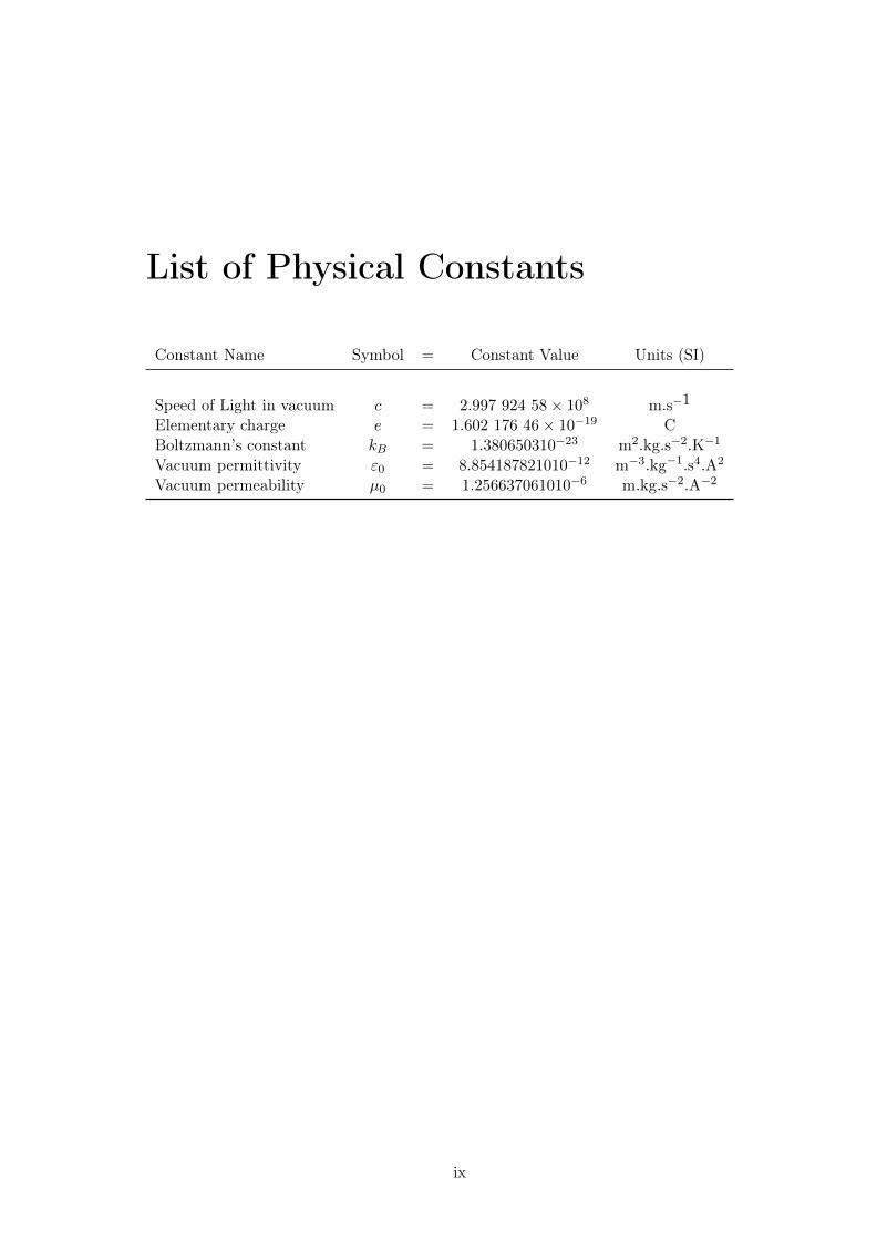
Constant Name Symbol = Constant Value Units (SI)

Speed of Light in vacuum c = 2.997 924 58× 108 m.s−1

Elementary charge e = 1.602 176 46× 10−19 CBoltzmann’s constant kB = 1.380650310−23 m2.kg.s−2.K−1

Vacuum permittivity ε0 = 8.854187821010−12 m−3.kg−1.s4.A2

Vacuum permeability µ0 = 1.256637061010−6 m.kg.s−2.A−2

ix

x LIST OF PHYSICAL CONSTANTS

Glossary

APL: Antenna Protection LimiterDC: Direct CurrentECRH: Electron Cyclotron Resonant HeatingHFS: High Field SideFDTD: Finite Difference Time DomainFEM: Finite Element MethodICRH: Ion Cyclotron Resonant HeatingITER: International Thermonuclear Experimental ReactorFS: Faraday ScreenILP: ITER Like PrototypeJET: Joint European TokamakLH: Lower HybridLCFS: Last Closed Flux SurfaceLFS: Low Field SideLPT: Limiteur Pompé Toroidal, french acronym standing for Toroidal Pumped Limiter(TPL)LPA: Limiteur deProtection d’Antenne, french acronym standing forAntennaProtectionLimiter (APL)MHD: MagnetohydrodynamicNBI: Neutral Beam InjectionPEC: Perfect Electric ConductorPMC: Perfect Magnetic ConductorPFCs: Plasma Facing ComponentsPML: Perfectly Matched LayerRDL: Resonant Double LoopRF: Radio-FrequencySBC: Sheath Boundary ConditionSOL: Scrape Off LayerSSWICH: Self-consistent Sheaths & Waves for Ion Cyclotron HeatingTE: Transverse ElectricTM: Transverse MagneticTOPICA: TOrino Polytechnic Ion Cyclotron AntennaWEST: W Environment in Steady-state Tokamak

xi

xii GLOSSARY

Contents

Remerciements/Acknowledgments i

List of notations v

List of Physical Constants ix

Glossary xi

Contents xiii

1 Introduction 11.1 Thermonuclear fusion . . . . . . . . . . . . . . . . . . . . . . . . . . . . . . 11.2 Magnetic confinement fusion . . . . . . . . . . . . . . . . . . . . . . . . . . . 2

1.2.1 Magnetic confinement . . . . . . . . . . . . . . . . . . . . . . . . . . 21.2.2 Short history . . . . . . . . . . . . . . . . . . . . . . . . . . . . . . . 31.2.3 The tokamak magnetic configuration . . . . . . . . . . . . . . . . . . 3

1.3 Heating and current drive methods in a fusion plasma . . . . . . . . . . . . 51.3.1 Ohmic heating . . . . . . . . . . . . . . . . . . . . . . . . . . . . . . 51.3.2 Neutral beams injection . . . . . . . . . . . . . . . . . . . . . . . . . 61.3.3 Radio-Frequency (RF) waves heating in general . . . . . . . . . . . . 71.3.4 Electron Cyclotron Resonance Heating (ECRH) . . . . . . . . . . . . 71.3.5 Lower Hybrid (LH) . . . . . . . . . . . . . . . . . . . . . . . . . . . . 81.3.6 Typical parameters of a few tokamaks . . . . . . . . . . . . . . . . . 8

1.4 Ion Cyclotron Resonance Heating (ICRH) . . . . . . . . . . . . . . . . . . . 91.4.1 Principle . . . . . . . . . . . . . . . . . . . . . . . . . . . . . . . . . . 101.4.2 Main ICRH wave absorption scenarios . . . . . . . . . . . . . . . . . 10

1.5 ICRH challenges . . . . . . . . . . . . . . . . . . . . . . . . . . . . . . . . . 111.5.1 Wave power coupling to the plasma . . . . . . . . . . . . . . . . . . . 111.5.2 Radio-frequency sheaths . . . . . . . . . . . . . . . . . . . . . . . . . 12

1.6 Thesis outline . . . . . . . . . . . . . . . . . . . . . . . . . . . . . . . . . . . 13

2 Theoretical and experimental background required for the thesis 152.1 Theory of ICRH waves . . . . . . . . . . . . . . . . . . . . . . . . . . . . . . 15

2.1.1 The Maxwell’s equations . . . . . . . . . . . . . . . . . . . . . . . . . 152.1.2 Dielectric tensor within the cold plasma approximation in the SOL . 162.1.3 General dispersion relation for plane waves . . . . . . . . . . . . . . 18

xiii

xiv CONTENTS

2.1.4 Fast and slow waves in the ICRH frequency domain . . . . . . . . . 182.1.4.1 Dispersion relation . . . . . . . . . . . . . . . . . . . . . . . 182.1.4.2 Electric field polarization . . . . . . . . . . . . . . . . . . . 192.1.4.3 Resonance and cut-off . . . . . . . . . . . . . . . . . . . . . 20

2.2 Theory of fast wave coupling to the plasma . . . . . . . . . . . . . . . . . . 212.2.1 Wave excitation by a phased array of straps . . . . . . . . . . . . . . 212.2.2 Wave coupling to the plasma . . . . . . . . . . . . . . . . . . . . . . 222.2.3 Coupling resistance definition . . . . . . . . . . . . . . . . . . . . . . 242.2.4 Review of the different historical ways to model wave coupling . . . 242.2.5 Why emulating radiating boundary conditions? . . . . . . . . . . . . 262.2.6 Short history of radiating boundary conditions . . . . . . . . . . . . 27

2.3 Generation of radio-frequency sheaths by waves . . . . . . . . . . . . . . . . 272.3.1 Recall of the Debye sheath physics . . . . . . . . . . . . . . . . . . . 282.3.2 Properties derived from principles driving oscillating sheaths for self-

consistent modelling . . . . . . . . . . . . . . . . . . . . . . . . . . . 302.3.2.1 Splitting of RF and DC quantities . . . . . . . . . . . . . . 312.3.2.2 Sheath rectification . . . . . . . . . . . . . . . . . . . . . . 322.3.2.3 Sheath capacitance . . . . . . . . . . . . . . . . . . . . . . . 33

2.3.3 Sheath boundary conditions . . . . . . . . . . . . . . . . . . . . . . . 342.3.4 DC biasing model of the SOL plasma with DC conductivity tensor . 362.3.5 Previous RF sheath modelling . . . . . . . . . . . . . . . . . . . . . . 39

2.4 Overview of the ICRH system on Tore Supra . . . . . . . . . . . . . . . . . 402.4.1 Synopsis of the excitation on high power waves in tokamaks . . . . . 402.4.2 ICRH system on Tore Supra . . . . . . . . . . . . . . . . . . . . . . . 412.4.3 Two electrical layouts for the Tore Supra ICRH antennas . . . . . . 41

2.4.3.1 The classical Tore Supra ICRH antenna . . . . . . . . . . . 422.4.3.2 The load resilient ITER like prototype (ILP) ICRH antenna 43

2.4.4 The lateral antenna limiters . . . . . . . . . . . . . . . . . . . . . . . 442.4.5 Two Faraday screen designs on Tore Supra . . . . . . . . . . . . . . . 452.4.6 Diagnostics on the Tore Supra ICRH antenna . . . . . . . . . . . . . 47

2.5 Summary . . . . . . . . . . . . . . . . . . . . . . . . . . . . . . . . . . . . . 49

3 Perfectly Matched Layer to emulate radiating boundary conditions forwaves in magnetized plasmas 513.1 The Perfectly Matched Layer method . . . . . . . . . . . . . . . . . . . . . . 513.2 Mathematical description of the Perfectly Matched Layer . . . . . . . . . . 53

3.2.1 Introduction . . . . . . . . . . . . . . . . . . . . . . . . . . . . . . . . 533.2.2 Wave damping via artificial coordinate stretching in the complex

plane: qualitative introduction via a simple example in 1D . . . . . . 533.2.3 Formulation of the spatial coordinates stretching problem in 3D Carte-

sian geometry with full permittivity and permeability tensors . . . . 543.2.4 Interpretation of the PML as an artificial lossy medium . . . . . . . 55

3.3 Reflection of plane waves by a 1D PML . . . . . . . . . . . . . . . . . . . . 563.3.1 Analytical reflection coefficient in presence of a PML . . . . . . . . . 573.3.2 Criteria for choosing the stretching function properties to minimize

the analytical reflection coefficient . . . . . . . . . . . . . . . . . . . 583.3.3 Application to polynomial stretching function . . . . . . . . . . . . . 593.3.4 Qualitative reflections on the choice of the PML parameters and on

numerical errors due to discretization . . . . . . . . . . . . . . . . . . 59

CONTENTS xv

3.4 Numerical tests with plane waves in an homogeneous magnetized plasmacompared to analytical predictions of the reflection coefficient . . . . . . . . 603.4.1 Assessment of the reflection coefficient in numerical simulations with

the standing wave ratio . . . . . . . . . . . . . . . . . . . . . . . . . 603.4.2 Test for PML in perpendicular direction and in parallel direction . . 623.4.3 Numerical optimization of the PML for a given plane wave . . . . . 65

3.4.3.1 Influence of the PML depth LPML on η . . . . . . . . . . . 653.4.3.2 Influence of the elements size hmax⊥ and type on η . . . . . 653.4.3.3 Influence of the stretching function order p on η . . . . . . 673.4.3.4 Influence of the stretching function coefficient S′′ on η . . . 68

3.4.4 Simultaneous handling of two polarizations in gyrotropic medium . . 693.4.5 From reflection coefficient to Poynting vector flux . . . . . . . . . . . 71

3.5 Summary . . . . . . . . . . . . . . . . . . . . . . . . . . . . . . . . . . . . . 73

4 Fast wave coupling code for ICRH antennas facing a fusion magnetizedplasma in Comsol relying on the Perfectly Matched Layer technique:Application on Tore Supra 754.1 Modelling, implementation and numerical tests . . . . . . . . . . . . . . . . 76

4.1.1 Link between Poynting vector and coupling resistance . . . . . . . . 764.1.2 Description of the wave coupling experiment . . . . . . . . . . . . . . 774.1.3 Modelling of the Tore Supra ICRH antennas and of the edge plasma 784.1.4 Requirement on the PMLs . . . . . . . . . . . . . . . . . . . . . . . . 824.1.5 Simulation setup and resources requirements . . . . . . . . . . . . . 854.1.6 Test of the PMLs with a 2D antenna in a fusion plasma environment 87

4.2 Comparison of Fast wave coupling properties obtained from the simulationswith 2D and 3D simplified Tore Supra ICRH antennas geometries with ex-periments . . . . . . . . . . . . . . . . . . . . . . . . . . . . . . . . . . . . . 884.2.1 Launched and coupled spectrum . . . . . . . . . . . . . . . . . . . . 884.2.2 Influence of the antenna geometry elements of the coupling resistance 894.2.3 Influence of the current distribution on the strap of the coupling

resistance . . . . . . . . . . . . . . . . . . . . . . . . . . . . . . . . . 914.2.4 Comparison of the classical antenna with the ILP antenna . . . . . . 914.2.5 Possible origins for the overestimation of the coupling resistance . . . 93

4.3 Conclusions & Prospects for the Fast Wave coupling code with the PerfectlyMatched Layer technique . . . . . . . . . . . . . . . . . . . . . . . . . . . . 944.3.1 Summary on FW coupling computations relying on the PML technique 944.3.2 Preliminary optimizations of FW coupling with a improved antenna

design based on the ILP antenna for WEST . . . . . . . . . . . . . . 954.3.3 In the long term . . . . . . . . . . . . . . . . . . . . . . . . . . . . . 97

5 Development of an antenna-plasma code SSWICH-SWwith a self-consistentdescription of RF sheaths effects 995.1 Physics in SSWICH-SW . . . . . . . . . . . . . . . . . . . . . . . . . . . . . 100

5.1.1 Tore Supra geometry in the vicinity of the ICRH antenna in SSWICH1005.1.2 RF wave propagation: slow wave . . . . . . . . . . . . . . . . . . . . 1025.1.3 Oscillating sheath voltage . . . . . . . . . . . . . . . . . . . . . . . . 1045.1.4 DC biasing of the SOL plasma . . . . . . . . . . . . . . . . . . . . . 1055.1.5 Initialization: asymptotic model of SSWICH-SW . . . . . . . . . . . 106

5.2 Numerical implementation in Comsol Multiphysics . . . . . . . . . . . . . . 108

xvi CONTENTS

5.2.1 Architecture of the code in Comsol . . . . . . . . . . . . . . . . . . . 1085.2.2 Antenna description through an interface with the TOPICA antenna

code . . . . . . . . . . . . . . . . . . . . . . . . . . . . . . . . . . . . 1095.2.3 Mesh & Solver . . . . . . . . . . . . . . . . . . . . . . . . . . . . . . 1135.2.4 Typical memory and CPU time requirements . . . . . . . . . . . . . 115

5.3 Numerical tests of SSWICH-SW-2D . . . . . . . . . . . . . . . . . . . . . . 1155.3.1 Standalone tests of the slow wave propagation module with RF sheath

boundary conditions and fixed sheath width . . . . . . . . . . . . . . 1165.3.2 Comparison of multi-2D approach with 3D for Tore Supra with the

asymptotic model in standalone . . . . . . . . . . . . . . . . . . . . . 1205.3.3 Comparison of the fully coupled model with the asymptotic model

during a power scan . . . . . . . . . . . . . . . . . . . . . . . . . . . 1225.4 Status and prospects for SSWICH . . . . . . . . . . . . . . . . . . . . . . . 124

6 Comparison of SSWICH-SW-2D simulations with experimental observa-tions on Tore Supra and predictions for ITER 1276.1 Review of the experimental observations on Tore Supra during the 2011

campaign . . . . . . . . . . . . . . . . . . . . . . . . . . . . . . . . . . . . . 1276.1.1 Comparison of two Faraday screens . . . . . . . . . . . . . . . . . . . 1286.1.2 Left/right symmetrisation of strap voltages and consequences on RF

sheaths . . . . . . . . . . . . . . . . . . . . . . . . . . . . . . . . . . 1296.1.3 Magnitude and topology of the enhanced RF sheaths on CBSB Fara-

day screen . . . . . . . . . . . . . . . . . . . . . . . . . . . . . . . . . 1306.2 Simulations with TOPICA/SSWICH-SW-2D for Tore Supra . . . . . . . . . 132

6.2.1 Typical simulation results on the antenna side limiters . . . . . . . . 1336.2.2 Relative comparison of the two Faraday screens . . . . . . . . . . . . 1366.2.3 Different possible mechanisms to excite RF sheaths . . . . . . . . . . 1386.2.4 Sensitivity of the radial pattern of VDC to perpendicular DC conduc-

tivity . . . . . . . . . . . . . . . . . . . . . . . . . . . . . . . . . . . . 1406.2.5 Estimation of values of perpendicular DC conductivity consistent

with observations . . . . . . . . . . . . . . . . . . . . . . . . . . . . . 1476.2.6 Effect of unbalanced strap voltage on the distribution left/right of

the heat fluxes on inner face of the lateral limiters . . . . . . . . . . 1496.2.7 Comparison of intermediate electrical designs of the antenna in order

to identify the weak element in the CBSB FS . . . . . . . . . . . . . 1506.3 Estimations of parallel heat fluxes on the blanket shielding modules (BSM)

for ITER . . . . . . . . . . . . . . . . . . . . . . . . . . . . . . . . . . . . . 1546.3.1 Modelling of ITER ICRH antenna . . . . . . . . . . . . . . . . . . . 1546.3.2 Simplified geometry of the BSM in SSWICH . . . . . . . . . . . . . . 1556.3.3 Estimation of parallel heat fluxes . . . . . . . . . . . . . . . . . . . . 1566.3.4 Difficulties for modelling the antenna and estimating heat fluxes on

the BSM . . . . . . . . . . . . . . . . . . . . . . . . . . . . . . . . . . 1566.4 Summary and Prospects . . . . . . . . . . . . . . . . . . . . . . . . . . . . . 157

Conclusion 159

Contents xvii

A Error between exact solution and PML solution in the semi-infinite prob-lem 167

B Analytic link between reflection coefficient and Poynting vector in thecase of a plane wave 169

C Non-linear DC plasma potential diffusion analytical model with a DCconductivity tensor in a simplified 4 regions geometry 173C.1 Outline of the 4 regions model . . . . . . . . . . . . . . . . . . . . . . . . . . 173C.2 DC plasma potential radial variation in the private SOL . . . . . . . . . . . 175C.3 Radial extension of the DC plasma potential in the free SOL . . . . . . . . 176C.4 Connection between the 4 regions at the antenna limiter leading edge . . . . 178

Bibliography 181

List of Publications 195

Long résumé I

Chapter 1

Introduction

1.1 Thermonuclear fusion

Our current civilization consumes every day large and increasing amount of energy com-ing from non-sustainable sources that are dangerous for the Earth environment and willwear off in the future [1]. Achieving sustainable energy is a monumental challenge thatMankind must pass. Thermonuclear fusion, the energy powering the stars, is one possiblecandidate to provide abundant, clean and sustainable energy if it can be harnessed for civilapplications.

The energy released in the nuclear fusion reactions of nuclei with lower masses thaniron comes from the difference in the nuclear binding energy ∆E. The masses of nuclei areactually always smaller than the sum of the nucleon masses constituting them. Einstein’senergy-mass relation tells us that ∆E = ∆m c2 (≈ MeV, i.e. 6 orders of magnitude largerthan the energy released in chemical reactions of burning fossil fuels).

Nuclear fusion reactions are governed by the strong nuclear force binding the protonsand the neutrons in the nucleus and acting over a distance of the order of the nucleonradius. Above this distance the repulsive Coulomb force between the positively chargednuclei dominates. To approach a pair of nuclei close enough so that the fusion reactioncan occur, the Coulomb repulsion between the fusing nuclei must be overcome with highkinetic energies.

From the possible nuclear fusion reactions, the deuterium-tritium (21D −31 T ) reaction

has by far the largest cross-section with the maximum at relatively low kinetic energiesand temperature and is therefore the most promising candidate for future fusion reactors,as it is the easiest to achieve as a potential energy source [2]:

21D +3

1 T →42 He(3.56 MeV) +1

0 n(14.03 MeV) (1.1)

The distribution of ∆E ≈ 17.6 MeV of the reaction between the 4He (α particle) andthe neutron is inversely proportional to their masses mn/mα = Eα/En.

In order to maximize the cross-section of the D-T reaction, the optimal temperaturerange is Ti ≥ 20 keV. At such high temperatures, matter exists in a state of ionized gas.In the case when it is quasi-neutral, it is called plasma [3]. Quasi-neutrality is given by thefollowing expression:

N∑k=1

Zk ·nk + ne = 0, (1.2)

where N is the number of ion species, nk is the ion density of species k with electric chargeZk and ne is the electron density. Each species in the plasma is associated with a plasma

1

2 CHAPITRE 1

frequency:

ω2ps =

q2snsε0ms

, (1.3)

with ε0 the permittivity of vacuum, ns and qs the density and electric charge of thespecies s (ions of species k + electrons) respectively. The quantity qs is taken to bealgebraic, so that for the electrons qs = −e and qs = Zse for the ions.

The level of performance of the plasma can be measured by introducing the enhance-ment factor Q [3] which corresponds to the ratio of the power released into the plasma byfusion reactions Pfus and the level of power injected into the plasma Pinj . The Q = 1 limitis called the break-even, it corresponds to the state where the plasma is sustained to equalparts by the fusion energy power and by the external power input, while the Q = +∞limit is called ignition where the plasma is self-sustained without any external means. Theignition condition [4] given by the Lawson criterion can be derived from a simple energybalance in the fusion reactor:

nτET ≥ 3.1021 keVs−1. (1.4)

In plasma physics, it is convenient to write temperatures in electronvolt (eV) thatdefines the amount of energy gained by a single electron moving across an electric po-tential difference of 1 V. The conversion between K and eV is done with the formula:T (eV) = T (K) kB/e with kB the Boltzmann constant and e the electric charge. Severalpossibilities can be considered in order to reach the Lawson criterion. With Ti ≥ 20 keV,two parameters remain in the triple product. Two main directions can be explored onEarth to satisfy the Lawson criterion [5], as the huge gravitation force existing in the coreof stars cannot be reproduced on Earth:

• Inertial confinement aims at obtaining very dense plasmas (n ∼ 1031 m−3) for veryshort time (τE ∼ 10−11 s). These conditions are reached with focused high en-ergy lasers beams heating and compressing the fuel target consisting of a deuterium-tritium pellet. Large scale experiments exploring this option are the NIF in the USand the Laser Mégajoule in France.

• Magnetic confinement consists in using strong magnetic fields (several teslas) to gen-erate a magnetic "bottle" confining the plasma [3]. The aim is thus to increasesignificantly the energy confinement time (τE ∼ 1 s) without any direct contact withthe material of the bottle vessel (that would cool down the plasma) of a "low" densityplasma (n ∼ 1020 m−3).

1.2 Magnetic confinement fusion

1.2.1 Magnetic confinement

Charged particles in a magnetic field have helical trajectories around the magnetic fieldlines [5]. Movement along the field lines is free. The extent ρs of the helix perpendicularto the magnetic field line is called Larmor radius. Perpendicularly to the magnetic fieldof amplitude B, each particle s of mass ms and charge qs has a cyclotron motion at thepulsation:

Ωs =qsB

ms, (1.5)

1.2. MAGNETIC CONFINEMENT FUSION 3

The cyclotron frequency Ωs for a species s is one of the natural frequencies of a plasma.With a perpendicular velocity v⊥ it gives for the Larmor radius:

ρs =v⊥Ωs

=msv⊥qsB

. (1.6)

As the Larmor radius is inversely proportional to the amplitude of the magnetic field,a stronger magnetic field will provide better confinement properties. In devices relying onmagnetic confinement, the amplitude of the magnetic field is typically of several teslas (T),compared to Earth magnetic field amplitude of 3.1 10−5 T at the equator. In the followingof this thesis, ‖ index will denote the direction along the static magnetic field B while the⊥ index will denote the two others dimensions which are perpendicular to the magneticfield.

1.2.2 Short history

Several magnetic configurations (magnetic mirrors, stellerators) have been studied since thebeginning of nuclear fusion research in the 1950’s. The confinement properties also dependon the geometry of the magnetic field. Historically the first devices confining magneticallythe plasma with open field lines were linear. However the important particle and energylosses at the extremities of the field lines are not compatible with the requirement on theenergy confinement time for sustainable energy production. Avoiding these losses led tocreating the simplest magnetic configuration in which the magnetic field lines are closedby closing the device on itself to form a torus. This is unfortunately not enough to achieveconfinement since with a purely toroidal magnetic field particles still experience an outwarddrift due to the curvature and the gradient of the magnetic field. The solution is to add apoloidal component to the magnetic field to twist the field lines helically around the torus.The field lines thus wind up around nested magnetic surfaces, cancelling on average theoutward drift of the particles: particles derive outward then inward along a field line. Theparticle orbits are thus periodic and confined inside the vessel.

Two main approaches exist to generate this poloidal magnetic field. In devices calledstellarator [6], the poloidal magnetic field is produced externally by field coils placed aroundthe torus. In devices called tokamaks, the poloidal magnetic field is produced indirectlythrough a toroidal electric current in the plasma. The tokamak concept [3], invented bySoviet physicists in the 1960’s, is currently the most successful magnetic configuration. Ithas been besides widely promoted by many research institutes (a couple hundred of devicesin the world) and has obtained the best results in terms of fusion power.

1.2.3 The tokamak magnetic configuration

A diagram of the tokamak concept [5] is shown in Figure 1.1. The toroidal magnetic fieldBt is produced by toroidal field coils surrounding the torus. The poloidal magnetic field Bpin a tokamak is generated indirectly through the transformer effect. The resulting helicalmagnetic field B is thus the superposition of both components. In tokamaks the poloidalfield is typically smaller by one order of magnitude than the toroidal field. The magneticconfiguration is thus completely defined only in the presence of a plasma. This makes oftokamaks intrinsic pulsed devices since the transformer cannot be maintain continuously,unless additional methods produces non-inductive current drive. Poloidal field coils areadded to the design for additional positioning and shaping of the plasma as well as forstability by active feedback.

4 CHAPITRE 1

The essential geometrical parameters in a tokamak are the aspect ratio A = R/a whereR is the major radius of the torus and a the horizontal minor radius. The ellipticity κ isthe ratio of vertical minor radius b over the horizontal minor radius a. Vertically elongatedplasmas offer better confinement properties, as well as high toroidal magnetic field Bt. Themagnetic field Bt evolves as 1/R with the maximum at the inner side of the coil called highfield side (HFS) and the minimum at the outer side of the coil called low field side (LFS).For stability, essential parameters are the plasma current Ip, β defined by the ratio of theplasma pressure over the magnetic pressure that measures the efficiency of the magneticconfinement and the safety factor q indicating how the field lines are twisted around theflux surfaces: q = rBt/RBp. It is connected to MHD stability.

As a tokamak is axisymmetric, all the toroidal cross sections are identical in the confinedregion (plasma core). Nested magnetic surfaces, where the magnetic field is everywheretangent to the surfaces, can thus be represented by their cross section in the radial/poloidalplane, as shown in Figure 1.2. Some quantities have a constant value on magnetic surfacesonly changing from surface to surface. Among them are the temperature T , the density n,the safety factor q and the current density J . Assuming a circular cross section (b = a),each magnetic surface is indexed by its minor radius r and each surface quantity is onlyfunction of r.

Control of the plasma-wall interaction [7] is crucial for the performance of the device,as it determines the damage of the plasma facing components (PFCs) that reduces the life-time of the machine and its reliability and the plasma contamination by impurities inducingradiation which reduces the energy confinement time τE . The limit of the confined plasmais determined by the last closed flux surface (LCFS): the separatrix. The region beyondthe separatrix, where magnetic field lines are open (i.e. connected to the wall), is calledScrape Off Layer (SOL). The two main existing configurations in tokamaks are shown onFigure 1.2. The first one is the limiter (left) that keeps away the plasma from the PFCsby a carefully designed piece of material. Consequently the interaction takes place at the

Figure 1.1: Schematic view of the tokamak concept.

1.3. HEATING AND CURRENT DRIVE METHODS IN A FUSION PLASMA 5

Figure 1.2: Magnetic configuration of the JET tokamak with a limiter (left) and with adivertor (right).

limiter. The second configuration is the divertor (right) that consists in modifying themagnetic field at the separatrix: an X-point is formed where the poloidal field is zero. It ismore flexible since the position of the X-point can be moved in a controlled manner. Theplasma-wall interaction occurs here far away from the confined plasma, providing betterperformances since fewer impurities can enter the core plasma to radiate.

1.3 Heating and current drive methods in a fusion plasma

In a future operating fusion reactor, part of the energy generated through nuclear fusionreactions (α particles) will serve to maintain the plasma temperature as fresh fuel is in-troduced. However, in the start-up phase of a reactor, the plasma still have to be heatedby external means to its operating temperature (>10 keV). Furthermore, external heatingpresents a way to keep operational control over the burning plasma, thus keeping it in thesub-ignition state. Moreover in current magnetic fusion experiments, the fusion power isinsufficient to maintain the burning plasma. Different methods to heat a plasma to fusionrelevant conditions, shown on Figure 1.3, exist and will be presented in this section.

1.3.1 Ohmic heating

Since the plasma is an electrical conductor, it is possible to heat the plasma by inducinga current through it. In fact, the induced current to provide the poloidal magnetic fieldalso heats through the Joule effect. The heating caused by the induced current is calledohmic (or resistive) heating. As the transformer effect is inherently a pulsed process dueto the limit in magnetic flux (there are also other limitations on long pulses), tokamaksmust therefore either operate for short periods or rely on other means of heating and non-inductive current drive by external means or by optimizing naturally occurring currents inthe plasma (bootstrap current associated to pressure gradient). A steady state operationof a tokamak requires at least 20% of the plasma current provided non-inductively.

Furthermore the heat generated depends on the resistivity of the plasma η and theamount of electric current running through it. But as the temperature T of heated plasmarises, the resistivity decreases as T−3/2 by the nature of Coulomb collisions and ohmic

6 CHAPITRE 1

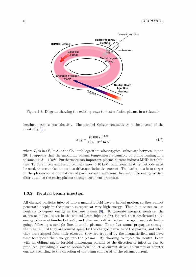
Figure 1.3: Diagram showing the existing ways to heat a fusion plasma in a tokamak.

heating becomes less effective. The parallel Spitzer conductivity is the inverse of theresistivity [3]:

σ‖,S =(0.001Te)

3/2

1.65 10−9 ln Λ, (1.7)

where Te is in eV, ln Λ is the Coulomb logarithm whose typical values are between 15 and20. It appears that the maximum plasma temperature attainable by ohmic heating in atokamak is 3− 4 keV. Furthermore too important plasma current induces MHD instabili-ties. To obtain relevant fusion temperatures (>10 keV), additional heating methods mustbe used, that can also be used to drive non inductive current. The basics idea is to targetin the plasma some populations of particles with additional heating. The energy is thendistributed to the entire plasma through turbulent processes.

1.3.2 Neutral beams injection

All charged particles injected into a magnetic field have a helical motion, so they cannotpenetrate deeply in the plasma excepted at very high energy. Thus it is better to useneutrals to deposit energy in the core plasma [8]. To generate energetic neutrals, theatoms or molecules are in the neutral beam injector first ionized, then accelerated to anenergy of several hundred of keV, and after neutralized to become again neutrals beforegoing, following a straight line, into the plasma. These fast atoms propagate throughthe plasma until they are ionized again by the charged particles of the plasma, and whenthey are stripped from their electron, they are trapped by the magnetic field and havetime to deposit their energy into the plasma. By choosing to inject the neutral beamwith an oblique angle, toroidal momentum parallel to the direction of injection can beproduced, providing a way to obtain non inductive current drive: co-current or countercurrent according to the direction of the beam compared to the plasma current.

1.3. HEATING AND CURRENT DRIVE METHODS IN A FUSION PLASMA 7

1.3.3 Radio-Frequency (RF) waves heating in general

Radio-frequency electromagnetic waves are generated by oscillators outside the torus. Ashot plasmas are weakly collisional, RF wave damping has to rely on collisionless wave-particle mechanisms. If the waves have a frequency (and wavelength) corresponding to anatural frequency of the plasma and the correct polarization, energy or momentum can betransferred to the charged particles in the plasma. The wave energy is then distributedfrom the resonant particle population to the bulk plasma trough collisions. Assuming aplane wave with harmonic oscillations in exp (−iωt+ ik · r), the resonance condition forthe resonant particles population reads:

ω − pΩs − k‖v‖s = 0, (1.8)

where p is the cyclotron harmonic number, k‖ the parallel component of the wave vectorand v‖s the component of the s particle velocity parallel to the static magnetic field.

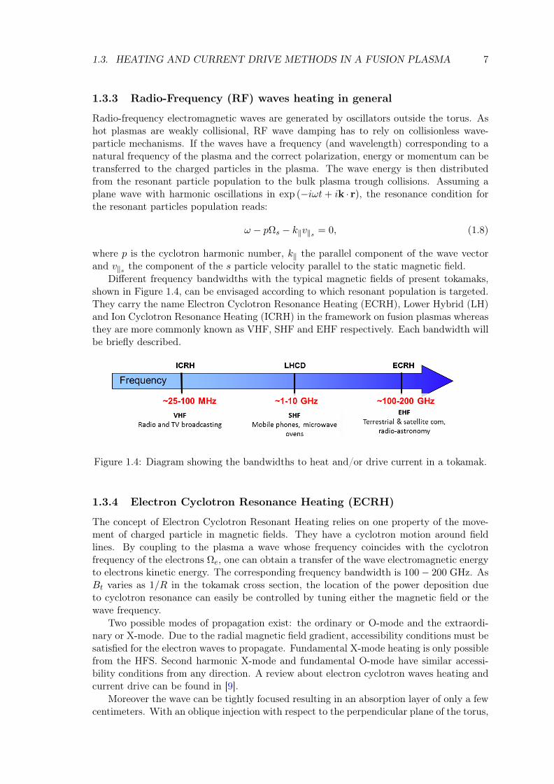
Different frequency bandwidths with the typical magnetic fields of present tokamaks,shown in Figure 1.4, can be envisaged according to which resonant population is targeted.They carry the name Electron Cyclotron Resonance Heating (ECRH), Lower Hybrid (LH)and Ion Cyclotron Resonance Heating (ICRH) in the framework on fusion plasmas whereasthey are more commonly known as VHF, SHF and EHF respectively. Each bandwidth willbe briefly described.

Figure 1.4: Diagram showing the bandwidths to heat and/or drive current in a tokamak.

1.3.4 Electron Cyclotron Resonance Heating (ECRH)

The concept of Electron Cyclotron Resonant Heating relies on one property of the move-ment of charged particle in magnetic fields. They have a cyclotron motion around fieldlines. By coupling to the plasma a wave whose frequency coincides with the cyclotronfrequency of the electrons Ωe, one can obtain a transfer of the wave electromagnetic energyto electrons kinetic energy. The corresponding frequency bandwidth is 100− 200 GHz. AsBt varies as 1/R in the tokamak cross section, the location of the power deposition dueto cyclotron resonance can easily be controlled by tuning either the magnetic field or thewave frequency.

Two possible modes of propagation exist: the ordinary or O-mode and the extraordi-nary or X-mode. Due to the radial magnetic field gradient, accessibility conditions must besatisfied for the electron waves to propagate. Fundamental X-mode heating is only possiblefrom the HFS. Second harmonic X-mode and fundamental O-mode have similar accessi-bility conditions from any direction. A review about electron cyclotron waves heating andcurrent drive can be found in [9].

Moreover the wave can be tightly focused resulting in an absorption layer of only a fewcentimeters. With an oblique injection with respect to the perpendicular plane of the torus,

8 CHAPITRE 1

current drive can also be produced with efficiency close to lower hybrid. Experiments havealso demonstrated that the ECRH method is useful for the plasma start-up, the control ofMHD instabilities such as stabilizing the Neoclassical Tearing Mode [10, 11] or the sawtoothoscillation [12], which requires a very localized and peaked current density profile. Electroncyclotron waves can be launched in vacuum and propagate directly into the plasma withoutattenuation or interaction with the edge, before being locally absorbed in the resonanceregion. Reviews on ECRH and ECCD can be found in the following references [13, 14]

1.3.5 Lower Hybrid (LH)

Another frequency method in the gigahertz range is the Lower Hybrid Heating and CurrentDrive. The large parallel electric field carried by LH waves propagating along the magneticfield was shown to lead to strong electron Landau damping (p = 0 in (1.8)) and consequentlyto electron heating and non-inductive current drive (LHCD). The capability to also produceoff-axis current allows the development of advanced tokamak scenarios by controlling thecurrent profile to create internal transport barrier in the plasma in addition with thebootstrap current.

For the lower hybrid waves to have access to the plasma in this frequency range, theparallel refractive index n‖ must satisfy an accessibility condition [15]. The LH waves areconsequently evanescent at the plasma edge and efficient coupling of the waves requires theLH waves antenna at proximity to the plasma. Furthermore the current drive efficiency isinversely proportional to the square of n‖ index: small n‖ are favoured. To generate therequired spectrum necessary to satisfy to the accessibility condition, antennas composedof multiple phased waveguides are used [15].

Moreover, the high current drive efficiency makes of Lower Hybrid Current Drive(LHCD) system a crucial actuator to save inductive flux and to generate additional plasmacurrent in present day tokamak experiments [16]. Several superconducting tokamaks (ToreSupra, TRIAM-1M, HT-7, EAST) have demonstrated the feasibility of long pulse opera-tion using LHCD. For example, a discharge on Tore Supra of 6 min was performed in 2003at a plasma current of Ip = 0.5 MA, a magnetic field Bt = 3.4 T and 3 MW of LH power[16]. More recently higher LH power 5 MW have been coupled in combination with 3 MWof ICRH power during a 18 s pulse on Tore Supra. In ITER, steady-state operation witha mix of D-T fuel is foreseen to be with 100% of non-inductive current drive.

1.3.6 Typical parameters of a few tokamaks

The characteristics of the Tore Supra tokamak, the upgrade of Tore Supra defined as theWEST (W Environment in Steady-state Tokamak) project and the ITER machine canbe found in Table 1.1. Numbers in between brackets signify proposal for upgrade and assuch not included in the baseline.

Tore Supra is considered as a large tokamak with a circular plasma cross-section (majorradius R = 2.4 m and minor radius a = 0.7 m) whose last closed flux surface (LCFS) is de-fined by the intersection of the magnetic field lines with the bottom toroidal pumped limiteror with the outboard antenna protection limiter (APL). The maximal plasma current andtoroidal magnetic field are Ip < 1.5 MA and B = 3.8 T, respectively. Its main features arethe superconducting toroidal field coils and the actively cooled first wall and components,which make actually the Tore Supra tokamak an ideal machine for the study of long plasmadischarges [17]. Tore Supra exclusively relies on RF heating systems, especially ICRH andcan drive large amount of non-inductive current with LH.

1.4. ION CYCLOTRON RESONANCE HEATING (ICRH) 9

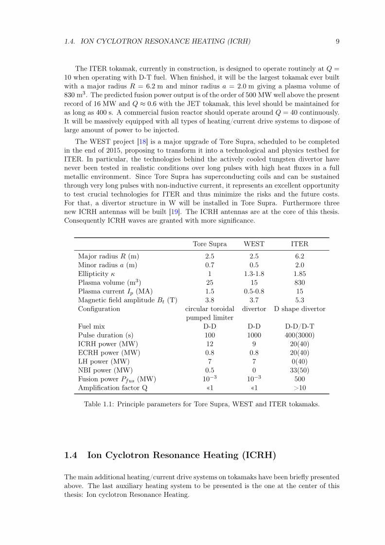
The ITER tokamak, currently in construction, is designed to operate routinely at Q =10 when operating with D-T fuel. When finished, it will be the largest tokamak ever builtwith a major radius R = 6.2 m and minor radius a = 2.0 m giving a plasma volume of830 m3. The predicted fusion power output is of the order of 500 MW well above the presentrecord of 16 MW and Q ≈ 0.6 with the JET tokamak, this level should be maintained foras long as 400 s. A commercial fusion reactor should operate around Q = 40 continuously.It will be massively equipped with all types of heating/current drive systems to dispose oflarge amount of power to be injected.

The WEST project [18] is a major upgrade of Tore Supra, scheduled to be completedin the end of 2015, proposing to transform it into a technological and physics testbed forITER. In particular, the technologies behind the actively cooled tungsten divertor havenever been tested in realistic conditions over long pulses with high heat fluxes in a fullmetallic environment. Since Tore Supra has superconducting coils and can be sustainedthrough very long pulses with non-inductive current, it represents an excellent opportunityto test crucial technologies for ITER and thus minimize the risks and the future costs.For that, a divertor structure in W will be installed in Tore Supra. Furthermore threenew ICRH antennas will be built [19]. The ICRH antennas are at the core of this thesis.Consequently ICRH waves are granted with more significance.

Tore Supra WEST ITER

Major radius R (m) 2.5 2.5 6.2Minor radius a (m) 0.7 0.5 2.0Ellipticity κ 1 1.3-1.8 1.85Plasma volume (m3) 25 15 830Plasma current Ip (MA) 1.5 0.5-0.8 15Magnetic field amplitude Bt (T) 3.8 3.7 5.3Configuration circular toroidal divertor D shape divertor

pumped limiterFuel mix D-D D-D D-D/D-TPulse duration (s) 100 1000 400(3000)ICRH power (MW) 12 9 20(40)ECRH power (MW) 0.8 0.8 20(40)LH power (MW) 7 7 0(40)NBI power (MW) 0.5 0 33(50)Fusion power Pfus (MW) 10−3 10−3 500Amplification factor Q «1 «1 >10

Table 1.1: Principle parameters for Tore Supra, WEST and ITER tokamaks.

1.4 Ion Cyclotron Resonance Heating (ICRH)

The main additional heating/current drive systems on tokamaks have been briefly presentedabove. The last auxiliary heating system to be presented is the one at the center of thisthesis: Ion cyclotron Resonance Heating.

10 CHAPITRE 1

1.4.1 Principle

Heating at the ion cyclotron resonance is based on the same principles as electron cy-clotron heating, except that electrons are replaced by ions to establish the wave-particlesresonance. The frequency domain is between 25 MHz and 100 MHz. Since its also relieson cyclotron resonance, the power deposition is also localized and mainly on ions. Bylaunching asymmetric k‖ spectra, current drive can also be obtained.

ICRH proves to be very effective for heating the ions inside the plasma. Presentlymost large and medium size tokamaks use ICRH to couple large amount (several MW)of power to the plasma using different scenarios. A review of ICRH heating and currentdrive scenarios was made in Ref.[20]. One of the advantages is that the frequencies cur-rently in operation are essentially the same necessary for future reactors. This limits thenecessary technological development. The ICRH system on Tore Supra will be presentedin Section 2.4.

ICRH mainly heat ions in the plasma, on the contrary to others systems that onlyheat ions indirectly by collisions with electrons during thermalization. ICRH antennasemit two kinds of waves: the fast magnetosonic wave (FW) useful for heating and theslow magnetosonic wave (SW) generated parasitically whose properties will be detailed inChapter 2. Propagation of the fast wave is strongly perpendicular to the static magneticfield, with no accessibility issue to the plasma center.

1.4.2 Main ICRH wave absorption scenarios

There are a priori several possible heating scenarios with the fast magnetosonic ion wave.Some of them are presented here. It is useful to look at the wave absorption mechanismsin the plasma [21]. Although radio-frequency heating is similar to a microwave oven, theabsorption mechanism is different. For a plasma the absorption at the resonance occursby collisionless damping. The first scenario is absorption at the fundamental ion cyclotronresonance (ω = Ωi and p = 1 in (1.8)). This is the simplest mechanism. The perpendicularcomponent of the polarized wave rotates in the same direction as the cyclotron motion of theions around magnetic field lines. The wave is thus absorbed by the ions whose cyclotronmotion is in resonance with the wave pulsation (ω = Ωi). The ions are consequentlyaccelerated in the perpendicular direction. It is can be shown that for a single ion speciesplasma the wave polarization around the resonance rotates exactly in the opposite directionof the gyration motion of the ions. This solution is therefore not a viable option for heatinga plasma as the screening of the wave electric field on the ion gyro-motion prevents thetransfer of power from the wave to the single ion species plasma.

The second possibility is harmonic absorption. This happens when the wave pulsationis a multiple of the ion cyclotron frequency (ω = pΩi, with p an integer). Let us takean example with p = 2. The ion is thus accelerated during half the cyclotron period anddecelerated during the other half. If the wave electric field is homogeneous, there is no nettransfer of energy between wave and ion. On the contrary, with an inhomogeneous electricfield, the field will be larger one side of the revolution. There is thus a net transfer of energy.The efficiency of the transfer depends on the inhomogeneity of the electric field (linked tothe plasma parameters) and on the Larmor radius of the ion (linked to the perpendicularvelocity) [22]. The efficiency is also decreasing with increasing harmonic number.

The third possibility is minority heating. It consists in adding in the plasma a smallquantity (≈ 5%) of another species where the resonant species is largely in minority. Thewave frequency is chosen to produce wave-resonance at the fundamental of the minority.The damping zone is localized at the ion-ion hybrid resonance located between the individ-

1.5. ICRH CHALLENGES 11

ual cyclotron resonance of the two species. With the minority ion population, it turns outthat the wave polarization yields a component in the direction of the minority ions rota-tion. It is desirable for the minority species to have a higher cyclotron frequency than themajority species. In practice, hydrogen (11H) or helium-3 (32He) are chosen in deuteriumplasma. The efficiency is independent of the temperature and weakly dependent on thedensity. The wave energy is then distributed to the majority ions through collisions [21].

1.5 ICRH challenges

ICRH is an effective method to transfer to the plasma large amount of power to the ions.There is however still some issues to be solved. The main challenges from the generatorto the central plasma that the ICRH community still has to achieve to obtain a reliablehigh power steady state system are introduced here. Only some of them are among theobjectives of this thesis work.

In the core plasma of a reactor, α particles created by nuclear fusion reactions couldlead to parasitic absorption of ICRH power, increasing the losses and decreasing heatingefficiency [23].

As it will be further explained in Section 2.2.1, an ICRH antenna consists in a phasednetwork of poloidal straps of current. The imperfect coupling limits the amount of powerthat can be effectively transferred to the plasma for a given strap current. A significantfraction of the power maintaining the current distribution on the straps can thus be reflectedtowards the generator. To avoid this, an impedance matching network has to be inserted inthe straps network to isolate the generator from the antenna [24]. This matching network isgetting more complex with the number of straps. Another complication arises from rapidtime-scales of the changes of the conditions at the edge of the plasma that require fastmatching systems [25].

In a reactor, an ICRH antenna should be able to provide external high level of powerin steady state. This is nowadays unachievable. Progresses on thermal exhaust on theantenna, the transmission lines and the generators still have to done.

The challenges concerning this thesis were at the interface between the antenna andthe plasma, crucial for the antenna integrity and performance: fast wave power couplingto the plasma and radio-frequency sheaths in the vicinity of the antenna.

1.5.1 Wave power coupling to the plasma

Wave absorption in the ICRH range of frequencies is nowadays well understood. Goodtheoretical models exist are available to predict wave absorption in the core [26–29]. Con-ditions for strong absorption of the fast magnetosonic wave are known and can be realizedand controlled experimentally. However, before reaching the absorption layer in the plasmacore, the fast wave must be launched effectively from the antenna structure. This will bedetailed in Section 2.2.1. As it will be described in Section 2.1.4, the FW must cross anevanescent layer at the edge of the plasma, where the plasma density is lower than thewave cutoff density. The simplest solution would be to place the antenna at a positionwhere the plasma density is higher than the cutoff density, so that the power carried bythe fast wave can be transmitted to the plasma region without losses.

In reality, the antenna cannot however be placed that close to the plasma since damagesof the antenna could become critical due to the high heat fluxes in the plasma (hightemperature and high density). Moreover that would facilitate antenna erosion and thesubsequent plasma pollution by metallic impurities would radiate the plasma energy. The

12 CHAPITRE 1

antenna must therefore be isolated from the plasma. As a result, the antenna is placed inthe SOL and the fast wave must tunnel through the evanescent region, as thin as possible,before reaching a sufficiently dense plasma where the wave can propagate towards theplasma core. The position of the antenna is thus a balance between the integrity of theantenna and the power loss during the tunnelling.

The complexity of the antennas geometries requires numerical treatment, but there isgood confidence that the underlying physics is mostly understood at least in the linear case.Several wave coupling codes for ICRF waves already exist: TOPICA [30, 31] ICANT [32])or ANTITER2 [30]. Chapter 4 introduces a novel way to simulate wave coupling for ToreSupra ICRH antennas that relies on a method commonly used for classical media in orderto handle outgoing propagative waves but not for magnetized plasmas that is presented inChapter 3.

Even if the antenna is placed far away in the SOL where the plasma has low densityand low temperature, the antenna and its neighbouring objects can still be damaged bythe consequences of RF sheaths that is the other challenge raised in this thesis.

1.5.2 Radio-frequency sheaths

Heating of the plasma using Ion Cyclotron Resonant Heating (ICRH) is essential to achievethe high temperatures required to reach fusion relevant conditions. However, in addition tothe desired heating in the core plasma, spurious interactions with the plasma edge of mag-netic fusion devices and material boundary have been documented by many experimentaland theoretical studies and have been known to occur due to non-linear mechanisms [33].

Among them, one of the most important mechanism is the RF sheath formation [34]in which ICRH waves is enhancing the sheath potential on objects in the vicinity of theantenna, often setting the operational limits of the radio-frequency (RF) systems.

As a result of the increased sheath potential by RF-sheath rectification due to thepresence of the slow wave, ions are significantly accelerated in the close vicinity of wallmaterial causing enhanced sputtering releasing impurities [35], increased heat fluxes [36](up to several MW/m2) on the antennas themselves during pulses and convection cells inthe SOL inducing density re-distribution [37–39] modifying the coupling properties of theantenna. RF sheaths were observed in various experiments on several machines such Alca-tor C-Mod [40], Tore Supra [41], ASDEX-Upgrade [42] and TEXTOR [37]. Perturbationswith other active ICRH antennae were reported on JET in mixed phasing scenarios [43].On JET, Tore Supra, Alcator C-Mod and EAST, lower hybrid wave coupling was locallyperturbed on particular launching waveguides, connected magnetically to powered ICRFantennas [44]. One other inherent effect of RF sheath formation is the appearance of DCcurrents in the SOL in the vicinity of the antenna [37, 42] and on probes far from theantenna [45, 46].

RF-sheaths spatial topology and magnitude are a priori influenced by the active RFstrap currents and by the image currents induced on the surrounding passive structures.For reliable ICRH operation at high power over long pulses, spurious interactions due toRF sheaths must be minimized. The usual ways to act on these RF sheaths experimentallyis to modify the operational scenario (i.e. changing the phase between current straps) [47]or the launcher design [48, 49]. The quantities measured in the experiments are (1) RF-generated impurities (measurement of the increased impurity influx to the core plasma),(2) missing power and reduced heating efficiency (e.g. due to sheath power dissipation), (3)hot spots on the antenna and surrounding limiters (also due to sheath power dissipation)and (4) effects of RF sheath-driven convection cells.

1.6. THESIS OUTLINE 13

Finally other interesting phenomena related to RF sheath-plasma interactions couldpotentially yield significant effects on tokamak operations: sheath-plasma wave [50] andsheath-plasma resonances [51, 52].

If one seeks a truly accurate description of RF-sheath interactions with first principles,a kinetic description with the detailed sheath structures must be done. However the RFsheaths are so complex that it is better to start with low order analytic approaches. More-over if the aim is to evaluate effects such as the impact of sheaths on waves in the SOL andsheath potentials in the worst case scenario, it is then possible to fix the engineering limitsof the antenna and thus guide the design of antennas. Furthermore, in that case thesedetails may be considered as high-order effects. The results have then to be confronted toexperimental observations and higher order effects implemented if necessary. For detailedunderstanding and predictive capability useful for quantitative evaluation, numerical simu-lation of sheath-plasma interactions with realistic geometry and plasma profiles is required.This is the philosophy that this thesis will follow.

A novel self-consistent model of the interplay of the slow wave propagation and ofDC biasing of the SOL in a magnetized plasma due to RF near-fields sheaths has beendeveloped during this thesis. The model, that will be exhaustively presented in Chapter 5,most notably include a sheath boundary condition [53] essentially assuming that sheatheffects on a SOL plasma are captured through the boundary condition for plasma analysiswithout using the field quantities in the sheaths. Another novel feature is a finite effectiveDC conductivity tensor to produce DC currents in addition to asymmetric voltage [54]. Asit will be shown in Chapter 6, the model has been successfully applied for comparison withunexpected results on Tore Supra [55] when one antenna was equipped with a prototypeFaraday screen [56], whose purpose will be explained in Section 2.4.5, supposed to minimizeRF sheaths [48].

1.6 Thesis outline

This thesis is at the beginning stage of a wider project whose ultimate objective is tosimulate an ICRH antenna facing a plasma as a whole. In a near future the objective isto able to model simultaneously fast wave coupling with RF sheaths due to the slow waverectification in a self-consistent manner. This thesis presents the embryos of two separatecodes - one for wave coupling and one for RF sheaths - that in principle could be mergedtogether to form a single code. The thesis thus mainly focuses on the fast wave couplingissue and on RF sheaths issue. In order to analyse and bring some insight to the previouslymentioned issues, the present thesis is organised as follows:

• Chapter 2 introduces the necessary theoretical background about ICRH physics tounderstand this thesis. The first section recalls briefly the waves existing in a coldmagnetized plasma in the ICRH frequency range. The second section is a reviewof the state of the art about ICRH waves generation, coupling and propagation ispresented. In the third section, the same is done for RF sheaths physics. Theirpurpose is to show what has already been done and understood but also to point outsome limits. The last section shows a brief description of the technological elementsthat constitutes an ICRH antenna with a specific focus on Tore Supra.

• Chapter 3 presents the Perfectly Matched Layer method [57] commonly used forclassical dielectric media to absorb outgoing waves without reflection. The formalismis applied here for magnetized plasmas. The specificities of this medium with respectto the PML method are outlined. Numerical benchmarks are performed with plane

14 CHAPITRE 1

waves in homogeneous magnetized plasmas by quantifying the efficiency of the PMLwith a reflection coefficient compared with analytical predictions. Limits of the PMLare identified and solutions to go around for fusion tokamaks plasmas are presented.

• Chapter 4 is devoted to fast wave coupling simulations of ICRH antennas whereradiating outgoing waves are dealt with the Perfectly Matched Layer method pre-sented in Chapter 3. 2D and 3D models of simplified Tore Supra ICRH antennashave been implemented in the code. The coupling efficiency of ICRH waves eval-uated from simulation results is compared with experimental data. The necessarylevel of complexity of the antenna geometry to reproduce the experiments is investi-gated. An immediate prospect for the coupling code is shown with some elements ofa preliminary study for the design of the new ICRH antennas for WEST. The end ofthis chapter presents some long term prospects for the fast wave coupling code andfor the improvements of the PML method.

• Chapter 5 shows the development of a novel model, called Self-consistent Sheaths &Waves for IonCyclotronHeating (SSWICH), to model self-consistently the interplaybetween the slow magnetosonic wave and DC biasing of the edge plasma by theintermediate of RF sheaths. In the first section, the physics behind the SSWICHcode is presented, coupling together in a self-consistent manner elements presentedin Chapter 2. The implementation of the model in the multiphysics software Comsolis detailed in the second section. Benchmark tests of SSWICH are shown in the thirdsection. Finally the fourth section identifies some prospects for SSWICH as well asthe possible improvements that could be realized.

• Chapter 6 is an application of the SSWICH code for Tore Supra ICRH antennascoupled with the antenna code TOPICA [31]. The simulation results are comparedto the main experimental observations summarized in the first section. The secondsection is devoted to the simulation results and their interpretation. SSWICH hasbeen able to reproduce key observations and justify the theoretical model in Chap-ter 5. A non-linear analytical model of the DC biasing is used for benchmarkingSSWICH and for extrapolation to realistic Tore Supra geometry parameters. In thethird section, some predictions for the blanket shielding module around the ICRHantenna in ITER are presented. The fourth section gives a brief summary of thischapter.

• The Conclusion recalls the thesis objectives with its motivations. A synthesis onthe two main parts of this thesis is performed and some prospects are discussed inconjunction with the thesis objectives. The difficulties are also mentioned. Finallythe advancement of the project to simulate an ICRH antenna is examined.

Chapter 2

Theoretical and experimentalbackground required for the thesis

This chapter is devoted to give an overview of the theory of plasma waves, wave coupling tothe plasma and RF sheaths physics observed in the Scrape Off Layer of a tokamak duringICRH operations, as it is understood until now. The goal here is to derive the equationsthat govern the behaviour of plasma waves in the SOL and the interaction between wavesand sheaths forming on every material surface.

The plan in this chapter is as follows. In the first part, a description of the electro-magnetic waves existing within the cold plasma approximation is presented for the ICRHfrequency domain. Then wave excitation and coupling to the plasma will be summarized.The different ways to model wave coupling in the ICRH and LH bandwidths will be recalledand special attention will be given to radiating boundary condition. The second part isfocused of RF sheaths physics. A brief summary of the past theoretical and experimen-tal works is presented is presented. The different mechanisms and properties behind RFsheaths physics are presented. The concept of “sheath boundary condition” is introducedas well as a DC biasing model with finite DC conductivity. The last part is dedicated, asan illustration, to a brief description of the ICRH system technology with the example ofTore Supra ICRH system.

2.1 Theory of ICRH waves

2.1.1 The Maxwell’s equations

We start from the widely known macroscopic Maxwell’s equations:∇×E = −∂tB,∇×H = jant + ∂tD,∇ · D = ρant,∇ · B = 0,

(2.1)

where c is the speed of light, E is the electric field, H the magnetic induction, D the electricdisplacement and B the magnetic field. These RF fields are excited by antenna currentsjant and space charge ρant.

The first two equations in the system (2.1) are a set of two first order partial differentialequations connecting E and H fields to some partial space derivatives of their components.The other two equations are gauge relationships.

15

16 CHAPITRE 2

Maxwell’s equations describe how the fields react to the presence of charges and cur-rents. The wave problem thus needs to be complemented with constitutive relations to beself-consistent. The constitutive relations aim at describing how the fields produce chargesand currents in the medium.

Assuming small amplitude perturbation, E, B, H, D and jant in (2.1) can be expendedas follows:

A (r, t) = A0 + A1 (r, t) , (2.2)

where the subscripts 0 and 1 denote the zero order equilibrium quantity (static field) andthe first order perturbed (RF fields) quantities (A1 << A0). Linearising, the constitutiverelations take the form: D = ¯εE and B = ¯µH, where for the sake of generality the dielectrictensor ¯ε and magnetic permeability tensor ¯µ are full due to the anisotropy of magnetizedplasmas. All information about the properties of the considered medium are contained in¯ε and ¯µ. Throughout this thesis, RF quantities are assumed to oscillate in time as e−iωt

where ω is the wave pulsation and the contribution of the slow-time variations of the RFfield stay negligible. Assuming thus a monochromatic wave, the time derivative ∂t canbe replaced by −iω. The general vectorial time-harmonic wave propagation problem in amedium reads:

∇×E1 = iωB1,∇×H1 = −iωD1 + jant1 ,∇ · D1 = ρant1 ,∇ · B1 = 0.

(2.3)

In the system (2.3), substituting the first equation into the second equation and usingthe constitutive relations lead to the Helmholtz equation:

∇× ¯µ−1 (∇×E1) +ω2

c2¯ε · E1 = +iωµ0jant1 , (2.4)

where µ0 is the vacuum permeability. In the following, the equivalent dielectric de-scription is used. The permeability tensor becomes ¯µ = µ0

¯1.

2.1.2 Dielectric tensor within the cold plasma approximation in the SOL

Plane waves oscillating spatially as eik · r are assumed, with k the wavenumber. With thecondition k⊥ρLs << 1 satisfied with k⊥ the perpendicular wavenumber and ρs the Larmorradius for a particle of species s defined in (1.6), it can be shown that the plasma can bemodelled with fluid equations neglecting the thermal effects. This thesis is focused on wavesin the SOL where temperature for electrons and ions are less than 100 eV, which fulfils thecold plasma conditions [58]. Being also far away from resonances permits to integrate overthe velocity space and to use fluid equations to describe the wave propagation.

The density ns and mean fluid velocity us must satisfy the moment’s conservation:particle conservation without sources and momentum conservation without collisions.

∂tns +∇ · (nsus) = 0,

nsms (∂tus + (us ·∇) us) = −∇ · ¯Ps + nsqs (E + us ×B) ,(2.5)

where ¯Ps is the pressure tensor of the species s. Within the cold plasma approximation,the first term in the right hand side (RHS) about pressure can be neglected. Taking intoaccount only the first order terms in the momentum equation for each species (2.5) todescribe the wave propagation without non-linear effects and focusing of monochromaticplane wave mode yields:

2.1. THEORY OF ICRH WAVES 17

− iωus1 =qsE1

ms+

qsms

us1 ×B0. (2.6)

It is convenient to multiply (2.6) by n0qs/ε0 to introduce the plasma frequency (1.3)and cyclotron frequency (1.5) for each species:

− iωn0qsε0

us1 +n0qsε0

Ωsb× us1 = ω2psE1, (2.7)

where b = B0/B is the unit vector along the magnetic field direction. The solution forthe mean fluid velocity us thus gives:

n0qsε0

us = −i

(ωω2

ps

Ω2s − ω2

)E1 −

ω2ps

Ω2s − ω2

Ωsb×E1 +iω2ps

(Ω2s − ω2)ω

Ωs (b · E1) b. (2.8)

This fluid velocity directly yields the current (j1 =∑

s nsqsus1) as a linear functionof E1. By comparing with Ohm’s law (j1 = ¯σRFE1), the RF conductivity tensor ¯σRFis obtained which is inserted into ¯ε = ¯1 + i¯σRF /ωε0 to get the expression for the colddielectric tensor. It is enough to define the dielectric properties of the medium. Labellingz the direction of anisotropy (i.e. that of the confinement magnetic field B) the dielectrictensor ¯ε takes the form given by Stix in [58]:

¯ε =

ε⊥ −iεX 0iεX ε⊥ 00 0 ε‖

, (2.9)

where ε‖, ε⊥ and εX are called usually the Stix parameters written as:

ε‖ = 1−∑s

ω2ps

ω2, (2.10)

ε⊥ =1

2(εR + εL) , (2.11)

εX =1

2(εR − εL) , (2.12)

εR = 1−∑s

ω2ps

ω (ω + Ωs), (2.13)

εL = 1−∑s

ω2ps

ω (ω − Ωs), (2.14)

in which ωps and Ωs were defined in Section 1.1 and Section 1.2.1. The medium responseis thus frequency dependent, resulting in dispersion. Also note that ¯ε is gyrotropic (i.e.non-null non diagonal terms in the tensor due to the presence of the static magnetic field).

Plane wave with harmonic oscillations in exp (−iωt+ ik · r) are now assumed. In suchmedium, different kind of plane waves can propagate at different speeds. This property isat the origin of the Faraday effect or the Hall effect, since it breaks the tensor symmetry.Charge ambipolarity in the plasma is assumed to be retained: ne0 = ni0 = n0. The com-ponents of the dielectric tensor ¯ε are however independent of the wave vector componentson the contrary to the hot plasma dielectric tensor [59]. Hereafter, the subscript 1 will beomitted.

18 CHAPITRE 2

2.1.3 General dispersion relation for plane waves

Having obtained the dielectric tensor ¯ε, the wave equation has simple analytic solutions forplane waves. An exhaustive review of waves in plasmas can be found in major textbookssuch as [22], [58] and [60]. Assuming a plane wave, ∇ can be replaced by ik. It implicitlyimplies that a homogeneous plasma with constant density and a constant magnetic fieldin space at equilibrium is considered. The Helmholtz equation given by (2.4) thus reads inthe region where jant = 0:

k× (k×E) +ω2

c2¯ε · E = 0. (2.15)

At this point it is convenient to introduce the dimensionless vector n which has themagnitude of the refractive index and is parallel to k:

n =kc

ω. (2.16)

with c the speed of light in vacuum. The wave equation (2.15) is rewritten:

n× (n×E) + ¯ε · E = 0. (2.17)

The Stix coordinate system is defined with:

ζ =k⊥|k⊥|

, b =B

|B|, $ =

b× k⊥|k⊥|

. (2.18)

In a homogeneous plasma, the two perpendicular direction have equivalent roles. If k⊥does not have a poloidal component, then the Stix frame coincides with the tokamak frame(x,y,z=b). (2.15) becomes in the Stix frame with n = n⊥ζ + n‖b:ε⊥ − n2

‖ −iεX n‖n⊥iεX ε⊥ − n2 0n‖n⊥ 0 ε‖ − n2

⊥

EζE$E‖

= 0 (2.19)

Evaluating the determinant of (2.19) yields the fourth order in n⊥ dispersion relation:

(n2‖ − ε⊥

) (n2 − ε⊥

) (n2⊥ − ε‖

)− n2

‖n2⊥(n2 − ε⊥

)−(n2⊥ − ε⊥

)= 0. (2.20)

2.1.4 Fast and slow waves in the ICRH frequency domain

2.1.4.1 Dispersion relation

In the ICRH frequency domain (30− 100 MHz), two eigenmodes, called slow wave (SW)and fast wave (FW), exists in the cold plasma approximation. They appear coupled in(2.20). Within two limiting case, (2.20) can be reduced to two second order dispersionrelations. They both obey the ordering

∣∣ε‖∣∣ >> ∣∣∣n2‖

∣∣∣ , |ε⊥| , |ε×|. Their respective dispersionrelation reads away from the coupling region (ε⊥ 6= n2

‖):

n2⊥FW =

(εR−n2

‖

)2(εL−n2

‖

)2(ε⊥−n2

‖

) with∣∣ε‖∣∣ >> ∣∣n2

⊥FW∣∣ , (2.21)

n2⊥SW = ε‖

(1−

n2‖ε⊥

)with

∣∣ε‖∣∣ ≈ ∣∣n2⊥FW

∣∣ . (2.22)

2.1. THEORY OF ICRH WAVES 19

When ε⊥ ≈ n2‖ the value of n2

⊥ for the FW becomes very large, whereas its valuebecomes very small for the SW. In this case the orderings that were used to decouple thefast and slow waves are no longer valid.

The wave phase velocity vp and the wave group velocity vg are described by the followingexpressions [60]:

vp =ω

k, vg =

∂ω

∂k. (2.23)

A wave is considered a forward (backward) wave if the directions of its phase and groupvelocities are the same (opposite) for collinear velocities [60]. In the case of non-collinearvelocities this definition is generalized in a natural manner using the scalar product. Thescalar product of the phase and group velocities is positive for a forward wave and negativefor a backward wave. The fast wave is consequently from this definition a forward wavewhereas the slow wave is a backward wave [58].

2.1.4.2 Electric field polarization

The polarization is defined as the eigenvector associated with one eigenvalue of the matrixgiven in (2.19). The polarizations for the fast and slow waves are determined from theappropriate sub-matrices of (2.19). Taking the third component of the vector given by(2.19) yields for the FW: ∣∣∣∣E‖Eζ

∣∣∣∣ =

∣∣∣∣n‖n⊥ε‖∣∣∣∣ << 1. (2.24)

The parallel component of the electric field E‖ can thus be neglected when talkingabout the fast wave. The fast wave is thus a transverse electric (TE) wave. It reduces(2.19) to: (

ε⊥ − n2‖ −iεX

iεX ε⊥ − n2

)(EζE$

)≈ 0. (2.25)

It yields for the fast wave polarization:

E$Eζ

= iεX

ε⊥ − n2. (2.26)

Similarly, the slow wave ordering gives:

EζE$

= −in2⊥ε⊥

>> 1. (2.27)

The poloidal component of the electric field E$ can thus be neglected when talkingabout the slow wave. Using the Maxwell’s-Faraday law, it induces B‖ = 0, whateverthe value of the poloidal wavenumber ky. The slow wave can then be called a magnetictransverse wave. It reduces (2.19) to the sub-matrix:(

ε⊥ − n2‖ n‖n⊥

n‖n⊥ ε‖ − n2⊥

)(EζE‖

)≈ 0, (2.28)

yielding for the slow wave polarization:

EζE‖

=n⊥n‖

n2‖ − ε⊥

. (2.29)

20 CHAPITRE 2

Figure 2.1: Example of the wave behaviour near a cutoff.

Note that the dispersion relations given by (2.22) can be also be found with the sub-matrices given by (2.25) and (2.28).

When∣∣ε‖∣∣ is high the FW and the SW are totally decoupled. In that case the parallel

electric field E‖ is mainly due to the SW. The fast wave is a compressional Alfvén waveand can be seen, in the low frequency limit (ω << Ωi), as a compressional oscillations ofthe magnetic field lines whereas the slow wave is the torsional or shear Alfvén wave, atthe origin of a vast phenomenology in space and laboratory plasmas [61]. The transverseelectric polarization of the fast wave make it a very good candidate for cyclotron heatingsince it is possible to reach a resonance to synchronize the particle cyclotron motion withthe wave polarization. At this point strictly speaking, a kinetic description should be used.This means that the fast wave will carry the RF power to the central plasma.

2.1.4.3 Resonance and cut-off

Here n‖ (or k‖) is assumed to be determined by the antenna. A resonance condition for awave appears when n⊥ becomes infinite (i.e. phase velocity vp and wavelength λ tend tozero). From (2.21), the FW resonance occurs at ε⊥ = n2

‖. From (2.22), the SW resonanceoccurs at ε⊥ = 0, which corresponds to the lower hybrid resonance. A cutoff conditionmaterializes a change from propagating (i.e. real n⊥) to evanescent (i.e. imaginary n⊥)wave when n2

⊥ goes through zero. For a chosen wave frequency, cutoffs define the plasmadensity and the static magnetic field above or below which the wave ceases to propagate(phase velocity vp and wavelength λ tend to infinity). In the example shown in Figure 2.1,the wave ceases to propagate above a critical density. Before that the wavelength has beenincreasing due to the plasma. At a cutoff region, the wave is reflected. Beyond the cutoffis the evanescent region where the wave will decay exponentially. From (2.21), the FWexhibits two cutoffs - called right cutoff and left cutoff - whose expressions are given by:

n2‖ = εR, (2.30)

n2‖ = εL. (2.31)

From (2.22), the SW also a priori exhibits two cutoffs: n2‖ = ε⊥ and ε‖ = 0. However

2.2. THEORY OF FAST WAVE COUPLING TO THE PLASMA 21

within typical fusion plasmas, the density is such that for waves in the ICRH frequencydomain ε‖ << 0. Therefore ε‖ = 0 is never encountered.

Determining the two cutoff density expressions for the fast wave and the slow wavecutoff yields for a single ion species plasma:

nc,SW = ε0mee2

gige(

1−n2‖

)gi+ge

memi

, (2.32)

nc,R = ε0e2

(1mi

1(ω+Ωi)ω

+ 1me

1(ω+Ωe)ω

)−1 (n2‖ − 1

), (2.33)

nc,L = ε0e2

(1mi

1(ω−Ωi)ω

+ 1me

1(ω−Ωe)ω

)−1 (n2‖ − 1

), (2.34)

with gi = ω−Ωiω+Ωi

and ge = ω−Ωeω+Ωe

.Now that we have seen the properties of the existing waves in a cold plasma for the

ICRH range of frequencies, we will see how can waves can be generated and sent into theplasma for heating or current drive purposes. The wave generation is constrained by theproperties detailed in this present section.

2.2 Theory of fast wave coupling to the plasma

2.2.1 Wave excitation by a phased array of straps

In the ICRH frequency domain, the wavelength of electromagnetic waves in vacuum λ0

is typically of the order of a few meters (λ0 = c/f0 ∼ 6 m at f0 = 50 MHz). This is ofthe same order as the reactor size. ICRH waves therefore cannot be propagated as quasi-optical beams from a generator to the target plasma. The antenna would hardly fit intothe vacuum vessel of the tokamak. They rather have to be transmitted along coaxial linesand excited inside the vacuum vessel filled by the plasma.

The aim is to generate a fast wave that will propagate transversely to the magneticfield for injecting power into the plasma. As the fast wave is primarily a TE wave, itcan be generated, as shown on Figure 2.2(a), by an inductive loop fed with an poloidaloscillating current jant,RF,y, the source of RF currents in Maxwell’s equations (2.3) whichhas to be determined in a self-consistent manner. Due to accessibility constraints andvoltage stand-off considerations the poloidal current straps are small compared to the sizeof the machine and are localized in horizontal ports at the low field side of the machine.As the cold plasma is an anisotropic dielectric medium, the launched RF electric fieldis commonly decomposed into individual plane waves for which well-defined propagationproperties were established above.

The wavenumber spectrum in the toroidal direction k‖ and poloidal direction ky areimposed by the geometry of the launcher, while wave-numbers (generally complex) in theradial direction are deduced from a dispersion relation of the form k2

⊥ = f(ω0, k2‖, ¯ε)), such

as the ones shown in (2.21) and (2.22). In order to tailor the launched k‖ spectrum, thecurrent straps are frequently arranged in 1D (toroidal) or 2D (toroidal/poloidal) phasedarrays. An illustration is shown in Figure 2.2(b) for a two straps array. The main param-eters are the strap width wstrap, the strap spacing estrap, the strap height Lstrap and thecurrent distribution on the strap that change the propagation constant [32, 62]. Neglectingthe finite extension of the straps in the poloidal direction (Lstrap → ∞) and the finitethickness of the strap (dstrap → 0), an analytical expression for the k‖ spectrum of the

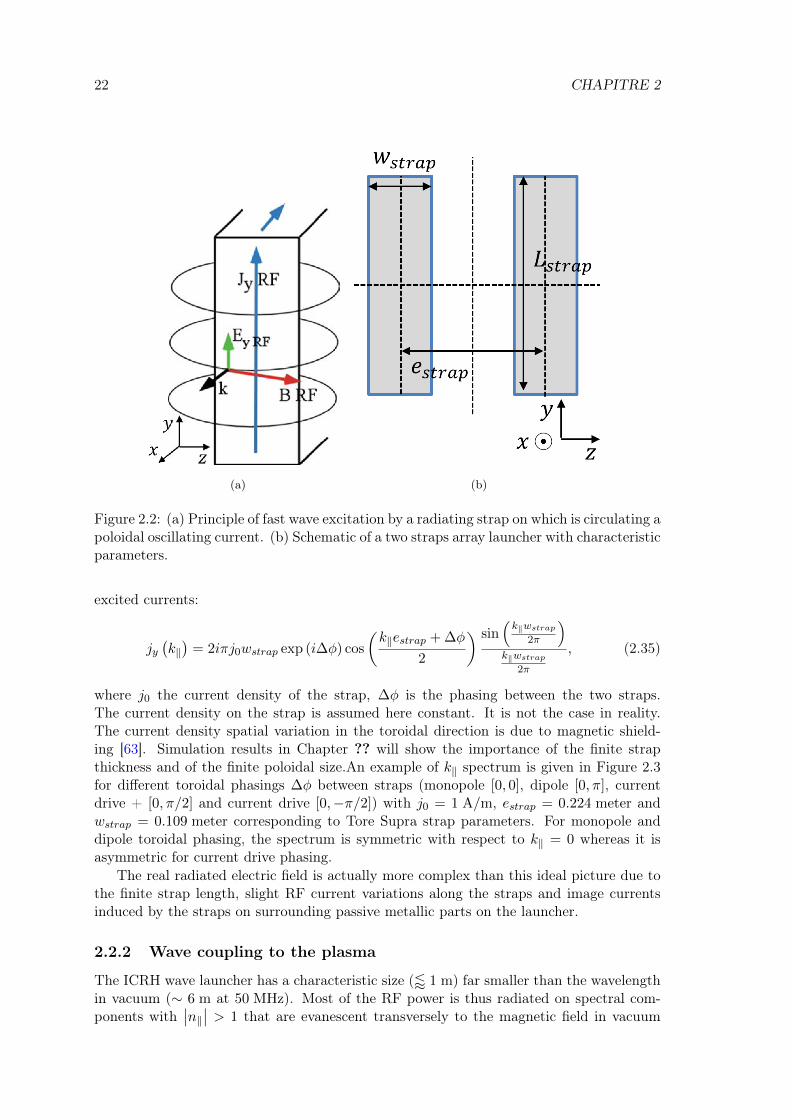
22 CHAPITRE 2

(a) (b)

Figure 2.2: (a) Principle of fast wave excitation by a radiating strap on which is circulating apoloidal oscillating current. (b) Schematic of a two straps array launcher with characteristicparameters.

excited currents:

jy(k‖)

= 2iπj0wstrap exp (i∆φ) cos

(k‖estrap + ∆φ

2

) sin(k‖wstrap

2π

)k‖wstrap

2π

, (2.35)

where j0 the current density of the strap, ∆φ is the phasing between the two straps.The current density on the strap is assumed here constant. It is not the case in reality.The current density spatial variation in the toroidal direction is due to magnetic shield-ing [63]. Simulation results in Chapter ?? will show the importance of the finite strapthickness and of the finite poloidal size.An example of k‖ spectrum is given in Figure 2.3for different toroidal phasings ∆φ between straps (monopole [0, 0], dipole [0, π], currentdrive + [0, π/2] and current drive [0,−π/2]) with j0 = 1 A/m, estrap = 0.224 meter andwstrap = 0.109 meter corresponding to Tore Supra strap parameters. For monopole anddipole toroidal phasing, the spectrum is symmetric with respect to k‖ = 0 whereas it isasymmetric for current drive phasing.

The real radiated electric field is actually more complex than this ideal picture due tothe finite strap length, slight RF current variations along the straps and image currentsinduced by the straps on surrounding passive metallic parts on the launcher.

2.2.2 Wave coupling to the plasma

The ICRH wave launcher has a characteristic size (/ 1 m) far smaller than the wavelengthin vacuum (∼ 6 m at 50 MHz). Most of the RF power is thus radiated on spectral com-ponents with

∣∣n‖∣∣ > 1 that are evanescent transversely to the magnetic field in vacuum

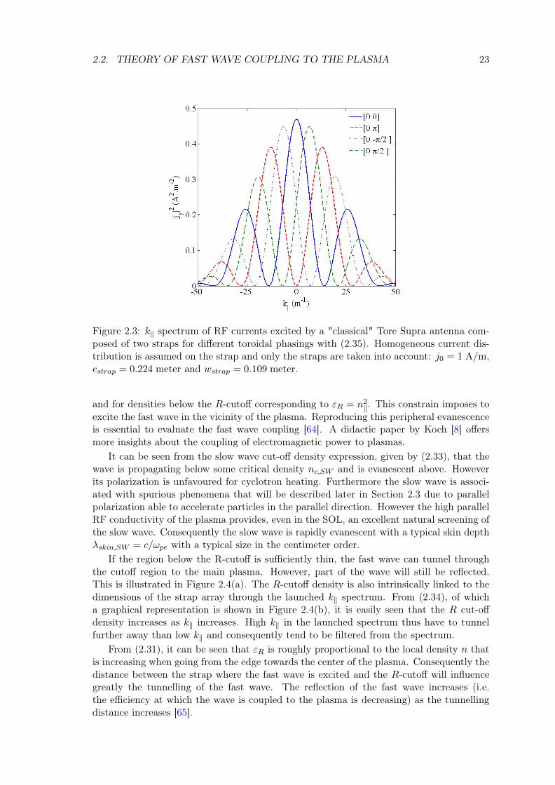
2.2. THEORY OF FAST WAVE COUPLING TO THE PLASMA 23

Figure 2.3: k‖ spectrum of RF currents excited by a "classical" Tore Supra antenna com-posed of two straps for different toroidal phasings with (2.35). Homogeneous current dis-tribution is assumed on the strap and only the straps are taken into account: j0 = 1 A/m,estrap = 0.224 meter and wstrap = 0.109 meter.

and for densities below the R-cutoff corresponding to εR = n2‖. This constrain imposes to

excite the fast wave in the vicinity of the plasma. Reproducing this peripheral evanescenceis essential to evaluate the fast wave coupling [64]. A didactic paper by Koch [8] offersmore insights about the coupling of electromagnetic power to plasmas.

It can be seen from the slow wave cut-off density expression, given by (2.33), that thewave is propagating below some critical density nc,SW and is evanescent above. Howeverits polarization is unfavoured for cyclotron heating. Furthermore the slow wave is associ-ated with spurious phenomena that will be described later in Section 2.3 due to parallelpolarization able to accelerate particles in the parallel direction. However the high parallelRF conductivity of the plasma provides, even in the SOL, an excellent natural screening ofthe slow wave. Consequently the slow wave is rapidly evanescent with a typical skin depthλskin,SW = c/ωpe with a typical size in the centimeter order.

If the region below the R-cutoff is sufficiently thin, the fast wave can tunnel throughthe cutoff region to the main plasma. However, part of the wave will still be reflected.This is illustrated in Figure 2.4(a). The R-cutoff density is also intrinsically linked to thedimensions of the strap array through the launched k‖ spectrum. From (2.34), of whicha graphical representation is shown in Figure 2.4(b), it is easily seen that the R cut-offdensity increases as k‖ increases. High k‖ in the launched spectrum thus have to tunnelfurther away than low k‖ and consequently tend to be filtered from the spectrum.

From (2.31), it can be seen that εR is roughly proportional to the local density n thatis increasing when going from the edge towards the center of the plasma. Consequently thedistance between the strap where the fast wave is excited and the R-cutoff will influencegreatly the tunnelling of the fast wave. The reflection of the fast wave increases (i.e.the efficiency at which the wave is coupled to the plasma is decreasing) as the tunnellingdistance increases [65].

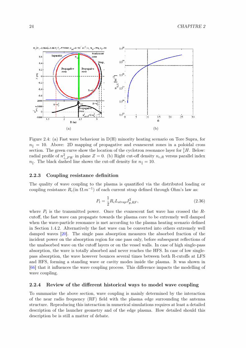
24 CHAPITRE 2

(a) (b)

Figure 2.4: (a) Fast wave behaviour in D(H) minority heating scenario on Tore Supra, forn‖ = 10. Above: 2D mapping of propagative and evanescent zones in a poloidal crosssection. The green curve show the location of the cyclotron resonance layer for 1

1H. Below:radial profile of n2

⊥,FW in plane Z = 0. (b) Right cut-off density nc,R versus parallel indexn‖. The black dashed line shows the cut-off density for n‖ = 10.

2.2.3 Coupling resistance definition

The quality of wave coupling to the plasma is quantified via the distributed loading orcoupling resistance Rc(in Ω.m−1) of each current strap defined through Ohm’s law as:

Pt =1

2RcLstrapJ

2y,RF , (2.36)

where Pt is the transmitted power. Once the evanescent fast wave has crossed the R-cutoff, the fast wave can propagate towards the plasma core to be extremely well dampedwhen the wave-particle resonance is met according to the plasma heating scenario definedin Section 1.4.2. Alternatively the fast wave can be converted into others extremely welldamped waves [20]. The single pass absorption measures the absorbed fraction of theincident power on the absorption region for one pass only, before subsequent reflections ofthe unabsorbed wave on the cutoff layers or on the vessel walls. In case of high single-passabsorption, the wave is totally absorbed and never reaches the HFS. In case of low single-pass absorption, the wave however bounces several times between both R-cutoffs at LFSand HFS, forming a standing wave or cavity modes inside the plasma. It was shown in[66] that it influences the wave coupling process. This difference impacts the modelling ofwave coupling.

2.2.4 Review of the different historical ways to model wave coupling

To summarize the above section, wave coupling is mainly determined by the interactionof the near radio frequency (RF) field with the plasma edge surrounding the antennastructure. Reproducing this interaction in numerical simulations requires at least a detaileddescription of the launcher geometry and of the edge plasma. How detailed should thisdescription be is still a matter of debate.

2.2. THEORY OF FAST WAVE COUPLING TO THE PLASMA 25

Due to limited computational resources, the wave propagation away from the antennaas well as its absorption in the hot core plasma are generally included only as boundaryphenomena in wave coupling codes. Only the vicinity of the antenna is modelled. Soinstead of a volume enclosed by the metallic wall of the tokamak, we have only a fractionof the volume in the vicinity of the antenna with some metallic boundaries and some openboundaries on the computational domain. A similar approach is adopted for Lower Hybridwaves. An exception is presented in ref. [49], where the whole plasma cross-section ismodelled within the cold plasma approximation with artificial collisions. Furthermore,as only the edge plasma is simulated due to computational resources, no mechanism isnaturally included to simulate wave single pass absorption that normally happens in thecentral hot plasma by cyclotron resonance. Some trick has to be included to emulate waveabsorption. Finally in low single-pass regimes of power absorption, cavity modes [66] canbe formed, characterized by partial wave reflection in the boundary condition.

Summarizing waves coupling to the plasma and waves propagation towards the coremagnetized plasma is made difficult due to the strong anisotropy, gyrotropy and inhomo-geneity of the plasma. Therefore the typical wavelengths strongly depend on the directionof the wave propagation with respect to the static magnetic field. The elements in thedielectric tensor ¯ε can have opposite sign. Gyrotropic media are also birefringent. Besides,the hot core plasma can become spatially dispersive. Within the cold plasma approxima-tion, the medium is dispersive in time but not in space.

In the literature several strategies were followed to implement this plasma side bound-ary condition. The standard tool is the spectral surface admittance/impedance matrixformalism [66, 67] according to what is the easiest quantity to manipulate in a given situa-tion. Advanced wave coupling codes relying on this method are TOPICA [30, 31] ICANT[32]) or ANTITER2 [30] for ICRH waves, as well as TOPLHA [68] and ALOHA [69] forLH waves. The method is quite general: it can handle spatially dispersive media and cav-ity modes [66]. However, strictly speaking the interface where the boundary condition isapplied should be a slab approximation of the whole tokamak toroidal/poloidal extension,whereas the emitted near field is intense only in a limited portion of this surface. Besides,the spectral character of the boundary condition is generally not well adapted to the nu-merical methods applied in the main simulation domain near the antenna structure. Allthis translates in a heavy numerical cost as Fourier transforms and multiple integrals arerequired to match the plane waves of the plasma to the vacuum modes. Furthermore, suchcodes model the antenna in vacuum, whereas in reality the antenna is surrounded by a lowdensity plasma that has been neglected until now.

While many heating scenarios have low single pass absorption, antennas are usuallydesigned assuming high single pass absorption. One easy solution to emulate this situationis to implement a lossy radiation medium featuring artificial collisions [70]. But usingthis method, the wave reflection is marginally controlled. In order to use commercial RFsimulation softwares (HFSS [71], MWS [72]), the plasma is even sometimes replaced with anequivalent lossy isotropic dielectric [73–75]. It simplifies the situation as the gyrotropy andthe anisotropy both disappear. However, since the birefringence is also suppressed, only oneeigenmode of the plasma is correctly reproduced. Therefore mode conversion between slowwave and fast wave cannot be reproduced. Furthermore only positive dielectric constantscan be handled in most commercial softwares. In these cases the inner boundary conditionto apply is similar to radiating or transparent boundary conditions.

26 CHAPITRE 2

(a) (b)

Figure 2.5: A finite region of interest where sources, inhomogeneous media, non-linearitiesare being investigated. (a) Sketch of a typical bounded wave-equation problem. An absorb-ing layer is placed adjacent to the edges of the computational region to absorb outgoingwaves without reflection coming from the edge of the absorber. (b) Sketch of a typicalunbounded wave-equation problem that we want to solve as exactly as possible to reality.Courtesy of Steven J. Johnson [79]

2.2.5 Why emulating radiating boundary conditions?

Since in most cases it is impossible to find an analytical solution to Maxwell’s equations(especially in realistic geometries), numerous computational methods have been developedto solve them in a discretized space (finite difference [76], finite element (FEM) [77], finitevolume, transmission line matrix [78]). In all these techniques, the physical space is splitinto elementary cells, elements, volumes that must be smaller than the shortest wavelengthof interest and the smallest details of the geometry of the objects placed within the region ofinterest. Nevertheless, computers do not - and never will - have the computational resourcesto handle an infinite number of elementary cells. It means that Maxwell’s equations canonly be solved for a finite region of space (see Fig. 2.5(a)) and finite spatial resolution.

This is however inconsistent with unbounded problems in electromagnetisms, illustratedby Fig. 2.5(b). In other words, the physical boundary conditions should be placed at infin-ity. On the other hand the unbounded physical space is replaced by a finite computationaldomain due to finite resources. If the problem is solved within this bounded medium,the obtained solution is erroneous. This is the case here since the enclosed torus withmetallic walls cannot be entirely simulated and thus the computational domain is only theimmediate vicinity of the antenna. There are thus some open boundary conditions in thereduced volume. Finding a way to correctly treat open boundaries in radiation problemsis thus one of the accepted challenges in numerical modelling and in particular for finiteelement modelling in order to overcome such contradictory requirements. The answer isthe so-called absorbing boundary conditions (ABCs).

While keeping in mind that the substitution is not perfect, they emulate the infinitespace that surrounds a finite computational domain. Satisfying some requirements, thecomputed solution is then a good estimation of what would be computed, if it was feasible,

2.3. GENERATION OF RADIO-FREQUENCY SHEATHS BY WAVES 27

within a infinite domain. Nevertheless, these ABCs only absorb fields and cannot in anycase replace the sources of the electromagnetic fields. The sources cannot therefore beplaced outside of the ABCs.

The requirements that a ABCs should fulfil depends on its location with respect to thesource of the field. If the ABC is only able to handle homogeneous plane waves, it mustthen be placed far from any sources. If the ABC is however able to handle evanescentfields, it can then be placed close to the source, thus reducing the overall computationaldomain cost.

2.2.6 Short history of radiating boundary conditions

Several local ABCs solutions have been developed over the years. To summarize, thereexist two categories of ABCs:

• global ABCs[80]: the field at any point on the enclosing boundary of a given volumecan be expressed as retarded-time integral of the field upon a surface enclosing allthe sources,

• local ABCs: the field on the boundary is expressed as a function of the field in thevicinity (closest points of the mesh) of the considered point.

As global ABCs are computationally expensive, all widely used ABCs in the past arelocal ABCs. The first technique was extrapolation [81]. It was then followed by “radiatingboundary” [82]. Another one was the matched layer which consisted in surrounding thedomain with an absorbing medium whose impedance matches the impedance of the mainsimulation domain. The most popular one was the one-way approximation of the waveequation initially described by Engquist-Majda ABC [83] for acoustic waves. It was thenapplied to electromagnetism by Mur [84] and generalized later by Trefethen and Halpern[85]. Higdon ABC [86] is also based on the one-way approximation.

However, all of the previously cited ABC techniques share the same Achilles heel.A wave is only absorbed without reflection in particular cases: a plane wave propagatingperpendicularly to the boundary. Since realistic problems in electromagnetism involve bothtravelling and evanescent waves, it is not well suited. In the 1990’s new techniques have thusbeen developed to emulate radiating boundary conditions inside a bounded computationaldomain while overcoming the limitations of the standard ABCs: Perfectly Matched Layer[57] and complementary operators method (COM)[87]. The PML technique will be furtherdeveloped in Chapter 3. The aim here is to use the PML to handle outgoing waves withoutreflections in a plasma filled domain where both the slow wave and fast wave exist. Onthe antenna structure, the boundary conditions could be different from metallic boundaryconditions that are commonly applied in order to account for the non-linear wave-plasmainteractions at the wall due to RF sheaths that will be presented in the next section.

2.3 Generation of radio-frequency sheaths by waves

Spurious interactions [35–37] due to RF sheaths [34] between the peripheral plasma ofmagnetic fusion devices and powered ICRH antennas are often setting the operational limitsof the radio-frequency systems and can even perturb other antennas [44]. Investigationon plasma sheath formation by RF waves has established that the most likely origin ofthis physical mechanism is RF rectification [88, 89]. However, in a tokamak device withICRH power, RF sheaths are associated with plasma waves, which have quite-complicated

28 CHAPITRE2

structures, and they are often classified into the following two broad categories: far-fieldsheaths and near-field sheaths.

First, RF sheaths, referred to as far-field sheaths, are generated on material surfaceswhen a launched FW propagates to a wall due to SOL propagation or poor central ab-sorption [90] and the magnetic flux surfaces do not match the wall shape. In this case theincident FW typically generates a reflected FW and an evanescent SW by mode conversionat the wall together with the rectified sheath potential. Robust analytical models to under-stand the mechanisms behind far-field sheath formation have been developed [51, 91, 92].The sheath potentials resulting from far-field sheaths are considered to be less importantthan near-field sheaths from the standpoint of local damage to material structures. How-ever, if far-field sheaths cover a substantial portion of the wall, it could lead to reducedheating efficiency by sheath power dissipation in the entire sheath volume.

Second, sheaths on the antenna surface and nearby material boundaries, such as lim-iters, are referred to as near-field sheaths. The physical mechanisms behind RF near-fieldssheaths will be explained in Chapter 2. Near-field sheaths are ascribed to the generationof the parasitic slow wave by the current straps on the ICRH antenna. The slow wavehas a large E‖ component (electric field component parallel to the background magneticfield), that can be generated by either antenna currents with a component parallel to themagnetic field line or by spatial variation of the distribution of charge of the straps. Theslow wave then propagates until it reaches a material surface.

Before going in details in the current understanding of the physical ingredients in RFsheath formation, let us introduce some basics concept about sheath with the thermal orDebye sheath.

2.3.1 Recall of the Debye sheath physics

A volume, as illustrated by Figure 2.6, occupied by charged particles consists of two sepa-rate regions:

• The first is the plasma itself which usually fills the majority of the available space.The plasma is by definition electrically neutral or at least quasi-neutral at scale largerthan the Debye length.

• The second is the sheath surrounding all the plasma in the chamber, usually thin andadjacent to a solid surface, which has a greater density of positive ions, and hencean overall excess positive charge, that balances an opposite negative charge on thesurface of a material with which it is in contact.

Poisson’s equation allows determining the characteristic length over which any pertur-bation of potential inside the plasma is screened. The sheath typical size is of the order ofa few electronic Debye length given by [93]:

λDe =

(ε0kBTenee2

)1/2

. (2.37)

Taking typical SOL conditions with Te = 20 eV and ne = 1018 m3 yields a sheath size ofthe order of 10−4 m. This length is much smaller than the typical size of the open magneticfield lines in the SOL. Furthermore, it is also smaller than the typical particles mean freepath in the SOL [3]. This sheath can thus be assumed collisionless.

Due to their higher mobility more electrons reach the wall than ions. As more electronsthan ions leave the plasma, a separation of charge is occurring and positive charge density

2.3 GENERATION OF RADIO-FREQUENCY SHEATHS 29

Figure 2.6: Sketch of the Debye sheath formation at the walls and of transport of particlestowards the walls.

appears in a thin region corresponding to the sheath. The negative potential of the wall inrespect to the plasma generated a self-consistent electric field which repels the electrons andspeed up the ions. In the beginning this electric field is not sufficient to repel significantlythe electrons flux. As more electrons leave the plasma, this electric field increases untilan equilibrium dynamical state is reached where the ions and electrons fluxes in absolutevalue are equal on the wall. At this moment the loss of ions and electrons on the wallare equal. Ions gain energy in the sheath at the expense of the electrons which are cooleddown because only the high velocity electrons can leave the plasma while the other onesare repelled by the sheath potential.

By analysing the sheath side of the plasma-sheath interface, we will find the Bohmcriterion. Assuming steady state, no collisions, inertia free electrons and a Maxwelliandistribution function of the electrons, the Bohm criterion giving the speed of the ions atthe sheath entrance vse can be obtained. Using quasi-neutrality in the plasma, the Poisson’sequation in the sheath, momentum conservation and energy conservation, it gives at theend [93, 94]:

vse ≥ cs =

[kB (Te + γTi)

mi

]1/2

, (2.38)

where γ = 1 for isothermal flow, 5/3 for adiabatic flow with isotropic pressure or 3 for 1Dadiabatic flow, the subscript se denotes the sheath edge with the plasma and cs the soundspeed. In the following, isothermal flow will be assumed. It thus yields γ = 1. The ionvelocity at the sheath entrance must be equal or higher than the sound speed in order toreach the wall. A generalized Bohm criterion has been found within a kinetic approach[95].

Since the ion mean velocity in the plasma is null, the Bohm criterion justifies theexistence of an intermediate quasi-neutral region between the sheath and the plasma whosemain purpose is to transfer energy from the electrons to the ions in order to accelerate themto the sound speed at the sheath entrance. It can alternatively be seen as an “imperfection”in the Debye shielding [93]. As a consequence, a small but non-zero electric field exists inthis region called presheath whose size is much larger than the sheath size. The density atthe sheath edge, due to the pre-sheath existence, is only half of the plasma density at thestagnation point [93]:

nse =ni2. (2.39)

It also gives a condition on the ion speed in the presheath-sheath interface: vse ≤ cs.The ion velocity at the sheath entrance is thus vse = cs.

30 CHAPITRE2

Equalling electrons and ions fluxes at the sheath entrance gives the potential drop inthe sheath compared to the plasma [93]:

Vf =kBTe

2eln

[2πme

mi

(1 +

TiTe

)]. (2.40)

This potential is also called floating potential since no other force, except the one createdby the plasma, acts on the wall. Note that the density does not intervene. Since theelectron mass is much smaller than the ion mass, Vf is negative. The Ti dependence iseasily explained. The higher the ion temperature is, the higher the ion flux of the wall is andthe lower the electric field necessary to accelerate them to the Bohm speed is. The floatingpotential is this smaller. The 1/Te dependence is explained by the inverse reasoning. Foran electrically insulated wall, the wall will be negatively biased at Vf . For a wall connectedto ground, the plasma will be positively biased to −Vf . The I-V characteristic of a 1Dnon-magnetized sheath has the following form [93]:

I = j+

[1− exp

(e (Vf − V )

kBTe

)](2.41)

wherej+ = 0.5enics (2.42)

is the local ion saturation current, Vf the local floating potential given by (2.40) and Vf−Vis the potential difference between the plasma and the collecting plate. It has a ionic termcontribution (first term on the left hand side) and a electronic contribution (second termin the left hand side). This expression holds true as long as Vf − V > 0 (i.e. as long as asheath exists at the plasma-wall interface).

When there is no magnetic field or when the magnetic field is normal of the wall inan ideal situation, it has no influence on the sheath description [93]. In reality however,surfaces are tilted to spread the power onto the target. The tilt of the magnetic fieldwill change the sheath description [96]. For the sheath to form, the incident angle of themagnetic field compared to the wall should not be too small. Otherwise, if case of grazingincidence, the electron loss to the wall is negligible due to the gyromotion of the electrons.The criterion for the sheath formation takes the following form:

sinα =BnB

>

(me

mi

)1/2

, (2.43)

where Bn is the perpendicular component of the static magnetic field with respect thewall. Below that limit the present sheath theory becomes questionable since ions canbe lost faster than electrons. When the magnetic field is not perpendicular to the wall,another region called magnetic presheath appears [96–98]. It mainly affects the ion velocitycondition at the sheath edge that must be along the magnetic field direction.

Until now, no RF electric fields were assumed. When they exist, the electrons arefurther accelerated and the electron density in the sheath oscillates at the wave frequencywhile the ions are considered immobile. It results that more electrons are lost and theplasma becomes positively charged to compensate this additional losses induced by the RFelectric field component, as it will be shown in Section 2.3.2.

2.3.2 Properties derived from principles driving oscillating sheaths forself-consistent modelling

Self-consistent modelling of RF sheaths towards first principles have just started a fewyears ago to take into account the fact that the RF sheath itself modifies the boundary

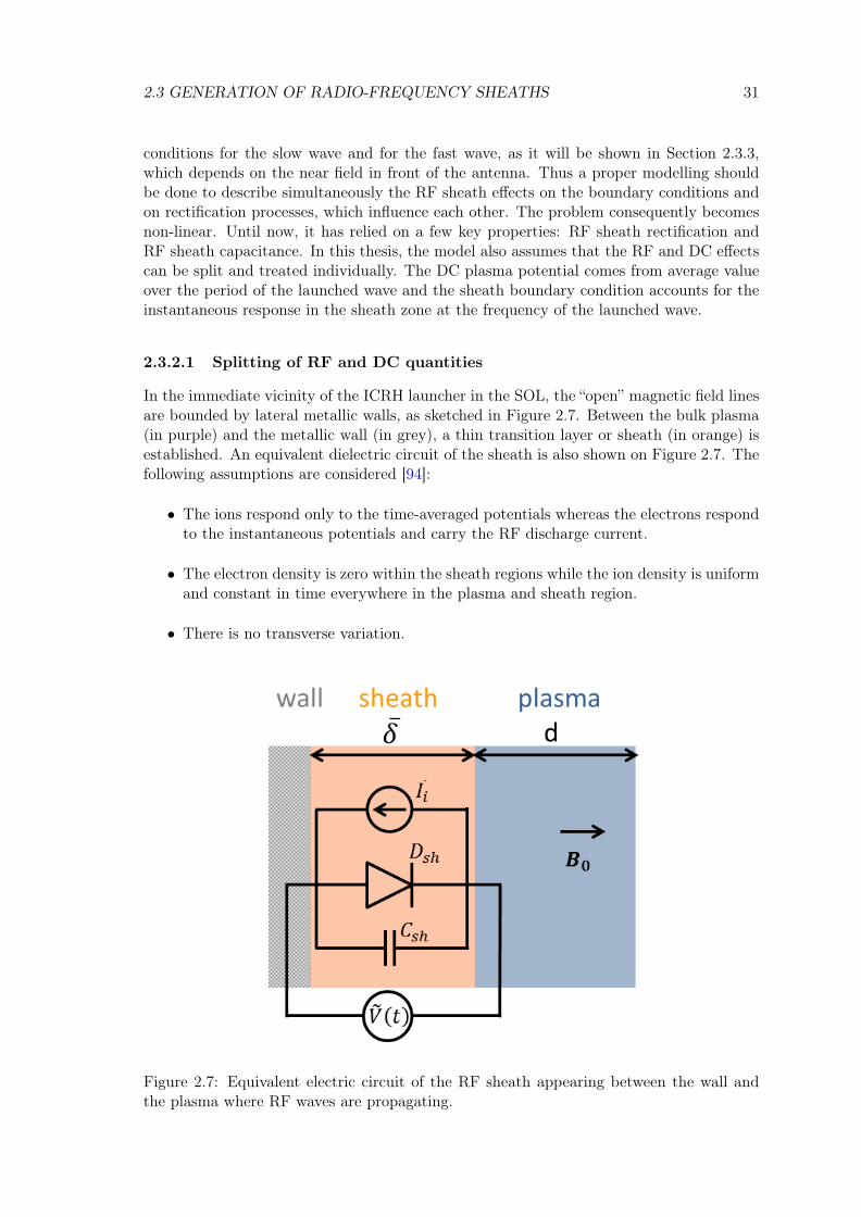
2.3 GENERATION OF RADIO-FREQUENCY SHEATHS 31

conditions for the slow wave and for the fast wave, as it will be shown in Section 2.3.3,which depends on the near field in front of the antenna. Thus a proper modelling shouldbe done to describe simultaneously the RF sheath effects on the boundary conditions andon rectification processes, which influence each other. The problem consequently becomesnon-linear. Until now, it has relied on a few key properties: RF sheath rectification andRF sheath capacitance. In this thesis, the model also assumes that the RF and DC effectscan be split and treated individually. The DC plasma potential comes from average valueover the period of the launched wave and the sheath boundary condition accounts for theinstantaneous response in the sheath zone at the frequency of the launched wave.

2.3.2.1 Splitting of RF and DC quantities

In the immediate vicinity of the ICRH launcher in the SOL, the “open” magnetic field linesare bounded by lateral metallic walls, as sketched in Figure 2.7. Between the bulk plasma(in purple) and the metallic wall (in grey), a thin transition layer or sheath (in orange) isestablished. An equivalent dielectric circuit of the sheath is also shown on Figure 2.7. Thefollowing assumptions are considered [94]:

• The ions respond only to the time-averaged potentials whereas the electrons respondto the instantaneous potentials and carry the RF discharge current.

• The electron density is zero within the sheath regions while the ion density is uniformand constant in time everywhere in the plasma and sheath region.

• There is no transverse variation.

Figure 2.7: Equivalent electric circuit of the RF sheath appearing between the wall andthe plasma where RF waves are propagating.

32 CHAPITRE2

From (2.10), the admittance of a bulk plasma slab of thickness d and cross-sectionalarea A gives in the absence of magnetic field and with electron–neutral collisions [94]:

Yp = jωC0 +1

jωLp +Rp, (2.44)

where C0 = ε0A/d is the vacuum capacitance, Lp = ω−2pe C

−10 is the plasma inductance

and Rp = νmLp is the plasma resistance. νm is the electron–neutral collision frequency formomentum transfer. This form for Yp represents the series combination of Lp and Rp inparallel with C0. The displacement current that flows through C0 is much smaller than theconduction current that flows through Lp and Rp. Assuming that the sheath capacitancehas a similar form than the plasma capacitance Csh = ε0A/δ gives when compared a factord/δ. The sheath capacitance is thus much greater than the plasma capacitance since d δ.

In the same way comparing Csh with Lp gives a ratio ω−2pe C

−20 δ/d. With the typical

electron density in the SOL of a tokamak being ≈ 1018 m−3, it results in Lp Csh. Theinductive impedance of the bulk plasma is small compared to the capacitive impedance ofthe sheaths, such that almost all the applied RF voltage due to RF waves appears acrossthe sheath. The electrostatic approximation is assumed in the sheath region. The resistivepart of the sheath is neglected. It is assumed that the RF current is mainly a displacementgoing through the capacitor branch of the circuit. When dealing with DC currents, theconduction currents through the sheaths go entirely through the diode [94]. Consequentlya clear separation can be made between RF and DC effects. Association of DC currentswith the diode and RF current with the capacitor is the simplest model. More complexmodels would assume otherwise.

The instantaneous sheath potential V (t) is supposed to be composed of a DC part VDCand of an RF part oscillating at the RF generator frequency ω0 and with amplitude VRF .No other frequency is considered, contrary to [99]. It yields:

V (t) = VDC + VRF cos (ω0t) , (2.45)

where VRF is function of the RF electric field ERF whose field distribution is supposedknown. VRF is the oscillating sheath voltage generated by RF waves. The wall is assumedelectrically grounded, so that the DC sheath potential VDC is also the local DC plasmapotential. The instantaneous sheath voltage V (t) associated with the instantaneous con-duction current into the sheath I (t) gives the ideal sheath I-V characteristic:

I (t) = j+

1− exp

e(Vf − V (t)

)kBTe

(2.46)

where j+ is the local ion saturation current (2.42), Vf the local floating potential in theabsence of RF waves given by (2.40). The factor 0.5 in j+ accounts for the density drop inthe presheath according to (2.39). cs is the ion sound speed at the sheath entrance ((2.38))and ni is the plasma density. This I-V electrical characteristic was rigorously establishedfor DC sheaths with a wall normal to B. No equivalent presently exists with tilted B0,like the Chodura model for DC sheaths [96].

2.3.2.2 Sheath rectification

Since the sheath exhibits a non-linear I-V characteristic, a rectification process occurs thatprovide the RF to DC coupling. The sheath I-V characteristic established for DC behaviour

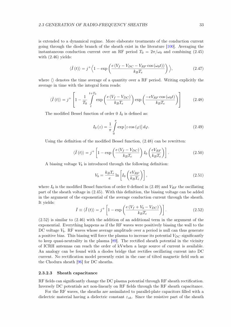
2.3 GENERATION OF RADIO-FREQUENCY SHEATHS 33

is extended to a dynamical regime. More elaborate treatments of the conduction currentgoing through the diode branch of the sheath exist in the literature [100]. Averaging theinstantaneous conduction current over an RF period T0 = 2π/ω0 and combining (2.45)with (2.46) yields:

〈I (t)〉 = j+⟨

1− exp

(e (Vf − VDC − VRF cos (ω0t))

kBTe

)⟩, (2.47)

where 〈〉 denotes the time average of a quantity over a RF period. Writing explicitly theaverage in time with the integral form reads:

〈I (t)〉 = j+

1− 1

T0

t+T0∫t

exp

(e (Vf − VDC)

kBTe

)exp

(−eVRF cos (ω0t)

kBTe

) (2.48)

The modified Bessel function of order 0 I0 is defined as:

I0 (z) =1

π

π∫0

exp [z cos (ϕ)] dϕ. (2.49)

Using the definition of the modified Bessel function, (2.48) can be rewritten:

〈I (t)〉 = j+

[1− exp

(e (Vf − VDC)

kBTe

)I0

(eVRFkBTe

)]. (2.50)

A biasing voltage Vb is introduced through the following definition:

Vb =kBTee

ln

[I0

(eVRFkBTe

)], (2.51)

where I0 is the modified Bessel function of order 0 defined in (2.49) and VRF the oscillatingpart of the sheath voltage in (2.45). With this definition, the biasing voltage can be addedin the argument of the exponential of the average conduction current through the sheath.It yields:

I ≡ 〈I (t)〉 = j+

[1− exp

(e (Vf + Vb − VDC)

kBTe

)]. (2.52)

(2.52) is similar to (2.46) with the addition of an additional term in the argument of theexponential. Everything happens as if the RF waves were positively biasing the wall to theDC voltage Vb. RF waves whose average amplitude over a period is null can thus generatea positive bias. This biasing will force the plasma to increase its potential VDC significantlyto keep quasi-neutrality in the plasma [89]. The rectified sheath potential in the vicinityof ICRH antennas can reach the order of kVwhen a large source of current is available.An analogy can be found with a diodes bridge that rectifies oscillating current into DCcurrent. No rectification model presently exist in the case of tilted magnetic field such asthe Chodura sheath [96] for DC sheaths.

2.3.2.3 Sheath capacitance

RF fields can significantly change the DC plasma potential through RF sheath rectification.Inversely DC potentials act non-linearly on RF fields through the RF sheath capacitance.

For the RF waves, the sheaths are assimilated to parallel-plate capacitors filled with adielectric material having a dielectric constant εsh. Since the resistive part of the sheath

34 CHAPITRE2

is neglected, εsh does not include an imaginary term representing power dissipation in thesheath. This description is motivated since the sheath is a region depleted of electronssimilar to vacuum. In-line with this view, the distance between the capacitor plate is ofthe order of the local, time average sheath width δ. It is implicitly assumed that theRF current through the sheaths is predominantly a linear displacement current that goesexclusively through the capacitor. Despite the high RF oscillations amplitude, the sheathwidth δ follows the Child-Langmuir law for plane electrodes [101, 102]:

δ (x, y) = λDe

(eVDC (x, y)

kBTe

)3/4

, (2.53)

where λDe is the electron Debye length whose expression is given by (2.37).The Child-Langmuir law was established for DC sheaths. In the context of capacitive

RF discharges, more refined models were developed in [100, 103]. In presence of high powerwaves, the instantaneous sheath width may be subject to large RF oscillations at frequencyω0 around its mean value, which may affect the sheath capacitance. They indicate that theChild-Langmuir law should be modified by multiplying it by a factor

√50/27 ≈ 1.36 to

take into account oscillating effects whereas the effective sheath dielectric constant shouldbe εsh ∼ 1.226 instead of εsh ∼ 1. The dimensionality of the ratio εsh/δ is equivalent to acapacitance per surface unit:

C∗sh =εshδ. (2.54)

2.3.3 Sheath boundary conditions

The sheath capacitance C∗sh will modify the behaviour of the sheaths in presence of RFwaves. Since the sheath width δ usually is much thinner by several orders of magnitudethan the typical toroidal extension L‖ of the simulation domain, its consequence on theRF electric field propagation is accounted for via a RF sheath boundary condition (SBC)that replaces the classical metallic boundary condition, as it will be shown later duringnumerical tests in Chapter 5. Myra and D’Ippolito developed the sheath boundary con-ditions formalism to account for this effect [53]. Although they rigorously prevail only atthe sheath/plasma interface, the RF-SBC is applied directly at the wall. Then it wouldbe virtually impossible at this time to calculate detailed wave phenomena over the entirevolume of the SOL and in the sheaths simultaneously. As the typical spatial scales are verydifferent, a prohibitive number of grid points would be required in the mesh if the typicalgrid size is adjusted to the size needed to get a fine enough spatial resolution of the physicsin the sheath region. Thus huge amount of computational resources would be required andconsumed. Some adjustments could be however made with multi-scales grids but the gridsshould not be vastly different at the interfaces for a numerically stable calculation.

An arbitrary tilt of the static magnetic field is envisaged as shown in Figure 2.8. Thecomplete derivation can be found in [53, 104]. Two coordinate systems are defined. Thefirst one is defined with respect to the magnetic field whereas the second one is definedwith respect to the wall surface or the sheath surface. The RF electric field E relative toboth the sheath surface and the magnetic field thus reads:

E=(Enen + Et) exp (ik · r− iωt)=(E‖b + E⊥

)exp (ik · r− iωt) . (2.55)

In ICRH, the value of k0 is usually much smaller compared to kt. The sheath is alsoassumes to be thin. Then the electrostatic approximation is valid in the sheath region.

2.3 GENERATION OF RADIO-FREQUENCY SHEATHS 35

Figure 2.8: Schematic representation of the sheath and the two coordinate systems definedwhen the magnetic field is tilted. The first system is with respect to the magnetic field(b, e⊥). The second system is with respect to the wall (et, en). The normal en is definedto point from the wall to the plasma.

This requires:|kt| δ 1, (2.56)

where δ is till the local time averaged sheath width. In the electrostatic limit, the electricfield in the sheath is expressed only with the electric potential Φsh as follows:

E(sh) = −∇V (sh)RF . (2.57)

Since the interest is only on the sheath effect on the fundamental wave component atfrequency ω, the oscillating motion of the sheath at frequency ω can be neglected. Theboundary condition is thus applied at the location of the time averaged sheath width.Electromagnetism theory imposes the continuity of Dn = en · D = en · ¯ε · E across an ar-bitrary interface. Here the interface separates the plasma region from the sheath region.Superscripts (pl) and (sh) denote quantities on the plasma side and on the sheath side re-spectively. A discontinuity in the mean density is assumed between the plasma and sheath.Consequently a discontinuity is also present in the dielectric tensor. εsh is the sheath di-electric constant defined in Section 2.3.2.3. At the plasma-sheath interface, continuity ofDn reads:

D(sh)n ≡ εshE(sh)

n = D(pl)n . (2.58)

In the electrostatic limit, (2.57) is combined with (2.58) to give:

− εsh∇V shRF = D(pl)

n . (2.59)

Integrating (2.59) from the metallic wall through the sheath in the direction of thenormal vector en yields:

− εshΦ(sh) = δD(pl)n , (2.60)

with the conditions V (sh)RF = 0 on the wall and V

(sh)RF = VRF at the sheath-plasma inter-

face. Taking the tangential gradient Et = −∇tφ of (2.60) and imposing the continuityof the tangential electric field Et across an interface according to classical macroscopicelectromagnetism theory yields:

Et(sh) = ∇t

(δ

εshD(pl)n

). (2.61)

36 CHAPITRE2

which gives the constraint only involving the RF fields on the plasma side of the sheath-plasma interface. Note that in the limit when the sheath vanishes (δ → 0), (2.61) reducesto the usual metallic BC. Remembering (2.54), (2.61) can be re-written:

Et(pl) = ∇t

(1

C∗shD(pl)n

). (2.62)

The superscript (sh) in (2.61) is replaced by (pl) in (2.62) on the left hand side. From(2.62), the right hand side represents the effect of the sheath capacitance on the parallelelectric field structure. It will thus influence the slow wave propagation in the plasma.

In the case where B is perpendicular to the wall, en = b and et = e⊥. Dropping alsothe (pl) superscript, (2.62) consequently reads:

E⊥ = ∇⊥(

1

C∗shD‖

). (2.63)

The sheath capacitance expression in (2.54) allows us to define an expression for theoscillating sheath voltage VRF in (2.45) that reads:

VRF =

∮ERF · dl =

Dn

C∗sh. (2.64)

It may be noteworthy to recall that when∣∣ε‖∣∣ is high that the FW and the SW are

totally decoupled. Moreover if the wall is perpendicular to B than Dn = ε‖E‖. In thatcase the parallel electric field E‖ is mainly due to the SW.

A new class of modes, called Sheath-Plasma Waves (SPW) [53], arises from the SBCsas they do not exist with metallic BCs.

The form of (2.62) results of course from the approximation that the current carriedthrough the sheath is a displacement current in the immobile ion limit. What wouldbecome the SBC if a part of conduction current was also accounted for? The electrostaticapproximation is justified in the thin sheath limit. As the sheath width δ was averaged overtime, the SBC moreover assumed the static sheath approximation that neglect the effectsof the wave harmonics and of the sheath dynamical oscillations. The density is assumed asthe time average density in the present model. The impact of the fast time scale physicson slow time scale physics only started to be considered due to its complexity [105].

The derivation of the sheath boundary condition assumes that the sheath is effectivelya vacuum region for the RF waves, which corresponds to the zero-th order in the sheathdescription [92].

The resistive part of the sheath was neglected and only its capacitive nature was ac-counted for. Calculations in ref [53] however suggest that the validity of this assumptionis better for larger amplitude of E‖.

Finally kinetic effects must be considered to investigate the correct physics inside thesheath, at least to verify that the present assumptions made to derive the sheath boundarycondition are enough to capture the essential physics. It thus raises the question on how toconnect a kinetic sheath with a cold plasma and how to handle the additional cost of kineticequations where integrals must be evaluated numerically instead of analytical expressions.

2.3.4 DC biasing model of the SOL plasma with DC conductivity tensor

A constant homogeneous electric field applied perpendicularly to the static magnetic fieldB in fully ionized plasmas causes E×B drift for both ions and electrons with a common

2.3 GENERATION OF RADIO-FREQUENCY SHEATHS 37

velocity in amplitude and in direction. Thus, no separation of charges occurs, no frictionoccurs and hence no particles flux and no DC currents along the electric field direction aregenerated. The transverse DC conductivity in steady state is zero. In partially ionizedplasmas, DC current are simply proportional to the applied electric field with the relationj = σDCE where σDC is the DC conductivity determined by collisions between chargedparticles and neutrals.

Several observations indicating the presence of perpendicular DC currents have never-theless been reported in many experiments such as ASDEX Upgrade [106]. One exampleis provided by biasing experiments where an electrode is installed into the plasma insidethe separatrix and a voltage is applied between the electrode and the limiter (or divertor).It results first in a bias of the whole flux surface due to the huge Spitzer parallel conduc-tivity (1.7). Second, radial DC current flows from the core through the separatrix towardsanother electrode (limiter) was measured [107]. A flux average transverse DC conductivityhas thus been deduced.

Moreover DC currents, ascribed to RF sheaths, have been observed in several exper-iments on TEXTOR [37], ASDEX Upgrade [108] and Tore Supra [46] in the vicinity ofactive ICRH antennas. Negative currents have been measured near the antenna structureand positive current far from it [42] on magnetic field lines connected to the powered ICRHantenna. Probes are measuring significant floating potential on the outer side of the activeantenna [45]. However the path between the probe and the antenna follow the magneticfield line that is intersected by the antenna side limiter, as it will be shown in Section 2.4.Then how can the probe measure floating potential on the outer side of the limiter whenit is not supposed to be connected magnetically to the active part of the antenna? Dur-ing the last experimental campaign on Tore Supra in 2011, larger radial structures of thefloating potential with larger amplitude was measured on the prototype Faraday screen(see Section 2.4.5) compared to the classical Faraday screen. Is there a link between boththat can explained the larger structures? Is the antenna status and geometry modifyingthe transport parameters of the SOL.

It is noteworthy to mention that the DC perpendicular conductivity can only be asmall fraction of the parallel Spitzer conductivity (1.7), since huge gradient of DC plasmapotential will appear in the radial direction [45, 109].

Several theoretical modelling of RF sheaths proposed explanations for DC currents[54, 110]. Different mechanisms for the formation of radial electric field in a tokamak havebeen proposed [111, 112]: ions-neutrals collisions, viscosity and inertia. DC currents infully ionized plasmas arise only in presence of inhomogeneous electric fields (polarizationcurrent is neglected since there is no temporal derivative of the electric field). As a result,the DC current density is not proportional to the electric field but to its spatial derivatives.Ions-neutrals collisions are associated with the first order derivative whereas viscosity andinertia are associated with second and third derivatives, respectively. This indicates that,generally speaking, it is incorrect to introduce the DC conductivity tensor as it is commonlydefined. Instead one can introduce with analogy an “effective” DC conductivity tensor usingdimensionality arguments.

Writing the particle and momentum balance equations for electrons and ions givesaccess to the expressions of the different terms for the perpendicular DC current [112].Each term is associated to one possible mechanism of radial DC currents formation writtenwith the DC plasma potential VDC :

• Friction ion-neutrals: In the case of ion collisions with neutrals, the transverse

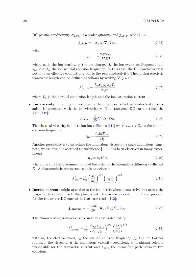
38 CHAPITRE2

DC plasma conductivity σ⊥DC is a scalar quantity and j⊥i−N reads [112]:

j⊥i−N = −σ⊥DC∇⊥VDC , (2.65)

with

σ⊥DC = −niq2i νiN

MiΩ2i

, (2.66)

where ni is the ion density, qi the ion charge, Ωi the ion cyclotron frequency andνiN << Ωci the ion neutral collision frequency. In this case, the DC conductivity isnot only an effective conductivity but is the real conductivity. Then a characteristictransverse length can be defined as follows by writing ∇ · j = 0:

λ2j,i−N =

L‖σ⊥DCkBTe

2ej+, (2.67)

where L‖ is the parallel connexion length and the ion saturation current.

• Ion viscosity: In a fully ionised plasma the only linear effective conductivity mech-anism is associated with the ion viscosity η. The transverse DC current takes theform [112]:

j⊥vis =η

B2∇⊥∆⊥VDC (2.68)

The classical viscosity is due to ion-ion collisions [111] where νii << Ωci is the ion-ioncollision frequency:

ηB =0.3nTiνii

Ω2i

(2.69)

Another possibility is to introduce the anomalous viscosity ηA since anomalous trans-port, whose origin is ascribed to turbulence [113], has been observed in many exper-iments:

ηA = niMiµ, (2.70)

where µ is a mobility assumed to be of the order of the anomalous diffusion coefficientD. A characteristic transverse scale is associated:

λ2vis = ρ2

ci

(Mi

me

)1/4( µ

ρ2ciνii

)1/2

. (2.71)

• Inertia currents might arise due to the ion inertia when a convective flux across themagnetic field exist inside the plasma with transverse velocity ud. The expressionfor the transverse DC current in that case reads [112]:

j⊥inertia = −niMi

B2(u⊥ ·∇⊥)∇⊥VDC . (2.72)

The characteristic transverse scale in that case is defined by:

λ2inertia = ρ2

ci

(udcs

λmfpρci

)2/3(Mi

me

)1/3

(2.73)

with me the electron mass, νii the ion ion collision frequency, ρci the ion Larmorradius, η the viscosity, µ the anomalous viscosity coefficient, ud a plasma velocityresponsible for the transverse current and λmfp the mean free path between twocollisions.

2.3 GENERATION OF RADIO-FREQUENCY SHEATHS 39

2.3.5 Previous RF sheath modelling

We have seen that sheaths are thin positively charged regions in between the plasmaand a wall whose existence maintains quasi-neutrality in the plasma. When sheaths aresubjected to a RF potential in discharges or to RF waves in tokamaks, they oscillate andinduce strong DC rectified potentials in the plasma [114]. An exhaustive description of RFsheaths would be fairly complex as different time scales and length scales would have to beaccounted for with a kinetic description of a magnetized plasma containing several specieswhere RF oscillations exist over a complex geometry such as a antenna. Such a descriptionis presently impossible (and may always be). Instead partial advancements have been madeby focusing individually on one aspect of the general problem with tools (theoretical andnumerical) getting more and more complex. A few of these major advancements, in myopinion, will be briefly stated here.

The cold plasma approximation is usually adopted in the description. The most com-mon way to treat RF sheaths has been by evaluating a rectified potential due to RF wavespenetrating the sheaths. A voltage difference thus appears between two 1D capacitor platesalong the magnetic field line calculated with

∫|E · dl|. This approach has been able to pre-

dict the poloidal location of high sheath regions on “long field lines” and strap phasingeffects. A Faraday screen prototype on Tore Supra was designed following this approachby minimizing the integrated parallel electric field along long field lines. But recent unex-pected results during experiments with the ICRH system on [56] show that this Faradayscreen failed to minimize RF sheaths. On Alcator C-Mod, a field aligned antenna did notminimize RF sheaths [49, 109] but it did reduce sputtering and impurity contamination.The main issues likely come from the dimensionality reduction from 2D to 1D by integrat-ing along field lines and the lack of the reverse feedback of the influence of the plasma DCbiasing on the RF wave propagation. Linking only the fast time scale to the slow timescale is not enough. The reverse feedback of the slow time scale on the fast time scale isalso necessary. In addition this approach seems to favour the far electric field whereas thenear electric fields are more likely to play a role in RF formation on the antenna structure.A better description of the magnetic field lines topology is also necessary.

One main issue if the numerical simulation covers a significant volume is the prohibitivenumerical cost of meshing the sheaths and the plasma due to their very different scalelengths whether with the finite difference or the finite elements methods. A truly accuratedescription of RF-sheath interactions needs also to consider kinetic effects and detailedsheath structures. However to capture the essential impact of sheaths on waves in the SOLand sheath potentials, the concept of RF sheaths boundary condition was developed byMyra and D’Ippolito [53, 91]. It is now able to handle the fast wave in addition to theslow wave. The sheaths at the material boundaries are treated as a thin vacuum layer forthe RF waves. A similar approach was pursued for modelling sheath formation in plasmaprocessing [115, 116].

Kohno [92] adopted the sheath boundary conditions formalism in a new finite elementnumerical scheme for analysing self-consistent radio-frequency (RF) sheath-plasma interac-tion problems in the ion cyclotron range of frequencies in simplified models for the SOL ofa tokamak. He performed numerical analyses in one and two-dimensional domains severalimportant physical properties (e.g. existence of multiple roots, hysteresis effects, sheath-plasma waves). However, even if the description is self-consistent, the description of theslow time-scale remains simple. No DC conductivity tensor is considered. No DC currentsexchange are thus allowed. The antenna description is also simple. However the finiteelement scheme allows a better description of the antenna geometry in the future.

An attempt by Van Compernolle to implement the sheath boundary condition into

40 CHAPITRE2

TOPICA antenna code [31, 117] using a realistic ICRH antenna model was made [118].However, this work stopped at a primitive level. First, the sheath boundary condition isintroduced to a vacuum RF model. This corresponds to a vacuum sheath. The bound-ary condition is thus not coupled with the plasma dielectric tensor, yielding unphysicalconsequences.

Smithe [119, 120] has been modelling on large scale computers with the time domainsoftware package VORPAL [121] the behaviour of 3D imported drawings of the antennafacing a cold plasma with non linear sheath boundary conditions. He also investigatedthe numerical stability of finite difference time domain scheme mixing together implicitand explicit terms in the context of non-linear phenomena involving radio-frequency waves[122].

Electromagnetism PIC (Particle in Cell) simulations for sufficiently small volumes cangrasp relevant sheaths physics [123]. However PIC methods cannot be used for largevolumes such as simulating the behaviour of an ICRH antenna in the SOL of a tokamakdue to the prohibitive numerical cost and time.

An asymmetric double probe model can lead to the generation of parallel DC currents[54]. Comparison of the fluid model with a PIC code gave similar results. A more accuratefluid description of the density with the DC potential is performed in [124]. Howeverthe double probe rectification model is simple. Circulation of DC currents decreases theDC plasma potential. The transverse transport is enhanced by convective fluxes and DCcurrents able to bring density around the biased flux tube.

A recent work tried to account for the wave dynamic in the sheaths and the densityin the sheaths with respect to the orientation of the magnetic field [105]. It proposed togo even further to first principles and simultaneously solving Maxwell equations togetherwith the equation of motion and the continuity equation (possibly augmented with theenergy equation) rather than solving the equation of motion is an approximate way for acold plasma. In addition, a detailed description of the ion and electron behaviour in thesheath layer itself is possible in order to understand the power losses in the sheath. TheSBC approach cannot take these effects into account. Only the fast time-scale is accountedfor. Such sophisticated description is however even more costly and numerical convergenceis not ensured.

2.4 Overview of the ICRH system on Tore Supra

During RF heating and current drive, electromagnetic waves are launched from the outeredge of the plasma usually at low field side due to technical accessibility and propagate toa desired location inside the plasma where absorption must take place. This section willgive a brief overview on the inner working if an ICRH system focusing on Tore Supra. Thesystem is designed to couple high power waves to the plasma with the maximum achievableefficiency while keeping at an acceptable level the spurious interactions due to the presenceof the RF sheaths that often impose the operational limits of the system as local overheatedzone (i.e. hot spots) and impurity release into the plasma.

2.4.1 Synopsis of the excitation on high power waves in tokamaks

Whatever the frequency domain, the schematic diagram of the RF system, shown on Fig-ure 2.9, is the same. The RF source is driven by a high voltage power supply which, inturn, is connected to the standard electrical grid at 50 Hz. The electromagnetic energycarried by the waves is transmitted from the source to the launcher through a transmission

2.4. OVERVIEW OF THE ICRH SYSTEM ON TORE SUPRA 41

Figure 2.9: Schematic diagram of a RF system on a tokamak.

line network. The launcher is a structure that acts as an interface between the transmissioncircuit and the edge of the plasma.

The type of source depends upon the operating frequency. For ICRH typical frequen-cies, the source is called tetrode [125] or triode, whereas for LH and ECRH they are calledrespectively klystron [126] and gyrotron [127]. They usually deliver power between 100 kWand 1 MW CW.

The type of transmission circuit also depends of the frequency domain. For LH andECRH typical frequencies, waveguides are used. They are rectangular gas pressurized forLH whereas they are circular vacuum pumped for ECRH. For ICRH, the transmission linesare coaxial waveguides pressurized with nitrogen.

The launcher form is also frequency dependent. The ECRH system uses mirrors [128]whereas the LH system uses an array of waveguides [129]. For the frequency domain evokedin this thesis, it was shown in Section 2.2.1 that the launcher must be an array of radiatingstraps. Only the ICRH system will be further described in the context of Tore Supra.

2.4.2 ICRH system on Tore Supra

As the main additional heating system and the only means to heat the ions, in the absenceof high-power neutral beam injection, the ICRH system [41, 130] plays a central role inplasma scenario developments on Tore Supra.

As said above, a RF system on a tokamak is composed on RF source, a transmissionline for the waves transmission to the launcher and a launcher. On Tore Supra, threehorizontal ports are dedicated to ICRH antennas. These ports are fed by six transmissionlines connected to the RF power plant composed of three modules of two generators each,one per launcher. The six identical RF power lines each features a synthesizer, a modulator,a solid-state wideband amplifier and a three-stage THALES tetrode amplifier. The highpower stage is based on a TH525 tube [131]. The pulse duration is limited to 30 s atnominal power (2.2 MW per generator) and 500 kW in steady-state operation.

Because of the launcher electrical circuit, the six 80 m long coaxial transmission linesinstalled from the generator to the torus hall operate in nearly matched conditions in mostsituations. They are pressurized by 3 bar of nitrogen to raise the arcing threshold (i.e.lower the sensitivity to arcs). In terms of operation and development, the most criticalpart of the transmission line is the vacuum window, located just behind the vessel portplate for easy maintenance and replacement. The present thermal limitation of the RFlines is 2.5 MW for 30 s or 800 kW in steady state.

2.4.3 Two electrical layouts for the Tore Supra ICRH antennas

A Tore Supra ICRH antenna is a sizable object with typical dimensions about 8 m ×60 cm× 60 cm that weights about 5 tons. It is designed to operate in the frequency range

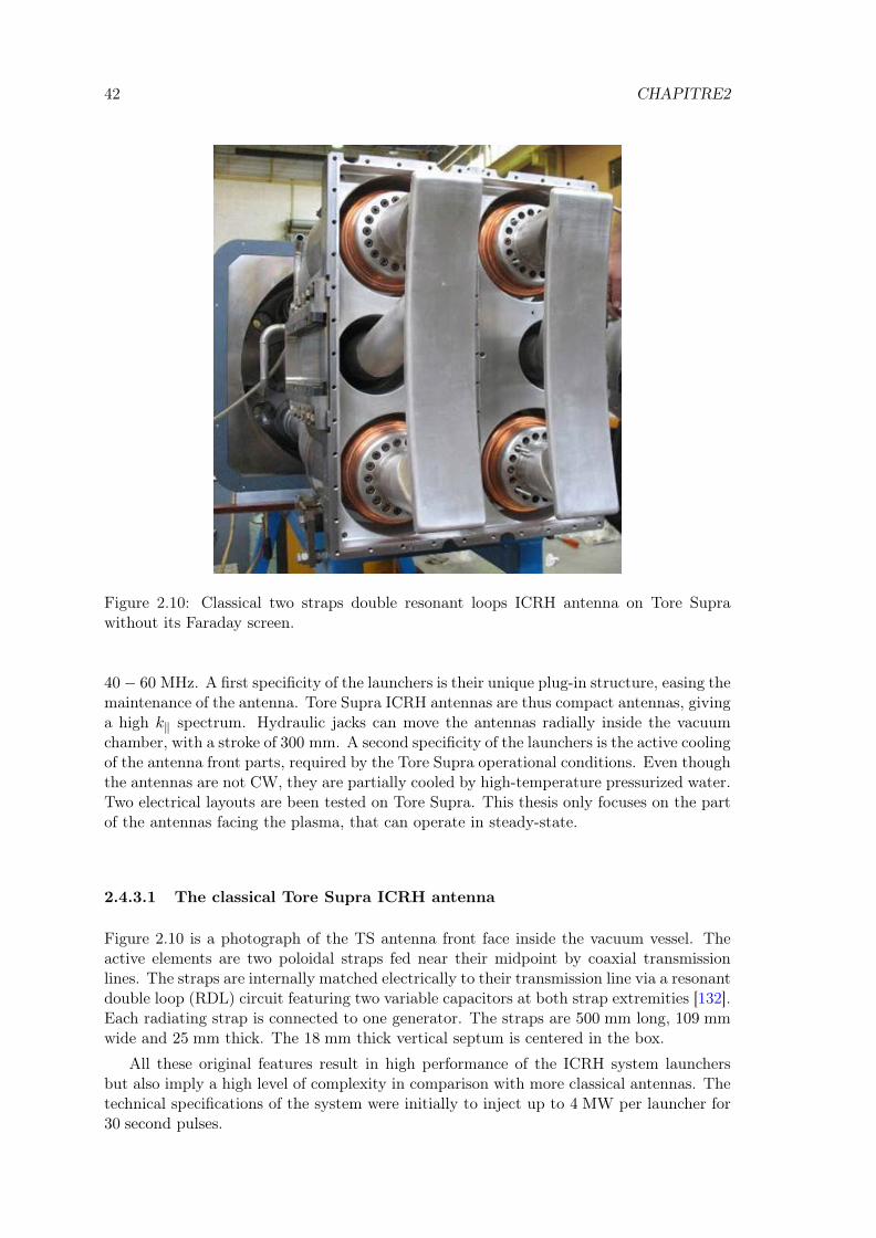
42 CHAPITRE2

Figure 2.10: Classical two straps double resonant loops ICRH antenna on Tore Suprawithout its Faraday screen.

40− 60 MHz. A first specificity of the launchers is their unique plug-in structure, easing themaintenance of the antenna. Tore Supra ICRH antennas are thus compact antennas, givinga high k‖ spectrum. Hydraulic jacks can move the antennas radially inside the vacuumchamber, with a stroke of 300 mm. A second specificity of the launchers is the active coolingof the antenna front parts, required by the Tore Supra operational conditions. Even thoughthe antennas are not CW, they are partially cooled by high-temperature pressurized water.Two electrical layouts are been tested on Tore Supra. This thesis only focuses on the partof the antennas facing the plasma, that can operate in steady-state.

2.4.3.1 The classical Tore Supra ICRH antenna

Figure 2.10 is a photograph of the TS antenna front face inside the vacuum vessel. Theactive elements are two poloidal straps fed near their midpoint by coaxial transmissionlines. The straps are internally matched electrically to their transmission line via a resonantdouble loop (RDL) circuit featuring two variable capacitors at both strap extremities [132].Each radiating strap is connected to one generator. The straps are 500 mm long, 109 mmwide and 25 mm thick. The 18 mm thick vertical septum is centered in the box.

All these original features result in high performance of the ICRH system launchersbut also imply a high level of complexity in comparison with more classical antennas. Thetechnical specifications of the system were initially to inject up to 4 MW per launcher for30 second pulses.

2.4. OVERVIEW OF THE ICRH SYSTEM ON TORE SUPRA 43

Figure 2.11: Front face of the ILP antenna with the massive poloidal septum and itsFaraday screen.

2.4.3.2 The load resilient ITER like prototype (ILP) ICRH antenna

ICRH antennas adaptation is one of the critical issues in the H-mode environment in theITER baseline scenarios. In H-mode plasmas, the electrical circuit must compensate suddenincreases in antenna coupling due to fast density modifications during edge localized modes(ELMs) [133] in order to prevent a mismatch in the circuit tripping the generators. This ledto the development of several techniques to provide load-resilient electrical layouts underfast perturbations of the edge plasma density facing the antenna [134]. The developmentof an ITER-like prototype (ILP) ICRH antenna for Tore Supra was initiated in 2003 [135].This project aimed at testing and understanding the behaviour of the ITER-like electricrelevant scheme during plasma operation. The design of this prototype is based on theconjugate-T concept proposed for ITER [24] to deal with fast loading perturbations dueto ELM activities or pellet injection and provided the first indications on the load tolerantproperties of the electrical circuit [136].

The ILP antenna is illustrated by Figure 2.11. It features two toroidally adjacentITER-like resonant double loops (RDL) with poloidal symmetry. Each RDL is composedof two poloidal current straps short-circuited on top or bottom of the antenna box andconnected in series to a variable tuning capacitor at the other one. Each RDL is fed from aconjugate-T layout connected to the main coaxial line. Compared with the “conventional”RDL circuit, this RF circuit has lower sensitivity to a high variation of the resistive partof the load [25, 137]. The thinner (15 mm) and shorter (236 mm), but wider (131 mm)straps are further away from the plasma compared to the classical antenna by 18 mm.

44 CHAPITRE2

As toroidal mutual coupling between straps and asymmetries greatly influence on theperformance of the load resilience conjugate-T and render complicated the task of find-ing a match point, due to a high sensitivity to the power and phase balance between thetwo resonant circuits, the antenna was equipped with a Faraday screen displaying mas-sive poloidal and toroidal septa with a thick protrusion on the antenna front to reduceinter straps coupling. The 18 mm thick vertical septum, centered in the box, present a80 mm large protrusion. “Sharp” edges were smoothed off to improve the voltage standoffcapability without arcing.

2.4.4 The lateral antenna limiters

Each ICRH and LH antenna side limiter [138] consists of two completely identical lateralprotections, bolted on the left and right side of the antenna mouth (see Figure 2.12). Theirpurpose is to protect the delicate components of the antennas from heat fluxes comingfrom the plasma. The latest generation of actively cooled guard limiter must allow ToreSupra operation at high power (15 MW convective + 10 MW radiative) for long pulses.They are mainly composed of three parts: the active part, which is facing the plasma, theside plates and the header for the water supply.

Figure 2.12: Guard limiter of Tore Supra antennas.

The active part is made out of 30 100 mm long elementary components made of CuCrZralloy, called fingers shown on Figure 2.12. Like all the other PFCs of Tore Supra, thefinger is actively cooled by pressurized water at 150 C and feature a 10 MW m−2 exhaustcapability. The stainless steel header, located just behind the protection, allows waterto feed the 30 fingers in parallel by groups of ten, each group composed of three fingersconnected in series. A thin film of boron carbide (B4C) is applied by plasma sprayingtechnique to surfaces not covered by CFC which receive a flux below 1 MW m−2. Thelarge toroidal extension of the limiter dimension allows by geometrical effect, to spread outthe deposited power density. The toroidal surface of the limiter is indeed built in such a

2.4. OVERVIEW OF THE ICRH SYSTEM ON TORE SUPRA 45

way that it is almost tangent to the LCFS. The perpendicular flux seen by the finger isthus minimised.

2.4.5 Two Faraday screen designs on Tore Supra

Section 2.3 has shown that RF sheaths are generally attributed to SW rectification. Al-though poloidal strap arrays are meant to excite the FW, as shown in Section 2.2.1, the SWis still excited parasitically. The sources of the SW are parallel RF currents and oscillatingspace charges on the antenna metallic structure. In an ideal situation, the straps are alwaysaligned with the static magnetic field. In reality it is however not the case. In presenceof field line pitch a small j‖RF appears along the vertical strap. This, in principle, shouldhowever not happen if the antenna structure is perfectly aligned with the static magneticfield [49]. Moreover non-homogeneous surface charge along the vertical direction of thestraps can also generate a parallel electric field, i.e. SW. In order to filter-out specificallythe SW [139], an object, called Faraday Screen (FS), is interposed between the straps andthe plasma, consisting of metallic rods roughly aligned with the tilted field lines. It addi-tionally protects the straps from heat fluxes coming from the plasma [40]. As illustrated onFigure 2.13(a) and (b), the Faraday screen acts in principle as a polarizing mirror lettingthrough only the FW and filtering out the SW. When it sees a RF electric field parallelto its rods (SW), the FS induces image parallel RF currents in the opposite direction.The incident electric field is thus reflected, as shown on Figure 2.13(a). On the contrary,in presence of transverse electric fields (FW), the FS only develops limited RF currents(“magnetic shielding” [32, 139]), letting the RF wave through, as shown on Figure 2.13(b),nearly unperturbed. Experiments have shown “thermal advantage” for protecting the an-tenna from the fluxes coming from the plasma. The “electrical advantage” is still underdebate.

On Tore Supra ICRH present antennas, the antenna box is closed on its plasma sideby an actively cooled Faraday screen made of steel, copper-plated to reduce RF lossesand its plasma-facing part is coated with boron carbide (B4C) to limit high Z impuritycontamination of the plasma.

(a) (b)

Figure 2.13: Principle of the Faraday screen (FS) concept as seen from inside the antennabox. Reaction of the FS to incident RF electric field (a) parallelly and (b) transversely tothe metallic FS rods.

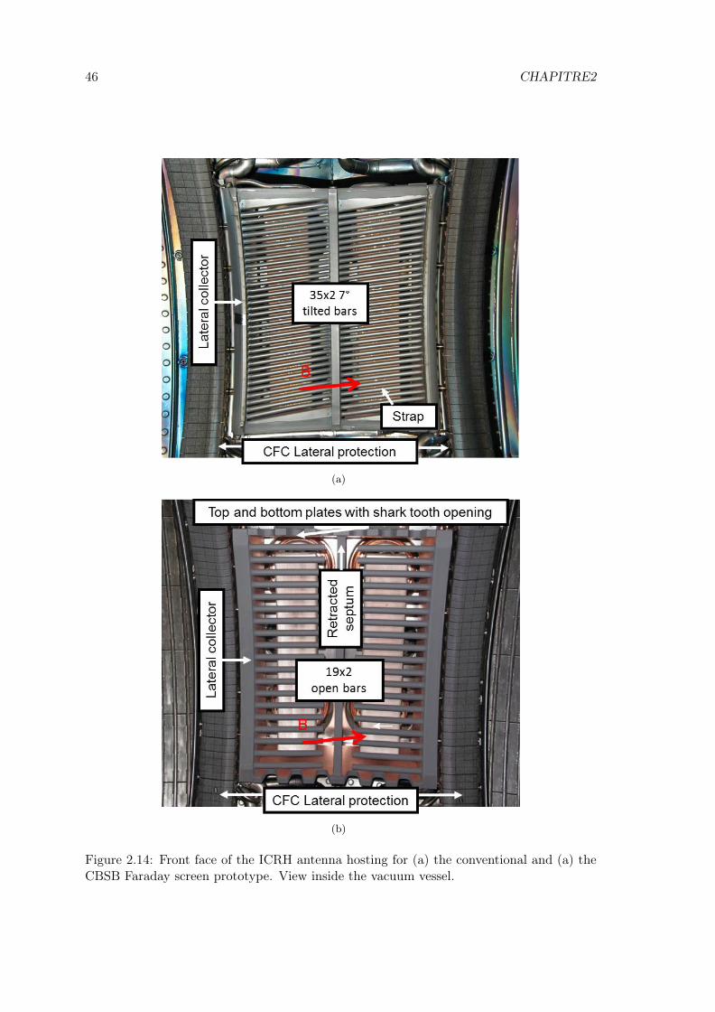
46 CHAPITRE2

(a)

(b)

Figure 2.14: Front face of the ICRH antenna hosting for (a) the conventional and (a) theCBSB Faraday screen prototype. View inside the vacuum vessel.

2.4. OVERVIEW OF THE ICRH SYSTEM ON TORE SUPRA 47

Two types of FS have been tested on Tore Supra: a classical FS and a prototype FSillustrated respectively by Figure 2.14(a) and Figure 2.14(b). The prototype ICRH FSaimed at answering the questions related to thermal, mechanical and electrical upgradesfor Tore Supra and ITER high-power long-discharge operations. The thermomechanicaldesign aimed at increasing the heat exhaust capability [140] in order to reduce the thermallimitation and increase the fatigue cycle within the scope of the high-power long-dischargeoperation. The electrical design aimed at minimizing spurious phenomena due to RFsheaths.

Using the standard modelling approach to mitigate RF sheaths until now by minimizingthe line-integrated parallel electric field led to cut paths for parallel RF currents on theantenna structure on long open field lines passing in front of the antenna [48].

Therefore the prototype FS is characterized electrically, by a slotted frame with “sharkteeth” and cantilevered horizontal rods, as opposed to tilted bars (by 7) attached ontheir two sides on the classical FS [36]. Cantilevered FS bars from the vertical septumadditionally lower the mechanical stress level. The FS bars are also thicker (15 mm vs12 mm) and their number was reduced from 34 to 19 to conserve transparency definedas the amount of the Faraday screen surface not covered by metal. The central septumwas retracted radially. It is also called cantilevered bars and slotted box (CBSB) Faradayscreen.

In view of long pulse operation at high power the new FS is actively cooled on its bars,septum and lateral collectors. Its cooling scheme was revised to accommodate the newfront face design. Each FS bar features a coaxial inner return pipe, such that water inletand outlet are located on the same side. The lateral collector have been enlarged (3.7 cm)to receive fast ion losses and with reduced welds in critical areas [140]. This improvesthe heat exhaust up to 1 MW/m2 CW (and transiently 2 MW/m2), versus 0.5 MW/m2

(respectively 1 MW/m2) for the classical screen. Only one of three antennas was equippedwith CBSB Faraday screen, while the other two antennae were equipped with classicalFaraday screens on Figure 2.14(a).

2.4.6 Diagnostics on the Tore Supra ICRH antenna

It was seen in this chapter that the properties of the SOL on a tokamak in the immediateenvironment of the ICRH antennas is crucial for their proper operations (wave coupling,spurious interaction due to RF sheaths). Tore Supra is a tokamak equipped with numerousdiagnostics. Some of them are dedicated to monitor the ICRH antennas and measurephysical quantities for later analysis. During Tore Supra plasma operation, the protection ofPFCs (i.e. antenna can be considered as PFCs) relies basically on the surface temperatureTIR (measured by infrared thermography [141]) and metallic impurity (measured with ahigh-resolution vacuum ultraviolet spectrometer) monitoring systems. Furthermore ICRHantennas are not only PFCs in the sense that they not only have to keep the structuralproperties but also their electrical properties.

When hot spots are detected on the antenna during RF pulses by infrared monitoringsystem, the IR real-time control (IR-RTC) safety system [142] is triggered if TIR exceeds athreshold fixed by regulations. It results in a decrease in the injected power level. Howeverhot spots can be due to either intense heat loads that the actively cooled system of theantenna cannot moderate resulting in the rise of TIR or either to flaking of the the B4Ccoating. In that case the region identified as flaking is excluded from the real-time controlmonitoring system.

RF measurements through capacitive probes at the top and bottom of each strap allow

48 CHAPITRE2

voltage control of the straps (in left/right strap magnitude and phase). Line RF power(forward/reflected amplitude and phase) are also measured in the feed line at generatoroutput and at antenna input. In complement of RF measurements diagnostics, several arcsafety systems [143] have been implemented to prevent any destructive damage due to arcsin the antenna and transmission lines. The safety systems stop the generator for typically50 ms, the estimated time to kill an arc. Concerning the matching capability, a feedbackmatching system was implemented to allow assessment every 2 ms. Fast servomotors adjustthe capacitor at the desired position [41]. A real time automatic matching monitoringsystem allows following loading variations on a 100 ms time scale.

Direct measurements with reciprocating Langmuir probes allow quantifying quantifythe SOL perturbations in the vicinity of an active ICRH antenna. Two-dimensional (2D)mappings by reciprocating Langmuir probes [38, 144] are possible on Tore Supra. TheLangmuir probes are magnetically connected to the ICRH antennas. The connection pointsare labelled by their altitude and their radial position with respect to the leading edge ofthe side limiters with an 0.5 cm accuracy. Radial resolution is provided by the probereciprocation (i.e. the depth of the probe plunge). The probe is immersed into the SOLduring the discharge several times. Between the plunges the edge safety factor q (a) ischanged in little steps. As a consequence the magnetic connections of the probe to theantenna move up poloidally providing poloidal resolution.

Figure 2.15: Schematics of the ICRH antennas toroidal locations in Tore Supra, withrespect to the reflectometer. Q5, Q1 and Q2 label the ICRH antennas. LPA and LPTrefer to the antenna limiter and toroidal limiter, respectively. The magnetic connectionsof the reflectometer are also shown. The figure is adapted from [145].

The density is measured with a reflectometer [146]. It is noteworthy to show thelocations of the ICRH antennas with respect to the reflectometer port. Figure 2.15 shows anillustration of the torus wall unwrapped along the toroidal direction z. The reflectometer islocated in the same port that the antenna protection (LPA). As the LPA is radially closer tothe LCFS than the ICRH antennas, the LPA acts as a solid boundary. The z = 0 referenceposition is the LPA toroidal position. While moving along the toroidal direction, theantenna placed in the port plug Q5 is the closest antenna with respect to the reflectometer,followed by Q1 and finally Q2. The reflectometer is generally magnetically connected tothe toroidal limiter (LPT). The field lines intersect the LPT below the ICRH antenna Q5.The density measurements in this thesis are averaged to smooth the fluctuations. Thedensity profile measured in front of the reflectometer will be assumed to be also the onein front of the antenna. Thus the density n is a profile depending along on the radialcoordinate x.

Other diagnostics on Tore Supra that were not used during this thesis, are available tomonitor and measure the impact of ICRH antennas.

2.5. SUMMARY 49

2.5 Summary

In conclusion of this chapter, we have seen that in the ICRH frequency domain (30− 100 MHz)two kind of cold plasma waves can exist with very different properties: the slow wave andthe fast wave. The fast wave due to its polarization will be useful for plasma heating andcurrent drive. It is however evanescent at low density and cannot be perfectly coupled tothe plasma. The slow wave, by exciting RF sheaths, is deemed at the origin of spuriousinteractions in the edge plasma that fix the operational limits of the antenna. Until nowthese two effects have been studied independently. On the contrary, they should be simu-lated simultaneously in a self-consistent manner. One of the consequences of RF sheaths isthe modification of the density distribution in front of the ICRH antenna due to convectioncells. Since the density is modified, the evanescence length that the fast wave has to tunnelthrough is also modified. The efficiency of the coupling of the FW is thus also changed.Typically antennas are programmed to couple a constant amount of power. The antennathus adapt its voltage to couple the required amount of power. The amount of power thatcan be coupled depends on the evanescence length which in turn depends on the density.The density is modified by RF sheaths whose magnitude depends on the voltage on theantenna. The amplitude of RF sheaths has also been seen to depend on the fine details inthe design of the antenna.

The model that has to be developed and implemented in numerical simulations shouldthus:

• be self-consistent,

• emulate single pass absorption,

• reproduce accurately FW coupling,

• be versatile in terms of geometry to handle complex ICRH antenna geometries,

• allow the full definition of a cold plasma with anisotropy, gyrotropy and inhomogene-ity,

• be compatible with the implementation RF sheaths through SBCs,

• be compatible with the finite element method,

• accept realistic tokamak plasma parameters,

• correctly reproduce past and present observations to guide the design of future ICRHantennas and predict their behaviour on typical plasma scenarios.

50 CHAPITRE2

Chapter 3

Perfectly Matched Layer to emulateradiating boundary conditions forwaves in magnetized plasmas

The first part of the thesis consisted in finding a novel manner to model the outgoingpropagative FW without reflection as the simulation domain is only the edge plasma. Thisconstitutes one the two essential pieces for the code modelling wave coupling and RFsheaths simultaneously in a self-consistent manner.

Perfectly Matched Layers (PMLs)[57] are nowadays a common tool to emulate radiat-ing boundary conditions at infinity. They are commonly used in classical dielectric material.However they have never been used in fusion plasmas. As explained in Section 2.1, therealready exist several methods to model antenna wave coupling to the plasma with theirown strengths and weaknesses. Another objective is to find a wave coupling modellingmethod compatible with the presence of realistically modelled plasma around the antennato account at the same time and self-consistently for wave-edge plasma interactions suchas RF sheaths.

This chapter is devoted to provide a synthetic view of the PML technique as it isknown in order to understand how to use it later for tokamak magnetized plasmas. Thefirst section introduces the method in general and focuses then on PMLs requirements incases of magnetized plasmas. The aim is to handle outgoing waves in an open boundariesdomain filled with plasma without reflection. The second section gives a mathematicaldescription of the PML technique as well as how it works. The last section is devoted tocompute the analytical reflection coefficient occurring for a 1D PML with plane waves. Theresulting expression gives some hints on the manner to parametrise the PML for optimaluse. A number of tests are then performed numerically with monochromatic plane waves.The reflection coefficient calculated from the simulations is then compared to the analyticalpredictions. Finally an alternative to the reflection coefficient only defined for plane wavesis presented when dealing with a spectrum of plane waves emitted by an antenna.

3.1 The Perfectly Matched Layer method

The Perfectly Matched Layer (PML) concept was originally formulated by Bérenger in1994 [147] for use with Maxwell’s equations in Cartesian coordinates, and since that timethere have been several related reformulations of PML for both Maxwell’s equations andfor other wave equations.

51

52 CHAPITRE3

In order to provide the non-reflecting boundary condition for an open-domain problem,an absorbing layer as thin as possible, called a PML, is added at the boundaries of themain calculation domain to simulate problems with open boundaries, especially in theFinite Difference Time Domain (FDTD)[148] and Finite Elements Method (FEM). ThePML itself is generally ended by a perfect conductor. But in a properly tuned PML thislatter boundary condition should play only a minor role. Therefore, a PML is not strictlyspeaking a boundary condition but an additional domain absorbing incident radiationswithout producing reflections ideally. It acts like a buffer area between the medium andthe boundary condition. It provides good performances for a wide range of incident anglesor eigenvector number while being as insensitive as possible to the shape of the wavesfronts.

The key property of a PML that distinguishes it from an ordinary absorbing material isthat it is designed so that waves incident upon the PML from a non-PML medium do notreflect at the interface. This property allows the PML to strongly absorb outgoing wavesfrom the interior of a computational region without reflecting them back into the interior.

From a mathematics viewpoint, a perfectly matched layer is an analytic continua-tion of the wave equation into complex coordinates under the requirement that the waveimpedance should remain unaffected as in ref.[149]. It means that one (or more) of thecoordinates is mapped into complex numbers. The effect is to replace inside this particularregion propagating (oscillating) waves by exponentially decaying ones. The PML principleworks in time domain and in frequency domain for any kind of discretization of an arbi-trary wave equation. The mathematical form are however different in time domain and infrequency domain. The focus here is on frequency domain PML. Applications on PML intime domain are shown in references [147, 148].

This approach is known as stretched-coordinate PML. This complex coordinateapproach, while not the original one, is elegant and general in the sense that it allows toextend this technique to other wave equations and other coordinate systems “easily”. Thetransformation can be defined for others coordinate systems and for an arbitrary “waveequation”.

Different PML formulations were done, but they have all been unified under the sameformalism in [150]. The different interpretations of the PML have also been shown tobe equivalent: complex stretched coordinates perpendicular the medium-PML interface,physical lossy medium with dependent electric and magnetic currents densities.

An exhaustive literature exists for classical dielectric such as air but it is scarce forcomplex dielectric media such as cold magnetized plasmas. Recently this technique startedbeing used in inhomogeneous ionospheric plasmas [151].

A cold magnetized plasma is equivalent to a birefringent gyrotropic medium as shownby the tensor given by (2.9). For example PMLs already exist for the propagation of oneeigenmode of magnetized plasmas, generally in 2D transverse to the confinement magneticfield, described by a scalar Helmholtz equation [152]. We would like to extend this resultin 3D for the two eigenmodes, described by a vectorial wave equation, in view of manyapplications in lots of contents.

Specific radiation conditions thus need to be emulated simultaneously for two eigen-modes. But, these two eigenmodes present a great disparities of scale lengths (i.e. verydifferent wave vector radial component nx) resulting in very different properties for theslow wave and the fast wave.

Moreover, in our case the antenna used to excite the waves launches a wide spectrumof n‖. Both propagative and evanescent waves can exist. Furthermore, in this spectrum,a n‖ window will give rise to n⊥ close to zero (i.e. very long wavelengths). Management

3.2 MATHEMATICAL DESCRIPTION 53

of this region around the cutoff is of serious concern. Finally forward and backward wavescan coexist if ε‖ < 0 and ε⊥ > 0. The PML will select one of the two. We have thereforeto make sure that the one selected is the one carrying the power towards the plasma.

Is it possible to obtain a PML for such a medium? How to control the reflection? Isit possible to construct a PML working for both polarizations at the same time? How toobtain a PML for a spectrum of n‖ offering the best compromise? How to cope with thecutoffs? How to minimize the numerical cost while keeping an acceptable accuracy? Howto measure the reflections for both travelling and evanescent waves? What are the limitsthat we cannot go beyond? Those are a few questions to which we have to find answers to.

3.2 Mathematical description of the Perfectly Matched Layer

3.2.1 Introduction

The aim is to define the PML as an artificial anisotropic absorbing medium, where thestandard equations of electrodynamics can be applied in their usual form. A completeformulation of general closed-form PML in bi-anisotropic and dispersive media can befound in [150] and is briefly summarized below. The case treated here considered theconstitutive relations D = ¯εE and B = ¯µH, where for the sake of generality the dielectrictensor ¯ε and magnetic permeability tensor ¯µ are full. In the constitutive relations B onlydepends on H and D on E on the contrary to the general case treated in [150].

In the following development, the system of equations (2.3) is replaced with a modifiedwave propagation problem solved over the whole computation domain including the PMLlayer and radiation conditions at the boundaries of the main simulation domain. Forthat purpose we envisage the most general PML in the three directions. Following [150],the Cartesian space coordinates in (2.3) are transformed by an analytic continuation toa complex variable spatial domain [153, 154]. This mathematical transformation, centralto the PML theory, is written with stretching function deforming the Cartesian space.The effect of this transformation is to alter propagative modes into exponentially decayingmodes in the PML layer, allowing reflectionless absorption of the electromagnetic waveswithin a finite length assumed to be smaller than the studied spatial zone.

3.2.2 Wave damping via artificial coordinate stretching in the complexplane: qualitative introduction via a simple example in 1D

Let us take first a simple example to pedagogically illustrate the principle on which thePML relies on: a PML designed to absorb travelling waves propagating in the x direction.

Let’s also assume that the stretching function takes the form Sx(x) = 1 + iσ(x)ω0

with ω0

the wave pulsation and σ some function of x. The transformation of the real coordinateto complex stretched coordinate in that case reads:

x→ x+i

ω0

∫ x

σ(x′)dx′, (3.1)

where σ (x) is a damping function following:σ (x) = 0 if x < 0,σ (x) > 0 if x > 0.

(3.2)

54 CHAPITRE3

If σ > 0, the integral in (3.1) reads:

σ > 0 ⇒∫ x

σ(x′)dx′ > 0 (3.3)

⇒ limx→+∞

∫ x

σ(x′)dx′ → +∞ (3.4)

For a wave of dependence in eikx travelling in +x direction (k > 0), it thus gives:

ikx ⇒ ik

(x+

i

ω0

∫ x

σ(x′)dx′)

(3.5)

⇒ ikx− k

ω0

∫ x

σ(x′)dx′. (3.6)

As limx→+∞ e− kω0

∫ x σ(x′)dx′= 0, the wave is thus attenuated as shown in:

limx→+∞

ei(kx−ω0t)e− kω0

∫ x σ(x′)dx′= 0. (3.7)

In that case, each time an x derivative appears in the wave equation, it is replaced by:

∂x →1

1 + iσ(x)ω0

∂x. (3.8)

The typical length associated by the gradient is thus proportional to σ/ω0. If this ratio islarger than one, the propagating wave is damped faster over a shorter distance.

3.2.3 Formulation of the spatial coordinates stretching problem in 3DCartesian geometry with full permittivity and permeability ten-sors

After this qualitative example, let us go to a general 3D case. The solution of the problemin 3D Cartesian geometry should remain unchanged in the main computational domainwhere the stretched coordinates coincide with the normal ones. The analytic continuationis formally expressed by the following transformation:

u→ tu =

∫ u

0Su(u′)du′, (3.9)

where Su are the complex stretching functions [155] and u stands for any of the Carte-sian coordinates x, y, z. Su can be chosen with great flexibility, but should depend exclu-sively on coordinate u. The imaginary part will damp the incoming propagative waveswhereas the real part will take care of the evanescent ones.

In the stretched complex space, the Maxwell’s equations read:∇S ×E = +iω0 ¯µH,∇S ×H = −iω0 ¯εE + jant,∇S · [¯εE] = ρant,∇S · [¯µH] = 0.

(3.10)

Within the new formulation, the wave problem in the PML takes the same form as(2.3), but the differential operator ∇ in Cartesian coordinates is replaced by the modifiedoperator ∇S in stretched coordinates, defined as:

3.2 MATHEMATICAL DESCRIPTION 55

∇S ≡

∂x

Sx(x)∂y

Sy(y)∂z

Sz(z)

= ¯S−1 ·∇ , (3.11)

where

¯S ≡

Sx(x) 0 00 Sy(y) 00 0 Sz(z)

. (3.12)

3.2.4 Interpretation of the PML as an artificial lossy medium

Since ∂/∂x commutes with Sy(y) and Sz(z), and ¯S is a diagonal tensor, the two differentialoperators ∇ and ∇S are related for any vector field a(x, y, z) by the following properties:

¯Λ · [∇S × a] = ∇×(

¯S · a), (3.13)

det(

¯S)∇S · a = ∇ · ( ¯Λ · a), (3.14)

where ¯Λ = det(

¯S)

¯S−1 and det ¯S = SxSySz.

A simple mnemonic trick for ¯Λ is to remember that the Si function does not appearfor the i direction.

Combining (3.11), (3.13) and (3.14), the modified wave propagation problem in thePML can be reformulated using the standard differential operators as:

∇×(

¯S · E)

= +iω0

(¯Λ · ¯µ · ¯

S−1)(

¯S · H)

∇×(

¯S · H)

= −iω0

(¯Λ · ¯ε · ¯S−1

)(¯S · E

)+ ¯Λ · jant,

∇ ·[(

¯Λ · ¯ε · ¯S−1)(

¯S · E)]

= det(

¯S)ρant,

∇ ·[(

¯Λ · ¯µ · ¯S−1)(

¯S · H)]

= 0.

(3.15)

The new set of equations (3.15) can have the following interpretation. They can beseen formally as the standard equations of electrodynamics in system (2.3). However, theoriginal RF fields E and H are replaced respectively by artificial RF fields ¯SE and ¯SH.The original and artificial RF fields coincide inside the main simulation domain, where thestretching tensor is the identity tensor ( ¯S = ¯1).

The artificial RF fields propagate in an artificial absorbing medium with modifieddielectric and magnetic properties [156, 157]. The original tensors ¯ε and ¯µ are replacedrespectively with the artificial tensors ¯εPML and ¯µPML. From a general dielectric tensor¯ε, one obtains the perfectly matched tensor ¯εPML:

¯εPML ≡ ¯Λ · ¯ε · ¯S−1 =

εxx

Sy(y)Sz(z)Sx(x) εxySz(z) εxzSy(y)

εyxSz(z) εyySz(z)Sx(x)Sy(y) εyzSx(x)

εzxSy(y) εzySx(x) εzzSx(x)Sy(y)Sz(z)

. (3.16)

56 CHAPITRE3

This is the most general tensor one can find. Then according to the situation, the tensorcan be simplified by considering the zeros εij elements. Considering in which directionsthe stretching occurs can also simplify the tensor by putting to 1 some of the Su (u).

The same stretching needs to be applied to the magnetic permeability tensor. Originaland artificial tensors again coincide in the main simulation domain. These two propertiescharacterize the artificial medium called perfectly matched layer. Also note that the threetensors ¯Λ, ¯S−1 and ¯µ commute if the tensor ¯µ is diagonal.

The present formulation is valid for any permittivity and permeability tensors ¯ε and ¯µand can be implemented indifferently in 1D, 2D and 3D. As all the needed information iscontained in the modified constitutive tensor properties ¯εPML and ¯µPML and only the Eand H fields are required the formulation is aesthetic and straightforward to implement,especially in commercial software which authorize the definitions of exotic media.

To minimize reflections for inhomogeneous media, the constitutive parameters ¯ε and ¯µat any transverse plane inside the PML are equal to those at the plasma-PML interface,and invariant along the normal direction to the interface. Inhomogeneities present inthe transverse directions will eventually produce reflections inside the PML. However, suchreflections contribute only along the transverse directions to the interface [158]. Reflectionscan get in the continuous case arbitrary small, until a reflectionless PML is achieved. Thenext section will show how for a 1D PML by solving analytically the wave equation in adomain plasma+PML.

3.3 Reflection of plane waves by a 1D PML

In order to get insight into the main properties of the PML, we exhibit general rules totune the PML and assess its implementation in numerical codes. A simple test case isfirst considered, for which analytical results are available: plane wave propagation in halfspace filled with homogeneous medium with radiation at infinity. Since the original waveproblem is linear, many realistic RF fields of physical interest can be decomposed into acharacteristic spectrum of plane waves. This test problem, although academic, is usefulto guide PML implementation. For the sake of generality Cartesian coordinates (r, l, h)are temporarily defined. RF field oscillation as e+ikll+ikhh is assumed parallel to the halfspace border and propagation is solved along the coordinate r (see figure Figure 3.1). Inflattened tokamak geometry, depending on the PML, r can represent any of the principaldirections parallel or normal to the confinement magnetic field. In presence of radiationconditions the wave equation (1) in the half-plane (r > 0) has solutions of the form:

Eexact (r, kh, kl) = E0(kh, kl)e+ikrre+iklle+ikhh. (3.17)

In this expression, the wave vector k and wave polarization E0(kh, kl) are respectivelyeigenvalue and eigenvector of the wave equation:

n× (n×E) + ¯ε · E = 0, (3.18)

where ¯µ = µ0¯1, n = k/k0 is the index vector and k0 = ω/c the modulus of the wave vector

in vacuum. In birefringent media like magnetized plasmas, several eigenmodes can coexist.Only one of them is considered in our test problem. The dispersion relation, given by thedeterminant of (3.18), is then generally expressed as:

k2r = f

(ω, k2

l , k2h, ¯ε). (3.19)

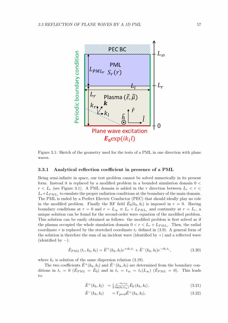
3.3 REFLECTION OF PLANE WAVES BY A 1D PML 57

Figure 3.1: Sketch of the geometry used for the tests of a PML in one direction with planewaves.

3.3.1 Analytical reflection coefficient in presence of a PML

Being semi-infinite in space, our test problem cannot be solved numerically in its presentform. Instead it is replaced by a modified problem in a bounded simulation domain 0 <r < Lr (see Figure 3.1). A PML domain is added in the r direction between Lr < r <Lr+LPMLr to emulate the proper radiation conditions at the boundary of the main domain.The PML is ended by a Perfect Electric Conductor (PEC) that should ideally play no rolein the modified problem. Finally the RF field E0(kh, kl) is imposed in r = 0. Havingboundary conditions at r = 0 and r = L∞ ≡ Lr + LPMLr and continuity at r = Lr, aunique solution can be found for the second-order wave equation of the modified problem.This solution can be easily obtained as follows: the modified problem is first solved as ifthe plasma occupied the whole simulation domain 0 < r < Lr + LPMLr . Then, the radialcoordinate r is replaced by the stretched coordinate tr defined in (3.9). A general form ofthe solution is therefore the sum of an incident wave (identified by +) and a reflected wave(identified by −):

EPML (tr, kh, kl) = E+(kh, kl)e+ikrtr + E−(kh, kl)e

−ikrtr , (3.20)

where kr is solution of the same dispersion relation (3.19).The two coefficients E+(kh, kl) and E−(kh, kl) are determined from the boundary con-

ditions in tr = 0 (EPML = E0) and in tr = t∞ = tr(L∞) (EPML = 0). This leadsto:

E+(kh, kl) = i2e−ikrt∞

sin(krt∞)E0 (kh, kl) , (3.21)

E−(kh, kl) = ΓpredE+(kh, kl), (3.22)

58 CHAPITRE3

withΓpred = − exp (2ikrt∞) (3.23)

a complex reflection coefficient. Comparing EPML with Eexact the ideal situation wouldbe to reach E+ = E0 and E− = 0 for all physically useful values of (kh, kl) excited in thewave propagation problem. These conditions are fulfilled if |Γpred| << 1. Therefore theamplitude of the reflection coefficient is a figure of merit of the efficiency of the PML.

Several conclusions can already be drawn independently of any particular choice forSr(r). First, to achieve |Γpred| << 1 the stretching function Sr(r) needs to incorporate acomplex part in order to damp the incoming propagative waves in the bounded PML, sothat the modified spatial path is necessarily stretched in the complex plane: t∞ = t′∞+it′′∞.The PML becomes effectively perfectly reflectionless as t′∞ and t′′∞ tend to infinity. Forfinite values of t∞ the PML will fail in the vicinity of a cutoff layer, for which |kr| assumesvery small values. The spectral width of the unfavourable region in kr depends on thevalues t′∞ and t′′∞ and can be made arbitrarily small, at the expense of larger PML size tohandle the larger wavelength.

Secondly, in an anisotropic medium the applied stretching is the same for all the eigen-modes despite possibly very disparate wavelengths in direction r. The PML thereforeneeds to be adapted to the largest wavelength while being able to resolve properly thewave structure and ensure a smooth stretching to avoid spurious numerical reflections.

Stretching the space coordinates allows contracting the space, thus bringing what canbe considered as infinity at a finite value.

3.3.2 Criteria for choosing the stretching function properties to mini-mize the analytical reflection coefficient

Each direction of our anisotropic medium needs its own perfectly matched layer character-ized by its stretching tensor ¯S as shown in Figure 3.1.

Perfectly matched layers are usually designed to only attenuate propagating waveswithout reflection by definition. Purely evanescent waves are transformed into oscillatingwaves in the PML but do not decay more quickly. Attenuation of evanescent waves canhowever be accelerated by adding a real coordinate stretch in the PML.

A large range of stretching functions Su(u) can be envisaged for the PML. The maincriteria are:

• Sr(r) should be continuous across the interface r = Lr (medium/PML interface).

• Sr(r) should also be sufficiently smooth within the PML.

• The damping should have the appropriate sign to get power sent to the plasma.

• The stretching function parameters (LPMLr , S′r, S′′r , pr) should be chosen with theconstraint that the fields must vanish before reaching the end of the PML. As long asthe truncation is done after a long enough distance (where the exponential tails aresmall), the boundary condition used will not matter. If that condition is realized, thenthe perfect electric conductor (PEC) boundary condition is automatically satisfied.

As a consequence of these assumptions, no discontinuity should be present in the PML.Therefore the PML cannot replace sources of electromagnetic fields. They only absorb fieldsproduced by sources located inside the surrounded domain. Since PMLS are designed forthe absorption of travelling waves, this means implicitly that they must be placed somedistance from the sources and outside the possible evanescent region that can numerically

3.3 REFLECTION OF PLANE WAVES BY A 1D PML 59

costly to handle. As a corollary to the discontinuity, each point in a volume space boundedwith a PML must be in direct visibility from any other point of this volume, i.e., theinterface between the inner medium and the PML must be either plane (in the Cartesiancase) or concave, in the general case [159].

3.3.3 Application to polynomial stretching function

A common choice, but not unique, for the PML is a stretching function having a polynomialform:

Sr (r) =

1 for 0 ≤ r ≤ Lr,1 + (S′r + iS′′r )

(r−LrLPMLr

)prfor Lr ≤ r ≤ L∞,

(3.24)

where Lr, LPMLr , pr, S′r S′′r are respectively the position of the medium/PML interface,the PML depth, the order of the stretching function, the real stretch and the imaginarystretch. This leads to: t∞ = L∞+(S′r + iS′′r )

(LPMLrpr+1

). The analytical reflection coefficient

for forward waves (real positive kr) yields:

ηpred ≡ |Γpred| = exp

(−2krLPMLr

S′′rpr + 1

)(3.25)

Similar calculation can be done for backward waves (real negative kr). For evanescentwaves (pure imaginary kr), it reads:

ηpred = exp

[−2 |kr|

(Lr + LPMLr

1 + S′rpr + 1

)]. (3.26)

3.3.4 Qualitative reflections on the choice of the PML parameters andon numerical errors due to discretization

Formula (3.25) provides some hints to minimize the wave reflection in the simulation do-main and the associated numerical cost. A deep PML always improves the accuracy of theresult, at the expense of larger CPU and memory requirements, since the PML also needsto be meshed. It might seem desirable to take large S′′ as well as low p up to some valuewhere the resulting gradient in the stretched direction cannot be computed by the meshwithout local mesh refinement to avoid additional errors. If local refinement is necessary,then the gain in numerical cost is limited and ultimately cancelled. Formula (3.25) alsoconfirms that grazing incident angles or cutoffs (kr → 0 greatly affect the effectivenessof the PML in its reflectionless properties. For formula (3.26), the same hints still applyreplacing S′′ by 1 + S′. These qualitative hints will have to be checked numerically.

These analytical results only quantify the error introduced when switching from theoriginal Maxwell’s equations to the modified ones. The PML is a mathematical objectdefined to remove perfectly all the reflected waves at the boundary. However its formulationwas done for continuous media. All the defaults of the PML come from the discretization ofa continuous medium into a finite number of points. From a numerical viewpoint the totalerror should also incorporate extra wave reflection due to space discretization or round-offerrors in numerical schemes. The boundary between the PML and the medium is no longerreflectionless, but the reflection are small because the discretization is presumably a “goodapproximation” of the exact wave equation. They are discussed in ref.[160] in the contextof finite differences.

60 CHAPITRE3

Reflections can be made arbitrary small, even without a PML, by slowly varying themedium properties. It results for the PML in the absorption coefficient σ gradually turnedon from zero over a short distance of the scale of the wavelength of the wave. As absorp-tion gradually increases, reflections goes to zero due to an adiabatic theorem [161]. Witha non-PML absorber, getting acceptable reflections requires very thick absorbing layer asabsorption is very slowly turned on [162]. Increasing the resolution also increases the effec-tiveness of the PML, as it approaches the exact wave equation. The required effectivenessis then function on the application. It means that the σ profile in the PML is not uniform.The profile is however uniform in the direction perpendicular to the medium/PML inter-face. The PML is thus not uniform and as such can be seen as a stratified medium withthe typical size of one stratum having the typical element size.

Thinking on the increase of the stretching coefficient leads to think that always keepingthe same slope between two adjacent grid points would be beneficial for the minimization ofthe numerical spurious reflection. Indeed the gradient length would stay constant. This isnot the case for polynomial function whose slope is always increasing except for order one.Geometrical functions however satisfy this property. Geometrical functions are neverthelessmore difficult to implement, especially with finite elements in non-regular grids. Moreoverregular grids are incompatible with multi-scale grids as they will encounter joining issuesat the interfaces of the different grids.

After this discussion on the effect of discretization of the efficiency of the PML, let usturn to numerical simulations for plane waves to verify that the PML is indeed workingbut has numerical limits.

3.4 Numerical tests with plane waves in an homogeneousmagnetized plasma compared to analytical predictions ofthe reflection coefficient

The PML method has been introduced for a possible usage for magnetized plasmas that areanisotropic, gyrotropic and inhomogeneous media. The presence of cutoffs is also a concernas well as the possible coexistence of forward and backward waves. To start with, it is im-portant to know if the current PML formulation works well for homogeneous magnetizedplasmas. Both the slow and fast waves were tested for various conditions. A 2D homoge-neous plasma with a radial PML with a polynomial profile of Sx(x) is simulated by FEMusing the Comsol Multiphysics software. Then the reflection coefficient for monochromaticplane waves was computed and compared to the expected value found in 3.25.

3.4.1 Assessment of the reflection coefficient in numerical simulationswith the standing wave ratio

To assess the PML performance in numerical simulations, the amplitude reflection coeffi-cient Γ ≡ E−/E+ should be quantified for a given set of PML parameters. It is written asΓsim ≡ ηsim exp (iϕ) with amplitude ηsim = |Γsim| ≤ 1 and phase ϕ. Only the magnitudeof Γsim is of interest. In order to extract ηsim, one can evaluate the modulus of the RFelectric field E (r, l) over all plasma domain:

|E|2 =∣∣E+

∣∣2 [1 + η2sim + 2ηsim cos (2krr + ϕ)

]. (3.27)

In the ideal case of a perfect PML (ηsim = 0), |E|2 is constant over the domain.In presence of wave reflection (ηsim > 0), the field amplitude pattern exhibits periodic

3.4 NUMERICAL TESTS WITH PLANE WAVES 61

modulations along direction r, whereas wave fronts may have oblique incidence. This isclearly visible on Figure 3.2(a) with l = z and r = x. The wavelength of the amplitudemodulations can be used to test the dispersion relation in the main plasma. The position ofthe maxima and minima can be used to calculate the phase ϕ (modulo 2π). The amplitudeof the spatial modulations are representative of the quantitative value of ηsim.

In telecommunications, the standing wave ratio (SWR) of a partial standing wave inan electrical transmission line [163] is defined as the ratio of its amplitude at an antinode(maximum) to the amplitude at an adjacent node (minimum). By analogy, a SWR is here

(a)

(b)

Figure 3.2: Illustration of radial modulations of the field amplitude. A harmonic excitationis prescribed at the location x = 0. The wave then travels through the plasma and isattenuated when reaching the PML. (a) Map of the norm of the electric field |E| wherereflection is visible by the presence of radial modulations of |E| in vacuum. l = z, r = x,h = y. (b) A “good” case in blue and a “bad” case in red are represented.

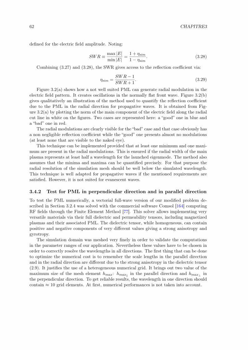
62 CHAPITRE3

defined for the electric field amplitude. Noting:

SWR ≡ max |E|min |E|

=1 + ηsim1− ηsim

. (3.28)

Combining (3.27) and (3.28), the SWR gives access to the reflection coefficient via:

ηsim =SWR− 1

SWR+ 1. (3.29)

Figure 3.2(a) shows how a not well suited PML can generate radial modulation in theelectric field pattern. It creates oscillations in the normally flat front wave. Figure 3.2(b)gives qualitatively an illustration of the method used to quantify the reflection coefficientdue to the PML in the radial direction for propagative waves. It is obtained from Fig-ure 3.2(a) by plotting the norm of the main component of the electric field along the radialcut line in white on the figures. Two cases are represented here: a “good” one in blue anda “bad” one in red.

The radial modulations are clearly visible for the “bad” case and that case obviously hasa non negligible reflection coefficient while the “good” one presents almost no modulations(at least none that are visible to the naked eye).

This technique can be implemented provided that at least one minimum and one maxi-mum are present in the radial modulations. This is ensured if the radial width of the mainplasma represents at least half a wavelength for the launched eigenmode. The method alsoassumes that the minima and maxima can be quantified precisely. For that purpose theradial resolution of the simulation mesh should be well below the simulated wavelength.This technique is well adapted for propagative waves if the mentioned requirements aresatisfied. However, it is not suited for evanescent waves.

3.4.2 Test for PML in perpendicular direction and in parallel direction

To test the PML numerically, a vectorial full-wave version of our modified problem de-scribed in Section 3.2.4 was solved with the commercial software Comsol [164] computingRF fields through the Finite Element Method [77]. This solver allows implementing veryversatile materials via their full dielectric and permeability tensors, including magnetizedplasmas and their associated PML. The dielectric tensor, while homogeneous, can containpositive and negative components of very different values giving a strong anisotropy andgyrotropy.

The simulation domain was meshed very finely in order to validate the computationsin the parameter ranges of our application. Nevertheless these values have to be chosen inorder to correctly resolve the wavelengths in all directions. The first thing that can be doneto optimize the numerical cost is to remember the scale lengths in the parallel directionand in the radial direction are different due to the strong anisotropy in the dielectric tensor(2.9). It justifies the use of a heterogeneous numerical grid. It brings out two value of themaximum size of the mesh element hmax: hmax‖ in the parallel direction and hmax⊥ inthe perpendicular direction. To get reliable results, the wavelength in one direction shouldcontain ≈ 10 grid elements. At first, numerical performances is not taken into account.

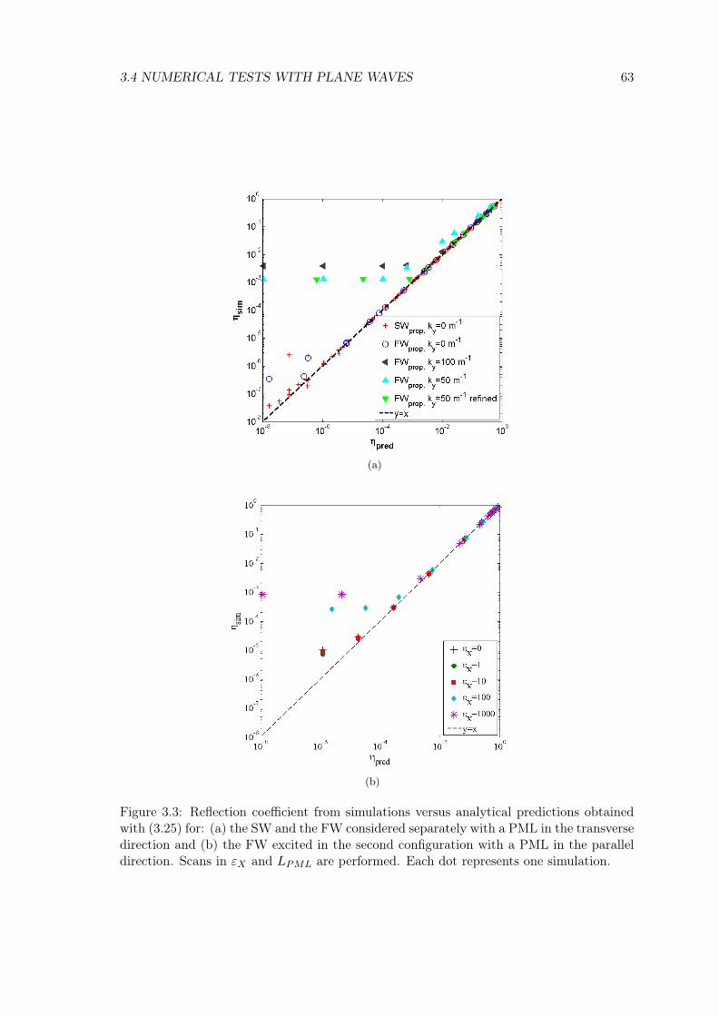
3.4 NUMERICAL TESTS WITH PLANE WAVES 63

(a)

(b)

Figure 3.3: Reflection coefficient from simulations versus analytical predictions obtainedwith (3.25) for: (a) the SW and the FW considered separately with a PML in the transversedirection and (b) the FW excited in the second configuration with a PML in the paralleldirection. Scans in εX and LPML are performed. Each dot represents one simulation.

64 CHAPITRE3

The PML was tested in 2D in two configurations representative of a magnetic fusionplasma: PML in the radial direction x and PML in the parallel direction z, while periodicboundary conditions were applied in the other directions. All the work has been performedwith pulsation ω0 = 2πf0 where f0 = 57 MHz.

The first configuration corresponds to l = z, r = x and h = y in Figure 3.1. The planewave is excited by providing at x = 0 an electric field of the form e−ikzz with kz = 2Nπ/Lzwhere N is the mode number and Lz the parallel width of the simulation domain. For theFW this electric field is oriented along the y direction whereas it is along the z direction forthe SW. The plasma eigenmodes were studied independently. Several ε‖, ε⊥, N , LPML,S′′r , p, ky and mesh size have been tried.

To include ky 6= 0 in 2D simulations, the ky terms in the wave equation were added tothe dielectric tensor ¯ε. The stretching in the PML must also be included for these ky terms.The tensor ¯ny containing all the elements depending on ny = ky/k0 with their respectivestretching reads with ¯µ = ¯1:

¯ny ≡

− Sz(z)Sx(x)Sy(y)n

2y

Sz(z)Sx(x)Sy(y)nynx 0

Sz(z)Sx(x)Sy(y)nxny 0 Sx(x)

Sy(z)Sz(z)nynz

0 Sx(x)Sy(z)Sz(z)nzny − Sx(x)

Sy(z)Sz(z)n2y

. (3.30)

The second configuration corresponds to l = x, r = z and h = y in Figure 3.1. The planewave is excited by providing at z = 0 an electric field of the form e−ikxx with kx = 2Nπ/Lxwhere N is the mode number and Lx the radial width of the simulation domain. Insteadof applying input conditions along the parallel direction, they are applied on the radialdirection. The dispersion relation given by (2.21) is also reversed: k‖ = f (k⊥). Priorknowledge of k2

z is nevertheless necessary as the FW wave polarization depends on it whenthe Stix tensor given by (2.9) is not diagonal.

The reflection coefficient ηsim was then computed with the method presented in Sec-tion 3.4.1 for propagative modes and compared with the prediction given by (3.25) ηpred.The results are shown on Figure 3.3(a) for the first configuration.

An excellent agreement can be observed between predictions and simulations as longas ηsim > 10−5 with ky = 0 m−1. Below that limit the simulated reflection coeffi-cient saturates, which is attributed to numerical effects. This saturation occurs when2kxLPMLS

′′r (p+ 1)−1 > 10.

With ky 6= 0 m−1 prior knowledge of the dispersion relation is required to compute kxfrom ky and kz that are imposed. The effective dielectric tensor ¯εPML becomes ¯εPML+ ¯ny.With ky 6= 0 m−1 the reflection coefficients are more sensitive to the mesh. Neverthelessηsim < 10−2 have been reached. Some sensitivity to the mesh resolution can be observed.

For evanescent modes, the radial profile of Ez and Ey were fitted by an exponentiallydecaying function for the slow wave and the wave respectively and compared to the ana-lytical prediction for kx. The PML was placed in the decay of the wave to get finite waveamplitude at the PML entrance. Excellent fits were found while the PML depth is largerthan half the typical wavelength associated to kx. Larger value of S′r (here S′r = 1) wouldeven diminish further the PML depth.

The results for the second configuration are shown in Figure 3.3(b). Only the FW isconsidered. A scan in εX was performed while varying the PML depth LPMLt to observethe effect of the gyrotropy in ¯ε. Similar behaviour is observed. The saturation is howeveroccurring at higher ηsim values and is dependent on the gyrotropy of the dielectric tensor.Increasing the mesh resolution in the radial direction did not allow reaching a smallersaturation level.

3.4 NUMERICAL TESTS WITH PLANE WAVES 65

3.4.3 Numerical optimization of the PML for a given plane wave

Now that it has been seen that it is possible to obtain a working PML for one plane waveeigenmode, it is crucial to know the influence of the different PML and mesh parameters(hmax, p, S

′′ and LPML) in order to optimize it and therefore reduce its computationalcost that causes an additional strain on the available resources. The “desired” domain isthus not only the plasma but the “needed” the union plasma+PML. The observed influenceof a parameter can then be compared to what is predicted analytically from (3.25). Thisrelatively academic test for plane waves will bring guidelines for the more complex situationwith realistic antenna geometries in Chapter 4.

The following part is done only for the Fast Wave with a radial PML (r = x and l = z)and ky = 0 m−1. The parametric dependence should not depend anyway of the choice ofthe wave. The stretching coefficient S′′ is chosen to be negative to get a positive groupvelocity and thus an antenna emitting power that is sent into the plasma.

The simulations were defined with the following parameters: ε‖ = −10000, ε⊥ = 1000,εX = 100 for the Stix parameters, the parallel dimension of the domain L‖ = 1 m andthe perpendicular dimension of the medium L⊥ = 0.4 m. With the parallel mode numberN = 2, it gives k‖ = 2Nπ/L‖ = 4π m−1 corresponding to a parallel wavelength λ‖ = 0.5 m.With Stix parameters defined above, it gives using the dispersion relation for the fast wave,given by (2.21), kx = 35.4 m−1 corresponding to a radial wavelength λ⊥ ≈ 0.18 m.

The optimization procedure consists in finding the best set of PML parameters andgrid parameters giving a reflection coefficient ηchoice that is thought to be acceptable foraccuracy and numerical cost.

3.4.3.1 Influence of the PML depth LPML on η

The test consisted in verifying that (3.25) was correct in saying that the reflection isdecreasing as the PML depth LPML is increasing for all other PML parameters fixed:S′ = 1, S′′ = −1 and p = 2. The test should also compare the PML depth LPML to theradial wavelength since the PML is placed in the radial direction. hmax‖ = 0.02 m waschosen giving 25 elements per wavelength. The same procedure has to be done for theradial wavevector. With hmax⊥ = 0.01 m, it gives about 18 elements per wavelength. Theresults of this scan are shown on Figure 3.4. The reflection coefficient is decreasing whenLPML is increasing up to some limit that could be due to the mesh parameters. It willbe tested in the next parametric scan. More importantly the simulations results followthe prediction given by (3.25). It can also be seen that the worse reflection coefficient areobtain for LPMLkx < 1 meaning that the PML depth is smaller than the typical radialwavelength. This effect can easily be observed in (3.25). With a small product LPMLkx itis more difficult to obtain a high value for the exponent. It will unfortunately be the casein the region near the cutoffs where kx ≈ 0, meaning high wavelength. The best thing todo would be then to place the plasma/PML interface far away from the cutoffs region inorder to avoid any incoming problem.

3.4.3.2 Influence of the elements size hmax⊥ and type on η

The first parametric scan has shown a limit in the agreement between simulations andpredictions for η possibly due to the mesh parameters. In order to correct it, several valuesof hmax⊥ have been tested. For all of them, there were at least two elements per wavelengthgiving a minimum resolution of the wavelength. The grid resolution is kept the same inboth the medium and the PML. The other PML parameters are: S′ = 1, S′′ = −1 and

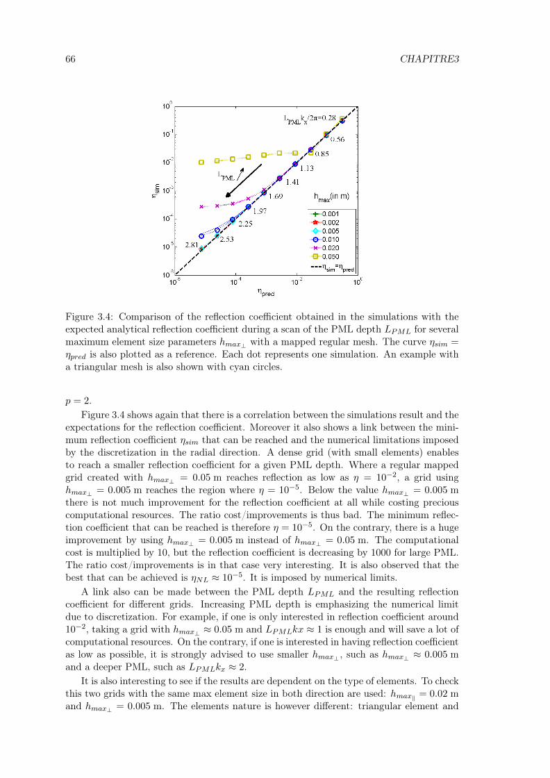
66 CHAPITRE3

Figure 3.4: Comparison of the reflection coefficient obtained in the simulations with theexpected analytical reflection coefficient during a scan of the PML depth LPML for severalmaximum element size parameters hmax⊥ with a mapped regular mesh. The curve ηsim =ηpred is also plotted as a reference. Each dot represents one simulation. An example witha triangular mesh is also shown with cyan circles.

p = 2.Figure 3.4 shows again that there is a correlation between the simulations result and the

expectations for the reflection coefficient. Moreover it also shows a link between the mini-mum reflection coefficient ηsim that can be reached and the numerical limitations imposedby the discretization in the radial direction. A dense grid (with small elements) enablesto reach a smaller reflection coefficient for a given PML depth. Where a regular mappedgrid created with hmax⊥ = 0.05 m reaches reflection as low as η = 10−2, a grid usinghmax⊥ = 0.005 m reaches the region where η = 10−5. Below the value hmax⊥ = 0.005 mthere is not much improvement for the reflection coefficient at all while costing preciouscomputational resources. The ratio cost/improvements is thus bad. The minimum reflec-tion coefficient that can be reached is therefore η = 10−5. On the contrary, there is a hugeimprovement by using hmax⊥ = 0.005 m instead of hmax⊥ = 0.05 m. The computationalcost is multiplied by 10, but the reflection coefficient is decreasing by 1000 for large PML.The ratio cost/improvements is in that case very interesting. It is also observed that thebest that can be achieved is ηNL ≈ 10−5. It is imposed by numerical limits.

A link also can be made between the PML depth LPML and the resulting reflectioncoefficient for different grids. Increasing PML depth is emphasizing the numerical limitdue to discretization. For example, if one is only interested in reflection coefficient around10−2, taking a grid with hmax⊥ ≈ 0.05 m and LPMLkx ≈ 1 is enough and will save a lot ofcomputational resources. On the contrary, if one is interested in having reflection coefficientas low as possible, it is strongly advised to use smaller hmax⊥ , such as hmax⊥ ≈ 0.005 mand a deeper PML, such as LPMLkx ≈ 2.

It is also interesting to see if the results are dependent on the type of elements. To checkthis two grids with the same max element size in both direction are used: hmax‖ = 0.02 mand hmax⊥ = 0.005 m. The elements nature is however different: triangular element and

3.4 NUMERICAL TESTS WITH PLANE WAVES 67

mapped square elements. The other PML parameters were kept still the same as before:S′ = 1, S′′ = −1 and p = 2. For small PMLs no difference on the reflection coefficient hasbeen seen on Figure 3.4. However, a discrepancy appears for LPMLkx > 2 and η < 10−4.Numerical grids effects are the root cause of this discrepancy. It means that the results aresensitive to the grid elements nature below this threshold. This is of course not physical. Itthus gives the limit reachable for the reflection coefficient measurements as the result shouldnot be grid dependent. The minimum reflection coefficient achievable is then reassessed:η = 10−5 → η = 10−4. Reaching more accurate results would require a finer refinement ofthe mesh especially in the parallel direction and a finer sampling in the data set used fordata exportation.

3.4.3.3 Influence of the stretching function order p on η

Another PML parameter appearing in the analytical reflection coefficient is the PML orderp. The influence of this parameter will be highlighted here. Stretching order p = 2, 3, 4have been tested. The other parameters are: triangular element with hmax⊥ = 0.01 m,S′ = 1 and S′′ = −1. It is intuitive from (3.25) that low order is preferable. Neverthelessp = 1 is avoided in order to retain the continuity of the first derivative of the stretchingfunction S in (3.24) at the medium/PML interface (r = Lr in Figure 3.1). Simulationresults are showed in Figure 3.5. The reflection coefficients resulting from the simulationsbehave as expected from the analytical formula. It is also clear that (3.25) is correct whensaying that low order give smaller reflection coefficient for a given PML depth. It alsoconfirms that large PML depth give better results. However, a PML depth as small aspossible is aimed at in order to minimize the computational cost. As a consequence, fromnow on, p = 2 will be used as the stretching function order.

Figure 3.5 shows again that for the considered mesh the minimum value of the reflectioncoefficient that can be reached is ∼ 10−5. That level is reached faster with low PML orderas expected from (3.25). η decreases faster with a low PML order and consequently reach

Figure 3.5: Reflection coefficient from the simulations versus the PML depth normalizedto the radial wave vector component for several order value. S′ = 1, S′′ = −1, hmax⊥ =0.01 m. The dashed lines are the predicted reflection coefficient.

68 CHAPITRE3

the numerical saturation level faster.

3.4.3.4 Influence of the stretching function coefficient S′′ on η

It has been seen that the reflection coefficient that can be reasonably achieved is η = 10−4.Looking at Figure 3.4, it can be deduced that to achieve this condition, it is enough totake hmax⊥ = 0.005 m, thus limiting the computational cost to what is necessary.

In (3.25) it can easily be seen that increasing S′′ will decrease the reflection coefficientuntil the saturation level near η ≈ 10−5 where the simulation dots stop following thepredictions. This is true, but it does not take into account neither the discretization dueto the grid, nor the fact that a spatial stretching function can be interpreted as a complexdensity gradient. Increasing S′′ will then also produce a steeper gradient in the stretchingfunction used to transform the coordinate. If the grid is not dense enough to correctlyresolve the gradient, some spurious reflection will appear.

This is what happens in Figure 3.6 for high value of S′′. For example, in the case S′′ = 50or S′′ = 20 a non monotonous behaviour is seen. ηsim also are far from the predictions. It isinterpreted as the presence of numerical artefacts. The results are otherwise in accordancewith the expectations. If the acceptability for the reflection coefficient is fixed at η = 10−4,there is a great improvement in term of computational resources when increasing |S′′| from1 to 8. The necessary PML depth goes from LPML ≈ 0.4 m to LPML ≈ 0.05 m. Whenspeaking in radial wavelength unit, it corresponds to a transition from LPMLkx ≈ 2.3 toLPMLkx ≈ 0.3.

Figure 3.6 shows that being too careful with LPML and S′′ brings out a serious overcost.At the other extremity, it is not necessary to use extreme S′′ value. It is important to noticethat for high S′′ the sensibility on LPML causes huge variations on the reflection coefficientη. The variation in ρ due the variation of one element or 1 cm is more important for highS′′ than for low S′′. Taking a moderate value, such as |S′′| = 4, already allow to obtain aPML of about half the wavelength of the considered wave while not be too sensible.

Figure 3.6: Plot of the reflection coefficient obtained in the simulations in function of thePML depth for several stretching value. S′ = 1, p = 2, hmax⊥ = 0.005 m. The dashedlines are the predicted reflection coefficient.

3.4 NUMERICAL TESTS WITH PLANE WAVES 69

Looking now at the κ factor (κ = LPML/hmax) corresponding to the number of elementsin the radial dimension of the PML, it goes from 40 in the conservative case to 5 in theextreme case. Concerning the moderate case, κ is equal to 10.

To conclude Section 3.4.3, let us summarize the main results. Numerical simulationswith plane waves in homogeneous plasmas has confirmed analytical predictions given by(3.25). It has also confirmed the existence of numerical limits explained in Section 3.3.4.A common advice in textbook [147] is to take a PML depth of the order of the consideredwavelength which has been confirmed here. This advice will be followed in Chapter 4.The order p = 2 is favoured as it obtain lower reflection for a smaller PML than higherorder as expected from (3.25). The imaginary stretching coefficient can be tuned, butshould not go beyond S

′′= 10. The grid resolution has also shown to be an important

parameter. The wave, of course, should correctly be resolved with around 10 grid pointsinside a wavelength. It is advised to take at least 5 grid points in the PML [147]. To avoidhuge numerical cost, a cutoff should be avoided since the wavelength is large. Let us focusnow of a more fundamental issue with PML formulation when forward and backward wavescoexist simultaneously in a medium.

3.4.4 Simultaneous handling of two polarizations in gyrotropic medium

Remembering that the stretched space coordinate is written as t∞ = t′∞ + it′′∞, fulfillingthe condition ηpred << 1 means:

exp(|kr| t′∞

)>> 1 with kr = i |kr| , (3.31)

exp(|kr| t′′∞

)>> 1 with kr = |kr| , (3.32)

exp(|kr| t′′∞

)<< 1 with kr = − |kr| . (3.33)

Conditions (3.32) and (3.33) are incompatible. In practice choosing the sign of t′′∞ viathe sign of S′′r will “select” the sign of the phase velocity in direction r for the propagatingplane wave that will “emerge” from the numerical simulations. While PMLs can be devisedto emulate correct radiations conditions at infinity for both [forward+evanescent] or [back-ward+evanescent] waves, the PML in its present formulation is not suitable for handling[forward+backward] waves simultaneously.

This issue is of practical importance when modelling radiation from antennas. In suchproblems the physically relevant plane waves are those that carry RF power away fromthe antenna, i.e. those with a group velocity directed towards the PML in direction r. Inisotropic media, for symmetry reasons the group velocity is always parallel to the phasevelocity. In anisotropic plasmas it can happen that the physically relevant componentscorrespond to forward waves for one eigenmode and backward waves for the alternativepolarisation, leading to incompatibility when both propagative eigenmodes need to behandled simultaneously. A similar situation was also met for wave propagation in flowingfluids or orthotropic solids [165]. This is an area where significant progress still has to beperformed.

It is illustrated in Figure 3.7(a) and in Figure 3.7(b) with r = x and l = z for respec-tively the FW and the SW. The same sign for imaginary stretch was taken for propagativeplane waves. The main component of the Poynting vector for the FW wave is radial. ThePoynting vector lies mainly in the parallel direction for the SW. The power is transmittedto the plasma for the FW while with the same stretch the power flows from the plasma tothe wall in the case of SW.

70 CHAPITRE3

(a)

(b)

Figure 3.7: 2D map of the real part of the electric field for: (a) the Fast Wave (forwardwave) and (b) the Slow Wave (backward wave). The magnetic field is along the toroidaldirection. ε‖ < 0, ε⊥ > 0 and S′′ < 0 in order to “select” forward waves. The blackarrows correspond to the Poynting vector. In (a) ε‖ = −105, ε⊥ = 103, ε× = 102. In (b)ε‖ = −105, ε⊥ = 102, ε× = 1. In both cases N = 2, pr = 2, S′′r = −1 and S′r = 1.

3.4 NUMERICAL TESTS WITH PLANE WAVES 71

3.4.5 From reflection coefficient to Poynting vector flux

It was extensively verified that the modulus of the amplitude reflection coefficient observedin plane waves simulations agrees with the analytical predictions. Looking for radial modu-lations of the RF field amplitude is only possible for plane waves, as the notion of reflectioncoefficient can only be defined for plane waves. This ideal case is far from reality where abroadband spectrum of wave-numbers, such as excited by realistic ion cyclotron antennasin magnetic Fusion devices, exists. As the system is linear, a reflection coefficient can stillbe evaluated for each plane wave assuming that plane waves can easily be distinguishedeven in the presence of several kinds of PMLs replacing the periodic boundary conditionused previously. Defining a spectrum of plane waves from the simulations is only possiblewith some transverse boundary conditions. This process, if possible, will moreover be longand fastidious. In more realistic simulations, another quantity can be monitored: the RFpower transferred through the PML interface, i.e. the flux of the Poynting vector. SincePMLs are meant to emulate radiation at infinity, this transmitted power should be insen-sitive to variations of the PML parameters in the successful simulations. For the case of aplane wave, an explicit analytic expression linking Poynting vector and reflection coefficientcan be derived. The complete derivation is shown in Appendix B. Scalar expressions arenow replaced by vectorial ones for one eigenmode. The electric field reads:

E(x, k‖, ky

)=[E+ exp (ikxx) + E− exp (−ikxx)

]eikzz+ikyy. (3.34)

Section 3.4.4 showed that a PML cannot be adapted simultaneously for propagatingfast and slow wave. As in the ICRH applications, the fast wave carries the RF power to bedeposited in the plasma, it will be the one treated. Moreover the slow wave is evanescentin the considered range of densities and therefore it never reaches the PML. The fast waveelectric field reads: E = Ey (iαx+ 1y) with α = εX

ε⊥−n2‖.

Since plane waves are considered, H = cµ0

n × E. With the incident (index +) andreflected wave (index −) propagating in opposite radial directions, the total induction Hreads:

H = H+ + H− =c

µ0n+ ×E+ +

c

µ0n− ×E−. (3.35)

The incident and reflected poloidal field amplitudes are related by the complex reflectioncoefficient Γ ≡ η exp (iϕ). The radial component of the time average Poynting vector Pxthus yields:

Px =1

2< (E×H∗)x = ε0c

∣∣E+y0

∣∣22

nx(1− η2

). (3.36)

The poloidal electric field Ey0 imposed at the position x = 0 is:

Ey0 = E+y0

(1 + ηeiϕ

). (3.37)

Multiplying (3.37) by its complex conjugate and combining it with (3.36), yields:

Px = ε0c|Ey0 |

2

2nx

1− η2

1 + 2η cos (ϕ) + η2. (3.38)

The cosine can change sign in the denominator, thus giving a damped oscillatory be-haviour of the coupled power as the reflection coefficient η approaches unity.

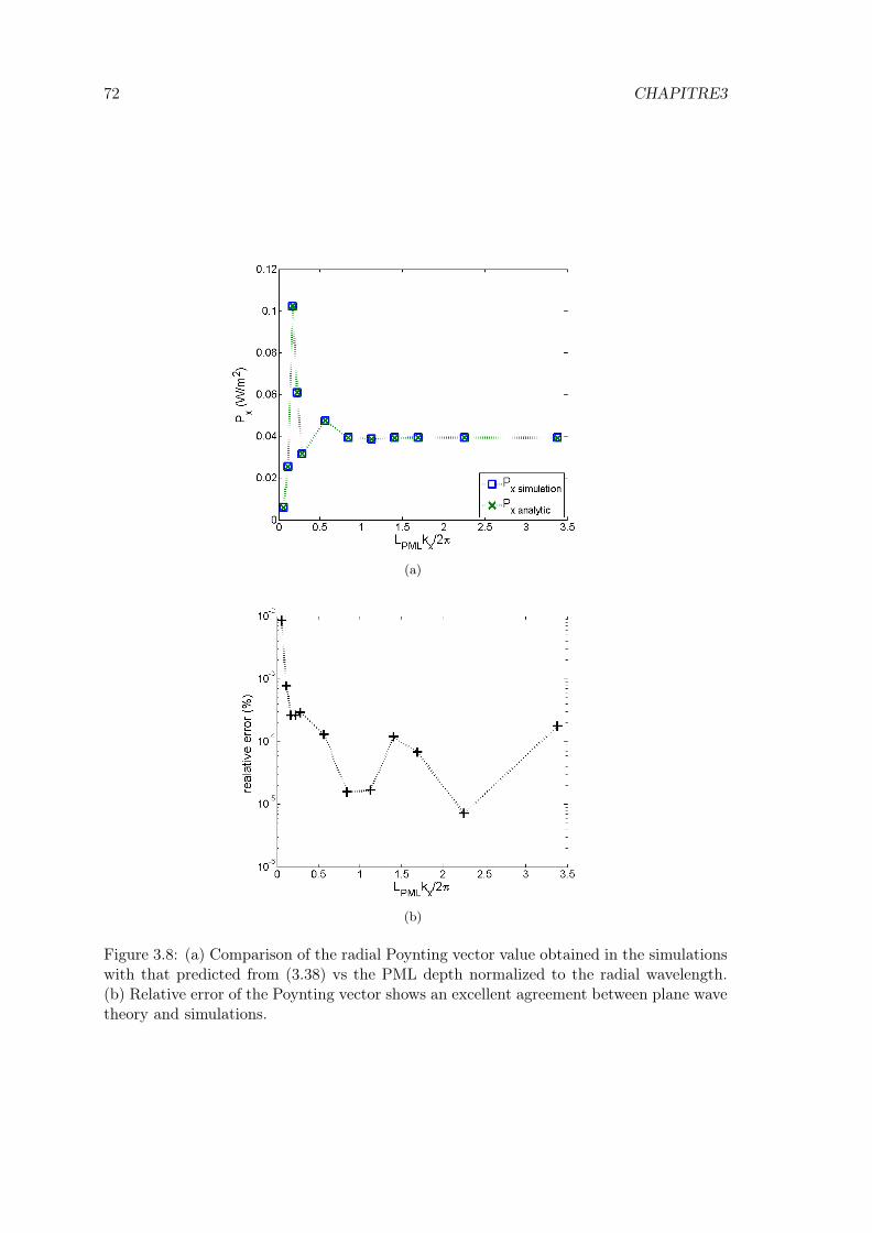
72 CHAPITRE3

(a)

(b)

Figure 3.8: (a) Comparison of the radial Poynting vector value obtained in the simulationswith that predicted from (3.38) vs the PML depth normalized to the radial wavelength.(b) Relative error of the Poynting vector shows an excellent agreement between plane wavetheory and simulations.

3.5. SUMMARY 73

A confirmation of this feature has been performed. The results are shown in Fig-ure 3.8(a). The PML depth was progressively reduced while keeping the plasma domainidentical. The parameters of the scan are: N = 2, ε‖ = −105, ε⊥ = 103 and ε× = 102,S′r = 1, S′′r = −1, pr = 2, L‖ = 1 m and L⊥ = 0.4 m. Triangular finite elements ofsize 2 cm were used with a 10 scale factor in the mesh in the radial direction. The scalefactor is the ratio of the typical element size in both directions. The value of the radialcomponent of the Poynting vector is then compared to its prediction from (3.38). Theagreement between predictions and simulations is excellent as the relative error is small. Italso confirmed that taking a PML depth larger than the radial wavelength does not allowmuch improvement on the Poynting vector. The transmitted power is therefore anotherpossible qualitative indicator to monitor the quality of the PML in realistic simulations,faster than evaluating a reflection coefficient for each plane wave in the excited spectrumof wave-numbers.

3.5 Summary

An original use of PML method has been successfully performed in homogeneous mag-netized plasmas. Within this approach, the PML technique is used to emulate radiatingboundary conditions at infinity. Magnetized plasmas contain several specificities that couldbe a priori of concern for the application of PMLs for vectorial simulation of time-harmonicwave propagation in magnetized plasmas.

The first issue concerns its formulation for gyrotropic dielectric tensors with off-diagonalelements. A versatile formulation was found in the literature and was interpreted as stan-dard wave propagation in an artificial medium with damping properties. Its implementa-tion is quite general, aesthetic and easy to accomplish.

PMLs have been at first tested on homogeneous magnetized plasmas for plane wavesusing the finite element method in the Comsol software. For plane waves, the PML ef-ficiency has been evaluated both analytically and numerically by a reflection coefficient.Agreement with simulations is excellent as long as a threshold due to numerical effects isnot reached. This assessment provides useful guidelines for PML implementation in morerealistic simulations, where a compromise between low reflection and numerical cost needsto be found over a broadband spectrum of plane waves. For given PML parameters, thereflection is enhanced near a cutoff layer. For propagative plane waves in vacuum, this cor-responds to the case of grazing incidence, where the PML behaviour is known to degrade.The spectral domain of low PML reflection can be reduced by enlarging the PML size, atthe expense of increased memory requirements and computational time. A better solutionis therefore to avoid placing a PML in the neighbourhood of a cutoff for all relevant modesin the radiated power spectrum.

A second specificity is related to the birefringence of magnetized plasmas, implying thecoexistence of plane-wave eigenmodes with very different properties. The incompatibility ofthe present PML formulation to handle simultaneously forward and backward propagativewaves has been demonstrated analytically and illustrated numerically. Similar situationwas also met for wave propagation in flowing fluids or orthotropic solids [165]. This is anarea where significant progress still has to be performed. A way to overcome this criticalissue in a tokamak simulation is to exploit the plasma spatial inhomogeneity and let itreflect one of the polarizations, the slow wave in our application. The PML is thus onlyadapted for the other polarization, the FW here. The situation here however consideredan homogeneous plasma. The PML behaviour in presence of an inhomogeneous mediumwould nevertheless have to be first checked in Chapter 4.

74 CHAPITRE3

Finite values of ky have also been considered. It does not indicate any particularissue. However interplay between ky and the discretization of the grids has been observed.Furthermore the accuracy reached for finite ky values is less than with ky = 0 for identicalmesh parameters. Reflection coefficient of 10−3 has nevertheless been obtained. Thisindicates that for finite size antenna where ky spectrum exist, PML can be used and thatthe limits of the PML technique comes from the discretization. It should however beconceded that an exhaustive scan of the impact of finite ky has not been performed by lackof time and other priorities. This could be envisaged as a prospect. Instead a rapid checkwith a couple of values has been done.

Numerical optimization for plane waves in homogeneous plasmas of PML and meshparameters brought some guidelines that will be useful for the application of PMLs forantenna geometries. The PML depth should be of the order of the corresponding wave-length in the PML direction. The PML order p = 2 will be used. Increasing the valueof the imaginary stretch can reduce significantly the PML depth and thus the numericalcost, but can also cause spurious effects since the gradient in the PML will not be resolvedby the mesh any more. That brings some conditions of the mesh parameters. It shouldof course resolve the wave accurately. For that, a common advice is to have around 10grid points per wavelength. The same mesh parameters will be also used in the PML. Itis noteworthy to recall that the PML can be rendered perfectly reflection less only in thecontinuous wave equation. But finer mesh resolution in the discretization get us closer tothat ideal situation. Polynomial stretching function have been used here and will be usedin Section 4, but a possible prospect to reduce and control furthermore the numerical spu-rious reflection could be to use geometrical stretching function that always keep a constantgradient between adjacent grid points.

An formal equivalence for plane waves between normal component to the medium-PML interface of the Poynting vector and reflection coefficient have been demonstrated.The former quantity will be easier to use with ICRH antennas that emit a spectrum ofplane waves. The next step is thus to apply the PML technique in a code calculating FWcoupling for ICRH antenna in a tokamak plasma environment.

Chapter 4

Fast wave coupling code for ICRHantennas facing a fusion magnetizedplasma in Comsol relying on thePerfectly Matched Layer technique:Application on Tore Supra

The formalism outlined in Section 3.2 is very versatile and can be adapted to a largeset of configurations. We would like to include the PML technique for the first time intokamak plasmas (to our knowledge) in a fast wave coupling code having a full cold plasmadescription and an ICRH antenna geometry in high single-pass absorption scenarios.

As the goal here is to simulate and predict the behaviour of the ICRH antenna in agiven experiment, which does not radiate a plane wave, we have to test and improve theimplementation proposed in the previous part. This PML layers have been designed to beuse in 3D configurations and for sure there are limitations that we describe in the case ofsimulations of Tore Supra antennas. Similar studies using PMLs have been done in thecase of wave propagation and mode conversion in inhomogeneous ionospheric magnetizedplasmas [151]. Some limitations of the PML have been encountered in the study of thePML properties for plane waves in Section 3.4 and in this chapter we will show how, inthe simulations of Tore Supra ICRH antennas, to overcome these limitations.

Moreover the proposed solution is applicable only in a given domain, which is describedin detail as all the numerical requirements and all the tools needed to reconnect the sim-ulation to experimental parameters to validate the code. Depending on the degree ofsophistication of the antenna modelling, we deduce what should be a good description ofthe antenna to reach its correct behaviour in experiments. However as usual in simulationswe have to determine a good compromise between computer limitations and desired degreeof accuracy, for which some indications are provided. As a result, the full-wave near fieldis simulated in two or three dimensions to interpret fast wave coupling experiments carriedout on the Tore Supra tokamak.

This exercise provides the opportunity to discuss concrete PML implementation issuesin realistic cases, with emphasis on specificities due to anisotropy and birefringence:

• PML adapted to a broadband spectrum of plane waves, how to estimate its qualitya priori and check it a posteriori.

75

76 CHAPITRE 4

• PML adapted to different directions in tokamak.

• Where to place the PML with respect to the antenna structure in order to capturethe relevant fast wave physics.

• Avoid the eigenmode incompatibility issues discussed in Section 3.4.4.

The first part of this chapter introduces the experimental parameters and the experimentalobservations that the fast wave coupling code should be able to reproduce. Then theantenna and plasma modelling is discussed. Finally the implementation and the testsof the PML technique with an antenna geometry in the context of tokamak magnetizedplasmas is performed. In the second part, simulations in 2D and in 3D are compared toexperimental values of the coupling resistance. Also addressed is the accuracy level neededin the antenna geometry to produce quantitative wave coupling results compatible withthe measurements. A comparison with simulations performed with the reference code inthis domain is also performed. The last part is devoted to some prospects on the shortterm for WEST antennas coupling studies and in the longer term.

4.1 Modelling, implementation and numerical tests

4.1.1 Link between Poynting vector and coupling resistance

As it was shown formally for plane waves in Section 3.4.5, the Poynting vector can bea figure of merit of the reflection instead of the reflection coefficient. More specificallythe evolution with changes of PML parameters of the component of the Poynting vectorperpendicular to the interface plasma-PML can be of interest. The figure of merit stillholds true for an antenna, as it is exciting a spectrum of plane waves.

In the simulations, integrating over the contour separating the plasma from the PMLregion the normal component to the contour of the Poynting vector gives the power car-ried by the wave leaving the plasma. This also corresponds to the power that is cou-pled/transmitted to the plasma from the antenna. This is performed by computing thecross product of the electric field E and of the conjugate of the magnetic induction H∗:

Pt =

∫contour

(E×H∗)n ds, (4.1)

where s denotes the coordinate along the contour. The transmitted power is explicitlylinked to the coupling resistance Rc defined in (2.36).

On Tore Supra, this linear coupling resistance Rc in Ω/m is obtained from standingantenna voltage and capacitor measurements through a commonly used transmission linemodel of the antenna [41]:

Rc = 2Pt

(Lstrap

∫strap|IRF (s)|2 ds

)−1

, (4.2)

where IRF (s) denotes the RF peak current profile along the strap (assumed sinusoidal in2D), Pt the net time averaged transmitted power in the feeding line and Lstrap the lengthof the strap. The resistance per length unit is adjusted over a large band of frequenciesto reproduce experimental matching values on vacuum taking into account geometricalparameters of the line in the characteristic line impedance. On plasmas, it gives coherentresults with expectations [65].

4.1. MODELLING, IMPLEMENTATION AND NUMERICAL TESTS 77

4.1.2 Description of the wave coupling experiment

Wave coupling was assessed in dedicated RF pulses conducted in dipole phasing, using theD(H) minority heating scenario at 57 MHz, with minority fraction 5% and with magneticfield B0 = 3.87 T at R = 2.37 m (see Figure 2.4(a)). The classical antenna, introduced inSection 2.4, was located at Rant = 3.13 m, which denotes the radial position of the leadingedge of the antenna limiter, the innermost part of the antenna. For these experimentsthe FW single pass absorption was effective, which motivates using PMLs to emulate FWradiation to the main plasma. During the RF pulse #43026 the plasma separatrix waspushed back progressively from the antenna. Over this radial scan the density profile wasmeasured by reflectometry with an estimated ±1 cm uncertainty in the radial position ofeach density point [65, 146]. The time average density profiles over 0.5 sec intervals areshown in Figure 4.1(a). The radial positions of the separatrix Rsep, known with a 0.5 cmaccuracy, are also averaged over time.

In Tore Supra it was found that Rc is well characterized by a parameter representativeof the wave tunnelling through the edge plasma: the radial distance between the radiatingstraps and a characteristic cut-off layer for the fast wave, evaluated for k‖ = 13 m−1 themaximum in the RF current spectrum in dipole strap phasing [65]. The cut-off density is:ncutoff,FW = 9.3× 1018 m

−3. In Figure 4.1(b) Rc was plotted against the measured strap-cutoff distance, that was moved from about 5 cm to 10 cm (see Figure 4.1(a)). Exponentialvariation of Rc with Rstrap−Rcutoff is evidenced, consistent with an evanescence process.Rstrap and Rcutoff denote respectively the position of the front face of the strap and theposition of the cutoff layer. The coupling resistance is assumed to behave as [65]:

Rc ∼ exp (−2 < kx > [Rstrap −Rcutoff ]) , (4.3)

where < kx > can be seen as an average value of kx over the radial path strap/cutoff [65].< kx > is indicative of the slope of the curve in Figure 4.1(b).

The same procedure was followed in the pulse #40574 where several antennas wereavailable: two classical antennas and the ILP antenna, also introduced in Section 2.4. Inthis pulse, the antennas were at 48 MHz and the central magnetic field was accordinglychanged to 3.1 T to keep the cyclotron resonance position invariant. One classical antenna,named here classical (2), and the ILP antenna were placed at Rant = 3.13 m while the otherclassical antenna, named classical (1), was located 2 cm behind of the two others radiallyat Rant = 3.15 m. The antennas were active one by one with the same power. The plasmaenvironment around the antennas is assumed to be equivalent.

The radial position of the separatrix was moved horizontally over 5 cm to modify thedistance between the strap and the considered cut-off layer (see Figure 4.1(c)). It getsto similar results for Rc, as shown in Figure 4.1(d). The two classical antennas coupledsimilar amount of power taking into account the 2 cm difference in their radial position.The ILP antenna coupling efficiency was however only 40% of the one for the classicalantenna for the same distance. It was attributed to the 1.8 cm shift outwards for thestraps position in the ILP antenna (represented by the horizontal shift between the blueand red curve in Figure 4.1(d)). It does not explain however the vertical shift betweenthe red and green curves, since the distance strap-cutoff is equivalent for both antennas.The explanation is most probably in the antenna design. We will come back later on thisissue (see Section 4.3.2) once the fast wave coupling code for ICRH antennas in tokamakplasmas relying on the PML technique has been checked.

78 CHAPITRE 4

(a) (b)

(c) (d)

Figure 4.1: Density profiles versus major radius R for the pulses (a) #43026 and (c)#43026. The density profile is modified by moving the separatrix Rsep (vertical dashedlines). The sketch of an antenna (not to scale) is drawn to give an idea of the radialdistances involved. Experimental coupling resistance values versus distance strap/cutofffor the pulses (b) #43026 and (d) #40574. Each circle represents one measurement of Rc.Three antennas with the same power were used in #40574. Two antennas (blue and green)are of the classical type and one was the ILP antenna (red).

4.1.3 Modelling of the Tore Supra ICRH antennas and of the edgeplasma

To reproduce numerically the experimental observations, the full-wave time-harmonic vec-torial Maxwell’s equations given by the system (2.3) were solved in two dimensions (ra-dial/toroidal) and three dimensions in the edge plasma domain surrounding the wavelauncher geometry, using the FEM method with the Comsol Multiphysics commercial soft-ware [166].

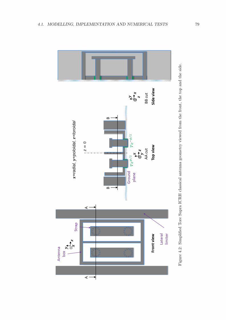
4.1. MODELLING, IMPLEMENTATION AND NUMERICAL TESTS 79

Figure4.2:

Simplified

ToreSu

praIC

RH

classicala

ntenna

geom

etry

view

edfrom

thefron

t,thetopan

dtheside.

80 CHAPITRE 4

Figure4.3:

Simplified

ToreSu

praIC

RH

ITER-like

prototyp

ean

tenn

ageom

etry

view

edfrom

theba

ck,the

side

andthetop.

4.1. MODELLING, IMPLEMENTATION AND NUMERICAL TESTS 81

Full designs of the antennas with CAD draws are available for TOPICA simulations.However such details are resources consuming. A simplified version of the classical ToreSupra ICRH antenna geometry, shown in Figure 2.10, is here included in the model. For thesake of simplicity the plasma and the antenna structure were flattened in the toroidal andpoloidal directions. The shape of the different objects composing the design is as simpleas possible with as few objects as possible. Both the active straps and their surroundingpassive elements contribute a priori to the fast wave coupling and need to be included inthe antenna description. The objects that are kept are both active radiating straps, theantenna box, the central septum and the lateral limiters. An investigation of the necessarydescription of these objects will be presented later in Section 4.2.2. The Faraday screen isnot included. After simplification, the classical antenna looks like in Figure 4.1.3.

All boundaries of the passive components are treated as perfect electric conductorsin the simulation domain. Tore Supra ITER-like prototype antenna [137], shown in Fig-ure 2.11 has also been modelled with a flattened geometry, shown in Figure 4.1.3. Thesame considerations are also assumed to be true.

In 2D geometry in the toroidal/radial plane, both antennas appear to have similar inthe design. The difference is in the strap width and the massive protruding part of thepoloidal septum. The straps are also further away from the plasma in the ILP antenna.This 2D top view of the antenna is misleading as 3D drawings show that they are quitedifferent. A massive horizontal septum is present on the ILP antenna. The straps are alsoquite different. The classical antenna has two long straps while the ILP antenna has fourshort straps with the short-circuit on the top and bottom of the antenna box.

As including a feeding line is impossible for a 2D infinite strap, the fast wave is excitedin 2D simulations by imposing a surface current density on each strap face independently,with the condition that the total current on the strap is 1 A. It is noteworthy to mentionthat this situation is not self-consistent but an ad hoc choice. Self-consistency can only beachieved in 3D. It is also possible to change the current balance between front face andback face, thus imposing more current on one face than on the other (see Figure 4.1.3).The surface current density is assumed homogeneous in the toroidal direction. In realitydue to magnetic shielding, the current distribution is peaked on the sides of the strap [63].Magnetic shielding also occurs due to current loop of the Faraday screen rods [32], thatare not included here. The current densities on the sides are linearly ramped up from thevalue at the back to the value on the front to keep continuity of the current density alongthe strap contour, as shown in Figure 4.1.3.

In the ideal 3D model the complete resonant double loop (RDL) scheme should bereproduced and its match point should be found before simulating the antenna [167]. Herea simpler procedure is followed to simulate the perfectly matched RDL. The coaxial lineand the capacitors are not modelled. Instead RF voltages are imposed at the RF portsconnected to the capacitors (see Figure 4.1.3), with an imposed phase between the topand bottom of the straps. The RF current then develops self-consistently along the straps,treated as perfect metallic conductors.

The simulated magnetic field is assumed horizontal (i.e. no poloidal component),whereas its actual pitch angle is estimated to be 3.5 in the reported experiment. Further-more since the Faraday screen is not included or at least tilted FS rods are not included,left/right antenna symmetry can be assumed. Only half of the antenna can therefore besimulated, with a symmetry condition on the plane z = 0 (see Figure 4.1.3), to reduceby half the numerical cost in 3D. Tilted FS rods and tilted B would however break thesymmetry. The full antenna would thus have to be included.

With a dipole ([0, π]) toroidal phasing between straps, this symmetry condition is ac-

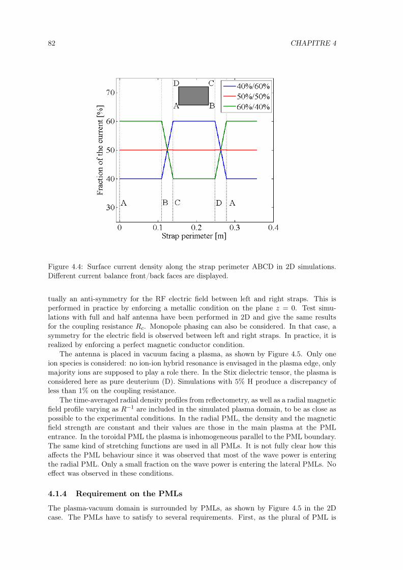
82 CHAPITRE 4

Figure 4.4: Surface current density along the strap perimeter ABCD in 2D simulations.Different current balance front/back faces are displayed.

tually an anti-symmetry for the RF electric field between left and right straps. This isperformed in practice by enforcing a metallic condition on the plane z = 0. Test simu-lations with full and half antenna have been performed in 2D and give the same resultsfor the coupling resistance Rc. Monopole phasing can also be considered. In that case, asymmetry for the electric field is observed between left and right straps. In practice, it isrealized by enforcing a perfect magnetic conductor condition.

The antenna is placed in vacuum facing a plasma, as shown by Figure 4.5. Only oneion species is considered: no ion-ion hybrid resonance is envisaged in the plasma edge, onlymajority ions are supposed to play a role there. In the Stix dielectric tensor, the plasma isconsidered here as pure deuterium (D). Simulations with 5% H produce a discrepancy ofless than 1% on the coupling resistance.

The time-averaged radial density profiles from reflectometry, as well as a radial magneticfield profile varying as R−1 are included in the simulated plasma domain, to be as close aspossible to the experimental conditions. In the radial PML, the density and the magneticfield strength are constant and their values are those in the main plasma at the PMLentrance. In the toroidal PML the plasma is inhomogeneous parallel to the PML boundary.The same kind of stretching functions are used in all PMLs. It is not fully clear how thisaffects the PML behaviour since it was observed that most of the wave power is enteringthe radial PML. Only a small fraction on the wave power is entering the lateral PMLs. Noeffect was observed in these conditions.

4.1.4 Requirement on the PMLs

The plasma-vacuum domain is surrounded by PMLs, as shown by Figure 4.5 in the 2Dcase. The PMLs have to satisfy to several requirements. First, as the plural of PML is

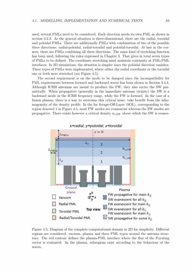
4.1. MODELLING, IMPLEMENTATION AND NUMERICAL TESTS 83

used, several PMLs need to be considered. Each direction needs its own PML as shown insection 3.2.3. As the general situation is three-dimensional, there are the radial, toroidaland poloidal PMLs. There are additionally PMLs with combination of two of the possiblethree directions: radial-poloidal, radial-toroidal and poloidal-toroidal. At last in the cor-ners, there are PMLs combining all three directions. The same kind of stretching functionhas been used, following the rules expressed in Chapter 3. That gives in total seven typesof PMLs to be defined. The coordinate stretching must maintain continuity at PML-PMLinterfaces. In 2D simulations, the situation is simpler since the poloidal direction vanishes.Three types of PMLs were implemented, where either the radial coordinate or the toroidalone or both were stretched (see Figure 4.5).

The second requirement is on the mode to be damped since the incompatibility forPML requirements between forward and backward waves has been shown in Section 3.4.4.Although ICRH antennas are meant to produce the FW, they also excite the SW par-asitically. When propagative (generally in the immediate antenna vicinity) the SW is abackward mode in the ICRH frequency range, while the FW is forward. In the case of afusion plasma, there is a way to overcome this critical issue: take benefit from the inho-mogeneity of the density profile. In the far Scrape-Off-Layer (SOL), corresponding to theregion denoted 1 in Figure 4.5, most FW modes are evanescent whereas the SW modes arepropagative. There exists however a critical density nc,SW above which the SW is evanes-

Figure 4.5: Diagram of the complete computational domain in 2D for simplicity. Differentregions are considered: vacuum, plasma and three PML types around the antenna struc-ture. The red contour defines the plasma-PML interface where the flux of the Poyntingvector is evaluated. In the plasma, subregions exist according to the behaviour of thewaves.

84 CHAPITRE 4

cent whatever k‖. This occurs when ε⊥ = 0, corresponding to nc,SW ≈ 1.3 · 1017 m−3 in our

simulations. Above the SW cutoff the wave becomes evanescent, it is naturally reflected bythe plasma and penetrates only for density below the cutoff density. Above, an exponentialdecay is present which avoids the use of PML for SW at densities above the cutoff density(natural screen of SW). As no power associated to SW goes at high density and even ifthe PML does not work for SW, no spurious effects of the computation are induced. Thesolution is thus to place the radial PML beyond the location of the SW cutoff. The PMLthus only has to be adapted for the FW.

As the antenna structure is placed in vacuum and the density at the antenna limiterleading edge is 1018 m

−3, the SW is here always evanescent. This condition is presentlyincompatible with the study of RF sheaths [34] requiring also the density profile up to theantenna radial position. For these additional radial positions the slow wave can possiblybe propagative (see Section 2.1.4). Issue with lower hybrid resonance (ε⊥ = 0) is avoidedin this thesis by a sharp transition between vacuum and plasma at density above thisresonance. But the countered part is a reflection associated to the index jump. Moreovera shallow density profile crossing the layer ε⊥ = 0 could produce resonance cones [168–170]. It becomes in that situation impossible to adapt the PML due to the singularityintroduced by the resonance cone by remembering that a singularity is associated withdiscontinuity incompatible with the use of PML (see Section 3.3.2). A comparison in2D with an exponentially decaying density profile between the side limiters (where theminimum density still gives ε⊥ < 0) but vacuum in the antenna box has not shown asignificant difference on Rc (second decimal).

Other requirements related to the FW physics exist for the PML position. In region2 on Figure 4.5, the SW is evanescent, as is the FW below the cutoff density nc,FW ≈9.3 · 1018 m

−3 for the main mode. To reproduce ICRH wave coupling, it is important toreproduce the peripheral tunnelling of all the important plane wave components in thelaunched k‖ spectrum. The plasma-PML interface should be placed radially beyond theposition of the highest nc,FW for the considered modes. Knowing the FW dispersionrelation (2.21), nc,FW can be easily found. The FW in the region denoted as 3 is nowpropagative for the main k‖ in the spectrum.

Moreover further caution should be taken in order to avoid any problem because ofthese cut-off layers (kx → 0), which would be requiring huge PML depth. This should beavoided to minimize the numerical cost of the PML. The PML entrance should thus beplaced even further, at a radial position where the radial wavelength is much smaller. Thisis illustrated by Figure 4.6 where the radial wavelength is computed with the fast wavedispersion relation (2.21) for the first density profile in Figure 4.1(a). Characteristic valuesof k‖ in the antenna spectrum were taken. They indicate several informations. First, thePML interface should be placed after the cutoff indicated on Figure 4.6 by the peaks inthe radial wavelength. Second, they indicate that the radial wavelength is rather large justafter the cutoff. It is therefore necessary to place the PML interface at the location wherethe wavelength is smaller in order to limit the computational cost. Less importance isgiven to high value in the k‖ spectrum since they are preferentially reflected by the plasma.In practise the position of the radial PML interface is chosen by looking at k‖ = 13 m−1

corresponding to the maximum in the spectrum. The PML interface was placed in thefollowing around x ≈ 0.4 m where the radial wavelength for k‖ = 13 m−1 is approximately0.2 m. A scan around this position has shown a small variation of Rc. This process wasdone here manually, but it could in principle be automated, if the antenna k‖ spectrum,the density profile and the dispersion relation are known.

4.1. MODELLING, IMPLEMENTATION AND NUMERICAL TESTS 85

Figure 4.6: Radial wavelength λx (in m) versus the radial direction x (in m) pointingtowards the plasma center for different characteristic values in the antenna k‖ spectrum:minimum value, optimal value and maximum value.

4.1.5 Simulation setup and resources requirements

Simulations were performed on a dedicated computer equipped with two Intel Xeon E560processors and up to 24 Go of RAM memory. The domain is meshed by triangular finiteelements in 2D and tetrahedral elements in 3D. The 2D simulations were performed with amaximum element size of 0.01 m and a scaling in the mesh (2, 1)(x,z) whereas it was 0.04 mand a scaling (3, 1, 2)(x,y,z) in 3D. The plasma domain is about 0.5 m × 0.15 m × 1 m inthe parallel, radial and poloidal direction respectively. It gives for the effective simulationdomain (i.e. without the PMLs) a 0.12 m2 surface with ≈ 80, 000 triangle elements in 2Dand a 0.12 m3 volume with ≈ 190, 000 tetrahedral elements in 3D. Comparing a simulationwith PML to the entire volume in Tore Supra

(25 m3

)gives at least a factor 200 for the

plasma volume (not counting the PML volume and vacuum) for the memory and CPUusage and even more if hot plasma effects have to be included. It consumes about 3 Go ofRAM memory in 2D and about 18 Go in 3D. Gyrotropy in the dielectric tensor consumessignificantly more memory than the non gyrotropic case. The main limitation to simulatefiner geometry in 3D is the RAM memory. To reduce the numerical cost in 3D, onlyhalf of the antenna is simulated with an anti-symmetry condition on the plane z = 0 asexplained in Section 4.1.3. The PMLs domains are meshed in the same way as the plasma.These meshes are not fine enough to accurately resolve the slow wave dynamic spatiallythat is anyway reflected by the plasma. With these settings a typical simulations in 2Dis done in less than one minute while the simulation time in 3D is greatly dependent onthe required accuracy and on the presence or not of gyrotropy in the dielectric tensor. 3Dresults without gyrotropy and a precision of 10−3 can be obtained within 2 hours whereaswith gyrotropy it can take 1 day. As a comparison, to produce each surface impedancematrix [8], TOPICA [31] needs approximately 4 hours with 576 cores on a supercomputer.

86 CHAPITRE 4

(a)

(b)

Figure 4.7: 2D map of (a) < (Ey) and (b) = (Ey) in V/m radiated by the antenna in thetoroidal/radial plane (dimensions in meter) with the first density profile. The black arrowsrepresent the Poynting vector. The abscissa axis represents the toroidal direction while theordinate axis denotes the radial direction written under the form x = Rref −R where R isthe major radius and Rref the position of the back of the antenna box.

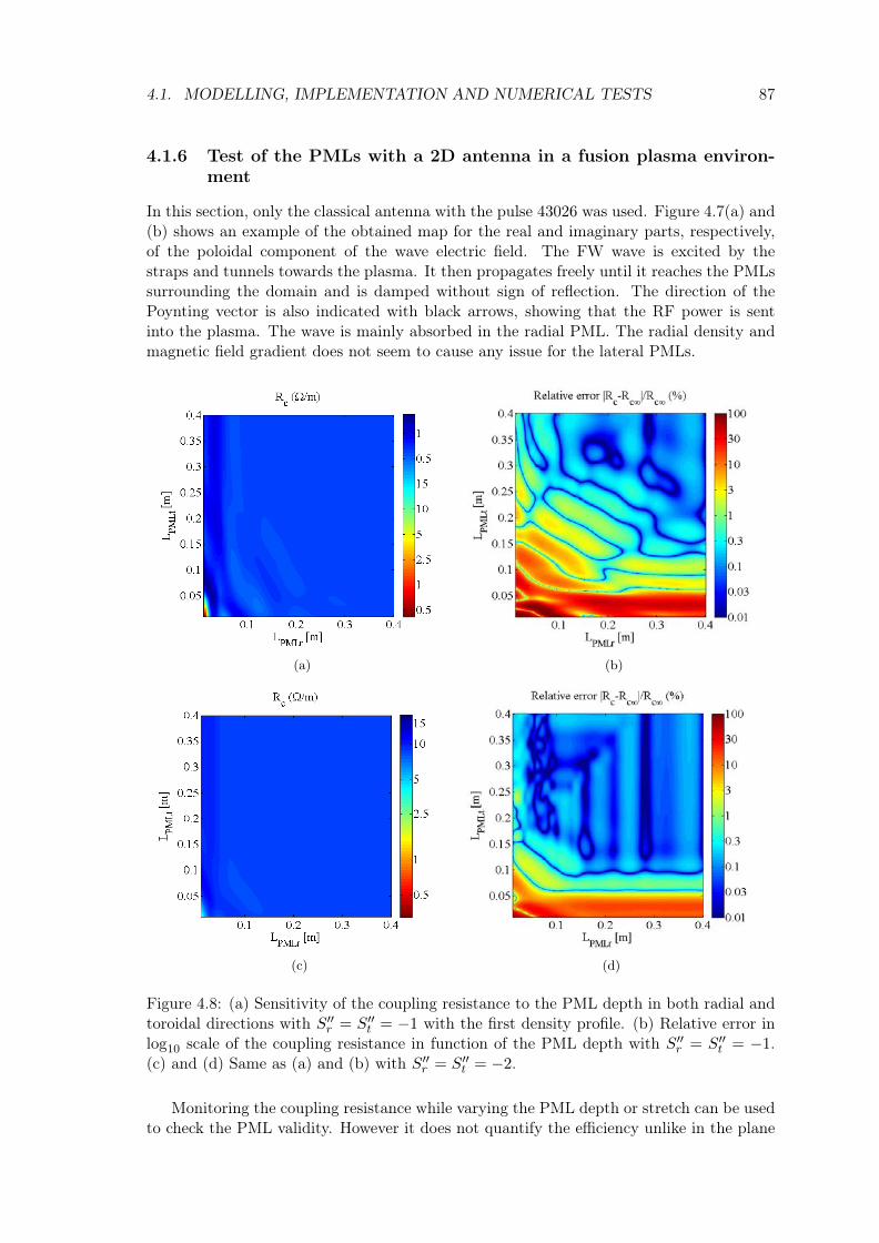
4.1. MODELLING, IMPLEMENTATION AND NUMERICAL TESTS 87

4.1.6 Test of the PMLs with a 2D antenna in a fusion plasma environ-ment

In this section, only the classical antenna with the pulse 43026 was used. Figure 4.7(a) and(b) shows an example of the obtained map for the real and imaginary parts, respectively,of the poloidal component of the wave electric field. The FW wave is excited by thestraps and tunnels towards the plasma. It then propagates freely until it reaches the PMLssurrounding the domain and is damped without sign of reflection. The direction of thePoynting vector is also indicated with black arrows, showing that the RF power is sentinto the plasma. The wave is mainly absorbed in the radial PML. The radial density andmagnetic field gradient does not seem to cause any issue for the lateral PMLs.

(a) (b)

(c) (d)

Figure 4.8: (a) Sensitivity of the coupling resistance to the PML depth in both radial andtoroidal directions with S′′r = S′′t = −1 with the first density profile. (b) Relative error inlog10 scale of the coupling resistance in function of the PML depth with S′′r = S′′t = −1.(c) and (d) Same as (a) and (b) with S′′r = S′′t = −2.

Monitoring the coupling resistance while varying the PML depth or stretch can be usedto check the PML validity. However it does not quantify the efficiency unlike in the plane

88 CHAPITRE4

wave case.Figure 4.8(a) and Figure 4.8(c) show that the Rc is not PML dependent if the PML is

large enough. Both the radial PML and the toroidal PML have to be taken into account.Scans were performed by varying the PML depth cm by cm. In these scans, the followingparameters have been used: L‖ = 0.5 m, L⊥ = 0.15 m. The same current density wasenforced on the front and the back of the strap. The first density profile (the closest to theantenna) in Figure 4.1(a) was taken. The results were then smoothed. When the PML isnot large enough, the oscillatory behaviour seen for plane waves is recovered. Increasingthe PML depth suppresses the oscillations. The results are then no more PML dependent.The size of the PML can be compared to the radial wavelength at the plasma-radial PMLinterface (≈ 0.2 m) for the maximum in the n|| spectrum given by FW dispersion rela-tion (2.21). The relative error is calculated by comparing the Rc values to the case withLPMLr = LPMLt = 0.4 m. Figure 4.8(b) and Figure 4.8(d) show that less 1% discrepancycan be achieved for a cheaper numerical cost and for the same mesh by increasing theimaginary stretching factor as expected from (3.25).

In the following, LPMLr = LPMLt = LPMLp = 0.1 m and S′′r = S′′t = S′′p = −2 aretaken. An arbitrary choice has fixed a good accuracy at less than 1% error on Rc. Aconservative choice is done for the value of the imaginary stretch. Indeed, Section 3.4 hasshown that the optimal value for a plane wave is S′′ = −8. However here, a spectrum ofplane waves is present. Taking S′′ = −2 seems a good compromise to reduce the numericalcost due to the mesh size while keeping an acceptable accuracy and saving working timeto verify the impact of S′′ on the numerical cost and accuracy of Rc. It allows, accordingto Figure 4.8(d), to obtain less than 1% error for Rc with a PML that has roughly a sizeof half the wavelength. With these parameters, implementing the PMLs roughly increasesby 60% the domain surface in 2D and it roughly doubles the domain volume in 3D, alsoincreasing by the same amount the total number of elements. Further optimization is stillpossible for either numerical cost or accuracy.

4.2 Comparison of Fast wave coupling properties obtainedfrom the simulations with 2D and 3D simplified ToreSupra ICRH antennas geometries with experiments

Being tested, the model can now be used to study the FW coupling properties and comparethe results with the experimental observations. The study quantities are the results of theknowledge of the previous studies done with the existing codes ICANT [32], TOPICA [31].We also study the role and impact of modelling sophistication on the simulation results.

4.2.1 Launched and coupled spectrum

The first thing to be done is to obtain the power spectrum of the FW wave. The coupledpower spectrum is computed by performing the product of the Fourier transform of Eand B on the radial plasma-PML interface giving the flux of the radial component of thePoynting vector. The power spectrum was evaluated by taking an overly large domain inthe toroidal direction in order to get most of the absorption in the radial PML. The lateralsides of the red contour defined in Figure 4.1.3 can therefore be neglected.

The maximum of the RF current spectrum in dipole strap phasing is actually obtainedat n‖ = 10.9, corresponding to k‖ = 13 m−1, by looking at Figure 4.9. Negative n‖ are notshown since the profile is symmetrical with dipole toroidal phasing.

4.2 COMPARISON FW COUPLING WITH EXPERIMENTS 89

Figure 4.9: Squared amplitude of analytical Fourier spectrum for the RF current onthe straps (black straight curve) and coupled power (colour dashed curves) spectrum atplasma/PML interface for the different configurations vs n‖ for Rstrap−Rcutoff = 0.045 m.Negative n‖ are not shown since the profile is symmetrical with [0π] phasing.

The maximum of the power spectrum is however situated at n‖ = 8.2, correspondingto k‖ = 9.7 m−1and consistent with the results obtained with ICANT in [65], and thesecondary lobe vanishes. This is explained since the plasma actually reflects preferentiallythe high k‖ waves. Integrating the power spectrum also allows to recover the couplingresistance Rc.

4.2.2 Influence of the antenna geometry elements of the coupling resis-tance

Only the first profile in Figure 4.1(a) has been used to study the impact of the antennageometry in 2D. It is shifted radially to modify the distance between the strap and the cut-off layer. This is not strictly speaking equivalent to shifting the position of the separatrix asthe shape (gradient) of the profile is not modified while moving the separatrix necessarilymodified the radial gradients. But this procedure allows to reproduce the exponential decayof the FW coupling with only Rstrap−Rcutoff as shown in Figure 4.10. Some discrepancycan however be seen by observing the blue dots and the cyan stars, obtained with the realprofiles, at high Rstrap −Rcutoff .

Several features were progressively added in the antenna geometry: the presence ofpassive objects and the strap thickness. The trend provided by including these features gotowards the experimental coupling resistance values. This shows that these elements areimportant to recover a fair agreement between simulations and measured coupling resis-tances. The strap thickness changes the amplitude of Rc while the passive objects changeboth the amplitude of Rc and the slope. This is consistent with Figure 4.9. Changingthe geometry of the antenna modifies the amplitude of the main lobe in the power spec-trum. An oversimplified geometry overestimates the amplitude. The thickness of the strap

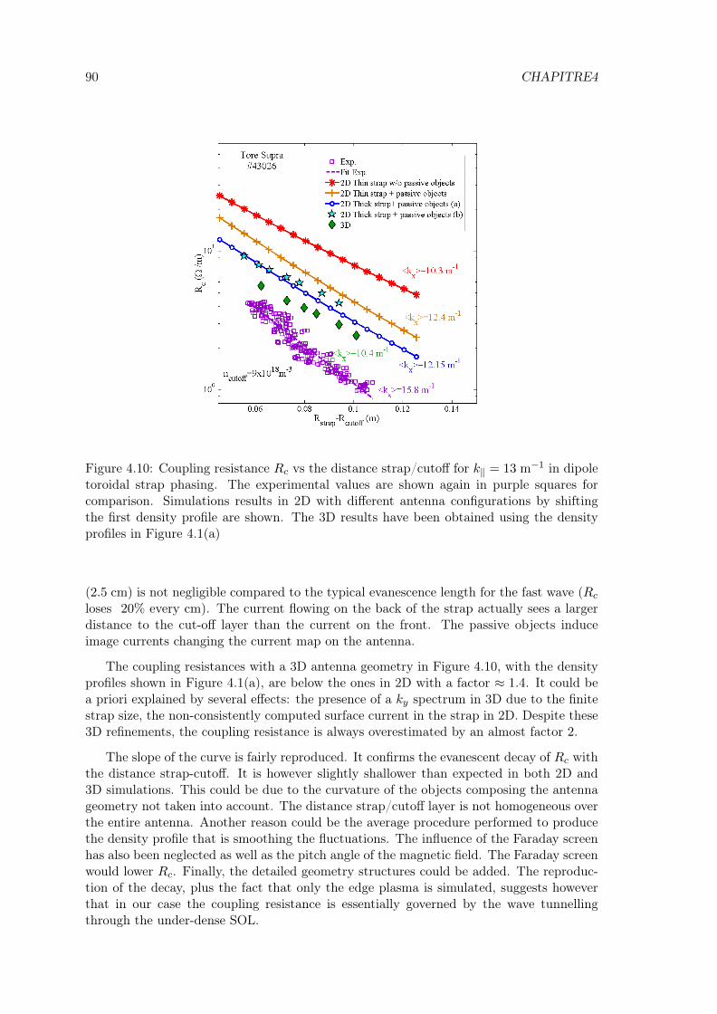
90 CHAPITRE4

Figure 4.10: Coupling resistance Rc vs the distance strap/cutoff for k‖ = 13 m−1 in dipoletoroidal strap phasing. The experimental values are shown again in purple squares forcomparison. Simulations results in 2D with different antenna configurations by shiftingthe first density profile are shown. The 3D results have been obtained using the densityprofiles in Figure 4.1(a)

(2.5 cm) is not negligible compared to the typical evanescence length for the fast wave (Rcloses 20% every cm). The current flowing on the back of the strap actually sees a largerdistance to the cut-off layer than the current on the front. The passive objects induceimage currents changing the current map on the antenna.

The coupling resistances with a 3D antenna geometry in Figure 4.10, with the densityprofiles shown in Figure 4.1(a), are below the ones in 2D with a factor ≈ 1.4. It could bea priori explained by several effects: the presence of a ky spectrum in 3D due to the finitestrap size, the non-consistently computed surface current in the strap in 2D. Despite these3D refinements, the coupling resistance is always overestimated by an almost factor 2.

The slope of the curve is fairly reproduced. It confirms the evanescent decay of Rc withthe distance strap-cutoff. It is however slightly shallower than expected in both 2D and3D simulations. This could be due to the curvature of the objects composing the antennageometry not taken into account. The distance strap/cutoff layer is not homogeneous overthe entire antenna. Another reason could be the average procedure performed to producethe density profile that is smoothing the fluctuations. The influence of the Faraday screenhas also been neglected as well as the pitch angle of the magnetic field. The Faraday screenwould lower Rc. Finally, the detailed geometry structures could be added. The reproduc-tion of the decay, plus the fact that only the edge plasma is simulated, suggests howeverthat in our case the coupling resistance is essentially governed by the wave tunnellingthrough the under-dense SOL.

4.2 COMPARISON FW COUPLING WITH EXPERIMENTS 91

4.2.3 Influence of the current distribution on the strap of the couplingresistance

Since the current distribution on the strap is not self-consistently computed in 2D, it isinteresting to know the sensitivity of the coupling resistance Rc when the current ratio If/Ibin % between the front and the back of the strap changes while keeping continuity on thestrap sides with a linear function. Again in 2D, only the first density profile in Figure 4.1(a)is used. The profile is shifted radially to modify the distance Rstrap − Rcutoff .The ratioIf/Ib is varied from 40%/60% to 55%/45% in Figure 4.11. It can be observed that Rc issensitive to the current balance between the front and the back of the strap. Changing thecurrent distribution by 20% changes the coupling resistance by 40-50%.

Rc is higher when more current is on the front of the strap closer to the cutoff. Morecurrent is closer to the plasma, the coupling efficiency is therefore better. The current onthe back and on the front of the 3D strap have been computed and compared. They givevalues around 45%/55%, which corresponds to results in 2D where a current distributionbetween 40− 45%/60− 55% is used.

Figure 4.11: Coupling resistance Rc vs the distance strap/cutoff for different current bal-ance front/back in 2D compared to 3D simulations and experiments.

4.2.4 Comparison of the classical antenna with the ILP antenna

To invalidate the possibility that the overestimation of Rc could be due to an error in thecode, another pulse (#40574) has been studied where several antennas were available: 2classical antennas and the ITER-like antenna. As the wave frequency (f0 = 48 MHz) forthis pulse is only slightly changed, the other parameters (especially the PML parameters)are kept identical. The coupling resistance Rc is evaluated for each antenna with thedensity profiles shown in Figure 4.1(c) with a 2D geometry and a 3D geometry.

92 CHAPITRE4

(a)

(b)

Figure 4.12: Coupling resistance Rc versus Rstrap−Rcutoff for pulse 40574. Experimentalvalues (circles). The colours represent the 3 active antennas. Comparison with (a) Comsolin 2D (squares) and 3D (diamonds) (b) Comsol in 3D (diamonds) and TOPICA (triangles).Two dashed blue lines shows the sensitivity of Rc from a ±2 cm change in the distancestrap-cutoff for the experimental results.

4.3 CONCLUSIONS & PROSPECTS 93

Figure 4.12(a) shows that both classical antennas, shifted radially by ≈ 2 cm, follow thesame curve, strengthening the affirmation that Rc depends mainly here upon the distancestrap/cutoff. It also shows that the ITER-like antenna coupling resistance is about 40%of the classical antenna one, despite thinner straps that should in principle increase thecoupling efficiency. This ratio is also well recovered with Comsol in 2D and in 3D and alsocorresponds to the experimental observations on Rc. Moreover, the exponential decay withthe distance to the cutoff is also fairly reproduced.

Comparing the pulse #40574 at f0 = 48 MHz with the pulse #43026 at f0 = 57 MHzshows that Rc is overall smaller for the pulse #40574. The amount of power that can becarried by a wave is frequency dependent and increasing with the frequency. From thisconsideration, it is expected that coupling is better at a higher frequency.

However, Rc is still overestimated by a factor ≈ 2. A 3D geometry taking into accountthe finite length of the strap allows us to get closer to reality, but it is still not enough.A comparison of the model in Comsol with TOPICA was also performed for this pulse.TOPICA model included a more detailed geometrical description of the antennas witha Faraday screen. The coupling resistance Rc on this pulse is also overestimated withsimulations, but by a smaller factor between 1.4 − 1.6 depending on the profile lookedupon. Despite this, the relative factors of comparison between antennas are been wellrecovered in 2D and in 3D with Comsol and with TOPICA. If an error is present in thecode, this error is systematic and exists in both codes.

4.2.5 Possible origins for the overestimation of the coupling resistance

Section 4.2.4 has shown that a comprehensive description of the antenna geometry explainspartially the overestimation of Rc. The most probable explanation is the magnetic shieldingand the filtering of the electrostatic component of the electric field due to the presence ofthe Faraday screen changing the wave propagation constant β [32]. Modification of thepropagation constant has in turn an influence on the radiated power and thus of thecoupling resistance Rc. Including the Faraday screen in the Comsol model geometry wouldtherefore provide estimations closer to TOPICA.

Another possible explanation for at least part of the overestimation of coupling resis-tance in simulations compared to experiments could be due to a difference in the conventionbetween both evaluations. In the Tore Supra database, the coupling resistance representsa coupled power for 1A on the straps (on average over the strap length). TOPICA cal-culate coupled powers for 1A at the feeders. In Comsol 1V is imposed at the feeders. Itturns out that there could be a substantial difference between these conventions: 1A onthe feeders would not necessarily results in 1A on the strap and the coupling resistancewould be possibly be overestimated. More quantitative assessment of this effect is needed.

Part of the overestimation can also be interpreted as an uncertainty on the radialdistance between the strap and the cutoff by adding ≈ 2 cm to the evaluation basedon experiment. There are several uncertainties that can cumulate: ±1 cm for the radialposition given by the reflectometer, ±0.5− 1 cm for the position of the objects in situ undervacuum conditions. 1 cm variation change Rc by ∼ 20%. There is also an uncertainty onthe capacitance values to evaluate the experimental coupling efficiency. The capacitance isevaluated for a batch of capacitors. The retained value is an average value over this batch.The real value for a given capacitor can vary of ±10% around this average value.

Influence of the slow wave dynamic, which is removed here through a vacuum antennabox and a mesh not fine enough in the antenna box, cannot be eliminated. The slowwave can, through RF sheath rectification [89], create a convection cell in front of the

94 CHAPITRE4

antenna [38]. The distance strap-cutoff and the density gradient of the profile wouldthus be modified. Consequently the efficiency at which the fast wave is coupled to theplasma would also be modified. In that case the density profile in front of the antennais not the same as the one measured in front of the reflectometer due to the convectioncells [38]. Moreover this convection cell does not modify uniformly the density in frontof the antenna. The distance to the cutoff would thus be the same poloidally along thestrap. Convection could also explain the slope is steeper in the experiments than in thesimulations. Furthermore both polarization can get coupled by depolarisation processeswhen the wall is tilted with respect to the static magnetic field B [171]. The overestimationdoes not however seem to be related to an issue with the PML technique.

4.3 Conclusions & Prospects for the Fast Wave coupling codewith the Perfectly Matched Layer technique

4.3.1 Summary on FW coupling computations relying on the PML tech-nique

An original way to compute fast wave coupling in a tokamak plasma environment is to relyon the PML technique to emulate radiating boundary conditions at infinity, in situationsof good wave single-pass absorption. After having checked that the PML works for planewaves in homogeneous plasmas, simulations were performed with an ICRH antenna tostudy FW coupling properties.

The position of the PML interface has been discussed. The incompatibility of simulta-neous forward and backward propagative waves is solved by exploiting the tokamak plasmaspatial inhomogeneity. The plasma thus reflects one of the polarizations, the slow wavein our application. The PML is thus only adapted for the other polarization, the FWhere. The PML interface must be at a location where the SW is evanescent and the FWis propagative. Moreover to avoid any issue with the FW cutoff, the PML interface shouldbe far away.

The resulting FW coupling model has been implemented and solved using the finiteelement method in the Comsol software. The model includes a simplified flattened 2D or3D geometry of a Tore Supra ICRH antenna, as well as the detailed profiles of the edgedensity, up to a radial position slightly beyond a critical cutoff layer for the FW. Thecoupling resistance Rc has been showed to be a figure of merits easier to use for antennasthan the reflection coefficient.

The measured coupling resistances Rc of the Tore Supra antenna have been reproducedover a radial displacement of the target plasma, in heating scenarios with good single passabsorption. The absolute values ofRc are always overestimated. Evaluations with TOPICAoverestimateRc but by a smaller factor (≈ 1.5), equivalent to the factor between 2D and 3D.This could be related to uncertainty of the actual distance strap-cutoff. The overestimationis not however related to an issue with the PML technique. An exponential decay ofRc with the distance strap-cutoff has been recovered. The decay is slightly shallowerthan the experimental decay. This property, plus the fact that only the edge plasma issimulated, suggests that in our case the coupling resistance is essentially governed by thewave tunnelling through the under-dense SOL. The placement of the antenna in vacuumin the present model misses the slow wave field influence on coupling. This feature shouldbe modified to check the importance of the slow wave on coupling directly or indirectlywith RF sheaths and the generation of convective cells [172].

The necessary level of antenna geometrical description was also investigated. A fair

4.3 CONCLUSIONS & PROSPECTS 95

picture of the coupling resistance can already be achieved within a few minutes by sim-ulating a simple 2D (toroidal/radial) cross-section of the launcher. The results get closerto reality as the geometry is refined. However more and more computational resources areneeded, which is incompatible with fine antenna design optimization. As it is fast, a widerange of geometries can be explored. It was found that the strap thickness, as well as someelectrically passive elements as the septum and the antenna box have to be included in theantenna design to reproduce faithfully FW coupling. A more detailed geometry, such asthe ones used in TOPICA, would certainly give results closer to reality.

Compared to alternative approaches for modelling ICRH wave propagation, our pro-posed model presents some advantages as well as drawbacks. As the PML technique isused, there is no need for spectral surface admittance matrices and Fast Fourier tranform(FFT). The computational cost is lower. However, using PMLs is limited to heating sce-narios with high single pass absorption. As for the surface admittance matrix formalism,the present PML formulation needs to be implemented at a flat interface. Using the FEMmethod is convenient to handle simultaneously complex wave launcher geometry and aninhomogeneous-anisotropic radiation medium. However this direct method (as opposed tospectral ones) is limited to spatially non-dispersive media, such as cold plasmas. This isnot really a problem as only the cold edge has to be modelled in high coupling scenarios.Moreover PMLs in low coupling scenarios serve no purposes. Including a density profileand handling the full dielectric tensor is more realistic than propagation in an equiva-lent isotropic lossy dielectric. In particular both eigenmodes of the gyrotropic plasmaare retained in the radiated near RF field, which could be important e.g. for simulat-ing radio-frequency sheaths in the vicinity of the antenna [173, 174]. But using the coldplasma dielectric tensor makes the numerical resolution more difficult and its subsequentconvergence slower, at least in 3D.

Several prospects exist for this code with different timelines. In the short term, itwill be used in combination with others codes (TOPICA, HFSS) for the design studieson the new ICRH antennas for WEST. The present code in Comsol can provide fastcalculations for FW coupling with a full cold plasma description for parametric scans offine geometrical parameters scans. Antenna adaptation is not achievable with the presentversion of the code. With HFSS, FW coupling and antenna adaptation are possible butonly with diagonal media, on the contrary to Comsol that accept arbitrary tensors. Finallywith TOPICA, both FW coupling and antenna adaptation are possible but require verydetailed geometries. However the high level of computation resources needed for one caseexcludes fine parametric scans. Several others prospects with in mind a longer timelinecan be foreseen.

4.3.2 Preliminary optimizations of FW coupling with a improved an-tenna design based on the ILP antenna for WEST

For the major upgrade of Tore Supra into the WEST platform, three new ICRH antennasare needed. Their design will be an improved version of the ILP that shows insensitivityto load variations compared to the classical antennas with an internal matching system.The improvements must also be compatible with an active cooling system for long pulses.However, as illustrated by Figure 4.12(b), the coupling properties of the ILP were not atthe level of the classical antennas. It has thus to be improved for the new antennas tocouple larger amount of power to WEST plasmas.

Refining the geometry provide results closer to reality as the cost of computational,hardly compatible with fine antenna optimization. A fair picture of the coupling re-

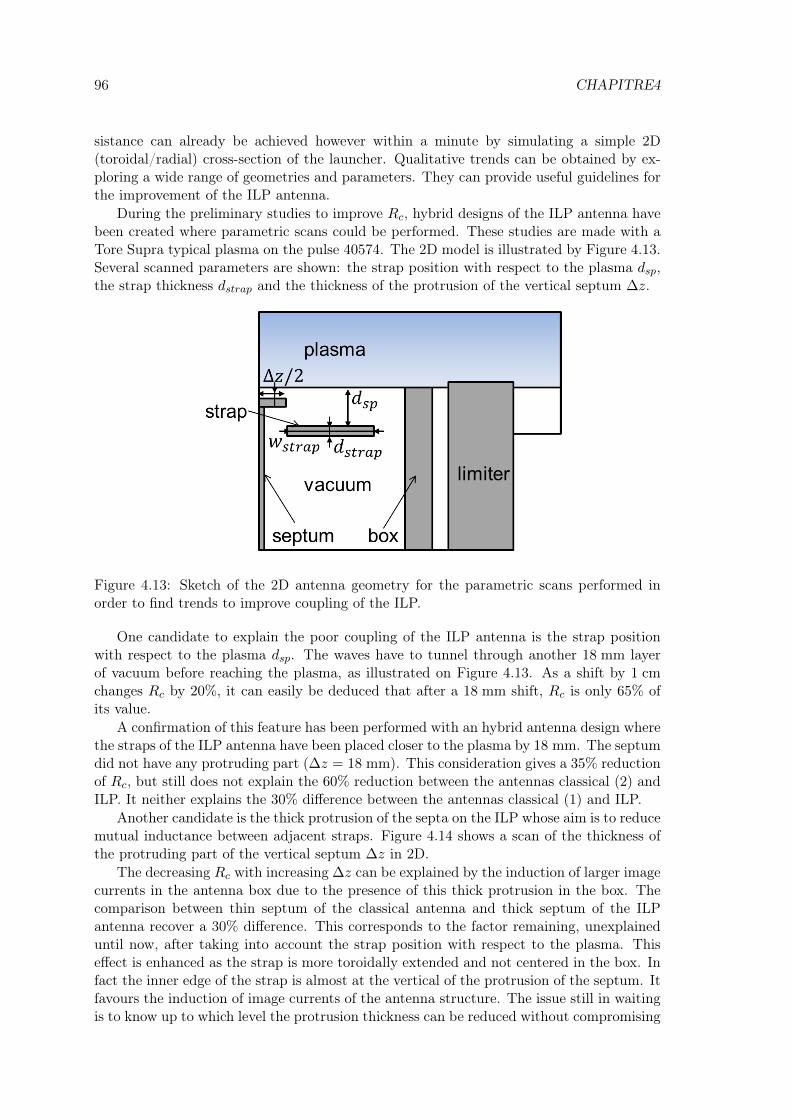
96 CHAPITRE4

sistance can already be achieved however within a minute by simulating a simple 2D(toroidal/radial) cross-section of the launcher. Qualitative trends can be obtained by ex-ploring a wide range of geometries and parameters. They can provide useful guidelines forthe improvement of the ILP antenna.

During the preliminary studies to improve Rc, hybrid designs of the ILP antenna havebeen created where parametric scans could be performed. These studies are made with aTore Supra typical plasma on the pulse 40574. The 2D model is illustrated by Figure 4.13.Several scanned parameters are shown: the strap position with respect to the plasma dsp,the strap thickness dstrap and the thickness of the protrusion of the vertical septum ∆z.

Figure 4.13: Sketch of the 2D antenna geometry for the parametric scans performed inorder to find trends to improve coupling of the ILP.

One candidate to explain the poor coupling of the ILP antenna is the strap positionwith respect to the plasma dsp. The waves have to tunnel through another 18 mm layerof vacuum before reaching the plasma, as illustrated on Figure 4.13. As a shift by 1 cmchanges Rc by 20%, it can easily be deduced that after a 18 mm shift, Rc is only 65% ofits value.

A confirmation of this feature has been performed with an hybrid antenna design wherethe straps of the ILP antenna have been placed closer to the plasma by 18 mm. The septumdid not have any protruding part (∆z = 18 mm). This consideration gives a 35% reductionof Rc, but still does not explain the 60% reduction between the antennas classical (2) andILP. It neither explains the 30% difference between the antennas classical (1) and ILP.

Another candidate is the thick protrusion of the septa on the ILP whose aim is to reducemutual inductance between adjacent straps. Figure 4.14 shows a scan of the thickness ofthe protruding part of the vertical septum ∆z in 2D.

The decreasing Rc with increasing ∆z can be explained by the induction of larger imagecurrents in the antenna box due to the presence of this thick protrusion in the box. Thecomparison between thin septum of the classical antenna and thick septum of the ILPantenna recover a 30% difference. This corresponds to the factor remaining, unexplaineduntil now, after taking into account the strap position with respect to the plasma. Thiseffect is enhanced as the strap is more toroidally extended and not centered in the box. Infact the inner edge of the strap is almost at the vertical of the protrusion of the septum. Itfavours the induction of image currents of the antenna structure. The issue still in waitingis to know up to which level the protrusion thickness can be reduced without compromising

4.3 CONCLUSIONS & PROSPECTS 97

matching.The ILP antenna had thinner strap than the classical antenna. This will not be the

case for WEST antennas, as the straps will be actively cooled. The straps thus need to bethicker to incorporate water pipes. A thicker strap will decrease Rc. The reason is simpleand is exactly the same as the difference between infinitely thin strap and finite thicknessstrap. Part of the current radiates from the front face of the strap and part from the part ofthe strap. With a thicker strap, the distance from the back of the strap is larger, thus thetunnelling length is larger for part of the current. Consequently Rc is smaller. Additionalsmall gains can be expected by optimizing the strap width, the strap position in the box.Moreover more parameters are available in 3D. The Faraday screen will be included atleast with not tilted bars to evaluate the impact of the Faraday screen on coupling and onthe strap electric length for antenna adaptation. The next step will be then to calculatethe coupling properties on WEST typical plasmas scenarios.

4.3.3 In the long term

The present model either in 2D or in 3D only gives access to the coupling resistance. Tosimulate more detailed electrical properties, e.g. the full input impedance matrix necessary[67] to match the antenna, a more comprehensive 3D geometry including the antennafeeders is necessary. This extension is possible at the expense of a computational cost inresources and time and the addition of matching module as an equivalent electric circuit.

While including a density profile and handling the full dielectric tensor is more realisticthan propagation on an equivalent isotropic lossy dielectric, it also renders the numericalresolution of the cold plasma dielectric tensor more difficult and its subsequent convergenceslower, at least in 3D, due to the gyrotropy and inhomogeneity. More robust algorithmwould be a nice feature.

Extending the density profile up to the antenna radial position would also allow to

Figure 4.14: Parametric scan in 2D of the thickness of the protrusion of the vertical septumwith a density profile for the pulse 40574. All other antenna parameters correspond to theILP antenna.

98 CHAPITRE4

include the slow wave physics in the model. A finer mesh would also be required toaccurately resolve the slow wave typical scale. It also raise the problem of whether or notput a finite density on the strap itself.

Some improvements on the PML itself can be envisaged. The impossibility of coexist-ing backward and forward waves is a major issue. As for the surface admittance matrixformalism, the present PML formulation needs to be implemented at a flat interface. Butin reality, the static magnetic field is curved imposing plasma curvature in both poloidaland toroidal directions. Checking the PML behaviour with curvature should be done. Insuch geometries, the PML formulation should be written in a different coordinates systemthan the Cartesian system. In my opinion, the medium-PML interface should be kept oniso-density lines to conserve the impedance continuity along the interface instead of havinga flat interface crossed by several iso-density surfaces. Extending this formulation to curvi-linear interface [154] is necessary to be able to couple this wave coupling model with anabsorption model [175]. This could provide a solution to get around the issue with multi-pass absorption. A generalisation of the PML technique to convex domain of arbitraryshape and not only rectangular is presented in Ref [176] with prismoidale coordinates.

The implemented PML is versatile and its application to Fusion plasmas is not limited tothe FW coupling simulations discussed here. Numerous prospects can be imagined. Futureprospects include implementing the PML technique for Lower Hybrid waves coupling [70].In this case the PML would have to be adapted for the slow wave, which is a backward mode.The most challenging issue in that case is the presence of the lower hybrid resonance thatwill be in my opinion of concern for the lateral PMLs where the resonance is encounteredat some point perpendicularly to the interface. If no trick can be found to circumvent thisissue, then only classic ABCs manually adapted to account for the inhomogeneity can beof use.

This model relying on the PML technique can in principle handle a finite densityin the antenna box. Another possible application is thus describing self-consistently RFsheaths that arise in the vicinity of ICRH antennas [49, 108, 140, 177] that give oftenthe operational limits of the antenna. A comprehensive explanation of the underlyingmechanism is yet forthcoming. This application requires a very detailed description ofthe antenna environment, so that simulating the full plasma is excluded. In particularboth eigenmodes of the gyrotropic plasma are retained in the radiated near RF field.Our present RF sheaths model (SSWICH) [173, 174] only accounts for the slow wave,which is naturally evanescent above a critical density. Including the fast wave in thenear field description requires implementing radiation conditions at the inner boundary ofthe simulation model to handle the propagative outgoing waves. Moreover having a fullself-consistent description of the waves coupling with RF sheaths would present a greatinterest for the reliability of the predictions. For that to happen, the slow wave, that is thecoupling code correctly meshed, would need to be meshed really finely, especially in theradial direction. Furthermore symmetry could not be assumed. Thus the entire antennawould have to be modelled. This would require much more memory that was is presentlyavailable. The behaviour of the PML technique in the presence of sheath-plasma waves[33] is also not clear yet.

Chapter 5

Development of an antenna-plasmacode SSWICH-SW with aself-consistent description of RFsheaths effects

Until now, this thesis was focused on FW coupling to the plasma. RF sheaths can modifythe local density in front of the antenna and thus influence the coupling properties onthe antenna. In the past, RF sheaths have been treated mostly sequentially through apost-treatment of the output of the antenna codes relying of a simple rectification model.The goal was then to minimize the integrated parallel electric field along field lines. Thisapproach was also used to design a new generation Faraday screen on Tore Supra [56] inorder to minimize the magnitude RF sheaths. On Alcator C-Mod, symmetry considerationsled to design a field aligned antenna [49] to reduce SOL interactions. It also naturallyresults into minimizing

∫E‖dl. In reality, the observations were not conformed to the

predictions. On Alcator C-Mod, the impurity contamination and the impurity sources atthe antenna decrease while the plasma potential remains unchanged. On Tore Supra, theimpurity content was similar whereas the magnitude of the plasma potential was muchhigher. More advanced modelling of RF sheaths is thus needed. The relation betweenimpurities production and the plasma potential also needs to be understood. The sheathsfeedback impact of RF wave propagation has been until now neglected. The observationsof DC currents in the SOL with active antennas were unexplained.

Experiments have thus highlighted some shortcomings of classical sheaths models. Thefeedback effect of the plasma of the wave propagation should be accounted for. The fieldline topology in the vicinity of the antenna should be better described in order to accountfor long field lines passing in front of the antenna and short field lines connected to theside limiters. A mechanism to generate significant DC currents is also necessary.

This chapter is devoted to the description of a novel model of RF sheaths. In thefirst part the equations of the model are presented with the boundary conditions neededto solve the model. In the second part the numerical implementation in Comsol and itscoupling to the TOPICA antenna code is discussed. In the third part, some numerical testsof part of the model are performed to verify some of the assumptions made initially in themodel development. The model is also compared in simple situations to analytic solutions.Finally in the fourth section, the status and prospects for this code are presented.

99

100 CHAPITRE 5

5.1 Physics in SSWICH-SW

Although no consensus presently exists over an alternative approach, RF-sheath physicsneeds improvement towards the first principles mechanisms driving the non-linear inter-actions between the RF waves and the edge plasma. Our proposed approach, SSWICH(Self-Consistent Sheaths and Waves for Ion Cyclotron Heating) includes in its currentform the minimum required physics package to model self-consistently RF wave propaga-tion in the bounded SOL plasma and the resulting DC biasing of the SOL from both endsof open magnetic field lines.

The model involves DC quantities as well as harmonic RF waves oscillating at theICRH fundamental wave frequency ω0. No other frequency is included on the contrary tothe model in ref.[99] that includes harmonic frequency of ω0 . Our model also assumes thatRF and DC quantities can be split as explained in Section 2.3.2.1. It assumes that the RFcurrent exclusively goes through the capacitance and the DC current through the diode onthe sheath equivalent circuit in Figure 2.7. The resistance part of the sheath is neglected.

A three-fluid approach is followed, inspired by earlier work on RF plasma discharges[100, 103] and recently applied to tokamaks [53, 118]. Three fields are solved for: the RFparallel field E‖, oscillating sheath voltages VRF (both varying as exp(−iωt) at the RFpulsation ω0) and the DC plasma potential VDC . Furthermore some transport coefficientsremain phenomenological. The RF and DC parts of the model are coupled by non-linearRF and DC sheath boundary conditions at both ends of open magnetic field lines. As fluidfields are treated here, the concept of flux tubes [93] is not as important as in previousmodelling.

The following model is valid for high amplitude collisionless RF sheaths parallel to Bin flat geometry, with immobile ions and inertia-less electrons. The following descriptionis a priori valid in 2D and in 3D, but is shown in 2D for simplicity.

5.1.1 Tore Supra geometry in the vicinity of the ICRH antenna in SS-WICH

The geometry actually considered in Tore Supra simulations is already rather complex, asillustrated by Figure 5.1(b). The geometry is shown here with Tore Supra geometry inmind, but could be applied to other devices with the condition that wall boundaries areeither parallel or perpendicular to B.

The simulation domain in the parallel/radial 2D plane, sketched on Figure 5.7, is a setof bounded straight magnetic field lines aligned along z in the SOL of a magnetized plasmain the vicinity of an IC antenna located on the low field side of a flattened tokamak. Thecomputational domain considered here is a cut at one vertical position in the parallel/radial2D plane of the full 3D antenna geometry, illustrated by Figure 5.1(a). The geometry ofthe objects is simplified to satisfy the condition on the orientation of the static magneticfield B. They thus have a rectangular form instead of a domed form to enlarge the surfacewetted by the plasma.

The domain contains protruding material objects able to intercept magnetic field lines,e.g. antenna side limiters, developing sheaths. Sheath boundary conditions, introduced inSection 2.3, are enforced on the lateral boundaries for both the RF part and the DC part ofthe problem, as illustrated on Figure 5.1(b) where the sheaths width are overly exaggeratedto be visible. Even more complex geometries will be progressively implemented when thecondition on the orientation of the magnetic field will have been overcome.

5.1. PHYSICS IN SSWICH-SW 101

(a)

(b)

Figure 5.1: (a) 3D model of the Tore Supra antenna geometry. A parallel/radial plane isalso represented to show SSWICH simulation domain. (b) 2D toroidal/radial plane domainwith typical dimensions. The orange rectangles correspond to boundaries where sheathsboundary conditions are enforced. The SOL plasma is shown in level of blue with a lightercolour in the private SOL since the density is smaller. The red dashed line shows wherethe DC plasma potential shown for example on Figure 6.6(b) is evaluated.

102 CHAPITRE 5

Since the antenna is positioned inside the vacuum vessel, a finite density plasma canexist around the antenna. Recessed areas behind the leading edge of the limiter have tobe included in the modelling, since in Tore Supra the antennas are not positioned on thevacuum vessel position.

The free SOL, where long connexion lengths exist, surrounds the antenna. A radialdensity profile is assumed there. The private region of the antenna, defined as the collectionof field lines hitting the side limiter on both their toroidal sides, is distinguished from therest of the SOL since the parallel connexion length is much smaller than in the free SOL. Itthus has a steeper density gradient, following Stangeby’s model [93]. The steeper densitygradient is computed within the diffusive regime:

np (x) = nle exp

(xle − xλp

), (5.1)

where np and nle are respectively the density in the private SOL and at the leading edgeof the side limiters, xle is the radial position of the side limiter and λp is the characteristiclength of the density gradient defined with:

λp = λf

√(l‖,0

l‖,1

), (5.2)

where λf is the characteristic length of the density gradient in the free SOL, l‖,0 is theparallel connexion length in the private SOL and l‖,1 is the parallel connexion length inthe free SOL. The parallel connexion length are illustrated on Figure 5.1(b).

Due to limited computational resources (in CPU time, RAM memory and raw com-puting power), a multi-2D approach was applied, whereby several radial/parallel planes atdifferent poloidal positions are solved independently. Neglecting poloidal derivative ∂y isrequired. This is valid when the poloidal gradient lengths are much larger than the radialgradients lengths. The effect of the third dimension will be evaluated as a test of the multi-2D approach with a simplified version of SSWICH in Section 5.3. The third dimension isthen recovered by assembling the 2D planes together. SSWICH cannot therefore computein its present version the field at the antenna aperture that is about 0.5 m wide. It wasduring this thesis coupled to the TOPICA antenna code [31]. As the current SSWICHmodel only account for the SW in a 2D domain, it is called SSWICH-SW-2D. Let us seenow the physics included in SSWICH for the self-consistent 3D modelling of RF sheaths.

5.1.2 RF wave propagation: slow wave

At the RF frequency ω0, the SOL plasma is characterized by the cold dielectric tensor¯ε (x, ω0) [58] given in (2.9). Let us recall that the cold plasma is gyrotropic and birefringent.Inhomogeneity can also occur in case of a density gradient in the profile. Two polarizationsconsequently exist in a cold plasma: the fast wave and the slow wave whose propertieswere summarized in Section 2.1.4.

Here we are not interested in the transverse electric field, useful for heating, but in theparallel electric field, deemed responsible of the spurious wave-plasma interactions in thevicinity of ICRH antennas. As the plasma is highly anisotropic in the parallel direction,ε‖ is high in magnitude (highly negative) compared to other dielectric constants (i.e. ε⊥and εX) and squared refractive indexes (n2

‖ and n2⊥). E‖ (x, y, z, ω0) is therefore entirely

due to the SW and is written in the model as an Helmholtz equation without any volumesources:

5.1. PHYSICS IN SSWICH-SW 103

ε‖∆‖E‖ + ε⊥∆⊥E‖ + ε‖ε⊥ (ω0/c)2E‖ = 0, (5.3)

where ∆ is the Laplace operator. Since the condition B perpendicular to the wall isimposed, the fast wave and the slow wave are completely decoupled. The fast wave impactcan thus be neglected. However, in reality, arbitrary angles between the wall and themagnetic field B exist. Mode conversion of the fast wave for arbitrary angles can occurand generate a slow wave outside the private SOL [51, 92]. This aspect is here neglected.The sources terms of E‖ are rejected in the boundary condition at the antenna aperture.

Boundary conditions are needed to solve the SW equation in the appropriate environ-ment. The RF waves are emitted through an aperture in the metallic chamber wall atthe radial boundary x = 0 of width l‖ ≈ 0.5 m (thick blue line on Figure 5.1(b)). TheRF electric field E‖ap (y, z) is prescribed at this boundary by imposing a 2D map of E‖typically produced by an antenna code in the absence of sheaths. This input map excitesthe whole RF+DC physical model.

At the ICRH frequencies, the parallel dielectric constants ε‖ is always highly negativebecause of the SOL density. Therefore, plane SW are evanescent whatever the parallelwave-numbers k‖ composing the excited spectrum above a critical density correspondingto ε⊥ = 0. Metallic boundary condition is thus enforced E‖ (x = L⊥, y, z) = 0 on the mainplasma side of the simulation since the SW is assumed to be completely extinguished asthe density there (i.e. ε⊥ < 0) is higher than this critical density. Metallic BCs are alsoimposed at the outer vessel boundary outside the antenna aperture as well as all otherboundaries parallel to B. This latter condition is questionable, especially on protrudingobjects in the SOL, but is unfortunately imposed when working with B perpendicularto the wall. This condition imposes E‖ = 0 on both edges at the leading edge of thelimiter. Thus no rectification is possible. This condition could be replaced in the RF partof the model by the full SBC [53]. The FW however could not be neglected however. Theconditions to establish are more complicated due to oblique reflections, which can inducemode conversion (i.e. ∂x∂z spatial derivative are there to ensure this possibility). Moreoverno similar conditions presently exist for the rectification in the DC part of the model.

Since the sheath (in orange on Figure 5.1(b)) is usually thinner than the typical exten-sion of the simulation domain, its consequence on the RF field propagation is accounted forvia a RF sheath boundary condition [53]. It replaces the usual metallic boundary condi-tion for boundaries perpendicular to B, instead of meshing finely the domain to resolve thesheaths typical scale. Sheath boundary conditions are one of the characteristic features ofthe SSWICH code that was developed during this thesis. Although they rigorously prevailat the sheath/plasma interface, the RF-SBCs are applied directly at the wall. Assumingthat at ω0 the RF current through the sheath is mainly a displacement current, the sheathis assimilated to a parallel plate capacitor of width δ, filled with a dielectric material of di-electric constant εsh introduced in Section 2.3.2.3. With B normal to the wall, the RF-SBCis given by (2.63):

E⊥ = ±∇⊥(δε‖E‖/εsh

), (5.4)

where the opposite signs for the opposite walls account for the reversal of the normal direc-tion n: + when en · z = +1 and − when en · z = −1. The radial/poloidal distribution ofδ, function of the radial and poloidal coordinates, needs to be determined self-consistently.The condition of the orientation of the magnetic field B, while restrictive, allows us to avoidthe fast wave, thus only keeping the slow wave. This condition is applied on boundariesperpendicular to B.

104 CHAPITRE 5

Conservation of the RF electric displacement D in the SOL plasma is expressed as:

∇ · ¯εE ≈ ε⊥∇⊥ · E⊥ − iεX (∇×E⊥)‖ + ε‖∂‖E‖ = 0. (5.5)

Since the SW exhibits essentially a transverse magnetic polarization, the second termat the RHS of (5.5) can be neglected. E⊥ in (5.5) can be replaced by its expression givenby (5.4).

ε⊥∆⊥

(δDpl

n /εsh

)= ±ε‖∂‖E‖ (x, y, z = zlateral boundary) , (5.6)

where the sign + accounts for lateral boundaries with en · ez = 1 and the sign − accountsfor lateral boundaries with en · ez = −1. zlateral boundary denotes the positions along theparallel direction corresponding to the lateral boundaries on Figure 5.1(b). The quantityδDpl

n /εsh at the right hand side (RHS) of (5.6) physically defines an oscillating RF voltageVRF across the sheaths that drives the rectification of the DC plasma potential. As B isperpendicular to the wall, it gives Dn = D = ε‖E‖. Assuming that the distributions onVRF and δ are known along all relevant boundaries, Dirichlet boundary conditions for theE‖ are applied on the lateral boundaries in the code using:

E‖ = ± εshε‖δ

VRF , (5.7)

where the oscillating sheath voltage VRF and the sheath width have to be determined self-consistently. The quantity C∗ = εsh/δ actually defined the sheath capacitance per surfaceunit (2.54).

5.1.3 Oscillating sheath voltage

The oscillating sheath voltage VRF makes the transition between RF wave propagation andDC biasing of the plasma. Inverting the side of the terms in (5.6) gives:

ε⊥∆⊥VRF = ±ε‖∂‖E‖ (x, y, z = zlateral boundary) , (5.8)

where zlateral boundary denotes the positions along the parallel direction corresponding to thelateral boundaries on Figure 5.1(b). The sign is chosen according to the rule for (5.6). Thisequation is valid whatever the dielectric tensor and in the presence of radial inhomogeneityin the density profile. It allows solving VRF along the lateral boundaries without a prioriknowledge of the self-consistent distribution of δ.

In (5.8), the oscillating sheath voltage is generated by the slow wave within a spatialdifferential equation. VRF is null in the absence of sheaths. The RF voltage VRF is thustreated as a unknown field independent of E‖, the source term. The formulation makes itconvenient to evaluate VRF with some stability. Physically it is explained by invoking thesheath-plasma wave (SPW) [53] to excite VRF . These properties can explain why the RFvoltages penetration [173] in the plasma is deeper than the SW skin depth characteristicof its evanescence above its cutoff density (2.33). The penetration of RF voltage is notactually governed by the slow wave equation (5.3) but by the capacitive properties of theRF sheath, written in the SBC (5.7).

Boundary conditions are needed to complete the description and allow the resolutionof (5.8) in the geometry illustrated by Figure 5.1(b). The condition VRF = 0 is applied onthe inner plasma boundary, on the outer wall as well as on any other boundary parallelto B such as the front face of the protruding limiters. On the lateral boundaries, a zeroflux boundary condition is enforced. Even if (5.8) is solved everywhere in the domain froma numerical point of view, it only makes sense physically across a sheath that only existalong objects boundaries.

5.1. PHYSICS IN SSWICH-SW 105

5.1.4 DC biasing of the SOL plasma

The third equation solves the electrostatic DC plasma potential VDC (x, y, z) by expressingthe local balance of DC electric charge over the simulation volume with a partial differentialequation without sources:

σ‖DC∆‖VDC + σ⊥DC∆⊥VDC = 0, (5.9)

where σ‖DC is the Spitzer parallel DC conductivity and σ⊥DC a small phenomenologicaleffective DC perpendicular conductivity, which has been discussed in Section 2.3.4. Oneother main novel feature in the RF sheath modelling within SSWICH is the inclusion of afinite DC conductivity tensor ¯σDC to account for exchange of DC currents between adjacentflux tubes in the SOL. Through this process, a given sheath gets coupled to its neighboursas well as with the sheath at the opposite wall along the same field line, providing amechanism of DC current formation that will be discussed more deeply in Section 6.2.3.DC currents are thus allowed to flow both in the parallel direction and in the transversedirection. This “non-locality” was investigated in refs [43, 54] and is needed to reproducethe measured DC currents created by RF sheaths [46, 108] in the vicinity of active ICRHantennas.

In a collisionless plasma the linear DC transverse conductivity should be rigorously zero.However some transverse DC current transport was evidenced experimentally. Rigorously,the transverse DC plasma conductivity takes the form of a diffusion operator only in thecase of ion-neutral collisions [112]. However, this mechanism alone cannot explain the farmore intense effective transverse DC conductivity observed in the SOL of tokamak plasmas.

Two perpendicular DC conductivity are actually considered: one for the free SOLσ⊥DCf and one for the private region σ⊥DCp with σ⊥DCf < σ⊥DCp. This inequalityactually considers that the turbulence level is higher in the private SOL than in the freeSOL. This assumption comes a afterthought of the parallel connexion length in the SOL.In the free SOL, the parallel connexion length are rather long (several tens of m). Moreoverthey travel though the high field side (HFS) and the low field side (LFS) on the tokamak.We know that the curvature of magnetic field line is favourable for confinement on theHFS and unfavourable on the LFS. When averaging over the entire field line in the freeSOL, the curvature is thus slightly unfavourable. Let us do the identical reasoning forthe short field line in the private SOL of the antenna located at low field side in theunfavourable region. When averaging over the length of the short field line, the curvatureis very unfavourable. It leads to think that the interchange turbulence level is higher inthe private SOL compared to the free SOL. Such a view justify the choice of differentDC conductivities in both regions of the SOL and gives more sense to a finite spatialextension in the SOL of the RF sheath effects. The effective DC conductivity that modelphenomenologically the transverse transport of DC currents should thus be higher in theprivate SOL compared to the free SOL.

SBCs are also needed to completely define the DC part of the code and find a solution.The general DC SBCs state that the local DC current leaving the bulk plasma is the DCcurrent into the sheath. Using (2.52) and for boundaries perpendicular to B, the non-linearsheath I-V characteristic describing the conduction current gives:

jDC · n = i+[1− exp

(Vf + Vb − VDC

Te

)], (5.10)

with n the normal to the surface and the floating potential without RF Vf was defined by(2.40). This BC will make use of the oscillating sheath voltage computed previously by the

106 CHAPITRE 5

intermediate of the biasing voltage Vb given by (2.51) in Section 2.3.2. Let us recall thateverything is happening as if sheath rectification was positively biasing the walls. On theinner plasma side, it is assumed that no perturbation is reaching the core plasma, so thatVDC = Vf is enforced due to the zero current exchange between plasma and wall connectedto the quasi-neutrality condition.

This expression is limited by a saturating condition when the sheath vanishes whenthe electron saturation current is reached. This saturation can be expressed starting from(2.40):

jmax =

[kBTee

1

2π

mi

me

1

1 + TiTe

]1/2

. (5.11)

(5.10) thus becomes:

jDC · n = i+[1−min

(jmax, exp

(Vf + Vb − VDC

Te

))]. (5.12)

The outer vessel boundary is assumed far away radially, so that no net perpendicularDC current is collected by the wall (jDC · n = 0, i.e. classical metallic BC). The modelalso assumes this condition for any boundary of the protruding object parallel to B, as noworking sheath model exits in that case. This is clearly something that should be improved.

Once a solution has been found for VDC , the sheath width can be determined from aChild-Langmuir law given by (2.53).

The refinements proposed by Liebermann for the dynamics of a high voltage, capacitiveRF sheath assuming stationary state, collisionless ion motion and inertialess electrons [103]were accounted for in SSWICH. It modifies the sheath width δ which is larger than a Child’slaw sheath for the same DC voltage and ion current density and the sheath dielectricconstant εsh that is seen by the waves as a dielectric and not as vacuum anymore. Theratio of these two previous quantities is the effective sheath capacitance C∗sh in (5.7). Withδ finally determined, the self-consistent loop is closed as the sheath capacitance can befound and re-injected in the wave propagation problem. A robust starting point for theconvergence process of the loop still however has to be determined.

5.1.5 Initialization: asymptotic model of SSWICH-SW

Despite the assumptions made and having only three coupled equations ((5.3), (5.8) and(5.9)), SSWICH is still fairly complex. To compute the SW fields E‖ in presence of RF-SBCs, it is necessary to know a priori the 2D (radial/poloidal) spatial distribution δ (x, y)of the sheath widths along lateral boundaries of the simulation domain that is computedlater on with the output of the third module on DC biasing via the Child-Langmuir lawand the distribution of VRF (x, y) that is determined by the second module. Moreover toknow the plasma potential patterns needed to evaluate δ (x, y) with the Child-Langmuirlaw, it is necessary to know the 2D map E‖ (x, y) at the lateral boundaries.

In the first version of the self-consistent code, there were only two fluid-fields and twoequations. VRF was an explicit function of E‖ and the plasma parameters:

VRF =ε‖

εshδE‖. (5.13)

Moreover an ad-hoc constant and uniform value for the sheath width was provided asan initial condition for the self-consistent loop. The power was ramped up step by step toprogressively excite sheaths starting from boundary conditions close to metallic ones when

5.1. PHYSICS IN SSWICH-SW 107

δ ≈ 0. This attempt failed far away from the typical power typically operated by an ICRHantenna. The non-linearity of the equations prevent the algorithm from finding a solutionin a limited number of iterations. Moreover the possibility of multiple roots was proposedin [92]. This cause a numerical problem as which root the model will take and how to jumpfrom one root to another if case of bifurcation.

Therefore, a “first guess” into the self-consistent loop is valuable, as algorithms suchas Newton-Raphson, are sensitive to the starting point for their convergence. A completedescription of the asymptotic model with spectral resolution in 3D within a parallelepipedicgeometry can be found in ref[173]. The same concepts are used here in the context of amore complex geometry.

For the purpose of RF sheath assessment in tokamak environment, an interesting regimeis when the DC biasing gets very intense at high injected power. From Child-Langmuir law(2.53), the sheath width δ grows to very large values. In this, as we call it, “wide sheathregime” some physical quantities become nearly independent of δ [173]. The principle isthen to write the field with a Taylor expansion into successive approximations:

E‖ = E0‖ +

λcritδE1‖ + o

(E2‖

), with

λcritδ

<< 1. (5.14)

This asymptotic development helps to understand why the first attempt for the self-consistent loop failed. The formulation experiences convergence issues due to the mixingof different order in the quantities [173].

At the aperture, the same boundary condition is applied as in the RF wave propagation:a field map of the parallel electric field at the aperture E‖,ap. The boundary conditionsare kept the same on the plasma side and the outer wall, as well as on any other boundaryparallel to B: E‖ = 0. On the lateral boundaries simplified SBC in the wide sheath regimeare written, instead of writing metallic condition (∂‖E‖ = 0). Postulating that the sheathwidth δ is large and that VRF cannot increase indefinitely yield for (5.7) E‖,as = 0.

This asymptotic method [173] is valid whatever the 2D input RF field map, in presenceof a radial profile for the plasma parameters, and with no assumption a priori about theself-consistent 2D sheath widths distribution δ (x, y). It does not exhibit convergence issueor root selection issue as its expression is explicit. The SW module can thus be solvedexplicitly without prior knowledge of the DC plasma potentials before entering the self-consistent loop. Within the asymptotic regime, only one of possible roots remains. Asa result, the starting point of the self-consistent loop is explicitly placed on one branchof solutions.The counterpart of the asymptotic regime is a restricted validity domain asλcrit/δ << 1 must be satisfied.

A simple criterion has been proposed and tested in rectangular geometry in Ref [173]to identify the validity domain.

λcritδ

=

∣∣∣∣∣ εsh2ε⊥

lyk0

π

l⊥δ

coth

(k0 |ε⊥|1/2 l‖,0

2

)∣∣∣∣∣ << 1, (5.15)

where ly is the poloidal dimension, λcrit is the critical sheath size for the asymptotic treat-ment validity, k0 is the wavenumber in vacuum, εsh is the sheath dielectric constant definedin Section 2.3.2.3 and ε⊥ is the perpendicular component is the Stix tensor (2.9). Thisasymptotic solution, serving as the starting point for the coupled model, is the last missingpiece in the present physical model. The model can now be implemented numerically.

108 CHAPITRE 5

5.2 Numerical implementation in Comsol Multiphysics

5.2.1 Architecture of the code in Comsol

The SSWICH model is implemented numerically in the commercial software COMSOLmultiphysics [164] to take advantage of the Finite Element Method [77] for complex ge-ometries. A commercial software Comsol was chosen before the start of this thesis forits user-friendly graphical interface, the possibility to couple several physics and to definemedium with full tensor properties on the contrary to other softwares (HFSS, MWS), theready to use natively equations or boundary conditions. Implementing the SBCs in TOP-ICA has been tried, but for vacuum sheaths as an arbitrary medium cannot be definedbefore the antenna aperture. HFSS licences are available at the IRFM institute, but thissoftware is too specialized towards electromagnetic applications. Moreover implementingthe SBCs in HFSS would have been next to impossible. Comsol and MWS remain in thelist for the possible choice. However, Comsol can offer other possible applications than inelectromagnetism, which is not the case of MWS. Nevertheless the Comsol Multiphysicslicence is not available at CEA on high performances computer (HPC) due to the financialcost of the cluster licence for several nodes. Since the numerical resources are thus limited,only 2D applications are presently possible. Adapting the code to HPC would furthermorerequire time for efficient computing.

Furthermore my group do not dispose of a numerical support team whose main pur-pose is the development and programming of the code. Consequently, it would have beenimpossible to write a functioning “home-made”code during the three years of this thesisfrom scratch using the python, C or Fortran languages while providing at the end physicalrelevant results for complex geometries. As an example, the development of the TOPICAcode, considered as the reference for ICRH applications started in the beginning of theyears 2000 and is still an ongoing process. Furthermore my education was about physics ingeneral and especially in plasma physics and not on numerical programming and analysis.Comsol, on the other hand, offered an efficient mean to investigate the physics withoutheavy code development.

The SSWICH code in its present version is combining together three equations andthree-fluid fields fully coupled by RF sheaths properties. The schematic representationof the SSWICH code is shown in Figure 5.2. Each equation is modelled within its ownmodule by including a new physics module in Comsol. There are thus four modules: onefor each equation and one for the asymptotic solution of the RF wave propagation. Eachmodule is implemented in 2D. They are called RF wave propagation, asymptotic RF wavepropagation, oscillating sheath voltage and DC biasing. The variables in each module arerespectively E‖, E‖,as, VRF , VDC . The boundary conditions are then added in each module.The modules are coupled together by RF sheath properties, explained in Section 2.3.2: thegeneration of oscillating sheath voltage by RF waves, RF sheath rectification and sheathcapacitance.

The RF wave propagation module and its asymptotic version are modelled by a nativelyimplemented scalar Helmholtz equation for E‖. The dielectric tensor ¯ε is reduced to 2Dkeeping the radial and toroidal directions. It gives a anisotropic diagonal tensor. The DCbiasing module is modelled with the natively available Poisson equation with no volumicsources of DC current. The DC conductivity tensor is also reduced to 2D with the samedirections. Finally the oscillating sheath voltage is also modelled with a Poisson equationwith a source term in ε‖/ε⊥∂‖E‖.

It is worth mentioning that the convention in Comsol is the so-called engineer conven-tion (exp (+iω0t)), different from the one used in this thesis (exp (−iω0t)). The sign of

5.2. NUMERICAL IMPLEMENTATION IN COMSOL MULTIPHYSICS 109

complex number is thus changed as complex number should be replaced by their conjugatecomplex number. For example the dielectric tensor ¯ε in Comsol is the conjugate tensor ofthe Stix tensor in (2.9). The default frame in Comsol maybe not be the one used here. Itwill thus change the positioning of the elements in the tensors.

Figure 5.2: Schematic representation of the algorithm used in the SSWICH code. Thethree fluids are solved in their own module and are coupled together through RF sheathproperties. An asymptotic version of the SW module is initiating the iterative loop toensure convergence.

The oscillating sheath voltage module solving VRF distribution implemented in 2D asthe other ones could be reduced to 1D as an oscillating voltage make sense only across asheath. Presently VRF is solved everywhere. But VRF only has a meaning on the lateralboundaries where sheaths exist. VRF , instead of being solved with one 2D module, couldthus be solved in 1D in as many modules as there are boundaries with SBCs. It wouldalso reduce the computational resources required since 2D modelling on the entire domainis far more consuming than several 1D modelling for every lateral boundary.

5.2.2 Antenna description through an interface with the TOPICA an-tenna code

It has been seen that the system is excited by imposing a 2D (toroidal/poloidal) map ofE‖ at an “antenna aperture”, shown with a blue line in Figure 5.1(b), in the RF wavepropagation module. This input map of SSWICH is one output of the antenna codeTOPICA [31] computed in the absence of sheaths in vacuum with a realistic 3D geometryof the antenna. This input has to be seen as a total electric field, which mixes inwardwaves and backward waves. The antenna radiates on the plasma, treated as a boundaryconditions, through an aperture. 3D informations are thus present in SSWICH via the inputfield map of the antenna. Examples of 3D antenna geometries implemented in TOPICAare shown for an antenna equipped with the classical screen and with the CBSB screen

110 CHAPITRE 5

in respectively Figure 5.3(a) and Figure 5.3(b). The different Faraday screen designs wereintroduced in Section 2.4.5. Nevertheless it is possible to use instead waveguide modes orinput coming from other codes, as the interface is realized through a file containing thegrid points of a map of the RF parallel electric field.

The near field amplitudes are scaled by the RF voltages Vstrap imposed on the strapsfeeders. The same trick as in Section 4.1.3 is used in TOPICA to simulate an adapted ToreSupra antenna with TOPICA. The RF voltage is imposed on the ports connected to thecapacitors lines (top and bottom) whereas the central coaxial line replacing the power lossin the resonant circuit has a null voltage.

(a)

(b)

Figure 5.3: 3D model of the antenna geometry implemented in TOPICA equipped with(a) classical Faraday screen and (b) the CBSB FS.

5.2. NUMERICAL IMPLEMENTATION IN COMSOL MULTIPHYSICS 111

In order to comply with the magnetic field B perpendicular to the wall in the SBCs,the input RF field map (see Figure 5.4(a)) was expressed in a tilted coordinate systemwhere y and z are respectively poloidal and parallel directions. The antenna thus appearstilted as a parallelogram (see Figure 5.4(b)).

(a) (b)

Figure 5.4: (a) Toroidal/poloidal map of the antenna before tilting. (b) Parallel/poloidalmap of the antenna after tilting. This tilted map is the input of SSWICH. In tiltedcoordinates, the antenna appears like a parallelogram.

Initially the setup on TOPICA (see Figure 5.5) included the antenna structure withthe surrounding side limiters and a large domain around it. The situation was similar tothe setup in Ref [48] with the addition of the limiters. The embedding of the antennain TOPICA in between poloidal limiters change the way image currents can develop onmetallic surfaces. It does not however change the density decay [93] as no density ispresent in the antenna. TOPICA cannot provide a solution on a plane that does intersectan object. Consequently the solution cannot be given on the Faraday screen plane butslightly in front of it. The last plasma magnetic surface (TOPICA aperture) follows thepoloidal curvature of both limiters at a distance of 5 mm, and the estimated plasma ripplealong the toroidal direction with curvature radius ≈ 1.75 m. A similar surface, calledEF (electric field) surface, located 2.5 mm in front of the limiters (in vacuum) allows tocompute all the components of the electric field with a better spatial resolution (8 mmfor EF surface vs 34 mm on aperture). The simulation was then launched within a largedomain. But in practise the results obtained from this setup had a poor resolution withsmall scale structures due to the mesh as the volume was larger than without the limiters.Moreover SBCs are not included in TOPICA and the antenna is placed in vacuum whereasin SSWICH a plasma surrounds the antenna and SBCs are applied as its main aim is tomodel RF sheaths. Intense spurious interactions on the antenna limiters attributed to RFsheaths have been observed. Therefore it makes more sense to include the antenna limiterin SSWICH than in TOPICA even with a simplified geometry. The antenna limiter inSSWICH also defines several regions in the SOL with different properties: the free and theprivate SOLs.

To correct this, the side limiters structures were removed from the 3D geometry in

112 CHAPITRE 5

Figure 5.5: Sketch of the original setup with the side limiter surrounding the antennaframe and of the modified setup where the side limiter were removed in order to place theaperture closer and increase the resolution. The modified setup is similar to the setup usedby Mendes in ref [48] (no side limiters or surrounding structures), but with a much smalleraperture and cavity to emulate the presence of limiters. The directions in the tokamak areindicated.

TOPICA. The simulation domain boundaries were placed at the location of the side limitersto emulate their presence. TOPICA aperture keeps following the poloidal curvature of bothlimiters (even though they are removed from the simulated domain). The absence of theside limiters and a smaller curvature radius (≈ 1.65 m), again to follow toroidally theestimated plasma ripple, allowed to reduce the distance with the FS of about 8 mm. Sincethe domain is smaller, a better resolution is adopted for both surfaces (7.5 mm for EFsurface vs 16 mm on aperture). The drawback is that we do not benefit from the detailedgeometry of the limiters. Furthermore image currents developing around the antennastructure (limiter face in the free SOL and the vacuum chamber) are not taken in account.But the effect of the limiter on RF sheaths is retained as a simple rectangular limitergeometry is included in SSWICH. Figure 5.6(a) is the output of TOPICA for the antennaequipped with CBSB FS and for a 1 V input on the strap.

To take into account the distance between antenna aperture in TOPICA and the realradial position of the FS and the evanescence of the SW, the field map is extrapolated towhat it should be at the FS with:

E‖FS = E‖ap exp

(∫ xap

xFS

dx

λskinSW (ni (x))

), (5.16)

where E‖ap is the field map at the TOPICA aperture, xFS and xap are respectivelythe radial position of the FS and the TOPICA aperture and λskinSW = c/wpe is the skindepth for the SW with ωpe the local electron plasma frequency and c the speed of light.The extrapolation coefficient is actually an average value of the evanescence of the SWover the radial density profile. The skin depth of the SW is obtained in the electrostaticlimit by neglecting the ion dynamic and k‖ = 0 in the SW dispersion relation. (5.16)corrects the attenuation of the SW homogeneously for all modes contained in the field

5.2. NUMERICAL IMPLEMENTATION IN COMSOL MULTIPHYSICS 113

(a)

(b)

Figure 5.6: Real (left) and imaginary (right) parts of E‖ field map for the antenna equippedwith the CBSB FS (see Figure 2.14(b)) for Vstrap = 1 V. (a) provided by Topica (b) afterextrapolation on the Faraday screen plane with (5.16).

map with a constant positive factor, while rigorously the attenuation factor should beevaluated for all modes individually by decomposing the E‖ field map in Fourier space.However while the deconvolution in Fourier space does not cause any particular issue, thereverse transformation gives that the high k values, ascribed to numerical noise due tofinite discretization, are greatly enhanced. Moreover, when a 3D version of SSWICH willbe available, this extrapolation procedure will not be necessary any more as the 3D antennageometry will be directly imported in SSWICH and the solution will be possibly obtainedon the Faraday screen plane. An illustration of (5.16) is shown on Figure 5.6(b). Theevanescence factor for the SW in this case is about 5.

5.2.3 Mesh & Solver

The computational domain is meshed by default with triangular elements. A scaling factorbetween the directions is possible to account for the anisotropy in the plasma. It allows

114 CHAPITRE 5

reducing the number of elements and thus reduces the memory consumption and CentralProcessing Unit (CPU) time necessary for one simulation. Nevertheless the acceptablescaling is far below what one would expect by looking at the typical scale ratio in theplasma. The scale length are much larger in the toroidal direction than in the radialdirection due to the presence of the static magnetic field for both the dielectric tensor ¯εand the DC conductivity tensor ¯σDC . For high scaling values of the discretization mesh,numerical instabilities near the SBCs at the lateral boundaries of a few mesh nodes havebeen experienced. For this reason the scaling between the radial and toroidal directionis never pushed beyond 30. Asymptotic preserving scheme [178] have being developed toovercome this well-known problem, but do not seem to be implemented with Comsol. Localmesh refinement is still possible, but the refinement has to be in both directions to keepthe scaling ratio from increasing to high values.

The SSWICH-SW-2D model is solved iteratively within a self-consistent loop (see Fig-ure 5.2) using the MUMPS [179] package (MUltifrontal Massively Parallel sparse directsolver) and a segregated approach in four steps to facilitate convergence of the iterations.The first iteration solves the model within the asymptotic regime to provide a first guessof the final solution. The first three steps solve respectively the asymptotic SW wavepropagation E‖,as, the asymptotic sheath voltage VRF,as and the asymptotic DC plasmapotential VDC,as sequentially. They provide an initial solution for the coupled non-linearmodel that start with the second loop. This constitutes the fourth step. As the DC biasingmodule is by itself non-linear, it is also iteratively solved where the convergence is stoppedafter a maximum number of iterations fixed at 80 if it did not converge sooner with thetolerance of the convergence fixed at 10−3. For the iterative self-consistent loop, the samecondition is applied with a simple convergence loop. A Newton-Raphson scheme is used.

Once convergence has been achieved, several quantities over the entire simulation do-main are available that can be later used for physical interpretation of experimental obser-vations: E‖,as, VRF,as, VDC,as, E‖, VRF , VDC and others derived quantities such as j‖,DC ,j⊥,DC , ∂⊥VDC , ∂2

⊥VDC and δ.Some numerical instability was sometimes observed on a few nodes on the lateral bound-

aries. More robust and/or faster convergence scheme could be later tried. A numericalmethod such as minimum polynomial extrapolation (MPE) provide more robust and fasterconvergence scheme. It is not likely that such methods are implemented in Comsol. Othersolver packages are available in Comsol: Pardisio and Spooles. Furthermore numerousoptions exist for the choice and parametrization of the solver that were left at their defaultvalue automatically determined by Comsol until now. It would nevertheless have to beverified than the numerical implementation of the model is still compatible with the con-vergence scheme. Adaptative meshing during the iterative resolution has not been triedyet, due to a lack of time.

It has been mentioned in Section 5.1.1 that the poloidal direction is recovered by scan-ning successive vertical positions during the multi-2D procedure. It is usually done witha 1 cm step far smaller than the poloidal scale length. In order to avoid a tedious manualscan, an automation was developed using the optional livelink [166] Matlab/Comsol. Mat-lab [180] and Comsol [166] are used in a client/server relationship with Matlab managingthe simulation through a Matlab script. When the Matlab script is launched, it loadsall the simulation parameters from a dedicated file before launching Comsol through thislivelink. Then the order is given to the Comsol server load the Comsol file containingSSWICH. The simulations parameters are then entered in SSWICH. After achieving con-vergence, results (image, value, 1D grids, 2D grids,...) that have been defined previouslyare automatically exported in a directory with the simulation number. This livelink can

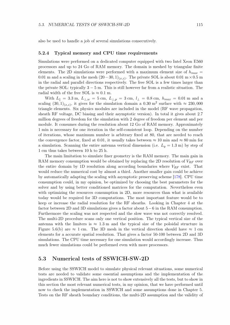
5.3. NUMERICAL TESTS OF SSWICH-SW-2D 115

also be used to handle a job of several simulations consecutively.

5.2.4 Typical memory and CPU time requirements

Simulations were performed on a dedicated computer equipped with two Intel Xeon E560processors and up to 24 Go of RAM memory. The domain is meshed by triangular finiteelements. The 2D simulations were performed with a maximum element size of hmax =0.01 m and a scaling in the mesh (20−30, 1)(x,z). The private SOL is about 0.01 m×0.5 min the radial and parallel directions respectively. The free SOL is a few times larger thanthe private SOL: typically 3− 5 m. This is still however far from a realistic situation. Theradial width of the free SOL is ≈ 0.1 m.

With L‖ = 3.3 m, L⊥,w = 5 cm, L⊥,p = 3 cm, l⊥ = 0.8 cm, hmax = 0.01 m and ascaling (30, 1)(x,z), it gives for the simulation domain a 0.30 m2 surface with ≈ 230, 000triangle elements. Six physics modules are included in the model (RF wave propagation,sheath RF voltage, DC biasing and their asymptotic version). In total it gives about 2.7million degrees of freedom for the simulation with 2 degree of freedom per element and permodule. It consumes during the resolution about 12 Go of RAM memory. Approximately1 min is necessary for one iteration in the self-consistent loop. Depending on the numberof iterations, whose maximum number is arbitrary fixed at 80, that are needed to reachthe convergence factor, fixed at 0.01, it usually takes between ≈ 10 min and ≈ 80 min fora simulation. Scanning the entire antenna vertical dimension (i.e. Ly = 1.3 m) by step of1 cm thus takes between 10 h to 25 h.

The main limitation to simulate finer geometry is the RAM memory. The main gain inRAM memory consumption would be obtained by replacing the 2D resolution of VRF overthe entire domain by 1D resolution along according boundaries where VRF exist. Thatwould reduce the numerical cost by almost a third. Another smaller gain could be achieveby automatically adapting the scaling with asymptotic preserving scheme [178]. CPU timeconsumption could, in my opinion, be optimized by choosing the best parameters for thesolver and by using better conditioned matrices for the computation. Nevertheless evenwith optimizing the resources consumption in 2D, more resources than what is availabletoday would be required for 3D computations. The most important feature would be tokeep or increase the radial resolution for the RF sheaths. Looking in Chapter 4 at thefactor between 2D and 3D simulations gives a factor about 5−6 in the RAM consumption.Furthermore the scaling was not respected and the slow wave was not correctly resolved.The multi-2D procedure scans only one vertical position. The typical vertical size of theantenna with the limiters is ≈ 1.3 m and the typical size of the poloidal structure inFigure 5.6(b) are ≈ 1 cm. The 3D mesh in the vertical direction should have ≈ 1 cmelements for a accurate spatial resolution. That gives a factor 50-100 between 2D and 3Dsimulations. The CPU time necessary for one simulation would accordingly increase. Thusmuch fewer simulations could be performed even with more processors.

5.3 Numerical tests of SSWICH-SW-2D

Before using the SSWICH model to simulate physical relevant situations, some numericaltests are needed to validate some essential assumptions and the implementation of theingredients in SSWICH. The aim here is not to show extensively all the tests, but to show inthis section the most relevant numerical tests, in my opinion, that we have performed untilnow to check the implementation in SSWICH and some assumptions done in Chapter 5.Tests on the RF sheath boundary conditions, the multi-2D assumption and the validity of

116 CHAPITRE 5

the asymptotic model at high power are shown.

5.3.1 Standalone tests of the slow wave propagation module with RFsheath boundary conditions and fixed sheath width

The first tests to be performed have been on the RF wave propagation module in stan-dalone. The aim was to verify that the implementation of sheath boundary conditions inComsol was actually working. A simple situation, with the geometry illustrated by Fig-ure 5.7, where simulations results can be compared to an analytical solution was identified.It consists in a rectangular waveguide filled with plasma and with a modified boundary con-dition: sheath boundary condition (SBC) instead of metallic boundary condition (PEC).

Figure 5.7: Sketch of the geometry in a 2D radial/toroidal plane of a rectangular boxfilled with an homogeneous plasma. Sheath boundary conditions are enforced on lateralboundaries.

It also includes a few simplifying assumptions:

• The SOL plasma is assumed homogeneous.

• Both dielectric constants ε‖ and ε⊥ are assumed negative. This condition ensuresthe evanescence of the slow wave whatever the value of k‖ and ky. Moreover this isactually the case in the SOL of a tokamak above a critical density nc,SW . Howeverbelow it (ε‖ < 0 and ε⊥ > 0), it can happen that the SW becomes propagative abovea critical value of k‖. The plasma is also likely to develop resonance cones [169].

• The SOL/main plasma boundary is placed far away from the evanescent region. It isthen considered to be an infinity and a vanishing boundary condition for the parallelelectric field E‖ = 0 can be enforced. In case of propagative slow wave, it should bereplaced by a radiating boundary condition at infinity.

• The self-consistency RF+DC is dismissed by assuming the sheath width δ to beconstant, fixed by the user and the same at both extremities of open flux tubes.

Assuming a 2D rectangular waveguide filled with a homogeneous SOL plasma and fixedconstant sheath width δ at both extremities, the problem can be solved analytically by themethod of separation of variables. In order to simulate waveguide eigenmodes for this test,

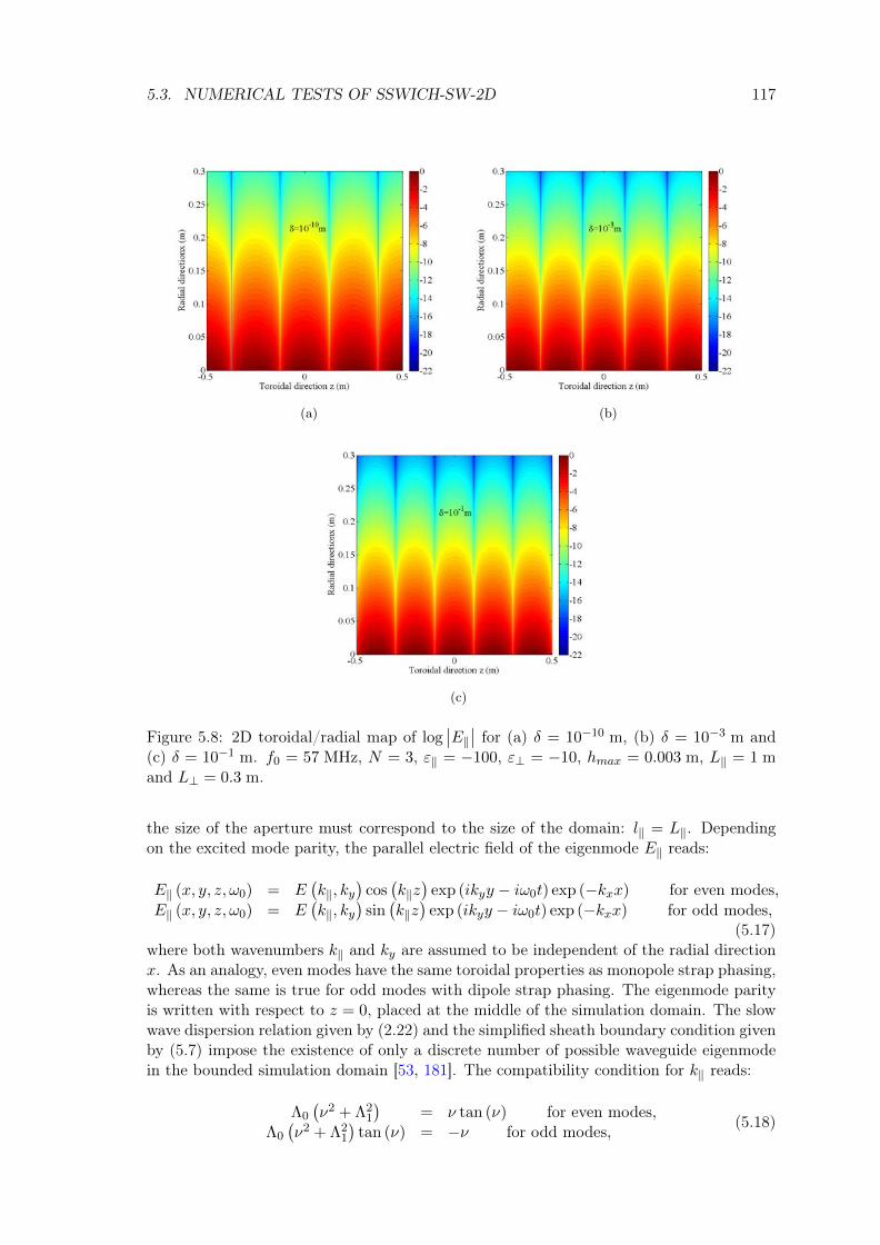
5.3. NUMERICAL TESTS OF SSWICH-SW-2D 117

(a) (b)

(c)

Figure 5.8: 2D toroidal/radial map of log∣∣E‖∣∣ for (a) δ = 10−10 m, (b) δ = 10−3 m and

(c) δ = 10−1 m. f0 = 57 MHz, N = 3, ε‖ = −100, ε⊥ = −10, hmax = 0.003 m, L‖ = 1 mand L⊥ = 0.3 m.

the size of the aperture must correspond to the size of the domain: l‖ = L‖. Dependingon the excited mode parity, the parallel electric field of the eigenmode E‖ reads:

E‖ (x, y, z, ω0) = E(k‖, ky

)cos(k‖z)

exp (ikyy − iω0t) exp (−kxx) for even modes,E‖ (x, y, z, ω0) = E

(k‖, ky

)sin(k‖z)

exp (ikyy − iω0t) exp (−kxx) for odd modes,(5.17)

where both wavenumbers k‖ and ky are assumed to be independent of the radial directionx. As an analogy, even modes have the same toroidal properties as monopole strap phasing,whereas the same is true for odd modes with dipole strap phasing. The eigenmode parityis written with respect to z = 0, placed at the middle of the simulation domain. The slowwave dispersion relation given by (2.22) and the simplified sheath boundary condition givenby (5.7) impose the existence of only a discrete number of possible waveguide eigenmodein the bounded simulation domain [53, 181]. The compatibility condition for k‖ reads:

Λ0

(ν2 + Λ2

1

)= ν tan (ν) for even modes,

Λ0

(ν2 + Λ2

1

)tan (ν) = −ν for odd modes, (5.18)

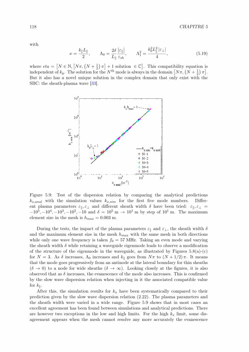
118 CHAPITRE 5

with

ν =k‖L‖

2, Λ0 =

2δ

L‖

∣∣ε‖∣∣εsh

, Λ21 =

k20L

2‖ |ε⊥|4

, (5.19)

where eta =[N ∈ N,

[Nπ,

(N + 1

2

)π]

+ 1 solution ∈ C]. This compatibility equation is

independent of ky. The solution for theN th mode is always in the domain[Nπ,

(N + 1

2

)π].

But it also has a novel unique solution in the complex domain that only exist with theSBC: the sheath-plasma wave [33].

Figure 5.9: Test of the dispersion relation by comparing the analytical predictionskx,anal with the simulation values kx,sim for the first five mode numbers. Differ-ent plasma parameters ε‖, ε⊥ and different sheath width δ have been tried: ε‖, ε⊥ =−105,−104,−103,−102,−10 and δ = 105 m → 101 m by step of 101 m. The maximumelement size in the mesh is hmax = 0.003 m.

During the tests, the impact of the plasma parameters ε‖ and ε⊥, the sheath width δand the maximum element size in the mesh hmax with the same mesh in both directionswhile only one wave frequency is taken f0 = 57 MHz. Taking an even mode and varyingthe sheath width δ while retaining a waveguide eigenmode leads to observe a modificationof the structure of the eigenmode in the waveguide, as illustrated by Figures 5.8(a)-(c)for N = 3. As δ increases, Λ0 increases and k‖ goes from Nπ to (N + 1/2)π. It meansthat the mode goes progressively from an antinode at the lateral boundary for thin sheaths(δ → 0) to a node for wide sheaths (δ → ∞). Looking closely at the figures, it is alsoobserved that as δ increases, the evanescence of the mode also increases. This is confirmedby the slow wave dispersion relation when injecting in it the associated compatible valuefor k‖.

After this, the simulation results for kx have been systematically compared to theirprediction given by the slow wave dispersion relation (2.22). The plasma parameters andthe sheath width were varied in a wide range. Figure 5.9 shows that in most cases anexcellent agreement has been found between simulations and analytical predictions. Thereare however two exceptions in the low and high limits. For the high kx limit, some dis-agreement appears when the mesh cannot resolve any more accurately the evanescence

5.3. NUMERICAL TESTS OF SSWICH-SW-2D 119

length (kxhmax ∼ 1). A finer mesh is needed. In the low kx cases, the evanescence lengthof the mode is so large (kxL⊥ ∼ 1) that when reaching the inner boundary condition of thedomain, the vanishing boundary condition cannot be satisfied. In that case two solutionsare available: take a larger domain in the radial direction or enforcing a radiating BCinstead of a vanishing BC.

In some cases, it was seen that a low amplitude parasitic mode was excited once theslow wave amplitude was close to vanishing. One example is shown in Figure 5.10 withε‖ = −105, ε⊥ = −102, εsh = 1, δ = 105 m, N = 3, L‖ = 1 meter and L⊥ = 0.3 meter.In the region denoted as 1 in Figure 5.10, the slow wave excited an even mode at x = 0 isevanescent and follows the prediction given by dispersion relation (2.22). In region 2, a lowamplitude parasitic mode appears with the remaining low amplitude of the evanescent slowwave. In region 3, the slow wave has completely vanished and only remains the parasiticmode. This amplitude of this mode and the subsequent error between the simulations andthe analytical solution decreases as the mesh resolution increases.

Figure 5.10: 2D toroidal/radial map of log∣∣E‖∣∣ with ε‖ = −105, ε⊥ = −102, εsh = 1,

δ = 105 m, N = 3, L‖ = 1 m and L⊥ = 0.3 m. Three specific regions are drawn to identifythe presence of a low amplitude parasitic mode with the evanescent slow wave.

A second observation can be made. This mode is evanescent in the toroidal direc-tion and propagates along the radial direction on boundaries. It disappears when theSBC reduces to PEC (δ = 0 m). Moreover this parasitic mode is not modified when thewavenumber k‖ changes. The numerical solution is therefore unique. A mode with theseproperties has been shown to exist with SBC: the sheath-plasma wave (SPW) [53]. Ananalysis of the evanescence length in the toroidal direction and of the periodicity of thepropagation in the radial direction has shown that this mode has the same properties asexpected from the SPW with these parameters. The amplitude of this mode is moreoverchanging with the mesh resolution. The finer the mesh was, the lowest the amplitude was.We thus conclude that this parasitic mode is a Sheath-Plasma Waves (SPW) excited hereby numerical errors.

Since the SPW propagate along material surfaces in presence of SBC, an idea to solvepotential issues between SPW and PML that was exposed as a source of concern in Sec-tion 4.3.3, is to place the plasma-PML interface far away radially in the plasma where no

120 CHAPITRE 5

material object exists. If that case, the SPW will become evanescent once the SBC ceasesto exist since no wall can give a support for the propagation of the SPW.

The results shown here for the SW wave propagation module with sheath boundarycondition were performed with even modes. Similar properties would nevertheless havebeen obtained with odd modes.

5.3.2 Comparison of multi-2D approach with 3D for Tore Supra withthe asymptotic model in standalone

This test aims to verify one of the assumptions made in the establishment of SSWICH-SW-2D. To make the numerical cost acceptable in-line with our available resources, poloidalderivatives have been assumed to be negligible. We are proposing here to test this as-sumption with a more simplified version of SSWICH-SW that only entails the asymptotictreatment with spectral resolution of an homogeneous plasma within a parallelepipedic ge-ometry in 3D [173]. This version of SSWICH, implemented in Matlab, provides a solutionwithin a minute.

Since the main advantage of this version of SSWICH is its ability to handle a paral-lelepipedic 3D geometry, we can evaluate the impact of a finite ky spectrum of the E‖ fieldmap such as Figure 5.6(a). Since only a parallelepipedic geometry is possible, the simu-lation domain is only the private SOL. A cut in a 2D radial/toroidal plane is shown onFigure 5.7. Extrapolating the SW evanescence for each modes individually is not an issuein this particular case since no inverse Fourier transform on the E‖ field map is necessary.Infinite parallel DC conductivity is assumed in this model whereas no transverse DC con-ductivity is allowed. Since the parallel Spitzer conductivity is infinite, VDC is homogeneousalong field lines (i.e. flute assumption). Thus the two sides of the antenna do not need tobe distinguished. The DC plasma potential VDC,as on one particular flux tubes exclusivelydepends on the biasing voltages at both extremities on this flux tube denoted by the duplet(x, y). VDC is thus evaluated with the following analytic expression:

VDC,as =1

2(Vb,l + Vb,r) + ln

[cosh

(1

2(Vb,l − Vb,r)

)], (5.20)

where Vb,l and Vb,r are respectively the biasing voltage on the left and the right sides ofthe antenna calculated with (2.51).

The simulations parameters of this test are: ni = 51017 m−3, Ti = 20 eV, Te = 20 eV,Ly = 1.4 m, L‖ = 0.55 m, L⊥ = 1 cm and Vstrap = 30 kV. Figure 5.11(a) is a 2D map inthe radial/poloidal plane of the asymptotic plasma DC potential VDC,as with the E‖ fieldmap in Figure 5.6(a). The two humps poloidal topology is characteristic of Tore SupraICRH antennas. Further detailed discussion will occur in Chapter 6. It can also be seenthat the gradient of VDC,as associated with each direction will have different scale-lengths.The typical gradient scale length in the poloidal direction (≈ 10 cm)is much larger than inthe radial direction (≈ 1 cm). This provides a first argument for neglecting the poloidalgradient in the equations with respect to the radial gradient. Two tests cases have beenthen performed. One has a finite ky spectrum defined by the E‖ field map and in the othercase ky = 0 is enforced. The relative error for VDC,as has been evaluated and is shown onFigure 5.11(b). An error of at most 10% is expected by neglecting the poloidal derivativesfor the case of a Tore Supra antenna. The maximum error is obtained in regions where thefield map goes from zero to small finite value of E‖. Moreover this is the maximum error.Over most of the 2D map, the error level is much lower at around 1%. Simulations withother parameters give similar results.

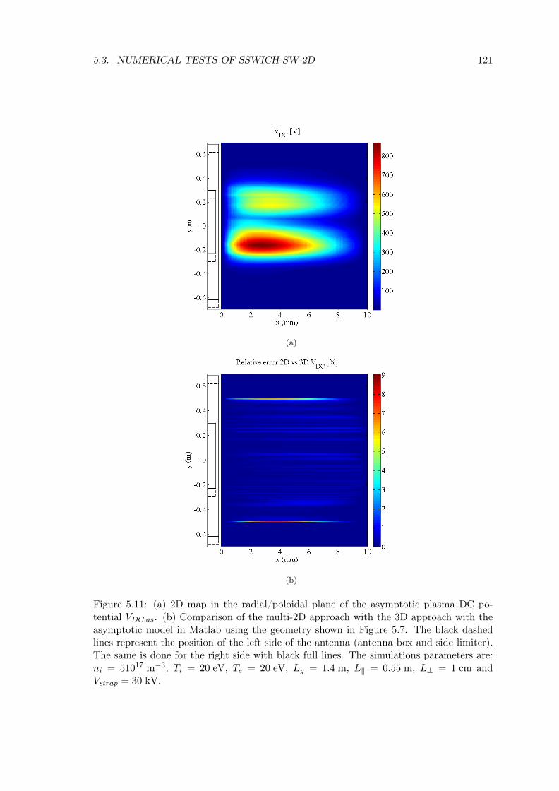
5.3. NUMERICAL TESTS OF SSWICH-SW-2D 121

(a)

(b)

Figure 5.11: (a) 2D map in the radial/poloidal plane of the asymptotic plasma DC po-tential VDC,as. (b) Comparison of the multi-2D approach with the 3D approach with theasymptotic model in Matlab using the geometry shown in Figure 5.7. The black dashedlines represent the position of the left side of the antenna (antenna box and side limiter).The same is done for the right side with black full lines. The simulations parameters are:ni = 51017 m−3, Ti = 20 eV, Te = 20 eV, Ly = 1.4 m, L‖ = 0.55 m, L⊥ = 1 cm andVstrap = 30 kV.

122 CHAPITRE 5

We conclude that, for the case of Tore Supra antennas in first approximation, thepoloidal derivatives can indeed be neglected. The fully coupled model SSWICH-SW in 2Dcan thus be used with a multi-2D approach to simulate the entire 3D antenna.

5.3.3 Comparison of the fully coupled model with the asymptotic modelduring a power scan

The last test to be presented in this thesis consisted in comparing the solution provided atthe end by the asymptotic model and the coupled model during a power scan. The amountof power is directly linked to the strap voltage. The asymptotic model was establishedin the wide sheaths regime at high power. Thus the discrepancy between the asymptoticmodel and the coupled power should get reduced as the strap voltage increases. Thesimulations were performed for only one vertical position. It was chosen at y = 0.2 m nearthe bottom corner of the antenna box, as illustrated by Figure 5.12.

Figure 5.12: 3D model of the Tore Supra antenna geometry. A parallel/radial plane aty = −0.2 m, where the tests of the fully coupled version of SSWICH will be tested, isrepresented to show approximatively the vertical position where the maximum of VDC areexpected as shown on Figure 5.11(a).

This test is presented here for the classical Faraday screen, illustrated by Figure 5.3(a).The strap voltage was progressively increased step by step. For each step, the value ofthe DC plasma potential at the leading edge of the side limiter VDC,le was evaluated fromthe asymptotic solution and the solution of the coupled model. The results are plottedon Figure 5.13(a). The amplitude of VDC,le increases when Vstrap increases. A fit gives adependence as V 2/3

strap.Looking at Figure 5.13(b), the relative error between both solutions is decreasing as

Vstrap is increasing. From a 45% error at low strap voltage, the relative error decreases toless than 10% for Vstrap = 50 kV. Moreover the qualitative trend is still decreasing at thispoint.

At high Vstrap numerical crashes in the loop of the coupled model was sometimes seenwhen a result of the type ∞/0 was encountered on a few nodes for one iteration alwayson lateral boundaries when SBCs are applied. This was ascribed to issue with the meshsince the crash do not always occur on the same nodes and that changing slightly the meshdistribution correct this issue. Being able to use finer mesh with lower scaling betweendirections would hopefully solve this problem.

5.3. NUMERICAL TESTS OF SSWICH-SW-2D 123

(a)

(b)

Figure 5.13: (a) Comparison of DC plasma potential at the leading edge with coupled modelVDC,le (red straight curve with squares) and asymptotic model VDC,le,as (blue dashed curvewith circles) versus the strap voltage. (b) Relative error versus strap voltage. Each dotrepresents one simulation. The other simulation parameters are: Te = 10 eV, Ti = 20 eV,L‖ = 3.3 m, nle = 1.7 m−3, σ⊥DC,p = 7.110−8σ‖,S and σ⊥DC,p = 2.610−6σ‖,S .

124 CHAPITRE 5

This test confirms that the asymptotic expansion is correct and that its validity is getbetter as high power which is the most interesting case for antenna since it is when themore important heat fluxes are evaluated on the antenna.

5.4 Status and prospects for SSWICH

The SSSWICH code was developed during this thesis to describe self-consistently RFsheaths. It models the interplay between the slow wave propagation and the resultingpositive DC biasing of the edge of a magnetized plasma. It was seen early during thethesis than using a three field-fluid description (wave parallel electric field E‖, oscillatingsheath voltage VRF and DC plasma potential VDC) is better for the convergence thanusing only two. The code main features are sheath boundary conditions, the finite DCconductivity tensor, the full description of cold plasma, a more realistic geometry thanksto the finite element method, the ability to simulate antenna through field maps computedwith TOPICA and a multi-2D procedure to recover the third direction. The model wasimplemented in Comsol Multiphysics. The resulting code is called SSWICH-SW-2D. Toautomate numerous simulations, an interaction with Matlab has been created.

Numerical tests have shown that the SBCs modify the structure of the SW. The multi-2D procedure is indeed correct as in the case of Tore Supra the poloidal derivatives canbe neglected. Comparison of SSWICH-SW-2D with an analytic model of the DC biasingled us to suspect a non-linear broadening of the VDC structure with the amplitude of VDCdue to the presence of a DC perpendicular conductivity. A comparison of the fully-coupledmodel with the asymptotic model during a power scan reveals that indeed the asymptoticmodel is true at high power.

Despite the numerical tests already performed on the individual modules and on SS-WICH itself, there are still much more fundamental tests to be done on the self-consistentmodel concerning the uniqueness of the solution, the convergence of the iterative scheme tothe solution. These fundamental nature of these open issues are first related to the multi-plicity of the solution and the neighbourhood of the possible multiple solutions [92]. Secondthere are numerical limits to the Newton-Raphson iterative scheme due possibly to poorinitial estimate, overshoot or stationary point that are identified as the major issues. Forthat these reasons a limit of the number of iterations was placed. Combining the methodwith a more robust one would bring a better mitigation capability of non-convergence orslow convergence. One other numerical issue is concerning the optimization of the mesh.

Several limitations exist in SSWICH due to some assumptions that were made to sim-plify the problem. These assumptions could be either removed or replaced by more realisticones:

1. The walls are always assumed to be perpendicular or parallel to the magnetic field B,thus restricting the possible geometries to the ones with lateral boundaries normalto B. It is in the current model a essential assumption to neglect the fast waveand to simplify the expression of SBCs. With a shaped lateral wall or limiter, theangle is arbitrary. When the wall is arbitrarily oriented with respect to B, it washowever proved that the FW and the SW cannot be decoupled any more at thelateral boundaries of the simulation domain [171]. Both modes need to be treatedsimultaneously to describe the RF sheath excitation as mode conversion can occur.It means that the RHS in (5.3) would contain some source terms depending on theFW.

2. Additionally (5.3) need to be completed by a wave equation for the fast wave. A way

5.4. STATUS AND PROSPECTS FOR SSWICH 125

to damp the propagative FW would however be required at the end of the compu-tational domain to avoid reflection on the boundaries of the domain. A techniquesuch as the Perfectly Matched Layer [57, 150] for cold magnetized plasmas could beused. That technique has been shown to be of interest for FW coupling in a tokamakplasmas [182]. Combining the FW coupling code presented in Chapter 4 with theSSWICH code will give full self-consistent description of the waves coupling with RFsheaths. Additionally the Child-Langmuir law (2.53) would be changed to accountfor shaped lateral walls (e.g. Ref. [183] for cylindrical geometries). It would alsobe interesting to know the fraction of the power going to the slow wave lost on theantenna structure due to sheath dissipation. It requires to add an imaginary part toεsh [53]. Additionally a more refined analysis should be later done as flute assump-tion is considered. However the finite perpendicular DC conductivity considered inthe model can possibly break the flute assumption.

3. While a radial gradient exists in the density profile, the density is assumed to beinvariant in the poloidal and parallel direction (except in the private SOL). Obser-vations however show that the density is affected by active ICRH antennae due toRF sheaths. The model thus need in a future version to include a density equationto self-consistently evaluate the DC potential pattern with the density [184]. An al-ternative would be to add a fourth module that would re-evaluate the density profilewithin the iterative loop. It will even become more critical when the FW is alsoincluded as the distance between the antenna straps and the FW cutoff density is themain parameter to determine FW coupling [182] and thus to adapt the strap voltageto couple a constant amount of power. Moreover modifying the density would alsomodify the sheaths boundary conditions as the density in the sheath is linked to theplasma density.

4. This issue also indicates that the code coupling TOPICA/SSWICH-SW is not self-consistent. TOPICA uses as input a radial density profile, assumed to be constantpoloidally and toroidally, to compute the electric field map at the antenna aperture.This map is the input of SSWICH-SW to calculate the DC potential distributionthat modifies the density by inducing poloidal gradients and toroidal gradients. Anew solution should thus be computed with TOPICA using this new density profilesand so on until convergence is reached.

5. Another possible development is about a 3D version of SSWICH. Neglecting poloidalderivative would not be required anymore and a 3D antenna geometry could bedirectly implemented. It would however require a much greater amount of computa-tional resources. It is finely entangled with the previous point, as modelling densityconvection cells has to be done in 3D.

6. Other formulae exist in the literature for the sheath capacitance [100] that couldreplace the current one. A sensitivity study to the formula of the sheath capacitanceshould be performed to identify the sensitivity of the results to the chosen model.

7. Several phenomena are moreover missing or assumed negligible here that could pos-sibly be integrated in a full self-consistent description of RF sheaths. The radialtransport of DC currents is here modelled with constant effective perpendicular DCconductivities whereas in reality there could be a spatial dependence. Moreover thetransport coefficient should be described self-consistently with the rest of the model.

126 CHAPITRE 5

Secondary electron emissions, ion sputtering have also been neglected. An investiga-tion of their impact of RF sheaths should be done to know if they enhanced or notRF sheaths. If they lower the magnitude of RF sheaths, SSWICH could be seen aspredicting a worst case result.

Those are long terms prospects. SSWICH in its present version coupled with TOPICAhas been used to reproduce some of the unexpected observations during the last exper-imental campaign on Tore Supra in 2011. Comparisons of numerical simulations withexperimental observations is the purpose of Chapter 6.

Chapter 6

Comparison of SSWICH-SW-2Dsimulations with experimentalobservations on Tore Supra andpredictions for ITER

Improved modelling included in the SSWICH code, presented in Chapter 5, was motivatedto explain why the minimization of the integrated parallel electric field along “long fieldlines” predicted RF sheaths mitigation [48] for the new FS design while in practise thesheaths were significantly enhanced on the antenna structure and its side limiters.

This chapter is devoted to show that self-consistent modelling is already able to re-produce and explain some of the experimental observations along the side limiters of theantenna on Tore Supra. In order to do that, this chapter will start by recalling the majorobservations on the ICRH antenna during RF pulses in the 2011 campaign. Then a com-parison between experimental observations and simulations results will be performed. Italso proposes a possible explanation for the appearance of significant rectified potentialsstructures on the outer side of the antenna limiters. The design element deemed respon-sible for RF sheath induced enhancement of the plasma potential is presented. Finallysome estimates for the parallel heat fluxes performed within a simplified geometry of theblanket shielding module of the ITER ICRH antenna are shown. Difficulties related toITER modelling are also discussed.

6.1 Review of the experimental observations on Tore Supraduring the 2011 campaign

During the latest experimental campaign on Tore Supra in 2011, several sessions werededicated to the minimization of RF sheaths in Tore Supra [185]. Two types of FS, withdifferent electrical designs, were compared on the same plasmas: the classical design anda proposed electrical design, shown in Section 2.4.5 supposed to mitigate RF sheaths ac-cording to the results in [48]. Multiple diagnostics on TS were available: infrared (IR)thermography [141], two-dimensional mappings by reciprocating Langmuir probes [39, 43],VUV spectroscopy [186], calorimetry of actively cooled plasma facing components [187].The major experimental observations for RF sheaths on the ICRH antennas have been per-formed with infrared cameras and probes. This section is a review of the main experimentalobservations on the ICRH antenna that we are proposing to reproduce and interpret with

127

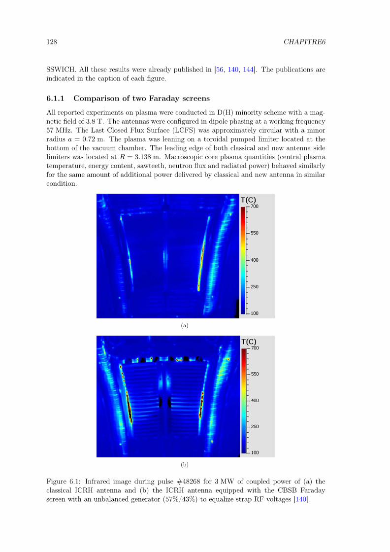
128 CHAPITRE6

SSWICH. All these results were already published in [56, 140, 144]. The publications areindicated in the caption of each figure.

6.1.1 Comparison of two Faraday screens

All reported experiments on plasma were conducted in D(H) minority scheme with a mag-netic field of 3.8 T. The antennas were configured in dipole phasing at a working frequency57 MHz. The Last Closed Flux Surface (LCFS) was approximately circular with a minorradius a = 0.72 m. The plasma was leaning on a toroidal pumped limiter located at thebottom of the vacuum chamber. The leading edge of both classical and new antenna sidelimiters was located at R = 3.138 m. Macroscopic core plasma quantities (central plasmatemperature, energy content, sawteeth, neutron flux and radiated power) behaved similarlyfor the same amount of additional power delivered by classical and new antenna in similarcondition.

(a)

(b)

Figure 6.1: Infrared image during pulse #48268 for 3 MW of coupled power of (a) theclassical ICRH antenna and (b) the ICRH antenna equipped with the CBSB Faradayscreen with an unbalanced generator (57%/43%) to equalize strap RF voltages [140].

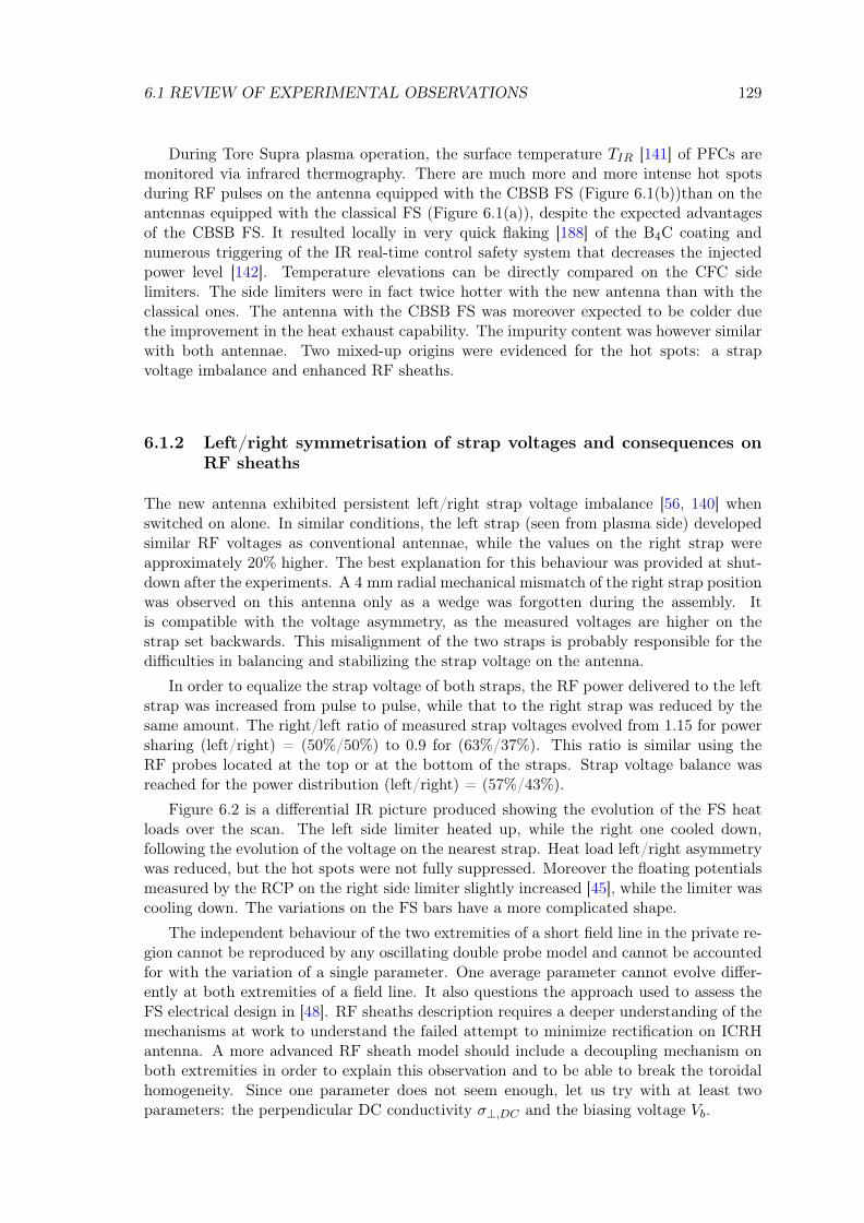
6.1 REVIEW OF EXPERIMENTAL OBSERVATIONS 129

During Tore Supra plasma operation, the surface temperature TIR [141] of PFCs aremonitored via infrared thermography. There are much more and more intense hot spotsduring RF pulses on the antenna equipped with the CBSB FS (Figure 6.1(b))than on theantennas equipped with the classical FS (Figure 6.1(a)), despite the expected advantagesof the CBSB FS. It resulted locally in very quick flaking [188] of the B4C coating andnumerous triggering of the IR real-time control safety system that decreases the injectedpower level [142]. Temperature elevations can be directly compared on the CFC sidelimiters. The side limiters were in fact twice hotter with the new antenna than with theclassical ones. The antenna with the CBSB FS was moreover expected to be colder duethe improvement in the heat exhaust capability. The impurity content was however similarwith both antennae. Two mixed-up origins were evidenced for the hot spots: a strapvoltage imbalance and enhanced RF sheaths.

6.1.2 Left/right symmetrisation of strap voltages and consequences onRF sheaths

The new antenna exhibited persistent left/right strap voltage imbalance [56, 140] whenswitched on alone. In similar conditions, the left strap (seen from plasma side) developedsimilar RF voltages as conventional antennae, while the values on the right strap wereapproximately 20% higher. The best explanation for this behaviour was provided at shut-down after the experiments. A 4 mm radial mechanical mismatch of the right strap positionwas observed on this antenna only as a wedge was forgotten during the assembly. Itis compatible with the voltage asymmetry, as the measured voltages are higher on thestrap set backwards. This misalignment of the two straps is probably responsible for thedifficulties in balancing and stabilizing the strap voltage on the antenna.

In order to equalize the strap voltage of both straps, the RF power delivered to the leftstrap was increased from pulse to pulse, while that to the right strap was reduced by thesame amount. The right/left ratio of measured strap voltages evolved from 1.15 for powersharing (left/right) = (50%/50%) to 0.9 for (63%/37%). This ratio is similar using theRF probes located at the top or at the bottom of the straps. Strap voltage balance wasreached for the power distribution (left/right) = (57%/43%).

Figure 6.2 is a differential IR picture produced showing the evolution of the FS heatloads over the scan. The left side limiter heated up, while the right one cooled down,following the evolution of the voltage on the nearest strap. Heat load left/right asymmetrywas reduced, but the hot spots were not fully suppressed. Moreover the floating potentialsmeasured by the RCP on the right side limiter slightly increased [45], while the limiter wascooling down. The variations on the FS bars have a more complicated shape.

The independent behaviour of the two extremities of a short field line in the private re-gion cannot be reproduced by any oscillating double probe model and cannot be accountedfor with the variation of a single parameter. One average parameter cannot evolve differ-ently at both extremities of a field line. It also questions the approach used to assess theFS electrical design in [48]. RF sheaths description requires a deeper understanding of themechanisms at work to understand the failed attempt to minimize rectification on ICRHantenna. A more advanced RF sheath model should include a decoupling mechanism onboth extremities in order to explain this observation and to be able to break the toroidalhomogeneity. Since one parameter does not seem enough, let us try with at least twoparameters: the perpendicular DC conductivity σ⊥,DC and the biasing voltage Vb.

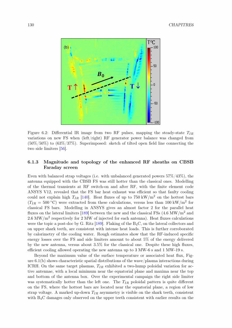
130 CHAPITRE6

Figure 6.2: Differential IR image from two RF pulses, mapping the steady-state TIRvariations on new FS when (left/right) RF generator power balance was changed from(50%/50%) to (63%/37%). Superimposed: sketch of tilted open field line connecting thetwo side limiters [56].

6.1.3 Magnitude and topology of the enhanced RF sheaths on CBSBFaraday screen

Even with balanced strap voltages (i.e. with unbalanced generated powers 57%/43%), theantenna equipped with the CBSB FS was still hotter than the classical ones. Modellingof the thermal transients at RF switch-on and after RF, with the finite element codeANSYS V12, revealed that the FS bar heat exhaust was efficient so that faulty coolingcould not explain high TIR [140]. Heat fluxes of up to 750 kW/m2 on the hottest bars(TIR = 500 C) were extracted from these calculations, versus less than 100 kW/m2 forclassical FS bars. Modelling in ANSYS gives an almost factor 2 for the parallel heatfluxes on the lateral limiters [189] between the new and the classical FSs (4.6 MW/m2 and2.6 MW/m2 respectively for 2 MW of injected for each antenna). Heat fluxes calculationswere the topic a post-doc by G. Ritz [189]. Flaking of the B4C, on the lateral collectors andon upper shark teeth, are consistent with intense heat loads. This is further corroboratedby calorimetry of the cooling water. Rough estimates show that the RF-induced specificenergy losses over the FS and side limiters amount to about 5% of the energy deliveredby the new antenna, versus about 3.5% for the classical one. Despite these high fluxes,efficient cooling allowed operating the new antenna up to 3 MW-6 s and 1 MW-19 s.

Beyond the maximum value of the surface temperature or associated heat flux, Fig-ure 6.1(b) shows characteristic spatial distributions of the wave/plasma interactions duringICRH. On the same target plasmas, TIR exhibited a two-hump poloidal variation for ac-tive antennae, with a local minimum near the equatorial plane and maxima near the topand bottom of the antenna box. Over the experimental campaign the right side limiterwas systematically hotter than the left one. The TIR poloidal pattern is quite differenton the FS, where the hottest bars are located near the equatorial plane, a region of lowstrap voltage. A marked up-down TIR asymmetry is visible on the shark teeth, consistentwith B4C damages only observed on the upper teeth consistent with earlier results on the

6.1 REVIEW OF EXPERIMENTAL OBSERVATIONS 131

Figure 6.3: 3D model of the Tore Supra antenna geometry. A poloidal/radial plane alongthe outer side of the antenna side limiter indicates where the Vfloat 2D map with the probeand VDC 2D map in the simulation is evaluated.

corners of conventional FS and the direction of the magnetic field [36].Spatial heat loads measurements are complemented by reciprocating Langmuir probe

(RCP) mapping [38]. The RCP is connected magnetically to the outer face of the rightside limiter of the new antenna. In order to obtain a detailed 2D map, PhD topic ofMartin Kubic [144], the probe is immersed into the SOL during the discharge severaltimes. Between the plunges plasma current is decreased in little steps. As a consequencethe magnetic connections of the probe to the antenna move up poloidally providing poloidalresolution. Radial resolution is achieved by the depth of the probe plunge.

The floating potential Vfloat of the probe is mapped in 2D in Figure 6.4 versus theconnection point coordinates, over six 1 MW RF pulses with 7 reciprocations per shot.Vfloat reached a maximum of 170 V, while earlier measurements with a classical antennadid not exceed 100 V in similar conditions [39]. The most intense zones are located aroundthe top and the bottom corners of the antenna box, similar to the heat loads localization onthe side limiters. Vfloat was also observed to change with the density [45]. The structurehowever presents an up-down asymmetry. Such a mapping corresponds well to resultsobtained in earlier TS experiments [38]. The maximum is located surprisingly radiallyapproximately 2 cm behind the leading edge of the side limiters, with 5 mm uncertainty inthe field line tracing, while it was previously observed on Tore Supra and Alcator C-Mod[190] on the leading edge. With the classical screen, the full radial width of RF-perturbedzone is comparable to the expected uncertainty given by the magnetic reconstruction. Withthe prototype CBSB screen, the structure is so wide (∼ 3 cm) that there can be no doubtthat the probe is indeed magnetically connected to the side limiter and that high positivebiasing occurs on field lines connected to the side limiter [45].

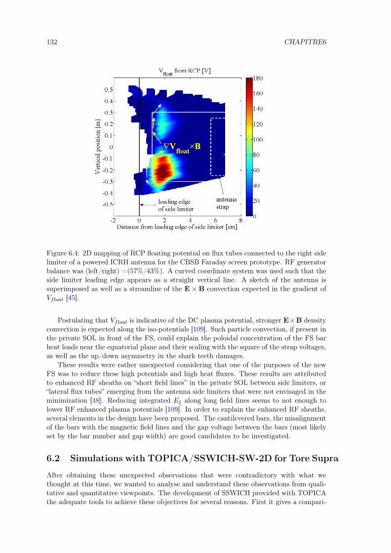
132 CHAPITRE6

Figure 6.4: 2D mapping of RCP floating potential on flux tubes connected to the right sidelimiter of a powered ICRH antenna for the CBSB Faraday screen prototype. RF generatorbalance was (left/right) =(57%/43%). A curved coordinate system was used such that theside limiter leading edge appears as a straight vertical line. A sketch of the antenna issuperimposed as well as a streamline of the E×B convection expected in the gradient ofVfloat [45].

Postulating that Vfloat is indicative of the DC plasma potential, stronger E×B densityconvection is expected along the iso-potentials [109]. Such particle convection, if present inthe private SOL in front of the FS, could explain the poloidal concentration of the FS barheat loads near the equatorial plane and their scaling with the square of the strap voltages,as well as the up/down asymmetry in the shark teeth damages.

These results were rather unexpected considering that one of the purposes of the newFS was to reduce these high potentials and high heat fluxes. These results are attributedto enhanced RF sheaths on “short field lines” in the private SOL between side limiters, or“lateral flux tubes” emerging from the antenna side limiters that were not envisaged in theminimization [48]. Reducing integrated E‖ along long field lines seems to not enough tolower RF enhanced plasma potentials [109]. In order to explain the enhanced RF sheaths,several elements in the design have been proposed. The cantilevered bars, the misalignmentof the bars with the magnetic field lines and the gap voltage between the bars (most likelyset by the bar number and gap width) are good candidates to be investigated.

6.2 Simulations with TOPICA/SSWICH-SW-2D for Tore Supra

After obtaining these unexpected observations that were contradictory with what wethought at this time, we wanted to analyse and understand these observations from quali-tative and quantitative viewpoints. The development of SSWICH provided with TOPICAthe adequate tools to achieve these objectives for several reasons. First it gives a compari-

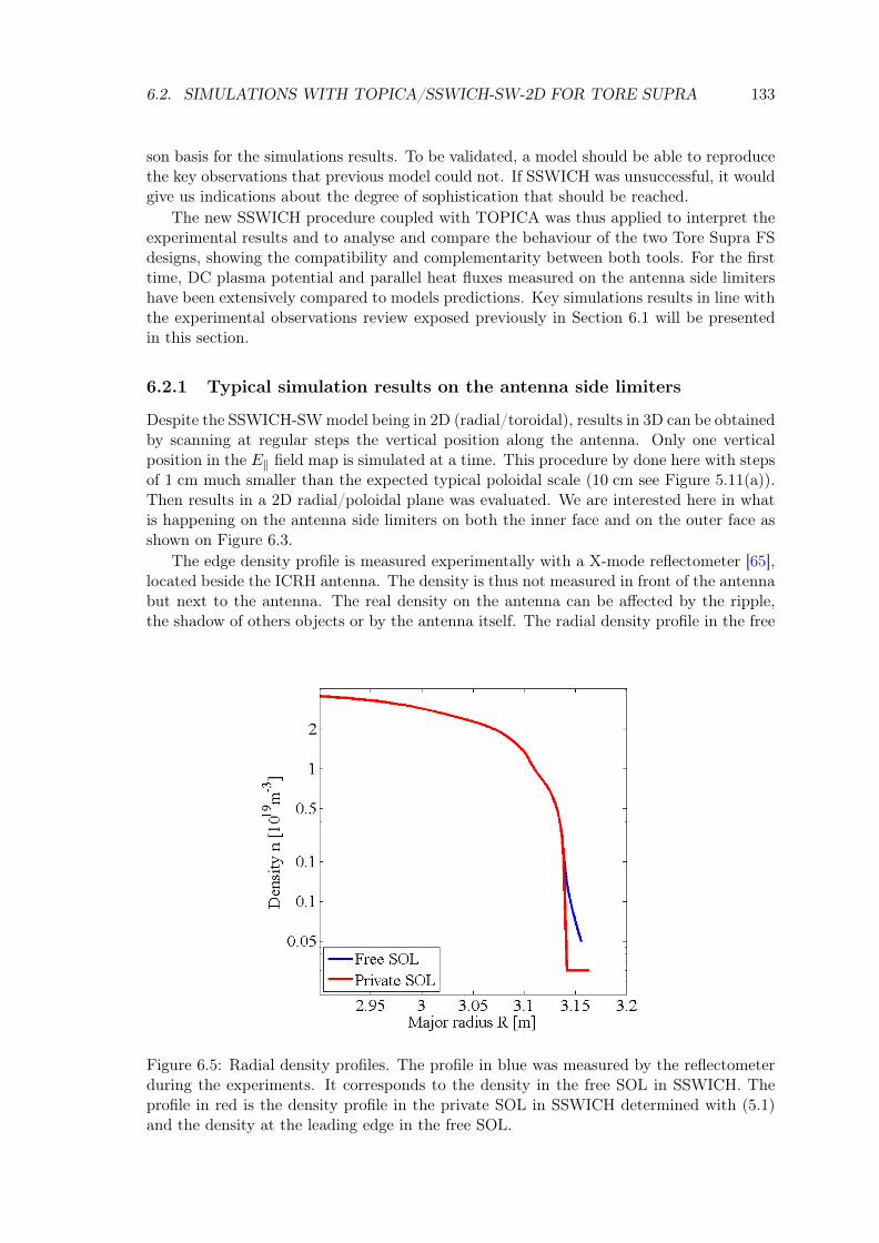
6.2. SIMULATIONS WITH TOPICA/SSWICH-SW-2D FOR TORE SUPRA 133

son basis for the simulations results. To be validated, a model should be able to reproducethe key observations that previous model could not. If SSWICH was unsuccessful, it wouldgive us indications about the degree of sophistication that should be reached.

The new SSWICH procedure coupled with TOPICA was thus applied to interpret theexperimental results and to analyse and compare the behaviour of the two Tore Supra FSdesigns, showing the compatibility and complementarity between both tools. For the firsttime, DC plasma potential and parallel heat fluxes measured on the antenna side limitershave been extensively compared to models predictions. Key simulations results in line withthe experimental observations review exposed previously in Section 6.1 will be presentedin this section.

6.2.1 Typical simulation results on the antenna side limiters

Despite the SSWICH-SWmodel being in 2D (radial/toroidal), results in 3D can be obtainedby scanning at regular steps the vertical position along the antenna. Only one verticalposition in the E‖ field map is simulated at a time. This procedure by done here with stepsof 1 cm much smaller than the expected typical poloidal scale (10 cm see Figure 5.11(a)).Then results in a 2D radial/poloidal plane was evaluated. We are interested here in whatis happening on the antenna side limiters on both the inner face and on the outer face asshown on Figure 6.3.

The edge density profile is measured experimentally with a X-mode reflectometer [65],located beside the ICRH antenna. The density is thus not measured in front of the antennabut next to the antenna. The real density on the antenna can be affected by the ripple,the shadow of others objects or by the antenna itself. The radial density profile in the free

Figure 6.5: Radial density profiles. The profile in blue was measured by the reflectometerduring the experiments. It corresponds to the density in the free SOL in SSWICH. Theprofile in red is the density profile in the private SOL in SSWICH determined with (5.1)and the density at the leading edge in the free SOL.

134 CHAPITRE6

SOL in SSWICH is the density measured by the reflectometer. It is illustrated in blue byFigure 6.5. The density in the private SOL in red is evaluated with (5.1). The density atthe leading edge of the side limiters is identical for both profiles.

Let us see now what looks like a typical result following this procedure with the field mapfor the CBSB FS illustrated by Figure 5.6(b). The simulation parameters were Te = 10 eV,Ti = 20 eV, Vstrap = 30 kV and l‖,1 = 3.3 m, σ⊥DC,f/σ‖,S = 7.1 10−8, σ⊥DC,f/σ‖,S =2.5 10−6, l‖,2 ≈ 1.3 m. The tilt of the magnetic field is 7. Figure 6.6(b) shows the DCplasma potential evaluated on the outer face on the right side limiter with the CBSBFaraday screen (see Figure 5.3(b)) where the probes are magnetically connected. Weassume that the average floating potential measured with probes is representative of theDC plasma potential. The simulation result can be then compared to the observations bothqualitatively and quantitatively. Some key agreements with the experiments are recovered.

First the overall two-hump poloidal structure, observed experimentally, of the heatloads and on the floating potential on side limiters could also be reproduced. The floatingpotential measured on the probe is assumed to be representative of the DC plasma potentialboth in amplitude and in topology. The minimum is observed near the equatorial planewhereas the maximum are observed near the antenna box corners. This is a robust invariantoutput that was systematically observed whatever the parameters. For that reason, thepoloidal topology is mainly dependent on the input E‖ field map i.e. on the electricaldesign on the antenna, and not on the numerous simulation parameters. This two-humppoloidal structure could also be obtained by previous modelling [48]. So it is not by itselfa discriminating test but a necessary result to obtain for any model.

Second SSWICH can obtain, with our choice of simulation parameters, a presence ofDC plasma potential not only on the inner face of the side limiter in the private SOL ofthe antenna but also on the outer face in the free SOL. This is a new feature that did notexist in the version of SSWICH used in [174] whereas insignificant VDC were evaluated in

(a) (b)

Figure 6.6: 2D Map of the DC plasma potential VDC obtained with SSWICH in thepoloidal/radial plane at the position shown by dark dashed line in Figure 5.1(b) for (a) theconventional Faraday screen and (b) the CBSB Faraday screen prototype.

6.2. SIMULATIONS WITH TOPICA/SSWICH-SW-2D FOR TORE SUPRA 135

the free SOL. The topology of VDC is identical on the inner face and on the outer face ofthe side limiters. But the amplitudes are different. This feature is rendered possible bythe inclusion of a DC perpendicular conductivity in SSWICH whose role and impact onthe simulation results would be detailed later on in this chapter.

Third an up-down asymmetry is also obtained similar to the experiments. A factor≈ 2 is recovered between the maximum amplitude of the VDC top peak compared to theamplitude of the bottom peak. This also corresponds to experimental observations (seeFigure 6.4).

There are however some disagreements remaining. The first is on the radial positionof the maximum of the VDC structure that was observed for the CBSB Faraday screen inthe experiments shifted outwards by 2 cm behind the leading edge and in the shadow ofthe limiters. However in the simulations, the maximum is always observed radially at theposition of the leading edge of the limiters. There are several possible a priori explanations.The first possible explanation is an error in the reconstruction of the trajectories of themagnetic field lines. But this would not explain why this phenomenon is only observed forthe antenna with the CBSB FS. The second explanation supposes the existence of an un-known physical mechanism that shift uniformly outwards by several centimeters the entireVDC structure and that is significant only with high magnitude of VDC . This mechanism,if it exists, has not been yet identified, and as such is not modelled within the presentSSWICH code.

The second main disagreement is on the quantitative values that do not correspondexactly to the experiments results. Maximum VDC value of 140 V have been obtained thathas to be compared with the 170 V in the experiments (see Figure 6.4). The uncertaintyof the quantitative values can be explained with two main reasons.

First, some of the simulations parameters are loosely constrained almost to the pointof being free parameters for some of them. Moreover they appear to be extremely sensitiveto these badly known parameters. The parallel connexion lengths in the SOL are quitedifficult to obtain with accuracy due to the complex topology of the magnetic field linesand magnetic connexions to other objects.

The magnitude of the results is also sensitive to the input density. The density inthe private SOL has never been measured experimentally. Instead it is evaluated fromanalytic considerations [93]. It is simply extrapolate from the ratio of the parallel connexionlength in free in private SOLs and the density in free SOL measured by reflectometry [146]combined into a simple model [93]. However new antennas on ASDEX Upgrade [191, 192]and WEST [19] will be equipped with a reflectometer. The density in the free SOL wasmeasured in front of the reflectometer that is placed next to the antenna and not in frontof the antenna. The density in front of the reflectometer may not be the density in frontof the antenna due to convection cells [38].

The quantitative values of perpendicular DC conductivity are still unknown in the SOLof tokamaks. This is only when talking about average values at zero order. A first ordercorrection would be then to add a spatial dependence. This discussion will be furthercontinued later in this chapter.

Second, our available resources do not allow us to simulate a more realistic set of pa-rameters characteristic of Tore Supra. As an example, the parallel connexion length to aprobe along a magnetic field line connected to the side limiter of the antenna is estimatedin Tore Supra to be of the order of 10− 15 m. We are far from that in SSWICH as theconnexion length is of the order of ≈ 1 m. Furthermore the domain of DC perpendicularconductivities compatible with the observations is not yet within our reach as the associ-ated characteristic transverse scale lengths require finer numerical grids (i.e. more RAM

136 CHAPITRE6

memory and more CPU time). Nevertheless relative comparisons of simulation results willbe attempted.

From these 2D VDC spatial distribution, DC electric field can be expected in the poloidaland radial directions, as EDC = −∇VDC . Cross-field convection via local EDC × B driftvelocities is then evaluated with the formula v = −∇VDC × B/B2 [94]. Estimates of thedrift velocities give about 6000 km/s in the poloidal direction and 100 km/s in the radialdirection, in agreement with observations [109].

The average sheath width δ is another possible output of the code. (a) and (b) showδ on the inner and outer face of the antenna side limiter respectively from the Child-Langmuir law (2.53) and the correction proposed by Lieberman [103]. The two densityprofiles distinguishing free SOL from private SOL (see Figure 6.5) are accounted for. Thesheath width follows a similar pattern at the DC plasma potential. Sheath widths of a theorder of 100 microns are evaluated. This is much smaller than the typical grid size in theparallel direction (i.e. 1 cm). The sheath width is of the order of the typical grid size inthe radial direction. Even meshing the sheath with only one element is thus out of ourreach, due to the prohibitive numerical cost. More realistically several elements (i.e. ≈ 10)would be needed to accurately mesh the sheath. Replacing metallic boundary conditionsby sheath boundary conditions is thus nowadays the only way to evaluate numerically in ashort time RF sheaths effects self-consistently in a domain containing an ICRH antenna inthe SOL of a tokamak plasma. It also indicate that the direct measurement of the electricfield in the sheath will require a high resolution spectrometer in order to do for ICRHantennas what was performed for LH antennas by Klepper [193].

6.2.2 Relative comparison of the two Faraday screens

The procedure TOPICA/Multi SSWICH-SW-2D has also been used to compare relativelythe results with the two Faraday screens on Tore Supra. This relative comparison iswith respect to each other with the same simulation parameters and with respect to the

(a) (b)

Figure 6.7: 2D Map of the average sheath width δ for the CBSB Faraday screen prototypewith the same parameters as in Figure 6.6(b) on (a) the inner face on the antenna sidelimiter and on (b) the outer face. The red solid curve denotes the antenna box while thered dashed curve denoted the strap. The sheath only exists up to the leading edge of thelimiter.

6.2. SIMULATIONS WITH TOPICA/SSWICH-SW-2D FOR TORE SUPRA 137

relative comparison from the experiments. The simulation parameters are the same as inSection 6.2.1. The connexion length in the free SOL is much smaller in the simulationsthan in the experiments due to limited computational resources. At this moment thechoice of perpendicular DC conductivities is arbitrary. The impact of that parameter willbe discussed later and a better choice of perpendicular DC conductivities will be proposed.

The simulations results suggest that the CBSB FS enhances RF sheaths compared tothe classical screen instead of reducing them, in line with the experiments. Indeed it can beseen that the magnitude of VDC on Figure 6.6(b) is much higher than on Figure 6.6(a). Amaximum value of ≈ 140 V is reached on the CBSB FS while only ≈ 60 V for the classicalscreen. The absolute values are lower than the experiments values. The density, known toimpact the magnitude of Vfloat [45], and other parameters could influence the magnitudeof VDC in the simulations. An uncertainty thus persists on the quantitative value of themagnitude of VDC . The relative comparison of the amplitude of VDC however recover afactor 2 on the amplitude that is consistent with the experiments.

The maximum of the VDC structure is as previously observed radially at the leading edgeof the antenna side limiters for both Faraday screens. This is consistent with observationson the classical FS and on others devices [109]. It is however inconsistent with the probemeasurements on the CBSB Faraday screen (see Figure 6.4).

The poloidal structure does seem however close to the equatorial plane compared tothe CBSB Faraday screen. This could be related to some difficulties that were encounteredwhen modelling the classical screen in TOPICA with the revised procedure. Indeed, theresulting E‖ field map seemed more sensitive to the mesh in TOPICA especially on theregularity of the mesh. The classical FS, while having lower amplitude, has been paradox-ically more difficult to handle than the CBSB Faraday screen, surely due to the situationbeing more subtle on the classical screen than on the CBSB screen.

Beyond VDC directly known from SSWICH, the parallel heat fluxes deposited on theside limiters can be analytically evaluated [93]. The total heat flux parallel to the fieldlines Q‖,tot is the sum of the ion heat flux and the electron heat flux. The ions in the modelare assumed to lose the same amount of energy at both extremities on a field line. The ionheat flux averaged over one RF cycle is explicitly determined with the following analyticalexpression [93]:

Q‖,i = j+

[VDC (x, y) + 2.5

kBTie

]. (6.1)

The electrons population is assumed to be thermal and each electron carries an averageenergy 2kBTe/e [93]. The number of electrons collected by the wall is governed by the DCbiasing. Multiplying (5.10) by the average energy per electron gives the electron heat fluxover an RF cycle:

Q‖,e,k =2kBTee

j+ exp

[eVf + Vb,k (x, y)− VDC (x, y)

kBTe

], (6.2)

where k = r, l denotes the left and right sides, j+, Vf and Vb,k are determined respec-tively with (2.42), (2.40) and (2.51).

With the parameters above, parallel heat fluxes on the inner face of the side limitersgives ≈ 1 MW/m2 for the classical screen and ≈ 2.5 MW/m2 for the CBSB screen. Thecorrect relative comparison factor is reproduced, but the magnitude is within a factor 2of the actual measures. The uncertainty on the quantitative values can again be ascribedto loosely constrained parameters such as the perpendicular DC conductivity in the freeSOL and in the private SOL, that can changed the magnitude of VDC and the parallel heatfluxes. The role of these DC conductivities will be unravelled in the next section. The

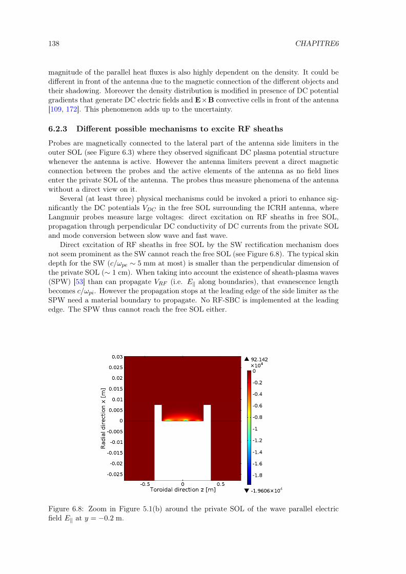
138 CHAPITRE6

magnitude of the parallel heat fluxes is also highly dependent on the density. It could bedifferent in front of the antenna due to the magnetic connection of the different objects andtheir shadowing. Moreover the density distribution is modified in presence of DC potentialgradients that generate DC electric fields and E×B convective cells in front of the antenna[109, 172]. This phenomenon adds up to the uncertainty.

6.2.3 Different possible mechanisms to excite RF sheaths

Probes are magnetically connected to the lateral part of the antenna side limiters in theouter SOL (see Figure 6.3) where they observed significant DC plasma potential structurewhenever the antenna is active. However the antenna limiters prevent a direct magneticconnection between the probes and the active elements of the antenna as no field linesenter the private SOL of the antenna. The probes thus measure phenomena of the antennawithout a direct view on it.

Several (at least three) physical mechanisms could be invoked a priori to enhance sig-nificantly the DC potentials VDC in the free SOL surrounding the ICRH antenna, whereLangmuir probes measure large voltages: direct excitation on RF sheaths in free SOL,propagation through perpendicular DC conductivity of DC currents from the private SOLand mode conversion between slow wave and fast wave.

Direct excitation of RF sheaths in free SOL by the SW rectification mechanism doesnot seem prominent as the SW cannot reach the free SOL (see Figure 6.8). The typical skindepth for the SW (c/ωpe ∼ 5 mm at most) is smaller than the perpendicular dimension ofthe private SOL (∼ 1 cm). When taking into account the existence of sheath-plasma waves(SPW) [53] than can propagate VRF (i.e. E‖ along boundaries), that evanescence lengthbecomes c/ωpi. However the propagation stops at the leading edge of the side limiter as theSPW need a material boundary to propagate. No RF-SBC is implemented at the leadingedge. The SPW thus cannot reach the free SOL either.

Figure 6.8: Zoom in Figure 5.1(b) around the private SOL of the wave parallel electricfield E‖ at y = −0.2 m.

6.2. SIMULATIONS WITH TOPICA/SSWICH-SW-2D FOR TORE SUPRA 139

Figure 6.9: |VRF | vs distance from the Faraday screen on the inner face on the side limiterin blue (see blue dashed line on Figure 6.10 and on the outer face of the limiter in red (seered dashed line).

Figure 6.10: Circulation of DC currents from the private SOL to the free SOL and plasmapotential around the right limiter (from the plasma) of the antenna at the vertical positiony = −0.2 m. The axes are in meter. The black arrows represent DC currents whereas thecolour scale denote the amplitude of VDC . The red dashed line corresponds to the outerface of the side limiter whereas the blue dashed line denotes the inner face.

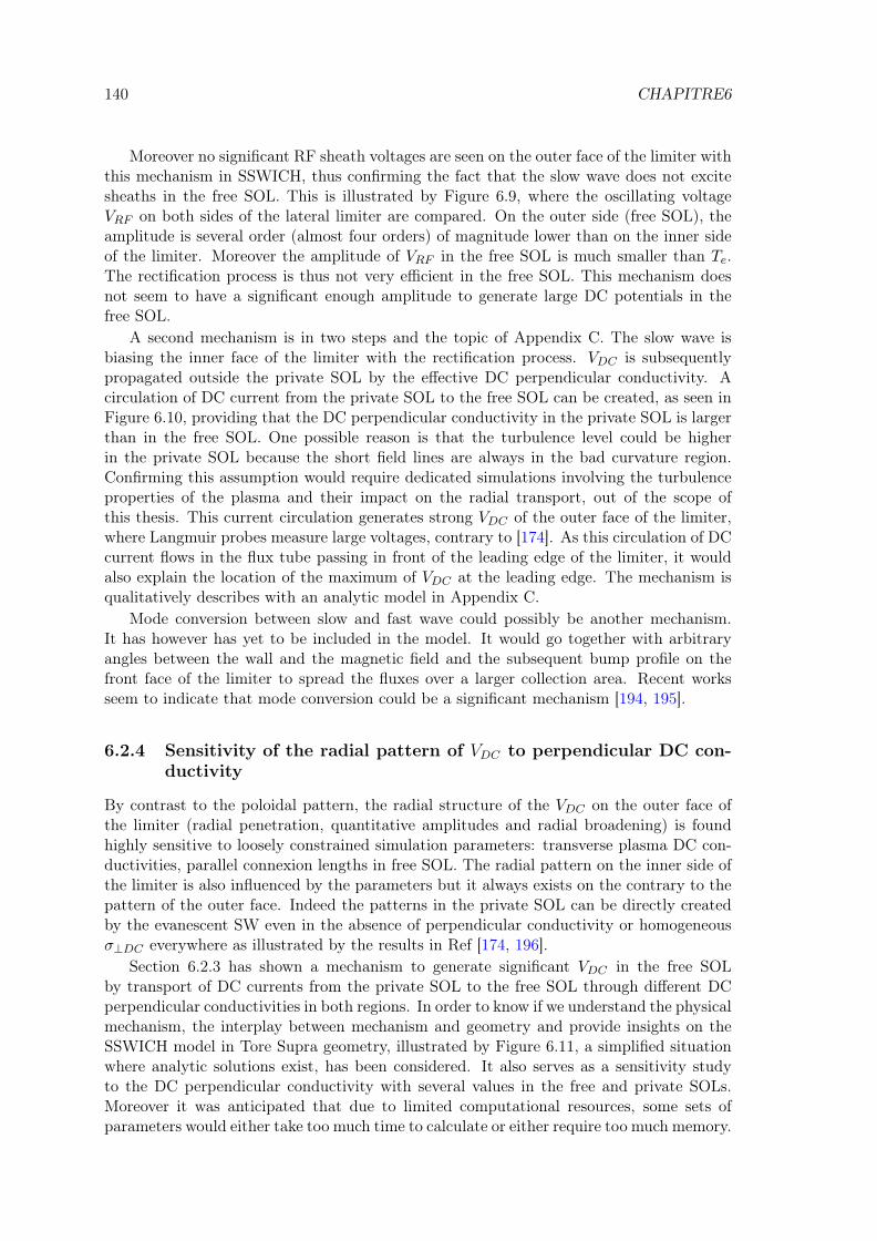
140 CHAPITRE6

Moreover no significant RF sheath voltages are seen on the outer face of the limiter withthis mechanism in SSWICH, thus confirming the fact that the slow wave does not excitesheaths in the free SOL. This is illustrated by Figure 6.9, where the oscillating voltageVRF on both sides of the lateral limiter are compared. On the outer side (free SOL), theamplitude is several order (almost four orders) of magnitude lower than on the inner sideof the limiter. Moreover the amplitude of VRF in the free SOL is much smaller than Te.The rectification process is thus not very efficient in the free SOL. This mechanism doesnot seem to have a significant enough amplitude to generate large DC potentials in thefree SOL.

A second mechanism is in two steps and the topic of Appendix C. The slow wave isbiasing the inner face of the limiter with the rectification process. VDC is subsequentlypropagated outside the private SOL by the effective DC perpendicular conductivity. Acirculation of DC current from the private SOL to the free SOL can be created, as seen inFigure 6.10, providing that the DC perpendicular conductivity in the private SOL is largerthan in the free SOL. One possible reason is that the turbulence level could be higherin the private SOL because the short field lines are always in the bad curvature region.Confirming this assumption would require dedicated simulations involving the turbulenceproperties of the plasma and their impact on the radial transport, out of the scope ofthis thesis. This current circulation generates strong VDC of the outer face of the limiter,where Langmuir probes measure large voltages, contrary to [174]. As this circulation of DCcurrent flows in the flux tube passing in front of the leading edge of the limiter, it wouldalso explain the location of the maximum of VDC at the leading edge. The mechanism isqualitatively describes with an analytic model in Appendix C.

Mode conversion between slow and fast wave could possibly be another mechanism.It has however has yet to be included in the model. It would go together with arbitraryangles between the wall and the magnetic field and the subsequent bump profile on thefront face of the limiter to spread the fluxes over a larger collection area. Recent worksseem to indicate that mode conversion could be a significant mechanism [194, 195].

6.2.4 Sensitivity of the radial pattern of VDC to perpendicular DC con-ductivity

By contrast to the poloidal pattern, the radial structure of the VDC on the outer face ofthe limiter (radial penetration, quantitative amplitudes and radial broadening) is foundhighly sensitive to loosely constrained simulation parameters: transverse plasma DC con-ductivities, parallel connexion lengths in free SOL. The radial pattern on the inner side ofthe limiter is also influenced by the parameters but it always exists on the contrary to thepattern of the outer face. Indeed the patterns in the private SOL can be directly createdby the evanescent SW even in the absence of perpendicular conductivity or homogeneousσ⊥DC everywhere as illustrated by the results in Ref [174, 196].

Section 6.2.3 has shown a mechanism to generate significant VDC in the free SOLby transport of DC currents from the private SOL to the free SOL through different DCperpendicular conductivities in both regions. In order to know if we understand the physicalmechanism, the interplay between mechanism and geometry and provide insights on theSSWICH model in Tore Supra geometry, illustrated by Figure 6.11, a simplified situationwhere analytic solutions exist, has been considered. It also serves as a sensitivity studyto the DC perpendicular conductivity with several values in the free and private SOLs.Moreover it was anticipated that due to limited computational resources, some sets ofparameters would either take too much time to calculate or either require too much memory.

6.2. SIMULATIONS WITH TOPICA/SSWICH-SW-2D FOR TORE SUPRA 141

Figure 6.11: Sketch of the 4 regions geometry and main notations in a 2D radial/toroidalplane. The levels of blue are indicative of the plasma density. The levels of red are indicativeof the intensity of the DC plasma potential. The black arrows indicate a circulation of DCcurrents from the private SOL to the free SOL.

As in Section 5.1, the magnetic field lines are either perpendicular or parallel to theboundaries. The domain is constituted of four regions: the private SOL of an ICRHantenna (region 0), the inner free SOL (region 1) and two outer free SOLs (region 2 and3) on both toroidal sides of the antenna limiters. x is the radial direction and z is theparallel direction. Region 0 radially extends from x = 0 to x = L⊥, whereas region 1 spansfrom x = −∞ to x = 0 and region 2 and 3 from x = 0 to x = +∞. The four regions areconnected in x = 0.

Each region denoted by the subscript k = 0, 1, 2, 3 is characterized by three essentialparameters assumed constant:

• the parallel connection length l‖,k of the open magnetic field lines,

• a scalar transverse DC conductivity for the DC current σ⊥DC,k,

• a density nk.

A transverse diffusion length in the region k for the DC plasma potential can thus bedefined:

λ2j,k =

l‖,kσ⊥DC,kkBTe

2ej+k

, (6.3)

where j+k is the ion saturation current in the region k defined by (2.42). The factor 1/2

accounts for the two sheaths at both extremities. The value of σ⊥DC,k is adjusted inorder to reproduce the characteristic transverse length for the DC current associated withthe physical mechanisms [112] (friction with neutrals, viscosity, inertia) briefly exposed inSection 2.3.4.

Sheath rectification of intense near RF fields is biasing the walls to a potential Vb asexplained in Section 2.3.2.2. The biasing voltage Vb is assumed to exist only in the privateSOL and to be homogeneous over the two sides of region 0. The wall biasing Vb is assumedto be transferred to the SOL DC plasma potential VDC via the circulation of DC currentsbetween the several regions. With this analytical model, a thin flux tube passing just infront of the antenna side limiter is transporting the DC current from the private SOL to

142 CHAPITRE6

the free SOL. The private SOL can thus be resumed for the free SOL as a punctual sourceof DC currents located at the leading edge of the side limiter.

Several characteristics can then be derived. The full derivation is performed in Ap-pendix C. This analytical model indicates that non-linear broadening with the amplitudeof VDC should occur. The half width at half maximum of the potential peak due to non-linear broadening reads simple expression within two asymptotic cases:

∆x1

λj,1=

ln 2 +VDC,le12Te

if VDC,le/Te < 4,√2(VDC,leTe− 1)−√

VDC,leTe− 2 if VDC,le/Te > 4.

(6.4)

where VDC,le is the amplitude of the DC plasma potential at the leading edge of the sidelimiters. λj,1 ln 2 is the width ∆x1 that would have been obtained with the linear modelwhereas the second term accounts for a non-linear broadening of the potential peak forfinite bias.

To test the expression of the non-linear broadening in (6.4), simulations with SSWICH-SW-2D were performed with the field maps shown in Figure 5.6(b). To limit the amountof necessary computation, only one parallel/radial plane at y = −0.2 m was simulated asillustrated by Figure 5.12. This vertical position was chosen since it is approximately theregion where the maximum of VDC are expected as shown on Figure 5.11(a).

In the simulations, region 2 and 3 in Figure 6.11 are equivalent since the geometry issymmetric and the density profile is the same. It gives λj,2 = λj,3. The amplitude of VDCat the leading edge is also evaluated. The half size at half maximum are evaluated on eachside of the peak of VDC . The full size at half maximum in the simulations ∆xsim is thusobtained by summing both half widths: ∆xsim = ∆x1 + ∆x2.

In the analytic model homogeneous densities are assumed in each region. This is notthe case in the simulations. Instead in the simulations, the density is averaged over halfthe peak of VDC with respect to the position of the leading edge. It therefore gives anaverage density higher on the plasma side of the leading edge than of the vacuum vesselwall side. The density in the private SOL is averaged.

The parallel connection length are l‖,0 = 0.55 m, l‖,1 = 3.3 m and l‖,2 = l‖,3 = 1.275 mwith the limiter 10 cm wide. The DC perpendicular conductivities are known since theyare imposed. With these parameters, the associated λj,k can then be calculated. Thepredicted full widths at half maximum ∆xanalytic are then obtained with (6.4) where theamplitude of VDC,le is the one obtained from the simulations.

Figure 6.12 is the result of the comparison of the radial broadening of VDC structureagainst the analytical predictions in (6.4).

It confirms that, within the linear regime of the sheaths, the full width at half maximum∆x of the VDC structure scales as a diffusion length λ1 + λ2. Moreover a non-lineardependence of the broadening of ∆x with VDC,le is found. The analytical formula is howeveralways below the simulation points within an almost constant 20% margin.

A possible explanation is a violation of the flute assumption in the vicinity of the leadingedge of the side limiter that is the interface along the same field line of very disparate regionssince an infinitely thin flux tube is assumed in the analytic model as the mean of transportof the DC currents from the private SOL to the free SOL. In reality the tube has a finitewidth that is likely set by the DC perpendicular conductivity in the private SOL. Thiswould broaden even more the VDC structure.

The radial broadening is also larger on the wall side than on the plasma side, as observedin probe measurements (see Figure 6.4) and in the simulations (see Figure 6.6(b)). Thisanalytic model can give an explanation to this phenomenon. One when looking at (6.3)

6.2. SIMULATIONS WITH TOPICA/SSWICH-SW-2D FOR TORE SUPRA 143

would suspect that the radial broadening is larger on the plasma side since the parallelconnection length is larger on the plasma side. But one would ignore the denominator. j+

k

is not the same in both region since a radial density gradient exist. The density is alsomuch larger on the plasma side. This ratio of parallel connection length over the density islarger on the wall side with respect to the leading edge of the side limiter. The transversescale length calculated with (6.3) is thus larger. This is opposite to the first intuition.

Figure 6.12: Comparison of the full width at half maximum ∆x of the VDC structure in thefree SOL obtained with the simulations with the analytical formula (6.4) for the CBSB FS.Different values of σ⊥DC,p and σ⊥DC,f were taken. Each point represents one simulation.The others parameters are: Ti = 20 eV, Te = 20 eV, L‖ = 3.3 m and Vstrap = 30 kV.

The analytic model not only provides insights on the radial size of the DC potentialstructure but also of the amplitude of these structures. Linking the amplitude at theleading edge with the parameters in the free and private SOL has been attempted. In alinearised regime, the DC plasma potential at the leading edge reads:

VDC,leVb

=

1 +λj,1 + λj,2 + λj,3

λj,0 tanh(L⊥λj,0

)−1

. (6.5)

The amplitude of VDC,le at the leading edge can be qualitatively understood by thefollowing. The amplitude is first set by the amount of DC currents that the private SOL candraw. This total current is determined by the effective private SOL that contributes to theDC currents that are leaving the private SOL that is itself linked to the perpendicular DCconductivity in the private SOL. Second the amplitude of VDC,le is also set by the amountof DC currents that can flow into the free SOL that is determined by the perpendicularDC conductivity in the free SOL and the surface over which the currents can be depositedthat depends on the parallel connection length in the free SOL. Third the intensity of thebias in the private SOL also has an impact on the amplitude of VDC,le. The more intensethe bias is, the more DC currents can be draw. Since the amount of current is limited inthe parallel direction, then it can only flow in the perpendicular direction. This brings arefinement into the model since the amount of DC currents that can be drawn from thesheaths in the private SOL is also limited as the sheath has to exist.

144 CHAPITRE6

(a)

(b)

Figure 6.13: (a) Comparison of the amplitude of VDC at the leading edge of the sidelimiters obtained with the simulations with the analytical formula (6.5) for the CBSB FS.(a) Comparison of the asymptotic amplitude of VDC,le at high σ⊥DC,p with the analyticformula (6.6). Different values of σ⊥DC,p and σ⊥DC,f were taken. Each point representsone simulation. The others parameters are: Ti = 20 eV, Te = 20 eV, L‖ = 3.3 m andVstrap = 30 kV.

6.2. SIMULATIONS WITH TOPICA/SSWICH-SW-2D FOR TORE SUPRA 145

A comparison of the simulations results for the DC plasma potential at the leadingedge of the side limiters with the analytic predictions of (6.5) has been performed. It isillustrated by Figure 6.13(a). The correct shape is qualitatively reproduced at least forthe upper part of the curves. VDC,le has an asymptotic value at large σ⊥DC,p. For thebottom part, it was seen a posteriori that the simulations grid was not fine enough toresolve accurately the transverse scale associated with the DC perpendicular conductivity.This is due to limited computational resources. It results in DC currents not being ableto go from a grid point to an adjacent grid point in the radial direction. It should also benoted that when normalized to their asymptotic value at high σ⊥DC,p, the curves coincide.They thus follow similar parametric dependences.

The predictions of the quantitative values of VDC,le are however loose, but within afactor 2. This can be explained by the simplicity of the analytic model that has beenlinearised. Moreover electron saturation, given by (5.11), is not yet accounted for. Whenelectron saturation occurs, the sheath ceases to exist. More intense bias cannot increasethe amount of currents any more. This condition is written within two extreme cases as:

VDC,le =

Y(1 + Y

6

)if Y ≤ 1.5,

Y 2

2 + 1 if Y > 1.5,(6.6)

whereY = − L⊥

λj,1 + λj,2 + λj,3

〈jsh〉j+0

(6.7)

The predictions of analytic formula (6.6) has been then compared to the asymptoticvalues at high σ⊥DC,p of VDC,le obtained in the simulations. This comparison is illustratedby Figure 6.13(b). The analytic model does not agree with the simulations. It can beconcluded that something is missing in the analytic model to understand the mechanismsetting the amplitude of VDC .

The parametric dependence of the amplitude and of the radial broadening of VDC areextremely sensitive to the DC perpendicular conductivity that largely remain unknownin the SOL of tokamaks. However this mechanism of formation of DC plasma potentialin the free SOL give some hints and constrains of the DC perpendicular conductivity,at least relatively between the private and the free SOLs. Indeed the DC perpendicularconductivity in the private SOL σ⊥DC,p has to be high enough to draw significant DCcurrents from the sheaths into the private SOL and allow them to leave the private SOL.This is illustrated on Figure 6.14(a) and (b) where small and large σ⊥DC,p are chosen.

With a small σ⊥DC,p, the DC currents are trapped in the private SOL. VDC amplitudeis consequently intense in the private SOL and low in the free SOL. On the contrary witha large σ⊥DC,p, DC currents can flow into the free SOL in addition to the private SOL andgenerate significant VDC in the free SOL. The amplitude of VDC is consequently lower inthe private SOL.

The relationship between the amplitude VDC in the private SOL and the amplitudeof VDC at the leading edge with the SOL plasma parameters remain unknown. Satisfyingsimultaneously the requirements on amplitude and size of VDC on the outer face of theside limiter where probes are connected structure cannot be accomplished with an homo-geneous σ⊥DC in the whole SOL as illustrated by Figure 6.14(a). The DC perpendicularconductivity in the free SOL σ⊥DC,f should however be relatively smaller compared toσ⊥DC,p as to limit the flow of DC currents radially. Indeed no significant VDC amplitudehas been measured in the plasma. To obtain a significant VDC amplitude in the free SOL,we thus have to postulate a higher transport level in the private SOL compared to the freeSOL.

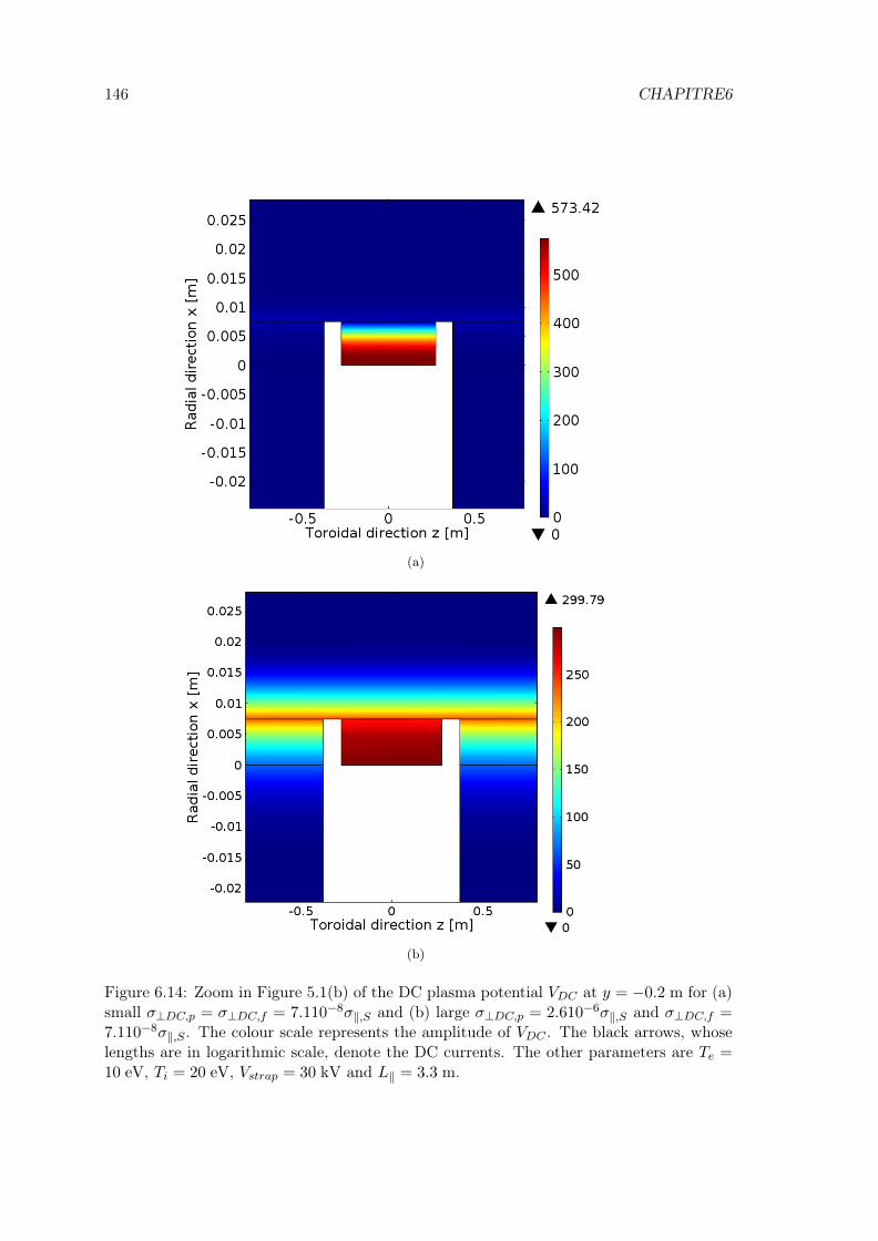
146 CHAPITRE6

(a)

(b)

Figure 6.14: Zoom in Figure 5.1(b) of the DC plasma potential VDC at y = −0.2 m for (a)small σ⊥DC,p = σ⊥DC,f = 7.110−8σ‖,S and (b) large σ⊥DC,p = 2.610−6σ‖,S and σ⊥DC,f =7.110−8σ‖,S . The colour scale represents the amplitude of VDC . The black arrows, whoselengths are in logarithmic scale, denote the DC currents. The other parameters are Te =10 eV, Ti = 20 eV, Vstrap = 30 kV and L‖ = 3.3 m.

6.2. SIMULATIONS WITH TOPICA/SSWICH-SW-2D FOR TORE SUPRA 147

6.2.5 Estimation of values of perpendicular DC conductivity consistentwith observations

It was shown that the radial pattern of the VDC structure is highly sensitive to loosely con-strained parameters such as the perpendicular DC conductivity. Our approach is thereforeto treat the inverse problem and to try to estimate a domain of perpendicular DC con-ductivity whose values are compatible with the measured experimental broadening. Inorder to accomplish this task, we need to consider the real connection length of a probemagnetically connected to the outer face of the side limiter: l‖,2 ≈ 10− 15 m. This thusrequire a domain whose total size in the parallel direction L‖ is of the order of 20− 30 m.

The model with a domain length of this magnitude cannot be solved due to our limitednumerical resources. Despite the fact that we do not have the numerical resources, ananalytical model of non-linear DC biasing in a four regions domain is available. The com-plete analytic derivation is presented in Appendix C. This analytic model was furthermorebenchmarked against SSWICH-SW-2D simulations in Section 6.2.4. Instead of simulationsin Comsol, we will reproduce the experimental broadening of the radial structure of VDCby analytic considerations.

Figure 6.15: σ⊥DC,p/σ‖,S versus σ⊥DC,f/σ‖,S . The perpendicular DC conductivity domaincompatible with experiments is represented by a green rectangle. The lines represent thedifferent limits.

When trying to determine a domain of compatible value of perpendicular DC conduc-tivities in the free and private SOLs, the first thing one can do is think about the minimumand maximum value that they can take. The minimum value is determined through theLarmor radius, as the minimum transverse scale cannot be smaller than the ion Larmorradius (1.6). For deuterium ion at the Bohm speed with B = 2.93 T and Ti = 20 eV, itgives ρs = 0.27 mm. The other parameters are Te = 10 eV, l‖,0 = 0.55 m, l‖,2 = 10 m andthe density at the leading edge nle = 1.7 1018 m−3. For the perpendicular DC conductivityit reads, reversing (6.3), in the free SOL σ⊥DC,f,m/σ‖,S = 1.6 10−10 and in the private SOLσ⊥DC,f,m/σ‖,S = 3 10−9. They are represented on Figure 6.15 by black dotted lines.

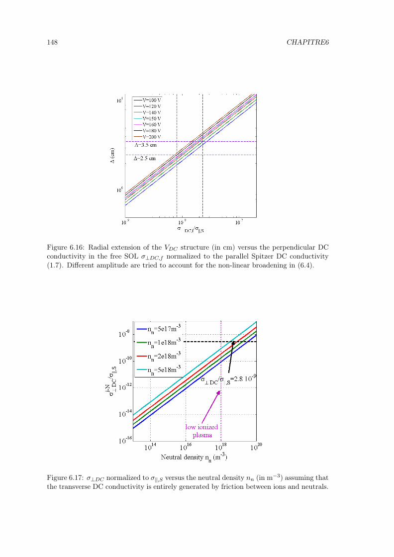
148 CHAPITRE6

Figure 6.16: Radial extension of the VDC structure (in cm) versus the perpendicular DCconductivity in the free SOL σ⊥DC,f normalized to the parallel Spitzer DC conductivity(1.7). Different amplitude are tried to account for the non-linear broadening in (6.4).

Figure 6.17: σ⊥DC normalized to σ‖,S versus the neutral density nn (in m−3) assuming thatthe transverse DC conductivity is entirely generated by friction between ions and neutrals.

6.2. SIMULATIONS WITH TOPICA/SSWICH-SW-2D FOR TORE SUPRA 149

The maximum transverse scale cannot be larger than the total radial SOL dimension(≈ 10 cm) as the main plasma is unperturbed. The same procedure gives the maximumallowed perpendicular DC conductivity σ⊥DC,p,M/σ‖,S = 5.2 10−4 in the private SOL andσ⊥DC,f,M/σ‖,S = 2.9 10−5 in the free SOL. They are represented on Figure 6.15 by blackdashed and dotted lines. This gives a first large domain.

Let us see if we can reduce the surface of the domain with the analytic model in Sec-tion 6.2.4. The application of (6.4) is shown on Figure 6.16 for different VDC,le amplitude.To obtain the observed extension (3± 0.5 cm) with the measured maximum amplitude(150± 30 V) and l‖2 ∼ 10 m, (6.4) indicates that σ⊥DC,f/σ‖,S = [0.8 − 2.1]10−8 is re-quired. They are represented by green full lines on Figure 6.15.

The link between amplitude of the VDC at the leading edge and conductivity has notbeen yet fully understood as well as its dependence with the parallel connexion length.Nevertheless a private perpendicular DC conductivity higher than in the free SOL is re-quired. Then we know that σ⊥DC,p/σ‖,S ≥ 0.82 10−8, shown with a red dashed line onFigure 6.15, is required to create a significant DC currents circulation from the privateSOL to the free SOL. This current circulation is saturating when DC currents are drawnfrom the entire radial extension of the private SOL (≈ 1 cm). It is represented by the bluedashed line on Figure 6.15. The average density in the private SOL is 〈np〉 = 7.6 1017 m−3.It gives σ⊥DC,p,sat/σ‖,S ≈ 2.6 10−6).

These values of perpendicular DC conductivities cannot be explained invoking frictionion-neutrals alone ever when taking a low ionized plasma and a high neutral density (i.e.neutral density nn = 1018 m−3). There is still at least one order of magnitude missing.Beyond collisions, they are also hard to explain with classical or neo-classical mechanisms.The most likely origin comes from anomalous transport [113].

6.2.6 Effect of unbalanced strap voltage on the distribution left/right ofthe heat fluxes on inner face of the lateral limiters

An original experiment was shown in Section 6.1.2 to balance the strap voltages since theright strap was positioned radially 4 mm behind the left strap. When changing the powerbalance on the generators to equalize the strap voltage, it was observed that the relativevariation of the surface temperature TIR of the antenna was evolving in opposite directionbetween the left side and the right side of the antenna. Both extremities of the same shortfield lines did not have the variation relative evolution when changing the power balance ofthe generators. This could not be explained by the variation of one integrated parametersuch as

∫E‖dl or any others. We then supposed that at least two independent parameters

must be involved.Let us now check, with the TOPICA/SSWICH-SW-2D procedure, if we can do better

and reproduce then explain what is happening. Unfortunately we cannot at the momentreproduce the misalignment of both straps since the 4 mm mismatch is of the order of oneelement in TOPICA simulations (5 mm). TOPICA would thus see the straps as alignedwith this kind of grids. We can however change the strap voltage balance. Instead of havingVstrap on both straps, we thus have Vstrap ± 15% or Vstrap ∓ 15%. It is thus equivalent athaving a power balance on the straps 57%/43% and 43%/57% respectively. This test wasonly performed for one vertical position (y = −0.2 m), such as the situation illustrated onFigure 5.12. The E‖ was computed in TOPICA with the CBSB FS geometry as it was onthe antenna equipped with this FS that this was observed.

The simulation parameters were Te = 10 eV, Ti = 20 eV, Vstrap = 30 kV and l‖,1 =3.3 m, σ⊥DC,f/σ‖,S = 2.5 10−8, σ⊥DC,f/σ‖,S = 2.5 10−6, l‖,2 ≈ 1.3 m.

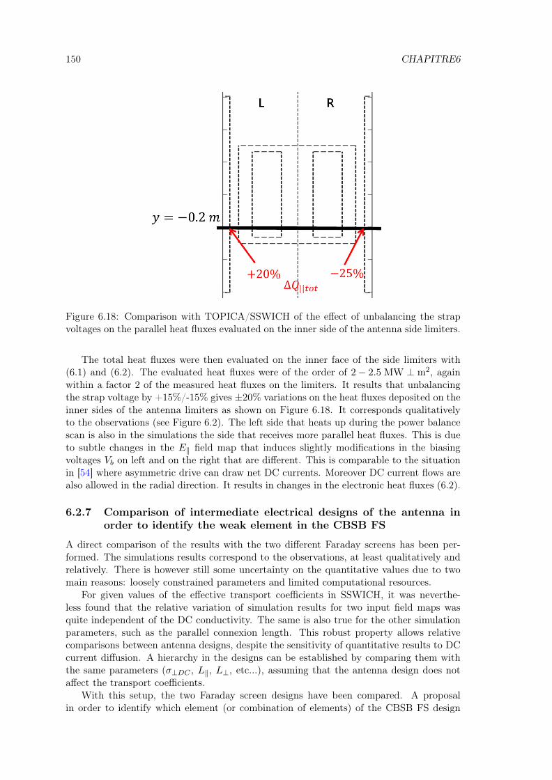
150 CHAPITRE6

Figure 6.18: Comparison with TOPICA/SSWICH of the effect of unbalancing the strapvoltages on the parallel heat fluxes evaluated on the inner side of the antenna side limiters.

The total heat fluxes were then evaluated on the inner face of the side limiters with(6.1) and (6.2). The evaluated heat fluxes were of the order of 2− 2.5 MW ⊥ m2, againwithin a factor 2 of the measured heat fluxes on the limiters. It results that unbalancingthe strap voltage by +15%/-15% gives ±20% variations on the heat fluxes deposited on theinner sides of the antenna limiters as shown on Figure 6.18. It corresponds qualitativelyto the observations (see Figure 6.2). The left side that heats up during the power balancescan is also in the simulations the side that receives more parallel heat fluxes. This is dueto subtle changes in the E‖ field map that induces slightly modifications in the biasingvoltages Vb on left and on the right that are different. This is comparable to the situationin [54] where asymmetric drive can draw net DC currents. Moreover DC current flows arealso allowed in the radial direction. It results in changes in the electronic heat fluxes (6.2).

6.2.7 Comparison of intermediate electrical designs of the antenna inorder to identify the weak element in the CBSB FS

A direct comparison of the results with the two different Faraday screens has been per-formed. The simulations results correspond to the observations, at least qualitatively andrelatively. There is however still some uncertainty on the quantitative values due to twomain reasons: loosely constrained parameters and limited computational resources.

For given values of the effective transport coefficients in SSWICH, it was neverthe-less found that the relative variation of simulation results for two input field maps wasquite independent of the DC conductivity. The same is also true for the other simulationparameters, such as the parallel connexion length. This robust property allows relativecomparisons between antenna designs, despite the sensitivity of quantitative results to DCcurrent diffusion. A hierarchy in the designs can be established by comparing them withthe same parameters (σ⊥DC , L‖, L⊥, etc...), assuming that the antenna design does notaffect the transport coefficients.

With this setup, the two Faraday screen designs have been compared. A proposalin order to identify which element (or combination of elements) of the CBSB FS design

6.2. SIMULATIONS WITH TOPICA/SSWICH-SW-2D FOR TORE SUPRA 151

enhances the sheaths was to create hybrid electrical designs in between classical and CBSBFSs. In order to do this, we have identified the major electrical differences in the FS designbetween the classical screen and the CBSB screen. Of course, two main differences arealready contained in the acronym. The differences in the electric design are:

1. the cantilevered bars that are not connected to the central septum,

2. the slotted frame with the, so-called, shark teeth,

3. the tilt of the bars not present on the CBSB screen, clearly visible when comparingFigure 2.14(a) with Figure 2.14(b),

4. the gap between FS bars related to the number of bars and their individual size.

(a) (b)

Figure 6.19: 3D model of the hybrid geometry in between the classical FS and the CBSBFS implemented in TOPICA to identify the faulty element the difference. (a) classicalscreen with cantilevered FS bars and (b) classical screen with half the bars with constantgap between bars.

The first step consisted in creating a 3D model of the hybrid design starting from theclassical screen as a reference where one element is modified at a time. It resulted in twohybrid geometries illustrated in Figures 6.19(a) and (b). The impact of the shark teethwas considered to be only local and for this reason was not studied. For the tilt of the bars,removing the tilt of the bars in the classical screen geometry would have been a long andpainful process to ensure all proper electrical connections to the septum as not only thetilt has to be changed but also the bars parameters and positioning. Adding an electricalconnection to the septum for the bars on the CBSB screen would have similarly encounterthe same difficulties. Instead we kept identical the 3D models of the classical and theCBSB screens and we changed the tilt of the magnetic field in the TOPICA simulations.Instead of 7 tilt, -7, 0 were enforced for the CBSB screen whereas it was 0 and 14 forthe classical screen.

Simulations results show that reducing the number of bars (i.e. increasing the gapbetween bars) is marginal on the impact of RF sheaths on the DC plasma potential withthe present version of SSWICH (see Figure 6.20(b)). The conclusion is identical for thetilt of the bars (see Figure 6.21(a)-(d)). It should be noted that high tilt (14) increases

152 CHAPITRE6

(a) (b)

Figure 6.20: 2D Map of the DC plasma potential VDC obtained with SSWICH in thepoloidal/radial plane at the position shown by dark dashed line in Figure 5.1(b) for hybridelectrical designs: (a) classical screen with cantilevered bars and (b) classical screen withhalf the bars number.

slightly the amplitude of VDC for the classical screen (see Figure 6.21(b)). Some preliminaryresults with the asymptotic model only has however indicated a sensitivity to the densitywhen looking at the impact of the tilt of the bars, especially at low density. Up to 20%difference has been evaluated. This would have to be confirmed and studied deeper withself-consistent version of SSWICH. The alignment of the bars with the magnetic field canonly be perfectly realized for one plasma current value. Nevertheless, as it has been shownon Alcator C-Mod, the impurity content seems to be not directly correlated to the DCplasma potential [109, 190]. Moreover, it remains to be determined if the potential gainfrom the electrical point of view justifies the added mechanical complexity of the design.

Simulations however suggest (see Figure 6.20(a)) that creating numerically an hybridconfiguration by cutting the bars on the classical screen enhanced greatly the RF sheathsin the vicinity of the antenna when the side limiters are also taken into account. Thisconfiguration gives results that are the closest to the CBSB Faraday screen for both thespatial topology and the amplitude of VDC .

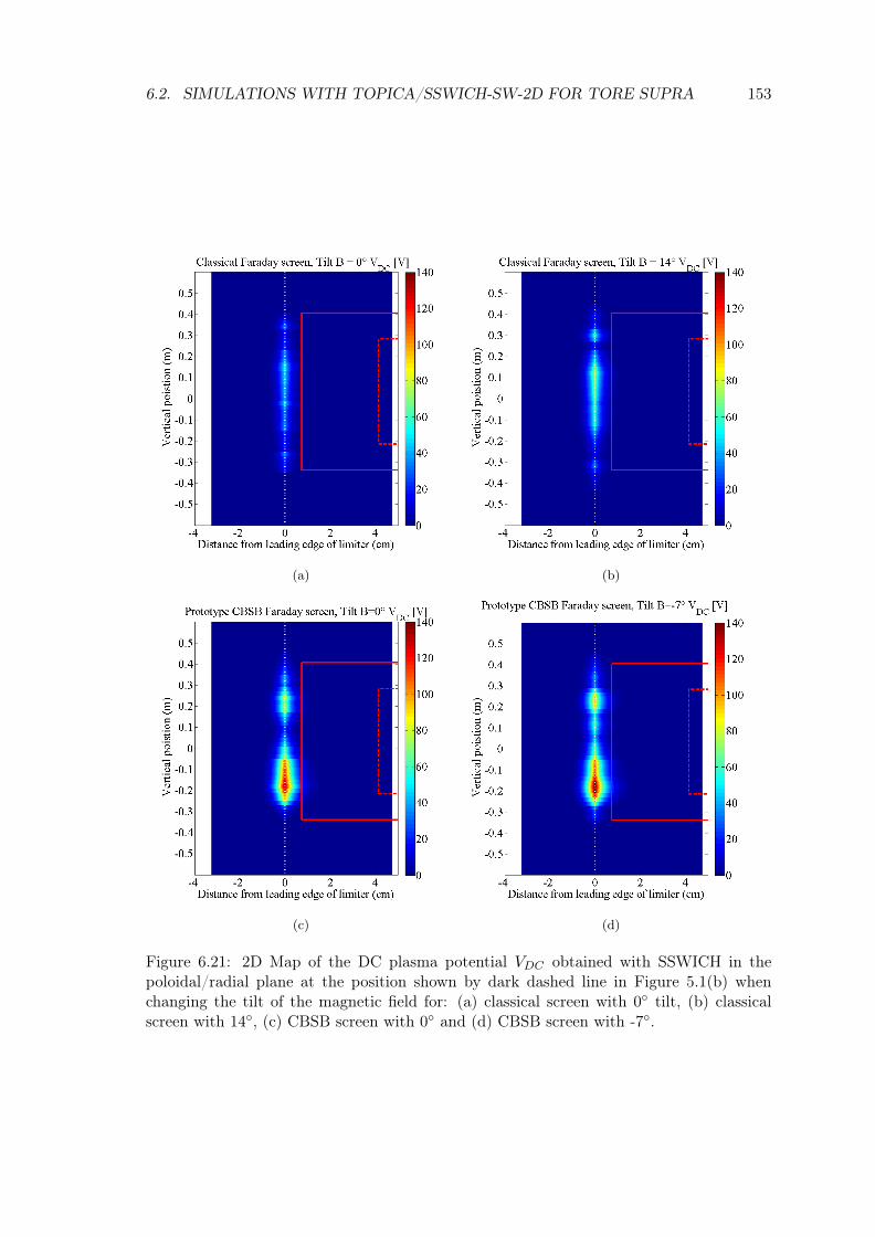
6.2. SIMULATIONS WITH TOPICA/SSWICH-SW-2D FOR TORE SUPRA 153

(a) (b)

(c) (d)

Figure 6.21: 2D Map of the DC plasma potential VDC obtained with SSWICH in thepoloidal/radial plane at the position shown by dark dashed line in Figure 5.1(b) whenchanging the tilt of the magnetic field for: (a) classical screen with 0 tilt, (b) classicalscreen with 14, (c) CBSB screen with 0 and (d) CBSB screen with -7.

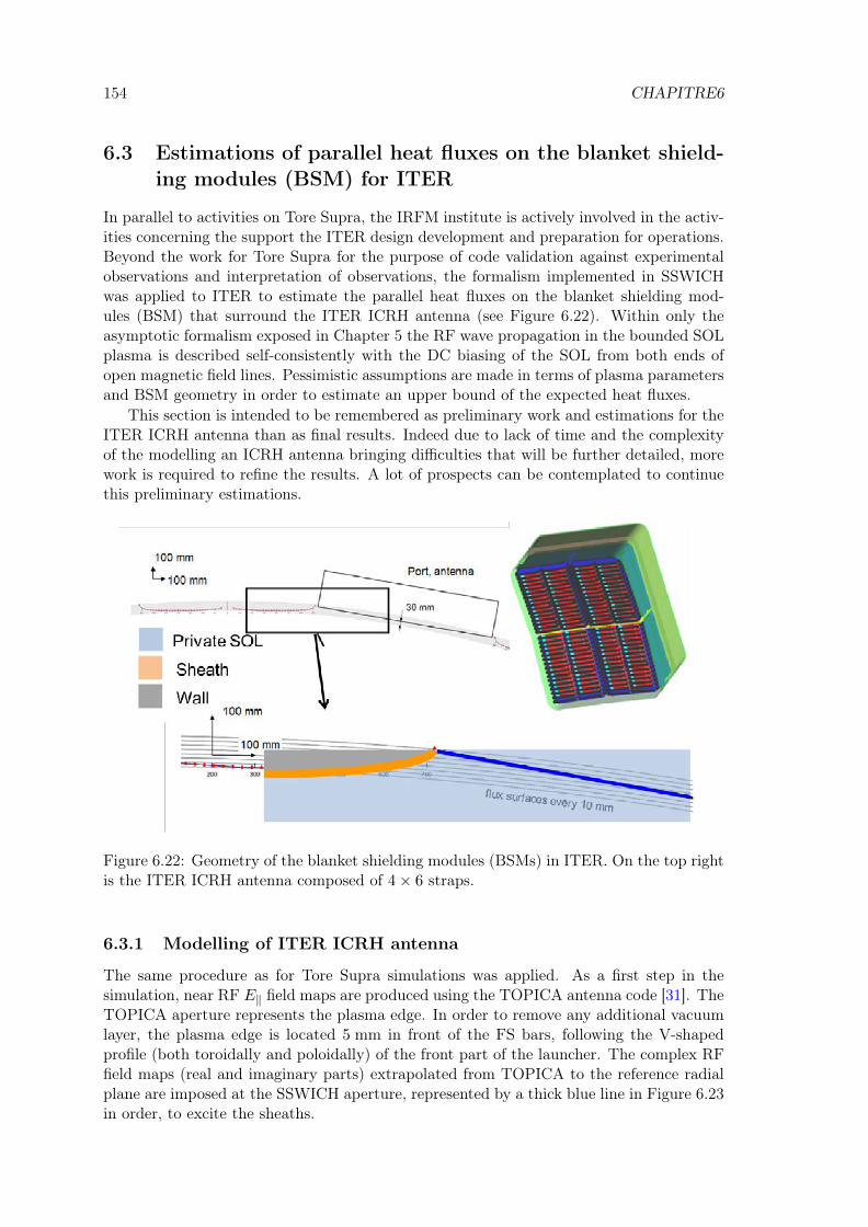
154 CHAPITRE6

6.3 Estimations of parallel heat fluxes on the blanket shield-ing modules (BSM) for ITER

In parallel to activities on Tore Supra, the IRFM institute is actively involved in the activ-ities concerning the support the ITER design development and preparation for operations.Beyond the work for Tore Supra for the purpose of code validation against experimentalobservations and interpretation of observations, the formalism implemented in SSWICHwas applied to ITER to estimate the parallel heat fluxes on the blanket shielding mod-ules (BSM) that surround the ITER ICRH antenna (see Figure 6.22). Within only theasymptotic formalism exposed in Chapter 5 the RF wave propagation in the bounded SOLplasma is described self-consistently with the DC biasing of the SOL from both ends ofopen magnetic field lines. Pessimistic assumptions are made in terms of plasma parametersand BSM geometry in order to estimate an upper bound of the expected heat fluxes.

This section is intended to be remembered as preliminary work and estimations for theITER ICRH antenna than as final results. Indeed due to lack of time and the complexityof the modelling an ICRH antenna bringing difficulties that will be further detailed, morework is required to refine the results. A lot of prospects can be contemplated to continuethis preliminary estimations.

Figure 6.22: Geometry of the blanket shielding modules (BSMs) in ITER. On the top rightis the ITER ICRH antenna composed of 4× 6 straps.

6.3.1 Modelling of ITER ICRH antenna

The same procedure as for Tore Supra simulations was applied. As a first step in thesimulation, near RF E‖ field maps are produced using the TOPICA antenna code [31]. TheTOPICA aperture represents the plasma edge. In order to remove any additional vacuumlayer, the plasma edge is located 5 mm in front of the FS bars, following the V-shapedprofile (both toroidally and poloidally) of the front part of the launcher. The complex RFfield maps (real and imaginary parts) extrapolated from TOPICA to the reference radialplane are imposed at the SSWICH aperture, represented by a thick blue line in Figure 6.23in order, to excite the sheaths.

6.3 ESTIMATIONS OF PARALLEL HEAT FLUXES FOR ITER 155

The complex RF field maps are evaluated at the mid-band RF frequency f0 = 47.5 MHz.They were normalized for 20 MW RF power coupled to plasma in matched conditions. TheITER antenna features a 6 × 4 phased strap array as seen on Figure 6.22. Five toroidalstrap phasings were studied: [0, π, 0, π], [0, 0, π, π], [0, π, π, 0], CD+ and CD−. The strapsare grouped by triplets in the poloidal direction and the poloidal phasing between tripletsis fixed at ˘π/2.

To be consistent, the plasma profile, the position of the plasma edge in front of thelauncher and imposed coupled power to the plasma (20 MW) have been kept constant forboth designs and for all five simulated phasings.

6.3.2 Simplified geometry of the BSM in SSWICH

The ITER ICRH antenna is surrounded by blanket shielding modules creating a privateSOL around the ICRH launcher in the same way as the antenna limiters on Tore Supra(see Figure 6.22). The curvature of the BSM makes a realistic modelling of the geometryout of our reach at the present time since field line must be either parallel or perpendicularthe walls. The main consequence is that the formalism cannot handle curved field linesconnecting the Faraday screen bars to the BSM. Instead, the sheath-related parallel heatfluxes are estimates on the two BSMs, assimilated to flat plates normal to B. The geometryof the ITER antenna was flattened in both toroidal and poloidal directions. Parallel heatloads of similar magnitude are expected in front of FS bars. For our estimates the simulationdomain is restricted to a parallelepipedic zone representing the private SOL shadowedby the two BSMs surrounding the ITER antenna (see Figure 6.23). This zone is notparallelepipedic in a realistic geometry as shown in Figure 6.22.

Since the asymptotic treatment alone is adopted here and the simulation domain onlyconsists in the private SOL between the BSM, the 3D parallelepipedic geometry is similarto the one shown in Figure 5.7 with different dimensions. The radial recess of the antennabehind the BSM modules, averaged over the antenna surface (i.e. 1 cm) is the radial depthl⊥ of the private SOL. The sensitivity of the results to l⊥ was studied in Ref [173]. Inpractice the TOPICA aperture extends over lTOP = 1.72 m. Here l‖ = 1.75 m. Thesimulation results were moreover shown to be very sensitive to the gap between the lateralsides of the TOPICA aperture and the location of the walls [173]. The parallel connection

Figure 6.23: Simplified geometry of the BSMs for the sheath assessment with SSWICH.The aspect ratio was not preserved.

156 CHAPITRE6

length l‖ in the private SOL was thus chosen as small as possible, in order to minimize thetoroidal gap to the lateral walls, thus providing “pessimistic estimates” for the RF-relatedheat loads.

6.3.3 Estimation of parallel heat fluxes

With the simplified geometry of the BSMs shown in Figure 6.23, a first run of simulationswere performed within the asymptotic model framework. All five phasing were considered.

The local plasma in the private SOL is treated as homogeneous with n = 21018 m−3,Te = 10 eV, Ti = 20 eV, B = 3.93 T and ε‖ = −72182 and ε⊥ = −23.25. For theseparameters the slow wave is evanescent whatever the duplet

(k‖, ky

). The DC plasma

potential was evaluated with (5.20) and the parallel heat fluxes with (6.1) and (6.2)For the “reference” sheath estimates, the field map were extrapolated in a reference

radial plane located midway between the TOPICA aperture and the FS. The simulationresults are summarized in Table 6.1 for the maximum of the oscillating sheath voltage onboth sides, the DC plasma potential and the parallel heat fluxes on both sides.

The first thing that can be said is that we retrieve a similar hierarchy in toroidal phasingas for JET antennas [177]. The heat fluxes expected on both sides are similar. They arein the range 2− 4 MW/m2. It should be nevertheless reminded that these results wereobtained at the TOPICA aperture and extrapolated on the FS plane. Thus the impactof the SW evanescence is uncertain. Sensitivity study of the extrapolation length hasshown high sensitivity on the results. For example an extra extrapolation of 5 mm (i.e.approximately at the FS location) has resulted in an increase of up to 50 % of Q‖,max[196]. Furthermore the simulations here were performed without any DC conductivity.Thus non-local effects are not included.

Phasing [0, π, 0, π] [0, 0, π, π] [0, π, π, 0] CD+ CD−

|VRF,l,max| (V) 319 560 413 265 692|VRF,r,max| (V) 191 668 331 316 641VDC,max (V) 313 658 406 311 683Q‖,l,max

(MW/m2

)2.2 3.9 2.7 2.0 4.3

Q‖,r,max(MW/m2

)2.0 4.1 2.5 2.2 4.1

Table 6.1: Summary of the sheaths properties with five toroidal strap phasings.

6.3.4 Difficulties for modelling the antenna and estimating heat fluxeson the BSM

These estimations are only preliminary as many difficulties appear when one to model andestimate the heat fluxes on the BSM. The first difficulty is related to the geometry thatis quite complex. It was here greatly simplified assuming the worst case scenario whenthe fluxes are incident to the material surfaces and not spread over a larger surface withoblique incidence.

A second difficulty is due to the size of the huge antenna that makes it costly tosimulate entirely. The mesh resolution is thus limited. On the E‖ field maps produced byTOPICA, the near field structure looks dominated by small scale features hardly relatedto a particular element of antenna design. The variations with antenna phasing are alsodifficult to explain. This situation is specific of the “high-density target plasma” and is incontrast with the typical maps obtained at low density. In these circumstances, specific E‖

6.4. SUMMARY AND PROSPECTS 157

field patterns can be clearly associated with the strap phasing, the different antenna boxesas well as the end of FS bars.

Moreover with our current resources, attempting to simulate the entire ITER antennawith the multi-2D procedure in SSWICH-SW-2D was not done due to the excessive timeit would take. The RAM memory consumption would also be an issue as high meshresolution is needed in the radial direction and the scaling between directions cannot bechosen arbitrary high. The mesh should also be able to resolve the effective transport scaleof the DC currents. Finally the CPU time has to be shared with other tasks and othersusers. Despite these limitations, a few simulations have been performed in Comsol withfinite DC conductivities at one vertical position for a phasing CD−. With a homogeneousperpendicular DC conductivity, the heat loads remain in the range 3− 4 MW ⊥ m2 despitea variation over several orders of magnitude. The ion heat fluxes however were found tobe decreasing with increasing perpendicular DC conductivity which might be beneficial toreduce sputtering.

Another difficulty is the number of possible toroidal phasings that render difficult adetail study on the parametric dependence which take lots of time. On top of this thedesign of the antenna is constantly changing, as it is still of course in the design phase.This renders difficult a follow up in the study as well as ascribing a result to a modificationin the design or to the numerous parameters.

The results are, as for Tore Supra simulations, highly sensitive to loosely constrainedparameters. The estimations on the heat fluxes are also highly sensitive to the densityprofile that is itself a prediction. As for Tore Supra, the field maps are not produced onthe Faraday screen plane but a few millimeters in front of it. The field maps are thusextrapolated on the Faraday screen plane with an evanescence factor of the SW. Onlydetailed parametric scans can thus provide an accurate description of the situation toestimate the heat fluxes. The number of possible combinations is thus enormous.

All these difficulties related to uncertainties led us to take lots of cautions by assum-ing the worst case scenario. This could lead to overestimating the actual heat fluxes onthe BSMs and consequently overestimating the necessary heat exhaust capability of theantenna cooling system.

6.4 Summary and Prospects

This chapter has first reviewed the major experiments results on Tore Supra during the teston plasmas of a prototype Faraday screen that was supposed to minimize the magnitude ofRF sheaths. In reality, it was found unfortunately found that this Faraday screen enhancedRF sheaths.

SSWICH combined with TOPICA in the multi-2D procedure has been applied to ToreSupra to see if these unexpected observations could be unravelled by more advanced RFsheaths modelling. Key experimental observations have been reproduced with a novelmodelling of RF sheaths in SSWICH. Enhanced magnitude of RF sheaths is found withthe CBSB Faraday screen compared to the classical screen with SSWICH. The poloidaltopology is a robust and invariant result that mainly depends on the electrical design butnot on the numerous parameters. The radial topology is however greatly dependent on thesimulations parameters whose some of them are loosely constrained. The radial topologyon the outer face of the side limiter is also dependent on a mechanism to generate significantVDC . One possible mechanism, proposed here, is a circulation of DC currents from theprivate SOL to the free SOL through an effective perpendicular DC conductivity higher inthe private SOL than is the free SOL. For this feature to be valid, a higher turbulence level

158 CHAPITRE6

in the private SOL needs to be postulated. A qualitative disagreement between experimentsand simulations is on the radial position of the radial structure of VDC that is found on theleading edge in the simulations but 2 cm behind in the experiments for the CBSB Faradayscreen only. An explanation has been yet found.

Qualitative results have been correctly reproduced. Quantitative results however arehighly dependent on the simulations parameters. Results for the parallel heat fluxes andDC plasma potential are nevertheless found in the correct range. Using the observationsand a benchmarked analytical model of the transport of DC currents, a window of DCperpendicular conductivities compatible with the observations has been found. SSWICHcombined with TOPICA has also found that strap unbalance can lead to changes in electronheat fluxes on the inner face of the side limiter.

These simulations results affirm that the lateral limiters should be accounted for inthe RF sheaths assessment. The topology of the magnetic field lines are different with alimiter. Short field lines have to be distinguished from long field lines. It also implies thatthe more important RF sheaths consequences occur on short field lines connected to thelateral limiters, on the contrary to the assessment performed during the design phase ofthe CBSB FS [48] that only focused on long field lines. An investigation of the electricaldesign of the CBSB Faraday screen suggests that the cantilevered bars are the elements inthe design enhancing the magnitude of RF sheaths and its spurious effects.

Preliminary results for ITER with the asymptotic model only have been performed ina worst case scenario basis assuming an overly simplified geometry of the blanket shieldingmodules normal to the field lines. Several antenna phasing were tested. Maximum heatfluxes of 5 MW ⊥ m2 are expected. More work is however required to study the impactof loosely constrained parameters on the predictions. This study will continue in parallelwith the evolution of SSWICH to refine the estimations with more accurate ones. ToreSupra results could also be refined with newer version of SSWICH or with more realis-tic/constrained simulation parameters.

Conclusion

Heating the tokamak central plasma to fusion relevant conditions requires external heatingsystems such as RF systems. ICRH antennas, injecting into the plasma several MW ofpower, are commonly used in large tokamaks. To design an ICRH antenna able to coupleefficiently and reliably large amount of RF power into a magnetized plasma for long pulses(or in steady state) in a metallic environment, it is necessary to understand the interactionsbetween wave and the edge plasma: wave coupling and RF sheaths formation.

This PhD thesis aimed at proposing a common framework in which a sophisticateddescription of RF sheath formation in the vicinity of ICRH antenna in SOL of tokamakplasmas could be modelled self-consistently with wave coupling. Indeed, previous modellingand antenna design relied on the minimization of

∫ ∣∣E‖ · dl∣∣ from antenna codes withoutsheaths. This approach had some successes since the antennas do work and could explainsome phenomena. But RF sheaths description was not self-consistent as they were onlytreated a posteriori of the calculation of the wave radiation pattern by the antenna with acrude rectification model. The design of the prototype Faraday screen [140] for Tore Suprawith this approach on long field lines led to cutting the bars thinking that interruptingthe path of parallel currents would reduce RF sheaths oscillations. Experiments prove thecontrary as the magnitude of measured sheaths effects (heat loads, probe floating poten-tials) were significantly enhanced compared to the classical Faraday screen. Moreover thedesign of a field aligned antenna for Alcator C-Mod considering symmetry did not reducethe amplitude of the plasma potentials measured by emissive probes but still somehowlowered the impurity content (less sputtering). RF sheaths also have a feedback impact onthe coupling properties on the antenna since the density can be locally modified changingthe size of the evanescence layer in front of the antenna. The strap voltage for a constantcoupled power thus also changes, in turn changing the amplitude of the RF sheaths. Thisproblem should thus be treated ideally simultaneously and fully consistently. Due to thecomplexity of the problem, the limited resources and manpower and the three year lim-itations of this thesis, these two phenomena were however, modelled, for this first step,separately but in compatible approaches to anticipate the development of a single codecombining both. Two codes were thus successfully developed during this thesis: one forfast wave coupling without sheaths and one for self-consistent RF sheaths formation andslow wave propagation.

The choice of modelling with the commercial software Comsol Multiphysics was madebefore the start of this thesis to ease the development strains. The multiphysics purposeand the finite element feature of Comsol make it easy to be used by numerous people andto model multiphysics problems such as these ones in complex geometries. It also gives thefreedom of modifying the equations. Moreover the three years constrain on the durationof this thesis in addition with the requirement to provide physical relevant results did notgive the freedom of writing a code. The counterpart is the impossibility to access the innerworking of the equation solver and the limitation to run it on only one workstation as part

159

160 CONCLUSION

of the licence agreements.The first code is modelling fast wave coupling to the plasma. It contains a full de-

scription of a cold plasma with anisotropic, gyrotropic and inhomogeneity properties inthe dielectric tensor. Tore Supra ICRH antennas simplified geometries were implementedat the same time in 2D and in 3D. Realistic density and magnetic field radial profiles wereincluded for the simulations. The fast wave being propagative above some critical density,the perfectly matched layer technique in frequency domain, commonly used for classical di-electrics, was implemented for magnetized plasmas to mimic single pass-absorption withoutnumerical reflections of outgoing propagative waves. The PML concept relies on the trans-formation of the real space coordinates to complex stretched coordinates in the directionof absorption.

The PML was first tested on homogeneous plasmas with monochromatic plane waves.It was seen that low reflection could be achieved provided that the PML satisfies someconstraints. First the PML is only perfectly reflectionless for the exact wave equation.Discretization inevitably induces some reflection. This phenomenon can be reduced by afiner mesh closer to the exact wave equation. Second no singularity should be present inthe PML. Third the PML should not be placed next to a cutoff since it would significantlyincrease the numerical cost. For plane waves, a numerical formula tested against simula-tions indicates that the PML depth must be of the order value of the wavelength in thePML direction to have low reflection. Near a cutoff, the wavelength is huge, requiringa large PML. Fourth the current PML formulation cannot handle forward and backwardwaves simultaneously. This issue arises in some anisotropic media where several eigen-modes exist, whose group velocity vector is not collinear to the phase velocity. This issuecan be resolved in our situation by letting the plasma reflect the evanescent SW abovesome critical density and thus placing the PML interface where the SW is extinguishedand only the FW subsists. Fifth the PML should only be used with convex domains sinceonce a wave enters the PML it should not be allowed to leave the PML or cross again thestudied medium.

After checking that the reflection coefficient only defined for plane waves could be re-placed by tracking the modulations of the coupling resistance, easier to obtain for spectrumof plane waves, the PML technique was implemented into a code to evaluate the couplingresistance of phased strap arrays. Simulations with Tore Supra antennas were comparedto experimental measurements of the coupling resistance and to the TOPICA antennacode. The qualitative trends are correctly reproduced, but the magnitude is always overes-timated by a factor 1.5-2 by both codes due probably to uncertainties on the actual size ofthe evanescence layer. The necessary degree of sophistication of the antenna geometry wasalso investigated: the strap thickness, the presence of passive antenna elements in additionto active elements.

TOPICA provides results closer to the experiments than this new wave coupling code,since the antenna geometry in TOPICA is much more detailed at the expense of thenumerical cost. This FW coupling code however can provide a fair result within a minutein 2D. Very fine and numerous parameters scans can thus be considered before usingTOPICA for accurate results on a few cases during the design phase of an antenna. Thisprocedure is currently being used for the design of new ICRH antennas for WEST.

Improvements of the PML formulation should be considered to resolve the issue withsimultaneous propagating forward and backwards waves. Handling the concave plasmacurvature could very likely to be the harder issue to handle in order to simulate real-istic plasmas. A more appropriate coordinate system than Cartesian coordinate can becontemplated.

CONCLUSION 161

This approach with PMLs and full plasma description is in principle compatible withthe presence of a finite density inside the antenna box. Including RF sheath modelling intothis code can therefore be contemplated for the future. There is however the ongoing issueon the way to cross the lower hybrid resonance.

The second part of the thesis objectives, carried on in parallel, consisted in developingan innovative model of the interplay, due to RF sheaths, of RF wave propagation andthe resulting positive DC biasing of the edge plasma in the vicinity of an ICRH antenna.The model, called SSWICH, rests on previous works realized by Myra and D’Ippolito forsheath boundary condition and Lieberman for the description of the sheath capacitance.This model considers that some RF wave propagation effects occur on the rapid time-scaleand the DC biasing of the plasma on the slow time-scale. The two time-scales are coupledtogether by the RF sheaths. The RF sheaths are seen as an electrical circuit composedof a capacitance and a diode in parallel. The RF effects acts only on the capacitancewhereas the DC effects act only on the diode. That approach accounts for the rapidlyvarying RF electric field and the slowly varying electrostatic electric field responsible forzero order flows. However the density is treated up to now as being invariant poloidallyand unchanged by the RF sheaths even if the radial gradient is accounted for. An equation(or system of equations) describing the evolution of the density over the slow time scale ismissing. Moreover the plasma inductance and the sheath resistivity are neglected comparedto the sheath capacitance. Keeping them as first order terms in the expansion could bebeneficial. It would however break the association capacitance/displacement current/fasttime scale on one side and diode/conduction current/ slow time scale on the other side.

The description of the slow time-scale in SSWICH is more rigorous than in previousmodels while still being coupled to the fast time-scale. An effective DC conductivitytensor is considered. The parallel DC conductivity is the usual Spitzer conductivity thatallows flows of DC currents in the parallel direction in case of asymmetric biasing. Aneffective perpendicular DC conductivity is added in the description to allow exchange ofDC currents between adjacent flux tubes and thus propagate the DC biasing. This choicewas motivated by measuring during experiments significant DC currents flows when theantenna is active. The nature of transverse transport of DC currents is however most likelynot diffusive but anomalous (turbulence). It cannot thus be described in principle witha conductivity. The perpendicular DC conductivity is nevertheless considered here as aneffective phenomenological transport coefficient enough for a zero order description of theDC currents flows. The values found to agree with the experiments can only be explainedwith anomalous transport. It is thus likely that the nature of the transport of DC currentsdo not obey a Fick’s law. An effective conductivity can thus only quantify a zero orderapproximation.

Moreover an investigation of the relevancy of a spatial dependence should be done. Thetransport could be modified by the presence of an antenna and the fact that it is active ornot. The transport coefficient should in that case be described self-consistently with the restof the model. A recent study with the code TOKAM-2D [197] on the impact of polarizedprobes in the ionic regime in the SOL has shown that the turbulence characteristics arenot only modified locally near the probe but that oscillations occur also far away [198]. Itwas also observed that two probes have an asymmetrical mutual influence on each other.

Despite this more sophisticated description, SSWICH is still quite simple comparedto the full complexity of the RF sheath formation. Significant improvements can still beadded. Only the slow wave has been included until now. The fast wave would have tobe included as well. It implies a way to handle outgoing propagative waves and describefast wave coupling. This aspect will be provided by the perfectly matched layer technique

162 CONCLUSION

already implemented in the fast wave coupling code developed during this thesis. Includingthe fast wave will also induce mode conversion with the slow wave. It requires the fulldescription of a cold plasma and provides another mechanism to generate significant DCplasma potential at the leading edge of the antenna side limiter. Another improvementwould be to add a density equation in the model to account for transport of the densitythrough convection cells in addition to transport of DC currents. This requires a 3Ddescription of the full model. Local density inhomogeneity near the antenna are alsotriggered by a ponderomotive effect [199], that was also investigated in the context ofnon-linear coupling for LH [70]. To model fast wave coupling together with RF sheaths,a feedback at constant coupled power should also be developed to emulate the behaviourof the antenna experimentally and replace the present condition in SSWICH with a givenstrap voltage.

The geometry implemented in SSWICH accounts for the geometry the SOL in thevicinity of the antenna as well as the topology of the magnetic field lines due to theinclusion in the assessment of the side limiters that distinguish long field lines and shortfield lines. The geometrical description of the antenna environment, while more complexthat what was done until now, is still far from the real one. More detailed objects shapeand dimensions of the vicinity of the ICRH antenna would be a nice contribution. It goes inline with an arbitrary orientation of the magnetic field compared to the objects boundariesand the inclusion of the fast wave.

From this viewpoint, RF sheath models in cold plasma discharge benefits from a simplergeometry that can also be exactly known. The understanding of the mechanisms behindthe formation of RF sheaths in plasma processing discharges is more advanced than intokamaks. Other phenomena, included in plasma processing, such as secondary electronemission, sputtering, that has been neglected in tokamaks until now, should be studiedas least sequentially to evaluate if they favour or not the magnitude of RF sheaths. Sec-ondary electron emission (i.e. similarly to emissive probes) would a priori lower the sheathpotential. Sputtering will add species in the plasma. The multi-species plasma would thuschange the Bohm criterion for the ions. The description of sheaths in plasma processing ismore advanced on these aspects, as explained in the following review paper [200]. If theyfavour the magnitude of RF sheaths, they must be included in the modelling for a worstcase scenario. The underlying properties are the same. The power is however lower (kW)than in tokamaks (MW) even compared to the temperature (1 eV and 10 eV in the SOLof tokamaks). The RF excitation is also much different as it is a biasing electrode with aRF potential.

Nothing in the formalism a priori prevents modelling the far-field sheaths [92] with thenear-field sheaths. The fast wave as well as arbitrary angles with the magnetic field ishowever missing. The biggest challenge, in my opinion, would be to handle the naturalreflection of the fast wave coming from the main plasma due to low single pass absorptionthat can be caused for example by steep density gradient, improper minority concentrationsin the plasma.

Improvements can also be performed on the computational resources consumption. Thefocus until now has been on obtaining a working model. For a given case, an optimizationof the model to consume less memory and less CPU time can now be accomplished. Thesheath oscillating module could be modelled in 1D along lateral boundaries instead of in 2D.The memory consumption would be thus reduced. Applying more sophisticated/refinedsolver options could lead to better computing performances and faster convergence. Morerobust numerical convergence scheme would also provide better performances and avoid thenumerical instabilities related to the mesh or the interaction of the mesh with the sheath

CONCLUSION 163

boundary conditions sometimes encountered. Moreover the ever increasing computingpower will allow more realistic cases to be run. These processes are necessary to go to a3D description with more physics of the electrical behaviour of an ICRH antenna facing amagnetized plasma in realistic conditions.

One must not forget that one of the most important criterion of the success of a codeis the user interface. On the way, a user-friendly interface for the code should also beconsidered. At some point, this code should become an engineer tool. The code shouldthus at that point be easy to parametrize in order to evaluate the heat fluxes, DC potentials,sputtering yield on the antenna. This code would provide the limits that an antenna shouldhave to handle while facing a plasma and the electrical design, thermo-mechanical designdefined accordingly.

SSWICH has been coupled with TOPICA in the cases of Tore Supra antennas. Firstsome validation tests have been performed. The poloidal derivatives have been confirmedas negligible on first approximation. The dimensionality reduction to 2D is thus justified.A power scan has also proved that the asymptotic model can provide an accurate picturerapidly at high power. There subsists however still unknowns on the inner working ofthe coupled model. Only part of the model has been tested against simple models whereanalytic solutions exist. The starting point of the simulations has been changed to achieveconvergence at high power with an asymptotic model. The entry point in the coupledconvergence loop is thus different than at first thoughts. It also determines the solutionbranch on which the coupled model is initially starting the iterative loop. The possibilityof multiple roots is still under examination. A possible study would be to check themultiplicity of the solutions when starting from high power regime and low power regime.

An extensive direct comparison between simulations and experiments has been per-formed for the first time. This has been made possible since realistic antenna geometrieshave been modelled and experimentally measured profiles have been input in SSWICH.Results can consequently be directly compared. Key experimental observations have beenreproduced numerically and have good agreement with experiments. The more robust re-sult is the poloidal topology of RF sheaths that is invariant with the simulation parametersand mainly determined by the electrical design of the antenna via the TOPICA field map.The maximum amplitude of the DC plasma potential is observed near the top and bottomof the antenna box structure, whereas the minimum is observed on the equatorial plane.An up-down asymmetry was recovered. The relative comparison of two Faraday screendesigns tested on Tore Supra also corresponds to experiments. Decoupling the sheaths atboth extremities of the same open field line was possible as both extremities on a field linein the private SOL evolve differently during the power balance scan on the straps. Thisis ascribed to the finite DC perpendicular conductivity and the asymmetric DC biasing ofboth extremities that introduces subtle changes in the electronic parallel heat fluxes.

One important result is that the lateral limiters influence the electrical behaviour of theantenna. Long field lines should be discriminated from short field lines in the SOL for futureRF sheaths assessments. More globally the immediate environment of the antenna, thatcan modify the SOL properties in the vicinity of the antenna, should be accounted for. Ingeneral the magnetic connections of the antennas to neighbouring objects are asymmetricwhereas for simplicity the geometry was considered as symmetric in this thesis.

Some other observations are still under examination. The radial position of the DCplasma potential structure was always found on the leading edge on the lateral limiter in thesimulations whereas it was found for the CBSB screen only located behind by ≈ 2 cm in theexperiments. This result was only observed once as for the classical screen on Tore Supraand probe measurements on other tokamaks the maximum is always found on the leading

164 CONCLUSION

edge as in the simulations. It remains until now unexplained. A possible explanation couldbe an unidentified mechanism shifting the structure of the DC plasma potential. Anotherpossibility is that we are overestimating the confidence with which we are evaluating themagnetic connections of the probe on the limiter.

While the qualitative results are in good agreement with the experiments, the quanti-tative results are highly sensitive to loosely constrained simulation parameters, such as theeffective perpendicular DC conductivity in the SOL of a tokamak. The parallel connectionlengths are estimated in the range 10− 15 m on Tore Supra. Moreover the parallel heatfluxes are also highly dependent on the density and the temperatures. The density pro-file is assumed to be unchanged in front of the antenna with respect to the reflectometer,located far from the ICRH antenna. This is not the case in reality as the shadow of thedifferent objects will change the magnetic topology in the SOL. Moreover a significantDC plasma potential amplitude will induce convective cells of the density in front of theantenna. This could also be partially linked to the numerical limits that do not allow us tosimulate realistic connection lengths and perpendicular DC conductivities. This is why thequantitative values are hard to obtain and the confidence in their reliability is questionable.Nevertheless quantitative values are found in the correct range. Parallel heat fluxes arefound for example within a factor 2 of the measured ones.

Comparison of simulation results with an analytic model of transport of DC currents ina four region geometry was successful. It gives insights on the inner working of SSWICHand proves that we have understood qualitatively the mechanism at work to generate sig-nificant DC plasma potentials in the free SOL. Circulation of DC currents from the privateSOL to the free SOL is a possible mechanism to generate significant DC plasma poten-tial on the outer face of the lateral limiters if an effective DC conductivity tensor withfinite conductivities in both parallel and transverse directions is included in the model.Parametric analytic dependencies with the DC conductivity, density, the parallel connex-ion length (and other quantities) have also been identified and compared to simulations.Since the quantitative value for the DC plasma potential given by simulations are highlysensitive to loosely constrained parameters, we reversed the procedure. Instead of guessingthe “correct” value for the DC conductivity in both regions, we looked for a window ofperpendicular DC conductivity values consistent with the experiments data on the widthand amplitude of the DC plasma potential structure. Since realistic parameters cannot besimulated due to computing capabilities limitations, the analytic model of transport of DCcurrents was used instead. It gave at the end a domain of conductivities compatible withthe amplitude and the broadening of the DC plasma potential structure measured duringthe experiments with probes. It would have to be checked experimentally. The domain ofperpendicular DC conductivities found cannot be explained invoking a collisional process.

State of the art 2D probe mapping of the floating potential and the ion energy andinfrared systems looking at the antennas are available on Tore Supra. This made of ToreSupra, in my opinion, one of the best devices presently to study RF sheaths. The freeSOL on Tore Supra benefits thus of a good characterization. These measurements haveallowed benchmarking some features of SSWICH at least qualitatively and relatively whencomparing two Faraday screens. Despite the quality of these diagnostics, the properties ofthe private SOL, essential for the quantitative results even in the free SOL, remain largelyunknown. As an example, probes cannot be magnetically connected to the private SOLdue to the presence of the limiters. The only informations are indirect through the infraredcameras that are difficult to link to the evolution of several parameters simultaneously andfrom DC currents measured when the antenna is active. Moreover the radial resolution islimited by the line of sight of the camera. The metallic impurity content of the plasma

CONCLUSION 165

when the antenna is active is different. This is however difficult to link to one parameteror to one region of the antenna. The density and the temperature in the private SOLare almost unknown. They have been, until now, defined through analytic considerations.The connexion lengths in the SOL are approximately known, but more accuracy would beuseful.

It has to be conceded that measuring the properties of the private SOL is not an easytask. More efforts should however be devoted to provide more informations to characterizemore accurately RF sheaths and the SOL plasma in the private SOL and to obtain anestimation of the loosely constrained parameters. Besides linking measurements in thefree SOL with measurements in the private SOL would provide a better interpretation ofthe present observations. To address at least partially this issue, it is proposed to installa reflectometer(s) on the antenna itself in ASDEX Upgrade [191] and WEST [19]. Thedensity could be thus measured in between the antenna limiters. Another possibility isa direct measurement of the electric field in the sheaths with a spectrometer [193]. Themain issues are the signal/noise ratio and the resolution of the spectrometer. The ionvelocity distribution in the sheath could be measure by Laser Induced Fluorescence [201].It remains to be seen if these diagnostics are compatible with tokamak usage.

This would reduce the discrepancy in the quantitative values and would require fewersimulations as the value of the parameters would be known within a more restrain domain.Moreover a more extensive database for several machines with very different plasma pa-rameters and different antenna designs should be constituted to test the models and therelevancy of new additions in the models. It would provide precious informations to un-derstand the level of sophistication in the physics ingredients needed to obtain an accuratedescription of RF sheaths, discriminate the models and justify a posteriori the choices madein the model development. With several antenna designs, a relationship between the elec-trical design and the sheaths properties could be established. Moreover it would provide aguideline for the development of the models to privilege some ideas and save developmenttime. Small devices dedicated to the study of RF sheaths such as ALINE or ISHTAR aresorely needed to bring progress to the description of RF sheaths as it will be easier toobtain data than on larger tokamaks in dedicated experiments with a limited number ofpulses such as Tore Supra, JET or ASDEX-Upgrade where some parameters are moreoverunknown (perpendicular DC conductivity, temperature ion and electron and density inprivate SOL). However SSWICH and other models should be tested and benchmarked inthe meantime on several machines to bring universality in the description of RF sheaths.While waiting for more data to be produced, my personal opinion would be to comparecodes, as a first step, on a common case, that has still to be defined. Collaboration wouldthus be facilitated.

Despite the uncertainty of the quantitative values, the TOPICA/SSWICH procedurehas already been applied to preliminary estimations for ITER. These results should howeverconsider really carefully: the magnitude is uncertain as a lot of assumptions are made aboutthe plasma parameters. However the assumed geometry is a worst case scenario withincident heat fluxes. These results are more indicative than predictive in the magnitude.However the relative comparisons are more reliable if the same parameters can be assumedfor the comparison of different electrical designs. This was assumed to be the case andit suggested that the cantilevered bars on the CBSB Faraday screen on Tore Supra arethe guilty elements in the electrical design for the enhancement of the magnitude of RFsheaths. The same procedure could be used to guide the design of future antennas duringthe conception phase (such as the Faraday screen for the WEST antennas) by looking atthe relative evolution of the results.

166 CONCLUSION

There was not enough time during this thesis to couple together the FW couplingcode and the RF sheaths code. This would constitute the topic of another PhD. Thegoal then would be to simulate self-consistently the RF sheaths with the feedback on FWcoupling for a constant coupled power to the plasma that was exposed as a possible prospectfor improvement of SSWICH-SW-2D. This, if achievable, would render more reliable thequantitative predictions made with the code and more strongly guide the antenna design.Including a convective model of density transport is also considered for this new PhDthesis. Simulating in 3D a model containing more physical ingredients and a more realisticgeometry of the region in the vicinity of the ICRH antenna (including oblique RF sheathphysics) with realistic plasma parameters will require more computing power. Antennamatching could also be added.

Appendix A

Error between exact solution andPML solution in the semi-infiniteproblem

EPML

(tx, ky, k‖

)is the analytical solution of the semi-infinite problem with the domain

plasma + PML + PEC written using (3.20), (3.21) and (3.22).

EPML

(tx, ky, k‖

)=

1

1− ηE0

(ky, k‖

)[exp (ikxtx)

− η exp (−ikxtx)] . (A.1)

To further quantify the error made when using PMLs, let us now evaluate the differenceEPML

(tx, ky, k‖

)− Eexact

(x, ky, k‖

)in the main simulation domain given respectively by

(3.20) and (3.17):

EPML

(tx, ky, k‖

)− Eexact

(x, ky, k‖

)=

2iη

1− ηsin (kxx) E0

(ky, k‖

), (A.2)

The infinite norm is now taken:

∥∥∥∥∥EPML

(tx, ky, k‖

)Eexact

(x, ky, k‖

) − 1

∥∥∥∥∥∞

= max

(∣∣∣∣ 2iη

1− ηsin (kxx)

exp (ikxx)

∣∣∣∣)x∈[0;L1]

=

∣∣∣∣ 2η

1− η

∣∣∣∣max

(∣∣∣∣ sin (kxx)

exp (ikxx)

∣∣∣∣)x∈[0;L1]

(A.3)

The maximum relative error for propagating waves (real kx) over the main simulationdomain is bounded by: ∥∥∥∥∥EPML

(tx, ky, k‖

)Eexact

(x, ky, k‖

) − 1

∥∥∥∥∥∞

<

∣∣∣∣ 2η

1− η

∣∣∣∣ . (A.4)

A similar analysis can be done for evanescent waves (kx = i |kx|). It thus reads, provided2|kx|L1 >> 1: ∥∥∥∥∥EPML

(tx, ky, k‖

)Eexact

(x, ky, k‖

) − 1

∥∥∥∥∥∞

≈∣∣∣∣ η

1− η

∣∣∣∣ exp (2 |kx|L1) . (A.5)

167

168 APPENDIX A

Appendix B

Analytic link between reflectioncoefficient and Poynting vector in thecase of a plane wave

This appendix is devoted to show the full demonstration of the formal analytic relationshipbetween oscillations in the radial component of the Poynting vector and reflection coefficientin the case of radial propagation of a plane wave with the polarization of the fast wave.The electric field with both incident and reflected waves reads:

E(x, k‖, ky

)=[E+ exp (ikxx) + E− exp (−ikxx)

]eikzz+ikyy. (B.1)

As in the ICRH applications, the fast wave carries the RF power to be deposited inthe plasma, it will be the one treated. The electric field of a wave can thus be rewrittenby factorizing by the y component as:

E = Ey

iα1iβ

, (B.2)

where [58]α = Ex

Ey= εX

ε⊥−n2‖,

β = EzEy

= − ε‖n‖n⊥

,(B.3)

with α and β real numbers. ¯µ = ¯1 is assumed for the sake of simplicity, so B = µ0H.The total magnetic induction vector yields assuming a plane wave:

H = H+ + H− =c

µ0n+ ×E+ +

c

µ0n− ×E− (B.4)

where the incident (index +) and reflected wave (index −) propagate in opposite radialdirections:

n+ =

nxnynz

, n− =

−nxnynz

. (B.5)

The total electric field and magnetic induction yields:

E = E+ + E− = E

iα1iβ

(B.6)

169

170 APPENDIX B

and

H =c

µ0

inyβE − n‖Ein‖βE − inxβFnxF − inyαE

, (B.7)

withE = E+

y + E−y ,

F = E+y − E−y .

(B.8)

The time average Poynting vector is defined as:

P =1

2< (E×H∗) . (B.9)

The relationship between the total electric field and the incident electric field reads:

Ey = E+y

(1 + ηeiϕ

), (B.10)

where η is the reflection coefficient and ϕ the phase between incident and reflected waves.Together they form the complex reflection coefficient Γ ≡ η exp (iϕ).

Combining (B.7) and (B.8) in (B.9) yields:

P =ε0c

2<

nx(1 + β2

)EF ∗ − n‖αβEE∗ + inyαEE

∗

ny(α2 + β2

)EE∗ − in‖βEE∗ − inxαEF ∗

n‖(1 + α2

)EE∗ − nxαβEF ∗ + inyβEE

∗

, (B.11)

with

EE∗ =∣∣E+

y

∣∣2 [1 + 2η cos (2kxx− ϕ) + η2],

EF ∗ =∣∣E+

y

∣∣2 [1− 2iη sin (2kxx− ϕ)− η2].

(B.12)

Only the radial component is of interest. The radial component of the time averagePoynting vector Px thus yields:

Px =ε0c

2<[nx(1 + β2

)EF ∗ − n‖αβEE∗ + inyαEE

∗] . (B.13)

The imaginary terms disappear and (B.13) gives:

Px =ε0c

2

∣∣E+y

∣∣2 [nx (1− η2)− βαn‖

(1 + 2η cos (2kxx− ϕ) + η2

)+ β2nx

(1− η2

)].

(B.14)For the fast wave, a common choice is to consider β → 0. This means that the fast

wave electric field has a very low parallel component. (B.14) gets further simplified:

Px = ε0c

∣∣E+y

∣∣22

nx(1− η2

). (B.15)

Since a homogeneous plasma is considered for a plane wave, the radial component ofthe Poynting vector is conserved when moving radially. The subscript 0 denotes a quantityat x = 0. We take the poloidal electric field Ey imposed at the position x = 0. Multiplying(B.10) by its complex conjugate yields:

|Ey0 |2 =

∣∣E+y0

∣∣2 (1 + 2η cos (ϕ) + η2). (B.16)

Combining (B.16) with (B.15) gives the final expression:

Px = ε0c|Ey0 |

2

2nx

1− η2

1 + 2η cos (ϕ) + η2. (B.17)

B ANALYTIC LINK FOR A PLANE WAVE 171

Oscillations of the radial component of the Poynting vector are following the evolutionof the reflection coefficient and the phase between incident and reflected wave. The cosinecan change sign in the denominator, thus giving a damped oscillatory behaviour of thecoupled power as the reflection coefficient η approaches unity.

One unknown remains in (B.17): the phase between incident and reflected waves. Itcan be evaluated by the following way. The two waves can interfere constructively and theresulting amplitude Emax is the sum of their amplitudes:

Emax = E+ (1 + η) . (B.18)

At x = 0, (B.1) becomes:

E0 = E+0 + E−0 = E+

0 [1 + η exp (iϕ)] . (B.19)

Keeping only the poloidal component yields: At x = 0, (B.1) becomes:

Ey0 = E+y0 + E−y0 = E+

y0 [1 + η exp (iϕ)] . (B.20)

The square of (B.20) reads:

|Ey0 |2 =

∣∣E+y0

∣∣2 [1 + 2η cos (ϕ) + η2]. (B.21)

Combining (B.18) in (B.21) yields:

|Ey0 |2 =|Emax|2

(1 + η2)

[1 + 2η cos (ϕ) + η2

]. (B.22)

Finally the cosine of the phase can be expressed as:

cos (ϕ) =1

2η

[(1 + η)2 |E0|2

|Emax|2− 1− η2

]. (B.23)

cos (ϕ) can thus be evaluated by looking at the electric field at x = 0, the maximumof the electric field Emax and the amplitude of the reflection coefficient η. Alternatively,cos (ϕ) could be determined by looking at the spatial location of the maximum of theamplitude of Ey, corresponding to 2kxx+ ϕ = 2nπ.

172 APPENDIX B

Appendix C

Non-linear DC plasma potentialdiffusion analytical model with a DCconductivity tensor in a simplified 4regions geometry

C.1 Outline of the 4 regions model

This appendix treats only analytically the DC part of the more general SSWICH model.To provide insights into the SSWICH model in Tore Supra geometry, a simplified situationis considered where analytical solutions exist, as illustrated by Figure C.1. Due to limitedcomputational resources, some sets of parameters are either taking too much simulationstime or either require too much memory. For that reason, an analytical model benchmarkagainst simulations would be useful to extrapolate to what is happening in these cases outof our present reach. Such a model could also permit to evaluate the impact of futurerefinements on the limiter geometry and the accuracy of a simulation at the border ofnumerical stability. Moreover an analytical model takes much less time and resources tosolve and offers a good opportunity to test if the physical mechanisms have been correctlymodelled and understood.

As in Section 5.1, the magnetic field lines are either perpendicular or parallel to theboundaries. The domain (see Figure C.1) is constituted of four regions: the private SOLof an ICRH antenna (region 0), the inner free SOL (region 1) and two outer free SOLs(region 2 and 3) on both toroidal sides of the antenna limiters. x is the radial directionand z is the parallel direction. Region 0 radially extends from x = 0 to x = L⊥, whereasregion 1 spans from x = −∞ to x = 0 and region 2 and 3 from x = 0 to x = +∞. Thefour regions are connected in x = 0.

Each region denoted by the subscript k = 0, 1, 2, 3 is characterized by three essentialparameters assumed constant:

• the parallel connection length l‖,k of the open magnetic field lines,

• a transverse DC conductivity for the DC current σ⊥DC,k,

• a density nk.

The geometry is not assumed symmetrical on both sides of the antenna. In reality, thetopology of magnetic field lines in the SOL is rather complicated, as some objects are

173

174 APPENDIX C

Figure C.1: Sketch of the 4 regions geometry and main notations in a 2D radial/toroidalplane. The levels of blue are indicative of the plasma density. The levels of red are indicativeof the intensity of the DC plasma potential. The black arrows indicate a circulation of DCcurrent from the private SOL to the free SOL.

magnetically connected to others on one side but not one the other side. Moreover, as theobjects can be moved relatively to others, the connexion lengths are also modified. Thismodel aim at understanding the SOL behaviour in the vicinity of the leading edge of theside limiters x = 0. The analytic treatment will in practise consider homogeneous regionswith the radial average density in each region. For example, the ICRH antenna on ToreSupra can be connected to an LH antenna.

To ease calculations the transverse DC conductivity is treated here as via Ohm’s law,but its value is adjusted so that it can reproduce the characteristic transverse length forthe DC current associated with the physical mechanisms [112] (friction with neutrals,viscosity, inertia) briefly exposed in Section 2.3.4. With these parameters as well as theion and electron temperatures Ti and Te (assumed constant over the entire domain), atransverse diffusion length for the DC plasma potential can be defined:

λ2j,k =

l‖,kσ⊥DC,kkBTe

2ej+k

, (C.1)

where j+k is the ion saturation current in the region k defined by (2.42). The factor 2

accounts for the two sheaths at both extremities. The radial size of the region coloured inlevel of red thus depends on the corresponding transverse diffusion length.

This analytical model assumes that the DC bias of the I-V sheath characteristics (duee.g. to RF oscillations) mostly exist in the private SOL of the antenna. In the private SOL,due to sheath rectification of intense near RF fields, the walls (grounded in practice) areassumed to behave as if they were biased to a potential Vb as explained in Section 2.3.2.2.For the sake of simplicity Vb is assumed homogeneous over the two sides of region 0. It issupposed that this wall biasing is present only in the private SOL, i.e. in the free SOL thetwo toroidal extremities of the open field lines are assumed to be connected via sheaths toelectrically grounded walls. This is the reason why the level of red is shown as darker onFigure C.1. The wall biasing Vb is assumed to perturb the entire SOL by being transferredto the SOL DC plasma potential VDC via the circulation of DC currents between the severalregions allowed by a finite DC conductivity tensor with elements in the parallel and in the

C.2. DC PLASMA POTENTIAL RADIAL VARIATION IN THE PRIVATE SOL 175

perpendicular directions.If the perpendicular DC conductivity in the private SOL is large enough, so the trans-

verse diffusion length in the private SOL is larger than the radial depth of the private SOLl⊥, then the entire private SOL is drawing transverse currents that can flow in the freeSOL.

Assuming that no volumic charge exist and stationnary state, the charge conservationreads ∇ · J = 0. In order to simplify the problem, in each region it is supposed that theplasma potential is homogeneous toroidally (flute assumption in z direction). Truthfullythe assumption is not exactly satisfied since a small toroidal inhomogeneity in the plasmapotential is needed to create parallel currents connecting the regions together with thelarge parallel Spitzer conductivity ((1.7)). The third direction (poloidal in a tokamak) isalso ignored. The situation can thus be seen as a tube with finite width of DC current justin front of the antenna limiter distributing current from the private SOL to the free SOL.The balance of DC currents inside each region individually reads:

jsh (x) = l‖,lσ⊥,k∂2xxVDC,k = j+

k

[1− exp

(eVb,k + Vf − VDC,k (x)

kBTe

)], (C.2)

with the biasing voltage defined as:

Vb,k =

Vb if k = 0,

0 if k = 1, 2, 3.(C.3)

As in Section 5.1, the current in the sheath is assumed to be saturating when the sheathvanishes. This brings a maximum value of the electronic contribution (exponential termin (C.2)) given by (5.11). (C.2) is an approximation of the vorticity equation [43] withthe vorticity Ω = ∇2

⊥φ. Moreover the convective term in the vorticity equation v ·∇Ω isapproximated by σ⊥DC,kΩ. The convective non-linearity is neglected. However the sheathnon-linearity on the right hand side of (C.2), associated with the Boltzmann factor, isretained. Normalized quantities are defined as:

φk = eVDC,k − Vf

kBTe, φb =

eVbkBTe

. (C.4)

It simplifies the expression of (C.2):

λ2j,iφ

′′i = 1− exp (φb − φi) , (C.5)

where prime denotes the derivative with respect to x. In the geometry described by Fig-ure C.1, the DC plasma potential in the free SOL has a peak centered on x = 0 in the radialdirection. The aim in the following is to characterize analytically in a simple manner theamplitude and the radial broadening of the peak in each region as well as the dependenceon the parameters (λj,k, φb, l⊥, σ⊥DC,k,...).

C.2 DC plasma potential radial variation in the private SOL

Let us start by looking at the private SOL (region 0). The differential expression given in(C.5) for region 0 (private SOL )is rather complicated:

λ2j,0φ

′′0 = 1− exp (φb − φ0) . (C.6)

176 APPENDIX C

The outer boundary of the private SOL in x = L⊥ is supposed electrically insulated.The enforced boundary condition thus reads:

φ′0 (x = L⊥) = 0. (C.7)

Integrating (C.6) with the boundary condition (C.7) yields:

λ2j,0φ

′0 (x = 0) = −

L⊥∫0

jsh (x)

j+0

dx = −L⊥〈jsh〉j+0

(C.8)

(C.6) can nevertheless be solved analytically in the linear regime. Linearising (C.6)yields:

− λ2j,0∂

2xxφ0 + φ0 = φb. (C.9)

The solution of the linearised differential equation in region 0 given by (C.9) subjectto boundary condition (C.7) reads:

φ0 (x) = φb − φ0 cosh

(L⊥ − xλj,0

). (C.10)

The integration constant φ0, unknown at this moment, will be determined later byconnecting the private SOL to the free SOL assuming continuity in the plasma potential.

C.3 Radial extension of the DC plasma potential in the freeSOL

In the inner free SOL (region 1), (C.5) reads:

λ2j,1φ

′′1 = 1− exp (−φ1) . (C.11)

The inner plasma is at the floating potential far away from the biased region:

φ1 (x→ −∞) = 0. (C.12)

Multiplying (C.11) by φ′1, one finds for x < 0:

d

dx

(λ2j,1φ

′1

)2

2− φ1 − exp (−φ1)

= 0. (C.13)

The boundary conditions at infinity defined in (C.12) is then used to determine theproper integration constant:

1

2

(φ′1

)2− φ1 − exp (−φ1) = −1. (C.14)

Integrating (C.14) gives access to the radial profile of the normalized DC plasma po-tential in the region 1 under the form x (φ1) provided that the potential at the antennalimiter leading edge φ (0) is known:

x (φ1) = −λj,1

φ(0)∫φ1

dψ

[2 (ψ − 1− exp (−ψ))]1/2. (C.15)

C.3 RADIAL EXTENSION 177

If φ (0) 1, the sheaths characteristic can be linearised and (C.15) explicitly inverted.Linearising yields exp (−ψ) ∼ 1−ψ+ψ/2 + o

(ψ3). Inserting this linearisation into (C.15)

gives:x (φ1)

λj,1≈ ln

(φ1

φ (0)

)⇔ φ1

φ (0)≈ exp

(x

λj,1

). (C.16)

The DC plasma potential decreases with the distance to the antenna limiter leadingedge. The half width at half maximum ∆x1 is defined as the radial position where thepotential φ (0) is halved. It yields for (C.15):

∆x1 (φ1) = −λj,1 (σ⊥DC,1)

φ(0)∫φ(0)/2

dψ

[2 (ψ − 1− exp (−ψ))]1/2. (C.17)

Explicit expression can be found within two extreme cases: φ (0) 1 and φ (0) 1.The two solutions read:

∆x1

λj,1=

ln 2 + φ1

12 if φ1 < 4,√2 (φ1 − 1)−

√φ1 − 2 if φ1 > 4.

(C.18)

λj,1 ln 2 is the width ∆x1 that would have been obtained with the linearised model givenby (C.16) whereas the second term accounts for a non-linear broadening of the potentialpeak for finite bias proportional to the amplitude of the bias. The second expression is validfor high bias. In that case the broadening is following the square root of the amplitude ofthe bias.

Figure C.2: Half width at half maximum normalized to the DC potential diffusion lengthin region 1 λj,A versus the normalized DC potential peak in region 1 at the leading edgeof the antenna limiter (x = 0) φ1. The exact numerical solution (C.17) is shown, as wellas two approximate formulas (C.18)

Figure C.2 plots the half width at half maximum normalized to the DC potentialdiffusion length in region 1 ∆x1/λj,1 versus the normalized DC potential peak in region

178 APPENDIX C

1 at the leading edge of the antenna limiter φ1. It verifies that the two approximateexpressions in (C.18) provide fair predictions of the exact formula (C.17) over the widerange of DC potentials. The transition from one approximate expression to the otherseems to occur around φ1 ≈ 4.

Similar results are found for the region 2 and 3 for the normalized potential φ2 andφ3 by replacing respectively λj,1 by λj,2 and λj,3 and ∆HWHM,1 by and ∆HWHM,2 and∆HWHM,3.

C.4 Connection between the 4 regions at the antenna limiterleading edge

A form of solutions has been obtained for each of the four regions individually with oneunknown quantity remaining. In order to obtain a self-consistent solution of the DC plasmapotential over the whole spatial domain, the regions in the SOL must be connected at theinterface x = 0 corresponding here to the leading edge of the antenna limiter. To achievethis aim, continuity of the DC plasma potential is enforced at x = 0:

φ0 (0) = φ1 (0) = φ2 (0) = φ3 (0) = φ (0) . (C.19)

φ (0) is then determined from the balance of transverse DC current across the interfacex = 0. The net DC current flowing in region 1 is the difference between the currentcoming from region 0 (private SOL) and the DC current lost to region 2 and region 3.Mathematically, it yields:

l‖,1σ⊥DC,1∂xVDC,1 (x = 0) =∑

k=0,2,3

l‖,kσ⊥DC,k∂xVDC,k (x = 0) (C.20)

Using the normalized quantity given by (C.4), (C.20) is similarly written:

λ2j,1φ

′1 (x = 0) =

∑k=0,2,3

λ2j,kφ

′k (x = 0) . (C.21)

When the sheath characteristic are linearised, the current balance equation given by(C.21) can be explicitly solved. It yields:

λj,1φ (0) = λj,0 [φb − φ (0)] tanh

(L⊥λj,0

)− λj,2φ (0)− λj,3φ (0) . (C.22)

It thus gives for the normalized DC plasma potential at the interface x = 0:

φ (0)

φb=

1

1 +λj,1+λj,2+λj,3

λj,0 tanh

(L⊥λj,0

) . (C.23)

Considering that the electron saturation regime has been reached for the sheaths inregion 0, another expression can be obtained. The quantity 〈jsh〉 is assumed to be known.In the free SOL, (C.14) is used as well as (C.8) in the private SOL. The DC current balanceis re-expressed as:

−L⊥ 〈jsh〉j+0= (λj,1 + λj,2 + λj,3)

√2 (exp (−φ (0)) + φ (0)− 1)

= (λj,1 + λj,2 + λj,3)F (φ (0)) .(C.24)

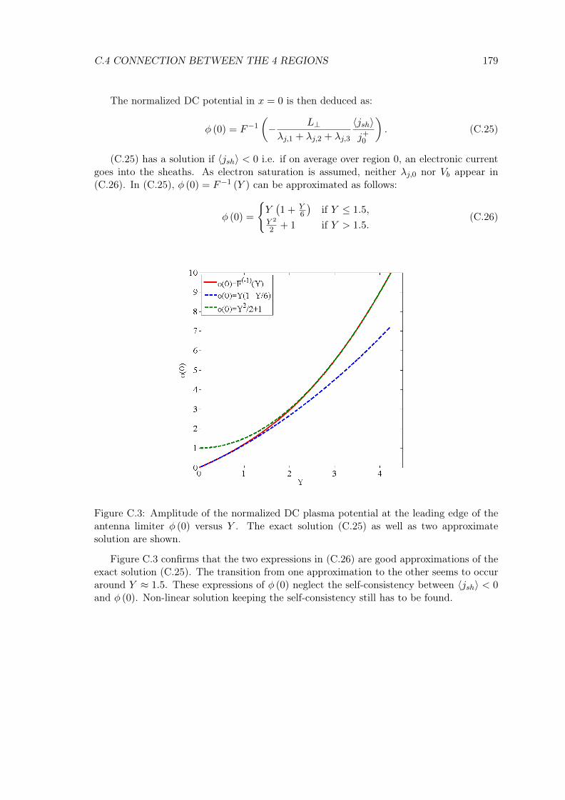
C.4 CONNECTION BETWEEN THE 4 REGIONS 179

The normalized DC potential in x = 0 is then deduced as:

φ (0) = F−1

(− L⊥λj,1 + λj,2 + λj,3

〈jsh〉j+0

). (C.25)

(C.25) has a solution if 〈jsh〉 < 0 i.e. if on average over region 0, an electronic currentgoes into the sheaths. As electron saturation is assumed, neither λj,0 nor Vb appear in(C.26). In (C.25), φ (0) = F−1 (Y ) can be approximated as follows:

φ (0) =

Y(1 + Y

6

)if Y ≤ 1.5,

Y 2

2 + 1 if Y > 1.5.(C.26)

Figure C.3: Amplitude of the normalized DC plasma potential at the leading edge of theantenna limiter φ (0) versus Y . The exact solution (C.25) as well as two approximatesolution are shown.

Figure C.3 confirms that the two expressions in (C.26) are good approximations of theexact solution (C.25). The transition from one approximation to the other seems to occuraround Y ≈ 1.5. These expressions of φ (0) neglect the self-consistency between 〈jsh〉 < 0and φ (0). Non-linear solution keeping the self-consistency still has to be found.

180 APPENDIX C

Bibliography

[1] J. Ongena and G. Van Oost. Energy for Future Centuries - Prospects for FusionPower as a Future Energy Source. Fusion Science and Technology, 53 (2T), 3-15, Feb2008. http://www.ans.org/pubs/journals/fst/a_1686.

[2] G. Van Oost and E. Rebhan. Thermonuclear Burn Criteria. Fusion Science andTechnology, 53 (2T), 16-26, Feb 2008. http://www.ans.org/pubs/journals/fst/a_1687.

[3] J. Wesson. Tokamaks, 3rd ed. Clarendon Press-Oxford, 2004.

[4] J.D. Lawson. Some Criteria for a Power Producing Thermonuclear Reactor. Proc.Royal Physical Society B, 70, 6-10, 1957.

[5] R.R. Weynants. Fusion Machines. Fusion Science and Technology, 53 (2T), 37-43,Feb 2008. http://www.ans.org/pubs/journals/fst/a_1689.

[6] D.A. Hartmann. Stellerators. Fusion Science and Technology, 53 (2T), 44-55, Feb2008. http://www.ans.org/pubs/journals/fst/a_1690.

[7] U. Samm. Plasma-Wall Interactions in Magnetically Confined Fusion Plasmas. Fu-sion Science and Technology, 53 (2T), 223-228, Feb 2008. http://www.ans.org/pubs/journals/fst/a_1708.

[8] R. Koch. Fast Particle Heating. Fusion Science and Technology, 53 (2T), 184-193,Feb 2008. http://www.ans.org/pubs/journals/fst/a_1703.

[9] E. Westerhof. Electron Cyclotron Waves. Fusion Science and Technology, 53 (2T),202-209, Feb 2008. http://www.ans.org/pubs/journals/fst/a_1694.

[10] R.J. La Haye. Neoclassical tearing modes and their control. Physics of Plasmas, 13,055501 (18pp), May 2006.

[11] C.C. Hegna and Callen J.D. On the stabilization of neoclassical magnetohydrodynam-ics teraing modes using current drive or heating. Physics of Plasmas, 4, 2940-2946,May 1997.

[12] A. Mück et al . Sawtooth control experiments on ASDEX Upgrade. Plasma Physicsand Controlled Fusion, 47, 1633-1655, Oct. 2005.

[13] M. Bornatici et al . Electron-cyclotron emission and absorption in fusion plasmas.Nuclear Fusion, 23, 1153-1257, Sept. 1983.

[14] R. Prater. Heating and current drive by electron cyclotron waves. Physics of Plasmas,11, 2349-2376, Apr 2004.

181

182 BIBLIOGRAPHY

[15] R.A. Cairns. Radiofrequency heating of plasmas. IOP Publishing, Bristol, 1991.

[16] D. Van Houtte et al . Recent fully non-inductive operation results in Tore Suprawith 6 minute, 1 GJ plasma discharges. Nuclear Fusion, 44, L11-L15, Apr 2004.

[17] M. Chatelier and Equipe Tore Supra. Integration of high power, long pulse operationin Tore Supra in prparation for ITER. Nuclear Fusion, 47, S579–S589, Oct. 2007.

[18] D. Van Houtte et al . The West Project: a Major Upgrade of Tore Suprafor Preparing ITER Operation in a Tungsten Environment. In Proc. IEE 25thSymposium on Fusion Engineering (SOFE), San Francisco, CA, USA, pages(WO1–6), 2013. http://advprojects.pppl.gov/SOFE2013/SOFE_Presentations/12_Wednesday/WO1-6vanHoutte.pdf.

[19] D. Guilhem et al . Radio frequency additional heating systems issues for the Tore-Supra WEST project. Proc. IEE 25th Symposium on Fusion Engineering (SOFE),San Francisco, CA, USA, 2013.

[20] A. Becoulet. Heating and current drive regimes in the ion cyclotron range of fre-quency. Plasma Physics Controlled Fusion, 38, A1-A11, Dec. 1996.

[21] F.W. Perkins. ICRH Heating Theory. IEEE Transactions on Plasma Science, 12,53-63, June 1984.

[22] M. Brambilla. Kinetic theory of plasma waves. Oxford science publications, 1998.

[23] D. Zarzoso. Kinetic description of the interaction between energetic particles andwaves in fusion plasmas. PhD thesis, Ecole Doctorale de l’Ecole Polytechnique(France), 2012.

[24] G. Bosia. On the automatic control of the ITER ion cyclotron system. FusionEngineering and Design, 82, 662-665, Oct. 2007.

[25] A. Argouarch et al . ICRH ITER like antenna tested on TS commissioning, electricalmodeling and load resilience studies. Fusion Engineering and Design, 84, 275-278,2009.

[26] M. Brambilla. Numerical simulations of ion cyclotron waves in tokamaks plasmas.Plasma Physics and Controlled Fusion, 41, 1-34, Jan 1999.

[27] D. Borba W. and Kerner. CASTOR-K: Stability Analysis of Alfvén Eigenmodes inthe Presence of Enegetic Ions on Tokamaks. J. Computional Physics, 153, 101-138,March 1999.

[28] E.F. Jaeger et al . Self-consistent full-wave and Fokker-Planck calculations for ioncyclotron heating in non Maxwellian plasmas. Physics of Plasmas, 13, 056101 (9pp),May 2006.

[29] R.J. Dumont. Variational approach to radiofrequency waves in magnetic fusion de-vices. Nuclear Fusion, 49, 075033 (14pp), July 2009.

[30] A. Messiaen et al . Performance of the ITER ICRH system as expected from TOPICAand ANTITER II modelling. Nuclear Fusion, 50, 025026 (21pp), Feb. 2010.

BIBLIOGRAPHY 183

[31] V. Lancellotti et al . TOPICA: an accurate and efficient numerical tool for analysisand design of ICRF antennas. Nuclear Fusion, 46, S476-S499, July 2006.

[32] S. Pécoul et al . Numerical modeling of the coupling of an ICRH antenna with aplasma with self-consistent antenna currents. Computer Physics Communications,146, 166-187, July 2002.

[33] J.R. Myra et al . Nonlinear ICRF-plasma interactions. Nuclear Fusion, 46, S455-S468, July 2006.

[34] J.M. Noterdaeme and G. Van Oost. The interaction between waves in the ion cy-lotron range of frequencies and the plasma boundary. Plasma Physics and ControlledFusion, 35, 1481-1511, Nov. 1993.

[35] D.A. D’Ippolito et al . A model of sheath-driven impurity by ICRH antennas. PlasmaPhysics and Controlled Fusion, 33, 607-642, June 1991.

[36] L. Colas et al . Ion Cyclotron Resonant Heating in Tore Supra. Fusion Science andTechnology, 56, 1173-1204, Oct 2009. http://www.ans.org/pubs/journals/fst/a_9173.

[37] R. Van Nieuwenhove and G. Van Oost. Experimental study of sheath currents on thescrape-off-layer durin ICRH of TEXTOR. Plasma Physics and Controlled Fusion,34, 525-532, April 1992.

[38] L. Colas et al . 2-D mapping of ICRH-induced SOL perturbations in Tore Supratokamak. J. Nuclear Materials, 363–365, 555–559, June 2007.

[39] M. Kubic et al . Attenuation of ICRH-induced potentials in the SOL of Tore Supra.Proc. 19th Topical Conf. on Radio Frequency Power in Plasmas, 1-3 June, Newport,RI, USA, AIP Conf. Proc., 1406, 215-218, June 2011.

[40] S.J. Wukitch et al . RF plasma edge interactions and their impact on ICRF antennaperformance in Alcator C-Mod. J. Nuclear Materials, 363-365, 491-497, 2007.

[41] L. Colas et al . Key results of long pulse ICRH operation in Tore Supra. NuclearFusion, 46, 500-513, July 2006.

[42] V. Bobkov et al . ICRF antenna-plasma interactions and its influence onW sputteringin ASDEX upgrade. Journal of Nuclear Materials, 415, S1005-S1008, Sep. 2011.

[43] D.A. D’Ippolito et al . Modelling of mixed-phasing antenna-plasma interactions onJET A2 antennas. Nuclear Fusion, 42, 1357-1365, Dec. 2002.

[44] A. Ekedahl et al . Density Convection near Radiating ICRF Antennas and its Effecton the Coupling of Lower Hybrid Waves. Proc. 15th Top. Conf. on Radio FrequencyPower in Plasmas (19-21 May 2003, Moran, Wyoming 2003) AIP Conf. Proc., 694,259–262, 2003.

[45] M. Kubic et al . Measurements of RF-induced SOL modifications in Tore Supratokamak. Proc. 20th International Conference on Nuclear Engineering and the ASME2012 Power Conference (ICONE20-POWER2012) 30 July-3 August, Anaheim, CA,USA, 5, 191-197, 2012.

184 BIBLIOGRAPHY

[46] J. Gunn et al . Power and particle fluxes at the plasma edge of ITER: Specificationsand Physics Basics. In Proc. 22nd IAEA Fusion Energy Conference - 50th Anniver-sary of Controlled Nuclera Fusion, Geneva (Switzerland) 13/10-18/10, EXP/P6-32,2008.

[47] M. Bures et al . The modification of the plasma edge and impurity productionby antenna phasing during ICRH heating on JET. Plasma Physics and ControlledFusion, 30, 1496-167, Feb. 1988.

[48] A. Mendes et al . Reduction of RF-sheaths potentials by compensation or suppressionof parallel RF currents on ICRF antennas. Nuclear Fusion, 50, 025021 (17pp), Feb.2010.

[49] M.L. Garrett and S.J. Wukitch. Mitigation of radio frequency sheaths through mag-netic field-aligned ICRF antenna design. Fusion Engineering and Design, 87, 1570-1575, 2012.

[50] J.R. Myra et al . Sheath-plasma waves and anamalous loading in ion-Bernstei-waveexperiments. Physical Review Letters, 66, 1173–1176, 1991.

[51] D.A. D’Ippolito et al . Far-field sheaths due to fast waves incident on materialsurfaces. Physics of Plasmas, 15, 102501 (12pp), Oct. 2008.

[52] R.L. Stenzel. Instability of the sheath-plasma resonance. Physical Review Letters,60, 704-707, Feb. 1988.

[53] D.A. D’Ippolito and J.R. Myra. A radio-frequency sheath boundary condition andits effect on slow wave propagation. Physics of plasmas, 13, 102508 (12pp), Oct.2006.

[54] A. Ngadjeu et al . Generation of DC currents by ICRH near fields in the Scrape-off-Layer. J. Nuclear Materials, 415, S1009-S1012, Aug. 2012.

[55] J. Jacquot et al . Radio-frequency sheaths physics: Experimental characterizationon Tore Supra and related self-consistent modeling. In Proc. 20th Topical Conferenceon Radio Frequency Power in Plasmas, Sorrento, Italy, June 25-28 2013, submittedto Physics of Plasmas, 2013. Invited Talk I3.7.

[56] L. Colas et al . RF-sheath patterns modification via novel Faraday screen and strapvoltage imbalance on Tore Supra ion cyclotron antennae. J. Nuclear Materials, 438,S330-S333, July 2013.

[57] J.-P. Bérenger. A perfectly matched layer for the absorption of electromagnetic waves.J. Computional Physics, 114, 185-200, Oct. 1994.

[58] T.H. Stix. The Theory of Plasma Waves, second edition. AIP, 1992.

[59] I.B. Bernstein. Waves in a Plasma in a Magnetic Field. Physical Review, 109, 10-21,Jan 1958.

[60] D.G. Swanson. Plasma Waves, second edition. IoP series on Plasma Physics, Taylor& Francis, 2003.

[61] L. Chen. Alfvén waves: a journey between space and fusion plasmas. Plasma PhysicsControlled Fusion, 50, 124001 (14pp), Dec. 2008.

BIBLIOGRAPHY 185

[62] R. Koch. A global solution of the ICRH problem based on the combined use of aplanar coupling model and hot-plasma ray-tracing in tokamak geometry. ComputerPhysics Communications, 40, 1-22, May 1986.

[63] S. Pécoul et al . Selfconsistent determination of currents on ICRH antennae takinginto account magnetic shielding. Proc. 25th EPS conf. Praha ECA vol.22C p.1586,1998.

[64] A. Messiaen and R. Weynants. ICRH antenna coupling physics and optimum plasmaedge density profile. Application to ITER. Plasma Physics and Controlled Fusion,53, 085020 (29pp), Aug. 2011.

[65] F. Clairet et al . ICRF coupling and edge density profile on Tore Supra. PlasmaPhysics and Controlled Fusion, 46, 1567-1580, Oct. 2004.

[66] P. Descamps et al . Excitation of global modes in textor and comparison with theory.Plasma Physics Controlled Fusion, 33, 1109-1133, Sep. 1991.

[67] L. Colas. H.D.R.: Linear and non-linear Physics of high power radio-frequency wavesin the edge of magnetized plasmas. PhD thesis, U.F.R. Sciences et Techniques de laMatière et des Procédés, Ecole doctorale EMMA, 2009.

[68] D. Milanesio et al . TOPLHA: an accurate and efficient numerical tool for analysisand design of LH antennas. Nuclear Fusion, 52, 013008 (7pp), Jan. 2012.

[69] J. Hillairet et al . ALOHA: an Advanced LOwer Hybrid Antenna coupling code.Nuclear Fusion, 50, 125010 (17pp), Dec. 2010.

[70] M. Preynas et al . Experimental characterization and modelling of non-linear cou-pling of the lower hybrid current drive power on Tore Supra. Nuclear Fusion, 53,013012 (18pp), Jan. 2013.

[71] http://www.ansoft.com/products/hf/hfss/.

[72] https://www.cst.com/Products/CSTMWS.

[73] P.U. Lamalle et al . Recent developments in ICRF antenna modelling. NuclearFusion, 46, 432-443, April 2006.

[74] F. Louche et al . Eigenmode analysis of the ITER ICRF antenna plug and electricalsolution to the grounding of the antenna. Nuclear Fusion, 49, 065025 (11pp), May2009.

[75] F. Louche et al . 3D electromagnetic optimization of the front face of the ITERICRF antenna. Nuclear Fusion, 51, 103002 (20pp), Aug. 2011.

[76] K.S. Yee. Numerical solution of initial boundary value problems involving Maxwell’sequations in isotropic media. IEEE Transactions on Antennas Propagation, 14, 302-307, May 1966.

[77] G. Strang and G. Fix. An Analysis of The Finite Element Method. Prentice Hall,1973.

[78] C. Christopoulos. The Transmission Line Modeling Method: TLM. Piscataway, NY,IEEE Press, 1995.

186 BIBLIOGRAPHY

[79] S.G. Johnson. Notes on Perfectly Matched Layers (PMLs).

[80] M.J. Grote and J.B. Keller. Non reflecting boundary conditions for Maxwell’s equa-tions. J. Computational Physics, 139, 327-342, Jan. 1998.

[81] A. Taflove and M.E. Brodwin. Numerical solution of steady-state electromagneticscattering problems using the time-dependant Maxwell’s equations. IEEE Transac-tions on Microwave Theory and Techniques, 23, 623-630, Aug. 1975.

[82] R. Holland. THREDE - Free-Field EMP coupling and scattering code. IEEE Trans-actions on Nuclear Science, 24, 2416-2421, Dec. 1977.

[83] B. Engquist and A. Majda. Absorbing boundary conditions for the numerical simu-lation of waves. Mathematics of Computation, 31, 629-651, July 1977.

[84] G. Mur. Absorbing boundary conditions for the finite-difference approximation of thetime-domain electromagnetic field equations. IEEE Transactions on ElectromagneticCompatibility, 23, 377-382, Nov. 1981.

[85] L.N. Trefethen and L. Halpern. Well-posedness of one-way wave equations and ab-sorbing boundary conditions. Mathematics of Computation, 47, 421-435, Oct. 1986.

[86] R. Higdon. Numerical absorbing boundary conditions for the wave equations. Math-ematics of Computation, 49, 65-90, July 1987.

[87] O.M. Ramahi. Complementary operators: A method to annihilate artificial reflec-tions arising from the truncation of the computational domain in the solution ofpartial differential equations. IEEE Transactions on Antennas Propagation, 43, 697-704, July 1995.

[88] H.S. Butler and G.S. Kino. Plasma Sheath Formation by Radio-Frequency Fields.Physics of Fluids, 6, 1346-1355, Sept. 1963.

[89] F.W. Perkins. Radiofrequency sheaths and impurity generation by ICRH antennas.Nuclear Fusion, 29, 583-592, Apr. 1989.

[90] T. Hellsten et al . Influence of coupling to spectra of weakly damped eigenmodesin the ion cyclotron range of frequencies on parasitic absorption in rectified radiofrequency sheaths. Physics of Plasmas, 12, 032505 (9pp), March 2005.

[91] J.R. Myra et al . Far-field sheaths from waves in the ion cyclotron range of frequen-cies. Physics of Plasmas, 1, 2890-2900, Sept. 1994.

[92] H. Kohno et al . Numerical analysis of radio-frequency sheath-plasma Interactionsin the ion cyclotron range of frequencies. Physics of Plasmas, 19, 012508 (9pp), Jan2012.

[93] P.C. Stangeby. The Plasma Boundary of Magnetic Fusion Devices. IOP, 2000.

[94] A.L. Lieberman and A.J. Lichtenberg. Principles of Plasma Discharges and MaterialProcessing, Second Edition. Wiley-Interscience, Inc Publication, 2005.

[95] K.-U. Riemann. The Bohm criterion and sheath formation. J. Physics D: AppliedPhysics, 24, 493-518, April 1991.

BIBLIOGRAPHY 187

[96] R. Chodura. Plasma-wall transition in an oblique magnetic field. Physics of Fluids,25, 1628-1633, Sept. 1982.

[97] K.-U. Riemann. Theory of the plasma–sheath transition in an oblique magnetic field.Contribution to Plasma Physics, 34, 127-132, Feb. 1994.

[98] E. Ahedo. Structure of the plasma-wall interaction in an oblique magnetic field.Physics of Plasmas, 4, 4419-4430, Dec. 1997.

[99] E. Faudot et al . Parametric study of two-dimentional potential structures induced byradio-frequency sheaths coupled with transverse currents in front of the Ion CyclotronResonance Heating antenna. Physics of Plasmas, 13, 042512 (16pp), Apr. 2006.

[100] V.A. Godyak and N. Sternberg. Dynamic model of the electrode sheaths in symmet-rically driven rf discharges. Physical Review A, 42, 2299-2312, Aug. 1990.

[101] C.D. Child. Discharge from hot CaO. Physics Review (Series I), 32, 492-511, May1911.

[102] I. Langmuir. The effect of space charge and residual gases on thermionic currents inhigh vacuum. Physical Review, 2, 450-486, Dec. 1913.

[103] M.A. Lieberman. Analytical Solution for Capacitive RF Sheath. IEEE Transactionson Plasma Science, 16, 638-644, Dec. 1988.

[104] H. Kohno. Numerical Analysis of Radio-Frequency Sheath-Plasma Interactions inthe Ion Cyclotron Range of Frequencies. PhD thesis, Massachussets Institute ofTechnology (USA), 2011.

[105] D. Van Eester et al . Connection coefficients for cold plasma wave propagation nearmetallic surfaces. Plasma Physics and Controlled Fusion, 55, 055001 (17pp), May2013.

[106] K. Gunther and A. Carlson. Fluid theory of Langmuir probes in magnetized plasmawith open flux tubes. Contribution to Plasmas Physics, 34, 484-489, Feb. 1994.

[107] J. Cornelis et al . Predicting the radial electric field imposed by externally drivenradial currents in tokamaks. Nuclear Fusion, 34, 171-183, Feb. 1994.

[108] V. Bobkov et al . Assessment of compatibility of ICRF antenna operation with fullW wall in ASDEX Upgrade. Nuclear Fusion, 50, 035004 (11pp), March 2010.

[109] S.J. Wukitch et al . Characterization and performance of a field aligned ion cyclotronrange of frequency antenna in Alcator C-Mod. Physics of Plasmas, 20, 056117 (8pp),May 2013.

[110] D.A. D’Ippolito et al . Analysis of rf sheaths interactions in TFTR. Nuclear Fusion,38, 1543-1563, Oct. 1998.

[111] S.I. Braginskii. Transport processes in a plasma. Review of Plasma Physics, 1,205-311, 1965.

[112] V.A. Rozhansky V.D. Shafranov and O.G. Bakunin. Review Plasma Physics: Mech-anisms of Transverse Conductivity and Generation of Self-Consistent Electric Fieldsin Strongly Ionized Magnetized Plasma, volume 24. ed. Springer, 2008.

188 BIBLIOGRAPHY

[113] Ph. Ghendrih et al . Theoretical analysis of the influence of external biasing on lonrange turbulent transport in the scrape-off-layer. Nuclear Fusion, 43, 1013-1022, Oct.2003.

[114] V.A. Godyak and A.A. Kuzovnikov. Rectifying properties of rf discharges. Soviet J.Plasma Physics, 1, 276-280, May-June 1975.

[115] E.F. Jaeger et al . Power deposition in high-density inductively coupled plasma toolsfor semiconductor processing. Physics of Plasmas, 2, 2597-2604, June 1995.

[116] M.D. Carter et al . Combined rf and transport effects in in magnetized capacitivedischarges. J. of Applied Physics, 100, 073305 (13pp), Oct. 2006.

[117] R. Maggiora. Efficient 3D/1D selfconsistent integral-equation analysis of ICRH an-tennae. Nuclear Fusion, 44, 846-868, Aug. 2004.

[118] B. Van Compernolle et al . Implementation of sheath effects into TOPICA. In Proc.35th EPS Conference on Plasma Physics, HerVonissos, Crete, Greece, 9-13 June2008, volume 32 ECA, pages 1106–1109, 2008.

[119] D. Smithe et al . 3D TimeDomain Simulations of ITER Antenna Modules with EdgePlasma. Proc. 19th Topical Conf. on Radio Frequency Power in Plasmas, 1-3 June,Newport, RI, USA, AIP Conf. Proc., 1406, 65-68, 2011.

[120] D. Smithe et al . Quantitative modelling of ICRH antennas with integrated time do-main RF sheath and plasma physics. In Proc. 20th Topical Conf. on Radio frequencyPower in Plasma, Sorrento, 2013.

[121] C. Nieter and J.R. Cary. VORPAL: a versatile plasma simulation code. J. Compu-tational Physics, 196, 448-473, May 2004.

[122] D. Smithe. Finite-difference time-domain simulation of fusion plasmas at radiofre-quency times scales. Physics of Plasmas, 14, 056104 (7pp), Apr. 2007.

[123] T.G. Jenkins et al . Time-domain simulation of nonlinear radiofrequency phenomena.Physics of Plasmas, 20, 012116, Jan. 2013.

[124] E. Faudot et al . Fluid modeling of radio frequency and direct currents in a biasedmagnetized plasma. Physics of Plasmas, 20, 043514 (14pp), Apr. 2013.

[125] J. Voge. Les tubes aux hyperfréquences: Triodes et tétrodes, klystrons, magnétrons,tubes à onde progressive, amplificateurs paramétriques et quantiques. Éditions Ey-rolles, 1959.

[126] L. Delpech et al . Design and validation of a 700 kW/CW water load for 3.7 GHzklystrons. Fusion Engineering and Design, 86, 815-818, Oct. 2011.

[127] E. Westerhof. Electron cyclotron resonance heating on TEXTOR. Nuclear Fusion,43, 1371-1383, Nov. 2003.

[128] A.G.A. Verhoeven. The design of an ECRH system for JET-EP. Nuclear Fusion, 43,1477-1486, Nov. 2003.

[129] D. Guilhem et al . Manufacturing process and tests of a Lower Hybrid PassiveActive Multijunction launcher for long pulses experimenents on Tore Supra. FusionEngineering and Design, 86 (6-8), 513-517, Oct. 2011.

BIBLIOGRAPHY 189

[130] H. Kuus et al . The ICRH system for Tore Supra. Proc. 15th SOFT, 1988.

[131] THALES. Technical Note Tetrode TH 525/TH 525A. https://www.thalesgroup.com/sites/default/files/asset/document/TH525_A%20.pdf.

[132] T.L. Owens T.L. et al . ICRF antenna and feedthrough development at the OakRidge National Laboratory. Proc. 6th Topical Conf. on RF Plasma Heating, 1985.

[133] H. Wilson. Edge Localized Modes in Tokamaks. Fusion Science and Technology, 53(2T), 161-169, Feb 2008. http://www.ans.org/pubs/journals/fst/a_1702.

[134] I. Monakhov. Tests of load-tolerant external conjugate-T matching system for A2ICRH antenna at JET. Fusion Engineering and Design, 74, 467-471, Nov. 2005.

[135] K. Vulliez et al . Tore Supra ICRH antenna prototype for next step devices. FusionEngineering and Design, 66-68, 531-535, Sep. 2003.

[136] K. Vulliez et al . First results of the Tore Supra ITER like ICRH antenna prototype.Fusion Engineering and Design, 74, 267-271, Nov. 2005.

[137] K. Vulliez et al . Validation of the load-resilient ion cyclotron resonance frequencyantenna concept on Tore Supra plasmas. Nuclear Fusion, 48, 065007 (6pp), 2008.

[138] G. Agarici et al . First plasma experiments in Tore Supra with a new generationof high heat flux limiters for RF antennas. Fusion Engineering and Design, 49-50,145-150, Nov. 2000.

[139] D.W. Faulconer. Adverse shielding of the heating field and high ohmic loss introducedby electrostatic shields employed in radio-frequency heating of plasma. J. AppliedPhysics, 54, 3810-3817, July 1983.

[140] Y. Corre et al . Characterization of heat flux generated by ICRH heating withcantilevered bars and a slotted box Faraday screen. Nuclear Fusion, 52, 103010(11pp),Oct. 2012.

[141] D. Guilhem et al . Tore-Supra infrared thermography system, a real steady-statediagnostic. 23rd Symposium on Fusion Technology (SOFT 23), Venice, Italy, FusionEngineering and Design, 74, 879-883, Nov. 2005.

[142] Ph. Moreau et al . RF heating optimization on Tore Supra using feedback control ofinfrared measurements. Fusion Engineering and Design, 82, 1030-1035, March 2007.

[143] G. Berger-By. Arc security system on harmonics detection for the Tore Supra ICRHtransmitter. Fusion Engineering and Design, 82, 716-722, 2007.

[144] M. Kubic et al . Measurement of sheath potential in RF-biased flux tubes using aretarding field analyser in Tore Supra tokamak. J. Nuclear Materials, 438, 509–512,July 2013.

[145] G. Hornung. Étude de la turbulence plasma par réflectométrie a balayage ultra rapidesur le tokamak Tore Supra. PhD thesis, Aix-Marseille Université (France), 2013.

[146] F. Clairet et al . Edge density profile measurements by X-mode reflectometry onTore Supra. Plasma Physics and Controlled Fusion, 43, 429-441, April 2001.

190 BIBLIOGRAPHY

[147] J.-P. Bérenger. Perfectly Matched Layer (PML) for Computational Electromagnetics.Morgan & Claypool, 2007.

[148] A. Taflove S.C. Hagness. Computational Electrodynamics: The Finite-DifferenceTime-Domain Method, 3rd ed. Artech House Publishers, 2005.

[149] Jin Jianming. The Finite Element Method in Electromagnetisms, 2nd Edition. Wiley-IEEE Press, 2002.

[150] F.L. Teixeira and W.C. Chew. General Closed-Form PML Constitutive Tensors toMatch Arbitrary Bianisotropic and Dispersive Linear Media. IEEE Microwave andGuided Wave Letters, 8, 1804-1807, June 1998.

[151] N.A. Gondarenko et al . Perfectly matched layers for radio wave propagation ininhomogeneous magnetized plasmas. J. Computational Physics, 194, 481-504, March2004.

[152] Mario Augusto Velasco Sanchez. Improvements to a solver of the Helmholtz Equation.PhD thesis, Erasmus Mundus Program on Nuclear Fusion Science and EngineeringPhysics, Université Henri Poincaré, 2009.

[153] F.L. Teixeira and W.C. Chew. Unified analysis of perfectly matched layers usingdifferential forms. Microwave and Optical Technology Letters, 20, 124-126, Jan. 1999.

[154] F.L. Teixeira and W.C. Chew. Complex space approach to perfectly matched layers:a review and some new developments. International J. of Numerical Modelling:Electronic Networks, Devices and Fields, 13, 441-455, Sep. 2000.

[155] W.C. Chew and W. Weedon. A 3D perfectly matched medium from modifiedMaxwell’s equations with stretched coordinates. Microwave and Optical TechnologyLetters, 7, 599-604, Jan. 1994.

[156] Z.S. Sacks et al . A perfectly matched anisotropic absorber for use as an absorbingboundary condition. IEEE Transactions on Antennas and Propagation, 43, 1460-1463, Dec. 1995.

[157] S.D. Gedney et al . An anisotropic perfectly matched layer absorbing media for thetruncation of FDTD latices. IEEE Transactions on Antennas and Propagation, 44,1630-1639, Dec. 1996.

[158] F.L. Teixeira and W.C. Chew. Split-Field and Anisotropic-Medium PML-FDTD Im-plementations for Inhomogeneous Media. IEEE Transactions on Microwave Theoryand Techniques, 50, 30-35, January 2002.

[159] F.L. Teixeira and W.C. Chew. On causality and dynamic stability of perfectlymatched layers for FDTD simulation. IEEE Transactions on Antennas Propagation,47, 775-785, 1999.

[160] I. Singer and E. Turkel. A perfectly matched layer for the Helmholtz equation in asemi-infinite strip. J. Computional Physics, 201, 439-465, Dec. 2004.

[161] S.G. Johnson et al . Adiabatic theorem and continuous coupled-mode theory forefficient taper transitions in photonic crystals. Physical Review E, 66, 066608, Dec.2002.

BIBLIOGRAPHY 191

[162] A.F. Oskooi. The failure of perfectly matched layers, and towards their redemptionby adiabatic absorbers. Optics Express, 16, 11376-11392, July 2008.

[163] C. Balanis. Antenna Theory: analysis and design. Wiley 3rd, 2005.

[164] R.W. Pryor. Multiphysics modeling using COMSOL: a first principles approach.Jones and Bartlett Publishers, 2011.

[165] E. Becache et al . Stability of perfectly matched layers, group velocities andanisotropic waves. J. Computational Physics, 188, 399-433, July 2003.

[166] http://www.comsol.com/.

[167] D. Milanesio et al . Analysis of the Tore Supra ICRF antenna with TOPICA. PlasmaPhysics and Controlled Fusion, 49, 405-419, April 2007.

[168] R.K. Fisher and R.W. Gould. Resonance Cones in the Field Pattern of a ShortAntenna in an Anisotropic Plasma. Physical Review Letter, 22, 1093-1095, May1969.

[169] J.R. Myra and D.A. D’Ippolito. Resonance cone interactions With a Self-ConsistentRadio-Frequency Sheath. Physical Review Letter, 101, 195004 (4pp), Nov. 2008.

[170] P.M. Bellan. Fundamental of Plasma Physics. Cambridge University Press, Cam-bridge, England, 2006.

[171] D.A. D’Ippolito and J.R. Myra. Analytic model of near-field radio-frequency sheaths.I. Tenuous plasma limit. Physics of Plasmas, 16, Feb. 2009.

[172] L. Colas et al . RF current distribution and topology of RF sheath potentials in frontof ICRF antennae. Nuclear Fusion, 45, 767-782, Aug. 2005.

[173] L. Colas et al . Self consistent radio-frequency wave propagation and peripheraldirect current plasma biasing: Simplified three dimensional non-linear treatment inthe “wide sheath” asymptotic regime. Physics of Plasmas, 19, 092505 (15pp), Sept.2012.

[174] J. Jacquot et al . Recent advances in self-consistent RF sheath modeling and relatedphysical properties: Application to Tore Supra IC antennae. Proc. 39th EPS ECAvol.32 P-2.105, 2012. http://ocs.ciemat.es/EPSICPP2012PAP/pdf/P2.038.pdf.

[175] R.J. Dumont and D. Zarzoso. Heating and current drive by ion cyclotron waves inthe activated phase of ITER. Nuclear Fusion, 53, 013002 (12pp), Nov. 2013.

[176] M. Lassas and E. Somersalo. Analysis of the PML equations in general convexgeometry. In Proc. Royal Society Edinburgh Sect. A, volume 131(5), pages 1183–1207, 2001.

[177] P. Jacquet et al . Heat loads on JET plasma facing components from ICRF and LHwave absorption in the SOL. Nuclear Fusion, 51, 103018 (16pp), Oct. 2011.

[178] C. Besse et al . Efficient Numerical Methods for Strongly Anisotropic Elliptic Equa-tions. J. Scientific Computing, 55, 231-254, Apr. 2013.

192 BIBLIOGRAPHY

[179] P.R. Amestoy et al . Multifrontal parallel distributed symmetric and unsymmetricsolvers. Computer Methods in Applied Mechanics and Engineerin, 184, 501-520, Apr.2000.

[180] http://www.mathworks.com/products/matlab/.

[181] L. Colas. Note de Travail: Self-Consistent description of near RF field propagationand DC sheath potential build-up in tokamak SOL plasma. Technical report, CEA,IRFM, 2009.

[182] J. Jacquot et al . 2D and 3D modeling of wave propagation in cold magnetizedplasma near the Tore Supra ICRH antenna relying on the Perfectly Matched Layertechnique. Plasma Physics and Controlled Fusion, 55, 115004 (17pp), Nov. 2013.

[183] I. Langmuir and K. Blodgett. Currents limited by space charge between coaxialcylinders. Physical Review, 22, 347-356, Oct. 1923.

[184] V. Rozhansky et al . Plasma Depletion and Electron Current Saturation for PositivelyBiased Flush-Mounted Probe in Magnetic Field. In 26th EPS Conf. on ControlledFusion and Plasma Physics, Maastricht, 14 - 18 June 1999, ECA.

[185] X. Litaudon et al . Physics and technology in the ion-cyclotron range of frequencyon Tore Supra and TITAN test facility: implication for ITER. Nuclear Fusion, 53,083012 (11pp), Aug. 2013.

[186] O. Meyer et al . Impurity production monitoring during RF experiments in ToreSupra. J. Nuclear Materials, 390-391, 879-883, June 2009.

[187] M. Chantant et al . Calorimetry measurements during high energy discharges atTore Supra. Fusion Engineering and Design, 74, 897-902, Nov. 2005.

[188] Y. Corre et al . Heat flux calculation and problem of flaking of boron carbide coatingson the Faraday screen of the ICRH antennas during Tore Supra high power, long pulseoperation. Fusion Engineering and Design, 86, 429-441, June 2011.

[189] G. Ritz et al . Calculation of heat fluxes induced by radio frequency heating onthe actively cooled protections of ion cyclotron resonant heating (ICRH) and lowerhybrid (LH) antennas in Tore Supra. Fusion Engineering and Design, 88, 899-902,2013.

[190] I. Cziegler et al . Ion-cyclotron range of frequencies in the scrape-of-layer: finestructure radial electric fields. Plasma Physics and Controlled Fusion, 54, 105019(9pp), Oct. 2012.

[191] A. Kallenbach et al . Recent ASDEX Upgrade Results and Future Extension Plans.IEEE Transactions on Plasma Science, 40, 605-513, March 2012.

[192] V. Bobkov et al . ICRF operation with improved antennas in ASDEX Upgrade withW wall. Nuclear Fusion, 53, 093018 (9pp), Aug. 2013.

[193] C. Klepper et al . Dynamic Stark Spectroscopic Measurements of Microwave ElectricFields Inside the Plasma Near a High-Power Antenna. Physical Review Letters., 110,215005 (5pp), May 2013.

BIBLIOGRAPHY 193

[194] D.A. D’Ippolito et al . Modeling far-field RF sheaths in Alcator C-Mod. In Proc.20th Topical Conf. on Radio frequency Power in Plasma, Sorrento, Italy, 2013.

[195] J.R. Myra et al . Role of magnetic field tangency in ICRH sheath interactions. InProc. 20th Topical Conf. on Radio frequency Power in Plasma, Sorrento, Italy, 2013.

[196] L. Colas et al . RF sheath estimates on blanket shielding modules surrounding theITER Ion Cylotron Antenna using the SSWICH asymptotic model. Technical report,CEA, IRFM, 2011.

[197] Y. Sarazin. Etude de la turbulence de bord dans les plasmas de tokamaks. PhD thesis,Université Joseph Fourier - Grenoble 1 (France), 2012.

[198] C. Colin. Modélisation umérique des mesures de flux par sonde mobile dans le plasmade bord des tokamaks, 2012. Master thesis Université Henri Poincaré Nancy-Metz(France).

[199] D. Van Eester et al . Ion cylotron resonance heating-induced density modificationsnear antennas. Plasma Physics and Controlled Fusion, 55, 025002 (12pp), Feb. 2013.

[200] S. Robertson et al . TOPICAL REVIEW: Sheaths in laboratory and space plasmas.Plasma Physics and Controlled Fusion, 55, 093001, Sep. 2013.

[201] B. Jacobs et al . Temporally resolved ions velocity distribution measurements in aradio-frequency plasma sheath. Physics of Plasmas, 18, 053503 (5pp), May 2011.

194 BIBLIOGRAPHY

List of Publications

1st author

J. Jacquot et al . Radio-frequency sheaths physics: Experimental characterization on ToreSupra and related self-consistent modeling. In Proc. Invited Talk 20th Topical Conferenceon Radio Frequency Power in Plasmas, Sorrento, Italy, June 25-28 2013, submitted toPhysics of Plasmas

J. Jacquot et al. 2D and 3D modeling of wave propagation in cold magnetized plasmanear the Tore Supra ICRH antenna relying on the Perfectly Matched Layer technique.Plasma Physics and Controlled Fusion, 55, 115004 (17pp), Nov. 2013.http://dx.doi.org/10.1088/0741-3335/55/11/115004

J. Jacquot et al. Recent advances in self-consistent RF sheath modeling and relatedphysical properties: Application to Tore Supra IC antennae. Proc. 39th EPS ECA vol.32P-2.105, 2012.http://ocs.ciemat.es/EPSICPP2012PAP/pdf/P2.038.pdf

J. Jacquot et al. Self-consistent non-linear radio-frequency wave propagation and pe-ripheral plasma biasing. Proc. 19th Topical Conf. on Radio Frequency Power in Plasmas,1-3 June, Newport, RI, USA, AIP Conf. Proc. 1406, p.211-214, 2011.http://dx.doi.org/10.1063/1.3664962

Co-author

D. Guilhem et al. Radio frequency additional heating systems issues for the Tore-SupraWEST project. Proc. IEE 25th Symposium on Fusion Engineering (SOFE), San Fran-cisco, CA, USA, 5pp, 2013.http://dx.doi.org/10.1109/SOFE.2013.6635379

A. Bécoulet et al. Science and technology research and development in support toITER and the broader approach. Nuclear Fusion, 53(8), 104023(17pp), Oct. 2013.http://dx.doi.org/10.1088/0029-5515/53/10/104023

195

196 LIST OF PUBLICATIONS

X.Litaudon et al. Physics and Technology in the Ion-cyclotron Range of Frequencyon Tore Supra and TITAN test facility: implication for ITER. Nuclear Fusion, 53(8),083012(11pp), Aug. 2013.http://dx.doi.org/10.1088/0029-5515/53/8/083012

M. Kubic et al. Measurement of sheath potential in RF-biased flux tubes using a re-tarding field analyser in Tore Supra tokamak. J. Nuclear Materials, 438, p.509–512, July2013.http://dx.doi.org/10.1016/j.jnucmat.2013.01.105

L. Colas et al. RF-sheath patterns modification via novel Faraday screen and strapvoltage imbalance on Tore Supra ion cyclotron antennae. J. Nuclear Materials, 438, S330-S333, July 2013.http://dx.doi.org/10.1016/j.jnucmat.2013.01.061

Y. Corre et al. Characterization of heat flux generated by ICRH heating with can-tilevered bars and a slotted box Faraday screen. Nuclear Fusion, 52, 103010(11pp), 2012.http://dx.doi.org/10.1088/0029-5515/52/10/103010

L. Colas et al. Self consistent radio-frequency wave propagation and peripheral directcurrent plasma biasing: Simplified three dimensional non-linear treatment in the “widesheath” asymptotic regime. Physics of Plasmas, 19, 092505 (15pp), Sept. 2012.http://dx.doi.org/10.1063/1.4750046

A. Koehn et al. Full-wave modeling of the O-X mode conversion in the Pegasus toroidalexperiment. Physics of plasmas, 18(8), 082501 (9pp), Aug. 2011.http://dx.doi.org/10.1063/1.3609828

Long résumé

Ce travail de thèse s’inscrit dans le contexte global de la fusion thermonucléaire. Le but estde domestiquer sur Terre l’énergie des étoiles afin de produire de l’énergie en abondancesur des échelles de temps très longs et sans déchet difficile à gérer. Une voie pour réaliser cetype de production d’énergie sur Terre est d’utiliser des bouteilles magnétiques fermées surelle-mêmes appelées tokamaks. Dans ce tokamak, il devrait être possible de maintenir destrès hautes températures de l’ordre de 100 millions de degrés pour atteindre des conditionspermettant la fusion d’un noyau de deutérium avec un noyau de tritium. Ces deux élémentscorrespondent aux deux isotopes de l’hydrogène. A ces températures la matière existesous forme de plasma, dans lequel les électrons sont détachés des noyaux. Dans ce milieuplasma, les interactions électromagnétiques dominent bien que ce milieu soit globalementneutre et conduisent à un comportement collectif des particules face à une perturbation.Ce comportement collectif, résumé dans un tenseur diélectrique gyrotrope, se traduit parl’existence de modes d’oscillation permettant de transporter de l’énergie dans le plasma.Différentes techniques sont possibles pour chauffer le plasma à ces températures extrêmesnécessaires à la fusion des noyaux. Un chauffage par des ondes radio-fréquences (RF) estpossible dans le domaine des fréquences cyclotroniques ioniques (FCI) (30− 100 MHz)afin d’atteindre les températures requises dans un plasma de fusion. Les grands tokamakssont pour la plupart équipés de systèmes de chauffage FCI permettant d’injecter plusieursMWde puissance additionnelle dans le plasma. Les antennes FCI sont composées d’unréseau phasé de rubans métalliques parcourus par un courant RF.

Afin d’obtenir un chauffage efficace du plasma central, une bonne compréhension desinteractions entre les ondes et le plasma de bord est cependant nécessaire. Comme lesondes FCI sont évanescentes à basse densité, elles doivent traverser par effet tunnel unecouche d’évanescence [65]. L’antenne, pour avoir un couplage efficace, doit donc être placéeprès du plasma. Des interactions non-linéaires, dues aux gaines RF [34] déterminent alorssouvent les limites opérationnelles des systèmes de chauffage. Ces effets délétères ont étéobservés sur différents tokamaks [40–42] sous différentes formes telles que des points chaudssur les antennes [36], de l’érosion [35], des modifications locales de la densité au voisinagedes antennes par des cellules de convection [37]. Or l’efficacité du couplage de l’onde estprincipalement déterminée par la largeur de la zone d’évanescence. Comme les asservisse-ments du point de fonctionnement de l’antenne sont conçus pour délivrer une puissancecouplée au plasma constante, la tension appliquée à l’antenne est donc changée, ce qui vaaussitôt modifier l’amplitude des gaines RF et ainsi de suite. De forts courants DC (DirectCurrent) ont également été mesurés quand les antennes sont actives [42]. Il a égalementété observé des interactions non-linéaires avec d’autres antennes [44]. Il est primordial queces phénomènes soient compris afin que le système de chauffage soit parfaitement contrôléet fiable à haute puissance sur de très longues durées dans un environnement métalliqueafin d’obtenir des plasmas stables satisfaisant aux conditions nécessaires aux réactions defusion du deutérium et du tritium..

I

II LONG RÉSUMÉ

Une modélisation auto-cohérente des gaines RF dans un code de couplage de l’onde n’aencore jamais été réalisée. Chacun de ces deux problèmes est en soi-même ardu. Les objectifsde cette thèse étaient de modéliser séparément mais de façon compatible le couplage d’ondeet la formation de gaines RF afin de les coupler au sein d’un unique code.

Les simulations ont été réalisées avec le logiciel commercial sous licence Comsol Mul-tiphysics [166]. Ce choix a été fait avant mon arrivée en thèse afin d’éviter un fastidieuxdéveloppement numérique qui n’était pas réalisable en 3 ans avec la main d’œuvre dispo-nible tout en produisant une analyse physique pertinente d’observations expérimentales.L’aspect élément finis [77] a été un élément prépondérant dans le choix puisque qu’il per-met d’inclure des géométries complexes en 3D. Le logiciel Comsol a aussi été choisi pourson aspect multi-physique qui en fait un outil disponible pour d’autres utilisateurs menantd’autres travaux en parallèle comme le problème de dissipation thermique dans l’antenneou le calcul des contraintes mécaniques induites lors d’une disruption. Comme le problèmeà traiter présente en lui-même des aspects multi-physiques, ce choix s’est imposé de lui-même. Ici, les équations génériques à résoudre correspondent aux équations de Helmholtzet Poisson. L’interface graphique est également ergonomique et simple d’utilisation et per-met aussi des sous-niveaux avec plus d’options. Les équations (ou leurs formes) nativementimplémentées ne répondent pas cependant forcément à nos besoins. Cette limitation estinterne à Comsol, ce qui réduit les choix possibles pour l’équation générique à résoudre.Il est cependant possible de les modifier légèrement dans les sous-niveaux. Ce choix pré-sente cependant certaines contraintes, la principale étant le manque de contrôle du solveurpermettant la résolution des équations. Les problèmes de convergence et de stabilité sontdonc difficiles à maîtriser.

Des restrictions internes au CEA (Commissariat à l’énergie atomique et aux énergiesalternatives) existent aussi. Le coût de la licence limite le nombre d’heures par utilisateuret le nombre de processeurs. Une autre limite est à caractère numérique est due à la taillemémoire disponible et le temps de calcul sur les stations déterminant directement le nombred’éléments maximum pour les simulations (ces contraintes interviennent rapidement lorsdu passage en 3D).

Le plasma du tokamak de forme torique est déplié d’abord sous forme de cylindre quiest lui-même déplié sous forme de plan, afin d’éliminer des effets de courbure dans la di-rection toroidale et dans la direction poloidale. Cette hypothèse se justifie partiellementcar la taille des domaines étudiés a des dimensions plus faibles que les caractéristiquesgéométriques du plasma de tokamak. La propagation d’onde est ici modélisée dans la Sec-tion à l’Ombre des Limiteurs (SOL) du plasma d’un tokamak, où les lignes de champsmagnétiques sont ouvertes et connectées à des objets matériels. La propagation d’ondesaux fréquences considérées dans la SOL peut être décrite dans l’approximation plasmafroid. Au contraire, le plasma central est bien confiné par des lignes de champs fermées.Dans ce cas le tenseur diélectrique, communément appelé tenseur de Stix [58], caractérisantles propriétés du plasma magnétisé, la réponse du courant plasma RF à un champ élec-trique RF est locale en espace et non-locale en temps. Pour une onde monochromatique samodélisation passe par l’écriture d’un tenseur dépendant uniquement de la fréquence. Cetenseur présente une très grande anisotropie. Cela provient simplement du libre déplace-ment des particules chargées dans la direction du champ magnétique. Il présente aussi unegyrotropie puisque certains éléments non diagonaux sont non nuls traduisant la présencede l’effet Hall. En présence de champ magnétique DC les particules chargées n’oscillentpas nécessairement dans une direction colinéaire au champ RF. Ce tenseur est égalementinhomogène traduisant la présence des gradients radiaux du champ magnétique et de ladensité. Les éléments du tenseur peuvent donc changer de signe.

LONG RÉSUMÉ III

Dans ce milieu biréfringent, pour une même direction de propagation deux types d’ondespeuvent coexister simultanément [58]. Dans ce domaine de fréquences FCI, elles sont ap-pelées onde rapide et onde lente. L’onde rapide est progressive alors que l’onde lente estrégressive. Une onde est dite progressive quand sa vitesse de phase et sa vitesse de groupesont colinéaires. L’onde rapide est évanescente en dessous d’une densité critique alors quel’onde lente l’est au-dessus d’une autre densité critique. Ces propriétés peuvent être faci-lement retrouvées à partie des relations de dispersions [22]. Dans les conditions de notreétude, l’onde rapide a une polarisation transverse électrique. Elle peut donc se propagertransversalement au champ magnétique jusqu’au centre du plasma où par résonance cy-clotronique avec les ions, l’énergie de l’onde est transmise au plasma. Les antennes FCIsont conçues en conséquence pour générer l’onde rapide avec des rubans de courant phaséverticaux. L’onde lente est générée de façon parasite du fait des courants induits sur lastructure d’antenne et son environnement.

Une bonne compréhension dans l’ensemble de couplage d’onde est à présent acquise,du moins en régime linéaire en l’absence des interactions indirectes non-linéaires. Toutefoisles manières de modéliser le couplage [30–32, 66] sont difficilement compatibles avec uneétude détaillée et réaliste des gaines RF de manière auto-cohérente. La première étape dela thèse a été consacrée à trouver une manière nouvelle de modéliser le couplage d’ondesFCI au plasma qui puisse être compatible a priori avec un ajout futur de la modélisationde gaines RF [182]. Cette partie linéaire utilise les équations de Maxwell macroscopiquesen présence d’un plasma froid magnétisé et d’objets de géométrie complexes.

L’effet des gaines RF étant supposé principalement lié à la présence de l’onde lente,nous sommes seulement intéressés au comportement du plasma au voisinage de l’antenne.A cause de ressources numériques limitées, la propagation d’ondes loin de l’antenne etl’absorption dans le chaud plasma de cœur sont généralement inclus seulement en tant queconditions aux limites. Pour ces raisons, seulement une fraction du volume du tokamak estsimulée. Il devient nécessaire de trouver une manière d’absorber les ondes propagatives aufrontière du domaine afin d’émuler l’absorption dans le cas où l’absorption par passage estquasi-totale. Sans ces conditions de bord, des réflexions d’origine numérique se produisentaux frontières du domaine. En dépit du fait que de nombreux scénarios de chauffage ontune faible absorption par passage, les études de conception d’antenne sont toutes réaliséesen faisant l’hypothèse d’une forte absorption par passage. Différentes stratégies existentpour éviter la réflexion numérique. Des collisions artificielles peuvent être ajoutées [70].Dans ce cas, la réflexion n’est pas contrôlée. La manière la plus courante est de traiterle plasma en tant que conditions aux limites avec des admittances de surface [66]. Cetteméthode est capable de gérer des basses absorptions par passage. Elle réclame cependantun coût numérique important du fait de la nécessité de faire correspondre les modes dansle vide avec les modes du plasma. De plus les antennes sont face à un plasma tout en étantplacées dans le vide. Or une gaine ne peut pas exister dans le vide. Une autre manière estde fabriquer une zone absorbante sans saut d’indice. La meilleure technique de ce point devue est la technique des couches parfaitement adaptées (CPA plus connues sous l’acronymeanglais PML signifiant perfectly matched layer) [57]. C’est une méthode communémentemployée avec des milieux classiques afin de gérer les ondes sortantes propagatives sansréflexion numérique.

Pour appliquer ce type de conditions de bord, il faut savoir que les plasmas magnéti-sés ont des propriétés assez originales : anisotropie, gyrotropie, inhomogénéité, vitesses degroupe des deux modes avec des signes opposés. Il est possible de remplacer le plasma parun diélectrique équivalent [73, 74]. En conséquence de quoi, la contribution de l’un des deuxmodes est perdu. Les CPA ont notablement avancé au point de tenter de les appliquer aux

IV LONG RÉSUMÉ

plasmas de fusion [150, 151]. Dans le domaine fréquentiel, le concept des CPA repose surune transformation de l’espace des coordonnées réelles vers des coordonnées complexes touten étirant l’espace afin d’amener ce qui peut être considéré comme l’infini à une distancefinie. Cette distance représente la taille de la CPA. Cette transformation ne modifie pas lespropriétés du plasma. La partie complexe de la transformation agit sur les ondes propa-gatives tandis que la partie réelle agit sur les ondes évanescentes. La transformation dansune direction dépend uniquement de la coordonnée dans cette direction. La magnitude del’étirement permet de moduler le taux d’absorption de l’onde dans la CPA. La formula-tion trouvée des CPA est élégante et facile à implémenter. En effet la CPA peut être vuecomme un matériau artificiel ayant des tenseurs diélectrique et perméabilité magnétiqueparticuliers. Les champs dans les équations de Maxwell ne sont pas modifiés dans le plasmamais correspondent à des champs artificiels dans la CPA [157]. Des transformations de typepolynômial ont été employées pour implémenter les CPA dans Comsol.

Cette technique a tout d’abord été testée sue des plasmas magnétisés homogènes dansune boîte rectangulaire pour lesquels une solution analytique avec des ondes planes existeafin de pouvoir comparer les prédictions analytiques pour le coefficient de réflexion avec lessimulations. Le coefficient de réflexion est uniquement défini pour des ondes planes. Cestests ont permis de vérifier des intuitions données par une formule analytique sur l’impactdes paramètres des CPA et du plasma. Une grande CPA diminue la réflexion. Un conseilusuel est de choisir une CPA de la taille de l’ordre de la longueur d’onde pour satisfaireaux conditions d’application de la méthode WKB, nécessaire pour éviter les réflexionsd’origine numérique liées à une trop grande variation de l’indice. Un polynôme d’ordrefaible est préférable. Par la suite un ordre 2 est choisi. Les coefficients d’étirement doiventêtre préférablement choisi grands. Cependant de trop grandes valeurs induisent égalementdes réflexions numériques du fait de l’inadéquation de l’étirement avec le maillage du faitd’une trop grande variation spatiale des champs sur la taille d’une maille de calcul.

Ces tests académiques ont aussi permis de mettre en évidence certaines limites desCPA. Les CPA peuvent être parfaitement sans réflexion seulement pour l’équation d’ondeexacte. La discrétisation du problème en vue d’une résolution numérique induit un certainniveau de réflexion d’origine numérique. Un maillage raffiné permet de se rapprocher decette limite sans réflexion. Il a aussi été identifié qu’une singularité ne doit pas être présentedans les CPA. Placer une CPA à proximité d’une coupure,où l’onde est réfléchie naturelle-ment par le milieu, génère un surcout numérique qui peut être évité en éloignant la CPA.Il a été également vu qu’un niveau de réflexion acceptable peut être atteint dans les casabsorbés. La gyrotropie, mêlant différentes directions du fait d’éléments non-diagonaux,de augmente la réflexion ainsi que la présence de modes poloidaux. Un maillage avec unemeilleure résolution permet de corriger ces effets. L’impossibilité de la coexistence simul-tanée d’une onde progressive et d’une onde régressive a été constatée. Cela est dû au choixdu signe du coefficient d’étirement de la partie imaginaire de la transformation. Un choixdoit donc être fait. Dans un tokamak, un gradient radial de densité existe. Or l’onde lenteest évanescente au-delà d’une densité critique [58]. Le mieux est alors de laisser le plasmaréfléchir naturellement l’onde lente et de concevoir la CPA pour l’onde rapide uniquement.

Dans les expériences, l’efficacité à laquelle est réalisée le couplage de la puissance vé-hiculée par l’onde au plasma est évaluée par la résistance de couplage. Une équivalenceentre coefficients de réflexion et oscillations de la résistance de couplage dans les simu-lations a été établie analytiquement et vérifiée pour des ondes planes. Dans le cas d’uneantenne rayonnant un spectre d’ondes planes, les oscillations de la résistance de couplageavec les paramètres de la CPA sont plus commodes à surveiller que le coefficient de réflexionstrictement valable pour une onde plane.

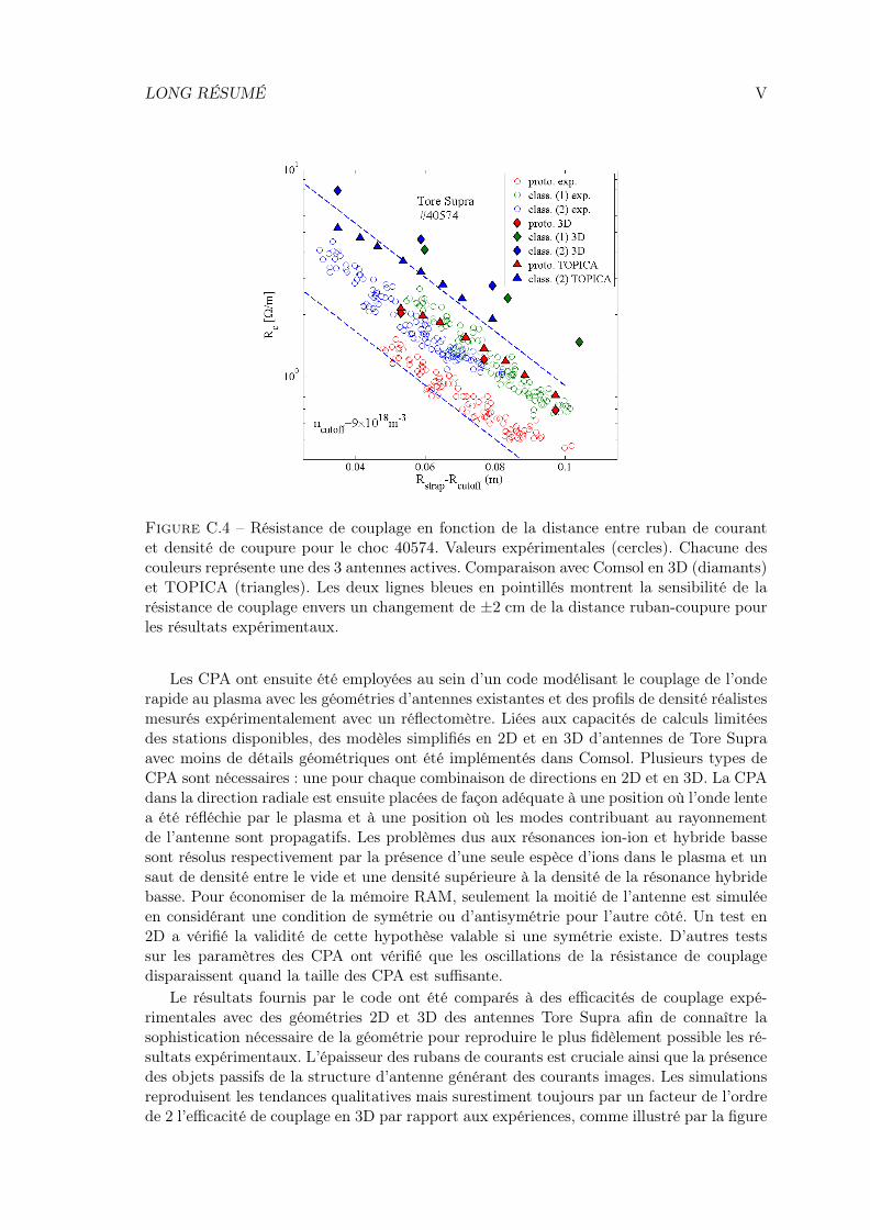
LONG RÉSUMÉ V

Figure C.4 – Résistance de couplage en fonction de la distance entre ruban de courantet densité de coupure pour le choc 40574. Valeurs expérimentales (cercles). Chacune descouleurs représente une des 3 antennes actives. Comparaison avec Comsol en 3D (diamants)et TOPICA (triangles). Les deux lignes bleues en pointillés montrent la sensibilité de larésistance de couplage envers un changement de ±2 cm de la distance ruban-coupure pourles résultats expérimentaux.

Les CPA ont ensuite été employées au sein d’un code modélisant le couplage de l’onderapide au plasma avec les géométries d’antennes existantes et des profils de densité réalistesmesurés expérimentalement avec un réflectomètre. Liées aux capacités de calculs limitéesdes stations disponibles, des modèles simplifiés en 2D et en 3D d’antennes de Tore Supraavec moins de détails géométriques ont été implémentés dans Comsol. Plusieurs types deCPA sont nécessaires : une pour chaque combinaison de directions en 2D et en 3D. La CPAdans la direction radiale est ensuite placées de façon adéquate à une position où l’onde lentea été réfléchie par le plasma et à une position où les modes contribuant au rayonnementde l’antenne sont propagatifs. Les problèmes dus aux résonances ion-ion et hybride bassesont résolus respectivement par la présence d’une seule espèce d’ions dans le plasma et unsaut de densité entre le vide et une densité supérieure à la densité de la résonance hybridebasse. Pour économiser de la mémoire RAM, seulement la moitié de l’antenne est simuléeen considérant une condition de symétrie ou d’antisymétrie pour l’autre côté. Un test en2D a vérifié la validité de cette hypothèse valable si une symétrie existe. D’autres testssur les paramètres des CPA ont vérifié que les oscillations de la résistance de couplagedisparaissent quand la taille des CPA est suffisante.

Le résultats fournis par le code ont été comparés à des efficacités de couplage expé-rimentales avec des géométries 2D et 3D des antennes Tore Supra afin de connaître lasophistication nécessaire de la géométrie pour reproduire le plus fidèlement possible les ré-sultats expérimentaux. L’épaisseur des rubans de courants est cruciale ainsi que la présencedes objets passifs de la structure d’antenne générant des courants images. Les simulationsreproduisent les tendances qualitatives mais surestiment toujours par un facteur de l’ordrede 2 l’efficacité de couplage en 3D par rapport aux expériences, comme illustré par la figure

VI LONG RÉSUMÉ

1. Ce facteur diminue avec la sophistication de la description de la géométrie de l’antenne.Une comparaison avec le code référence de couplage FCI TOPICA [31] comportant unegéométrie très réaliste donne également un facteur 1.5. Cette différence est expliquée parle plus grand raffinement de TOPICA allant de pair avec un maillage plus fin mais nécessi-tant un coût numérique plus important en mémoire et en temps de calcul. Ce facteur entresimulations et expériences est probablement dû à une incertitude sur la réelle largeur de lacouche d’évanescence. L’influence de l’écran de Faraday causant un écrantage magnétique[32] a été aussi négligée.

Dans l’immédiat ce code est utilisable tel quel pour des calculs de couplage d’ondes. Ilva être utilisé en complément de TOPICA pour concevoir de nouvelle antenne pour projetWEST, étant une transformation majeure de Tore Supra. Même sans atteindre le degréde sophistication de TOPICA, ce code de couplage peut donner un résultat pertinent enquelques minutes en 2D ou en quelques heures en 3D sur une simple station de travail alorsque TOPICA réclame sur un supercalculateur plusieurs heures pour un cas. Un grandnombre d’études paramétriques très détaillées peut donc être envisagées pour identifier lesdomaines de paramètres pertinents avant de confirmer avec TOPICA. A terme, ce codea vocation à être intégré dans un code plus global modélisant de manière auto-cohérentecouplage d’ondes et gaines RF [33, 34].

Parallèlement une description novatrice auto-cohérente des gaines RF modélisant lapropagation d’ondes RF et la polarisation DC positive résultante du bord d’un plasmamagnétisé a été développée durant cette thèse. La physique des gaines RF est un sujetextrêmement ardu étudié depuis plusieurs décennies. Ceci étant dû à un comportementhautement non-linéaire. La gaine classique/thermique [93] est une région dont l’épaisseurest très fine comparée aux dimensions caractéristiques du plasma. Cette zone tampon char-gée positivement permet de préserver la quasi-neutralité du plasma se trouvant à l’intérieurd’une enveloppe matérielle. Lorsque la gaine est soumise à un potentiel RF d’amplitudesupérieure au potentiel flottant, elles se mettent à osciller [103], permettant alors la géné-ration d’un potentiel continu.

Des progrès ont été réalisés dans leur compréhension en complexifiant peu à peu leurdescription. La description des gaines RF nécessite plusieurs échelles de temps, plusieurséchelles de longueurs et la prise en compte de l’orientation du champ magnétique. Lespremière études ont d’abord porté sur la description de l’interaction entre les ondes RFentrant dans la gaine et le potentiel électrostatique. Cela a conduit au mécanisme derectification des potentiels RF qui induit un phénomène d’auto-polarisation DC du plasma[114] modifiant ainsi les conditions de bord vu par l’onde. La propagation d’ondes RFmodifie le plasma. Les modèles précédents négligeaient cependant la rétroaction du plasmasur la propagation des ondes rapides et lentes.

Pour éviter de mailler les gaines nécessitant des grilles très fines et donc un coût nu-mérique prohibitif, des conditions aux limites de type gaine du point de vue RF ont étédéveloppées par Myra et D’Ippolito [53]. Des conditions similaires existent pour les plas-mas de décharges non magnétisés. Ces conditions sont appliquées à la place de conditionsmétalliques sur les parois alors que strictement elles ne sont valides qu’à l’entrée de lagaine. Un essai a été fait afin d’inclure ce type de conditions dans TOPICA mais pour desgaines dans le vide [118]. Ces conditions considèrent dans l’approximation électrostatiqueque du point de vue des ondes RF à la fréquence fondamentale, la gaine de taille moyennetemporellement δ peut être vue comme un capacité plane avec un matériau de constantediélectrique εsh entre les plaques de la capacité. Le courant dans la gaine est principalementun courant de déplacement. Cette description est appropriée puisque la gaine est une régionvidée d’électrons assimilable au vide. Cela a mis en évidence la propriété de capacité de la

LONG RÉSUMÉ VII

gaine RF. Cette capacité varie de façon inversement proportionnelle à la taille de gaine etau potentiel électrostatique selon la loi de Child-Langmuir [102].

La description auto-cohérente des gaines RF plus proche des premiers principes a seule-ment commencé il y a quelques années. Il est supposé que les échelles de temps rapide etlente peuvent être séparées. Certaines propriétés clés sont connues : la redressement decourant RF en courant DC et la capacité. Du point du vue électrique, les gaines sont doncvues comme une diode et une capacité en parallèle. La diode permet de passer de l’échellede temps rapide à l’échelle de temps lent. L’inverse est vrai pour la capacité.

Une modélisation auto-cohérente a été réalisée par Kohno [92] en combinant ces prin-cipes. La description de l’échelle de temps lente était cependant simpliste. En effet, les cou-rants DC n’étaient pas autorisés puisque le tenseur de conductivité DC était nul. L’onderapide et l’onde lente ont toutefois été prises en compte et l’orientation arbitraire du champmagnétique autorisait la conversion de mode.

Un projet similaire a été entrepris durant cette thèse [55]. Ce projet de modélisationauto-cohérente de la propagation d’onde et la polarisation DC du plasma de bord estappelé SSWICH (Self-consistent Waves and Sheaths for Ion Cylotron heating). La géo-métrie du modèle est une représentation simplifiée du voisinage d’une antenne FCI dansTore Supra. La forme des objets est simplifiée afin que les lignes de champ magnétiquessoient perpendiculaires à la surface des objets (i.e. parallèle à la normale de la surface)ou parallèle à la surface des objets. Cette restriction est due à l’écriture des conditionsaux limites de ce modèle qui ne tolèrent pas pour le moment une orientation arbitrairede champ magnétique. Deux types de plasmas de bord sont considérés. La zone entre leslimiteurs entourant l’antenne pour la protéger des flux provenant du plasma est appeléeSOL privée. Les lignes de connexion étant courtes, la densité décroit plus rapidement quedans la SOL libre à l’extérieur des limiteurs, selon le modèle élaboré par Stangeby [93]. Leslongueurs de connexion sont plus longues que dans la SOL privée. Seule l’onde lente estdonc prise en compte. Toutefois, lorsque l’anisotropie du plasma est très grande, il peutêtre dit que le champ électrique parallèle à l’origine des gaines RF est principalement dûà l’onde lente. Le modèle est limité à deux dimensions dans le plan radial/toroidal pourl’instant à cause de limitations dans les ressources informatiques. La troisième dimensionpeut être cependant prise en compte au travers d’une procédure multi-2D où les positionsverticales sont successivement changées. Cela nécessite cependant de négliger les dérivéespoloidales (modèle en tranches). Cette hypothèse fut testée par la suite dans un contextesimplifié. Pour ces raisons, la version actuelle de SSWICH est appelée SSWICH-SW-2D(SSWICH pour l’onde lente en deux dimensions).

Le modèle actuel le plus développé durant cette thèse contient le minimum d’ingrédientsphysiques nécessaires pour une description auto-cohérente de la formation des gaines RF.Il est implémenté dans Comsol sous forme de modules couplés. Il s’agit d’une descriptionfluide couplant trois quantités : le champ électrique parallèle, la tension de gaines oscillanteset le potentiel électrostatique du plasma. Chaque module décrit un phénomène traduisantune propriété de gaines RF.

Le premier module modélise la propagation d’ondes RF dans un plasma froid magnétisé.Pour l’instant, les conditions de type gaine sont implémentées pour les cas où les lignesde champ magnétique sont perpendiculaires à la paroi. Une carte de champ électriqueest imposée à l’embouchure de l’antenne. Cette carte est produite dans TOPICA sansgaine avec une géométrie 3D. Le modèle est donc capable de prendre en compte des cartesde champs réalistes. Le couplage entre SSWICH et TOPICA n’est cependant pas auto-cohérent.

Un deuxième module calcule les tensions de gaines oscillantes à partir de la distribution

VIII LONG RÉSUMÉ

de champ électrique parallèle traitée comme terme source de cette tension de gaine. Cemodule pourrait être amélioré pour consommer beaucoup moins de ressources puisquequ’une tension de gaine ne peut exister qu’au voisinage d’une paroi. A l’heure actuelle,la résolution se déroule dans tout le domaine. A la place ce module en 2D pourrait êtreremplacé par plusieurs modules en 1D le long des parois où une tension oscillante de gainepeut être évaluée.

Le troisième module modélise la conservation des courants DC dans le plasma. Lacondition aux limites sur les parois latérales est similaire à la caractéristique courant-tensiond’une diode. Une tension redressée est cependant ajoutée par le processus de redressement.Tout se passe donc comme si les ondes RF polarisaient positivement la paroi. Cette auto-polarisation est ensuite diffusée à travers le plasma par un tenseur de conductivité DC nonnul. Il a été montré qu’une asymétrie dans ces tensions redressées aux extrémités d’unemême ligne de champ pouvait générer des courants parallèles du côté où la tension redresséeest la plus importante vers l’autre côté [54]. Du transport de courant DC transversalementau champ magnétique est de plus possible ici à travers une conductivité DC perpendiculaireeffective modélisant de manière phénoménologique des processus ayant une origine liée àla présence de la turbulence [113].

La non-linéarité du problème rend la convergence de la boucle auto-cohérente trèsdifficile avec un schéma de type Newton-Raphson. Pour faciliter la convergence le pointd’entrée dans la boucle a été changé en remplaçant la solution initiale nulle par une solutionasymptotique valide dans le cas des gaines ayant une étendue spatiale importante existantà haute puissance, pertinent dans le cas de chauffage FCI. Dans ce cas, les conditionsaux limites du module de propagation d’ondes RF sont simplifiées puisque la taille degaine δ disparait. Il n’est plus nécessaire de connaître a priori la distribution des potentielsélectrostatiques. Cela permet de donner un solide point de départ assez proche du pointde convergence de la solution finale. Une comparaison de la solution asymptotique avecla solution de modèle couplé a été réalisée lors d’une étude en puissance en changeant latension sur l’antenne.

Ce modèle a été couplé avec le code d’antenne TOPICA pour le cas des antennesTore Supra de façon interprétative avec des simulations numériques afin d’éclaircir desobservations inattendues sur un écran de Faraday dont le schéma électrique minimisaitprétendument les gaines RF [48]. Un écran de Faraday est un objet monté sur l’antenne.Ces deux rôles sont d’agir comme un polariseur pour filtrer le champ électrique parallèle[139], responsable des gaines RF, et de protéger l’antenne des flux provenant du plasma[40].

Certaines observations clés ont pu être reproduites. Le motif poloidal du potentielplasma DC est un résultat robuste qui dépend essentiellement du schéma électrique del’antenne alors que le motif radial est très sensible à des paramètres très mal connus. Laconductivité DC perpendiculaire, négligée jusqu’à présent, est un mécanisme possible detransport de courants DC dans la SOL en conjonction avec la polarisation DC asymétriquede tubes de flux. L’onde lente, évanescente ne peut donc pas atteindre la SOL libre. Parcontre elle peut polariser la SOL privée par le processus de rectification. Le potentielredressé est ensuite propagé à la SOL libre par transport radial de courants DC avecla conductivité DC perpendiculaire. Cela permet d’obtenir des potentiels électrostatiquessignificatifs sur la face extérieure des limiteurs où les sondes sont connectées durant lesexpériences [45]. Pour que ce mécanisme fonctionne, un niveau de turbulence plus élevédans la SOL privée que dans la SOL libre est requis contrairement à [174]. En pratique laconductivité DC perpendiculaire est plus élevée dans la SOL privée.

Une comparaison de SSWICH avec un modèle analytique de la partie DC du problème

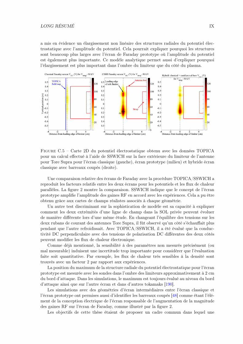
LONG RÉSUMÉ IX

a mis en évidence un élargissement non linéaire des structures radiales du potentiel élec-trostatique avec l’amplitude du potentiel. Cela pourrait expliquer pourquoi les structuressont beaucoup plus larges avec l’écran de Faraday prototype où l’amplitude du potentielest également plus importante. Ce modèle analytique permet aussi d’expliquer pourquoil’élargissement est plus important dans l’ombre du limiteur que du côté du plasma.

Figure C.5 – Carte 2D du potentiel électrostatique obtenu avec les données TOPICApour un calcul effectué à l’aide de SSWICH sur la face extérieure du limiteur de l’antennepour Tore Supra pour l’écran classique (gauche), écran prototype (milieu) et hybride écranclassique avec barreaux coupés (droite).

Une comparaison relative des écrans de Faraday avec la procédure TOPICA/SSWICH areproduit les facteurs relatifs entre les deux écrans pour les potentiels et les flux de chaleurparallèles. La figure 2 montre la comparaison. SSWICH indique que le concept de l’écranprototype amplifie l’amplitude des gaines RF en accord avec les expériences. Cela a pu êtreobtenu grâce aux cartes de champs réalistes associés à chaque géométrie.

Un autre test discriminant sur la sophistication de modèle est sa capacité à expliquercomment les deux extrémités d’une ligne de champ dans la SOL privée peuvent évoluerde manière différente lors d’une même étude. En changeant l’équilibre des tensions sur lesdeux rubans de courant des antennes Tore Supra, il fût observé qu’un côté s’échauffait pluspendant que l’autre refroidissait. Avec TOPICA/SSWICH, il a été évalué que la conduc-tivité DC perpendiculaire avec des tensions de polarisation DC différentes des deux côtéspeuvent modifier les flux de chaleur électronique.

Comme déjà mentionné, la sensibilité à des paramètres non mesurés précisément (oumal mesurable) induisent une incertitude trop importante pour considérer que l’évaluationfaite soit quantitative. Par exemple, les flux de chaleur très sensibles à la densité sonttrouvés avec un facteur 2 par rapport aux expériences.

La position du maximum de la structure radiale du potentiel électrostatique pour l’écranprototype est mesurée avec les sondes dans l’ombre des limiteurs approximativement à 2 cmdu bord d’attaque. Dans les simulations, le maximum est toujours évalué au niveau du bordd’attaque ainsi que sur l’autre écran et dans d’autres tokamaks [190].

Les simulations avec des géométries d’écran intermédiaires entre l’écran classique etl’écran prototype ont permises aussi d’identifier les barreaux coupés [48] comme étant l’élé-ment de la conception électrique de l’écran responsable de l’augmentation de la magnitudedes gaines RF sur l’écran de Faraday, comme illustré par la figure 2.

Les objectifs de cette thèse étaient de proposer un cadre commun dans lequel une

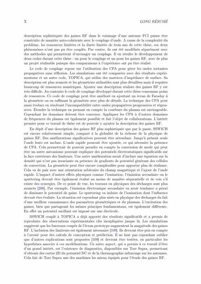
X LONG RÉSUMÉ

description sophistiquée des gaines RF dans le voisinage d’une antenne FCI puisse êtreconstruite de manière auto-cohérente avec le couplage d’onde. A cause de la complexité duproblème, les ressources limitées et la durée limitée de trois ans de cette thèse, ces deuxphénomènes n’ont pas pu être couplés. Par contre, ils ont été modélisés séparément avecdes méthodes qui permettent d’envisager un couplage. Il en résulte le développement dedeux codes durant cette thèse : un pour le couplage et un pour les gaines RF, avec de plusun projet réalisable puisque des comparaisons à l’expérience ont pu être réalisé.

Le code de couplage repose sur l’utilisation des CPA pour gérer les ondes sortantespropagatives sans réflexion. Les simulations ont été comparées avec des résultats expéri-mentaux et un autre code, TOPICA, qui utilise des matrices d’impédance de surface. Sadescription est plus avancée et les géométries utilisables sont plus détaillées mais il requièrebeaucoup de ressources numériques. Ajouter une description réaliste des gaines RF y esttrès difficile. Au contraire le code de couplage développé durant cette thèse consomme poinsde ressources. Ce code de couplage peut être amélioré en ajoutant un écran de Faraday àla géométrie ou en raffinant la géométrie avec plus de détails. La technique des CPA peutaussi évoluer en résolvant l’incompatibilité entre ondes propagatives progressives et régres-sives. Étendre la technique en prenant en compte la courbure du plasma est envisageable.Cependant les domaines doivent être convexes. Appliquer les CPA à d’autres domainesde fréquences du plasma est également possible et fait l’objet de collaborations. L’intérêtpremier pour ce travail de thèse est de pouvoir y ajouter la description des gaines RF.

En dépit d’une description des gaines RF plus sophistiquée que par le passé, SSWICHest encore relativement simple, comparé à la globalité de la richesse de la physique degaines RF. Des améliorations significatives peuvent être attendues. Jusqu’à présent seulel’onde lente est incluse. L’onde rapide pourrait être ajoutée, ce qui nécessite la présencede CPA. Cela permettrait de pouvoir prendre en compte la conversion de mode qui peutêtre un autre mécanisme pouvant expliquer des potentiels électrostatiques significatifs surla face extérieure des limiteurs. Une autre amélioration serait d’inclure une équation sur ladensité qui n’est pas invariante en présence de gradients de potentiel générant des cellulesde convection. La géométrie peut être encore complexifiée pour apporter plus de réalisme.Cela va de pair avec une orientation arbitraire du champ magnétique et l’ajout de l’onderapide. L’impact d’autres effets physiques comme l’ionisation, l’émission secondaire ou lesputtering devrait être également évalué au moins de manière séquentielle et de voir s’ilexiste des synergies. De ce point de vue, les travaux en physiques des décharges sont plusavancés [200]. Par exemple, l’émission électronique secondaire va avoir tendance a prioride diminuer le potentiel de gaine. Le sputtering va induire de l’ionisation dont l’influencedevrait être évaluée. La situation est cependant plus aisée en physique des décharges du faitd’une meilleur connaissance des paramètres géométriques et du plasmas. L’excitation desgaines, bien que partageant les mêmes principes fondamentaux, est également différente.En effet un potentiel oscillant est imposé sur une électrode.

SSWICH couplé à TOPICA a déjà apporté des résultats significatifs et a permis dereproduire des observations expérimentales clés inexpliquées jusque là. Les simulationssuggèrent que les barreaux coupés de l’écran prototype augmentent la magnitude des gainesRF. L’inclusion des limiteurs est également nécessaire [109]. Ils devront être pris en compteà l’avenir pour des calculs de conception et prédiction. Il ne faut pas cependant oublierque d’autres explications sont proposées [109] et devront être testées, en particulier leshypothèses associer à ces modélisations. Un autre aspect, qui a permis à ce travail d’êtred’un grand intérêt, est l’existence de diagnostics, disponibles sur Tore Supra, permettantd’obtenir des cartes 2D du potentiel DC et de la thermographie infrarouge sur les antennes.Cela fait de Tore Supra une des machines les mieux équipés pour l’étude des gaines RF.

LONG RÉSUMÉ XI

Les propriétés de la région privée de l’antenne reste cependant assez mystérieuse. Unmanque relatif de données expérimentales sur la région privée de l’antenne est à constateret a causé des soucis pour l’avancée de la thèse. La tâche n’est pas aisée. Des effort supplé-mentaires devraient être fournis pour caractériser les gaines RF dans cette zone avec desdonnées supplémentaires. Cela permettrait aussi de donner une meilleure interprétation aurésultats actuellement obtenus. Dans cette perspective, de petites machines telles que ISH-TAR ou ALINE dédiées à l’étude des gaines RF dans un environnement plus simple et plusfacilement maîtrisable que la SOL d’un tokamak représente une excellente opportunité. Unecomparaison des différents codes dans un cadre d’étude commun devrait également êtreentrepris pour identifier le degré de sophistication nécessaire ou des ingrédients à ajouter.Pour terminer, une attention particulière devrait être apportée à l’interface utilisateur ducode car l’utilisation d’un code est fortement lié à sa clarté et sa capacité à être mis enœuvre facilement.

RésuméUne bonne compréhension des interactions entre les ondes à la fréquence cyclotroniqueionique (FCI) (40− 80 MHz) et le plasma de bord est nécessaire pour injecter de façonfiable de fortes puissances dans un plasma de fusion en continu. Les objectifs de cette thèseétaient de modéliser séparément, avec Comsol Multiphysics, mais de façon compatible lecouplage d’ondes et la formation de gaines radio-fréquences (RF), qui rétroagissent sur lecouplage, pour aboutir à terme à une modélisation auto-cohérente.

Modéliser le couplage de l’onde rapide nécessite une description détaillée de l’antenneémettrice (2D ou 3D) et du plasma environnant par une approche pleine onde en plasmafroid. L’absorption des ondes sortant du domaine de simulation est émulée par des couchesparfaitement adaptées, rendues compatibles avec un tenseur diélectrique plasma. Les ten-dances expérimentales des résistances de couplage des antennes de Tore Supra sont qua-litativement reproduites mais l’efficacité de couplage est surestimée probablement à caused’une incertitude sur la largeur réelle de la couche d’évanescence des ondes FCI.

Parallèlement une description novatrice auto-cohérente, incluant les effets des gainesRF, de la propagation de l’onde lente et de la polarisation DC (Direct Current) résultantedu bord d’un plasma magnétisé a été développée avec le minimum d’ingrédients physiques.Dans le cas des antennes Tore Supra, le couplage du code avec TOPICA a permis d’expli-citer qualitativement certaines observations inattendues sur un écran de Faraday dont leschéma électrique visait à minimiser les gaines RF. Un transport de courants DC dans laSOL est apparu nécessaire pour expliquer les structures radiales des mesures. Les barreauxcoupés sont les éléments de l’antenne responsable de l’augmentation du potentiel plasma.

Mots-clés : gaine, onde, auto-cohérent, conditions aux limites, plasma, magnétisé,polarisation, Tore Supra, antenne, FCI, modélisation, Comsol

AbstractA correct understanding of the interactions between the edge plasma and the ion cyclotron(IC) waves (40− 80 MHz) is needed to inject reliably large amount of power required forself-sustainable fusion plasmas. These thesis objectives were to model separately, withComsol Multiphysics, but in compatible approaches the wave coupling and the RF sheathformation to anticipate development of a single code combining both.

Modelling of fast wave coupling requires a detailed description of the antenna (2D or3D) and of the plasma environment by a full wave approach for a cold plasma. Absorptionof outgoing waves is emulated by perfectly matched layers, rendered compatible with aplasma dielectric tensor. Experimental trends for the coupling resistance of the antennasof Tore Supra are qualitatively reproduced but the coupling efficiency is overestimated,most probably due to uncertainty of the real evanescence length of IC waves.

In parallel a novel self-consistent description, including RF sheaths, of the interplaybetween the cold wave propagation and DC (Direct Current) biasing of the magnetizededge plasma of a tokamak was developed with the minimum set of physics ingredients. ForTore Supra antenna cases, the code coupled with TOPICA allowed to unveil qualitativelysome unexpected observations on the latest design of Tore Supra Faraday screens whoseelectrical design was supposed to minimize RF sheaths. From simulations, a DC currenttransport appears necessary to explain the radial structures of measurements. Cantileveredbars have been identified as the design element in the antenna structure enhancing theplasma potential.

Keywords: sheath, wave, self-consistent, boundary conditions, plasma, magnetized,polarization, Tore Supra, antenna, ICRH, modelling, Comsol