arX

iv:0

812.

0812

v2 [

astr

o-ph

] 1

6 Ju

l 200

9Draft version July 16, 2009Preprint typeset using LATEX style emulateapj v. 04/20/08

COMPARISON OF SPECTRAL SLOPES OF MAGNETOHYDRODYNAMIC AND HYDRODYNAMICTURBULENCE AND MEASUREMENTS OF ALIGNMENT EFFECTS

A. Beresnyak, A. LazarianDept. of Astronomy, Univ. of Wisconsin, Madison, WI 53706

Draft version July 16, 2009

ABSTRACT

We performed a series of high-resolution (up to 10243) direct numerical simulations of hydro andMHD turbulence. Our simulations correspond to the ”strong” MHD turbulence regime that cannotbe treated perturbatively. We found that for simulations with normal viscosity the slopes for en-ergy spectra of MHD are similar to ones in hydro, although slightly more shallower. However, forsimulations with hyper viscosity the slopes were very different, for instance, the slopes for hydro sim-ulations showed pronounced and well-defined bottleneck effect, while the MHD slopes were relativelymuch less affected. We believe that this is indicative of MHD strong turbulence being less local thanKolmogorov turbulence. This calls for revision of MHD strong turbulence models that assume local“as-in-hydro case” cascading. Non-locality of MHD turbulence casts doubt on numerical determina-tion of the slopes with currently available (5123–10243) numerical resolutions, including simulationswith normal viscosity. We also measure various so-called alignment effects and discuss their influenceon the turbulent cascade.Subject headings: MHD – turbulence – ISM: kinematics and dynamics

1. INTRODUCTION

Turbulence is ubiquitous in astrophysical fluids whichare characterized by high Reynolds numbers. It af-fects key astrophysical processes, e.g. star formation(Elmegreen & Scalo 2004, McKee & Ostriker 2007). Theobservational signatures of turbulence are numerous andwell documented. For instance, random fluctuations onall scales, which is a sign of turbulence, has been detectedby a variety of observational techniques (see Crovisier& Dickey 1983, O’Dell & Castaneda, Armstrong et al.1994, Lazarian 2009). Turbulence is universal, becausethe laminar flows with high Reynolds numbers are practi-cal impossibility. It is driven by a variety of mechanismssuch as supernova explosions starbursts, stellar winds,AGN jets, etc. In Keplerian flows turbulence is gen-erated by magnetorotational instability (Velikhov 1959,Chadrasekhar 1960, Balbus & Hawley 1991). Galacticdisks are subject to the cosmic ray-induced Parker’s in-stability (Parker 1966).

Although, historically, hydrodynamic turbulence hasbeen applied to astrophysics, now it is accepted that foralmost all astrophysical fluid flows are coupled with mag-netic fields, at least on large scales. This necessitatesthe use of the dynamic equations that include electriccurrents and magnetic fields. The simplest approach inthis respect is the continuous non-relativistic one-fluiddescription, known as magnetohydrodynamics or MHD.This approach is broadly applicable to most of the astro-physical environments, such as Solar wind, Interstellarand Intercluster Medium, molecular clouds, stars interi-ors, and so on, although there are some exceptions, suchas ultra-relativistic jets and shocks, where full relativis-tic equations should be used or small scales of MolecularClouds, where, due to relatively low ionization rate, thetwo-fluid description of ions and neutrals is more appro-priate.

Electronic address: andrey, lazarian@astro.wisc.edu

The importance of astrophysical turbulence inspiresmuch of theoretical and numerical work aimed at un-derstanding its properties. We should clarify, however,that there are different types of MHD turbulence. Inthis paper we deal with strong MHD turbulence, whichcan not be treated perturbatively. The theory of weakAlfvenic turbulence, which has limited applicability toastrophysics, is discussed elsewhere (Sridhar & Goldre-ich 1994, Ng & Bhattacharjee 1996, Lazarian & Vishniac1999, Galtier et al. 2000, 2002). In order to study thebasic properties of MHD cascade and to be able to di-rectly compare to previous work, we restricted ourselvesto so-called balanced MHD turbulence or turbulence withzero net cross-helicity. The properties of imbalanced tur-bulence are studied in a companion paper Beresnyak &Lazarian (2009).

The issue of the spectral slopes of MHD turbulence hascaused a substantial interest recently. A sizable num-ber of papers attempting to measure true asymptoticspectral slope of high-Reynolds number MHD turbulencefrom direct numerical simulations appeared to date. Forexample, simulations of weakly compressible MHD tur-bulence performed in Haugen et al. (2003, 2004) usedfinite-difference code with numerical resolution of up to10243 with explicit viscous and resistive dissipation. Theenergy spectral slope for MHD was observed to be shal-lower than −5/3 which was interpreted as the influenceof the bottleneck effect. Another example is the paperof Muller & Grappin (2005) who measured the spectralslopes of decaying MHD turbulence without mean fieldand driven MHD turbulence with strong mean field. Thepseudospectral method with ordinary viscosity was ranat a numerical resolution of up to 10243. The authors ar-gued that the slope was close to −3/2 in the mean-fieldcase.

The motivation behind these and many other paperswas to understand the nature of the turbulent cascade.The turbulent energy transfer is, in a sense, a cen-

2

tral issue of turbulence, be it hydrodynamic or MHD.And while hydrodynamic turbulence has its “StandardModel”, the nature of MHD cascade is still debated.

An important first step in turbulence theory was madeby Iroshnikov (1963) and Kraichnan (1965) who noticedthat there is a local magnetic field which can not beexcluded by a choice of reference frame, like the aver-age velocity in hydrodynamics. Furthermore, they as-sumed that turbulence is weak, because perturbationsare smaller than the mean field. This implicitly assumedlocal isotropic dynamics and happened to be a mistake,since the turbulent cascade preferred perpendicular di-rection, i.e. produced perturbations that are more andmore anisotropic, this way increasing interaction and pre-venting turbulence from becoming weak.

The understanding of various aspects of MHD turbu-lence, including the role of turbulence anisotropy, com-pressibility, etc. resulted in a number of publications(see Dobrowolny, Mangeney, & Veltri 1980, Shebalin,Matthaeus & Montgomery 1983, Montgomery & Turner1984, Higdon 1984). For the most part of the paperwe will consider incompressible MHD turbulence, whichproperties are dominated by the Alfvenic perturbations.Interestingly enough, some properties of Alfvenic turbu-lence carry over not only to nearly incompressible lowMach number flows, but also for flows with Mach num-bers larger than unity (Cho & Lazarian 2003, see also§9.3).

It has been realized that interactions of Alfvenic modesin MHD turbulence has a tendency of getting stronger asthe cascades unfolds. Goldreich & Sridhar (1995, hence-forth GS95) proposed a particular model of strong tur-bulence when the interaction strength is being controlledby two competing processes: a perpendicular cascade (aconcept rigorously developed in a theory of weak Alfvenicturbulence, e.g. Galtier et al 2000), which tends to in-crease the interaction, and a decorrelation due to cas-cading which tends to increase the frequency of pertur-bations, and thus decrease the interaction. GS95 con-cluded that the interaction has to be marginally strong(“critical balance”), and therefore, the cascade has tobe of strong Kolmogorov type and has a spectral slopeof around −5/3. Predictions of this model, such asscale-dependent anisotropy, were subsequently observedin three-dimensional simulations (Cho & Vishniac 2000,Maron & Goldreich 2001, etc).

Recently, however, a number of models, motivated bynumerical spectral slopes shallower than −5/3, appeared(Boldyrev 2005, 2006, Gogoberidze 2007). The interestto this field has been heated by the numerical discov-ery of so-called scale-dependent polarization alignment(Beresnyak & Lazarian 2006), which was interpreted ina subsequent publication by Mason et al (2006) in favorof Boldyrev’s (2006) modification of GS95 model.

This paper is bringing attention to serious difficultiesthat appear when one tries to measure true asymptoticslopes from direct three-dimensional numerical simula-tions which have rather moderate Reynolds numbers.By comparing spectra of hydrodynamic and MHD tur-bulence we found that MHD turbulence might be muchmore nonlocal that Kolmogorov turbulence, and, there-fore, require much higher resolution to obtain spectralslope by brute force approach. The second part of thispaper brings polarization alignment to more numerical

scrutiny and compares the simulation results to theory.Our simulations allow to test some of the existing conjec-tures about properties of MHD turbulence. For instance,these results allow us to reject a conjecture in Boldyrev(2006) that the alignment is limited by the magnitude oflocal field wandering.

In what follows in §2 we describe our approach basedon comparing the properties of MHD and hydrodynamicturbulence, present our numerical setup in §3, presentspectra in §4, discuss anisotropy in §5, discuss the in-teraction weakening and the alignment effects in §6 and§7, respectively, and provide some more hints of the non-locality of the MHD cascade in §8. In §9 we compareour numerical results with the existing theoretical pre-dictions, as well as with the previous numerical work; wealso discuss the applicability of findings obtained with in-compressible simulations to the real-world compressibleastrophysical turbulence. Our conclusions are summa-rized in §10.

2. SLOPE MEASUREMENTS

Various claims were made on the value of MHD spec-tral slope, most of which were motivated by either Kol-mogorov −5/3 slope of strong turbulence (Kolmogorov1941, GS95), or various versions of −3/2 slope (Irosh-nikov 1963, Kraichnan 1965, Gogoberidze 2007, Boldyrev2006, etc). Most numerical studies aimed to confirm ei-ther of the above. A number of critical issues were over-looked, though. Below we present a novel perspective toslopes measurements in MHD. It turns out that it is in-correct to measure slopes directly from 3D numerics dueto a systematic error that comes with so-called bottle-neck effect. Also, it is impossible to measure MHD slopeby comparison with hydro slope, because the bottleneckeffect turns out to be different in hydro and MHD. Thisdifference, however, allows us to criticize models that relyon strong local Kolmogorov cascading, such as GS95 orBoldyrev (2006) 1.

To be precise, −5/3 is not the exact predicted slope forincompressible hydrodynamics. This number comes fromthe Kolmogorov self-similar cascade, but soon it was re-alized that realistic turbulence is not exactly self-similar.To correct for this, various models of intermittency wereproposed (Kolmogorov 1962, Obukhov 1962), with themost popular being She-Leveque model (1994) in whichthe predicted slope is around −1.70. This slope was veryclose to what was observed in highest-resolution DNSof Kaneda et al. (2003). In the aforementioned work itwas possible to separate spectrum into inertial range andrelatively more flat part that was due to a bottleneckeffect. Although modifications of S-L model for MHDturbulence have been proposed, numerical studies stilloften compare the spectrum slope with −5/3. Similarly,when one proposes a model of turbulence with −3/2 spec-tral slope it is often that numerical studies aim to findan exact correspondence with this slope, without regardfor intermittency. We believe that this is one importantstumbling block in numerical determination of slopes.

The other, probably much more important misunder-standing, is to disregard the systematic error that any

1 Local cascading models normally use a formula ǫ = ρv2

l /τl,where vl is the velocity perturbation on scale l, τl is the cascadingtimescale and ǫ is a constant equal to the energy dissipation rateper unit volume.

Comparison of MHD and Hydro turbulence 3

numerical measurement of slopes in DNS brings with it.The bottleneck effect is a pile-up of energy before thedissipation scale due to the relative lack of energy inthe dissipation range (see, e.g., Falkovich 1994). Dueto relatively low resolution of currently available simula-tions, this systematic error is always present. To makeit worse, most researchers present simulations with thehighest numerical resolution only. Although the amountof numerical resources available to different groups differsubstantially, most “high resolution” simulations to-datehave numerical boxes between 5123 and 10243. Fromthe point of length of inertial interval, and the influenceof bottleneck effect, the differences in linear scale of themultiple of two are tiny. Another systematic error comesfrom the effect of the driving scale. Often there is a dipright after the driving scale, an anti-bottleneck effect ofsorts, which appears, possibly, due to the excess of en-ergy on the driving scale. We are not aware of driventurbulence simulations that were able to get rid of thiseffect. We belive that disregarding these two effects andpresent numerical slopes as having no systematic errorat all is wrong.

In this paper we compare hydrodynamic and MHD en-ergy slopes obtained with the same code, the same driv-ing and exactly the same linear dissipation. Since thereare good theoretical predictions for asymptotic isotropichydro turbulence, we can try to use those. If one findsthat the nature of energy transfer in MHD and hydro issimilar (this is suggested in GS95 model where a stronglocal Kolmogorov-like cascade is assumed), then we candirectly compare MHD and hydro slopes and make state-ments on MHD slope. Unfortunately, as we show inthe two subsequent sections, this is not the case. Thedefining feature of our simulations is the use of differenttypes of linear dissipation, namely natural viscosity andhyper-viscosity. Although there had been some similarityin spectral slopes of MHD and hydro in normal-viscouscase, the hyper-viscous cases were very different. Thissuggests that the nature of MHD and hydro cascades aredifferent and one can not use slope comparison betweenMHD and hydro to get rid of the aforementioned system-atic error.

3. NUMERICAL SETUP

Incompressible MHD and Navier-Stokes equations canbe written in the following simple form

∂tw± + S(w∓ · ∇)w± = −νn(−∇2)n

w±, (1)

where S is a solenoidal projection and w± (Elsasser

variables) are defined in terms of velocity v and magneticfield in velocity units b = B/(4πρ)1/2 as w

+ = v + b

and w− = v − b. Navier-Stokes equation is a special

case of equations (1), where b ≡ 0 and, therefore, bothequations are equivalent with w+ ≡ w−. The RHS ofthis equation is a linear dissipation term which is calledviscosity or diffusivity for n = 1 and hyper-viscosity orhyper-diffusivity for n > 1. Here we assumed that vis-cosity and magnetic diffusivity is the same for velocityand magnetic field. This is almost never true for re-alistic astrophysical plasmas. However, as long as onewants to study the dynamics of large scale turbulence,it is acceptable. This is because the dissipation termsin today’s numerical simulations are never as small as to

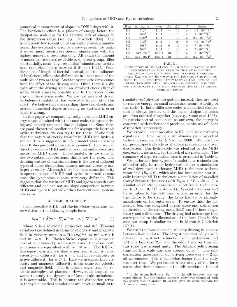
Run nx · ny · nz x:y:z B0 ∆t∗ f dissip.

H1 5123 1:1:1 – 16 v 4.5 · 10−4k2

H2 7683 1:1:1 – 10 v 7 · 10−13k6

H3 10243 1:1:1 – 7 v 2.2 · 10−13k6

M1 5123 1:1:1 1 24 v 4.5 · 10−4k2

M2 7683 1:1:1 0 10 v 7 · 10−13k6

M3 7683 1:1:1 1 10 v 7 · 10−13k6

M4 512 · 7682 10:1:1 10 10 v 7 · 10−13k6

M5 512 · 10242 10:1:1 10 10 w± 2.2 · 10−13k6

TABLE 1Description of simulations. * - ∆t is the duration of the

high resolution runs, prior to that we ran lowerresolution runs for a long time to ensure stationary

state. E.g. we ran B0 = 0 case for 180 time units prior togoing to high resolution. Only last 3-4 time units of highresolution runs were used for measurements. One time

unit corresponds to an eddy turnover time of the largestcoherent eddies.

simulate real physical dissipation, instead, they are usedto remove energy on small scales and assure stability ofthe code. In finite-difference codes a numerical dissipa-tion is always present and the linear dissipation termsare often omitted altogether (see, e.g., Stone et al 1998).In pseudospectral code, such as our own, the energy isconserved with rather good precision, so the use of lineardissipation is necessary.

We evolved incompressible MHD and Navier-Stokesequations in time using a well-known pseudospectraltechnique (see, e.g., Cho & Vishniac 2000). We have cho-sen pseudospectral code as it allows precise control overdissipation. Our hydro code was identical to the MHDone, except, naturally, for the lack of magnetic field. Thesummary of high-resolution runs is presented in Table 1.

We performed four types of simulations: a simulationof statistically isotropic hydro turbulence; a simulationof well-developed stationary MHD turbulence withoutmean field (B0 = 0), which also has been called statisti-cally isotropic MHD turbulence; a simulation of so-calledtransAlfvenic turbulence (with B0 = 1, δB ∼ δv ∼ 1); asimulation of strong anisotropic subAlfvenic turbulence(with B0 = 10, δB ∼ δv ∼ 1). Special attention hadto be taken to the last case, where, in order for theturbulence to be strong, the fields had to be stronglyanisotropic on the outer scale. To ensure this, the nu-merical box was elongated in real space and x-direction(a direction of the strong mean field) was 10 times longerthan y and z directions. The driving had anisotropy thatcorresponded to the dimensions of the box. Thus in thiscase our setup is similar to one in Maron & Goldreich(2001).

We used random solenoidal velocity driving in k-spacebetween k=2 and 3.5. The largest coherent eddy size L(determined by structure function technique) was around1/4 of a box size (2π) and the eddy turnover time forthis scale was around unity. The Alfvenic self-crossingtime for this scale was also around unity 2. The self-correlation timescale for our driving force was τ = 2 forall wavemodes. This is somewhat longer than the eddyturnover time. We performed a test study of the forcecorrelation time influence on the self-correlation time of

2 In the strong field case, B0 = 10, the Alfven speed was tentimes higher, but the largest coherent eddy was elongated withx/y aspect ratio of around 10, so this gives the same estimate forAlfvenic crossing time.

4

velocity, taking τ = 1/4, 2, 8 and found no systematic de-pendence. The self-correlation timescale of velocity wasalways around unity. We concluded that, in the caseof strong turbulence, the self-correlation timescale of ve-locity is primarily determined by nonlinear interaction,rather than driving 3. We ran another, higher resolutionsimulation, trying to find a difference in slopes betweensimulations with τ = 2 and τ = 6 and found none. Note,that numerical studies do vary in terms of τ . For in-stance, Muller & Grappin (2005) used driving constantin time, and Haugen et al. (2004) used δ-correlated driv-ing. Our tentative conclusion is that the difference in τmarginally affects the results of numerical simulations ofturbulence. In addition, in simulation M5 we used El-sasser driving 4 instead of velocity driving, to check if itchanges the tendencies observed in previous runs.

One of the advantages of driven versus decaying simu-lations is that it describes a stationary random process,so, by applying ergodic hypothesis one can approximatestatistical averages with time-averages. While, in decay-ing simulations, if one wants to average over time to re-duce fluctuations, some hypothesis on the decaying pro-cess has to be adopted 5.

4. SPECTRA (3D-AVERAGED AND 1D).

Usually, bottleneck effect, a pile-up of energy nearthe dissipation scale, is discussed in relation to hyper-viscosity (Cho & Vishniac 2000) or numerical viscosity(Kritsuk et al. 2008). But the bottleneck effect wasalso predicted (Falkovich 1994) and numerically observed(Kaneda et al. 2003) for normal viscosity. This meansthat the slopes, measured in limited resolution simula-tions with normal viscosity, do not necessarily reflect trueasymptotic slopes.

Fig. 1 shows Ek, a three-dimensional power spectrumF (k) integrated over angle in k-space:

Ek =

∫|k|=k

F (k)dk. (2)

This is the most popular choice for spectrum in numer-ical turbulence since it is fairly straightforward to cal-culate. Because k-space is discrete, the integration is asummation of energies of all modes that lay in a shell of k-magnitudes between n and n+1. The number of modes,that fall into each shell, fluctuates, so this spectrum hasa characteristic toothed shape which is not remedied bytime integration. We plot Ek so that our results can bedirectly compared to previous numerical work that usedthis quantity.

In the strongly anisotropic, subAlfvenic simulations (asin runs M4 M5) it makes sense to measure a perpendic-ular spectrum (i.e., integrated over k‖ and then over thedirection of k⊥). This spectrum, however, was virtuallyidentical to 3D spectrum integrated over solid angle, i.e.,Ek, so, for uniformity, we plot only Ek in all cases.

3 One can argue that in case of the absence of nonlinear termthe equation ∂tv = f will give infinite correlation time for v evenif f self-correlation time is finite.

4 Each of the pair of Elsasser-field equations in MHD bear closeresemblance to Navier-Stokes equation. Elsasser variables are de-fined as w± = v ± b, where b is magnetic field in velocity units.

5 Normally, one wants to normalize the spectrum as inMuller & Grappin (2005), but this entails the hypothesis that spec-tra are similar at different stages of decay.

Fig. 1.— Three-dimensional angle-integrated spectra for all runs,compensated by a factor of k3/2. We multiplied the spectra by aquotient of 3 to separate them from each other. Top: H1, M1;middle: H2, M2, M3, M4; bottom: H3, M5. A significant increasein perceived “inertial interval” between top plot and bottom plotsis mostly due to difference between normal viscosity and hyper-viscosity, rather than resolution.

The parallel spectrum (integrated over k⊥) was of nointerest to us, since there are no clear theoretical predic-tions for it 6.

We also measured so-called one-dimensional spectraPk, which is a power spectrum of the vector field sampledalong an arbitrary line and then averaged over ensemble.It can also be written as a Fourier transform of the cor-relation function B(r) (Monin & Yaglom 1975):

Pk =1

π

∫ ∞

−∞

e−ikrB(r)dr. (3)

Although most simulations measure Ek, the struc-ture/correlation function scalings are the primary predic-tions of the Kolmogorov model, so it makes more sense tomeasure Pk rather than Ek. Also, Pk is less prone to bot-tleneck effect (Dobler et al. 2003). We measured Pk by

6 One can relate this spectrum to the parallel structure func-tion, calculated with respect to global mean field. This SF, how-ever, do not show properties, predicted by GS95 model. The pre-ferred way is to calculate SFs with respect to local mean field(Cho & Vishniac 2000).

Comparison of MHD and Hydro turbulence 5

Fig. 2.— One-dimensional spectra, compensated by k3/2.

averaging over directions in each particular snapshot andthen averaging over time. Pk is presented in Fig 2. Forthe fully statistical homogeneous isotropic sample withinfinite spacial resolution and infinite dimensions onecan derive relation Ek = −kdPk/dk (Monin & Yaglom1975). Numerically speaking, for a discrete sample withperiodic boundaries this relation is satisfied fairly well.It ensures that in an infinite inertial interval Ek and Pk

will have the same slope. In a limited resolution of oursimulations the slopes of Ek and Pk are fairly differentthough. We feel that this difference is another useful in-dication that numerical determination of slopes is ratherlimited (see also §2).

5. ANISOTROPY

Hydrodynamic turbulence is presumed to be isotropicon small scales, while MHD turbulence is anisotropic andthis anisotropy increases to small scales without limit(GS95). The scale-dependent anisotropy, predicted byGS95 was first observed in Cho & Vishniac (2000) bythe method of second-order structure functions and con-firmed in a number of subsequent publications. It is crit-ical that structure function is calculated with respect tothe local magnetic field, otherwise the scale-dependentanisotropy is not observed (see discussion on various def-inition of the “local mean field” in Beresnyak & Lazarian2008). Fig. 3 shows two-dimensional structure functionwhere x-axis measured distance along local mean mag-netic field while y-axis measured distance perpendicularto the field. In hydrodynamic case the “preferred” direc-tion was chosen arbitrarily. Quite predictably, the hydro-

Fig. 3.— Contours of the structure function < |v(r+R)−v(r)|2+|b(r + R) − b(r)|2 >r where R takes arbitrary angles with respectto the local magnetic field (for hydro case this direction was chosento be along x). X-axis is perpendicular component, while y-axis is

parallel component. Dashed line correspond to GS95 r‖ ∼ r2/3

⊥ .Hydro turbulence show isotropy on small scales, while MHD tur-bulence show scale-dependent anisotropy.

dynamic turbulence is isotropic. The MHD turbulence,however, is scale-dependently anisotropic. For example,B0 = 0 case is isotropic on outer scale and B0 = 1 caseis almost isotropic on outer scale, but on small scalesboth are anisotropic with anisotropy ratio of around 4.The B0 = 10 case is anisotropic on outer scale and thisanisotropy increases by about a factor of 4 towards smallscales. These results are approximately consistent withthe predictions of GS95.

In order to study deviations from prediction of GS95,

r‖ ∼ r2/3⊥ , we created a correspondence between parallel

and perpendicular scales and plotted it on Fig. 4. Thiscorrespondence was achieved by finding equal values ofparallel and perpendicular second order structure func-tions as in Cho & Vishniac (2000) or Maron & Goldreich(2001). The observed deviations could be connected tononlocality, and/or alignment effects which are discussedfurther.

6. NUMERICAL EVIDENCE OF INTERACTIONWEAKENING

In GS95 turbulent non-linear interactions are strongand the cascading happens fast. In this approach theKolmogorov’s ∼ −5/3 spectral slope is expected. In or-der to explain shallower slopes Boldyrev (2006) conjec-tured that interaction is depleted in strong anisotropicturbulence by a factor which is similar to that in theIroshnikov-Kraichnan (IK) model, i.e. δv/vA. In sim-ulations with real viscosity we obtain MHD dissipationscale dνMHD which is somewhat larger than hydro dis-sipation scale dνHD, which can be an indication of de-pletion of interaction. Figs 1 and 2, upper panel, indi-cate that dνMHD is approximately 1.3 times larger thandνHD, which is consistent with the difference in dissipa-tion scales of Kolmogorov and IK models, assuming thelength of the inertial interval L/dν of around 7. However,this result can also be explained by the difference in Kol-

6

Fig. 4.— Deviation of anisotropy from GSlaw Goldreich & Sridhar (1995) Λ ∼ λ2/3. M2, M3 and M4are shown. M5 shows behavior similar to M4, and M1 is similarto M3.

mogorov constant CK of hydro and MHD turbulence.Indeed, for MHD CK ∼ 2.2 (Biskamp 2003), while for

hydro CK ∼ 1.6 (Frisch 1995), also note that dν ∼ C3/4K .

Thus, this way of proving the weakening of interaction isstill controversial.

7. ALIGNMENT EFFECTS.

While most MHD turbulence models use mean-fieldapproach and assume that turbulence is characterizedfully by spectrum or structure functions of the fields,i.e. 〈δv2〉 and 〈δb2〉, recently a considerable attention hasbeen drawn to so-called alignment effects (Boldyrev 2005;Beresnyak & Lazarian 2006; Boldyrev 2006). The align-ment effects can be understood, in general, as a propertyof multi-variate pdf of the fields containing various corre-lations. The scale-independent alignment effects are notso interesting, because they can only modify the Kol-mogorov constant of turbulence, while scale-dependentalignment can, in principle, modify the slope.

Consider the alignment of Alfven mode when all per-turbations are perpendicular to the local magnetic field,i.e. lie in the same plane. For this purpose we use struc-ture functions where vectors are projected on l × B di-rection where l is the direction, connecting two points(Beresnyak & Lazarian 2006). While a study a full mul-tivariate PDF could be an overwhelming task, one canintroduce a few statistical measures of alignment thatcould be of interest. Alignment, derived from zeroth or-der statistical moments: angle alignment,

AA = 〈| sin θ|〉, (4)

where θ is an angle between Elsasser variables perturba-tions δw+ = δv + δb and δw− = δv− δb, another anglealignment,

AA2 = 〈| sin θ2|〉, (5)

where θ2 is an angle between δv and δb. Alignmentderived from second order statistical moments, “polar-ization intermittency” (Beresnyak & Lazarian 2006):

PI = 〈|δw+δw− sin θ|〉/〈|δw+δw−|〉; (6)

imbalance measure

IM = 〈|δ(w+)2 − δ(w−)2|〉/〈δ(w+)2 + δ(w−)2〉; (7)

imbalance correlation

IC = 〈|δw+δw−|〉/〈δ(w+)2 + δ(w−)2〉, (8)

velocity and magnetic fields correlation

FC = 〈|δv||δb|〉/〈δv2 + δb2〉 (9)

(we found that FC is almost constant in our measure-ments and it will be assumed constant thereafter). IMand IC are describing the same effect, namely dynamicimbalance between Elsasser variables δw+ and δw−, butin a different way. For independently distributed Gaus-sian fluctuations one has AA = AA2 = PI = IM = 2/π,IC = 1/π.

Physically, one may have only two types of alignment,because there are four variables (two vectors) minusnormalization and minus one arbitrary rotation alongaxis perpendicular to the magnetic field. Let us choosePI and IC as two measures of alignment. PI is inter-esting, because it is the factor, by which an interac-tion is reduced in a nonlinear MHD term (δw · ∇)δz ∼(δw · kz)δz ∼ δwkzδz sin θ with respect to mean field es-timate of δwkzδz (Boldyrev 2005). This quantity, alongwith AA, was first measured in numerical simulations byBeresnyak & Lazarian (2006). In the subsequent publi-cation Mason et al. (2006) used a second order structurefunction measure, very similar to PI, termed “dynamicalignment”

DA = 〈|δvδb sin θ2|〉/〈|δv||δb|〉. (10)

It can be expressed, to a constant, as DA ∼ PI ·IC/FC ∼PI · IC (since w

+ × w− = −2v × b), i.e. it is a combi-

nation of polarization intermittency and imbalance cor-relation IC. It is not clear yet, whether intermittent im-balance can reduce interaction in the balanced turbu-lence. For example, if one estimates energy dissipationas δw+δw−(δw+ + δw−)/λ (Lithwick et al. 2007), it isinsensitive to the dynamic imbalance δw±±ǫ, to the firstorder of ǫ. But one also may argue that the imbalancedcase is more complicated and the interaction is reduced(Beresnyak & Lazarian 2008, 2009)

Numerically speaking, alignment effects were very sim-ilar for all sub-Alfvenic and trans-Alfvenic cases7. Fig.4 shows different alignment measures described in thissection for M5 (B0 = 10, Elsasser driving). In the mid-dle of the inertial interval alignment factors depend on kas AA ∼ k0.022, AA2 ∼ k0.059, PI ∼ k0.105, IC ∼ k0.084,IM ∼ k−0.090, DA ∼ k0.207. Note, that DA is shortof the k0.25 dependence predicted for “alignment an-gle” in Boldyrev (2006). The alignment dependence inthe velocity-driven, B = 10 M4 simulation is somewhatdifferent: AA ∼ k0.028, AA2 ∼ k0.052, PI ∼ k0.137,IC ∼ k0.054, IM ∼ k−0.057, DA ∼ k0.189. If one wantedto explain the difference in slopes between M4 and M5(∼ 0.05, Fig 2) by the difference in DA slopes (accord-ing to Boldyrev (2006) the DA slope α adds 2/3α to thespectral slope), such an explanation would be impossible.

7 Beresnyak & Lazarian (2006) observed alignment not only inincompressible simulations, but in trans-Alfvenic, trans-sonic com-pressible simulations as well.

Comparison of MHD and Hydro turbulence 7

Fig. 5.— Various alignment measurement from M5.

On the other hand, M4 and M5 are significantly differ byIM, which suggests that shallow slopes are primarily dueto imbalance.

M3 (B0 = 1, velocity driven) simulation show align-ment effects which are similar to M4. This directly con-tradicts to the prediction in Boldyrev (2006), that thealignment is a function of δB/B0, as we observe essen-tially the same alignment in simulations with δBL/B0 =1 and δBL/B0 = 0.1 (see also Fig. 6). We therefore con-clude that the alignment is an intermittency effect8 thataccumulates along the cascade, rather than being deter-mined rigidly by δBλ/B0 as in Boldyrev (2006). Alter-natively, the alignment could be a natural feature of thenonlocal energy transfer. This calls for further investiga-tion.

8. OTHER HINTS ON NONLOCALITY.

In the sub-Alfvenic turbulence, the properties are well-represented by Elsasser variables w± and, if we assumelocality of interaction of δw+

l and δw−l , the properties

of δvl and δbl are supposed to be identical. However,we observed notable differences even after large statisti-cal averaging. Namely, the magnetic energy was higherthan kinetic energy in subAlfvenic runs M4 and M5.The last case, which was driven by Elsasser variables,show 50% magnetic energy excess on large scales andaround 20% on small scales. This so-called residual en-ergy which was proposed to have “-2” spectrum scaling(Muller & Grappin 2005) but was somewhat shallowerthan “-2” in this Elsasser driven run. Other runs didnot show any regular scaling for residual energy. For ex-ample, statistically isotropic MHD turbulence M2 showdominance of kinetic energy on large scales (which is typ-ical for MHD turbulence driven with velocity on outerscale), but on small scales magnetic energy dominates(which is typical for almost any driven MHD turbulence).This reinforces our conjecture that currently available 3DMHD simulations do not yet exhibit inertial ranges andthe flat portion of the spectrum can not be considered apart of the inertial range of local Kolmogorov-type tur-

8 An intermittency correction is usually written as a function ofthe ration of the scale in question to the outer scale, e.g. δv2

l =

C(ǫl)2/3(l/L)α, where (l/L)α is the intermittency correction. Inour case we also see that the alignment is a function of l/L.

bulence until a number of other conditions are satisfied,among which is an equipartition between spectral kineticand magnetic energies.

9. DISCUSSION

9.1. Theory

The nature of the turbulent cascade and the slope ofthe spectrum of fluctuations is a central issue of tur-bulence and has been discussed in a majority of pa-pers devoted to turbulence theory and numerics. Thehydrodynamic isotropic turbulence has its “StandardModel” which is based on Kolmogorov’s assumption ofself-similarity 9 and Kolmogorov’s “-4/5 law”:

〈(δv‖(l))3〉 = −

4

5ǫl. (11)

Assuming similarity 〈(δv‖(l))3〉 ∼ 〈(δv(l))2〉3/2 one ob-

tains the second order structure function slope of 2/3which correspond to spectral slope of −5/3. In MHD, re-lations, similar to Kolmogorov’s “-4/5 law”, exists, e.g.,

〈δw∓‖ (l)(δw±(l))2〉 = −

4

Dǫ±l (12)

(Chandrasekhar 1951, Politano & Pouquet 1998)10.However, in MHD case, this does not directly hints onscalings for 〈(δw±(l))2〉 and it is not clear which similar-ity hypothesis has to be adopted. A nice demonstrationof this is to apply the aforementioned exact relations tothe case of weak turbulence, where, in the ansatz of three-wave interaction, one has to obtain 〈δw∓

‖ (l)(δw±(l))2〉 ∼

a(l)〈(δw(l))4〉/vA (anisotropy a(l) is defined as a ratioof parallel scale Λ(l) to perpendicular scale l), whichis very much unlike the Kolmogorov similarity hypothe-sis. Thus, the spectral slope scalings are still uncertain,which stimulates further research in this field, includingattempts to measure the slope numerically.

The nonlocality of turbulent energy transfer has beenclaimed in quite a few publications. In the discussionof this numerical work we will mention the most rele-vant ones and defer more exhaustive discussion to futurereview papers.

It was suggested in Gogoberidze (2007) that in MHDturbulence with strong mean field the nonlinear inter-action could be nonlocal, with outer scale perturbationsdecorrelating high-frequency interacting eddies, leadingto IK-type (Iroshnikov 1963; Kraichnan 1965) interactionweakening and −3/2 spectrum. However, in aforemen-tioned model the energy cascading itself is local 11 andis performed by high-frequency eddies, i.e. there is noenergy transfer from large scales directly to small scales.We conclude that this model can not explain the lack ofbottleneck effect, observed in simulations.

In a recent model of imbalanced MHD turbulence(Beresnyak & Lazarian 2008) the eddies of the dominant

9 This assumption is not precisely satisfied because of so-calledintermittency. The most popular descriptions of intermittency areprobabilistic models (Obukhov 1962, Kolmogorov 1962, She & Lev-eque 1994). They give corrections to spectral slopes and higher-order scaling exponents assumed in self-similar model

10 D = 3 for statistical isotropy and isotropic structure functionor D = 2 for cylindrical symmetry and perpendicular structurefunction, e.g. in turbulence with strong mean field.

11 In a sense that ǫ = v2

l /τl is used, see also §2.

8

Fig. 6.— A comparison of DA in sub-Alfvenic (M4, dotted) andtrans-Alfvenic (MHD3b1h, dashed) simulations with δB/B pre-diction of Boldyrev (2006). δB/B is estimated from 2nd ordertransverse (or isotropic) structure function.

component on a certain scale are aligned not with re-spect to the local magnetic field on the same scale as inCho & Vishniac (2000) (balanced turbulence), but withrespect to magnetic field on some larger scale. Onemay speculate that even in the balanced case the dy-namic imbalance can cause polarization alignment, or,more likely, that these effects are interrelated. WhileBeresnyak & Lazarian (2008), by itself, is a mean fieldmodel and reproduce locality, “-5/3” spectrum and “2/3”anisotropy of GS95 in the balanced limit, its future exten-tions to include local imbalance and polarization align-ment seems promising.

Does the hypothesis of Boldyrev (2006) that the v andb alignment is limited by field wandering is justified fromtheory ground? In a little thought experiment one canimagine a perfectly aligned state where the magnitudesof v and b are equal. This is a case of a perfect im-balance and also an exact solution of MHD equations.Such a state will propagate without distortion, in otherwords, no de-alignment is going to happen, although thisstate certainly has some level of field wandering. Thisthought experiment hints that the hypothesis of v andb alignment being limited by field wandering directlycontradicts MHD equations. The effect of local imbal-ance, therefore, has to be treated in a more complicatedway. Fig. 6 shows a comparison between field wandering(δB/B) and “dynamic alignment” in transAlfvenic M3and subAlfvenic M4. We see that in subAlfvenic casethe dynamic alignment is an order of magnitude off theδB/B, which is in contrast with Boldyrev (2006) whichsuggest that DA ∼ δB/B.

9.2. Previous numerical work

The study of weakly compressible MHD turbulence byHaugen et al. (2003, 2004) revealed some difference inbottleneck effect in hydro and MHD cases, although theauthors reported bottleneck behaviour as “very similar”.The difference was small, possibly, due to adopted firstorder viscous and resistive dissipation. Aforementionedwork, however, used finite-difference code and, inadver-tently, the numerical dissipation had a different characterin MHD and hydro simulations, which precluded a rig-orous comparison. Nevertheless, we can say that it isconsistent with what we see in our incompressible simu-lations.

Biskamp et al. (1998) studied two-dimensional MHD

and EMHD turbulence. They noticed that both MHDand EMHD cases have an unusual nonlocal bottleneckeffect, which appeared differently depending on numer-ical resolution. It is possible that spectral flatteningfrom such an effect can be perceived as a ”false” in-ertial interval and lead to an incorrect estimate of theslope. Although there had been much discussion on theanalogy between two-dimensional MHD turbulence andMHD turbulence with strong mean field, the predom-inant picture is that Alfvenic turbulence is essentiallythree-dimensional (GS95, Cho & Vishniac 2000, Maron& Goldreich 2001, Cho et al. 2002).

Yousef et al. (2007) claimed that in the statisticallyisotropic MHD turbulence (similar to our simulation M2)one has a folded magnetic field structures that directlynon-locally interact with outer-scale motions. They con-cluded that one can not use Kolmogorov argumentationbecause of this nonlocality. We, however, belive, thatKraichnan’s argumentation regarding the dominance oflocal mean field, i.e. the Alfven effect, is correct even inthe case of B0 = 0. This is somewhat hard to demon-strate in 3D numerics, however, because for B0 = 0 thereis a transition region between outer scale and inertial in-terval where kinetic energy dominates and the magneticspectrum is very flat, i.e., there is no clear dominance ofthe large-scale magnetic field. Also the use of first-order(natural) viscosity in aforementioned three-dimensionalsimulations made the inertial range very short, whichcreated an illusion of a universal folded magnetic fieldstructure.

Alexakis et al. (2005a, 2005b) used a specific numeri-cal tool to quantify the transfer of energy between scalesin both hydro and MHD turbulence. They claimed thatMHD case is somewhat nonlocal. However, the moreradical claim is that the hydro cascade and the largerpart of MHD cascade is extremely local, i.e. the energyis not transferred between k and 2k, as in Kolmogorovmodel, but instead between k and k + k0 where k0 is de-termined by outer scale, which breaks self-similarity. Wefind these results rather puzzling and defer discussion un-til independent confirmation is available. Until then, weassume that Kolmogorov picture is roughly appropriatefor isotropic hydrodynamic turbulence with large inertialrange.

9.3. Implications for astrophysical turbulence

Realistic astrophysical turbulence is, in general, com-pressible. The examples of weakly compressible flowsare the quiet convection in main sequence stars and tur-bulence in very hot intracluster gas. The turbulence inmost of the Interstellar Medium, however, is stronglycompressible, due to effective cooling. This raises thequestion of to what extend the results of incompressiblesimulations are applicable to astrophysics. Intuitively,one could expect that weak small-amplitude Alfven andslow-mode turbulent perturbations should be nearly in-compressible. The question is how to deal with the fastmode and large-amplitude MHD turbulence in compress-ible fluids.

The coupling of Alfvenic motions and compressible mo-tions is a difficult subject. Theoretical arguments thatfast, slow and Alfven modes may create independent en-ergy cascades were provided in GS95, Lithwick & Goldre-ich (2001) and Cho & Lazarian (2003). These arguments

Comparison of MHD and Hydro turbulence 9

were applicable to strong Alfvenic turbulence12. Cho &Lazarian (2002, 2003) numerically demonstrated that foreven for appreciable Mach numbers (up to 10), the prop-erties of Alfvenic modes (scalings and anisotropy) weresimilar to those in incompressible simulations13. Theyalso showed that the decay time for the Alfvenic modesis fast and not mediated through coupling with com-pressible motions, which used to be the common wisdomat the time of the study. The effect of scale-dependentpolarization alignment, a characteristic of Alfvenic cas-cade discussed in this paper, happen to be present inboth compressible and incompressible MHD simulations(Beresnyak & Lazarian 2006). While the extend to whichstrong shocks can modify the Alfvenic cascade deservesmore study, the arguments above make us confident thatthe studies of incompressible turbulence are of primaryimportance to understand astrophysical turbulence.

There is another issue, which is frequently ignoredwhen one compares numerical MHD with interstellarturbulence. If magnetic fields are perfectly frozen intothe fluid, turbulence creates multiple small-scale currentsheets which are difficult to dissipate. Within such zonesthe frozen-in condition is no longer valid and magneticreconnection takes place (see Biskamp 2000, Priest &Forbes 2000, Bhattacharjee 2004, Zweibel & Yamada2009). The Lundquist number S ≡ LVA/η that char-acterizes how well magnetic fields are frozen in (L is thescale of the current sheet and η is magnetic diffusivity),is very high, e.g. > 1010, for most astrophysical flu-ids and is fairly low, e.g. < 104, for MHD simulations.If magnetic reconnection in astrophysics depends on S,this presents not only a problem for most of MHD sim-ulations, e.g. simulations of dynamo, molecular clouds,accretion disks, but also means that the numerical re-sults on turbulent scalings may not be trusted. We be-lieve that the extensive observational data suggests thatmagnetic reconnection is fast. Also, a model predictingfast reconnection in turbulent fluids, Lazarian & Vish-niac (1999), has been successfully tested in Kowal et al.

(2009). This gives additional support to numerical test-ing of astrophysical turbulence.

The slopes and turbulence anisotropies are importantfor a variety of astrophysical phenomena. For instance,scattering and turbulent acceleration of cosmic rays de-pends on the scaling of MHD turbulence (see Chandran2000, Yan & Lazarian 2002, 2004). So does the per-pendicular diffusion of cosmic rays and heat transportin plasmas (Narayan & Medvedev 2001, Lazarian 2006).Naturally, it is important to establish the true scalingsof MHD turbulence. This paper testifies that a higherresolution numerical simulations are required for accu-rate testing of the present and future MHD turbulencemodels.

10. CONCLUSIONS

We conclude that although the Kolmogorov-likeGoldreich-Sridhar (GS95) model is appealing, simple andcaptures some essential physical properties of the strongMHD turbulence, such as scale-dependent anisotropy, itshould be amended to explain cascade nonlocality andscale-dependent alignment effects. How to achieve thisis the issue of the future research, as we demonstrate thatthe existing attempts to improve GS95 do not agree wellwith the presented numerical simulations. In addition,we issue a note of warning that the numerical measure-ments of the spectral slope that served as a motivation formany of theoretical studies are unlikely to represent thetrue theoretical slopes due to the non-locality of MHDcascade.

AB thanks IceCube project for support of his research.AB thanks TeraGrid and NCSA for providing computa-tional resources. AL acknowledges the NSF grant AST-0808118 and support from the Center for Magnetic Self-Organization. Both authors are grateful to anonymousreferee for useful suggestions.

12 The more detailed study (Chandran 2005) of weak Alfvenicturbulence in a pressure-less medium showed that the interactionsbetween the fast and Alfvenic modes may be significant in a certainregions of k-space.

13 Density perturbations, which are absent in incompressibleflows, are definitely affected by compressible motions. However,

Beresnyak et al. (2005) found that the structure of logarithmof density reveal scale-dependent anisotropy, similar to GS95 law.This presumes that a significant fraction of density structures arecreated by shearing by Alfvenic perturbations.

REFERENCES

Alexakis, A., Mininni, P. D., & Pouquet, A. 2005, Phys. Rev.Lett., 95, 26, 264503

Alexakis, A., Mininni, P. D., & Pouquet, A. 2005, Phys. Rev. E,72, 4, 046301

Armstrong, J. W., Rickett, B. J., & Spangler, S. R. 1995, ApJ,443, 209

Balbus, S. A., & Hawley, J. F. 1991, ApJ, 376, 214Beresnyak, A., Lazarian, A., & Cho, J. 2005, ApJ, 624, 93LBeresnyak, A., Lazarian, A. 2006, ApJ, 640, L175Beresnyak, A., Lazarian, A. 2008, ApJ, 678, 961Beresnyak, A., Lazarian, A. 2009, ApJ submitted,

arXiv:0904.2574Bhattacharjee, A. 2004, ARA&A, 42, 365Biskamp, D., Schwarz, E., & Celani, A. 1998, Phys. Rev. Lett. 81,

4855Biskamp, D. 2000, Magnetic Reconnection in Plasmas

(Cambridge, UK:Cambridge University Press)Biskamp, D. 2003, Magnetohydrodynamic Turbulence.

(Cambridge: CUP)Boldyrev, S. 2005, ApJ, 626, L37

Boldyrev, S. 2006, Phys. Rev. Lett., 96, 115002Chandran B.D.G., Phys. Rev. Lett., 85 (22), 4656-4659 (2000)Chandran, B. D. G. 2005, Physical Review Letters, 95, 265004Chandrasekhar, S. 1951, Proc. Roy. Soc. London, Ser. A, 204, 435Chandrasekhar, S. 1960, Proceedings of the National Academy of

Science, 46, 253Cho, J., & Lazarian, A. 2002, Phys. Rev. Lett., 88, 24, 5001Cho, J., & Lazarian, A. 2003, MNRAS, 345, 325Cho, J., Lazarian, A., & Vishniac, E. T. 2002, ApJ, 564, 291Cho, J. & Vishniac, E. 2000, ApJ, 539, 273Crovisier, J., & Dickey, J. M. 1983, A&A, 122, 282Dobler, W., Haugen, N. E., Yousef, T. A., Brandenburg, A. 2003,

Phys. Rev. E, 68, 026304Dobrowolny, M., Mangeney, A., & Veltri, P. 1980, Physical

Review Letters, 45, 144Elmegreen, B. G., & Scalo, J. 2004, ARA&A, 42, 211Galtier, S., Nazarenko, S.V., Newel, A.C., Pouquet, A., J. Plasma

Phys., 63, 447 (2000)Galtier, S., Nazarenko, S., Newell, A., & Pouquet, A., ApJ, 564,

L49 (2002)

10

Gogoberidze, G. 2007, Phys. Plasmas, 14, 022304Goldreich, P., & Sridhar, S. 1995, ApJ, 438, 763Falkovich, G. 1994, Phys. of Fluids, 6, 1411Frisch, U. 1995, Turbulence, the legacy of A.N.Kolmogorov,

Cambridge: CUPHaugen, N. E., Brandenburg, A., Dobler, W. 2003, ApJ, 597, L141Haugen, N. E., Brandenburg, A., Dobler, W. 2004 Phys. Rev. E,

70, 016308Higdon, J. C. 1984, ApJ, 285, 109Iroshnikov, P.S. 1963, AZh, 40, 742Kaneda, Y., Ishihara, T., Yokokawa, M., Itakura, K., & Uno, A.

2003, Phys. Fluids, 15, L21Kolmogorov, A. 1941, Dokl. Akad. Nauk SSSR, 31, 538Kolmogorov, A.N., J. Fluid Mech. 13, 82 (1962)Kowal, G., Lazarian, A., Vishniac, E., Otmianowska-Mazur K.

2009, ApJ, submitted, arXiv:0903.2052Kraichnan, R.H. 1965, Phys. Fluids,8, 1385Kritsuk, A.G., Norman, M. L., Padoan, P., Wagner, R. 2008,

ApJ, 665, 416Lazarian, A. 2009, Space Science Reviews, 143, 357Lazarian, A., & Vishniac, E. T. 1999, ApJ, 517, 700 (LV99)Lazarian, A. 2006, ApJ, 645, 25LLithwick, Y., Goldreich, P., & Sridhar, S. 2007, ApJ, 655, 269Maron, J., & Goldreich, P. 2001, ApJ, 554, 1175Mason, J., Cattaneo, F., Boldyrev, S., 2006, Phys. Rev. Lett., 97,

255002McKee, C. F., & Ostriker, E. C. 2007, ARA&A, 45, 565Muller, W.-C., & Biskamp, D. 2000, Physical Review Letters, 84,

475

Muller, W.-C. & Grappin, R. 2005, Phys Rev Lett 95, 114502Monin, A.S., Yaglom, A.M. 1975, Statistical Fluid Mechanics:

Mechanics of Turbulence, NY: DoverMontgomery, D., & Turner, L. 1981, Physics of Fluids, 24, 825Narayan, R. & Medvedev, M. V. 2001, ApJ, 562, 129LNg, C. S., & Bhattacharjee, A. 1996, ApJ, 465, 845O’dell, C. R., & Castaneda, H. O. 1987, ApJ, 317, 686Obukhov, A. M. 1962, J. of Geophys. Res., 67, 3011Parker, E. N. 1966, ApJ, 145, 811Politano, H.,& Pouquet, A. 1998, Phys. Rev. E, 57, 21Priest, E., & Forbes, T. 2000, Magnetic Reconnection,

(Cambridge, UK:Cambridge University Press)She, Z.-S. & Leveque, E., Phys. Rev. Lett., 72, 336 (1994)Shebalin, J. V., Matthaeus, W. H., & Montgomery, D. 1983,

Journal of Plasma Physics, 29, 525Sridhar, S., & Goldreich, P. 1994, ApJ, 432, 612Stone, J. M., Ostriker, E. C., & Gammie, C. F. 1998 ApJ, 508,

L99Velikhov, E.P. 1959, Soviet Phys.–JETP Lett, 36, 1398Yan, H., & Lazarian, A. 2002, Physical Review Letters, 89, 1102Yan, H., & Lazarian, A. 2004, ApJ, 614, 757Yousef, T. A., Rincon, F., & Schekochihin, A. A. 2007, J. Fluid

Mech. 575, 111Zweibel, E., & Yamada, M. 2009, ARA&A, in press