www.elsevier.com/locate/rse

Remote Sensing of Environ

Comparison of evaporative fractions estimated from AVHRR and

MODIS sensors over South Florida

Virginia Venturinia, Gautam Bishta, Shafiqul Islama,*, Le Jiangb

aDepartment of Civil and Environmental Engineering, University of Cincinnati, 765 Baldwin Hall, Mail Location 210071, P.O. Box 210071,

Cincinnati, OH 45221-0071, United StatesbIMSG at NOAA/NESDIS, NOAA Science Center, Camp Springs, MD 20746, USA

Received 25 March 2004; received in revised form 15 June 2004; accepted 26 June 2004

Abstract

Remote sensing cannot provide a direct measurement of evapotranspiration (ET) but it can provide a reasonably good estimate of

Evaporative Fraction (EF), defined as the ratio of ET and available energy. Recent studies have successfully estimated EF using a contextual

interpretation of radiometric surface temperature (T0) and normalized difference vegetation index (NDVI) such as from the Advanced Very

High Resolution Radiometer (AVHRR) onboard NOAA-14 satellite. To provide a continuous monitoring capability for EF, it is important to

explore the utility of such an approach to recently launched sensors with better spectral resolution. Here, we explore the utility of Moderate

Resolution Imaging Spectroradiometer (MODIS), onboard EOS Terra satellite, sensors to estimate EF over large areas. We compare and

contrast EF estimates from AVHRR and MODIS sensors over South Florida. We also explore the sensitivity of NDVI and T0 to sensor

response functions (SRFs) and atmospheric variables. Our results show that NDVI–T0 space, when using T0 from a single channel derived

temperature, is affected by the SRFs and overpass times. Despite differences in NDVI and T0 estimates from AVHRR and MODIS sensors, it

appears that they capture similar contextual information of energy partitioning and the EF estimates are comparable. Our results suggest that

the proposed EF estimation is relatively insensitive to changes in absolute values of T0, induced by local atmospheric conditions and sensor

viewing angles, and EF is primarily determined by the overall contextual space of NDVI–T0 diagram.

D 2004 Elsevier Inc. All rights reserved.

Keywords: Evaporative fractions; AVHRR; MODIS

1. Introduction

Many agricultural, water resources and forest manage-

ment applications require the knowledge of ET over a range

of spatial and temporal scales. Satellite remote sensing

provides an unprecedented spatial coverage of critical land

surface and atmospheric data that are logistically and

economically impossible to obtain through ground-based

observation networks. Remote sensing, however, cannot

readily measure variables like wind speed, air temperature

and vapor pressure that are needed to estimate ET over large

heterogeneous areas. Several studies have attempted to

0034-4257/$ - see front matter D 2004 Elsevier Inc. All rights reserved.

doi:10.1016/j.rse.2004.06.020

* Corresponding author.

E-mail address: Shafiqul.Islam@uc.edu (S. Islam).

estimate ET over large areas using a combination of remote

sensing observations and ancillary surface and atmospheric

data (e.g., Bastiaanssen et al., 1996; Jackson et al., 1977;

Holwill & Stewart, 1992; Moran et al., 1994; Nishida et al.,

2003; Norman et al., 2003; Seguin et al., 1989). In making

these calculations, it is necessary to make several assump-

tions about the extrapolation of atmospheric variables and

resistance terms from the measurement points to other pixels

(Beven & Fisher, 1996).

Recently, Jiang and Islam (2001) have proposed a direct

estimation of evaporative fraction (EF), defined as the ratio

of ET and available energy, using remotely sensed

vegetation index and temperature. This method makes fewer

assumptions and reduces the complexity of ET estimation

over large heterogeneous areas. A key feature of this model

is that it takes established methods and integrates those in a

ment 93 (2004) 77–86

V. Venturini et al. / Remote Sensing of Environment 93 (2004) 77–8678

unique and relatively simple fashion. It derives spatially

distributed EF by using a contextual interpretation of a

relationship between easily measured surface variables—

radiometric surface temperature (T0) and normalized differ-

ence vegetation index (NDVI). A key advantage of using a

contextual formulation is that it holds true for a wide of

range of surface conditions and possibly valid over a wide

range of pixel scales. It uses spatial context (i.e., spatial

variation of collocated surface processes) from satellite

images to estimate EF with minimum number of free

parameters and ancillary data.

Another key advantage of this method is that absolute

high accuracy in land surface temperature is not required to

obtain EF. It has been shown (Islam et al., 2002, 2003; Jiang

& Islam, 2001) that a single channel T0, so long as it is

scaled, is content to extract values of EF in conjunction with

the triangle method.

This model has been shown to work well with remotely

sensed data from AVHRR sensors onboard NOAA-14

(Islam et al., 2002, 2003; Jiang & Islam, 2001). Over the

last several years, new sensors with better resolution and

improved spectral response functions became operational. It

would be beneficial to provide a continuous monitoring

capability of EF by extending the methodology to other

sensors such as newer AVHRR sensors or MODIS

channels. There are important differences in AVHRR and

MODIS visible, near infrared (NIR) and thermal infrared

(TIR) channels and response functions (Huete et al., 2002;

Justice et al., 2002; Trishchenko et al., 2002; Wan &

Dozier, 1996). Consequently, it is expected that NDVI and

T0 estimated from AVHRR and MODIS sensors would be

different. A key question we want to address here is dHowdoes the EF estimate differ from AVHRR and MODIS

sensors?T We will compare and contrast estimates of EF

from AVHRR and MODIS sensors over South Florida. In

this paper we aim to further explore the sensitivity of

NDVI–T0 contextual spaces and EF estimates to sensor

characteristics. We will also investigate the effects of

atmospheric conditions by comparing EF values derived

from a single channel temperature (MODIS-T31) without

atmospheric corrections, and from MODIS land surface

temperature (TS) product, which account for atmospheric

and viewing angle corrections.

Table 1

AVHRR-3 on NOAA-14 and MODIS sensor characteristics

AVHRR M

Channel name Band # Band width (Am) Spatial resolution (m) C

Red Band 1 0.580–0.680 1090 R

NIR Band 2 0.725–1.100 1090 N

Thermal IR Band 4 10.30–11.30 1090 T

Thermal IR Band 5 11.41–12.38 1090 T

NETDb 0.12 K N

Radiometric resolution 10 bits R

a Original band spatial resolution. MOD021KM provides the integrated digitb NETD: Thermal IR-Noise Equivalent temperature difference.

2. AVHRR and MODIS sensors: an overview

Among various satellite sensors, AVHRR, onboard

NOAA polar orbiting satellites, has one of the longest

records for research and applications. It provides NDVI and

T0 data for over 20 years (Gleason et al., 2002; Myneni et

al., 1995; Price, 1983; Trishchenko et al., 2002; Sobrino et

al., 1991; Verstraete & Pinty, 1996). They have also

provided the foundations for a new generation of sensing

systems such as MODIS, onboard Earth Observing System

(EOS) Terra satellite launched in December 1999. MODIS

instrument has higher number of bands and better radio-

metric resolution than AVHRR sensor and provides new

opportunities to monitor surface status over large areas.

The AVHRR on board NOAA-14, operational since

1995, has five channels including red, infrared, and thermal

part of the spectrum. AVHRR images cover large areas and

provide acquisition of two images per day with a resolution

of approximately 1000 m. All five channels of AVHRR

have been used to characterize different land surface

attributes. For example, Channels 1 and 2 may be used to

estimate normalized difference vegetation index while

channels 4 and 5 may be used to estimate surface temper-

ature. The first EOS satellite, Terra, was launched on

December 18, 1999 with MODIS as one of the five sensors

onboard. It has 36 spectral bands between 0.405 and 14.385

Am whose spatial resolutions range is from 250 to 500 and

1000 m.

Table 1 displays the sensor characteristics for AVHRR

and MODIS. Note that we only listed band names, number,

bandwidths and spatial resolution of the four channels used

in this study.

MODIS and AVHRR on board NOAA-14 (hereafter

AVHRR) spectral response function (SRF) for channels in

visible, NIR and TIR wavelengths differ in shape, band-

width and central wavelengths. AVHRR visible and NIR

spectral reflectances are substantially distinct from MODIS

reflectances. For instance, Trishchenko et al. (2002)

reported differences between MODIS and AVHRR visible

(20–30%) and NIR (10–15%) reflectances that cause NDVI

estimates to differ up to 25%, for the same surfaces and

standard atmospheric conditions. Differences due to atmos-

pheric variables (e.g., water vapor, aerosol optical depth and

ODIS

hannel name Band # Band width (Am) Spatial resolution (m)

ed Band 1 0.620–0.670 250a

IR Band 2 0.841–0.876 250a

hermal IR Band 31 10.78–11.28 1090

hermal IR Band 32 11.70–12.27 1090

ETD 0.05 K

adiometric resolution 12 bits

al numbers at 1090 m.

V. Venturini et al. / Remote Sensing of Environment 93 (2004) 77–86 79

ozone amount) seem to be less significant than those due to

SRF characteristics. Huete et al. (2002) reported similar

differences between MODIS- and AVHRR-NDVI estimates,

although both NDVI products mimic the vegetation

seasonal cycle well.

The radiometric brightness temperature in the TIR

window, ranging from 8 to 12 Am, is affected by SRF

characteristics, viewing angles and atmospheric conditions.

Thus, differences between MODIS and AVHRR TIR

radiances may be expected since the quality of the TIR

data depends on the sensor radiometric resolutions, SRF and

signal-to-noise ratio, displayed in Table 1.

MODIS science team has developed a global product for

retrieving TS. Hence, the so-called MOD11 product contains

TS and band emissivities (for bands 31 and 32) at spatial

resolutions of 1 and 5 km for clear sky days on daily base.

The generalized split window method is used to calculate TS

for those pixels, whose emissivities are known in bands 31

and 32 (Wan & Dozier, 1996). The physics-based day/night

land surface temperature algorithm is used to retrieve TS at 5

km (Wan & Li, 1997).

Fig. 1. South Florida water management district.

3. Estimation of EF using remote sensing

Jiang and Islam’s (2001) model for EF is based on the

existence of a physically meaningful relationship between

EF and remotely detectable spatial parameters, such as

NDVI and T0. For realistic heterogeneous land surface

conditions, the combination of parameters (NDVI, T0) is

expected to reveal important thermodynamic and physical

information. Previous studies (Carlson & Ripley, 1997;

Carlson et al., 1995; Price, 1990; Gillies et al., 1997; Jiang

& Islam, 1999) have shown that T0 and NDVI exhibit a

characteristic triangular pattern whose boundaries constitute

limiting conditions for the surface fluxes.

Jiang and Islam’s (2001) approach is based on a

modification of the Triangle Method (Gillies & Carlson,

1995; Gillies et al., 1997), so-called because of the

triangular distribution of pixels customarily observed when

the data is plotted in surface radiant temperature–vegetation

index space. Most of the discussion related to the triangle

bounds has focused on the warm edge of the pixel

distribution, so called because the highest surface temper-

atures tend to exhibit a well-defined boundary over a range

of vegetation amounts. Jiang and Islam (2001) assumed that

the pixels along the warm edge represent minimum

evaporation for the bare soil component of a pixel in each

vegetation class, while actual magnitude of evaporation can

vary for different vegetation classes. Then, EF is estimated

by simple linear interpolation between the sides of the

triangle. It has been proposed by Moran et al. (1994) that the

interior of the triangle scales linearly with respect to the

surface turbulent energy fluxes, who also referred to the

pixel envelope as a trapezoid. Such an interpretation of T0–

NDVI relationship provides a basis to obtain EF for each of

the pixel in an image. For a detailed description of EF and

ET estimation we refer to Jiang and Islam (2001).

4. Study area and data

Our study area is the South Florida Water Management

District (SFWMD) which is extended between longitude

82.325W to 79.942W and latitude 24.369N to 28.564N. Fig.

1 depicts SFWMD domain. This area is characterized by a

variety of land covers such as residential, pasture, brush,

woods, grassland, swamps, sea grass and open water among

others classes. Summers throughout the state are long,

warm, and relatively humid. Winters are mild with periodic

invasions of cool to occasionally cold air. The annual

average temperature is about 294 K.

The data set for this study consists of pairs of MODIS

Level 1B products and NOAA-14 Level 1B High-Reso-

lution Picture Transmission (HRPT) data. We used MODIS

MOD021KM product since it provides calibrated digital

numbers for each band at 1.09-km spatial resolution. Note

that Table 1 displays the original spatial resolution of

MODIS red and NIR bands. Besides the channel digital

number, the geolocation, i.e., latitude, longitude and view-

ing angle, of each pixel are also available. NOAA-14

overpasses the South Florida during daytime at about 2200

UTC (5:00 pm local time) in 2001 while EOS-Terra does it

at about 1600 UTC (11:00 am local time).

Pairs of daytime images for 6 days in year 2001 were

selected mainly according to the following criteria: the study

area presents clear sky at NOAA-14 and MODIS overpass

times (March 8th, April 1st, April 2nd and April 3rd). Clear

sky condition was characterized as larger than 85% of the

Table 2

AVHRR and MODIS image information

Julian

day

Date Satellite

name

Overpass

time (UTC)

Image

quality

Mean

viewing

angle (8)

JD67 March 8th AVHRR 2116–2130 Clear 58.69

MODIS 1545–1550 Clear 53.94

JD81 March 22nd AVHRR 2203–2217 Few

clouds

63.09

MODIS 1555–1600 Few

clouds

33.72

JD91 April 1st AVHRR 2144–2158 Clear 58.40

MODIS 1635–1640 Clear 29.87

JD92 April 2nd AVHRR 2131–2145 Clear 56.87

MODIS 1540–1545 Clear 59.11

JD93 April 3rd AVHRR 2119–2133 Clear 53.88

MODIS 1620–1630 Clear 7.04

JD274 October 1st AVHRR 2214–2231 Partially

Cloudy

68.72

MODIS 1635–1641 Partially

Cloudy

39.06

Table 4

Comparison between AVHRR-NDVI and MODIS-NDVI

RMSE Bias R2

JD67 0.216 0.198 0.892

JD81 0.194 0.178 0.855

JD91 0.193 0.171 0.907

JD92 0.198 0.171 0.912

JD93 0.263 0.235 0.906

JD274 0.350 0.323 0.771

V. Venturini et al. / Remote Sensing of Environment 93 (2004) 77–8680

study area being clear. Although at times clouds are present

over the same areas, NOAA-14 and MODIS images may

present cloudy pixel located in different areas suggesting

that the atmospheric conditions changed during the daytime.

Table 2 summarizes the image information (Julian day, date,

satellite overpass time, image quality and mean viewing

angle). The SFWMD domain is divided into 265 columns

by 466 rows with an approximate pixel resolution of 1.0 km.

NDVI values are computed after the digital counts of red

and NIR channels were converted to reflectance. Channel 4

(from AVHRR) and 31 (from MODIS) radiances were

calculated to compute T4 and T31. Then a simple cloud

masking threshold (T0b273 K) was applied to remove cloudy

pixels. In this study, we also use MODIS TS data product at

1-km spatial resolution to investigate the sensitivity of EF

estimates to single channel temperature (T31 for MODIS).

5. Comparison between NDVI and T0 derived from

AVHRR and MODIS sensors

5.1. Comparison between AVHRR-NDVI and MODIS-NDVI

Table 3 displays the NDVI mean, maximum, minimum

and standard deviation (r) derived from AVHRR and

Table 3

AVHRR- and MODIS-NDVI mean, maximum, minimum and standard deviation

AVHRR

Mean Max. Min r

JD67 0.178 0.514 0.0000 0.109

JD81 0.209 0.540 0.0000 0.114

JD91 0.308 0.619 0.0008 0.096

JD92 0.296 0.587 0.0003 0.093

JD93 0.230 0.496 0.0002 0.081

JD274 0.160 0.410 0.0000 0.099

MODIS images for the 6 days. MODIS-NDVI means are

up to 23% larger than those from AVHRR, while maximum

MODIS-NDVI can be 30% larger than AVHRR maximum

NDVI values. Similar results were reported by Trishchenko

et al. (2002).

We summarize the root mean square errors (RMSE), bias

and correlation coefficient (R2) derived from MODIS-NDVI

and AVHRR-NDVI in Table 4. In general, RMSEs and bias

values are approximately 0.2, which represents 30% of this

maximum NDVI values reported in Table 3. These values

are comparable to those reported in literature (Huete et al.,

2002; Trishchenko et al., 2002). These differences are

attributed mainly to the SRFs (not shown here). In fact,

MODIS red and NIR channels are narrower than those of

AVHRR. AVHRR red and NIR bands overlap at wave-

lengths 0.68–0.7 Am, right where the chlorophyll absorption

band is located, while MODIS red band is clearly separated

from the NIR band. Bandwidth superposition, as it is

observed in AVHRR bands, contaminates the red channel

reflectance, and causes NDVI values significantly decrease.

Atmospheric variables, such as water vapor and ozone

content, may also contribute to the discrepancies observed;

however, they are less important than the SRFs effects,

(Huete et al., 2002; Trishchenko et al., 2002). In general, R2

(0.85–0.91) indicates good agreements between the sensors,

for all the days examined here.

5.2. Comparison between AVHRR-T4 and MODIS-T31

Table 5 shows that the mean T4 and T31 are comparable.

T31 maximum and minimum temperatures and standard

deviations are, however, larger than those of T4. Table 6

compares and contrasts T4 and T31 in terms RMSE, bias,

and R2. RMSE values are in between 2 and 5 K and biases

are less than 1 K except for JD93. R2 values range from 0.1

(r)

MODIS

Mean Max. Min r

0.333 0.675 0.0006 0.242

0.346 0.745 0.0002 0.239

0.474 0.796 0.0001 0.102

0.457 0.691 0.0002 0.085

0.458 0.796 0.0000 0.107

0.383 0.734 0.0000 0.225

Table 5

AVHRR channel 4 and MODIS channel 31 mean, maximum, minimum and standard deviation (r)

AVHRR-T4 (K) MODIS-T31 (K)

Mean Max. Min r Mean Max. Min r

JD67 294.81 302.59 285.95 2.05 295.29 307.88 285.78 3.47

JD81 293.54 299.21 287.89 1.24 294.45 305.48 278.33 4.65

JD91 297.44 303.60 292.62 1.22 298.71 305.62 291.99 2.15

JD92 297.48 303.24 277.37 1.69 297.74 303.13 289.20 2.34

JD93 298.34 302.87 282.55 1.69 302.70 313.76 292.20 3.61

JD274 294.15 298.89 277.02 2.66 294.35 302.54 273.16 3.37

V. Venturini et al. / Remote Sensing of Environment 93 (2004) 77–86 81

to 0.7. We note that the EOS-Terra and NOAA-14 overpass

times have a difference of about 4–5 h. Such a difference in

the overpass time may cause T4 and T31 to differ by 3–5 K

for clear sky conditions (Santanello & Friedl, 2003).

MODIS image for JD93 is at 78 off-nadir while AVHRR

image, for the same day, is at 548 off-nadir (Table 2). This

may explain the large bias and RMSE for JD93 (Table 6).

6. Analysis of EF estimates

EF may be defined as follows:

EF ¼ LE

Rn � Gð Þ ¼ /D

D þ c

��ð1Þ

where LE is the latent heat flux, / combines the effects of

Priestley–Taylor’s parameters a and Budyko–Thornwaite–

Mather’s wetness parameter (Jiang & Islam, 2001), Rn is the

net radiation, G is the soil heat flux, D is the slope of

saturated vapor pressure at the air temperature and c is the

psychrometric constant.

The Triangle Method (Section 3) is applied to derive /while D is estimated from air temperature (Ta) data. In this

work, we use the same source of Ta for calculation of D in

AVHRR and MODIS derived / values. Previous work

showed that D, though dependent on Ta, is not highly

sensitive to Ta (Jiang et al., 2003). In practice, use of

remotely sensed domain mean surface temperature, or

remotely sensed average inland water surface temperature

within the image scene would be sufficient to determine the

magnitude of D. Thus, a comparison of EF or / for AVHRR

and MODIS would provide similar insight, although EF can

be more easily interpreted by general readers.

Table 6

Comparison between AVHRR-T4 and MODIS-T31

RMSE (K) Bias (K) R2

JD67 2.801 0.548 0.616

JD81 4.144 0.877 0.662

JD91 2.323 1.271 0.445

JD92 2.420 0.337 0.331

JD93 5.390 4.368 0.499

JD274 4.071 �0.023 0.096

6.1. Comparison between EF estimated from AVHRR and

MODIS triangular spaces

In order to calculate EF, we first derive the warm edge of

the triangular space from AVHRR–NDVI–T4 and MODIS–

NDVI–T31. Fig. 2 displays the triangular space for 2 days:

(a) JD67 and (b) JD93. As discussed in Section 4, MODIS

and AVHRR sensors yield different NDVI–T0 scatter plots.

The pixel distributions within the triangular space change

from one sensor to the other for all days. Overall, MODIS-

NDVI is larger than AVHRR-NDVI; thus, pixels in NDVI–

T31 scatter plot are displaced about +0.2 units in the NDVI

axis. NDVI–T31 plots also spread out in the T0-axis,

resulting in steeper warm edges for MODIS. Yet, a

triangular shape is observed in all of the plots and for all

the days examined here, indicating that the contextual

relationship between NDVI and TS is captured by both

sensors.

Table 7 compares AVHRR-/ and MODIS-/, in terms

of mean, maximum, minimum and standard deviation (r)./ values estimated from AVHRR and MODIS have

differences of F0.08 in mean while r values are similar

for both. The RMSEs, displayed in Table 8, vary from

0.08 to 0.19. / displays a moderate to poor correlation

between both sensors, with R2 ranging from 0.4 to 0.7.

Despite the SRFs differences and different estimates of

NDVI and T0 presented earlier, / estimates seem to be

comparable in term of RMSE and bias. Fig. 3 compares

AVHRR-/ and MODIS-/, for the same days shown in

Fig. 2. There appears to be good agreement between /estimates from both sensors resulting in moderate scatter-

ing for both days.

To evaluate the similarities and differences of /estimates at smaller scales than the entire SFWMD domain,

now we look at windows of 36 pixels (6�6 pixels). This 36-

pixel window is moved around the study area in every /image derived from both sensors and for all case days. Thus,

a localized comparison, in addition to the global analysis for

the entire domain, is done for a better interpretation of the

comparison metrics used in this work. This moving window

is positioned in 10 different places within SFWMD on each

pair of MODIS-/ and AVHRR-/ maps, then RMSE, bias

and R2 are calculated. Our results show that R2 values run

from �0.74 to 0.92 and about 50% of them are above 0.5.

The maximum and minimum absolute RMSEs estimated are

Fig. 2. AVHRR and MODIS NDVI–T0 scatter plots. For Julian day 67 (a) AVHRR and (b) MODIS. For Julian day 93 (c) AVHRR and (d) MODIS.

V. Venturini et al. / Remote Sensing of Environment 93 (2004) 77–8682

0.28 and 0.045, respectively, while the maximum bias is

0.195. These results are shown in Fig. 4, where MODIS-/and AVHRR-/ are provided. Fig. 4a displays a very poor

R2 and very good RMSE and bias. Fig. 4b exhibits good R2

and similar values of RMSE and bias, while Fig. 4c shows

very good R2, RMSE and bias. These scatter plots indicate a

good agreement between / estimates, regardless of R2

values. This detailed analysis suggests that R2, by itself,

does not explain the relationship between AVHRR and

MODIS / estimates.

Table 7

/ mean, maximum, minimum and standard deviation (r) from AVHRR and MO

AVHRR

Mean Max. Min r

JD67 1.105 1.260 0.789 0.084

JD81 1.077 1.260 0.569 0.113

JD91 1.049 1.260 0.368 0.136

JD92 1.018 1.260 0.499 0.136

JD93 0.960 1.260 0.569 0.151

JD274 0.989 1.260 0.399 0.175

In this study, D is estimated using the same air temper-

ature values for AVHRR and MODIS; thus, we can extend

the results of / comparison to those of EF. For instance,

Islam et al. (2003) obtained EF values over South Florida

from AVHRR data as well as from ground measurements for

1998 and 1999. Their results for clear sky days show

RMSEs and biases varying from 0.12 to 0.2 and from �0.05

to 0.14, respectively. It is encouraging to note that RMSEs

and biases in / estimated from AVHRR and MODIS

sensors are comparable to those of Islam et al. (2003).

DIS

MODIS

Mean Max. Min r

1.090 1.260 0.648 0.106

1.005 1.260 0.633 0.125

1.132 1.260 0.721 0.084

1.067 1.260 0.772 0.104

1.020 1.260 0.569 0.129

0.919 1.260 0.477 0.160

Table 8

Comparison between AVHRR-/ and MODIS-/

RMSE Bias R2

JD67 0.081 �0.015 0.677

JD81 0.109 �0.069 0.768

JD91 0.147 0.088 0.518

JD92 0.133 0.046 0.486

JD93 0.137 0.062 0.605

JD274 0.188 �0.055 0.442

V. Venturini et al. / Remote Sensing of Environment 93 (2004) 77–86 83

6.2. Comparison of / estimated from MODIS-T31 and TS

product

One of the main criticisms of using one channel

brightness temperature approach to estimate T0, is that it

is affected by atmospheric variables and viewing angles

(Price, 1983; Wan & Dozier, 1996). Although the TIR bands

allocated in the 10–12 Am window are transparent to

radiation, water vapor absorption is likely to produce error.

It may cause the brightness temperature to differ from the

actual surface temperature by 5–10 K (Price, 1983).

Correcting remotely sensed data, such as brightness

temperature, by atmospheric profiles for a number of

important variables are necessary when remote sensing data

are required to provide equivalence or substitute for those

traditionally detected by ground-based measurement. In

practice, this poses tremendous challenge to the remote

sensing community in their effort to incorporate different

correction procedures that account for atmospheric attenu-

ation effects. These procedures are often troublesome and

uncertain in nature by themselves given the amount of

independent observation data sources and the accuracy of

the data they require to satisfy the physical and mathemat-

ical constraints. A number of key assumptions are often

required to be made regarding the stability of atmospheric

condition or mean atmospheric status. The correction

procedures often increase the operational difficulty due to

these limitations, and they are only feasible at centralized

Fig. 3. Comparison between AVHRR-/ and MODIS-

operational agencies (e.g., NOAA or NASA) that have, over

the decades, established sophisticated and streamlined

automatic data processing for a number of different data

sources. The comparison study in this paper implies that for

applications that rely on contextual information from remote

sensing, such lengthy and complex corrections to remote

sensing data may not be necessary. Consequently, data

interdependency can be reduced to a minimum level to ease

the overhead of experimentally and operationally utilizing

remote sensing data by a broader science and application

community. In this regard, contextual information based

approaches should be explored to a larger extent for future

remote sensing applications.

In order to investigate the effect of atmospheric

conditions in T0 and EF estimates, we first contrast MODIS

T31 without atmospheric corrections (as described in

Section 4) and MODIS TS product. Then, we derive

MODIS-/ derived from these two temperatures. We

performed these comparisons for four clear sky days:

JD67, JD91, JD92 and JD93, given that MODIS TS product

is not available for cloudy days.

Table 9 gives the results of contrasting T31 and MODIS

TS product (RMSEs, biases, R2 and maximum differences).

The maximum RMSE and bias are about 3.52 and 3.14 K,

respectively, while the maximum difference between TS and

T31 is 10.6 K. These differences between T0 and TS agree

with those reported by Sobrino et al. (1991) for tropical

atmospheres. We must note, however, R2 values are very

high for the days considered here. Based on these results

one may speculate that, although T31 may not accurately

represent actual surface temperature, their correspondence

with TS is very high.

To obtain the triangular spaces, TS were plotted against

MODIS-NDVI. TS is computed from the generalized split-

window methods as a linear combination of T31 and T32.

Note that when T31 and T32 are positively related and

linearly combined with all positive coefficients to obtain TS,

a pixel’s relative position within the triangular space can be

/ data. (a) Julian day 67 and (b) Julian day 93.

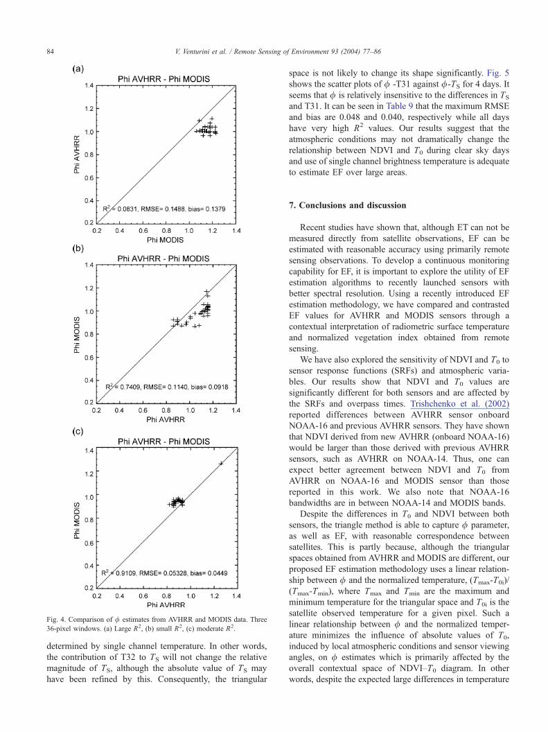
Fig. 4. Comparison of / estimates from AVHRR and MODIS data. Three

36-pixel windows. (a) Large R2, (b) small R2, (c) moderate R2.

V. Venturini et al. / Remote Sensing of Environment 93 (2004) 77–8684

determined by single channel temperature. In other words,

the contribution of T32 to TS will not change the relative

magnitude of TS, although the absolute value of TS may

have been refined by this. Consequently, the triangular

space is not likely to change its shape significantly. Fig. 5

shows the scatter plots of / -T31 against /-TS for 4 days. It

seems that / is relatively insensitive to the differences in TS

and T31. It can be seen in Table 9 that the maximum RMSE

and bias are 0.048 and 0.040, respectively while all days

have very high R2 values. Our results suggest that the

atmospheric conditions may not dramatically change the

relationship between NDVI and T0 during clear sky days

and use of single channel brightness temperature is adequate

to estimate EF over large areas.

7. Conclusions and discussion

Recent studies have shown that, although ET can not be

measured directly from satellite observations, EF can be

estimated with reasonable accuracy using primarily remote

sensing observations. To develop a continuous monitoring

capability for EF, it is important to explore the utility of EF

estimation algorithms to recently launched sensors with

better spectral resolution. Using a recently introduced EF

estimation methodology, we have compared and contrasted

EF values for AVHRR and MODIS sensors through a

contextual interpretation of radiometric surface temperature

and normalized vegetation index obtained from remote

sensing.

We have also explored the sensitivity of NDVI and T0 to

sensor response functions (SRFs) and atmospheric varia-

bles. Our results show that NDVI and T0 values are

significantly different for both sensors and are affected by

the SRFs and overpass times. Trishchenko et al. (2002)

reported differences between AVHRR sensor onboard

NOAA-16 and previous AVHRR sensors. They have shown

that NDVI derived from new AVHRR (onboard NOAA-16)

would be larger than those derived with previous AVHRR

sensors, such as AVHRR on NOAA-14. Thus, one can

expect better agreement between NDVI and T0 from

AVHRR on NOAA-16 and MODIS sensor than those

reported in this work. We also note that NOAA-16

bandwidths are in between NOAA-14 and MODIS bands.

Despite the differences in T0 and NDVI between both

sensors, the triangle method is able to capture / parameter,

as well as EF, with reasonable correspondence between

satellites. This is partly because, although the triangular

spaces obtained from AVHRR and MODIS are different, our

proposed EF estimation methodology uses a linear relation-

ship between / and the normalized temperature, (Tmax-T0i)/

(Tmax-Tmin), where Tmax and Tmin are the maximum and

minimum temperature for the triangular space and T0i is the

satellite observed temperature for a given pixel. Such a

linear relationship between / and the normalized temper-

ature minimizes the influence of absolute values of T0,

induced by local atmospheric conditions and sensor viewing

angles, on / estimates which is primarily affected by the

overall contextual space of NDVI–T0 diagram. In other

words, despite the expected large differences in temperature

Table 9

Comparison between T31 and LST—MODIS-/ from T31 and MODIS-/ from LST

T31 versus LST T31-/ versus LST-/

RMSE (K) Bias (K) R2 Max. difference (K) RMSE Bias R2 Max. difference

JD67 2.929 2.864 0.985 10.64 0.019 �0.005 0.987 0.256

JD91 3.286 3.231 0.972 6.39 0.048 0.040 0.950 0.149

JD92 3.518 3.471 0.971 6.88 0.039 0.029 0.969 0.184

JD93 3.217 3.144 0.989 8.69 0.025 0.013 0.987 0.222

V. Venturini et al. / Remote Sensing of Environment 93 (2004) 77–86 85

and NDVI between satellites, the normalization procedures

for temperature and NDVI, in conjunction with the triangle

method, are able to recover the / parameter, otherwise

knows as a moisture availability, with reasonable corre-

spondence between satellites. This is true for a wide variety

of ambient conditions evidenced by the number of case days

in this study.

One of the main criticisms of using one channel

brightness temperature approach to estimate T0, is that it

is affected by atmospheric variables and viewing angles.

Our / estimates from single channel brightness temperature

and optimal land surface temperatures suggest that, absolute

values of temperature do not dramatically change the

Fig. 5. Comparison between MODIS-/ derived from T4 and

relationship between NDVI and T0 during clear sky days.

Consequently, we argue that the use of single channel

brightness temperature appears to be adequate for the

estimation of EF in conjunction with the triangle method

evaluated in this study over large areas.

Although TS values can be derived using split-window

method, their accuracy is questionable at the daily scale. We

often see the multiday (e.g., 14-day or 16-day) composite of

TS from AVHRR or MODIS, which are not directly

applicable for the proposed method. For near real-time

applications, the split-window method (without other cor-

rections that need atmospheric parameter) is a fast way for TS

given the prescribed parameters sets in this method.

LST. For Julian days (a) 67, (b) 91, (c) 92 and (d) 93.

V. Venturini et al. / Remote Sensing of Environment 93 (2004) 77–8686

However, the uncertainties related to these parameters and

their dependencies on channel specific land surface emis-

sivity will introduce difficult issues to address—in fact,

many of these issues are not fully resolved in the research

community at this point. The TS at the daily scale involves

atmospheric and radiative transfer corrections in addition to

the split-window technique. Then, the dependencies on other

data sources could be a serious constraint to apply our

methodology in different areas (e.g., with no trained

expertise at local level in interpreting and handling these

correction procedures).

One of the limitations of such a comparison, however,

lies in the possible pixel level geolocation mismatch at the

sensor resolution scale between AVHRR and MODIS

sensors. Furthermore, year 2001 is the last year of

NOAA-14 operational observation and satellite degradation

may cause systematic biases in AVHRR derived NDVI and

T0. Nevertheless, our comparisons have shown that such

NOAA-14 data is usable in deriving / or EF with

reasonable accuracy. The limited area (e.g., SFWMD) and

clear day comparisons may not be enough to address the

capability of the / or EF estimation method evaluated in

this study for more diversified atmospheric conditions.

Further comparisons for cloudy days need to be performed

before generalized conclusions can be made. Comparison

case studies presented here, nevertheless, indicate general

applicability of the EF estimation methodology for different

sensor systems and easily available satellite data.

References

Bastiaanssen, W. G. M., Pelgrum, H., Menenti, M., & Feddes, R. A. (1996).

Estimation of surface resistance and Priestley–Taylor a-parameter at

different scales. In J. Stewart, E.T. Engman, R.A. Feddes, & Y. Kerr

(Eds.), Scaling up in hydrology using remote sensing (pp. 93–111).

New York7 Wiley.

Beven, K. J., & Fisher, J. (1996). Remote sensing and scaling in hydrology.

In J. Stewart, E.T. Engman, R.A. Feddes, & Y. Kerr (Eds.), Scaling up

in hydrology using remote sensing (pp. 93–111). New York7 Wiley.

Carlson, T. N., Gillies, R. R., & Schmugge, T. J. (1995). An interpretation

of methodologies for indirect measurement of soil water content.

Agricultural and Forest Meteorology, 77, 191–205.

Carlson, T. N., & Ripley, D. A. J. (1997). On the relationship between

fractional vegetation cover, leaf area index, and NDVI. Remote Sensing

of Environment, 62, 241–252.

Gleason, A. C. R., Prince, S. D., Goetz, S. J., & Small, J. (2002). Effects of

orbital drift on land surface temperature measured by AVHRR thermal

sensors. Remote Sensing of Environment, 79, 147–165.

Gillies, R. R., & Carlson, T. N. (1995). Thermal remote sensing of surface

soil water content with partial vegetation cover for incorporation into

climate models. Journal of Applied Meteorology, 34, 745–756.

Gillies, R. R., Carlson, T. N., Cui, J., Kustas, W. P., & Humes, K. S. (1997).

A verification of the dtriangleT method for obtaining surface soil water

content and energy fluxes from remote measurements of the Normalized

Difference Vegetation Index (NDVI) and surface radiant temperature.

International Journal of Remote Sensing, 18(15), 3145–3166.

Holwill, C. J., & Stewart, J. B. (1992). Spatial variability of evaporation

derived from aircraft and ground-based data. Journal of Geophysical

Research, 97(D17), 19061–19089.

Huete, A., Didan, K., Miura, T., Rodriguez, E. P., Gao, X., & Ferreira, L.

G. (2002). Overview of the radiometric and biophysical performance of

the MODIS vegetation indices. Remote Sensing of Environment, 83,

195–213.

Islam, S., Jiang, L., & Eltahir, E. (2002). Satellite based evapotranspiration

estimates. Final project report, South Florida Water Management

District, September 2002, p. 74.

Islam, S., Jiang, L., & Eltahir, E. (2003). Satellite based evapotranspiration

estimates. Final project report, South Florida Water Management

District, September 2003.

Jackson, R. D., Reginato, R. J., & Idso, S. B. (1977). Wheat canopy

temperature: A practical tool for evaluating water requirements. Water

Resources Research, 13, 651–656.

Jiang, L., & Islam, S. (1999). A methodology for estimation of surface

evapotranspiration over large areas using remote sensing observations.

Geophysical Research Letters, 26(17), 2773–2776.

Jiang, L., & Islam, S. (2001). Estimation of surface evaporation map over

southern Great Plains using remote sensing data. Water Resources

Research, 37(2), 329–340.

Jiang, L., Islam, S., & Carlson, T. N. (2003). Uncertainties in latent heat

flux measurement and estimation: Implications for using a simplified

approach with remote sensing data. In review at Canadian Journal of

Remote Sensing.

Justice, C. O., Townshend, J. R. G., Vermonte, E. F., Masuoka, E.,

Wolfe, R. E., Saleous, N., et al. (2002). An overview of MODIS land

data processing and product status. Remote Sensing of Environment,

83, 3–15.

Moran, M. S., Clarke, T. R., Kustas, W. P., Weltz, M., & Amer, S. A.

(1994). Evaluation of hydrologic parameters in a semiarid rangeland

using remotely sensed spectral data. Water Resources Research, 30(5),

1287–1297.

Myneni, R. B., Maggion, S., Iaquinta, J., Privette, J. L., Gobron, N., Pinty,

B., et al. (1995). Optical remote sensing of vegetation: Modeling,

caveats and algorithms. Remote Sensing of Environment, 51, 169–188.

Nishida, K., Nemani, R. R., Running, S. W., & Glassy, J. M. (2003). An

operational remote sensing algorithm of land evaporation. Journal of

Geophysical Research, 108(D9), 4270.

Norman, J. M., Anderson, M. C., Kustas, W. P., French, A. N., Mecikalski,

J., Torn, R., et al. (2003). Remote sensing of surface energy fluxes at

101-m pixel resolutions. Water Resources Research, 39(8), 1221.

Price, J. C. (1983). Estimating surface temperature from satellite thermal

infrared data—A simple formulation for the atmospheric effect. Remote

Sensing of Environment, 13, 353–361.

Price, J. C. (1990). Using spatial context in satellite data to infer regional

scale evaporanspiration. IEEE Transactions on Geoscience and Remote

Sensing, 28(5), 940–948.

Santanello Jr., J., & Friedl, M. (2003). Diurnal covariation is soil heat flux

and net radiation. Journal of Applied Meteorology, 42, 851–862.

Seguin, B., Assad, E., Fretaud, J. P., Imbernom, J. P., Kerr, Y., &

Lagouarde, J. P. (1989). Use of meteorological satellite for rainfall and

evaporation monitoring. International Journal of Remote Sensing, 10,

1001–1017.

Sobrino, J. A., Coll, C., & Caselles, V. (1991). Atmospheric correction for

land surface temperature using NOAA-11 AVHRR channels 4 and 5.

Remote Sensing of Environment, 38, 19–34.

Trishchenko, A., Cihlar, J., & Li, Z. (2002). Effects of spectral function on

surface reflectance and NDVI measured with moderate resolution

satellite sensors. Remote Sensing of Environment, 81, 1–18.

Verstraete, M. M., & Pinty, B. (1996). Designing optimal indexes for

remote sensing applications. IEEE Transactions on Geoscience and

Remote Sensing, 34(5), 1254–1264.

Wan, Z., & Dozier, J. (1996). A generalized split-window algorithm for

retrieving land-surface temperature from space. IEEE Transactions on

Geoscience and Remote Sensing, 43(4), 892–905.

Wan, Z., & Li, Z. (1997). A physics-based algorithm for retrieving land

surface emissivity and temperature from EOS/MODIS data. IEEE

Transactions on Geoscience and Remote Sensing, 35(4), 980–996.