Estuarine, Coastal and Shelf Science 233 (2020) 106518

Available online 3 December 20190272-7714/© 2019 Elsevier Ltd. All rights reserved.

Comparing trophic levels estimated from a tropical marine food web using an ecosystem model and stable isotopes

Jianguo Du a,*, Petrus Christianus Makatipu b, Lily S.R. Tao c, Daniel Pauly d, William W. L. Cheung d, Teguh Peristiwady b, Jianji Liao a, Bin Chen a,**

a Third Institute of Oceanography, Ministry of Natural Resources, Xiamen, 361005, China b Bitung Marine Life Conservation, Research Centre for Oceanography, Indonesian Institute of Sciences, Bitung, 97255, Indonesia c The Swire Institute of Marine Science, University of Hong Kong, Hong Kong, China d Institute for the Oceans and Fisheries, The University of British Columbia, Vancouver, V6T 1Z4, Canada

A R T I C L E I N F O

Keywords: Ecopath model Stable isotope analysis Trophic level Niche width Coral reef North Sulawesi

A B S T R A C T

Comparing the outputs of food web models with those from other independent approaches is necessary to build confidence in the use of these models to help manage fisheries. Mass-balance models such as Ecopath with Ecosim (EwE) and stable isotope analysis are widely used to describe food webs, but the results from these methodologies are rarely compared. In this study, an Ecopath model was developed to study the food web in the Bitung area, North Sulawesi, Indonesia and compare it with results from stable isotopes. Stable isotope data were available for 19 out of 50 functional groups defined in the model, including fishes, crustaceans, squids, sea cucumbers and other invertebrates. The trophic levels and niches of these functional groups estimated from the Ecopath model were compared with those calculated from nitrogen and carbon isotope data. The trophic levels of 19 functional groups were estimated to range from 2.00 (sea cucumber) to 3.84 (coral trout). Trophic levels estimated from Ecopath were correlated with those derived from stable isotopes (r2

spearman ¼ 0.71, n ¼ 19, p <0.001). On the average, Ecopath overestimated trophic levels of the functional groups in the model by about 2.4% compared to those calculated from stable isotopes, which is very encouraging. It is still suggested, however, that trophic level estimation should be cross-validated by using mass-balance models and SIA whenever possible.

1. Introduction

As ecosystem-based management is increasingly being adopted for marine conservation and natural resource management worldwide (Barbier et al., 2008; Leslie, 2018), the use of ecosystem models for management and forecasting purposes has also strongly increased. Ex-amples of commonly used ecosystem models include Ecopath with Ecosim (EwE) model (Christensen et al. 2008, 2014; Downing et al., 2012), OSMOSE (Shin and Cury, 2001), the Atlantis model (Fulton et al., 2011) and Linear Inverse Modelling (Grami et al., 2011; Legendre and Niquil, 2013), Amongst these models, the most widely applied model is EwE, with over 570 EwE models published worldwide by the early 2000s (Coll�eter et al., 2015).

Unfortunately, validation of EwE model outputs are only performed in a small subset of those published, even though this is an important step towards building confidence in their practical applications (Dame

and Christian, 2008). Amongst the many outputs that Ecopath models produce, trophic levels (TLs) are a useful metric for model validation. Ecopath models calculate TLs for different functional groups in a given ecosystem based on the diet composition matrices specified among groups, usually based on previous analyses of stomach contents, and the relative abundance of each group in the model. Validating the estimated TLs from a model can help build confidence in the representation of its trophic relationships, as required for an accurate representation of ecosystem structure and functions.

Stable isotope analysis (SIA) is considered one of the most effective methods to validate trophic levels estimated from food web models (Dame and Christian, 2008), and has become an important approach for investigating trophic interactions of food webs in the past few decades (Peterson and Fry, 1987; Post, 2002). Given that the difficulty and limitation of stomach content analysis, carbon and nitrogen stable isotope ratios have been shown to be very useful tool to understand

* Corresponding author. Third Institute of Oceanography, Ministry of Natural Resources, China. ** Corresponding author.

E-mail addresses: dujianguo@tio.org.cn (J. Du), chenbin@tio.org.cn (B. Chen).

Contents lists available at ScienceDirect

Estuarine, Coastal and Shelf Science

journal homepage: http://www.elsevier.com/locate/ecss

https://doi.org/10.1016/j.ecss.2019.106518 Received 24 September 2019; Received in revised form 26 November 2019; Accepted 2 December 2019

Estuarine, Coastal and Shelf Science 233 (2020) 106518

2

animal diets (Papiol et al., 2012), from primary producers (Vizzini and Mazzola, 2003; Christianen et al., 2017) to top predators (Estrada et al., 2003; Stewart et al., 2017), and even at the community level, i.e., within entire food webs (Layman et al., 2007; Phillips et al., 2014; Flynn et al., 2018). Comparing TLs and trophic niche widths estimates from Ecopath and from SIA allows validation of the model (Dame and Christian, 2008; Deehr et al., 2014). Such validation has been undertaken in several in-stances (Kline and Pauly, 1998; Nilsen et al., 2008; Milessi et al., 2010; Navarro et al., 2011; Du et al., 2015; Lassalle et al., 2014). However, the use of independent methods for evaluating whether these models pro-vide reasonable results is not routinely applied (Christensen and Wal-ters, 2004; Fulton et al., 2011; Lassalle et al., 2014).

Quantitative information on the biodiversity of the Bitung marine ecosystem in North Sulawesi has been reported, including fishery landings (Naamin et al., 1996; Dharmadi et al., 2015), fish diversity (Kimura and Matsuura, 2003; Du et al. 2016a, 2018, 2016b; Peristiwady et al., 2016), seagrass (Riani et al., 2012), coral reefs (Hadi et al., 2016) and benthos cover (Lin et al., 2018). However, the system as a whole has not been described using a mass-balance model, that could be used to support ecosystem-based management initiatives, though this area is at the centre of multiple fishing activities in Indonesia’s Eastern Region. Here, using the marine ecosystems in Bitung as a case study, we compared the TLs and trophic niches of key functional groups from an

Ecopath model (predicted values) and SIA (empirical data), in order to evaluate whether Ecopath models make reasonable predictions about the trophic structure of ecosystems, considering the complexity of models used for ecosystem-based management and decision making.

2. Materials and methods

2.1. Study area

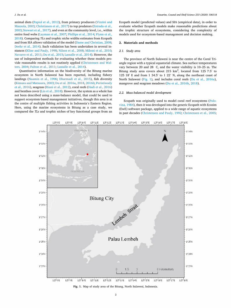
The province of North Sulawesi is near the centre of the Coral Tri-angle region with a typical equatorial climate. Sea surface temperatures vary between 20 and 28 �C, and the water visibility is 10–25 m. The Bitung study area covers about 215 km2, located from 125�7.50 to 125�180 E and from 1�34.50 to 1�22’ N, along the northeast coast of North Sulawesi (Fig. 1), and includes coral reefs (Du et al., 2016a), mangrove and seagrass meadows (Du et al., 2016b, 2018).

2.2. Mass-balanced model development

Ecopath was originally used to model coral reef ecosystems (Polo-vina, 1984), then it was developed into the generic Ecopath with Ecosim (EwE) software package, applied to a wide range of aquatic ecosystems in past decades (Christensen and Pauly, 1992; Christensen et al., 2005;

Fig. 1. Map of study area of the Bitung, North Sulawesi, Indonesia.

J. Du et al.

Estuarine, Coastal and Shelf Science 233 (2020) 106518

3

Colleter el al. 2015; Villasante et al., 2016). This study used EwE version 6.5, available at http://www.ecopath.org/.

To reduce the complexity of the food web, species with similar ecological roles were aggregated into similar ‘functional groups’ or guilds. The model assumes that the total amount produced or consumed by a functional group is equal to the amount that goes out of the func-tional group through fishing mortality, predation, migration and biomass accumulation, i.e.:

Bi⋅ðP=BÞi⋅EEi ¼ Yi þXn

j¼1Bj⋅ðQ=BÞj ⋅ DCij þ Bi⋅BAi þ Ei (1)

where i and j are prey and predator groups, B is biomass, P is the pro-duction, EE is the ecotrophic efficiency, Y is the fishery catch, Q is

consumption, DC is the diet composition, BA is the biomass accumula-tion and E is the net immigration (Christensen et al., 2008). All fluxes are assumed to remain self-similar during the period covered, here 2012 to 2017. The model is balanced by solving Equation (1) simultaneously for all groups in the model; therefore, one of the input parameters (such as B, P/B, Q/B or EE) for each group can be left to be estimated by the model.

For the Bitung ecosystem, 50 functional groups were aggregated from 297 species exploited by local fisheries, and other flora and fauna, including 19 functional groups for which stable isotope data were available. Fisheries catches originated from the Fishery Bureau of Bitung for the years 2012–2017; the catch of each species was allocated to 17 functional groups, using information from different fishing gears such as trawls, purse seines, gillnets, poles and lines, and traps. The values of P/

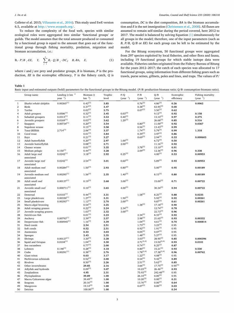
Table 1 Basic input and estimated outputs (bold) parameters for the functional groups in the Bitung model. (P/B: production-biomass ratio; Q/B: consumption-biomass ratio).

Group name Landing (t km� 2

year� 1) Biomass (t km� 2)

Trophic level

P/Q (year� 1)

P/B (year� 1)

Q/B (year� 1)

Ecotrophic efficiency

Fishing mortality (year� 1)

1 Sharks\whale\dolphin 0.00265[1] 0.42[2] 3.85 0.76[2] 4.86[2] 0.26 0.0062 2 Birds 0.37[2] 3.47 0.38[2] 63.95[2] 0.00 3 Turtles 0.02[2] 2.75 0.07[2] 3.50[2] 0.62 4 Adult groupers 0.0506[1] 0.32[3] 3.45 0.03[2] 9.12[2] 0.92 0.158 5 Subadult groupers 0.0313[1] 0.11[3] 3.53 0.40[2] 13.10[2] 0.97 0.275 6 Juvenile groupers 0.0169[1] 0.03[3] 3.62 1.20[2] 26.68[2] 0.85 0.516 7 Snappers 0.00734[1] 0.20[3] 3.54 0.80[2] 11.00[2] 0.92 0.0367 8 Napoleon wrasse 0.15[3] 3.58 0.56[2] 13.43[2] 0.99 9 Tuna\Billfish 2.714[1] 2.06[3] 3.37 1.74[2] 5.79[2] 0.99 1.318 10 Coral trout 0.01[3] 3.84 0.39[2] 3.97[2] 0.86 11 Rays 0.21[3] 3.27 0.69[2] 2.94[2] 0.33 0.000603 12 Adult butterflyfish 0.20[3] 2.97 1.00[2] 6.72[2] 0.50 13 Juvenile butterflyfish 0.08[3] 2.71 2.00[2] 11.16[2] 0.92 14 Cleaner wrasse 0.01[3] 3.35 3.78[2] 13.10[2] 0.91 15 Medium pelagic 0.150[1] 0.44[3] 3.28 2.09[2] 12.36[2] 0.96 0.338 16 Adult large reef

associated 0.0242[1] 3.18[3] 2.92 0.25[2] 4.00[2] 0.53 0.00953

17 Juvenile large reef associated

0.0242[1] 2.54[3] 3.01 0.60[2] 5.89[2] 0.93 0.00953

18 Adult medium reef associated

0.00284[1] 1.50[3] 2.93 0.80[2] 5.00[2] 0.95 0.00189

19 Juvenile medium reef associated

0.00295[1] 1.56[3] 2.35 1.40[2] 8.15[2] 0.80 0.00189

20 Adult small reef associated

0.00137[1] 0.19[3] 2.68 3.00[2] 15.00[2] 0.71 0.00722

21 Juvenile small reef associated

0.000711[1] 0.10[3] 2.65 4.00[2] 30.34[2] 0.94 0.00722

22 Demersal 0.0103[1] 0.44[3] 3.31 1.58[2] 8.25[2] 0.88 0.0235 23 Large planktivore 0.00330[1] 1.27[3] 3.31 1.50[2] 5.92[2] 0.92 0.00261 24 Small planktivore 0.00293[1] 1.12[3] 2.70 2.00[2] 9.87[2] 0.61 0.00261 25 Macro-algal browsing 0.54[3] 2.25 1.38[2] 17.18[2] 0.90 26 Adult scraping grazers 0.22[3] 2.24 2.34[2] 12.74[2] 0.78 27 Juvenile scraping grazers 1.03[3] 2.32 3.00[2] 22.73[2] 0.96 28 Detritivore fish 0.01[3] 2.23 2.34[2] 8.33[2] 0.92 29 Anchovy 0.00793[1] 2.39[3] 2.57 2.98[2] 21.65[2] 0.93 0.00332 30 Deeperwater fish 0.000945[1] 1.16[3] 3.39 1.04[2] 4.61[2] 0.70 0.000814 31 Hard corals 2.54 2.51 1.73[2] 3.23[2] 0.95 32 Soft corals 0.52 2.51 0.92[2] 1.91[2] 0.95 33 Anemonies 0.33 3.03 0.05[2] 0.07[2] 0.95 34 Sponges 2.43 2.35 1.48[2] 5.27[2] 0.95 35 Shrimps 0.00127[1] 3.20[3] 2.28 3.03[2] 28.95[2] 0.85 0.000396 36 Squid and Octopus 0.0104[1] 1.04[3] 3.30 2.71[2,4] 13.54[2,4] 0.93 0.0101 37 Sea cucumbers 0.77[3] 2.00 0.74[2] 8.25[2] 0.87 38 Lobsters 0.148[1] 0.28[3] 3.18 0.80[2] 15.21[2] 0.93 0.530 39 Crabs 0.00291[1] 0.38[3] 2.76 1.78[2,4] 17.38[2,4] 0.96 0.00762 40 Giant triton 0.03 3.17 1.22[2] 4.08[2] 0.95 41 Herbivorous echiniods 0.52[3] 2.00 0.54[2] 9.42[2] 0.89 42 Bivalves 8.50[3] 2.26 2.51[2] 5.62[2] 0.85 43 Other invertebrates 29.85 2.16 3.66[2] 17.75[2] 0.95[5]

44 Jellyfish and hydroids 0.09[3] 3.07 10.23[2] 26.46[2] 0.93 45 Zooplankton 4.95 2.31 75.93[2] 242.48[2] 0.95 46 Phytoplankton 39.89 1.00 26.10[2] 0.00[2] 0.95 47 Macro/Calcareous algae 39.49[2] 1.00 10.20[2] 0.00[2] 0.31 48 Seagrass 20.16[2] 1.00 13.76[2] 0.00[2] 0.64 49 Mangroves 19.14[2] 1.00 0.07[2] 0.00[2] 0.03 50 Detritus 100.00[2] 1.00 0.34

J. Du et al.

Estuarine, Coastal and Shelf Science 233 (2020) 106518

4

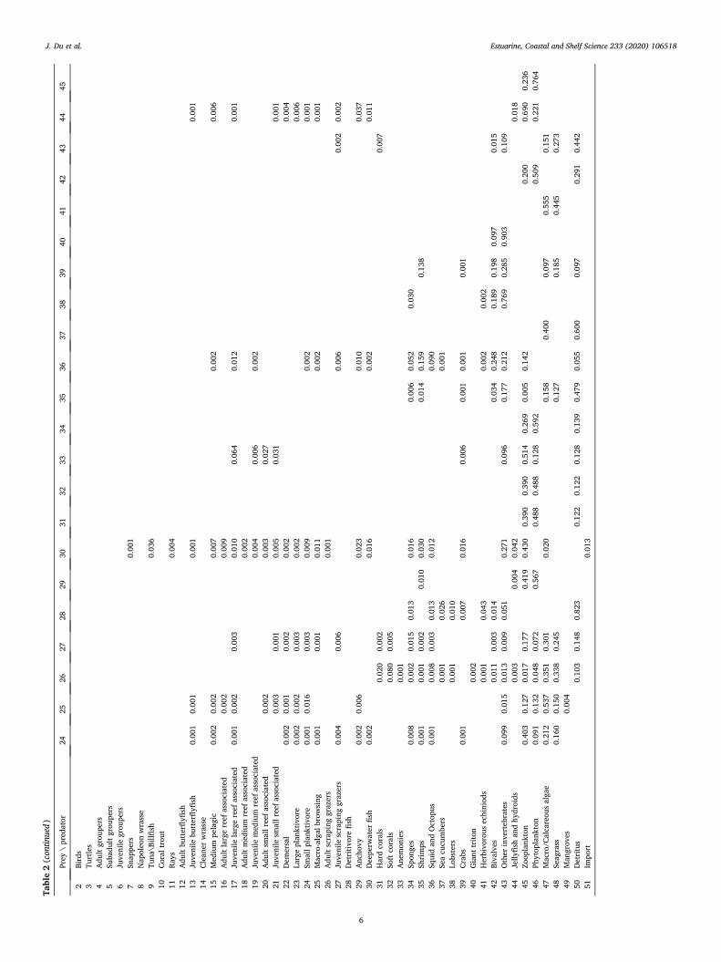
B, Q/B (Table 1) and diet composition (Table 2) for each functional group were adapted from the Raja Ampat model, which also pertains to a coral reef ecosystem. This model of an area 500 km to the southeast, consists of 98 functional groups (Pitcher et al., 2007; Bailey and Pitcher, 2008; Piroddi et al., 2010; Varkey et al., 2012; Hoover et al., 2013). The biomass values of 35 out of 50 functional groups in the Bitung ecosystem model, such as fishes, crabs, shrimps, squids and sea cucumbers, were estimated by the survey data from Underwater Visual Census (UVC) conducted from 2012 to 2017. For the biomass of multi-stanza groups, such as groupers, butterfly fish, large reef associated fish, planktivore fish and scraping grazers, the biomass of each stanza group was esti-mated by the proportion published in the Bird’s Head area (Bailey and Pitcher, 2008). The biomass values of 7 out of 50 functional groups which were not estimated in the survey, such as birds, turtle and sea-grass values from the Raja Ampat model were used (Table 1). For 8 other functional groups, including difficult and soft corals, whose biomasses were hard to estimate, the EE values were set to 0.95 based on the Raja Ampat model, and the biomasses were left for the model to estimate.

2.3. Trophic levels and omnivory index from the Ecopath model

Trophic levels start with TLs ¼ 1 in primary producers and detritus, and a TL of 1 þ [the weighted average of the preys’ TL] for consumers. Following this method, a consumer eating 20% plants (with TL ¼ 1) and 80% herbivores (with TL ¼ 2) will have a TL of 1 þ [0.2 � 1 þ 0.8 � 2] ¼2.8.

TLs can be formulated as follows:

TLi ¼ 1þXn

j¼1DCij � TLj (2)

where i is the predator of prey j, DCij is the fraction of prey j in the diet of predator i and TLj is the TL of prey j (Christensen et al., 2008).

The omnivory index (OI) is estimated as the variance of the TL of a consumer’s prey groups (Pauly et al., 1993). When the OI is zero, the consumer is specialized to feed on a single TL, while a large value il-lustrates that the consumer is a generalist which feeds on many TLs (Pauly et al., 1993; Christensen et al., 2008).

OIi ¼Xn

j¼1

�TLj � ðTLi � 1Þ

�2� DCij (3)

where, TLj is the TL of prey j, TLi is the TL of the predator i, and, DCij is the proportion prey j constitutes to the diet of predator i (Christensen et al., 2008).

The square root of the OI is the standard error of the TLs measuring the uncertainty of its exact value as a result of both sampling and omnivory variability.

2.4. Stable isotopes process

The SIA was performed on 19 functional groups, including 14 fish groups, shrimps, squid, sea cucumber, crab and other invertebrates, consisting of 315 individuals from 115 species. All samples were collected in July and August of 2016; the white muscle of the specimens were collected, and then were freeze-dried at minus 40 �C, ground into powder, then sieved with 120 meshes (aperture diameter: 125 μm). The stable isotope signals were measured using a mass spectrometer con-nected to an elemental analyzer (Flash EA1112 HT). The δ15N was calculated by the following equation:

δ15Nð‰Þ¼Rsample � Rstandard

Rstandard� 1000 (4)

The limits of detection were 0.2‰ for δ15N. R represents the 15N/14N.

2.5. Trophic levels and trophic niche width from SIA

TLs of each fauna were calculated according to Post (2002):

TLconsumer ¼TLbasis þ�δ15Nconsumer � δ15Nbasis

��TEF (5)

where TLbasis is the TL of a primary consumer, used to calculate the TLs of other consumers in the ecosystem (Vander Zanden and Rasmussen, 1999; Post, 2002), and is usually assumed to be 2. δ15Nconsumer is the value measured for other consumers. The δ15Nbasis is δ15N of fauna that are herbivores. In this study, Cypraea tigris, Purpura lapillus and Trochus sp. were identified as the common species at the base of the Bitung food web. TEF is the δ15N trophic enrichment factor for a difference between a consumer and its source, and the average δ15N enrichment per trophic level used in this study is 3.4 parts per thousand (Vander Zanden and Rasmussen, 2001).

2.6. Trophic niche width calculation

In the stable isotope analysis, the niche width of each group or species was represented in terms of the area the population occupies on the δ13C-δ15N biplot based on all specimens within a group/species (Table 3). The area was determined by the standard ellipse area (SEAc) (Jackson et al., 2011). All analyses were performed using the SIAR package (Stable Isotope Analysis in R 3.3.2, version 4.2) and SIBER metrics (Stable Isotope Bayesian Ellipses, version 2.1.3). Original methods of the community level metrics and tools for analyzing food web using stable isotopic data can be seen in Layman et al. (2007, 2012).

2.7. Comparison between Ecopath and stable isotope results

The TLs of each functional group calculated by the Ecopath model were plotted against the corresponding TLs calculated by SIA, and their relationship was tested by the Spearman-rank correlation coefficient test (Zar, 1999). For multi-species functional groups, TLSIA was determined as the mean TLs of the species included in the model compartment for which SIA data existed, weighted by their relative biomass. Similarly, comparisons were done between the square root of OI from Ecopath and the SD of TLSIA, and also between SEAc and OI values.

3. Results

3.1. Ecopath model outputs

The input data such as landings, biomass, P/B, Q/B, diet composition and basic estimated like TLs, ecotrophic efficiency and mortality rates from the Bitung model are summarized in Tables 1 and 2. In the Ecopath model, sharks, coral trout, groupers and Napoleon wrasse are considered the major top predators, with the TLs >3.5. Groupers and tuna/billfish were the main target of the fisheries. The mean TLs of the major exploited groups in the ecosystem is 3.35. Phytoplankton, macroalgae, seagrass, mangroves and detritus were the main food sources for lower trophic level organisms, with the TLs ¼ 1.0 (Fig. 2). Groups with TL �3.0 represent about 14.89% of the total biomass in Bitung ecosystem. Moreover, besides the higher TL groups like sharks and birds, and the lower TL groups like mangrove, the EE of most groups (77%) is over 0.85 (Table 3), suggested that most productions from these groups was transferred to their grazers and/or predators.

For those functional groups for which stable isotope signatures are available, the model estimated TLs ranging between 2.00 (sea cucum-ber) and 3.84 (coral trout). The OI calculated by the Ecopath model suggested that the Bitung ecosystem consisted of functional groups ranging from highly specialized consumer (OI ¼ 0.13 for groupers and coral trout) to generalist predator (OI ¼ 0.67 for rays, OI ¼ 0.44 for small planktivores) (Table 3).

J. Du et al.

Estuarine, Coastal and Shelf Science 233 (2020) 106518

5

Tabl

e 2

Die

t com

posi

tion

of fu

nctio

nal g

roup

s in

the

Bitu

ng m

odel

, the

sum

of e

ach

colu

mn

bein

g eq

ual t

o on

e (a

dapt

ed fr

om th

e Ra

ja A

mpa

t mod

el, P

itche

r et a

l., 2

007;

Bai

ley

and

Pitc

her,

2008

; Pir

oddi

et a

l., 2

010;

Var

key

et a

l.,

2012

; Hoo

ver

et a

l., 2

013)

.

Prey

/pre

dato

r 1

2 3

4 5

6 7

8 9

10

11

12

13

14

15

16

17

18

19

20

21

22

23

1 Sh

arks

/wha

les/

dolp

hins

0.

018

0.

001

2

Bird

s

3

Turt

les

4 A

dult

grou

pers

0.00

3 0.

001

0.

001

0.00

1

0.00

1

5 Su

badu

lt gr

oupe

rs

0.

001

0.00

1 0.

001

0.00

3

0.00

2

0.00

2

6 Ju

veni

le g

roup

ers

0.

001

0.00

2 0.

001

0.00

1 0.

001

0.

001

0.

001

7

Snap

pers

0.

001

0.

009

0.00

2 0.

002

0.00

9 0.

019

0.

031

0.

001

0.

001

0.

001

0.

002

0.

003

8

Nap

oleo

n w

rass

e

0.03

8

0.00

2

9 Tu

na/b

illfis

h 0.

016

0.00

2

0.03

6

0.

019

0.00

1

0.

007

10

Cora

l tro

ut

0.

005

11

Ra

ys

0.00

1 0.

001

0.

001

12

A

dult

butt

erfly

fish

0.00

1

0.00

2 0.

004

0.00

8 0.

007

0.00

8

0.03

2

0.00

2

0.00

2 0.

002

13

Juve

nile

but

terfl

yfish

0.

002

0.

006

0.00

1 0.

001

0.00

2 0.

008

0.

041

0.

001

0.

007

0.00

1

0.00

3 0.

001

14

Clea

ner

wra

sse

0.

001

0.00

2 0.

004

0.00

1

0.00

4

15

Med

ium

Pel

agic

0.

052

0.00

9

0.

009

0.

006

0.03

3 0.

001

0.00

4 16

A

dult

larg

e re

ef a

ssoc

iate

d 0.

008

0.

015

0.03

5 0.

034

0.04

2 0.

002

0.

170

0.

004

0.00

2 0.

002

0.

001

0.

009

0.00

1 17

Ju

veni

le la

rge

reef

ass

ocia

ted

0.01

4

0.01

0 0.

030

0.10

1 0.

035

0.04

0

0.21

6 0.

001

0.00

1

0.00

4 0.

040

0.00

5 0.

002

0.00

4 0.

002

0.00

3 0.

003

0.02

4 0.

018

18

Adu

lt m

ediu

m r

eef a

ssoc

iate

d 0.

011

0.

097

0.07

3 0.

021

0.01

8 0.

006

0.

015

0.03

0

0.01

3 0.

012

0.

001

19

Juve

nile

med

ium

ree

f ass

ocia

ted

0.00

2

0.05

0 0.

181

0.08

7 0.

026

0.01

7

0.01

3

0.01

0 0.

037

0.

003

0.01

0 0.

020

0.04

3 0.

012

0.

026

0.00

8 20

A

dult

smal

l ree

f ass

ocia

ted

0.00

1

0.01

4 0.

006

0.01

1 0.

026

0.02

8

0.02

3 0.

001

0.

032

0.00

4 0.

002

0.

010

0.00

1

0.01

0 0.

002

21

Juve

nile

sm

all r

eef a

ssoc

iate

d

0.

030

0.06

0 0.

008

0.00

1

0.09

0

0.00

2 0.

050

0.00

6 0.

002

0.00

1 0.

001

0.00

1 0.

007

0.

008

0.00

3 22

D

emer

sal

0.02

0

0.00

7 0.

014

0.01

8 0.

009

0.03

7

0.01

2 0.

001

0.00

1

0.00

4 0.

001

0.00

4 0.

002

0.00

2 0.

001

0.00

6 0.

001

0.02

6 0.

001

23

Larg

e pl

ankt

ivor

e 0.

048

0.

025

0.06

1 0.

042

0.04

2 0.

012

0.02

2 0.

034

0.

001

0.03

0 0.

003

0.00

2 0.

014

0.01

0 0.

005

0.00

3 0.

003

0.02

6 0.

026

0.04

2 24

Sm

all p

lank

tivor

e 0.

027

0.00

7

0.01

0 0.

012

0.00

9 0.

032

0.04

9 0.

015

0.02

8

0.02

1 0.

028

0.00

3 0.

003

0.00

5 0.

002

0.00

3 0.

005

0.02

1 0.

003

25

Mac

ro-a

lgal

bro

wsi

ng

0.00

1

0.04

7 0.

007

0.01

1 0.

027

0.01

2

0.01

2

0.00

1

0.00

5 0.

004

0.00

2 0.

001

0.00

3 0.

001

0.00

7 0.

001

26

Adu

lt sc

rapi

ng g

raze

rs

0.00

2

0.02

0 0.

050

0.04

5 0.

028

0.00

3

0.04

8 0.

001

0.

001

0.00

1 0.

002

0.

007

0.

005

0.00

5 27

Ju

veni

le s

crap

ing

graz

ers

0.00

2

0.05

0

0.02

0 0.

002

0.02

4

0.00

1 0.

031

0.

002

0.07

9 0.

004

0.01

0 0.

006

0.01

6

0.00

4 0.

004

28

Det

ritiv

ore

fish

0.00

1 0.

001

0.00

1 0.

002

0.

060

0.

001

0.

001

29

A

ncho

vy

0.01

4 0.

100

0.

070

0.06

7 0.

126

0.08

1 0.

016

0.09

2 0.

056

0.

012

0.16

3 0.

021

0.01

1 0.

030

0.

030

0.09

4 0.

016

30

Dee

perw

ater

fish

0.

032

0.

016

0.02

5 0.

036

0.01

8 0.

014

0.01

1 0.

051

0.

008

0.01

6 0.

002

0.00

1 0.

001

0.

025

0.00

8 31

H

ard

cora

ls

0.

060

0.00

6 0.

308

0.

011

0.00

3 0.

037

0.00

1

32

Soft

cora

ls

0.

005

0.00

3

0.

007

0.00

3

0.00

1

33

Ane

mon

ies

0.00

5

0.00

1

34

Spon

ges

0.

020

0.12

6

0.07

5 0.

073

0.

002

0.12

4 0.

008

0.

010

0.00

8 0.

010

0.00

6 0.

003

0.00

7 0.

012

0.00

6 35

Sh

rim

ps

0.00

1

0.01

8 0.

167

0.09

0 0.

024

0.11

1

0.01

3 0.

018

0.04

2 0.

010

0.00

1

0.02

1 0.

030

0.00

1 0.

020

0.00

1 0.

026

0.00

1 0.

188

0.04

8 36

Sq

uid

and

Oct

opus

0.

110

0.

002

0.00

3 0.

047

0.02

9 0.

083

0.00

2 0.

021

0.00

3 0.

011

0.00

6

0.00

3 0.

017

0.00

5 0.

008

0.00

5 0.

001

0.

017

0.00

8 37

Se

a cu

cum

bers

0.

075

0.04

5

0.00

2 0.

001

0.

005

0.00

1 0.

002

0.00

1

0.02

8

38

Lobs

ters

0.00

3 0.

001

0.00

1 0.

002

0.00

6

0.00

2 0.

001

0.

001

0.

001

39

Cr

abs

0.

006

0.01

9 0.

005

0.02

4 0.

032

0.05

0

0.00

1 0.

002

0.00

4

0.00

1 0.

003

0.00

1 0.

006

0.00

1 0.

004

0.

012

0.00

2 40

G

iant

trito

n

0.00

1 0.

001

0.00

1 0.

002

0.00

6

0.00

2 0.

001

0.00

1 41

H

erbi

voro

us e

chin

iods

0.

007

0.

008

0.03

9

0.00

1 0.

001

0.

001

0.

001

0.00

1

0.00

8

42

Biva

lves

0.00

2 0.

007

0.

013

0.06

9 0.

001

0.

054

0.00

8 0.

006

0.

024

0.02

3 0.

040

0.00

5 0.

006

0.

014

0.02

1 43

O

ther

inve

rteb

rate

s 0.

097

0.06

1 0.

188

0.24

0 0.

185

0.19

4 0.

141

0.20

4 0.

005

0.01

3 0.

081

0.26

9 0.

356

0.55

0 0.

008

0.22

5 0.

367

0.24

6 0.

072

0.23

2 0.

192

0.22

1 0.

105

44

Jelly

fish

and

hydr

oids

0.

005

0.11

3

0.00

5

0.

005

0.00

2

0.00

2 0.

001

0.00

1 0.

005

0.00

4 0.

001

0.

015

45

Zoop

lank

ton

0.06

5

0.00

8 0.

112

0.10

3 0.

068

0.15

2 0.

080

0.03

5

0.00

8 0.

215

0.06

0

0.32

5 0.

170

0.32

9 0.

202

0.11

3 0.

162

0.22

0 0.

108

0.59

8 46

Ph

ytop

lank

ton

0.09

6 0.

240

0.

134

0.00

6 0.

011

0.02

0

0.08

0

0.01

9 47

M

acro

/Cal

care

ous

alga

e

0.25

5

0.10

1 0.

142

0.

115

0.10

2 0.

125

0.33

6 0.

188

0.21

7 0.

054

0.02

6 48

Se

agra

ss

0.20

5

0.03

0 0.

068

0.

090

0.09

3 0.

093

0.35

8 0.

183

0.14

3

0.01

8 49

M

angr

oves

50

Det

ritu

s

0.00

6

0.03

7

0.11

6

0.06

7 0.

050

0.02

8 0.

150

0.04

1 0.

005

51

Impo

rt

0.45

5 0.

798

0.76

4

0.80

0

0.17

5

Prey

\ p

reda

tor

24

25

26

27

28

29

30

31

32

33

34

35

36

37

38

39

40

41

42

43

44

45

1 Sh

arks

\wha

le\d

olph

in

0.00

2

0.

001

(con

tinue

d on

nex

t pag

e)

J. Du et al.

Estuarine, Coastal and Shelf Science 233 (2020) 106518

6

Tabl

e 2

(con

tinue

d)

Prey

\ p

reda

tor

24

25

26

27

28

29

30

31

32

33

34

35

36

37

38

39

40

41

42

43

44

45

2 Bi

rds

3 Tu

rtle

s

4

Adu

lt gr

oupe

rs

5

Suba

dult

grou

pers

6 Ju

veni

le g

roup

ers

7 Sn

appe

rs

0.00

1

8 N

apol

eon

wra

sse

9 Tu

na\B

illfis

h

0.

036

10

Co

ral t

rout

11

Rays

0.

004

12

A

dult

butt

erfly

fish

13

Juve

nile

but

terfl

yfish

0.

001

0.00

1

0.

001

0.

001

14

Cl

eane

r w

rass

e

15

M

ediu

m p

elag

ic

0.00

2 0.

002

0.00

7

0.

002

0.

006

16

A

dult

larg

e re

ef a

ssoc

iate

d

0.00

2

0.

009

17

Ju

veni

le la

rge

reef

ass

ocia

ted

0.00

1 0.

002

0.

003

0.

010

0.

064

0.

012

0.

001

18

A

dult

med

ium

ree

f ass

ocia

ted

0.00

2

19

Juve

nile

med

ium

ree

f ass

ocia

ted

0.00

4

0.00

6

0.00

2

20

Adu

lt sm

all r

eef a

ssoc

iate

d

0.00

2

0.

003

0.

027

21

Juve

nile

sm

all r

eef a

ssoc

iate

d

0.00

3

0.00

1

0.00

5

0.03

1

0.

001

22

D

emer

sal

0.00

2 0.

001

0.

002

0.

002

0.

004

23

La

rge

plan

ktiv

ore

0.00

2 0.

002

0.

003

0.

002

0.

006

24

Sm

all p

lank

tivor

e 0.

001

0.01

6

0.00

3

0.00

9

0.

002

0.

001

25

M

acro

-alg

al b

row

sing

0.

001

0.

001

0.

011

0.00

2

0.00

1

26

Adu

lt sc

rapi

ng g

raze

rs

0.00

1

27

Juve

nile

scr

apin

g gr

azer

s 0.

004

0.

006

0.

006

0.00

2 0.

002

28

D

etri

tivor

e fis

h

29

A

ncho

vy

0.00

2 0.

006

0.02

3

0.

010

0.

037

30

D

eepe

rwat

er fi

sh

0.00

2

0.

016

0.00

2

0.01

1

31

Har

d co

rals

0.

020

0.00

2

0.00

7

32

Soft

cora

ls

0.08

0 0.

005

33

Ane

mon

ies

0.

001

34

Sp

onge

s 0.

008

0.

002

0.01

5 0.

013

0.

016

0.00

6 0.

052

0.

030

35

Sh

rim

ps

0.00

1

0.00

1 0.

002

0.

010

0.03

0

0.

014

0.15

9

0.13

8

36

Sq

uid

and

Oct

opus

0.

001

0.

008

0.00

3 0.

013

0.

012

0.09

0

37

Sea

cucu

mbe

rs

0.00

1

0.02

6

0.00

1

38

Lobs

ters

0.

001

0.

010

39

Crab

s 0.

001

0.

007

0.

016

0.

006

0.

001

0.00

1

0.00

1

40

G

iant

trito

n

0.00

2

41

Her

bivo

rous

ech

inio

ds

0.00

1

0.04

3

0.00

2

0.00

2

42

Biva

lves

0.

011

0.00

3 0.

014

0.03

4 0.

248

0.

189

0.19

8 0.

097

0.

015

43

O

ther

inve

rteb

rate

s 0.

099

0.01

5 0.

013

0.00

9 0.

051

0.

271

0.

096

0.

177

0.21

2

0.76

9 0.

285

0.90

3

0.10

9

44

Jelly

fish

and

hydr

oids

0.

003

0.

004

0.04

2

0.01

8

45

Zoop

lank

ton

0.40

3 0.

127

0.01

7 0.

177

0.

419

0.43

0 0.

390

0.39

0 0.

514

0.26

9 0.

005

0.14

2

0.

200

0.

690

0.23

6 46

Ph

ytop

lank

ton

0.09

1 0.

132

0.04

8 0.

072

0.

567

0.

488

0.48

8 0.

128

0.59

2

0.50

9

0.22

1 0.

764

47

Mac

ro/C

alca

reou

s al

gae

0.21

2 0.

537

0.35

1 0.

301

0.

020

0.15

8

0.40

0

0.09

7

0.55

5

0.15

1

48

Seag

rass

0.

160

0.15

0 0.

338

0.24

5

0.12

7

0.18

5

0.44

5

0.27

3

49

Man

grov

es

0.00

4

50

Det

ritu

s

0.10

3 0.

148

0.82

3

0.12

2 0.

122

0.12

8 0.

139

0.47

9 0.

055

0.60

0

0.09

7

0.29

1 0.

442

51

Im

port

0.

013

J. Du et al.

Estuarine, Coastal and Shelf Science 233 (2020) 106518

7

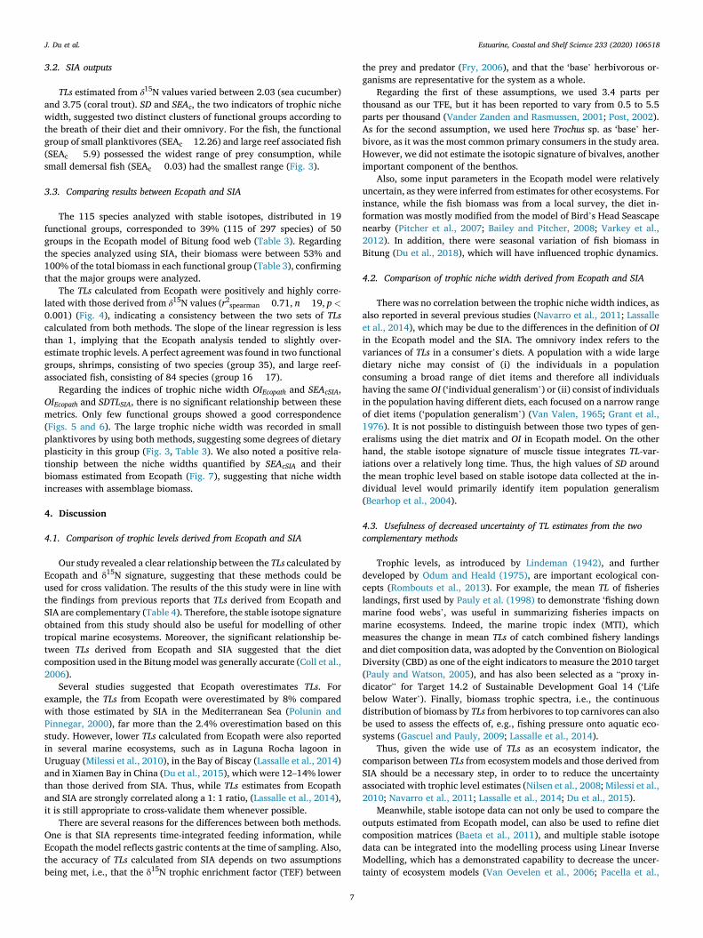
3.2. SIA outputs

TLs estimated from δ15N values varied between 2.03 (sea cucumber) and 3.75 (coral trout). SD and SEAc, the two indicators of trophic niche width, suggested two distinct clusters of functional groups according to the breath of their diet and their omnivory. For the fish, the functional group of small planktivores (SEAc ¼ 12.26) and large reef associated fish (SEAc ¼ 5.9) possessed the widest range of prey consumption, while small demersal fish (SEAc ¼ 0.03) had the smallest range (Fig. 3).

3.3. Comparing results between Ecopath and SIA

The 115 species analyzed with stable isotopes, distributed in 19 functional groups, corresponded to 39% (115 of 297 species) of 50 groups in the Ecopath model of Bitung food web (Table 3). Regarding the species analyzed using SIA, their biomass were between 53% and 100% of the total biomass in each functional group (Table 3), confirming that the major groups were analyzed.

The TLs calculated from Ecopath were positively and highly corre-lated with those derived from δ15N values (r2

spearman ¼ 0.71, n ¼ 19, p <0.001) (Fig. 4), indicating a consistency between the two sets of TLs calculated from both methods. The slope of the linear regression is less than 1, implying that the Ecopath analysis tended to slightly over-estimate trophic levels. A perfect agreement was found in two functional groups, shrimps, consisting of two species (group 35), and large reef- associated fish, consisting of 84 species (group 16 þ 17).

Regarding the indices of trophic niche width OIEcopath and SEAcSIA, OIEcopath and SDTLSIA, there is no significant relationship between these metrics. Only few functional groups showed a good correspondence (Figs. 5 and 6). The large trophic niche width was recorded in small planktivores by using both methods, suggesting some degrees of dietary plasticity in this group (Fig. 3, Table 3). We also noted a positive rela-tionship between the niche widths quantified by SEAcSIA and their biomass estimated from Ecopath (Fig. 7), suggesting that niche width increases with assemblage biomass.

4. Discussion

4.1. Comparison of trophic levels derived from Ecopath and SIA

Our study revealed a clear relationship between the TLs calculated by Ecopath and δ15N signature, suggesting that these methods could be used for cross validation. The results of the this study were in line with the findings from previous reports that TLs derived from Ecopath and SIA are complementary (Table 4). Therefore, the stable isotope signature obtained from this study should also be useful for modelling of other tropical marine ecosystems. Moreover, the significant relationship be-tween TLs derived from Ecopath and SIA suggested that the diet composition used in the Bitung model was generally accurate (Coll et al., 2006).

Several studies suggested that Ecopath overestimates TLs. For example, the TLs from Ecopath were overestimated by 8% compared with those estimated by SIA in the Mediterranean Sea (Polunin and Pinnegar, 2000), far more than the 2.4% overestimation based on this study. However, lower TLs calculated from Ecopath were also reported in several marine ecosystems, such as in Laguna Rocha lagoon in Uruguay (Milessi et al., 2010), in the Bay of Biscay (Lassalle et al., 2014) and in Xiamen Bay in China (Du et al., 2015), which were 12–14% lower than those derived from SIA. Thus, while TLs estimates from Ecopath and SIA are strongly correlated along a 1: 1 ratio, (Lassalle et al., 2014), it is still appropriate to cross-validate them whenever possible.

There are several reasons for the differences between both methods. One is that SIA represents time-integrated feeding information, while Ecopath the model reflects gastric contents at the time of sampling. Also, the accuracy of TLs calculated from SIA depends on two assumptions being met, i.e., that the δ15N trophic enrichment factor (TEF) between

the prey and predator (Fry, 2006), and that the ‘base’ herbivorous or-ganisms are representative for the system as a whole.

Regarding the first of these assumptions, we used 3.4 parts per thousand as our TFE, but it has been reported to vary from 0.5 to 5.5 parts per thousand (Vander Zanden and Rasmussen, 2001; Post, 2002). As for the second assumption, we used here Trochus sp. as ‘base’ her-bivore, as it was the most common primary consumers in the study area. However, we did not estimate the isotopic signature of bivalves, another important component of the benthos.

Also, some input parameters in the Ecopath model were relatively uncertain, as they were inferred from estimates for other ecosystems. For instance, while the fish biomass was from a local survey, the diet in-formation was mostly modified from the model of Bird’s Head Seascape nearby (Pitcher et al., 2007; Bailey and Pitcher, 2008; Varkey et al., 2012). In addition, there were seasonal variation of fish biomass in Bitung (Du et al., 2018), which will have influenced trophic dynamics.

4.2. Comparison of trophic niche width derived from Ecopath and SIA

There was no correlation between the trophic niche width indices, as also reported in several previous studies (Navarro et al., 2011; Lassalle et al., 2014), which may be due to the differences in the definition of OI in the Ecopath model and the SIA. The omnivory index refers to the variances of TLs in a consumer’s diets. A population with a wide large dietary niche may consist of (i) the individuals in a population consuming a broad range of diet items and therefore all individuals having the same OI (‘individual generalism’) or (ii) consist of individuals in the population having different diets, each focused on a narrow range of diet items (‘population generalism’) (Van Valen, 1965; Grant et al., 1976). It is not possible to distinguish between those two types of gen-eralisms using the diet matrix and OI in Ecopath model. On the other hand, the stable isotope signature of muscle tissue integrates TL-var-iations over a relatively long time. Thus, the high values of SD around the mean trophic level based on stable isotope data collected at the in-dividual level would primarily identify item population generalism (Bearhop et al., 2004).

4.3. Usefulness of decreased uncertainty of TL estimates from the two complementary methods

Trophic levels, as introduced by Lindeman (1942), and further developed by Odum and Heald (1975), are important ecological con-cepts (Rombouts et al., 2013). For example, the mean TL of fisheries landings, first used by Pauly et al. (1998) to demonstrate ‘fishing down marine food webs’, was useful in summarizing fisheries impacts on marine ecosystems. Indeed, the marine tropic index (MTI), which measures the change in mean TLs of catch combined fishery landings and diet composition data, was adopted by the Convention on Biological Diversity (CBD) as one of the eight indicators to measure the 2010 target (Pauly and Watson, 2005), and has also been selected as a “proxy in-dicator” for Target 14.2 of Sustainable Development Goal 14 (‘Life below Water’). Finally, biomass trophic spectra, i.e., the continuous distribution of biomass by TLs from herbivores to top carnivores can also be used to assess the effects of, e.g., fishing pressure onto aquatic eco-systems (Gascuel and Pauly, 2009; Lassalle et al., 2014).

Thus, given the wide use of TLs as an ecosystem indicator, the comparison between TLs from ecosystem models and those derived from SIA should be a necessary step, in order to to reduce the uncertainty associated with trophic level estimates (Nilsen et al., 2008; Milessi et al., 2010; Navarro et al., 2011; Lassalle et al., 2014; Du et al., 2015).

Meanwhile, stable isotope data can not only be used to compare the outputs estimated from Ecopath model, can also be used to refine diet composition matrices (Baeta et al., 2011), and multiple stable isotope data can be integrated into the modelling process using Linear Inverse Modelling, which has a demonstrated capability to decrease the uncer-tainty of ecosystem models (Van Oevelen et al., 2006; Pacella et al.,

J. Du et al.

Estuarine, Coastal and Shelf Science 233 (2020) 106518

8

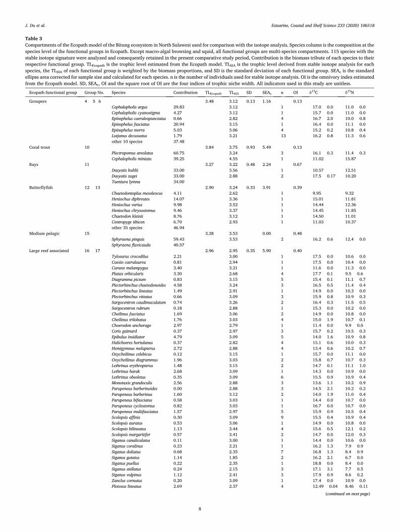
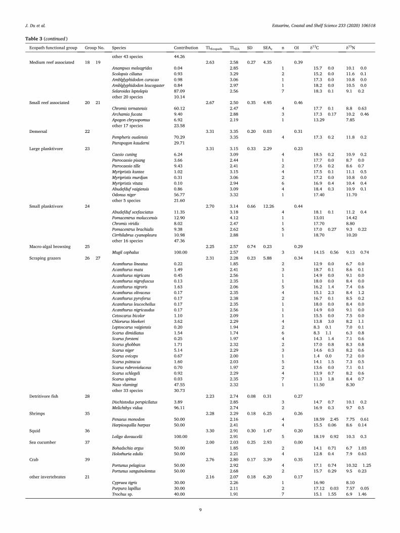
Table 3 Compartments of the Ecopath model of the Bitung ecosystem in North Sulawesi used for comparison with the isotope analysis. Species column is the composition at the species level of the functional groups in Ecopath. Except macro-algal browsing and squid, all functional groups are multi-species compartments. 115 species with the stable isotope signature were analyzed and consequently retained in the present comparative study period, Contribution is the biomass tribute of each species to their respective functional group. TLEcopath is the trophic level estimated from the Ecopath model. TLSIA is the trophic level derived from stable isotope analysis for each species, the TLSIA of each functional group is weighted by the biomass proportions, and SD is the standard deviation of each functional group. SEAc is the standard ellipse area corrected for sample size and calculated for each species. n is the number of individuals used for stable isotope analysis. OI is the omnivory index estimated from the Ecopath model. SD, SEAc, OI and the square root of OI are the four indices of trophic niche width. All indicators used in this study are unitless.

Ecopath functional group Group No. Species Contribution TLEcopath TLSIA SD SEAc n OI δ13C δ15N

Groupers 4 þ 5þ6 3.48 3.12 0.13 1.16 0.13 Cephalopholis argus 29.83 3.12 1 � 17.0 � 0.0 11.0 � 0.0 Cephalopholis cyanostigma 4.27 3.12 1 � 15.7 � 0.0 11.0 � 0.0 Epinephelus caeruleopunctatus 0.66 2.82 4 � 16.7 � 2.0 10.0 � 0.8 Epinephelus fasciatus 20.94 3.15 1 � 16.4 � 0.0 11.1 � 0.0 Epinephelus merra 5.03 3.06 4 � 15.2 � 0.2 10.8 � 0.4 Lutjanus decussatus 1.79 3.21 13 � 16.2 � 0.8 11.3 � 0.6 other 10 species 37.48

Coral trout 10 3.84 3.75 0.93 5.49 0.13 Plectropomus areolatus 60.75 3.24 3 � 16.1 � 0.3 11.4 � 0.3 Cephalopholis miniata 39.25 4.55 1 � 11.02 15.87

Rays 11 3.27 3.22 0.48 2.24 0.67 Dasyatis kuhlii 33.00 3.56 1 � 10.57 12.51 Dasyatis zugei 33.00 2.88 2 � 17.5 � 0.17 10.20 Taeniura lymna 34.00

Butterflyfish 12 þ 13 2.90 3.24 0.33 3.91 0.39 Chaetodontoplus mesoleocus 4.11 2.62 1 � 9.95 9.32 Heniochus diphreutes 14.07 3.36 1 � 15.01 11.81 Heniochus varius 9.98 3.52 1 � 14.44 12.36 Heniochus chrysostomus 9.46 3.37 1 � 14.45 11.85 Chaetodon kleinii 8.76 3.12 1 � 14.50 11.01 Centropyge tibicen 6.70 2.93 1 � 11.03 10.37 other 35 species 46.94

Medium pelagic 15 3.28 3.53 0.00 0.48 Sphyraena pinguis 59.43 3.53 2 � 16.2 � 0.6 12.4 � 0.0 Sphyraena flavicauda 40.57

Large reef associated 16 þ 17 2.96 2.95 0.35 5.90 0.40 Tylosurus crocodilus 2.21 3.00 1 � 17.5 � 0.0 10.6 � 0.0 Caesio caerulaurea 0.81 2.94 1 � 17.5 � 0.0 10.4 � 0.0 Caranx melampygus 3.40 3.21 1 � 11.6 � 0.0 11.3 � 0.0 Platax orbicularis 3.30 2.68 4 � 17.7 � 0.1 9.5 � 0.6 Diagramma pictum 0.83 3.15 5 � 15.4 � 0.1 11.1 � 0.7 Plectorhinchus chaetodonoides 4.58 3.24 3 � 16.5 � 0.5 11.4 � 0.4 Plectorhinchus lineatus 1.49 2.91 1 � 14.9 � 0.0 10.3 � 0.0 Plectorhinchus vittatus 0.66 3.09 3 � 15.9 � 0.8 10.9 � 0.3 Sargocentron caudimaculatum 0.74 3.26 2 � 16.4 � 0.3 11.5 � 0.5 Sargocentron rubrum 0.18 2.88 1 � 15.3 � 0.0 10.2 � 0.0 Cheilinus fasciatus 1.69 3.06 2 � 14.9 � 0.0 10.8 � 0.0 Cheilinus trilobatus 1.76 3.03 4 � 15.0 � 1.9 10.7 � 0.1 Choerodon anchorago 2.97 2.79 1 � 11.4 � 0.0 9.9 � 0.0 Coris gaimard 0.37 2.97 3 � 15.7 � 0.2 10.5 � 0.3 Epibulus insidiator 4.79 3.09 5 � 14.0 � 1.6 10.9 � 0.8 Halichoeres hortulanus 0.37 2.82 4 � 15.1 � 0.6 10.0 � 0.3 Hemigymnus melapterus 2.72 2.88 4 � 13.4 � 0.6 10.2 � 0.7 Oxycheilinus celebicus 0.12 3.15 1 � 15.7 � 0.0 11.1 � 0.0 Oxycheilinus diagrammus 1.96 3.03 2 � 15.8 � 0.7 10.7 � 0.3 Lethrinus erythropterus 1.48 3.15 2 � 14.7 � 0.1 11.1 � 1.0 Lethrinus harak 2.68 3.09 1 � 14.3 � 0.0 10.9 � 0.0 Lethrinus obsoletus 0.35 3.09 6 � 15.5 � 0.9 10.9 � 0.4 Monotaxis grandoculis 2.56 2.88 3 � 13.6 � 1.1 10.2 � 0.9 Parupeneus barberinoides 0.00 2.88 3 � 14.5 � 2.1 10.2 � 0.2 Parupeneus barberinus 1.60 3.12 2 � 14.0 � 1.9 11.0 � 0.4 Parupeneus bifasciatus 0.58 3.03 1 � 14.4 � 0.0 10.7 � 0.0 Parupeneus cyclostomus 0.82 3.03 1 � 16.7 � 0.0 10.7 � 0.0 Parupeneus multifasciatus 1.57 2.97 5 � 15.9 � 0.9 10.5 � 0.4 Scolopsis affinis 0.30 3.09 9 � 15.5 � 0.4 10.9 � 0.4 Scolopsis auratus 0.53 3.06 1 � 14.9 � 0.0 10.8 � 0.0 Scolopsis bilineatus 1.13 3.44 4 � 15.6 � 0.5 12.1 � 0.2 Scolopsis margaritifer 0.57 3.41 2 � 14.7 � 0.0 12.0 � 0.3 Siganus canaliculatus 0.11 3.00 1 � 14.4 � 0.0 10.6 � 0.0 Siganus coralinus 0.23 2.21 1 � 16.2 � 1.3 7.9 � 0.9 Siganus doliatus 0.68 2.35 7 � 16.8 � 1.3 8.4 � 0.9 Siganus gutatus 1.14 1.85 2 � 16.2 � 2.1 6.7 � 0.0 Siganus puellus 0.22 2.35 1 � 18.8 � 0.0 8.4 � 0.0 Siganus stellatus 0.24 2.15 3 � 17.1 � 3.1 7.7 � 0.5 Siganus vulpinus 1.12 2.41 3 � 17.9 � 0.9 8.6 � 0.2 Zanclus cornutus 0.20 3.09 1 � 17.4 � 0.0 10.9 � 0.0 Plotosus lineatus 2.69 2.37 4 � 12.49 � 0.04 8.46 � 0.11

(continued on next page)

J. Du et al.

Estuarine, Coastal and Shelf Science 233 (2020) 106518

9

Table 3 (continued )

Ecopath functional group Group No. Species Contribution TLEcopath TLSIA SD SEAc n OI δ13C δ15N

other 43 species 44.26 Medium reef associated 18 þ 19 2.63 2.58 0.27 4.35 0.39

Anampses meleagrides 0.04 2.85 1 � 15.7 � 0.0 10.1 � 0.0 Scolopsis ciliatus 0.93 3.29 2 � 15.2 � 0.0 11.6 � 0.1 Amblglyphidodon curacao 0.98 3.06 1 � 17.3 � 0.0 10.8 � 0.0 Amblglyphidodon leucogaster 0.84 2.97 1 � 18.2 � 0.0 10.5 � 0.0 Selaroides leptolepis 87.09 2.56 7 � 18.3 � 0.1 9.1 � 0.2 other 20 species 10.14

Small reef associated 20 þ 21 2.67 2.50 0.35 4.95 0.46 Chromis ternatensis 60.12 2.47 4 � 17.7 � 0.1 8.8 � 0.63 Archamia fucata 9.40 2.88 3 � 17.3 � 0.17 10.2 � 0.46 Apogon chrysopomus 6.92 2.19 1 � 13.29 7.85 other 17 species 23.58

Demersal 22 3.31 3.35 0.20 0.03 0.31 Pempheris oualensis 70.29 3.35 4 � 17.3 � 0.2 11.8 � 0.2 Pterapogon kauderni 29.71

Large planktivore 23 3.31 3.15 0.33 2.29 0.23 Caesio cuning 6.24 3.09 4 � 18.5 � 0.2 10.9 � 0.2 Pterocaesio pisang 3.66 2.44 1 � 17.7 � 0.0 8.7 � 0.0 Pterocaesio tille 9.43 2.41 2 � 17.6 � 0.2 8.6 � 0.7 Myripristis kuntee 1.02 3.15 4 � 17.5 � 0.1 11.1 � 0.5 Myripristis murdjan 0.31 3.06 2 � 17.2 � 0.0 10.8 � 0.0 Myripristis vitata 0.10 2.94 6 � 16.9 � 0.4 10.4 � 0.4 Abudefduf vaigiensis 0.86 3.09 4 � 18.4 � 0.3 10.9 � 0.1 Odonus niger 56.77 3.32 1 � 17.40 11.70 other 5 species 21.60

Small planktivore 24 2.70 3.14 0.66 12.26 0.44 Abudefduf sexfasciatus 11.35 3.18 4 � 18.1 � 0.1 11.2 � 0.4 Pomacentrus moluccensis 12.90 4.12 1 � 13.01 14.42 Chromis viridis 8.02 2.47 1 � 17.70 8.80 Pomacentrus brachialis 9.38 2.62 5 � 17.0 � 0.27 9.3 � 0.22 Cirrhilabrus cyanopleura 10.98 2.88 1 � 18.70 10.20 other 16 species 47.36

Macro-algal browsing 25 2.25 2.57 0.74 0.23 0.29 Mugil cephalus 100.00 2.57 3 � 14.15 � 0.56 9.13 � 0.74

Scraping grazers 26 þ 27 2.31 2.28 0.23 5.88 0.34 Acanthurus lineatus 0.22 1.85 2 � 12.9 � 0.0 6.7 � 0.0 Acanthurus mata 1.49 2.41 3 � 18.7 � 0.1 8.6 � 0.1 Acanthurus nigricans 0.45 2.56 1 � 14.9 � 0.0 9.1 � 0.0 Acanthurus nigrofuscus 0.13 2.35 1 � 18.0 � 0.0 8.4 � 0.0 Acanthurus nigroris 1.63 2.06 5 � 16.2 � 1.4 7.4 � 0.6 Acanthurus olivaceus 0.17 2.35 4 � 15.1 � 2.3 8.4 � 1.2 Acanthurus pyroferus 0.17 2.38 2 � 16.7 � 0.1 8.5 � 0.2 Acanthurus leucocheilus 0.17 2.35 1 � 18.0 � 0.0 8.4 � 0.0 Acanthurus nigricaudus 0.17 2.56 1 � 14.9 � 0.0 9.1 � 0.0 Cetoscarus bicolor 1.10 2.09 1 � 15.5 � 0.0 7.5 � 0.0 Chlorurus bleekeri 3.62 2.29 4 � 13.8 � 3.0 8.2 � 1.1 Leptoscarus vaigiensis 0.20 1.94 2 � 8.3 � 0.1 7.0 � 0.1 Scarus dimidiatus 1.54 1.74 6 � 8.3 � 1.1 6.3 � 0.8 Scarus forsteni 0.25 1.97 4 � 14.3 � 1.4 7.1 � 0.6 Scarus ghobban 1.71 2.32 2 � 17.0 � 0.8 8.3 � 0.8 Scarus niger 5.14 2.29 3 � 14.6 � 0.3 8.2 � 0.6 Scarus oviceps 0.67 2.00 1 � 1.4 � 0.0 7.2 � 0.0 Scarus psittacus 1.60 2.03 5 � 14.1 � 1.5 7.3 � 0.5 Scarus rubroviolaceus 0.70 1.97 2 � 13.6 � 0.0 7.1 � 0.1 Scarus schlegeli 0.92 2.29 4 � 13.9 � 0.7 8.2 � 0.6 Scarus spinus 0.03 2.35 7 � 11.3 � 1.8 8.4 � 0.7 Naso vlamingi 47.55 2.32 1 � 11.50 8.30 other 33 species 30.73

Detritivore fish 28 2.23 2.74 0.08 0.31 0.27 Dischistodus perspicilatus 3.89 2.85 3 � 14.7 � 0.7 10.1 � 0.2 Melichthys vidua 96.11 2.74 2 � 16.9 � 0.3 9.7 � 0.5

Shrimps 35 2.28 2.29 0.18 6.25 0.26 Penaeus monodon 50.00 2.16 4 � 18.59 � 2.45 7.75 � 0.61 Harpiosquilla harpax 50.00 2.41 4 � 15.5 � 0.06 8.6 � 0.14

Squid 36 3.30 2.91 0.30 1.47 0.20 Loligo duvaucelii 100.00 2.91 5 � 18.19 � 0.92 10.3 � 0.3

Sea cucumber 37 2.00 2.03 0.25 2.93 0.00 Bohadschia argus 50.00 1.85 2 � 14.1 � 0.71 6.7 � 1.03 Holothuria edulis 50.00 2.21 4 � 12.8 � 0.4 7.9 � 0.63

Crab 39 2.76 2.80 0.17 3.39 0.35 Portunus pelagicus 50.00 2.92 4 � 17.1 � 0.74 10.32 � 1.25 Portunus sanguinolentus 50.00 2.68 2 � 15.7 � 0.29 9.5 � 0.23

other invertebrates 21 2.16 2.07 0.18 6.20 0.17 Cypraea tigris 30.00 2.26 1 � 16.90 8.10 Purpura lapillus 30.00 2.11 2 � 17.12 � 0.03 7.57 � 0.05 Trochus sp. 40.00 1.91 7 � 15.1 � 1.55 6.9 � 1.46

J. Du et al.

Estuarine, Coastal and Shelf Science 233 (2020) 106518

10

2013). Furthermore, a new isotope mixing model (‘IsoWeb’), which uses stable isotope data from all components in a food web, can estimate the diet composition of its consumers (Kadoya et al., 2012). This is a critical

step in quantifying the trophic interactions in an ecosystem (Lassalle et al., 2014).

Funding

The present study was supported by grants from the National Natural Science Foundation of China (no. 41676096), the China-Indonesia Maritime Cooperation Fund project “China-Indonesia Bitung Ecological Station Establishment” (research permits no./FRP/E5/Dit.KI/VI/2016),

Fig. 2. Trophic flow diagram of the balanced trophic model of Bitung, North Sulawesi. The components of the system are structured along the vertical axis according to their trophic level. The area of each circle is proportional to the biomass of each functional group.

Fig. 3. Stable isotope bi-plots illustrating the isotopic niche of each functional group. (a) Large reef associated fishes, including 41 species; (b) Small plank-tivore, including 5 species; (c) Groupers, including 6 species. For each func-tional group, species are represented by identical symbols, and a line encloses its corrected standard ellipse area (SEAc).

Fig. 4. Linear regression between trophic levels estimated from Ecopath model and stable isotope analysis for Bitung ecosystem (solid line). The broken line represents a 1:1 relationship.

J. Du et al.

Estuarine, Coastal and Shelf Science 233 (2020) 106518

11

National Key R & D Program of China (no. 2017YFC1405101), and the China-Canada Marine Ecosystem Research project. DP acknowledges support from the Sea Around Us, itself supported by a number of phil-anthropic foundations.

Author contribution statement

Jianguo Du: Conceptualization, Methodology, Writing - Original Draft. Petrus Christianus Makatipu: Investigation, Resources. Lily S.R. Tao: Formal analysis. Daniel Pauly: Writing - Review & Editing. William W.L. Cheung: Writing - Review & Editing. Teguh Peristiwady: Investi-gation, Resources. Jianji Liao: Investigation, Resources. Bin Chen: Writing - Review & Editing, Supervision.

Declaration of competing interest

The authors declare that they have no known competing financial interests or personal relationships that could have appeared to influence the work reported in this paper.

Notes: [1]- Fishery Statistics of Fishery Bureau of Bitung, 2017); [2]-

Bailey and Pitcher (2008); [3]-this study; [4]- Piroddi et al., (2010); [5]- Hoover et al., (2013).

Acknowledgements

We would like to express our gratitude to Dr. Xijie Yin (Third Insti-tute of Oceanography, Ministry of Natural Resources) for his help in the analysis of stable isotopes.

References

Baeta, A., Niquil, N., Marques, J.C., Patrício, J., 2011. Modelling the effects of eutrophication, mitigation measures and an extreme flood event on estuarine benthic food webs. Ecol. Model. 222, 1209–1221.

Ecological and economic analyses of marine ecosystems in the Bird’s Head Seascape, Papua, Indonesia: II. In: Bailey, M., Pitcher, T.J. (Eds.), Fish Cent. Res. Rep. 16 (1), 186.

Barbier, E.B., Koch, E.W., Silliman, B.R., Hacker, S.D., Wolanski, E., Primavera, J., Stoms, D.M., 2008. Coastal ecosystem-based management with nonlinear ecological functions and values. Science 319 (5861), 321–323.

Bearhop, S., Adams, C.E., Waldron, S., Fuller, R.A., MacLeod, H., 2004. Determining trophic niche width: a novel approach using stable isotope analysis. J. Anim. Ecol. 73 (5), 1007–1012.

Christensen, V., Pauly, D., 1992. Ecopath II - a software for balancing steady-state ecosystem models and calculating network characteristics. Ecol. Model. 61, 169–185.

Christensen, V., Walters, C.J., 2004. Ecopath with Ecosim: methods, capabilities and limitations. Ecol. Model. 172, 109–139.

Christensen, V., Walters, C.J., Pauly, D., 2005. Ecopath with Ecosim: a User’s Guide. Fisheries Centre, University of British Columbia, Vancouver.

Christensen, V., Walters, C.J., Pauly, D., Forrest, R., 2008. Ecopath with Ecosim Version 6 User Guide. Lenfest Ocean Futures Project. University of British Columbia, Vancouver.

Fig. 5. Standard ellipse areas (SEAc) estimated from SIA plotted against the corresponding OI value. Code corresponding to the names of functional groups see Table 1.

Fig. 6. Standard deviations (SD) of TLs estimated from SIA plotted against the corresponding square root of OI derived from the Ecopath model. Code corre-sponding to the names of functional groups see Table 1.

Fig. 7. Standard ellipse areas (SEAc) estimated from SIA plotted against the corresponding square root of biomass value from the Ecopath model. Code corresponding to the names of functional groups see Table 1.

Table 4 Correlation analysis between TLs estimates from Ecopath model and Stable isotope in previous studies.

Study area r2 n References

Bitung in North Sulawesi 0.74 19 Present study Subtropical Bay in China 0.696 23 Du et al. (2015) Continental shelf of the Bay of Biscay 0.72 16 Lassalle et al. (2014) South Catalan Sea 0.69 24 Navarro et al. (2011) Subtropical lagoon in Uruguay 0.82 14 Milessi et al. (2010) Fjord in northern Norway 0.72 19 Nilsen et al. (2008) Prince William Sound 0.99 7 Kline and Pauly (1998)

Note: At Salt marsh ponds in Virginia, TLs from Ecopath matched those from δ15N data for three of the four networks, but no coefficient and numerical data provided (Dame and Christian, 2008).

J. Du et al.

Estuarine, Coastal and Shelf Science 233 (2020) 106518

12

Christensen, V., Coll, M., Piroddi, C., Steenbeek, J., Buszowski, J., Pauly, D., 2014. A century of fish biomass decline in the ocean. Mar. Ecol. Prog. Ser. 512, 155–166.

Christianen, M.J.A., Middelburg, J.J., Holthuijsen, S.J., Jouta, J., Compton, T.J., Van der Heide, T., Olff, H., 2017. Benthic primary producers are key to sustain the Wadden Sea food web: stable carbon isotope analysis at landscape scale. Ecology 98 (6), 1498–1512.

Coll, M., Palomera, I., Tudela, S., Sarda, F., 2006. Trophic flows, ecosystem structure and fishing impacts in the South Catalan Sea, Northwestern Mediterranean. J. Mar. Syst. 59, 63–96.

Coll�eter, M., Valls, A., Guitton, J., Gascuel, D., Pauly, D., Christensen, V., 2015. Global overview of the applications of the Ecopath with Ecosim modeling approach using the EcoBase models repository. Ecol. Model. 302, 42–53.

Dame, J.K., Christian, R.R., 2008. Evaluation of ecological network analysis: validation of output. Ecol. Model. 210, 327–338.

Deehr, R.A., Luczkovich, J.J., Hart, K.J., Clough, L.M., Johnson, B.J., Johnson, J.C., 2014. Using stable isotope analysis to validate effective trophic levels from Ecopath models of areas closed and open to shrimp trawling in Core Sound, NC, USA. Ecol. Model. 282, 1–17.

Du, J.G., Cheung, W.W.W., Zheng, X.Q., Chen, B., Liao, J.J., Hu, W.J., 2015. Comparing trophic structure of a subtropical bay as estimated from mass-balance food web model and stable isotope analysis. Ecol. Model. 312, 175–181.

Du, J.G., Hu, W.J., Makatipu, P.C., Peristiwady, T., Chen, B., Dirhamsyah, 2016a. Common Reef Fishes of North Sulawesi, Indonesia. Science Press, Beijing.

Du, J.G., Wang, Y.G., Peristiwady, T., Liao, J.J., Makatipu, P.C., Huwae, R., Ju, P.L., Loh, K.H., Chen, B., 2018. Temporal and spatial variation of fishes community and their nursery in a tropical seagrass meadow. Acta Oceanol. Sin. 37, 63–72.

Du, J.G., Zheng, X.Q., Peristiwady, T., Liao, J.J., Makatipu, P.C., Yin, X.J., Hu, W.J., Koagouw, W., Chen, B., 2016b. Food sources and trophic structure of fishes and benthic macroinvertebrates in a tropical seagrass meadow revealed by stable isotope analysis. Mar. Biol. Res. 12, 748–757.

Dharmadi, Fahmi , Satria, F., 2015. Fisheries management and conservation of sharks in Indonesia. Afr. J. Mar. Sci. 37 (2), 249–258.

Downing, A.S., Van Nes, E.H., Janse, J.H., Witte, F., Cornelissen, I.J., Scheffer, M., Mooij, W.M., 2012. Collapse and reorganization of a food web of Mwanza Gulf, Lake Victoria. Ecol. Appl. 22, 229–239.

Fishery Bureau of Bitung, 2017. Fishery Statistics of Fishery Bureau of Bitung, 2012- 2017.

Estrada, J.A., Rice, A.N., Lutcavage, M.E., Skomal, G.B., 2003. Predicting trophic position in sharks of the north-west Atlantic Ocean using stable isotope analysis. J. Mar. Biol. Assoc. U. K. 83 (6), 1347–1350.

Flynn, K.J., Mitra, A., Bode, A., 2018. Toward a mechanistic understanding of trophic structure: inferences from simulating stable isotope ratios. Mar. Boil. 165, 147.

Fry, B., 2006. Stable Isotope Ecology, 1 st ed. Springer, p. 308. Fulton, E.A., Link, J.S., Kaplan, I.C., Savina-Rolland, M., Johnson, P., Ainsworth, C.,

Horne, P., Gorton, R., Gamble, R.J., Smith, A.D.M., Smith, D.C., 2011. Lessons in modelling and management of marine ecosystems: the Atlantis experience. Fish Fish. 12, 171–188.

Gascuel, D., Pauly, D., 2009. EcoTroph: modelling marine ecosystem functioning and impact of fishing. Ecol. Model. 220 (21), 2885–2898.

Grami, B., Rasconi, S., Niquil, N., Jobard, M., Saint-B�eat, B., Sime-Ngando, T., 2011. Functional effects of parasites on food web properties during the spring diatom bloom in Lake Pavin: a linear inverse modeling analysis. PLoS One 6 (8), e23273.

Grant, P.R., Grant, B.R., Smith, J.N., Abbott, I.J., Abbott, L.K., 1976. Darwin’s finches: population variation and natural selection. P. Nati. Acad. Sci. USA. 73 (1), 257–261.

Hadi, T.A., Hadiyanto, Budiyanto, A., Niu, W.T., Suharsono, 2016. The morphological and species diversity of sponges on coral reef ecosystems in the Lembeh Strait. Bitung. Mar. Res. Indone. 40 (2), 65–77.

Hoover, C., Pitcher, T., Christensen, V., 2013. Effects of hunting, fishing and climate change on the Hudson Bay marine ecosystem: I. Re-creating past changes 1970–2009. Ecol. Model. 264, 130–142.

Jackson, A.L., Inger, R., Parnell, A.C., Bearhop, S., 2011. Comparing isotopic niche widths among and within communities: SIBER–Stable Isotope Bayesian Ellipses in R. J. Anim. Ecol. 80 (3), 595–602.

Kadoya, T., Osada, Y., Takimoto, G., 2012. IsoWeb: a Bayesian isotope mixing model for diet analysis of the whole food web. PLoS One 7 (7), e41057.

Kimura, S., Matsuura, K. (Eds.), 2003. Fishes of Bitung: Northern Tip of Sulawesi, Indonesia. Ocean Research Institute, University of Tokyo.

Kline, T.C., Pauly, D., 1998. Cross-validation of trophic level estimates from a mass- balance model of Prince William Sound using 15N/14N data. In: Fishery Stock Assessment Models. Alaska Sea Grant College Program. AK-SG-98-01.

Lassalle, G., Chouvelon, T., Bustamante, P., Niquil, N., 2014. An assessment of the trophic structure of the Bay of Biscay continental shelf food web: comparing estimates derived from an ecosystem model and isotopic data. Prog. Oceanogr. 120, 205–215.

Layman, C.A., Araujo, M.S., Boucek, R., Hammerschlag-Peyer, C.M., Harrison, E., Jud, Z. R., Post, D.M., 2012. Applying stable isotopes to examine food-web structure: an overview of analytical tools. Biol. Rev. 87 (3), 545–562.

Layman, C.A., Arrington, D.A., Monta~na, C.G., Post, D.M., 2007. Can stable isotope ratios provide for community-wide measures of trophic structure? Ecology 88 (1), 42–48.

Legendre, L., Niquil, N., 2013. Large-scale regional comparisons of ecosystem processes: methods and approaches. J. Mar. Syst. 109, 4–21.

Leslie, H.M., 2018. Value of ecosystem-based management. P. Nati. Acad. Sci. USA. 115 (14), 3518–3520.

Lin, J., Huang, Y., Arbi, U.Y., Lin, H., Azkab, M.H., Wang, J., Zhang, S., 2018. An ecological survey of the abundance and diversity of benthic macrofauna in Indonesian multispecific seagrass beds. Acta Oceanol. Sin. 37 (6), 82–89.

Lindeman, R.L., 1942. The trophic-dynamic aspect of ecology. Ecology 23 (4), 399–417. Milessi, A.C., Danilo, C., Laura, R.G., Daniel, C., Javier, S., Rodríguez-Gallegod, L., 2010.

Trophic mass-balance model of a subtropical coastal lagoon, including a comparison with a stable isotope analysis of the food-web. Ecol. Model. 221, 2859–2869.

Naamin, N., Mathews, C., Monintja, D., 1996. Studies of Indonesian Tuna Fisheries, Part 1: Interactions between Coastal and Offshore Tuna Fisheries in Manado and Bitung, North Sulawesi. FAO Fisheries Technical Paper, pp. 282–297.

Navarro, J., Coll, M., Louzao, M., Palomera, I., Delgado, A., Forero, M.G., 2011. Comparison of ecosystem modelling and isotopic approach as ecological tools to investigate food webs in the NW Mediterranean Sea. J. Exp. Mar. Biol. Ecol. 401, 97–104.

Nilsen, M., Pedersen, T., Nilssen, E.M., Fredriksen, S., 2008. Trophic studies in a high- latitude fjord ecosystem-a comparison of stable isotope analyses (δ13C and δ15N) and trophic-level estimates from a mass-balance model. Can. J. Fish. Aquat. Sci. 65, 2791–2806.

Odum, W.E., Heald, E.J., 1975. The detritus-based food web of an. Estuar. Res. Chem. Biol. Estuar. Syst. 1, 265.

Pacella, S.R., Lebreton, B., Richard, P., Phillips, D., DeWitt, T.H., Niquil, N., 2013. Incorporation of diet information derived from Bayesian stable isotope mixing models into mass-balanced marine ecosystem models: a case study from the Marennes-Ol�eron Estuary. France. Ecol. Model. 267, 127–137.

Papiol, V., Cartes, J.E., Fanelli, E., Rumolo, P., 2012. Food web structure and seasonality of slope megafauna in the NW Mediterranean elucidated by stable isotopes: relationship with available food source. J. Sea Res. 77, 53–69.

Pauly, D., Christensen, V., Dalsgaard, J., Froese, R., Torres, F., 1998. Fishing down marine food webs. Science 279 (5352), 860–863.

Pauly, D., Soriano-Bartz, M.L., Palomares, M.L.D., 1993. Improved construction, parametrization and interpretation of steady-state ecosystem models. In: Christensen, V., Pauly, D. (Eds.), Trophic Models of Aquatic Ecosystems, pp. 1–13.

Pauly, D., Watson, R., 2005. Background and interpretation of the ‘marine trophic index’as a measure of biodiversity. Philos. Trans. R. Soc. Lond. B Biol. Sci. 360, 415–423.

Peristiwady, T., Koagouw, W., Du, J.G., Makatipu, P.C., 2016. Meganthias Kingyo (kon, Yoshino and Sakurai, 2000)(perciformes: Serranidae) from Bitung, North Sulawesi, Indonesia: first record from the Southwestern Pacific ocean. Mar. Res. Indones. 40 (2), 41–47.

Peterson, B.J., Fry, B., 1987. Stable isotopes in ecosystem studies. Annu. Rev. Ecol. Systemat. 293–320.

Phillips, D.L., Inger, R., Bearhop, S., Jackson, A.L., Moore, J.W., Parnell, A.C., Ward, E.J., 2014. Best practices for use of stable isotope mixing models in food-web studies. Can. J. Zool. 92 (10), 823–835.

Piroddi, C., Bearzi, G., Christensen, V., 2010. Effects of local fisheries and ocean productivity on the northeastern Ionian Sea ecosystem. Ecol. Model. 221, 1526–1544.

Ecological and economic analyses of marine ecosystems in the Bird’s Head Seascape, Papua, Indonesia: I. In: Pitcher, T.J., Ainsworth, C.H., Bailey, M. (Eds.), Fish Cent. Res. Rep. 15 (5), 184.

Polovina, J.J., 1984. Model of a coral reef ecosystem I. The ECOPATH model and its application to French Frigate Shoals. Coral Reefs 3, 1–11.

Polunin, N.V.C., Pinnegar, J.K., 2000. Trophic-level dynamics inferred from stable isotopes of carbon and nitrogen. In: Briand, F. (Ed.), Fishing Down the Mediterranean Food-Webs?, vol. 12. CIESM Workshop Series, pp. 69–72.

Post, D.M., 2002. Using stable isotopes to estimate trophic position: models, methods, and assumptions. Ecology 83, 703–718.

Riani, E., Djuwita, I., Budiharsono, S., Purbayanto, A., Asmus, H., 2012. Challenging for seagrass management in Indonesia. J. Coast. Res. 15 (3), 234–242.

Rombouts, I., Beaugrand, G., Artigas, L.F., Dauvin, J.C., Gevaert, F., Goberville, E., Kopp, D., Lefebvre, S., Luczak, C., Spilmont, N., Travers-Trolet, M., Villanueva, M.C., Kirby, R.R., 2013. Evaluating marine ecosystem health: case studies of indicators using direct observations and modelling methods. Ecol. Indicat. 24, 353–365.

Shin, Y.J., Cury, P., 2001. Exploring fish community dynamics through size-dependent trophic interactions using a spatialized individual-based model. Aquat. Living Resour. 14, 65–80.

Stewart, J.D., Rohner, C.A., Araujo, G., Avila, J., Fernando, D., Forsberg, K., Semmens, B. X., 2017. Trophic overlap in mobulid rays: insights from stable isotope analysis. Mar. Ecol. Prog. Ser. 580, 131–151.

Varkey, D., Ainsworth, C.H., Pitcher, T.J., 2012. Modelling reef fish population responses to fisheries restrictions in marine protected areas in the coral triangle. J. Mar. Biol. 2012 https://doi.org/10.1155/2012/721483. Article ID 721483, 18 pages.

Van Oevelen, D., Soetaert, K., Middelburg, J.J., Herman, P.M., Moodley, L., Hamels, I., Moens, T., Heip, C.H.R., 2006. Carbon flows through a benthic food web: integrating biomass, isotope and tracer data. J. Mar. Res. 64 (3), 453–482.

Van Valen, L., 1965. Morphological variation and width of ecological niche. Am. Nat. 99 (908), 377–390.

Vander Zanden, M.J., Rasmussen, J.B., 1999. Primary consumer δ13C and δ15N and the trophic position of aquatic consumers. Ecology 80, 1395–1404.

J. Du et al.

Estuarine, Coastal and Shelf Science 233 (2020) 106518

13

Vander Zanden, M.J., Rasmussen, J.B., 2001. Variation in δ15N and δ13C trophic fractionation: implications for aquatic food web studies. Limnol. Oceanogr. 46, 2061–2066.

Villasante, S., Arreguín-S�anchez, F., Heymans, J.J., Libralato, S., Piroddi, C., Christensen, V., Coll, M., 2016. Modelling marine ecosystems using the Ecopath with

Ecosim food web approach: new insights to address complex dynamics after 30 years of developments. Ecol. Model. 331, 1–4.

Vizzini, S., Mazzola, A., 2003. Seasonal variations in the stable carbon and nitrogen isotope ratios (13C/12C and 15N/14N) of primary producers and consumers in a western Mediterranean coastal lagoon. Mar. Biol. 142 (5), 1009–1018.

Zar, J.H., 1999. Biostatistical Analysis, fourth ed. Prentice-Hall, Englewood Cliffs.

J. Du et al.