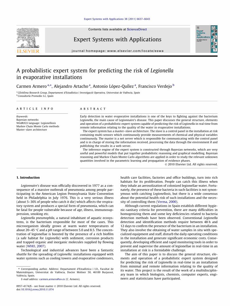
Expert Systems with Applications 38 (2011) 6637–6643

Contents lists available at ScienceDirect

Expert Systems with Applications

journal homepage: www.elsevier .com/locate /eswa

A probabilistic expert system for predicting the risk of Legionellain evaporative installations

Carmen Armero a,⇑, Alejandro Artacho a, Antonio López-Quílez a, Francisco Verdejo b

a GEeitEma Research Group, Departament d’Estadística i Investigació Operativa, Universitat de València, Spainb Consultoría Promedio S.L, Spain

a r t i c l e i n f o

Keywords:Bayesian networksWinBUGS language: LegionellosisMarkov Chain Monte Carlo methodsMaster–slave architecture

0957-4174/$ - see front matter � 2010 Elsevier Ltd. Adoi:10.1016/j.eswa.2010.11.074

⇑ Corresponding author. Address: Departament d’Matemàtiques, Universitat de València, Doctor MValència, Spain.

E-mail address: carmen.armero@uv.es (C. Armero)

a b s t r a c t

Early detection in water evaporative installations is one of the keys to fighting against the bacteriumLegionella, the main cause of Legionnaire’s disease. This paper discusses the general structure, elementsand operation of a probabilistic expert system capable of predicting the risk of Legionella in real time fromremote information relating to the quality of the water in evaporative installations.

The expert system has a master–slave architecture. The slave is a control panel in the installation at riskcontaining multi-sensors which continuously provide measurements of chemical and physical variablescontinuously. The master is a net server which is responsible for communicating with the control paneland is in charge of storing the information received, processing the data through the environment R andpublishing the results in a web server.

The inference engine of the expert system is constructed through Bayesian networks, which are veryuseful and powerful models that put together probabilistic reasoning and graphical modelling. Bayesianreasoning and Markov Chain Monte Carlo algorithms are applied in order to study the relevant unknownquantities involved in the parametric learning and propagation of evidence phases.

� 2010 Elsevier Ltd. All rights reserved.

1. Introduction

Legionnaire’s disease was officially discovered in 1977 as a con-sequence of a massive outbreak of pneumonia among people par-ticipating in the American Legion Pennsylvania State Conventionheld in Philadelphia in July 1976. This is a very serious illness(about 5–30% of people who catch it die) which affects the respira-tory system and produces a special form of pneumonia, which canbe fatal for people vulnerable because of age, illness, immunosup-pression, smoking etc.

Legionella pneumophila, a natural inhabitant of aquatic ecosys-tems, is the bacterium responsible for most of the cases. Thismicroorganism ideally grows at warm water temperatures ofabout 20–45 �C and a pH range of between 5.0 and 8.5. The concen-tration of legionellae is boosted by the presence of a rich biofilm(a safe habitat for Legionella) with sediment, corrosion productsand trapped organic and inorganic molecules supplied by flowingwater (WHO, 2007).

Technological and industrial advances have been a fantasticshuttle for the spreading of Legionella: installations equipped withwater systems such as cooling towers and evaporative condensers,

ll rights reserved.

Estadística i I.O., Facultat deoliner 50, 46100 Burjassot,

.

health care facilities, factories and office buildings, turn into richhabitats for its proliferation. People can catch this illness whenthey inhale an aerosolization of colonized legionellae water. Fortu-nately, the presence of these bacteria in such facilities is not synon-ymous with catching Legionellosis, but there is a wide consensusabout the potential health risk of such installations and the neces-sity of controlling them (Verma, 2000).

Although current regulations in Spain establish different hygie-nic-sanitary criteria for prevention, there are many difficulties inhomogenizing them and some key deficiencies related to bacteriadetection methods have been observed. Conventional Legionelladetection and identification methods require between 48 h and12 days to confirm the presence of the bacterium in an installation.They also involve the obtaining of water samples in situ with spe-cialized equipment and staff, disturb the daily operating conditionsin the installation and generate significant economic costs. Conse-quently, developing efficient and rapid monitoring tools in order toprevent and supervise the amount of legionellae in real-time in aninstallation at risk is a formidable challenge.

The aim of this paper is to discuss the general structure, ele-ments and operation of a probabilistic expert system designedfor predicting the risk of Legionella in real-time in an installationfrom minimal and remote information relating to the quality ofits water. This project is the result of the work of a multidisciplin-ary team in which biologists, chemists, computer experts, engi-neers and statisticians have participated.

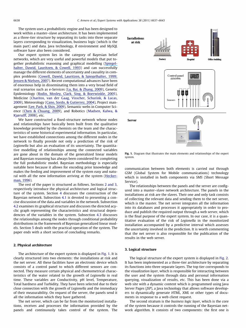
Fig. 1. Diagram that illustrates the main elements and relationships of the expertsystem.

6638 C. Armero et al. / Expert Systems with Applications 38 (2011) 6637–6643

The system uses a probabilistic engine and has been designed towork within a master–slave architecture. It has been implementedas a three-tier structure by separating its tasks into three separatelayers corresponding to visualization, business logic (which is themain part) and data. Java technology, R environment and MySQLsoftware have also been considered.

Our expert system lies in the category of Bayesian beliefnetworks, which are very useful and powerful models that put to-gether probabilistic reasoning and graphical modelling (Spiegel-halter, Dawid, Lauritzen, & Cowell, 1993) and can successfullymanage the different elements of uncertainty and causality in com-plex problems (Cowell, Dawid, Lauritzen, & Spiegelhalter, 1999;Jensen & Nielsen, 2007). Recent computational advances have beenof enormous help in disseminating them into a very broad field ofreal scenarios such as e-Services (Lu, Bai, & Zhang, 2009), GeneticEpidemiology (Rodin, Mosley, Clark, Sing, & Boerwinkle, 2005),Medicine (Charitos, van der Gaag, Visscher, Schurink, & Lucas,2009), Meteorology (Cano, Sordo, & Gutierrez, 2004), Project man-agement (Lee, Park, & Shin, 2009), Semantic webs in Computer Sci-ence (Chen & Chuang, 2009), and Robotics (Madsen, Kalwa, &Kjærulff, 2008), etc.

We have constructed a fixed-structure network whose nodesand relationships have basically been built from the qualitativeknowledge provided by the chemists on the team and the charac-teristics of some historical experimental information. In particular,we have established connections among the different nodes in thenetwork to finally provide not only a prediction of the risk ofLegionella but also an evaluation of its uncertainty. The quantita-tive modelling of relationships among the connected variablesare gone about in the domain of the generalized linear modelsand Bayesian reasoning has always been considered for completingthe full probabilistic model. Bayesian methodology is especiallysuitable here because it allows for encoding prior knowledge andmakes the feeding and improvement of the system easy and natu-ral with all the new information arriving at the system (Hecker-man, 1996).

The rest of the paper is structured as follows. Sections 2 and 3,respectively introduce the physical architecture and logical struc-ture of the system. Section 4 discusses the construction of theBayesian network. Subsection 4.1 is devoted to presenting a con-cise discussion of the data and variables in the network. Subsection4.2 examines its graphical structure and discusses the directed acy-clic graph representing the characteristics and structural depen-dencies of the variables in the system. Subsection 4.3 discussesthe relationships among the nodes through conditional probabilitydistributions in the framework of Bayesian generalized linear mod-els. Section 5 deals with the practical operation of the system. Thepaper ends with a short section of concluding remarks.

2. Physical architecture

The architecture of the expert system is displayed in Fig. 1. It isclearly structured into two elements: the installations at risk andthe net server. All these facilities have an electronic device whichconsists of a control panel to which different sensors are con-nected. They measure certain physical and chemometrical charac-teristics of the water related to the growth of Legionella in realtime. These variables are Conductivity, pH level, Temperature,Total hardness and Turbidity. They have been selected due to theirclose connection with the growth of Legionella and the immediacyof their measurability. On request of the server, the panels send itall the information which they have gathered.

The net server, which can be far from the monitorized installa-tions, receives and processes the information provided by thepanels and continuously takes control of the system. The

communication between both elements is carried out throughGSM (Global System for Mobile communications) technologywhich is installed in both components via SMS (Short MessageService).

The relationships between the panels and the server are config-ured into a master–slave network architecture. The panels in theinstallations at risk are the slaves. Their one and only task consistsof collecting the relevant data and sending them to the net server,which is the master. The net server integrates all the informationinto its databases and processes it appropriately in order to pro-duce and publish the required output through a web server, whichis the final purpose of the expert system. In our case, it is a quan-titative evaluation of the risk of Legionella in the monitorizedinstallation accompanied by a predictive interval which assessesthe uncertainty involved in the prediction. It is worth commentingthat the net server is also responsible for the publication of theresults in the web server.

3. Logical structure

The logical structure of the expert system is displayed in Fig. 2.It has been implemented as a three-tier architecture by separatingits functions into three separate layers. The top tier corresponds tothe visualization layer, which is responsible for interacting betweenthe user and the system through data and personal informationquerying, visualization of results, etc. This has been done via aweb site with a dynamic content which is programmed using JavaServer Pages (JSP), a Java technology that allows software develop-ers to dynamically generate HTML, XML or other types of docu-ments in response to a web client request.

The second stratum is the business logic layer, which is the coreof the system because it controls the running of the Bayesian net-work algorithm. It consists of two components: the first one is

Fig. 2. Logical structure of the expert system.

C. Armero et al. / Expert Systems with Applications 38 (2011) 6637–6643 6639

Tomcat, the Apache Software Foundation, a web container thatoperates as a web application server supporting Servlets and JSPs,whose task is to insert and edit data in the database and send infor-mation to the visualization layer. The second element is an applica-tion capable of communicating with the control panels in order toreceive, process and store the information recorded by the sensors.This is a Java service that uses the following application program-ming interfaces (APIs):

� SMSLib, a library which is devoted to sending and receiving SMSmessages via a compatible GSM modem,� RXTX, a library which allows the GSM modem to be connected

with the serial port of the server,� JRI, a Java/R Interface which allows to operate the R free soft-

ware environment to be run inside Java applications,� JDBC (Java Database Connectivity), suitable for extracting and

storing information out of and within the database, and finally,� JFreeChart, a chart library which produces the graphics corre-

sponding to the outcomes of the process.

The final level is the data layer, which is in charge of the datastorage, not only of the Bayesian network information but also ofthe personal information corresponding to the users, the availabil-ity and state of slaves, IP addresses, assigned tasks, etc. The rela-tional database has been constructed with MySQL software.

1 For interpretation of colour in Fig. 3, the reader is referred to the web version ofthis article.

4. Bayesian network

4.1. The data

Once the expert system has been constructed it will only be-come fully operational when the panels begin to send data to thenet server. Before that moment, and as a part of the general con-struction process, a historical data set from six cooling towerswhich were monitorized monthly during the period 2002–2006have been considered. They have been used to feed data into the

expert system in the first step of the Bayesian learning process inorder to improve the knowledge of the relevant parameters inthe system and examine the adequacy of the model selected.

These data include records for a total of 13 variables, all relatedto the quality of the water, which have been considered as risk fac-tors associated with the growth of Legionella, together with theinformation dealing with the monitoring of the response variable,the risk of Legionella. This is a binary variable which is positivewhen the number of legionellae bacteria, expressed in colonyforming units per ml of water, is above the established 100 cfus/ml risk threshold.

The predictor variables in the set are Conductivity, Iron, Level ofaerobic bacteria at 22 �C and at 36�, Level of chlorides, pH level,Salinity, Simple and Complete alkalinity, Solids in suspension,Temperature, Total hardness and Turbidity. Note that Conductivity,pH level, Temperature, Total hardness and Turbidity are the vari-ables which will be recorded by the panels in installations at riskand whose measuring will be carried out in real time. The remain-ing variables in the historical set cannot be recorded in real timefrom the panels because they need some extra time and laboratorytesting. However, their information will also be valuable for thesystem because they will be regularly analyzed in the laboratoryand the results obtained incorporated into the expert system inconsecutive Bayesian relearning processes.

4.2. Graphical structure

Our expert system combines qualitative and quantitative mod-elling. In the qualitative framework, it is useful to employ a picto-rial representation of the relationships among the differentvariables of the ES in order to conceptualize the probabilistic mod-elling mechanism. It is a directed acyclical graph (DAG) where eachnode stands for a variable and the arcs between nodes indicateassociation between variables: the unidirectional relation X ? Yis for causal dependency between nodes X and Y, and the missingedges between variables are for conditional independency. IfX ? Y, we say that node X is one of Y’s parents and node Y is oneof X’s children.

Fig. 3 displays a directed acyclic graph (DAG) representing thecharacteristics and structural dependencies of the variables inour system. This definitive picture is the result of a general discus-sion among the members of the project, mainly based on thechemical expertise provided by the chemists and the availabilityof different sources of experimental information. We will now ex-plain the construction of this graph.

All nodes in the network are hierarchically arranged in four lev-els. The first level (nodes in lilac) corresponds to the set of obser-vable variables which will be measured in real time from thepanels. They are orphan nodes. In addition, we have explicitlyintroduced here some useful nodes which are chemically-baseddiscretizations of pH (see pH1 and pH2 in Fig. 3) and temperature(see T1 in Fig. 3) that allow us to consider different effects on thenodes separately and visualize the general structure of the graphbetter.

Variables in the second stratum (in blue)1 correspond to theones examined in the historical set which are not recorded bythe panels. Nodes in the first level are the parent nodes of thesevariables. In the third stage we have introduced four non observa-ble and intermediate variables (in green) which have the task ofconnecting the information from preceding levels to the responsevariable. This is done through different relationships based onthe theoretical knowledge of the system and chemists expert

T

PH

T1

PH2

PH1

THARD

COND

TURBI

PH3

ALKAC

SAL

SOLID

CL

ALKA

FE

AER22

AER36

RSI

INCRUST

CORR

BIOFILM

LEG

Fig. 3. Directed graphical model representing the characteristics and structural dependencies of the nodes in the system. The name of the variables in the network isexpressed in terms of acronyms. Lilac nodes are PH for pH level, T for Temperature, THARD for Total hardness, COND for Conductivity and TURBI for Turbidity. With the same colournodes pH1 and pH2 and T1 are, respectively, transformations of the pH level and Temperature. Blue nodes are ALKA and ALKAC for representing Simple and Complete alkalinityrespectively, SAL for Salinity, CL for Level of chlorides, SOLID for Solids in suspension, FE for Iron and AER22 and AER26 are for the Level of aerobic bacteria at 22 �C and at 36�,respectively. Green nodes are INCRUST, which stands for the Level of incrustation, RSI for the Ryzar stability index, CORR for Corrosion and BIOFILM for Biofilm. The final node is therisk of Legionella which is represented as LEG. (For interpretation of the references to colour in this figure legend, the reader is referred to the web version of this article.)

6640 C. Armero et al. / Expert Systems with Applications 38 (2011) 6637–6643

information in order to feed the (last) level where the risk ofLegionella is registered with appropriate information. These latentnode variables are the Level of incrustation, Corrosion, Biofilmand the Ryznar stability index. This last one is an empirical mea-sure of the scaling or corrosive tendency of water based on thepH at saturation in calcium carbonate which has a well-knowndeterministic expression according to pH, Salinity, Simple alkalin-ity, Temperature and Total hardness. We are aware that the inclu-sion of this variable in the model could be a bit redundant, but wehave retained it because it provides the system with robustness inthat the allocation of relationships about corrosion and scaling arenot completely based on definite criteria. As we have mentionedbefore, the last level of the graph is constituted by the variable inwhich we are interested, the risk of Legionella, which is in orangein the graph.

Most of these variables have different behaviour depending onthe season of the year the measurement is recorded. For this reasonsome families will implicitly include a parent node which will sendinformation to the child related to the current season of the year.This information will be introduced into the modelling as a fixedseasonal effect. For the sake of visual clarity, seasonal nodes havenot been explicitly included in Fig. 3 and will usually be omittedin the conditional expressions.

4.3. Conditional probability distributions

After specifying the set X of nodes in the system we have tocomplete the construction of the Bayesian network. This is doneby specifying a joint probabilistic distribution, p(xjh), for X which

is not fully determined and depends on an unknown parametricvector h. BN have the property of d-separation which allows thejoint probability distribution to be factorized as the product ofthe conditional distribution of each node given its parents,

pðxjhÞ ¼Yx2X

pðxjpaðxÞ; hÞ; ð4:1Þ

where pa(X) denotes the set of parents of node X. Within Bayesianreasoning, the current information on the parameters h in the net-work is expressed through a prior distribution, p(h), which is a prob-ability distribution for h. Assuming global independence among theset of parameters corresponding to the conditional distribution ofdifferent nodes, pðhÞ ¼

Qx2X pðhxÞ, we will have

pðxjhÞ ¼Yx2X

pðxjpaðxÞ; hxÞ; ð4:2Þ

and the joint probability distribution of nodes and parameters couldbe expressed as:

pðx; hÞ ¼Yx2X

pðxjpaðxÞ; hxÞpðhxÞ: ð4:3Þ

Bayesian methods combine the experimental information abouth contained in the likelihood function with the joint prior distribu-tion p(h) by means of Bayes’ theorem. This process leads to theposterior distribution p(hjx) which contains all the relevant infor-mation (both subjective and experimental) about h. When globalindependence is assumed and complete data are observed, poster-ior global dependence will be also conserved, and consequently:

Fig. 4. Estimation of the predicted posterior mean of the risk of Legionella, 95%posterior prediction interval and histogram of the simulated sample correspondingto the posterior predictive distribution of the risk of Legionella as the result of theinformation sent by the monitorized installation panel on December 01, 2007.

C. Armero et al. / Expert Systems with Applications 38 (2011) 6637–6643 6641

pðhjxÞ ¼Yx2X

pðhxjfaðxÞÞ; ð4:4Þ

where here fa(X) represents the family of node X, which is this nodeand its parents.

According to (4.3), and with the clear objective of learningabout the probabilistic behaviour of the network through the jointdistribution of all variables, the conditional distribution of eachnode given its parents has been examined. Before doing this task,and in order to simplify the modelling process a bit, we have trans-formed all continuous nodes in the network to be in the unit inter-val and have always selected a beta distribution (Castillo,Gutierrez, & Hadi, 1997) for modelling them. This is a very flexibledensity bounded over a finite range with many different shapesdepending on the parameters chosen. In addition, we have re-stricted the freedom of these parameters to the size of the histor-ical data set. This condition barely impoverishes the modelling butmakes the inferential process easier. Also, following Castillo et al.(1997), discrete variables have been categorized in order to be con-sidered as binomial models whose values are ordered by followinga direct connection with the values of the examined variable.

Bayesian Generalized Linear Models have been the generalframework for connecting each node with its parents (see Armero,Artacho, & López-Quı́lez, 2009; for a wide and detailed discussionabout the statistical modelling of all conditional probabilities inthe network). In particular, for each X beta (binomial) node withparents pa(X), the logit link has been used to model the conditionalexpectation (probability), which we represent by px, as a linearcombination of the parent nodes whose b0xi

coefficients are theparameters to be estimated,

logitðpxÞ ¼ bx0þX

xi2paðxÞbxi

xi: ð4:5Þ

In general, prior independence has been considered for the bxi’s

parameters involved in each conditional modelling and prior dis-tributions containing very scarce information have been elicited.This is done to allow them to surf freely in such a wide parametricspace and so data will have all the strength to locate their valuesproperly. Nevertheless, in order to avoid any chance of obtainingimproper posteriors, we have always used proper densities (usu-ally normal distributions with mean zero and variance 1000). Also,we would like to point out that links for unobservable variableshave been subjectively assessed by using the prior information ofchemical experts.

Posterior distributions for parameters are not usually analyticaland numerical methods of integration for approximating them areextremely demanding on computer resources, especially whendealing with high dimensional problems. For this reason we havemoved into the simulation world, particularly into Markov ChainMonte Carlo methods (MCMC from now on). They are good atdrawing an approximate sample of the particular posterior distri-bution examined, from which we can approximate the quantitiesof the parameters that are of interest in the problem. In our case,this procedure will provide a random sample

hðsÞx ¼ ðbðsÞxi; i ¼ 0; . . . ; ]paðxÞÞ; s ¼ 1; . . . ; S

n oð4:6Þ

of size S of the posterior distribution of the parametric vector (hx)associated to each conditional distribution p(xjpa(x),hx). This com-putational process can be implemented automatically and for thispurpose we have used the WinBUGS language (Spiegelhalteret al., 2003) in this paper. This is a free software environment whichallows us to focus on the correct definition of the model and inter-nally takes care of all elements involved in the approximate samplediscussed before.

5. The expert system in action

The phase of parametric learning discussed before is the firstprobabilistic activity of the inference engine of the expert system.Only when it is completed, will the expert system be ready tostart properly: all new evidence sent by the panels to the serverwill be immediately processed by the inference engine to pro-duce the relevant outcomes about the risk of Legionella in themonitorized installation. The way in which the system carriesout that task is as follows: a configuration file is used to setthe moment at which the server has to connect with each con-trol panel. Just at that moment the server communicates withthe panel and receives data from the sensors through the li-braries SMSLib and RXTX. Immediately after, the interface JRIsends the information to the R application in order for the Bayes-ian network to process it appropriately. The library JFreeChartsummarizes the outcomes of the algorithm and displays themto the users.

Fig. 4 presents an English version (the original is in Spanish)of the results obtained in real time with regard to the values ofthe variables measured by the panel on a particular date (Decem-ber 01, 2007) and time (14.10.43). It is an estimation of the pre-dicted posterior mean of the risk of Legionella, a 95% posteriorprediction interval for that risk which assesses the uncertaintyrelated to that prediction and a histogram of the simulated sam-ple corresponding to the posterior predictive distribution of therisk of Legionella. The system also generates an updated pictureof the temporal evolution of both point and interval predictions.Fig. 5 shows an English version of this information from October2007 to April 2008. Both Figs. 4 and 5 correspond to the sameinstallation at risk, specifically a cooling tower located in theprovince of València whose name cannot be divulged. This towerhas registered no incidents related to Legionella in that period oftime.

The general process in charge of disseminating the new evi-dence provided by the panels sequentially operates from the firstnodes until the final one, the risk of Legionella, passing throughthe corresponding intermediate nodes. We want to point out that

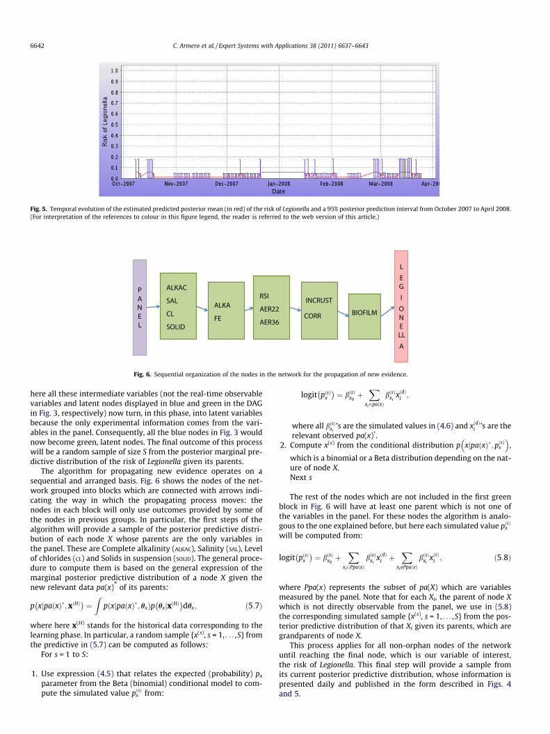
Fig. 5. Temporal evolution of the estimated predicted posterior mean (in red) of the risk of Legionella and a 95% posterior prediction interval from October 2007 to April 2008.(For interpretation of the references to colour in this figure legend, the reader is referred to the web version of this article.)

Fig. 6. Sequential organization of the nodes in the network for the propagation of new evidence.

6642 C. Armero et al. / Expert Systems with Applications 38 (2011) 6637–6643

here all these intermediate variables (not the real-time observablevariables and latent nodes displayed in blue and green in the DAGin Fig. 3, respectively) now turn, in this phase, into latent variablesbecause the only experimental information comes from the vari-ables in the panel. Consequently, all the blue nodes in Fig. 3 wouldnow become green, latent nodes. The final outcome of this processwill be a random sample of size S from the posterior marginal pre-dictive distribution of the risk of Legionella given its parents.

The algorithm for propagating new evidence operates on asequential and arranged basis. Fig. 6 shows the nodes of the net-work grouped into blocks which are connected with arrows indi-cating the way in which the propagating process moves: thenodes in each block will only use outcomes provided by some ofthe nodes in previous groups. In particular, the first steps of thealgorithm will provide a sample of the posterior predictive distri-bution of each node X whose parents are the only variables inthe panel. These are Complete alkalinity (ALKAC), Salinity (SAL), Levelof chlorides (CL) and Solids in suspension (SOLID). The general proce-dure to compute them is based on the general expression of themarginal posterior predictive distribution of a node X given thenew relevant data pa(x)* of its parents:

p xjpaðxÞ�;xðHÞ� �

¼Z

p xjpaðxÞ�; hxð Þp hxjxðHÞ� �

dhx; ð5:7Þ

where here x(H) stands for the historical data corresponding to thelearning phase. In particular, a random sample {x(s), s = 1, . . . ,S} fromthe predictive in (5.7) can be computed as follows:

For s = 1 to S:

1. Use expression (4.5) that relates the expected (probability) px

parameter from the Beta (binomial) conditional model to com-pute the simulated value pðsÞx from:

logit pðsÞx

� �¼ bðsÞx0

þX

xi2paðxÞbðsÞxi

xðdÞi ;

where all bðsÞxi’s are the simulated values in (4.6) and xðdÞi ’s are the

relevant observed pa(x)*.2. Compute x(s) from the conditional distribution p xjpaðxÞ�; pðsÞx

� �,

which is a binomial or a Beta distribution depending on the nat-ure of node X.Next s

The rest of the nodes which are not included in the first greenblock in Fig. 6 will have at least one parent which is not one ofthe variables in the panel. For these nodes the algorithm is analo-gous to the one explained before, but here each simulated value pðsÞx

will be computed from:

logit pðsÞx

� �¼ bðsÞx0

þX

xi2PpaðxÞbðsÞxi

xðdÞi þX

xiRPpaðxÞbðsÞxi

xðsÞi ; ð5:8Þ

where Ppa(x) represents the subset of pa(X) which are variablesmeasured by the panel. Note that for each Xi, the parent of node Xwhich is not directly observable from the panel, we use in (5.8)the corresponding simulated sample {x(s), s = 1, . . . ,S} from the pos-terior predictive distribution of that Xi given its parents, which aregrandparents of node X.

This process applies for all non-orphan nodes of the networkuntil reaching the final node, which is our variable of interest,the risk of Legionella. This final step will provide a sample fromits current posterior predictive distribution, whose information ispresented daily and published in the form described in Figs. 4and 5.

C. Armero et al. / Expert Systems with Applications 38 (2011) 6637–6643 6643

In addition to the information provided by the panel, which isthe real-time food nourishing our expert system, new informationis introduced into the system. Periodically, specimens of nonreal-time observable nodes are also taken from the cooling tower,analyzed in the laboratory and sent to the server. At that moment,the expert system will have at its disposal both the data collecteddirectly from the panel as well as those recorded from the labora-tory. This situation will automatically start a new relearning phase,generated by sequentially applying Bayes’ theorem, which will up-date the information of the unknown parametric vector and conse-quently, improve the quality of the system.

6. Conclusions

We have constructed an expert system capable of instanta-neously predicting the risk of Legionella in remote cooling towersfrom the only monitorization of real-time information on theirwater quality. The system uses a probabilistic engine and has beendesigned to work within a master–slave architecture. Bayesiannetworks have been used to model and connect relationships anddependencies among the different nodes in the network to finallyprovide not only a prediction of the risk of Legionella but also anevaluation of its uncertainty.

Acknowledgements

Special thanks to the Ministerio de Educación y Ciencia grantsMTM2007-61554 and MTM2010-19528, Conselleria Empresa, Uni-versitat i Ciència de la Generalitat Valenciana grant GV/2007/079and Ministerio de Industria, Turismo y Comercio FIT-350300-2006-87.

References

Armero, C., Artacho, A., & López-Quı́lez, A. (2009). Bayesian models to develop anexpert system for assessing the risk of Legionella in cooling towers. TechnicalReport GEeitEma 2009/79. Universitat de València.

Cano, R., Sordo, C., & Gutierrez, J. M. (2004). Applications of Bayesian networks inmeteorology. In Gámez et al. (Eds.), Advances in Bayesian networks(pp. 309–327). Springer.

Castillo, E., Gutierrez, J. M., & Hadi, A. S. (1997). Expert systems and probabilisticnetwork models. New York: Springer-Verlag.

Charitos, T., van der Gaag, L. C., Visscher, S., Schurink, K. A. M., & Lucas, P. J. F. (2009).A dynamic Bayesian network for diagnosing ventilator-associated pneumoniain ICU patients. Expert Systems with Applications, 36, 1249–1258.

Chen, R. C., & Chuang, C. H. (2009). Automatic construction of a domain ontologyusing a projective adaptive resonance theory neural network and Bayesiannetwork. Expert Systems, 25(4), 414–430.

Cowell, R. G., Dawid, A. P., Lauritzen, S. L., & Spiegelhalter, D. J. (1999). Probabilisticnetworks and expert systems. New York: Springer-Verlag.

Heckerman D. (1996). A tutorial on learning Bayesian networks. Technical ReportMSRTR-95-06, Microsoft Research.

Jensen, F. V., & Nielsen, T. D. (2007). Bayesian networks and decision graphs (Seconded.). New York: Springer.

Lee, E., Park, Y., & Shin, J. G. (2009). Large engineering project risk managementusing a Bayesian belief network. Expert Systems with Applications, 36,5880–5887.

Lu, J., Bai, C., & Zhang, G. (2009). Cost-benefit factor analysis in e-services usingbayesian networks. Expert Systems with Applications, 36, 4617–4625.

Madsen, A. L., Kalwa, J., & Kjærulff, U. B. (2008). Risk Management in Robotics. In O.Pourret, P. Naim, & B. Marcot (Eds.), Bayesian networks: A practical guide toapplications (pp. 345–363). Chichester, UK: Wiley.

Rodin, A., Mosley, T. H., Jr., Clark, A. G., Sing, C. F., & Boerwinkle, E. (2005). Mininggenetic epidemiology data with Bayesian networks. Application to APOE genevariation and plasma lipid levels. Journal of Computational Biology, 12(1), 1–11.

Spiegelhalter, D. J., Dawid, A. P., Lauritzen, S. L., & Cowell, R. G. (1993). Bayesiananalysis in expert systems. Statistical Science, 8, 219–247.

Spiegelhalter D. J., Thomas A., Best N. & Lunn D. WinBUGS Version 1.4 User Manual,2003. <http://www.mrc-bsu.cam.ac.uk/bugs/winbugs/manual14.pdf> [20 May2008].

Verma, P. (2000). Cooling water treatment hand book. New Delhi, India: Albatross.WHO (World Health Organization). (2007). Legionella and the prevention of

Legionellosis. WHO: Geneva.