Natural and artificial radioactivity in the Svalbard glaciers
5th EARSeL Workshop on Remote Sensing of the Coastal Zone 25 Prague, Czech Republic, 1st – 3rd June, 2011
COMPARISON BETWEEN SATELLITE RADIOMETERS AND LIDAR FLUOROSENSOR IN THE ARCTIC SEA OFF THE SVALBARD
ISLANDS
Luca Fiorani1, Francesco Colao1, Maurizio Guarracino1, Salvatore Marullo1, Antonio Palucci1 and Davod Poreh2
1. ENEA, UTAPRAD-DIM, Frascati, Italy; [email protected] 2. ENEA guest with ICTP fellowship
ABSTRACT
Ocean color satellite radiometers have widely proven their outstanding capabilities as diagnostic tools of the world ocean biogeochemical cycles. Recently, SeaWiFS, MODIS and MERIS images have been merged to provide a better coverage (see: http://www.globcolour.info). Notwithstanding this remarkable success, chlorophyll measurements in coastal zones are still affected by not negli-gible uncertainties. This study, by the comparison between lidar and satellite data in the Arctic Sea near the Svalbard Islands confirm this behavior: while the match-up of these sensors is good off shore, satellite values are substantially lower near the coasts.
INTRODUCTION
Remote sensing is a very widely used method in environmental science, and has lots of applica-tions for geomonitoring, and geohazards. There are two main types of remote sensing: passive remote sensing and active remote sensing. Passive sensors detect natural radiation that is emitted or reflected by the object or surrounding area being observed. Reflected sunlight is the most com-mon source of radiation measured by passive sensors. Active collection, on the other hand, emits energy in order to scan objects and areas whereupon a sensor then detects and measures the ra-diation that is reflected or backscattered from the target. Combining these two methods is a state of art challenge and has got a lot of applications in geosciences. For the past 30 years, earth ob-servation satellites and remote laser measurements (lidar) have provided scientists with more ac-curate data, allowing them to understand better the physical phenomena at stake in earth climate. During the past decade the need for monitoring change in our environment on short and mid-term has kept increasing as on-orbit remote sensing revealed the real extent of human activity impact on our planet’s weather. Ocean satellites nowadays are gathering physical properties for chloro-phyll-a (Chl-a), phytoplanktons, gelbstoffe, etc. Three most capable sensors which are supported by satellite services are: SeaWiFS on GeoEye’s Orbview-2 mission, MODIS on NASA’s Aqua mis-sion and MERIS on ESA’s ENVISAT mission. The GlobColour service (http://www.globcolour.info), distributes global daily, 8-day and monthly data sets at 4.6 km resolution for the main bio-optical parameters. One obvious way to extend lidar and satellite capabilities is to merge their data streams together to provide robust merged climate data records with measurable uncertainty bounds. Up to now, limited concrete effort has taken place to demonstrate how these data can be used together in any systematic way. For this reason, here we present and implement a formalism for comparing global satellite ocean color data streams to lidar data sets producing uniform data products. The starting point of this study is the comparison of lidar Chl-a data, gathered from a ship in the Arctic Sea near the Svalbard Islands, with GlobColour’s satellite data. For this purpose we averaged our lidar data inside each pixel and then compared lidar and satellite values. Inter-comparisons between the different merged datasets will help in further refining the techniques used. Unfortunately, 8-day averaged data did not show promising results. On the contrary, the ap-plication of this analysis to daily data lead to good results. As far as our analysis is concerned, for near shore data satellite and lidar are far from correlation, and vice versa for off shore data they mainly have similar amounts of Chl-a and more correlated behavior. Compared to each of the orig-
5th EARSeL Workshop on Remote Sensing of the Coastal Zone 26 Prague, Czech Republic, 1st – 3rd June, 2011
inal data source, the products derived from the merging procedure show enhanced global daily coverage and lower uncertainties in the retrieved variables provided daily data are used.
satellite data
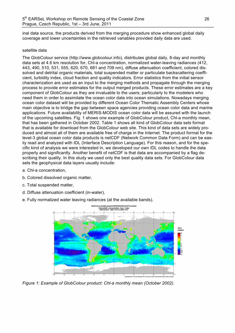
The GlobColour service (http://www.globcolour.info), distributes global daily, 8-day and monthly data sets at 4.6 km resolution for, Chl-a concentration, normalized water-leaving radiances (412, 443, 490, 510, 531, 555, 620, 670, 681 and 709 nm), diffuse attenuation coefficient, colored dis-solved and detrital organic materials, total suspended matter or particulate backscattering coeffi-cient, turbidity index, cloud fraction and quality indicators. Error statistics from the initial sensor characterization are used as an input to the merging methods and propagate through the merging process to provide error estimates for the output merged products. These error estimates are a key component of GlobColour as they are invaluable to the users; particularly to the modelers who need them in order to assimilate the ocean color data into ocean simulations. Nowadays merging ocean color dataset will be provided by different Ocean Color Thematic Assembly Centers whose main objective is to bridge the gap between space agencies providing ocean color data and marine applications. Future availability of MERIS-MODIS ocean color data will be assured with the launch of the upcoming satellites. Fig. 1 shows one example of GlobColour product, Chl-a monthly mean, that has been gathered in October 2002. Table 1 shows all kind of GlobColour data sets format that is available for download from the GlobColour web site. This kind of data sets are widely pro-duced and almost all of them are available free of charge in the Internet. The product format for the level-3 global ocean color data products is netCDF (Network Common Data Form) and can be eas-ily read and analyzed with IDL (Interface Description Language). For this reason, and for the spe-cific kind of analysis we were interested in, we developed our own IDL codes to handle the data properly and significantly. Another benefit of netCDF is that data are accompanied by a flag de-scribing their quality. In this study we used only the best quality data sets. For GlobColour data sets the geophysical data layers usually include:
a. Chl-a concentration,
b. Colored dissolved organic matter,
c. Total suspended matter,
d. Diffuse attenuation coefficient (in-water),
e. Fully normalized water leaving radiances (at the available bands).
Figure 1: Example of GlobColour product: Chl-a monthly mean (October 2002).

5th EARSeL Workshop on Remote Sensing of the Coastal Zone 27 Prague, Czech Republic, 1st – 3rd June, 2011
Table 1: Output product overview of GlobColour data.
LIDAR data
A detailed description of the ENEA Lidar Fluorosensor (ELF) has already been given elsewhere [Barbini et al. 2001], here we will only recall its main features. For a description of the AREX 2007 oceanographic campaign in the Arctic Sea near the Svalbard Islands, the reader is referred to a recent study [Cisek et al. 2010]. Our work on lidar-satellite comparison has been published in many papers [Fiorani et al. 2002, 2004, 2005, 2006a, 2006b, 2007, 2008]. ELF is a LIF-based instru-ment, conceived for the oceanographic campaigns aboard the research vessel (RV) Italica, in the framework of the Italian Antarctic Research Program (PNRA). It consists mainly of a frequency-tripled Nd :YAG laser (transmitter) and of a Cassegrain telescope coupled to the detectors (receiv-er): the laser emits a pulse at 355 nm to the sea surface and the telescope collects the backscat-tered light at different wavelengths. The radiation is then directed through a fibre bundle to four spectral bandpass filters and is detected with photomultiplier tubes. The four optical channels cor-respond to Raman scattering of water (404 nm) and fluorescence of chromophoric dissolved or-ganic matter (CDOM) (450 nm), phycocyanin (650 nm) and chlorophyll-a (680 nm). The operation of ELF is assisted by some ancillary instruments: lamp spectrofluorometer, pulsed amplitude fluo-rometer, solar radiance detector and global positioning system. At first, the fluorescence signals are released in Raman units, i.e. they are normalized to the water Raman peak (the relative sensi-tivity of the photomultiplier tubes has been calibrated observing with the lamp spectrofluorometer emission spectra of samples excited at 355 nm). Afterwards, they are converted into absolute con-centrations by calibration against chemical analysis on the same water. The investigated layer is about 10 m thick. The typical specifications of ELF are listed in Table 2.
Table 2: Specifications of ELF during a typical operation in oceanographic campaigns.

5th EARSeL Workshop on Remote Sensing of the Coastal Zone 28 Prague, Czech Republic, 1st – 3rd June, 2011
Figure 2: The study area is the Arctic Sea near the Svalbard Islands. The colored line is the ship track. The color corresponds to the Chl-a level (CL) in mg m-3.
Comparison between satellite and lidar data
8-day GlobColour data
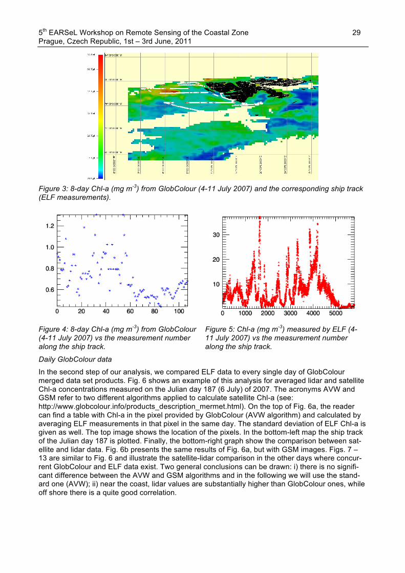
In the first step of our study, we compared ELF data to 8-day GlobColour merged data sets prod-ucts. The 8-day time interval enables the gathering of enough simultaneous measurements and the level-3 processing level ensured the highest accuracy of data sets. For achieving even more accuracy, we used flagged data. Although these choices involved a rather poor granularity, they have been considered as the best compromise. The resolution of ELF is very different, since a la-ser pulse is emitted every 0.1 s and its footprint on the water surface sizes around 10 cm. In order to compare the data, all the ELF measurements falling in a GlobColour pixel were averaged. Dur-ing the 16 days of the Italian participation of AREX 2007 (July 2007), ELF measured surface Chl-a concentrations in the Arctic Sea as presented in Fig. 2. For the entire time of ELF data acquisition, laser data are classified with different colors. We divided our LIDAR data in three sets in order to match with the satellite images. For instance, Fig. 3 shows the laser data gathered on 4-11 July 2007 and the corresponding merged GlobColour data sets. Fig. 4 and 5 show the Chl-a concentra-tions for satellite and ELF, respectively, along the ship track. It can be noticed that there is a re-markable difference in amount of Chl-a concentrations with these two methods. We suspected that this happened because of the time discrepancy: while the GlobColour data are averaged in a 8-day period, ELF measurement are averaged in a 1-minute interval, so between the two determination there can be a 8-day lag. For this reason, we developed an IDL code to compare daily GlobColour data with ELF measurements.
5th EARSeL Workshop on Remote Sensing of the Coastal Zone 29 Prague, Czech Republic, 1st – 3rd June, 2011
Figure 3: 8-day Chl-a (mg m-3) from GlobColour (4-11 July 2007) and the corresponding ship track (ELF measurements).
Figure 4: 8-day Chl-a (mg m-3) from GlobColour (4-11 July 2007) vs the measurement number along the ship track.
Figure 5: Chl-a (mg m-3) measured by ELF (4-11 July 2007) vs the measurement number along the ship track.
Daily GlobColour data
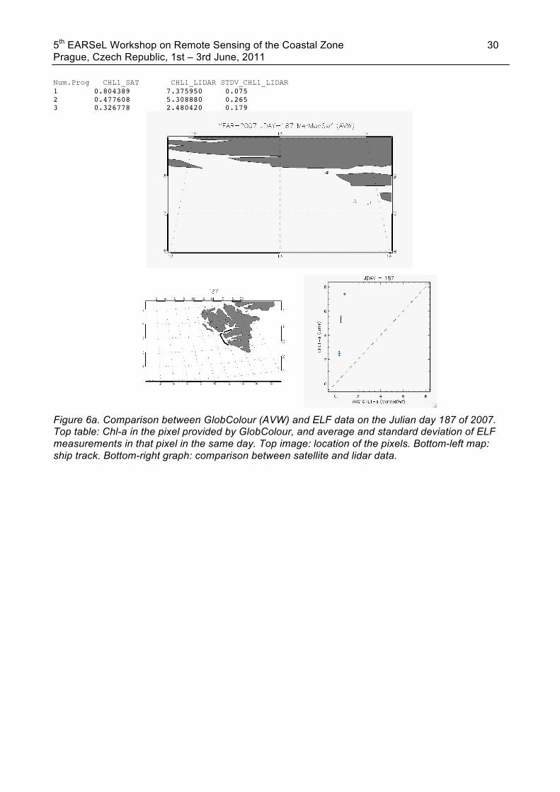
In the second step of our analysis, we compared ELF data to every single day of GlobColour merged data set products. Fig. 6 shows an example of this analysis for averaged lidar and satellite Chl-a concentrations measured on the Julian day 187 (6 July) of 2007. The acronyms AVW and GSM refer to two different algorithms applied to calculate satellite Chl-a (see: http://www.globcolour.info/products_description_mermet.html). On the top of Fig. 6a, the reader can find a table with Chl-a in the pixel provided by GlobColour (AVW algorithm) and calculated by averaging ELF measurements in that pixel in the same day. The standard deviation of ELF Chl-a is given as well. The top image shows the location of the pixels. In the bottom-left map the ship track of the Julian day 187 is plotted. Finally, the bottom-right graph show the comparison between sat-ellite and lidar data. Fig. 6b presents the same results of Fig. 6a, but with GSM images. Figs. 7 – 13 are similar to Fig. 6 and illustrate the satellite-lidar comparison in the other days where concur-rent GlobColour and ELF data exist. Two general conclusions can be drawn: i) there is no signifi-cant difference between the AVW and GSM algorithms and in the following we will use the stand-ard one (AVW); ii) near the coast, lidar values are substantially higher than GlobColour ones, while off shore there is a quite good correlation.
5th EARSeL Workshop on Remote Sensing of the Coastal Zone 30 Prague, Czech Republic, 1st – 3rd June, 2011
Num.Prog CHL1_SAT CHL1_LIDAR STDV_CHL1_LIDAR 1 0.804389 7.375950 0.075 2 0.477608 5.308880 0.265 3 0.326778 2.480420 0.179
Figure 6a. Comparison between GlobColour (AVW) and ELF data on the Julian day 187 of 2007. Top table: Chl-a in the pixel provided by GlobColour, and average and standard deviation of ELF measurements in that pixel in the same day. Top image: location of the pixels. Bottom-left map: ship track. Bottom-right graph: comparison between satellite and lidar data.

5th EARSeL Workshop on Remote Sensing of the Coastal Zone 31 Prague, Czech Republic, 1st – 3rd June, 2011
Num.Prog CHL1_SAT CHL1_LIDAR STDV_CHL1_LIDAR 1 0.837994 7.375950 0.075 2 0.540990 5.308880 0.265 3 0.263172 4.116420 0.246 4 0.282228 2.480420 0.179
Figure 6b. Comparison between GlobColour (GSM) and ELF data on the Julian day 187 of 2007. Top table: Chl-a in the pixel provided by GlobColour, and average and standard deviation of ELF measurements in that pixel in the same day. Top image: location of the pixels. Bottom-left map: ship track. Bottom-right graph: comparison between satellite and lidar data.
5th EARSeL Workshop on Remote Sensing of the Coastal Zone 32 Prague, Czech Republic, 1st – 3rd June, 2011
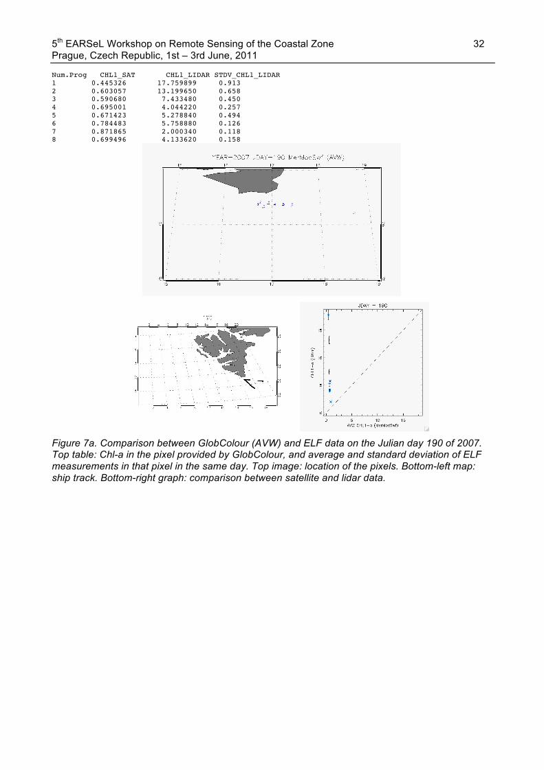
Num.Prog CHL1_SAT CHL1_LIDAR STDV_CHL1_LIDAR 1 0.445326 17.759899 0.913 2 0.603057 13.199650 0.658 3 0.590680 7.433480 0.450 4 0.695001 4.044220 0.257 5 0.671423 5.278840 0.494 6 0.784483 5.758880 0.126 7 0.871865 2.000340 0.118 8 0.699496 4.133620 0.158
Figure 7a. Comparison between GlobColour (AVW) and ELF data on the Julian day 190 of 2007. Top table: Chl-a in the pixel provided by GlobColour, and average and standard deviation of ELF measurements in that pixel in the same day. Top image: location of the pixels. Bottom-left map: ship track. Bottom-right graph: comparison between satellite and lidar data.
5th EARSeL Workshop on Remote Sensing of the Coastal Zone 33 Prague, Czech Republic, 1st – 3rd June, 2011
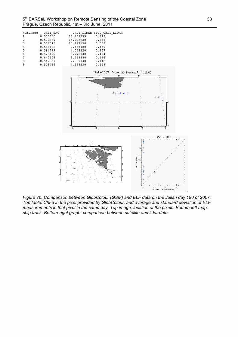
Num.Prog CHL1_SAT CHL1_LIDAR STDV_CHL1_LIDAR 1 0.500360 17.759899 0.913 2 0.570339 15.227730 0.368 3 0.557615 13.199650 0.658 4 0.550168 7.433480 0.450 5 0.584799 4.044220 0.257 6 0.525105 5.278840 0.494 7 0.647308 5.758880 0.126 8 0.542057 2.000340 0.118 9 0.509434 4.133620 0.158
Figure 7b. Comparison between GlobColour (GSM) and ELF data on the Julian day 190 of 2007. Top table: Chl-a in the pixel provided by GlobColour, and average and standard deviation of ELF measurements in that pixel in the same day. Top image: location of the pixels. Bottom-left map: ship track. Bottom-right graph: comparison between satellite and lidar data.

5th EARSeL Workshop on Remote Sensing of the Coastal Zone 34 Prague, Czech Republic, 1st – 3rd June, 2011
Num.Prog CHL1_SAT CHL1_LIDAR STDV_CHL1_LIDAR 1 0.523360 0.404680 0.064
Figure 8a. Comparison between GlobColour (AVW) and ELF data on the Julian day 193 of 2007. Top table: Chl-a in the pixel provided by GlobColour, and average and standard deviation of ELF measurements in that pixel in the same day. Top image: location of the pixels. Bottom-left map: ship track. Bottom-right graph: comparison between satellite and lidar data.
5th EARSeL Workshop on Remote Sensing of the Coastal Zone 35 Prague, Czech Republic, 1st – 3rd June, 2011
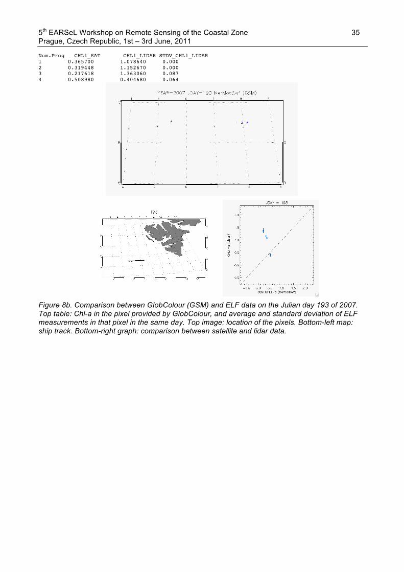
Num.Prog CHL1_SAT CHL1_LIDAR STDV_CHL1_LIDAR 1 0.365700 1.078640 0.000 2 0.319448 1.152670 0.000 3 0.217618 1.363060 0.087 4 0.508980 0.404680 0.064
Figure 8b. Comparison between GlobColour (GSM) and ELF data on the Julian day 193 of 2007. Top table: Chl-a in the pixel provided by GlobColour, and average and standard deviation of ELF measurements in that pixel in the same day. Top image: location of the pixels. Bottom-left map: ship track. Bottom-right graph: comparison between satellite and lidar data.
5th EARSeL Workshop on Remote Sensing of the Coastal Zone 36 Prague, Czech Republic, 1st – 3rd June, 2011
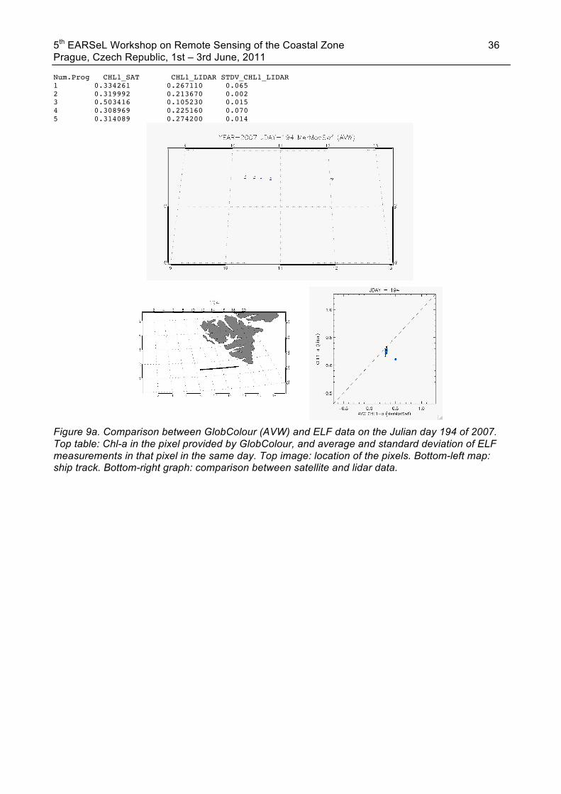
Num.Prog CHL1_SAT CHL1_LIDAR STDV_CHL1_LIDAR 1 0.334261 0.267110 0.065 2 0.319992 0.213670 0.002 3 0.503416 0.105230 0.015 4 0.308969 0.225160 0.070 5 0.314089 0.274200 0.014
Figure 9a. Comparison between GlobColour (AVW) and ELF data on the Julian day 194 of 2007. Top table: Chl-a in the pixel provided by GlobColour, and average and standard deviation of ELF measurements in that pixel in the same day. Top image: location of the pixels. Bottom-left map: ship track. Bottom-right graph: comparison between satellite and lidar data.

5th EARSeL Workshop on Remote Sensing of the Coastal Zone 37 Prague, Czech Republic, 1st – 3rd June, 2011
Num.Prog CHL1_SAT CHL1_LIDAR STDV_CHL1_LIDAR 1 0.273806 0.153460 0.010 2 0.300742 0.267110 0.065 3 0.306982 0.213670 0.002 4 0.653982 0.105230 0.015 5 0.253208 0.225160 0.070 6 0.272477 0.274200 0.014
Figure 9b. Comparison between GlobColour (GSM) and ELF data on the Julian day 194 of 2007. Top table: Chl-a in the pixel provided by GlobColour, and average and standard deviation of ELF measurements in that pixel in the same day. Top image: location of the pixels. Bottom-left map: ship track. Bottom-right graph: comparison between satellite and lidar data.

5th EARSeL Workshop on Remote Sensing of the Coastal Zone 38 Prague, Czech Republic, 1st – 3rd June, 2011
Num.Prog CHL1_SAT CHL1_LIDAR STDV_CHL1_LIDAR 1 1.336257 5.925990 0.461 2 1.296629 2.980030 0.125 3 0.918390 1.095950 0.113 4 0.610192 0.737940 0.047 5 0.615630 1.538960 0.091 6 0.486040 0.647700 0.080 7 0.625889 0.282330 0.013 8 0.589282 0.290040 0.020 9 0.518415 0.358920 0.024 10 0.337668 0.174420 0.014
Figure 10a. Comparison between GlobColour (AVW) and ELF data on the Julian day 195 of 2007. Top table: Chl-a in the pixel provided by GlobColour, and average and standard deviation of ELF measurements in that pixel in the same day. Top image: location of the pixels. Bottom-left map: ship track. Bottom-right graph: comparison between satellite and lidar data.
5th EARSeL Workshop on Remote Sensing of the Coastal Zone 39 Prague, Czech Republic, 1st – 3rd June, 2011
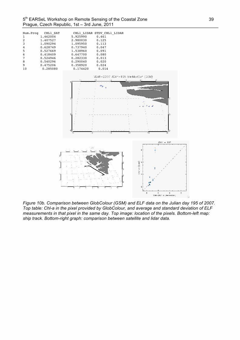
Num.Prog CHL1_SAT CHL1_LIDAR STDV_CHL1_LIDAR 1 1.462004 5.925990 0.461 2 1.407527 2.980030 0.125 3 1.090294 1.095950 0.113 4 0.628749 0.737940 0.047 5 0.527669 1.538960 0.091 6 0.418409 0.647700 0.080 7 0.524946 0.282330 0.013 8 0.540296 0.290040 0.020 9 0.475206 0.358920 0.024 10 0.285080 0.174420 0.014
Figure 10b. Comparison between GlobColour (GSM) and ELF data on the Julian day 195 of 2007. Top table: Chl-a in the pixel provided by GlobColour, and average and standard deviation of ELF measurements in that pixel in the same day. Top image: location of the pixels. Bottom-left map: ship track. Bottom-right graph: comparison between satellite and lidar data.

5th EARSeL Workshop on Remote Sensing of the Coastal Zone 40 Prague, Czech Republic, 1st – 3rd June, 2011
Num.Prog CHL1_SAT CHL1_LIDAR STDV_CHL1_LIDAR 1 2.594991 1.535450 0.253 2 2.150297 7.293660 0.357 3 1.841837 1.566710 0.031 4 1.521465 2.397260 0.528 5 1.496413 10.554670 0.414 6 2.625373 3.488500 0.143 7 1.580080 2.768380 0.268 8 0.940003 2.727570 0.429 9 2.279920 3.352960 0.416 10 1.398523 3.086550 0.443 11 0.911980 2.071090 0.170 12 0.990220 2.279670 0.121 13 1.022945 2.546580 0.198 14 1.173489 2.025860 0.103 15 1.051090 1.907910 0.222 16 0.877675 2.834330 0.511 17 1.213764 1.468990 0.110 18 1.276240 2.624560 0.232 19 0.978954 0.495510 0.051 20 0.596678 0.287490 0.026 21 0.633549 0.327020 0.039 22 0.712424 0.658220 0.311 23 0.780075 0.536590 0.059 24 0.581368 0.365500 0.044 25 0.750050 0.723970 0.141 26 1.145122 1.701630 0.100 27 0.829650 0.658250 0.127 28 1.091328 1.694220 0.051
Figure 11a. Comparison between GlobColour (AVW) and ELF data on the Julian day 196 of 2007. Top table: Chl-a in the pixel provided by GlobColour, and average and standard deviation of ELF measurements in that pixel in the same day. Top image: location of the pixels. Bottom-left map: ship track. Bottom-right graph: comparison between satellite and lidar data.
5th EARSeL Workshop on Remote Sensing of the Coastal Zone 41 Prague, Czech Republic, 1st – 3rd June, 2011
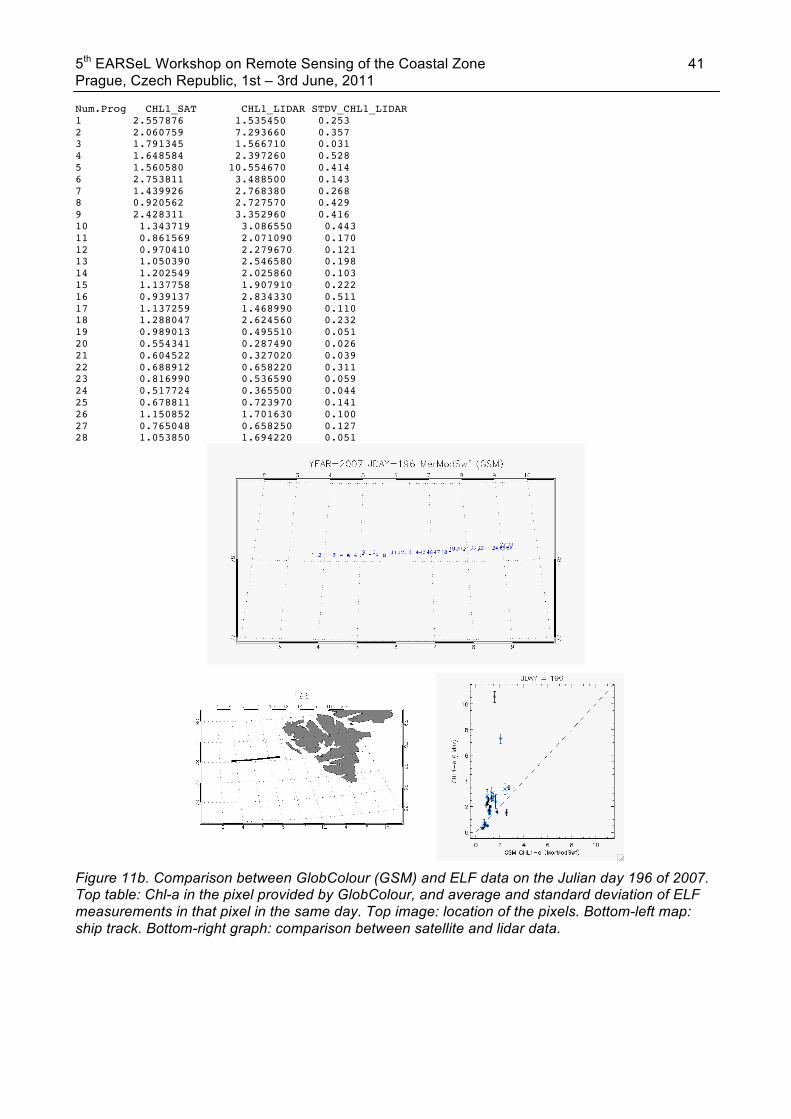
Num.Prog CHL1_SAT CHL1_LIDAR STDV_CHL1_LIDAR 1 2.557876 1.535450 0.253 2 2.060759 7.293660 0.357 3 1.791345 1.566710 0.031 4 1.648584 2.397260 0.528 5 1.560580 10.554670 0.414 6 2.753811 3.488500 0.143 7 1.439926 2.768380 0.268 8 0.920562 2.727570 0.429 9 2.428311 3.352960 0.416 10 1.343719 3.086550 0.443 11 0.861569 2.071090 0.170 12 0.970410 2.279670 0.121 13 1.050390 2.546580 0.198 14 1.202549 2.025860 0.103 15 1.137758 1.907910 0.222 16 0.939137 2.834330 0.511 17 1.137259 1.468990 0.110 18 1.288047 2.624560 0.232 19 0.989013 0.495510 0.051 20 0.554341 0.287490 0.026 21 0.604522 0.327020 0.039 22 0.688912 0.658220 0.311 23 0.816990 0.536590 0.059 24 0.517724 0.365500 0.044 25 0.678811 0.723970 0.141 26 1.150852 1.701630 0.100 27 0.765048 0.658250 0.127 28 1.053850 1.694220 0.051
Figure 11b. Comparison between GlobColour (GSM) and ELF data on the Julian day 196 of 2007. Top table: Chl-a in the pixel provided by GlobColour, and average and standard deviation of ELF measurements in that pixel in the same day. Top image: location of the pixels. Bottom-left map: ship track. Bottom-right graph: comparison between satellite and lidar data.

5th EARSeL Workshop on Remote Sensing of the Coastal Zone 42 Prague, Czech Republic, 1st – 3rd June, 2011
Num.Prog CHL1_SAT CHL1_LIDAR STDV_CHL1_LIDAR 1 1.999454 7.244120 1.533 2 1.440065 7.623830 0.912 3 2.756575 4.135960 0.374 4 3.389980 4.232010 0.485 5 2.536015 4.752950 0.512 6 2.331920 0.759450 0.220 7 0.484889 0.580550 0.154
Figure 12a. Comparison between GlobColour (AVW) and ELF data on the Julian day 197 of 2007. Top table: Chl-a in the pixel provided by GlobColour, and average and standard deviation of ELF measurements in that pixel in the same day. Top image: location of the pixels. Bottom-left map: ship track. Bottom-right graph: comparison between satellite and lidar data.
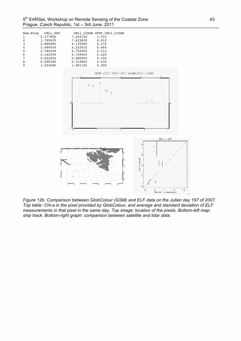
5th EARSeL Workshop on Remote Sensing of the Coastal Zone 43 Prague, Czech Republic, 1st – 3rd June, 2011
Num.Prog CHL1_SAT CHL1_LIDAR STDV_CHL1_LIDAR 1 2.377826 7.244120 1.533 2 1.789029 7.623830 0.912 3 2.886896 4.135960 0.374 4 3.499554 4.232010 0.485 5 2.789329 4.752950 0.512 6 2.142939 0.759450 0.220 7 0.652054 0.580550 0.154 8 0.598396 0.310800 0.035 9 1.024586 1.081150 0.209
Figure 12b. Comparison between GlobColour (GSM) and ELF data on the Julian day 197 of 2007. Top table: Chl-a in the pixel provided by GlobColour, and average and standard deviation of ELF measurements in that pixel in the same day. Top image: location of the pixels. Bottom-left map: ship track. Bottom-right graph: comparison between satellite and lidar data.

5th EARSeL Workshop on Remote Sensing of the Coastal Zone 44 Prague, Czech Republic, 1st – 3rd June, 2011
Num.Prog CHL1_SAT CHL1_LIDAR STDV_CHL1_LIDAR 1 0.594773 0.592120 0.269 2 0.573727 5.328030 0.245 3 0.544332 4.163370 0.460 4 0.533192 5.255890 0.332
Figure 13a. Comparison between GlobColour (AVW) and ELF data on the Julian day 198 of 2007. Top table: Chl-a in the pixel provided by GlobColour, and average and standard deviation of ELF measurements in that pixel in the same day. Top image: location of the pixels. Bottom-left map: ship track. Bottom-right graph: comparison between satellite and lidar data.
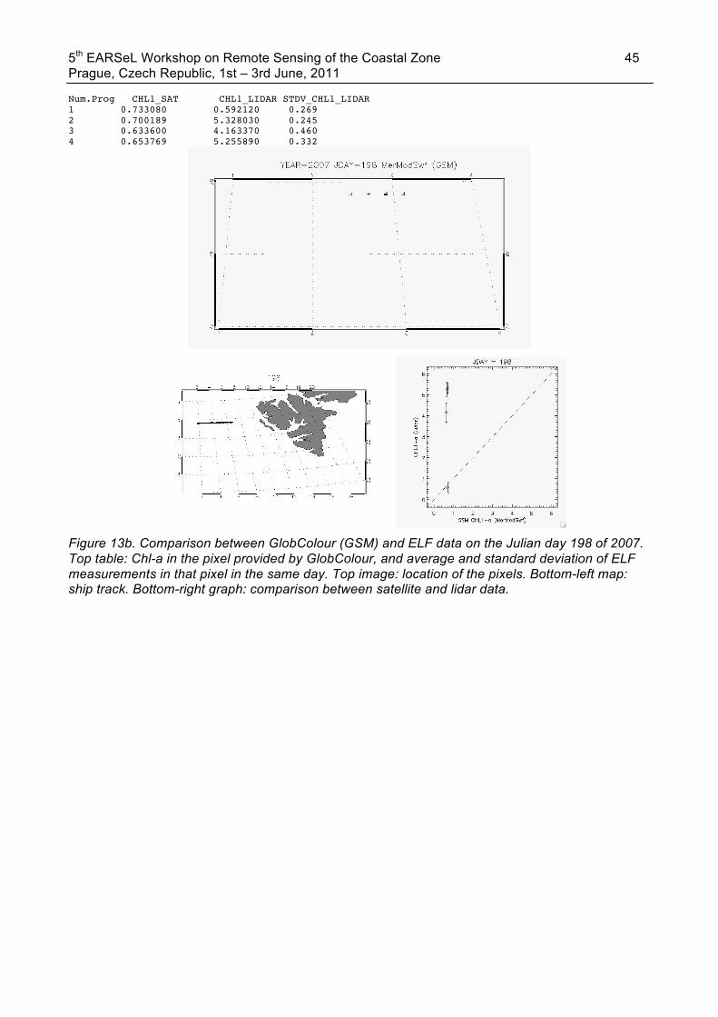
5th EARSeL Workshop on Remote Sensing of the Coastal Zone 45 Prague, Czech Republic, 1st – 3rd June, 2011
Num.Prog CHL1_SAT CHL1_LIDAR STDV_CHL1_LIDAR 1 0.733080 0.592120 0.269 2 0.700189 5.328030 0.245 3 0.633600 4.163370 0.460 4 0.653769 5.255890 0.332
Figure 13b. Comparison between GlobColour (GSM) and ELF data on the Julian day 198 of 2007. Top table: Chl-a in the pixel provided by GlobColour, and average and standard deviation of ELF measurements in that pixel in the same day. Top image: location of the pixels. Bottom-left map: ship track. Bottom-right graph: comparison between satellite and lidar data.
5th EARSeL Workshop on Remote Sensing of the Coastal Zone 46 Prague, Czech Republic, 1st – 3rd June, 2011
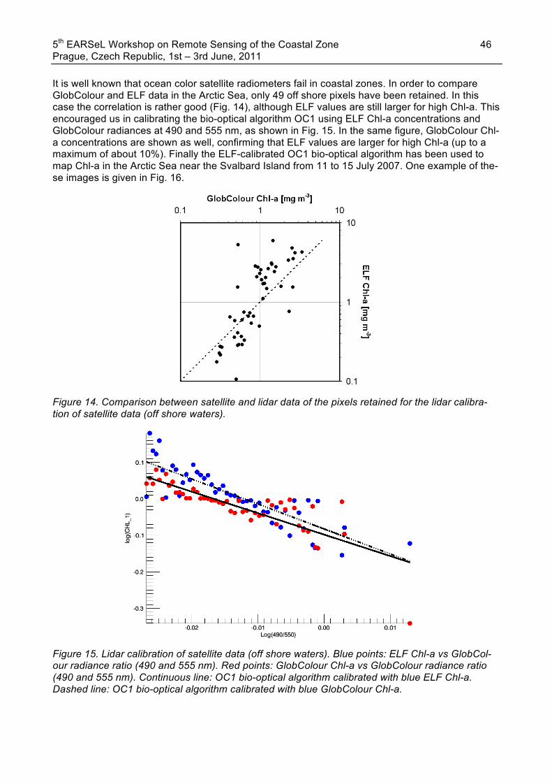
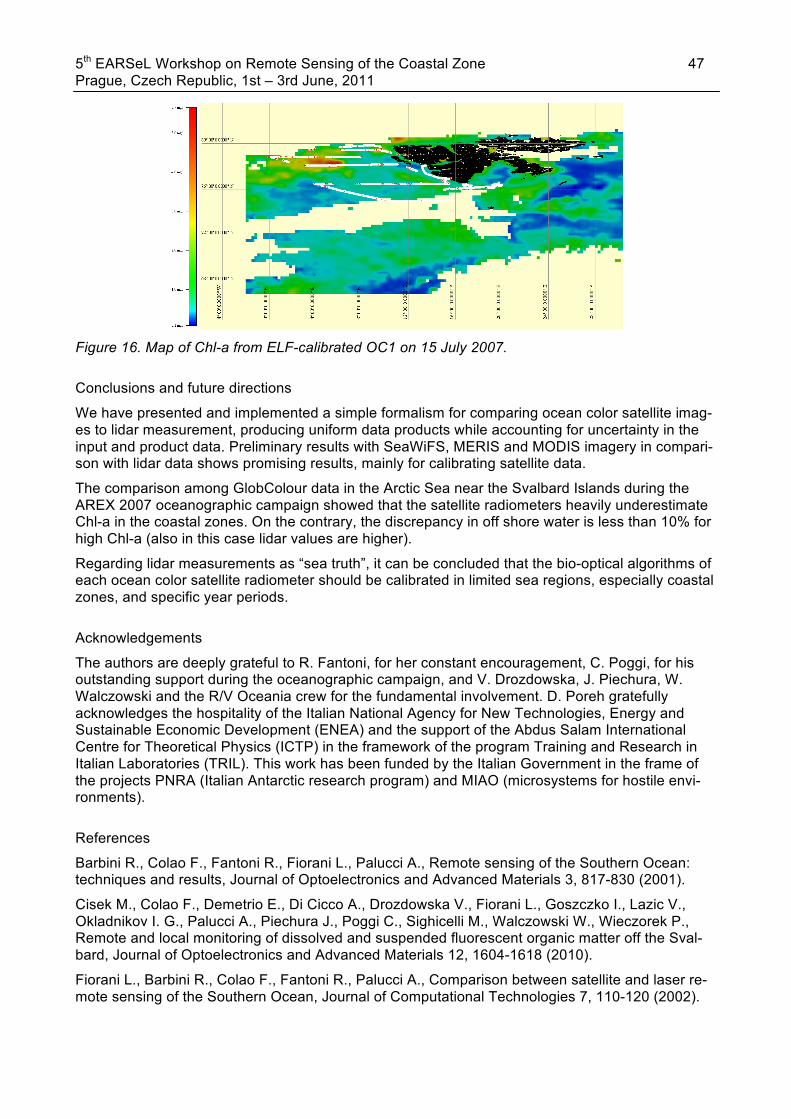
It is well known that ocean color satellite radiometers fail in coastal zones. In order to compare GlobColour and ELF data in the Arctic Sea, only 49 off shore pixels have been retained. In this case the correlation is rather good (Fig. 14), although ELF values are still larger for high Chl-a. This encouraged us in calibrating the bio-optical algorithm OC1 using ELF Chl-a concentrations and GlobColour radiances at 490 and 555 nm, as shown in Fig. 15. In the same figure, GlobColour Chl-a concentrations are shown as well, confirming that ELF values are larger for high Chl-a (up to a maximum of about 10%). Finally the ELF-calibrated OC1 bio-optical algorithm has been used to map Chl-a in the Arctic Sea near the Svalbard Island from 11 to 15 July 2007. One example of the-se images is given in Fig. 16.
Figure 14. Comparison between satellite and lidar data of the pixels retained for the lidar calibra-tion of satellite data (off shore waters).
Figure 15. Lidar calibration of satellite data (off shore waters). Blue points: ELF Chl-a vs GlobCol-our radiance ratio (490 and 555 nm). Red points: GlobColour Chl-a vs GlobColour radiance ratio (490 and 555 nm). Continuous line: OC1 bio-optical algorithm calibrated with blue ELF Chl-a. Dashed line: OC1 bio-optical algorithm calibrated with blue GlobColour Chl-a.
5th EARSeL Workshop on Remote Sensing of the Coastal Zone 47 Prague, Czech Republic, 1st – 3rd June, 2011
Figure 16. Map of Chl-a from ELF-calibrated OC1 on 15 July 2007.
Conclusions and future directions
We have presented and implemented a simple formalism for comparing ocean color satellite imag-es to lidar measurement, producing uniform data products while accounting for uncertainty in the input and product data. Preliminary results with SeaWiFS, MERIS and MODIS imagery in compari-son with lidar data shows promising results, mainly for calibrating satellite data.
The comparison among GlobColour data in the Arctic Sea near the Svalbard Islands during the AREX 2007 oceanographic campaign showed that the satellite radiometers heavily underestimate Chl-a in the coastal zones. On the contrary, the discrepancy in off shore water is less than 10% for high Chl-a (also in this case lidar values are higher).
Regarding lidar measurements as “sea truth”, it can be concluded that the bio-optical algorithms of each ocean color satellite radiometer should be calibrated in limited sea regions, especially coastal zones, and specific year periods.
Acknowledgements
The authors are deeply grateful to R. Fantoni, for her constant encouragement, C. Poggi, for his outstanding support during the oceanographic campaign, and V. Drozdowska, J. Piechura, W. Walczowski and the R/V Oceania crew for the fundamental involvement. D. Poreh gratefully acknowledges the hospitality of the Italian National Agency for New Technologies, Energy and Sustainable Economic Development (ENEA) and the support of the Abdus Salam International Centre for Theoretical Physics (ICTP) in the framework of the program Training and Research in Italian Laboratories (TRIL). This work has been funded by the Italian Government in the frame of the projects PNRA (Italian Antarctic research program) and MIAO (microsystems for hostile envi-ronments).
References
Barbini R., Colao F., Fantoni R., Fiorani L., Palucci A., Remote sensing of the Southern Ocean: techniques and results, Journal of Optoelectronics and Advanced Materials 3, 817-830 (2001).
Cisek M., Colao F., Demetrio E., Di Cicco A., Drozdowska V., Fiorani L., Goszczko I., Lazic V., Okladnikov I. G., Palucci A., Piechura J., Poggi C., Sighicelli M., Walczowski W., Wieczorek P., Remote and local monitoring of dissolved and suspended fluorescent organic matter off the Sval-bard, Journal of Optoelectronics and Advanced Materials 12, 1604-1618 (2010).
Fiorani L., Barbini R., Colao F., Fantoni R., Palucci A., Comparison between satellite and laser re-mote sensing of the Southern Ocean, Journal of Computational Technologies 7, 110-120 (2002).

5th EARSeL Workshop on Remote Sensing of the Coastal Zone 48 Prague, Czech Republic, 1st – 3rd June, 2011
Fiorani L., Barbini R., Colao F., De Dominicis L., Fantoni R., Palucci A., Artamonov E. S., Combi-nation of lidar, MODIS and SeaWiFS sensors for simultaneous chlorophyll monitoring, EARSeL eProceedings 3, 8-17 (2004).
Fiorani L., Barbini R., Colao F., Fantoni R., Okladnikov I. G., Palucci A., Integration of shipborne lidar and spaceborne radiometer: application to the Antarctic coastal environment, Proceedings of SPIE 5885, 174-181 (2005).
Fiorani L., Fantoni R., Lazzara L., Nardello I., Okladnikov I. G., Palucci A., Lidar calibration of satel-lite sensed CDOM in the Southern Ocean, EARSeL eProceedings 5, 89-99 (2006a).
Fiorani L., Okladnikov I. G., Palucci A., First algorithm for chlorophyll-a retrieval from MODIS-Terra imagery of sun-induced fluorescence in the Southern Ocean, International Journal of Remote Sensing 27, 3615-3622 (2006b).
Fiorani L., Okladnikov I. G., Palucci A., Lidar-calibrated regional models for satellite retrieval of primary productivity in the Southern Ocean, Journal of Optoelectronics and Advanced Materials 9, 3939-3945 (2007).
Fiorani L., Okladnikov I. G., Palucci A., Remote Sensing of the Southern Ocean by MERIS, MODIS, SeaWiFS and ENEA Lidar, Journal of Optoelectronics and Advanced Materials 10, 1482-1488 (2008).
Copyright © 2022 FDOKUMEN