Operational implementation of a LiDAR inventory in Boreal Ontario

512 Juillet/Août 2011, Vol. 87, No 4 — the Forestry ChroNiCle

Operational implementation of a LiDAR inventory in Boreal Ontario

by Murray Woods1, Doug Pitt2, Margaret Penner3, Kevin Lim4, Dave Nesbitt1, Dave Etheridge5 and Paul Treitz6

ABSTRACTAn existing Light Detection and Ranging (LiDAR) data set captured on the Romeo Malette Forest near Timmins, Ontario,was used to explore and demonstrate the feasibility of such data to enrich existing strategic forest-level resource inventorydata. Despite suboptimal calibration data, stand inventory variables such as top height, average height, basal area, grosstotal volume, gross merchantable volume, and above-ground biomass were estimated from 136 calibration plots and validated on 138 independent plots, with root mean square errors generally less than 20% of mean values. Stand densities(trees per ha) were estimated with less precision (30%). These relationships were used as regression estimators to predictthe suite of variables for each 400-m2 tile on the 630 000-ha forest, with predictions capable of being aggregated in any user-defined manner—for a stand, block, or forest—with appropriate estimates of statistical precision. This pilot study demonstrated that LiDAR data may satisfy growing needs for inventory data to scale operational/tactical, throughstrategic needs, as well as provide spatial detail for planning and the optimization of forest management activities.

Key words: forest inventory, Light Detection and Ranging (LiDAR), models, Seemingly Unrelated Regression

RÉSUMÉUn ensemble de données LiDAR (télédétection par laser) recueillies pour la Forêt Roméo Malette près de Timmins enOntario, a été utilisé pour étudier et démontrer la possibilité d’utiliser ces données pour enrichir les données existantesd’inventaire des ressources forestières de premier plan. Malgré une calibration des données inférieure à ce qui était souhaité, les variables d’inventaire des peuplements comme la hauteur moyenne supérieure, la hauteur moyenne, la surface terrière, le volume brut total, le volume marchand total et la biomasse au-dessus du sol ont été estimées à partirde 136 parcelles de calibration et validées pour 138 parcelles indépendantes, avec une erreur quadratique moyenne géné-ralement inférieure à 20 % des valeurs moyennes. La densité des peuplements (arbres par hectare) a été estimée avecmoins de précision (30 %). Ces relations ont été utilisées comme estimateurs de régressions utilisées pour générer unesérie de variables pour chaque unité de 400 m2 de la forêt de 630 000 ha, avec des prédictions cumulables selon la requêtede l’utilisateur—pour un peuplement, pour un bloc ou pour la forêt— avec des estimations appropriées d’une précisionstatistique. Ce projet pilote a démontré que les données LiDAR pourraient répondre aux besoins sans cesse croissants en matière de données d’inventaire pour définir les plans opérationnels/tactiques, bien que stratégiques, ainsi que pourétablir les détails spatiaux requis pour la planification et l’optimisation des activités d’aménagement forestier.

Mots clés : inventaire forestier, LiDAR (télédétection au laser), modèles, régressions apparemment indépendantes

1Ontario Ministry of Natural Resources, Southern Science & Information Section, 3301 Trout Lake Road, North Bay, Ontario P1A 4L7. E-mail: [email protected] Wood Fibre Centre, Canadian Forest Service, 1219 Queen St. E., Sault Ste. Marie, Ontario, P6A 2E5.3Forest Analysis Ltd. RR#4, 1188 Walker Lake Dr., Huntsville, Ontario P1H 2J6.4Lim Geomatics Inc., P.O. Box 45089, 680 Eagleson Road, Ottawa, Ontario K2M 2G0.5Ontario Ministry of Natural Resources, Northeast Science & Information Section, P.O. Bag 3020, South Porcupine, Ontario P0N 1H0.6Department of Geography, Queen’s University, Kingston, Ontario K7L 3N6.

IntroductionLight Detection and Ranging (LiDAR) applications inforestry have been studied since 1982 (Arp et al. 1982). Overthe past decade, improvements in global positioning systems(GPS), inertial navigation systems (INS), computer hardware,LiDAR processing software, and reduced acquisition costshave promoted many of these applications from research tooperational status in several jurisdictions (Næsset 2004,Evans et al. 2006, Stephens et al. 2007). Examples include pre-dictive hydrology modeling (Murphy et al. 2008, Mandl-burger et al. 2009), road location optimization and construc-tion (Akay et al. 2004, Aruga et al. 2005, White et al. 2010),harvest block engineering (Chung et al. 2004), habitat defini-

tion (Clawges et al. 2008, Hinsley et al. 2008), and timberquantification (Holmgren and Jonsson 2004, Næsset 2004,Parker and Evans 2007). Research conducted specifically inOntario has focused on estimating forest inventory and bio-physical variables for tolerant northern hardwoods (Lim et al.2001, 2002, 2003; Todd et al. 2003; Lim and Treitz 2004;Woods et al. 2008), boreal mixedwoods (Thomas et al. 2006,2008) and conifer plantations (Chasmer et al. 2006). Currentacquisition costs, including classification of LiDAR points,derivation of digital elevation models (DEMs) and digital sur-face models (DSMs), have positioned LiDAR as a potentiallyoperationally affordable alternative when the development ofa precision forest inventory is considered a requirement.

July/August 2011, Vol. 87, No. 4 — the Forestry ChroNiCle 513

Current provincial forest inventories in Canada are basedon air photo interpretation for the delineation of forestedpolygons and the estimation of tree species composition,average height, site occupancy (i.e., stocking or crown clo-sure) and stand age. In the past, photo interpreters viewedoverlapping hardcopy photographic images under stereo-scopes; today, most interpreters view digital photographs andconduct interpretation in a “softcopy” environment on acomputer screen. With interpreted height and stand age (sup-ported by limited ground sampling), stand site productivity isinferred (i.e., from site class or site index). In Ontario, forexample, normal and empirical yield table estimates for anaggregated forest community are then used to assign an “aver-age” basal area and volume to a group of similar stand condi-tions based on the assessment of site productivity and speciescomposition. Such provincial inventory products aredesigned to provide aspatial forest-level quantifications forstrategic planning, under the assumption that detailed fieldsampling be conducted to supplement these inventorieswhere and when stand-level accuracy is required for tacticaland operational planning and activity.

Over the past decade, however, typical Canadian forestmanagement has evolved into a complex spatial balancing actbetween industrial wood demands and a daunting array ofnon-timber values, enveloping a highly sensitive, fully con-strained wood supply across the country. As a result, spatiallyaccurate quantifications of our forest resources are nowneeded for spatial forest management modellingand planning at both the strategic and tacticalscales. Field sampling to obtain such detailedinventory attributes over very large areas is felt bymany to be impractical and largely unaffordable,creating serious need for enhanced inventorytechnologies capable of generating quantitativespatial data with stand-level accuracy.

Despite reported success in the application ofLiDAR to complement forest inventories aroundthe world, operational adoption in Ontario andelsewhere in Canada has been tentative. A verycomplex tenure system that exists between forestcompanies that operate on Crown land and theprovinces that own more than 90% of the forestedland in Canada explains some of the reluctance tomove forward with new technology—one partyarguing that the other should pay for the addedinformation. Tenure reform, being discussed orundertaken in a number of Canadian provinces,may resolve some of this debate. But there alsoexists a degree of scepticism and uncertaintyamongst professionals about the capacity ofLiDAR to predict forest inventory attributes inour largely unmanaged Canadian forests, condi-tions that differ in structure and complexity fromthose in Scandinavia and elsewhere whereLiDAR has been proven. As such, LiDAR has yetto be applied to the operational prediction of for-est inventory parameters in the relatively unman-aged boreal forest conditions of Ontario.

In 2004–05, Tembec Inc., a forest productscompany, flew digital imagery and “wall-to-wall”LiDAR coverage (~0.5 pt/m2) on approximately630 000 ha of the Romeo Malette Forest (RMF),

near Timmins Ontario, with the goal that these data bettersupport forest road construction and harvest block engineer-ing. In 2009, a research project designed to investigate theeffects of decimated LiDAR point densities on forest inven-tory attribute model prediction accuracy and precision (Tre-itz et al. 2010) was undertaken on the RMF. Although the net-work of field plots used for this latter study was not intended,or its stratification developed, specifically to support con-struction of a landscape inventory product, its existence pro-vided us with opportunity to develop, test, and demonstratethe process of applying LiDAR-predicted forest inventoryattributes to an entire boreal forest management unit. Ourobjective for the research reported herein was to explore anddemonstrate the feasibility of LiDAR to augment existingstrategic inventory data with the spatial data needed for tacti-cal and operational decision-making and planning in typicalCanadian boreal conditions.

MethodsStudy areaThe RMF is located in the northeast portion of Ontario’sBoreal Forest near Timmins, Ontario (Fig. 1). The RMF is anactive forest management unit with 505 945 ha of productiveforest, 32 931 ha of unproductive forest land and 44 722 ha ofnon-forested land (the remainder of the 629 878-ha forestbeing patent land or land under other ownership). The forestis characterized by extensive coniferous stands on poorly

Fig. 1. Location of the Romeo Malette Forest within north-eastern Ontario.


drained lowlands, and gently rising uplands dominated byintolerant hardwoods, conifers, and mixedwoods. The north-ern portion (40% of the forest area) is located on the claybeltand is best described as relatively flat to gently rolling, inter-spersed with depressions and eskers. Elevation ranges from305 to 320 metres above sea level, with extensive clay deposits,high water table, and poor drainage. The remaining southernarea of the forest consists of moderately rolling topographyderived from glacial deposits, with well-drained boulderysand tills overlying bedrock. Elevation ranges from 305 to 380metres above sea level. Dominant species are black spruce(Picea mariana [Mill.] BSP), white birch (Betula papyriferaMarsh.), trembling aspen (Populous tremuloides Michx.), jackpine (Pinus banksiana Lamb.), eastern white cedar (Thujaoccidentalis L.), white spruce (Picea glauca [Moench] Voss),eastern larch (Larix laricina [Du Roi] K. Koch), and balsamfir (Abies balsamea [L.] Mill.). Minor species include blackash (Fraxinus nigra Marsh.), yellow birch (Betula alleghanien-sis Britt.), soft maple (Acer rubrum L.), and red (Pinus resinosaAit.) and white pine (Pinus strobus L.).

LiDAR data and data processingLiDAR data were collected for the RMF during the summerseasons of 2004 and 2005 using an upgraded Leica ALS40 air-borne laser scanner mounted in a King Air 90 aircraft. Thebase mission was flown at 2740 m with a 20° field of view,scan rate of 30 Hz, and a maximum pulse repetition fre-quency of 32 300 Hz. This configuration resulted in a cross-track spacing of 2.87 m, an along-track spacing of 2.4 m, anaverage sampling density of 0.46 points m-2, and a swathwidth of approximately 1 km.

A bald-earth DEM and a DSM were produced by the ven-dor using their proprietary methods. Unfortunately, theprocessed LiDAR data (standard LAS version 1.0 format)were provided to the client in an unclassified state (no assign-ment of LiDAR returns to a “ground” or “non-ground” class).Without classified LiDAR data, the typical approach of nor-malizing LiDAR points against a Triangular Irregular Net-work (TIN) derived from classified ground points was notpossible (i.e., given a return and its x–y coordinate, subtractthe z-value for that x–y coordinate on the DEM from its orig-inal z-value), thereby necessitating an alternate approach. Theapproach adopted was to normalize the LiDAR points (allreturns) against a RMF 2-m DEM that had been processedfrom the vendor’s derived DEM. No filtering on return typewas applied. No height threshold was applied to eliminatepoints close to the ground (e.g., between 0 m and 2 m). How-

ever, because of the presence of z-spikes in the LiDAR data,any points above 35 m were filtered out.

Predictor variables were derived statistics from the nor-malized LiDAR data. In each case, “all” returns were used andheight thresholds were not used to filter point data. Potentialpredictors included basic statistics of mean height (mean),standard deviation (std_dev), and absolute deviation aroundthe mean height (abs_dev), as well as deciles of LiDAR canopyheight (i.e., p10…p90) and the maximum (max) LiDARheight. For each plot, the range of LiDAR height measure-ments was divided into 10 equal intervals and the cumulativeproportion of LiDAR returns found in the first nine intervalsprovided as many additional predictors (i.e., d1 … d9). Thefinal two predictors were calculated as the number of firstreturns divided by all returns intersecting a sample plot (Da)and the number of first and only returns divided by all returnsintersecting a sample plot (Db). The entire RMF was thensubdivided into contiguous 400-m2 (20 m × 20 m) tiles or pre-diction units (PUs) and the above suite of predictor variablescalculated for each, creating a 20 m × 20 m raster surface pop-ulated with LiDAR predictors.

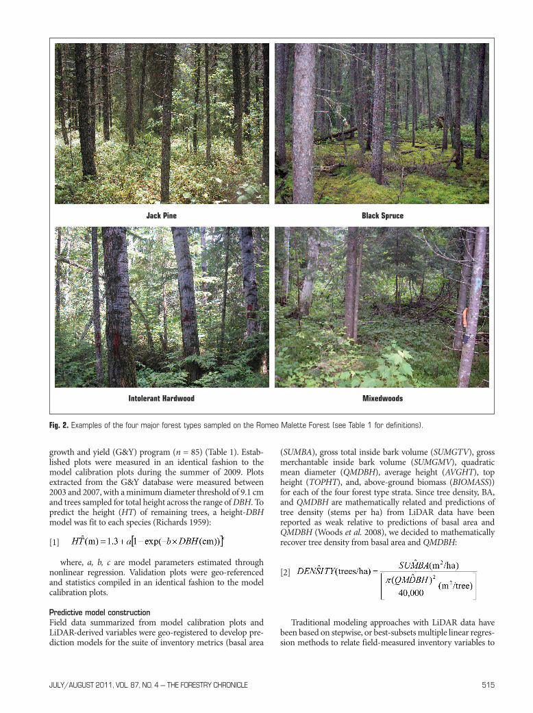
Field dataA total of 136 circular 400-m2 plots were established in fourdifferent broad forest types on the study area during theperiod of May to October 2008 (Table 1; Fig. 2). The four- tofive-year lag between LiDAR capture and field samplingnecessitated that recently harvested and naturally disturbedareas be excluded from sampling. Within each of the plotsestablished, all trees ≥9.1 cm diameter at breast height (DBH)were measured with a diameter tape and assessed for species,status (live or dead), and crown class (e.g., dominant, co-dominant). A Vertex™ hypsometer was used to measureheight to base of live crown and total tree height for everytree. Heights of deciduous species were measured in a leaf-offperiod to obtain the most accurate height possible. The cen-tre of each circular plot was geo-referenced with a TrimblePro XT™ kinematic GPS unit connected to a Hurricane™antenna, which was mounted on a tripod. A minimum of 300GPS points was collected for each post position and laterpost-processed against a base station to achieve sub-meteraccuracy. Individual tree data for each plot were compiled toexpress per-hectare values using the equations presented inTable 2.

Subsequently, a similar, independent set of model valida-tion plots was assembled through a combination of newestablishments (n = 53) or plots extracted from the provincial

Table 1. Description of major forest types sampled on the Romeo Malette Forest (see Fig. 2)

Forest type Description Species criteria n (calibration) n (validation)

Jack pine Jack pine-dominated conifer Jack pine ≥50% and (conifera) ≥70% 35 44Black spruce Black spruce-dominated conifer Black spruce ≥50% and <50% 34 35

(conifer) ≥70% and jack pineIntolerant hardwood Hardwood-dominated Hardwoodb ≥70% 33 28 Mixedwood All other polygons (Hardwood) or (conifer) >30% and <70% 34 31

Totals 136 138

aConifer = jack pine, black spruce, balsam fir, white spruce, cedar, larch, hemlock, white pine, and/or red pinebHardwood = poplar, white birch, hard maple, upland hardwoods, and/or lowland hardwoods


growth and yield (G&Y) program (n = 85) (Table 1). Estab-lished plots were measured in an identical fashion to themodel calibration plots during the summer of 2009. Plotsextracted from the G&Y database were measured between2003 and 2007, with a minimum diameter threshold of 9.1 cmand trees sampled for total height across the range of DBH. Topredict the height (HT) of remaining trees, a height-DBHmodel was fit to each species (Richards 1959):

[1]

where, a, b, c are model parameters estimated throughnonlinear regression. Validation plots were geo-referencedand statistics compiled in an identical fashion to the modelcalibration plots.

Predictive model constructionField data summarized from model calibration plots andLiDAR-derived variables were geo-registered to develop pre-diction models for the suite of inventory metrics (basal area

(SUMBA), gross total inside bark volume (SUMGTV), grossmerchantable inside bark volume (SUMGMV), quadraticmean diameter (QMDBH), average height (AVGHT), topheight (TOPHT), and, above-ground biomass (BIOMASS))for each of the four forest type strata. Since tree density, BA,and QMDBH are mathematically related and predictions oftree density (stems per ha) from LiDAR data have beenreported as weak relative to predictions of basal area andQMDBH (Woods et al. 2008), we decided to mathematicallyrecover tree density from basal area and QMDBH:

[2]

Traditional modeling approaches with LiDAR data havebeen based on stepwise, or best-subsets multiple linear regres-sion methods to relate field-measured inventory variables to

Jack Pine Black Spruce

Intolerant Hardwood Mixedwoods

Fig. 2. Examples of the four major forest types sampled on the Romeo Malette Forest (see Table 1 for definitions).


LiDAR predictor variables (Gobakken and Næsset 2003,Næsset et al. 2005). In blind application, these approaches canlead to models that contain a large number of predictor vari-ables; such models often exhibit multicollinearity (as indi-cated by high variance inflation factors [VIFs]), they may lacklogical structure, and/or produce unstable predictions fordata outside the calibration set. Moreover, the residual errorsin the resulting system of multiple regressions for the full suiteof inventory metrics being estimated may be correlated acrossequations. One procedure designed to account for this lattersituation is Seemingly Unrelated Regressions, or SUR (Greene1993). If such correlations exist between equations, SUR pro-vides increased estimation efficiency (greater prediction pre-cision) than ordinary least squares, and the same result asordinary least squares if no correlation exists.

Through the use of SUR and no more than two of the best,most logical predictor variables for each inventory metric, weattempted to develop a set of robust, minimalist LiDAR pre-

diction equations that reflect “biological reality”. Rather thanuse a blind, forward or backwards selection process, wesought logical predictor variables that were highly correlatedwith the dependent variable and associated with low VIF val-ues. For example, maximum height was avoided as a predic-tor because it is highly dependent on the size of the sampleunit and LiDAR density (as LiDAR density increases or theplot area increases, maximum height tends to increase (i.e., ahigher probability of a return from the tip of a tree crown)).Instead, the more stable p90 height or the mean · p90 were sig-nificant and used. In another example, stand volume, aderived variable, is highly correlated with basal area and treeheight. Thus, it made sense that key predictor variables usedfor SUMBA and TOPHT also be prominent in the predictionof SUMGMV or SUMGTV. Each relationship was examinedfor nonlinear trends and model residuals tested to verify thatthe assumptions of homogeneity of variance and normalitywere met; transformations and nonlinear applications were

Table 2. Equation or method used to calculate forest inventory attributes

Ground metric Description

Top height (m) (TOPHT) The average of the 100 stems per hectare with the largest diameter (DBH).Average height (m) (AVGHT) The average height of all trees 9.1 cm DBH and larger.Density (stems per ha) (DENSITY) Number of live trees 9.1 cm DBH and larger, expressed per- hectare.

Quadratic mean DBH (cm) (QMDBH) , where n is the number of stems in a plot.

Basal area (m2 ha-1) (SUMBA)

Value obtained by summing the squared DBH of each tree in a 0.04-ha plot and converting thissum to area measure in m2.

Gross total volume (inside bark) Individual tree total volume calculated from:(m3 ha-1) (SUMGTV) b1 * DBH2*(1-0.04365* b2)2/( b3+(0.3048 * b4/Ht)),

where b1…4 are regression coefficients provided in Honer et al. (1983) that vary by species, andHt is tree height in m. Per-hectare value is calculated by summing the volume of each tree anddividing by the plot area (ha).

Gross merchantable volume (inside bark) Individual tree merchantable volume calculated from its total volume, multiplied by:(m3 ha-1) (SUMGMV) (b1 + b2(X) + b3(X2)),

where b1…3 are regression coefficients provided in Honer et al. (1983) that vary by species, andX = [(1+Hs/Ht)(Dtop2/DBH2)]Hs = Stump height (0.2m)Ht = Total tree height (m)Dtop = Minimum Top Diameter (inside bark) (10.0 cm)

Per-hectare value is calculated by summing the volume of each tree and dividing by the plotarea (ha).

Aboveground Biomass (Kg ha-1) Individual tree biomass calculated from (BIOMASS) b1 * DBHb2

where b1, 2 are regression coefficients provided in (Ter-Mikaelian and Korzukhin 1997) thatvary by species. Per-hectare value is calculated by summing the biomass of each tree and dividing by the plotarea (ha).


generally not necessary. For each forest stratum, the system ofprediction models was fit using SUR (SYSLIN procedure ofSAS®; SAS Institute Inc. 2008).

One disadvantage of relying on the pre-existing plot net-work for this investigation was that these plots were located inrelatively mature forest conditions and did not fully samplethe range of development stages that exist on the forest as awhole. As a result, we confined predictions to stands that wereat least 11 m in height (the minimum average tree height inthe calibration data). Moreover, we avoided potential for neg-ative predictions by forcing non-significant (α > 0.10) inter-cepts to 0, or setting significant negative intercepts to zero andthen rescaling the affected models.

LiDAR-based prediction of forest inventory metricsExisting forest resource inventory (FRI) polygons were usedto classify every PU on the RMF forest according to the foresttype definitions provided in Table 1. Appropriate SUR predic-tion equations were then applied to predict SUMBA,SUMGTV, SUMGMV, QMDBH, AVGHT, TOPHT, and, BIO-MASS for each PU on the forest. Statistical precision valuesfor regression estimates derived from the aggregation of indi-vidual PUs were calculated using formulae summarized byCunia (1985) and illustrated in Appendix 1.

ResultsPredictive modelsCalibration plots were located in relatively mature stand con-ditions (e.g., mean stand top height ranging from 16.7 m to22.6 m; Table 3). LiDAR predictor variables used in the SURmodels tended to be similar across the four forest types (Table4). The mean and mean · p90 were generally the strongest pri-mary predictor variables for most forest types and inventoryattributes. AVGHT, however, was best predicted by a lowercanopy percentile (p80 or p60) in all forest types except intol-erant hardwood. Secondary LiDAR predictors (where signif-

icant) included lower height percentile measurements (p20,p30, p60, or p70) in the prediction of SUMBA, SUMGTV,SUMGMV, and BIOMASS. Attributes such as TOPHT,QMDBH, and AVHGT tended to utilize estimates of canopydensity metrics (d6, d7) for their secondary predictor.

Model Root Mean Square Errors (RMSEs) and relativeRMSE (RMSE% = RMSE expressed as a percentage of themean value being predicted) are given for the four foresttypes. Model precision varied slightly among forest types,with no clear trends related to forest type (Table 4). TOPHTand AVGHT had the lowest unexplained variations, withRMSE% ranging between 3.8% and 8.8% (0.8 m and 1.2 m).Unexplained variation in QMDBH was generally around 10%(1.5–2.0 cm). The remaining variables, generally volume-related attributes, had higher unexplained variation, withRMSE% ranging from 16.1% to 24.3%.

Plot-level validationStatistics for the inventory attributes of the validation plotswere similar (Table 5) to those of the model calibration plots(Table 3). Comparison of observed and predicted values forthe validation plots produced RMSE values (Table 6) of rela-tively similar magnitude to the model RMSEs in each foresttype (Table 4). In intolerant hardwood validation plots, pre-dictions of SUMBA, SUMGTV and SUMGMV, AVGHT andTOPHT were slightly less precise (1.4% to 3.8%), whereas pre-dictions of QMDBH and BIOMASS were more precise thanobserved in model calibration. In mixedwood plots, weobserved slightly less precision (0.1% to 3.7%) in the valida-tion prediction of all inventory metrics except SUMGTV andAHGHT. Validation precision in jack pine was better thanexpected for SUMBA, SUMGTV, and BIOMASS and lowerthan expected for SUMGTV, QMDBH, AVGHT, and TOPHT(2.2% to 6.2%). In black spruce validation, we observedslightly less precision (0.8% to 2.9%) in the prediction ofQMDBH, AVGHT and TOPHT.

Table 3. Summary of calibration plot statistics for the Romeo Malette Forest. See Table 2 for variable definitions.

Variable Mean Min Max Std. Dev. Mean Min Max Std. Dev.

Jack pine (n = 35) Black spruce (n = 34)

TOPHT (m) 20.2 11.7 24.8 3.1 16.7 12.2 20.8 2.5AVGHT (m) 16.1 8.9 19.8 2.1 12.9 9.1 16.4 2.2DENSITY (stems ha-1) 1414.5 600.4 2376.6 470.5 1643.0 500.0 3002.0 691QMDBH (cm) 17.0 12.2 22.7 2.8 14.2 10.9 18.9 2.0SUMBA (m2 ha-1) 21.2 12.9 53.9 9.6 25.8 6.3 44.3 10.5SUMGTV (m3 ha-1) 248.8 57.7 464.0 94.1 162.7 34.1 320.8 79.4SUMGMV (m3 ha-1) 105.4 28.3 401.1 88.7 109.0 14.0 249.4 62.6BIOMASS (Kg ha-1) 127 458 43 966 244 507 45 404 100 833 23 456 174 523 42 733

Intolerant hardwoods (n = 33) Mixedwoods (n = 34)

TOPHT (m) 22.6 13.1 29.3 3.6 22.3 11.4 30.4 3.8AVGHT (m) 16.7 11.8 20.3 2.0 15.6 9.9 19.4 2.0DENSITY (stems ha-1) 1198.5 550.4 1851.2 307.8 1102.2 500.3 2201.5 334.2QMDBH (cm) 18.2 10.6 23.9 3.7 19.4 12.7 24.6 2.7SUMBA (m2 ha-1) 31.4 4.83 54.5 10.8 32.7 6.3 61.2 10.5SUMGTV (m3 ha-1) 266.5 24.6 531.2 119.9 265.1 29.0 655.4 117.0SUMGMV (m3 ha-1) 216.2 4.6 462.9 116.7 223.1 12.5 579.4 108.1BIOMASS (Kg ha-1) 128 732 10 829 260 067 55 040 138 493 24 615 259 487 45 676


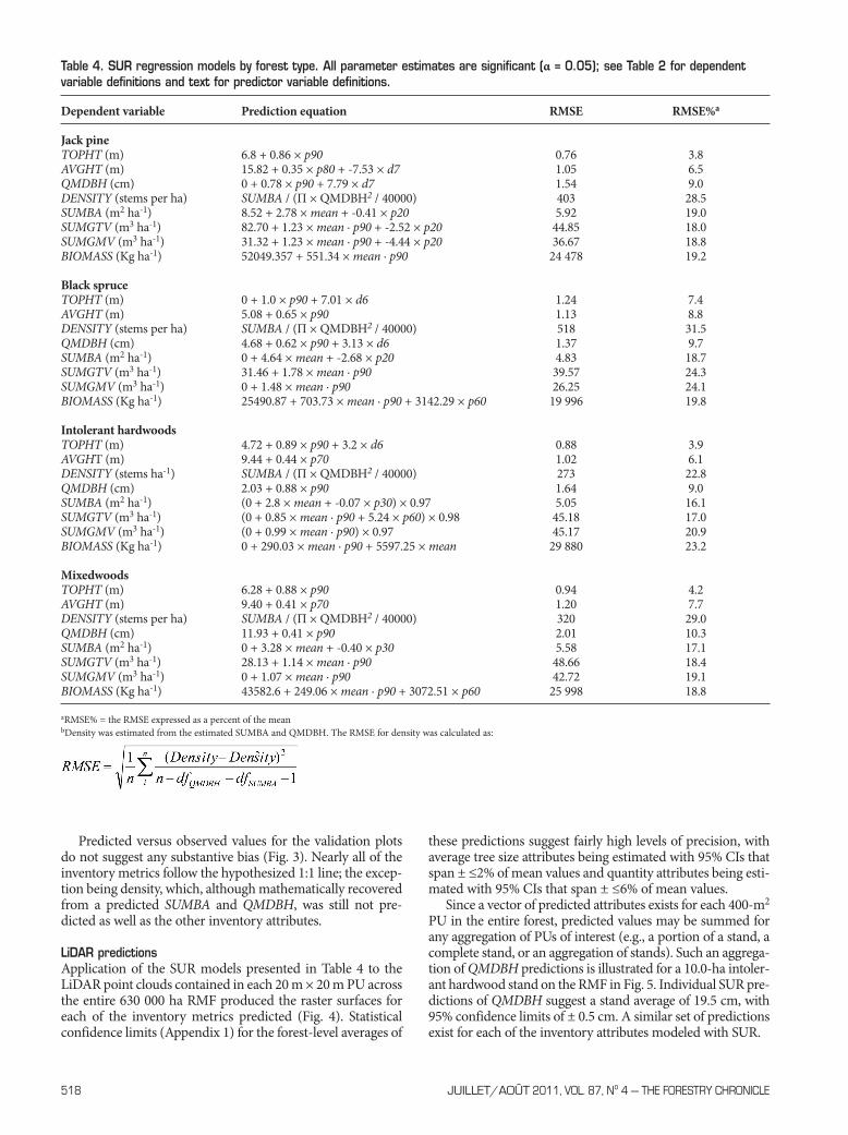
Predicted versus observed values for the validation plotsdo not suggest any substantive bias (Fig. 3). Nearly all of theinventory metrics follow the hypothesized 1:1 line; the excep-tion being density, which, although mathematically recoveredfrom a predicted SUMBA and QMDBH, was still not pre-dicted as well as the other inventory attributes.

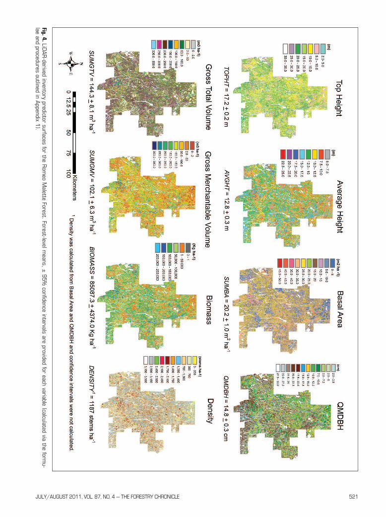
LiDAR predictionsApplication of the SUR models presented in Table 4 to theLiDAR point clouds contained in each 20 m × 20 m PU acrossthe entire 630 000 ha RMF produced the raster surfaces foreach of the inventory metrics predicted (Fig. 4). Statisticalconfidence limits (Appendix 1) for the forest-level averages of

these predictions suggest fairly high levels of precision, withaverage tree size attributes being estimated with 95% CIs thatspan ± ≤2% of mean values and quantity attributes being esti-mated with 95% CIs that span ± ≤6% of mean values.

Since a vector of predicted attributes exists for each 400-m2

PU in the entire forest, predicted values may be summed forany aggregation of PUs of interest (e.g., a portion of a stand, acomplete stand, or an aggregation of stands). Such an aggrega-tion of QMDBH predictions is illustrated for a 10.0-ha intoler-ant hardwood stand on the RMF in Fig. 5. Individual SUR pre-dictions of QMDBH suggest a stand average of 19.5 cm, with95% confidence limits of ± 0.5 cm. A similar set of predictionsexist for each of the inventory attributes modeled with SUR.

Table 4. SUR regression models by forest type. All parameter estimates are significant (α = 0.05); see Table 2 for dependentvariable definitions and text for predictor variable definitions.

Dependent variable Prediction equation RMSE RMSE%a

Jack pineTOPHT (m) 6.8 + 0.86 × p90 0.76 3.8AVGHT (m) 15.82 + 0.35 × p80 + -7.53 × d7 1.05 6.5QMDBH (cm) 0 + 0.78 × p90 + 7.79 × d7 1.54 9.0DENSITY (stems per ha) SUMBA / (Π × QMDBH2 / 40000) 403 28.5SUMBA (m2 ha-1) 8.52 + 2.78 × mean + -0.41 × p20 5.92 19.0SUMGTV (m3 ha-1) 82.70 + 1.23 × mean · p90 + -2.52 × p20 44.85 18.0SUMGMV (m3 ha-1) 31.32 + 1.23 × mean · p90 + -4.44 × p20 36.67 18.8BIOMASS (Kg ha-1) 52049.357 + 551.34 × mean · p90 24 478 19.2

Black spruceTOPHT (m) 0 + 1.0 × p90 + 7.01 × d6 1.24 7.4 AVGHT (m) 5.08 + 0.65 × p90 1.13 8.8 DENSITY (stems per ha) SUMBA / (Π × QMDBH2 / 40000) 518 31.5QMDBH (cm) 4.68 + 0.62 × p90 + 3.13 × d6 1.37 9.7SUMBA (m2 ha-1) 0 + 4.64 × mean + -2.68 × p20 4.83 18.7SUMGTV (m3 ha-1) 31.46 + 1.78 × mean · p90 39.57 24.3SUMGMV (m3 ha-1) 0 + 1.48 × mean · p90 26.25 24.1BIOMASS (Kg ha-1) 25490.87 + 703.73 × mean · p90 + 3142.29 × p60 19 996 19.8

Intolerant hardwoodsTOPHT (m) 4.72 + 0.89 × p90 + 3.2 × d6 0.88 3.9AVGHT (m) 9.44 + 0.44 × p70 1.02 6.1DENSITY (stems ha-1) SUMBA / (Π × QMDBH2 / 40000) 273 22.8QMDBH (cm) 2.03 + 0.88 × p90 1.64 9.0SUMBA (m2 ha-1) (0 + 2.8 × mean + -0.07 × p30) × 0.97 5.05 16.1SUMGTV (m3 ha-1) (0 + 0.85 × mean · p90 + 5.24 × p60) × 0.98 45.18 17.0SUMGMV (m3 ha-1) (0 + 0.99 × mean · p90) × 0.97 45.17 20.9BIOMASS (Kg ha-1) 0 + 290.03 × mean · p90 + 5597.25 × mean 29 880 23.2

Mixedwoods TOPHT (m) 6.28 + 0.88 × p90 0.94 4.2AVGHT (m) 9.40 + 0.41 × p70 1.20 7.7DENSITY (stems per ha) SUMBA / (Π × QMDBH2 / 40000) 320 29.0QMDBH (cm) 11.93 + 0.41 × p90 2.01 10.3SUMBA (m2 ha-1) 0 + 3.28 × mean + -0.40 × p30 5.58 17.1SUMGTV (m3 ha-1) 28.13 + 1.14 × mean · p90 48.66 18.4SUMGMV (m3 ha-1) 0 + 1.07 × mean · p90 42.72 19.1BIOMASS (Kg ha-1) 43582.6 + 249.06 × mean · p90 + 3072.51 × p60 25 998 18.8

aRMSE% = the RMSE expressed as a percent of the meanbDensity was estimated from the estimated SUMBA and QMDBH. The RMSE for density was calculated as:


Discussion The challenge of scaling up from plot-based results to land-scape implementation is often expounded on as a limitationto the acceptance of LiDAR for forest inventory application,particularly in Canada’s large and relatively unmanagedforests. The objective of this investigation was to develop, test,and demonstrate the process of applying LiDAR-predictedforest inventory attributes to an operational boreal forestmanagement unit. Our results suggest that LiDAR-based pre-dictions offer the advantages of complementing existing for-est inventory data with value-added, spatially explicit esti-mates of stand attributes, with quantifiable levels of precision.Sampling specifically for regression equation development,better PU classification, and specific LiDAR data acquisitionstandards offer opportunities for improving precision infuture applications.

Potential advantages ScalabilityWhile sound, sustainable forest management decisionsrequire accurate, forest-level statistics, the on-the-groundimplementation of strategic plans require precise spatialinformation at the tactical or operational scales. Existing for-est resource inventories generally provide adequate data forstrategic decision-making, but require supplementary fieldsampling for operational implementation. An advantage of“wall-to-wall” LiDAR coverage and the modeling approachtested in this study is that the forest inventory is built from the20 m × 20 m prediction unit as its finest unit of resolution(e.g., Fig. 5). Through LiDAR, strategic, forest–level data (e.g.,Fig. 4) are generated by aggregating individual 400-m2 pre-dictions, providing complete scalability from operational/tac-tical, through strategic. With such a LiDAR-based inventory

Table 6. Prediction precision statistics for validation plots, by forest type, for the Romeo Malette Forest. See Table 2 for depend-ent variable definitions.

Jack pine Black spruce Intolerant hardwoods Mixedwoods(n = 45) (n = 35) (n = 27) (n = 31)

Dependent variable RMSE RMSE%a RMSE RMSE% RMSE RMSE% RMSE RMSE%

TOPHT (m) 1.3 7.5 1.4 8.2 1.2 5.8 1.1 5.2AVGHT (m) 1.3 8.7 1.6 11.7 1.2 7.5 0.7 4.5DENSITY (stems per ha) 427 28 494 32 349 27 642 42QMDBH (cm) 1.6 11.4 1.5 10.2 1.6 8.8 2.6 14.0SUMBA (m2 ha-1) 3.7 14.3 4.2 16.4 5.6 18.2 5.4 17.5SUMGTV (m3 ha-1) 25.8 13.9 31.4 18.6 50.2 20.5 40.3 17.3SUMGMV (m3 ha-1) 30.1 25.0 25.4 21.8 48.5 24.7 36.2 19.2BIOMASS (Kg ha-1) 15 006.3 15.9 16 407.0 16.2 28 951.5 21.5 28 879.1 22.2

aRMSE% = the RMSE expressed as a percent of the mean

Table 5. Summary of validation plot statistics for the Romeo Malette Forest. See Table 2 for variable definitions.

Dependent variable Mean Min Max Std. Dev. Mean Min Max Std. Dev.

Jack pine (n = 44) Black spruce (n = 35)

TOPHT (m) 17.3 14.0 22.7 2.5 17.3 13.9 20.6 1.9AVGHT (m) 15.1 12.9 19.9 1.8 14.0 11.6 16.4 1.3DENSITY (stems per ha) 1644.9 825.6 2501.7 439.6 1530.3 375.3 2776.9 598.9QMDBH (cm) 14.4 11.3 19.8 2.2 14.6 11.5 18.9 1.7SUMBA (m2 ha-1) 25.9 16.4 38.6 6.3 25.5 6.4 41.1 9.4SUMGTV (m3 ha-1) 186.7 98.8 319.2 61.0 169.0 35.6 284.7 69.8SUMGMV (m3 ha-1) 122.3 34.6 262.2 61.6 116.3 19.0 217.4 55.2BIOMASS (Kg ha-1) 95 341 54 405 156 979 27 157 101 465 23 157 173 030 39 160

Intolerant hardwoods (n = 28) Mixedwoods (n = 31)

TOPHT (m) 21.7 17.8 27.9 3.0 21.1 16.4 27.2 2.6AVGHT (m) 16.6 14.7 21.1 1.6 15.1 13.0 18.7 1.3DENSITY (stems per ha) 1187.4 850.6 1926.3 290.3 1166.1 575.4 1976.3 351.0QMDBH (cm) 18.5 13.1 23.9 2.7 18.7 13.0 26.1 3.3SUMBA (m2 ha-1) 31.6 20.7 60.1 9.3 30.6 20.3 57.1 8.4SUMGTV (m3 ha-1) 257.1 141.7 581.3 107.5 233.3 139.3 429.5 81.7SUMGMV (m3 ha-1) 207.0 94.7 508.6 105.2 193.4 86.5 385.5 79.9BIOMASS (Kg ha-1) 138 427 70 959 242 124 44 148 129 869 87 589 263 486 39 489


supplement, the need for supplementary field sampling andground truthing should be greatly diminished. This projecthas demonstrated that LiDAR data and predictions are notoverly “voluminous” to work with at an operational scale, andcan efficiently be processed to a forest landscape scale with agrid precision of 400 m2.

Spatial dataA shift from aspatial to spatial modeling and planning isunderway in Ontario and elsewhere. Improved spatial relia-bility of inventory attributes is needed for wood and habitatsupply estimation and allocation, particularly as forestresources become fully constrained. Moreover, plans in

Fig. 3. Predicted vs. Observed inventory metrics for n = 138 validation plots on the Romeo Malette Forest.


Fig. 4.LiDAR

-derived inventory predictor surfaces for the Rom

eo Malette Forest. Forest-level m

eans, ± 95%

confidence intervals are provided for each variable (calculated via the formu-

lae and procedures outlined in Appendix 1).


Ontario and Quebec to market standing timber will requireprecise information on the spatial distribution of productsize, quality, and value. Similarly, recent initiatives to assessthe potential of bioproducts and requirements for carbonaccounting require sound spatial estimates with known relia-bility. Current yield estimates for wood supply modeling inOntario and several other provinces are derived from theapplication of an average yield curve, adjusted for speciescomposition and site quality in the imputation of specificstand values. Such imputed values are not predicted fromanything measured from specific stands and they offer noindication of the spatial arrangement of values within a stand(e.g., Fig. 6).

While spatially explicit forest estimates have been derivedfrom satellite imagery in the past (e.g., LeMay et al. 2008), rel-atively low precision has tended to impede operational useand uptake. Airborne LiDAR-based predictions, however, canoffer very precise spatial estimates of inventory attributes atrelatively fine resolution (e.g., 400 m2; QMDBH illustrated inFig. 5) that may be readily incorporated into spatial planningto ensure best use and value maximization of on-site forest

products, habitat protection, and well-planned harvestingactivities. For example, rather than allocate the entire 10 ha ofthe stand in Fig. 5, it may make economic and ecologicalsense to allocate only those portions of the stand offering anaverage piece size over 20 cm QMDBH (Fig. 5), targeted forthe mill of choice. It would be quite impractical to field sam-ple an area of interest to generate data with equivalent spatialresolution.

Within-polygon variabilityIn operational planning, understanding how inventory attrib-utes vary within areas of interest may be more important thanknowing their averaged values, for such variability directlyinfluences factors such as operational costs and habitat qual-ity. The advantages of high spatial resolution LiDAR-basedpredictions, discussed above, may be extended to illustratingand indexing within-polygon variability. Simple colour-coded maps illustrating the magnitude and variability of keyinventory attributes effectively illustrate the heterogeneity ofan inventory metric within an area of interest (stand or block)and would be invaluable spatial planning tools. For example,

Fig. 5. Example of Ontario’s standard ADS40 imagery (left), overlaid with existing forest resource inventory polygon lineage, and the cor-responding LiDAR-based prediction of QMDBH for each 400-m2 PU (right). The stand centred in the image belongs to the intoleranthardwood forest type; note the range of average QMDBH predictions throughout. The average QMDBH is 19.5 cm, with a 95% confi-dence interval for the mean encompassed by ± 0.5 cm.


understanding the range of average tree sizes in the standdepicted in Fig. 5 would be extremely important informationfor deciding which products might be available for specificprocessing facilities, which type of harvesting system orequipment may offer the least costs, and so on. Again, suchproducts would be difficult or impossible to attain with afield-based sample alone.

Statistical precisionOne of the chief complaints about existing provincial inven-tory data is that measures of statistical precision and confi-dence are largely absent (e.g., Fig. 6) or unattainable (Pitt andPineau 2009). Typically, one hopes that the mean imputedvalue for a polygon, based on an existing set of yield curves,will be close to the actual conditions encountered in the field.An advantage of “wall-to-wall” coverage of LiDAR data andthe modeling approach illustrated in this study is the ability toquantify precision based on the regression estimates of anypredicted stand attribute (see Appendix 1). This, coupled withthe high-resolution spatial nature of the data, offers the veryunique advantage of being able to quickly make calculationsof the mean and statistical confidence for any aggregation of400-m2 predictions in which one may be interested (e.g., Fig.4 and Fig. 5). Currently, when a harvest block is assembled asa group of stands or portions of stands, and riparian zonesand other wildlife features spatially identified and removed,the only reasonable means of quantifying the outcome isthrough supplementary field sampling. With LiDAR-basedpredictions, this task becomes a simple GIS exercise of aggre-gating the PUs involved in the area of interest, summing oraveraging the predicted attributes for these PUs, and calculat-ing the associated expressions of statistical confidence. WithLiDAR, aggregations to meet multi-modeling or operationalconstraints (e.g., piece-size, minimum volume requirements,

constraints on operational costs), or spatialhabitat retention targets, are possible andquantifiable.

Operational validationMany of the advantages of LiDAR-basedpredictions cited above have been observedand verified by managers on the RMF usingthe LiDAR-based predictions generated inthis study. While we cautioned these man-agers against application of the predictivesurfaces in quantitative forecasting (giventhe limitations noted in the underlying sam-pling design), we were interested in theirfeedback on the potential operational use-fulness of the LiDAR-based predictions as asupplement to the existing forest resourceinventory data. At the time of writing, ourpredictions had been compared to actualscaled harvest volumes on 31 recently har-vested blocks encompassing a total of 4400ha and multiple forest types. Followingadjustments for cull and residual tree reten-tion, individual block volume predictionswere observed to fall within 10%, on aver-age, of actual scaled volumes (L. Morandin,Operations Superintendent, Tembec, per-sonal communication, June 2010). Of

Fig. 6. Example of the FRI stand description for Fig. 5 example.Stand ID: 445354200; species composition: trembling aspen(PT) 90%, black spruce (SB) 10%; 100 years old; 26 m inheight; stocking of 1.0 (100%); Stand area is 10.0 ha.

Fig. 7. Example of trembling aspen pockets within a forest resource inventory typed“black spruce” stand (left), identified using LiDAR canopy predictors (right).


greater operational significance, these managers recognizedthat the spatial predictions of average tree size could havebeen used to better schedule and organize product flow onthese blocks, ultimately reducing harvesting and wood han-dling costs. They are seeing the LiDAR enhanced inventorysupplement as a welcome addition to the benefits that theyhave already derived from the very accurate LiDAR-pro-duced digital terrain model, through optimized harvestingtrail and road layout, accurate prediction of hydrology andwet areas, and better landscape and productivity classifica-tion (C. St. Amand, Forest Information Services Coordina-tor, Tembec, personal communication, May 2010).

Opportunities for improvementSampling for model developmentAs reported earlier, the plot network borrowed for model cal-ibration in this investigation was not established for the pur-pose of inventory development. The plots available weredrawn from fairly coarse stratification (i.e., four very broadforest types) and limited to relatively mature forest condi-tions. For example, this project used an “intolerant hard-wood” dataset that was comprised of trembling aspen andwhite birch, either in pure states or various mixtures.Although both species exhibit similar visual structural silhou-ettes, the height–diameter ratio (and therefore height–volumeratio) between the two species is vastly different. As a result,we tended to underestimate volume in aspen-leading standsand overestimate it in white birch-leading situations. It islikely that similar errors were made in the other forest types.Moreover, there was a four- to five-year lag between LiDARcapture and field data collection in this study. Although thegrowth of these unmanaged boreal stands may be consideredslow relative to that of other forests, such a lag undoubtedlyincreased variability in our predictive models and will renderthem biased if applied to future LiDAR acquisitions.

Despite such shortcomings in our calibration data, how-ever, validation results were encouraging (Fig. 3), suggestingthat LiDAR-based regression estimators may be relativelyrobust. We suspect that the precision and accuracy of predic-tive equations would be improved if they were built from tem-porally registered data and if the forest of interest were subdi-vided into as many unique types as is deemed meaningful formanagement, with model calibration plots then being allo-cated throughout the full range of forest development stagespresent in each. As a rule of thumb, each predictive modelshould be based on at least 30 plots distributed throughout therange of the variable being predicted (Cunia 1985).

Better Prediction Unit classificationIn this investigation, we applied the LiDAR prediction mod-els to an existing stand polygon inventory derived fromhuman “softcopy” photo interpretation. The LiDAR-pre-dicted surfaces were produced at a finer scale than the con-ventional forest inventory polygon (e.g., 400 m2 comparedto a minimum mapping criteria of ≥8 ha). As a result, small“islands” of different species were often included withinlarger polygons, causing misclassification of the LiDAR PU(e.g., a trembling aspen pocket in an upland spruce-domi-nated stand) and prediction error when the incorrect modelwas applied (Fig. 7). The potential for similar errors existswhenever the photo interpreter misclassifies the species in apolygon.

One possible solution to this problem is to have the inter-preter delineate finer pockets of pure species within largerpolygons (e.g., by imposing a smaller minimum stand size)and allow users of the inventory to spatially aggregate thefiner-scale product to meet their needs. A more practicalpotential solution, and an area of ongoing operationalresearch and development, is to utilize semi-automated imageanalysis to identify and classify species based on individualtree crown (ITC) classifications (Gougeon and Leckie 2003,Leckie et al. 2003). Through this approach, species-specificinformation per 400-m2 tile could be used to correctly classifyeach PU, presumably resulting in better estimates.

In this investigation, we adopted an interim solution tothis problem that used the LiDAR predictor attributes toidentify attribute thresholds bounded by the LiDAR modelcalibration data. For example, any 400-m2 PU within aspruce-dominated polygon that had a mean · p90 value abovethe values found in the model calibration dataset was flaggedas being outside the parameters for that species model set(Fig. 7). For all PU cells where this was found to be the case,a generic “all species” model (Table 7) was implemented, sincethe species within these “islands” were unknown. This refine-ment was only implemented for the black spruce and jackpine forest strata where distinct “islands” of species wereclearly detectible. The general result of implementing thissolution was to lower inventory estimates; the impact of theseadjustments on stand values was likely negligible, thoughuntested.

Stand density estimationPoor model performance was observed in the estimation ofDENSITY (stems per ha) (Fig. 3). Predicting the number ofstems, either with a direct predictive equation using LiDAR

Table 7. Generic SUR regression models for all forest types. All parameter estimates are significant (α = 0.05); see Table 2 fordependent variable definitions and text for predictor variable definitions.

All species Dependent variable Prediction equation RMSE RMSE%a

TOPHT (m) 4.53 + 0.91 × p90 + 2.35 × d6 1.01 4.9 AVGHT (m) 11.26 + 0.41 × p80 + -3.05 × d7 1.23 8.0 DENSITY (stems per ha) SUMBA / (Π × QMDBH2 / 40000) 489 36.5 QMDBH (cm) 3.9 + 0.67 × p90 + 0.04 × Db 1.85 10.7 SUMBA (m2 ha-1) 9.43 + 2.67 × mean + -0.70 × p30 6.64 21.9 SUMGTV (m3 ha-1) 85.85 + 1.10 × mean · p90 + -5.35 × p30 52.94 22.5SUMGMV (m3 ha-1) 35.41 + 1.11 × mean · p90 + -5.41 × p30 43.81 23.6BIOMASS (Kg ha-1) 106376.58 + 288.67 × mean · p90 + -42667.01 × d7 31 434 25.4

aRMSE% = the RMSE expressed as a percent of the mean


canopy statistics or through attempts to recover it from pre-dicted SUMBA and QMDBH, still provides an unsatisfactoryRMSE in comparison to the other stand metrics tested. It islikely that the best method to obtain estimates of density willbe found with more sophisticated individual-tree, high-den-sity LiDAR models, or through semi-automated image analy-sis methods aimed at isolating individual tree crowns (ITC).As mentioned above, the latter approach is being investigatedthrough ongoing research and development activities inOntario and elsewhere.

LiDAR data quality and derived surfacesAppropriate acquisition specifications, quality control ofproduct, and careful processing of LiDAR data are necessaryfor producing high-quality inventory estimates. Failure tomaintain high standards on each of these elements will jeop-ardize the quality of the inventory product. The LiDAR lever-aged for this project was an inaugural acquisition for forestrypurposes in Ontario and limited knowledge of acquisitionspecifications existed at the time. As a result, several issueswith the dataset became apparent when we applied it beyondits original envisioned specifications. Most significant was thelack of a classified LiDAR dataset, as a vendor-delivered prod-uct, that could be easily used to normalize the LiDAR returnsfor predictor surface development. As discussed earlier, theproject team arrived at an alternative method to permit thereduction of the unclassified data to returns above a vendor-delivered DEM product. However, there were situationswithin the remaining “non-ground” point cloud whereextreme LiDAR “Z” values were found due to a coarse DEMproduct under dense canopy cover. As a result, there were aminimal number of raster cells (usually found on well-treedesker formations) where LiDAR predictor estimates werespurious. Based on the relatively few occurrences of this issueand the lack of another method to resolve it, no adjustmentsto the inventory estimates were attempted. This issue isunique to this LiDAR dataset and can be avoided throughproper acquisition and processing specifications.

CostThe cost of LiDAR acquisition and processing has decreasedover the past decade and increased value in the derived infor-mation products continues to be demonstrated through thisand similar efforts. This trend is likely to persist as improvedsystems come on line and vendors compete for market share.The ability to process, model and manage large LiDARdatasets has been successfully piloted with this study and willlikely improve with future computing capacity. Ultimately, thecosts of LiDAR data acquisition must be weighed against theenhanced decision-making power conveyed by a 100% cen-sus of vertical forest structure, and the corresponding quanti-tative, spatial data stemming from a grid resolution of 400 m2,permitting the computation of standard errors and confi-dence intervals for estimates for any portion of the landscape(e.g., individual stands, groups of stands). Ancillary benefits,including the optimization of forest road construction, wetareas and site productivity mapping, riparian zone definition,and the mitigation of environmental impacts associated withforest operations, represent real cost savings that may be dis-counted against first-time LiDAR data acquisition costs.

In this paper we illustrate the use of LiDAR for completecoverage of an area of interest. Instead, cost savings may be

realized by employing LiDAR as a sampling tool, where stripsor large plots of a forest are covered with LiDAR and the sub-sequent predictions for these areas adjusted by calibrationequations produced from a subset of co-registered field-measured plots (e.g., the two-phase or double samplingmethod illustrated by Parker and Evans [2004, 2007]).Although potentially less expensive, sampling with LiDARwould not allow some of the benefits described above to befully realized, such as tactical to strategic scalability, completespatial data coverage, and full within-polygon variabilitydescription.

Conclusion and RecommendationsThe results of this pilot-investigation have been encouragingand suggest that it is feasible to use LiDAR to make detailedspatial predictions of forest inventory parameters, as supple-ments to existing strategic-level forest inventory data inCanada’s boreal forest. Variables such as tree height, quadraticmean diameter, and merchantable volume may be predictedfor individual 400-m2 tiles and these predictions aggregatedin any manner the user desires—stand, block, forest—com-plete with appropriate estimates of statistical precision. Suchdata satisfy growing needs for inventory data to scale opera-tional/tactical, through strategic needs, as well as provide spa-tial detail for planning (e.g., through inputs to spatial modelssuch as Patchworks, Woodstock-Stanley and FPInterface) andthe optimization of forest management activities. We recom-mend that future research be directed at fusing LiDAR tech-nology with semi-automated image analyses to produce astand-alone, operational, enhanced forest inventory.

AcknowledgmentsThe project team would like to acknowledge the financialsupport of the Canadian Wood Fibre Centre (CWFC) and Ontario Centres of Excellence. They, along with in-kind support of Tembec, the Canadian Ecology Centre –Forest Research Partnership, Ontario Ministry of NaturalResources, and Queen’s University, were instrumental in thesuccess of this pilot study. We owe special thanks to theOntario Growth and Yield program and the Forest Ecosys-tem Science Co-operative Inc. for providing validation plotdata from their provincial network, Chad St Amand andLino Morandin, Tembec, for their expertise in reviewing theinventory output, Ken Durst (formally of Tembec) for hisvision and foresight of what LiDAR could offer forest man-agement, and Michael Hoepting, CWFC, for his assistancewith Fig. 3 and thoughtful comments on an earlier version ofthis manuscript. Drs. David Evans and Val LeMay providedthorough editorial reviews that improved this manuscript.Lastly, our sincere thanks to the field crews who establishedan excellent network of model-building and validation plotsthrough all types of weather conditions to permit the studyto be completed at all.

ReferencesAkay, A. E., I.R. Karas, J. Sessions, A. Yuksel, N. Bozali and R.Gundogan. 2004. Using high-resolution digital elevation model forcomputer-aided forest road design, The Proceedings for XXth Inter-national Society for Photogrammetry and Remote Sensing (ISPRS)Congress, Istanbul, Turkey, July.Arp, H., J. Griesbach and J. Burns. 1982. Mapping in tropicalforests: a new approach using the laser APR. Photo. Eng. RemoteSensing 48: 91–100.


Aruga, K., J. Sessions and A.E. Akay. 2005. Application of an air-borne laser scanner to forest road design with accurate earthworkvolumes. The Japanese Forest Society, J. For. Res. 10(2): 113–123.Chasmer, L., C. Hopkinson and P. Treitz. 2006. Examining theinfluence of changing laser pulse repetition frequencies on coniferforest canopy returns. Photo. Eng. Remote Sensing 72(12):1359–1367.Chung, W., J. Sessions and H.R. Heinimann. 2004. An applicationof a heuristic network algorithm to cable logging layout design. Int.J. For. Engineering 15(1): 11–24.Clawges, R. K. Vierling, L. Vierling and E. Rowell. 2008. The useof airborne LiDAR to assess avian species diversity, density, andoccurrence in a pine/aspen forest. Remote Sensing Environ. 112:2064–2073.Cunia, T. 1985. More basic designs for survey sampling: two-stageand two-phase sampling, ratio and regression estimators and sam-pling on successive equations. Forest Biometry Monograph Series,Monograph No. 4. State of New York, College of Environmental Sci-ence and Forestry, Syracuse, NY. 368 p.Draper, N.R. and H. Smith. 1998. Applied Regression Analysis,Third Edition. John Wiley & Sons, Inc. New York. 706 p.Evans, D.L., S.D. Roberts and R.C. Parker. 2006. LiDAR – A newtool for forest measurements? For. Chron. 82(2): 211–218. Gobakken, T. and E. Næsset. 2003. ScandLaser, Umeå, Sweden.Determination of tree size distribution models in mature forest fromlaser scanner data. In J. Hyyppä, E. Næsset, H. Olsson, T. GranqvistPahlen and H. Reese. (eds.). Proceedings of the Workshop Scand-laser Scientific Workshop on Airborne Laser Scanning of Forests.September 3–4, 2003, Umeå, Sweden. pp. 71–77. Working paper112, 2003. Swedish University of Agricultural Sciences, Departmentof Forest Resource Management and Geomatics.Gougeon, F.A. and D.G. Leckie. 2003. Forest information extrac-tion from high spatial resolution images using an individual treecrown approach. Natural Resources Canada, Canadian Forest Serv-ice, Pacific Forestry Centre, Victoria, BC. Information Report BC-X-396E. 27 p.Greene, W.H. 1993. Econometric Analysis. Macmillan PublishingCompany, Toronto, ON. 791 p.Hinsley, S.A., R.A. Hill, P.E. Bellamy, N.M. Harrison, J.R. Speak-man, A. K. Wilson and P.N. Ferns. 2008. Effects of structural andfunctional habitat gaps on breeding woodland birds: working harderfor less. Landscape Ecol., 23:615–626 DOI 10.1007/s10980-008-9225-8.Holmgren J. and T. Jonsson. 2004. Large scale airborne laser scan-ning of forest resources in Sweden. In International Archives of Pho-togrammetry, Remote Sensing and Spatial Information Sciences,Vol. XXXVI - 8/W2, 2004.Honer, T.G., M.F. Ker and I.S. Alemdag. 1983. Metric timber tablesfor the commercial tree species of central and eastern Canada. Fred-ericton NB, Maritimes Forest Research Centre. EnvironmentCanada, Canadian Forestry Service. Information Report M–X–140.139 p.Johnson, E. 2000. Forest Sampling Desk Reference. CRC Press LLC,Boca Raton, FL. 985 p.Leckie, D.G., F.A. Gougeon, N. Walsworth and D. Paradine. 2003.Stand delineation and composition estimation using semi-auto-mated individual tree crown analysis. 2003. Remote Sensing Envi-ron. 85: 355–369.LeMay, V., J. Maedel and N. Coops. 2008. Estimating stand struc-tural details using variable-space nearest neighbour analyses to linkground data, forest cover maps, and landsat imagery. Remote Sens-ing Environ. 112: 2578–2591.Lim, K., P. Treitz, A. Groot and B. St-Onge. 2001. Estimation ofIndividual Tree Heights using LiDAR Remote Sensing. In Proceed-ings, 23rd Canadian Symposium on Remote Sensing, Sainte-Foy,Québec, August 21–24. pp. 243–250.

Lim, K., P. Treitz, I. Morrison and K. Baldwin. 2002. Estimatingabove–ground biomass using LiDAR remote sensing. In Proceed-ings, SPIE Symposium on Remote Sensing, Agia Pelagia, Crete,Greece, September 23–27, 2002.Lim, K., P. Treitz, K. Baldwin, I. Morrison and J. Green. 2003.LiDAR remote sensing of biophysical properties of tolerant northernhardwood forests. Can. J. Remote Sensing 29(5): 658–678.Lim, K. and P. Treitz. 2004. Estimation of aboveground forest bio-mass from airborne discrete return laser scanner data using canopy-based quantile estimators, Scand. J. For. Res. 19: 558–570.Mandlburger, G., C. Hauer, B. Höfle, H. Habersack and N. Pfeifer.2009. Optimisation of LiDAR derived terrain models for river flowmodelling. Hydrol. Earth Syst. Sc. 13: 1453–1466.Murphy, P. N. C., J. Ogilvie, F. Meng and P. Arp. 2008. Stream net-work modelling using lidar and photogrammetric digital elevationmodels: a comparison and field verification. Hydrol. Process. 22:1747–1754.Næsset, E. 2004. Accuracy of forest inventory using airbornelaser–scanning: evaluating the first Nordic full–scale operationalproject. Scand. J. For. Res. 19: 554–557.Næsset, E., O.M. Bollandsås, O.M. and T. Gobaggen. 2005. Com-paring regression methods in estimation of biophysical properties offorest stands from two different inventories using laser scanner data.Remote Sensing Environ. 94: 541–553.Parker, R.C. and D. L. Evans. 2004. An application of LiDAR in adouble-sample forest inventory. Western J. Appl. For. 19(2): 95–101.Parker, R.C. and D.L. Evans. 2007. Stratified light detection andranging double-sample forest inventory. South. J. Appl. For. 31(2):66–72.Pitt, D. and J. Pineau. 2009. Forest inventory research at the Cana-dian Wood Fibre Centre: Notes from a research coordination work-shop, June 3–4, 2009, Pointe Claire, QC. For. Chron. 85: 859–869.Richards, F.J. 1959. A flexible growth function for empirical use. J.Exp. Bot. 10(29): 290–300.SAS Institute Inc. 2008. SAS OnlineDoc® 9.2. Cary, NC: SAS Insti-tute Inc.Stephens, P.R., P.J. Watt, D. Loubser, A. Haywood and M.O. Kim-berly. 2007. Estimation of carbon stocks in New Zealand plantedforest using airborne scanning LiDAR. IAPRS Volume XXXVI, Part3/W52.Ter-Mikaelian, M. and M. Korzukhin. 1997. Biomass equations forsixty-five North American tree species, For. Ecol. Manage. 97: 1–24.Thomas, V., P. Treitz, J.H. McCaughey and I. Morrison. 2006.Mapping stand–level forest biophysical variables for a mixedwoodboreal forest using LiDAR: an examination of scanning density. Can.J. For. Res. 36: 34–47. Thomas, V., P. Treitz, J.H. McCaughey, T. Noland and L. Rich.2008. Canopy chlorophyll concentration estimation using hyper-spectral and lidar data for a boreal mixedwood forest in northernOntario, Canada. Int. J. Rem. Sens. 29(4): 1029–1052.Todd, K. W., F. Csillag and P.M. Atkinson. 2003. Three-dimen-sional mapping of light transmittance and foliage distribution usingLiDAR. Can. J. Remote Sensing 29: 544–555.Treitz, P., K. Lim, M. Woods, D. Pitt, D. Nesbitt and D. Etheridge.2010. LiDAR data acquisition and processing protocols for forestresource inventories in Ontario, Canada. Silvilaser 2010 – Freiburg,Germany, September 2010 (in press).White, R., B. Dietterick, T. Mastin and R Stohman. 2010. Forestroads mapped using LiDAR in steep forested terrain. Rem. Sens. 2:1120–1141. doi:10.3390/rs2041120Woods, M., K. Lim and P. Treitz. 2008. Predicting forest stand vari-ables from LiDAR data in the Great Lakes – St. Lawrence forest ofOntario. For. Chron. 84(6): 827–839.


Appendix 1Equations used for the aggregation of any Np predictionunits (PUs) – calculation of an overall mean, or total, and itsstandard error.

In the following paragraphs, we summarize the procedureused to estimate inventory variables on an area of interest thathas complete (“wall-to-wall”) LiDAR coverage. We attempt tooffer a concise presentation of the sampling formulae used,not as an original contribution, but as an adaptation and sum-mary of the detail available in texts such as Cunia (1985),Draper and Smith (1998), and Johnson (2000).

In the paper, we describe subdividing the forest landbaseinto N contiguous 20 m × 20 m tiles, or prediction units(PUs). LiDAR predictor variables were available for each PUdue to complete coverage. Within a given forest type, welocated n PUs on the ground and measured forest inventoryvariables of interest, such as SUMGTV (Table 3). The spatiallypaired ground and LiDAR data for these n plots were thenused to develop a suite of equations for the prediction of theinventory variables of interest. For example, for the jack pineforest type, we produced (Table 4):

[A1]

where the dependent variable is gross total volume and theindependent or predictor variables mean, p90, and p20 are asdescribed in the text. The objective was then to apply thisregression estimator to any Np PUs, such as a stand, a block(consisting of an aggregate of stands or portions of stands), orthe entire forest (i.e., 1 ≤ Np ≤ N). The usual regressionassumptions of homogeneity of variance and normality oferrors apply, and predictions for individual PUs and groups ofPUs rely on the assumption that the linear model is correct. Insome situations, transformations of X and, possibly Y may benecessary to meet these assumptions, or Y may be betterdescribed as a nonlinear function of X. In such cases, predic-tions and their standard errors are still attainable (see Draperand Smith 1998); however, specific procedures are beyond thescope of this presentation.

In the case of a regression estimator, using matrix algebraand ordinary least squares, we have the following:

k = the number of LiDAR predictor variables being usedincluding the intercept (e.g., 3 in [A1]; intercept,mean · p90, and p20).

Np = the number of PUs for which the prediction pertains(1 ≤ Np ≤ N).

n = the subset of PUs involved in paired sampling (e.g.,35 for the jack pine type).

X = an Np × k matrix of observations of the LiDAR pre-dictor variables across all Np PUs (the first column ofthis matrix is populated by “1” if an intercept is used).

x = an n × k matrix of observations of the LiDAR predic-tor variables across the n PUs (the first column beingpopulated by “1” for the estimation if the intercept, ifused).

y = an n × 1 vector of observations of the inventory vari-able of interest across the n PUs.

μx = k × 1 vector of mean values of the predictor variablesfrom all Np PUs (the first value being 1 if an interceptis used).

μy = the average of the inventory variable of interestacross Np pixels (i.e., the value that we are trying topredict).

b = is a k × 1 vector of parameter estimates from themultiple regression of y on x, given by b = [x’x]-1x’y.

MSE = the mean square error from the multiple regres-sion of y on x

i.e.,

Given the above, the model-based predicted value of themean �y is:

[A2]

and the predicted value of the total, �y, is:

[A3]

The model-based standard error of the predicted mean is:

,

where VCOV = the parameter variance covariance matrix.This standard error is estimated by:

[A4]

and the estimated standard error of the total is:

[A5]

These estimated standard errors are not affected by thevariability of, or correlation between, the Np observations ofthe individual predictors within X. Consequently, as long asthe averaged values of the predictors (μx) are the same, twoareas with Np PUs but different individual values for the pre-dictors will have the same estimated mean [A2] and standarderror [A4]. The matrix notation presented above may be usedto express the simple regression case, as well as regressionwithout an intercept.

Simultaneous estimation of a system of regression equa-tions (SUR)Without delving into details that can be found in Greene(1993), we note that when a system of equations is fit usingSUR (Seemingly Unrelated Regression), the standard error ofthe predicted mean is estimated as before, exceptis generated from the SUR fit. That is:

[A6] , where

= is the estimated variance covariance matrixof the coefficients from the SUR fit.

With [A1] as an example, making an estimation of themean for Np = 1000 PUs (40 ha) where the overall averages ofthe LiDAR predictors mean, p90, and p20 are 9.04, 20.84, and0.81, respectively:


From [A2], �̂y = 312.8 m3/ha, and, from [A6], s�̂y = 8.4m3/ha. The 95% confidence limits around this estimatedmean would be ± t0.05, 33 = 2.03 × 8.4 m3/ha = ± 17.1 m3/ha.Confidence intervals constructed in this manner will containthe true mean 95% of the time. Using [A3] and [A5], 40 hawould contain, on average, 12 512 ± 682 m3, with 95% confi-dence.

Combining estimates from different stand typesWhen an area of interest consisted of PUs representing morethan one forest type, the predictions from the different regres-sion estimators were combined to obtain an overall estimate.In these situations, we viewed the forest types as differentstrata, each having its own regression estimator, and calcu-lated the area-weighted average of the individual strata esti-mates:

[A7]

Similarly,

[A8]

Operational implementation of a LiDAR inventory in Boreal Ontario

Documents

Transcript of Operational implementation of a LiDAR inventory in Boreal Ontario