Comparing the bias and misspecification in ARFIMA models

COMPARING THE BIAS AND MISSPECIFICATION IN ARFIMA MODELS

BY JEREMY SMITH, NICK TAYLOR AND SANJAY YADAV

University of Warwick, University of Manchester and Financial OptionsResearch Centre, University of Warwick

First version received January 1996

Abstract. We investigate the bias in both the short-term and long-term parametersfor a range of autoregressive fractional integrated moving-average (ARFIMA) modelsusing both semi-parametric and maximum likelihood (ML) estimation methods. Theresults suggest that, provided the correct model is estimated, the ML methodoutperforms the semi-parametric methods in terms of the bias and smaller mean squareerrors in both the long-term and short-term parameter estimates. These biases oftencause model selection criteria to select an incorrect ARFIMA specification. Takingaccount of the potential misspecification the biases associated with the ML proceduretend to increase, although it continues to have a smaller worst-case bias than either ofthe semi-parametric procedures.

1. INTRODUCTION

Papers by Ray (1993) and Smith and Yadav (1994) investigate the forecastingaccuracy to autoregressive fractional integrated moving-average (ARFIMA)models, compared with high ordered autoregressive (AR) models. Both papersfind only a limited potential gain from using the correct ARFIMA model, evenwhen the fractional integration parameter d is assumed to be known. Estimationof the fractional parameter d makes the forecasting gain of the ARFIMA modelcompared with a high ordered AR model disappear. Part of the explanation forthe relatively poor performance of the ARFIMA model is the bias that can arisefrom estimating the fractional parameter. Sowell (1992), Agiakloglou et al.(1993), Cheung (1993b) and Reisen (1994) show that, across a variety ofalternative estimation techniques, there can be a considerable bias fromestimating the fractional integration (long-run) parameter d in the presence ofnon-zero AR and/or moving-average (MA) (short-run) parameters in ARFIMAmodels.

This bias in the long-run parameter can lead to problems of identifying theshort-run parameter. This issue has been investigated by Schmidt and Tschernig(1993) and Crato and Ray (1995), who calculate the probability of choosing thecorrect ARFIMA specification using a number of alternative selection criteria.

Using both the Gaussian maximum likelihood (ML) method and two semi-parametric estimation methods (those of Geweke and Porter-Hudak (GPH)

0143-9782/97/05 507–527 JOURNAL OF TIME SERIES ANALYSIS Vol. 18, No. 5# 1997 Blackwell Publishers Ltd., 108 Cowley Road, Oxford OX4 1JF, UK and 350 Main Street,Malden, MA 02148, USA.

(1983) and Robinson (1995)), in this paper we look at issues of bias in thelong-run and short-run parameters, as well as problems of misspecification ofthe ARFIMA models according to a number of selection criteria. The threemethods used in this paper have been employed in the fractional integrationliterature. The GPH procedure has been programmed into the packageRegression Analysis of Time Series (RATS),1 Lobato and Robinson (1996)illustrate the importance of the Robinson (1995) procedure and Sowell (1992)and Cheung (1993a) have both employed the ML procedure. However, all threeestimation procedures are only asymptotically justifiable in a rigorous way andthe asymptotic theory, and the conditions for it, are the major differencebetween the parametric and semi-parametric approaches. The results reported inthis paper increase our understanding of the finite sample properties of theseestimators and offer some guidance as to which of the alternative procedures issuperior.

The next section considers the bias in both the long-run and the short-runparameters from estimating the correct ARFIMA model. In Section 3 weanalyse the probability of selecting the correct model using the Akaikeinformation criterion (AIC), the Hannan–Quinn criterion (HQ) and the Schwarzcriterion (SC), as well as the problem of potential misspecification of the modelfrom using the ML procedure. Section 4 offers some concluding remarks.

2. ARFIMA MODELS

In this section we discuss the form of the model used and the nature of theexperiments undertaken. Consider the simple ARFIMA model of the form

Φ(L)(1 ÿ L)d yt � Θ(L)ε t (1)

where Φ(L) � 1 ÿ φ1 L ÿ φ2 L2ÿ � � � ÿ φ p Lp and Θ(L) � 1 � θ1 L � θ2 L2

�

� � � � θq Lq are polynomials in the lag operator L, Φ(z) and Θ(z) have rootsoutside the unit circle and d 2 (ÿ0:5, 0.5). A number of alternative estimatorshave been developed for estimating the fractionally integrated model (1). Welook into the properties of two semi-parametric estimators which yield consistentestimates of the long-run parameter d despite the absence of a parametricspecification of the spectrum across all frequencies. The estimators are (i) theGPH procedure using the trimming approach of Robinson (1995) and (ii) theaverage periodogram method of Robinson (1994) and Lobato and Robinson(1996) (APER). These estimators are then compared with the performance of theML estimator used by Dahlhaus (1989) and Sowell (1992),2 which estimates thelong-run and short-run parameters simultaneously and hence is inconsistent if theshort-run parameters are misspecified. Consequently, we investigate theimplications of misspecification of the short-run parameters for all estimationmethods and construct measures of effective bias, which is computed bymultiplying the probability of observing a particular ARFIMA model by the biasassociated with the parameter estimates from that ARFIMA model.

508 J. SMITH, N. TAYLOR AND S. YADAV

# Blackwell Publishers Ltd 1997

Of the range of alternative models nested in Equation (1), only three modelsare considered: the ARFIMA(1, d, 0), the ARFIMA(0, d, 1) and theARFIMA(1, d, 1). The results for all estimation procedures are based uponthe same 500 replications of the error process. In all cases the errors are drawnfrom a standard normal distribution using the NAG library (routine G05DDF)and the sample size is 256. The fractional processes described by Equation (1)are constructed from the autocovariance function, and explicit formulae forcomputing these autocovariance functions are given in Sowell (1992).

2.1. Bias in the long-run parameter

In this section we concentrate on the bias in the long-run fractionally integratedparameter d. The results for the bias in the fractional integration parameter d andthe mean square error (MSE) of these parameter estimates are reported in TablesI–IV. The results are similar to those seen elsewhere and are only brieflydiscussed here.

Table I reports the bias and MSE for ARFIMA(1, d, 0) models when usingthe GPH procedure. As estimates of d vary with the number of terms(bandwidth) included from the spectral density function, we report results forthree values of the bandwidth parameter, m � (T 0:5, T 0:6, T 0:7).3 The resultsare similar to those shown by Cheung (1993b) and demonstrate that the bias ind is basically invariant to the true value of d, but varies positively with the ARparameter φ. The bias in d is relatively small for values of φ , 0:8, while forlarge positive values of the AR parameter, φ > 0:8, there is a large positivebias in d due to the problem of identifying stationary processes close to theunit circle. The large MSEs associated with these estimates are due primarily tothe large parameter variance. Increasing the bandwidth from m � T 0:5 generallyincreases the bias in d owing to the inclusion of too many terms from themiddle to high frequency range in the spectral density. However, offsetting thisincrease in the bias is the substantial reduction in the variance associated withtaking a larger number of points from the spectral density. Consequently, apartfrom the case when the bias in the d parameter is large, the MSE associatedwith our estimated d parameters is generally largest for m � T 0:5 and smallestfor m � T 0:7.

For the ARFIMA(0, d, 1) model (Table II) the bias in d is again largelyinvariant with the true value of d and varies positively with the MA parameterθ. The bias in d is generally small for θ .ÿ0:8 but becomes increasinglynegative as θ approaches ÿ1. This is due to the difficulty of identifying astationary model from an over-differenced series. Again in choosing thebandwidth parameter there is a clear trade-off of bias versus efficiency.

When using the APER procedure, increasing the bandwidth parameter fromm � T 0:5 generally increases the bias in d for the ARFIMA(1, d, 0) andARFIMA(0, d, 1) models.4 The trade-off between bias and efficiency is lessmarked than with the GPH results. Tables III and IV report the results for allbandwidth parameters for the ARFIMA(1, d, 0) and ARFIMA(0, d, 1) models.

COMPARING THE BIAS AND MISSPECIFICATION IN ARFIMA MODELS 509


The bias is associated with both the short-run and long-run parameters; inparticular the bias is positively related to the AR and MA coefficients andnegatively related to the true value of d. While generally the problemassociated with a large positive AR coefficient and a large negative MAcoefficient is still evident, for d . 0 and φ � 0:8 the bias is comparativelysmall.

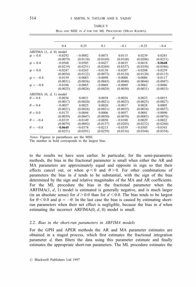
Assuming that the mean of the process is known, the bias in the fractionalintegration parameter from using the ML procedure (Table V) tends to be smallrelative to that observed in the two semi-parametric procedures. In addition, thebias is predominantly negative for all values of d and for all AR or MAparameters. This contrasts slightly with the results of Sowell (1992). For neitherthe ARFIMA(1, d, 0) model nor the ARFIMA(0, d, 1) model is there evidence

TABLE I

BIAS AND MSE IN d FOR THE GPH PROCEDURE: ARFIMA(1, d, 0) MODEL

d

φ m 0.4 0.25 0.1 ÿ0.1 ÿ0.25 ÿ0.4

0.8 16 0.3918 0.3892 0.4132 0.3780 0.3971 0.4077(0.2774) (0.2754) (0.2911) (0.2676) (0.2741) (0.3061)

0.4 0.0454 0.0417 0.0608 0.0228 0.0492 0.0577(0.1293) (0.1209) (0.1222) (0.1304) (0.1192) (0.1446)

0.0 0.0015 ÿ0.0021 0.0169 ÿ0.0212 0.0082 0.0203(0.1271) (0.1198) (0.1190) (0.1300) (0.1146) (0.1380)

ÿ0.4 ÿ0.0067 ÿ0.0112 0.0085 ÿ0.0317 0.0025 0.0185(0.1267) (0.1207) (0.1201) (0.1324) (0.1121) (0.1390)

ÿ0.8 ÿ0.0089 ÿ0.0141 0.0059 ÿ0.0295 0.0114 0.0459(0.1235) (0.1201) (0.1187) (0.1280) (0.1127) (0.1392)

0.8 28 0.5324 0.5361 0.5378 0.5361 0.5402 0.5415(0.3260) (0.3300) (0.3310) (0.3307) (0.3335) (0.3374)

0.4 0.0935 0.0935 0.0908 0.0850 0.0941 0.0954(0.0502) (0.0508) (0.0492) (0.0517) (0.0508) (0.0532)

0.0 0.0017 0.0010 ÿ0.0015 ÿ0.0075 0.0043 0.0082(0.0417) (0.0425) (0.0413) (0.0444) (0.0415) (0.0435)

ÿ0.4 ÿ0.0189 ÿ0.0206 ÿ0.0228 ÿ0.0289 ÿ0.0140 ÿ0.0071(0.0418) (0.0433) (0.0421) (0.0456) (0.0408) (0.0438)

ÿ0.8 ÿ0.0238 ÿ0.0260 ÿ0.0275 ÿ0.0312 ÿ0.0085 0.0134(0.0412) (0.0432) (0.0419) (0.0453) (0.0405) (0.0435)

� 0.8 49 0.6367 0.6549 0.6521 0.6609 0.6620 0.6660(0.4235) (0.4466) (0.4426) (0.4537) (0.4564) (0.4604)

0.4 0.1691 0.1797 0.1712 0.1782 0.1817 0.1864(0.0466) (0.0497) (0.0464) (0.0493) (0.0517) (0.0518)

0.0 ÿ0.0072 0.0023 ÿ0.0064 0.0009 0.0063 0.0125(0.0184) (0.0177) (0.0171) (0.0174) (0.0184) (0.0172)

ÿ0.4 ÿ0.0616 ÿ0.0530 ÿ0.0615 ÿ0.0539 ÿ0.0458 ÿ0.0368(0.0221) (0.0206) (0.0209) (0.0205) (0.0202) (0.0187)

ÿ0.8 ÿ0.0757 ÿ0.0678 ÿ0.0756 ÿ0.0660 ÿ0.0509 ÿ0.0293(0.0238) (0.0221) (0.0227) (0.0222) (0.0201) (0.0188)

Notes: Figure in parentheses are the MSE.The number in bold corresponds to the largest bias.



of the bias varying systematically with the AR or MA parameter. In particular,there is no substantial positive (negative) bias associated with a large positive(negative) AR (MA) coefficient. All parameters are estimated with a highdegree of precision.

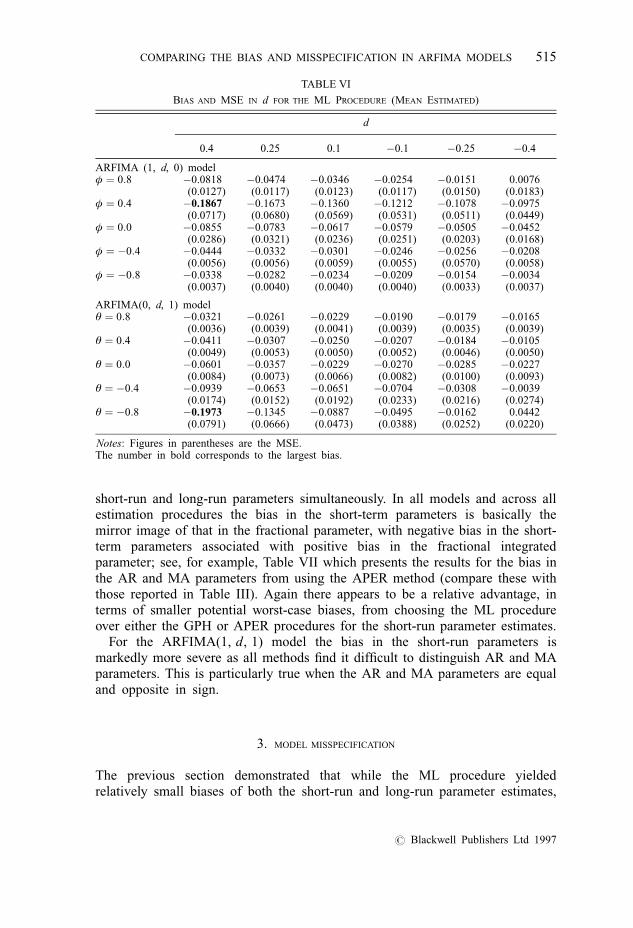
However, as Cheung and Diebold (1994) demonstrate, the ML method losesa lot of its superiority when the mean of the process has to be estimated. Thisis due to the difficulty of estimating the mean in the presence of long memory(d . 0). The bias in the fractional parameter d when the mean is estimatedcontinues to be negative for almost all parameter combinations (see Table VI).In comparing Table VI with Table V, there is a deterioration in the performanceof the ML method for all values of d, although this is much more marked ford . 0:0. The bias in the ARFIMA(0, d, 1) model tends to increase as the MA

TABLE II

BIAS AND MSE IN d FOR THE GPH PROCEDURE: ARFIMA(0, d, 1) MODEL

d

θ m 0.4 0.25 0.1 ÿ0.1 ÿ0.25 ÿ0.4

0.8 16 0.0116 0.0085 0.0277 ÿ0.0098 0.0172 0.0260(0.1272) (0.1192) (0.1191) (0.1302) (0.1173) (0.1392)

0.4 0.0102 0.0067 0.0257 ÿ0.0121 0.0159 0.0252(0.1276) (0.1191) (0.1190) (0.1302) (0.1167) (0.1395)

0.0 0.0015 ÿ0.0021 0.0169 ÿ0.0212 0.0082 0.0203(0.1271) (0.1198) (0.1190) (0.1300) (0.1146) (0.1380)

ÿ0.4 ÿ0.0418 ÿ0.0462 ÿ0.0267 ÿ0.0651 ÿ0.0288 ÿ0.0105(0.1275) (0.1221) (0.1213) (0.1319) (0.1111) (0.1411)

ÿ0.8 ÿ0.3993 ÿ0.3980 ÿ0.3668 ÿ0.3715 ÿ0.2880 ÿ0.1926(0.2856) (0.2769) (0.2505) (0.2582) (0.2108) (0.1891)

0.8 28 0.0272 0.0273 0.0241 0.0182 0.0284 0.0302(0.0426) (0.0430) (0.0415) (0.0448) (0.0428) (0.0448)

0.4 0.0225 0.0226 0.0196 0.0134 0.0241 0.0263(0.0424) (0.0428) (0.0415) (0.0447) (0.0424) (0.0445)

0.0 0.0017 0.0010 ÿ0.0015 ÿ0.0075 0.0043 0.0082(0.0417) (0.0425) (0.0413) (0.0444) (0.0415) (0.0435)

ÿ0.4 ÿ0.0896 ÿ0.0918 ÿ0.0947 ÿ0.0992 ÿ0.0814 ÿ0.0730(0.0490) (0.0512) (0.0507) (0.0537) (0.0469) (0.0500)

ÿ0.8 ÿ0.5390 ÿ0.5375 ÿ0.5314 ÿ0.5091 ÿ0.4547 ÿ0.3836(0.3314) (0.3323) (0.3234) (0.3058) (0.2574) (0.2109)

0.8 49 0.0603 0.0706 0.0619 0.0689 0.0726 0.0782(0.0218) (0.0224) (0.0210) (0.0222) (0.0240) (0.0231)

0.4 0.0470 0.0573 0.0485 0.0554 0.0597 0.0653(0.0204) (0.0208) (0.0195) (0.0206) (0.0222) (0.0213)

0.0 ÿ0.0072 0.0023 ÿ0.0064 0.0009 0.0063 0.0125(0.0184) (0.0177) (0.0171) (0.0174) (0.0184) (0.0172)

ÿ0.4 ÿ0.1844 ÿ0.1758 ÿ0.1844 ÿ0.1752 ÿ0.1652 ÿ0.1548(0.0522) (0.0486) (0.0511) (0.0483) (0.0453) (0.0418)

ÿ0.8 ÿ0.6675 ÿ0.6549 ÿ0.6550 ÿ0.6265 ÿ0.5922 ÿ0.5373(0.4637) (0.4465) (0.4464) (0.4130) (0.3749) (0.3209)

Notes: Figures in parentheses are the MSE.The number in bold corresponds to the largest bias.



coefficient approaches ÿ1, although the bias remains largely unrelated to theAR parameter in the ARFIMA(1, d, 0) model. The MSEs continue to besmaller, on the whole, than those associated with either of the semi-parametricprocedures. All subsequent references to the ML method, unless otherwisestated, relate to the case when the mean is estimated.

From Tables I–IV and VI no one procedure unambiguously dominates, interms of smallest biases, for all parameter values considered. A heuristic rulemight suggest using the ML method for estimating the fractional parameter dfor both ARFIMA(1, d, 0) and ARFIMA(0, d, 1) models, as there is lesslikelihood of incurring a substantial bias. Moreover, the gain from using theML procedure rather than the semi-parametric methods is particularlypronounced when either the AR parameter approaches unity or the MAparameter approaches ÿ1. Consequently, the worst-case bias for the ML

TABLE III

BIAS AND MSE IN d FOR THE APER PROCEDURE: ARFIMA(1, d, 0) MODEL

d

φ m 0.4 0.25 0.1 ÿ0.1 ÿ0.25 ÿ0.4

0.8 16 ÿ0.0130 0.0775 0.1665 0.2387 0.2919 0.3354(0.0043) (0.0137) (0.0401) (0.0803) (0.1171) (0.1576)

0.4 ÿ0.1102 ÿ0.0589 ÿ0.0049 0.0160 0.0399 0.0591(0.0229) (0.0218) (0.0268) (0.0447) (0.0578) (0.0783)

0.0 ÿ0.1253 ÿ0.0795 ÿ0.0305 ÿ0.0167 0.0058 0.0240(0.0277) (0.0264) (0.0299) (0.0481) (0.0592) (0.0794)

ÿ0.4 ÿ0.1286 ÿ0.0838 ÿ0.0357 ÿ0.0235 0.0023 0.0238(0.0287) (0.0274) (0.0308) (0.0496) (0.0591) (0.0791)

ÿ0.8 ÿ0.1296 ÿ0.0851 ÿ0.0371 ÿ0.0245 0.0123 0.0482(0.0290) (0.0277) (0.0309) (0.0505) (0.0576) (0.0781)

0.8 28 0.0438 0.1571 0.2579 0.3657 0.4350 0.4870(0.0026) (0.0264) (0.0698) (0.1411) (0.1985) (0.2534)

0.4 ÿ0.0662 ÿ0.0052 0.0383 0.0762 0.1003 0.1144(0.0086) (0.0079) (0.0141) (0.0286) (0.0361) (0.0506)

0.0 ÿ0.1013 ÿ0.0550 ÿ0.027 ÿ0.0066 0.0073 0.0140(0.0160) (0.0133) (0.0166) (0.0275) (0.0308) (0.0435)

ÿ0.4 ÿ0.1103 ÿ0.0676 ÿ0.0434 ÿ0.0265 ÿ0.0138 ÿ0.0059(0.0183) (0.0155) (0.0186) (0.0294) (0.0318) (0.0449)

ÿ0.8 ÿ0.1129 ÿ0.0712 ÿ0.0475 ÿ0.0295 ÿ0.0108 0.0088(0.0189) (0.0161) (0.0192) (0.0298) (0.0315) (0.0448)

0.8 49 0.0738 0.2024 0.3158 0.4484 0.5276 0.5998(0.0055) (0.0413) (0.1006) (0.2030) (0.2817) (0.3648)

0.4 ÿ0.0210 0.0545 0.0996 0.1585 0.1843 0.2211(0.0020) (0.0059) (0.0157) (0.0343) (0.0471) (0.0655)

0.0 ÿ0.0909 ÿ0.0479 ÿ0.0392 ÿ0.0165 ÿ0.0161 0.0039(0.0115) (0.0078) (0.0115) (0.0146) (0.0195) (0.0236)

ÿ0.4 ÿ0.1187 ÿ0.0876 ÿ0.0917 ÿ0.0813 ÿ0.0884 ÿ0.0725(0.0181) (0.0144) (0.0201) (0.0229) (0.0291) (0.0313)

ÿ0.8 ÿ0.1269 ÿ0.0988 ÿ0.1060 ÿ0.0971 ÿ0.1003 ÿ0.0784(0.0203) (0.0168) (0.0232) (0.0263) (0.0314) (0.0326)




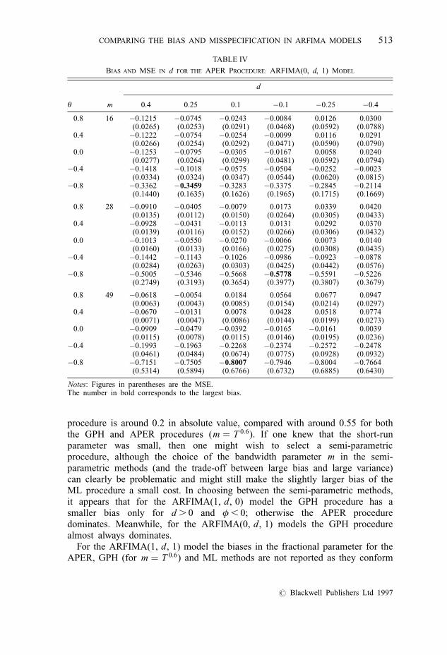
procedure is around 0.2 in absolute value, compared with around 0.55 for boththe GPH and APER procedures (m � T 0:6). If one knew that the short-runparameter was small, then one might wish to select a semi-parametricprocedure, although the choice of the bandwidth parameter m in the semi-parametric methods (and the trade-off between large bias and large variance)can clearly be problematic and might still make the slightly larger bias of theML procedure a small cost. In choosing between the semi-parametric methods,it appears that for the ARFIMA(1, d, 0) model the GPH procedure has asmaller bias only for d . 0 and φ , 0; otherwise the APER proceduredominates. Meanwhile, for the ARFIMA(0, d, 1) models the GPH procedurealmost always dominates.

For the ARFIMA(1, d, 1) model the biases in the fractional parameter for theAPER, GPH (for m � T 0:6) and ML methods are not reported as they conform

TABLE IV

BIAS AND MSE IN d FOR THE APER PROCEDURE: ARFIMA(0, d, 1) MODEL

d

θ m 0.4 0.25 0.1 ÿ0.1 ÿ0.25 ÿ0.4

0.8 16 ÿ0.1215 ÿ0.0745 ÿ0.0243 ÿ0.0084 0.0126 0.0300(0.0265) (0.0253) (0.0291) (0.0468) (0.0592) (0.0788)

0.4 ÿ0.1222 ÿ0.0754 ÿ0.0254 ÿ0.0099 0.0116 0.0291(0.0266) (0.0254) (0.0292) (0.0471) (0.0590) (0.0790)

0.0 ÿ0.1253 ÿ0.0795 ÿ0.0305 ÿ0.0167 0.0058 0.0240(0.0277) (0.0264) (0.0299) (0.0481) (0.0592) (0.0794)

ÿ0.4 ÿ0.1418 ÿ0.1018 ÿ0.0575 ÿ0.0504 ÿ0.0252 ÿ0.0023(0.0334) (0.0324) (0.0347) (0.0544) (0.0620) (0.0815)

ÿ0.8 ÿ0.3362 ÿ0.3459 ÿ0.3283 ÿ0.3375 ÿ0.2845 ÿ0.2114(0.1440) (0.1635) (0.1626) (0.1965) (0.1715) (0.1669)

0.8 28 ÿ0.0910 ÿ0.0405 ÿ0.0079 0.0173 0.0339 0.0420(0.0135) (0.0112) (0.0150) (0.0264) (0.0305) (0.0433)

0.4 ÿ0.0928 ÿ0.0431 ÿ0.0113 0.0131 0.0292 0.0370(0.0139) (0.0116) (0.0152) (0.0266) (0.0306) (0.0432)

0.0 ÿ0.1013 ÿ0.0550 ÿ0.0270 ÿ0.0066 0.0073 0.0140(0.0160) (0.0133) (0.0166) (0.0275) (0.0308) (0.0435)

ÿ0.4 ÿ0.1442 ÿ0.1143 ÿ0.1026 ÿ0.0986 ÿ0.0923 ÿ0.0878(0.0284) (0.0263) (0.0303) (0.0425) (0.0442) (0.0576)

ÿ0.8 ÿ0.5005 ÿ0.5346 ÿ0.5668 ÿ0.5778 ÿ0.5591 ÿ0.5226(0.2749) (0.3193) (0.3654) (0.3977) (0.3807) (0.3679)

0.8 49 ÿ0.0618 ÿ0.0054 0.0184 0.0564 0.0677 0.0947(0.0063) (0.0043) (0.0085) (0.0154) (0.0214) (0.0297)

0.4 ÿ0.0670 ÿ0.0131 0.0078 0.0428 0.0518 0.0774(0.0071) (0.0047) (0.0086) (0.0144) (0.0199) (0.0273)

0.0 ÿ0.0909 ÿ0.0479 ÿ0.0392 ÿ0.0165 ÿ0.0161 0.0039(0.0115) (0.0078) (0.0115) (0.0146) (0.0195) (0.0236)

ÿ0.4 ÿ0.1993 ÿ0.1963 ÿ0.2268 ÿ0.2374 ÿ0.2572 ÿ0.2478(0.0461) (0.0484) (0.0674) (0.0775) (0.0928) (0.0932)

ÿ0.8 ÿ0.7151 ÿ0.7505 ÿ0.8007 ÿ0.7946 ÿ0.8004 ÿ0.7664(0.5314) (0.5894) (0.6766) (0.6732) (0.6885) (0.6430)




to the results we have seen earlier. In particular, for the semi-parametricmethods, the bias in the fractional parameter is small when either the AR andMA parameters are approximately equal and opposite in sign so that theireffects cancel out, or when φ , 0 and θ . 0. For other combinations ofparameters the bias in d tends to be substantial, with the sign of the biasdetermined by the sign and relative magnitudes of the MA and AR coefficients.For the ML procedure the bias in the fractional parameter when theARFIMA(1, d, 1) model is estimated is generally negative, and is much larger(in an absolute sense) for d . 0:0 than for d , 0:0. The bias tends to be largestfor θ , 0:0 and φ � ÿθ. In the last case the bias is caused by estimating short-run parameters when their net effect is negligible, because the bias in d whenestimating the incorrect ARFIMA(0, d, 0) model is small.

2.2. Bias in the short-run parameters in ARFIMA models

For the GPH and APER methods the AR and MA parameter estimates areobtained in a staged process, which first estimates the fractional integrationparameter d, then filters the data using this parameter estimate and finallyestimates the appropriate short-run parameters. The ML procedure estimates the

TABLE V

BIAS AND MSE IN d FOR THE ML PROCEDURE (MEAN KNOWN)

d

0.4 0.25 0.1 ÿ0.1 ÿ0.25 ÿ0.4

ARFIMA (1, d, 0) modelφ � 0:8 ÿ0.0292 ÿ0.0082 0.0075 0.0115 0.0239 0.0281

(0.0079) (0.0110) (0.0169) (0.0168) (0.0206) (0.0231)φ � 0:4 ÿ0.0568 ÿ0.0505 ÿ0.0427 ÿ0.0635 ÿ0.0618 ÿ0.0648

(0.0219) (0.0251) (0.0269) (0.0357) (0.0350) (0.0386)φ � 0:0 ÿ0.0247 ÿ0.0243 ÿ0.0138 ÿ0.0207 ÿ0.0208 ÿ0.0259

(0.0054) (0.0122) (0.0072) (0.0124) (0.0120) (0.0115)φ � ÿ0:4 ÿ0.0159 ÿ0.0083 ÿ0.0098 ÿ0.0088 ÿ0.0086 ÿ0.0117

(0.0031) (0.0036) (0.0043) (0.0040) (0.0044) (0.0047)φ � ÿ0:8 ÿ0.0106 ÿ0.0065 ÿ0.0069 ÿ0.0089 ÿ0.0062 ÿ0.0086

(0.0025) (0.0026) (0.0029) (0.0030) (0.0031) (0.0033)

ARFIMA (0, d, 1) modelθ � 0:8 ÿ0.0036 0.0031 0.0038 ÿ0.0026 0.0023 ÿ0.0015

(0.0017) (0.0020) (0.0021) (0.0025) (0.0025) (0.0027)θ � 0:4 ÿ0.0057 0.0025 0.0026 ÿ0.0017 0.0028 0.0005

(0.0021) (0.0026) (0.0031) (0.0035) (0.0034) (0.0037)θ � 0:0 ÿ0.0175 ÿ0.0044 0.0006 ÿ0.0057 0.0001 ÿ0.0090

(0.0039) (0.0047) (0.0050) (0.0070) (0.0083) (0.0076)θ � ÿ0:4 ÿ0.0319 ÿ0.0149 ÿ0.0050 ÿ0.0100 0.0029 ÿ0.0022

(0.0079) (0.0092) (0.0157) (0.0205) (0.0232) (0.0260)θ � ÿ0:8 ÿ0.0645 ÿ0.0374 ÿ0.0215 ÿ0.0359 ÿ0.0305 ÿ0.0343

(0.0251) (0.0291) (0.0259) (0.0316) (0.0344) (0.0354)




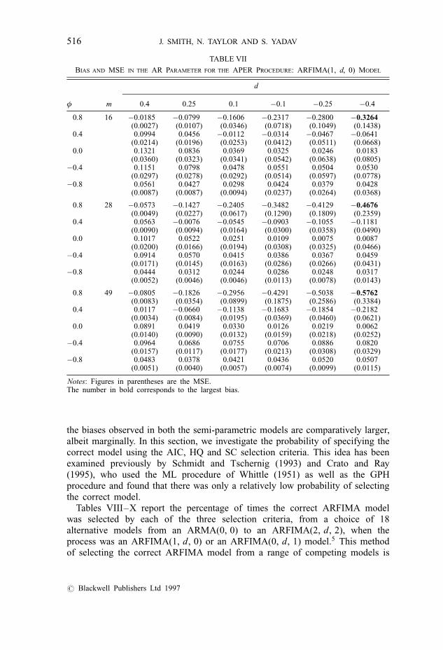
short-run and long-run parameters simultaneously. In all models and across allestimation procedures the bias in the short-term parameters is basically themirror image of that in the fractional parameter, with negative bias in the short-term parameters associated with positive bias in the fractional integratedparameter; see, for example, Table VII which presents the results for the bias inthe AR and MA parameters from using the APER method (compare these withthose reported in Table III). Again there appears to be a relative advantage, interms of smaller potential worst-case biases, from choosing the ML procedureover either the GPH or APER procedures for the short-run parameter estimates.

For the ARFIMA(1, d, 1) model the bias in the short-run parameters ismarkedly more severe as all methods find it difficult to distinguish AR and MAparameters. This is particularly true when the AR and MA parameters are equaland opposite in sign.

3. MODEL MISSPECIFICATION

The previous section demonstrated that while the ML procedure yieldedrelatively small biases of both the short-run and long-run parameter estimates,

TABLE VI

BIAS AND MSE IN d FOR THE ML PROCEDURE (MEAN ESTIMATED)

d

0.4 0.25 0.1 ÿ0.1 ÿ0.25 ÿ0.4

ARFIMA (1, d, 0) modelφ � 0:8 ÿ0.0818 ÿ0.0474 ÿ0.0346 ÿ0.0254 ÿ0.0151 0.0076

(0.0127) (0.0117) (0.0123) (0.0117) (0.0150) (0.0183)φ � 0:4 ÿ0.1867 ÿ0.1673 ÿ0.1360 ÿ0.1212 ÿ0.1078 ÿ0.0975

(0.0717) (0.0680) (0.0569) (0.0531) (0.0511) (0.0449)φ � 0:0 ÿ0.0855 ÿ0.0783 ÿ0.0617 ÿ0.0579 ÿ0.0505 ÿ0.0452

(0.0286) (0.0321) (0.0236) (0.0251) (0.0203) (0.0168)φ � ÿ0:4 ÿ0.0444 ÿ0.0332 ÿ0.0301 ÿ0.0246 ÿ0.0256 ÿ0.0208

(0.0056) (0.0056) (0.0059) (0.0055) (0.0570) (0.0058)φ � ÿ0:8 ÿ0.0338 ÿ0.0282 ÿ0.0234 ÿ0.0209 ÿ0.0154 ÿ0.0034

(0.0037) (0.0040) (0.0040) (0.0040) (0.0033) (0.0037)

ARFIMA(0, d, 1) modelθ � 0:8 ÿ0.0321 ÿ0.0261 ÿ0.0229 ÿ0.0190 ÿ0.0179 ÿ0.0165

(0.0036) (0.0039) (0.0041) (0.0039) (0.0035) (0.0039)θ � 0:4 ÿ0.0411 ÿ0.0307 ÿ0.0250 ÿ0.0207 ÿ0.0184 ÿ0.0105

(0.0049) (0.0053) (0.0050) (0.0052) (0.0046) (0.0050)θ � 0:0 ÿ0.0601 ÿ0.0357 ÿ0.0229 ÿ0.0270 ÿ0.0285 ÿ0.0227

(0.0084) (0.0073) (0.0066) (0.0082) (0.0100) (0.0093)θ � ÿ0:4 ÿ0.0939 ÿ0.0653 ÿ0.0651 ÿ0.0704 ÿ0.0308 ÿ0.0039

(0.0174) (0.0152) (0.0192) (0.0233) (0.0216) (0.0274)θ � ÿ0:8 ÿ0.1973 ÿ0.1345 ÿ0.0887 ÿ0.0495 ÿ0.0162 0.0442

(0.0791) (0.0666) (0.0473) (0.0388) (0.0252) (0.0220)




the biases observed in both the semi-parametric models are comparatively larger,albeit marginally. In this section, we investigate the probability of specifying thecorrect model using the AIC, HQ and SC selection criteria. This idea has beenexamined previously by Schmidt and Tschernig (1993) and Crato and Ray(1995), who used the ML procedure of Whittle (1951) as well as the GPHprocedure and found that there was only a relatively low probability of selectingthe correct model.

Tables VIII–X report the percentage of times the correct ARFIMA modelwas selected by each of the three selection criteria, from a choice of 18alternative models from an ARMA(0, 0) to an ARFIMA(2, d, 2), when theprocess was an ARFIMA(1, d, 0) or an ARFIMA(0, d, 1) model.5 This methodof selecting the correct ARFIMA model from a range of competing models is

TABLE VII

BIAS AND MSE IN THE AR PARAMETER FOR THE APER PROCEDURE: ARFIMA(1, d, 0) MODEL

d

φ m 0.4 0.25 0.1 ÿ0.1 ÿ0.25 ÿ0.4

0.8 16 ÿ0.0185 ÿ0.0799 ÿ0.1606 ÿ0.2317 ÿ0.2800 ÿ0.3264(0.0027) (0.0107) (0.0346) (0.0718) (0.1049) (0.1438)

0.4 0.0994 0.0456 ÿ0.0112 ÿ0.0314 ÿ0.0467 ÿ0.0641(0.0214) (0.0196) (0.0253) (0.0412) (0.0511) (0.0668)

0.0 0.1321 0.0836 0.0369 0.0325 0.0246 0.0183(0.0360) (0.0323) (0.0341) (0.0542) (0.0638) (0.0805)

ÿ0.4 0.1151 0.0798 0.0478 0.0551 0.0504 0.0530(0.0297) (0.0278) (0.0292) (0.0514) (0.0597) (0.0778)

ÿ0.8 0.0561 0.0427 0.0298 0.0424 0.0379 0.0428(0.0087) (0.0087) (0.0094) (0.0237) (0.0264) (0.0368)

0.8 28 ÿ0.0573 ÿ0.1427 ÿ0.2405 ÿ0.3482 ÿ0.4129 ÿ0.4676(0.0049) (0.0227) (0.0617) (0.1290) (0.1809) (0.2359)

0.4 0.0563 ÿ0.0076 ÿ0.0545 ÿ0.0903 ÿ0.1055 ÿ0.1181(0.0090) (0.0094) (0.0164) (0.0300) (0.0358) (0.0490)

0.0 0.1017 0.0522 0.0251 0.0109 0.0075 0.0087(0.0200) (0.0166) (0.0194) (0.0308) (0.0325) (0.0466)

ÿ0.4 0.0914 0.0570 0.0415 0.0386 0.0367 0.0459(0.0171) (0.0145) (0.0163) (0.0286) (0.0266) (0.0431)

ÿ0.8 0.0444 0.0312 0.0244 0.0286 0.0248 0.0317(0.0052) (0.0046) (0.0046) (0.0113) (0.0078) (0.0143)

0.8 49 ÿ0.0805 ÿ0.1826 ÿ0.2956 ÿ0.4291 ÿ0.5038 ÿ0.5762(0.0083) (0.0354) (0.0899) (0.1875) (0.2586) (0.3384)

0.4 0.0117 ÿ0.0660 ÿ0.1138 ÿ0.1683 ÿ0.1854 ÿ0.2182(0.0034) (0.0084) (0.0195) (0.0369) (0.0460) (0.0621)

0.0 0.0891 0.0419 0.0330 0.0126 0.0219 0.0062(0.0140) (0.0090) (0.0132) (0.0159) (0.0218) (0.0252)

ÿ0.4 0.0964 0.0686 0.0755 0.0706 0.0886 0.0820(0.0157) (0.0117) (0.0177) (0.0213) (0.0308) (0.0329)

ÿ0.8 0.0483 0.0378 0.0421 0.0436 0.0520 0.0507(0.0051) (0.0040) (0.0057) (0.0074) (0.0099) (0.0115)




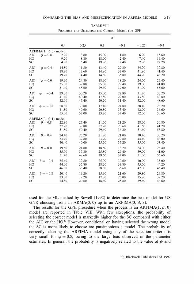
used for the ML method by Sowell (1992) to determine the best model for USGNP, choosing from an ARMA(0, 0) up to an ARFIMA(3, d, 3).

The results for the GPH procedure when the process is an ARFIMA(1, d, 0)model are reported in Table VIII. With few exceptions, the probability ofselecting the correct model is markedly higher for the SC compared with eitherthe AIC or the HQ.6 However, conditional on having selected the wrong modelthe SC is more likely to choose too parsimonious a model. The probability ofcorrectly selecting the ARFIMA model using any of the selection criteria isvery small for φ � 0:8, owing to the large bias observed in the parameterestimates. In general, the probability is negatively related to the value of φ and

TABLE VIII

PROBABILITY OF SELECTING THE CORRECT MODEL FOR GPH

d

0.4 0.25 0.1 ÿ0.1 ÿ0.25 ÿ0.4

ARFIMA(1, d, 0) modelAIC φ � 0:8 2.20 3.80 15.00 1.80 6.20 15.60HQ 9.20 8.80 18.00 2.40 7.40 19.40SC 4.80 5.40 19.80 2.40 7.80 22.20

AIC φ � 0:4 14.80 11.80 13.40 29.20 34.20 32.80HQ 18.80 13.60 14.80 33.00 41.80 41.40SC 19.20 14.40 14.80 35.80 44.20 46.20

AIC φ � 0:0 19.60 24.80 18.60 18.20 24.00 26.40HQ 35.00 37.80 25.80 29.40 39.00 41.00SC 51.40 48.60 29.60 37.00 51.00 55.60

AIC φ � ÿ0:4 29.80 30.20 15.00 22.80 31.20 30.20HQ 41.40 40.40 17.80 29.00 43.80 40.80SC 52.60 47.40 20.20 31.40 52.00 48.60

AIC φ � ÿ0:8 28.80 30.80 17.40 24.80 28.40 26.20HQ 41.80 40.60 20.80 33.40 42.00 36.60SC 55.00 53.00 23.20 37.40 52.00 50.60

ARFIMA(0, d, 1) modelAIC θ � 0:8 22.80 27.40 21.60 21.20 28.60 30.80HQ 37.20 39.80 27.20 28.60 41.60 41.20SC 51.80 50.40 29.60 36.20 51.60 55.80

AIC θ � 0:4 24.40 25.20 21.20 21.00 30.40 30.20HQ 33.20 32.80 23.20 29.80 44.40 43.00SC 40.40 40.00 25.20 35.20 55.00 53.40

AIC θ � 0:0 19.60 24.80 18.60 18.20 24.00 26.40HQ 35.00 37.80 25.80 29.40 39.00 41.00SC 51.40 48.60 29.60 37.00 51.00 55.60

AIC θ � ÿ0:4 35.60 32.80 25.00 30.60 40.00 38.00HQ 44.00 35.80 28.20 33.80 45.60 44.20SC 46.80 33.40 28.80 35.60 47.00 45.40

AIC θ � ÿ0:8 20.40 16.20 15.60 21.60 29.80 29.80HQ 23.00 19.20 17.80 25.00 35.20 37.20SC 24.80 20.60 18.60 25.80 39.60 46.60



improves for jdj further from zero, although at best it is rarely above 50%. Forφ . 0:0 both the AR(1) and the AR(2) models are frequently selected inpreference to the ARFIMA(1, d, 0) model, while for φ , 0 the ARMA(2, 1)model is frequently selected. Models above an ARFIMA(1, d, 1) are rarelyselected.

When the true model is an ARFIMA(0, d, 1) model (Table VIII) the resultsagain show that the probability of selecting the correct model rarely rises above50%. In this case, for d � �0:1, the MA(1) model is often selected inpreference to the correct model irrespective of the value of the MA coefficient,while for larger values of jdj, MA(1), ARMA(1, 2) or ARFIMA(1, d, 1)

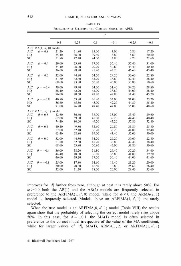
TABLE IX

PROBABILITY OF SELECTING THE CORRECT MODEL FOR APER

d

0.4 0.25 0.1 ÿ0.1 ÿ0.25 ÿ0.4


AIC φ � 0:4 29.00 23.80 17.60 35.40 37.40 31.00HQ 34.40 26.20 20.20 40.60 44.40 40.40SC 36.00 28.20 21.40 43.20 46.60 45.40

AIC φ � 0:0 32.00 44.80 34.20 29.20 30.60 22.80HQ 51.80 62.60 45.20 38.80 42.40 38.40SC 68.60 73.80 50.80 45.00 53.80 50.60

AIC φ � ÿ0:4 39.00 49.40 34.60 31.40 34.20 28.80HQ 58.40 62.20 42.00 38.80 44.00 38.40SC 76.00 70.60 47.20 42.80 51.40 45.20

AIC φ � ÿ0:8 40.80 53.80 36.80 33.00 31.00 25.20HQ 56.60 65.80 45.00 42.20 44.80 35.40SC 71.00 76.20 49.40 47.00 55.00 48.60


AIC θ � 0:4 40.40 49.80 32.60 29.80 31.80 25.80HQ 57.00 62.40 36.20 38.20 44.80 39.40SC 63.40 68.80 39.00 43.40 55.00 50.00

AIC θ � 0:0 32.00 44.80 34.20 29.20 30.60 22.80HQ 51.80 62.60 45.20 38.80 42.40 38.40SC 68.60 73.80 50.80 45.00 53.80 50.60

AIC θ � ÿ0:4 36.00 38.20 31.80 29.40 37.20 34.60HQ 44.40 40.80 36.80 35.80 41.80 39.20SC 46.60 39.20 37.20 36.40 44.00 41.60

AIC θ � ÿ0:8 25.00 17.80 14.60 16.40 21.20 20.00HQ 30.00 20.60 16.80 18.80 25.60 26.40SC 32.00 21.20 18.00 20.00 29.40 33.60



models tend to be selected. In these models high ordered ARFIMA models dohave a non-negligible probability of being selected.

Table IX reports the selection probabilities for the APER procedure for theARFIMA(1, d, 0) and ARFIMA(0, d, 1) models. The probability of selectingthe correct model for an ARFIMA(1, d, 0) is greater than that observed withthe GPH procedure for d .ÿ0:1 and is approximately equal to that observedwith the GPH procedure for d , 0:0. The probability of selecting the correctmodel for this procedure is negatively related to φ, a result which is consistentwith the direction of the bias observed (Table I).The results for theARFIMA(0, d, 1) model show that for d . 0 and θ . 0 there is the greatest

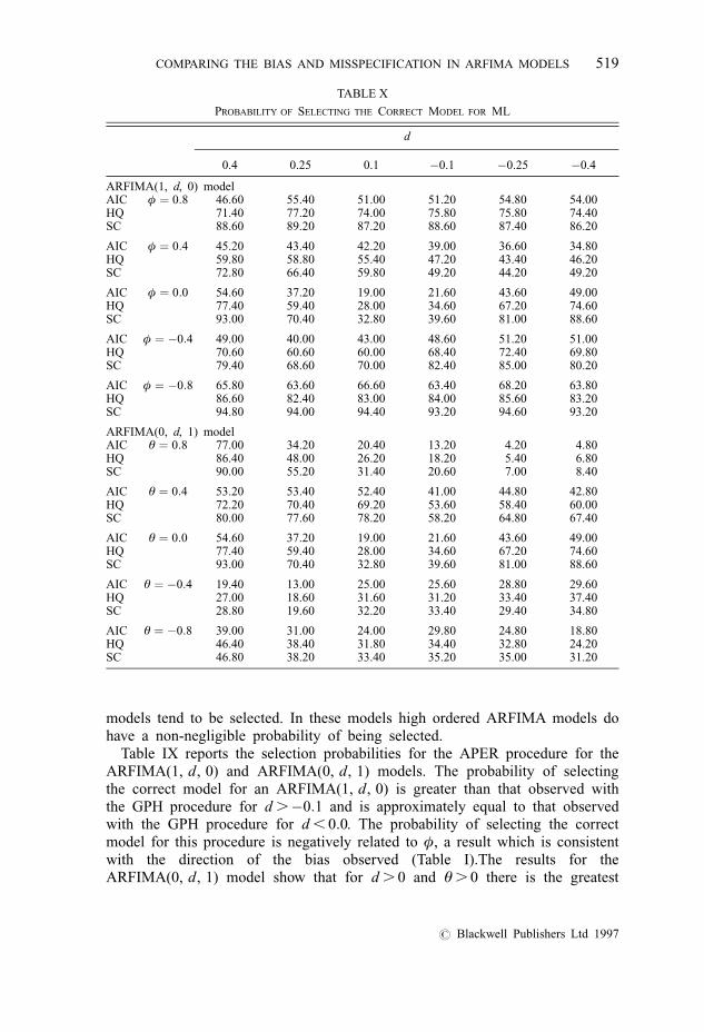
TABLE X

PROBABILITY OF SELECTING THE CORRECT MODEL FOR ML

d

0.4 0.25 0.1 ÿ0.1 ÿ0.25 ÿ0.4


AIC φ � 0:4 45.20 43.40 42.20 39.00 36.60 34.80HQ 59.80 58.80 55.40 47.20 43.40 46.20SC 72.80 66.40 59.80 49.20 44.20 49.20

AIC φ � 0:0 54.60 37.20 19.00 21.60 43.60 49.00HQ 77.40 59.40 28.00 34.60 67.20 74.60SC 93.00 70.40 32.80 39.60 81.00 88.60

AIC φ � ÿ0:4 49.00 40.00 43.00 48.60 51.20 51.00HQ 70.60 60.60 60.00 68.40 72.40 69.80SC 79.40 68.60 70.00 82.40 85.00 80.20

AIC φ � ÿ0:8 65.80 63.60 66.60 63.40 68.20 63.80HQ 86.60 82.40 83.00 84.00 85.60 83.20SC 94.80 94.00 94.40 93.20 94.60 93.20


AIC θ � 0:4 53.20 53.40 52.40 41.00 44.80 42.80HQ 72.20 70.40 69.20 53.60 58.40 60.00SC 80.00 77.60 78.20 58.20 64.80 67.40

AIC θ � 0:0 54.60 37.20 19.00 21.60 43.60 49.00HQ 77.40 59.40 28.00 34.60 67.20 74.60SC 93.00 70.40 32.80 39.60 81.00 88.60

AIC θ � ÿ0:4 19.40 13.00 25.00 25.60 28.80 29.60HQ 27.00 18.60 31.60 31.20 33.40 37.40SC 28.80 19.60 32.20 33.40 29.40 34.80

AIC θ � ÿ0:8 39.00 31.00 24.00 29.80 24.80 18.80HQ 46.40 38.40 31.80 34.40 32.80 24.20SC 46.80 38.20 33.40 35.20 35.00 31.20



probability of correctly selecting an ARFIMA(0, d, 1) over that observed forthe GPH procedure, and the probabilities are approximately equal otherwise.The distribution of the probabilities across the competing models is roughlysimilar (even though the numbers are smaller) to that observed for the GPHprocedure. Therefore, while the GPH procedure generally yields slightly smallerbiases of the fractional parameter in ARFIMA(0, d, 1) models, it actually has asmaller probability of identifying them compared with the APER procedure.

The results for the ML procedure are shown in Table X.7 For both theARFIMA(1, d, 0) and ARFIMA(0, d, 1) models the probability of selecting thecorrect model is invariably greater than that for either the GPH or APERprocedure, the exception being the ARFIMA(0, d, 1) model with θ � 0:8 andθ � ÿ0:4. For the ML procedure, the probability of selecting the correct modelfor an ARFIMA(1, d, 0) (ARFIMA(0, d, 1)) model is greater for φ , 0 (θ . 0)and these probabilities increase with the size of the AR parameter. Theprobabilities vary marginally over d and are generally slightly smaller the closerd is to zero. The SC shows a much greater likelihood of selecting the correctmodel. However, conditional on the incorrect model being selected, thiscriterion is more likely to select an ARMA specification, which would imply asubstantial bias in both the long-run and short-run coefficients.

3.1. Effective bias

As was stated in Section 2, the semi-parametric (GPH and APER) methodsestimate the fractional parameter irrespective of the short-run parameters.Consequently, misspecification of the ARFIMA process only leads to biases inthe short-run parameters. In comparison, the ML procedure estimates the short-run and long-run parameters simultaneously; therefore problems of misspecifica-tion of the model will lead to bias in both the long-run and short-run parameters.Therefore, in talking about the bias in d for the ML procedure, it is necessary tocalculate the effective bias in the ML procedure, defined as

effective bias �X18

i�1

pr (model i) 3 bias i

where pr (model i) is the probability of selecting the ith model, bias i is the biasin d associated with estimating model i, and i values 1–9 relate to the nineARMA( p, q)8p, q < 2 models and i values 10–18 relate to the nineARFIMA( p, d, q)8p, q > 2 models. The results corresponding to the effectivebias for the ARFIMA(1, d, 0) and ARFIMA(0, d, 1) models are reported inTable XI.

Some points are worth emphasizing in these tables. First, a comparison ofTable XI with Table VI often shows a greater degree of bias associated withthe ML procedure than was previously stated, which means that theperformance of the ML procedure has deteriorated relative to the APER andGPH procedures. To demonstrate this point, in Table XI we have marked, with



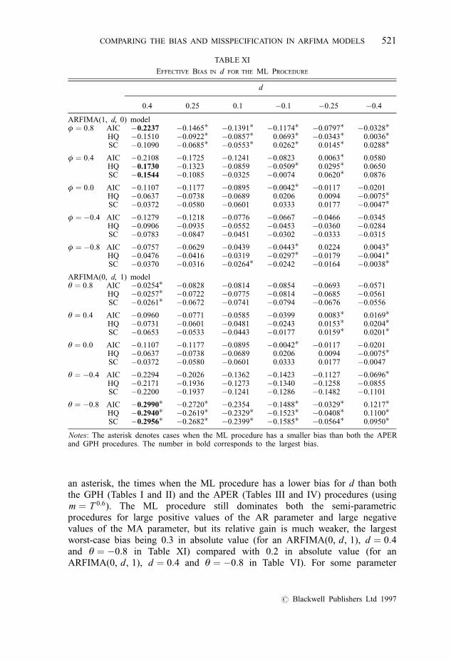
an asterisk, the times when the ML procedure has a lower bias for d than boththe GPH (Tables I and II) and the APER (Tables III and IV) procedures (usingm � T 0:6). The ML procedure still dominates both the semi-parametricprocedures for large positive values of the AR parameter and large negativevalues of the MA parameter, but its relative gain is much weaker, the largestworst-case bias being 0.3 in absolute value (for an ARFIMA(0, d, 1), d � 0:4and θ � ÿ0:8 in Table XI) compared with 0.2 in absolute value (for anARFIMA(0, d, 1), d � 0:4 and θ � ÿ0:8 in Table VI). For some parameter

TABLE XI

EFFECTIVE BIAS IN d FOR THE ML PROCEDURE

d

0.4 0.25 0.1 ÿ0.1 ÿ0.25 ÿ0.4

ARFIMA(1, d, 0) modelφ � 0:8 AIC ÿ0.2237 ÿ0.1465� ÿ0.1391� ÿ0.1174� ÿ0.0797� ÿ0.0328�

HQ ÿ0.1510 ÿ0.0922� ÿ0.0857� 0.0693� ÿ0.0343� 0.0036�

SC ÿ0.1090 ÿ0.0685� ÿ0.0553� 0.0262� 0.0145� 0.0288�

φ � 0:4 AIC ÿ0.2108 ÿ0.1725 ÿ0.1241 ÿ0.0823 0.0063� 0.0580HQ ÿ0.1730 ÿ0.1323 ÿ0.0859 ÿ0.0509� 0.0295� 0.0650SC ÿ0.1544 ÿ0.1085 ÿ0.0325 ÿ0.0074 0.0620� 0.0876

φ � 0:0 AIC ÿ0.1107 ÿ0.1177 ÿ0.0895 ÿ0.0042� ÿ0.0117 ÿ0.0201HQ ÿ0.0637 ÿ0.0738 ÿ0.0689 0.0206 0.0094 ÿ0.0075�

SC ÿ0.0372 ÿ0.0580 ÿ0.0601 0.0333 0.0177 ÿ0.0047�

φ � ÿ0:4 AIC ÿ0.1279 ÿ0.1218 ÿ0.0776 ÿ0.0667 ÿ0.0466 ÿ0.0345HQ ÿ0.0906 ÿ0.0935 ÿ0.0552 ÿ0.0453 ÿ0.0360 ÿ0.0284SC ÿ0.0783 ÿ0.0847 ÿ0.0451 ÿ0.0302 ÿ0.0333 ÿ0.0315

φ � ÿ0:8 AIC ÿ0.0757 ÿ0.0629 ÿ0.0439 ÿ0.0443� 0.0224 0.0043�

HQ ÿ0.0476 ÿ0.0416 ÿ0.0319 ÿ0.0297� ÿ0.0179 ÿ0.0041�

SC ÿ0.0370 ÿ0.0316 ÿ0.0264� ÿ0.0242 ÿ0.0164 ÿ0.0038�

ARFIMA(0, d, 1) modelθ � 0:8 AIC ÿ0.0254� ÿ0.0828 ÿ0.0814 ÿ0.0854 ÿ0.0693 ÿ0.0571

HQ ÿ0.0257� ÿ0.0722 ÿ0.0775 ÿ0.0814 ÿ0.0685 ÿ0.0561SC ÿ0.0261� ÿ0.0672 ÿ0.0741 ÿ0.0794 ÿ0.0676 ÿ0.0556

θ � 0:4 AIC ÿ0.0960 ÿ0.0771 ÿ0.0585 ÿ0.0399 0.0083� 0.0169�

HQ ÿ0.0731 ÿ0.0601 ÿ0.0481 ÿ0.0243 0.0153� 0.0204�

SC ÿ0.0653 ÿ0.0533 ÿ0.0443 ÿ0.0177 0.0159� 0.0201�

θ � 0:0 AIC ÿ0.1107 ÿ0.1177 ÿ0.0895 ÿ0.0042� ÿ0.0117 ÿ0.0201HQ ÿ0.0637 ÿ0.0738 ÿ0.0689 0.0206 0.0094 ÿ0.0075�

SC ÿ0.0372 ÿ0.0580 ÿ0.0601 0.0333 0.0177 ÿ0.0047

θ � ÿ0:4 AIC ÿ0.2294 ÿ0.2026 ÿ0.1362 ÿ0.1423 ÿ0.1127 ÿ0.0696�

HQ ÿ0.2171 ÿ0.1936 ÿ0.1273 ÿ0.1340 ÿ0.1258 ÿ0.0855SC ÿ0.2200 ÿ0.1937 ÿ0.1241 ÿ0.1286 ÿ0.1482 ÿ0.1101

θ � ÿ0:8 AIC ÿ0.2990� ÿ0.2720� ÿ0.2354 ÿ0.1488� ÿ0.0329� 0.1217�

HQ ÿ0.2940� ÿ0.2619� ÿ0.2329� ÿ0.1523� ÿ0.0408� 0.1100�

SC ÿ0.2956� ÿ0.2682� ÿ0.2399� ÿ0.1585� ÿ0.0564� 0.0950�

Notes: The asterisk denotes cases when the ML procedure has a smaller bias than both the APERand GPH procedures. The number in bold corresponds to the largest bias.



values, φ � ÿ0:4 and φ � ÿ0:4, the ML procedure actually has a larger bias,for all values of d, than the better of the two semi-parametric methods. Second,the bias in d is invariably smallest for the SC, owing to the fact that thisprocedure has the highest probability of selecting the correct model for boththe ARFIMA(1, d, 0) and ARFIMA(0, d, 1) models (see Table X). For bothARFIMA models the effective bias is worst for the AIC.

Despite the fact that the ML method has lost some of its superiority, it stillhas the smallest worst-case (effective) bias, i.e. there are no parameter valueswhich cause the effective bias in d to be larger than 0.15 (0.30) in absolutevalue (using the SC) for the ARFIMA(1, d, 0) (ARFIMA(0, d, 1)) model. Incontrast, the GPH procedure exhibits a maximum bias of 0.54 (0.54) inabsolute value and the APER procedure a maximum bias of 0.48 (0.58) inabsolute value for the ARFIMA(1, d, 0) (ARFIMA(0, d, 1)) model.

Given that one is interested in specifying the entire ARFIMA model for anyseries, it is essential to calculate the effective bias for the short-run as well asthe long-run parameters. Whereas the semi-parametric procedures estimated thelong-run parameter without a full parametric specification of the spectraldensity, estimates of the short-run parameters for these two procedures areconditional on the model selected. Consequently, we calculated effective biasfor the ML as well as the GPH and APER procedures, although only the resultsfrom the former of these methods is presented.

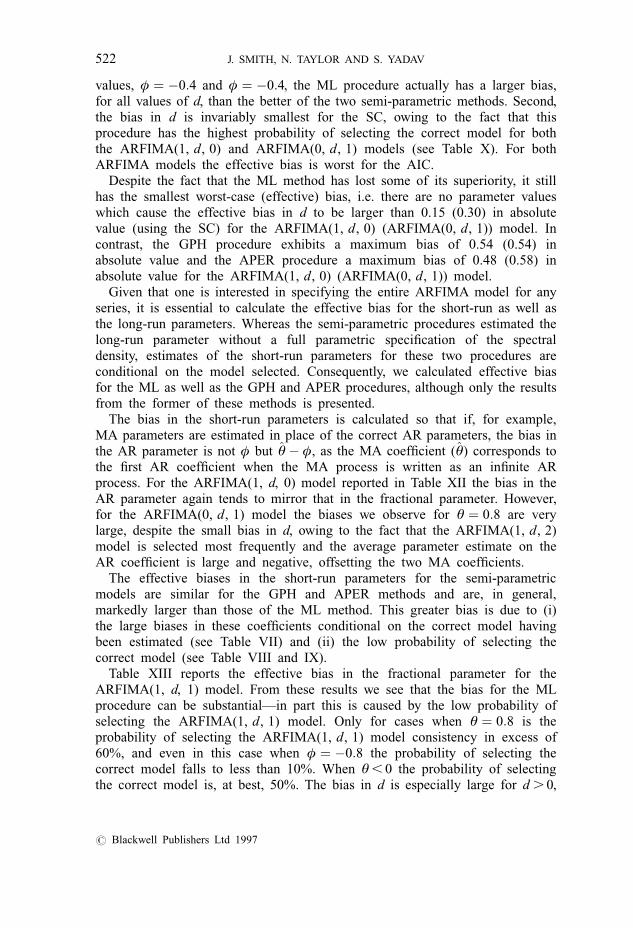
The bias in the short-run parameters is calculated so that if, for example,MA parameters are estimated in place of the correct AR parameters, the bias inthe AR parameter is not φ but ^θ ÿ φ, as the MA coefficient (^θ) corresponds tothe first AR coefficient when the MA process is written as an infinite ARprocess. For the ARFIMA(1, d, 0) model reported in Table XII the bias in theAR parameter again tends to mirror that in the fractional parameter. However,for the ARFIMA(0, d, 1) model the biases we observe for θ � 0:8 are verylarge, despite the small bias in d, owing to the fact that the ARFIMA(1, d, 2)model is selected most frequently and the average parameter estimate on theAR coefficient is large and negative, offsetting the two MA coefficients.

The effective biases in the short-run parameters for the semi-parametricmodels are similar for the GPH and APER methods and are, in general,markedly larger than those of the ML method. This greater bias is due to (i)the large biases in these coefficients conditional on the correct model havingbeen estimated (see Table VII) and (ii) the low probability of selecting thecorrect model (see Table VIII and IX).

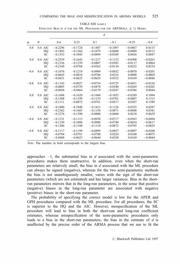
Table XIII reports the effective bias in the fractional parameter for theARFIMA(1, d, 1) model. From these results we see that the bias for the MLprocedure can be substantial—in part this is caused by the low probability ofselecting the ARFIMA(1, d, 1) model. Only for cases when θ � 0:8 is theprobability of selecting the ARFIMA(1, d, 1) model consistency in excess of60%, and even in this case when φ � ÿ0:8 the probability of selecting thecorrect model falls to less than 10%. When θ , 0 the probability of selectingthe correct model is, at best, 50%. The bias in d is especially large for d . 0,



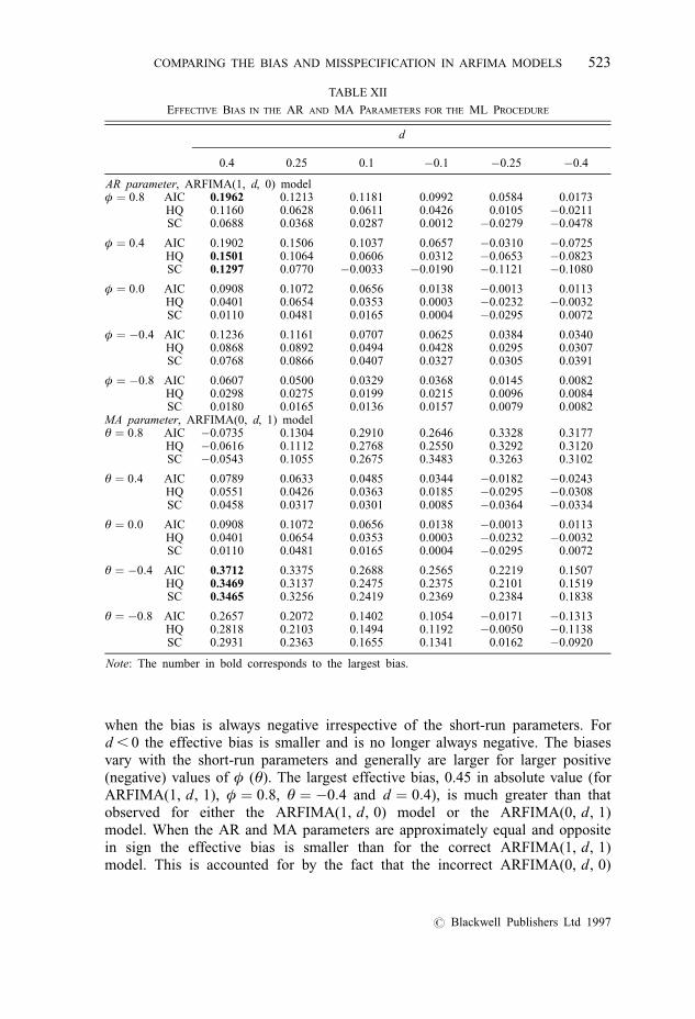
when the bias is always negative irrespective of the short-run parameters. Ford , 0 the effective bias is smaller and is no longer always negative. The biasesvary with the short-run parameters and generally are larger for larger positive(negative) values of φ (θ). The largest effective bias, 0.45 in absolute value (forARFIMA(1, d, 1), φ � 0:8, θ � ÿ0:4 and d � 0:4), is much greater than thatobserved for either the ARFIMA(1, d, 0) model or the ARFIMA(0, d, 1)model. When the AR and MA parameters are approximately equal and oppositein sign the effective bias is smaller than for the correct ARFIMA(1, d, 1)model. This is accounted for by the fact that the incorrect ARFIMA(0, d, 0)

TABLE XII

EFFECTIVE BIAS IN THE AR AND MA PARAMETERS FOR THE ML PROCEDURE

d

0.4 0.25 0.1 ÿ0.1 ÿ0.25 ÿ0.4

AR parameter, ARFIMA(1, d, 0) modelφ � 0:8 AIC 0.1962 0.1213 0.1181 0.0992 0.0584 0.0173

HQ 0.1160 0.0628 0.0611 0.0426 0.0105 ÿ0.0211SC 0.0688 0.0368 0.0287 0.0012 ÿ0.0279 ÿ0.0478

φ � 0:4 AIC 0.1902 0.1506 0.1037 0.0657 ÿ0.0310 ÿ0.0725HQ 0.1501 0.1064 0.0606 0.0312 ÿ0.0653 ÿ0.0823SC 0.1297 0.0770 ÿ0.0033 ÿ0.0190 ÿ0.1121 ÿ0.1080

φ � 0:0 AIC 0.0908 0.1072 0.0656 0.0138 ÿ0.0013 0.0113HQ 0.0401 0.0654 0.0353 0.0003 ÿ0.0232 ÿ0.0032SC 0.0110 0.0481 0.0165 0.0004 ÿ0.0295 0.0072

φ � ÿ0:4 AIC 0.1236 0.1161 0.0707 0.0625 0.0384 0.0340HQ 0.0868 0.0892 0.0494 0.0428 0.0295 0.0307SC 0.0768 0.0866 0.0407 0.0327 0.0305 0.0391

φ � ÿ0:8 AIC 0.0607 0.0500 0.0329 0.0368 0.0145 0.0082HQ 0.0298 0.0275 0.0199 0.0215 0.0096 0.0084SC 0.0180 0.0165 0.0136 0.0157 0.0079 0.0082

MA parameter, ARFIMA(0, d, 1) modelθ � 0:8 AIC ÿ0.0735 0.1304 0.2910 0.2646 0.3328 0.3177

HQ ÿ0.0616 0.1112 0.2768 0.2550 0.3292 0.3120SC ÿ0.0543 0.1055 0.2675 0.3483 0.3263 0.3102

θ � 0:4 AIC 0.0789 0.0633 0.0485 0.0344 ÿ0.0182 ÿ0.0243HQ 0.0551 0.0426 0.0363 0.0185 ÿ0.0295 ÿ0.0308SC 0.0458 0.0317 0.0301 0.0085 ÿ0.0364 ÿ0.0334

θ � 0:0 AIC 0.0908 0.1072 0.0656 0.0138 ÿ0.0013 0.0113HQ 0.0401 0.0654 0.0353 0.0003 ÿ0.0232 ÿ0.0032SC 0.0110 0.0481 0.0165 0.0004 ÿ0.0295 0.0072

θ � ÿ0:4 AIC 0.3712 0.3375 0.2688 0.2565 0.2219 0.1507HQ 0.3469 0.3137 0.2475 0.2375 0.2101 0.1519SC 0.3465 0.3256 0.2419 0.2369 0.2384 0.1838

θ � ÿ0:8 AIC 0.2657 0.2072 0.1402 0.1054 ÿ0.0171 ÿ0.1313HQ 0.2818 0.2103 0.1494 0.1192 ÿ0.0050 ÿ0.1138SC 0.2931 0.2363 0.1655 0.1341 0.0162 ÿ0.0920

Note: The number in bold corresponds to the largest bias.



model is often selected. However, the biases for this case are markedly greaterthan those for either the GPH or APER procedures.

Even though no procedure clearly dominates the other procedures across theparameter values considered here, the ML procedure still has the smallestworst-case bias, as the GPH (APER) procedure has a maximum bias of 0.58(0.57) in absolute value for φ � 0:8, θ � 0:8 and d � ÿ0:25 (θ � ÿ0:4,θ � ÿ0:8 and d � 0:10).

4. CONCLUDING REMARKS

We have looked at the bias in both the fractional integration parameter d and theshort-run AR and MA parameters in ARFIMA models. The results suggest that,of the procedures considered, provided the correct ARFIMA model is fitted theML procedure is probably superior to the GPH or APER procedures. Clearly,when either the AR coefficient approaches unity or the MA coefficient

TABLE XIII

EFFECTIVE BIAS IN d FOR THE ML PROCEDURE FOR THE ARFIMA(1, d, 1) MODEL

d

φ θ 0.4 0.25 0.1 ÿ0.1 ÿ0.25 ÿ0.4

0.8 ÿ0.8 AIC ÿ0.1958 ÿ0.1550 ÿ0.1249 ÿ0.0418 ÿ0.0360 ÿ0.0503HQ ÿ0.1390 ÿ0.1081 ÿ0.0947 ÿ0.0131 ÿ0.0077 ÿ0.0296SC ÿ0.0961 ÿ0.0813 ÿ0.0830 0.0038 0.0048 ÿ0.0191

0.4 ÿ0.8 AIC ÿ0.3841 ÿ0.3432 ÿ0.3161 ÿ0.2983 ÿ0.2557 ÿ0.1361HQ ÿ0.3854 ÿ0.3387 ÿ0.3042 ÿ0.2975 ÿ0.2960 ÿ0.2003SC ÿ0.3866 ÿ0.3340 ÿ0.3000 ÿ0.2938 ÿ0.3290 ÿ0.2528

ÿ0.4 ÿ0.8 AIC ÿ0.3601 ÿ0.3670 ÿ0.2874 ÿ0.1818 0.0318 0.2253HQ ÿ0.3835 ÿ0.3950 ÿ0.3275 ÿ0.2148 ÿ0.0170 0.1958SC ÿ0.4259 ÿ0.4331 ÿ0.3612 ÿ0.2506 ÿ0.0441 0.1584

ÿ0.8 ÿ0.8 AIC ÿ0.3354 ÿ0.3156 ÿ0.1776 ÿ0.0382 0.1909 0.3853HQ ÿ0.3611 ÿ0.3458 ÿ0.2015 ÿ0.0712 0.1526 0.3518SC ÿ0.3959 ÿ0.3788 ÿ0.2306 ÿ0.1000 0.1181 0.3191

0.8 ÿ0.4 AIC ÿ0.4378 ÿ0.3768 ÿ0.3523 ÿ0.3068 ÿ0.1732 ÿ0.0333HQ ÿ0.4487 ÿ0.3856 ÿ0.3209 ÿ0.2656 ÿ0.1354 ÿ0.0205SC ÿ0.4568 ÿ0.3906 ÿ0.1813 ÿ0.0923 ÿ0.0123 0.1204

0.4 ÿ0.4 AIC ÿ0.1256 ÿ0.1283 ÿ0.1039 ÿ0.0163 ÿ0.0148 ÿ0.0288HQ ÿ0.0764 ÿ0.0829 ÿ0.0815 0.0138 0.0050 ÿ0.0116SC ÿ0.0486 ÿ0.0672 ÿ0.0708 0.0260 0.0119 ÿ0.0085

ÿ0.4 ÿ0.4 AIC ÿ0.1661 ÿ0.1732 ÿ0.1539 ÿ0.1525 ÿ0.1160 ÿ0.0439HQ ÿ0.1792 ÿ0.1836 ÿ0.1733 ÿ0.1705 ÿ0.1378 ÿ0.0770SC ÿ0.1967 ÿ0.2049 ÿ0.1960 ÿ0.1959 ÿ0.1677 ÿ0.1045

ÿ0.8 ÿ0.4 AIC ÿ0.1474 ÿ0.1511 ÿ0.1277 ÿ0.1121 ÿ0.0247 0.1151HQ ÿ0.1640 ÿ0.1690 ÿ0.1508 ÿ0.1356 ÿ0.0491 0.0855SC ÿ0.1855 ÿ0.1907 ÿ0.1818 ÿ0.1675 ÿ0.0738 0.0573



approaches ÿ1, the substantial bias in d associated with the semi-parametricprocedures makes them unattractive. In addition, even when the short-runparameters are relatively small, the bias in d associated with the ML procedurecan always be signed (negative), whereas for the two semi-parametric methodsthe bias is not unambiguously smaller, varies with the sign of the short-runparameters (which are not estimated) and has larger variances. Bias in the short-run parameters mirrors that in the long-run parameters, in the sense that positive(negative) biases in the long-run parameter are associated with negative(positive) biases in the short-run parameter.

The probability of specifying the correct model is low for the APER andGPH procedures compared with the ML procedure. For all procedures, the SCis superior to the HQ and the AIC. However, misspecification of the MLprocedure will lead to bias in both the short-run and long-run coefficientestimates, whereas misspecification of the semi-parametric procedures onlyleads to a bias in the short-run parameters; the bias in the estimate of d isunaffected by the precise order of the ARMA process that we use to fit the

TABLE XIII (cont.)

EFFECTIVE BIAS IN d FOR THE ML PROCEDURE FOR THE ARFIMA(1, d, 1) MODEL

d

φ θ 0.4 0.25 0.1 ÿ0.1 ÿ0.25 ÿ0.4

0.8 0.4 AIC ÿ0.2296 ÿ0.1724 ÿ0.1487 ÿ0.1097 ÿ0.0467 0.0115HQ ÿ0.1803 ÿ0.1264 ÿ0.1079 ÿ0.0680 ÿ0.0009 0.0513SC ÿ0.1553 ÿ0.1045 ÿ0.0849 ÿ0.0369 0.0436 0.0847

0.4 0.4 AIC ÿ0.2539 ÿ0.1643 ÿ0.1217 ÿ0.1133 ÿ0.0508 ÿ0.0263HQ ÿ0.2336 ÿ0.1239 ÿ0.0807 ÿ0.0583 ÿ0.0117 0.0064SC ÿ0.2169 ÿ0.0768 ÿ0.0362 ÿ0.0134 0.0252 0.0534

ÿ0.4 0.4 AIC ÿ0.1076 ÿ0.1219 ÿ0.0909 ÿ0.0032 ÿ0.0070 ÿ0.0201HQ ÿ0.0643 ÿ0.0810 ÿ0.0704 0.0216 0.0088 ÿ0.0069SC ÿ0.0431 ÿ0.0625 ÿ0.0629 0.0332 0.0169 ÿ0.0046

ÿ0.8 0.4 AIC ÿ0.1142 ÿ0.0927 ÿ0.0754 ÿ0.0725 ÿ0.0451 ÿ0.0336HQ ÿ0.0885 ÿ0.0729 ÿ0.0478 ÿ0.0540 ÿ0.0269 ÿ0.0202SC ÿ0.0694 ÿ0.0464 ÿ0.0179 ÿ0.0247 ÿ0.0386 0.0044



ÿ0.4 0.8 AIC ÿ0.1231 ÿ0.1113 ÿ0.0938 ÿ0.0717 ÿ0.0563 ÿ0.0494HQ ÿ0.1150 ÿ0.1096 ÿ0.0988 ÿ0.0740 ÿ0.0654 ÿ0.0617SC ÿ0.1206 ÿ0.1188 ÿ0.1118 ÿ0.0872 ÿ0.0795 ÿ0.0829

ÿ0.8 0.8 AIC ÿ0.1117 ÿ0.1199 ÿ0.0899 ÿ0.0037 ÿ0.0097 ÿ0.0200HQ ÿ0.0704 ÿ0.0781 ÿ0.0700 0.0224 0.0100 ÿ0.0075SC ÿ0.0488 ÿ0.0623 ÿ0.0644 0.0328 0.0169 ÿ0.0044

Note: The number in bold corresponds to the largest bias.



data. In calculating the effective bias in d for the ML procedure, the SC yieldsthe smallest bias. However, all selection criteria show a deterioration in theperformance of the ML procedure relative to that of the GPH and APERprocedures for both the ARFIMA(1, d, 0) and ARFIMA(0, d, 1) models.Nevertheless, the ML method still possesses the property of having the smallestworst-case bias. Calculating the effective bias for the short-run parameters forthe ML and APER procedures shows that there is an advantage to using theML procedure.

Finally, increasing the number of parameters in the ARFIMA model by oneto allow for an ARFIMA(1, d, 1) model can yield serious bias results. For theML procedure the probability of identifying the correct ARFIMA model can bevery small and as a result this yields large effective bias results. In fact, theworst-case effective bias for the fractional parameter d associated with theARFIMA(1, d, 1) model is 0.45 compared with 0.3 for the ARFIMA(0, d, 1)model. However, this is still smaller than that associated with the GPH andAPER procedures where the largest effective bias is 0.58 and 0.57, respectively.

NOTES

1. The procedure is GPH.SRC.2. The authors would like to thank Fallow Sowell for providing his Fortran program for estimating

the ML model.3. The trimming parameter was set at 2 for both the APER and GPH procedures, although the results

do not change qualitatively for changes in the trimming parameter.4. The largest bias associated with m � 28 is around 0.5, compared with around 0.3 associated with

m � 16.5. We have limited p, q < 2 as the ML procedure is particularly computer intensive.6. All results are available from the authors upon request.7. When the mean is assumed known, the probability of selecting the correct model is invariably

slightly higher than those reported in Table X.

ACKNOWLEGEMENT

The authors would like to thank an anonymous referee and one of the associateeditors for helpful comments and suggestions.

REFERENCES

AGIAKLOGLOU, C., NEWBOLD, P. and WOHAR, M. (1993) Bias in an estimator of the fractionaldifference parameter. J. Time Ser. Anal. 14, 235–46.

CHEUNG, Y.-W. (1993a) Long memory in foreign exchange rates J. Bus. Econ. Stat. 11, 93–101.—– (1993b) Tests for fractional integration: a Monte Carlo investigation. J. Time Ser. Anal. 14,

331–45.—– and DIEBOLD, F. X. (1994) On the maximum-likelihood estimation of the differencing

parameter of fractionally integrated noise with unknown mean. J. Economet. 62, 301–16.CRATO, N. and RAY, B. K. (1995) Model selection and forecasting for long-range dependent

processes. Mimeo.



DAHLHAUS, R. (1989) Efficient parameter estimation for self-similar processes. Ann. Stat. 17, 1749–66.

GEWEKE, J. and PORTER-HUDAK, S. (1983) The estimation and application of long memory timeseries models. J. Time Series Anal. 3, 177–83.

HAUSER, M. A. (1993) On the selection of moving average and fractionally integrated models.Paper presented at the IFAC Workshop on Economic Time Series Analysis and SystemIdentification, 1–3 July 1992, Vienna.

LOBATO, I. and ROBINSON, P. M. (1996) Averaged periodogram estimation of long memory. J.Economet. 73, 303–24.

RAY, B. K. (1993) Modeling long-memory processes for optimal long-range prediction. J. Time Ser.Anal. 14, 511–25.

REISEN, V. A. (1994) Estimation of the fractional difference parameter in the ARFIMA( p, d, q)model using the smoothed periodogram. J. Time Ser. Anal. 15, 335–50.

ROBINSON, P. M. (1994) Semiparametric analysis of long-memory time series. Ann. Stat. 22, 515–39.

—– (1995) Log-periodogram regression of time series with long range dependence. Ann. Stat. 23,1048–72.

SCHMIDT, C. M. and TSCHERNIG, R. (1993) Identification of fractional ARIMA models in thepresence of long memory. Paper presented at the IFAC Workshop on Economic Time SeriesAnalysis and System Identification, 1–3 July 1993, Vienna.

SMITH, J. and YADAV, S. (1994) Forecasting costs incurred from unit differencing fractionallyintegrated processes. Int. J. Forecasting 10, 507–14.

SOWELL, F. (1992) Maximum likelihood estimation of stationary univariate fractionally integratedtime series models. J. Economet. 53, 165–88.

WHITTLE, P. (1951) Hypothesis Testing in Time Series Analysis. Uppsala: Almquist and Wiksells.



Comparing the bias and misspecification in ARFIMA models

Documents

Transcript of Comparing the bias and misspecification in ARFIMA models