College of Engineering - SUST Repository
79
1 Sudan University of Sciences and Technology College of Engineering Aeronautical Engineering Department PERFORMANCE VALIDATION OF L-410 TURBOLET A Project Submitted In Partial Fulfillment for the Requirements of the Degree of B.S.c (Honor) In Aeronautical Engineering Prepared By: 1. AHMED MOHAMMED SULIMAN. 2. HAMID MAHMOUD HAMID HASSAN. 3. RAYAN ABDEL-WAHAB ALAMIN. Supervised By: Dr. SAKHR BABEKIR ABU DARAG Oct 2015
-
Upload
khangminh22 -
Category
Documents
-
view
0 -
download
0
Transcript of College of Engineering - SUST Repository
1
Sudan University of Sciences and Technology
College of Engineering
Aeronautical Engineering Department
PERFORMANCE VALIDATION OF L-410 TURBOLET
A Project Submitted In Partial Fulfillment for the
Requirements of the Degree of B.S.c (Honor) In Aeronautical Engineering
Prepared By:
1. AHMED MOHAMMED SULIMAN. 2. HAMID MAHMOUD HAMID HASSAN. 3. RAYAN ABDEL-WAHAB ALAMIN.
Supervised By:
Dr. SAKHR BABEKIR ABU DARAG
Oct 2015

2
} *
{ …
15.

3
DEDICATION
To those whom burnt and die daily to maintain a better life for us...
Our power supplies…
Our parents.
To our guide and our light in darkness…
Our control system…
Our teachers.
And first of all to our leader…
Dr. SAKHR BABEKIR ABU DARAG.

4
Acknowledgement
To everybody participates in performing our mission of representing this project in its final form or helps us by his effort, his time, by a note, a comment or any way; we are very thankful to you and very proud with your participation.

5
ABSTRACT
Many researches have been done in the field of analyzing the performance characteristics for different aircrafts, but by using the analytical approach.
Hence this project is introduced to simulate the performance validation of L-410turbolet by using the drag polar obtained by using computational fluid dynamics (CFD);because of the reliability of this procedure and its high ability to compute and analyze the complex systems. FLUENT package is the program that used to do the computations. The results were realistic and were in consistence with the aerodynamic theories. Also the actual manufacturer engine characteristics data have been employed in simulating the performance validation and in designing the MATLAB software in order to obtain the most proper results and to minimize as possible the error which can results from using only the theoretical formulas of the analytical approach.

6
Table of contents:
Content Page
Abstract
Table of Contents I
List of symbols Ii
List of Tables iv
List of Figures v
CHAPTER ONE–Introduction
1.1: Overview. 1
1.2: Objectives. 2
1.3: Problem Statements. 2
1.4: Proposed Solutions: 2
1.5: Motivates. 2
1.6: Contribution. 3
1.7: Project Outlines. 3
CHAPTER TWO – LITERATURE REVIEW
2.1: Early Predications of airplane Performance 4
2.2: Computational methods in air craft design 7
2.3: L-410turbolet airplane 12
CHAPTER THREE – AIRPLANE PERFORMANCE
3.1: Introduction 15
3.2: Equation of Motion 16
3.3 : Thrust Required For Level , Uncelebrated Flight 19
3.4: Thrust Available and Maximum Velocity 19
3.5: power Required for level , Uncelebrated Flight 20
3.6: Power Available and Maximum Velocity 22

7
3.7:Attitude Effect on Power Required and Available 23
3.8: Rate of Climb 24
3.9: Gliding Flight 26
3.10 : Absolute and Service Ceilings 26
3.11: Range and Endurance – Propeller – DrivenAirplane 28
3.12: NACA Cowling and the Fillet 32
CHAPTER FOUR –RESULTS AND DISCUSSION
4.1: Results 37
4.1.1 General View on C.F.D Main steps 37
4.1.2 Results Obtained with EXCEL 40
4.1.3 Results Obtained with MATLAB 52
4.2: Discussion 57
4.3: Comparison between 1-410turbolet performance
and ATONOV an-2 performance
61
CHAPTRE FIVE – CONCLUSION AND RECOMMENDATIONS
5.1: Conclusions 62
5.2 :Recommendations 62
References
Appendix

8
List of Symbols
Parameter Symbol
Aerodynamic deceleration
Da
Deceleration with aerodynamic brake Dtotal
Friction drag coefficient Cf
Rynlods number Re
9
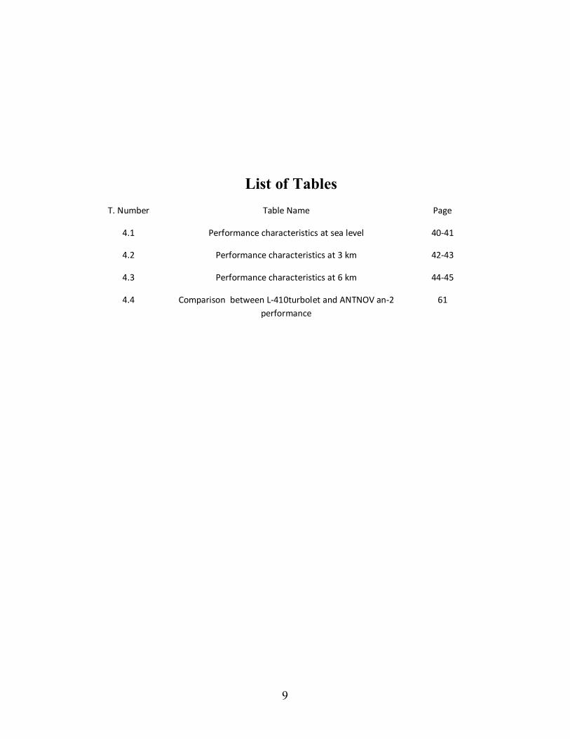
List of Tables
Page Table Name T. Number
40-41 Performance characteristics at sea level 4.1
42-43 Performance characteristics at 3 km 4.2
44-45 Performance characteristics at 6 km 4.3
61 Comparison between L-410turbolet and ANTNOV an-2 performance
4.4

10
List of figures
Fig.Number Figure name Page
4.1 The wing and wind tunnel final view in GAMBIT 37
4.2 The case reading in FLUENT 37
4.3 The grid display in FLUENT 38
4.4 Final forces results in FLUENT 38
4.5 Final forces results in FLUENT 39
4.6 Velocity versus power required 46
4.7 Velocity versus power available 47
4.8 Velocity versus rate of climb 48
4.9 Velocity versus acceleration 49
4.10 Velocity versus deceleration without aerodynamic brake
50
4.11 Velocity versus deceleration with aerodynamic brake
51
4.12 Velocity versus power required - power available Obtained with MATLAB
52
4.13 Velocity versus rate of climb Obtained with MATLAB
53
4.14 Velocity versus acceleration Obtained with MATLAB
54
4.15 Velocity versus deceleration without aerodynamic brake Obtained with MATLAB
55

11
4.16 Velocity versus deceleration with aerodynamic brake Obtained with MATLAB
56
CHAPTER ONE
INTRODUCTION

12
1: C hapter One: Introduction
1.1: Overview The airplane did not just “happen”. When you see an air craft in the sky, You are observing
the resulting action of the natural law of the nature that govern flight the human
understanding of this laws of flight did not come easily. It has evolved over the past 2,500
years, starting with ancient Greek science. It was not until a cold day in December 1903 that
these laws were finally harnessed by human begins to a degree sufficient to allow a heavier-
than- air, powered, human carrying machine to execute a successful sustained flight through
the air. On December 17 of that year, Orville and Wilbur Wright, with pride and great
satisfaction, reaped the fruit of their labors and became the first to fly the first successful
flying machine. But they had no way of knowing the tremendous extent to which their
invention of the first successful airplane was to dominate the course of the twentieth century
technically, socially, and politically.
The L-410Turbulet airplane is the subject of this project. The purpose of this project is to pass
on to you appreciation of the laws of flight and the embodiment of these laws in a form that
allows the understanding and predication of how the airplane will actually perform in the air
(airplane performance) and how to approach the creation of the airplane in the first place in
order to achieve a desired performance or mission (the creative process of airplane design).
The process of airplane performance and airplane design are intimately coupled one did not
happened without the other. Therefore, the purpose of this project is to present the elements of
the L-410turbolet performance, and to do so in such fashion as to give you both a technical
and philosophical understanding of the process.
1.2: Objectives The main purpose in this project is to use the EXCEL software to design a program for
simulating the performance of the L-410turbolet airplane in both the steady level flight under
different flight conditions (temperature, altitude, density, and velocity).and to study the
unsteady flight of this airplane. And to write a MATLAB code capable to investigate different
performance parameters at different flight conditions.
Also a CFD approach is concerned, this approach is limited to exploring a 3D-CAD drawing
of the aircraft wing, and then using a standard CFD package (FLUENT) to simulate the floe
over aircraft wing airfoils under consideration in order to obtain the actual drag polar.

13
1.3: Problem statement The performance simulation of any aircraft can be easily performed by the analytical
approach using the traditional formal equations. But the hard task is to predict the exact
performance validation by implementing the real engine characteristics data, which is difficult
to obtain. The problem statement of this project is to validate the exact performance of the L-
410turbolet computationally by designing performance simulation software with MATLAB.
1.4: Proposed solutions Designing a program to generate a conceptual simulation for the performance validation of
the L-410turbolet airplane using the empirical drag polar and the real engine characteristics
curve. The software has the capability to investigate different performance parameters at
different flight conditions.
1.5: Motivations An airplane is a flying vehicle. Such as any other machine, it is judged by its performance.
Some of the questions that usually come to mind are how fast can it fly? How high can it fly?
How fast and how steep can it climb? How far can it go with tank-load of fuel? What length
of runway does it need for take-off and landing? How sharp and how far can it turn? Answers
to these and many other questions from the subject of this project.
1.6: Contribution The designed program enables analysis and study of performance characteristics of both
steady level flight, and unsteady flight for any airplane when the required data is available.
Also we should express a method by which the drag polar variation could be estimated if not
given.
1.7: Project outlines This project contains five chapters:
Chapter one: introduction.
Chapter two: literature review.
Chapter three: Airplane performance.
Chapter four: Results and discussion.
Chapter five: conclusion and recommendations.

14
2: C hapter two: Li terature R eview:
CHAPTER TWO
LITERATURE REVIEW

15
2.1: Early predications of airplane performance The airplane of today is a modern work of art and engineering. In turn, the predication of
airplane performance is sometimes viewed as relatively modern discipline. However, contrary
to intuition, some of the basic concepts have roots deep in history: indeed, some of the very
techniques were begin used in practice only a few years after the Wright brothers’ successful
first flight in 1903. This section traces a few historic paths for some of the basic ideas of
airplane performance, as follows:
1. Some understanding of the power required for an airplane was held by Gorge
Cayley. He understood the rate of energy lost by an airplane in steady flight under
gravitational attraction must be essentially the power must be supplied by an engine
to maintain steady, level flight. In 1853 Cayley wrote ;
The whole apparatus when loaded by a weight equal to that of the man intended
ultimately to try the experiment and with the horizontal rudder (the elevator)
described in the essay before sent, adjusted so as to regulate the oblique descent from
some elevated point, to its proper pitch, it may be expected to skim down, with no
force but its own gravitation, in an angle of about 11 degrees with the horizon; or
possibly, if well executed, as to direct resistance something less, at a speed of about
36 feet per second, if loaded 1 pound to each square foot of surface. This having by
repeated experiments, in perfectly calm weather, been ascertained, for both the safety
of the man, and the datum required, let the wings be plied with the man’s utmost
strength; and let the angle measured by the greater extent of horizontal range of flight
be noted; when this point by repeated experiments, has been accurately found.
2. The drag polar, represents simply a plot of versus , illustrating that
varies as the square of . Acknowledge of the drag polar is essential to the
calculation of the airplane performance. It is interesting that the concept of the drag
polar was first introduced by the Frenchman M.Eiffel about 1890. Eiffel was
interested in determining the laws of resistance (drag) on bodies of various shapes,
and he conducted such drag measurements by dropping bodies from the Eiffel Tower
and measuring their terminal velocity.
3. No general understanding of the predication of airplane performance existed before
the twentieth century. At best it was understood by the time that lift and drag varied
as the first power of the area, and as the second power of velocity, but this doesn’t
constitute a performance calculation. However this picture radically changed in 1911.
In this year the Frenchman Duchene received the Month yon prize from the Paris
Academy of sciences for his book entitled The Mechanics of the Airplane: A study of

16
the Principles of Flight. In this book, the basic elements of airplane performance are
put forth for the first time. Duchene gives curves for power required and power
available, he discussed airplane maximum velocity; he also gives a relation for the
rate of climb. Later, in 1917, Duchene’s book was translated into English by John
Ledeboer and T.O’B Hubbard. Finally, during 1918-1920, three additional books on
airplane performance were written, the most famous being the authoritative Applied
Aerodynamics by Leonard Barstow.
In their project “Aircraft Optimization for Maximum Endurance” Ahmed
Mohammed Abd-Naby and his group have show advanced technique to improve the
endurance performance for unmanned aerial vehicles, which by use of a constrained
objective function minimization technique to maximize the endurance. Referring the
objective function and the constraints a design program has been constructed in
MATLAB that able to calculate endurance in several iterations using an initial design
variables and constraints. Also the program draws diagrams illustrate the optimization
process in the various iterations until the new modified design variable are available
to give the best optimum endurance value.
In their project “Performance Analysis For Airplane” Osama AbdallahAlnour and his
team have ended from the technical portion and the detailed computer program for
the accurate estimation of (sust-91) performance and they have represented the
summarized final results.

17
2.2: Computational methods in air craft design Computational methods have revolutionized the aircraft design process. Prior to the mid
sixties aircraft were designed and built without the benefit of computational tools. Design
information was mostly provided by the results of analytic theory combined with a fair
amount of experimentation. Analytic theories continue to provide invaluable insight into the
trends present in the variation of the relevant parameters in a design.
However, for detailed design work, these theories often lack the necessary accuracy,
especially in the presence of non-linearity (transonic flow, large structural deflections, and
real-life control systems) with the advent of the digital computer and the fast development of
the field of numerical analysis , a variety of complex calculation methods have become
available to the designer. Advancements in computational methods have pervaded all
disciplines: aerodynamics, structures, propulsion, guidance, control systems integration,
multidisciplinary optimization, etc.
The role of computational methods in the aircraft design process is to provide detailed
information to facilitate the decisions in the design process at the lowest possible cost and
with adequate turnaround (turnaround is the required processing time from the point a piece
of information is requested until it is finally available to the designer in a form that allows it
to be used). In summary computational methods ought to:
Allow the simulation of the behavior of complex systems beyond the reach
of analytic theory.
Provide detailed design information in timely fashion.
Enhance our understanding of engineering systems by expanding our
ability to predict their behavior.
Provide the ability to perform multidisciplinary design optimization.
Increase competitively and lower design and production costs.
Computational methods are nothing but tools in the aircraft designer’s toolbox that
allow him to complete a job. In fact, the aircraft designer is often more interested in
the interactions between the disciplines that the methods apply to (Aerodynamics,
Structure, Control, Propulsion, and mission profile) than the individual methods
themselves. This view of the design process is often called multidisciplinary design
(one can also term it multidisciplinary computational design). Moreover, a designer
often wants to find a combination of design choices for the involved disciplines that
produces an overall better airplane. If the computational predication methods for all
disciplines are available to the designer, optimization procedures can be coupled to

18
produce Multidisciplinary Design Optimization (MOD) tools. In a nutshell, via a
combination of analytic methods and simple computational tools an optimum
aircraft design for a specifically chosen mission.
The current status of computational methods is such that the use of certain set of
tools has become routine practice at all major aerospace corporations (this includes
simple aerodynamic models, linear structural models, and basic control system
design). However, a vast amount of work remains to be done in order to make more
refined non-linear techniques reach the same routine use status. Moreover, MDO
work has been performed using some of the simpler models, but only a few
attempts have been made to couple high-fidelity non-linear disciplines to produce
optimum designs. Although computational methods are a wonderful resource the
process of aircraft design, their misuse can have catastrophic consequences. The
following considerations must be always in your mind when you decide to accept
as valid the results of computational procedures:
A solution is only as good as the model that is being solved: if you try to
solve a problem with high non-linear content using a computational method
designed for linear problems you results will make no sense.
The accuracy of numerical solution depends heavily on the sophistication
of the disceritaization procedure employed and the size of the mesh used.
Lower order methods with under resolved meshes provide solutions where
the margin error is quite large.
The range of validity of the results of a given calculation depends on the
model that is the heart of the procedure: if you are using an in-viscid
solution procedure to approximate the behavior of attached flow, but the
actual flow is separated, your results will make no sense.
Information overload. Computational procedures flood the designer with a
wealth of information that sometimes is complete nonsense! When
analyzing the results provided by a computational method do not
concentrate on how beautiful the color pictures are, be sure that the
computational results follow the expected trends.
Let’s examine the status of the more relevant aerospace disciplines to which
computational methods have been applied. These include applied aerodynamics,
structural analysis, and control system design.
Computational methods first began to have a significant impact on aerodynamics
analysis and design in the period of 1965-75. This decade saw the introduction of
19
panel methods which could solve the linear flow models for arbitrarily complex
geometry in both subsonic and supersonic flow. It also saw the appearance of the
first satisfactory methods for treating the non-linear equations of transonic flow,
and the development of the hodograph method for design of the shock free
supercritical airfoils.
Panel methods are based on the distribution of surface singularities on a given
configuration of interest, and gained wide-spread acceptance throughout the
aerospace industry. They have achieved their popularity largely due to the fact that
the problems can be easily setup and solutions can be obtained rather quickly on
today’s desktop computers. The calculation of potential flows around bodies was
first realized with the advent of the surface panel methodology originally developed
at the Douglas Company. During the years, additional capability was added t these
surface panel methods. These additions includes the use of higher order, more
accurate formulations, the introduction of lifting capability, the solution of unsteady
flows, and the coupling with various boundary layer formulations.
Panel methods lie at the bottom of complexity pyramid for the solution of
aerodynamic problems. They represent a versatile and useful method to obtain a
good approximation to a flow field in a very short time. Panel methods, however,
cannot offer accurate solutions for a variety of high-speed non-linear flows of
interest to the designer. For these kinds of flows, a more sophisticated model of the
flow equations is required. Efficient flight is generally achieved by the use of
smooth and streamlined shapes which avoid flow separation and minimize viscous
effects; with the consequence that useful predication can be made using in-viscid
models. In-viscid calculations with boundary layer corrections can provide quite
accurate prediction of lift and drag when the flow remains attached, but the iteration
between the in-viscid outer solution and the inner boundary layer solution becomes
increasingly difficult with the onset of separation. Procedures for solving the full
viscous equations are likely to be needed for the simulation of arbitrary complex
separated flows, which may occur at high angles of attack or with bluff bodies. In
order to treat flows at high Reynolds number. Turbulent effects by Reynolds
averaging of the fluctuating …..
Elham Hassan and her work team in their project “Analyzing Flow over the Wing
Using CFD” have analyze the flow over NACA 23012 airfoil and over finite wing
using Computational Fluid Dynamics (CFD). The results were good enough to be
used in design processes, and were inconsistence with the aerodynamic theories.

20
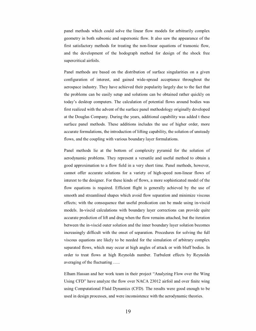
2.310turbolet airplane The L 410 aircraft is an all metal upper-wing aircraft powered by two turboprop engines GE
H80-200, which is configured as a civil version for 19 passengers, transport or special
mission aircraft. L 410 aircraft are operated in more than 50 countries on five continents.
Most of them were delivered to Russia, others to Africa, South East Asia, and Southern
America and also to Europe. The manufacturer has produced more than 1,100 L 410 aircraft
so far. At present, the current version L 410 UVP E20 is on the market as a successor of L
410 family. Its unique flight characteristics and operational benefits are fully recognized such
as follows:
Short take off and landing on short airstrips
Operation from unpaved runway
Low operational and maintenance costs
Excellent performance in high temperature and high altitude environment
Wide variety of equipment with possible installation of special removable kits
Large cargo compartments
Exceed safety standards and easy flight operation
The most spacious cabin in its aircraft category
The L410 is very successful Czech commuter which was first built in response to Soviet
requirements, but has sold widely around the globe.
First design studies of the original 15 seat L 410 began in 1966. The resulting conventional
design was named the Turbo let, and was developed to be capable of operations from
unprepared strips. The power plant chosen was the all new Walter or Motor let M 601, but
this engine was not sufficiently developed enough to power the prototypes, and Pratt &
Whitney Canada PT6A27s were fitted in their place. First flight occurred on April 16 1969,
and series production began in 1970. Initial production L 410s were also powered by the
PT6A, and it was not until 1973 that production aircraft L 410Ms featured the M 601.
The basic L 410 was superseded from 1979 by the L 410 UVP with a 47cm (1ft 7in) fuselage
stretch, M 601B engines and detail refinements. The UVP was in turn replaced by the M
601E powered UVPE in which the toilet and baggage compartments were repositioned
allowing more efficient seating arrangements for up to 19 passengers. The UVPE is the
current production version.
The L 420 is an improved variant with more powerful M 601F engines, higher weights and
improved performance designed to meet western certification requirements. It first flew on
November 10 1993 and was awarded US FAA certification in May 1998.

21
Ayres took control of Let in September 1998 and plans to further develop the 410/420 line.
22

23
3: C hapter Three: Airplane Performance:
CHAPTER THREE
AIRPLANE PERFORMANCE

24
3.1: Introduction The aerodynamic forces and moments exerted on a body moving
through a fluid stem from two sources:
1. The pressure distribution 2. The shear stress distribution
Both acting over the body surface. The physical laws governing such phenomena were examined, with various applications to aerodynamic flows. The airplane will be considered a rigid body on which is exerted four natural forces: lift, drag, propulsive thrust, and weight. Concern will be focused on the movement of the airplane as it responds to these forces. Such considerations form the core of flight dynamics, an important discipline of aerospace engineering. Studies of airplane performance fall under the heading of flight dynamics.
In these studies, we will no longer be concerned with aerodynamic details; rather, we will generally assume that the aerodynamicists have done their work and provided us with the pertinent aerodynamic data for a given airplane. These data are usually packaged in the form of a drag polar for the complete airplane, given as
퐶 = 퐶 . + : (3.1a)
Here, CD is the drag coefficient for the complete airplane; CL is the total lift coefficient, including the small contributions from the horizontal tail and fuselage; and CD is defined as the parasite drag coefficient, which contains not only the profile drag of the wing, but also the friction and pressure drag of the tail surfaces, fuselage, engine nacelles, landing gear, and any other component of the airplane which is exposed to the airflow. At transonic: and supersonic speeds, CD.e also contains wave drag. Because of changes in the flow field around the airplane -especially changes in the amount of separated flow over parts of the airplane – as the angle of attack is varied, CD.e will change with angle of attack; that is, CD.e is itself a function of lift coefficient. A reasonable approximation for this function is
퐶 = 퐶 . + 푟퐶
Where r is an empirically determined constant. Hence. Eq. (3.la) can be written as

25
퐶 = 퐶 . + 푟 + 퐶 (3.1b)
In Eqs. (3.1a) and (3.1b), e is the familiar span efficiency factor, which takes into account the nonelliptical lift distribution on wings of general shape. Let us now redefine e such that it also includes the effect of the variation of parasite drag with lift; i.e., let us write Eq. (3.1b) in the form
퐶 = 퐶 . + (3.1c)
Where CD.0 is the parasite drag coefficient at zero lift and the term 퐶 휋푒퐴푅⁄ includes both induced drag and the contribution to parasite drag due to lift. In Eq. (3.1c), our redefined e, which now includes the effect of r from Eq. (3.1b), is called the Oswald efficiency factor (named after W. Bailey Oswald, who first established this terminology in NACA report no. 408 in l933). In this chapter, the basic aerodynamic properties of the airplane will be described by Eq. (3.1c). and we will consider both CD.0 and e as known aerodynamic quantities, obtained from the aerodynamicist. We will continue to designate 퐶 휋푒퐴푅⁄ by CD.0,where CD.0 now has the expanded interpretation as the coefficient of drag due to lift, including both the contributions due to induced drag and the increment in parasite drag due to angle of attack different than훼 = 훼 . For compactness, wewill designate CD.0 as simply the parasite drag coefficient, although we recognize to be more precisely the parasite drag coefficient at zero lift, i.e., the value of CD.0when푎 = 푎 .
To study the performance of an airplane, the fundamental equations, which govern its translational motion through the air, must first be established, as follows.
3.2: Equations of Motion Consider an airplane in flight. The flight path (direction of motion
of the airplane) is inclined at an angle 휃 with respect to the horizontal. The flight path direction and the relative wind are along the same line. The mean chord line is at a geometric angle of attack 훼with respect to the flight path direction. There are four physical forces acting on the airplane:

26
Figure 3.1 Force diagram for an airplane in flight.
1. Lift L, which is perpendicular to the flight path direction 2. Drag D, which is parallel to the fight path direction 3. Weight W, which acts vertically toward the center of the earth (and hence is inclined at
the angle 휃with respect to the lift direction) 4. Thrust T, which in general is inclined at the angle 훼 with respect to the flightpath
direction
When an object moves along a curved path, the motion is called curvilinear, as opposed to motion along a straight line, which is rectilinear. Newton’s second law, which is a physical statement that force = mass X acceleration, holds in either case. Consider a curvilinear path. At a given point on the path, set up two mutually perpendicular axes, one along the direction of the flight path and the other normal to the fight path. Applying Newton’s law along the flight path,
∑ 퐹|| = 푚푎 = 푚 (3.2)
where∑ 퐹||is the summation of all forces parallel to the flight path, 푎 = 푑푉 푑푡⁄ isthe acceleration along the flight path, and V is the instantaneous value of the airplane’s flight velocity. (Velocity V is always along the flight path direction, by definition.) Now, applying Newton’s law perpendicular to the flight path, we have
∑ 퐹 = 푚 (3.3)
where∑ 퐹 is the summation of all forces perpendicular to the flight path and is the
acceleration normal to a curved path with radius of curvature푟 . Thisnormal acceleration 푉 푟⁄ should be familiar from basic physics. The right-handside of Eq. (3.3) is nothing other than the “centrifugal force.”
27
∑ 퐹∥ = 푇 cos 훼⊺ − 퐷 − 푊 sin 휃 (3.4)
And the forces perpendicular to the flight path (positive upward and negative downward) are
∑ 퐹 = 퐿 + 푇 sin 훼 − 푊 cos 휃 (3.5)
Combining Eq. (3.2) with (3.4) and (3.3) with (3.5) yields
푇 cos 훼 − 퐷 − 푊 sin 휃 = 푚 (3.6)
퐿 + 푇 sin 훼 − 푊 cos 휃 = 푚 (3.7)
Equations (3.6) and (3.7) are the equations of motion for an airplane in translational flight. (Note that an airplane can also rotate about its axes. Also note that we are not considering the possible sidewise motion of the airplane.
Equations (3.6) and (3.7) describe the general two-dimensional translational motion of an airplane in accelerated flight. The performance of an airplane for such unaccelerated flight conditions is called static performance. This may, at first thought, seem unduly restrictive; however, static performance analyses lead to reasonable calculations of maximum velocity, maximum rate of climb, maximum range, etc. —parameters of vital interest in airplane design and operation.
With this in mind, consider level, unaccelerated flight. Level flight means that the flight path is along the horizontal: that is,휃 = 0. Unaccelerated flight means that the right-hand sides of Eqs. (3.6) and (3.7) are zero. Therefore, these equations reduce to
푇 cos 훼 = 퐷 (3.8)
퐿 + 푇 sin 훼 = 푊 (3.9)
Furthermore, for most conventional airplanes, 훼 is small enough that cos 훼 =1andsin 훼 = 0. Thus, from Eq. (3.8) and (3.9),
푇 = 퐷 (3.10)
퐿 = 푊 (3.11)
Equations (3.10) and (3.11) are the equations of motion for level, unaccelerated flight. In level, unaccelerated flight, the aerodynamic drag is balanced by the thrust of the engine, and the aerodynamic lift is balanced by the weight of the airplane-almost trivial, but very useful, results.

28
3.3: Thrust Required For Level, Unaccelerated Flight Consider an airplane in steady level fight at a given altitude and a given velocity. For flight at this velocity, the airplane’s power plant (e.g., turbojet engine or reciprocating engine—propeller combination) must produce a net thrust which is equal to the drag. The thrust required to obtain a certain steady velocity is easily calculated as:
푇 = 퐷 = 푞 푆퐶 (3.12)
퐿 = 푊 = 푞 푆퐶 (3.13)
= (3.14)
Thus, from Eq. (3.14), the thrust required for an airplane to fly at a given velocity in level, unaccelerated flight is
푇 = ⁄ = ⁄ (3.15)
(Note that a subscript R has been added to thrust to emphasize that it is thrust required.)Thrust required 푇 for a given airplane at a given altitude, varies with velocity푉 .
3.4: Thrust Available and Maximum Velocity Thrust required푇 , it dictated by the aerodynamics and weight of the airplane itself, it is an airframe-associated phenomenon. In contrast, the thrust available 푇 is strictly associated with the engine of the airplane; it is the propulsive thrust provided by an engine-propeller combination, a turbojet, a rocket, etc. Suffice it to say here that reciprocating piston engines with propellers exhibit a variation of thrust with velocity. Thrust at zero velocity (static thrust) is a maximum and decreases with forward velocity. At near-sonic flight speeds, the tips of the propeller blades encounter the same compressibility problems and the thrust available rapidly deteriorates. On the other hand, the thrust of a turbojet engine is relatively constant with velocity. These two power plants are quite common in aviation today; reciprocating engine-propeller combinations power the average light, general aviation aircraft, whereas the jet engine is used by almost all large commercial transports and military combat aircraft.
3.5: Power Required For Level, Unaccelerated Flight Power is a precisely defined mechanical term; it is energy per unit
time. The power associated with a moving object can be illustrated by a block moving at constant velocity V under the influence of the constant force F.
푃표푤푒푟 =푒푛푒푟푔푦
푡푖푚푒=
푓표푟푐푒 × 푑푖푠푡푎푛푐푒푡푖푚푒
= 푓표푟푐푒 ×푑푖푠푡푒푛푐푒
푡푖푚푒
푝표푤푒푟 = 퐹 = 퐹푉 (3.16)

29
Where 푑 (푡 − 푡)⁄ is the velocity V of the object. Thus, Eq. (3.16) demonstrates that the power associated with a force exerted on a moving object is force X velocity, an important result.
Consider an airplane in level, unaccelerated flight at a given altitude and with velocity푉 . The thrust required is푇 . From Eq. (3.16) the power required 푃 is therefore
푃 = 푇 푉 (3.17)
The effect of the airplane aerodynamics (퐶 and퐶 ) on 푃 is readily obtained by
푃 = 푇 푉 = ⁄ 푉 (3.18)
퐿 = 푊 = 푞 푆퐶 =12
휌 푉 푆퐶
Hence 푉 = (3.19)
푃 =푊
퐶 퐶_퐷⁄2푊
휌 푆퐶
푃 = 훼 ⁄ (3.20)
In contrast to thrust required, which varies inversely as 퐶 퐶⁄ power required varies
inversely as퐶 ⁄ 퐶 .
The power-required curve is defined as a plot of푃 , note that it qualitatively resembles the thrust-required curve of. As the airplane velocity increases, 푃 first decreases, goes through aminimum, and then increases. At the velocity for minimum power required, theairplane is flying at the angle of attack which corresponds to a maximum퐶 ⁄ 퐶 .
We demonstrated that minimum 푇 aerodynamically correspondsto equal parasite and induced drag. An analogous but different relation holds at minimum 푃
푃 + 푇 푉 = 퐷푉 = 푞 푆 퐶 . +퐶
휋푒퐴푅푉

30
푃 =푞 푆퐶 . 푉
Parasite power required + 푞 푆푉Induced power required
(3.21)
Therefore, as in the earlier case of푇 , the power required can be split into therespective contributions needed to overcome parasite drag and drag due to lift.Also as before, the aerodynamic conditions associated with minimum R can be obtained from Eq. (3.21) by setting 푑푃 푑푉⁄ = 0. To do this, first obtain Eq. (3.21) explicitly in terms of 푉
Recalling that 푞 = 휌푉 and 퐶 = 푊 푃휌 푉 푆.
푃 =12
휌 푉 푆푊 휌 푉 푆
휋푒퐴푅
푃 = 휌 푉 푆퐶 . + (3.22)
For minimum power required, 푑푃 푑푉⁄ = 0 Differentiating Eq. (6.28) yields
푑푃푑푉
=12
휌 푉 푆퐶 . −푊 휌 푉 푆
휋푒퐴푅
=32
휌 푉 푆 퐶 . −푊 휌 푆 푉
휋푒퐴푅
=32
휌 푉 푆 퐶 . −퐶
휋푒퐴푅
= 휌 푉 푆 퐶 . − 퐶 . = 0For minimum 푃
Hence, the aerodynamic condition that holds at minimum power required is
퐶 . =13
퐶 .
The point on the power-required curve that corresponds to minimum 푇 iseasily obtained by drawing a line through the origin and tangent to the 푃 curve. The point of tangency corresponds to minimum 푇 (hence maximum퐿 퐷⁄ ).
3.6: Power Available and Maximum Velocity Note again that 푃 is a characteristic of the aerodynamic design and weight of the aircraft itself. In contrast, the power available 푃 is a characteristic of the power plant. However, the following comments are made to expedite our performance analyses.

31
A Reciprocating Engine-Propeller Combination A piston engine generates power by burning fuel in confined cylinders and using this energy to move pistons, which in turn deliver power to the rotating crankshaft, The power delivered to the propeller by the crankshaft is defined as the shaft brake power P, (the word “brake” stems from a method of laboratory testing which measures the power of an engine by loading it with a calibrated brake mechanism). However, not all of P is available to drive the airplane; some of it is dissipated by inefficiencies of the propeller itself. Hence, the power available to propel the airplane, 푃 , is given by
푃 = 휂푃 (3.24)
Where휂 is the propeller efficiency,휂 < 1. Propeller efficiency is an importantquantity and is a direct product of the aerodynamics of the propeller. It is alwaysless than unity. For our discussions here, both휂and P are assumed to be known quantities for a given airplane.
A remark on units is necessary. In the engineering system, power is in푓푡. 푙푏/푠; in the SI system, power is in watts [which are equivalent to N.m/s. However, the historical evolution of engineering has left us with a horrendously inconsistent (but very convenient) unit of power, which is widely used, namely, horsepower. All reciprocating engines are rated in terms of horsepower and it is important to note that
1 horsepower = 550 ft.lb/s
=746 W Therefore, it is common to use shaft brake horsepower bhp in place of P, and horsepower available ℎ푝 in place of 푃 . Equation (3.24) still holds in the form
ℎ푝 = (휂)(푏ℎ푝) (3.24)
3.7: Altitude Effects on Power Required and Available With regard to 푃 , curves at altitude could be generated by repeating the calculations of the previous sections, with 휌 appropriate to the given altitude. However, once the sea-level 푃 curve is calculated by means of this process, the curves at altitude can be more quickly obtained by simple ratios, as follows. Let the subscript “0” designate sea-level conditions.
푉 = (3.25)
푃 . = (3.26)
where푉 , 푃 . , and 휌 are velocity, power, and density at sea level. At altitude, where the density is 휌, these relations are
푉 = (3.27)

32
푃 . = (3.28)
Now, strictly for the purposes of calculation, Let퐶 remain fixed between sea level and altitude. Hence, because 퐶 = 퐶 . + 퐶 휋푒퐴푅⁄ 퐶 also remains fixed.
푉 = 푉⁄
(3.29)
and 푃 = 푃 .⁄
(3.30)
3.8: Rate of Climb Consider an airplane in steady, unaccelerated, climbing flight. The
velocity along the flight path is푉 and the flight path itself is 푉
Figure 3.2 Airplane in climbing flight.
Inclined to the horizontal at the angle휃. As always, lift and drag are perpendicular and parallel to 푉 , and the weight is perpendicular to the horizontal. Thrust Tis assumed to be aligned with the flight path. Here, the physical difference from our previous discussion on level flight is that T is not only working to overcome the drag, but for climbing flight it is also supporting a component of weight. Summing forces parallel to the flight path, we get
푇 = 퐷 + 푊 sin 휃 (3.31)
And perpendicular to the flight path, we have
퐿 = 푊 cos 휃 (3.32)
Note that the lift is now smaller than the weight.

33
푇푉 = 퐷푉 + 푊푉 sin 휃
= 푉 sin 휃 (3.33)
푉 sin 휃, is the airplane’s vertical velocity. This vertical velocity is called the rate of climb R/C:
푅 퐶⁄ = 푉 sin 휃 (3.34)
푇푉 is the power available. The second term is 퐷푉 , which for level flight is the power required. For climbing flight, however, 퐷푉 isno longer precisely the power required, because power must be applied toovercome a component of weight as well as drag. Nevertheless, for small angles of climb, say 0 <200, it is reasonable to neglect this fact and to assume that the퐷푉 term is given by the level-flight푃 . With this,
푇푉 = 퐷푉 = 푒푥푐푒푠푠 푝표푤푒푟
Where the excess power is the difference between power available and power required, for propeller-driven and jet-powered aircraft, respectively, we obtain
푅 퐶⁄ = (3.36)
3.9: Gliding Flight Consider an airplane in a power-off glide. The forces acting on this aircraft are lift, drag, and weight; the thrust is zero because the power is off. The glide flight path makes an angle 휃below the horizontal. For an equilibriumunaccelerated glide the sum of the forces must be zero.
Summing forces along the flight path, we have,
퐷 = 푊 sin 휃 (3.37)
and perpendicular to the flight path
퐿 = 푊 cos 휃 (3.38)
The equilibrium glide angle can be calculated by
sin 휃cos 휃
=퐷퐿
or tan 휃 = ⁄ (3.39)
Clearly, the glide angle is strictly a function of the lift-to-drag ratio; the higher the L/D, the shallower the glide angle. From this, the smallest equilibrium glide angle occurs at(퐿 퐷⁄ ) , which corresponds to the maximum range for the glide.

34
3.10: Absolute and Service Ceilings The effects of altitude on 푃 and 푃 . For the sake of discussion, consider a propeller-driven airplane: the results of this section will be qualitatively the same for a jet. As altitude increases, the maximum excess power Decreases. In turn, maximum R/C decreases.
There is some altitude high enough at which the P4 curve becomes tangent to the 푃 curve. The velocity at this point is the only value at which steady, level flight is possible; moreover, there is zero excess power, hence
Figure 3.3 Variation of excess power with altitude.
zero maximum rate of climb, at this point. The altitude at which maximum 푅/퐶 = 0 is defined as the absolute ceiling of the airplane. A more useful quantity is the service ceiling, defined as that altitude where the maximum R/C = 100 ft/min. The service ceiling represents the practical upper limit of steady, level flight.

35
Figure 3.4 Determination of time to climb
Note that the CJ-1 climbs to 20,000 ft in one-eighth of the time required by the CP-1; this is to be expected for a high-performance executive jet transport in comparison to its propeller-driven piston engine counterpart.
3.11: Range and Endurance-Propeller-Driven Airplane
Range is technically defined as the total distance (measured with respect to the ground) traversed by the airplane on a tank of fuel. A related quantity is endurance, which is defined as the total time that an airplane stays in the air on a tank of fuel. In different applications, it may be desirable to maximize one or the other of these characteristics. The parameters which maximize range are different from those which maximize endurance; they are also different for propeller- and jet-powered aircraft. The purpose of this section is to discuss these variations for the case of a propeller-driven airplane; jet airplanes will be considered in the next section.

36
A Physical Consideration One of the critical factors influencing range and endurance is the specific fuel consumption, a characteristic of the engine. For a reciprocating engine, specific fuel consumption (commonly abbreviated as SFC) is defined as the weight of fuel consumed per unit power per unit time. As mentioned earlier, reciprocating engines are rated in terms of horsepower, and the common units (although inconsistent) of specific fuel consumption are
푆퐹퐶 =퐼푏 표푓 푓푢푒푙(푏ℎ푝)(ℎ)
Where (bhp) signifies shaft brake horsepower.
First, consider endurance. On a qualitative basis, in order to stay in the air for the longest period of time, common sense says that we must use the minimum number of pounds of fuel per hour. On a dimensional basis this quantity is proportional to the horsepower required by the airplane and to the SFC:
퐼푏 표푓 푓푢푒푙ℎ
= (푆퐹퐶)(ℎ푝 )
Therefore, minimum pounds of fuel per hour is obtained with minimum ℎ푝 . Since minimum pounds of fuel per hour gives maximum endurance, we quickly conclude that
Maximum endurance for a propeller-driven airplane occurs when the airplane is flying at minimum power required.
Maximum endurance for a propeller-driven airplane occurs when the airplane is flying at a velocity such that 퐶 ⁄ 퐶 is maximum.
Now, consider range. In order to cover the longest distance (say, in miles), common sense says that we must use the minimum number of pounds of fuel per mile. On a dimensional basis, we can state the proportionality
퐼푏 표푓 푓푢푒푙푚푖
∝(푆퐹퐶)(ℎ푝 )
푉
(Check the units yourself; assuming V is in miles per hour.) As a result, minimum pounds of fuel per mile are obtained with a minimumℎ푝 푉⁄ . This minimum value of ℎ푝 푉⁄ precisely corresponds to maximum L/D.
Maximum range for a propeller-driven airplane occurs when the airplane is flying at a velocity such that 퐶 /퐶 is maximum.

37
B Quantitative Formulation The important conclusions written above in italics were obtained from purely physical reasoning. We will develop quantitative formulas which substantiate these conclusions and which allow the direct calculation of range and endurance for given conditions.
In this development, the specific fuel consumption is couched in units that are consistent, i.e.,
푙푏 표푓 푓푢푒푙
푓푡 × (푠) 표푟
푁 표푓 푓푢푒푙(푗/푠) (푠)
For convenience and clarification, y will designate the specific fuel consumption with consistent units.
Consider the product cPdt, where P is engine power and dt is a small increment in time. The units of this product are (in the English engineering system)
푐푃 푑푡 =퐼푏 표푓 푓푢푒푙
(푓푡 × 퐼푏/푠)(푠)푓푡 × 퐼푏
푠(푠) = 퐼푏표푓 푓푢푒푙
Therefore, cPdt represents the differential change in the weight of the fuel due to consumption over the short time period dt. The total weight of the airplane, W, is the sum of the fixed structural and payload weights, along with the changing fuel weight. Hence, any change in Wis assumed to be due to the change in fuel weight. Recall that W denotes the weight of the airplane at any instant. Also, letW0= gross weight of the airplane (weight with full fuel and payload), Wf = weight of the fuel load, and W1= weight of the airplane without fuel. With these considerations, we have
푊 = 푊 − 푊
and 푑푊 = 푑푊 = −푐푃 푑푡
or 푑푡 = − (3.40)
The minus sign in Eq. (3.40) is necessary because dt is physically positive (time cannot move backward, except in science fiction novels), while at the same time W is decreasing (hence dW is negative). Integrating Eq. (3.40) between time r = 0, where W = W0, (fuel tanks full), and time t = E, where W = W1 (fuel tanks empty), we find
푑푡 =푑푊푐푃
퐸 = ∫ (3.41)
In Eq. (3.41), E is the endurance in seconds.
38
To obtain an analogous expression for range, multiply Eq. (3.40) by 푉 :
푣 . dt = − (3.42)
In Eq. (3.42), 푉 푑푡 is the incremental distance ds covered in time푑푡.
푑푡 = − (3.43)
The total distance covered throughout the flight is equal to the integral of Eq.(3.43) from s = 0, where W = W0 (full fuel tank), to s = R, where W = W1(empty fuel tank):
푑푠 =푉 푑푊
푐푃
Or 푅 = ∫
C Breguet Formulas (Propeller-Driven Airplane) For level, unaccelerated flight, 푃 = 퐷푉 . Also, to maintain steady conditions, the pilot has adjusted the throttle such that power available from the engine-propeller combination is just equal to the power required: 푃 = 푃 = 퐷푉
푃 = = (3.45)
푅 = ∫ = ∫ = ∫ (3.46)
푅 = ∫ 푑푊 = ∫ (3.47)
of level, unaccelerated flight. However, for practical use, it will be further simplified by assuming that,퐿 퐷⁄ = 퐶 퐶⁄ , and c are constant throughout the flight. This is a reasonable approximation for cruising flight conditions. Thus, Eq. (3.47) becomes
푅 =휂푐
퐶퐶
푑푊푊
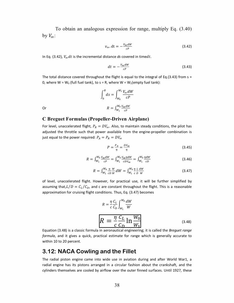
푅 = ln (3.48)
Equation (3.48) is a classic formula in aeronautical engineering; it is called the Breguet range formula, and it gives a quick, practical estimate for range which is generally accurate to within 10 to 20 percent.
3.12: NACA Cowling and the Fillet The radial piston engine came into wide use in aviation during and after World War1, a radial engine has its pistons arranged in a circular fashion about the crankshaft, and the cylinders themselves are cooled by airflow over the outer finned surfaces. Until 1927, these

39
cylinders were generally directly exposed to the main airstream of the airplane. As a result, the drag on the engine-fuselage combination was inordinately high. The problem was severe enough that a group of aircraft manufacturers met at Langley Field on May 24, 1927, to urge NACA to undertake an investigation of means to reduce this drag. Subsequently, under the direction of Fred E. Wick, an extensive series of tests was conducted in the Langley 20-ft propeller research tunnel using a Wright Whirlwind J-5 radial engine mounted to a conventional fuselage. In these tests, various types of aerodynamic surfaces, called cowlings, were used to cover, partly or completely, the engine cylinders, directly guiding part of the airflow over these cylinders for cooling purposes but at the same time not interfering with the smooth primary aerodynamic flow over the fuselage.
Figure 3.5 Engine mounted with no cowling.
Figure 3.6 Engine mounted with full cowling.

40
Best cowling, completely covered the engine. The results were dramatic! Compared with the uncowled fuselage, a full cowling reduced the drag by a stunning 60 percent! Taken directly from Wick’s report entitled “Drag and Cooling with Various Forms of Cowling for a Whirlwind Radial Air-Cooled Engine,” NACA technical report no. 313, published in 1928. After this work, virtually all radial engine-equipped airplanes since 1928 have been designed with a full NACA cowling. The development of this cowling was one of the most important aerodynamic advancements of the1920s; it led the way to a major increase in aircraft speed and efficiency.
A few years later, a second major advancement was made, but by a completely different group and on a completely different part of the airplane. In the early 1930s, the California Institute of Technology at Pasadena, California, established a program in aeronautics under the direction of Theodore vonKarman. Von Karman, a student of Ludwig Prandil, became probably the leading aerodynamicist of the 1920-1960 time-periods. At Caltech, von Karman established an aeronautical laboratory of high quality, which included a large
„

41
Figure 3.7 Reduction t» drag due to a full cowling.
Figure 3.58 Illustration of the wing fillet

42
Subsonic wind tunnel funded by a grant from the Guggenheim Foundation. The first major experimental program in this tunnel was a commercial project for the Douglas Aircraft Company. Douglas was designing the DC-1, the forerunner of a series of highly successful transports (including the famous DC-3, which revolutionized commercial aviation in the 1930s). The DC-1 was plagued by unusual buffeting in the region where the wing joined the fuselage. The sharp corner at the juncture caused severe flow field separation, which resulted in high drag as well as shed vortices which buffeted the tail. The Caltech solution, which was new and pioneering, was to fair the trailing edge of the wing smoothly into the fuselage.
These fairings, called fillets, were empirically designed and were modeled in clay on the DC-1 wind-tunnel models. The best shape was found by trial and error. The addition of a fillet solved the buffeting problem by smoothing out the separated flow and hence also reduced the interference drag. Since that time, fillets have become a standard airplane design feature. Moreover, the fillet is an excellent example of how university laboratory research in the 1930s contributed directly to the advancement of practical airplane design.

37
C hapter Four: R es ults & Dis cus s ion
CHAPTER FOUR
RESULTS AND DISCUSSION

38
4.1-Results 4.1.1: view on general CFD main steps
Fig: 4.1: The wing and wind wind-tunnel final view in
GAMBIT
Fig: 4.2: The case reading in FLUENT

39
Fig: 4.3: The grid display in FLUENT

40
Fig: 4.5: The final forces results in FLUENT
41
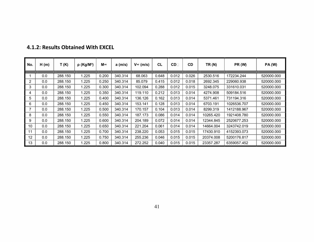
4.1.2: Results Obtained With EXCEL
No. H (m) T (K) ρ (Kg/M³) M∞ a (m/s) V∞ (m/s) CL CD CD TR (N) PR (W) PA (W)
1 0.0 288.150 1.225 0.200 340.314 68.063 0.648 0.012 0.026 2530.516 172234.244 520000.000 2 0.0 288.150 1.225 0.250 340.314 85.079 0.415 0.012 0.018 2692.345 229060.938 520000.000 3 0.0 288.150 1.225 0.300 340.314 102.094 0.288 0.012 0.015 3248.075 331610.031 520000.000 4 0.0 288.150 1.225 0.350 340.314 119.110 0.212 0.013 0.014 4274.908 509184.516 520000.000 5 0.0 288.150 1.225 0.400 340.314 136.126 0.162 0.013 0.014 5371.461 731194.316 520000.000 6 0.0 288.150 1.225 0.450 340.314 153.141 0.128 0.013 0.014 6703.191 1026536.707 520000.000 7 0.0 288.150 1.225 0.500 340.314 170.157 0.104 0.013 0.014 8299.319 1412188.967 520000.000 8 0.0 288.150 1.225 0.550 340.314 187.173 0.086 0.014 0.014 10265.420 1921408.780 520000.000 9 0.0 288.150 1.225 0.600 340.314 204.189 0.072 0.014 0.014 12344.845 2520677.253 520000.000
10 0.0 288.150 1.225 0.650 340.314 221.204 0.061 0.014 0.014 14664.004 3243742.019 520000.000 11 0.0 288.150 1.225 0.700 340.314 238.220 0.053 0.015 0.015 17430.910 4152393.073 520000.000 12 0.0 288.150 1.225 0.750 340.314 255.236 0.046 0.015 0.015 20374.008 5200176.817 520000.000 13 0.0 288.150 1.225 0.800 340.314 272.252 0.040 0.015 0.015 23357.287 6359057.452 520000.000

42
No. ΔP (w) RC m/s V_Tr.min (m/s)
at (m/s²)
1/at (s²/m) R (N) Dt
(m/s²) 1/Dt
(s²/m) Da (m/s²) R2 (N) D.total (m/s²)
1/D.total (s²/m)
1 347765.756 5.539 30.530 0.798 1.253 -2530.516 -0.395 -2.529 11627.833 -14158.349 -2.212 -0.452 2 290939.062 4.634 30.492 0.534 1.872 -2692.345 -0.421 -2.377 18168.488 -20860.833 -3.260 -0.307 3 188389.969 3.001 30.409 0.288 3.468 -3248.075 -0.508 -1.970 26162.623 -29410.698 -4.595 -0.218 4 10815.484 0.172 29.926 0.014 70.483 -4274.908 -0.668 -1.497 35610.237 -39885.145 -6.232 -0.160 5 -211194.316 -3.364 29.880 -0.242 -4.125 -5371.461 -0.839 -1.191 46511.330 -51882.792 -8.107 -0.123 6 -506536.707 -8.068 29.800 -0.517 -1.935 -6703.191 -1.047 -0.955 58865.902 -65569.094 -10.245 -0.098 7 -892188.967 -14.210 29.670 -0.819 -1.221 -8299.319 -1.297 -0.771 72673.954 -80973.272 -12.652 -0.079 8 -1401408.78 -22.321 29.441 -1.170 -0.855 -10265.42 -1.604 -0.623 87935.484 -98200.904 -15.344 -0.065 9 -2000677.25 -31.866 29.325 -1.531 -0.653 -12344.85 -1.929 -0.518 104650.493 -116995.34 -18.281 -0.055 10 -2723742.02 -43.383 29.211 -1.924 -0.520 -14664.00 -2.291 -0.436 122818.982 -137482.99 -21.482 -0.047 11 -3632393.08 -57.855 29.013 -2.383 -0.420 -17430.91 -2.724 -0.367 142440.949 -159871.86 -24.980 -0.040 12 -4680176.82 -74.544 28.871 -2.865 -0.349 -20374.01 -3.183 -0.314 163516.395 -183890.40 -28.733 -0.035 13 -5839057.45 -93.002 28.808 -3.351 -0.298 -23357.29 -3.650 -0.274 186045.321 -209402.60 -32.719 -0.031
Table: 4.1 performance characteristic at sea level
43
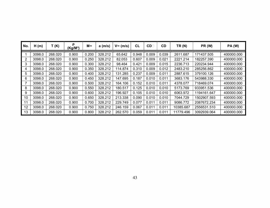
No. H (m) T (K) ρ (Kg/M³) M∞ a (m/s) V∞ (m/s) CL CD CD TR (N) PR (W) PA (W)
1 3098.0 268.020 0.900 0.200 328.212 65.642 0.948 0.009 0.039 2611.687 171437.505 400000.000 2 3098.0 268.020 0.900 0.250 328.212 82.053 0.607 0.009 0.021 2221.214 182257.390 400000.000 3 3098.0 268.020 0.900 0.300 328.212 98.464 0.421 0.009 0.015 2236.713 220234.944 400000.000 4 3098.0 268.020 0.900 0.350 328.212 114.874 0.310 0.009 0.012 2483.210 285256.862 400000.000 5 3098.0 268.020 0.900 0.400 328.212 131.285 0.237 0.009 0.011 2887.615 379100.126 400000.000 6 3098.0 268.020 0.900 0.450 328.212 147.695 0.187 0.010 0.011 3683.176 543988.330 400000.000 7 3098.0 268.020 0.900 0.500 328.212 164.106 0.152 0.010 0.011 4378.077 718469.074 400000.000 8 3098.0 268.020 0.900 0.550 328.212 180.517 0.125 0.010 0.010 5173.769 933951.536 400000.000 9 3098.0 268.020 0.900 0.600 328.212 196.927 0.105 0.010 0.010 6063.972 1194161.647 400000.000
10 3098.0 268.020 0.900 0.650 328.212 213.338 0.090 0.010 0.010 7044.729 1502907.593 400000.000 11 3098.0 268.020 0.900 0.700 328.212 229.749 0.077 0.011 0.011 9086.772 2087672.234 400000.000 12 3098.0 268.020 0.900 0.750 328.212 246.159 0.067 0.011 0.011 10385.687 2556531.510 400000.000 13 3098.0 268.020 0.900 0.800 328.212 262.570 0.059 0.011 0.011 11779.496 3092939.064 400000.000

44
No. ΔP (w) RC m/s V_Tr.min (m/s)
at (m/s²)
1/at (s²/m) R (N) Dt
(m/s²) 1/Dt
(s²/m) Da (m/s²) R2 (N) D.total (m/s²)
1/D.total (s²/m)
1 228562.495 3.640 38.196 0.544 1.838 -2611.687 -0.408 -2.451 7945.566 -10557.253 -1.650 -0.606 2 217742.610 3.468 38.196 0.415 2.412 -2221.214 -0.347 -2.881 12414.946 -14636.161 -2.287 -0.437 3 179765.056 2.863 38.196 0.285 3.506 -2236.713 -0.349 -2.861 17877.523 -20114.236 -3.143 -0.318 4 114743.138 1.828 38.196 0.156 6.407 -2483.210 -0.388 -2.577 24333.295 -26816.504 -4.190 -0.239 5 20899.874 0.333 38.196 0.025 40.202 -2887.615 -0.451 -2.216 31782.262 -34669.877 -5.417 -0.185 6 -143988.330 -2.293 37.391 -0.152 -6.565 -3683.176 -0.575 -1.738 40224.426 -43907.601 -6.861 -0.146 7 -318469.074 -5.072 37.391 -0.303 -3.298 -4378.077 -0.684 -1.462 49659.785 -54037.862 -8.443 -0.118 8 -533951.536 -8.505 37.391 -0.462 -2.164 -5173.769 -0.808 -1.237 60088.340 -65262.108 -10.197 -0.098 9 -794161.647 -12.649 37.391 -0.630 -1.587 -6063.972 -0.947 -1.055 71510.090 -77574.062 -12.121 -0.083 10 -1102907.6 -17.567 37.391 -0.808 -1.238 -7044.729 -1.101 -0.908 83925.036 -90969.765 -14.214 -0.070 11 -1687672.23 -26.881 36.327 -1.148 -0.871 -9086.772 -1.420 -0.704 97333.178 -106419.95 -16.628 -0.060 12 -2156531.51 -34.348 36.327 -1.369 -0.731 -10385.69 -1.623 -0.616 111734.516 -122120.20 -19.081 -0.052 13 -2692939.06 -42.892 36.327 -1.603 -0.624 -11779.496 -1.841 -0.543 127129.049 -138908.55 -21.704 -0.046
Table: 4.2 performance characteristics at 3km

45
No. H (m) T (K) ρ (Kg/M³) M∞ a (m/s) V∞ (m/s) CL CD CD TR (N) PR (W) PA (W)
1 6094.0 248.550 0.653 0.200 316.066 63.213 1.410 0.008 0.075 3352.797 211941.084 300000.000 2 6094.0 248.550 0.653 0.250 316.066 79.017 0.902 0.008 0.036 2474.516 195527.626 300000.000 3 6094.0 248.550 0.653 0.300 316.066 94.820 0.626 0.008 0.021 2133.527 202300.718 300000.000 4 6094.0 248.550 0.653 0.350 316.066 110.623 0.460 0.008 0.015 2069.732 228960.254 300000.000 5 6094.0 248.550 0.653 0.400 316.066 126.426 0.352 0.009 0.013 2352.653 297437.604 300000.000 6 6094.0 248.550 0.653 0.450 316.066 142.230 0.278 0.009 0.012 2621.372 372837.121 300000.000 7 6094.0 248.550 0.653 0.500 316.066 158.033 0.226 0.009 0.011 2984.964 471722.918 300000.000 8 6094.0 248.550 0.653 0.550 316.066 173.836 0.186 0.009 0.010 3427.918 595896.748 300000.000 9 6094.0 248.550 0.653 0.600 316.066 189.640 0.157 0.010 0.011 4341.789 823375.378 300000.000 10 6094.0 248.550 0.653 0.650 316.066 205.443 0.133 0.010 0.011 4988.518 1024856.005 300000.000 11 6094.0 248.550 0.653 0.700 316.066 221.246 0.115 0.010 0.010 5701.098 1261346.709 300000.000 12 6094.0 248.550 0.653 0.750 316.066 237.050 0.100 0.010 0.010 6476.908 1535348.435 300000.000 13 6094.0 248.550 0.653 0.800 316.066 252.853 0.088 0.010 0.010 7314.122 1849396.821 300000.000

46
No. ΔP (w) RC m/s
V_Tr.min (m/s)
at (m/s²)
1/at (s²/m) R (N) Dt (m/s²) 1/Dt
(s²/m) Da
(m/s²) R2 (N) D.total (m/s²)
1/D.total (s²/m)
1 88058.916 1.403 46.186 0.218 4.594 -3352.797 -0.524 -1.909 5345.126 -8697.922 -1.359 -0.736 2 104472.374 1.664 46.186 0.207 4.841 -2474.516 -0.387 -2.586 8351.759 -10826.275 -1.692 -0.591 3 97699.282 1.556 46.186 0.161 6.211 -2133.527 -0.333 -3.000 12026.533 -14160.060 -2.213 -0.452 4 71039.746 1.131 46.186 0.100 9.966 -2069.732 -0.323 -3.092 16369.448 -18439.180 -2.881 -0.347 5 2562.396 0.041 44.846 0.003 315.771 -2352.653 -0.368 -2.720 21380.503 -23733.156 -3.708 -0.270 6 -72837.121 -1.160 44.846 -0.080 -12.497 -2621.372 -0.410 -2.441 27059.699 -29681.071 -4.638 -0.216 7 -171722.918 -2.735 44.846 -0.170 -5.890 -2984.964 -0.466 -2.144 33407.036 -36392.000 -5.686 -0.176 8 -295896.748 -4.713 44.846 -0.266 -3.760 -3427.918 -0.536 -1.867 40422.514 -43850.431 -6.852 -0.146 9 -523375.378 -8.336 43.680 -0.431 -2.319 -4341.789 -0.678 -1.474 48106.132 -52447.921 -8.195 -0.122 10 -724856.005 -11.545 43.680 -0.551 -1.814 -4988.518 -0.779 -1.283 56457.891 -61446.409 -9.601 -0.104 11 -961346.709 -15.312 43.680 -0.679 -1.473 -5701.098 -0.891 -1.123 65477.791 -71178.889 -11.122 -0.090 12 -1235348.435 -19.676 43.680 -0.814 -1.228 -6476.908 -1.012 -0.988 75165.831 -81642.739 -12.757 -0.078 13 -1549396.821 -24.678 43.680 -0.957 -1.044 -7314.122 -1.143 -0.875 85522.012 -92836.134 -14.506 -0.069
Table: 4.3 performance characteristics at 6km

47
Fig: 4.6: Velocity versus Power Required
0.000
1000000.000
2000000.000
3000000.000
4000000.000
5000000.000
6000000.000
7000000.000
0.000 100.000 200.000 300.000
Power Required
Velocity
sea level
3km
6km

48
Fig: 4.7: Velocity Versus Power Available
0.000
100000.000
200000.000
300000.000
400000.000
500000.000
600000.000
0.000 50.000100.000150.000200.000250.000300.000
power available
velocity
sea level
3km
6km

49
Fig: 4.8: Velocity Versus Rate of climb
-100.000
-80.000
-60.000
-40.000
-20.000
0.000
20.000
0.000 50.000100.000150.000200.000250.000300.000
rate of climb
velocity
sea level
3km
6km

50
Fig: 4.9: Velocity Versus Acceleration
-4.000
-3.500
-3.000
-2.500
-2.000
-1.500
-1.000
-0.500
0.000
0.500
1.000
1.500
0.000 50.000 100.000150.000200.000250.000300.000
aceleration
velocity
sea level
3km
6km

51
Fig: 4.10: Velocity Versus Deceleration without Aerodynamic
Brake
-4.000
-3.500
-3.000
-2.500
-2.000
-1.500
-1.000
-0.500
0.0000.000 50.000 100.000 150.000 200.000 250.000 300.000
deceleration
velocity
sea level
3km
6km

52
Fig: 4.11: Velocity Versus Deceleration with Aerodynamic Brake
-35.000
-30.000
-25.000
-20.000
-15.000
-10.000
-5.000
0.0000.000 50.000100.000150.000200.000250.000300.000
decleration with aerodynamic brake
velocity
sea level
3km
6km

53
4.1.3: Results obtained with MATLAB
Fig: 4.12: velocity versus power required- power available
50 100 150 200 250 3000
1
2
3
4
5
6
7x 10
6
Velocity m/sec
Pow
er R
equi
red
Wat
t
h=0h=3098h=6049PA at h=0PA at h=3098PA at h=6049

54
Fig: 4.13: velocity versus rate of climb
50 100 150 200 250 300-100
-80
-60
-40
-20
0
20
Velocity m/sec
Rat
e of
Clim
b (m
/sec
)
h=0h=3098h=6049

55
Fig: 4.14: velocity versus acceleration
50 100 150 200 250 300-3.5
-3
-2.5
-2
-1.5
-1
-0.5
0
0.5
1
Velocity m/sec
Acc
eler
atio
n m
/sec
2
h=0h=3098h=6049

56
Fig: 4.15: velocity versus deceleration without aerodynamic brake
50 100 150 200 250 300-4
-3.5
-3
-2.5
-2
-1.5
-1
-0.5
0
Velocity m/sec
Dec
eler
atio
n w
ithou
t Bra
kes
m/s
ec2
h=0h=3098h=6049

57
Fig: 4.16: deceleration with aerodynamic brake
50 100 150 200 250 300-35
-30
-25
-20
-15
-10
-5
0
Velocity m/sec
Dec
eler
atio
n w
ith B
rake
s m
/sec
2
h=0h=3098h=6049

58
3.13: Discussion
For every aerodynamic body there is a relation between and that can be expressed as an equation or plotted on a graph.
Both the equation and the graph are called the drag polar. Virtually the aerodynamic information about an airplane necessary for a performance analysis is wrapped up in the drag polar. We have examined this matter and construct a suitable expression for the profile drag polar for the L-410turbolet airplane. The profile drag is a combination of two types of drag: skin-friction drag and pressure drag due to flow separation. Skin-friction drag: is due to the frictional shear stress acting on the surface of the wing. Pressure drag due to flow separation is caused by the imbalance of the pressure distribution in the drag direction when the boundary layer separates from the wing surface. The recommended formula developed by White and Christophe in which the skin-friction drag is more easily calculated in an explicit manner from:
(3.49)
(3.50)
We can recognize that the zero lift drag increases as the velocity increases; and this increment is due to the increment of both Reynolds number, and the adverse pressure gradient.
In Airplane performance and design, drag is perhaps the most important aerodynamic quantity. It is also important to

59
recognize that the analytical predication of drag is much harder and more tenuous than that of lift. Closed form analytical expressions for drag exist only in special cases. How ever faced with this situations people responsible for airplane design and analyses have assimilated many empirical data on drag, and have synthesized various methodologies for drag predication.
Hence in the previous section we have provide a graphical and an analytical formulas for only aspects of drag for the L-410turbolet aircraft, and hopefully we give some idea of what can be done by predict drag for purposes of preliminary performance analyses and conceptual design of airplane.
The induced flow effects due to wing-tip vortices result in an extra component of drag on three dimensional lifting body. This extra drag is called induced drag. Induced drag is purely a pressure drag caused by the wing-tip vortices which generate an induced perturbing flow field over the wing which in turn perturbs the pressure distribution over the wing surface in such a way the integrated pressure distribution yields an increase in drag. The induced drag for a high-aspect-ratio straight wing, prandtl’s lifting line theory shows that the induced drag coefficient defined by:
(3.51) Where “e” is the span efficiency factor given by:
(3.52)
“ ” is calculated from lifting line theory. It is a function of aspect ratio and taper ratio.

60
For the subsonic transport the elements labeled wing, body, empennage, engine installations, interference, leaks, under carriage, and flaps are the contributors to the zero-lift parasite drag, that is, they stem from friction drag and pressure drag (due to flow separation). The element labeled lift-dependent drag (drag due to lift) stems from the increment of parasite drag associated with the change of angle of attack from the zero lift value, and the induced drag. Note that the most of the drag at cruise is parasite drag, where as the most of drag at takeoff is lift-dependent drag, which in this case is mostly induced drag, associated with high lift coefficient at takeoff.
Propellers are driven by reciprocating piston engines or by gas turbine (turboprop). The engines in both these cases are rated in terms of power not thrust.
We can clearly from figure (4.6) see that the power required increase as the free stream velocity increase (at constant altitude) and this for two reasons; first in this region of flight velocity (region of velocity stability) , the zero-lift drag increases as the square of free stream velocity. At high velocity the total drag is dominated by the zero-lift drag. Hence, as the velocity of the airplane increases, and the thrust required increase. Also the power required is the product of thrust required and free stream velocity which will result in further increase of power required as the free stream velocity increase. From other point of view we find that the power required at constant velocity decrease with increase of altitude and this because the decrease in density with increasing altitude which we lead to a decrease in the value of drag and hence the thrust required which in turn will decrease the power required value.
We can note from figure (4.7) that the power available (at constant altitude) is constant with respect to the free stream velocity, and this is understandable when we know that the power available for propeller driven aircraft is the product of the shaft power (which is a constant value with respect to the flight velocity) and the propeller efficiency (which changes by a neglect able value with the flight velocity), and this can make us understand why propeller driven aircrafts are expressed in term of power instead of thrust terms (as in turbojet and turbofan aircrafts).Also we can note that the power available decrease with increasing altitude and this occurs as the efficiency of the fuel combustion process decrease as the air density decrease with increasing altitude.
From figure (4.8) it is clear that both the net power and the rate of climb (at constant altitude) decrease with increasing the free stream velocity and this can be simply understood because the power required increase while the power available is constant. And physically this is because the propeller encounters problems with increasing velocity which

61
may include tip separation or at more high speeds shock wave formation at the tip of propeller blades.
And from the same reasons discussed in the previous paragraph we can see from figure (4.9) that the acceleration of the aircraft decrease with increasing free stream velocity (at constant altitude) and vice versa. And at increasing the altitude the (at constant velocity) the acceleration will decrease.
In contrast we find from fig (4.10) and fig (4.11) as the free stream velocity (at constant altitude) the value of both deceleration without aerodynamics brake and deceleration with aerodynamic brake will increase, but the deceleration with aerodynamic brake will increase more than the deceleration without aerodynamic brake because it is composed of two components; the drag (thrust required), and the aerodynamic brake and both components increase with increasing the flight velocity. When the altitude increase (for a given flight velocity) both deceleration with aerodynamic brake and without aerodynamic brake will decrease as a result to the decreased air density.

62
4.3 comparisons between L-410turbolet and ANTONOV an-2 in main performance parameters
Performance parameter ANTONOV an-2 L-410turbolet
Max speed 258 km/hr 388 km/hr Cruising speed 190 km/hr 365 km/hr Service ceiling 14750 ft 24300 ft Initial rate of climb 700 ft/min 1378 ft/min Empty weight 3300 kg 3925 kg Maximum take-off weight 5500 kg 6400 kg
Table 4.4

63
CHAPTER FIVE
CONCLUSION AND RECOMMENDATIONS

64
5.1 Conclusion
The drag polar of L-410turbolet has been estimated using computational fluid dynamics techniques (CFD), then the performance characteristics of the aircraft have been calculated at different speeds of flight and different altitudes using EXCEL software, and their variation has been plotted in curves. Also a MATLAB code has been made in order to ease the usage of these calculations for any other air craft by modifying the inputted data simply. Finally a comparison has been made between the main performance parameters of L-410turbolet and ANTONOV an-2 to show the development after modification.
5.2 Recommendations
To study the stability and control characteristics of L-410turbolet and to design a program to compute these characteristics at various conditions.
To study the advantages and disadvantages of employing an auto throttle system or a fuel control system in order to control the acceleration and deceleration process of the L-410turbolet according to the computed variation.
To study the effects of re designing the L-410turbolet wings’ with a fillet in order to improve the aerodynamic efficiency and the resulted improvement in the mechanics of flight characteristics.
To study the performance characteristics of the L-410turbolet using the analytical approach and then using the graphical approach and to compare between the results obtained by two methods.

65
References:
John D.Anderson, Jr, “INTRODUCTION TO FLIGHT”, McGraw-Hill Book Company, 1989.
John D.Anderson, Jr, “AIRCRAFT PERFORMANCE AND DESIGN”, McGraw-Hill Book Company, 1999.
Bandu N. Pamadi, “PERFORMANCE, STABILITY, DYNAMICS AND CONTROL OF AIRPLANE”, American Institute of Aeronautics and Astronautics, Reston, Virginia, 1998.

66
Appendix

67
Wing's vertex data:
Tip airfoil:
NACA Section 63A412
(Stations and ordinates given
in per cent of airfoil chord)
Upper Surface Lower Surface
Station Ordinate Station Ordinate
0.0000 0.0000 0.0000 0.0000
0.5000 1.2675 0.5000 -0.7126
0.7500 1.4974 0.7500 -0.8852
1.2500 1.8861 1.2500 -1.1361
2.5000 2.6280 2.5000 -1.5647
5.0000 3.7194 5.0000 -2.1048
7.5000 4.5629 7.5000 -2.4761
10.0000 5.2586 10.0000 -2.7576
15.0000 6.3594 15.0000 -3.1571
20.0000 7.1819 20.0000 -3.4100
25.0000 7.7886 25.0000 -3.5529
30.0000 8.2104 30.0000 -3.6027
35.0000 8.4477 35.0000 -3.5504
40.0000 8.5152 40.0000 -3.4042
45.0000 8.4194 45.0000 -3.1679
50.0000 8.1775 50.0000 -2.8591
55.0000 7.8036 55.0000 -2.4943
60.0000 7.3104 60.0000 -2.0912
65.0000 6.7074 65.0000 -1.6673
70.0000 6.0031 70.0000 -1.2434

68
75.0000 5.2068 75.0000 -0.8511
80.0000 4.3221 80.0000 -0.5417
85.0000 3.2964 85.0000 -0.3697
90.0000 2.2249 90.0000 -0.2345
95.0000 1.1248 95.0000 -0.1291
100.0000 -0.0000 100.0000 0.0000
L.E. radius = 0.990 percent c
slope of mean line at LE = 0.1902
NACA 63A412
(Stations and ordinates given
in per cent of airfoil chord)
Upper Surface Lower Surface
Station Ordinate Station Ordinate
0.0000 0.0000 0.0000 0.0000
0.3184 1.0676 0.6816 -0.8427
0.5467 1.3129 0.9533 -0.9966
1.0170 1.7148 1.4830 -1.2323
2.2248 2.4818 2.7752 -1.6380
4.6874 3.6000 5.3126 -2.1576
7.1737 4.4625 7.8263 -2.5172
9.6716 5.1738 10.3284 -2.7897
14.6864 6.2995 15.3136 -3.1767
19.7158 7.1413 20.2842 -3.4209
24.7538 7.7632 25.2462 -3.5575
29.7972 8.1969 30.2028 -3.6026
34.8442 8.4429 35.1558 -3.5472
39.8926 8.5155 40.1074 -3.4000

69
44.9407 8.4214 45.0593 -3.1647
49.9866 8.1784 50.0134 -2.8582
55.0289 7.8011 54.9711 -2.4965
60.0665 7.3031 59.9335 -2.0967
65.0985 6.6945 64.9015 -1.6757
70.1246 5.9843 69.8754 -1.2538
75.1458 5.1824 74.8542 -0.8618
80.1745 4.2886 79.8255 -0.5499
85.1703 3.2602 84.8297 -0.3746
90.1195 2.1990 89.8805 -0.2373
95.0609 1.1113 94.9391 -0.1304
100.0000 -0.0000 100.0000 0.0000
L.E. radius = 0.990 percent c
slope of mean line at LE = 0.1902

70
Root airfoil:
NACA Section 63A418
(Stations and ordinates given
in per cent of airfoil chord)
Upper Surface Lower Surface
Station Ordinate Station Ordinate
0.0000 0.0000 0.0000 0.0000
0.5000 1.8226 0.5000 -0.9511
0.7500 2.1423 0.7500 -1.2135
1.2500 2.6849 1.2500 -1.6245
2.5000 3.7246 2.5000 -2.3843
5.0000 5.2327 5.0000 -3.3969
7.5000 6.3836 7.5000 -4.1143
10.0000 7.3239 10.0000 -4.6720
15.0000 8.7963 15.0000 -5.4916
20.0000 9.8805 20.0000 -6.0428
25.0000 10.6655 25.0000 -6.3920
30.0000 11.1883 30.0000 -6.5651
35.0000 11.4513 35.0000 -6.5536
40.0000 11.4750 40.0000 -6.3710
45.0000 11.2712 45.0000 -6.0272
50.0000 10.8698 50.0000 -5.5536
55.0000 10.2950 55.0000 -4.9795
60.0000 9.5663 60.0000 -4.3309
65.0000 8.7008 65.0000 -3.6344
70.0000 7.7168 70.0000 -2.9225
75.0000 6.6378 75.0000 -2.2415

71
80.0000 5.4752 80.0000 -1.6469
85.0000 4.1704 85.0000 -1.1960
90.0000 2.8056 90.0000 -0.7828
95.0000 1.4317 95.0000 -0.4192
100.0000 -0.0000 100.0000 0.0000
L.E. radius = 1.794 percent c
slope of mean line at LE = 0.1902
NACA 63A418
(Stations and ordinates given
in per cent of airfoil chord)
Upper Surface Lower Surface
Station Ordinate Station Ordinate
0.0000 0.0000 0.0000 0.0000
0.2474 1.4409 0.7526 -1.2160
0.4654 1.7753 1.0346 -1.4591
0.9185 2.3380 1.5815 -1.8554
2.0990 3.4230 2.9010 -2.5793
4.5367 4.9877 5.4633 -3.5453
7.0132 6.1788 7.9868 -4.2335
9.5085 7.1519 10.4915 -4.7678
14.5291 8.6762 15.4709 -5.5534
19.5728 9.8003 20.4272 -6.0799
24.6297 10.6164 25.3703 -6.4108
29.6952 11.1640 30.3048 -6.5697
34.7662 11.4444 35.2338 -6.5488
39.8392 11.4778 40.1608 -6.3623
44.9115 11.2766 45.0885 -6.0198

72
49.9800 10.8717 50.0200 -5.5515
55.0429 10.2894 54.9571 -4.9848
60.0983 9.5506 59.9017 -4.3442
65.1451 8.6738 64.8549 -3.6550
70.1830 7.6788 69.8170 -2.9483
75.2137 6.5901 74.7863 -2.2695
80.2556 5.4120 79.7444 -1.6733
85.2493 4.1029 84.7507 -1.2173
90.1743 2.7579 89.8257 -0.7962
95.0899 1.4067 94.9101 -0.4258
100.0000 -0.0000 100.0000 0.0000
L.E. radius = 1.794 percent c
slope of mean line at LE = 0.1902

73