I

بسم ميحرلا نمحرلا هللا

Sudan University of Science and

Technology

Faculty of Engineering

Aeronautical Engineering Department

Synthesize of Design of

Lateral Autopilot

Thesis Submitted in Partial Fulfillment of the Requirements for the

Degree of Bachelor of Science. (BSc Honor)

By:

1. Safa Abd Elwahab Mohammed Ahmed

2. Safa Najm Elden Mohammed Ali

Supervised By:

Dr. Osman Imam

October, 2016

I

يةاآل

:قال تعالى

من عباده العلماء )... ...(إنما يخشى للا

82جزء من آية /فاطرسورة

II

ABSTRACT

Autopilot systems have been until now crucial to flight control for decades and have been

making flight easier, safer, and more efficient.

This is a report of a project aimed to Synthesize of Design by modeling and simulating a

lateral autopilot for Boeing747-E by going through all design steps starting from longitudinal

derivatives ends to evaluation using assumptions of equations of motions, MATLAB and

control theories.

The longitudinal motion has two modes: short mode and Long mode (phugoid), results

showed a stability problem at the long period (phugoid), solved by fixing a PD controller.

Lateral motion has three modes; rolling, spiral, and Dutch roll. The dynamic response was

oscillated during Dutch roll mode. The challenge is to make the passengers comfortable that

not to sense the oscillation. Thus to enhance the stability a gain ( ) were added in the

feedback loop.

Results were presented as a dynamic response in the time domain and analyzed using root

locus to evaluate the addition of the controllers on the longitudinal and lateral stability, the

location of the poles and zeros on the plan and their effect on the modes was clear and

positives.

III

التجريد

وبالتالي أصبح ،وقد جعل الرحلة أسهل و أكثر أمنا ،حاسما في التحكم في الطيران منذ عقودقد كان نظام الطيار اآللي

. نعمة لصناعة الطيران

وفي هذا البحث سوف يسلط الضوء علي , نظام الطيران اآللي يتعامل مع استقرار الطائرة للديناميات الطولية والعرضية

لذا فإن الغرض األساسي من هذا البحث . ديها مزيد من التحدي ألسباب عديدةديناميات استقرارية الطائرة الجانبية التي ل

E -747هو إعادة تصميم و تقييم أداء الطيار اآللي الجانبي علي االستجابة الديناميكية عن طريق البرامج وتحديد البوينغ

التي E -747لبوينغ تم استخدام المشتقات الهوائية و االستقرارية وجميع المواصفات ل و ان قدكنموذج للتعامل معها ،

.نحتاجها لوضع النموذج والتحقق من مشتقات استقراره

لديه مشكلة من االستقرار وهو في ( (phugoidتبين أن الوضع فترة طويلة للطائرات في الحركة الطوليةكنتيجة لهذا

حركة الجانبية للطائرة التي تعتبر الجزء الرئيسي من المشروع والتي لديها اكثر من طريقة مقارنة أيضا لل. حاجة للسيطرة

. و تأثيره علي االستقرار األفقي((Dutch rollمع الحركة الطولية و كذلك أيضا تحديات و مشاكل اللفة الهولندية

و مربع أداة التحكم للمحاكاة(PD)ام وحدة تحكملحل هذه المشاكل ،كان العمل مع نموذج تحكم ،و هذا يتحقق باستخد

SIMULINK) ) للسيطرة الصحيحة عن كثب و مناسبة االستجابة الديناميكية للطائرة في الحركات الطولية والعرضية،.

.وهذا يعني أنه يمكن القول بأن النتائج مرضيه،و كذلك العمل مع تقييم الطيار اآللي الجانبي

IV

ACKNOWLEDGEMENT

we would like to express our gratitude and appreciation to all those who gave us the

possibility to complete this thesis. A special thanks go to the head of the project, Mr. Osman

Imam whose have given his full effort in guiding the team in achieving the goal as well as his

encouragement to maintain our progress in track.

many thanks to our project coordinator, Ms. Raheeg wahbi, whose help, stimulating

suggestions and encouragement, helped us to coordinate our project.

we would also like to acknowledge with much appreciation the crucial role of the aviation

department, who gave us all we need to get learn, labs and workshops, good doctors and

teaching assistant whose give us knowledge and how to apply this knowledge and also how

to respect this knowledge.

Last but not least, we would to appreciate the guidance given by other supervisor, Mr. Emad

El Hade and all whose helped or try to helped us in our project.

V

DEDICATION

Our parents: Thank you for your unconditional support with our studies. We are honoured to

have you as our parents. Thank you for giving us a chance to prove and improve ourselves

through all our walks of life. Please do not ever change. We love you.

Our family: Thank you for believing in us; for allowing us to further our studies. Please do

not ever doubt our dedication and love for you.

Our brothers and our sisters: Hoping that with this research We have proven to you that there

is no mountain higher as long as God is on our side. Hoping that you all will fulfil your

dreams.

VI

Table of Contents

I………………………………………………………………………………………………اآلية

ABSTRACT…………………………………………………………………………………..II

III……..……………………………………………………………………………………التجريد

ACKNOWLEDGEMENT…………………………………………………………………...IV

DEDICATION………………………………………………………………………………..V

List of Figure…………………………………………………………………………………IX

List of Table…………………………………………………………………………………XII

List of Symbols…………………………………………………………………………….XIII

1Chapter One: Introduction……………………………………………………………………1

1.1Overview ..................................................................................................................... 1

1.2Aim and Objectives ...................................................................................................... 1

1.2.1 Aim ....................................................................................................................... 1

1.2.2Objectives ............................................................................................................. 1

1.3Statement of the Problem .............................................................................................. 1

1.4proposed solution ......................................................................................................... 2

1.5Methodology ................................................................................................................ 2

1.6Thesis Outline .............................................................................................................. 3

2Chapter Two: Literature Review…………………………………………………………. 4

2.1History and Background ............................................................................................... 4

2.1.1Introduction ........................................................................................................... 4

2.1.2Replacement of Human Pilot ................................................................................. 4

2.1.3Flight Control System ............................................................................................ 5

2.1.4History................................................................................................................... 9

2.1.5Techniques Available .......................................................................................... 10

2.1.6Components of Autopilot ..................................................................................... 11

VII

2.1.7Aircraft Dynamics ............................................................................................... 12

2.1.8Aircraft dynamic modes ....................................................................................... 12

1)Phugoid (longer period) oscillations ......................................................................... 12

2)Short period oscillations ........................................................................................... 12

1)Roll subsidence mode ............................................................................................... 13

2)Spiral mode .............................................................................................................. 13

3)Dutch roll ................................................................................................................. 15

2.1.9Displacement Autopilot ....................................................................................... 16

2.1.10Lateral Displacement Autopilot ......................................................................... 17

2.2Stability and control ................................................................................................... 18

3Chapter Three: Calculation……………………………………………………………….. 21

3.1Longitudinal Calculation ............................................................................................ 21

1.3.3Longitudinal Motions ........................................................................................... 21

3.1.2Longitudinal Displacement autopilot ................................................................... 30

1.3.1Longitudinal simulation ........................................................................................ 33

3.1.4Longitudinal control ............................................................................................ 35

3.2Lateral Calculation ..................................................................................................... 37

3.2.1Lateral/Directional Motions ................................................................................. 37

3.2.2Lateral autopilot................................................................................................... 45

3.2.3Lateral simulation ................................................................................................ 48

3.2.4Lateral control ..................................................................................................... 49

3.2.5The lateral Evaluation .......................................................................................... 52

4Chapter Four: Results……………………………………………………………………….56

4.1Longitudinal Result .................................................................................................... 56

4.1.1longtidunal motion ............................................................................................... 56

4.1.2Longitudinal Displacement Autopilot .................................................................. 58

4.1.3Longitudinal Simulation ...................................................................................... 59

VIII

4.1.4Longitudinal Control ........................................................................................... 60

4.2Lateral/Directional Result ........................................................................................... 61

4.2.1Lateral/Directional Motions ................................................................................. 61

4.2.2Lateral Autopilot ................................................................................................. 64

4.2.3Lateral Simulation ............................................................................................... 65

4.2.4Lateral Control .................................................................................................... 66

5Chapter Five: Discussion………………………………………………...…………………67

5.1Longitudinal Discussion ............................................................................................. 67

5.2Lateral Discussion ...................................................................................................... 71

6Chapter Six: Conclusion…………………………………………………………………….78

6.1Conclusion ................................................................................................................. 78

6.2Recommendations ...................................................................................................... 78

6.3Future Work ............................................................................................................... 78

IX

List of Figure

Figure (2-1): primary control system ..................................................................................... 6

Figure (2-2): Power Assisted Flight Control System .............................................................. 7

Figure (2-3): Power Operated Flight Control System ............................................................. 7

Figure (2-4): Fly-by-wire System .......................................................................................... 8

Figure (2-5): Basic Components of an Autopilot ................................................................. 11

Figure(2- 6): Displacement autopilot of longitudinal motion ............................................... 16

Figure(2- 7): Type (1) displacement autopilot of longitudinal motion ................................. 17

Figure (2-8): Displacement lateral autopilot ........................................................................ 18

Figure (2-9): System response, when fuzzy controller is applied.......................................... 19

Figure (2-10): System response when PID is applied ........................................................... 19

Figure (3-1) :General Root Locus of longitudinal modes ..................................................... 27

Figure (3-2) :Root Locus of Boeing 747-E longitudinal modes ............................................ 27

Figure (3-3) Response of longitudinal motion ..................................................................... 29

Figure (3-5): Block diagram for the displacement autopilot with pitch rate feedback added

for damping......................................................................................................................... 30

Figure (3-4): Displacement autopilot of Boeing 747-E ........................................................ 30

Figure (3-6): Block diagram of a similar, simple feedback system ....................................... 31

Figure (3-7): Root Locus Diagram for Inner Loop ............................................................... 31

Figure (3-8): Block diagram of the outer loop ..................................................................... 32

Figure(3- 9): Root Locus Diagram for Outer Loop .............................................................. 32

Figure (3-11): The response of pitch angle ( ) for Boeing 747-E at 20,000 ft ...................... 33

Figure (3-10): Block diagram of simulation for Boeing 747-E longitudinal autopilot ........... 33

Figure (3-12): The response of pitch rate( ) for Boeing 747-E at 20,000 ft .......................... 34

Figure (3-13): The response of elevator deflection ( ) for Boeing 747-E at 20,000 ft ........ 34

Figure (3-14): Displacement longitudinal autopilot of Boeing 747-E with PD controller ..... 35

Figure (3-15): Root Locus of Boeing 747-E longitudinal modes after adding the PD controller

........................................................................................................................................... 36

Figure (3-16): Response of longitudinal motion after adding the PD controller .................... 36

Figure (3-17): The response of lateral motion for Boeing 747-E .......................................... 42

Figure (3-18): Rolling mode ................................................................................................ 43

Figure (3-19): Spiral mode .................................................................................................. 43

X

Figure (3-20): Dutch Roll .................................................................................................... 44

Figure (3-21): Basic lateral autopilot ................................................................................... 45

Figure (3-23): Block diagram of the Dutch roll damper for the root locus study .................. 46

Figure (3-22) : Block diagram of Dutch roll damper ............................................................ 46

Figure (3-24): Root locus for the Dutch roll damper for of the washout circuit equal to 1 sec

........................................................................................................................................... 47

Figure (3-26): Response of the aircraft (r) with Dutch roll damping for

volt/(deg/sec) for a pulse aileron deflection ......................................................................... 48

Figure (3-25): Block diagram of simulation for Boeing 747-E lateral autopilot .................... 48

Figure (3-27): Response of the aircraft with Dutch roll damping for

volt/(deg/sec) for a pulse aileron deflection ......................................................................... 49

Figure(3- 28): Block diagram of the Dutch roll damper with controller ............................... 49

Figure(3- 29): lateral autopilot: r to with ............................................................ 50

Figure (3-30): lateral autopilot: r to with ............................................................ 50

Figure(3- 31): lateral autopilot: r to with ............................................................ 50

Figure (3-32): Root locus of Dutch roll damper at equal to 1 ........................................... 52

Figure (3-33): Root locus of Dutch roll damper at equal to -1 .......................................... 53

Figure (3-34): Root locus of Dutch roll damper at equal to -1.6 ...................................... 53

Figure (3-36): Root locus of Dutch roll damper at equal to -5 .......................................... 54

Figure (3-35): Root locus of Dutch roll damper at equal to -2 .......................................... 54

Figure(3- 37): Root locus of Dutch roll damper at equal to -10 ........................................ 55

Figure(4- 1): Root Locus of Boeing 747-E longitudinal modes ............................................ 57

Figure (4-2): Response of longitudinal motion .................................................................... 57

Figure (4- 3): Root Locus Diagram for Inner Loop .............................................................. 58

Figure(4- 4): Root Locus Diagram for Outer Loop .............................................................. 58

Figure (4-5):The response of pitch angle ( ) for Boeing 747-E at 20,000 ft ......................... 59

Figure (4-6):The response of pitch rate ( ) for Boeing 747-E at 20,000 ft ........................... 59

Figure (4-7): The response of elevator deflection ( ) for Boeing 747-E at 20,000 ft .......... 59

Figure(4- 8): Root Locus of Boeing 747-E longitudinal modes after adding the PD controller

........................................................................................................................................... 60

Figure (4-9): Response of longitudinal motion after adding the PD controller...................... 60

Figure (4-10): The response of lateral motion for Boeing 747 .............................................. 62

Figure (4-11): Rolling mode ................................................................................................ 62

XI

Figure (4-12): Spiral mode .................................................................................................. 63

Figure (4-13):Dutch Roll ..................................................................................................... 63

figure (4-14): Root locus for the Dutch roll damper for of the washout circuit equal to 1 sec

........................................................................................................................................... 64

Figure (4-15):Response of the aircraft (r) with Dutch roll damping for

volt/(deg/sec) for a pulse aileron deflection ......................................................................... 65

Figure (4-16): Response of the aircraft with Dutch roll damping for

volt/(deg/sec) for a pulse aileron deflection ......................................................................... 65

Figure (4-17): lateral autopilot: r to with ............................................................ 66

Figure (4-18): Response of the aircraft (r) with Dutch roll damping after adding controller . 66

XII

List of Table

Table (3-1) : The various dimensional stability derivatives related to their dimensionless

aerodynamic coefficient in a longitudinal motion................................................................. 24

Table (3-2) :specification of Boeing 747-E .......................................................................... 25

Table (3-3): Aerodynamic coefficients ................................................................................ 25

Table (3-4): Dimensional stability derivatives ..................................................................... 25

Table (3-5): The various dimensional stability derivatives related to their dimensionless

aerodynamic coefficient in a lateral motion ......................................................................... 39

Table(3- 6): specification of Boeing 747-E .......................................................................... 39

Table (3-7): The aerodynamic coefficient ............................................................................ 40

Table (3-8): The dimensional stability derivatives .............................................................. 40

Table (3-9): The lateral modes ............................................................................................ 41

XIII

List of Symbols

Greek Letters

𝛼 Angle of attack

𝛽Side-slip angle

Aileron deflection

Elevator deflection

Throttle total deflection

Root of modes 𝜆

Heading angle

Pitch angle

Roll angle

Natural frequency

Damping ratio

Small Letters

Lift coefficient

Proportional portion of lift coefficient signal

Lift curve slope

Drag coefficient

g Gravitational acceleration

m Aircraft mass

p Roll rate

XIV

q Pitch rate

q Dynamic pressure

r Yaw rate

u Velocity of aircraft in the x-body direction

v Body frame side velocity in the y-body direction

w Body frame velocity in the z-body direction

x The state vector

The derivative of state vector

y Output vector

Capital Letters

A State matrix of a state space representation

B Input matrix of a state space representation

C Output matrix of a state space representation

D Carry through term matrix of a state space representation

Moment of inertia about the x-body axis

Moment of inertia about the y-body axis

Moment of inertia about the z-body axis

Product of inertia

Product of inertia

Product of inertia

W Aircraft weight

1

1 Chapter One: Introduction

1.1 Overview

An autopilot is a mechanical, electrical, or hydraulic system used in an aircraft to relieve the

human pilot. The original use of an autopilot was to provide pilot relief during cruise modes.

Autopilots perform functions more rapidly and with greater precision than the human pilot. In

addition to controlling various types of aircraft and spacecraft, autopilots are used to control

ships or sea-based vehicles.

An autopilot is unique pilot. It must provide smooth control and avoid sudden and erratic

behavior. The intelligence for control must come from sensors such as gyroscopes,

accelerometers, altimeters, airspeed indicators, automatic navigators, and various types of

radio-controlled data links. The autopilot supplies the necessary scale factors, dynamics

(timing), and power to convert the sensor signals into control surface commands. These

commands operate the normal aerodynamic controls of the aircraft.

1.2 Aim and Objectives

1.2.1 Aim

Study of synthesize of design of Boeing747-E aim autopilot.

Focus on lateral autopilot design and analysis of its performance.

Propose a controller for the lateral autopilot for Boeing747-E to enhance the dynamic

behavior of it.

1.2.2 Objectives

Propose a suitable method for simulate the lateral autopilot.

Evaluate the performance.

Propose and modify lateral autopilot.

1.3 Statement of the Problem

The nonlinearity nature of lateral autopilot is a big challenge for its complex nature and

multimode oscillation and more control surfaces are involving in.

Boeing747-E is chosen to make Synthesize of Design and analysis.

2

1.4 proposed solution

The primary purpose of this research work is to redesign and evaluate the performance of

lateral autopilot on the dynamic response by means of software of Boeing747-E.

1.5 Methodology

The methodology will used in the project contain of theoretical, analytical , and simulation

methods .

Case study is a fixed wing aircraft. The Synthesize of Design procedures for the controller

model will be applied through the process below:

1. Aircraft model description

a. Basic specification (weight, size, aerodynamic data, and hence the dynamic

stability characteristics) of Boeing747-E.

b. Linearization and decomposition of the equations

c. Check stability derivatives.

d. State space modeling of the aircraft.

2. controller model

a. Calculate aerodynamic forces.

b. Calculate the dynamic response under specific condition.

c. Use aerodynamic forces and equations of motion to obtain controller model.

d. Analysis.

e. Simulation

3. Calculations supplement in chapter three file.

4. Solve the equation of motion for longitudinal stability.

5. Check lateral stability.

6. Simulation and practical implementation of the controller.

7. Evaluate using Root locus.

8. Analysis and comparison of the results.

3

1.6 Thesis Outline

Chapter One: Introduction

Chapter Two: Literature Review

Chapter Three: Calculation

Chapter Four: Results

Chapter Five: Discussion

Chapter Six: Conclusion

Appendices

4

2 Chapter Two: Literature Review

2.1 History and Background

2.1.1 Introduction

"An autopilot is a mechanical, electrical, or hydraulic system used in an aircraft to relieve the

human pilot. The original use of an autopilot was to provide pilot relief during cruise modes.

Autopilots perform functions more rapidly and with greater precision than the human pilot. In

addition to controlling various types of aircraft and spacecraft, autopilots are used to control

ships or sea-based vehicles". [1]

"An autopilot is unique pilot. It must provide smooth control and avoid sudden and erratic

behavior. The intelligence for control must come from sensors such as gyroscopes,

accelerometers, altimeters, airspeed indicators, automatic navigators, and various types of

radio-controlled data links. The autopilot supplies the necessary scale factors, dynamics

(timing), and power to convert the sensor signals into control surface commands. These

commands operate the normal aerodynamic controls of the aircraft".[1]

2.1.2 Replacement of Human Pilot

"In the aircraft control systems, human pilots play a very important role as they have certain

advantages. Human pilots are highly adaptable to unplanned situations, means they can react

according to the desired conditions. Also they have broad-based intelligence and can

communicate well with other humans". [1]

"But still autopilots have advantages over the human pilot which forced it to replace human

pilot. These advantages are described below.

1) Autopilots have high reaction speed as comparison to human pilot.

2) They can communicate well with computers, which is difficult for human.

3) They can execute multiple events and tasks at the same time.

4) They also eliminate risk to on-board pilot.

Autopilot relieves human pilot from fatigue".[1]

5

2.1.3 Flight Control System

"A flight control system is either a primary or secondary system. Primary flight controls

provide longitudinal (pitch), directional (yaw), and lateral (roll) control of the aircraft.

Secondary flight controls provide additional lift during takeoff and landing, and decrease

aircraft speed during flight, as well as assisting primary flight controls in the movement of the

aircraft about its axis. Some manufacturers call secondary flight controls auxiliary flight

controls. All systems consist of the flight control surfaces, the respective cockpit controls,

connecting linkage, and necessary operating mechanisms. Basically there are three type of

flight control systems as discussed below". [1]

2.1.3.1 Mechanical

"Mechanical flight control systems are the most basic designs. They are basically unboosted

flight control systems. They were used in early aircraft and currently in small aero planes

where the aerodynamic forces are not excessive. The flight control surfaces (ailerons,

elevators, and rudder) are moved manually through a series of push-pull rods, cables, bell

cranks, sectors, and idlers. Since an increase in control surface area in bigger and faster

aircraft leads to a large increase in the forces needed to move them, complicated mechanical

arrangements are used to extract maximum mechanical advantage in order to make the forces

required bearable to the pilots. This arrangement is found on bigger or higher performance

propeller aircraft.

Some mechanical flight control systems use servo tabs that provide aerodynamic assistance to

reduce complexity. Servo tabs are small surfaces hinged to the control surfaces. The

mechanisms move these tabs, aerodynamic forces in turn move the control surfaces reducing

the amount of mechanical forces needed.

This arrangement was used in early piston-engined transport aircraft and early jet

transports".[1]

The primary flight control system is illustrated in Figure (2-1).

6

2.1.3.2 Hydro mechanical

"They are power boosted flight control systems. The complexity and weight of a mechanical

flight control systems increases considerably with size and performance of the airplane.

Hydraulic power overcomes these limitations. With hydraulic flight control systems aircraft

size and performance are limited by economics rather than a pilot's strength. In the power-

boosted system, a hydraulic actuating cylinder is built into the control linkage to assist the

pilot in moving the control surface. A hydraulic flight control systems has 2 parts:

1) Mechanical circuit

2) Hydraulic circuit

The mechanical circuit links the cockpit controls with the hydraulic circuits.

Like the mechanical flight control systems, it is made of rods, cables, pulleys, and sometimes

chains. The hydraulic circuit has hydraulic pumps, pipes, valves and actuators. The actuators

are powered by the hydraulic pressure generated by the pumps in the hydraulic circuit. The

actuators convert hydraulic pressure into control surface movements. The servo valves

control the movement of the actuators. The pilot's movement of a control causes the

mechanical circuit to open the matching servo valves in the hydraulic circuit. The hydraulic

circuit powers the actuators which then move the control surfaces. These Powered flight

controls are employed in high performance aircraft, and are generally of two types (i) power

assisted and (ii) power operated, which are shown in the Figures 2 and 3 respectively. Both

systems are similar in basic forms but to overcome the aerodynamic loads forces are required,

which decides the choice of either of the above system".[1]

Figure (2-1): primary control system

7

Figure (2-2): Power Assisted Flight Control System

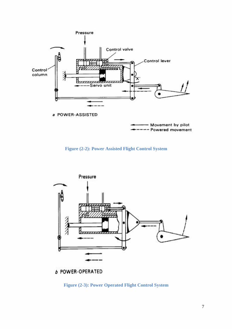
Figure (2-3): Power Operated Flight Control System

8

2.1.3.3 Fly by wire (FBW)

"Fly-by-wire is a means of aircraft control that uses electronic circuits to send inputs from the

pilot to the motors that move the various flight controls on the aircraft. There are no direct

hydraulic or mechanical linkages between the pilot and the flight controls. The total

elimination of all the complex mechanical control runs and linkages-all commands and

signals are transmitted electrically along wires, hence the name fly-by-wire and also there is

interposition of a computer between the pilot’s commands and the control surface actuators

which is incorporated with air data sensors which supply height and airspeed information to

the computer. The fly-by-wire system is shown in Figure (2-4).

Figure (2-4): Fly-by-wire System

Mechanical and hydraulic flight control systems are heavy and require careful routing of

flight control cables through the airplane using systems of pulley and cranks. Both systems

often require redundant backup, which further increases weight. Another advantages of FBW

system are discussed below:

1) Provides high-integrity automatic stabilization of the aircraft to compensate for the

loss of natural stability and thus enables a lighter aircraft with a better overall

performance.

2) Makes the ride much smoother than one controlled by human hands. The capability

of FBW systems to maintain constant flight speeds and altitudes over long distances

is another way of increasing fuel efficiency. The system acts much like cruise

9

controls on automobiles: less fuel is needed if throttles are untouched over long

distances.

3) More reliable than a mechanical system because of fewer parts to break or

malfunction. FBW is also easier to install, which reduces assembly time and costs.

FBW maintenance costs are lower because they are easier to maintain and

troubleshoot, and need fewer replacement parts.

Electrical wires for a flight control system takes up less space inside fuselages, wings, and

tail components. This gives designers several options. Wings and tail components can be

designed thinner to help increase speed and make them aerodynamically cleaner, and also to

reduce weight. Space once used by mechanical linkages can also be used to increase fuel

capacities to give the aircraft greater range or payload".[1]

2.1.4 History

"In the early days of transport aircraft, aircraft required the continuous attention of a pilot in

order to fly in a safe manner. This created very high demands on crew attention and high

fatigue. The autopilot is designed to perform some of the tasks of the pilot.

The first aircraft autopilot was developed by Sperry Corporation in 1912. The autopilot using

gyros to sense the deviation of the aircraft from the desired attitude and servo motors to

activate the elevators and ailerons was built under the direction of Dr. E. A. Sperry. The

apparatus, called Sperry Aero plane Stabilizer, installed in the Curtis Flying Boat, Won

prominence on the 18th June, 1914. Elmer Sperry demonstrated it two years later in 1914,

and proved his credibility of the invention, by flying the plane with his hands up .

The autopilot connected a gyroscopic attitude indicator and magnetic compass to

hydraulically operated rudder, elevator, and ailerons. It permitted the aircraft to fly straight

and level on a compass course without a pilot's attention, thus covering more than 80 percent

of the pilot's total workload on a typical flight. This straight-and-level autopilot is still the

most common, least expensive and most trusted type of autopilot. It also has the lowest pilot

error, because it has the simplest controls.

In the early 1920s, the Standard Oil tanker J.A Moffet became the first ship to use autopilot.

The early aircrafts were primarily designed to maintain the attitude and heading of the

aircraft. With the advent of the high performance aircrafts, new problems have arisen i.e.

unsatisfactory dynamic characteristics.

10

To obtain the more performance, several improvements have been done. Now day’s modern

autopilots are dominating. Modern autopilots generally divide a flight into take-off, ascent,

level, descent, approach, landing, and taxi phases.

Modern autopilots use computer software to control the aircraft. The software reads the

aircraft's current position, and controls a flight control system to guide the aircraft. In such a

system, besides classic flight controls, many autopilots incorporate thrust control capabilities

that can control throttles to optimize the air-speed, and move fuel to different tanks to balance

the aircraft in an optimal attitude in the air. Although autopilots handle new or dangerous

situations inflexibly, they generally fly an aircraft with a lower fuel-consumption than all but

a few of the best pilots".[1]

2.1.5 Techniques Available

"The basic aim of an autopilot is to track the desired goal. Autopilot can be displacement type

or pitch type. There are different techniques available to design an autopilot like model-

following control, sliding mode control, model predictive control, robust control, lyapunov

based control, adaptive control and dynamic inversion control. Every technique has its

disadvantages, so to improve the disadvantages new techniques are proposed.

Dynamic Inversion is a design technique which is based on feedback linearization, basically

it achieves the effect of gain scheduling. This approach transforms the nonlinear system a

linear time invariant form. The transformation is then inverted to obtain a nonlinear control

law, but the limitation of this technique is that it cannot be applied to nonminimum phase

plants. In this technique, the set of existing dynamics are canceled out and replaced by a

designer selected set of desired dynamics. Dynamic inversion is similar to model following

control, in that both methodologies invert dynamical equations of the plant and an appropriate

co-ordinate transformation is carried out to make the system looklinear so that any known

linear controller design can be used.

Lyapunov based control design techniques use the Lyapunov's stability theorem for nonlinear

systems and come up with adaptive control solutions that guarantee stability of the error

dynamics (i.e. the tracking error remains bounded in a small neighborhood about zero) or

sometimes assure asymptotic stability (i.e. the tracking error goes to zero). In sliding mode

control , the essential idea is to first lay out a path for the error signal that leads to zero.

11

Then the control solution is found in such a way that the error follows this path, finally

approaching zero. In doing so, however, the usual problems encountered are high magnitudes

of control and control chattering. In Predictive control , the error signal is first predicted for

some future time (based on a model that may or may not be updated in parallel). The control

solution at the current time step is then obtained from an error minimization algorithm that

minimizes cost function, which is a weighted average of the error signal. In this study of

autopilots, classical methods are used to find the response when the command is given".[1]

2.1.6 Components of Autopilot

"The basic components of the autopilot is shown in the figure (2-5).

Figure (2-5): Basic Components of an Autopilot

Aircraft motion is usually sensed by a gyro, which transmits a signal to a computer (see

illustration). The computer commands a control servo to produce aerodynamic forces to

remove the sensed motion. The computer may be a complex digital computer, an analog

computer (electrical or mechanical), or a simple summing amplifier, depending on the

complexity of the autopilot. The control servo can be a hydraulically powered actuator or an

electromechanical type of surface actuation. Signals can be added to the computers that

supply altitude commands or steering commands. For a simple autopilot, the pitch loop

controls the elevators and the roll loop controls the aileron. A directional loop controlling the

rudder may be added to provide coordinated turns". [1]

12

2.1.7 Aircraft Dynamics

2.1.7.1 Equation of motion

Equations of motion are equations that describe the behavior of a system in terms of

its motion as a function of time (e.g., the motion of a particle under the influence of

a force). Sometimes the term refers to the differential equations that the system satisfies

(e.g., Newton's second law or Euler–Lagrange equations).[2,3]

2.1.8 Aircraft dynamic modes

The dynamic stability of an aircraft is how the motion of an aircraft behaves after it has been

disturbed from steady non-oscillating flight.[2,3]

2.1.8.1 Longitudinal modes

Oscillating motions can be described by two parameters, the period of time required for one

complete oscillation, and the time required to damp to half-amplitude, or the time to double

the amplitude for a dynamically unstable motion. The longitudinal motion consists of two

distinct oscillations, a long-period oscillation called a phugoid mode and a short-period

oscillation referred to as the short-period mode.[2,3]

1) Phugoid (longer period) oscillations

The longer period mode, called the "phugoid mode" is the one in which there is a large-

amplitude variation of air-speed, pitch angle, and altitude, but almost no angle-of-attack

variation. The phugoid oscillation is really a slow interchange of kinetic energy (velocity)

and potential energy (height) about some equilibrium energy level as the aircraft attempts to

re-establish the equilibrium level-flight condition from which it had been disturbed. The

motion is so slow that the effects of inertia forces and damping forces are very low. Although

the damping is very weak, the period is so long that the pilot usually corrects for this motion

without being aware that the oscillation even exists. Typically the period is 20–60 seconds.[2]

2) Short period oscillations

With no special name, the shorter period mode is called simply the "short-period mode". The

short-period mode is a usually heavily damped oscillation with a period of only a few

seconds. The motion is a rapid pitching of the aircraft about the center of gravity. The period

is so short that the speed does not have time to change, so the oscillation is essentially an

angle-of-attack variation. The time to damp the amplitude to one-half of its value is usually

13

on the order of 1 second. Ability to quickly self damp when the stick is briefly displaced is

one of the many criteria for general aircraft certification.[2]

2.1.8.2 Lateral-directional modes

Lateral-directional" modes involve rolling motions and yawing motions. Motions in one of

these axes almost always couples into the other so the modes are generally discussed as the

Lateral-Directional modes.

There are three types of possible lateral-directional dynamic motion: roll subsidence mode,

Dutch roll mode, and spiral mode. [2,4]

1) Roll subsidence mode

Roll subsidence mode is simply the damping of rolling motion. There is no direct

aerodynamic moment created tending to directly restore wings-level, i.e. there is no returning

"spring force/moment" proportional to roll angle. However, there is a damping moment

(proportional to roll rate) created by the slewing-about of long wings. This prevents large roll

rates from building up when roll-control inputs are made or it damps the roll rate (not the

angle) to zero when there are no roll-control inputs.

Roll mode can be improved by adding dihedral effects to the aircraft design, such as high

wings, dihedral angles or sweep angles. [2]

2) Spiral mode

If a spirally unstable aircraft, through the action of a gust or other disturbance, gets a small

initial roll angle to the right, for example, a gentle sideslip to the right is produced. The

sideslip causes a yawing moment to the right. If the dihedral stability is low, and yaw

damping is small, the directional stability keeps turning the aircraft while the continuing bank

angle maintains the sideslip and the yaw angle. This spiral gets continuously steeper and

tighter until finally, if the motion is not checked, a steep, high-speed spiral dive results. The

motion develops so gradually, however that it is usually corrected unconsciously by the pilot,

who may not be aware that spiral instability exists. If the pilot cannot see the horizon, for

instance because of clouds, he might not notice that he is slowly going into the spiral dive,

which can lead into the graveyard spiral.

To be spirally stable, an aircraft must have some combination of a sufficiently large dihedral,

which increases roll stability, and a sufficiently long vertical tail arm, which increases yaw

damping. Increasing the vertical tail area then magnifies the degree of stability or instability.

14

The spiral dive should not be confused with a spin.[3]

a) Detection

While descending turns are commonly performed by pilots as a standard flight maneuvers,

the spiral dive is differentiated from a descending turn owing to its feature of accelerating

speed. It is therefore an unstable flight condition, and pilots are trained to recognize its onset

and to implement recovery procedures safely and immediately. Without intervention by the

pilot, acceleration of the aircraft will lead to structural failure of the airframe, either as a

result of excess aerodynamic loading or flight into terrain. Spiral dive training therefore

revolves around pilot recognition and recovery.[3]

b) Recovery

Spiral dive accidents are typically associated with visual flight (non-instrument flight) in

conditions of poor visibility, where the pilot's reference to the visual natural horizon is

effectively reduced, or prevented entirely, by such factors as cloud or darkness. The inherent

danger of the spiral dive is that the condition, especially at onset, cannot be easily detected by

the sensory mechanisms of the human body. The physical forces exerted on an airplane

during a spiral dive are effectively balanced and the pilot cannot detect the banked attitude of

the spiral descent. If the pilot detects acceleration, but fails to detect the banked attitude

associated with the spiral descent, a mistaken attempt may be to recovery with mere back

pressure (pitch-up inputs) on the control wheel. However, with the lift vector of the aircraft

now directed to the centre of the spiral turn, this erred nose-up input simply tightens the spiral

condition and increases the rate of acceleration and increases dangerous airframe loading. To

successfully recover from a spiral dive, the lift vector must first be redirected upward

(relative to the natural horizon) before backpressure is applied to the control column. Since

the acceleration can be very rapid, recovery is dependent on the pilot's ability to quickly close

the throttle (which is contributing to the acceleration), position the lift vector upward, relative

to the Earth's surface before the dive recovery is implemented; any factor that would impede

the pilot's external reference to the Earth's surface could delay or prevent recovery. The quick

and efficient completion of these tasks is crucial as the aircraft can accelerate through

maximum speed limits within only a few seconds, where the structural integrity of the

airframe will be compromised.

For the purpose of flight training, instructors typically establish the aircraft in a descending

turn with initially slow but steadily accelerating airspeed – the initial slow speed facilitates

15

the potentially slow and sometimes erred response of student pilots. The cockpit controls are

released by the instructor and the student is instructed to recover. It is not uncommon for a

spiral dive to result from an unsuccessful attempt to enter a spin, but the extreme nose-down

attitude of the aircraft during the spin-spiral transition makes this method of entry ineffective

for training purposes as there is little room to permit student error or delay.

All spiral dive recoveries entail the same recovery sequence: first, the throttle must be

immediately closed; second, the aircraft is rolled level with co-ordinate use

of ailerons and rudder; and third, backpressure is exerted smoothly on the control wheel to

recover from the dive.[3]

3) Dutch roll

The second lateral motion is an oscillatory combined roll and yaw motion called Dutch roll,

perhaps because of its similarity to an ice-skating motion of the same name made by Dutch

skaters; the origin of the name is unclear. The Dutch roll may be described as a yaw and roll

to the right, followed by a recovery towards the equilibrium condition, then an overshooting

of this condition and a yaw and roll to the left, then back past the equilibrium attitude, and so

on. The period is usually on the order of 3–15 seconds, but it can vary from a few seconds for

light aircraft to a minute or more for airliners. Damping is increased by large directional

stability and small dihedral and decreased by small directional stability and large dihedral.

Although usually stable in a normal aircraft, the motion may be so slightly damped that the

effect is very unpleasant and undesirable. In swept-back wing aircraft, the Dutch roll is

solved by installing a yaw damper, in effect a special-purpose automatic pilot that damps out

any yawing oscillation by applying rudder corrections. Some swept-wing aircraft have an

unstable Dutch roll. If the Dutch roll is very lightly damped or unstable, the yaw damper

becomes a safety requirement, rather than a pilot and passenger convenience. Dual yaw

dampers are required and a failed yaw damper is cause for limiting flight to low altitudes, and

possibly lower mach numbers, where the Dutch roll stability is improved.[2]

16

2.1.9 Displacement Autopilot

2.1.9.1 Longitudinal Displacement Autopilot

"The simplest form of autopilot, which is the type that first appeared in aircraft and is still

being used in some of the older transport aircraft, is the displacement-type autopilot. This

autopilot was designed to hold the aircraft in straight and level flight with little or no

maneuvering capability. A block diagram such an autopilot is shown in figure (2-6).

For this type of autopilot the aircraft is initially trimmed to straight and level flight, the

reference aligned, and then the autopilot engaged. If the pitch attitude varies from the

reference, a voltage eg is produced by the signal generator on the vertical gyro. This voltage is

then amplified and fed to the elevator servo. The elevator servo can be electromechanical or

hydraulic with an electrically operated valve. The servo then positions the elevator, causing

the aircraft to pitch about the Y axis and so returning it to the desired pitch attitude".[5]

2.1.9.2 Type1 and Type0 System

"Block diagram of the type0 and type1 system are shown in figures (2-6) and (2-7)

respectively. Difference between the type0 and type1 system is in the steady state error. In

type0 system there is steady state error for unit step input, but in type1 system there is no

such type of steady state error. In the type1system, there is one inner loop, this inner loop

contains two blocks, one for the aircraft dynamics and other for the combined amplifier and

elevator servo. For the internal loop, S(rg) is used as feedback whose value is tuned. In the

outer loop, S(amp) is the outer loop gain with unity feedback. In the type0 system there is no

need of the internal loop. To make the system type0 a differentiator is used with the aircraft

dynamics, so in this case there is no need of S(rg), but the same autopilot is used for the both

type of systems". [5]

Figure(2- 6): Displacement autopilot of longitudinal motion

Vertical

gyro

Amplifier Elevator

Servo

Aircraft

dynamics

17

Figure(2- 7): Type (1) displacement autopilot of longitudinal motion

2.1.10 Lateral Displacement Autopilot

"AS most aircraft are spirally unstable, there is no tendency for the aircraft to return to its

initial heading and roll angle after it has been disturbed from equilibrium by either a control

surface deflection or a gust. Thus the pilot must continually make corrections to maintain a

given heading. The early lateral autopilots were designed primarily to keep the wing level

and hold the aircraft on a desired heading. A vertical gyro was used for the purpose of

keeping the wing level, and a directional gyro was used for the heading reference.

Figure(2-8 )is a block diagram of such an autopilot. This autopilot had only very limited

maneuvering capabilities. Once the references were aligned and the autopilot engaged, only

small heading changes could be made. This was generally accomplished by changing the

heading reference and thus yawing the aircraft through the use of the rudders to the new

heading. Obviously such a maneuver was uncoordinated and practical only for small heading

changes. Due to the lack of maneuverability and the light damping characteristic of the Dutch

roll oscillation in high-performance aircraft, this autopilot is not satisfactory for our present-

day aircraft. present-day lateral autopilots are much more complex. In most cases it is

necessary to provide artificial damping of the Dutch roll. Also, to add maneuverability,

provisions are

provided for turn control through the defection of the aileron, and coordination is achieved by

proper signals to the rudder. In this discussion of lateral autopilots the damping of the Dutch

roll is discussed first, followed by methods of obtaining coordination, and then the complete

autopilot is examined".[5]

18

2.2 Stability and control

There are many ways for controlling an aircraft mechanism, such as classical controllers,

adaptive controllers, neural controllers, etc.[6]

The first case study deal with fuzzy controller which is introduced by Lutfi Zadeh in 1973

and a fuzzy controller consists an input stage, a processing stage and an output stage. Input

stage of a fuzzy controller turns inputs (such as sensors, switches etc.) to a suitable function

and truth table values. These functions are called membership functions. In processing stage,

a fuzzy controller generates a result for each rule and combine them. As a result of these

stages, output stage converts them to a value which is going to be used in controller. Also it is

being used for creating nonlinear controllers with some heuristic information. This heuristic

information comes from an operator, who designs the controller, and it enters a decision

making process and then it produces some outputs for controllers.[6]

by using Boeing747-E aerodynamic and stability derivatives’ and all specifications need for

modeling, then deal with design of the fuzzy controller as following steps:

Fuzzy system as piecewise-linear interpolation.

Parameter characterization and coding.

Fuzzy rule tuning.

Evaluation of design solution.

Figure (2-8): Displacement lateral autopilot

19

This case study deal with lateral autopilot for Boing747-E by using fuzzy control and give

results.[6]

Evaluation: This method even if it is better in complex system design and multiple systems

can be joined while creating it, it’s have a little bit of complexity.[6]

The second case study used classic PID controller, after also modeling for Boeing747-E and

used its transfer function then used PID tools for control and evaluation the design.[6,7]

Figure (2-10): System response when PID is applied

Evaluation: as it is seen, PID controller gives a little error on system for steady-state. Also

there is no oscillation, which is better for a system, because if a system makes oscillation, it

Figure (2-9): System response, when fuzzy controller is applied.

20

shows that system responds your effects, moves your effect to a suitable place and stabilizes

the system.[6,7]

Both fuzzy and PID give similar responses, sometimes PID may seem a little bit better, also

PID controller is distinction by simplicity and reliability, availability of its tools and ease of

construction.[6,7]

Thus the lateral autopilot for Boing747-E will used PID as controlling technique.[6,7]

21

3 Chapter Three: Calculation

3.1 Longitudinal Calculation

3.1.1 Longitudinal Motions

Develop the small-disturbance equations for longitudinal motions in standard state-variable

form. Recall that the linearized equations describing small longitudinal perturbations from a

longitudinal equilibrium state can be written:

(3-1)

(3-2)

(3-3)

If we introduce the longitudinal state variable vector

(3-4)

and the longitudinal control vector

(3-5)

these equations are equivalent to the system of first-order equations

(3-6)

Where x˙ represents the time derivative of the state vector x, and the matrices appearing in

this equation are:

1) Longitudinal Motion

2) Longitudinal Autopilot

3) Longitudinal Simulation

4) Longitudinal Control

1) Lateral Motion

2) Lateral Autopilot

3) Lateral Simulation

4) Lateral Control

5) Lateral Evaluation

Longitudinal Calculation Lateral Calculation

22

The inverse of

As premultiplying Eq. (6) by gives the standard form:

(3-11)

(3-8 )

0)

(3-7)

(3-9)

(3-10 )

0)

23

Where :

A is the state matrix

B is the input matrix

x is the state vector

η is the control vector

The A and B consist of aircraft’s dimensional stability and control derivatives.

Note that:

(3-15)

(3-14)

(3-12)

(3-13)

24

Where:

µ is aircraft mass parameter is typically large (on the order of 100), it is common

to neglect with respect to unity and to neglect relative to , in which case the

matrices A and B can be approximated as:

This is the approximate form of the linearized equations for longitudinal motions as they

appear in many texts.

The various dimensional stability derivatives appearing in Equations. (3-16) and (3-17) are

related to their dimensionless aerodynamic coefficient in Table (3-1)

Table (3-1) : The various dimensional stability derivatives related to their dimensionless

aerodynamic coefficient in a longitudinal motion

Variable X Z M

U

Q

(3-16)

(3-17)

25

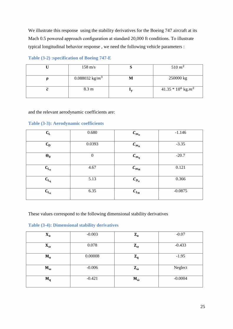
We illustrate this response using the stability derivatives for the Boeing 747 aircraft at its

Mach 0.5 powered approach configuration at standard 20,000 ft conditions. To illustrate

typical longitudinal behavior response , we need the following vehicle parameters :

Table (3-2) :specification of Boeing 747-E

U 158 m/s S 510

ρ 0.088032 kg/ M 250000 kg

8.3 m 41.35 * kg.

and the relevant aerodynamic coefficients are:

Table (3-3): Aerodynamic coefficients

0.680 -1.146

0.0393 -3.35

0 -20.7

4.67

0.121

5.13

0.366

6.35

-0.0875

These values correspond to the following dimensional stability derivatives

Table (3-4): Dimensional stability derivatives

-0.003 -0.07

0.078 -0.433

0.00008 -1.95

-0.006 Neglect

-0.421 -0.0004

26

3.1.1.1 Characteristic Equation

Given square matrix A the equation

(3-18)

Equation (3-18) is called characteristic equation of matrix A.

𝜆 denotes the determinant of the argument (square) matrix , and I is identity matrix its

dimension= dimension of matrix A

The roots of characteristic equation.( 3-18) are called the eigen values of the matrix A and are

usually denoted by

r1,r2,…, rn where n is the number of columns or rows of matrix A

3.1.1.2 Aircraft Characteristic Equation

It is polynomial equation which is fourth order in S- domain as follow

(3-19)

Where coefficients a, b, c, d and e are real quantities.

Equation(3-19)can be written as:

(3-20)

27

For stable oscillation type of motion, the roots of these characteristic equation on S-plan.

-2 -1.5 -1 -0.5 0 0.5 1 1.5 2-1

-0.5

0

0.5

1Root Locus

Real Axis

Im

aginary A

xis

0 1000 2000 3000 4000 5000 6000-2

-1.5

-1

-0.5

0

0.5

1Step Response

time (sec)

pitch angle (rad)

Figure (3-11) :General Root Locus of longitudinal modes

Figure (3-12) :Root Locus of Boeing 747-E longitudinal modes

28

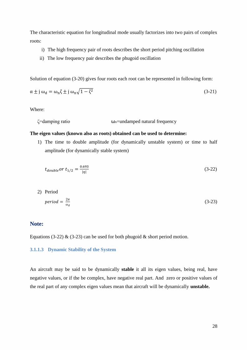
The characteristic equation for longitudinal mode usually factorizes into two pairs of complex

roots:

i) The high frequency pair of roots describes the short period pitching oscillation

ii) The low frequency pair describes the phugoid oscillation

Solution of equation (3-20) gives four roots each root can be represented in following form:

(3-21)

Where:

ζ=damping ratio ωn=undamped natural frequency

The eigen values (known also as roots) obtained can be used to determine:

1) The time to double amplitude (for dynamically unstable system) or time to half

amplitude (for dynamically stable system)

(3-22)

2) Period

(3-23)

Note:

Equations (3-22) & (3-23) can be used for both phugoid & short period motion.

3.1.1.3 Dynamic Stability of the System

An aircraft may be said to be dynamically stable it all its eigen values, being real, have

negative values, or if the be complex, have negative real part. And zero or positive values of

the real part of any complex eigen values mean that aircraft will be dynamically unstable.

29

The complex eigen values of Boeing 747-E:

𝜆 = -0.4547 ± 0.9436i

𝜆 = -0.0009 ± 0.0633i

This aircraft is dynamically stable.

The first two pair of roots are for short period oscillation mode and the other pair for phugoid

oscillation

= 1.048 rad/s = 0.0638 rad/s

3.1.1.4 Longitudinal Modes of Typical Aircraft

The natural response of most aircraft to longitudinal perturbations typically consists of two

under damped oscillatory modes having rather different time scales. One of the modes has a

relatively short period and is usually quite heavily damped; this is called the short period

mode. The other mode has a much longer period and is rather lightly damped; this is called

the phugoid mode.

-2 -1.5 -1 -0.5 0 0.5 1 1.5 2-1

-0.5

0

0.5

1Root Locus

Real Axis

Im

agin

ary A

xis

0 1000 2000 3000 4000 5000 6000-2

-1.5

-1

-0.5

0

0.5

1Step Response

time (sec)

pitch angle

(rad)

Figure (3-13) Response of longitudinal motion

30

3.1.2 Longitudinal Displacement autopilot

This autopilot was designed to hold the aircraft in straight and level flight with little or no

maneuvering capability. A block diagram of Boeing 747-E longitudinal autopilot is shown in

figure (3-4).

And the displacement autopilot for Boeing 747-E with pitch rate feedback added for damping

as show in figure (3-5):

Figure (3-15): Block diagram for the displacement autopilot with pitch rate feedback

added for damping

Figure (3-14): Displacement autopilot of Boeing 747-E

Vertical

gyro

Amplifier Elevator

Servo

31

3.1.2.1 Inner Loop Transfer Function

In Automatic control we derived the transfer function of a simple feedback system. In the

figure below a feedback system similar to our inner loop is shown.

Figure (3-16): Block diagram of a similar, simple feedback system

By simplifying the inner loop transfer function:

=

(3-24)

The root locus of the inner loop is drawn as follows:

Figure (3-17): Root Locus Diagram for Inner Loop

-10 -8 -6 -4 -2 0 2 4-80

-60

-40

-20

0

20

40

60

80Root Locus

Real Axis (seconds-1)

Imag

inar

y A

xis

(sec

onds

-1)

32

3.1.2.2 Outer Loop Transfer Function

Figure (3-18): Block diagram of the outer loop

Transfer function of the outer loop,

is found as in the Equation (3-25)

=

(3-25)

The root locus of the outer loop is drawn as follows:

-25 -20 -15 -10 -5 0 5 10-15

-10

-5

0

5

10

15Root Locus

Real Axis (seconds-1)

Imag

inar

y A

xis

(sec

onds

-1)

K

Outer loop

V.G Amp

Integrator

Figure(3- 19): Root Locus Diagram for Outer Loop

33

3.1.3 Longitudinal simulation

Figure (3-21): The response of pitch angle ( ) for Boeing 747-E at 20,000 ft

Figure (3-20): Block diagram of simulation for Boeing 747-E longitudinal autopilot

34

Figure (3-22): The response of pitch rate( ) for Boeing 747-E at 20,000 ft

Figure (3-23): The response of elevator deflection ( ) for Boeing 747-E at 20,000 ft

35

3.1.4 Longitudinal control

3.1.4.1 Introduction

No adopt, the adding of controller to the pitch attitude autopilot improve the performance of

the aircraft specially at longitudinal motion. This improvement can be done by different

procedures but we found by assistant with graphical methods in Matlab, the best way to

increase reliability of our aircraft system, adding the PD controller with suitable calculated

gain.

3.1.4.2 controller Selection

Based upon previous procedures about different controllers, the optimum proposed controller

that have open loop transfer function as:

(3-26)

The contribution of this controller upon the aircraft longitudinal channel was improving the

system response that can be seen obviously in decreasing the overall specifications

comparing with the system before adding the PD controller. It is effected in the specifications

of the system. The setting time became very short and more convenient to the aircraft system

and users. Also the decrease of rise time and overshoot in input step response as shown in

preceding figures.

The overall transfer function of the aircraft with selected controller is

(3-27)

This can be represented by a block diagram as in figure (3-14).

Figure (3-24): Displacement longitudinal autopilot of Boeing 747-E with PD controller

PD

Controller

Elevator

Servo

36

From the previous block diagram was to improve the positions (increase stability) of phugoid

pole and shows through the root locus in below

Figure (3-25): Root Locus of Boeing 747-E longitudinal modes after adding the PD

controller

Also the response of longitudinal motion was improving that can be seen obviously in

decreasing the overall specifications by adding the PD controller. Where the response up to

steady state error in less time.

Figure (3-26): Response of longitudinal motion after adding the PD controller

-5 -4 -3 -2 -1 0 1-15

-10

-5

0

5

10

15Root Locus

Real Axis (seconds-1)

Imagin

ary

Axis

(seconds

-1)

0 2 4 6 8 10 12-5.1

-5

-4.9

-4.8

-4.7

-4.6

-4.5

-4.4

-4.3Step Response

time (seconds)

pitch a

ngle

(ra

d)

37

3.2 Lateral Calculation

3.2.1 Lateral/Directional Motions

Develop the small-disturbance equations for lateral/directional motions in standard state-

variable form. Recall that the linearized equations describing small lateral/directional

perturbations from a longitudinal equilibrium state can be written:

(3-28)

(3-29)

(3-30)

Using a procedure similar to the longitudinal case, we can develop the equations of motion

for the lateral dynamics.

If we introduce the lateral/directional state variable vector

(3-31)

The lateral/directional control vector

(3-32)

These equations are equivalent to the system of first-order equations

(3-33)

Where:

represents the time derivative of the state vector x

(1)

(2)

(3)

(3-34)

38

For most flight vehicles and situations, the ratios and are quite small. Neglecting these

quantitieswith respect to unity allows us to write the A and B matrices for lateral directional

motions as:

The various dimensional stability derivatives ( , , ,…) appearing in above equations

are related to their dimensionless aerodynamic coefficients as follows

(3-35)

(3-36)

(3-37)

39

Table (3-5): The various dimensional stability derivatives related to their dimensionless

aerodynamic coefficient in a lateral motion

Variable Y L N

V

R

3.2.1.1 Modes of Typical Aircraft

The natural response of most aircraft to lateral/directional perturbations typically consists of:

One damped oscillatory mode This mode has a relatively short period and can be relatively

lightly damped, especially for swept-wing aircraft; this is called the Dutch Roll mode. And

two exponential modes One of which is usually very heavily damped and represents the

response of the aircraft primarily in roll; it is called the rolling mode. The second exponential

mode, called the spiral mode, can be either stable or unstable, but usually has a long enough

time constant that it presents no difficulty for piloted vehicles, even when it is unstable.

We illustrate this response again using the stability derivatives for the Boeing 747 aircraft at

its Mach 0.5 powered approach configuration at standard 20,000 ft conditions. This is the

same vehicle and trim condition used to illustrate typical longitudinal behaviour. In addition,

for the lateral/directional response we need the following vehicle parameters

Table(3- 6): specification of Boeing 747-E

U 158 m/s S 510

P 0.088032 kg/ M 250000 kg

8.3 m 18.6 * kg.

58* kg. 1.2* kg.

B 59.75 m Q 8667 N/

40

and the aerodynamic derivatives are:

Table (3-7): The aerodynamic coefficient

-0.90 Clp 0.323-

0.212 -0.193

-0.278

-0.0687

0.147

These values correspond to the following dimensional stability derivatives:

Table (3-8): The dimensional stability derivatives

-0.1007 -0.0176

0.00497 -0.8766

-0.281 -0.0694

0.443 0.5754

-0.281

and the dimensionless product of inertia factors are:

=

= 0.0645 and =

= 0.0207

Using these values, the plant matrix is found to be

=

A

41

The characteristic equation is given by:

𝜆 = + 1.2592 + 1.1897 + 1.0833 s + 0.215 =0

And its roots are:

𝜆

𝜆

𝜆

All its eigen values (roots) being real, have negative values, or be complex, have negative

real part. Therefore the aircraft is Stable, but there is one very slow pole.

There are three modes, but they are a lot more complicated than the longitudinal case.

Table (3-9): The lateral modes

Slow mode -0.0194 Spiral Mode slow, often unstable.

Fast real -1.0766 Roll Damping well damped.

Oscillatory -0.0812± 0.9877 i Dutch Roll damped oscillation in yaw,

that couples into roll.

3.2.1.1.1 The damping ratio ,undamped natural frequency of the Dutch Roll mode

Assume the two roots can be represented as follows:

(3-38)

Damping ratio:

=

= 0.0819 (3-39)

where and are the real and imaginary parts of the respective roots, and the undamped

natural frequency of the mode is

=

=

=0.9915 (3-40)

42

The period of the Dutch Roll mode is then given by:

=

=

=6.355 Sec (3-41)

And the number of cycles to damp to half amplitude is

=

=

= 1.343 (3-42)

Thus, the period of the Dutch Roll mode is seen to be on the same order as that of the

longitudinal short period mode, but is much more lightly damped.

3.2.1.1.2 The times to damp to half amplitude for the rolling and spiral modes

The times to damp to half amplitude for the rolling and spiral modes are seen to be

=

=

= 0.644 Sec and

=

=

= 35.73 Sec

The responses characteristic of these aircraft is illustrated in following figure:

0 10 20 30 40 50 60 70 80 90 100-30

-20

-10

0

10

20

30

Step Response

time (sec)

v (m

/s)

Figure (3-27): The response of lateral motion for Boeing 747-E

43

The responses characteristic of these three mode are illustrated in following figures:

Figure (3-28): Rolling mode

Figure (3-29): Spiral mode

44

Figure (3-30): Dutch Roll

45

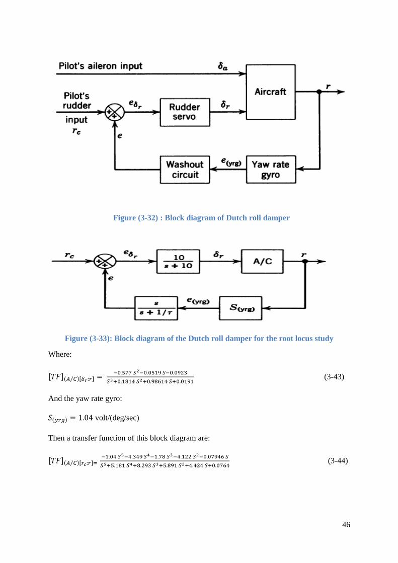
3.2.2 Lateral autopilot

As continues work on the autopilot of the aircraft, after longitudinal autopilot we will work

on the lateral autopilot. This autopilot had only very limited maneuvering capabilities, a

block diagram of Boeing 747-E lateral autopilot is shown in figure (3-21).

3.2.2.1 Damping of Dutch roll

As previously mentioned that the rudder excites primarily the Dutch roll mode; the Dutch roll

that is observed in yow rate and side slip response from an aileron deflection is caused by the

yawing moment resulting from the aileron deflection. For these reasons the usual method of

damping the Dutch roll is to detect the yaw rate with a rate gyro and use this signal to deflect

the rudder. Figure below is a block diagram of the Dutch roll damper. The washout circuit

produces an output only during the transient period. If the yaw rate signal did not go to zero

in the steady state, then for a positive yaw rate, for instance, the output of the yaw rate gyro

would produce a positive rudder deflection. This would result in an uncoordinated maneuver

and require a larger pilot's rudder input to achieve coordination.

Figure (3-31): Basic lateral autopilot

46

Figure (3-33): Block diagram of the Dutch roll damper for the root locus study

Where:

(3-43)

And the yaw rate gyro:

volt/(deg/sec)

Then a transfer function of this block diagram are:

(3-44)

Figure (3-32) : Block diagram of Dutch roll damper

47

From above transfer function produce the root locus in the figure (3-24):

-20 -15 -10 -5 0 5 10-5

-4

-3

-2

-1

0

1

2

3

4

5Root Locus

Real Axis (seconds-1)

Im

agin

ary A

xis

(seconds

-1)

Figure (3-34): Root locus for the Dutch roll damper for of the washout circuit equal to 1 sec

48

3.2.3 Lateral simulation

The figures below shows the results of a computer simulation of the aircraft with the Dutch

roll damper.

Figure (3-36): Response of the aircraft (r) with Dutch roll damping for

volt/(deg/sec) for a pulse aileron deflection

Figure (3-35): Block diagram of simulation for Boeing 747-E lateral autopilot

49

Figure (3-37): Response of the aircraft with Dutch roll damping for

volt/(deg/sec) for a pulse aileron deflection

3.2.4 Lateral control

We can stabilize or modify the lateral dynamics using a variety of feedback architectures.

And we show on figure below a block diagram of this yaw damper, using proportional

feedback.

Figure(3- 38): Block diagram of the Dutch roll damper with controller

The transfer function of the aircraft dynamic in the block are:

(3-45)

Rate gyro

r (s)

(s)

(s)

Rudder actuator

Controller

Aircraft

dynamic

50

Note that:

The gain of the plant is negative ( ), so if , then , so

must draw a root locus (negative feedback).

-8 -6 -4 -2 0 2 4-1

-0.8

-0.6

-0.4

-0.2

0

0.2

0.4

0.6

0.8

1Root Locus

Real Axis (seconds-1)

Imagin

ary

Axis

(seconds

-1)

-5 -4 -3 -2 -1 0 1 2-1.5

-1

-0.5

0

0.5

1

1.5Root Locus

Real Axis (seconds-1)

Imagin

ary

Axis

(seconds

-1)

Figure(3- 41): lateral autopilot: r to with

Figure(3- 39): lateral autopilot: r to with

Figure (3-40): lateral autopilot: r to with

51

Root locus with looks pretty good as we have authority over the four poles. And at

= −1.6 results in a large increase in the Dutch roll damping mode have combined into a

damped oscillation.

Also the response of Dutch roll damper was improving that can be seen obviously in

decreasing the overall specifications by adding the controller. Where the response up to

steady state error in less time.

Figure (3-31): Response of the aircraft (r) with Dutch roll damping after adding

controller

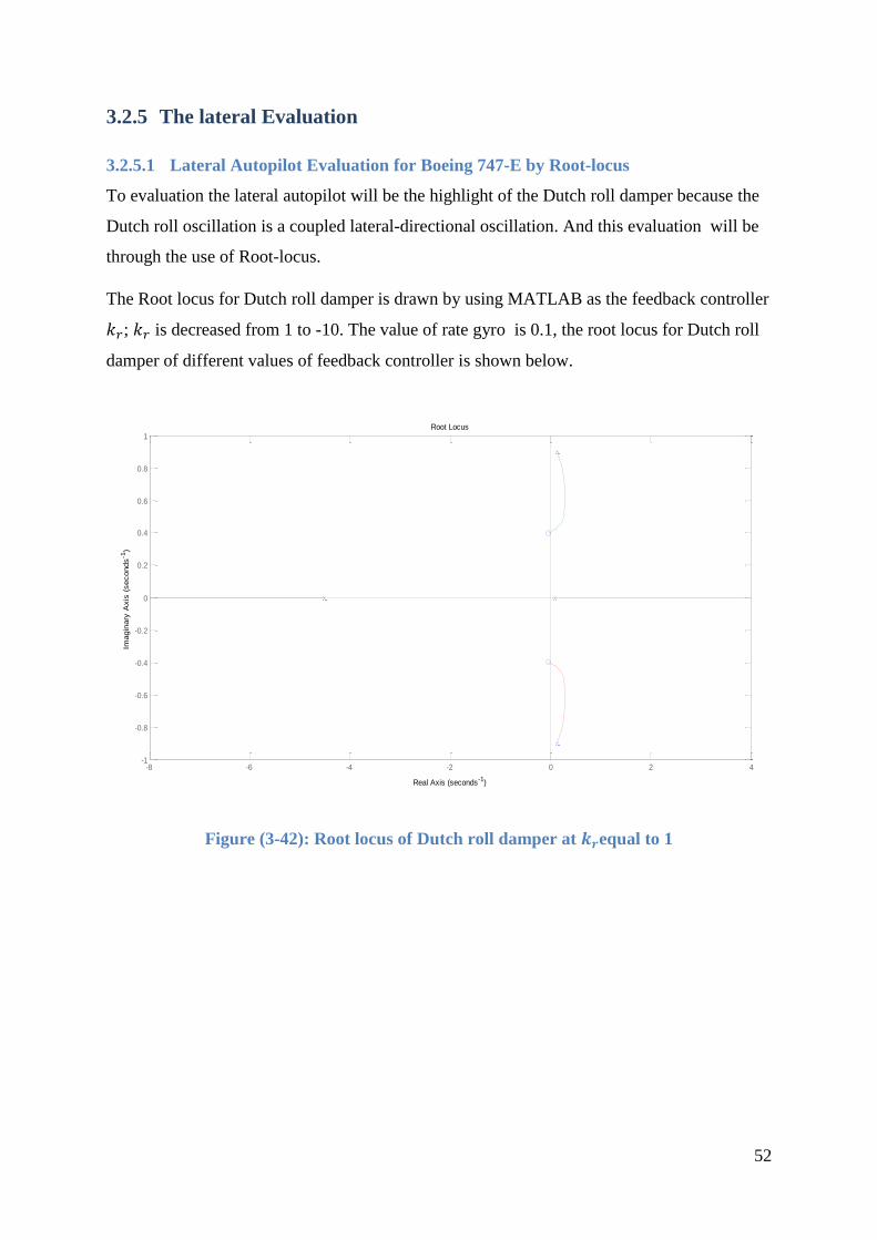
52

3.2.5 The lateral Evaluation

3.2.5.1 Lateral Autopilot Evaluation for Boeing 747-E by Root-locus

To evaluation the lateral autopilot will be the highlight of the Dutch roll damper because the

Dutch roll oscillation is a coupled lateral-directional oscillation. And this evaluation will be

through the use of Root-locus.

The Root locus for Dutch roll damper is drawn by using MATLAB as the feedback controller

; is decreased from 1 to -10. The value of rate gyro is 0.1, the root locus for Dutch roll

damper of different values of feedback controller is shown below.

Figure (3-42): Root locus of Dutch roll damper at equal to 1

-8 -6 -4 -2 0 2 4-1

-0.8

-0.6

-0.4

-0.2

0

0.2

0.4

0.6

0.8

1Root Locus

Real Axis (seconds-1)

Imagin

ary

Axis

(seconds

-1)

53

Figure (3-43): Root locus of Dutch roll damper at equal to -1

-5 -4 -3 -2 -1 0 1 2-1.5

-1

-0.5

0

0.5

1

1.5Root Locus

Real Axis (seconds-1)

Imagin

ary

Axis

(seconds

-1)

-6 -5 -4 -3 -2 -1 0 1 2 3-1.5

-1

-0.5

0

0.5

1

1.5Root Locus

Real Axis (seconds-1)

Imagin

ary

Axis

(seconds

-1)

Figure (3-44): Root locus of Dutch roll damper at equal to -1.6

54

Figure (3-46): Root locus of Dutch roll damper at equal to -5

-10 -8 -6 -4 -2 0 2 4-4

-3

-2

-1

0

1

2

3

4Root Locus

Real Axis (seconds-1)

Imagin

ary

Axis

(seconds

-1)

-10 -8 -6 -4 -2 0 2 4-1.5

-1

-0.5

0

0.5

1

1.5Root Locus

Real Axis (seconds-1)

Imagin

ary

Axis

(seconds

-1)

Figure (3-45): Root locus of Dutch roll damper at equal to -2

55

Figure(3- 47): Root locus of Dutch roll damper at equal to -10

Evaluation:

To evaluate the response, it can be clearly seen that it was selected various value of negative

gain with observing the root locus.

It was noted that when the negative gain increased poles move to left, but there is a certain

value that’s run over it will case overshooting in transit response.

-4 -3 -2 -1 0 1 2 3-5

-4

-3

-2

-1

0

1

2

3

4

5Root Locus

Real Axis (seconds-1)

Imagin

ary

Axis

(seconds

-1)

56

4 Chapter Four: Results

4.1 Longitudinal Result

4.1.1 longtidunal motion

Table (4-1) : Aerodynamic coefficients

0.680 -1.146

0.0393 -3.35

0 -20.7

4.67

0.121

5.13

0.366

6.35

-0.0875

Table (4-2) : Dimensional stability derivatives

-0.003 -0.07

0.078 -0.433

0.00008 -1.95

-0.006 Neglect

-0.421 -0.0004

Table (4-3) : The roots and natural frequency

Roots of short period -0.4547 ± 0.9436i 1.048 rad/s

Roots of long period -0.0009 ± 0.0633i 0.0638 rad/s

57

Figure(4- 48): Root Locus of Boeing 747-E longitudinal modes

Figure (4-49): Response of longitudinal motion

-2 -1.5 -1 -0.5 0 0.5 1 1.5 2-1

-0.5

0

0.5

1Root Locus

Real Axis

Im

agin

ary A

xis

0 1000 2000 3000 4000 5000 6000-2

-1.5

-1

-0.5

0

0.5

1Step Response

time (sec)

pitch angle

(rad)

-2 -1.5 -1 -0.5 0 0.5 1 1.5 2-1

-0.5

0

0.5

1Root Locus

Real Axis

Im

agin

ary A

xis

0 1000 2000 3000 4000 5000 6000-2

-1.5

-1

-0.5

0

0.5

1Step Response

time (sec)

pitch angle

(rad)

58

4.1.2 Longitudinal Displacement Autopilot

Figure (4- 50): Root Locus Diagram for Inner Loop

Figure(4- 51): Root Locus Diagram for Outer Loop

-10 -8 -6 -4 -2 0 2 4-80

-60

-40

-20

0

20

40

60

80Root Locus

Real Axis (seconds-1)

Imag

inar

y A

xis

(sec

onds

-1)

-25 -20 -15 -10 -5 0 5 10-15

-10

-5

0

5

10

15Root Locus

Real Axis (seconds-1)

Imag

inar

y A

xis

(sec

onds

-1)

59

4.1.3 Longitudinal Simulation

Figure (4-52):The response of pitch angle ( ) for Boeing 747-E at 20,000 ft

Figure (4-53):The response of pitch rate ( ) for Boeing 747-E at 20,000 ft

Figure (4-54): The response of elevator deflection ( ) for Boeing 747-E at 20,000 ft

60

4.1.4 Longitudinal Control

Figure(4- 55): Root Locus of Boeing 747-E longitudinal modes after adding the PD

controller

Figure (4-56): Response of longitudinal motion after adding the PD controller

-5 -4 -3 -2 -1 0 1-15

-10

-5

0

5

10

15Root Locus

Real Axis (seconds-1)

Imagin

ary

Axis

(seconds

-1)

0 2 4 6 8 10 12-5.1

-5

-4.9

-4.8

-4.7

-4.6

-4.5

-4.4

-4.3Step Response

time (seconds)

pitch a

ngle

(ra

d)

61

4.2 Lateral/Directional Result

4.2.1 Lateral/Directional Motions

Table (4-4): The aerodynamic coefficient

-0.90 Clp 0.323-

0.212 -0.193

-0.278

-0.0687

0.147

Table (4-5): The dimensional stability derivatives

-0.1007 -0.0176

0.00497 -0.8766

-0.281 -0.0694

0.443 0.5754

-0.281

Table (4-6): The lateral modes

Slow mode -0.0194 Spiral Mode slow, often unstable.

Fast real mode -1.0766 Roll Damping well damped.

Oscillatory mode -0.0812± 0.9877 i Dutch Roll damped oscillation in yaw,

that couples into roll.

Table (4-7): The damping ratio ,undamped natural frequency, the period, and the

number of cycles to damp to half amplitude of the Dutch Roll mode

0.0819 0.9915

6.355 Sec 1.343

Table (4-8) :The times to damp to half amplitude for the rolling and spiral modes

0.644 Sec

35.73 Sec

62

Figure (4-57): The response of lateral motion for Boeing 747

Figure (4-58): Rolling mode

0 10 20 30 40 50 60 70 80 90 100-30

-20

-10

0

10

20

30

Step Response

time (sec)

v (

m/s

)

63

Figure (4-59): Spiral mode

Figure (4-60):Dutch Roll

64

4.2.2 Lateral Autopilot

figure (4-61): Root locus for the Dutch roll damper for of the washout circuit equal to

1 sec

-20 -15 -10 -5 0 5 10-5

-4

-3

-2

-1

0

1

2

3

4

5Root Locus

Real Axis (seconds-1)

Im

agin

ary A

xis

(seconds

-1)

65

4.2.3 Lateral Simulation

Figure (4-62):Response of the aircraft (r) with Dutch roll damping for

volt/(deg/sec) for a pulse aileron deflection

Figure (4-63): Response of the aircraft with Dutch roll damping for

volt/(deg/sec) for a pulse aileron deflection

66

4.2.4 Lateral Control

Figure (4-64): lateral autopilot: r to with

Figure (4-65): Response of the aircraft (r) with Dutch roll damping after adding

controller

-5 -4 -3 -2 -1 0 1 2-1.5

-1

-0.5

0

0.5

1

1.5Root Locus

Real Axis (seconds-1)

Imagin

ary

Axis

(seconds

-1)

67

5 Chapter Five: Discussion

5.1 Longitudinal Discussion

The graph shows Root Locus of Boeing 747-E longitudinal

modes ,it can be clearly seen that the system(longitduinal

motion) is condintionly stable.

The longitudinal motion have four poles two for short period

and the other two for long period (phugoid), short period poles

is stable and long period poles its clearly seen its poorly stable

which are locates nearly zero .

The system called contdionly stable and its not desirble since

if the gain drops beyond the critical value for some reason, the

system becomes unstable .

This graph shows Response of longitudinal motion (short

response); it can be clearly see that the Transient response is

not satisfactory (due to short mode).

Although longitudinal motion of the system is stable (from its

root locus) but the Transient response is not satisfactory

expressed in the Response of the longitudinal motion,

Overall its need to make its derisible as possible by reshaped

the root locus by using PD controller.

-2 -1.5 -1 -0.5 0 0.5 1 1.5 2-1

-0.5

0

0.5

1Root Locus

Real Axis

Im

aginary A

xis

0 1000 2000 3000 4000 5000 6000-2

-1.5

-1

-0.5

0

0.5

1Step Response

time (sec)

pitch angle (rad)

-2 -1.5 -1 -0.5 0 0.5 1 1.5 2-1

-0.5

0

0.5

1Root Locus

Real Axis

Im

aginary A

xis

0 1000 2000 3000 4000 5000 6000-2

-1.5

-1

-0.5

0

0.5

1Step Response

time (sec)

pitch angle (rad)

68

The graph shows Root Locus Diagram for Inner Loop, it

can be clearly seen that the root locus its been more

stable than the previous one ,that’s due to the adding an

inner feed back loop utilizing a rate gyro and that’s used

to increase the damping of short/long period oscillation.

This graph shows Root Locus Diagram for Outer Loop;

it can be clearly see that the additional pole on the

original is results from the integrating gyro.

It was used outer loop (type1 system) to eliminate the

steady state error for a step input.

(able to control aircraft)

-10 -8 -6 -4 -2 0 2 4-80

-60

-40

-20

0

20

40

60

80Root Locus

Real Axis (seconds-1)

Imagin

ary

Axis

(seconds

-1)

-25 -20 -15 -10 -5 0 5 10-15

-10

-5

0

5

10

15Root Locus

Real Axis (seconds-1)

Imagin

ary

Axis

(seconds

-1)

69

The graph describes The response of pitch angle ( ) for

Boeing 747-E at 20,000 ft, it can be clearly seen that the

Transient response is satisfactory.

This amendment obtained in the response due to adding

an inner feed back loop utilizing a rate gyro.

The graph describes The response of pitch rate ( ) for

Boeing 747-E at 20,000 ft it can be seen that the

Transient response is satisfactory but Steady-state error

is too large (control requirement for longitudinal

motion ).

The graph describes The response of elevator deflection

( ) for Boeing 747-E at 20,000 ft, it can be clearly seen

that the response suffering down overshoot (need

control to make improvement to its specifications).

70

The graph shows Root Locus of Boeing 747-E longitudinal

modes after adding the PD controller, it can be clearly seen

that the system(longitduinal motion) is stable.

There are four poles two for short period and the other two

for long period (phugoid), short period poles is stable and

long period poles also here is stable(phugoid mode is stable

) that’s due to using PD controller .

This root locus diagram is results of reshaped a root locus of

longtidinal motion(befor adding controller) to get satisfactory

Transient response with satisfactory steady-state error.

The graph shows Response of longitudinal motion after

adding the PD controller; it can be clearly see that the

Transient response is satisfactory (due using PD controller or

inner loop) satisfactory steady state error.

the response is desirable (satisfactory Transient response and

steady state error) that’s as results of increasing the damping

by using (inner feedback loop) and using PD controller.

-5 -4 -3 -2 -1 0 1-15

-10

-5

0

5

10

15Root Locus

Real Axis (seconds-1)

Im

agin

ary A

xis

(seconds

-1)

0 2 4 6 8 10 12-5.1

-5

-4.9

-4.8

-4.7

-4.6

-4.5

-4.4

-4.3Step Response

time (seconds)

pitch angle (rad)

71

5.2 Lateral Discussion

The graph describes response of lateral motion

for Boeing 747-E (yaw rate), it can be clearly

seen that the response has obvious oscillatory.

The response is lightly damped and need 100 sec

(1 min and 40 sec) or more, thus the lateral

motion require a control to increase damping to

get more suitable response.

The graph shows Rolling mode, it can be clearly

seen that the response has well damped.

Roll mode has no yaw rate (zero) and small side

slip and has obvious roll angle and roll rate,

mode is heavily damped (real fast), its fully

damped at approximately (3 sec).

Thus the roll mode is stable and don’t make any

problems.

0 10 20 30 40 50 60 70 80 90 100-30

-20

-10

0

10

20

30

Step Response

time (sec)

v (

m/s

)

72

The graph shows Spiral mode; it can be clearly

seen that this mode is slow (often unstable).

Spiral mode has small yaw rate and side slip, and

has obvious roll angle and roll rate.

The response is damped at (80 sec) its slow mode

and its need a control.

The graph shows Dutch Roll; it can be clearly

seen that the response has Oscillatory (lightly

damped).

The mode has oscillation of roll angle and role

rate, side slip and yaw rate (damped oscillation).

Thus its necessary to use control to increase this

light damp to get desired response in Dutch mode

which well heavily damped.

73

The graph shows Root locus for the Dutch roll damper for of the washout circuit equal to 1 sec , its can be cleary seen that’s

is stable.

-20 -15 -10 -5 0 5 10-5

-4

-3

-2

-1

0

1

2

3

4

5Root Locus

Real Axis (seconds-1)

Imagin

ary

Axis

(seconds

-1)

74

The graph shows Response of the aircraft (r)

with Dutch roll damping for

volt/(deg/sec) for a pulse aileron deflection it

can be clearly seen that response its clearly

damped .

The graph shows Response of the aircraft

with Dutch roll damping for

volt/(deg/sec) for a pulse aileron deflection, it

can be seen that the response of rudder

deflection has small steady state error and

satisfactory transit response.

75

The graph shows root locus lateral

autopilot: r to with

It’s can be clearly seen that it’s not stable,

thus to make control by using positive gain

to move the pole in root locus lead to

unstable.

The graph shows root locus lateral

autopilot: r to with

It’s can be clearly seen that it’s stable, thus

to make control by using negative gain to

move the pole in root locus lead to stable

-8 -6 -4 -2 0 2 4-1

-0.8

-0.6

-0.4

-0.2

0

0.2

0.4

0.6

0.8

1Root Locus

Real Axis (seconds-1)

Imagin

ary

Axis

(seconds

-1)

-5 -4 -3 -2 -1 0 1 2-1.5

-1

-0.5

0

0.5

1

1.5Root Locus

Real Axis (seconds-1)

Imagin

ary

Axis

(seconds

-1)

76

The graph show Response of the aircraft (r) with Dutch roll damping after adding controller, it can be clearly seen that the

response is completely damped to zero, that’s the Dutch roll oscillate its clearly damped by using gain to control.

77

The graph shows Root locus of Dutch roll damper at equal

to -1, its stable due to using the negative gain which is move

the poles to stable(LHS).

When K= -1 (stable).

The graph shows Root locus of Dutch roll damper at equal to -

2, its stable due to using the negative gain which is move the

poles to stable(LHS).

When K= -2 (increase negative gain move poles to better stable

location ).

The graph shows Root locus of Dutch roll damper at equal

to -5, its stable due to using the negative gain which is move

the poles to stable(LHS).

When K= -5 (increase negative gain lead to increase stable).

The graph shows Root locus of Dutch roll damper at equal to -

10, its stable due to using the negative gain which is move the

poles to stable(LHS).

When K=-10 (increase negative gain lead to increase stable).

-10 -8 -6 -4 -2 0 2 4-4

-3

-2

-1

0

1

2

3

4Root Locus

Real Axis (seconds-1)

Im

agin

ary A

xis

(seconds

-1)

-4 -3 -2 -1 0 1 2 3-5

-4

-3

-2

-1

0

1

2

3

4

5Root Locus

Real Axis (seconds-1)

Imagin

ary

Axis

(seconds

-1)

-6 -5 -4 -3 -2 -1 0 1 2 3-1.5

-1

-0.5

0

0.5

1

1.5Root Locus

Real Axis (seconds-1)

Im

agin

ary A

xis

(seconds

-1)

-10 -8 -6 -4 -2 0 2 4-1.5

-1

-0.5

0

0.5

1

1.5Root Locus

Real Axis (seconds-1)

Im

agin

ary A

xis

(seconds

-1)

78

6 Chapter Six: Conclusion

By the end of this project a lot of skills have been earned and important knowledge acquired.

The overlapping between the control, dynamic and programming makes it deserves to spend

the time on it to apply and manage the engineering work.

6.1 Conclusion

Synthesize of Design of Boeing747-E is studied and nonlinear nature of its lateral autopilot is

focus on.

Although the designer had covered a big deal of work to overcome the problem occurred in

lateral autopilot but still some weakness which we tried to overcome by using PD controller

is proposed to damp the longitudinal oscillatory better than the one which is used, and a bure

gain controller to enhance the Dutch roll oscillatory controller.

Results and comparison are carried out on chapters four and five, shows the difference

between the proposed controller and the existing one which shows a better performance

6.2 Recommendations

Due to lack of data it was not easy to work with lateral motion, that we recommend and

advice to work as a structural group projects, that can give a chance to design SUST aircraft

and use its specifications to apply the theories. Some suggestions for a future work based on

the results from the project are in the next section.

6.3 Future Work

As future work we suggest to make an autopilot for Boieng747-E by using another

controlling technique and we suggest to work with fuzzy controller as future work and

compare its results in longitudinal and lateral motion and the performance of the aircraft with

the results of this project which (which is used PID controller not control tool box for

SIMULINK).

we faced trouble effort while calculate all aerodynamic and stability derivative for the

aircraft, thus we suggest to make program (may in Matlab) to calculate those derivative for

every aircraft we inter it in the program.

79

References

1. Siddharth Goya., Study of a Longitudinal Autopilot For Different Aircraft.

2. Nelson, R.C., Flight stability and automatic control. Vol. 2. 1998: WCB/McGraw

Hill.

3. BANDU. N. PAMAD, Performance, Stability, Dynamics, and Control of Airplanes.

4. Cook, M.V., Flight dynamics principles: a linear systems approach to aircraft

stability and control. 2012: Butterworth-Heinemann.

5. JOHN H.BLAKELOCK., Automatic Control Of Aircaft and Missile

6. Mustafa Can Buken., FUZZY CONTROLLER DESIGN FOR LATERAL

MOVEMENT FOR BOEING 747 AIRCRAFT .

7. Gloria Cortés Concha., Development of an Automatic Flight Control System .

80

Appendices

Appendix A

General parameters of Boeing 747-E:

035 Wing area ( )

7.0 Aspect ratio

8.3 Chord, (m)

900 Total related thrust (KN)

0.25 Centre of gravity (c.g.)

Pilot's location (m)- relative to c.g.

26.2

-3.05

250000 Weight (Kg)

Inertias (Kg )

18.6

41.35

58

1.2

Stability Characteristics of the Boeing 747-E:

1) Longitudinal Stability Characteristics:

81

2) Lateral/Directional Stability Characteristics:

82

Appendix B

MATLAB Program

1) Longitudinal MATLAB Program

a) Longitudinal MATLAB Program for Boeing 747-E Before Controller

%Being 747-E %geometric data (will be added later) %aerodynamic data (will be added later) %nondimensional stability derivatives(latter) %flight condition g0=9.81; theta0=0.0; v0=158; alpha=6.8*pi/180; u0=v0*cos(alpha) ; %dimensional longitudinal stability Derivatives xu=-0.003; xw=0.078; zu=-0.07; zw=-0.433; zwd=-0.0157; zz=1-zwd; zq=-1.95; mu=0.00008; mw=-0.006; mwd=-0.0004; mq=-0.421; %----------------- xde=0.616; zde=-5.15; %check mde=-1.09; %----------------- a=[ xu xw 0 -g0*cos(theta0) zu/zz zw/zz (u0+zq)/zz -g0*sin(theta0)/zz mu+mwd*zu/zz mw+mwd*zw/zz mq+(u0+zq)*mwd/zz -mwd*g0*sin(theta0)/zz 0 0 1 0] b=[xde;zde/zz;mde+mwd*zde/zz;0.0]; %out put is pithch c=[0 0 0 1]; d=[0]; % transfer function representation [num,den]=ss2tf(a,b,c,d) printsys(num,den) % check stability r=roots(den) for n=1:length(r) if real(r(n))<0.0 disp('airplane is stable') else disp('airplane is not stable') end end subplot(2,1,1) % plot root locus rlocus(num,den) % short mode and phugoid roots imagr1=imag(r(1))

83

imagr2=imag(r(2)) imagr3=imag(r(3)) imagr4=imag(r(4)) for m=1:4

if imagr1>imagr3 disp('short period mode roots are') rs1=r(m) rs2=r(m) ns=real(r(m)) ws=imag(r(m)) end if imagr3<imagr1 disp('phugoid mode roots are') rp1=r(m) rp2=r(m) np=real(r(m)) wp=imag(r(m)) end end

subplot(2,1,2) %for input elevator deflection angle 0.2 rad step(a,0.2*b,c,d) xlabel('time ') ylabel('pitch angle (rad)')

b) Longitudinal MATLAB Program for Boeing 747-E After Controller

syms t; t=0:0.1:100; num=[-5 -6.255 -2.853]; den=[1 0.99 1.226]; i=tf(num,den); num1=[-10]; den1=[1 10]; p=tf(num1,den1); c=series(i,p); num3=[1]; den3=[1 0]; s=tf(num3,den3); a=series(c,s); d=feedback(a,1); subplot(2,1,1) rlocus(d) [a,b,c,d]=tf2ss(num,den) printsys(a,b,c,d) subplot(2,1,2) %for input elevator deflection angle 0.2 rad step(a,0.2*b,c,d) xlabel('time ') ylabel('pitch angle (rad)')

84

2) Lateral MATLAB Program

a) Lateral MATLAB Program for Boeing 747-E Before Controller

%Boeing 747-E %geometric data (will be added later) %aerodynamic data (will be added later) %nondimensional stability derivatives(latter) %flight condition g0=9.81; theta0=0.0; v0=158; alpha=0.0*pi/180; u0=v0*cos(alpha) ; %dimensional lateral stability Derivatives yv=-0.1007; yp=-0.281; yr=0.443; lv=-0.0176; lp=-0.8766; lr=0.5754; nv=0.00497; np=-0.0694; nr=-0.281; ix=-0.0645; iz=-0.0207; %control stability derivatives ydr=4.1569; yda=0.0; ldr=0.0559; lda=0.1852; ndr=-0.5767; nda=0.0080025; xz=1-ix*iz;

%----------------- %a=[yv yp g0*cos(theta0) yr-u0 % (lv+ix*nv)/xz (lp+ix*np)/xz 0 (lr+ix*nr)/xz % (nv+iz*lv)/xz (np+iz*lp)/xz 0 (nr+iz*lr)/xz % nv np 0 nr]

a=[yv yp g0*cos(theta0) yr-u0 lv lp 0 lr 0 1 0 0 nv np 0 nr]

b=[ydr 0 (ldr+ix*ndr)/xz (lda+ix*nda)/xz 0 0 (ndr+iz*ldr)/xz (nda+iz*lda)/xz] %out put is c=[1 0 0 0]; d=[1 0]; % transfer function representation %[num,den]=ss2tf(a,b,c,d) %printsys(num,den) % check stability %r=roots(den) %if you use ss

85

r=eig(a)

for n=1:length(r) if real(r(n))<0.0 disp('airplane is stable') else disp('airplane is not stable') end end

%for input elevator deflection angle 0.2 rad t=0:0.1:100 step(a,0.2*b,c,d,1,t) xlabel('time ') ylabel('v (m/s)')

b) Lateral MATLAB Program for Dutch roll damper of Boeing 747-E After Controller

syms t; t=0:0.1:100; num=[-0.577 -0.0519 -0.0923]; den=[0.1814 0.98614 0.0191 0]; i=tf(num,den); num1=[4]; den1=[1 4]; p=tf(num1,den1); c=series(i,p); s=1.04; m=-1.6; e=s*m; d=feedback(c,e); rlocus(d)