The Diffusion Limit of Transport Equations II: Chemotaxis Equations


NIRMA UNIVERSITTY JOURNAL OF ENGINEERING AND TECHNOLOGY, VOL.1, NO.1, JAN-JUN 2010 1
Cohesion Factor Relations for Cubic Equations ofState: Soave-Redlich-Kwong Equation of State
M.H.Joshipura, S.P.Dabke and N.Subrahmanyam
Abstract—Cubic Equations of States (CEOS), a well celebratedtool for predicting phase equilibrium, can be compared based onthe accuracy of the prediction of vapor pressure. Accurate vaporpressure prediction is completely dependent on cohesion factorused in CEOS. In the present work, six cohesion function modelsfor Soave Redlich Kwong (SRK) Equations of State (EOS),available in literature have been compared. 313 compounds,compromising of 29 different classes of families, have beenselected for the study. The reduced temperatures were studiedin three regions; (i) Tr<0.7 (ii) Tr ≥ 0.7 and (iii) entire rangefrom freezing point to critical point. It was observed that allthe models compared here show the acceptable behavior exceptmodel proposed by Soave (Soave, 1992). Some families showedvery high deviation in AAD, which can be attributed to morethan one factor like polarity, acentricity, and association.
Index Terms—Alpha function; Cohesion Factor; Soave RedlichKwong EOS; Vapor Pressure.
I. INTRODUCTION
IN the present era of computational advancement the useof process simulators is inevitable. These simulators are
like black box and if we do not provide them with the properinput the output generated are always doubtful. For gettingthe meaningful results from the simulator one needs to select aproper thermodynamic model. Amongst various available ther-modynamic model options, equations of state (EOS) approachis widely acceptable. Ranging from molecular based SAFTEOS[1] to empirical cubic equations of state (CEOS) are avail-able to be used. The simplicity and applicability of CEOS havemade them top on the league and have attracted the processengineers for their continuous enhancement. Soave-Redlich-Kwong (SRK)[2] and Peng-Robinson (PR)[3] EOS are wellrecognized. They can, in principle, accurately represent theVapor Liquid Equilibrium (VLE) relationship in binary andmulticomponent mixtures, provided proper mixing rule isavailable and pure component vapor pressure is accuratelyreproduced. Any EOS is evaluated on different basis likeestimation of saturated liquid density, prediction of criticalconstants, prediction of Joule Thomson inversion curves etc.,but most important factor for comparing EOS is prediction ofvapor pressure using proper cohesion/alpha function. In thepresent study SRK EOS is used for the estimation of vaporpressure of 313 compounds using six different cohesion factor
M.H. Joshipura and N. Subramnian are with department of ChemicalEngineering, Institute of Technology, Nirma University, Ahmedabad-382481, email:[email protected] S.P. Dabke is withDepartment of Chemical Engineering, M.S. University, Baroda-390001, email:sudhir [email protected], N. Subrahmanyam is Adjunctprofessor at Department of Chemical Engineering, Institute of Technology,Nirma University, email:[email protected]
models resulting in more than 95000 data points. SRK EOS isselected as it is widely accepted, two parameter EOS model,for the prediction of VLE.
II. EQUATION OF STATE AND COHESION FACTORRELATIONSHIP
SRK EOS model is expressed as,
P =RT
ν − b −ai (T )
ν (ν + b) + b (ν − b) (1)
where
ai(T ) =ψα (Tr)R2T 2
c
Pc(2)
andb =
ΩRTcPc
(3)
Values for α and ψ are characteristics constant for SRKEOS and the values are 0.08664 and 0.42748 respectively.α (Tr) represents the cohesion factor popularly known as alphafunction. Its value was unity for the van der Waals EOS. Rightfrom the introduction of the Redlich-Kwong (RK) EOS [4], themodification of cohesion function has been the subject of theinterest. Many researchers have proposed different cohesionfunctions there after [5]-[15] It was first shown by Wilson in1960 [10] that this cohesion factor is a function of temperatureand acentric factor. RK and PR EOS improved the cohesionfactor by expressing it as a polynomial in acentric factor. Soave[5] further modified the RK EOS cohesion factor. Correlationsproposed for SRK EOS can be categorized in two basic types:Polynomial in acentric factor and Corresponding state type i.e.linear in acentric factor
(α = α0 + ω
(α1 − α0
)). Six popular
models for cohesion factor were selected representing abovementioned two categories. Cohesion (alpha) function modelswith their parameters are listed in Table I .
III. VAPOR PRESSURE: ESTIMANT AND DATABASE
For present study total twenty nine different families ofchemicals have been considered. Some important familiesare elements, oxides, halides, alkanes, cycloalkanes, alkenes,aromatic hydrocarbons, halogenated alkanes, alcohols, ethers,ketones etc. In all total three hundred and thirteen (313)compounds were considered in the present study. Compoundswere selected such that their physical properties have a widerange. The ranges of all the properties are listed in Table II.
Selected compounds cover almost entire range of the possibleindustrial important compounds. For all the compounds pseudo
2 NIRMA UNIVERSITTY JOURNAL OF ENGINEERING AND TECHNOLOGY, VOL.1, NO.1, JAN-JUN 2010
TABLE ICOHESION FACTOR MODELS CONSIDERED IN THE PRESENT STUDY
Model No. α (Tr)
M1[4][1 +
(A+Bω + Cω2
) (1− TD
r
)]1/EA=0.48;B=1.574;C=-0.176;D=0.5;E=0.5
M2[5][1 +
(A+Bω + Cω2 +Dω3
) (1− TE
r
)]1/FA=0.47979;B=1.576;C=-0.1925;D=0.025;E=0.5;F=0.5
M3[6] TAr e
(B(1−TCr )) + ω
(TDr e
(E(1−TFr )) − TA
r e(B(1− TC
r
)))A=0.012252;B=0.544;C=0.948247;
D=-0.6142;E=0.544306;F=2.494152
M4[7][1 +
(A+Bω + Cω2
) (1− TD
r
)]1/EA=0.48508;B=1.55171;C=-0.15613;D=0.5;E=0.5
M5 [8][1 +m1 (1− Tr) + n1
(1− T 0
r .5)]2
m1 = 0.8484 + 1.515ω − 0.44ω2;n1 = 2.756m1− 0.7
M6 [9] α0 + ω (α1 − α0) A0 = 0.517224;B0 = −0.428098
α0 =[1 +
A0(1−Tr)+B0(1−Tr)2+C0(1−Tr)3+D0(1−Tr)
6
Tr
]C0 = −0.0551291;D0 = 0.005803
α1 =[1 +
A1(1−Tr)+B1(1−Tr)2+C1(1−Tr)3+D1(1−Tr)
6
Tr
]A1 = 1.92645451;B1 = −0.635957;
C1 = −0.879041;D1 = 0.1061225
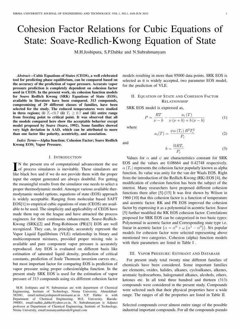
Fig. 1. Variation in deviation with temperature for 1-Pentenol
TABLE IIRANGE OF PROPERTIES OF SELECTED COMPOUNDS
Property(Unit) RangeMinimum Maximum
Critical Temperature (K) 33.18 1735Critical Pressure (bar) 10.4 1608Critical Compressibility Factor 0.184 0.628Acentric factor -0.22 2.389Dipole Moment (dbye) 0 4.07
experimental vapor pressure data were generated using vaporpressure equation reported by Yaws [14]. The coefficients forvapor pressure equation were valid through out temperaturerange from freezing point to critical point for almost all thecompounds. Vapor pressure prediction using SRK EOS wascarried out with the help of equi-fugacity criteria algorithm[15] implemented using MATLAB. MATLAB code generatedvapor pressure predictions at 51 various temperatures betweenfreezing point and critical point for each of the 313 compoundsstudied.
Fig. 2. Variation in deviation with temperature for Xenon
IV. RESULTS AND DISCUSSION
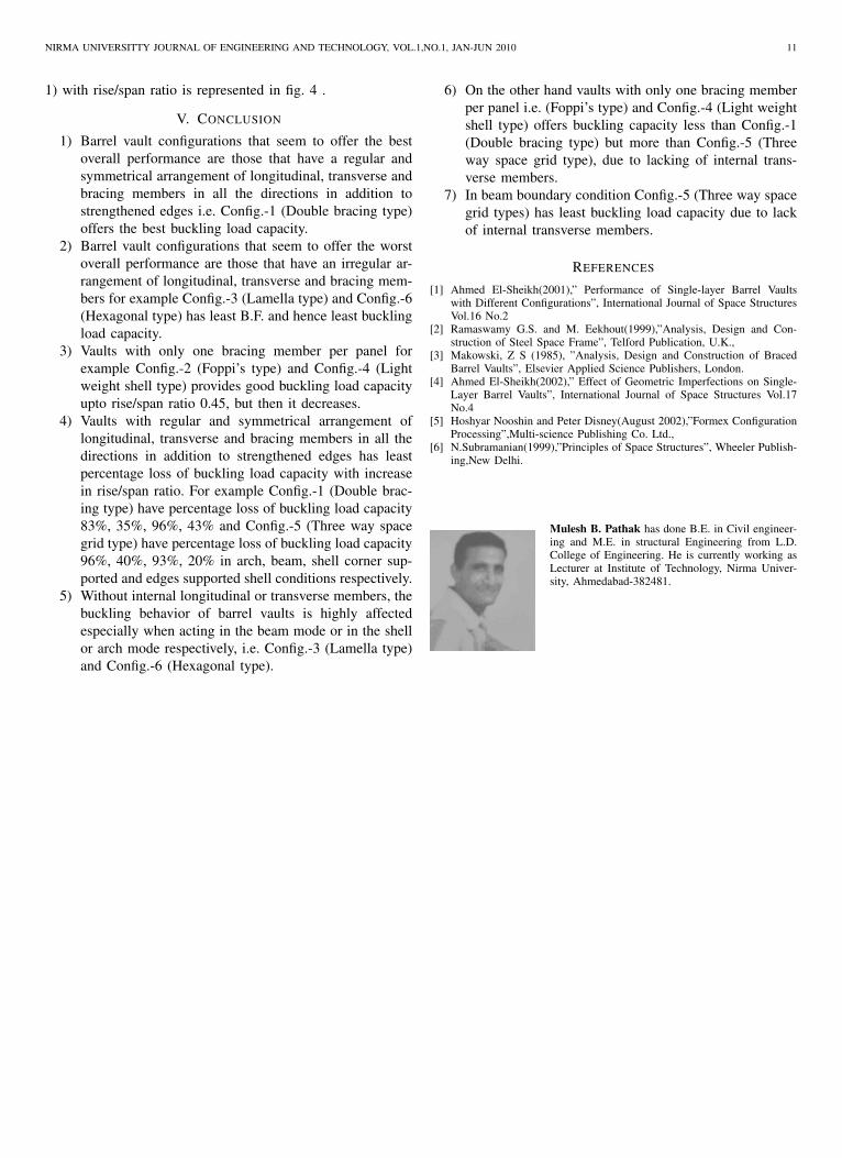
Variation of deviation (Deviation=∑ | (vpcal−vpexp)
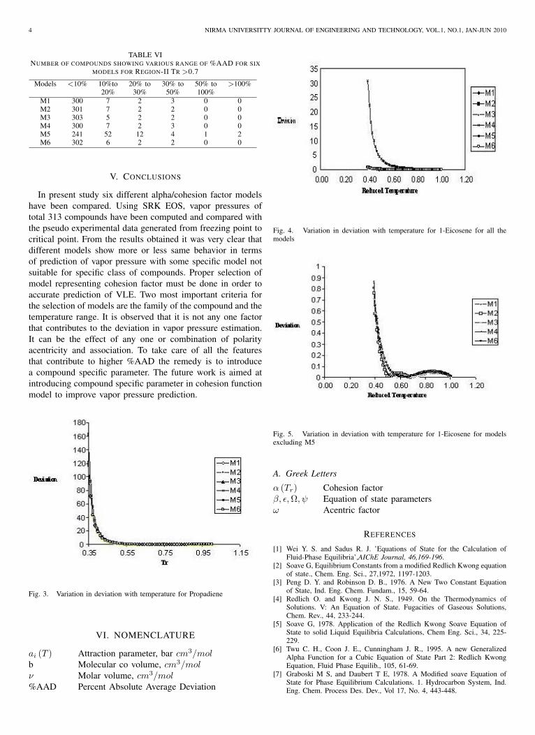
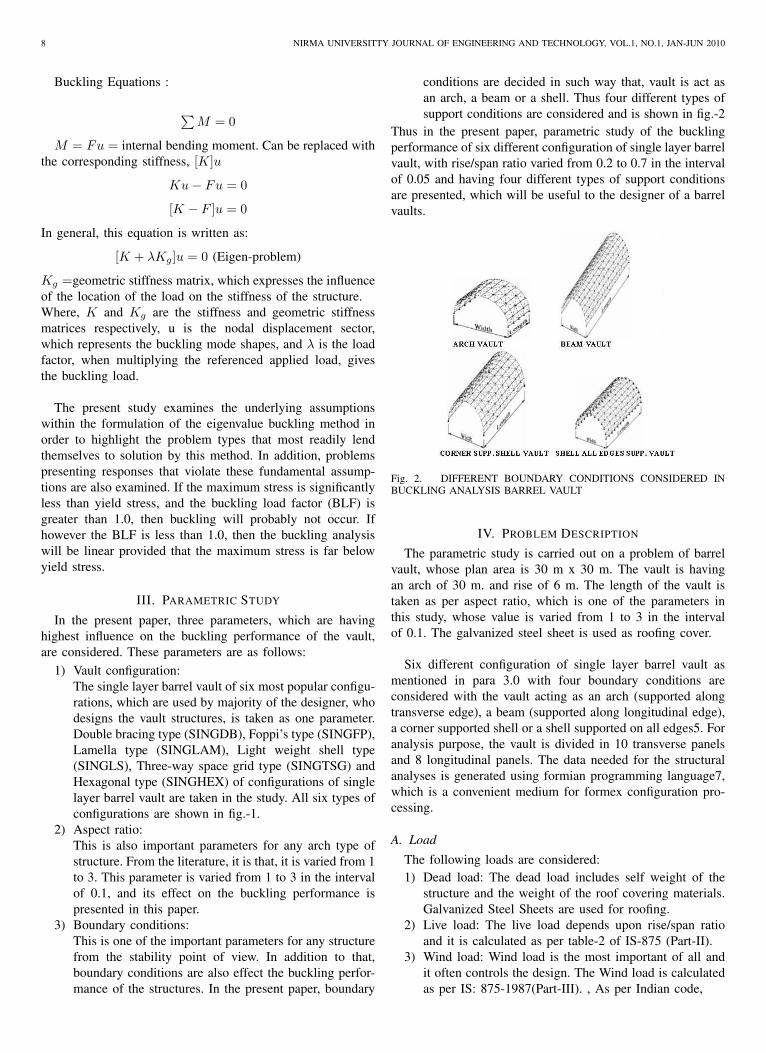
vpexp) |with reduced temperature is shown in figure 1-5 for somerepresentive compounds. For 1-Eicosene Fig. 4 shows theeffect of reduced temperature for all the models. Since de-viation for model 5 is very high compared to other models,the deviation for other models are not visible. This can beobserved separately as shown in Fig. 5. One can observethat the deviation in predicting vapor pressure is very highin the region of reduced temperature less than 0.7 for allcompounds with all the models. Variation in the deviation wassome random function of reduced temperature in the case ofxenon but looking at the deviation values with 0.045 being themaximum, the profile can be considered as almost flat. Thebehavior at supercritical condition was studied earlier [16] andit was found that the cohesion factor with exponential formbehave properly in supercritical region.
Percent Absolute Average Deviation %AAD =(100/N)
∑ vpcal−vpexpvpexp , where N is number of data
NIRMA UNIVERSITTY JOURNAL OF ENGINEERING AND TECHNOLOGY, VOL.1,NO.1, JAN-JUN 2010 3
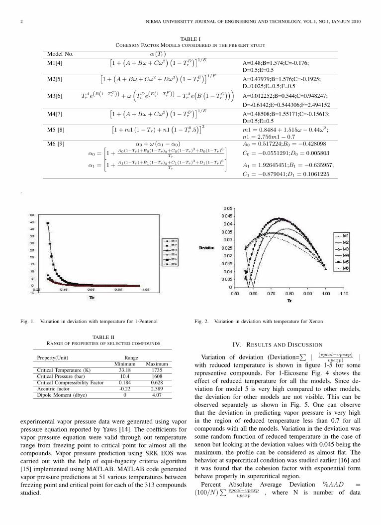
TABLE IIIGLOBAL %AAD FOR THE TWENTY FOUR FAMILIES FOR ALL THE MODELS
Sr. No. Family NC NP M1 M2 M3 M4 M5 M5
1 Elements 11 561 5.530465 5.487029 954.67 5.833413 4.248911 30.469542 NitrogenCompounds 2 102 6.494939 6.477105 6.216155 6.482561 5.941286 6.2921163 Oxides 6 306 4.802966 4.894486 4.86573 4.790565 6.146633 4.9039814 Sulfides 2 102 4.56952 4.563021 3.221615 4.680732 4.484693 3.92515 Chlorides 1 51 3.18553 3.169913 2.439712 3.406223 2.810688 2.3990616 Oxyhelides 1 51 3.173488 3.18587 2.935781 3.130261 5.29759 2.1254147 InorganicCompounds 2 102 10.54289 10.55172 10.95954 10.38885 9.665578 10.799238 Alkanes 56 2856 5.063944 5.021835 4.344802 5.080992 31.75321 4.6517079 Cycloalkanes 28 1428 11.32668 11.40835 9.807308 11.14786 21.00557 9.191612
10 Alkenes 24 1224 8.300484 8.230618 6.723448 8.218378 64.38055 6.44361911 Alkynes 3 153 5.057852 5.047834 5.17691 4.988396 4.519664 5.26053712 Aromatic Hydrocarbons 43 2193 7.229732 7.267374 6.49371 7.209193 20.09188 6.60116813 Halogenated Alkanes 18 918 6.625655 6.633071 6.605537 6.555804 7.79344 6.5535814 Halogenated cycloalkanes 1 51 1.750407 1.798463 1.683846 1.785519 6.728683 2.12301215 Halogenated aromatic hydrocarbons 6 306 3.35086 3.388715 3.263023 3.329795 11.95539 3.46171716 Aldehydes 2 102 9.851131 9.808161 9.583923 9.86807 8.27609 9.76431617 Ketones 8 408 8.95334 8.953088 8.948816 8.980401 13.25756 9.21645318 Alkanoic Acid 2 102 6.738862 6.73266 5.645571 6.704222 32.28159 6.04430819 Esters 3 153 3.179019 3.201067 3.630822 3.108809 8.377952 3.81768520 Phenols 4 204 7.140333 6.763621 6.592857 6.757421 21.08847 10.8091521 Heterocyclic Oxygen Compounds 3 153 7.130636 7.154224 7.46101 6.96686 8.355813 7.00823922 Heterocyclic Nitrogen Compounds 3 153 4.713028 4.811935 5.102364 4.531199 10.77566 4.99180323 Hydrocarbon Nitrogen Compounds 14 714 9.279721 9.281399 9.47755 9.231517 13.48429 9.63476324 Sulfur Compounds 4 204 8.103672 8.095621 8.856863 7.916671 9.683429 8.889783
Global 247 12597 6.337298 6.330299 45.61279 6.295571 13.85019 7.307413
TABLE IVCOMPARISON OF THE MODELS FOR THE FAMILIES SHOWING HIGHER %AAD
Sr. No. Family NC NP M1 M2 M3 M4 M5 M51 Alkadiens 9 459 106.9955 107.2222 114.7703 106.1511 135.9766 109.87512 Halogenated lkenes 2 102 20.04912 20.12007 19.48645 19.75882 22.83724 18.226543 Alcohols 32 1632 137.1214 136.5753 103.531 140.1646 608.2656 106.1564 Ethers 8 408 40.13992 40.22085 40.95173 39.78387 48.3108 39.947155 Others 15 765 18.6932 17.35986 15.82237 17.99158 2943.318 16.21999
Global 66 3366 64.5996 64.2996 58.9129 64.3361 751.7416 58.0849
points) between predicted and pseudo experimental vaporpressures was used for comparison of various models foralpha function. Since, some of the families showed very highAAD their results are reported separately. Table III reportsthe family wise AAD for all the models as well as GlobalAAD for twenty four families where as Table IV reportsthe same for remaining five families (for which AAD wasobserved to be high). Both the tables show that M5 (Soave1992) model has the highest deviation compared to all othermodels. Model M3 (Twu et al) show high deviation as canbe seen in Table III. However, a closer look at AAD valuesof Model M3, will show that very high deviation in elementsfamily makes the Global AAD of model M3 very high.Analysis of compounds considered in elements showed thatmercury (which is considered to associate) was responsiblefor very high deviation in elements family for all most all themodels especially in model M3. Except that all the modelsshow acceptable behavior for vapor pressure predictions.
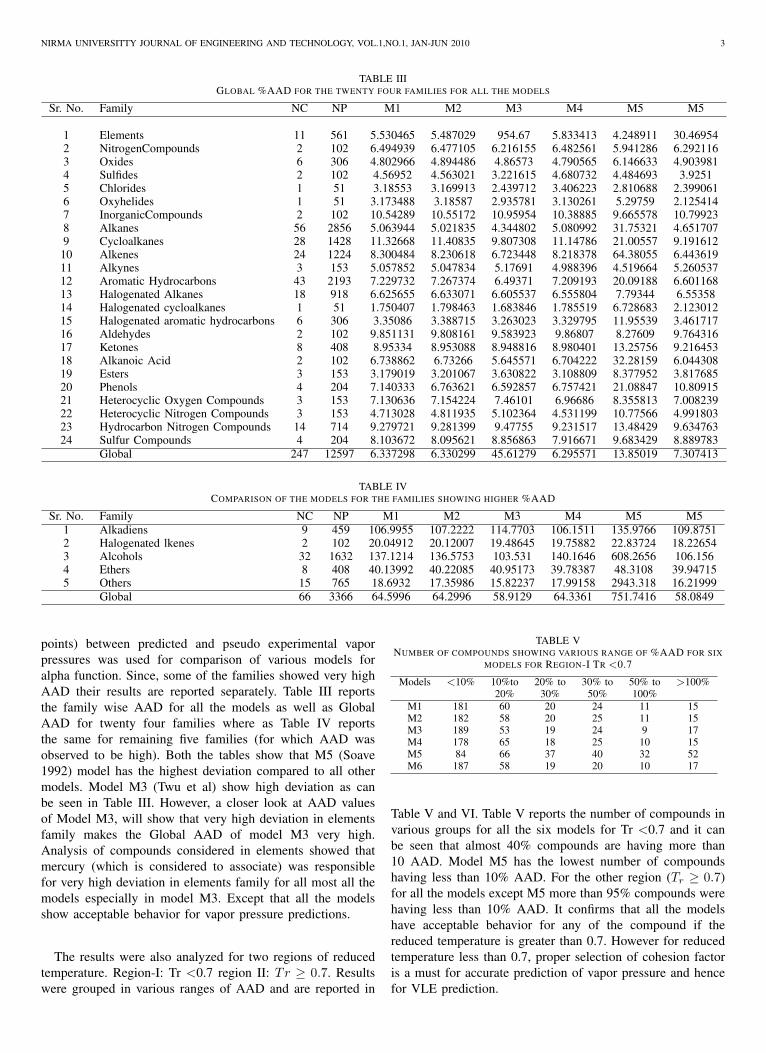
The results were also analyzed for two regions of reducedtemperature. Region-I: Tr <0.7 region II: Tr ≥ 0.7. Resultswere grouped in various ranges of AAD and are reported in
TABLE VNUMBER OF COMPOUNDS SHOWING VARIOUS RANGE OF %AAD FOR SIX
MODELS FOR REGION-I TR <0.7
Models <10% 10%to 20% to 30% to 50% to >100%20% 30% 50% 100%
M1 181 60 20 24 11 15M2 182 58 20 25 11 15M3 189 53 19 24 9 17M4 178 65 18 25 10 15M5 84 66 37 40 32 52M6 187 58 19 20 10 17
Table V and VI. Table V reports the number of compounds invarious groups for all the six models for Tr <0.7 and it canbe seen that almost 40% compounds are having more than10 AAD. Model M5 has the lowest number of compoundshaving less than 10% AAD. For the other region (Tr ≥ 0.7)for all the models except M5 more than 95% compounds werehaving less than 10% AAD. It confirms that all the modelshave acceptable behavior for any of the compound if thereduced temperature is greater than 0.7. However for reducedtemperature less than 0.7, proper selection of cohesion factoris a must for accurate prediction of vapor pressure and hencefor VLE prediction.
4 NIRMA UNIVERSITTY JOURNAL OF ENGINEERING AND TECHNOLOGY, VOL.1, NO.1, JAN-JUN 2010
TABLE VINUMBER OF COMPOUNDS SHOWING VARIOUS RANGE OF %AAD FOR SIX
MODELS FOR REGION-II TR >0.7
Models <10% 10%to 20% to 30% to 50% to >100%20% 30% 50% 100%
M1 300 7 2 3 0 0M2 301 7 2 2 0 0M3 303 5 2 2 0 0M4 300 7 2 3 0 0M5 241 52 12 4 1 2M6 302 6 2 2 0 0
V. CONCLUSIONS
In present study six different alpha/cohesion factor modelshave been compared. Using SRK EOS, vapor pressures oftotal 313 compounds have been computed and compared withthe pseudo experimental data generated from freezing point tocritical point. From the results obtained it was very clear thatdifferent models show more or less same behavior in termsof prediction of vapor pressure with some specific model notsuitable for specific class of compounds. Proper selection ofmodel representing cohesion factor must be done in order toaccurate prediction of VLE. Two most important criteria forthe selection of models are the family of the compound and thetemperature range. It is observed that it is not any one factorthat contributes to the deviation in vapor pressure estimation.It can be the effect of any one or combination of polarityacentricity and association. To take care of all the featuresthat contribute to higher %AAD the remedy is to introducea compound specific parameter. The future work is aimed atintroducing compound specific parameter in cohesion functionmodel to improve vapor pressure prediction.
Fig. 3. Variation in deviation with temperature for Propadiene
VI. NOMENCLATURE
ai (T ) Attraction parameter, bar cm3/molb Molecular co volume, cm3/molν Molar volume, cm3/mol%AAD Percent Absolute Average Deviation
Fig. 4. Variation in deviation with temperature for 1-Eicosene for all themodels
Fig. 5. Variation in deviation with temperature for 1-Eicosene for modelsexcluding M5
A. Greek Letters
α (Tr) Cohesion factorβ, ε,Ω, ψ Equation of state parametersω Acentric factor
REFERENCES
[1] Wei Y. S. and Sadus R. J. ’Equations of State for the Calculation ofFluid-Phase Equilibria’,AIChE Journal, 46,169-196.
[2] Soave G, Equilibrium Constants from a modified Redlich Kwong equationof state., Chem. Eng. Sci., 27,1972, 1197-1203.
[3] Peng D. Y. and Robinson D. B., 1976. A New Two Constant Equationof State, Ind. Eng. Chem. Fundam., 15, 59-64.
[4] Redlich O. and Kwong J. N. S., 1949. On the Thermodynamics ofSolutions. V: An Equation of State. Fugacities of Gaseous Solutions,Chem. Rev., 44, 233-244.
[5] Soave G, 1978. Application of the Redlich Kwong Soave Equation ofState to solid Liquid Equilibria Calculations, Chem Eng. Sci., 34, 225-229.
[6] Twu C. H., Coon J. E., Cunningham J. R., 1995. A new GeneralizedAlpha Function for a Cubic Equation of State Part 2: Redlich KwongEquation, Fluid Phase Equilib., 105, 61-69.
[7] Graboski M S, and Daubert T E, 1978. A Modified soave Equation ofState for Phase Equilibrium Calculations. 1. Hydrocarbon System, Ind.Eng. Chem. Process Des. Dev., Vol 17, No. 4, 443-448.

NIRMA UNIVERSITTY JOURNAL OF ENGINEERING AND TECHNOLOGY, VOL.1,NO.1, JAN-JUN 2010 5
[8] G Soave, 1993, Improving the Treatment of Heavy Hydrocarbons by theSRK EOS, Fluid Phase Equilib., 84, 339-342.
[9] Souahi F., Sator S., Albane S. A., Kies F. K., Chitour C. E., 1998.Development of a New Form for the Alpha Function of the Redlich-Kwong Cubic Equation of State, Fluid Phase Equilib., 153, 73-80.
[10] Twu C. H., Sim W. D. and Tassone V., 2002. Getting a Handle onAdvanced Cubic Equation of State, Chem. Engg. Prog., 58-65.
[11] Valderrama J. O., Arce P. F., Ibrahim A. A., 1999. Vapor-LiquidEquilibrium of H2S-Hydrocarbon Mixtures Using a Generalized CubicEquation of State, Can. J. of Chem. Eng., 77, 1239-1243.
[12] Poling B.E., Prausnitz J. M., and O.Connell J. P., 2001. The Propertiesof Gases and Liquids, International Edition, Mc-GrawHill Publication,New York.
[13] Hernandez Garduza O., Garcia-Sanchez F., Apam-Martinez D. andVazques-Roman R., 2002. Vapor Pressures of Pure Compounds using thePeng-Robinson Equation of State with Three Different Attractive Terms,Fluid Phase Equilb,. 198, 195-228.
[14] Yaws C. L., 1992. Chemical Properties Hand Book, Mc GrawHillPublication, New York.
[15] S I Sandler, 1999, Chemical and Engineering Thermodynamics, thirded., John Wiley & Sons, Inc.
[16] Joshipura M H, Dabke S P and Subrahmanyam N, 2007, Cohesion FactorRelations for Cubic Equations of State-Part I: Peng-Robinson Equation ofState, Proceedings International Conference on Modeling and SimulationCoimbatore.
Milind H. Joshipura is working as an AssistantProfessor in Chemical Engineering Department ofInstitute of Technology in Nirma University, Ahmed-abad. He has obtained his B.E. in Chemical En-gineering from D.D.I.T ,Nadiad (Autonomous Uni-versity) in the year 2000 and Masters in ChemicalEngineering from The M S University, Baroda inyear 2002. His research interest also includes Phaseequilibria studies and Modeling and Simulation. Heis a Life member of ISTE and Associate member ofIndian Institute of Chemical Engineers (IIChE).
S.P.Dabke is a Reader in Chemical EngineeringDepartment at The M S University of Baroda,Vadodara. He received his BE in Chemical Engi-neering from The M S University, Baroda in 1973and M.Tech. from IIT, Kanpur in 1976. His re-search interest includes Thermodynamics and PhaseEquilibria, Modeling and Simulation, and PolymericMaterials. Prof. Dabke is Life Member of IndianInstitute of Chemical Engineers.
N. Subramanyam is an Adjunct Professor at Chem-ical Engineering Department, Institute of Technol-ogy, Nirma University, Ahmedabad. He did hisB.Tech. from Andhra University in 1962 and Ph.Dfrom IISc, Bangalore in 1968. His research inter-ests are Catalysis, Process Developments and Bio-chemical Engineering. He has guided six Ph.D.s andmore than fifty PG students. He is a Fellow Instituteof Engineers, Fellow Indian Institute of ChemicalEngineers and Life Member of ISTE. He was theNational President in IIChE in the year 1999.

6 NIRMA UNIVERSITTY JOURNAL OF ENGINEERING AND TECHNOLOGY, VOL.1, NO.1, JAN-JUN 2010
Buckling Strength of Single-Layer Steel BracedBarrel Vaults
Mulesh K. Pathak, B. J. Shah
Abstract—Barrel vault is a simple structural formation madeup of a network of longitudinal, transverse and bracing memberswith curvature in one direction. The configuration of the vault,or in other words the way in which the members are positionedand connected, has a major effect on the vault’s structuralperformance, aesthetics and cost.
Buckling is a critical state of stress and deformation, at whicha slight disturbance causes a gross additional deformation, orperhaps a total structural failure of the part. Structural behaviorof the part beyond ’buckling’ is not evident from the normalarguments of static. Buckling failures do not depend on thestrength of the material, but are a function of the componentdimensions & modulus of elasticity. Therefore, materials with ahigh strength will buckle just as quickly as low strength ones. If astructure is subject to compressive loads, then a buckling analysismay be necessary. The study presented in this paper is intendedto help designers of steel braced barrel vaults by identifying thesignificant differences determining which configuration(s) wouldbe best in different conditions of use. The study presented is ofparametric type and covers several other important parameterslike rise to span ratio, different boundary conditions, such thatbarrel vault acts as an arch, as a beam or as a shell, The bucklingstrength of a six different configuration of a single layer bracedbarrel vaults are presented in this paper for aspect ratio varyingfrom 1-3 and having four different types of boundary conditions.Through consideration of these parameters, the paper presentsan assessment of the effect of the vault configuration on theoverall buckling strength.
Index Terms—structure, buckling, barrel vaults, sapn ra-tio, single layerstructure, buckling, barrel vaults, sapn ratio, sin-gle layer
I. INTRODUCTION
BArrel vaults are a popular way of spanning large openareas with few intermediate supports. The past four
decades saw an expanding interest in this form of construction.This is understandable because these structures can providea form of roof construction combining low cost and rapiderection with a pleasing appearance. Hundreds of success-ful barrel vault applications for basement, intermediary andground floors now exist all over the world covering publichalls, exhibition centre, aero plane hangers and many otherbuildings. This structure is usually used in all types of environ-ment: urban, rural, plain, mountain or seaside[1]. Barrel vaultshave been built with many different configurations involvingdifferent arrangements of longitudinal, transverse and bracingmembers including those sketched in Fig.1. Starting fromthe basic Configuration-1, bracing members can be placedin different orientations and with different intensities up tothe most congested Configuration-6 for single layer barrel
Mulesh K. Pathak, is with Department of Civil Engineering, Instituteof Technology, Nirma University, B. J. Shah is with Department of CivilEngineering, L. D. College of Engineering, Ahmedabad-380015
vault[2]one:foo. With every variation, it is expected that theperformance of the vault would change, leading sometimesto advantageous improvements in the vault’s strength/weightratio, stiffness/weight ratio, failure mode, member stress distri-bution, material consumption, degree of redundancy, aestheticsand cost[4]. This paper presents the results of a parametricstudy to identify the effects of adopting different barrel vaultconfigurations on the vault’s buckling behavior. The study con-siders wide variations of many important parameters includingrise/span ratio, boundary conditions and configurations. Thebuckling strength of the vault structure is find out using theSTAAD-PRO software. The data needed for the numericalanalyses was generated using formex configuration processing,which is based on formex algebra principles[5].
II. BUCKLING ANALYSIS
”Buckling” is used as a generic term to describe the strengthof structures, generally under in-plane compressions and/orshear. It is particularly dangerous because it is a catastrophicfailure that gives no warning. The buckling strength or capacitycan take into account the internal redistribution of loadsdepending on the situation.
(A) Buckling capacity with allowance for redistributionof load :This defines the lower bound value of the bucklingcapacity. For slender structures, this is defined as theideal elastic buckling stress. This is more conserva-tive than the upper bound value given by Method1 and ensures that the panel does not suffer largeelastic deflections with consequent reduced in-planestiffness.
(B) Buckling capacity with no allowance for redistribu-tion of load :This defines the lower bound value of the bucklingcapacity. For slender structures, this is defined as theideal elastic buckling stress. This is more conserva-tive than the upper bound value given by Method1 and ensures that the panel does not suffer largeelastic deflections with consequent reduced in-planestiffness.
Buckling loads are critical loads where certain types ofstructures become unstable. Each load has an associated buck-led mode shape; this is the shape that the structure assumes ina buckled condition. There are two primary means to performa buckling analysis:
1) Eigenvalue :Eigenvalue (bifurcation) buckling analysis is useful forfinding the load factor and corresponding buckling shape

NIRMA UNIVERSITTY JOURNAL OF ENGINEERING AND TECHNOLOGY, VOL.1,NO.1, JAN-JUN 2010 7
Fig. 1. PRINCIPAL CONFIGURATIONS OF STEEL BRACED SINGLE LAYER BARREL VAULTS
for a given set of loads and constraints. Eigenvalue buck-ling analysis predicts the theoretical buckling strengthof an ideal elastic structure. It computes the structuraleigenvalues for the given system loading and constraints.This is known as classical Euler buckling analysis.Buckling loads for several configurations are readilyavailable from tabulated solutions[6]. However, in real-life, structural imperfections and nonlinearities preventmost real world structures from reaching their eigenvaluepredicted buckling strength; i.e. it over-predicts theexpected buckling loads.
2) Nonlinear :Nonlinear buckling analysis is more accurate than eigen-value analysis because it employs non-linear, large-deflection; static analysis to predict buckling loads. Itsmode of operation is very simple: it gradually increasesthe applied load until a load level is found whereby thestructure becomes unstable (i.e. suddenly a very smallincrease in the load will cause very large deflections).The true non-linear nature of this analysis thus permitsthe modeling of geometric imperfections, load pertur-bations, material nonlinearities and gaps. For this typeof analysis, small off-axis loads are necessary to initiatethe desired buckling mode.
The lowest buckling load is of most practical significance, andis normally achieved when the tangent stiffness associatedwith a mode of deformation becomes zero, such a modethen referred to as the buckling mode. Of course, numeroussophisticated procedures and computational tools have been
developed over the past few decades that deal with structuralbuckling, both in terms of simplified linear eigenvalue analysisand through tracing the geometrically nonlinear response aswell as material nonlinearity. While the approach proposed inthis paper does not deal with a new class of problem, it shedsnew light on the buckling analysis of skeletal structures,enabling better understanding of the buckling mechanisms, andit provides a simplified and practical framework for bucklingpredictions, importantly, using linear analysis principles. Asmentioned above, buckling can be related to the singularityof the tangent stiffness matrix, which in turn consists of twoparts. The first part is the material stiffness matrix whichis related to the deformational stiffness of the components,taking into account the connectivity of components in thecurrent geometric configuration of the structure. For linearelastic components, the material stiffness is identical to thelinear elastic stiffness, but updating the structural geometryto include the effect of any displacements. The second partis the geometric stiffness matrix, which is related to thecomponent forces, and in some cases to the applied loading,taking into account the effect of a change in geometry fromthe current configuration. For typical structures, the materialstiffness is positive for all deformation modes, mathematicallyreferred to as positive-definite, whereas the geometric stiffnesscan admit negative values for certain modes, depending onthe component forces and applied loading. It is thereforethe effect of a negative geometric stiffness that can lead toa singular overall tangent stiffness matrix, and hence buckling.
8 NIRMA UNIVERSITTY JOURNAL OF ENGINEERING AND TECHNOLOGY, VOL.1, NO.1, JAN-JUN 2010
Buckling Equations :
∑M = 0
M = Fu = internal bending moment. Can be replaced withthe corresponding stiffness, [K]u
Ku− Fu = 0
[K − F ]u = 0
In general, this equation is written as:
[K + λKg]u = 0 (Eigen-problem)
Kg =geometric stiffness matrix, which expresses the influenceof the location of the load on the stiffness of the structure.Where, K and Kg are the stiffness and geometric stiffnessmatrices respectively, u is the nodal displacement sector,which represents the buckling mode shapes, and λ is the loadfactor, when multiplying the referenced applied load, givesthe buckling load.
The present study examines the underlying assumptionswithin the formulation of the eigenvalue buckling method inorder to highlight the problem types that most readily lendthemselves to solution by this method. In addition, problemspresenting responses that violate these fundamental assump-tions are also examined. If the maximum stress is significantlyless than yield stress, and the buckling load factor (BLF) isgreater than 1.0, then buckling will probably not occur. Ifhowever the BLF is less than 1.0, then the buckling analysiswill be linear provided that the maximum stress is far belowyield stress.
III. PARAMETRIC STUDY
In the present paper, three parameters, which are havinghighest influence on the buckling performance of the vault,are considered. These parameters are as follows:
1) Vault configuration:The single layer barrel vault of six most popular configu-rations, which are used by majority of the designer, whodesigns the vault structures, is taken as one parameter.Double bracing type (SINGDB), Foppi’s type (SINGFP),Lamella type (SINGLAM), Light weight shell type(SINGLS), Three-way space grid type (SINGTSG) andHexagonal type (SINGHEX) of configurations of singlelayer barrel vault are taken in the study. All six types ofconfigurations are shown in fig.-1.
2) Aspect ratio:This is also important parameters for any arch type ofstructure. From the literature, it is that, it is varied from 1to 3. This parameter is varied from 1 to 3 in the intervalof 0.1, and its effect on the buckling performance ispresented in this paper.
3) Boundary conditions:This is one of the important parameters for any structurefrom the stability point of view. In addition to that,boundary conditions are also effect the buckling perfor-mance of the structures. In the present paper, boundary
conditions are decided in such way that, vault is act asan arch, a beam or a shell. Thus four different types ofsupport conditions are considered and is shown in fig.-2
Thus in the present paper, parametric study of the bucklingperformance of six different configuration of single layer barrelvault, with rise/span ratio varied from 0.2 to 0.7 in the intervalof 0.05 and having four different types of support conditionsare presented, which will be useful to the designer of a barrelvaults.
Fig. 2. DIFFERENT BOUNDARY CONDITIONS CONSIDERED INBUCKLING ANALYSIS BARREL VAULT
IV. PROBLEM DESCRIPTION
The parametric study is carried out on a problem of barrelvault, whose plan area is 30 m x 30 m. The vault is havingan arch of 30 m. and rise of 6 m. The length of the vault istaken as per aspect ratio, which is one of the parameters inthis study, whose value is varied from 1 to 3 in the intervalof 0.1. The galvanized steel sheet is used as roofing cover.
Six different configuration of single layer barrel vault asmentioned in para 3.0 with four boundary conditions areconsidered with the vault acting as an arch (supported alongtransverse edge), a beam (supported along longitudinal edge),a corner supported shell or a shell supported on all edges5. Foranalysis purpose, the vault is divided in 10 transverse panelsand 8 longitudinal panels. The data needed for the structuralanalyses is generated using formian programming language7,which is a convenient medium for formex configuration pro-cessing.
A. Load
The following loads are considered:1) Dead load: The dead load includes self weight of the
structure and the weight of the roof covering materials.Galvanized Steel Sheets are used for roofing.
2) Live load: The live load depends upon rise/span ratioand it is calculated as per table-2 of IS-875 (Part-II).
3) Wind load: Wind load is the most important of all andit often controls the design. The Wind load is calculatedas per IS: 875-1987(Part-III). , As per Indian code,

NIRMA UNIVERSITTY JOURNAL OF ENGINEERING AND TECHNOLOGY, VOL.1,NO.1, JAN-JUN 2010 9
Design For wind Load
Vz = Vb ∗K1 ∗K2 ∗K3
Where Vz is the design wind speed at any height in m/s; .K1 is risk coefficient=1.06 for this case (table-1 IS: 875 Part-3); K2 is terrain, height and structure size factor = 0.76 forcat.4 and class B case (table-2 IS:875 Part-3); K3 = topographyfactor =1 for this case. So, Vz = 31.4184 m/s
Design Wind Pressure
Pd = 0.6V 2z = 592.2695N/m2
Wind force
F = (Cpe − Cpi) ∗A ∗ Pd
Where, Cpe = External pressure coefficient and Cpi =Internal pressure coefficient. The external pressure coefficientCpe = is taken considering the case of roof on elevatedstructure as per table-15 of IS: 875,Part-III (fig.3).In thetable15 of IS-875 values of external pressure coefficients aregiven at interval of 0.1 of H/l ratio. The Excel sheet is usedfor calculation of the intermediate values of Cp = by linearinterpolation. Internal pressure coefficient is based on thepermeability of structure and in this problem, it taken as ±0.2. In this case surface design pressure varies with height, thesurface areas of the structural element may be sub-divided sothat the specified pressures are taken over appropriate areas.Here the total height of the structure was divided into ten equalparts and wind force per sq.m area was calculated using Excelsheet. Positive wind load indicates the force acting towardsthe structural element (pressure) and negative away from it(suction).
Fig. 3. PRESSURE DISTRIBUTION FOR ROOF ON ELEVATED AS PERIS: 875(Part-3)
TABLE ITUNING PARAMETERS FOR THE SYSTEM
H/1 C C20.1 -0.8 -0.80.2 -0.9 -0.70.3 -1.0 -0.30.4 -1.1 +0.40.5 -1.2 +0.7
Four wind load cases were considered(a) Wind load parallel to ridge with Cpi = 0.2
(b) Wind load parallel to ridge with Cpi = −0.2(c) Wind load perpendicular to ridge with Cpi = 0.2(d) Wind load perpendicular to ridge with Cpi = −0.2
The wind load was applied as concentrated loads on thenodes of a barrel vault. Determination of wind force onthe curved surface of the barrel vault is complex task andhence in-house computer program is prepared to calculatewind force at each node of the structure. The nodal loads aredetermined by calculating the area surrounding each node,and multiplying this area by the total factored load. TheExcel sheet is used for the calculation of nodal load. Thisprocess was repeated for each configuration with a differentrise/span ratio and boundary condition.
Following load cases and load combinations are consideredin the analysis
1) Dead load2) Live load3) Wind load parallel to ridge (Cpi = −0.2)4) Wind load parallel to ridge (Cpi = 0.2)5) Wind load perpendicular to ridge (Cpi = −0.2)6) Wind load perpendicular to ridge (Cpi = 0.2)7) Dead load + Live load8) Dead load + Wind load parallel to ridge (Cpi = −0.2)9) Dead load + Wind load parallel to ridge (Cpi = 0.2)
10) Dead load + Wind load perpendicular to ridge (Cpi =−0.2)
11) Dead load + Wind load perpendicular to ridge (Cpi =0.2)
12) Dead load + Live load + Wind load parallel to ridge(Cpi = −0.2)
13) Dead load + Live load + Wind load parallel to ridge(Cpi = 0.2)
14) Dead load + Live load + Wind load perpendicular toridge (Cpi = −0.2)
15) Dead load + Live load + Wind load perpendicular toridge (Cpi = 0.2)
B. Buckling Analysis
Based on the basic loads and load combinations, loads ateach joint of the vault geometry are calculated. The structureis modeled as space truss and accordingly static analysis iscarried out using software. The preliminary analysis & designis carried out using professional software STAAD-Pro. Allrequired checks of IS: 800-1984 are being taken care in thedesign. To get the optimum sections, the facilities given in theSTAAD-Pro are also exploited.
From an analysis point of view, a buckling analysis is usedto find the lowest multiplication factor for the load that willmake a structure buckle. The result of such an analysis is anumber of buckling load factors (BLF). The first BLF (thelowest factor) is always the one of interest. If it is less thanunity, then buckling will occur due to the load being appliedto the structure. The analysis is also used to find the shapeof the buckled structure. Here buckling analysis is done usingSTAAD-Pro 2007 and the variation of first B.F. (i.e. in mode

10 NIRMA UNIVERSITTY JOURNAL OF ENGINEERING AND TECHNOLOGY, VOL.1, NO.1, JAN-JUN 2010
Fig. 4. Response obtained for step change to set point for First Order System for the Ziegler -Nichols tuning parameters
NIRMA UNIVERSITTY JOURNAL OF ENGINEERING AND TECHNOLOGY, VOL.1,NO.1, JAN-JUN 2010 11
1) with rise/span ratio is represented in fig. 4 .
V. CONCLUSION
1) Barrel vault configurations that seem to offer the bestoverall performance are those that have a regular andsymmetrical arrangement of longitudinal, transverse andbracing members in all the directions in addition tostrengthened edges i.e. Config.-1 (Double bracing type)offers the best buckling load capacity.
2) Barrel vault configurations that seem to offer the worstoverall performance are those that have an irregular ar-rangement of longitudinal, transverse and bracing mem-bers for example Config.-3 (Lamella type) and Config.-6(Hexagonal type) has least B.F. and hence least bucklingload capacity.
3) Vaults with only one bracing member per panel forexample Config.-2 (Foppi’s type) and Config.-4 (Lightweight shell type) provides good buckling load capacityupto rise/span ratio 0.45, but then it decreases.
4) Vaults with regular and symmetrical arrangement oflongitudinal, transverse and bracing members in all thedirections in addition to strengthened edges has leastpercentage loss of buckling load capacity with increasein rise/span ratio. For example Config.-1 (Double brac-ing type) have percentage loss of buckling load capacity83%, 35%, 96%, 43% and Config.-5 (Three way spacegrid type) have percentage loss of buckling load capacity96%, 40%, 93%, 20% in arch, beam, shell corner sup-ported and edges supported shell conditions respectively.
5) Without internal longitudinal or transverse members, thebuckling behavior of barrel vaults is highly affectedespecially when acting in the beam mode or in the shellor arch mode respectively, i.e. Config.-3 (Lamella type)and Config.-6 (Hexagonal type).
6) On the other hand vaults with only one bracing memberper panel i.e. (Foppi’s type) and Config.-4 (Light weightshell type) offers buckling capacity less than Config.-1(Double bracing type) but more than Config.-5 (Threeway space grid type), due to lacking of internal trans-verse members.
7) In beam boundary condition Config.-5 (Three way spacegrid types) has least buckling load capacity due to lackof internal transverse members.
REFERENCES
[1] Ahmed El-Sheikh(2001),” Performance of Single-layer Barrel Vaultswith Different Configurations”, International Journal of Space StructuresVol.16 No.2
[2] Ramaswamy G.S. and M. Eekhout(1999),”Analysis, Design and Con-struction of Steel Space Frame”, Telford Publication, U.K.,
[3] Makowski, Z S (1985), ”Analysis, Design and Construction of BracedBarrel Vaults”, Elsevier Applied Science Publishers, London.
[4] Ahmed El-Sheikh(2002),” Effect of Geometric Imperfections on Single-Layer Barrel Vaults”, International Journal of Space Structures Vol.17No.4
[5] Hoshyar Nooshin and Peter Disney(August 2002),”Formex ConfigurationProcessing”,Multi-science Publishing Co. Ltd.,
[6] N.Subramanian(1999),”Principles of Space Structures”, Wheeler Publish-ing,New Delhi.
Mulesh B. Pathak has done B.E. in Civil engineer-ing and M.E. in structural Engineering from L.D.College of Engineering. He is currently working asLecturer at Institute of Technology, Nirma Univer-sity, Ahmedabad-382481.
12 NIRMA UNIVERSITTY JOURNAL OF ENGINEERING AND TECHNOLOGY, VOL.1, NO.1, JAN-JUN 2010
Region based Multimodality Image Fusion MethodTanish Zaveri and Mukesh Zaveri
Abstract—This paper proposes a novel region based imagefusion scheme based on high boost filtering concept using discretewavelet transform. In the recent literature, region based imagefusion methods show better performance than pixel based imagefusion method. The graph based normalized cutest algorithmis used for image segmentation. Proposed method is a novelidea which uses high boost filtering concept to get an accuratesegmentation using discrete wavelet transform. This concept isused to extract regions from input registered source images whichis then compared with different fusion rules. The new MMSfusion rule is also proposed to fuse multimodality images. Thedifferent fusion rules are applied on various categories of inputsource images and resultant fused image is generated. Proposedmethod is applied on large number of registered images of variouscategories of multifocus and multimodality images and resultsare compared using standard reference based and nonreferencebased image fusion parameters. It has been observed fromsimulation results that our proposed algorithm is consistent andpreserves more information compared to earlier reported pixelbased and region based methods.
Index Terms—Normalized cutset, discrete wavelet transform,high boost filter
I. INTRODUCTION
WE use the term image fusion to denote a process bywhich multiple images or information from multiple
images is combined. These images may be obtained from dif-ferent types of sensors. With the availability of the multisensordata in many fields, such as remote sensing, medical imagingor machine vision, image fusion has emerged as a promisingand important research area. In other words, Image fusion isa process of combining multiple input images of the samescene into a single fused image, which preserves full contentinformation and also retaining the important features fromeach of the original images. There has been a growing interestin the use of multiple sensors to increase the capabilities ofintelligent machines and systems. Actually computer systemshave been developed that are capable of extracting meaningfulinformation from the recorded data coming form the differentsources. The integration of data, recorded from a multisensorsystem, together with knowledge, is known as data fusion [1,2, 3, 4, 5, 6]. With the availability of the multisensor datain many fields, such as remote sensing, medical imaging ormachine vision; image fusion has emerged as a promising andessential research area. The fused image should have moreuseful information content compared to the individual image.The different image fusion methods can be evaluated usingdifferent fusion parameters [7, 8, 9] and each parameter variesdue to different fusion rule effect. In general, the parameter
Tanish Zaveri is with Electronics & Communication Engineering De-partment Institute of Technology, Nirma Universityt, Ahmedabad-382481and Mukesh Zaveri is with Department of Computer Engineering, SardarVallabhbhai National Institute of Technology, Surat- 390002, India,Email:[email protected] and [email protected]
used to design fusion rules is based on experiments or itadaptively changes with the change in image contents so itis very difficult to get the optimal fusion effect which canpreserve all important information from the source images.Image fusion system has several advantages over single imagesource and resultant fused image should have higher signalto noise ratio, increased robustness and reliability in theevent of sensor failure, extended parameter coverage andrendering a more complete picture of the system [1]. Theactual fusion process can take place at different levels ofinformation representation. A common categorization is todistinguish between pixel, feature and decision level, althoughthere may be crossings between them. Image fusion at pixellevel amounts to integration of low-level information, in mostcases physical measurements such as intensity.
The simple pixel based image fusion method is to take theaverage of the source images pixel by pixels which leads toundesired side effects in the resultant image. There are varioustechniques for image fusion at pixel level are available inliterature [2, 4, 5, 6]. The region based algorithm has manyadvantages over pixel base algorithm like it is less sensitive tonoise, better contrast, less affected by misregistration but at thecost of complexity [2]. Recently researchers have recognizedthat it is more meaningful to
combine objects or regions rather than pixels. Piella [3]has proposed a multiresolution region based fusion schemeusing link pyramid approach. Recently, Li and young [10] haveproposed multifocus image fusion using region segmentationand spatial frequency.
Zhang and Blum [4] proposed a categorization of multiscaledecomposition based image fusion schemes for multifocusimages. As per the literature [2, 4] large part of research onmultiresolution (MR) image fusion has focused on choosing anappropriate representation which facilitates the selection andcombination of salient features. The issues to be address arethe specific type of MR decomposition like pyramid, wavelet,linear, morphological etc. and the number of decompositionlevels. More decomposition levels do not necessarily pro-duces better results [4] but by increasing the analysis depthneighboring features of lower band may overlap. This givesrise to discontinuities in the composite representation andthus introduces distortions, such as blocking effect or ringingartifacts into the fused image. The first level discrete wavelettransform (DWT) based decomposition is used in proposedalgorithm to keep it free from disadvantages of Multiscaletransform.
In this paper, a novel region based image fusion algorithm isproposed. The proposed method provides powerful frameworkfor region based image fusion method which produces goodquality fused image for different categories of images. Thenovelty of our algorithm lies in the way high boost filtering
NIRMA UNIVERSITTY JOURNAL OF ENGINEERING AND TECHNOLOGY, VOL.1,NO.1, JAN-JUN 2010 13
concept used to segment decomposed images using DWT.The novel fusion rule Mean Max Standard deviation (MMS)is also proposed to measure the activity level between twosegmented regions of multimodality images. The normalizedcut algorithm [11] is used to segment input images. Thepaper is organized as follows. Section 2 gives a brief intro-duction of DWT and normalized cut segmentation algorithm.In this section brief concept of high boost filtering alsoexplained. Proposed algorithm is described in section 3. Thebrief introduction of reference based and nonreference basedimage fusion parameters are described brief in section 4. Thesimulation results are depicted in section 5. It is followed byconclusion.
II. BASIC THEORY
The proposed algorithm is using on discrete wavelet trans-form, normalized cut segmentation algorithm and high boostfiltering approach which is describe brief in this section.
Wavelet Transform
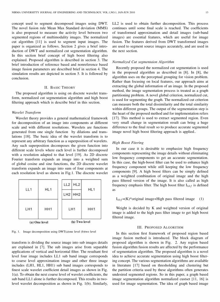
Wavelet theory provides a general mathematical frameworkfor decomposition of an image into components at differentscale and with different resolutions. Wavelets are functionsgenerated from one single function by dilations and trans-lations [18]. The basic idea of the wavelet transform is torepresent any arbitrary function as a superposition of wavelets.Any such superposition decomposes the given function intodifferent scale levels where each level is further decomposedwith a resolution adapted to that level [19]. As 2D discreteFourier transform expands an image into a weighted sumof global cosine and sine functions, the 2D discrete wavelettransform expands an image into sum of four components ateach resolution level as shown in Fig.1. The discrete wavelet
Fig. 1. Image decomposition using DWT(a)one level (b)two level
transform is dividing the source image into sub images detailsare explained in [7]. The sub images arise from separableapplications of vertical and horizontal filter. The resultant firstlevel four image includes LL1 sub band image correspondsto coarse level approximation image and other three imageincludes (LH1, HL1, HH1) sub band images corresponds tofinest scale wavelet coefficient detail images as shown in Fig.1(a). To obtain the next coarse level of wavelet coefficients, thesub band LL1 alone is further decomposed. This results in two-level wavelet decomposition as shown in Fig. 1(b). Similarly,
LL2 is used to obtain further decomposition. This processcontinues until some final scale is reached. The coefficientsof transformed approximation and detail images (sub-bandimages) are essential features, which are useful for imagefusion. The features derived from DWT transformed imagesare used to segment source images accurately, and are used inthe next section.
Normalized Cut segmentaion Algorithm
Recently proposed the normalized cut segmentation is usedin the proposed algorithm as described in [8]. In [8], thealgorithm uses on the perceptual grouping for vision problem.Rather than focusing on local features, our approach aims atextracting the global information of an image. In the proposedmethod, the image segmentation process is treated as a graphpartitioning problem. A novel global criterion, normalized cut,is used for segmenting the graph. The normalized cut criterioncan measure both the total dissimilarity and the total similaritywithin different groups. The output of the segmentation step isthe heart of the proposed method and for implementation refers[17]. This method is used to extract segmented region. Evenvery small change in segmentation result can bring a hugedifference to the final result so to produce accurate segmentedimage novel high boost filtering approach is applied..
High Boost Fitering
In our case it is desirable to emphasize high frequencycomponents representing the image details without eliminatinglow frequency components to get an accurate segmentation.In this case, the high-boost filter can be used to enhance highfrequency component while still keeping the low frequencycomponents [9]. A high boost filters can be simply definedas a weighted combination of original image and the highpass filtered version of the image. It is also called as highfrequency emphasis filter. The high boost filter Ihbf is definedas
Ihbf=(K)*original image+High pass filtered image (1)
Weight is decided by K and weighted version of originalimage is added to the high pass filter image to get high boostfiltered image.
III. PROPOSED ALGORITHM
In this section first framework of proposed region basedimage fusion method is introduced. The block diagram ofproposed algorithm is shown in Fig. 2. Any region basedfusion algorithm fusion results are affected by the performanceof segmentation algorithm. The proposed algorithm is a novelidea to achieve accurate segmentation using high boost filter-ing concept. The various segmentation algorithms are availablein literature [17] based on thresholding and clustering butthe partition criteria used by these algorithms often generatesundesired segmented regions. So in this paper, a graph basedimage segmentation algorithm normalized custset [11, 16] isused for image segmentation. The idea of graph based image
14 NIRMA UNIVERSITTY JOURNAL OF ENGINEERING AND TECHNOLOGY, VOL.1, NO.1, JAN-JUN 2010
segmentation is that the set of points are represented as aweighted undirected graph [10, 11] where the nodes of thegraph are the points in the image. Each pair of nodes isconnected by edge and weight on each edge is a function ofsimilarity between nodes. In our method, a strong similarityrelation between nodes is established using high boost filtering.
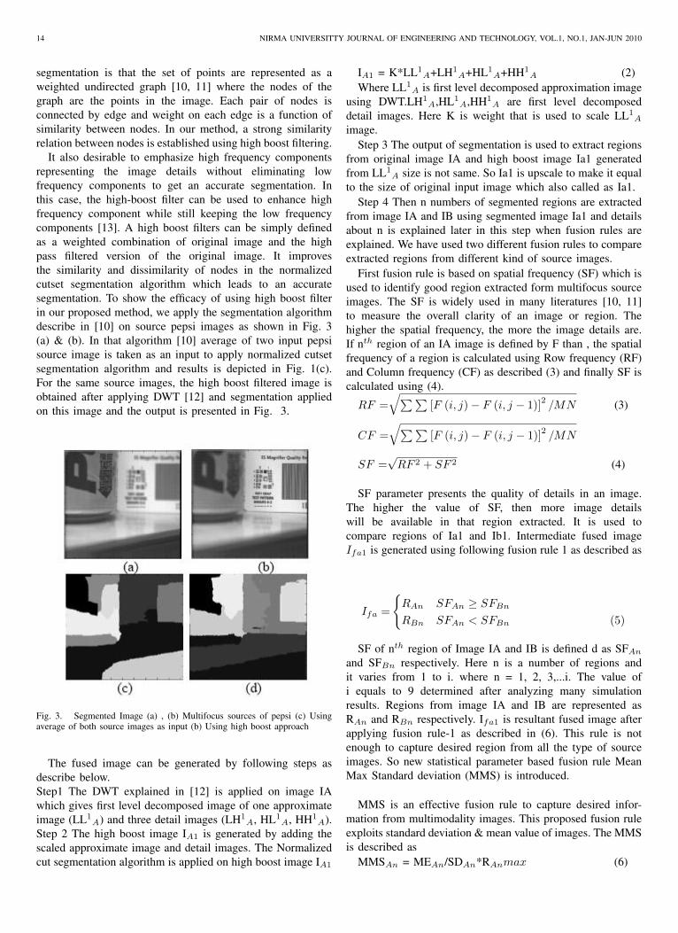
It also desirable to emphasize high frequency componentsrepresenting the image details without eliminating lowfrequency components to get an accurate segmentation. Inthis case, the high-boost filter can be used to enhance highfrequency component while still keeping the low frequencycomponents [13]. A high boost filters can be simply definedas a weighted combination of original image and the highpass filtered version of the original image. It improvesthe similarity and dissimilarity of nodes in the normalizedcutset segmentation algorithm which leads to an accuratesegmentation. To show the efficacy of using high boost filterin our proposed method, we apply the segmentation algorithmdescribe in [10] on source pepsi images as shown in Fig. 3(a) & (b). In that algorithm [10] average of two input pepsisource image is taken as an input to apply normalized cutsetsegmentation algorithm and results is depicted in Fig. 1(c).For the same source images, the high boost filtered image isobtained after applying DWT [12] and segmentation appliedon this image and the output is presented in Fig. 3.
Fig. 3. Segmented Image (a) , (b) Multifocus sources of pepsi (c) Usingaverage of both source images as input (b) Using high boost approach
The fused image can be generated by following steps asdescribe below.Step1 The DWT explained in [12] is applied on image IAwhich gives first level decomposed image of one approximateimage (LL1
A) and three detail images (LH1A, HL1
A, HH1A).
Step 2 The high boost image IA1 is generated by adding thescaled approximate image and detail images. The Normalizedcut segmentation algorithm is applied on high boost image IA1
IA1 = K*LL1A+LH1
A+HL1A+HH1
A (2)Where LL1
A is first level decomposed approximation imageusing DWT.LH1
A,HL1A,HH1
A are first level decomposeddetail images. Here K is weight that is used to scale LL1
A
image.Step 3 The output of segmentation is used to extract regions
from original image IA and high boost image Ia1 generatedfrom LL1
A size is not same. So Ia1 is upscale to make it equalto the size of original input image which also called as Ia1.
Step 4 Then n numbers of segmented regions are extractedfrom image IA and IB using segmented image Ia1 and detailsabout n is explained later in this step when fusion rules areexplained. We have used two different fusion rules to compareextracted regions from different kind of source images.
First fusion rule is based on spatial frequency (SF) which isused to identify good region extracted form multifocus sourceimages. The SF is widely used in many literatures [10, 11]to measure the overall clarity of an image or region. Thehigher the spatial frequency, the more the image details are.If nth region of an IA image is defined by F than , the spatialfrequency of a region is calculated using Row frequency (RF)and Column frequency (CF) as described (3) and finally SF iscalculated using (4).
RF =√∑∑
[F (i, j)− F (i, j − 1)]2/MN (3)
CF =√∑∑
[F (i, j)− F (i, j − 1)]2/MN
SF =√RF 2 + SF 2 (4)
SF parameter presents the quality of details in an image.The higher the value of SF, then more image detailswill be available in that region extracted. It is used tocompare regions of Ia1 and Ib1. Intermediate fused imageIfa1 is generated using following fusion rule 1 as described as
Ifa =
RAn SFAn ≥ SFBnRBn SFAn < SFBn (5)
SF of nth region of Image IA and IB is defined d as SFAnand SFBn respectively. Here n is a number of regions andit varies from 1 to i. where n = 1, 2, 3,...i. The value ofi equals to 9 determined after analyzing many simulationresults. Regions from image IA and IB are represented asRAn and RBn respectively. Ifa1 is resultant fused image afterapplying fusion rule-1 as described in (6). This rule is notenough to capture desired region from all the type of sourceimages. So new statistical parameter based fusion rule MeanMax Standard deviation (MMS) is introduced.
MMS is an effective fusion rule to capture desired infor-mation from multimodality images. This proposed fusion ruleexploits standard deviation & mean value of images. The MMSis described as
MMSAn = MEAn/SDAn*RAnmax (6)
NIRMA UNIVERSITTY JOURNAL OF ENGINEERING AND TECHNOLOGY, VOL.1,NO.1, JAN-JUN 2010 15
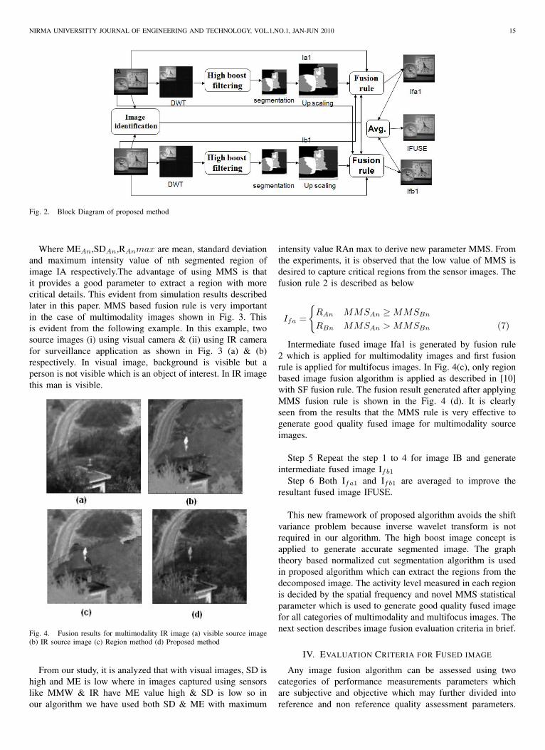
Fig. 2. Block Diagram of proposed method
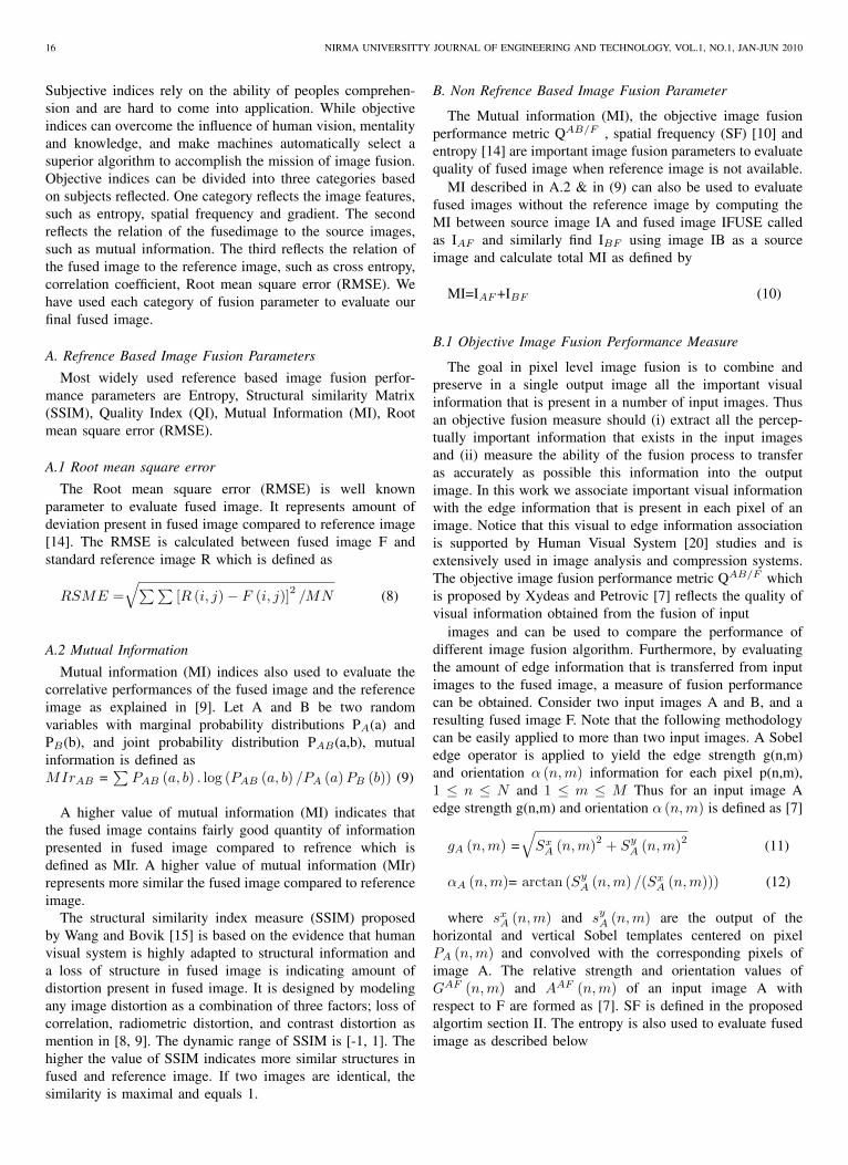
Where MEAn,SDAn,RAnmax are mean, standard deviationand maximum intensity value of nth segmented region ofimage IA respectively.The advantage of using MMS is thatit provides a good parameter to extract a region with morecritical details. This evident from simulation results describedlater in this paper. MMS based fusion rule is very importantin the case of multimodality images shown in Fig. 3. Thisis evident from the following example. In this example, twosource images (i) using visual camera & (ii) using IR camerafor surveillance application as shown in Fig. 3 (a) & (b)respectively. In visual image, background is visible but aperson is not visible which is an object of interest. In IR imagethis man is visible.
Fig. 4. Fusion results for multimodality IR image (a) visible source image(b) IR source image (c) Region method (d) Proposed method
From our study, it is analyzed that with visual images, SD ishigh and ME is low where in images captured using sensorslike MMW & IR have ME value high & SD is low so inour algorithm we have used both SD & ME with maximum
intensity value RAn max to derive new parameter MMS. Fromthe experiments, it is observed that the low value of MMS isdesired to capture critical regions from the sensor images. Thefusion rule 2 is described as below
Ifa =
RAn MMSAn ≥MMSBn
RBn MMSAn > MMSBn (7)
Intermediate fused image Ifa1 is generated by fusion rule2 which is applied for multimodality images and first fusionrule is applied for multifocus images. In Fig. 4(c), only regionbased image fusion algorithm is applied as described in [10]with SF fusion rule. The fusion result generated after applyingMMS fusion rule is shown in the Fig. 4 (d). It is clearlyseen from the results that the MMS rule is very effective togenerate good quality fused image for multimodality sourceimages.
Step 5 Repeat the step 1 to 4 for image IB and generateintermediate fused image Ifb1
Step 6 Both Ifa1 and Ifb1 are averaged to improve theresultant fused image IFUSE.
This new framework of proposed algorithm avoids the shiftvariance problem because inverse wavelet transform is notrequired in our algorithm. The high boost image concept isapplied to generate accurate segmented image. The graphtheory based normalized cut segmentation algorithm is usedin proposed algorithm which can extract the regions from thedecomposed image. The activity level measured in each regionis decided by the spatial frequency and novel MMS statisticalparameter which is used to generate good quality fused imagefor all categories of multimodality and multifocus images. Thenext section describes image fusion evaluation criteria in brief.
IV. EVALUATION CRITERIA FOR FUSED IMAGE
Any image fusion algorithm can be assessed using twocategories of performance measurements parameters whichare subjective and objective which may further divided intoreference and non reference quality assessment parameters.
16 NIRMA UNIVERSITTY JOURNAL OF ENGINEERING AND TECHNOLOGY, VOL.1, NO.1, JAN-JUN 2010
Subjective indices rely on the ability of peoples comprehen-sion and are hard to come into application. While objectiveindices can overcome the influence of human vision, mentalityand knowledge, and make machines automatically select asuperior algorithm to accomplish the mission of image fusion.Objective indices can be divided into three categories basedon subjects reflected. One category reflects the image features,such as entropy, spatial frequency and gradient. The secondreflects the relation of the fusedimage to the source images,such as mutual information. The third reflects the relation ofthe fused image to the reference image, such as cross entropy,correlation coefficient, Root mean square error (RMSE). Wehave used each category of fusion parameter to evaluate ourfinal fused image.
A. Refrence Based Image Fusion Parameters
Most widely used reference based image fusion perfor-mance parameters are Entropy, Structural similarity Matrix(SSIM), Quality Index (QI), Mutual Information (MI), Rootmean square error (RMSE).
A.1 Root mean square error
The Root mean square error (RMSE) is well knownparameter to evaluate fused image. It represents amount ofdeviation present in fused image compared to reference image[14]. The RMSE is calculated between fused image F andstandard reference image R which is defined as
RSME =√∑∑
[R (i, j)− F (i, j)]2/MN (8)
A.2 Mutual Information
Mutual information (MI) indices also used to evaluate thecorrelative performances of the fused image and the referenceimage as explained in [9]. Let A and B be two randomvariables with marginal probability distributions PA(a) andPB(b), and joint probability distribution PAB(a,b), mutualinformation is defined asMIrAB =
∑PAB (a, b) . log (PAB (a, b) /PA (a)PB (b)) (9)
A higher value of mutual information (MI) indicates thatthe fused image contains fairly good quantity of informationpresented in fused image compared to refrence which isdefined as MIr. A higher value of mutual information (MIr)represents more similar the fused image compared to referenceimage.
The structural similarity index measure (SSIM) proposedby Wang and Bovik [15] is based on the evidence that humanvisual system is highly adapted to structural information anda loss of structure in fused image is indicating amount ofdistortion present in fused image. It is designed by modelingany image distortion as a combination of three factors; loss ofcorrelation, radiometric distortion, and contrast distortion asmention in [8, 9]. The dynamic range of SSIM is [-1, 1]. Thehigher the value of SSIM indicates more similar structures infused and reference image. If two images are identical, thesimilarity is maximal and equals 1.
B. Non Refrence Based Image Fusion Parameter
The Mutual information (MI), the objective image fusionperformance metric QAB/F , spatial frequency (SF) [10] andentropy [14] are important image fusion parameters to evaluatequality of fused image when reference image is not available.
MI described in A.2 & in (9) can also be used to evaluatefused images without the reference image by computing theMI between source image IA and fused image IFUSE calledas IAF and similarly find IBF using image IB as a sourceimage and calculate total MI as defined by
MI=IAF+IBF (10)
B.1 Objective Image Fusion Performance Measure
The goal in pixel level image fusion is to combine andpreserve in a single output image all the important visualinformation that is present in a number of input images. Thusan objective fusion measure should (i) extract all the percep-tually important information that exists in the input imagesand (ii) measure the ability of the fusion process to transferas accurately as possible this information into the outputimage. In this work we associate important visual informationwith the edge information that is present in each pixel of animage. Notice that this visual to edge information associationis supported by Human Visual System [20] studies and isextensively used in image analysis and compression systems.The objective image fusion performance metric QAB/F whichis proposed by Xydeas and Petrovic [7] reflects the quality ofvisual information obtained from the fusion of input
images and can be used to compare the performance ofdifferent image fusion algorithm. Furthermore, by evaluatingthe amount of edge information that is transferred from inputimages to the fused image, a measure of fusion performancecan be obtained. Consider two input images A and B, and aresulting fused image F. Note that the following methodologycan be easily applied to more than two input images. A Sobeledge operator is applied to yield the edge strength g(n,m)and orientation α (n,m) information for each pixel p(n,m),1 ≤ n ≤ N and 1 ≤ m ≤ M Thus for an input image Aedge strength g(n,m) and orientation α (n,m) is defined as [7]
gA (n,m) =√SxA (n,m)
2+ SyA (n,m)
2 (11)
αA (n,m)= arctan (SyA (n,m) /(SxA (n,m))) (12)
where sxA (n,m) and syA (n,m) are the output of thehorizontal and vertical Sobel templates centered on pixelPA (n,m) and convolved with the corresponding pixels ofimage A. The relative strength and orientation values ofGAF (n,m) and AAF (n,m) of an input image A withrespect to F are formed as [7]. SF is defined in the proposedalgortim section II. The entropy is also used to evaluate fusedimage as described below
NIRMA UNIVERSITTY JOURNAL OF ENGINEERING AND TECHNOLOGY, VOL.1,NO.1, JAN-JUN 2010 17
(13)
AAF (n,m)=||αA (n,m)αA (n,m) |−Π/2| /Π/2 (14)
These are used to derive the edge strength and orientationpreservation values
QAFg (n,m)=Γg/1 + ekg(GAF (n,m)−σg) (15)
QAFα (n,m)=Γg/1 + ekα(AAF (n,m)−σα) (16)
QAFg (n,m)and QAFα (n,m) model perceptual loss ofinformation in F, in terms of how well the strength andorientation values of a pixel p(n,m) in A are represented inthe fused image. The constants Γg ,κg ,σg and Γα, κα, σαdetermine the exact shape of the sigmoid functions used toform the edge strength and orientation preservation values,see equations (15) and (16). Edge information preservationvalues QAB/F is then defined as
QAB/F (n,m)=N∑
n=1
M∑
m=1
QAF (n,m)WA (n,m)
+QBF (n,m)WB (n,m)
/N∑
i=1
M∑
j=1
(WA (i, j) +WB (i, j)
)(17)
with 0 ≤ QAF (n,m) ≤ 1. A value of 0 corresponds tothe complete loss of edge information, at location (n,m), astransferred from A into F.QAF (n,m) = 1 indicates ”fusion”from A to F with no loss of information.
B.3 Information Entropy
Entropy is an index to evaluate the information quantitycontained in an image. The entropy of the fused image F isdefined as
E=−∑L−1i=0 Pi (f) log2 Pi (f) (18)
Where p is the normalized histogram of the fused imageto be evaluated in our case it is IFUSE, L is maximum valuefor a pixel in the image which defines the total of grey levels.The entropy issued to measure the overall information in thefused image. The larger the entropy value better the fusionresults. The simulation results are discussed in detail in thenext section.
V. EXPERIMENTAL RESULTS AND DISCUSSION
The novel region based image fusion algorithm describedin previous section has been implemented using Matlab 7.The proposed algorithm are applied and evaluated usinglarge number of dataset images which contain broad rangeof multifocus and multimodality images of various categorieslike multifocus with only object, object plus text, onlytext images and multi modality IR (Infrared) and MMW(Millimeter Wave) images to verify the robustness of analgorithm and simulation results are shown in Fig. 5 to 10.
In the proposed method, high boost filtering approach isused to increase the accuracy of segmentation and as describedin (1) are used with the K equal to 5 for pair of multimodalityimages and K equal to 2 for pair of multifocus images. Thesevalues are determined after analyzing the simulation resultsof many experiments which improve the visual quality offinal fused image. The performance of proposed algorithmevaluated using standard reference based and nonreferencebased image fusion evaluation parameters explained in pre-vious section and proposed algorithm simulation results arecompared with earlier reported region based [5] and pixelbased image fusion algorithm [10] and simulation results aredepicted in Table I, II and III.
A. Fusion Resutls of multi-focus images
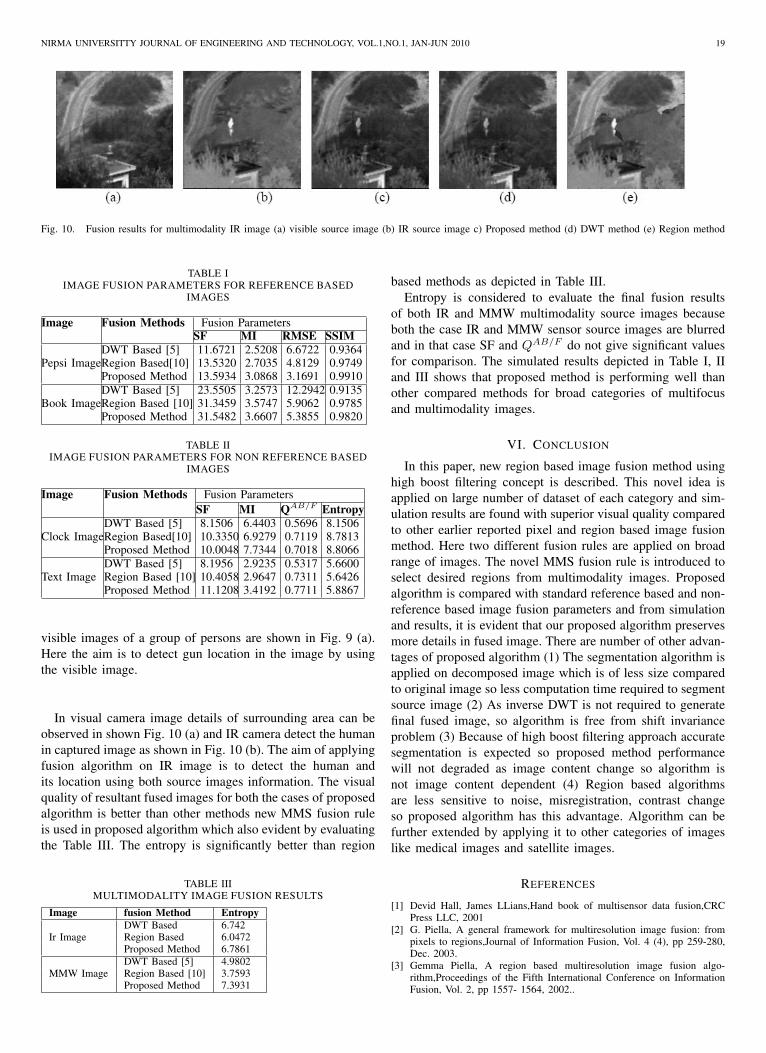
The multifocus images available in our dataset are of threekinds (1) object images (2) only text images and (3) objectplus text images which are shown in Fig. 5 (a) & (b) clockimage, Fig. 6 (a) & (b) text image, Fig. 8 (a) & (b) pepsiimage and Fig. 8 (a) & (b) book image respectively. In Fig.5 to 8 column (a) multifocus images, left portion is blurredand in column (b) of same figure, right portions of imagesis blurred and column (c) shows the corresponding fusedimage obtained by applying proposed method and column(d) and (e) are resultant fused image obtained by applyingpixel based DWT method proposed by Wang [5] and regionbased fusion method proposed by Li and Yang [10]. The visualquality of the resultant fused image of proposed algorithmis better than the fused image obtained by other comparedmethods. The reference based and non reference based imagefusion parameters comparisons are depicted in Table I andTable II. All reference based image fusion parameters SF,MIr, RMSE and SSIM are significantly good for proposedalgorithm compared to other methods as depicted in Table I.Also non reference based image fusion parameters as depictedin Table II are better than compared methods. In Table II, SFand QAB/F are remarkably better than other compared fusionmethods which also evident from the visual quality of resultantfused image.
B. Fusion of infrared and MMW images
The effectiveness of the proposed algorithm can be provedby extending it to its application to the multimodalityconcealed weapon detection (MMW images) and IR images.MMW camera image with the gun is shown in Fig. 9 (b) and

18 NIRMA UNIVERSITTY JOURNAL OF ENGINEERING AND TECHNOLOGY, VOL.1, NO.1, JAN-JUN 2010
Fig. 5. Fusion results of multi-focus image of clock (a), (b) Multi-focus source images (c) Proposed method (d) DWT method (e) Region method
Fig. 6. Fusion results of multi-focus image of text (a), (b) Multi-focus source images (c) Proposed method (d) DWT method (e) Region method
Fig. 7. Fusion results multi-focus image of pepsi (a), (b) Multi-focus source images (c) Proposed method (d) DWT method (e) Region method
Fig. 8. Fusion results multi-focus image of book (a), (b) Multi-focus source images (c) Proposed method (d) DWT method (e) Region method
Fig. 9. Fusion results for multimodality MMW image (a) Visual image (b) MMW image (c) Proposed method (d) DWT method (e) Region method
NIRMA UNIVERSITTY JOURNAL OF ENGINEERING AND TECHNOLOGY, VOL.1,NO.1, JAN-JUN 2010 19
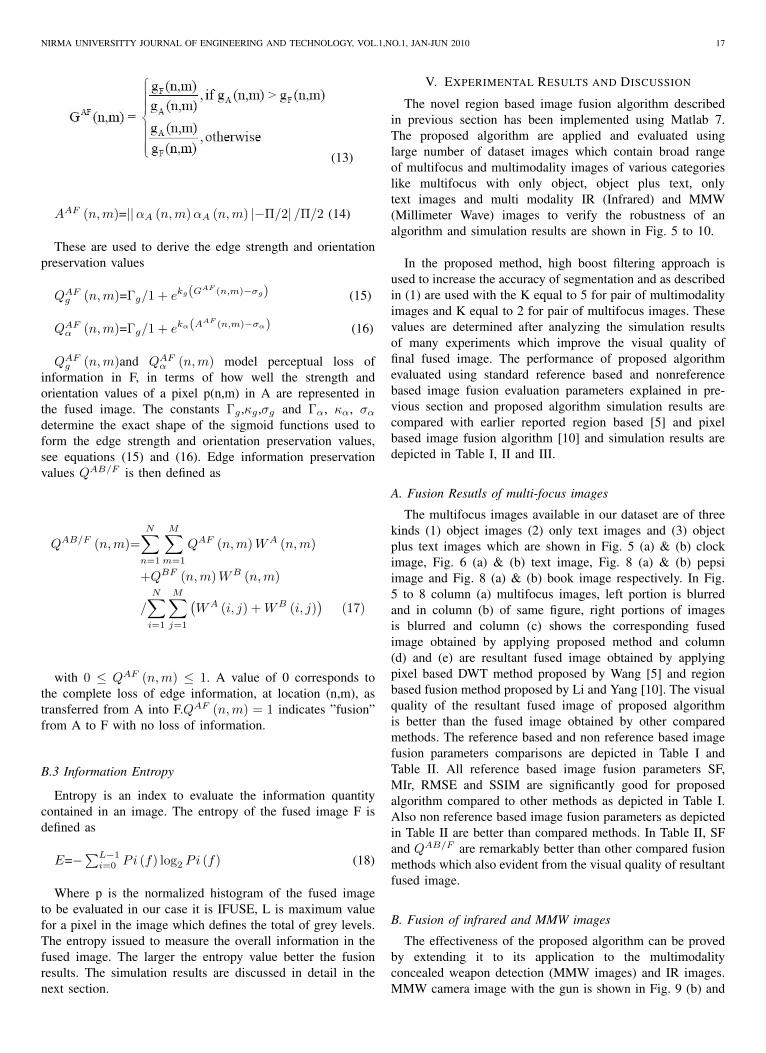
Fig. 10. Fusion results for multimodality IR image (a) visible source image (b) IR source image c) Proposed method (d) DWT method (e) Region method
TABLE IIMAGE FUSION PARAMETERS FOR REFERENCE BASED
IMAGES
Image Fusion Methods Fusion ParametersSF MI RMSE SSIM
DWT Based [5] 11.6721 2.5208 6.6722 0.9364Pepsi ImageRegion Based[10] 13.5320 2.7035 4.8129 0.9749
Proposed Method 13.5934 3.0868 3.1691 0.9910DWT Based [5] 23.5505 3.2573 12.2942 0.9135
Book ImageRegion Based [10] 31.3459 3.5747 5.9062 0.9785Proposed Method 31.5482 3.6607 5.3855 0.9820
TABLE IIIMAGE FUSION PARAMETERS FOR NON REFERENCE BASED
IMAGES
Image Fusion Methods Fusion ParametersSF MI QAB/F Entropy
DWT Based [5] 8.1506 6.4403 0.5696 8.1506Clock ImageRegion Based[10] 10.3350 6.9279 0.7119 8.7813
Proposed Method 10.0048 7.7344 0.7018 8.8066DWT Based [5] 8.1956 2.9235 0.5317 5.6600
Text Image Region Based [10] 10.4058 2.9647 0.7311 5.6426Proposed Method 11.1208 3.4192 0.7711 5.8867
visible images of a group of persons are shown in Fig. 9 (a).Here the aim is to detect gun location in the image by usingthe visible image.
In visual camera image details of surrounding area can beobserved in shown Fig. 10 (a) and IR camera detect the humanin captured image as shown in Fig. 10 (b). The aim of applyingfusion algorithm on IR image is to detect the human andits location using both source images information. The visualquality of resultant fused images for both the cases of proposedalgorithm is better than other methods new MMS fusion ruleis used in proposed algorithm which also evident by evaluatingthe Table III. The entropy is significantly better than region
TABLE IIIMULTIMODALITY IMAGE FUSION RESULTS
Image fusion Method EntropyDWT Based 6.742
Ir Image Region Based 6.0472Proposed Method 6.7861DWT Based [5] 4.9802
MMW Image Region Based [10] 3.7593Proposed Method 7.3931
based methods as depicted in Table III.Entropy is considered to evaluate the final fusion results
of both IR and MMW multimodality source images becauseboth the case IR and MMW sensor source images are blurredand in that case SF and QAB/F do not give significant valuesfor comparison. The simulated results depicted in Table I, IIand III shows that proposed method is performing well thanother compared methods for broad categories of multifocusand multimodality images.
VI. CONCLUSION
In this paper, new region based image fusion method usinghigh boost filtering concept is described. This novel idea isapplied on large number of dataset of each category and sim-ulation results are found with superior visual quality comparedto other earlier reported pixel and region based image fusionmethod. Here two different fusion rules are applied on broadrange of images. The novel MMS fusion rule is introduced toselect desired regions from multimodality images. Proposedalgorithm is compared with standard reference based and non-reference based image fusion parameters and from simulationand results, it is evident that our proposed algorithm preservesmore details in fused image. There are number of other advan-tages of proposed algorithm (1) The segmentation algorithm isapplied on decomposed image which is of less size comparedto original image so less computation time required to segmentsource image (2) As inverse DWT is not required to generatefinal fused image, so algorithm is free from shift invarianceproblem (3) Because of high boost filtering approach accuratesegmentation is expected so proposed method performancewill not degraded as image content change so algorithm isnot image content dependent (4) Region based algorithmsare less sensitive to noise, misregistration, contrast changeso proposed algorithm has this advantage. Algorithm can befurther extended by applying it to other categories of imageslike medical images and satellite images.
REFERENCES
[1] Devid Hall, James LLians,Hand book of multisensor data fusion,CRCPress LLC, 2001
[2] G. Piella, A general framework for multiresolution image fusion: frompixels to regions,Journal of Information Fusion, Vol. 4 (4), pp 259-280,Dec. 2003.
[3] Gemma Piella, A region based multiresolution image fusion algo-rithm,Proceedings of the Fifth International Conference on InformationFusion, Vol. 2, pp 1557- 1564, 2002..
20 NIRMA UNIVERSITTY JOURNAL OF ENGINEERING AND TECHNOLOGY, VOL.1, NO.1, JAN-JUN 2010
[4] Zhong Zhang and Rick Blum,A categorization of multiscale decompo-sition based image fusion schemes with a performance study for digitalcamera application, Proceedings of IEEE, Vol. 87 (8), pp 1315-1326, Aug1999.
[5] Anna Wang, Jaijining Sun and Yueyang Guan,The application to wavelettransform to multimodality medical image fusion, IEEE InternationalConference on Networking, Sensing and Control, pp. 270-274, 2006.
[6] Miao Qiguang and Wang Baoshul,A novel image fusion method usingcontourlet transform, International Conference on Communications, Cir-cuits and Systems Proceedings, Vol. 1, pp 548-552, 2006.
[7] C.S. Xydeas and V. Petrovic, Objective image fusion performance mea-sure, Electronics Letters, Vol. 36 (4), pp 308-309, February 2000
[8] Yin Chen, Rick S. Blum, A automated quality assessment algorithm forimage fusion, Image and vision computing (Elsevier), 2008.
[9] Zheng Liu and Robert Laganiere, On the use of phase congruency toevaluate image similarity, IEEE International Conference on Acoustics,Speech and Signal Processing, ICASSP, Vol. 2, pp 937-940, 2006.
[10] Shutao Li and Bin Yang, Multifocus image fusion using region segmen-tation and spatial frequency, Image and Vision Computing, Elsevier, Vol.26, pp. 971-979, 2008.
[11] J. Shi and J. Malik,Normalized cuts and image segmentation, IEEETransactions on Pattern Analysis and Machine Intelligence, Vol. 22 (8),pp888-905, 2000.
[12] S.G. Mallat,A theory for multiresoultuion signal decomposition: thewavelet representation, IEEE Trans. On Pattern Analysis and MachineIntelligence, Vol. 2(7), pp. 674-693, July 1989.
[13] Kayan Najarian, Robert Splinter, Biomedical Signal and Image process-ing,CRC Press, pp. 60-61, 2006.
[14] Rofael Gonzales, Richard Woods,Digital Image Processing, PearsonEducation, 2nd ed., 2006
[15] Zhou Wang, Alan Bovik,A universal image quality index, IEEE signalprocessing letters, Vol. 9, pp. 81-81, Mar. 2002.
Tanish Zaveri received his BE degree from SardarVallabhbhai Regional College of Engineering, Suratunder South Gujarat University in 1998 and obtainedhis M.Tech. Degree from Indian Institute of Technol-ogy, Bombay, India in 2005. He is currently pursuinghis h.D. in Multimodality Image Fusion from SardarVallabhbhai National Institute of Technology, Surat.He is presently working as an assistant professorin Electronics and Communication Engineering De-partment, Nirma University, Ahmedabad, India. Hisresearch interests are mainly focused on multimodal-
ity image fusion, image classification, biomedical image processing andspeech processing. He is a Life member of Indian Society of TechnicalEducation and Institution of Electronics and Telecommunication Engineers.He is also a member of Institute of Electrical and Electronics Engineers.
Mukesh Zaveri received the B.E. degree in electron-ics engineering from Sardar Vallabhbhai RegionalCollege of Engineering and Technology, Surat, India,in 1990, the M.E. degree in electrical engineeringfrom Maharaja Sayajirao University, Baroda, India,in 1993, and the Ph.D. degree in electrical engineer-ing from the Indian Institute of Technology, Bombay,Mumbai, in 2005. He is currently an AssistantProfessor and the Head of the Computer EngineeringDepartment, Sardar Vallabhbhai National Institute ofTechnology. His current research interests include
the area of signal and image processing, multimedia, computer networks,sensor networks, and wireless communications.
NIRMA UNIVERSITTY JOURNAL OF ENGINEERING AND TECHNOLOGY, VOL.1, NO.1, JAN-JUN 2010 21
User Centric Job Management In Grid UsingMultiple Agents An Unified Approach
Madhuri Bhavsar
Abstract—It has always been accepted that a communityof HPC users requires interactive, on demand access to HPCresources. Grid middleware technologies have been aimed at theexecution of the sequential batch jobs which is a dominatingparadigm, while lacking support for interactive applications.The reason is that grid middleware was developed for computeintensive jobs, which may run for a long time before a resultbecomes available, which may sometimes leads to unattendedexecution of jobs. To extend this application domain by providinginteractivity support to the users, Agent based technology is used.The research work which is explored and partially implementedconsiders various aspects of interactive job management inthe grid enviroment.This paper explores the specific natureof scheduling the grid based interactive jobs which is closelyanalyzed and reveals the complex approach adopted by intelligentand multiagent technology.
Index Terms—Grid computing, agents, Job Scheduling, HPC.
I. INTRODUCTION
GRID Computing can be seen as a high performancecomputing system facilitating the sharing of compute
resources, allowing users to discover and use remote resources.Users are able to submit the jobs to remote resources andtypically have no explicit control over the resources. Thus bothusers and resources can be viewed as autonomous entities,where this autonomy gives rise to inherent uncertainty, sincean individual can not predict how another will respond toa changing situation.. There are two main kinds of jobs inthe grid system; Regular (Batch) jobs and interactive jobs.The main difference between those types is that in the in-teractive jobs, the time slot reserved for running a job ona computational machine must be synchronized with userpreferences. Interactive access is defined to be when userscan input information into the application and receive timelyvisual output from the application. Typically the user preparesa job, submits it to the grid, waits for it to be completed andretrieves the output after the job is executed [1]. The users needthe HPC system to excel at their jobs providing interactiveon demand access to HPC systems. Currently Interactive, ondemand access to HPC systems has only been enabled ona very limited basis which is described in section 3. Weinvestigate the effectiveness of using agents to manage the usercentric job execution and propose the multiagent frameworkwhich facilitates the graphical visualization for user to managehis jobs. The framework which is proposed is an extension tothe exiting grid middleware architecture.
Madhuri Bhavsar is with the Department of Computer Science and Engi-neering, Institute of Technology, Nirma University, Ahmedabad, India, e-mail:[email protected]
II. AGENTS
The driving force behind grid computing is the need toshare computing resources in a coordinated manner. Gridcomputing environment is inherently an open environmentin which control is distributed between autonomous entitiesthereby increasing complexity as well as dependability. Thiscomplexity is exacerbated in open environment were indepen-dently developed autonomous agents interact with each otherin order to achieve their goals.
An agent can be viewed as an encapsulated system com-ponent that is situated in some environment and is capable offlexible and autonomous actions in that environment in orderto meet its design objectives and should exhibit features likeReactivity, Autonomy, and Social Ability and Proactive ness.Usage of this technology provides a flexible approach whichcan alleviate a number of issues presented in distributed andGrid based systems. This agent technology is emerging as oneof the unifying standards for the integration of distributed ap-plication and facilitating the user for resolving the complexityarising during job handling.
III. RELATED WORK
In recent years sufficient work has been undertaking fromthe deploying of various technology for exploring grid servicesto the use of agent technology for solving various issues in thegrid. Authors of [2]presented GAIN (Grid Agent Infrastruc-ture), a multi agent system that supports reliable execution ofgrid workflow application. [3]Supports enhancement in loadbalancing using agents which could include fresh node intothe system along with simulation. [4]provides agent basedframework for grid resource management by solving thecomplexities like heterogeneous substrates, policy extensibilityand many more. [5]used agent technology for reactive poweroptimization for which they have designed a grid computingarchitecture. [6]Proposed a grid architecture MAGDA basedon mobile agents and resolved various issues in grid by usingfeatures such as migration, cloning & messaging. [7]Exploredvarious capabilities of existing resource managers along withinteractive and on demand access potential offered and alsocompares on-demand features of four prominent batch queuingsystem.It has also come up with LLGrid project which islarge scale interactive grid system handles parallel matlabprocesses. [8]Provides architecture of Multi agent systemconsisting exception diagnosis agents. [9]Defined the workin which an agent based grid management infrastructure iscoupled with a performance driven task scheduling that hasbeen developed for local grid load balancing. [10]Proposedthe notion of an agent based grid computing infrastructure

22 NIRMA UNIVERSITTY JOURNAL OF ENGINEERING AND TECHNOLOGY, VOL.1, NO.1, JAN-JUN 2010
(AGCI) which is developed to manage healthcare processes inreal world setting.Authors of [11]Developed AgentTeamwork,which is a grid computing middleware system that dispatchesa collection of mobile agents to coordinate a user job overremote computers. This AgentTeamwork has a mobile agentexecution platform facilitates jobs migration and resumptionof jobs.
IV. MULTIAGENT FRAMEWORK
Most of the early work on grids has been for batch jobs.In this paper we introduce and describe an architecture andruntime environment for enabling interactive grid based onmultiagents. To handle both the types of job execution methodslike batch execution and interactive execution, agents canprovide a useful abstraction at each of the Grid layers. By theirability to adapt to the prevailing circumstances, agents willprovide services that are very dynamic and robust, and suitablefor a Grid environment. Agents can be used to extend exist-ing computational infrastructures. Few research groups havefocused on offering an environment to combine the conceptof computational grid and agents. An agent can be depicted asan autonomous entity packaged of a set of internal modules,three of which, i.e., for internal scheduling, problem solvingand social communication routing, are normative and othersare optional. A multi-agent system which is composed ofheterogeneous, autonomous entities, have their own problem-solving capabilities and interact with one another in order toachieve an overall goal. Multi-agent systems emphasize boththe autonomy of individual agents and the cooperation betweenagents. In general, coordination is about using a mechanismto manage the interdependencies between the collaborativeactivities of agents. For this paper the proposed agent willcombine stated functionalities described above and work as anindependent module for the client application. An agent willaccept job parameters from the client and accordingly providethem to grid middleware for further measures and also keep thetrack of the job. The detailed working is described in furtherdiscussion of this paper.
A. Functionality of a System
Job management is again an indispensable task for thegrid computing environment. Execution of job requires theresources but before that it is necessary to identify the require-ment of the jobs, allocation of the resources and takes care theprocessing of the jobs . All these tasks have to be taken careby the job management system. Usually this JMS consists ofthree components i.e. Queue Manager, Scheduler & ResourceManager. The term interactive job management refers toavailability and accessibility and accessibility of various tasksof job while it is executing. Various functionalities whichshould be addressed and implemented via agents are -
1) Job Submission2) Job status3) Job Monitoring4) Job Cancellation5) Job Destroy
Fig. 1. Multiple Agents in the framework.
Projected MultiAgent framework is composed of variousagents who offer demanded functionalities to the user areshown in the figure 1 & 2, whereas figure 3 shows the lifecycleof a job execution. These functionalities are distributed tofollowing agents.
• Interface-Agent :- Currently user needs to submit thecompute intensive job at the command prompt whichtakes long time for execution. Once submitted, manualintervention is difficult. This Interface-agent facilitates auser to interact with the grid system and allows a user tosubmit the job. User is also given a privilege to specifythe resources if known in advance.
• Controller-Agent :- This is core agent responsible for allthe activities needs to be carried out by the MultiAgentsystem.
• Info-Agent :- Normally Grid system which is composedwith Globus, provides directory service called MDS. Dueto anonymous problem, nirmagrid does not have MDS.So this Info-Agent created is responsible for providingrepository of existing resources and jobs. This agentendows with current status of available resources alongwith their configuration details which can accept jobs forexecution.
• Job-Creating Agent :- This framework is aimed at usercentric level providing flexibility to the user for usage ofthe grid. This agent is self running agent helps the systemin creation and maintaining the job along with creationof identification mechanism.
• Resource-Allocation-Agent :- Acts as a resource handlerin the system allocates the resources to the job accordingto the demand.
• Job-Managing-Agent :- If Submitted job is a batch job,avails the computational power and gets executed pro-vided every action in the system is working appropriately.Interactive job needs to be monitored and if neededcertain actions are invoked by the user. Job-Managing-Agent helps user to pact with the system for submitting,

NIRMA UNIVERSITTY JOURNAL OF ENGINEERING AND TECHNOLOGY, VOL.1,NO.1, JAN-JUN 2010 23
suspending, resuming and destroying the job.
Fig. 2. MultiAgent system providing interactivity for job handling.
Fig. 3. Job Execution life cycle.
During the implementation, various responsive issuesneeded to be handles are
• Unauthorized Access Control :- Interactivity with theGrid system may prone to the unauthorized job & mali-cious user. Though Grid security infrastructure providessecurity features, access control to the grid system shouldbe handled at the fine grain level.
• Performance issues :- Compute intensive jobs submittedby the user are sensitive to QoS parameters like executiontime, response time, latency between Main agent andgrid system, Number of jobs executed etc. In additionto providing flexibility to the user our multiagent systemshould support these QoS parameters.
• Agent based scheduling :- Normally Grid system whichis composed with Globus, provides directory servicecalled MDS. Due to anonymous problem, nirmagrid doesnot have MDS. So this Info-Agent created is responsiblefor providing repository of existing resources and jobs.
This agent endows with current status of available re-sources along with their configuration details which canaccept jobs for execution.
V. PARTIAL IMPLEMENTATION
Implementation of this multiagent framework is partiallycompleted which is deployed on the grid environment con-figured with Globus 4.0 on Fedora platform. The end usercan request for interactive use from any machine which isalso configured in the grid. This activity is an extensionto the Globus functionality, so that it can also be used forsubmitting request through graphical session. Figures 4 & 5shows functionality supported by an Interface agent and Job-Managing agents.
Fig. 4. Implementation of an Interface agent.
VI. CONCLUSION AND FUTURE WORK
Interactive grids extend the application domain for gridcomputing system from traditional batch jobs to graphicalinteractive sessions. In this paper we introduced agent basedinteractive grid job management. Agents identified presentsdemanded functionality to the grid user. Remaining agents, af-ter implementation needs to be deployed on the heterogeneousgrid platform which we have configured with 80 machines andhoping to cover almost all computers available on the campus.
ACKNOWLEDGMENT
The author would like to thank postgraduate students of M.Tech programme in computer science & Engineering for their
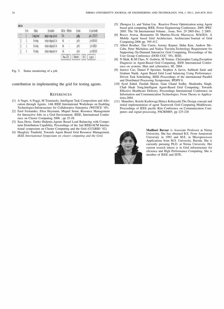
24 NIRMA UNIVERSITTY JOURNAL OF ENGINEERING AND TECHNOLOGY, VOL.1, NO.1, JAN-JUN 2010
Fig. 5. Status monitoring of a job.
contribution in implementing the grid for testing agents.
REFERENCES
[1] A Nagri, A Poggi, M Tomaiuolo, Intelligent Task Composition and Allo-cation through Agents, 14th IEEE International Workshops on EnablingTechnologies:Infratrsucture for Collaborative Enterprise (WETICE ’05).
[2] Enol Fernandez, Elisa Heymann, Miquel Senar, Resource Managementfor Interactive Jobs in a Grid Environment, IEEE, International Confer-ence on Cluster Computing 2006 , pp 25-28.
[3] Sasa Desic, Darko Huljenic,Agents Based Load Balancing with Compo-nent Distribution Capability, Proceedings of the 2nd IEEE/ACM Interna-tional symposium on Cluster Computing and the Grid (CCGRID ’02).
[4] Huaglory Tianfield, Towards Agent Based Grid Resource Management,IEEE International Symposium on cluster computing and the Grid.
[5] Zhongxu Li, and Yutian Liu, Reactive Power Optimization using Agentbased grid computing IEEE, Power Engineering Conference, 2005. IPEC2005. The 7th International Volume , Issue, Nov. 29 2005-Dec. 2 2005.
[6] Rocco Aversa, Beniamino Di Martino,Nicola Mazzocca, MAGDA: AMobile Agent based Grid Architecture, Architecture’Journal of GridComputing,2006 pp. 395-412.
[7] Albert Reuther, Tim Currie, Jeremy Kepner, Hahn Kim, Andrew Mc-Cabe, Peter Michaleas and Nadya Travinin,Technology Requirement forSupporting On-Damand Interatcive Grid Computing, Proceedings of theUser Group Conference (DOD-UGC ’05), IEEE.
[8] N Shah, K-M Chao, N. Godwin, M Younas, Christopher Laing,ExceptionDiagnosis in Agent-Based Grid Computing, IEEE International Confer-ence on systems, Man and cybernetics, III, 2004.
[9] Junwei Cao, Daniel P Spooner, Stephen A Jarvis, Subhash Saini andGraham Nudd, Agent Based Grid Load balancing Using Performance-Driven Task Scheduling, IEEE Proceedings of the international Paralleland Distributed Processing Symposium, IPDPS’0.
[10] Syed Zahid, Fazilah Haron, Gian Chand Sodhy, Shailendra Singh,Chah Huah Yong,Intelligent Agent-Based Grid Computing: TowardsEffective Healthcare Delivery, Proceedings International Conference onInformation and Communication Technologies: From Theory to Applica-tions,2004.
[11] Munehiro, Koichi Kashiwagi,Shinya Kobayashi,The Design concept andinitial implementation of agent Teamwork Grid Computing Middleware,Proceedings of IEEE pacific Rim Conference on Communication Com-puters and signal processing, PACRIM05, pp 225-228
Madhuri Bavsar is Associate Professor at NirmaUniversity, She has obtained B.E. From AmarawatiUniversity in 1992 and M.E. in MicroprocessorApplications from M.S. University, Baroda. She iscurrently pursuing Ph.D. at Nirma University. Hercurrent reserch interst is in Grid infrastructure foreScience and High Performance Computing. She ismember of IEEE and ISTE.
NIRMA UNIVERSITTY JOURNAL OF ENGINEERING AND TECHNOLOGY, VOL.1, NO.1, JAN-JUN 2010 25
Automatic Generation of CNC Part Program forCylindrical Components from DXF File
Jatin Dave and V.R.Iyer
Abstract—his paper describes the methodology for the auto-matic extraction of the co ordinates from dxf file and generationof CNC part program for the cylindrical components. The paperuses the method discussed in the survey for the extraction of theco ordinate from dxf file and recognition of some basic featurelike horizontal line, vertical line and inclined line. After collectingthe co ordinates the algorithm is developed to arrange thesecoordinate to write a CNC part program. While arranging theco ordinate, sequences of the features are also considered so thatit will be useful in creating tool motion. For writing a CNC partprogram, the practical aspect like depth of cut is also consideredand sequence of features are also taken care so that propertool path is generated. his paper describes the methodology forthe automatic extraction of the co ordinates from dxf file andgeneration of CNC part program for the cylindrical components.The paper uses the method discussed in the survey for theextraction of the co ordinate from dxf file and recognition ofsome basic feature like horizontal line, vertical line and inclinedline. After collecting the co ordinates the algorithm is developedto arrange these coordinate to write a CNC part program. Whilearranging the co ordinate, sequences of the features are alsoconsidered so that it will be useful in creating tool motion. Forwriting a CNC part program, the practical aspect like depth ofcut is also considered and sequence of features are also takencare so that proper tool path is generated. T
Index Terms—CNC Program, Tool motion,feature extrac-tion, recognition
I. INTRODUCTION
FEATURING plays an important role in the decision-making of design and manufacturing related activities.
The rationale of feature based design is to provide explicitlydesign/manufacturing features at the modeling level and torelieve the designer’s load of manipulating low-level graphicprimitives to convey the design intent. The importance ofthe features lies in the fact that features are very promisingin establishing a good link between the CAD and CAM,which is essential for improving product quality and reducingtime to market. Feature technology allows use of exportsystem to automatically generate manufacturing instructionsfrom design input. Feature based design is a process in whichparts are specified in terms of their constituent parameterizedform features. Feature design has allowed users essentiallyto capture design intention. Functional relationships amongpart features can be defined. Manufacturing information canbe captured and associated with a feature. CAD/CAM systemuses mainly design by feature or feature recognition techniqueto capture information of co ordinates values and feature. Therecognition process may be automatic by rule based system or
Jatin Dave and V.R. Iyer are with Department of Mechanical Engineering,Institute of Technology, Nirma University, SG Highway, Ahmedabad 382481
semi automatic [1],[2].The automatic system involves algorithms that are used toread information of the object from its geometric file, extractvalues of various features and recognize various features.Semi automatic system involves user intervention for inputof various parameters like manufacturing parameters of aparticular process. Researchers for manufacturing processes,to store information for design features and for generation ofprocess plan, develop many CAD/CAM and CAPP systems.Also there are systems available that mainly emphasizesgeneration of NC part programs. Continuous efforts are goingon to develop algorithms and software to directly generateNC part program just by having a solid model or drawing asan input without user involvement. This work is concentratedon developing a computer program that uses a data exchangefile of a drawing of a model to generate NC part program.This program runs in three stages. The first stage consists ofretrieving co - ordinates values from drawing file, second stagearranges the co - ordinate and features as per the sequence ofmachining operation and third stage generates the NC partprogram
II. CAD/CAM DATA EXCHANGE
Product design and manufacturing procedure uses varietyof software to prepare solid models, assembly, analysis filesand manufacturing models. It becomes increasingly importantto find effective procedures for exchanging these databases.Fundamental incompatibilities among entity representationsgreatly complicate exchanging modeling data amongCAD/CAM systems. Even simple geometric entities such ascircular arcs are represented by incompatible forms in manysystems.The database exchange problem is complicated further by thecomplexity of CAD/CAM systems, the varying requirementsof organizations using them, the restrictions on access toproprietary database information, and the rapid pace oftechnological change Transferring data between dissimilarCAD/CAM systems must embrace the complete productdescription stored in its database. Four types of modelingdata make up this description.
1) Shape data. This data consists of both geometrical andtopological information as well as part or form features.
2) Non shape data. It includes graphics data such asshaded images, and global data as measuring units ofthe database and the resolution of storing the databasenumerical values.
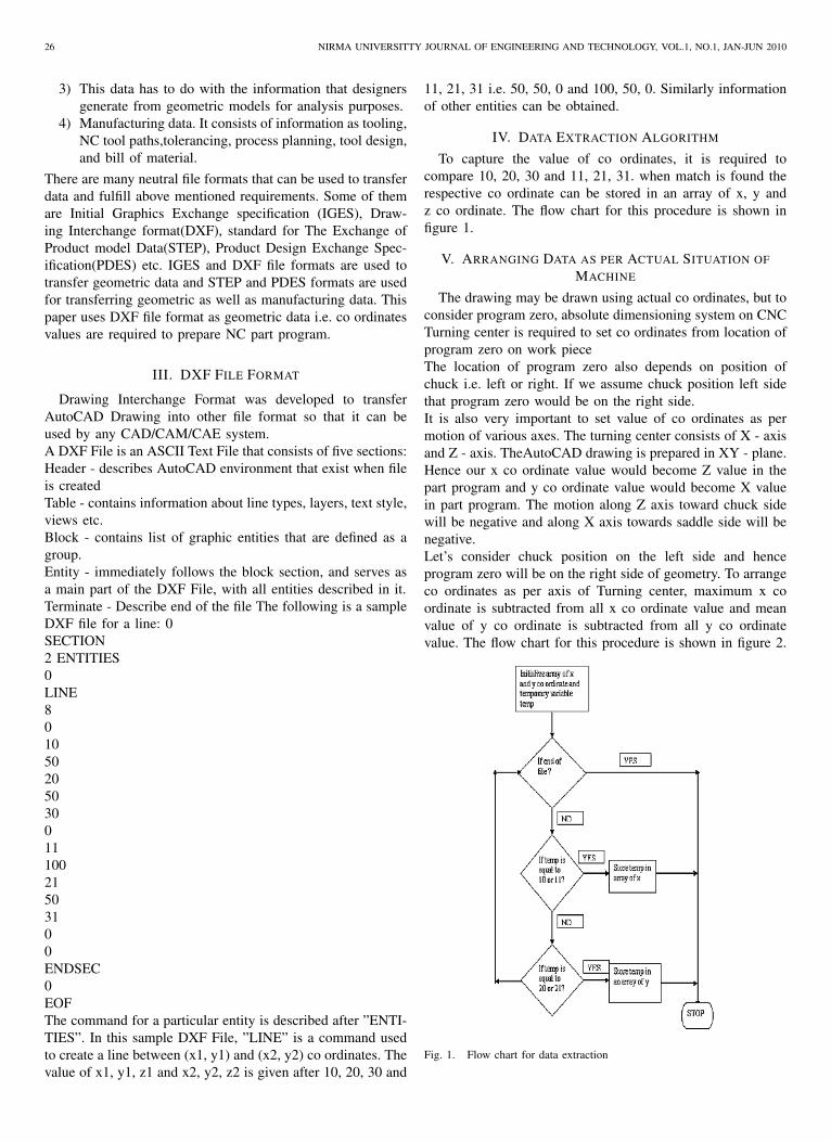
26 NIRMA UNIVERSITTY JOURNAL OF ENGINEERING AND TECHNOLOGY, VOL.1, NO.1, JAN-JUN 2010
3) This data has to do with the information that designersgenerate from geometric models for analysis purposes.
4) Manufacturing data. It consists of information as tooling,NC tool paths,tolerancing, process planning, tool design,and bill of material.
There are many neutral file formats that can be used to transferdata and fulfill above mentioned requirements. Some of themare Initial Graphics Exchange specification (IGES), Draw-ing Interchange format(DXF), standard for The Exchange ofProduct model Data(STEP), Product Design Exchange Spec-ification(PDES) etc. IGES and DXF file formats are used totransfer geometric data and STEP and PDES formats are usedfor transferring geometric as well as manufacturing data. Thispaper uses DXF file format as geometric data i.e. co ordinatesvalues are required to prepare NC part program.
III. DXF FILE FORMAT
Drawing Interchange Format was developed to transferAutoCAD Drawing into other file format so that it can beused by any CAD/CAM/CAE system.A DXF File is an ASCII Text File that consists of five sections:Header - describes AutoCAD environment that exist when fileis createdTable - contains information about line types, layers, text style,views etc.Block - contains list of graphic entities that are defined as agroup.Entity - immediately follows the block section, and serves asa main part of the DXF File, with all entities described in it.Terminate - Describe end of the file The following is a sampleDXF file for a line: 0SECTION2 ENTITIES0LINE80105020503001110021503100ENDSEC0EOFThe command for a particular entity is described after ”ENTI-TIES”. In this sample DXF File, ”LINE” is a command usedto create a line between (x1, y1) and (x2, y2) co ordinates. Thevalue of x1, y1, z1 and x2, y2, z2 is given after 10, 20, 30 and
11, 21, 31 i.e. 50, 50, 0 and 100, 50, 0. Similarly informationof other entities can be obtained.
IV. DATA EXTRACTION ALGORITHM
To capture the value of co ordinates, it is required tocompare 10, 20, 30 and 11, 21, 31. when match is found therespective co ordinate can be stored in an array of x, y andz co ordinate. The flow chart for this procedure is shown infigure 1.
V. ARRANGING DATA AS PER ACTUAL SITUATION OFMACHINE
The drawing may be drawn using actual co ordinates, but toconsider program zero, absolute dimensioning system on CNCTurning center is required to set co ordinates from location ofprogram zero on work pieceThe location of program zero also depends on position ofchuck i.e. left or right. If we assume chuck position left sidethat program zero would be on the right side.It is also very important to set value of co ordinates as permotion of various axes. The turning center consists of X - axisand Z - axis. TheAutoCAD drawing is prepared in XY - plane.Hence our x co ordinate value would become Z value in thepart program and y co ordinate value would become X valuein part program. The motion along Z axis toward chuck sidewill be negative and along X axis towards saddle side will benegative.Let’s consider chuck position on the left side and henceprogram zero will be on the right side of geometry. To arrangeco ordinates as per axis of Turning center, maximum x coordinate is subtracted from all x co ordinate value and meanvalue of y co ordinate is subtracted from all y co ordinatevalue. The flow chart for this procedure is shown in figure 2.
Fig. 1. Flow chart for data extraction

NIRMA UNIVERSITTY JOURNAL OF ENGINEERING AND TECHNOLOGY, VOL.1,NO.1, JAN-JUN 2010 27
VI. FEATURE RECOGNITION
This paper describes the procedure for recognizing featurefor straight turning, step turning, taper turning and facingoperation. It is necessary that all condition to recognize a lineshould be implemented in the program. This program givesoutput as per absolute
Fig. 2. Arranging data as per chuck position
dimensioning system; hence y co ordinate value is multi-plied by 2. The following rules are used to determine varioustypes of line and further type of operation required.
IF((X1[i-1]!=X1[i])&(Y1[i-1]==Y1[i]))THEN line is verti-cal and step turning Z[n1-1]=X1[i] AND X[n1-1]=2*Y1[i];
IF ((X1[i-1]==X1[i])&(Y1[i-1]!=Y1[i])) THEN line is Hor-izontal and straight turning Z[n1-1]=X1[i] AND X[n1-1]=2*Y1[i];
IF((X1[i-1]!=X1[i])&(Y1[i-1]!=Y1[i])) THEN line isInclined and taper turning Z[n1-1]=X1[i] AND X[n1-1]=2*Y1[i];
IF(X1[i-1]==0&Y1[i-1]==0) THEN end of file and readingof file is stopped
VII. SAMPLE RUN OF THE PROGRAM
The program is written in JAVA Language. A user interfaceis developed to enter a particular DXf file to be read. The
output contains generation of drawing, display of co ordinatevalue and co ordinates after arranging as per the actualarrangement of machine. Finally an out put file ”job.nc” isgenerated which contains NC Part program. This part programis now ready to transfer on CNC machine and can be used forfurther manufacturing of a component
Fig. 3. User Interface of the program
VIII. THE NC PART PROGRAM
N005 G71 G90 G54 G95 lfN010 G00 X0 Z5 lfN015 G01 X0 Z0 F0.5 lfN020 G01 X52.0 lfN025 G01 Z-110F0.5 lfN030 G01 X54.0F0.5 lfN035 G01 Z0 F0.5 lfN040 G01 X52.0 F0.5 lf N045 G01 X50.0 lf N050 G01 Z-30F0.5 lfN055 G01 X50 Z-60 F0.5 lfN060 G01 X52 F0.5 lfN065 G01 Z0 F0.5 lfN070 G01 X50.0 F0.5 lfN075 G01 X48.0 lfN080 G01 Z-30F0.5 lfN085 G01 X50 Z-60 F0.5 lfN090 G01 X52 F0.5 lfN095 G01 Z0 F0.5 lfN0100 G01 X48.0 F0.5 lfN0105 G01 X46.0 lfN0110 G01 Z-30F0.5 lfN0115 G01 X50 Z-60 F0.5 lfN0245 G01 Z0 F0.5 lfN0250 G01 X38.0 F0.5 lfN0255 G01 X36.0 lfN0260 G01 Z-30F0.5 lfN0265 G01 X50 Z-60 F0.5 lfN0270 G01 X52 F0.5 lfN0275 G01 Z0 F0.5 lfN0280 G01 X36.0 F0.5 lfN0285 G01 X34.0 lfN0290 G01 Z-30F0.5 lfN0295 G01 X50 Z-60 F0.5 lf

28 NIRMA UNIVERSITTY JOURNAL OF ENGINEERING AND TECHNOLOGY, VOL.1, NO.1, JAN-JUN 2010
N0300 G01 X52 F0.5 lfN0305 G01 Z0 F0.5 lfN0310 G01 X34.0 F0.5 lfN0315 G01 X32.0 lfN0320 G01 Z-30F0.5 lf N0325 G01 X50 Z-60 F0.5 lfN0330 G01 X52 F0.5 lfN0335 G01 Z0 F0.5 lfN0340 G01 X32.0 F0.5 lfN0345 G01 X30.0 lfN0350 G01 Z-30F0.5 lfN0355 G01 X50 Z-60 F0.5 lfN0360 G01 X52 F0.5 lfN0365 G01 Z0 F0.5 lfN0370 G01 X30.0 F0.5 lfN0375 G01 X28.0 lfN0380 G01 Z-30F0.5 lfN0385 G01 X50 Z-60 F0.5 lfN0390 G01 X52 F0.5 lfN0395 G01 Z0 F0.5 lfN0400 G01 X28.0 F0.5 lfN0405 G01 X26.0 lfN0410 G01 Z-30F0.5 lfN0415 G01 X50 Z-60 F0.5 lfN0420 G01 X52 F0.5 lfN0425 G01 Z0 F0.5 lfN0430 G01 X26.0 F0.5 lfN0435 G01 X24.0 lfN0440 G01 Z-30F0.5 lfN0445 G01 X50 Z-60 F0.5 lfN0450 G01 X52 F0.5 lfN0455 G01 Z0 F0.5 lfN0460 G01 X24.0 F0.5 lfN0465 G01 X22.0 lfN0470G01 Z-30F0.5 lfN0475 G01 X50 Z-60 F0.5 lfN0480 G01 X52 F0.5 lfN0485 G01 Z0 F0.5 lfN049 0 G01 X22.0 F0.5 lfN0495 G01 X20.0 lfN0500 G01 Z-30F0.5 lfN0505 G01 X50 Z-60 F0.5 lfN0510 G01 X52 F0.5 lfN0515 G01 Z0 F0.5 lfN0520 G01 X20.0 F0.5 lfN0525 G01 X18.0 lfN0530 G01 Z-30F0.5 lfN0535 G01 X50 Z-60 F0.5 lfN0540 G01 X52 F0.5 lfN0120 G01 X52 F0.5 lfN0125 G01 Z0 F0.5 lfN0130 G01 X46.0 F0.5 lfN0135 F0.5 lfN0150 G01 X52 F0.5 lfN0155 G01 Z0 F0.5 lfN0160 G01 X44.0 F0.5 lfN0165 G01 X42.0 lfN0170 G01 Z-30F0.5 lfN0175 G01 X50 Z-60 F0.5 lf
N0180 G0 X52 F0.5 lfN0185 G01 Z0 F0.5 lfN0190 G01 X42.0 F0.5 lfN0195 G01 X40.0 lfN0200 G01 Z-30F0.5 lfN0205 G01 X50 Z-60 F0.5 lfN0210 G01 X52 F0.5 lfN0215 G01 Z0 F0.5 lfN022 G01 X40.0 F0.5 lfN0225 G01 X38.0 lfN0230 G01 Z-30F0.5 lf N0235 G01 X50 Z-60 F0.5 lfN0240 G01 X52 F0.5 lfN0545 G01 Z0 F0.5 lfN0550 G01 X18.0 F0.5 lfN0555 G01 X16.0 lfN0560 G01 Z-30F0.5 lfN0565 G01 X50 Z-60 F0.5 lfN0570 G01 X52 F0.5 lfN0575 G01 Z0 F0.5 lfN0580 G01 X16.0 F0.5 lfN0585 G01 X14.0 lfN0590 G01 Z-30F0.5 lfN0595 G01 X50 Z-60 F0.5 lfN0600 G01 X52 F0.5 lfN0605 G01 Z0 F0.5 lfN0610 G01 X14.0 F0.5 lfN0615 G01 X12.0 lfN0620 G01 Z-30F0.5 lfN0625 G01 X50 Z-60 F0.5 lfN0630 G01 X52 F0.5 lfN0635 G01 Z0 F0.5 lfN0640 G01 X12.0 F0.5 lfN0645 G01 X10 Z0 F0.5 lfN0650 G01 X10 Z-30 F0.5 lfN0655 G01 X50 Z-60 F0.5 lfN0660 G01 X50 Z-110 F0.5 lfN0665 G01 X55 F0.5 lfN0665 G00 X300 Z300 lfN0670 M02 lf
IX. CONCLUSION
This program can be customized to meet a specific familyof components. Hence this software may be cost effective forsmall scale industries which can not afford high cost software.Further it can be expanded to consider features like arc,groove, internal holes, thread etc. as per same programmingtechnique.
REFERENCES
[1] Ersan ASLAN, Ulvi SEKER, Nedim ALPDEM IR ”Data ExtractionFrom CAD Model For Rotational Parts to be Machined at TurningCentres” , J. of Engineering and Environmental Science, 23 (1999) , 339- 347
[2] Yakup YILDIZ*, Ihsan KORKUT, Ulvi SEKER, ”Development of aFeature Based CAM System for Rotational Parts”, G.U. Journal of Science19(1): 35-40 (2006).
[3] Autodesk , Autocad help center.

NIRMA UNIVERSITTY JOURNAL OF ENGINEERING AND TECHNOLOGY, VOL.1,NO.1, JAN-JUN 2010 29
Jatin Dave is Asst. Professor in the Departmentof Mechanical Engineering, Institute of Technology,Nirma University, he has obtained B.E. From GujaratUniversity in 1999 and M.E. in 2002 from the sameUniversity, . He is currently pursuing Ph.D. at NirmaUniversity. His current reserch interst is in CAD,Kinemetics and Robotics. His life member of IndianSociety for Technical Eduaction.
V. R.Iyer is Professor in the Department ofMechanical Engineering, Institute of Technology,Nirma University, he has obtained B.E. From Re-gionalEngineering college, Trichy in 1972 and M.E.from Indian Institute of Technology, Bomabay in1985. He is currently pursuing Ph.D. at NirmaUniversity. His current reserch interst is in CAD,Kinemetics and Robotics. His life member of Insti-tution of Engineers and Indian Society for TechnicalEduaction.
30 NIRMA UNIVERSITTY JOURNAL OF ENGINEERING AND TECHNOLOGY, VOL.1, NO.1, JAN-JUN 2010
HEAT TRANSFER ANALYSIS OF HEATGENERATING WIRE USING FINITE ELEMENT
METHODDipak J Parmar and Bhargav M. Chavada
Abstract—This paper describes the numerical results of theheat transfer from heat generating wire at different conditionsby finite element method. The parametric effects on heat transferwere investigated. The varied parameters included ambientconditions, as well as the shape of the cross-section. The nu-merical results show that the type of the medium where theheat generating wire immerges has strong effects on the heat-dissipation rate. As the size of the diameter the heat dissipation tothe ambient is decreased. The effects of free convection conditionson the wire surface are also significant. However, the effect of theshape of the cross-section is not very strong. The results presentedin this paper provide useful information for the application ofheat generating wire.
Index Terms—Heat transfer, finite element, heat dissipation
I. INTRODUCTION
HEAT conduction issue is one of the hot topics in theresearch area. It has wide applications in industry and
our daily life, such as electrical furnaces, electrical heatingappliances, and ventilation of computer chips. Among thoseheat conduction problems, the heating elements are the coretopic of the heat conduction problems. Different heating ele-ments demonstrate different characteristics in heat conduction.Among many different structures of the heating elements, thewire has been used in many areas because of its compactstructure and large thermal expansion. This study has analyzedthe heat transfer of the heat generating wire under differentconditions by using the finite element method. It providessome useful information on designs and applications of heatgenerating wire.
II. FINITE ELEMENT METHOD FOR HEATCONDUCTION
In general, heat conduction problems can be studied byexperimental, analytical, and numerical methods. In the ex-perimental method, measurements may be very difficult insome applications. In analytical method, it is impossible to getaccurate solutions of differential equations in most problems.With the advancement of computational technologies, thenumerical simulation is now widely used to help resolvingthe difficulty. Various numerical methods can be used to solveheat conduction problems, such as finite differential method,variation perturbation. Boundary element method and finiteelement method. In this study, the finite element method is
Dipak Parmar is with Department of Mechanical Engineering Instituteof technology Nirma University Ahmedabad-382481,India and Bhargav M.Chavada is with G.H.Patel College of Engineering,V.V.Nagar 38xxxx, [email protected]
used. Heat conduction problems could be divided into twocategories: the steady state and the unsteady state. In a .threedimensional heat conduction with internal heat generationproblem, the unsteady state temperature distribution T(x, y,z,t) in a Cartesian coordinator system in the domain can besolved by the following differential equation’”:
pc∂T
∂τ− ∂
dx
(k∂T
dx
)− ∂
dy
(k∂T
dy
)− ∂
dz
(k∂T
dz
)−Q = 0;
(1)The equation is a heat balance equation, where t is time, k isheat conductivity, p is the density, c is the heat capacity, andQ is the rate of the heat generated per volume from the heatsource of the material. The boundary conditions for solvingthis equation should meet the following conditions in the Ωdomain:
Γ1 + Γ2 + Γ3 = Γ
where,Γ1 + Γ2 + Γ3 = Γ are 1st, 2nd and 3rd types of boundaryconditions, respectively. If T and Q are unchanged with thetime, i.e. ∂T
∂τ -o , the Equation (1) becomes the steady stateheat conduction equation. This study considers the steady stateheat conduction problems with the heat generation. In thefinite element method, Galerkin’s approach can be used toconvert the heat conduction equation (1) to the finite elementequation”’. The corresponding finite element matrix of theunsteady state heat conduction is given as follows:
CT +KT = F (2)
Where, C is the matrix of the heat capacity, K is the matrix ofthe heat conduction, T is the matrix of temperature, and F isthe matrix of the temperature loading. In Equation (2) if thefirst term becomes zero, the equation becomes the steady stateheat conduction finite element equation. For a 2-Dimentionalheat conduction problem, the elements of the matrix could beexpressed as
Kv =∑
e
Kev +
∑
e
Hev (3)
Fi =∑
e
F eQt +∑
e
F eqt +∑
e
F em (4)
Each term in Equations 3 and 4 can be expressed asfollowings: The contribution of each cell to the matrix of heatconduction:
Keij =
∫Qe
(k ∂Ni
∂x∂Ni
∂x + k ∂Ni
∂y∂Ni
∂y
)∂ Ω

NIRMA UNIVERSITTY JOURNAL OF ENGINEERING AND TECHNOLOGY, VOL.1,NO.1, JAN-JUN 2010 31
The correction of heat transfer boundary condition of each cellto the matrix of heat conduction:
Heij =
∫Γe3
hNi Nj ∂ Γ
The temperature loading generated by heat souse in each cell:
F eQi =∫
Ωe ρ QNi Nj ∂ Ω
The temperature loading from constant surface heat flux:
F eqi =∫
Γe2
qNi ∂ Γ
The temperature loading from the convection on the surface:
F eHi =∫
Γe3
HTa Ni ∂ Ω
Where, Ni, Nj are the weighing functions. This approach hasconverted the steady state heat conduction differential equationin a space domain ? into the initial value problem of anordinary integration equation of temperature T at a numberof nodes. For a 3-Dimentional heat conduction problem, asimilar method can be used for deriving the correspondingfinite element equation of heat conduction.
III. RESULTS AND DISCUSSION
Based on the above heat conduction analysis using the finiteelement method, the heat transfer from a wire at differentconditions was analyzed in this study. A wire is a typicalstructure used for generating heat. Figure 1(a) shows theschematic of a wire. The shape of the cross-section of the wireis circular. The finite element model of the wire is shown infigure 1(b).
Fig. 1. Model of solid wire
Table 1 lists a typical set of parameters conductivity, am-bient temperature used for the baseline case in this study.In theoretical analysis, an infinite wire is assumed. In thenumerical analysis the length of the wire is taken 5m andadiabatic condition is assumed at the two ends of wire.
Fig. 2. FEM of wire
Diameter of wire 0.5mLength of wire 5mHeat generation rate 30 kW/m3
Convection heat transfer coefficient 60 W/m2KConductivity of Pure Copper 401 W/m KAmbient Temperature 30oC
Table: - 1 Set of parameters for wire.
Based on the above heat conduction analysis using the finiteelement method, the problem of heat generating wire is solvedby ANSYS 9 analysis software for above set of parameters.The temperature distribution with in the heat generating wireis shown in figure 2.
Fig. 3. Temperature distribution in Heat Generating Wire
A. The Effects of Medium Type
Heat transfer between a heat generator and its surroundingsis affected by the type of mediums. In this paper, calculationsare performed for a pure copper wire with the circular cross-section in still water, air and a magnesia brick. Only heattransfer by conduction in the medium is considered. Figure3 shows the surface temperature versus the heat generationat different types of mediums. At the same heat generation
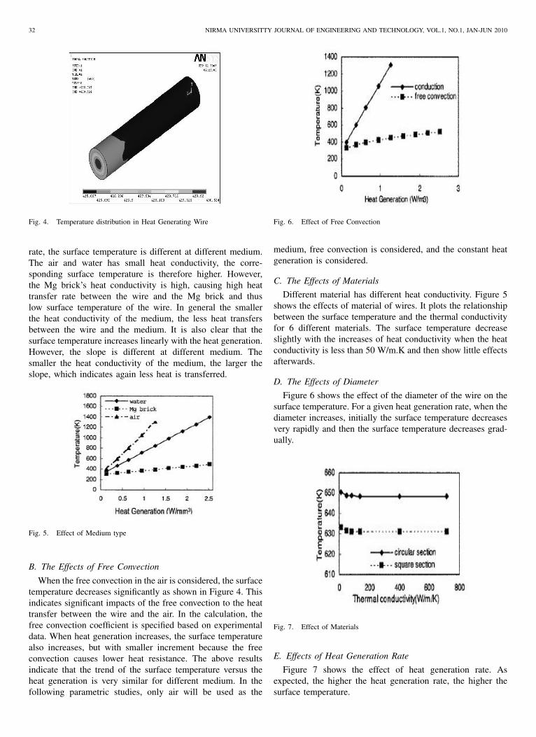
32 NIRMA UNIVERSITTY JOURNAL OF ENGINEERING AND TECHNOLOGY, VOL.1, NO.1, JAN-JUN 2010
Fig. 4. Temperature distribution in Heat Generating Wire
rate, the surface temperature is different at different medium.The air and water has small heat conductivity, the corre-sponding surface temperature is therefore higher. However,the Mg brick’s heat conductivity is high, causing high heattransfer rate between the wire and the Mg brick and thuslow surface temperature of the wire. In general the smallerthe heat conductivity of the medium, the less heat transfersbetween the wire and the medium. It is also clear that thesurface temperature increases linearly with the heat generation.However, the slope is different at different medium. Thesmaller the heat conductivity of the medium, the larger theslope, which indicates again less heat is transferred.
Fig. 5. Effect of Medium type
B. The Effects of Free Convection
When the free convection in the air is considered, the surfacetemperature decreases significantly as shown in Figure 4. Thisindicates significant impacts of the free convection to the heattransfer between the wire and the air. In the calculation, thefree convection coefficient is specified based on experimentaldata. When heat generation increases, the surface temperaturealso increases, but with smaller increment because the freeconvection causes lower heat resistance. The above resultsindicate that the trend of the surface temperature versus theheat generation is very similar for different medium. In thefollowing parametric studies, only air will be used as the
Fig. 6. Effect of Free Convection
medium, free convection is considered, and the constant heatgeneration is considered.
C. The Effects of MaterialsDifferent material has different heat conductivity. Figure 5
shows the effects of material of wires. It plots the relationshipbetween the surface temperature and the thermal conductivityfor 6 different materials. The surface temperature decreaseslightly with the increases of heat conductivity when the heatconductivity is less than 50 W/m.K and then show little effectsafterwards.
D. The Effects of DiameterFigure 6 shows the effect of the diameter of the wire on the
surface temperature. For a given heat generation rate, when thediameter increases, initially the surface temperature decreasesvery rapidly and then the surface temperature decreases grad-ually.
Fig. 7. Effect of Materials
E. Effects of Heat Generation RateFigure 7 shows the effect of heat generation rate. As
expected, the higher the heat generation rate, the higher thesurface temperature.
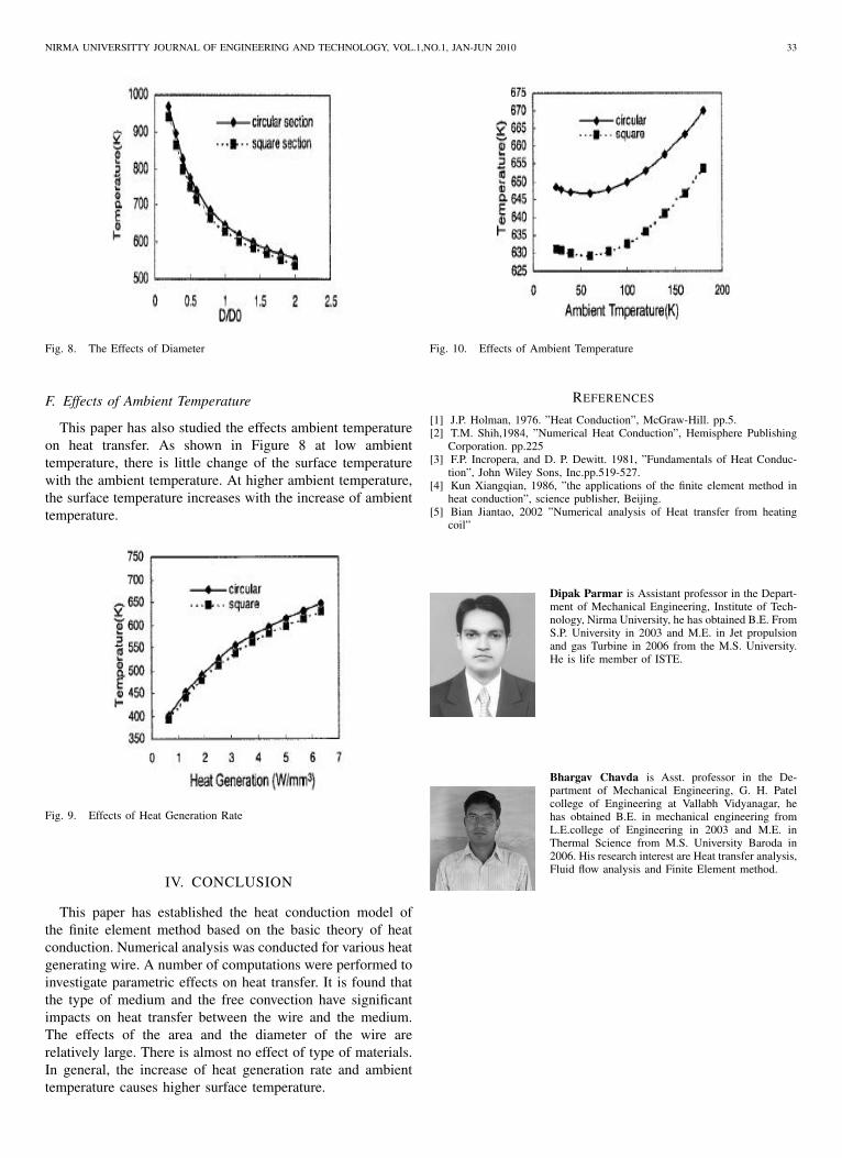
NIRMA UNIVERSITTY JOURNAL OF ENGINEERING AND TECHNOLOGY, VOL.1,NO.1, JAN-JUN 2010 33
Fig. 8. The Effects of Diameter
F. Effects of Ambient Temperature
This paper has also studied the effects ambient temperatureon heat transfer. As shown in Figure 8 at low ambienttemperature, there is little change of the surface temperaturewith the ambient temperature. At higher ambient temperature,the surface temperature increases with the increase of ambienttemperature.
Fig. 9. Effects of Heat Generation Rate
IV. CONCLUSION
This paper has established the heat conduction model ofthe finite element method based on the basic theory of heatconduction. Numerical analysis was conducted for various heatgenerating wire. A number of computations were performed toinvestigate parametric effects on heat transfer. It is found thatthe type of medium and the free convection have significantimpacts on heat transfer between the wire and the medium.The effects of the area and the diameter of the wire arerelatively large. There is almost no effect of type of materials.In general, the increase of heat generation rate and ambienttemperature causes higher surface temperature.
Fig. 10. Effects of Ambient Temperature
REFERENCES
[1] J.P. Holman, 1976. ”Heat Conduction”, McGraw-Hill. pp.5.[2] T.M. Shih,1984, ”Numerical Heat Conduction”, Hemisphere Publishing
Corporation. pp.225[3] F.P. Incropera, and D. P. Dewitt. 1981, ”Fundamentals of Heat Conduc-
tion”, John Wiley Sons, Inc.pp.519-527.[4] Kun Xiangqian, 1986, ”the applications of the finite element method in
heat conduction”, science publisher, Beijing.[5] Bian Jiantao, 2002 ”Numerical analysis of Heat transfer from heating
coil”
Dipak Parmar is Assistant professor in the Depart-ment of Mechanical Engineering, Institute of Tech-nology, Nirma University, he has obtained B.E. FromS.P. University in 2003 and M.E. in Jet propulsionand gas Turbine in 2006 from the M.S. University.He is life member of ISTE.
Bhargav Chavda is Asst. professor in the De-partment of Mechanical Engineering, G. H. Patelcollege of Engineering at Vallabh Vidyanagar, hehas obtained B.E. in mechanical engineering fromL.E.college of Engineering in 2003 and M.E. inThermal Science from M.S. University Baroda in2006. His research interest are Heat transfer analysis,Fluid flow analysis and Finite Element method.
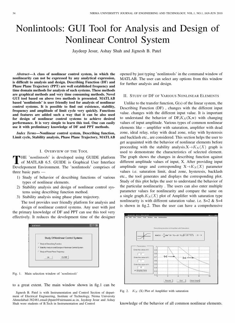
34 NIRMA UNIVERSITTY JOURNAL OF ENGINEERING AND TECHNOLOGY, VOL.1, NO.1, JAN-JUN 2010
Nonlintools: GUI Tool for Analysis and Design ofNonlinear Control System
Jaydeep Jesur, Ashay Shah and Jignesh B. Patel
Abstract—A class of nonlinear control system, in which thenonlinearity can not be expressed by any analytical expression,is difficult to analysis and design. Describing Function (DF) andPhase Plane Trajectory (PPT) are well established frequency andtime domain methods for analysis of such systems. These methodsare graphical methods and very time consuming methods. NovelGUI tool based on above two methods is presented. MATLABbased ’nonlintools’ is user friendly tool for analysis of nonlinearcontrol systems. It is possible to find out existence, stability,frequency and amplitude of limit cycle very quickly. Functionsand features are added such a way that it can be also usedfor design of nonlinear control systems to achieve desiredperformance. It is very simple to learn this tool. One can easilyuse it with preliminary knowledge of DF and PPT methods.
Index Terms—Nonlinear control system, Describing function,Limit cycle, Stability analysis, Phase Plane Trajectory, MATLAB
I. OVERVIEW OF THE TOOL
THE ’nonlintools’ is developed using GUIDE platformof MATLAB 6.5. GUIDE is Graphical User Interface
Develepoment Environment. The ’nonlintools’ comprises ofthree basic parts —
1) Study of behavior of describing functions of varioustypes of nonlinear elements.
2) Stability analysis and design of nonlinear control sys-tems using describing function method.
3) Stability analysis using phase plane trajectory.The tool provides user friendly platform for analysis anddesign of nonlinear control systems. Any user with just
the primary knowledge of DF and PPT can use this tool veryeffectively. It reduces the development time of the designer
Fig. 1. Main selection window of ’nonlintools’
to a great extent. The main window shown in fig.1 can be
Jignesh B. Patel is with Instrumentation and Control Section of depart-ment of Electrical Engineering, Institute of Technology, Nirma UniversityAhmedabad-382481,email:[email protected], Jaydeep Jesur and AshayShah were students of B.Tech in Instrumentation and Control
opened by just typing ’nonlintools’ in the command window ofMATLAB. The user can select any options from this windowfor further analysis and design.
II. STUDY OF DF OF VARIOUS NONLINEAR ELEMENTS
Unlike to the transfer function, G(s) of the linear system, theDescribing Function (DF) , changes with the different inputvalue. changes with the different input value. It is importantto understand the behavior of DF,KN (X,w) with changingvalues of input amplitude. Various types of common nonlinearelements like – amplifier with saturation, amplifier with deadzone, ideal relay, relay with dead zone, relay with hysteresisand backlash etc., are considered. This section helps the user toget acquainted with the behavior of nonlinear elements beforeproceeding with the stability analysis.X→KN (X) graph isused to demonstrate the characteristics of selected element.The graph shows the changes in describing function againstdifferent amplitude values of input, X. After providing inputamplitude range and corresponding X→KN (X) parametervalues i.e. saturation limit, dead zone, hysteresis, backlashetc., the tool generates and displays the corresponding plot.Study of this plot helps the user to understand the behavior ofthe particular nonlinearity . The users can also enter multipleparameter values for nonlinearity and compare the same ona single graph.KN (X) plot of Amplifier with saturation typenonlinearity is with different saturation value. i.e. S=2 & S=4is shown in fig.2. Thus the user can have a comprehensive
Fig. 2. KN (X) Plot of Amplifier with saturation
knowledge of the behavior of all common nonlinear elements.

NIRMA UNIVERSITTY JOURNAL OF ENGINEERING AND TECHNOLOGY, VOL.1,NO.1, JAN-JUN 2010 35
III. STABILITY ANALYSIS USING DF METHOD
For a linear control system, various stability analysis meth-ods such as Routh Hurwitz stability criterion, Nyquist stabilitycriterion, Root locus, Bode plot etc., are available. Similarly,DF method is frequency domain method for stability analysisof nonlinear control system. The fundamental approach isto plot the polar plot of the linear part of the system, andinvestigate its intersections with locus of −1
KN (X) . It is usedto check the generation of limit cycle in nonlinear controlsystems. Limit cycle is self sustained oscillations of fixedfrequency and amplitude. If G(jw ) curve encloses the entire
−1KN (X) curve, then the system is unstable. If there is nointersection between the loci and polar plot and if the polarplot does not enclose the −1
KN (X) curve, then the system isstable. If there is an intersection than the limit cycle generatesand stability of the limit cycle is required to check. The basicsteps in the DF method are as follows:
1) Get the polar plot of the linear part.2) Find −1
KN (X) from the KN (X) of a given nonlinearityand plot it on the same graph taking different values ofX.
3) Find out whether the limit cycle exist or not by findingthe intersection of both the graphs
4) Calculate the value of frequency and Amplitude X ofthe limit cycle.
To perform all the above-mentioned steps manually is a timeconsuming task. Probabilities of mistakes increases manifoldin manual method. The suggested tool performs all abovesteps with the help of MATLAB file and directly generatesthe end results. The package is developed in view to reducethe analysis time. The GUI environment provides user-friendlyplatform. Flexibility is provided to enter the linear part of thesystem. The tool can take the linear part up to seventh order.
Linear transfer function can be entered in form of:1) Zero- Pole and Gain.2) Ratio of polynomialsAlso the user can specify the frequency range and the step
size of the polar plot. The next step is to select the typeof nonlinearity and its parameters. Here also the user canspecify the amplitude range and step size to plot the −1
KN (X)plot. It also provides the pictorial view of the block diagramof the concerned nonlinear system for easy interpretation.After selection of linear and nonlinear system parameters,the tool generates and displays the corresponding plots. Theplots convey about the stability condition of the system. Itshows intersections as well the direction of both the plots.Intersection of both plots is highlighted by a red star
Typical result is shown in the fig. 3 at lower left corner bycircle. These results include following three answers:-
1) Frequency (w) of Limit Cycle2) Amplitude(X) of Limit Cycle
Stability of the limit cycle depends on whether the directionof the plot is from zero to infinity or from infinity to zero. Forbetter understanding the direction of −1
KN (X) plot is shown bythe red arrow on the −1
KN (X) plot itself. Moreover the commenton stability is also displayed based on the numerical and
graphical results calculated by the tool. Thus, by just clickingon the button ’Results’, it gives all the answers along withstability of the selected nonlinear system.
Fig. 3. An example of stability analysis of nonlinear system.
In the entire tool, a typical menu bar has been added atthe top of the GUI. The menu bar provides all necessaryfunctionalities along with well documented necessary help tothe user.
IV. DESIGN OF NONLINEAR CONTROL SYSTEM
’Design’ button on analysis window opens a separate win-dow, ’Design Tool’ which enables user to design a nonlinearcontrol system as per required specifications. As shown infig. 4, a design window provides facility to choose desiredspecifications like amplitude of limit cycle. User can alsoenter the desired value of magnitude of G(jw), which is thedeciding factor in generating limit cycles. The tool computestransfer function of required linear part of system as wellsuggest parameter value of the nonlinear elements to achievedesired specifications. The results are shown by encirclementin fig. 4. The tool plots improved −1
KN (X) plot and G (jw) plotaccording to the suggested linear and nonlinear part of thesystem. Comment on stability is again checked and mentionedin the comment box.
V. STABILITY ANALYSIS USING PPT
Third part of the tool is based on Phase Plane Trajectory(PPT) method. This method has following advantages:
1) It is time domain method, so the results are easily tointerpret.
2) It is more accurate as there is no linearization.The coordinate plane with axis that corresponds to the
dependant x1=x variable and its first derivative x2=dxdt called
’phase-plane’. The curve described by the state point (x1, x2)in the phase plane with time as running parameter is calledphase trajectory. It is also graphical technique. Manual wayis to plot phase trajectory on e versus de
dt too much timeconsuming as first it requires drawing of isoclines. This toolprovides the analysis window as shown in fig. 5. Selectionof nonlinearity is given in the popup menu. User has to enter
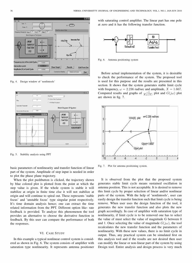
36 NIRMA UNIVERSITTY JOURNAL OF ENGINEERING AND TECHNOLOGY, VOL.1, NO.1, JAN-JUN 2010
Fig. 4. Design window of ’nonlintools’
Fig. 5. Stability analysis using PPT
basic parameters of nonlinearity and transfer function of linearpart of the system. Amplitude of step input is needed in orderto plot the phase plane trajectory.
When the plot pushbutton is clicked, the trajectory shownby blue colored plot is plotted from the point at which thestep value is given. If the whole system is stable it willstabilize at origin in finite time else it will not stabilize atorigin and will continue to spiral out. These represents ’stablefocus’ and ’unstable focus’ type singular point respectively.It’s time domain analysis hence; one can extract the timerelated information from the PPT. Different option like- ratefeedback is provided. To analyze this phenomenon the toolprovides an alternative to choose the derivative function infeedback. By this user can compare the performance of boththe responses.
VI. CASE STUDY
In this example a typical nonlinear control system is consid-ered as shown in Fig. 6. The system consists of amplifier withsaturation type nonlinearity. It represents antenna positioner
with saturating control amplifier. The linear part has one poleat zero and it has the following transfer function.
Fig. 6. Antenna positioning system
Before actual implementation of the system, it is desirableto check the performance of the system. The proposed toolis used for this purpose and the results are presented in thissection. It shows that the system generates stable limit cyclewith frequency, ω = 2.236 rad/sec and amplitude, X = 1.667.Computed results and graphs of −1
KN (X) plot and G(jω) plotare shown in fig. 7.
Fig. 7. Plot for antenna positioning system.
It is observed from the plot that the proposed systemgenerates stable limit cycle means sustained oscillation inantenna position. This is not acceptable. It is desired to removethis limit cycle by proper selection of linear and/or nonlinearparts of the system. With the help of ’nonlintools’, user caneasily design the transfer function such that limit cycle is beingremove. When user uses the design function of the tool, itgenerates the new transfer function and also plots the newgraph accordingly. In case of amplifier with saturation type ofnonlinearity, if limit cycle is to be removed one has to selectthe value of must select the value of magnitude G between 0and 1. Once selecting the value of magnitude G(jω), the toolrecalculates the new transfer function and the parameters ofnonlinearity. With these new values, there is no limit cycle inoutput. Thus, any practical system can be simulated first onthis analysis tool and if the results are not desired then usercan modify the linear or non-linear part of the system by usingDesign tool. Entire analysis and design process is very much
NIRMA UNIVERSITTY JOURNAL OF ENGINEERING AND TECHNOLOGY, VOL.1,NO.1, JAN-JUN 2010 37
user friendly.
VII. CONCLUSION
In this paper a novel analysis and design tool for nonlinearcontrol system is presented. The tool would greatly facilitatethe simulation of nonlinear systems. The tool is expected tobe useful in designing of nonlinear control systems alongwith the behavior study of nonlinear elements. The tool canaccept various types of common nonlinearities along withlinear system up to seventh order. This capabilities makesthe system very much general purpose. The tool uses newgeneration of GUIs developed in MATLAB, which greatlyenhance the user’s ease of operation. A case study of antennapositioner system demonstrates the application of the tool foractual applications. It is simple yet very effective. All theabove mentioned results are in line of the theoretical facts.’nonlintools’ has potential to use as tool in the teaching-learning process of nonlinear control course. Learning timeof the tool is very less with user friendly GUI and requiredhelp documents.
REFERENCES
[1] I.J.Nagrath, M.Gopal,”Control Systems Engineering”, New Age Interna-tional 2004.
[2] Ken Dutton, etl. ”The Art Of Control Engineering” Addition WesleyLongman, 1997
[3] M.Gopal, ” Control Systems, Principles And Design”,Tata McGrawHill,1997
[4] Hassan K. Khalil, ”Nonlinear Systems”, New York : Prentice Hall, 2002[5] Thomas L. Vincent and Walter J. Grantham, ”Nonlinear and Optimal
Control Systems”, New York: John Wiley & Sons. Inc., 1997[6] Torkel Glad and Lennart Ljung, ” Control Theory”, Taylor & Fransis &
Sons. Inc. , 2002[7] http://www.mathworks.commatlabcentral
Jaydeep Jesur Obtained his B.E. in Instrumentationand Control Engineering in 2009 from Nirma Uni-versity.
Jignesh B. Patel is Associate Professor at Insti-tute of Technology, Nirma University, Ahmedabad-382481. He has done M.Tech. (Instrumentation)from IIT, Kharagpur.
38 NIRMA UNIVERSITTY JOURNAL OF ENGINEERING AND TECHNOLOGY, VOL.1, NO.1, JAN-JUN 2010
Survey of VLSI Test Data Compression MethodsUsha Mehta
Abstract—It has been seen that the test data compression hasbeen an emerging need of VLSI field and hence the hot topicof research for last decade. Still there is a great need and scopefor further reduction in test data volume. This reduction may belossy for output side test data but must be lossless for input sidetest data. This paper summarizes the different methods appliedfor lossless compression of the input side test data, starting withsimple code based methods to combined/hybrid methods. Thebasic goal here is to prepare survey on current methodologiesapplied for test data compression and prepare a platform forfurther development in this avenue.
Index Terms—VLSI, Testing, data compression
I. NEED OF TEST DATA COMPRESSION
AS a result of the emergence of new fabrication technolo-gies anddesign complexities,standard stuck-at scan tests
are no longer sufficient. The number of tests and correspond-ing data volume increase with each new fabrication processtechnology.
Fig. 1. Volume of Test Data
As fabrication technologies evolve, test application timeand test data volume are drastically increasing just to maintaintest quality requirements. New tests require: greater than 2Xthe test time to handle devices that double in gate count butmaintain the same number of scan channels, 3X to 5X thenumber of patterns to support at-speed scan testing for thegrowing population of timing defects at 130-nm and smallerfabrication processes, and 5X the number of patterns tohandle multiple-detect and new DFM-based fault models.
Thus, the starting point is 10X compression just to maintaintester throughput and 20X if new fault models are used,
Usha Mehta is with the Department of Electronics & Communica-tion Institute of Technology, Nirma University Ahmedabad-382481, e-mail:[email protected]
which becomes 40X if the next design doubles in size. If youconsider reducing the block-level routing and top-level scanpins by 5X, that means you need 5X more compression ontop of the existing compression. Supporting multisite testingor DFM-based fault models will triple the compressionrequirements at a minimum. A major benefit of compressionis to reduce test pin count, which is a major cost benefitat manufacturing. As a result, some companies are alreadylooking for compression well beyond 100X tester cyclereduction[4][5].
Conventional external testing involves storing all testvectors and test response on an external tester-that is, ATE.But these testers have limited speed, memory, and I/Ochannels. The test data bandwidth between the tester andthe chip is relatively small; in fact, it is often the bottleneckdetermining how fast you can test the chip. Testing cannotproceed any faster than the amount of time required totransfer the test data:
Test time ≥(amount of test data on tester) / (number oftester channels X tester clock rate)[1]
The resurgence of interest in test data compression hasalso led to new commercial tools that can provide over 10Xcompression for large industrial designs. For example, theOPMISR and SmartBIST[3] tools from IBM and the TestKom-press tool from Mentor Graphics[2] reduce test data volumeand testing time through the use of test data compression andon-chip decompression.
II. TEST DATA COMPRESSION TECHNIQUES
Fig. 2. Test data compression.
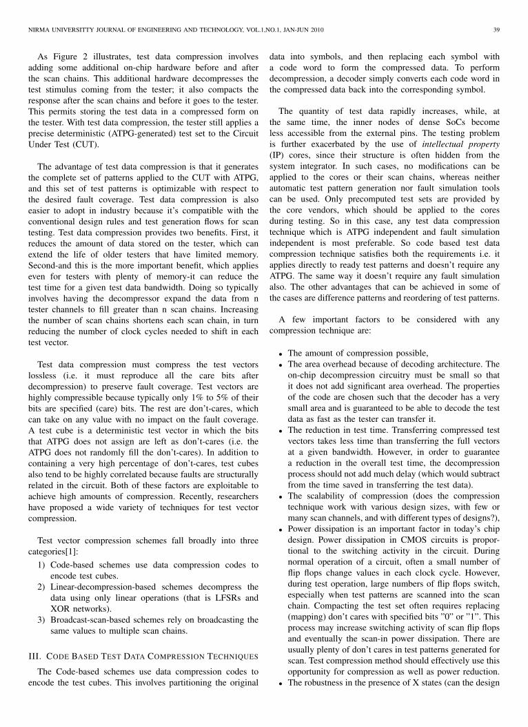
NIRMA UNIVERSITTY JOURNAL OF ENGINEERING AND TECHNOLOGY, VOL.1,NO.1, JAN-JUN 2010 39
As Figure 2 illustrates, test data compression involvesadding some additional on-chip hardware before and afterthe scan chains. This additional hardware decompresses thetest stimulus coming from the tester; it also compacts theresponse after the scan chains and before it goes to the tester.This permits storing the test data in a compressed form onthe tester. With test data compression, the tester still applies aprecise deterministic (ATPG-generated) test set to the CircuitUnder Test (CUT).
The advantage of test data compression is that it generatesthe complete set of patterns applied to the CUT with ATPG,and this set of test patterns is optimizable with respect tothe desired fault coverage. Test data compression is alsoeasier to adopt in industry because it’s compatible with theconventional design rules and test generation flows for scantesting. Test data compression provides two benefits. First, itreduces the amount of data stored on the tester, which canextend the life of older testers that have limited memory.Second-and this is the more important benefit, which applieseven for testers with plenty of memory-it can reduce thetest time for a given test data bandwidth. Doing so typicallyinvolves having the decompressor expand the data from ntester channels to fill greater than n scan chains. Increasingthe number of scan chains shortens each scan chain, in turnreducing the number of clock cycles needed to shift in eachtest vector.
Test data compression must compress the test vectorslossless (i.e. it must reproduce all the care bits afterdecompression) to preserve fault coverage. Test vectors arehighly compressible because typically only 1% to 5% of theirbits are specified (care) bits. The rest are don’t-cares, whichcan take on any value with no impact on the fault coverage.A test cube is a deterministic test vector in which the bitsthat ATPG does not assign are left as don’t-cares (i.e. theATPG does not randomly fill the don’t-cares). In addition tocontaining a very high percentage of don’t-cares, test cubesalso tend to be highly correlated because faults are structurallyrelated in the circuit. Both of these factors are exploitable toachieve high amounts of compression. Recently, researchershave proposed a wide variety of techniques for test vectorcompression.
Test vector compression schemes fall broadly into threecategories[1]:
1) Code-based schemes use data compression codes toencode test cubes.
2) Linear-decompression-based schemes decompress thedata using only linear operations (that is LFSRs andXOR networks).
3) Broadcast-scan-based schemes rely on broadcasting thesame values to multiple scan chains.
III. CODE BASED TEST DATA COMPRESSION TECHNIQUES
The Code-based schemes use data compression codes toencode the test cubes. This involves partitioning the original
data into symbols, and then replacing each symbol witha code word to form the compressed data. To performdecompression, a decoder simply converts each code word inthe compressed data back into the corresponding symbol.
The quantity of test data rapidly increases, while, atthe same time, the inner nodes of dense SoCs becomeless accessible from the external pins. The testing problemis further exacerbated by the use of intellectual property(IP) cores, since their structure is often hidden from thesystem integrator. In such cases, no modifications can beapplied to the cores or their scan chains, whereas neitherautomatic test pattern generation nor fault simulation toolscan be used. Only precomputed test sets are provided bythe core vendors, which should be applied to the coresduring testing. So in this case, any test data compressiontechnique which is ATPG independent and fault simulationindependent is most preferable. So code based test datacompression technique satisfies both the requirements i.e. itapplies directly to ready test patterns and doesn’t require anyATPG. The same way it doesn’t require any fault simulationalso. The other advantages that can be achieved in some ofthe cases are difference patterns and reordering of test patterns.
A few important factors to be considered with anycompression technique are:
• The amount of compression possible,• The area overhead because of decoding architecture. The
on-chip decompression circuitry must be small so thatit does not add significant area overhead. The propertiesof the code are chosen such that the decoder has a verysmall area and is guaranteed to be able to decode the testdata as fast as the tester can transfer it.
• The reduction in test time. Transferring compressed testvectors takes less time than transferring the full vectorsat a given bandwidth. However, in order to guaranteea reduction in the overall test time, the decompressionprocess should not add much delay (which would subtractfrom the time saved in transferring the test data).
• The scalability of compression (does the compressiontechnique work with various design sizes, with few ormany scan channels, and with different types of designs?),
• Power dissipation is an important factor in today’s chipdesign. Power dissipation in CMOS circuits is propor-tional to the switching activity in the circuit. Duringnormal operation of a circuit, often a small number offlip flops change values in each clock cycle. However,during test operation, large numbers of flip flops switch,especially when test patterns are scanned into the scanchain. Compacting the test set often requires replacing(mapping) don’t cares with specified bits ”0” or ”1”. Thisprocess may increase switching activity of scan flip flopsand eventually the scan-in power dissipation. There areusually plenty of don’t cares in test patterns generated forscan. Test compression method should effectively use thisopportunity for compression as well as power reduction.
• The robustness in the presence of X states (can the design
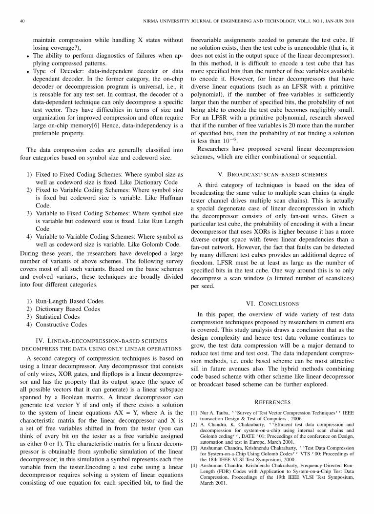
40 NIRMA UNIVERSITTY JOURNAL OF ENGINEERING AND TECHNOLOGY, VOL.1, NO.1, JAN-JUN 2010
maintain compression while handling X states withoutlosing coverage?),
• The ability to perform diagnostics of failures when ap-plying compressed patterns.
• Type of Decoder: data-independent decoder or datadependant decoder. In the former category, the on-chipdecoder or decompression program is universal, i.e., itis reusable for any test set. In contrast, the decoder of adata-dependent technique can only decompress a specifictest vector. They have difficulties in terms of size andorganization for improved compression and often requirelarge on-chip memory[6] Hence, data-independency is apreferable property.
The data compression codes are generally classified intofour categories based on symbol size and codeword size.
1) Fixed to Fixed Coding Schemes: Where symbol size aswell as codeword size is fixed. Like Dictionary Code
2) Fixed to Variable Coding Schemes: Where symbol sizeis fixed but codeword size is variable. Like HuffmanCode.
3) Variable to Fixed Coding Schemes: Where symbol sizeis variable but codeword size is fixed. Like Run LengthCode
4) Variable to Variable Coding Schemes: Where symbol aswell as codeword size is variable. Like Golomb Code.
During these years, the researchers have developed a largenumber of variants of above schemes. The following surveycovers most of all such variants. Based on the basic schemesand evolved variants, these techniques are broadly dividedinto four different categories.
1) Run-Length Based Codes2) Dictionary Based Codes3) Statistical Codes4) Constructive Codes
IV. LINEAR-DECOMPRESSION-BASED SCHEMESDECOMPRESS THE DATA USING ONLY LINEAR OPERATIONS
A second category of compression techniques is based onusing a linear decompressor. Any decompressor that consistsof only wires, XOR gates, and flipflops is a linear decompres-sor and has the property that its output space (the space ofall possible vectors that it can generate) is a linear subspacespanned by a Boolean matrix. A linear decompressor cangenerate test vector Y if and only if there exists a solutionto the system of linear equations AX = Y, where A is thecharacteristic matrix for the linear decompressor and X isa set of free variables shifted in from the tester (you canthink of every bit on the tester as a free variable assignedas either 0 or 1). The characteristic matrix for a linear decom-pressor is obtainable from symbolic simulation of the lineardecompressor; in this simulation a symbol represents each freevariable from the tester.Encoding a test cube using a lineardecompressor requires solving a system of linear equationsconsisting of one equation for each specified bit, to find the
freevariable assignments needed to generate the test cube. Ifno solution exists, then the test cube is unencodable (that is, itdoes not exist in the output space of the linear decompressor).In this method, it is difficult to encode a test cube that hasmore specified bits than the number of free variables availableto encode it. However, for linear decompressors that havediverse linear equations (such as an LFSR with a primitivepolynomial), if the number of free-variables is sufficientlylarger then the number of specified bits, the probability of notbeing able to encode the test cube becomes negligibly small.For an LFSR with a primitive polynomial, research showedthat if the number of free variables is 20 more than the numberof specified bits, then the probability of not finding a solutionis less than 10−6.
Researchers have proposed several linear decompressionschemes, which are either combinational or sequential.
V. BROADCAST-SCAN-BASED SCHEMES
A third category of techniques is based on the idea ofbroadcasting the same value to multiple scan chains (a singletester channel drives multiple scan chains). This is actuallya special degenerate case of linear decompression in whichthe decompressor consists of only fan-out wires. Given aparticular test cube, the probability of encoding it with a lineardecompressor that uses XORs is higher because it has a morediverse output space with fewer linear dependencies than afan-out network. However, the fact that faults can be detectedby many different test cubes provides an additional degree offreedom. LFSR must be at least as large as the number ofspecified bits in the test cube. One way around this is to onlydecompress a scan window (a limited number of scanslices)per seed.
VI. CONCLUSIONS
In this paper, the overview of wide variety of test datacompression techniques proposed by researchers in current erais covered. This study analysis draws a conclusion that as thedesign complexity and hence test data volume continues togrow, the test data compression will be a major demand toreduce test time and test cost. The data independent compres-sion methods, i.e. code based scheme can be most attractivesill in future avenues also. The hybrid methods combiningcode based scheme with other scheme like linear decopressoror broadcast based scheme can be further explored.
REFERENCES
[1] Nur A. Tauba, ‘‘Survey of Test Vector Compression Techniques’’ IEEEtransaction Design & Test of Computers , 2006.
[2] A. Chandra, K. Chakrabarty, ‘‘Efficient test data compression anddecompression for system-on-a-chip using internal scan chains andGolomb coding’’, DATE ’01: Proceedings of the conference on Design,automation and test in Europe, March 2001.
[3] Anshuman Chandra, Krishnendu Chakrabarty, ‘‘Test Data Compressionfor System-on-a-Chip Using Golomb Codes’’ VTS ’00: Proceedings ofthe 18th IEEE VLSI Test Symposium, 2000.
[4] Anshuman Chandra, Krishnendu Chakrabarty, Frequency-Directed Run-Length (FDR) Codes with Application to System-on-a-Chip Test DataCompression, Proceedings of the 19th IEEE VLSI Test Symposium,March 2001.

NIRMA UNIVERSITTY JOURNAL OF ENGINEERING AND TECHNOLOGY, VOL.1,NO.1, JAN-JUN 2010 41
[5] Anshuman Chandra, Krishnendu Chakrabarty, Test Data Compressionand Test Resource Partitioning for System-On-Chip Using Frequency-Directed Run-Length (FDR) Codes IEEE Transactions on Computers ,Volume 52 Issue 8, August 2003.
[6] Xrysovalantis Kavousianos, Emmanouil Kalligeros, Dimitris Nikolos,Multilevel-Huffman test-data compression for IP cores with multiplescan chains, IEEE Transactions on Very Large Scale Integration (VLSI)Systems , Volume 16 Issue 7 , July 2008.
Usha Mehta received B.E. degree in electronicsengineering from Gujarat University and MasterDegree in VLSI Design from Nirma University. Cur-rently She is Associate Professor in Electronics andCommunication Engineering Department, of Insti-tute of Technology, Nirma University. Her researchinterests include ATPG, Test Data Compression andDFT. She is a member of the IEEE, IETE, VSI andISTE.
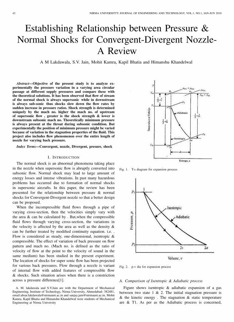
42 NIRMA UNIVERSITTY JOURNAL OF ENGINEERING AND TECHNOLOGY, VOL.1, NO.1, JAN-JUN 2010
Establishing Relationship between Pressure &Normal Shocks for Convergent-Divergent Nozzle-
A ReviewA M Lakdawala, S.V. Jain, Mohit Kamra, Kapil Bhatia and Himanshu Khandelwal
Abstract—Objective of the present study is to analyze ex-perimentally the pressure variation in a varying area circularpassage at different supply pressures and compare these withthe theoretical solutions. It has been observed that flow of streamof the normal shock is always supersonic while in downstreamis always sub-sonic thus shocks slow down the flow rates bysudden increase in pressure ratios. Shock strength is determineduniquely by the mach no. higher the mach no. of upstreamof supersonic flow , greater is the shock strength & lower isdownstream subsonic mach no. Theoretically minimum pressureis always present at the throat during subsonic condition. Butexperimentally the position of minimum pressure might be variedbecause of variation in the stagnation properties of the fluid. Thisproject also includes flow phenomenon over the entire length ofnozzle for varying back pressure.
Index Terms—Convergent, nozzle, Divergent, presure, shock
I. INTRODUCTION
The normal shock is an abnormal phenomena taking placein the nozzle when supersonic flow is abruptly converted intosubsonic flow. Normal shock may lead to large amount ofenergy losses and intense vibrations. In past many hazardousproblems has occurred due to formation of normal shocksin supersonic aircrafts. In this paper, the review has beenpresented for the relationship between pressure & normalshocks for Convergent-Divergent nozzle so that a better designcan be proposed.
When the incompressible fluid flows through a pipe ofvarying cross-section, then the velocities simply vary withthe area & can be calculated by . But,when the compressiblefluid flows through varying cross-section, the variations inthe velocity is affected by the area as well as the density &can be further treated by modified continuity equation. i.e. .Flow is considered as steady, one-dimensional, isentropic &compressible. The effect of variation of back pressure on flowpattern and mach no. (Mach no. is defined as the ratio ofvelocity of flow at the point to the velocity of sound in thesame medium) has been studied in the present experiment.The location of shocks for super sonic flow has been projectedfor various back pressures. Flow through a nozzle is variantof internal flow with added features of compressible flow& shocks. Such situation arises when there is a constrictionacross a pressure difference[1].
A. M. lakdawala and S.V.Jain are with the Department of MechanicalEngineering, Institute of Technology, Nirma University, Ahmedabad- 382481,email:[email protected] and [email protected], MohitKamra, Kapil Bhatia and Himanshu Khandelwal were students of MechanicalEngineering at Nirma University
Fig. 1. T-s diagram for expansion process
Fig. 2. p-v dia for expansion process
A. Comparison of Isentropic & Adiabatic process
Figure shows isentropic & adiabatic expansion of a gasbetween two state 1 & 2. The initial stagnation pressure is& the kinetic energy . The stagnation & static temperatureare & T1. As per as the Adiabatic process is concerned,
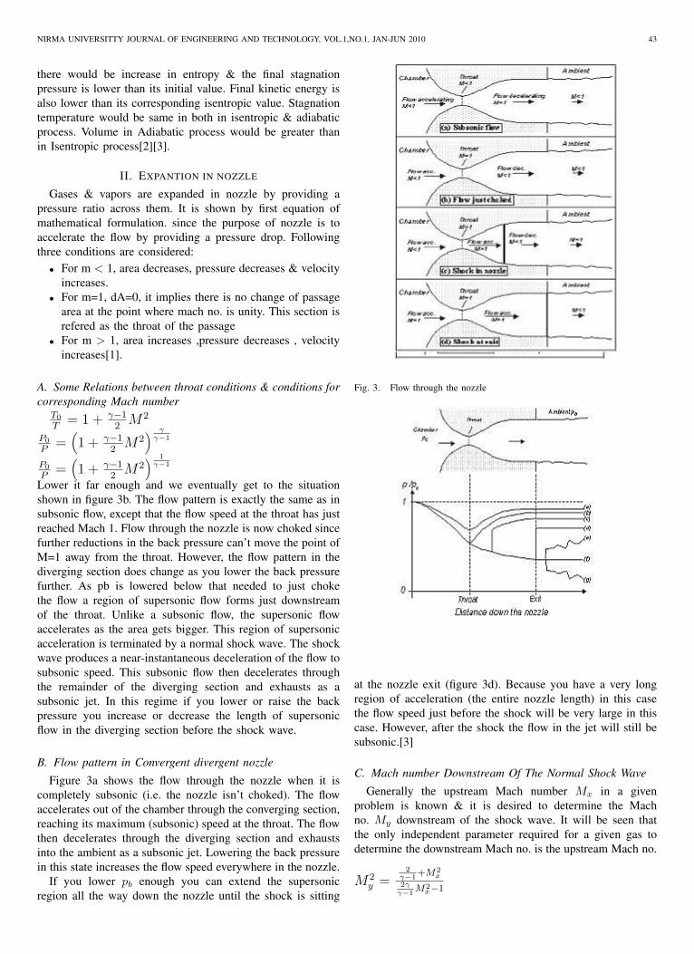
NIRMA UNIVERSITTY JOURNAL OF ENGINEERING AND TECHNOLOGY, VOL.1,NO.1, JAN-JUN 2010 43
there would be increase in entropy & the final stagnationpressure is lower than its initial value. Final kinetic energy isalso lower than its corresponding isentropic value. Stagnationtemperature would be same in both in isentropic & adiabaticprocess. Volume in Adiabatic process would be greater thanin Isentropic process[2][3].
II. EXPANTION IN NOZZLE
Gases & vapors are expanded in nozzle by providing apressure ratio across them. It is shown by first equation ofmathematical formulation. since the purpose of nozzle is toaccelerate the flow by providing a pressure drop. Followingthree conditions are considered:
• For m < 1, area decreases, pressure decreases & velocityincreases.
• For m=1, dA=0, it implies there is no change of passagearea at the point where mach no. is unity. This section isrefered as the throat of the passage
• For m > 1, area increases ,pressure decreases , velocityincreases[1].
A. Some Relations between throat conditions & conditions forcorresponding Mach number
T0T
= 1 + γ−12M2
P0
P=
(1 + γ−1
2M2
) γγ−1
P0
P=
(1 + γ−1
2M2
) 1γ−1
Lower it far enough and we eventually get to the situationshown in figure 3b. The flow pattern is exactly the same as insubsonic flow, except that the flow speed at the throat has justreached Mach 1. Flow through the nozzle is now choked sincefurther reductions in the back pressure can’t move the point ofM=1 away from the throat. However, the flow pattern in thediverging section does change as you lower the back pressurefurther. As pb is lowered below that needed to just chokethe flow a region of supersonic flow forms just downstreamof the throat. Unlike a subsonic flow, the supersonic flowaccelerates as the area gets bigger. This region of supersonicacceleration is terminated by a normal shock wave. The shockwave produces a near-instantaneous deceleration of the flow tosubsonic speed. This subsonic flow then decelerates throughthe remainder of the diverging section and exhausts as asubsonic jet. In this regime if you lower or raise the backpressure you increase or decrease the length of supersonicflow in the diverging section before the shock wave.
B. Flow pattern in Convergent divergent nozzle
Figure 3a shows the flow through the nozzle when it iscompletely subsonic (i.e. the nozzle isn’t choked). The flowaccelerates out of the chamber through the converging section,reaching its maximum (subsonic) speed at the throat. The flowthen decelerates through the diverging section and exhaustsinto the ambient as a subsonic jet. Lowering the back pressurein this state increases the flow speed everywhere in the nozzle.
If you lower pb enough you can extend the supersonicregion all the way down the nozzle until the shock is sitting
Fig. 3. Flow through the nozzle
at the nozzle exit (figure 3d). Because you have a very longregion of acceleration (the entire nozzle length) in this casethe flow speed just before the shock will be very large in thiscase. However, after the shock the flow in the jet will still besubsonic.[3]
C. Mach number Downstream Of The Normal Shock Wave
Generally the upstream Mach number Mx in a givenproblem is known & it is desired to determine the Machno. My downstream of the shock wave. It will be seen thatthe only independent parameter required for a given gas todetermine the downstream Mach no. is the upstream Mach no.
M2y =
2γ−1
+M2x
2γγ−1
M2x−1

44 NIRMA UNIVERSITTY JOURNAL OF ENGINEERING AND TECHNOLOGY, VOL.1, NO.1, JAN-JUN 2010
Static pressure ratio across the shock
PyPx
= 2γγ−1
M2x − γ−1
γ+1
D. Density Ratio Across the Shock (The Rankine-HugoniotEquation):
PyPx
=( γ+1
2 )M2x
1+( γ−12 )M2
x
=1+ γ−1
γ+1
PyPx
γ−1γ+1
+PyPx
E. Strength of Shock Wave:A parameter is defines the strength of a shock wave is
often used in shock wave analysis.
ξ =2γγ−1
(PyPx−1
)
2
2γγ−1−
(PyPx−1
)
III. CONCLUSION:It has been observed that increasing the stagnation pressure
displaces the shock position in the downstream, away from thethroat. This shows that if the length of the divergent portion isreduced than the designed condition, shock will travel towardsthe throat thereby making the entire flow subsonic, with highpressure waves in the divergent portion.
IV. FUTURE WORK:In future the project setup containing one convergent and
divergent nozzle, piezometers for measuring the pressure atdifferent point along the nozzle will be prepared to find outthe position of normal shock wave inside the nozzle. Fromthis setup the relationship between pressure & normal shockwave for convergent- divergent nozzle will be established forvarying inlet pressure as well as back pressure.
V. NOMENCLATURE:A1 Area at inletA2 Area at outletV1 Velocity of fluid at inletV2 Velocity of fluid at outletPx Pressure at inletPy Pressure at outletM Mach numberMx Upstream Mach numberMy Downstream Mach numberT0 Stagnation temperatureT Temperature at corresponding Mach no.P0 Stagnation pressure
REFERENCES
[1] http://www.wikipedia.org[2] S.M.Yahya-”Fundamentals of Compressible Flow with Aircraft and
Rocket Propulsion”, With SI Units-New Age International Publisher,Third Edition,pp 88-188.
[3] John J. Bertin & Michael L. Smith ”Aerodynamics For Engineers”, 3rdedition,pp 346-350.
Absar Lakdawala has obtained his B.E. degreein Mechanical Engineering from Gujarat Universityand M.E. degree in Mechanical Engineering fromIIT Delhi. his research interests are Internal Com-busion Engine, Computaional Fluid Dynamics andThermal System Simulation.
Sanjay Jain has obtained his B.E. and M.E. Degreein Mechanical Engineering from Gujarat Universityand IIT Roorkee Respectively. His research areasar Alternate Energy Sources, Fluid Flow and gasDynamics.
Mohit Kamra will be graduating in MechanicalEngineering from Nirma University in 2010.
Himanshu Khandelwal will be graduating in Me-chanical Engineering from Nirma University in2010.
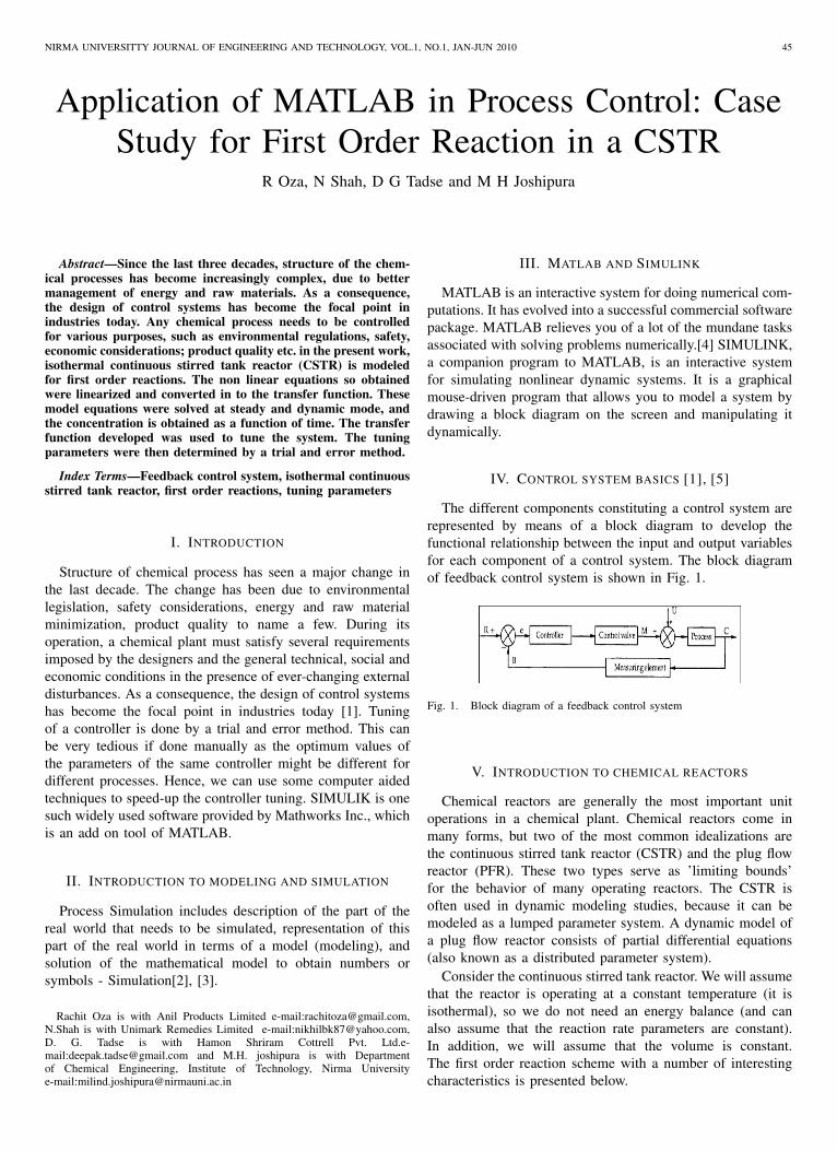
NIRMA UNIVERSITTY JOURNAL OF ENGINEERING AND TECHNOLOGY, VOL.1, NO.1, JAN-JUN 2010 45
Application of MATLAB in Process Control: CaseStudy for First Order Reaction in a CSTR
R Oza, N Shah, D G Tadse and M H Joshipura
Abstract—Since the last three decades, structure of the chem-ical processes has become increasingly complex, due to bettermanagement of energy and raw materials. As a consequence,the design of control systems has become the focal point inindustries today. Any chemical process needs to be controlledfor various purposes, such as environmental regulations, safety,economic considerations; product quality etc. in the present work,isothermal continuous stirred tank reactor (CSTR) is modeledfor first order reactions. The non linear equations so obtainedwere linearized and converted in to the transfer function. Thesemodel equations were solved at steady and dynamic mode, andthe concentration is obtained as a function of time. The transferfunction developed was used to tune the system. The tuningparameters were then determined by a trial and error method.
Index Terms—Feedback control system, isothermal continuousstirred tank reactor, first order reactions, tuning parameters
I. INTRODUCTION
Structure of chemical process has seen a major change inthe last decade. The change has been due to environmentallegislation, safety considerations, energy and raw materialminimization, product quality to name a few. During itsoperation, a chemical plant must satisfy several requirementsimposed by the designers and the general technical, social andeconomic conditions in the presence of ever-changing externaldisturbances. As a consequence, the design of control systemshas become the focal point in industries today [1]. Tuningof a controller is done by a trial and error method. This canbe very tedious if done manually as the optimum values ofthe parameters of the same controller might be different fordifferent processes. Hence, we can use some computer aidedtechniques to speed-up the controller tuning. SIMULIK is onesuch widely used software provided by Mathworks Inc., whichis an add on tool of MATLAB.
II. INTRODUCTION TO MODELING AND SIMULATION
Process Simulation includes description of the part of thereal world that needs to be simulated, representation of thispart of the real world in terms of a model (modeling), andsolution of the mathematical model to obtain numbers orsymbols - Simulation[2], [3].
Rachit Oza is with Anil Products Limited e-mail:[email protected],N.Shah is with Unimark Remedies Limited e-mail:[email protected],D. G. Tadse is with Hamon Shriram Cottrell Pvt. Ltd.e-mail:[email protected] and M.H. joshipura is with Departmentof Chemical Engineering, Institute of Technology, Nirma Universitye-mail:[email protected]
III. MATLAB AND SIMULINK
MATLAB is an interactive system for doing numerical com-putations. It has evolved into a successful commercial softwarepackage. MATLAB relieves you of a lot of the mundane tasksassociated with solving problems numerically.[4] SIMULINK,a companion program to MATLAB, is an interactive systemfor simulating nonlinear dynamic systems. It is a graphicalmouse-driven program that allows you to model a system bydrawing a block diagram on the screen and manipulating itdynamically.
IV. CONTROL SYSTEM BASICS [1], [5]
The different components constituting a control system arerepresented by means of a block diagram to develop thefunctional relationship between the input and output variablesfor each component of a control system. The block diagramof feedback control system is shown in Fig. 1.
Fig. 1. Block diagram of a feedback control system
V. INTRODUCTION TO CHEMICAL REACTORS
Chemical reactors are generally the most important unitoperations in a chemical plant. Chemical reactors come inmany forms, but two of the most common idealizations arethe continuous stirred tank reactor (CSTR) and the plug flowreactor (PFR). These two types serve as ’limiting bounds’for the behavior of many operating reactors. The CSTR isoften used in dynamic modeling studies, because it can bemodeled as a lumped parameter system. A dynamic model ofa plug flow reactor consists of partial differential equations(also known as a distributed parameter system).
Consider the continuous stirred tank reactor. We will assumethat the reactor is operating at a constant temperature (it isisothermal), so we do not need an energy balance (and canalso assume that the reaction rate parameters are constant).In addition, we will assume that the volume is constant.The first order reaction scheme with a number of interestingcharacteristics is presented below.
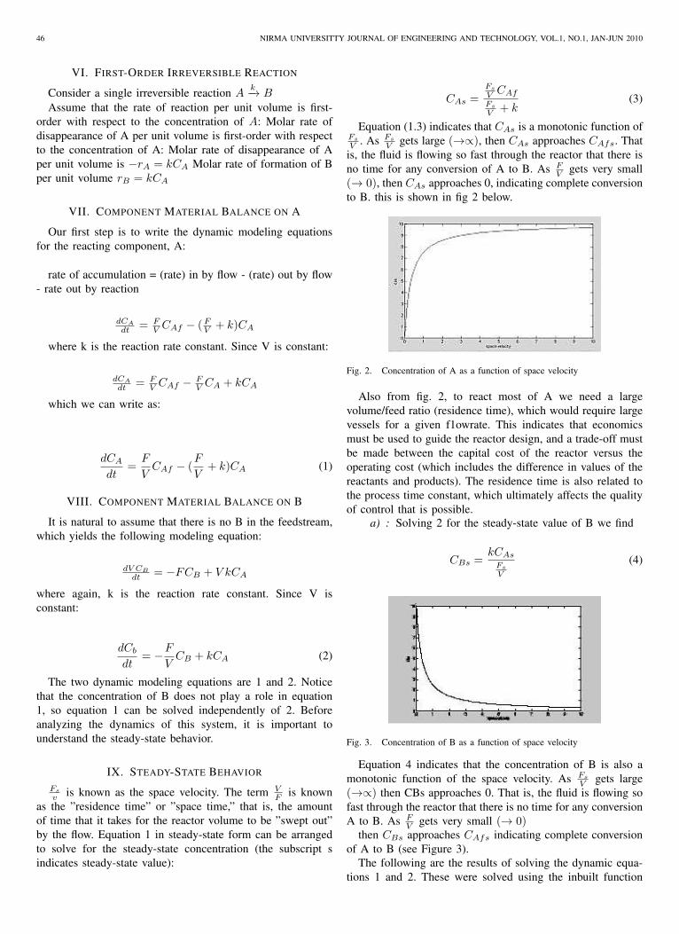
46 NIRMA UNIVERSITTY JOURNAL OF ENGINEERING AND TECHNOLOGY, VOL.1, NO.1, JAN-JUN 2010
VI. FIRST-ORDER IRREVERSIBLE REACTION
Consider a single irreversible reaction A k−→ BAssume that the rate of reaction per unit volume is first-
order with respect to the concentration of A: Molar rate ofdisappearance of A per unit volume is first-order with respectto the concentration of A: Molar rate of disappearance of Aper unit volume is −rA = kCA Molar rate of formation of Bper unit volume rB = kCA
VII. COMPONENT MATERIAL BALANCE ON A
Our first step is to write the dynamic modeling equationsfor the reacting component, A:
rate of accumulation = (rate) in by flow - (rate) out by flow- rate out by reaction
dCA
dt = FV CAf − (FV + k)CA
where k is the reaction rate constant. Since V is constant:
dCA
dt = FV CAf − F
V CA + kCA
which we can write as:
dCA
dt=F
VCAf − (
F
V+ k)CA (1)
VIII. COMPONENT MATERIAL BALANCE ON B
It is natural to assume that there is no B in the feedstream,which yields the following modeling equation:
dV CB
dt = −FCB + V kCA
where again, k is the reaction rate constant. Since V isconstant:
dCb
dt= −F
VCB + kCA (2)
The two dynamic modeling equations are 1 and 2. Noticethat the concentration of B does not play a role in equation1, so equation 1 can be solved independently of 2. Beforeanalyzing the dynamics of this system, it is important tounderstand the steady-state behavior.
IX. STEADY-STATE BEHAVIOR
Fs
v is known as the space velocity. The term VF is known
as the ”residence time” or ”space time,” that is, the amountof time that it takes for the reactor volume to be ”swept out”by the flow. Equation 1 in steady-state form can be arrangedto solve for the steady-state concentration (the subscript sindicates steady-state value):
CAs =Fs
V CAf
Fs
V + k(3)
Equation (1.3) indicates that CAs is a monotonic function ofFs
V . As Fs
V gets large (→∝), then CAs approaches CAfs. Thatis, the fluid is flowing so fast through the reactor that there isno time for any conversion of A to B. As F
V gets very small(→ 0), then CAs approaches 0, indicating complete conversionto B. this is shown in fig 2 below.
Fig. 2. Concentration of A as a function of space velocity
Also from fig. 2, to react most of A we need a largevolume/feed ratio (residence time), which would require largevessels for a given f1owrate. This indicates that economicsmust be used to guide the reactor design, and a trade-off mustbe made between the capital cost of the reactor versus theoperating cost (which includes the difference in values of thereactants and products). The residence time is also related tothe process time constant, which ultimately affects the qualityof control that is possible.
a) : Solving 2 for the steady-state value of B we find
CBs =kCAs
Fs
V
(4)
Fig. 3. Concentration of B as a function of space velocity
Equation 4 indicates that the concentration of B is also amonotonic function of the space velocity. As Fs
V gets large(→∝) then CBs approaches 0. That is, the fluid is flowing sofast through the reactor that there is no time for any conversionA to B. As F
V gets very small (→ 0)then CBs approaches CAfs indicating complete conversion
of A to B (see Figure 3).The following are the results of solving the dynamic equa-
tions 1 and 2. These were solved using the inbuilt function

NIRMA UNIVERSITTY JOURNAL OF ENGINEERING AND TECHNOLOGY, VOL.1,NO.1, JAN-JUN 2010 47
in MATLAB - ode45. This basically uses the Runge-Kuttamethod of the 4th order. The concentration of A is also firstorder with respect to CAf , but a second order transfer functionrelates CAf , to the concentration of B. The transfer functionwas obtained by first obtaining the state space models4,5 andthen using the inbuilt function ’ss2tf’ in MATLAB to convertthe state-space form into the transfer function form.As seenin fig 4 and 5, the response of B to a change in the feedcomposition of A is slower than the response of A for thesame change.
Fig. 4. Transient response to initial conditions perturbed from the steadystate value of CA(0) = 2.5
Fig. 5. Transient response to initial conditions perturbed from the steadystate value of CB(0) = 5
X. PROCESS CONTROL OF FIRST ORDER SYSTEM
The following feed-back system (fig 6) for a servo-typeproblem is developed using SIMULINK.
Fig. 6. Feedback Control System for First Order System
The main task is to determine the tuning parameters. For thiswe adopt a trial and error method (the Ziegler-Nichols closedloop method [6]). We shall consider tuning the PI controllerand not the PID controller since the first order process has agood speed of response. A PID control is normally used toincrease the speed of closed-loop response.[8]
The graph obtained for the values mentioned in Table I isshown in Fig. 7. This shows an unstable nature of the givensystem.
Fig. 7. Response obtained for step change to set point for First Order System
TABLE IPARAMETERS ASSUMED FOR PI CONTROLLER FOR THE GIVEN SYSTEM
Parameters ValueProportional 13.9Integral 5
To make it stable we assumed some new values of the tuningparameters as shown in Table II. The nature of the responseobtained is shown in Fig. 8.
Fig. 8. Response obtained for step change to set point for First Order System
According to Ziegler Nichols method the value of controllerproportional gain that causes the continuous oscillations isKcu = 13.8575. The response obtained is shown below inFig. 9.

48 NIRMA UNIVERSITTY JOURNAL OF ENGINEERING AND TECHNOLOGY, VOL.1, NO.1, JAN-JUN 2010
TABLE IIPARAMETERS ASSUMED FOR PI CONTROLLER FOR THE GIVEN SYSTEM
Parameters ValueProportional 13.5Integral 5
Fig. 9. Response obtained for step change to set point for First Order System
From the above figure the peak to peak period also calledthe ”Critical Period”, is Pu = 0.24 (i.e. distance between twosuccessive peaks).
According to Ziegler Nichols Closed-Loop OscillationMethod [6] and Tyreus-Luyben method [6], tuning parametersfor a PI controller are as shown below in Table III :
TABLE IIITUNING PARAMETERS FOR THE SYSTEM
Method kc τIZiegler- Nichols Kcu ∗ 0.5 = 6.235875 Pu
1.2= 0.2
Tyreus-Luyben Kcu3.2
= 4.33 Pu ∗ 2.2 = 0.528
Using the above mentioned parameters the closed loopresponse for the first order reaction is shown in Fig. [?] andfig 11 below.
Fig. 10. Response obtained for step change to set point for First OrderSystem for the Ziegler -Nichols tuning parameters
Fig. 11. Response obtained for step change to set point for First OrderSystem for the Tyreus-Luyben tuning parameters
XI. CONCLUSION
From Fig. 10 and Fig. 11 we can conclude that for a unitstep change in the set point, the response curve shows theconcentration approaching towards unity which indicates thatthe derived model equation for the process is correct and alsothe tuning parameters for the same are obtained using ZieglerNichols Method and the Tyreus-Luyben method. It can also beseen that the tuning parameters determined using the Tyreus-Luyben method result in less oscillatory responses and areless sensitive to changes in process conditions as compared toZiegler-Nichols method.
XII. FUTURE WORK
For more accuracy, the system can be checked with differenttuning methods and the a comparison can be carried out withrespect to stability testing.
REFERENCES
[1] George Stephanopoulos, ”Chemical Process Control”, Eastern EconomyEdition, pp. 3-20, 55-87.
[2] J.Ingham, I.J.Dunn, ”Chemical Engineering Dynamics - An introductionto modeling and computer simulation”, 2nd Edition, Wiley VCH, pp.1-6,19
[3] Brian Roffel & Ben Betlam, ”Process dynamics and control - Modelingfor prediction and control”, John Wiley and Sons,P. 169-178. c udraPratap, ”Getting started with MATLAB 7 - A quick introduction forscientists and engineers”, Oxford University Press.
[4] Rudra Pratap, ”Getting started with MATLAB 7 - A quick introductionfor scientists and engineers”, Oxford University Press.
[5] R.P. Vyas, ”Process Instrumentation and Control”, Dennett and Co., P.99-105.
[6] B.Wayne Bequette, ”Process Control - Modeling, design and Simulation”,Prentice Hall of India, pp.80-83,195-199, 573-578
[7] B.Wayne Bequette, ”Process Dynamics - Modeling, analysis and Simu-lation”, Prentice Hall of India, pp.3-6, 108-110, 506-527
[8] Pao C. Chau, ”Process Control: A First Course with MATLAB”, Cam-bridge University Press, pp.103-105.
[9] Bruce. A Finlayson,”Introduction to Chemical Engineering Computing”,Wiley Interscience, pp.111-119.
[10] W.L.Luyben, ”Process Modeling, Simulation and Control for ChemicalEngineers”, Mc-Graw Hill, pp. 14-38.
[11] W.L.Luyben, M.L.Luyben, ”Essentials of Process Control”, Mc-GrawHill, pp. 1-5.
NIRMA UNIVERSITTY JOURNAL OF ENGINEERING AND TECHNOLOGY, VOL.1,NO.1, JAN-JUN 2010 49
Rachit Oza has obtained his B.Tech in ChemicalChemical Engineering from Nirma University in2009.
Nikhil Shah has obtained his B.Tech Chemi-cal ChemicalEngineering from Nirma Universityin2009.
Deepak Tadse has obtained his B.Tech and M.Techin Chemical Chemical technology from Nagpur Uni-versity. His research interest include polymer sci-ence,process equipment design and polymerizationreaction engineering. He is life member of ISTE.
Milind H. Joshipura is working as an AssistantProfessor in Chemical Engineering Department ofInstitute of Technology in Nirma University, Ahmed-abad. He has obtained his B.E. in Chemical En-gineering from D.D.I.T ,Nadiad (Autonomous Uni-versity) in the year 2000 and Masters in ChemicalEngineering from The M S University, Baroda inyear 2002. His research interest also includes Phaseequilibria studies and Modeling and Simulation. Heis a Life member of ISTE and Associate member ofIndian Institute of Chemical Engineers (IIChE).

50 NIRMA UNIVERSITTY JOURNAL OF ENGINEERING AND TECHNOLOGY, VOL.1, NO.1, JAN-JUN 2010
CP Case Study: Cleaner Production in anAgricultural Industry
S. P. Sharma and G. H. Ban
Abstract—Agriculture is the backbone of Indian economy. Upto 70% of the population is engaged in farm sector directlyor indirectly. Growing Indian population needs sufficient farmproduct. During the Green Revolution, achieving high crop yieldsat any cost was the ultimate goal. The emphasis now is onsustainable agriculture-increasing yields without harming theenvironment at low cost. In the last half of the 20th century,there has been a growing worldwide movement among govern-ment and industry to change the way industry interact withthe environment. Cleaner production is outcome this progress.Cleaner production is a way of looking at what causes waste andthen figuring out the best way to reduce the pollution before itis created. Applying CP tools to the industry is really worth?
Index Terms—Clean production, sustainable agricul-ture, scrapped equipments
I. INTRODUCTION
THE primary function of the industry is to process inputresources in to products. However all the inputs are
not transformed in to product, the portion that does not gettransformed in to products comes out as waste. This trans-formation in to waste depends on the technology employedand efficiency of the production process. Identify activities orareas in process where wastes don’t need to be created, such aswhere efficiency can be improved; where less-toxic substancescan be substituted for more-toxic ones, and where, water orother raw materials can be saved.
Cleaner Production aims to prevent pollution, reduce theuse of energy, water and material resources and minimizewaste, profitably and without reducing production capacity. Itinvolves rethinking conventional methods to achieve ’Smarter’products, product components, and production processes. TheUnited Nations Environment Program (UNEP) defines CleanerProduction as ’The continuous application of an integrated pre-ventive environmental strategy applied to processes, products,and services to increase efficiency and reduce risks to Humansand the environment’[1][2].
II. CLEANER PRODUCTION TECHNIQUES
Cleaner production techniques are methods, which areemployed to find the way out for prevention of pollution.Generally the applicable methods for cleaner production in theIndian context can be classified in the following categories:
• Waste reduction at source– Good housekeeping– Process Changes
S.P Sharma is with Department of Chemical Engineering Institute ofTechnology Nirma University Ahmedabad-382481 and G.H. Ban is with L.D.College of Engineering, Ahmedabad,India
• On-site Recycling• Product Modification• Energy Conservation[1][6]
III. BENEFITS OF THE CLEANER PRODUCTION
Apart from reducing the manufacturing costs and thus,improving the profitability, cleaner production offers severalother benefits as follow.
• Conservation of raw materials & energy• Lower costs• Improved environment• Quality improvement & market requirement• Improved efficiency & better access to fionance [1][6]
IV. BARRIERS TO CLEANER PRODUCTION
Barriers are positive, proactive steps that cleaner productionadvocates can take to overcome the resistance to new ideas andpractices that often blocks cleaner production programme.
The major barriers are as follows:• Attitudinal barriers• Systematic barriers• Organizational barriers• Technical barriers• Economic barriers• Government barriers [1][7]
V. CLEANER PRODUCTION METHODOLOGY
The approach to be adopted for the exploitation of themaximum CP potential should be a systematic, step-by-stepapproach. The approach must be flexible enough to adaptto unexpected circumstances. One of the most successfulapproaches developed by NPC and which has been used withconsiderable success in various industrial sectors.
The approach consists of six steps or stages:• Getting Started• Analyzing Process Steps• Generating Cleaner Production Opportunities• Selecting Cleaner Production Solutions• Implementing Cleaner Production solutions• Sustaining Cleaner Production [1]
VI. ABOUT THIOPHANATE METHYL
Thiophanate-methyl is a systemic fungicide used to controlvarious diseases caused by fungal pathogens. TPM was firstregistered as a pesticide in the U.S. in 1973 for use as afungicide. EPA issued a Registration Standard for TM inMarch 1996. Thiophanate-methyl inhibits fungi growth by
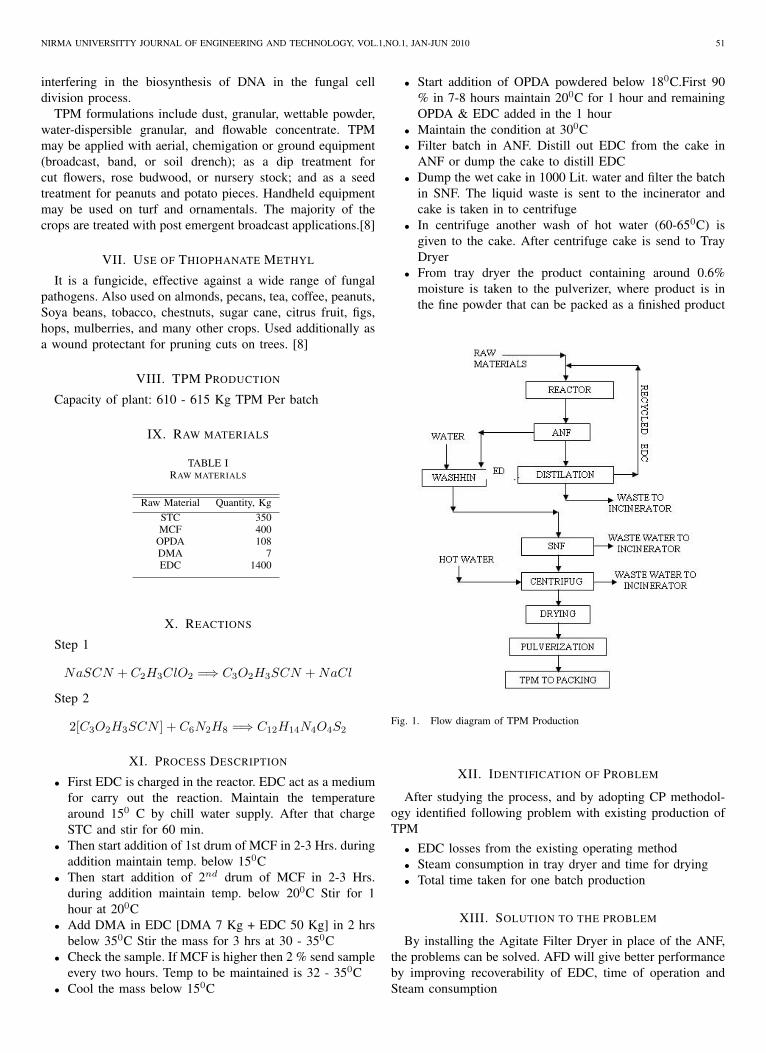
NIRMA UNIVERSITTY JOURNAL OF ENGINEERING AND TECHNOLOGY, VOL.1,NO.1, JAN-JUN 2010 51
interfering in the biosynthesis of DNA in the fungal celldivision process.
TPM formulations include dust, granular, wettable powder,water-dispersible granular, and flowable concentrate. TPMmay be applied with aerial, chemigation or ground equipment(broadcast, band, or soil drench); as a dip treatment forcut flowers, rose budwood, or nursery stock; and as a seedtreatment for peanuts and potato pieces. Handheld equipmentmay be used on turf and ornamentals. The majority of thecrops are treated with post emergent broadcast applications.[8]
VII. USE OF THIOPHANATE METHYL
It is a fungicide, effective against a wide range of fungalpathogens. Also used on almonds, pecans, tea, coffee, peanuts,Soya beans, tobacco, chestnuts, sugar cane, citrus fruit, figs,hops, mulberries, and many other crops. Used additionally asa wound protectant for pruning cuts on trees. [8]
VIII. TPM PRODUCTION
Capacity of plant: 610 - 615 Kg TPM Per batch
IX. RAW MATERIALS
TABLE IRAW MATERIALS
Raw Material Quantity, KgSTC 350MCF 400
OPDA 108DMA 7EDC 1400
X. REACTIONS
Step 1
NaSCN + C2H3ClO2 =⇒ C3O2H3SCN +NaCl
Step 2
2[C3O2H3SCN ] + C6N2H8 =⇒ C12H14N4O4S2
XI. PROCESS DESCRIPTION
• First EDC is charged in the reactor. EDC act as a mediumfor carry out the reaction. Maintain the temperaturearound 150 C by chill water supply. After that chargeSTC and stir for 60 min.
• Then start addition of 1st drum of MCF in 2-3 Hrs. duringaddition maintain temp. below 150C
• Then start addition of 2nd drum of MCF in 2-3 Hrs.during addition maintain temp. below 200C Stir for 1hour at 200C
• Add DMA in EDC [DMA 7 Kg + EDC 50 Kg] in 2 hrsbelow 350C Stir the mass for 3 hrs at 30 - 350C
• Check the sample. If MCF is higher then 2 % send sampleevery two hours. Temp to be maintained is 32 - 350C
• Cool the mass below 150C
• Start addition of OPDA powdered below 180C.First 90% in 7-8 hours maintain 200C for 1 hour and remainingOPDA & EDC added in the 1 hour
• Maintain the condition at 300C• Filter batch in ANF. Distill out EDC from the cake in
ANF or dump the cake to distill EDC• Dump the wet cake in 1000 Lit. water and filter the batch
in SNF. The liquid waste is sent to the incinerator andcake is taken in to centrifuge
• In centrifuge another wash of hot water (60-650C) isgiven to the cake. After centrifuge cake is send to TrayDryer
• From tray dryer the product containing around 0.6%moisture is taken to the pulverizer, where product is inthe fine powder that can be packed as a finished product
Fig. 1. Flow diagram of TPM Production
XII. IDENTIFICATION OF PROBLEM
After studying the process, and by adopting CP methodol-ogy identified following problem with existing production ofTPM
• EDC losses from the existing operating method• Steam consumption in tray dryer and time for drying• Total time taken for one batch production
XIII. SOLUTION TO THE PROBLEM
By installing the Agitate Filter Dryer in place of the ANF,the problems can be solved. AFD will give better performanceby improving recoverability of EDC, time of operation andSteam consumption
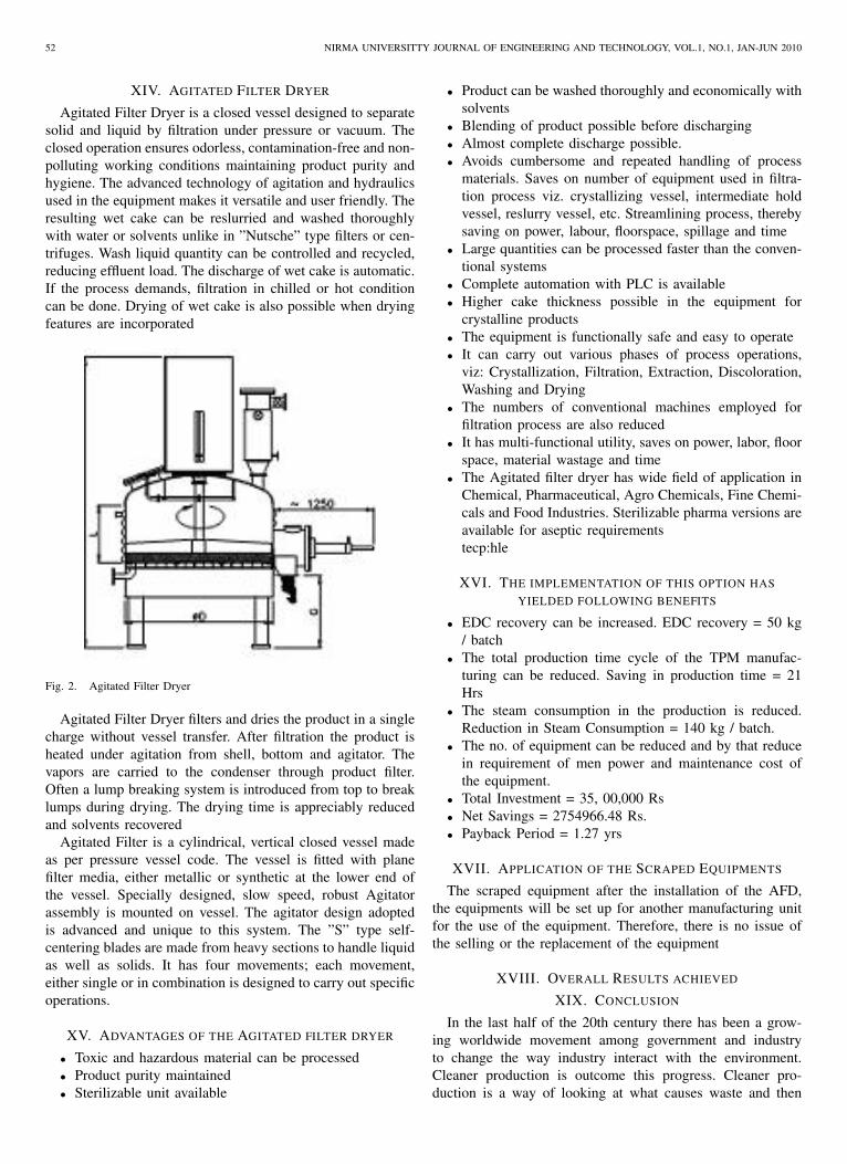
52 NIRMA UNIVERSITTY JOURNAL OF ENGINEERING AND TECHNOLOGY, VOL.1, NO.1, JAN-JUN 2010
XIV. AGITATED FILTER DRYER
Agitated Filter Dryer is a closed vessel designed to separatesolid and liquid by filtration under pressure or vacuum. Theclosed operation ensures odorless, contamination-free and non-polluting working conditions maintaining product purity andhygiene. The advanced technology of agitation and hydraulicsused in the equipment makes it versatile and user friendly. Theresulting wet cake can be reslurried and washed thoroughlywith water or solvents unlike in ”Nutsche” type filters or cen-trifuges. Wash liquid quantity can be controlled and recycled,reducing effluent load. The discharge of wet cake is automatic.If the process demands, filtration in chilled or hot conditioncan be done. Drying of wet cake is also possible when dryingfeatures are incorporated
Fig. 2. Agitated Filter Dryer
Agitated Filter Dryer filters and dries the product in a singlecharge without vessel transfer. After filtration the product isheated under agitation from shell, bottom and agitator. Thevapors are carried to the condenser through product filter.Often a lump breaking system is introduced from top to breaklumps during drying. The drying time is appreciably reducedand solvents recovered
Agitated Filter is a cylindrical, vertical closed vessel madeas per pressure vessel code. The vessel is fitted with planefilter media, either metallic or synthetic at the lower end ofthe vessel. Specially designed, slow speed, robust Agitatorassembly is mounted on vessel. The agitator design adoptedis advanced and unique to this system. The ”S” type self-centering blades are made from heavy sections to handle liquidas well as solids. It has four movements; each movement,either single or in combination is designed to carry out specificoperations.
XV. ADVANTAGES OF THE AGITATED FILTER DRYER
• Toxic and hazardous material can be processed• Product purity maintained• Sterilizable unit available
• Product can be washed thoroughly and economically withsolvents
• Blending of product possible before discharging• Almost complete discharge possible.• Avoids cumbersome and repeated handling of process
materials. Saves on number of equipment used in filtra-tion process viz. crystallizing vessel, intermediate holdvessel, reslurry vessel, etc. Streamlining process, therebysaving on power, labour, floorspace, spillage and time
• Large quantities can be processed faster than the conven-tional systems
• Complete automation with PLC is available• Higher cake thickness possible in the equipment for
crystalline products• The equipment is functionally safe and easy to operate• It can carry out various phases of process operations,
viz: Crystallization, Filtration, Extraction, Discoloration,Washing and Drying
• The numbers of conventional machines employed forfiltration process are also reduced
• It has multi-functional utility, saves on power, labor, floorspace, material wastage and time
• The Agitated filter dryer has wide field of application inChemical, Pharmaceutical, Agro Chemicals, Fine Chemi-cals and Food Industries. Sterilizable pharma versions areavailable for aseptic requirementstecp:hle
XVI. THE IMPLEMENTATION OF THIS OPTION HASYIELDED FOLLOWING BENEFITS
• EDC recovery can be increased. EDC recovery = 50 kg/ batch
• The total production time cycle of the TPM manufac-turing can be reduced. Saving in production time = 21Hrs
• The steam consumption in the production is reduced.Reduction in Steam Consumption = 140 kg / batch.
• The no. of equipment can be reduced and by that reducein requirement of men power and maintenance cost ofthe equipment.
• Total Investment = 35, 00,000 Rs• Net Savings = 2754966.48 Rs.• Payback Period = 1.27 yrs
XVII. APPLICATION OF THE SCRAPED EQUIPMENTS
The scraped equipment after the installation of the AFD,the equipments will be set up for another manufacturing unitfor the use of the equipment. Therefore, there is no issue ofthe selling or the replacement of the equipment
XVIII. OVERALL RESULTS ACHIEVED
XIX. CONCLUSION
In the last half of the 20th century there has been a grow-ing worldwide movement among government and industryto change the way industry interact with the environment.Cleaner production is outcome this progress. Cleaner pro-duction is a way of looking at what causes waste and then
NIRMA UNIVERSITTY JOURNAL OF ENGINEERING AND TECHNOLOGY, VOL.1,NO.1, JAN-JUN 2010 53
TABLE IIRESULTS ACHIEVED
Sr.No Parameter Before CP After CP % Saving1 EDC Recovery 200 lit 250 lit 25
Recovery2 Steam 893.025 753.2 16
consumption Kg /batch kg /batch
figuring out the best way to reduce the pollution before itis created. Historically, people looked for ways to controlpollution after it was created while here emphasis on ”sourcereduction”. Try to reduce the waste first and then recycle. Thisapproach can benefit the environment and save money. Thisis what industries are looking for profit. Cleaner production isbest technique for environmental protection with economicalbenefit.
At Agricultural Industry, three problems were identified, forovercome these problems Agitated Filter Dryer (technologyup gradation) option implemented and due that recovery ofEDC from operation, saving of the steam consumption andtotal production time is reduced. With removal of EDC fromthe wastewater, treatment cost associated with waste will bereduced and recovery of EDC as valuable product will berecycled, gain environment as well as economical benefit tothe company.
REFERENCES
[1] Training Manual, ”National Productivity Council”[2] Bhatt B. I. & Vora S. M. ”Stoichiometry” second edition, Tata Mc Graw
Hill Publishing Company Ltd., New Delhi, pp 60-87 & pp 67-291, 1990.[3] Perry R. H., Green D. W. & Malony J. A. ”Perry’s chemical engineers
handbook”, 6th edition, Mc Graw Hill Book Co., Singapore - pp 1025-1110,1984.
[4] Shreve R. N. & Brink J. A. ”Chemical Process Ind.” 4th edition, McGraw Hill Kogakusha Ltd, Tokyo, pp 641-643, 1977.
[5] Dryden C. E. ”Outlines of chemical technology” 2nd edition, EffiliatedEast West Press Pvt. Ltd., New Delhi,pp 619-647
[6] www.cleanerproduction.com[7] www.epa.sa.gov.au/pdfs/cpsmiths.pdf[8] www.chinesepesticide.com/fungicide.htm[9] www.hlengineers.com/construction.html
S.P. Sharma is Assistant Professor with Departmentof Chemical Engineering, Nirma University, he ob-tained his B. E. in Chemical engineering and M.E.in Environmental management.

BOOK REVIEWSControl System ComponentsAuthor: M.D.DesaiPublisher: Prentice Hall indiapages:437Price: Rs. 295
The purpose of this book is to acquaint the stu-dent with the engineering principles and fundamentalcharacteristics of a number of components used in theimplementation of many types of control systems. Theoperation of each component is discussed and explainedin detail in order to illustrate the function and actionof each component in the composite system. Examplesare used wherever possible to illustrate the principlesdiscussed. Diagrammatic illustrations are used profuselythroughout the book to make the descriptive textinteresting and self-explanatory.Although a large number of books dealing with thetheory of control engineering are available, most of themdo not deal with the varied range of components usedin modern control systems. This book is an attempt tofill this need. It comprehensively covers many typicalcomponents of primary interest to the control-systemengineer. A number of different types of electrical,electromechanical, electronic, hydraulic and pneumaticcontrol devices, which form integral parts of open-loopand closed-loop control systems, have been presentedto enable the students to understand all the types ofcontrol systems or equipment that they may encounterin different fields of industry.This book is especially designed to cater to the needof a one-semester course in Control System Compo-nents, particularly for the undergraduate students ofInstrumentation and Control Engineering. It will alsobe a highly useful text for the students of ElectricalEngineering and Mechanical Engineering during theirstudy of the theory of Control Engineering. This bookwill teach them about the components required to buildpractical control systems.
Advanced FPGA Design: ArchitectureImplementation and OptimizationAuthor: Steve KiltsPublisher: John Wiley & SonsPages: 336Price: US Dollars 99.0
This book provides the reader with issues of ad-vanced FPGA design as the underlying theme of thework. In practice, an engineer typically needs to bementored for several years before these principles areappropriately utilized. The topics that are discussedin this book are essential to designing FPGA’s beyondmoderate complexity. The goal of the book is to presentpractical design techniques that are otherwise onlyavailable through mentorship and real-world experience.There are a number of books on FPGA design, butfew of these truly address advanced real-world topicsin detail. This book attempts to cut out the fat ofunnecessary theory, speculation on future technologies,and the details of outdated technologies. It is written ina terse, concise format that addresses the various topicswithout wasting the reader’s time. Many sections in thisbook assume that certain fundamentals are understood,and for the sake of brevity, background informationand/or theoretical frameworks are not always coveredin detail. Instead, this book covers in-depth topics thathave been encountered in real-world designs. In someways, this book replaces a limited amount of industryexperience and access to an experienced mentor and willhopefully prevent the reader from learning a few thingsthe hard way. It is the advanced, practical approach thatmakes this book unique.

Copyright © 2022 FDOKUMEN


![[2002] A. FERRARESE, La popolazione di Soave in età moderna. Strutture familiari, evoluzione demografica, congiunture. In: Soave ‘terra amenissima, villa suavissima’; a cura di](https://static.fdokumen.com/doc/165x107/6313aecfb033aaa8b2103155/2002-a-ferrarese-la-popolazione-di-soave-in-eta-moderna-strutture-familiari.jpg)