Wolfgang KinzelbachInstitute of Environmental Engineering

ETH Zürich

Groundwater modeling:Basics and equations

Groundwater II

Where are groundwater modelsrequired?

• For integrated interpretation of data• For improved understanding of the functioning of

aquifers• For the determination of aquifer parameters• For prediction• For design of measures• For risk analysis• For planning of sustainable aquifer management

Examples• Installation of new well fields

– Sustainability? Environmental impacts? Water quality?

• Well head protection zones– Size and shape of catchment, travel times

• Design of remediation measures– Feasibility, optimization of costs

• Risk analysis of repositories (e.g. for radioactivewaste)

Why models?• Relative inaccessibility of object of interest• Scarce data in geosciences required conceptual

model for analysis• Complexity of nature requires simplification• Connection between quantities of interest and

measurable quantities• Slowness of processes requires predictive capability• Big effort in interpretation justified by high cost of

data

Types of groundwater models• Flow models (saturated flow, homogeneous fluid)

– Modeled quantity: Piezometric head h– Derived quantity: Darcy-velocity v

• Solute transport models (hydrodynamicallyinactive, dissolved substances)– Modeled quantity: concentration c– Derived quantity: mass flux j

• Unsaturated flow and multiphase flow• Coupled models

– density, soil mechanics, temperature– complex chemistry

Basic equations• Starting from first principles:

– Conservation of mass (or volume if density is constant)– Conservation of dissolved mass (solute)

• General approach based on the following quantities:– Extensive quantity Φ (volume, dissolved mass) – Intensive quantity ξ = Extensive quantity per unit volume

(porosity, concentration)– Flux j (of volume, diss. mass) (Quantity per unit area and time)– Source-sink distribution σ (volume per geometric volume and

time, diss. mass per water volume and time)

General principle: in 1D (for simplicity)

x

Δx

Fluxin Fluxout

Storage is change in extensive quantity

Gain/loss from volumesources/sinks

Conservation law in words:

Cross-sectional area AVolume V = AΔx

x+Δx

Time interval [t, t+Δt]

( ) _in outFlux Flux A t source density V t Storage− ⋅ ⋅Δ + ⋅ ⋅Δ =

General principle in 1D

)()())()(( ttttVtAxxjxj Φ−Δ+Φ=Δ⋅⋅+Δ⋅⋅Δ+− σ

tttt

xxxjxj

Δ−Δ+

=+Δ

Δ+− )()()()( ξξσ

Division by ΔtΔxA yields:

In the limit Δt, Δx to 0:

txj

∂∂

=+∂∂

−ξσ

General principle in 3D

tzj

yj

xj zyx

∂∂

=+∂∂

−∂

∂−

∂∂

−ξσ

tj

∂∂

=+⋅∇−ξσ

or

Water balance: in 1D

x

Δx

Storage can be seen as changein intensive quantity

Gain/loss by volumesources/sinks

Conservation equation for water volume

x+Δx

Time interval [t, t+Δt]

)(vx xjin = )(vx xxjout Δ+=

)()())(v)(v( xx tVttVtVwtAxxx waterwater −Δ+=Δ⋅⋅+Δ⋅⋅Δ+−

Density assumed constant!

V=AΔx

Water balance: in 1D continued

th

dhdnw

x ∂∂

=+∂

∂− xv

xhKandS

dhdn

x ∂∂

−== v0

tn

tVVw

xxxx waterx

ΔΔ

=Δ

Δ=+

Δ−Δ+

−)/()(v)(vx

Using the definition of the storage coefficient and Darcy‘s law:

In the limit

thSw

xhK

x ∂∂

=+∂∂

∂∂

0)(

(Vwater/V=n)

Generalization to 3D

thSw

zyx ∂∂

=+∂∂

−∂

∂−

∂∂

− 0zyx vvv

vv vv vyx zwith - h andx y z

∂∂ ∂= ∇ + + = ∇ ⋅

∂ ∂ ∂K

thSwh)(

∂∂

=+∇⋅∇ 0K

Multitude of aquifers through distributions of K, S0 and wand boundary and initial conditions

+ Initial conditions+ Boundary conditions

In practical applications: often 2D and 2.5 D models

thSqh)(T

∂∂

=+∇⋅∇

2D confined Aquifer: by integration over z-coordinate

2D unconfined Aquifer: by integration over z-coordinate

thnqh)Bottomh(K

∂∂

=+∇−⋅∇ )(

with T=K(Top-Bottom) andS= S0(Top-Bottom)

with n= porosity

2.5 D by vertical coupling of 2D layers throughleakage-term

1 1( ) (i layer i layer i i layer i layer iq h h h h 1)λ λ− −= − + − +(λ=Kvert/Δz)

• First type: h on boundaryspecified

• Second type: given on boundary

• Third type: given on boundary

• Further: Free surface p=0, evaporation boundary, moving boundary

nh

Boundary conditions for flow

∂∂ /

nhh ∂∂⋅+⋅ /βα

• Use natural hydrogeological boundaries (e.g. rivers, waterdivides, end of aquifers)

• Use as few fixed head boundaries as possible (at least one isnecessary in a steady state model)

• At upstream boundaries use fixed flux boundary. At downstream boundaries use fixed head boundary.

• Use third type boundary conditions for distant fixed heads. • Streamlines are boundaries of the second type. Careful: If

used together with pumping, check whether changes in flux between the two streamlines stay small against total flow through the stream tube.)

Practical rules for setting boundaryconditions in flow models

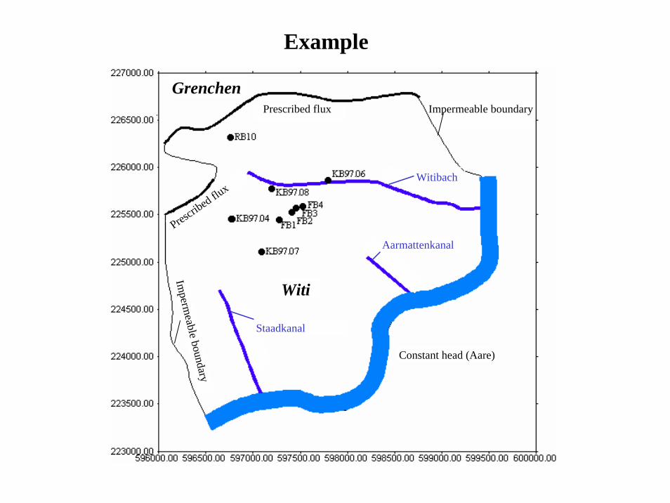
Prescribed flux

Prescrib

ed flux

Impermeable boundary

Imperm

eable boundary

Witi

Constant head (Aare)

Grenchen

Witibach

Staadkanal

Aarmattenkanal

Example

And now the same for transport of a solute...

• The flux is more complicated:• It is composed of

– Advective Flux – Diffusive Flux– Dispersive Flux

• Total flux:

cjconv v=

cnDj mdiff ∇−=

cnjdisp ∇−= D

dispdiffadvtot jjjj ++=

(v ist Darcy-velocity)

Mass balance: in 1D

x

Δx

Storage of dissolved mass

Losses from degradationand reaction according to 1st order reaction.Gains by injection

Conservation equation for dissolved mass

x+Δx

)(, xj xtotal )(, xxj xtotal

time interval [t, t+Δt]

Δ+

))()(())()((

tmttmtVcwtVnctAxxjxj intotal,xtotal,x

−Δ+

=Δ⋅⋅⋅+Δ⋅⋅⋅⋅−Δ⋅⋅Δ+− λ

V=AΔx

Mass balance: in 1D continued

tncwcnc

xj

intotal,x

∂∂

=+−∂

∂−

)(λ

tVtcVttcVwcnc

xxjxxj waterwater

intotal,xtotal,x

Δ⋅−Δ+⋅

=+−Δ

−Δ+−

/))()(()()(λ

In the limit:

Substitution of expression into fluxes:

tncwcnc

xcDDn

xxc in

Lmx

∂∂

=+−∂∂

+⋅∂∂

+∂

∂−

)(1

))(()v( λ

With n = constant and pore velocity u = v/n:

tc

nwcc

xcDD

xxc in

Lmx

∂∂

=+−∂∂

+∂∂

+∂

∂− λ))(()u(

Mass balance: generalization to 3D

Again: + boundary conditions + initial conditions

tc

nwcccDc in

m ∂∂

=+−∇+⋅∇+⋅∇− λ))(()u( D

With )()(u)(u)(u zyx cuzc

yc

xc

⋅∇=∂

∂+

∂

∂+

∂∂

⎥⎥⎥

⎦

⎤

⎢⎢⎢

⎣

⎡=∇+=+

T

T

L

mdispdiff

DD

DundcDjj

000000

)( DD

In a system, in which u isparallel to x-axis!

und

• Still more complete version

• required: Flow field u and• parameter: n, D (d.h. αL, αT, αTv,Dm), R, λ

)()(1 ccnRwccD

Rc

Ru

tc

in −+−∇∇+∇−=∂∂ λ

Storage

Advection

Dispersion

Degradation

External sources/sinks

Retardation

Transport equation

Illustration of transportFlow direction

t=0

t=ΔtAdvection

Advection and dispersion

Advection, dispersion and adsorption

Advection, dispersion, adsorption and degradation

x

x

x

x

x

Boundary conditions for thetransport equation

• First type: c prescribed on boundary, determines advective flux

• Second type: prescribed on boundary, determinesdiffusive-dispersive flux (usually usedto make a boundary impervious fordiffusion/dispersion, e.g. on streamlinealong impervious boundary

• Third type: prescribed on boundary, determines total flux

• Transmission boundary on boundary (or D=0 on boundary)

nc ∂∂ /

ncc ∂∂⋅+⋅ /βα

0/ 22 =∂∂ nc

c=0 impervious0/ =∂∂ nc

transmission

impervious

first or third type

Analysis of type of equations

• Flow equation (K and S0 constant)

th

xh

SK

∂∂

=∂∂

2

2

0

Type: Parabolic equation, diffusion equation withdiffusion coefficient K/S0

• Transport equation (n and u constant)

0+∂∂

tc

2

2

=∂∂xcD−

∂∂xcu

Type: mixed, two types of terms

Has consequences for solution method!

Special properties of transportequation

Tdisp = L2/D

• If only advection: Hyperbolic equation, describingthe propagation of a shock front along characteristiclines (trajectories), typical time scale

Tadv = L/u• If only diffusion: Parabolic equation, describing

diffusive spreading in all directions of space up to boundaries. Slowing down due to decreasinggradients, typical time scale

• Invariant: Peclet-number = Tdisp/Tadv = uL/D

L correspondsto Δx in numericalmodel!