This article was downloaded by: [University of Southampton Highfield]On: 25 June 2012, At: 04:51Publisher: Taylor & FrancisInforma Ltd Registered in England and Wales Registered Number: 1072954 Registeredoffice: Mortimer House, 37-41 Mortimer Street, London W1T 3JH, UK

Journal of Applied StatisticsPublication details, including instructions for authors andsubscription information:http://www.tandfonline.com/loi/cjas20

Clustering microarray data using model-based double K-meansFrancesca Martella a & Maurizio Vichi aa Scienze statistiche, Sapienza Universitá di Roma, Roma, Italy

Available online: 01 May 2012

To cite this article: Francesca Martella & Maurizio Vichi (2012): Clustering microarray data usingmodel-based double K-means, Journal of Applied Statistics, DOI:10.1080/02664763.2012.683172

To link to this article: http://dx.doi.org/10.1080/02664763.2012.683172

PLEASE SCROLL DOWN FOR ARTICLE

Full terms and conditions of use: http://www.tandfonline.com/page/terms-and-conditions

This article may be used for research, teaching, and private study purposes. Anysubstantial or systematic reproduction, redistribution, reselling, loan, sub-licensing,systematic supply, or distribution in any form to anyone is expressly forbidden.

The publisher does not give any warranty express or implied or make any representationthat the contents will be complete or accurate or up to date. The accuracy of anyinstructions, formulae, and drug doses should be independently verified with primarysources. The publisher shall not be liable for any loss, actions, claims, proceedings,demand, or costs or damages whatsoever or howsoever caused arising directly orindirectly in connection with or arising out of the use of this material.

Journal of Applied Statistics2012, iFirst article

Clustering microarray data usingmodel-based double K-means

Francesca Martella∗ and Maurizio Vichi

Scienze statistiche, Sapienza Universitá di Roma, Roma, Italy

(Received 30 May 2011; final version received 3 April 2012)

The microarray technology allows the measurement of expression levels of thousands of genessimultaneously. The dimension and complexity of gene expression data obtained by microarrays createchallenging data analysis and management problems ranging from the analysis of images produced bymicroarray experiments to biological interpretation of results. Therefore, statistical and computationalapproaches are beginning to assume a substantial position within the molecular biology area. We considerthe problem of simultaneously clustering genes and tissue samples (in general conditions) of a microarraydata set. This can be useful for revealing groups of genes involved in the same molecular process as well asgroups of conditions where this process takes place. The need of finding a subset of genes and tissue samplesdefining a homogeneous block had led to the application of double clustering techniques on gene expres-sion data. Here, we focus on an extension of standard K-means to simultaneously cluster observations andfeatures of a data matrix, namely double K-means introduced by Vichi (2000). We introduce this model ina probabilistic framework and discuss the advantages of using this approach. We also develop a coordinateascent algorithm and test its performance via simulation studies and real data set. Finally, we validate theresults obtained on the real data set by building resampling confidence intervals for block centroids.

Keywords: microarray data; model-based biclustering; double K-means; stratified resamplingprocedure; coordinate ascent algorithm

1. Introduction

In the last decade, the continuous production of large data sets has posed the problem to minethe relevant information by means of the “dimensionality reduction” of objects and features.Statistical literature provides many clustering techniques for the identification of “homogeneous”groups of objects which are perceived as “similar” to one another within each group [15]. Theycan be applied to obtain a clustering of features as well. If the interest is to cluster both objectsand features, then these methods can be applied as both objects and features successively andindependently [31]. However, results depend on whether objects or features are classified first.

To overcome this problem, objects and features can be partitioned simultaneously rather thansuccessively as suggested by Fisher [12]. This case will be referred to as double clustering.

∗Corresponding author. Email: francesca.martella@uniroma1.it

ISSN 0266-4763 print/ISSN 1360-0532 online© 2012 Taylor & Francishttp://dx.doi.org/10.1080/02664763.2012.683172http://www.tandfonline.com

Dow

nloa

ded

by [

Uni

vers

ity o

f So

utha

mpt

on H

ighf

ield

] at

04:

51 2

5 Ju

ne 2

012

2 F. Martella and M. Vichi

Such methodologies are also known under other names, including biclustering, block clustering,bidimensional clustering, subspace clustering co-clustering, simultaneous clustering and block-modeling, and the basic idea consists of identifying blocks, that is, sub-matrices of the observeddata matrix, which satisfy some specific characteristics of homogeneity and which may vary withdifferent approaches. Moreover, units and variables forming each block specify a unit clusterand a variable cluster. For applying double clustering methods, it is necessary that features areexpressed in the same scale of measurement, so that entries are comparable among both rowsand columns; otherwise, they need to be rescaled. The most important advantage of a double(rather than a sequential) clustering is that the former allows to highlight the eventual interac-tion or dependence between objects and features helping in their characterization by using an“overall” objective function that cannot be reduced to a simple combination of row and columnobjective functions.

Starting with the pioneering work of Hartigan [19] and with the decision-theoretic work of Bock[6], during the past three decades, this class of methods has been widely developed by variousauthors in different fields such as marketing, customer satisfaction, social network, psychol-ogy, text mining, election and nutritional analyses. In particular, in microarray analysis, a majorproblem consists in clustering patients or tissue samples (in general, experimental conditions)with similar behavior with respect to gene expression. However, applying clustering successivelyto patients and tissue samples leads to significant difficulties. In fact, many activation patternsare common to groups of genes only under specific experimental conditions. Therefore, doubleclustering of genes and tissue samples allows to achieve the further goal of detecting groups ofgenes with similar functions characterizing a specific subset of experimental conditions. Thisapproach was first introduced to gene expression analysis by Cheng and Church [9] with the term“biclustering”. Since then, several alternative biclustering approaches have been used within geneexpression analysis [3,8,10,13,23,24,29,37,38].

Most methodologies referred above are heuristic procedures that do not use a clustering modeland a clear statistical estimation method to optimize a criterion able to measure the disagreementbetween the given model and observed data (as it is the case in clustering literature based on least-squares (LS) or maximum-likelihood (ML) methods). Bock [6] proposed a statistical model and aniterative algorithm, in case of quantitative data, optimizing the LS criterion. Bock [7] also proposeda double clustering for contingency tables. Govaert [16] proposed a simultaneous clustering ofobjects and features for binary data. Govaert and Nadif [17] considered a simultaneous partitionof objects and features by using a Bernoulli mixture approach and proposing a new version ofthe classification expectation maximization (CEM) algorithm: block CEM algorithm. Vichi [35]introduced a double K-means clustering, which is the two-way partition version of a standardK-means model given by McQueen [28]. Rocci and Vichi [30] proposed a multi-way partitioning,which is useful when the observed data are characterized by a more complex structure (e.g.measurements of variables on units considered in different occasions). For an overview of doubleclustering methods, two structured taxonomies of double clustering methods have been proposedby Van Mechelen et al. [33] and Madeira and Oliveira [26]. In the former paper, the overviewstarts from a traditional statistical/data analytic perspective, while in the latter paper, the topicis discussed on the bioinformatics side. Besides the methods discussed in this section, otherapproaches to double clustering have been introduced. Van Mechelen [32] and Van Mechelenand Schepers [34] have proposed to include in a unique and more general model the most ofdouble clustering methods proposed in the literature by focusing on some aspects of clusters tobe formed and mathematical operators used to define overlapping clustering. More recently, Liand Zha [25] proposed a two-way Poisson mixture model, Govaert and Nadif [18] proposed adouble clustering with Bernoulli mixture models, Wyse and Friel [36] suggested its extension in aBayesian approach, and Martella et al. [27] proposed extensions of mixture models for biclusteringin microarray data.

Dow

nloa

ded

by [

Uni

vers

ity o

f So

utha

mpt

on H

ighf

ield

] at

04:

51 2

5 Ju

ne 2

012

Journal of Applied Statistics 3

The starting point of our proposal is double K-means clustering [35]. A serious limitation ofthis model is related to the heuristic procedures used for determining the correct number of blocks.Moreover, standard double K-means assumes the Euclidean distance as a distance function, andtherefore, spherical clusters are detected. However, it is well known that the use of a distancemeasure that takes into account the shape of the clusters is in general more appropriate. In orderto overcome these problems, we propose double K-means in a probabilistic framework, wherethe choice of the number of clusters is less arbitrary and homogeneous but unrestricted clustervariances are allowed, inducing the use of a Mahalanobis distance to assess dissimilarities toidentify clusters. The paper is organized as follows.

In Section 2, we present double K-means in order to simultaneously cluster units and vari-ables [35]. Here, the model parameters are estimated by using an LS approach, optimizing aquadratic objective function subject to a set of constraints due to the required clustering structure(e.g. partitions, coverings or packing) and the clustering type (hard or fuzzy). Section 3 discussesour proposal and a coordinate ascent algorithm to give an efficient solution to the fitting model.Moreover, we describe properties, model selection and the stratified resampling procedure to val-idate the results. Section 4 contains the results obtained on simulation studies in order to evaluateperformance of our proposal, while Section 5 describes the results obtained on a benchmark geneexpression data. Conclusions are discussed in Section 6.

2. Double K-means

Gene expression data are typically arranged in an n × J matrix, X, with rows corresponding togenes and columns corresponding to tissue samples (in general, experimental conditions). Eachentry, xij, represents the expression level of the gene corresponding to row i under the specificcondition corresponding to column j (i = 1, . . . , n; j = 1, . . . , J). The double K-means modelsupposes that data matrix X is written as follows:

X = UXV′ + E, (1)

where U (n × K), K ≤ n, represents the binary and row stochastic matrix of the gene clustermembership, where uik = 1 if the ith gene belongs to cluster k, 0 otherwise; V(J × Q), Q ≤ J ,represents the binary and row stochastic matrix of the tissue sample cluster membership, wherevjq = 1 if the jth tissue sample belongs to the tissue sample cluster q, 0 otherwise; X (K × Q) isa matrix of the block gene-tissue sample centroids, where the generic element xkq is the expectedprofile of the kth gene cluster and the qth tissue sample cluster (k = 1, . . . , K ; q = 1, . . . , Q).Finally, E (n × J) represents a residual component matrix.

It can be noticed that when V = IJ or U = In, the double K-means collapses into the ordinaryK-means on the genes or on the tissue samples, respectively.

In particular, the model can be expressed in a row form as

xi = VX′ui + ei, i = 1, . . . , n, (2)

where xi is a (J × 1) vector representing the ith gene and ui is the ith gene membership vector.Vector ei represents the ith row of E.

In the same way, model (1) can be expressed in a column form as

xj = UXvj + ej, j = 1, . . . , J , (3)

Dow

nloa

ded

by [

Uni

vers

ity o

f So

utha

mpt

on H

ighf

ield

] at

04:

51 2

5 Ju

ne 2

012

4 F. Martella and M. Vichi

where xj is an (n × 1) vector representing the jth tissue sample and vj is the jth tissue samplemembership vector. Vector ej represents the jth column of E.

The problem of determining a block partition of the gene expression matrix X can be formalizedby considering the loss function

minU,X,V

‖X − UXV′‖2, (4)

subject to constraints uik ∈ {0, 1}, i = 1, . . . , n, k = 1, . . . , K ;∑K

k=1 uik = 1, i = 1, . . . , n; vjq ∈{0, 1}, j = 1, . . . , J , q = 1, . . . , Q;

∑Qq=1 vjq = 1, j = 1, . . . , J .

In other words, we require that each block consists of entries that are as much similar as possiblein an LS sense. Let us suppose U and V are the corresponding estimates; in this case, problem (4)can be reduced to determinate the LS solution of a generalized multivariate regression problem

minX

‖X − UXV′‖2, (5)

which leads to the solutionˆX = (U

′U)−1U

′XV(V

′V)−1. (6)

However, since U and V are unknown, Vichi [35] proposed an alternating least-squares (ALS)algorithm for parameter estimation. It sequentially and recursively solves assignment problems,as shown in Table 1. The ALS algorithm, at each step, monotonically decreases the loss functionconverging to a stationary point (local or global minimum). Initial values for U and V can berandomly chosen; obviously, using different random starting points for U and V, we can increasethe chance of finding a global minimum.

3. ML approach

Let us consider the double K-means model written in row form (2) and assume that the meanvector and the covariance matrix of the random vector xi can be written as E(xi) = VX

′ui and

Var(xi) = �, respectively (i = 1, . . . , n). Here, it can be noticed that for reasons of parsimony, theassumption of homoscedasticity for the covariance matrix is specified. It is further assumed that

xi|ui ∼ MVN(VX′ui, �),

that is, the density of xi|ui has the following form:

f (xi, φ) = 1√(2π)J

|�|−1/2 exp

{−1

2(xi − VX

′ui)

′�−1(xi − VX′ui)

}, (7)

where φ = {X, �, U,V} is the parameter set. Moreover, ui and vj are supposed to be fixed variables.

Table 1. ALS algorithm for double K-means.

Initialization Choose initial values for U and V. Such values can be chosen randomly or in arationale way

Step 1: Update X Given the current estimates of U and V, update X using Equation (6)Step 2: Update U Minimize Equation (4) over U, given the current estimate of V and XStep 3: Update V Minimize Equation (4) over V, given the current estimate of U and XStopping rule Function (4) is computed for the current values of U, V and X

If the function is considerably lower than in the previous iteration, U, V and Xare updated once more according to steps 1, 2 and 3. Otherwise, the process has

converged

Dow

nloa

ded

by [

Uni

vers

ity o

f So

utha

mpt

on H

ighf

ield

] at

04:

51 2

5 Ju

ne 2

012

Journal of Applied Statistics 5

Let (x1, x2, . . . , xn) be a sample of i.i.d. J-dimensional observations drawn from the densityf (xi, φ); the corresponding likelihood function for fixed U and V matrices is given by

L(U,V, X, �) = 1√(2π)Jn

|�|−n/2 exp

{−1

2

n∑i=1

(xi − VX′ui)

′�−1(xi − VX′ui)

}

= 1√(2π)Jn

|�−1|n/2 exp

{−1

2tr[�−1(X − UXV′)′(X − UXV′)]

}, (8)

and thus the log-likelihood function is

l = ln L(U,V, X, �) = −nJ ln√

2π + n

2ln |�−1| − 1

2tr[�−1(X − UXV′)′(X − UXV′)]. (9)

Nevertheless, when a biclustering problem occurs, the matrices U and V are not specified andhave to be estimated. Maximum-likelihood estimation (MLE) of model parameters is obtainedby maximizing the log-likelihood function, l, with respect to U, V, X and � subject to binary androw stochastic constraints on U and V shown in the previous section.

Fixed U and V, the optimal X and � are the ML solutions of the (generalized) multivariateregression problem X = UXV′ + E, where E is a residual term.

However, since U and V are unknown, the MLEs of the double K-means model can be obtainedby algorithms that alternatively maximize the log-likelihood function. The fundamental steps ofthese algorithms can be described as follows.

• Updating X:When U, V and � are fixed, the ML estimate of X is given by solving the correspondinglikelihood equations

∂l

∂X∝ ∂

∂X

{−1

2tr

[�−1(X − UXV′)′(X − UXV′)

]} = 0,

that is,∂l

∂X∝ U′X�−1V − U′UXV′�−1V = 0

which leads to the ML estimator of X is given by

ˆX = (U′U)−1U′X�−1V(V′�−1V)−1. (10)

• Updating �:When U, X and V are fixed, the ML estimate of � is given by solving the correspondinglikelihood equations

∂l

∂�−1 ∝ ∂

∂�−1

{n

2ln |�−1| − 1

2tr

[�−1(X − UXV′)′(X − UXV′)

]} = 0,

that is,∂l

∂�−1 ∝ n

2� − 1

2(X − UXV′)′(X − UXV′) = 0,

and then the ML estimator of � is given by

� = 1

n(X − UXV′)′(X − UXV′). (11)

As far as the updating of U and V is concerned, the estimation is achieved row by row; that is,by putting the value 1 in the column position where the complete log-likelihood is maximized.

Dow

nloa

ded

by [

Uni

vers

ity o

f So

utha

mpt

on H

ighf

ield

] at

04:

51 2

5 Ju

ne 2

012

6 F. Martella and M. Vichi

In formulas as follows:• Updating U:

When V, X and � are fixed, for each i = 1, . . . , n, let

uik ={

1 if l(·, uik = 1) = maxh l(·, uih = 1) h = 1, . . . , K , h = k,

0 otherwise.(12)

• Updating V:When U, X and � are fixed, for each j = 1, . . . , J , let

vjq ={

1 if l(·, vjq = 1) = maxz l(·, vjz = 1) z = 1, . . . , Q, z = q,

0 otherwise.(13)

In the case of heteroscedasticity, the likelihood function of the sample data under the Gaussianassumption became as follows:

L(U,V, x1, . . . xK , �1, . . . , , �K) =n∏

i=1

K∏k=1

MVN(xiuik|Vxk , �k), (14)

where xiuik represents the ith observation in the kth cluster, xk and �k are the row-cluster-specificmean vector in the reduced Q-dimensional space (i.e. the kth row of X) and the row-cluster-specificcovariance matrix, respectively. Thus, the log-likelihood function of the model is given by

l(U,V, x1, . . . xK , �1, . . . , , �K) =n∑

i=1

K∑k=1

log MVN(xiuik|Vxk , �k). (15)

After some algebra, the following ML estimator for the row-cluster-specific covariance matrix isgiven by

�k =n∑

i=1

(xiuik − Vxk)(xiuik − Vxk)′(ukuk)

−1. (16)

The updating of U and V are similar to the homoscedastic case where the log-likelihood functionis given by Equation (15).

3.1 The coordinate ascent algorithm

In this section, the algorithm for parameter estimations of double K-means model under anML approach is presented. In particular, this algorithm performs a coordinate ascent on the log-likelihood function, that is, it picks a block of parameters and optimizes the log-likelihood functionover this block, considering all other parameters as fixed.

Initialization. Some initial values are chosen for U and V. Such values can be chosen randomlyor in a rationale way (e.g. using an ALS algorithm for double K-means [35]).Step 1: Update X, with V, U and � fixed, by using formula (10).Step 2: Update �, with V, U and X fixed, by using formula (11).Step 3: Update U, with V, � and X fixed, by using formula (12).Step 4: Update V, with U, � and X fixed, by using formula (13).Stopping rule. The function value l(·) is computed for the current values of U, V, X and �.At each step of the algorithm, each parameter vector or matrix is to be updated in turn by

Dow

nloa

ded

by [

Uni

vers

ity o

f So

utha

mpt

on H

ighf

ield

] at

04:

51 2

5 Ju

ne 2

012

Journal of Applied Statistics 7

maximizing Equation (9) with respect to one of the parameter matrices conditionally uponthe others. The log-likelihood function increases at each step, or at least never decreases. Ifthe likelihood difference is above a specific threshold, then U, V, X and � are updated oncemore according to Steps 1–4. Otherwise, the process is supposed to have converged. Since thelikelihood is bounded above, the monotonicity property of the algorithm guarantees that thesequence of the function values converges to a stationary point, which usually turns out to beat least a local maximum.

To increase the chance of finding the global maximum, standard practice suggests to run thealgorithm several times starting from different initial values for U and V, retaining the bestsolution in terms of maximized log-likelihood or penalized criteria values.

Since in most practical cases, the number of genes is very large, we may speed up the algorithmby reducing the dimensionality of the genes space, working on sub-matrices having K rows insteadof n, K < n [30].

To show how to implement such modification, let U = UL−1u , where Lu = (U′U)1/2, that is, a

diagonal matrix having on the main diagonal the square roots of cluster cardinalities (U′U = I).

We can notice that

l(·) ∝ ‖�−1/2(X − ULuXV′)′‖2

= ‖�−1/2X′ − �−1/2VX′LuU

′‖2

= ‖�−1/2X′‖2 + ‖�−1/2VX′LuU

′‖2 − 2tr(�−1/2X′ULuXV′�−1/2)

= ‖�−1/2X′‖2 + ‖U′X�−1/2‖2 − ‖U

′X�−1/2‖2

+ ‖�−1/2VX′LuU

′‖2 − 2tr(U′X�−1/2�−1/2VX

′Lu)

= ‖�−1/2X′‖2 − ‖U′X�−1/2‖2 + ‖�−1/2(U

′X − LuXV′)′‖2. (17)

Therefore, in Steps 3 and 4 of the algorithm (update of U and V), it would be more conve-nient in terms of computational time to maximize −‖U

′X�−1/2‖2 + ‖�−1/2(U

′X − LuXV′)′‖2

and ‖�−1/2(U′X − LuXV′)′‖2, respectively, instead of the full log-likelihood function. The two

maximizations are equivalent, but the latter may be faster, since it works on sub-matrices havingK instead of n rows.

3.2 LS vs. ML double K-means and model selection

3.2.1 Properties

In order to show the differences between the LS and ML double K-means in terms of cluster-ing properties, let us start by reminding the well-known decomposition of the homoscedasticcovariance matrix � given by

� = B + W, (18)

where W represents the within-row-cluster covariance matrix

W = 1

n(X − UXV′)′(X − UXV′) = 1

n

n∑i=1

(xi − VX′ui)(xi − VX

′ui)

′ (19)

and B is the between-row-cluster covariance matrix

B = 1

nVX

′U′UXV′ = 1

n

n∑i=1

VX′uiu′

iXV′. (20)

Dow

nloa

ded

by [

Uni

vers

ity o

f So

utha

mpt

on H

ighf

ield

] at

04:

51 2

5 Ju

ne 2

012

8 F. Martella and M. Vichi

It could be easily shown that the minimization of Equation (4) corresponds to the minimizationof tr(W) (i.e. the maximization of tr(B)); in fact, we have

minU,X,V

‖X − UXV′‖2 = minU,X,V

tr[(X − UXV′)′(X − UXV′)]

= minU,X,V

[n tr(W)], (21)

which in turn, corresponds to assume the Euclidean distance as the distance function in the model,leading to spherical row-clusters with equal volumes (� = I). Hence, a more flexible solutionfor the model (1) is obtained by replacing the Euclidean distance by the Mahalanobis distance.This allows for both adequately accounting for correlations of the data set and specifying theFisher discriminant criterion [11] under Gaussian assumption. Furthermore, the Mahalanobisdistance is scale invariant. In the formula, the following generalized least-squares (GLS) problemis defined by

minU,X,V

‖X − UXV′‖2�−1 min

U,X,Vtr[�−1(X − UXV′)′(X − UXV′)] = min

U,X,V[n tr(�−1W)] (22)

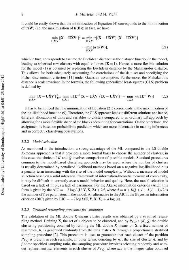
It has to be noticed that the minimization of Equation (21) corresponds to the maximization ofthe log-likelihood function (9). Therefore, the GLS approach leads to different solutions and hence,different allocations of units and variables to clusters compared to an ordinary LS approach byallowing for a more flexible shape of the blocks accounting for correlations. On the other hand, theassignment is based on probabilistic predictors which are more informative in making inferencesand in correctly classifying observations.

3.2.2 Model selection

As mentioned in the introduction, a strong advantage of the ML compared to the LS doubleK-means approach is that it provides a more formal basis to choose the number of clusters; inthis case, the choice of K and Q involves comparison of possible models. Standard procedurescommon to the model-based clustering approach may be used, where the number of clustersis usually determined by penalized likelihood methods based on a negative log-likelihood plusa penalty term increasing with the rise of the model complexity. Without a measure of modelselection based on a solid inferential framework of information-theoretic measure of complexity,it may be difficult to correctly assess model behavior and quality. Here, the model selection isbased on a lack of fit plus a lack of parsimony. For the Akaike information criterion (AIC), thisform is given by the AIC = −2 log L(U,V, X, �) + 2d, where d = n + KQ + J + J(J + 1)/2 isthe number of free parameters in the model. An alternative to the AIC is the Bayesian informationcriterion (BIC) given by BIC = −2 log L(U,V, X, �) + d log (n).

3.2.3 Stratified resampling procedure for validation

The validation of the ML double K-means cluster results was obtained by a stratified resam-pling method. Defining X, the set of n objects to be clustered, and by PK ,Q a (K , Q) the doubleclustering partitioning obtained by running the ML double K-means on X, a fixed number ofresamples, B, is generated randomly from the data matrix X through a proportionate stratifiedsampling procedure [2]. This procedure is used to guarantee that each cluster of the partitionPK ,Q is present in each resample. In other terms, denoting by nA, the size of cluster A, and byf some specified sampling ratio, the sampling procedure involves selecting randomly and with-out replacement n0A elements in each cluster of PK ,Q, where n0A is the integer value obtained

Dow

nloa

ded

by [

Uni

vers

ity o

f So

utha

mpt

on H

ighf

ield

] at

04:

51 2

5 Ju

ne 2

012

Journal of Applied Statistics 9

by rounding f · nA up to the nearest integer. The value of f has been chosen 0.8 in the intervalsuggested by Ben-Hur et al. [4]. (1 − α)-level percentile confidence intervals for block centroidsare defined by using α/2 and 1 − α/2 percentiles of the resampling empirical distribution as thelimits of the 100(1 − α)% confidence interval. In order to evaluate the number of clusters, theresampling empirical distribution of the BIC criterion under the null model that specifies the nullhypothesis of absence of clusters can be used. The absence of the cluster structure was guaranteedby a single multivariate Gaussian distribution with mean vector and covariance matrix equal tothat of the data matrix X. The Gaussian distribution was 5% truncated to avoid the fact that theclustering algorithm identifies partitions with clusters of outliers. The stability of the clusters wasalso assessed by evaluating the probability of each object to belong to each class after they areaffected by small changes in the data set.

4. Simulation studies

To study the performance of the (model-based) double K-means, we carried out a simulationstudy. In particular, the performance of the algorithm has been evaluated in terms of

(1) the degree of agreement between the true and the estimated partition membership by usingthe modified Rand index [21]. In case of perfect agreement between the true and the estimatedpartitions, the index value is equal to one. In particular, we computed Mrand(U, Ub) betweenthe true matrix U and the estimated matrix Ub and Mrand(V, Vb) between the true matrix Vand the estimated matrix Vb;

(2) the number of times the fitted partition of units is equal to the true partition, that is, Mrand(U,Ub)=1 and the number of times the fitted partition of variables is equal to the true partition,that is, Mrand(V, Vb)=1;

(3) the computational complexity.

In each experiment, B = 100 data sets have been generated according to model (1) in a J = 80dimensional space with a number of units equal to n = 2000; each row, xi, is supposed to bedrawn from a J-variate Gaussian distribution with mean vector VX

′ui and covariance matrix �.

Then, blocks are randomly placed within the data matrix.Three error levels (low, medium and high) have been considered in order to have different levels

of homogeneity within blocks. The error levels have been defined by multiplying the covariancematrix, �, by 5,10, 50, respectively. In Figures 1 and 2(a)–(c), we show the data set types withlow, medium and high; if error level is low, the structure of the blocks is well visible. On thecontrary, if the error level is high, the structure of blocks is lost. Then, rows and columns havebeen randomly permuted and the designed algorithm has been applied to recover blocks andspecifically partitions of units and variables generating the data (Figures 1 and 2(a2)–(c2)).

We have considered two different situations:

(1) the data matrix is formed by six blocks defining a partition of units with K = 3 clusters anda partition of variables with Q = 2 clusters;

(2) the data matrix is formed by 24 blocks defining a partition of units with K = 6 clusters anda partition of variables with Q = 4 clusters.

The design of the simulation experiments is shown in Table 2. As observed in Section 3.1,the algorithm begins with random starting values U and V. Since the proposed algorithm is veryefficient in term of computational complexity (CPU time), we were able to fix a large numberof random starts (equal to 100) to increase the chance to detect the optimal solution, although

Dow

nloa

ded

by [

Uni

vers

ity o

f So

utha

mpt

on H

ighf

ield

] at

04:

51 2

5 Ju

ne 2

012

10 F. Martella and M. Vichi

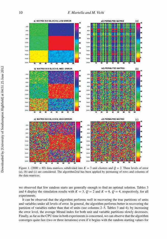
Figure 1. (2000 × 80) data matrices subdivided into K = 3 unit clusters and Q = 2. Three levels of error(a), (b) and (c) are considered. The algorithm2rid has been applied by permuting of rows and columns ofthe data matrices.

we observed that few random starts are generally enough to find an optimal solution. Tables 3and 4 display the simulation results with K = 3, Q = 2 and K = 6, Q = 4, respectively, for allexperiments.

It can be observed that the algorithm performs well in recovering the true partitions of unitsand variables under all levels of error. In general, the algorithm performs better in recovering thepartition of variables rather than that of units (see columns 2–5, Tables 3 and 4); by increasingthe error level, the average Mrand index for both unit and variable partitions slowly decreases.Finally, as far as the CPU time in both experiments is concerned, we can observe that the algorithmconverges quite fast (two or three iterations) even if it begins with the random starting values for

Dow

nloa

ded

by [

Uni

vers

ity o

f So

utha

mpt

on H

ighf

ield

] at

04:

51 2

5 Ju

ne 2

012

Journal of Applied Statistics 11

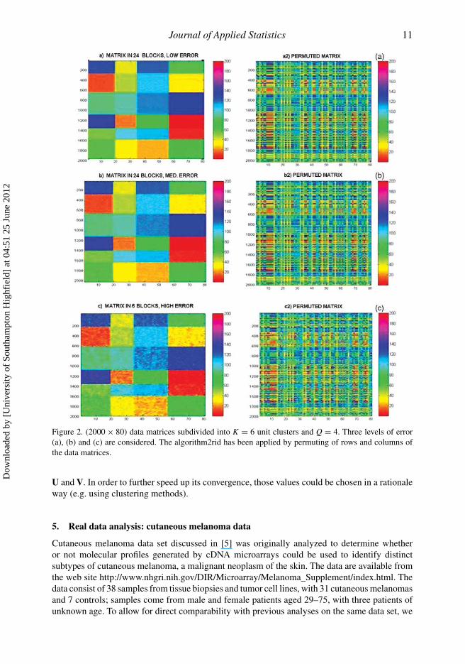
Figure 2. (2000 × 80) data matrices subdivided into K = 6 unit clusters and Q = 4. Three levels of error(a), (b) and (c) are considered. The algorithm2rid has been applied by permuting of rows and columns ofthe data matrices.

U and V. In order to further speed up its convergence, those values could be chosen in a rationaleway (e.g. using clustering methods).

5. Real data analysis: cutaneous melanoma data

Cutaneous melanoma data set discussed in [5] was originally analyzed to determine whetheror not molecular profiles generated by cDNA microarrays could be used to identify distinctsubtypes of cutaneous melanoma, a malignant neoplasm of the skin. The data are available fromthe web site http://www.nhgri.nih.gov/DIR/Microarray/Melanoma_Supplement/index.html. Thedata consist of 38 samples from tissue biopsies and tumor cell lines, with 31 cutaneous melanomasand 7 controls; samples come from male and female patients aged 29–75, with three patients ofunknown age. To allow for direct comparability with previous analyses on the same data set, we

Dow

nloa

ded

by [

Uni

vers

ity o

f So

utha

mpt

on H

ighf

ield

] at

04:

51 2

5 Ju

ne 2

012

12 F. Martella and M. Vichi

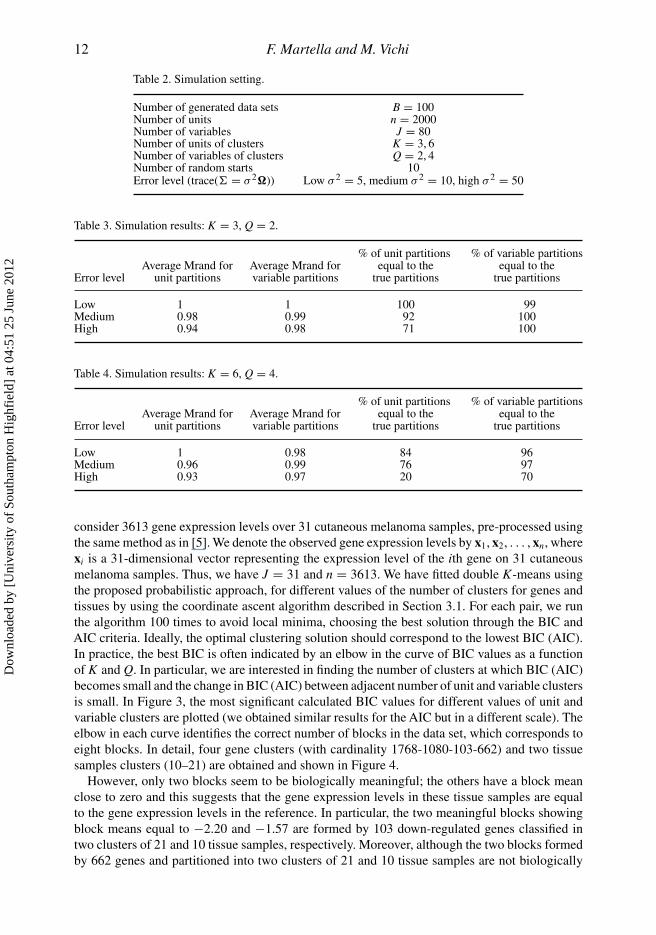
Table 2. Simulation setting.

Number of generated data sets B = 100Number of units n = 2000Number of variables J = 80Number of units of clusters K = 3, 6Number of variables of clusters Q = 2, 4Number of random starts 10Error level (trace(� = σ 2�)) Low σ 2 = 5, medium σ 2 = 10, high σ 2 = 50

Table 3. Simulation results: K = 3, Q = 2.

% of unit partitions % of variable partitionsAverage Mrand for Average Mrand for equal to the equal to the

Error level unit partitions variable partitions true partitions true partitions

Low 1 1 100 99Medium 0.98 0.99 92 100High 0.94 0.98 71 100

Table 4. Simulation results: K = 6, Q = 4.

% of unit partitions % of variable partitionsAverage Mrand for Average Mrand for equal to the equal to the

Error level unit partitions variable partitions true partitions true partitions

Low 1 0.98 84 96Medium 0.96 0.99 76 97High 0.93 0.97 20 70

consider 3613 gene expression levels over 31 cutaneous melanoma samples, pre-processed usingthe same method as in [5]. We denote the observed gene expression levels by x1, x2, . . . , xn, wherexi is a 31-dimensional vector representing the expression level of the ith gene on 31 cutaneousmelanoma samples. Thus, we have J = 31 and n = 3613. We have fitted double K-means usingthe proposed probabilistic approach, for different values of the number of clusters for genes andtissues by using the coordinate ascent algorithm described in Section 3.1. For each pair, we runthe algorithm 100 times to avoid local minima, choosing the best solution through the BIC andAIC criteria. Ideally, the optimal clustering solution should correspond to the lowest BIC (AIC).In practice, the best BIC is often indicated by an elbow in the curve of BIC values as a functionof K and Q. In particular, we are interested in finding the number of clusters at which BIC (AIC)becomes small and the change in BIC (AIC) between adjacent number of unit and variable clustersis small. In Figure 3, the most significant calculated BIC values for different values of unit andvariable clusters are plotted (we obtained similar results for the AIC but in a different scale). Theelbow in each curve identifies the correct number of blocks in the data set, which corresponds toeight blocks. In detail, four gene clusters (with cardinality 1768-1080-103-662) and two tissuesamples clusters (10–21) are obtained and shown in Figure 4.

However, only two blocks seem to be biologically meaningful; the others have a block meanclose to zero and this suggests that the gene expression levels in these tissue samples are equalto the gene expression levels in the reference. In particular, the two meaningful blocks showingblock means equal to −2.20 and −1.57 are formed by 103 down-regulated genes classified intwo clusters of 21 and 10 tissue samples, respectively. Moreover, although the two blocks formedby 662 genes and partitioned into two clusters of 21 and 10 tissue samples are not biologically

Dow

nloa

ded

by [

Uni

vers

ity o

f So

utha

mpt

on H

ighf

ield

] at

04:

51 2

5 Ju

ne 2

012

Journal of Applied Statistics 13

Figure 3. Number of unit and variable clusters vs. BIC values for the Bittner et al. [5] data.

Figure 4. Best double K-means solution: K=4, Q=2.

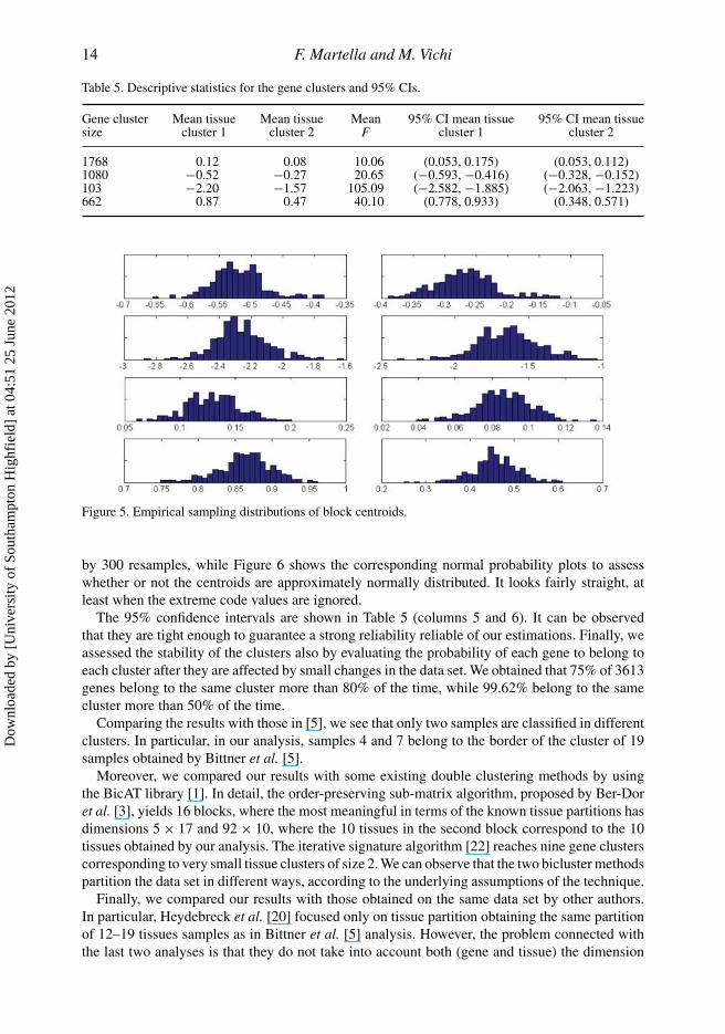
significant, the corresponding block means could be significatively different. This considerationentitles us to believe that some of these genes could be significant in explaining the tissue partition.Therefore, following the idea of Rocci andVichi [30], we analyzed the genes ability to discriminatebetween the two tissue clusters through the computation of the Fisher F test statistics for each gene.Results are reported in Table 5 (column 4). It seems clear that the cluster containing 103 genes is themost discriminant, followed by 662 up-regulated genes, while the cluster containing 1768 geneshas the lowest discriminant power. Furthermore, we validated the results by building confidenceintervals for the block centroids, xkq, through a resampling method described in Section 3.2.3.In detail, indicating by PK ,Q the obtained optimal partition (here K = 4, Q = 2), 300 resamplesare generated. Figure 5 shows the empirical sampling distributions of block centroids generated

Dow

nloa

ded

by [

Uni

vers

ity o

f So

utha

mpt

on H

ighf

ield

] at

04:

51 2

5 Ju

ne 2

012

14 F. Martella and M. Vichi

Table 5. Descriptive statistics for the gene clusters and 95% CIs.

Gene cluster Mean tissue Mean tissue Mean 95% CI mean tissue 95% CI mean tissuesize cluster 1 cluster 2 F cluster 1 cluster 2

1768 0.12 0.08 10.06 (0.053, 0.175) (0.053, 0.112)1080 −0.52 −0.27 20.65 (−0.593, −0.416) (−0.328, −0.152)103 −2.20 −1.57 105.09 (−2.582, −1.885) (−2.063, −1.223)662 0.87 0.47 40.10 (0.778, 0.933) (0.348, 0.571)

Figure 5. Empirical sampling distributions of block centroids.

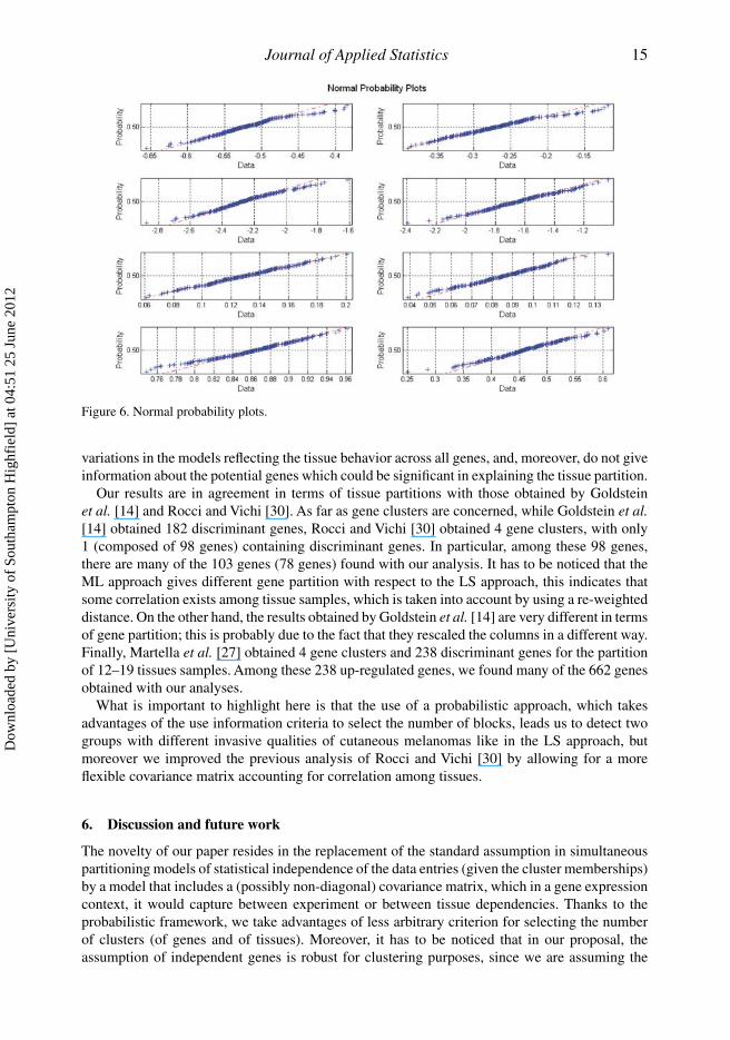
by 300 resamples, while Figure 6 shows the corresponding normal probability plots to assesswhether or not the centroids are approximately normally distributed. It looks fairly straight, atleast when the extreme code values are ignored.

The 95% confidence intervals are shown in Table 5 (columns 5 and 6). It can be observedthat they are tight enough to guarantee a strong reliability reliable of our estimations. Finally, weassessed the stability of the clusters also by evaluating the probability of each gene to belong toeach cluster after they are affected by small changes in the data set. We obtained that 75% of 3613genes belong to the same cluster more than 80% of the time, while 99.62% belong to the samecluster more than 50% of the time.

Comparing the results with those in [5], we see that only two samples are classified in differentclusters. In particular, in our analysis, samples 4 and 7 belong to the border of the cluster of 19samples obtained by Bittner et al. [5].

Moreover, we compared our results with some existing double clustering methods by usingthe BicAT library [1]. In detail, the order-preserving sub-matrix algorithm, proposed by Ber-Doret al. [3], yields 16 blocks, where the most meaningful in terms of the known tissue partitions hasdimensions 5 × 17 and 92 × 10, where the 10 tissues in the second block correspond to the 10tissues obtained by our analysis. The iterative signature algorithm [22] reaches nine gene clusterscorresponding to very small tissue clusters of size 2. We can observe that the two bicluster methodspartition the data set in different ways, according to the underlying assumptions of the technique.

Finally, we compared our results with those obtained on the same data set by other authors.In particular, Heydebreck et al. [20] focused only on tissue partition obtaining the same partitionof 12–19 tissues samples as in Bittner et al. [5] analysis. However, the problem connected withthe last two analyses is that they do not take into account both (gene and tissue) the dimension

Dow

nloa

ded

by [

Uni

vers

ity o

f So

utha

mpt

on H

ighf

ield

] at

04:

51 2

5 Ju

ne 2

012

Journal of Applied Statistics 15

Figure 6. Normal probability plots.

variations in the models reflecting the tissue behavior across all genes, and, moreover, do not giveinformation about the potential genes which could be significant in explaining the tissue partition.

Our results are in agreement in terms of tissue partitions with those obtained by Goldsteinet al. [14] and Rocci and Vichi [30]. As far as gene clusters are concerned, while Goldstein et al.[14] obtained 182 discriminant genes, Rocci and Vichi [30] obtained 4 gene clusters, with only1 (composed of 98 genes) containing discriminant genes. In particular, among these 98 genes,there are many of the 103 genes (78 genes) found with our analysis. It has to be noticed that theML approach gives different gene partition with respect to the LS approach, this indicates thatsome correlation exists among tissue samples, which is taken into account by using a re-weighteddistance. On the other hand, the results obtained by Goldstein et al. [14] are very different in termsof gene partition; this is probably due to the fact that they rescaled the columns in a different way.Finally, Martella et al. [27] obtained 4 gene clusters and 238 discriminant genes for the partitionof 12–19 tissues samples. Among these 238 up-regulated genes, we found many of the 662 genesobtained with our analyses.

What is important to highlight here is that the use of a probabilistic approach, which takesadvantages of the use information criteria to select the number of blocks, leads us to detect twogroups with different invasive qualities of cutaneous melanomas like in the LS approach, butmoreover we improved the previous analysis of Rocci and Vichi [30] by allowing for a moreflexible covariance matrix accounting for correlation among tissues.

6. Discussion and future work

The novelty of our paper resides in the replacement of the standard assumption in simultaneouspartitioning models of statistical independence of the data entries (given the cluster memberships)by a model that includes a (possibly non-diagonal) covariance matrix, which in a gene expressioncontext, it would capture between experiment or between tissue dependencies. Thanks to theprobabilistic framework, we take advantages of less arbitrary criterion for selecting the numberof clusters (of genes and of tissues). Moreover, it has to be noticed that in our proposal, theassumption of independent genes is robust for clustering purposes, since we are assuming the

Dow

nloa

ded

by [

Uni

vers

ity o

f So

utha

mpt

on H

ighf

ield

] at

04:

51 2

5 Ju

ne 2

012

16 F. Martella and M. Vichi

local independence within each block. The performance of the proposed model is highlightedby experimental comparisons on both simulated and gene expression data sets. Although theproposed algorithm converges very fast, this improvement is clearly gained by paying an increaseof the computational time with respect to the LS approach, related to the calculation of theinverse and determinant of the covariance matrix, which increases with the number of tissues. Apossible extension of our proposal may be to allow for different variable partitions in each unitcluster, generalizing the work of Rocci and Vichi [30]. Another encouraging research directionis on investigating how the double K-means could be extended to categorical data and to definespecific criteria to evaluate the discriminant power of unit clusters with respect to variable clustersand vice versa.

References

[1] S. Barkow, S. Bleuler, A. Prelic, P. Zimmermann, and E. Zitzler, BicAT: A biclustering analysis toolbox,Bioinformatics 22(10) (2006), pp. 1282–1283.

[2] P. Beltran and G. Ben Mufti, Loevinger’s measures of rule quality for assessing cluster stability, Comput. Statist.Data Anal. 50 (2006), pp. 992–1015.

[3] A. Ben-Dor, B. Chor, R. Karp, and Z. Yakhini, Discovering local structure in gene expression data: The order-preserving submatrix problem, J. Comput. Biol. 10 (2003), pp. 373–384.

[4] A. Ben-Hur, A. Elisseeff, and I. Guyon, A stability based method for discovering structure in clustered data, PacificSymposium on Biocomputing, Vol. 7, Lihue, Hawaii, 2002, pp. 6–17,

[5] M. Bittner, P. Meltzer, P. Chen, Y. Jiang, E. Seftor, M. Hendrix, M. Radmacher, R. Simon, Z. Yakhini, A. Ben-Dor,N. Sampas, E. Dougherty, E. Wang, F. Marincola, C. Gooden, J. Lueders, A. Glatfelter, P. Pollock, J. Carpten, E.Gillanders, D. Leja, K. Dietrich, C. Beaudry, M. Berens, D. Alberts, V. Sondak, N. Hayward, and J. Trent, Molecularclassification of cutaneous malignant by gene expression profiling, Nature 406(6795) (2000), pp. 536–540.

[6] H.H. Bock, Automatische Klassifikation, Vandenhoeck and Ruprecht, Gottingen, 1974.[7] H.H. Bock, Two-way clustering for contingency tables maximizing a dependence measure, in Between Data Science

and Applied Data Analysis, M. Schader, W. Gaul, and M. Vichi, eds., Springer, Heidelberg, 2003, pp. 143–155.[8] A. Califano, G. Stolovitzky, and Y. Tu, Analysis of gene expression microarrays for phenotype classification, Proc.

Int. Conf. Intell. Syst. Mol. Biol. 8 (2000), pp. 75–85.[9] Y. Cheng and G.M. Church, Biclustering of expression data, Proceedings of the Eighth International Conference on

Intelligent Systems for Molecular Biology (ISMB), Vol. 8, La Jolla/San Diego, CA, USA, 2000, pp. 93–103.[10] H. Cho, I.S. Dhillon, Y. Guan, and S. Sra, Minimum sum-squared residue co-clustering of gene expression data,

Proceedings of the Fourth SIAM International Conference on Data Mining, Lake Buena Vista, Florida, USA, 2004,pp. 114–125.

[11] R.A. Fisher, The use of multiple measurements in taxonomic problems, Ann. Eugenics 7(2) (1936), pp. 179–188.[12] W. Fisher, Clustering and Aggregation in Economics, Johns Hopkins, Baltimore, MD, 1969.[13] G. Getz, E. Levine, and E. Domany, Coupled two-way clustering analysis of gene microarray data, Proc. Natl Acad.

Sci. 97(22) (2000), pp. 12079–12084.[14] D. Goldstein, D. Ghosh, and E. Conlon, Statistical issues in the clustering of gene expression data, Stat. Sinica 12

(2002), pp. 219–241.[15] A.D. Gordon, Classification, 2nd ed., Chapman and Hall/CRC, Boca Raton, FL, 1999.[16] G. Govaert, Simultaneous clustering of rows and columns, Control Cybernet. 24 (1995), pp. 437–458.[17] G. Govaert and M. Nadif, Clustering with block mixture models, Pattern Recogn. 36(2) (2003), pp. 463–473.[18] G. Govaert and M. Nadif, Block clustering with Bernoulli mixture models: Comparison of different approaches,

Comput. Statist. Data Anal. 52(6) (2008), pp. 3233–3245.[19] J.A. Hartigan, Direct clustering of a data matrix, J. Am. Statist. Assoc. 67 (1972), pp. 123–129.[20] A.V. Heydebreck, W. Huber, A. Poustka, and M. Vingron, Identifying splits with clear separation: A new class

discovery method for gene expression data, Bioinformatics 17 (2001), pp. 107–114.[21] L. Hubert and P. Arabie, Comparing partitions, J. Classification 2 (1985), pp. 193–218.[22] J. Ihmels, G. Friedlander, S. Bergmann, O. Sarig,Y. Ziv, and N. Barkai, Revealing modular organization in the yeast

transcriptional network, Nat. Genet. 31 (2002), pp. 370–377.[23] Y. Kluger, R. Basri, J.T. Chang, and M. Gerstein, Spectral biclustering of microarray data: Coclustering genes and

conditions, Genome Res. 13(4) (2003), pp. 703–716.[24] L. Lazzeroni and A. Owen, Plaid models for gene expression data, Stat. Sinica 12(1) (2002), pp. 61–86.[25] J. Li and H. Zha, Two-way Poisson mixture models for simultaneous document classification and word clustering,

Comput. Statist. Data Anal. 50(1) (2006), pp. 163–180.

Dow

nloa

ded

by [

Uni

vers

ity o

f So

utha

mpt

on H

ighf

ield

] at

04:

51 2

5 Ju

ne 2

012

Journal of Applied Statistics 17

[26] C. Madeira Sara and L. Oliveira Arlindo, Biclustering algorithms for biological data analysis: A survey, IEEE/ACMTrans. Comput. Biol. Bioinform. 1 (2004), pp. 24–45.

[27] F. Martella, M. Alfó, and M. Vichi, Biclustering of gene expression data by an extension of mixtures of factoranalyzers, Int. J. Biostat. 4(1) (2008), p. 1–19.

[28] J.B. McQueen, Some methods for classification and analysis of multivariate observations, Proceedings of 5thBerkeley Symposium on Mathematical Statistics and Probability, University of California Press, Berkeley, CA,Vol. 1, 1967, pp. 281–297.

[29] T.M. Murali and S. Kasif, Extracting conserved gene expression motifs from gene expression data, Proc. PacificSymp. Biocomputing 8 (2003), pp. 77–88.

[30] R. Rocci and M. Vichi, Two-mode multi-partitioning, Comput. Stat. Data Anal. 52 (2008), pp. 1984–2003.[31] R.C. Tryon, Cluster Analysis, Edwards Bros., Ann Arbor, MI, 1939.[32] I. Van Mechelen, Biclustering methods for microarray gene expression data: Towards a unifying taxonomy. Data

Science and Classification, in 10th Jubilee Conference of the International Federation of Classification Societies,Ljubljana, Slovenia, 2006.

[33] I.Van Mechelen, H.H. Bock, and P. De Boeck, Two-mode clustering methods: A structured overview, Statist. MethodsMed. Res. 13 (2004), pp. 363–394.

[34] I. Van Mechelen and J. Schepers, A unifying model for biclustering. Atti del convegno di COMPSTAT2006, Universitádegli Studi di Roma La Sapienza, Rome, Italy, 2006.

[35] M. Vichi, Double k-means clustering for simultaneous classification of objects and variables, in Advances in Clas-sification and Data Analysis, S. Borra, R. Rocci, M. Vichi, and M. Schader, eds., Springer, Heidelberg, 2000,pp. 43–52.

[36] J. Wyse and N. Friel, Block clustering with collapsed latent block models, Stat. Comput. 22(2) (2012), pp. 415–428.[37] J. Yang, W. Wang, H. Wang, and P. Yu, δ-Clusters: Capturing subspace correlation in a large data set, Proceedings

of the 18th IEEE International Conference on Data Engineering, San Jose, California, 2002, pp. 517–528.[38] J. Yang, H. Wang, W. Wang, P. Yu, U. Ibm, U. Chapel, H. Ibm, T.J. Watson, and T.J. Watson, Enhanced biclustering

on expression data, Proceedings of the Third IEEE Conference on Bioinformatics and Bioengineering, Bethesda,MD, USA, 2003, pp. 321–327.

Dow

nloa

ded

by [

Uni

vers

ity o

f So

utha

mpt

on H

ighf

ield

] at

04:

51 2

5 Ju

ne 2

012