STATISTICAL ANALYSIS OF MICROARRAY DATA
213
-
Upload
khangminh22 -
Category
Documents
-
view
0 -
download
0
Transcript of STATISTICAL ANALYSIS OF MICROARRAY DATA

A KATHOLIEKE UNIVERSITEIT LEUVENFACULTEIT INGENIEURSWETENSCHAPPENDEPARTEMENT ELEKTROTECHNIEKKasteelpark Arenberg 10, 3001 Leuven (Heverlee)
STATISTICAL ANALYSIS OF MICROARRAY DATA:APPLICATIONS IN PLATFORM COMPARISON,
COMPENDIUM DATA, AND ARRAY CGH
Promotoren:Prof. dr. ir. Y. MoreauProf. dr. ir. B. De Moor
Proefschrift voorgedragen tothet behalen van het doctoraatin de ingenieurswetenschappen
door
Joke ALLEMEERSCH
December 2006


A KATHOLIEKE UNIVERSITEIT LEUVENFACULTEIT INGENIEURSWETENSCHAPPENDEPARTEMENT ELEKTROTECHNIEKKasteelpark Arenberg 10, 3001 Leuven (Heverlee)
STATISTICAL ANALYSIS OF MICROARRAY DATA:APPLICATIONS IN PLATFORM COMPARISON,
COMPENDIUM DATA, AND ARRAY CGH
Jury:Prof. dr. ir. H. Neuckermans, voorzitterProf. dr. ir. Y. Moreau, promotorProf. dr. ir. B. De Moor, co-promotorProf. dr. F. HolstegeProf. dr. M. KuiperProf. P. RouzeProf. dr. ir. E. SchrevensProf. dr. ir. J. VandewalleProf. dr. ir. J. Vermeesch
Proefschrift voorgedragen tothet behalen van het doctoraatin de ingenieurswetenschappen
door
Joke ALLEMEERSCH
U.D.C. 681.3*J3, 519.23 December 2006

c©Katholieke Universiteit Leuven � Faculteit IngenieurswetenschappenArenbergkasteel, B-3001 Heverlee (Belgium)
Alle rechten voorbehouden. Niets uit deze uitgave mag vermenigvuldigden/of openbaar gemaakt worden door middel van druk, fotocopie, mi-cro�lm, elektronisch of op welke andere wijze ook zonder voorafgaandeschriftelijke toestemming van de uitgever.
All rights reserved. No part of the publication may be reproduced in anyform by print, photoprint, micro�lm or any other means without writtenpermission from the publisher.
D/2006/7515/97
ISBN 978-90-5682-763-2

Voorwoord
Traditioneel begint elk doctoraat terecht met een woord van dank en ookhier mag dat niet ontbreken.
Wanneer Prof. Yves Moreau me vroeg om te komen werken in deBioinformatica groep op de data-analyse van microarrays, ben ik daar opingegaan zonder goed te weten wat Bioinformatica was, laat staan wat eenmicroarray was. Misschien gelukkig maar. . . Nu, een viertal jaar later, benik blij dat ik toen �ja� gezegd heb. Yves, bedankt om me in deze wereldbinnen te loodsen. Je enthousiasme en gedrevenheid werkten aanstekelijk.Ook een woord van dank voor mijn co-promotor, Prof. Bart De Moor voorde kansen, de steun en de middelen die nodig waren om aan dit doctoraatte werken.
I also thank the members of the jury and in particular the readingcommittee, Prof. Pierre Rouze, Prof. Eddie Schrevens, and Prof. JoosVandewalle, for their reading efforts and their valuable remarks.
The CAGE project was a good opportunity for nice collaborations. Firstof all, I have to acknowledge Prof. Pierre Hilson and Prof. MartinKuiper for the close collaboration, while working on the benchmark ofthe CATMA array, which was a fruitful experience for me. Naming allpersons involved in the CAGE project would result in a long list, thereforeI will only mention some of them. Thank you Helen Parkinson, forstruggling together with the MAGE-ML �les, Wolfram Brenner for thepleasant collaboration during your stay here in Leuven, Gert Sclep for allthe confusing emails, Dawn Little, Tom Bogaert, Paul Van Hummelen, and

ii Voorwoord
last but not least Steffen Durinck, my colleague at ESAT. You described usin your own PhD text as a �great team�. And, although you were runningaway all the time, I must admit that there is some truth in it. I reallyenjoyed our close collaboration and I hope that we can stay in touch and,who knows, perhaps our paths will cross again.
Gedurende het laatste jaar, werkte ik ook nauw samen met Femke Hannesen Prof. Joris Vermeesch. Allebei hartelijk bedankt voor de aangenamesamenwerking.
Veel dank gaat uit naar de ganse Bioinformatica groep � Cynthia,Karen, Steven, Stein, Bert, Gert en de ganse groep � voor de dagelijksewerksfeer: bedankt! Ook van harte bedankt aan de mensen die instaanvoor de praktische regelingen en dan in het bijzonder Ida, Bart en Ilse.
Onrechtstreeks, maar zeker zo belangrijk voor dit werk is de invloedvan mijn achterban, waar ik steeds terecht kon voor de noodzakelijkeontspanning en a�eiding. Christoph, Kirsten, Mario, Aurore, Joze�en,Nathalie, iedereen in de Kon. St. Martinusharmonie in Tessenderlo,waarbij ik al een 15-tal jaar elke vrijdagavond een muzikale uitlaatklepvind, het gezelschap van in de Duitse lessen, de cello les,. . . Allemaal nedikke merci!
Jeroen en So�e, ik denk dat we ons de �bende van de Lombaarden� mogennoemen. Dankzij jullie is het bij ons een gezellige boel, waar het altijdleuk is om 's avonds thuis te komen. Hopelijk kunnen we nog een paarjaartjes in elkaars gezelschap wonen!
Papa, mama, Simon & Veerle, dankzij jullie kan ik met een goed gevoelzeggen dat ik uit een heel warm nest kom. Jullie stonden altijd voor mijklaar. Niets was te veel voor jullie.
Steven, jongen, mercikes voor al je steun. Dankzij jou heb ik in alle rustdit doctoraat kunnen afwerken. We gaan er samen nog iets moois vanmaken. . .
Joke

Abstract
Since the mid-1990s microarrays have become a well-established tech-nology to measure when, where, and to what extent a gene is expressed,on a genomewide scale. Whereas early experiments included only a fewhybridizations, the tendency is now growing towards large compendiumprojects producing hundreds of samples and providing information on thegene expression at different developmental stages, under different environ-mental conditions or of different mutants.This Ph.D. has been carried out within the framework of the CAGE project,a European demonstration project that aimed at composing an atlas of geneexpression of Arabidopsis thaliana throughout its life cycle and under avariety of stress conditions. As a microarray platform, the Complete Tran-scriptome MicroArray or CATMA array was developed within this project.Its utility had not yet been proven and, therefore, a dedicated experimentwas set up to benchmark the CATMA array against two well-establishedplatforms. Different aspects of the platforms are compared in this thesisand the results for the CATMA array are promising.The main contribution of this Ph.D. to the CAGE project is the prepro-cessing of the microarray data. Within the CAGE project, microarray dataexchange and storage was done in MAGE-ML format, so that CAGE isa well-annotated, MIAME-compliant compendium. To facilitate data ex-change in MAGE-ML format, a software package RMAGEML is presented,enabling to import MAGE-ML �les in the statistical environment R and toupdate the MAGE-ML �les with preprocessed values. The package is nowpart of the Bioconductor package, which is a major open source tool forthe statistical analysis of microarray data.

ii Abstract
Using this RMAGEML package, a data preprocessing pipeline is developedfor an automated preprocessing and quality assessment of the CAGE data.With this high-throughput data preprocessing pipeline, a sizable set ofmore than 2,000 hybridizations is preprocessed, ready for an in-depth anal-ysis.To conclude, a nice example shows the improvement a well-chosen exper-imental design can bring. ArrayCGH is a microarray technology that canbe used to detect aberrations in the ploidy of DNA segments in the genomeof patients with congenital anomalies. In this Ph.D., I present a tool to an-alyze arrayCGH loop designs in which three patients are placed in a loopdesign, which is advantageous over the classical dye-swap approach.

Korte inhoud
Gedurende de laatste 10 jaar zijn microroosters geevolueerd tot een geves-tigde techniek voor het meten van gen expressie, voor duizenden genenin parallel. Oorspronkelijk werden microrooster experimenten opgezetals kleinschalige experimenten, bestaande uit een gelimiteerd aantalhybridizaties. Tegenwoordig verschuift de aanpak van microrooster ex-perimenten meer en meer naar grootschalige compendium experimenten,waarbij honderden stalen gehybridiseerd worden en die informatie ver-schaffen over gen expressie in verschillende ontwikkelingsstadia, onderbepaalde omgevingsinvloeden, of van verschillende mutanten.
Dit doctoraat kadert binnen het CAGE project, een Europees demonstratieproject, dat streefde naar het samenstellen van een atlas van gen expressievan de plant Arabidopsis thaliana gedurende zijn groei cyclus en onder eenreeks van stress condities. Als microrooster platform werd gekozen voorde Complete Transcriptome MicroArray of CATMA microrooster. De ca-paciteiten van dit platform waren nog niet bewezen en daarom werd er eenexperiment opgezet dat toeliet om de CATMA array te toetsen aan tweegevestigde microrooster platformen. Verschillende aspecten van de plat-formen werden vergeleken in dt werk en de resultaten van de CATMAarray bleken veelbelovend te zijn.De voornaamste bijdrage van dit doctoraat aan het CAGE project was hetnormaliseren van de microrooster data. Binnen het CAGE project, werdvoor de data uitwisseling en bewaring geopteerd voor het MAGE-ML for-maat. Dit garandeert de goede annotatie van de CAGE experimenten, zodathet project voldoet aan de MIAME vereisten. Om de data uitwisseling in

iv Korte inhoud
MAGE-ML formaat te vereenvoudigen, hebben we een software pakketRMAGEML gebouwd, dat toelaat om data opgeslagen in MAGE-ML for-maat te importeren in de statistische omgeving van R en om verwerkte datatoe te voegen aan de oorspronkelijke MAGE-ML �le. Dit pakket maakt nudeel uit van de Bioconductor pakketten.Dit RMAGEML pakket is een belangrijk onderdeel van een data verwerkingspijplijn, die hier ontwikkeld werd voor een automatische normalisatie enkwaliteitscontrole van de CAGE data. Met deze data verwerkings pijplijn,werd een aanzienlijke data set van meer dan 2.000 hybridizaties klaarge-maakt voor verdere analyse.Ten slotte tonen we in een mooi voorbeeld de verbetering die een goedgekozen experimenteel design kan brengen. Array CGH is een micro-rooster, ontwikkeld voor het detecteren van chromosomale afwijkingen.Dit doctoraat toont een analyse tool voor de analyse van array CGH loopdesigns, waarbij drie patienten in een loop design vergeleken worden, wateen signi�cante verbetering is ten opzichte van de klassieke twee-aan-tweevergelijkingen.

Contents
Voorwoord i
Abstract i
Korte inhoud iii
Contents v
Nederlandse samenvatting ix
Glossary xxi
Publication list xxiii
1 Introduction 1
2 Microarray technologies to measure gene expression 112.1 Cell biology in a nutshell . . . . . . . . . . . . . . . . . . 12
2.1.1 The structure of DNA . . . . . . . . . . . . . . . 122.1.2 DNA codes the formation of proteins . . . . . . . 14
2.2 Experimenting with DNA . . . . . . . . . . . . . . . . . . 182.2.1 Reverse transcription . . . . . . . . . . . . . . . . 192.2.2 Polymerase Chain Reaction . . . . . . . . . . . . 19
2.3 DNA microarrays . . . . . . . . . . . . . . . . . . . . . . 192.3.1 Applications of microarray experiments . . . . . . 21

vi CONTENTS
2.3.2 Different analysis steps in a microarray experiment 222.3.3 Publicly available microarray data . . . . . . . . . 23
2.4 Alternative techniques to assess gene expression . . . . . . 262.5 CGH arrays . . . . . . . . . . . . . . . . . . . . . . . . . 28
3 Technical aspects of DNA microarray technologies 333.1 Two-channel arrays . . . . . . . . . . . . . . . . . . . . . 34
3.1.1 Different probes . . . . . . . . . . . . . . . . . . 343.1.2 Quality assessments and normalization of two-
channel arrays . . . . . . . . . . . . . . . . . . . 403.2 Single-channel arrays . . . . . . . . . . . . . . . . . . . . 48
3.2.1 Short oligonucleotides: Affymetrix . . . . . . . . 483.2.2 Normalization of Affymetrix chips . . . . . . . . . 493.2.3 Quality assessment of Affymetrix chips . . . . . . 55
3.3 Finding differentially expressed genes . . . . . . . . . . . 603.3.1 LIMMA or Linear Models for MicroArray data . . 603.3.2 General Linear models . . . . . . . . . . . . . . . 64
4 Benchmark of CATMA array 694.1 The CATMA project . . . . . . . . . . . . . . . . . . . . 704.2 The CATMA benchmark strategy . . . . . . . . . . . . . . 714.3 Coverage of the different platforms . . . . . . . . . . . . . 724.4 Design of the experiment . . . . . . . . . . . . . . . . . . 754.5 Data acquisition and normalization . . . . . . . . . . . . . 794.6 Dynamic range and sensitivity . . . . . . . . . . . . . . . 804.7 In vivo coverage . . . . . . . . . . . . . . . . . . . . . . . 834.8 Speci�city . . . . . . . . . . . . . . . . . . . . . . . . . . 874.9 Signal reproducibility . . . . . . . . . . . . . . . . . . . . 884.10 False positives and FDR . . . . . . . . . . . . . . . . . . 934.11 False negatives . . . . . . . . . . . . . . . . . . . . . . . 974.12 Conclusion . . . . . . . . . . . . . . . . . . . . . . . . . 98
5 The CAGE project 1095.1 Compendium of Arabidopsis Gene Expression or CAGE . 1105.2 The design of the experiments within CAGE . . . . . . . . 114
5.2.1 The oligo reference design . . . . . . . . . . . . . 114

CONTENTS vii
5.2.2 Implications of oligo reference design on normal-ization . . . . . . . . . . . . . . . . . . . . . . . . 117
5.3 Data preprocessing pipeline . . . . . . . . . . . . . . . . . 1205.3.1 RMAGEML . . . . . . . . . . . . . . . . . . . . 1215.3.2 Data extraction . . . . . . . . . . . . . . . . . . . 1225.3.3 Data preprocessing . . . . . . . . . . . . . . . . . 1235.3.4 Quality assessment . . . . . . . . . . . . . . . . . 1245.3.5 The CAGE pipeline architecture . . . . . . . . . . 127
5.4 The CAGE data production . . . . . . . . . . . . . . . . . 1275.5 Time-course experiments on leaf development . . . . . . . 128
5.5.1 Data analysis steps . . . . . . . . . . . . . . . . . 1305.5.2 (Dis)agreement between CAGE partners . . . . . . 132
5.6 High-light stress on catalase-de�cient plants . . . . . . . . 1325.6.1 The context of the experiment . . . . . . . . . . . 1335.6.2 Design of the experiment . . . . . . . . . . . . . . 1355.6.3 Data analysis steps . . . . . . . . . . . . . . . . . 1365.6.4 Differentially expressed genes . . . . . . . . . . . 1395.6.5 The expression pro�les . . . . . . . . . . . . . . . 139
5.7 Conclusion . . . . . . . . . . . . . . . . . . . . . . . . . 142
6 Analysis of loop design experiments for Array CGH 1456.1 Array CGH to detect chromosomal aberrations . . . . . . 145
6.1.1 The basic principle of array CGH experiments . . 1466.1.2 Alternative technologies . . . . . . . . . . . . . . 1466.1.3 Applications . . . . . . . . . . . . . . . . . . . . 147
6.2 A loop design for array CGH . . . . . . . . . . . . . . . . 1476.3 The different analysis methods . . . . . . . . . . . . . . . 149
6.3.1 Preprocessing . . . . . . . . . . . . . . . . . . . . 1496.3.2 Mixed model approach . . . . . . . . . . . . . . . 1496.3.3 The LIMMA approach . . . . . . . . . . . . . . . 151
6.4 Benchmarking the mixed models and LIMMA approach . 1526.4.1 The test data set . . . . . . . . . . . . . . . . . . . 1536.4.2 Signal-to-noise ratios . . . . . . . . . . . . . . . . 1546.4.3 True positive and false positive rate . . . . . . . . 155
6.5 Optimization of the LIMMA approach . . . . . . . . . . . 1576.5.1 Completely and partially deleted targets . . . . . . 157

viii CONTENTS
6.5.2 The non-con�rmed positives . . . . . . . . . . . . 1596.6 Implementation in a web application . . . . . . . . . . . . 159
6.6.1 Data processing . . . . . . . . . . . . . . . . . . . 1606.6.2 Architecture . . . . . . . . . . . . . . . . . . . . . 161
6.7 Conclusion . . . . . . . . . . . . . . . . . . . . . . . . . 162
7 Conclusions and future directions 1657.1 The CAGE project . . . . . . . . . . . . . . . . . . . . . 1657.2 ArrayCGH . . . . . . . . . . . . . . . . . . . . . . . . . . 168
Index 171
References 173

Nederlandse samenvattingStatistische verwerking van
microrooster data: toepassingen inplatform vergelijkingen,
compendium data en array CGH
Hoofdstuk 1: InleidingHet einde van grote sequentie analyse projecten betekende het begin vanhet ontcijferen van de informatie verborgen in het DNA. In het DNAliggen de genen, die alle erfelijke informatie bepalen, verborgen. Eenbelangrijke stap is het lokaliseren van de genen in de DNA sequentie. Devolgende uitdaging bestaat dan uit het toewijzen van functies aan elk vandeze genen.Een belangrijk hulpmiddel hierbij zijn de DNA microroosters (microar-rays), die ons in staat stellen om te meten waar, wanneer en in welkemate een gen actief is, en dit voor duizenden genen in parallel. Eenmicrorooster experiment brengt een massa data voort en de analysevan deze microrooster data is bijna een statistische discipline op zichgeworden. In deze thesis worden een aantal aspecten van microroosterdata analyse belicht. De thesis is als volgt opgebouwd.

x Nederlandse samenvatting
Hoofdstuk 2 en 3 geven een gedetailleerde inleiding op het onderwerp. InHoofdstuk 2 worden de, in deze context, belangrijke begrippen uit de celbiologie ge�ntroduceerd. Via het centrale dogma, leiden we het begrip genen, meer speci�ek, genexpressie in. Het idee achter microroosters en deanalyse van microrooster experimenten wordt ook voorgesteld. Hoofd-stuk 3 wordt dan direct een stuk technischer. Er bestaan verschillendemicrorooster platformen met elk hun eigen karakteristieken. We stellentwee groepen microroosters voor, de microrooster met twee kanalenen met een enkel kanaal. Beide microrooster types hebben hun eigennormalisatie vereisten, die we kort bespreken.
In Hoofdstuk 4 maken we de vergelijking tussen drie microroosterplatformen, die gebruikt worden voor de plant Arabidopsis thaliana. Eenexperiment speciaal opgezet voor deze vergelijking laat ons toe om deverschillende aspecten van de platformen te vergelijken.
Vervolgens beschrijven we in Hoofdstuk 5 een compendium project,namelijk het Compendium of Arabidopsis Gene Expression of CAGEproject. Dit is een Europees project met als doel het opbouwen vaneen genexpressie compendium van de plant Arabidopsis thaliana in deverschillende groei stadia en voor een reeks stress condities. Uiteindelijkedoel was de productie van een 2.000 biologische stalen, telkens tweemaal gehybridiseerd op, in totaal, 4.000 microroosters. De stalen wordengeproduceerd in acht laboratoria in Europa. De bioinformatica groep inESAT was verantwoordelijk voor het normaliseren van deze data.Om deze data, en ook alle andere gepubliceerde data, op een betekenisvollemanier publiek te maken, is het belangrijk dat de data voldoende gean-noteerd is. Daarom werd de data binnen het CAGE project opgeslagenin MAGE-ML formaat, een XML taal, ontwikkeld door de MicroarrayGene Expression Database groep als een standaard voor het beschrijvenvan microrooster experimenten. Het CAGE project was een van deeerste projecten, die het MAGE-ML formaat actief gebruikten (i.e., nietenkel om data op te slaan, maar ook voor de data communicatie), en erbestond nog geen software om data opgeslagen in MAGE-ML formaat teimporteren in statistische dataverwerkingsprogramma's. In dit werk wordter een stukje software gepresenteerd, die het mogelijk maakt om data te

Nederlandse samenvatting xi
extraheren uit MAGE-ML formaat en om verwerkte data toe te voegen aande MAGE-ML �les.Voor het verwerken van de data van 4.000 hybridisaties hebben we eenautomatische dataverwerkingspijplijn ontwikkeld. Deze pijplijn start vande data, zoals opgeslagen in MAGE-ML formaat, extraheert de nodigeinformatie voor de normalisatie van de data en voegt de genormaliseerdedata toe aan de oorspronkelijke MAGE-ML �le. Ondertussen worden denodige �guren en statistieken gegenereerd voor kwaliteitscontrole van deverschillende hybridisaties.
Een andere toepassing van de microrooster technologie is array CGH,een microrooster platform voor de detectie van chromosomale afwijkin-gen. Detectie van deze afwijkingen geeft inzicht in het ontstaan en deontwikkeling van de gerelateerde pathologieen. In Hoofdstuk 6 stellenwe een data analyse tool voor die loop design experimenten verwerkt.Dit design heeft voordelen ten opzichte van de klassieke paarsgewijzevergelijking van patienten, waarbij een test patient vergeleken wordt meteen normale, referentie patient. Twee methodes voor de analyse van ditloop design worden voorgesteld en met elkaar vergeleken. De te verkiezenmethode is ge�mplemeteerd in een webapplicatie.
Alle analyses, uitgevoerd in dit werk, werden met de open-source, statis-tische software R (http://www.r-project.org) uitgevoerd. R is eenlopend project, waaraan iedereen code kan toevoegen. Een succesvol voor-beeld hiervan is Bioconductor (http://www.bioconductor.org), eenreeks pakketten voor de analyse van genomische data. Bioconductor is eenpopulaire tool geworden voor de analyse van microrooster data.
Hoofdstuk 2: Microrooster technologie voor hetmeten van genexpressieGenen zijn stukjes DNA die de nodige informatie bevatten om eiwitten tesynthetiseren. Het centrale dogma beschrijft dit proces in twee stappen:transcriptie (het omzetten van DNA in mRNA) en translatie, waarbij hetmRNA vertaald wordt in een eiwit. Bijgevolg, bepalen de hoeveelheid en

xii Nederlandse samenvatting
het type DNA dat gekopieerd wordt in RNA, welke eiwitten aangemaaktworden. En dit is exact wat microroosters zullen meten. Indien het DNAvan een gen gekopieerd is als RNA, dan is dit gen tot expressie gekomenen microroosters meten genexpressie.Microroosters plaatsen duizenden cDNAs of oligonucleotides (de proben)op een plaatje en laten hierop een te analyseren staal over lopen. Doordatcomplementaire DNA strengen speci�ek met elkaar binden (i.e., hy-bridiseren), kan men de genexpressie status voor alle (duizenden) genen,vertegenwoordigd met een probe op de microrooster, meten.Het gelijktijdig meten van deze duizenden genen leidt tot een massagegevens. De analyse van deze data gebeurt in een aantal stappen.De data wordt eerst genormaliseerd, zodat verschillen in de data vanniet-biologische aard weggewerkt worden. Vervolgens worden lijstensamengesteld met genen die een verschil in expressieniveau vertonentussen twee of meerdere stalen. Voor deze genen kan men dan de ex-pressiepro�elen weergeven en met elkaar vergelijken (bijvoorbeeld, doormiddel van clustering). Op deze manier kan men genen identi�ceren, dieeen rol spelen in bepaalde processen en eventueel een functie associeren.
Hoofdstuk 3: Technische aspecten van DNA micro-rooster technologieEr bestaan verschillende microrooster platformen. Ze kunnen op de eersteplaats opgesplitst worden als microroosters met een of twee kanalen. Eenverdere opsplitsing gebeurt dan op basis van de gebruikte proben.Bij de twee kanalen microroosters, hybridiseren twee stalen, gelabeld mettwee verschillende kleuren (zie Figuur 3.1, pagina 36). Het best gekend, indeze categorie, zijn waarschijnlijk de cDNA microroosters, waarbij PCRgeampli�ceerde cDNAs gespot worden op de microroosters.Een beter alternatief zijn de long oligonucleotide microroosters. Gebaseerdop de sequentie informatie alleen, kan men oligonucleotides ontwerpendie speci�eker voor het gen zijn dan de complete cDNAs, zodat cross-hybridisatie vermeden kan worden, en tegelijkertijd voldoende lang zijnom enkel te binden met het desbetreffende gen. Deze oligonucleotidesworden in silico gesynthetiseerd en op de array geprint of in situ gesyn-

Nederlandse samenvatting xiii
thetiseerd. Op deze manier maakt men ook geen gebruik van PCRproducten, wat cross-contaminatie vermijdt, maar de techniek is vrij duur.Een derde platform dat we vermelden is de Complete Arabidopsis Tran-scriptome MicroArray of CATMA, een microrooster ontwikkeld voor destudie van genexpressie in de plant Arabidopsis thaliana. Deze plant wordtvaak als model organisme gebruikt omwille van de korte levenscyclus.Deze CATMA array is het resultaat van een Europees project dat Gene-speci�c Sequence Tags of GSTs voor alle gekende en voorspelde genenwilden samenstellen. De GSTs hebben een lengte van 150 �a 500bp en min-der dan 70% overeenkomst met eender welke sequentie in het Arabidopsisgenoom. Later werd deze set nog uitgebreid naar minder speci�eke GSTs,zodat ook genen, behorend tot een genfamilie opgenomen werden. Metdeze GSTs werd de CATMA array gespot. Voor deze GSTs werden ookPCR primers ontworpen zodat cross-contaminatie vermeden wordt. Ditwerd gedaan door aan de 5′ uiteindes van de oligonucleotide speci�ekeprimers, een paar primers te hechten, gebaseerd op de coordinaten vande GST in de 384 well plate, namelijk een combinatie van 16 primers(r1, . . . , r16) en 24 primers (c1, . . . , c24).Voor de normalisatie van deze data voeren we een achtergrond correctieuit en �tten we een Loess regressie lijn door de MA-plot, per printtip. De log-ratios worden dan nog uitgemiddeld over de dye-swap (i.e.,hybridisatie waarbij de staal-kanaal combinatie omgewisseld is).
Bij de microroosters met een kanaal (zie Figuur 3.7, pagina 50), besprekenwe de short oligonucleotide microroosters van Affymetrix. Op eenAffymetrix chip wordt een gen niet meer gemeten door een DNA streng,maar door een probe set, bestaande uit 11 �a 20 probe paren. Elk probepaar bestaat uit een oligonucleotide van lengte 25bp (perfect match) eneen tweede, gelijkaardige oligonucleotide, waarbij enkel de middelstenucleotide veranderd is (mismatch). De metingen van de probe setsworden door Affymetrix standaard gecombineerd in een expressiewaardemet MicroArray Suite 5.0 (MAS 5.0). In Bioconductor bestaat er ook eenalternatief, die de mismatch waardes niet in rekening brengt, namelijkRobust Multi-array Average (RMA).

xiv Nederlandse samenvatting
Hoofdstuk 4: Benchmark van de CATMA arrayDoor het zorgvuldig opzetten van de GST collectie had men hogeverwachtingen over de kwaliteit van de CATMA array. Dit hoofdstuk isgewijd aan de vergelijking van de CATMA array met twee commercieleplatformen, Agilent en Affymetrix. In de studie nemen we het standpuntvan de typische microrooster gebruiker in: we zoeken een gevestigdeservice provider (VIB-MAF, SeviceXS en NASC voor CATMA, Agilenten Affymetrix, respectievelijk) en vertrouwen op de gangbare analysemethodes.Het experiment werd als volgt opgezet. Aan een zelfde staal RNA werdenzeven paren spike RNAs met gekende concentratie toegevoegd. Dezeconcentratie bedroeg 10.000 cpc1 voor spike paar 1 en verminderdetelkens met factor 10 tot 0,1 cpc voor spike paar 6 en 0 voor spike paar7. Dit is spike mix 1. Spike mix 2 wordt dan gemaakt door spike 2 tot7 een concentratie te geven van 10.000 gaande tot 0,1 en spike 1 eenconcentratie van 0. Analoog worden er zo 7 spike mixen gemaakt, tot elkespike in elke concentratie gemeten wordt (zie Tabel 4.3, pagina 79). Eenreferentie spike mix bevat elke spike met een concentratie van 100 cpc.Voor de microroorsters met twee kanalen worden de zeven spike mixengehybridiseerd ten opzichte van de referentie spike mix, met een dye-swap,wat het totaal op 14 hybridisaties brengt. Voor het Affymetrix platformworden de zeven spike mixen gehybridiseerd en de referentie spikemix wordt op een aparte, achtste slide gehybridiseerd (zie Figuur 4.2,pagina 78). De data op de CATMA array werden genormaliseerd metachtergrond correctie en een Loess regressie per print tip. Voor Agilenten Affymetrix gebruikten we de bijgeleverde expressie waardes. OpAffymetrix pasten we naast MAS 5.0 ook nog RMA toe.Dit design stelt ons in staat om verschillende aspecten van de platformente bekijken, zoals het bereik van de metingen, zoals getoond in Figuur 4.3op pagina 81. Hierop scoorde de CATMA array goed � qua sensitiviteitkregen alle platformen problemen tussen de 10 en 1 cpc, maar voorde hoge intensiteiten had CATMA geen enkel probleem, terwijl zowelAffymetrix als Agilent saturatie verschijnselen vertoonden. Ook uitstatistische testen bleek dat Agilent niet in staat was om voor een aantal
1copies per cell

Nederlandse samenvatting xv
spikes te discrimineren tussen een concentratie van 1.000 en 10.000,terwijl CATMA hier geen problemen ondervond. Voor alle platformen kongeen cross-hybridisatie van de spikes gevonden worden, ook al werdendie in heel hoge concentratie toegevoegd. Gebaseerd op het achtergrondstaal, konden we de in vivo coverage, het percentage valse positieven en designaal-ruis relatie bekijken. Voor de in vivo coverage � gemeten als hetaantal genen met een signaal boven de achtergrond � hadden Affymetrixen CATMA een sterke overeenkomst, terwijl bij Agilent meer dan 90%van de genen een signaal boven de achtergrond vertoonden, zodat dezestatistiek weinig betekenis heeft. Verder toonde de signaal-ruis relatie eensterk verschil tussen de MAS 5.0 en de RMA normalisatie, die een veelhogere reproduceerbaarheid, onafhankelijk van de intensiteit, had.In het algemeen kunnen we stellen dat CATMA gemakkelijk de vergeli-jking doorstaat en een uitstekend alternatief is voor de commercieleplatformen. Deze platform vergelijking werd gepubliceerd in Allemeerschet al. (2005).
Hoofdstuk 5: Het CAGE projectIn November 2002 startte het Compendium of Gene Expression of CAGEproject, een Europees demonstratie project van 3 jaar, in samenwerkingmet acht laboratoria en 2 bioinformatica groepen. De acht laboratoriazouden 1.000 biologische stalen produceren, met een biologische herhal-ing. Deze stalen bevatten verschillende plantonderdelen van 3 ecotypes,een aantal stress condities en mutanten. Elk laboratorium kon ongeveerde helft van de stalen de�nieren in functie van hun eigen onderzoek. Destalen zouden gehyhridiseerd worden met een technische herhaling; watresulteert in 4.000 hybridisaties. Als platform werd de CATMA arraygebruikt. De grootste bijdrage van onze groep was het preprocessen en dekwaliteitscontrole van de data.Binnen het CAGE project, werd geopteerd voor een referentie design,waarbij elk staal ten opzichte van hetzelfde referentie staal gehybridiseerdwordt. Als referentie wordt een mix van de 16 primers r1, . . . , r16gebuikt. Omdat aan elke GST een van die 16 primers is toegevoegd, zal ditreferentie staal op elke probe binden. Hierdoor heeft het geen betekenis

xvi Nederlandse samenvatting
meer om alle log-ratios te normaliseren rond 0 met een Loess regressie. Inde plaats zullen we algemene lineaire modellen (�General Linear Models�(GLM)) gebruiken die de effecten van de verschillen tussen de 16 primersin het referentie kanaal (zie Figuur 5.3 op pagina 120) en de print-tipeffecten in beide kanalen verwijderen.Deze within-slide normalisatie is ge�mplementeerd in een automatischedataverwerkingspijplijn. Omdat er binnen het CAGE project gekozenwerd voor het gebruik van het MAGE-ML formaat om de data op te slaanen uit te wisselen en omdat we voor de data analyse gekozen hebbenvoor het statistische programma R, was de eerste taak het maken van eenimport functie voor de MAGE-ML �les in R. Dit deel werd gemaakt alseen zelfstandig R-pakket RMAGEML, dat niet alleen MAGE-ML �les kanimporteren, maar ook, bijvoorbeeld, genormaliseerde waardes kan toevoe-gen aan de MAGE-ML �les. Het pakket is ondertussen opgenomen bij deBioconductor pakketten (www.bioconductor.org) en gepubliceerd inDurinck et al. (2004).De pijplijn wordt ondersteund door een lokale MySQL databank, diebijhoudt welke experimenten genormaliseerd zijn en waar de bijhorende�les opgeslagen zijn. Om de pijplijn te laten lopen, wordt een Perlscript opgeroepen en dit script controleert of er een nieuw experimentbeschikbaar is, door de genormaliseerde experimenten opgeslagen in delokale databank te vergelijken met de lijst beschikbare experimenten op deftp site van de European Bioinformatics Institute (EBI, www.ebi.ac.uk).Indien er een nieuw experiment gevonden wordt, wordt dit gedownload.Vervolgens roept het Perl script een R-script op, die de data normaliseerten de databank aanvult. De MAGE-ML �le wordt geupdate met degenormaliseerde waardes en er wordt een HTML pagina per hybridis-atie gemaakt, die statistieken en �guren bevat, die toelaten voor eenkwaliteitscontrole. Het Perl script plaatst vervolgens de MAGE-ML �lemet de genormaliseerde waardes terug op de ftp site van de EBI en checktof er nog experimenten wachten op normalisatie.De data productie ging veel trager dan aanvankelijk verwacht werd. Deeerste data zou geproduceerd worden na de eerste 6 maanden van hetproject, maar kwam uiteindelijk pas in de 31ste maand van het project(zie Figuur 5.6, pagina 129). Een data analyse van het compendium lagdan ook niet meer binnen het tijdsbestek. Een kleine analyse, waarbij

Nederlandse samenvatting xvii
twee, dezelfde tijdreeksexperimenten van bladontwikkeling, geproduceerddoor twee verschillende partners, met elkaar vergeleken worden, tonenwel dat de genexpressie patronen voor de signi�cante genen gelijkaardigepatronen vertonen.Het CAGE project was wel een aanleiding om samen te werken metverschillende partners voor de data analyse van hun onderzoeksexper-imenten. Een voorbeeld van een dergelijke analyse is een experimentin samenwerking met de VIB-PSB dat het effect van licht stress nagaatop catalase de�ciente planten, onder normale en hoge concentraties vanCO2. Met mixed model technieken, zoals voorgesteld in Wol�nger et al.(2001), werden de signi�cante genen eruit ge�lterd. Clustering van dezegenexpressiepro�elen leidde tot een groep genen, die duidelijk geactiveerdworden door fotorespiratorisch H2O2. Een biologische validatie van hetexperiment is nog niet gebeurd.
Hoofdstuk 6: Analyse van array CGH loop design ex-perimentenDit hoofdstuk is gewijd aan een andere toepassing van microroosters,array CGH, voor het detecteren van chromosomale afwijkingen bijpatienten door het vergelijken van genomisch DNA. Typisch wordt ineen dergelijk experiment, gelijkaardig aan de klassieke microroosterexperimenten met twee kanalen, een test patient vergeleken met eennormale, referentie patient op een slide en een tweede slide wordt dangebruikt voor de dye-swap. Een groot nadeel van deze methode is denormale patient ook afwijkingen kan vertonen en deze kan men nietonderscheiden van de afwijkingen van de test patient. Een duplicatie vaneen kloon bij de test patient kan men niet onderscheiden van een deletie bijde referentie patient, en omgekeerd. Het design dat hier wordt voorgesteldis een loopdesign, waarbij 3 patienten met elkaar vergeleken worden,zoals getoond in Figuur 6.1, op pagina 148. Voor de data analyse vandit loopdesign stellen we twee methodes voor: de mixed model aanpak(Wol�nger et al. (2001)) en LIMMA (Smyth (2004)). De mixed modelaanpak schat de effecten op basis van de intensiteiten, terwijl LIMMA

xviii Nederlandse samenvatting
werkt met de log-ratios van de intensiteiten. Beide methodes werdenvergeleken op basis van de signal-to-noise ratio (SN)
SNdupl/del =|meandupl/del −mean non-aberrant|√
12
(vardupl/del + varnon-aberrant
)
en het aantal valse positieven en valse negatieven. Voor beide statistiekenbleek dat LIMMA de beste keuze was. De methode werd ook nog verderver�jnd, door het onderscheid te maken tussen een volledige en een partieledeletie of duplicatie.De methode werd ge�mplementeerd als een webapplicatie, die de gebruik-ers toestaat om de gpr �les te uploaden en een R-script op te roepen diede LIMMA methode uitvoert en een HTML pagina genereert met de resul-taten.
Hoofdstuk 7: ConclusiesDeze thesis kadert voor het grootste deel binnen het Europees demonstratieproject CAGE. Een eerste bijdrage bestond uit een performantie studievan de CATMA array, door deze te vergelijken met de twee commercieleplatformen van Agilent en Affymetrix. Het experiment demonstreert datde CATMA array op zijn minst een evenwaardig platform is.De grootste bijdrage van ESAT was de ontwikkeling van een automatischedataverwerkingspijplijn en kwaliteitscontrole van de data. Omdat binnenhet CAGE project geopteerd werd voor het MAGE-ML formaat voordata uitwisseling en omdat de dataverwerking in R gedaan werd, waseen eerste, belangrijke stap het maken van import functies voor �les inMAGE-ML formaat naar de statistische omgeving van R. Dit resulteerdein een Bioconductor pakket RMAGEML (Durinck et al. (2004)).De dataverwerkingspijplijn maakte het mogelijk om de hybridisatiesgeproduceerd binnen het CAGE project op een automatische manier tenormaliseren. Het is waarschijnlijk de eerste dataverwerkingspijplijn diestart van data in MAGE-ML formaat en MAGE-ML �les kan exporterenmet genormaliseerde waardes.Voor elke hybridisatie werd er ook een HTML pagina gegenereerd voorde kwaliteitscontrole. Het manueel nagaan van de kwaliteit van elke

Nederlandse samenvatting xix
hybridisatie en het verhelpen van de upload fouten en onnauwkeurighedenin de MAGE-ML codering heeft voor een signi�cante verbetering van dedata set gezorgd.De data productie was trager dan verwacht en de data analyse van deeigenlijke data in compendium moet dan ook nog starten. Om ef�cient tewerk te gaan, zal er nauw samengewerkt moeten worden met biologen.De eerste belangrijke stappen zullen zijn om nog meer inzicht te krijgen inde kwaliteit van de data, door bijvoorbeeld het gedrag van gekende genenna te gaan, en om de data te groeperen in grote blokken van vergelijkbareexperimenten.
Een tweede toepassing van microroosters was het analyseren van loopdesign experimenten op array CGH. Twee methodes werden hieropvergeleken en LIMMA (Smyth (2004)) lijkt ons de meest aangewezenmethode. Deze analyse methode werd ge�mplemeteerd in een webappli-catie.Voor deze tool zijn nog uitbreidingen mogelijk. Eens er een voldoendegrote data set voor een bepaald array versie aanwezig is, zou menkloon speci�eke standaard deviaties kunnen implementeren in de t-test,gebaseerd op alle data. De tool houdt nu ook nog geen rekening met declassi�catie van de naburige klonen. Indien deze in rekening gebrachtzouden worden, zou men ook afwijkende regio's kunnen de�nieren naastindividuele klonen.


Glossary
AQBC Adaptive Quality Based Clustering, 136
CATMA Complete Arabidopsis Transcriptome MicroArray, 36cDNA complementary DNA, 19CGH Comparative Genomic Hybridization, 29
DNA deoxyribonucleic acid, 12
EST Expressed Sequence Tag, 32
FDR false discovery rate, 93FISH Fluorescence In Situ Hybridization, 28FP False Positive, 153
gDNA genomic DNA, 29GLM General Linear Model, 62
GST Gene-speci�c Sequence Tag, 36
IM Ideal Mismatch, 50

xxii Glossary
IVT in vitro transcription, 47
LIMMA Linear Models for MicroArray data, 58
MAGE-ML MicroArray Gene Expression Markup Language, 25MAGE-OM MicroArray Gene Expression Object Model, 25MAS 5.0 MicroArray Suite 5.0, 49MGED Microarray Gene Expression Database group, 25MIAME Minimum Information About a Microarray Experiment, 25MM MisMatch, 47mRNA messenger RNA, 15
PCR Polymerase Chain Reaction, 19PM Perfect Match, 47
REML restricted maximum likelihood, 65RMA Robust Multi-array Average, 52RNA ribonucleotide acid, 14rRNA ribosomal RNA, 16RT reverse transcription, 18
SN Signal-to-Noise ratio, 149
TAIR The Arabidopsis Information Resource, 36TIGR The Institute for Genome Research, 70TP True Positive, 151tRNA transfer RNA, 16

Publication list
• Hilson P., Allemeersch J., Altmann T., Aubourg S., Avon A., BeynonJ., Bhalero R. P., Bitton F., Caboche M., Cannoot B., Chardakov V.,Cognet-Holliger C., Colot V., Crowe M., Darimont C., Durinck S.,Eickhoff H., Falcon de Languevialle A., Farmer E. E., Grant M., KuiperM. T. R., Lehrach H., Leon C., Leyva A., Lundenberg J., Lurin C.,Moreau Y., Nietfeld W., Serizet C., Tabrett A., Taconnat L., Thareau V.,Van Hummelen P., Vercruysse S., Vuylsteke M., Weingartner M., Weis-beek P. J., Wirta V., Wittink F. R. A., Zabeau M., Small I. Versatile gene-speci�c sequence tags for Arabidopsis functional genomics: Transcriptpro�ling and reverse genetics applications. Genome Research, vol. 14,no. 10b, Oct. 2004, pp. 2176-2189.
• Durinck S., Allemeersch J., Carey V. J., Moreau Y., De Moor B. Im-porting MAGEML format microarray data into BioConductor. Bioin-formatics, vol. 20, no. 18, Dec. 2004, pp. 3641-3642.
• Allemeersch J., Durinck S., Vanderhaeghen R., Alard P., Maes R.,Seeuws K., Bogaert T., Coddens K., Deschouwer K., Van HummelenP., Vuylsteke M., Moreau Y., Kwekkeboom J., Wijfjes A. H. M., MayS., Beynon J., Hilson P., Kuiper M.T.R. Benchmarking the CATMAmicroarray: a novel tool for Arabidopsis transcriptome analysis. PlantPhysiology, vol. 137, Feb. 2005, pp. 588-601.
• Denolet E., De Gendt K., Allemeersch J., Engelen K., Marchal K., VanHummelen P., Tan K. A. L., Sharpe R. M., Saunders P. T. K., SwinnenJ. V., Verhoeven G. The effect of a Sertoli cell-selective knockout of the

xxiv Publication list
androgen. Molecular Endocrinology, vol. 20, no. 2, Feb. 2006., pp.321�334.
• Allemeersch J., Van Vooren S., Hannes F., De Moor B., Vermeesch J.,Moreau Y. An experimental loop design improves the detection of con-genital chromosomal aberrations by array CGH. Internal report 06-190,Department of Electrical Engineering, ESAT-SCD, Katholieke Univer-siteit Leuven (Leuven, Belgium), 2006.

Chapter 1Introduction
This opening chapter gives a general introduction to microarraysand addresses in short the different aspects of microarrays that willbe discussed in the course of the thesis. The chapter concludeswith an outline of the thesis and an overview of the contents of thefollowing chapters.
The completion of sequencing programs, as for example the HumanGenome Project (The International Human Genome Sequencing Consor-tium (2001)), was not the end, but merely the start of the unraveling of theinformation hidden in the DNA. Buried within the DNA sequences arethe genes (i.e., DNA sequences that code for proteins), which determinealmost all the inherited characteristics of species. The set of genes thatare expressed in a cell gives an indication of the state of the cell (i.e., itslocation, developmental stage, shape, stress response, etc). Gaining insightin the location of those genes within the genome, their functions andmutual interactions, will lead to a higher understanding of the functioningof each organism.

2 Introduction
An important tool to gain insight in gene functions, which will have acentral position in this work, are DNA microarrays. They enable to studygene expression � namely to measure when, where, and to what extenta gene is active � for thousands of genes simultaneously. Microarrayswere introduced in the 1990s in various forms (i.e., nylon macroarrayswith radioactive detection (Gress et al. (1992)), glass microarrays with�uorescent detection (Schena et al. (1995)), and oligonucleotide chips with�uorescent detection (Lockhart et al. (1996)), Jordan (2002)) and causeda revolution in functional genomics. They allow to screen thousands ofgenes in parallel, in contrast to the earlier techniques which could onlyfocus on a few genes at a time. Therefore, microarrays have become apopular research tool and the use of microarrays grows exponentially (seeFigure 1.1).
In its early days, microarray experiments were set up as small-scaleexperiments. They included only a limited number of hybridizations.Nowadays, the tendency is growing towards large compendia projects,that produce a large number of hybridizations and provide informationon the gene expression at different developmental stages, under differentenvironmental conditions, or of different mutants (Moreau et al. 2003).More and more, this data is made available to the community.To ensure that the wealth of data pouring out of such compendia is turnedinto meaningful knowledge, is a great challenge, which has been acceptedby the science of computational biology or bioinformatics. Bioinformaticscombines techniques from applied mathematics, informatics, and statis-tics, to facilitate the handling of these huge amounts of data.This thesis will focus mainly on the statistical aspect of microar-ray data analysis. Currently, there exists no standardized wayof microarray data analysis � a statistical tower of Babel (Alli-son et al. (2006)) � and it does not look as if such standardiza-tion will be obtained in the near future, but the microarray com-munity is striving for it. Recently, a US-wide initiative, MAQC(http://www.nature.com/nbt/focus/maqc/index.html), hasbeen taken, aiming to provide quality control tools to the microarraycommunity and to develop guidelines for microarray data analysis.Carefully selecting the appropriate tools for preprocessing and analysis

Introduction 3
1990
1991
1992
1993
1994
1995
1996
1997
1998
1999
2000
2001
2002
2003
2004
2005
2006
0
1000
2000
3000
4000
5000
6000
7000
Figure 1.1: Number of publications on microarray related research.The histogram shows a rapid increase in number of publications involv-ing microarrays over the last 10 years. The numbers correspond to thenumber of publications containing `microarray', `microarrays', `micro ar-ray', or `micro arrays' in the titles or abstracts as stored in the pubmeddata base (www.pubmed.gov). The number of publications for 2006 wasonly counted until May, 2006, and then extrapolated. The numbers wereprovided by Steven Van Vooren.
of microarrays is vital to distinguish biological information from chancevariation and hence, to avoid misleading results.
Deliverables and achievementsThe majority of the work presented in this thesis has been done withinthe framework of the Compendium of Arabidopsis Gene Expression orCAGE project, a European Demonstration project, that aimed at buildinga compendium of gene expressions of Arabidopsis thaliana throughoutits life cycle and under a variety of stress conditions. The ultimate goal

4 Introduction
was the production of 2,000 biological samples, hybridized on 4,000microarrays. The samples were grown and hybridized by eight differentlaboratories in Europe.
Different microarray platforms exist, each requiring its speci�c normal-ization needs (see Chapter 3). Within the CAGE project, the CompleteArabidopsis Transcriptome MicroArray or CATMA array was chosen.This platform owns certain advantages over the more classical cDNAplatform, as the probes are designed to guarantee a higher gene speci�cityand to avoid cross-contamination (Hilson et al. (2004), Chapter 3).Whether CATMA is a good alternative to the more expensive, commercialplatforms had not yet been demonstrated at the start of this thesis.Therefore, one of the �rst tasks of this work was to benchmark theCATMA array against two commercial, oligonucleotide-based platforms.In an experiment, set up for this purpose, the same sample was hybridizedon all three platforms. The sample was chosen such that it allowed toassess and compare all aspects of the resulting expression values in detail.Personal contribution to this benchmarking experiment was the prepro-cessing of the CATMA and Affymetrix data (Section 4.5), and the actualstatistical analysis of the platform comparison. The latter allowed todraw conclusions on the dynamic range and sensitivity, in vivo coverage,speci�city, signal reproducibility, false positive rate, and false negativerate (presented in Sections 4.6 - 4.11). A complete overview of thisbenchmarking is shown in Chapter 4 and is published in Allemeersch et al.(2005).
The size of large compendium projects, such as the CAGE project, bearsconsequences towards data preprocessing and storage. To communicatebetween all different partners involved in the project, and to make thedata really usable to the community, all data has to be well-annotated sothat researchers can analyze the experiment appropriately, interpret theresults correctly and reproduce the experiment. The MicroArray GeneExpression Markup Language or MAGE-ML, an XML language, has beendeveloped by the Microarray Gene Expression Database group (MGED;http://www.mged.org) as a standard for microarray data description.The CAGE project was one of the �rst projects that wished to use this

Introduction 5
MAGE-ML format actively (i.e., not only to store the data, but also toextract the data again). However, no facilities were provided to extractthe data and to import it in a statistical environment. In this work, a toolenabling to import data in the statistical environment R and to add prepro-cessed data to the MAGE-ML �les is presented. This tool is available asan independent R-package, RMAGEML, which has been added to the Bio-conductor packages. The work has been published in Durinck et al. (2004).
This RMAGEML package has been used to construct a data preprocessingpipeline for the CAGE project. The preprocessing of the 4,000 microarraysrequires an automated approach. Therefore a data preprocessing pipelineis presented that starts from the data, as stored in MAGE-ML format,normalizes the data within slide, according to the experimental design thatwas used, and updates the MAGE-ML �le with the corrected intensities.In the meantime, images and statistics for quality assessment are generatedand made available to the partners. A database system is also updated tokeep track of all preprocessed data. This data preprocessing pipeline ispresented in Chapter 5.Preprocessing of data depends on the design that has been used in anexperiment. For the majority of the hybridizations in the CAGE project,a special kind of reference design is used; all samples are hybridizedagainst an arti�cial reference sample, that produces a constant signal inthe reference channel. This design made the typically used normalizationapproach (i.e., Loess normalization) inappropriate and forced us to �nd analternative preprocessing method. We propose in this work a within-arraynormalization, using General Linear Models (Chapter 5). This normal-ization, along with a Loess normalization for the classical dye-swapexperiments, has been implemented in the preprocessing pipeline.
Starting from the data generated in the preprocessing pipeline, the moreexciting work can start: the actual analysis of the data generated inthe CAGE project. However, as there was a serious delay in the dataproduction, this analysis could not be completed within the framework ofthis thesis. Therefore, we have to restrict ourselves to a short preview ofa comparison between two partners in Chapter 5. The chapter concludeswith an experiment on the in�uence of high-light stress on catalase

6 Introduction
de�cient plants, in collaboration with one of the CAGE partners.
The last topic, outside of the scope of the CAGE project, is the analysisof arrayCGH data. ArrayCGH is a microarray platform for the detectionof chromosomal deletions and duplications. The detection of suchaberrations in speci�c patients enables us to gain insight in the originationand development of diseases. In this work, a speci�c analysis tool forarray CGH loop designs is presented and demonstrated. This design placesthree patients in a loop design, which has advantages over the classicaltwo-by-two, dye-swap comparisons. Two different analysis methods areintroduced (i.e., mixed models on the absolute intensities and a linearmodel of the log-ratios of the intensities (LIMMA)). Both methods arecompared, based on signal-to-noise ratios and true and false positive rates.LIMMA turned out to be preferable and is implemented in a web-basedapplication.
A more schematic overview of the contents and the organization of thethesis is shown in Figure 1.2 and in Table 1.1.
All analyses in R with BioConductorAll analyses shown in this work have been performed with the free, open-source statistical software R (http://www.r-project.org/), an im-plementation of the statistical programming language S. A second, com-mercial implementation is S-Plus. The initiative for R was taken in 1995 byRoss Ihaka and Robert Gentleman (hence the name R) at the Department ofStatistics of the University of Auckland in Auckland, New Zealand (Ihakaand Gentleman (1996)). R is an ongoing project and a large group of indi-viduals has contributed to it, by adding or debugging R code.The community can also add packages that group a number of classesand functions for a speci�c task. An excellent and successful exampleis the Bioconductor project (http://www.bioconductor.org; Gentle-man et al. (2004)), where statisticians and bioinformaticians have devel-oped and are still developing a number of packages for the analysis ofgenomic data. The project started in 2001 and takes now the lead in the

Introduction 7
analysis of microarray data. Bioconductor comprises analysis tools andgraphical methods for the preprocessing of microarray data, identi�cationof differentially expressed genes, and graph theoretical analysis. For an-notation, it provides links to the public databases and mappings betweendifferent probe identi�ers.The analyses presented in this work will make use of Bioconductor andshow its strength.

8 Introduction
Figure 1.2: Organization of the thesis. This �gure provides an overviewof the contents of the thesis and how it is organized in the different chapters.

Introduction 9
Topi
cs&
achi
evem
ents
Chap
ter
Publ
icat
ion
Gen
eral
intro
duct
ion
onba
sicco
ncep
tsin
cell
biol
ogy,
thei
deao
fmic
roar
rays
tom
easu
rege
neex
pres
sion,
and
arra
yCG
Hto
dete
ctco
pynu
mbe
rvar
iatio
ns2
Tech
nica
lasp
ects
ofm
icro
arra
ysto
mea
sure
gene
expr
essio
n.D
iscus
siono
ftwo
ands
ingl
ech
anne
larra
ys,w
ithan
umbe
rofa
ltern
ativ
esfo
rpro
bede
sign.
Intro
duct
iono
fthe
CATM
Aar
ray,
anar
ray
desig
ned
forA
rabi
dops
istra
nscr
ipto
mea
naly
sis
3H
ilson
etal
.(20
04)
Benc
hmar
king
ofth
eCA
TMA
arra
yag
ains
ttwo
com
mer
cial
olig
onuc
leot
ide
plat
form
s(i.
e.,A
gile
ntan
dA
ffym
etrix
),to
asse
ssdy
nam
icra
nge,
sens
itivi
ty,sp
eci�
city,
repr
o-du
cibi
lity,
and
false
disc
over
yra
te
4A
llem
eers
chet
al.(
2005
)
Pres
enta
tion
ofCo
mpe
ndiu
mof
Ara
bido
psis
Gen
eEx
pres
sion
orCA
GE
proj
ect.
Cont
ri-bu
tions
:5
-Cho
iceo
fapp
ropr
iate
prep
roce
ssin
gm
etho
dfo
rthe
olig
ore
fere
nced
esig
n-D
atap
repr
oces
sing
pipe
linef
oran
auto
mat
edqu
ality
asse
ssm
enta
ndda
tapr
epro
cess
ing
-RM
AGEM
L:an
Rpa
ckag
eto
faci
litat
eco
mm
unic
atio
nbe
twee
nda
tasto
red
inM
AGE-
ML
form
atan
dth
eRen
viro
nmen
tfor
data
anal
ysis
Dur
inck
etal
.(20
04)
-Pre
limin
ary
inte
r-lab
orat
ory
com
paris
onof
data
gene
rate
din
CAG
E-A
naly
sisof
ares
earc
hexp
erim
entw
ithin
CAG
Eto
asse
ssth
ein�
uenc
eofh
igh-
light
stres
son
cata
lase
de�c
ient
Arab
idop
sispl
ants
unde
rnor
mal
and
high
conc
entra
tion
ofC
O2
Arra
yCG
Hto
dete
ctch
rom
osom
alab
erra
tions
.D
iscus
sion
ofth
ead
vant
ages
ofa
loop
desig
nov
erth
ecl
assic
aldy
e-sw
apde
sign.
Dev
elop
men
tofa
web
-bas
edan
alys
isto
olof
arra
yCG
Hlo
opde
signs
.Thi
swor
kis
done
incl
ose
colla
bora
tion
with
the
Dep
artm
ento
fH
uman
Gen
etic
s.Co
ntrib
utio
ns:
6
-Pro
posa
loft
woan
alys
ism
etho
ds:m
ixed
mod
elsa
ndLI
MM
A-B
ench
mar
king
ofbo
thm
etho
ds
Tabl
e1.1
:Con
tent
sand
achi
evem
ents
inth
isth
esis.


Chapter 2Microarray technologies tomeasure gene expression
In this introductory chapter, the reader gets acquainted with allconcepts that will be used in this work. A general introduction togene expression is given. Starting with the structure of the DNAand via the Central Dogma, the concept of gene expression willbe introduced. Gene expression will be measured with microarraytechnology, a high throughput technology to measure gene expres-sion for thousands of genes simultaneously. We will stress on thecomplexity of the data generated by microarrays and point at thenecessity for standardized data formats, to facilitate the interpreta-tion and integration of the data.A second, completely distinct class of arrays, array CGH, is intro-duced at the end of the chapter, as a technique to detect chromoso-mal aberrations.

12 Microarray technologies to measure gene expression
2.1 Cell biology in a nutshellThis section introduces the concepts in cell biology essential to understandgene expression. The structure of DNA is explained, and its mechanismfor the coding of proteins.
2.1.1 The structure of DNAIn the 1940s deoxyribonucleic acid (DNA) was conjectured to be thecarrier of the genetic information in organisms (Avery et al. (1944)). Butthe mechanism by which the DNA gives instructions to the cell and howthe information contained in the DNA was passed on from a cell to itsdaughter cells was not clear, until the determination of the double helixstructure of the DNA by James Watson and Francis Crick in 1953.In that model a DNA molecule consists of two long polynucleotide chains,the DNA strands, built out of four types of nucleotides (see Figure 2.1).These consist each of a sugar, deoxyribose, attached to a single phosphategroup and a base, which can be adenine (A), cytosine (C), guanine (G),or thymine (T). The two DNA strands are each formed by a chain ofalternating sugars and phosphates. These two chains are held together byhydrogen bonds between the bases. Because of the chemical structure ofthe bases, hydrogen bonds can exist exclusively between the pairs A andT and between C and G. This is called complementary base pairing. Asadenine (A) and guanine (G) consist of two rings, while cytosine (C) andthymine (T) of one single ring, complementary base pairing leads to basepairs of equal width and keeps the two DNA strands at equal distance. Thetwo strands wind around each other and form a double helix.In each strand the subunits of the nucleotides are lined up in the samedirection, which gives a polarity to the strand. According to this polarity,one end of the strand is called the 3′ end and the other end is the 5′ end,which corresponds to the numbering of the carbon atoms of the sugarmolecule. The complementary strand has then the opposite direction, from5′ to 3′ (see Figure 2.2).

2.1 Cell biology in a nutshell 13
Figure 2.1: The DNA molecule. The double helix of the DNA is shownalong with details of how the bases, sugars and phosphates connect to formthe structure of the molecule. DNA is a double-stranded molecule twistedinto a helix. Each strand, comprised of a sugar-phosphate backbone andattached bases, is connected to a complementary strand. The bases areadenine (A), thymine (T), cytosine (C), and guanine (G). A and T are con-nected by two hydrogen bonds. G and C are connected by three hydrogenbonds. The �gure was obtained from the National Human Genome Re-search Institute (http://www.genome.gov/glossary.cfm).

14 Microarray technologies to measure gene expression
2.1.2 DNA codes the formation of proteinsThe information contained in the DNA instructs the synthesis of proteins.A protein can be seen as a long chain built from a selection of 20 aminoacids; this chain is folded in a 3D structure. The proteins execute most ofthe functions in the cell.Pieces of DNA that contain the necessary information to synthesize aprotein are called protein coding genes. The transformation of genesinto proteins can roughly be described in two steps: transcription, whichtranscribes DNA into RNA, and translation, which translates RNA intoproteins (Figure 2.3). This fundamental principle
DNA↓ transcription
RNA↓ translation
protein
is often called the central dogma of molecular biology. Both steps will beexplained here into more detail.Next to the protein coding genes, there exists also a second type of genes inthe genome: the non-coding genes. Non-coding RNA genes encode func-tional RNA molecules. Many of these RNAs are involved in the control ofgene expression, particularly protein synthesis.
Transcription: From DNA to RNA
The transcription process copies a piece of the DNA information. There-fore the enzyme RNA polymerase moves along the DNA and unwinds andopens the DNA helix in front of it. One of these strands (in the directionfrom 3′ to 5′) serves then as a template and with this template a new strandis formed by complementary base pairing with incoming ribonucleotides.This new single stranded chain of ribonucleotides is called ribonucleotideacid or RNA. Next to the fact that RNA is single stranded, it differs alsofrom DNA by its content. The nucleotides contain the sugar ribose instead

2.1 Cell biology in a nutshell 15
Figure 2.2: The structure of the RNA and DNA molecule. The chemicalstructure of both RNA and DNA is displayed. In contrast to DNA, RNAcontains the base uracil instead of thymine and it is single stranded. The�gure can be found at http://www.ktf-split.hr/glossary/en_o.php?def=nucleic%20acid.
of deoxyribose and RNA contains also the bases adenine (A), cytosine (C),and guanine (G), but the fourth base is uracil (U) instead of thymine. Asthymine, uracil can also only base-pair with adenine. However, the strengthof the binding between uracil and adenine is much lower than that betweenthymine and adenine. As a result, RNA does not form stable double he-lices, but only partially hybridizes with itself (see Figure 2.2).
Different kinds of RNA can be produced. The majority of the RNA mole-cules will specify the amino acid sequence of the proteins and is calledmessenger RNA or mRNA. But there exists also RNA that has a functionon its own, as we will see in the translation step.

16 Microarray technologies to measure gene expression
For eukaryotes, the transcription process takes place in the nucleus of thecell. The translation step, in which the actual protein is formed, will takeplace outside of the nucleus, in the cytoplasm, but before the mRNA isexported from the nucleus, the mRNA is processed. At the 5′ end, an a-typical nucleotide is attached (the base guanine along with a methyl group)and at the 3′ end, the RNA is cut off and a series of A nucleotides are added.This is called the poly(A) tail. These two additions make the mRNA morestable and therefore more feasible to export the mRNA from the nucleus.Apart from these small changes, people also discovered in the 1970s thatonly a small part of the mRNA sequence is coding for a protein. Beforethe mRNA leaves the nucleus, RNA splicing takes place. In this process,the non-coding sequence parts (introns) are cut out of the primary mRNAand only the coding parts (exons) are retained and get into the cytoplasm.In prokaryote cells, which have no nucleus, the protein synthesis is lesscomplicated. Both processes � transcription and translation � occur atthe same place in the cell and there is no notice of introns and exons. Hencethere is no processing step of the mRNA and the translation process oftenstarts before the transcription step is actually �nished.
Translation: From RNA to proteins
The translation step can be described as a decoding step in which themRNA strand, composed of 4 nucleotides, is translated into a chain builtfrom 20 different amino acids. The code behind the translation is thateach group of three nucleotides (codon) codes for one speci�c amino acid.Transfer RNA (tRNA) is a small molecule that can recognize and bind toa speci�c codon, again by complementary base pairing. Each tRNA isthen also linked to the amino acid corresponding to the codon (see Fig-ure 2.3). The deciphering is then effected in the cytoplasm by the ribo-some�a big complex consisting out of more than 50 proteins and a numberof RNA molecules (ribosomal RNA or rRNA). The ribosome moves alongthe mRNA strand starting from the 5′ end. For each codon it captures thecomplementary tRNA and binds its amino acids to form the protein chain.

2.1 Cell biology in a nutshell 17
Figure 2.3: Transcription and translation. For eukaryote cells, tran-scription takes place in the nucleus of the cell. During transcription DNAis transcribed to RNA. This RNA is exported out of the nucleus intothe cytoplasm, where the mRNA is translated into a protein. The �g-ure was obtained from the National Human Genome Research Institute(http://www.genome.gov/glossary.cfm).
Gene expression
The concise description of the transcription and translation process illus-trates how the information contained in the DNA of a gene is transformedinto the construction of the proteins, which are essential for all cell pro-cesses. Hence, the type and the amount of copied information from thecell in�uences which proteins are produced and therefore, indirectly alsothe characteristics or the phenotype of the cell and consequently of the or-ganism. If the DNA of a gene is transcribed into RNA, then this gene is

18 Microarray technologies to measure gene expression
called expressed.The initiation of the transcription by the RNA polymerase is tightly regu-lated by regulatory proteins, called transcription factors. They activate orrepress the gene expression (i.e., the level of transcription of the DNA ofthe gene). Gene expression can be disturbed by modi�cations of the DNAsequence (insertions and deletions � likely to affect the protein sequenceas well) or by other chemical modi�cations that do not change the nu-cleotide sequence itself (epigenetics). For example, most cancers involvethe epigenetic silencing of genes that normally control cell proliferation.Microarrays quantify the gene expression. And this is done on a globalscale: the transcription abundance is measured for thousands of genes si-multaneously. Whole-genome arrays enable biologists even to study therole of all known and predicted genes in a genome at once.One of the fundamental criticisms on the microarray technology was thatDNA microarrays measure the gene expression at transcription level andnot the actual protein concentrations, which seem to be more directly re-lated to the cell functions than the mRNA expression levels. However,measuring the expression at protein level genomewide is more dif�cult.Therefore measuring the gene expression at transcription level is still valu-able as a resource for studying expression pro�les. It provides us also withdifferent, but therefore not much less valuable information.
2.2 Experimenting with DNARecent technological developments allow us to study the DNA in a waythat was completely new and caused a revolution. We can sequence theDNA, isolate the DNA of a speci�c gene from a genome and replicate thisDNA as many times as we wish. These techniques gave a new dimensionto the study of the DNA and enabled microarray technology, and hence thestudy of expression of the genes, their function, and their interactions witheach other, on a large scale.As an example, we will introduce two commonly used methods, ReverseTranscription (RT) and Polymerase Chain Reaction (PCR). These two tech-niques will also be referred to when we explain the production of microar-rays in Chapter 3.

2.3 DNA microarrays 19
2.2.1 Reverse transcriptionReverse transcription (RT) is a process in which double stranded DNAis formed from mRNA (i.e., we reverse a part of the central dogma). Ingeneral, synthesis of a new DNA strand requires a primer, a nucleotide se-quence, that can serve as a starting point. A primer binds on the RNA andan enzyme will then add nucleotides to this existing strand. In case of RT,we need a primer that can bind on the mRNA to initiate the reverse tran-scription. As all mRNAs have a poly(A) tail (Section 2.1.2), an oligo(dT)primer, a chain of Ts, will recognize the mRNA in the solution. The en-zyme reverse transcriptase is added and will build the �rst DNA strand,nucleotide per nucleotide, starting from the primer and complementary tothe mRNA strand. The resulting strand of spliced DNA is called comple-mentary DNA or cDNA.
2.2.2 Polymerase Chain ReactionPolymerase Chain Reaction (PCR) ampli�es or generates a large numberof copies of a DNA sequence. In general, PCR starts from double strandedDNA (see Figure 2.4). In a �rst step the DNA is heated and the two strandsare separated. Two primers, each complementary to one of the two DNAstrands and at the opposite side of each other, are added in a large amount.When the DNA cools down, the primers will bind to the two DNA strands.The enzyme DNA polymerase is added and the DNA is synthesized startingfrom the two primers. The DNA is heated again and after a number of PCRrounds, exponentially many DNA molecules are produced.
2.3 DNA microarraysAlready since the mid-1970s, we were capable of measuring gene expres-sion, with techniques called Southern blotting and later with Northernblotting. Southern blotting is used to recognize a DNA sequences anduses a piece of DNA as probe, whereas Northern blotting uses a piece ofmessenger RNA as probe and is applied to recognize RNA sequences. Forboth methods the probe is radioactively labeled and distributed over a gel

20 Microarray technologies to measure gene expression
Figure 2.4: Polymerase Chain Reaction. In a �rst step the DNA isheated and the two strings are separated. Two primers are added in largeamount and when the DNA cools down, these primers bind to the twoDNA strands. Starting from the two primers, the DNA is synthesized.These steps are repeated several times. The desired piece of DNA isobtained and the amount of this DNA will grow exponentially. The �g-ure was obtained from the National Human Genome Research Institute(http://www.genome.gov/glossary.cfm).
containing a sample of RNA or DNA. The complementary base pairingproperty of DNA makes that this oligonucleotide probe binds solely onits complementary strand. Measuring the amount of radiation, gives an

2.3 DNA microarrays 21
indication of the amount probe present in the RNA or DNA sample.Hence, it was possible to measure quantitative differences of expressionfor a selected gene.
A microarray can be understood as performing thousands of Southern orNorthern blottings in parallel. Instead of distributing one probe over a gelwith RNA or DNA, thousands of probes are now �xed on a solid surfaceand the RNA sample is spread over these probes. In general, a microarraycan be described as a chip with up to 45,000 spots on a slide. Each spotcontains DNA material (for details, see Chapter 3) of a known gene. Inan experiment, RNA is extracted from a biological sample. This RNAis �uorescently labeled and brought into contact with the probes on themicroarray. The genes will bind, or hybridize, exclusively to the probeson the microarray with a complementary sequence. The excess material iswashed off. The microarray is then scanned and the �uorescence signalis measured. These intensities give an indication of the RNA levels in thebiological sample. With this vague description a �rst introduction to theidea of microarrays is given. In Chapter 3, a more detailed descriptionwill be given, by presenting different microarray platforms. However, acomplete overview of all possible microarray techniques with the differentprotocol choices for all steps in the process, is beyond the scope of thiswork.
2.3.1 Applications of microarray experimentsThe power of microarrays to analyze thousands of genes in parallel in-creased the speed of experimental progress signi�cantly. Over the past fewyears, the number of probes printed on the array increased and high densityarrays now allow to measure gene expression genomewide � analysis ofthe entire human genome can now be done in one single run.Microarrays are used in all �elds of biology, for plants, animals and hu-mans, and this for a variety of biological questions. Expression pro�lescan be compared between organisms at different developmental stages, un-der different environmental stress conditions, or in different disease states.The general goal of all these experiments is to �nd the function, the reg-

22 Microarray technologies to measure gene expression
ulation of the genes and their interaction with other genes. Assessing thefunction of genes is mainly obtained by making the assumption that genesthat share approximately the same expression patterns, are likely to have asimilar biological function. Therefore, the classical output of microarrayexperiments consists of a number of clusters, showing genes with a similarbehavior under different conditions.
2.3.2 Different analysis steps in a microarray experimentThe standard data analysis of a microarray experiment to obtain theseclusters with similar expression pro�les can be described in a few steps(Figure 2.5). The analysis starts from the data, as they come out ofthe scanner. These `raw' data are tab-delimited �les, that contain theintensities and a number of other characteristics of the spots, as spots size,a quality �ag for each spot and so on. Before this data can be actuallyanalyzed, some quality assessment and normalization steps are required.The quality assessment can help to discover serious quality problems,or even mistakes that occurred in one of the preceding steps. If thequality assessment does not disclose any serious irregularities, that requirereperforming one or more hybridizations, the analysis can continue andthe data can be normalized.Normalization serves to remove all bias in the data that is of a non-biological nature. Consider, for example, an experiment with 2 samples,each hybridized on a slide. By comparing the different slides, we want toensure ourselves that the detected differences in expression relate to thedifference between the samples and cannot be ascribed to the differencebetween the slides. Normalization can partly be done by a careful designof the experiment. If the experiment is, for example, set up in such away that the use of the arrays is well balanced for the different samples,with a suf�cient number of repeats for each sample, taking the averageover all repeats will reduce these array effects signi�cantly. Additionalexamples will be given in Paragraph 3.4. Next to an appropriate design ofexperiments, additional normalization or preprocessing steps have to beperformed between and within arrays. These are platform speci�c and willbe discussed in detail in Chapter 3.Once the data are suf�ciently preprocessed, one can start to detect which

2.3 DNA microarrays 23
genes are differentially expressed (i.e., have different expression levelsfor the different samples). To assess this, the classical statistical tools(e.g., t-test and General Linear models) can be used. A speci�c problemwith this kind of analyses is that we perform these tests for all geneson the slide, which means thousands of tests at once. Therefore specialcare has to be taken for multiple testing. If we want to select a listof signi�cantly differentially expressed genes, we want to control thefalse positive rate (i.e., the proportion of genes that are falsely calleddifferentially expressed). Corrections to control the false positive rateare often rather conservative, so that a number of truly signi�cant genesare missed. An alternative is to control the false discovery rate, whichis the expected proportion of false positives among the tests found to besigni�cant. We will see an example of that in Section 4.10. The eventuallist of differentially expressed genes will then feed the clusters.These analysis steps are performed by a statistician. For the interpretationof the clusters and the biological mechanism behind these expressionpro�les, statisticians have to go back to the biologist. They will try to �ndtheir way through this massive amount of data. Bioinformaticians try toprovide tools that can help the biologists. Huge databases (OMIM, GeneOntology (http://www.geneontology.org/)) are set up to collectgene annotation information from previous experiments. Another way toincrease the power of the data analysis of an experiment is to combine thenew data with data from previously performed experiments (Aerts et al.(2006); Moreau et al. (2003); Rhodes et al. (2002)).
2.3.3 Publicly available microarray dataOne can use the published research results of an experiment, but often,people prefer to obtain the complete original data set. Making this high-throughput data available is highly desirable, as it not only allows scientiststo replicate an experiment, it also permits them to add this publicly avail-able data to their own data, which enriches their data and enables a fastergrowth of knowledge in the �eld.The means to make this data available was often limited to referring to aweb site, mentioned in the paper. But, as every author has its own data for-mats, data is fragmented and it becomes hard to compare and combine the

24 Microarray technologies to measure gene expression
Figure 2.5: Work�ow in the analysis of a microarray experiment. Start-ing from the speci�c biological question, addressed by the experiment, acarefully chosen design of the experiment is set up. Based on this design,the required hybridizations are performed. If the quality assessment de-tects no inferior hybridizations, data can be analyzed. For the resulting listof differentially expressed genes, the expression pro�les can be assessedand clustered. Alternative data sources and microarray compendia datacan assist for the biological interpretation of the expression pro�les.

2.3 DNA microarrays 25
different data sources. To make this data meaningful for the community,the authors need to describe the experiment in full detail. This includes adescription of the sample (i.e., its cell type and the environmental condi-tions to which is was subjected). There exists also a variety of microarrayplatforms. Hence, the platform that has been used and its probes on theplatform have to be described. Although it is preferable to receive the databefore any analysis has been applied to it, data is often processed and onlythe resulting expression values are available, lacking quality measures andindications for reliability. Therefore, at least all necessary data analysissteps to obtain the processed data require a detailed description. Anothershortcoming is the maintenance of the authors' web sites, that cannot beguaranteed.
Minimum Information About a Microarray Experiment (MIAME).A �rst, important step towards standardization was initiated by the Mi-croarray Gene Expression Database group (MGED; http://www.mged.org), which aimed to de�ne the minimum information that is required tointerpret the results of the experiment and to enable the reproduction of theexperiment. They presented a document called The Minimum InformationAbout a Microarray Experiment or MIAME (Brazma et al. (2001)), deter-mining all information that should be provided to describe an experiment.The ultimate purpose of MIAME is to supply a structure that can be usedto build public microarray databases in a way that they are meaningful tothe community and enable data base queries.
MicroArray Gene Expression (MAGE). Based on the MIAMErequirements, a data structure, called MicroArray Gene Expression orMAGE, has been developed (Spellman et al. (2002)). This comprisesan object model, MAGE-OM, that consists of a number of `packages',each describing a particular aspect of the microarray experiments. Forexample, the AuditAndSecurity package contains the informationon the contact that created or modi�ed the data. In such a package anumber of `classes' are grouped. The AuditAndSecurity packagecontains, for example, the classes Organization and Person. Theclasses can be described as a set of attributes and associations with otherclasses. The class Person has amongst others the attributes lastName,

26 Microarray technologies to measure gene expression
firstName, and address.To store this type of data, the eXtensible Markup Language or XMLlanguage was chosen. XML is a markup language, comparable to HTML,but, in contrast to HTML, it is speci�cally suited for the storage of thedescription of data, without any directions for its presentation. The datais structured with tags and attributes, that allow to extract the data rapidlyfrom the XML �le. The vocabulary that can be used in the XML is oftende�ned in the Document Type De�nition (DTD) � it declares the structureof the documents via a tag and attribute list, containing the allowabletags and attributes, respectively, along with a speci�cation of its possiblecontents.The MAGE object model has been translated into a DTD. This XML rep-resentation of the MAGE-OM is called the MicroArray Gene ExpressionMarkup Language or MAGE-ML. A short example is shown in Figure 2.6.Based on MIAME guidelines and MAGE, public microarray repositorieshave been built. At the moment, the two main databases are GeneExpression Omnibus (GEO; http://www.ncbi.nlm.nih.gov/geo/;Barrett et al. (2005)) at the National Center for Biotechnology Information(NCBI) and ArrayExpress (http://www.ebi.ac.uk/microarray/ArrayExpress/arrayexpress.html; Brazma et al. (2003)) at theEuropean Bioinformatics Institute (EBI). By submitting data to thesepublic repositories, both the maintenance and the completeness of the datasets is guaranteed.
The use of MIAME is stimulated by the fact that prestigious journals asNature, Cell, and The Lancet require MIAME compliant data sets as a con-dition for publication (DeFrancesco (2002)). Nature and Cell require eventhat authors submit their microarray data to one of the public repositories.
2.4 Alternative techniques to assess gene expressionBeside microarrays, a whole range of alternative techniques to mea-sure gene expression on a genome-wide scale are available. Whereasmicroarray analysis is hybridization-based, others are sequence- orfragment-based. ESTs, SAGE, and MPSS are examples of sequence-based

2.4 Alternative techniques to assess gene expression 27<AuditAndSecurity_package>
<Contact_assnlist><Person
identifier="PERS:Wolfram_Brenner:CAGE_MPI"address="Ihnestrasse 73"phone="++49-(0)30-8413-1697"email="[email protected]"lastName="Brenner" firstName="Wolfram"><Roles_assnlist>
<OntologyEntry category="Roles" value="submitter"/></Roles_assnlist><Affiliation_assnref>
<Organization_ref identifier="ORG:MPI fr molekulareGenetik:Lehrach"/>
</Affiliation_assnref></Person><Organization
identifier="ORG:MPI fr molekulare Genetik:Lehrach"name="Lehrach">
<Parent_assnref><Organization_ref identifier="ORG:MPI fr molekulare
Genetik"/></Parent_assnref>
</Organization><Organization
identifier="ORG:MPI fr molekulare Genetik"name="MPI fr molekulare Genetik" address="Ihnestrasse 73,
Berlin, Berlin, 14195, Germany"/></Contact_assnlist>
</AuditAndSecurity_package>
Figure 2.6: MAGE - ML example. A small piece of the MAGE-ML de-scription of an experiment is shown, namely the AuditAndSecuritypackage. This part speci�es for example the submitter of the experiment.The attributes of each class are listed with their corresponding values. As-sociations with other classes can be recognized by the tags with assnadded to it. For example, Affiliation is an association to Person.As also ref has been added, it references to an Organization, which canbe found by the identifier in the tag Organization ref. Thispiece of MAGE-ML code is obtained from an experiment within the CAGEproject (Section 5.1).
techniques, whereas cDNA-AFLP is fragment-based.Gene expression measurement by high-throughput sequencing of Ex-pressed Sequence Tags (ESTs; Okubo and Matsubara (1997)) involvescounting of ESTs that are sequenced per gene. As this does not rely onprevious sequence information, it is a valuable technique for the discoveryof new genes. However, EST sequencing is laborious and expensive.Serial Analysis of Gene Expression or SAGE (Velculescu et al. (1995))reduces the DNA sequencing effort by sequencing concatenated tags de-

28 Microarray technologies to measure gene expression
rived from transcripts. SAGE is based on counting sequence tags of 14 bpfrom cDNA libraries. Contrary to EST, SAGE requires that the genomesequence of the organism or a substantial cDNA sequence database isavailable in order to identify the corresponding genes. To facilitate targetidenti�cation, the LongSAGE method was developed by Saha et al.(2002). LongSAGE generates 21 bp tags, which allow unique assignmentof tags to genomic sequences. However, quanti�cation of lowly expressedgenes requires sequencing of a large number of tags, which implies a highcost. Massively Parallel Signature Sequencing or MPSS (Brenner et al.(2000)) improves SAGE as it is a parallel sequencing method that cangenerate 100-1000 short sequence signatures in one single analysis. It alsogenerates longer (16-20 bp) signatures to make gene identi�cation moreaccurate. However the method is technical demanding. The cDNA-AFLP(Bachem et al. (1996)) technique applies the standard Ampli�ed FragmentLength Polymorphism or AFLP (Vos et al. (1995)) protocol, as describedfor genomic DNA, on a cDNA template. This low cost procedure involvescleavage of the cDNA population by two restriction enzymes, followedby adaptor ligation to these fragments to allow for PCR ampli�cation.The ampli�ed fragments are then presented as a banding pattern on asequencing gel. The differences in the intensity of the bands provide agood measure of the relative differences in the levels of gene expression.cDNA-AFLP does not require prior sequence information. Separatelyobtained datasets, however, cannot readily be compared.
2.5 CGH arraysIn this section a completely distinct class of arrays, CGH array, is intro-duced. CGH array is used in cytogenetics to detect chromosomal devia-tions. But to introduce this, we will go back in history.In 1956, for the �rst time, the correct number of chromosomes wasmentioned. Tijo and Levan suggested that a human cell contains 23 pairsof chromosomes (Figure 2.7) (Tijo and Levan (1956)). At the end of thesame year this number was independently con�rmed by Ford and Hamer-ton (Ford and Hamerton (1956)). Very rapidly chromosomal deviationsfrom this rule were observed. Some cells contained more than two sets

2.5 CGH arrays 29
Figure 2.7: Human karyotyping. From this picture it was established thathuman cells count 2n = 46 chromosomes. This picture was reproducedfrom Trask (2002).
of chromosomes (polyploidy), others had an extra or a missing copy ofone or more speci�c chromosomes (aneuploidy). Next to aberrations inchromosome number, also deviations in the chromosome structure havebeen observed. Segments of the chromosome can be removed or have anadditional copy (i.e., deletions and duplications, respectively). The studyof the detection of such chromosomal abnormalities is called cytogenetics.The link between speci�c chromosomal abnormalities and diseases wassoon made, increasing the importance of cytogenetics in medicine. Al-ready in 1959, the observation was made that trisomy 21 (i.e., three copiesof chromosome 21 instead of two) causes Down Syndrome (Lejeune et al.(1959)). In fact, chromosomal deviations appear quite often; about 1 outof the 100-200 newborns have a chromosomal abnormality (Shaffer andBejjani (2004)). Hence, detection of these aberrations and their in�uenceon the phenotype becomes an important and interesting �eld.
Various techniques have been developed to detect chromosomal deviations(Oostlander et al. (2004)). At the end of the 1950s, it was possible tocapture cells in their metaphase stage. At this second phase of mitosisthe chromosomes are well condensed and spread from each other (Fig-

30 Microarray technologies to measure gene expression
Figure 2.8: Chromosomal banding. After treatment a banding patternbecomes visible, which enables identi�cation of every single chromosome(Smeets 2004).
ure 2.7) and it is then easy to arrange them into pairs (karyotyping). It wasthis technique that enabled to count chromosomes and to observe numericchromosomal aberrations.Structural chromosomal abnormalities remained invisible until the late1960s. With chromosomal banding techniques (Figure 2.8) the metaphasechromosomes were stained such that dark and light bands become visiblealong the length of the chromosome. This allows not only detectionof numeric chromosomal abnormalities, but also for detection of largestructural aberrations. Alterations of 3-5Mb are detectable; for alterationssmaller than 3Mb, the resolution of this method is not re�ned enough.In the 1980s �uorescence in situ hybridization (FISH) was developed.Cloned segments of genomic DNA of speci�c chromosome regions are�uorescently labeled (Figure 2.9). These probes hybridize to their com-plementary sequences and produce a �uorescent signal at these speci�clocations on the human chromosomes. Fluorescent light gives a higherresolution and allows to test for a number of chromosomal locationsat a time, as different �uorochromes can be used. But, for ef�cientuse, you need prior knowledge of the type and location of the possiblechromosomal abnormalities. The technique is also time-consuming asonly a small number of segments (i.e., a minute part of the genome) canbe tested at a time.

2.5 CGH arrays 31
Figure 2.9: FISH. (A) FISH colors a speci�c DNA sequence, in this casea segment of 150 kb of chromosome 1, with a �uorescent signal (red).(B) Multicolour FISH: Several genomic sequences are analyzed simulta-neously. Both pictures are reproduced from Trask (2002).
In 1992 comparative genomic hybridization (CGH) was introduced byKallioniemi et al. (1992). Genomic DNA (gDNA) (i.e., DNA sequencesthat include exons and introns, coding and noncoding regions) of both atest and a normal, reference sample is isolated and labeled with �uorescentdyes in red and green, respectively. The DNAs hybridize to normalhuman metaphase chromosomes and ratios of the intensities of testversus reference signals display the chromosomal abnormalities. If achromosomal region is present in both the test and reference sample, bothsamples will hybridize and we obtain a ratio of one. In case there is adeletion, only the reference sample will hybridize and we get a negativelog-ratio. Similarly the log-ratio will be positive if a segment is duplicated.The CGH technique has still its limitations, as it makes use of metaphasechromosomes, which limits its resolution.Recently these problems are solved by replacing the metaphase chro-mosomes by cloned DNA segments on an array as targets for thehybridization. These CGH arrays use arrays of up to ±40,000 humanclones, spread over all chromosomes in the genome. With CGH arraynot only the resolution has increased, you also do not need any priorinformation about the expected deletion or duplication, as was the case

32 Microarray technologies to measure gene expression
with FISH, and it is less labor intensive. We will further elaborate on thearray CGH technology in Chapter 6.
Chapter 3Technical aspects of DNAmicroarray technologies
Microarrays can be split mainly into two classes, the two-channelarrays and the single-channel arrays. For two-channel arrays, twolabeled samples are hybridized onto one single slide, resulting intotwo separate intensities. These intensity values are often reportedas log2-ratios. Whereas for single-channel arrays, only one sam-ple is hybridized and this results in more or less absolute measure-ments. This major difference implies that the data coming fromboth types of platforms has to be treated distinctly and requires spe-ci�c normalization methods. A further categorization can be madebased on the probes used on the slides. The choice of the probeshas an in�uence on the quality of the measurements, and has con-sequences towards normalization. In the following sections the dif-ferent microarray types and their speci�c normalization methodswill be presented. We restrict ourselves to only those techniquesthat were used in this work. At the end of the chapter an introduc-tion to �nding differentially expressed genes is given.

34 Technical aspects of DNA microarray technologies
3.1 Two-channel arraysAs two-channel arrays are used most in this work, we will �rst focus onthese. For two-channel arrays, two samples are hybridized on the microar-ray, labeled with two different dyes. A schematic overview of these stepsis shown in Figure 3.1.
3.1.1 Different probesIn a �rst section the classical cDNA microarrays will be described. Theprobes used on a cDNA microarray are complementary DNA (cDNA)clones. We will discuss two additional types of two-channel microarrayswith alternative probe sets, namely the long oligonucleotide array fromAgilent and the GST based CATMA microarray for Arabidopsis thaliana.
cDNA microarrays
A �rst step to build a microarray is to select the probes, that will be printedon the array. For cDNA microarrays, the probes can correspond to knowngenes, short (200 to 500 base pairs) DNA sequences that are part of acDNA, i.e. an expressed sequence tag (EST), or cDNAs from librariesof interest. The actual probes are cDNA clones obtained from mRNAthrough reverse transcription (Section 2.2.1). To make suf�cient cDNAclones to print on a microarray, the cDNA clones are ampli�ed with PCR(Section 2.2.2). Therefore a second primer (complementary to the cDNAstrand) is added and the DNA is ampli�ed by many rounds of PCR. ThePCR product is then spotted on the array by a set of pins. These pins dipinto the PCR product, take a small amount of PCR product and drop it onthe microarray surface. The cDNA probes in the PCR product are doublestranded, therefore the array is heated, so that the DNA is separated andcan bind to complementary strings.As cDNA microarrays are two-channel arrays, two samples, an experimen-tal and a reference sample, will be hybridized to the array. Hence, cDNAsare synthesized from the mRNA of the experimental sample and from themRNA of the reference sample. These two samples are labeled with a redand green �uorescent dye, called Cy5 and Cy3, respectively. There existsa number of methods for labeling: an overview can be found in Yang et al.

3.1 Two-channel arrays 35
(2000). The labeled experimental sample is mixed together with referencesample and deposited on the array. If a gene is present in one or both ofthe samples, then it will bind to its complementary cDNA probe, againbased on the complementary base pairing property. If it is present in bothsamples, the spot will emit a Cy3 and a Cy5 �uorescent signal. If it ispresent in only one of the samples, either a Cy5 or a Cy3 intensity will bemeasured, depending on in which sample it was expressed. If it is absentfor both samples, it will not hybridize and no signal will be emitted.Before the intensities can be measured, the array is washed to remove theunbound sample. A scanner is then used to measure the Cy3 and Cy5signals. These signals then have to be preprocessed. This is described inSection 3.1.2.
The advantage of cDNA microarrays is the low cost, compared to alterna-tive microarrays as oligonucleotide arrays (Sections 3.1.1 and 3.2.1), andtherefore it was often used in the academic world. However, it has someserious shortcomings, which have eroded their attractiveness and by nowthey have essentially fallen out of favor. As the EST libraries are often farfrom complete and represent a fraction of the genes in a species, it is dif�-cult to obtain full-genome coverage. The cDNA clones are also ampli�edby PCR from clones that grow in bacterial cultures and these cultures areoften stored in well plates, each typically containing 96 or 384 wells. Butbacteria can contaminate other wells and this cross-contamination leads toclone sets that contain other sequences than they are assumed to contain(Knight (2001)). Gene families also share a high degree of identity andcDNA probes are not guaranteed to be gene speci�c. It is possible that oneof the genes in a family is expressed at a low level, while another memberof the family is expressed at a high level. Because of the high sequencesimilarity, this highly expressed gene can also bind to the probe, designedfor the low-expressed gene, although its sequence is not completely com-plementary. This phenomenon is called cross-hybridization. In such case,the expression of the low-expressed gene will be concealed by the high ex-pression of the cognate gene.An alternative for cDNA microarrays, that can bypass these shortcomings,is long oligonucleotide arrays.

36 Technical aspects of DNA microarray technologies
Figure 3.1: Two channel microarray experiment. For two different celltypes A and B the RNA is extracted and cDNA is synthesized from themRNA. The two samples are labeled in Cy3 and Cy5 and hybridized on thetwo-channel microarray. If a gene is expressed in the sample and presenton the array, the gene will bind to the corresponding probe and a Cy3 orCy5 signal will be emitted, depending on in which samples the gene isexpressed.

3.1 Two-channel arrays 37
Long oligonucleotide platforms
Nowadays many genomes have been sequenced and the availability ofthis sequence data allows people to design a microarray in silico. Thisled to a whole new class of microarrays, the oligonucleotide microarrays.Two types can be distinguished, the short and the long oligonucleotidearrays. As long oligonucleotide arrays are also two-channel arrays,their normalization is highly comparable to the cDNA microarrays andtherefore, we will discuss them in this section. For short oligonucleotidearrays, we refer to Section 3.2.1.Oligonucleotide arrays are created by pre-synthesizing the oligonu-cleotides in silico and then depositing them on the array, or by synthesizingthe oligonucleotides in situ, directly on the surface of the array. Based onthe sequence information alone, regions within genes can be selected insuch a way that they offer greater speci�city than the full-length cDNAclones (i.e., they are better able to distinguish closely related sequencesand therefore limit the potential for cross-hybridization). In addition, theselected oligonucleotides are suf�ciently long to avoid unrelated binding(cfr. short oligonucleotides, Section 3.2.1). All oligonucleotides are alsodesigned to have the same length, which guarantees more consistenthybridization conditions for every single gene on the array.A study by Hughes et al. (2001) shows that the ideal length for oligonu-cleotides to guarantee a satisfactory degree of hybridization speci�city andsensitivity is obtained for 60-mers.Agilent (http://www.agilent.com) provides a commercial long oligo-nucleotide platform, based on oligonucleotides of length 60 base pairs. Theslides are printed with Agilent's non-contact industrial inkjet printing pro-cess. With this inkjet printing technology, any selected oligonucleotide canbe synthesized in situ, directly on the glass microarray surface. This inkjetprinting technology deposits oligo monomers onto specially prepared glassslides, and builds based on digital sequence �les the oligonucleotides base-by-base. Therefore they bypass the need for PCR products. The print tipmakes no contact with the slide surface and prevents irregularities due tosurface contact, resulting in more spot uniformity. The use of non contactprinters is not limited to oligonucleotide arrays (e.g., piezoelectric print-ers), but it is less frequently used for cDNA microarrays, mainly due to

38 Technical aspects of DNA microarray technologies
cost issues and the amount of probe required for printing.
GST arrays - CATMA
The third type of two-channel arrays that we will introduce, is theComplete Arabidopsis Transcriptome MicroArray or CATMA array, solelydesigned for the study of the Arabidopsis thaliana plant.Arabidopsis thaliana is a small plant that is widely usedas a model organism in plant biology, as it has impor-tant advantages for research. It has a short life cycle:it takes 6 weeks from starting into growth until matureseeds. Its genome is quite small (about 120Mb) and ithas 5 chromosomes. Detailed information on Arabidop-sis can be found at The Arabidopsis Information Resource(TAIR; www.arabidopsis.org). The picture is ob-tained from http://www.arabidopsis.org/images/arabi_bw1tr.gif.The CATMA array is the result of a collaborative project joining theefforts and resources of laboratories in eight European countries. Theproject (http://www.catma.org) started in 2000 and aimed to produceGene-speci�c Sequence Tags (GSTs) for all known and predicted genes inthe genome sequence (Hilson et al. (2004)). First, the Arabidopsis genomewas reannotated with the EuG�ene gene prediction software (Schiex et al.(2001)), leading to a set of about 29,600 predicted genes. For thesepredicted genes, GSTs and their speci�c PCR primers were designed withSpeci�c Primers and Amplicon Design Software (SPADS; Thareau et al.(2003)), in such a way that the GSTs have a length of 150-500 bp andless than 70% identity with any other part of the Arabidopsis genome(Thareau et al. (2003)). In a �rst round, this resulted in a set of 21,120in silico GSTs. All information on the GSTs is accessible through theCATMA database (Crowe et al. (2003); http://www.catma.org; alsorelayed by other Arabidopsis web sites). Since then, this collection hasbeen updated with 3,456 additional in silico tags (24,576 in total; Hilsonet al. (2004)). These additional GSTs are derived from genes belongingto gene families and therefore its nucleotide sequence is too similar toother family members to design a speci�c GST. These genes were added

3.1 Two-channel arrays 39
by using less stringent parameters, as for example increasing the identitycutoff of 70%. Furthermore, improvements of the Arabidopsis genomeannotations and the gene prediction software changed the original geneset. A third round, based on more recent Arabidopsis genome annotations,generated by EuG�ene gene prediction software and augmented withTIGR 5 gene models from The Institute for Genomic Research (TIGR;http://www.tigr.org/), led to the design of an additional set of about5,760 GSTs, and in total a set of about 30,000 GSTs.These GST sets are excellent probes for the production of spotted arrays.They are not only carefully designed, guaranteeing an improved sensitivityand speci�city. Also their PCR primers are designed in such a way thatcross contamination is avoided. The GSTs were �rst ampli�ed from thegenomic DNA with oligonucleotide speci�c primers, but to the 5′ end ofthese primers an extension is added (see Figure 3.2). This pair of extensionsequences is a combination of one of twenty-four arbitrary PCR primersand one of sixteen arbitrary primers. The allocation of a pair of theseprimers is based on the coordinates on the 384 well plate (16 rows × 24columns). The second ampli�cation round of the complete GST collectionis then executed with these 40 (= 24 + 16) primers. In this way, eachGST is ampli�ed by one, unique primer pair, corresponding to its placeon the well plate, and the cross-contamination problem, mentioned for thespotted cDNA arrays, is avoided.
The GST amplicons as well as the arrays printed with the CATMA GSTsare available from the Nottingham Arabidopsis Stock Centre (NASC,http://nasc.nott.ac.uk/). The GST amplicons can easily be ream-pli�ed and subsets can be selected to print dedicated arrays. Furthermore,the GSTs can be cloned and used for other functional studies (Hilsonet al. (2004)). Because its probes are designed from the complete genomesequence rather than selected from available cDNA or EST collections,it minimizes homologies between probes, and maximizes the genomecoverage. Therefore, it de�nitely is an ideal low-cost option for in-housespotting. In Chapter 4, we will assess whether it can stand the comparisonwith the commercial, oligonucleotide-based arrays, by benchmarking itssensitivity, speci�city, and coverage in an experiment designed speci�callyfor this purpose.

40 Technical aspects of DNA microarray technologies
Figure 3.2: The �rst ampli�cation round of the GSTs. The GSTs are�rst ampli�ed with GST speci�c primers, each extended at the 5′ with aspeci�c primer pair. This primer pair is chosen according to the locationof the GST on the 384 well plate. Forty arbitrary primers are chosen, onefor each column (c1-c24) and one for each row (r1 - r16). For example, theGST in the second row and the third column will have the primer pair (r2,c3). This �gure is based on Figure 3 in Hilson et al. (2004).
3.1.2 Quality assessments and normalization of two-channelarrays
The scanner provides a number of statistics for each spot. In all analysesof two-channel arrays, we will make use of the mean foreground and themedian background intensities of the Cy3 and Cy5 channel (Yang et al.(2000)). These intensities will be abbreviated as Rf and Rb for the Cy5foreground and background intensity, respectively, and, analogously, Gfand Gb for the Cy3 foreground and background intensity. We will also ex-tract the local standard deviations of these statistics. The last feature thatwe will use are the �ags, which are scanner and user dependent. The usercan �ag spots of poor quality (e.g., spots that are absent, too small, unevenhybridization (such as spots with a doughnut shape)). Some scanners also�ag for saturated spots (i.e., the spot pixel intensity values exceed the de-tection range and their measured intensities reached a plateau).The spots on an array are also grouped in bigger blocks, which we willcall grids. For spotted arrays, as cDNA arrays and the CATMA array, each

3.1 Two-channel arrays 41
(a) (b)
Figure 3.3: Image of the Cy5 background intensities. The log2 Cy5background intensities are plotted for two slides, in order to visualize spa-tial effects. (a) One of the print tips shows a defect. (b) The image ofthe background intensities shows little irregularity and this seems to be anice hybridization. The images were created with the function maImage,which is part of the marray package (Bioconductor). The data shown inthe �gure is part of the data produced within the CAGE project (Chapter 5).
grid is spotted with a speci�c print tip. Hence there can exist differencesbetween the grids, caused by the print tip. We will call this the print-tipeffects.
Images of the intensities
A color image of the values of a statistic for each spot on the slide canshow spatial effects in the data and expose entire regions of poor quality.For example, by plotting the background intensities, one can visualize dustparticles or �ngerprints. For spotted arrays, if one of the print tips worksabnormally or the cover slip is badly removed, this also becomes visible.An example is shown in Figure 3.3.

42 Technical aspects of DNA microarray technologies
Signals signi�cantly different from background
Another measure to assess the hybridization sensitivity is by computing thepercentage of probes on an array that report a hybridization signal. Thereare several possible rules to call a spot above the background hybridiza-tion level. One can compare the Cy3 and Cy5 foreground intensities (Fg)with the local background measurements (Bg). Often simple rules are ap-plied, such as for example Fg > 1.5Bg. In this work, we wanted to includethe standard deviation of the intensities into the decision rule. If not men-tioned otherwise, we have adopted the following decision rule. A signalwas considered above background if it ful�lled the following criterion forboth channels:
Fg > Bg + 2sd(Bg), (3.1)
i.e., a signal or foreground intensity (Fg) is called signi�cant if it is largerthan the background intensity (Bg) plus two times the standard deviationof background. Under the assumption that the intensities measured forall pixels follow a normal distribution, this formula can be interpreted asrequiring that the foreground intensity lies outside the 97.5% con�denceinterval of the background intensities. The ratio
Fg− Bgsd(Bg)
is often called the signal-to-noise ratio and therefore this rule puts a thresh-old on the signal-to-noise ratio. At one point we will use a more stringentrule, in which also the standard deviation of the foreground is taken intoaccount
Fg > Bg + 2
√var(Bg)
2+
var(Fg)2
, (3.2)
i.e., a signal or foreground intensity is called signi�cant if it is larger thanthe background intensity plus two times the standard deviation of back-ground and foreground, computed as the square root of the average of theirvariances. If the microarray contains negative controls (spots that containDNA that should not hybridize), one can also compare the foreground in-tensities of the spots with those of the negative controls, instead of the localbackground.

3.1 Two-channel arrays 43
Correlation plots
Another diagnostic plot is a visualization of the correlations between thedifferent samples in an experiment. This can help to detect anomalies in thesamples, as, for example, two identical hybridizations in one experiment ortwo swapped hybridizations. One can also visualize the non-biological ef-fects as different array batches used within one experiment, at what timethe hybridizations were done, or who performed the different hybridiza-tions. An example is shown in Figure 3.4.
Background subtraction and log-transformation
The measured Cy3 and Cy5 foreground intensities include also a contri-bution that is not due to the hybridization of the sample to the probe, andtherefore, it is common practice to subtract for each spot an estimate ofthe background intensity from the foreground intensity. However, there isstill a lot of discussion about whether background subtraction is advisableor not. In this work, we will apply a background subtraction, unless it isexplicitly mentioned differently. Different methods exist to subtract thisbackground (Yang et al. (2000)). Here, local background subtraction willbe applied, so the background will be estimated locally from the area closearound the spot.We will typically work with the base 2 log transformed data. This transfor-mation evens out strongly skewed data and makes the data more normallydistributed. This also reduces the dependency of the variation of the in-tensities on the magnitude of the intensities. Therefore, we will work withlog2 intensities, de�ned as
G = log2(Gf− Gb) and R = log2(Rf− Rb). (3.3)
Loess Normalization
If one considers a self-self experiment (i.e., two identical samples are hy-bridized on one single slide) and one plots the log2 Cy5 and log2 Cy3 in-tensity values (R and G, respectively) versus each other, one expects themto lie along the diagonal. But, as shown in Figure 3.5(a), this is not the case.This effect is caused in essence by the effect of the two different dyes that

44 Technical aspects of DNA microarray technologies
Figure 3.4: Visualization of the correlation between the samples. Thispanel shows the correlation between the samples of a time course experi-ment. The experiment compares leaf samples of Arabidopsis Columbia atdifferent developmental stages (Table 5.2); each time hybridized against acommon reference (see Section 5.2.1). Correlation was computed betweenthe log2 ratios of the measured intensities above background (according toEquation 3.1). Correlations are colored from red (high correlation) to darkgreen (low correlation (i.e., below 0.70)). From the graph it is clear thatthe sample at developmental stage 1.06 correlates better with samples at1.02 and 1.04 than with the replicate sample at stage 1.06. Similarly, oneof the samples at stage 1.02 correlates better with the samples at 1.06 and1.08 than with its replicates. This was indicative of a possible swap of twosamples.

3.1 Two-channel arrays 45
Figure 3.4: (continued) Visualization of the correlation between thesamples. If the two possible erroneous samples are exchanged, the corre-lation plot look as is expected from such experiment. Later on this mistakewas con�rmed by the lab where the experiment was done. This data is partof the data produced within the CAGE project (Chapter 5).
were used, because, biologically, there is no difference between the sam-ples. Typically, red intensities (Cy5 - channel) tend to be lower than thegreen (Cy3) intensities. Instead of plotting intensities of the two-channelsversus each other, this plot is typically rotated clockwise over 45◦ and then,

46 Technical aspects of DNA microarray technologies
after scaling, the log ratios are plotted versus the mean intensities, namely
M = log2
(Rf− RbGf− Gb
)= R−G (3.4)
versusA = log2
√(Rf− Rb)(Gf− Gb) =
12(R + G), (3.5)
with R and G as de�ned in 3.3. This plot of M (Minus) versus A (Add) isgenerally called an MA-plot (see Figure 3.5(b)). This MA-plot also showsthe dye effects, as one expects that the plot is centered around M = 0,which is clearly not the case. Based on these M and A values, we willnormalize the data for this dye effect by �tting a robust locally weightedregression, or Loess regression, for M based on the values of A (Cleveland(1979)). Loess is a local �tting method, that �ts at a value Ai a valueMi that is based on the data points in the neighborhood of Ai. In ourparticular case, this neighborhood will include a portion of 40% of thedata points. The choice of this portion has an in�uence on the degree ofsmoothness. Loess is weighted in the sense that it weights the different datapoints according to their distance from the point Ai. The weight functionat a point x within the neighborhood of Ai is de�ned as
w(x) =
(1−
∣∣∣∣x−Ai
d(Ai)
∣∣∣∣3)3
,
where d(Ai) equals the maximal distance within the span. One can in-terpret this as a weighted regression, based on the points within a slidingwindow as shown in Figure 3.6.To remove the print-tip effects, one can also split up the data into groups,printed by the same print tip. By �tting separate Loess lines for each groupand by correcting the intensity by its corresponding Loess lines, not onlythe dye effect will be removed, but data is then also corrected for the print-tip effect. Of course, this can only work if the array is suf�ciently large.
Dye swap
Another additional normalization method to remove the dye effects, is byperforming a dye swap. This technical replication of the experiment con-sists of duplicating the labeling and hybridization step, but with the dyes
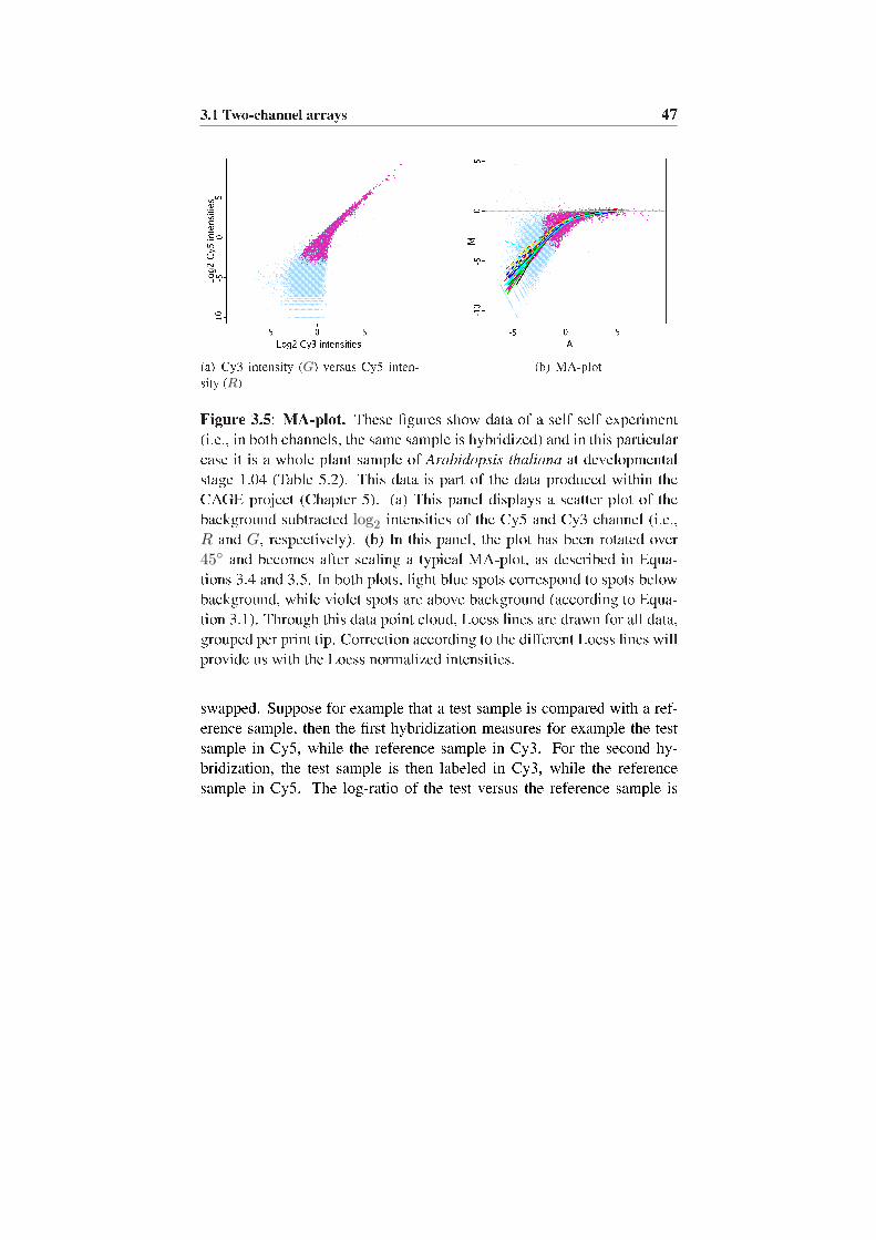
3.1 Two-channel arrays 47
(a) Cy3 intensity (G) versus Cy5 inten-sity (R)
(b) MA-plot
Figure 3.5: MA-plot. These �gures show data of a self-self experiment(i.e., in both channels, the same sample is hybridized) and in this particularcase it is a whole plant sample of Arabidopsis thaliana at developmentalstage 1.04 (Table 5.2). This data is part of the data produced within theCAGE project (Chapter 5). (a) This panel displays a scatter plot of thebackground subtracted log2 intensities of the Cy5 and Cy3 channel (i.e.,R and G, respectively). (b) In this panel, the plot has been rotated over45◦ and becomes after scaling a typical MA-plot, as described in Equa-tions 3.4 and 3.5. In both plots, light blue spots correspond to spots belowbackground, while violet spots are above background (according to Equa-tion 3.1). Through this data point cloud, Loess lines are drawn for all data,grouped per print tip. Correction according to the different Loess lines willprovide us with the Loess normalized intensities.
swapped. Suppose for example that a test sample is compared with a ref-erence sample, then the �rst hybridization measures for example the testsample in Cy5, while the reference sample in Cy3. For the second hy-bridization, the test sample is then labeled in Cy3, while the referencesample in Cy5. The log-ratio of the test versus the reference sample is

48 Technical aspects of DNA microarray technologies
Figure 3.6: Loess regression. At each point an estimate is obtained fromthe points within a window centered around that point, obtained by linearor quadratic, weighted regression. Afterwards all estimates are connectedand a loess regression line is obtained.
then computed as
12
[log2
(R1
testG1
reference
)− log2
(R2
referenceG2
test
)],
where R and G are the background corrected intensities and the superscriptindicates the hybridization.
3.2 Single-channel arraysA second class of microarrays are the short oligonucleotide arrays. Shortoligonucleotide arrays are single-channel arrays (i.e., they use only onedye). Therefore, there will be no issue of dye effects.Affymetrix (http://www.affymetrix.com) is probably the most usedshort oligonucleotide platform and with its speci�c probe design, it re-quires a completely different normalization strategy.
3.2.1 Short oligonucleotides: AffymetrixThese short oligonucleotides are synthesized on the slide by using a setof masks. By covering the slide with a mask, a selection of positions on

3.2 Single-channel arrays 49
the chip is exposed and light will then be used to activate these unpro-tected sites. At these activated positions, nucleotides will bind, resulting inthe synthesis of one nucleotide at the positions chosen with the mask. Anew mask is then applied and the same process is repeated. After severalrounds, the desired set of probes is obtained. In this way a lot of differentmasks are required and this makes the Affymetrix chip a rather expensivechip.On an Affymetrix chip, a gene is not represented anymore by one singleDNA strand, but by a probe set, consisting of 11 to 20 probe pairs. Eachprobe pair is composed of two short oligonucleotides of length 25bp. Onematches with a part of the sequence of the gene and is called the perfectmatch (PM ). The second oligonucleotide has the same sequence as theperfect match, except for a single mismatch in the middle of the oligonu-cleotide (at the 13th position), and is therefore called the mismatch (MM )probe. These mismatch probes are assumed to measure the nonspeci�cbinding and are therefore often used as a kind of background correction.Disadvantage of this setup is that these oligonucleotides are so short thatthey are sometimes not gene speci�c.The sample is prepared by �rst obtaining double-stranded cDNA from themRNA sample via reverse transcription (Section 2.2.1). From this cDNA,cRNA is synthesized via in vitro transcription (IVT) (i.e., transcriptionwithin a laboratory mixture that contains all the necessary components).The nucleotides used to perform this transcription are biotinylated, so thatthe cRNA is labeled. Afterwards the cRNA is fragmented into smallerpieces and hybridized on the array (see Figure 3.7).
3.2.2 Normalization of Affymetrix chipsThe probe design and the fact that they are single-channel arrays require ofcourse a completely different preprocessing. In this work, both MicroAr-ray Suite 5.0 (MAS 5.0) and Robust Multi-array Average (RMA) will beapplied to normalize the Affymetrix data. At the moment, these two areprobably the most popular normalization methods. There are a number ofalternatives as, for example, Model Based Expression Index (MBEI, Li andWong (2001)), GCRMA (Wu and Irizarry (2005)), but we refer to litera-ture for discussion of those methods and restrict ourselves to MAS 5.0 and

50 Technical aspects of DNA microarray technologies
Figure 3.7: Single channel microarray experiments - Affymetrix: Fortwo different cell types, the RNA is extracted and cRNA is obtained fromthe mRNA, via RT and IVT. The two samples are each hybridized on aseparate Affymetrix chip.
RMA.

3.2 Single-channel arrays 51
Normalization can be described in a few steps:
1. Background subtraction.
2. Computing the expression value: The set of intensities of the differentprobe pairs {(PMij ,MMij)|j = 1, . . . , ni} have to be combined intoone single expression value xi for each gene i.
3. Normalization step.
These steps will be described for both methods, MAS 5.0 and RMA.
MicroArray Suite 5.0
Background subtraction The MAS 5.0 algorithm applies a backgroundcorrection. Therefore it breaks the array up into, by default, 16 rectangularzones and it computes for each region the 2nd percentile signal of the cells.This is then the background for that zone. The local background b(x, y) fora cell (x, y) is de�ned as an average background, weighted according to thedistance between its array coordinates and the centers of the 16 differentzones. One also computes a local noise value n(x, y) as the standard devi-ation of the lowest 2% cell intensities. And the adjusted intensity, noted asa(x, y), is then de�ned as
a(x, y) = max(I(x, y)− b(x, y), 0.5n(x, y))1,
where I(x, y) is the maximum of the intensity at (x, y) and 0.5. For sim-plicity, we will denote the set of background corrected MM and PM val-ues also as MM and PM , respectively.
Computing the expression value In this step, we will combine the setof background-adjusted intensities of the probe pairs {(PMij , MMij)|j =1, . . . , ni} into one single expression value xi for each probe set i.Until 2001, Affymetrix used AvDiff as a default to compute the expres-sion values. This AvDiff approach was included in the previous version,
1The constants, given in the equations are the default values as applied in MAS 5.0, butthey can be changed.

52 Technical aspects of DNA microarray technologies
MAS 4.0. AvDiff computes the expression measurement as an averageover all PMij values, corrected by the mismatch value MMij :
xi =1ni
ni∑
j=1
∆ij =1ni
ni∑
j=1
(PMij −MMij) .
To make the average more robust towards outliers, the algorithm computedthe average for a subset, consisting of those differences ∆ij within 3 stan-dard deviations from the mean of ∆(2), . . . , ∆(ni−1), where ∆(k) is the kth
smallest difference.However, for about one third of the measurements, the MM value is ac-tually higher than the PM value (Irizarry et al. (2003)) and, hence, theexpression value can become a negative number with this computationmethod. Also, a linear scale is not optimal as the variance then heavilydepends on the intensity. MAS 5.0 (Affymetrix (2001)) attempts to bypassthese shortcomings. First, the MM -values are replaced by an Ideal Mis-match (IM ) value, which equals the MM value if PM > MM , but hasbeen corrected to be smaller than PM if PM ≤ MM . Therefore a kindof robust average log-ratio, called the biweight speci�c background (SB),is computed as
SBi = Tbi ({log2(PMij)− log2(MMij)|j = 1, . . . , ni}) , (3.6)
where Tbi denotes Tukey's Biweight average.Tukey's biweight average computes a robust average that is unaffected byoutliers. Suppose, in general, one wants to compute this robust average fora set of points a = {ak|k = 1, . . . , n}. Hence in our speci�c case, a equals{log2(PMij) − log2(MMij)|j = 1, . . . , ni}. First, you have to computethe median M of the values ak and for each data point ak, the absolutedistance from this median M is computed. From these absolute deviationsthe median S is calculated, which gives an indication of the spread of ak
around their median. With these statistics, a distance2 is computed for eachdata value as
uk =ak −M
5S + 0.0001.
2The constants, given in the equations are the default values as applied in MAS 5.0, butthey can be changed.
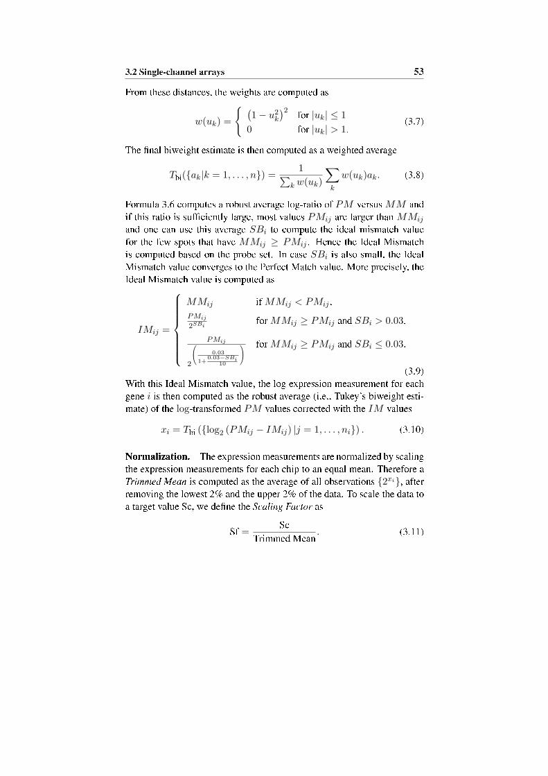
3.2 Single-channel arrays 53
From these distances, the weights are computed as
w(uk) =
{ (1− u2
k
)2 for |uk| ≤ 10 for |uk| > 1.
(3.7)
The �nal biweight estimate is then computed as a weighted average
Tbi({ak|k = 1, . . . , n}) =1∑
k w(uk)
∑
k
w(uk)ak. (3.8)
Formula 3.6 computes a robust average log-ratio of PM versus MM andif this ratio is suf�ciently large, most values PMij are larger than MMij
and one can use this average SBi to compute the ideal mismatch valuefor the few spots that have MMij ≥ PMij . Hence the Ideal Mismatchis computed based on the probe set. In case SBi is also small, the IdealMismatch value converges to the Perfect Match value. More precisely, theIdeal Mismatch value is computed as
IMij =
MMij if MMij < PMij ,PMij
2SBifor MMij ≥ PMij and SBi > 0.03,
PMij
2
0@ 0.03
1+0.03−SBi
10
1A
for MMij ≥ PMij and SBi ≤ 0.03.
(3.9)With this Ideal Mismatch value, the log expression measurement for eachgene i is then computed as the robust average (i.e., Tukey's biweight esti-mate) of the log-transformed PM values corrected with the IM values
xi = Tbi ({log2 (PMij − IMij) |j = 1, . . . , ni}) . (3.10)
Normalization. The expression measurements are normalized by scalingthe expression measurements for each chip to an equal mean. Therefore aTrimmed Mean is computed as the average of all observations {2xi}, afterremoving the lowest 2% and the upper 2% of the data. To scale the data toa target value Sc, we de�ne the Scaling Factor as
Sf =Sc
Trimmed Mean . (3.11)

54 Technical aspects of DNA microarray technologies
In our data sets this target value Sc will equal 100. The reported MAS 5.0expression measurement is then de�ned as
MAS 5.0 expression value(i) = Sf ∗ 2xi . (3.12)
In this work, MAS 5.0 expression values will always refer to the expressionvalues as de�ned in Equation 3.12. Within MAS 5.0, there is limited �ex-ibility in the normalization procedure and a description of the alternativescan be found in Affymetrix (2002).
Robust Multi-array Average
Robust Multi-array Average (RMA, Irizarry et al. (2003)) is an almostequally popular method to apply background correction, to normalize thedata between the slides, and to compute the expression measurements.Contrary to MAS 5.0, this RMA approach does not make use of the MM -values, as the MM -values are likely to measure both non-speci�c bindingand signal. Therefore, they add noise to the data and can lead to a biasin the corrected PM signal. The RMA method is available as part of theaffy package within Bioconductor.
Background subtraction. The background is estimated globally foreach array, by assuming that the PM values for probe set i and probej can be described as PMij = bij + sij with an exponential signalsij ∼ Exp(α), a normal background bij ∼ N(µ, σ2). Given the PerfectMatch values and estimates of α, µ, and σ, the signal values can becomputed as E[sij |PMij ]. Under the given assumptions, this equals
E[sij |PMij ] = a + σφ
(aσ
)− φ(
PMij−aσ
)
Φ(
aσ
)+ Φ
(PMij−a
σ
)− 1
,
with a = PMij −µ−σ2α and φ and Φ are the density and the cumulativedistribution function of the normal distribution, respectively. The estimatesfor α, µ, and σ are estimated globally from the data in an ad hoc way.

3.2 Single-channel arrays 55
Normalization. RMA forces the background corrected probe intensitiesto have the same distribution for each array, by applying quantile normal-ization. Therefore, all data is placed in a matrix in such way that eachcolumn corresponds to a chip and each row to a gene. Data are sortedfor each column in increasing order and the average is taken for each row.These averages replace the original values in all columns. The last stepis to unsort the columns to their original order. For example, on all chipsthe smallest value after quantile normalization will be the average of theoriginal smallest values over all chips.
Computing the expression value. Once the PM -values are backgroundcorrected and normalized, a linear model is �tted to their log2-transformedvalues for each probe set i:
log2 (PMaj) = µa + αj + εaj ,
where µa is the global, overall effect of the probe set on array a, αj repre-sents the probe effect for the jth probe in the probe set with the constraintthat
∑j αj = 0 and εaj is the residual for the jth probe on array a. Our
interest is, of course, the estimates of the log expression levels µa for ar-ray a. This effect is estimated in a robust way, by using median polish(Tukey (1949)). Therefore, the expression values are placed in a matrix;rows correspond for example to the arrays and columns to the probes. Themedians of the rows are subtracted from the corresponding rows and nextthe medians of the columns are subtracted from their columns. These stepsare repeated iteratively until all row and column medians are zero. The ob-tained, residual matrix is then subtracted from the original matrix. Theseare the �tted values and if you take the average for each row, you obtainfor each array an estimate for the probe set.
3.2.3 Quality assessment of Affymetrix chipsAffymetrix provides a number of guidelines to judge whether the hy-bridizations within an experiment are satisfactory. This quality assessmentis typically done after the MAS 5.0 or RMA normalization step.

56 Technical aspects of DNA microarray technologies
Visualization methods
RNA-degradation plots RNA-degradation plots help to assess the RNAquality. To this end, the individual probes in a probe set are ordered accord-ing to their location relative to the 5′ end of the targeted RNA molecule.Since RNA degradation typically starts from the 5′ end of the molecule, wewould expect probe intensities to be systematically lower at that end of aprobe set when compared to the 3′ end. On each chip, the PM -values arecombined according to their location in the probe set and averaged overthe probe sets. These values are then plotted against their location. It isimportant that these RNA degradation lines are all more or less parallel.An example of an RNA degradation plot is shown in Figure 3.8.
MA plot For two-channel arrays, MA-plots were a useful tool to detectaberrant behavior in the intensities. Affymetrix is a single channel plat-form, and hence, there is no straightforward way to make an MA-plot.Therefore, MA-plots for Affymetrix chips are de�ned in alternative ways.The expression measurements are plotted against a synthetic reference ar-ray, which is created by taking the probe-wise medians over all hybridiza-tions in the experiment. Alternatively, one makes the MA-plots of eachpairwise comparison.
Density plots of the PM values Histograms of the PM values enableto detect arrays with overall higher or lower intensities or can indicate sat-uration effects. These cause a small �blob� at the high intensities.
Quantitative quality assessment
The main quantitative indications for the quality of the arrays can be sum-marized in one single graph. An example is shown in Figure 3.9. Inthis graph, each line (separated by dashed lines) corresponds to one of thechips. The names of the chips are written on the left side.
Detection calls MAS 5.0 computes the Present and Absent calls for allspots, comparable to Section 3.1.2 for the two-channel arrays. This is done

3.2 Single-channel arrays 57
RNA degradation plot
5’ <−−−−−> 3’ Probe Number
Log2
Mea
n In
tens
ity s
cale
d
0 2 4 6 8 10
010
2030
40
123456789
Figure 3.8: RNA-degradation plot. This plot shows the RNA-degradation effect for an experiment with 9 Affymetrix chips. The PMvalues of the 9 hybridizations are base 2 log transformed, averaged bytheir location in the probe sets over all probe sets. They are scaled to havea standard deviation of 1 to make the trend more visible. They show alla similar increasing trend, except for the �rst hybridization, which has astrongly deviating behavior. This plot is produced with the AffyRNAdegand plotAffyRNAdeg functions of the affy package from Bioconduc-tor.
by computing a discriminating score for each probe pair (PMij , MMij),de�ned as
Rij =PMij −MMij
PMij + MMij.
If an MMij value becomes small compared to the PMij value, this ratioRij will converge to 1. In case the MMij value is comparable to or largerthan the PMij value, this discriminating score Rij will be small or nega-

58 Technical aspects of DNA microarray technologies
QC Stats
1.CEL
2.CEL
3.CEL
4.CEL
5.CEL
6.CEL
7.CEL
8.CEL
9.CEL
321−3 −2 −1 0
36.33%161.75
52.03%45.26
47.27%36.26
49.85%43.39
51.08%40.14
52.79%41.23
51.86%40.25
52.51%40.66
52.92%39.68
AFFX−b−ActinAFFX−GAPDH
Figure 3.9: Quality statistics plot. This plot summarizes the quality as-sessment statistics for an experiment with 9 Affymetrix chips. A detaileddescription of the various parameters can be found in Section 3.2.3. In thiscase both the background and the percentage of Present calls are coloredred; this is caused by the fact that the �rst hybridization has a low percent-age of Present calls and a high background. The Scaling factors and the3′/5′ ratios for β-actin and GAPDH are within the expected ranges. Com-bined with the information in Figure 3.8, Hybridization 1 seems to havea deviating behavior. This plot is produced with the function qc of thesimpleaffy package from Bioconductor.
tive. A detection p-value pi for probe i is then computed by testing whethermedianj(Rij) equals a small value τ or is larger than τ . The default valuefor τ is 0.015. This test is done with a one-sided Wilcoxon's signed ranktest (Affymetrix (2002)). Depending on the detection p-value pi, a probe

3.2 Single-channel arrays 59
is called Present, Absent, or Marginal according to the following rule3
pi < α1 Present call
α1 ≤ pi < α2 Marginal call
α2 ≤ pi Absent call(3.13)
The percentages of Present calls are indicated for each hybridization inFigure 3.9, as the top left number. These numbers should be more or lesscomparable. In the �gure, the percentages are colored red if there is aspread of more than 10% across the whole experiment, which can indicatethat at least one of the hybridizations is of inferior quality.
Average background Similar to the percentage of present calls, also theaverage background should be comparable across the slides. Differences inthe background can indicate different amounts of cRNA or differences inhybridization ef�ciency which resulted in a brighter chip. The backgroundvalues are colored red if the range of the values is larger than 20 units.
The scaling factor The scaling factor (as de�ned in Equation 3.11)shows the amount of scaling necessary to bring the mean expression levelto an equal mean and therefore, it also re�ects the overall expressionlevel on an array. Affymetrix suggests that the scaling factors should beless than three-fold different from the overall average scaling factor. Thescaling factors are drawn as a line from the zero-fold line of the image toits scaling factor value and they should fall within the blue strip on theimage, which indicates the three-fold of the overall mean scaling factor.
The 3′/5′ ratios for β-actin and GAPDH To assess the RNA samplequality, one can make use of the genes β-actin and GAPDH. These genesare expressed in most cell types. These are also relatively long genes andmost Affymetrix chips contain separate probesets for the 3′, the middleand the 5′ region. The ratio of the probe set at the 3′ to the probe setat the 5′ end gives an indication of the RNA degradation or inef�cient
3The default values for α1 and α2 are 0.04 and 0.06, respectively.

60 Technical aspects of DNA microarray technologies
transcription of the cRNA. Affymetrix states that the 3′/5′ ratio for β-actinshould be lower than 3. As the GAPDH gene is smaller, the cut-off valuefor GAPDH is set at 1.25. In Figure 3.9, these 3′/5′ ratios for β-actin andGAPDH are indicated with triangles and circles, respectively. The dashedlines display the values from -3 to 3.
The hybridization controls: BioB, BioC, BioD, and CreX Prior to thehybridization, transcripts derived from completely unrelated material arespiked in. In this way nothing else should hybridize to their probe sets andtheir intensity is a measure for the hybridization and scanning quality. Thetranscripts BioB, BioC, BioD, and CreX are added in increasing concen-tration (1.5 pM4, 5 pM , 25 pM , and 100 pM ). The concentration of BioBcorresponds to the lower detection limit, and Affymetrix suggests that itshould be called Present in about 50% of the chips. The other three tran-scripts should always be called Present and their expression measurementsshould increase.
3.3 Finding differentially expressed genesIn this section, a number of methods to detect differentially expressedgenes will be presented. We will not provide a complete overview of allpossible methods, but we will restrict ourselves to those techniques thatwere applied in this work.
3.3.1 LIMMA or Linear Models for MicroArray dataThis method represents the design of any microarray experiment in termsof a linear model �tted for each gene separately. To test for differential ex-pression, the gene-speci�c variance estimates are improved in a Bayesianway by using the information from all genes. The method is implementedin a Bioconductor package called limma. We will give here an overviewof the method; a more detailed description can be found in Smyth (2004).
4pico molar

3.3 Finding differentially expressed genes 61
Describing the experimental design with a linear model
To explain this into more detail, we focus �rst on the construction of thelinear model. Therefore we have to make the distinction between two andsingle-channel arrays. First, in case of two-channel arrays, the log-ratiosyg = log2(Rg)− log2(Gg) of the Cy5 intensity Rg over the Cy3 intensityGg are modeled for each gene g. Consider for example the following loopdesign
C
↙ ↖A −→ B
in which two contrasts (e.g., (Bg−Ag) and (Cg−Bg)) have to be estimatedfor each gene g, as the contrast of the third slide can be expressed as a linearcombination of these two contrasts. The log-ratios (yg1, yg2, yg3) from thethree microarrays can then be used to estimate the contrasts (Bg−Ag) and(Cg −Bg) as
E
yg1
yg2
yg3
=
1 00 1−1 −1
(Bg −Ag
Cg −Bg
). (3.14)
Or, in general, we can write it as a matrix
X =
1 00 1−1 −1
representing the design of the experiment and therefore called the designmatrix, and coef�cient vectors αg =
(Bg −Ag Cg −Bg
)T, contain-
ing the effects for gene g.In the case of single-channel arrays, instead of the log-ratios, the log-intensities are measured. For example, consider an experiment of 5 slides,in which sample A is measured three times and sample B is measured

62 Technical aspects of DNA microarray technologies
twice, the design matrix and the effects can then be written as
X =
1 01 01 00 10 1
and αg =
(Ag
Bg
).
Analogously, all designs can be described with a design matrix X and aneffect vector αg, in such a way that
yg = Xαg + εg,
where ε is a noise term. The contrasts or the independent variables will beestimated for each gene from the dependent variables (i.e., the log-ratios)via a linear regression. Further, we assume that the variance of yg can bewritten as var(yg) = Wgσ
2g , with Wg a positive-de�nite weight matrix.
The model can be �tted with an ordinary least squares �t of the linearmodel for each gene and this is also what we will apply in this work.
Testing for differential expression
The contrasts of interest can be equal to the estimated effects, but some-times additional comparisons between the RNA samples are of interest.Therefore we will denote all contrasts of interest as a vector βg, consist-ing of linear combinations of the elements in αg, described with a contrastmatrix C:
βg = CT αg.
Suppose, for example, we have a loop design as described in 3.14 and ourcontrasts of interest are not only the effects Bg−Ag and Cg−Bg, but alsoAg − Cg, then we want to test
βg =
Bg −Ag
Cg −Bg
Ag − Cg
=
1 00 1−1 −1
(Bg −Ag
Cg −Bg
)= CT αg.

3.3 Finding differentially expressed genes 63
By �tting the model to our data, estimates αg for the coef�cients αg, s2g for
σ2g , and a positive de�nite matrix Vg, such that var(αg) = Vgs
2g, are ob-
tained. From these, estimates for all contrasts of interest can be computed,as βg = CT αg and var(βg) = CT VgCs2
g. These contrasts are assumed tobe approximately normal with mean βg and covariance matrix CT VgCσ2
g
and the residual variance s2g is assumed to follow a scaled chi-square dis-
tributions2g ∼
σ2g
dgχ2
dg.
With an ordinary t-test, one can test whether an estimated contrast βgj forcontrast j and gene g equals 0, with the t-test statistic
tgj =βgj
sg√
vgj,
where vgj is the jth diagonal element of the covariance matrix Vg. LIMMAuses an empirical Bayes t-test in the sense that the standard deviations arebased on the data of all genes and not only on the data available for thespeci�c gene. In this way, the test exploits the fact that the model is �ttedin parallel for thousands of genes. This t-test is called the moderated t-test.A prior estimate for the standard deviation s0 with d0 degrees of freedomis estimated, based on the measurements of all genes (Smyth (2004)). Thisprior updates the gene speci�c standard deviation and the posterior
s2g =
d0s20 + dgs
2g
d0 + dg
is used for the moderated t-test with test statistic
tgj =βgj
sg√
vgj.
This tgj follows a t-distribution with dg + d0 degrees of freedom, which isnarrower and re�ects the fact that information has been borrowed from theensemble of genes to make inferences about each single gene.

64 Technical aspects of DNA microarray technologies
3.3.2 General Linear modelsA second method to �nd differentially expressed genes is by �tting generallinear models (Kerr et al. (2000), Wol�nger et al. (2001)). Prior to thespeci�cation of the models, used to analyze microarray experiments, wegive a short description of general linear models.
An introduction to concepts in general linear models
General linear models (GLM) are probably the most used technique instatistics. The technique serves to �nd the statistical relation between oneor more explanatory variables and a response variable. In this work, allexplanatory variables will be treated in a qualitative way (e.g., two growthconditions of plants) and their values can be interpreted as labels that groupthe data. In some cases the explanatory variable can have a quantita-tive connotation, but then it is treated as a qualitative variable (e.g., low,medium, versus high temperature). No assumptions about the statisticalrelation between the factors and the response are made. The explanatoryvariables are called factors and their values are called the factor levels. Acombination of such factor levels is called a treatment.An important distinction between two types of factors have to be made.They can model a �xed effect or a random effect. A �xed effect is an effectfor which the levels are chosen for their intrinsic importance. For example,one wants to compare the two growth conditions for plants. For a ran-dom effect, on the contrary, one wants to model a population of levels andthere is no direct interest in the levels that are actually used. The levelsare merely chosen to represent the population. For example, if different re-searchers lead to a difference in the measurements taken in an experiment,then one can chose, for example, �ve researchers and assess the effect ofthe different persons working on the experiment. In this case, the interestis not the effect of those �ve, particular persons, but merely to generalizeto the effect of having different persons working on an experiment. If both�xed and random effects are used, we call the model a mixed model.In the text, we will denote �xed factors by Greek letters, while random fac-tors are denoted by Roman letters. Their subscripts will indicate the level.For example, ai denotes the ith level of a random factor a.In the following section, a general linear model speci�c for the analysis of

3.3 Finding differentially expressed genes 65
a microarray experiment, as was proposed in Kerr et al. (2000) and Wol�n-ger et al. (2001), will be presented.
Microarray experiment in terms of a general linear model
Consider for example a classical dye-swap experiment, in which two sam-ples are compared on two arrays. We can then introduce a factor ai, thatrepresents the array effect, with two levels i = {1, 2} corresponding toArray 1 and 2. Secondly, we have a factor δj to measure the Dye effect,again with two levels corresponding to the dyes Cy3 and Cy5. Analo-gously, the sample effects can be modeled as a factor τk with k = 1, 2. Foreach gene g, we will measure log intensities yijkg for all index combina-tions (i, j, k) ∈ {(1, 1, 1), (1, 2, 2), (2, 1, 2), (2, 2, 1)}. Remark, that sucha dye-swap experiment has a Latin square design. A model describing thisexperiment can be written as follows:
yijkg = µ + ai + δj + τk + γg + (aγ)ig + (τγ)kg + eijkg, (3.15)
where
yijkg are the log-intensity of gene g for treatment k, dye j, and array i,
µ is the global mean,
a is the main array effect (random effect; i = 1, . . . , # arrays),
δ is the main dye effect (�xed effect; j = 1, 2),
τ is the main treatment or sample effect (�xed effect; k = 1, . . . ,#samples),
γ is the main gene effect for gene (�xed effect; g = 1, . . . ,# genes),
e is the random error effect.
All random effects ai, (aγ)ig, and eijkg are assumed to be normally dis-tributed with mean 0 and variance σ2
a, σ2aγg
, and σ2e , respectively.
The effects a, δ, and τ are used to normalize the data for array, dye andsample effects. The main effect γ accounts for the average effects of the

66 Technical aspects of DNA microarray technologies
individual genes and the interaction term aγ accounts for the spot effect.All these effects have a normalization purpose and are not of primary in-terest.The effect that is of interest is the interaction term τγ of treatment× genes.These interaction effects (τγ)ig account for differences that can not be as-cribed to the combination of the main effects of treatment i and gene g. Ifan interaction effect (τγ)ig is signi�cantly different from 0, the gene g isdifferentially expressed. And this is what we will test for to �nd the list ofdifferentially expressed genes.Due to the large number of genes, it is computationally intensive to �t thismodel. Therefore, this model is split up into two parts, a normalizationmodel and a gene-speci�c model (Wol�nger et al. (2001)). In the �rst step,the normalization model
yijkg = µ + ai + δj + τk + rijkg (3.16)
is �tted. The interpretation of the effects is similar to the interpretation asin the global model 3.15. On these residuals rijkg, a gene-speci�c model
rijkg = γg + (aγ)ig + (τγ)kg + eijkg
is �tted for each gene. Again, the interpretation of the effects is similar tothe effects de�ned in 3.15, but now they are �tted for each gene separately.Depending on the design of an experiment, this model can change. Theidea behind the normalization and gene-speci�c mixed models was pro-posed in Wol�nger et al. (2001). Similar models, in which all factors weretreated as �xed were proposed in Kerr et al. (2000).
Fitting the mixed model
In the case of a general linear model with only �xed effects, this model canbe �tted as in R with the function aov. This will provide the least squaressolution.To �t mixed models in R, the library nlme and, more speci�cally, thefunction lme can be used. If we denote the �xed factors as a vector β andthe random factors for the ith subject as bi, then we can model the responseyi for the ith subject as
yi = Xiβ + Zibi + εi,
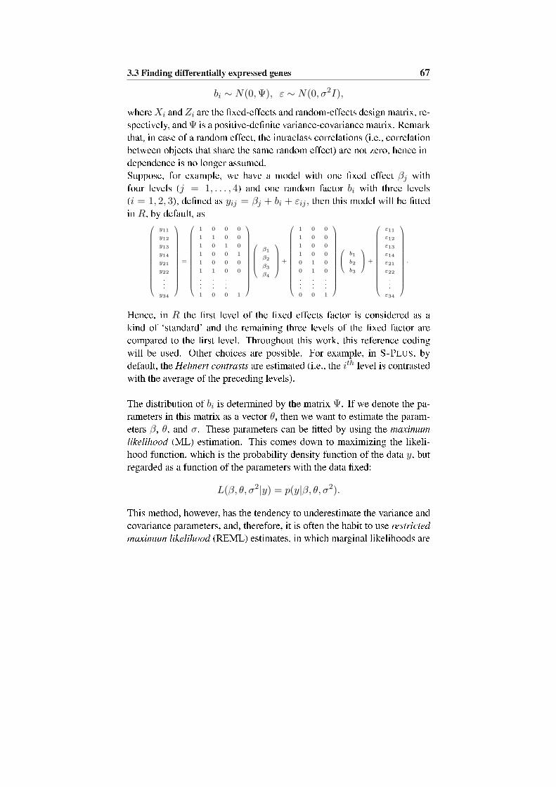
3.3 Finding differentially expressed genes 67
bi ∼ N(0, Ψ), ε ∼ N(0, σ2I),
where Xi and Zi are the �xed-effects and random-effects design matrix, re-spectively, and Ψ is a positive-de�nite variance-covariance matrix. Remarkthat, in case of a random effect, the intraclass correlations (i.e., correlationbetween objects that share the same random effect) are not zero, hence in-dependence is no longer assumed.Suppose, for example, we have a model with one �xed effect βj withfour levels (j = 1, . . . , 4) and one random factor bi with three levels(i = 1, 2, 3), de�ned as yij = βj + bi + εij , then this model will be �ttedin R, by default, as
0BBBBBBBBBBBBBBB@
y11
y12
y13
y14
y21
y22...
y34
1CCCCCCCCCCCCCCCA
=
0BBBBBBBBBBBBBBB@
1 0 0 0
1 1 0 0
1 0 1 0
1 0 0 1
1 0 0 0
1 1 0 0
......
......
1 0 0 1
1CCCCCCCCCCCCCCCA
0BBBB@
β1
β2
β3
β4
1CCCCA
+
0BBBBBBBBBBBBBBB@
1 0 0
1 0 0
1 0 0
1 0 0
0 1 0
0 1 0
......
...0 0 1
1CCCCCCCCCCCCCCCA
0B@
b1
b2
b3
1CA +
0BBBBBBBBBBBBBBB@
ε11
ε12
ε13
ε14
ε21
ε22...
ε34
1CCCCCCCCCCCCCCCA
.
Hence, in R the �rst level of the �xed effects factor is considered as akind of `standard' and the remaining three levels of the �xed factor arecompared to the �rst level. Throughout this work, this reference codingwill be used. Other choices are possible. For example, in S-PLUS, bydefault, the Helmert contrasts are estimated (i.e., the ith level is contrastedwith the average of the preceding levels).
The distribution of bi is determined by the matrix Ψ. If we denote the pa-rameters in this matrix as a vector θ, then we want to estimate the param-eters β, θ, and σ. These parameters can be �tted by using the maximumlikelihood (ML) estimation. This comes down to maximizing the likeli-hood function, which is the probability density function of the data y, butregarded as a function of the parameters with the data �xed:
L(β, θ, σ2|y) = p(y|β, θ, σ2).
This method, however, has the tendency to underestimate the variance andcovariance parameters, and, therefore, it is often the habit to use restrictedmaximum likelihood (REML) estimates, in which marginal likelihoods are

68 Technical aspects of DNA microarray technologies
used to estimate the variance components. The restricted maximum like-lihood estimation, as de�ned by Laird and Ware (1982), is an empiricalBayesian approach, in which the variance components are estimated, byassuming a locally uniform prior distribution for β and by integrating theseout of the likelihood:
LR(θ, σ2|y) =∫
L(β, θ, σ2|y)dβ.
Maximizing this restricted likelihood provides estimates for θ and σ2. Withthese parameters, estimates for β can be obtained via the ordinary ML esti-mation with known variance components. All details on the computationscan be found in Pinheiro and Bates (2000).Assessing the signi�cance of the �xed effects is done with the Wald F -test.From the model
yi = Xiβ + Zibi + εi,
bi ∼ N(0, Ψ), ε ∼ N(0, σ2I),
follows thatyi ∼ N(Xiβ, ZiΨZ ′i + σ2I).
The hypothesis that
H0 : Lβ = 0 versus Ha : Lβ 6= 0
is tested with an approximate Wald F -test (i.e., a multivariate generaliza-tion of the t-test):
F =
(β − β
)′L′
[L
(∑Ni=1 X ′
iV−1i (θ, σ)Xi
)L′
]−1L
(β − β
)
rank(L)
where Vi = ZiΨZ ′i + σ2I .
After the introduction of all these concepts and statistical methods, we canstart with the actual analysis of the data. As announced in Chapter 1, wewill start with the benchmarking of the CATMA array against two com-mercial platforms, Agilent and Affymetrix.

Chapter 4Benchmark of CATMA array
The Arabidopsis research community has been blessed with mul-tiple independent resources for transcript pro�ling, both from com-mercial sources and academic core facilities. However, today, mi-croarrays that do not carry probes for the majority of transcrip-tion units identi�ed in the genome, in particular cDNA arrays, arequickly becoming obsolete. Therefore, this is an opportune mo-ment to introduce the CATMA array (Section 3.1.1) as an alterna-tive to the limited coverage cDNA and commercial, more expensiveoligonucleotide arrays. The aim of this work was to describe, in de-tail, the performance of the CATMA array in comparison with theoligonucleotide-based platforms commercialized by Agilent (Ara-bidopsis 2 oligo array) and Affymetrix (ATH1 GeneChip probe ar-ray; Redman et al. 2004), and to present these results as a referenceto the Arabidopsis research community. This work has been pub-lished in Allemeersch et al. (2005).

70 Benchmark of CATMA array
4.1 The CATMA projectThe CATMA project (http://www.catma.org) was initiated by Frenchand Belgian laboratories in December 1999 and joined by additionalgroups from Germany (July 2000), the Netherlands, Switzerland, theUnited Kingdom (October 2000), Spain (January 2001) and Sweden(September 2001). The project aimed to produce Gene-speci�c SequenceTags (GSTs, Section 3.1.1) for all genes in the genome sequence (Hilsonet al. (2004)). Before one can start to search for GSTs, the actual genes inthe �ve Arabidopsis chromosomes have to be identi�ed. The choices madefor launching the project re�ect the status of the knowledge in February2001 when the structure of only a minority of Arabidopsis genes (about2000) had been determined experimentally. Therefore the project also hadto rely on gene prediction to identify the boundaries of each transcriptionunit and of the exon(s) within it.At the start of the large scale GST synthesis within the CATMA project,the chromosome annotations published by the Arabidopsis Genome Initia-tive (AGI) sequencing centers were not homogeneous. Different tools hadbeen adopted by different centers and had evolved over time. Accordingto an evaluation of the gene prediction algorithms used for the annotationof the Arabidopsis nuclear genome, the EuG�ene package, developedby Schiex et al. (2001), offered the most reliable results. Therefore, acomplete updated annotation of the Arabidopsis genome, provided byEuG�ene and based on a uniform set of parameters, was originally chosento design the CATMA GSTs and this resulted in a set of 21,120 in silicoGSTs (version 1). Since then, the collection has been updated with 3,456additional in silico tags (24,576 in total; version 2). These additionalGSTs are derived from genes belonging to gene families and therefore itsnucleotide sequence is too similar to other family members to design aspeci�c GST. These genes were added by using less stringent parameters,as, for example, increasing the identity cutoff of 70% and by taking intoconsideration added 3′ untranslated regions (UTRs). A second groupare GSTs for which the PCR ampli�cation failed the �rst time and forwhich alternative primers were found. And also improvements of theArabidopsis genome annotations and the gene prediction software changedthe original gene set. A third additional GST set has now been created in

4.2 The CATMA benchmark strategy 71
the framework of the CAGE project (Section 5.1), based on more recentArabidopsis genome annotations, generated by EuG�ene gene predictionsoftware and augmented with TIGR 5 gene models from The Institute forGenomic Research (TIGR; http://www.tigr.org/), led to the designof an additional set of about 5,760 GSTs, and in total a set of about 30,000GSTs.On 21st June 2002 the CATMA database was made public, allowing fullsearching of the �rst 21,120 validated GSTs (v1). In March 2004, thedatabase was updated to total of 24,576 GSTs. The update history of theCATMA database and website is described in the CATMA status page(http://www.catma.org/status.html).With these GSTs, the Complete Arabidopsis Transcriptome MicroArray orCATMA array was built.
4.2 The CATMA benchmark strategySeveral genome-scale microarrays are now available for Arabidopsistranscript pro�ling and choosing a particular platform will depend onvarious criteria including genome coverage, data quality, dynamic range,and sensitivity, as well as more practical factors such as availability, price,and logistics. We present here a detailed analysis of the main technicalcharacteristics of the CATMA array, and compared them with the AgilentArabidopsis 2 oligo array (Agilent array, Section 3.1.1) and the AffymetrixATH1 genome array (Affymetrix array; Section 3.2.1). Together, thesearrays cover the three probe types now used in genome-scale microarrays:PCR amplicons (150 to 500 bp, CATMA), the long oligonucleotides(60mer, Agilent) and the short oligonucleotide sets (25mer, Affymetrix).
For all three platforms, the RNA labeling, hybridization, scanning, anddata extraction were performed by a laboratory offering routine microarrayservices with that particular platform, and following its standard protocolsand processes: VIB-MAF microarray facility to process the CATMAarrays, ServiceXS (a service facility in The Netherlands) for Agilent andthe Nottingham Arabidopsis Stock Center for Affymetrix. Hence, alldatasets were produced independently by laboratories best positioned

72 Benchmark of CATMA array
to provide service with their particular platform. In all three cases, theplatforms were equipped with the standard suite of hardware and softwarecommercially distributed by the Amersham, Agilent, and Affymetrixcompanies, respectively. The whole analysis is done from the position ofa regular customer, that chooses a reliable service provider and trusts thetools, as provided by the microarray companies.
Several studies have already described microarray platform comparisonand quality assessment based on various approaches (Chudin et al. (2002);Kuo et al. (2002); Yuen et al. (2002); Lee et al. (2003); Nimgaonkar et al.(2003); Tan et al. (2003)). A common method for platform comparisonis to determine the concordance of differential expression measurementsbetween contrasted biological samples. Such studies both pointed toplatform-speci�c expression differences (Kuo et al. (2002); Moreau et al.(2003); Tan et al. (2003)) or illustrated a broad concordance betweendifferent platforms (Barczak et al. (2003)).We have chosen not to focus on gene-for-gene comparison of ratioreports between platforms, but rather on the comparative analysis of RNAsamples designed speci�cally to test the hybridization characteristics ofthe platforms. Instead we have selected probes that gave no signal ina large number of experiments (data not shown). Prior to labeling, thecorresponding RNA of these probes has been added to a single biologicalsample in a known concentration, i.e. spiked in. We have spiked thebiological sample with a range of calibrated quantities, making it feasibleto assess different aspects of the platform.
4.3 Coverage of the different platformsBefore we start with the actual assessment of the hybridization qualitiesof the platform, we will compare the coverage of the platforms (i.e.,determine which genes are represented in each of the compared arrays).Therefore, the sequences of their respective DNA features, or probes,were analyzed with BLASTN, an algorithm for comparing biologicalsequences, against all the transcription units described in the Arabidopsisgenome annotation provided in January 2004 by The Institute for Genome

4.3 Coverage of the different platforms 73
Research (TIGR release 5.0).
The total number of array probes or probe sets was 18,981 (CATMAversion 1), 22,072 (CATMA version 2), 21,500 (Agilent), and 22,763(Affymetrix). At the time of the analysis, the CATMA GSTs wereproduced in two successive rounds and this in silico analysis presents boththe data on CATMA v1 and CATMA v2. All hybridization data presentedbelow were obtained with arrays printed with the initial version of therepertoire, CATMA version 1. Also, approximately 1,000 of the probesets on Affymetrix ATH1 arrays permit cross-hybridization to one or moreother closely related genes, thus allowing transcript detection of up to24,000 genes.
The TIGR 5.0 genome annotation contains a total of 26,207 protein-codinggenes. In addition, it describes genomic regions with homology to openreading frames of transposable elements1 (2,355) and pseudogenes2
(1,652), accounting for an additional 3,786 annotations and 29,993annotations in total. The coverage is summarized in Table 4.1.The probe design for all platforms was done with genome annotations pre-dating TIGR 5.0. With the continued re�nements in the gene predictionalgorithms, some of these gene models have become obsolete. As a result,all platforms contain probes designed according to previous TIGR genemodels that do not appear anymore in the latest release.Of the 22,072 probes on the CATMA version 2 array, 21,019 probes matchan AGI code. Because the same gene model is sometimes covered by mul-tiple probes, this set covers a total of 19,910 of the TIGR5 AGI codes (in-cluding 575 pseudogenes or transposable elements). It is remarkable thata total of 1,053 Arabidopsis sequences have probes only on the CATMAarray, and 996 of these are designed to target genes uniquely identi�ed bythe EuG�ene gene prediction software (Schiex et al. (2001)). An additional57 probes consist of sequences designed to target TIGR3 gene models thatdo not appear anymore in TIGR5.
1DNA sequences that can move around to different positions within the genome of asingle cell (i.e., transposition). In the process, they can cause mutations and change theamount of DNA in the genome.
2genes that once coded for a protein, but that have mutated and that no longer work

74 Benchmark of CATMA array
CATMA v1 CATMA v2 Agilent AffymetrixArabidopsis 2 ATH 1
Probes/probe sets 18,852 22,072 21,500 22,763Transposable elements 363 575 572 946plus pseudogenesTIGR 5.0 18,122 21,019 20,921 22,348On TIGR annotation 46 57 579 260prior to 5.0EuG�ene annotation 684 996 - -Organelle genomes - - - 155
Table 4.1: Overview of in silico coverage: For all three platforms, thenumber of probes/probesets that match TIGR 5.0 genome annotation isgiven. As all platforms are designed with genome annotations of earlierTIGR gene models or with different gene models, as EuG�ene for CATMA,they contain also genes that are not present in the TIGR 5.0 gene models.Affymetrix is the only platform that contains probes for mitochondrial andchloroplast genes.
For Agilent, 20,921 of the 21,500 probes match a gene model with an AGIcode. Again, because sometimes more than one probe targets a single genemodel, these probes cover 21,090 TIGR5 genes, of which 572 sequencestarget pseudogenes or transposable elements. An additional 579 probesconsist of sequences designed on the basis of the TIGR3 genome annota-tion, evidently concerning gene models that are absent from TIGR5.For Affymetrix, 22,348 out of the 22,763 probe sets match a gene modelwith an AGI code. They cover 23,315 AGI codes of the TIGR5 model,including 946 pseudogenes and transposable elements. An additional setof 260 probes was designed against the TIGR3 models that did not appearanymore in the TIGR5 collection. Affymetrix also has 155 probe sets, tar-geting genes from mitochondrion and chloroplast. This is the only platformthat contains probes for mitochondrial and chloroplast genes.The coverage of TIGR 5.0 and the overlap of the genes between the differ-ent platforms is shown in Figure 4.1.

4.4 Design of the experiment 75
Figure 4.1: The coverage of the TIGR 5.0 gene models by the differ-ent probe repertoires. Probe numbers of the CATMA version 2 array, theAgilent Arabidopsis 2 oligo array and Affymetrix ATH1 genome array aresuperimposed on the TIGR5 annotation. Numbers between parentheses re-fer to non-protein-coding genes, pseudogenes and transposable elements.These three arrays have 14,979 genes in common. A total of 3,213 TIGR5genes are not covered by any platform. Each platform contains probe se-quences that are not supported by TIGR5. Part of these sequences relate toTIGR3 models that are not supported anymore in TIGR5 (57 for CATMA,597 for Agilent, and 260 for Affymetrix). CATMA in addition contains 996probes designed for genes predicted by an alternative gene�nder EuG�ene(Schiex et al. (2001)), whereas Affymetrix contains 155 probe sets for or-ganelle genes.
4.4 Design of the experimentWe chose to evaluate the performance of the three array types by per-forming the same standardized experiment on each of these platforms.The samples were constructed in an arti�cial way, making it feasible toassess different aspects of the platform. The base for all samples was asingle batch of total RNA extracted from Arabidopsis thaliana Columbia(Col) whole shoots harvested at the developmental stage 1.04 (Boyes et al.

76 Benchmark of CATMA array
(2001), Table 5.2). To this shoot total RNA sample, in vitro synthesizedpolyadenylated RNA species (from now on referred to as spike RNAs)were added in known, well-chosen concentrations. The choice of thegenes corresponding to the spike RNAs was not arbitrary. First of all, tobe sure that we only measure the added quantities and no unknown signalfrom the shoot total RNA base sample, the spike RNAs were chosen insuch a way that they gave no signal in previous experiments on CATMAand Affymetrix chips. Secondly, they have to be represented on all threearrays. However, a small mistake was made here, as one spike RNAwas not represented on the Agilent chip. In this way, fourteen cDNAclones were selected (Table 4.2) and used as templates to synthesizepolyadenylated spike RNAs. We assumed that 14 spikes would allow foran in-depth cross platform comparison and 14 is still a number that couldpractically be handled. As you see in the table, spike 6 was not representedon the Agilent chip.
These fourteen spikes were added in different concentrations to the shoottotal RNA sample. Therefore, each spike RNA was mixed in equal amountwith one of the other spike RNAs to obtain seven pairs of spike RNAs atequal concentration. They are labeled `a' through `g' in Figure 4.2. Theseseven spike RNA pairs were then combined to construct seven spike mixesin a design similar to a Latin square design. Each mix contained six of theseven spike pairs in staggered concentrations from 0.1 to 10,000 copies percell (cpc), covering �ve logs (Table 4.3). As a result, all spike mixes con-tained equal quantities amounting to approximately 7.4% of the endoge-nous cellular poly(A)RNA content of in-vitro synthesized poly(A)RNA,assuming that a cell contained on average 300,000 transcripts. Spike 13was eliminated from further analysis because its quality was insuf�cient(see Section 4.6).To convert the spike hybridization signals to ratios an eighth sample wasprepared, called the reference sample, consisting of the base shoot totalRNA, but completed with all spike RNAs now at the same concentrationof 100 cpc. Thereby, the comparison of the seven RNA samples to thereference sample should theoretically yield signal ratios ranging from100-fold to 0.001-fold across the gene subset corresponding to the spikeRNAs, and a signal ratio of 1 for all other genes. Hybridization series

4.4 Design of the experiment 77
Spik
eNam
eA
tcod
eAT
H1-
1215
01CA
TMA
GST
Agi
lent
IdSp
ike1
At1
g485
8026
1302
atCA
TMA
1a39
680
AT1G
4858
0.1
Spik
e2A
t1g5
2560
2621
48at
CATM
A1a
4359
0AT
1G52
560.
1Sp
ike3
At3
g622
3025
1252
atCA
TMA
3a55
370
AT3G
6223
0.1
Spik
e4A
t3g1
9920
2579
94at
CATM
A3a
1954
0AT
3G19
920.
1Sp
ike5
At3
g175
2025
8347
atCA
TMA
3a16
945
AT3G
1752
0.1
Spik
e6A
t1g7
9760
2613
45at
CATM
A1a
6890
0Sp
ike7
At5
g067
6025
0648
atCA
TMA
5a05
955
AT5G
0676
0.1
Spik
e8A
t4g3
7780
2530
67at
CATM
A4a
3929
0AT
4G37
780.
1Sp
ike9
At4
g379
0025
3012
atCA
TMA
4a39
410
AT4G
3790
0.1
Spik
e10
At1
g023
6025
9443
atCA
TMA
1a01
350
AT1G
0236
0.1
Spik
e11
At3
g499
6025
2238
atCA
TMA
3a43
010
AT3G
4996
0.1
Spik
e12
At5
g223
8024
9940
atCA
TMA
5a19
840
AT5G
2238
0.1
Spik
e13
At5
g662
3024
7134
atCA
TMA
5a61
590
AT5G
6623
0.1
Spik
e14
At5
g404
2024
9353
atCA
TMA
5a36
085
AT5G
4042
0.1
Tabl
e4.2
:The
14cD
NAclo
ness
elect
edto
gene
rate
thes
pike
RNAs
.The
num
bero
fthe
spik
e,as
used
inth
etex
t,is
indi
cate
d,al
ong
with
theg
eneA
tcod
e,th
epro
bese
tide
nti�
eron
theA
ffym
etrix
chip
,the
CATM
AG
STid
enti�
er,a
ndth
epro
beid
enti�
eron
theA
gile
ntar
ray.

78 Benchmark of CATMA array
Figure 4.2: Schematic representation of the experimental design. Eachgraph represents the concentrations of the different spike RNA pairs inthe RNA sample(s) hybridized to a single array. (A) Two-channel arrays(CATMA and Agilent). In series 1 to 7, the RNA samples containing thespike RNAs in staggered concentration were used as template to synthesizethe Cy5 labeled targets, whereas the reference sample was used for the Cy3labeled target. The dye-swaps were hybridized in the 1′ to 7′ series. Cy3and Cy5 were co-hybridized. (B) Single-channel arrays (Affymetrix). Theseven RNA samples containing the spike RNAs in staggered concentrationsand the eighth reference sample were each hybridized on a single array.
were set up to perform all possible combinations with the available RNAsamples. Therefore, a distinction has to be made between the two-channelarrays and the single-channel arrays. For two-channel arrays (CATMAand Agilent), each individual RNA sample was compared directly tothe reference sample, and both dye-swaps were analyzed, resulting in14 slides for each platform (Figure 4.2A). For the single-channel arrays

4.5 Data acquisition and normalization 79
Spike Spike Spike Spike Spike Spike Spike Spike Ref. mixnumber mix 1 mix 2 mix 3 mix 4 mix 5 mix 6 mix 71, 8 (a) 10,000 0 0.1 1 10 100 1,000 1002, 9 (b) 1,000 10,000 0 0.1 1 10 100 1003, 10 (c) 100 1,000 10,000 0 0.1 1 10 1004, 11 (d) 10 100 1,000 10,000 0 0.1 1 1005, 12 (e) 1 10 100 1,000 10,000 0 0.1 1006 (f ) 0.1 1 10 100 1,000 10,000 0 1007, 14 (g) 0 0.1 1 10 100 1,000 10,000 100
Table 4.3: Concentration (copies per cell) of the 14 spike RNAs for the7 different spike mixes and the reference mix. Each spike RNA wascalibrated and mixed in equal amount with one of the other spike RNAs toobtain seven pairs at equal concentration (labeled a− g).
(Affymetrix), each of the seven spike mixes were hybridized to one slide,and the reference sample was hybridized on an additional eighth slide(Figure 4.2B). Although the total number of hybridizations on Affymetrixarrays was only half that of the two-channel arrays, this fact actuallyre�ects the practical application of the different platforms for a singleobservation. On two-channel arrays, one usually measures one probe pergene in a dye-swap; while on single-channel arrays a gene is measured asa probeset in a single hybridization.
4.5 Data acquisition and normalizationAs the experiment involves different platforms, different normalizationmethods, speci�c for each platform, had to be used. The purpose ofthe study was to benchmark the CATMA array against two commercialplatforms and therefore, the analysis was done from the position of aregular customer. Hence the typical, custom normalization methods,accepted as standard by the microarray data community, were applied.The CATMA array data were normalized after subtracting for each featurethe median background intensity from the mean foreground intensity.Generally speaking, it is still common practice to include backgroundsubtraction in the normalization. However, it is a point of discussion and

80 Benchmark of CATMA array
for some of the analyses presented in this work, results will be shownfor both approaches, with and without background subtraction. Afterbackground subtraction, the data were log2 transformed and normalizedusing the standard Loess normalization (Section 3.4), for each print tipseparately. These Loess normalized log2 ratios were averaged over thetwo dye-swaps. The ratios were then computed as the exponential base 2of that average.
Similarly, the log10 ratios calculated from Agilent array hybridizations assupplied by the service provider were averaged over the two dye-swapsand the �nal ratio was also expressed as the exponential base 10 (Agilent(2003)).
The raw Affymetrix data were preprocessed with two software packages.As with Agilent, the expression measurements as supplied by the serviceprovider were used. They were computed with Affymetrix MicroarraySuite (MAS) 5.0 (Affymetrix (2001); Section 3.2.2). In addition, the datawere also normalized by ourselves with RMA (Irizarry et al. (2003); Sec-tion 3.2.2). Because the Affymetrix platform does not allow for direct,within chip, comparisons of two samples, ratios were calculated for theseven spike mixes relative to the eighth reference spike mix.
4.6 Dynamic range and sensitivityMicroarray data typically provide information about the level of transcriptsrelative to a reference. Therefore, it is critical to investigate the dynamicrange of the different platforms (i.e., whether they display a linear dose-response relationship between transcript abundance and hybridization sig-nal) and to determine the span of this dynamic range. In our experimentaldesign, the spike RNA concentration range covered all biologically rele-vant transcript levels and this broad range enabled us to compare the dy-namic range of all three platforms in a straightforward manner.For all three platforms the ratios of the different spike RNAs were extractedas described in Section 4.5. By computing the ratios a mistake was discov-ered. Despite the quality control of all spike RNAs, the RNA concentration

4.6 Dynamic range and sensitivity 81
Figure 4.3: Normalized intensity ratios. The abscissa indicates the cellcopy number equivalent in spike mix 1 to 7. The ordinate shows the re-sulting ratios relative to the reference mix (all at concentration of 100 cpc)for the different platforms. (A) CATMA. (B) Agilent. (C) Affymetrix withMAS 5.0 preprocessed data. (D) Affymetrix with RMA preprocessed data.
of spike 13 was overestimated and no meaningfull conclusions could bedrawn for the analysis of this spike RNA. Therefore it was omitted fromall subsequent analyses. The ratio measurements for all remaining 13 spikeRNAs on all three platforms are shown in Figure 4.3.Each panel in the �gure is the summary of a complete hybridization series(14 arrays for both CATMA and Agilent; eight arrays for Affymetrix),where each curve represents the signal ratios associated with one of the 13spike RNAs. The signal ratios are for each spike plotted left to right fromthe highest to the lowest concentration. In this way, the panels provide

82 Benchmark of CATMA array
Figure 4.4: Dose-response curves for the CATMA array. Dose-responsecurve from the intensity measurements on CATMA, without backgroundsubtraction.
an overview of the hybridization dynamic range for all platforms. In allof them, the ratios calculated for samples at 100 cpc were close to 1, aswas expected, because the reference sample contains all spike RNAs atthat same concentration. CATMA arrays displayed a near perfect dynamicrange over three logs (10,000 to 10 cpc), while Agilent and Affymetrixarrays had a somewhat wider spread of the curves with dynamic rangeseldom beyond two logs (1,000 to 10 cpc), depending on the spike RNA,and on the preprocessing method for Affymetrix. For CATMA, thedose-response curves were also made in case no background correctionwas applied. Figure 4.4 suggests that background subtraction gives betterresults than without background subtraction.
The high concentrations (ratios superior to 1) provide information onsaturation effects (see Section 3.1.2), that can arise when the scan settingsare so high that some pixels exceed the software limit. Clearly, only theCATMA platform reported accurately ratios for spike RNAs at the highestconcentration (10,000 cpc; 100-fold ratio; Figure 4.3A), where both theAffymetrix and Agilent platforms showed a marked collapse (Figure 4.3B,4.3C, and 4.3D), perhaps due to these saturation effects. Interestingly, the

4.7 In vivo coverage 83
Agilent data output automatically �ags probes that show signal saturation.Out of the 12 probes corresponding to spike RNAs and represented onthe Agilent array, 10 of them were �agged as saturated in both channelswhen hybridized with spikes at 10,000 cpc. None were �agged at lowerconcentrations. Notably, 27 additional Agilent probes, sharing no homol-ogy with the spike RNAs, were also �agged for saturation (see Table 4.4),ranging between 6 and 18 genes for the Cy3 and between 16 and 25 genesfor the Cy5 channel. This con�rms that such high concentrations of upto 10,000 cpc can also be relevant in biological processes. Most of themrepresent nuclear genes involved in chloroplast function.
The low concentrations (ratios below 1) inform on the sensitivity of eachplatform, as it shows how signals of the lower target concentrations getconfounded with background noise. Overall, for all three platforms, lin-earity of the dynamic range ends around 10 cpc and the signal reaches abottom plateau marking the limit of sensitivity around 1 cpc. Although theposition of the plateaus for some spikes may in fact re�ect a low level oftranscription for the spike RNA cognate genes, they most probably indicatenon speci�c background hybridization because the curves are not rankedin any conserved order across the platforms. Together, these observationssuggest that the three platforms have similar sensitivity.
4.7 In vivo coverageThe percentage of the probes on an array that report a hybridization signalcan also be interpreted as a measure of platform sensitivity. However, thecomparative analysis of this parameter across the platforms is dif�cult be-cause it depends on many factors, including scanner characteristics, dataextraction software, and, subject to many different interpretations, the de-cision rule to declare that a signal is above background hybridization level.Aware of these differences, a summary of the results as they were exportedby the particular data extraction software speci�c to each platform is pre-sented. But due to all these factors mentioned above, these results can yieldstrikingly distinct results. Only genes transcribed in the base Col shootsample were considered in this analysis, based on the three hybridization

84 Benchmark of CATMA array
Agilent Gene description Hybridizations with Hybridizations withIdenti�er Cy5-saturated signal Cy3-saturated signalAT1G08380.1 expressed protein 1, 2, 3, 4, 5, 6, 7, 7, 3′, 6′
1′, 2′, 5′, 6′, 7′
AT5G38410.1 ribulose bisphosphate All 1, 2, 3, 4, 5, 6, 7,carboxylase small chain 3B 1′, 3′, 4′, 5′, 6′, 7′
AT1G61520.1 Chlorophyll A-B binding 1, 2, 5, 6, 7, 1′, 3′protein / LHCI type III 1′, 2′, 5′, 6′, 7′
AT1G55670.1 photosystem I reaction 1, 2, 3, 4, 5, 6, 7, 7, 1′, 3′, 5′, 6′center subunit V 1′, 2′, 4′, 5′, 6′, 7′
AT1G79040.1 photosystem II 10 All 1, 2, 3, 4, 5, 6, 7,kDa polypeptide 1′, 3′, 4′, 5′, 6′, 7′
AT2G06520.1 membrane protein, putative, 7 Allcontains 2 transmembrane domains
AT1G29910.1 Chlorophyll A-B binding All Allprotein 2, chloroplast
AT1G31330.1 photosystem I reaction center All 1, 2, 3, 4, 5, 6, 7,subunit III family protein 1′, 3′, 4′, 5′, 6′
AT2G34420.1 Chlorophyll A-B binding All 1, 2, 3, 4, 5, 6, 7,protein / LHCII type I 1′, 3′, 4′, 5′, 6′, 7′
AT1G67090.1 ribulose bisphosphate All Allcarboxylase small chain 1A
AT5G26110.1 expressed protein 6′ 6′
AT2G30570.1 Cytochrome P450 71A12, putative All AllAT1G29920.1 chlorophyll A-B binding All All
protein 165/180, chloroplastAT2G34430.1 Chlorophyll A-B binding All All
protein / LHCII type IAT1G06680.1 photosystem II oxygen-evolving All 3,6
complex 23AT5G66570.1 oxygen-evolving enhancer 1, 2, 3, 5, 6, 7, 1′,3′,5′,6′
protein 1-1, chloroplast 1′, 3′, 4′, 5′, 6′, 7′
AT3G47470.1 Chlorophyll A-B binding 1, 2, 4, 5, 6, 7, 1′, 3′, 5′, 6′protein 4, chloroplast 1′, 2′, 5′, 6′, 7′
AT4G10340.1 chlorophyll A-B binding All 1′, 3′, 4′, 6′protein CP26, chloroplast
AT1G30380.1 photosystem I reaction center Allsubunit psaK, chloroplast, putative
Table 4.4: Description of genes, �agged for saturation. The table(continued on the following page) contains all genes that were �agged atleast once for saturation in one of the Agilent data �les, omitting the RNAspikes. Along with their Agilent identi�er, the list also provides the num-bers of the hybridizations, as de�ned in Figure 4.2, for which the signalwas �agged for saturation.

4.7 In vivo coverage 85
Agilent Gene description Hybridizations with Hybridizations withIdenti�er Cy5-saturated signal Cy3-saturated signalAT2G39730.2 ribulose bisphosphate 4, 5, 6, 7
carboxylase/oxygenase activaseAT4G38970.1 fructose-bisphosphate 1, 2, 4, 5, 7, 5′
aldolase, putative 1′, 3′, 4′, 5′, 6′, 7′
AT4G02770.1 photosystem I reaction center 1, 2, 5, 7,subunit II, chloroplast, putative 1′, 5′, 6′, 7′
AT5G54270.1 chlorophyll A-B binding 5′, 7′protein / LHCII type III
AT3G54890.1 Chlorophyll A-B binding 1, 2, 3, 4, 5, 6, 7, 13, 14, 1′,2′,3′,protein / LHCI type I 1′, 2′, 3′, 4′, 6′, 7′ 4′,5′,6′,7′,
AT1G20340.1 Plastocyanin 5, 7, 5′, 7′
AT1G15820.1 Chlorophyll A-B binding All 1, 2, 4, 5, 6, 7,protein, chloroplast 1′, 3′, 4′, 5′, 6′, 7′
AT1G51400.1 photosystem II 5 kD protein 5′, 7′
Table 4.4: Continued
series (Figure 4.2). All spike probes and the various controls were omitted.For CATMA data, a signal was considered above background if it ful�lledthe criterion as de�ned in Equation 3.2 for both channels, namely
Fg > Bg + 2
√var(Bg)
2+
var(Fg)2
. (4.1)
The fraction of CATMA probe signals above this threshold ranged be-tween 40.4% and 54.3% (average 50.6%). Separate experiments with leafand shoot RNAs conducted with CATMA arrays also routinely showedthat more than 50% of the probes yielded signal signi�cantly abovebackground according to the same criterion.
For Agilent, the information was extracted from the features, that wereprovided in the raw data �les, gIsWellAboveBG and rIsWellAboveBG(Agilent (2003)). The vast majority of the probes were labeled withsignal above background in both channels: between 93.6% and 99.6%(average 96.9%). Because it is highly unlikely that over 95% of theArabidopsis genes are actually transcribed in Col shoots, we investigatedthe background and foreground values for the control features in the

86 Benchmark of CATMA array
complete Agilent data set. As expected, an average of 99.1% of thepositive controls displayed signal above background, but oddly some 74%of the negative controls were also �agged as such. When we changedthe feature extraction mode to spatial detrending instead of backgroundsubtraction (Feature Extraction Software version 7.5) we observed someimprovement. With these settings, the percentage of �agged negativecontrols decreased from 74% to 25.9%, but on average still 91.9% ofall Arabidopsis probes gave a `signi�cant' signal. We have not triedother alternative procedures for feature extraction, and we subsequentlyused the data obtained following standard background subtraction for allsubsequent analyses presented below. Our observations, however, suggestthat the raw data features gIsWellAboveBG and rIsWellAboveBG aboutsignal signi�cance have no absolute biological relevance. Applying thesame decision rule, as de�ned in Equation 3.2, as for the CATMA dataset resulted in an even larger percentage of probes with signal abovethreshold, above 99.85% for all hybridizations. By setting an alternativethreshold de�ned as the median signal of the negative controls plus twostandard deviations of the median signals, 63.1% of the Arabidopsisprobes scored positive.
For Affymetrix data, we also relied on the �ags that were provided in thedata �les (i.e., the number of probe sets labeled as Present by the DetectionCall function in the MAS 5.0 software (Section 3.2.3)). Between 50.5%and 57.0% of all probe sets were assigned present calls (average of 53.9%).
As the in vivo coverage estimated for CATMA and Affymetrix is compa-rable, we made a more detailed comparison of the in vivo coverage. Basedon the AGI codes, 14,844 genes had matching probes both on the CATMAv1 array and the Affymetrix chips. A gene was called present, if the signalwas above background, according to the platform speci�c decision rules,in at least half of the hybridizations. The overlap between the present andabsent calls was computed for the set of common genes and the results areshown in the Table 4.5. We observe that 83.7% of the genes detected onCATMA arrays are also detected by Affymetrix, and 79.4% vice versa.

4.8 Speci�city 87
Present on Number of genesBoth CATMA and Affymetrix 7,167Only CATMA 1,400Only Affymetrix 1,855None of them 4,422Total 14,844
Table 4.5: Comparison of in vivo coverage. The numbers indicate genesrepresented on both CATMA v1 and Affymetrix ATH1 arrays and thatyield a signi�cant signal upon hybridization with Col shoot target. As dis-cussed, the Agilent platform was not included in this comparison becauseof the apparent lack of biological signi�cance of the Agilent present calls.
4.8 Speci�cityProbe speci�city was assessed by looking for cross-hybridization ofspike RNAs to probes other than the cognate probes. For each of the13 spike RNAs we focused on the three highest concentrations (10,000,1,000, and 100 cpc) among the labeled targets and checked whethercross-hybridization could be detected. Therefore, we blasted the spikeRNA sequences against the probe sequences of the three differentplatforms. We used an E-value of 10.0 as a threshold to declare a hitsigni�cant. Due to the short probe lengths of the Affymetrix platform, thecorresponding E-values were high and usually only concerned one of theprobes of a probe set (although all probes were tested). In the CATMAprobe repertoire, some of the spikes gave fewer than three BLAST hitswith an E-value below 10.0 (not counting the cognate probe), indicatingvery low levels of cross-homology. For each platform the normalizedintensity ratios of the top three BLAST hits (i.e., provided there are at leastthree signi�cant matches) were plotted, along with the intensity ratios ofthe cognate spike probe. None of the graphs gave an indication of thepresence of cross-hybridization on any of the platforms. In Figure 4.5the plots are shown for one of the spike RNAs (spike 1); all other plotsare comparable. For spike 1, there was only one signi�cant hit with theCATMA probes, namely CATMA5a02070 (E-value 0.55). The three

88 Benchmark of CATMA array
top-hits on Agilent were A 84 P22838, A 84 P168433, and A 84 P22774(all with E-value 1.1) and on Affymetrix we found 252867 at (E-value0.68), 263330 at (E-value 2.7), and 262647 at (E-value 2.7). In the graphthe cellular copy number equivalent in spike mixes 1 to 7 is shown versusthe resulting ratios relative to the reference mix, as in Figure 4.3. Thecognate dose-response curves are in red; the non-cognate probe curves inblack. Clearly, Figure 4.5 shows no consistent correspondence betweenthe cognate probe signal associated with a consecutive series of (high)spike concentrations and the signals of non-cognate probe curves.None of the three platforms showed evidence of cross-hybridization, sincewe could not detect hybridization patterns associated with any of these setsof spike RNAs, for any of the spike RNAs tested, in any of the microarraytypes. This is remarkable considering that a spike RNA is present at10,000 cpc.
4.9 Signal reproducibilityBecause the majority of the labeled target consisted of a single Colshoot RNA sample, transcript level measurements should theoreticallybe invariant across all hybridizations for all genes, except for thosecorresponding to spike RNAs. Therefore, the different hybridization seriesessentially consisted of a high number of replicates, eight (on Affymetrixchips) or fourteen repetitions (on the two-channel arrays) (Figure 4.2), thatare valuable to assess characteristics of the platforms.In particular, our data set was used to investigate whether the relationshipbetween signal reproducibility and intensity across the transcript levelrange depends on the platform. Because the array signal is de�ned asplatform-speci�c intensity, the log2 intensity values were �rst convertedto a unique scale by Z-score transformation, so that the signal valuedistribution had a mean equal to zero and a standard deviation equal to 1(Tan et al. (2003)). Furthermore, to compare similarly sized datasets, wecalculated and plotted the Z-score curves for speci�c subsets of the data.We took the converted values from the seven Affymetrix hybridizationswith RNA samples containing the spike RNAs in staggered concentration(1 to 7 in Figure 4.2B, excluding the reference sample). For two-channel

4.9 Signal reproducibility 89
Figure 4.5: Hybridization signals for highest-ranking homologyprobes. Dose response curves for the probe matching each spike mRNAin each system and for the non-cognate probes most closely related to eachspike mRNA sequence. In each graph the cell copy number equivalentin spike mix 1 to 7 (x-axis) versus the resulting normalized intensity ra-tios relative to the reference mix (y-axis) are shown as in Figure 4.3. Thematching probe curves are in red; the three non-cognate probe curves inblack. (A) CATMA. (B) Agilent. (C) Affymetrix with MAS 5.0 prepro-cessed data. (D) Affymetrix with RMA preprocessed data.
arrays, we used the seven pair-wise averages of the Cy5 and Cy3 intensitiescorresponding to the same RNA samples in the reciprocal dye-swaps(Cy5 from 1 to 7 and Cy3 from 1' to 7' in Figure 4.2A, excluding thesignals from the reference channels). In doing so, we used a 7-slide dataequivalent for all three platforms (two-color datasets typically include a

90 Benchmark of CATMA array
dye-swap hybridization) and compared the Affymetrix 11-probe set design(that actually measures each transcript 11 times, exporting an average)with the dye-swap design. Furthermore, only the set of 13,036 genes withcognate probes on all three arrays were considered, omitting, however,those matching the spike RNAs.
Figure 4.6 shows the corresponding Z-score frequency plots. Becausethese plots illustrate the distribution of the normalized data within- andacross-platform, they allow a direct comparison of the hybridization char-acteristics of the different systems. The Z-score distributions of the in-dividual arrays in any given group were all very similar, indicating thathybridizations were highly reproducible. The frequency distributions ofCATMA, Agilent, and the Affymetrix RMA values had pro�les suggestiveof a Gaussian distribution, but sometimes with quite distinct `shoulders'.For instance, the CATMA data displayed a signi�cant broadening of thepeak, and the Affymetrix MAS 5.0 values even showed a distinct bimodaldistribution with an additional smaller peak at lower intensity. Affymetrixdata analyzed with RMA had a Z-score distribution very similar to the dis-tribution of CATMA data. The difference between MAS 5.0 and RMAindicates that at least part of the bimodality of the distributions resultedfrom data preprocessing.
To visualize the signal reproducibility in function of intensity, we plottedthe Z-score standard deviation against the Z-score mean for each gene(Figure 4.7). The Loess lines representing the overall trend for eachsystem are shown collectively in Figure 4.8.CATMA values for background-subtracted data (CATMA BGS) showedvariability independent of signal for high to medium intensity, but grad-ually increasing for low signal. In contrast, CATMA non-backgroundsubtracted data (CATMA non-BGS) resulted in a �atter Loess showing asomewhat decreased variability at low intensity. Agilent had overall highervariability increasing at both ends of the intensity spectrum. We presumethat the variability at low intensity results from background subtraction,whereas higher intensity values may re�ect saturation. Finally, MAS 5.0variability was low for high to medium signal but with a sharp increasefollowed by a conspicuous drop for the lower intensity values. This pro�le

4.9 Signal reproducibility 91
Figure 4.6: Distribution of the Z-scores. For each platform seven indi-vidual density functions are shown, each representing one particular hy-bridization.
was strikingly different for RMA-processed Affymetrix data, wherethe variability was overall very low and independent of intensity. Thisbehavior is consistent with the statistical strategy behind RMA, whichaims at reducing signal variance.
The same signal intensities (used to compute the Z-scores) were also usedto assess the correlation between intensity values across platforms. Werestricted the analysis to the genes that were present on all three platforms,and that displayed a signi�cant signal indicative of detected expression,on both the CATMA and Affymetrix arrays (i.e., the gene was detectedabove the platform-speci�c threshold in at least four out of the eighthybridizations with Affymetrix chips and seven out of 14 hybridizationson CATMA arrays (similar to Section 4.7)). Both restrictions led to asubset of 6,473 common genes. The pairwise scatter plots of the log2
intensities are shown in Figure 4.9.

92 Benchmark of CATMA array
Figure 4.7: Standard deviation versus mean intensity of the Z-scores.The color scale of the plot re�ects the density of the cloud (yellow toblue, highest to lowest density). The colored line through the data cloudrepresents the Loess line indicating the overall trend in the data. (A)CATMA; (B) Agilent; (C) Affymetrix with MAS 5.0 preprocessed data;(D) Affymetrix with RMA preprocessed data.
The resulting plots indicate a signi�cant correlation between the individualsignal values, and hence the hybridization characteristics of the probeelements. This is particularly satisfactory considering that the strategyfor probe design was quite distinct for the three array types. The corre-

4.10 False positives and FDR 93
Figure 4.8: Summary of signal reproducibility in function of intensity.The Loess lines represent for each data set the overall trend of the Z-scorestandard deviation as a function of the Z-score mean for each gene.
lation coef�cients for pair-wise comparisons are listed in Table 4.9. Notsurprisingly, the highest correlation was measured between the MAS 5.0and RMA expression values, both obtained from the same Affymetrixchips. Furthermore, there was a fair agreement of signal intensities whenAffymetrix was compared to either CATMA or Agilent. The comparisonof CATMA to Agilent yielded the lowest correlation.
4.10 False positives and FDROne of the most important issues in microarray analysis is the reliabilityin the measurement of gene expression differences. On the one hand,poorly chosen boundaries to de�ne meaningful fold changes may includetoo many false positives or false negatives. On the other hand, microarraystatistics must cope with genome-wide datasets and minimize the numberof false positives that may result from the multiple-testing problem (Ben-jamini and Hochberg (1995); Storey and Tibshirani (2003)). However,it is now generally accepted that the Bonferroni correction is much toorestrictive. We have investigated systematically the accuracy of the plat-

94 Benchmark of CATMA array
Figure 4.9: Pairwise platform comparison of the intensities. Compari-son of the log2 intensities of the genes common to all three platforms andabove detection threshold on Affymetrix and CATMA for at least half ofthe hybridizations.
forms in calling differentials using various statistical tools. Although ourexperimental design does not address the reliability of small fold-changes

4.10 False positives and FDR 95
Platforms CorrelationCATMA/Agilent 0.5833CATMA/Affymetrix MAS 5.0 0.6619CATMA/Affymetrix RMA 0.6681Agilent/Affymetrix MAS 5.0 0.7157Agilent/Affymetrix RMA 0.7292Affymetrix MAS 5.0/Affymetrix RMA 0.9728
Table 4.6: Correlation between the platforms. Correlation between theplatforms was calculated for the log2 intensity signals of genes with probeson all three platforms. Only those genes were compared that were given apresent call by the Affymetrix MAS 5.0 software in at least four out of theeight hybridizations and scored above background for at least seven out ofthe fourteen hybridizations on CATMA arrays.
(our lowest actual real fold-change is 10), it is useful because we havea large amount of measurements of fold-changes equal to 1. Again webene�t from the fact that all hybridizations rely on a single batch of Colshoot RNA, and the hybridizations series therefore essentially consist ineight or fourteen repetitions (Figure 4.2) and are valuable to assess in depththe robustness of the platforms. Taking advantage of our datasets andexcluding the spike controls, we estimated the fraction of genes that are er-roneously called differentially expressed using the statistical tool LIMMA(Smyth (2004); Section 3.3.1). A gene was called differentially expressedif the moderated t-test had a p-value, corrected to control for the falsediscovery rate (FDR), smaller than 0.05 (Benjamini and Hochberg (1995)).
This Benjamini-Hochberg procedure to control the false discovery rateworks as follows. Suppose, one has m hypothesis tests H1,H2, . . . ,Hm
with their corresponding p-values p1, p2, . . . , pm. If one orders these p-values as p(1), p(2), . . ., p(m), one can compute k such that
k = maxi
(p(i) ≤
i
mq
)
for a chosen value q. By rejecting those hypothesis tests H(i) with

96 Benchmark of CATMA array
i = 1, 2, . . . , k, the false discovery rate is controlled at q (Benjamini andHochberg (1995)).
To simulate a biological sample comparison for each platform, data fromeight hybridizations were randomly assembled in two groups of fourhybridizations. For Affymetrix, the expression measurements of these twosubgroups were compared as two different samples each hybridized fourtimes. For example, hybridization 1, 4, 5, and 8 (hybridization numberingas in Figure 4.2) measure an arti�cial sample A, while hybridization 2, 3,6, and 7 measure sample B. As these sample names A and B are assignedat random in this arti�cial comparison and measure actually the samesample for all hybridizations, there should be no differentially expressedgenes. For the two-channel arrays, one subgroup was used to calculatelog-ratios of a two-sample comparison, while the second group was usedto obtain dye-swap ratios. For example, hybridization 1, 3, 5′, and 7′measure sample A in Cy5 versus sample B in Cy3; while hybridization 4,6, 7, and 2′ measure the dye-swap (i.e., sample A in Cy3 and sample B inCy5).
We next used LIMMA to identify genes that appeared to be differentiallyexpressed, based on these eight log-ratios. To get an average estimateof this false positive fraction, the procedure was repeated for all 70possible different permutations of two sets of four arrays from the eightAffymetrix hybridizations, and for 70 different random assemblies ofthe two-channel platform array sets. The results are shown in Table 4.7.Because identical samples were compared, all differential genes arefalse positive observations. For each platform the minimum, averageand maximum false positive rates are shown. The average false positivefraction was 2.16% for CATMA BGS, whereas it was 3.43% and 8.62%for Agilent and Affymetrix (MAS 5.0), respectively. The RMA-processedAffymetrix data yielded a smaller fraction of 7.71%, whereas the CATMAdata analyzed without background subtraction (CATMA non-BGS) gave0.73% false positives. These percentages would result in signi�cantnumbers of falsely identi�ed differentially expressed genes, as indicatedin the fourth column of Table 4.7. Interestingly, CATMA BGS gave thelowest range in the false positive fractions calculated in the 70 iterations,

4.11 False negatives 97
Platforms Low High Mean SD Mean False Total% % % Positives Gene No.
CATMA BGS 1.60 2.77 2.16 0.19 410 18,967CATMA non-BGS 0.30 1.98 0.73 0.33 138 18,967Agilent 0.56 14.59 3.43 2.60 559 21,487Affymetrix MAS 5.0 5.58 19.69 8.62 3.59 1,959 22,732Affymetrix RMA 1.72 36.11 7.71 7.52 1,753 22,732
Table 4.7: Detection of false positives. For each platform, we selected allgene probes, omitting the spikes. For each platform and data preprocess-ing method, the percentages and numbers are given of genes �agged bythe LIMMA procedure as differentially expressed. The results re�ect 70iterations of the LIMMA procedure, as described in the text.
with a standard deviation of 0.189. These results have to be treated withsome caution as they not only re�ect platform characteristics but also howwell the LIMMA model �ts the different datasets.
4.11 False negativesFinally, we compared the accuracy of the platforms based on their ability toavoid false negative observations. Instead of investigating intensity valuesfor invariant genes, we now focused on those corresponding to the thirteenspike RNAs and determined whether the data supported the correct statisti-cal identi�cation of 10-fold concentration increases. For that purpose, theLIMMA procedure was used to test whether spike genes were detected asdifferentially expressed when comparing consecutive spike mixes (1 vs. 2,2 vs. 3, etc.; Table 4.3). The p-values obtained from the moderated t-testwere corrected to control the FDR, according to the method of Benjaminiand Hochberg (1995), with a signi�cance threshold of 0.05. The resultsof the consecutive concentration comparisons are given in Table 4.8. Forboth CATMA and Agilent data LIMMA failed to distinguish correctly be-tween a transcript absent and present at 0.1 cpc or between 0.1 and 1 cpc,con�rming that the sensitivity threshold was between 1 and 10 cpc. Inthe CATMA data set this difference was correctly detected for 10 out of

98 Benchmark of CATMA array
13 cases, and for 6 out of 12 in the Agilent data. Additionally, for Agi-lent, four of the spikes were not accurately differentiated between 1,000and 10,000 cpc, which can be explained by the saturation effect alreadyobserved in the dose-response curves (Figure 4.3). The number of falsenegatives from the Affymetrix data could not be estimated because of theinsuf�cient numbers of replicates; each intensity in the range from 0.1 to10,000 was only measured once for each spike, except for the intensity of100.
4.12 ConclusionTwo technologies have dominated the microarray �eld: cDNA andoligonucleotide arrays. The main advantage of cDNA microarrays (Sec-tion 3.1.1) has been their relatively low cost. Affymetrix oligonucleotidearrays (Section 3.2.1), however, take advantage of the available genomesequence and are considered to offer higher reproducibility, but at ahigher cost. More recently, long oligonucleotide platforms (60 − 80mers;Section 3.1.1) have emerged as a competing technology. Whereas the costof these oligonucleotide-based technologies is slowly decreasing, multipleproblems appear with the cDNA-based arrays, as the dif�culty in obtainingfull-genome coverage, lack of standardization among laboratories, higherlevels of noise, and cross-hybridization between homologous transcripts(Section 3.1.1).Here, we present the CATMA array for Arabidopsis that addresses theseshortcomings. It is based on a standardized genome-scale PCR ampliconlibrary, with minimal cross-hybridization and high quality control. Thelibrary is available at low cost for the production of spotted arrays.
To assess the quality of the data obtained with CATMA arrays, twocommercial platforms, Affymetrix and Agilent arrays, were includedin the performance study. All datasets were produced independentlyby laboratories best positioned to provide service with their particularplatform. The differences observed resulted from a combination offactors: the arrays themselves but also all the equipment necessary fortheir processing, including the hybridization and washing station, the slide

4.12 Conclusion 99
Spike 0 0.1 1 10 100 1,000RNA vs vs vs vs vs vs
0.1 1 10 100 1,000 10,000CATMA CATMA CATMA CATMA CATMA CATMA
1 0 0 -1 -1 -1 -12 0 0 0 -1 -1 -13 -1 +1 -1 -1 -1 -14 0 0 -1 -1 -1 -15 -1 0 -1 -1 -1 -16 +1 -1 -1 -1 -1 -17 0 0 -1 -1 -1 -18 0 +1 -1 -1 -1 -19 0 +1 -1 -1 -1 -110 0 0 -1 -1 -1 -111 0 0 0 -1 -1 -112 0 0 -1 -1 -1 -114 0 0 0 -1 -1 -1
Agilent Agilent Agilent Agilent Agilent Agilent1 0 0 -1 -1 -1 02 0 0 -1 -1 -1 -13 0 0 0 -1 -1 -14 0 0 0 -1 -1 -15 0 0 -1 -1 -1 07 0 0 0 -1 -1 -18 -1 0 -1 -1 -1 -19 0 +1 0 0 -1 -110 0 -1 0 -1 -1 011 -1 0 -1 -1 -1 -112 0 0 -1 -1 -1 014 0 0 0 -1 -1 -1
Table 4.8: Detection of false negatives. The LIMMA procedure was usedto compare consecutive sets of concentrations (0.1 cpc against 0 cpc, 1 cpcagainst 0.1 cpc, etc.). `-1' and `+1' indicate that the gene is �agged byLIMMA as down-regulated or up-regulated, respectively, whereas `0' isused for genes that do not appear to be differentially expressed. All pair-wise comparisons should theoretically be assigned `-1'.
scanner, and the software application producing the raw microarray data

100 Benchmark of CATMA array
�le.
The comparison was based on a single, large shoot RNA sample spikedwith synthetic poly(A) RNAs in various quantities. These were addedto evaluate signal detection over a range of biologically meaningfulabundance classes. The spike concentrations spanned a wide range ofsubsequent 10-fold dilutions, covering both the high, intermediate, andscarce abundance classes, allowing us to establish the detection dynamicrange. We chose to use a signi�cant number of spikes (14) to guaranteethe robustness of the study and to attempt to address more extensively thanmost studies the potential for illegitimate hybridization. Except for thefaulty Spike 13, all spike RNAs showed extremely similar hybridizationcharacteristics, and the hybridization results, combining the spike genesand the genes transcribed in Arabidopsis shoots, constituted an extensivedata set for a detailed comparison of the different platforms. The CATMAarray performed very well when compared to the commercial oligonu-cleotide systems. Even at the highest concentrations (10,000 copiesper cell), it showed no sign of saturation or signal decrease, whereasAgilent and Affymetrix arrays conspicuously lacked signal linearity in thatrange. For Affymetrix, RMA-processed data were slightly less saturatedcompared to MAS 5.0. In the Agilent data output �le, some of the spikeprobes at the highest concentrations were �agged as saturated, togetherwith 27 other probes, almost all corresponding to nuclear genes withchloroplast function (see Table 4.4), suggesting they still representedbiologically relevant transcript levels. Although we could have performedmultiple scans at different laser powers or detector gains, we chose to usea single setting because that is how microarray data are produced routinelyby service providers. Also, integration of data resulting from multiplescans is cumbersome. Our results indicated that for abundant mRNAs, theCATMA array performed substantially better than both the short and longoligonucleotide arrays and will yield more accurate ratio-fold changes forsuch transcripts.
Overall, the three platforms were comparable in sensitivity, althoughresults varied somewhat according to spikes. For some, the signal was stillabove background level at a concentration of 1 copy per cell, equivalent

4.12 Conclusion 101
to scarce RNAs. Because of the numerous replicates in the experimentaldesign, the CATMA and Agilent platform sensitivity could be assessedwith the LIMMA algorithm. The discrimination between subsequentspike RNA levels started to deteriorate between 1 and 10 copies per cell(Table 4.8), for which CATMA data yielded a correct call for 10 out of13 spikes, whereas the Agilent data were accurate for 6 out of 12 spikes.Thus, we conclude that the sensitivity of CATMA arrays was at leastequivalent to that of the Agilent arrays. A direct LIMMA comparisonof Affymetrix with the other platforms was not possible because theAffymetrix experiment lacked suf�cient replicates.
The analysis of CATMA data with background signal correction clearlyproduced the best dose response curves (for comparison, see Figure 4.4).However, background subtraction introduced a signi�cant level of varianceinto the data, particularly for low signal. These somewhat contradictory�ndings illustrate the fact that there is still no single solution for datapreprocessing: it remains prudent to test various alternatives even at thepreprocessing level to thoroughly mine microarray datasets for informa-tion about gene expression levels. This is also evident from the differencesobserved between the Affymetrix results obtained with the MAS 5.0 orRMA packages. In our comparison, the RMA package outperformedMAS 5.0 for all studied parameters: dynamic range, reproducibilityacross the range of signal intensity, in particular for low or backgroundsignal, and FDR. The better performance of the RMA software clearlydemonstrates that the mismatch features, not taken into consideration byRMA, are better discarded to measure gene expression. Interestingly,the datasets generated for this study, containing numerous repetitionsand including three competing systems, may serve for the comparativeevaluation of improved and future algorithms. The choice of preprocessingprotocols is especially important to establish coherent repositories of datacompendia, as such large databases will hold data from heterogeneoussources. A major challenge will be to effectively integrate data fromdifferent platforms for analysis and mining purposes, for example by usingcross-platform normalization methods (Ferl et al. (2003))) or by takingp values, computed from the expression measurements of the differentexperiments (Rhodes et al. (2002)).

102 Benchmark of CATMA array
CATMA array probes were selected to exclude homology exceeding70% identity. A similar design strategy was used for the probes ofthe two oligonucleotide arrays. Therefore, it came as no surprise thatcross-hybridization could not be detected for any of the arrays, not evenwith spike RNAs at 10,000 copies per cell representing up to 3.3% ofthe poly(A) RNA pool. The ability of the tested platforms to excludecross-hybridization problems because of sequence homology is a bigadvantage over cDNA-based arrays.
The coverage of the three arrays was matched against the latest TIGRannotation (release 5.0) of the Arabidopsis genome. The CATMA v2array is comparable with the oligonucleotide arrays. Yet, microarrayprobe design has a moving target and all platforms will further evolvewith advances in genome annotation because experimental transcriptiondata are constantly growing, gene prediction algorithms are continu-ously improving, and new genome sequences are becoming available.The design of CATMA v3 yields an additional 6,000 probes, takingadvantage of both the TIGR 5.0 annotation and the gene models ob-tained with recent improvements of the EuG�ene gene �nder (http://bioinformatics.psb.ugent.be/genomes_ath_index.php).Likewise, Affymetrix is working on a new version of the ATH array, andAgilent has introduced the Arabidopsis 3 oligonucleotide array with closeto 40,000 features. It will take a few more years before the Arabidopsisgene repertoire becomes completely stable, and additional updates of thearray feature sets will be necessary.
Hence, the sensitivity, speci�city, and coverage of the CATMA array makeCATMA a strong competitor for other microarrays currently available forgenome-scale transcript pro�ling. Because its probes are designed from thecomplete genome sequence rather than selected from available cDNA orEST collections, it minimizes homologies between probes, and maximizesthe genome coverage. The up-front investment in the clone library has thusresulted in an ideal low-cost alternative for in-house spotting.These series of synthetic RNAs provided detailed information about thedynamic response of the microarrays. Our results indicate that CATMA

4.12 Conclusion 103
arrays perform equally well as Agilent or Affymetrix arrays in terms ofsensitivity, speci�city, and the ability to prevent detection of false negativeand false positive genes in differential expression studies. However, boththe long and short oligonucleotide platforms suffer from signal saturationat high target concentrations, whereas the CATMA array does not. Thesolid performance of the CATMA array makes it a valid platform forfunctional genomics studies, and a well-managed core facility may beable to offer CATMA array service at a cost highly competitive withcommercial alternatives.
Material and MethodsPlant material and RNA extractionArabidopsis (Arabidopsis thaliana L.) Heynh. Col-1 seeds were sown, cold strati�ed (at4◦C for 7 days), and grown at long-day conditions (22◦C, 16h light/ 8h dark, with cool-white light [tube code: 840] 65 mEm−2s−1 photosynthetically active radiation) on agar-solidi�ed culture medium (1×MS [Duchefa, Haarlem, The Netherlands], 0.5 gL−1 MES,pH 6.0, 1 gL−1 sucrose and 0.6% plant tissue culture agar [LabM, Bury, UK]). Wholeshoots were harvested at growth stage 1.04 corresponding to a fourth leaf length of approx-imately 1 mm (Boyes et al. (2001); developmental stage equivalent to TAIR developmentterm 0000399), 6h after dawn, and immediately frozen in liquid nitrogen. Total RNA wasextracted from pooled plant material using the TRIzol reagent (Invitrogen, Carlsbad, CA).
Preparation of spiked RNA samplesSpike poly(A) RNAs were synthesized from selected cDNA clones (Table 4.2;EMBL accession nos. AI997299, AI996580, AI998315, AI999518, AI995329,AW004197, AI995484, AI993419, AI994579, AI994777, AI992430, AI995003,AI995254, and AI994049) from a 6K cDNA collection distributed originally byIncyte, now available through Open Biosystems (Huntsville, AL; see http://www.microarray.be/servicemainframe.htm) and constructedby NotI-SalI directional cloning in either Lambda ZipLox (Invitrogen) or pSPORT1.All clones were validated for this particular study by sequencing. Plasmid DNA waslinearized by NotI digestion, the restriction site being positioned immediately after thepoly(A) tail sequence; 1 µg of linearized plasmid was used as template for the in vitrosynthesis of sense transcripts with the T7 RNA polymerase (AmpliScribe T7 HighYield transcription kit; Epicentre, Madison, WI). Following DNAseI treatment, thetranscribed RNAs were puri�ed by ammonium-acetate precipitation and resuspendedin diethyl pyrocarbonate-treated water. The quality and quantity of all RNA samples(spikes and Col shoot total RNA) were assessed with the RNA LabChip (Bioanalyzer

104 Benchmark of CATMA array
2100; Agilent Technologies) and classical spectrophotometry. Despite our efforts tocarefully quality control all spike RNAs, we originally overestimated Spike 13 RNAconcentration and integrity and could not draw meaningful conclusions from it in the anal-ysis of the hybridization data. We therefore omitted this spike from all subsequent analyses.
A large batch (500 µg) of Arabidopsis (Columbia) shoot RNA was diluted to 1 µgµL1
and used to prepare 7 test samples at a �nal concentration of 0.5 µgµL1, each containinga full range of spike RNAs at concentrations ranging from 0.1 to 10,000 cpc. Care wastaken to use water containing total RNA at all dilution steps, to prevent the loss of spikeRNAs at low concentrations through adsorption on plastic surfaces. An eighth RNA samplewas constructed containing all RNA spikes at a concentration corresponding to 100 cpc.The eight RNA samples were constructed each in a single separate tube, aliquoted, andprocessed according to the protocols speci�c to each platform. All RNA samples wereagain checked for quality and quantity with the RNA LabChip at the end of the dilutionprocedure.
CATMA GST microarrayDesign and synthesis of primary and secondary GST amplicons were described elsewhere(Thareau et al. (2003); Hilson et al. (2004)). As described, the GSTs primarily match(3′) exons or 3′ untranslated region (UTR) sequences and occasionally (2.9%) containintron sequences. The CATMA v1 array used in this study consisted of 19,992 features,including 18,981 unique GSTs, 768 positive/negative controls (Amersham BioSciences),and 243 blanks. GST PCR products were puri�ed with MinElute UF plates (Qiagen,Hilden, Germany) and arrayed in 50% dimethyl sulfoxide on Type VIIstar re�ectiveslides (Amersham BioSciences) using a Lucidea Array spotter (Amersham BioSciences).The spots had a diameter of approximately 100 microns and were 173 × 173 micronsapart. The array design can be accessed via the ArrayExpress database as accessionnumber A-MEXP-10 (http://www.ebi.ac.uk/arrayexpress) or via theVIB MicroArray Facility Web site (http://www.microarrays.be). Prior tohybridization, the slides were washed in 2× saline-sodium phosphate-EDTA buffer, 0.2%SDS for 30 min at 25◦C.
RNA was ampli�ed using a modi�ed protocol of in vitro transcription as describedpreviously (Puskas et al. (2002)). Brie�y, 5µg of total RNA was reverse transcribedto double-stranded cDNA using an anchored oligo(dT) + T7 promoter [5′-GGCCAG-TGAATTGTAATACGACTCACTATAGGGAGGCGG-T24(ACG)-3′ (Eurogentec,Seraing, Belgium)]. From this cDNA, RNA was produced via T7-in vitro transcriptaseuntil an average yield of 10 to 30µg of ampli�ed RNA. The ampli�ed RNA (5µg)was labeled with dCTP-Cy3 or Cy5 (Amersham BioSciences), by reverse transcriptionusing random nonamer primers (Genset, Paris). The resulting probes were puri�ed withQiaquick (Qiagen) and analyzed for ampli�cation yield and incorporation ef�ciencyby measuring the DNA concentration at 280 nm, Cy3 incorporation at 550, and Cy5incorporation at 650 using a Nanodrop spectrophotometer (NanoDrop Technologies,

4.12 Conclusion 105
Rockland, DE). A good target had a labeling ef�ciency of 1 �uorochrome every 30 to 80bases. For each target, 40 pmol of incorporated Cy5 or Cy3 were mixed in 210µL ofhybridization solution containing 50% formamide, 1× hybridization buffer (AmershamBioSciences), 0.1% SDS. Each spike mix was hybridized against the reference RNA(spikes at 100 cpc) and repeated with dye swap to make up 14 hybridizations in total(Figure 4.2).
Hybridization and posthybridization washing were performed at 45◦C with an AutomatedSlide Processor (Amersham BioSciences). Posthybridization washing was done in 1xsodium chloride/sodium citrate buffer (SSC), 0.1% SDS, followed by 0.1× SSC, 0.1%SDS and 0.1× SSC. Arrays were scanned at 532 nm and 635 nm using a GenerationIII scanner (Amersham BioSciences). Images were analyzed with ArrayVision (ImagingResearch, St. Catharines, Canada).
All protocols are available at the VIB MicroArray Facility Web site (http://www.microarrays.be) and at ArrayExpress under accession numbers P-MEXP-578, P-MEXP-579, P-MEXP-581, P-MEXP-582 for Cy3 labeling, Cy5 labeling, hybridization,and scanning, respectively. The CATMA transcript pro�ling data have been submitted toArrayExpress under accession number E-MEXP-30.
Agilent and Affymetrix MicroarraysThe protocols used by ServiceXS for Agilent data production were published by AgilentTechnologies, in particular the manuals Low RNA Input Fluorescent Linear Ampli�cationKit (version 1.0, February 2003) and Agilent 60-mer Oligo Microarray ProcessingProtocol (version 7.0, April 2004). Arrays were scanned with maximum (100%) laserintensity in both channels (default settings) to obtain maximum sensitivity. Lower intensityscanning may correct for saturated features. Features were extracted with backgroundsubtraction or with spatial detrending (Feature Extraction Software version 7.5). Spatialdetrending estimates the background signal by �tting a surface over the lowest 1% to2% of the intensities. By subtracting this surface �t, a systematic intensity gradienton the microarray is removed, thereby correcting for a background trend rather thanlocal background measurements that may be biased. Apart from a slight decrease in thepercentage of spots above background, spatial detrending gave essentially the same resultas the background-subtraction method.
The procedures used for Affymetrix data production are described in the documentationprovided by NASC (http://nasc.nott.ac.uk/; Craigon et al. (2004)), avail-able together with the data from the ArrayExpress database (http://www.ebi.ac.uk/arrayexpress, accession no. E-NASC-32). For Affymetrix data, the hybridiza-tion characteristics of the internal RNA controls (Section 3.2.3) were monitored as an ad-ditional quality control: (1) the 3′:5′ ratios for GAPDH and β-actin ranged from 1.0287to 1.2408 and from 1.8012 to 2.1705, respectively, and are all indicative of successful hy-bridizations; (2) the spike controls (BioB, BioC, BioD, BioM, and CreX) were present on

106 Benchmark of CATMA array
all chips, except for BioB 5′ and BioB 3′ called `Marginal' for chips 1 and 3, respectively;(3) when scaled to a target intensity of 100 (using Affymetrix MAS 5.0 software), scalingfactors for all arrays were within acceptable limits (ranging between 0.311 and 0.518), aswere background and mean intensity values. For all hybridizations, quality and quantityof starting RNA were veri�ed by agarose gel electrophoresis and RNA LabChip analysis.The Agilent and Affymetrix transcript pro�ling data have been submitted to ArrayExpressunder accession numbers E-MEXP-197 and E-NASC-43, respectively.
In Silico CoverageThe coverage of the three platforms was compared by BLAST analysis of their probesequences against TIGR 5.0 gene models. The sequences of these gene models, includingpseudogenes and transposable elements, were extracted from the XML �les describingthe chromosomes (at ftp://ftp.tigr.org/pub/data/a_thaliana/ath1/PSEUDOCHROMOSOMES). The probes of Affymetrix and Agilent weredesigned based on TIGR annotation releases 2 and 3, respectively (available in the archivesat http://www.tigr.org). The probes of CATMA were designed on gene modelspredicted by the EuG�ene software (Schiex et al. (2001)), supplemented with gene modelsuniquely described in the TIGR 3 release. For the analysis of Affymetrix and Agilentprobes, we used only exonic sequences to correctly position probes that span exon bound-aries. In line with the original design criteria employed for the GSTs, we used completegene models including 3′ UTRs, to be able to correctly locate probes that were designed tospan intron-exon boundaries or exon-3′ UTR boundaries. The set of sequences extractedfrom the TIGR �les for the comparison against Affymetrix and Agilent contained the com-plete gene structure (exons, introns, and 3′ UTR sequences) of all protein-encoding genes,including their splice variants, and the pseudogenes. For CATMA, we extracted exon andintron sequences of all protein-encoding genes, and the pseudogene sequences. For bothdatabanks, we added either the full 3′ UTR sequence or arbitrarily the 150 bases followingthe stop codon (when the 3′ UTR was shorter than 150 bases or if no 3′ UTR was available).
The sequences of the Affymetrix probe sets were retrieved from the company's Web site(http://www.affymetrix.com/), the sequences of the Agilent probes wereretrieved from the company Web site (http://www.agilent.com; restrictedpages requiring transfer agreement for access), and CATMA v2 were derived from theArray Design File accession number A-MEXP-58, publicly available at ArrayExpress(http://www.ebi.ac.uk/arrayexpress/). Perl scripts were used toextract the genes from XML �les, to reconstitute exonic gene sequences, to adjust 3′ UTRsequences, and to automate the BLAST and extraction of data from the BLAST output �les.
CATMA sequences (150 − 500 bp) matched TIGR 5.0 when aligned over at least 150bases allowing for at most two discrepancies (base mismatch or gap); Agilent sequences(60mer) when aligned over the whole probe length allowing at most one base mismatchor gap; and Affymetrix probe sets (11 probes of 25 bases each) when at least eight probesfrom a set aligned perfectly. Splice variants were merged to allow comparison of CATMA

4.12 Conclusion 107
hits (BLAST against gene) with Agilent and Affymetrix hits (BLAST against all possiblesplice variants). TIGR 5.0 genes represented by features in the different arrays were simplycounted based on these criteria.


Chapter 5The CAGE project
In this chapter a European project, the Compendium of Arabidop-sis Gene Expression or CAGE project, will be presented. This largeproject aimed at delivering a compendium of gene expression pro-�les in Arabidopsis thaliana. In a �rst section, the project will bepresented. The following sections will elaborate on the deliverablesof the CAGE project, for which our group had an active role. Firstof all, this includes a data preprocessing pipeline. All data commu-nication between the partners, involved in the project, was done viaMAGE-ML. The pipeline that we will present here starts thereforefrom MAGE-ML �les, extracts all necessary information, performsa quality assessment and applies a within-slide normalization. Theexperimental design, imposed by the CAGE consortium, requestedan alternative normalization strategy. Therefore, this design and itsimplications towards data normalization will be discussed. Fromthe preprocessed data, users can then start to analyze experimentsin depth.

110 The CAGE project
As the data production within the CAGE project was slowerthan anticipated, the analysis of the compendium was not anymorewithin the scope of this work. But, we will present a preview ofa smaller analysis, that compares two time series on leaf develop-ment, produced by two different partners.Within the CAGE project, analyses of smaller subsets of the CAGEdata set have been performed in close collaboration with some ofthe partners. This chapter will conclude with an example of suchan analysis.
5.1 Compendium of Arabidopsis Gene Expressionor CAGE
The Compendium of Arabidopsis Gene Expression or CAGE project is aEuropean Demonstration project (project no. QLK3CT200202035) thataimed at producing an atlas of gene expression of Arabidopsis thalianathroughout its life cycle and under a variety of stress conditions. Theproject involved eleven partners (see Table 5.1) and started on Novem-ber 1, 2002. Initially, it ended after three year, on October 31, 2005, butthis period was extended with an additional 6 months, until April 30, 2006.Most partners already collaborated within the CATMA project (partners 1� 9, Section 4.1).Within the project, a total of 2,000 RNA samples were planned. For each
sample, a biological replicate was planned, hence the sample list consistsout of 1,000 different biological conditions.The sample list contains three ecotypes Columbia (Col),Landsberg erecta(Ler), and Wassilewskija (Ws), which are three commonly used ecotypesas genetic background for mutants.The samples can be divided in three groups:
� the wild type samples:this sample list contains amongst others:
� time series of whole plant, leaf (1+2), and rootThe time series covered the major developmental stages. As ade�nition of the growth stages, the different stages described inBoyes et al. (2001) were used (see Table 5.2).

5.1 Compendium of Arabidopsis Gene Expression or CAGE 111
Abb
revi
atio
nPa
rtner
1V
IB-P
SBV
IB,D
epar
tmen
tofP
lant
Gen
etic
s,G
ent,
Belg
ium
2V
IB-M
AF
VIB
,Mic
roA
rray
Faci
lity,
Leuv
en,B
elgi
um3
URG
VU
nite
deRe
cher
chee
nG
enom
ique
Veg
etal
e,IN
RA,E
vry,
Fran
ce4
RUU
Dep
artm
ento
fMol
ecul
arG
enet
ics,
Uni
vers
ityof
Utre
cht,
Utre
cht,
TheN
ethe
rland
s5
HRI
Hor
ticul
ture
Rese
arch
Inte
rnat
iona
l,W
elle
sbou
rne,
UK
6U
NIL
Gen
eExp
ress
ion
Labo
rato
ry,I
nstit
uteo
fEco
logy
,Uni
vers
ityof
Laus
anne
,Lau
sann
e,Sw
itzer
land
7M
PI-M
GM
ax-P
lanc
kIn
stitu
tofM
olec
ular
Gen
etic
s,D
epar
tmen
tofL
ehra
ch,B
erlin
,Ger
man
y8
CSIC
Cent
roN
acio
nald
eBio
tecn
olog
�a,M
adrid
,Spa
in9
SLU
Dep
artm
ento
fFor
estG
enet
icsa
ndPl
antP
hysio
logy
,Um
ea,S
wed
en10
ESAT
-SCD
Dep
artm
ento
fEle
ctric
alEn
gine
erin
g,K
atho
lieke
Uni
vers
iteit
Leuv
en,L
euve
n,Be
lgiu
m11
EBI
Euro
pean
Bioi
nfor
mat
icsI
nstit
ute,
Hin
xton
,UK
Tabl
e5.
1:Pa
rtne
rsin
the
CAG
Epr
ojec
t:Th
ista
ble
show
sth
elis
toft
hepa
rtner
sin
volv
edin
the
CAG
Epr
ojec
t.Th
roug
hout
thet
ext,
then
umbe
ring
and
abbr
evia
tions
asm
entio
ned
inth
etab
lew
illbe
used
toin
dica
tesp
eci�
cpar
tner
s.

112 The CAGE project
� �ower and silique samples at single time points� stress conditions, as for example salt stress, drought, day length,
or temperature on Col
� mutant samples:samples, in which speci�c genes are knocked out or have an upregulatedgene activity
� research samples:For each partner, about half of the samples were de�ned in function oftheir own internal research projects.
Partners 1 and 4 are the big data producers and aimed at producing each400 samples. The remaining data producing partners (3, 5− 9) planned todeliver each 200 samples.
The compendium data is being made available to the community as apublicly accessible database by the European Bioinformatics Institute(Partner 11), enabling query and upload, so that the compendium can evenbe expanded after the termination of the CAGE project.
The project not only aimed to supply a compendium of gene expressiondata, but it had also other related and important aspirations.First of all, as a microarray platform the CATMA array was chosen andthis project aimed to demonstrate the utility of the CATMA array. ThisCATMA array was a novel platform at the start of the project and its ca-pacity had not yet been demonstrated. The benchmarking of the CATMAarray against two commercial platforms, as presented in Chapter 4, wastherefore also done within the framework of the CAGE project.As all data were produced by different partners, it was vital to agree ona set of guidelines for the data production, as, for example, growth andsampling conditions, RNA extraction and hybridization protocols. Thesestandardizations had as purpose to reduce the noise of the data and toincrease the quality. These guidelines will also be at the disposal of futuremicroarray users.To further increase the standardization, all microarrays would also beproduced by one single partner, the VIB MicroArray Facility (partner 2).

5.1 Compendium of Arabidopsis Gene Expression or CAGE 113
Stage Approx. number DescriptionNumber of days after sowing
0.0 Seed germination0.1 3.0 (on plates) Seed imbibition0.5 4.3 (on plates) Radicle emerges from seed coat0.7 5.5 (on plates) Hypocotyl and cotyledon emerge
from seed coat1 Leaf development
1.0 6.0 (on plates) Cotyledons fully open1.02 10.3 (on plates), 12.5 2 rosette leaves > 1 mm1.03 14.4 (on plates), 15.9 3 rosette leaves > 1 mm1.04 16.5 4 rosette leaves > 1 mm1.05 17.7 5 rosette leaves > 1 mm1.06 18.4 6 rosette leaves > 1 mm1.08 20.0 8 rosette leaves > 1 mm1.10 21.6 10 rosette leaves > 1 mm1.12 23.3 12 rosette leaves > 1 mm1.14 25.5 14 rosette leaves > 1 mm
3 Rosette growth3.20 18.9 Rosette is 20% of �nal size3.50 24.0 Rosette is 50% of �nal size3.70 27.4 Rosette is 70% of �nal size3.90 29.3 Rosette growth is complete
5 In�orescence emergence5.10 26.0 First �ower buds are visible
in the rosette, plant has not yet bolted6 Flower production
6.00 31.8 First �ower is open6.10 35.9 10% �owers to be produced are open6.50 43.5 50% �owers to be produced are open6.90 49.4 Flowering complete
8 Silique or fruit ripening. Seed pods become brownand then shatter.
8.00 48.0 First silique or seed pod shatters.9 Whole plant senescence begins. Plant
starts to lose, pigment becoming brownish.9.70 Senescense complete
Table 5.2: Developmental stages: This table lists the developmentalstages at which samples were taken within the CAGE project. This is asubset of the stages as de�ned in Boyes et al. (2001).

114 The CAGE project
As a design, a reference design was used and each sample had a technicalreplicate, hence a total of 4,000 microarrays were planned.The project also aimed to establish a data submission and processingpipeline, and analytical tools for the Arabidopsis research community. Inthis part, our group was involved.After this brief overview of the different aspects of the CAGE project, wewill discuss more into detail the design of the experiment.
5.2 The design of the experiments within CAGEThe ultimate goal of the CAGE project was to set up a compendium and,therefore, it is vital that samples produced under a variety of conditions orfrom different ecotypes can be combined and compared. Hence, within theproject, there was decided to use a reference design (i.e., all samples arecompared against a common reference sample, see Figure 5.1(a)). For theCAGE project an arti�cial reference sample was used.The choice for a reference design is not a straightforward decision, whileother, more advanced designs are available, as a loop or factorial design(see Figure 5.1(b) and (c), respectively). The main advantage of a loopdesign or a factorial design is that they are more powerful and provide ahigher informativeness for speci�c questions. However, to obtain these de-signs, well-de�ned questions have to be de�ned. Such complex designsare also harder to carry out. Therefore, at the start of the project, it was de-cided to use a reference design. However, by now, more advanced designsare probably a viable option.For the research samples, the different partners had the choice to followthat decision and to stick to the reference design, or to set up more ad-vanced designs to answer their speci�c research questions of interest.
5.2.1 The oligo reference designAs described in Section 3.1.1, to all GST probes a primer pair was added(see Figure 3.2). This primer pair corresponds to the location of the GSTon the well plate and was a combination of 16 and 24 primers, that we willdenote as r1 − r16 and c1 − c24, respectively. The reference mix usedwithin the CAGE project is a mix of the primers r1, . . ., and r16. We will

5.2 The design of the experiments within CAGE 115
Figure 5.1: Design of experiments. The �gure shows three possible de-signs. (a) A reference design: all samples are compared to a commonreference sample. (b) A loop design: direct comparisons among the sam-ples, arranged as a loop. (c) A 3 × 2 factorial design: direct dye-swapcomparisons are made between the levels of the factors (see Section 3.3.2).
call this sample the oligo reference sample. As all probes on the CATMAarray contain one of these 16 primers, this oligo reference sample will bindeverywhere and produce a constant signal for all spots.For the technical replicates, no dye-swap was performed. The oligo ref-erence sample was each time labeled in Cy3 and the actual samples ofinterest in Cy5. Support for this choice can be found in Sterrenburg et al.(2002):
�When using a common reference, the experimental target can al-ways be labeled with the same dye without having different gene-label interactions and thus it is not necessary to perform a dye-swap.Therefore, under our experimental conditions, the data suggest la-beling the target with Cy5 and the reference with Cy3.�
A small experiment, which supported this choice, was the following. Part-ner 3 performed six hybridizations in which RNA samples of buds and

116 The CAGE project
Hybridization Cy3 Cy51 buds leaves2 leaves buds3 oligo ref buds4 oligo ref leaves5 buds oligo ref6 leaves oligo ref
Table 5.3: Small experiment to test the effect of the dye choice for theoligo reference sample. Six hybridizations allow to get an idea of theoptimal choice for the channel for the oligo reference sample: the Cy3, theCy5 channel, or a dye-swap.
leaves are compared. Two hybridizations compare buds and leaves directlyon a single slide, with a dye-swap. Another set of two hybridizations com-pares the leaves and buds sample in the Cy5 channel to the oligo referencesample in the Cy3 channel. The last two hybridized the leaves and budssample in the Cy3 channel and the oligo reference sample in the Cy5 chan-nel (Table 5.3). Data were appropriately normalized with Loess normaliza-tion for hybridization 1 and 2 and General Linear Models for hybridization3 � 6 (Section 5.2.2). Log-ratios between the two samples, leaves and buds,can be computed directly or via the oligo reference sample with oligo ref-erence sample in Cy3, Cy5, or in both. In the case of the dye-swap (usinghybridizations 1 and 2 in Table 5.3), the log-ratio of leaves versus buds iscomputed as
12
[log
( leavesCy5buds Cy3
)
1
− log( budsCy5
leavesCy3
)
2
]. (5.1)
The numbers of the hybridizations (as de�ned in Table 5.3) used for thecomputations are indicated in the subscripts.Via the oligo reference hybridizations (Hybridizations 3 and 4) with thereference sample in the Cy3 channel, a similar log-ratio can be computed

5.2 The design of the experiments within CAGE 117
Constructed log-ratio Correlationwith hybridizations 3 and 4 0.928
with hybridizations 5 and 6 0.788
with hybridizations 3, 4, 5, and 6 0.912
Table 5.4: Correlation between direct and indirect log-ratios. The tableshows the correlation between the log-ratio computed as in Formula 5.1and the reconstructed log-ratios, computed via the oligo reference (i.e.,with oligo reference in Cy3, in Cy5, or in both). As a reference, the cor-relation between the dye-swap hybridizations (i.e., hybridizations 1 and 2)equals 0.963.
as
log
(LeavesCy5
Oligo RefCy3
)
4
− log
(BudsCy5
Oligo RefCy3
)
3
. (5.2)
Analogously, the log-ratio can also be computed with the oligo referencein the Cy5 channel, by using Hybridizations 5 and 6. Or, one can take adye-swap into account and combine all four hybridizations 3 � 6 by takingthe average. The correlations between these three constructed log-ratiosand the direct log-ratio (Formula 5.1) can be found in Table 5.4. From thistable, it is clear that, based on the correlations, the log-ratios obtained viathe oligo reference in the Cy3 channel show the highest agreement with thedirect log-ratios. This result suggests that the choice of labeling the oligoreference sample in Cy3, without a dye-swap, is a sensible decision.
5.2.2 Implications of oligo reference design on normalizationAs the oligo reference channel produces a constant signal in the Cy3 chan-nel, the MA-plot has a completely different shape and the commonly usedLoess normalization (Section 3.4) will fail in this case. In Figure 5.2(a), anMA-plot of Spike mix 1, as used also in the benchmarking of the CATMAarray (Section 4.4), versus the oligo reference channel is shown. The typ-ical shape of an MA-plot as presented in Figure 3.5(b) has disappeared;instead, a rather straight cloud along a diagonal axis is visible. This is a

118 The CAGE project
side effect of the fact that the oligo reference channel has a more or lessconstant signal. An MA-plot therefore represents
M = log2
(R
G
)≈ log2 (R)− constant
versusA = log2
(√RG
)≈ 1
2log2(R) + constant.
The classical normalization strategies as Loess correction assume thatthe majority of the genes is not differentially expressed between twosamples in the Cy3 and Cy5 channel, which comes down to log-ratios Mthat are centered around 0. As we have in this case an arti�cial sample,producing a constant signal, this assumption is not valid anymore. Thus, itmakes no sense to normalize the log-ratios to zero by performing a Loesscorrection (Figure 5.2(b)) and an alternative normalization procedure hasto be applied.
A �rst normalization step that seemed to be opportune in the case of us-ing an oligo reference design, was to correct for the primer effect. Theintensities of the oligo reference channel are less constant than expectedand a signi�cant difference between the 16 primers has been observed. Forexample, a small self-self experiment was performed in which the oligoreference was hybridized in both channels. By making an MA-plot, thedifferent primers could be clearly distinguished (see Figure 5.3). For alldata in the CAGE project, this effect is removed by �tting an General Lin-ear model through the intensities of the oligo reference channel (i.e., theCy3 channel). This one-factor model can be written as
yij = µ + πi + rij , (5.3)
where yij are the background corrected log2 Cy3 intensities, µ is anoverall average, π is the primer effect with 16 levels (i = r1, . . ., andr16) and rij is the random normal error term for intensity j with primer i.These corrected intensities rij will be retained.
The second normalization that can be applied is a normalization for theprint-tip effect, which is normally removed with a Loess normalization

5.2 The design of the experiments within CAGE 119
(a) MA-plot prior to normalization (b) MA-plot after Loess normalization
Figure 5.2: MA-plot in case of oligo reference design. In the MA-plots,a hybridization of spike mix 1 (as de�ned in Section 4.4 and Table 4.3)versus the oligo reference channel is shown. The spikes in the data set areindicated with small squares. (a) Prior to Loess normalization, the MA-plot has an atypical form. (b) Performing a Loess normalization, causesthe MA-plot to shrink into one dense cloud.
(Section 3.4). But as this is not appropriate in this case, this effect will alsobe corrected by �tting an one-factor General Linear model. The model canbe de�ned as
yij = µ + τi + eij ,
where yij are the background corrected log2 Cy5 intensities or the forprimer effect corrected log2 Cy3 intensities (i.e., rij from Equation 5.3), µis the overall average, τ is the print-tip effect and eij is the random errorterm for intensity j and print tip i. These corrected intensities eij are thenthe corrected log intensities.
These within-slide normalizations were incorporated in a data preprocess-ing pipeline, developed speci�cally for the CAGE project.

120 The CAGE project
Figure 5.3: MA-plot of oligo reference versus oligo reference sample.In the MA-plot of this self-self experiment, the data points are colored ac-cording to its corresponding primer (r1, . . ., or r16). Through each of the16 data clouds a Loess line is �tted. The different clouds can clearly be dis-tinguished, indicating that the Cy3 and Cy5 intensities behave differentlyfor each primer.
5.3 Data preprocessing pipelineOur main contribution to the CAGE project was to set up a data preprocess-ing pipeline. All data producing partners submit their data to MIAMEx-press at EBI. With a few web forms, they can describe their experiments indetail and upload the corresponding data �les. The data uploaded to MI-AMExpress is then processed and MAGE-ML �les are created (Parkinsonet al. (2005), Section 2.3.3). The data preprocessing pipeline downloadsthese MAGE-ML �les; it performs a quality assessment of the data andpreprocesses the data with a within-slide normalization. These correctedvalues are added to the MAGE-ML �le and an updated version is sent backto EBI. If the data is curated successfully, they are stored in ArrayExpress.Each experiment gets an accession number and a password and data be-

5.3 Data preprocessing pipeline 121
Figure 5.4: Data �ow in the CAGE project. All partners submit theirdata to MIAMExpress. The MAGE-ML output is downloaded to ESAT fora quality assessment and normalization. An updated version of the MAGE-ML, completed with the preprocessed data values, is sent back to EBI. AtEBI this data will be uploaded to ArrayExpress and made available to thepartners.
comes accessible to the partners. About six months after the completion ofthe project, the data will be made publicly available. A schematic repre-sentation of the data �ow within the CAGE project is shown in Figure 5.4.In the following section we will describe a few aspects of the data prepro-cessing pipeline into more detail.
5.3.1 RMAGEMLThe data preprocessing and quality assessment part of the pipeline is writ-ten in R, calling the packages of Bioconductor. Therefore an import func-tion for MAGE-ML �les into R was required and as such function waslacking, a �rst important task was to provide these import tools. A Biocon-ductor package RMAGEML was written (Durinck et al. (2004)). This pack-age extracts the information from MAGE-ML documents for two-channel

122 The CAGE project
microarray experiments and maps this information to the required Biocon-ductor objects for the analysis of two-channel microarrays. One can choosebetween the marrayRaw object as de�ned within the marray packageor the RGlist objects as required within the limma package. The infor-mation, that is extracted from the MAGE-ML �les, is
� The layout of the slides (i.e., the number of grids and spots within agrid)
� Information about the probes, as for example identi�ers for the corre-sponding genes
� The samples that were labeled and hybridized on the slides
� The available quantitation types (i.e., an indication of the kind of datathat can be found in tab delimited data �les)
An experiment of 18 hybridizations and 5184 spots takes 39 s to import ona 1.9 GHz system with 256 MB RAM. The time to load in an experimentis mainly slowed down by reading in the xml �le describing the ArrayDe-sign. But, as within CAGE a limited number of versions of the CATMAarray was used, we could speed up the data preprocessing signi�cantly byreading in the ArrayDesign �le only once. Once the necessary informationwas extracted from this ArrayDesign �le, this information was stored in Robjects and re-used for each slide with this array design.
5.3.2 Data extractionIn the speci�c case of our data preprocessing pipeline, the pipelinechecks whether a new experiment is available at EBI and, if there is anexperiment, the data (i.e., the MAGE-ML �le describing the experimentand the tab delimited text �les with the intensity data) are transferred toESAT and placed into a directory. Based on the contents of this directory,the RMAGEML package creates an object mageom, a reference to theMAGE Object Model comprised in the MAGE-ML �le. This is done withthe function importMAGEOM.From the mageom object, we extract the array type(s), on which theexperiments are performed (i.e., different versions of the CATMA array)

5.3 Data preprocessing pipeline 123
with the RMAGEML functions getArrayID. And secondly, the partner towhom the experiment belongs, is extracted with the getOrganizationfunction. Based on the array types, the different objects, describing thelayout and probes on the slide, are loaded. Each partner has also its ownquantitation types and based on the extracted partner information, thecorrect ones will be used. All the extracted information (i.e., the layout,probes description, quantitation types, and tab delimited text �les withthe intensities) allow to create an marrayRaw object with the RMAGEMLfunction makeMarrayRaw. This object contains only the foreground andbackground intensities of each spot for both channels, but no indicationon the reliability of the measurements. Therefore, also the columns withthe local standard deviations of the foreground and background will beextracted separately.
5.3.3 Data preprocessingThe majority of the experiments consists out of hybridizations againstthe oligo reference, but for the research samples, the partners were freeto opt for the classical dye-swap approach. Based on the names ofthe samples, the pipeline detects the design that was used and hence,which normalization is appropriate. In the case of a classical dye-swapexperiment, the log-ratios were normalized with a Loess correction perprint tip (Section 3.4). Alternatively, if an oligo reference was used in oneof the channels, the General Linear Model normalization, as describedin Section 5.2.2, was applied. So, �rst the oligo reference channel iscorrected for primer effects and secondly, both channels are correctedseparately for print-tip effects.In both cases, these normalizations are within slide. This was the bestoption, as global normalization depends on the samples that are hybridizedwithin the experiments. The sizes of the experiments that were uploadeddiffer a lot. For some partners, a complete biological experiment wasuploaded at once (with up to 100 hybridizations); others uploaded theirhybridizations two by two. Afterwards, these corrected intensities canbe combined according to the analysis that is planned and data can benormalized and analyzed in depth, corresponding to the speci�c needs.

124 The CAGE project
Each time a hybridization is preprocessed, an HTML �le is generated, al-lowing to assess the quality of the hybridization.
5.3.4 Quality assessmentThe main criteria applied to assess the quality of the data are already dis-cussed in Section 3.1.2. As �rst criterion, the HTML �les display for eachhybridization the number and the percentage of spots above backgroundin both channels. These numbers are computed in three different ways:(1) Fg > Bg + 2sd(Bg), (2) Fg > Bg + 2
√var(Bg)
2 + var(Fg)2 , and (3)
Fg > Bg +2sd(Fg). Typically, we expect that about 40−50% of the spotsare above background when applying the �rst criterion. The remainingcriteria that involve the standard deviation of the foreground intensity aremore stringent and less comparable between the partners.For the hybridizations that use the oligo reference sample in one of thechannels, the percentage of present calls is also computed for that channelseparately. As this sample should hybridize for all probes, the signalshould be above background in almost all spots. A percentage above 95%is expected.
The typical images as an image of the foreground and backgroundintensities (e.g., Figure 3.3) and MA-plot (e.g., Figure 3.5(b) andFigure 5.2(a)) are made and displayed in the HTML �les. For thehybridizations against the oligo reference, also the primer effects beforeand after normalization are shown, by making a boxplot of the oligo refer-ence intensities per primer. Similarly, the print-tip effects are shown priorto normalization, by plotting the Cy3 and Cy5 log2-intensities per print tip.
To the samples, there were also external control spikes added. These canbe divided in mainly two classes: the calibration spikes, that measure arange of intensities in both the Cy3 and Cy5 channel, and the ratio spikes,that measure a ratio between the Cy3 and Cy5 channel. An overview ofthe different spikes is shown in Table 5.5. For the hybridizations againstthe oligo reference the spikes are only present in the Cy5 channel and thebase 10 log-ratios were plotted along with their expected values. For the

5.3 Data preprocessing pipeline 125
Spike name Cy5:Cy3 ratio amount Cy5 amount Cy3pg/2µl pg/2µl
cYIR01 1:1 30,000 30,000cYIR02 1:1 10,000 10,000cYIR03 1:1 3,000 3,000cYIR04 1:1 1,000 1,000cYIR05 1:1 300 300cYIR06 1:1 100 100cYIR07 1:1 30 30cYIR08 1:1 10 10cYIR09 1:1 3 3cYIR10 1:1 1 1nYIR1 0 0 0rYIR1 1:3 100 300rYIR2 3:1 300 100rYIR3 1:3 1,000 3,000rYIR4 3:1 3,000 1,000rYIR5 1:10 30 300rYIR6 10:1 300 30rYIR7 1:10 1,000 10,000rYIR8 10:1 10,000 1,000
Table 5.5: Spike controls. This table shows the added amounts for thecalibration spikes (cYIR01-cYIR10) and the ratio spikes (rYIR1-rYIR8).
remaining hybridizations, the Cy3 versus the Cy5 intensities were plotted.Examples are shown in Figure 5.5.
Next to these quality assessments on the hybridization level, also an HTML�le per experiment was generated. These HTML �les give an overview ofthe percentages of spots above background for each hybridization in theexperiment and, more importantly, they provide the correlation betweenthe technical replicates and between all hybridizations in the experiment.Between the technical replicates the correlation is expected to be around0.90. Correlations were visualized in a heatmap (i.e., a color image of

126 The CAGE project
(a) (b)
Figure 5.5: The control spikes. (a) In case of the oligo reference design,the base 10 log-ratios are plotted for all hybridizations in the experiment asbox plots along with their expected values (black box). For the calibrationspikes (cYIR01-cYIR10, denoted as c1, . . ., c10, respectively) a decreasingbehavior is expected. The ratio spikes are denoted as r1, . . ., r8. (b) In thecase of dye-swap hybridizations, the Cy3 intensities are plotted againstthe Cy5 intensities. We expect that the ratios for calibration spikes (witha color ranging from pink (low amount) to violet-red (high amount)) liealong the diagonal axis with slope 1 and the ratio spikes (colored green(low amount) or red (high amount)) have log ratios lying around the axeswith slopes 1
10 , 13 , 3, or 10. The data shown in the examples are chosen
from HTML �les generated within the CAGE project.
the correlation matrix). This allows to detect quickly if a hybridizationdeviates from the other hybridizations in the experiment. An example wasshown in Figure 3.4.
For all experiments, these HTML �les are carefully inspected and deviatingexperiments or hybridizations were reported to the partner, responsible forthe experiment. This allows the partner to correct and re-upload the faultyhybridizations or experiments.

5.4 The CAGE data production 127
5.3.5 The CAGE pipeline architectureThe technical aspects behind the CAGE preprocessing pipeline are de-scribed here. As mentioned before, all data analysis was done in R withthe Bioconductor packages. The data preprocessing pipeline keeps trackof the processed experiment, the location of the �les and created HTMLpages, and the hybridizations samples via a local MySQL data base.The pipeline itself ran via a Perl script. When the Perl script was exe-cuted, the FTP site of EBI (Partner 11) was checked for new experiments,by comparing the list of processed experiments in our MySQL databasewith the experiments available at their FTP site. In the case of a new ex-periment, the Perl script downloads the data of the experiment (i.e., theMAGE-ML �le describing the experiments and the tab delimited �les withthe intensity data). Once the data is downloaded and extracted, an R scriptis called. This script detects the new experiment and processes it, as de-scribed above. Hence, the data are normalized and we create the HTML�les for quality assessment and an updated MAGE-ML �le. Once this is�nished, the R session is closed. The Perl script compresses the exportedMAGE-ML, puts it back at the FTP site of the EBI, and checks for newexperiments.
5.4 The CAGE data productionThe data production within the CAGE project ran less smoothly thananticipated. The majority of the data arrived at ESAT during the extensionperiod. The �rst MAGE-ML data were processed in the 31st month (June2005) of the project. Half of the data reached ESAT in the last month ofthe extension of the project. An overview of the data production is shownin Figure 5.6. Various reasons caused this delay.The VIB-MAF (Partner 2), which committed to print the 4,000 slides,experienced problems with their microarray printer, which forced them tosuspend their array production and to change to a new printing robot. Thisdelayed the data production for most partners, as they had to wait for theirslides.Due to the move of VIB-PSB (Partner 1) to new buildings, the plantgrowth rooms were too unstable to grow the plant material. The actual

128 The CAGE project
hybridizations of the samples, produced by VIB-PSB, was done by VIB-MAF and they also suffered from hybridization problems. Since early2005, the signal intensities were too low. This problem was eventuallysolved by switching to a new slide type.Partner 4, RUU, together with VIB-PSB the only two big data producersin the project, only worked on the project during November 2003 untilJune 2005. Their contributions to the CAGE project stopped, as theirpost-doc resigned. From the 800 hybridizations, only 106 passed throughthe CAGE pipeline, and we are not sure yet whether the quality allows usto integrate this data into the compendium.These speci�c problems, and perhaps a global underestimation of the workrequired within the CAGE project, led to a signi�cant delay in the dataproduction. This demanded an extension of the project with half a year,and work has to be continued even after this period.
Now (July 2006), there is a signi�cant amount of data (i.e., 2,154 hy-bridizations) available, which is already a nice deliverable. This data setcontains a wide range of samples, which is not easy to summarize in afew sentences. Details on the produced samples can be found at http://www.cagecompendium.org/SampleList/view_public.php.
This data production delay prohibited us from a thorough analysis of thedata, within the framework of this Ph.D. We were mainly restricted to thepreprocessing of the hybridizations. An analysis of the compendium datacould only start after the project was �nished.
In the following section, we will give a small example that compares a timecourse experiment, performed by two partners in the CAGE project.
5.5 Time-course experiments on leaf developmentWithin the CAGE project, two partners (UNIL and MPI-MG, Partner 6 and7) performed the same time course experiment. They produced samples ofleaf 1+2 of Columbia Arabidopsis thaliana at the important growth stages,such that leaf development can be assessed from these data sets. The de-

5.5 Time-course experiments on leaf development 129
Months
Num
ber
of h
ybrid
izat
ions
050
010
0015
0020
00
31 32 33 34 35 36 37 38 39 40 41 42
CSICMPIUNILURGVHRIRUUSLUPSB
Month 1 3 4 5 6 7 8 9 In totalPSB URGV RUU HRI UNIL MPI CSIC SLU
31 � Jun 2005 0 36 0 52 44 92 104 0 32832 � Jul 2005 0 36 0 52 88 92 104 0 37233 � Aug 2005 0 60 106 52 196 140 104 0 65834 � Sep 2005 0 60 106 52 196 140 104 0 65835 � Oct 2005 0 114 106 52 196 140 168 16 79236 � Nov 2005 0 114 106 52 196 140 216 16 84037 � Dec 2005 0 120 106 80 196 140 216 16 87438 � Jan 2006 0 117 106 80 220 140 216 60 93939 � Feb 2006 0 138 106 80 220 140 216 60 96040 � Mar 2006 0 160 106 80 220 148 216 60 99041 � Apr 2006 70 254 106 384 312 400 404 172 2,10242 � May 2006 86 254 106 384 312 408 432 172 2,154
Figure 5.6: Data preprocessing status. Each bar in the graph correspondsto the number of hybridizations, preprocessed by our data preprocessingpipeline, and this is plotted for each month, since the start of the CAGEproject. The actual data started arriving in month 31 (June 2005). The col-ors correspond to the partner that produced the data. The numbers shownin the graph are listed below in the table.

130 The CAGE project
velopmental stages (as de�ned in Boyes et al. (2001) or in Table 5.2) atwhich samples were harvested were
1.02 1.04 1.06 1.08 1.10 1.12 1.14 5.10 6.10.
At each time point, we have four hybridizations (i.e., two biological re-peats, with each a technical replicate), except for time point 1.04. Forthis time point, we have 8 hybridizations: four biological replicates witheach two technical replicates. All samples are hybridized against the oligoreference sample, as described in Section 5.2.1. The hybridizations weredone on CATMA version 2.3 (A-MEXP-120 in ArrayExpress). The ac-cession numbers of the experiments in ArrayExpress are E-CAGE-21 andE-CAGE-43 for MPI-MG and UNIL, respectively.The purpose of the analysis presented in this section is to assess whetherthe gene expression patterns over time are conserved between the two part-ners. Therefore, both data sets will be analyzed separately and in a secondstep, the obtained expression pro�les are then compared.
5.5.1 Data analysis stepsFor both partners, the data were preprocessed by the CAGE preprocessingpipeline, as described in Section 5.3. In this way, data are background cor-rected and corrected for primer and print-tip effects.On average, 33.6% of the spots were above background for MPI-MG,while for UNIL 44.5% of the spots were above background (accordingto Equation 3.1). Only those genes with more than two measurementsabove background over all hybridizations were retained for the analysis.This gives a set of 12,598 genes for MPI-MG and 16,221 for UNIL. Theoverlap between those two groups is a set of 11,347 genes. Hence, forMPI-MG, this cut-off seems to be more stringent.The remaining values below background were imputed as follows. If weencounter such a missing value, we will search for the 10 genes that havean expression pro�le that is closest to the gene with the missing value(s)(according to Euclidean distance between the remaining, not missing val-ues). We will replace the missing value by the average of these 10 notmissing values. In the case that more than 50% of the values are missing,the overall average of the sample is inserted.

5.5 Time-course experiments on leaf development 131
As explained in Section 3.3.2, the models of Wol�nger are, for computa-tional reasons, split up into two parts, namely the normalization model andthe gene-speci�c model. The normalization model is a global model thatalso normalizes the data, in this speci�c case, for array and sample effects.In the case of an oligo reference design, the signal in de Cy3 channel ismore or less constant. We will �t the models on the log-ratio values, andcan therefore omit the dye-effect. The model can be written as follows:
yij = µ + ρi + aj + rij , (5.4)
where yij are the normalized log2-ratios, µ is a global average, the factor ρi
�ts the sample effects (for i = 1, . . . , 20 samples), the second factor aj isa random array effects factor (j = 1, . . . , 40 arrays), and rij is the randomerror term. The residuals obtained from this model are then corrected forarray and sample effects and on these residuals the gene-speci�c modelwill be �tted for each gene.As gene-speci�c model, we model the time effect. The factor array is alsoadded as a random factor to remove spot effects. Hence for each gene g,we have the following model:
rtjg = γg + (τγ)tg + (aγ)jg + etjg, (5.5)
where
� rtjg corresponds to the residuals as obtained in Equation 5.4
� γg is the gene effect
� (τγ)tg is the time factor (�xed) with 9 levels t = 1.02, 1.04, . . ., and6.10
� (aγ)jg estimates the spot effect (random)
� etjg is the random error term
For both partners, we then select the group of genes with a signi�cant timeeffect. We will use the Wald's F -test to compute signi�cance values forthis effect.

132 The CAGE project
5.5.2 (Dis)agreement between CAGE partnersWe will measure the agreement between the partners based on the correla-tions between the expression pro�les. If we consider the group of 11,347genes, that were shared by the two partners, the average correlation be-tween the expression pro�les is low (i.e., mean correlation of 0.196 andmedian of 0.217). To get an idea of the distribution of the correlations, ahistogram of the correlations is shown in Figure 5.7(a). However, thesegenes are not all related to the leaf development process.By restricting the data set to the set of genes that reach a certain signi�-cance level α for the time effect, the well-correlated genes are retained. If,for example, we retain those genes with a p-value smaller than 0.001 forboth partners, we retain a set of 2,164 genes. Their correlation equals onaverage 0.549 (median correlation = 0.662). A histogram of the distribu-tion of the correlations is shown in Figure 5.7(b). Applying a Benjamini-Hochberg (see Section 4.10) correction and selecting those genes that havea corrected p-value smaller than 0.001, further restricts the data set and in-creases the mean and median correlation to 0.592 and 0.701, respectively.These results can also be seen by plotting histograms of the negative log2
p-values, according to the correlation, as in Figure 5.8. In this graph, bothpartners show an increasing trend (i.e., p-values become more signi�cant)as the correlation increases. Hence, we demonstrate that expression pro-�les for the genes of interest (i.e., involved in the leaf development process)are conserved between two partners.
5.6 High-light stress on catalase-de�cient plantsOnly for a few speci�c experiments, a more detailed analysis could bedone. In the following section, we will focus on one experiment, done incollaboration with VIB-PSB. The experiment aims to assess the in�uenceof high light on catalase-de�cient plants.

5.6 High-light stress on catalase-de�cient plants 133
Correlation
Fre
quen
cy
−1.0 −0.5 0.0 0.5 1.0
010
020
030
040
0
(a)Correlation
Fre
quen
cy
−1.0 −0.5 0.0 0.5 1.0
050
100
150
200
(b)
Figure 5.7: Correlation between expression pro�les for UNIL andMPI-MG. (a) The histogram shows the distribution of the correlation be-tween the expression pro�les of UNIL and MPI-MG, for all genes in com-mon (i.e., 11,347 genes). (b) If we restrict to those genes with a signi�canttime effect, we retain the well-correlated genes.
5.6.1 The context of the experimentHydrogen peroxide (H2O2) is a chemical that is formed naturally by organ-isms through their metabolism. It is toxic and therefore, it is essential forplant survival that H2O2 is decomposed quickly into other, less danger-ous, chemicals. Any abundant H2O2 production is mainly counteractedby the enzyme catalase. Catalase converts H2O2 into harmless water andoxygen:
2H2O2 → 2H2O + O2.
One of the processes that can increase the H2O2 level in plants is pho-torespiration. During this process the plant takes up oxygen and it releasescarbon dioxide (CO2). Thereby it reduces the yield of photosynthesis�less O2 is formed. Photorespiration takes place when the oxygen levels inthe leafs are relatively high compared to carbon dioxide levels. Therefore,the process occurs on hot and dry days. In this situation, the stomata (i.e.,minute breathing pores of leaves) are closed to prevent dehydration, but

134 The CAGE project
(a) UNIL (b) MPI-MG
Figure 5.8: Boxplot of the negative log p-values, per correlation be-tween the expression pro�les. The expression pro�les are grouped in 20classes, according to their correlation. For each group the boxplot of theircorresponding negative, base 2 log transformed p-values is plotted. (a)UNIL. (b) MPI-MG.
in the meantime, this also prevents CO2 from entering. Hence, the O2
concentration in the leafs will exceed the CO2 concentration.During high-light stress (HL), Noctor et al. (2002) showed that photores-piration is the main source of H2O2 produced in the plant. But thanksto catalase, this abundant H2O2 is removed and therefore the plant doesnot suffer from the high-light stress. However, in catalase-de�cient plants(i.e., plants with a reduced catalase activity level) high-light stress caninduce spontaneous cell death by insuf�cient removal of H2O2.
At VIB-PSB, several experiments were done to assess the in�uence ofhigh-light stress on the catalase-de�cient plants (Vandenabeele et al.(2003, 2004); Vanderauwera et al. (2005)). For example, in Vanden-abeele et al. (2004) the in�uence of high-light stress was assessed forcatalase-de�cient plants after high-light irradiation for 0h, 3h, 8h, and23h. For the catalase-de�cient plants, cell death was already visible after

5.6 High-light stress on catalase-de�cient plants 135
Figure 5.9: Cell death in catalase-de�cient plants after high-lightstress. The �gure shows middle-aged leaves of Arabidopsis of controland catalase-de�cient plants that were exposed to high-light stress for 23h.When applying high levels of CO2, the induction of cell death in thecatalase-de�cient plants is counteracted. This �gure was obtained fromVandenabeele et al. (2004).
8 hours of high-light stress, while the control plants remained healthy.However, as one can expect, under high concentrations of CO2 theinduction of cell death in the catalase-de�cient plants due to high-lightstress was weakened (see Figure 5.9). In Vandenabeele et al. (2004), thiseffect was mentioned, but no microarray experiment was performed toassess the in�uence of this increased level of CO2 at gene expression level.
The experiment described here will compare the effects of high-light stressbetween catalase-de�cient Arabidopsis plants and control plants, and thiswith and without the addition of carbon dioxide.
5.6.2 Design of the experimentIn Arabidopsis, the catalase family consists of three genes (i.e., At1g20630,At4g35090, and At1g20620, or cat1, cat2, and cat3, respectively). Ascat2 is usually highly expressed in leafs, transgenic Arabidopsis plants

136 The CAGE project
were grown with decreased levels of cat2 (Vandenabeele et al. (2004)).In this particular experiment, catalase-de�cient Arabidopsis Col plants(CAT2HP1) were grown with 20% of total residual catalase activity.In the experiments mentioned above, the high-light stress was appliedduring 0h, 3h, 8h, and 23h, and in the catalase-de�cient plants cell deathappeared to be induced already after 8h of high light. Therefore, the lasttime point at 23h was excluded from this analysis. Also, to assess theearly responders, instead of 3h, samples were collected a �rst time at 1hof high-light stress. Hence, high-light irradiation was applied for 0h, 1h,and 8h.This comparison was not only done under the normal air conditions (i.e.,CO2 level of 400 ppm1 and 21% O2), but also under high levels of CO2
(i.e., 1500 ppm and 21% O2).For each condition, leaf material of 6 week-old plants was harvested andRNA was extracted of pools of leaves of 20 up to 30 plants. Two biologicalreplicates were taken under each condition and hybridized twice, suchthat we have for each condition two biological replicates with each twotechnical replicates. In total, the experiment comprises 48 hybridiza-tions. The design of the experiment is summarized in Table 5.6. Thehybridizations were done on the CATMA slide version 2.3 (A-MEXP-120at ArrayExpress).
5.6.3 Data analysis stepsFor this experiment, the percentage of spots above background (accordingto Equation 3.1) equals on average 39.54% (ranging between 28.6%and 59.1%). The correlation between the technical repeats of the rawdata ranges between 0.854 and 0.940 with an average of 0.9082. Carefulinspection of the HTML �les, generated by the tools of the CAGE pipeline,gave no indication of severe problems with quality. Therefore, the qualityof the slides is not brilliant, but fair enough.The data analysis is similar to the data analysis steps, as described inSection 5.5.1. Again, we start from the data as preprocessed in theCAGE preprocessing pipeline (see Section 5.3). The base 2 log-ratios,computed from these residuals were reasonably normally distributed (see
1ppm= parts per million

5.6 High-light stress on catalase-de�cient plants 137
HL Control CAT2HP1Time high CO2 high CO2
0h HL 2 biol with 2 biol with 2 biol with 2 biol with
2 tech repl 2 tech repl 2 tech repl 2 tech repl
1h HL 2 biol with 2 biol with 2 biol with 2 biol with
2 tech repl 2 tech repl 2 tech repl 2 tech repl
8h HL 2 biol with 2 biol with 2 biol with 2 biol with
2 tech repl 2 tech repl 2 tech repl 2 tech repl
Table 5.6: Design of the catalase experiment. Catalase-de�cient plants(CAT2HP1) are compared to normal control plants after high-light irradi-ation for 0h, 1h, and 8h. This was done under normal levels and underhigh levels of CO2 (i.e., 400 ppm and 1500 ppm, respectively). For eachcondition, two biological replicates with each two technical replicates wereproduced.
Figure 5.10) and on these log-ratios the Wol�nger models, as introducedin Section 3.3.2, will be �tted.
Prior to the �tting of the Wol�nger models, missing values were alsoimputed, as described in Section 5.5. Of course, the Wol�nger modelsdeviate from the models in Section 5.5, as we have now a completelydifferent design. The normalization model can be written as follows:
yij = µ + ρi + aj + rij , (5.6)
where yij are the normalized log2-ratios, µ is a global average, the factorρi �ts the sample effects (for i = 1, . . . , 24 samples), the second factor aj
is a random array effects factor (j = 1, . . . , 48 arrays), and rij is the ran-dom error term. As a gene-speci�c model, we choose for a complete modelincluding three factors for the effects of duration of the high-light irradia-tion, the genotype effect (i.e., control versus catalase-de�cient plants), andthe CO2 factor to estimate the effect of high versus normal concentrationsof carbon dioxide, and we include the interaction between these differentfactors. The factor array is also added as a random factor to remove spot

138 The CAGE project
Figure 5.10: Histogram and normal quantile plot of the log-ratios. Thehistogram and normal quantile plot show the distribution of the log2-ratiosas obtained with the CAGE preprocessing tools (i.e., background correctedand normalized for primer and print-tip effects).
effects. Hence for each gene i, we have the following model:
ritgcj = γi + (τγ)ti + (χγ)gi + (ωγ)ci+(τχγ)tgi + (χωγ)gci + (τχγ)tci+(τχωγ)tgci + (aγ)ji + eitgcj ,
(5.7)
where
� ritgcj corresponds to the residuals as obtained in Equation 5.6
� γi is the gene effect for gene i
� (τγ)ti is the Time factor (�xed) for gene i with 3 levels t =0h, 1h, and 8h
� (χγ)gi estimates the Genotype effect (�xed) for gene i with 2 levelsg = control, CAT2HP1
� (ωγ)ci measures the CO2 effect (�xed) for gene i with 2 levels c =Not, + CO2
� (aγ)ji estimates the spot effect (random)
� eitgcj is the random error term

5.6 High-light stress on catalase-de�cient plants 139
5.6.4 Differentially expressed genesA �rst group of genes that we select are genes with a signi�cant interactioneffect between all three factors (i.e., Time x Genotype x CO2). Forthese genes, information on all three factors is required to make somepredictions on their expression levels. We will use the Wald's F -testto decide whether this triple interaction effect is signi�cant. Insteadof applying corrections for multiple testing, we make the threshold forsigni�cantly expressed genes stringent by calling a gene differentiallyexpressed if p < 0.001. In this way we select a set of 137 genes.Similarly, for the remaining genes, we can also test for signi�cantinteractions between two factors (i.e., Time x Genotype, Time x CO2,or Genotype x CO2). In this way an additional set of 245 genes isselected. The numbers of genes for the different interactions are shown inFigure 5.11(a). For example, there are 189 genes with only a signi�cantTime x CO2 interaction, meaning that the effect of high-light irradiationdepends on the CO2 concentration.Hence, for the genes with one or more interaction effects (382 genes), itdoes not make sense to investigate the main effects of Time, Genotype,or CO2. Therefore, we will treat this group separately and search forsigni�cant main effects solely for the remaining group of genes. With thesame tests, we �nd in total 1,943 genes with one or more signi�cant maineffects. The numbers per factor are shown in Figure 5.11(b).
5.6.5 The expression pro�lesThe expression pro�les will be presented as clusters. Many clusteringalgorithms exist. In this case, we will employ Adaptive quality-basedclustering or AQBC (De Smet et al. (2002)). This clustering techniquehas the nice advantage that no knowledge about unpredictable parameters,as, for example the number of clusters, is required. Instead, two moreintuitive parameters have to be chosen, namely the minimal probability ofa gene belonging to cluster (between 0.5 and 1) and the minimal numberof genes in a cluster. As a required probability, 0.95 was chosen and theminimal number of genes in a cluster was chosen equal to two.The �rst group of genes that was clustered, are the genes with one or more

140 The CAGE project
(a) Signi�cant interaction terms (b) Signi�cant main effects
Figure 5.11: Signi�cant double interaction and main effects terms. (a)The Venn diagram shows for each combination of two factors the numberof signi�cant interactions, after excluding those genes with a signi�canttriple interaction. In total, this is a set of 245 genes. (b) The numberof genes with signi�cant main effects and their overlap are shown (afteromitting those genes with one or more signi�cant interaction terms). Intotal, this is a set of 1,943 genes.
signi�cant interaction terms. Their expression patterns are standardized(i.e., with mean 0 and standard deviation 1). Clustering this set of 382genes resulted in 34 clusters. The �rst three major clusters with 20 ormore elements are shown in Figure 5.12. In the �gure, the expressionpro�les are split according to their genotype and CO2 concentration. Forexample, the �rst cluster consists of genes that are strongly up-regulatedfor catalase-de�cient Arabidopsis plants. Under a high concentrationof CO2 however, the gene expression of this group of genes becomesagain comparable with the expression pattern measured for the controlplants. This indicates that this group of genes are induced speci�cally byphotorespiratoric H2O2 (i.e., H2O2 that is produced by photorespiration).
Similarly, the genes with a signi�cant main time effect (1,893 genes) canbe clustered. Under the same choice of parameters, this resulted in 24clusters. The three largest clusters can be found in Figure 5.13. In theseclusters, genes can be found with a similar gene expression over time,independent of the genotype and the CO2 concentration.

5.6 High-light stress on catalase-de�cient plants 141
0h 1h 8h 0h 1h 8h 0h 1h 8h 0h 1h 8h
Col−0: WT Col−0: WT+CO2
CAT2AS CAT2AS+CO2
−2
−1
01
23
(a) Cluster 1 (79 genes)
0h 1h 8h 0h 1h 8h 0h 1h 8h 0h 1h 8h
Col−0: WT Col−0: WT+CO2
CAT2AS CAT2AS+CO2
−2
−1
01
2
(b) Cluster 2 (42 genes)
0h 1h 8h 0h 1h 8h 0h 1h 8h 0h 1h 8h
Col−0: WT Col−0: WT+CO2
CAT2AS CAT2AS+CO2
−1
01
2
(c) Cluster 3 (20 genes)
Figure 5.12: Clustering genes with signi�cant interaction terms. Thegenes with a signi�cant interaction term (382 genes in total) are clusteredwith AQBC clustering. The three largest clusters are displayed in the �g-ure.

142 The CAGE project
The biological validation is still ongoing. The effects of high light inthe catalase-de�cient plants were comparable to the results found in Van-derauwera et al. (2005), which describes a similar experiment done onAffymetrix chips. The effect of high CO2 concentrations was howevernew in this study and the affected genes still have to be assessed.
5.7 ConclusionThe Compendium of Arabidopsis Gene Expression or CAGE project was aEuropean demonstration project, involving eight data producing and twobioinformatics partners, that aimed at building an atlas of gene expres-sion of Arabidopsis thaliana, under a variety of conditions. Our maincontributions to the project was the development of a data preprocessingpipeline. One part of the pipeline, namely the communication betweendata stored in MAGE-ML format and a statistical environment as R and itsBioconductor packages, resulted in an on its own standing Bioconductorpackage, called RMAGEML.
The use of the oligo reference as a design had implications towards datapreprocessing and made the classical Loess normalization inappropriate.Therefore, next to Loess normalization, normalization with General Linearmodels, speci�c for this design, was implemented in the CAGE pipeline.
The CAGE pipeline is probably the �rst pipeline that incorporated the useof MAGE-ML �les and therefore, it suffered from the inaccuracy of theMAGE-ML �les. Although the pipeline was automatic, it broke downmany times, due to inconsistencies in the MAGE-ML �les, as, for example,changed quantitation types, parts of the MAGE-ML that `duplicated', andwrong name of the oligo reference sample. These were probably causedby the fact that MAGE-ML is perhaps too complex and too �exible. Andeven, if data was preprocessed in the end, errors were detected, via thequality assessment of the HTML �le generated by the pipeline, as, for ex-ample, Cy3 and Cy5 intensities that were swapped, hybridizations that gotmixed up, or even the order of the intensities in the tab delimited �les got

5.7 Conclusion 143
0h 1h 8h 0h 1h 8h 0h 1h 8h 0h 1h 8h
Col−0: WT Col−0: WT+CO2
CAT2AS CAT2AS+CO2
−2
−1
01
2
(a) Cluster 1 (785 genes)
0h 1h 8h 0h 1h 8h 0h 1h 8h 0h 1h 8h
Col−0: WT Col−0: WT+CO2
CAT2AS CAT2AS+CO2
−2
−1
01
2
(b) Cluster 2 (581 genes)
0h 1h 8h 0h 1h 8h 0h 1h 8h 0h 1h 8h
Col−0: WT Col−0: WT+CO2
CAT2AS CAT2AS+CO2
−2
−1
01
2
(c) Cluster 3 (120 genes)
Figure 5.13: Clustering genes with signi�cant interaction terms. Thegenes with a signi�cant Time term (1,893 genes in total) are clustered withAQBC clustering. The three largest clusters are shown in the �gure.

144 The CAGE project
switched and intensities did not correspond anymore to the correct genes.Or, data had to be rescanned, due to ill-chosen scanner setting, leading tosaturation. We played an important role in �agging these problems and inameliorating the data set as much as possible. Though manual interven-tion was often required, the pipeline was able to follow the data production.
As the data production within CAGE was a lot slower than anticipated(i.e., half of the data set (more than 1,000 hybridizations) have beenpreprocessed in the last month of the extension), an in depth data analysison the data produced within the CAGE project became impossible withinthis time frame and data analysis of the compendium will still continuefor some time after the project. However, a short preview of a comparisonbetween two partners, that performed the same time course experiment ofleaf development, looks promising.
The CAGE project was an excellent opportunity for setting up closer col-laborations with the partners, involved in the CAGE project. The Biocon-ductor training session, organized by our group to make the different part-ner acquainted with the Bioconductor tools, were a stimulation for closercollaborations. A number of dedicated, research experiments have beenanalyzed together in collaboration with speci�c CAGE partners and arenow waiting for biological validation. We have discussed here, as an ex-ample, an experiment in collaboration with VIB-PSB, on the in�uence ofhigh-light stress on catalase-de�cient plants, under a normal and a highconcentrations of CO2.

Chapter 6Analysis of loop design
experiments for Array CGH
As introduced in Section 2.5, Array Comparative Genomic Hy-bridization or array CGH allows us to detect for DNA copy num-ber aberrations with a high resolution. In this chapter, we present atool to analyze array CGH experiments in which three patients arecompared in a loop design. This has important advantages, com-pared to the classical set-up in which a test patient is compared toa normal, reference patient on two slides (including a dye-swap).We will elaborate on the choice of this design and compare twoanalysis approaches. Based on the signal-to-noise ratio and falsepositive and false negative rates, we will decide which method ispreferable. This method is then implemented in a web based tool.
6.1 Array CGH to detect chromosomal aberrationsArray Comparative Genomic Hybridization (array CGH) uses a genomicDNA microarray to detect copy-number aberrations and variations at high

146 Analysis of loop design experiments for Array CGH
resolution on a genomewide scale. Compared to classical karyotyping, itoffers a resolution between 10kb and 1Mb, instead of about 5Mb.
6.1.1 The basic principle of array CGH experimentsThe most frequent experimental setup for array CGH consists in com-paring genomic DNA of a patient (test) with that of a normal individual(reference) using a two-channel microarray consisting of DNA segmentsspread across the whole genome. DNA from the test and referencesamples is extracted, labeled with different �uorescent dyes (usually Cy3and Cy5), hybridized to the microarray, and then scanned by two-channel�uorescence. Aneuploid chromosomal regions are detected as probes witha deviant log ratio of the intensities of the test against reference signal(approximately log2(1/2) for a deletion and log2(3/2) for a duplication).Usually the experiment is repeated in a dye-swap with the �uorescentlabeling of test and reference exchanged. The signals are then averagedover the dye-swap replicates to reduce the signal-to-noise ratio.
The array CGH probes that are used in this work are PCR ampli�edBacterial Arti�cial Chromosomes (BAC) clones. All analysis shown inthis work has been done in close collaboration with Centrum MenselijkeErfelijkheid Leuven (CME-UZ). They use a 3k array, which guarantees agenomewide coverage with a ∼1Mb resolution, but they aim at switchingto a 32k BAC clone array (Ishkanian et al. (2004)). This tiling set ofclones will increase the resolution with 10 fold. All analysis shown hereis performed on the 3k BAC clone array. However, the discussion appliesequally to spotted long oligo platforms and, therefore, we will refer to ourprobes as targets.
6.1.2 Alternative technologiesSeveral laboratories have also used cDNA arrays, designed for expressionpro�ling, as an alternative technique. Advantage is that deletions or du-plications are then directly mapped to a gene instead of a position on the

6.2 A loop design for array CGH 147
genome. But this method cannot compete with the current platforms interms of achievable resolution.Another, more important technique are SNP genotyping platforms. A sin-gle nucleotide polymorphism (SNP) is a DNA sequence variation occurringwhen a single nucleotide (A, C, G, or T) in the genome differs betweenmembers of the species. SNPs make up 90% of all human genetic vari-ations and is thereby the most common genetic variation in the chromo-some. Single nucleotide polymorphism comparative genomic hybridiza-tion (SNP-CGH) places oligonucleotide SNPs on an array. They allowto simultaneously genotype thousands of SNP markers across the humangenome, whereas array CGH methods are unable to query genomic DNAon an allele-speci�c basis.
6.1.3 ApplicationsArray CGH allows the analysis of patients with constitutional and acquiredgenetic disorders. These analyses lead to the detection of disease causinggenomic imbalances. Array CGH can be applied for prenatal screeningby analysis of fetal DNA. Recent developments focus on the reducing therequired amount of DNA, such that array CGH can detect chromosomalimbalances from a single cell. This can be important for the diagnosis inpreimplantation embryos (Le Caignec et al. (2006)).Also, in cancer, array CGH has important applications. The comparison ofdifferentially labeled normal and pathological DNA from tumors againstreference DNA identi�es segmental genomic alterations. These DNA copynumber gains and losses allow to detect regions associated with cancerand to validate candidate cancer-related genes. The high resolution of thetechnique also leads to the detection of small, novel alterations that may beimportant for the disease, but which are not detectable by lower-resolutiontechniques.
6.2 A loop design for array CGHThe alternative design proposed here is a loop design in which threehybridizations are carried out with three test patients that are comparedwith each other: Patient 1 versus Patient 2, Patient 2 versus Patient 3, and

148 Analysis of loop design experiments for Array CGH
Patient 3 versus Patient 1, as shown in Figure 6.1.This design measures the intensities of three test samples in a statisticallybalanced way and requires no normal reference sample. Hence, only threearrays are used to analyze three patients and to obtain two measurementsfor each of them. For the classical dye-swap design, half of the resourcesare consumed to measure the reference sample of a normal individual and,therefore, six arrays would be necessary to obtain as many measurementsfrom the test samples.Extensive genomic variation (called copy number variation) is alsopresent in normal individuals. So, in the classical dye-swap design,a deviant log ratio for one target in the test sample could just as wellbe associated with the reciprocal target in the reference sample. Thedif�culty in disambiguating deviations between the test and referencesample prevents us also from replacing the reference sample with a secondtest sample in the dye-swap design. The loop design, on the contrary,unambiguously associates a deviation to the correct sample by lookingfor a unique pattern of log ratios. For example, a duplication in Patient1 will be associated approximately to a positive log ratio in the Patient1 vs. Patient 2 hybridization, a negative log ratio in the Patient 3 vs.Patient 1 hybridization, and a null log ratio in the Patient 2 vs. Patient 3hybridization. No deletion or duplication in another patient will displaythe same pattern, so the association is unambiguous.
Patient 1
↗ ↘Patient 2 ←− Patient 3
Cy 5 Cy3Slide 1 Patient 1 Patient 3Slide 2 Patient 2 Patient 1Slide 3 Patient 3 Patient 2
Figure 6.1: The loop design. Schematic overview of the loop design, inwhich three patients are compared. The table shows the three hybridiza-tions. This numbering of the slides will be used throughout the text.

6.3 The different analysis methods 149
6.3 The different analysis methodsTo analyze such a loop design, a number of approaches are possible. Ina �rst step, prior to �tting the loop design and to estimate the contrastsbetween the patients, we will preprocess the data to remove dye effects.A �rst method that we will apply to detect aberrant targets, is the mixedmodel approach as proposed by Wol�nger (Section 3.3.2), on the absoluteintensities. Secondly, we will �t the LIMMA models (Section 3.3.1) onthe log2-ratio intensities. These two methods provide two different waysto estimate for each target the contrasts between the different patients inthe loop design. We compare both methods on a test data set and we willimplement the method with the best signal-to-noise-ratio as a user-friendlyweb application.
6.3.1 PreprocessingPrior to all methods explained below, basic preprocessing steps were per-formed. The spot intensities were corrected for local background and onlythose spots with a signal above background, according to Equation 3.1,were retained for the analysis. In this way, only few spots are lost, as al-most all spots are above background (on average 96.6%, computed over19 loop designs or 57 hybridizations). The ratios of the Cy5 to the Cy3intensities were computed for each target and base 2 log transformed. Thelog-ratios are normalized using a spatial Loess normalization, in which oneapplies a loess regression to �t the log2-ratios (M -values) on the coordi-nates on the slide as predictor variables.
6.3.2 Mixed model approachFirstly, we will apply the mixed model approach as proposed by Wol�ngeret al. (2001) (see Section 3.3.2). The models were described to analyzecDNA microarrays, but they are generally valid and can be applied for theanalysis of CGH array in a straightforward manner. As the mixed models,proposed in Wol�nger et al. (2001), estimate effects on the absolute inten-sities, instead of the log2-ratios, we will extract the corrected Cy3 and Cy5intensities from the spatial Loess corrected log2-ratios (M ) and the average

150 Analysis of loop design experiments for Array CGH
log2 intensity values (A), as{
Green = (−M + 2A)/2, andRed = (M + 2A)/2.
(6.1)
Again, the mixed models as proposed in Wol�nger et al. (2001) consist outof two submodels, the normalization model and the target-speci�c model.
The normalization model
This model will normalize for array, dye, and patient effects. The �ttedmodel can be written as follows:
ycij = µ + τi + aj + (τa)ij + rcij ,
where ycij are the Cy3 and Cy5 intensities, as computed in Equation 6.1,µ is the overall average, τi is the �xed patient effect with three levels (i =patient 1, 2, 3), aj estimates the random array effect (also with three levelsj = array 1, 2, or 3), and (τa)ij �ts the interaction effect between thepatient and array effect, and in this way it also corrects for the dye effect.
The target-speci�c model
For each target, we extract the residuals rcij from the normalization modeland �t a target-speci�c model:
rcij = κc + (κτ)ci + (κa)cj + ecij ,
where rcij are the residuals obtained from the normalization model, κc isthe overall average for Target or Clone c, (κτ)ci is the �xed patient effectfor Target c with three levels (i = patient 1, 2, 3), (κa)cj estimates the spoteffect for Target c and Array j, and ecij �ts the random error effect.
Finding the duplicated or deleted targets
Our main interest is in the estimates of the (κτ)ci effects, which re�ectthe difference between the patients for Target c. Speci�cally, we assesswhether the contrasts Patient 2 vs. Patient 1 (= (κτ)c2 − (κτ)c1) and

6.3 The different analysis methods 151
Classi�cation Log-Ratio Log-Ratiopatient1 / patient2 /patient3 patient1
Duplication for patient1 positive negativeDuplication for patient2 0 positiveDuplication for patient3 negative 0
Deletion for patient1 negative positiveDeletion for patient2 0 negativeDeletion for patient3 positive 0
Table 6.1: Classi�cation of the targets. Each target is classi�ed as upreg-ulated (positive), downregulated (negative), or not differentially expressed(0) for all three contrasts (i.e., patient 1 versus 3, patient 2 versus 1, andpatient 3 versus 2). Based on these results a target can be recognized asduplicated (deleted) for Patient 1, 2, or 3, according to this scheme.
Patient 1 vs. Patient 3 (= (κτ)c1− (κτ)c3) are equal to zero with a Wald'sF -test. In the case where the contrast is signi�cantly larger than zero fora chosen signi�cance level α, we call this contrast positive. In the casewhere it is smaller than zero, it is called negative. Else we assign 0. Basedon this hypothesis testing, the targets are classi�ed as duplicated or deletedaccording to the classi�cation shown in Table 6.1. For example, if thecontrast Patient 1 vs. Patient 3 (= (κτ)c1 − (κτ)c3) is positive and thecontrast Patient 2 vs. Patient 1 (= (κτ)c2 − (κτ)c1) is negative for atarget, then this target is likely to be duplicated for Patient 1. In some rarecases, we obtain as result a target that has, for example, a negative valuefor both contrasts (κτ)c1 − (κτ)c3 and (κτ)c2 − (κτ)c1, which is none ofthe combinations in Table 6.1. In this case, we call the target strange.
6.3.3 The LIMMA approachAn alternative statistical tool is a linear model of the log ratios LIMMA(Section 3.3.1, Smyth (2004)). In contrast to the mixed models, this tech-nique �ts the 2D spatial Loess corrected log2-ratios directly. As a model,

152 Analysis of loop design experiments for Array CGH
we can apply the model as described in Equation 3.14. In this particu-lar case, we can choose the following contrasts Cc1 = log2(Pc1/Pc3) andCc2 = log2(Pc2/Pc1), where Pci corresponds to the true underlying sig-nal for Target c for Patient i. These contrasts correspond to the samplesthat were directly compared on the �rst two slides in Figure 6.1 and theobserved log ratios on these slides should on average be equal to the con-trast. The data of the third slide should then correspond on average toCc3 = log2(Pc3/Pc2) = −Cc1 − Cc2. The linear model that �ts the datacan be written as
E
yc1
yc2
yc3
= XCc =
1 00 1
−1 −1
(Cc1
Cc2
),
where E denotes the expectation of a random variable, X is the matrix oflinear dependencies, Cc is the vector of contrasts for Target c, and yci de-notes the log2 ratio for Target c measured on the ith slide. For each target,the least squares estimates of the three contrasts are obtained. To clas-sify the contrasts as signi�cantly up-, downregulated, or not differentiallyexpressed, we apply the moderated t-statistic as implemented in LIMMA(Section 3.3.1). The p-values from the moderated t-test were correctedto control the false discovery rate with Benjamini-Hochberg (Benjaminiand Hochberg (1995) or Section 4.10). Similarly to the mixed modelsapproach, we can detect targets that are duplicated or deleted for a pa-tient, based on the p-values of the contrasts. For a chosen cut-off valueα, we decide whether a target is not differentially expressed (0), upregu-lated (positive), or downregulated (negative) for a contrast. Based on thetwo contrasts, we can again classify a target as duplicated or deleted for apatient according to Table 6.1. Again, we can obtain strange targets.
6.4 Benchmarking the mixed models and LIMMAapproach
Both methods, mixed models and LIMMA approach, provide two distinctways to analyze the loop design experiments. To decide which methodis preferable, we will �rst check which estimation method separates the

6.4 Benchmarking the mixed models and LIMMA approach 153
aberrant and the non-aberrant targets best. This will already give a hint towhich method is preferred. Secondly, we will compare the false positiveand false negative rates for a number of cut-off values α. Based on thisinformation, we will decide which method to use.
6.4.1 The test data setFor the comparison of the analysis approaches, will consider a data set,consisting out of nine loop designs. In 15 out of these 27 patients, previ-ously large deletion or duplication regions were detected by by the Centerfor Human Genetics in Leuven. The aberrations were detected using ba-sic statistics in excel (Vermeesch et al. (2005)). Subsequent to the excelanalysis, a region is scored aberrant, if one target passes the threshold of4 × SD and if two or more �anking targets were passing the threshold oflog2
(32
)−2×SD as described in Vermeesch et al. (2005). If a deletion ora duplication larger than 3Mb was detected, FISH was performed to con-�rm the results of the array. In case of a duplication smaller than 3Mb weopted to perform a quantitative PCR (qPCR) experiment. In total, 15 outof 27 patients show one or multiple targets anomalies where as 12 patientsare apparently normal due to the results of the array.The array CGH slides that are used in these loop design experiments, con-tain two copies of each target. We will combine these six Cy3 and six Cy5measurements.A short summary of the data set is shown in Table 6.2. In total, this dataset comprises 635 aberrant targets: 274 deleted and 361 duplicated targets.Two experiments (i.e., Experiments 1 and 9) include a sex mismatch. Asfor those experiments, the Y chromosome is absent for at least one of thepatients, the measurements on the Y chromosome were excluded for bothexperiments from all computations. Because the X chromosome has re-gions with chromosome Y homology, the intensity ratios of chromosomeX targets are also more variable for those patients, and hence also the Xchromosome was excluded from the computations for experiment 1 and 9.In total, this reduced data set comprises 328 aberrant targets: 116 deletedand 212 duplicated targets. Over all 9 experiments, we have a set of 30,668measurements for non-aberrant targets.

154 Analysis of loop design experiments for Array CGH
Experiment Patient Deletions/duplications length1 1 deletion on 13 25
2 duplication of X 1492 1 duplication of 18 1023 1 deletion on 10 6
2 duplication on 7 203 duplication on 15 43
4 2 deletion on 4 155 1 deletion on 12 146 1 deletion on 9 6
3 deletion on 12 77 2 duplication on 5 13
2 deletion on 18 168 1 duplication on 13 15
1 deletion on 13 129 1 duplication on 7 11
1 deletion on 7 152 deletion of X 1583 duplication on 21 8
Table 6.2: Loop design test data set. The nine loop design experiments,listed in the table, will be used as a test data set to compare the two meth-ods, LIMMA and mixed models. For each aberration present in the exper-iment the number of targets on the slide lying in the deleted or duplicatedregion is indicated.
6.4.2 Signal-to-noise ratiosAssessing which method is best capable of distinguishing between the in-tensities of aberrant and non-aberrant targets can be done by computingsignal-to-noise-ratios (SN) (for both deletions and duplications separately)as
SNdupl/del =|meandupl/del −meannon-aberrant|√
12
(vardupl/del + varnon-aberrant
) .

6.4 Benchmarking the mixed models and LIMMA approach 155
Mixed model Linear modelNnon-aberrant 30,668 30,668meannon-aberrant 0.00701 -0.00064s.d.non-aberrant 0.11306 0.06914Ndupl 212 212meandupl 0.48515 0.48777s.d.dupl 0.12920 0.11967SNdupl 3.93861 4.99782Ndel 116 116meandel 0.76779 0.78468s.d.del 0.22275 0.18787SNdel 4.30702 5.54778
Table 6.3: Signal-to-noise ratios. For the three methods (i.e., taking theaverage over the measurements, the mixed models, and the LIMMA ap-proach), the number of targets, average, and standard deviation (s.d.) ofthe log2-ratios are given for the non-aberrant, duplicated, and deleted tar-gets. Based on these numbers the signal-to-noise ratios are computed.
As we have collected a data set with 212 duplicated targets, 116 deleted,and 30,668 non-aberrant targets, we can compute the SN values based onthe absolute values of the contrasts Patient 1 vs. Patient 3 and Patient 2 vs.Patient 1, for both LIMMA and the mixed model. The results are shown inTable 6.3.As could be expected, the signal-to-noise ratio is larger for the deletedtargets than for the duplicated targets. The LIMMA approach, however,leads to a signi�cant reduction in the noise, especially for the non-aberranttargets, and this results in a larger signal-to-noise ratio. Therefore, thesestatistics are favorable for the LIMMA approach.
6.4.3 True positive and false positive rateIn this section, we will assess the classi�cation capability to call a targetduplicated or deleted.

156 Analysis of loop design experiments for Array CGH
First, we compute for a number of signi�cance levels α, the percentage ofthe duplicated and deleted targets that are correctly classi�ed as duplicatedand deleted, respectively, in our test data set, according to both methods.These true positive (TP) rates are shown for the mixed models andLIMMA method in Figure 6.2 in function of the signi�cance level α.For the LIMMA method, the TP rate reaches a maximum of 0.954 for asigni�cance level α = 0.009. Afterwards, this TP rate drops a little, assome targets become strange targets for larger signi�cance levels α.For the classi�cation with the mixed models, the TP rates grow slowly asthe signi�cance level increases. Within this range of signi�cance levels α,it never reaches the maximum TP rate value obtained with the LIMMAapproach. Perhaps it comes closer to the result obtained with LIMMA ifwe allow for even larger signi�cance levels α, but this will increase thefalse positive rate and the number of strange targets.
Outside the duplicated and deleted regions, other targets were alsoclassi�ed as duplicated or deleted. These positives can be false positives,due to technical artifacts, or they can indicate true biological variations. Atthis point, we will not make the distinction between both kinds of aberranttargets, as it does not affect the method comparison, and we will refer tothis set of positives as non-con�rmed positives. At a later stage, this set ofnon-con�rmed positives will be examined in depth, for one method andone signi�cance level α.The number of these non-con�rmed positives is shown in Figure 6.3. The�gure shows that there is no clear difference in the non-con�rmed positiverates between both methods. For low signi�cance levels α the linear modelhas a slightly smaller number of non-con�rmed positives.
The combined results on the TP and FP rate lead to the conclusion thatLIMMA is the preferable method.

6.5 Optimization of the LIMMA approach 157
0.00 0.02 0.04 0.06 0.08 0.10
0.0
0.2
0.4
0.6
0.8
1.0
cut−off value
TP
rat
e
LIMMAMixed models
Figure 6.2: True positive rate. For the mixed models and the LIMMA ap-proach, the true positive (TP) rates are plotted for a number of signi�cancelevels α with a green and red line, respectively.
6.5 Optimization of the LIMMA approachIn the previous section, we focussed on how well the different methods �tthe measurements by assessing its capability to divide the non-aberrant tar-gets from the deviating targets and by comparing the FP and TP rates. Thisindicated that the LIMMA approach was best suited to distinguish thesegroups of targets, although also the LIMMA approach has a fairly high FPrate. However, we did not yet bene�t from all available information.
6.5.1 Completely and partially deleted targetsTo further optimize the target classi�cation, we will use the fact that if, forexample, a target of Patient 1 is deleted or duplicated, its contrast Patient 2

158 Analysis of loop design experiments for Array CGH
0.00 0.02 0.04 0.06 0.08 0.10
0.00
0.02
0.04
0.06
0.08
cut−off value
FP
rat
eLIMMALIMMA (no partial deletions)Mixed models
Figure 6.3: False positive rate. For the mixed models and the LIMMAapproach, the false positive (FP) rates are plotted for the range of signi�-cance levels α with a green and red line, respectively. The FP rate for thecomplete deletions or duplications, obtained via LIMMA is indicated inblue.
vs. Patient 1 should theoretically be equal to
log2
(21
)= −1 or log2
(23
)= 0.58,
respectively. However, nonlinear saturation effects in the signals cause adeviation from these values. Instead of taking the theoretically expectedvalues (i.e., ±1 and ±0.58), we will estimate the expected values based onthe LIMMA estimates of the contrasts for the group of con�rmed deletionsand duplications, after exclusion of the deletions and duplications on the Xand Y chromosome. This results in an average for the absolute log-ratiosof 0.86 for the deleted targets and 0.54 for the duplicated targets.Therefore, if we detect with the LIMMA method a target that is likely to be

6.6 Implementation in a web application 159
duplicated or deleted, we extract its contrasts Cc1 and Cc2. If their absolutevalue is not larger than 0.54 or 0.86, respectively, we use an adapted versionof the moderated t-test, as implemented in LIMMA. We use the same stan-dard deviation of the contrasts, as computed within the previous LIMMAprocedure, and test one-sidedly the hypothesis H0 : C = 0.54 versus Ha :|C| < 0.54 for the duplicated targets and H0 : |C| = 0.86 versus Ha :|C| < 0.86 for the deleted targets. If we cannot reject the hypothesis at asigni�cance level α for both tests, we call the target completely deleted orduplicated, else we call the targets partially deviating. As a signi�cancelevel, we choose α = 0.01.For this signi�cance level, the non-con�rmed positives restricted to the tar-gets that are completely deleted is plotted as a blue line in Figure 6.3. Thisnon-con�rmed positives rate is smaller than 0.001.
6.5.2 The non-con�rmed positivesThe non-con�rmed positives rate obtained in the previous sections is not adirect indication of the false positives rate, as they can comprise not onlyfalse positives, but also both true positives or polymorphic targets. A poly-morphism is a naturally occurring variation in the DNA sequence, that oc-curs more frequently than can be accounted for by mutation alone. Often,a variant that occurs in more than 1 percent of the population is called apolymorphism.To detect such polymorphisms, we compose a list of 46 normal patientsand assess the targets that are deleted or duplicated twice or more for thesepatients. This resulted in a list of potential polymorphic clones, as shownin Table 6.4. If we ignore these clones in the computation of the FP rate,the FP rate further decreases.
6.6 Implementation in a web applicationThe LIMMA method is implemented as a web application and is publiclyavailable at www.esat.kuleuven.be/loop.

160 Analysis of loop design experiments for Array CGH
Clone ID # detected ChromosomeSC1 1Mb PACE9 9 1NONSC1B4 9 15NONSC24B9 7 5SC9BACMbset 1F12 7 17SC10BAC-1Mbset-1E12 6 10NONSC16A2 5 5NONSC32E3 5 16nonsc43G1 5 17NONSC24A3 5 -SC6PAC1Mbset1F9 4 6SC10BAC-1Mbset-1A3 4 10NONSC31C3 4 17SC13 1Mb BAC1A5 4 YSC1 1Mb BAC1G5 3 1NONSC10G9 3 2Cancer 1G8 3 5NONSC10C7 3 7Cancer 1A10 3 11SC13 1Mb BAC1E4 3 13nonsc34A4 3 16nonsc40E7 3 16NONSC8F4 3 17NONSC33A5 3 19NONSC3C7 2 2NONSC8D3 2 2telomereG1 2 2nonsc40D1 2 4NONSC10B6 2 5NONSC2C8 2 8nonsc40A4 2 8nonsc41E2 2 8NONSC11G2 2 8telomereB8 2 14NONSC32B9 2 15NONSC10C3 2 16SC22 0.75 BACB8 2 22
Table 6.4: Polymorphic clones. The list of potential polymorphic clones.Next to their identi�er, an indication of the number of times it was detectedas deviating, along with its chromosome (if determined).
6.6.1 Data processingOn �rst use, the user is asked to create a username and password. On sub-sequent login the application offers three components: an upload wizardfor GPR �les, a slide view which provides an overview of all uploadedhybridizations, and a loop design view offering reports of all loop design

6.6 Implementation in a web application 161
experiments.The upload wizard allows to upload the hybridization data in GenePix GPR�le format. You have to specify the unique identi�ers for the Cy5 and Cy3samples: these are used to verify loop designs as valid, and as sample ref-erences throughout the tool.The slide view provides an overview of the basic information on uploadedhybridizations. Each hybridization record can be folded open to view tech-nical information, timing, and lab information. In this view, three hy-bridizations that make up a single loop design can be checked, and theseselected hybridizations are combined into a loop design.After submitting three hybridizations as a new loop design, a new entry isadded in the loop design view. A status comment indicates what phase ofthe analysis is active. When done, four reports can be viewed: an overview,and three individual patient reports.The overview report will display the experimental design and quality as-
sessment information, as, for example, the Cy5 and Cy3 slide backgroundimages (as in Section 3.3), and the MA-plots (see Section 3.5(b)) beforeand after spatial Loess normalization (see Section 6.3.1). Signi�cantlyaberrant targets are shown in an overview, highlighting targets previouslymarked as polymorphic (Table 6.4). If needed, a list of signi�cantly aber-rant targets and a list of all targets can be downloaded from this report asa tab delimited text �le for further processing. A graphical overview (asfor example in Figure 6.4) shows normal and aberrant targets ordered bychromosomal position for all hybridizations.The individual patient reports show quality statistics and a graphical dis-play of the signi�cantly aberrant targets, for the speci�c patient. On thisoverview, the user can zoom in to individual chromosomes (see, for exam-ple, Figure 6.5). A table provides an overview of aberrant targets, and canagain be downloaded as a tab delimited �le.
6.6.2 ArchitectureThe web application consists of a set of Java Server Pages that are runin Apache Tomcat java application servers on two different machines. Asingle MySQL instance with daily back up is used as a back end data storeand holds user and hybridization loop design data. GPR �les are stored on

162 Analysis of loop design experiments for Array CGH
raid disks with daily backup, as are images and statistics results. Statisticsand visualization scripts were written in R and make use of Bioconductormodules. Instances of RServe, a daemon interface to R which accepts andhandles remote calls from Java, are installed on two Unix machines forincreased availability.
6.7 ConclusionThe analysis of the loop designs on array CGH is a nice example of theimprovement a well-chosen experimental design can bring. It improvedthe analysis in two ways: the resources better spent, and this loop designallows also to classify correctly the targets as duplicated or deleted.
The analysis of the loop design was done in two ways with the mixedmodel approach, as proposed by Wol�nger et al. (2001), and LIMMA(Smyth (2004)). Both the signal-to-noise ratio and the false positive andfalse negative rates gave indications that the LIMMA approach clearlyoutperformed the mixed model approach. We do not draw any conclusionwith regard to the suitability of one class of method versus the other ingeneral. In our setting, we hypothesize that the mixed model was lessrobust to deviation from the underlying normality assumptions or thatthe more compact (fewer parameters) estimation procedure of the linearmodel increased its robustness.The results indicate that the experimental loop design, together with astatistical analysis by a linear model, provides an ef�cient procedure forthe detection of chromosomal aberrations in congenital anomalies by arrayCGH. It is signi�cantly superior to the classical setup by doubling the useof resources and unambiguously assigning variation to the correct patient.
This method was implemented in web-based application. The tool is usedby two laboratories (i.e., Center for Human Genetics, Leuven, Belgium andService de Genetique, Reims, France).

6.7 Conclusion 163
Figure 6.4: Graphical overview of deletions and duplications. The �g-ure, as shown in the overview report, displays all duplications and deletionsfor each hybridization, ordered according to the location on the chromo-some. The partial and the complete deletions or duplications are indicatedas triangles and squares, respectively. Grey symbols show the non-aberranttargets, the blue symbols are aberrant for patient 74537, the red symbolsare aberrant for patient 165531, and the green symbols for patient 75022.In this example, you can detect clearly that patient 74537 has a deletion onchromosome 1 and patient 165531 has a deletion of chromosome X and aduplication of chromosome Y. This indicates a clear sex mismatch.

164 Analysis of loop design experiments for Array CGH
Figure 6.5: Graphical overview of deletions and duplications per pa-tient and per chromosome. Per patient, �gures are made by takingthe average of the log-ratios. For example, for patient 1 the average12
(log
(patient1patient3
)− log
(patient2patient1
))is shown. This �gure shows the
average log-ratios for patient 74537 on chromosome 1. Then we see clearlythat the deletion is at the end of the chromosome.

Chapter 7Conclusions and future
directions
Finally, a discussion of the work, presented in this thesis, and someindications for related, future research...
7.1 The CAGE projectThe majority of this work was done within the framework of the Com-pendium of Arabidopsis Gene Expression or CAGE project. The projectaimed at producing 2,000 biological samples of Arabidopsis thaliana, tobuild an atlas of gene expression throughout its life cycle and under avariety of stress conditions.
As a platform the Complete Transcriptome MicroArray or CATMA arraywas chosen. People in the CATMA consortium had high expectationsconcerning the CATMA array, as the design of the probes was so carefullydone, but its utility had not yet been proven. This was the motivationto set up a dedicated experiment that compares the CATMA array with

166 Conclusions and future directions
two alternative, commercial, well established platforms, namely the longoligonucleotide platform of Agilent and the short oligonucleotide platformof Affymetrix. Different aspects of the platforms were compared and theresults for the CATMA array are promising. We can state that the CATMAplatform performs at least as well as the two other platforms. We can nowonly hope that the CATMA array will continue to be used and that the dataproduced within the CAGE project can stimulate this. This work has beendone under the guidance of Dr. M. Kuiper and Dr. P. Hilson (VIB-PSB,Gent). The results were published in Allemeersch et al. (2005).
Our main contribution to the CAGE project was the preprocessing of theCAGE data. Within the CAGE project, microarray data exchange andstorage of the experiments was done in MAGE-ML format. In this way,CAGE is a well annotated, MIAME compliant compendium.At the start of the project, there were no tools available to importMAGE-ML �les into a microarray data analysis environment. Thereforea software package RMAGEML for the statistical environment R has beenwritten, that enables to import MAGE-ML �les and to export the �lesagain, updated with preprocessed values. This work has been done incollaboration with my former colleague Dr. Steffen Durinck and Dr. V.Carey (Channing lab, Harvard). The package is now part of Bioconductorand the tool has been published in Durinck et al. (2004).For the preprocessing and quality assessment of the 4,000 hybridizations,produced within the CAGE project, we developed a preprocessingpipeline, that preprocesses the data in an automatic way, starting fromthe raw data in MAGE-ML format. To our knowledge it is the �rstpipeline that incorporates data stored in MAGE-ML format and can exportMAGE-ML �les, updated with the preprocessed values.For each hybridization, the preprocessed data, and �gures and statisticsfor quality assessment were made available via a web application. Allhybridizations were checked manually and the partner that generated thedata was warned in case of serious quality problems or erroneous data.Although the pipeline was built to work in an automatic way, many manualinterventions were required, due to incorrect submission of the data by thepartners or by errors in the MAGE-ML encoding (e.g., constantly changingquantitation types, missing labels for the samples etc.). Some of these

7.1 The CAGE project 167
problems could have been avoided by simplifying the data submissionand, for example, by not allowing for free text in the submission tool. Inthe end, to fasten up the data submission, EBI allowed to upload the dataof large experiments in excel sheets, which simpli�ed the submission andled to a signi�cant decrease in errors.The data production was slow, due to a number of problems, as, forexample, problems with the growth chambers and the printing of thearrays. Now, at the end of the project, a sizable data set has been producedwith more than 2,000 hybridizations and the actual analysis of the com-pendium data set can start. The analysis of some smaller experiments is inprogress, in close collaboration with the speci�c partners who producedthe experiment. An example, in collaboration with VIB-PSB, was shown.
Future directionsWe showed a very short example of a comparison between two partners,
but the actual analysis of the compendium data still has to start. This workshould be done in close collaboration with biologists.A �rst, important step will be to assess the quality and the comparabilityof the data produced by the different partners. This can be done by studies,similar to the comparison of the two partners as shown in this work, butalso (and perhaps to a larger extent) by including biological knowledge as,for example, by checking the behavior of selected, well-known genes.Another important step, also requiring biological knowledge, will be togroup the experiments, such that the data can be divided in large blocksthat describe comparable conditions. Then the actual analysis to assessagreement or disagreement between the partners can start.Most likely, data will have to be analyzed for each partner separatelyand signi�cance results then have to be combined afterwards, instead ofcombining the expression measurements of the different partners.As an alternative, we should also incorporate the CAGE data as an im-portant source of information to increase the power of gene prioritizationapplications, as for example Endeavour (Aerts et al. (2006)).In any case, the analysis of the expression data produced in the CAGEprojects can start now and will continue still for quite some time.

168 Conclusions and future directions
The CAGE project was also an ideal opportunity to bring the MAGE-MLformat into practice. As this was one of the �rst cases in which MAGE-MLwas used for data exchange, we suffered a lot from child diseases. MAGE-ML format is complex and, therefore, not many data analysis applicationssupport MAGE-ML currently. We advocate to simplify MAGE-ML, byde�ning how MAIME should be coded into MAGE-ML and by reduc-ing the number of free text inputs. The MGED community is workingon the development of a second version of MAGE that eliminates ambi-guities (Ball and Brazma (2006)). Once a simpler version of MAGE hasbeen developed, our RMAGEML package should follow adaptations to thestandard and keep up to date.
7.2 ArrayCGHWe described an analysis tool to analyze arrayCGH loop designs, in whichthree patients are placed in a loop design. This has advantages over theclassical two-by-two comparison in which a patient is compared to anormal, reference patient. Not only are the resources better spent, this loopdesign allows also to classify correctly the clones as duplicated or deleted.In a two-by-two comparison, it is not clear whether an aberrant clone isduplicated for the patient of interest or deleted for the normal, referencepatient and vice versa. By comparing a patient with two other patients, thevast majority of the clones can be classi�ed correctly.To analyze the loop design, two methods have been tested, namely themixed model approach, as proposed by Wol�nger et al. (2001), andLIMMA. The signal-to-noise ratios and the false positive and falsenegative rates led to the conclusion that the LIMMA approach waspreferable to the mixed model approach. This method was implementedin web-based application. The tool is now used by two laboratories (i.e.,Center for Human Genetics, Leuven, Belgium and Service de Genetique,Reims, France). The publication of this tool is in progress.
Future directionsThis analysis tool can be optimized in many ways. One important task,

7.2 ArrayCGH 169
that has to be done in any case, is to store all targets on the array in adatabase, such that the database can be updated regularly and, hence, thatthe tool will always refer to the correct annotation of the targets. By stor-ing the information of the targets and the aberrations detected for speci�cpatients in a database, it becomes also straightforward to link this informa-tion to phenotypical information and text mining tools.A second modi�cation could be to integrate clone-speci�c standard devia-tions. We have already observed that the different clones have a differentstandard deviation and by extracting these standard deviations over a largeset of loop design experiments, clone-speci�c standard deviations can beestimated more accurately and can be implemented in the t-test. This canhelp to classify the targets on the X chromosome more correctly.A third improvement would be to include the information of the neighbor-ing clones. At the moment, each clone on itself is classi�ed as deleted,duplicated or non-aberrant. For the aberrant clones, we also test whetherthis clone is likely to be completely or partially deleted or duplicated. But,both tests ignore the classi�cation of the adjacent clones. Taking this in-formation into account will lead to the identi�cation of a region that isduplicated or deleted, instead of a list of individual clones, and make thetool more attractive.


Index
aneuploidy, 27AvDiff, 49
Benjamini-Hochberg, 95
CATMA, 36array, 36project, 36
cDNA arrays, 32central dogma, 14CGH array, 30codon, 16complementary base pairing, 12cross-hybridization, 33cytogenetics, 28
DNA, 12cDNA, 19gDNA, 29
EST, 32exon, 16
FISH, 29
gene, 14expression, 18
General linear models, 62
GST, 36
in vitro transcription, 47intron, 16
LIMMA, 58Loess regression, 44
MA-plot, 44MAGE, 25
MAGE-ML, 4, 26MAGE-OM, 25
MIAME, 25MicroArray Suite 5.0, 49
nucleotide, 12
poly(A) tail, 16Polymerase Chain Reaction, 19polymorphism, 159polyploidy, 27primer, 19
quantile normalization, 53
R, 6reverse transcription, 19ribosome, 16RMA, 52

172 INDEX
RNA, 14mRNA, 15rRNA, 16splicing, 16tRNA, 16
saturation, 38Scaling Factor, 51
transcription, 14translation, 16

References
Aerts, S., Lambrechts, D., Maity, S., Van Loo, P., Coessens, B., De Smet,F., Tranchevent, L., De Moor, B., Marynen, P., Hassan, B., Carmeliet,P., and Moreau, Y. (2006), �Gene prioritization through genomic datafusion,� Nature Biotechnology, 24, 537�544.
Affymetrix (2001), �Microarray Suite User Guide, Version5.� http://www.affymetrix.com/products/software/specific/mas.affx.
� (2002), �Statistical Algorithms Description Document,� http://www.affymetrix.com/support/technical/whitepapers/sadd_whitepaper.pdf.
Agilent (2003), �Feature Extraction Software User Manual v. 7.1. In, Ed6th,� .
Allemeersch, J., Durinck, S., Vanderhaeghen, R., Alard, P., Maes, R.,Seeuws, K., Bogaert, T., Coddens, K., Deschouwer, K., Van Humme-len, P., Vuylsteke, M., Moreau, Y., Kwekkeboom, J., Wijfjes, A. H. M.,May, S., Beynon, J., Hilson, P., and Kuiper, M. (2005), �Benchmark-ing the CATMA microarray: a novel tool for Arabidopsis transcriptomeanalysis.� Plant Physiology, 137, 588�601.
Allison, D. B., Cui, X., Page, G. P., and Sabripour, M. (2006), �Microarraydata analysis: from disarray to consolidation and consensus,� Nat RevGenet, 7, 55�65.

174 REFERENCES
Avery, O. T., MacLeod, C. M., and McCarty, M. (1944), �Studies on theChemical Nature of the Substance Inducing Transformation of Pneumo-coccal Types.� Journal of Experimental Medicine, 79, 137�158.
Bachem, C. W., van der Hoeven, R. S., de Bruijn, S. M., Vreugdenhil, D.,Zabeau, M., and Visser, R. G. (1996), �Visualization of differential geneexpression using a novel method of RNA �ngerprinting based on AFLP:analysis of gene expression during potato tuber development,� Plant J,9, 745�753.
Ball, C. A. and Brazma, A. (2006), �MGED standards: work in progress,�OMICS, 10, 138�144.
Barczak, A., Rodriguez, M., Hanspers, K., Koth, L., Tai, Y., Bolstad, B.,Speed, T., and Erle, D. (2003), �Spotted long oligonucleotide arrays forhuman gene expression analysis,� Genome Res, 13, 1775�1785.
Barrett, T., Suzek, T. O., Troup, D. B., Wilhite, S. E., Ngau, W.-C., Ledoux,P., Rudnev, D., Lash, A. E., Fujibuchi, W., and Edgar, R. (2005), �NCBIGEO: mining millions of expression pro�les�database and tools,� Nu-cleic Acids Res, 33, 562�566.
Benjamini, Y. and Hochberg, Y. (1995), �Controlling the false discoveryrate: a practical and powerful approach to multiple testing,� J R Stat SocSer B, 57, 289�300.
Boyes, D., Zayed, A., Ascenzi, R., McCaskill, A., Hoffman, N., Davis,K., and Gorlach, J. (2001), �Growth stage-based phenotypic analysisof Arabidopsis: a model for high throughput functional genomics inplants,� Plant Cell, 13, 1499�1510.
Brazma, A., Hingamp, P., Quackenbush, J., Sherlock, G., Spellman, P.,Stoeckert, C., Aach, J., Ansorge, W., Ball, C. A., Causton, H. C.,Gaasterland, T., Glenisson, P., Holstege, F. C., Kim, I. F., Markowitz,V., Matese, J. C., Parkinson, H., Robinson, A., Sarkans, U., Schulze-Kremer, S., Stewart, J., Taylor, R., Vilo, J., and Vingron, M. (2001),�Minimum information about a microarray experiment (MIAME)-toward standards for microarray data,� Nat Genet, 29, 365�371.

REFERENCES 175
Brazma, A., Parkinson, H., Sarkans, U., Shojatalab, M., Vilo, J., Abey-gunawardena, N., Holloway, E., Kapushesky, M., Kemmeren, P., Lara,G. G., Oezcimen, A., Rocca-Serra, P., and Sansone, S.-A. (2003),�ArrayExpress�a public repository for microarray gene expression dataat the EBI,� Nucleic Acids Res, 31, 68�71.
Brenner, S., Johnson, M., Bridgham, J., Golda, G., Lloyd, D. H., Johnson,D., Luo, S., McCurdy, S., Foy, M., Ewan, M., Roth, R., George, D.,Eletr, S., Albrecht, G., Vermaas, E., Williams, S. R., Moon, K., Bur-cham, T., Pallas, M., DuBridge, R. B., Kirchner, J., Fearon, K., Mao, J.,and Corcoran, K. (2000), �Gene expression analysis by massively paral-lel signature sequencing (MPSS) on microbead arrays,� Nat Biotechnol,18, 630�634.
Chudin, E., Walker, R., Kosaka, A., Wu, S., Rabert, D., Chang, T., andKreder, D. (2002), �Assessment of the relationship between signal in-tensities and transcript concentration for Affymetrix GeneChip arrays,�Genome Biol, 3.
Cleveland, W. S. (1979), �Robust Locally Weighted Regression andSmoothing Scatterplots,� Journal of the American Statistical Associa-tion, 74, 829�836.
Craigon, D., James, N., Okyere, J., Higgins, J., Jotham, J., and May, S.(2004), �NASCArrays: a repository for microarray data generated byNASC's transcriptomics service,� Nucleic Acids Res, 32, 575�577.
Crowe, M., Serizet, C., Thareau, V., Aubourg, S., Rouze, P., Hilson, P.,Beynon, J., Weisbeek, P., van Hummelen, P., Reymond, P., Paz-Ares, J.,Nietfeld, W., and Trick, M. (2003), �CATMA: a complete ArabidopsisGST database,� Nucleic Acids Res, 31, 156�158.
De Smet, F., Mathys, J., Marchal, K., Thijs, G., De Moor, B., and Moreau,Y. (2002), �Adaptive quality-based clustering of gene expression pro-�les,� Bioinformatics, 18, 735�746.
DeFrancesco, L. (2002), �Journal trio embraces MIAME,� The Scientist,10.

176 REFERENCES
Durinck, S., Allemeersch, J., Carey, V. J., Moreau, Y., and De Moor, B.(2004), �Importing MAGE-ML format microarray data into BioConduc-tor,� Bioinformatics, 20, 3641�3642.
Ferl, G., Timmerman, J., and Witte, O. (2003), �Extending the utility ofgene pro�ling data by bridging microarray platforms,� Proc Natl AcadSci U S A, 100, 10585�10587.
Ford, C. and Hamerton, J. (1956), �The chromosomes of man,� Nature,178, 1020�1023.
Gentleman, R. C., Carey, V. J., Bates, D. M., Bolstad, B., Dettling, M.,Dudoit, S., Ellis, B., Gautier, L., Ge, Y., Gentry, J., Hornik, K., Hothorn,T., Huber, W., Iacus, S., Irizarry, R., Leisch, F., Li, C., Maechler, M.,Rossini, A. J., Sawitzki, G., Smith, C., Smyth, G., Tierney, L., Yang, J.Y. H., and Zhang, J. (2004), �Bioconductor: open software developmentfor computational biology and bioinformatics,� Genome Biol, 5, R80.
Gress, T. M., Hoheisel, J. D., Lennon, G. G., Zehetner, G., and Lehrach,H. (1992), �Hybridization �ngerprinting of high-density cDNA-libraryarrays with cDNA pools derived from whole tissues,� Mamm Genome,3, 609�619.
Hilson, P., Allemeersch, J., Altmann, T., Aubourg, S., Avon, A., Beynon,J., Bhalerao, R., Bitton, F., Caboche, M., Cannoot, B., Chardakov, V.,Cognet-Holliger, C., Colot, V., Crowe, M., Darimont, C., Durinck, S.,Eickhoff, H., de Longevialle, A., Farmer, E., Grant, M., Kuiper, M.,Lehrach, H., Leon, C., Leyva, A., Lundeberg, J., Lurin, C., Moreau, Y.,Nietfeld, W., Paz-Ares, J., Reymond, P., Rouze, P., Sandberg, G., Se-gura, M., Serizet, C., Tabrett, A., Taconnat, L., Thareau, V., Van Hum-melen, P., Vercruysse, S., Vuylsteke, M., Weingartner, M., Weisbeek,P., Wirta, V., Wittink, F., Zabeau, M., and Small, I. (2004), �Versa-tile gene-speci�c sequence tags for Arabidopsis functional genomics:transcript pro�ling and reverse genetics applications,� Genome Res, 14,2176�2189.
Hughes, T. R., Mao, M., Jones, A. R., Burchard, J., Marton, M. J., Shan-non, K. W., Lefkowitz, S. M., Ziman, M., Schelter, J. M., Meyer, M. R.,

REFERENCES 177
Kobayashi, S., Davis, C., Dai, H., He, Y. D., Stephaniants, S. B., Cavet,G., Walker, W. L., West, A., Coffey, E., Shoemaker, D. D., Stoughton,R., Blanchard, A. P., Friend, S. H., and Linsley, P. S. (2001), �Expres-sion pro�ling using microarrays fabricated by an ink-jet oligonucleotidesynthesizer,� Nat Biotechnol, 19, 342�347.
Ihaka, R. and Gentleman, R. (1996), �R: A Language for Data Analysisand Graphics,� Journal of Computational and Graphical Statistics, 5,299�314.
Irizarry, R., Hobbs, B., Collin, F., Beazer-Barclay, Y., Antonellis, K.,Scherf, U., and Speed, T. (2003), �Exploration, normalization, and sum-maries of high density oligonucleotide array probe level data,� Biostatis-tics, 4, 249�264.
Ishkanian, A. S., Malloff, C. A., Watson, S. K., DeLeeuw, R. J., Chi, B.,Coe, B. P., Snijders, A., Albertson, D. G., Pinkel, D., Marra, M. A.,Ling, V., MacAulay, C., and Lam, W. L. (2004), �A tiling resolutionDNA microarray with complete coverage of the human genome,� NatGenet, 36, 299�303.
Jordan, B. (2002), �Historical background and anticipated developments,�Ann N Y Acad Sci, 975, 24�32, historical Article.
Kallioniemi, A., Kallioniemi, O., Sudar, D., Rutovitz, D., Gray, J., Wald-man, F., and Pinkel, D. (1992), �Comparative genomic hybridization formolecular cytogenetic analysis of solid tumors,� Science, 258, 818�821.
Kerr, M. K., Martin, M., and Churchill, G. A. (2000), �Analysis of variancefor gene expression microarray data,� J Comput Biol, 7, 819�837.
Knight, J. (2001), �When the chips are down,� Nature, 410, 860�861,news.
Kuo, W., Jenssen, T., Butte, A., Ohno-Machado, L., and Kohane, I. (2002),�Analysis of matched mRNA measurements from two different microar-ray technologies,� Bioinformatics, 18, 405�412.
Laird, N. and Ware, J. (1982), �Random-effects models for longitudinaldata,� Biometrics, 38, 963�974.

178 REFERENCES
Le Caignec, C., Spits, C., Sermon, K., De Rycke, M., Thienpont, B., De-brock, S., Staessen, C., Moreau, Y., Fryns, J.-P., Van Steirteghem, A.,Liebaers, I., and Vermeesch, J. R. (2006), �Single-cell chromosomal im-balances detection by array CGH,� Nucleic Acids Res, 34, e68.
Lee, J., Bussey, K., Gwadry, F., Reinhold, W., Riddick, G., Pelletier, S.,Nishizuka, S., Szakacs, G., Annereau, J., Shankavaram, U., Lababidi,S., Smith, L., Gottesman, M., and Weinstein, J. (2003), �ComparingcDNA and oligonucleotide array data: concordance of gene expressionacross platforms for the NCI-60 cancer cells,� Genome Biol, 4.
Lejeune, J., Gauthier, M., and Turpin, R. (1959), �Human chromosomes intissue cultures.� C R Hebd Seances Acad Sci, 248, 602�603.
Li, C. and Wong, W. (2001), �Model-based analysis of oligonucleotide ar-rays: Expression index computation and outlier detection.� Proceedingsof the National Academy of Science USA, 98, 31�36.
Lockhart, D. J., Dong, H., Byrne, M. C., Follettie, M. T., Gallo, M. V.,Chee, M. S., Mittmann, M., Wang, C., Kobayashi, M., Horton, H., andBrown, E. L. (1996), �Expression monitoring by hybridization to high-density oligonucleotide arrays,� Nat Biotechnol, 14, 1675�1680.
Moreau, Y., Aerts, S., De Moor, B., De Strooper, B., and Dabrowski, M.(2003), �Comparison and meta-analysis of microarray data: from thebench to the computer desk,� Trends Genet, 19, 570�577.
Nimgaonkar, A., Sanoudou, D., Butte, A., Haslett, J., Kunkel, L., Beggs,A., and Kohane, I. (2003), �Reproducibility of gene expression acrossgenerations of Affymetrix microarrays,� BMC Bioinformatics, 4, 27�27.
Noctor, G., Veljovic-Jovanovic, S., Driscoll, S., Novitskaya, L., and Foyer,C. H. (2002), �Drought and oxidative load in the leaves of C3 plants: apredominant role for photorespiration?� Ann Bot (Lond), 89 Spec No,841�850.
Okubo, K. and Matsubara, K. (1997), �Complementary DNA se-quence (EST) collections and the expression information of the humangenome,� FEBS Lett, 403, 225�229.

REFERENCES 179
Oostlander, A., Meijer, G., and Ylstra, B. (2004), �Microarray-based com-parative genomic hybridization and its applications in human genetics,�Clin Genet, 66, 488�495.
Parkinson, H., Sarkans, U., Shojatalab, M., Abeygunawardena, N., Con-trino, S., Coulson, R., Farne, A., Lara, G. G., Holloway, E., Kapushesky,M., Lilja, P., Mukherjee, G., Oezcimen, A., Rayner, T., Rocca-Serra, P.,Sharma, A., Sansone, S., and Brazma, A. (2005), �ArrayExpress�a pub-lic repository for microarray gene expression data at the EBI,� NucleicAcids Res, 33, 553�555.
Pinheiro, J. and Bates, D. (2000), Mixed-effects models in S and S-PLUS,Springer-Verlag.
Puskas, L., Zvara, A., Hackler, L., and Van Hummelen, P. (2002), �RNAampli�cation results in reproducible microarray data with slight ratiobias,� Biotechniques, 32, 1330�1334.
Redman, J., Haas, B., Tanimoto, G., and Town, C. (2004), �Developmentand evaluation of an Arabidopsis whole genome Affymetrix probe ar-ray,� Plant J, 38, 545�561.
Rhodes, D., Barrette, T., Rubin, M., Ghosh, D., and Chinnaiyan, A. (2002),�Meta-analysis of microarrays: interstudy validation of gene expressionpro�les reveals pathway dysregulation in prostate cancer,� Cancer Res,62, 4427�4433.
Saha, S., Sparks, A. B., Rago, C., Akmaev, V., Wang, C. J., Vogelstein, B.,Kinzler, K. W., and Velculescu, V. E. (2002), �Using the transcriptometo annotate the genome,� Nat Biotechnol, 20, 508�512.
Schena, M., Shalon, D., Davis, R. W., and Brown, P. O. (1995), �Quantita-tive monitoring of gene expression patterns with a complementary DNAmicroarray,� Science, 270, 467�470.
Schiex, T., Moisan, A., and Rouze, P. (2001), �EUG �ENE: an eukary-otic gene �nder that combines several sources of evidence,� Lect. NotesComput. Sci., 2066, 111�125.

180 REFERENCES
Shaffer, L. G. and Bejjani, B. A. (2004), �A cytogeneticist's perspective ongenomic microarrays,� Human Reproduction Update, 10, 221�226.
Smeets, D. F. C. M. (2004), �Historical prospective of human cytogenetics:from microscope to microarray,� Clin Biochem, 37, 439�446.
Smyth, G. (2004), �Linear models and empirical bayes methods for as-sessing differential expression in microarray experiments.� StatisticalApplications in Genetics and Molecular Biology, 3.
Spellman, P. T., Miller, M., Stewart, J., Troup, C., Sarkans, U., Chervitz,S., Bernhart, D., Sherlock, G., Ball, C., Lepage, M., Swiatek, M., Marks,W. L., Goncalves, J., Markel, S., Iordan, D., Shojatalab, M., Pizarro, A.,White, J., Hubley, R., Deutsch, E., Senger, M., Aronow, B. J., Robin-son, A., Bassett, D., Stoeckert, C. J. J., and Brazma, A. (2002), �Designand implementation of microarray gene expression markup language(MAGE-ML),� Genome Biol, 3, RESEARCH0046.
Sterrenburg, E., Turk, R., Boer, J. M., van Ommen, G. B., and den Dun-nen, J. T. (2002), �A common reference for cDNA microarray hybridiza-tions,� Nucleic Acids Res, 30, e116.
Storey, J. and Tibshirani, R. (2003), �Statistical signi�cance forgenomewide studies,� Proc Natl Acad Sci U S A, 100, 9440�9445.
Tan, P., Downey, T., Spitznagel, E., Xu, P., Fu, D., Dimitrov, D., Lempicki,R., Raaka, B., and Cam, M. (2003), �Evaluation of gene expression mea-surements from commercial microarray platforms,� Nucleic Acids Res,31, 5676�5684.
Thareau, V., Dehais, P., Serizet, C., Hilson, P., Rouze, P., and Aubourg, S.(2003), �Automatic design of gene-speci�c sequence tags for genome-wide functional studies,� Bioinformatics, 19, 2191�2198.
The International Human Genome Sequencing Consortium, T. (2001),�Initial sequencing and analysis of the human genome,� Nature, 409,860�921.
Tijo, J. and Levan, A. (1956), �The chromosome number of man.� Hered-itas, 42, 1�6.

REFERENCES 181
Trask, B. (2002), �Human cytogenetics: 46 chromosomes, 46 years andcounting,� Nat Rev Genet, 3, 769�778, historical Article.
Tukey, J. W. (1949), �One degree of freedom test for non-additivity.� Bio-metrics, 5, 232�242.
Vandenabeele, S., Van Der Kelen, K., Dat, J., Gadjev, I., Boonefaes, T.,Morsa, S., Rottiers, P., Slooten, L., Van Montagu, M., Zabeau, M., Inze,D., and Van Breusegem, F. (2003), �A comprehensive analysis of hydro-gen peroxide-induced gene expression in tobacco,� Proc Natl Acad SciU S A, 100, 16113�16118.
Vandenabeele, S., Vanderauwera, S., Vuylsteke, M., Rombauts, S., Lange-bartels, C., Seidlitz, H. K., Zabeau, M., Van Montagu, M., Inze, D., andVan Breusegem, F. (2004), �Catalase de�ciency drastically affects geneexpression induced by high light in Arabidopsis thaliana,� Plant J, 39,45�58.
Vanderauwera, S., Zimmermann, P., Rombauts, S., Vandenabeele, S.,Langebartels, C., Gruissem, W., Inze, D., and Van Breusegem, F. (2005),�Genome-wide analysis of hydrogen peroxide-regulated gene expres-sion in Arabidopsis reveals a high light-induced transcriptional clusterinvolved in anthocyanin biosynthesis,� Plant Physiol, 139, 806�821.
Velculescu, V. E., Zhang, L., Vogelstein, B., and Kinzler, K. W. (1995),�Serial analysis of gene expression,� Science, 270, 484�487.
Vermeesch, J. R., Melotte, C., Froyen, G., Van Vooren, S., Dutta, B., Maas,N., Vermeulen, S., Menten, B., Speleman, F., De Moor, B., Van Humme-len, P., Marynen, P., Fryns, J.-P., and Devriendt, K. (2005), �Molecularkaryotyping: array CGH quality criteria for constitutional genetic diag-nosis,� J Histochem Cytochem, 53, 413�422.
Vos, P., Hogers, R., Bleeker, M., Reijans, M., van de Lee, T., Hornes, M.,Frijters, A., Pot, J., Peleman, J., and Kuiper, M. (1995), �AFLP: a newtechnique for DNA �ngerprinting,� Nucleic Acids Res, 23, 4407�4414.
Wol�nger, R. D., Gibson, G., Wol�nger, E. D., Bennett, L., Hamadeh,H., Bushel, P., Afshari, C., and Paules, R. S. (2001), �Assessing gene

182 REFERENCES
signi�cance from cDNA microarray expression data via mixed models,�J Comput Biol, 8, 625�637.
Wu, Z. and Irizarry, R. (2005), �Stochastic Models Inspired by Hybridiza-tion Theory for Short Oligonucleotide Arrays.� J Comput Biology, 12,882�93.
Yang, Y., Buckley, M., Dudoit, S., and Speed, T. (2000), �Comparison ofmethods for image analysis on cDNA microarray data,� .
Yuen, T., Wurmbach, E., Pfeffer, R., Ebersole, B., and Sealfon, S. (2002),�Accuracy and calibration of commercial oligonucleotide and customcDNA microarrays,� Nucleic Acids Res, 30.

Curriculum vitae
Joke Allemeersch was born in Diest on April 11, 1979. She obtained aMaster's degree in Mathematics at the Katholieke Universiteit Leuven in2001. Her master thesis on integration techniques �Vergelijkende studievan integratietechnieken� was performed under supervision of Prof. Dr. J.Quaegebeur. After graduation, she obtained in 2002 a Master of Science inStatistics with summa cum laude distinction, also at the K.U.Leuven. Forthis degree, she made a study on �A wavelet-based estimator of the Hurstparameter applied to Ethernet traf�c Data�, under the guidance of Prof. Dr.W. Van Assche. In October 2002 she joined ESAT-SCD as a Ph.D. studentin the �eld of Bioinformatics under the supervision of Prof. Dr. Y. Moreauand Prof. Dr. B. De Moor.