
Linguistic and Statistical Extensions of Data Oriented Parsing
213
Linguistic and Statistical Extensions of Data Oriented Parsing Evita Linardaki A thesis submitted for the degree of Doctor of Philosophy Department of Language and Linguistics University of Essex December 2006
-
Upload
independent -
Category
Documents
-
view
1 -
download
0
Transcript of Linguistic and Statistical Extensions of Data Oriented Parsing

Linguistic and Statistical Extensionsof Data Oriented Parsing
Evita Linardaki
A thesis submitted for the degree of
Doctor of Philosophy
Department of Language and Linguistics
University of Essex
December 2006

Abstract
This thesis explores certain linguistic and statistical extensions of Data-Oriented Parsing
(DOP). The central idea in DOP is to analyse new input on the basis of a collection
of fragment-probability pairs. In its simplest version, Tree-DOP, the fragments used
are subparts of simple phrase structure trees. Resolving ambiguity (i.e. selecting the
optimal analysis) involves identifying the Most Probable Parse (MPP). Though empirical
evaluation has shown state-of-the-art results, the linguistic expressive mechanism of this
model is very limited. In addition, the algorithm used to compute the MPP has been
shown to suffer from several disadvantages.
The aim of the thesis is two-fold. In the first part, we seek to explore how the linguis-
tic dimension of DOP can be enhanced. To this end, we investigate how the framework
can be applied to representations based on a richer annotation scheme, specifically that
of Head-driven Phrase Structure Grammar (HPSG). This investigation culminates in
the development of an HPSG-DOP model, which takes maximal advantage of the un-
derlying formalism. The proposed model embodies a number of positive characteristics
on a theoretical level, like its linguistic expressivity which is greater than that of any
other DOP model described in the literature. In addition, the close interaction between
the linguistic and the data-oriented dimensions avoids certain statistical flaws found in
existing models.
The second part of the thesis explores the process of resolving ambiguity from a
statistical point of view. The formal status of DOP is not always reflected in its practical
applications, which raises theoretical questions about the disambiguation procedure.
We suggest distributing the total probability mass of the training corpus among its
various categories to overcome this problem. In addition, we observe that some of the
existing DOP estimators suffer from strong size sensitive bias effects. To overcome these,
we develop a new estimator for identifying the optimal analysis that alleviates these
bias effects by assuming a uniform distribution over the fragments descending from a
given corpus tree.

Acknowledgements
This thesis would never have come to exist without the help of a number of people. The
first I would like to mention are my supervisors Doug Arnold and Aline Villavicencio.
Special thanks to Doug for the endless supervision sessions (especially towards the end),
but mainly for the ideas that were born from his “what about in this case?” questions.
Many thanks to Aline as well for always finding the time, but mainly for always finding
the words to keep me from crossing that very thin line ...
I would also like to express my deep appreciation to Guenter Neumann without whose
help the experiments reported in this thesis would never have been carried out. I am
indebted to Celine Ginty for her invaluable contribution in setting up a running envi-
ronment for these experiments. I would also like to thank the Empirikio Foundation for
their financial support without which this work would perhaps not have been completed.
A big thank you to Frederik Fouvry for always rescuing me from my LaTeX mis-
fortunes. Thanks to my friends Ada Zabetaki, Euripides Tziokas and Yasu Kawata for
offering a glass of wine during the good times, and a shoulder to lean on during the bad
times. Special thanks to Maria Flouraki for the countless coffee break visits that almost
always ended up in fruitless attempts to figure out HPSG (...they paid out eventually).
Many thanks to Jo Angouri for being the voice of common sense during the last year,
when I had none left myself.
A very special thank you to Dimitris for the endless phone calls, the surprise visits,
but mainly for always believing that the time to submit would come. Last but not
least, I would like to thank my parents for their continuous support (at all levels) and
encouragement throughout my periods of despair, and my sister Kapi and her new family
for reminding me all that there is to look forward to after this.
to my parents,
Gianni and Drosoula Linardaki

Table of Contents
Abstract i
Acknowledgements ii
Table of Contents iii
List of Acronyms viii
1 Introduction 1
1.1 From Context-Free Rules to Phrase Structure Chunks . . . . . . . . . . . 1
1.2 Data Oriented Parsing . . . . . . . . . . . . . . . . . . . . . . . . . . . . . 3
1.2.1 DOP1: The Starting Point . . . . . . . . . . . . . . . . . . . . . . 3
1.2.2 Coping with Unknown Lexical Items . . . . . . . . . . . . . . . . . 7
1.3 Problem Statement . . . . . . . . . . . . . . . . . . . . . . . . . . . . . . . 10
1.4 Overview of the Thesis . . . . . . . . . . . . . . . . . . . . . . . . . . . . . 10
I DOP from a linguistic point of view 13
2 Linguistic Extensions of DOP 14
2.1 Introduction . . . . . . . . . . . . . . . . . . . . . . . . . . . . . . . . . . . 14
2.2 TIGDOP . . . . . . . . . . . . . . . . . . . . . . . . . . . . . . . . . . . . 15
2.3 LFG-DOP . . . . . . . . . . . . . . . . . . . . . . . . . . . . . . . . . . . . 19
2.4 Summary . . . . . . . . . . . . . . . . . . . . . . . . . . . . . . . . . . . . 29

TABLE OF CONTENTS iv
3 Head-driven Phrase Structure Grammar 30
3.1 Introduction . . . . . . . . . . . . . . . . . . . . . . . . . . . . . . . . . . . 30
3.2 Inheritance . . . . . . . . . . . . . . . . . . . . . . . . . . . . . . . . . . . 31
3.2.1 Type Inheritance Hierarchy . . . . . . . . . . . . . . . . . . . . . . 31
3.2.2 Types vs Dimensions . . . . . . . . . . . . . . . . . . . . . . . . . . 33
3.3 Feature Structures . . . . . . . . . . . . . . . . . . . . . . . . . . . . . . . 34
3.3.1 Basic Ideas . . . . . . . . . . . . . . . . . . . . . . . . . . . . . . . 34
3.3.2 Structure Sharing . . . . . . . . . . . . . . . . . . . . . . . . . . . 36
3.3.3 Feature Structure Subsumption . . . . . . . . . . . . . . . . . . . . 37
3.3.4 Consistency, Inference and Unification . . . . . . . . . . . . . . . . 38
3.4 HPSG Type Theory . . . . . . . . . . . . . . . . . . . . . . . . . . . . . . 40
3.4.1 Total Well-Typedness and Sort-Resolvedness . . . . . . . . . . . . 41
3.4.2 The Sign and its Features . . . . . . . . . . . . . . . . . . . . . . . 41
3.4.3 Phrasal and Lexical Specific Features . . . . . . . . . . . . . . . . 43
3.4.4 Principles and Schemata . . . . . . . . . . . . . . . . . . . . . . . . 45
3.4.5 Hierarchical Lexicon . . . . . . . . . . . . . . . . . . . . . . . . . . 47
3.4.6 Agreement in HPSG . . . . . . . . . . . . . . . . . . . . . . . . . . 49
3.5 Putting It All Together: A Linguistic Example . . . . . . . . . . . . . . . 51
3.6 Summary . . . . . . . . . . . . . . . . . . . . . . . . . . . . . . . . . . . . 56
4 An Existing Approach to HPSG-DOP 58
4.1 Introduction . . . . . . . . . . . . . . . . . . . . . . . . . . . . . . . . . . . 58
4.2 An HPSG-DOP Approximation . . . . . . . . . . . . . . . . . . . . . . . . 59
4.2.1 Instantiating the DOP parameters . . . . . . . . . . . . . . . . . . 59
4.2.2 Decomposing with HFrontier . . . . . . . . . . . . . . . . . . . . . 63
4.3 Evaluating Decomposition . . . . . . . . . . . . . . . . . . . . . . . . . . . 67
4.3.1 The software . . . . . . . . . . . . . . . . . . . . . . . . . . . . . . 67
4.3.2 The setup . . . . . . . . . . . . . . . . . . . . . . . . . . . . . . . . 70
4.3.3 Comparing the Decomposition Variants . . . . . . . . . . . . . . . 74
4.3.4 Unattaching Modifiers . . . . . . . . . . . . . . . . . . . . . . . . . 76

TABLE OF CONTENTS v
4.4 Summary . . . . . . . . . . . . . . . . . . . . . . . . . . . . . . . . . . . . 84
5 A More Formal Approach to HPSG-DOP 86
5.1 Introduction . . . . . . . . . . . . . . . . . . . . . . . . . . . . . . . . . . . 86
5.2 Utterance Representation . . . . . . . . . . . . . . . . . . . . . . . . . . . 87
5.3 Fragment Representation & Decomposition . . . . . . . . . . . . . . . . . 90
5.3.1 Fragment Representation . . . . . . . . . . . . . . . . . . . . . . . 90
5.3.2 Decomposition Operations . . . . . . . . . . . . . . . . . . . . . . . 94
5.3.3 Unheaded Constructions . . . . . . . . . . . . . . . . . . . . . . . . 107
5.3.4 Intensionality vs Extensionality . . . . . . . . . . . . . . . . . . . . 109
5.4 Combining the Fragments . . . . . . . . . . . . . . . . . . . . . . . . . . . 112
5.4.1 Head-driven Composition . . . . . . . . . . . . . . . . . . . . . . . 113
5.4.2 Binding in HPSG-DOP . . . . . . . . . . . . . . . . . . . . . . . . 117
5.5 Fragment Probabilities . . . . . . . . . . . . . . . . . . . . . . . . . . . . . 121
5.6 Outstanding Issues . . . . . . . . . . . . . . . . . . . . . . . . . . . . . . . 126
5.7 Conclusions . . . . . . . . . . . . . . . . . . . . . . . . . . . . . . . . . . . 131
II DOP from a statistical point of view 134
6 Computational Complexity of DOP 135
6.1 Introduction . . . . . . . . . . . . . . . . . . . . . . . . . . . . . . . . . . . 135
6.2 Parsing Complexity . . . . . . . . . . . . . . . . . . . . . . . . . . . . . . . 135
6.2.1 Fragments as context-free rules . . . . . . . . . . . . . . . . . . . . 136
6.2.2 PCFG reduction . . . . . . . . . . . . . . . . . . . . . . . . . . . . 137
6.3 Reducing the Complexity of Finding the MPP . . . . . . . . . . . . . . . 140
6.3.1 Monte Carlo Disambiguation . . . . . . . . . . . . . . . . . . . . . 142
6.3.2 An Alternative to Monte Carlo Sampling . . . . . . . . . . . . . . 145
6.4 Alternative Disambiguation Criteria . . . . . . . . . . . . . . . . . . . . . 147
6.4.1 The Maximum Constituents Parse . . . . . . . . . . . . . . . . . . 148

TABLE OF CONTENTS vi
6.4.2 MBL-DOP . . . . . . . . . . . . . . . . . . . . . . . . . . . . . . . 149
6.4.3 Simplicity-DOP . . . . . . . . . . . . . . . . . . . . . . . . . . . . . 151
6.4.4 Combining Likelihood and Simplicity . . . . . . . . . . . . . . . . . 153
6.5 The Most Probable Shortest Derivation . . . . . . . . . . . . . . . . . . . 154
6.6 Summary . . . . . . . . . . . . . . . . . . . . . . . . . . . . . . . . . . . . 155
7 Probability Estimation in DOP 157
7.1 Introduction . . . . . . . . . . . . . . . . . . . . . . . . . . . . . . . . . . . 157
7.2 Simple DOP estimators . . . . . . . . . . . . . . . . . . . . . . . . . . . . 158
7.2.1 Problems with DOP1 . . . . . . . . . . . . . . . . . . . . . . . . . 158
7.2.2 The Bonnema estimator . . . . . . . . . . . . . . . . . . . . . . . . 160
7.2.3 The Maximum Likelihood Estimator . . . . . . . . . . . . . . . . . 162
7.3 Bias and Consistency . . . . . . . . . . . . . . . . . . . . . . . . . . . . . . 163
7.3.1 Bias . . . . . . . . . . . . . . . . . . . . . . . . . . . . . . . . . . . 163
7.3.2 Consistency . . . . . . . . . . . . . . . . . . . . . . . . . . . . . . . 164
7.4 Non-trivial DOP estimators . . . . . . . . . . . . . . . . . . . . . . . . . . 165
7.4.1 Back-off DOP . . . . . . . . . . . . . . . . . . . . . . . . . . . . . . 165
7.4.2 DOP* . . . . . . . . . . . . . . . . . . . . . . . . . . . . . . . . . . 167
7.4.3 DOPα . . . . . . . . . . . . . . . . . . . . . . . . . . . . . . . . . . 169
7.5 Summary . . . . . . . . . . . . . . . . . . . . . . . . . . . . . . . . . . . . 171
8 Reconsidering Disambiguation under DOP 172
8.1 Introduction . . . . . . . . . . . . . . . . . . . . . . . . . . . . . . . . . . . 172
8.2 Cross-Categorical Constituent Comparison . . . . . . . . . . . . . . . . . . 172
8.2.1 Problem Definition . . . . . . . . . . . . . . . . . . . . . . . . . . . 173
8.2.2 Putting all Fragments under a Single Category . . . . . . . . . . . 176
8.2.3 Redefining the Probability of a Derivation . . . . . . . . . . . . . . 178
8.3 Fragment Probability Estimation . . . . . . . . . . . . . . . . . . . . . . . 182
8.3.1 A New Estimator . . . . . . . . . . . . . . . . . . . . . . . . . . . . 183
8.3.2 A Linguistic Example . . . . . . . . . . . . . . . . . . . . . . . . . 187

TABLE OF CONTENTS vii
8.4 Conclusions . . . . . . . . . . . . . . . . . . . . . . . . . . . . . . . . . . . 188
9 Conclusions 190
9.1 Concluding Remarks . . . . . . . . . . . . . . . . . . . . . . . . . . . . . . 190
9.2 Directions for Future Research . . . . . . . . . . . . . . . . . . . . . . . . 192
Bibliography 194

List of Acronyms
ACNF Approximated CNF
ATIS Air Travel Information System
AVG Attribute Value Grammar
AVM Attribute Value Matrix
CFG Context-Free Grammar
CNF Chomsky Normal Form
DAG Directed Acyclic Graph
DOP Data-Oriented Parsing
DOT Data-Oriented Translation
FUG Functional Unification Grammar
GHFP Generalised HFP
GPSG Generalised Phrase Structure Grammar
HFP Head Feature Principle
HPSG Head-driven Phrase Structure Grammar
LFG Lexical Functional Grammar
LKB Linguistic Knowledge Building
MBL Memory-Based Learning
MBLP Memory-Based Language Processing
MCP Maximum Constituents Parse
MGD Most General Dependency
MPD Most Probable Derivation
MPP Most Probable Parse
MT Machine Translation
NLP Natural Language Processing
PCFG Probabilistic Context-Free Grammar
PMPG Pattern-Matching Probabilistic Grammar
SCFG Stochastic Context-Free Grammar
SLTG Stochastic Lexicalised Tree Grammar
STSG Stochastic Tree Substitution Grammar
TAG Tree Adjoining Grammar
TIG Tree Insertion Grammar
TSG Tree Substitution Grammar
WSJ Wall Street Journal

Chapter 1
Introduction
This chapter delivers an introductory account of the Data Oriented Parsing framework
in order to provide the reader with the relevant background to follow the thesis.
1.1 From Context-Free Rules to Phrase Structure Chunks
Traditional linguistic models make use of a set of rules for analysing an utterance (i.e.
parsing). Such models are only concerned with the coverage of the resulting grammars
(known as competence grammars). As a result, they cannot accurately simulate the hu-
man process of assigning syntactic analysis. It has been shown that people illustrate a
strong preference for previously experienced analyses over new ones (Pearlmutter and
MacDonald, 1992; Juliano and Tanenhaus, 1993) and more frequently experienced analy-
ses over less frequently experienced ones. A number of psycholinguistic experiments
provide evidence in favour of the frequency-based dimension of language processing.
Grosjean (1980), for example, showed that high-frequency words are recognised earlier
than low frequency ones. Jurafsky et al. (2001) confirmed previous findings on the effects
of word-frequency on word-production. Another piece of evidence comes from the case of
ambiguous words, where the relative frequency of their possible syntactic categories plays
a central role in resolving ambiguity. Two representative examples from the literature
that are hard for humans to process are the following:
(1.1) The old man the boats. (from Jurafsky, 1996)

1.1 From Context-Free Rules to Phrase Structure Chunks 2
(1.2) The complex houses married students. (adapted from Jurafsky, 1996)
The first sentence is hard to process because the word man is a lot more likely to occur
as a noun than as a verb, and the second because the words complex and houses are a
lot more likely to occur as an adjective and a noun than as a noun and a verb respec-
tively. Further evidence for the probabilistic nature of syntax comes from the variation
in verbal subcategorisation frames, causing syntactic roles to be gradient, something that
categorical models cannot capture (Manning, 2003). The recognition of the probabilistic
properties displayed in human language processing has led to the statistical enrichment
of Natural Language Processing (NLP) models.
One approach in statistical NLP involves associating the rules of a competence gram-
mar with probabilities computed from large-scale syntactically annotated corpora. The
probability associated with each rule reflects its likelihood of being applied at some stage
of the derivation process. A statistically enriched model making use of context-free rules
is known as a Probabilistic Context-Free Grammar (PCFG) or a Stochastic Context-
Free Grammar (SCFG) (Manning and Schutze, 1999). More recent work in the area of
statistical NLP has involved probabilistic enrichment of more sophisticated formalisms
like Tree Adjoining Grammars (TAGs) (Joshi and Schabes, 1997; Chiang, 2000), and
Tree Insertion Grammars (TIGs), (Schabes and Waters., 1995; Hwa, 1998).
No matter how expressive a formalism may be, simply adding probabilities to rules
cannot provide an optimal disambiguation criterion because disambiguation preferences
are “memory-based” and can depend on arbitrarily large syntactic constructions (Bod
et al., 2003). The need for constructions of arbitrary size becomes more evident with
phenomena like collocations and idiomatic expressions (e.g. kick the bucket, take/make∗
a walk, make/take∗ an arrangement) where the relationship between the verb and its
complement cannot be captured in the scope of a single rule (intuitively it requires a
tree structure which is more than one level deep).
Data-Oriented Parsing (DOP) models (first developed by Bod, 1992, 1993 on the
basis of suggestions by Scha, 1990) provide a solution to this problem. The trees of a
syntactically annotated corpus are decomposed into smaller chunks known as subtrees or

1.2 Data Oriented Parsing 3
fragments, each of which is assigned some probability based on its relative frequency of oc-
currence. The set of all trees used for extracting the fragments is referred to as a training
corpus or a treebank. The set of all subtrees with their associated probabilities is referred
to as a fragment corpus or a DOP grammar. New input strings are analysed by combin-
ing these partial structures into full analyses (known as parse trees or parses) spanning
the entire input. Resolving ambiguity amounts to identifying the optimal complete parse
which in most cases is taken to be the most probable parse. An instantiation of the DOP
framework is identified by a formal definition of the following four parameters:
1. the representation to be used for utterance analysis,
2. the structures to be used in analysing an utterance and the decomposition
operations that produce them,
3. the composition operations to be used in combining substructures, and
4. the probability model to be used for disambiguation.
Different instantiations to these parameters give rise to different DOP models. The
data-oriented approach has also been extended to Machine Translation (MT) (DOT:
Poutsma, 2000, 2003). In the next section we present the formal aspects of the DOP
framework.
1.2 Data Oriented Parsing
The first DOP model is known as Tree-DOP because it makes use of simple phrase
structure trees. We start with describing DOP1, the simplest instantiation of this.
1.2.1 DOP1: The Starting Point
DOP1, being a version of Tree-DOP, makes use of syntactically labelled phrase structure
trees to represent utterance analysis (parameter 1). It is obvious, even at this early stage,
that the capabilities of this representation are rather limited, since it only describes the
surface syntactic structure of linguistic strings. It constitutes, however, a useful starting
point, mainly due to its simplicity.

1.2 Data Oriented Parsing 4
According to Bod and Scha (1997, 2003), a subtree t of a tree T is a valid analysis
component (parameter 2) if it consists of more that one node, it is connected and each
of its nodes has the same daughter nodes (excluding leaf nodes) as the corresponding
node in T . In (1.3), (b) is a valid subtree of (a), whereas (c) is not because it is missing
the NP daughter that the corresponding VP node in (a) has.
(1.3) (a) SPPP
NP
Mary
VPHH
V
likes
NP
John
(b) SHH
NP VPZZ
V NP
(c) SHH
NP
Mary
VP
V
Two decomposition operations are employed to produce the above subtrees: Root and
Frontier. The former takes any node of T and turns it into the root of a new subtree,
erasing all nodes of T but the selected one and the ones this dominates. The new subtree
is, then, processed by the Frontier operation, which selects a set of nodes other than its
root and erases all subtrees these dominate. Applying Root to the tree in (1.3(a)) would,
therefore, produce the subtrees in Figure 1.1.
(a) SPPP
NP
Mary
VPHH
V
likes
NP
John
(b) VPHH
V
likes
NP
John
(c) NP
Mary
(d) V
likes
(e) NP
John
Figure 1.1: Subtrees produced by the Root operation.
Applying the Frontier operation to the same tree gives rise to the structures in Figure 1.2.
Saaa!!!
NP
Mary
VPbb""
V
likes
NP
John
Saa!!
NP VPbb""
V
likes
NP
John
SHH
NP
Mary
VPZZ
V NP
John
Saa!!
NP
Mary
VPQQ
V
likes
NP
SHH
NP VPQQ
V
likes
NP
Saa!!
NP
Mary
VPZZ
V NP
SHH
NP VPQQ
V NP
John
SHH
NP VPZZ
V NP
SHH
NP
Mary
VP
SQQ
NP VP
Figure 1.2: Subtrees produced by the Frontier operation.

1.2 Data Oriented Parsing 5
When processing a new input string, composition (parameter 3) takes place in terms
of leftmost substitution of a non-terminal leaf node. A more formal definition of leftmost
substitution, found in (Bod, 1995, pg. 23), is: the composition of subtrees t and u, t u,
yields a copy of t in which its leftmost nonterminal leaf node has been identified with
the root node of u (i.e. u is substituted on the leftmost nonterminal leaf node of t). An
example of tree composition is illustrated in Figure 1.3 below.
Saaa!!!
NP VPbb""
V
likes
NP
NP
Mary
SPPP
NP
Mary
VPbb""
V
likes
NP
−→
Figure 1.3: Tree-composition with leftmost substitution.
Accordingly, composition in Figure 1.4 is invalid because AP is not the leftmost nonter-
minal of the initial subtree. This structure cannot be generated because the derivation
initial sub- tree requires its leftmost NP node to be substituted before any other substi-
tution takes place.
Saaa!!!
NP VPbb""
V
likes
AP
APHH
red roses
−→×SPPP
NP VPaa!!
V
likes
APHH
red roses
Figure 1.4: Invalid leftmost substitution.
An important characteristic of this composition operation is that it is left associative.
Consequently, x y z always means ((x y) z) and never (x (y z)). Each parse tree
can typically be derived in many ways (Figure 1.5).
(a) VPbb""
V
likes
NP
NP
John
(b) VPZZ
V NP
V
likes
NP
John
(c) VPQQ
V NP
John
V
likes
(d) VPHH
V
likes
NP
John
Figure 1.5: Multiple derivations of a single parse tree.

1.2 Data Oriented Parsing 6
When processing a new input string with a broad range fragment corpus, usually
containing a few thousand subtrees, it is very often the case that more than one parse
trees will be generated. The set of all possible parse trees of a string is known as its
parse forest or parse space. Determining the most probable element of this set is what
the term disambiguation typically refers to.
Disambiguation in DOP1 (parameter 4) is based on computing the Most Probable
Parse (MPP). The method for doing so is an extension of a simple frequency counter
whose proper application relies on the following statistical assumptions:
1. the elements in the fragment corpus are stochastically independent, and
2. the fragment corpus represents the total population (not just a sample) of subtrees.
Let t be a subtree in the fragment corpus with frequency |t|. Then the probability of t
being used at some stage of the derivation process is defined as the ratio of its frequency
over the frequency of all subtrees ti with the same root in the fragment corpus (1.4).
(1.4) P (t) =|t|∑
r(ti)=r(t)
|ti|
Suppose, now, a certain derivation d involves the composition of subtrees < t1, .., tn >.
Since the fragments are stochastically independent, the probability of d is the product
of the probabilities of the individual fragments taking part in the derivation (1.5).
(1.5) P (d) = P (t1) × ... × P (tn) =n∏
i=1
P (ti)
What we need to identify is the probability of each parse tree T , in order to select the most
probable one. In other stochastic models that do not allow for fragments of arbitrary
size, and especially in cases where the subtree depth is limited to one, each parse tree
has one derivation, so the probability of the parse tree is associated with the probability
of its derivation (Charniak, 1997). In DOP, however, assuming all derivations dj of T
are mutually exclusive, the probability of a parse tree is the sum of the probabilities of

1.2 Data Oriented Parsing 7
its individual derivations (1.6).
(1.6) P (T ) =
m∑
j=1
dj =
m∑
j=1
n∏
i=1
P (ti)
DOP1 can more formally be classified as a Stochastic Tree Substitution Grammar
(STSG). Bod and Scha (1997) describe this formalism as a five-tuple < VN , VT , S,R, P >
with VN and VT representing a finite set of nonterminal and terminal symbols respec-
tively. S is the distinguished member of VN which constitutes the starting point in terms
of generation and the end point in terms of parsing. R represents the fragment corpus
(i.e. a finite set of elementary trees whose top and interior nodes are marked by some
VN symbols and whose leaf nodes are marked by some VN or VT symbols). Finally, P
is a function assigning to every member t of R a probability P (t) as described above.
An STSG whose subtree depth is limited to one is equivalent to a SCFG. STSGs are
stochastically stronger than SCFGs due to their ability to encode context (Bod, 1998).
As already mentioned, DOP1 computes the probability of a parse tree by summing
over the products of the probabilities of the fragments used in each of its derivations. It
is possible, however, that words that are unknown to the training (and hence fragment)
corpus might occur when processing new input. In such cases even if we allow the
unknown word to match freely any possible category, the probability of the resulting
parse tree will be zero since the probability of the subtreeC
unkn wordis zero in the
fragment corpus for all values of C. DOP1 is, hence, unable to handle input with unknown
lexical items. In the section that follows we describe some of the approaches that have
been proposed to deal with this issue.
1.2.2 Coping with Unknown Lexical Items
The Most Probable Partial Parse
One possibility, suggested by Bod (1995), is to parse the string as in DOP1, substituting
unknown words by all possible lexical categories. The most probable partial parse is
then computed by calculating the probability of the parse surrounding the unknown

1.2 Data Oriented Parsing 8
word. Each unknown word is then assigned the lexical category it is identified with
in the optimal partial parse. The partial parse method, also known as DOP2, is an
attractive extension to DOP1 mainly due to its simplicity and the fact that it does not
differentiate the two versions of DOP in the case of input strings not containing unknown
words. It is not, however, founded on any statistical principle, which raises theoretical
questions about its application within the framework.1
Viewing the Treebank as a Sample
The need for a statistically better founded solution to the problem of unknown lexical
items led Bod to the development of a third version of Tree-DOP known as DOP3.
DOP3 is identical to DOP1 in everything but the probability assignment model used
in computing the most probable analysis. The crucial difference is a change in how the
fragment corpus is treated. It is no longer considered as the population of all possible
subanalyses, but rather as a sample of the entire population. Consequently, population
probabilities turn into sample probabilities, which are subsequently used to estimate the
population probabilities.
The immediately evident advantage of this approach is that a subtree with unknown
terminal elements, and hence a zero sample probability, may have a non-zero population
probability. This observation is enough to open up the space of statistically founded ap-
proaches to dealing with unknown and unknown-category words. It also means, however,
that the simple frequency counter used so far suffices no more. Bod (1995) proposes the
so called Good-Turing method instead, which estimates the expected population proba-
bilities based on the observed sample probabilities. Note that, formally speaking, DOP3
is not equivalent to an STSG since not all structural units are assumed to be known.
From a cognitive perspective, this model presents two very interesting aspects. Firstly,
due to the very low probabilities of unseen types, it will allow for mismatches in the per-
ceived parse only if no parse can be found otherwise. Even in those cases, it shows a
1Empirical evaluation of DOP2 is reported in Bod (1995). The model was tested on a version of theAir Travel Information System (ATIS) corpus containing 750 trees and against different subtree depths(the depth of a subtree is the length of its longest path). DOP2 achieved a maximum parse accuracy of42% in parsing strings containing unknown words. Its overall parse accuracy (strings with and withoutunknown words) was 63%.

1.2 Data Oriented Parsing 9
strong preference towards keeping their number minimal. Secondly, it tends to resist
mismatches of closed-class words (such as prepositions and determiners) over open-class
words (such as verbs and nouns). This is due to the substitution probability of a closed-
class word being higher than that of an open-class word, hence, the cost of a mismatch
is higher for the former than for the latter.2
Though Good-Turing is a statistically founded estimator, its application is somewhat
complex. An attempt to check whether the same accuracy results can be achieved by a
simpler to apply estimator that would just assign lower probabilities to unknown than to
known subtrees led to the formation of yet another Tree-DOP version, known as DOP4.
Instead of Good-Turing, DOP4 uses the Add -k method. The general idea behind it
is to add some constant k to the frequency of each type (including the unseen types)
and adjust the frequencies so that the probabilities of all types in the sample space sum
up to one.3
A perhaps more sophisticated way of dealing with unknown lexical items is by the help
of an external dictionary, which lead to the fifth instantiation of DOP, namely DOP5. In
DOP5, before parsing an input string the words are looked up in the dictionary. Parsing
and disambiguation then takes place as in DOP3, but in this case terminal nodes are
only allowed to mismatch with words not found in the dictionary.4 DOP5 is the most
statistically and cognitively enhanced version of Tree-DOP. We have to keep in mind,
however, that, being based on simple phrase structure representations, it provides only a
rather crude syntactic account of language performance. Hence its linguistic capabilities
are limited. In addition the disambiguation procedure assumed by all Tree-DOP versions
has been shown to suffer both computationally and statistically.
2Evaluation of DOP3 against DOP2 (again in Bod, 1995) showed a considerable improvement over theresults obtained by the latter. Parse accuracy in the case of string containing unknown words increasedto 62%, with the overall parse accuracy reaching 83%.
3DOP4 was tested in the same environment as DOP3 for different values of k. The best results,achieved for k = 0.01, remained below the Good-Turing levels in the case of strings containing unknownwords.
4DOP5 was tested using once again the same test environment with the additional help of the LongmanDictionary. Parse accuracy in the case of sentences containing unknown words reached 88%.

1.3 Problem Statement 10
1.3 Problem Statement
The thesis is divided in two parts. Due to the simplicity of the representation used for
utterance analysis and the operation used for combining substructures, the linguistic
expressive mechanism employed by Tree-DOP is unavoidably rather limited. This un-
derpins the motivation for the first part which explores the linguistic dimensions of the
DOP framework. Its core is the portrayal of a DOP model (in Chapter 5) based on the
Head-driven Phrase Structure Grammar (HPSG) formalism.
The incentive for the second part of the thesis, which explores certain dimensions
of the disambiguation procedure, emerged from the realisation of some grey areas in
the process of identifying the optimal parse. Disambiguation in DOP is an NP-complete
problem (Sima’an, 1996) and the estimator employed by DOP1 is biased and inconsistent
(Johnson, 2002) (we will return to these concepts for a more detailed description later
on). The aim of our considerations is to put forward certain proposals for tackling some
of the above issues.
1.4 Overview of the Thesis
Apart from this introduction, the thesis consists of eight chapters. The first of these
(i.e. Chapter 2) portrays two alternative DOP models that grew out of attempts to
enhance its linguistic sensitivity. The first one enriches the composition process with
an additional operation known as insertion, while the second makes use of a richer
annotation scheme, that of Lexical Functional Grammar (LFG). This chapter provides
a picture of what is arguably the most linguistically sophisticated DOP model currently
available and pinpoints its limitations.
Chapters 3 to 5 explore an alternative route for enhancing DOP linguistically assum-
ing a different representational basis, that of HPSG. In Chapter 3, we give an overview
of the HPSG formalism. We introduce the type inheritance hierarchy concept that is
largely based on the subsumption relation and describe how linguistic information is
modelled in terms of feature structures. HPSG feature structures are licensed by the so
called signature which is an inheritance hierarchy on types enriched with various appro-

1.4 Overview of the Thesis 11
priateness conditions. In this chapter we pay particular attention to the formalities of
the underlying typed feature logic in order to prepare the ground for the discussion in
the following chapters.
The first attempt to combine DOP with the HPSG annotation scheme led to the
development (by Neumann, 1998) of the model described in Chapter 4. This model
still makes use of phrase structure trees that approximate, however, feature structures.
Neumann’s approach differs from other DOP models in some fairly standard practice
aspects like the operations used for decomposing complete analyses into fragments. In
order to motivate the approach to be adopted in the following chapter, we describe a set
of experiments carried out to test the effect of these modifications.
The first “true” HPSG-DOP model is presented in Chapter 5. Our description of the
model formally instantiates each of the four DOP parameters presented in the current
chapter. We start by identifying the representation to be used for utterance analysis
as valid HPSG feature structures. We move on to extending the traditional decomposi-
tion operations so that they can be sensibly interpreted in the underlying logic of HPSG.
Following this, we propose a head-driven approach to composition and provide a descrip-
tion of the stochastic process to be employed in computing the likelihood of the proposed
analyses. We finish with a critical discussion of issues open to further improvement.
Moving on to the second part of the thesis, Chapter 6 explores the computational
complexity of parsing and disambiguation under DOP. We present a number of parsing
and disambiguation strategies from the literature ranging from parsing with CFGs and
non-deterministic ambiguity resolution to redefining the notion of the optimal parse in
terms of alternative (to the MPP) criteria. We move on to proposing a new criterion for
identifying the optimal parse which is greatly more efficient to compute than the MPP.
Chapter 7 introduces some key concepts in estimation theory (like bias and consis-
tency) and provides an overview of the various estimators that have been proposed in
the DOP literature for identifying the MPP.
Chapter 8 considers several disambiguation related factors. The first issue raised
is DOP’s inability to compare analyses cross-categorically. We show that this problem
can be satisfactorily solved by re-evaluating the current definition for computing the

1.4 Overview of the Thesis 12
probability of a derivation. Following this, we describe an alternative trivial estimator
that reduces the bias effects of other estimators proposed in the literature.
The thesis concludes in Chapter 9 with a brief overview of the main points discussed
and identifies potential areas for future research.

Part I
DOP from a linguistic point of view

Chapter 2
Linguistic Extensions of DOP
From a linguistic point of view Tree-DOP is rather deficient. This chapter presents two
alternative approaches to DOP that aimed at enhancing its linguistic sensitivity.
2.1 Introduction
From a linguistic point of view Tree-DOP has two shortcomings. The first can be at-
tributed to the nature of the composition operation. Tree-substitution relies on tree de-
composition in order to to allow for unattachment or insertion of structures like adjuncts
(adjectives, adverbs, embedded clauses, etc). This unavoidably results in the loss of po-
tentially significant statistical dependencies among the various subtree parts. Section 2.2
presents a Tree Insertion Grammar (TIG) version of DOP (developed by Hoogweg, 2000)
that solves this problem by enriching the traditional composition process of DOP with
the insertion operation.
The second shortcoming arises from the limitations of the representation used for
utterance analysis. Simple phrase structure trees and subtrees are based on, and hence
can only account for, the surface constituent structure of an input string. This insuffi-
ciency could be overcome by the use of richer annotation formalisms that can account
for underlying both syntactic and semantic dependencies. This observation led to the
development (by Bod and Kaplan, 1998) of a DOP model enriched with LFG annotations
which will be presented in Section 2.3 of this chapter.

2.2 TIGDOP 15
2.2 TIGDOP
In this section we present TIGDOP, a Tree-DOP model developed by Hoogweg (2000,
2003), that uses both leftmost substitution and a restricted form of Tree Adjoining
known as tree insertion to combine subtrees. The additional composition operation is
employed to deal more efficiently with the phenomenon of adjunct insertion/extraction.
The problem is that Tree-DOP, just like other STSG models, cannot attach or unattach
modifiers and yet keep all the statistical dependencies between the various parts of the
corpus tree intact. Consider, for example, the analysis of “The old dog barked” in (2.1).
The fragment corpus produced from decomposing (2.1) does not contain a fragment
representation for the sentence “The dog barked” under DOP1.
(2.1) SPPPP
NPHH
D
The
NZZ
ADJ
old
N
dog
VP
V
barked
In analogy to other TIGs, TIGDOP is enriched with a restricted version of adjunction,
namely the insertion operation, to capture such dependencies. The main difference
between a TIG and a TAG (Tree Adjoining Grammar) is that the former is designed to
derive only context free languages by means of certain restrictions on adjunction.
The definition of a TIG somewhat resembles that of a Tree Substitution Grammar
(TSG). A TIG is defined as a five-tuple < VT , VN , I, A, S >, where VT and VN are finite
sets of terminal and nonterminal symbols and S ∈ VN is the distinguished symbol. These
three parameters are identical to the equivalent in a TSG. I is a finite set of initial trees
and A is a finite set of auxiliary trees. Their union (I ∪A) is equivalent to the finite set
of elementary trees (i.e. subtrees) in the case of a TSG.
Initial and auxiliary trees have the following characteristics in common. The root and
all interior nodes are labelled by VN symbols, while all their frontier nodes are labelled
with a terminal or nonterminal symbol or the empty string ǫ. What they differ in is the
way their VN frontier nodes are marked. In the case of initial trees (Figure 2.1(a)), all of

2.2 TIGDOP 16
them are marked for substitution (↓). In the case of auxiliary trees (Figure 2.1(b)) all but
one, the so called foot node (*), are marked for substitution. The label of the foot node
must be the same as that of the root node. An initial tree has no frontier node µ labelled
in the same way as its root node. This condition blocks elementary trees that can be
used as auxi- liary from also being used as initial. The path from the root to the foot
of an auxiliary tree is called its spine. Auxiliary trees that have all nonterminal frontier
nodes to the left or right of the foot, are called left or right auxiliary respectively. Those
with all frontier nodes, other than the foot, empty are called empty and all remaining
are called wrapping auxiliary trees.
(a) NPZZ
ADJ↓ N↓
(b) NPQQ
ADJ↓ NP*
Figure 2.1: Example of an initial and an auxiliary tree.
TIGDOP is specified in terms of the same four parameters already seen in the descrip-
tion of the various Tree-DOP instances. The representation used for utterance analyses
is once again syntactically labelled phrase structure trees.
The units to be used when analysing an utterance are elements of the set of elemen-
tary subtrees of the corpus trees. A subtree t of a tree T is valid iff it consists of more
than one node, it is connected and each non-frontier node µ in t has the same daughter
nodes as either the corresponding one in T , or a leftmost or rightmost daughter of µ in T
with the same label as µ. This last condition is what makes the definition of valid frag-
ments different to that of Tree-DOP. It is also what enables unattachment of modifiers
without loosing any of the statistical dependencies. Note that the tree representation of
the string “The dog barked” in (2.2) is now a valid subtree of the corpus tree representing
the utterance “The old dog barked” in (2.1) because the N in (2.2) has the same daughters
as the rightmost daughter of the topmost N in (2.1) (also labelled by N).
(2.2) Saa!!
NPQQ
D
The
N
dog
VP
V
barked

2.2 TIGDOP 17
The operations used to combine the above described fragments are leftmost substi-
tution, just like in the case of Tree-DOP, and insertion (Figure 2.2).
SHH
NPcc##
D
The
N↓
VP
V
barked
NZZ
ADJ
old
N↓ N
dog=
SHH
NPcc##
D
The
N
dog
VP
V
barked
NZZ
ADJ
old
N* =
SPPPP
NPHH
D
The
NZZ
ADJ
old
N
dog
VP
V
barked
Figure 2.2: Derivations of “The old dog barked” using leftmost substitution and insertion.
Insertion is a restricted version of adjunction in that it does not allow empty or
wrapping auxiliary trees. Moreover, insertion does not allow adjunction of a left auxiliary
tree on any node on the spine of a right auxiliary tree (2.3(a)) and vice versa (2.3(b)).
(2.3) (a) A
\\
B
wb
A∗
A
ee
%%
A∗ C
wc
(b) A
ee
%%
C
wc
A∗
A
JJJ
A∗ B
wb
HHHHHHj
Adjunction is also prohibited on any node µ lying on the right of the spine of a left
auxiliary tree (2.4(a)) or vice versa (2.4(b)).
(2.4) (a) AHHH
B
wb
CHHHH
A∗ X
ǫ
Y
ǫ
(b) AHHH
CHHHH
X
ǫ
Y
ǫ
A∗
B
wb
To restrict ambiguity, TIGs also disallow adjunction on nodes marked for substitution
as well as the root and foot nodes of auxiliary trees because the same tree structures can
also be generated by adjunction on the roots of the substituted trees or by simultaneous
adjunctions on the nodes where other auxiliary trees are adjoined respectively.
Finally, the probability model employed by TIGDOP for disambiguation is very sim-
ilar to that of DOP1, only slightly modified to allow for the distinction between initial
and auxiliary trees. Once again all subtrees are considered to be stochastically indepen-
dent and the treebank is treated as the entire population of subtrees. The probability of

2.2 TIGDOP 18
selecting an initial tree α from I is:
(2.5) P (α) =|α|∑
t∈I:
r(t)=r(α)
|t|
The probability of selecting an auxiliary tree β from AL depending on whether it is also
a member of AR is:
P (β|β /∈ AR) =|β|∑
t∈AL:
r(t)=r(β)
|t| or P (β|β ∈ AR) =1
2
|β|∑
t∈AL:
r(t)=r(β)
|t|
The probability of selecting an auxiliary tree γ from AR is defined similarly to the above.
The probability of substitution of an elementary tree is simply the probability of selecting
the tree.
A left or right stop adjunction at some node blocks further left or right adjunc-
tions respectively from taking place at that node. The probability of left or right stop
adjunction at some node n is defined as:
PL(none, n) =|ρ′||ρ| and PR(none, n) =
|µ′||µ|
where |ρ′| and |µ′| denote the number of nodes in the corpus that have the same label
as n, but do not have a leftmost or rightmost daughter respectively labelled as n, and
|ρ| and |µ| denote the totality of nodes in the corpus that have the same label as n.
The probability of adjunction of a left (β) or right (γ) auxiliary tree on some node n
is hence defined as the product of the probability that no left or right stop adjunction
takes place and the probability of (β) or (γ) respectively (2.6).
PL(β, n) = (1 − PL(none, n)) × P (β)
PR(γ, n) = (1 − PR(none, n)) × P (γ)
(2.6)
In TIGDOP just like in the case of Tree-DOP, it is possible to have several different
ways of deriving the same tree. The probability of a derivation d =< α0, op1(α1, n1),...,

2.3 LFG-DOP 19
opn(αn, nn) > is hence defined as:
P (d) = PI(a0) ×∏
i
Popi(αi, ni)
where PI(α0) = P (α) is the probability of selecting the initial tree α and Popi(ai, ni) is
the probability of substituting or adjoining the elementary tree αi at node n.
Unlike Tree-DOP, however, TIGDOP can also generate various trees by a single
derivation. This is typical of TAGs in general, where the notion of derivation is under-
specified. Assuming a uniform distribution for the probabilities of the different parse
trees produced from a single derivation, the probability of a parse tree becomes:
P (T ) =∑
i
P (di)
|ti|
where |ti| is the total number of parse trees di derives.
Even though TIGDOP is more sensitive than Tree-DOP to the concept of modifier
attachment/unattachment it still carries the linguistic limitations emanating from the
use of syntactically labelled phrase structure trees. The idea of combining DOP’s ability
to account for statistical dependencies among the various parts of a parse tree with a
representation capable of capturing linguistic dependencies beyond the level of surface
structure constituency gave rise to the linguistically more powerful LFG-DOP model
which we present in the following section.
2.3 LFG-DOP
As the name suggests, LFG-DOP is a data oriented application of the LFG formalism.
The representations employed consist of:
• a phrase structure tree (known as the c-structure) which is based on the surface
syntactic constituency of a linguistic string,
• its corresponding functional structure (known as the f -structure) which uses the
Attribute Value Matrix (AVM) notation to represent grammatical relations such

2.3 LFG-DOP 20
as subject, predicate and object, and morpho-syntactic features such as tense and
number and semantic forms
• a correspondence function φ between the two that maps the nodes of the c-structure
onto their corresponding units of the f -structure.
Figure 2.3 shows the LFG analysis for the string “John loves Mary”. The representation
used for utterance analysis, therefore, is the triple < c, φ, f >.
SPPP
NP
John
VPHH
V
loves
NP
Mary
subj
pred ‘John’
num sg
per 3rd
case nom
tense present
pred ‘love〈SUBJ,OBJ〉’
obj
pred ‘Mary’
num sg
per 3rd
case acc
Figure 2.3: LFG representation of the utterance “John loves Mary”.
A tree node carries information only about the f -structures that are φ-accessible
from itself. An f -structure unit f is φ-accessible from a node n iff either n is φ-linked to
f (that is, f = φ(n)) or f is contained within φ(n) (that is, there is a chain of attributes
that leads from φ(n) to f) (Bod and Kaplan, 1998). The φ-correspondence provides
information about the relation of the surface and the underlying syntactic structure of
an utterance.
In addition, an f -structure must comply with the three well-formedness conditions
of LFG: uniqueness, coherence and completeness. To satisfy these conditions, first of
all, attributes must have a unique value. Moreover, all grammatical functions must be
required by some predicate within the local f -structure, and the f -structure must have
all the grammatical functions required by a predicate. For a more thorough introduction
to LFG, the reader is directed to Bresnan (2001) and Dalrymple (2001).
The decomposition operations that produce the fragments used for analysing new in-
put in this model are Root and Frontier, as in Tree-DOP, slightly modified so that they
can apply to the more complex LFG representations. Keeping in mind that these oper-

2.3 LFG-DOP 21
ations need to produce structural units consisting of a c-structure and its corresponding
f -structure such that the subunits of the f -structure are φ-accessible from the nodes of
the c-structure, Root and Frontier for LFG representations are defined as follows: Root
selects any node of the c-structure c, turns it into the root of a new subtree c′, erasing
all the nodes of c but the selected one and the ones it dominates. The φ links departing
from the erased nodes are also erased, as well as the subunits of the initial f -structure
f that are not φ-accessible from the remaining nodes. Root also deletes in the resulting
f -structure f ′ all semantic forms (i.e. PRED attributes and their values) that do not
correspond to the nodes of c′. Applying Root to the VP and the the NP nodes in Fig-
ure 2.3 yields the strucures in Figure 2.4 (note that the semantic form of “John” has
been deleted in (α)):
(α)
VPHH
V
loves
NP
Mary
subj
num sg
per 3rd
case nom
tense present
pred ‘love〈SUBJ,OBJ〉’
obj
pred ‘Mary’
num sg
per 3rd
case acc
(c) NP
Mary
pred ‘Mary’num sgper 3rdcase acc
(b) NP
John
pred ‘John’num sgper 3rdcase nom
Figure 2.4: LFG-DOP fragments produced by Root from the representation in Figure 2.3.
Frontier, on the other hand, selects a set of nodes in c′, other than its root, and
erases all subtrees these dominate (c′′). It also deletes the φ links and any semantic
forms corresponding to the erased nodes. Unlike Root, Frontier does not erase any other
subunits of the f -structure since they are φ-accessible from the root of c′′.
The result of applying Frontier to the NP node of the structure in Figure 2.4(α) is
shown in Figure 2.5. The semantic form of the leaf node “Mary” has been deleted.

2.3 LFG-DOP 22
Note how Root and Frontier have not affected the presence of the subject’s NUM feature.
This reflects the fact that in most languages verbs carry information about their subject’s
number. The object’s number is retained as well reflecting the fact that in some languages
the verb also carries information about its object’s number.
VPbb""
V
loves
NP
subj
num sg
per 3rd
case nom
tense present
pred ‘love〈SUBJ,OBJ〉’
obj
num sg
per 3rd
case acc
Figure 2.5: LFG-DOP fragment produced by Frontier from the representation in Figure 2.4(α).
Having said this, the fact remains that in most languages verbs do not carry in-
formation about their object’s number. In order to account for both cases, Bod and
Kaplan (1998) formulated a third decomposition operation, known as Discard, to gener-
alise over the structures produced by Root and Frontier. Discard erases combinations of
attribute-value pairs in the f -structure other than those whose values φ-correspond to the
remaining nodes in the c-structure. Applying Discard to the fragment in Figure 2.4(c),
for example, produces the structures in Figure 2.6.
NP
Mary
pred ‘Mary’
num sg
per 3rd
NP
Mary
pred ‘Mary’
num sg
case acc
NP
Mary
pred ‘Mary’
per 3rd
case acc
NP
Mary
[
pred ‘Mary’
num sg
]
NP
Mary
[
pred ‘Mary’
per 3rd
]
NP
Mary
[
pred ‘Mary’
case acc
]
NP
Mary
[
pred ‘Mary’]
Figure 2.6: LFG-DOP fragments produced by Discard from the third fragment in Figure 2.4.

2.3 LFG-DOP 23
It might seem that some of the structures in Figure 2.6 are underspecified, but since
there is no universal principle obliging the verb to agree in number with either the subject
or the object they cannot be ruled out. In an example such as “John loved Mary” it is
at least debatable whether we want to specify the subject’s number in the f -structure
φ-corresponding to the VP c-structure.
The number of fragments fD generated by Discard from a fragment f ′ =< c, φ, f >
equals the number of ways attribute-value pairs can be deleted from f without violating
the φ-links (Hearne, 2005) as shown in equation (2.7),
(2.7) |fD| = 2m∏
fx
|fx + 1|∏
fy
|fy| − 1
where m is the number of attribute-value pairs in the outermost f -structure unit, fout, of
f ′ whose values are complex, and fx and fy are the complex values of an attribute-value
pair in fout which is not φ-linked and which is φ-linked to a c-structure node respectively.
The explosion in the number of fragments an LFG-DOP fragment corpus contains in
comparison to a Tree-DOP fragment corpus follows from equation (2.7). This together
with the fact that an empirical evaluation comparing LFG-DOP with and without the
Discard operator showed the former to outperform the latter only very slightly (Bod
and Kaplan, 2003) advocates the suggestion of constraining the application of Discard
linguistically (Way, 1999).
Recall that composition in Tree-DOP is carried out by means of leftmost substi-
tution of a non-terminal leaf node X with a X-rooted subtree. This is not far from
the operation used to combine fragments in LFG-DOP, slightly modified, of course, to
enable its application to the more elaborate LFG representations. In fact composition
in LFG-DOP takes place in two stages. Initially the c-structures are combined just as
in Tree-DOP. Then the f -structures corresponding to the matching nodes are unified.
In Figure 2.7, for example, the f -structure associated with the fragment description of
“Mary” is unified with the OBJ value of the f -structure of the derivation initial frag-
ment. Composition succeeds if both stages are carried out successfully and the resulting
f -structure satisfies the conditions of uniqueness, coherence and completeness.

2.3 LFG-DOP 24
SPPP
NP
John
VPbb""
V
loves
NP
subj
pred ‘John’
num sg
per 3rd
case nom
tense present
pred ‘love〈SUBJ,OBJ〉’
obj[ ]
NP
Mary
pred ‘Mary’
num sg
per 3rd
case acc
−→SPPP
NP
John
VPHH
V
loves
NP
Mary
subj
pred ‘John’
num sg
per 3rd
case nom
tense present
pred ‘love〈SUBJ,OBJ〉’
obj
pred ‘Mary’
num sg
per 3rd
case acc
Figure 2.7: LFG-DOP composition operation.
One issue that arises is that, by generalising over fragments produced by Root and
Frontier, Discard often results in underspecified structures like:
NP
children
[
pred ‘child’]
Since the [NUM pl ] attribute value pair has been deleted this could successfully
combine with a structure like (2.8) to produce a well-formed representation for the ill-
formed string ∗Children loves Mary.
(2.8)
SPPP
NP VPHH
V
loves
NP
Mary
subj[
num sg]
tense present
pred ‘love〈SUBJ,OBJ〉’
obj
pred ‘Mary’
num sg
per 3rd
case acc
Bod and Kaplan (1998, 2003) attack this problem by redefining the notion of gram-
maticality with respect to a given corpus as follows: a sentence is grammatical iff it
has at least one valid representation with at least one derivation solely using fragments

2.3 LFG-DOP 25
generated by Root and Frontier and not by Discard.
As previously mentioned, the disambiguation algorithm employed in DOP1 is a sto-
chastic process based on a simple frequency counter. In LFG-DOP the underlying con-
cept of how to calculate derivation or final representation probabilities remains the same,
though its application differs slightly because of the validity conditions LFG imposes on
the fragments produced. Again, fragments are assumed to be stochastically independent
and their set as a whole is assumed to represent the total population of fragments. The
competition probability (CP (f |CS)) of a fragment f is, therefore, defined as the ratio
of its frequency over the totality of frequencies of all valid fragments belonging to the
same competition set (CS).
(2.9) CP (f |CS) =|f |∑
f ′∈CS
|f ′|
Accordingly, the probability of a derivation d =< f1, f2, ..., fn > and the resulting rep-
resentation R are defined by equations (2.10) and (2.11) respectively.
P (d) =
n∏
i=1
CP (fi|CSi)(2.10)
P (R) =
m∑
j=1
P (dj)(2.11)
Relative frequency estimation in LFG-DOP, however, has the same bias effects towards
large parse trees as in the case of Tree-DOP. In addition, the validity of a representation
in LFG-DOP cannot be ensured at each step of the stochastic process. Compliance with
the completeness condition, for example, can only be checked on the final representation.
This allows for assigning probabilities to invalid representations, which causes some prob-
ability mass to be wasted when disregarding them (i.e.∑
P (T is valid ) < 1). Bod and
Kaplan (1998, 2003) attack this problem by normalising in terms of the probability mass
assigned to valid representations (i.e. validity sampling) as shown in equation (2.12).
(2.12) P (T |T is valid) =P (T )∑
T ′ is valid
P (T ′)

2.3 LFG-DOP 26
There are various LFG-DOP versions. The above probability definitions hold in all of
them. The difference among them lies in the way the competition sets are defined. One
possibility, for example, is based on the category of the root node of the c-structure, just
as in Tree-DOP. This would, of course, produce many invalid representations during the
derivation process, which would then be ruled out during validity sampling.1 Under this
view the competition set CSi corresponding to the ith derivation step consists of all the
fragments whose root node matches the leftmost substitution site (LSS) of di−1. The
above definition can be expressed more formally as:
(2.13) CSi = f : root(f) = LSS(di−1)
Another possibility is to impose a second condition ensuring uniqueness during the
derivation process. Competition sets, therefore, consist of elements whose c-structure
root nodes are of the same category and whose f -structures can be consistently unified
with the f -structure corresponding to the c-structure they will combine with (2.14).
(2.14) CSi = f : root(f) = LSS(di−1) ∧ unique(di−1 f)
A third way would be to additionally ensure coherence during derivation. The compe-
tition set corresponding to the ith derivation step is, under this approach, defined as
consisting of fragments whose c−structure is of the appropriate root category, and for
which the (di−1 f) unification output validates uniqueness and coherence (2.15).
(2.15) CSi = f : root(f) = LSS(di−1) ∧ unique(di−1 f) ∧ coherent(di−1 f)
This would only leave completeness to be evaluated during validity sampling.2 Unlike
the previous two conditions, completeness is a property of the final representation (i.e.
monotonic property), so it cannot be evaluated at an earlier stage.
1An LFG-DOP parsing algorithm enforcing only the category matching condition is described inCormons (1999).
2A more detailed description of the probability model used in LFG-DOP and examples comparing itsvarious instantiations can be found in Bod and Kaplan (1998) and Bod and Kaplan (2003).

2.3 LFG-DOP 27
So far, we have described how fragment probabilities for the ith derivation step ∀i > 1
are computed. The next thing to determine is the fragment probabilities for i = 1 (i.e.
the derivation initial step). One possibility is to apply Tree-DOP’s estimator. That is
to say that the probability of the derivation initial fragment in LFG-DOP is equal to
its relative frequency of occurrence conditioned upon its c-structure root node category.
As noted by Bod and Kaplan (2003), however, the simple relative frequency estimator
(simple RF) makes no distinction between the fragments generated by Discard and those
generated by Root and Frontier. This together with the fact that the number of Discard
generated fragments is far greater than that of Root and Frontier generated ones results
in the simple RF assigning too much probability mass to generalised fragments, thus
triggering biased predictions for the best parse.
This issue was first identified by Bod and Kaplan (2003), who suggested an alternative
relative frequency based method for computing fragment probabilities based on treating
Root and Frontier generated fragments as seen events and Discard generated fragments
as unseen events. Their proposed estimator, discount RF as they label it, redistributes
the total probability mass of 1 to seen and unseen fragments by assigningn1
N(where n1
is the number of fragments occurring once and N is the total number of seen fragments)
of the overall probability mass to the bag containing unseen fragments and the remaining
1 − n1
Nto the bag containing seen fragments. Fragment probabilities under this model
are, hence, defined as in equation (2.16). As the discount RF assigns a fixed amount
of probability mass to each bag, the number of Discard generated fragments no longer
affects the probabilities of Root and Frontier generated fragments.
(2.16) P (f) =
(1 − n1
N)
|f |∑
f ′∈seen
|f ′| , if f ∈ seen
(n1
N)
|f |∑
f ′∈unseen
|f ′| , if f ∈ unseen
An in practice comparison of LFG-DOP (using the discount RF estimator) and Tree-
DOP reported in Bod and Kaplan (2003), shows the former to outperform the latter.

2.3 LFG-DOP 28
The two models were trained and tested on the same data and using the same evaluation
metrics, which seems to suggest that LFG-DOP’s linguistic superiority contributes in
increasing the parse accuracy achieved by simple tree structures. The discount RF
estimator, however, remains as biased as the simple RF one. This issue was raised
by Hearne and Sima’an (2004), who proposed an alternative disambiguation algorithm
based on back-off parameter estimation3.
LFG-DOP’s linguistic power has made it an attractive model for natural language ap-
plications that go beyond parsing, like MT. LFG-DOT (Way, 2001, 2003) is an LFG data-
oriented approach to MT that improves upon both Data-Oriented Translation (DOT)
and alternative LFG-MT systems.
Even though the expressive power of LFG-DOP constitutes a great advancement
over the simple surface syntactic constituency accounted for by the context-free phrase
structure trees of the traditional Tree-DOP model, there are certain aspects that remain
troublesome. The first of these resides in the nature of the Discard operation. Discard was
formulated to generalise over the fragments produced by Root and Frontier in order to in-
crease LFG-DOP’s generative capacity. The lack of linguistic foundations backing up its
existence, however, together with the fact that Discard applies in the same manner lan-
guage independently, enables the production of ill-formed analyses which have to be ruled
out by limiting the notion of grammaticality to the parse forest generated by fragments
produced by Root and Frontier. The existence of fragments that cannot by themselves
produce grammatical output is, from a linguistic point of view, at least obscure.
A second point to note about Discard is that the number of fragments it produces per
Root or Frontier generated fragment is exponential to the number of attribute-value pairs
in the f structure that are not φ-accessible from the remaining nodes in the c-structure.
This further deteriorates the already limited computational efficiency that characterises
processing new input under DOP.
The third challenge LFG-DOP is phased with is that not all well-formedness condi-
tions can be checked during the derivation process. The fact that completeness can only
be checked on the final representations allows for the possibility of complete derivations
3We will introduce back-off estimation in some detail in Chapter 7.

2.4 Summary 29
being ruled out if they do not satisfy completeness, thus causing their probability mass
to be wasted. Even though normalisation is put in force to deal with this issue, it has
been argued that it serves to masquerade rather than solve the issue that relative fre-
quency estimation in the case of Attribute Value Grammars (AVGs) does not maximise
the likelihood of the training data (Abney, 1997).
2.4 Summary
The aim of this chapter was to present two linguistically more enhanced DOP models.
The first one, TIGDOP, enjoys an extra composition operation called insertion, which is
a restricted form of adjunction. The fragment validity conditions in TIGDOP have been
slightly modified to enable unattachment of modifiers without losing the possibly signif-
icant statistical dependencies among the remaining subconstituents. TIGDOP, however,
remains a model of narrow linguistic aptitude due to the limited capabilities of the simple
phrase structure trees used for utterance representation.
The second model, LFG-DOP, takes advantage of the richer LFG annotation scheme
which enables it generate analyses that go beyond surface structure constituency. In ad-
dition, a new decomposition operation, Discard, was formulated to generalise over frag-
ments generated by Root and Frontier, making LFG-DOP a highly robust NLP model.
The fact that the application of Discard, however, is not in any way constrained has also
created some problems. The lack of linguistic constraints allows for the possibility of
generating intuitively invalid representations thus arousing the need for a new corpus-
based notion of grammaticality. Additionally, the unconstrained application of Discard
causes the size of the fragment corpus to explode. Last but not least, the fact that the
LFG well-formedness conditions cannot be checked on incomplete representations causes
the relative frequency estimator to no longer identify a true probability distribution over
the parse space of the fragment corpus.

Chapter 3
Head-driven Phrase Structure
Grammar
This chapter provides a general introduction to the HPSG formalism with its main focus
being the formal aspects of the underlying typed feature logic which we will be using later
on in the thesis.
3.1 Introduction
Head-driven Phrase Structure Grammar (HPSG), (Pollard and Sag, 1987, 1994; Sag
and Wasow, 1999) and (Ginzburg and Sag, 2000), is theory of grammar that puts great
emphasis on the mathematical modelling of linguistic objects. These entities, whether
phrasal or lexical, are modelled by a single type of complex object, the feature structure,
which will be introduced in greater detail in the next section. The main focus of this
chapter will be on describing how the formalism encodes linguistic information and in-
troducing some basic concepts and operations from the typed feature logic, which will
be used later on in the development of an HPSG-DOP model.
HPSG is a sign-based formalism. That is, it makes use of structured complexes of
linguistic information (e.g. syntactic, semantic, discourse-related, etc.) known as signs
to describe all types of expressions (e.g. words, sentences, subsentencial phrases, etc.). In
addition, it has a non-derivational surface-oriented grammatical architecture. In a non-

3.2 Inheritance 31
derivational account phrasal structures are not derived from other structures through
movement operations (as in various Chomskyan approaches). Rather they emerge from
the interaction of feature structures with certain rules and principles. As a result, lin-
guistic substructures are linked by structure sharing rather than constituent movement.
The term “surface oriented” describes the way that HPSG provides a direct account of
the surface order of elements in any given string. This is similar to what happens in LFG
(Bresnan, 1982, 2001) and other unification-based formalisms like Functional Unification
Grammar (FUG) (Kay 1979, 1985) and Generalised Phrase Structure Grammar (GPSG)
(Gazdar et al., 1985; Bennett, 1995).
Another key characteristic of HPSG is that it belongs to the class of lexicalist ap-
proaches to the study of human language. Words are the absolute source of all types of
linguistic information. This information is passed up to the phrasal level through con-
struction types which portray the concept of phrasal objects being projections of their
lexical heads.
An HPSG grammar consists of a signature and a theory. The signature is a type
hierarchy enriched with feature declarations (Penn, 2000) which serves to specify the
ontology of linguistic entities in the world. We will return to this in Section 3.4. The
theory poses certain constraints on what constitutes a legal object. Several HPSG vari-
ants exist at present. This chapter aims at introducing some fundamental concepts all
variants presuppose, rather than examining their differences.
3.2 Inheritance
3.2.1 Type Inheritance Hierarchy
An inheritance hierarchy on types is an organisational taxonomy that starts from a single
most general type (e.g. agr in Figure 3.1) which is divided into more specific types (e.g.
per, num), these further subdivided into even more specific subtypes (e.g. 1st, 2nd) and
so on. The leaf nodes (e.g. 2-sg) of such a hierarchy are its most specific types and they
are often referred to as being maximal in the sense of maximally informative. Inheritance
hierarchies are used to capture generalisations.

3.2 Inheritance 32
agrXXXXXX
perPPPP
1st
1-sg
2nd
2-sg
3rd
3-sg
numPPPP
sing plQQQQ
1-pl 2-pl 3-pl
hhhhhhhh
hhhhhhh
hhhhhhhh
hhhhhhh
hhhhhhhh
hhhhhhh
Figure 3.1: Inheritance Hierarchy
The concept of the more general including the more specific is formalised by the
notion of subsumption. We write x ⊑ y, read x subsumes y and mean x is more general
than or equal to y, or y is at least as specific as x.1 Any type in a given hierarchy is
said to subsume itself and all its subtypes (i.e. all of its own daughters, their daughters,
etc, if one thinks about the inheritance hierarchy as a tree structure). Subsumption has
three important characteristics. First of all, it is reflexive. That is, for every type x it is
true that x ⊑ x. Secondly, it is transitive in that if x ⊑ y (x subsumes y) and y ⊑ z (y
subsumes z), then x ⊑ z (x also subsumes z). Thirdly, it is antisymmetric, so if x ⊑ y
and y ⊑ x, then x = y.
More formally an inheritance hierarchy on types is defined as a finite bounded com-
plete partial order <Type,⊑>. Any two types are said to be consistent if they share
a common upper bound (i.e. subtype). In Figure 3.1, for example, 3rd and sing are
consistent since they share the subtype 3-sg. The most general upper bound of a set of
consistent types is known as their least upper bound. Similarly, a common supertype of
some set of types is known as a lower bound. The most specific lower bound of some
set of types is referred to as their greatest lower bound. The type agr in Figure 3.1
is a lower bound of 1st and 3rd, while per is their greatest lower bound. Notice that,
counter-intuitively, the upper bound of two types is “lower” in the inheritance hierarchy
than their lower bound.2
1The notation is not consistent in the feature structure literature. Copestake (2000), for example,uses x ⊑ y to denote y subsumes x. We have adopted the notation used in Carpenter (1992).
2This is due to the fact that in artificial intelligence it is common practice to draw inheritancehierarchies upwards directed, so that the most general type is found at the bottom of the tree. In thisordering notation, subtypes correspond to positions higher in the tree than supertypes. The terms arenow used independently of the inheritance hierarchy direction.

3.2 Inheritance 33
Unification is an operation that combines the descriptive content of various objects.
In the case of type unification the output is a single most general type subsumed by all
unification participants (i.e. their least upper bound).3
3.2.2 Types vs Dimensions
The types in an inheritance network can either be interpreted disjunctively or con-
junctively. The two interpretations differ in that disjunctive types do not stand in a
subsumption relation, hence they do not have an upper bound (i.e. they are mutually
exclusive). Conjunctive types, on the other hand, do have at least one upper bound so
they are not mutually exclusive. The types per and num in Figure 3.1, for example, are
conjunctive. Types 1st and 2nd, on the other hand, or sing and pl are disjunctive. A
multi-dimensional inheritance hierarchy makes use of both conjunctive and disjunctive
interpretation of types. In such cases, it is common practice to refer to conjunctive
ones as dimensions. We will henceforth mark dimensions in boxed uppercase text as in
Figure 3.2 to reflect the interpretational difference.
agrXXXXXX
PERPPPP
1st
1-sg
2nd
2-sg
3rd
3-sg
NUMXXXX
sing plZZZZ
1-pl 2-pl 3-pl
hhhhhhhh
hhhhhhh
hhhhhhhh
hhhhhhh
hhhhhhhh
hhhhhhh
Figure 3.2: Multi-dimensional Inheritance Hierarchy
Dimensions typically describe distinct properties rather than classes of their common
immediate supertype (IST). In other words, they convey the idea that agr can be divided
into more fine grained agreement patterns (subtypes) in terms of the PER and NUM
properties. Multi-dimensional hierarchies are in fact abbreviations of single-dimensional
ones, which only make use of disjunctive types. Figure 3.3 depicts two single-dimensional
expansions of the network in Figure 3.2.
3It is natural to think of an increase in specificity as an increase in “informational content”.

3.3 Feature Structures 34
agrXXXXXX
1st@@
1-sg 1-pl
2nd@@
2-sg 2-pl
3rd@@
3-sg 3-pl
agrPPPPP
singHHH
1-sg 2-sg 3-sg
plHHH
1-pl 2-pl 3-pl
Figure 3.3: Single-dimensional expansions of the network in Figure 3.2
3.3 Feature Structures
3.3.1 Basic Ideas
The basic mechanism used to model linguistic entities in HPSG is the typed feature
structure. The easiest way to conceptualise a feature structure is as a Directed Acyclic
Graph (DAG) with labelled arcs and nodes (Figure 3.4). The labels on the nodes rep-
resent types and are hierarchically organised as described in the previous section. Arcs
are labelled by feature symbols indicating that a source node (e.g. agr in Figure 3.4)
carries a feature (e.g. PER) whose value is the target node’s label (i.e. 3rd). Types in
these graphs typically correspond to linguistic entities, while features correspond to the
properties of these entities.
noun agr
sing
3rd
AGREEMENT
NUM
PER
Figure 3.4: A feature structure typeset as a DAG.
The features labelling the arcs are also defined in the type hierarchy. Each feature
is introduced at a unique type in the hierarchy and will be carried by all its subtypes.
When a feature is introduced, an appropriate type is also associated with its value. An
inheritance hierarchy enriched with feature declarations is also known as a signature.
The information inherited in such taxonomies is a conjunction of features and their
associated values. In Figure 3.5, for example, the feature PER with the value per is
introduced at the type agr-per. As a result, subtypes of agr-per inherit PER with values

3.3 Feature Structures 35
subsumed by per.
agrhhhhhhhh((((((((
[
agr-per
per per
]
``````
[
first
per 1st
]
1-sg
[
secondper 2nd
]
2-sg
[
thirdper 3rd
]
3-sg
[
agr-num
num num
]
PPPPP[
sing
num sg
] [
plural
num pl
]
@@@@
1-pl 2-pl 3-pl!!!!!!!
((((((((
((((((((
(((
hhhhhhhh
hhhhhhhh
hhhhhhh
hhhhhhhh
hhhhhhhh
hhhhh
``````
``````
`````
Figure 3.5: An Inheritance Hierarchy enriched with features.
We are now ready to define the feature structure more formally. Take F to denote
some set of features and < T,⊑> an inheritance hierarchy of types. Following Carpenter
(1992), a feature structure is defined as a tuple FS=< Q, q, θ, δ > where:
• Q: a finite set of nodes rooted at q
• q ∈ Q: the root node
• θ : Q → T : a total node typing function, and
• δ : F × Q → Q : a partial feature value function.
Feature structures can grow into arbitrarily complex representations, in which case type-
setting them as DAGs becomes rather inconvenient. Attribute-value pairing provides a
more compact way of representing feature structures. In the AVM notation, the type
of the object being modelled is usually written on the top left hand side of the square
brackets, with the features (also called attributes) following in upper case letters beneath
it. Features and their values are depicted in pairs. This notation is nowadays used al-
most as standard practice. The DAG in Figure 3.4 represents the same feature structure
as the AVM in (3.1).4
(3.1)
noun
agreement
agr
num sing
per 3rd
4In Pollard and Sag (1994) AVMs are not used to represent feature structures, but rather sets ofconstraints which are satisfied by some feature structure(s). This does not concern us, however, since wewill not be making use of the particular interpretation in this thesis.

3.3 Feature Structures 36
A sequence of features is known as a path. In (3.1) the value of the path AGREEMENT|NUM
is sing and that of AGREEMENT|PER is 3rd. Yet another way of representing a fea-
ture structure is as a set of paths and their values (e.g. (AGREEMENT|NUM sing),
(AGREEMENT|PER 3rd)). These sets are less easily readable, however, so the AVM no-
tation is widely preferred.
So far we have seen features whose values are either atomic or another feature struc-
ture (e.g. the values of NUM and AGREEMENT respectively). Depending on the property
being described, however, the value of a feature can also be a boolean, a set, an or-
dered list, or even a “functionally dependent” value (e.g. the concatenation of two lists).[
AUX -]
could, for example, be used to modell the non-auxiliary nature of a verb like give.
Similarly,[
COMPS 〈NP, PP〉]
could be used to represent the subcategorisation frame of
the same verb (i.e. it requires two complements, NP and PP, in that particular order).
3.3.2 Structure Sharing
Having briefly described how feature-value pairs are used to model linguistic entities
brings as to the issue of a single value being shared by multiple features or paths. Fea-
ture structures provide a very powerful and flexible way of encoding information sharing
through token identity. This notion is used to express sharing of a single piece of informa-
tion by several entities. Token identical values refer to a single object. The alternative
to this is what is known as type identity, which refers to two distinct objects of the same
type that simply look alike. Even though these have the same structure, they are not oth-
erwise related to one another. For instance, the nouns “suicide” and “murder” describe
a killing relation. In the first case the person that does the killing is the same as the one
being killed, whereas in the second it is not. Values that are shared by more than one
path are known as re-entrancies and they are graphically indicated by the same (boxed)
number. Figure 3.6 depicts the difference between token and type identity graphically.
suiciderelation killing
killer 1 :someone
killed 1
murderrelation killing
killer someone
killed someone
Figure 3.6: Token vs type identity.

3.3 Feature Structures 37
In the labelled DAG notation structure sharing is depicted as some value to which
more than one path lead (3.2(a) vs (b)).
(3.2) (a) (b)suicide
killing
soneone
RELATION
KILLER
KILLED
murder
killing
soneone
soneone
RELATION
KILLER
KILLED
Types are, in fact, subject to two different interpretations of identity conditions,
intensional and extensional. Under the extensional interpretation, type identity collapses
to token identity. A more detailed discussion of these concepts will follow in Chapter 5.
3.3.3 Feature Structure Subsumption
The notion of feature structure subsumption is an extension of the notion of type sub-
sumption introduced in Section 3.2.1. Take FS and FS ′ to denote two feature structures,
p and p′ two paths in FS departing from the root of FS, r(FS), and v(p, r(FS)) the value
of path p in FS. Then FS ⊑ FS ′, iff:
• every pair of p and p′ shared in FS is also shared in FS ′, and
• v(p, r(FS)) ⊑ v(p, r(FS ′)).
The intuition behind this definition is that a feature structure FS subsumes another
feature structure FS ′ if and only if every path that exists in FS also exists in FS ′, any
two paths that are shared in FS are also shared in FS ′, and the value of any path in
FS subsumes the value of the same path in FS ′. Take, for instance, the inheritance
hierarchy in Figure 3.2 and f1, f2 and f3 to denote the three feature structures in (3.3)
in the order they appear.
(3.3)[
nounagreement agr
]
⊑
noun
agreement
agr
num num
per per
⊑
noun
agreement
agr
num sing
per 3rd
The above subsumption relation holds because:

3.3 Feature Structures 38
v(ǫ, r(f1)) = noun ⊑ noun = v(ǫ, r(f2))
v(ǫ, r(f2)) = noun ⊑ noun = v(ǫ, r(f3))
v(AGREEMENT|NUM, r(f2)) = num ⊑ sing = v(AGREEMENT|NUM, r(f3))
v(AGREEMENT|PER, r(f2)) = per ⊑ 3rd = v(AGREEMENT|PER, r(f3))
v(AGREEMENT, r(f1)) = agr ⊑
agr
num num
per per
= v(AGREEMENT, r(f2))
v(AGREEMENT, r(f2)) =
agr
num num
per per
⊑
agr
num sing
per 3rd
= v(AGREEMENT, r(f3))
3.3.4 Consistency, Inference and Unification
The type hierarchy puts certain restrictions on the feature structures it licences by associ-
ating types with appropriate features and features with appropriate values. This no-
tion of appropriateness between types and their features and features and their values
determines feature structure consistency. A feature structure is consistent if and only
if it satisfies all relevant appropriateness conditions. Recall the inheritance hierarchy in
Figure 3.5 repeated (slightly enriched) in (3.4). ⊤ is the universal (i.e. most general)
type in the hierarchy.
(3.4)
⊤hhhhhhhhhhh(((((((((((
per-numaaa!!!
perHHH
1st 2nd 3rd
num\\
sg pl
agrhhhhhhhh((((((((
[
agr-per
per per
]
XXXXXX[
first
per 1st
]
1-sg
[
secondper 2nd
]
2-sg
[
thirdper 3rd
]
3-sg
[
agr-num
num num
]
PPPP[
sing
num sg
] [
plural
num pl
]
eeee
%%%%
1-pl 2-pl 3-pl
!!!!!!!!!!
XXXXXX
XXXXXX
XXXXXX
``````
``````
``````
``
XXXXXX
XXXXXX
XXXX
The first two feature structures in (3.5) are not consistent with the hierarchy in (3.4).
The first one is inconsistent because NUM is introduced on agr-num, which does not

3.3 Feature Structures 39
subsume second. The second is inconsistent because even though NUM is an appropriate
feature for sing its value 3rd is not appropriate for that feature since it is not subsumed
by num. The last one, on the other hand, is consistent because 1st and pl are appropriate
values for PER and NUM respectively. Moreover, the feature PER is appropriate for first,
which is a supertype of 1-pl. Similarly, NUM is appropriate for plural which is also a
supertype of 1-pl.
(3.5)
[
secondnum sg
] [
sing
num 3rd
]
1-pl
per 1st
num pl
Inheritance can also be used to expand feature structures with respect to a signa-
ture. The structure in (3.6(a)), for example, which is a notational variant of the type
2-pl, inherits the properties of its supertypes (i.e. [PER 2nd ] from second and [NUM pl ]
from plural) giving rise to the feature structure in (3.6(b)). This expansion process is
known as type inference.
(3.6) (a)[
2-pl]
(b)
2-pl
per 2nd
num pl
Next we turn to the process of combining descriptive content. In analogy with type
unification, the output of feature structure unification is a new feature structure that
contains neither more nor less information than what is contained in the unification
participants (3.7).
(3.7)
[
agr
num sg
]
⊔[
agr
per 3rd
]
=
agr
num sg
per 3rd
The operation of unifying two feature structures will produce the most general feature
structure subsumed by both of them (i.e. their least upper bound). This, of course,
implies that the bits of information can be sensibly combined. Trying, for example,
to unify the feature structures in (3.8) will lead to unification failure (indicated by the
symbol ⊥) because there is not object that can be sensibly interpreted as being both
singular and plural.
(3.8)
[
agr
num sg
]
⊔[
agr
num pl
]
= ⊥

3.4 HPSG Type Theory 40
Successful unification depends on value compatibility. Values along the same path
in the unification participants need to have an upper bound in order to be compatible.
In the previous example unification failed because there is no type subsumed by both
sg and pl according to the hierarchy in (3.4). It should be obvious that unification
cannot change information destructively or, in fact, in any way other than to make it
more specific. This entails that re-entrancies are left intact during unification because
token identity is more specific than type identity. Assuming, for example, that John is a
subtype of someone then unification in (3.9) will succeed preserving the token identity.
(3.9)
suiciderelation killing
killer 1 someone
killed 1
⊔
suiciderelation killing
killer John
killed John
=
suiciderelation killing
killer 1 John
killed 1
3.4 HPSG Type Theory
Some major types in the HPSG ontology are sign, synsem and category. The first of these
is the general type of all linguistic strings. Objects of sort synsem are used to model the
syntactico-semantic characteristics of signs and category is the type of object identifying
the syntactic category and subcategorisation properties of some entity. A more detailed
account of HPSG types and their associated features will follow in Section 3.4.4.
Some HPSG accounts make use of multi-dimensional type hierarchies. Figure 3.7
(adapted from Ginzburg and Sag (2000):363) uses the CLAUSALITY and HEADEDNESS
dimensions to encode clausal and headedness properties of phrase.
phrase
CLAUSALITY
clause
rel-cl core-cl ger-cl
non-clause
HEADEDNESS
hd-ph
hd-comp-ph hd-subj-ph hd-fill-ph sai-ph hd-only-ph
non-hd-ph
Figure 3.7: Multi-dimensional type hierarchy

3.4 HPSG Type Theory 41
Recall that dimensions are not mutually exclusive. Consequently, the subtypes of
different dimensions will not be mutually exclusive either. Rel-cl, for example, is a
subtype of clause, so it can only inherit information from this type. Ger-cl, on the other
hand, being a subtype of both clause and hd-comp-ph, enjoys information inheritance
from both sources.
3.4.1 Total Well-Typedness and Sort-Resolvedness
As already mentioned at the beginning of Section 3.3.1, HPSG is based on a system of
typed feature structures. Carpenter (1992) distinguishes between two notions of typing,
depending on the required restrictiveness, that of a well-typed feature structure and a
totally well-typed one. A feature structure is said to be well-typed if each of its features
is appropriate for its type and it takes an appropriate value. This property restricts
the admissible combinations of types and features. For a feature structure to be totally
well-typed it is furthermore required to have all the appropriate features present.
Another potential property of a feature structure is sort-resolvedness which restricts
the degree of generality of its node values. If these values are maximally specific then the
feature structure is said to be sort-resolved (as opposed to simply sorted). Pollard and
Sag (1994) argue that the feature structures employed in HPSG should be both totally
well typed and sort-resolved so that they constitute total descriptions of the elements
of the linguistic world they model. Certain phenomena, however, like coordination of
unlikes (e.g. “Pat is [wealthy and a Republican]”) pose serious problems for this approach.
On these grounds, Sag (2003) suspends the sort-resolvedness requirement.
3.4.2 The Sign and its Features
The HPSG linguistic ontology is a system of signs. These can be either of type phrase
describing phrasal constituents or lex-sign describing words and lexemes (3.10). Lex-sign
is further divided into the types lexeme and word. The former is used in the modelling
of uninflected word forms while the latter is the type of already inflected word forms.
The main difference between the two is that while objects of type word can take part in

3.4 HPSG Type Theory 42
the formation of phrasal signs, objects of type lexeme cannot.5
(3.10) ⊤XXXXXXXXX
QQQQ
sign
phon list(string)
synsem synsem
aaaaa
!!!!![
lex-sign
arg-st list(synsem)
]
@@
word lexeme
[
phrase
dtrs list(sign)
]
[
synsem
local local
]
category
The linguistic information encoded by the type sign is fairly standard (3.11). All signs
have the attributes PHON and SYNSEM, which are introduced in the type hierarchy on sign
and are thus inherited by all its subtypes. The value of PHON describes the phonological
content of the sign in question.
(3.11)
sign
phon 〈string〉
synsem
synsem
local
local
category
cathead pos
subj 〈synsem〉
spr 〈sysnem〉
comps 〈sysnem〉
content content
context context
slash
local
wh
param
rel
ref
The value of SYNSEM is used to encode the syntactic and semantic characteristics of
the sign. It bears the attributes LOCAL, SLASH, WH and REL.6 The value of LOCAL (of
type local) bears the features CATEGORY, CONTENT and CONTEXT. The former identifies
the syntactic category of the sign by the feature HEAD, and the arguments the sign
5Attributive measure noun phrases (e.g. “two mile race”) are an exception to this rule in that theyallow lexemes (i.e. “mile”) to take part in their formation according to Flickinger and Bond (2003).
6The features introduced by the type synsem vary among different HPSG variants. The above selectionis in accordance with Ginzburg and Sag (2000). In Pollard and Sag (1994), for example, synsem hasattributes LOCAL and NONLOCAL. The value of NONLOCAL in its turn bears the features SLASH,QUE and REL.

3.4 HPSG Type Theory 43
requires in order to become saturated (complete) by the features SUBJ, SPR and COMPS.
The content of the value of HEAD varies depending on the category of the sign. It
typically contains basic features related with its category e.g. case for nouns, verbal form
for verbs, etc. The values of SUBJ, SPR and COMPS are lists containing synsem objects
that describe properties of any subject, specifier or complement respectively that the sign
subcategorises for. The CONTENT value is an object of type content representing the
semantic content of the sign. Its subtypes nom-obj (nominal-object),psoa (parametrised
state of affairs) and quant (quantifier) are used to describe the context independent
information of nominals, verbs and determiners respectively. The context dependent
information of the sign is described by the value of CONTEXT.
The values of SLASH, WH, REL represent information that is not local to the sign. The
value of SLASH is a set of objects of type local used to handle unbounded dependency
phenomena like filler-gap constructions (e.g. “John, she loves ”). The feature REL is
used for the description of relative clauses. Its value is a set of ref objects (referential
indices) in relative pronoun descriptions and the empty set () otherwise. The WH
attribute is used in the analysis of wh- constructions. Its value is a set of npro objects
(a subtype of nom-obj representing the semantic content of non-pronouns) in the case of
interrogative wh-words and quantifiers and nothing in all other cases.
3.4.3 Phrasal and Lexical Specific Features
In addition to PHON and SYNSEM, signs of type phrase have the attribute DTRS (daugh-
ters) whose value is an object of type cons-struc (3.12).
(3.12)
[
phrase
dtrs cons-struc
]
The type cons-struc has two main subtypes, hd-struc (headed structure) and coord-
struc (coordinate structure) (3.13). The type hd-struc introduces the feature HD-DTR,
which is consequently inherited by all its subtypes and whose value is the synsem of
the head daughter of the phrase. The subtypes of hd-struc in (3.13) further introduce
the features SUBJ-DTR, SPR-DTR, COMP-DTRS, ADJUNCT-DTR, MARKER-DTR and FILLER-

3.4 HPSG Type Theory 44
DTR respectively. The values of these features are lists containing the synsem objects
describing the relevant non-head daughter of phrase in each case.
(3.13) cons-struc
hd-struc
hd-subj-struc
hd-spr-struc
hd-comp-struc
hd-adjunct-struc
hd-marker-struc
hd-filler-struc
coord-struc
The structure in (3.14(a)), for example, is part of the representation of a phrase
consisting of a specifier and a head daughter. The value of DTRS serves to describe the
constituent structure of the phrase, much like phrase structure trees in other formalisms.
The tree notation has, in fact, extended to HPSG where it is standard practice to use
a tree with feature structure labels (3.14(b)) as an informal shorthand for the DTRS
attribute-value pair.
(3.14) (a)
phrase
phon⟨
the boy⟩
ss | ... |hd 1
dtrs
hd-spr-struc
hd-dtr
word
phon⟨
boy⟩
ss | ... |hd 1 noun
spr-dtr
⟨
word
phon⟨
the⟩
ss | ... |hd det
⟩
(b)
phrase
phon⟨
the boy⟩
ss | ... |hd 1
@@@@@
word
phon⟨
the⟩
ss | ... |hd det
word
phon⟨
boy⟩
ss | ... |hd 1 noun
HSPR
Lexical signs (i.e. of type lex-sign) possess the feature ARG-ST (3.15) whose value is
an ordered list of synsem objects corresponding to the arguments (subject, specifier and
any complements) required by the lex-sign being described.
(3.15)
[
lex-sign
arg-st 〈synsem〉
]

3.4 HPSG Type Theory 45
3.4.4 Principles and Schemata
In the previous sections we saw how a type hierarchy can be used to describe an ontology
of linguistic entities. In this section we will briefly consider some of the restrictions posed
on objects of type phrase in HPSG. The multi-dimensional type hierarchy in Figure 3.7
(repeated in (3.16) below) shows the taxonomical organisation of English phrases.
(3.16) phrase
CLAUSALITY
clause
rel-cl core-cl ger-cl
non-clause
HEADEDNESS
hd-ph
hd-comp-ph hd-subj-ph hd-fill-ph sai-ph hd-only-ph
non-hd-ph
Phrases are organised according to their HEADEDNESS and CLAUSALITY status. As a re-
sult, all maximal (in the sense of maximally specific) phrasal types inherit properties
from both dimensions. Typical HEADEDNESS related information concerns aspects like
whether the phrase in question is headed or non-headed (e.g. coordinate structures),
as well as what the function of the non-head daughter(s) is (e.g. subject, complement,
etc.). CLAUSALITY, on the other hand, serves to identify the clausal function of a given
phrase (i.e. whether it is a main or relative clause, if it has a declarative or interrogative
function, etc).
Restrictions on feature values are easy to encode in the type hierarchy at the point
where the relevant features are introduced. Nonetheless, it is often necessary to express
restrictions on the value of features deeply embedded. These can either be expressed by
expanding the hierarchy to include subtypes of the type where the restricted attributes
are introduced or by an additional set of constraints imposing certain restrictions on
the objects licensed by the signature. The former approach causes the size of the type
hierarchy to explode resulting in a highly complex system. To avoid this, well-formedness
criteria are typically expressed as a set of constraints, which are most commonly known
as principles and schemata (Pollard and Sag, 1994).

3.4 HPSG Type Theory 46
Principles generally refer to universal while schemata to structure (and hence langua-
ge) specific constraints. The two most fundamental principles governing structure in
HPSG are the so called Head Feature Principle (HFP) and the Valence Principle. The
former states that the HEAD value of any hd-ph is structure-shared with the HEAD value
of its head daughter. The Valence Principle requires that in a headed phrase the value
of each of its valence features SUBJ, SPEC and COMPS is the head daughter’s value for
that feature minus the synsems of the realised non-head daughters. The HFP ensures
that headed phrases are projections of their head daughter (Figure 3.8), while the Va-
lence principle ensures that any unsaturated subcategorisation requirements of a head
daughter are projected to the mother. In recent HPSG works there has been a shift
in the way universal constraints are encoded from principles to the so called appropriate-
ness conditions which are expressed in terms of default constraints on types (Ginzburg
and Sag, 2000).
[
hd-phrase
ss | loc |head 1
]
bbbbb
"""""[
sign
ss | loc |head 1
]
[
sign]
H non-H
Figure 3.8: Graphical representation of the HFP.
A third very important principle is the so called ID Principle, which defines what
constitutes a legal configuration of immediate constituency. The ID Principle states
that any headed phrase has to satisfy exactly one of the six ID schemata that license all
plausible local structures. Three of these describe the selectional properties of heads and
are known as the head-specifier, head-subject and head-complement schemata. Structures
licensed by the first two are required to have found any complements they subcategorised
for (i.e. to have an empty COMPS value). In addition, the head-subject schema constraints
its head daughter to an empty SPR value. The fourth (head-adjunct) schema formalises
the assumption that adjuncts select the heads they modify via the MOD feature of the
adjunct daughter which is required to be structured shared with the synsem value of the

3.4 HPSG Type Theory 47
head daughter. The head-marker schema describes the selectional properties of markers
(also known as complementisers “that”, “for”, etc.). Finally, the head-filler schema,
typically used in the treatment of unbounded dependencies, cancels out the SLASH value
of the head daughter.
In the recent literature ID schemata have been replaced by construction types (e.g.
hd-subj-struc, hd-comp-struc, etc.). Under this view, the DTRS value has changed to a
list of signs, while HD-DTR has become a top-level attribute. The representation of “the
boy” in (3.14(a)) hence becomes as in (3.17).
(3.17)
hd-spr-struc
phon⟨
the boy⟩
ss | ... |hd 1
dtrs
⟨
word
phon⟨
the⟩
ss | ... |hd det
, 2
⟩
hd-dtr 2
word
phon⟨
boy⟩
ss | ... |hd 1 noun
Generally speaking, construction types describe the value relationship between some
attributes of the mother and its daughters. What they do not describe, however, is the
order in which the subconstituents appear. It is common practice to assume that these
are ordered as in the DTRS list. There are numerous more principles governing structure,
but the overview presented here will be sufficient for the requirements of this thesis.
3.4.5 Hierarchical Lexicon
This section will present an overview of how the lexicon is organised. The fact that
information in HPSG originates at the lexical level and is subsequently projected to the
phrasal level does not necessarily require lexical entries of extremely large size. The ar-
chitecture of the lexicon, which is organised as a multi-dimensional inheritance hierarchy,
is such that it allows most of the information to be inferred. Leaf types inherit the vast
majority of attributes from their supertypes leaving lexical entries only with the need to
encode information specific to the individual lexeme.

3.4 HPSG Type Theory 48
Modelling regularities in the lexicon in terms of a type hierarchy has been standard
practice since Flickinger (1987) (see also Ginzburg and Sag, 2000; Sag et al., 2003, among
others). Following Ginzburg and Sag (2000), we can classify lexemes according to their
part of speech category (e.g. verb, preposition, etc.) and their argument selectional
characteristics (transitive, intransitive, etc). These two properties are distinct and any
lexeme can be described in terms of a conjoined interpretation of the two. The multiple
inheritance hierarchy in (3.18), shows how the two dimensions PART-OF-SPEECH and
ARG-SELECTION can be used in defining basic types of lexemes, which can then be used
to define more complex types. The leaf nodes in the hierarchy (not all have been explicitly
spelled out) constitute the maximal (i.e. most specific) lexemic types in the lexicon.
(3.18)
sign
phon 〈string〉
synsem synsem
[
lex-sign
arg-st 〈synsem〉
]
XXXXXXXXXXX
PART-OF-SPEECH
HHHHHH
v-lx
ss | loc |cat |hd
vform vform
aux boolean
pol boolean
ARG-SELECTIONQQQQQ
[
intr-lxarg-st 〈〉
]
intr-v-lex
trn-lx
arg-st⟨
synsem⟩
PPPP
PPPP
a-lx n-lx
This taxonomical organisation of the lexicon greatly reduces the amount of infor-
mation left to be encoded at the lexical entry level. Consider, for example, the word
“walks” as an instance of intr-v-lex. This allows at least the partial description in (3.19)
to be inferred. As a result, the lexical entry of “walks” need only specify things like its
phonological content and the semantic relation it describes.

3.4 HPSG Type Theory 49
(3.19)
intr-v-lex
synsem | local
cat
head
verbvform fin
aux -
pol -
subj⟨
1
⟩
spr⟨ ⟩
comps⟨ ⟩
arg-st⟨
1 NP⟩
The reason the lexicon is hierarchically organised is to capture generalisations. That
is, to avoid repetition of linguistic information shared by entire word classes in individual
lexical entries, a phenomenon more commonly known as vertical redundancy. Missing
generalisations such as “verbs subcategorise for a subject”, or “transitive verbs subcat-
egorise for a complement” are typical examples of such type of redundancy.
There is another type of redundancy relating to different word forms of a single
lexeme. This is known as horizontal redundancy. Lexical rules are commonly used to
deal with this type of redundancy by expressing a systematic relation between word
forms (Meurers, 1995). Examples of phenomena dealt with by lexical rules include most
instances of inflectional morphology, such as 3rd person singular form for verbs, or plural
for nouns, polyvalency patterns such as the relation between the active and passive forms
of a verb or derivational morphology variants like -ly sufixation (e.g. the relationship
between an adjective such as clear and an adverb such as clearly), etc.
Lexical rules are expressed as constraints in the signature. They have been generally
viewed from a procedural point of view. Lexical rules take as input some base (in the
sense of basic, or not yet processed) form (i.e. a lexeme or a word) that satisfies a set
of relevant constraints and output some other non-base word form, which subsequently
can be used as input to another lexical rule. Lexical rules can also be viewed from a
declarative point of view as describing generalisations among different forms.
3.4.6 Agreement in HPSG
This section discusses the treatment of agreement patterns in HPSG. Intuitively, agree-
ment is thought of as a phenomenon of form variation at the syntactic level. Purely

3.4 HPSG Type Theory 50
syntactic approaches, however, fail to account for instances of agreement mismatches
like those of singular plurals (3.20), or collectives (3.21) vs (3.22), etc.
(3.20) Eggs is my favourite breakfast.
(3.21) The faculty is voting itself a raise.
(3.22) The faculty are voting themselves a raise.
The HPSG account of agreement is more semantically oriented, allowing some interaction
with the syntactic level. To say that “a verb agrees with its subject” or “a pronoun with
its antecedent” is to say that the verb or pronoun identifies certain properties of the
index of the word it agrees with. Consider, for example, a 3rd person, singular present-
tense verb like “sleeps”. Figure 3.9 shows the relevant part of the HPSG representation
of this verb.
intr-v-lxphon 〈 sleeps 〉
ss | loc
local
cat
cat
head
verbvform fin
tense pres
subj
⟨
ss | loc
cat |head
[
nouncase nom
]
cont | indx
ref
per 3rd
num sing
⟩
Figure 3.9: Partial HPSG representation of the verb ”sleeps”.
This description constraints the subject of “sleeps” to being a nominative nominal
with 3rd-person singular index. As a result, “sleeps” can combine with nominals like
“he”, “she”, “Mary”, etc. of 3rd-person sing INDX value, but not with pronouns such
as “I” or “they”. Since agreement involves referential index sharing, the HFP cannot
play a role in its account. This, however, does not pose any problems because the
Valence Principle takes care of passing to the mother any unsaturated subcategorisation
requirements of the head daughter.

3.5 Putting It All Together: A Linguistic Example 51
With respect to the previously mentioned examples in (3.20-3.22), if a common noun
such as “eggs” is used to denote an aggregate entity (which is not its usual sense) then it
is assigned a singular index. Similarly, collective nouns such as “faculty” can be analysed
both as aggregate and non-aggregate entities by defining their INDX value accordingly.
Pronoun-antecedent agreement also involves INDX value structure sharings much like
in the case of a verb agreeing with its subject. Consider, for example, the sentence
in (3.23) under the interpretation that “she” refers back to “Mary”.
(3.23) Maryi thinks shei is pretty.
In the corresponding HPSG representation, the INDX value of “she” is structure
shared with the INDX value of “Mary”. Eligible patterns of nominal reference in HPSG are
identified by the Binding Principle which we will introduce in greater detail in Chapter 5.
3.5 Putting It All Together: A Linguistic Example
In this section we illustrate how HPSG analyses are built from the interaction of the
concepts and processes described in the previous sections. We will consider the simple
example in (3.24) for expository purposes (the same line of thinking can be applied to
arbitrarily large sentences) and show how deep linguistic phrasal descriptions emerge
from combining word descriptions. In doing so, we will use a tree structure with feature
structure labels. We prefer this way of describing the DTRS attribute and its value (the
AVM notation can become very tedious to read) and will thus be using tree abbreviations
throughout the thesis.
(3.24) She feeds the bull.
Let us start with the word “bull”. Its lexical entry would contain the information in
(3.25) (i.e. it is pronounced as /bull/ and it is used to describe objects that are bulls).

3.5 Putting It All Together: A Linguistic Example 52
(3.25)
comm-n-lxphon 〈 bull 〉
ss | loc | cont
npro
indx 1
restr
psoa
reln bull
inst 1
All remaining information can be inferred from the signature. The fact that “bull” is
of type comm-n-lx identifies some of its category related properties like the fact that its
SS|LOC|CAT|HEAD value will be of type noun and that it requires a determiner (at least
in the singular). In addition, its SS|LOC|CAT|SUBJ and COMPS values will be empty lists
(i.e. it does not require a subject or any complements). The fact that the CONT value
is npro (i.e. non-pronoun) allows identification of the INDX value as ref. Finally, the
PER, NUM and GEND are derived from the position of the entry in the lexical hierarchy
(i.e. bull is defined as a subsort of a type whose INDX value is a subsort of 3rd, sing and
masc). Notice that nothing has been said so far about the CASE value of “bull”, which
remains underspecified in the lexicon (i.e.[
case case]
).
Similarly, the lexical entry for “the” would be as in (3.26). Again the type det-lx
allows to infer the HEAD value
[
detspec npro
]
(i.e the constituent to be specified has to have
a CONT value of type npro) and the saturated subcategorisation nature of the element
in question.
(3.26)
det-lxphon 〈 the 〉
ss 7
synsem
loc
local
cont
the-rel
indx
[
ref
per 3rd
]
restr
According to the Valence Principle, the two descriptions in (3.25) and (3.26) are
combined through unification into a saturated (since the noun merges with the specifier it
subcategorised for) hd-spr-struc type of construction (3.27) with the following properties:
its phonological content is the concatenation of the phonological contents of its daughters.
Its HEAD and CONT values are structured shared with those of its head daughter (i.e.
“bull”). These structure sharings are imposed by the HFP and the Semantics Principle

3.5 Putting It All Together: A Linguistic Example 53
(which states that the CONT value of a headed phrase is structure shared with the CONT
value of its head daughter) respectively.7
(3.27)
hd-spr-struc
phon append(
ph1 ph2)
ss | loc
local
cat
cat
head 1
subj/spr/comps 〈 〉
cont 2
PPPPPPPPPPPP
det-lx
phon ph1 〈 the 〉
ss 3
synsem
loc
local
cat
cat
head
det
spec
[
indx 4
restr 5
]
subj/spr/comps 〈 〉
cont
the-rel
indx
[
ref
per 3rd
]
restr
arg-st 〈 〉
comm-n-lx
phon ph2 〈 bull 〉
ss
synsem
loc
local
cat
cat
head 1
[
nouncase case
]
subj/comps 〈 〉
spr 〈 3 〉
cont 2
npro
indx 4
ref
per 3rd
num sing
gend masc
restr 5
psoa
reln bull
inst 4
arg-st 〈 3 〉
Moving on to the word “feeds”, its type trns-v-lx (i.e. transitive verbal lexeme)
encodes most of its category related properties; a non-auxiliary verb subcategorising for
a nominative nominal subject and an accusative nominal complement (3.28(a)). The
base form “feed”, in (3.28(b)), enforces the structure sharing of the subject’s and object’s
CONT values with the FEEDER and FED values of the verb’s content respectively. Finally,
the inflected verbal form is constructed by the corresponding lexical rule which takes as
input the base form “feed” and outputs “feeds” (3.28(c)) with its HEAD value being finite
and present tense and its SUBJ value restricted to having a 3rd-person singular index.
7The Semantics Principle is, in fact, more complex involving features we have not introduced. Sincesemantics will not play a primary role in this thesis, we have assumed the simpler preliminary version of(Pollard and Sag, 1994, pg. 48).
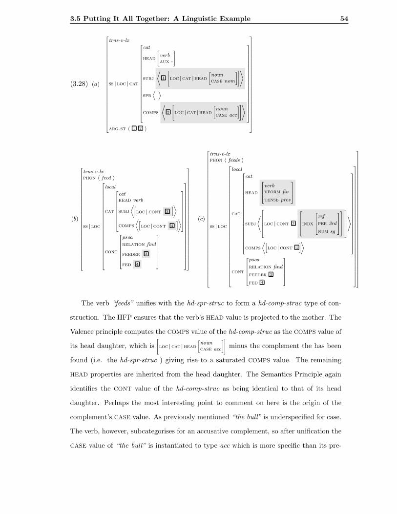
3.5 Putting It All Together: A Linguistic Example 54
(3.28) (a)
trns-v-lx
ss | loc |cat
cat
head
[
verbaux -
]
subj
⟨
1
[
loc |cat |head
[
nouncase nom
]
]⟩
spr⟨ ⟩
comps
⟨
2
[
loc |cat |head
[
nouncase acc
]
]⟩
arg-st 〈 1 2 〉
(b)
trns-v-lxphon 〈 feed 〉
ss | loc
local
cat
cathead verb
subj
⟨
[
loc | cont 3
]
⟩
comps
⟨
[
loc |cont 4
]
⟩
cont
psoa
relation find
feeder 3
fed 4
(c)
trns-v-lxphon 〈 feeds 〉
ss | loc
local
cat
cat
head
verbvform fin
tense pres
subj
⟨
loc |cont 3
indx
ref
per 3rd
num sg
⟩
comps
⟨
[
loc |cont 4
]
⟩
cont
psoa
relation find
feeder 3
fed 4
The verb “feeds” unifies with the hd-spr-struc to form a hd-comp-struc type of con-
struction. The HFP ensures that the verb’s HEAD value is projected to the mother. The
Valence principle computes the COMPS value of the hd-comp-struc as the COMPS value of
its head daughter, which is[
loc | cat | head
[
nouncase acc
]
]
minus the complement the has been
found (i.e. the hd-spr-struc ) giving rise to a saturated COMPS value. The remaining
HEAD properties are inherited from the head daughter. The Semantics Principle again
identifies the CONT value of the hd-comp-struc as being identical to that of its head
daughter. Perhaps the most interesting point to comment on here is the origin of the
complement’s CASE value. As previously mentioned “the bull” is underspecified for case.
The verb, however, subcategorises for an accusative complement, so after unification the
CASE value of “the bull” is instantiated to type acc which is more specific than its pre-

3.5 Putting It All Together: A Linguistic Example 55
vious case value. The produced hd-comp-struc is, finally, combined with the nominative
pronoun “she” to form the hd-subj-struc construction in Figure 3.10.
hd-subj-struc
phon append(
ph1 ph2)
ss | loc
local
cat
cat
head 4
subj/spr/comps 〈 〉
cont 5
prn-lx
phon ph1 〈 she 〉
ss 2
synsem
loc
local
cat
cat
head
[
noun
case nom
]
subj/spr/comps 〈 〉
cont
ppro
indx 1
ref
per 3rd
num sing
gend fem
restr
arg-st 〈 〉
hd-comp-struc
phon ph2 append(
ph3 ph4)
ss | loc
local
cat
cat
head 4
verb
vform fin
tense present
aux -
subj 〈 2 〉
spr/comps 〈 〉
cont 5
psoa
relation feed
feeder 1
fed 9
trns-v-lx
phon ph3 〈 feeds 〉
ss | loc
local
cat
cat
head 4
subj 〈 2 〉
spr 〈 〉
comps 〈 3 〉
cont 5
arg-st 〈 2 3 〉
hd-spr-struc
phon ph4 append(
ph5 ph6
)
ss 3
synsem
loc
local
cat
cat
head 6
subj/spr/comps 〈 〉
cont 10
det-lx
phon ph5 〈 the 〉
ss 7
synsem
loc
local
cat
cat
head
det
spec
indx 9
restr 8
subj/spr/comps 〈 〉
cont
the-rel
indx
[
ref
per 3rd
]
restr
arg-st 〈 〉
comm-n-lx
phon ph6 〈 bull 〉
ss
synsem
loc
local
cat
cat
head 6
[
noun
case acc
]
subj/comps 〈 〉
spr 〈 7 〉
cont 10
npro
indx 9
ref
per 3rd
num sing
gend masc
restr 8
psoa
reln bull
inst 9
arg-st 〈 7 〉
Figure 3.10: HPSG analysis of the sentence “She feeds the bull”.

3.6 Summary 56
The HFP and the Semantics Principle apply in the same manner as before. The
Valence Principle computes the new SUBJ value as being the empty list. Notice that,
had the subject been a pronoun like “I” or “you”, then the sentence would have been
ungrammatical because the PER value of the subject required by the verb (i.e. 3rd-
person) is not compatible with the PER value of the actual subject (1st and 2nd for “I”
and “you” respectively).
In this example, we have not considered non-local information (i.e. the attributes
SLASH, WH and REL together with their associated values). This is because typesetting
an HPSG feature structure with all its features is not feasible in the space provided. The
underlying idea of how these values are handled is the same. They percolate up the tree
(through structure sharing) until they are discharged at an appropriate construction type.
3.6 Summary
In this chapter, we have presented an overview of the HPSG formalism to provide the
reader with sufficient background to follow the topics that will be raised in the remain-
der of the first part of this thesis. We set off in Section 3.2 by introducing some basic
concepts from the typed feature logic like the type inheritance taxonomy and the sub-
sumption relation.
In Section 3.3, we moved on to presenting in some detail how feature structures are
used to model linguistic information. These representations are licensed by a well de-
fined signature consisting of a type hierarchy and a set of appropriateness conditions.
Information sharing is expressed by token identity (structure sharing) rather than trans-
formations. The signature determines what constitutes a legal description of an item.
The hierarchical organisation of the signature extends the subsumption relation to fea-
ture structures. Different descriptions of objects can be combined (so long as they are
compatible with respect to the signature) into one more specific feature structure by
unification.
Having outlined these basic concepts and procedures, we moved on to presenting
HPSG as a typed feature grammar formalism (Section 3.4). We started by defining two

3.6 Summary 57
formal properties, total well-typedness and sort-resolvedness that HPSG feature struc-
tures possess. Following this, the most basic type in the HPSG ontology, the sign, and its
features were introduced. Feature structures of type sign are used to model all phrasal
or lexical types of linguistic objects. All signs carry the features PHON and SYNSEM, via
which they describe the phonological and syntactico-semantic properties of the object
being modelled. In addition, words and lexemes (objects of type lex-sign) carry the fea-
ture ARG-ST which describes their subcategorisation requirements, while phrases (objects
of type phrase) carry the feature DTRS which describes their constituent structure.
Even though type hierarchies are very powerful for describing an ontology of linguistic
entities, some of the descriptions they license need to be ruled out. Signs need, therefore,
to be constrained by some restrictions typically expressed as a set of constraints. These
are most commonly known as principles and schemata or appropriateness conditions.
Next we discussed how the hierarchical organisation of the lexicon helps deal effi-
ciently with the issue of vertical redundancy by enabling lexical entries to infer the vast
majority of their characteristics, leaving them with the need to encode only some min-
imal (typically phonological and semantic related) information at the lexical level. We
moved on to introducing the problem of horizontal redundancy and discussed how lexical
rules are used to deal with this issue. In Section 3.4.6, we illustrated how agreement
is handled in HPSG through structure sharing of referential indices. The chapter con-
cludes in Section 3.5 with a linguistic example that shows how the above concepts work
in practice.

Chapter 4
An Existing Approach to
HPSG-DOP
This chapter presents one approach to HPSG-DOP that was proposed by Neumann
(2003). The basic idea in Neumann’s model is to extract a Stochastic Lexicalised Tree
Grammar (SLTG) from an HPSG source grammar and a given corpus and use it in a
manner similar to Tree-DOP.
4.1 Introduction
When considering a data oriented approach to HPSG, four key questions arise, each re-
lated to the instantiation of one of the DOP parameters. Out of the four, one seems more
crucial. What do the potential fragments look like? This chapter presents one approach
to enriching DOP with HPSG-like data structures that was described by Neumann (2003)
and is based on the use of syntactically labelled phrase structure trees that approximate
HPSG feature structures. The elements in the fragment corpus are atomically labelled
phrase structure subtrees. Decomposition in this model is head-driven and limits the
number of lexical anchors to one per subtree. This limitation has some undesirable side
effects. To overcome these, we suggest a modification that is largely based on extending
the Frontier operation of Tree-DOP to this model. We present an empirical evaluation
of the two decomposition techniques based on some pilot experiments we conducted.

4.2 An HPSG-DOP Approximation 59
4.2 An HPSG-DOP Approximation
Neumann (2003) proposes an approach to HPSG-DOP which involves extracting a Sto-
chastic Lexicalised Tree Grammar (SLTG) from an HPSG source grammar and a given
corpus. First, all sentences of the training corpus are parsed using a predefined HPSG
grammar. An SLTG extracted from the results is then used for further processing. An
SLTG is a particular instantiation of an STSG where each elementary tree is required
to have at least one terminal element. An SLTG is more formally defined as a 5-tuple
< VN , VT , S,R, P > where:
• VN is a finite set of nonterminal symbols.
• VT is a finite set of terminal symbols.
• S ∈ VN is the distinguished symbol.
• R is a finite set of elementary trees each of which has at least one terminal element.
• P is a function assigning to every tree t ∈ R a probability P (t), s. t. for each root
node α it is required that∑
t:root(t)=a
p(t) = 1.
4.2.1 Instantiating the DOP parameters
Utterance representation in Neumann’s model consists of labelled phrase structure trees.
Node labels are atomic and represent the HPSG rule-schema applied during the corre-
sponding derivation step (Figure 4.1). These symbols are defined as part of the HPSG
source grammar and represent sets of feature constraints, which allows to check eligibility
of the resulting parse trees with respect to the HPSG source grammar.
SubjH````
HSpecbb""
The boy
HAdj-IXXXX
NonTrnsLe
left
HCompPPPP
in the morning
Figure 4.1: SLTG initial tree.

4.2 An HPSG-DOP Approximation 60
The rule names in the figures and the examples are as in the LinGO ERG.1 SubjH,
HSpec, HComp and HAdj-I denote that the subject-head, specifier-head, head-complement
or head-adjunct rule was applied during the corresponding derivation step respectively.
Decomposition in this model is guided by the HFP (Section 3.4.4), which requires
the mother of a headed construction to share its most salient properties with its head
daughter. It consists of three operations. Firstly, non-head subtrees of the initial tree
are cut off marking the cutting points for substitution (indicated by *).
SubjH````
HAdj-IPPPP
NonTrnsLe
left
=⇒ SubjHXXXX
HSpec* HAdj-Iaaa!!!
NonTrnsLe
left
HComp*HCompPPPP
in the morning
HSpecbb""
The boy
Figure 4.2: Decomposition (step 1): All non-head subtrees of the initial tree are cut off.
This process is recursive, so it further processes individually each of the subtrees that
are cut off. As a result, each of the extracted subtrees has exactly one lexical anchor
(e.g. left for the subtree produced in Figure 4.2). The path leading from the head lexical
anchor (left) to the root (SubjH) of the tree in question identifies its head chain. Each
subtree of the head chain is also copied in the bag of subtrees (Figure 4.3).
SubjHXXXX
HSpec* HAdj-Iaaa!!!
NonTrnsLe
left
HComp*
HAdj-IPPP
NonTrnsLe
left
HComp*
Figure 4.3: Decomposition (step 2): Each subtree of the head chain is copied in the fragment corpus.
Decomposition, as described thus far, corresponds to the more traditional Root and
Frontier operations, with the application of Frontier being restricted, firstly, to non-head
nodes only and, secondly, to all non-head nodes rather than any combination of them.
Finally, a third operation is employed to deal with modifier/adjunct unattachment.
This operation inserts a copy of a tree with the modifier unattached into the fragment
1LinGO ERG: LinGO English Resource Grammar (http://lingo.stanford.edu/).

4.2 An HPSG-DOP Approximation 61
corpus. In binary branching constructions unattaching a modifier involves raising the
head daughter of a node x, whose non-head daughter is a modifier m, into the position
of x (Figure 4.4).
SubjHXXXX
HSpec* HAdj-Iaaa!!!
NonTrnsLe
left
HComp*
=⇒ SubjHaaa!!!
HSpec* NonTrnsLe
left
Figure 4.4: Modifier unattachment
This process unattaches one modifier at a time and is applied recursively in cases
of multiple modifiers. The motivation for this additional operation is to ensure that
the fragment corpus contains both modified and unmodified trees so that a modified
constituent (like “left” in “The boy left in the morning”) can also appear unmodified
when parsing new input (as in “The boy left”). Unattaching modifiers this way produces
fragments analogous to those described by Hoogweg (2003) in his TIGDOP model. As
we shall see, however, composition in this model is not extended with the insertion
operation (see Section 2.2). Notice that when adopting a special treatment for adjuncts
special attention should be paid on defining what constitutes an adjunct. There is a
small number of verbs, for example, like “meant” and “bodes” in (4.1)-(4.2) that select
adverbial complements. If these are treated as adjuncts, the above operation would lead
to the production of subtrees contributing to the analysis of ill-formed examples like
“The teacher meant” or “This bodes”.
(4.1) The teacher meant well.
(4.2) This bodes well.
Once all subtrees have been extracted, root and substitution nodes undergo speciali-
sation. This process involves replacing the rule labels (e.g. HSpec, HComp) of these nodes
with their corresponding category labels (eg. NP, PP) as in Figure 4.5. Category labels
identify equivalence classes for different signs and they are defined in the type hierarchy
of the HPSG source grammar.

4.2 An HPSG-DOP Approximation 62
SubjHXXXX
HSpec* HAdj-IPPP
NonTrnsLe
left
HComp*
=⇒
S
SubjHPPPP
NP* HAdj-IHHH
NonTrnsLe
left
PP*
Figure 4.5: Specialisation of root and substitution nodes.
The strongest point of Neumann’s decomposition technique, over the one described
by Bod, is that it is linguistically better motivated. Subtrees are always anchored at
their lexical heads as opposed to random lexical items. This together with the fact that
node category labels are defined in the type hierarchy of the original HPSG grammar
and they express equivalence classes enables an HPSG like expansion of SLTG trees (like
the one in Figure 4.1) into full blown feature structures (like those described in Chapter
3) according to the relevant feature constraints.
Composition in this model is carried out by substitution in both directions of the
head lexical anchor as depicted in Figure 4.6 below.
S
SubjHPPPP
NP* HAdj-IHHH
NonTrnsLe
left
PP*
NPQQ
DET∗ boy
DET
the
PPbb""
PrepLe
in
NP∗
NPHH
DET∗ morning
DET
the
S
SubjH`````
=⇒ HSpecbb""
The boy
HAdj-IPPPP
NonTrnsLe
left
HCompPPPP
in the morning
Figure 4.6: Incrementally left to right composition.
Even though composition is bidirectional, the string is expanded incrementally left
to right (i.e. initially from right to left on the left of the lexical anchor, followed by left
to right substitution on the right of the lexical anchor). A complete parse tree can be
unfolded into an HPSG representation by expanding the rule labels and lexical types to

4.2 An HPSG-DOP Approximation 63
the corresponding feature structures.
Disambiguation is based on the MPP using the simple frequency counter found in
other versions of DOP. The competition sets required for calculating fragment probabil-
ities are identified by syntactic category labels (recall that root and substitution nodes
make use of such labels).
Even though decomposition under this approach is linguistically better justified, one
of the advantageous characteristics of Tree-DOP has been lost: its ability to capture the
relationship of multiple lexical items in an input string. Consider the example in (4.3(a)).
(4.3) (a) S
SubjHXXXXX
HSpecbb""
The boy
HAdj-IPPPP
NonTrnsLe
left
HCompPPPP
in the morning
(b) S
SubjHPPPP
NP* HCompHHH
NonTrnsLe
left
PP*
Decomposing this tree in the manner described above limits the number of lexical
anchors to one per subtree (4.3(b)). As a result, DOP’s ability to capture lexical co-
occurrences (e.g. “boy” and “left”) and study their interdependencies is lost. In addition,
this way of decomposing trees undermines the supposition on which the entire DOP
philosophy is based, that all fragments count in determining the optimal analysis. This
is due to the fact that a large number of the subtrees generated under Tree-DOP are no
longer produced (e.g. the subtree anchored at both “boy” and “left”).
4.2.2 Decomposing with HFrontier
As already mentioned, limiting the number of lexical anchors to one brings to surface
some undesirable effects. In this section we explore an alternative way of decomposing
trees which is partly based on Neumann (1998) and partly on the traditional Tree-DOP
decomposition approach in order to avoid these side effects.
Root applies as in Tree-DOP. It takes a non-terminal node of an initial tree, turns it
into the root of a new tree erasing all nodes but the selected one and the ones it dominates.
Then a head-driven version of Frontier, which we call HFrontier in analogy with Tree-

4.2 An HPSG-DOP Approximation 64
DOP, selects any set of non-head nodes and erases all subtrees these dominate. Notice
that HFrontier cannot apply to any of the nodes along the tree’s head chain. Figure 4.7
shows all subtrees produced from the initial tree in the centre. The arrows point from
non-head nodes in the initial tree to the corresponding subtrees that have these marked
for substitution.
S
SubjHXXXX
NP* HAdj-IPPP
NonTrnsLe AdvLe
S
SubjHXXXX
NP* HAdj-I
PPPNonTrnsLe ADV*
S
SubjHhhhhh(((((
HSpecaa!!
DetLe NounLe
HAdj-IPPP
NonTrnsLe ADV*
S
SubjHhhhhhh((((((
HSpecPPP
DetLe NounLe
HAdj-IPPP
NonTrnsLe AdvLe
S
SubjH````
HSpecaa!!
DET* NounLe
HAdj-Iaaa!!!
NonTrnsLe Advle
S
SubjHhhhhh(((((
HSpecaa!!
DET* NounLe
HAdj-IPPP
NonTrnsLe ADV*
Figure 4.7: Tree decomposition with HFrontier.
The main advantage of this modified decomposition operation is that it poses no
restriction, other than those posed by the tree structure itself, to the maximum number of
lexical anchors a subtree is allowed to have. Moreover, the minimum of one lexical anchor
is preserved since HFrontier cannot erase the head lexical anchor. Since headedness
information is preserved, this way of tree production is linguistically as well justified as
the one presented in Section 4.2.1. In order to obtain a clearer view of the differences
between the three decomposition processes (Root and Frontier, Root and HFrontier and
Neumann’s operations) we will apply them to the parse tree of the sentence “He chased
the cat” in (4.4) and compare the resulting fragment corpora.

4.2 An HPSG-DOP Approximation 65
(4.4) SPPP
NP
PRN
He
VPHHH
V
chased
NP
ll,,D
the
N
cat
For convenience, we shall use part of speech categories to label tree nodes in all
examples. We will also abstract on the lexical items allowing for grammatical categories
at the lexical level to take the role of terminal elements. Figures 4.8 and 4.9 show the
fragment corpora produced after application of Bod’s and Neumann’s decomposition
operations respectively.
Sbb""
NP
PRN
VPcc##
V NP
@@D N
Sbb""
NP* VPcc##
V NP
ll,,D N
Sbb""
NP
PRN
VP
ll,,V NP*
SZZ
NP* VP
@@V NP*
S
ll,,NP
PRN
VP∗
S
ll,,NP∗ VP∗
VP
ll,,V NP
@@D N
VP
@@V NP*
NP
@@D N
NP
PRN
Figure 4.8: Root and Frontier: no restriction on the number of lexical anchors.
SQQ
NP* VP
@@V NP*
VP
@@V NP*
NP
@@D N
NP
PRN
Figure 4.9: Head-driven decomposition: exactly one lexical anchor per subtree.
The collection of trees in Figure 4.10 is generated by Root and HFrontier. These
subtrees are not restricted to having one lexical anchor. The resulting grammar is,
therefore, better equipped to handle syntactic dependencies resulting from word co-
occurrences, as well as to capture some distributional information.

4.2 An HPSG-DOP Approximation 66
Saaa!!!
NP
PRN
VPbb""
V NP
ll,,D N
SHHH
NP
PRN
VPZZ
V NP*
SHHH
NP* VPbb""
V NP
ll,,D N
SHHH
NP* VPZZ
V NP*
VPbb""
V NP
ll,,D N
VPZZ
V NP*
NP
ll,,D N
NP
PRN
Figure 4.10: Root & HFrontier: minimum of one lexical anchor per subtree.
Root and HFrontier produce subtrees that allow a phrasal sign to share the value of
its local features with its head daughter. The process as a whole is guided by the Head
Feature Principle of HPSG. The bag of subtrees in Figure 4.10 is both linguistically
founded and it allows for multiple lexical anchors. The subtrees produced provide more
complete descriptions in the sense that headedness information is not lost. Subtrees
like the ones marked in gray in Figure 4.8, where the lexical anchor, if present, grounds
information that cannot percolate up the tree via its head chain, are no longer produced.
Having said this, Root and HFrontier construct a grammar significantly larger than
the one described by Neumann (2003). In fact, the size of the new grammar is exponential
to the number of non-head nodes (one fragment per combination of non-head nodes
is created), while Neumann’s set of decomposition operations produces a grammar of
size linear to the number of non-terminal nodes (one fragment per non-terminal node is
created). This also causes the operation that unattaches modifiers to have a significantly
greater impact on the size of the grammar generated by HFrontier than by Neumann’s
alternative which, of course, will have a negative effect on processing efficiency. The
following section describes some experiments we conducted in order to compare the
effects the two decomposition procedures have on parse accuracy.

4.3 Evaluating Decomposition 67
4.3 Evaluating Decomposition
This section describes the experiments we conducted on a VerbMobil corpus of 2000
utterances in order to test which combination of decomposition operations generates the
fragment corpus that achieves the highest parse accuracy. We compare several fragment
corpora, all generated from the same training corpus but with different decomposition
operations. We aim at examining the effect of
• limiting the number of lexical anchors to one, and
• unattaching modifiers.
The evaluation criterion used is exact parse accuracy of the proposed tree against
some gold standard. The fragment corpora were created from the analyses proposed by
the LKB parser (using the LinGO English Resource Grammar) for each sentence of the
training data. The test data was also batch parsed by the LKB system and the proposed
analyses constitute our gold standard.
4.3.1 The software
This section will provide a brief overview of the three software tools, LKB, [incr tsdb()]
and HDOP, that were used in setting up the running environment for the experiments
conducted. The setup for creating the various fragment corpora is shown in Figure 4.11.
VerbMobil
LinGOERG
[incr tsdb()]
LKB→ HDOP
[incr tsdb()]parseditems
→ → →treebank HDOP
FTC1
FTCn↑
↓ →
→Figure 4.11: Setup for creating the fragment corpora FTCi.
• LKB
The system used to acquire the HPSG analyses of the training data is the Linguistic
Knowledge Building (LKB) system developed by Copestake (1992). LKB is a constraint

4.3 Evaluating Decomposition 68
oriented grammar and lexicon development environment implemented in LISP. It was
designed for parsing and generation with unification-based formalisms. It has been exten-
sively tested with HPSG grammars, although it was initially intended to be framework
independent. Documentation on the various versions of LKB can be found in Copestake
(1993, 2000, 2002). The LKB makes use of a bottom-up chart-based parser. The time
and space cost of unification when processing large scale grammars in unification-based
frameworks is very high. This is mainly due to the amount of copying that takes place,
which itself is very costly. The LKB parser uses quasi-destructive unification (for more
details see Tomabechi, 1991, 1992) to avoid unnecessary copying costs.
The parser can be run either in an exhaustive mode or in an agenda-driven best-first
search mode. When in exhaustive mode, it uses a breadth-first CKY-like algorithm. By
going through the input string from left to right, it builds all passive edges ending at the
current input position, before moving on to the next position. Only passive items are
actually introduced in the chart. It also makes use of a set of pre-unification filters like
the Quick Check introduced by Malouf et al. (2000). Quick Check is a vector of path
values associated with a given feature structure. Before any unification attempt of two
feature structures, their corresponding Quick Check vectors are tested for compatibility.
Unification is attempted only if the two are found to be compatible, since it is bound to
fail otherwise.
• [incr tsdb()]
[incr tsdb()] (usually referred to as tsdb) is a package developed by Oepen (2001)
to serve primarily as an evaluation and benchmarking tool (Oepen and Carroll, 2000;
Oepen and Callmeier, 2000) in lexicalised constraint based grammar engineering. The
package offers a wide range of modules that facilitate the evaluation task. It has a struc-
tured database comprising test and reference data with annotations of varying degrees
of information. It also offers several tools for feeding new data to the system, browsing
through the available data and selecting suitable subsets for further processing. It in-
corporates a wide variety of performance measures to choose from when testing as well
as both tabular and graphical displays to facilitate the task of examining the results.

4.3 Evaluating Decomposition 69
[incr tsdb()] can be used on top of an existing LKB platform (as was the case for the
experiments reported here) or as a stand alone application. [incr tsdb()] processed items
are stored in LISP association list format (Figure 4.12).
((:ERROR . ””) (:GCS . 0) (:RPEDGES . 6) (:RAEDGES . -1) (:PEDGES . 24) (:AEDGES . 7) (:L-STASKS . 7)
(:WORDS . 15) (:OTHERS . 28808) (:SYMBOLS . 0) (:CONSES . 227192) (:COPIES . 59) (:UNIFICATIONS
. 101) (:P-FTASKS . 1435) (:P-STASKS . 58) (:P-ETASKS . 87) (:TGC . 0) (:TCPU . 40) (:TOTAL . 40)
(:FIRST . 40) (:READINGS . 1) (:PARSE-ID . 862) (:I-ID . 1861) (:I-WF . 1) (:I-LENGTH . 5) (:I-INPUT .
“you were booked on Monday?”) (:I-ID . 1861) (:RESULTS ((:TREE . “(S (S (NP (you)) (VP (VP (V (were))
(VPP (V (booked (STEM))))) (PP-I (P-I (on)) (NP (Monday))))))”) (:DERIVATION . ROOT CL 0 5
(SUBJH 0 5 (YOU 0 1 (“you” 0 1))(HADJS UNS 1 5 (HCOMP 1 3 (BE C WERE 1 2 (“were” 0 1))(PASSIVE
2 3 (PSP VERB INFL RULE 2 3 (BOOK V2 2 3 (“booked” 0 1)))))(HCOMP 3 5 (ON DAY 3 4 (“on” 0 1))
(MONDAY1 4 5 (“Monday” 0 1)))))) (:RESULT-ID . 0) (:PARSE-ID . 862))))
Figure 4.12: [incr tsdb()] output for the utterance “you were booked on Monday?”.
The (:TREE) and (:DERIVATION) entries of each [incr tsdb()] processed item (marked
in bold in Figure 4.12) were used by HDOP to create the treebank.
• HDOP
HDOP is a computational implementation of the HPSG-DOP model described in Sec-
tion 4.2. It is a prerelease software tool programmed in LISP, which was developed by
and used for the experiments reported in Neumann (1999, 2003). HDOP was used to
create, train and test an SLTG from a set of [incr tsdb()] parsed items. Most implemen-
tation modules were used as designed by Neumann except for the training phase modules
which were altered in order to reflect decomposition by Root and HFrontier.
The :TREE and :DERIVATION values of [incr tsdb()] parsed items such as the one
in Figure 4.12 are used for the extraction of SLTG trees, which are subsequently used
for creating and training the grammar. The root node labels of both the :TREE and
:DERIVATION values (S and ROOT CL in Figure 4.12 respectively) are used in labelling
the root node of the resulting SLTG tree (“root-cl . S” in (4.5(a))). Intermediate nodes
take their names from the corresponding nodes in the :DERIVATION value of the relevant
[incr tsdb()] parsed item (e.g. “SubjH”, “ HComp”, etc.). The resulting trees are stripped
of their words by replacing all preterminal nodes by their corresponding category labels

4.3 Evaluating Decomposition 70
(e.g. (BE C WERE 1 2 (“were” 0 1)) in the :DERIVATION value is replaced by BE C WERE LE).
The SLTG tree corresponding to the entry in Figure 4.12 is shown in (4.5(a)):
(4.5) (a) root-cl . S
SubjH`````
PERS
PRO-LEHAdj-uns````
HCompaaa!!!
BE-C
WERE-LEpassive
TRANS-LE-PSP
V -INF L-RULE
HCompPPP
TEMP
PREP -LE
DAY -OF
WEEK-LE
(b) root-cl . S
SubjHXXXXX
PERS
PRO-LEHAdj-unsXXXX
HCompaaa!!!
BE-C
WERE-LEpassive
TRANS-LE-PSP
V -INF L-RULE
(:SUBST . PP-I)
During decomposition substitution nodes undergo specialisation by replacing their
HPSG rule label, e.g. “HComp” in (4.5(a)), by some category label, e.g. “PP-I” in (b).2
Category labels are defined in the hierarchy of the source grammar and they identify
equivalence classes among different types of signs. Parsing in HDOP is performed in-
crementally left to right as described in Section 4.2. Special attention is paid to the
tree selection phase in order to increase as much as possible the efficiency of the parser.
Several pruning methods, described in more detail in the next section, will be applied
during this stage. Finally, disambiguation takes place as described by Bod (1995).
4.3.2 The setup
The experiments described in the following sections were conducted on the same Verb-
Mobil corpus used by Neumann (2003). The corpus consists of 2000 dialogue utterances
of average length 7.8 words. The topic of the dialogues is scheduling meetings. The first
1000 utterances were used for training the system and the next 1000 for testing it. The
training set was batch processed by the [incr tsdb()] system using the LKB parser and
the LinGO ERG. Valid parses were found in 831 cases. We filtered-out trees of depth
≥ 14, which left us with a training set of 803 SLTG trees. We will refer to this set as
VrMtrain from this point onwards. The corpus might seem too small to offer credible
validity to our observations, but it constitutes a reasonable starting point.
2“:SUBST” serves to identify substitution nodes.

4.3 Evaluating Decomposition 71
Throughout the experiments several grammars (i.e. bags of fragments) were created,
all from VrMtrain. The first two grammars we built, NEUM1 and HF1 henceforth, differed
with respect to the decomposition operations applied to the training corpus. In the
former, we followed Neumann’s procedure as described in Section 4.2.1 (i.e. all non-
head subtrees of the initial tree are cut off), while in the latter we applied HFrontier
as suggested in Section 4.2.2 (i.e. any combination of non-head subtrees of the initial
tree are cut off). In both cases the initial trees were stripped of their words. To avoid
explosion of the size of HF1, modifier unattachment was not applied during creation of
either grammar. Moreover, in the case of HF1 all non-head preterminal nodes of subtrees
were marked for substitution.
NEUM1 and HF1 consisted of 1640 and 19554 subtrees respectively. 174 lexical types
were identified. Consequently, NEUM1 has an average of 9.4 subtrees per head lexical
anchor while HF1 has an average of 112.4 subtrees. This huge increase in the number of
subtrees is attributed to the fact that Neumann’s decomposition produces one subtree per
tree being processed, while HFrontier produces one subtree per combination of non-head
nodes in the tree being processed. As it can be seen in Table 4.1, some lexical types
anchor significantly more trees than others. In HF1, COORD C LE, WILL POS LE and
BE C AM LE for example, anchor 2272, 2262 and 1749 subtrees respectively, while others
like HAVE BSE AUX LE, S ADV LE and WH NP ADV LE only anchor one. The numbers for
the same types in NEUM1 are 56, 74 and 133 for the first three types respectively and
one for each of the last three.
COORD WILL BE C HAVE BSE S ADV LE WH NPC LE POS LE AM LE AUX LE ADV LE
NEUM1 56 74 133 1 1 1
HF1 2272 2262 1749 1 1 1
Table 4.1: The most frequent and infrequent lexical types in NEUM1 and HF1.
The dramatic increase in the number of trees overall, and especially for those lexical
types that anchor several hundreds of trees, is expected to negatively affect the com-
putational cost of parsing. For this reason we applied a set of filtering criteria in order
to reduce the number of trees that take part in the parsing process without affecting

4.3 Evaluating Decomposition 72
the resulting parse space. To this end, the system was tuned to disregard subtrees that
cannot possibly take part in any of the derivations of the input string such as:
1. trees whose yield contained any element that was not in the input string (more
precisely any element not in the list of possible types of the input words),
2. trees where the number of substitution and terminal nodes to the left of the head
lexical anchor exceeded the number of words preceding the corresponding item in
the input string
3. trees where the number of substitution and terminal nodes to the right of the head
lexical anchor exceeded the number of words following the corresponding item in
the input string
4. trees that had a second anchor immediately before or after the head lexical anchor
whose type did not match the type of the word immediately before or after the
input position in the string
5. trees that contained a substitution node immediately before or after the head lexical
anchor that could not be expanded to a sequence of types ending in or starting by
the type of the word preceding or following respectively the input position in the
string.
The information on possible beginnings and endings of trees is maintained in the
grammar by means of a hash table which stores for each constituent in the training
corpus its type (i.e. its root) and the types of lexical items that can start and end
its yield. If, therefore, the node on the left of the lexical anchor cannot end, when
expanded, in one of the possible lexical types of the item preceding the input
position or the one on the right cannot start by one of the possible types of the
item following the input position then the subtree is disregarded.
To comprehend the significance of these pruning strategies consider the example in (4.6).
(4.6) They will leave tomorrow.
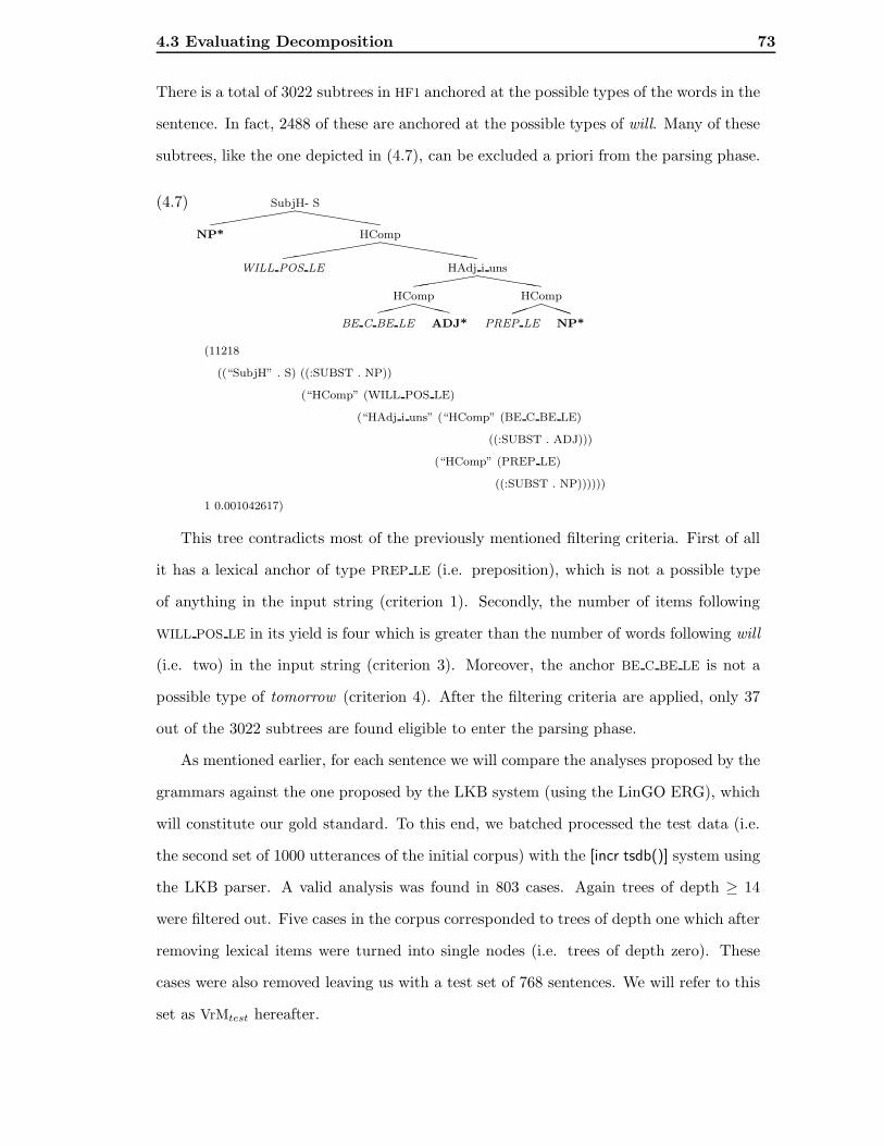
4.3 Evaluating Decomposition 73
There is a total of 3022 subtrees in HF1 anchored at the possible types of the words in the
sentence. In fact, 2488 of these are anchored at the possible types of will. Many of these
subtrees, like the one depicted in (4.7), can be excluded a priori from the parsing phase.
(4.7) SubjH- Shhhhhh((((((
NP* HComphhhhhhh(((((((
WILL POS LE HAdj i unshhhhh(((((
HCompXXX
BE C BE LE ADJ*
HCompPPP
PREP LE NP*
(11218
((“SubjH” . S) ((:SUBST . NP))
(“HComp” (WILL POS LE)
(“HAdj i uns” (“HComp” (BE C BE LE)
((:SUBST . ADJ)))
(“HComp” (PREP LE)
((:SUBST . NP))))))
1 0.001042617)
This tree contradicts most of the previously mentioned filtering criteria. First of all
it has a lexical anchor of type PREP LE (i.e. preposition), which is not a possible type
of anything in the input string (criterion 1). Secondly, the number of items following
WILL POS LE in its yield is four which is greater than the number of words following will
(i.e. two) in the input string (criterion 3). Moreover, the anchor BE C BE LE is not a
possible type of tomorrow (criterion 4). After the filtering criteria are applied, only 37
out of the 3022 subtrees are found eligible to enter the parsing phase.
As mentioned earlier, for each sentence we will compare the analyses proposed by the
grammars against the one proposed by the LKB system (using the LinGO ERG), which
will constitute our gold standard. To this end, we batched processed the test data (i.e.
the second set of 1000 utterances of the initial corpus) with the [incr tsdb()] system using
the LKB parser. A valid analysis was found in 803 cases. Again trees of depth ≥ 14
were filtered out. Five cases in the corpus corresponded to trees of depth one which after
removing lexical items were turned into single nodes (i.e. trees of depth zero). These
cases were also removed leaving us with a test set of 768 sentences. We will refer to this
set as VrMtest hereafter.

4.3 Evaluating Decomposition 74
4.3.3 Comparing the Decomposition Variants
We run the SLTG parser on VrMtest, first using NEUM1 and then HF1 so that it stopped
after the first complete was found. NEUM1 was able to parse 651 sentences, which
corresponds to an overall coverage of 84.77%, while HF1 parsed 641 corresponding to a
coverage of 83.46%. During parsing, each sentence was allocated a certain amount of
time, at the end of which if no successful parses had been produced the parser timed
out. The difference in coverage between the two grammars is due to the growth in size
of HF1 over NEUM1, causing a greater amount of time outs. Had no time limits been
posed, the coverage of both grammars would have been the same since all subtrees in
NEUM1 are also contained in HF1. Note that NEUM1 generates the exact same parse trees
as HF1 with the only difference being that it generally requires more substitution steps
for doing so.
For each sentence we tested whether the analysis proposed by the SLTG parser was
the same as the one suggested by the LKB parser. In the case of NEUM1, 105 of the
768 analyses were identical, corresponding to an exact match accuracy of 13.67%. When
using HF1 this was the case for 100 of the proposed trees. Exact derivation accuracy for
HF1 was, therefore, 13.03% corresponding to a relative decrease of approximately 5%.
These results are very disappointing. This should not be surprising, however, taking
into account the fact that the parser proposed the first analysis it derived rather than
evaluating several analyses and proposing the most likely one. To this end, a second
run was conducted using the same training and test data, only this time the parser was
called in exhaustive mode, allowing for probabilistic disambiguation. The system was
set to allow each sentence 20 seconds for parsing. If at the end of this time interval no
parse had been found, the system timed out and moved on to the next sentence. Both
grammars made use of the probability model described in Bod (1995) for disambiguating
the generated analyses. The possible parses for each string were stored in a hash table.
They were subsequently organised into groups of equally likely parses based on their
probability in descending order.
Parse accuracy was calculated in this case by checking whether the analysis proposed

4.3 Evaluating Decomposition 75
by the LKB system was amongst the 1, 2, 3, 5 and 10 most likely groups of parses
proposed by the system. The results obtained from testing the two grammars on VrMtest
are summarised in Figure 4.13 below. The X-axis shows the 1, 2, 3, 5 and 10 most
probable groups of equally likely parses, and the Y-axis shows the number of utterances
for which the LKB gold standard analysis was a member of these groups. The graph
on the right is simply a magnification of the one on the left serving to make score
differences more apparent for readability purposes. This format will be used throughout
the remainder of this chapter.
1 2 3 5 01
1
100
200
300
NEUM1 132 190 208 230 271
HF1 147 199 213 234 277
1 2 3 5 10
Exact Parse Accuracy on VrMtest
0
200
400
600
NEUM1 132 190 208 230 271
HF1 147 199 213 234 277
1 2 3 5 10
Exact Parse Accuracy on VrMtest
Figure 4.13: Parse accuracy results of NEUM1 and HF1 on VrMtest
Figure 4.13 shows that the non-traditional way of decomposing trees (i.e. limiting
the number of lexical anchors to one) seems to have a negative effect on the exact parse
accuracy achieved by the resulting grammar. HF1 presents a 11.4% relative increase in
accuracy over NEUM1 in the most likely analyses proposed by the two grammars. This
increase, though at lesser levels, is also evident in the following groups where it ranges
from approximately 4.7% to 1.7%.
An interesting point to check is whether the two grammars still present a difference
in accuracy when tested on the training data. To check this, we tested both HF1 and
NEUM1 on VrMtrain. The results are shown in Figure 4.14.

4.3 Evaluating Decomposition 76
200
300
400
500
NEUM1 225 298 329 379 424
HF1 281 352 385 425 473
1 2 3 5 10
Exact Parse Accuracy on VrMtrain
0
200
400
600
800
NEUM1 225 298 329 379 424
HF1 281 352 385 425 473
1 2 3 5 10
Exact Parse Accuracy on VrMtrain
Figure 4.14: Parse accuracy results of NEUM1 and HF1 on VrMtrain
When comparing the first more likely suggestions of both systems on the training
data, the difference becomes even more apparent. Exact parse accuracy levels for the
most likely parse increase from 16.4% to 28% in the case of NEUM1 and from 18.3%
to 35% in the case of HF1. HF1 thus presents a 24.9% relative increase in accuracy
over NEUM1. This increase can also be observed in the following most likely groups of
proposed parses where it ranges from approximately 18.1% to 11.6%. The difference
in performance of the two systems on VrMtrain presents great interest. The fact that
the mere existence of the extra trees produced by HFrontier results in such significant
increase in the accuracy achieved, seems to indicate that the grammar produced in this
manner is better equipped to handle and disambiguate the syntactic dependencies it has
learned.
4.3.4 Unattaching Modifiers
Even though enabling probabilistic disambiguation improved the performance of both
systems, the scores still remain very low. In order to identify the reasons behind the poor
performance of HF1 and NEUM1, we examined the parse forests generated by the SLTG
parser for several sentences of both the training and the test parts of the corpus. The
first and perhaps most salient observation was that the system wasted a great amount
of resources in generating pairs of almost identical trees like the ones in Figure 4.15.

4.3 Evaluating Decomposition 77
The only place the members of these pairs differ is in their respective root node labels.
In fact, one of the two trees (Figure 4.15(b)) is a copy of the daughter of the other
trees’s (Figure 4.15(a)) root node. In addition note how the root node of the tree in (a)
does not encode any HPSG rule (unlike the labels of the remaining nodes in the tree).
Instead these symbols were introduced in the LinGO ERG to serve as start symbols, thus
marking completeness of constituents. For example the label “root cl” in (a) denotes the
root of a clausal constituent.
root-cl . VPP
HComp
HOW-ABOUTN-OR-P-LE
HSpec
DET-LE NAdj-rr
NOUN-PPCOMPLE-NOUN-LEX
HComp
PREPOPTCOMP-LE
DEICTICPRO-LE
HComp . VPP
HOW-ABOUTN-OR-P-LE
HSpec
DET-LE NAdj-rr
NOUN-PPCOMPLE-NOUN-LEX
HComp
PREPOPTCOMP-LE
DEICTICPRO-LE
(b) Equivalent tree without(a) Tree with start symbol the start symbol
Figure 4.15: Pairs of almost identical parse trees generated by the parser.
In order to optimise the performance of the parser, we deleted all start symbols from
the corpus. This cut down the number of subtrees produced by half thus significantly
reducing the search space of alternatives during parsing. Moreover, it broadened the
domain of the grammar because any generated passive constituent could now stand as
a complete parse. One might, of course, argue against this view of a parse being simply
a complete constituent. When processing corpora in certain domains, however, like
dialogues or titles (film, song, article, etc), where full sentences are rarely encountered,
it might be a view worth considering.3
The observed decrease in the number of subtrees produced allowed us to unattach
modifiers during decomposition. In this phase we created four distinct grammars by
applying both decomposition operations to the training corpus with and without modifier
unattachment after omission of any start symbols. Table 4.2 summarises the design
choices and the size for each of the resulting grammars.
3We will return to this point in Chapter 8.

4.3 Evaluating Decomposition 78
Neumann Decomp. Root & HFrontier Decomp.
+ modif. unattach. NEUM2 - 1562 HF2 - 21402
− modif. unattach. NEUM3 - 1408 HF3 - 15573
Table 4.2: Grammars created after removing all start symbols.
In the case of applying modifier unattachment the grammars produced, NEUM2 and
HF2, contained 1562 and 21402 subtrees respectively. Once again the grammars were used
to parse and disambiguate VrMtest. The parse forest of each utterance was organised into
probability identifiable groups in descending order just like in the previous section. The
VrMtest scores of NEUM2 and HF2 together with the previously created NEUM1 and HF1
are presented in Figure 4.16.
0
200
400
600
NEUM2 206 285 329 356 383
HF2 216 283 324 359 387
NEUM1 132 190 208 230 271
HF1 147 199 213 234 277
1 2 3 5 10
Exact Parse Accuracy on VrMtest
100
200
300
400
NEUM2 206 285 329 356 383
HF2 216 283 324 359 387
NEUM1 132 190 208 230 271
HF1 147 199 213 234 277
1 2 3 5 10
Exact Parse Accuracy on VrMtest
Figure 4.16: Parse accuracy results of NEUM2, HF2, NEUM1 and HF1 on VrMtest.
A dramatic relative increase in exact parse accuracy is evident. HF2 presents a 46.9%
relative increase in the first most likely parse(s) over its earlier version HF1. Similarly,
the observed increase in the case of NEUM2 over NEUM1 is 56.1%. This large difference
seems to suggest that the use of start symbols can significantly harm the performance of
a DOP model if these have no purpose other than to mark completeness of constituents.
A perhaps surprising observation is that even though HF1 scores higher in exact parse
accuracy than NEUM1, this improvement is no longer evident in their new counterparts

4.3 Evaluating Decomposition 79
HF2 and NEUM2 respectively. The new grammars present comparable performance with
HF2 slightly surpassing NEUM2 only when considering the first most likely parse(s). To
check whether the effect of the decomposition operations applied during the grammar
creation phase has entirely disappeared, we also tested the new grammars on the training
data VrMtrain. The results are summarised in Figure 4.17.
0
200
400
600
800
NEUM2 346 450 501 561 626
HF2 371 489 548 608 649
NEUM1 225 298 329 379 424
HF1 281 352 385 425 473
1 2 3 5 10
Exact Parse Accuracy on VrMtrain
200
400
600
NEUM2 346 450 501 561 626
HF2 371 489 548 608 649
NEUM1 225 298 329 379 424
HF1 281 352 385 425 473
1 2 3 5 10
Exact Parse Accuracy on VrMtrain
Figure 4.17: Exact parse accuracy results of NEUM2, HF2, NEUM1 and HF1 on VrMtrain.
Note that HF2 presents a 32.1% relative increase in the first most likely parse(s) over
its earlier version HF1. Similarly, the observed increase in the case of NEUM2 over NEUM1
is 53.8%. The training data offers further evidence in favour of omitting start symbols
from the corpus. With regards to decomposition attributed differences, Figure 4.17
shows that the scores still favour the traditional decomposition operations. HF2 presents
a 7.2% and 8.7% relative increase in the first one and two most likely groups over NEUM2.
These results offer further support to Bod’s initial argument that all fragments in the
treebank affect the disambiguation process. Ambiguity resolution seems, therefore, to
be partly frequency-based and partly memory-based. The relative weight of the two
dimensions depends on the degree of learning. The memory-based dimension will surpass
the frequency-based on largely learned data with the reverse holding in the case of mostly
new data.
The HF variants are naturally expected to score higher than the NEUM variants

4.3 Evaluating Decomposition 80
on VrMtrain because of their ability to incorporate the memory-based dimension in the
processing phase. Having said this, one might expect the difference between HF2 and
NEUM2 to be greater on VrMtrain, but they would anticipate that it is at least slightly
evident on VrMtest as well. Figure 4.16, however, contradicts this expectation.
The difference in the variation of the scores between training and test data might be
caused by the inability of the disambiguation algorithm to meaningfully compare con-
stituents of different categories. The inability of meaningful cross-categorical comparison
causes constituents that belong to a less densely populated category to be assigned higher
probabilities than constituents belonging to a more densely populated category under
the relative frequency estimator used here (we will return to this in Chapter 8). This can
cause severe distortions in the way probability is distributed amongst the resulting parse
space elements. The reason the problem becomes more acute on the test data might be
that the frequency-based dimension of disambiguation gains weight on VrMtest. In other
words, it might be the case that the memory-based dimension (which is stronger than
the frequency-based in the training data) can undo some of the harm.
Grammars NEUM3 and HF3 were created in the same way as NEUM2 and HF2 re-
spectively, only this time modifiers were not unattached during decomposition of the
corpus trees. They consisted of 1408 and 15573 subtrees respectively. The results of
these grammars were examined from two different points of view. Firstly, we looked
for any difference in accuracy based on the decomposition process hypothesis. The two
grammars were again used to parse the test as well as the training parts of the corpus.
The results are depicted in Figure 4.18 on the next page.
Once again, the performance of NEUM3 is poorer than that of HF3, with the differ-
ence being significantly higher when tested on the training data (VrMtrain). In comparing
the first more likely parse(s) the relative increase reaches 15.9% for VrMtrain, while it
is only 3.4% in the case of VrMtest. Again, this suggests that syntactic dependencies
can be learned (hence the difference in accuracy of the two grammars when tested on
VrMtrain and VrMtest). It appears, however, that the extra subtrees introduced by mod-
ifier unattachment may negatively affect the learning process. Note how NEUM2 and
HF2 (the earlier counterparts of NEUM3 and HF3 respectively produced by unattaching

4.3 Evaluating Decomposition 81
1 2 3 5 03
3
0
200
400
600
NEUM3 352 452 510 577 633
HF3 408 531 578 602 645
1 2 3 5 10
Exact Parse Accuracy on VrMtrain
0
200
400
600
NEUM3 203 280 326 351 374
HF3 210 287 328 359 385
1 2 3 5 10
Exact Parse Accuracy on VrMtest
200
300
400
NEUM3 203 280 326 351 374
HF3 210 287 328 359 385
1 2 3 5 10
Exact Parse Accuracy on VrMtest
350
450
550
650
NEUM3 352 452 510 577 633
HF3 408 531 578 602 645
1 2 3 5 10
Exact Parse Accuracy on VrMtrain
Figure 4.18: Exact parse accuracy results of NEUM3 and HF3 on VrMtest and VrMtrain.
modifiers) attained comparable results with neither constantly surpassing the other in
the accuracy levels achieved on VrMtest (Figure 4.16).
NEUM3 and HF3, on the other hand, still present a constant difference in favour of HF3
in all groups compared, even though this has become admittedly even less evident than
before. This could be attributed to the somewhat reduced bias (in comparison to HF2) for
certain root labels.4 HF3 is smaller than HF2 by almost 6,000 subtrees. Keeping in mind
that the number of subtrees produced is exponential to the size of the initial corpus tree,
and that modifiers are more likely to occur in larger constructions, it can be anticipated
that the subtrees resulting from unattaching modifiers add to the current bias towards
large corpus trees. The present data, however, can only provide an indication for the
4The estimator used for calculating parse tree probabilities here has been shown to be biased towardslarge trees (Johnson, 2002). A more in depth discussion on this will follow in Chapter 7.

4.3 Evaluating Decomposition 82
arguments we have made. If we were to investigate these observations further we would
need to use large scale corpora.
The scores of HF3 and NEUM3 were also checked against those of HF2 and NEUM2 re-
spectively in order to test the extent to which the extra subtrees produced by unattach-
ing modifiers affect the exact parse accuracy of the resulting grammar. Even though
unattaching modifiers during decomposition amplifies the domain of the resulting gram-
mar, it also increases the size of the grammar whether this is produced by Root and
HFrontier or by the alternative suggested by Neumann (2003). The following compar-
isons aim at investigating the trade off between the advantage of a broader domain
and the disadvantage of a computationally more expensive increased search space in the
grammars produced.
0
200
400
600
NEUM2 206 285 329 356 383
NEUM3 203 280 326 351 374
1 2 3 5 10
Exact Parse Accuracy on VrMtest
200
300
400
NEUM2 206 285 329 356 383
NEUM3 203 280 326 351 374
1 2 3 5 10
Exact Parse Accuracy on VrMtest
Figure 4.19: Exact parse accuracy results for NEUM2 and NEUM3 on VrMtest.
In the case of the NEUM variants (Figure 4.19) modifier unattachment seems to offer
a small improvement in the accuracy achieved on the test data which can be attributed
to the amplified domain of NEUM2 over NEUM3. This slight increase in accuracy com-
bined with the fact that an otherwise small grammar increases only by 154 subtrees
(approximately 11%) in size could justify the existence of modifier unattachment as a
formal decomposition operation in this case.
An interesting observation, however, arises from examining the graph in Figure 4.20.
In the case of the HF variants the results seem to suggest the opposite. Modifier unattach-
ment, in this case, does not affect the accuracy achieved on the test data. Even though

4.3 Evaluating Decomposition 83
HF2 enjoys a broader domain than HF3, and therefore greater coverage, it also suffers
from greater ambiguity. This together with the fact that the increase in size of an already
large grammar is by 5829 trees (approximately 37.4%), which can be expected to affect
the computational cost of processing new data significantly, make the load of the extra
subtrees one not worth carrying in this case.
0
200
400
600
HF2 216 283 324 359 387
HF3 210 287 328 359 385
1 2 3 5 10
Exact Parse Accuracy on VrMtest
200
300
400
HF2 216 283 324 359 387
HF3 210 287 328 359 385
1 2 3 5 10
Exact Parse Accuracy on VrMtest
Figure 4.20: Exact parse accuracy results of HF2 and HF3 on VrMtrain.
From the above, it is clear that each of the factors discussed affects the exact parse
accuracy achieved by the head-driven DOP implementation to some extent. Overall de-
composing with HFrontier seems to be advantageous in terms of reflecting dependencies
in the training corpus, while special attention is needed with possible start symbols that
do not carry any category related meaning. Overall the HF grammar variants achieve
higher accuracy levels than their corresponding NEUM counterparts. Efficiency wise,
however, it has to be mentioned that all HF variants were considerably slower in process-
ing new data, with time costs ranging from three to five times more than those of their
corresponding NEUM grammar counterparts.
The reasons behind the overall low level of the scores reported here in comparison
with other scores reported in the literature are numerous. The first is that we used a
very small corpus for training the system each time, so the accuracy levels are a priori
expected to be less than those of similar systems that were trained on thousands of
sentences. Moreover, the lexicon we used presents great amounts of ambiguity, which

4.4 Summary 84
also had a negative effect on the performance of the grammars. Additionally, the metric
used to evaluate the system (exact parse accuracy) is a lot stricter than those typically
used in the literature (labelled precision and recall). Any given parse suggested by the
system was deemed either correct or wrong.
Last but perhaps most importantly, the reported results are on the unrestricted DOP
model, which has been shown to suffer from strong bias effects towards large trees with
the relative frequency estimator used here (a more detailed discussion on this will follow
in Chapter 7). An interesting point that arises from the last observation is that the bias
towards large trees is significantly larger in the HF variants than their corresponding
NEUM counterparts. This suggests that the performance differences attributed to the
decomposition operations applied during the grammar creation process may, in fact, be
significantly greater than what we observed.
4.4 Summary
The aim of this chapter was to present the first attempt of enriching DOP with HPSG-
like data structures (Section 4.2). This approach (suggested by Neumann, 2003) is
based on extracting an SLTG from an HPSG parsed training corpus. Node labels in the
trees correspond to the HPSG rule applied during the corresponding derivation step and
represent sets of feature value constraints which enables expansion of the resulting parse
trees to full blown feature structures.
Decomposition in this model is head-driven. Unlike Tree-DOP, however, the number
of anchors in the subtrees is limited to one. This undermines DOP’s ability to take full
advantage of its memory-based dimension. On these grounds, we extended Tree-DOP’s
Frontier operation, so that it applies in a head-driven manner, to HFrontier.
The two operations were compared and contrasted in Section 4.3. The results of the
experiments conducted can be summarised as follows. Decomposing with HFrontier is,
on the one hand, crucial for exploiting the memory-based dimension of DOP. On the
other hand, however, grammars produced in this manner embody significantly larger
processing costs than their corresponding one-lexical-anchor per subtree counterparts.

4.4 Summary 85
Neumann’s HPSG-DOP model, however, carries certain disadvantages, some of which
are similar to LFG-DOP. The first is that well-formedness of the resulting structures
cannot be checked during the derivation process. This, of course, causes the estimator to
leak probability mass, as explained in Chapter 2. In addition, the specialisation process
during decomposition does not allow the model to take full advantage of the HPSG
formalism. This affects the coverage of the resulting grammars, which is somewhat
reduced in comparison to what would be allowed by the linguistic constraints.
Bearing this in mind, we move on, in the next chapter, to presenting a linguistically
more sensitive approach to HPSG-DOP.

Chapter 5
A More Formal Approach to
HPSG-DOP
In the previous chapter we presented Neumann’s data-oriented approach to HPSG. Ex-
tracting an SLTG from an HPSG parsed training corpus, however, is not the only way
of moving towards HPSG-DOP. This chapter presents a linguistically more sensitive
approach that makes direct use of the feature structure modelling mechanism.
5.1 Introduction
This chapter presents an HPSG-DOP model making direct use of feature structure frag-
ments. The main part of the chapter is organised as follows. In Section 5.2 we provide
a formal definition of the representations to be used for utterance analysis. In Section
5.3 we describe the shape of the HPSG fragments eligible for the fragment corpus. We
move on to proposing how the traditional decomposition operations can be extended to
HPSG-DOP and formalising these in terms of the subsumption, unification and inference
concepts of typed feature logic. We also show why unheaded structures pose a problem
if a strictly head-driven approach to decomposition is adopted. Section 5.4 discusses how
composition in this model can be made more sensitive to the concept of headedness which
is of primary importance to the HPSG formalism. Section 5.5 describes the stochastic
process employed for disambiguation. In Section 5.6 we provide a critical discussion of

5.2 Utterance Representation 87
outstanding issues and conclude in Section 5.7 with a brief overview of the HPSG-DOP
architecture.
5.2 Utterance Representation
The first parameter to be instantiated in any DOP model is the representation to be
used for utterance analysis. Previously, in Chapter 3, we saw that utterance analyses
in HPSG are represented by feature structures. Phrasal signs have the attribute DTRS
whose value is an ordered list of signs. Headed phrases bear, in addition, the attribute
HD-DTR which identifies the head daughter in the DTRS value.
As already mentioned, phrasal signs are typically drawn as phrase structure trees
whose node labels are feature structure descriptions not carrying the DTRS and HD-DTR
attributes but that otherwise conform to the signature of the HPSG grammar. The two
descriptions in (5.1) are considered equivalent. This notation is commonly used in typed
feature formalisms and their applications (e.g. LKB) where the concept of a parse tree
is formalised as being an abbreviation for the complete representation of a structure
corresponding to the valid parse (Copestake, 2002). We shall be using the tree, AVM
and DAG notations interchangeably in this chapter.
(5.1)
a
eee
%%%b c
a
dtrs⟨
1 b,c⟩
hd-dtr 1
H non-H
The HPSG formalism imposes three restrictions on the validity of feature structures
that serve as models of linguistic entities. The first states that feature structures are
required to be sorted. In other words, they have to be labelled with a sort symbol which
indicates the type of object the structure is modelling. Moreover, they have to be well-
typed, meaning that the attributes used to describe them are determined by their sort.
Finally, feature structures are required to be totally well-typed (i.e. include all attributes
appropriate for their sort). Note that most sentential descriptions will in fact be sort-
resolved as well. This is due to the fact that the maximal types in the signature are as
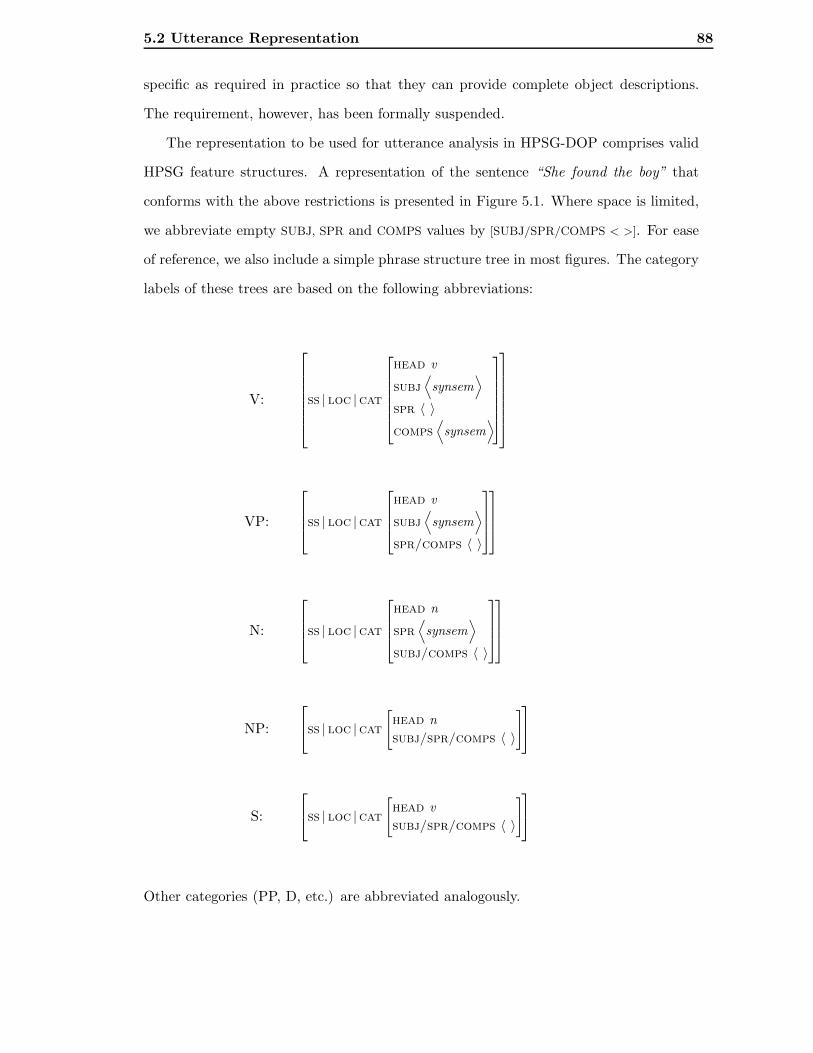
5.2 Utterance Representation 88
specific as required in practice so that they can provide complete object descriptions.
The requirement, however, has been formally suspended.
The representation to be used for utterance analysis in HPSG-DOP comprises valid
HPSG feature structures. A representation of the sentence “She found the boy” that
conforms with the above restrictions is presented in Figure 5.1. Where space is limited,
we abbreviate empty SUBJ, SPR and COMPS values by [SUBJ/SPR/COMPS < >]. For ease
of reference, we also include a simple phrase structure tree in most figures. The category
labels of these trees are based on the following abbreviations:
V:
ss | loc |cat
head v
subj⟨
synsem⟩
spr 〈 〉comps
⟨
synsem⟩
VP:
ss | loc |cat
head v
subj⟨
synsem⟩
spr/comps 〈 〉
N:
ss | loc |cat
head n
spr⟨
synsem⟩
subj/comps 〈 〉
NP:
ss | loc |cat
[
head n
subj/spr/comps 〈 〉
]
S:
ss | loc |cat
[
head v
subj/spr/comps 〈 〉
]
Other categories (PP, D, etc.) are abbreviated analogously.

5.2 Utterance Representation 89
hd-subj-struc
phon append(
ph1 ph2
)
ss | loc
local
cat
cat
head 4
subj/spr/comps 〈 〉
cont 5
word
phon ph1 〈 she 〉
ss 2
synsem
loc
local
cat
cat
head
[
noun
case nom
]
subj/spr/comps 〈 〉
cont
ppro
indx 1
restr
arg-st 〈 〉
hd-comp-struc
phon ph2 append(
ph3 ph4)
ss | loc
local
cat
cat
head 4
verb
vform fin
aux -
pol -
subj 〈 2 〉
spr/comps 〈 〉
cont 5
word
phon ph3 〈 found 〉
ss | loc
local
cat
cat
head 4
subj 〈 2 〉
spr 〈 〉
comps 〈 3 〉
cont 5
psoa
relation find
finder 1
ref
per 3rd
num sing
gend fem
found 9
arg-st 〈 2 3 〉
hd-spr-struc
phon ph4 append(
ph5 ph6)
ss 3
synsem
loc
local
cat
cat
head 6
subj/spr/comps 〈 〉
cont
npro
indx 9
ref
per 3rd
num sing
gend masc
restr 8
psoa
reln boy
inst 9
word
phon ph5 〈 the 〉
ss 7
synsem
loc
local
cat
cat
head
det
spec
indx 9
restr 8
subj/spr/comps 〈 〉
cont
the-rel
indx
[
ref
per 3rd
]
restr
arg-st 〈 〉
word
phon ph6 〈 boy 〉
ss
synsem
loc
local
cat
cat
head 6
[
noun
case acc
]
subj/comps 〈 〉
spr 〈 7 〉
cont
npro
indx 9
restr 8
arg-st 〈 7 〉
Saaa!!!
NP
She
VPHHH
V
found
NPll,,
D
the
N
boy
Figure 5.1: HPSG analysis of the sentence “She found the boy”.

5.3 Fragment Representation & Decomposition 90
5.3 Fragment Representation & Decomposition
The second parameter to be defined is what constitutes a valid structure to be used in
analysing new input and the operations that produce these structures.
5.3.1 Fragment Representation
In this section we explore the space of validity constraints the HPSG-DOP fragments
would have to comply with. In considering eligibility of fragments, the natural place to
start from is trees using feature structure labels, because they are easier to conceptualise,
and gradually move on to a formal definition of feature structure fragments.
Since we are considering tree structures with feature structure labels, we have to take
into account validity both in terms of the subtree structure (as in Tree-DOP) and the
node labels (from the point of view of HPSG). In the case of Tree-DOP, a valid subtree
of a corpus tree is one that consists of more than one node, it is connected and all its
non-leaf nodes have the same daughters as the corresponding ones in the corpus tree
(Bod, 1995; Bod and Scha, 1997).
In considering eligibility from the HPSG point of view, we will examine whether it
is essential that we relax in the case of fragments some of the validity constraints posed
on the initial representations. In order to identify which constraints (if any) should be
relaxed, let us work our way from the desired outcome backwards. When parsing some
input the generated structure is required to be a valid HPSG representation (i.e. a totally
well-typed sorted feature structure). Validity is checked against the signature of some
predefined grammar. It follows that the sortedness constraint cannot be relaxed because
even partly unsorted feature structures are not part of the finite bounded complete partial
order identified by the signature associated with that grammar (Chapter 3). Similarly,
well-typedness cannot be disregarded because node types are determined by a partial
feature value function that forms part of the definition of a feature structure.
Further requiring that fragments are totally well-typed turns out to be unproblematic.
If a feature is allowed to take the most general value licenced by the signature, its
informational content becomes so limited that it can be included in a description without

5.3 Fragment Representation & Decomposition 91
posing any restrictions other than the minimal imposed by the signature via inference.
Note that, had we adopted the traditional HPSG view on the representational mechanism
requiring feature structures to be sort-resolved, we would need to suspend the condition
in the case of fragments because the notion of a sort-resolved fragment is incoherent (i.e.
a complete partial object description).
Eligible phrasal fragments should, therefore, be subtrees labelled by sorted and to-
tally well-typed feature structure descriptions. Combining this with the first two criteria
suggested by Bod and Scha (that a subtree consists of more than one node and it is
connected) gives rise to the following definition.
Fragment validity (preliminary version): Tfrag is a valid subtree of some corpus tree
Tinit if Tfrag
• is of depth zero and its root (and only) node label is a sorted and totally well-typed
feature structure of type word that subsumes some lexical node in Tinit, or
• consists of more than one node, it is connected, its root node label is of some
phrasal type and each of its node labels is a sorted and totally well-typed feature
structure that subsumes the corresponding node label in Tinit.
These are the minimum restrictions that the fragments of any HPSG-DOP model
should be required to satisfy. For the particular instantiation we describe, we propose
to additionally constrain each fragment to a minimum of one lexical anchor.
Given that, formally, HPSG does not make use of phrase structure trees, we will now
express the above in terms of feature structures. For familiarity, let us think of a non-
empty DTRS value as a feature structure with the attributes FIRST and REST. Then the
subtree dominated by any node of the initial tree (other than the root) can be accessed
through the path identified by some combination of FIRST’s and REST’s. In (5.2(a)), for
example, we can refer to the subtree rooted at e, or similarly in (5.2(b)) the feature struc-
ture rooted at e, as the value of DTRS|REST|FIRST|DTRS|FIRST of a, which we will further
abbreviate to DTRS|REST|FIRST|FIRST, omitting all (but the first) DTRS attributes.

5.3 Fragment Representation & Decomposition 92
(5.2) (a)
aPPP
b
c
dHH
ell,,
f g
h
(b)
a
dtrs
⟨[
bdtrs 〈c〉
]
d
dtrs
⟨
[
edtrs 〈f g〉
]
h
⟩
⟩
Take fsinit to be a valid HPSG analysis of some sentence in the corpus. Take fsdtri
to denote the feature structure description of the ith daughter of fsinit. In addition,
take p to be a path of the form DTRS | ... | FIRST departing from the root node of fsinit
and v(p, r(fsinit)) to refer to the value of p. The above criteria can be combined in the
following definition:
Fragment validity (final version): A sorted and totally well-typed feature structure
fsfrag is a valid substructure of the corpus analysis fsinit iff it is either of type word and
fsfrag ⊑ fsdtri, or
• it is of a type strictly more specific than phrase and fsfrag subsumes fsinit or some
daughter of fsinit (i.e. fsfrag ⊑ fsinit or fsfrag ⊑ fsdtri), and
• its DTRS value is of the same length as the DTRS value of fsinit or fsdtrirespec-
tively, and
• each element in the DTRS value of fsfrag subsumes the corresponding element in
the DTRS value of fsinit or fsdtrirespectively (i.e. v(p, r(fsfrag)) ⊑ v(p, r(fsinit)) or
v(p, r(fsfrag)) ⊑ v(p, r(fsdtri))), and
• it has at least one lexical anchor (i.e. ∃ path p′ of the form DTRS| ... | FIRST whose
value is of type word such that v(p′, r(fsfrag)) ⊑ v(p′, r(fsinit)) if fsfrag ⊑fsinit and
v(p′, r(fsfrag)) ⊑ v(p′, r(fsdtri)) otherwise.
Let us consider an example based on the corpus analysis in Figure 5.2. The feature
structures denoted by reentrancies 6 and 7 (marked in gray) are valid fragments. In
fact, even some more general descriptions subsuming 6 and 7 are also valid.

5.3 Fragment Representation & Decomposition 93
hd-subj-struc
phon append(
ph1 ph2)
ss | loc
local
cat
cathead 4
subj/spr/comps 〈 〉
cont 5
dtrs 〈
word
phon ph1 〈 she 〉
ss 2
synsem
loc
local
cat
cat
head
[
nouncase nom
]
subj/spr/comps 〈 〉
cont
ppro
indx 1
restr
arg-st 〈 〉
, 6 〉
hd-dtr 6
hd-comp-struc
phon ph2 append(
ph3 ph4)
ss | loc
local
cat
cat
head 4
verbvform fin
aux -
pol -
subj 〈 2 〉
spr/comps 〈 〉
cont 5
psoa
relation find
finder 1
found 1
dtrs
⟨
7
word
phon ph3 〈 found 〉
ss
loc
local
cat
cathead 4
subj 〈 2 〉
spr 〈 〉
comps 〈 3 〉
cont 5
arg-st 〈 2 , 3 〉
,
word
phon ph4 〈 herself 〉
ss 3
synsem
loc
local
cat
cat
head
[
nouncase acc
]
subj/spr/comps 〈 〉
cont
refl
indx 1
ref
per 3rd
num sing
gend fem
restr
arg-st 〈 〉
⟩
hd-dtr 7
SPPPP
NP
She
VPaaaa!!!!
V
found
NP
herself
Figure 5.2: HPSG corpus analysis of the sentence “She found herself”.

5.3 Fragment Representation & Decomposition 94
The descriptions in Figure 5.3, however, even though they look very similar to 6
and 7 in Figure 5.2, they are not valid fragments. The DTRS value of the first one is not
of the required length (i.e. the corresponding node in the initial representation had two
daughters), while the second one is neither of type word nor of some type more specific
than phrase.
hd-comp-struc
phon ph3
ss | loc
local
cat
cathead 4
subj 〈 2 〉
spr/comps 〈 〉
cont 5
dtrs
⟨
7
word
phon ph3 〈 found 〉
ss
loc
local
cat
cathead 4
subj 〈 2 〉
spr 〈 〉
comps 〈 3 〉
cont 5
arg-st 〈 2 , 3 〉
⟩
hd-dtr 7
sign
phon ph3 〈 found 〉
ss
loc
local
cat
cathead 4
subj 〈 2 〉
spr 〈 〉
comps 〈 3 〉
cont 5
Figure 5.3: Invalid HPSG-DOP fragments
The above definition of fragment validity allows for many different HPSG-DOP in-
stantiations. These fragments are in essence generalisations of a corpus analysis or some
part of it. Different choices on the degree of specificity of these structures will, therefore,
give rise to different models. Having identified what constitutes a valid HPSG-DOP
fragment, we will now turn to investigating how such fragments are produced.
5.3.2 Decomposition Operations
The decomposition operations employed in this model are Root and HFrontier. Recall
that these operations need to produce structural units that are sorted and totally well-
typed feature structures. Root is defined as follows:
Take fsinit to denote the description of the initial totally well-typed and sorted feature
structure and p to be a path of the form DTRS|...|FIRST departing from the root node of

5.3 Fragment Representation & Decomposition 95
fsinit. Root inserts in the bag of fragments a description of
• the greatest lower bound of all feature structures that subsume fsinit and satisfy
all relevant type constraints, and
• the greatest lower bound of all feature structures that subsume v(DTRS|p|FIRST,
r(fsinit)) and satisfy all relevant type constraints ∀p such that v(DTRS|p|FIRST,
r(fsinit)) is defined.
Consider, for example, the fragment in Figure 5.4. Suppose Root is applied to the
value v(DTRS|REST|FIRST,hd-spr-struc).
hd-spr-struc
phon append(
ph1 ph2)
ss | loc
local
cat
cathead 5
subj/spr/comps 〈 〉
cont 2
word
phon ph1 〈 the 〉
ss 4
synsem
loc
local
cat
cat
head
det
spec
[
indx 1
restr 3
]
subj/spr/comps 〈 〉
cont
the-rel
indx
[
ref
per 3rd
]
restr
arg-st 〈 〉
word
phon ph2 〈 boy 〉
ss | loc
local
cat
cathead 5 noun
spr 〈 4 〉
subj/comps 〈 〉
cont 2
npro
indx 1
ref
per 3rd
num sing
gend masc
restr 3
psoa
reln boy
inst 1
arg-st 〈 4 〉
Figure 5.4: Corpus fragment.
Even though the description in (5.3) subsumes the corresponding one in Figure 5.4,
it is not valid on the basis that it does not satisfy all relevant type constraints, assuming
that the lexical entry for “boy” restricts its CONT to being of type npro with third person,
singular and masculine index.

5.3 Fragment Representation & Decomposition 96
(5.3)
wordphon 〈boy〉
ss | loc
local
cat
cathead noun
spr 〈 1 〉
subj/comps 〈 〉
cont nom-obj
arg-st 〈 1 〉
Consider now all the descriptions that arise by allowing 2 in (5.4) to take any of
the values depicted in (5.5). All of these structures subsume the corresponding one in
Figure 5.4 and they all satisfy the relevant type constraints.
(5.4)
wordphon 〈boy〉
ss | loc
local
cat
cathead noun
spr 〈 2 〉
subj/comps 〈 〉
cont
npro
indx 1
ref
per 3rd
num sing
gend masc
restr
psoa
reln boy
inst 1
arg-st 〈 2 〉
(5.5)
synsem
loc
local
cat
cathead det
subj 〈 〉
spr 〈 〉
comps 〈 〉
cont
the-rel
indx
[
ref
per 3rd
]
restr
synsem
loc
local
cat
cathead det
subj 〈 〉
spr 〈 〉
comps 〈 〉
cont
the-relindx ref
restr
synsem
loc
local
cat
cathead det
subj 〈 〉
spr 〈 〉
comps 〈 〉
cont the-rel
Root determines the greatest lower bound of all descriptions like the above. Its output
is shown in (5.6), where 1 is as in (5.4).

5.3 Fragment Representation & Decomposition 97
(5.6)
wordphon 〈boy〉
ss
synsem
loc
local
cat
cathead noun
spr 〈 2
synsem
loc
local
cat
cathead det
subj/spr/comps 〈 〉
〉
subj/comps 〈 〉
cont
npro
indx 1
restr
psoa
reln boy
inst 1
arg-st 〈 2 〉
Next we turn to defining HFrontier. Before doing so, let us consider the notion of
erasing paths in a feature structure. Take, for example the description in (5.7(a)) and
assume we want erase the path CONT|INDX. One view is that this process will produce
the structure in (5.7(b)).
(5.7) local
cat n
ref npro
CAT
CONT
HEAD
INDX
(a) (b) local
cat n
CATHEAD
A feature structure can also be thought of as a set of paths. The set including the
path CONT|INDX (which we want to erase) identifies the feature structure in (5.8).
(5.8) local npro ref
CONT INDX
Note how the feature structure in (5.7(a)) is the most general unifier of the ones in
(5.7(b)) and (5.8). Similarly, given the feature structure in (5.8) (i.e. the one we want to
erase), the one in (5.7(b)) is its most general co-unificant in producing the initial feature
structure. In other words, (5.7(b)) is the greatest lower bound of all feature structures
that can be successfully unified with the one in (5.8) to produce the initial structure

5.3 Fragment Representation & Decomposition 98
(5.7(a)). Based on what has been said thus far we can take erasing some path p of a
feature structure fs to refer to the process of finding the most general co-unificant of the
feature structure identified by p in producing fs.
In HPSG-DOP, however, valid fragments are required to be totally well-typed (i.e. all
attributes appropriate for their type must be present). In this context, we define erasing
some path p in a feature structure fs as the process that determines the most general
totally well-typed co-unificant of the feature structure identified by p in producing fs.
Reconsidering the previous example under the new definition, the structure in (5.7(b))
is no longer the outcome of erasing CONT|INDX in (5.7(a)) because it is not totally well-
typed. The attribute CONT is appropriate for the type local and has to be present in
its description. The most general value licenced for this attribute is content. The HEAD
value (i.e. n) of the entity being described, however, constrains it further to being of
type nom-obj. The type nom-obj, in its turn, carries the attribute INDX with value ref.
The outcome of erasing CONT|INDX in (5.7(a)) is depicted in (5.9). It is clear from the
above that the term erasing is somewhat misleading in that part (rather than all) of the
information associated with the path in question is eliminated.
(5.9) local
cat n
refnom-obj
CAT
CONT
HEAD
INDX
The notions of paths and values are interrelated. Neither of the two can be sensibly
interpreted without the other. In any given feature structure each path has to point to
some value, and for each value (with the possible exception of the root node value) there
must be some path pointing to it. Just as (sets of) paths identify feature structures, path
values also identify feature structures, and since we are able to talk about erasing paths,
we should also be able to talk about erasing values. But what happens when we want to
erase the value of some path without erasing the path itself? Erasing the value of the path
CONT in (5.8), for example, cannot possibly result in the structure depicted in (5.10).

5.3 Fragment Representation & Decomposition 99
(5.10) local
CONT
Remember that node values in feature structures are determined by a partial feature
value function which identifies what type (i.e. sort) is appropriate for each feature and,
hence, path. Consequently, erasing values can only be taken to mean generalising over
values (as was the case for paths).
The next question is how much to generalise over these values. Is, for example, ⊤ a
sensible option? Clearly not, because the result is so general that it subsumes inconsistent
feature structures. The type ⊤ is not appropriate for the value of CONT. This points to
the direction of generalising as much as possible with respect to the constraints posed by
the remaining nodes in the feature structure. Under this view, erasing the CONT value
in (5.8) gives rise to the structure in (5.11).
(5.11) local content
CONT
Note, how, the feature structure in (5.11) is the most general consistent feature
structure that satisfies all relevant type constraints and contains all paths of the initial
structure other than those departing from the erased value. This observation provides us
with the necessary means to define the process of erasing in feature structures, so that
it is equally applicable to both paths and values. Take p to denote a path in the feature
structure fs, such that r(p) = r(fs). Then
• erasing p in fs is the process that determines the most general totally well-typed
co-unificant of p|v(p, r(fs)) in producing fs that satisfies all relevant type constraints
• erasing v(p, r(fs)) is the process that determines the most general totally well-typed
co-unificant of p|v(p, r(fs)) in producing fs that satisfies all relevant type constraints
and contains p.
Let us now consider what happens in the case of erasing a value that is shared by multiple
paths (e.g. synsem in (5.12)) or, similarly, erasing a path that contains values structure

5.3 Fragment Representation & Decomposition 100
shared with other paths.1
(5.12)
noun elist
noun
v
nom
Mary
found
list
word
cat
synsem cat elist
word elist
elist
accF
DTRS
R|FSS
COMPS|F
SS|LOC|CAT
LOC|CAT
SUBJ
SPR
COMPS
HD
CASESPR
CASE
PHON
PHON
SUBJ|F|SS|LOC|CAT|HD
HD
synsem
Assume that the feature structure in (5.12) is a totally well-typed subpart of the
DTRS value of the hd-comp-struc representation of the string “found Mary”. What will
the outcome of erasing v(DTRS|R|F|,synsem) be? Clearly all nodes not accessible from
DTRS|R|F| are not affected. The structure sharing is also retained because the result
would otherwise be inconsistent (it would violate the constraints posed by the hd-comp-
struc type of construction). The outcome of erasing this value is shown in (5.13).
(5.13)
/?/ sign
elist
noun
v
nom found
list
word
cat
DTRSF
R|F
SS
COMPS|FSS|LOC|CAT
SPR
CASE
PHON
SUBJ|F|SS|LOC|CAT|HD
HD
synsem
But what does /?/ correspond to? Based on our previous discussion, the value of
the node /?/ in (5.13) is the one identified in the most general totally well-typed feature
structure that when unified with DTRS|R|F|v(DTRS|R|F, synsem) gives rise to the feature
structure in (5.12). Turning to the computation of the actual value, now, the node is an
1Due to space limitations FIRST and REST have been abbreviated to F and R respectively.

5.3 Fragment Representation & Decomposition 101
element of a COMPS list, so it has to be at least of type synsem. Moreover, the lexical
type of “found” poses two more restrictions on the verb’s complement, that it has to be
nominal and accusative.2 As a result, the new node label becomes as in (5.14).
(5.14) synsem noun acc
LOC|CAT|HDCASE
This procedure of erasing values provides us with the necessary means for defining HFron-
tier so that it can be sensibly interpreted in typed feature logic.
HFrontier erases any set of values v(DTRS|p|REST∗|FIRST,r(fsph)) of a phrasal sign
fsph, such that
v(DTRS|p|REST*|FIRST, r(fsph)) 6=
v(HD-DTR, r(fsph)) if p is empty,
v(DTRS|p|HD-DTR, r(fsph)) otherwise.
Let us consider an example of applying HFrontier to the analysis of the sentence
“She found the boy” in Figure 5.1, repeated in (5.15) on the next page. The available
space does not suffice for the corresponding DAG representation, so we have used the
AVM-enriched tree notation in this case instead. Suppose HFrontier selects the hd-
spr-struc node to apply to. This amounts to erasing v(DTRS|REST|FIRST|REST| FIRST,
hd-subj-struc).
2Strictly speaking the sort on the node labelled by word would be something like str-v-lex (i.e. strictlytransitive verbal lexeme) which would be associated with the relevant constraint.

5.3 Fragment Representation & Decomposition 102
(5.15)
hd-subj-struc
phon append(
ph1 ph2
)
ss | loc
local
cat
cat
head 4
subj/spr/comps 〈 〉
cont 5
word
phon ph1 〈 she 〉
ss 2
synsem
loc
local
cat
cat
head
[
noun
case nom
]
subj/spr/comps 〈 〉
cont
ppro
indx 1
restr
arg-st 〈 〉
hd-comp-struc
phon ph2 append(
ph3 ph4)
ss | loc
local
cat
cat
head 4
verb
vform fin
aux -
pol -
subj 〈 2 〉
spr/comps 〈 〉
cont 5
word
phon ph3 〈 found 〉
ss | loc
local
cat
cat
head 4
subj 〈 2 〉
spr 〈 〉
comps 〈 3 〉
cont 5
psoa
relation find
finder 1
ref
per 3rd
num sing
gend fem
found 9
arg-st 〈 2 3 〉
hd-spr-struc
phon ph4 append(
ph5 ph6)
ss 3
synsem
loc
local
cat
cat
head 6
subj/spr/comps 〈 〉
cont
npro
indx 9
ref
per 3rd
num sing
gend masc
restr 8
psoa
reln boy
inst 9
word
phon ph5 〈 the 〉
ss 7
synsem
loc
local
cat
cat
head
det
spec
indx 9
restr 8
subj/spr/comps 〈 〉
cont
the-rel
indx
[
ref
per 3rd
]
restr
arg-st 〈 〉
word
phon ph6 〈 boy 〉
ss
synsem
loc
local
cat
cat
head 6
[
noun
case acc
]
subj/comps 〈 〉
spr 〈 7 〉
cont
npro
indx 9
restr 8
arg-st 〈 7 〉
Saaa!!!
NP
She
VPHHH
V
found
NPll,,
D
the
N
boy

5.3 Fragment Representation & Decomposition 103
Based on the constraints imposed by the remaining nodes, the following properties
can be inferred. Since the node is a member of the hd-comp-struc’s DTRS value it has
to be at least of sort sign. The feature declarations in the signature identify PHON
and SYNSEM (abbreviated to SS) as appropriate attributes for this type (5.16(a)). The
hd-comp-struc type reinforces reentrancies 3 and ph4 , while the attribute LOC with
value local is appropriate for all subtypes of synsem (5.16(b)).3 CAT and CONT are
appropriate features for any object of type local, with their most general values being
cat and content respectively (5.16(c)). The lexical type of found restricts its complement
to being an accusative nominal without, however, posing any further restrictions on the
complement’s subcategorisation frame (5.16(d)). Finally, the CONT value of all nominals
is at least of sort nom-obj with attribute INDX. The lexical entry of found restricts this
INDX value to being structure shared with the FOUND value in its own content ( 9 ). The
INDX value is of sort ref (nominals have referential indices) with appropriate attributes
PER, NUM and GEND. These attributes will have the most general values licenced by the
signature (i.e. per, num and gend respectively) (5.16(e)).
(5.16) (a)
sign
phon 〈phon〉
ss synsem
(b)
sign
phon ph4 〈 phon 〉
ss 3
[
synsem
loc local
]
(c)
sign
phon ph4 〈 phon 〉
ss 3
synsem
loc
localcat cat
cont content
(d)
sign
phon ph4 〈 phon 〉
ss 3
synsem
loc
local
cat
cat
head
[
nouncase acc
]
cont content
(e)
sign
phon ph4 〈 phon 〉
ss 3
synsem
loc
local
cat
cat
head
[
nouncase acc
]
cont
nom-obj
indx 9
ref
per per
num num
gend gend
3The tags show structure sharing with other nodes in the fragment in (5.15).

5.3 Fragment Representation & Decomposition 104
The output of HFrontier is shown in Figure 5.5.
hd-subj-struc
phon append(
ph1 ph2)
ss | loc
local
cat
cathead 4
subj/spr/comps 〈 〉
cont 5
word
phon ph1 〈 she 〉
ss 2
synsem
loc
local
cat
cat
head
[
nouncase nom
]
subj/spr/comps 〈 〉
cont
ppro
indx 1
ref
per 3rd
num sing
gend fem
restr
arg-st 〈 〉
hd-comp-struc
phon ph2 append(
ph3 ph4)
ss | loc
local
cat
cat
head 4
verbvform fin
aux -
pol -
subj 〈 2 〉
spr/comps 〈 〉
cont 5
psoa
relation find
finder 1
found 6
word
phon ph3 〈 found 〉
ss | loc
local
cat
cathead 4
subj 〈 2 〉
spr 〈 〉
comps 〈 3 〉
cont 5
arg-st 〈 2 3 〉
sign
phon ph4 〈 phon-cont 〉
synsem 3
synsem
loc
local
cat
cat
head
[
nouncase acc
]
cont
nom-obj
indx 6
ref
per per
num num
gend gend
Figure 5.5: Fragment produced by HFrontier
In this section we have formalised decomposition in HPSG-DOP so that it can be
interpreted in typed feature logic. Root and HFrontier solely rely on the subsumption

5.3 Fragment Representation & Decomposition 105
relation and the process of erasing path values in a feature structure which, as shown,
can be defined in terms of the unification and inference procedures.
One advantage of the HFrontier operation in HPSG-DOP over Frontier and Dis-
card in LFG-DOP is that it does not generalise over fragments language independently.
Assuming that the signature of an HPSG grammar describes all language specific depen-
dencies, then the path-value pairs encoding a dependency will never be erased, so long
as they can be inferred. In LFG-DOP, for example, it is the case that the NUM feature of
the VP “eats” (generated by Root from, say, “John eats”) can be discarded. This allows
the VP to combine with a plural subject (e.g. “people”) to produce a well-formed analy-
sis for an ill-formed string (i.e. “People eats”). In HPSG-DOP, on the other hand, the
path-value pairs that can be erased are restricted by the signature. The PER and NUM
attributes will, therefore, remain intact, since they are constrained by the type theory.
This is, of course, a direct consequence of the greater use of typing in HPSG, which is
not the case for the LFG formalism.
HPSG-DOP’s power to capture such dependencies is not restricted to the syntactic
level. Recall the analysis of the sentence “She found herself” in Figure 5.2. Assume
HFrontier applies to the “she” node producing the fragment in (5.17). Even though
this constituent is missing its subject, the fragment retains some of the information to
be associated with it, without the risk of undergeneration. Firstly, the lexical entry
of the head lexical anchor “found” restricts the HEAD value of the missing subject to
being a nominative nominal. The most specific CONT value that can be deduced from
this is nom-obj. Additionally, the head lexical anchor also takes care of the structure
sharing between the INDX value of the missing subject and the object with its FINDER
and FOUND values respectively.
Note that the subject-object coindexation is not lost. The presence of the anaphor
“herself” in this fragment triggers application of the Binding Theory, which states that
a reflexive in this type of construction must be coindexed with an antecedent.4 In other
words, the coindexation in this case can be inferred, so it is not affected by HFrontier.
4We will return for a more formal introduction to the Binding Theory and to the issue of expressingit as part of the signature in Section 5.4.2.
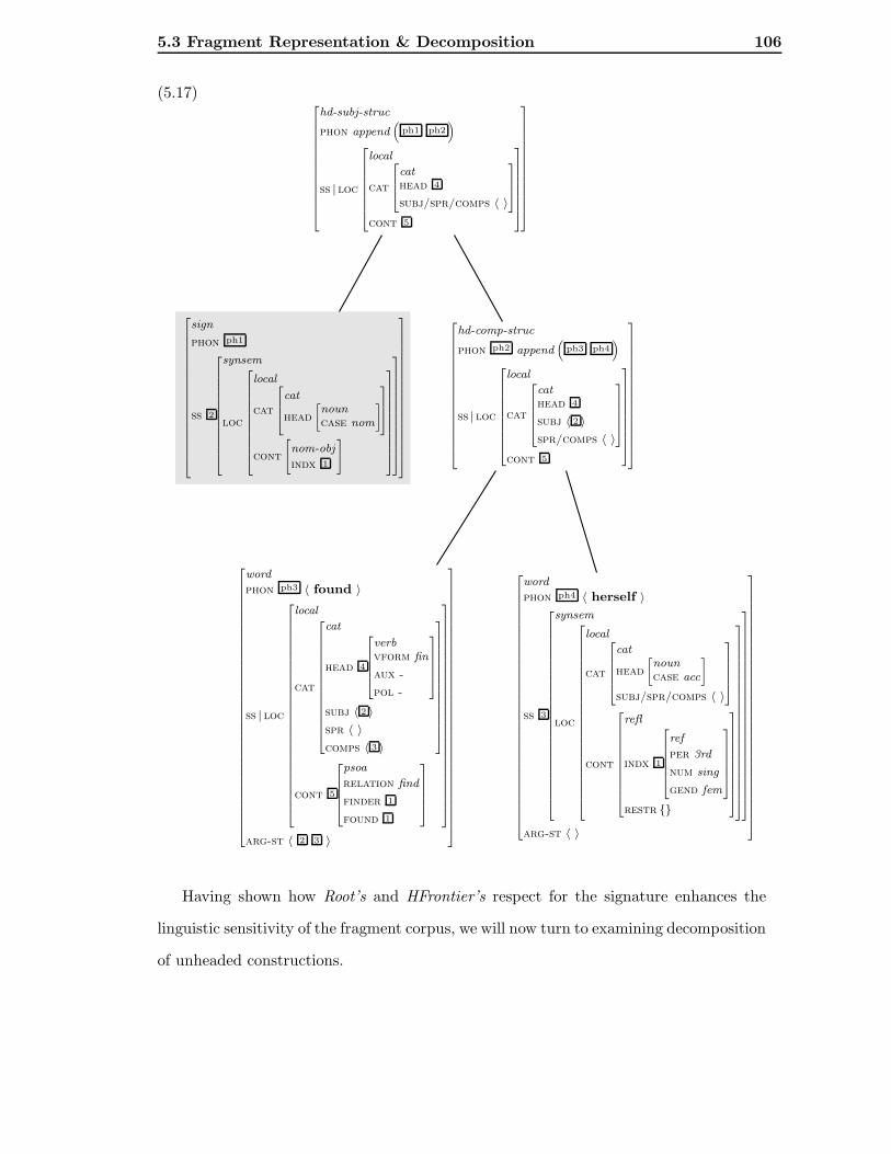
5.3 Fragment Representation & Decomposition 106
(5.17)
hd-subj-struc
phon append(
ph1 ph2)
ss | loc
local
cat
cathead 4
subj/spr/comps 〈 〉
cont 5
sign
phon ph1
ss 2
synsem
loc
local
cat
cat
head
[
nouncase nom
]
cont
[
nom-obj
indx 1
]
hd-comp-struc
phon ph2 append(
ph3 ph4)
ss | loc
local
cat
cathead 4
subj 〈 2 〉
spr/comps 〈 〉
cont 5
word
phon ph3 〈 found 〉
ss | loc
local
cat
cat
head 4
verbvform fin
aux -
pol -
subj 〈 2 〉
spr 〈 〉
comps 〈 3 〉
cont 5
psoa
relation find
finder 1
found 1
arg-st 〈 2 3 〉
word
phon ph4 〈 herself 〉
ss 3
synsem
loc
local
cat
cat
head
[
nouncase acc
]
subj/spr/comps 〈 〉
cont
refl
indx 1
ref
per 3rd
num sing
gend fem
restr
arg-st 〈 〉
Having shown how Root’s and HFrontier’s respect for the signature enhances the
linguistic sensitivity of the fragment corpus, we will now turn to examining decomposition
of unheaded constructions.

5.3 Fragment Representation & Decomposition 107
5.3.3 Unheaded Constructions
Unlike other DOP models, the decomposition operations described in the previous section
are very sensitive to certain linguistic parameters. On the one hand, this makes the
generated fragments linguistically more sensitive. On the other hand, special attention
is needed to ensure that the decomposition operations are applicable to all (linguistic)
types of representations. HFrontier, for example, makes reference to the head daughter of
a constituent, thus presupposing that if the constituent is phrasal, it is also headed. This
assumption is true for most linguistic signs. There are, however, cases like coordinate
structures (5.18) which are phrasal and widely considered to be unheaded.
(5.18) The boy and the girl left.
Coordinate structures are of interest for the model described thus far because they do
not carry the HD-DTR attribute, which can result in the production of illegal fragments
by HFrontier as so far defined. Assume that the sentence in (5.18) has roughly the
structure in (5.19(a)):
(5.19) (a) hd-subj-strucPPPPP
n-coord-strucHHHH
hd-spr-struc
ll
,,the boy
hd-comp-strucZZZ
and hd-spr-struc
ll
,,the girl
left
(b) n-coord-strucaaaa!!!!
hd-spr-struc
ll
,,the boy
hd-comp-strucQQQ
and hd-spr-struc
ll
,,the girl
(c) n-coord-struc
@@sign sign
Applying Root to the topmost non-head daughter results in the fragment rooted at n-
coord-struc (5.19(b)). Since HFrontier can apply to any combination of non-head daugh-
ters and since coordinate structures do not have a head daughter, HFrontier can se-
lect both the hd-spr-struc and the hd-comp-struc nodes, when processing the structure
in (5.19(b)), constructing a fragment that violates the minimum of one lexical anchor
(5.19(c)). Insisting on the one lexical anchor requirement, however, is important. Recall,
for example, the representation of the sentence “She found herself” in Figure 5.2. Take
the fragment produced by applying Root to the hd-comp-struc node (i.e. the VP) and

5.3 Fragment Representation & Decomposition 108
assume HFrontier applies to both its daughters (i.e. V and NP). The resulting fragment
is depicted in (5.20).
(5.20)
hd-comp-struc
phon append(
ph1 ph2)
ss | loc
local
cat
cathead 1
subj 2 list(synsem)
spr 4 list(synsem)
comps 〈 〉
cont 5
sign
phon ph1
ss | loc
local
cat
cathead 1 pos
subj 2
spr 4
comps 〈 3 〉
cont 5 content
sign
phon ph2
ss 3
synsem
loc
local
cat
cathead pos
subj/spr/comps list(synsem)
cont content
Notice that there is nothing to prevent this fragment, which in essence is a represen-
tation of the hd-comp-struc type constraint, from being used in parsing a syntactically
unrelated constituent like the PP to Mary. Such fragments are even more general than
their corresponding Tree-DOP counterparts, which seriously undermines our initial ar-
gument for a linguistically enhanced DOP model.
We need to revise HFrontier, therefore, so that it can be sensibly applied to unheaded
constructions as well. We can easily do this by means of the following definition:
In a phrasal representation fsph, HFrontier erases any set of values v(DTRS|p|REST∗|
FIRST,r(fsph)), such that
v(DTRS|p|REST*|FIRST, r(fsph)) 6=
v(HD-DTR, r(fsph)) if p is empty,
v(DTRS|p|HD-DTR, r(fsph)) otherwise.
so long as v(DTRS|p, r(fs′ph)) in the resulting fragment fs′ph has at least one daughter

5.3 Fragment Representation & Decomposition 109
strictly subsumed by sign. Path p is again defined as a sequence of FIRST’s and REST’s
ending in a FIRST. In unheaded constructions, the application of HFrontier is now re-
stricted by the last condition which basically states that any combination of non-head
daughters can be erased other than all of them.
Next, we turn to examining how identity should be interpreted in HPSG-DOP.
5.3.4 Intensionality vs Extensionality
In this section we explore whether the identity conditions imposed on feature structures
pose a problem for HPSG-DOP. Carpenter (1992) identifies two types of feature struc-
tures based on the identity interpretation they assume. The first one interprets identity
intensionally while the second extensionally.
Under the intensional interpretation it is possible for all attributes in two feature
structures of the same type to have token-identical values without the necessity of iden-
tifying the two feature structures, while under the extensional interpretation it is not.
The feature structures in Figure 5.6 are hence different if interpreted intensionally, while
the same if interpreted extensionally.
cat
subj
⟨
synsem
loc | cont | indx
ref
per 1 3rd
num 2 sing
gend 3 fem
⟩
comps
⟨
synsem
loc |cont | indx
ref
per 1
num 2
gend 3
⟩
cat
subj
⟨
4
synsem
loc | cont | indx
ref
per 1 3rd
num 2 sing
gend 3 fem
⟩
comps⟨
4
⟩
Figure 5.6: Feature structures with identical feature values.
Carpenter (1992) claims that the reason behind the existence of the intensional-only
interpretation in certain linguistic theories (e.g. LFG) is that they are untyped. In such
cases the fact that two nodes look alike is not enough to identify them because there
are no restrictions on adding, for example, extra features that would differentiate them
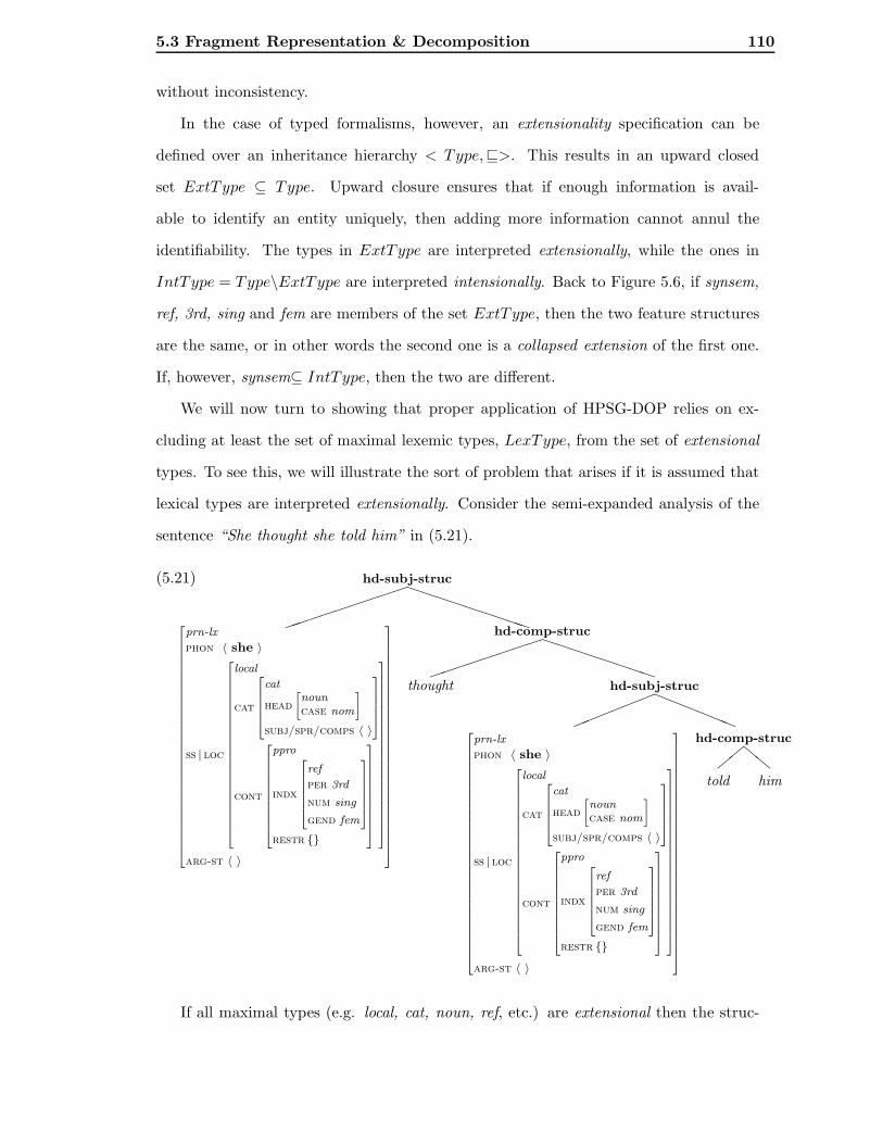
5.3 Fragment Representation & Decomposition 110
without inconsistency.
In the case of typed formalisms, however, an extensionality specification can be
defined over an inheritance hierarchy < Type,⊑>. This results in an upward closed
set ExtType ⊆ Type. Upward closure ensures that if enough information is avail-
able to identify an entity uniquely, then adding more information cannot annul the
identifiability. The types in ExtType are interpreted extensionally, while the ones in
IntType = Type\ExtType are interpreted intensionally. Back to Figure 5.6, if synsem,
ref, 3rd, sing and fem are members of the set ExtType, then the two feature structures
are the same, or in other words the second one is a collapsed extension of the first one.
If, however, synsem⊆ IntType, then the two are different.
We will now turn to showing that proper application of HPSG-DOP relies on ex-
cluding at least the set of maximal lexemic types, LexType, from the set of extensional
types. To see this, we will illustrate the sort of problem that arises if it is assumed that
lexical types are interpreted extensionally. Consider the semi-expanded analysis of the
sentence “She thought she told him” in (5.21).
(5.21) hd-subj-strucPPPPPPPPP
prn-lx
phon 〈 she 〉
ss | loc
local
cat
cat
head
[
nouncase nom
]
subj/spr/comps 〈 〉
cont
ppro
indx
ref
per 3rd
num sing
gend fem
restr
arg-st 〈 〉
hd-comp-strucPPPPPPPP
thought hd-subj-struc
aaaaaa
!!!!!!
prn-lx
phon 〈 she 〉
ss | loc
local
cat
cat
head
[
nouncase nom
]
subj/spr/comps 〈 〉
cont
ppro
indx
ref
per 3rd
num sing
gend fem
restr
arg-st 〈 〉
hd-comp-struc
ll
,,
told him
If all maximal types (e.g. local, cat, noun, ref, etc.) are extensional then the struc-

5.3 Fragment Representation & Decomposition 111
ture in (5.21) becomes as in (5.22) where all type identities have collapsed to token
identities.
(5.22) hd-subj-strucPPPPPPPPP
prn-lx
phon 1 〈 she 〉
ss | loc 2
local
cat 3
cat
head 4
[
nouncase 5 nom
]
subj/spr/comps 6 〈 〉
cont 7
ppro
indx 8
ref
per 9 3rd
num 10 sing
gend 11 fem
restr 6
arg-st 6 〈 〉
hd-comp-strucPPPPPPPPP
thought hd-subj-struc
aaaaaa
!!!!!!
prn-lx
phon 1 〈 she 〉
ss | loc 2
local
cat 3
cat
head 4
[
nouncase 5 nom
]
subj/spr/comps 6 〈 〉
cont 7
ppro
indx 8
ref
per 9 3rd
num 10 sing
gend 11 fem
restr 6
arg-st 6 〈 〉
hd-comp-struc
ll
,,
told him
If, in addition, LexType ⊆ ExtType (i.e. prn-lx is an extensional type) the feature
structure in (5.22) collapses to the one in (5.23).
(5.23) hd-subj-strucQQQ
hd-comp-strucHHHH
thought hd-subj-strucbbb
"""
prn-lx
phon 〈she〉
ss | loc
local
cat
cat
head
[
nouncase nom
]
subj/spr/comps 〈 〉
cont
ppro
indx
ref
per 3rd
num sing
gend fem
restr
arg-st 〈 〉
hd-comp-struc
ZZZ
told him

5.4 Combining the Fragments 112
The problem with this representation is that the value shared by the paths DTRS|FIRST
and DTRS|REST|FIRST|REST|FIRST|FIRST is a potential candidate node for HFrontier. If
HFrontier selects to erase the value of DTRS|FIRST then the exact same value can be
inferred from the path DTRS|REST|FIRST|REST|FIRST|FIRST and vice versa. As a result,
HFrontier cannot but apply to the value of both paths. Even if we take this to be the
case, however, the structure sharing does not disappear since it precedes the set of paths
identified by the erased value. As a result, the fragment produced is of very limited
generative value since it can only be used for parsing sentences like “The boyi thought
the boyi told him” where the two NP’s are structure shared, but not sentences like “She
thought the boy told him” as desired.
The problem fades away if we impose the intensionality condition on maximal lexemic
types. If LexType ⊆ IntType, the structure in (5.22) no longer collapses to the one in
(5.23), and HFrontier can apply to the value of either path as in previous examples. Note
that LexType ⊆ IntType does not prevent the structure in (5.21) from collapsing to the
one in (5.22). In order to avoid this, we need to extend the intensionality condition to
all maximal types in the hierarchy.
Having identified how initial representations are decomposed into fragments in HPSG-
DOP, we will now turn to the instantiation of the third parameter in the DOP framework,
the composition operation to be used in deriving new analyses.
5.4 Combining the Fragments
As previously mentioned, Tree-DOP and head-driven DOP employ different methods of
combining subtrees during derivation. The former uses leftmost substitution as described
in Chapter 1. The latter expands some subtree incrementally left to right starting from
the head lexical anchor as described in Chapter 4. Even though Neumann’s approach to
composition touches upon the notion of headedness, so it would seem more appropriate
than the first one for an HPSG-DOP model, the fact that it is incrementally rightwards
directed prevents it from being linguistically defensible. The concepts of headedness
and locality are of central importance in the HPSG formalism. It is, therefore, at least

5.4 Combining the Fragments 113
desirable to reflect these concepts in the composition phase of an HPSG-DOP model.
The idea of combining composition with the linguistic notion of head is borrowed from
existing parsing strategies. Head-driven parsing was first put forward by Kay (1989).
His suggestion was largely based on the fact that the head of a rule subcategorises for the
other daughters, so it can determine to a great extent what these must be. In addition
since heads and their mothers typically share the same morphosyntactic properties, top-
down identification of a potential head should be possible. Kay (1989) described two
parsing algorithms, the head-driven chart parser and the head-corner parser. The first
of these is in essence a shift reduce parser that “reduces” only when a category matching
the head of a rule has been found. The second locates a potential head for a phrase and
proceeds parsing bidirectionally. Since then, numerous head-driven parsing algorithms
have been developed and implemented (Lavelli and Satta, 1991; Bouma and van Noord,
1993; van Noord, 1994, among others). This section will present a totally head-driven
approach to composition, which is largely based on the underlying idea of the head-
corner parser described by Sikkel and Op den Akker (1993) and its extension to typed
feature structures (Moll, 1995).
5.4.1 Head-driven Composition
Composition in HPSG-DOP takes place by unifying the expansion nodes of an active
fragment with some other fragment. In the HPSG context, we define an active fragment
as a feature structure containing some path p of the form DTRS|...|FIRST whose value
is of type sign.
The head chain of the initial active fragment identifies the order in which expansion
nodes (i.e. nodes of type sign) are to be considered as composition sites. Starting
from the head lexical anchor, unification takes place so that each node along the path
leading from the head lexical anchor to the root of the feature structure dominates a
passive constituent before the next node along the path is considered. Similarly to active
fragments, we define a passive fragment as a feature structure that does not contain any
path p of the form DTRS|...|FIRST whose value is of type sign.
If a node x dominates an active fragment, its non-head daughter is considered. If it

5.4 Combining the Fragments 114
is sign-based, it is further expanded through unification. If it is not sign-based, the same
process is repeated along its own head chain, until the dominated fragment becomes
passive. Composition is bidirectional with the direction being identified at each step
(rather than in some predefined manner) by the head chain of the fragment rooted at
the node being considered.
We will illustrate the head-driven composition operation by means of a simple exam-
ple. Assume a toy bag of fragments containing the feature structure representations of
the following three subtrees:
SHHH
NP VPZZ
V
found
NP
NP
she
NP
him
Figure 5.7 (on the next page) shows the first step in deriving a representation for
the sentence “She found him”. The first internal node, hd-comp-struc, along the head
chain of the initial fragment dominates an active subfragment since one of its daughters
is of type sign. The rightmost terminal node is, therefore, the first node to be expanded.
Unification of the two fragments proves successful and since hd-comp-struc now domi-
nates a passive fragment we advance one step along the path of the head chain to the
root node hd-subj-struc.
This again dominates a sign node, which identifies the next composition point. In the
second composition step, presented in Figure 5.8, fragment unification is also successful
resulting in a valid feature structure representation.
The approach presented here is advantageous over leftmost or incrementally left to
right composition in that it is better equipped to take maximal advantage of the type
theory. Assuming binary branching constructions, at least one phrasal subconstituent is
constructed at each derivation step. Phrasal constituents are characterised by some of
HPSG’s principles and schemata which express general grammatical constraints. Since
these typically percolate up the head-chain, the head-driven composition process will
result in earlier realisation of the linguistic constraints expressed by the signature.

5.4
Com
bin
ing
the
Fragm
ents
115
26666666666664
hd-subj-struc
phon append
ph1 ph2
ss | loc
26666664local
cat
264cathd 4
subj/spr/comps 〈 〉
375cont 5
37777775377777777777752666666666666666664
sign
phon ph1 〈 phon cont 1 〉
ss 2
2666666666664synsem
loc
26666666664local
cat
264cat
hd
nouncase nom
375cont
"nom-obj
indx 1
# 377777777753777777777775
377777777777777777526666666666666664
hd-comps-struc
phon ph2 append
ph3 ph4
ss | loc
2666666664local
cat
26664cathd 4
subj 〈 2 〉
spr/comps 〈 〉
37775
cont 5
377777777537777777777777775
26666666666666666666666664word
phon ph3 〈 found 〉
ss | loc
266666666666666666664local
cat
26666664cathd 4
subj 〈 2 〉
spr 〈 〉
comps 〈 3 〉
37777775
cont 5
26664psoa
reln find
finder 1
found 6
37775377777777777777777775
377777777777777777777777752666666666666666666666666666666664
word
phon ph4 〈 him 〉
ss 3
26666666666666666666666664
synsem
loc
26666666666666666666664
local
cat
26664cat
hd
nouncase acc
subj/spr/comps 〈 〉
37775
cont
26666666664ppro
indx 6
266664ref
per 3rd
num sing
gend masc
377775
restr
3777777777537777777777777777777775
37777777777777777777777775
arg-st 〈 〉
37777777777777777777777777777777752
6
6
6
6
6
6
6
6
6
6
6
6
4
hd-subj-struc
phon append“
ph1 ph2”
ss | loc
2
6
6
6
6
6
6
4
local
cat
2
6
4
cathd 4
subj/spr/comps 〈 〉
3
7
5
cont 5
3
7
7
7
7
7
7
5
3
7
7
7
7
7
7
7
7
7
7
7
7
5
2
6
6
6
6
6
6
6
6
6
6
6
6
6
6
6
6
6
4
sign
phon ph1 〈 phon cont 1 〉
ss 2
2
6
6
6
6
6
6
6
6
6
6
6
4
synsem
loc
2
6
6
6
6
6
6
6
6
6
4
local
cat
2
6
4
cat
hd
»
nouncase nom
–
3
7
5
cont
"
nom-obj
index 1
#
3
7
7
7
7
7
7
7
7
7
5
3
7
7
7
7
7
7
7
7
7
7
7
5
3
7
7
7
7
7
7
7
7
7
7
7
7
7
7
7
7
7
5
2
6
6
6
6
6
6
6
6
6
6
6
6
6
6
6
6
6
6
6
6
6
6
6
4
hd-comps-struc
phon ph2 append“
ph3 ph4”
ss | loc
2
6
6
6
6
6
6
6
6
6
6
6
6
6
6
6
6
4
local
cat
2
6
6
6
4
cathd 4
subj 〈 2 〉
spr/comps 〈 〉
3
7
7
7
5
cont 5
2
6
6
6
4
psoa
reln find
finder 1
found 6
3
7
7
7
5
3
7
7
7
7
7
7
7
7
7
7
7
7
7
7
7
7
5
3
7
7
7
7
7
7
7
7
7
7
7
7
7
7
7
7
7
7
7
7
7
7
7
5
2
6
6
6
6
6
6
6
6
6
6
6
6
6
6
6
6
4
word
phon ph3 〈 found 〉
ss | loc
2
6
6
6
6
6
6
6
6
6
6
6
4
local
cat
2
6
6
6
6
6
6
4
cathd 4
subj 〈 2 〉
spr 〈 〉
comps 〈 3 〉
3
7
7
7
7
7
7
5
cont 5
3
7
7
7
7
7
7
7
7
7
7
7
5
3
7
7
7
7
7
7
7
7
7
7
7
7
7
7
7
7
5
2
6
6
6
6
6
6
6
6
6
6
6
6
6
6
6
6
6
4
sign
phon ph4 〈 phon cont 2 〉
ss 3
2
6
6
6
6
6
6
6
6
6
6
6
4
synsem
loc
2
6
6
6
6
6
6
6
6
6
4
local
cat
2
6
4
cat
hd
»
nouncase acc
–
3
7
5
cont
"
nom-obj
index 6
#
3
7
7
7
7
7
7
7
7
7
5
3
7
7
7
7
7
7
7
7
7
7
7
5
3
7
7
7
7
7
7
7
7
7
7
7
7
7
7
7
7
7
5
Figure 5.7: The head-driven composition operation (step 1).
2
6
6
6
6
6
6
6
6
6
6
6
6
6
6
6
6
6
6
6
6
6
6
6
6
6
6
6
6
6
4
wordphon 〈 him 〉
ss | loc
2
6
6
6
6
6
6
6
6
6
6
6
6
6
6
6
6
6
6
6
6
6
4
local
cat
2
6
6
6
4
cat
hd
»
nouncase acc
–
subj/spr/comps 〈 〉
3
7
7
7
5
cont
2
6
6
6
6
6
6
6
6
6
4
ppro
indx
2
6
6
6
6
4
ref
per 3rd
num sing
gend masc
3
7
7
7
7
5
restr
3
7
7
7
7
7
7
7
7
7
5
3
7
7
7
7
7
7
7
7
7
7
7
7
7
7
7
7
7
7
7
7
7
5
arg-st 〈 〉
3
7
7
7
7
7
7
7
7
7
7
7
7
7
7
7
7
7
7
7
7
7
7
7
7
7
7
7
7
7
5
=

5.4
Com
bin
ing
the
Fragm
ents
116
26666666666664
hd-subj-struc
phon append
ph1 ph2
ss | loc
26666664local
cat
264cathd 4
subj/spr/comps 〈 〉375
cont 5
377777753777777777777526666666666666666666666664
word
phon ph1 〈 she 〉
ss 2
266666666666666664synsem
loc
2666666666666664local
cat
26664cat
hd
nouncase nom
subj/spr/comps 〈 〉
37775cont
264refl
indx 1
restr
3753777777777777775
377777777777777775arg-st 〈 〉
3777777777777777777777777526666666666666664
hd-comps-struc
phon ph2 append
ph3 ph4
ss | loc
2666666664local
cat
26664cathd 4
subj 〈 2 〉
spr/comps 〈 〉
37775
cont 5
377777777537777777777777775
2666666666666666666666666666666664word
phon ph3 〈 found 〉
ss | loc
26666666666666666666666666664local
cat
26666664cathd 4
subj 〈 2 〉
spr 〈 〉
comps 〈 3 〉
37777775
cont 5
2666666666664
psoa
reln find
finder 1
266664ref
per 3rd
num sing
gend fem
377775
found 6
377777777777537777777777777777777777777775
37777777777777777777777777777777752666666666666666666666666666666664
word
phon ph4 〈 him 〉
ss 3
26666666666666666666666664
synsem
loc
26666666666666666666664
local
cat
26664cat
hd
nouncase acc
subj/spr/comps 〈 〉
37775
cont
26666666664ppro
indx 6
266664ref
per 3rd
num sing
gend masc
377775
restr
3777777777537777777777777777777775
37777777777777777777777775
arg-st 〈 〉
37777777777777777777777777777777752
6
6
6
6
6
6
6
6
6
6
6
6
4
hd-subj-struc
phon append“
ph1 ph2”
ss | loc
2
6
6
6
6
6
6
4
local
cat
2
6
4
cathd 4
subj/spr/comps 〈 〉
3
7
5
cont 5
3
7
7
7
7
7
7
5
3
7
7
7
7
7
7
7
7
7
7
7
7
5
2
6
6
6
6
6
6
6
6
6
6
6
6
6
6
6
6
6
4
sign
phon ph1 〈 phon cont 1 〉
ss 2
2
6
6
6
6
6
6
6
6
6
6
6
4
synsem
loc
2
6
6
6
6
6
6
6
6
6
4
local
cat
2
6
4
cat
hd
»
nouncase nom
–
3
7
5
cont
"
nom-obj
indx 1
#
3
7
7
7
7
7
7
7
7
7
5
3
7
7
7
7
7
7
7
7
7
7
7
5
3
7
7
7
7
7
7
7
7
7
7
7
7
7
7
7
7
7
5
2
6
6
6
6
6
6
6
6
6
6
6
6
6
6
6
4
hd-comps-struc
phon ph2 append“
ph3 ph4”
ss | loc
2
6
6
6
6
6
6
6
6
4
local
cat
2
6
6
6
4
cathd 4
subj 〈 2 〉
spr/comps 〈 〉
3
7
7
7
5
cont 5
3
7
7
7
7
7
7
7
7
5
3
7
7
7
7
7
7
7
7
7
7
7
7
7
7
7
5
2
6
6
6
6
6
6
6
6
6
6
6
6
6
6
6
6
6
6
6
6
6
6
6
6
4
word
phon ph3 〈 found 〉
ss | loc
2
6
6
6
6
6
6
6
6
6
6
6
6
6
6
6
6
6
6
6
4
local
cat
2
6
6
6
6
6
6
4
cathd 4
subj 〈 2 〉
spr 〈 〉
comps 〈 3 〉
3
7
7
7
7
7
7
5
cont 5
2
6
6
6
4
psoa
reln find
finder 1
found 6
3
7
7
7
5
3
7
7
7
7
7
7
7
7
7
7
7
7
7
7
7
7
7
7
7
5
3
7
7
7
7
7
7
7
7
7
7
7
7
7
7
7
7
7
7
7
7
7
7
7
7
5
2
6
6
6
6
6
6
6
6
6
6
6
6
6
6
6
6
6
6
6
6
6
6
6
6
6
6
6
6
6
6
6
6
4
word
phon ph4 〈 him 〉
ss 3
2
6
6
6
6
6
6
6
6
6
6
6
6
6
6
6
6
6
6
6
6
6
6
6
6
4
synsem
loc
2
6
6
6
6
6
6
6
6
6
6
6
6
6
6
6
6
6
6
6
6
6
4
local
cat
2
6
6
6
4
cat
hd
»
nouncase acc
–
subj/spr/comps 〈 〉
3
7
7
7
5
cont
2
6
6
6
6
6
6
6
6
6
4
ppro
indx 6
2
6
6
6
6
4
ref
per 3rd
num sing
gend masc
3
7
7
7
7
5
restr
3
7
7
7
7
7
7
7
7
7
5
3
7
7
7
7
7
7
7
7
7
7
7
7
7
7
7
7
7
7
7
7
7
5
3
7
7
7
7
7
7
7
7
7
7
7
7
7
7
7
7
7
7
7
7
7
7
7
7
5
arg-st 〈 〉
3
7
7
7
7
7
7
7
7
7
7
7
7
7
7
7
7
7
7
7
7
7
7
7
7
7
7
7
7
7
7
7
7
5
=
Figure 5.8: The head-driven composition operation (step 2).
2
6
6
6
6
6
6
6
6
6
6
6
6
6
6
6
6
6
6
6
6
6
6
6
6
6
6
6
6
6
4
wordphon 〈 she 〉
ss | loc
2
6
6
6
6
6
6
6
6
6
6
6
6
6
6
6
6
6
6
6
6
6
4
local
cat
2
6
6
6
4
cat
hd
»
nouncase nom
–
subj/spr/comps 〈 〉
3
7
7
7
5
cont
2
6
6
6
6
6
6
6
6
6
4
ppro
indx
2
6
6
6
6
4
ref
per 3rd
num sing
gend fem
3
7
7
7
7
5
restr
3
7
7
7
7
7
7
7
7
7
5
3
7
7
7
7
7
7
7
7
7
7
7
7
7
7
7
7
7
7
7
7
7
5
arg-st 〈 〉
3
7
7
7
7
7
7
7
7
7
7
7
7
7
7
7
7
7
7
7
7
7
7
7
7
7
7
7
7
7
5

5.4 Combining the Fragments 117
The head-driven composition process presented here has one key advantage: that
it respects the signature 100%, so it will produce only grammatical output, so long as
grammaticality is entirely defined in terms of the signature. Unfortunately, this is not
the case in standard HPSG (e.g. Pollard and Sag, 1994), where a number of phenomena
are described using principles stated outside the signature. For the most part, it is
possible to restate these principles inside the signature (immediate dominance schemata,
for example, are stated as constraints on the types of construction). This is not the
case, however, for all of them. In particular, the Binding Theory appears to resist this
re-analysis. The following section addresses this issue by exploring the possibility of
resolving the binding conditions during the derivation process.
5.4.2 Binding in HPSG-DOP
Binding is concerned with the identification of legal patterns of nominal reference (e.g.
the relationship between a reflexive and its antecedent). Before describing Binding in
HPSG let us introduce some terminology. A synsem object X is said to locally a-
command another synsem object Y iff X is less oblique than Y . The notion of obliqueness
can be expressed as: a synsem object X is said to be less oblique than another synsem
object Y (both appearing on the same ARG-ST value) iff X precedes (i.e. is to the left of)
Y on the ARG-ST value. X a-commands Y iff there exists synsem object Z such that X
locally a-commands Z and Z dominates Y . X is said to a-bind Y if it a-commands it and
the INDX values of X and Y are structure shared. An object that is not a-bound is a-free.
HPSG Binding Theory:
• Principle A: A locally a-commanded anaphor must be locally a-bound.
e.g. “Shei always talks about herselfi” vs *“Shei always talks about himselfj”
• Principle B: A personal pronoun must be locally a-free.
e.g. “Maryi always talks about herj” vs *“Maryi always talks about heri”
• Principle C: A nonpronoun must be a-free.
e.g. “Shei always talks about Maryj” vs *“Shei always talks about Maryi”

5.4 Combining the Fragments 118
Since the Binding Theory identifies relationships of synsem objects, the natural place to
define it would be in the ARG-ST value of appropriate predicates. Principles A and B
could be informally stated by the constraints in (5.24(a)) and (5.24(b)) respectively.
(5.24) (a)[
arg-st 〈 NPi,.., NP:anai,.. 〉]
(b)[
arg-st 〈 NPi,.., NP:proj,.. 〉]
, i 6= j
Principle C, on the other hand, makes reference to the concept of a-freedom inde-
pendent of the local domain parameter. A-freedom can, hence, depend on an arbitrary
number of ARG-ST values a-commanding the nonpronoun. As a result, it cannot be
expressed as a constraint in the signature.5
With respect to how binding works in HPSG-DOP, the above suggest that if incor-
porating Principles A and B in the signature suffices to identify all legal patterns of
nominal reference, then unification can guarantee well-formedness of the resulting struc-
tures. We will now turn to illustrating that the simplified assumption of identifying all
legal patterns of nominal reference solely based on Principles A and B is in fact valid.
We will look into the behaviour of nominals by classifying them in two categories
based on whether their binding properties can be expressed in the signature. The first
category hence includes anaphors and personal pronouns, while the second nonpronouns.
Note that the nominals in the second category share one characteristic in common; the
need to guarantee that their INDX value is not structure shared with any other INDX
value, rather than the opposite. This need for INDX value differentiation in the case of
nonpronouns covers the entire sentential domain. Consequently, we need to make sure
that there are no coindexations left over during decomposition that can cause violation
of Principle C during processing new input.
Recall that in a given phrasal feature structure fsinit, HFrontier can erase any
v(DTRS|p|REST∗|FIRST,r(fsinit)) producing a fragment fsfrag that is the most general to-
tally well-typed feature structure that satisfies all relevant type constraints and fsfrag⊔
DTRS|p|REST∗|FIRST|v(DTRS|p|REST∗|FIRST,r(fsinit)) = fsinit.
5The concepts of a-command, a-bound and a-free are the same as o-command, o-bound, and o-freein Pollard and Sag (1994). These were replaced in Manning and Sag (1999) to reflect the argumentstructure basis of the binding theory.

5.4 Combining the Fragments 119
Take, now, fsinit to denote the feature structure description of “She found herself”
repeated simplified in Figure 5.9(a). Suppose HFrontier erases v(DTRS|FIRST,hd-subj-
struc) (i.e. the “she” node). Is fsfrag going to retain the structure sharing as (b) in the
same figure or loose it as in (c)? The answer, in this case, will be “retain it” because
after the incorporation of Binding Principle A in the signature, the fragment description
in Figure 5.9(c) is no longer consistent.
(a) hd-subj-strucQQQQQ
she:
[
ppro
indx 1
]
hd-comp-struc :
psoa
finder 1
found 1
@@@
found herself:
[
refl
indx 1
]
(b) hd-subj-struc
ZZZZ
[
nom-obj
indx 1
]
hd-comp-struc :
psoa
finder 1
found 1
llll
,,,,
found herself:
[
refl
indx 1
]
√
(c) hd-subj-struc
ZZZZ
[
nom-obj
indx 2
]
hd-comp-struc :
psoa
finder 2
found 1
llll
,,,,
found herself:
[
refl
indx 1
]
× (d) hd-subj-struc
ZZZZZ
she:
[
ppro
indx 1
]
hd-comp-struc :
psoa
finder 1
found 1
JJJJ
found
[
nom-obj
indx 1
]
×
(e) hd-subj-struc
ZZZZZ
she:
[
ppro
indx 1
]
hd-comp-struc :
psoa
finder 1
found 2
JJJJ
found
[
nom-obj
indx 2
]
√
Figure 5.9: The INDX structure sharing is lost during decomposition unless this violates Principle A.
Consider now the case where HFrontier erases v(DTRS|REST|FIRST|REST|FIRST,hd-
subj-struc) (i.e. the “herself” node). Is fsfrag going to retain the structure sharing as
in (d) or loose it as in (e)? These fragments do not contain an anaphor, so Principle
A is no longer a relevant constraint. Both descriptions are in fact consistent and both

5.4 Combining the Fragments 120
satisfy the unification condition, but since (e) is more general than (d) it is this structure
HFrontier will produce. From the above, it follows that index structure sharings will be
retained in the fragments only if an anaphor is present.
Consider a fragment corpus containing the fragment in Figure 5.9(e), where the INDX
values of the verb’s subject and complement are not shared, and the word descriptions
of “Mary”, “her”, “herself”, “him” and “himself”. When deriving an analysis for the
string “She found her” in (5.25), the personal pronoun “her” is not affected by the
constraint expressing Principle A, so composition will produce the analysis in (5.25(a)),
which satisfies all the constraints, rather than the one in (5.25(b)) which violates Principle
B. Similarly, in (5.26) the nonpronoun “Mary” does not fall within the scope of the
Principle A constraint so the generated analysis will lack the INDX structure sharing.
(5.25) (a) Shei found herj . vs (b) ∗Shei found heri.
(5.26) (a) Shei found Maryj . vs (b) ∗Shei found Maryi.
(5.27) (a) Shei found herselfi. vs (b) ∗Shei found herselfj .
(5.28) (a) Shei found himj . vs (b) ∗Shei found himselfj .
In (5.27) the picture is quite different. Under the light of the suggestion made in this
section, where Principles A and B are in fact part of the signature, unification will now
also take care of the subject-object coindexation since the result would otherwise be an
inconsistent feature structure (violating the Principle A constraint). Similarly, (5.28(a))
can be produced since it is in accordance with the relevant constraints while (5.28(b))
violates Binding Principle A, so unification in this case will fail.
The above indicate that HPSG-DOP is not affected by the inability to encode Prin-
ciple C in the signature. This is because INDX structure sharings originating from nodes
that have been processed by HFrontier are lost during decomposition unless there is a
node not processed by HFrontier which enforces Principle A. The fragments themselves,
hence, incorporate Principle C by default, which will only be overwritten during compo-
sition when the right input (e.g. an anaphor) for an appropriate constraint is found.
The immediate advantage of incorporating constraints expressing Binding Principles
A and B in the signature is that composition in HPSG-DOP can now guarantee to

5.5 Fragment Probabilities 121
produce grammatical-only output. This ensures checking for well-formedness during
rather than after derivation. In the case of LFG-DOP, for example, it is not viable
to check completeness during the derivation process, thus ruling out the possibility of
ensuring well-formedness in an efficient manner. We will return to the advantages of
being able to guarantee well-formedness during derivation in the following section.
5.5 Fragment Probabilities
As in other DOP models, a final feature structure representation will typically have
many different derivations, and any string may have many different feature structure
representations. This section focuses on the stochastic process used for selecting the most
probable among the different representations. We use Tree-DOP’s relative frequency
estimator as a starting point. In Tree-DOP subtree probabilities are defined as in (5.29).
(5.29) P (ti) =|ti|∑
root(t)=root(ti)
|t|
The set of all composable subtrees at each derivation step is hence identified by
its category root(ti). Category matching in HPSG-DOP would roughly correspond to
classifying fragments based on their head features and subcategorisation frame. Two
fragments will hence be considered as competing (i.e. belonging to the same competition
set) if they share the same values for all CAT features (i.e. HEAD, SUBJ, SPR and COMPS).
The probability of a fragment fi is, therefore, defined as in (5.30). In the case of under-
specified HEAD values (e.g. [HEAD noun]), the values are expanded in all possible ways
(e.g.[
head
[
nouncase nom
]
]
, ...) and the resulting fragments are classified accordingly.
(5.30) P (fi) =|fi|∑
v(SS|LOC|CAT,r(f))=v(SS|LOC|CAT,r(fi))
|f |
The probabilities of a derivation d =< f1, f2, ..., fn > and a final representation R
that has m derivations dj are hence defined as in (5.31) and (5.32) respectively.

5.5 Fragment Probabilities 122
(5.31) P (d) =
n∏
i=1
P (fi)
(5.32) P (R) =m∑
j=1
P (dj)
One issue in the above stochastic process is that it does not guarantee to identify
a probability distribution over the set of valid representations. This is very similar to
what happens in the case of category-identifiable sample spaces in LFG-DOP, where
the reason behind the probability mass leak is that the stochastic process assigns some
probability to invalid structures. In the case of HPSG-DOP, the problem occurs because
the stochastic process assigns part of the probability mass to non-existent derivations.
The underlying issue is the same; i.e. part of the probability mass is assigned outside
the parse space.
In order for the likelihood of the parse space to be maximised, the following must hold.
Firstly, the probability mass of each competition set must be 1. Secondly, each active
fragment must be able to combine successfully with all fragments in the competition set
identified by its next expansion node. Thirdly, the result of successful composition must
be a valid representation. We will next show that the second condition is not satisfied
by the stochastic process described thus far.
Take the feature structure representations of the NP’s “she” and “he” in (5.33(a))
and (5.33(b)) respectively.
(5.33) (a)
wordphon 〈 she 〉
ss | loc
local
cat
cat
head
[
nouncase nom
]
subj/spr/comps 〈 〉
cont
ppro
indx
ref
per 3rd
num sing
gend fem
restr
arg-st 〈 〉
(b)
wordphon 〈 he 〉
ss | loc
local
cat
cat
head
[
nouncase nom
]
subj/spr/comps 〈 〉
cont
ppro
indx
ref
per 3rd
num sing
gend masc
restr
arg-st 〈 〉
Consider now the not fully expanded fragment in (5.34).

5.5 Fragment Probabilities 123
(5.34) hd-subj-strucXXXXXXXXX
sign
phon 〈phon cont 〉
ss | loc
local
cat
cat
head
[
nouncase nom
]
cont
[
nom-obj
indx 1
]
hd-comp-strucPPPPPPP
wordphon 〈 herself 〉
ss | loc |cont | indx 1
ref
per 3rd
num sing
gend fem
found
This description should be able to combine with either fragment in (5.33) since they
both belong to the same set of composable fragments (i.e. they have the same CAT
values). Note, however, that unification with the “he” fragment will, in fact, fail because
the subject’s INDX value 1 is structure-shared with the INDX value of “herself” in the
same fragment which is [GEND fem]. Syntactic category related information does not,
therefore, suffice in identifying appropriate competition sets for composition.
Next, we turn to defining the various sets of composable fragments in such a way
that any given fragment fi can be successfully combined with all members of the set
identified by each of its expansion nodes. Since previous derivation steps can affect the
specificity of such nodes, competition sets in HPSG-DOP cannot be predetermined. This
resembles the second version of LFG-DOP, where unifiability is determined at each step
in order to take into account the Uniqueness condition of LFG. The probability definition
of LFG-DOP fragments can easily be extended to HPSG-DOP.
Under this view, a competition set includes all fragments that can be successfully
unified with the next expansion site (NES) of some other feature structure fragment f.
Suppose fi−1 is the fragment produced before the ith step of the derivation process. The
probability of the next fragment to be used is defined as:
(5.35) P (fi) =|fi|∑
f is unifiablewith NES(fi−1)
|f |
This estimator still requires a probability to be determined for each fragment for
the case of derivation initial selection. Since there are no previous derivation steps, the

5.5 Fragment Probabilities 124
competition sets are not in any way restricted so relative frequency based on category
matching can be used to determine these probabilities.
It has been argued (Abney, 1997) that relative frequency estimation constitutes a
non-optimal approach to probabilistic AVGs. Abney claims that the independence as-
sumption cannot be applied to deep linguistic analysis (such as HPSG representations),
due to the fragments of such analyses being in fact equipped to handle both syntactic
and semantic dependencies, raising consistency issues about the particular estimation
process. Log-linear or maximum entropy models (Abney, 1997; Miyao and Tsujii, 2002;
Miyao et al., 2003) are generally deemed as more suitable for formalisms that can account
for such dependencies because they do not rely on the independence assumption.
Abney’s argument, however, is based on previous approaches to stochastic unification-
based formalisms (Brew, 1995) which treat AVGs as CFGs with attribute labels and path
equations (5.36). Feature structures are viewed as DAGs and hence the process of gen-
erating a feature structure is the same as the process used to generate a DAG (i.e. node
substitution).
(5.36)
R1. verb → SUBJ:word OBJ:word <SUBJ NUM> = <OBJ NUM> (1/2)R2. verb → SUBJ:word (1/2)R3. word → NUM:sing (2/3)R4. word → NUM:pl (1/3)
Take the grammar in (5.36) to be a simple PCFG (disregarding the path equation).
The trees of the string language it generates together with their associated probabilities
are as in (5.37). Tree probabilities are computed as the product of the probabilities of
the rules used in their derivation. The probability of the first tree below is thus 12
23
23 = 2
9 .
(5.37) verb
JJJ
word
sing
word
sing
verb
JJJ
word
pl
word
pl
verb
JJJ
word
sing
word
pl
verb
JJJ
word
pl
word
sing
verb
word
sing
verb
word
pl
(2/9) (1/18) (1/9) (1/9) (1/3) (1/6)
SUBJ SUBJ SUBJ SUBJ SUBJ SUBJOBJ OBJ OBJ OBJ
NUM NUM NUM NUM NUM NUM NUM NUM NUM NUM
Suppose now that the grammar in (5.36) (containing the path equation) is in fact an
AVG. The structures it licences are depicted in (5.38). Note that the probabilities of all

5.5 Fragment Probabilities 125
possible structures sum up to 79 < 1.
(5.38) verb
\\\
word word
verb
\\\
word word
verb
word
sing
verb
word
plsing pl\\\
\\\
SUBJSUBJ SUBJOBJ OBJ SUBJ
NUM NUM NUM NUM NUM NUM
(2/9) (1/18) (1/3) (1/6)
Clearly, relative frequency estimation in this case fails to identify a probability distri-
bution over L(G). This represents, however, an oversimplified view of AVGs. At least in
the case of HPSG, DAGs constitute only the means for representing feature structures.
So, even though DAGs can be generated through node substitution, feature structures
are generated through unification (and perhaps inference in some cases). The difference
between unification and node substitution, however, is crucial since it means that the
derivation of the first feature structure in (5.38) has two rather than three steps (i.e.
<R1,R3> rather than < R1, R3, R3>). Switching from node substitution to unifica-
tion suffices to rectify the relative frequency estimator’s inability to define a probability
distribution over all possible structures (i.e. the new probabilities of the structures in
(5.38) become 1/3, 1/6, 1/3 and 1/6 respectively).
The underlying problem is not caused by the nature of node substitution as opposed
to unification, but rather by the fact that the former can cause invalid derivations to
surface. That is not, of course, to say that unification cannot fail to produce valid
derivations in AVGs. In fact, it can (e.g. unification of the fragments in (5.33(b)) and
(5.34)) and when it does, it offers further evidence validating Abney’s argument on
relative frequency estimation.
By definition (of the competition sets), however, unification in an HPSG-DOP deriva-
tion is guaranteed to succeed, so no probability mass is wasted because of unification
failure. In addition, the resulting feature structure is guaranteed to be a valid HPSG
representation (Section 5.4.2). The previously raised issue of probability leak observed in
LFG-DOP because of a certain amount of the overall probability mass being assigned
to invalid representations does not, therefore, occur in this case. This, of course, does

5.6 Outstanding Issues 126
not show that relative frequency is the best estimation algorithm for HPSG-DOP, but
rather that, depending on the view one takes on feature structures, it is not necessarily
a non-optimal approach.
5.6 Outstanding Issues
In the previous sections we demonstrated how the type theory facilitates HPSG-DOP
to handle highly articulate representations. The data-oriented dimension of this model
enables it to generate beyond the training data, while its close relationship with the
signature serves to limit its generative capabilities to linguistically valid descriptions.
One issue we have conveniently avoided so far is discussing the effect of information
determined by factors that lie outside the scope of the signature (e.g. pragmatic) on
HPSG-DOP. That is to say, is our model equipped to handle efficiently cases where the
type theory “overgenerates”? One such example of information being determined outside
the type theory is the nominal reference of exempt anaphors. We believe there are more
cases that we have not thought about.
Recall that Principle A of the Binding theory states that a locally a-commanded
anaphor must be locally a-bound. This implies that anaphors that are not locally a-
commanded need not be a-bound. In (5.39) - (5.40), for example, “himself” and “them-
selves” are not a-commanded because the ARG-ST value of “picture” contains only one
element (i.e. a PP).6 Such anaphors are known as exempt because they are exempted
from the binding conditions.
(5.39) Johni took a picture of himselfi. (Runner, 1998)
(5.40) Theyi saw pictures of themselvesi. (Asudeh and Dalrymple, 2005)
The implication of “need not” is what makes identifying the nominal reference of
such anaphors go astray, because it does not determine whether exempt anaphors are,
6Case-marking prepositions are assumed to make no contribution the the CONT value of their PPprojections, whose CONT value is consequently structure shared with the CONT value of its NP com-plement.

5.6 Outstanding Issues 127
in fact, a-bound or not, and if yes to what. Consequently, the type theory in these cases
licences more than what is intuitively correct. In the case of “John took a picture of
himself”, for example, “John” does not have to be coindexed with “himself”, so (5.41)
is perfectly acceptable for the type theory and, for the same reason, so is (5.42).
(5.41) *Johni took a picture of himselfj .
(5.42) *Mary took a picture of himself.
It has been suggested that cases like (5.39) do not in fact involve an exempt anaphor,
but a complex predicate “take a picture” which would make Principle A applicable in
this case. Treating some verb-complement expressions as complex predicates, however,
seems to be an ad-hoc solution to the problem, because it still does not account for
numerous examples like “He burned a picture of himself”, which could not be plausibly
considered as complex predicates.
The question that hence arises is the following: suppose that the training data does
not contain cases like (5.41) and (5.42), yet it contains many cases like (5.39) and (5.40),
is HPSG-DOP going to “recognise” the inclination in the training data favouring a-bound
anaphors or not? In other words, is the non-occurrence of a-free anaphors enough to
block their existence in the construction of new analyses? And in case it is not enough,
does HPSG-DOP at least show a preference for, rather than against, coindexation in
such cases? Clearly, we would like the answer to be that a-free anaphors never appear
in the final representations, or at least if they do, they are highly unlikely to do so, but
let us see what happens in practice.
Take a simple training corpus containing the representation of the sentence “Johni
took a picture of himselfi” in (5.43). What we want to determine is whether the analysis
proposed by HPSG-DOP corresponds to (5.39) or (5.41). Starting from decomposition,
HFrontier produces fourteen fragments rooted at subj-hd-struc. In six out of the fourteen,
either the spr-hd-struc or the bottom hd-comp-struc is chosen to be marked for expansion.
We will leave these fragments aside for the moment and return to them later in the
discussion.

5.6 Outstanding Issues 128
(5.43) subj-hd-strucPPPPPP
noun-lxphon 〈John〉
indx 1
prep-lx
of
hd-comp-strucPPPPPP
trns-v-lx
took
spr-hd-strucPPPPPP
det-lx
a
hd-adj-strucPPPPP
noun-lx
picture
hd-comp-strucPPPPP
noun-lxphon 〈himself〉
indx 1
ref
per 3rd
num sing
gend masc
The remaining eight fragments result from HFrontier erasing the possible combina-
tions of the noun-lx:John, det-lx:a and noun-lx:himself nodes. Recall that the result of
erasing the value v(p, r(fs)) of some path p in a feature structure fs is the most general
co-unificant of p|v(p, r(fs)) in producing fs that satisfies all relevant type constraints
and contains p. Defining the process of erasing in terms of unification has the following
effect: information that cannot be inferred is reflected in the fragment. Consider, for
example, the structures in (5.44) as possible candidates for the fragment generated by
erasing the node description of “himself”.
(5.44) (f1)subj-hd-strucbbb
"""
noun-lx
Johni
hd-comp-strucbbb
"""
trns-v-lx
took
spr-hd-strucbbbb
""""
det-lx
a
hd-adj-struc
QQQ
noun-lx
picture
hd-comp-struc
@@
prep-lx
of
signj
(f2)subj-hd-strucbbb
"""
noun-lx
Johni
hd-comp-strucbbb
"""
trns-v-lx
took
spr-hd-strucbbbb
""""
det-lx
a
hd-adj-struc
QQQ
noun-lx
picture
hd-comp-struc
@@
prep-lx
of
signi

5.6 Outstanding Issues 129
Is fragment f1 or f2 the one actually produced? According to our definition of erasing val-
ues, it is the one that when unified with ferased, where ferased is DTRS|REST|...|
noun-lx
phon⟨
himself⟩
... ...
,
results in the initial structure, finit, in (5.43).
But, f1 ⊔ ferased 6= finit because the coindexation cannot be inferred. On the other
hand, f2 ⊔ ferased = finit, so HFrontier will in fact generate f2 thus retaining the infor-
mation that was determined outside the signature. This will be the case for each of the
eight fragments we are considering at present. Now, since information cannot be lost
during composition, these structure sharings will be present in the final representation(s)
derived by any of these eight fragments. As a result, even if the fragments we left aside
derive an analysis without the coindexation, the fragment corpus will rightfully rule in
favour of the coindexation at least under some estimators.
Based on what we have said thus far, it seems that an HPSG-DOP fragment corpus
offers an adequate approach to identifying all legal patterns of nominal reference, even
those of exempt anaphors. Unfortunately, this is far from being true. As we shall show
next, representations containing exempt anaphors turn out to cause serious problems.
The first problem relates to the six fragments we earlier left aside, where either the
spr-hd-struc or the bottom hd-comp-struc in (5.43) is to be processed by HFrontier. Take,
for example the case where spr-hd-struc is to be marked for expansion. The generated
fragment is a feature structure f3 that has to satisfy the following: f3 ⊔ ferased = finit,
where ferased is now DTRS|REST|FIRST|REST|FIRST|spr-hd-struc, and finit is again the
initial structure in (5.43). f3 will, therefore, roughly look like the description in (5.45),
or its corresponding tree abbreviation in (5.46), which is an invalid HPSG-DOP fragment.
(5.45)
subj-hdlist
...
...
hd-comp
phrase phrase phrase sign
ref
DTRS
REST
FIRST
FIRST
DTRS|R|FDTRS|R|F DTRS|R|F DTRS|R|F
INDX
SS|LOC|CONT|INDX

5.6 Outstanding Issues 130
(5.46) subj-hd-strucXXXXX
hd-comp-strucXXXXX
trns-v-lx
took
phrasePPPP
sign phrasePPP
sign phraseHHH
sign[
sign
indx 1
]
noun-lxphon 〈John〉
indx 1
Even if we ignore these fragments (on validity grounds) another more serious problem
arises. The regular binding patterns (i.e. those specified by the binding theory) can no
longer be accounted for. Imagine we add in the training corpus the representation of the
sentence “Bill loves Mary”. Then, given that the fragment corpus contains fragments
such as f2 in (5.44), there is nothing to prevent coindexation of “John” and “Bill” when
deriving an analysis for the sentence “John took a picture of Bill” (recall that Principle
C cannot be expressed as a constraint in the signature).
The above leave no choice but to treat information determined outside the type the-
ory in some special manner so that it is not inherited by the fragments. One way this
could be done is by ignoring such bits of information during decomposition, which, of
course, amounts to ignoring them in the initial representations. Under this view, we need
to redefine the representation used for utterance analysis (DOP parameter 1) from being
a valid HPSG representation fsHPSG to being the most general feature structure that
subsumes fsHPSG and satisfies all the type constraints that fsHPSG satisfies. The new
definition causes the representation of a sentence like “Johni took a picture of himselfi”
to reduce to the representation of “Johni took a picture of himselfj”. The effect of this
modification is that exempt anaphors, on the one hand, will be a-free in the representa-
tions derived by HPSG-DOP, but on the other regular nominal reference patterns can
now be determined by the fragment corpus regardless of the phenomena occurring in the
training data.
Recall that the source of the problem was that the type theory “overgenerates”. One
way of looking at this situation is hence to adopt the HPSG point of view according

5.7 Conclusions 131
to which the occurrence of a-free anaphors is linguistically valid so long as they are
exempt. Even though this argument could be defensible from a linguistic point of view,
it constitutes a less than satisfactory solution from the data-oriented point of view. The
fact that no matter how much we overtrain a fragment corpus we will never be able to
capture these dependencies when analysing new input stands in sharp contradiction with
the DOP philosophy.
An alternative viewpoint would be to consider representations containing a-free ana-
phors as invalid. The consequences of this suggestion, however, are more serious than
what might meet the eye at first. If such representations are deemed as invalid, yet the
model cannot be refrained from deriving them, then validity can no longer be guaranteed
during composition causing all undesirable consequences mentioned earlier to surface.
In addition, the generative capacity of the grammar would be negatively affected since
occurrences of a-bound exempt anaphors, on the one hand, cannot be derived and a-free
ones, on the other hand, are deemed as invalid.
A third option would be to treat the INDX value of ana entities (i.e. anaphors)
as “special” or “privileged” so that paths leading to the INDX value of an ana are not
accessible to HFrontier. Even though, this suggestion provides the desired restrictions, it
constitutes an ad-hoc approach to the issue under discussion because it requires individual
identification of “privileged” nodes for each property that is determined outside the type
theory rather than provide a uniform treatment for all such cases.
The fourth and perhaps more appealing course of action would be to find some way
of expressing all linguistic constraints in the signature. Such an attempt, however, falls
outside the scope of this thesis.
5.7 Conclusions
In this chapter we presented a new DOP model based on the syntactically and seman-
tically more articulated representations of HPSG. Initially we defined decomposition in
terms of two operations Root and HFrontier, which act based on the subsumption or-
dering of the signature and the type inference procedure. Following this, we portrayed

5.7 Conclusions 132
a head-driven approach to composition that uses the head-chain of a fragment to deter-
mine the order in which its expansion nodes are to be considered. This approach gives
priority to analyses of complete subconstituents thus allowing greater inference amounts
at an earlier stage. We observed that the model’s respect for the type theory allows it to
produce almost always valid representations. The fact that binding conditions, however,
require checking outside the type theory did not allow the validity of final representa-
tions to be guaranteed. To overcome this problem, we suggested incorporating Binding
Principles A and B as constraints in the signature. The effect of this alteration in con-
junction with the fact that the shape of the fragments does not allow Principle C to be
violated ensures that linguistically invalid representations are not produced.
In the following section we described how Tree-DOP’s relative frequency estimator
can be extended to HPSG fragments. We illustrated that relative frequency based on
category matching does not describe a true estimator because some of the fragments in
a given competition set lead to unsuccessful derivations. As an alternative, we proposed
that fragment probabilities are determined prior to each derivation step, based on the set
of competing fragments identified in terms of unifiability with the node to be expanded at
the following derivation step. We argued that since derivations cannot fail the concerns
raised in the literature about relative frequency estimation in AVGs do not apply to this
model.
In the last section of the chapter we contemplated on the behaviour of HPSG-DOP
with regards to information that is not determined by the type theory like the nominal
reference of exempt anaphors. We put forward several courses of action and concluded
that ignoring such information in the initial representations is at present the most sat-
isfactory, still far from perfect though, solution.
The general architecture portrayed here allows for various HPSG-DOP instantiations,
which will typically differ in the degree of specificity the fragments are allowed to have
and the stochastic process employed for disambiguation. An alternative HPSG-DOP
model could, for example, be defined by disallowing HFrontier to process any node
along the head chain rather than any head node overall. The linguistic sensitivity of
HPSG-DOP is far greater than that of any of the DOP models described in the previous

5.7 Conclusions 133
chapters. HPSG-DOP takes full advantage of the underlying formalism which makes it
linguistically appealing. In addition to this, its data-oriented dimension enables it to
express relationships that rely on concepts not easily defined in the signature such as
domains of potentially arbitrary size.

Part II
DOP from a statistical point of view

Chapter 6
Computational Complexity of
DOP
This chapter aims at illustrating the computational complexity of parsing and disam-
biguation under DOP1 and describe various proposals from the literature on attacking
the issue.
6.1 Introduction
One problem that appears to have restricted the wider use of DOP is its computational
complexity, which will be the main focus of this chapter. One characteristic inherent
to DOP due to the nature of the decomposition process is its huge grammar size. The
decomposition operations applied to each element of the training corpus, produce a
number of subtrees exponential to the size of the initial tree. This in conjunction with
the typical optimisation criterion (i.e. the MPP) make processing new input a task of
exponential time and space requirements.
6.2 Parsing Complexity
The composition operation defined for Tree-DOP identifies one potential parsing algo-
rithm which, however, relies on the use of all possible fragments in the corpus. This makes

6.2 Parsing Complexity 136
it a very inefficient approach to the task of computing the parse forest of a given string.
This section presents an overview of the parsing strategies typically employed in DOP.
6.2.1 Fragments as context-free rules
In the first DOP implementations the parse forest of a given sentence was computed
using standard chart parsing algorithms (like CKY). Each subtree ti was viewed as a
context-free rewrite rule of the form root(ti) −→ yield(ti). Indices were used to link
rewrite rules to fragments in order to prevent same-looking rules describing subtrees
with distinct internal structures (Figure 6.1) from merging. The fragment corpus was
hence reduced to a CFG.
S@@
a XSS
b c
S@@
XSS
a b
c
SQQ
a b c
Figure 6.1: Fragments with identical root and yield but different internal structure.
As pointed out by Sima’an (1999), however, the CKY algorithm can be of limited
practicality in this case because it requires transformation of the CFG into Chomsky
Normal Form (CNF), which can result in a dramatic increase in the grammar size, with
the worst case being squaring the initial size.1
As an alternative Sima’an (1999) proposes a two phase parsing algorithm that com-
putes the parse space of a given input string more efficiently. In the first phase an approx-
imation of the required parse forest is computed from an Approximated CNF (ACNF)
of the CFG underlying the given DOP treebank. The advantage of the ACNF trans-
formation over traditional CNF transformation is that the size of the ACNF CFG is
guaranteed to be in the same order as that of the original CFG. In the second phase, an
optimisation technique is used to reduce the computed parse space to the corresponding
DOP parse space. This involves assigning a unique address to each node in the fragment
corpus (Figure 6.2). The addresses are used to link the CFG rules with the fragments
1A CFG rule is in CNF if its left-hand side consists of one nonterminal and its right-hand side consistsof either two nonterminals or a single terminal.

6.2 Parsing Complexity 137
in which they occur.
NP1
cc##D2
the
N3
boy
NP4
ll,,D5
the
N6
NP7
ll,,D8 N9
boy
NP10ZZ
D11 N12
D13
the
N14
boy
(t1) (t2) (t3) (t4) (t5) (t6)
Figure 6.2: A fragment corpus where each node has been assigned a unique address.
Each derivation can be identified by the addresses assigned to the nodes of the parse
tree it gives rise to. The tree in (6.1), for example is the outcome of the derivation (t2t6).
(6.1) NP4
cc##D5
the
N14
boy
Even though this parsing algorithm achieves time complexity at most linear with re-
spect to the fragment corpus size, it does not allow direct computation of fragment
probabilities. These have to be retrieved using the node addresses to identify the corre-
sponding subtrees.
6.2.2 PCFG reduction
An alternative approach to reducing the computational cost of parsing was put forward
by (Goodman, 2003) who suggested reducing a given DOP fragment corpus to a PCFG
that contains at most eight rules for each node in the training data. His suggestion is
based on building a PCFG equivalent to a given DOP1 fragment corpus (equivalent in
that they both generate the same parse trees and strings with the same probabilities).
In building the PCFG, each node of some elementary tree is assigned a unique number
called its address. A new non-terminal of the form Ak is created for each non-terminal
in the training data, as shown in (6.2). The new non-terminals are called interior while
the original ones exterior.
(6.2) Sbb""
NP
pn
VPZZ
v NPll,,
d n
=⇒ S1aa!!NP2
pn
VP3HHv NP4
bb""d n

6.2 Parsing Complexity 138
For each node Aj dominating a binary branching construction likeAjbb""
Bk Cl
the fol-
lowing eight rules (with their associated probabilities) are extracted:
Aj → BC (1/aj) A → BC (1/a)
Aj → BkC (bk/aj) A → BkC (bk/a)
Aj → BCl (cl/aj) A → BCl (cl/a)
Aj → BkCl (bkcl/aj) A → BkCl (bkcl/a)
where aj denotes the number of Aj-rooted nontrivial subtrees and a the sum of all A-
rooted subtrees (i.e. a =∑
jaj). Since there are bk Bk-rooted subtrees and one B-rooted
subtree possibilities for the left branch and, similarly, cl Cl-rooted subtrees and one
C-rooted subtree for the right branch, aj = (bk + 1)(cl + 1).
The PCFG resulting from the training data in (6.2) is presented below:
(r1) S1 → NP VP (1/6) (r2) S→ NP VP (1/6)
(r3) S1 → NP2 VP (1/6) (r4) S→ NP2 VP (1/6)
(r5) S1 → NP VP3 (2/6) (r6) S→ NP VP3 (2/6)
(r7) S1 → NP2 VP3 (2/6) (r8) S→ NP2 VP3 (2/6)
(r9) VP3 → v NP (1/2) (r10) VP→ v NP (1/2)
(r11) VP3 → v NP4 (1/2) (r12) VP→ v NP4 (1/2)
(r13) NP2 → pn (1) (r14) NP→ pn (1/2)
(r15) NP4 → d n (1) (r16) NP→ d n (1/2)
In this case there are no multiple copies of the same rule. Increasing the training data,
however, will very likely result in multiple copies of rules such as S → NP VP, VP → v NP,
etc. In such cases the multiple copies are merged into one rule with probability equal to
the sum of the probabilities of the individual rules before merging.
A subderivation of this PCFG is said to be homomorphic to a DOP subtree iff it has
exterior non-terminals labelling its root and leaves and interior labelling all other nodes.
The PCFG subderivation (r6 r9), for example, is homomorphic to the subtree in (6.3).
(6.3) Sbb""
NP VP@@
v NP
A PCFG derivation is said to be homomorphic to a DOP derivation if for every DOP
substitution there is a corresponding PCFG subderivation (one to many relationship).

6.2 Parsing Complexity 139
Exterior non-root non-terminal nodes in the PCFG derivation correspond to substitution
nodes in DOP. The two-subtree DOP derivation in (6.4(a)) is thus homomorphic to the
four-rule PCFG derivation r8 r13 r9 r16 in (6.4(b)).
(6.4) (a) Sbb""
NP
pn
VP@@
v NP
NPll,,
d n
(b) SHH
NP2
pn
VP3
ZZv NP
ll,,d n
The probability of a DOP derivation equals the sum of the probabilities of its homo-
morphic PCFG subderivations. A PCFG tree is said to be homomorphic to a DOP tree
if turning internal non-terminals to external makes the two identical. The parse trees
produced by this PCFG are homomorphic and of equal probability to those produced
by DOP2.
(6.5) SXXX
NP
Mary
VPaa!!
V
kissed
NP
John
SXXX
NP
Jane
VPPPP
V
chased
NPbb""
D
the
N
cat
The reduction in grammar size is already obvious even in a small corpus such as the
one depicted in (6.5). The corresponding PCFG contains fifteen rules expanding S (6.6)
versus the thirty S-rooted subtrees the corresponding DOP fragment corpus contains.
(6.6) S1 → NP V P (1/10) S → NP V P (1/16)
S1 → NP2 V P (1/10) S → NP2 V P (1/32)
S1 → NP V P3 (4/10) S → NP V P3 (4/32)
S1 → NP2 V P3 (4/10) S → NP2 V P3 (4/32)
S6 → NP V P (1/22) S → NP7 V P (1/32)
S6 → NP V P8 (10/22) S → NP V P8 (10/32)
S6 → NP7 V P8 (10/22) S → NP7 V P8 (10/32)
S6 → NP7 V P (1/22)
The PCFG reduction described by Goodman (2003) can be easily applied to other
versions of DOP as well. Limiting the subtree depth , for example, as in Bod (2001)
2Proof of this argument can be found in Goodman (2003)

6.3 Reducing the Complexity of Finding the MPP 140
could be simulated in the DOP-equivalent PCFG by adding an index number to each
node generated that will keep track of the depth of each node. Productions would thus
be of the form, Aej → Be−1
k Ce−1l , where e represents the maximum depth limit. This,
however, increases the grammar size by up to a factor of e. Similarly, other techniques like
limiting the number of substitution sites, the number of terminals or adjacent terminals
could be applied.
As pointed out by Hearne (2005), however, the parse space corresponding to the
PCFG-reduction contains CFG rules rather than fragments and these rules specify syn-
tactic categories which do not appear in the corresponding fragment corpus. Conversion
to the DOP parse space format is possible but computationally expensive.
6.3 Reducing the Complexity of Finding the MPP
In the case of a SCFG disambiguation is not a complex issue, because any given tree can
only be derived in one possible way. Computing the MPP, therefore, comes down to
computing the Most Probable Derivation (MPD). The Viterbi algorithm provides an in-
expensive optimisation technique by computing the optimal derivation (optimal being the
one with the highest probability) through elimination of low probability subderivations.
Suppose we want to parse the sentence Mary fed the cat using a SCFG and that the
relevant rules for parsing the NP the cat are the following: NP→ N, NP→ D N, NP→ D NP,
N→ cat and D→ the. Bottom-up parsing will produce the derivations d1 and d2 shown
in (6.7). The subscripts represent the probability of each fragment.
(6.7) d1 = NP1/3 QQ
D N
D1
the
N1
cat
= NP1/3
ZZD
the
N
cat
d2 = NP1/3 ZZ
D NP
D1
the
NP1/3
N
N1 =
cat
NP1/9
ZZD
the
NP
N
cat
Obviously, both d1 and d2 are plausible, but since P (d1) > P (d2), we can disregard d2

6.3 Reducing the Complexity of Finding the MPP 141
on the grounds that it cannot possibly lead to the most probable derivation.
In the case of STSGs, however, like DOP1 even though computing the MPD can
be done in polynomial time (Chappelier and Rajman, 1998), the most likely derivation
and parse tree do not always coincide. Since the probability of a parse tree is the
sum of the probabilities of its individual derivations, it is possible for a low probability
subderivation to contribute towards the most probable parse. Consider, for example, the
fragment corpus in (6.8).
(6.8) Scc##
x y
Scc##
A
x
B
y
Scc##
A B
y
Scc##
A
x
B
Scc##
A B
A
x
B
y
(1/3) (1/6) (1/6) (1/6) (1/6) (1) (1)
Suppose we want to parse the string xy. Applying the Viterbi algorithm points to-
wards the direction of the first tree in (6.8) because it has one derivation with probability
(1/3). The second tree in (6.8) has four derivations with probabilities (1/6) each, which
are eliminated since they are less probable than (1/3). The probability of the second
tree, however, is (2/3), so the Viterbi algorithm has failed to correctly identify the opti-
mal parse tree. Of course, there exist other optimisation techniques, but it is clear from
this example that a best first search does not always disambiguate correctly. The Viterbi
algorithm is deterministic (i.e. it identifies the most probable derivation with certainty,
not just with a high likelihood) and it requires polynomial processing time, but it does
not always identify the correct parse tree.
If T represents the parse forest of some utterance u and P (ti) the probability of each
parse tree ti in T , then disambiguation under DOP1 can be mathematically expressed as:
(6.9) t∗ = argmaxti∈T (P (ti))
Sima’an (1996, 1999) proved that computing the MPP is an NP-complete problem. A
more in depth discussion on the tractability of optimising disambiguation problems can
be found in Sima’an (2002). Consequently, the optimisation formula in (6.9) cannot be

6.3 Reducing the Complexity of Finding the MPP 142
solved by a deterministic polynomial time algorithm3. The reason why ambiguity in
DOP1 cannot be resolved efficiently is that finding the MPP involves searching for a
parse that maximises the sum of the probabilities of derivations defined in terms of that
parse (Sima’an, 2003).
Since exponential time disambiguation is not an affordable compromise the next step
is to look for a non-deterministic algorithm that would reduce disambiguation time to
polynomial. The disadvantage of non-deterministic algorithms is that they only provide
estimates. In this case, it would be an estimate of the most likely parse of a sentence
in a STSG. When the error of the estimate can be made arbitrarily small, however, it
is an alternative worth pursuing. In the following section we describe several sampling
techniques that have been used to estimate the MPP.
6.3.1 Monte Carlo Disambiguation
Monte Carlo methods are based on random sampling. Random selection of a subderiva-
tion at some node sharing occurs when a subderivation d with a probability k times
larger than a second one d′ is also k times more likely to be selected at that node shar-
ing. After selecting subderivations at random, a random derivation of the entire sentence
can be retrieved by tracing back the individual selections at each node sharing. The time
complexity of generating a random derivation is equal to that of generating the most
probable derivation, since at each node sharing (X) the upper bound of the number of
possible subderivations is equal to the number of X-rooted subtrees.
According to the Law of Large Numbers, if sufficiently many derivations are sampled,
the most frequently occurring parse converges to the most probable one. The question
is how large the sample set of derivations needs to be to provide a reliable estimate of
the relative frequencies of the elements in the parse forest. Reliability of an estimate
is measured in terms of the so called standard error σ which is the square root of the
variance. The variance of a parse i with probability pi is pi(1 − pi)/N , which has a
maximum of 1/4N at pi = 0.5. It follows that σ ≤ 1/(2√
N) → N ≥ 1/(4σ2), so the
lower bound of N is the smallest integer larger than 1/(4σ2).
3For NP-complete problems the known deterministic algorithms have exponential time complexity.

6.3 Reducing the Complexity of Finding the MPP 143
A small standard error in the reliability of the sample, however, does not always
guarantee a reliable estimate for the MPP. If, for example, there is some parse i with
pi very close to p0, it is likely for i to distort the distribution of parses in the sample.
We thus need to limit the probability that the most frequently generated parse does not
coincide with the MPP. The upper bound of this probability, known as most probable
parse error (or MPP error), is given by
∑
i6=0
(1 − (√
p0 −√
pi)2)N
where p0 is the probability of the most probable parse, pi is the probability of each of
the remaining parses in the sample set and N is the number of sampled derivations.
As N increases, the upper bound becomes smaller (usually required to be no greater
than 0.05). Note, however, that if there is a pi very close to p0, we need to make N
very large to achieve any confidence worth mentioning (i.e. low MPP error). Moreover,
if there is no single most probable parse (i.e. if there is at least one parse with pi=p0),
the upper bound of the probability of error becomes 1. The selected parse cannot,
therefore, be the most probable one, a trivial observation since there is no unique most
probable parse. If we keep on sampling in such a case the most frequently occurring
parse will not converge on a single parse, but rather it will keep switching among the
most probable ones.
In order to apply Monte Carlo methods to a given problem, it is necessary to describe
it in terms of a probability density function (PDF). Random sampling is then carried
out and as the number of sample elements increases the calculations converge to some
value which constitutes the proposed approximation. In connection to estimating the
MPP in DOP, a search over a random sample of derivations is carried out. If the
sample set is made large enough, then the proportion of derivations of a given parse
tree in the set will eventually converge to the sum of the sampling probabilities of all its
individual derivations.
One algorithm for sampling a random derivation from a derivation forest was de-
scribed in Bod (1995). This algorithm was later shown to suffer from inefficiency (Good-

6.3 Reducing the Complexity of Finding the MPP 144
man, 1998). In addition, it does not always sample a unique random derivation (Hoog-
weg, 2000). As Chappelier and Rajman (2003) point out, in order for the convergence
property to be of use in estimating the DOP probability of a given parse tree, the fol-
lowing must hold.
• derivation sampling can be done in polynomial time,
• the DOP probability of any given parse tree of the input sentence can be estimated
from the derivation sample,
• the estimation function can be efficiently computed on the sampled set, and
• the convergence for the MPP occurs quite early (i.e. for a derivation sample of size
significantly smaller than the size of the derivation population).
They move on to presenting two different algorithms that satisfy the first three condi-
tions. The first is known as rescored sampling and uses a predefined sampling probability
for the item decompositions in the chart. The second is known as exact sampling and uses
a sampling probability for the item decompositions such that the sampling probability
of a parse tree is equal to its conditional DOP probability.
Going into the exact details of the sampling algorithms is beyond the scope of this
thesis, so we will only mention their most salient characteristics. In brief, rescored sam-
pling relies on the use of an easy to compute rescoring factor which makes the sampling
process simple and transparent. Exact sampling, on the other hand, is based on the
assumption that the sampling probability Ps of a parse tree T is directly (without the
use of any rescoring factors) equal to its conditional population probability knowing
the input sentence (PDOP |wmi ). The best parse is thus guaranteed to have the highest
sampling probability. If the sample is made large enough the probability of the most
frequent parse in the sample will eventually converge towards the population probability
of the MPP. The size of the sample has a direct consequence on the probability of error
allowed for. This statistical control over the probability of error constitutes the main
advantage of exact sampling. In addition, exact sampling converges faster to the correct
distribution of parse trees than rescored sampling.

6.3 Reducing the Complexity of Finding the MPP 145
6.3.2 An Alternative to Monte Carlo Sampling
Bonnema (2003) suggested an alternative approach to Monte Carlo sampling which uses
subtrees to evaluate the elements of a given parse forest in terms of recursive sampling.
A recursive sampling algorithm is based on the recursive definition of the probability of
a parse tree, otherwise known as its inside probability in the case of PCFGs. The inside
probability βj(p, q) of a tree rooted at N j and spanning over wp through wq is defined as:
βj(p, q) = P (N j ⇒ wpq) = P (wpq|N jpq, G)
where G is some PCFG.
Since parse trees in DOP can be derived in multiple ways, the recursive definition of
a parse tree probability has to be adapted accordingly. Let τ be a tree in the training
corpus, α a subtree of τ rooted at the root node of τ , C(τ, α) the set of subconstituents
of τ rooted at non-terminal leaves of α and σ(τ) the set of subtrees that are rooted at
the root node of τ . The recursive definition of the probability of a parse tree is:
P (τ) =∑
α∈σ(τ)
p(α)∏
τ ′∈C(τ,α)
P (τ ′)
Let Ωτ = σ(τ) denote the sample space of subtrees rooted at the root of τ and assume
p(α) = 0 ∀α /∈ G. The probability of a parse tree is approximated by equation (6.10).
(6.10) P (τ) =∑
α∈Ωτ
p(α)∏
τ ′∈C(τ,α)
P (τ ′)
An estimator that selects uniformly a random subtree α from Ωτ and returns the
quantity in (6.11) is defined.
(6.11) |Ωτ |p(α)∏
τ ′∈C(τ,α)
P (τ ′)
If sufficiently many trials are carried out, then the mean value of the quantity estimated
in (6.11) will converge to P (τ). The rate of convergence depends on the variance of the

6.3 Reducing the Complexity of Finding the MPP 146
estimator. The smaller the variance the faster the convergence. There is, however, no
guarantee that the variance will be small. On the contrary, since the size of σ(τ) (and
consequently Ωτ ) increases exponentially with the size of τ , it is very likely especially for
large parse trees to have a great number of subtrees not in G leading to zero parse tree
probabilities. As a result, an exponential number of trials might be required even for a
small number of non-zero outcomes. Bonnema (2003) attacks this problem by restricting
the sample space Ωτ taking advantage of some features projected from the treebank.
Before taking the discussion any further let us first introduce the notion of the Most
General Dependency (MGD). Let G be an STSG containing all the subtrees of the initial
DOP treebank TC. Let τ be some parse tree and x and y nodes of τ . The MGD of x and
y in τ is the smallest subtree of τ containing both x and y. In Figure 6.3, for example,
(b) and (c) are the MGDs of the S/D and S/V node pairs of the first tree respectively.
(a) SPPPNP
Jane
VPaa!!V
fed
NPbb""
D
the
N
cat
(b) Saa!!NP VP
HHV NP
QQD N
(c) Saa!!NP VP
QQV NP
Figure 6.3: Most General Dependency examples
It follows that if the MGD of the root node x and some other node y in τ are not
in G, then no subtree starting in x and containing y can be in G. In Figure 6.3, for
example, if the MGD in (c) is not in G, then the one in (b) cannot be in G either. By
determining for all nodes y 6= x in τ whether the MGD of x and y is in G, we can identify
a tree τ that contains all longest MGDs. That is τ ∈ σ(τ) starts at x and contains all
nodes y whose MGD with x is in G. As a result all paths t from the root node of τ to
one of its leaves belong in G. τ itself does not necessarily belong in G, since the paths
that define it might come from different subtrees of the treebank. For all paths t ∈ σ(τ)
that also belong in G, however, it is true that they also belong in σ(τ ). The construction
of τ from τ is very inexpensive. It can be done in N steps, with N being the number of
non-root nodes of τ .

6.4 Alternative Disambiguation Criteria 147
Let, now Ωτ = σ(τ) be the new delimited sample space. P (τ) now becomes:
(6.12) P (τ) =∑
α∈Ωτ
p(α)∏
τ ′∈C(τ,α)
P (τ ′)
The estimator is adapted to uniformly select a random subtree α from Ωτ , thus now
returning the value:
|Ωτ |p(α)∏
τ ′∈C(τ,α)
P (τ ′)
The delimited sample space Ωτ is typically much smaller than Ωτ and contains a lot less
subtrees not in G, so zero outcome events are substantially less frequent than in Ωτ .
Bonnema (2003) tested the rate of convergence by approximating the probability
of nine large trees with size of over 35 nodes from the OVIS domain using both a
delimited and an undelimited sample space. Convergence when using the delimited
sample space was a lot faster with the estimated value lying between P (τ)/2 and 2
P (τ) at approximately 200 iterations as opposed to 40,000 when using the undelimited
sample space.
The above of course holds when |Ωτ | is substantially smaller than |Ωτ |. The worst
scenario is that |Ωτ | = |Ωτ | which is very infrequent for large trees. If it does occur,
however, convergence is expected to be quite slow. Even though when dealing with small
trees this is a more common phenomenon, in these cases there is no need to sample since
deterministically computing P (τ) is cheaper.
6.4 Alternative Disambiguation Criteria
A lot has been said so far about the inefficiency of resolving ambiguity under DOP from
a computational point of view. In the previous section, various sampling techniques were
introduced, all aiming at estimating the MPP. In this section we present a number of
alternative solutions from the literature, all based on the same intuition: redefining the
best parse.
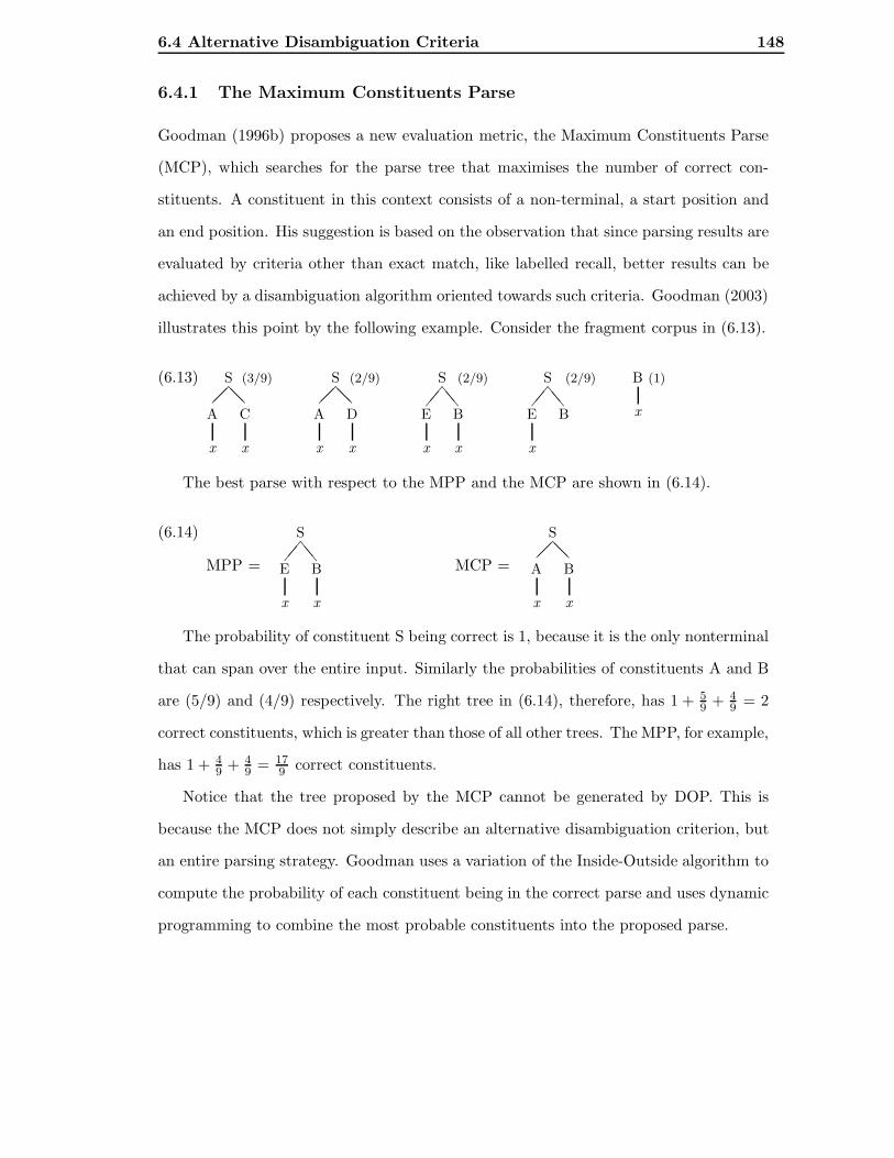
6.4 Alternative Disambiguation Criteria 148
6.4.1 The Maximum Constituents Parse
Goodman (1996b) proposes a new evaluation metric, the Maximum Constituents Parse
(MCP), which searches for the parse tree that maximises the number of correct con-
stituents. A constituent in this context consists of a non-terminal, a start position and
an end position. His suggestion is based on the observation that since parsing results are
evaluated by criteria other than exact match, like labelled recall, better results can be
achieved by a disambiguation algorithm oriented towards such criteria. Goodman (2003)
illustrates this point by the following example. Consider the fragment corpus in (6.13).
(6.13) S
@@A
x
C
x
S
@@A
x
D
x
S
ee%%E
x
B
x
S
ee%%E
x
B
B
x
(3/9) (2/9) (2/9) (2/9) (1)
The best parse with respect to the MPP and the MCP are shown in (6.14).
(6.14) S
ee%%E
x
B
x
S
@@A
x
B
x
MPP = MCP =
The probability of constituent S being correct is 1, because it is the only nonterminal
that can span over the entire input. Similarly the probabilities of constituents A and B
are (5/9) and (4/9) respectively. The right tree in (6.14), therefore, has 1 + 59 + 4
9 = 2
correct constituents, which is greater than those of all other trees. The MPP, for example,
has 1 + 49 + 4
9 = 179 correct constituents.
Notice that the tree proposed by the MCP cannot be generated by DOP. This is
because the MCP does not simply describe an alternative disambiguation criterion, but
an entire parsing strategy. Goodman uses a variation of the Inside-Outside algorithm to
compute the probability of each constituent being in the correct parse and uses dynamic
programming to combine the most probable constituents into the proposed parse.

6.4 Alternative Disambiguation Criteria 149
6.4.2 MBL-DOP
De Pauw (2003) proposes a more efficient approach to disambiguation in which the
memory-based side of DOP is exploited. A parse tree is evaluated in terms of its similarity
to previously experienced structures. Memory-Based Learning (MBL) assumes that
problems can be solved by direct reference to similar previously experienced events.
Memory-Based Language Processing (MBLP) (Daelemans, 1999; Daelemans et al., 2003)
makes direct reuse of previous experience by storing past experience in memory during
the learning phase and using it to solve new problems during the testing phase. It
classifies the results based on their similarity to the examples in memory.
Pattern matching in DOP
DOP shares some of the characteristics of MBLP. Ambiguity resolution is memory based
making direct use of the fragments extracted during training. The alternative to DOP’s
MPP would be to analyse a new input item by searching for the most similar item in
memory and recovering its tree structure. In resolving pattern matching, two issues arise,
first, what the level of matching is, and second, what exactly is similarity between items.
For the former De Pauw (2003) proposes the clausal level, as the sentential level
turns out to be too large. It is possible for two sentences that look very much alike to
turn out to have very dissimilar tree structures (e.g. “She wants a drink” vs “She wants
to drink”). With respect to the latter, he suggests defining similarity on the basis of
the number and size of the patterns used in constructing a tree. Similarity is, therefore,
maximal when the number of chunks combined is minimised, and their size maximised.
The memory based interpretation of DOP employs a bottom up indexing system
to encode contextual information. Starting from the bottom this mechanism initially
searches for terminal nodes and assigns to them an index. A new index is created and
stored in memory for unseen data structures. If the structure has been experienced and
indexed before the index is retrieved from memory (Figure 6.4). The process is applied
recursively for each level in a bottom up manner until the top node is indexed.
Once all nodes of the training corpus have been indexed a Pattern-Matching Proba-

6.4 Alternative Disambiguation Criteria 150
SPPP
NP
prn
VPXXX
v NPPPP
NPQQ
det n
PPaa!!
pp NPQQ
det n
=⇒
SXXX
NP@2
prn
VPXXX
v NPPPP
NP@1QQ
det n
PPaa!!
pp NP@1QQ
det n
=⇒
SXXX
NP@2
prn
VPXXX
v NPPPP
NP@1QQ
det n
PP@1aa!!
pp NP@1QQ
det n
=⇒
SXXX
NP@2
prn
VPXXX
v NP@3PPP
NP@1QQ
det n
PP@1aa!!
pp NP@1QQ
det n
=⇒
SXXX
NP@2
prn
VP@1XXX
v NP@3PPP
NP@1QQ
det n
PP@1aa!!
pp NP@1QQ
det n
=⇒
S@1XXX
NP@2
prn
VP@1XXX
v NP@3PPP
NP@1QQ
det n
PP@1aa!!
pp NP@1QQ
det n
Figure 6.4: Iterative indexing of nodes
bilistic Grammar (PMPG) is created in a way analogous to the one described by Good-
man (1996a). The PMPG corresponding to the last tree in Figure 6.4 is presented in
Figure 6.5. When testing, indexing takes place in the same bottom up manner as with
training, with the only difference being that no new indices are created. The root node
of a tree is hence indexed only if the entire structure can be retrieved from memory.
Everything below an indexed node is pruned. The probability of a parse tree is defined
as the product of the probabilities of its corresponding PMPG rules, not taking into
account the retrieved nodes. This equates to backing-off to a PCFG induced from the
training set to retrieve the probabilities of the rewrite rules used in constructing the
pruned tree.

6.4 Alternative Disambiguation Criteria 151
S@1 → NP@2 VP@1 S → NP@2 VP@1 NP@3 → NP PP@1 NP → NP PP@1
S@1 → NP@2 VP S → NP@2 VP NP@3 → NP@1 PP NP → NP@1 PP
S@1 → NP VP@1 S → NP VP@1 NP@3 → NP PP NP → NP PP
S@1 → NP VP S → NP VP NP@1 → det n NP → det n
NP@2 → prn NP → prn PP@1 → pp NP@1 PP → pp NP@1
VP@1 → v NP@3 VP → v NP@3 PP@1 → pp NP PP → pp NP
VP@1 → v NP VP → v NP NP@1 → det n NP → det n
NP@3 → NP@1 PP@1 NP → NP@1 PP@1
Figure 6.5: Pattern-Matching Probabilistic Grammar
The probability of the parse tree in (6.15(a)), for example, with respect to the PMPG
in Figure 6.5 is equal to the probability of the pruned tree in (6.15(b)), which in turn is
equal to P (S → NP VP) × P (VP → v NP) × P (NP → NP PP)
(6.15) (a) SPPP
NPQQ
det n
VPPPP
v NPPPP
NP
prn
PPaa!!
pp NPQQ
det n
SPPP
NP@1 VPPPP
v NPaa!!
NP@2 PP@1
(b)
In a series of experiments conducted on the ATIS corpus and the Wall Street Journal
corpus aiming to compare the PMPG disambiguator to a simple PCFG one, De Pauw
(2003) reports an increase in exact match. Overall parse accuracy, however, remained
below DOP1 standards. It turns out that the PMPG disambiguator overestimates sub-
structure size during pattern matching.
6.4.3 Simplicity-DOP
It is a well-known fact that stochastic grammars show a strong preference for shorter
derivations. In the case of CFGs this results in smaller parse trees with fewer nodes,
which does not provide any assurance in producing the correct parse tree of a sentence.
When using tree fragments rather than rewrite rules, however, the picture becomes quite
different. The shortest derivation in this case does not necessarily generate the smallest
parse tree. This is due to the fact that larger rather than smaller fragments may take

6.4 Alternative Disambiguation Criteria 152
part in the derivation. In the light of this observation Bod (2000b) developed a non-
probabilistic DOP model, known as Simplicity-DOP, that takes advantage of this bias
in favour of the shortest derivation in resolving ambiguity more efficiently.
In Simplicity-DOP the optimal parse tree is defined as being the one generated by
the shortest derivation. Of course there is no guarantee that only a single tree will
be generated by the smallest possible number of subtrees. In such cases, Simplicity-
DOP backs off to the simple frequency counter used in many other DOP versions. The
frequency counter, however, is not used to calculate subtree probabilities, but rather
subtree ranks. The most frequent subtree of any given root node is thus assigned a rank
of 1 with the next most frequent following with a rank 2, etc. These ranks are redefined
in Bod (2002), in order to adjust the score of a low-ranked elementary tree that might,
however, have high-ranked subtrees. Under the new definition the rank of a subtree is
the average value of the initial rank of that tree and the initial ranks of all its subtrees.
Then the ranks of the shortest derivations are computed by summing over the ranks of
the individual subtrees involved in each one. The proposed tree is the one corresponding
to the shortest derivation with the smallest sum.
The shortest derivations can be easily generated by converting subtrees into rewrite
rules of the form root(ti) −→ yield(ti) as described in Section 6.2.2. Indices are again
used to link rules to the subtrees they originated from in order to maintain their internal
structure. All rules are assigned equal probabilities. Then the task of finding the shortest
derivation comes down to finding the most probable derivation which can be efficiently
computed by the Viterbi algorithm.
An empirical evaluation of the performance of DOP1 and Simplicity-DOP reported
in Bod (2000b), showed the latter to perform at least equally well as the former on the
ATIS and the OVIS corpora at subtree depth limits 5 and 6. Unsurprisingly, at small
subtree depths Simplicity-DOP did not perform well since the shortest derivation in these
cases brings up once again the issue of generating the smallest parse tree. Experiments
on a more broad coverage domain using the WSJ corpus have, however, shown DOP1
to perform better than Simplicity-DOP at almost all depths with the exception of 8
where the two were found to have comparable performance. Despite the difference in

6.4 Alternative Disambiguation Criteria 153
the results, Simplicity-DOP constitutes a competent model when taking into account its
great simplicity.
6.4.4 Combining Likelihood and Simplicity
The Simplicity-DOP model described in the previous section achieves relatively high
performance results (though below DOP1 standards), while at the same time it greatly
reduces the computational cost of disambiguation. In order to take advantage of the
strengths of both models, Bod (2003) proposed two alternative versions of DOP that
would combine the benefits of DOP1 and Simplicity-DOP by either selecting the sim-
plest tree from the m most probable (Simplicity-Likelihood-DOP or DOPSL) or the
most probable among the m simplest (Likelihood-Simplicity-DOP or DOPLS). When
m = 1, DOPSL is reduced to DOP1 and DOPLS to Simplicity-DOP. Similarly, as m
approaches the size of the parse tree forest DOPSL converges to Simplicity-DOP and
DOPLS converges to DOP1.
DOPSL and DOPLS were tested on the WSJ corpus using the PCFG-reduction of
Goodman (2003) (with the rule probabilities suggested in Bod, 2001) at different values
of m between 1 and 1000. Both models presented an increase in accuracy as m increased
from 1. DOPSL, however, reached its maximum accuracy levels (90.8% and 90.7% for
LP and LR respectively) at 12 ≤ m ≤ 14 and then started to deteriorate, while the
accuracy of DOPLS kept increasing up until m ≃ 100 where it reached its maximum
accuracy (89.7% LP and 89.4% LR) and stayed at the same levels after that.
Concluding the discussion on what constitutes the best parse (the most probable or
the simplest), both have their advantages and disadvantages. The former achieves higher
accuracy levels but is quite costly, while the latter achieves somewhat lower accuracy
levels but it is a lot simpler. Combining the two into a DOPSL model seems to outperform
the previous two in bringing high accuracy levels together with small processing costs.

6.5 The Most Probable Shortest Derivation 154
6.5 The Most Probable Shortest Derivation
In this section, we describe a likelihood enriched shortest derivation criterion and il-
lustrate that it is an improved approximation of the optimal parse over the shortest
derivation one and the DOPLS one. The most probable shortest derivation (MPSD)
criterion defines the optimal parse tree t∗ as being the one with the most likely shortest
derivation.
t∗ = arg maxt
PMPSD(t) = arg maxt
P (dshortest(t))
DOPMPSD is a frequency-based extension of Simplicity-DOP. The fact that DOPMPSD
compares on a likelihood basis rather than on a length basis the shortest derivations
of each parse of the input string makes it less sensitive to the issue of data sparseness.
Consider, for example the treebank in (6.16) where t1 occurs 7 times, t2 once and t3, t4
and t5 occur 10, 8 and 9 times respectively.
(6.16) Sbb""
t1: A
a
B
b
Sbb""
t2: X
a
Y
b
Sbb""
t3: X
x
Y
y
SHH
t4: x y
SHH
t5: v w
(×7) (×1) (×10) (×8) (×9)
When parsing the string “ab”, there are two shortest derivations of length one corre-
sponding to the fragments t1 and t2 respectively. In this case, Simplicity-DOP backs-off
to the frequency ranking of the subtrees (see section 6.4.3 for the computation of sub-
tree ranks). The final rank assigned to fragment t1 is 5, while to t2 it is 19/4. Since
rank(t1)>rank(t2), t2 becomes the proposed analysis, even though t1 is seven times more
frequent in the training data. The above example poses no problems for DOPMPSD be-
cause PMPSD(t1) = 7/89 while PMPSD(t2) = 1/89, so t1 naturally becomes the proposed
analysis for the string “ab”.
DOPMPSD also resembles to a certain extent the DOPLS model in that it combines like-
lihood and simplicity. Unlike DOPLS, however, it does not inherit DOP1’s bias towards
large trees because it does not sum over the probabilities of alternative derivations.
Even though PMPSD(t), is not a true estimator because it does not identify a prob-
ability distribution over the set of all possible parses (i.e.∑
tPMPSD(t) ≤ 1 rather than

6.6 Summary 155
∑
tPMPSD(t) = 1), it is characterised by one desirable property typically required of es-
timators, that of rank consistency. The concept of rank consistency will be introduced
more formally in the following chapter, but the intuition is that it preserves the fre-
quency ranking of the trees in the training corpus. Next, we show that DOPMPSD is
rank consistent. Let TC be some training corpus and FTC the resulting fragment cor-
pus. Additionally, let d(t) denote some derivation of t, and l(d) the length of d. Then,
∀ t ∈ TC, t ∈ FTC and l(dshortest(t)) = 1. It follows that:
PMPSD(t) = P (dshortest(t)) =|t|F TC
|r(t)|F TC
=|t|TC
|r(t)|F TC
Then ∀ t1, t2 ∈ TC such that r(t1) = r(t2), the following holds:
|t1|TC ≤ |t2|TC ⇒ |t1|TC
|r(t1)|F TC
≤ |t2|TC
|r(t1)|F TC
⇒ |t1|TC
|r(t1)|F TC
≤ |t2|TC
|r(t2)|F TC
⇒ PMPSD(t1) ≤ PMPSD(t2)
Even though DOPMPSD suffers from a statistical point of view, it provides a likelihood-
based approach to the computationally attractive shortest derivation. DOPMPSD enjoys
great efficiency advances over DOP1, because the shortest derivation can be computed
efficiently through Viterbi optimisation under the assumption that all fragments are
equally likely. In addition, from a cognitive perspective it has long been argued that
although people seem to register frequencies, the human disambiguator does not calculate
the probability of all derivations of a certain analysis when resolving ambiguity.
6.6 Summary
The focus of this chapter was the computational complexity of processing new input
under DOP. Parsing as directed by the composition operation is extremely inefficient and
has consequently never been implemented. Instead a number of alternative strategies
are employed all using some kind of CFG backbone for generating the parse forest of an

6.6 Summary 156
input string.
In addition, computing the MPP has been shown to be NP-complete. In order to
avoid exponential time disambiguation, approximations of the MPP are typically used in
practical applications. We presented several approaches to approximating the MPP from
the literature, some based on Monte Carlo sampling and others on recursive sampling.
Following this, we gave an overview of other DOP-like models that resolve ambiguity
more efficiently by adopting different criteria for the best parse. Evaluation metrics
in these models include the Maximum Constituents Parse, the degree of similarity to
previously experienced events, the shortest derivation and a combination of simplicity
(i.e. shortest derivation) and likelihood (i.e. MPP).
The chapter concluded with suggesting a new evaluation metric for the optimal parse
in DOP based on the most probable shortest derivation. The MPSD criterion suffers
from a statistical point of view in that it does not identify a probability distribution over
the set of all possible parses. Notwithstanding its statistical status, it also enjoys several
advantages over the traditional MPP criterion with the most salient of these being the
great reduction in the cost of computing the optimal analysis. The practical capabilities
of DOPMPSD are still to be evaluated in practice.

Chapter 7
Probability Estimation in DOP
In this chapter we introduce some key concepts from estimation theory and present an
overview the various estimators that have been devised for computing the MPP.
7.1 Introduction
The issue of the probabilistic algorithm employed in DOP for disambiguation purposes
has been the focus of several discussions in the literature, starting from Bod (1992,
1995). As already mentioned, DOP decomposes the elements of a training corpus TC
into subtrees and assigns some probability to each of these. The subtree probabilities
were initially associated with their relative frequency of occurrence in the fragment corpus
FTC as shown in (7.1).
(7.1) P (ti) =|ti|FTC∑
r(t)=r(ti)
|t|FTC
The DOP1 estimator, however, was shown by Johnson (2002) to be biased and incon-
sistent. The aim of this chapter is to present the problems that arise from these two
properties, and describe how other existing estimators attempt to solve these.
The chapter is structured as follows: Section 7.2 discusses some of the practical lim-
itations of DOP1 and presents two alternative estimators as potential partial solutions
to DOP1’s problems. Section 7.3 introduces more formally the concepts of bias, consis-

7.2 Simple DOP estimators 158
tency, strong consistency and rank consistency. Finally, in Section 7.4 we describe three
non-trivial estimators from the literature and discuss how they stand with respect to the
desirable properties an estimator should have.
7.2 Simple DOP estimators
7.2.1 Problems with DOP1
The subtree probability definition in (7.1) in conjunction with the fact that the number
of subtrees extracted from a corpus tree grows exponentially with the tree size assign
a disproportionate amount of the overall probability mass to large subtrees. To illus-
trate the bias of DOP1 towards large subtrees let us consider an example. Take the
corpus in Figure 7.1.
(t1) S
@@a b
(×3) (t2) Sll,,
P
a
Q
b
(×1)
Figure 7.1: Toy training corpus.
The resulting fragment corpus is shown in Figure 7.2.
S
@@a b
S
ll,,P
a
Q
b
S
ll,,P
a
Q
S
ll,,P Q
b
S
ll,,P Q
P
a
Q
b
(3/7) (1/7) (1/7) (1/7) (1/7) (1) (1)
Figure 7.2: Fragment corpus enriched with subtree probabilities.
Quite straightforwardly, t1 is assigned a total probability of 3/7 while t2 4/7 mak-
ing it the preferred analysis for the string ab even though t1 is three times more likely in
the training data. The obvious problem that arises from the overwhelming proportion
of probability mass assigned to subtrees extracted from large corpus trees is classifica-
tion errors.
The bias effects can get very strong. Quoting Bonnema and Scha (2003), for a
treebank containing 1000 balanced binary trees, 999 out of which are of depth five and

7.2 Simple DOP estimators 159
one of depth six, 99.8% of the total probability mass is assigned to the subtrees extracted
from the corpus tree of depth six. It is natural to wonder, therefore, how DOP1 has
managed to produce such significant results as those reported in the literature so far.
The answer is through imposing a set of constraints such as limiting the maximum
subtree depth or the maximum number of substitution sites or lexical items in a subtree.
An additional drawback of the DOP1 estimation method is that it is inconsistent.
Consider, for example, the corpus in (7.2) where the first tree occurs twice and the second
three times. The resulting fragment corpus is depicted in (7.3).
(7.2) (t1) SZZ
X
a
Y
b
(×2) (t2) Scc##
Z
a
Z
b
(×3)
(7.3) SZZ
X
a
Y
b
SZZ
X Y
b
SZZ
X
a
Y
Scc##
Z
a
Z
b
Scc##
Z Z
b
Scc##
Z
a
Z
(1/10) (1/10) (1/10) (3/20) (3/20) (3/20)
SZZ
X Y
Scc##
Z Z
Z
a
Z
b
X
a
Y
b(1/10) (3/20) (1/2) (1/2) (1) (1)
Since the two corpus trees are of the same structure and have the same size, the
second one should be the preferred analysis of the string “ab” since it is more frequent.
Calculating the parse tree probabilities, however, shows that:
P (t1) =1
10+
1
10+
1
10+
1
10=
4
10=
32
80
P (t2) =3
20+
3
20
1
2+
3
20
1
2+
3
20
1
4=
27
80
DOP1, therefore, identifies t1 as the preferred analysis, indicating that it is incon-
sistent. The inconsistency does not occur only for the particular relative frequencies in
this example. Consider the training corpus in (7.2) to be of size n, with the relative
frequency of t1 being p and that of t2 being 1− p. A consistent estimator would propose
analysis t1 for the string “ab” for all p > 1/2. The total number of S-rooted subtrees

7.2 Simple DOP estimators 160
produced from this corpus is 4n. The parse tree probabilities now become:
P (t1) =pn
4n+
pn
4n+
pn
4n+
pn
4n= p
P (t2) =(1 − p)n
4n+
(1 − p)n
4n
1
2+
(1 − p)n
4n
1
2+
(1 − p)n
4n
1
4=
9(1 − p)
16
DOP1 proposes t1 when P (t1) > P (t2) ⇒ p > 9(1−p)/16 ⇒ p > 9/25. The inconsistency
hence causes DOP1 to propose the wrong analysis ∀9/25 < p > 12.5/25. The notions of
bias and consistency will be introduced more formally in Section 7.3.
7.2.2 The Bonnema estimator
Bonnema et al. (1999, 2000) proposed an alternative estimator to tackle DOP1’s bias
towards large fragments. On the basis that the elements in the training corpus do
not carry any information about the subtree-probability pairs that were used in their
derivation, the new estimator makes use of Laplace’s principle of insufficient reason,
which states that in the absence of information regarding a set of alternative solutions
all possibilities should be assigned equal probabilities. All derivations of the trees in the
treebank are a priory considered equally likely.
Assuming a uniform distribution over the derivations of a single tree τ , the substitu-
tion probability P (ti) of a subtree ti, is defined as the number of derivations of τ that
start with ti divided by the total number of derivations δ(τ) of τ .
(7.4) P (ti) =|d ∈ δ(τ) : d = ti ...|
|δ(τ)|
Let N(τ) denote the number of non-root non-terminal nodes in τ . Then |δ(τ)| = 2N(τ)
(i.e. the number of possible derivations of τ equals the cardinality of the powerset of
the set of non-root non-terminal nodes of τ). After ti is substituted on τ , N(τ) − N(ti)
substitution nodes remain available. Equation (7.4) becomes:
(7.5) P (ti) =2N(τ)−N(ti)
2N(τ)= 2−N(ti)

7.2 Simple DOP estimators 161
Equation (7.5) defines the substitution probability of ti in terms of its complexity. When
generalising over every tree in TC, the total probability mass (i.e. 1) of each root category
is divided among its members in such a way that each one receives a proportion analogous
to its relative frequency of occurrence. The probability of a subtree ti, hence, becomes:
(7.6) P (ti) = 2−N(ti)|ti|FTC∑
r(t)=r(ti)
|t|TC
The probability of a derivation d a parse tree T are defined as in DOP1, so they become:
P (d) =
m∏
i=1
2−N(ti)|ti|FTC∑
r(t)=r(ti)
|t|TC
(7.7)
P (T ) =
n∑
j=1
mj∏
i=1
2−N(tij ) |tij |FTC∑
r(t)=r(tij )
|t|TC
(7.8)
The probabilities assigned to the fragment corpus in Figure 7.2 (at the beginning of
Section 7.2.1) by this estimator are 3/4, 1/16, 1/16, 1/16, 1/16, 1 and 1 respectively. The
probabilities of the initial subtrees in Figure 7.1 hence become 3/4 and 1/4, reflecting the
fact that the first tree is three times more frequent than the second in the training data.
The reduction of the probability mass assigned to large subtrees is quite radical in
comparison to DOP1. Take, for example, the treebank in (7.9), with t2 occurring six times.
(7.9) U````
t1 : Uaaa!!!
Ucc##
A
a
B
b
Ucc##
C
c
D
d
Uaaa!!!
Ucc##
E
e
F
f
Ucc##
G
g
H
h
UXXXX
t2 : X
x
Y ×6
y
Take f1 and f2 to denote the fragments that have the exact same structure as t1 and
t2 respectively. Their corresponding DOP1 and DOPBonn probabilities are:
PDOP1(f1) = 1/766 PBonn(f1) = 1/212992
PDOP1(f2) = 3/383 PBonn(f2) = 3/26

7.2 Simple DOP estimators 162
This estimator was shown by Bonnema and Scha (2003) to be consistent for PCFG
distributions. DOPBonn, however, suffers from the reverse situation to DOP1 (i.e. it
is biased towards small fragments). Despite this fact, it should perform better than
DOP1 on the unrestricted DOP model because its preference towards small subtrees is
not as strong as DOP1’s preference towards large subtrees. To the best of our knowledge
this argument has not been tested. In the case of the restricted DOP model, however,
Sima’an and Buratto (2003) report very disappointing empirical results on the OVIS
corpus for the Bonnema estimator. This suggests that DOPBonn seriously underestimates
substructure size as a disambiguation parameter. We will illustrate this limitation in
Chapter 8 where we propose an alternative DOP estimator that addresses this issue.
7.2.3 The Maximum Likelihood Estimator
The Maximum Likelihood Estimator (MLE) assigns probabilities to corpus fragments
such that the probability of the treebank is maximised. In order for the probability of
the treebank to be maximised, all trees in TC must be assigned a probability equal to
their relative frequency in TC (7.10).
(7.10) PMLE(ti) =|ti|TC∑
r(t)=r(ti)
|t|TC
The only subtrees that have a non-zero frequency in TC are those that occur as full
parse trees in the training data. Consider, for example, a training corpus consisting
of the tree in (7.11(a)). The corresponding fragment corpus enriched with the subtree
probabilities assigned by the MLE is depicted in (7.11(b)).
(7.11) (a) X
@@Y
a
Y
b
(b) X
@@Y
a
Y
b
X
@@Y Y
b
X
@@Y
a
Y
X
@@Y Y
Y
a
Y
b
(1) (0) (0) (0) (0) (0)
As can be seen, DOPMLE completely overfits the treebank, assigning zero proba-
bilities to all parse trees outside TC. Consequently, DOPMLE is consistent (Zollmann,

7.3 Bias and Consistency 163
2004), but it is of no practical use unless cross-validation is put in force to avoid overfit-
ting Bod (2000a, 2006).
7.3 Bias and Consistency
In this section we formalise the notion of an estimator and introduce two key properties
in estimation theory: those of bias and consistency. We will start with defining some
terminology commonly used in statistical parsing. Following Zollmann and Sima’an
(2005), we define a probabilistic parsing model as a tuple < G,P > that consists of a
grammar G (the fragment corpus in the case of DOP) generating a set of parses Ω, and
a probability distribution P over the set of parses Ω, P : Ω → [0, 1]. A treebank TC
is a sequence of samples from Ω. A treebank of size n (i.e. TC =< t1, t2, .., tn >) is a
sequence of n independent variables (TC ∈ Ωn) distributed according to the probability
function P .
An estimator est is a function that determines a probability distribution over the
set of all possible parses Ω based on the training data (i.e. the treebank). We will
use estn : Ωn → M , where M is the set of probability distributions over Ω, to denote
an estimator whose input is a treebank of size n. For a particular sequence TC ∈ Ωn,
estn(TC) = P , where P ∈ M . It follows that estn(TC) is a random variable whose values
range over the probability distributions P in M . estn(X) (where X can take values TCi
such that TCi ∈ Ωn) is a function of random variables and as such its expected value
(i.e. long-term average) is given by:
(7.12) E[estn(X)] =∑
X
estn(X)P (X)
7.3.1 Bias
An estimator is unbiased for some probability distribution P over Ω iff ∀ TCi ∈ Ωn
distributed according to P , E[estn(TCi)] = P . In order to show that an estimator
is biased with respect to some probability model M it suffices to find some sequence
TC =< t1, t2, .., tn > distributed according to P ∈ M for which E[estn(TC)] 6= P .

7.3 Bias and Consistency 164
Generally speaking, being unbiased is a desirable property of an estimator. Having
said this, there are estimation problems where either the issue of bias is of limited
importance or, as Hardy (2003) points out, a biased estimator is better than any unbiased
estimator. In the case of DOP, Zollmann (2004) showed that bias is, in fact, a necessary
property of an estimator so that it does not completely overfit the treebank.
7.3.2 Consistency
Let TC be a treebank whose elements are distributed according to the distribution P .
Then an estimator is said to be consistent iff it approaches P in the limit (i.e. when the
treebank size grows to infinity). Consistency is typically determined in terms of a loss
function L(estn(TC), P ) which measures the difference between the estimate estn(TC)
and the true parameter P . An estimator estn is consistent with respect to M if its
expected loss at P approaches zero in the limit (7.13).
(7.13) limn→∞
E[L(estn(TC), P )] = 0, ∀P ∈ M
It is evident from the above that the concept of consistency varies depending on how
the loss function is defined. Johnson (2002), for example, defines the loss function as:
L(estn(TC), P ) =∑
t∈Ω
P (t)[estTC(t) − P (t)]2
where estTC(t) is an abbreviation of estn(TC)(t). Prescher et al. (2003), on the other
hand, define the loss function as:
L(estn(TC), P ) = |estn(TC) − P |
Another way of determining a consistent estimator is in terms of an admissible error ǫ.
Quoting Zollmann (2004), an estimator is then considered consistent if for each ǫ > 0, its
estimate deviates from the true parameter by more than ǫ with a probability approaching
zero when the sample size approaches infinity (7.14). Zollmann terms this notion strong
consistency, in order to differentiate it from the previous notion of consistency, and shows

7.4 Non-trivial DOP estimators 165
that strong consistency implies consistency.
(7.14) limn→∞
supt∈Ω
∑
TC∈Ωn
|estTC(t)−P (t)|≥ǫ
P (TC) = 0
Nguyen (2004) introduces yet another consistency related concept, that of rank con-
sistency, to refer to the property of an estimator that preserves the frequency ranking
of the trees in the training corpus. An estimator is, hence, considered rank consistent if
∀ t1, t2 ∈ TC such that P (t1) ≤ P (t2), estTC(t1) ≤ estTC(t2).
7.4 Non-trivial DOP estimators
Even though, bias is a necessary property of any DOP estimator that does not com-
pletely overfit the treebank, the bias of DOP1 towards large fragments and the bias
of the Bonnema estimator towards small fragments negatively affect their performance.
Inconsistency only makes matters worse. This section will present three alternative es-
timators from the DOP literature that have tackled these issues through methods other
than posing a set of constraints such as maximum depth or number of lexical anchors, etc.
7.4.1 Back-off DOP
Sima’an and Buratto (2003) have suggested that the effects of DOP1’s bias towards large
fragments can be alleviated through recursive estimation of the DOP parameters (i.e.
the weights of the fragments). The estimator they propose is based on the hierarchical
organisation of derivations in terms of the so called back-off graph. Subtrees are classified
as being complex or atomic. A complex subtree t is one for which there exist two other
subtrees t1 and t2 such that t = t1 t2. According to the definition of the derivation
probability in DOP P (t1 t2|r(t1)) = P (t1|r(t1))P (t2|r(t2)), where r(ti) denotes the
root of ti. The chain-rule states that P (t1 t2|r(t1)) = P (t1|r(t1))P (t2|t1, r(t1)). The
derivation t1 t2, therefore, assumes that P (t2|t1) ≈ P (t2|r(t2)). This weakening of
context from P (t2|t1) to P (t2|r(t2)) is known as a back-off. The derivation t1 t2 is said
to be a back-off of t. Atomic subtrees are those that do not have any back-off.

7.4 Non-trivial DOP estimators 166
The back-off graph is a directed acyclic graph whose nodes consist of subtree pairs
(derivations of length two) that constitute the back-off of some other complex fragment.
The edges in the graph point from one complex subtree in a given node to the node
containing its back-off. The first layer in the hierarchy consists of the subtrees that do
not participate in the back-off of any other fragment (i.e. the full parse trees in the
training data). Each of the remaining layers consists of fragment pairs that constitute
the back-offs of fragments in the previous layer. Consider, for example, the fragment
corpus in Figure 7.3 produced from the treebank containing t1.
t1 Sbb""
NP
John
VP
V
slept
t2 SQQ
NP
John
VP
V
t3 SQQ
NP
John
VP
t4 SQQ
NP VP
V
slept
t5 SZZ
NP VP
V
t6 SZZ
NP VP
t7 VP
V
slept
t8 VP
V
t9 V
slept
t10 NP
John
Figure 7.3: Fragment corpus produced from tree t1.
The back-off graph for the fragments is shown in Figure 7.4. t0 is the start symbol.
t0 t1
t2 t9 t3 t7 t4 t10
t3 t8 t5 t10 t6 t10 t8 t9 t5 t9 t6 t7
t6 t10 t6 t8 t8 t9
9 ?
XXXXXXXXXXXXXXXz
/
@@@@R
?
PPPPPPPPPPPPq
)
AAAAU
@@@@R
?
Figure 7.4: Back-off graph of the subtrees in Figure 7.3.

7.4 Non-trivial DOP estimators 167
Once this partial order over subtrees has been determined, estimation of the frag-
ment probabilities is carried out iteratively by transferring probability mass from com-
plex fragments to their back-offs. Initially each subtree ti is assigned some probability
P 0(ti|r(ti)) = Pf (ti|r(ti)) based on a predefined estimator (e.g. DOP1). After each iter-
ation j this probability estimate P j(ti|r(ti)) is updated to the newly computed estimate
PBO(ti|r(ti)). The algorithm used for transferring probability mass from one fragment
to another is an adaptation of the Katz formula and is expressed by:
PBO(t2|t1) =
P jGT (t2|t1) + α(t1)Pf (t2|r(t2)) if [P j(t2|t1) > 0]
α(t1)Pf (t2|r(t2)) otherwise
where α(t1) = 1−∑t2:f(t1,t2)>0
P jGT (t2|t1) is a normalisation factor ensuring that the probabilities of
subtrees with the same root sum up to one. The PBO(t|r(t)) and PBO(t1|r(t1)) estimates
are given by:
PBO(t|r(t)) = Pf (t1|r(t1))P jGT (t2|t1)
PBO(t1|r(t1)) = (1 + α(t1))Pf (t1|r(t1))
Back-off parameter estimation in Tree-DOP (also extended to LFG-DOP by Hearne
and Sima’an, 2004) has produced very promising empirical results on the OVIS corpus
(Sima’an and Buratto, 2003). The fact that it uses DOP1 to compute the initial fragment
probabilities, however, means that it inherits DOP1’s inconsistency, as pointed out by
Prescher et al. (2003).
7.4.2 DOP*
As already seen in Section 7.2.3, DOPMLE, even though consistent, it is of no practical
use. DOP*, proposed by Zollmann (2004), is the first consistent estimator to assign
non-zero probabilities to parse trees outside the training corpus. DOP* approximates
the concept of maximum likelihood, but avoids overfitting using held-out estimation.
The training corpus TC is split into two parts, the extraction corpus EC from which
the fragments are extracted, and the held-out corpus HC from which the fragment prob-

7.4 Non-trivial DOP estimators 168
abilities are computed so that the likelihood of the EC-derivable part of HC (i.e. the set
of trees in HC that can be derived from the fragments extracted from EC) is maximised.
According to Zollmann (2004), this can be achieved by maximising the joint probability
of the shortest derivations of the parse trees in HCEC. We use HCEC and HCnon−EC
to refer to the EC-derivable and the non EC-derivable parts of HC respectively. The
DOP* estimation process can be summarised as follows:
First, the probability mass punkn to be reserved for smoothing is determined by:
(7.15) punkn =|HCnon−EC|
|HC|
For each fragment fk (k = 1...N) involved in the shortest derivations of the trees
in HCEC compute the quantity rk based on the relative frequency of the fragment’s
occurrence in the shortest derivations of the parse trees in HCEC:
rk =∑
t∈HC
|t|HC
|sd(t)|
|sd(t)|∑
i=1
|fk|sdi(t)
where |sd(t)| is the number of shortest derivations of t and |fk|sdi(t) is the number of
times fk occurs in the ith shortest derivation of t. For each non-terminal R in TC set:
βR = punkn if R ∈ Root
1 otherwise
where Root is the set of root nodes of the fragments fk. Then each fragment fk is
assigned some weight β(fk)
(7.16) β(fk) = (1 − βr(fk))rk
N∑
k=1
rk
and for all other fragments fi in FTC, β(fi) = 0. The smoothing weight βsmooth(f)
of all fragments in FTC is determined by:
(7.17) βsmooth(f) =βr(f)|f |FTC∑
r(f ′)=r(f)
|f ′|FTC

7.4 Non-trivial DOP estimators 169
Final fragment probabilities in DOP* are determined by:
(7.18) P (f) = β(f) + βsmooth(f)
An interesting point about this estimator is that it does not necessarily assign a
non-zero probability to all fragments in FTC. A conjoined interpretation of equations
(7.16), (7.17) and (7.18) implies that a fragment f has zero probability unless it either
participates in a shortest derivation of some tree in HCEC or there is at least one parse
tree in HC that cannot be derived from the fragments extracted from EC (i.e. there is
some probability mass reserved for smoothing). Clearly, if the second condition is not
met, a large number of fragments would be assigned zero probabilities. This, on the
one hand, increases the efficiency of the model to a great extent but, on the other, it
negatively affects its coverage.
7.4.3 DOPα
Based on the intuition that when a tree appears more often than another tree in the train-
ing corpus the former should have a higher probability in the language than the latter,
Nguyen (2004) devised an alternative estimator, DOPα, which preserves the frequency
ranking of trees in the training corpus (i.e. it is rank consistent).
The DOPα philosophy relies on changing the current view of what a treebank really
is. So far a treebank consisted of all full parse trees used for training. A treebank and
a training corpus were synonymous. Nguyen (2004) suggests that a treebank should
contain not only the full parses used for training, but all fragments extracted from those
trees as well. This means that the estimator should be able to generate not only the full
parse trees in TC but also all fragments in FTC.
The existing definition of a derivation in terms of left-most substitution, however,
does not allow extending the current definitions of derivation and parse tree probability
to partial analyses. Consider, for example, the subtrees in (7.19).

7.4 Non-trivial DOP estimators 170
(7.19) t1 S
ll,,NP VP
ee%%V NP
Jim
t2 Scc##
NP
Jim
VP
\\V NP
t3 S
ll,,NP VP
\\V NP
t4 S
@@NP VP
t5 VP
ee%%V NP
Jim
t6 VP
\\V NP
t7 NP
Jim
Even though (t3 t7), (t4 t5) and (t4 t6 t7) could in principle produce t1, leftmost
substitution restricts the possible derivations of t1 to the length one derivation consisting
of t1 itself. The fragment t2, on the other hand, has three possible derivations: (t2),
(t3t7) and (t4t7t6). To overcome this problem, Nguyen (2004) extends the derivation
process to derivation* which combines fragments in all possible ways. In the case of
complete parse trees, the concepts of derivation* and its probability are equivalent to
the original concepts of a DOP derivation and its probability respectively. In what
follows, we use Pα(fi) and pα(fi) to refer to the probabilities of fi as a (partial) tree and
as a fragment respectively.
Once the estimator is enabled to generate all fragments in the fragment corpus,
preserving the frequency ranking can be achieved by assigning to parse trees (whether
partial or complete) probabilities analogous to their relative frequency in the fragment
corpus. In other words,
Pα(f) = α|f |FTC∑
f ′
|f ′|FTC= α × rfF TC(f)
The probability of a subtree f as a fragment rather than as a partial parse tree turns
out to be:
pα(f) =
α × rfF TC(f) if depth(f) = 1
α × rfF TC(f) − P′
α(f) if depth(f) > 1
where P′
α(f) =∑
d(f)length(d(f))>1
Pα(d(f)).
Nguyen (2004) provides a tractable recursive estimator for pα(f). The proportional-
ity factor α is determined by successive reductions from the value one until the condition
Pα(f) = α × rfF TC(f) is satisfied ∀f ∈ FTC, in which case the resulting estimator be-
7.5 Summary 171
comes rank consistent. Empirical evaluation on the OVIS corpus of the DOPα estimator
against DOP1 showed DOPα to start outperforming DOP1 on the exact match criterion
after subtree depth four. This is in line with the theoretical motivation of DOPα, in
which the probability assigned to a large fragment only accounts for the interdependen-
cies of its subparts.
7.5 Summary
We have provided a general overview of the various approaches to parameter estimation
within the DOP framework. We presented a number of different estimators and discussed
some of their formal properties with respect to the bias and consistency concepts of
estimation theory. In short, DOP1 has been shown to be biased towards large trees and
inconsistent. The Bonnema estimator was proposed as an answer to DOP1’s bias but
turned out to be susceptible to the reverse situation (i.e. biased towards small trees).
The MLE estimator, though unbiased and consistent, completely overfits the treebank
raising practicality issues.
From an estimation theoretical point of view, things stand better with the non-trivial
estimators presented in the last section. Back-off DOP, even though sensitive to DOP1’s
inconsistency, adequately addresses the issue of bias towards large fragments. DOP*,
on the other hand, is the only consistent estimator proposed thus far to the best of our
knowledge. Finally, DOPα is also not biased towards large fragments, while at the same
time it guaranties retaining the frequency ranking of the elements in the treebank.

Chapter 8
Reconsidering Disambiguation
under DOP
This chapter investigates certain issues related to current disambiguation practices in
DOP with special reference to the derivation and fragment probabilities.
8.1 Introduction
This chapter investigates certain issues related to current disambiguation practices in the
DOP framework. In Section 8.2 we address the need for meaningful comparison of trees
that belong to different categories and suggest two alternatives on how to overcome the
problem. In Section 8.3 we investigate how the negative effects of DOP1’s bias for large
trees and DOPBonn’s bias towards small trees can be alleviated by ensuring a controlled
preference for large over small substructure size. We illustrate that the proposed esti-
mator adequately deals with disambiguation cases that pose problems for the other two.
8.2 Cross-Categorical Constituent Comparison
None of the estimators presented in Chapter 7 take into account the fact that before
initiating the derivation process, no information regarding the potential root of the con-
stituent to be derived is known. On the contrary, the probabilities associated with

8.2 Cross-Categorical Constituent Comparison 173
the subtrees presuppose that the root node of a subtree is known before the relevant
derivation step. This section concentrates on the problems that arise from not taking
into account our ignorance about the category of the constituent to be derived. Two
alternative solutions are put forward and compared on an efficiency basis.
8.2.1 Problem Definition
The estimators presented thus far make use of sample spaces containing only trees of a
single category, thus assuming that the root node label of a subtree is known in advance.
This, of course, is the case for all subtrees taking part in the derivation process except
for the first one. In this instance, considering the probability associated with the subtree
given its root category causes the probability of the whole derivation to be conditioned
upon some predefined root category. As a result, parse tree probabilities can be sensibly
interpreted only within the limits of some specific root identifiable sample space.
Formally speaking, this does not pose problems for STSGs because their definition
assumes a start symbol. In practice, however, start symbols are either not used in their
strict sense, or multiple start symbols are defined to allow for parsing subsentential
phrases. Taking this to be the case, leads to the following fundamental question. How
do we compare trees belonging to different categories?
Consider, for example the following situations. Given a predefined DOP grammar,
is a given word like book more likely to be parsed as a noun or as a verb? Or even, is a
constituent like her leaving school more likely to be parsed as an DP, or as a VP? In certain
domains the need for cross-categorical comparison is greater. In human disambiguation
this is strongly related to the amount of context available. Phrases such as film, song or
article titles, that appear out of context present a higher degree of ambiguity. The film
title “Super Size Me”, for example could either be a VP or an NP. Assuming that the
mere existence of these situations identifies the need for cross-categorical comparison,
we will turn to investigating how this can be achieved.
We will first illustrate how the disambiguation algorithms discussed in previous chap-
ters assign to corpus trees probabilities disanalogous to what is expected, based on their
observed relative frequency and known facts about independence of events. Our discus-

8.2 Cross-Categorical Constituent Comparison 174
sion will be based on the following observation. Fragment probabilities are identified
with respect to some root-identifiable part of the corpus being the sample space of al-
ternatives so they sum up to n, where n is the number of distinct root categories in the
corpus, so they are not true probabilities.
In order to illustrate our point, we will be presenting examples using the DOP1 and
the Bonnema estimators. The reason we have chosen these is because their underlying
estimation process is simpler and more straightforward than that of the non-trivial es-
timators presented in the previous chapter. We want to emphasise, however, that the
need for cross-categorical comparison is independent to the underlying estimator. The
following discussion and the solutions to be proposed hold for all of them, since they all
assume that the category of the constituent to be derived is known in advance.
Consider, for example, the treebank in (8.1) giving rise to the fragment corpus in
(8.2). For each subtree we have calculated both its PDOP1 and its PBonn probability.
(8.1) (ta) DPaa!!
D
his
VGer
leaving
(tb) VPaa!!
D
him
VGer
leaving
(tc) VPHH
V
left
NP
N
Jane
(8.2) DPHH
D
his
VGer
leaving
DPbb""
D
his
VGer
DPHH
D VGer
leaving
DPbb""
D VGer
VPHH
D
him
VGer
leaving
VPHH
D
him
VGer
PDOP1 : (1/4) (1/4) (1/4) (1/4) (1/10) (1/10)
PBonn : (1/4) (1/4) (1/4) (1/4) (1/8) (1/8)
VPbb""
D VGer
VPHH
D VGer
leaving
VPbb""
V
left
NP
N
Jane
VPQQ
V NP
N
Jane
VPQQ
V
left
NP
N
VPQQ
V NP
N
PDOP1 : (1/10) (1/10) (1/10) (1/10) (1/10) (1/10)
PBonn : (1/8) (1/8) (1/16) (1/16) (1/16) (1/16)
VPQQ
V
left
NP
VPQQ
V NP
NP
N
Jane
NP
N
N
Jane
V
left
D
his
D
him
VGer
leaving
PDOP1 : (1/10) (1/10) (1/2) (1/2) (1) (1) (1/2) (1/2) (1)
PBonn : (1/8) (1/8) (1/2) (1/2) (1) (1) (1/2) (1/2) (1)

8.2 Cross-Categorical Constituent Comparison 175
Even though the corpus does not meet the independence constraint, which states
that the application of a rewrite rule, or the selection of a subtree in this case, is an
independent event, two conclusions can be drawn about the probabilities of ta, tb and
tc by observing the data. First tc does not exhibit any internal dependencies. In a
PCFG analogy, this translates as: the fact that VP → V NP is selected does not affect
the probability of neither V being expanded as “left” nor NP being expanded as N.
The probability assigned to tree tc should, therefore, be equal to its observed relative
frequency.
Trees ta and tb, on the other hand, do exhibit internal dependencies. D is a lot more
likely to be expanded as “his” rather than “him” given that the rule DP → D VGer
has been selected. This positive tendency of (DP → D VGer) and (D → his) occurring
together, however, is equal to the positive tendency of (VP → D VGer) and (D → him)
occurring together. As a result, the probabilities assigned to ta and tb are expected to
be equal given that their observed relative frequencies are the same. Table 8.1, however,
shows that neither model reflects the expected observations. Clearly, the fact that VP
is a more densely populated root category disrupts the way probabilities are assigned to
constituents of different categories. This disruption can cause misclassification errors.
(ta) (tb) (tc)
Relative frequency 1/10 1/10 1/10
PDOP1 3/4 3/10 6/10
PBonn 3/4 3/8 4/8
Table 8.1: Relative frequencies, DOP1 and DOPBonn probabilities of ta, tb and tc.
The probabilities seen so far are conditioned upon the root node label, hence they
constitute a reasonable measure of comparison only if they are interpreted as such. Each
of the sample spaces identified by some category has a total probability mass of 1. 3/4
is not, therefore, the probability of ta. Rather, given that a tree starts with DP, it shows
its likelihood of being this particular tree. Similarly, given that the tree to be derived
starts with VP, its probability of being tb is 3/10 or 3/8 depending on the estimator used.
Next, we will demonstrate that DOPBonn is not capable of generating trees with
true probabilities. We chose the particular estimator at random, but the same holds

8.2 Cross-Categorical Constituent Comparison 176
for all other estimators presented in Chapter 7, since they all define the probability
of a derivation as the product of the probabilities of the fragments taking part in the
derivation. Suppose we have a sample of size n consisting of trees tx and ty below,
with relative frequencies rf(tx) = p and rf(ty) = (1 − p), where p can take any value
from 0 to 1.
(8.3) (tx) (ty)
AZZ
X
z
X
z
BZZ
Y
z
Y
z
Given that the resulting corpus meets the independence constraint, the trees should be
generated with probabilities PBonn(tx) = p/3 and PBonn(ty) = (1 − p)/3, which are the
relative frequencies of tx and ty in the training corpus depicted in (8.3). By definition,
PBonn(tx) =4∑
j=1
n∏
i=12−N(tij ) |tij |F TC
|r(tij)|TC=
4∑
j=1
n∏
i=1
14
|tij |F TC
|r(tij)|TC= 1
4
4∑
j=1
n∏
i=1
|tij |F TC
|r(tij)|TC
In this example, however, |tij | = |r(tij)| = pn because there is no other constituent in
the corpus with the same root as tx. As a result, regardless of the frequencies of tx and
ty in the corpus, tx is always going to be assigned a probability of 1 (PBonn(tx) = 1).
This, again, is an unsurprising finding since the probability mass assigned to each root
category is 1 and tx has no other tree in its own sample space to share this probability
with. One might wonder about the probability of ty, which seems to be 0. This reflects
the probability of ty with respect to the sample space identified by category A (i.e.
P(ty|A)), and since ty is not of category A, its probability is naturally zero. If we change
our working sample space from the one identified by A to the one identified by B, the
probability of ty becomes 1 (Pcond(ty)=P(ty|B)=1) and that of tx 0.
8.2.2 Putting all Fragments under a Single Category
The question of how to compare trees cross-categorically remains. The above discussion
suggests that DOP is not equipped to handle such a task. One way of attacking the
problem would be to incorporate a pseudo start-symbol, Z, in the design of the gram-
mar. The reason Z is a pseudo start symbol is that it is not a member of the set of

8.2 Cross-Categorical Constituent Comparison 177
nonterminal symbols identifying the grammar. It is an extra symbol employed to simply
mark constituent completeness and it does not bare any category related meaning at
all. If the pseudo start symbol is formally incorporated in the grammar, parsing will
generate, for each input string, pairs of almost identical parse trees, where one element
will include the start symbol and one will not. A parse tree will then be considered
complete iff it is anchored at exactly all the items in the input and it is rooted at the
pseudo start symbol Z (for ease of reference we will refer to Z simply as a start symbol
henceforth).
Z should be formally integrated in the grammar creation process, in order to reflect
the fact that all initial trees and their subconstituents are complete fragments. Since
the output of Root explicitly spells out all complete constituents found in the training
data, it is there that Z should be introduced. Under this view the training corpus would
contain all subtrees produced by Root and a copy of each one of these rooted at the start
symbol. The set of complete constituents produced from the training corpus in (8.3) is
presented in (8.4).
(8.4) (t′x) (t′y)
Z
All,,
X
z
X
z
Z
Bll,,
Y
z
Y
z
Z
X
z
Z
Y
z
All,,
X
z
X
z
Bll,,
Y
z
Y
z
X
z
Y
z
pn (1 − p)n 2pn 2(1 − p)n pn (1 − p)n 2(1 − p)n 2pn
Recalculating the probabilities shows that:
PBonn(t′x) =8∑
j=1
n∏
i=1
2−N(tij ) |tij||r(tij)|
=4∑
j=1
n∏
i=1
2−3 p n
pn + (1 − p)n + 2pn + 2(1 − p)n
+
8∑
j=5
n∏
i=1
2−1 p n
pn + (1 − p)n + 2pn + 2(1 − p)n2−21
=4
8
p n
3n+
4
8
p n
3n=
p
3

8.2 Cross-Categorical Constituent Comparison 178
Similarly, PBonn(t′y) = (1 − p)/3. Formally incorporating a start symbol as part of the
grammar creation process thus provides a way of addressing the issues discussed so far.
It enables cross-categorical constituent comparison, and it assigns to trees probabilities
that agree with the assumptions made based on their observed relative frequencies. The
only problem is that the fragment corpus more than doubles in size. While a set of m
initial trees produce a grammar of size n without a start symbol, the same set of initial
trees produces a grammar of size greater than 2n with a start symbol. This otherwise
unjustifiable increase in the number of subtrees would have a significant negative impact
on the computational cost of resolving ambiguity with the new grammar.
8.2.3 Redefining the Probability of a Derivation
An alternative to the approach discussed in the previous section comes from considering
the issue of known vs unknown information at each derivation step. When initiating the
derivation process nothing is known about the potential root category of the first subtree
to be selected. In other words, the first subtree f1 is selected with respect to the sample
space identified by the fragment corpus. Each subsequent fragment fi taking part in
the derivation, on the other hand, is selected with respect to the sample space identified
by all fragments having the same root as fi. It seems, therefore, that two probabilities
should be associated with each subtree to reflect what is known before its selection; a
prior probability which will be used for derivation initial selection and a conditional one
which will be used if the subtree is selected later on in the derivation process.
In what follows we investigate how the probability of a derivation, and consequently
that of a parse tree, will be affected by this argument. From this point onwards we will
use P (t|r(t)) to refer to the probability of a subtree that is conditioned upon its root
category and P (t) to refer to the probability of a subtree with respect to the sample
space identified by the fragment corpus. Similarly, we will also use P (d|r(t1)) to refer
to the probability of a derivation as defined in the literature so far, and P (d) to refer to
the new definition of the probability of a derivation that makes use of P (t) for the initial
subtree.
Let P (ti|r(ti)) be the probability distribution identified by one (any one) of the

8.2 Cross-Categorical Constituent Comparison 179
estimators presented in Chapter 7. Moreover, assume that P (ti|r(ti)) assigns to a subtree
ti probability λ(ti). According to the Bayes’ theorem:
(8.5) P (ti|r(ti)) =P (ti ∩ r(ti))
P (r(ti))=
P (ti)P (r(ti)|ti)P (r(ti))
=P (ti)
P (r(ti))
Rearranging (8.5), we get:
(8.6) P (ti) = P (ti|r(ti))P (r(ti)) = P (r(ti))λ(ti)
Note that, according to (8.6), the fragment corpus probability of a subtree depends on
the probability of its root category and its previous weight λ(ti).
Let now tij denote a subtree taking part in the derivation dj , with t1j being the initial
subtree of dj . The probability of a derivation dj =< t1j , ..., tmj > is now defined as the
product of the fragment corpus probability of the initial subtree and the probabilities of
all subsequent subtrees with respect to their root identifiable sample spaces.
P (dj) = P (t1j)
m∏
i=2
P (tij|r(tij))
= P (r(t1j))λ(t1j)m∏
i=2
λ(tij)
= P (r(t1j))
m∏
i=1
λ(tij)
= P (r(t1j))P (dj |r(t1j))
The above shows that the prior probability of the derivation initial subtree need not
be known in order to compute the probability of a derivation. P (dj) only depends on
P (dj |r(t1j)) and the probability of the root node category of the resulting parse tree T .
Consequently, the probability of T becomes:
(8.7) P (T ) =
k∑
j=1
P (dj) =
k∑
j=1
P (r(t1j))P (dj |r(t1j)) = P (r(T ))P (T |r(T ))
Similarly, P (T ) depends on the probability of T given its root node category and the

8.2 Cross-Categorical Constituent Comparison 180
probability of its root node category. In order to see the effect of this modification, let
us re-examine the examples considered earlier. With respect to the example in (8.1), the
new probabilities become:
P (ta) = P(DP)PBonn(ta|r(ta)=DP) = (1/10)(3/4) = 3/40 and
P (tb) = P(VP) PBonn(tb|r(tb)=VP) = (2/10)(3/8) = 3/40,
which confirms our observation that the two probabilities should be equal. Moreover,
the probability of tc, P (tc) = P(VP) PBonn(tc|r(tc)=VP) = (2/10)(4/8) = 1/10, is equal to
its observed relative frequency, as anticipated, since tc presents no internal dependencies.
Turning now to the second example in (8.3) the new probabilities are as follows:
P (tx) = P (A)PBonn(tx|r(tx)=A) =pn
pn + (1 − p)n + 2pn + 2(1 − p)n1 =
p
3
P (ty) = P (B)PBonn(ty|r(ty)=B) =(1 − p)n
pn + (1 − p)n + 2pn + 2(1 − p)n1 =
1 − p
3
These probabilities accurately reflect what was expected (they are equal to the relative
frequencies of the corresponding trees) for any value of p.
In the DOP literature, a training corpus TC is taken to consist of the initial trees
used for training. In the discussion above, we silently took an alternative view of what a
treebank consists of. We assumed that TC contains all fragments produced by Root from
the set of initial trees in order to enable comparison of complete subconstituents as well.
This change in what the training corpus actually contains is by no means necessary, so
long as the root probabilities and the relative frequencies are computed with respect to
the same corpus.
Next we show that the above modification in the derivation probability definition
does not affect the (in)consistency status of the underlying estimator. Let TC be a
training corpus that contains m different root categories. Let TCi denote some part
of TC that contains trees of the same root category such thatm⋃
i=1(TCi) = TC. Let
P (t|r(t)) be a probability distribution over Ωr(i), where r(i) denotes the root category
(i.e. start symbol) of TCi. Then if P (t|r(t)) is consistent with respect to the probability

8.2 Cross-Categorical Constituent Comparison 181
models induced by each TCi, P (t) will be consistent with respect to the probability
model induced by TC. According to Zollmann (2004), if P (t|r(t)) is consistent then
there exist two positive real numbers ǫ and q such that:
(8.8)∑
TCi∈Ω|TCi|
r(i)
|rfTCi(t)−P (t|r(t))|≥ǫ
P (TCi|r(i)) ≤1
4nǫ2≤ q, ∀ n ≥ 1
4ǫ2q
What we will show is that if (8.8) holds then∑
TC∈Ωn
|rfTC(t)−P (t)|≥ǫ
P (TC) ≤ q.
∑
TC∈Ωn
|rfTC(t)−P (t)|≥ǫ
P (TC) =m∑
i=1
∑
TCi∈Ω|TCi|
r(i)
|rfTC(t)−P (t)|≥ǫ
P (r(i))P (TCi|r(i))
=m∑
i=1
∑
TCi∈Ω|TCi|
r(i)
| |TC||TCi|
rfTC(t)− |TC||TCi|
P (t)|≥ |TC||TCi|
ǫ
P (r(i))P (TCi|r(i))
=
m∑
i=1
∑
TCi∈Ω|TCi|
r(i)
|rfTCi(t)−P (t|r(t))|≥
|TC||TCi|
ǫ
P (r(i))P (TCi|r(i))
≤m∑
i=1
∑
TCi∈Ω|TCi|
r(i)
|rfTCi(t)−P (t|r(t))|≥ |TC|
|TCi|ǫ
P (TCi|r(i))
by (8.8)≤
m∑
i=1
1
4n( |TC||TCi|
ǫ)2by (8.8)≤
m∑
i=1
q(|TCi||TC| )
2
=q
|TC|2m∑
i=1
(|TCi|)2 ≤ q
|TC|2 |TC|2 = q

8.3 Fragment Probability Estimation 182
Redefining the derivation probability in order to enable cross-categorical constituent
comparison is both linguistically and statistically more sound than the approach de-
scribed in Section 8.2.2. In addition, it does not suffer from any additional processing
costs while at the same time the ambiguity of the resulting grammar is not affected.
The modification proposed here is of particular interest to the HPSG-DOP model
presented in the first part of this thesis. This is due to the fact that the need for mean-
ingful cross-categorical comparison becomes more acute in this model, the reason being
that a start structure (i.e. the equivalent of a start symbol in a CFG) is sometimes not
formally specified. In such cases, the start structure is taken to be the most general fea-
ture structure licenced (i.e.[
⊤]
) (Copestake, 2002). Since[
⊤]
subsumes all phrasal
and lexical descriptions licenced by the grammar, no CAT feature based classification is
appropriate for identifying the competition set of derivation initial fragments.
8.3 Fragment Probability Estimation
In Chapter 7, we illustrated DOP1’s bias towards large fragments. DOPBonn, which
was designed to tackle this issue, ends up in the reverse situation, as we shall show
next. In this section we introduce a new estimator that improves over the performance
of these two, by allowing for a restricted (in comparison to DOP1) preference towards
large substructure size.
Let us first illustrate DOPBonn’s bias towards small trees via a simple example. Take
the treebank in (8.9) where the X-rooted trees occur once each and the Z-rooted tree
occurs n times (i.e. n is a positive integer).
(8.9) X
ZQQ
A
a
B
b
X
ZQQ
C
c
D
d
ZQQ
C
a
D
b
The corresponding fragment corpus enriched with the weights DOPBonn assigns to its
elements is depicted in (8.10).

8.3 Fragment Probability Estimation 183
(8.10) X
ZQQ
A
a
B
b
X
ZQQ
A
a
B
X
ZQQ
A B
b
X
ZQQ
A B
X
ZQQ
C
c
D
d
X
ZQQ
C
c
D
X
ZQQ
C D
d
X
ZQQ
C D
X
Z
2−4 2−4 2−4 2−4 2−4 2−4 2−4 2−4 2−1
ZQQ
A
a
B
b
ZQQ
A
a
B
ZQQ
A B
b
ZQQ
C
c
D
d
ZQQ
C D
d
ZQQ
C
c
D
ZQQ
C
a
D
b
ZQQ
C
a
D
ZQQ
C D
b
2−2
n+22−2
n+22−2
n+22−2
n+22−2
n+22−2
n+22−2nn+2
2−2nn+2
2−2nn+2
ZQQ
A B
ZQQ
C D
A
a
B
b
C
c
D
d
C
a
D
b
2−2
n+2 2−2 n+1n+2 1 1 1
n+11
n+1n
n+1n
n+1
What we are interested in is comparing the X-rooted analyses of the string “ab”.
P
(
X
ZHH
A
a
B
b
)
= 4 × 2−4 + 4 × (2−1 2−2
n + 2) =
1
4+
1
2(n + 2)
P
(
X
ZHH
C
a
D
b
)
= 2−4( n
n + 1
)2+2−3
[ n
n + 2+
2n
n + 2
n
n + 1+
n + 1
n + 2
( n
n + 1
)2]
=n2
16(n + 1)2+
n
8(n + 2)× 4n + 1
n + 1
DOPBonn will, therefore, wrongly propose the second analysis for string “ab”, whenever:
n2
16(n + 1)2+
n
8(n + 2)× 4n + 1
n + 1>
1
4+
1
2(n + 2)⇒ n > 4
8.3.1 A New Estimator
The derivation probability is upperly bound by the probability of the derivation initial
subtree. The problem with DOPBonn is that it penalises large subtrees so much that a

8.3 Fragment Probability Estimation 184
long derivation whose probability will be bounded by that of a smaller subtree can end
up having a higher probability than a derivation that was actually seen. Even though
bias is a necessary property of any DOP estimator that does not completely overfit the
treebank (Zollmann, 2004), its effects on performance should be minimised. In addition,
when dealing with size-sensitive biased estimators, one should show preference for the
one favouring large over small substructure size because it is better equipped to capture
more linguistic dependencies (Sima’an and Buratto, 2003). In other words, a small bias
towards large substructure size is preferable.
One way of ensuring a preference towards large substructure size is by assuming a
uniform distribution of all possible derivations of each tree in the treebank after the
derivation initial step. This way a derivation of length greater than one will always be
less likely than a length-one derivation, because its initial upper bound probability will
be reduced at each successive derivation step. Let TC be a treebank consisting of a
single constituent tree τ . Let σ(τ) denote the set of initial fragments τ gives rise to and
|σ(τ)| the size of this set. Then the probability of t becomes:
(8.11) P (t) =1
|σ(τ)|
Let dx denote a derivation of length x. From Equation (8.11) it follows that:
P (d1) =1
|σ(τ)| ≥ P (d>1)
Consider now a treebank TC containing more than one constituent trees. Each
fragment t might belong to the set of initial fragments of more than one constituent
trees. From each of these it will receive a weight of 1|σ(τ)| . Activating the Maximum
Likelihood Principle, the probability of a subtree t is now defined by the probability
function:
(8.12) P (t) =∑
τ : t∈σ(τ)
1
|σ(τ)||τ |TC∑
τ ′: r(τ ′)=r(τ)
|τ ′|TC
=∑
τ : t∈σ(τ)
1
|σ(τ)|rfTC(τ)

8.3 Fragment Probability Estimation 185
Note that each subtree can receive different probability amounts from its various
source trees depending on their size. The probability of a derivation d =< t1...tn > is
again the product of the probabilities of the fragments taking part in the derivation:
(8.13) P (d) =n∏
i=1
(
∑
τ : ti∈σ(τ)
1
|σ(τ)|rfTC(τ)
)
Accordingly, the probability of a parse tree T is:
(8.14) P (T ) =m∑
j=1
n∏
i=1
(
∑
τ : tij∈σ(τ)
1
|σ(τ)|rfTC(τ)
)
To see the performance effects of this estimator, let us reconsider the example in
(8.9). The frequency of the X category in the training corpus is two. The number of
subtrees extracted from each X-rooted tree is five. Each X-rooted fragment is assigned
a probability P (ti) = 15 × 1
2 = 110 apart from
X
Z, which occurs twice and is, therefore,
assigned a probability of 210 . The probabilities of all remaining fragments coincide with
those of DOPBonn in (8.10). The new probabilities for the X-rooted analyses of the
string “ab” become:
P
(
X
ZHH
A
a
B
b
)
= 4 × 1
10+ 4 × 2
10× 1
4(n + 2)=
2
5+
2
10(n + 2)
P
(
X
ZHH
C
a
D
b
)
=1
10
( n
n + 1
)2+
1
40
[ n
n + 2+
2n
n + 2
n
n + 1+
n + 1
n + 2
( n
n + 1
)2]
=n2
10(n + 1)2+
n
40(n + 2)× 4n + 1
n + 1
The estimator will propose the second analysis when:
n2
10(n + 1)2+
n
40(n + 2)× 4n + 1
n + 1>
2
5+
2
10(n + 2)

8.3 Fragment Probability Estimation 186
This inequality, however, is false ∀ n > 0. The new estimator will, as a result, propose
the analysis seen in the training data no matter how large n gets.
Note that, since all fragments of a given tree receive equal amounts of its overall
probability mass and since there are more large fragments than small ones, the above
estimator is clearly biased towards large fragments. Unlike DOP1, however, this bias is
constrained by the relative frequency of the source tree in the treebank. As a result, the
estimator shows a clear yet controlled preference for large fragments.
Having illustrated the improved performance of the new estimator over DOPBonn,
we will now turn to comparing it with DOP1. Consider the training corpus in (8.15),
with T1 occurring once and T2 occurring n times.
(8.15) Shhhhh(((((
T1 : XPPP
UZZ
A
a
B
b
VQQ
C
c
D
d
YPPP
WZZ
E
e
F
f
ZQQ
G
g
H
h
Sbb""
T2 : A
a
B
b
The generated fragment corpus contains 680 distinct S-rooted subtrees. The 676
produced from T1 have DOP1 weights 14n+676 , while the four produced from T2 have
n4n+676 . What we are interested in is the preferred analysis for the string “ab”. Intuitively
if n > 1, the optimal analysis should be T2. Since we are comparing trees with different
root categories, we will compute derivation probabilities as defined in Section 8.2.3. Let
T3 denote the tree
UHH
A
a
B
b. Let t2i and t3i denote the fragments of T2 and T3 respectively.
The DOP1 probabilities of T2 and T3 are:
PDOP1(T2) = P (S)
4∑
i=1
P (t2i) =n + 1
3n + 15× 4 × n
4n + 676=
n + 1
3n + 15
n
n + 169
PDOP1(T3) = P (U)4∑
i=1
P (t3i) =1
3n + 15× 4 × 1
4=
1
3n + 15
Doing the calculations shows that DOP1 proposes T2 for n > 13. In other words,
even if T1 only occurs once and T2 occurs 12 times in the training corpus, DOP1 will

8.3 Fragment Probability Estimation 187
still rule in favour of T3 being the preferred analysis for “ab”. Under the new estimator,
the weight of each of the 676 subtrees of T1 is 1676 × 1
n+1 while the weight of each of the
four subtrees of T2 is 14 × n
n+1 . The probabilities of T2 and T3 hence become:
Pnew(T2) = P (S)
4∑
i=1
P (t2i) =n + 1
3n + 15× 4 × 1
4× n
n + 1=
n
3n + 15
Pnew(T3) = P (U)4∑
i=1
P (t3i) =1
3n + 15× 4 × 1
4=
1
3n + 15
confirming our previous observation that T2 should be the optimal analysis for all n > 1.
8.3.2 A Linguistic Example
In this section we illustrate with a linguistic example how the above described estimation
procedure provides an improved account of the training data over both the DOP1 and
the Bonnema estimators. Consider the toy training corpus in Figure 8.1, where T1 occurs
twice and T2 three times.
T1: Saaa!!!
NP
She
VPaaa!!!
V
likes
NPHHH
A
visiting
NP
relatives
×2 T2: Saaa!!!
NP
She
VPHH
V
hates
NP
relatives
×3
Figure 8.1: Training Corpus
Take T3 to be the parse of the string “She likes relatives” below.
SHHH
NP
She
VPbb""
V
likes
NP
relatives
Based on the training data, the following facts should be true:
• T2 should be more likely than T1, and

8.4 Conclusions 188
• T1 should be more likely than T3.
The DOP1, the Bonnema and the proposed estimators assign probabilities to parse
trees T1, T2 and T3 as shown in Table 8.2.
T1 T2 T3
DOP1 165.54 10−3 129.11 10−3 46.14 10−3
DOPBonn 86.97 10−3 258.542 10−3 101.53 10−3
New 129.53 10−3 237.87 10−3 75.19 10−3
Table 8.2: Parse tree probabilities
The first row in the table shows that DOP1 fails to account for the fact that T2
occurs more often than T1 in the training data. This is a direct consequence of the
estimator’s bias favouring large corpus trees. Similarly, the second row demonstrates
that DOPBonn assigns an unseen tree (i.e. T3), with a lot less derivations than the seen
tree T1, a considerably larger amount of probability mass than T1. This results from the
estimator’s bias towards small fragments. The proposed estimator, on the other hand,
verifies in both cases what was anticipated from observing the training data (i.e. T1 is
less likely than T2 as well as more likely than T3).
8.4 Conclusions
This chapter looked into several disambiguation related issues in DOP. In Section 8.2 we
argued that DOP does not provide the necessary ground for cross-categorical comparison
of trees. We briefly discussed how formally incorporating a pseudo start symbol in the
design of the grammar can offer the necessary grounds for meaningful disambiguation
across categories. Even though this approach solves the problem, it raises the size of the
grammar to more than twice its original size, causing the the ambiguity inherent to the
grammar to increase significantly.
As an alternative we proposed redefining the probability of a derivation in DOP, in
order to reflect the fact that the root node label of the first constituent to be selected
is unknown when initiating the derivation process. This approach translates the cate-

8.4 Conclusions 189
gory specific probability of a given derivation into category independent by assigning a
weighted amount of the overall probability mass of the training corpus to each root node
label. This approach is both linguistically and statistically more sound. In addition, it
does not suffer from any additional processing costs while at the same time it does not
affect the ambiguity of the resulting grammar.
In Section 8.3, we presented a new estimator that readdresses the issue of the
substructure-size sensitive bias of an estimator based on the following observation. Given
that a training corpus consists of a single tree t, we can ensure preference for seen deriva-
tions over unseen ones by allowing the probabilities of all the derivations of t to be equal
after the derivation-initial step and be reduced at each subsequent derivation step. We il-
lustrated by means of examples that the new estimator performs better that both DOP1
and DOPBonn in cases where the latter two encounter problems.

Chapter 9
Conclusions
9.1 Concluding Remarks
This thesis aimed at making a contribution to two key areas of the DOP framework; the
linguistic and the statistical one. The core of the first part was the portrayal of an HPSG-
DOP model making direct use of feature structure fragments. The discussion began
with a brief introduction to the Tree-DOP, a DOP model using simple phrase structure
trees and identification of its linguistic limitations. In Chapter 2, we gave an overview
of TIGDOP and LFG-DOP, two models that were born from the attempt to enhance
DOP’s linguistic sensitivity. Even though LFG-DOP constitutes a great advancement
from a linguistic point of view, some gray areas in its application have been identified and
are open to further investigation. The most salient of these are that the application of
Discard is not linguistically motivated and that not all LFG well-formedness conditions
can be checked efficiently (i.e. during the derivation process).
We moved on to introducing the HPSG formalism (Chapter 3), paying particular
attention to its formal foundations in order to prepare the ground for the discussion to
follow. Chapter 4 presented the first HPSG-DOP model described by Neumann (1999,
2003). Neumann’s approach is based on extracting an SLTG from a given HPSG parsed
training corpus. The SLTG is used for further processing in a manner similar to Tree-
DOP, only the results can be unfolded to full-blown HPSG feature structures by expand-
ing the constraints associated with the node labels. Even though this approach to DOP

9.1 Concluding Remarks 191
is linguistically more sensitive than Tree-DOP, it also carries some of the disadvantages
associated with LFG-DOP.
Chapter 5 presented a formal description of a DOP model making direct use of HPSG
representations. The general architecture can be summarised as follows: The represen-
tation used for utterance analysis is totally well-typed and sorted feature structures
licenced by a predefined HPSG signature. The fragments used for constructing new
analyses are totally well-typed and sorted subparts of the initial representation. These
fragments are produced by Root and HFrontier, two decomposition operations defined in
terms of the subsumption relation, and the unification and inference procedures of the
underlying typed feature logic. Composition in this model is head-driven and directed
as dictated by the fragment’s head chain. The proposed approach to composition grants
priority to unification candidates that give rise to complete substructures, thus allowing
greater amounts of inference at an earlier stage in comparison to other unification candi-
dates in the same feature structure. Finally, disambiguation is based on identifying the
most probable parse using relative frequency estimation.
The second part of this thesis concentrated on the issue of disambiguation in DOP.
We started by a brief discussion on the computational complexity of parsing and resolv-
ing ambiguity (Chapter 6). Even though the MPP has produced remarkable empirical
results, the cost of computing it is so high that it prohibits the use of deterministic algo-
rithms for its identification. We presented an overview of existing strategies that reduce
the time and space requirements of traditional disambiguation, ranging from the use of
non-deterministic algorithms in identifying the MPP to other easier to compute evalua-
tion metrics. An alternative approach that identifies the optimal parse tree based on the
most probable of the competing shortest derivations was put forward. Even though this
criterion suffers from a statistical point of view, its computation enjoys great efficiency
advances over the MPP.
We moved on to introducing the concepts of bias and consistency from estimation
theory (Chapter 7), and gave an overview of the various existing estimators used for
computing the MPP in DOP. The two trivial estimators DOP1 and DOPBonn have been
shown to suffer from structure size sensitive bias effects, the former towards large trees,

9.2 Directions for Future Research 192
while the latter towards small trees.
The thesis concludes in Chapter 8 with two suggestions on the way derivation and
fragment probabilities are defined in DOP. With regards to the first of these, we observed
that even though Tree-DOP is a type of STSG, the distinguished symbol is sometimes
not appropriately used (i.e. complete constituents are allowed to be rooted at other
symbols). This causes the need for cross-categorical comparison to arise, which the
current definition of the probability of a derivation is not equipped to handle. A slight
modification in this definition suffices to rectify this situation by distributing the overall
probability mass of the training corpus to the possible root categories.
The next issue we considered is the effect of an estimator’s bias in its disambiguation
performance. Bias is a necessary property of any estimator that does not completely
overfit the treebank. The bias of DOP1 towards large trees and DOPBonn towards small
trees, however, has been shown to negatively affect their choices for the optimal parse.
A new estimator that addresses this issue was put forward. Its underlying concept
is to show preference for shorter derivations by penalising longer ones for the extra
derivation steps. A potentially overwhelming bias towards large substructures is avoided
by constraining the probability mass assigned to the subtrees of some initial tree by the
relative frequency of the initial tree in the training corpus. Since the estimator does not
presuppose a particular kind of representation, it can be straightforwardly integrated
with HPSG-DOP.
9.2 Directions for Future Research
The DOP model presented in this thesis enjoys a number of positive characteristics.
The most salient of these is its great linguistic power. One area, however, which we
feel deserves further attention is how HPSG-DOP can become a more robust model of
language performance. Robustness (i.e. the ability to deal with input which is in some
way ill-formed or extra-grammatical) could be approached in different ways. In the case
of unknown words, for example, the techniques described for Tree-DOP by Bod (1995)
(see Chapter 1) can be straightforwardly extended to this model. Robust unification

9.2 Directions for Future Research 193
(Fouvry, 2003), which is based on extending the signature to a lattice to include the
unique joins of every set of incompatible types, provides a promising alternative approach
to this issue.
HPSG-DOP also has a main disadvantage, its immense computational complexity.
The great disambiguation costs of simpler DOP models are further deteriorated by the
additional burden of the online computation of the sets of competing fragments prior
to each derivation step and the significant cost of unification during parsing. We feel,
therefore, that the computational efficiency of HPSG-DOP is an issue open for further
improvement. One way of dealing with this situation could be in terms of an HPSG
analog of the PCFG reduction described by Goodman (2003) for the case of Tree-DOP.
An alternative approach might be in terms of a cheaper to compute best parse criterion
like the most probable shortest derivation proposed in Chapter 6.
HPSG-DOP takes full advantage of the signature thus enabling the fragments pro-
duced to extend their ability of capturing dependencies beyond the syntactic level. In
addition, well-formedness of the final representation in this model can be checked during
the derivation process which means that, unlike other unification-based models, relative
frequency estimation is not necessarily a non-optimal solution to the task of computing
the MPP. While we have discussed how HPSG-DOP behaves from a theoretical point
of view, its empirical evaluation remains outstanding. We plan to implement HPSG-
DOP in the near future and compare it with other linguistically rich DOP models (e.g.
LFG-DOP).
Last but not least, we hypothesise that the estimator proposed in the final chapter
alleviates the negative bias effects of DOP1 and DOPBonn by allowing for a controlled
preference of large over small substructure size. Implementing the proposed estimator
and assessing its effect on accuracy (both with the more traditional Tree-DOP model
and with HPSG-DOP) remains a goal for future research.

Bibliography
Steven P. Abney. Stochastic Attribute-Value Grammars. Computational Linguistics, 23
(4):597–618, 1997.
Ash Asudeh and Mary Dalrymple. Binding Theory. In Keith Brown, editor, Encyclopedia
of Language and Linguistics. Elsevier, Amsterdam, 2nd edition, 2005.
Paul Bennett. A course in Generalized Phrase Structure Grammar. UCL Press, 1995.
Rens Bod. A Computational Model of Language Performance: Data Oriented Parsing.
In Proceedings COLING’92, Nantes, France, 1992.
Rens Bod. Using an Annotated language Corpus as a Virtual Stochastic Grammar. In
Proceedings of AAAI’93, Washington D.C., 1993.
Rens Bod. Enriching Linguistics with Statistics: Performance Models of Natural Lan-
guage. PhD thesis, Universiteit van Amsterdam, Amsterdam, The Netherlands, 1995.
Rens Bod. Beyond Grammar: An Experience-Based Theory of Language. CSLI Publi-
cations, Stanford, 1998.
Rens Bod. Combining Semantic and Syntactic Structure for Language Modeling. In
Proceedings ICSLP-2000, Beijing, China, 2000a.
Rens Bod. Parsing with the Shortest Derivation. In Proceedings of COLING 2000,
volume 1, pages 69–75, Saarbruecken, Germany, 2000b.
Rens Bod. What is the Minimal Set of Fragments that Achieves Maximal Parse Acuu-
racy? In Proceedings of the ACL 2001, Toulouse, France, 2001.
BIBLIOGRAPHY 195
Rens Bod. A Unified Model of Structural Organization in Language and Music. Journal
of Artificial Intelligence Research, 17:289–308, 2002.
Rens Bod. An Efficient Implementation of a New DOP Model. In Proceedings of the
EACL 2003, pages 19–26, Budapest, Hungary, April 2003.
Rens Bod. An All-Subtrees Approach to Unsupervised Parsing. In Proceedings ACL-
COLING 2006, Sydney, 2006.
Rens Bod and Ronald Kaplan. A Probabilistic Corpus-Driven Model for Lexical Func-
tional Analysis. In Proceedings of COLING-ACL’98, Montreal, Canada, 1998.
Rens Bod and Ronald Kaplan. A DOP Model for Lexical-Functional Grammar. In
Remko Scha Rens Bod and Khalil Sima’an, editors, Data-Oriented Parsing, chapter 12,
pages 211–233. CSLI Publications, Stanford, California, 2003.
Rens Bod and Remko Scha. Corpus-Based Methods in Language and Speech Process-
ing, chapter Data-Oriented Language Processing, pages 137–173. Kluwer Academic
Publishers, Boston, 1997.
Rens Bod and Remko Scha. A DOP model for Phrase-Structure Trees. In Remko Scha
Rens Bod and Khalil Sima’an, editors, Data-Oriented Parsing, chapter 2, pages 13–24.
CSLI Publications, Stanford, California, 2003.
Rens Bod, Remko Scha, and Khalil Sima’an. Data-Oriented Parsing, chapter Introduc-
tion, pages 1–9. CSLI Publications, Stanford, California, 2003.
Remko Bonnema. An Alternative Approach to Monte Carlo Parsing. In Remko Scha
Rens Bod and Khalil Sima’an, editors, Data-Oriented Parsing, chapter 7, pages 107–
124. CSLI Publications, Stanford, California, 2003.
Remko Bonnema, Paul Buying, and Remko Scha. A new probability model for Data
Oriented Parsing. In Paul Dekker and Gwen Kerdiles, editors, Proceedings of the 12th
Amsterdam Colloquium, pages 85–90, Amsterdam, The Netherlands, 1999.

BIBLIOGRAPHY 196
Remko Bonnema, Paul Buying, and Remko Scha. Parse Tree Probability in DOP. In
Alexander Gelbukh, editor, Proceedings of the Conference on Intelligent Text Process-
ing and Computational Linguistics, Mexico City, Mexico, 2000. Instituto Polytechnico
Nacional.
Remko Bonnema and Remko Scha. Reconsidering the Probability Model for DOP. In
Remko Scha Rens Bod and Khalil Sima’an, editors, Data-Oriented Parsing, chapter 3,
pages 25–42. CSLI Publications, Stanford, California, 2003.
Gosse Bouma and Gertjan van Noord. Head-driven Parsing for Lexicalist Grammars:
Experimental Results. In Proceedings of the 6th European Chapter of the ACL, pages
71–80, University of Utrecht, The Netherlands, 1993.
Joan Bresnan. The Mental Representation of Grammatical Relations. MIT Press, Cam-
bridge MA, 1982.
Joan Bresnan. Lexical-Functional-Syntax. Blackwell Textbooks in Linguistics. Blackwell,
Oxford, 2001.
Chris Brew. Stochastic HPSG. In Proceedings of the 7th Conference of the European
Chapter of the Association for Computational Linguistics, pages 83–89, Dublin, Ire-
land, 1995.
Bob Carpenter. The Logic of Typed Feature Structures, volume 32 of Cambridge Tracts
in Theoretical Computer Science. Cambridge University Press, 1992.
Jean-Cedric Chappelier and Martin Rajman. A Generalized CYK Algorithm for parsing
Stochastic CFG. In TAPD Workshop, pages 133–137, Paris, 1998.
Jean-Cedric Chappelier and Martin Rajman. Parsing DOP with Monte Carlo Tech-
niques. In Remko Scha Rens Bod and Khalil Sima’an, editors, Data-Oriented Parsing,
chapter 6, pages 83–106. CSLI Publications, Stanford, California, 2003.
Eugene Charniak. Statistical parsing with a context-free grammar and word statistics. In
Proceedings of AAAI’97, pages 598–603, Menlo Park, 1997. AAAI Press/MIT Press.

BIBLIOGRAPHY 197
David Chiang. Statistical parsing with an automatically-extracted tree adjoining gram-
mar. In Proceedings of the 38th Annual Meeting of the Association for Computational
Linguistics, pages 456–463, Hong Kong, China, 2000.
Ann Copestake. The ACQUILEX LKB. Representation Issues in Semi-Automatic Ac-
cquisition of Large Lexicons. In Proceedings of the 3rd ACL Conference on Applied
Natural Language Processing, pages 88–96, Trento, Italy, 1992.
Ann Copestake. The Compleat LKB. Technical Report 316, University of Camridge
Computer Laboratory, 1993.
Ann Copestake. Definitions of typed feature structures. Natural Language Engineering.
Special Issue on Efficient Processing with HPSG, 6(1), 2000.
Ann Copestake. Implementing Typed Feature Structure Grammars. CSLI Publications,
2002.
Boris Cormons. Analyse et desambiguisation: Une Approche a base de corpus (Data-
Oriented Parsing) pour les representations lexicales fonctionnelles. PhD thesis, Uni-
versite de Rennes, France, 1999.
Walter Daelemans. Memory-Based Language Processing. Journal for Experimental and
Theoretical Artificial Intelligence (JETAI), 11(3), 1999.
Walter Daelemans, Jakub Zavrel, Ko van der Sloot, and Antal van den Bosch. TiMBL:
Tilburg Memory Based Learner, version 5.0, Reference Guide. Technical Report 03-10,
ILK, Tilburg University, 2003.
Mary Dalrymple. Lexical Functional Grammar, volume 34 of Syntax and Semantics.
Academic Press, New York, 2001.
Guy De Pauw. An Approximation of DOP through Memory-Based Learning. In
Remko Scha Rens Bod and Khalil Sima’an, editors, Data-Oriented Parsing, chapter 9,
pages 147–168. CSLI Publications, Stanford, California, 2003.

BIBLIOGRAPHY 198
Dan Flickinger and Francis Bond. A Two-Rule Analysis of Measure Noun Phrases.
In Stefan Muller, editor, Proceedings of the 10th International Conference on Head-
Driven Phrase Structure Grammar, pages 111–121. CSLI Publications, 2003.
Daniel Flickinger. Lexical Rules in the Hierarchical Lexicon. PhD thesis, Stanford Uni-
versity, 1987.
Frederik Fouvry. Robust Processing for Constraint-based Grammar Formalisms. PhD
thesis, University of Essex, April 2003.
Gerald Gazdar, Ewan Klein, Geoffry K. Pullum, and Ivan A. Sag. Generalized Phrase
Structure Grammar. Basil Blackwell, Oxford, 1985.
Jonathan Ginzburg and Ivan A. Sag. Interrogative Investigations. CSLI Publications,
Stanford, 2000.
Joshua Goodman. Efficient algorithms for parsing the DOP model. In Conference on
Empirical Methods in Natural Language Processing, pages 143–152, May 1996a.
Joshua Goodman. Parsing Algorithms and Metrics. In Proceedings of the 34th Annual
Meeting of the ACL, pages 177–183, Santa Cruz, CA, June 1996b.
Joshua Goodman. Parsing Inside-Out. PhD thesis, Harvard University, Cambridge,
Massachussets, 1998.
Joshua Goodman. Efficient Parsing of DOP with PCFG-Reductions. In Remko Scha
Rens Bod and Khalil Sima’an, editors, Data-Oriented Parsing, chapter 8, pages 125–
146. CSLI Publications, Stanford, California, 2003.
Francois Grosjean. Spoken word recognition processes and the gating paradigm. Per-
ception and Psychophysics, 28(4):267–283, October 1980.
Michael Hardy. An Illuminating Counterexample. The American Mathematical Monthly,
110:234–238, March 2003.
Mary Hearne. Data-Oriented Models of Parsing and Translation. PhD thesis, School of
Computing, Dublin City University, Dublin, January 2005.

BIBLIOGRAPHY 199
Mary Hearne and Khalil Sima’an. Structured Parameter Estimation for LFG-DOP. In
N. Nicolov, K. Bontcheva, G. Angelova, and R. Mitkov, editors, Recent Advances in
Natural Language Processing III: Selected papers from the RANLP 2003, volume 260
of Current Issues in Linguistic Theory, pages 183–192. John Benjamins, 2004.
Lars Hoogweg. Extending DOP1 with the Insertion Operation. Master’s thesis, Univer-
sity of Amsterdam, January 2000.
Lars Hoogweg. Extending DOP with Insertion. In Remko Scha Rens Bod and Khalil
Sima’an, editors, Data-Oriented Parsing, chapter 17, pages 317–335. CSLI Publica-
tions, Stanford, California, 2003.
Rebecca Hwa. An Empirical Evaluation of Probabilistic Lexicalized Tree-Insertion Gram-
mars. In COLING-ACL, pages 557–563, Montreal, Canada, 1998.
Mark Johnson. The DOP Estimation Method is Biased and Inconsistent. Computational
Linguistics, 28:71–76, March 2002.
Aravind K. Joshi and Yves Schabes. Tree-Adjoining Grammars. In Grzegorz Rozenberg
and Arto Salomaa, editors, Handbook of Formal Languages, volume 3, chapter 2, pages
69–124. Springer-Verlag, Berlin, 1997.
Cornell Juliano and Michael K. Tanenhaus. Contingent Frequency Effects in Syntactic
Ambiguity Resolution. In Proceedings of the 15th Annual Conference of the Cognitive
Science Society, University of Colorodo, 1993. Laurence Erlbaum Associates.
Daniel Jurafsky. A Probabilistic Model of Lexical and Syntactic Access and Disambigua-
tion. Cognitive Science, 20:137–194, 1996.
Daniel Jurafsky, Alan Bell, Michelle Gregory, and William D. Raymond. Probabilistic
Relations between Words: Evidence from Reduction in Lexical Production. In Joan
Bybee and Paul Hopper, editors, Frequency and the emergence of linguistic structure,
pages 229–254. John Benjamins, 2001.
Martin Kay. Functional Grammar. In Proceedings of the 5th Annual Meeting of the
Berkeley Linguistics Society, pages 142–158, 1979.

BIBLIOGRAPHY 200
Martin Kay. Parsing in Functional Unification Grammar. In David R. Dowty, Lauri
Karttunen, and Arnold M. Zwicky, editors, Natural Language Parsing: Psychological,
Computational, and Theoretical Perspectives, Studies in Natural Language Processing,
chapter 7, pages 251–278. Cambridge University Press, 1985.
Martin Kay. Head driven Parsing. In Proceedings of the Workshop on Parsing Technolo-
gies, Pittsburg, 1989.
Alberto Lavelli and Giorgio Satta. Bidirectional Parsing of Lexicalized Tree Adjoining
Grammars. In Proceedings of the 5th European Chapter of the ACL, pages 27–32,
Berlin, Germany, 1991.
Robert Malouf, John Carroll, and Ann Copestake. Efficient feature structure operations
without compilation. Natural Language Engineering, 6(1):29–46, 2000.
Christopher D. Manning. Probabilistic Syntax. In Rens Bod, Jennifer Hay, and Ste-
fanie Jannedy, editors, Probabilistic Linguistics, chapter 8, pages 289–341. MIT Press,
Cambridge, Massachusetts, 2003.
Christopher D. Manning and Ivan A. Sag. Dissociations between Argument Structure
and Grammatical Relations. In Gert Webelhuth, Jean-Pierre Koenig, and Andreas
Kathol, editors, Lexical And Constructional Aspects of Linguistic Explanation, pages
63–78. CSLI Publications, Stanford, CA, 1999.
Christopher D. Manning and Hinrich Schutze. Foundations of Statistical Natural Lan-
guage Processing. MIT Press, Cambridge, Massachusetts, 1999.
Detmar Meurers. Towards a Semantics for Lexical Rules as used in HPSG. In Proceedings
of the Conference on Formal Grammar, Barcelona, Spain, 1995.
Yusuke Miyao, Takashi Ninomiya, and Jun’ichi Tsujii. Probabilistic modeling of argu-
ment structures including non-local dependencies. In Proceedings of the Conference on
Recent Advances in Natural Language Processing, pages 285–291, Borovets, Bulgaria,
2003.

BIBLIOGRAPHY 201
Yusuke Miyao and Jun’ichi Tsujii. Maximum entropy estimation for feature forests. In
Proceedings of the Human Language Technology Conference, 2002.
Mark Moll. Head-Corner Parsing using Typed Feature Structures. Master’s thesis,
University of Twente, August 1995.
Gunter Neumann. Automatic Extraction of Stochastic Lexicalized Tree Grammars from
Treebanks. In 4th workshop on tree-adjoining grammars and related frameworks,
Philadelfia, PA, USA, August 1998.
Gunter Neumann. Learning Stochastic Lexicalized Tree Grammars from HPSG. Tech-
nical report, DFKI, Saarbruecken, 1999.
Gunter Neumann. A Data-Driven Approach to Head-Driven Phrase Structure Gram-
mar. In Remko Scha Rens Bod and Khalil Sima’an, editors, Data-Oriented Parsing,
chapter 13, pages 233–251. CSLI Publications, Stanford, California, 2003.
Thuy Linh Nguyen. Rank Consistent Estimation: The DOP Case. Master’s thesis, ILLC,
Amsterdam, The Netherlands, November 2004.
Stephan Oepen. [incr tsdb()] — Competence and Performance Laboratory. User Manual.
Saarbrucken, Germany, 2001. in preparation.
Stephan Oepen and Ulrich Callmeier. Measure for measure: Parser cross-fertilization.
Towards increased component comparability and exchange. In Proceedings of the 6th
International Parsing Technology Wworkshop, pages 183–194, Trento, Italy, 2000.
Stephan Oepen and John Carroll. Parser engineering and performance profiling. Natural
Language Engineering, 6(1):81–97, 2000.
Neal J. Pearlmutter and Maryellen C. MacDonald. Plausibility and Syntactic Ambiguity
Resolution. In Proceedings of the 14th Annual Conference of the Cognitive Science
Society, Indian University, 1992. Laurence Erlbaum Associates.
Gerald B Penn. The Algebraic Structure of Attributed Type Signatures. PhD thesis,
School of Computer Science, Carnegie Mellon University, Pittsburgh, PA, 2000.

BIBLIOGRAPHY 202
Carl J. Pollard and Ivan A. Sag. Information-based Syntax and Semantics. Number 13
in CSLI Lecture Notes. CSLI Publications, Stanford University, 1987.
Carl J. Pollard and Ivan A. Sag. Head-driven Phrase Structure Grammar. Chicago
University Press, 1994.
Arjen Poutsma. Data-Oriented Translation: Using the Data-Oriented Parsing framework
for Machine Translation. Master’s thesis, University of Amsterdam, The Netherlands,
2000.
Arjen Poutsma. Machine Translation with Tree-DOP. In Remko Scha Rens Bod and
Khalil Sima’an, editors, Data-Oriented Parsing, chapter 18, pages 339–358. CSLI Pub-
lications, Stanford, California, 2003.
Detlef Prescher, Remko Scha, Khalil Sima’an, and Andreas Zollmann. On the Statistical
Consistency of DOP Estimators. In Proceedings of the 14th Meeting of Computational
Linguistics in the Netherlands, Antwerp, Belgium, 2003.
Jeffrey T. Runner. BT Exempt Anaphors: An Argument from Idiom Interpretation. In
Emily Curtis, James Lyle, and Gabriel Webster, editors, Proceedings of WCCFL 16,
pages 367–381. CSLI Publications, 1998.
Ivan A. Sag. Coordination and Underspecification. In Jong-Bok Kim and Stephen
Wechsler, editors, Proceedings of the 9th International Conference on Head-Driven
Phrase Structure Grammar, pages 267–291, Stanford, 2003. CSLI Publications.
Ivan A. Sag and Thomas Wasow. Syntactic Theory: A Formal Introduction. CSLI
Publications, Stanford, 1999.
Ivan A. Sag, Thomas Wasow, and Emily M. Bender. Syntactic Theory: A Formal
Introduction. CSLI Publications, Stanford, 2 edition, 2003.
Remko Scha. Language Theory and Language Technology; Competence and Perfor-
mance. In Q. de Kort and G Leerdam, editors, Computertoepassingen in de Neerlan-
distiek, Almere, 1990. LVVN-Jaarboek.

BIBLIOGRAPHY 203
Yves Schabes and Richard C. Waters. Tree Insertion Grammar: A cubic-time parsable
formalism that lexicalizes Context-Free Grammar without changing the trees pro-
duced. Computational Linguistics, 21(4):479–513, 1995.
Klaas Sikkel and Rieks Op den Akker. Predictive Head-Corner Chart Parsing. In Pro-
ceedings of the 9rd International Workshop on Parsing Technologies, pages 267–275,
Tilburg, The Netherlands, August 1993.
Khalil Sima’an. Computational Complexity of Probabilistic Disambiguation by means
of Tree Grammars. In Proc. of the 16th COLING, volume 2, pages 1175–1180, Copen-
hagen, Denmark, August 1996.
Khalil Sima’an. Learning Efficient Disambiguation. ILLC Dissertation Series 1999-02.
ILLC Publications, Universiteit Utrecht, 1999.
Khalil Sima’an. Computational Complexity of Probabilistic Disambiguation. Grammars,
5(2):125–151, 2002.
Khalil Sima’an. Computational Complexity of Disambiguation under DOP1. In
Remko Scha Rens Bod and Khalil Sima’an, editors, Data-Oriented Parsing, chapter 5,
pages 63–81. CSLI Publications, Stanford, California, 2003.
Khalil Sima’an and Luciano Buratto. Backoff Parameter Estimation for the DOP Model.
In N. Lavrac, D. Gamberger, H. Blockeel, and L. Todorovski, editors, Proceedings of
the European Conference on Machine Learning, Lecture Notes in Artificial Intelligence,
pages 373–384. Springer, 2003.
Hideto Tomabechi. Quasi-Destructive Graph Unification. In Proc. of the 29th ACL, pages
315–322, Berkeley, California, June 1991. Association for Computational Linguistics.
Hideto Tomabechi. Quasi-Destructive Graph Unification with Structure-Sharing. In
Proc. of the 14th COLING, number Nantes, France, pages 440–446, August 1992.
Gertjan van Noord. Head Corner Parsing. In R.L. Johnson C.J. Rupp, M.A. Rosner,
editor, Constraints, Language and Computation, chapter 12, pages 315–338. Academic
Press, 1994.

BIBLIOGRAPHY 204
Andy Way. A Hybrid Architecture for Robust MT using LFG-DOP. Special Issue on
Memory-Based Learning, Journal of Experimental and Theoretical Artificial Intelli-
gence, 11:441–471, 1999.
Andy Way. LFG-DOT: A Hybrid Architecture for Robust MT. PhD thesis, Department
of Language & Linguistics, University of Essex, Colchester, UK, 2001.
Andy Way. Machine Translation Using LFG-DOP. In Remko Scha Rens Bod and Khalil
Sima’an, editors, Data-Oriented Parsing, chapter 19, pages 359–384. CSLI Publica-
tions, Stanford, California, 2003.
Andreas Zollmann. A Consistent and Efficient Estimator for the Data-Oriented Parsing
Model. Master’s thesis, ILLC, Amsterdam, The Netherlands, May 2004.
Andreas Zollmann and Khalil Sima’an. A Consistent and Efficient Estimator for Data-
Oriented Parsing. Journal of Automata, Languages and Combinatorics (JALC), 2005.
Accepted for publication (2005).