Submitted 15 September 2014Accepted 28 November 2014Published 16 December 2014

Corresponding authorEsther Quintero,esther.quintero@conabio.gob.mx

Academic editorPatricia Gandini

Additional Information andDeclarations can be found onpage 12

DOI 10.7717/peerj.703

Copyright2014 Quintero et al.

Distributed underCreative Commons CC-BY 4.0

OPEN ACCESS

A statistical assessment of populationtrends for data deficient MexicanamphibiansEsther Quintero1, Anne E. Thessen2,3, Paulina Arias-Caballero1 andBarbara Ayala-Orozco1

1 Subcoordinacion de Especies Prioritarias, Direccion General de Analisis y Prioridades, ComisionNacional para el Conocimiento y Uso de la Biodiversidad, Mexico D.F., Mexico

2 The Data Detektiv, Waltham, MA, USA3 The Ronin Institute for Independent Scholarship, Montclair, NJ, USA

ABSTRACTBackground. Mexico has the world’s fifth largest population of amphibians and thesecond country with the highest quantity of threatened amphibian species. About10% of Mexican amphibians lack enough data to be assigned to a risk category by theIUCN, so in this paper we want to test a statistical tool that, in the absence of specificdemographic data, can assess a species’ risk of extinction, population trend, and tobetter understand which variables increase their vulnerability. Recent studies havedemonstrated that the risk of species decline depends on extrinsic and intrinsic traits,thus including both of them for assessing extinction might render more accurateassessment of threats.Methods. We harvested data from the Encyclopedia of Life (EOL) and the publishedliterature for Mexican amphibians, and used these data to assess the populationtrend of some of the Mexican species that have been assigned to the Data Deficientcategory of the IUCN using Random Forests, a Machine Learning method that givesa prediction of complex processes and identifies the most important variables thataccount for the predictions.Results. Our results show that most of the data deficient Mexican amphibians thatwe used have decreasing population trends. We found that Random Forests is a solidway to identify species with decreasing population trends when no demographic datais available. Moreover, we point to the most important variables that make speciesmore vulnerable for extinction. This exercise is a very valuable first step in assigningconservation priorities for poorly known species.

Subjects Biodiversity, Bioinformatics, Computational Biology, Conservation BiologyKeywords Mexican amphibians, Statistical assessment, Encyclopedia of life, Random forests,Data harvest, IUCN categories

INTRODUCTIONEfforts to assign risk categories to species are one of the first steps in planning conservation

strategies. One of the most recognized efforts to assign risk categories to species is that

of the International Union for Conservation of Nature (IUCN), which recognizes seven

different extinction risk categories for evaluating species: two of them are for species

How to cite this article Quintero et al. (2014), A statistical assessment of population trends for data deficient Mexican amphibians. PeerJ2:e703; DOI 10.7717/peerj.703

that are already extinct (Extinct and Extinct in the wild), three are for those considered

as threatened (Critically Endangered, Endangered, and Vulnerable), two are for those

species that are not yet threatened (Near Threatened and Least Concern), whereas the

last one is for those species about which not enough information is known to perform an

evaluation (Data Deficient). The IUCN also lists species that have not yet been evaluated

(Not Evaluated).

IUCN’s criteria for assigning a threat category to a species are “quantitative in nature”

meaning that punctuation is given for each category according to a given criteria, but both

the quality and the uncertainty attached to any data in the evaluation vary. Estimates,

inferences, projections and suspected facts based on related data are acceptable, as long as

they can be supported and specified in the documentation. Moreover, time lag between

assessments, human errors associated to them, and the lack of knowledge of the specialists

on any given criteria may cause bias to the results of the assessments.

The Data Deficient category (DD) is assigned to those species in which the available data

is not enough to determine a threat category, not even indirectly: for example, through the

status of their habitat or other causal factors (IUCN, 2012). Only approximately 75,000

out of the 2 million described species are evaluated by the IUCN, and one sixth of them

are Data Deficient (http://www.iucnredlist.org/about/summary-statistics), with 25% of all

amphibians classified as such (Stuart et al., 2004). By lacking a threat status, Data Deficient

species are not taken into account for conservation programs, potentially placing them

at a higher risk of extinction. Thus, it is our objective to evaluate a statistical method to

obtain the population trend of some species categorized as DD as a first step in prioritizing

conservation actions. Our motivation is to test a more automated method of evaluating

risk that can use a wider variety of available data and still give accurate results.

Recent studies have demonstrated that the risk of species decline depends on the specific

threats they face, such as habitat loss, presence of invasive species, and pathogens (extrinsic

traits), and the species’ own biological ability to cope with these threats (intrinsic traits),

such as clutch and body size. Thus, including intrinsic traits along with extrinsic threats

for assessing extinction might render a more accurate assessment of threat (Murray et al.,

2011; Tingley, Hitchmough & Chapple, 2013), and thus improve allocation of resources

(Cardillo & Meijaard, 2012).

Among all terrestrial vertebrates, amphibians are the group with more “rapidly

declining species” recognized (Stuart et al., 2004). Mexico has the world’s fifth largest

population of amphibians (Frost, 2014; Ochoa-Ochoa & Flores-Villela, 2006) with around

375 documented species, and the second country with the highest quantity of threatened

amphibian species, 211 (IUCN, 2014) and whereas 38 (10%) amphibian species are

currently listed as DD (IUCN, 2014) due to the lack of data (i.e., geographic distribution,

threats, population status, etc.) to assign them to a risk status. The development of tools

that allow assessing species’ risk of extinction in the absence of specific demographic

data, as well as understanding which variables increase vulnerability to extinction could

improve our ability to prioritize; focus, and or direct conservation actions in between field

assessments or other types of research can be carried out.

Quintero et al. (2014), PeerJ, DOI 10.7717/peerj.703 2/15

The first Global Amphibian Assessment (Stuart et al., 2004) found that amphibian

declines are not random, but are associated to ecological traits (i.e., stream associated

species), geographic distribution (i.e., montane areas in the Neotropics, Australia

and New Zealand), and specific taxonomic groups (i.e., Leptodactylidae, Bufonidae,

Ambystomatidae, Hylidae, and Ranidae). Moreover, they divided the causes of decline

in three groups: over-exploitation, defined as those declining due to heavy extraction

(concentrated in species in East and Southeastern Asia); reduced habitat, defined as

those that were suffering from extreme habitat loss (concentrated in Southeast Asia, West

Africa, and the Caribbean); and enigmatic declines, those that are declining even though

suitable area remains (restricted mostly to South America, Mesoamerica, Puerto Rico and

Australia). Enigmatic declines were found to be positively associated with streams at high

elevations in the tropics, and chytridiomycosis emerged as the most likely culprit.

Chytridiomycosis is a fungal disease caused by Batrachochytrium dendrobatidis, and

has been related to the decline of at least 43 species of amphibians in Latin America

(Lips et al., 2006). In Mexico, there is an association between higher elevations (from

939 to 3,200 m) and the prevalence of the infection, but does not seem very common

throughout tropical rain forests or lowland deserts (Frıas-Alvarez et al., 2008). The reason

for this marked preference for high areas with temperate climates may be that the optimal

range of growth for this fungus is between 17 and 25 C (Piotrowski, Annis & Longcore, 2004;

Longcore, Pessier & Nichols, 1999). Different surveys for the presence of chytridiomycosis in

Mexico have found the presence of the fungus in different ecosystems, including those that

have reported “enigmatic declines” in amphibian populations (Frıas-Alvarez et al., 2008;

Murrieta-Galindo et al., 2014). The finding by these authors suggests that chytridiomycosis,

along with other threats, may be contributing to some of the amphibian declines.

In this study we harvested data for Mexican amphibians from the Encyclopedia of

Life (EOL) and from published literature and used these data to assess the population

trend of some of the Mexican species assigned to the DD category by the IUCN using

Random Forests, a Machine Learning method algorithm that gives a prediction of complex

processes and identifies the most important variables that account for the predictions

(Breiman, 2001; Cutler et al., 2007; Murray et al., 2011). A recent assessment of DD

mammals using and comparing multiple Machine Learning tools found that Random

Forests perform very well for this type of predictions (Bland et al., in press). This is the

first attempt to evaluate DD Mexican amphibians, and we hope to open the door to an

improvement of the assessment of other groups for which we might lack demographic

data. At the same time, we want to show how automatically harvesting data from online

repositories can be used to answer biological relevant questions.

METHODSSelecting traits for the analysisIn order to assess the population traits of those species listed as Data Deficient, we selected

previously identified intrinsic traits that can predispose species to a greater degree of

Quintero et al. (2014), PeerJ, DOI 10.7717/peerj.703 3/15

vulnerability, as well as a series of extrinsic traits that have been associated to amphibian

decline (Lips, Reeve & Witters, 2003; Stuart et al., 2004).

The extrinsic traits in our analysis were: habitat use; habitat loss/degradation, one of

the biggest concerns for biodiversity (Assessment, 2005; Brooks et al., 2002; Frıas-Alvarez et

al., 2008; Groombridge, 1992; Lips, Reeve & Witters, 2003; Parra-Olea, Garcıa-Parıs & Wake,

1999; Wyman, 1990); desiccation of bodies of water, which can take place independently

of habitat loss and/or degradation (treated separately from other threats due to the high

dependence of many amphibian species on them); presence of introduced species; presence

of pollution; impact of known climatic fluctuations, as some authors have speculated

that changes in precipitation patterns could indirectly contribute to the decline of some

amphibian species, especially in those more sensitive to moisture changes (Carey et

al., 2001; Kiesecker, Blaustein & Belden, 2001; Pounds & Crump, 1994); harvest for pet

trade; presence of chytridiomycosis; and presence of other diseases that may decimate

populations. The intrinsic traits selected for our analysis were snout-vent length, as species

with larger body size have been observed to have a greater chance of decline than those

with a smaller one (Lips, Reeve & Witters, 2003), and ova and clutch size as they are

indirect measures of reproductive effort and reproductive rates, respectively, both linked

to biological vulnerability, development type and breeding habitat, as species that depend

on aquatic habitats seem to be more vulnerable than terrestrial ones (Lips, Reeve & Witters,

2003). The intrinsic traits were used here as a way to understand life history, ecological

preferences, and vulnerability of the analyzed species (Lips, Reeve & Witters, 2003; Murray

et al., 2011). Finally, we used the published population trend data from the IUCN Red

List (IUCN, 2014), as our goal was to determine the population trend for the DD species.

Unfortunately, the terms associated to population trend (decreasing, increasing, stable,

unknown) in the Red List assessments are not quantitative, but rather associated with

expert knowledge. In this respect, we might not have an accurate account of how steeply

or rapidly a population is declining. Moreover, we are aware of the caveat of using these

kinds of data, which might not be completely objective or may even harbor mistakes, as the

primary data source for our analysis. However, they are the only means we have to try to

statistically assess the population trend for DD species, and we decided to use them for the

purpose of this first exercise.

Automated data harvesting from encyclopedia of lifeStarting with a list of scientific names of amphibians in Mexico (Table S1), relevant

data and text were harvested from EOL using TraitBank (CS Parr, N Wilson, K Schulz,

P Leary, J Hammock, J Rice, RJ Corrigan Jr, 2014, unpublished data) and the EOL API

respectively (Parr et al., 2014). API stands for Application Programming Interface. An API

is a piece of software that allows computers to share data without the need for repeated

human action (http://en.wikipedia.org/wiki/Application programming interface). The

code written for this project can be found at GitHub (https://github.com/diatomsRcool/

MexicanAmphibians). Data from EOL TraitBank was retrieved by searching for taxon and

measurement and downloaded as a .csv file. The EOL API was used to filter and harvest

Quintero et al. (2014), PeerJ, DOI 10.7717/peerj.703 4/15

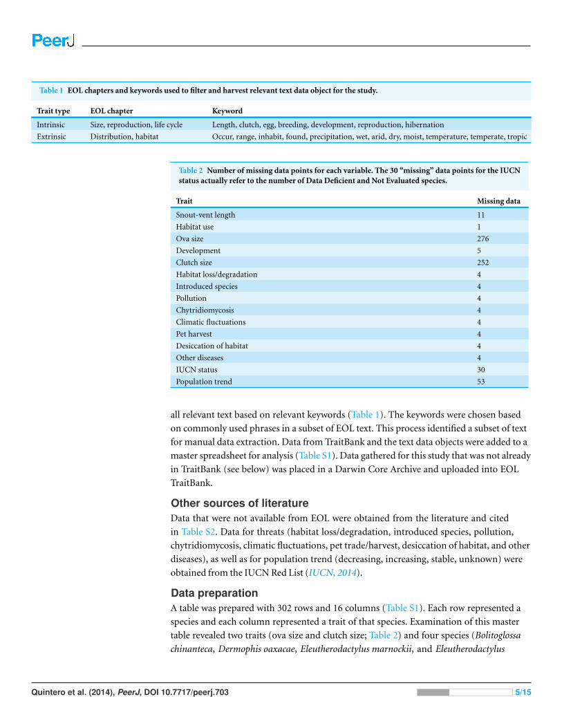
Table 1 EOL chapters and keywords used to filter and harvest relevant text data object for the study.

Trait type EOL chapter Keyword

Intrinsic Size, reproduction, life cycle Length, clutch, egg, breeding, development, reproduction, hibernation

Extrinsic Distribution, habitat Occur, range, inhabit, found, precipitation, wet, arid, dry, moist, temperature, temperate, tropic

Table 2 Number of missing data points for each variable. The 30 “missing” data points for the IUCNstatus actually refer to the number of Data Deficient and Not Evaluated species.

Trait Missing data

Snout-vent length 11

Habitat use 1

Ova size 276

Development 5

Clutch size 252

Habitat loss/degradation 4

Introduced species 4

Pollution 4

Chytridiomycosis 4

Climatic fluctuations 4

Pet harvest 4

Desiccation of habitat 4

Other diseases 4

IUCN status 30

Population trend 53

all relevant text based on relevant keywords (Table 1). The keywords were chosen based

on commonly used phrases in a subset of EOL text. This process identified a subset of text

for manual data extraction. Data from TraitBank and the text data objects were added to a

master spreadsheet for analysis (Table S1). Data gathered for this study that was not already

in TraitBank (see below) was placed in a Darwin Core Archive and uploaded into EOL

TraitBank.

Other sources of literatureData that were not available from EOL were obtained from the literature and cited

in Table S2. Data for threats (habitat loss/degradation, introduced species, pollution,

chytridiomycosis, climatic fluctuations, pet trade/harvest, desiccation of habitat, and other

diseases), as well as for population trend (decreasing, increasing, stable, unknown) were

obtained from the IUCN Red List (IUCN, 2014).

Data preparationA table was prepared with 302 rows and 16 columns (Table S1). Each row represented a

species and each column represented a trait of that species. Examination of this master

table revealed two traits (ova size and clutch size; Table 2) and four species (Bolitoglossa

chinanteca, Dermophis oaxacae, Eleutherodactylus marnockii, and Eleutherodactylus

Quintero et al. (2014), PeerJ, DOI 10.7717/peerj.703 5/15

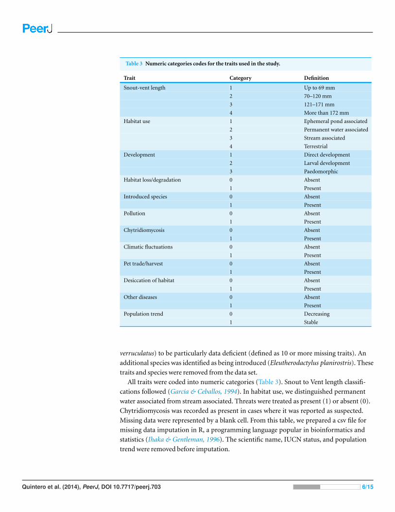
Table 3 Numeric categories codes for the traits used in the study.

Trait Category Definition

Snout-vent length 1 Up to 69 mm

2 70–120 mm

3 121–171 mm

4 More than 172 mm

Habitat use 1 Ephemeral pond associated

2 Permanent water associated

3 Stream associated

4 Terrestrial

Development 1 Direct development

2 Larval development

3 Paedomorphic

Habitat loss/degradation 0 Absent

1 Present

Introduced species 0 Absent

1 Present

Pollution 0 Absent

1 Present

Chytridiomycosis 0 Absent

1 Present

Climatic fluctuations 0 Absent

1 Present

Pet trade/harvest 0 Absent

1 Present

Desiccation of habitat 0 Absent

1 Present

Other diseases 0 Absent

1 Present

Population trend 0 Decreasing

1 Stable

verruculatus) to be particularly data deficient (defined as 10 or more missing traits). An

additional species was identified as being introduced (Eleutherodactylus planirostris). These

traits and species were removed from the data set.

All traits were coded into numeric categories (Table 3). Snout to Vent length classifi-

cations followed (Garcıa & Ceballos, 1994). In habitat use, we distinguished permanent

water associated from stream associated. Threats were treated as present (1) or absent (0).

Chytridiomycosis was recorded as present in cases where it was reported as suspected.

Missing data were represented by a blank cell. From this table, we prepared a csv file for

missing data imputation in R, a programming language popular in bioinformatics and

statistics (Ihaka & Gentleman, 1996). The scientific name, IUCN status, and population

trend were removed before imputation.

Quintero et al. (2014), PeerJ, DOI 10.7717/peerj.703 6/15

Missing data imputationWe used the mice package (Van Buuren & Groothuis-Oudshoorn, 2011) in R to impute

missing values (http://cran.r-project.org/web/packages/mice/mice.pdf). Imputation is a

statistical method for replacing missing data with a probable value based on other available

information (Little & Rubin, 2002). The mice package uses Gibbs sampling of the rest of

the data set to generate imputations (Casella & George, 1992). It is used to avoid bias that

may be introduced by deleting cases with missing values. This was necessary because the

randomForest function did not tolerate missing values. All data were imported into R as

factors, i.e., categories. The Snout-Vent Length, Habitat Use, and Development Type were

imputed as polytomous logistic regression (polyreg). The other traits were imputed using

logistic regression (logreg). These settings are important for proper imputation. Missing

Population Trend data were not imputed. Ten independent imputations were performed

for each missing value. The final value was the mode of the 10 imputations. The data set

before imputation can be found in Table S1. A summary of missing data can be found in

Table 2 and Table S1. The data set after imputation can be found in Table S3. The data

set that includes the imputed data was used for predicting the population trend for those

species that were Data Deficient according to the IUCN evaluation.

Predicting population trendsWe used the randomForest package in R (Liaw & Wiener, 2002) to make predictions

about the population trends for each species of amphibian (http://cran.r-project.org/

web/packages/randomForest/randomForest.pdf). Random Forests is a machine learning

method for classifying objects into categories by building a decision tree (Breiman, 2001).

In this case, we wanted to classify species into stable vs. declining population trend.

Random Forests generates multiple decision trees using a random selection of traits

at each split in the tree. For x traits, the square root of x traits are used at each split.

The final tree depends on the mode of the output of the individual decision trees. It is

important to notice that the resulting population trend, just as in the case of that reported

by IUCN, was not quantitative, but rather just a general tendency. We are aware that this

lack of quantitative data may categorize two species with different natural histories and

demographic trends in the same category, but we are also certain that this was the only way

to proceed with the amount and nature of data that we have. At the same time, this general

trend would result in exactly the very first step to assign conservation priorities to those

species that at the moment are categorized as DD.

Preparing the randomForest was a three-step process: the first step was using training

data, i.e., traits for those species with known population trends, to generate a random

forest object. The second step was testing the random forest object on a separate data set of

species with known population trends. The third step was using the random forest object

to make predictions about population trends for those species listed as Data Deficient and

Not Evaluated by the IUCN (IUCN, 2014).

The data set of species with known population trends was randomly divided in two to

make a training set and a test set. The training data (including the imputed data) was read

Quintero et al. (2014), PeerJ, DOI 10.7717/peerj.703 7/15

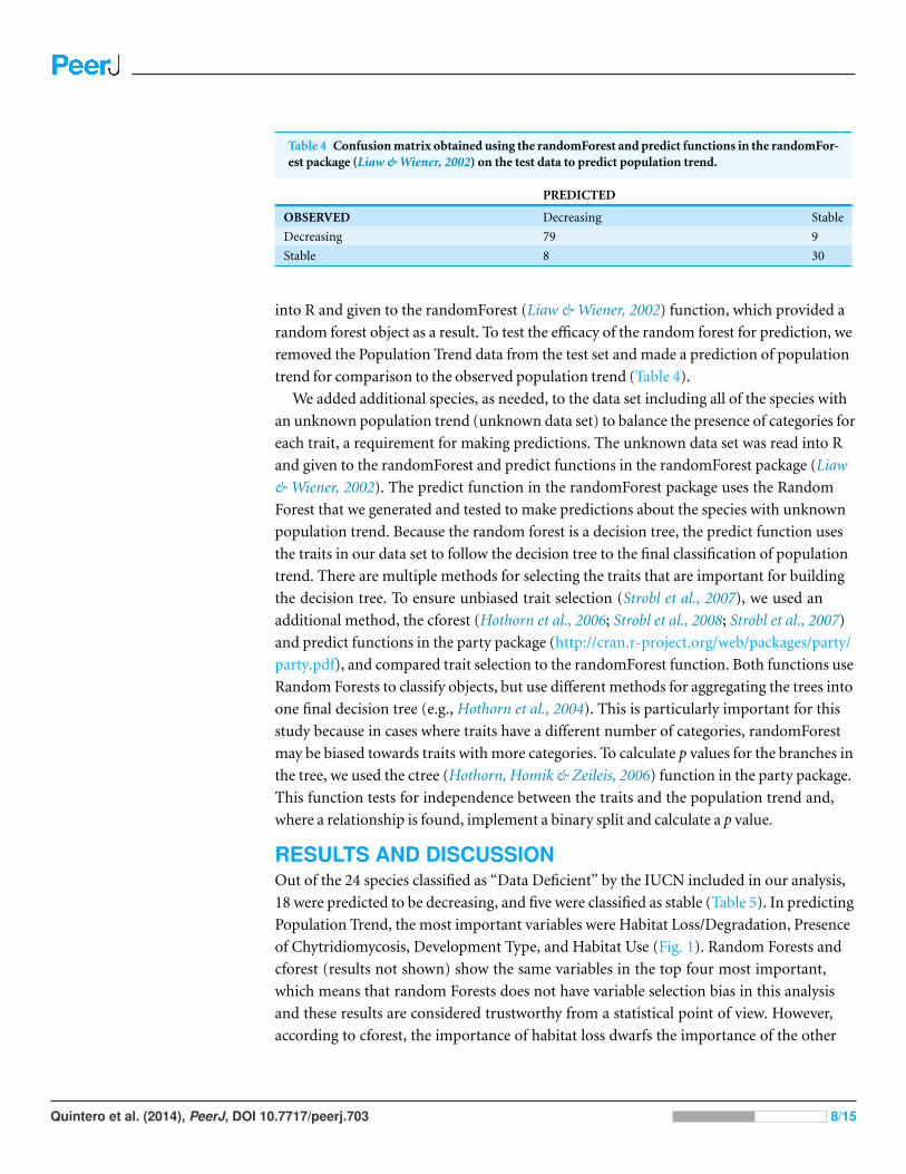
Table 4 Confusion matrix obtained using the randomForest and predict functions in the randomFor-est package (Liaw & Wiener, 2002) on the test data to predict population trend.

PREDICTED

OBSERVED Decreasing Stable

Decreasing 79 9

Stable 8 30

into R and given to the randomForest (Liaw & Wiener, 2002) function, which provided a

random forest object as a result. To test the efficacy of the random forest for prediction, we

removed the Population Trend data from the test set and made a prediction of population

trend for comparison to the observed population trend (Table 4).

We added additional species, as needed, to the data set including all of the species with

an unknown population trend (unknown data set) to balance the presence of categories for

each trait, a requirement for making predictions. The unknown data set was read into R

and given to the randomForest and predict functions in the randomForest package (Liaw

& Wiener, 2002). The predict function in the randomForest package uses the Random

Forest that we generated and tested to make predictions about the species with unknown

population trend. Because the random forest is a decision tree, the predict function uses

the traits in our data set to follow the decision tree to the final classification of population

trend. There are multiple methods for selecting the traits that are important for building

the decision tree. To ensure unbiased trait selection (Strobl et al., 2007), we used an

additional method, the cforest (Hothorn et al., 2006; Strobl et al., 2008; Strobl et al., 2007)

and predict functions in the party package (http://cran.r-project.org/web/packages/party/

party.pdf), and compared trait selection to the randomForest function. Both functions use

Random Forests to classify objects, but use different methods for aggregating the trees into

one final decision tree (e.g., Hothorn et al., 2004). This is particularly important for this

study because in cases where traits have a different number of categories, randomForest

may be biased towards traits with more categories. To calculate p values for the branches in

the tree, we used the ctree (Hothorn, Homik & Zeileis, 2006) function in the party package.

This function tests for independence between the traits and the population trend and,

where a relationship is found, implement a binary split and calculate a p value.

RESULTS AND DISCUSSIONOut of the 24 species classified as “Data Deficient” by the IUCN included in our analysis,

18 were predicted to be decreasing, and five were classified as stable (Table 5). In predicting

Population Trend, the most important variables were Habitat Loss/Degradation, Presence

of Chytridiomycosis, Development Type, and Habitat Use (Fig. 1). Random Forests and

cforest (results not shown) show the same variables in the top four most important,

which means that random Forests does not have variable selection bias in this analysis

and these results are considered trustworthy from a statistical point of view. However,

according to cforest, the importance of habitat loss dwarfs the importance of the other

Quintero et al. (2014), PeerJ, DOI 10.7717/peerj.703 8/15

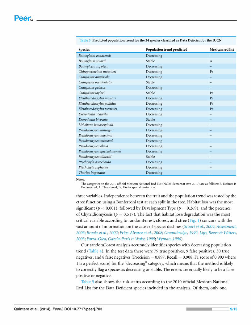
Table 5 Predicted population trend for the 24 species classified as Data Deficient by the IUCN.

Species Population trend predicted Mexican red list

Bolitoglossa oaxacensis Decreasing –

Bolitoglossa stuarti Stable A

Bolitoglossa zapoteca Decreasing –

Chiropterotriton mosaueri Decreasing Pr

Craugastor amniscola Decreasing –

Craugastor occidentalis Stable –

Craugastor pelorus Decreasing –

Craugastor taylori Stable Pr

Eleutherodactylus maurus Decreasing Pr

Eleutherodactylus pallidus Decreasing Pr

Eleutherodactylus teretistes Decreasing Pr

Exerodonta abdivita Decreasing –

Exerodonta bivocata Stable –

Lithobates lemosespinali Decreasing –

Pseudoeurycea amuzga Decreasing –

Pseudoeurycea maxima Decreasing –

Pseudoeurycea mixcoatl Decreasing –

Pseudoeurycea obesa Decreasing –

Pseudoeurycea quetzalanensis Decreasing –

Pseudoeurycea tlilicxitl Stable –

Ptychohyla acrochorda Decreasing –

Ptychohyla zophodes Decreasing –

Thorius insperatus Decreasing –

Notes.The categories on the 2010 official Mexican National Red List (NOM-Semarnat-059-2010) are as follows: E, Extinct; P,Endangered; A, Threatened; Pr, Under special protection.

three variables. Independence between the trait and the population trend was tested by the

ctree function using a Bonferroni test at each split in the tree. Habitat loss was the most

significant (p < 0.001), followed by Development Type (p = 0.269), and the presence

of Chytridiomycosis (p = 0.517). The fact that habitat loss/degradation was the most

critical variable according to randomForest, cforest, and ctree (Fig. 1) concurs with the

vast amount of information on the cause of species declines (Stuart et al., 2004; Assessment,

2005; Brooks et al., 2002; Frıas-Alvarez et al., 2008; Groombridge, 1992; Lips, Reeve & Witters,

2003; Parra-Olea, Garcıa-Parıs & Wake, 1999; Wyman, 1990).

Our randomForest analysis accurately identifies species with decreasing population

trend (Table 4). In the test data there were 79 true positives, 9 false positives, 30 true

negatives, and 8 false negatives (Precision = 0.897. Recall = 0.908; F1 score of 0.903 where

1 is a perfect score) for the “decreasing” category, which means that the method is likely

to correctly flag a species as decreasing or stable. The errors are equally likely to be a false

positive or negative.

Table 5 also shows the risk status according to the 2010 official Mexican National

Red List for the Data Deficient species included in the analysis. Of them, only one,

Quintero et al. (2014), PeerJ, DOI 10.7717/peerj.703 9/15

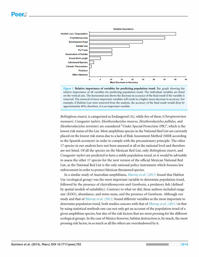
Figure 1 Relative importance of variables for predicting population trend. Bar graph showing therelative importance of all variables for predicting population trend. The individual variables are listedon the vertical axis. The horizontal axis shows the decrease in accuracy of the final result if the variable isremoved. The removal of more important variables will result in a higher mean decrease in accuracy. Forexample, if Habitat Loss were removed from the analysis, the accuracy of the final result would drop byapproximately 40%; therefore, it is an important variable.

Bolitoglossa stuarti, is categorized as Endangered (A), while five of them (Chiropterotriton

mosaueri, Craugastor taylori, Eleutherodactylus maurus, Eleutherodactylus pallidus, and

Eleutherodactylus teretistes) are considered “Under Special Protection (PR)”, which is the

lowest risk status of the List. Most amphibian species in the National Red List are currently

placed on the lowest risk status due to a lack of Risk Assessment Method (MER according

to the Spanish acronym) in order to comply with the precautionary principle. The other

17 species in our analysis have not been assessed at all at the national level and therefore

are not listed. Of all the species on the Mexican Red List, only Bolitoglossa stuarti, and

Craugastor taylori are predicted to have a stable population trend, so it would be advisable

to assess the other 17 species for the next version of the official Mexican National Red

List, as the National Red List is the only national policy instrument which foresees law

enforcement in order to protect Mexican threatened species.

In a similar study of Australian amphibians, Murray et al. (2011) found that Habitat

Use (ecological group) was the most important variable to determine population trend,

followed by the presence of chytridiomycosis and Gambusia, a predatory fish (defined

by spatial models of suitability). Contrary to what we did, these authors included range

size (EOO), abundance, and testes mass, and the presence of Gambusia. Although our

study and that of Murray et al. (2011) found different variables as the most important to

determine population trend, both studies concurs with that of Murray et al. (2011) in that

by using statistical methods one can not only get an account of the population trend of a

given amphibian species, but also of the risk factors that are most pressing for the different

ecological groups. In the case of Mexico however, habitat destruction is, by much, the most

pressing risk factor, in as much as all the others are overshadowed by it.

Quintero et al. (2014), PeerJ, DOI 10.7717/peerj.703 10/15

CONCLUSIONSThe use of Random Forests seems to be a solid way to identify species with decreasing

population trends in the absence of demographic data in order to prioritize those in need

of further assessment. The kind of exercise that we show here can be a first approach

when planning conservation priorities, as some of the most endangered species might also

be those for which most information is lacking. Moreover, this method has the advantage

of not having to depend on aggregated museum locality data that may not have been

properly curated by experts, as is the case for some assessment efforts (Hjarding, Tolley &

Burgess, 2014).

Intrinsic factors, such as the ova and clutch size, can give important information about

how life history can affect the population trend of a species. Unfortunately, the amount

of data we had for those traits was so limited that we felt that including data that had

mostly been statistically generated could introduce an extra bias to our analysis. The fact

that so little information on the natural history of these endangered species is available is

a major challenge that needs to be addressed to successfully prevent their extinction. In

addition, our aggregated data set can be used to set data collection priorities to fill in gaps.

Fortunately, as we show here, this lack of information should not deter the efforts to assess

risk status and assign priorities to their conservation.

We would also like to call attention into the fact that the most recent global amphibian

assessment was just conducted in September 2014. In this latest assessment the experts

have expressed that, in fact, Chytridiomycosis is not the big concern it was thought

to be 10 years ago, when the last global assessment was performed. This view, along a

deeper knowledge of the complexity of the disease, is also mirrored in recent studies,

which show that many amphibians have either developed resistance to the disease or some

communities seem to be thriving even when the fungus is still present (Ellison et al., 2014;

Gervasi et al., 2014; Langhammer et al., 2014; Louca, Lampo & Doebeli, 2014; McMahon et

al., 2014; Scheele et al., 2014). However, experts also agree that habitat loss is still the biggest

concern for amphibians and biodiversity in general (P Arias-Caballero, pers. comm.,

2014).

Although it is not our claim that efforts like the one we present here should substitute

for field research or other forms of assessments, we want to emphasize the importance of

these exercises as part of the comprehensive effort to pinpoint research and assessment

necessities to inform public policy and advance the conservation of the species. For

instance, it would be very interesting to replicate this exercise with other DD species in

different taxonomic groups. Moreover, we want to emphasize how important it is to use

data archived in digital libraries such as EOL and BHL and statistical tools to answer

questions that are difficult to tackle otherwise.

ACKNOWLEDGEMENTSThe authors would like to thank the National Evolutionary Synthesis Center, the

Biodiversity Heritage Library and the Encyclopedia of Life for their support of this

Quintero et al. (2014), PeerJ, DOI 10.7717/peerj.703 11/15

project. AET would like to thank the Boston Python User Group and PyLadies Boston

for programming advice and support.

ADDITIONAL INFORMATION AND DECLARATIONS

FundingThis work was supported by a grant “Using Digital Libraries to Discover Biodiversity and

Evolution” from the Richard Lounsbery Foundation to CR McClain, and additional funds

from CONABIO to E Quintero and P Arias-Caballero. The funders had no role in study

design, data collection and analysis, decision to publish, or preparation of the manuscript.

Grant DisclosuresThe following grant information was disclosed by the authors:

Richard Lounsbery Foundation.

CONABIO.

Competing InterestsAnne E. Thessen is the owner and founder of The Data Detektiv. Esther Quintero, Paulina

Arias-Caballero, and Barbara Ayala-Orozco are employees of the Comision Nacional para

el Conocimiento y Uso de la Biodiversidad.

Author Contributions• Esther Quintero conceived and designed the experiments, analyzed the data, wrote the

paper, reviewed drafts of the paper.

• Anne E. Thessen performed the experiments, analyzed the data, wrote the paper,

prepared figures and/or tables, reviewed drafts of the paper.

• Paulina Arias-Caballero analyzed the data, prepared figures and/or tables, reviewed

drafts of the paper.

• Barbara Ayala-Orozco reviewed drafts of the paper.

Data DepositionThe following information was supplied regarding the deposition of related data:

GitHub (https://github.com/diatomsRcool/MexicanAmphibians).

Supplemental InformationSupplemental information for this article can be found online at http://dx.doi.org/

10.7717/peerj.703#supplemental-information.

REFERENCESBland LM, Collen B, Orme DL, Bielby J. 2014. Predicting the conservation status of data-deficient

species. Conservation Biology In Press DOI 10.1111/cobi.12372.

Breiman L. 2001. Random forests. Machine Learning 45:15–32.

Quintero et al. (2014), PeerJ, DOI 10.7717/peerj.703 12/15

Brooks TM, Mittermeier RA, Mittermeier CG, Da Fonseca GAB, Rylands AB, Konstant WR,Flick P, Pilgrim J, Oldfield S, Magin G, Hilton-Taylor C. 2002. Habitat loss and extinction inthe hotspots of biodiversity. Conservation Biology 16:909–923DOI 10.1046/j.1523-1739.2002.00530.x.

Cardillo M, Meijaard E. 2012. Are comparative studies of extinction risk useful forconservation? Trends in Ecology & Evolution 27:167–171 DOI 10.1016/j.tree.2011.09.013.

Carey C, Heyer WR, Wilkinson J, Alford RA, Arntzen JW, Halliday T, Hungerford L, Lips KR,Middleton EM, Orchard SA, Rand AS. 2001. Amphibian declines and environmental change:use of remote-sensing data to identify environmental correlates. Conservation Biology15:903–913 DOI 10.1046/j.1523-1739.2001.015004903.x.

Casella GM, George EI. 1992. Explaining the Gibbs sampler. The American Statistician46(3):167–174 DOI 10.1080/00031305.1992.10475878.

Cutler DR, Edwards TC, Beard KH, Cutler A, Hess KT, Gibson J, Lawler JJ. 2007. Random forestsfor classification in ecology. Ecology 88:2783–2792 DOI 10.1890/07-0539.1.

Ellison AR, Savage AE, DiRenzo GV, Langhammer P, Lips KR, Zamudio KR. 2014. Fightinga losing battle: vigorous immune response countered by pathogen suppression ofhost defenses in the chytridiomycosis-susceptible frog Atelopus zeteki. G3 4:1275–1289DOI 10.1534/g3.114.010744.

Frıas-Alvarez P, Vredenburg V, Familiar-Lopez M, Longcore J, Gonzalez-Bernal E,Santos-Barrera G, Zambrano L, Parra-Olea G. 2008. Chytridiomycosis survey in wild andcaptive Mexican amphibians. EcoHealth 5:18–26 DOI 10.1007/s10393-008-0155-3.

Frost DR. 2014. Amphibian species of the world: an online reference. Version 6.0. New York:American Museum of Natural History. Available at http://researchamnhorg/herpetology/amphibia/indexhtml.

Garcıa A, Ceballos G. 1994. Guıa de campo de los reptiles y anfibios de la costa de Jalisco. Mexico:Fundacion Ecologica de Cuixmala, A.C.

Gervasi SS, Hunt EG, Lowry M, Blaustein AR. 2014. Temporal patterns in immunity, infectionload and disease susceptibility: understanding the drivers of host responses in the amphibian-chytrid fungus system. Functional Ecology 28:569–578 DOI 10.1111/1365-2435.12194.

Groombridge B. 1992. Global biodiversity: status of the Earth’s living resources. World ConservationMonitoring Centre. New York, NY: Chapman & Hall.

Hjarding A, Tolley KA, Burgess ND. 2014. Red List assessments of East African chameleons: a casestudy of why we need experts. Oryx DOI 10.1017/S0030605313001427.

Hothorn T, Lausen B, Benner A, Radespiel-Troger M. 2004. Bagging survival trees. Statistics inMedicine 23(1):77–91 DOI 10.1002/sim.1593.

Hothorn T, Buehlmann P, Dudoit S, Molinaro A, Van Der Laan A. 2006. Survival ensembles.Biostatistics 7:355–373 DOI 10.1093/biostatistics/kxj011.

Hothorn T, Homik K, Zeileis A. 2006. Unbiased recursive partitioning: a conditionalinference framework. Journal of Computational and Graphic Statistics 15:651–674DOI 10.1198/106186006X133933.

Ihaka R, Gentleman R. 1996. R: A language for data analysis and graphics. Journal ofComputational and Graphical Statistics 5(3):299–314 DOI 10.1080/10618600.1996.10474713.

IUCN. 2012. IUCN red list categories and criteria. Version 3.1. Gland, Switzerland and Cambridge:IUCN.

Quintero et al. (2014), PeerJ, DOI 10.7717/peerj.703 13/15

IUCN. 2014. The IUCN red list of threatened species. Version 2014.1. Available at http://www.iucnredlist.org (accessed 12 May 2014).

Kiesecker JM, Blaustein AR, Belden LK. 2001. Complex causes of amphibian population declines.Nature 410:681–684 DOI 10.1038/35070552.

Langhammer PF, Burrowes PA, Lips KR, Bryant AB, Collins JP. 2014. Suceptibility to theAmbiphian chytrid fungus varies with ontogeny in the direct-developing frog Eleutherodactyluscoqui. Journal of Wildlife Diseases 50:438–446 DOI 10.7589/2013-10-268.

Liaw A, Wiener M. 2002. The random forest package. R News 2:18–22.

Lips KR, Brem F, Brenes R, Reeve JD, Alford RA, Voyles J, Carey C, Livo L, Pessier AP,Collins JP. 2006. Emerging infectious disease and the loss of biodiversity in a Neotropicalamphibian community. Proceedings of the National Academy of Sciences of the United States ofAmerica 103:3165–3170 DOI 10.1073/pnas.0506889103.

Lips KR, Reeve JD, Witters LR. 2003. Ecological traits predicting amphibian population declinesin Central America. Conservation Biology 17:1078–1088DOI 10.1046/j.1523-1739.2003.01623.x.

Little RJ, Rubin DB. 2002. Statistical analysis with missing data. 2nd edition. Hoboken, NJ: WileyInterscience.

Longcore JE, Pessier AP, Nichols DK. 1999. Batrachochytrium dendrobatidisgen. et sp. nov., achytrid pathogenic to amphibians. Mycologia 91:219–227 DOI 10.2307/3761366.

Louca S, Lampo M, Doebeli M. 2014. Assessing host extinction risk following exposureto Batrachochytrium dendrobatidis. Proceedings of the Royal Society B-Biological Sciences281:20132783 DOI 10.1098/rspb.2013.2783.

McMahon TA, Sears BF, Venesky MD, Bessler SM, Brown JM, Deutsch K, Halstead NT, Lentz G,Tenouri N, Young S, Civitello DJ, Ortega N, Fites JS, Reinert LK, Rollins-Smith LA, Raffel TR,Rohr JR. 2014. Amphibians acquire resistance to live and dead fungus overcoming fungalimmunosuppression. Nature 511:224–227 DOI 10.1038/nature13491.

Millenium Ecosystem Assessment. 2005. Ecosystems and human well-being: biodiversity synthesis.Washington, DC: World Resources Institute.

Murray KA, Rosauer D, McCallum H, Skerratt LF. 2011. Integrating species traits with extrinsicthreats: closing the gap between predicting and preventing species declines. Proceedings of theRoyal Society B: Biological Sciences 278:1515–1523 DOI 10.1098/rspb.2010.1872.

Murrieta-Galindo R, Parra-Olea G, Gonzalez-Romero A, Lopez-Barrera F, Vredenburg VT.2014. Detection of Batrachochytrium dendrobatidis in amphibians inhabiting cloud forestsand coffee agroecosystems in central Veracruz, Mexico. European Journal of Wildlife Research60:431–439 DOI 10.1007/s10344-014-0800-9.

Ochoa-Ochoa LM, Flores-Villela O. 2006. Areas de Diversidad y Endemismo de la HerpetofaunaMexicana. Mexico, D.F: Universidad Nacional Autonoma de Mexico—Comision Nacional parael Conocimiento y Uso de la Biodiversidad.

Parra-Olea G, Garcıa-Parıs M, Wake DB. 1999. Status of some populations of Mexicansalamanders (Amphibia: Plethodontidae). Revista de Biologıa Tropical 47:217–223.

Parr CS, Wilson N, Leary P, Schulz KS, Lans K, Walley L, Hammock JA, Goddard A, Rice J,Studer M, Holmes JTG, Corrigan Jr RJ. 2014. The encyclopedia of life v2: providingglobal access to knowledge about life on Earth. Biodiversity Data Journal 2:e1079DOI 10.3897/BDJ.2.e1079.

Quintero et al. (2014), PeerJ, DOI 10.7717/peerj.703 14/15

Piotrowski JS, Annis LA, Longcore JE. 2004. Physiology of Btarachochytrium dendronbatis, achytrid pathogen of amphibians. Mycologia 96:9–15 DOI 10.2307/3761981.

Pounds JA, Crump ML. 1994. Amphibian declines and climate disturbance: the case of the goldentoad and the Harlequin frog. Conservation Biology 8:72–85DOI 10.1046/j.1523-1739.1994.08010072.x.

Scheele B, Guarino F, Osborne W, Hunter DA, Skerratt LF, Driscoll DA. 2014. Decline andre-expansion of an amphibian with high prevalence of chytrid fungus. Biological Conservation170:86–91 DOI 10.1016/j.biocon.2013.12.034.

Strobl C, Boulesteix AL, Kneib T, Augustin T, Zeileis A. 2008. Conditional variable importancefor random forests. BMC Bioinformatics 9:307 DOI 10.1186/1471-2105-9-307.

Strobl C, Boulesteix AL, Zeileis A, Hothorn T. 2007. Bias in random forest variableimportance measures: illustrations, sources and a solution. BMC Bioinformatics8:25 DOI 10.1186/1471-2105-8-25.

Stuart SN, Chanson JS, Cox NA, Young BE, Rodrigues ASL, Fischman DL, Waller RW. 2004.Status and trends of amphibian declines and extinctions worldwide. Science 306:1783–1786DOI 10.1126/science.1103538.

Tingley R, Hitchmough RA, Chapple DG. 2013. Life-history traits and extrinsic threatsdetermine extinction risk in New Zealand lizards. Biological Conservation 165:62–68DOI 10.1016/j.biocon.2013.05.028.

Van Buuren S, Groothuis-Oudshoorn K. 2011. Mice: multivariate imputation by chainedequations. R Journal of Statistical Software 45:1–67.

Wyman RL. 1990. What’s happening to the amphibians? Conservation Biology 4:350–352DOI 10.1111/j.1523-1739.1990.tb00307.x.

Quintero et al. (2014), PeerJ, DOI 10.7717/peerj.703 15/15