The Latent Process Decomposition ofcDNA Microarray Data Sets

Simon Rogers, Mark Girolami, Colin Campbell, and Rainer Breitling

Abstract—We present a new computational technique (a software implementation, data sets, and supplementary information are

available at http://www.enm.bris.ac.uk/lpd/) which enables the probabilistic analysis of cDNA microarray data and we demonstrate its

effectiveness in identifying features of biomedical importance. A hierarchical Bayesian model, called Latent Process Decomposition

(LPD), is introduced in which each sample in the data set is represented as a combinatorial mixture over a finite set of latent processes,

which are expected to correspond to biological processes. Parameters in the model are estimated using efficient variational methods.

This type of probabilistic model is most appropriate for the interpretation of measurement data generated by cDNA microarray

technology. For determining informative substructure in such data sets, the proposed model has several important advantages over

the standard use of dendrograms. First, the ability to objectively assess the optimal number of sample clusters. Second, the ability to

represent samples and gene expression levels using a common set of latent variables (dendrograms cluster samples and gene

expression values separately which amounts to two distinct reduced space representations). Third, in constrast to standard cluster

models, observations are not assigned to a single cluster and, thus, for example, gene expression levels are modeled via combinations

of the latent processes identified by the algorithm. We show this new method compares favorably with alternative cluster analysis

methods. To illustrate its potential, we apply the proposed technique to several microarray data sets for cancer. For these data sets it

successfully decomposes the data into known subtypes and indicates possible further taxonomic subdivision in addition to highlighting,

in a wholly unsupervised manner, the importance of certain genes which are known to be medically significant. To illustrate its wider

applicability, we also illustrate its performance on a microarray data set for yeast.

Index Terms—cDNA microarray, latent variable modeling, cluster analysis.

�

1 INTRODUCTION

IN recent years, there has been a large growth in thevolume of microarray data. Machine learning techniques

have been very useful in extracting information from thesedata sets. For example, unsupervised techniques such ashierarchical cluster analysis have been used to indicatetentative new subtypes for some cancers [1], [6] and toidentify biologically relevant structure in large data sets.Using class labels, supervised learning methods will havean increasingly important role to play in indicating thedetailed subtype of a disease, its expected progression, andthe best treatment strategy.

Cluster analysis is the most common data analysismethod used throughout the microarray literature. Genera-tion of a dendrogram allows the inference of possible groupstructure within the data and, thus, the identification ofrelated samples or functionally similar genes. A weaknessof clustering by dendrogram is that there is no natural wayto objectively assess the most probable number of structures

which underlie the data. Probabilistic model-based cluster-ing can overcome this problem and clustering based onmixtures of multivariate Gaussians has been proposed in[9], for example. However, as the number of features (geneprobes) typically far exceeds the number of samples, theestimated within-class covariances will be singular. There-fore, extensive gene selection is a prerequisite to anyprobabilistic model-based clustering and in [9] a furtherlevel of feature extraction is required to obtain a sufficientlylow-dimensional subspace within which the clustering isperformed. For the purposes of biological interpretation, itwould be better if group structure could be identified usingthe original set of genes probed in the microarrayexperiment with the model used to identify those genesresponsible for the group structure. We will show that thisis achieved naturally by the model proposed in this paper.

The main assumption underlying most clustering meth-ods, whether dendrogram-based or probabilistic, is that asample or gene is assigned exclusively to one class only.While this may be appropriate if mutually exclusive classesare inherent in the data, this assumption would not be validif a number of biological processes interact to influence agiven gene expression level, for example. Alternatively, asample might validly share some characteristics with two ormore sample clusters. It is therefore best to obtain modelswhich are not restricted by this mutual exclusion of classesassumption.

Models overcoming this mutual exclusion assumptionhave already been proposed in the literature. An example isthe Plaid Model of Lazzeroni and Owen [8] which allowsfor overlaps between clusters. Another example is a model

IEEE/ACM TRANSACTIONS ON COMPUTATIONAL BIOLOGY AND BIOINFORMATICS, VOL. 2, NO. 2, APRIL-JUNE 2005 143

. S. Rogers and M. Giralomi are with the Bioinformatics Research Centre,Department of Computing Science, A416, Fourth Floor, DavidsonBuilding, University of Glasgow, Glasgow G12 8QQ, Scotland, UnitedKingdom. E-mail: {srogers, girolami}@dcs.gla.ac.uk.

. C. Campbell is with the Department of Engineering Mathematics, Queen’sBuilding, Bristol University, Bristol BS9 1TR, United Kingdom.E-mail: C.Campbell@bris.ac.uk.

. R. Breitling is with the Molecular Plant Science Group & BioinformaticsResearch Centre, Institute for Biomedical and Life Sciences, University ofGlasgow, Glasgow G12 8QQ, United Kingdom.E-mail: r.breitling@bio.gla.ac.uk.

Manuscript received 12 Sept. 2004; revised 11 Nov. 2004; accepted 7 Dec.2004; published online 2 June 2005.For information on obtaining reprints of this article, please send e-mail to:tcbb@computer.org, and reference IEEECS Log Number TCBB-0141-0904.

1545-5963/05/$20.00 � 2005 IEEE Published by the IEEE CS, CI, and EMB Societies & the ACM

recently proposed by Segal et al. [10], in which aprobabilistic relational model (PRM) for gene expressionis developed. PRM is shown to successfully identify knownbiological processes and provides improved interpretabilityover comparable methods [10]. However, PRM requires anestimation algorithm which, in its exact form, is NP-hard,and so various heuristics are required to make the modelestimation tractable.

In this paper, we will present a new approach to theanalysis of microarray data which is motivated by the aboveconsiderations and adopts the Latent Dirichlet Allocation(LDA) approach to data modeling [2]. We have called themethod Latent Process Decomposition with a processdefined as a set of functionally related datapoints (samplesor genes). We use the term process, rather than cluster,because a sample or gene can have partial membership ofseveral processes simultaneously, in contrast to manycluster analysis approaches, as discussed above.

Latent Process Decomposition has linear computationalscaling in the number of genes, arrays andprocesses. It is ableto provide a representation of microarray data sets whichsimultaneously reflects group structure across samples andgenes as well as the possible interplay between multipleprocesses responsible for measured gene expression levels.Furthermore, it has advantages over alternative approachessuch as the use of dendrograms, mixture models [9], NaiveBayes, and other approaches. In Section 2, wewill outline themethod,with fullderivationandpseudocode listingsgiven intheAppendix,while in Section 3,wewill outlineperformanceon medical and biological data sets. We have implementedLPD in Matlab and Cþþ and this code is freely available athttp://www.enm.bris.ac.uk/lpd.

2 LATENT PROCESS DECOMPOSITION

2.1 Model Specification

In probabilistic terms, the data generation process for atissue sample can be described as follows (Fig. 1b): For acomplete microarray data set, a Dirichlet prior probabilitydistribution for the distribution of possible processes isdefined by the K-dimensional parameter �. For a tissuesample a, a distribution � over a set of mixture componentsindexed by the discrete variable k is drawn from a single

prior Dirichlet distribution. Then, for each of the G features

g (generally uniquely mapping to genes), we draw a process

index k from the distribution � with probability �k which

selects a Gaussian defined by the parameters �gk and �gk.

The level of expression ega for gene g from sample a is then

drawn from the kth Gaussian denoted as Nðegajk; �gk; �gkÞ.This is then repeated for each of A tissue samples. It can be

easily seen that this generative process ensures that each

sample has its own specific distribution of processes and

that each measured level of gene expression in the sample is

obtained by repeatedly sampling the process index from the

sample-specific Dirichlet random variable �, thus allowing

the possibility of a number of processes having an effect on

the measured levels of gene expression.This is a biologically more realistic representation than

the mixture model which underlies all forms of clustering,

see Fig. 1a, where only one process or class is responsible

for all the measured gene expression, thus disregarding

gene-specific differences in effect (�gk) and noise (�gk) or the

sample-specific interaction of various processes.

2.2 Learning with Uniform Priors: The MaximumLikelihood Solution

For a model with a set of parameters,H, and data D, Bayes’s

rule gives

pðHjDÞ / pðDjHÞpðHÞ; ð1Þ

where pðDjHÞ is the likelihood and pðHÞ is the prior on our

parameters H. We are interested in finding the set of

parametersH that maximizes pðHjDÞ (the maximum posterior

orMAP solution). In the case of a uniform (or uninformative)

prior, this is themaximum likelihood solution.Wewill begin

by deriving the maximum likelihood solution and then

extend this to a nonuniform (or informative) prior in

Section2.3.The log-likelihoodof a set ofA training samples is:

log pðDj�; �; �Þ; ð2Þ

which can be factorized over individual samples as follows:

log pðDj�; �; �Þ ¼XAa¼1

log pðaj�; �; �Þ: ð3Þ

144 IEEE/ACM TRANSACTIONS ON COMPUTATIONAL BIOLOGY AND BIOINFORMATICS, VOL. 2, NO. 2, APRIL-JUNE 2005

Fig. 1. Graphical model representations of LPD. (a) Cluster model structure. (b) LPD model structure.

Marginalizing over the latent variable � allows us to expand

this expression as follows:

log pðDj�; �; �Þ ¼XAa¼1

log

Z�

pðaj�; �; �Þpð�j�Þd�; ð4Þ

where the probability of the sample conditioned on the

means, variances, and process weightings can be expressed

in terms of its individual components giving the following:

log pðaj�; �; �Þ¼ log

Z�

YGg¼1

XKk¼1

Nðegajk; �gk; �gkÞ�k

( )pð�j�Þd�;

ð5Þ

where Nðajk; �; �Þ denotes a normal distribution in process

k with mean � and standard deviation �.Variational inference can be employed to estimate the

parameters of this model and full details are given in the

Appendices. A lower bound on (5) can be inferred by the

introduction of variational parameters and the following

iterative update equations provide estimates of the two

variational parameters Qkga and �ak

Qkga ¼Nðegajk; �gk; �gkÞ exp ð�akÞ½ �PK

k0¼1 Nðegajk; �gk0 ; �gk0 Þ exp ð�ak0 Þ½ �; ð6Þ

�ak ¼ �k þXGg¼1

Qkga; ð7Þ

for given �k and where ðzÞ is the digamma function. The

model parameters are obtained from the following update

equations:

�gk ¼PA

a¼1QkgaegaPAa0¼1Qkga0

; ð8Þ

�2gk ¼PA

a¼1Qkgaðega � �gkÞ2PAa0¼1Qkga0

: ð9Þ

The update rule for the Dirichlet model parameter �k is

found from the derivatives of the � dependent terms in the

likelihood [2]. Thus, the �k are modified after each iteration

of the above updatings using a standard Newton-Raphson

technique (see [2, Appendix A.4.2], and the Appendix of

this paper for further details).The generative process described above for samples can

equally be used over genes (the features). In probabilistic

terms: For each gene g, a Dirichlet random variable is

sampled, then for each experimental condition a, an index is

drawn with probability �k, and then the expression level egais sampled from the appropriate Gaussian with mean and

variance �ak, �ak, respectively. Note that representing genes

in this manner only requires a change of indices in the

parameters which simply amounts to a transpose of the

expression matrix. We will give one example of a decom-

position over genes (the yeast cell cycle data set) later in

Section 3.2.1.

2.3 Learning with Nonuniform Priors: The MAPSolution

In the previous section, we derived a set of update equations,guaranteed to converge to a local maximum of the lowerbound on the likelihood.Wenowextend this argument to theMAP solutionwith informative priors. A suitable prior on themeans could be a Gaussian distributionwith zeromean. Thiswould reflect a prior belief that most genes will beuninformative and will have log-ratio expression valuesaroundzero (i.e., they areunchanged compared to a referencesample). For the variance, we may wish to define a prior thatpenalizes overcomplex models and avoids overfitting. Over-fitting may occur when Gaussian functions contract onto asingle data point causing poor generalisation and numericalinstability.With a suitable choice for the prior an extension ofour previous derivation to the full MAP solution isstraightforward. Our combined likelihood and prior expres-sion is (assuming a uniform prior on �):

pð�; �; �jDÞ / pðDj�; �; �Þpð�Þpð�Þ: ð10Þ

Taking the logarithm of both sides, we see that themaximization task is given by:

�; �; � ¼ argmax�;�;�

log pðGj�; �; �Þ þ log pð�Þ þ log pð�Þ:

ð11Þ

Thus, we can simply append these terms onto our boundon (1). Noting that they are functions of � and � only (andany associated hyperparameters), we conclude that theseterms only change the update equations for �ak and �ak. Letus assume the following priors:

pð�gkÞ / N ð0; ��Þ; ð12Þ

pð�2gkÞ / exp � s

�2gk

( ); ð13Þ

i.e., a zero-mean Gaussian for the means and an improperprior for �gk (i.e., not integrating to unity over its domain)which gives zero weight to �gk ¼ 0 and asymptoticallyapproaches 1 as �gk approaches infinity. Plots of these priorscan be seen in Fig. 2 where �� ¼ 0:1 and s ¼ 0:1.

Adding these to our original bound, we now have todifferentiate the following expression to obtain updates for�gk and �gk

XAa¼1

Qgka log pðegaj�gk; �gkÞ þ log pð�gkÞ þ log pð�gkÞ: ð14Þ

Performing the necessary differentiations, we are leftwith the following new updates

�gk ¼�2�PA

a¼1Qgkaega

�2gk þ �2�PA

a¼1Qgka

; ð15Þ

�2gk ¼PA

a¼1Qgkaðega � �gkÞ2 þ 2sPAa¼1Qgka

: ð16Þ

These expressions clearly show the effect of the priors. In(15), we see that we now have a dependancy on both �2gk and�2�. In the limit of�2� ! 1, we effectively have auniformprior

ROGERS ET AL.: THE LATENT PROCESS DECOMPOSITION OF CDNA MICROARRAY DATA SETS 145

and we recover our original update equations for themaximum likelihood solution. In the opposite limit of�2� ! 0, we find �gk ! 0 as we would expect. In (16), theprior is effectively putting a lower bound on the value of �2gk.As s! 0, the prior approaches auniformdistribution over allpositive reals and we recover our original �2gk update.

2.4 Computing the Likelihood and ParameterInitialization

Once the model parameters have been estimated, we cancalculate the likelihood for a collection of samples A0 using:

L ¼YA0

a¼1

Z�

YGg¼1

XKk¼1

Nðegajk; �gk; �gkÞ�k

( )pð�j�Þd�; ð17Þ

where we estimate the expectation over the Dirichletdistribution by averaging over N samples drawn from theestimated Dirichlet prior pð�j�Þ

L �YA0

a¼1

1

N

XNn¼1

YGg¼1

XKk¼1

Nðegajk; �gk; �gkÞ�kn

( ): ð18Þ

Before iteratively updating Qkga, �ak, �gk, �2gk, and �k

various parameter values need to be initialized. In thenumerical experiments reported below, the process meanvalues�gkwere initializedtothemeanexpressionvalueacrossthe data set for each gene. Similarly, the variances�2gkwere setto the variance of their respective genes. The �k values wereinitialized to 1 for all k and the variational Dirichletparameters �a were initialized to a positive random number.

3 NUMERICAL EXPERIMENTS

To evaluate the performance of Latent Process Decomposi-tion (LPD) we applied it to four microarray data sets. Forthe first three data sets (prostate, lung, and lymphomacancer), we show that LPD compares favorably with othercluster analysis methods, including dendrograms andNaive-Bayes, in its ability to classify samples. In the fourthexample for the yeast cell cycle [11], we show that LPD cangenerate a rich, biologically relevant description of complexexperiments. In these numerical studies, the only prepro-cessing was to take the logarithm of the data values (base 2)

if this had not already been performed by the originators ofthe data set. Any likelihood calculations were approximatedby (18) where samples from pð�j�Þ were taken by usingk independent samples from gamma distributions withparameters �k and then normalizing the result to sum to 1.The algorithm performs EM-like updates of the variationaland model parameters. As such, convergence is guaranteed,although only to a local maximum of the training likelihoodand not to the global maximum. Therefore, any analysisgiven below corresponds to the best solution (in terms ofthe likelihood) achieved over several starts with differentinitial �a values.

When estimating the best value of K for a particular dataset, an N-fold cross-validation procedure was used. Thisconsisted of randomly partitioning the data into N subsets,one of which would be removed before training and thenused to calculate the likelihood. Each of the N subsetswould be left out in turn and the N likelihood values wouldbe averaged to give the estimate of the true value.

3.1 Prostate Cancer Data Set

Our first cancerdata set comes froma studyofprostate cancerby Dhanasekaran et al. [4] consisting of 54 samples with9,984 features (weused their completedata set correspondingto the supplementary information of [4, Fig. 8]). This data setconsists of 14 samples for benign prostatic hyperplasia(labeled BPH), three normal adjacent prostate (NAP), onenormal adjacent tumour (NAT), 14 localized prostate cancer(PCA), one prostatitis (PRO), and 20 metastatic tumours(MET).Wewill use this data set to compareperformancewithuniformpriors andnonuniformpriors and to compareLatentProcess Decomposition with hierarchical cluster analysis.

Fig. 3a shows the result of hierarchical cluster analysisusing a dendrogram with average linkage and a Euclideandistance measure. Although some local structure can beidentified, we see that the dendrogram gives a poorseparation between known classes (in line with resultspresented in Dhanasekaran et al. [4]). However, the numberof differentially expressed genes can be expected to be smallrelative to the total number of genes. As an unsupervisedmethod we cannot use prior class knowledge but we canuse a prior belief that genes varying little across samples areless likely to be interesting. Hence, to investigate the impact

146 IEEE/ACM TRANSACTIONS ON COMPUTATIONAL BIOLOGY AND BIOINFORMATICS, VOL. 2, NO. 2, APRIL-JUNE 2005

Fig. 2. Example priors for LPD �gk and �gk parameters. (a) Prior for �gk. (b) Prior for �gk.

of feature selection we ranked genes based on varianceacross samples and used the subset of features with highestvariance. Fig. 3b shows the corresponding result forperforming hierarchichal clustering on this reduced dataset. Although the dendrogram manages to split metastaticfrom the rest successfully, the difference between PCA andBPH is still unclear and it is very difficult to infer from thisdendrogram just how many clusters are present.

In Fig. 4 (lower and descending curve) we give the hold-out log-likelihood versus K, the number of processes, with auniform prior and using the top-ranked 500 features. The log-likelihood peaks at about K ¼ 4 processes, after which amodel with uniform prior overfits the training data as weincrease thenumber ofprocesses. This is to be expectedwith amaximum likelihood approach as we are allowing themodeltoomuch freedombynot penalising complexity. To solve thisproblem,wecan incorporate the informativepriorsdiscussedin Section 2.3. We will discuss the determination of theparameters in these priors shortly. However, to illustrateperformancewegive the log-likelihood versusKplot in Fig. 4

(top, level curve) using values of �2� ¼ 0:1 and s ¼ 0:1.We seethat the log-likelihood remains approximately constant as thenumber of processes is altered, rather than descending as Kincreases.

Fig. 5a provides an explanation for this behaviour: this is adecomposition of the prostate data into K ¼ 10 processeswith a uniform prior (and using the top 500 genes ranked byvariance). Given that the estimated optimum number ofprocesses is 4, we might expect the model to severely overfit,as indeed it does. However, if we introduce priors with �2� ¼0:1 and s ¼ 0:5, we obtain the decomposition seen in Fig. 5b.Weobserve that thedecomposition is over just fourprocesses,with the remaining six processes empty. This is very usefulsince, given suitable values for the prior parameters, we donot need to decide the exact number of processes. We alsonotice that the decomposition is much cleaner. For example,themetastatic samples (MET) have no overlap with localizedprostate cancer (PCA) and the benign and normal samplesindicating they are a distinct state.

Although we can avoid overfitting with correct para-meters for the prior, this still leaves the question of thecorrect choice of these prior parameters. Our numericalinvestigations across different data sets indicated that themean parameter, ��, had negligible effect and we typicallyset this parameter to 0:1. However, performance diddepend on s, the variance parameter. In Fig. 6, we plotfrom a cross validation study of the log-likelihood versus sfor the 500 top-ranked genes in the prostate data set. Wenotice a peak at s ¼ 0:1, though any choice for s on therange 0:1 and 0:5 appears satisfactory.

It may appear that we have gained very little by movingfrom cross-validation over processes to one over s, butarguably this is not the case for two reasons. First, we aredealing with a small number of samples and, hence, byremoving some samples for cross-validation, we could easilyremove a substantial proportion of one particular class,suggesting a bias toward underestimating the number ofclasses present. The variance parameter on the other hand is ameasure of noise that should be class independent and,hence, should be the same regardless of whether or not thefull data set is being used. Also, the number of processespresentwill bedependent on theparticular data set and couldvary greatly depending on the given study. On the other

ROGERS ET AL.: THE LATENT PROCESS DECOMPOSITION OF CDNA MICROARRAY DATA SETS 147

Fig. 3. Result of hierachichal cluster analysis on the prostate data set, using average linkage and a Euclidean distance measure. (a) Dendrogram

with all features. (b) Dendrogram with top-ranked 500 features.

Fig. 4. Hold-out log-likelihood (y-axis) versus the K (x-axis) using the top

ranked 500 genes in the prostate cancer data set using a nonuniform

prior as given in Section 2.3 (upper, level curve) and a uniform prior

(lower, descending curve) as described in Section 2.2.

hand, the contribution made by noise is a consequence of theexperimental procedure and we may expect the optimumvalue of s to vary very little across data sets. Indeed, in thefollowing sections, we shall see that this is the case.

One advantage of LPD over standard clustering techni-ques is the ease with which information can be extractedfrom the derived model. In this prostate cancer example, wecould be interested in finding those genes most differen-tially expressed between localized prostate cancer (PCA)and the metastatic samples (MET), for example. Thefollowing score can be used to rank genes:

Z ¼ j�gi � �gjjffiffiffiffiffiffiffiffiffiffiffiffiffiffiffiffiffiffi�2gi þ �2gj

q ; ð19Þ

where i and j correspond to the two processes beingcompared. Genes ranking highly will be those with largeseparation between their means and small standarddeviations—corresponding to genes whose values fallconsistently into two distinct clusters. In Table 1, we givea list of the 10 top-ranked genes based on this score. Plots of

the mixture densities defined by the latent processes andthe actual data values for three of these genes can be seen inFig. 7. These three plots show that the extracted genesappear to distinguish well between localized cancer andmetastasis and, importantly, have been highlighted assignificant without the use of the class labels. An investiga-tion of these genes (Dr. Jeremy Clark, personal commu-nication) indicates that some of them are potentiallysignificant for cancer biology. For example, CTGF is animmediate-early gene induced by growth factors or certainoncogenes. The expressed protein binds to integrins andmodulates the invasive behavior of certain human cancercells [3]. Similarly, it has been reported [5] that tumorangiogenesis and tumor growth are critically dependent onthe activity of EGR1.

We have used the likelihood as our measure of modelperformance. One issue that we have not yet explored ishow these likelihood values compare with those foralternative, and possibly simpler, cluster analysis methods.The most obvious comparison is with a standard Gaussianmixture model. The main difference between LPD and a

148 IEEE/ACM TRANSACTIONS ON COMPUTATIONAL BIOLOGY AND BIOINFORMATICS, VOL. 2, NO. 2, APRIL-JUNE 2005

Fig. 5. K ¼ 10 process decomposition of the prostate cancer data set using the top 500 genes. The peaks represent the confidence in the

assignment of the ath sample to the kth process using �ak. (a) With a uniform prior. (b) Using a nonuniform prior with �2� ¼ 0:1 and s ¼ 0:5.

Fig. 6. Hold-out log-likelihood (y-axis) as a function of the variance prior parameter s (x-axis) using the top 500 features in the prostate data set.

Gaussian mixture model is the repeated sampling for eachfeature in LPD allowing each sample to be represented by acombination of processes.

Due to the large number of features involved, it iscomputationally infeasible to use a Gaussian mixture modelwith full covariance matrices and thus we shall constrainthe matrices to be diagonal (equivalent to Gaussians alignedwith the coordinate axis). Fig. 8 shows the log-likelihoodcurves using maximum likelihood (i.e., no priors) for LPDand Naive-Bayes. We see that Naive-Bayes begins over-fitting immediately, suggesting only two clusters in thedata. LPD rises above Naive-Bayes to a peak at K ¼ 4processes before dropping toward the Naive-Bayes curve asK increases. Although the difference in the log-likelihood isnot huge, it is statistically significant, given the error bars,and the suggestion of only two clusters from Naive-Bayes ismisleading. Note that we have used the maximum like-lihood approach for training LPD to give the fairestcomparison with Naive-Bayes which is also trained bymaximum likelihood. It is also worth noting the relativesizes of the error bars. For Naive-Bayes, it is possible tocalculate the likelihood exactly, whereas with LPD we musttake samples from the Dirichlet. The error bars for the twomethods are certainly of the same order, suggesting thatmost variation is due to the cross-validation procedure thusallowing us to be confident in our LPD likelihoodapproximation method.

3.2 Lung Cancer Data Set

The lung cancer data set [6] consists of 73 gene expressionprofiles from normal and tumour samples with the tumorslabelled as squamous, large cell, small cell, and adenocarci-

noma. Ten-fold cross validation was performed for values of

K between 2 and 20 with and without parameter priors and

the results are shown in Fig. 9. As for the prostate cancer

example,wenotice anonuniformprior avoidsoverfitting and

causes the log-likelihood to plateau. In [6], the authors

identified seven clusters in the data—with the adenocarci-

noma samples falling into three separate clusters with strong

correlation with clinical outcomes. For their ordering (which

ROGERS ET AL.: THE LATENT PROCESS DECOMPOSITION OF CDNA MICROARRAY DATA SETS 149

TABLE 1Top 10 Genes Separating Localized Prostate from Metastatic Prostate Cancer

Genes are ranked by Z.

Fig. 7. Inferred density plots for three genes separating localized prostate cancer (PCA, process 2) from the metastatic samples (MET, process 4) in

Fig. 5b. Actual data values are shown below the mixtures, separated by class with circles representing expression values for localized prostate

cancer and crosses representing values for metastatic prostate cancer samples. (a) Early growth response (EGR1). (b) Connective tissue growth

factor (CTGF). (c) Dopachrome delta-isomerase, tyrosine-related protein 2 (DCT).

Fig. 8. Hold-out log-likelihood (y-axis) for maximum likelihood LPD

(upper curve) and Naive-Bayes (lower curve) for various value of K(x-axis). The top 500 features are used for both models.

we will follow), samples 1-19 belong to adenocarcinomacluster 1, samples 20-26 belong to adenocarcinoma cluster 2,samples 27-32 are normal tissue samples, samples 33-43 areadenocarcinoma cluster 3, samples 44-60 are squamous cellcarcinomas, samples 61-67 are small cell carcinomas, andsamples 68-73 are from large cell tumors. For this exampleand the following data set (for lymphoma), features selectionwas found to have little effect sowe give the analysis withoutfeature selection.

As in the previous section, the plateauing of the log-likelihood with a nonuniform prior suggests that we areusing more processes than are necessary and additionalprocesses are left empty. The onset of a plateau in the log-likelihood indicates the minimum number of processes touse and K ¼ 10 would seem reasonable. The cross-valida-tion study over s is given in Fig. 10 and we can see a peakbetween 0:3 and 0:5. This is approximately the same peakvalue found for the prostate cancer data set.

In Fig. 11, we use LPD to decompose the data into10 processes with the bars representing the normalized

�ak values (equivalent to Epð�j�aÞ½��) and expressing theconfidence in the allocation of the ath sample to thekth process. The samples are in the order in which they arepresented in the original paper [6].

First, we observe that the clustering by dendrogram isaccurately reproduced by latent process decomposition.One notable difference is that the last two entries for thesmall cell carcinoma grouping are placed with the adeno-carcinoma cluster 2 by latent process decomposition withhigh values of probability (close to one). For the originalclustering by dendrogram, these two samples are twoadenocarcinomas inaccurately placed by the dendrogram ina cluster with small cell carcinomas. This difference istherefore in favor of latent process decomposition. Forlatent process decomposition, we find that the adenocarci-noma clusters 1 and 2 decompose across processes 1 and 2and adenocarcinoma cluster 3 is almost exclusively repre-sented by process 4. There are rare instances of adenocarci-noma placed in processes 9 and 10. The normal samples(process 3) and large cell tumors (process 8) are verydistinct. The squamous cell carcinomas are decomposabledinto processes 5 and 6, both of which have little common-ality with any other tumor types in the data set. This mightsuggest possible further taxonomic decomposition intosubtypes. However, this possibility should be treated withcaution: decomposition into subprocesses could also mirrorthe different genetic stages of a single subtype, for example.

In [6], the class labels were used to extract genes whichdistinguished well between the different adenocarcinomaclusters. Using the Z-score described in the previoussection, we give the top 10 ranked genes distinguishingprocesses 1 and 4 (adenocarcinoma 1 and adenocarcinoma3) in Table 2. Of these top genes, numbers 1, 2, and 10 werediscussed in [6] as being significant for cancer biology.Also, the biological relevance of the detected genes ishighlighted by the internal consistency of the list: twoantagonistic proteins of sugar metabolism and a variety oftransmembrane proteins (including two solute carriers)dominate the picture. Importantly, and in constrast toGarber et al. [6], these features have been extracted with noprior knowledge of class membership.1

Finally, as for the prostate cancer study, we can use thehold-out log-likelihood to compare LPD with Naive-Bayes.Again, we will use the maximum likelihood method to train

150 IEEE/ACM TRANSACTIONS ON COMPUTATIONAL BIOLOGY AND BIOINFORMATICS, VOL. 2, NO. 2, APRIL-JUNE 2005

Fig. 9. Hold-out log-likelihood (y-axis) versus K (x-axis) for the lung

cancer data set with (upper, level curve) and without parameter priors

(lower, descending curve).

Fig. 10. Hold-out log-likelihood (y-axis) as a function of s (x-axis) for the

lung cancer data set.

Fig. 11. Normalized �ak values for a 10 process decomposition of the

lung cancer data.

1. For a more complete list and comparisons between other processes,see http://www.enm.bris.ac.uk/lpd.

both models to ensure a fair comparison. The results can beseen in Fig. 12. Although the difference between the twomethods is small, LPD tends to overfit less quickly as Kincreases.

3.3 Lymphoma Cancer Data Set

Next, we consider the Lymphoma data set of Alizadeh et al.[1], which consists of 96 samples of normal and malignantlymphocytes. In this study, the authors used samples fromdiffuse large B-cell lymphoma (DLBCL), the most commonform of non-Hodgkin’s lymphoma in addition to includingdata for follicular lymphoma (FL), chronic lymphocyticleukaemia (CLL), and other cell types.

Determining the hold-out log-likelihood versus K with10-fold cross-validation, we find overfitting with a max-imum likelihood solution while the log-likelihood plateausafter K ¼ 10, suggesting this is the smallest number ofprocesses to use for a good fit to the data. Using K ¼ 10 wecan cross-validate over different values of the variance priorparameter s and the results are shown in Fig. 13.

Adecomposition intoK ¼ 10processes (using the value ofs that gave themaximum in Fig. 13) can be seen in Fig. 14. Thesamples are presented in the same order as Alizadeh et al. [1]with samples 1 to 16 largely consisting of DLBCL withsamples 1 and 2 consisting of two DLBCL cell lines (OCI Ly3and Ly10), while 10 and 11 are tonsil germinal cell samples.

Samples, 17 to 47 consist of DLBCL, samples 48 to 57, 58 to 63,and 65 to 70 consist of bloodB andother samples, sample 64 isthe OCI Ly1 cell line, sample 71 is a single DLBCL sampleplaced in with this general cluster of blood B and othertissues, samples 72-80 are follicular lymphoma (FL), samples85 to 95 are CLL, and 96 is a lone DLBCL sample. Thedecomposition agrees well with the structure obtained usinga dendrogram [1]. Decomposition of the DLCL samples intoseveral processes suggests substructure supporting thediscussion in [1]. LPD and the dendrogram do differ, e.g.,sample 71 (DLCL) is now partly grouped with the otherDLCL samples and not the FL samples in contrast to thedendrogram.Also, process 6 brings together theOCI sampleswhich was not achieved by the dendrogram.

Finally, in Fig. 15, we compare the hold-out log-like-lihood for LPD with that for the Naive-Bayes model. As inthe previous examples, we see that LPD does not overfit asquickly and suggests a greater number of processes than theNaive-Bayes model. It also gives a higher maximum value,suggesting it is better suited to this particular data set.

3.4 Yeast Cell Cycle Data Set

For the next example, we have used the yeast cell cycle dataset of Spellmanet al. [11]. In this study, the authors investigatewhich yeast genes show periodically varying expressionlevels during cell cycle progression, using whole-genomemicroarrays covering approximately 6,200 genes. Using across-validation study of log-likelihood versus s with a

ROGERS ET AL.: THE LATENT PROCESS DECOMPOSITION OF CDNA MICROARRAY DATA SETS 151

TABLE 2Top Lung Genes, Ranked by Z

Fig. 12. Hold-out log-likelihood (y-axis) for maximum likelihood LPD (top

curve for K ¼ 5) and Naive-Bayes (bottom curve for K ¼ 5) for various

value of K (x-axis).

Fig. 13. Hold-out log-likelihood (y-axis) versus the variance prior

parameter, s (x-axis), for the lymphoma data set.

Fig. 14. K ¼ 10 process decomposition of the lymphoma data.

nonuniformprior,we found the curveachieved itspeakvalueat s ¼ 0 suggesting that anonuniformpriorwasnot of benefit.Thus, the results in this section are presented using themaximum likelihood solution of Section 2.2. In contrast to theprevious three examples, wewill nowdecompose over genesrather than samples (see the end of Section 2.2). In Fig. 16, weperform a comparison of the log-likelihood curves versus Kfor threemethods and in all cases LPD gives the best solutionfor these data sets.

Fig. 16 compares the predictive likelihood for LPD,Naive-Bayes and a Bayesian network model introduced bySegal [10]. Segal’s model decomposed the data into a set ofprocesses where each gene’s membership of each process isdefined by a separate binary variable. Each process has anactivity value defined for each array. The expression valuefor a particular gene in a particular array is assumed to beGaussian where the mean is the sum of the activities foreach process to which this gene belongs. This method isconsidered to be state-of-the-art and as such we haveincluded it in our comparisons. One problem with Segal’smethod is that estimating the binary membership para-meters exactly is NP-hard and so for values of K greaterthan 10, it becomes very time consuming. It is for thisreason that the likelihood curves for Segal’s method stops atK ¼ 10 processes in Fig. 16. Various heuristics exist toestimate these variables, but given the relative difference inlog-likelihood between this and the other two methods, itseemed unnecessary to implement them.

While the previous data sets for cancer mainly demon-strate the performance of LPD in categorising data, this cellcycle data can reveal the biological usefulness of theidentified latent processes and their combinations in anygiven sample. In this respect, LPD is able to provide a farricher picture than is available from a simple clusteringapproach. Fig. 16 shows that for this data set between 5 and10 processes give the highest predictive likelihood. Fromthe well-characterized biology of the experiment, we expectone process corresponding to each of the known cell cyclephases (G1, S, G2, M, MG1, as defined in the original paper[7]) plus a small number of “classifying” processes thatdistinguish between the four different synchronization

methods that were used in the experiment. Fig. 17 showsthe 10 processes defined by LPD. It can easily be seen thatprocesses 1 and 3 represent “classifying” processes thatcharacterize alpha factor/elutriation synchronization andCDC15 synchronization, respectively. Processes 2, 4, 6, and8 correspond to cycling processes and each of them can beuniquely mapped to one of the major cell cycle phases byreference to the biological information given in [7] (high-lighted in Fig. 17). The fifth cell cycle phase, G2, which isvery short in exponentially growing yeast cultures, is notrecovered as a distinct process but can easily be obtained bythe linear combination of the adjacent S and M phases (notshown). The remaining processes (5, 7, 9, and 10) seem to bedominated by noise and experimental artefacts (particularlyin process 7). This emphasizes that identification of the mostparsimonious number of latent processes is an extremelyuseful feature of the LPD approach. This would be evenmore important in experiments without previous knowl-edge of the underlying process structure, where theidentification of the really informative processes wouldnot be as easy as in the present test case.

From a biological point of view, it is particularlynoteworthy that the cycling processes were identifiedwithout any prior reference to the time-series structure ofthe experiment. The original publication used a Fouriertransformation to determine the expression peaks ofcyclically expressed genes and Pearson correlation withknown cell cycle-regulated genes to assign them to cell cyclephases. In the case of LPD, the same can be achieved byreference to the gene-specific variational parameter �gk. Thisis shown in Fig. 18, where the expression of a classical G1phase marker gene (cyclin CLN2) is indeed representedmost strongly by process 2, which according to Fig. 17,corresponds to peak expression in G1.

Fig. 19 shows amore complex example of the power of thisapproach. Thehistone genes,which code for themainproteincomponent of chromosomes, are known to be most stronglyexpressed in S phase, when new chromosomes need to beassembled. Indeed, Fig. 19 shows that expression of one

152 IEEE/ACM TRANSACTIONS ON COMPUTATIONAL BIOLOGY AND BIOINFORMATICS, VOL. 2, NO. 2, APRIL-JUNE 2005

Fig. 15. Hold-out log-likelihood (y-axis) as a function of K (x-axis) for

maximum likelihood LPD and the Naive-Bayes Gaussian mixture model.

Fig. 16. Comparison of the log-likelihood (y-axis) versus K (x-axis) forLPD (top curve) and a Naive-Bayes mixture model (middle curve). Wehave additionally made a comparison with a Bayesian Network modelintroduced by Segal et al. [10] (bottom curve) which represents processmembership over genes rather than samples.

representative histone (H1) is dominated by the S phase-

specific process 8 (compare Fig. 17). However, there are alsosignificant contributions by processes 2 and 6 (G1 and

M phase) and the measured expression profile (solid line in

Fig. 19, lower panel) shows clearly that this specific histonehas a much broader expression range that extends well

beyond S phase. This is not entirely unexpected as theproduction of histone proteins shouldprecede the replication

of DNA that defines S phase.

4 CONCLUSION

Our experimental results strongly indicate that latent

process decomposition is an effective technique for dis-

covering structure within microarray data. It has several

advantages over the use of dendrograms or simple

clustering: unambiguous determination of the number of

processes via cross-validation using a hold-out (predictive)

ROGERS ET AL.: THE LATENT PROCESS DECOMPOSITION OF CDNA MICROARRAY DATA SETS 153

Fig. 17. The 10 processes identified by LPD for the yeast cell cycle. The cycling processes peak in the various phases of the cell cycle as highlighted

on subplots 2, 4, 6, and 8. The four different synchronization methods are indicated at the top. Our numbering convention is odd numbers starting

from the top subfigure for the left-hand figures and even numbers starting from the top for the right-hand figures.

Fig. 18. The expression levels of the G1-specific cyclin CLN2 YPL256Cpeaks in G1 phase (lower panel, solid line). The dotted line is the sum ofthe mean for each process weighted by the value of the gene-specificvariational parameter for each process (top bar chart). In this case, it canbe seen that the second process profile (G1 phase) is indeed dominantfor this gene.

Fig. 19. The expression levels of the histone H1 gene (YPL127C) peaksin S phase (lower panel, solid curve). The dotted line is the sum of themean for each process weighted by the value of the gene-specificvariational parameter for each process (top bar chart). In this case, it canbe seen that a combination of the second, sixth, and eighth processprofiles is required for this histone. This combination corresponds to theG1, M, and S phase processes identified by LPD (Fig. 17).

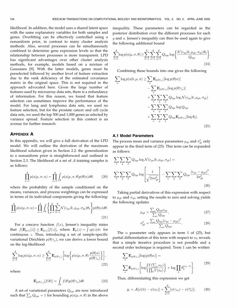
likelihood. In addition, the model uses a shared latent spacewith the same explanatory variables for both samples andgenes. Overfitting can be effectively controlled using anonuniform prior, in contrast to many cluster analysismethods. Also, several processes can be simultaneouslycombined to determine gene expression levels so that therelationship between processes is more transparent. LPDhas significant advantages over other cluster analysismethods, for example, models based on a mixture ofGaussians [9]. With the latter models, genes must bepreselected followed by another level of feature extractiondue to the rank deficiency of the estimated covariancematrix in the original space. This is not required in theapproach advocated here. Given the large number offeatures used by microarray data sets, there is a redundancyof information. For this reason, we found that featureselection can sometimes improve the performance of themodel. For lung and lymphoma data sets, we used nofeature selection, but for the prostate cancer and cell cycledata sets, we used the top 500 and 1,000 genes as selected byvariance spread. Feature selection in this context is anavenue for further research.

APPENDIX A

In this appendix, we will give a full derivation of the LPD

model. We will outline the derivation of the maximum

likelihood solution given in Section 2.2: the generalization

to a nonuniform prior is straightforward and outlined in

Section 2.3. The likelihood of a set of A training samples is

as follows:

YAa¼1

pðaj�; �; �Þ ¼YAa¼1

Z�

pðaj�; �; �Þpð�j�Þd�; ð20Þ

where the probability of the sample conditioned on the

means, variances, and process weightings can be expressed

in terms of its individual components giving the following:

YAa¼1

pðaj�; �; �Þ¼YAa¼1

Z�

YGg¼1

XKk¼1

Nðegajk; �gk; �gkÞ�k

( )pð�j�Þd�:

ð21Þ

For a concave function fðxÞ, Jensen’s inequality states

that f EpðzÞ½z�� �

� EpðzÞ½fðzÞ�, where EpðzÞ ¼RzpðzÞdz for

continuous z. Thus, introducing a set of sample-specific

variational Dirichlets pð�j�aÞ, we can derive a lower bound

on the log-likelihood

XAa¼1

log pðaj�; �; �Þ �XAa¼1

Epð�j�aÞ log pðaj�; �; �Þ pð�j�Þpð�j�aÞ

� �� �;

ð22Þ

where

Epð�j�aÞ fð�Þ½ � ¼Z�

fð�Þpð�j�aÞd�: ð23Þ

A set of variational parameters Qkga are now introduced

such thatP

k Qkga ¼ 1 for bounding pðaj�; �; �Þ in the above

inequality. These parameters can be regarded as the

posterior distribution over the different processes for each

g and a. Jensen’s inequality can then be used again to give

the following additional bound

XAa¼1

log pðaj�; �; �Þ�XKk¼1

XAa¼1

XGg¼1

Qkga logNðegajk; �gk; �gkÞ�k

Qkga

� �:

ð24Þ

Combining these bounds into one gives the followingXa

log pðajb; �; �Þ �Xa

Epð�j�aÞ½log pð�j�Þ�

�Xa

Epð�j�aÞ½log pð�j�aÞ�

þXa

Xg

Xk

Qkga logNðegajk; �gk; �gkÞ

�Xa

Xg

Xk

Qkga logQkga

þXa

Xg

Xk

QkgaEpð�j�aÞ½log �k�:

ð25Þ

A.1 Model Parameters

The process mean and variance parameters �gk and �2gk only

appear in the third term of (25). This term can be expanded

as follows:Xa

Xg

Xk

Qkga logNðegajk; �gk; �gkÞ ¼

Xa

Xg

Xk

Qkga log1ffiffiffiffiffiffiffiffiffiffiffiffi2��2gk

q264

375�

Xa

Xg

Xk

Qkgaðega � �gkÞ2

2�2gk:

ð26Þ

Taking partial derivatives of this expression with respect

to �gk and �gk, setting the results to zero and solving yields

the following updates

�gk ¼P

a QkgaegaPa Qkga

; ð27Þ

�2gk ¼P

a Qkgaðega � �gkÞ2Pa Qkga

: ð28Þ

The � parameter only appears in term 1 of (25), but

partial differentiation of this term with respect to �k reveals

that a simple iterative procedure is not possible and a

second order technique is required. Term 1 can be writtenXa

Epð�j�aÞ½logðpð�j�Þ� ¼

Xa

Epð�j�aÞ log�ðP

k �kÞQk �ð�kÞ

� �þ log

Yk

�ð�k�1Þk

" #:

ð29Þ

Thus, differentiating this expression we get

gi ¼ A �ð Þ � �ið Þ½ � þXAa¼1

�iað Þ � �að Þ½ �; ð30Þ

154 IEEE/ACM TRANSACTIONS ON COMPUTATIONAL BIOLOGY AND BIOINFORMATICS, VOL. 2, NO. 2, APRIL-JUNE 2005

from which we can derive the corresponding Hessian

Hij ¼ 0 �ð Þ � �ijA 0 �ið Þ; ð31Þ

�new ¼ �old �Hð�oldÞ�1gð�oldÞ; ð32Þ

where Hð�Þ is the Hessian matrix and gð�Þ is the gradient.For i; j ¼ 1; . . . ;K, their components are given by:

gi ¼ A �ð Þ � �ið Þ½ � þXAa¼1

�iað Þ � �að Þ½ �; ð33Þ

Hij ¼ 0 �ð Þ � �ijA 0 �ið Þ; ð34Þ

where �a ¼PK

j¼1 �jc, � ¼PK

k¼1 �k, and 0 �ð Þ is the trigamma

function. Since the Hessian matrix is of the form

H ¼ diagðhÞ þ 1z1T ; ð35Þ

matrix inversion can be avoided [2] and the ith componentof the correction in the iterative update rule can be foundfrom

ðH�1gÞi ¼ ðgi � rÞ=hi; ð36Þwhere

r ¼Xkj¼1

ðgj=hjÞ !

= z�1 þXkj¼1

h�1j

!: ð37Þ

A.2 Variational Parameters

First, Qkga appears in terms 3, 4, and 5 of (25). Taking these

terms, removing summations over k, a, and g and adding a

Lagrangian to satisfy the summation constraint, we have

Qkga logNðegajk; �gk; �gkÞ �Qkga logQkga þQkgaEpð�j�aÞ

½log �k� � �Xa

Qkga � 1

!;

ð38Þ

taking partial derivatives with respect to Qkga and settingthese to zero gives

0¼ logNðegajk; �gk; �gkÞ�ðlog½Qkga� þ 1Þ þEpð�j�aÞ½log �k� � �;

ð39Þ

solving for � and rearranging gives the following update forQkga

Qkga ¼Nðegajk; �gk; �gkÞ exp½Epð�j�aÞ½log �k��PA

a0¼1 Nðega0 jk; �gk; �gkÞ exp½Epð�j�a0 Þ½log �k��; ð40Þ

where

Epð�j�aÞ½log �k� ¼ �ð�akÞ ��Xj

�aj

!: ð41Þ

Now, the �ak variable appears in terms 1, 2, and 5 of the

above bound. Extracting these terms and removing summa-

tions over k and a leaves

�Epð�j�aÞ½log pð�j�aÞ� þEpð�j�aÞ½log pð�j�Þ�þXg

QkgaEpð�j�aÞ½log �k�: ð42Þ

Now,

Epð�j�aÞ½log pð�j�aÞ� ¼Z�

log�ðP

k �akÞQk �ð�akÞ

þXk

ð�ak � 1Þ log½�k�" #

pð�j�aÞd�

¼ log�ðP

k �akÞQk �ð�akÞ

� �þXk

ð�ak � 1ÞEpð�j�aÞ

½log �k�

¼ log�ðP

k �akÞQk �ð�akÞ

� �þXk

ð�ak � 1Þ

½�ð�akÞ ��Xj

�aj

!�;

ð43Þ

and similarly for the pð�j�Þ term. Therefore, the relevantterms simplify to the following (again, omitting unneces-sary summations and non-�ak terms)

�k��akþXg

Qkga

!�ð�akÞ ��

Xj

�aj

!" #�log

�ðP

k �akÞQk �ð�akÞ

� �:

ð44Þ

Taking partial derivatives with respect to �ak and settingthese to zero leaves

�k � �ak þXg

Qkga

!�0ð�akÞ ��0

Xj

�aj

!" #¼ 0; ð45Þ

giving the following update for �ak

�ak ¼ �k þXg

Qkga: ð46Þ

A.3 Pseudocode Listings

Algorithm 1: Latent Process Decomposition algorithm. Weused a tolerance tol1 ¼ 10�5 to avoid Gaussians collapsingonto a single point, and tol2 ¼ 10�10 for the � updating.

Parameter Initialization. From (6), we can see that inorder to update Qkga, we need values for �gk, �gk, and �ak.The first two are initialized to the array means and standarddeviations, respectively. The �ak values were initialized topositive random numbers since, with the means andstandard deviations uniform over the K processes, uniform

ROGERS ET AL.: THE LATENT PROCESS DECOMPOSITION OF CDNA MICROARRAY DATA SETS 155

�ak values would place the algorithm in a local minima ofthe likelihood and training could not proceed.

Numerical Stability. There are several points where thealgorithm could potentially lose numerical stability. If aGaussian contracts onto a single point, its standarddeviation will shrink to zero and its probability densityfunction will approach 1. To avoid this, we apply a lowerbound to the value of �2gk. The choice of the value of thisbound is important since, if the value is too low, numericalproblems will persist, while if it is too high it wouldoverconstrain the model and prevent it from fitting the data.For the update equation for Qkga, we find a second possiblesource of instability. From (6), we occasionally find that wereach the limits of machine precision and both thenumerator and the denominator approach zero. To circum-vent this, we added a small constant (10�100) to each valuein Q before normalization (i.e., before performing thedivision in (6)). Finally, when calculating the likelihood,we have to compute a product over the g. For a largenumber of genes, this product soon becomes smaller thanthe machine precision. However, we are ultimately inter-ested in the logarithm of this product (the log-likelihood)and so we can perform the following numerical trick toavoid a problem. Namely, we observe that the expressionwe wish to evaluate is of the form log

Pi

Qj Rij. This can be

rewritten

logXi

exp i

" #¼ log

Xi

expfi þKg expð�KÞ" #

¼ logXi

expði þKÞ" #

�K;

if i ¼P

j logRij, which can be readily evaluated given asuitable choice for K. Given that the i values will all benegative, a suitable choice is �max½i� so that we areeffectively incrementing all i values so that the maximumvalue is 0. Following the implementation of these precau-tions, the algorithm is robust.

ACKNOWLEDGMENTS

The authors would like to thank Dr. Jeremy Clark, Instituteof Cancer Research, London, for comments on the genesmentioned in Section 3.1.1. The work of Rainer Breitlingwas supported by a BBSRC grant (17/GG17989) and ColinCampbell and Simon Rogers were supported by EPSRCgrant GR/R96255 and an EPSRC DTA award.

REFERENCES

[1] A.A. Alizadeh et al., “Distinct Types of Diffuse Large B-CellLymphoma Identified by Gene Expression Profiling,” Nature,vol. 403, no. 3, pp. 503-511, Feb. 2000.

[2] D.M. Blei, A.Y. Ng, and M.I. Jordan, “Latent Dirichlet Allocation,”J. Machine Learning Research, vol. 3, pp. 993-1022, 2003.

[3] C.C. Chang et al., “Connective Tissue Growth Factor and Its Rolein Lung Adenocarcinoma Invasion and Metastasis,” J. Nat’l CancerInst., vol. 96, pp. 344-345, 2004.

[4] S.M. Dhanasekaran et al., “Delineation of Prognostic Biomarkersin Prostate Cancer,” Nature, vol. 412, pp. 822-826, 2001.

[5] R.G. Fahmy et al., “Transcription Factor EGR-1 Supports FGF-Dependent Angiogenesis during Neovascularization and TumorGrowth,” Nature Medicine, vol. 9, pp. 1026-1032, 2003.

[6] E. Garber et al., “Diversity of Gene Expression in Adenocarcinomaof the Lung,” Proc. Nat’l Academy of Sciences of the USA, vol. 98,no. 24, pp. 12784-12789, 2001.

[7] A.P. Gasch et al., “Genomic Expression Program in the Responseof Yeast Cells to Environmental Changes,” Molecular Biology of theCell, vol. 11, pp. 4241-4257, 2000.

[8] L.C. Lazzeroni and A. Owen, “Plaid Models for Expression Data,”Statistica Sinica, vol. 12, pp. 61-86, 2002.

[9] G.J. McLachlan, R.W. Bean, and D. Peel, “A Mixture Model-BasedApproach to the Clustering of Microarray Expression Data,”Bioinformatics, vol. 18, no. 3, pp. 413-422, 2002.

[10] E. Segal, A. Battle, and D. Koller, “Decomposing Gene Expressioninto Cellular Processes,” Proc. Eighth Pacific Symp. Biocomputing(PSB), pp. 89-100, 2003.

[11] P. Spellman et al., “Comprehensive Identification of Cell Cycle-Regulated Genes of the Yeast Saccharomyces Cerevisiae byMicroarray Hybridization,” Molecular Biology of the Cell, vol. 9,pp. 3273-3297, 1998.

Simon Rogers received a degree in electricaland electronic engineering from the University ofBristol (2001) during which he was awarded theSander prize for the best final year examinationresults, and the PhD degree in engineeringmathematics from the University of Bristol(2004). During June 2004, he was a visitingresearcher in the Bioinformatics Research Cen-tre at the University of Glasgow where he nowholds a postdoctoral research position.

Mark Girolami received a degree in mechanicalengineering from the University of Glasgow(1985), and the PhD in computer science fromthe University of Paisley (1998). He was adevelopment engineer with IBM from 1985 until1995 when he left to pursue an academic career.From May to December 2000, Dr. Girolami wasthe TEKES visiting professor at the Laboratory ofComputing and Information Science in HelsinkiUniversity of Technology. In 1998 and 1999, he

was a research fellow at the Laboratory for Advanced Brain SignalProcessing in the Brain Science Institute, RIKEN, Wako-Shi, Japan.

Colin Campbell received a degree in physicsfrom Imperial College, London (1981), and thePhD degree in applied mathematics from King’sCollege, London (1984). Subsequently, he heldpostdoctoral positions at the University of Stock-holm and Newcastle University. He joined theFaculty of Engineering at Bristol University in1990. His main interests are learning theory,algorithm design, and decision theory. Currenttopics of interest include kernel-based methods,

Bayesian generative models, and the application of these techniques toreal world problems, mainly in the area of medical decision support,bioinformatics, and onco-informatics.

Rainer Breitling received a degree in biochem-istry from the University of Hanover, Germany(1997), and the PhD degree in biochemistry fromTechnische Universitat Munchen (2001). FromJune 2001 to April 2003, he worked as apostdoctoral fellow in bioinformatics in theDepartment of Biology at San Diego StateUniversity. Since May 2003, he has been aresearch assistant at the University of Glasgow,Scotland, where he works on the development of

automated interpretation techniques for biomedical microarray data sets.

. For more information on this or any other computing topic,please visit our Digital Library at www.computer.org/publications/dlib.

156 IEEE/ACM TRANSACTIONS ON COMPUTATIONAL BIOLOGY AND BIOINFORMATICS, VOL. 2, NO. 2, APRIL-JUNE 2005