Grade of Membership and Latent Structure Models with ...

Grade of Membership and Latent Structure ModelsWith Application to Disability Survey Data

Elena Aleksandrovna EroshevaAugust 2002

Department of StatisticsCarnegie Mellon University

Pittsburgh, PA 15213

Submitted in partial fulfillment of the requirementsfor the degree of Doctor of Philosophy

Thesis Committee:Stephen E. Fienberg

�, Chair

Brian W. Junker�

Nicole A. Lazar�

Burton H. Singer�

Copyright c�

2002 Elena A. Erosheva

�Department of Statistics, Carnegie Mellon University�Office of Population Research, Princeton University

Abstract

Multivariate categorical data, such as binary or multiple choice individual responses to a set of

questions, are abundant in the social sciences. These data can be recorded in a multi-way con-

tingency table, which quickly becomes sparse with any practical sample size when the number of

questions goes up. Latent structure models, such as latent class and latent trait models, provide

a way to model the distribution of counts in a large sparse contingency table based on assump-

tions about the latent structure of the data. This work examines a relatively new latent structure

model, the Grade of Membership (GoM) model, integrating the GoM language and ideas with

more standard statistical literature on latent variable models. The GoM model assumes that indi-

viduals can have mixed membership in several subpopulations. Representing the GoM model as

a constrained latent class model leads naturally to the Bayesian estimation framework developed

and implemented in this dissertation. The analysis of a subset of functional disability data from

the National Long Term Care survey provides an illustration of using the GoM and other latent

structure models to describe the distribution of counts in a large sparse contingency table. Finally,

a general class of mixed membership models is presented that unifies the latent structure of the

GoM model and two other mixed membership models that recently appeared in the genetics and

the machine learning literatures.

i

Acknowledgments

This work would never have been initiated if it were not my husband’s dream to obtain his

doctoral degree in the Unites States. I am glad that I joined him in this endeavor, and that Carnegie

Mellon happened to be our school of choice.

First and foremost, I would like to thank my thesis advisor, Stephen Fienberg. He introduced

me to the literature on the Grade of Membership model, which became the main focus of my

dissertation research. His constant guidance, care, unconditional support, and soft advice during

two and a half years count for much more than just a piece of higher education. He gave me a lot

of freedom to make my own choices and to satisfy my own curiosity, and yet enough direction not

to become frustrated at difficult times. His many exceptional professional and personal qualities

have helped make my dissertation a positive experience. To him I give my deepest thanks.

I would also like to express my appreciation to the members of my committee. Discussions

with Brian Junker were both educational and stimulating at all times, and his positive attitude

was contagious. Brian introduced me to the world of psychometrics and gave numerous helpful

suggestions about technical writing. Since the time when I first came to Carnegie Mellon four

years ago, Nicole Lazar has constantly supported me with much needed encouragement and gentle

criticism. Although I had not met Burton Singer before my defense day, studying his work has

broadened my understanding of statistical applications in the social sciences.

I owe many thanks to the faculty, stuff, and my fellow students at the Department of Statistics.

To name only a few, I would like to thank Howard Seltman for sharing many useful programming

suggestions, Tom Minka for asking sharp questions and bringing in a different perspective, and my

iii

only constant officemate and a good friend Can Cai for always being there to listen.

I am eternally grateful to my family for believing in me and for continuously supporting my

desire to stay in school for 21 years. I am most indebted to my husband, Pavel Nikitin, for his

patience and understanding.

I thank the Center for Demographic Studies, Duke University, for providing the data from

the National Long-Term Care Survey and the Inter-University Consortium for Political and Social

Research for providing additional documentation; I thank both institutions for the assistance in

working with the data. The preparation of this thesis was supported in part by Grant No. 1R03

AG18986-01, from the National Institute on Aging to Carnegie Mellon University, and by National

Science Foundation Grant No. EIA-9876619 to the National Institute of Statistical Sciences.

I dedicate this dissertation to the memory of my grandfather, my first teacher, Nikolai Petrovich

Ermakov.

iv

Contents

1 Grade of Membership Model as one of the Latent Structure Models 1

1.1 Statistical Literature Review and Historical Comments . . . . . . . . . . . . . . . 2

1.2 Grade of Membership (GOM) Model . . . . . . . . . . . . . . . . . . . . . . . . . 6

1.2.1 Standard Model Formulation and Notation . . . . . . . . . . . . . . . . . 6

1.2.2 Matrix Formulation . . . . . . . . . . . . . . . . . . . . . . . . . . . . . . 9

1.3 Links With Psychometrics and Item Response Theory . . . . . . . . . . . . . . . . 10

1.3.1 Latent Structure Analysis . . . . . . . . . . . . . . . . . . . . . . . . . . . 10

1.3.2 Item Response Theory . . . . . . . . . . . . . . . . . . . . . . . . . . . . 13

1.3.3 Factor Analysis . . . . . . . . . . . . . . . . . . . . . . . . . . . . . . . . 16

1.4 Estimation . . . . . . . . . . . . . . . . . . . . . . . . . . . . . . . . . . . . . . . 20

1.4.1 Joint, Conditional, and Marginal Likelihood . . . . . . . . . . . . . . . . . 20

1.4.2 Manton, Woodbury, and Tolley’s fixed point iteration algorithm. . . . . . . 23

1.4.3 Other Estimation Methods . . . . . . . . . . . . . . . . . . . . . . . . . . 25

1.4.4 Discussion. . . . . . . . . . . . . . . . . . . . . . . . . . . . . . . . . . . 27

2 Comparing Latent Structures of the Grade of Membership, Rasch, and Latent Class

Models 31

2.1 Heterogeneity Representations: �� table . . . . . . . . . . . . . . . . . . . . . 32

2.1.1 Preliminaries . . . . . . . . . . . . . . . . . . . . . . . . . . . . . . . . . 32

v

2.1.2 Latent class models . . . . . . . . . . . . . . . . . . . . . . . . . . . . . . 35

2.1.3 Rasch model . . . . . . . . . . . . . . . . . . . . . . . . . . . . . . . . . 39

2.1.4 Grade of Membership model . . . . . . . . . . . . . . . . . . . . . . . . . 41

2.2 Similarities and Differences: Comparing Heterogeneity Manifolds . . . . . . . . . 44

2.3 Increasing Dimensionality . . . . . . . . . . . . . . . . . . . . . . . . . . . . . . 47

2.4 Conclusion . . . . . . . . . . . . . . . . . . . . . . . . . . . . . . . . . . . . . . 49

3 Latent Class Representation 51

3.1 Introduction . . . . . . . . . . . . . . . . . . . . . . . . . . . . . . . . . . . . . . 51

3.2 GoM Model as a Generalization of the Latent Class Models . . . . . . . . . . . . . 53

3.2.1 Latent Class Model . . . . . . . . . . . . . . . . . . . . . . . . . . . . . . 53

3.2.2 GoM Model . . . . . . . . . . . . . . . . . . . . . . . . . . . . . . . . . . 55

3.3 Haberman’s latent class model with constraints . . . . . . . . . . . . . . . . . . . 56

3.4 Equivalence between Haberman’s latent class model and the GoM model. . . . . . 60

3.5 Interpretation . . . . . . . . . . . . . . . . . . . . . . . . . . . . . . . . . . . . . 61

3.5.1 Parallel with sufficient experiments . . . . . . . . . . . . . . . . . . . . . 61

3.5.2 Stochastic subject and random sampling . . . . . . . . . . . . . . . . . . . 63

4 Data Augmentation and Bayesian Estimation Algorithms for the Grade of Member-

ship Model 65

4.1 Bayesian Model Formulation . . . . . . . . . . . . . . . . . . . . . . . . . . . . . 66

4.1.1 Choice of Priors . . . . . . . . . . . . . . . . . . . . . . . . . . . . . . . 66

4.1.2 Choice of Hyperprior . . . . . . . . . . . . . . . . . . . . . . . . . . . . . 68

4.2 Data Augmentation . . . . . . . . . . . . . . . . . . . . . . . . . . . . . . . . . . 70

4.3 Markov Chain Monte Carlo Algorithms . . . . . . . . . . . . . . . . . . . . . . . 74

4.3.1 Gibbs Sampler . . . . . . . . . . . . . . . . . . . . . . . . . . . . . . . . 74

4.3.2 Metropolis-Hastings Within Gibbs . . . . . . . . . . . . . . . . . . . . . . 75

vi

4.4 Choosing the Number of Extreme Profiles . . . . . . . . . . . . . . . . . . . . . . 79

4.4.1 Overview of Model Selection Methods . . . . . . . . . . . . . . . . . . . 79

4.4.2 Calculating DIC for the GoM Model . . . . . . . . . . . . . . . . . . . . . 82

4.5 Implementation Notes . . . . . . . . . . . . . . . . . . . . . . . . . . . . . . . . . 83

5 Studying Disability in the Elderly 87

5.1 Motivation and Significance . . . . . . . . . . . . . . . . . . . . . . . . . . . . . 87

5.1.1 Functional Disability: Activities of Daily Living and Instrumental Activi-

ties of Daily Living . . . . . . . . . . . . . . . . . . . . . . . . . . . . . . 88

5.1.2 Disability Trends in the United States . . . . . . . . . . . . . . . . . . . . 89

5.2 Literature Review . . . . . . . . . . . . . . . . . . . . . . . . . . . . . . . . . . . 91

5.2.1 Summed Indexes and Hierarchical Scales . . . . . . . . . . . . . . . . . . 91

5.2.2 Latent Dimensionality . . . . . . . . . . . . . . . . . . . . . . . . . . . . 93

5.2.3 Psychometric Models . . . . . . . . . . . . . . . . . . . . . . . . . . . . . 98

6 NLTCS: Preliminary Data Analysis 101

6.1 National Long-Term Care Survey . . . . . . . . . . . . . . . . . . . . . . . . . . . 101

6.2 Data Set and Exploratory Data Analysis . . . . . . . . . . . . . . . . . . . . . . . 103

6.2.1 Subset of 16 ADL/IADL Measures . . . . . . . . . . . . . . . . . . . . . 103

6.2.2 Marginal Frequencies and Simple Statistics . . . . . . . . . . . . . . . . . 105

6.2.3 Frequent Responses . . . . . . . . . . . . . . . . . . . . . . . . . . . . . 105

6.2.4 Total Number of Disabilities . . . . . . . . . . . . . . . . . . . . . . . . . 107

6.3 Testing Unidimensionality . . . . . . . . . . . . . . . . . . . . . . . . . . . . . . 108

6.3.1 Item Response Theory Methods for Assessing Dimensionality . . . . . . . 108

6.3.2 Applying the Approach of Holland and Rosenbaum . . . . . . . . . . . . . 110

6.4 Factor Analysis . . . . . . . . . . . . . . . . . . . . . . . . . . . . . . . . . . . . 113

6.5 Latent Class Analysis . . . . . . . . . . . . . . . . . . . . . . . . . . . . . . . . . 121

vii

6.6 Conclusion . . . . . . . . . . . . . . . . . . . . . . . . . . . . . . . . . . . . . . 131

7 NLTCS: Grade of Membership Analysis 135

7.1 Preliminaries . . . . . . . . . . . . . . . . . . . . . . . . . . . . . . . . . . . . . 135

7.2 Results . . . . . . . . . . . . . . . . . . . . . . . . . . . . . . . . . . . . . . . . . 138

7.3 Conclusions . . . . . . . . . . . . . . . . . . . . . . . . . . . . . . . . . . . . . . 156

8 Common Framework for Mixed Membership Models 161

8.1 Genetics . . . . . . . . . . . . . . . . . . . . . . . . . . . . . . . . . . . . . . . . 162

8.2 Machine Learning . . . . . . . . . . . . . . . . . . . . . . . . . . . . . . . . . . . 164

8.2.1 Models . . . . . . . . . . . . . . . . . . . . . . . . . . . . . . . . . . . . 164

8.2.2 Approximate Inference Techniques . . . . . . . . . . . . . . . . . . . . . 167

8.3 Class of Mixed Membership Models . . . . . . . . . . . . . . . . . . . . . . . . . 169

9 Conclusions and Future Research 175

9.1 Conclusions. . . . . . . . . . . . . . . . . . . . . . . . . . . . . . . . . . . . . . . 175

9.2 Future Research . . . . . . . . . . . . . . . . . . . . . . . . . . . . . . . . . . . . 177

A C Code: Metropolis-Hastings Within Gibbs for the GoM Model 181

B Simulation Studies: GoM model 191

B.1 Simulation Study with BUGS . . . . . . . . . . . . . . . . . . . . . . . . . . . . . 191

B.1.1 GoM Model Specification for BUGS . . . . . . . . . . . . . . . . . . . . 191

B.1.2 Simulation Example: Fixed Hyperparameters . . . . . . . . . . . . . . . . 193

B.2 Comparison of BUGS and the C Code . . . . . . . . . . . . . . . . . . . . . . . . 201

B.3 Simulation Study with the C Code: Estimating � . . . . . . . . . . . . . . . . . . 205

B.4 Simulation Study with the C Code: Estimating Hyperparameters . . . . . . . . . . 205

C List of Triggering questions for 16 ADL/IADL Measures 209

viii

D SAS Code: Calculating Tetrachoric Correlations 213

E BUGS Code for Latent Class Models 215

ix

List of Figures

1.1 Examples of item response functions with � �� and �� (dotted), �� (solid), �� (dashed). . . . . . . . . . . . . . . . . . . . . 19

2.1 Surface of independence in the full parameter space �� "!$# �%� ��&!(' �%� �� .Contour lines are given for better perception of the 3-dimensional surface. . . . . . 34

2.2 Latent class probabilistic mixture model heterogeneity manifold in the marginal

space �)�+* �&!�# �,* � . . . . . . . . . . . . . . . . . . . . . . . . . . . . . . . . . . 37

2.3 Latent class probabilistic mixture model heterogeneity manifold in the full param-

eter space � �-� � �.!$# �/� ��&!(' �-� �� . . . . . . . . . . . . . . . . . . . . . . . . . . 38

2.4 Latent trait Rasch model heterogeneity manifold in the marginal space �)�+* �&!�# �* � . . . . . . . . . . . . . . . . . . . . . . . . . . . . . . . . . . . . . . . . . . . . 38

2.5 Latent trait Rasch model heterogeneity manifold in the full parameter space �/�� "!$# �/� ��&!(' �/� �� . . . . . . . . . . . . . . . . . . . . . . . . . . . . . . . . . . 40

2.6 GoM model heterogeneity manifold in the marginal space �)�,* �0!$# ��* � . . . . . . 42

2.7 GoM model heterogeneity manifold in the full parameter space �1�� 2!$# �� (!(' �/� �� . . . . . . . . . . . . . . . . . . . . . . . . . . . . . . . . . . . . . . . 43

2.8 Illustration for the numerical example. The straight line is the heterogeneity man-

ifold for the latent class probabilistic model. The curve on the surface is the het-

erogeneity manifold for the GoM model. Points correspond to 3��45��76 . . . . . 48

4.1 GoM graphical diagram . . . . . . . . . . . . . . . . . . . . . . . . . . . . . . . . 84

xi

6.1 The number of observed response patterns by total number of disabilities. . . . . . 107

6.2 Three latent classes. Histogram of posterior probabilities of being a member of

each latent class. N=21,574 . . . . . . . . . . . . . . . . . . . . . . . . . . . . . . 125

6.3 Four latent classes. Histogram of posterior probabilities of being a member of each

latent class. N=21,574. . . . . . . . . . . . . . . . . . . . . . . . . . . . . . . . . 127

6.4 Five latent classes. Histogram of posterior probabilities of being a member of each

latent class. N=21,574. . . . . . . . . . . . . . . . . . . . . . . . . . . . . . . . . 130

7.1 Plots of successive iterations and posterior density estimates for the hyperparame-

ters � !�89�0!�8"�"! and 8 � for the GoM model with 3 extreme profiles. . . . . . . . . . . 144

7.2 Plots of successive iterations and posterior density estimates of * ��:;� <.! * ��:;� <2! *=� :;� <.!and * ��:;� > for the GoM model with 3 extreme profiles. . . . . . . . . . . . . . . . . 145

7.3 Plots of successive iterations and posterior density estimates of the hyperparame-

ters � !�89�0!�8"�"! and 8 � for the GoM model with 4 extreme profiles. . . . . . . . . . . 148

7.4 Plots of successive iterations and posterior density estimates of * ��:;� � ! * ��:;� � ! *=� :;� � !and *=? :;� � for the GoM model with 4 extreme profiles. . . . . . . . . . . . . . . . . 149


ters � !�89�0!�8"�"!�8 � for the GoM model with 5 extreme profiles. . . . . . . . . . . . . 152


ters 8 ? !�8"<.! and conditional response probabilities * ��: @ and * ��: @ for the GoM model

with 5 extreme profiles. . . . . . . . . . . . . . . . . . . . . . . . . . . . . . . . . 153

7.7 Plots of successive iterations and posterior density estimates of *A� : @"! *B? : @"! * <�: @ and* <�:;� � for the GoM model with 5 extreme profiles. . . . . . . . . . . . . . . . . . . 154

B.1 Simulation 2. Membership scores for first extreme profile versus the number of

observed response pattern. . . . . . . . . . . . . . . . . . . . . . . . . . . . . . . 195

xii

B.2 Simulation 3. Membership scores for first extreme profile versus the number of

observed response pattern. . . . . . . . . . . . . . . . . . . . . . . . . . . . . . . 196

B.3 Simulation 2. Conditional probability of observing response patterns 1 through 16

under the GoM model, given the extreme profile probabilities and the simulated

GoM scores. . . . . . . . . . . . . . . . . . . . . . . . . . . . . . . . . . . . . . . 197

B.4 Simulation 3. Conditional probability of observing response patterns 1 through 16

under the GoM model, given the extreme profile probabilities and the simulated

GoM scores. . . . . . . . . . . . . . . . . . . . . . . . . . . . . . . . . . . . . . . 197

B.5 Posterior distribution for the first extreme profile probabilities, CD�E�2�F�F� . . . . . . 198

B.6 Posterior distribution conditional response probabilities of the second extreme pro-

file, CG�H�2�F�F� . . . . . . . . . . . . . . . . . . . . . . . . . . . . . . . . . . . . . 199

B.7 Posterior distribution for selected conditional response probabilities, C��H�2�I� . . . 200

B.8 Posterior distribution for the first extreme profile probabilities, obtained by using

C code . . . . . . . . . . . . . . . . . . . . . . . . . . . . . . . . . . . . . . . . . 203

B.9 Posterior distribution for the second extreme profile probabilities, obtained by us-

ing C code . . . . . . . . . . . . . . . . . . . . . . . . . . . . . . . . . . . . . . . 204

B.10 Posterior distribution for the hyperparameters, obtained by using C code . . . . . . 208

xiii

List of Tables

2.1 Example . . . . . . . . . . . . . . . . . . . . . . . . . . . . . . . . . . . . . . . . 36

3.1 Simple example: Extreme profile probabilities for the GoM model. . . . . . . . . . 61

3.2 Simple example: Latent class representation of the GoM model. Latent class and

conditional response probabilities. . . . . . . . . . . . . . . . . . . . . . . . . . . 62

5.1 Katz ADL index. ADL functions: feeding (1), continence (2), transferring (3),

going to the toilet (4), dressing (5) and bathing (6). . . . . . . . . . . . . . . . . . 93

6.1 Marginal frequencies of 16 measures from NLTCS. . . . . . . . . . . . . . . . . . 105

6.2 Cell counts for the most frequent observed responses. . . . . . . . . . . . . . . . . 106

6.3 Total number of ADLs by total number of IADLs. Sample size 21,574. . . . . . . . 108

6.4 Cohran-Mantel-Haenszel chi-square statistics for 16 ADL/IADL measures, pooled

data. . . . . . . . . . . . . . . . . . . . . . . . . . . . . . . . . . . . . . . . . . . 112

6.5 Tetrachoric correlations of 16 ADL/IADL measures, pooled data. . . . . . . . . . . 114

6.6 Five largest eigenvalues for the matrix of tetrachoric correlations, pooled data. . . . 115

6.7 Rotated factor loadings and communality estimates, pooled data . . . . . . . . . . 115

6.8 Five largest eigenvalues for the matrix of tetrachoric correlations, 1982 wave. . . . 116

6.9 Rotated factor loadings and communality estimates, 1982 wave. . . . . . . . . . . 117



xv


6.13 Rotated factor loadings and communality estimates, 1989 wave . . . . . . . . . . . 119



6.16 Posterior mean(standard deviation) estimates for 2-class LCM. . . . . . . . . . . . 123




6.20 Observed and expected cell counts for frequent response patterns under 2-, 3-, 4-,

and 5-class latent class models. . . . . . . . . . . . . . . . . . . . . . . . . . . . . 132

7.1 Posterior mean (standard deviation) estimates for GoM model with 2 extreme pro-

files. . . . . . . . . . . . . . . . . . . . . . . . . . . . . . . . . . . . . . . . . . . 140


files. . . . . . . . . . . . . . . . . . . . . . . . . . . . . . . . . . . . . . . . . . . 146


files. . . . . . . . . . . . . . . . . . . . . . . . . . . . . . . . . . . . . . . . . . . 150


files. . . . . . . . . . . . . . . . . . . . . . . . . . . . . . . . . . . . . . . . . . . 155

7.5 DIC for the GoM model with J�� 2, 3, 4, and 5 extreme profiles. . . . . . . . . . . 156

7.6 Observed and expected cell counts for frequent response patterns under 2, 3, 4, and

5 extreme profile GoM models. . . . . . . . . . . . . . . . . . . . . . . . . . . . . 157

B.1 Observed and expected frequencies for the test data under the GoM model with

known hyperparameters . . . . . . . . . . . . . . . . . . . . . . . . . . . . . . . . 194

B.2 Posterior mean and standard deviation for the structural parameters . . . . . . . . . 201

xvi

B.3 Posterior mean and standard deviation for the structural parameters, two runs of

BUGS code, 1000 iterates . . . . . . . . . . . . . . . . . . . . . . . . . . . . . . . 202

B.4 Posterior mean and standard deviation for the structural parameters, 1000 iterates . 202

B.5 Comparison of the posterior mean and standard deviation for the structural param-

eters for BUGS and the C code, 10,000 iterates . . . . . . . . . . . . . . . . . . . 202

B.6 Comparison of the posterior mean and standard deviation for the structural param-

eters for BUGS and the C code, 100,000 iterates . . . . . . . . . . . . . . . . . . . 205

B.7 Approximate posterior distribution parameters and posterior mean of K . Simula-

tion data with four items, two extreme profiles, LNMPO�QR��S� ! �T��VU distribution. . . . . . 206

B.8 Posterior mean and standard deviation for the structural parameters and the hyper-

parameters: Simulation 3 data . . . . . . . . . . . . . . . . . . . . . . . . . . . . 207

B.9 Observed and expected frequencies for Simulation 3 data under the GoM model

with unknown hyperparameters . . . . . . . . . . . . . . . . . . . . . . . . . . . . 207

xvii

Chapter 1

Grade of Membership Model as one of the

Latent Structure Models

Survey data usually contain answers to a number of yes/no or multiple choice questions for each

sampled person. With no other information, these data can also be recorded in the form of a

multidimensional contingency table with a cell value being the number of observed responses

corresponding to a particular discrete response pattern. This type of data is common in social and

political sciences as well as in health sciences. Different research questions may arise depending

on the context of the problem, which in turn call for different statistical methodologies.

For many discrete data problems it is sufficient to assume that individuals are homogeneous

in their responses. This assumption naturally leads to log-linear type of models and allows the

study of inter-dependences among observed variables. In the middle of the 20th century, however,

researchers began to develop models that could be used to capture how individuals differ in their

expected responses. In some cases, for example, in response to the question “have you ever con-

sidered buying a pick-up truck?”, it may be something as simple as gender differences that matters.

In other, more complicated situations, the probability of an individual having a particular response

pattern may depend on a non-observable quantity or trait. Examples of such latent quantities are:

1

an indicator of being a member of one of the latent classes (latent class model), an ability parameter

(item response theory models), or a grade of membership score (Grade of Membership model).

1.1 Statistical Literature Review and Historical Comments

The Grade of Membership (GoM) model was developed by Max Woodbury in the 1970s as a mul-

tivariate statistical technique for medical classification (Woodbury, Clive and Garson 1978, Clive,

Woodbury and Siegler 1983). GoM health-related applications now cover a wide spectrum of

studies, ranging from studying depression (Davidson, Woodbury, Zisook and Giller 1989) and

schizophrenia (Manton, Woodbury, Anker and Jablensky 1994) to identifying genetic components

in Alzheimer’s disease (Corder and Woodbury 1993). Papers describing these applications, coau-

thored by Woodbury, Manton, Stallard and Tolley (in various combinations), have been published

in different journals, with only three of these appearing in major U.S. statistical journals (Manton,

Stallard and Woodbury 1991, Tolley and Manton 1992, Woodbury, Manton and Tolley 1997). In

1994, Manton, Woodbury and Tolley gathered the pieces on methodological issues of the GoM

model together in a monograph “Statistical Applications Using Fuzzy Sets”, but, as Haberman

(1995) pointed out, that description needs to be further integrated with more standard statistical

literature on latent variable models.

Although the GoM model is most frequently described as a fuzzy sets model, it fits naturally

within the framework of latent structure models. In fact, as I show in Section 1.3.1, two latent

structure models discussed by Lazarsfeld and Henry (1968) in “Latent Structure Analysis”, the

polynomial traceline model and the latent content model, share a special case which, in turn, is a

special case of the GoM model. Thus, these three models coincide in the low-dimensional special

case, although they generalize differently to higher dimensions.

The polynomial traceline and the latent content models have received little attention since the

1970s, partly because of computational difficulties associated with parameter estimation, and partly

2

because of the development of other latent structure models around the same time, namely, com-

mon item response theory (IRT) and latent class models. Van der Linden and Hambelton (1997)

provide a recent overview of IRT models. Bartholomew and Knott (1999) describe the current

state of latent class modeling.

The GoM and IRT models share a similar feature in that they involve two sets of unknown

parameters: individual- and item-specific. Although in discussions with others I have learned

that researchers have thought about the connections between the GoM and IRT models, there is

no published literture comparing theese models. In this thesis, I provide a general framework to

view the GoM model in the context of IRT models in Section 1.3.2. In addition, in Chapter 2,

I compare geometrically the GoM and the Rasch models with a special focus on heterogeneity

representations, in the context of a two by two contingency table.

Because the GoM model formulation resembles factor analysis and principal components anal-

ysis, understanding the interrelation among these models can provide valuable insights. Manton

et al. (1994) and Marini, Li and Fan (1996) outline some similarities and differences between the

GoM model and factor analysis. Wachter (1999) finds that solutions obtained from the GoM model

are remarkably close to solutions from principal components analysis in the one-dimensional case.

In Section 1.3.3 of this thesis, I discuss general factor analysis approaches for binary data and show

their relationship to the GoM model.

Current GoM estimation methods are likelihood-based. The number of parameters in the GoM

model, as well as in IRT models, increases with the number of subjects (and items), and this

complicates the task of parameter estimation. In Section 1.4, I focus on different types of likelihood

functions that arise from this setting, and provide an overview of current GoM estimation methods

in the literature.

Latent class models were first introduced by Paul Lazarsfeld in the late 1940s. Developments

from the 1940s to the late 1960s are described in the book by Lazarsfeld and Henry (1968), where

they considered both latent class and latent trait models and treated them as fundamentally differ-

3

ent. More recent literature contains examples that show close interplay between latent class and

latent trait models (Lindsay, Clogg and Grego 1991, Hoijtink and Molenaar 1997). Regarding the

GoM model, there is a belief that GoM should be superior to latent class when the number of

discrete variables is large and the frequencies of the cell counts are small (Manton, Woodbury and

Tolley 1994, Singer 1989), but this needs to be further supported by theory and simulation studies.

Comparing the GoM and latent class models theoretically, Manton et al. (1994, pp. 40-46) take the

point of view that the conventional latent class model is a special case of the GoM model. How-

ever, Haberman (1995), reviewing Manton, Woodbury, and Tolley’s monograph (1994), suggests

that the GoM model is in fact a special case of latent class models with constraints. In Chapter 3,

I develop a common framework to explain these seemingly contradictory statements. Under this

framework, I provide detailed proofs for the latent class representation of the GoM model.

As reviewed in Section 1.4, existing estimation methods for different versions of the GoM

model are maximum-likelihood based. In Chapter 4, I develop a Bayesian approach, assuming the

membership scores are realizations of random variables from a Dirichlet distribution. Using a sim-

ilar assumption, Potthoff, Manton, Woodbury, and Tolley (2000) employ a maximum likelihood

method to fit the GoM model in low-dimensional special cases, and note that substantial increases

in programming time and effort prevent them from estimating the model in higher dimensions.

Under the Bayesian approach, although the standard GoM model has a hierarchical structure, full

conditional distributions are intractable. I consider adding another level to the model hierarchy by

augmenting the data with latent class indicators from the latent class representation of the GoM

model (described in Chapter 3). This approach allows us to obtain draws from posterior distribu-

tions of the model parameters via methods of Markov chain Monte Carlo (MCMC). In Section 4.3,

I provide two MCMC algorithms, for the cases when the distribution of the GoM scores is known

and when it is unknown. The algorithms are not restricted to low-dimensional cases. When di-

mensionality goes up, the algorithms require increases in computer time and possible adjustments

of tuning parameters, but no additional coding. Section 4.4.1 contains an overview of model se-

4

lection methods that can be used for choosing between GoM models with different dimensions. In

Section 4.4.2, I provide formulae for calculating a Bayesian measure of fit, the deviance informa-

tion criteria (Spiegelhalter, Best, Carlin and van der Linde 2002), for the GoM model. I conclude

Chapter 4 with notes on implementation of the MCMC algorithms (Appendix A provides the C

code).

The GoM model analysis has been applied extensively to disability survey data (Berkman,

Singer and Manton 1989, Manton and Woodbury 1991, Manton et al. 1991, Corder, Woodbury and

Manton 1992, Corder, Woodbury and Manton 1996, Kinosian, Stallard, Lee, Woodbury, Zbrozek

and Glick 2000). In Chapter 5, I provide an overview of the general problem of studying disability

in the elderly. I focus on functional disability measures such as activities of daily living and

instrumental activities of daily living. The literature review of quantitative methods currently used

for data analysis on functional disability, given in Section 5.2, raises the importance of using

multivariate latent structure models for analyzing disability data.

The analysis of a subset of functional disability data from the National Long-Term Care survey

(NLTCS) in Chapters 6 and 7 provides an illustration of using the GoM and other latent structure

models to describe the distribution of counts in a large sparse contingency table. I begin with

an exploratory data analysis in Chapter 6. I then proceed to using latent structure models, such as

factor analysis and latent class models, in Sections 6.4 and 6.5. Finally, I provide the GoM analysis

of the functional disability data in Chapter 7.

Recently, separately from developments of statistical applications in sociology, education and

psychology, new statistical models in genetics and in machine learning have been published that

are remarkably similar to the GoM model. For example, Pritchard, Stephens, and Donnelly (2000)

develop a clustering model with admixture, which is similar to the latent class representation of the

GoM model, for applications to multilocus genotype data. In machine learning, Hofmann’s (2001)

Probabilistic Latent Semantic Analysis and Blei, Ng, and Jordan’s (2001) Latent Dirichlet Alloca-

tion models, similar to different variations of the GoM model, are used to study the composition of

5

documents. These models represent “individuals” as having partial membership in several “sub-

populations” and employ the same conditional probability structure as the GoM model, but they

differ in their sampling assumptions. In Chapter 8, I first describe these models and their rela-

tionship to the GoM model. I then present a class of mixed membership models which includes,

but is not limited to, the GoM and the examples of mixed membership models from genetics and

machine learning. The common framework presented in Section 8.3 will allow us to develop new

mixed membership models for other data types, and to borrow estimation approaches and theoret-

ical results across the different literatures.

1.2 Grade of Membership (GOM) Model

1.2.1 Standard Model Formulation and Notation

The general data structure in focus can be described as a collection of individual (subject) responses

for a number of discrete variables (items). We assume individuals are randomly sampled from a

population of interest, and items are fixed. An educational test and a survey questionnaire are two

common examples of such a data structure.

The GoM model assumes that a population can be characterized by its extreme profiles (i.e.,

subpopulations). The extreme profiles are defined by conditional response probabilities for each

item. Individuals are characterized by subject specific parameters, the membership scores, which

indicate “proportions” of membership in each of the extreme profiles.

Consider discrete responses on W polytomous items for C individuals recorded in binary form:�=XZY\[]�E� , if individual M responds to item ^ in category _ , M`�a� ! �.�"� ! C , ^G�H� ! �.�.� ! W , _��E� ! �.�"� !(b Y .Let �=XZYc[ also denote the corresponding binary random variable. Thus, in what follows, �dX;Yc[ will

denote both the observed response of individual M to item ^ and the corresponding random variable.

We will point out the distinction between the random variable �eXZYc[ and the observed response �]XZYc[ ,6

whenever the question may arise.

Suppose there are J extreme profiles in the population. Assume that each subject can be

characterized by a vector of membership scores, 3FX5�fQg3hX �0! �.�.� ! 39XjikU , where the l th component

corresponds to the membership score for the l th extreme profile. The membership scores are

non-negative and sum to unity over the extreme profiles for each subject:imn$o � 39X n �H� ! M`�H� ! �"�.� ! C]�The extreme profile response probabilities, denoted by * n Y\[ , are the probabilities of response in

category _ to question ^ for a complete member of the l th extreme profile* n Yc[=�qpKrVQs�=XZY\[=�E�Tt 39X n �E�VU0� (1.1)

Additional assumptions needed to complete the formulation of the GoM model (Manton et al

1994, pp. 12-13) are the following: (1) the conditional probability that individual M responds to

question ^ in category _ , given the GoM scores, ispKrVQs�=X;Yc[=�H��t 39XgUu� imn(o � 3hX nwv * n Y\[gx (1.2)

(2) conditional on the values of the GoM scores, the responses �AXZY\[ are independent for different

values of ^ ; (3) the responses �yXZY\[ are independent for different values of M ; (4) the GoM scores, 3zX n ,

are realizations of the components of a random vector with some distribution L�Qs3�U .Of the four assumptions given by Manton et al. (1994), the first three are essential. Assumption

(1) postulates that individual response probabilities are convex combinations of response probabil-

ities from the J extreme profiles weighted by subject-specific GoM scores, and assumption (3)

corresponds to individuals being randomly sampled from a population.

Assumption (2) is known as the local independence assumption in psychometrics. The follow-

ing theorem, proved by Suppes and Zanotti (1981), characterizes conditional local independence

for discrete variables:

7

Theorem If a random variable � has only a finite number of possible values then there always

exists a one-dimensional latent random variable # such that Qs� !$# U satisfies latent conditional

independence (the coordinates of � are independent given # ).

It is often said that a latent variable # , which satisfies the condition of local independence,

explains the association structure between the observed variables. Holland and Rosenbaum (1986,

p. 1525) comment on this theorem as follows: “In practical terms, latent conditional independence

taken alone is neither a mathematical assumption — since for some # it is, in effect, always satisfied

— nor a scientific hypothesis — since it places no testable restrictions on the behavior of observed

data. These considerations emphasize the importance of other conditions in addition to latent

conditional independence. Conditions such as linearity, monotonicity or functional form are not

incidental conveniences, but rather are the features of latent variable models that give them testable

consequences in observed data.”

Assumption (4) has an ambiguous status in the GoM model literature. It is not used in the

GoM estimation procedure described by Manton et al. (1994, pp. 22-24), nor is it implemented in

the software package for the GoM model (Decision Systems, Inc. 1999). Nonetheless, in a recent

article, Potthoff, Manton, Woodbury and Tolley (2000) use the GoM model with assumption (4),

employing a Dirichlet distribution for the membership scores. They refer to the resulting class of

models as Dirichlet generalization of the latent class models. Similarly, using the GoM model in

marketing research, Varki, Cooil and Rust (2000) assume that the distribution of the membership

scores is a mixture of a Dirichlet and a point mass distribution at the extreme profiles, and refer to

this model as a fuzzy latent class model.

Versions of the GoM model with and without assumption (4) can be termed as mixed-effects

and fixed-effects GoM models, respectively, by analogy with mixed-effects and fixed-effects linear

models (Verbeke and Molenberghs 2000). The difference is that the former treats the membership

scores as random according to assumption (4), and the latter treats them as fixed effects.

8

1.2.2 Matrix Formulation

Let individuals correspond to rows and item response categories correspond to columns of a matrix

of response probabiities { . Then, given the subject-specific membership scores and extreme profile

response probabilities, subject response probabilities for the GoM model can be written in the

matrix form { � |~} ! (1.3)

where { is a C ��Q bk�`� �"�.� ��b�� U matrix with W blocks { �&! �.�.� ! { � , | is a C ��QRJ�W�U matrix withW identical blocks |y , and } is a Q J�W�U��Q bk�u� �.�.� ��b�� U block-diagonal matrix with W blocks} �0! �.�.� ! } � . The {AY ! |] and }�Y blocks are

{AY��

� � Y � �.�.�� Y\�.�� Y � �.�.�� Y\�.��"�.� �.�.� �.�.��BXZY � �.�.�,�BX;Yc�.��"�.� �.�.� �.�.��=� Y � �.�.��=� Y��

�\��|]��

��

3 �� .�.��3 � i3 �� .�.��3 � i�"�.��.�.� �.�.�39X � �.�.�%39Xji�"�.��.�.� �.�.�3h� � �.�.��3I�\i

�\��}�Y��

��

* � Y � �.�.�E* �P� �.�* � Y � �.�.�E* �\� �.��.�.� �.�.� �.�"�* n Y � �.�.�H* n � �.��.�.� �.�.� �.�"�*]i~Y � �.�.��*]i��.�

�\��

The unknown parameter �=XZY\[ can be viewed as the true probability that person M responds to question^ in category _ . The matrix formulation (1.3) represents a product multinomial setup.

Notice that when only dichotomous items are considered, we have * n Y � ��-* n Y � . Thus, for

dichotomous cases, we shall omit the index _~�� ! � and denote* n Yw�qpKrVQs�=XZYk�E��t 39X n �H�VU ! (1.4)

the probability of observing positive response to item ^ from extreme profile l .

9

1.3 Links With Psychometrics and Item Response Theory

Originating from within the intersection of statistics, psychology and sociology, psychometrics

may be regarded as the discipline concerned with quantification and analysis of human differences

(Browne 2002). Factor analysis, structural equations, scaling, latent class and item response theory

(IRT) models may all be considered as components of psychometric analysis. Although the GoM

model first appeared in the context of a medical diagnosis problem, the GoM analysis undoubt-

edly has the same general goal, which can be formulated as quantification and analysis of human

differences.

In this section, I consider the case of dichotomous responses. I first discuss two latent structure

models developed by Lazarsfeld in the 1950s and 1960s that are closely related to the GoM model.

I then show how the GoM model fits under a general IRT framework. Finally, I formalize the simi-

larity between GoM and factor analysis. The material presented here also serves as an introduction

to Chapters 2 and 3 of this thesis, where I provide further details on the relationship between the

GoM, IRT, and latent class models.

1.3.1 Latent Structure Analysis

Lazarsfeld and Henry’s 1968 monograph Latent Structure Analysis is the first overview of latent

structure models and their applications in social sciences, mainly in psychology and sociology. In

this monograph, the three main components of latent structure models were identified: a latent

component, a manifest component, and the local independence assumption. A latent component

involves assumptions about the nature and the distribution of latent variables. A manifest compo-

nent specifies distributional assumptions about manifest variables, conditional on the latent vari-

ables. The local independence assumption, also known as conditional independence, states that

responses to manifest (observable) variables are conditionally independent, given latent variables.

Latent variables, introduced in this way, account for interdependence among manifest variables.

10

Latent variables can be discrete or continuous, leading to either latent class or latent trait

models (Lazarsfeld and Henry 1968, p. 157). Latent class models originated in sociology, and were

derived from a concept of social classes. Latent trait models, in contrast, originated in psychology,

where the assumption of a continuous latent variable is plausible for many constructs of interest;

for example, aptitude or intelligence. Lazarsfeld and Henry (1968) treat latent class and latent trait

models as fundamentally different in their underlying assumptions.

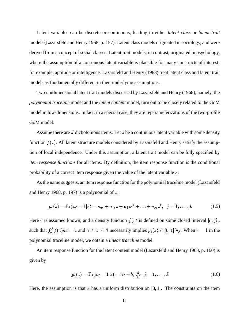
Two unidimensional latent trait models discussed by Lazarsfeld and Henry (1968), namely, the

polynomial traceline model and the latent content model, turn out to be closely related to the GoM

model in low-dimensions. In fact, in a special case, they are reparameterizations of the two-profile

GoM model.

Assume there are W dichotomous items. Let ' be a continuous latent variable with some density

function ��Q ' U . All latent structure models considered by Lazarsfeld and Henry satisfy the assump-

tion of local independence. Under this assumption, a latent trait model can be fully specified by

item response functions for all items. By definition, the item response function is the conditional

probability of a correct item response given the value of the latent variable ' .

As the name suggests, an item response function for the polynomial traceline model (Lazarsfeld

and Henry 1968, p. 197) is a polynomial of ' :�zYhQ ' U��pKr2Qg��Y��E��t ' UK�+�zsY � � � Y '�� Y ' � � �.�"� � �F�sY ' � ! ^G�H� ! �.�.� ! W�� (1.5)

Here O is assumed known, and a density function ��Q ' U is defined on some closed interval Z !$¡~¢ ,such that £B¤¥ ��Q ' U\¦ ' �%� and /§ ' § ¡ necessarily implies ��YhQ ' U�¨� Z� ! � ¢=© ^ . When Oª�� in the

polynomial traceline model, we obtain a linear traceline model.

An item response function for the latent content model (Lazarsfeld and Henry 1968, p. 160) is

given by �«Y9Q ' U��pKrVQg��Yw�E��t ' UK�+�VY �-¬ Y 'IY ! ^G�� ! �.�"� ! WT� (1.6)

Here, the assumption is that ' has a uniform distribution on ®� ! � ¢ . The constraints on the item

11

parameters for the latent content model are as follows: (1) ¦IY°¯±� ; (2) ��²��VY�²�� ; (3) �³²�VY ��¬ Y�²�� ; (4) ¬ Y�´�� .

When ¦9Yk�H� , the latent content model is similar to the linear traceline model and is a reparam-

eterization of the GoM model with two extreme profiles. To demonstrate this, consider the GoM

model conditional probability of a correct response to item ^ , given membership scores 3 � and 3 � :�«YhQs3 �0! 3 � UK�+pKr.Qs��Y��H�Tt ' Uu�,* � Y$3 �~� * � Y$3 � �,* � Y03 �d� * � YIQµ�w�¶3 � Uu��* � Y � QP* � Y��-* � Y·U�3 � �The correspondence between parameters of the latent content and parameters of the two-profile

GoM model is as follows:�VYw�,* � Y !¶¬ Yk�,* � Y��/* � Y !¸' �q3 �0! ^G�� ! �.�.� ! WT�Note that if the GoM extreme profiles are labeled in such a way that * � X$�¹* � X�´�� , the latent content

model constraints (1)-(4) hold. Thus, the polynomial traceline, the latent content, and the GoM

models all share the same low-dimensional structure. These three models, however, generalize

differently to higher dimensional settings.

Some features of the linear traceline model, emphasized by Lazarsfeld and Henry, are worth

pointing out:º the model is flexible in that the probability of a positive response increases with ' at different

rates for each item;º the data to which this model may be applied must show radically different patterns from

those of the latent class models;º this model has little similarity to factor analysis.

Lazarsfeld and Henry in their 1968 book do not elaborate on how the observed data patterns must

be different under the two models, but the general structure of the book suggests that they most

likely refer to differences in expected values of the manifest variables, and their pairs, triples, and

12

so forth. Exploring further in this direction, a number of more recent articles in psychometric litera-

ture contain attempts to distinguish between various latent structures on the basis of characteristics

for observable variables (Holland 1981, Rosenbaum 1984, Holland and Rosenbaum 1986, Holland

1990a, Junker and Ellis 1997, Bartolucci and Forcina 2000, Yuan and Clarke 2001).

To model the variation in the latent variable in the linear traceline model, Lazarsfeld and Henry

place a uniform distribution on ' . This assumption allows them to use the method of moments for

parameter estimation. As a generalization, instead of a uniform, they also consider using a Beta

distribution for the latent variable. Their reasoning is that the uniform assumption seems to be

restrictive in using the latent content model in many situations, and a distribution with the most

weight about some modal value and light tails “would probably be more appealing”. The authors

conclude that it is “very hard to make any progress toward the solution of the latent content model”

without making any further assumptions about the parameters of the Beta distribution. The method

of moments becomes hopeless in most cases when distributions other than a uniform are placed on

the latent variables.

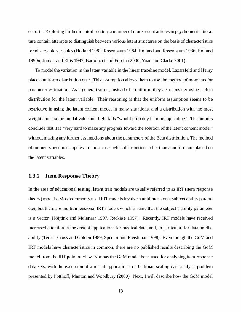
1.3.2 Item Response Theory

In the area of educational testing, latent trait models are usually referred to as IRT (item response

theory) models. Most commonly used IRT models involve a unidimensional subject ability param-

eter, but there are multidimensional IRT models which assume that the subject’s ability parameter

is a vector (Hoijtink and Molenaar 1997, Reckase 1997). Recently, IRT models have received

increased attention in the area of applications for medical data, and, in particular, for data on dis-

ability (Teresi, Cross and Golden 1989, Spector and Fleishman 1998). Even though the GoM and

IRT models have characteristics in common, there are no published results describing the GoM

model from the IRT point of view. Nor has the GoM model been used for analyzing item response

data sets, with the exception of a recent application to a Guttman scaling data analysis problem

presented by Potthoff, Manton and Woodbury (2000). Next, I will describe how the GoM model

13

fits in a general IRT framework provided by Holland (1990a). This framework is based on the

mixed-effects approach to latent variables.

As before, assume a test with W dichotomous items is given. Denote by �°�»Qg� �&! � �.! �"�.� ! � � Uan observed response pattern. Assume test responses are collected for a random sample of Csubjects from a population of interest. Let ¼KQs�eU be the observed cell count of the response pattern� . Denote by ��Qs�eU½�±pKr.Qs�eU the population frequency of a response pattern � . These data can

also be recorded in the form of a multidimensional contingency table with each cell containing

the number of observed responses corresponding to a particular discrete response pattern. The

likelihood function is then a multinomial ¾s¿ ��Qg�eUµÀ9Á ¿&Â ! (1.7)

where ��Qs�eU are unknown parameters. Constructing a model for ��Qs�eU means placing restrictions on

the set of all possible � �probability vectors, Ã � :Ã � ��ÄV4Å�³4BQg�eU�tV4�Qs�eUk¯³� and

m ¿ 4�Qs�eUu�E�IÆ«�Let Ç denote the subject-level parameter usually referred to as ability in IRT context. A general

IRT model is given by the integral form (Holland 1990b)��Qs�eU±� È ¾ YÊÉ YhQRÇ�x��Y·Uc¦«ËNQ ÇFU ! (1.8)

where É YIQ ÇTx��Y·U is the item response function if �TY��H� (a correct response), and it is one minus the

item response function otherwise. Specific IRT models are determined by additional assumptions

on the functions É YhQ v U and ËNQ v U .From this perspective, the GoM model is an IRT model with the subject-level parameter being

the membership vector 3G�%Qs3 �(! 3 �"! �.�.� ! 3 n U , and É -function of the form

É YhQs3yx��Y&U±� imn(o � 3 n * n Y ¿ � ! (1.9)

14

where * n Y\ � * n Y � �Ì� and hence É YIQg3yx(�zUG�Í�ª� É YhQs3yx.�2U . For the GoM model, a parametric

distribution of the GoM scores can be taken as ËNQg3�UÎ� Dirichlet Á ¥IÏ :;Ð;Ð;Ð : ¥VÑ Â Qg3 �0! �.�.� ! 3Fi�U with some

parameters �0! �.�.� ! `i .

Holland (1990a) points out that the formula for ��Qg�eU in equation (1.8) can be viewed in at least

two ways. First, it is a way to get legitimate values for the cell probabilities. Second, one might be

able to give some reasons why a particular expression for ��Qg�eU might be compatible with the data.

Holland divides the rationales for IRT models given by equation (1.8) into two types, the “random

sampling” and the “stochastic subject” rationales.

Under the random sampling rationale, different values of ability Ç simply define strata in a

population. The function É Y9QRÇ�x��Y"U gives the proportion of people from the Ç th stratum that answer��Y to the ^ th question. The random sampling rationale does not lead to a specific choice of item

response function É YhQRÇ�x.�VU , and the GoM item response function É YhQs3yx��Y&U is simply one of the

ways to get legitimate cell probabilities.

The stochastic subject rationale views the performance of each subject as inherently unpre-

dictable and the item response function É YhQRÇ�x.�VU as a mathematical model for this unpredictability.

For example, in educational testing, such factors as subjects’ emotional and physical wellbeing

have been considered as contributors to variability. Similarly, psychological and physiological

components may be regarded as sources of within-individual variability in the context of a disabil-

ity survey. Under the stochastic subject rationale, É YhQRÇ�x.�VU is interpreted as the probability of a

correct response of an individual with ability Ç . For the GoM model, the item response functionÉ YIQg3ex"�VU is linear in the latent parameter. The linear form of É YIQg3ex"�VU implies that a change in the

probability of a correct response induced by a change in a subject’s membership score does not

depend on the subject’s initial membership score.

15

1.3.3 Factor Analysis

Another way to represent latent trait models is through factor analysis for dichotomous variables.

The history of factor analysis goes back to Spearman’s one-factor intelligence model (Spearman

1904). Factor analysis of binary data has the same objective as the classic factor analysis of con-

tinuous data: the goal is to find factors that explain interrelationships among observable variables.

Factors serve in the role of latent variables. The classic factor analysis model for metric variables� �&! �.�"� ! � � is ��Y � �VYc � �VY �µ#��d� �"�.� � �VYci # i �ÓÒ Y ! ^G�E� ! �.�.� ! W ! (1.10)

where factor scores are assumed # ��Q #��0! �.�.� !�# i�U�Ô�Õ¹i�Q � !$Ö U , the error Ò YªÔ×Õ�QR� !�Ø Y"U , and # is

independent of Ò .Although the factor model (1.10) is sometimes used for discrete data, this is inappropriate

because of a disagreement between the right and the left hand sides. On the right hand side, #and Ò Y are assumed independent and normally distributed and thus can take on any values, whereas��Y on the left hand side can take on only discrete values. Assuming �=Y is dichotomous, equation

(1.10) can be adjusted to develop a factor analysis model for binary data in several ways.

A traditional psychometric approach to factor analysis of binary data is based on the assumption

of an underlying latent variable. We assume that the observed binary variable �]Y is a dichotomized

version of an underlying continuous latent variable �dÙY , and treat �eÙY as if it had been generated by

the classical factor analysis model� ÙY � � ÙYc � � ÙY � #��d� �.�"� � � ÙY�i # i �-Ò Y ! ^G�H� ! �.�.� ! W�� (1.11)� ÙY is not observable, but one only needs a correlation matrix to fit a factor model. Based on

observed counts in a 2 � 2 table for each pair ��Y and �][ , and assuming � ÙY and � Ù[ are bivariate

normal, one can estimate the correlation between � ÙY and � Ù[ . The maximum likelihood estimator,

based on this assumption, is the tetrachoric correlation coefficient (Harris 1982). Having obtained

16

the matrix of tetrachoric correlations for observed binary variables, factor analysis can be carried

out in the usual way.

A general approach to factor analysis for binary data which demonstrates a close interplay

between latent trait (IRT) models and factor analysis, is given by Bartholomew, Steele, Moustaki

and Galbraith (2002). Since the observed data take on values � and � , a factor analysis model can

be specified by a function that links the conditional probability of a correct response pKr2Qg�]Y��H��t # Uwith a linear combination of factors. This function is the usual link function for generalized linear

models (McCullagh and Nelder 1989). Link functions are typically chosen to map the range Z� ! � ¢onto the range Q\��Ú ! Ú�U , and to be monotonic.

One convenient choice of the link function, employed in log-linear models, is the logistic:

logit Ä9pKr.Qs��Y��H��t # U(Æ � �9Y\ � �VY �µ#«�d� �.�.� � �VY�i # i ! ^G�E� ! �.�.� ! W ! (1.12)

where by definition logit Q ÛeUÜ� Ý�ÞFßÎQsÛeàBQµ��ÛAUcU . This model is also known as the logit latent

trait model. A special unidimensional case of the logit latent trait model, the Rasch model, is quite

popular in educational testing because of its simplicity and attractive theoretical properties (Fischer

and Molenaar 1995).

A second choice of the link is the inverse of the Normal cumulative density function á5â �, also

known as probit (and sometimes referred to as normit). The resulting factor model with probit

link function corresponds to the underlying latent variable approach to factor analysis described

above. Thus, since the logit and the probit functions are nearly equivalent, results from fitting the

logit latent trait model are similar to those obtained by factor analysis of tetrachoric correlations.

Bartholomew and Knott (1999) show that these two models become identical when the distribution

of the underlying latent variables is standard logistic rather than normal.

A third possible choice of the link function for a discrete factor analysis model is the identity

function, where we simply assumepKrVQg��Yw�E��t # U�� 9Y\ � �VY �µ#«�d� �.�.� � �VY�i # i ! ^G�H� ! �.�.� ! W�� (1.13)

17

Bartholomew et al. (2002) point out that this factor model has two flaws. First, the left hand side of

equation (1.13) is a probability (which is between � and � ), whereas the right hand side can take on

any real value. Second, they question whether a linear rate of change in probability for the whole

range of # �1Q #��0! �.�"� !$# ikU is justified, comparing to a rate of change that varies depending on the

value of the latent variables.

While the first flaw represents a serious problem for a model with normal factors # , we can

think of at least two reasons why the second flaw may not be a drawback. First, one could come

up with some substantive justifications in favor of both a linear and a curvilinear function that

relate the conditional probability of response to values of latent variables. Second, although an

inverse logit function has a sigmoid shape, depending on the parameters, it can be very close or

identical to a linear function for a wide range of latent variable values. To illustrate this, consider

the unidimensional logit latent trait model

logit Ä9pKr2Qg�TY��t # U0Æ � �VYc � �9Y �µ# � (1.14)

The probability of a positive response as a function of the latent variable, known as the item

response function in psychometrics, for the unidimensional logit model is given by the inverse

logit: pKrVQs��Yk�E��t # U�� ã0äTå QR�VYc � �VY �µ# U� � ã&äTå QR�VYc � �9Y �µ# U !¶# ¨/Q\��Ú ! Ú�U&� (1.15)

Figure 1.1 gives three examples of item response functions for different parameter values in equa-

tion (1.15). If the distribution of a latent variable is concentrated in the range where the item

response function is close to linear, the overall relationship between the latent variable and the

probability of a correct response can be approximately described as linear.

The disagreement between the values on the right hand side and on the left hand side of the

factor model (1.13) can be avoided by considering range-restricted distributions on the latent vari-

ables and by placing constraints on the factors. This approach is precisely the one taken by the

18

Figure 1.1: Examples of item response functions with � k�� k�+��k�� and �� E� (dotted), �� +�T�� (solid), �� (dashed).

GoM model. Consider a factor analysis model with J�� factors and an identity link functionpKr2Qg��Y��H��t # Uæ� �9Y\ � �VY �µ#«�d� �.�.� � �VY�i â �ç# i â �(! ^G�H� ! �.�.� ! W��Suppose now that the latent factors #T�0! �.�.� !$# i â � are restricted to add up to a value less than one.

Define # i-�E�d�èQ #«�I� �"�.� �é# i â � U . Then the above factor model with Jê�ë� factors and an identity

link function can be reparameterized aspKr2Qs��Y��t # Uæ� �FìY � #��d� �FìY � #I�`� �.�"� � �FìY�i # i ! ^G�E� ! �.�.� ! W ! (1.16)

where �Fìi �+�z ! �FìY n ��z � � n ! lí�H� ! �.�.� ! J»��I�The model in equation (1.16) is exactly the GoM model with J extreme profiles. Here, the mem-

bership scores are # �%Q #��0! �.�.� !$# i�U and the extreme profile response probabilities are � ìX n .

19

Thus, the GoM model can be described as a discrete factor analysis with an identity link func-

tion. The GoM model with J extreme profiles corresponds to a discrete factor analysis model withJ�� factors.

1.4 Estimation

Existing methods of estimation for the GoM model are maximum-likelihood based. In Sec-

tion 1.4.1, I describe joint, conditional and marginal likelihood functions in relation to the GoM

model. In Section 1.4.2 I introduce Manton, Woodbury and Tolley’s (1994) iterative algorithm. I

re-derive the equations for this algorithm, following their recipe (Manton et al., 1994, pp. 68-70),

and obtain somewhat different results. Finally, I provide an overview of other estimation methods

that have appeared in the literature for various versions of the GoM model in Section 1.4.3, and I

conclude with discussion of theoretical developments in maximum-likelihood estimation for latent

structure and the GoM models in Section 1.4.4.

In addition, Section 8.2.2 of this thesis provides related material about estimation techniques

that have been developed for models in the machine learning literature that are similar to the GoM

model.

1.4.1 Joint, Conditional, and Marginal Likelihood

Latent structure models contain two sets of parameters: item parameters, which are common for all

individuals, and subject parameters, which are individual-specific. If we assume that the number

of items is fixed and the number of subjects increases, then the number of subject parameters

increases as well (however, there can only be as many distinct subject parameters as there are

distinct response patterns). Under such an assumption, Neyman and Scott (1948) call the subject

parameters incidental and the item parameters structural.

There are three likelihood-based approaches to deal with incidental parameters in this situation:

20

(1) one can treat them as fixed but unknown parameters, (2) one can treat them as realizations of

random variables from some distribution, or (3) one can eliminate them from the likelihood by

considering the conditional distribution given the sufficient statistics for incidental parameters,

provided the sufficient statistics exist. The first two approaches correspond to the fixed-effects and

the mixed-effects variations of a latent structure model, and give rise to the joint and marginal

maximum likelihood estimation methods, but estimation methods based on fixed-effects approach

do not allow for population level inferences. Maximizing the likelihood under the third approach

corresponds to the conditional maximum likelihood method (Andersen 1970).

Conditional likelihood. Before considering the joint and marginal forms of GoM likelihood, we

explain why the conditional maximum likelihood method is not applicable for the GoM model.

First, notice that because the membership scores and the item parameters can not be written as

separate factors, the GoM model does not belong to the exponential family. Barankin and Maitra

(1963, Theorems 5.1, 5.2, and 5.3) characterized the class of conditional distributions (of mani-

fest variables given the latent variables) of latent structure models for which there exists a set of

minimal sufficient statistics for the incidental parameters. Bartholomew and Knott (1999, p. 20)

note that the necessary and sufficient conditions for the existence of sufficient statistics amount to

the requirement that at least Wí�ÊJ of the conditional distributions are of exponential type, subject

to weak regularity conditions. Obviously, these conditions do not hold for the GoM model. The

GoM conditional distributions are not of exponential type, and no constraints can be imposed on

the parameters to satisfy this requirement. Hence, no sufficient statistics exist for the membership

scores in the GoM model, and conditional maximum likelihood estimation is not applicable in its

traditional sense.

21

Joint likelihood. If we assume that individual GoM scores are fixed unknown constants, the

likelihood function for the GoM model isb QP} ! |�t î�Uæ� ¾ X ¾ Y ¾ [ Q m n 3hX nwv * n Yc[SU ¿0ï �Rð ! (1.17)

where }�� Äh* n Y\[íñ l�� ! �.�.� ! J ! ^�� ! �"�.� ! W ! _é� � ! �.�"� !(b Y2Æ are the item parameters,|Ó�òÄ23hX n ñ�Mó�ô� ! �.�.� ! C ! l�� ! �"�.� ! J�Æ are the subject parameters, and data î��òÄ2�eX;Yc[wñ³Mó�� ! �"�.� ! Õ ! ^��æ� ! �"�.� ! W ! _��æ� ! �"�.� !(b Y.Æ are the observed responses for all subjects. Manton et

al. (1994) refer to equation (1.17) as the “conditional” GoM likelihood, explaining that in (1.17)

one treats the parameters 3IX n as unknown constants and thus conditions on them. However, in

psychometrics, the form of a likelihood function with subject-level parameters treated as unknown

constants is usually referred to as a joint or unconditional likelihood (Holland 1990b). The term

conditional likelihood seems to be reserved for the case when conditioning is based on the sufficient

statistics for incidental parameters (Andersen 1970, Holland 1990b, Lindsay et al. 1991, Maris

1998). We shall refer to equation (1.17) as the joint GoM likelihood to be consistent with this

more commonly used terminology.

Marginal likelihood. Under the mixed-effects approach, we assume that the GoM scores follow

the distribution L ¥ Q v U parameterized by vector . The likelihood function with subject parameters

integrated out is b QR} ! �t î�Uæ� È ¾ X ¾ Y ¾ [ Q m n 3 n * n Y\[SU ¿0ï �Rð ¦«L ¥ Qg3BU0� (1.18)

We shall use the term marginal GoM likelihood to refer to equation (1.18) throughout this the-

sis, consistent with the psychometric literature (e.g., Holland 1990a), even though Manton et al.

(1994) refer to equation (1.18) as the “unconditional” GoM likelihood, contrasting it with the

“conditional” likelihood in equation (1.17).

22

1.4.2 Manton, Woodbury, and Tolley’s fixed point iteration algorithm.

The estimation method presented by Manton, et al. (1994, p. 68) is an iterative maximization of the

constrained joint likelihood function with respect to both parameter sets, structural and incidental.

At each step, the joint likelihood is maximized with respect to one parameter set, keeping the other

set constant. Manton, et al. (1994, pp. 68-70) point out that the iterative optimization method

provided in their book is based on “the missing information principle”.

Manton et al. (1994, p. 68) provide two sets of equations to sequentially update the estimates:39X n � ��=Xjõ=õ �mX o � �.�m [ o �kö �=X;Yc[ 3TÙX n v *]Ùn Yc[÷ n Qs3 ÙX n v * Ùn Yc[ U2ø (1.19)

* n Y\[�� ÷ �X o ��ù �=XZY\[fú$ûï7ü(ý þ ûü �Rð÷ ü Á ú�ûïÿü ý þ ûü � ð Â��÷ �X o � ù �=X;Y�õ ÷ �"�[ o � ú�ûïÿü ý þ ûü �Rð÷ ü Á ú ûï7ü ý þ ûü �Rð Â � ! (1.20)

where 3TÙX n ! *yÙn Y\[ are the values from the previous iteration, and �eXjõ=õ�� ÷ Y ÷ [ �=XZY\[ . They also

provide the recipe, saying that equations (1.19) and (1.20) are obtained by maximizing the likeli-

hood b QP} ! |�t î�U with Lagrange multipliers corresponding to the constraints÷ �.�[ o � * n Yc[��ò� ! l°�� ! �"�.� ! J ! ^í�a� ! �.�"� ! W and

÷ in(o � 39X n �a� ! M�� ! �.�.� ! C . An algebraic check shows that estimates

derived by updating equations (1.19) and (1.20) do not satisfy the constraints:im n 39X n � ��=Xjõ=õ im n �m X �"�m [ ö �=XZYc[ 3�ÙX n v *yÙn Y\[÷ n Qg3 ÙX n v * Ùn Y\[ U ø� ��=Xjõ=õ �m X �.�m [ ö �=XZY\[ v ÷ n Qg3�ÙX n v *]Ùn Y\[ U÷ n Qg3 ÙX n v * Ùn Y\[ U ø� �yõzY�õ�=Xjõ=õ�� !�.�m [ o � * n Y\[�� ÷ �.�[ o � ÷ �X o ��ù �=X;Yc[fú�ûïÿü ý þ ûü �Rð÷ ü Á ú�ûï7ü ý þ ûü � ð Â �÷ �X o ��ù �=X;Y�õ ÷ �"�[ o � ú ûïÿü ý þ ûü �Rð÷ ü Á ú�ûï7ü ý þ ûü � ð Â�� F�

23

By using the recipe provided by Manton et al. (1994), we obtain a different set of update

equations as follows. The joint likelihood function with the Lagrange multipliers has the form:Ý ÞIß b QP} ! |�t î�Uæ� �mX o � �mY o � �"�m [ o � �=XZYc[ v Ý ÞIß ö imn(o � Qs39X nwv * n Yc[jU ø� �m X o � ~X v ö imn(o � 3hX n �Ó� ø � imn(o � �mY o � ¡ n Y v �� .�m [ o � * n Yc[�� We differentiate the likelihood with respect to 3FX n and set the result to zero:� Ý ÞFß b QR} ! |�t î�U� 39X n � �mY o � �"�m [ o �kö �=XZYc[ v * n Y\[÷ n Qs39X nkv * n Yc[SU ø �¸~XA�+��Next, we multiply by the 3IX n and divide both sides by �X :3hX nwv ~X � 39X nkv �mY o � �"�m [ o � ö �=XZYc[ v * n Y\[÷ n Qs39X nkv * n Yc[SU ø !

39X n � �~X v �mY o � �.�m [ o � ö �=X;Yc[ 39X nwv * n Yc[÷ n Qs39X nwv * n Yc[SU ø �In order for 3hX n to satisfy the convexity conditions,

÷ n 3hX n �H� , it is clear that �XA�q�=Xjõ=õ ��+� . The

resulting equation for updating membership scores is39X n � ��=Xjõ=õ �mY o � �.�m [ o ��ö �=XZYc[ 3TÙX n v *]Ùn Y\[÷ n Qs3 ÙX n v * Ùn Y\[ U ø ! (1.21)

where 3TÙX n and *]Ùn Yc[ are the parameter values from the previous iteration. Equation (1.21) differs

from formula (1.19) in the index of the first summation.

Similarly, for the response probabilities of the extreme profiles, we obtain� Ý ÞIß b QR} ! |�t î�U� * n Yc[ � �mX o � ö �=XZY\[ v 39X n÷ n Qg3hX n�v * n Y\[SU ø � ¡ n Yw�+� !* n Yc[ v ¡ n Yf� * n Y\[ v �mX o � ö �=XZYc[ v 3hX n÷ in$o � Qs39X nkv * n Yc[SU ø !

* n Y\[�� ¡ n Y v �m X o � ö �=X;Yc[ v 3hX nkv * n Yc[÷ n Qg3hX nkv * n Yc[SU ø !24

and �"�m [ o � * n Yc[��E� � ¡ n Yw�� m X o � �"�m [ o � ö �=XZYc[ v 39X nwv * n Yc[÷ n Qs39X nkv * n Yc[SU2ø� â �Therefore, an update equation for the extreme profile parameters is

* n Y\[�� mX o � ö �=X;Yc[ 3�ÙX n v *yÙn Y\[÷ in Qs3 ÙX n v * Ùn Yc[ U ø�mX o � �"�m [ o �kö �=XZYc[ 3 ÙX n v * Ùn Yc[÷ in Qs3 ÙX n v * Ùn Yc[ U ø ! (1.22)

which is, again, different from equation (1.20) provided by Manton et al. (1994).

We do not use the iterative algorithm given by equations (1.21) and (1.22) for estimation of

the GoM model parameters because of an undetermined status of the joint maximum likelihood

parameter estimates in the GoM setting (see Section 1.4.4 for discussion).

1.4.3 Other Estimation Methods

DSIGoM. Decision Systems, Inc. provides the DSIGoM software package to estimate the pa-

rameters of the Grade of Membership model. DSIGoM maximizes the joint GoM likelihood with

respect to both sets of parameters, the extreme profile response probabilities and the membership

scores (Decision Systems, Inc. 1999). The software does not provide standard errors of the param-

eter estimates. The maximization method used in DSIGoM appears to be different from Manton,

Woodbury and Tolley’s (1994) iterative maximization algorithm, but the DSIGoM documentation

does not contain sufficient details to allow for a complete comparison of these two maximization

methods.

Wachter’s fixed-effects algorithm. For the case of two extreme profiles, J��,� , Wachter (1999)

gives an approximate GoM estimation method by considering the joint GoM likelihood. He con-

structs his algorithm by noticing that the task of maximizing the joint likelihood for the GoM

model can be thought of as a sum-of-squares minimization problem with respect to a particular

25

metric that he derives, which is a function of the observed response and the expected probability

of response given by the GoM model. Wachter shows that the functional form of the metric turns

out to be very close to the usual Euclidean metric, and uses this fact to develop an approximate

iterative GoM estimation algorithm for the special case of two extreme profiles. It is unclear how

good this approximation actually is.

Varki, Cooil, and Rust’s mixed-effects approach. In quantitative marketing research, Varki,

Cooil, and Rust (2000) work with a special case of the GoM model, where the number of extreme

profiles is predetermined by the number of classification categories of discrete item responses

(which is assumed to be the same for all items). In particular, they assume that the number of ex-

treme profiles, J , is the same as the number of polytomous response categories, b Y , for each item^í�%� ! �.�.� ! W . In this setting, the number of extreme profiles is known a priori. They consider the

mixed-effects version of the GoM model. They assume the incidental parameters, the membership

scores, follow a mixture distribution with two components: a Dirichlet and a point mass at the

extreme profiles. They refer to this modification of the GoM model as a fuzzy latent class model,

and illustrate it on a low-dimensional example with W-� � . They obtain the parameter estimates

via a constrained maximum likelihood procedure for the marginal form of the likelihood. They

provide minimal details about the likelihood maximization procedure implemented in Gauss.

Potthoff, Manton and Woodbury’s mixed-effects approach. Potthoff, Manton, and Woodbury

(2000) also consider a mixed-effects version of the GoM model. They assume that the GoM scores

follow a Dirichlet distribution, and refer to this version of the GoM model as a Dirichlet general-

ization of latent class models. They estimate the parameters by maximizing a penalized marginal

likelihood, where the penalty terms are included to ensure that no parameter estimates fall on the

boundary of the parameter space. They implement a Newton-Raphson procedure in the SAS/IML

package for low-dimensional QµW�§��«U special cases, and they point out that programming efforts

increase substantially as the dimensionality increases (Potthoff, Manton, Woodbury and Tolley

26

2000, page 321). They report no standard errors.

1.4.4 Discussion.

As I have reviewed above, the traditional and most frequently used estimation methods for the GoM

model are based on maximizing the joint GoM likelihood. Maximization of a joint likelihood is

usually carried out simultaneously with respect to both parameter sets. Since there is a notational

symmetry with respect to subject and item parameters in the likelihood, three different kinds of

asymptotics are possible: (1) when the number of items is fixed, and the number of subjects goes

to infinity, (2) when the number of subjects is fixed, and the number of items goes to infinity, and

(3) when both the number of items and the number of subjects go to infinity.

Neyman and Scott (1948) studied properties of maximum likelihood estimates derived by max-

imizing a joint likelihoods under scenario (1) (or, equivalently, (2)). Assuming the number of items

is fixed, they showed that (joint) maximum likelihood estimates of the structural parameters need

not be consistent (they did not consider consistency of incidental parameters because, since the

number of incidental parameters grows with sample size, the notion of consistency does not ap-

ply). They also showed that even if the estimates of the structural parameters are consistent, they

may not possess the property of asymptotic efficiency. These results for the joint likelihood func-

tion, which is a function of structural and incidental parameters, stand in contrast to the well-known

properties of classical maximum likelihood estimators in problems when the likelihood function

contains no incidental parameters.

Haberman (1977b) studied (joint) maximum likelihood parameter estimation for exponential

family models. He showed for the Rasch model that consistency and asymptotic normality of the

(joint) maximum likelihood estimates of the structural parameters can be achieved when both the

number of items W and the number of subjects C increase at a certain rate.

In some cases, it is possible to obtain consistency results for joint estimation methods other than

maximum likelihood. Thus, in psychometrics, Douglas (1997) presents simultaneous nonparamet-

27

ric estimation of subject parameters and item response functions. He uses a special procedure for

kernel-smoothed item response function estimation and shows that the true curves can be consis-

tently estimated.

Whereas theoretical developments on consistency of the joint maximum likelihood estimates

are model-specific, there are general results for the marginal maximum likelihood estimates. Kiefer

and Wolfowitz (1956) consider the problem of marginal maximum likelihood estimation in the

presence of infinitely many incidental parameters in a semiparametric setting. Imposing no para-

metric assumptions on the form of the distribution of incidental parameters, they show that, under

the usual regularity conditions, the (marginal) maximum likelihood estimates of the structural pa-

rameters as well as the nonparametric estimate of the distribution function of incidental parameters

are consistent.

The results on maximizing joint likelihoods indicate that this method of estimation should be

used with great caution. Model-specific asymptotic results are needed to understand the behavior

of the (joint) maximum likelihood estimates. It appears that no such results are available for the

joint maximum likelihood estimation of the GoM model. Tolley and Manton in their 1992 paper,

“Large sample properties of estimates of a discrete Grade of Membership model,” talk about con-

sistency of the GoM model maximum likelihood estimates. Never stating clearly which type of

likelihood is maximized, they begin by discussing the joint likelihood and proceed to using the

marginal likelihood for proofs that are based on Kiefer and Wolfowitz (1956). The paper claims to

prove consistency of the estimates of the structural parameters with respect to the distribution of the

membership scores. The confusion arises when one recalls that numerical estimation of the GoM

model is traditionally based on maximizing the joint likelihood. In fact, discussing consistency of

the GoM (joint) maximum likelihood estimates, Manton et al. (1994, p. 53) explicitly point out

that the arguments of consistency apply to the maximization of the marginal, and not the joint,

GoM likelihood. They support the consistency claim by saying that obtaining the joint maximum

likelihood estimates for the structural and incidental parameters “asymptotically maximizes” the

28

marginal likelihood (Manton et al. 1994, p. 67) (by plugging in the joint maximum likelihood es-

timates of structural parameters and the empirical moments of the membership scores’ distribution

based on their joint maximum likelihood estimates).

Parameter identifiability is another concern in using the joint likelihood for estimation of the

GoM model parameters. With no additional restriction on the parameter estimates, we can easily

find different sets of parameters that assign the same value to the joint likelihood. For example,

in the case of two extreme profiles and one item, we can shift the structural parameters toward

more extreme values and change the membership scores accordingly. That is, if the structural

parameters are ��ÿ� and �� , a positive response of a subject with respective membership scores of�� and ��S� contributes a factor of �T�7� v �T�� v ��S��+��ÿ�� to the likelihood. If we shift the value

of the first extreme profile from ��ÿ� to ��7� , the contribution to the joint likelihood is the same if the

membership scores are �� and ��7�� , that is ��7� v �� T�� v �T� ��a�T�7�� . A similar illustration

can be constructed in the case of multiple items and subjects.

Tolley and Manton (1992) and Manton et al. (1994) discuss the issue of GoM identifiability

from two different perspectives, but they do not comment explicitly and provide no practical solu-

tion to deal with multimodality in the parameter space of the type described above.

To summarize, existing GoM estimation methods are of maximum-likelihood type. Traditional

GoM estimation methods are based on maximizing the joint GoM likelihood function with no dis-

tributional assumptions on the GoM scores, and there are no asymptotic results for this approach.

The fuzzy latent class model used by Varki, Cooil, and Rust (2000) and the Dirichlet generaliza-

tion of the latent class models used by Potthoff et al. (2000) are mixed-effects versions of the GoM

model; they assume that the distribution of the GoM scores comes from a pre-determined paramet-

ric family. Estimation methods for these two versions of the GoM model are based on maximizing

marginal likelihood functions and have been implemented only in low-dimensional cases. There

is clearly a need for a reliable estimation method which can handle general cases and higher di-

mensions. We provide an attempt to develop such a method in this thesis by employing a Bayesian

29

approach and by putting distributions on both the incidental and the structural parameters.

30

Chapter 2

Comparing Latent Structures of the Grade

of Membership, Rasch, and Latent Class

Models

This chapter employs a geometric approach for describing the potential value of different discrete

data models to represent heterogeneity in individual responses. I examine log-linear, latent class,

latent class probabilistic mixture, GoM and Rasch models geometrically via population hetero-

geneity manifolds in the marginal space (based on marginal probabilities) and in the full parameter

space (based on cell probabilities). Population heterogeneity manifolds are obtained by letting

subject-specific parameters vary over the natural range while keeping other population parameters

fixed. The case of a � �/� contingency table is discussed in detail, and the generalization to � �tables with W ¯³� is sketched.

Even though there exist theoretical formulae for the probability of response patterns as func-

tions of the latent parameters, a geometric approach brings sharper understanding of model capabil-

ities with respect to describing population heterogeneity. Recent publications that have considered

geometric approaches are: Ramsay (1996), for the item response theory, and Woodbury, Manton,

31

and Tolley (1997), for the Grade of Membership model.

In Section 1, I consider the case of a �í�Ê� table in detail and employ a geometric approach to

examine the latent class, Rasch and GoM models. In Section 2, based on the geometric approach,

I discuss similarities and differences among these models from a stochastic subject perspective

(Holland 1990). I demonstrate geometrically the main distinction between the GoM model and

a latent class mixture model, which lies in the difference between the concepts of partial and

probabilistic memberships. I also show that, in special cases, the GoM model can be thought

of as being similar to the Rasch model in representing population heterogeneity. Finally, I show

that the GoM item parameters can provide quantities analogous to more general logistic IRT item

parameters. I conclude with discussing some aspects of increased dimensionality in Section 3 and

implications for data analysis in Section 4.

2.1 Heterogeneity Representations: �� table

2.1.1 Preliminaries

Consider a two by two table, normalized in such a way that all cell entries �A[��êpKr2Qg� � �,_ ! � � �� U , _ ! � �E� ! � , add up to one. Let � � and � � denote items, and * � �/� ��&� � � � �+pKr2Qg� � �H�VU ! * � �� ~� � �� +pKr2Qg� � ��VU denote corresponding marginal probabilities of positive responses.

� � � �� * �� -* �* � ��/* � 1

There can be two different geometric representations based on the two sets of parameters:

the cell probabilities, Ä(�][��Æ , and the marginal probabilities, Äh* �(! * � Æ . Note, without any model

restrictions, marginal probabilities can be identified from cell entries but not vice versa. Therefore,

32

a geometric representation for a set of marginal probabilities can be derived from a geometric

representation for the corresponding set of cell entries, but the converse in general is not true.

I will refer to the Z� ! � ¢ �- Z� ! � ¢ square in the Cartesian plane with the basis vectors QP* �(! * � U as

the marginal space. Since marginal probabilities for the same item necessarily add to unity, every

possible set of margins for a two by two table corresponds to a point in the marginal space and

vice versa. Ramsay (1996) calls the same construct the response probability space. The marginal

space is a simplification for the space of all possible multinomial probabilities used by Woodbury,

Manton and Tolley (1997) to examine the Grade of Membership (GoM) model.

Constraints for the cell probabilities, �y[��,¯+� ! _ ! � �� ! � and÷ [ : � �=[��³�� , define an object

in the four-dimensional Cartesian space. Consider a projection from the four-dimensional space

with orthogonal basis vectors corresponding to Qj� ��&! � � �.! � ��&! � �� U onto a subspace with the basis

corresponding to Q � � �2! � ��0! � �� U . The resulting object is a tetrahedron with the origin representing� �� E� , and three other vertexes representing � � � �E� , � �� H� , and � �� E� , respectively. Fienberg

and Gilbert (1970) used an isomorphic tetrahedron to describe the geometry of the cell entries of

a two by two table. This description is possible because there exists a one-to-one correspondence

between the set of points in the tetrahedron and the set of all possible two by two tables. I will

refer to the tetrahedron as the full parameter space.

Building a model for discrete data is equivalent to describing a relationship among the cell

probabilities in the full parameter space. The marginal representation is sufficient for a model if

there exists a one-to-one correspondence between a representation of the model in the full parame-

ter space and the corresponding representation in the marginal space. This is the case for all models

considered here. As I will show, however, understanding the geometry in the full parameter space

may be required in order to compare different model structures.

Consider the model of independence for a two by two table. The restriction placed by the

model on the cell probabilities is that the odds ratio is equal to one, or, equivalently� �� v � �� -� � � v � �� 33

Figure 2.1: Surface of independence in the full parameter space �)�-� � �.!$# �¸� ��&!(' �-� �� . Contour

lines are given for better perception of the 3-dimensional surface.

Eliminating � �� from this equation by using the constraint that the cell probabilities add up to one,

the resulting equation Qj� �� U � �� v Qµ��è� �� U � � �� v � � � �+�defines a two-dimensional surface of independence in the full parameter space (see Figure 2.1),

which is a part of a hyperboloid. Every point on the surface of independence corresponds to a

specific two by two independence table and, vice versa, every two by two independence table

corresponds to a point on the surface of independence. It is well known (Hilbert and Cohn-Vossen

1952) that a hyperboloid is ruled by two families of straight lines; for the surface of independence

these are the families of constant row and column margins (Fienberg and Gilbert 1970).

Suppose the population responses come from a distribution with fixed marginal probabilities* � and * � . The model of independence can then be represented geometrically by a single point

34

with coordinates QR* �(! * � U in the marginal space. Similarly, in the full parameter space, the model

of independence with fixed * �&! * � corresponds to a point on the surface of independence with

coordinates Q � � �.! � ��&! � �� U , where � � � �+* � Qµ�K�Ü* � U , � �� +* � Qµ�K�Ü* � U , and � �� aQµ�K�Ü* � U"Q\�K��* � U .For the independence model, individual responses are assumed to be homogeneous; every

individual has the same response probabilities �e[�� ! _ ! � �ò� ! � . Next, we consider several latent

structure models in which cell probabilities �y[�� vary from individual to individual according to the

value of his/her subject-specific parameter.

2.1.2 Latent class models

In this section, I first discuss the conventional latent class model, then I introduce a latent class

probabilistic mixture model.

Assume that there are two distinct classes in the population. As a hypothetical example, con-

sider students with math and history majors. If item � � is a math question and item � � is a history

question, then the two classes of students would rate the difficulty of the questions differently.

Thus, the marginal probabilities would not be homogeneous. Let * n[ �êpKr2Qg�][A�%��t��+��lBU ! _ ! lé�� ! � and � n[�� pKrVQs� � � _ ! � � � � t ' ��l�U ! _ ! � ! l��ò� ! � , where ' is the latent class indicator.

Population response probabilities for the two classes can be represented as

� � � �� * �� -* ��* �� -* �� 1

� � � �� * � �� -* � �* �� /* �� 1

The assumption that responses � � and � � are independent, conditionally on the latent class

(e.g., student’s major), is known as the local independence assumption:� n �� v � n�� /� n � � v � n�� ! l½�� ! �T�35

Lindsay, Clogg and Grego (1991) call the general case of this model with W binomial responses

and J latent classes the conventional latent class model.

To give an illustration, throughout this chapter I will use the values for the cell and marginal

probabilities from the numerical example (Table 2.1) given by Manton, Woodbury, Stallard and

Corder (1992, page 334).

Table 2.1: Example

� �

0.03 0.07 0.1

0.27 0.63 0.9

0.3 0.7 1

� �

0.48 0.32 0.8

0.12 0.08 0.2

0.6 0.4 1

Geometrically, marginal probabilities for the two classes correspond to two points ! �0! ! � with

coordinates QP* �� ! * �� U ! QP* � � ! * �� U in the marginal space (Figure 2.2), which, in turn, correspond to two

points " �0! " � with coordinates Qj� �� ! � �� ! � �� U ! Q � � � � ! � �� ! � �� U on the surface of independence in the

full parameter space (Figure 2.3). Population heterogeneity for the conventional latent class model

can be described as a discrete assignment for an individual to one of the latent classes.

Next, we are going to examine a latent class probabilistic mixture model where the population

parameters (latent class response probabilities) are known and fixed, and the subject-specific pa-

rameter, the probability of being a member of one of the latent classes, 4 , is unknown. We might

imagine that the subject-specific parameter varies over the population with some distribution, and

wish to consider how to describe the resulting responses. When the latent class conditional proba-

bilities of response are fixed, a probability 4 of being in one of the latent classes can be estimated

for each individual.

Geometrically, a population heterogeneity manifold is the surface generated by letting the sub-

ject specific parameter 4 vary over its natural range, while keeping all other population parameters

36

M2

M1

0

0.2

0.4

0.6

0.8

1

Y

0.2 0.4 0.6 0.8 1X

Figure 2.2: Latent class probabilistic mixture model heterogeneity manifold in the marginal space� �+* �0!�# �+* � .fixed. Specifically, let 4 be a subject specific probability of belonging to the first class. If 4 varies

continuously from 0 to 1, then the corresponding cell probabilities for individual responses vary

according to�=[�� pKr2Qg� � �q_ ! � � � � U� 4 v pKr.Qs� � �q_ ! � � � � t ' ��VU � Qµ��¶4FU v pKr.Qs� � �q_ ! � � � � t ' �+�FU !where _ ! � � � ! � . The values of �][�� that satisfy the above equation form a line segment ! � ! �(Figure 2.2) in the marginal space and a line segment " � " � in the full parameter space (Figure 2.3).

Line segments ! � ! � and " � " � are population heterogeneity manifolds for the latent class proba-

bilistic mixture model. Unless the marginal probabilities for either the response � � or the response� � are the same for the two classes, the line segment " � " � does not lie on the surface of indepen-

dence.

I should note, however, that only a finite number of possible distinct values of 4 can be es-

timated from discrete data, and that number can never be greater than the number of different

37

Figure 2.3: Latent class probabilistic mixture model heterogeneity manifold in the full parameter

space �)�-� � �2!$# �-� ��0!(' �-� �� .

0

0.2

0.4

0.6

0.8

1

Y

0.2 0.4 0.6 0.8 1X

Figure 2.4: Latent trait Rasch model heterogeneity manifold in the marginal space �)�+* �&!�# �,* � .38

patterns of the data records, � �for W dichotomous responses.

2.1.3 Rasch model

Subject specific parameters in IRT are usually called ability parameters. The Rasch model is one of

the most common IRT models. The marginal probability of response for the Rasch model depends

on the subject and item parameters through the logistic ogive function; no interaction between

subject and item parameters is allowed. I will consider two cases, the latent class Rasch model and

the latent trait Rasch model.

As before, � � and � � are two dichotomous items. Denote the subject ability parameter byÇ and the item difficulty parameters, here treated as fixed population parameters, by ¬h� and ¬(� ,respectively. Then, given the item difficulty parameters, a two by two table for the Rasch model is

� � � �� Q ÇFU � � � QRÇIU #%$'& Á)( â+* Ï Â� õ #%$'& Á)( â+* Ï Â� �� Q ÇFU � �� QRÇIU �� õ #%$'& Á)( â+* Ï Â#%$'& Á)( â+*-, Â� õ #%$'& Á)( â+*-, Â �� õ #%$.& Á�( â+*-, Â 1

And the local independence assumption becomes� �� QRÇ n U v � �� QRÇ n Uu�/� � � Q Ç n U v � �� Q Ç n U ! lí�H� ! �T�The assumption of two distinct classes in the population corresponds to two distinct values ofÇí�aÇ �&! Ç � . This results in the latent class Rasch model, which is technically a special case of the

conventional latent class model described earlier.

The latent trait Rasch model has the same set of parameters as the latent class Rasch model but

the ability parameter Ç is treated as being continuous. The items are assumed to be independent

for every value of Ç . If we let Ç vary from ��Ú to Ú , the marginal probabilities of responses* � ��Q ã0äTå QRÇ�� ¬"� U�UcàBQ\� � ã0äTå QRÇó� ¬"� U�U and * � �aQ ã&äTå Q Ç5� ¬(� UcU�àBQµ� � ã&äTå QRÇó� ¬(� U�U will vary from

39

Figure 2.5: Latent trait Rasch model heterogeneity manifold in the full parameter space �1�� 2!$# �-� ��0!$' �/� �� .0 to 1. Expressing one marginal probability as a function of another, heterogeneity in individual

responses can be represented by a curvilinear segment in the marginal space:* � QR* � U±� * � ã0ä�å Q ¬"� � ¬(� U��-* �d� * � ã&äTå Q ¬"� � ¬0� U !where * � and * � are the probabilities of correct responses, * � ¨-Q � ! �VU . This curve connects QR� ! �zU ,the point of “complete ignorance”, with Qµ� ! �VU , the point of “full knowledge”. The curvature of

the segment depends on the difference between the item difficulties. When ability increases until a

certain point, the marginal probability of a correct response to an easier item increases faster than

the marginal probability of a correct response to a more difficult item. After a certain ability level

is reached, the probability of a correct response for a harder item quickly catches up. Figure 2.4

shows an example of a Rasch model heterogeneity manifold in the marginal space for two items

such that ¬0� � ¬"� �a� . A curvilinear segment becomes a straight line in the marginal space when

40

the items are of the same difficulty, ¬&� � ¬.� �� .

Since the independence assumption is satisfied for every Ç ¨qQµ��Ú ! Ú�U , a corresponding het-

erogeneity manifold for the latent trait Rasch model in the full parameter space is a curve on the

surface of independence that connects the origin � �� 1� and the vertex � �� 1� . Varying Ç from��Ú to Ú is equivalent to varying * � �EpKrVQs� � �×�2U from 0 to 1. Expressing cell probabilities as

functions of * � for our convenience, a Rasch model heterogeneity manifold (Figure 2.5) is:� � � QP* � U±� * � v ö �w� * � ã&äTå Q ¬"� � ¬(� U��-* �~� * � ã0ä�å Q ¬"� � ¬(� U ø� �� QP* � U±� Q\�w�-* � U v ö * � ã&äTå Q ¬"� � ¬(� U��/* �� * � ã&äTå Q ¬.� � ¬(� U ø� �� QP* � U±� Q\�w�-* � U v ö �� * � ã&äTå Q ¬"� � ¬0� U��-* �d� * � ã&äTå Q ¬.� � ¬(� U ø !where * � ¨qQR� ! �2U and difficulty parameters ¬.� and ¬0� are fixed. Note that the local independence

condition holds for every value of the subject parameter Ç .

2.1.4 Grade of Membership model

Now consider the GoM model with two dichotomous items and two extreme profiles. The subject

specific parameter is 3-�fQg3 �(! 3 � U , the vector of the GoM scores. The extreme profile response

probabilities, * nY �×pKrVQg��YD��t 3 n �»�2U , l ! ^��»� ! � , are the item parameters for the GoM model

and are treated here as fixed population parameters.

Using similar notation as for the latent class model, a two by two table for the GoM model is

� � � �� Q |~U � � � Qs|~U 3 � * �� 3 � * � �� Q |~U � �� Qs|~U 3 � Qµ��-* �� U � 3 � Q\��-* � � U3 � * �� 3 � * �� 3 � Q\�w�-* �� U � 3 � Q\��/* �� U 1

The local independence assumption states that � � and � � are independent, given | :� �� Q |dU v � �� Qs|~UK�-� � � Qs|~U v � �� Q |~U0� (2.1)

41

M2

M1

0

0.2

0.4

0.6

0.8

1

Y

0.2 0.4 0.6 0.8 1X

Figure 2.6: GoM model heterogeneity manifold in the marginal space � ��* �&!$# �,* � .Assume the GoM scores vary over their natural range with some distribution. The set of result-

ing responses then represents a GoM population heterogeneity manifold in the marginal, and in the

full parameter space. Specifically, since the coordinates of the | vector add to one, I consider only

the first GoM score 3½�+3 � . A population heterogeneity manifold for the GoM model can then be

obtained by varying 3 from 0 to 1. In the marginal space,* � Qg3BUæ� 3 v * �� Q\�w�¶3�U v * � �* � Qg3BUæ� 3 v * �� Q\�w�¶3�U v * �� !where * � Qs3�U��pKr2Qg� � ��VU , * � Qg3BU��pur.Qs� � �%�VU , 3ë¨ÓQR� ! �2U , is a parametric representation of the

line segment ! � ! � , which is identical to a population heterogeneity manifold for the latent class

model (Figure 2.6), given that the latent classes coincide with the extreme profiles.

In the full parameter space, a heterogeneity manifold for the GoM model is a curve segment on

the surface of independence connecting " � and " � (Figure 2.7):� � � Qs3�Uæ� Qg3�* �� Qµ�w�¶3�U�* � � U v Qs3AQµ��¸* �� U � Q\�w�¶3�U"Qµ�w�-* �� UcU� �� Qs3�Uæ� Qg3AQ\�w�-* �� U � Qµ��°3BU·Q\��/* � � U�U v Qg3�* �� Qµ��3�U�* �� U42

Figure 2.7: GoM model heterogeneity manifold in the full parameter space �è�Ó� � �2!$# �� 0!(' �� .

43

� �� Qs3�Uæ� Qg3AQ\�w�-* �� U � Qµ��°3BU·Q\��/* � � U�U v Qg3AQ\�w�-* �� U � Qµ��¶3�U·Q\�w�-* �� U�U !where 3é¨/Q � ! �VU .2.2 Similarities and Differences: Comparing Heterogeneity Man-

ifolds

The GoM and the Rasch models. First, note that the Rasch model implicitly assumes existence

of two extreme classes: Ç��Ú for “complete ignorance” and Ç¶�±Ú for “full knowledge”.

In the simplest case described in this chapter, the loci of these two classes are fixed. Once we

introduce other item parameters, e.g., “guessing” and “slipping”, the “complete ignorance” and

“full knowledge” extreme classes for an IRT model may be at other locations in the marginal space

or, equivalently, on the surface of independence. Because monotone unidimensional IRT models

imply positive association between responses, not all locations of extreme classes are possible.

For example, the “complete ignorance” and “full knowledge” points can never be located at the

vertexes � � � � � ! � �� . For the GoM model, however, no monotonicity-based restrictions

are placed on the loci of the latent classes. Notice, even if the extreme classes imposed by an

IRT model match the extreme profiles of the GoM model, population heterogeneity manifolds in

general are not identical. A GoM manifold is fully determined by the locations of the extreme

profiles, whereas a Rasch manifold is determined not only by the extreme classes but also by the

item difficulty parameters in the model.

The GoM item parameters, * ’s, determine the locations of the extreme profiles. If the con-

ditional response probabilities of the extreme profiles are ordered in such a way that the mono-

tonicity requirement is satisfied, then the GoM extreme profiles can be interpreted as being the

“complete ignorance” and “full knowledge” classes, and in this case the GoM item parameters can

provide quantities analogous to IRT item parameters. Assuming the order * �� ´q* �� for � �a� ! � ,

44

deviations of the absolute values of the * ’s from 0 or 1 represent “guessing” and “slipping” pa-

rameters (see the population heterogeneity manifold for the GoM model on Figures 2.6 for an

illustration). Similarly, the difference * � � �)* �� represents discrimination power of the first item, and/ ��: � �EQP* � � ��* �� U�à�QP* �� * �� U provides a measure of relative discrimination of two items. If / ��: � �� ,

the two items provide the same discrimination in the sense that a change 0D3 in the subject score 3will result in the same change in the probabilities of getting the items correct. If / ��: � ²,� , then the

first item has less discrimination power than the second item.

Item difficulty, defined in IRT as the value of the latent variable that results into �� probability

of answering the item correctly, can also be calculated in terms of the extreme profile response

probabilities. Take the latent variable 3 to be the GoM score for the “full knowledge” extreme

profile. Take the item difficulties, 3 Á � Â and 3 Á � Â , to be the values of the GoM scores corresponding

to ��)� conditional probability of response for the two items, respectively. Assume that these GoM

scores exist (this is equivalent to assuming that “complete ignorance” and “full knowledge” ex-

treme profiles have conditional response probabilities, respectively, less than and greater than �� ).Then the item difficulties for the GoM model are such thatQµ��°3]Á � Â U�* �� 3=Á � Â * � � � ��Qµ��°3 Á � Â U�* �� 3 Á � Â * �� !which implies 3 Á � Â �%QR�T�)��-* �� U�àBQR* �� ¸* �� U , � �H� ! � .

The ability parameter Ç in the Rasch model plays a role similar to that of the GoM score 3 .

They both appear explicitly in the local independence assumption. For the case of two extreme

profiles, “complete ignorance” and “full knowledge”, 3 for the latter can be viewed as an IRT pro-

ficiency score. Likewise, a subject with some value of Ç can be considered a partial member of the

“complete ignorance” and “full knowledge” extreme classes for an IRT model. Since the property

of partial membership resulted in naming the GoM model a “fuzzy sets model”, by analogy, IRT

models can be thought of as “fuzzy sets models” as well.

Finally, following Ramsay (1996), we distinguish between Ç and 3 as being, respectively, ex-

45

trinsic and intrinsic to the manifolds. Thus, Ç is extrinsic in the sense that the position of Ç on its

domain, Q\��Ú ! Ú�U in our case, is only indirectly related to its position within the manifold itself.

That is, for a given geometrical representation of a population heterogeneity manifold, the value ofÇ by itself does not determine the position of a subject with that value of Ç on the manifold, unless

the mapping from the domain of Ç into the response probability space is specified. Parametric for-

mulation of IRT models provides this specification. In contrast, 3 for the GoM model is intrinsic

to the manifold, as it measures the distance along the manifold from its beginning, assuming the

manifold is normalized to have a unit length. Thus, by definition the arc length is�zO21w_-3.¼e354'6 � È ú 7889 ö � pKrVQ � �E��t ÛeU� Û ø � � ö � pur9Q � ��t ÛeU� Û ø � ¦«Û� È ú 7889 ö � ZÛ`QR* �� /* � � U � * � � ¢� Û ø � � ö � ;Û�QR* �� -* �� U � * �� ¢� Û ø � ¦zÛ� È ú;: QP* �� -* � � U � � QR* �� /* �� U � ¦zÛ� 3 v : QP* �� -* � � U � � QP* �� -* �� U � !

where the square root is just the length of the segment between the two extreme profiles. In other

words, 3 is a normalized arc length.

Ramsay (1996), in his geometrical approach to IRT argues that a parameterization intrinsic to

the manifold provides the natural, and only invariant, characterization of the latent trait, as well as

a useful measure of item discrimination.

The GoM and the latent class models. For both the GoM model and the latent class probabilistic

mixture model, no monotonicity-based restrictions are placed on the loci of the latent classes.

When the latent classes are the same as the extreme profiles, the population heterogeneity manifold

for the GoM model (Figure 2.6) appears to be identical to the latent class probabilistic mixture

heterogeneity manifold in the marginal space. A population heterogeneity manifold for the GoM

model represents the concept of partial membership, whereas a population heterogeneity manifold

for the latent class mixture model represents the concept of probabilistic membership. The major

46

distinction between these two membership concepts is in the local independence condition. The

local independence holds only for the latent classes themselves but not for a probabilistic mixture of

latent classes. On the contrary, the local independence does hold for all values of the GoM scores;

that is, for all degrees of partial membership. This distinction becomes apparent geometrically

when the two manifolds appear clearly different in the full parameter space.

To further illustrate the difference, we use the numerical example ( 2.1) with two dichotomous

variables given by Manton et al. (1992). Figure 2.8 shows that the latent class and the GoM model

heterogeneity manifolds for this example are clearly different. Notice, however, that if the two

classes shared the same marginal probability for an item, then the two manifolds would coincide in

both the marginal and the full parameter spaces. In that case, the line segment that connects the two

latent classes would lie on the surface of the hyperboloid of independence. The points on the man-

ifolds in Figure 2.8 correspond to the partial membership score and the probabilistic membership

score equal ��ÿ6 . The example demonstrates that the GoM and the latent class probabilistic mixture

models yield identical marginal subject-specific probabilities but different joint probabilities.

2.3 Increasing Dimensionality

The geometric representation can be extended to the � �table for WÊ¯q� . For example, for W��q� the

marginal space is a unit cube. The full parameter space is a seven-dimensional polyhedron. Even

though we can not display the independence manifold in a seven-dimensional space, it is clear that

a line which connects two arbitrary points on the manifold does not belong to the manifold unless

at least one pair of margins is the same for the two classes that are determined by the two points.

In the marginal space, a GoM [latent class probabilistic mixture] model population heterogeneity

manifold is a line segment in the cube connecting the two extreme profiles [latent classes]. In the

full parameter space, it is a straight line and a curve on the surface of independence for the latent

class probabilistic mixture model and the GoM models, respectively. For W°´Ó� the marginal space

47

Figure 2.8: Illustration for the numerical example. The straight line is the heterogeneity manifold

for the latent class probabilistic model. The curve on the surface is the heterogeneity manifold for

the GoM model. Points correspond to 3��³4Å��ÿ6 .

48

becomes a W -dimensional hypercube and the full parameter space becomes a QP� � �Ü�2U -dimensional

polyhedron. For the case of two extreme profiles, a GoM population heterogeneity manifold is still

represented by a straight line segment in the marginal space and a curve on the manifold of inde-

pendence connecting two extreme profiles in the full parameter space. A heterogeneity manifold

of the latent class probabilistic mixture model is a line segment connecting two latent classes in the

marginal and in the full parameter space. A heterogeneity manifold of the Rasch model, similarly

to the GoM model, is represented by a curve in the hypercube and by a corresponding curve on the

independence manifold in the polyhedron.

2.4 Conclusion

This chapter considers a geometric approach to examining heterogeneity representations of a series

of models that contain population as well as subject specific parameters. To obtain population

heterogeneity manifolds for each model, I assume the population parameters are fixed and the

subject specific parameters vary over their natural range. Comparing population heterogeneity

manifolds of the GoM model to those of the latent class and IRT models provides insights about the

GoM model in comparison to more familiar latent structure models. I demonstrate geometrically

the difference between the concepts of partial and probabilistic memberships, which is the main

distinction between the GoM model and the latent class probabilistic mixture model. I also show

that, in special cases, the GoM model can be thought of as being similar to the Rasch model in

representing population heterogeneity. Finally, I show that the GoM item parameters can provide

quantities analogous to the more general logistic IRT item parameters.

The treatment of latent structure models in this chapter largely ignores distributional assump-

tions that one might place on subject-specific parameters in these models, as well as estimation

issues. These two aspects are important for applied data analysis, but go beyond the scope of this

chapter. In this chapter I only examine parametric forms of the latent structure models via a geo-

49

metric approach, which allows me to compare the potential value of using different latent structure

models to represent population heterogeneity. For example, I demonstrate that a probabilistic mix-

ture of J latent classes in general is not equivalent to the GoM model with J extreme profiles in

representing population heterogeneity. However, if one treats the membership scores as random,

then, as Haberman (1995) suggested in his review of the Manton, Woodbury, and Tolley (1994)

monograph, the GoM model is in fact a special case of a latent class model with constraints. I

provide detailed proofs for the latent class representation of the GoM model in Chapter 3.

In summary, I demonstrate geometrically that the way the GoM model represents population

heterogeneity can be thought of as a combination of the latent trait and the latent class approaches.

As a latent structure model, the Grade of Membership might be considered a useful alternative for

a data analysis when both the classes of extreme responses, and an additional heterogeneity that

can not be captured by those latent classes, are expected in the population.

50

Chapter 3

Latent Class Representation

3.1 Introduction

When classifying individuals as members of latent classes, one can think about at least two types of

membership functions. For a full membership function, we consider every person to be a member

of one and only one of the J latent classes, and thus we restrict the membership vector to have

exactly one nonzero component. It can be assumed without loss of generality that this nonzero

value is � . The notion of full membership gives rise to traditional latent class models (e.g., see

Bartholomew and Knott 1999). Alternatively, we can consider a partial membership function,

which represents persons as partial members of each of the J latent classes. In this case, the Jcomponents of the membership vector are weights or nonnegative real numbers that are restricted

to sum to � . The partial or soft membership approach gives rise to the GoM model.

Because the partial membership vector is a generalization of the full membership vector, the

GoM model itself can be thought of as a generalization of the latent class model. In this sense, the

relationship between the GoM and the traditional latent class model is similar to the relationship

between the latent trait model and the latent class model described by Bartholomew and Knott

(1999, page 135): “The latent class model is a special case of the latent trait model in which the

51

prior distribution consists of discrete probability masses.” I explore this point of view in Sec-

tion 3.2.

Since the GoM model and the latent class model both focus on the existence of latent groups

in the population structure, it is of interest to compare them and to find out under what conditions

the two models are equivalent.

There are different ways to compare the GoM and the latent class models or to try to prove

equivalence. First, since one can treat the GoM subject parameters as either fixed but unknown

or as random, one can respectively chose to either use the fixed-effects or the mixed-effects GoM

model for the comparison. Second, since the extreme profiles in a GoM model and the classes in a

latent class model seem to reflect upon similar notions, one could focus a comparison on the GoM

and latent class models where the number of extreme profiles equals the number of latent classes.

Comparing the GoM and latent class models, Manton et al. (1994) considered the fixed-effects

GoM model and possibly unequal number of latent classes and extreme profiles. They concluded:

“latent class model is nested in the GoM model structure...”, but “...if we allow latent class model to

have more classes, then it is potentially possible to “fit” the realized data set as well as with GoM”

(p. 45). More recently, Potthoff, Manton, Woodbury and Tolley (2000) considered the random

effects framework in which the components of the GoM membership vector follow a Dirichlet

distribution. They then compared latent class and GoM models via a simulation study with four

dichotomous response items in a special case of two latent classes and two fixed extreme profiles

(with 0 and 1 conditional response probabilities for all items, respectively). Fixed-effects models

have been criticized because the inference they provide is restricted only to sampled individuals

and because the number of latent parameters grows linearly with sample size (Bartholomew and

Knott 1999), which presents difficulties in estimation.

In this chapter, I consider the mixed-effects approach and treat the membership scores as ran-

dom. I show in Section 3.2 that, when the latent class model is restricted to have the same number

of classes as the number of extreme profiles in the GoM model, the GoM model can be viewed as

52

a generalization of the latent class model. In Section 3.3, by relaxing the requirement of an equal

number of latent classes and extreme profiles, I explore a proposal by Haberman (1995) of a latent

class model with constraints that is equivalent to the mixed-effects GoM model. I prove the equiv-

alence in Section 3.4. Finally, I elaborate on interpretation issues for the latent class representation

of the GoM model in Section 3.5.

3.2 GoM Model as a Generalization of the Latent Class Models

All latent structure models discussed in this chapter, unless stated otherwise, use a general setup

with W discrete polytomous responses for C individuals. In this chapter, I omit the subject index

for ease of notation. As before, �ê� Qs� �0! �.�.� ! � � U are W manifest or observable variables. For^�� ! �.�.� ! W , ��Y can take on values _ Y�¨�<KY°� Ä«� ! �.�.� !$b Y.Æ . I denote by = � > �Y o � <KY the

set of all possible discrete outcomes. Response pattern _��QR_ �(! �.�.� ! _ � U determines a cell in the

cross-classification by the manifest variables = .

Formulating a latent structure model involves specification of two key components: (1) the

distribution of latent variables, and (2) the conditional distribution of manifest variables given

latent variables. Next, I describe these components for the latent class model and for the GoM

model under this common notation.

3.2.1 Latent Class Model

To develop the latent class model, I assume # ì ÔfË½Q # ì U is a multinomial latent class indicator

variable with distribution pKr2Q # ì �,lBUK�@? n ! lí�H� ! �.�.� ! J�� (3.1)

53

Let # � Q #��0! �.�"� !$# ikU be a full membership vector based on the value of the latent variable # ìdefined by

# n � ABBC BBD� ! if # ì �,l !� ! otherwise.

(3.2)

Then

��Q # Uæ� ABBC BBD? n ! if # n �H� and # []�� ! _ ��+l !� ! otherwise.

(3.3)

Denote the conditional probability of the manifest variable �BY taking on the value _ Y , given full

membership in the l th latent class, by* n Yc[ �� pKrVQg��Yw�+_ YFt # n �H�2U ! l½�� ! �.�.� ! J¶x�^G�H� ! �.�.� ! W�x�_ Yw�H� ! �.�.� !(b YV� (3.4)

Then the set of * ’s must satisfy the following constraints:m[ �FEHG.� * n Yc[ �k�E� ! lí�E� ! �.�.� ! J¶x�^G�E� ! �"�.� ! W�� (3.5)

This notation differs slightly from that in Section 1.2.1, since I use data recorded in the polytomous

format and I omit the subject index.

Because the full membership vector # has exactly one nonzero component, the conditional

probability for �TY , given the membership vector, can be written aspur.Qs��Y��q_ Y«t # Uæ� * n Yc[ �w� imn$o � # nwv * n Yc[ �.� (3.6)

By the local independence assumption, given the latent class membership, manifest variables are

independent. Thus, the conditional probability of observing the response pattern _ , given the value

of the latent membership vector # is� ��IKJ Q _(t # U��+pKr2Qs�)�+_$t # Uæ� �¾Y o � ö imn(o � # n�v * n Y\[ � ø � (3.7)

54

Integrating the latent variables out, we see that the observed joint distribution of the manifest

variables under the latent class model has the form� ��IKJ Q _RUu�+pKr.Qs� �q_ UÌ� È � ��IKJ Q _$t # U v ��Q # Uc¦ # � imn(o � ? nwv �¾Y o � * n Yc[ � ! (3.8)

which is a mixture model. The marginal probability of observing the response pattern _ is the sum

of the probabilities of observing _ from each of the latent classes weighted by their relative sizes,? n .

3.2.2 GoM Model

Next, to show that the GoM model can be thought of as a generalization of the latent class model,

I explain how the GoM model can be developed by employing the concept of partial membership.

The concept of partial membership is a generalization of full membership usually considered in

latent class models. Let 3½�×Qg3 �0! 3 �.! �.�.� ! 3Fi�U be a partial membership vector. Assume the compo-

nents 3 �0! 3 �.! �.�"� ! 3Ii , the grade of membership scores, are nonnegative random variables that sum

to 1. Denote the distribution of the GoM vector as LÜQs3�U .The main assumption of the GoM model is that of convexity in the conditional response prob-

abilities. Given the GoM scores, the conditional distribution of a manifest variable �=Y is given by

a convex combination of the extreme (full) membership probabilities, i.e.,pKr2Qs��Y��q_ Yzt 3�Uæ� imn(o � 3 nkv pKr2Qs��Y��_ YFt 3 n �H�VU ! (3.9)

where 3í�%Qs3 �0! �.�.� ! 3IikUk¨� ®� ! � ¢ i . In GoM terminology, when 3 n �a� for some lN�H� ! �.�.� ! J , the

conditional probabilities of the manifest variables correspond to the extreme cases which are the

extreme profiles. By analogy with notation in section 3.2.1, we denote the conditional probabilities

of the extreme profiles by* n Yc[ �f� pKr2Qg��Y��_ Yzt 3 n �H�2U ! l½�H� ! �.�.� ! J¶x`^D�E� ! �.�.� ! W�x�_ Yw�� ! �.�"� !(b YV� (3.10)

55

The * ’s are structural parameters of the model, common to all subjects. In this notation, we can

write equation (3.9) aspKr2Qg��Y��_ Yzt 3�Uæ� imn$o � 3 nkv * n Yc[ � ! ^G�H� ! �.�.� ! W�x�_ Y��H� ! �.�.� !(b YV� (3.11)

The GoM local independence assumption states that the manifest variables are conditionally

independent, given the latent variables. Thus, the conditional probability of observing a response

pattern _d�aQR_ �0! �.�"� ! _ � U is�MLON J QR_$t 3�UK�qpur.Qs�)�+_$t 3�UK� �¾Y o � pKrVQg��Yw�+_ YFt 3BUK� �¾Y o � imn(o � 3 nwv * n Y\[ �V� (3.12)

Integrating out the latent variables, i.e., the membership scores, we obtain the marginal distribution

as � LON J QR_ UK�P"½Qs�é�+_ Uu� È � LON J QR_$t 3�U\¦�L�Qs3�U�� È �¾Y o � imn(o � 3 nkv * n Y\[ �0¦«LÜQg3BU0� (3.13)

Note that _ Y appears as part of the index of the conditional probability in equations (3.4) and (3.10).

By re-coding the observed data in dichotomous format similar to the one in Section 1.2.1, we

can write the marginal probabilities in such a form that the observed responses appear as separate

arguments in equations (3.8) and (3.13), but this form would have no practical advantages for the

material presented in this chapter.

3.3 Haberman’s latent class model with constraints

Haberman (1995) proposed a set of constraints for a latent class model such that the resulting

marginal distribution of the manifest variables is exactly the same as under the GoM model. I

explore his proposal here and elaborate upon the details he provided.

To define latent classes, I consider the vector of W multinomial latent variables ' �aQ '«�&!$'.�2! �.�.� !('V� U ,each taking on values from the set Ä«� ! � ! �"�.� ! J�Æ . Here, the integer J is the same as the number of

56

the GoM extreme profiles described above. Denote by Q×��Ä«� ! � ! �.�.� ! J�Æ �the set of all possible

vectors ' . Then =æ�RQ is the index set for the cross-classification of the manifest and the latent

variables.

I can now state and prove an algebraic equality that will be the basis for the proofs of other

results in this chapter.

Lemma 3.3.1 For any two integers W and J , and for any two sets of real numbers Ä9� n ! l�� ! �"�.� ! J�Æ and Ä ¬ n Y ! lí�H� ! �.�.� ! J ! ^D�H� ! �"�.� ! W`Æ ,�¾Y o � imn$o � � n ¬ n Y � mS EHT �¾Y o � � S � ¬ S �PY ! (3.14)

where ' �%Q 'I�0!$'.�2! �.�.� !('V� U is such that ' ¨UQa� > �Y o � Ä«� ! � ! �.�"� ! J�Æ .

Proof The left hand side of equation (3.3.1) isQ � �c¬"��~� � �0¬(�� .�.� � �«i ¬ i � U"Q � �c¬.� �� 0¬(�� .�.� � �«i ¬ i � UA�.�"� (3.15)�.�"�2QR� �c¬"�P�� (¬(�\�Î� �.�.� � �«i ¬ i � U&� (3.16)

Multiplying these W sums out, we get a summation in which each term has W multipliers of � ’s

and corresponding, according to the l -index, W multipliers of ¬ ’s. Each product of � ’s, as well as

each product of ¬ ’s, can therefore be indexed by a vector ' ¨PQ , where ' Y would index the ^ th

multiplier: �¾Y o � imn$o � � n ¬ n Y � mS EHT �¾Y o � � S � ¬ S �PY2� (3.17)

Thus, the order of the product and the summation can be interchanged by changing the space over

which the summation is performed and by substituting ' Y -indices instead of l -indices.

Each ' ¨VQ in Lemma 3.3.1 defines a latent class. Let 3³� Qs3 �0! �"�.� ! 3IikUÜ¨òQR� ! �VU i with

cumulative density function LÜQg3BU . We show next that

? S � pKrVQ ' Uu�PWYX �� ¾Y o � 3 S � �� ! (3.18)

is a proper (prior) distribution on the latent classes labeled by the ' ’s.

57

Lemma 3.3.2 If a J -dimensional vector of random variables Qs3 �0! �.�.� ! 3Ii�U has a joint distributionLÜQg3BU on Q � ! �VU i , such that 3 �d� 3 �`� �"�.� � 3Ii-�H� , then

? S � WYX �� ¾Y o � 3 S � �� (3.19)

is a probability measure on Q .

Proof We show that (1) ? S are nonnegative and (2) they sum to one.

(1) Because the random variables 3 �0! 3 �.! �.�.� ! 3Fi are non-negative, the expected value of a product> �Y o � 3 S � is non-negative for all ' ¨UQ .

(2) By using properties of expectation and applying lemma 3.3.1 with � n �q3 n and ¬ n Yw�E� !�© l !�© ^ ,

we have: mS EZT ? S � mS EHT W[X �� ¾Y o � 3 S � �� \W[X �� mS EHT �¾Y o � 3 S � �� (3.20)

�\W[X �� ¾Y o � imn(o � 3 n �� ]WYX �� ¾Y o � � �� E�F� (3.21)

Since ©A' ¨^Q , ? S ¯³� and÷ S EHT ? S �H� , ? S is a probability measure on Q .

Corollary 3.3.3 The latent variables 'z�&!$'.�.! �.�.� !('V� are exchangeable.

Proof Every permutation of 'I�&!('.�.! �.�"� !('V� has the same joint distribution as every other permuta-

tion. By definition, 'I�&!('.�"! �.�.� !('V� are exchangeable.

To specify the conditional distribution for the manifest variables given the latent variables, we

make two additional assumptions. First, we assume that �BY is independent of '`_ , � ��-^ , given ' Y :"ÅOkQs��Yw��_ YFt ' UÍ� "5OkQg��Y��_ Yzt 'h�0!$'.�2! �.�.� !('V� U� "5OkQg��Y��_ Yzt ' Y&U ! (3.22)

where ' Y�¨�Ä«� ! �"�.� ! J�Æ is the value of the latent classification variable, and _jY�¨^<KY is the observed

value of the manifest variable ��Y . Thus, ��Y is directly influenced only by the ^ th component of the

latent classification vector ' .

58

Second, we assume that these conditional probabilities are given by

"5OwQs��Yk�+_ YFt ' Y·U±� * S �RY\[ � !Ì' Y�¨�Ä«� ! �.�.� ! J�Æ«x�^G�H� ! �.�.� ! W�x�_ Yw�E� ! �.�.� !(b Y9� (3.23)

In this fashion, the set of * s is the same as the set of the extreme profile probabilities for the GoM

model. These structural parameters must also satisfy the constraints:m[ �aEZG2� * S � Yc[ �w�� !æ©A' ¨UQ ! ^í¨�Ä«� ! �.�"� ! W`Æ«� (3.24)

The latent class model proposed by Haberman is fully defined by W exchangeable latent vari-

ables 'I�&! �"�.� !('V� and the conditional probability structure. Assuming further that the manifest vari-

ables are conditionally independent given the latent variables, we see that the observed probability

of the response pattern _ for the Haberman latent class model (HLCM) is�cb ��IKJ QR_ U±� "ÅOkQg� � �+_ �0! � � �+_ �.! �.�.� ! � � ��_ � U� mS EHT ®pKrVQd�³� ' U v "5OwQs� � �+_ �&! � � �q_ �2! �.�.� ! � � �+_ � t ' U ¢� mS EHT �� ? S v �� ¾Y o � pKrVQs��Yk�+_ YFt ' Y·U �� mS EHT �� WYX �� ¾Y o � 3 S � �� v �� ¾Y o � * S � Yc[ � �� (3.25)

The HLCM is a constrained latent class model, where the latent classes are determined by the ' ’s,

the latent classification vectors. The probability of observing response pattern _ in equation (3.25)

is the sum of the conditional probabilities of observing _ from each of the latent classes, weighted

by the latent class probabilities. The probability of latent class ' is the expected value of a W -fold

product of the membership scores, 3�� Qg3 �0! �"�.� ! 3IikU Ô LÜQg3�U , which are nonnegative random

variables that sum to 1. Notice that the probability of observing response pattern _ , given the latent

class ' , depends on the number of components in ' equal lè�1� ! �.�.� ! J , and does not depend on

the order of components.

59

3.4 Equivalence between Haberman’s latent class model and

the GoM model.

In the following lemma, I provide the proof of the equivalence between the marginal probabilities

of the observed response patterns for the GoM and the HLCM models.

Lemma 3.4.1 � LON J QR_ Uu�,� b ��IKJ Q _ U © _�¨e= .

Proof Consider the marginal probability of an arbitrary response pattern _�¨f= for the GoM

model: � LON J QR_ U±� È �¾Y o � imn(o � 3 nkv * n Yc[ �0¦«LÜQs3�U0�Applying lemma 3.3.1 with � n �q3 n !�¬ n Y��* n Y\[ � , and using properties of expectation, we have

�MLON J Q _RU±� È mS EZT �� ¾Y o �hg 3 S � v * S � Yc[ �ai � ¦«LÜQg3BU� È mS EZT �� ¾Y o �hg 3 S �ji v �¾Y o �hg * S �RYc[ �ai � ¦�L�Qs3�U� mS EZT �� W[X �� ¾Y o � 3 S � �� v �� ¾Y o � * S �RY\[ � Â ��

It follows that �cLON J QR_ U±� � b ��IKJ Q _ U&� (3.26)

Thus the observed probability distribution on the space of manifest variables for the GoM model

coincides with the observed probability distribution for the latent class model with constraints.

It follows that the GoM model can be reformulated as a latent class model with a prior distri-

bution on the latent classes given by a functional form of the individual GoM scores.

A different form of an algebraic equality that is similar to equation (3.26) appears in Tolley

and Manton (1992) and Manton et al. (1994). By using this equality they conclude that the

60

Table 3.1: Simple example: Extreme profile probabilities for the GoM model.

item j * � Y * � Yitem 1 0.08 0.77item 2 0.14 0.96item 3 0.03 0.90

marginal probability of observed responses under the GoM model depends on the order J moments

of the membership scores, but they do not consider the equivalence of the GoM and latent class

models. Referencing Manton et al. (1994), Varki, Cooil, and Rust (2000) provide a similar equality

for a special case of distribution L , and make similar conclusions regarding the moments of the

membership scores.

The details of the machinery are easy to see from a simple low dimension example. Consider

the GoM model with 2 extreme profiles. Suppose that 3 dichotomous items have extreme profile

probabilities as in Table 3.1. Given the membership scores 3 Ô LÜQg3BU , the latent class represen-

tation of the GoM model has � � �k� latent classes determined by latent classification vector ' .

Table 3.2 gives the latent class, as indicated by the values of ' , and the conditional response prob-

abilities. The first latent class has the conditional response probabilities from the first extreme

profile for all items. The second latent class has the conditional response probabilities for items 1

and 2 from the first extreme profile, and from the second extreme profile for item 3. Going through

all permutations, we obtain the eight latent classes, where the last one coincides with the second

extreme profile.

3.5 Interpretation

3.5.1 Parallel with sufficient experiments

Morris DeGroot in the 1960s studied the notion of sufficient experiments in the context of Bayesian

decision theory (DeGroot 1970). The precise definition of sufficient experiments is given by in-

61

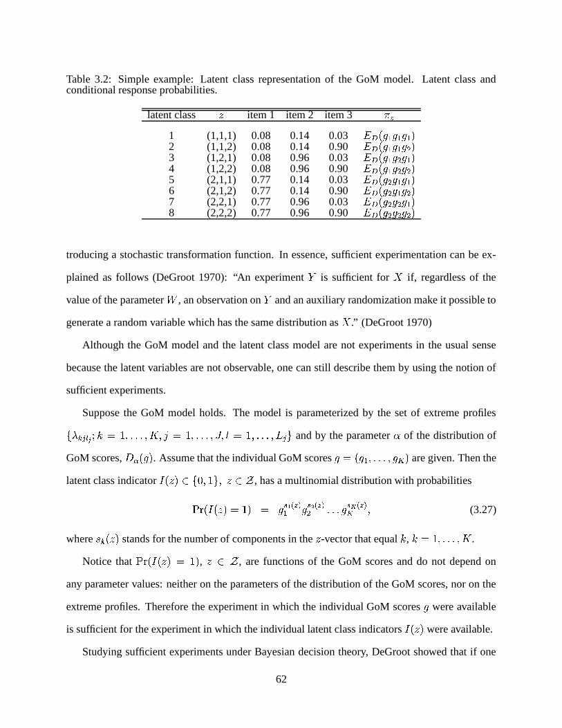
Table 3.2: Simple example: Latent class representation of the GoM model. Latent class andconditional response probabilities.

latent class ' item 1 item 2 item 3 ? S1 (1,1,1) 0.08 0.14 0.03 WlX�Qs3 � 3 � 3 � U2 (1,1,2) 0.08 0.14 0.90 WlX�Qs3 � 3 � 3 � U3 (1,2,1) 0.08 0.96 0.03 WlX�Qs3 � 3 � 3 � U4 (1,2,2) 0.08 0.96 0.90 WlX�Qs3 � 3 � 3 � U5 (2,1,1) 0.77 0.14 0.03 WlX�Qs3 � 3 � 3 � U6 (2,1,2) 0.77 0.14 0.90 WlX�Qs3 � 3 � 3 � U7 (2,2,1) 0.77 0.96 0.03 WlX�Qs3 � 3 � 3 � U8 (2,2,2) 0.77 0.96 0.90 WlX�Qs3 � 3 � 3 � U

troducing a stochastic transformation function. In essence, sufficient experimentation can be ex-

plained as follows (DeGroot 1970): “An experiment m is sufficient for

if, regardless of the

value of the parameter n , an observation on m and an auxiliary randomization make it possible to

generate a random variable which has the same distribution as

.” (DeGroot 1970)

Although the GoM model and the latent class model are not experiments in the usual sense

because the latent variables are not observable, one can still describe them by using the notion of

sufficient experiments.

Suppose the GoM model holds. The model is parameterized by the set of extreme profilesÄh* n Yc[ �.x0l°�ô� ! �.�.� ! J ! ^��ô� ! �.�.� ! W ! _w�ô� ! �"�.� !(b Y.Æ and by the parameter of the distribution of

GoM scores, L ¥ Qs3�U . Assume that the individual GoM scores 3��%Qg3 �0! �"�.� ! 3Ii�U are given. Then the

latent class indicator CeQ ' Uw¨°Ä9� ! �IÆ !u' ¨UQ , has a multinomial distribution with probabilitiespKr.Q CeQ ' Uu�E�2UÍ� 3po Ï Á S Â� 3qo , Á S Â� �"�.�c3qo Ñ Á S Âi ! (3.27)

where r n Q ' U stands for the number of components in the ' -vector that equal l , lí�H� ! �.�.� ! J .

Notice that pKr2QsCAQ ' U � �VU , ' ¨sQ , are functions of the GoM scores and do not depend on

any parameter values: neither on the parameters of the distribution of the GoM scores, nor on the

extreme profiles. Therefore the experiment in which the individual GoM scores 3 were available

is sufficient for the experiment in which the individual latent class indicators CeQ ' U were available.

Studying sufficient experiments under Bayesian decision theory, DeGroot showed that if one

62

were to encounter a statistical decision problem based on two experiments, one of which is suffi-

cient for another, in order to minimize one’s expected terminal uncertainty, one should choose to

observe the results of the sufficient experiment (DeGroot 1970). Rephrasing DeGroot’s results for

our case, given the choice of estimating the GoM scores or the latent class indicators, one should

choose to estimate the GoM scores for interpretation purposes.

3.5.2 Stochastic subject and random sampling

In Section 1.3.2, two rationales for formulating a latent structure model, the stochastic subject and

the random sampling rationales (Holland 1990a) are described. The stochastic subject rationale

assumes that human behavior is random, and latent quantities determine response probabilities of

a subject with that value of the latent variable. In contrast, the random sampling rationale assumes

that latent quantities define the probability of a correct response among subjects with that value

of their latent variable. Under the random sampling rationale, latent parameters are employed in

order to get legitimate values for probabilities of observable response patterns.

Using the random sampling rationale, interpretations of the GoM model and the latent class

representation of the GoM model are the same: they place the same probability structure on the

observed responses.

Adopting the stochastic subject rationale, under the GoM model, each of the W individual

marginal response probabilities is a linear combination of the response probabilities from J ex-

treme profiles, weighted by the GoM scores, and the probability of observing the whole pattern

is a W -fold product of these linear combinations. For a given set of GoM scores, the individual’s

responses to the manifest variables are being generated by a multinomial process with fixed prob-

abilities.

Given membership scores, the standard GoM interpretation states that every subject in the

population is a ‘partial member’ of the extreme profiles (Manton, Woodbury and Tolley 1994).

Consider the example of a health survey with J dichotomous questions. For Jô�+� , two estimated

63

extreme profiles could be interpreted as ‘healthy’ and ‘disabled’. A membership score for the

second extreme profile, 3 � , would then show how disabled the subject is relative to the ‘disabled’

profile.

In the standard latent class model, a population can be described as being composed of a num-

ber of latent classes. With W questions and J extreme profiles, the total number of latent classes

is J �. Each subject is considered to be a complete member of one of the latent classes at a certain

time. The membership score 3 n can then be interpreted as the proportion of questions that subject

answers as if he was a complete member of the l th extreme profile (with the same conditional

response probabilities). Taking the health survey example, a membership score 3 � �ò�VàI� would

mean that a subject with that score would answer a third of the survey questions as a ‘disabled’

person, and two thirds as a ‘healthy’ person. Notice the apparent conditional exchangeability of

the survey questions in this interpretation.

The latent class representation of the GoM model described in this chapter gives the basis for

the Bayesian estimation framework that the next chapter provides.

64

Chapter 4

Data Augmentation and Bayesian

Estimation Algorithms for the Grade of

Membership Model

In this chapter, I consider the case of dichotomous manifest variables. However, all statements

and algorithms developed here are applicable with some modification to the case of polytomous

manifest variables by using the binary data format from Section 1.2.1.

I start this chapter by formulating the Bayesian approach to the GoM model, paying particular

attention to choosing parametric forms of prior distributions. Although the standard GoM model

has a hierarchical structure, full conditional distributions are intractable. After augmenting data

with latent class indicators from the latent class representation of the GoM model, I can construct

Markov chain Monte Carlo (MCMC) algorithms for obtaining the posterior distribution of the

GoM model parameters. I provide these algorithms in Section 4.3. I then give an overview of

model selection methods that could be used for choosing the optimal number of extreme profiles,

and describe a Bayesian measure of fit, the deviance information criterion, which I use for the

GoM model. I have implemented the algorithms presented in this chapter in the C programming

65

language. Appendix A contains the C code, and Section 4.5 of this chapter contains some notes on

the implementation.

4.1 Bayesian Model Formulation

The Bayesian approach involves specifications of a probability model ��Qsî�t | ! }�U of data î , given

the parameters | and } , a prior ��Q | ! }uU , and, in some cases, a hyperprior.

For the GoM model, we assume the subject-level parameters, | , are independent of the struc-

tural parameters, } : ��Qs| ! }uU��,��Q |dUs��QR}uU . In a mixed-effects approach, the structural parameters} would be considered as fixed effects and the subject parameters | as random, 3 ÔEL ¥ Qs3�U . One

would then estimate the structural parameters, } , and the parameters of the distribution of the GoM

scores, . By analogy, in the Bayesian approach developed in this chapter, we place a hyperprior

on the GoM scores, but not on the structural parameters.

4.1.1 Choice of Priors

For parametric modelling, we need to choose a parametric form for prior and hyperprior distribu-

tions.

Structural parameters. Assuming independence among conditional response probabilities of

different items and of different extreme profiles, we place a prior distribution on the structural

parameters as ��QP}�Uu� i¾n(o � �¾Y o � ��QR* n Y·U ! (4.1)

where each conditional response probability, * n Y , is��QP* n Y&UK�Ptu3Z4\�yQ-v � n Y ! v � n Y·U0� (4.2)

66

In the absence of informative prior opinion about the response probabilities of the extreme profiles,

in what follows we use v � n Yk�\v � n Yk�H� ! l��E� ! �.�"� ! J ! ^G�� ! �.�"� ! W .

Membership scores. Recall that the GoM scores are nonnegative random variables that sum to 1.

A class of parametric distributions that accommodates such constraints is the family of Dirichlet

distributions, a multivariate generalization of the Beta family.

Dirichlet distribution. Suppose, 3ë� Qs3 �0! �.�.� ! 3IikU has a Dirichlet QR�U distribution with J cate-

gories and parameters Ê�%QR �(! �.�.� ! `i�U . The density function isLNMRO ¥ Qg3BUK�qLNMPO�Qs3�t �Uæ� w Q �&U> in(o � w Q n U i¾n(o � 3 ¥ ü â �n ! (4.3)

where n ´�� ! �k� ÷ n n , and÷ n 3 n �a� . The Dirichlet class consists of distributions obtained

by allowing the parameter vector to vary over the parameter space. Note that when n �×� forlí�H� ! �"�.� ! J , we obtain a uniform distribution on the simplex.

The Dirichlet distribution has a number of properties (see Aitchison, 1986, for a review). Those

of particular interest here are:

1. WNQs3 n Uu�� n àh� ! l��E� ! �"�.� ! J��2. 1yxVOhO�Qs3 n ! 3I[�UK�E�¹QR n �[�U �dzç� Q�Q ��¸ n U·QR��/�[�U�U â �dzç� ! l ! _~�H� ! �.�.� ! J��3. Every Dirichlet distribution can be obtained from the basis of independent, equally scaled,

gamma-distributed components.

Observations of vectors of proportions 3 on a number of subjects constitute a compositional data

set. Studying the statistical analysis of compositional data, Aitchison (1986) points out that the

strong structure that the Dirichlet distribution imposes may be too simple to realistically describe

compositional data. He supports his argument by saying that compositional data often exhibit

dependence structure other than just the sum constraint, and the Dirichlet distribution can not

67

accommodate positive correlations between some components because the correlations between

its components are always negative.

Prior for membership scores. The vectors of membership proportions in the GoM model aren’t

observable. Hence placing a Dirichlet distribution on the GoM scores becomes a part of the latent

structure assumptions. Dirichlet structure, however, might not be appropriate when there exists

strong prior knowledge about the extreme profiles, and when it is known a prori that memberships

in some extreme profiles exhibit positive dependence. While it is an open question whether placing

Dirichlet distribution on the GoM scores results in a testable assumption, resolving this question

goes beyond the scope of this thesis.

Because the Dirichlet distribution is conjugate to the multinomial, it seems to be a practical

choice for modelling the distribution of the GoM scores parametrically. We shall use the Dirichlet

distribution with density function (4.3) as the probability distribution of the GoM scores, for each

individual in the sample.

4.1.2 Choice of Hyperprior

Assuming the Dirichlet distribution, LNMPO ¥ Qs3�U , on the GoM scores, we are interested in estimating

the hyperparameters +�ÌQ �0! �.�.� ! `i�U , and we need to choose a hyperprior distribution. Good

and Crook (1987) studied the analogous question of choosing a hyperprior for Dirichlet random

variables in the case of a compound multinomial.

Hyperprior for compound multinomial. Suppose Õ observations are classified into J cate-

gories. The counts are Q � �&! �.�.� ! � n ! �.�.� ! � iwU , ÷ � n �EÕ . If the observed category proportions,3 �0! �.�.� ! 3Ii , are LNMRO ¥ Qs3�U , then Q � �0! �.�"� ! � iwU is a sample from the compound multinomial with

probability mass function (Levin and Reeds 1977):

"5OBQ � X�t �0U±� Õ|{> in(o � � X n { v w g ÷ in(o � n i> in(o � w QR n U v > in(o � w Q � X n � n Uw g Õ � ÷ in$o � n i �68

Good (1976) showed that assuming the subjective posterior expectation of observed proportions

to be of the form Q � n � n U�àBQ Õ � �0U , where �N� ÷ n , is equivalent to assuming the priorLNMRO ¥ Qs3�U density for 3 .

Treating the basis proportions of the Dirichlet parameters 8 n �� n àI� as known, Levin and

Reeds (1977) proved that the compound multinomial likelihood function for K given observed

multinomial data is unimodal in ` . It reaches its maximum at `ó²�Ú , if the minimum variance

unbiased estimate of the population repeat rate (defined as÷ n 3 �n ), is greater than �VàIJ , and the

maximum occurs at `��+Ú , otherwise.

Good and Crook (1987), using the Dirichlet property of invariance under collapsing categories,

proved that if the proportions 8 n are known, the hyperprior ��Q �U can be taken as a function of �alone (that is, ��Q �U is mathematically independent of the number of components, J ).

Using a variation of compound multinomial distribution for contingency tables, Good and

Crook (1987) place a log-Cauchy hyperprior on ��QR�0U . They regard the proportions 8 n as known,

and point out the following arguments in favor of the log-Cauchy: (1) it is proper, and (2) it is per-

missive toward large values of ` , which correspond to the prior belief that the basis proportions

are fairly accurate.

Hyperprior for the GoM model. The hyperprior choice of Good and Crook (1987) is not di-

rectly applicable to the GoM model for two reasons. First, since the compound multinomial sam-

ples categorized by the extreme profiles are not observable, we are also interested in estimating

the proportions 8 n . Second, the assumption that � is close to Ú for the GoM model is equivalent

to the independence assumption for the observed contingency table. Because the independence

structure is highly unlikely for large sparse tables, we are not interested in large values of K . Note

that a Dirichlet with ��+J and equal proportions 8 n corresponds to a uniform distribution in the

simplex, and a Dirichlet with `ó�%� corresponds to a point mass distribution at extreme profiles

(which is a traditional latent class model).

69

For our choice of a hyperprior in the Bayesian GoM model, ��Q �U , we reparameterize as �EQR �&! �.�.� ! �ikUu�+�VQ 89�0! �.�.� !�8 i�UK�+� 8B! (4.4)

where 8 n �ê n àI� and �� ÷ n n . In this fashion, 8 n represents the “proportion” of the popula-

tion that belongs to the l th extreme profile, and governs the “spread” of the distribution within

the convex set determined by the extreme profiles. The closer � is to 0, the more probability is

concentrated near the extreme profiles; similarly, for large � , more probability is concentrated

near the population average. This reparameterization seems reasonable because there might exist

prior information about one group of the parameters but not about another. Since K and 8 govern

two unrelated qualities of the distribution of the GoM scores, extreme profile proportions and a

shape of the distribution, we further assume that � and 8 are independent:��QR�UÍ� ��QR�0Us��Q 8 U ! (4.5)

where we take ��QR�&U±� }ª� �~� �yQ-� �&! � � U ! (4.6)��Q 8 Uæ� LNMPO�Qd��U0� (4.7)

In the absence of informative prior opinion about these quantities, we shall use a diffuse Gamma

for ��Q �0U , and a uniform distribution on the simplex for ��Q 8 U .4.2 Data Augmentation

Recall that the standard formulation of the GoM model postulates that a population can be charac-

terized by its extreme profiles, defined by their conditional response probabilities. Subject-specific

parameters are components of the vector of GoM scores that define “proportions” of membership

for each of the extreme profiles. Assume discrete responses are recorded on W dichotomous items

70

for C subjects. Let �]XÎ�ÌQs�=X �&! �.�.� ! �=X � U denote a response pattern, where �yXZY is a binary random

variable indicating the response of subject M to item ^ , Mk� � ! �.�"� ! C , ^ � � ! �.�.� ! W . Suppose there

are J extreme profiles (or basis subpopulations). Assume that each subject can be characterized

by a vector of membership (GoM) scores, 3FX��Qs39X �0! �.�.� ! 3hXji�U , one score for each extreme profile.

The GoM scores are non-negative and sum to unity over the extreme profiles for each subject:m n 39X n �E� ! M�� ! �.�"� ! C]� (4.8)

Extreme profile response probabilities, denoted by * n Y , are probabilities of positive response to

question ^ for a subject who is a complete member of the l th extreme profile:* n Yk�\"ÅO�Qs�=XZYk�H��t 3hX n ��VU&� (4.9)

We need the following additional assumptions: (1) the conditional probability of response of

individual M to question ^ , given the GoM scores, is

"5O�Qs�=XZY��E��t 39X�U�� imn(o � 3hX n�v * n Y2x (4.10)

(2) conditional on the values of the GoM scores, the responses �AXZY are independent for different

values of ^ ; (3) the responses �yXZY are independent for different values of M ; (4) the GoM scores 3zX nare realizations of the components of a random vector with Dirichlet distribution, LNMPO ¥ Qg3BU .

Using the standard GoM model formulation and omitting the subject index, we write the GoM

hierarchical model for each item ^D�E� ! �.�.� ! W as��Yzt 3 Ô tu3.O9¼ ö imn(o � 3 n�v * n Y ø !3 Ô LNMROBQ � !�8 U !* n YfÔ tu3Z4\�yQ-v � n Y ! v � n Y·U ! (4.11)��Ô }Å� �~� �eQ%� �&! � � U !8 Ô LNMROBQ��U&�71

The hierarchical structure (4.11) is inconvenient for Bayesian modelling because the full condi-

tional distributions of } and | are not readily available, since the joint density of the parameters

does not factor. Obtaining the complete full conditional distributions directly from (4.11) via

Bayes theorem requires integrating out the membership scores | . This type of integral is known as

a special case of Carlson’s multiple hypergeometric function (Dickey 1983) and is intractable an-

alytically, although Jiang, Kadane, and Dickey (1992) provide some approaches for computation.

For the same reason, using EM algorithm with membership scores treated as hidden variables is

a formidable task for this problem. Potthoff, Manton, Woodbury and Tolley’s (2000) maximum-

likelihood estimation method relies on a structure similar to (4.11) and uses the marginal likelihood

computed analytically in low-dimensional special cases.

Recall the latent class representation of the GoM model from Chapter 2 which introduces Wcategorical latent variables ' �æQ 'F�&!('.�2! �.�.� !('V� U , one for each observable discrete variable. Each

latent variable ' Y can take on J values from Ä«� ! � ! �.�"� ! J�Æ . In this fashion, the latent vector' ¨VQ � Ä«� ! � ! �"�.� ! J�Æ � defines a latent class. The probability mass function over the latent

classes is constrained to be the expected value of the W -fold product of the GoM scores:

? S �\"5OwQ 'h�&!$'.�.! �.�.� !('V� U±� W[X�� ¾Y o � i¾n(o � 3 S � ün �� !¸' ¨UQa�HÄ«� ! � ! �.�.� ! J�Æ � ! (4.12)

where ' Y n �E� , if ' Y��l , and ' Y n �� , otherwise.

This latent class representation adds another level to the model hierarchy. Suppressing the

subject index, for ^G�H� ! �.�.� ! W , we have:��Yzt ' Y Ô t�3.Oh¼ ö i¾n(o � * S � ün Y ø !' Yzt 3 Ô !qÛe_�4·Qµ� ! 3 �&! �.�.� ! 3IikU !3 Ô L½MPO�QR� !�8 U ! (4.13)* n YfÔ t�3Z4\�eQ-v � n Y ! v � n Y"U !�fÔ }Å� �~� �yQ-� �"! � � U !8 Ô L½MPO�Qd��U&�72

The latent realization ' Y determines the response probability for the observable �BY .The latent class representation of the GoM model leads naturally to a data augmentation ap-

proach (Tanner 1996) for computing the posterior distribution of the GoM model parameters.

We augment the observed data î with realizations of the latent classification variables � , where�-��Ä ' X5� Q ' X �&! �.�.� !(' X � U)ñ MD�f� ! �.�.� ! C=Æ . As before, let ' XZY n �� , if ' XZY �±l , and ' XZY n �æ� ,

otherwise.

The joint probability model for the parameters and augmented data can be derived in the fol-

lowing fashion:��Qsî ! � ! | ! } ! �U±� ��QR} ! �Ug��Qsî ! � ! |�t;} ! �U� ��QR}uUs��Q �U �¾X o � ��Qg�=X !(' X ! 3hXctZ} ! �U� ��QR}uUs��Q �U �¾X o � ��Qs�=X !$' X�t 39X ! } ! �Us��Qs39Xct;} ! �U ¢� ��QR}uUs��Q �U �¾X o � ��Qs�=X$t ' X ! 39X ! } ! �Us��Q ' X�t 3hX ! } ! �Ug��Qs39X\t;�U ¢� ��QR}uUs��Q �U �¾X o � ��Qs�=X$t ' X ! }�Us��Q ' X�t 3hX�Us��Qs39X�t;�U ¢� ��QR}uUs��Q �U �¾X o � ��Q ' X$t 3hX�Us��Qs�=X$t ' X ! }uU v LNMROBQg3hXct;�U ¢F! (4.14)

where ��Q ' X$t 3hX�U±� �¾Y o � i¾n(o � 3 S ï � üX n !��Qs�=X�t ' X ! }uU±� �¾Y o � i¾n(o � g * ¿ ï �n Y Qµ��-* n Y&U � â ¿ ï � i S ï � ü !L½MPO�Qs39X�t;�Uæ� w Q ÷ n n Uw QR � U&�S�S� w QR�iwU 3 ¥ Ï â �X � �"�.�c3 ¥VÑ â �Xji !

and ��QP}uU ! ��QR�U are assumed prior and hyperprior distributions.

By plugging ��Q ' Xct 39XsU and ��Qg�]X�t ' X ! }�U into equation (4.14), we obtain the joint distribution as��Qsî ! � ! | ! } ! �Uæ� ��QP}�Us��QR�U ö �¾X o � L½MPO�Qs39X�t;�U ø �¾X o � �¾Y o � i¾n(o � g 39X n * ¿ ï �n Y Qµ��-* n Y&U � â ¿ ï � i S ï � ü (4.15)

73

Complete conditional distributions of � , } and | are available from equation (4.15), and they allow

us to construct Markov chain Monte Carlo algorithms for obtaining the posterior distribution.

4.3 Markov Chain Monte Carlo Algorithms

Bayesian estimation methods provide several advantages. For example, posterior confidence inter-

vals for the parameter values are readily available from MCMC output whereas parameter standard

errors are not available from the current frequentist GoM software package (Decision Systems, Inc.

1999). Another advantage of using MCMC for latent structure models is that one does not have to

face a choice of either working with the joint likelihood or working with the marginal likelihood.

The output from Bayesian analysis can be used in dual fashion that can produce either estimate

with similar properties to those from marginal likelihood or estimates with similar properties to

those from joint likelihood (Patz and Junker 1999).

In this section, we provide MCMC algorithms for two cases: when the hyperparameters are

known, and when they are unknown. In the first case, the posterior distribution of the parameters

can be obtained via a Gibbs sampler. In the second case, an additional Metropolis-Hastings step is

needed to draw from the posterior distribution of the hyperparameters.

4.3.1 Gibbs Sampler

Suppose the hyperparameters are known. We can set up a Gibbs sampler algorithm by using

the complete conditional distributions derived from equation (4.15) as follows:��Q ' X�t0�.�.�®U�� ¾Y o � i¾n(o � g 3hX n * ¿ ï �n Y Q\��/* n Y&U � â ¿ ï � i S ï � ü ! (4.16)

��QP* n YFt0�.�.�®U�� QP* n Y&U v �¾X o � g * ¿ ï �n Y Q\��-* n Y&U � â ¿ ï � i ! (4.17)��Qg3hXct0�.�.�®U�� LNMPO�Qs39Xct �U v �¾Y o � i¾n$o � 3 S ï � üX n � (4.18)

74

where �.�.� stands for all other variables from î ! � ! | ! } . One simulation draw of the Gibbs sampler

consists of an imputation step and a posterior step (Tanner 1996). During the Q � � �VU st imputation

step, a realization of the latent classifications ' Á ��õ � ÂX is obtained for every person from the condi-

tional predictive distribution, given the parameter values from the � step. During the Q � � �VU st

posterior step, realizations of the parameters * Á ��õ � Ân Y and 3 Á ��õ � ÂX n are obtained from the augmented

posterior distribution, given the parameter values from the � step.

The Gibbs sampler algorithm, suppressing the step index � on the right hand side for ease of

notation, is given by:º Imputation step:

Sample ' XZY for M��×� ! �.�.� ! C ! ^N�×� ! �.�.� ! W , given parameter values from the � th step, from

a multinomial distribution,' Á ��õ � ÂXZY Ô !�Ûy_�4~Qµ� ! � �(! �.�.� ! �]ikU ! � n ��3hX n * ¿ ï �n Y Q\��/* n Y&U � â ¿ ï � � (4.19)º Posterior step:

Sample * n Y ! lí�E� ! �.�"� ! J ! ^G�� ! �.�"� ! W , given parameter values from the � th step, from a

Beta distribution,* Á ��õ � Ân Y Ô tu3Z4\� ö � � �mX o � �=XZY ' XZY n ! � � �mX o � Q ' XZY n �¶�=XZY ' X;Y n U ø � (4.20)

Sample the GoM scores 3IX for each individual Mè� � ! �.�"� ! C , given augmented data and

parameter values from the � th step, from a Dirichlet distribution,3 Á ��õ � ÂX Ô LNMPO2i �� d� �mY o � ' XZY �&! �.�.� ! `i � �mY o � ' XZY�i �� (4.21)

4.3.2 Metropolis-Hastings Within Gibbs

Metropolis-Hastings step for ` . If the Dirichlet parameter vector is unknown, we can obtain

samples from its posterior distribution via a Metropolis-Hastings step within the Gibbs sampler.

75

The full conditional distribution for ` , from equation 4.15, up to a constant of proportionality, is:��QR�Ft0�.�.�®U�� QR�0U �¾X o �� w Q �&Uw Q 8h� �0UA�.�.� w Q 8 i��(U i¾n(o � 3+� ü ¥`�X n � ! (4.22)

where �.�.� on the left hand side stands for all other variables.

If the prior on � is Gamma Q%� �0! � � U with shape parameter � � and inverse scale parameter � � then

the full conditional distribution for ` is proportional to��Q �ht0�.�.�ÿU�� Ï â � ã&äTå � � ö � � � imn(o � 8 n �m X o � Ý�ÞFßK3hX n ø � � � w QR�0Uw Q 8h� �0UA�.�"� w Q 8 i��&U � � � (4.23)

When �Å§�� , w QR�0U is approximately �VàI� . Thus, when �ª§a� , the full conditional distribu-

tion ��Q �It0�"�.�ÿU can be approximated withQR�Ft0�.�.�®U�� Ï â � ã0ä�å ö � ö � � � imn(o � 8 n �m X o � Ý�ÞFß�39X n ø � ø ö �VàI�> in(o � �2à 8 n � ø �� Ï â � â � õ=i�� ã&äTå ö � ö � � � imn(o � 8 n �m X o � Ý�ÞFßK3hX n ø � ø ��§ê� !

which is Gamma with parameters��QR�Ft0�.�.�ÿU�� w ö � �� CeQRJ��VU ! � � � imn(o � 8 n �m X o � Ý�ÞFßK3hX n ø ! ��§��F� (4.24)

Note that for Jf´H� , the shape parameter of the approximate distribution for � is greater than 1.

Both, the shape parameter and the inverse scale parameter increase with the number of subjects C ,

which reduces influence of the prior distribution parameters, � � and � � .When we are confident that � is less than one, we can use the approximation in equation (4.24)

as a proposal distribution. That would turn the Metropolis-Hastings step into a Metropolis step,

because the distribution (4.24) does not depend on the previous draw of K , but only on the values

of the GoM scores, 3hX n , and on the proportions, 8 n .

Alternatively, when `5§%� may not hold, we take the proposal distribution for the next draw,��Q Ù t Á � Â U , to be gamma with expected value set at the value of the last draw, Á � Â , and the shape

76

parameter set at a convenient constant / ´E� . Here, / is the tuning parameter for the Metropolis-

Hastings step. The inverse scale parameter for the proposal distribution is then / àh Á � Â , and the

proposal distribution is ��Q Ù t Á � Â U±� }Å� �~� � Á�� : � z ¥2��K�� Â QR Ù U&� (4.25)

In order to obtain the Q � � �2U st draw of ` , the Metropolis-Hastings algorithm requires:

1. Draw a candidate point �Ù from ��Q �Ù t Á � Â U ;2. Calculate the proposal ratio O ¥`� � ��QR`Ù t0�.�.�ÿUg��QR Á � Â t �Ù U��Q Á � Â t0�.�.�ÿUs��QR Ù t; Á � Â U x3. Assign Á ��õ � Â �q Ù with probability � MR¼`Ä«� ! O ¥`� Æ , otherwise assign Á ��õ � Â �+ Á � Â .

The proposal ratio for the Q � � �VU st draw of ` isO ¥`� � O ¥`� Qd!,U v O ¥`� Q��ÜU !where O ¥`� Q�!+UÍ� ö Ù Á � Â ø � Ï â � ã&äTå � � ö � � � imn(o � 8 n �mX o � Ý ÞFß�39X n ø Q Ù �/ Á � Â U � v

�� w Q �Ù U w Q 8h� Á � Â UA�.�.� w Q 8 i� Á � Â Uw QR Á � Â U w Q 89� Ù UA�"�.� w Q 8 i� Ù U � �O ¥`� Qd�ÜUæ� �� Á � Â Ù �� â � ã0äTå�� / QR Á � Â àI Ù �¸ Ù àh Á � Â U��`�

Here, O ¥`� Qd!,U is the likelihood component of the proposal ratio and O ¥`� Qd��U is the component of

the proposal ratio that accounts for non-symmetric proposal distribution.

77

Metropolis-Hastings step for 8 . The full conditional distribution for 8 , up to a constant of pro-

portionality, is: ��Q 8 t0�.�.�®U�� ã&äTå � � imn(o � 8 n �m X o � Ý�ÞFß�39X n � � w Q �(Uw Q 8h� �&UA�.�.� w Q 8 i��0U � � (4.26)

where �.�.� on the left hand side stands for all other variables.

The proposal distribution for 8 is centered at the previous draw and has reasonably small vari-

ance for each component. A reasonable choice is L½MPO�Q 8 Ù9t��9J 8 Á � Â� ! �.�"� ! �9J 8 Á � Âi U , which gives the

variance of the l th component to be 8 Á � Ân Qµ�K� 8 Á � Ân UcàBQd�9J � �VU . Denote the proposal distribution by��Q 8 Ù t 8 Á � Â UÍ� LNMPO Á�� i � ��K�Ï :;Ð;Ð;Ð : � i � ��O�Ñ Â Q 8 Ù U (4.27)

The Metropolis-Hastings sampling algorithm has three steps:

1. Draw a candidate point 8 Ù from ��Q 8 Ù t 8 Á � Â U ;2. Calculate the proposal ratio O � � ��Q 8 Ù t0�.�.�®Ug��Q 8 Á � Â t 8 Ù U��Q 8 Á � Â t0�.�.�®Ug��Q 8 Ù t 8 Á � Â U x3. Assign 8 Á ��õ � Â � 8 Ù with probability � MR¼`Ä«� ! O � Æ , otherwise assign 8 Á ��õ � Â � 8 Á � Â

.

The proposal ratio for 8 is

O � � ã&äTå � � imn(o � �mX o � Ý�ÞFßK3hX n Q 8 Ùn � 8 Á � Ân U � �� w Q 8 Á � Â� �0UA�"�.� w Q 8 Á � Âi �0Uw Q 8 Ù� �0UA�.�.� w Q 8 Ùi �0U � � vw Qd�9J 8 Á � Â� UA�.�.� w Qd�9J 8 Á � Âi Uw Qd�9J 8 Ù� UA�"�.� w Qd�9J 8 Ùi U v Q 8 Á � Â� U � û â � �.�.�.Q 8 Á � Âi U � û â �Q 8 Ù� U � ��K� â � �.�"�2Q 8 Ùi U � ��K� â � !

where � is a tuning parameter which can be set to a suitable constant. We choose the values of the

tunning paramters � and / to achive a compromise between the acceptance rates and the amount

of mixing in the chain.

78

One complete iteration of the MCMC algorithm for the case when the hyperparameters, , are

unknown consists of the Gibbs sampler for drawing � ! | and } derived in the previous section, and

two Metropolis-Hastings steps for drawing � and 8 provided above.

4.4 Choosing the Number of Extreme Profiles

Often the number of extreme profiles J in the GoM model is unknown. In such cases, we are

interested in obtaining inference about J or in determining which value of J provides the model

that fits the data best.

4.4.1 Overview of Model Selection Methods

Methods for model selection include reversible jump techniques, marginal likelihood methods

(such as Bayes factors), posterior predictive model checks, cross-validatory residual analysis and

penalized likelihood criteria such as BIC (Schwarz 1978) and AIC (Akaike information criteria)

(Akaike 1973).

Modifications of reversible jump MCMC methods (Green 1995) allow movement between

models of different dimensions and provide a natural solution for the model determination prob-

lem: the model posterior probabilities are the normalized amounts of time the MCMC chain spends

at each model.

Bayes factors also provide a tool for comparison between the posterior probabilities of two

models (Kass and Raftery 1995). There is a vast area of research in designing reversible jump

methods and computing Bayes factors (see, e.g., Hoijtink 2001, Chib and Jeliazkov 2001, Han

and Carlin 2001, Brooks, Giudici and Roberts 2003, and references therein). One of the major

difficulties in computing Bayes factors is the computation of marginal likelihood, defined as the

integration of the sampling density with respect to the prior distribution of the parameters, and not

the posterior, which is what we obtain via MCMC. Thus, MCMC output cannot be readily used

79

for Bayes factor calculations. Chib and Jeliazkov (2001) offer a method of computing marginal

likelihood that is based on the MCMC scheme which is used to simulate the posterior distribution

by rearranging the existing code and by splitting the parameter space into conventionally specified

blocks.

Most of these research efforts in reversible jump techniques and Bayes factor calculations is

focused on low-dimensional problems and, as pointed out by Han and Carlin (2001), these tech-

niques require substantial time and effort (both human and computer) for a very modest payoff,

that is, for a set of posterior model probability estimates for the models under consideration.

More computationally realistic alternatives for model comparison are posterior predictive model

checks (Rubin 1984), cross-validatory residual analysis, and approximations to penalized likeli-

hood criteria such as BIC and AIC.

Posterior predictive model checks are especially appealing when one is interested in a particular

feature of the data, but might be time consuming for big data sets and hierarchical models with

large numbers of parameters. Similarly, in such settings computational time is a constraint for

implementing cross-validatory residual analysis techniques such as “leave one out”.

More feasible alternatives that do not require a lot of additional programming are penalized

likelihood criteria, similar to the Bayesian information (Schwartz) criterion or Akaike information

criterion (AIC). Given that Ç is a vector of model parameters and the log likelihood _��+Ý ÞFß=Q b QRÇIU�Uis a parametric function of interest, the function�_ � W�QsÝ ÞFß b QRÇIUVt î�U�� mo o � Ý ÞFß]Q b QRÇ«Á o Â U�U ! (4.28)

can be considered as a measure of fit to be compared across the models (Carlin and Louis 2000),

where Ç Á o Â are draws from the posterior. One way to obtain a penalized likelihood criterion based

on�_ is to use the penalty term similar to BIC:�tªCq¡ � � �_e��Ý ÞIßK¼ !

where � is the number of parameters in the model and ¼ is the number of data points. However,

80

for the case of hierarchical models, it is not straightforward to understand what exactly are � and¼ . Moreover, in complex hierarchical models such as GoM, the parameters may even outnumber

observations. We do not pursue the direction of determining the number of free parameters for

the GoM model in this thesis. See Carlin and Louis (2000) for a general discussion on this topic,

and Spiegelhalter et al. (2002) for a set of references in smoothing and neural networks literature

which contain attempts to tackle this problem in some specialized settings.

Deviance information criterion. Another approach taken by Spiegelhalter, Best, Carlin and

van der Linde (2002) to address the problem of obtaining a measure of model fit is the deviance

information criterion DIC, defined as the Bayesian deviance evaluated at the parameter means plus

twice the effective number of parameters:LNC+¡ � L�Q ÇFU � �&�¢X ! (4.29)

where the Bayesian deviance isLÜQRÇIU±� ��Ý�ÞFß�Ä(��Qgîkt;ÇIU0Æ � ��Ý ÞIß�Ä£6�Qsî�U(Æ ! (4.30)

given that 6�Qsî�U is a function of the data, and the effective number of parameters is defined as�¢X � LÜQ ÇFU��/LÜQ ÇFU ! (4.31)

a ‘mean deviance minus the deviance of the means’. Spiegelhalter et al. (2002) provide a partial

decision theoretic justification for DIC and they also note that in models with negligible prior

information DIC and AIC are approximately equivalent. Note that the choice of 6�Qg�eU does not

influence the results of comparison.

In hierarchical models, calculation of a Bayesian deviance (4.30) depends on the choice of the

parameters on which the model is ‘focused’ (Spiegelhalter et al. 2002). Briefly, if we consider a

Bayesian model with data î , parameters Ç , and hyperparameters ¤ , we could focus either on Ç or

on ¤ . Thus, focusing on Ç , we may consider that the likelihood ��Qsîkt ÇFU and prior��QRÇIU±� È ��Q Çyt ¤�Us��Q�¤�Uc¦�¤ !81

compose the model. Focusing on ¤ , we may consider that the likelihood��Q # t ¤kU�� È ��Q # t;ÇIUs��Q Çyt ¤�Uc¦«Çand prior ��Q-¤kU compose the model. These two choices result in two different sets of likelihoods

and priors for each of the ‘focused’ models. Both choices lead to the same marginal distribution for

the observed data but can be considered as having different numbers of parameters. Spiegelhalter

et al. (2002, pg. 31) point out that “the parameters in the focus of a model should ideally depend

on the purpose of investigation, although in practice it is likely that the focus may be chosen on

computational grounds”. The computational advantage of DIC is that it is readily obtainable from

MCMC output, provided the likelihood b QRÇyt î�U , where Ç is the parameter in focus, is available in

closed form.

4.4.2 Calculating DIC for the GoM Model

For the GoM model, even though one might be most interested in the population parameters }and , the likelihood b QR} ! �t î�U is not available in closed from. If, on the other hand, our focus is

on | and * , then the MCMC output can be readily used for computing Bayesian deviance. Since

the standardizing function 6�Qsî�U is a function of the data alone and hence has no impact on model

comparison, we omit specifying a particular choice for 6�Qsî�U and set it to zero, 6�Qsî�U�¥�� .

Let 3 Á o ÂX n and * Á o Ân Y , r��H� ! �"�.� !j¦ , be draws from the posterior distribution. The pieces needed for

obtaining DIC are as follows:L�Q | ! }uUÍ� ��R§m X o � �mY o � Ý ÞFß g 39X n * n Y ¿ ï � Q\�� * n Y&U � â ¿ ï � i ! (4.32)

where 39X n � �¦ mo o � 3 Á o ÂX n ! * n Yw� �¦ mo o � * Á o Ân Y ! (4.33)

82

and LÜQ | ! }uU±� �� ¦ mo o � Ý�ÞFß]Q b Q Ç«Á o Â U�U (4.34)� �¦ mo o � §mX o � �mY o � Ý�ÞFß g 3 Á o ÂX n * ¿ ï �n Y Qµ��-* n Y&U � â ¿ ï � i�� (4.35)

Then the effective number of parameters is�¢X°� LÜQs| ! }uU��/LÜQ | ! }�U (4.36)

and the Bayesian measure of fit, DIC, can be found from equation (4.29). Models with smaller

DIC values are preferable. We shall use DIC to measure the goodness of fit of the GoM models

with different numbers of extreme profiles.

4.5 Implementation Notes

C code. Appendix A contains the C code implementation of the Gibbs sampler algorithm and the

Metropolis-Hastings steps described in Section 4.3. The program requires submitting starting val-

ues for the hyperparameters , for the conditional response probabilities } , and for the membership

scores, | . Other input files are a data file and a file with selected response patterns for computing

expected probabilities. If parameters of the prior distribution for the conditional response probabil-

ities are not supplied, the program uses a uniform prior for each response probability, * n Y . Standard

output files include draws of , } , and the values of the (joint) log-likelihood. The program can

produce optional output of the draws of membership scores, | , but a word of caution is in order.

As the number of MCMC iterations increases, the output of the membership scores can quickly

become enormous even with a modest number of observations for any number of extreme profiles.

In addition, the program calculates mean membership scores for each observed response pattern,

that can be used for computing the Bayesian measure of fit, DIC (calculated over the draws from a

stabilized posterior).

83

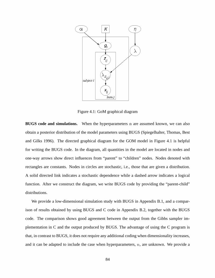
Figure 4.1: GoM graphical diagram

BUGS code and simulations. When the hyperparameters are assumed known, we can also

obtain a posterior distribution of the model parameters using BUGS (Spiegelhalter, Thomas, Best

and Gilks 1996). The directed graphical diagram for the GOM model in Figure 4.1 is helpful

for writing the BUGS code. In the diagram, all quantities in the model are located in nodes and

one-way arrows show direct influences from “parent” to “children” nodes. Nodes denoted with

rectangles are constants. Nodes in circles are stochastic, i.e., those that are given a distribution.

A solid directed link indicates a stochastic dependence while a dashed arrow indicates a logical

function. After we construct the diagram, we write BUGS code by providing the “parent-child”

distributions.

We provide a low-dimensional simulation study with BUGS in Appendix B.1, and a compar-

ison of results obtained by using BUGS and C code in Appendix B.2, together with the BUGS

code. The comparison shows good agreement between the output from the Gibbs sampler im-

plementation in C and the output produced by BUGS. The advantage of using the C program is

that, in contrast to BUGS, it does not require any additional coding when dimensionality increases,

and it can be adapted to include the case when hyperparameters, , are unknown. We provide a

84

simulation study with the C code for � in Appendix B.3 .

Finally, in Chapter 7 we use the C code for the Bayesian GoM analysis of a 16-way contingency

table, an extract of functional disability data from the National Long-Term Care Survey.

85

Chapter 5

Studying Disability in the Elderly

5.1 Motivation and Significance

Because of the rapid growth of the U.S. elderly population (Freudenheim 2001), the problem of

estimating and predicting trends in disability has received increased attention in the United States,

particularly in the past few years. The absolute and relative growth of the elderly population is

partly caused by greater longevity, but birth rates of the past also contribute to the phenomenon.

The expected rapid increase in the proportion of elderly in the United States is partly a result of

the aging of the “baby boom” babies born after World War II.

Caring for the elderly requires substantial informal care by family and friends, typically over

and above any formal care by professionals. Katz, in 1963, illustrated the importance of the prob-

lem as follows: “Although they constitute 11 percent of the total population, Americans 65 and

over account for 40 percent of hospitalization days in acute care hospitals, buy 25 percent of all

prescription drugs, spend 30 percent of the total health budget, and spend 50 percent of the federal

health budget.” These numbers, of course, have changed since the 1960s. It is projected that, by

the year 2025, 18.5 percent of the US population will be 65 years and older (Ostir, Carlson, Black,

Rudkin, Goodwin and Markides 1999). In the US, life expectancy at birth in 1995 was estimated

87

to be 72.5 years for men and 78.9 years for women, an increase of 25 years for men and 30 years

for women since 1900 (Ostir et al. 1999).

5.1.1 Functional Disability: Activities of Daily Living and Instrumental Ac-

tivities of Daily Living

Disability is a complex notion. Studying disability, Nagi (1965,1991) distinguishes a framework

of four distinct but interrelated concepts: active pathology, impairment, functional limitation, and

disability. Active pathology is characterized by an interference with normal processes, and efforts

of the organism to regain a normal condition. Impairment indicates a loss or abnormality of an

anatomical, physiological, mental or emotional nature. Functional limitation is a higher level of

impairment, it refers to manifestations at the level of the organism as a whole. Finally, disability

is an inability or limitation in performing within a sociocultural and physical environment, and

it refers to social rather than to organismic functions. Nagi (1991) points out that different types

of impairments and functional limitations may result in similar disability patterns, and, at the

same time, different disability patterns may arise from similar sets of impairments and functional

limitations.

Disability structure becomes more complex at older ages, when disability more often results

from losses of physiological functions due to general processes of senescence and/or from an inter-

action of multiple disease processes, rather than from a single disease process (Manton, Corder and

Stallard 1997). To cover the broad spectrum of disability manifestations in the elderly, geriatric

medicine focuses on the functional aspects of health associated with difficulties experienced by

individuals in performing certain activities that are considered normal for everyday living. Tradi-

tionally, these activities are divided into activities of daily living (ADLs) and instrumental activities

of daily living (IADLs). ADLs include basic activities of hygiene and personal care, such as eat-

ing, dressing, or moving inside the house. IADLs include basic activities necessary to reside in the

community, such as grocery shopping, telephoning, and housekeeping. A number of different bat-

88

teries of ADLs and IADLs have been used to assess functional limitation. Most of these batteries

include the same basic set of activities.

5.1.2 Disability Trends in the United States

Longer life is often associated with negative expectations about old age, such as declining intel-

lectual abilities and physical health. In the 1970s, it was predicted that technology would assist

people in living longer without curing them, which would result in a large number of disabled

elderly and, subsequently, in a dramatic increase in health care services and costs (Research High-

lights in the Demography and Economics of Aging 1999). This prediction was supported by studies

from the 1970s and early 1980s that showed that the proportion of older Americans limited in their

capacity to perform normal activities was increasing (Freedman and Soldo 1994, Waidmann and

Liu 2000). During the 1980s, however, the National Health Interview Survey and the Longitudinal

Study of Aging showed some modest improvements in self-reported disability prevalence (Waid-

mann and Liu 2000). In the 1990s, using summary measures on data from the National Long

Term Care Survey, Kenneth Manton and colleagues from the Center for Demographic Studies at

Duke University (Freedman and Soldo 1994, Manton et al. 1997, Manton and Gu 2001) showed

that disability trends among older Americans experienced sharp declines since the late 1980s. The

controversy that surrounds these findings is illustrated by an ongoing debate in the gerontology

literature (Mathiowetz and Lair 1994, Ostir et al. 1999).

Comparing findings on disability across surveys is problematic not only because different sur-

veys often use different sets of ADLs and IADLs, but also because differences in the wording

of questions and in the methods of assessment often result in targeting different substantive con-

structs. Thus, while some disability surveys target the need for help, questions in other surveys

are formulated to assess whether an activity can be performed at all, with or without any external

help. Moreover, formal assessments by an occupational therapist may show what elderly can do,

whereas interviews may reveal what elderly think they can do in real life (Barer and Nouri 1989). A

89

recent article by Ostir et al., (1999) compared findings concerning trends in active life expectancy

(active life expectancy is an estimated number of disability-free years a person can expect to live

before death) from the National Health Interview Survey, National Long Term Care survey, and

the Longitudinal Study on Aging. They concluded that “because of varying definitions, no clear

consensus exists as to whether active life expectancy is increasing or decreasing.”

Mathiowetz and Lair (1994) offer yet another perspective on why survey findings of declin-

ing disability trends should be treated with caution. They ask whether the findings of disability

improvement over time reflect reality or whether measurement error is responsible for the pat-

tern of change. They distinguish between two possible components that are likely to contribute

to measurement error. First, from the methodological standpoint, there are many factors that in-

fluence measurement of disability (Barer and Nouri 1989). Those most commonly mentioned in

the literature are: (1) confounding (the most disabled may have most difficulty as respondents);

(2) tendency of proxy responders to overestimate functional limitations; and (3) possibility of dif-

ferent interpretations of survey questions. Second, there is lack of knowledge about measurement

properties of the quantities used to assess disability among the elderly. Most of the quantitative

research on disability assessment, and, in particular, on changes in disability status over time, has

been limited to a discussion of the number of ADL difficulties (Mathiowetz and Lair 1994). The

summary score approach ignores the compositional structure of disability, such as differences over

time by a selected activity.

Mathiowetz and Lair conclude: “estimates of ADL difficulties and changes in ADL status over

time may have a significant error component. Given the lack of stability in these measures, our

findings further suggest that difficulties might be encountered in applying these measures in assess-

ment situations for long-term care eligibility. Although ADLs have a long tradition as powerful

predictors of future disability and service needs of the elderly, the findings presented [in the article]

would suggest that more research be undertaken to consider the measurement properties of ADLs

and other measures of functional limitation for the elderly in both cross-sectional and longitudinal

90

applications.” (1994, pages 260-261).

The substantive focus of this thesis is on statistical models that can be used to study disability

among the elderly and their potential implications for measurement of disability. Measurement of

individuals’ disability is very important in the context of the clinical therapeutic process, where

possible uses of a disability measure include describing the client’s problem, formulating a prog-

nosis, and evaluating the effects of occupational therapy interventions (Law and Letts 1989). It is

also an important issue for public policy debates on pensions, retirement, and future health care

spending, as well as for private insurance companies (Mathiowetz and Lair 1994). In addition,

more global questions, e.g., why disability rates experience change and what this may mean for

policy implications, also require a more complex micro-level measure of disability.

In this chapter, I give an overview of quantitative methods and statistical models that are com-

mon in the literature. I then emphasize the problem of latent dimensionality of disability, and

conclude with a discussion of psychometric modeling applications to studying disability.

5.2 Literature Review

5.2.1 Summed Indexes and Hierarchical Scales

The problem of measuring disability is complex in its definition and application. One of the reasons

is that there is no widely accepted definition of what disability is (Pfeirref 1999). Definitions

used by public programs providing specific assistance for disabled people vary, depending on the

purpose of the program. Different operational measures of disability have been used across surveys

(Freedman and Soldo 1994). Whereas some sources indicate that, despite existing methodological

issues, national measures of disability were shown to be consistent across surveys (Manton et al.

1997), others claim that the lack of the universal “gold standard” for measuring disability has

produced a wide range of estimates (Freedman and Soldo 1994). While there is a certain need

for a specialized disability measure for patients with particular disorders, there is also a need for

91

a standardized general measure of disability (see Barer and Nouri 1989, for discussion on the

necessity and possible uses of a standardized disability measure).

The basic approach to measuring disability is by using a summed index, where individual

scores on all items are summed to produce a total. One obvious sufficient condition for the summed

index (total score) to be valid is that all items are equal in ‘disability value’. This condition is

unlikely to hold, however, when ADL or IADL measures are considered: someone who cannot

climb into a bath is usually not assumed to be as equally disabled as someone who cannot eat.

Equality of ‘disability values’ for all items is sometimes confused with a necessary condition for

using a summed index (Eakin 1989). The summed index, or total score, has been used for a long

time in educational statistics as a measure of ability. It has been known since the 1960s that the total

score can be a useful measure when a set of items satisfies the Rasch model assumptions. However,

reported uses of the summed index in disability literature usually do not rely on any statistical

justification, with an exception of one recent data analysis article by Spector and Fleishman (1998).

The most common technique for measurement of functional disability is hierarchical scale

construction. For comparative reviews of more than fifteen ADL, IADL, and ADL+IADL scales

see (Barer and Nouri 1989), (Eakin 1989), (Law and Letts 1989), and (Aguero-Torres, Hilleras and

Winblad 2001). In these reviews, the authors recognize that construction of a hierarchical scale

involves ordering items by their natural difficulty. Specifically, the Guttman scaling assumption

states that items are passed in the order of natural difficulty. Thus, if an individual cannot perform

a certain activity, it is implied that he/she necessarily cannot perform all activities of a greater

difficulty. Usually, items are selected to form a scale on the basis of expert appraisal or on the

basis of statistical evidence (Law and Letts 1989). However, for many of the reported ADL/IADL

scales, it is unclear to what extent statistical procedures have been involved to help determine

item hierarchy. According to Law and Letts (1989), the index of ADL developed by Katz, Ford,

Moskowitz, Jackson and Jaffe (1963) was the only scale, among fifteen they reviewed, in which the

selection of items was validated statistically. The Katz ADL index (Table 5.1), originally developed

92

Table 5.1: Katz ADL index. ADL functions: feeding (1), continence (2), transferring (3), going to

the toilet (4), dressing (5) and bathing (6).

Grade Description

A Independent in all six functions

B Independent in all but one function

C Independent in all but (6) and one additional function

D Independent in all but (6,5) and one additional function

E Independent in all but (6,5,4) and one additional function

F Independent in all but (6,5,4,3) and one additional function

G Dependent in all six functions

Other Not classifiable as A-G

to assess disability among elderly patients with femoral fractures, uses six ADL activities (bathing,

dressing, using the toilet, transferring in and out of bed and in and out of chair, continence, and

feeding) to assign ordinal disability grades. Strictly speaking, the way the grades of the Katz index

are defined does not follow a strict hierarchical order as in Guttman scaling, because it permits one

activity to be unnamed at every possible stage. Any person who breaks this softened hierarchical

order is assigned to a separate category (see Table 5.1).

5.2.2 Latent Dimensionality

It is often assumed, explicitly or implicitly, that disability is unidimensional. Unidimensionality

can be stated in two interchangeable assumptions. First is the assumption that items that “mea-

sure” disability can be sorted in the order of natural difficulty. Second is the assumption that an

underlying disability construct is unidimensional (a scalar). The former is more frequently stated

in the medical and sociological literature on disability assessment than the latter. However, inde-

93

pendently of the form of the assumption, some contradictory statements can often be found in the

same papers. This indicates that assumptions of dimensionality often do not receive serious con-

siderations. Next, I will give a few examples which illustrate an uneasy relationship with assumed

dimensionality in disability assessment.

Thus, Barer and Nouri (1989, p. 179), reviewing hierarchical disability scales, mention that

when new items are introduced to the scale, they should not fall outside of “the domain of disabil-

ity”. Note that a hierarchical scale assumption necessary implies unidimensionality. The authors

do not discuss further the assumed dimensionality of the disability domain, but they do provide ta-

bles specifying different components involved in the construction of several ADL and IADL scales

(Barer and Nouri 1989, page 183). The ADL scales provided in these tables involve two or three

components out of self-care, mobility, continence, kitchen, and domestic, and the IADL scale in-

volves four components, namely, mobility, kitchen, domestic, leisure activities. The ordering of

components was not discussed.

Sometimes contradictory statements are simultaneously supported by the same data analysis.

Thus, Reboussin, Miller, Lohman, and Have (2002), hypothesize that “(a) there are qualitatively

different classes of functioning”, and “(b) individuals might lose functioning in a hierarchical

manner.” Conclusions from the data analysis presented in the paper support these two statements.

The contradictory nature of these two statements becomes apparent when the authors note that data

support for (a) gives an indication of the multidimensional nature of disability.

Another example is from a review of the assessment of activities of daily living by Eakin (1989)

who states that “all items taken together must define a unidimensional construct, for example, an

ADL ability”. The article then goes on to examine scales that involve ADL, as well as IADL

items, without mentioning that these combinations would probably define a new, not necessarily

unidimensional, construct.

Finally, one more example of contradictory dimensionality statements about disability can be

found in a 2001 review of activities of daily living in Current Opinion in Psychiatry (Aguero-Torres

94

et al. 2001). This article begins with a sentence: “Disability is a multidimensional concept that

cannot easily be captured in a single measure.” Without further discussion on dimensionality, the

article then provides an overview of the most commonly used measures of functional disability via

ADL, IADL and ADL+IADL items from an essentially unidimensional perspective, in particular

assuming that the IADL scales have been designed “to measure less severe disability.”

It is widely recognized that IADL items are different from ADL items in that they typically

require a higher level of cognitive functioning, but there is no clear consensus in the literature

whether ADL and IADL items measure one underlying construct. In fact, there appear to be two

traditions in using ADL and IADL items to assess functional disability: one is to consider these

two classes of items separately, and the other is to combine them in a single measurement.

The first tradition comes from a belief that ADL and IADL items measure qualitatively different

concepts. The idea that some of the ADL and IADL scales should be modeled separately was

supported by studies from the 1970-1980s (Fitzgerald, Smith, Martin, Freedman and Wolinsky

1993). On the other hand, the idea of combining ADL and IADL items together has its roots

in the hypothesized hierarchical relationship between IADL and ADL items, with IADL items

representing less severe disfunction (Spector, Katz, Murphy and Fulton 1987). Assuming the

hierarchical structure, the purpose of combining ADL and IADL items is to cover a broader range

of levels of functional disability. The hierarchical relationship between ADL and IADL items was

also supported by findings from several studies, which I will discuss next in some detail.

Thus, two studies based on Guttman scaling demonstrate the hierarchical relationship between

ADLs and IADLs through scale construction with ADL and IADL items combined (Spector et al.

1987, Sonn and Asberg 1991).

Spector et al. (1987) considered a hierarchical scale that involved two IADL (shopping and

transportation) and four ADL (bathing, dressing, transferring, and feeding) items. The items were

assumed to follow the strict hierarchical order as listed above, and the three-level scale was con-

structed. The grades of the scale were defined as: (1) independent in IADL and ADL, (2) depen-

95

dent in only IADL, and (3) dependent in IADL and ADL. The scale was tested on three different

samples of the elderly in the United States (see (Spector et al. 1987) for detailed description and

further references). Less than 2 percent of the individuals were dependent in ADL but not in IADL

(for each of the three different samples of sizes 1607, 1104, and 1637).

Sonn and Asberg (1991) combined five items from the Katz ADL index (all except continence)

with four IADL items (cooking, transportation, shopping and cleaning). The authors constructed a

nine-point hierarchical scale by ordering the items as following: shopping, cleaning, transportation,

cooking, bathing, dressing, going to toilet, transferring, and feeding. The ADL and IADL items

were studied in a population of 76-year-olds from Gothenburgh, Sweden. Out of 659 total response

patterns, 68 did not follow the hierarchical order. The subsequent construction of scale was similar

to the Katz ADL index in that each grade on the scale permits one activity to be unnamed.

In a later study, Spector and Fleishman (1998), combined 7 ADL and 8 IADL items on the same

scale, using factor analysis and item response theory. The data set in this study contained responses

from 2,977 functionally disabled elderly (elderly that indicated no ADL or IADL disability were

removed from the data), which was an extract from the 1989 National Long Term Care Survey.

The results indicate that although a strict hierarchical relationship between ADL and IADL items

was not confirmed (some of the IADL items were estimated higher in the hierarchy than some of

the ADL items), the ADL and IADL items can be combined together to constitute a scale.

Despite a widespread focus on unidimensional measures of disability when it comes to down

to earth measurement, it is frequently postulated that there are at least two qualitatively different

components to be distinguished, namely, physical and mental, although biologically this distinc-

tion is unclear. The former is often partitioned further into upper and lower body functioning,

whereas the latter refers to a person’s cognitive ability and emotional state, such as depression and

anxiety (Ostir et al. 1999). In Nagi’s framework (1991), physical problems with upper or lower

body functioning would be considered as functional limitations rather than disability. However, by

Nagi, disability results from functional limitations and impairments, hence it is logical to consider

96

physical components of disability as well.

Explicit discussions of the dimensionality of functional disability began to appear in the geron-

tology literature in the early 1990s. Overviews of publications that discuss dimensionality of dis-

ability as tapped by ADL and IADL items are given in (Fitzgerald et al. 1993) and (Spector and

Fleishman 1998). These two articles illustrate the controversy over whether functional disability

should be treated as a unidimensional or a multidimensional construct.

In a series of publications from the early 1990s, Wolinsky and colleagues suggested that tradi-

tionally assumed unidimensional ADL and IADL scales may actually be composed of three statis-

tically and conceptually different dimensions (Fitzgerald et al. 1993). The authors used principal

component and Pearson factor analysis with 12 traditional ADL and IADL items, and interpreted

the three distinct dimensions as: (1) basic ADLs, (2) household ADLs, and (3) cognitive or ad-

vanced ADLs. The items that loaded on these dimensions are, respectively, about the need of help

with: (1) bathing, dressing, getting out of bed, walking, and toileting, (2) meal preparation, shop-

ping, light and heavy housework, and (3) managing money, using the telephone, and eating. In

contrast, results of Spector and Fleishman (1998) from a factor analysis of tetrachoric correlations

of functional disability data with 16 ADL and IADL items showed one major factor underlines

15 out of 16 items (the removed item was “go places outside of walking distance”). Variations

between item pools, data sources and statistical techniques do not allow for a direct comparison

between these contradictory results.

This literature review suggests that many substantive researchers favor the assumption of a

unidimensional latent construct representing true disability score. However, at the same time, they

often make statements either about the nature of disability or about the items that are assumed

to reflect true disability that indicate multiple theoretical dimensions. Although many researchers

have recognized the multidimensional nature of disability, multivariate procedures have not be-

come widely used in analyzing disability survey data.

97

5.2.3 Psychometric Models

In general, functional disability survey data are similar in structure to educational/psychological

test/survey data, in particular: (1) responses to various items are recorded for each individual, (2)

individuals and items are assumed to be heterogeneous, and, (3) strictly speaking, no replications

are possible. Thus, problems of analyzing disability via recorded difficulties with ADL/IADL

measures should be related to problems of analyzing educational test data.

If we assume an underlying unidimensional disability (ability) structure, then a hypothetical

unidimensional disability model and a hypothetical unidimensional item response theory model

both should be monotone. That is, just as the probability of answering an item correctly should

increase when ability increases, so the probability of indicating difficulty with an ADL/IADL

measure should increase when disability increases. However, the usual normality assumption for

the ability score in IRT models may not be applicable in a disability context because of large

observed numbers of individuals with particular extreme response patterns (usually, but not always,

these are all-zero and all-one response patterns). From a test construction point of view, however,

this situation is likely to be avoided by limiting the sample to disabled individuals only and by

introducing more items to achieve a finer gradation on the upper end of the scale.

There are several examples in the literature when psychometrics methods have been used in ap-

plication to functional disability data. Thus, Katz et al. (1963) used Guttman scaling to construct

the Katz index of disability, and Teresi, Cross, and Golden (1989) employed methods of latent trait

analysis in order to detect “biased” ADL items, defined as those that have different underlying re-

sponse probability for different subgroups, e.g., subgroups of different sex or ethnicity. In the late

1980s and 1990s it was recognized that unidimensional IRT models can be potentially applicable

to studying functional disability with respective changes in the interpretation of parameters. Exam-

ples of the use of unidimensional IRT models to estimate ADL and IADL item parameters include

Teresi, Cross and Golden (1989) and Spector and Fleishman (1998) (the data analyzed in the latter

paper come from the National Long Term Care Survey, and I shall discuss the results of this paper

98

later in more detail).

Multidimensional statistical models, commonly used in psychometrics, include factor analysis,

latent class and multidimensional IRT models. As discussed earlier, factor analysis has been used

to determine multiple dimensions of functional disability (Fitzgerald et al. 1993) or to confirm

unidimensionalily of an underlying disability construct (Marx, Bombardier, Hogg-Johnson and

Wrigh 1999, Spector and Fleishman 1998). Latent class analysis, although applicable, seems to

be less popular for analyzing functional disability data. But Reboussin, Miller, Lohman and Have

(2002) have used latent classification variables derived from data on functional limitation items,

as response variables in a logistic regression model to assess effect of some exogenous covariates

such as age, sex and physical activity, on transition probabilities between latent classes.

Contingency tables constructed from categorical data on disability often contain only a few very

large cell counts but many small counts and counts of one, which indicates that the GoM model

can provide a useful alternative for analysis of such data. In fact, the GoM model has been applied

extensively to various data on disability in elderly individuals (Manton, Stallard, Woodbury and

Yashin 1986, Berkman et al. 1989, Manton and Woodbury 1991, Manton, Cornelius and Woodbury

1995), including data from the National Long-Term Care Survey (Manton et al. 1991, Woodbury,

Corder and Manton 1993, Corder et al. 1996, Kinosian et al. 2000, Manton and Singer 2001).

The heterogeneous manifestation of disability argues in favor of using a latent structure model

for analyzing disability data. Appropriate models ought to identify the basic disability dimensions

from a given set of items (survey questions) and to estimate individual scores (latent parameters).

The individual scores ought to have a substantially reduced dimension than original data and to

be meaningful and reliable indicators of disability. Subsequently, they can be utilized by govern-

mental policies, e.g., when selecting persons eligible for programs offering support for people with

disabilities.

In previous chapters of this thesis, I examined theoretically similarities and differences between

the GoM model and other latent structure models, such as latent class and item response theory

99

models. In the next chapter, I will illustrate some of these statistical models in the context of

survey data on disability. I will utilize an extract of data from the National Long-Term Care Survey

involving ADL and IADL measures similar to that analyzed in (Manton and Singer 2001).

100

Chapter 6

NLTCS: Preliminary Data Analysis

6.1 National Long-Term Care Survey

The National Long-Term Care Survey (NLTCS), conducted in 1982, 1984, 1989, 1994, and 1999,

was designed to assess chronic disability in the U.S. elderly Medicare-enrolled population. Since

elderly Medicare beneficiaries cover 97% of the U.S. elderly population, the NLTCS is the only

longitudinal panel survey representative of the total elderly population in the U.S (Corder and

Manton 1991). The survey was originally designed and implemented by the Health Care Financing

Administration (HCFA), but since 1987 survey design and data collection have been overseen by

the Center for Demographic Studies at Duke University with actual implementation by the U.S.

Bureau of the Census. The survey aims to provide data on the extent and patterns of functional

limitations (as measured by activities of daily living (ADL) and instrumental activities of daily

living (IADL), availability and details of informal caregiving, use of institutional care facilities,

and death. The survey’s target population consists of persons in the U.S. 65 years old and older

with limitation in activities of daily living or instrumental activities of daily living. NLTCS public

use data can be obtained trough the Center for Demographic Studies, Duke University, or through

101

the Inter-University Consortium for Political and Social Research, University of Michigan.

Beginning with a screening sample in 1982, individuals screened in were followed and addi-

tional samples were subsequently added. In 1982, first, 35,008 names of persons aged 65 or over

were drawn from the Medicare administrative records (Manton, Singer and Suzman 1993). These

persons were then screened (80% by telephone, 20% in person) for chronic disability. To be iden-

tified as chronically disabled, a sampled person had to have at least one limitation out of seven

ADLs or out of nine IADLs that had lasted (or was anticipated to last) more than 90 days (Man-

ton et al. 1997). From 35,008 persons screened, 6,393 were identified as living in the community

and having a chronic impairment. Of 6,393 chronically disabled, 6,088 responded to a detailed

in-home interview. In addition, the 1982 screening had identified 1,992 institutional residents and

26,623 community residents with no chronic disability. Persons identified as institutionalized were

not interviewed in 1982, although their status was noted. The subsequent waves of the survey were

administered in 1984, 1989, 1994, and 1999, and included detailed interview with home-dwelling

impaired elderly (community part of the questionnaire) and special interviews with institutional-

ized respondents or their proxies. Persons identified as disabled or in institutions, who survived

to the next wave, were reinterviewed. Those in the sample who did not initially have a chronic

disability were re-screened for disability at later survey waves. In addition, a new cohort of about

5,000 people passing age 65 between the successive surveys was screened for chronic disability.

This maintained the sample at about 20,000 Medicare enrollees in each wave. Those identified

as chronically disabled received a detailed interview either at home or in an institution (starting

from 1984 for the latter). The subsequent waves of the NLTCS have expanded further on other

features of the data but asked identical questions on disability using ADL and IADL activities. In

addition, Medicare Part A and Part B records are available and can be linked to the survey data via

a common identifier.

The public use NLTCS data files also contain the analytic file. Besides demographic variables

and information on deaths, health, functioning and use of special equipment for the 1982, 1984,

102

1989, and 1994 survey waves, the analytic file includes different types of survey weights: basic

prevalence weights and transition weights, generated by the Center for Demographic Studies, and

screener cross-sectional weights, generated by the U.S. Census Bureau. While it is a standard

practice to use survey weights for drawing inferences about various population aggregates, there

is limited agreement on their use in the context of model-based inferences. For example, Fienberg

(1989, and references therein) argues that using weights in statistical modelling is unjustified and

irrelevant, whereas Graubard and Korn argue for the use of weights for robustness. In the analyses

here, we ignore all of the survey weights, i.e., treat all individuals as if their weights were equal. Fi-

nally, we note that variables in the analytic file are the product of special analyses conducted by the

Center for Demographic Studies, including various correction factors and consistency checking.

6.2 Data Set and Exploratory Data Analysis

6.2.1 Subset of 16 ADL/IADL Measures

I extracted data on 16 ADL/IADL measures from the analytic file of the NLTCS public use data,

provided by the Center for Demographic Studies, Duke University. The data on 16 ADL/IADL

measures were based on the community part of the survey questionnaire. This extract is a subset

of data on 27 ADL/IADL measures analyzed by Manton and Singer (Manton and Singer 2001).

The subset consists of dichotomous responses to 6 ADL and 10 IADL measures. Specifically,

the ADLs are eating, getting in/out of bed, getting around inside, dressing, bathing, getting to the

bathroom or using toilet. The IADLs are doing heavy house work, doing light house work, doing

laundry, cooking, grocery shopping , getting about outside, traveling, managing money, taking

medicine, telephoning.

For every ADL/IADL measure, individuals were classified as being either disabled or healthy

on that measure based on a subset of triggering questions (Priboth 2001), provided in Appendix C.

103

If any of the triggering conditions were met (i.e., active help, standby help, equipment use, or un-

able to perform activity), the individual was considered disabled on that measure. The ADL/IADL

measures share up to three triggering questions. One way to study these data would be to analyze

individual responses to unique triggering questions. However, since most research on disability

focuses on ADL/IADL measures per se, I regard the structure imposed by the triggering questions

as definitions of the functional disability measures, and analyze dichotomous responses on the

ADL/IADL measures.

In this thesis, I focus on pooled data on 16 ADL/IADL measures from the 1982, 1984, 1989,

and 1994 NLTCS waves. Given that the difference in times between two consecutive waves is at

least two years, I assume that pooled data provide a good source for studying the underlying struc-

ture of disability. Since NLTCS is a longitudinal survey, other questions, for example, individual

disability histories or global changes in disability structure over time, may also be of great interest.

Although I briefly touch upon a few points regarding the latter in this thesis, I do not consider the

issues involving the longitudinal structure of the data as one of the main goals.

The goal of the analysis presented in this chapter is to explore an underlying structure of dis-

ability, tapped by the 16 ADL/IADL measures, through analyzing the distribution of cell counts

in the 16-way contingency table. I first describe marginal frequencies of the functional disabil-

ity measures and give some simple statistics for the observed cell counts. Next, I test whether a

latent unidimensionality assumption is appropriate for the data. Rejecting the unidimensionality

hypothesis, I then use factor analysis for dichotomous variables to get a general idea about under-

lying covariance structure and latent dimensionality. Finally, I fit a number of latent class models

to determine whether the extracted functional disability data can be successfully described by a

traditional latent class model with a modest number of classes.

104

6.2.2 Marginal Frequencies and Simple Statistics

Table 6.1 contains the marginal frequencies for 16 ADL/IADL measures pooled across four survey

waves, which range from 0.106 for eating to 0.676 for doing heavy house work.

To give a rough idea about the distribution of counts in the � � >contingency table, consider the

following characteristics. The total sample size is 21,574. Out of all possible � � > �H6�� ! �h�F6 com-

binations of response patterns, 3,152 occurred in the NLTCS sample. Thus, the average number

of observed response per combination is �T�¨��£�zàI��¨�F�ó�,6T��2� . Roughly 82% of the counts are less

than 5, 9% of the counts are 5 to 9, 5% are 10 to 19, and 4% are 20 and above. Out of all observed

combinations, 55% occurred only once.

Table 6.1: Marginal frequencies of 16 measures from NLTCS.

N variable frequency

1 eating 0.1062 getting in/out of bed 0.2763 getting around inside 0.4034 dressing 0.2085 bathing 0.4396 getting to the bathroom or using toilet 0.2487 doing heavy house work 0.6768 doing light house work 0.2179 doing laundry 0.35510 cooking 0.25911 grocery shopping 0.48612 getting about outside 0.55513 traveling 0.49314 managing money 0.22915 taking medicine 0.21116 telephoning 0.146

6.2.3 Frequent Responses

There are 24 response patterns in the data with observed counts greater than 100, and they account

for 42% of observations.

As can be seen from Table 6.2, these patterns are of two general types. The first type includes

105

first 18 rows in the table. These are relatively healthy people with at most four disabilities among

the mobility IADLs (traveling, getting about outside, grocery shopping) and at most one disability

among ADLs (either bathing or getting around inside). The observed cell counts from the first 18

patterns add up to 7851, which is 36% of all observed responses. The cell that corresponds to no

disabilities on the 16 ADL/IADL measures had the largest observed count of 3,853.

The last six rows in Table 6.2 correspond to the second general type. These are relatively dis-

abled people who are able to perform independently only up to three cognitive IADLs (managing

money, telephoning, taking medicine) and possibly eating ADL. For this type, the largest observed

count is 660 for the all-one (absolutely disabled) pattern. The last six patterns account for 1290

observed responses, which is approximately 6% of the total.

Table 6.2: Cell counts for the most frequent observed responses.

response pattern count

1 0 0 0 0 0 0 0 0 0 0 0 0 0 0 0 0 38532 0 0 0 0 1 0 0 0 0 0 0 0 0 0 0 0 2163 0 0 0 0 0 0 1 0 0 0 0 0 0 0 0 0 11074 0 0 0 0 1 0 1 0 0 0 0 0 0 0 0 0 1885 0 0 0 0 0 0 1 0 0 0 1 0 0 0 0 0 1226 0 0 0 0 0 0 0 0 0 0 0 1 0 0 0 0 3517 0 0 1 0 0 0 0 0 0 0 0 1 0 0 0 0 2068 0 0 0 0 0 0 1 0 0 0 0 1 0 0 0 0 3039 0 0 1 0 0 0 1 0 0 0 0 1 0 0 0 0 18210 0 0 0 0 1 0 1 0 0 0 0 1 0 0 0 0 10811 0 0 1 0 1 0 1 0 0 0 0 1 0 0 0 0 10612 0 0 0 0 0 0 0 0 0 0 0 0 1 0 0 0 19513 0 0 0 0 0 0 1 0 0 0 0 0 1 0 0 0 19814 0 0 0 0 0 0 1 0 0 0 1 0 1 0 0 0 19615 0 0 0 0 0 0 1 0 0 0 0 1 1 0 0 0 12316 0 0 0 0 0 0 1 0 0 0 1 1 1 0 0 0 17617 0 0 1 0 0 0 1 0 0 0 1 1 1 0 0 0 12018 0 0 0 0 1 0 1 0 0 0 1 1 1 0 0 0 10119 0 1 1 1 1 1 1 1 1 1 1 1 1 0 0 0 10220 1 1 1 1 1 1 1 1 1 1 1 1 1 0 1 0 10721 0 1 1 1 1 1 1 1 1 1 1 1 1 1 1 0 10422 1 1 1 1 1 1 1 1 1 1 1 1 1 1 1 0 16423 0 1 1 1 1 1 1 1 1 1 1 1 1 1 1 1 15324 1 1 1 1 1 1 1 1 1 1 1 1 1 1 1 1 660

106

0 5 10 15

010

0020

0030

0040

00

total number of disabilities

Figure 6.1: The number of observed response patterns by total number of disabilities.

6.2.4 Total Number of Disabilities

It is instructive to examine the distribution of the total number of disabilities per person, even

though it gives a simplified, one-dimensional view on the complex distribution of counts in the

16-way table. The distribution of the total number of disabilities per person, given in Figure 6.1, is

consistent with earlier observations on the most frequent response patterns. There are two modes.

The first distinct peak happens at the observed count of zero with 3,853 responses. These are

the healthy people with no disabilities. The next bar with the total of one observed disability is

almost half the height of the bar for the healthy people. Note that only one cell, all-zero responses,

contributes to the first bar, and 16 cells possibly contribute to the second bar. Despite the fact

that the number of potential contributing cells rapidly increases up to the category of eight total

disabilities, the empirical density steadily decreases up to the category with 13 total disabilities.

The second, much less pronounced peak is observed at the all-one response pattern, with all 16

disabilities. From Figure 6.1, however, it cannot be concluded if there are other high probability

density points in the multi-way table.

107

Examining the total number of ADL disabilities versus the total number of IADL disabilities

is also of interest. The cross-classification of ADL versus IADL totals is given in Table 6.3. As

expected, there is a strong dependence between the number of ADL and IADL disabilities. An

individual has a much greater chance to have a substantial number of ADL disabilities, if he/she

has more than seven IADL disabilities.

Table 6.3: Total number of ADLs by total number of IADLs. Sample size 21,574.

ADL(0) ADL(1) ADL(2) ADL(3) ADL(4) ADL(5) ADL(6)

IADL(0) 3853 302 61 24 9 3 5IADL(1) 1886 685 234 77 35 16 12IADL(2) 1137 682 361 186 76 32 23IADL(3) 815 564 364 208 94 46 32IADL(4) 628 488 441 297 168 73 52IADL(5) 387 405 328 281 182 102 59IADL(6) 230 228 223 217 143 123 59IADL(7) 147 185 201 197 175 216 148IADL(8) 87 90 122 142 156 236 284IADL(9) 53 82 85 108 121 260 375

IADL(10) 16 21 36 65 100 270 660

The exploratory data analysis presented in this section shows that there are two substantial

‘clusters’ in the data that can be labeled ‘healthy’ and ‘disabled’. These ‘clusters’ may approx-

imately describe as much as 50% of the obervations. In the next sections, I use latent structure

models, to determine whether there is an underlying structure in disability that describes full dis-

tribution of responses in the multi-way contingency table.

6.3 Testing Unidimensionality

6.3.1 Item Response Theory Methods for Assessing Dimensionality

Broad understanding of unidimensionality involves the notion of a latent trait. If a latent trait is

unidimensional (is a scalar), then we say the data follow a unidimensional model (Holland and

108

Rosenbaum 1986). More than 30 different methods have been developed within the item response

theory literature for assessing dimensionality for a test-like data setup (Hambleton and Rovinelli

1986, Nandakumar 1994, Hattie, Krokowski, Rogers and Swaminathan 1986, Meara, Robin and

Sireci 2000). The performance of these dimensionality tests is often studied on simulated data

under specific models, such as two-parameter (Rasch) and three-parameter logistic models, and

multidimensional compensatory models (van der Linden and Hambleton 1997). The approach for

detecting unidimensionality based on the work of Holland and Rosenbaum (1986) seems to be the

most attractive because it has solid statistical basis and relies on no additional assumptions about

the functional form of the latent trait or about partitioning items into subsets that possibly indicate

different dimensions.

Strictly speaking, the approach of Holland and Rosenbaum (1986) provides a test of unidimen-

sionality only when we are willing to assume latent conditional independence and monotonicity

in the model. Most latent structure models, including the GoM model, rely on latent conditional

independence as one of the basis assumptions. The monotonicity requirement for binary manifest

variables says that the probability of a positive response is a nondecreasing function of the latent

variable. Monotonicity is often a logical assumption in unidimensional models (e.g., for unidi-

mensional latent ability, we expect that the probability of answering an item correctly does not

decrease when latent ability increases).

From Theorem 6 (Holland and Rosenbaum 1986, p. 1533), it follows that a necessary condition

for latent unidimensionality is that the distribution of responses is conditionally associated. By

definition, the distribution of a random vector � is conditionally associated if, for any partitionQ #y!(' U of � and any function 6�Q ' U , the conditional covariance between any pair of nondecreasing,

bounded functions � and 3 of # , given 6�Q ' U , is nonnegative.

In particular, if # is a pair of items, ��Q # U is the first element of the pair, 3AQ # U is the second

element of the pair, ' denotes the remaining items, and 6�Q��U denotes the total score on the remain-

ing items, a test for nonnegative covariance between any pair of items given the total score on the

109

remaining items is

�GÎñ�¡©x¨ªeQP��Q # U ! 3AQ # UVt�6�Q ' U�UK¯³�� ñ©¡«x¬ªeQP��Q # U ! 3AQ # UVt�6�Q ' UcU�²��T�We can test the hypothesis of conditional association via Mantel-Haenszel statistic for a two by

two table for every pair of items, collapsed over individuals with the same total score. Denote by¼ �� o ! ¼ � o ! ¼e � o ! ¼e� o the number of individuals who have both, only the first, only the second and

none of the two items correct among 6�Q ' Uu�r score group. The Mantel-Haenszel statistic is then' � ¼ �� õë�®WNQ ¼ �� õ�U � ��: ¯ Q ¼ �� õ�U !where ¼ �� õè� m o ¼ �� o ! WNQ ¼ �� õ�UK� m o ¼ � õ o ¼Aõ � o¼dõ=õ o ! ¯ Qs¼ �� õ~Uu� m o ¼ � õ o ¼Aµõ o ¼dõ � o ¼dõB o¼ � õ=õ o Q ¼dõ � o ��VU �Significant ' , comparing to the lower tail of the standard normal distribution, implies that items in

the pair are not conditionally associated, given the sum of the remaining items. If a large number of

pairs are shown not to be conditionally associated, then the unidimensionality assumption is inap-

propriate. Note that even if the null hypothesis is not rejected, because Mantel-Haenszel test relies

on particular choices of functions and partitioning, we can not conclude that unidimensionality is

an appropriate assumption for the data.

6.3.2 Applying the Approach of Holland and Rosenbaum

The latent unidimensionality hypothesis for the subset of the NLTCS functional disability data was

tested by using Holland and Rosenbaum’s approach. Mantel-Haenszel statistics were computed

in SAS by using PROC FREQ with CMH (Cochran-Mantel-Haenszel) option within TABLES

statement, for every pair of variables. Overall, the unidimensionality hypothesis was rejected.

Details are provided below.

110

First, pooled data with sample size of 21574 were analyzed. The Cohran-Mantel-Haenszel

chi-square statistics and negatively associated pairs are provided in the Table 6.4. Out of 120

tests, six were rejected at the 0.01 significance level with Benjamini and Hochberg’s correction

for multiple comparison (Benjamini and Hochberg 1995). Therefore, for pooled data, the unidi-

mensionality hypothesis was rejected. The pairs that showned significant negative association are:

managing money and getting around inside, traveling and doing light house work, using telephone

and bathing, getting about outside and eating, taking medicine and getting about outside, using

telephone and getting about outside. Note that the Mantel-Haenszel test can only detect linear

association and only when it’s present in the predominant majority of subgroups. Thus significant

negative association between, for example, managing money and getting around inside means that,

given the total score for the rest of the variables, it is most likely that those who can not manage

money would be able to get around inside and vise versa. It should also be noted that more than

50% of pairs exhibit strong positive association after controlling for the main effects of all other

variables. However, only negative association is important for detecting multidimensionality.

To check whether negatively associated pairs are stable with respect to some of the external

parameters, the Mantel-Haenszel test was performed for subsets of the data extracted by survey

year and cohort groups.

Sample sizes for the survey years 1982, 1984, 1989, and 1994 are 6088, 5934, 4463, 5089

respectively. Significant negative association at 0.01 level (with Benjamini and Hochberg’s correc-

tion) was present for one pair, managing money and getting around inside, in the year 1984.

The individuals were divided into four cohorts by the year of birth: up to 1900, from 1901

to 1910, from 1911 to 1920, from 1921. Respective sample sizes are 4062, 7965, 8071, and

1476. Significant negative association at 0.01 level (with Benjamini and Hochberg’s correction)

was present for the pair using telephone and getting about outside for the third cohort, and at 0.05

level for the pairs using telephone and bathing, managing money and getting around inside, and

traveling and laundry for the second cohort.

111

Table 6.4: Cohran-Mantel-Haenszel chi-square statistics for 16 ADL/IADL measures, pooled data.

2 3 4 5 6 7 8 9 10 11 12 13 14 15 16

1 96 9 391 46 46 0 6 0 34 2 14 0 23 38 872 1408 188 62 128 25 31 19 0 4 40 1 6 13 03 10 61 222 7 3 3 1 13 2674 3 19 1 44 282 262 21 60 6 35 2 5 0 2 79 195 578 182 11 14 17 19 126 21 1 27 156 6 6 0 1 1 42 11 0 3 37 157 490 45 262 184 151 2 15 18 636 808 32 7 16 0 25 149 407 354 20 28 12 10 17

10 177 1 16 159 163 11811 92 1854 285 2 512 487 2 12 1113 138 15 1214 420 75415 204

The pairs with significant negative association are: (12,16), (5,16), (12,15), (3,14), (2,14), (8,13),

(4,12), and (1,12). The 0.01(0.05) significance level for the chi-square statistic with Benjamini and

Hochberg’s correction for the number of tests is 14(11). All numbers are shown as rounded up to

the nearest integer.

112

To summarize, notice that some pairs identified with the pooled data do continue to exhibit sig-

nificant negative association for some survey year and cohort subgroups, however, the association

patterns are not homogeneous across survey years or across cohort groups. Overall, the unidimen-

sionality hypothesis for the set of 16 ADL/IADL measures is rejected. The above findings also

indicate that the distribution of responses in the 16-dimensional space is a more complicated one

than can be described by a log-linear main effects model.

6.4 Factor Analysis

Since the unidimensionality hypothesis for the subset of functional disability data is rejected, the

next logical question to ask is how many underlying dimensions are in the data. The number of

significant factors in a factor analysis model can give an indication about latent dimensionality.

For a review of factor analysis for dichotomous data, see Section 1.3.3.

We fit a factor model for dichotomous data with probit link function (also known as the nor-

mit/normit model) by factor analyzing a matrix of tetrachoric correlations, which are defined in

the following way. Given two dichotomous variables, assume the underlying latent continuous

variables follow a bivariate normal distribution with correlation coefficient ° . The tetrachoric cor-

relation coefficient is then the maximum likelihood estimator of ° for the given �G�Ü� contingency

table (Harris 1982). Other algorithms of fitting the normit/normit model, based on maximum like-

lihood or generalized least squares methods (Bartholomew and Knott 1999, Muthen 1978), have

been shown to be approximated reasonably well by the simple solution based on factor analyzing

tetrachoric correlations.

The data were factor analyzed by using the principal components method with varimax rota-

tion. The number of factors selected was based on a combination of three criteria: number of

eigenvalues greater than unity, percent of sampling variance explained by each factor, and differ-

ence in percents of sampling variance explained between successive factors.

113

Table 6.5: Tetrachoric correlations of 16 ADL/IADL measures, pooled data.

1 2 3 4 5 6 7 8 9 10 11 12 13 14 15

1 12 .82 13 .73 .90 14 .90 .81 .72 15 .79 .74 .71 .80 16 .78 .79 .78 .81 .79 17 .63 .64 .62 .64 .65 .60 18 .79 .74 .67 .80 .71 .70 .88 19 .72 .68 .63 .73 .65 .63 .83 .90 110 .80 .68 .62 .78 .68 .66 .77 .91 .89 111 .66 .63 .62 .64 .63 .60 .76 .80 .82 .83 112 .50 .72 .87 .55 .65 .63 .64 .60 .61 .57 .66 113 .51 .53 .54 .53 .56 .51 .67 .59 .67 .65 .83 .66 114 .67 .50 .42 .62 .52 .50 .54 .67 .67 .76 .74 .41 .63 115 .73 .60 .50 .72 .59 .59 .57 .73 .69 .78 .65 .42 .54 .75 116 .70 .51 .41 .64 .46 .49 .47 .68 .66 .75 .62 .33 .50 .79 .73

Factor analysis of pooled data. Tetrachoric correlations given in Table 6.5 were calculated with

the POLYCHOR macro, and factor analyzed with PROC FACTOR in SAS. The code is included

in Appendix D. Notice that correlations among all variables are positive and are all larger than �� .One group of highly correlated items includes light house work, laundry and cooking. Pairwise

correlations among these items are around �T�� . Because correlations for this data are overall quite

large, no noticeable patterns can be seen.

The first five eigenvalues of the correlation matrix are shown in Table 6.6. The three largest

eigenvalues for the correlation matrix are greater than unity and account for 84.35% of the total

sample variance (where the first accounts for 69%). The percent of variance increases by only

3.66% when the number of factors is increased from three to four, and it increases by 6.38% while

increasing from two to three factors. For these reasons, three latent factors are retained.

Rotated factor loadings and communality estimates for the sixteen disability measures are pro-

vided in Table 6.4. Notice that loadings are all positive but one, and most are greater than ��7� .

Those loadings greater than �� are in bold and those between �� and ��)� are in italics. Varimax

rotation is performed to assist interpretation of the factors. After rotation, the first factor explains

114

31.47%, the second factor explains 30.03%, and the third factor explains 22.85% of the sampling

variance. Cumulative proportion of variance accounted by first three factors is 84.35%.

Table 6.6: Five largest eigenvalues for the matrix of tetrachoric correlations, pooled data.

Eigenvalue Difference Proportion Cumulative

1 11.0520 9.6297 0.6908 0.69082 1.4224 0.4015 0.0889 0.77973 1.0209 0.4356 0.0638 0.84354 0.5854 0.1846 0.0366 0.88015 0.4008 0.1341 0.0251 0.9051

Table 6.7: Rotated factor loadings and communality estimates, pooled dataItem Factor 1 Factor 2 Factor 3 Communality

Y1 eating 0.70068 0.63069 0.14919 0.91098Y2 in/out bed 0.82892 0.29938 0.31530 0.87615Y3 inside mobility 0.83501 0.11609 0.43361 0.89873Y4 dressing 0.73012 0.57192 0.18307 0.89368Y5 bathing 0.74688 0.34609 0.30559 0.77100Y6 toileting 0.80920 0.33532 0.23535 0.82263Y10 heavy h/w 0.40278 0.37482 0.68733 0.77514Y11 light h/w 0.49366 0.61405 0.48737 0.85830Y12 laundry 0.38703 0.58320 0.59160 0.91098Y13 cooking 0.40096 0.71270 0.47782 0.87615Y14 grocery shopping 0.29000 0.51862 0.73211 0.89873Y15 outside mobility 0.61455 -0.00218 0.69360 0.89368Y16 traveling 0.20663 0.33996 0.80011 0.77100Y17 managing money 0.15180 0.80436 0.37242 0.82263Y18 taking medicine 0.35582 0.78070 0.22020 0.77514Y19 telephoning 0.20707 0.85880 0.17861 0.85830

Six activities of daily living load highly on the first factor, which then may be called an ADL

factor. It is interesting that the IADL outside mobility also has a relatively high loading on this

factor. For the second factor, cooking, managing money, taking medicine and telephoning have

loadings larger than �� , and eating, dressing, light housework and grocery shopping have loadings

between �T�)� and �� . All of these activities include cognitive functioning to some extent. This

suggests that the second factor might be interpreted as cognitive disability. Another possible quality

that is common among the variables that have high loadings on the second factor is that they all

115

include fine motor skills of the upper body. Notice that mobility, inside and outside, as well as

getting in and out of bed, have very low loadings on the second factor, and these disability measures

are more associated with motor skills of the lower body.

Grocery shopping and traveling have high loadings on the third factor, together with heavy

housework, laundry and outside mobility. These items can be thought of as requiring considerable

physical strength. Thus, the third factor can be called a physical strength disability factor, which

is supported by low loadings for eating, dressing, taking medicine and telephoning on the third

factor.

Factor analysis of individual NLTCS waves. To see whether a similar pattern of factors is

present among individual waves in the data, the factor analysis was also performed for the 1982,

1984, 1989 and 1994 waves of the NLTCS separately.

Table 6.8: Five largest eigenvalues for the matrix of tetrachoric correlations, 1982 wave.


1 10.3011 8.6488 0.6438 0.64382 1.6523 0.5423 0.1033 0.74713 1.1100 0.3577 0.0694 0.81654 0.7523 0.2639 0.0470 0.86355 0.4884 0.1956 0.0305 0.8940

1982 wave. There are 6088 observations. The three largest eigenvalues are greater than unity and

account for 81.65% of the sampling variability (Table 6.8). The third factor contributes 6.94% to

the explained variability comparing to 4.7% contribution for the fourth factor. Factor loadings and

communality estimates after varimax rotation are given in Table 6.9. Factors account for 32.12%,

28.43%, and 21.09% of the sampling variability, respectively.

1984 wave. The sample has 5934 records. The matrix of tetrachoric correlations has three eigen-

values that are larger than unity (Table 6.10). The third factor accounts for 6.71% of the sampling

116

Table 6.9: Rotated factor loadings and communality estimates, 1982 wave.

Item Factor 1 Factor 2 Factor 3 Communality


variability comparing to 4.15% for the fourth factor. Three factors are retained. Factor loadings

after varimax rotation are given in Table 6.11.



1 10.7824 9.3118 0.6739 0.67392 1.4706 0.3969 0.0919 0.76583 1.0737 0.4091 0.0671 0.83294 0.6646 0.2190 0.0415 0.87455 0.4456 0.1697 0.0279 0.9023

1989 wave. There are 4463 observations. Calculation of tetrachoric correlations for the 1989

wave resulted in a missing value for the correlation between heavy house work and light house

work. The reason was that there were only three kinds of patterns present in the 1989 data for these

two variables: the pattern where heavy house work had value � and light house work had value �was not observed in 1989 (data from other waves contained up to five response patterns of this

kind). To perform factor analysis on this data, one pattern from the 1984 wave with heavy house

117




work= � and light house work= � was added to the data. In particular, it was the response pattern

from the 1984 wave that corresponds to the person with the latest birth date among respondents

with such combinations. Adding this pattern allowed for estimation of the tetrachoric correlation

between heavy house work and light house work. Introducing this additional observation to the

data only influenced slightly a few correlations among the other variables.



1 10.9771 9.5455 0.6861 0.68612 1.4316 0.4601 0.0895 0.77553 0.9715 0.4168 0.0607 0.83634 0.5547 0.1168 0.0347 0.87095 0.4379 0.1338 0.0274 0.8983

The five largest eigenvalues for the matrix of tetrachoric correlations of ADL/IADL measures

from 1989 wave are given in Table 6.12. For this wave, only two of the eigenvalues are greater

than unity, and the third eigenvalue is slightly less than 1. However, the presence of the third factor

still accounts for roughly six percent of the sampling variability comparing with only 3.47% for

118

the fourth factor. Therefore, three factors were retained.

Factor loadings and communality estimates after varimax rotation are in Table 6.13. Percents

of the sampling variance explained by each factor are 31.34, 29.79, and 22.49, respectively. The

three factors account for total of 83.63% of the sampling variance in the data.

Table 6.13: Rotated factor loadings and communality estimates, 1989 wave


Y1 eating 0.70654 0.61511 0.13582 0.89601Y2 in/out bed 0.34902 0.79504 0.29705 0.84214Y3 inside mobility 0.18745 0.82274 0.40951 0.87974Y4 dressing 0.63494 0.66375 0.18304 0.87720Y5 bathing 0.37229 0.75035 0.26485 0.77177Y6 toileting 0.22978 0.80081 0.24384 0.75355Y10 heavy h/w 0.35650 0.39660 0.69810 0.77172Y11 light h/w 0.63394 0.48624 0.48927 0.87768Y12 laundry 0.59579 0.38126 0.60422 0.86540Y13 cooking 0.71590 0.38261 0.49518 0.90410Y14 grocery shopping 0.49145 0.34159 0.72216 0.87972Y15 outside mobility 0.06299 0.66659 0.63211 0.84786Y16 traveling 0.26418 0.23512 0.81642 0.79162Y17 managing money 0.79273 0.14706 0.38450 0.79789Y18 taking medicine 0.81475 0.28848 0.19797 0.78623Y19 telephoning 0.87140 0.16831 0.22316 0.83747

1994 wave. In the 1994 there were a total of 5089 observations. The five largest eigenvalues for

the matrix of tetrachoric correlations are given in Table 6.14. Similarly to the previous wave, only

two of the eigenvalues are greater than unity. The third eigenvalue is now ��F� , but the third factor

still accounts for more than 5% of the sampling variance, whereas the fourth factor accounts only

for 2.89%. Therefore, three factors were retained in the solution.

The factor loadings and communality estimates after varimax rotation are given in Table 6.15.

The percentages of variance explained by each factor are 32.96, 30.47, and 25.02, respectively.

The cumulative percent of the sampling variance explained by the three factors is 88.44.

Conclusions. Comparing results of the factor analysis across waves, we can see that the largest

eigenvalue is increasing with time, whereas the second and the third largest eigenvalues are de-

119



1 12.1465 10.9750 0.7592 0.75922 1.1715 0.3392 0.0732 0.83243 0.8323 0.3704 0.0520 0.88444 0.4619 0.1946 0.0289 0.91335 0.2674 0.0388 0.0167 0.9300



Y1 eating 0.63591 0.70590 0.17371 0.93284Y2 in/out bed 0.34028 0.79596 0.38076 0.89432Y3 inside mobility 0.19579 0.76799 0.54636 0.92666Y4 dressing 0.59512 0.71582 0.22584 0.91756Y5 bathing 0.39273 0.72460 0.40752 0.84536Y6 toileting 0.33025 0.79156 0.33457 0.84757Y10 heavy h/w 0.44985 0.41763 0.68865 0.85102Y11 light h/w 0.62429 0.50180 0.47353 0.86577Y12 laundry 0.62104 0.42583 0.55308 0.87291Y13 cooking 0.72412 0.40878 0.47307 0.91524Y14 grocery shopping 0.58739 0.31854 0.69127 0.92435Y15 outside mobility 0.09841 0.52571 0.80618 0.93598Y16 traveling 0.44422 0.24211 0.78503 0.87221Y17 managing money 0.82604 0.20719 0.36537 0.85878Y18 taking medicine 0.76679 0.40142 0.24802 0.81063Y19 telephoning 0.87897 0.27176 0.18071 0.87909

120

creasing. The third largest eigenvalues for 1989 and 1994 waves are actually below unity, but they

still account for more than 5% of the sampling variability in the data. From these observation it

can be said that the covariance structure in the data is changing with time.

Despite slight changes in eigenvalues, results of the factor analysis are remarkably stable qual-

itatively across the waves. Results for all four waves of the data are consistent with each other,

and with the factor analytic results for the pooled data. To summarize, the covariance structure in

the data can be explained by three factors: (1) an ADL disability factor, which has high loadings

on all ADL variables plus on IADL outside mobility, (2) a cognitive disability (or it could be the

upper body disability) factor, with a mixture of high loadings on some ADL and IADL items that

involve cognitive functioning, and (3) a physical strength disability (or it could be the lower body

disability) factor which has high loadings on heavy housework, outside mobility, grocery shopping,

and traveling.

6.5 Latent Class Analysis

As shown in Chapter 3, the GoM model can be considered as a generalization of conventional

latent class models. In this section, the Bayesian framework is employed for latent class models

and the posterior mean estimates for the parameters of four models, with 2, 3, 4, and 5 classes, are

obtained. The goal is to learn about the underlying structure in the data, rather than to find a latent

class model with the optimal number of latent classes.

Assuming no prior opinion, a uniform prior distribution is placed on the latent class and con-

ditional response probabilities. Posterior distributions of the model parameters were obtained by

using BUGS software (Spiegelhalter et al. 1996). The code is provided in Appendix E. BUGS

output was then analyzed and assessed for convergence by using the CODA package of supple-

mentary Splus functions (Best, Cowles and Vines 1996). In particular, Geweke and Heidelberger

and Welch diagnostics, trace plots and summary statistics were throughly examined.

121

About 5,000 samples were enough to achieve convergence for each of the latent class mod-

els, after discarding the first few hundreds as a burn-in. Convergence diagnostics, trace plots, and

summary statistics generated by CODA indicated in each case the chain converged. These compu-

tations were time-consuming: it took more than 20 hours to run a single chain. The results of the

latent class analysis are summarized below in tables with posterior mean and standard deviation

estimates for each of the latent class models. By using these results, expected probabilities for

any cell in the 16-way table can be easily calculated. In conclusion, expected values for the most

frequent response patterns are provided, and the results are discussed.

Two classes. Results for the latent class model with 2 latent classes are given in Table 6.16.

Notice that the item response probabilities for the first class are greater than corresponding prob-

abilities for the second class, which is consistent with previous findings. Thus, the classes can be

interpreted as ‘disabled’ and ‘healthy’, respectively.

Three classes. A similar linear pattern of association is present in Table 6.17 for the 3-class latent

class model: the classes can be ordered by the ‘amount’ of disability present. For every ADL/IADL

measure, the conditional probability of impairment for the second class is lower than that for the

first class, and the conditional probability of impairment for the first class is lower than that for

the third class. Thus, the first, second, and third classes can be simply labeled ‘semi-healthy’,

‘healthy’, and ‘disabled’, respectively.

Given an observed pattern, we obtain the posterior probabilities for each latent class. Thus,

we have a set of 21,574 vectors of posterior probabilities (many of which are the same because

of the identical observed response patterns) of being a latent class member. Figure 6.2 shows the

histograms of the posterior probabilities of being a latent class member for the first, second, and

third latent classes. Based on the histograms, most of the individuals can be classified by their

posterior probabilities as pure members of one of the three latent classes. We have found that

the all-zero response pattern has the largest posterior probability of 0.99 for the second class, the

122

Table 6.16: Posterior mean(standard deviation) estimates for 2-class LCM.

class lí�H� class lí�+�� n 0.345(1e-04) 0.655(1e-04)* n :;� 0.298 (2e-04) 0.005 (2e-05)* n : � 0.656 (2e-04) 0.075 (7e-05)* n : � 0.801 (2e-04) 0.193 (1e-04)* n : ? 0.542 (2e-04) 0.031 (5e-05)* n : < 0.847 (1e-04) 0.223 (1e-04)* n : > 0.589 (2e-04) 0.068 (7e-05)* n : @ 0.983 (5e-05) 0.513 (1e-04)* n : ± 0.594 (2e-04) 0.018 (4e-05)* n : ² 0.832 (2e-04) 0.103 (9e-05)* n :;� 0.692 (2e-04) 0.030 (5e-05)* n :;�� 0.925 (1e-04) 0.253 (1e-04)* n :;� � 0.885 (1e-04) 0.380 (1e-04)* n :;� � 0.848 (1e-04) 0.306 (1e-04)* n :;� ? 0.522 (2e-04) 0.075 (8e-05)* n :;� < 0.504 (2e-04) 0.056 (6e-05)* n :;� > 0.349 (2e-04) 0.039 (5e-05)

The ADL items are: (1) eating, (2) getting in/out of bed, (3) getting around inside, (4) dressing,

(5) bathing, (6) using toilet. The IADL items are: (7) doing heavy house work, (8) doing light

house work, (9) doing laundry, (10) cooking, (11) grocery shopping, (12) getting about outside,

(13) traveling, (14) managing money, (15) taking medicine, (16) telephoning.

123


class lí�E� class lí�+� class lí�� n 0.395(6e-05) 0.422(7e-05) 0.183(6e-05)* n :;� 0.028 (3e-05) 0.002 (8e-06) 0.513 (1e-04)* n : � 0.285 (8e-05) 0.015 (3e-05) 0.855 (1e-04)* n : � 0.524 (9e-05) 0.069 (5e-05) 0.914 (7e-05)* n : ? 0.125 (6e-05) 0.016 (2e-05) 0.827 (1e-04)* n : < 0.537 (9e-05) 0.116 (6e-05) 0.969 (5e-05)* n : > 0.237 (8e-05) 0.024 (3e-05) 0.787 (1e-04)* n : @ 0.891 (6e-05) 0.335 (8e-05) 0.996 (2e-05)* n : ± 0.142 (7e-05) 0.002 (9e-06) 0.872 (9e-05)* n : ² 0.428 (1e-04) 0.021 (3e-05) 0.963 (5e-05)* n :;� 0.220 (8e-05) 0.005 (1e-05) 0.930 (8e-05)* n :;�� 0.708 (9e-05) 0.067 (5e-05) 0.971 (4e-05)* n :;� � 0.765 (8e-05) 0.200 (8e-05) 0.917 (7e-05)* n :;� � 0.711 (9e-05) 0.124 (7e-05) 0.874 (8e-05)* n :;� ? 0.238 (8e-05) 0.025 (3e-05) 0.680 (1e-04)* n :;� < 0.169 (7e-05) 0.031 (3e-05) 0.715 (1e-04)* n :;� > 0.103 (5e-05) 0.025 (3e-05) 0.516 (1e-04)





124

0.0 0.2 0.4 0.6 0.8 1.0

040

0080

00

first latent class (semi-healthy)

0.0 0.2 0.4 0.6 0.8 1.0

040

0080

00

second latent class (healthy)

0.0 0.2 0.4 0.6 0.8 1.0

050

0015

000

third latent class (disabled)

Figure 6.2: Three latent classes. Histogram of posterior probabilities of being a member of each

latent class. N=21,574

all-one response pattern has the largest posterior probability of 0.99 for the third class, and pattern��F�.�F��2�F�T�2��F�F�.�F�F� has the largest posterior probability for the first class.

Four classes. The estimates from the latent class model with four latent classes, given in Ta-

ble 6.18, do not confirm the linear structure of disability that is present for models with two and

three latent classes. Although the first class still has the lowest conditional probabilities of re-

sponse, and the fourth class still has the highest, the two middle classes can not be ordered. Be-

tween the two middle classes, the second class has higher response probabilities for the ADLs

(items 1-6) plus IADL outside mobility (item 12). Thus, approximate labels that could be assigned

125


class lí�E� class lí�+� class lí�� class lí�]�� n 0.413(6e-05) 0.220(6e-05) 0.183(6e-05) 0.185(4e-05)* n :;� 0.002 (8e-06) 0.041 (5e-05) 0.017 (3e-05) 0.504 (1e-04)* n : � 0.013 (2e-05) 0.492 (1e-04) 0.019 (5e-05) 0.858 (1e-04)* n : � 0.056 (5e-05) 0.856 (1e-04) 0.115 (1e-04) 0.926 (7e-05)* n : ? 0.018 (2e-05) 0.177 (1e-04) 0.064 (7e-05) 0.812 (1e-04)* n : < 0.119 (6e-05) 0.655 (1e-04) 0.370 (1e-04) 0.964 (5e-05)* n : > 0.026 (3e-05) 0.377 (1e-04) 0.055 (8e-05) 0.782 (1e-04)* n : @ 0.334 (8e-05) 0.866 (9e-05) 0.895 (9e-05) 0.995 (2e-05)* n : ± 0.002 (9e-06) 0.084 (8e-05) 0.199 (1e-04) 0.872 (9e-05)* n : ² 0.020 (3e-05) 0.331 (1e-04) 0.523 (2e-04) 0.964 (5e-05)* n :;� 0.004 (1e-05) 0.097 (1e-04) 0.347 (1e-04) 0.936 (7e-05)* n :;�� 0.054 (5e-05) 0.589 (1e-04) 0.845 (1e-04) 0.972 (4e-05)* n :;� � 0.195 (8e-05) 0.938 (6e-05) 0.535 (2e-04) 0.922 (7e-05)* n :;� � 0.117 (6e-05) 0.630 (1e-04) 0.794 (1e-04) 0.873 (8e-05)* n :;� ? 0.020 (3e-05) 0.104 (8e-05) 0.404 (1e-04) 0.675 (1e-04)* n :;� < 0.030 (3e-05) 0.094 (7e-05) 0.260 (1e-04) 0.706 (1e-04)* n :;� > 0.023 (3e-05) 0.030 (5e-05) 0.197 (1e-04) 0.508 (1e-04)





to the latent classes are: ‘healthy’, ‘ADL-disabled’, ‘IADL-disabled’, ‘disabled’. These are very

rough interpretations of the latent classes and should not be considered literally. Notice, for exam-

ple, that even though the IADL response probabilities for the second class are lower than those for

the third class, some of them are still substantial, e.g., 0.866 for heavy house work and 0.630 for

traveling.

Histograms of individual posterior probabilities of being a member of each latent class, given

the response pattern, are provided in Figure 6.3. Based on the histogram, most of the individuals

can be classified as pure members of one of the latent classes. The all-zero and all-one response

patterns have the largest posterior probabilities of 0.99 for the first class and for the fourth class,

respectively. Patterns that have the largest posterior probability for 0.99 or the second class are:��F�I�F�F�2�F�I�F�F��F�.�F�F� and �I�F�F�F�F�.�F�F�F�F�T�2�F�F�F� . These patterns both appeared twice in the data. Fi-

126

0.0 0.2 0.4 0.6 0.8 1.0

040

0080

00

first latent class (healthy)

0.0 0.2 0.4 0.6 0.8 1.0

040

0080

0014

000

second latent class (ADL-disabled)

0.0 0.2 0.4 0.6 0.8 1.0

050

0010

000

third latent class (IADL-disabled)

0.0 0.2 0.4 0.6 0.8 1.0

050

0015

000

fourth latent class (disabled)

Figure 6.3: Four latent classes. Histogram of posterior probabilities of being a member of each

latent class. N=21,574.

nally, the pattern that has the largest posterior probability for the third class is �F�F�I�F�F�F�F�T�F�F�2��I�F�F� ,

and this pattern appeared five times in the data.

Five classes. Estimated latent class probabilities and conditional response probabilities for the

5-class latent class model are given in Table 6.19. Now the ‘healthy’ and ‘disabled’ classes are

number four and five, respectively. The ‘healthy’ class has the lowest conditional probabilities for

all measures but telephoning, for which the third class has the lowest probability. The ‘disabled’

class has the highest response probabilities for all measures but getting about outside, for which

the first class has the highest probability of response. The all-zero and all-one response patterns

127

have the highest posterior probabilities of 0.99 for these classes, respectively.

The first class has the second highest conditional response probabilities for almost all measures,

except managing money, taking medicine and telephoning. Thus, this class is labeled as ‘semi-

disabled’. The conditional probabilities for almost all ADL measures and getting about outside

are especially high, relative to other classes. Notice, however, that some of the probabilities for

this class, although second highest among the five classes, are low in absolute value (e.g., those

for eating or doing light house work). One observed response pattern, �T�F�2�F��I�F�F�2��I�F�F�2�F� , which

appeared once in the data, has the maximum posterior probability for being a member of the first

class.

Class two has the second highest conditional response probabilities for managing money, taking

medicine and telephoning, therefore I label this class as ‘cognitive impairment’. Response pattern�F�F�I�F�F�F�F�I��F�2��I�F�F� , observed four times, has the highest posterior probability for the ‘cognitive

impairment’ class.

Class three, labeled ‘mobility impairment’, has high probabilities for measures that involve a

mobility component. Response pattern ��I�2�F��2�I�F�F�F��.�F�F�F� produced the highest posterior proba-

bility for the ‘mobility impairment’ class. This pattern was observed seven times in the data.

A histogram of individual posterior probabilities for each of the latent classes is given in Fig-

ure 6.4. Based on the posterior probabilities, most of the individuals can be classified as pure

members of one of the latent classes.

Expected counts for most frequent response patterns. Since the observed contingency table

has only a few very large cell counts, to see how well the models fit the data, we examine the

expected values under the 2-, 3-, 4- and 5-class latent class models for the response patterns with

observed frequency greater than 100 (Table 6.20).

There is only one cell that is fitted relatively well with the 2-class latent class model, corre-

sponding to the response pattern with bathing ADL as the only disability. The fit is particularly

128


class l½�E� class l½�,� class lí�� class lí�]� class lí�P�� n 0.149(3e-03) 0.166(4e-03) 0.195(4e-03) 0.356(4e-03) 0.135(3e-03)* n :;� 0.092 (7e-03) 0.019 (3e-03) 0.016 (3e-03) 0.002 (5e-04) 0.632 (1e-02)* n : � 0.640 (1e-02) 0.009 (2e-03) 0.284 (1e-02) 0.004 (1e-03) 0.903 (9e-01)* n : � 0.911 (8e-03) 0.066 (9e-03) 0.665 (1e-02) 0.005 (1e-03) 0.930 (5e-03)* n : ? 0.339 (1e-02) 0.064 (5e-03) 0.088 (6e-03) 0.014 (2e-03) 0.922 (7e-03)* n : < 0.818 (9e-03) 0.350 (1e-02) 0.478 (1e-02) 0.093 (4e-03) 0.986 (3e-03)* n : > 0.514 (1e-02) 0.047 (5e-03) 0.224 (9e-03) 0.016 (2e-03) 0.847 (8e-03)* n : @ 0.983 (3e-03) 0.888 (7e-03) 0.720 (9e-03) 0.302 (3e-01) 0.996 (1e-03)* n : ± 0.386 (4e-01) 0.187 (8e-03) 0.010 (2e-03) 0.002 (2e-03) 0.929 (6e-03)* n : ² 0.738 (1e-02) 0.516 (1e-02) 0.104 (8e-03) 0.017 (2e-02) 0.984 (3e-03)* n :;� 0.464 (2e-02) 0.334 (1e-02) 0.005 (2e-03) 0.004 (4e-03) 0.979 (3e-03)* n :;�� 0.889 (8e-03) 0.833 (9e-03) 0.349 (1e-02) 0.042 (3e-03) 0.981 (3e-03)* n :;� � 0.941 (5e-03) 0.477 (1e-02) 0.888 (8e-03) 0.108 (5e-03) 0.921 (5e-03)* n :;� � 0.829 (8e-03) 0.779 (8e-03) 0.455 (1e-02) 0.094 (4e-03) 0.878 (6e-03)* n :;� ? 0.270 (1e-02) 0.419 (1e-02) 0.040 (5e-03) 0.019 (2e-03) 0.781 (9e-03)* n :;� < 0.237 (1e-02) 0.271 (9e-03) 0.050 (4e-03) 0.029 (2e-03) 0.822 (9e-03)* n :;� > 0.101 (8e-03) 0.207 (8e-03) 0.017 (2e-02) 0.024 (2e-03) 0.627 (1e-02)





129

0.0 0.2 0.4 0.6 0.8 1.0

050

0015

000

first latent class (semi-disabled)0.0 0.2 0.4 0.6 0.8 1.0

050

0015

000

second latent class (cognitive impairment)

0.0 0.2 0.4 0.6 0.8 1.0

040

0010

000

third latent class (mobility impairment)0.0 0.2 0.4 0.6 0.8 1.0

040

0010

000

fourth latent class (healthy)

0.0 0.2 0.4 0.6 0.8 1.0

050

0015

000

fifth latent class (disabled)

Figure 6.4: Five latent classes. Histogram of posterior probabilities of being a member of each

latent class. N=21,574.

130

intolerable for the largest cell counts corresponding to the all-zero and all-one response patterns.

This suggests that there are enough data points ‘in between’ the all-zero and all-one responses that

keeps the two classes far from the extremes. For the 2-class model, the sum of squared differences

between observed and expected counts for the 24 frequent response patterns is 9,931,986.

The sum of squared differences for the 3-class model is now 1,824,483. Notice that adding a

latent class will always improve the overall fit of a latent class model. Thus, we expect the sum of

squared differences for the frequent response patterns to decrease somewhat each time a latent class

is added, and focus our attention on the magnitude of the decrease. Going up to three classes brings

a big improvement in fit for the large cell counts. The 3-class model does obviously better in fitting

the all-one and, especially, all-zero response patterns, relative to the 2-class model. There are now

a few counts that have expected counts that are very close to observed counts, corresponding to

patterns number 4, 5, 13, 22, and 23.

The improvement in fit from three to four classes is relatively modest. There is about the same

number of cells that show good fit, and the sum of squared differences between the observed and

the expected counts is 1,690,517. Finally, there is a steady improvement in going up from four to

five latent classes, but it is not as substantial as it was with the step from two to three latent classes.

The 5-class model is able to better fit the all-zero and all-one cell counts. The fit for the large count

cells improves on average: the sum of squared differences for the most frequent response patterns

for the 5-class latent class model is 654,317.

6.6 Conclusion

The distribution of observed counts in the 16-way contingency table reflects the structure of func-

tional disability, as tapped by the 16 functional disability measures, in the population of function-

ally impaired elderly people in the United States. As we have seen with the factor analysis, the

structure is not static, but it is quite stable qualitatively over time. This allows us to draw gen-

131

Table 6.20: Observed and expected cell counts for frequent response patterns under 2-, 3-, 4-, and5-class latent class models.

n response pattern observed 2 class 3 class 4 class 5 class

1 0 0 0 0 0 0 0 0 0 0 0 0 0 0 0 0 3853 828 2758 2831 32902 0 0 0 0 1 0 0 0 0 0 0 0 0 0 0 0 216 238 362 383 3383 0 0 0 0 0 0 1 0 0 0 0 0 0 0 0 0 1107 872 1393 1422 14354 0 0 0 0 1 0 1 0 0 0 0 0 0 0 0 0 188 250 186 193 1545 0 0 0 0 0 0 1 0 0 0 1 0 0 0 0 0 122 295 107 94 816 0 0 0 0 0 0 0 0 0 0 0 1 0 0 0 0 351 507 691 687 4247 0 0 1 0 0 0 0 0 0 0 0 1 0 0 0 0 206 121 52 43 538 0 0 0 0 0 0 1 0 0 0 0 1 0 0 0 0 303 534 358 350 2419 0 0 1 0 0 0 1 0 0 0 0 1 0 0 0 0 182 128 38 39 131

10 0 0 0 0 1 0 1 0 0 0 0 1 0 0 0 0 108 153 58 54 7911 0 0 1 0 1 0 1 0 0 0 0 1 0 0 0 0 106 37 17 39 12012 0 0 0 0 0 0 0 0 0 0 0 0 1 0 0 0 195 365 391 376 34513 0 0 0 0 0 0 1 0 0 0 0 0 1 0 0 0 198 384 205 197 16514 0 0 0 0 0 0 1 0 0 0 1 0 1 0 0 0 196 130 34 58 6015 0 0 0 0 0 0 1 0 0 0 0 1 1 0 0 0 123 236 76 61 8216 0 0 0 0 0 0 1 0 0 0 1 1 1 0 0 0 176 80 69 64 7617 0 0 1 0 0 0 1 0 0 0 1 1 1 0 0 0 120 19 72 53 6318 0 0 0 0 1 0 1 0 0 0 1 1 1 0 0 0 101 23 76 46 5219 0 1 1 1 1 1 1 1 1 1 1 1 1 0 0 0 102 27 25 28 1820 1 1 1 1 1 1 1 1 1 1 1 1 1 0 1 0 107 12 67 68 5721 0 1 1 1 1 1 1 1 1 1 1 1 1 1 1 0 104 30 135 138 11922 1 1 1 1 1 1 1 1 1 1 1 1 1 1 1 0 164 13 142 140 20223 0 1 1 1 1 1 1 1 1 1 1 1 1 1 1 1 153 16 144 143 19724 1 1 1 1 1 1 1 1 1 1 1 1 1 1 1 1 660 7 152 145 339

sum 9141 5305 7608 7652 8121

132

eral conclusions about functional disability in the elderly over the time period of 1982-1994 from

analyzing the pooled data.

The most obvious pattern in the data detected with the exploratory analysis is the existence

of two ‘clusters’ of observations near the all-zero and all-one response patterns. However, as the

results of the latent class analysis show, two latent classes are not sufficient to fully describe the

distribution of responses in the multi-way contingency table. Going from discrete 2-class assign-

ments to continuous latent variables by using a latent continuous unidimensional trait (factor) does

not solve the problem: the results of factor analysis indicate that one factor is not enough to fully

describe the covariance structure in the data. Moreover, the results from applying Holland and

Rosenbaum’s test demonstrate that any monotone unidimensional latent trait model that assumes

conditional independence of observed responses, given the value of the latent trait, is inappropriate

for the functional disability data. The factor analysis picks three significant factors, and examina-

tion of the fitted values for the most frequent response patterns does not indicate a clear preference

between 3-, 4-, and 5-class latent class models.

To summarize, the underlying structure of the data seems to involve multiple classes of extreme

responses as well as additional heterogeneity that can not be captured by modestly increasing the

number of latent classes. For this kind of data, a Grade of Membership analysis might offer a

useful alternative.

133

Chapter 7

NLTCS: Grade of Membership Analysis

7.1 Preliminaries

In this chapter, we present the Grade of Membership analysis of dichotomous responses on 16

ADL/IADL measures form the National Long-Term Care Survey, pooled across the 1982-1994

survey waves. We assume that individual membership scores follow a Dirichlet distribution with

unknown parameters and employ the Bayesian approach developed in Chapter 4. Using the Gibbs

algorithm with Metropolis-Hastings steps from Section 4.3.2, we estimate the posterior distribution

of the GoM model parameters (these are the conditional response probabilities for each disability

measure, and the hyperparameters of the distribution of membership scores). We use the C code

implementation of the algorithm, provided in Appendix A.

Prior distributions. Recall that the hyperparameters we use are the sum, � , and the vector of

relative proportions, 8 , of the Dirichlet components. For most individuals in the sample, we expect

their vectors of membership scores to be dominated by one component (i.e., most individuals are

close to one of the extreme profiles). Therefore, we set the prior for � to be Gamma QR� ! �2�zU . We

choose the prior for the relative proportions 8 to be uniform on the simplex. We put uniform prior

135

distributions on the conditional response probabilities, } , as well.

Starting values. From the simulation studies, given a sufficiently long run, we saw that the

starting values for } do not seem to influence results of the MCMC algorithm, up to a relabeling

of the extreme profiles. However, since the mixing of the algorithm is generally slow (i.e., it takes

some time for the parameters to move across the parameter space), it is desirable to choose starting

values that are likely to be close to the true values because that will help to reduce the length of

the burn-in. We use the estimates of the conditional response probabilities from the latent class

model with J classes as the starting values for the GoM model with J extreme profiles. We take

the posterior mean of � from the GoM model with J±�,� extreme profiles, or a smaller value,

to be the starting value for � for the GoM model with J extreme profiles, when the models are

fitted sequentially in the order of J . When most population members are close to the extreme

profiles, the value of � is likely to decrease when J increases. We choose the starting values

for the hyperparameters 8 to be equal to either �VàIJ or to the latent class probabilities, estimated

from the J class latent class model. Ideally, one needs to run a number of MCMC chains from a

variety of starting points across the parameter space in order to be absolutely sure that the posterior

distribution is unimodal and/or that the MCMC chain has not been stuck in one of the local modes.

In the analysis presented in this chapter we do not investigate sensitivity to the starting values.

Tuning and thinning parameters, chain length and burn-in. In order for an MCMC sampler

to run efficiently, the tuning parameters / (for ` ) and � (for vector 8 ) need to be adjusted for

each value of J . A good choice of the tuning parameters provides a compromise between the

acceptance rates of the Metropolis-Hastings steps and the amount of mixing. (Note that we would

like both the amount of mixing and the acceptance rates to be high, but sometimes high acceptance

rates may be associated with slow mixing of the chain.)

In this analysis, the acceptance rates for ` vary from 5% in higher dimensions to 11% in low

dimensions, and, similarly, for 8 from 9% to 28%. Since the acceptance rates are quite low, we in-

136

troduce thinning parameter 4 and keep every 4 th draw and discard the rest. Choosing the length of

a burn-in period does not appear to be a problem with our data. The chains generally do not expe-

rience long burn-in periods, except when starting values for the hyperparameters are very far from

the posterior means. The chains seem to need far fewer iterations to obtain approximate posterior

means for the parameters (i.e., the posterior means do not change much after a relatively small

number of samples), than they do to obtain perfect convergence diagnostics for all the parameters

and the log-likelihood.

Assessing convergence. The main objective of assessing convergence is to determine when it is

safe to stop sampling and use the samples to estimate characteristics of the distribution of interest.

Cowles and Carlin (1996) present a review of MCMC convergence diagnostics, where they rec-

ommend to use a combination of strategies in evaluating convergence. They also emphasize that

automatic monitoring of convergence is unsafe and should be avoided. We note that it is not pos-

sible to say with absolute certainty that a finite sample from an MCMC algorithm fully represents

an underlying stationary distribution, and that conclusions of convergence are rather subjective

depending on the choices of particular combinations of diagnostics and quantities of interest.

For our analysis, we monitor the convergence of each parameter via Geweke diagnostics, and

Heidelberger and Welch stationarity and interval halfwidth tests, available from the CODA package

(Best et al. 1996). In addition, we visually examine plots of successive iterations. These diagnos-

tic tools give us an indication about convergence of a univariate posterior distribution for each

of the parameters. To assess convergence of the multivariate posterior distribution, we examine

successive values of the log-likelihood with the same set of methods.

DIC calculation. We use the deviance information criterion, DIC, to compare between the GoM

models with different numbers of extreme profiles (see Section 4.4.2 for details). To obtain DIC

for the GoM model, we need posterior means of the structural parameters and posterior means of

the membership scores. Since we output the structural parameters from every 4 th sample during

137

each MCMC run, after the run is complete, we can first determine the length of the burn-in (e.g.,

by visually examining the plots of successive samples) and the amount of additional thinning.

Discarding the samples from the burn-in and imposing additional thinning, we can declare the

convergence of the chain to the posterior distribution, and calculate the posterior means of the

structural parameters. We cannot apply the same procedure for the membership scores because it

is extremely expensive to keep �T�¨��¬�)�¶J membership scores from each sample of the MCMC

algorithm. It is, however, easy and not expensive to calculate means of the membership scores

over a pre-selected number of iterations. One just needs to make sure that the selected samples are

from the posterior distribution of interest.

We use the following heuristic procedure. For each JÌ�� ! � ! � ! � ! � extreme profiles, we first

obtain several trial runs to adjust the tuning and thinning parameters, and to get an idea about the

number of samples and the amount of burn-in needed to achieve convergence. We then incorporate

the selected burn-in period and thinning into the program, and calculate the means of the member-

ship scores over this pre-selected sample. If convergence has been achieved for the pre-selected

sample, the means of the membership scores are the posterior means, and we can use them to cal-

culate DIC. Our experience with these data showed that the amount of burn-in does not seem to be

a problem, and that increases in the MCMC chain length give steady improvements in convergence

diagnostics. However, more work needs to be done to speed up the convergence and to improve

the mixing of the MCMC chain by either implementing a reparameterization, or by finding more

efficient choices of tuning parameters, or by using other MCMC sampling schemes.

7.2 Results

We present results from JÌ�H� ! � ! � ! � profile GoM models and compare them to the results fromJ�� ! � ! � ! � class latent class models (Chapter 6). The objectives of the comparison are two-fold.

First, we are interested to see whether the estimated extreme profiles are qualitatively similar to

138

the estimated latent classes. To answer this, we compare the conditional response probabilities.

Second, we are interested to see whether the GoM model provides a better description of the

data. Assuming that a better model would fit the frequent response patterns better, we examine the

fitted values for the frequent response patterns (the set of frequent response patterns is described in

Section 6.2.3). This approach is informal and does not account for different numbers of parameters

in the latent class and the GoM models. A more formal comparison between the latent class and

GoM models, which is not done in this thesis, could be based on the deviance information criterion,

DIC.

Two extreme profiles. Several MCMC runs with different lengths and different settings of the

tuning and thinning parameters produced very similar posterior mean estimates, independently of

the plausibility of convergence diagnostics. Chains of about 40,000 samples were generally enough

to achieve convergence of the structural parameters. The hyperparameter K turned out to be the

most difficult to achieve perfect convergence diagnostics, because of the slow mixing.

A chain of 90,000 samples with thinning parameter 4Å��2� gave perfect univariate convergence

diagnostics for all model parameters, after the first 10,000 samples were discarded as a burn-in.

The tuning parameters were set at / � �I� and �³� �I� . These settings produced acceptance

rates of 11% for � and 29% for 8 . The (joint) log-likelihood convergence diagnostics indicated

overall convergence of the multivariate posterior distribution. By examining the plots of successive

iterations, we can claim that the label-switching problem was not encountered in this analysis

because the two profiles are very well separated on each item.

Even though the exploratory data analysis has shown that the GoM model with two extreme

profiles would produce a rather poor fit to the data (Chapter 6), it is of interest to include the results

for the GoM analysis with two extreme profiles in order to allow for a comparison with the two

class latent class model and for completeness of the exposition.

Table 7.1 provides posterior mean and standard deviation estimates for the parameters of the

139

Table 7.1: Posterior mean (standard deviation) estimates for GoM model with 2 extreme profiles.

profile l��E� profile lí�+�* n :;� 0.319 (7e-03) 0.000 (9e-05)* n : � 0.817 (1e-02) 0.000 (5e-04)* n : � 0.962 (6e-03) 0.088 (5e-03)* n : ? 0.641 (1e-02) 0.000 (3e-04)* n : < 0.993 (4e-03) 0.128 (5e-03)* n : > 0.722 (9e-03) 0.004 (2e-03)* n : @ 1.000 (2e-04) 0.475 (6e-03)* n : ± 0.687 (1e-02) 0.000 (1e-04)* n : ² 0.982 (6e-03) 0.015 (3e-03)* n :;� 0.812 (1e-02) 0.000 (1e-04)* n :;�� 1.000 (3e-04) 0.161 (6e-03)* n :;� � 0.988 (3e-03) 0.297 (6e-03)* n :;� � 0.949 (4e-03) 0.222 (6e-03)* n :;� ? 0.625 (8e-03) 0.018 (3e-03)* n :;� < 0.598 (9e-03) 0.012 (2e-03)* n :;� > 0.404 (7e-03) 0.011 (2e-03)8 n 0.433 (4e-02) 0.567(4e-02)� 0.521 (2e-02)





140

GoM model with two extreme profiles. Here and everywhere else in this chapter, the posterior

means are truncated at three decimal places. The conditional response probabilities of the first

extreme profile are much higher than those of the second extreme profile for all items. Therefore,

the profiles can be labeled as ‘disabled’ and ‘healthy’, respectively. Comparing the estimates with

those from the 2 class latent class model (Table 6.16), we see that the GoM conditional response

probabilities are more extreme, i.e., they are larger for the ‘disabled’ category and smaller for the

‘healthy’ category. Since the GoM model accounts for heterogeneity between the extreme profiles,

this observation is consistent with our expectations. Comparing the estimated latent class proba-

bilities and the estimated relative proportions of Dirichlet distribution, we note that the Dirichlet

proportions are less extreme: the 2 class latent class model estimates that 34% of the elderly are

‘disabled’ and 66% are ‘healthy’, whereas the corresponding Dirichlet proportions are 0.43 and

0.57. The estimate of ` is 0.521, which corresponds to a bath-tub shaped Dirichlet (Beta) distri-

bution of the membership scores, as we expected.

Table 7.5 contains the DIC value together with the mean deviance, LÜQRÇIU , the deviance of the

means, LÜQ ÇIU , and the effective number of parameters, �cX , needed for DIC calculation.

Recall that there are 24 frequent response patterns in the data with observed counts greater than

100. The frequent response patterns, their observed and expected values under the GoM model are

given in Table 7.6. Comparing these results with the expected counts obtained under the 2 class

latent class model (see Table 6.20), we first note that the GoM model with two extreme profiles fits

the all-zero and the all-one response patterns better. Even though the latent class model provides a

better fit to a few other frequent response patterns, the GoM model does a better job overall. The

sum of squared differences between the expected and the observed counts for the frequent response

patterns is 7,472,788 for the two profile GoM model compared to 9,931,869 for the 2 class latent

class model.

141

Three extreme profiles. Initially, we set the starting values for 8 at the estimated latent class

probabilities from the three class latent class model. After a few preliminary runs, it became clear

that the posterior of each 8 n , lé�� ! � ! � , was concentrated approximately near 1/3. Therefore, we

set 1/3 as the starting value for each 8 n , for the successive runs. For the starting values of } , we

use the conditional response probabilities from the three class latent class model.

Examination of two chains with 80,000 samples retained (after 10,000 iterations of burn-in),

tuning parameters of / �\�F� and �5�+�h� , and thinning parameter 45�E�2� showed moderately good

convergence diagnostics. That is, about 20% of the parameters (the hyperparameter K and some

of the conditional response probabilities) did not achieve convergence, as indicated by the Geweke

diagnostics, and only one parameter ( � in one case and a conditional response probability in an-

other) did not pass the Heidelberger and Welch stationarity and interval halfwidth test. Examining

the log-likelihood, the Geweke diagnostic and the Heidelberger and Welch test disagreed (the latter

indicated convergence) for one chain, and both indicated good convergence for another chain. The

posterior mean estimates were similar from both runs.

We provide the results from a chain of 180,000 iterations (including 20,000 of burn-in), which

gave almost perfect convergence diagnostics with tuning parameters / �a�2�F� and �ª�ê�h� , and the

thinning parameter 4D�E�h� . That is, about 10% of the Geweke statistics for individual parameters

were significant at the 10% level. All parameters passed the Heidelberger and Welch tests. The

log-likelihood had significant Geweke statistic, but passed the Heidelberger and Welch test.

Figure 7.1 contains plots of successive iterations and density estimates for the hyperparameters� !�8h�(!�8.�.! and 8 � . Note that � did not pass Geweke convergence diagnostics, whereas diagnostics

for all 8 n , l³� � ! � ! � , indicated convergence. Figure 7.2 contains similar plots for conditional

response probabilities, * ��:;� <.! * ��:;� <.! *=� :;� <2! of IADL item taking medicine. These parameters had

favorable convergence tests. For comparison, we provide an additional plot in Figure 7.2, of the

conditional response probability * ��:;� > , which had the worst Geweke diagnostic in this analysis.

Examining the plots visually, we find no substantive differences in the behavior of the individual

142

chains in this plot.

Comparing the estimates of posterior means and standard deviations from the chains of 80,000

samples and 180,000 samples, we find the largest discrepancies are of the order �.� â � . Table 7.2

provides posterior mean and standard deviation estimates for the parameters of the GoM model

with three extreme profiles. Similarly to the three latent classes, the three extreme profiles can be

thought of as ‘semi-healthy’, ‘healthy’, and ‘disabled’, respectively. In the multivariate parameter

space, the extreme profiles are well separated, for example, by conditional response probabilities

of items 3 and 4. Thus, examining the behavior of the MCMC iterations, we can conclude that

no label-switching problem is encountered in this analysis. We note that the estimates of the

conditional response probabilities are more extreme for the GoM model with J��a� than for the

corresponding latent class model (see Table 6.17); all GoM estimates with one exception ( *d�ç? )are farther away from 0.5 than the latent class estimates. The estimated relative proportions of

the Dirichlet distribution are closer to 0.5 than the estimated latent class probabilities, and are not

ordered in the same way. The estimate of ` is 0.301, which is smaller than that from the two

extreme profile GoM model.

Table 7.5 reports the DIC value for the three profile GoM model. Table 7.6 contains the ex-

pected counts for the frequent response patterns. We note that there is a large improvement in fit,

compared to the GoM model with Jô�+� .

Four extreme profiles. For the starting values of } , we use the conditional response probabilities

from the four class latent class model. The starting value for � was 0.2, and it was 1/4 for each8 n , lí�H� ! � ! � ! � .We provide results from a chain of 180,000 samples (additional 25,000 were discarded as a

burn-in). The tuning parameters were / � �2�F� , �N��I� , and the thinning parameter was 4½��F� .

There were 15% of Geweke statistics significant at the 10% level. Heidelberger and Welch tests

indicated convergence for all but one parameter, *e� : @ . Both diagnostics indicated convergence of

143

iteration

alph

a0

0 2000 4000 6000 8000

0.26

0.3

0.34

Trace of alpha0

(1600 values per trace)

alpha0

0 0.5 1

020

40

Kernel density for alpha0

(1600 values)

•••••••••••••••••••••••••••••••••••••••••••••••••••••••••••••••••••••••••••••••••••••••••••••••••••••••••••••••••••••••••••••••••••••••••••••••••••••••••••••••••••••••••••••••••••••••••••••••••••••••••••••••••••••••••••••••••••••••••••••••••••••••••••••••••••••••••••••••••••••••••••••••••••••••••••••••••••• ••••••••••••••••••••••••••••••••••••••••••••••••••••••••••••••••••••••••••••••••••••••••••••••••••••••••••••••••••••••••••••••••••••••••••••••••••••••••••••••••••••••••••••••••••••••••••••••••••••••••••••••••••••••••••••••••••••••••• ••••••••••••••••••••••••••••••••••••••••••••••••••••••••••••••••••••••••••••••••••••••••••••••••••••••••••••••••••••••••••••••••••••••••••••••••••••••••••••••••••••••••••••••••••••••••••••••••••••••••••••••••••••••••••••••••••••••••••••••••••••••••••••••••••••••••••••••••• •••••••••••••••••••••••••••••••••••••••••••••••••••••••••••••••••••••••••••••••••••••••••••••••••••••••••••••••••••••••••••••••••••••••••••••••••••••••••••••••••••••••••••••••••••••••••••••••••••••••••••••••••••••••••••••••••••••••••••••••••••••••••••••••••••••••••••••••••••••••••••••••••••••••••••••••••••••••••••••••••••••••••••••••••••••••••••••••••••••••••••••••••••••••••••••••••••••••••••••••••••••••••••••••••••••••••••••••••••••••••••••••••••••••••••••••••••••••••••••••••••••••••••••••••••••••••••••••••••••••••••••••••••••••••••••••••••••••••••••••••••••••••••••••••••••••••••••••••••••••••••••••••••••••••••••

iteration

ksi1

0 2000 4000 6000 8000

0.2

0.3

0.4

Trace of ksi1


ksi1

0 0.5 1

010

Kernel density for ksi1

(1600 values)

•••••••• •••• ••• ••••••• •••••• ••••• •••••• •••• •••• •• •• •••••• • ••• ••• •••• ••• •••• •••• •• •••• ••••• •• •• ••••• •• ••• ••• ••• ••••••••• •••• •••• •••••• ••• •• ••• ••• ••• •••••• •• •• •• •••••• ••• ••••• • •••• •••••• ••••••• ••• •••• ••• • ••• ••••• ••• •• • ••••••• ••• •• •• • ••• • ••• ••• ••••• ••••• ••• •••• •••••••• ••• •••• ••••••• •• •• ••••••• • •••• •• •• • •••••••• •••• ••• ••••••• • ••• •• •• ••••• •••••• ••••••• •••• • •••••••• ••••• ••• ••• •••••• •• •• ••• ••• •• • •••• •• ••• •• ••• •• • ••• •• ••• •••• •••••••••• •••• • •• ••••••• •• ••••••••••• •••• ••••••••• •••••• ••• ••• ••••• ••••••••••• •• ••• ••••••••• •• ••• • •••• ••• ••• •••• ••••••• ••• •••• ••••• •• ••• •• ••• ••• •• •• •• ••• ••••• ••••••• ••••• ••• ••• •••• •• ••• •••••• • ••• •• ••••• ••••• ••• ••••••• •• •••• •• •••• •• ••• ••••• • •••• ••••• ••• • ••• •• ••• •• •••• •••••• ••• •• •• ••• •• •• ••••• • ••• ••••• ••• •• •••• ••••••••••• •• •••••••• ••••• ••• ••• ••• ••••••• ••• •• •••• • ••••••• • •• •• •• •• ••••• •• •••••• •• ••• ••••• •• •••• • • •• •••• •• •• •••••• • ••• •••• ••• ••• •• •• ••• • •••• •• ••••• •••••• • •• ••• ••• •• ••• •• ••••• ••• •• •• •• •• • •••••• ••••• •• •••••••••• •• •••• ••• ••••• •••••• ••• •• •• ••• •• •••• ••• ••••••• •••• ••• ••••••• •••• •••• •• •• •••• ••• ••••• •••••• •• ••• • •••• •••••••• ••• • •• ••• ••••••••••••• ••• •••• •••• •• •• • ••••• •• •••• •••••• • ••• ••••••• •• • ••• • •••••••• •• • •• ••• •• ••• •• •• •••••• ••••••• ••• •• ••••• •• ••••• ••• • ••••• ••• •• •• •• •••••••• •••• •• ••••••• •••• •••••• •• ••• • •••• •• •• ••• • •• ••• •••••••••••• •••• ••••• •••• •••• •••• •• • ••• •••• ••••• •• ••••• ••••••• •• •• ••••• ••• ••• •• •• • ••••• •• •••••• •• ••• ••••• •••• ••• ••• •• •• ••• • ••••• •••• • ••••• ••••• •• ••••••• ••• •• •••••••••• •••• •• ••••• •••••• ••••••••••• ••••••• •• ••• •••••••• ••• ••••• ••• •• ••• •••••• ••••••• •••••• ••• •••••••••••• ••• ••••••• •• ••• ••• •• •••• •••• ••••••• •••• •• •••••••••• •• ••

iteration

ksi2

0 2000 4000 6000 8000

0.2

0.3

0.4

0.5

Trace of ksi2


ksi2

0 0.5 1

0 5

10


(1600 values)

• •• ••• •••• ••• •• ••••• • •••• •••• ••• • •• •• ••• •• ••• •••• •• ••• •• ••• •• •• • ••• • •• •••• •••••• ••• ••• •••••• ••• • •••• •••• •• •• ••• •••• • ••• •••• •••••• •• ••• •• ••••• •• •• • •• ••••• ••• •• •••• •• • •• ••• •• •••• •• •• •••••• •••••• ••••••••• ••• ••• ••• •• •••• •• ••••• ••• •• ••• • •• •• ••• •• •• • •• •• •• ••• •••••• •••• •••• ••• ••••• ••• •• ••• ••• ••• ••• ••• ••• •• •••• ••• •• •••• • •••• •• ••••• •• ••• •••• •• ••• •••••• •• •••••• ••••• ••••• •• ••• ••• • ••• •• • •• •• • •• •• ••••••• • •• ••• ••• ••• • ••• •• ••• •••• •• ••• •••• ••••• ••• •••• •• ••••• • •• • •• ••••• •• • •••• •••• •• •• •• •••• • ••• • •••••••••••• ••• • •• •••• •• • •• ••• ••• •• •• •• ••• ••••••• ••• • •• ••••• •• •••• ••• •••• •••• •• • ••••• ••• •• •• •••••• ••• ••• ••••• •••• • •• •••• • ••• •••• • •• • •••• ••• •• •• ••• •• • •••• ••• •••• •• ••••• •••• •• •• ••••••• •• ••• •• •• ••• ••• • •••• • • • •• ••••••• •••• ••••••• •• •• ••• ••• •• ••• ••• •••• • ••• •••• ••••• •• •• •••••••• ••• • ••• •••• ••• ••• •• •• ••• •• • ••• •••• ••• ••••• • •• ••• •• •• •• ••• •••• ••• • •• •••• •• •• ••••• ••••• ••• • ••••••• ••• •••• •••• •••••• •••• • ••• ••• ••• • •• •••• •• •• • •• •• • •••••• • •• ••• •• • •••• •• • ••• ••••• ••• •• •••• ••• ••••• •• •••• •••• •• ••• • ••••• •• • ••• •••••• ••••• •••• •••• ••• • •••• ••••• ••••• •• •• •• •••••• •••• ••••• • • ••• •••• •• ••••• ••••• • ••• ••• ••• •• •••• •• • •••• ••••• ••• ••••••••• •••• •• •••••••• •• ••• ••• •••• • •• ••• • •••••• • ••• •• •••• ••• • ••• ••••• •• • ••• •• • •••• •• •••••••• •• ••••••• •• ••• •••••• •••••• ••• •• ••••••• • ••••• •••• ••• ••• •• •• •• •• • •• ••• ••• • •• • •••• •••• ••• ••• ••• •••••• •• •• •• •• •••••• •• • •••••• ••••••• •• •• •• ••• •••••••• • •• •• •• • ••• ••• •• •• ••• •• •••• •• ••••••• •• ••• ••• ••• ••• •• •••• ••• •• •• •• •• ••• ••• • ••• ••• ••• • •••• ••• •• •• •••• •••• •••• •••• ••••••••• •• ••• • •••• ••• • ••• •• •• •••• • • •••• ••••••••• ••••• ••• ••• •• •• • •••• •••• ••• •• •••••• • •• •• •••• ••••• •• ••••• •••• •• ••• •• • ••• ••••• ••• ••• •••• • •••• •• •• •• ••• ••

iteration

ksi3

0 2000 4000 6000 8000

0.2

0.3

0.4

0.5

Trace of ksi3


ksi3

0 0.5 1

0 5

10


(1600 values)

••••• •••••• •• •• ••• ••• •• ••• • •• • •••••• • •• ••••••• •••• • •• ••• •• •••••• • •• •• •• ••••• •••• •••• • •••••••• ••••• •••• •• •• •• ••••• ••• ••••• •••• •• • ••• •••••• •••• • ••• •• ••• •• • •• ••• ••• ••• •• ••••• • ••• •• •••• • ••••• •••• ••• • •• ••••••• •• ••••••• •••••• • ••• •••• •••• •• •• ••• •• ••• •• •• •• • •••• ••••• •••• •• ••• ••• •• ••• •• •••• •• ••• •••• ••••• ••• • ••••• •• •• •• ••• •• ••••• •••• • ••• • •• ••• •• •••• •••• ••• ••• ••• •• ••• •••• ••••• •• • •• ••• •• ••• •• •••• •• ••• •••• ••• ••• • ••••• •••• ••••• ••••• •••• •• ••••• • ••••••• •••• • •• ••• •••• ••• ••• •• ••• ••• •• •••• •• •••• ••• • •• •••••• ••• ••• •• •••• ••• •• ••••• •• •• ••••• • •••• •• • •• •••• •• •• •• ••• •••••• •••• •••••••• •• ••• ••• •• •• ••• ••• •• •••••• ••• •••••••• ••• ••••• •••••••• ••• •• ••••• ••••• ••••• ••••••• ••• •• •• •• •• •• •• ••• •• •• ••• •• •• • •• •••••• • •••• •••••••••• • ••• •• • ••••• •• ••• ••••• • •• ••••• ••• • •••• •• • ••• ••• ••••• • •• •• • ••• ••••••• ••••• •• ••• •• ••• • •• ••••• •• •••••• •••• •• ••• ••• •• ••••• ••• ••• ••••• ••• •••• •• ••• •• ••••• ••••• ••• ••• • •••• ••• •• ••• •• ••• ••• • •••••••• ••• ••••• • •• ••• ••• ••• •• • ••••• •• •• ••• •••• ••• •• • •••••• •• •• •• •••• •• •••• • • •• •••• •• • •• •• •••• ••• •• ••• •••••• ••••• •• •••• •• ••• • ••• ••• •••• ••••• •• ••• ••••• •• •••••••• ••••• ••••• ••• •••• •• •• •• ••• ••••• •••• • •• • •••• • •• •••• ••• •• ••• • ••• •• • ••• •• • ••••• • •••• •• • •••• ••• •• ••••• • •• •••• •••• ••• • ••• • •• ••••••• •••• • ••••• •• •• •• ••• ••••• •• ••• ••• •• ••• ••• •• •••• •••••• •• •• •••• •••••• •• •• • ••••• • • •• ••••• ••••• •••• ••••• • •••• •••• •••• •• ••• ••••• ••• •••• •• ••••• •• •• •••• •••• •• • ••••• •••• •••••• •••• •• •• •••• •• •••••• •• ••• •• ••• • •• • •• ••• •••••• •• •• •• ••• •• • ••• • ••• •• • ••• •• •• • •• •• •••• ••• • •• ••••• •••••••• •••• •• •••• • •• • ••• •• ••• •••• •••• ••••••• •••••• •• •• • •• •• •• •• ••••• •• •• ••••• •• •• ••••• •••• •••• ••• •• •• • ••••• •••• ••••• ••• ••• ••• •• • •• •••• •••• • • •••• •• •• • •• •

16 ADL/IADL measures. GoM model with 3 extreme profiles.

Figure 7.1: Plots of successive iterations and posterior density estimates for the hyperparameters� !�8h�(!�8.�.! and 8 � for the GoM model with 3 extreme profiles.

144

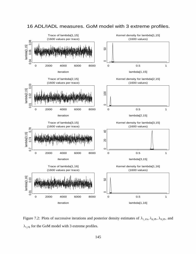
iteration

lam

bda[

1,15

]

0 2000 4000 6000 8000

0.04

0.06

0.08

Trace of lambda[1,15]


lambda[1,15]

0 0.5 1

0 5

0

Kernel density for lambda[1,15]

(1600 values)

•••••••••••••••••••••••••••••••••••••••••••••••••••••••••••••••••••••••••••••••••••••••••••••••••••••••••••••••••••••••••••••••••••••••••••••••••••••••••••••••••••••••••••••••••••••••••••••••••••••••••••••••••••••••••••••••••••••••••••••••••••••••••••••••••••••••••••••••••••••••••••••••••••••••••••••••••••••••••••••••••••••••••••••••••••••••••••••••••••••••••••••••••••••••••••••••••••••••••••••••••••••••••••••••••••••••••••••••••••••••••••••••••••••••••••••••••••••••••••••••••••••••••••••••••••••••••••••••••••••••••••••••••••••••••••••••••••••••••••••••••••••••••••••••••••••••••••••••••••••••••••••••••••••••••••••••••••••••••••••••••••••••••••••••••••••••••••••••••••••••••••••••••••••••••••••••••••••••••••••••••••••••••••••••••••••••••••••••••••••••••••••••••••••••••••••••••••••••••••••••••••••••••••••••••••••••••••••••••••••••••••••••••••••••••••••••••••••••••••••••••••••••••••••••••••••••••••••••••••••••••••••••••••••••••••••••••••••••••••••••••••••••••••••••••••••••••••••••••••••••••••••••••••••••••••••••••••••••••••••••••••••••••••••••••••••••••••••••••••••••••••••••••••••••••••••••••••••••••••••••••••••••••••••••••••••••••••••••••••••••••••••••••••••••••••••••••••••••••••••••••••••••••••••••••••••••••••••••••••••••••••••••••••••••••••••••••••••••••••••••••••••••••••••••••••••••••••••••••••••••••••••••••••••••••••••••••••••••••••••••••••••••••••••••••••••••••••••••••••••••••••••••••••••••••••••••••••••••••••••••••••••••••••••••••••••••••

iteration

lam

bda[

2,15

]

0 2000 4000 6000 8000

0.01

0.02

0.03



lambda[2,15]

0 0.5 1

010

0


(1600 values)

••••••••••••••••••••••••••••••••••••••••••••••••••••••••••••••••••••••••••••••••••••••••••••••••••••••••••••••••••••••••••••••••••••••••••••••••••••••••••••••••••••••••••••••••••••••••••••••••••••••••••••••••••••••••••••••••••••••••••••••••••••••••••••••••••••••••••••••••••••••••••••••••••••••••••••••••••••••••••••••••••••••••••••••••••••••••••••••••••••••••••••••••••••••••••••••••••••••••••••••••••••••••••••••••••••••••••••••••••••••••••••••••••••••••••••••••••••••••••••••••••••••••••••••••••••••••••••••••••••••••••••••••••••••••••••••••••••••••••••••••••••••••••••••••••••••••••••••••••••••••••••••••••••••••••••••••••••••••••••••••••••••••••••••••••••••••••••••••••••••••••••••••••••••••••••••••••••••••••••••••••••••••••••••••••••••••••••••••••••••••••••••••••••••••••••••••••••••••••••••••••••••••••••••••••••••••••••••••••••••••••••••••••••••••••••••••••••••••••••••••••••••••••••••••••••••••••••••••••••••••••••••••••••••••••••••••••••••••••••••••••••••••••••••••••••••••••••••••••••••••••••••••••••••••••••••••••••••••••••••••••••••••••••••••••••••••••••••••••••••••••••••••••••••••••••••••••••••••••••••••••••••••••••••••••••••••••••••••••••••••••••••••••••••••••••••••••••••••••••••••••••••••••••••••••••••••••••••••••••••••••••••••••••••••••••••••••••••••••••••••••••••••••••••••••••

iteration

lam

bda[

3,15

]

0 2000 4000 6000 8000

0.7

0.74

0.78



lambda[3,15]

0 0.5 1

020

40


(1600 values)

••••••••••••••••••••• •••••• •••••••••••••••••••• •••••••••• ••••••••••••••••••••••••••••••••••••••••••••••••••• ••••• ••••••••••••• ••••••••••••••••••••••••••••••••••••••••••••••••••••••••••••••• ••••••••••• •• •••••••••••••••••••••••••••• ••••••• •••••••••••• •••••••••••••••••••••••••••••••••••••••••••••••••••••••••••••• ••••••••••••••••••••••••••••••••••••••• ••••••• ••••••••••••• ••••••••••••••••••••••• ••••••••• ••••••••••••••••• ••••••••••••••••••••••••••••• ••••••••• •••••••••••••••••••••••• •••••••••••• •• ••••••••••••••••• •••••••••• ••••••• •••••••••••••••••••••••• •••••••••••••••••••••••••••••••••••••••• •••• •• ••••••••••••••••••••• ••••••••••••••••••••••••••••••••••••••••••• ••••••••••••••••••••••• ••••••• ••••••••••••••••••••••••••••• •••••••••••••••••• •••••••••••••••••••••••• ••••••••••••••••••••• ••••••••••••••••••••••••••• •••••••••••••••••••••••• •••••••••••••• •••••••••••••• ••••••••••••••••••••••••••••••••••••••••••••••••••••••••••••••••••• •••• •••••••••• ••••••••••••••••••••••••• •••••••••••••••••••••• •••••••••••••••••••••••••••••••••••••••••••••••••••••••••••••••• •••••• ••••••••••••••••• ••••••••••••••• •••••• •••••••••••••••••••••••••••••••••••• ••••••••••••••••••••••••••••• ••••••••••••• •••••••••••••••••••••••••• ••••••••••••••••••••••••••••••••••••••• •••••••••••••• •••••••••••••••••••• •••• ••••••••• •••••••••••••• •••••••••••••••••••••••••• •••••••••••••••••••••••••••••• ••••••••••••••••••••••••••••••• •••••••••••••••••••••••••• •••••••••••••••••••••• •••••••••••• •••••••••••••••••••••••••••••••••• ••• ••••••••••••••••••••••••••••••••••••••

iteration

lam

bda[

1,16

]

0 2000 4000 6000 8000

0.01

0.03



lambda[1,16]

0 0.5 1

0 5

0


(1600 values)

•••••••••••••••••••••••••••••••••••••••••••••••••••••••••••••••••••••••••••••••••••••••••••••••••••••••••••••••••••••••••••••••••••••••••••••••••••••••••••••••••••••••••••••••••••••••••••••••••••••••••••••••••••••••••••••••••••••••••••••••••••••••••••••••••••••••••••••••••••••••••••••••••••••••••••••••••••••••••••••••••••••••••••••••••••••••••••••••••••••••••••••••••••••••••••••••••••••••••••••••••••••••••••••••••••••••••••••••••••••••••••••••••••••••••••••••••••••••••••••••••••••••••••••••••••••••••••••••••••••••••••••••••••••••••••••••••••••••••••••••••••••••••••••••••••••••••••••••••••••••••••••••••••••••••••••••••••••••••••••••••••••••••••••••••••••••••••••••••••••••••••••••••••••••••••••••••••••••••••••••••••••••••••••••••••••••••••••••••••••••••••••••••••••••••••••••••••••••••••••••••••••••••••••••••••••••••••••••••••••••••••••••••••••••••••••••••••••••••••••••••••••••••••••••••••••••••••••••••••••••••••••••••••••••••••••••••••••••••••••••••••••••••••••••••••••••••••••••••••••••••••••••••••••••••••••••••••••••••••••••••••••••••••••••••••••••••••••••••••••••••••••••••••••••••••••••••••••••••••••••••••••••••••••••••••••••••••••••••••••••••••••••••••••••••••••••••••••••••••••••••••••••••••••••••••••••••••••••••••••••••••••••••••••••••••••••••••••••••••••••••••••••••••••••••••••••••••••••••••••••••••••••••••••••••••••••••••••••••••••••••••••••••••••••••••••••••••••••••••••••


Figure 7.2: Plots of successive iterations and posterior density estimates of * ��:;� <.! * ��:;� <2! *=� :;� <.! and* ��:;� > for the GoM model with 3 extreme profiles.

145


profile l��E� profile l��,� profile lí�+�* n :;� 0.000 (2e-04) 0.000 (2e-04) 0.452 (9e-03)* n : � 0.220 (7e-03) 0.000 (2e-04) 0.865 (8e-03)* n : � 0.537 (1e-02) 0.001 (9e-04) 0.941 (6e-03)* n : ? 0.035 (4e-03) 0.002 (1e-03) 0.825 (9e-03)* n : < 0.499 (9e-03) 0.063 (4e-03) 0.996 (3e-03)* n : > 0.176 (7e-03) 0.001 (8e-04) 0.789 (9e-03)* n : @ 0.911 (6e-03) 0.286 (7e-03) 1.000 (3e-04)* n : ± 0.018 (4e-03) 0.000 (2e-04) 0.900 (8e-03)* n : ² 0.307 (9e-03) 0.001 (5e-04) 0.999 (8e-04)* n :;� 0.057 (6e-03) 0.000 (2e-04) 0.983 (5e-03)* n :;�� 0.684 (9e-03) 0.009 (4e-03) 0.999 (7e-04)* n :;� � 0.858 (9e-03) 0.093 (5e-03) 0.949 (5e-03)* n :;� � 0.730 (9e-03) 0.057 (5e-03) 0.914 (5e-03)* n :;� ? 0.142 (6e-03) 0.006 (2e-03) 0.720 (8e-03)* n :;� < 0.061 (5e-03) 0.018 (2e-03) 0.742 (8e-03)* n :;� > 0.024 (4e-03) 0.018 (2e-03) 0.529 (9e-03)8 n 0.287 (3e-02) 0.345 (3e-02) 0.368 (3e-02)� 0.301 (8e-03)





146

the log-likelihood samples.

Figure 7.3 provides plots of successive iterations and posterior density estimates for the hy-

perparameters � !�8h�(!�8.�.! and 8 � (we omit 8 ? since 8 n add up to 1). Of the hyperparameters, only� has a significant Geweke statistic, which indicates lack of convergence. The plot of successive

iterations of � in Figure 7.3 shows slow mixing but looks fine otherwise. Figure 7.4 presents

successive iteration plots and posterior density estimates for the conditional response probabilities* ��:;� � ! * ��:;� � ! *]� :;� � ! and *=? :;� � of IADL item traveling. All parameters but *y? :;� � have favorable con-

vergence diagnostics. Visual inspection of the plots, however, does not provide a clear separation

among the parameters.

Comparing the results from this chain to results from another chain of 90,000 samples (with

additional burn-in of 10,000 samples, 4-�f�I� , / ��F� , �-�f�I� ), we found that the estimates

differ at most by �2� â � for both parameter sets, the conditional response probabilities } and the

hyperparameters, and 8 .

Table 7.3 provides posterior mean and standard deviation estimates for the parameters of the

GoM model with four extreme profiles. Again, we find that the extreme profiles are not that differ-

ent qualitatively from the latent classes in Table 6.18. We have ‘healthy’, ‘ADL-disabled’, ‘IADL-

disabled’, and ‘disabled’ profiles. The profiles are well separated in the multivariate parameter

space, for example, by the conditional response probabilities of items 5 and 13 (see Figure 7.4 for

an illustration). The estimates of the relative Dirichlet proportions, however, are in disagreement

with the latent class probability estimates. The estimate of � is now 0.197.

Table 7.5 provides the DIC value for the four profile GoM model, and Table 7.6 contains the

expected counts for the frequent response patterns. There is an improvement in fit, comparing to

the results from the GoM model with J �æ� , as indicated by decreased DIC value. However,

the expected counts for the frequent response patterns suggest the opposite; the fit for the frequent

response patterns actually becomes worse with J �� . This observation is in contrast to our

expectation that the GoM model fit for the frequent response patterns should improve every time

147

iteration

alph

a0

0 2000 4000 6000

0.16

0.2

Trace of alpha0


alpha0

0 0.5 1

0 5

0


(1200 values)

•••••••••••••••••••••••••••••••••••••••••••••••••••••••••••••••••••••••••••••••••••••••••••••••••••••••••••••••••••••••••••••••••••••••••••••••••••••••••••••••••••••••••••••••••••••••••••••••••••••••••••••••••••••••••••••••••••••••••••••••••••••••••••••••••••••••••••••••••••••••••••••••••••••••••••••••••••••••••••••••••••••••••••••••••••••••••••••••••••••••••••••••••••••••••••••••••••••••••••••••••••••••••••••••••••••••••••••••••••••••••••••••••••••••••••••••••••••••••••••••••••••••••••••••••••••••••••••••••••••••••••••••••••••••••••••••••••••••••••••••••••••••••••••••••••••••••••••••••••••••••••••••••••••••••••••••••••••••••••••••••••••••••••••••••••••••••••••••••••••••••••••••••••••••••••••••••••••••••••••••••••••••••••••••••••••••••••••••••••••••••••••••••••••••••••••••••••••••••••••••••••••••••••••••••••••••••••••••••••••••••••••••••••••••••••••••••••••••••••••••••••••••••••••••••••••••••••••••••••••••••••••••••••••••••••••••••••••••••••••••••••••••••••••••••••••••••••••••••••

iteration

ksi1

0 2000 4000 6000

0.1

0.2

0.3

0.4

Trace of ksi1


ksi1

0 0.5 1

010


(1200 values)

• ••• ••••••••••••• ••••• • ••••• •••••• •• •••• •••••• ••• ••• ••••• •••• ••••• • •••••• •••••••• •••• •• •• ••••• •••• •• •• ••••• • ••••••• •••• •• ••••• • •••••••• • ••••••••••••••••••• •••• •• •• •••• •• ••• •• •••• ••• •• ••••• ••• ••• •• •••• ••• ••••• • •• • ••• ••• •• ••••• • •••• •• •••• ••••• ••• •• •• •••••• ••••••••• •••• •• •••••••••• •••• ••••• ••• ••••• ••• ••• •• •• • •• ••• • •••• •• •• ••••••• •• ••• •••••• •• ••••• •• •••• •• ••• •• ••• • ••• • ••• ••••• •••••• •••••••• • •• ••••••• • •••• •• • •••• ••• ••••• ••• ••••• •• •• ••• • ••• •••• ••••••• ••• ••• •• • ••• ••••••••• ••• ••• •• •••• •••• •• ••• •• ••••• • •••• ••• ••• • •• •••••• •••••••• ••• ••• •••• •••••• •••••• •••• ••• ••••••• •• ••• •••••• •• ••• •• ••• •• ••• ••• •••••• ••••• ••• •••••• ••••• •••• •• •••• ••• ••••• ••• •• •• •• •• ••• •••••• •• ••••••••••••• •• ••••••• •• • ••••• • •••••• ••• •• ••• •••••• •••• ••• •• ••• •••••••• •••• •••••• ••••••• •• •••• ••• •• •••••• ••• •••• •••• •••• •••••••• •• •• •• ••••• ••••••••••••••• • •••• •••• •• •••• •••• • ••• •••••• ••• •••• •• •• ••••• ••••• ••• ••• •••• •••• •••• • ••••••••• •••• • ••••••• • ••••• •• •• •• •••••••• ••••• •••• •••••••••• • •••••• •••• ••• ••• •••••• ••••• •••• • •••••• ••••• •••• •••• ••• ••• ••• ••• •• •••••••• • •• ••• ••••• ••••••• •••• ••••• ••• ••• ••• ••• ••••• •• ••••••••• •••••••• ••••••• •••• •••• •• ••• •• ••• ••• • •••• ••••• •••••••••••••• •• •• ••••• •• •• •••• •••••• ••• •••••••••• • •••• •••• •• •

iteration

ksi2

0 2000 4000 6000

0.1

0.2

0.3

0.4

Trace of ksi2


ksi2

0 0.5 1

010


(1200 values)

••• •• •••••••••• •••• •• ••••••••• •• •• •••• •••• ••• •• •• •• •• •• •• ••••• •••• •••••••••• ••• •••• •• •• ••• • •• ••••• •• •••• • ••••• •••• •••• •••••• ••• ••• • •• •• •• ••• •• ••• ••• ••• ••••• ••••• •••• • •••• •• •• •••• ••••••• ••••• ••• ••• •• •••••••••• •••• •• ••• ••• •••• •••• • ••••• ••••• ••• • •• ••••• •• • •••• • •••• •••• ••••••• ••• •• ••••• ••• ••• ••••• ••••••••• •• •••• • •• ••• •• • •• ••••• ••••• ••• • •••• ••• ••• • •• •• •• ••••• •••• • •••••• •••••• •••• ••••• • ••• ••••• ••• •••• ••••• •• •• •••••• ••• •• ••• ••••• •• •• ••• ••••• •• •••• ••• ••• ••••• •••• •••••••••••••• •••••• ••••• •••• • ••••••• •••• •• •• ••• •••••• • •••••• •• •• ••• •••• •• •• •••• •• •• •••• • •• •• •• •• •• ••••• • ••• • •••• ••• •••• •• •• •••••• •••• ••• •• ••• • •••••••• ••••• •• ••• ••• •• • •••••••••• ••• ••• ••• •••• ••• ••••••• • •••••• ••• ••• •• •• •• •• •••••••• ••• •••••••• ••••••••••• •• •• •••• •• • ••• ••••• ••• •• ••••••••••• •• •••• ••••• • •••••• ••• •• • ••••• •••• ••• • ••• •••• •••• ••• • •••••• •••••••••• •••••••••• •• •• •• • ••• • ••••• • •• •• ••• •••• •• ••• •• ••• •••• •••• ••••••• • ••• ••• •••••• ••••••• ••• •• •• •• • •••• •••• ••• ••• •• •• •••••••• •••• ••••••• ••••• ••••• ••• ••• •••••• ••••• •• •••• ••••• •• •• •• ••• •• •••••• •••••• •• ••• • ••• •••• ••• •• •• •• • ••• ••••• ••• •••• ••• • •••• •••••• •• •• •••••• •••••• •• •• •••• ••••• •• ••• ••••• ••• •••• •••• • ••• •• ••• •••• ••• •••• • •• • •• ••• ••• •••••• ••••• •• ••••• •• •••••• •••••• •••• •• ••

iteration

ksi3

0 2000 4000 6000

0.1

0.2

0.3

0.4

Trace of ksi3


ksi3

0 0.5 1

0 5

10


(1200 values)

•• •• ••••••• ••••• •• •• ••••• • •••••••••••••• •• • ••••• •••••••• •••• ••••• ••• ••••• •• •••• •••• •• ••• ••• •• •• •• ••• •••• •• ••• ••• •••• •• •••• ••••• ••••• •• •• •• ••• ••• •• •• •••••••••••••••••••• •••••• ••• •• •••• ••• ••••• •• ••• ••••• •••••• ••• •• ••• •••• •••• ••• ••••• •••• • ••• •• • ••••••• •• ••• •• ••• •••• ••• •••• •• •• •• •• •••••••• •• •• ••••••••• ••••• • •• ••• •• • ••••• •••• • •••• •• •• ••••• ••• •••• •••••• •••• •••••• • • ••••• •• •• •• •• •• ••••• •••• •••• •• • ••••• • ••• ••• •• ••••• •••••• •••• ••• • •••• •• •• •••• •• •••••••• •• • •• ••••• • •• ••••••• •• • ••• •• ••• ••• • ••••••• •• •••• •••• •• •• •••••••••• ••• ••••• ••••• ••• ••• ••• ••• •• ••• •• •• •• •• •••• •• ••••• •••••• ••• ••• •• ••••••••••• • ••• •• •• •••••• •••• •• •••••••• ••••• •• ••••• •• •••••• ••• •• ••• •• •• ••••• •• ••• • •••• • •••• ••• ••••••••• ••• ••• ••••••• •• •• •••• ••• •• ••••• •••• ••••••• •• •• •• ••• •••• ••• • •••••• ••••• •• •• •••• •••• • •• •• •••• ••• ••••• ••• ••••• •••• ••• •• ••• •• ••• • ••• •••• •• ••• ••••• • •••• ••••• ••• •••• •• •••• ••• •••• •• ••••• ••• ••••• •••• •••• •••• ••• • ••• ••• •••• ••••• ••••• •• •• •••••• •• •••• • ••• •• ••• •• •• • •• ••••• •• •• •••• ••••••• •••• ••• •••• •• •••• •••• ••••• ••••• ••• •• •• •• •••• •• •• ••• ••• ••• •••• • •• •• •• •••••• •••• ••• •••• •• ••• ••• ••••••• ••• •• ••• ••• ••• • ••••• • •••• •••• •• •• •••• •• •••••• •••••• •• •• ••••••• •••••••• •••••• •• •• ••• • ••••• ••• •• •••• •••••• •••••• ••••• ••••• •


Figure 7.3: Plots of successive iterations and posterior density estimates of the hyperparameters� !�8h�(!�8.�.! and 8 � for the GoM model with 4 extreme profiles.

148

iteration

lam

bda[

1,13

]

0 2000 4000 6000

0

0.02

0.04



lambda[1,13]

0 0.5 1

0 5

0


(1200 values)

••••••••••••••••••••••••••••••••••••••••••••••••••••••••••••••••••••••••••••••••••••••••••••••••••••••••••••••••••••••••••••••••••••••••••••••••••••••••••••••••••••••••••••••••••••••••••••••••••••••••••••••••••••••••••••••••••••••••••••••••••••••••••••••••••••••••••••••••••••••••••••••••••••••••••••••••••••••••••••••••••••••••••••••••••••••••••••••••••••••••••••••••••••••••••••••••••••••••••••••••••••••••••••••••••••••••••••••••••••••••••••••••••••••••••••••••••••••••••••••••••••••••••••••••••••••••••••••••••••••••••••••••••••••••••••••••••••••••••••••••••••••••••••••••••••••••••••••••••••••••••••••••••••••••••••••••••••••••••••••••••••••••••••••••••••••••••••••••••••••••••••••••••••••••••••••••••••••••••••••••••••••••••••••••••••••••••••••••••••••••••••••••••••••••••••••••••••••••••••••••••••••••••••••••••••••••••••••••••••••••••••••••••••••••••••••••••••••••••••••••••••••••••••••••••••••••••••••••••••••••••••••••••••••••••••••••••••••••••••••••••••••••••••••••••••••••••••••••••••••••••••••••••••••••••••••••••••••••••••••••••••••••••••••••••••••••••••••••

iteration

lam

bda[

2,13

]

0 2000 4000 6000

0.54

0.58

0.62



lambda[2,13]

0 0.5 1

020


(1200 values)

•••••••••• •••••• ••••••••••••••••••••••••••••••••••••••••• ••••••••••••••••••••••••••••• ••••••••••••••••••••••• •••••••••••••••• •••••••••••••••••• ••••• ••• •••• • •• ••••••••••••••• •••••••• •••••••••••••• •••••••••••••••••• ••••••••••• •••••••••••••• •••••••••••••••••••••••••••••• •••••••••••••••••••••••••••• •••••••••••• •••• •••••••••••••• ••••• •• ••••••••••••••••••••••••• •••••••••••••• ••••••••••••••••••• •••••••••••••• ••••••••••••• ••••••• ••••••••••••• •••••••• •••••• •••••••••••••••••••••••••••• ••••••••••••• ••••••••••••• •••••••• •••••••••••••• ••••••••• •••••• •••••••• ••••••••••••••••••••••••• •••••••••• ••••••••••••••••• •• •••••••••••••••••••••••• •••• ••••••••••••••••••••••• •••• •••••••• •••••••••••••••••••••••••••••••••••• •••• ••••• •••• ••••••••••••• ••••••••••••••••••••• •••••••• •••••••••••••••••• ••••••••••••••• ••••••• ••••••• ••••••••• ••••••• ••••••• ••• ••••••••••••••••••••••••••••••••••••••••••• •••••••••••••••••••••• •••• ••••••••••••• •• •• ••••••••••••••••••••••••••••• ••••••••••••••••••••••••••••••••••• •• •••• ••••• ••••••••••• •••••••••••••••••••••••••••••••••• ••••••• ••••••••• •••••••••••••••••••••• ••••••••••••••••••••••••• ••••• •••••••••••••••••••••••••••• ••••••• ••••••••• •••••

iteration

lam

bda[

3,13

]

0 2000 4000 6000

0.7

0.75

0.8



lambda[3,13]

0 0.5 1

020


(1200 values)

••••••••••••••••••••••••••••••••••••••••• •••••••••••••• •••••••••••• •••• •••••••••••••••••••• •••••• ••••••••••••••••••••••• • •• •••••••••••••••••••••••• •••••••••••••••• ••••• •••••••••• •••••••• ••••••••• •••••••••••••••••••••••••••••••••••••••••••••••••••••••••••••••••••• •••••• ••••••••••••••••••• ••••• ••••••••••••••••••••••••••••••••••••• ••••••••• ••••••••••••••••••••••••••••••••••••••• • •••••••••••••• ••••••••••••••••••••••••• •••••••••••••••••••••••••••••••••• ••••••••••• ••••••••••••••••••• ••••••••••• ••••••• •••••• ••••••••••••••••••••••••••••• ••••••••• ••••••••••••••••••••••••••• •••• ••••••••• •••••••••• ••••••••••••••••••••••••••••••••• ••••••••••• ••••••• •••••••••••• •• ••••••••• ••••••••••••••••• •••••••••• ••••••••• •••••••••••••••••••••••••••• •••••••••••••• •••••••••••••••••••••••••••• ••••••••• ••••••••••••••••••••••••• ••••••• •••••••••••••••• •••• ••••••• •••••••••• •••••••••••••••••••• ••••••• ••••••••• ••• ••••••••• •••• •••••••••••••••••••••••••••••••••• ••••••••••••••••••• •••••••••••••• ••••••••••••••••••• ••••••••••••••••••••••••••••••••••••••• •••••• •••••• ••••••••• ••••• ••••••••••••••••• •••••••••••••••••••••••••••••••••••••••••••• ••••••••••• •••

iteration

lam

bda[

4,13

]

0 2000 4000 6000

0.88

0.92



lambda[4,13]

0 0.5 1

0 5

0


(1200 values)

•••••••••••••••••••••••••••••••••••••••••••••••••••••••••••••••••••••••••••••••••••••••••••••••••••• ••••••••••••••••••••••••••••••••••••••••••••••••••••••••••••••••••••••••••••••••••••••••••••••••••••••••••••••••••••••••••••••••••••••••••••••••••••••••••••••••••••••••••••••••••••••••••••••••••••••••••••••••••••••••••••••••••••••••••••••••••••••••••••••••••••••••••••••••••••••••••••••••••••••••••••••••••••••••••••••••••••••••••••• ••••••••••••••••••••••••••••••••••••••••••••••••••••••••••••••••••••••••••••••••••••••••••••••••••••••••••••••••••••••••••••••••••••• ••••••••••••••••••••••••••••••••••••••••••••••••••••••••••••••••• •••••••••••••••••••••••••••••••••••••••••••••••••••••••••••••••••••••••••••••••••••••••••••••••••••••••••••••••••••••••••••••••••••••••••••••••••••• ••••••••••••••••••••••••••••••••••••••••••••••••••••••••••••••••••••••••••••••••••••••• •••••••••••••••••••••••••••••••••••••••••••••••••••••••• ••••••••••••••••••••••••••••••••••••••••••••••••••••••••••••••••••••••••••••••••••••••••••••••••••••••••••••••••••••••••••••••••••••••••••••••••••••••••••••••••••••••••••••••••••••••••••••••••


Figure 7.4: Plots of successive iterations and posterior density estimates of * ��:;� � ! * ��:;� � ! *=� :;� � ! and*B? :;� � for the GoM model with 4 extreme profiles.

149


profile l��E� profile l��,� profile l��+� profile lí�\�* n :;� 0.000 (3e-04) 0.002 (2e-03) 0.001 (6e-04) 0.517 (1e-02)* n : � 0.000 (3e-04) 0.413 (1e-02) 0.001 (5e-04) 0.909 (7e-03)* n : � 0.001 (5e-04) 0.884 (1e-02) 0.018 (8e-03) 0.969 (5e-03)* n : ? 0.007 (2e-03) 0.101 (6e-03) 0.016 (4e-03) 0.866 (8e-03)* n : < 0.064 (4e-03) 0.605 (9e-03) 0.304 (9e-03) 0.998 (2e-03)* n : > 0.005 (2e-03) 0.316 (9e-03) 0.018 (4e-03) 0.828 (8e-03)* n : @ 0.230 (7e-03) 0.846 (7e-03) 0.871 (7e-03) 1.000 (3e-04)* n : ± 0.000 (2e-04) 0.024 (4e-03) 0.099 (7e-03) 0.924 (7e-03)* n : ² 0.000 (3e-04) 0.253 (9e-03) 0.388 (1e-02) 0.999 (1e-03)* n :;� 0.000 (2e-04) 0.029 (5e-03) 0.208 (1e-02) 0.987 (4e-03)* n :;�� 0.000 (3e-04) 0.523 (1e-02) 0.726 (1e-02) 0.998 (2e-03)* n :;� � 0.085 (5e-03) 0.997 (2e-03) 0.458 (1e-02) 0.950 (4e-03)* n :;� � 0.021 (4e-03) 0.585 (1e-02) 0.748 (1e-02) 0.902 (5e-03)* n :;� ? 0.001 (7e-04) 0.050 (5e-03) 0.308 (1e-02) 0.713 (8e-03)* n :;� < 0.013 (2e-03) 0.039 (4e-03) 0.185 (8e-03) 0.750 (8e-03)* n :;� > 0.014 (2e-03) 0.005 (2e-03) 0.134 (7e-03) 0.530 (9e-03)8 n 0.216 (2e-02) 0.247 (2e-02) 0.265 (2e-02) 0.272 (2e-02)� 0.197 (5e-03)





150

an additional extreme profile is added to the model. Thus, the improvement in overall fit, as

indicated by the DIC value, comes from the cells with less frequent response patterns. Recall that

approximately 58% of the observations come from the less frequent response patterns.

Five extreme profiles. As before, we use the conditional response probabilities from the latent

class model as the starting values for } . We set the starting value for � to be 0.2, and set 1/5 to be

the starting value for each 8 n , l½�H� ! �.�.� ! � .A chain of 150,000 iterations (without the burn-in of 30,000) with thinning parameter 4ª�³�F� ,

and tuning parameters / �»�2�F� and �)�1�I� showed weak convergence. Thus, about 15% of the

Geweke diagnostics and about 40% of the Heidelberger and Welch tests for individual parameters

indicated poor convergence. The plots of successive iterations did not reveal substantial problems,

however, except for the slow mixing of the chain. At the same time, the (joint) log-likelihood

values for a similar MCMC chain with the burn-in of 40,000 and thinning of 4Ó��z� showed

favorable convergence diagnostics. The posterior means from these two runs are very similar.

Figures 7.5 and 7.6 show plots of successive iterations and density estimates for the hyperpa-

rameters � and 8 n , l½�E� ! �.�.� ! � . Note that all hyperparameters but � had favorable convergence

diagnostics. Figures 7.6 and 7.7 contain plots of successive iterations and density estimates for

selected conditional response probabilities, * n : @ , lN�E� ! �.�.� ! J for IADL item (doing heavy house

work). All parameters * n : @ , lN�a� ! �"�.� ! J but * ��: @ had favorable convergence tests. The estimated

posterior density for * <�: @ in Figure 7.7 is indicated by a point mass at * <�: @ �� because the posterior

distribution is highly concentrated near that point. For comparison, in Figure 7.7, we provide the

additional plot of the conditional response probability * <�:;� � , which had the worst Geweke diagnos-

tic out of all other conditional response probabilities. Examining the plots visually, it is not clear

which of the chains have better behavior than others. It is clear, however, that there is a mixing

problem and that more samples should be obtained for the GoM model with J��\� .We report in Table 7.4 the posterior means for the GoM model parameters from the run with

151

iteration

alph

a0

0 1000 2000 3000 4000

0.1

0.12

0.14

Trace of alpha0


alpha0

0 0.5 1

0 5

0


(800 values)

•••••••••••••••••••••••••••••••••••••••••••••••••••••••••••••••••••••••••••••••••••••••••••••••••••••••••••••••••••••••••••••••••••••••••••••••••••••••••••••••••••••••••••••••••••••••••••••••••••••••••••••••••••••••••••••••••••••••••••••••••••••••••••••••••••••••••••••••••••••••••••••••••••••••••••••••••••••••••••••••••••••••••••••••••••••••••••••••••••••••••••••••••••••••••••••••••••••••••••••••••••••••••••••••••••••••••••••••••••••••••••••••••••••••••••••••••••••••••••••••••••••••••••••••••••••••••••••••••••••••••••••••••••••••••••••••••••••••••••••••••••••••••

iteration

ksi1

0 1000 2000 3000 4000

0.1

0.2

Trace of ksi1


ksi1

0 0.5 1

010

20


(800 values)

•••• ••••••• •••••••••••••••••• ••••••• ••• •• ••• ••••••• •• •••• ••• • •• •• ••••••••• •• •••••••• •• ••• •••• •••••••• • ••• ••• ••••••• • ••• •• ••••••••••••••••••• • •••••••••• ••••••••••••• ••• •• •••• •••••••• •• •••• ••••• •• •••••• •• •• •••••• ••••••• •• •••• ••••• ••••••• •••• •• • ••• ••• ••••• •••••• •••••• ••• ••••• •••••• •• •••••• •••••••••• ••• ••••• ••• ••••••• •• ••• ••••• •• ••••• •••• •••• •• ••••• •• ••• •••••• ••••• •••••• •••• ••• ••• •• ••• • •• •••••••••• ••• ••••••••• •••••••••••••• •• ••••••••• ••••• •• •••••••• ••••• ••• ••••• •••• •• ••••• • ••• ••• •• ••• •• •••• •••••• •••••• ••• •••••••• •• • •• •••••• •••• ••••••••••••• •••• ••• • ••••• •••••• ••• • ••••••• •• •••• ••• ••• ••• •••••••••••••••• ••••••• ••• ••••••• ••• •• •••• ••• ••• ••••••• ••• ••••••••• •••• •••• •••• ••••••• ••••• ••• •• •• ••••• ••••••••• •• • ••••••• •• ••• •••••••• • •••• •• ••• •• ••••• ••••••• ••• •••• •••••••••••• ••••••• ••••• ••• ••

iteration

ksi2

0 1000 2000 3000 4000

0.1

0.2

0.3

Trace of ksi2


ksi2

0 0.5 1

010


(800 values)

••• ••• •••• •• •• ••• •• • •• •• •••••• •••••• ••• •••••••••••••• •••••• ••• • •• •• ••• ••• ••••• •• •••••• •• •• •••••••••• •••••••• •• • ••••• ••••• • •• ••• ••• •••••• •• ••••••••••• ••••••• ••• •• ••• ••••••• •••••• ••• ••••• ••• ••• ••••••• •• •••••• •• •••• •••• ••••• ••••• • ••• •• •• ••• •••• •• •• ••• ••• •• ••••• •••• ••••• ••• •••• ••• ••••••• •• ••••••• • ••••• • •••• ••••• •••• ••• ••• ••• •••• •• •• •••• •• ••••• ••••• • •••• •••••••• •• •••• •••••• •••••••••• ••• ••••••• •• •••••••• •••• •••••••• •• •• ••• •••• •• •••••• •••••••• ••• •••••• ••••• •• ••••••••••• •••••••• ••• •• •• ••••• • •••• •• ••• •••••• •••• •••••••• ••••• •• ••••• ••• •• • •• ••••• •• ••• •• •••••••• •••• • •••••• ••• •• ••••• • •• •• •• •• ••• •••• •••••• •••• ••• ••• •• ••• •••••• •• • •• ••• •• ••• •• •• ••••••• •••• •• ••• •••• •••• •••• •• •• ••••••• •••••• ••• ••••• ••• ••••••• •• •••••••• •• ••• •• •••• •• •••• ••••• ••••• • •••••• •• •• •••••••••• ••• • ••• •• •••• •••• •••• •••• ••••

iteration

ksi3

0 1000 2000 3000 4000

0.1

0.2

0.3

Trace of ksi3


ksi3

0 0.5 1

010


(800 values)

• • ••••••• •••• •••••••••• •••• •••• ••• ••• ••• •• •••••••• ••• •••• ••••• •• •• • •••••• •• •• •••••••• ••• •••• ••••••••••••• •• •••• • •••••• • ••• ••• •••• •• •• ••••••• •• ••••••• ••••• ••• •••••••••• ••• ••• ••• ••• • ••• • •••• •• • •••• •• •• •• •• ••• ••• •••• ••••• •• •• ••• ••• •••• ••• •••••• •••• ••• •••••• • ••••••••••• •• •••• •••••• •••• ••••••••• •• • •••• •• ••• •• •• ••• ••• ••• ••• ••••• •• •• •••••• • ••• ••• •••• ••••••••••••• •••• •• •• ••• ••• •• ••••••• •• ••••••• •••• •••••••••••••• ••••• ••••••• •• ••• ••• • ••••••••••••• •• •••• •••• •••••• •••• •••••••••• ••••••••••• •• •••• ••• •• •• ••••• •• •• ••• •• ••• •• ••••• ••••• • •• • •••• • •••• •• •••••• •••• ••••••• • ••• • ••• •• •••••••••• • •••••••• • •• ••••• •• •• •• •••••••• •• • •• ••• ••• ••••• • ••• ••• ••• ••••••• •••••••••• ••••• ••••••••••• • •••• •• ••• ••• •• • •••••• •••• •••••••• ••••••• •• •••• •••••••• •••• •• •• ••• ••• •••••• •••••• •• •••• •••••••• ••• •••• •••••••• ••• •• •


Figure 7.5: Plots of successive iterations and posterior density estimates for the hyperparameters� !�8h�(!�8.�.!c8 � for the GoM model with 5 extreme profiles.

152

iteration

ksi4

0 1000 2000 3000 4000

0.1

0.2

0.3

Trace of ksi4


ksi4

0 0.5 1

010


(800 values)

• •••• ••• •••••••••• ••• ••••• ••••• • ••••• •••• •• •••• ••••••••• •••••• • •••• •• •• ••••••• •••• ••• ••• ••• •• ••• •• •••• • ••• ••• ••• •••••• •••• ••• •• ••• •••••••• ••••• •• ••• •••• ••• • ••• ••••• •• •• ••• ••• •••••• • ••• • •••••• •• ••• •• •• •••••• ••••• •• ••• •• •• ••• ••••• •••• •••• •••• •••••• •••• ••• ••• •••• •• •••••• ••• •••••• ••••••••••••• • ••• ••• • ••• •• •••• • •••••• •• ••• ••• ••• ••• ••••• ••••• ••• •••• •••• ••• •••• •• ••• •• •• •••••••• •••• •••• •• •• •••• ••• •••••• ••• •• •• ••••• ••• ••••••••••• •• •• •• • •• ••••• •••• •••••• ••••• •• • ••••• ••••• ••• •••• ••••••• •••• •••• •• •• • •• •••• • ••••• ••••• ••• •• •• ••• ••• •••• ••••••• •••• •••• ••• ••• •••••• •• •••• •••• ••••• •••• •••• ••••• •• •• •••• ••• •••••• ••••• •••• •• •••••• • ••• •• • •••• •• • ••• •••••••••• ••••• ••••••• • •••• ••• •••••• ••• •••• ••••• ••• •••• •••• •• •• •• •• ••• •••••• ••••••• •••• ••• •••••••••• ••• •••• ••• ••• •••• •• •••• ••• •••• ••• •• •••• •• •••••• •••••••

iteration

ksi5

0 1000 2000 3000 4000

0.1

0.2

0.3

Trace of ksi5


ksi5

0 0.5 1

010


(800 values)

•• •• ••• •••• •• ••• ••••• ••••• ••• ••• ••• •••••• •• ••••• •••• •••• ••••• ••••• •• •••• •••• •••• •• ••• ••••••••• •• ••• ••••••• ••••• ••• •••• ••••• •••••• ••• ••• ••• •• ••• ••• •• •••••••• •••••• •• •••• •• •• •••• •• •••• • ••••• ••• • ••• ••••• •••• •••• •••• ••• •••• •• ••••• ••• •••••• ••• • •••••• ••••••••••••••• •• •• • •••• •••••• •• • ••• ••••• ••••••••••••• •••• ••••• •• •••••• ••• ••• •••• •••• ••••• •••• •• •••• •••• •••• ••••• •••• ••• ••••••••• •••• •••••••• ••••••••• ••••••••• •• ••• ••••••• • ••••• ••••••• •••• ••• •••• ••• •••• • ••• ••• ••• •••••• ••••• ••••• •••••• ••• •• ••• •• •• •••••• •••• • ••••••• •••• •••••• •• •••••••• •••• ••••• •••• ••••• •• •• •• ••••• ••••••• ••••• •• • •• ••••• ••••• ••• •• •••• • •• •••••• • ••• •••• • ••••••• ••••• ••• •• •• ••• ••• ••••• ••• •• • •••••••••••• •••••••• •••• ••• •••••• •• •• ••• •• •• • •• ••• •• •••• •••• •• ••••• ••• ••• •••• ••••••• •• •• ••••• •••• •••••• ••• •• •• •• •• •••••• ••• •••• ••••••••••

iteration

lam

bda[

1,7]

0 1000 2000 3000 4000

0.94

0.98



lambda[1,7]

0 0.5 1

0 5

0


(800 values)

••••••••••••••••••••••••••••••••••••••••••••••••••••••••••••••••••••••••••••••••••••••••••••••••••••••••••••••••••••••••••••••••••••••••••••••••••••••••••••••••••••••••••••••••••••••••••••••••••••••••••••••••••••••••••••••••••••••••••••••••••••••••••••••••••••••••••••••••••••••••••••••••••••••••••••••••••••••••••••••••••••••••••••••••••••••••••••••••••••••••••••••••••••••••••••••••••••••••••••••••••••••••••••••••••••••••••••••••••••••••••••••••••••••••••••••••••••••••••••••••••••••••••••••••••••••••••••••••••••••••••••••••••••••••••••••••••••••••••••••••••••••••••••••••••••••••••••••••••••••••••••••••••••••••••••••••••••••••••••••••••••••••••••••••••••••••••••••••••••••••••••••••••••••••••••••••••••••••

iteration

lam

bda[

2,7]

0 1000 2000 3000 4000

0.86

0.9



lambda[2,7]

0 0.5 1

020

40


(800 values)

••••••••••••••••••••••••••••••••••• ••••••••••••••••• ••••••••••••••••••••••••••••••••••••••••••••••••••••••••••••••••••••••••••••••••••••••••••••• •••••••••••••••••••••••••••••••••••••••••••••• ••••••••••••••••••••• ••••••••••••••••••••••••••••••••••••••••••••••••••••••••••••••••••••••••••••••••••••••• ••••••• ••• ••••••••••••••••••• •••••••••• ••••••••••••• •••••••••• ••••••••••••••••••••••••••••••••••••••••••••••••••••••••••••••••••••••••••••••••••••••••••••••••••••••••••••••••••••••••••••••••••••• •••••••••••••••••••••••••••••••••••••••••••••• ••••••••••••••••••••••••• •••••••••••••••••••••••• ••••••••••••••••••••••••••••••••••••••••••••••••••••••• •••••••••••• •••••••••••••••••••••••••••••••••••••••••••••••••••••••••••••••• •••••••• •••••••••••••••


Figure 7.6: Plots of successive iterations and posterior density estimates for the hyperparameters8 ? !�8.<.! and conditional response probabilities * ��: @ and * ��: @ for the GoM model with 5 extreme

profiles.153

iteration

lam

bda[

3,7]

0 1000 2000 3000 4000

0.55

0.6

0.65



lambda[3,7]

0 0.5 1

020


(800 values)

•••••••• •••••••••••••••• •••••••••••••••••••••••••••••••••••••• ••••• ••••••••••••••••••••••••••••••••••••••••••••••••••••••••• •••••••••••• ••••• ••••••••••••••••••• ••••• ••• •••••••••••••••••••••••••••••••••••••••••••••••• ••••••••••••••••••••••••••• ••••••••••••••••••••• ••••••• •••• ••••••••• ••••••••••••••••••••••••••••••••••••••••••••••••••••••••••••••••• ••••••••• •••••••••••••••••••••••••••••••••• •••••••••••••••• ••••••• ••••• •••••••• ••• ••••••••••••••••••• ••••••••••••••••• ••••••••••••••• ••••••••••••••• •• ••••••••••• ••••••••••••••••••••• •••••••• •••••••••• •• ••••••••••• ••••••• ••••••••••••••••••••••••• ••••••••• ••••••••••••• ••••••••••• •• •••••• •••••••••••••••••••••••••••••••••••••••••••••• •••• ••••••••••••••••••••••• •••••••• ••••••••••••••••• •••••••••••• •••••••••••••••••

iteration

lam

bda[

4,7]

0 1000 2000 3000 4000

0.18

0.22



lambda[4,7]

0 0.5 1

020

40


(800 values)

•• •••••••••••••••••••••••••••••••••••••••••••• ••••••••••••••••••••••••••••••••••••••••••••••••••••••••••••••••••••••••••••••••••••••••••••• ••••••••••••••••••••••••••••••••• ••••••••••••••••••••••••••••••••••••••••••••••••••••••••••••••••••••••••••••••••• •••••••••••••••••••••••••••••••••••••••••• ••••••••••••••••••••••••••••••••••••••••••••••••••• ••••••••••••••••••••••••••••••••••••••••••••••••••••••••••••••••••••••••••• ••••••••••••••••••••••• •••••••••••••••••••••••••••••••••••••••••••••••••••••••••••••••••••••••• •••••••••••••••••••••••••••••••••••••••• ••••••• •••••••••••••••• ••••••••••••••••••••••••••••••••••••••••••••••••••••••••••••••••••••• ••••••••• ••••••••••••••••• •••••••••••••••••••••••••••••••••••••••••••••••• ••••••••••••••••••••••• •••••••••

iteration

lam

bda[

5,7]

0 1000 2000 3000 4000

0.99

70.

999



lambda[5,7]

0 0.5 1

0


(800 values)

•••••••••••••••••••••••••••••••••••••••••••••••••••••••••••••••••••••••••••••

iteration

lam

bda[

5,12

]

0 1000 2000 3000 4000

0.9

0.94



lambda[5,12]

0 0.5 1

0 5

0


(800 values)

•••••••••••••••••••••••••••••••••••••••••••••••• •••••••••••••••••••••••••••••••••••••••••••••••••••••••••••••••••••••••••••••••••••••••••••••••••••••••••••••••••••••••••••••••••••••••••••••••••••••••••••••••••••••••••••••••••••••••••••••••••••••••••••••••••••••••••••••••••••••••••••••••••••••••••••••••••••••••••••••••••••••••••••••••••••••••••••••••••••••••••••••••••••••••••••••••••••••••••••••••••••••••••••••••••••••••••••••••••••••••••••••••••••••••••••••••••••••••••••••••• ••••••••••••••••••••••••••••••••••••••••••••••••••••••••••••••••••••••••••••••••••••••••••••••••••••••••••••••••••••••••••••••••••••••••••••••••••••••••••••••••••••••••••••••••••••••••••••••••••••••••••••••••••••••••••••••••••••••••••••••••••••


Figure 7.7: Plots of successive iterations and posterior density estimates of *d� : @.! *B? : @"! * <�: @ and * <�:;� �for the GoM model with 5 extreme profiles.

154


profile lí�H� profile l��,� profile l��+� profile lí�\� profile lí�\�* n :;� 0.024 (4e-03) 0.004 (2e-02) 0.001 (1e-03) 0.000 (4e-04) 0.581 (2e-04)* n : � 0.580 (1e-02) 0.001 (8e-04) 0.112 (1e-02) 0.000 (3e-04) 0.919 (1e-04)* n : � 0.952 (8e-03) 0.047 (1e-02) 0.358 (2e-02) 0.000 (2e-04) 0.961 (8e-05)* n : ? 0.196 (9e-03) 0.035 (5e-03) 0.039 (5e-03) 0.006 (2e-03) 0.907 (1e-04)* n : < 0.748 (1e-02) 0.328 (1e-02) 0.344 (1e-02) 0.037 (5e-03) 0.997 (3e-05)* n : > 0.439 (1e-02) 0.026 (5e-03) 0.116 (8e-03) 0.001 (6e-04) 0.847 (1e-04)* n : @ 0.975 (5e-03) 0.894 (7e-03) 0.596 (1e-02) 0.210 (8e-03) 1.000 (6e-06)* n : ± 0.174 (1e-02) 0.158 (8e-03) 0.001 (5e-04) 0.000 (2e-04) 0.935 (9e-05)* n : ² 0.535 (2e-02) 0.499 (1e-02) 0.026 (5e-03) 0.001 (1e-03) 0.997 (3e-05)* n :;� 0.209 (1e-02) 0.303 (1e-02) 0.000 (3e-04) 0.000 (4e-04) 0.990 (6e-05)* n :;�� 0.825 (1e-02) 0.861 (1e-02) 0.132 (1e-02) 0.001 (1e-03) 0.993 (4e-05)* n :;� � 0.997 (2e-03) 0.483 (1e-02) 0.699 (2e-02) 0.001 (1e-03) 0.939 (8e-05)* n :;� � 0.806 (1e-02) 0.808 (1e-02) 0.268 (1e-02) 0.033 (4e-03) 0.890 (1e-04)* n :;� ? 0.143 (1e-02) 0.411 (1e-02) 0.005 (3e-03) 0.008 (2e-03) 0.745 (1e-04)* n :;� < 0.103 (8e-03) 0.247 (9e-03) 0.027 (4e-03) 0.019 (2e-03) 0.792 (1e-04)* n :;� > 0.027 (5e-03) 0.190 (8e-03) 0.007 (2e-03) 0.021 (2e-03) 0.576 (2e-04)8 n 0.170 (2e-02) 0.198 (2e-02) 0.207 (2e-02) 0.211 (2e-02) 0.213 (2e-02)� 0.121 (5e-03)





155

Table 7.5: DIC for the GoM model with Jô� 2, 3, 4, and 5 extreme profiles.

J L�QRÇFU LÜQ ÇIU �¢X DIC

2 255408 243904 11504 2669123 228000 212476 15524 2435244 213474 197652 15822 2292965 208484 191645 16839 225323

4G��z� . Qualitatively, the extreme profiles 1 to 5 are similar to the latent classes from Table 6.19,

and can be labeled as ‘semi-disabled’ (or ‘ADL-impaired’), ‘cognitively impaired’ (or ‘IADL-

impaired’), ‘healthy with possible mobility impairment’, ‘healthy’, and ‘disabled’, respectively.

We notice that the posterior mean estimate for � is 0.121, and the estimates of the relative Dirichlet

proportions are in disagreement with the estimated latent class probabilities. A modest decrease in

DIC (Table 7.5) and better expected values for the frequent response patterns (Table 7.6) indicate

an improvement in fit in going from the four profile to five profile GoM model.

7.3 Conclusions

Estimated conditional response probabilities of the extreme profiles and the latent classes provide

qualitatively similar description of the basic categories in the population of disabled elderly. This

is not surprising since the posterior mean of � is very small (from 0.521 for the GoM model

with two extreme profiles to 0.121 for the GoM model with five extreme profiles). If we compareJ latent classes with J extreme profiles, in most cases, we find that the order of the items by

the conditional response probabilities within an extreme profile is only slightly different from the

order within the corresponding latent class.

It is somewhat surprising that the Bayesian goodness of fit measure, DIC, did not pick JÍ��as the optimal number of profiles in the GoM mode, as was indicated by the factor analysis results

in Chapter 6. The value of DIC continues to decrease for J going from 2 to 5, with the most

156

Table 7.6: Observed and expected cell counts for frequent response patterns under 2, 3, 4, and 5extreme profile GoM models.

n response pattern observed J��,� J��+� J��@� J��\�1 0 0 0 0 0 0 0 0 0 0 0 0 0 0 0 0 3853 1249 2569 2055 28012 0 0 0 0 1 0 0 0 0 0 0 0 0 0 0 0 216 212 225 172 1773 0 0 0 0 0 0 1 0 0 0 0 0 0 0 0 0 1107 1176 1135 710 9124 0 0 0 0 1 0 1 0 0 0 0 0 0 0 0 0 188 205 116 76 1135 0 0 0 0 0 0 1 0 0 0 1 0 0 0 0 0 122 259 64 88 586 0 0 0 0 0 0 0 0 0 0 0 1 0 0 0 0 351 562 344 245 2507 0 0 1 0 0 0 0 0 0 0 0 1 0 0 0 0 206 69 20 23 1168 0 0 0 0 0 0 1 0 0 0 0 1 0 0 0 0 303 535 200 126 3249 0 0 1 0 0 0 1 0 0 0 0 1 0 0 0 0 182 70 44 71 170

10 0 0 0 0 1 0 1 0 0 0 0 1 0 0 0 0 108 99 51 39 16211 0 0 1 0 1 0 1 0 0 0 0 1 0 0 0 0 106 16 32 94 9412 0 0 0 0 0 0 0 0 0 0 0 0 1 0 0 0 195 386 219 101 16013 0 0 0 0 0 0 1 0 0 0 0 0 1 0 0 0 198 369 127 111 10814 0 0 0 0 0 0 1 0 0 0 1 0 1 0 0 0 196 86 41 172 9015 0 0 0 0 0 0 1 0 0 0 0 1 1 0 0 0 123 174 96 86 13216 0 0 0 0 0 0 1 0 0 0 1 1 1 0 0 0 176 44 136 162 9717 0 0 1 0 0 0 1 0 0 0 1 1 1 0 0 0 120 9 144 104 4118 0 0 0 0 1 0 1 0 0 0 1 1 1 0 0 0 101 12 127 90 5419 0 1 1 1 1 1 1 1 1 1 1 1 1 0 0 0 102 57 44 38 2220 1 1 1 1 1 1 1 1 1 1 1 1 1 0 1 0 107 35 88 104 9621 0 1 1 1 1 1 1 1 1 1 1 1 1 1 1 0 104 122 269 239 20222 1 1 1 1 1 1 1 1 1 1 1 1 1 1 1 0 164 55 214 246 27223 0 1 1 1 1 1 1 1 1 1 1 1 1 1 1 1 153 80 291 261 26624 1 1 1 1 1 1 1 1 1 1 1 1 1 1 1 1 660 36 233 270 362

Sum 9141 5917 6829 5683 7079

157

substantial decreases between J � � and J �� , and J �� and J �´� . The fit of the GoM

model for the frequent response patterns, as indicated by the expected values, deteriorates in going

from three to four extreme profiles. The value of DIC, however, decreases in going from three

to four extreme profiles, which indicates an overall improvement in fit. The overall improvement

in this case is likely to be due to a better fit of the four profile GoM model for the less frequent

response patterns, relative to that of the three profile GoM model.

It is also surprising to see that the latent class models with 3, 4, and 5 classes do a better job in

fitting the expected counts of the frequent response patterns, and the all-zero and all-one response

patterns in particular. This fact is especially interesting because there seems to be an easy “fix”

for the GoM model to better fit the all-zero and all-one response patterns by giving more weight to

the relative proportions of the ‘healthy’ and ‘disabled’ extreme profiles for each model. We notice

that one cannot make overall conclusions about the goodness of fit of the latent class models in

comparison to the GoM models by only examining the frequent response patterns. A more formal

comparison between the latent class and GoM models could be based on DIC.

We point out three possible reasons that may also explain our observations: GoM model spec-

ification problem, MCMC convergence problem, and additional heterogeneity in the data.

GoM model specification problem. The choice of the Dirichlet class for the distribution of the

membership scores may be too restrictive for our data (see discussion in Section 4.1.2) because

it imposes a strong structure on the components of the membership vector. Given the unit-sum

constraint, the components of Dirichlet are independent.

MCMC convergence problem. Although we noticed no obvious problems with MCMC chains

except slow mixing, additional work is needed to both understand the shape of the posterior distri-

bution and to be able to obtain perfect convergence results in a smaller amount of iterations. The

shape of the posterior can be explored, for example, by starting the chains from different points

in the parameter space. A better parameterization or a more efficient algorithm may improve the

158

mixing and speed up the convergence. Similarly, being more selective in choosing the tuning

parameters may be helpful. These are possible directions of the future research.

Additional heterogeneity problem. There might be additional heterogeneity in the data that is

not well described by the GoM model. For example, there could be an excess of people with all-

zero and all-one response patterns that is not possible to take into account with the GoM model.

That is, observations in the extreme cells may be of two kinds: true extreme responses and stochas-

tic extreme responses, those that happened to be observed as all-zero or all-one patterns by chance.

The latter part of the extreme responses can possibly be described with the GoM model, whereas

the former part cannot, without some additional constraints. In particular, given that all participants

in the survey first screened in as disabled, the composition of the all-zero cell is of interest.

Another sort of heterogeneity in this data comes from considering demographic characteristics

of the subjects. For example, stratification by age or by gender, prior to the GoM analysis, may

produce different results in fitting the GoM model.

On the other hand, some of the observations in our data set may be more homogeneous than

observations in a similar cross-sectional data set because of the longitudinal collapsing. Given

there was a large time difference (either two or five years) between the successive survey waves,

an assumption of independent individual records seems sensible for the first analysis attempt. In

addition, because the factor analysis (Chapter 6) indicated no major changes in the correlation

structure across the survey waves, the analysis of the pooled data reflects general underlying struc-

ture of disability. However, studying the longitudinal dependencies and incorporating them in the

model may improve the goodness of fit.

159

Chapter 8

Common Framework for Mixed

Membership Models

Recently, new statistical models in genetics and in machine learning have been published that are

remarkably similar to the GoM model. All of these models share the idea of mixed membership

or soft classification. They represent individuals as having partial membership in several subpop-

ulations and employ the same conditional probability structure as the GoM model, but they differ

in the sampling schemes underlying the data generation process. The articles describing these

models and their applications in genetics, machine learning, and GoM application areas, such as

demography and sociology, appear to have been developed independently and there are no common

references. Understanding the connections among these models will allow us to borrow estimation

approaches and theoretical results across the different literatures.

In Section 8.1, I describe a clustering model with admixture, developed by Pritchard, Stephens,

and Donnelly (2000) for applications to multilocus genotype data, and I explain its similarity to

the latent class representation of the GoM model. In the first part of Section 8.2, I introduce

the general problem of learning from text data and the Latent Semantic Analysis model (LSA),

a predecessor to the Probabilistic Latent Semantic Analysis (PLSA) model of Hofmann (2001).

161

Developed to study the composition of documents in machine learning, Hofmann’s (2001) PLSA

and Blei, Ng, and Jordan’s (2001) Latent Dirichlet Allocation (LDA) models, are also similar to

different variations of the GoM model. In the second part of Section 8.2, I describe PLSA and

LDA models and show their similarity to the fixed-effects and mixed-effects versions of the GoM

model, respectively. Finally, drawing from the structure of these models, in Section 8.3, I develop a

class of mixed membership models. This class includes, but is not limited to, the GoM, the PLSA,

the LDA, and the genetics clustering model with admixture.

8.1 Genetics

Pritchard, Stephens, and Donnelly (2000) work with multilocus genotype data. They assume that

the genetic makeup of individuals is drawn from J subpopulations, where J may be unknown.

Given genotypes of C diploid individuals at W loci, they are interested in a population structure that

is present at strictly genetic level (without relying on subjective assignments based on physical

characteristics or the geographic locations of sampled individuals). Each subpopulation is charac-

terized by a set of allele frequencies at each locus. Their goal is to identify the subpopulations and

individual memberships in these subpopulations.

Pritchard et al. consider two cases. In the simpler case, they assume that each individual has

originated completely from one of the J subpopulations. Given that the population of origin of

individual M is ' XA�,l , where lé¨�Ä«� ! �.�"� ! J�Æ , the genotypes Qg� Á � ÂXZY ! � Á � ÂX;Y U at the ^ th locus are assumed

to be generated by drawing alleles independently from the l th population frequency distribution:

"ÅO�Qs� Á � ÂX;Y ��_(t ' XA�,lBU±� * n Yc[ ! OÅ�H� ! � ! (8.1)

where * n Yc[ is the frequency of allele _ at locus ^ in subpopulation l . This setup is similar to the

traditional latent class model described in Section 3. Pritchard et al. refer to this model as the

clustering model without admixture.

The second model considered by Pritchard et al. allows for admixed individuals: in this case,

162

the genetic makeup of each individual can come from more than one subpopulation. In order

to formalize this assumption, they introduce a vector of admixture proportions for each individ-

ual M , 3hXÎ�ÌQs39X �0! �.�"� ! 39XjikU . The admixture proportions 3FX n have clear interpretation: they are the

proportions of individual M ’s genome that originated from subpopulation l . Denote by ' Á � ÂXZY the

subpopulation of origin of the allele � Á � ÂXZY . Given the admixture proportions (membership scores

in GoM terminology), the distribution of the latent classification variables for the M th individual is

given by

"ÅO�Q ' Á � ÂX;Y ��l�t 39XsUu��3hX n !and the genotypes are assumed to be generated by drawing alleles independently from the condi-

tional frequency distribution:

"5OBQg� Á � ÂXZY �+_$t ' Á � ÂXZY ��lBUu�,* n Yc[ ! O5�� ! �T�It is easy to see the similarities between the latent class representation of the GoM model from

Chapter 3 and the clustering model with admixture by Pritchard, Stephens and Donnelly. The

genetics application provides clear intuitive interpretations for the model parameters. Drawing

a parallel with the GoM model, the set of subpopulations in the clustering model plays the role

of extreme profiles, the loci play the role of items, and the number of possible alleles at a locus

is equivalent to the number of possible responses for an item. The only substantive difference

between the two models lies in the data generating process: whereas there are two allele copies

corresponding to two independent realizations of the subpopulation of origin at each locus for the

multilocus genotype data, there is only one realization of the observed response for each item in

the survey type data for which GoM was developed.

The model of Pritchard et al. assumes that the marker loci are unlinked and are at linkage

equilibrium with one another within subpopulations, and that there is Hardy-Weinberg equilib-

rium within subpopulations. These assumptions support conditional independence of the allele

drawings. As Pritchard et al. correctly notice, however, in the presence of several subpopulations,

163

equilibrium generally does not hold: “the model accounts for the presence of Hardy-Weinberg or

linkage disequilibrium by introducing population structure and attempts to find population group-

ings that (as far as possible) are not in disequilibrium.” (Pritchard et al. 2002, pg. 946)

The authors use an MCMC algorithm, similar to the one developed in this thesis, to estimate the

clustering model with admixture. They assume the admixture proportions are LNMPO9Mµ1¶6=_�3Z4·Q�� ! �.�.� ! ��Urandom variables, where � is an unknown parameter. They place a uniform Z� ! �2� ¢ prior on � and

use a Metropolis-Hastings step with a Normal proposal distribution to estimate the posterior.

8.2 Machine Learning

8.2.1 Models

Soft classification models were developed in the area of information retrieval, which is concerned

with such problems as machine learning from text, organizing collections of documents, and re-

turning a subset of documents in response to a query.

In a typical machine learning application, observed data come in the form of text documents.

Document M , M`�E� ! �.�.� ! C , consists of ·�X words with a common (finite) vocabulary of size ! .

The ‘Bag-of-words’ assumption, which states that the words in a document are independent

draws and hence are exchangeable, is a common assumption in machine learning. Ignoring the

order of words, a ‘bag-of-words’ representation of a collection of text documents is a matrix of

counts î�� Ä2�]X)��Æ , MN� � ! �"�.� ! C , � � � ! �.�.� ! ! , with the rows corresponding to documents,

columns corresponding to words in the vocabulary, and entries corresponding to the number of

times the � th word from the vocabulary is observed in the M th document.

In machine learning, the original idea of soft classification can be traced to Latent Semantic

Analysis (LSA) (?, ?, Hofmann 2001). LSA is based on the approximation to a singular value

164

decomposition of matrix î , obtained by setting all but the J largest singular values to zero:î � ¸U¹º ¯«» � (8.2)

This approximation is rank J optimal, in the sense that it minimizes the b�� matrix norm (Hofmann

2001). We can see the soft classification attempt from the matrix decomposition, which assigns l“topic membership scores” to each document via ¸ -matrix and W parameters (one for each word

in the vocabulary) for each “topic” via a ¯ -matrix. Latent Semantic Analysis is not a statistical

model per se: as Hofmann (2001, pg. 178) points out, the application of the singular value decom-

position to count data in machine learning remains ad hoc and does not have appropriate statistical

justification.

It is interesting to note that Manton et al. (1994, pg. 25) also considered using the singular value

decomposition, but did not implement it for estimation of the GoM model parameters because it

was “unclear that such an approach has any special justification.”

Probabilistic Latent Semantic Analysis (Hofmann 2001), as the name suggests, was largely

inspired by Latent Semantic Analysis. The PLSA model can also be written in a matrix decompo-

sition, similar to the singular value decomposition (8.2),{ � �¸ �º �¯¼» ! (8.3)

but with the expected probabilities {��Ä(�]X)��Æ (instead of the counts in LSA) on the left hand

side. The major difference between PLSA and LSA is that parameter estimates�¸ ! �º and

�¯ » in the

probabilistic version are now obtained via a maximum likelihood method.

More formally, PLSA assumes there are J (fixed) topics covered by a collection of docu-

ments. Each topic is characterized by (unknown) conditional probabilities, * n � , the probabilities

to observe word � from topic l . Each document is characterized by its (unknown) membership

vector, 3hXw�æQs39X �0! �"�.� ! 39Xji�U . The components of the membership vector can be thought of as the

proportions of document content originating from each of the J topics. The PLSA data generative

process for each word in each document M`�E� ! �.�"� ! C can then be described as follows:

165

1. Pick a topic lí�E� ! �.�"� ! J with multinomial probabilities given by membership scores;

2. Pick a word � �� ! �.�"� ! ! , given word probabilities for the selected topic.

The likelihood function for a collection of C documents given by Hofmann�¾X o � J¾� o � ö imn(o � 39X n * n � ø¿ ï �

(8.4)

is the joint likelihood, and it is remarkably similar to the joint likelihood of the GoM model (1.17).

Notice that the PLSA model begins with the formulation where the latent variables are the classifi-

cation variables, which results in the likelihood function where the latent variables are the member-

ship scores. Hoffman (2001, p. 183) points out that “despite of the discreteness on the introduced

latent variables, a continuous latent space is obtained.” He employs an Expectation-Maximization

algorithm to maximize the joint likelihood function with respect to both the words conditional

probabilities for each topic and the topic membership scores for each document. This is a fixed-

effects approach.

Hofmann’s PLSA model is not a fully generative model, i.e., the estimated parameters can not

be used to generate a new observation (a new “bag-of-words text document”). Blei, Ng, and Jordan

(2001) developed a generative version of PLSA, Latent Dirichlet Allocation (LDA), which is also

called Generative Aspect Model by Minka and Lafferty (2002). The data generative process for

the LDA model includes the two steps from PLSA: drawing a topic, conditional on the values of

membership scores, and drawing a word, conditional on the topic. In addition to these two steps,

in LDA, the topic membership scores are assumed to be random Dirichlet variables. This allows

to base the inference on the marginal likelihood function.

Suppose a Dirichlet distribution is parameterized by the vector , then the marginal likelihood

under the LDA model is È �¾X o � J¾� o � ö imn(o � 39X n * n � ø¿ ï � ¦«L ¥ Qs3�U ! (8.5)

166

which is very similar to the marginal likelihood for the GoM model in equation (1.18). Thus,

the LDA model can be thought of as a mixed-effects approach to estimation of Hofmann’s PLSA

model.

8.2.2 Approximate Inference Techniques

The area of machine learning places a lot of emphasis on developing fast computational algorithms

for obvious reasons. Search engines need to produce responses to a query within a fraction of

a second. To meet the time constraints, two fast approximate inference algorithms have been

developed for the LDA model: a variational algorithm by Blei, Ng, and Jordan (2001), and an

Expectation-Propagation algorithm by Minka and Lafferty (2002).

Blei, Ng and Jordan introduce the LDA model and the variational method for the LDA model

in their 2001 paper. They elaborate on details of the algorithm and provide some extensions to

the model in the 2003 paper. Approximate variational inference is based on finding a lower bound

for the posterior distribution of parameters in LDA model. For a text document with words �/�Qs� �&! �.�.� ! ��½AU , they use the variational distribution4BQg3 !(' t � ! / !a¾ Uæ� ��Qg3�t / U ½¾� o � ��Q ' �It ¾ �0U ! (8.6)

where / �%Q / �0! �"�.� ! / i�U , ¤ are the new sets of parameters, and��Qs3�t / Uæ� L½MPO�Q / U��Q ' �It ¾ �0U±� !qÛe_�4·Qµ� !j¾ �(U��Qs�=�It ' �0Ug��Q ' �(U !to obtain a lower bound for conditional probability ��Qg3 !$' t; ! *eU . They employ Jensen’s inequal-

ity with the variational distribution to find the lower bound for the marginal likelihood of a text

document, which turns out to be an analytic function of Dirichlet hyperparameters , conditional

probabilities * , and variational parameters / and ¤ . Estimates of and * are then found via an

algorithm which iterates between (1) estimating variational parameters / and ¾ (which is the same

167

as maximizing the lower bound with respect to / and ¾ ) and (2) maximizing the lower bound with

respect to and * . This algorithm can be thought of as an approximate EM algorithm where both| and � are hidden variables, and (1) and (2) are the E-step and the M-step, respectively.

Blei, Jordan and Ng refer to estimates of and * obtained in this fashion as approximate

maximum likelihood estimates. They show that the estimates of and * maximize the lower

bound of the likelihood, but provide no assessment of how close the lower bound of the variational

approximation gets to the exact likelihood value.

The Expectation-Propagation (EP) algorithm by Minka and Lafferty (2002) approximates the

marginal likelihood of the LDA model by employing a functional form, which is similar to that

used by Blei, Ng, and Jordan in obtaining their variational bound, but is not constrained to be a

bound. To find approximate maximum (marginal) likelihood estimates of } and , Minka and

Lafferty construct an approximative EM where only the membership scores, | , act as the hidden

variables. The E-step involves using the EP algorithm to compute an approximate posterior dis-

tribution for 3 . Given the approximate posterior for 3 , the M-step maximizes the lower bound of

the log (marginal) likelihood (found by applying Jensen’s inequality) with respect to both and } .

The maximization involves solving a Dirichlet maximum-likelihood problem for updating and

an integral approximation for updating } .

Minka and Lafferty (2002) present results of a simulation study to compare the performance

of variational Bayes and EP algorithms. They first notice that the joint maximum likelihood as a

function of conditional response probabilities } becomes flat after the conditional response proba-

bilities encompass observed frequencies of each word in each document. This means that the joint

maximum likelihood estimates are not unique, and that all joint maximum likelihood estimates get

farther away from the truth as the number of documents increases. They then show that the likeli-

hood approximation from the variational Bayes algorithm behaves similarly to the joint likelihood,

whereas the likelihood approximation from the EP algorithm is very close to the exact marginal

168

likelihood of the model.

8.3 Class of Mixed Membership Models

The Grade of Membership model, the clustering model with admixture, Probabilistic Latent Se-

mantic Analysis, and Latent Dirichlet Allocation models are all examples of mixed membership

models, based on the idea of mixed membership or soft classification. In this section, drawing

from the existing examples, I develop a class of mixed membership models.

The formulation of a mixed membership model consists of four parts: assumptions at the pop-

ulation, subject, and latent variable levels, and the sampling scheme. Population level assumptions

are common to all subjects and describe the structure of the population. Subject level assump-

tions specify the conditional distribution of manifest variables given the values of subject-specific

parameters. Latent variable assumptions state whether subject-specific parameters are considered

as unknown constants or as random variables, and, in case of the latter, specify a latent variable

distribution. A sampling scheme describes sampling details, such as the number of observed char-

acteristics and the number of replications.

1. Population level. Suppose we have a random sample of C subjects from a population of in-

terest. For each subject M , M��H� ! �.�.� ! C , we observe · independent replications of W characteristicsÄ2� Á � ÂX � ! �.�.� ! � Á � ÂX � Æ ½� o � . Since subjects are from a random sample, and replications are independent, I

will omit the indexes M and O in formulating the assumptions.

We assume that the population is composed of J original, or basis, subpopulations. Each

subpopulation l , l)�� ! �.�.� ! J , is fully characterized by: (1) its probability distributions for each

of the response variables, ��Qg��Yzt;Ç n Y&U , parameterized by (vector) Ç n Y , and (2) the local independence

assumption (within a subpopulation, responses to observed variables are independent).

169

2. Subject level. We assume that for each subject there is a parameter vector, 3½�1Qg3 �0! �"�.� ! 3Fi�U ,which contains as many components as there are basis subpopulations. The components of 3indicate degrees of membership in each of the subpopulations. I will refer to 3 as the membership

vector. The probability distribution of manifest variables � �&! �"�.� ! � � is fully defined by: (1) a

response probability for each of the variables �BY , conditional on the membership scores, and (2) the

local independence assumption (given the membership scores, the observed responses � �&! �.�.� ! � �are independent).

To define a subject’s conditional response probabilities, I consider two statements:

A. Given the membership scores, the probability distribution of �=Y is determined by a convex

combination of the response probabilities from each of the subpopulations, weighted by the

membership scores.

"ÅO�Qs��YFt 3BUæ� m n 3 n ��Qs��Yzt;Ç n Y&U (8.7)

B. Given the membership scores, the probability distribution of �BY is determined by a two-stage

process.

1) During the first stage, a latent classification variable ' Y is realized for response variable^ from the multinomial distribution

"5OBQ ' Yk�,l�t 3�Uæ� 3 n ! lí�E� ! �"�.� ! J�� (8.8)

The latent realization ' Y indicates the subpopulation of origin for ^ th observed variable.

2) During the second stage, the probability distribution of �BY is determined, conditional on

the value of latent classification variable ' Y :"5OBQg��Yzt ' Yw�+l�UÍ� ��Qs��Yzt;Ç n Y&U0� (8.9)

Note that statement B determines the same conditional probability distribution for response

variable ��Y as does statement A, because, under the two-stage process, by the law of total proba-

170

bility:

"5OBQg��Yzt 3�Uæ� m n "5O�Q ' Yk�+lBU'"5OBQg��YFt ' Yw�,l�U (8.10)� m n 3 n ��Qs��Yzt;Ç n Y&U0� (8.11)

Clearly, placing any distributional assumptions on 3 and defining the distribution of latent classifi-

cation variable ' Y by equation (8.8) will result in the identical distribution for observable variables

under either statement, A or B. Since A and B are latent structure assumptions that produce the

same distributions for observable variables, they are equivalent and indistinguishable from the data.

Thus, one can use either A or B to define a mixed membership model.

3. Latent variable level. We can assume that either the latent subject-specific parameters are

either fixed or they are random.

1. To obtain a fixed-effects mixed membership model, one can assume that the subject-specific

membership scores 3 are fixed but unknown. The conditional probability of observing� �&! �"�.� ! � � , given the parameters and membership scores, is

"5OBQg� �0! �.�.� ! � � t 3exa¿AU±� �¾Y o � ö imn(o � 3 n ��Qg��Y«t Ç n Y&U ø ! (8.12)

where ¿ denotes the parameter set Ä9Ç n Y�ñ¹l½�H� ! �.�.� ! J ! ^G�� ! �.�.� ! W�Æ .

2. To obtain a mixed-effects mixed membership model, one can treat the membership scores

as random. That is, assume the subject-specific values of 3 are realizations of latent vari-

ables from some distribution L ¥ , parameterized by vector . The probability of observing� �&! �"�.� ! � � , given the parameters, is:

"5OBQg� �0! �.�"� ! � � t ! ¿eU±� È �¾Y o � ö imn(o � 3 n ��Qg��Y«t Ç n Y&U ø ¦�L ¥ Qg3�U (8.13)

Similarly to the latent class representation of the GoM model, one can obtain a latent class

representation for any mixed membership model. As in the case of the GoM model, the

171

latent classes are defined by vectors of classification variables ' �×Q '«�&! �.�.� !('V� U�¨ÀQ , whereQ � Ä«� ! � ! �"�.� ! J�Æ � . It follows that the probability of observing � �&! �.�.� ! � � can also be

written in the latent class form

"ÅO�Qs� �0! �.�.� ! � � t; ! ¿dU±� m T �� W[X�� ¾Y o � i¾n(o � 3 S � ün �� ¾Y o � i¾n(o � ��Qg��Y«t Ç n Y&U S � ü � ! (8.14)

where ' Y n �1� , if ' YÅ�%l , and ' Y n �E� , otherwise. A detailed proof for the above equality can be

obtained by following steps from the equivalent result in Chapter 3 for the special case of the GoM

model.

4. Sampling scheme. The sampling scheme for a mixed membership model is determined by

the number of observed characteristics W , and by the number of replications for each of the ob-

served characteristics. For example, suppose · replications of W characteristics are observed,Ä2� Á � Â� ! �.�.� ! � Á � Â� Æ ½� o � . Each of the observed replications is assumed to have originated from its latent

subpopulation of origin, ' Á � ÂY , and the probability is

"5O g Ä2� Á � Â� ! �.�.� ! � Á � Â� Æ ½� o � t; ! ¿�iG� m T �� W[X � �� ½¾� o � �¾Y o � i¾n(o � 3 S ��Ád�� ün �� ½¾� o � �¾Y o � i¾n(o � ��Qs��YFt;Ç n Y·U S ��Á�� ü � � (8.15)

Note that, in general, W and · need not be the same across subjects.

The existing examples of mixed membership models can be derived from the general mixed

membership model framework with different choices of W and · .

Grade of Membership dichotomous response model. We observe either presence or absence ofW dichotomous characteristics for each subject. Subpopulation l probability distribution

for each of the response characteristics, ��Qg�BYzt;Ç n Y·U , is binomial, parameterized by a scalarÇ n Y×¨ Z� ! � ¢ . The parameter Ç n Y gives the probability of observing characteristic ^ in sub-

population l . There are no replications in the GoM model, that is, ·»�±� . Manton et al.

(1994) employ the fixed-effects assumption for the membership scores. Potthoff et al. (2000)

treat the membership scores as Dirichlet random variables and refer to the resulting model as

172

Dirichlet generalization of latent class models. (The GoM polytomous response model has

the same structure, but with a multinomial distribution ��Qs�BYFt;Ç n Y·U , parameterized by a vector

of probabilities for each of the categories.)

Clustering model with admixture. We observe · �� replications of W characteristics for each

subject. Subpopulation l probability distribution for each of the response characteristics,��Qg��YFt;Ç n Y·U , is multinomial, parameterized by a vector Ç n Y . The components of Ç n Y are the

frequencies of different allele types at locus ^ in subpopulation l . The membership scores

are the proportions of the subject’s genome originated from each of the basis subpopulations.

Pritchard et al. treat the membership scores as random.

Probabilistic Latent Semantic Analysis and Latent Dirichlet Allocation. We observe ·5X repli-

cations of Wq�æ� characteristic (word) for each subject (text document). Subpopulation lprobability distribution for each of the response characteristics, ��Qg�Kt;Ç n U , is multinomial, pa-

rameterized by a vector Ç n of probabilities for each word in the vocabulary. The membership

scores are degrees to which topic l is referred to in the document. In PLSA, the membership

scores are treated as fixed unknown constants. In LDA, the membership scores are treated

as random.

As can be seen from above, among the existing mixed membership models, the GoM model and

the LDA model are on the opposite extremes with respect to the sampling scheme. The GoM model

has W observed distinct characteristics but assumes no replications in the usual sense. The LDA

model has only one observed characteristic (an incoming word in a document), but a large number

of replications (equal to the length of a document). Thus, the GoM model deals with a multivariate

discrete random variable, whereas the LDA model deals with replications of a univariate random

variable. The genetics clustering model with admixture combines both types of sampling. That

is, W loci represent W observed characteristics and two allele copies at each locus represent ·��ê�replications.

173

In the common framework for mixed membership models that I have presented, the number

of observed characteristics does not have to be the same across subjects (this is a natural way to

handle missing values), nor does the number of replications has to be the same across subjects

(e.g., different lengths of text documents). As the problems grow in dimensionality, an important

question to ask in the common framework is which relative sizes of the sampling parameters, such

as W (number of observed characteristics), · (number of replications), Õ (number of subjects),

and number of components in Ç&Y n or Ç n , are more beneficial with respect to parameter estimation.

The common framework presented in this chapter will allow us to develop new mixed mem-

bership models for other data types, and to borrow estimation approaches and theoretical results

across the different literatures for existing examples of mixed membership models.

174

Chapter 9

Conclusions and Future Research

9.1 Conclusions.

Methodological contributions. Since the 1970s, researchers in such areas as demography and

disability have used the Grade of Membership (GoM) model for data analysis, but the model has

not received much attention in the statistical literature. In this thesis, I have examined the GoM

model in a systematic way from a statistical perspective.

The GoM model analysis has similar objectives with the latent structure analysis in psycho-

metrics. There are some historical links between the GoM model and the early development of the

latent structure models, and I have described them in this thesis.

An interesting feature of the GoM model that distinguishes it from other latent structure models

is that the GoM model is simultaneously a latent trait and a latent class model. Considering the

GoM model as a latent trait model, I have shown that it can be viewed as a generalization of

latent class models. Putting constraints on the structure and distribution of latent classes, I have

obtained the latent class representation of the GoM model. The latent class representation is useful

in two ways. First, through the data generating process that is based on the idea of mixed or soft

membership, it provides a more intuitive interpretation of heterogeneity in the data described by

175

the GoM model. Second, it allows for developing a tractable Bayesian framework.

As a latent structure model, the GoM model involves two sets of parameters, structural and in-

cidental. Different approaches of maximum-likelihood estimation exist in this setting. Traditional

GoM model estimation is based on maximizing the joint GoM likelihood, which has a number of

known and potential problems. The most reliable likelihood-based methods for the latent structure

models, the conditional and the marginal maximum likelihood, appear to be either impossible or

intractable in application to the GoM model.

In this thesis, I have utilized the Bayesian approach to estimation by putting distributions on

the membership scores as well as on the structural parameters of the GoM model. I have devel-

oped MCMC algorithms for obtaining samples from the posterior distribution of the GoM model

parameters. In this framework, I have assumed the membership scores are realizations of Dirichlet

random variables.

Recently, new statistical models in genetics and in machine learning appeared that are remark-

ably similar to the GoM model. All of these models share the idea of mixed membership or soft

classification. They represent individuals as having partial membership in several subpopulations

and employ the same conditional probability structure as the GoM model, but they differ in the

sampling schemes underlying the data generation process. I have unified the mixed membership

model examples from different literatures within a common framework. This common framework

will allow us to develop new mixed membership models, and to borrow estimation approaches and

theoretical results across the different literatures.

Data Analysis. For the data analytic part of this thesis, I concentrated on studying functional

disability among the elderly in the U.S., using data from the National Long-Term Care Survey

(NLTCS). Because of the rapid growth of the U.S. elderly population, studying disability among

the elderly is of high importance to the society. In particular, the question of estimating and pre-

dicting trends in disability has received increased attention over the past few years. For this thesis,

176

I have focused on understanding the manifestation of functional disability, tapped by 16 activi-

ties of daily living (ADL) and instrumental activities of daily living (IADL), through studying the

distribution of counts in the 16-way contingency table, pooled across four survey waves.

Although many researchers have recognized the multidimensional nature of disability, multi-

variate procedures have not become widely used in analyzing disability survey data. The assump-

tion that disability can be represented by an underlying unidimensional construct is still being

advocated in the disability literature. I have analyzed the 16-way contingency table using the GoM

and latent class models, as well as factor analysis techniques. These analyses strongly indicate that

the distribution of observed counts in the 16-way table can not be described with a unidimensional

model. The most significant substantive finding of the analyses is that, in contrary to a belief that

disability progresses from no impairment to IADL impairment and then to IADL and ADL impair-

ment, there is a significant proportion of the disabled elderly that are likely to be IADL- but not

ADL-impaired. The analyses also provide a detailed description of the interrelationship among the

ADL/IADL items, which is useful for substantive researchers in the field.

9.2 Future Research

GoM model. More work needs to be done to study characteristics of the distribution of counts

in multi-way contingency tables, consistent with the GoM model assumptions, and to find features

that distinguish that distribution from the distributions consistent with the latent class or latent trait

models, such as the Rasch model.

The MCMC algorithms used for obtaining the posterior distributions of the GoM model param-

eters need to be improved, to achieve better mixing of the chains and to speed up the convergence.

Alternative estimation algorithms, for example, an expectation-maximization (EM) algorithm, can

be constructed for the GoM model based on the approximation techniques that have already been

used for Latent Dirichlet Allocation, the mixed membership model in machine learning. These

177

two estimation approaches will allow for the direct comparison of results.

The results from the Bayesian approach need to be compared empirically to the results from tra-

ditional GoM estimation methods, for example, by using the DSIGoM software. Because DSIGoM

has limited flexibility in specifying the starting values and providing output quantities, the com-

parison is not trivial to set up, and the results may be partial and indirect.

Various extensions of the GoM model are possible. For longitudinal data, we may consider

modelling the dependence of successive observations and incorporating this dependence into the

GoM model. For data that show excess of observations in a few extreme cells in the contingency

table, it may be the case that the observations in those cells are heterogeneous from the modelling

point of view, that is, there might be a deterministic component and a stochastic component con-

tributing to the observations in these cells. Incorporating this heterogeneity in the GoM model may

improve the goodness of fit.

Studying Disability. The GoM model may better describe functional disability if additional

sources of heterogeneity are taken into account. One way to account for heterogeneity in various

demographic variables such as race and gender, available from the NLTCS data, is to do a strati-

fication on those variables prior to the GoM analysis. Stratifying by age may produce interesting

results that will allow for better understanding of the progression of disability.

In the functional disability data, there appears to be more observations with all-zero and all-

one responses than can be successfully modelled by the GoM model. Another source of additional

heterogeneity may be a possible explanation. Partitioning the all-zero and all-one responses into a

stochastic and a deterministic component (observations that represent individuals that are “movers”

and “stayers”, in relation to the all-zero and all-one response categories) may provide a solution in

this case.

Since the NLTCS is a longitudinal survey, incorporating repeated measures into the model will

provide information on individual disability histories and on global changes in disability structure

178

over time.

The results of the GoM analysis need to be confirmed via sensitivity analysis with respect to

the choice of the starting values. More work needs to be done to obtain a formal comparison of the

goodness of fit between the GoM and the latent class models.

Mixed membership models. The general mixed membership models framework is not limited

to the existing examples in the social science, machine learning and genetics literatures. It allows

for the development of new models for continuous data, as well as for combinations of discrete

and continuous responses. The framework also provides a natural tool to handling missing data.

In this thesis, I have assumed that the membership scores for the GoM model are random

realizations from Dirichlet distribution. A question of interest is whether this assumption is appro-

priate for the data at hand. This is an assumption about the latent structure, and it is not clear if it

is possible to develop diagnostic tools for testing this assumption under the GoM or under other

mixed membership models.

Finally, a semiparametric approach to mixed membership models can be considered, where the

distribution on the membership scores is specified nonparametrically. A semiparametric approach

should allow more flexibility in the specification of the models which will be of interest to many

substantive researchers.

179

Appendix A

C Code: Metropolis-Hastings Within Gibbsfor the GoM Model

/*includes Metropolis-Hastings step for sampling of theDirichlet paremeters of distribution for the GoM scores,calculates expected probabilities for supplied response patterns,calculates the log likelihood values at each iteration */

/* Gibbs sampler for the GoM model:Number of extreme profiles is fixed.

Burn-in is specifiedThinning of structural parameters outputthinning of GoM scores output

Output files:filename.out contains extreme profile parametersfilename.dirich contains hyperparametersfilename.scores contains GoM scores (optional)filename.exp contains expected probabilities for response patterns

that must be supplied in filename.prespfilename.mexp contains means of expected probabilities over ndrawsfilename.mscores contains means of the GoM scores for all subjectsfilename.loglikl contains log (joint) likelihood at every iteration

Call program with:thirdMH ’filename’ ’number of extreme profiles’ ’number of iterations’

In addition, ’fixalphas’, ’fixksi’, ’fixgik’ and ’fixlambda’ canbe given to fix some of the parameters during simulations,and ’outscores’ will produce output file with GoM scores */

/* To setup for use of C-IMSL on our Linux machines, type:source /usr/statlocal/vni/CTT3.0/ctt/bin/cttsetup.cshCompile the program with (use -g for debuging)$CC $CFLAGS -pedantic -othirdMH thirdMH.c -L. -g -lvmr $LINK_CNL */

#include <stdio.h>#include <stdlib.h>#include <math.h>#include <assert.h>#include <string.h>#include <imsl.h> /* Prototypes and constants for C-IMSL math routines */#include <imsls.h> /* Prototypes and constants for C-IMSL stat routines */#include "vmr.h" /* Prototypes and constants for Howard’s vector/matrix routines */

/* and Howard’s data file reader routine */

int main(int argc, char **argv) {char fname[128];int N; /* data rows (number of individuals) */int J; /* number of columns */int R; /* number of possible response patterns */int K=2; /* number of extreme profiles */int num=1000; /* number of simulations for Gibbs sampler */int fixalphas=0; /* run the program with fixed sum of the Dirichlet parameters */int fixksi=0; /* run the program with fixed proportions of the Dirichlet parameters */int fixgik=0; /* run the program with fixed GoM scores */int fixlambda=0; /* run the program with fixed etreme profile response probabilities */int outscores=0; /* generate an output file of simulated GoM scores */int burnin=9999; /* number of burnin draws discarded within the program */int thinlam=10; /* thinning for structural parameters */int thinscores=200; /* thinning for GoM scores */

181

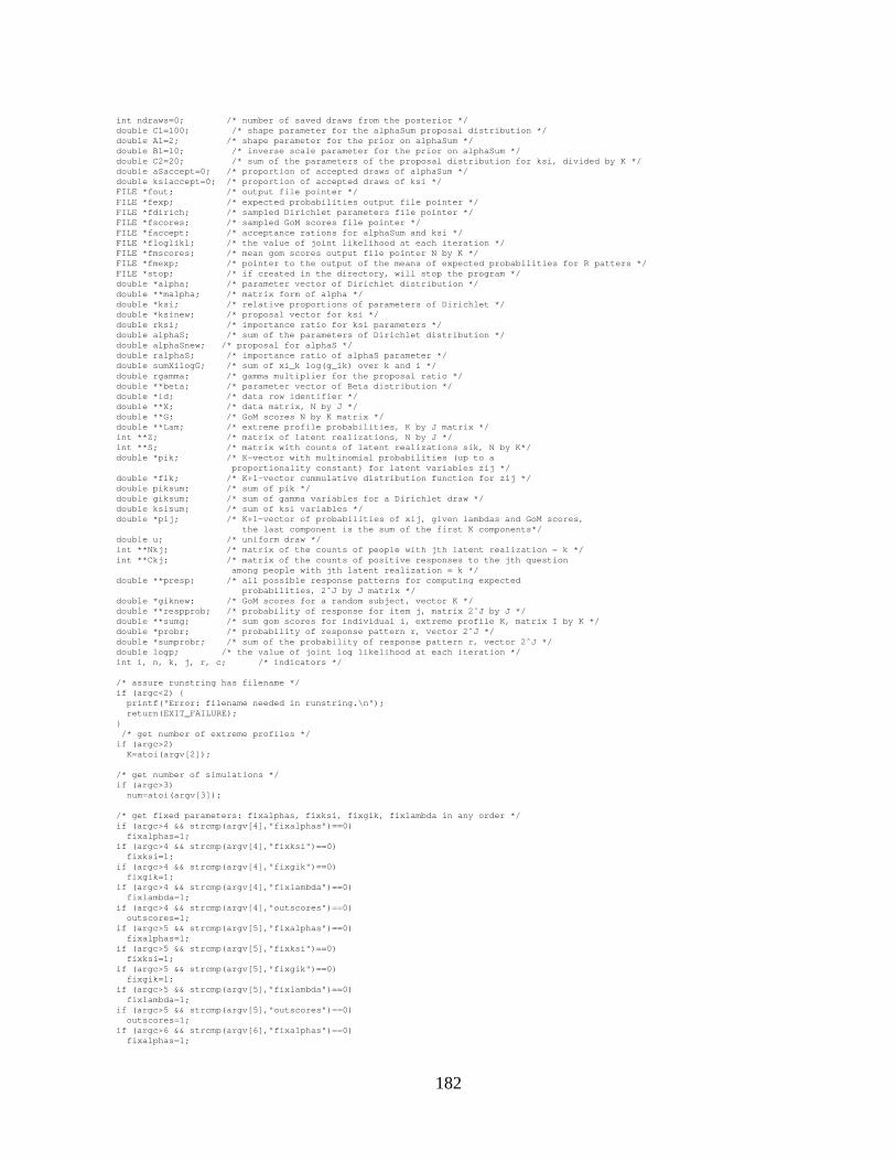
int ndraws=0; /* number of saved draws from the posterior */double C1=100; /* shape parameter for the alphaSum proposal distribution */double A1=2; /* shape parameter for the prior on alphaSum */double B1=10; /* inverse scale parameter for the prior on alphaSum */double C2=20; /* sum of the parameters of the proposal distribution for ksi, divided by K */double aSaccept=0; /* proportion of accepted draws of alphaSum */double ksiaccept=0; /* proportion of accepted draws of ksi */FILE *fout; /* output file pointer */FILE *fexp; /* expected probabilities output file pointer */FILE *fdirich; /* sampled Dirichlet parameters file pointer */FILE *fscores; /* sampled GoM scores file pointer */FILE *faccept; /* acceptance rations for alphaSum and ksi */FILE *floglikl; /* the value of joint likelihood at each iteration */FILE *fmscores; /* mean gom scores output file pointer N by K */FILE *fmexp; /* pointer to the output of the means of expected probabilities for R patters */FILE *stop; /* if created in the directory, will stop the program */double *alpha; /* parameter vector of Dirichlet distribution */double **malpha; /* matrix form of alpha */double *ksi; /* relative proportions of parameters of Dirichlet */double *ksinew; /* proposal vector for ksi */double rksi; /* importance ratio for ksi parameters */double alphaS; /* sum of the parameters of Dirichlet distribution */double alphaSnew; /* proposal for alphaS */double ralphaS; /* importance ratio of alphaS parameter */double sumXilogG; /* sum of xi_k log(g_ik) over k and i */double rgamma; /* gamma multiplier for the proposal ratio */double **beta; /* parameter vector of Beta distribution */double *id; /* data row identifier */double **X; /* data matrix, N by J */double **G; /* GoM scores N by K matrix */double **Lam; /* extreme profile probabilities, K by J matrix */int **Z; /* matrix of latent realizations, N by J */int **S; /* matrix with counts of latent realizations sik, N by K*/double *pik; /* K-vector with multinomial probabilities (up to a

proportionality constant) for latent variables zij */double *fik; /* K+1-vector cummulative distribution function for zij */double piksum; /* sum of pik */double giksum; /* sum of gamma variables for a Dirichlet draw */double ksisum; /* sum of ksi variables */double *pij; /* K+1-vector of probabilities of xij, given lambdas and GoM scores,

the last component is the sum of the first K components*/double u; /* uniform draw */int **Nkj; /* matrix of the counts of people with jth latent realization = k */int **Ckj; /* matrix of the counts of positive responses to the jth question

among people with jth latent realization = k */double **presp; /* all possible response patterns for computing expected

probabilities, 2ˆJ by J matrix */double *giknew; /* GoM scores for a random subject, vector K */double **respprob; /* probability of response for item j, matrix 2ˆJ by J */double **sumg; /* sum gom scores for individual i, extreme profile K, matrix I by K */double *probr; /* probability of response pattern r, vector 2ˆJ */double *sumprobr; /* sum of the probability of response pattern r, vector 2ˆJ */double logp; /* the value of joint log likelihood at each iteration */int i, n, k, j, r, c; /* indicators */

/* assure runstring has filename */if (argc<2) {

printf("Error: filename needed in runstring.\n");return(EXIT_FAILURE);

}/* get number of extreme profiles */

if (argc>2)K=atoi(argv[2]);

/* get number of simulations */if (argc>3)

num=atoi(argv[3]);

/* get fixed parameters: fixalphas, fixksi, fixgik, fixlambda in any order */if (argc>4 && strcmp(argv[4],"fixalphas")==0)

fixalphas=1;if (argc>4 && strcmp(argv[4],"fixksi")==0)

fixksi=1;if (argc>4 && strcmp(argv[4],"fixgik")==0)

fixgik=1;if (argc>4 && strcmp(argv[4],"fixlambda")==0)

fixlambda=1;if (argc>4 && strcmp(argv[4],"outscores")==0)

outscores=1;if (argc>5 && strcmp(argv[5],"fixalphas")==0)

fixalphas=1;if (argc>5 && strcmp(argv[5],"fixksi")==0)

fixksi=1;if (argc>5 && strcmp(argv[5],"fixgik")==0)

fixgik=1;if (argc>5 && strcmp(argv[5],"fixlambda")==0)

fixlambda=1;if (argc>5 && strcmp(argv[5],"outscores")==0)

outscores=1;if (argc>6 && strcmp(argv[6],"fixalphas")==0)

fixalphas=1;

182

if (argc>6 && strcmp(argv[6],"fixksi")==0)fixksi=1;

if (argc>6 && strcmp(argv[6],"fixgik")==0)fixgik=1;

if (argc>6 && strcmp(argv[6],"fixlambda")==0)fixlambda=1;

if (argc>6 && strcmp(argv[6],"outscores")==0)outscores=1;

if (argc>7 && strcmp(argv[7],"fixalphas")==0)fixalphas=1;





if (argc>8 && strcmp(argv[8],"fixalphas")==0)fixalphas=1;





/* read data from file */if (readfile(argv[1], &N, &J, &X)!=READFILE_OK) {

printf("Program is aborting.\n");return(EXIT_FAILURE);

}

/* read alpha vector of Dirichlet parameters; if none given, assign uniform */strcpy(fname, argv[1]);strcat(fname, ".alpha");if (readfile(fname, &r, &c, &malpha)!=READFILE_OK) {

mallocmat(VM_ERRQUIT, 1, &malpha, K, 1);for (k=0; k<K; k++) {

malpha[k][0]=1.0;}

} else {if (r!=K || c!=1) {printf("Error: %s is not %d by 1.\n", fname, K);return(EXIT_FAILURE);}

}alpha=malpha[0];

/* printvec("alpha = ", alpha, 2); */

/* read beta parameter values; if none given, assign uniform */strcpy(fname, argv[1]);strcat(fname, ".beta");if (readfile(fname, &r, &c, &beta)!=READFILE_OK) {

mallocmat(VM_ERRQUIT, 1, &beta, K, J);for (k=0; k<K; k++) {for (j=0; j<J; j++) {

beta[k][j]=1.0;}

}} else {

if (r!=K || c!=J) {printf("Error: %s is not %d by %d.\n", fname, K, J);return(EXIT_FAILURE);

}}

/* read lambda matrix */strcpy(fname, argv[1]);strcat(fname, ".lambda");if (readfile(fname, &r, &c, &Lam)!=READFILE_OK) {


}if (r!=K || c!=J) {

printf("Error: %s is not %d by %d.\n", fname, K, J);return(EXIT_FAILURE);

}

/* read G matrix */strcpy(fname, argv[1]);strcat(fname, ".G");if (readfile(fname, &r, &c, &G)!=READFILE_OK) {


183

}if (r!=N || c!=K) {

printf("Error: %s is not %d by %d.\n", fname, N, K);return(EXIT_FAILURE);

}

/* read presp matrix */strcpy(fname, argv[1]);strcat(fname, ".presp");if (readfile(fname, &R, &c, &presp)!=READFILE_OK) {


}if (c!=J) {

printf("Error: %s does not have %d columns.\n", fname, J);return(EXIT_FAILURE);}

/* open output file for structural parameters */strcpy(fname, argv[1]);strcat(fname, ".out");if ((fout=fopen(fname,"w"))==NULL) {

printf("Can’t create %s.\n", fname);return(EXIT_FAILURE);

}

/* open output file for GoM scores */if (outscores==1) {strcpy(fname, argv[1]);strcat(fname, ".scores");if ((fscores=fopen(fname,"w"))==NULL) {


}}

/* open output of the expected values file */strcpy(fname, argv[1]);strcat(fname, ".exp");if ((fexp=fopen(fname,"w"))==NULL) {


}

/* open output file for the parameters of Dirichlet */strcpy(fname, argv[1]);strcat(fname, ".dirich");if ((fdirich=fopen(fname,"w"))==NULL) {


}

/* open output file for the acceptance proportions for alphaSum and ksi */strcpy(fname, argv[1]);strcat(fname, ".accept");if ((faccept=fopen(fname,"w"))==NULL) {


}

/* open output file for the values of joint likelihood at each draw */strcpy(fname, argv[1]);strcat(fname, ".loglikl");if ((floglikl=fopen(fname,"w"))==NULL) {


}

/* open output file for the values of joint likelihood at each draw */strcpy(fname, argv[1]);strcat(fname, ".mscores");if ((fmscores=fopen(fname,"w"))==NULL) {


}

/* open output file for the mean values of expected probabilities */strcpy(fname, argv[1]);strcat(fname, ".mexp");if ((fmexp=fopen(fname,"w"))==NULL) {


}

/* allocate vectors and intenger matrices */mallocImat(VM_ERRQUIT, 4, &Z, N, J, &Nkj, K, J, &Ckj, K, J, &S, N, K);mallocmat(VM_ERRQUIT, 2, &respprob, R, J, &sumg, N, K);mallocvec(VM_ERRQUIT, 8, &pik, K, &fik, K+1, &giknew, K, &probr, R, &sumprobr, R,

184

&ksi, K, &ksinew, K, &pij, K+1);

/* initialize matrix of sums of the gom scores */zeromat(sumg,N,K);/* initialize vector of sums of the expected values */zerovec(sumprobr,R);

/* Initialize random number generator */imsl_random_option(6); /* best generator */imsl_random_seed_set(0); /* random start */

/* calculate alphaS and ksi from parameters of Dirichlet */alphaS = 0;for (k=0; k<K; k++){alphaS = alphaS + alpha[k];

}for (k=0; k<K; k++){ksi[k] = alpha[k]/alphaS;

}

/* MAIN LOOP to (repeatedly) do one iteration of Gibbs sampler with M-H step*/for (n=0; n<num; n++) {

/* stop the program when file "stop" is created in the directory */stop = fopen("stop","r");

if (stop!=NULL) break;

/* initialize matrix Nkj, the number of people with zij=k */zeroImat(Nkj,K,J);

/* initialize matrix Ckj, the number of positive responses to the jth question among these people */zeroImat(Ckj,K,J);

/* initialize matrix S, sik is the number of latent realizations that equal k for ith person */zeroImat(S,N,K);

/* initialize vector pij */zerovec(pij,K+1);

/* initiaize log likelihood */logp = 0;

/* sample J latent multinomial variables for every person */for (i=0; i<N; i++){for (j=0; j<J; j++){

/* initialize proportionality constant */piksum=0;/* initialize cummulative distribution at 0 */fik[0]=0;/* initialize zij */Z[i][j]=0;

/* calculate vector of multinomial probabilities pik */for (k=0; k<K; k++){

if (X[i][j]==1) {pik[k] = G[i][k]*Lam[k][j];

} else {pik[k]=G[i][k]*(1-Lam[k][j]);

}piksum = piksum + pik[k];

}

/* draw zij from multinomial pik *//* first draw uniform (0,1) */imsl_d_random_uniform( 1, IMSL_RETURN_USER, &u, 0);

/* compute the cumulative distribuiton for zij and *//* assign the value of zij to k such that: fik[k-1] < u <= fik[k] */for (k=1; Z[i][j]==0; k++){

fik[k] = fik[k-1] + pik[k-1]/piksum;

assert(k<=K);

/* after realization of zij is determined, add counts to appropriate cells of Nkj, Ckj and S*/if (u <= fik[k]) {

Z[i][j] = k;Nkj[k-1][j] = Nkj[k-1][j]+1;Ckj[k-1][j] = Ckj[k-1][j]+X[i][j];S[i][k-1] = S[i][k-1]+1;

}} /* end for (while) Z[i][j]=0 */

} /* end for j items */} /* end for i subjects */

/* GIBBS sampling for structural parameters */if (fixlambda==0) {for (k=0; k<K; k++)

185

for (j=0; j<J; j++) {/* draw lambdakj from Beta(1+ckj, 1+nkj-ckj), assume uniform prior (Beta(1,1)) */imsl_d_random_beta(1, 1.0+Ckj[k][j], 1.0+Nkj[k][j]-Ckj[k][j],

IMSL_RETURN_USER, Lam[k]+j, 0);}

}

/* GIBBS sampling for GoM scores */if (fixgik==0) {for (i=0; i<N; i++) {

/* initialize giksum */giksum = 0;/* draw gi from Dirichlet_K(alpha[1]+s[i,1], ..., alpha[K]+s[i,k]) *//* generate K Gamma random variables with shape parameters (alpha[k]+s[i,k]) and equal scale */for (k=0; k<K; k++) {

imsl_d_random_gamma(1, S[i][k]+alpha[k], IMSL_RETURN_USER, G[i]+k, 0);}

/* find giksum */for (k=0; k<K; k++) {

giksum=giksum + G[i][k];}/* Dirichlet */for (k=0; k<K; k++) {

G[i][k] = G[i][k]/giksum;/* sum of the gom scores for all iterations */if ((n%thinlam==0)&(n>burnin)) {

sumg[i][k] = sumg[i][k] + G[i][k];}

}

/* find the log likelihood component for ith individual */for (j=0; j<J; j++) {

pij[K] = 0;for (k=0; k<K; k++) {

if (X[i][j]==1) {pij[k] = G[i][k]*Lam[k][j];} else {pij[k] = G[i][k]*(1-Lam[k][j]);}pij[K] = pij[K]+pij[k];

}logp = logp + log(pij[K]);}

}} /* end for sampling GoM scores */

/* METROPOLIS-HASTINGS step for AlphaS */if (fixalphas==0) {/* first, assign importance ratio =1 */ralphaS = 1;/* draw a candidate alphaS point from proposal gamma distribution *//* with shape parameter C1 and inverse scale parameter C1/alphaS */imsl_d_random_gamma(1, C1, IMSL_RETURN_USER, &alphaSnew, 0);alphaSnew = alphaSnew/(C1/alphaS);

/* calculate importance ratio ralphaS */sumXilogG =0;/* calculate sumXilogG */for (k=0; k<K; k++) {

for (i=0; i<N; i++) {sumXilogG = sumXilogG + ksi[k]*log(G[i][k]);

}}/* calculate the gamma multiplier for the proposal ratio */rgamma= imsl_d_gamma(alphaSnew)/imsl_d_gamma(alphaS);for (k=0; k<K; k++) {

rgamma=rgamma*imsl_d_gamma(alphaS*ksi[k])/imsl_d_gamma(alphaSnew*ksi[k]);}/* multiply by the full conditional ratio component */

ralphaS = ralphaS*pow(alphaSnew/alphaS,A1-1)*pow(exp(-(B1-sumXilogG)*(alphaSnew-alphaS)/N)*rgamma,N);

/* multiply by the proposal distribution ratio components */ralphaS = ralphaS*pow(alphaSnew/alphaS,1-2*C1)*

exp(-C1*((alphaS/alphaSnew)-(alphaSnew/alphaS)));

/* accept candidate point with probability min{ralphaS,1} */if (ralphaS>=1) {

alphaS = alphaSnew;aSaccept = aSaccept+1;

}else{

imsl_d_random_uniform( 1, IMSL_RETURN_USER, &u, 0);if ( u<=ralphaS ){

alphaS = alphaSnew;aSaccept = aSaccept+1;

}}

186

} /* end of Metropolis-Hastings step for alphaS */

/* METROPOLIS-HASTINGS step for KSI */if (fixksi==0) {/* draw candidate point ksinew from Dirichlet_K(C2*K*ksi[1], ..., C2*K*ksi[K]) *//* generate K Gamma random variables with shape parameters (C2*K*ksi[k]) and equal scale */

for (k=0; k<K; k++) {imsl_d_random_gamma(1, C2*K*ksi[k], IMSL_RETURN_USER, ksinew+k, 0);

}/* find normalizing constant ksisum */ksisum = 0;for (k=0; k<K; k++) {

ksisum = ksisum + ksinew[k];}/* Dirichlet */for (k=0; k<K; k++) {

ksinew[k] = ksinew[k]/ksisum;}

/* calculate importance ratio rksi */rksi = 1;/* multiply by the likelihood ratio component *//* calculate the gamma multiplier for the proposal ratio */rgamma= 1;for (k=0; k<K; k++) {

rgamma=rgamma*imsl_d_gamma(alphaS*ksi[k])/imsl_d_gamma(alphaS*ksinew[k]);}rgamma = pow(rgamma,N);rksi = rksi*rgamma;for (k=0; k<K; k++) {

for (i=0; i<N; i++) {rksi = rksi*exp(alphaS*log(G[i][k])*(ksinew[k]-ksi[k]));

}}/* multiply by the proposal distribution ratio */for (k=0; k<K; k++) {rksi = (rksi*(imsl_d_gamma(C2*K*ksi[k])/imsl_d_gamma(C2*K*ksinew[k])))*

(pow(ksi[k],ksinew[k]-1)/pow(ksinew[k],ksi[k]-1));}

/* accept candidate point with probability min{rksi,1} */if (rksi>=1) {

for (k=0; k<K; k++) {ksi[k] = ksinew[k];

}ksiaccept = ksiaccept+1;

}else {

imsl_d_random_uniform( 1, IMSL_RETURN_USER, &u, 0);if ( u<=rksi ) {

for (k=0; k<K; k++) {ksi[k] = ksinew[k];

}ksiaccept = ksiaccept+1;

}}} /* end of Metropolis-Hastings step for ksi */

/* define Dirichlet parameters */for (k=0; k<K; k++){

alpha[k] = alphaS*ksi[k];}

/* OUTPUT AND EXPECTED VALUES */if ((n%thinlam==0)&(n>burnin)) {

/* print lambda parameters from every 10th iteration to "*.out" */ndraws = ndraws +1;for (i=0; i<K*J; i++)

fprintf(fout,"%9.8f ",Lam[0][i]);/* if (i%%500==0)

fflush(fout); */fprintf(fout,"\n");fflush(fout);

/* print K GoM scores from every 100th iteration to "*.scores" */if (n%thinscores==0) {

if (outscores==1) {for (i=0; i<N; i++)

for (k=0; k<K; k++) {fprintf(fscores,"%9.8f ",G[i][k]);

}fprintf(fscores,"\n");fflush(fscores);

}

187

}

/* print sum of the parameters of Dirichlet distribution from every 10th iteration to "*.dirich" */fprintf(fdirich,"%9.8f ",alphaS);for (k=0; k<K; k++) {

fprintf(fdirich,"%9.8f ",ksi[k]);}

/* print out the proposal ratios, if needed *//* fprintf(fdirich,"%20.10f ",ralphaS);

fprintf(fdirich,"%20.10f ",rksi); */fprintf(fdirich,"\n");fflush(fdirich);

/* print current acceptance ratios, if needed *//* fprintf(faccept,"AR alphaSum is %9.8f ",aSaccept/n);fprintf(faccept,"\n");fprintf(faccept,"AR ksi is %9.8f ",ksiaccept/n);fprintf(faccept,"\n"); */

/* print log likelihood to "*.loglikl" */fprintf(floglikl,"%10.4f ",logp);fprintf(floglikl,"\n");fflush(floglikl);

/* Calculate EXPECTED PROBABILITIES for .presp response patterns */

/* initialize matrix respprob of expected probabilities */zeromat(respprob,R,J);

/* draw random vector of GoM scores giknew for calculating expected probabilities *//* initialize giksum */giksum = 0;/* draw gi from Dirichlet_K(alpha[1], ..., alpha[K]) *//* generate K Gamma random variables with shape parameters alpha[k] and equal scale */for (k=0; k<K; k++)

imsl_d_random_gamma(1, alpha[k], IMSL_RETURN_USER, giknew+k, 0);/* find giksum */for (k=0; k<K; k++) {

giksum=giksum + giknew[k];}/* Dirichlet */for (k=0; k<K; k++) {

giknew[k] = giknew[k]/giksum;}

/* calculating expected probabilities */for (r=0; r<R; r++) {

probr[r]=1.0;for (j=0; j<J; j++) {

for (k=0; k<K; k++) {if (presp[r][j]==1) {

respprob[r][j] = respprob[r][j] + giknew[k]*Lam[k][j];} else {

respprob[r][j] = respprob[r][j] + giknew[k]*(1-Lam[k][j]);}

}probr[r] = probr[r]*respprob[r][j];

}sumprobr[r] = sumprobr[r] + probr[r];

}

/* print expected probabilities to "*.exp" */for (r=0; r<R; r++)

fprintf(fexp,"%13.12f ",probr[r]);fprintf(fexp,"\n");fflush(fexp);

} /* end of output */} /* end of simulations */

/* calculate and print acceptance ratios */aSaccept = aSaccept/num;ksiaccept = ksiaccept/num;fprintf(faccept,"overall acceptance ratio for alphaSum is %10.9f ",aSaccept);fprintf(faccept,"\n");fprintf(faccept,"overall acceptance ratio for ksi is %10.9f ",ksiaccept);fprintf(faccept,"\n");

/* calculate and print mean gom scores for each individual */for (i=0; i<N; i++) {for (k=0; k<K; k++) {

fprintf(fmscores,"%9.8f ",sumg[i][k]/ndraws);}

fprintf(fmscores,"\n");}

/* calculate and print extected values for R response patterns */for (r=0; r<R; r++) {

fprintf(fmexp,"%9.8f ", sumprobr[r]/ndraws);}

fprintf(fmexp,"\n");

188

fclose(fout);if (outscores==1)

fclose(fscores);fclose(fdirich);fclose(fexp);fclose(floglikl);fclose(fmscores);fclose(fmexp);return(EXIT_SUCCESS);

}

189

Appendix B

Simulation Studies: GoM model

B.1 Simulation Study with BUGS

B.1.1 GoM Model Specification for BUGS

When the number of extreme profiles and the distribution of the GoM scores are assumed known,we can use BUGS (Bayesian inference Using Gibbs Sampling) software package (Spiegelhalter etal. 1996) to obtain posterior distribution of the GoM model parameters by adapting the followingcode which is based on the directed graphical diagram for the GoM model given in Figure 4.1.

BUGS code for the GoM model with fixed hyperparameters: using latent class representation.

# data file must contain IxJ matrix of responses# four dichotomous questions# 1,000 sample size

model

gom;

const

I = 1000, # number of individualsJ = 4, # number of questionsR = 16, # number of possible response patternsK = 2; # number of pure types

var

resp[I,J], # observed responses (ith p subject, jth item)pos.resp[R,J], # matrix of all possible response patternsalpha[K], # parameters of the Dirichlet prior for GoM scoresbeta1[K,J], # first parameter of Beta prior for item parametersbeta2[K,J], # second parameter of Beta prior for item parametersg[I,K], # GoM scoreslambda[K,J], # item parametersz[I,J], # augmented latent categorical data

# for later use in computing Gˆ2:g.new[K], # GoM scores for ramdom subjectprob.resp[R,J],# probability of response for item jprob.g[R]; # probability of respose pattern r

data

resp in "sim3resp.dat", # reading the data filepos.resp in "sim3posresp.dat", # reading possible responsesbeta1 in "sim3b1prior.dat",beta2 in "sim3b2prior.dat"; # reading parameters beta1, beta2

191

inits g in "sim3gscore.dat",lambda in "sim3lambda.dat"; # sets initial data values

# to the true values

{#model

for (i in 1:I) {for (j in 1:J) {

z[i,j] ˜ dcat(g[i,]);resp[i,j] ˜ dbern(lambda[z[i,j],j]);

}g[i,] ˜ ddirch(alpha[]);

}

#priors

alpha[1] <- 0.1;alpha[2] <- 0.1;

for (k in 1:K){for (j in 1:J){

lambda[k,j] ˜ dbeta(beta1[k,j], beta2[k,j]);}

}

#compute probability of response pattern r#for later use in computing Gˆ2

g.new[] ˜ ddirch(alpha[]);for (r in 1:R)

{ for (j in 1:J){ prob.resp[r,j] <- g.new[1]*pow((lambda[1,j]),(pos.resp[r,j]))

*pow((1-lambda[1,j]),(1-pos.resp[r,j])) +g.new[2]*pow((lambda[2,j]),(pos.resp[r,j]))

*pow((1-lambda[2,j]),(1-pos.resp[r,j]));}

#probability to observe response pattern r given g.newprob.g[r] <- prob.resp[r,1]*prob.resp[r,2]*prob.resp[r,3]*prob.resp[r,4];

}

}

It is essential that a BUGS code for the GoM model is written by using the augmented dataform from the latent class representation. Literal coding of the hierarchical model based on stan-dard GoM formulation, provided below, does not result into a successful compilation of the pro-gram: the error message “unable to choose update method for node” means that BUGS is unableto conclude log-concavity of the likelihood. Note that placing a hyperprior the distribution ofthe GoM scores within BUGS produces similar problems with determining log-concavity of thedistributions.

BUGS code for the GoM model with fixed hyperparameters: using standard formulation.

# this is an attempt to compute the conditiponal probabilities of response# directly from the traditional GoM model (without latent class variables)

# This program DOES NOT COMPILE, and hence CANNOT BE USED# It encounters the following error message:# Unable to choose update method for node g[1,1],# which shows that data augmentation is essential for using BUGS# with the GoM model

# data file must contain IxJ matrix of responses# four dichotomous questions# 1,000 sample size

model

gom;

const

I = 1000, # number of individuals

192

J = 4, # number of questionsR = 16, # number of possible response patternsK = 2; # number of pure types

var

resp[I,J], # observed responses (ith p subject, jth item)pos.resp[R,J], # matrix of all possible response patternsalpha[K], # parameters of the Dirichlet prior for GoM scoresbeta1[K,J], # first parameter of Beta prior for item parametersbeta2[K,J], # second parameter of Beta prior for item parametersg[I,K], # GoM scoreslambda[K,J], # item parameters

# z[I,J], # augmented latent categorical data# for later use in computing Gˆ2

g.new[K], # GoM scores for ramdom subjectprob.resp[R,J],# probability of response for item jprob.g[R], # probability of respose pattern rprob[I,J]; # probability of response of subject i to item j

data

resp in "sim3resp.dat", # reading the data filepos.resp in "sim3posresp.dat", # reading possible responsesbeta1 in "sim3b1prior.dat",beta2 in "sim3b2prior.dat"; # reading parameters beta1, beta2

#inits g in "sim3gscore.dat",#lambda in "sim3lambda.dat"; # sets initial data values

# to the true values

{#model

for (i in 1:I) {for (j in 1:J) {

# z[i,j] ˜ dcat(g[i,]);# probability of response from the GoM model directly

prob[i,j] <- (lambda[1,j]*g[i,1]+lambda[2,j]*g[i,2])resp[i,j] ˜ dbern(prob[i,j]);

}g[i,] ˜ ddirch(alpha[]);

}

#priors

alpha[1] <- 0.1;alpha[2] <- 0.1;


lambda[k,j] ˜ dbeta(beta1[k,j], beta2[k,j]);}

}

#compute probability of response pattern r#for later use in computing Gˆ2

g.new[] ˜ ddirch(alpha[]);for (r in 1:R)

{ for (j in 1:J){ prob.resp[r,j] <- g.new[1]*pow((lambda[1,j]),(pos.resp[r,j]))

*pow((1-lambda[1,j]),(1-pos.resp[r,j])) +g.new[2]*pow((lambda[2,j]),(pos.resp[r,j]))

*pow((1-lambda[2,j]),(1-pos.resp[r,j]));}

#probability to observe response pattern r given g.newprob.g[r] <- prob.resp[r,1]*prob.resp[r,2]*prob.resp[r,3]*prob.resp[r,4];

}

}

B.1.2 Simulation Example: Fixed Hyperparameters

Consider the GoM model with two extreme profiles. Let the distribution of the GoM scores tobe Dirichlet with parameters (0.1,0.1) and the two extreme profiles to have low (0.05) and high(0.95) response probabilities, respectively. A contingency table of observed data generated by

193

the GoM model with these parameter specifications ought to contain large cell counts for all-zeroand all-one responses, and small cell counts for other response patterns. This corresponds to ageneral data structure that we are interested in analyzing with the GoM model. The objectivesof the simulations are: (1) to examine data generated by the GoM model, (2) to obtain posteriordistribution of structural parameters, and (3) to compare results with the true parameter values.

Table B.1: Observed and expected frequencies for the test data under the GoM model with knownhyperparameters

Response pattern Sim. 2 Sim. 2 Sim. 3 Sim. 3observed expected observed expected

1 0000 37 30.57 350 363.502 1000 3 3.12 38 39.273 0100 1 2.43 23 23.814 1100 1 1.16 7 9.755 0010 4 3.69 23 24.126 1010 0 1.12 9 8.687 0110 0 1.34 7 8.068 1110 4 4.07 25 23.859 0001 4 4.28 29 29.88

10 1001 1 1.17 11 10.2611 0101 1 1.36 8 9.6412 1101 3 3.84 39 36.3213 0011 0 1.31 10 8.3514 1011 1 2.35 22 22.1315 0111 5 4.88 31 29.2416 1111 35 33.28 368 353

Simulated data were generated in S-plus by the following procedure:

1. Supplyº the number of subjects C ,º the number of items W��@� ,º the number of extreme profiles J��,� ,º the conditional response probabilities for the extreme profiles * � YÓ� ��7�� ! * � YÓ��T�� ! ^D�H� ! �"�.� ! � ,º parameters of the Dirichlet (Beta) generating distribution for the membership scores � �q��S�2� ! � �+��S�2� ;

2. Draw C vectors of membership scores from the Dirichlet distribution;

194

response pattern

true

GoM

sco

re g

1

5 10 15

0.0

0.2

0.4

0.6

0.8

1.0

______

_

_

_

____

_

__

_

_

_

_

_

_

_____

_

___

_

_____

_

_

_

_

_

__

__

__

_

_

___

_

_

_

__

_

____ ________

_

__

_

_

_

__

_

_

_

___________

_

__

Simulation 2: Dir(0.1,0.1), rep(0.05,4), rep(0.95,4), I=100

Figure B.1: Simulation 2. Membership scores for first extreme profile versus the number of ob-served response pattern.

3. Draw C response patterns (one for each vector of the membership scores) from Bernoulliwith probabilities of success being convex combinations of the extreme profile responseprobabilities, given the GoM scores.

Two simulated data sets were generated with the sample sizes C of 100 and 1000, Simulation 2and Simulation 3, respectively. Observed frequencies of responses are given in Table B.1.2.

Figures B.1, B.2 contain plots of simulated membership scores in the first (low response prob-ability) extreme profile, 3 � . The membership scores, 3 � , are plotted versus the response patternnumbers from Table B.1.2, for two simulated data sets. Each short line represents one observation.A normal horizontal random noise was added to the observations for better readability.

From Figure B.2, it can be seen that large values of 3 � tend to have response patterns 1, 2, 3, 5,and 9, as their realizations. These response patterns have at most one positive response. Similarlypatterns 16, 15, 14, 12, and 8, tend to be realized from smaller 3 � scores; these response patternshave at least three positive responses. The response patterns with exactly two positive responseshave the smallest number of realizations, and 3 � values that resulted into these responses have nospecial characteristics. Figure B.1 for Simulation 2 with sample size of Cë� �2�F� , does not revealclear patterns.

Taking into account the extreme profile probabilities and the membership scores, Figures B.3and B.4 show the true probabilities to observe each of the response patterns obtained in the sampleunder the GoM model. Many of the probabilities are near �� for the all-zero or all-one responses,although there are some of those expected probabilities are much smaller, they have resulted intothe same extreme response patterns by pure chance. The patterns with three zeros or three oneshave probabilities concentrated around 0.08. The patterns with two zeros (or ones) have the small-est probabilities concentrated around 0.05. This tells us that for given extreme profiles and for

195

response pattern

true

GoM

sco

re g

1

5 10 15

0.0

0.2

0.4

0.6

0.8

1.0 _

_

_____

_

_

___

_

___

__

__

_

____________

_

_____

_

_____________________

_

___

_

_

__

____

_

___

_

___________________

_

__

_

_

_

______

_

__

_

______________

_

____

_

_______

_

___

_

_

_

__

_

_

_

______

_

_____________

_

____

_

____

_

_

_

_____

__

____

_

_________

_

____

_

____

_

________________

_

_

_

_________

_

_________________

_

_

_

_

___

_

________________

_

_____________

_

___

__

________

_

_

__

_

__________

_

_____ _

_

_

_

__

_

_

____

_

_

_

_

___

_

___

_

__

_

_

__

_

_

_

_

_

_

_

_ __

_

_

_

_

_

__

_

__

__

__

__

___

_

_

_

_

_

_

_

_

_

__

_

_

_

_

__

_

____

_

___

_

_

__

_

_

_

__

_

_

_

_

_

_

_

_

_

_

_

_ _

_

___

_

_

__

_

_

_

_______

_____

____

_

_

_

__

__

_

_

_

_

_

_

_

__

_

___

_

_

_

__

_

_

_

_

_

_

_

_

_

_

_

_

_

_

_

_

_

_

_

___

_

__

_

_

___

_

___

_

____

_

___

_

_

_

_

___

_

___

__

_

_

_

_

__

_

_

_

_

_

_

_

_

_

_

_

__

__

_

__

_

___

_

__

_

__ _

_

___

_

_

_

__

_

___

_

__

_

______

_

_

_

_

_

_

_

__

_

_

_

_

_

__

_

__

_

_

_

_

_____

_

_

__________

_

___________

_

_____________

_

_

_

________

_

_____________

_

_____

_

__________

_

__

_

_____

_

_____

_

_

_

_______

_

_

_

_

_

_______________

_

_

_

____________

_

________

_

_

_

____

_

______________

_

__________

_

__

______________

__

___________

_

________

_

__________________________________________________

______

_

_______________

_

_

___

_

_

_________

_

_

_

_____

_

__

_

______

_

___________


Figure B.2: Simulation 3. Membership scores for first extreme profile versus the number of ob-served response pattern.

given distribution of the GoM scores, each non-extreme responses pattern has a very small proba-bility of being observed.

Output analysis. For BUGS code, the parameters of Dirichlet distribution were fixed at true val-ues QR��S� ! �T��VU . The program uses the uniform, or Beta(1,1), prior for the structural parameters, andobtains samplers from the posterior distribution of the structural parameters given the data. Severalprogram runs with different starting values provided very similar results, up to the relabeling of theextreme profiles. The MCMC chains were ran for 1500 iterations, and first 500 iterations were dis-carded as a burn-in period. Posterior distribution was based on the following 1000 iterations. Theoutput was analyzed by using CODA (Convergence Diagnosis and Output Analysis Software forGibbs sampling output) software (Best et al. 1996). Mean and standard deviation for the posteriordistribution of structural parameters * n Y ! l�� ! � ! ^ � � ! � ! � ! � ! is given in Table B.2. Becausethe estimated extreme profiles are well separated, we can conclude that no label-switching problemwas encountered in this example by examining the successive iterations.

As expected, the means for the posterior distribution from the larger sample in most cases arecloser to the true parameter values of �T�7�� and �� , and the standard deviation is smaller com-paring to the results from the smaller sample. Posterior estimates show better agreement with truevalues for Simulation 3 with larger sample size. Successive iterations and posterior distributionsof the lambda-parameters are given in Figures B.5 and B.6 for Simulation 3. Similar plots for fourrepresentative parameters for Simulation 2 are in Figure B.7.

To assess overall model fit, expected counts for each cell (see Table B.1.2) were calculatedfrom the posterior distribution in the following fashion: (1) a vector of the GoM scores is drawnfrom the generating Dirichlet distribution at each iteration, (2) response probabilities for each cell

196

response pattern

true

pro

babi

lity

of r

espo

nse

5 10 15

0.0

0.2

0.4

0.6

0.8

1.0

_

_____

_

_

_

____

_

__

_

_

_

_

_

_

_

_

___

_

___

_

___

_

_

_

___

_ __

__ ___

_

____

_ _

_

__

_

_____

________

_

_

_

_

_

_

__

_

__

_

____________

_

__


Figure B.3: Simulation 2. Conditional probability of observing response patterns 1 through 16under the GoM model, given the extreme profile probabilities and the simulated GoM scores.

response pattern

true

pro

babi

lity

of r

espo

nse

5 10 15

0.0

0.2

0.4

0.6

0.8

1.0

__

_

_ ____

_

_

___

_

___

__

__

_

_________

__

_

_

_____

_

_

_________

_

__

_

________

_

____

_

_

_

_

__

_

_

_

___

_

____

_

_____________

_

__

_

_

_

__

____

_

__

_

__________

__

___

_

____

_

_______

_

__

_

_

_

_

_

_

_

_

_

______

_

__

___________

_

_

___

_

_____

_

_

_

_____

__

_

_

__

_

__________

_

____

_

____

_

______

_

_

_

________

_

_

_

______

_

____

_

__________

_

_______

_

_

_

_

___

_

_

__

____

__

____

___

_

__________

_

_

_

___

_

_

________

_

_

__

_

_

_

_

_________

_

____

_

_

____

__

____

__

_

_

___

_

___

___

_

_

__

__

_____

_ ____

_

_

_

___

_______

__

____

_

_____

______

__

__

_

____

_

________

_

___

_

_

_

__

__

___

__

_

______

____

_

________

_____ ____

_

____

__

_

_

_

_

_

________

_

____ _

__

______

__ _

___

_

_

__

___________

_

___

_

_______

__

_____

_

___

____

_____

____

_

__

_

__

__

_ ____

_______

_

__ _

_

___

__

_

______

_

__

_

__

____

_

_

_

___

_

_

_

_

_

_

_

_

__

_

_

_

_

_

_

_

____

_

_

_

____

_

_

_____

_

________

__

_

_

_

______

_

_

____

_

_

_

_______

_

_______ _____

_

______

_

__

_

_______

_

___

_

__

_

__

_

______

_

_

_

______

_

_

_

_

_

_

_

______________

_

_

_

_

_

_

_

________

_

_

_

_ ____

_

_

_

_

___

_

_ __

_

___________

_

_____

_

____

_

_

_

__________

_

_

_

_

__

__

_

________

_

________

_

_

_

______________

____

_

_________________

_

_____

__

__

_

_

_

_

__

_

____

_

__________

_

_

___

_

_

_________

_

_

_

_____

_

__

_

_____

_

__

_

________


Figure B.4: Simulation 3. Conditional probability of observing response patterns 1 through 16under the GoM model, given the extreme profile probabilities and the simulated GoM scores.

197

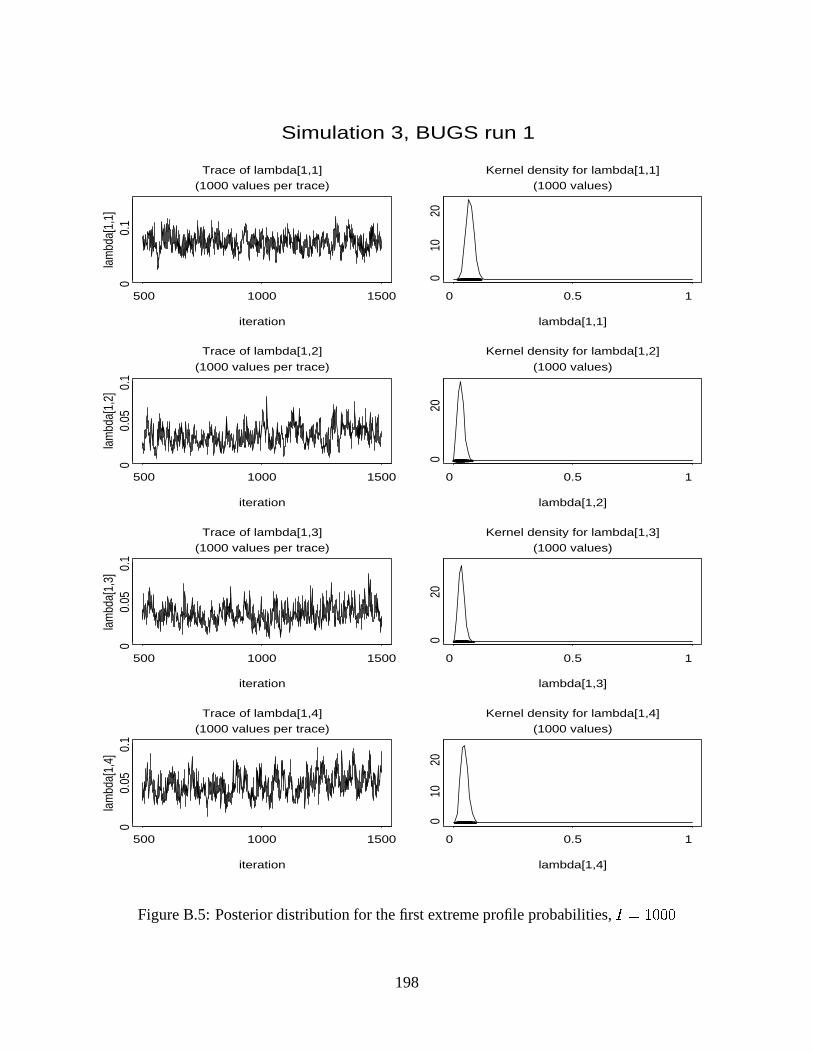
iteration

lam

bda[

1,1]

500 1000 1500

0

0.1



lambda[1,1]

0 0.5 1

010

20


(1000 values)

•••• ••••••••••••••• •••••• ••••••• •••• ••••• •••• •••••••••••••••••••• ••••••••• ••••••••••• •••••• • •••• • •••••• •••••• •••••••••• ••••• •••••••••• •••••••• •••• •••••••••••••••••• • •• ••• •• ••• •• •• ••• •••• •••••• •••••••••••••••••• ••••••• ••••••••••• ••• ••• ••••••••••• ••• •••••••••••••• ••••• ••••••••• ••••••••••••• •••••••••• •••• •••••• •••••••••••••••••• ••• ••••••••••••••• ••••••• ••••• ••••••••••••• •••• •••••••••••••••••••••••• ••••••••••••••••••••••• •••••••••••••••••••••••••••••••••• •••••• •••••••••• ••••••••• ••••••••••••••••••••••••• •••••••• •••••••••••• ••• •• ••••••••••••• ••• ••••••••••••••• •••••••••• ••• •• •• ••••••••• •• ••••••• ••••••••••••••• ••• •• ••••••••••••• •••• •••••• ••••••••••••••• •••••••••••••••••••••• •• •••••••••••• ••••••••••••••••••••••••••••••••••••••••••••••••••••••••• ••••••••• •••••••••••••••• • •••••••• ••••••••••• •••••••••• ••• •••••••••• ••••••••••• ••••• •••••••••••• •••• •••• •••••• ••••••••••• ••• ••••••• •••• ••• •• ••••••• ••••••• •••••• •••••••••••• ••••• ••• •••• ••••• ••••••••••••••••• ••• •••••••••••••••

iteration

lam

bda[

1,2]

500 1000 1500

0

0.05

0.1



lambda[1,2]

0 0.5 1

020


(1000 values)

•••••••••••••••• •••••••••••••••••••••••••••••••••••••••••• ••••••• •• ••••••••••• ••••••••••••••••••• ••••••• ••••••••••••••••••••••• •••••••••••• •••••••••••••• •••••••••••••••••••••••••••••••••••••••••••••••••••••••••••••••••••••••••••••••••••••••••• •••••••••••••••••••••••••••••••••••••••• ••••••••••••••••••••••••••••••• ••••••••••••••• •••• •••••••••••••••••••••••••••••••••••••••••••••••••••••••••••••• ••••••••••••• ••••••••••••••••••••••••• •••••••••••• •••••••••••••••••••••••••••••••••••••••••••• •••••••••••••••••••••••••• •••••••••••••••••••••••••••••••••••••••••••••••••••••••••••••••••• •• ••••••••••• ••••••••••• ••••••••• •••••••••••••••••••••••••••••••••••••••••••••••••••••••••••••••••••••••••••••••••• ••••••••••••••••••••••••••••••••••••••• ••••••••••• •••••• •••••••••••••••••••••••••••••• ••••••••••••••••••••• ••••••••••••••••••••••••••••• ••••••••••••••••• •• •• •••••••••••••••••••••••• •••••••••••••••••••••••••••••••••••••••••••• ••••••••• ••••••••••••••

iteration

lam

bda[

1,3]

500 1000 1500

0

0.05

0.1



lambda[1,3]

0 0.5 1

020


(1000 values)

•••••••••••••••• ••••••••••• ••••••••••••••••••••••••••••••••••• •••••••••••••••••••••• •••••••••••• ••• ••••••••••••••••••••••••••• ••••••••••••••••••••••••••••••••••••• ••••• •••••••••••••••••••••• ••••••••••••• •••••••••••••••••••••••••••••••• ••••••••••••••••••••••••••••••••••• •••••••••••••••••••• ••••••• •••••••••••• ••••••••••••• ••••••• ••••••••••••• ••• •••••••••••••••••••••••••••••••••••••••••••••••••••• •••••••••••••••••••• ••• ••••••••••• ••• ••••••••••••••••••••••••••••••• ••••••••••••••••••••••••••••••••••••••••••••••••••• •••••••••••••••••••••• ••••••••• •••••••••••••••••••••••••••••••• ••••••••• ••••••• ••••••••• ••••• ••••••••••• ••••••• •••••• ••••••••••• ••••••••••••• ••••••• ••••••••••••••••••••••••••••••• ••••••••••••••• ••••••••••• ••••••••••• •• ••••• •••••••••••••••••• ••••••••••••• ••••••••••••••••• •• ••••••••••••••••••••••••••••••••••••••••••••••••••••••••••••••••••••••••••••••••• ••••••••••••••• •••••••••••••••••••••••• ••••••••• ••••••••••••••••• •••

iteration

lam

bda[

1,4]

500 1000 1500

0

0.05

0.1



lambda[1,4]

0 0.5 1

010

20


(1000 values)

•••••••••••••••••• ••••••••• •••••••••••••••••••••••••••••••• •••••••••• ••• •••••••••••••••••••••• •••••• ••••••••••••••••• ••••••••••• ••••••• •••••••••••••••••••••••••••••••••• ••••••• ••• •••••••••••••••••••••••••••••• ••••••••• •••• ••••••••••••••••••••••••••••••••••••••••••••••••••••••••••••••• ••• ••• ••••••••••••••• ••••• •••••••• ••• ••• •••••••••••••••••••••••••••• ••••••••••• •••••••• ••••••••••••••••••••••••• •• •••••• •• ••••••••••••••••••••••••••••••••••••••••••••• •••••• ••• •••••••••••••••••••••••••••••••••••••••••••••••••••• ••••••• ••• ••••••••••••••• •••••••••••• •• •••••• ••••••••••••••••••••••••••••• •••••••••••••••••••••••••••••••••• ••••• ••••••••••••••••••••••••••• ••••• •••••••••••••••••••••••••••••• ••••••••••••••••••• •• •••••••••• •••••••••••••••••••••••••••••••••• •••• ••••••• •••••• •• •••••• ••••••••••••••••• •••••••••••••••••••• •••••••• •••••••••••••• ••• •••••••••• ••• ••••••••••• ••••••••••••••••• ••••••••••••••••••••• •••••••• ••••••••••• •••••••••••••••••• •• •••••• ••••••••

Simulation 3, BUGS run 1

Figure B.5: Posterior distribution for the first extreme profile probabilities, CG�E�.�F�F�198

iteration

lam

bda[

2,1]

500 1000 1500

0.9

0.95

1



lambda[2,1]

0 0.5 1

010

20


(1000 values)

•• •••••••••••••••••••••••••••• ••••••• ••• ••••••••••••••••••••••••• •••••••••••••••••••••••• •••••••••••••• •••••••• •• ••••••••••• ••••••••••••••• ••••••••••• ••••••••••• •••••••••••• ••••••••• •••••• ••••••••••••••••• •••••• •• •••• ••••••• •• ••••• ••••••••••• ••••••••••••••••••• • ••••• •••••••••••••••• ••••••••••• ••••••••••••• •• ••••• ••••• •••••••••• •••• •••••••• • •••••• ••••• ••••••••••• ••••••• ••••••••• ••• ••• •••••••• •••••••••••••••••••••• •••••••••••• •••••••••• •••••••• ••• ••••••••••••••••• ••••••••••••••• •••••••••••••••• •••••••••••••••••••••••••• •••••••••••••••••••••••• •••••••••• ••• •••••••• •••••••••••••• •••••••••••••••••••••••••• ••••••••••••• •••••••••••••••••• •••••• •••••••••••• •••••••••••••• ••••••••••••••••••• •••••••••••••• ••••• •••••••••••••• •• ••••• •••••••••••••••••••••••••••••• ••••••••••••••••••••••••••••••••• •••••••••••••••••••••••••••••••••••• •• ••••• ••••••••••••••••••• ••••••• •••••••• •••••• ••••••••• ••••• ••••••••••••••••••••••••••••••••••••••••••••••••••••••••• •

iteration

lam

bda[

2,2]

500 1000 1500

0.9

0.95

1



lambda[2,2]

0 0.5 1

010

20


(1000 values)

••••••••••••••••••••••••••••••••••••••••••••••••••••••••••••• •••••••••••••••••••••••••••••••••••••••••• •••••••••• ••••••••••••••••••••••••••• •••••••••••••••••••••••••••••••••••••••••••••••••••••••••••••••••••••••••••••••••••••••••••• •••••• ••••••••••••••••••••••••••••• •••••••••••••••••••• ••••••••••••••••••••••••••••••••••••••••••••••••••••••••••••• •••••••••••••• •••••••••••••••••••••••••••••••••••••••••••••••••• ••••••••••••••••••••••••••••••••••••••••••••••••••••• •••••••••••••••••••••••••••••••••••••••••••••••••••••••••••••••••••••••••••••••••••• ••••••••••••••••••••••••••••••••••••••••••••••••••••••••••••• •••••••••••• •••••••••••••••••••••••••••••••••••••••••••••••• •••••• ••••••••••••••••••••• •••• •••••• •••••••••••••••••••••••••••••••••••••••••••••••••••••••••••••••••••••••• ••••••••••••••••••••••••••• •••••••••••••••••••••••••••••••••••••••••••••• •••••••••••••• ••••••••••• ••••••••••••••••••••• ••••••••••••••••••••••••••••••••••••••••••••••••••••••••

iteration

lam

bda[

2,3]

500 1000 1500

0.85

0.95



lambda[2,3]

0 0.5 1

010

20


(1000 values)

•••••••••••••••••••••••••• •• •••••• •• •••••••• ••••••••••••• ••• ••••••••••••• ••••••• ••• •••• ••• •••••••••••••••••• ••••••• ••• •••••••• •••••••••••••••• ••••••••••••••••••••••••••••••••••••••• •••••• ••••••••••••••••• •• •••••• ••••••••••••••••• ••••••••••••• ••••••••••••••••••••• •••••••• •••••••• •• ••••••••••••••• •• ••••••••• ••••• ••• •• ••••••• •• •••• •••••••••••••••••• ••••••••••••••••••••••• ••••••••• ••••• ••• •• ••••••••••••• • ••••• •••••••••••••••••• •• •••••••••••••••••• •• •••••• ••••••••••••••••••••• •••••••••••••••••••• •••••••• ••••••••••••• ••••••••••• ••• ••••• ••••••••••••••••••• •••• ••••• •••••••••• ••••••••••• •••••••• ••••••••• •••••••••••••••••••••••• •••••• ••• •••••••••• •• •••• ••••• •••• ••••••• •••• •••••• •••• •••• •••••••••••••• •••••••••••••• •••••••••••••••••••••• •••••••••••••• •••••• ••••••• ••••• •••••••••••••••••••••• ••••••••••••••• •••••••••••• ••••••••••••• ••••••••••••••••••••••••••••••• ••• •••••••••• •••••••••••••••• •••••••••• •••• •••••••••••• ••• ••••••••• •• ••••••••••••••••••••••••••••••• •••••••••

iteration

lam

bda[

2,4]

500 1000 1500

0.9

0.95

1



lambda[2,4]

0 0.5 1

020


(1000 values)

••••• ••••••••••• •••••••••• ••••• •••••••••• ••••••••••••••••••••••••••••• •••••••••••••••••••••••••••• ••••••••••••••••••••• •••••••••••••••••••••••••••••••••••••••••••••• ••••••• •••••••••••••••••••• ••••••••••••••••••••••••••• ••••••••••••••••• ••• ••••••• •••••••••• ••••••• •••••••••••••••••••••••••••••••••••••••• ••• ••••••••••••••••••••••• ••••••••••••••••••••• ••••••••••••••••••••••••••••••••••••••••• •••••••••••••••••••••••••••• •••••••••••••••••••••••••••••••••••••••• •••••••• •••••••• ••••••••••••••••••••••••••••••••••••••••••••••• ••••••••••••••••••••••••••••••••••••••••••••••••••• •••••••••••••••••••••••••••••••••••••••••••••••••••• ••••••••••••••• ••••••••••••••••••••••••••••••••••••••• ••••••••• ••••••• •••• ••••• ••••• •• ••• •••••••• •••••••••••••••••••• •••• •••••••••••••••••••••••••••••••••••••• ••••••••• •••••••••••••••••••••• ••••• ••••••••• ••••••••••••••• •••••••••••••••••••••••••••••• ••••••••••• •••••••••••••••••••••••••••••••• •••• •••••••••••••••••••••• ••


Figure B.6: Posterior distribution conditional response probabilities of the second extreme profile,C��2�F�F�199

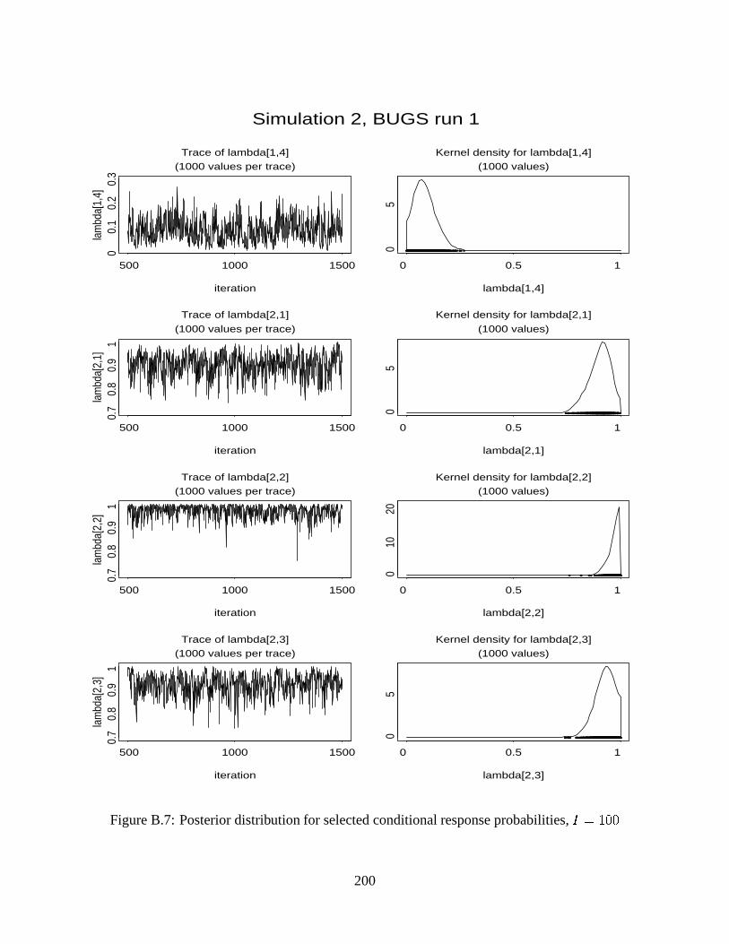
iteration

lam

bda[

1,4]

500 1000 1500

0

0.1

0.2

0.3



lambda[1,4]

0 0.5 1

0 5


(1000 values)

•••• ••• •• •• •• •• •• •••• • ••••••••••••••• • •• •• ••• ••• •••• •• •• •• •••• ••• • •• •• ••• •• • •• •• ••••• •• • ••• •••••• ••• • •••• • • • •••• •• •••• •• ••• •••• ••••• • •• • •• • •••• ••• •• ••• • •• ••• •• •• •• •••• •• ••••• •••••• • ••• ••• •••• •• •• • ••• ••••• •• • •••• ••• ••• ••• •• •••• ••• • ••• ••••• •• ••• •••••• • ••• ••• ••••••• • •• •••• ••• • ••• ••• ••• • •• •••• ••••• •• •••••• • •••• •••• •• • •••••• ••• • ••••• • •• ••• ••• •• •• • •• •• •••• •• ••••• • •••• •••• ••••• •••• ••••••• •• • •• •••• ••• •• •• •• ••• • •• •• •••• ••• •• •• ••• ••• • •••• •••••••• ••• • ••• •• ••• • ••• • •••• ••• •• •• ••• •• •• •• •• • ••• • •• •••• ••• •• ••• • ••••• ••• ••• •••• •• • •••• •••••••••••••• • ••• •••• ••••••• •• • •• ••• ••••• ••• ••• • ••••• ••• •• •• •• •• •• • ••••• ••• •• • •• ••••• •• • ••• ••• •• ••••• •• ••••• • •• •• ••• •• • •••• ••••• ••• •••• •• •••• •• ••• ••••• ••••• • •••• •••• • ••• •• • •• •• • •••••• ••• •••• ••• •••• ••••• ••• •••• ••••• •• •••• ••• •• •• • ••••• •• ••••• ••••• •••••• • •• •• ••• • •••• •• •• ••• •• •••• • •••••• •••• ••• • ••• •• • •••••••• •• ••• •••• ••• •• • •••• • •• •••••• ••••• • •••••• ••• •• • ••• •• •• •••••••••• •• • •••••• •• • •• ••••• • •••••••••• ••• ••••• ••• •••• • •• • ••• • •• ••••• ••• •••• ••• ••• ••• ••• •• •••• •••• ••• ••• •• • •

iteration

lam

bda[

2,1]

500 1000 1500

0.7

0.8

0.9

1



lambda[2,1]

0 0.5 1

0 5


(1000 values)

••• ••• ••••• •• • •• •• • •• •••• • ••• •• • ••••• •• •••• • •••• ••• • •• •• ••• •• • ••• ••• •••• • ••••• •• •••• •••••••• • •••• •• •• •••• •• •• • ••• • •• •• ••• • ••••• •• ••• •• •• •••••• • •• •••• •• •••••• •••• •• ••••• ••• ••• •• •• • •• •• ••• ••• ••• •• •••• •• ••• • •••• • • •••• •• • • •••• •• •• ••••• •••• •• ••• ••• ••••• •• •• •• •• • ••••• •• • •• • ••••••••••• • • ••• • •• ••••• •• ••••• •• •••••••• • •• •••• ••• •• ••• •• •• ••• •••• •••••• •• •• •••• ••••• ••••• •••• ••••• ••• ••• •• •• •• •• •• •• ••••• ••• ••• • • ••• ••••• •••• •• •• ••• •••• •• •• • ••• ••• •••••••• • •••• ••• ••• •• •••• •••••• •• •• •• • •••• •• ••• ••• • ••• •••• • ••• ••• ••••• •• •• •• •••• • ••• ••• ••• • ••• •• • ••• •• •• •••• ••• •• ••• • ••••• • ••• • ••• •••• •• •• •••••• •••• ••••• ••• •••••••• ••• •• •• • ••• •• • •••• ••• •• ••• ••• •• • ••• ••••• ••• • ••• ••••••• • •••• •• ••• ••• •• ••• •• ••• • ••• •••• ••• • ••• • •• ••• • ••••• ••• •• ••• ••••• •• ••• •• • •• •• ••• ••• • ••• • ••••••• •••••• •• ••• ••• • ••• •• ••• •••• •• ••• ••• •••• •• •• ••••• •• ••• •• ••• •• •••• ••••• •••• •• •• • •••• •••• • •• •• •••• •• ••••• •••• ••• • ••••• •• • ••••••• •••••• •• •• •• ••• •• •• ••• • ••• ••• • • •• •••• •••• •••• ••••••••• ••• ••• • •• •••• ••• • •• ••• •• •••• •• •• ••• •••• •••• ••••• ••••••••• ••••• •••••

iteration

lam

bda[

2,2]

500 1000 1500

0.7

0.8

0.9

1



lambda[2,2]

0 0.5 1

010

20


(1000 values)

• •• •••• ••• ••••••••••• ••• •• • •• •• ••• ••••• •••• •• ••• • ••••• •••••• • •••• ••••••••• •• •••••••••• •••• •• •• •••••• •••• ••• ••• • •••••• ••••••••••• •••• ••••• •• ••••••••••• ••••••••• ••••••••••••••• •••• ••• ••• •• •• •• •••• ••••• •••• ••••• •• ••••••••• •••• •••• ••••••••• •••••••••••••••••••••••• •••••••• ••••••• •••••• •••••• •••••••• •••• ••• ••• •••• •••••••• •••• ••••• •• •••• •••••••••• ••••• •• ••••••• • • •••••••••• •• ••• •• ••••••••••••• • •• •••• ••• • •••••• • •••••••• •• •••• ••• •••••••••• •••• ••• ••••• •• •• ••••• •••• •••• •••••••• ••• ••••••• •••••• ••••• •••• ••• ••• ••• •• ••• ••• • •• •••••••• ••• • •••• •• •• • ••• •••••••• ••• •••• •••• •• ••••• ••••• •••• ••••• ••• •• ••• •• ••• • ••••• • •••• •••••• •••••••• ••• •• ••• •••• •• •••• •• •• ••••••••• •• •••• ••• ••• • •• ••••••••• •• ••• ••••••• ••••• •• ••••••••• ••••••••••••• ••••• •• •••• •••••••••• ••••• ••• •••• •••• ••• •••••• •••••• •• • •••• • • ••• ••• ••• • ••••••••• • •• ••••• ••••••••• ••••••• • ••• • ••• • •• •••••• • •• •••• •••••••• ••• •••••••• •• •• ••• •••••• ••• •• • •• •• ••• • ••••••• •••••••• •• •• •••• •• ••• •• •••• ••••• ••••• •• •• •• •••••••• ••••••• ••••••• ••• •• • •• • ••••••••

iteration

lam

bda[

2,3]

500 1000 1500

0.7

0.8

0.9

1



lambda[2,3]

0 0.5 1

0 5


(1000 values)

• ••••••••• ••• •• • •• •••••••••• ••• •• ••• •••• • ••••• •• ••••• •••• •• •• •• •• • •••• ••• • ••• • ••• ••• ••• • ••••••• ••••••• •• •••••• •• ••• •• •••• • • • ••• ••• •• •• •• •• •• ••• ••• •• •• •• ••••• •• ••• ••••••• • • ••••••••• • ••• •• • ••••••• •• ••• ••• ••• • ••••••• •• •• ••• •• • ••• • •• ••••••• •••••• •• ••• • •••• ••• ••• •• • •• • ••••• ••••• •• ••••• ••• •• ••• •• • •• •••• ••• •• •• •• • ••• ••••••• •• • ••• •• •••• ••• • ••• •••• •• •• •• ••••• •• •••••• ••• •• •••••• •••••• ••• • •• ••• •• •• • •••• ••••• •• ••• •• ••• •• ••••••• •••• • ••••••••• ••• • •••• • •• •••• ••• •• • ••• ••• •••••• • ••••• •• •• •••• •• ••• ••••• •••• •• • ••••••• •• ••• ••• • ••• ••• •• •• • ••• • •• ••• •••• • • ••• •• •• • ••• ••••• •• ••••••• • ••• •• • •••• •• •••• • •• •• •••• •• ••••• • •• ••• • •• • ••• •••••• ••• •• • ••••• • ••• ••• •••••• ••• •••••• • • ••• •• ••• ••••• •• • ••• •• ••• •••• •• ••• ••• ••• •••• • ••••••• •• •••• •••• ••••• •• •• ••• • •• ••• •• •••••• • •••• ••• •••• •••• ••• •••• • ••• ••• •••••••• ••• •• ••• •• •• •• •••• • ••• • •• • ••• •••• •• •• •• • •••• •••• •••• • •• • ••• ••• •• ••••• • ••• ••••••••• • •••• •• •• •••• •••• • • ••••• ••• ••••• •••• • ••• • •• ••• ••• ••• ••• ••• •• •••••••• • •• •••• •• •• • •••• ••• • •• •••• •• •• •••• •••••• •••••••• •••• •• •


Figure B.7: Posterior distribution for selected conditional response probabilities, C��E�.�F�200

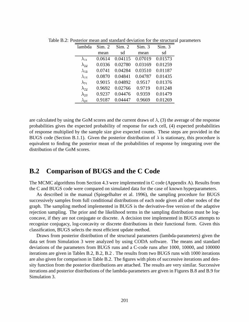
Table B.2: Posterior mean and standard deviation for the structural parameterslambda Sim. 2 Sim. 2 Sim. 3 Sim. 3

mean sd mean sd* �� 0.0614 0.04115 0.07019 0.01573* � � 0.0336 0.02780 0.03169 0.01259* � � 0.0741 0.04284 0.03510 0.01187* � ? 0.0870 0.04841 0.04787 0.01435* �� 0.9015 0.04892 0.9517 0.01376* �� 0.9692 0.02766 0.9719 0.01248* � � 0.9237 0.04476 0.9359 0.01479* � ? 0.9187 0.04447 0.9669 0.01269

are calculated by using the GoM scores and the current draws of * , (3) the average of the responseprobabilities gives the expected probability of response for each cell, (4) expected probabilitiesof response multiplied by the sample size give expected counts. These steps are provided in theBUGS code (Section B.1.1). Given the posterior distribution of * is stationary, this procedure isequivalent to finding the posterior mean of the probabilities of response by integrating over thedistribution of the GoM scores.

B.2 Comparison of BUGS and the C Code

The MCMC algorithms from Section 4.3 were implemented in C code (Appendix A). Results fromthe C and BUGS code were compared on simulated data for the case of known hyperparameters.

As described in the manual (Spiegelhalter et al. 1996), the sampling procedure for BUGSsuccessively samples from full conditional distributions of each node given all other nodes of thegraph. The sampling method implemented in BUGS is the derivative-free version of the adaptiverejection sampling. The prior and the likelihood terms in the sampling distribution must be log-concave, if they are not conjugate or discrete. A decision tree implemented in BUGS attempts torecognize conjugacy, log-concavity or discrete distributions in their functional form. Given thisclassification, BUGS selects the most efficient update method.

Draws from posterior distribution of the structural parameters (lambda-parameters) given thedata set from Simulation 3 were analyzed by using CODA software. The means and standarddeviations of the parameters from BUGS runs and a C-code runs after 1000, 10000, and 100000iterations are given in Tables B.2, B.2, B.2 . The results from two BUGS runs with 1000 iterationsare also given for comparison in Table B.2. The figures with plots of successive iterations and den-sity function from the posterior distributions are attached. The results are very similar. Successiveiterations and posterior distributions of the lambda-parameters are given in Figures B.8 and B.9 forSimulation 3.

201

Table B.3: Posterior mean and standard deviation for the structural parameters, two runs of BUGScode, 1000 iterates

lambda BUGS 1 BUGS 1 BUGS 2 BUGS 2 1 - 2 1 - 2mean sd mean sd mean diff sd diff j� ! � ¢ 0.07019 0.01573 0.070200 0.015700 0.00001 0.00003 j� ! � ¢ 0.03169 0.01259 0.031700 0.012600 0.00001 0.00001 j� ! � ¢ 0.03510 0.01187 0.035100 0.011900 0.00000 0.00003 j� ! � ¢ 0.04787 0.01435 0.047900 0.014400 0.00003 0.00005 ÿ� ! � ¢ 0.95170 0.01376 0.952000 0.013800 0.00030 0.00004 ÿ� ! � ¢ 0.97190 0.01248 0.972000 0.012500 0.00010 0.00002 ÿ� ! � ¢ 0.93590 0.01479 0.936000 0.014800 0.00010 0.00001 ÿ� ! � ¢ 0.96690 0.01269 0.967000 0.012700 0.00010 0.00001

Table B.4: Posterior mean and standard deviation for the structural parameters, 1000 iterateslambda BUGS BUGS C code C code BUGS-C BUGS-C

mean sd mean sd mean diff sd diff � ! � ¢ 0.07019 0.01573 0.070900 0.014900 -0.00071 0.00083 � ! � ¢ 0.03169 0.01259 0.028800 0.012000 0.00289 0.00059 � ! � ¢ 0.03510 0.01187 0.031600 0.012300 0.00350 -0.00043 � ! � ¢ 0.04787 0.01435 0.049100 0.014900 -0.00123 -0.00055 ®� ! � ¢ 0.95170 0.01376 0.952000 0.013700 -0.00030 0.00006 ®� ! � ¢ 0.97190 0.01248 0.969000 0.012700 0.00290 -0.00022 ®� ! � ¢ 0.93590 0.01479 0.937000 0.014800 -0.00110 -0.00001 ®� ! � ¢ 0.96690 0.01269 0.966000 0.012200 0.00090 0.00049

Table B.5: Comparison of the posterior mean and standard deviation for the structural parametersfor BUGS and the C code, 10,000 iterates

lambda BUGS BUGS C code C code BUGS-C BUGS-Cmean sd mean sd mean diff sd diff j� ! � ¢ 0.070600 0.015100 0.070657 0.015166 -0.000057 -0.000066 j� ! � ¢ 0.030000 0.011900 0.029101 0.012229 0.000899 -0.000329 j� ! � ¢ 0.034500 0.012300 0.035208 0.013026 -0.000708 -0.000726 j� ! � ¢ 0.049400 0.014200 0.048782 0.014129 0.0006189 0.000071 ÿ� ! � ¢ 0.951000 0.013400 0.951666 0.013343 -0.000666 0.000057 ÿ� ! � ¢ 0.973000 0.012300 0.972655 0.012119 0.000345 0.000181 ÿ� ! � ¢ 0.936000 0.014300 0.935930 0.014400 0.000070 -0.000100 ÿ� ! � ¢ 0.968000 0.012100 0.968173 0.012026 -0.000173 0.000074

202

iteration

lam

bda[

1,1]

0 500 1000

0

0.1



lambda[1,1]

0 0.5 1

010

20


(999 values)

••••••••••••••• ••••••••• ••• ••••••••••• ••••••• •••••• ••••••••••• •••• ••••••••••••••• •••• ••••••• ••••••••••••• •••••••• •••••••••••••••• •• ••••••••••• •• •••• ••••••••••••••• ••••••••••••••••••••• •••• ••••••••••••••• •••••••• ••••• •••••••••••••••••• ••• •••••••• ••••••••••••••••••••• ••••••••••••••• •••• •••• •••••• ••• ••• •• •••••••••• ••• •• •••••••••• •• •••••••••••• ••••••••••••••••••• •• •••••••••• •••••••••••••••••••••••••••••••••• •••••••••••••••••••••••••••••••••••••••••••••• ••• •• ••••••••••• ••••••••••••••••••••• •••••• ••••••••••••••••••••• ••• ••• ••••••••••••••••••• •••••• •••••••• •••• •••• •••••••••••• ••••••• •••••• • •••••• ••••••• ••••••••• ••••••••••••••••••••••• ••• ••••• ••••••••••••••••••••••• ••••••• ••••• •••••••••••••••• •••••• •••••••••••••••••••••••••••• ••••• •••••• •••••••••••••••••••• ••••••••••••••••••••••••••• ••••••••••••••••••••••• •••• ••••• ••••••• ••••••••••• •• ••••• ••••••••••••• •••• •• •••••• ••••••••• ••••• •• •••••••••• •• •••••••••••• •••••••••• •••••••••••••••• ••••••••• ••••••• •• ••••

iteration

lam

bda[

1,2]

0 500 1000

0

0.05

0.1



lambda[1,2]

0 0.5 1

020


(999 values)

••••••••••••••••••••••••••••••••••••••••••••••••••••••••••••••••••••••••••••••••••••••••• •••••••••••••• •••••••••••••••••••••••••••••••••••••• •••••••••••••••••••••••••• •••••••••••••••••••••• ••••••••••••••••••••••••••••••• ••••••••••• •• •••••••••••••••••••••••••••••••••••••••••••••••••••••••••••••••••••••••••••••••••••••••••••••••••••••••••••••••••••••••••••••••••••••••• ••••••••••••••••••••••••••••••••••••••••••••••••••••••••••••• ••••• •••••••••••••••••••••••• ••••••• ••••••••••••••••••••••••••••••••••••••••••••••••••••••••••••••• •• •••••••••••• •••••••••••••••••••••••••••••••••• ••••••••••• ••••• ••••••••••••••••• •••••••••••••••••••••••••••••••••••••••••••••••••••••••••••••••••••••••••••••••••••••••••••••••••••••••••• ••• ••• •• •••• ••••••••• ••••••••••••••••••••••••••• •••••••••••••••••••••••••• ••••••••••••••••••••••• •••••••••••••••••••••••••••••••••• ••••••••••••••• • •••••••••••••••••••••••••••••••••• ••••••••••••••••••••••••••••••••••••••••••••••••

iteration

lam

bda[

1,3]

0 500 1000

0

0.05

0.1



lambda[1,3]

0 0.5 1

020


(999 values)

••••••••• ••••••••••••••• ••••••••••••••••••••••••••••••••••••••••••••••• •• ••••••••• ••••••••••••••••••••••••••••••••••••••••••••••• •••••••••••••••••••••• •••••••••••••••• ••••••••••••••••••••••••••••••••••••••••• ••••••••••••••••••••••••••••• •••••••••••••••••••••••••••••••••••••• •••••••••••••• ••••••••• •••••••••••••••••••••••••••••••••••••••••••••••••••• •• •••••••••••••••••••••••••• •••••••••••••••••••••••••••• ••••••••••••••••••••••••••••••••••••••• ••••••••••••••••••••••• •••••• •••••••••• ••••••••••••••••••••••••••••••••••• •• ••• •••••••••••••••••••••••••••• •••••• ••••••••••• ••••••••••••••••••••••••••••• ••••• •••••••••• ••••••••••••••••••••••••••••••••••• •••••••••••••••••••••••••••••••••••••••••••••••••••••••••••••••••••••• ••••••••••••••• ••••••••••••••••• •••••••••••••••••••••••••••••••••••••• •••••••••••••••••• •••••••••••••••••••••••••••••••••••••••••••• •••••••••••••• ••••••••••••••••••••••••••••••••••••••••••••••••••• •• ••••••••••••••••• ••••

iteration

lam

bda[

1,4]

0 500 1000

0

0.05

0.1



lambda[1,4]

0 0.5 1

010

20


(999 values)

••••••• ••••••••••••••• •••••••••••••• •••••••••••••••••••••••••••••••••• ••••••••••••••••••••••••••••••••••••••• ••••••••••••••••••• •••• •• •••• •••••••• ••••••••• ••••••• •••••••••••••••••••••••• •• •• ••••••••••• •••••• ••••••••••••••••••••• ••••••••• ••••••••••••••••••••• ••• ••••••••• •••••••••••••••••••• ••••••••••••••••••••••• • ••••• •••••••••••••••••••••••• ••• •••••••• •••••••••••••••••••• ••••••••••• ••••••• •••••••••••••• ••• ••••••••••••••••••••••••••••• ••••••••••••• ••••••••••• •••••••••••••• ••••••••• •••••••••••• ••• ••••••• •••••••••••••••••••• ••• ••••••••• ••••• •••••••••••••••••• •••••• ••••• •••••• •••••••• ••••••••••••••••••••••••••••••• ••••• ••••••••••••••••• •••• •••••••••••••••• •••• •••••••• ••••••••••• •••••••••••••••••••••••••••••••••••••••••••• ••••••••••••••••••••••••• ••••••••••••••• ••••••• ••••••• ••••••••••••••••••••••• •••••••••••••••••••• ••••••••••••••••••••••••••••••••••••••••••••••••••••••••••••••••••••••••••••••••••••••••••••••••••••••••••••••••• •••••••••••••••••••

Simulation 3, Gibbs output from C code

Figure B.8: Posterior distribution for the first extreme profile probabilities, obtained by using Ccode

203

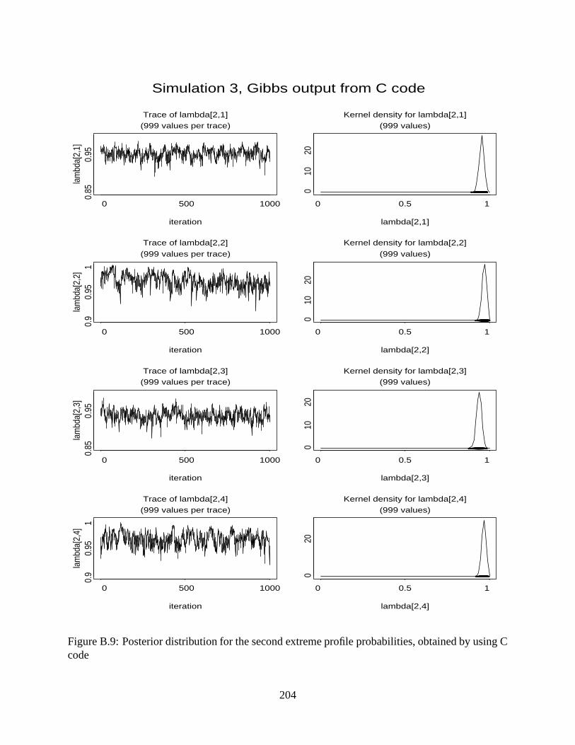
iteration

lam

bda[

2,1]

0 500 1000

0.85

0.95



lambda[2,1]

0 0.5 1

010

20


(999 values)

•••••••••••••••••••••••• •••••• ••••••••• ••••••••• ••••••••••••••••••• ••••••••••• •••••••• •••••••••••• •••••••••••• ••• ••••••••••••••••• •••••••••••• ••••••• •••••••• ••• ••••••• ••••••••••• •••••• •••••••••••• ••••••••••• •••••••••••• ••••••••• •••••• ••••••••••••••••••••••••• ••••••••• ••••••••••••• •••••••••••••• ••••••••••• •••• •••• •••••••••••••• ••••••••••• •••••••• ••••••••••••••••••••••••• ••••••• •••••••••• •••• • •••• ••• •••••••••••••••••••••••• •••• ••••••••••••••••••••• •••••••••••• ••••••••••••• •••••• ••••• •••• •••••••••••••••••• ••••••••••• ••••••••• ••••••••••••••••••••••••••••••••• •••• ••••••••••• •••• •••••••••••••••••••••••••••••••• •••••••••••• ••••••••••••••••••• ••••••••••••• ••••••••••••• •••••••••••••••••••••• •••••••••••••••••••••••••••• •••••••••••• ••••••••••••••••• ••• ••••••••••••••••••• •••••••••• •••••••••••••••••• •••••••••••• •••••••••• ••• •••••••• •••••• •••••• •••••• ••••••••••• •••••••••••••••• •••••••••••••••••••••••••••••••••••••••••••••••••• ••••••••• •• ••••••••••••••••••

iteration

lam

bda[

2,2]

0 500 1000

0.9

0.95

1



lambda[2,2]

0 0.5 1

010

20


(999 values)

•••••••••••••• ••••••••••••••••••••••••••••••••••••••••••••••••••••••••••••••••••••••••••••••••••••••••••••••• •••••••••••••••••••••••••••••••••••••••••••••••••••••••••••••••••• •••••••••••••••••••••••• ••••••• ••••••••••••••• •••••• •••••••••••••••••••••••••••••••••••••••••••••• ••••••••••••••••••••••••••••••••• •••• ••••••••••••• ••••••••••••••••• ••••••••••••••••••••••••••••••••••• ••••••••• •••••••••••••••••••••••••••••••••••••• •••••••••••••••••••••• •••••••••••••• •• ••••••••••••••••••• •••••••••••••••••••••••• ••••••••••••••••••••••••••••••••••••••••••••••••••••••••••••• •••• •• •••••••••••••••••••••••• •••••••••••••••••••••••••• ••• •••••••••••••••••••• ••••••••••••••••••• ••••••••••• •••••••••••••••••••••• ••••••• •••••••••••••••••••••••••••••••••••••••••••••••••••••••• •••• •••••••• •••••••••••••• •••••••••••••• •••••••••••••••• •••••• ••••••••••••••••••• ••••• •••••••••••••• •• ••••••••••••••••••••• •••••••••••••• ••••••••••• ••••••••••••••••••••••••••••••••••

iteration

lam

bda[

2,3]

0 500 1000

0.85

0.95



lambda[2,3]

0 0.5 1

010

20


(999 values)

•••••••••••••• •••••••••••••••••••••••••••••••• ••••••••••••• ••• ••••• •••••••••••• ••••••••••••• •••••••••••••••••••••• ••••••••••• •••••••••• ••••• •• •• •• ••••••••••••• ••••••• ••• ••••••••••• ••••• ••••••• ••• •••••••••••••••• •••••••••••••••••••• ••••••••• ••••••• ••••••••••••••••••• ••••••••••••••••••••••• •••• •• •••••• •••••••••••••••••••••••••••••••••••••• ••••• ••••••• • ••• •••••••••••••• ••••••••••••• ••••••••••••••••••••• •••••••••• ••••••••••• •• ••••••••••••••••••••••••••••••••••••••••• •••••••••••••• ••••••••• ••••••• ••••••••• ••• •• ••••• •••••••••• •• ••••• ••••••••••••••••••••••• ••••••••••• •••• •• •••••••••••••••••••• ••••• •••••• ••••••••• ••••••••••••• ••• ••••••••••••••••••••• ••••••••••••• ••••••••• ••••••••••••••••• ••••••• •••••••••• ••••• ••••• •••••••••••••• ••••••••••••••••• •••• •••• •••• •••••• •••••••••• ••••••••••••••••••••• ••••••••••••••••• ••••• •••••••••• ••••••••••••••••••••••••• ••••• •• •• ••• •••••••••••••••••••••••••••••• •••••• ••••••••• ••••••••••••• ••••••• ••••• •••••••••••••••••• •••••••

iteration

lam

bda[

2,4]

0 500 1000

0.9

0.95

1



lambda[2,4]

0 0.5 1

020


(999 values)

• •••••••••••••••••• ••••••••••••••••••••••• ••••••••••••••••••••••••••••••••••••••••••••••• ••••••••••••••••••••••••••••••••••••••• •••••••••••••••••••••• •••••••• •••••••••••• •••••••• •••• •••••••••• •••••••• ••••••••••••••••••••••••••••••••••••• •••••••••••• ••••••••••• ••••••••••••• ••••••• •••••••••••••••••••••••••••••••••••••••••••••••••• ••••••••••••••••••• ••••••••••••••••••••••••••• •••••••••••••••••••••••••••••••• ••••• •••••••••••••••• ••••• •••••••••••••••••••••••••••••••••••••••••••• ••••••••••••••••••••••••••••••••••••••••••••••••••••••••••••••••••••••••••••••••••••••••••••••• ••••••••••••• ••••••••••••••••••••••••••••••••••••••••• •••••••••••••••••••••••••••••••••••••••••• ••••• •••••••••• ••••••••••••••••••••••••••••••••••••••••••••••••••••••••••••• ••••••••••••••••••••••••••• •••••••••••••• •••• •••••••••••• ••••••••••••••••••••••••••••••••• ••••••••••••••••••••••••••••••••••••••••••••••••• •••••••••••••••••••• •• •• ••••••••••••••••••••••••••• •

Simulation 3, Gibbs output from C code

Figure B.9: Posterior distribution for the second extreme profile probabilities, obtained by using Ccode

204

Table B.6: Comparison of the posterior mean and standard deviation for the structural parametersfor BUGS and the C code, 100,000 iterates

lambda BUGS BUGS C code C code BUGS-C BUGS-Cmean sd mean sd mean diff sd diff � ! � ¢ 0.070293 0.015134 0.070233 0.01525579 0.000060 -0.000122 � ! � ¢ 0.029374 0.012141 0.029103 0.01225231 0.000271 -0.000111 � ! � ¢ 0.034965 0.012853 0.035308 0.01298734 -0.000343 -0.000134 � ! � ¢ 0.049072 0.014057 0.048904 0.01408018 0.000168 -0.000023 ®� ! � ¢ 0.951370 0.013336 0.951329 0.01340884 0.000041 -0.000073 ®� ! � ¢ 0.972480 0.011996 0.972894 0.01197439 -0.000414 0.000022 ®� ! � ¢ 0.936080 0.014363 0.936086 0.01448711 -0.000006 -0.000124 ®� ! � ¢ 0.967730 0.012149 0.96780 0.01211117 -0.000065 0.000038

B.3 Simulation Study with the C Code: Estimating Â �The Metropolis-Hastings step for ` was tested on simulation data for four items, two extremeprofiles with conditional response probabilities 0.05 and 0.95, and Dirichlet(0.1,0.1) distributionof the GoM scores, for sample sizes of 100, 500, 1000, and 10000. Starting values were taken tobe the true values for all model parameters. The chains ran for �2�F�F� iterations, both with fixed andsimulated GoM scores.

The results are summarized in Table B.7. The table provides information about the approximatedistribution of � , given the simulated membership scores and proportions of Dirichlet parameters(0.5 and 0.5 in this case), based on the approximation in equation (4.24). The shape and inversescale parameters of the approximate Gamma distribution are given, and the mean of K is calculatedbased on those parameters. The last two columns in the table give the posterior means of K ,obtained under simulated and fixed GoM scores, respectively.

When the draws are obtained conditional on true membership scores, the posterior means arevery close to the approximate values for all sample sizes. The posterior means are much lowerthan the approximate values for all sample sizes except 10000, when one does not condition of thetrue membership scores. Note that the true � value is 0.2 in this case.

B.4 Simulation Study with the C Code: Estimating Hyperpa-rameters

The objectives of this simulation are to confirm the performance of the C code on a simulated datawhen the hyperparameters, � and 8 , are unknown.

Simulation 3 data were used, and posterior distribution of the hyperparameters and the condi-tional response probabilities were estimated. The prior on � was chosen }Å� �~� �yQP� ! �.�zU , and theprior on 8 was uniform.

205

Table B.7: Approximate posterior distribution parameters and posterior mean of K . Simulationdata with four items, two extreme profiles, LNMROBQ �� ! ��S�VU distribution.

Sample size Shape Ù Inv.scale Ù Mean Ù Mean Ù�Ù Mean Ù�Ù�Ù100 105 550 0.191 0.092 0.181100 105 587 0.182 0.096 0.174500 505 2646 0.191 0.136 0.1941000 1005 5188 0.194 0.138 0.19710000 10005 51447 0.194 0.196 0.199Ù parameters of the approximate posterior distribution for � , given the proportions 8 n of the Dirich-

let parameters and the membership scores 3FX nÙ�Ù�Ù with simulated membership scoresÙ�Ù�Ù with fixed membership scores

Several MCMC trial runs were performed to select the chain length and the values of the tun-ning and thinning parameters. The chain length of 41000 (thinning=5) and the tunning parametersof / �ô�¨� (the tunning parameter for ` ) and �è�ô�¨� (tunning parameter for 8 ), which resultedin about 15% acceptance ratio for each hyperparameter, gave nice convergence results. These val-ues of tunning parameters provided a good compromise between low acceptance ratios and slowmixing of the chain.

The first thousand samplers were discarded as a burn-in. Geweke convergence diagnosticsindicated that all hyperparameters and all conditional response probabilities for the extreme profilesconverged. In addition, the (joint) log-likelihood values were monitored for assessing convergenceof the multivariate posterior distribution. Examination of successive iterations and Geweke statisticfor the log-likelihood indicated convergence of the multivariate posterior distribution.

Given the convergence behavior of the MCMC chains examined for the simulation data, wenotice that the algorithm mixes quite slowly. Therefore, large number of samplers is needed forconvergence. Because of slow mixing, choosing starting values that are likely to be close to thetrue values may speed up the convergence.

Posterior means and standard deviations of the parameters for this example are provided inTable B.4, expected values for each response pattern are provided in Table B.4. Plots of successiveiterations for the hyperparameters are in Figure B.10.

206

Table B.8: Posterior mean and standard deviation for the structural parameters and the hyperpa-rameters: Simulation 3 data

mean sd� 0.1470 0.05348h� 0.4890 0.01598.� 0.5110 0.0159* �� 0.0790 0.0181* � � 0.0378 0.0153* � � 0.0442 0.0153* � ? 0.0576 0.0171* �� 0.9407 0.0167* �� 0.9613 0.0161* � � 0.9251 0.0177* � ? 0.9576 0.0158

Table B.9: Observed and expected frequencies for Simulation 3 data under the GoM model withunknown hyperparameters

Response pattern observed expected1 0000 350 342.882 1000 38 39.193 0100 23 23.304 1100 7 9.565 0010 23 25.086 1010 9 8.587 0110 7 7.898 1110 25 25.859 0001 29 30.77

10 1001 11 10.3311 0101 8 9.6912 1101 39 39.7713 0011 10 8.3814 1011 22 24.6015 0111 31 32.5416 1111 368 361.59

207

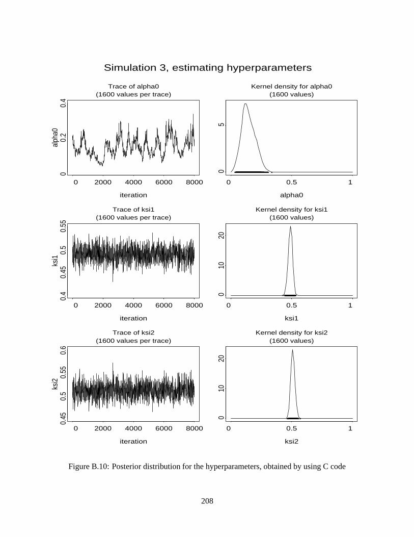
iteration

alph

a0

0 2000 4000 6000 8000

0

0.2

0.4

Trace of alpha0(1600 values per trace)

alpha0

0 0.5 1

0 5

Kernel density for alpha0(1600 values)

••• •• •••••••••••••••• •••••••••••••••••••••••••••••••••••••••••••••••••••••• ••••••••••••••• •••••••••• •• ••••••••••• •••••••••••••••• •••••••••••••••• ••••••••• •••••••• •••••••••••••••••••••••••••••••••••••••• •••••••••••••• ••••••••••••••••• •••••••••••••••• ••••• •••••••••••••••••••••••••••••••••••••••••••••••••••••••••••••••••••••••••••••••••••••••••••••••••••••••••••••••••••••••• ••••• •• •••••• •••••••••••••••••••••••••••••••••••••••••• ••••••••••••••••••••••••••••• •••••••••••••••••••••• ••••••••••••••••••••••••••••••••••••••••• ••••• •• • ••••••••• ••••••••••••••••• ••• •• ••••••••••••••••••••• ••••••••••••••• •••••••••••••••••••••••••••••••••••••••••••••••••••••••••••• ••• •••••• •••••• • •• • •••• •• •••••••••••••• •••••••••••••••••••• ••••••• • ••••••••••••• •••••••• •••••• •••• ••••• ••• •••••••••••• • ••• •• ••••• ••••••••••••••• ••••••••••••••••••••••••••••••• •••• •••••••••••••••••••••••••••••• ••••••• • •••• •••• •••• •••••••••••• ••• •••••••••••••••••••••••••••••••••••••••••••••••••••••••••••••••••••••••••••••••••••••••••••••••••••••••••••• • •••••••••• ••••• •• •••• •••••••••••••••••••••• •••••••••••••• •••••••••••••••••••••••••••••••••••••••••••••••••••••••••••• • •••• ••• •• •••••••••••• • ••• •••••••• ••• ••• ••• • ••••••• ••••••••••••••• • • ••••• •••••••••• • ••• ••••••••••••••••••••••••• •• •••••••• ••••••••••••••••• •••••••••••••••••••••••••••••••••••••••••• ••••••••••••••••••••••••••••••••••••••••••••••••••••••••••••••••••••••••••••••••• •••••••••••• • •••••••••••• ••••••••••••••••• •• • •• •••••••••••• •••••• ••• •••• •• •••••• • •• •••••••••••••

iteration

ksi1

0 2000 4000 6000 8000

0.4

0.45

0.5

0.55

Trace of ksi1(1600 values per trace)

ksi1

0 0.5 1

010

20

Kernel density for ksi1(1600 values)

••• •••• •••• •• ••••••••• • ••••• ••••••••••••• • •••••••••• ••••••••••• •• • ••• ••••••••• ••••••••••• ••• •••••• ••• ••••••• ••• •• •••• ••••••• ••••••• ••••••••• •• ••••• •••• •••• •••• •••••• •••• ••••••••••••••••••••••••• ••••••••••••• ••• ••••••••••••••• •••••••••••••• •• •••••••••• •••••••• ••• •• ••••••• •••• •• ••••••••••• ••• ••• •• ••• •• •••••••• •••••• ••••••••••• ••• •• ••••• •• ••• ••••••••••• ••••• ••• ••••• •••••••• •••• •••••••••• ••••• •••• ••••• •••••••• •••••••••••••••••••••• •••••• ••• ••• ••••••• ••••••••••• ••••••• ••••• ••••••••••••••• •••••••••• ••••••••••• • •••• ••• •••••••••••••••• •••••••••••••••• ••• ••••••••••• •••• ••••• ••• ••••••••••• ••••••• ••• ••• ••••• •••• •••• •• •••••••• •••• ••••••••• ••• ••• •• ••••••• •••••••••• •••••• •••• •••••• ••••• •••• • •• ••• •• ••••••• •• •• •• •••• ••• •••••••••••• •• ••• ••••••• ••••• •••••••••••• ••••••• •••••••••••••••••••• ••••••••••• • ••••••••• ••• •••• ••• •••••• ••••••••• ••• •• ••• •••• •••••• ••• •••• •• •• ••••••••••••••••• •• ••• •• •• •• • ••••••••• •• ••• •• ••• ••••••••• ••••• ••••• •• •••••• ••••••••• •••••• •••••• ••••• ••••• ••••• •••• ••••••••• •••••• •••••••••••• ••••••••••• •• •••••••••••• •••••••••••••••• ••• •• •••• ••••• ••••••••••• ••••••••••••••••••• •• ••••• •••• ••••• ••••• •••• •••••••• • ••••• ••••••••••• ••••••••••••••• •• ••••• •• •• ••••••• •••••••• •••• •••• •• •• •• •••••• ••••••• ••••••• ••• ••••••• ••••••• ••••• •••••• ••••••••• •••••••••••••••••••• •••••• ••••• •••••••• •••••• •••••••• ••• ••••••••••••••••• ••••• ••• •••••••••••••• ••• •••• •• •• ••• •••• ••••• •• ••••• ••••• •••••••••• ••••••••••••• •• ••• ••••••••••• ••••• ••• ••• •• •••••••••••• •••••• • ••••••••••••• •• ••••••• •••••••• ••••• •• •• •• ••• •••••••• •• •• •••• ••••••••••••• •••••• •• •••• •••••••••• ••

iteration

ksi2

0 2000 4000 6000 8000

0.45

0.5

0.55

0.6

Trace of ksi2(1600 values per trace)

ksi2

0 0.5 1

010

20

Kernel density for ksi2(1600 values)

• •••••••• ••• •••• ••••• •••••••• ••••• ••••• •••• ••••• •••••••••••••••• •••• •••••••••••••• •••• •••• ••• •••••• •••• ••••••••• •••••• ••••• •••••• ••••••••••• •••••••••• •••• •••••••• •••••• •• •••••••••• •••••••••••• ••• •• •••••••••• ••• ••• ••••• ••••••• ••• ••••••• •••• • ••••••• •••••••• ••• •••• ••••••• •• •• •••••••••••••• •• ••• ••• •• ••••••• •••• ••••••••••• •••••• •• ••• •• •• ••• ••• ••••••• •••••••• •••••• ••• ••••• •••••• ••• ••••• •••• • •••••• ••••••• ••• •••••••••••••••• •••••• ••• •••• •• •••• •• •••••••••••••••••••••• •••• ••• ••••••••••••••••••••••••• ••••• • •• ••• • •••••• •• •••••••••••• ••••• ••••••••••• ••• ••• ••••••••• ••• • •• ••• ••• ••••••••• •••••••• •••• ••••••••••• ••••• ••• •••••••••• •••• ••••••••• •••• •• ••••• •••••••••••• •••••• ••••• •••••• •••••••••• ••• •• ••• ••••••• •••• •• ••••••••••• • •••••••• •• ••••••• •• ••••• •••• ••••• •••••••• ••• ••• ••••••••••••••••••• •• ••• ••• ••• •••••• ••• •••••• •• ••••••• ••• ••••••• ••• ••••• •• ••••••• ••• ••••• ••••••• •••••••••••• •••• ••• •• •• •••••••••••• ••••• ••• ••• ••••• ••••••• •• ••••• ••••• • ••••••••••• •••• ••••• ••••••••••• ••• ••••••• •••• •••••••••••••••••••••••••••••••• •••••• ••••• •• ••••••••• •••••••••• ••• •••••• ••••••• ••••••••••• •••••••••••• •••••••• •••• •••••••• ••••••••••• ••••••••• •••••••• •••••••• ••• •• •••••• •••••• •• ••• •• •• •• ••••••• •••••••• •••••• •••••• ••••••••••••••••••••••••••••••• •• •••••••••• ••••••••• •••••• ••••• ••••••• ••••• ••• ••••• •••• • ••••••••••••••• ••••• •• •••• ••• •••••••••••••••••• •••••••• ••• •••• • ••• •••• • •• •• ••• ••• • ••••• •• •••••••••• •••••• ••• ••••••••••••• •• ••••• ••• •••••• •••• ••• •••••••• •••••••• •• •••• ••••• ••••••••• •••• ••••••• •• ••••••••• •••• •• •• •• • •••• • •••• •• ••••• ••••••• •••••• •••••••••• ••• •••••• ••••••••

Simulation 3, estimating hyperparameters

Figure B.10: Posterior distribution for the hyperparameters, obtained by using C code

208

Appendix C

List of Triggering questions for 16ADL/IADL Measures

1. ADL eating

(a) About how long has ... had help eating or used special dishes or special utensils?(b) About how long has ... not eaten?

(c) For which of these things did someone usually stay nearby? Eating.

2. ADL getting in/out of bed

(a) About how long has ... had help or used special equipment to get in or out of bed?(b) About how long has ... been unable to get out of bed?(c) For which of these things did someone usually stay nearby? Getting in/out of bed.

3. ADL getting around inside

(a) About how long has ... been unable to get out of bed?(b) About how long has ... had help or used special equipment to get around inside?

(c) For which of these things did someone usually stay nearby? Getting around inside.

4. ADL dressing

(a) About how long has ... been unable to get out of bed?(b) About how long has ... had help dressing or used special equipment or clothing?(c) About how long has ... been unable to dress?

(d) For which of these things did someone usually stay nearby? Dressing.

5. ADL bathing

(a) About how long has ... had help or used special equipment to bathe?

(b) About how long has ... been unable to bathe?(c) For which of these things did someone usually stay nearby? Bathing.

6. ADL toileting

(a) About how long has ... had help using the toilet or used special equipment?

209

(b) About how long has ... been unable to use the toilet?(c) For which of these things did someone usually stand nearby? Getting to the bathroom

or using the toilet.

7. IADL heavy housework

(a) About how long has ... been unable to get out of bed?(b) About how long has ... been unable to get around inside?(c) What is the reason ... cannot do heavy housework around the house - is that because of

a disability or a health problem, or is there some other reason?(d) Does someone regularly help ... with housework and laundry or do housework and

laundry for ...?

8. IADL light housework

(a) About how long has ... been unable to get out of bed?(b) About how long has ... been unable to get around inside?(c) What is the reason ... cannot do light housework around the house - is that because of

a disability or a health problem, or is there some other reason?(d) Does someone regularly help ... with housework and laundry or do housework and

laundry for ...?

9. IADL laundry

(a) About how long has ... been unable to get out of bed?(b) About how long has ... been unable to get around inside?(c) What is the reason ... cannot do ...’s own laundry - is that because of a disability or a

health problem, or is there some other reason?(d) Does someone regularly help ... with housework and laundry or do housework and

laundry for ...?

10. IADL cooking

(a) About how long has ... been unable to get out of bed?(b) About how long has ... been unable to get around inside?(c) What is the reason ... cannot prepare ...’s own meals - is that because of a disability or

a health problem, or is there some other reason?(d) Does someone regularly prepare meals for ... to eat here?

11. IADL groceries shopping

(a) About how long has ... been unable to get out of bed?

(b) About how long has ... been unable to get around inside?(c) What is the reason ... cannot shop for groceries - is that because of a disability or a

health problem, or is there some other reason?

(d) Does someone regularly help ... shop for groceries or do grocery shopping for ...?

12. IADL getting about outside


210

(b) About how long has ... been unable to get around inside?

(c) When ... goes outside, does someone usually help ... get around?

(d) When ... goes outside, does ... use special equipment like a cane or walker or a guidedog to help ... get about?

(e) What is the reason ... does not get about outside? Is it because of a disability or a healthproblem or is there some other reason?

13. IADL traveling


(b) About how long has ... been unable to get around inside?

(c) What is the reason ... does not get about outside? Is it because of a disability or a healthproblem or is there some other reason?

(d) Is the reason ... does not go places outside of walking distance by ...self because of adisability of health problem, or is there some other reason?

14. IADL managing money

(a) Is the reason ... cannot manage ...’s own money because of a disability or health prob-lem, or is there some other reason?

15. IADL taking medicine

(a) Does someone usually help ... take ...’s medicine?

16. IADL telephoning

(a) Is the reason ... cannot make ...’s telephone calls because of a disability or healthproblem, or is there some other reason?

211

Appendix D

SAS Code: Calculating TetrachoricCorrelations

/*Calculating matrix of tetrachoric correlations for pooled data on 16*disability measures.*The 16 measures are: eating, in/out bed, inside mobility, dressing,*bathing, toileting, heavy housework, light housework, laundry, cooking,*grocery, outside mobility, travel, money, medicine, telephone.*The variable numbers are taken from the PNAS paper by Singer and Manton;*/

libname perm ’E:/user/elenae/SAS/data’;Options ls=100 ps=600;

/* include polychor SAS macro */%inc ’E:/user/elenae/SAS/polychor.sas’;

/* since all responses are either present or missing (code 9);* remove missing rows*/data temp;set perm.meas16;if Y1 = 9 then delete;run;

%polychor(data=temp,

var= Y1 Y2 Y3 Y4 Y5 Y6 Y10 Y11 Y12 Y13 Y14 Y15 Y16 Y17 Y18 Y19,out=perm.tetra16corr,type=corr

);run;

Factor analysis: SAS program

libname perm ’E:/user/elenae/SAS/data’;Options ls=100 ps=600;

proc factordata = perm.tetra16corrmethod = prin nfact=3 rotate=varimax preplot plot;

run;

213

Appendix E

BUGS Code for Latent Class Models

#Bugs program for obtaining posterior distribution#for the unrestricted latent class model#with two (K=2) latent classes;#uniform on simplex prior on latent class probabilities;#uniform prior on conditional response probabilities;#random starting values.

#note: for N latent classes, set K=N

# data file must contain IxJ matrix of responses# of I subjects to J items

model

LCM;

constI = 21574, # number of individualsJ = 16, # number of questionsK = 2; # number of latent classes

varresp[I,J], # observed responses (ith subject, jth item)classprob[K], # latent class probabilitiespriorprob[K], # prior parameters for latent class probabilitieslambda[K,J], # item parameters, latent class response probabilitiesz[I]; # augmented latent class indicators

dataresp in "meas16.dat"; # reading the data file

{#model

for (i in 1:I) {z[i] ˜ dcat(classprob[]);

for (j in 1:J) {resp[i,j] ˜ dbern(lambda[z[i],j]);

}}

#priors

classprob[] ˜ ddirch(priorprob[]);

for (k in 1:K){priorprob[k] <- 1;

}


lambda[k,j] ˜ dbeta(1,1);}

}

}

215

Bibliography

Aguero-Torres, H., Hilleras, P. K., and Winblad, B. (2001), Disability in activities of daily livingamong the elderly, Current Opinion in Psychiatry 14, 355–359.

Aitchison, J. (1986), The Statistical Analysis of Compositional Data, Monographs on Statistics andApplied Probability, Chapman and Hall, New York.

Akaike, H. (1973), Information theory and an extension of the maximum likelihood principle, inSecond International Symposium on Information Theory, Petrox, B. N. and Caski, F., eds.,Budapest: Akademiai Kiado, 267–281.

Andersen, E. B. (1970), Asymptotic properties of conditional maximum-likelihood estimators(corr: 71v33 p167), Journal of the Royal Statistical Society, Series B, Methodological32, 283–301.

Baltes, P. B. and Mayer, K. U., eds. (1999), The Berlin Aging Study. Aging from 70 to 100, Cam-bridge University Press.

Barankin, E. W. and Maitra, A. P. (1963), Generalization of the Fisher-Darmois-Koopman-Pitmantheorem on sufficient statistics, Sankhy � A 25, 217–244.

Barer, D. and Nouri, F. (1989), Measurement of activities of daily living, Clinical Rehabilitation3, 179–187.

Bartholomew, D. J. and Knott, M. (1999), Latent Variable Models and Factor Analysis, Arnold.

Bartholomew, D.J., Steele, F., Moustaki, I., and Galbraith, J. (2002), The Analysis and Interpreta-tion of Multivariate Data for Social Scientists, Chapman and Hall/CRC.

Bartolucci, F. and Forcina, A. (2000), A likelihood ratio test for MTP � within binary variables, TheAnnals of Statistics 28, 1206–1218.

Beguin, A. A. and Glas, C. A. W. (1998), MCMC estimation of multidimensional IRT models,Technical report, Department of Educational Measurement and Data Analysis. University ofTwente, The Netherlands.

Benjamini, Y. and Hochberg, Y. (1995), Controlling the false discovery rate: A practical and pow-erful approach to multiple testing, Journal of the Royal Statistical Society, Series B, Method-ological 57, 289–300.

217

Berkman, L., Singer, B., and Manton, K. G. (1989), Black/white differences in health status andmortality among the elderly, Demography 26(4), 661–678.

Best, N., Cowles, M.K., and Vines, K. (1996), CODA: Convergence diagnosis and output analysissoftware for Gibbs sampling output (version 0.30), Technical report, MRC Cambridge, UK.

Blei, D. M., Jordan, M. I., and Ng, A. Y. (2003), Hierarchical bayesian models for applications ininformation retrieval, in Bayesian Statistics 7. Proceedings of the Seventh Valencia Interna-tional Meeting, Bernardo, J. M., Bayarri, M. J., Berger, J. O., Dawid, A. P., Heckerman, D.,Smith, A. F. M., and West, M., eds., Oxford University Press. To appear.

Blei, D. M., Ng, A. Y., and Jordan, M. I. (2001), Latent dirichlet allocation, Advances in NeuralInformation Processing Systems.

Brayne, C. and Johnson, J. B. (1999), Profile of disability in elderly people: estimates from alongitudinal population study, British Medical Journal 318(7191), 1108–1111.

Brooks, S. P., Giudici, P., and Roberts, G. O. (2003), Efficient construction of reversible jumpMarkov chain Monte Carlo proposal distributions, Journal of the Royal Statistical Society,Series B, Methodological. To appear.

Browne, M. W. (2002), Psychometrics, Statistics in the 21st Century 171–178.

Carlin, B. P. and Louis, T. A. (2000), Bayes and Empirical Bayes Methods for Data Analysis,Chapman & Hall.

Chib, S. and Jeliazkov, I. (2001), Marginal likelihood from the Metropolis-Hastings output, Jour-nal of the American Statistical Association 96(453), 270–281.

Clive, J., Woodbury, M. A., and Siegler, I. C. (1983), Fuzzy and crisp set-theoretic-based classifi-cation of health and disease. A qualitative and quantitative comparison, Journal of MedicalSystems 7(4), 317–331.

Corder, E. H. and Woodbury, M. A. (1993), Genetic heterogeneity in Alzheimer’s disease: A Gradeof Membership analysis, Genetic Epidemiology 10, 495–499.

Corder, L. S. and Manton, K. G. (1991), National surveys and the health and functioning of theelderly: The effects of design and content, Journal of the American Statistical Association86, 513–525.

Corder, L. S., Woodbury, M. A., and Manton, K. G. (1992), Loss to follow-up assessment: Ap-plication of grade of membership methods to aged population longitudinal sample loss tofollow-up in the National Long Term Care Survey, in ASA Proceedings of the Section onSurvey Research Methods, American Statistical Association (Alexandria, VA), 357–362.

Corder, L. S., Woodbury, M. A., and Manton, K. G. (1996), Proxy response patterns among theaged: Effects on estimates of health status and medical care utilization from the 1982-1984long-term care surveys, Journal of Clinical Epidemiology 49(2), 173–182.

218

Cowles, M. K. and Carlin, B. P. (1996), Markov chain Monte Carlo convergence diagnostics: Acomparative review, Journal of the American Statistical Association 91, 883–904.

Davidson, J.R.T., Woodbury, M. A., Zisook, S., and Giller, E.L. (1989), Classification of depres-sion by grade of membership: a confirmation study, Psychological Medicine 19, 987–998.

Decision Systems, Inc. (1999), User Documentation for DSIGoM. Version 1.0.

DeGroot, M. H. (1970), Optimal Statistical Decisions, McGraw-Hill.

Dickey, J. M. (1983), Multiple hypergeometric functions: Probabilistic interpretations and statisti-cal uses, Journal of the American Statistical Association 78, 628–637.

Douglas, Jeff (1997), Joint consistency of nonparametric item characteristic curve and ability esti-mation, Psychometrika 62, 7–28.

Eakin, P. (1989), Assessments of activities of daily living: A critical review, The British Journal ofOccupational Therapy 63, 11–15.

Erosheva, E. A. (2001), Comparing latent structures of the Grade of Membership, Rasch and latentclass models, unpublished manuscript.

Erosheva, E. A. (2002), The Grade of Membership model: Latent class representation and impli-cations for Bayesian estimation, unpublished manuscript.

Fienberg, S. E. (1989), Comments on “modeling considerations from a modeling perspective”, inPanel Surveys, Wiley (New York), 566–574.

Fienberg, S. E. and Gilbert, J. P. (1970), The geometry of a two by two contingency table, Journalof the American Statistical Association 65, 694–701.

Fienberg, S. E. and Meyer, M. M. (1983), Loglinear models and categorical data analysis withpsychometric and econometric applications, Journal of Econometrics 22, 191–214.

Fischer, G. H. and Molenaar, I. W. (1995), Rasch Models: Foundations, Recent Developments,and Applications, Springer-Verlag.

Fitzgerald, J. F., Smith, D. M., Martin, D. K., Freedman, J. A., and Wolinsky, F. D. (1993),Replication of the multidimensionality of activities of daily living, Journal of Gerontology48(1), S28–S31.

Freedman, V. and Soldo, B., eds. (1994), Trends in Disability at Older Ages: Summary of a Work-shop, National Academy Press, Washington, DC. Committee on National Statistics.

Freudenheim, M. (2001), Decrease in chronic illness bodes well for medicare costs, The New YorkTimes p. A16.

Good, I.J. (1976), On the application of symmetric dirichlet distribution and their mixtures tocontingency tables, The Annals of Statistics 4(6), 1159–1189.

219

Good, I.J. and Crook, J.F. (1987), The robustness and sensitivity of the mixed-dirichlet bayesiantest for ”independence” in contingency tables, The Annals of Statistics 15(2), 670–693.

Graubard, B. I. and Korn, E. L. (2002), Inference for superpopulation parameters using samplesurveys, Statistical Science 17, 73–96.

Green, P. J. (1995), Reversible jump Markov chain Monte Carlo computation and Bayesian modeldetermination, Biometrika 82, 711–732.

Haberman, S. J. (1977a), Maximum likelihood estimates in exponential response models, TheAnnals of Statistics 5, 815–841.

Haberman, S. J. (1977b), Product models for frequency tables involving indirect observation, TheAnnals of Statistics 5, 1124–1147.

Haberman, S. J. (1995), Book review of ‘Statistical Applications Using Fuzzy Sets’, by KennethG. Manton, Max A. Woodbury, and Larry S. Corder., Journal of the American StatisticalAssociation 1131–1133.

Hambleton, R. K. and Rovinelli, R. J. (1986), Assessing the dimensionality of a set of test items,Applied Psychological Measurement 10(3), 287–302.

Han, C. and Carlin, B. P. (2001), MCMC methods for computing Bayes factors: A comparativereview, Technical report, Division of Biostatistics, School of Public Health, University ofMinnesota, http://www.biostat.umn.edu.

Harris, B. (1982), “Tetrachoric correlation coefficient”, in Encyclopedia of Statistical Sciences,Kotz, Samuel, Johnson, Norman L. (Ed-in-chief), and Read, Campbell B., eds., Vol. 9, JohnWiley & Sons, Inc., 223–225.

Hattie, J. A., Krokowski, K., Rogers, J. H., and Swaminathan, H. (1986), An assessment of Stout’sindex of essential unidimensionality, Applied Psychological Measurement 20(1), 1–14.

Heinen, T. (1996), Latent Class and Discrete Latent Trait Models: Similarities and Differences,Sage, Newbury Park, CA.

Hilbert, D. and Cohn-Vossen, S. (1952), Geometry and the Imagination, Chelsea Publishing Com-pany. New York.

Hoff, P. D. (2000), Constrained nonparametric maximum likelihood via mixtures, Journal of Com-putational and Graphical Statistics 9(4), 633–641.

Hofmann, T. (1999), Probabilistic latent semantic analysis,http://citeseer.nj.nec.com/hofmann99probabilistic.html.

Hofmann, T. (2001), Unsupervised learning by probabilistic latent semantic analyis, MachineLearning 42, 177–196.

Hofmann, T. and Puzicha, J. (1999), Latent class models for collaborative filtering,http://www.cs.brown.edu/people/th/papers/HofmannPuzicha-IJCAI99.pdf.

220

Hoijtink, H. (2001), Confirmatory latent class analysis: Model selection using Bayes factors and(pseudo) likelihood ratio statistics, Multivariate Behavioral Research 36(4), 563–588.

Hoijtink, H. and Molenaar, I. W. (1997), A multidimensional item response model: Constrainedlatent class analysis using Gibbs sampler and posterior predictive checks, Psychometrika62(2), 171–189.

Holland, P. W. (1981), When are item response models consistent with observed data?, Psychome-trika 46, 79–92.

Holland, P. W. (1990a), The Dutch identity: A new tool for the study of item response models,Psychometrika 55, 5–18.

Holland, P. W. (1990b), On the sampling theory foundations of the item response theory models,Psychometrika 55(4), 557–601.

Holland, P. W. and Rosenbaum, P. R. (1986), Conditional association and unidimensionality inmonotone latent variable models, The Annals of Statistics 14, 1523–1543.

Jiang, T. J., Kadane, J. B., and Dickey, J. M. (1992), Computation of Carlson’s multiple hyper-geometric function O for Bayesian applications, Journal of Computational and GraphicalStatistics 1, 231–251.

Johnson, A. R. and Wichern, D. W. (1998), Applied Multivariate Statistical Analysis (Fourth Edi-tion), Prentice-Hall.

Junker, B. W. (1993), Conditional association, essential independence and monotone unidimen-sional item response models, The Annals of Statistics 21, 1359–1378.

Junker, B. W. and Ellis, J. L. (1997), A characterization of monotone unidimensional latent variablemodels, The Annals of Statistics 25, 1327–1343.

Kass, R. E. and Raftery, A. E. (1995), Bayes factors, Journal of the American Statistical Associa-tion 90, 773–795.

Katz, S., Ford, A.B., Moskowitz, R.W., Jackson, B.A., and Jaffe, M.W. (1963), Studies of illness inthe aged. the index of ADL: A standardized measure of biological and psychosocial function,Journal of the American Medical Association 185, 914–919.

Kiefer, J. and Wolfowitz, J. (1956), Consistency of the maximum likelihood estimator in the pres-ence of infinitely many incidental parameters, Annals of Mathematical Statistics 27(4), 887–906.

Kinosian, B. P., Stallard, E., Lee, J.H., Woodbury, M. A., Zbrozek, A. S., and Glick, H. A. (2000),Predicting 10-year care requirements for older people with suspected Alzheimer’s Disease,Journal of the American Geriatric Society 48(6), 631–638.

Kotz, S., Johnson, N. L. (Ed-in-chief), and Read, C. B. (Exec Ed) (1988), Encyclopedia of Statis-tical Sciences (Volume 8), Wiley.

221

Law, M. and Letts, L. (1989), A critical review of scales of activities of daily living, The AmericanJournal of Occupational Therapy 43, 522–528.

Lazarsfeld, P. F. and Henry, N. W. (1968), Latent Structure Analysis, Boston, MA: HoughtonMifflin.

Levin, B. and Reeds, J. (1977), Compound multinomial likelihood functions are unimodal: proofof a conjecture of I.J.Good, The Annals of Statistics 5(1), 79–87.

Lindsay, B., Clogg, C. C., and Grego, J. (1991), Semiparametric estimation in the Rasch model andrelated exponential response models, including a simple latent class model for item analysis,Journal of the American Statistical Association 83, 96–107.

Manton, K. G. and Gu, X. (2001), Changes in the prevalence of chronic disability in the UnitedStates black and nonblack population above age 65 from 1982 to 1999, Proceedings of theNational Academy of Sciences 98(11), 6354–6359.

Manton, K. G. and Singer, B. H. (2001), Variation in disability decline and Medicare expenditures,unpublished manuscript.

Manton, K. G. and Stallard, E. (1988), Chronic Disease Modelling, Charles Griffin.

Manton, K. G. and Stallard, E. (1997), Health and disability differences among racial and ethnicgroups, Racial and Ethnic Differences in the Health of Older Americans. 43–105. Committeeon Population, Commission on Behavioral and Social Sciences and Education.

Manton, K. G., Corder, L. S., and Stallard, E. (1997), Chronic disability trends in elderly UnitedStates populations: 1982-1994, Proceedings of the National Academy of Sciences 94, 2593–2598.

Manton, K. G., Cornelius, E. S., and Woodbury, M. A. (1995), Nursing home residents: A mul-tivariate analysis of their medical, behavioral, psychological, and service use characteristics,Journal of Gerontology 50A(5), M242–M251.

Manton, K. G., Singer, B. M., and Suzman, R. M. (1993), Forecasting the Health of ElderlyPopulations, Springer-Verlag, New York.

Manton, K. G., Stallard, E., and Woodbury, M. A. (1991), A multivariate event history modelbased upon fuzzy states: Estimation from longitudinal surveys with informative nonresponse,Journal of Official Statistics 7, 261–293.

Manton, K. G., Woodbury, M. A., and Tolley, H. D. (1994), Statistical Applications Using FuzzySets, Wiley-Interscience.

Manton, K. G., Woodbury, M. A., Anker, M., and Jablensky, A. (1994), Symptom profiles ofpsychiatric disorders based on graded disease classes: an illustration using data from theWHO International Pilot Study of Schizophrenia, Psychological Medicine 24, 133–144.

222

Manton, K. G., Woodbury, M. A., Stallard, E., and Corder, L. S. (1992), The use of grade-of-membership techniques to estimate regression relationships, Sociological Methodology22, 321–381.

Manton, K.G. and Woodbury, M. A. (1991), Grade of Membership generalizations and aging re-search, Experimental Aging Research 17(4), 217–226.

Manton, K.G., Stallard, E., Woodbury, M. A., and Yashin, A. I. (1986), Applications of the Gradeof Membership technique to event history analysis: extensions to multivariate unobservedheterogeneity, Mathematical Modelling 7, 1375–1391.

Marini, M. M., Li, X., and Fan, P. L. (1996), Characterizing latent structure: Factor analytic andGrade of Membership models, Sociological Methodology 26, 133–164.

Maris, E. (1998), On the sampling interpretation of confidence intervals and hypothesis tests in thecontext of conditional maximum likelihood estimation, Psychometrika 63, 65–71.

Maris, E. (1999), Estimating multiple classification latent class models, Psychometrika 64(2), 187–212.

Marx, R.G., Bombardier, C., Hogg-Johnson, S., and Wrigh, J.G. (1999), Clinimetric and psycho-metric strategies for development of a health measurement scale, Journal of Clinical Epi-demiology 52(2), 105–111.

Mathiowetz, N. A. and Lair, T. J. (1994), Getting better? Change or error in the measurement offunctional limitations, Journal of Economic and Social Measurement 20, 237–262.

McCullagh, P. and Nelder, J. A. (1989), Generalized Linear Models (Second Edition), Chapman& Hall.

Meara, K., Robin, F., and Sireci, S. G. (2000), Using multidimensional scaling to assess the di-mensionality of dichotomous item data, Multivariate Behavioral Research 35(2), 229–259.

Minka, T. and Lafferty, J. (2002), Expectation-propagation for the Generative Aspect Model,http://www.stat.cmu.edu/ minka/papers/aspect.html.

Muthen, B. (1978), Contributions to factor analysis of dichotomous variables, Psychometrika43, 551–560.

Nagi, S. Z. (1965), Some conceptual issues in disability and rehabilitation, In M. Sussman(Ed.),Sociology and Rehabilitation.

Nagi, S. Z. (1991), Disability concepts revisited: Implication for prevention, Disability in America:Toward a National Agenda for Prevention 309–327.

Nandakumar, R. (1994), Assessing dimensionality of a set of item responses - Comparison ofdifferent approaches, Journal of Educational Measurement 31(1), 17–35.

Neyman, J. and Scott, E. L. (1948), Consistent estimates based on partially consistent observations,Econometrica 16, 1–30.

223

Ostir, G. V., Carlson, J. E., Black, S. A., Rudkin, L., Goodwin, J. S., and Markides, K. S. (1999),Disability in older adults 1: Prevalence, causes, and consequences, Behavioral Medicine24(4), 147–156.

Patz, R. J. and Junker, B. W. (1999), A straightforward approach to Markov chain Monte Carlomethods for item response models, Journal of Educational and Behavioral Statistics 24, 146–178.

Pfeirref, D. (1999), The problem of disability definition : Again, Disability and Rehabilitation21(8), 392–395.

Potthoff, R. G., Manton, K. G., Woodbury, M. A., and Tolley, H. D. (2000), Dirichlet generaliza-tions of latent-class models, Journal of Classification 17, 315–353.

Priboth, B. (2001), “Triggering questions for ADL and IADL measures from the NLTCS”, Centerfor Demographic Studies, Duke University. (Personal communication).

Pritchard, J. K., Stephens, M., and Donnelly, P. (2000), Inference of population structure usingmultilocus genotype data, Genetics 155, 945–959.

Ramsay, J. O. (1996), A geometrical approach to item response theory, Behaviormetrika 23, 3–17.

Reboussin, B. A., Miller, M. E., Lohman, K. K., and Ten Have, T. R. (2002), Latent class mod-els for longitudinal studies of the elderly with data missing at random, Jurnal of the RoyalStatistical Society, Applied Statistics 51(1), 69–90.

Reckase, M.D. (1997), The past and future of multidimensional item response theory, AppliedPsychological Measurement 21(1), 25–36.

Research Highlights in the Demography and Economics of Aging (1999). Population ReferenceBureau for the National Institute on Aging.

Rogers, H. J. and Hattie, J. A. (1987), A Monte Carlo investigation of several person and item fitstatistics for item response models, Applied Psychological Measurement 11(1), 47–57.

Rosenbaum, P. R. (1984), Testing the conditional independence and monotonicity assumptions ofitem response theory, Psychometrika 49, 425–435.

Rubin, D. B. (1984), Bayesianly justifiable and relevant frequency calculations for the appliedstatistician, The Annals of Statistics 12, 1151–1172.

Schwarz, G. (1978), Estimating the dimension of a model, The Annals of Statistics 6, 461–464.

Singer, B. (1989), Grade of Membership representations: Concepts and problems, Probability,Statistics and Mathematics: Papers in Honor of Samuel Karlin 317–334.

Singer, B. H. and Manton, K. G. (1998), The effects of health changes on projections of healthservice needs for the elderly population of the United States, Proceedings of the NationalAcademy of Sciences 95(26), 15618–15622.

224

Sonn, U. and Asberg, K. H. (1991), Assessment of activities of daily living in the elderly, Scandi-navian Journal of Rehabilitation Medicine 23, 193–202.

Spearman, C. (1904), General intelligence objectively determined and measured, American Jour-nal of Psychology 15, 201–293.

Spector, W. D. and Fleishman, J. A. (1998), Combining activities of daily living with instrumentalactivities of daily living to measure functional disability, Journal of Gerontology: SOCIALSCIENCES 53B(1), S46–S57.

Spector, W. D., Katz, S., Murphy, J. B., and Fulton, J. P. (1987), The hierarchical relationship be-tween activities of daily living and instrumental activities of daily living, Journal of ChronicalDisability 40(6), 481–489.

Spiegelhalter, D. J, Best, N. G., Carlin, B. P., and van der Linde, A. (2002), Bayesian measures ofmodel complexity and fit, Journal of the Royal Statistical Society, Series B, Methodological64, 1–34.

Spiegelhalter, D., Thomas, A., Best, N., and Gilks, W. (1996), BUGS 0.5: Bayesian inferenceUsing Gibbs Sampling Manual (version ii), Technical report, MRC Cambridge, UK.

Suppes, P. and Zanotti, M. (1981), When are probability explanations possible?, Synthese, Inter-national Journal for Epistemology, Methodology and Philosophy of Science 48, 191–199.

Tanner, M. A. (1996), Tools for Statistical Inference. Methods for the Exploration of PosteriorDistributions and Likelihood Functions (Third Edition), Springer-Verlag.

Teresi, J. A., Cross, P. S., and Golden, R. R. (1989), Some applications of latent trait analysis tothe measurement of ADL, Journal of Gerontology 44(5), S196–S204.

Tesio, L., Granger, C.V., and Fiedler, R.C. (1997), A unidimensional pain/disability measure forlow-back pain syndromes, Pain 63(3), 269–278.

Tolley, H. D. and Manton, K. G. (1992), Large sample properties of estimates of a discrete Gradeof Membership model, Annals of the Institute of Statistical Mathematics 44, 85–95.

van der Linden, W. J. and Hambleton, R. K. (Ed) (1997), Handbook of Modern Item ResponseTheory, Springer-Verlag.

Varki, S., Cooil, B., and Rust, R. T. (2000), Modeling fuzzy data in qualitative marketing research,Journal of Marketing Research XXXVII, 480–489.

Verbeke, G. and Molenberghs, G. (2000), Linear Mixed Models for Longitudinal Data, Springer-Verlag New York, Inc.

Wachter, K. W. (1999), Grade of membership models in low dimensions, Statistical Papers40, 439–457.

Waidmann, T. A. and Liu, K. (2000), Disability trends among elderly persons and implications forthe future, Journal of Gerontology: SOCIAL SCIENCES 55B(5), S298–S307.

225

Ware, J.E., Bjorner, J.B., and Kosinski, M. (2000), Practical implications of item-response the-ory and computerizes adaptive testing - A brief summary of ongoing studies of widely usedheadache impact scales, Medical Care 38(9), 73–82.

Woodbury, M. A. and Manton, K. G. (1982), A new procedure for analysis of medical classifica-tion, Methods of Information in Medicine 21, 210–220.

Woodbury, M. A., Clive, J., and Garson, A. (1978), Mathematical typology: A Grade of Member-ship technique for obtaining disease definition, Computers and Biomedical Research 11, 277–298.

Woodbury, M. A., Corder, L. S., and Manton, K. G. (1993), Change over time: Observational state,missing data, and repeated measures in the Grade of Membership model, in Proceedings ofSection on Survey Methodology, American Statistical Association, Alexandria VA, 888–891.

Woodbury, M. A., Manton, K. G., and Tolley, H. D. (1997), Convex models of high dimensionaldiscrete data, Annals of the Institute of Statistical Mathematics 49, 371–393.

Wunderlich, Gooloo S., ed. (1999), Measuring Functional Capacity and Work Requirements:Summary of a Workshop, National Academy Press, Washington, DC. Committee to Re-view The Social Security Administration’s Disability Decision Process Research, Committeeon National Statistics.

Yuan, A. and Clarke, B. (2001), Manifest characterization and testing for certain latent properties,The Annals of Statistics 29, 876–898.

226

Grade of Membership and Latent Structure Models with ...

Documents

Transcript of Grade of Membership and Latent Structure Models with ...