Journal of Biomedical Informatics 43 (2010) 496–509

Contents lists available at ScienceDirect

Journal of Biomedical Informatics

journal homepage: www.elsevier .com/locate /y jb in

Background adjustment of cDNA microarray images by MaximumEntropy distributions

Christos Argyropoulos a,b, Antonis Daskalakis a, George C. Nikiforidis a, George C. Sakellaropoulos a,*

a Department of Medical Physics, School of Medicine, University of Patras, GR-26504 Rion, Greeceb Renal and Electrolyte Division, University of Pittsburgh Medical Center, A919 3550 Terrace Street Pittsburgh, PA 15261, USA

a r t i c l e i n f o

Article history:Received 13 January 2009Available online 31 March 2010

Keywords:Maximum EntropycDNAMicroarrayImage segmentationImage restorationGene expression

1532-0464/$ - see front matter � 2010 Elsevier Inc. Adoi:10.1016/j.jbi.2010.03.007

* Corresponding author. Fax: +30 2610969166.E-mail address: gsak@med.upatras.gr (G.C. Sakella

a b s t r a c t

Many empirical studies have demonstrated the exquisite sensitivity of both traditional and novel statis-tical and machine intelligence algorithms to the method of background adjustment used to analyzemicroarray datasets. In this paper we develop a statistical framework that approaches backgroundadjustment as a classic stochastic inverse problem, whose noise characteristics are given in terms of Max-imum Entropy distributions. We derive analytic closed form approximations to the combined problem ofestimating the magnitude of the background in microarray images and adjusting for its presence.

The proposed method reduces standardized measures of log expression variability across replicates insituations of known differential and non-differential gene expression without increasing the bias. Addi-tionally, it results in computationally efficient procedures for estimation and learning based on sufficientstatistics and can filter out spot measures with intensities that are numerically close to the backgroundlevel resulting in a noise reduction of about 7%.

� 2010 Elsevier Inc. All rights reserved.

1. Introduction

The advent of complementary DNA (cDNA) microarray technol-ogies enabled the simultaneous and specific [1] assessment of theexpression levels of thousands of genes [2,3]. The basic microarrayprocedure involves hybridization of complementary nucleic acidmolecules, one of which (target) has been immobilized in a solidsubstrate (e.g. glass) using a robotically controlled device (arrayer).Such targets form spots at the vertices of a rectangular lattice onthe solid substrate surface; each spot then serves as a highly spe-cific and sensitive detector of the corresponding gene. It is widelyappreciated that analysis of such datasets is confounded by a num-ber of technical factors which operate at the different stages, of themicroarray pipeline [4]. These factors not only result in as irregu-larities of spot features [5] but also impart the final microarray im-age with a non-negligible background.

The most common procedure for correcting for the presence ofthe background takes place after segmentation of the microarrayimage into spot (foreground) and background (regions), and in-volves the subtraction of an estimate (usually the mean or median)of the latter’s magnitude from the former. Despite the popularity ofthis approach, which is implemented as default in many softwarepackages i.e. Scanalyze [6], UCSF Spot [7], and TIGR’s Spotfinder[8], it is not entirely without problems. Empirical studies have

ll rights reserved.

ropoulos).

shown that this form of subtractive background correction mayhinder the ability to detect differential gene expression [9–11]and impact the performance of signal calibration algorithms[12,13]. Even more concerning is the fact that different methodsused to extract a sufficient statistic for the magnitude of the back-ground show very little agreement among them [14]. To overcomethese objections, alternative approaches for background correctionhave been put forward, e.g. subtractive correction using an esti-mate of the global rather than the local image background [9],morphological opening filters [14] and post-segmentation probabi-listic subtractive methods [10].

A common feature of the aforementioned methods is that theyfail to explicitly acknowledge extraneous constraints stemmingfrom the discrete bounded nature of the microarray image scale,the positivity as well as the different magnitude of hybridizationphenomena across cDNA microarrays. The most common manifes-tation of this error of omission is the generation of negative valuesin gene expression profiles, in direct contradiction to the physics ofthe experiment (additivity of fluorescent sources) and the acquisi-tion apparatus (digital positive scale). To counteract such effects, anumber of intuitive ad hoc solutions have been proposed. Theserange from arbitrarily setting negative corrected foreground val-ues to one [11], to a small percentile of the expression of all otherspots [15] and finally running the analysis without backgroundcorrection.

In the present work we take a different approach to the problemof background adjustment and propose a statistical correction

C. Argyropoulos et al. / Journal of Biomedical Informatics 43 (2010) 496–509 497

algorithm that is constrained by the discrete bounded nature of themicroarray image scale and the additivity of fluorescent sources.Under a set of weak assumptions about the global backgroundnoise of a microarray image we derive an approximation to the un-known distribution of this error source using the method of Maxi-mum Entropy [16,17]. This approximation is used to (a) estimatethe magnitude of the background noise by segmenting the imagehistogram and (b) correcting individual pixels for the presence ofnoise using the maximum likelihood estimator. To illustrate theeffects of our approach we apply it on publicly available microarrayimage sets and compare its effects to the default subtractive ap-proach. It is shown that the technique presented may have signif-icant benefits in terms of decreasing the bias and variance ofreplicate measurements under conditions of non-differential anddifferential gene expression.

2. Methods

2.1. Attributes of signal and background in microarray images

In this section we discuss the general attributes of the signaland the background in a microarray image that are encoded inthe background adjustment algorithm. These attributes are:

(1) The intensity values for all pixels in a microarray image areexpressed in a discrete, positive, integer scale with M + 1 ele-ments (e.g. M = 65,535 for a 16 bit image).

(2) The observed intensity level (D) of each pixel in the micro-array image obeys the additive noise model:

D ¼ Sþ Bj0 6 D 6 M ^ 0 6 S 6 M ^ 0 6 B 6 M ð1Þ

In this equation, S denotes the signal generation process,whereas B stands for the background process.

(1) The latent (unobserved) components of Eq. (1) are generatedby distinct physical processes in a microarray image. Thesignal generating process is due to the specific hybridizationbetween labeled mRNA species and spotted target mole-cules. The background process results from a combinationof non-specific hybridization phenomena, presence of non-cDNA fluorescent molecules, and diffusion of labeledparticles.

(2) Each microarray image can be segmented into two classes ofpixels i.e. foreground or spot (IS) and non-spot (background,IB).

These four statements may be viewed as cogent prior informa-tion that should be taken into account in describing the processesthat operate on microarray images. Such information is also rele-vant in specifying a mathematical error model for the intensitiesof microarray pixels, and a set of constraints regarding the vari-ables that appear in this model. For example the first statementsummarizes the features of the measurement apparatus used togenerate microarray images. The optical instruments that are usedare digital devices that generate positive images with finite dy-namic range (M) that is specific to each system. Fluorescent inten-sities that fall below the lower detection limit are set to zero, whilepixel intensities that exceed the upper detection limit are set to M.

The second statement specifies a constraint for the additivenoise model i.e. that the magnitudes of the latent processes shouldbe positive entities. Due to the finite range of microarray imagesthis particular additive model implies the existence of saturationphenomena. As the data (D) and the generating processes (S, B)an constrained to lie in the set of positive integers f0; 1;2; . . . ; Mg, an increase in the intensity of the noise will shift the re-

corded pixel intensity upwards. If that value is larger than theupper cutoff of the measurement apparatus, the intensity recordedwill saturate to M.

The fourth statement postulates the existence of a unique classassignment or labeling (L) of all distinct pixel intensities in the his-togram of a microarray image (IH) into two distinct classes IS and IB.Such a classification can be justified as follows: if a particularintensity belongs to the background class, then the magnitude ofthe S component of that pixel is zero. More formally we have thatL ¼ IB ) S ¼ 0 for each pixel in the image and this logical equiva-lence relation determines the following conditional class assign-ments: P(S|L = IB) = 0 for S – 0 or P(S|L = IB) = 1 for S = 0.

2.2. Maximum Entropy distributions for cDNA microarray images

The general attributes discussed in the previous sections con-strain the distributions for the spot and background processes ina finite sub-set of the non-negative integers. Since the support ofthe distributions is bounded from below (non-negativity of fluores-cent signals) and above (finite dynamic range of the measurementapparatus), the domain of support of the unknown distributions isbounded. As a consequence, these distributions could be uniquelycharacterized by their power moments i.e. the infinite sequence ofreal numbers: lk ¼

PMx¼0xk � pðxÞ for background and spot, respec-

tively [18]. On the other hand recovering of a probability densityof which a finite number of moments is known, is an in-deter-mined problem as there are, in general, an infinite variety of func-tions with the same first n moments. To stabilize the problem it isnecessary to impose some further condition which will act as aconstraint within the infinite dimensional function space and leadto a unique solution. The Maximum Entropy (MaxEnt) approach of-fers a definite procedure for the reconstruction of this approximantby selecting the distribution that maximizes the entropy H[p]functional:

H½p� ¼ �XM

x¼0

pðxÞ log pðxÞ ð2Þ

under the condition that the first m moments be equal to the truemoments. Such constraints are expressed in the form of numericalvalues regarding the expectations of functions of a discrete random(uncertain) variable x. By employing standard variational analysisarguments involving Lagrange multipliers it can be proved [19,20]that the MaxEnt distribution assumes the form:

pi � pðxiÞ ¼1Z

expð�Xm

j¼1

kjxjÞ;

Z �XM

x¼0

exp �Xm

j¼1

kjxj

!; lk ¼ �

@ log Z@kk

ð3Þ

In applications the values of the Lagrange multipliers are com-puted by equating the theoretical moments lk to the finite samplemoments of the same order. From an implementation standpoint,entropy maximization corresponds to a convex optimization prob-lem [21] whose unique solution i.e. the values of the Lagrange mul-tipliers kk may be obtained by efficient numerical algorithms evenfor spaces of extremely high dimensionality [22]. Even though thequality of the approximation to the unknown distribution in-creases with the number of moment constraints imposed [23], inpractice a very small number of moments (e.g. one or two) is suf-ficient for the purpose of the background adjustment of microarrayimages as we show in Section 4.

2.3. Specification of the background adjustment algorithm

Having established the constraints on the domains of definitionof the latent components S, B and the corresponding entropic

498 C. Argyropoulos et al. / Journal of Biomedical Informatics 43 (2010) 496–509

approximations we turn our attention to the problem of back-ground correction of a single microarray image. Since we are con-cerned with correcting for the presence of a global background, thedevelopment we will pursue from this point only considers theintensities of the image pixels and not their position within the im-age. Equivalently we will work with the histogram of the micro-array image (IH) defined as a vector of length M + 1 whose ithelement is equal to the number of pixels in the image with inten-sity equal to i. (ni) i.e. IH = {n0, n1, . . ., nM}. The components of a back-ground adjustment algorithm are the following:

� The functional form of the MaxEnt approximations pB (�jkB)and pS(�jkS) for spot and background, respectively, parameter-ized by the Langrangian vectors kB ¼ fkB;1; kB;2; . . . ; kB;mg andkS ¼ fkS;1; kS;2; . . . ; kS;vg with m the number of momentconstraints.� A procedure for the estimation of the parameters kB and kS from

the data of the image histogram.� A procedure for the classification of the intensity levels into

background (IB) and spot classes (IS). Such a classification maybe written as LH={l0, l1, . . ., lM}, where li = 1 if the ith histogramlevel has been classified as signal and li = 0 if it has been classi-fied as background.� An estimator for the intensity of the latent component S for all

intensity levels in the histogram. This estimator is conditionalon the classification of each intensity level that was determinedin the previous step. For intensity levels classified into the IB

class S is zero by definition, so we set S ¼ 0. For intensity levels(D) classified into the IS class, S can be calculated by the ‘‘plug-in” estimator: S ¼ D� lB;1, i.e. the difference between D and theestimate for the mean of the background distribution.

The parameters kB, kS and LH can be estimated simultaneouslyby adopting a ‘‘missing data” perspective which considers the his-togram class labels (LH) as missing descriptors of the process (spotor background) that most likely generated the various intensitylevels. By introducing the ‘‘missing data” descriptors, the secondand the third components of the background adjustment algorithmcan be implemented by iterating the steps of the Expectation–Maximization algorithm (EM) [24]. At convergence the EM willalso provide an estimate for the first moment of the backgroundprocess (lB;1) as the sample mean of the intensity levels that havebeen classified to the IB class. The steps of the background adjust-ment algorithm can be summarized as follows:

1. Initialization:a. Calculate initial values for the probabilities of the IS, IB clas-ses P(IS), P(IB). Assuming an ideal and circular spot geometryof diameter d, the ratio of the two probabilities K = P(IS)/P(IB)can be expressed as K = 4WH/Qpd2 � 1 where Q is the numberof spots, while W, H are the width and the height of the image(measured in pixels), respectively. Then P(IS)0 = K/(K + 1) andP(|IB)0 = 1/(K + 1).b. Label the pixels in the lower 1/(K + 1) quantiles of the im-age histogram as background and the remaining as signaland calculate the sample power moments fl1; . . . ; lvg forthe two classes.c. Calculate the values of the vectors of parameters k0

B andk0

S by maximizing the entropy functional: H ¼ log Zðk1; . . . ; knÞþ

Pmj¼1kjlj for each probability mass function

pB (�jkB) and pS(�jkS) separately. The moment constraintsused in the entropy maximization, are the ones computedin the previous step.

2. Labeling (Expectation–Maximization). For each intensity le-vel in the microarray image we iterate the following steps untilthe parameter estimates do not change in successive iterationsby a fixed% (e.g. 0.001%).

a. jth Expectation step: For the ith intensity level of the micro-array image calculate the expected values of the indicators li as:

E½Ii;B�j ¼pBðijk

j�1B ÞPðI

j�1B Þ

pBðijkj�1B ÞPðI

j�1B Þ þ pSðijk

j�1S ÞPðI

j�1S Þ

; E½Ii;S�j

¼ 1� E½Ii;B�j ð4Þ

b. jth Maximization step:1. Calculate the probabilities of the two classes as

PðIjBÞ ¼

1W � H

XM

i¼0

niE½Ii;B�j; PðIjSÞ ¼ 1� PðIj

BÞ ð5Þ

2. For k in {1, . . ., m} calculate the moment constraints:

ljB;k ¼

PMi¼0

ni � ik � E½Ii;B�j

PMi¼0

E½Ii;B�j; lj

S;k ¼

PMi¼0

ni � ik � E½Ii;S�j

PMi¼0

E½Ii;S�jð6Þ

3. Calculate new values for the Langrangian vectors kB andkS using Newton’s algorithm [22,25] in order to maximize the en-tropy of each distribution separately.

3. Background correction: After the EM algorithm has converged,the estimators S for each pixel intensity are calculated as:

E½Ii;s�conv P E½Ii;B�conv ) S ¼ i� lconvB;1

E½Ii;s�conv< E½Ii;B�conv ) S ¼ 0 ð7Þ

The estimators S are then used to create a new image which hasbeen adjusted for the global background. This restored image canbe processed by the same microarray software suites as the originalimage for the purposes of segmentation, spot finding and genequantification.

2.4. Comparative evaluation of background adjustment strategies

We evaluated the proposed background adjustment algorithm(abbreviated as EM/MAXENT from now on) to two widely usedstrategies for background adjustment:

� Strategy SBC: This method corresponds to the traditionalapproach of background correction by subtraction of a local esti-mate for the background at each spot from the correspondinggene expression measure after image segmentation and spotidentification.� Strategy NONE: The images are not adjusted for the presence of

the background. The gene expression measures originating fromthe image segmentation software are used verbatim for furtheranalyses.

The three strategies were compared in terms of their bias/vari-ance characteristics using spots by utilizing: (a) negative controlspots printed in the surface of microarrays (single channel assess-ments) (b) all spots in self–self hybridizations (two channel assess-ments) (c) under experimental conditions associated with knowndifferential expression (e.g. deletion mutants/antisense mRNAexperiments). In the first case the ‘‘true” intensity of the spots is zero,while in the second case the log-expression ratio should be zero forall gene probes spotted in the surface of the microarray. In the lastcase the expected log-expression ratio will deviate from zero forthese spots approaching the limit of detection for a particular exper-imental setup. Consequently depending on the specificity of thetargets used one should expect to get a very small value for the cor-responding gene expression ratio. Hence a technique that introducesa smaller bias should lead to more negative values for these particu-lar spots. In the presence of simultaneous measurements of gene

C. Argyropoulos et al. / Journal of Biomedical Informatics 43 (2010) 496–509 499

expression changes by a non-microarray technique (e.g. RT-PCR), thebias introduced by background adjustment strategies could bequantified more accurately comparing the expression ratios to thevalues obtained by the gold standard technique.

In order to quantify the bias and variance introduced by the var-ious background adjustment algorithms, we calculated the devia-tions of gene expression measures from their true value usingreplicate measurements. For negative control spots in any experi-ment and all spots in self–self hybridization experiments, the nor-mal theory empirical estimates of the bias and variance are givenby the average and root mean squared from the true value (xTrue)of zero:

BiasNormal ¼1

NiNj

Xj

Xi

ðxi;j � xTrueÞ ¼1

NiNj

Xj

Xi

xi;j ¼ x ð8Þ

VarianceNormal ¼ffiffiffiffiffiffiffiffiffiffiffiffiffiffiffiffiffiffiffiffiffiffiffiffiffiffiffiffiffiffiffiffiffiffiffiffiffiffiffiffiffiffiffiffiffiffiffiffiffiffiffiffiffi

1NiNj

Xj

Xi

ðxi;j � xTrueÞ2s

¼ffiffiffiffiffiffiffiffiffiffiffiffiffiffiffiffiffiffiffiffiffiffiffiffiffiffiffiffiffiffiffiffiffiffiffiffiffiffiffiffiffiffiffiffiffiffiffiffiffiffiffiffiffiffiffi

1NiNj

Xj

Xi

xi;j ¼ RMSðxÞs

ð9Þ

where i and j index the spots in an array and the arrays in an exper-imental dataset.

These measures coincide with the average and the root meansquare error summary statistics from the sample of replicate val-ues. Since these statistics are not robust with respect to deviationsfrom normality, we also report their robust theory alternatives [26]:

BiasRobust ¼ medianðfxi;j � xTruegÞ ¼ medianðfxi;jgÞ ð10Þ

VarianceRobust ¼1

NiNj

Xj

Xi

xi;j � xTrue

�� �� ¼ 1NiNj

Xj

Xi

xi;j

�� ��¼ MAEðxÞ ð11Þ

which coincide with the sample median and the mean absoluteerror, respectively. To apply these formulas for negative controlspots, we let xi,j stand for the un-normalized, raw intensity ob-tained after image analysis. In the case of self–self hybridizationexperiments xi,j is the log-transformed channel expression ratioafter a suitable global normalization transformation.

In other categories of control spots (e.g. salmon sperm DNA,hybridization buffer or carryover negative control spots) found inmicroarray images, the true value (xTrue) of the hybridization signalis likely to be different from zero. For such control spots, the sam-ple mean and median do not coincide with measures of bias (sincexTrue is unknown). However, the sample mean and median can stillbe used to rank background adjustment strategies, since these sta-tistics are location measures for the residual error after noisereduction by background adjustment. Furthermore, measures ofdispersion around the mean and the median do provide an empiricassessment of the performance variability of each backgroundadjustment strategy and thus of variance. Assuming normally dis-tributed measurements, variability around the mean is quantifiedby the sample standard distribution:

S ¼ffiffiffiffiffiffiffiffiffiffiffiffiffiffiffiffiffiffiffiffiffiffiffiffiffiffiffiffiffiffiffiffiffiffiffiffiffiffiffiffiffiffiffiffiffiffi

1NiNj

Xj

Xi

ðxi;j � xÞ2s

ð12Þ

The mean absolute deviation from the sample median (MAD-MD) and the median absolute deviation (MAD) are measures ofscale that are robust with respect to deviations from normalityand can be used to quantify variability around the median:

MADMDðxÞ ¼ 1NjNj

Xj

Xi

jxi;j �medianðxi;jÞj ð13Þ

MADðxÞ ¼ medianðjxi;j �medianðxi;jÞjÞ ð14Þ

A more formal assessment of the noise reduction properties ofthe different background adjustment algorithms in the case of

known differential expression is afforded by variance component(VarComp) or mixed-effects models. In their most general use,mixed-effects models are utilized to describe relationships be-tween a response variable (log-expression ratio in our case) andcertain explanatory covariates and/or grouping (classification) fac-tors in the data. VarComp models have been previously utilized tonormalize microarray experiments (in the form of analysis of var-iance (ANOVA) [27,28], and linear mixed models (LMM) [29]). Theyhave also been used to detect differential expressions whileaccounting for global (experimental conditions, print-tip or dye ef-fects) as well as gene specific sources of variability [28,30–33]. Thestatistical analysis of different background adjustment strategiesmay be undertaken by linear models that incorporate (a) fixed ef-fects (type of algorithm used), which are associated with an entirepopulation or with certain repeatable levels of experimental fac-tors and (b) random effects, which are associated with individualexperimental units (array) drawn at random from a populationand heteroscedastic error arising from different probes and algo-rithms. Assuming a gene that is quantified by Ni different probesin the surface of a single microarray, Nk repetitions of an experi-ment that quantifies the relative expression of that gene in twochannels (e.g. red and green) and Nj different background algo-rithms (3 in this case) to process the same images, we can invokethe following model for the log-expression ratio of gene yi;j;k:

Yi;j;k ¼ bj þ bk þ ei;j;k bk � Nð0;r2bÞ ei;j;k � Nð0;r2

i;jÞ ð15Þ

In the aforementioned equation, bj is the gene expression ratioestimated by each of the Nj algorithms (fixed effect), while bk is therandom effect representing the deviation of the kth replicate fromthe population mean bj. Finally, ei;j;k is a random variable modelingthe error in the replicate measurements from each microarray aris-ing from using multiple arrays and background adjustment algo-rithms. Stated in other terms, the variance terms in Eq. (15) r2

b

and r2i;j thus characterize the ‘‘between-array” and ‘‘within-array”

variability. As a first approximation, one can postulate that thetwo sources variability implicit in r2

i;j are independent and thusthis term factorizes as a product of two variances (p. 209, 213 in[34]): r2

i;j ¼ r2i;�r2

�;j. By fitting these models to replicated datasetsanalyzed by different background methods one can account forthree major sources of variability arising from differences in indi-vidual arrays (r2

b), replicate spots within each array (r2i;�) and pos-

sibly heteroscedastic algorithm error (r2�;jÞ.

A model based analysis of different background adjustmentalgorithms would then directly compare the fixed effects coeffi-cients bj to the log-expression ratio estimated by a gold standardtechnique to ascertain the bias. Additionally, the variances due tothe use of different algorithms may be quantified by examiningthe variances of each background adjustment algorithmr2�;jj ¼ 1; 2; 3. Statistical tests of significance (or equivalently con-

fidence intervals) may be applied on both bias and variance termsto formally compare the performance of the various algorithms.

3. Materials

3.1. Microarray datasets, image segmentation and normalization ofgene expression profiles

We applied the proposed background correction methods in thefollowing microarray datasets from the Stanford Microarray Data-base (Table 1):

a. The images from the DeRisi et al. experiment concerning theDiauxic shift of Saccharomyces cerevisiae [35].

b. Fourty self–self hybridizations obtained from the qualitycontrol program of the Arabidopsis Functional Genomics

Table 1Microarray datasets utilized.

Microarrayexperiment alias

SMD experiment set ID (experimentslide ID)

Number ofmicroarrayslides

Type and number ofcontrol spots per array

Design and replication structure Experimentyear

‘‘Diauxic” [35] 8 (NA) 7 ‘‘Empty” (82) Common Reference Sample(Cy3) 1997‘‘AFGC” [36,37] NA (10,750–10,789) 40 ‘‘SSDNA” (576) Self–self Hybridization Experiments. 8

plant clones in addition to the SSDNA2000

‘‘BAT3” [38] 3898 (45,331, 47,648, 45,415, 46,205,46,206, 46,271, 46,270, 47,647,45,414, 47,644, 48,824, 48,825),45,330, 47,645, 48,826, 49,842,48,884)

19 ‘‘Empty” (192) Hybridizations of HeLa cells expressingthe tetracycline transactivator againstHeLa cells transfected with sense (13/19)and antisense (6/19) clones for the humanBAT3 (HLA-B-associated transcript 3) gene

2003

‘‘Cholera” [39] 3833 (62,120, 62,121, 62,122, 62,123,50,958, 50,959, 50,960, 50,607,50,609, 50,966, 50,963, 50,964,50,965)

13 ‘‘Empty” (16)‘‘3XSSC” (176)‘‘SSDNA” (48)‘‘Carryover” (32)‘‘rRNA” (32)‘‘Chromosomal DNA”(80)

Common Reference Sample (wild type V.Cholerae at stationary growth phase)Comparison Channel:� Deletion Mutant for rpoS (stationary

phase alternative sigmafactor) (9/13)� Mid Log phase (4/13)

2004

‘‘Heat shock” 3207 (32,129–32,132) 4 ‘‘Empty” (64) Common Reference Sample (Cy3) againstnon heat stressed (2/4) and heat stressedE. histolytica (2/4)

2005

Characteristics of microarray datasets, control spots and replication numbers of microarray datasets utilized in the present study. The first column lists the alias used in thetext to refer to each microarray experiment.

500 C. Argyropoulos et al. / Journal of Biomedical Informatics 43 (2010) 496–509

Consortium project [36,37]. In this large technical replica-tion experiment, eight clones were spotted along with Sal-mon Sperm DNA (SSDNA) 576 times on the surface of themicroarray.

c. A sub-set of 19 hybridizations from a recent analysis [38] ofthe role of the BAT3 protein (HLA-B-associated transcript 3)in the pathogenesis of the African Swine Fever Virus.

d. A sub-set of 13 hybridizations from an analysis [39] of therpoS (stationary phase alternative growth factor) contribu-tion to the virulence of V. cholera.

e. Finally, a publicly available experiment assaying the heatshock response of the human protozoan parasite Entamoebahistolytica (total four images, two from heat stressed and twofrom non-heated parasites).

Microarrays in all five experiments utilized at least one negativecontrol spot (blank spots, SSDNA spots, 3XSSC spots) allowing theassessment of the biases introduced by the background adjustmentalgorithms in microarray signal detection process. One experiment(‘‘Cholera”) also used positive (rRNA spots, chromosomal DNA) andnon-specific hybridization controls (carryover spots) allowing amore detailed assessment of the noise suppression properties ofthe proposed algorithm. The degree of replication and the identityof the eight non-control targets used in the experiment from theAFGC facilitated the analysis of bias and variance of gene expres-sion ratios across a wide range of mRNA concentrations (from tran-scription factors to metabolic genes).

For two of the datasets (BAT3 and Cholera), additional informa-tion permitted an exploration of the bias/variance properties of thethree background adjustment algorithms in situations of biologicalsignal change. In the case of the BAT3 dataset, the authors hadquantified and reported the changes in BAT3 mRNA resulting fromstable transfection of sense and antisense clones under the sameconditions used in the microarray experiments. In the Cholera data-set, wild type strains in the mid log phase and deletion mutants forthe rpoS gene at the stationary phase were compared against wildtype strains at the stationary growth phase. Since rpoS is inducedat conditions of metabolic stress found in the stationary growthphase [40,41], the two comparisons involve biological states wherehybridization signals for the rpoS targets are very low or absent(wild type in mid log phase/deletion mutants in stationary phase)versus those which are present (wild type strains growing in sta-tionary phase).

For these datasets the raw microarray images were downloadedfrom SMD with the exception of the Diauxic set that was down-loaded from the MicroArray Genome Imaging and Clustering Tool(MAGIC) website [42] (http://www.bio.davidson.edu/projects/ma-gic/magic.html).

Wherever available, gridding information was extracted fromthe GenePix Results (GPR) files stored for each microarray imagein the SMD. Microarray images were then segmented with theseeded region growing algorithm implemented in the softwareSPOT [14]. To implement the EM/MAXENT strategy, backgroundadjusted images were processed by SPOT, while the originalimages were used for the SBC and NONE algorithms. For the SBCalgorithm, the mean of the background region was subtracted fromthe mean foreground value for each spot after the images had beensegmented. Unless stated otherwise, the channel median was usedas a measure of gene expression. Comparisons with empty spots(‘‘zero”) were carried out in the raw microarray scale, while loga-rithms (base 2) were taken prior to analyzing the results of allother spots in order to symmetrize the scale and improve the nor-mality of measurements. Non-positive measurements generatedby SBC and EM/MAXENT were excluded from analyses in the logtransformed scale. cDNA targets mapping to the same gene weremodeled as independent and identically distributed variates in lin-ear mixed model regressions.

In order to normalize the gene expression profiles we used theglobal median normalization method applied to a single channel orboth channels separately after log-transformation. More advancednormalization algorithms (e.g. lowess [43]) that propose correc-tions for spatial, intensity and dye dependent biases were not uti-lized for the comparison of control spots in this report, since suchalgorithms would hinder our ability to detect subtle biases intro-duced by the proposed method. Normalization implicitly assumesthat the majority of the log-expression ratios is zero and effects alocal correction to the raw data to shrink them back to the null.Lowess is a very effective way to effect this correction in a mannerthat exploits regional features in the M–A plots of any given micro-array hybridization. Hence, if the proposed method introduces anybiases, they would likely be masked by the application of advancednormalization algorithms. On the other hand, model basedcomparisons were carried out with both normalization methodsto assess the behavior of the proposed method under conditionssimilar to typical microarray analysis practice. All statistical analy-ses were carried out in R version 2.9.1 running on Linux Ubuntu

C. Argyropoulos et al. / Journal of Biomedical Informatics 43 (2010) 496–509 501

version 8.04. For linear mixed-effects regression models we usedthe R package nlme.

3.2. Software implementation, availability and requirements

The methods presented in this study have been implemented asa dynamically linked library in the C programming language acces-sible via a PERL interface. The software tool accepts as input TIFFmicroarray images and generates background adjusted images inthe same format suitable for processing in existing microarray soft-ware tools. Processing of a 16-bit 1024 � 1024 image is completewithin 15 s on a system with a Pentium 4 2.4 GHz Processor,512 MB RAM under Windows XP Home SP2. The software has beentested under Windows Vista Premium on a system with a PentiumDuo T9300 at 2.5 GHz. Executables, source code, PERL scripts andexample batch files are available at http://stat.med.upatras.gr/cDNA under the GNU GPL license.

4. Results

4.1. Visual exploration of the EM/MAXENT algorithm

The results of the restoration algorithms for a typical section ofa microarray image in the ‘‘Diauxic” dataset are shown in Fig. 1(this corresponds to Green Channel OD 1.8 in [35]). At its conver-gence, the binary classification of the image pixels by the EM algo-

Fig. 1. Typical Background Adjustments by the EM/MAXENT algorithm. Original Image (Aarea demarcated by the white rectangle in (A) has been expanded as 3-D intensity plot forthe z-axis among the first two images (10–15) and the conditionally restored image (0–

rithm has more or less correctly labeled the high intensity pixels assignal (Fig. 1B). After labeling, the background correction (step 3 ofthe proposed algorithm) effects a contrast enhancement in the ori-ginal image emphasizing the distinction between background andspot regions. Although this contrast enhancement is imperceptiblein the two dimensional images it can readily be appreciated inthree dimensional intensity plots. In Fig. 1C and D we plot thelog (base 2) intensity of the 3 � 3 sub-grid demarcated by thewhite rectangle in Fig. 1A. Application of the EM/MAXENT algo-rithm (Fig. 1D), leads to an increase in the contrast of the restoredimages across the spot boundaries of about three orders of magni-tude (�10 bits) when compared to the original image (Fig. 1C).

Increasing the number of moment constraints led to labelingsthat most closely resembled the expected appearance of a micro-array image for many slides (Fig. 2A–F). However, this increasewas not noted in all images (Fig. 3A–C) or even in the images ofthe two channels of a given microarray experiment e.g. contrastFig. 3D–F and Fig. 2D–F. Since two moment constraints led to lab-elings that were subjectively evaluated as adequate we used thelatter images as the source of all subsequent results.

4.2. Empirical analysis of bias and variance using control spots

In order to empirically assess the performance of the EM/MAX-ENT algorithm relative to SBC and the original data, we computedempirical estimates of the bias and the variance for the datasets of

), Output of EM algorithm at convergence (B). The intensities in bits of the pixels thethe original (C) and the EM/MAXENT adjusted image (D). Note the different scales of15).

Fig. 2. Examples of microarray images with improved labeling under two moment constraints First row of images: Original Image of Green Channel Experiment 10,751,dataset AFGC (A) as well as labeled images (output of EM) under a single (B) and two moment constraints (C). Second row of images: Original Image of Green ChannelExperiment 50,960, dataset ‘‘Cholera” (C) as well as labeled images (output of EM) under a single (D) and two moment constraints (E). (For interpretation of the references tocolor in this figure legend, the reader is referred to the web version of this paper.)

Fig. 3. Examples of microarray images with no obvious improvement of labeling under two moment constraints. First row of images: Original Image of Green ChannelExperiment 39,130, dataset ‘‘Heat shock” (A) as well as labeled images (output of EM) under a single (B) and two moment constraints (C). Second row of images: OriginalImage of Red Channel Experiment 50,960, dataset ‘‘Cholera” (C) as well as labeled images (output of EM) under a single (D) and two moment constraints (E). (Forinterpretation of the references to color in this figure legend, the reader is referred to the web version of this paper.)

502 C. Argyropoulos et al. / Journal of Biomedical Informatics 43 (2010) 496–509

Table 1 that employ the genes and probes presented in Table 2.Measures of bias are summarized in Table 3 for the five datasets as-sessed in this report. From this table several observations can bemade: (a) the distribution of the raw (uncorrected) spot intensitiesis positively skewed (mean > median), (b) background correctionby the EM/MAXENT leads to comparable or smaller bias for themajority of the datasets by virtue of smaller mean and median val-ues control spots compared to the SBC strategy. Furthermore, thisperformance is consistent in both channels in spite the presence ofdye specific bias. Using the robust (non normal) measure of bias, it

can be seen that the proposed strategy eliminates at least 50% of allspots whose intensities are not expected to differ from the back-ground in 4/5 datasets. Finally, the skewness of the distributionof the negative control spots is still evident after backgroundadjustment since the median for both EM/MAXENT is substantiallyless than the mean value. In line with the last observation wewould not expect to find a consistent pattern in the normal theorymeasures of variance (Table 4). Even though background adjust-ment was in general associated with decreased measures of vari-ability, there were cases where normal measures of variance e.g.

Table 2Identity of genes and probes assessed in this paper. Gene names, target ESTinformation and replication number whose bias/variance was assessed in the presentstudy.

Microarrayexperimentalias

ESTAccessionNos.

Gene name Number ofreplicates permicroarray

AFGC R30628 ATP synthase unit beta subunit 576AFGC T41923 Early auxin-inducible protein 11 576AFGC H37587 Heat Shock Transcription Factor 576AFGC T45712 AP2.2 DNA binding/transcription

factor576

AFGC R89981 Photosystem II type I chlorophylla b binding protein

576

AFGC H37113 Phosphate triose-phosphatetranslocator

576

AFGC N37788 Ribulose-bisphosphatecarboxylase small unit

576

AFGC R30007 Glutathione transferase-likeprotein

576

BAT3 AA434416 HLA-B-associated transcript 3 1BAT3 AA443593 HLA-B-associated transcript 3 1BAT3 AA598629 HLA-B-associated transcript 3 1BAT3 R39334 HLA-B-associated transcript 3 1BAT3 AI024421 HLA-B-associated transcript 3 1Cholera NA RNA polymerase sigma-38 factor

(rpoS)2

C. Argyropoulos et al. / Journal of Biomedical Informatics 43 (2010) 496–509 503

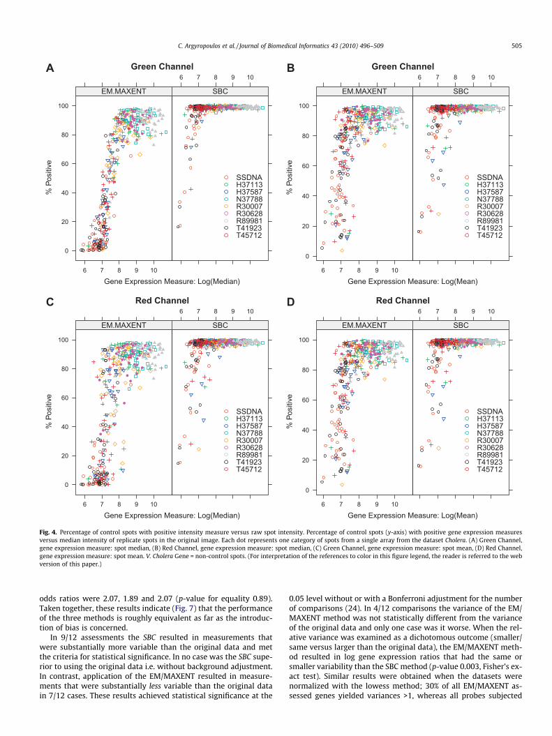
the Diauxic and Cholera dataset did increase after backgroundadjustment. Using robust measures of variance (e.g. MAE), therewas a consistent decrease in the variability effected by any methodof background adjustment (Table 5). Compared to the SBC, the EM/MAXENT method was characterized by smaller magnitudes of var-iance in almost all assessments; furthermore, the MAD statisticwas zero for 5/6 comparisons of Table 4 since the method esti-mated an intensity of zero for a substantial estimation of negativecontrol spots (Additional file 1 in http://stat.med.upatras.gr/cDNA).The relationship between the percentage of spots that are filteredout by the EM/MAXENT and SBC methods versus the raw spotintensities was evaluated graphically in the multiply controlledCholera dataset (Fig. 4).

On a per array and channel basis there appears to be a non-lin-ear (sigmoid) relationship between the percentage of replicatespots with positive intensities and the median raw intensity. Thisrelationship was observed irrespective of the measure of geneexpression used (median or mean), but was substantially attenu-ated for the SBC versus the EM/MAXENT method. Furthermore,

Table 3Empiric assessment of bias using negative control spots.

Negative control spot Bias measure Mean

Algorithm EM/MAXENT NONE

Red channelDataset

EMPTY Cholera 42.09 258.7Heat shock 304.88 469.8Diauxic 747.39 2085BAT3 25.01 153.6

SSDNA Cholera 334.07 492.9AFGC 547.38 1174

Green channelEMPTY Cholera 32.67 247.1

Heat shock 16.3 323.8Diauxic 678.82 2624BAT3 38.1 167.7

SSDNA Cholera 244.43 452.7AFGC 702.38 1332

Empiric assessment of channel specific bias in quantification of negative control spots forrobust (median) measures of bias are calculated for each of the three background assessmand dataset is indicated with bold face.

the results for the EM/MAXENT strategy were consistent in the fol-lowing sense: the percentage of positive intensities after back-ground adjustment were higher for positive control spots e.g.those corresponding to rRNA and genomic DNA targets than fornegative control ones (e.g. empty spots, SSDNA or 3XSSC).

4.3. Empirical analysis of bias and variance using self–selfhybridization experiments

To verify that the potential of the EM/MAXENT method to gen-erate spot intensities with reduced bias and variance we analyzedthe AFGC dataset consisting of a large number of replicate self–selfhybridizations using a small number of targets. The distributions ofthe log-expression ratios in these self–self hybridization experi-ments are shown in the box and whisker plots in Fig. 5.

It can be appreciated that the raw data have a very small bias;the median absolute value is <0.1 bits with the exception of probeR89981 that had a median log-expression ratio of 0.15. Applicationof the SBC method inflates the bias so that only 2/8 probes havemedians less than 0.1 bits and three out of the eight probes havean absolute bias of >0.25 bits. In addition, the variance of thelog-expression ratios increases after application of the SBC method.This is attested from the spread of the outliers in the plots and themagnitude of the MAD sample statistic (Additional file 2 in http://stat.med.upatras.gr/cDNA), which ranged from 1.01 to 1.82 timesthe magnitude of MAD in the original image. On the other hand,application of the EM/MAXENT method did not result in any appre-ciable increase in the bias, but was associated with decreased thevariability of results compared to the SBC corrected and possiblythe original images. To some extent the reduction in variability ef-fected by the EM/MAXENT can be attributed to the filtering of lowintensity spots out of the analysis. To see why, note that intensitiesfrom both channels have to be estimated as positive numbers inorder to calculate the log-expression ratio. If zero (EM/MAXENT)or non-positive intensities (SBC) are generated during backgroundadjustment the corresponding log ratios will be dropped from sub-sequent steps. Fig. 6 displays the scatterplots of the percentage ofpositive spot intensities after background adjustment versus themedian intensity in the original image for the nine spots (eightgenes and one negative) for each of the forty hybridizations inthe AFGC dataset.

Similarly to Fig. 4, a non-linear (sigmoid) relationship betweenthe percentage of retained (positive) spots and their medianexpression ratio is observed for the EM/MAXENT method. This

Median

SBC EM/MAXENT NONE SBC

7 46.35 0.00 185.00 6.258 313.14 0.00 162.50 28.00.43 847.07 0.00 1394.00 96.006 50.90 0.00 116.50 24.00

269.02 50.41 304.31 105.61.9 557.61 15.76 798.85 225.02

5 31.01 0.00 184 1.756 34.04 0.00 306.5 21.75.3 845.33 0.00 2006 1202 61.61 0.00 105 15.59 233.93 83.80 313.29 105.9.79 725.04 324.25 1034.86 496.63

two different types of such spots (blank and SSDNA). Both normal theory (mean) andent strategies assessed. The smallest (best performing) algorithm for each channel

Table 5Empiric assessment of variance using negative control spots robust measures.

Negative control spot Variance measure MAE MADMD MAD

Algorithm EM/MAXENT NONE SBC EM/MAXENT NONE SBC EM/MAXENT NONE SBC

Red channelDataset

EMPTY Cholera 42.09 258.77 52.26 42.09 108.32 51.06 0.00 70.79 15.20HeatShock 304.88 469.88 318.57 304.88 352.51 309.72 0.00 92.29 41.14Diauxic 747.39 2085.43 863.96 747.39 1071.94 833.81 0.00 643.45 166.05BAT3 25.01 153.66 53.93 25.01 66.99 44.57 0.00 49.67 25.20

SSDNA Cholera 270.26 433.32 224.48 270.26 209.43 164.22 0.00 131.58 68.20AFGC 445.07 1111.31 627.64 445.07 646.30 540.85 0.00 447.75 249.82

Green channelEMPTY Cholera 32.67 105.83 34.57 32.67 105.83 34.57 0.00 66.72 6.67

HeatShock 16.30 50.92 32.17 16.30 50.92 32.17 0.00 52.26 28.17Diauxic 678.82 1185.67 823.67 678.82 1185.67 823.67 0.00 916.25 183.84BAT3 38.10 92.74 58.12 38.10 92.74 58.12 0.00 54.86 18.53

SSDNA Cholera 191.42 412.24 206.62 179.47 195.43 141.42 125.28 165.31 78.58AFGC 385.74 1181.21 792.13 385.74 586.33 534.46 0.00 452.19 357.31

Empiric assessment of channel specific variance in quantification of negative control spots for two different types of such spots (blank and SSDNA). These are computed foreach of the three background assessment strategies assessed, without assuming normal distribution for the distributions of the spot intensities.

Table 4Empiric assessment of variance using negative control spots. Normal theory measures.

Negative control spot Variance measure RMS Standard deviation

Algorithm EM/MAXENT NONE SBC EM/MAXENT NONE SBC

Red channelDataset

EMPTY Cholera 550.32 609.28 517.43 550.03 552.93 516.59Heat shock 1684.07 1634.41 1583.02 1659.48 1568.48 1554.78Diauxic 4367.79 4647.39 4123.64 4306.95 4156.67 4039.06BAT3 632.44 680.80 659.03 632.00 663.29 657.12

SSDNA Cholera 2775.24 1702.84 1615.74 2756.71 1630.93 1594.14AFGC 2185.66 2433.91 2092.47 2116.06 2131.60 2016.84

Green channelEMPTY Cholera 386.57 468.70 349.54 386.12 399.21 349.01

Heat shock 132.81 337.85 84.35 132.06 96.43 77.33Diauxic 3207.59 3923.36 2865.08 3137.54 2918.89 2739.81BAT3 1239.39 1288.85 1275.53 1238.91 1278.00 1274.16

SSDNA Cholera 1054.40 1078.04 970.51 1026.30 978.93 942.46AFGC 1901.29 2196.84 1782.69 1766.83 1746.40 1628.63

Empiric assessment of channel specific variance in quantification of negative control spots for two different types of such spots (blank and SSDNA). These are computed foreach of the three background assessment strategies assessed, assuming normal distribution for the distributions of the spot intensities. The smallest (best performing)algorithm for each channel and dataset is indicated with bold face.

504 C. Argyropoulos et al. / Journal of Biomedical Informatics 43 (2010) 496–509

relationship is also present in an attenuated form for the SBC meth-od; the minimum value of the percentage of positive spots is 10%and the maximum is reached at a lower intensity compared tothe EM/MAXENT method.

4.4. Model based evaluation of bias and variance of backgroundadjustment methods

In order to better characterize the bias–variance performance ofthe three methods, we applied mixed-effects models to replicatemeasurements of genes whose ‘‘true” expression rate was knowneither because of the experimental design employed or becauseRT-PCR verification had been performed by the original investiga-tors. In the self–self hybridizations in the AFGC dataset, the truelog-expression ratio is zero, whereas the bacterial deletion mu-tants for the sigma factor (rpoS) in the Cholera dataset are expectedto have a negative log-expression ratio compared to the wild type.In the Cholera dataset, bacteria growing in the stationary phaseshould have a substantially higher log-expression ratio than cul-tures in the log phase. Finally in the BAT3 dataset [38] HeLA cellsstably transfected with expression vectors for sense and antisense

EST of the BAT3 locus had been compared to parental cell culturesthat did not express such ESTs by both microarray and RT-PCR.According to the latter, the BAT3 gene is down-regulated whenthe anti-sense/sense mutants were compared to the wild type. Inthe self–self hybridization experiments in which the true log-expression ratio was known to be equal to zero, the EM/MAXENTmethod yielded expression ratios that were consistently within20% of the true value. On the other hand, application of the SBCmethod yielded ratios that could be >30% (�0.33 in log scale) awayfrom the expected ratio.

To analyze the model based estimates of bias, the linear mixedmodel was applied to all three methods and the confidence inter-vals for the log-expression ratio were classified according to theinclusion of the expected log-expression ratio i.e. whether they in-cluded zero for the self–self hybridization experiments or whetherthey did not cross zero for down-regulated probes. The odds ratiosof correct classification of the log-expression ratio were 1.79 (nocorrection), 1.65 (EM/MAXENT) and 1.28 (SBC) for datasets nor-malized by the global median method (ANOVA p value testingthe equality of these three odds ratios was 0.23). When the data-sets were normalized with the lowess method, the corresponding

Green ChannelA

Gene Expression Measure: Log(Median)

% P

ositi

ve

0

20

40

60

80

100

6 7 8 9 10

EM.MAXENT

6 7 8 9 10

SBC

SSDNAH37113H37587N37788R30007R30628R89981T41923T45712

Green ChannelB

Gene Expression Measure: Log(Mean) %

Pos

itive

0

20

40

60

80

100

6 7 8 9 10

EM.MAXENT

6 7 8 9 10

SBC

SSDNAH37113H37587N37788R30007R30628R89981T41923T45712

Red ChannelC

Gene Expression Measure: Log(Median)

% P

ositi

ve

0

20

40

60

80

100

6 7 8 9 10

EM.MAXENT

6 7 8 9 10

SBC

SSDNAH37113H37587N37788R30007R30628R89981T41923T45712

Red ChannelD

Gene Expression Measure: Log(Mean)

% P

ositi

ve

0

20

40

60

80

100

6 7 8 9 10

EM.MAXENT

6 7 8 9 10

SBC

SSDNAH37113H37587N37788R30007R30628R89981T41923T45712

Fig. 4. Percentage of control spots with positive intensity measure versus raw spot intensity. Percentage of control spots (y-axis) with positive gene expression measuresversus median intensity of replicate spots in the original image. Each dot represents one category of spots from a single array from the dataset Cholera. (A) Green Channel,gene expression measure: spot median, (B) Red Channel, gene expression measure: spot median, (C) Green Channel, gene expression measure: spot mean, (D) Red Channel,gene expression measure: spot mean. V. Cholera Gene = non-control spots. (For interpretation of the references to color in this figure legend, the reader is referred to the webversion of this paper.)

C. Argyropoulos et al. / Journal of Biomedical Informatics 43 (2010) 496–509 505

odds ratios were 2.07, 1.89 and 2.07 (p-value for equality 0.89).Taken together, these results indicate (Fig. 7) that the performanceof the three methods is roughly equivalent as far as the introduc-tion of bias is concerned.

In 9/12 assessments the SBC resulted in measurements thatwere substantially more variable than the original data and metthe criteria for statistical significance. In no case was the SBC supe-rior to using the original data i.e. without background adjustment.In contrast, application of the EM/MAXENT resulted in measure-ments that were substantially less variable than the original datain 7/12 cases. These results achieved statistical significance at the

0.05 level without or with a Bonferroni adjustment for the numberof comparisons (24). In 4/12 comparisons the variance of the EM/MAXENT method was not statistically different from the varianceof the original data and only one case was it worse. When the rel-ative variance was examined as a dichotomous outcome (smaller/same versus larger than the original data), the EM/MAXENT meth-od resulted in log gene expression ratios that had the same orsmaller variability than the SBC method (p-value 0.003, Fisher’s ex-act test). Similar results were obtained when the datasets werenormalized with the lowess method; 30% of all EM/MAXENT as-sessed genes yielded variances >1, whereas all probes subjected

H37113 H37587 N37788 R30007 R30628 R89981 T41923 T45712

−3−2

−1

Probe ID

Rat

io o

f Log

Cha

nnel

Med

ians

−3−2

−1−3

−2−1

01

2

EM.MAXENTSBCNONE

Fig. 5. Effects of background adjustment on the bias and variance of log-expression ratios from self–self hybridizations. Box and whisker plot of log-expression ratios from theAFGC dataset, analyzed by three different strategies for background adjustment: SBC (A) no adjustment (B), and EM/MAXENT methods (C). Prior to obtaining these graphs, thebackground adjusted datasets were normalized by setting the median log-expression ratio equal to zero for each array separately.

Green ChannelA

Gene Expression Measure: Log(Median)

% P

ositi

ve

0

20

40

60

80

100

6 7 8 9 10

EM.MAXENT

6 7 8 9 10

SBC

SSDNAH37113H37587N37788R30007R30628R89981T41923T45712

Red ChannelB

Gene Expression Measure: Log(Median)

% P

ositi

ve

0

20

40

60

80

100

6 7 8 9 10

EM.MAXENT

6 7 8 9 10

SBC

SSDNAH37113H37587N37788R30007R30628R89981T41923T45712

Fig. 6. Percentage of negative and positive control spots with positive measures versus raw spot intensity. Percentage of control spots (y-axis) with positive gene expressionmeasures versus median intensity of replicate spots in the original image. Each dot represents one probe from a single array from the dataset AFGC. (A) Green Channel, geneexpression measure: spot median, (B) Red Channel, gene expression measure: spot median. (For interpretation of the references to color in this figure legend, the reader isreferred to the web version of this paper.)

506 C. Argyropoulos et al. / Journal of Biomedical Informatics 43 (2010) 496–509

to the SBC method had a ratio >1 (p-value 0.002 Fisher’s exact test).Expressed as a continuous outcome, the median variance of theEM/MAXENT method relative to the original data was 0.86 and0.88 when the datasets were normalized with the global medianand the tip-based lowess, respectively. In contrast, the median var-iance of the SBC method was 1.77 and 1.84 times, respectively.

5. Discussion

5.1. The role of background adjustment in microarray analysis

Ever since the introduction of microarrays in high throughputgene expression profiling, background correction has been

Background Correction Method

Obs

erve

d Lo

g Ex

pres

sion

Rat

io

−0.6

−0.4

−0.2

0.0

EM.MAXENT SBC NONE

Fig. 7. Observed versus expected (horizontal dashed line) log-expression ratio for the eight probes of the AFGC dataset for the three background adjustment methods.

C. Argyropoulos et al. / Journal of Biomedical Informatics 43 (2010) 496–509 507

considered a necessary step in the experimental pipeline [44],which may in fact have a significantly higher bearing on the finalresults than subsequent analytic steps i.e. normalization [11,14].A simple model is one which notes that in any given finite areaof the microarray surface there are both specific and non-specifichybridization sources of fluorescence, which combine additively.Such considerations lead to the additive background corruptionmodel that is endorsed by the traditional (SBC) and other alterna-tive approaches [9,10]. Yet, unless the adjustment algorithm isproperly constrained by extraneous pre-data information aboutthe measurement scale and the relative magnitude of the back-ground to the signal, its consistency in repeated applications islikely to suffer. This has indeed been the experience with previousevaluations of the default SBC method for background adjustment[11,14,45], a finding that we also observed in the five datasets weexamined in this report.

5.2. The rationale for Maximum Entropy methods in microarray imageanalysis

In order to make the most out of the initial ‘‘objective” informa-tion about the microarray measurement process, we used themethod of Maximum Entropy [46,47] to render such informationinto probability distributions. Our rationale for using this approachdoes not follow from the assumption that the data from microarrayexperiments come from such distributions. On the contrary, wefeel that the complexity of the microarray measurement processis so high, that the search for the ‘‘true” distribution of the micro-array data is a very difficult task and an approximation is neededinstead. However, our decision to express the sought after approx-imation in terms of Maximum Entropy distributions is motivated byboth theoretical and practical features that such distributions pos-sess. From the Bayesian viewpoint (a view that was not adoptedin this paper) their major theoretic attraction is their least informa-tive nature. Stated in other terms, such distributions are the ones

most compatible with the ‘‘objective” pre-data information at ourdisposal while being maximally noncommittal about the missinginformation. To a frequentist, the most appealing features wouldmost likely be the attainment of the lower bound of the Cramer-Rao inequality and the unbiased-ness of their moment estimators[48]. Stated in other terms, such distributions are expected toachieve the minimum error (bias and variance) out of all distribu-tions compatible with the initial information and the experimentaldata at hand. Last but certainly not least, MaxEnt distributions areendowed with computationally efficient procedures for estimationand learning based on sufficient statistics. This aspect is importantconsidering the large size of microarray images, which renderalternative approaches (e.g. Monte Carlo or resampling methods)computationally prohibitive for batch work. By embedding theMaximum Entropy distributions into the Expectation–Maximiza-tion algorithm we derived a computationally efficient probabilisticalgorithm (EM/MAXENT) for the adjustment of microarray images.

5.3. Discussion and Interpretation of evaluation results

The technical innovation of the EM/MAXENT algorithm pro-vides a partial answer to the following important questions: (a)should we even attempt to correct gene expression measures forthe microarray background? (b) If so, what is the best method toachieve this? We approached both questions by calculating empir-ical measures of bias and variance from multiple categories of neg-ative control and non-control spots from five datasets generatedover the course of a decade. These measures of bias and variancewere then utilized to compare the proposed method to thestandard, subtractive approach, using the uncorrected data asreference. Our results indicate that the subtractive approach ischaracterized by a considerable magnitude of empiric bias and var-iance in the case of spots that are expressed close to background.On the other hand the proposed method does not appear to sufferfrom these disadvantages and the method can filter out spot

508 C. Argyropoulos et al. / Journal of Biomedical Informatics 43 (2010) 496–509

measures with intensities that are numerically close to the back-ground level.

An alternative semi-quantitative view of the EM/MAXENT algo-rithm is that it implements a thresholded filter with a non-linearactivation function. Such a filter would reject spots with intensitiesthat are indistinguishable from the background of a given imagebut would correct all the others using a statistically consistent esti-mator for the level of the noise. From this perspective the improve-ment noted in the measures of variance in the model basedassessments can be traced to the efficiency of the entropic distribu-tions in approximating the unknown distribution of the back-ground with the least error. The implications for the analysis ofother microarray datasets can be understood by referring to thevariance of the EM/MAXENT and SBC method relative to the origi-nal data. Using the model based estimates (Section 4.4) as an indexof method performance, the former method results in a reductionin the standard deviation by 1�

ffiffiffiffiffiffiffiffiffiffi0:86p

7:3% compared to theoriginal data. On the other hand application of the SBC method willincrease the standard deviation by

ffiffiffiffiffiffiffiffiffiffi1:77p

� 1 33%. Assumingthat the signal to noise ratio of microarray measurements falls bythe square root of the sample size, application of the EM/MAXENTmethod may reduce the required sample size by 14% for a given le-vel of an experimental noise and signal to noise ratio. On the otherhand, the SBC method will increase the required sample size by 77%relative to the original uncorrected data in line with previousreports.

5.4. Outlook and directions for future work

A few limitations of the proposed methodology and open meth-odological relations should be noted when evaluating its merits forroutine work. These relate to the optimality of a local (rather thandescribed herein global) background adjustment procedure, theneed to derive a more realistic additive/multiplicative inversemeasurement error model that could link background adjustmentand normalization. We postulate that such a derivation may befacilitated by the adoption of a Bayesian perspective, a directionthat we are actively pursuing. Furthermore, the estimated reduc-tions in variance should serve as rough initial estimates whichcould be improved upon by applying the proposed EM/MAXENTmethod to additional datasets. Ideally these datasets should in-clude independent quantification of the expression ratio of multi-ple genes with non array based techniques, in order to facilitatemeaningful comparisons of bias and variance. Finally, we note thatone natural extension of the proposed statistical framework/back-ground correction methods involves oligo-nucleotide arrays (e.g.Affymetrix). Even though in such arrays, an explicit segmentationof the raw image to signal and background (Step 2, Labeling, Sec-tion 2.3) is not required, estimation of the background intensity(from mismatch probes) and correction of perfect match probesunder moment constraints (Step 3, Section 2.3) could be consid-ered. In this regard it is interesting to note that one of the algo-rithms that is used to preprocess such arrays (PLIER) [49] isbased on a distribution that shares some common features withthe proposed method: additivity of signal and background, respectof the positive nature of the microarray images and an inverse rela-tionship between the error distributions of signal and background[50].

6. Conclusion

Background correction has been considered a necessary step inthe experimental pipeline of high throughput gene expression pro-filing. The proposed method for background adjustment based onMaximum Entropy reduces standardized measures of log expres-

sion variability across replicates in situations of differential andnon-differential gene expression without increasing the bias. Itincorporates computationally efficient procedures for estimationand learning based on sufficient statistics and can filter out spotmeasures with intensities that are numerically close to the back-ground level.

References

[1] Southern E, Mir K, Shchepinov M. Molecular interactions on microarrays. NatGenet 1999;21:5–9.

[2] Taniguchi M, Miura K, Iwao H, Yamanaka S. Quantitative assessment of DNAmicroarrays – comparison with Northern blot analyses. Genomics2001;71:34–9.

[3] Alizadeh A, Eisen M, Botstein D, Brown PO, Staudt LM. Probing lymphocytebiology by genomic-scale gene expression analysis. J Clin Immunol1998;18:373–9.

[4] Tu Y, Stolovitzky G, Klein U. Quantitative noise analysis for gene expressionmicroarray experiments. Proc Natl Acad Sci USA 2002;99:14031–6.

[5] Balagurunathan Y, Wang N, Dougherty ER, Nguyen D, Chen Y, Bittner ML, et al.Noise factor analysis for cDNA microarrays. J Biomed Opt 2004;9:663–78.

[6] Eisen MB. ScanAlyze. Available from: http://rana.lbl.gov/EisenSoftware.htm.[7] Jain AN, Tokuyasu TA, Snijders AM, Segraves R, Albertson DG, Pinkel D. Fully

automatic quantification of microarray image data. Genome Res2002;12:325–32.

[8] Saeed AI, Bhagabati NK, Braisted JC, Liang W, Sharov V, Howe EA, et al. TM4microarray software suite. Methods Enzymol 2006;411:134–93.

[9] Yang YH, Buckley MJ, Speed TP. Analysis of cDNA microarray images. BriefBioinform 2001;2:341–9.

[10] Kooperberg C, Fazzio TG, Delrow JJ, Tsukiyama T. Improved backgroundcorrection for spotted DNA microarrays. J Comput Biol 2002;9:55–66.

[11] Qin LX, Kerr KF. Empirical evaluation of data transformations and rankingstatistics for microarray analysis. Nucleic Acids Res 2004;32:5471–9.

[12] Huber W, von Heydebreck A, Sultmann H, Poustka A, Vingron M. Variancestabilization applied to microarray data calibration and to the quantification ofdifferential expression. Bioinformatics 2002;18(Suppl. 1):S96–S104.

[13] Durbin BP, Hardin JS, Hawkins DM, Rocke DM. A variance-stabilizingtransformation for gene-expression microarray data. Bioinformatics2002;18(Suppl. 1):S105–10.

[14] Yang YH, Buckley MJ, Dudoit S, Speed TP. Comparison of methods for imageanalysis on cDNA microarray data. J Comput Graph Stat 2002;11:108–36.

[15] Li Q, Fraley C, Bumgarner RE, Yeung KY, Raftery AE. Donuts, scratches andblanks: robust model-based segmentation of microarray images.Bioinformatics 2005;21(12):2875–82.

[16] Caticha A, Preuss R. Maximum entropy and Bayesian data analysis: entropicprior distributions. Phys Rev E 2004;70(4):046127 (12 pages).

[17] Jaynes ET. Discrete prior probabilities: the entropy principle. In: Bretthorst GL,editor. Probability theory: the logic of science. Cambridge University Press;2003. p. 343–71.

[18] Tagliani A. Hausdorff moment problem and maximum entropy: a unifiedapproach. Appl Math Comput 1999;105(2–3):291–305.

[19] Jaynes ET. Information theory and statistical mechanics. Phys Rev2010;106(4):620–30.

[20] Jaynes ET. Information theory and statistical mechanics. II. Phys Rev1957;108(2):171–90.

[21] Malouf R. A comparison of algorithms for Maximum Entropy parameterestimation. In: CoNLL. Taipei, Taiwan; 2002. p. 49–55.

[22] Skilling J, Bryan RK. Maximum entropy image reconstruction-generalalgorithm. Mon Not R Astron Soc 1984;211(1):111–24.

[23] Mead LR, Papanicolaou N. Maximum entropy in the problem of moments. JMath Phys 1984;25:2404–17.

[24] Dempster AP, Laird NM, Rubin DB. Maximum likelihood from incomplete datavia the EM algorithm. J R Stat Soc 1977;39:1–38.

[25] Zellner A, Highfield RA. Calculation of maximum entropy distributions andapproximation of marginal posterior distributions. J Econ 1988;37:195–209.

[26] Pham-Gia T, Hung TL. The mean and median absolute deviations. MathComput Model 2001;34:921–36.

[27] Kerr MK, Martin M, Churchill GA. Analysis of variance for gene expressionmicroarray data. J Comput Biol 2000;7:819–37.

[28] Churchill GA. Using ANOVA to analyze microarray data. Biotechniques2004;37:173–5 [177].

[29] Haldermans P, Shkedy Z, Van Sanden S, Burzykowski T, Aerts M. Using linearmixed models for normalization of cDNA microarrays. Stat Appl Genet MolBiol 2007;6 [Article 19].

[30] Wolfinger RD, Gibson G, Wolfinger ED, Bennett L, Hamadeh H, Bushel P, et al.Assessing gene significance from cDNA microarray expression data via mixedmodels. J Comput Biol 2001;8:625–37.

[31] Moser RJ, Reverter A, Kerr CA, Beh KJ, Lehnert SA. A mixed-model approach forthe analysis of cDNA microarray gene expression data from extreme-performing pigs after infection with Actinobacillus pleuropneumoniae. J AnimSci 2004;82:1261–71.

[32] Hoeschele I, Li H. A note on joint versus gene-specific mixed model analysis ofmicroarray gene expression data. Biostatistics 2005;6:183–6.

C. Argyropoulos et al. / Journal of Biomedical Informatics 43 (2010) 496–509 509

[33] Chen JJ, Delongchamp RR, Tsai CA, Hsueh HM, Sistare F, Thompson KL, et al.Analysis of variance components in gene expression data. Bioinformatics2004;20:1436–46.

[34] Pinheiro JC, Bates DM. Mixed-effects models in S and S-PLUS. NewYork: Springer; 2000.

[35] DeRisi JL, Iyer VR, Brown PO. Exploring the metabolic and genetic control ofgene expression on a genomic scale. Science 1997;278:680–6.

[36] Finkelstein D, Ewing R, Gollub J, Sterky F, Cherry JM, Somerville S. Microarraydata quality analysis: lessons from the AFGC project. Arabidopsis FunctionalGenomics Consortium. Plant Mol Biol 2002;48:119–31.

[37] Finkelstein DB, Sterky F, Gollub J, Keegstra K, Miura E, Simon V, et al. Qualityand Statistical Analysis of AFGC Microarray Data. In: 11th InternationalConference on Arabidopsis Research. Madison, Wisconsin; 2000.

[38] Chang AC, Zsak L, Feng Y, Mosseri R, Lu Q, Kowalski P, et al. Phenotype-basedidentification of host genes required for replication of African swine fevervirus. J Virol 2006;80:8705–17.

[39] Nielsen AT, Dolganov NA, Otto G, Miller MC, Wu CY, Schoolnik GK. RpoScontrols the Vibrio cholerae mucosal escape response. PLoS Pathog2006;2:e109.

[40] Loewen PC, Hu B, Strutinsky J, Sparling R. Regulation in the rpoS regulon ofEscherichia coli. Can J Microbiol 1998;44:707–17.

[41] Hengge-Aronis R. Signal transduction and regulatory mechanisms involved incontrol of the sigma(S) (RpoS) subunit of RNA polymerase. Microbiol Mol BiolRev 2002;66:373–95 [table of contents].

[42] Heyer LJ, Moskowitz DZ, Abele JA, Karnik P, Choi D, Campbell AM, et al. MAGICtool: integrated microarray data analysis. Bioinformatics 2005;21:2114–5.

[43] Yang YH, Dudoit S, Luu P, Lin DM, Peng V, Ngai J, et al. Normalization for cDNAmicroarray data: a robust composite method addressing single and multipleslide systematic variation. Nucleic Acids Res 2002;30:e15.

[44] Qin L, Rueda L, Ali A, Ngom A. Spot detection and image segmentation in DNAmicroarray data. Appl Bioinform 2005;4:1–11.

[45] Smyth GK, Yang YH, Speed T. Statistical issues in cDNA microarray dataanalysis. Methods Mol Biol 2003;224:111–36.

[46] Jaynes ET. Information theory and statistical mechanics. Phys Rev1957;106:620.

[47] Shore JE, Johnson RW. Axiomatic derivation of the principle of maximumentropy and the principle of minimum cross-entropy. IEEE Trans InformTheory 1980;26(1):26–37.

[48] Jaynes ET. Where do we stand on Maximum Entropy? In: Levine R, Tribus M,editors. The maximum entropy formalism. Cambridge, MA: The MIT Press;1978. p. 15–118.

[49] Therneau TM, Ballman KV. What does PLIER really do? Cancer Inform2008;6:423–31.

[50] Sakellaropoulos GC, Daskalakis A, Nikiforidis GC, Argyropoulos C. Uncoveringfine structure in gene expression profile by maximum entropy modeling ofcDNA microarray images and kernel density methods. In: Andriani Daskalaki,editor. Handbook of Research on Systems Biology Applications in Medicine;2009. p. 221–38.