c o m p u t e r m e t h o d s a n d p r o g r a m s i n b i o m e d i c i n e 9 5 ( 2 0 0 9 ) 72–88

journa l homepage: www. int l .e lsev ierhea l th .com/ journa ls /cmpb

A comparative study of individual and ensemble majorityvote cDNA microarray image segmentation schemes,originating from a spot-adjustable based restorationframework

Antonis Daskalakisa,∗, Dimitris Glotsosb, Spiros Kostopoulosa,Dionisis Cavourasb, George Nikiforidisa

a Medical Image Processing and Analysis Laboratory (MIPA), Department of Medical Physics, School of Medicine, University of Patras,Rio, Patras 265 04, Greeceb Department of Medical Instruments Technology, Technological Educational Institute of Athens, Ag. Spyridonos Street, Aigaleo, 122 10Athens, Greece

a r t i c l e i n f o

Article history:

Received 19 June 2008

Received in revised form

23 September 2008

Accepted 12 January 2009

Keywords:

cDNA microarray

Segmentation

a b s t r a c t

The aim of this study was to comparatively evaluate the performances of various seg-

mentation algorithms, in conjunction with a noise reduction step, for gene expression

levels intensity extraction in cDNA microarray images. Different segmentation algorithms,

based on histogram and unsupervised classification methods, which have never been pre-

viously employed in microarray image analysis, were employed either individually or in

ensemble majority vote structures for separating spot-images from background pixels.

The performances of segmentation algorithms or ensemble structures were evaluated by

assessing the validity and reproducibility of gene expression levels extraction in simu-

lated and real cDNA microarray images. By processing high quality simulated images, the

Restoration

Majority vote segmentation

highest segmentation accuracy was achieved by an ensemble structure (Histogram Concav-

ity, Gaussian Kernelized Fuzzy-C-Means, Seeded Region Growing). Optimum performance

in terms of processing time and segmentation precision for low quality simulated and

replicated real cDNA microarray images was attained by the Histogram Concavity algo-

rithm.

est (targets) and are printed on a glass microscope slide by

1. Introduction

Microarray technology has become one of the most powerfultools in the field of genetic research [1,2]. Microarrays enablethe high throughput profiling of thousands of distinct gene

expression levels in a single hybridization experiment and,thus, provide to molecular biologists and bioinformaticians aglobal, simultaneous view, on the transcription levels of an

∗ Corresponding author. Tel.: +30 6972 895794.E-mail address: daskalakis@med.upatras.gr (A. Daskalakis).

0169-2607/$ – see front matter © 2009 Elsevier Ireland Ltd. All rights resdoi:10.1016/j.cmpb.2009.01.007

© 2009 Elsevier Ireland Ltd. All rights reserved.

organism’s genes under a range of conditions or processes[3,4].

In a typical microarray experiment, thousands of DNAsequences, called probes, are obtained from the genes of inter-

a robotic arrayer, thus, forming circular spots [5,6]. In orderto create a genome expression profile of a biological systemwith microarrays, one has to compare the relative abundance

erved.

c o m p u t e r m e t h o d s a n d p r o g r a m s i n

Fig. 1 – Flowchart illustrating the basic stages of thep

oiicC6sslTttcTia

m

roposed methodology.

f each one of these gene sequences in two samples. Accord-ngly, from each sample, the messenger RNA (Ribonucleic acid)s extracted, isolated, and labelled using different fluores-ent dyes (the most usually used are the red-fluorescent dyey5 and the green-fluorescent dye Cy3 with emissions in the30–660 nm and 510–550 nm respectively). Following, the twoamples are mixed and hybridized within the arrayed DNApots [7]. After hybridization, the arrays are scanned usingasers that excite each dye at the appropriate wavelength.he relative fluorescence between each dye, on each spot, is

hen recorded using methods contingent upon the nature ofhe labelling reaction, i.e. confocal laser scanner, and chargedouple devices [8,9]. The output of such systems is two 16-bitIFF images, one for each fluorescent channel. The relative

ntensities of the spots at each channel represent the relativebundance of the DNA product in each of the two samples.

In order to extract those relative intensities from theicroarray images, a well-known algorithmic pipeline is uti-

b i o m e d i c i n e 9 5 ( 2 0 0 9 ) 72–88 73

lized [10]. The latter employs a series of image processingtechniques namely gridding, segmentation, and intensityextraction [11]. Subsequently, the extracted transcription lev-els are further analyzed, through data mining techniques that(i) assist biologists in understanding function of genes and (ii)facilitate the extraction of meaningful biological conclusions[12]. Notwithstanding, microarrays suffer from an inherentlack of precision due to multiple sources of noise (biologi-cal and experimental), which are introduced in a microarrayexperiment. Noise complicates the task of microarray imageanalysis and, thus, it directly affects subsequent data analy-sis [14]. As a consequence, improper treatment of noise mightpreclude the extraction of meaningful biological conclusions[13].

Noise confounds all microarray image processing steps(i.e. gridding, segmentation, intensity extraction), and mostlythe segmentation step. Inaccurate determination of spotsboundaries, during the segmentation process, evokes wrongestimation of the relative mean spots’ intensities. Therefore,the reproducibility and validity of the gene expression lev-els, derived from microarray images, is degraded. To this end,several studies have been proposed [15–18], in which imageenhancement is suggested as a solution to the microarrayimage noise problem. Results of these studies have indicateda superior quality of the enhanced images, without how-ever examining whether enhancement leads to more accuratespot segmentation or to reduction of the variability of theextracted gene expression levels. Nonetheless, as the findingsof our previous study [19] have revealed, individual restorationof spot-images, when combined with spots structural infor-mation, facilitates spot’s segmentation and, consequently,improves genes quantification in terms of validity and repro-ducibility.

Notwithstanding, the fairly common low quality ofmicroarrays [20] renders the task of microarray segmenta-tion challenging and, thus, the need arises to investigatethe performance of various segmentation approaches, espe-cially in cases where microarray image quality is low. To thisend, several approaches for the demanding task of microar-ray segmentation have been proposed [21–26]. Among them,histogram based segmentation techniques and unsupervisedclassification techniques have been proven to provide higherreproducibility in the extracted intensities for images char-acterized as highly noisy [14,20]. Those techniques, however,have not examined whether, if preceded by a noise reduc-tion step (adjustable spot-image restoration [19]), might leadto more accurate spot segmentation and to a further improve-ment of the reproducibility of the extracted gene expressionlevels.

In this study a thorough investigation of the performanceof various cDNA microarray image segmentation tech-niques, originating from an adjustable spot-image restorationframework, is presented. Explicitly, the present study com-prises three cascade stages: (i) a spot-images restorationstage, presented by our group elsewhere [19], in which arobust framework of microarray image processing techniques,

designed to take into account the effect of local spot-imagenoise in microarray images, was utilized, (ii) a spot-imagessegmentation stage, in which 5 different segmentation tech-niques were employed individually and in ensemble majority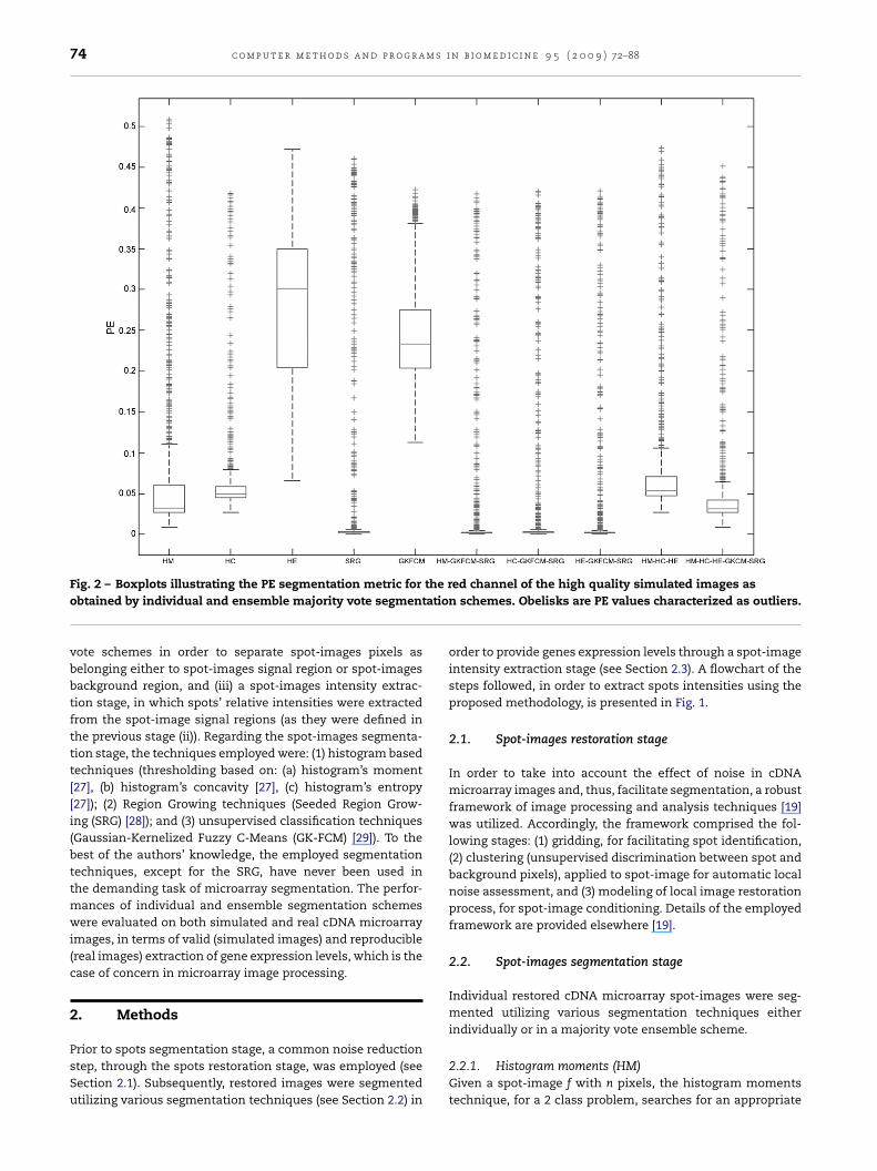

74 c o m p u t e r m e t h o d s a n d p r o g r a m s i n b i o m e d i c i n e 9 5 ( 2 0 0 9 ) 72–88

the rtatio

Fig. 2 – Boxplots illustrating the PE segmentation metric forobtained by individual and ensemble majority vote segmen

vote schemes in order to separate spot-images pixels asbelonging either to spot-images signal region or spot-imagesbackground region, and (iii) a spot-images intensity extrac-tion stage, in which spots’ relative intensities were extractedfrom the spot-image signal regions (as they were defined inthe previous stage (ii)). Regarding the spot-images segmenta-tion stage, the techniques employed were: (1) histogram basedtechniques (thresholding based on: (a) histogram’s moment[27], (b) histogram’s concavity [27], (c) histogram’s entropy[27]); (2) Region Growing techniques (Seeded Region Grow-ing (SRG) [28]); and (3) unsupervised classification techniques(Gaussian-Kernelized Fuzzy C-Means (GK-FCM) [29]). To thebest of the authors’ knowledge, the employed segmentationtechniques, except for the SRG, have never been used inthe demanding task of microarray segmentation. The perfor-mances of individual and ensemble segmentation schemeswere evaluated on both simulated and real cDNA microarrayimages, in terms of valid (simulated images) and reproducible(real images) extraction of gene expression levels, which is thecase of concern in microarray image processing.

2. Methods

Prior to spots segmentation stage, a common noise reductionstep, through the spots restoration stage, was employed (seeSection 2.1). Subsequently, restored images were segmentedutilizing various segmentation techniques (see Section 2.2) in

ed channel of the high quality simulated images asn schemes. Obelisks are PE values characterized as outliers.

order to provide genes expression levels through a spot-imageintensity extraction stage (see Section 2.3). A flowchart of thesteps followed, in order to extract spots intensities using theproposed methodology, is presented in Fig. 1.

2.1. Spot-images restoration stage

In order to take into account the effect of noise in cDNAmicroarray images and, thus, facilitate segmentation, a robustframework of image processing and analysis techniques [19]was utilized. Accordingly, the framework comprised the fol-lowing stages: (1) gridding, for facilitating spot identification,(2) clustering (unsupervised discrimination between spot andbackground pixels), applied to spot-image for automatic localnoise assessment, and (3) modeling of local image restorationprocess, for spot-image conditioning. Details of the employedframework are provided elsewhere [19].

2.2. Spot-images segmentation stage

Individual restored cDNA microarray spot-images were seg-mented utilizing various segmentation techniques eitherindividually or in a majority vote ensemble scheme.

2.2.1. Histogram moments (HM)Given a spot-image f with n pixels, the histogram momentstechnique, for a 2 class problem, searches for an appropriate

c o m p u t e r m e t h o d s a n d p r o g r a m s i n b i o m e d i c i n e 9 5 ( 2 0 0 9 ) 72–88 75

Table 1 – . Mean values (in terms of intensity) of the PE segmentation metric for both channels of high quality simulatedimages as obtained by the boxplots of Figs. 1 and 2.

High quality HM HC HE SRG GKFCM HM GKFCMSRG

HC GKFCMSRG

HE GKFCMSRG

HM HC HE HM HC HE SRGGKFCM

tsc

s

m

w

bhtpbbtt

Fi

Red channel 0.076 0.067 0.277 0.044 0.246 0.031Green channel 0.072 0.064 0.275 0.040 0.245 0.027

hreshold value, which separates f into two pixel classes: i/thepot-image signal class and ii/the spot-image backgroundlass.

Initially, the spot-image ith moment is calculated from thepot-image f histogram as

i = 1n

∑j

nj(hj)i, i = 1, 2, 3, . . . (1)

here nj is the total number of pixels in f with gray value hj.Considering that image f is a blurred version of an ideal

ilevel image g, which consists of pixels with only 2 gray values

0 and h1 (h0 < h1), then the histogram moment thresholdingechnique searches for a threshold value t, such that if allixel gray values of the spot-image signal class are replaced

y gray value h0 and all pixel gray values of the spot-imageackground class are replaced by gray value h1, then the firsthree moments (taking as m0 = 1) of image f are preserved inhe resulting bilevel image g [27].

ig. 3 – PE segmentation metric boxplots for the green channel ondividual and ensemble majority vote segmentation schemes. O

0.030 0.032 0.080 0.0530.026 0.028 0.076 0.050

Accordingly, if p0 and p1 are the fractions of the pixelsbelonging to the spot-image signal and background classesrespectively, the threshold value t is calculated as the closestvalue to the p0-tile of the histogram of f, defined as:

po = 1n

∑hj≤t

nj, (2)

where the values of p0 and p1 are obtained as the solution ofequations:

p0 + p1 = 1 (3)

and

m′i = mi, i = 1, 2, 3 (4)

f the high quality simulated images as obtained bybelisks are PE values characterized as outliers.

76 c o m p u t e r m e t h o d s a n d p r o g r a m s i n b i o m e d i c i n e 9 5 ( 2 0 0 9 ) 72–88

Table 2 – . Mean values (in terms of intensity) of the PE segmentation metric for both channels of low quality simulatedimages as obtained by the boxplots of Figs. 3 and 4.

Low quality HM HC HE SRG GKFCM HM GKFCMSRG

HC GKFCMSRG

HE GKFCMSRG

HM HC HE HM HC HE SRGGKFCM

30

Red channel 0.302 0.110 0.287 0.208 0.283 0.15Green channel 0.300 0.107 0.285 0.207 0.282 0.15

2.2.2. Histogram entropy (HE)Given a spot-image f, the probability distribution of its gray-levels can be defined as p1, p2, . . ., pn. In order to separatethe spot-image signal from the spot-image background, thisprobability distribution is appropriately modified to derive twodistinct probability distributions: one for the pixels belongingto the spot-image region (defined for discrete values from 1 tos) and one for the pixels of spot-image background (definedfor discrete values from s + 1 to n) defined as:

Signal :p1

ps,

p2

ps, ...,

ps

ps(5)

and

Background :ps+1

1 − ps,

ps+2

1 − ps, ...,

pn

1 − ps(6)

Fig. 4 – Boxplots illustrating the PE segmentation metric for the robtained by individual and ensemble majority vote segmentatio

0.151 0.155 0.243 0.1390.149 0.152 0.241 0.135

Accordingly, the entropies associated with each distribu-tion are defined as:

H (signal) = −s∑

i=1

pi

psln

pi

ps(7)

and

H (background) = −n∑

i=1+s

pi

1 − psln

pi

1 − ps(8)

The appropriate threshold value t, that separates the spot-image signal region from the spot-image background region,

is then calculated as the gray-level value, which maximizesthe quantity [27]:

t = arg max{

H(signal) + H(background)}

(9)

ed channel of the low quality simulated images asn schemes. Obelisks are PE values characterized as outliers.

s i n

2GHthabmteheh

E

wla

2Giisp

Fi

c o m p u t e r m e t h o d s a n d p r o g r a m

.2.3. Histogram concavity (HC)iven a spot-image f and by defining the spot-image histogramover a set of gray-levels g0, g1,. . ., gt−1, the height of the his-

ogram may be obtained at these gray-levels as h(g0), h(g1),. . .,(gt−1), where h(gt) /= 0 for all i. Then H might be regarded astwo-dimensional region from which its convex hull H̄ mighte constructed and, thus, a threshold value t might be deter-ined by the histogram’s concavities. Accordingly, possible

hreshold values are those gray-values at which the differ-nce h̄(gi) − h(gi) (where h̄(gi) is the height H̄ and h(gi) is theeight of H at gray level gi) has local maxima [27]. In order toliminate spurious concavities, which are attributed as “noisy”istogram’s spikes, a balance measure is introduced [30]:

i =

⎧⎨⎩

gt−1∑j=g0

h(j)

⎫⎬⎭

⎧⎨⎩

gt−1∑j=gi

h(j)

⎫⎬⎭ (10)

here Ei measures the balance of the histogram about the grayevel gi. Thus, maxima of h̄ − h, when the value of E is small, arettributed as spurious maxima and, consequently, are ignored.

.2.4. Seeded region growing (SRG)iven a spot-image f, the SRG algorithm separates the spot-

mage signal region from the spot-image background region byteratively growing contiguous signal pixel regions that differtatistically from the background region [19]. Providing a set ofredefined seed points as starting points for the segmentation,

ig. 5 – PE segmentation metric boxplots for the green channel ondividual and ensemble majority vote segmentation schemes. O

b i o m e d i c i n e 9 5 ( 2 0 0 9 ) 72–88 77

the algorithm iteratively grows those pixel regions by includ-ing the most homogenous pixels from the neighborhood tothe segmented regions [11,28]. In our approach, the initialseed point at each spot-image was predefined at the spots’restoration stage through the clustering step (the clusteringstep resulted in 2 regions: (i) spot-image signal region and(ii) spot-image background region. As initial seed the centroidof the spot-image signal region was utilized). This iterativeprocedure of growing pixel regions within each spot-imagecontinued until all pixels of the spot-image were assigned toeither the spot-image signal region or its background.

2.2.5. Gaussian-kernelized fuzzy-C-means (GK-FCM)Given a spot-image f, the Gaussian-Kernelized Fuzzy C-Means (GK-FCM) unsupervised classification algorithm [29]was employed to discriminate the spot-image signal pix-els from pixels belonging to surrounding background. TheGK-FCM, based on a random initialization process, searchesiteratively for cluster centers (centroids) that minimized thedissimilarity function:

J =M∑

i=1

Ji = 2

M∑i=1

N∑j=1

ui,jm

(1 − exp

(−di,j(xj, ci)

�2

))(11)

where xj, j = 1, 2, . . ., N are the pixels of the spot-image, ci, i = 1,2, . . ., M are the cluster centers, di,j is the Euclidean distancebetween centroid ci and data point xj, � is the spread of the

f the high quality simulated images as obtained bybelisks are PE values characterized as outliers.

78 c o m p u t e r m e t h o d s a n d p r o g r a m s i n b i o m e d i c i n e 9 5 ( 2 0 0 9 ) 72–88

Fig. 6 – M–A plots for a randomly selected simulated image employing the HM (a), HC (b), HE (c), SRG (d), GKFCM (e),HM-GKFCM-SRG (f), HC-GKFCM-SRG (g), HE-GKFCM-SRG (h), HM-HC-HE (i), and HM-HC-HE GKFCM-SRG (j) segmentationtechniques.

c o m p u t e r m e t h o d s a n d p r o g r a m s i n b i o m e d i c i n e 9 5 ( 2 0 0 9 ) 72–88 79

(Con

Gbips

2Iseu

Fig. 6 –

aussian Kernel (� = 0.5), ui,j is the element of a fuzzy mem-ership function matrix U = [ui,j] with values 0 ≤ ui,j ≤ 1, and m

s a weighting component (m = 2). The output of the iterativerocedure is two clusters containing the pixels belonging topot-image signal region and spot-image background-region.

.2.6. Majority vote ensemble segmentation scheme

n order to explore whether the performance of individualegmentation techniques is increased when combined in annsemble segmentation scheme, the majority vote rule wastilized [31]. The majority vote scheme goes with the decision

Table 3 – . Mean values (in terms of extracted intensities ratio)experiments.

HM HC HE SRG GKFCM HM GKFCMSRG

Replicatedexpressionlevels

0.167 0.153 0.171 0.174 0.431 0.180

tinued).

when there is a consensus for it or at least more than halfof the individual segmentation techniques agree on it. Con-sequently, segmentation outputs from each technique wereappropriately modified (pixels belonging to the spot-imagesignal region were labeled 1 while pixels belonging to the spot-image background region were labeled 0) and were combinedto form the final segmentation decision that satisfies:

Gr(X) =R∑

i=1

dr,i(X) (12)

of the calculated 10 pairwise MAE for the 5 replicated

HC GKFCMSRG

HE GKFCMSRG

HM HC HE HM HC HE SRGGKFCM

0.177 0.190 0.162 0.173

80 c o m p u t e r m e t h o d s a n d p r o g r a m s i n b i o m e d i c i n e 9 5 ( 2 0 0 9 ) 72–88

Fig. 7 – A randomly selected simulated spot-image (a) and its corresponding binary form employing the HM (b), HC (c), HE(h), H

(d), SRG (e), GKFCM (f), HM-GKFCM-SRG (g), HC-GKFCM-SRG

HM-HC-HE-GKFCM-SRG (k) segmentation techniques.

where r is the class, X is the unknown spot-image pixel,i = 1, 2, . . ., R is the odd number of segmentation tech-niques involved in the majority vote scheme, dr,i is thebinary decision value {0, 1}, 0 corresponds to spot-image back-

ground class and 1 to spot-image signal class. For a twoclass problem, if G1(X) > G2(X), the unknown pixel X is clas-sified to class 1 (signal), otherwise X is classified to class 2(background).

E-GKFCM-SRG (i), HM-HC-HE (Fig. 6j), and

2.3. Spot-images intensity extraction stage

In order to extract spots relative intensities, spot-imagesignal regions, as characterized either by individual seg-

mentation techniques or by the ensemble majority votesegmentation scheme, were referred to the original spot-images, since intensities in the processed spots-imageswere altered by the restoration process. Subsequently, all

c o m p u t e r m e t h o d s a n d p r o g r a m s i n b i o m e d i c i n e 9 5 ( 2 0 0 9 ) 72–88 81

(Con

ei

3

Imvi

Fig. 7 –

xtracted intensities were normalized using global normal-zation [32].

. Material

ndividual and ensemble segmentation schemes perfor-ances were evaluated employing both simulated (in terms of

alidity) and real cDNA (in terms of reproducibility) microarraymages.

tinued).

3.1. Simulated cDNA images

A total of 100 publicly available [33] simulated cDNAmicroarrays images (50 high quality images and 50 lowquality images) were evaluated. Each image contained

1000 spots, with realistic characteristics, produced by Nyk-ter et al.’s [13] microarray simulator. High quality imageswere characterized by low level noise and low variabil-ity in spot sizes and shapes while low quality images

82 c o m p u t e r m e t h o d s a n d p r o g r a m s i n b i o m e d i c i n e 9 5 ( 2 0 0 9 ) 72–88

atesed a

Fig. 8 – Boxplots depicts the pairwise MAE between all replicspot is illustrated here). Obelisks are MAE values characteriz

were characterized by higher noise levels, varying spotdiameters, and more irregularities in the spots’ shapes[20].

In each simulated image, pixels were pre-assigned asbelonging to spot-image signal region or background. Thus,the pixel-based segmentation accuracy of individual andensemble segmentation schemes, in terms of validity, wasassessed employing the Probability of Error (PE) metric definedas [34]:

PE = P(O) × P(B|O) + P(B) × P(O|B) (13)

where P(B|O) is the probability of error in classifying objectsas background, P(O|B) is the probability of error in classifyingbackground as objects, P(O) and P(B) are a priori probabilitiesof objects and background in spot-images. For our case, thesignal region of the spot-image is considered to be the objectthat must be discriminated from its background.

3.2. Real cDNA images

A publicly available dataset [33] was employed, comprising5 real cDNA microarrays images (each one containing 12.288

spots). Microarray images were produced according to a repli-cated experiment, in which five replicated hybridizations fromone experiment were performed. Due to the replication pro-cess, each spot should have the same gene expression ratio

(totally 10 MAE values from which the mean value for eachs outliers.

and, thus, the performances of individual and ensemble seg-mentation schemes, in terms of reproducibility, were accessedthrough the pairwise Mean Absolute Error (MAE) between thereplicated images (altogether 10 pairwise MAE values) [20].

4. Results

Regarding the majority vote ensemble classification scheme,all possible combinations for the available segmentation tech-niques were evaluated. Boxplots of Figs. 2 and 3 illustrate thesegmentation accuracy for the high quality simulated images,employing the PE segmentation metric (as described in Section3.1) for the red and green channels. Table 1 provides the meanvalues of the PE boxplots of Figs. 2 and 3, in terms of intensities,for the evaluated 50 high quality simulated images for bothchannels (red and green). Boxplots of Figs. 4 and 5 depict thesegmentation accuracy for the low quality simulated images,as calculated by the PE segmentation metric for the intensitiesextracted from both channels. Table 2 summarizes the meanvalues of the PE boxplots (Figs. 4 and 5), in terms of intensity,for the evaluated 50 low quality simulated microarray images.Fig. 6 illustrates the M–A plots for the segmentation methods

employed in the present study (Fig. 6a–j), considering a ran-domly selected simulated microarray image. Fig. 7 shows onelow quality spot-image and corresponding binary segmentedimages (Fig. 7a–k).

c o m p u t e r m e t h o d s a n d p r o g r a m s i n b i o m e d i c i n e 9 5 ( 2 0 0 9 ) 72–88 83

Fig. 9 – M–A plots for a randomly selected real cDNA microarray image employing the HM (a), HC (b), HE (c), SRG (d), GKFCM(e), HM-GKFCM-SRG (f), HC-GKFCM-SRG (g), HE-GKFCM-SRG (h), HM-HC-HE (i), and HM-HC-HE-GKFCM-SRG (j) segmentationtechniques.

84 c o m p u t e r m e t h o d s a n d p r o g r a m s i n b i o m e d i c i n e 9 5 ( 2 0 0 9 ) 72–88

(Con

Fig. 9 –

Regarding real cDNA microarray images, Fig. 8 shows thecalculated pairwise MAE between the extracted expressionratios of all possible pairs (as described in Section 3.2) for thedataset of the 5 replicated images. Table 3 provides the meanvalues of the pairwise MAE (Fig. 8), as they were calculated forthe extracted expression levels of the 5 replicated images.

Similarly to Figs. 6 and 7, Fig. 9 a–j and Fig. 10 a–k illus-trate M–A plots and single spot-image segmentation results,but this time considering real microarray images.

5. Discussion

Microarray technology suffers from several sources of errorsthat affect the accuracy and validity of the extracted geneexpression levels, influencing, in this way inference of accu-

rate biological conclusions. The most affected stage in themicroarray image analysis pipeline is the segmentation stage.Notwithstanding, as the results of our previous study haverevealed [19], when noise reduction is applied locally on each

tinued).

spot-image, prior to the segmentation stage, the results of thesegmentation stage are improved. Thus, in this study, the per-formances of various segmentation algorithms were explored,either on individual or ensemble majority vote schemes, inconjunction with a noise reduction step, which was based onan adjustable spot-image restoration framework [19].

Since performance evaluation of microarray image seg-mentation algorithms is not a straightforward task to considerin real microarray images [20], a dataset of 100 simulatedimages was employed. In each one of these simulated images,the a priori knowledge of spot-image signal and backgroundregions allowed for the assessment of the segmentation accu-racy through the Probability of Error segmentation metric.Moreover, the variability of the simulated images (50 images ofhigh and 50 of low quality) rendered the possibility to demon-strate the sensitivity of the evaluated segmentation schemes

(individual and ensemble) plausible.

As expected, the performances of the segmentation algo-rithms on good quality images were higher as compared tothose on low quality images. This is clearly supported by the

s i n

oTbi

s

FeH

c o m p u t e r m e t h o d s a n d p r o g r a m

btained segmentation accuracies, as they are depicted onables 1 and 2. Accuracies for both individual and ensem-

le segmentation schemes were reduced as the quality of themages was degraded.

Regarding high quality simulated images, the highestegmentation accuracy in terms of mean Probability of

ig. 10 – A randomly selected real cDNA microarray spot-image (mploying the HM (b), HC (c), HE (d), SRG (e), GKFCM (f), HM-GKFCM-HC-HE (j), and HM-HC-HE-GKFCM-SRG (k) techniques.

b i o m e d i c i n e 9 5 ( 2 0 0 9 ) 72–88 85

Error, for both red and green channels, was achieved bythe ensemble majority scheme, in which the thresholding

based on histogram’s concavity, the Gaussian KernelizedFuzzy-C-Means, and the Seeded Region Growing techniquesparticipated (mean PE was found 0.030 and 0.026 for thered and green channel respectively) (HC-GKFCM-SRG). This

Fig. 7a) and its corresponding segmentation resultM-SRG (g), HC-GKFCM-SRG (h), HE-GKFCM-SRG (i),

86 c o m p u t e r m e t h o d s a n d p r o g r a m s i n b i o m e d i c i n e 9 5 ( 2 0 0 9 ) 72–88

(Con

Fig. 10 –

might be attributed to the diverse theoretical framework ofeach segmentation algorithm. Complementary informationof individual segmentation techniques was exploited by the

ensemble majority vote scheme and, thus, the segmentationaccuracy improved.

Regarding low quality simulated images, the highestsegmentation accuracy was achieved by the thresholding

tinued).

technique, which is based on the histogram concavity (themean PE was found 0.110 and 0.107 for the red and greenchannels respectively) (HC). This might be attributed to the

fact that HC determines the threshold value, which separatesthe spot-image signal region from its background by analyz-ing the concavity of the histogram. The latter provides a goodthreshold value in cases where the histogram of a spot-image

s i n

iaad

baramdetmbMwtue(tamtt

sGrwTws

bwmttcHHlb

6

Amocitsqe(i

r

c o m p u t e r m e t h o d s a n d p r o g r a m

s not well separated (i.e. in the ideal case the histogram ofspot-image forms a valley between the spot-image’s signal

nd background regions) and this is usually observed in highlyegraded spot-images.

Regarding real microarray images, the actual spot-imageoundaries and, thus, the spots intensity levels were notvailable. Therefore, an alternative method, in terms ofeproducible gene expression levels, should be selected forssessing the performances of individual and ensembleajority vote schemes. Accordingly, a properly designed

ataset of 5 replicated real cDNA microarray images wasmployed [20]. Due to the replication, each spot should havehe same intensity ratio throughout the replicated experi-

ents, and therefore the “sameness” of the replicates coulde assessed by utilizing the pairwise MAE (totally 10 pairwiseAE values). Fig. 8 illustrates the boxplots of MAE as theyere calculated for the spots extracted intensities ratios of

he 5 replicated images and Table 3 depicts the mean val-es of those boxplots. The lowest MAE value, in terms ofxtracted intensities ratios, was achieved by the HC techniquemean MAE was found 0.153). Lower MAE values are indica-ive of higher segmentation performances and, thus, of moreccurate extraction of gene expression levels. Since real cDNAicroarrays are characterized by a fairly common low quality,

hose results are in line with the results obtained by the HCechnique on the low quality simulated microarray images.

Additionally, it might be interesting to notice that for bothimulated and real microarray images the performance of theKFCM algorithm, in terms of validity (simulated images) and

eproducibility (real images), is relative low when comparedith results obtained by the rest of the evaluated techniques.his might be attributed to the GKFCM’s random initialization,hich causes variations in the segmentation results each time

egmentation of the same spot-image is performed.Regarding spots intensity extraction, for a 6000 × 2160, 16-

it cDNA image containing 12,288 spots, the processing timesere 490, 561, 1246, 726 and 1960 s for the individual seg-entation techniques, for the HM, HC, HE, SRG and GKFCM

echniques, respectively. Similarly, for each combination ofhe ensemble majority vote segmentation scheme, the pro-essing times were 2882, 1435, 2449, 2039 and 3165 s for theM-GKFCM-SRG, HC-GKFCM-SRG, HE-GKFCM-SRG, HM-HC-E and HM-HC-HE-GKFCM-SRG, respectively. This might seem

engthy, however, it must be stressed that the code has not yeteen optimized for speed.

. Conclusion

s the results of this study indicate, the performances oficroarray segmentation techniques are strongly depended

n the quality of the cDNA images to be processed. Inases where the quality of cDNA images is high (simulatedmages), the utilization of an ensemble majority vote segmen-ation scheme (HC-GKFCM-SRG) seems to provide the highestegmentation accuracy. However, in cases where the image

uality is degraded, which is usually observed in real worldxperiments, the selection of a histogram based techniquesuch as HC) proved to provide reliable and reproducible resultsn reasonable processing time.

b i o m e d i c i n e 9 5 ( 2 0 0 9 ) 72–88 87

e f e r e n c e s

[1] A.A. Alizadeh, L.M. Staudt, Genomic-scale gene expressionprofiling of normal and malignant immune cells, Curr. Opin.Immunol. 12 (2000) 219–225.

[2] M.B. Eisen, P.T. Spellman, P.O. Brown, D. Botstein, Clusteranalysis and display of genome-wide expression patterns,Proc. Natl. Acad. Sci. U.S.A. 95 (1998) 14863–14868.

[3] J. DeRisi, L. Penland, P.O. Brown, M.L. Bittner, P.S. Meltzer, M.Ray, Y. Chen, Y.A. Su, J.M. Trent, Use of a cDNA microarray toanalyse gene expression patterns in human cancer, Nat.Genet. 14 (1996) 457–460.

[4] J.L. DeRisi, V.R. Iyer, P.O. Brown, Exploring the metabolic andgenetic control of gene expression on a genomic scale,Science 278 (1997) 680–686.

[5] E. Southern, K. Mir, M. Shchepinov, Molecular interactionson microarrays, Nat. Genet. 21 (1999) 5–9.

[6] Mark Schena, Microarray Biochip Technology, EatonPublishing Company, 2000.

[7] P.O. Brown, D. Botstein, Exploring the new world of thegenome with DNA microarrays, Nat. Genet. 21 (1999) 33–37.

[8] K.K. Jain, Current status of fluorescent in-situ hybridisation,Med. Device Technol. 15 (2004) 14–17.

[9] P.A. t Hoen, F. de Kort, G.J. van Ommen, J.T. den Dunnen,Fluorescent labelling of cRNA for microarray applications,Nucleic Acids Res. 31 (2003) e20.

[10] A.N. Jain, T.A. Tokuyasu, A.M. Snijders, R. Segraves, D.G.Albertson, D. Pinkel, Fully automatic quantification ofmicroarray image data, Genome Res. 12 (2002) 325–332.

[11] Y.H. Yang, M.J. Buckley, T.P. Speed, Analysis of cDNAmicroarray images, Brief Bioinform 2 (2001) 341–349.

[12] M. Schena, Genome analysis with gene expressionmicroarrays, Bioessays 18 (1996) 427–431.

[13] M. Nykter, T. Aho, M. Ahdesmaki, P. Ruusuvuori, A.Lehmussola, O. Yli-Harja, Simulation of microarray datawith realistic characteristics, BMC Bioinformatics 7 (2006)349.

[14] A.A. Ahmed, M. Vias, N.G. Iyer, C. Caldas, J.D. Brenton,Microarray segmentation methods significantly influencedata precision, Nucleic Acids Res. 32 (2004) e50.

[15] X.H. Wang, R.S. Istepanian, Y.H. Song, Microarray imageenhancement by denoising using stationary wavelettransform, IEEE Trans. Nanobiosci. 2 (2003) 184–189.

[16] R. Lukac, K.N. Plataniotis, B.A.N. Smolka, Venetsanopoulos,cDNA microarray image processing using fuzzy vectorfiltering framework, J. Fuzzy Sets Syst. (2005), Special issueon fuzzy sets and systems in bioinformatics.

[17] M. Mastriani, A.E. Giraldez, Microarrays denoising viasmoothing of coefficients in wavelet domain, Int. J. Biomed.Sci. 1 (2006) 1216–1306.

[18] R. Lukac, B. Smolka, Application of the adaptivecenter-weighted vector median framework for theenhancement of cDNA microarray, Int. J. Appl. Math.Comput. Sci. 13 (2003) 369–383.

[19] A. Daskalakis, D. Cavouras, P. Bougioukos, S. Kostopoulos, D.Glotsos, I. Kalatzis, G.C. Kagadis, C. Argyropoulos, G.Nikiforidis, Improving gene quantification by adjustablespot-image restoration, Bioinformatics 23 (2007) 2265–2272.

[20] A. Lehmussola, P. Ruusuvuori, O. Yli-Harja, Evaluating the

performance of microarray segmentation algorithms,Bioinformatics 22 (2006) 2910–2917.

[21] J. Angulo, J. Serra, Automatic analysis of DNA microarrayimages using mathematical morphology, Bioinformatics 19(2003) 553–562.

m s i

88 c o m p u t e r m e t h o d s a n d p r o g r a

[22] V. Barra, Robust segmentation and analysis of DNAmicroarray spots using an adaptative split and mergealgorithm, Comput. Methods Programs Biomed. 81 (2006)174–180.

[23] J. Rahnenfuhrer, Image analysis for cDNA microarrays,Methods Inf. Med. 44 (2005) 405–407.

[24] O. Demirkaya, H.M. Asyali, M.M. Shoukri, Segmentation ofcDNA microarray spots using Markov random fieldmodeling, Bioinformatics 21 (2005) 2994–3000.

[25] R. Nagarajan, Intensity-based segmentation of microarrayimages, IEEE Trans. Med. Imaging 22 (2003) 882–889.

[26] R.J. Stanley, M. Gattapulli, C.W. Caldwell, Microarray image

spot segmentation using the method of projections, Biomed.Sci. Instrum. 38 (2002) 387–392.

[27] P.K. Sahoo, P.K. Soltani, A. Wong, A survey of thresholdingtechniques, Comput. Vision Graphics Image Process. 41(1988) 223–260.

n b i o m e d i c i n e 9 5 ( 2 0 0 9 ) 72–88

[28] S.A. Hojjatoleslami, J.R.I.T. Kittler, Region growing: a newapproach, EEE Trans. Image Process. 7 (1998) 1079–1084.

[29] D.Q. Zhang, S.C. Chen, A novel kernelized fuzzy C-meansalgorithm with application in medical image segmentation,Artif. Intell. Med. 32 (2004) 37–50.

[30] A. Rosenfeld, P. De La Terre, Histogram concavity analysis asan aid in threshold selection, IEEE Trans. Syst. ManCybernet. SMC-13 (1983) 231–235.

[31] J. Kittler, M. Hatef, R.W. Duin, J. Matas, On combiningclassifiers, IEEE Trans. Pattern Anal. Mach. Intell. 20 (1998)226–239.

[32] J. Schuchhardt, D. Beule, A. Malik, E. Wolski, H. Eickhoff, H.Lehrach, H. Herzel, Normalization strategies for cDNA

microarrays, Nucleic Acids Res. 28 (2000) E47.

[33] http://www.cs.tut.fi/sgn/csb/spotseg/.[34] S.U. Lee, S.Y. Chung, R.H. Park, A comparative performance

study of several global thresholding techniques forsegmentation, CVGIP 52 (1990) 171–190.