Microarray Data Analysis

Pietro Hiram Guzzi Editor

Methods and ApplicationsSecond Edition

Methods in Molecular Biology 1375

M E T H O D S I N M O L E C U L A R B I O L O G Y

Series EditorJohn M. Walker

School of Life and Medical SciencesUniversity of Hertfordshire

Hatfield, Hertfordshire, AL10 9AB, UK

For further volumes:http://www.springer.com/series/7651

Microarray Data Analysis

Methods and Applications

Second Edition

Edited by

Pietro Hiram Guzzi

Department of Surgical and Medical Sciences,University “Magna Græcia” of Catanzaro, Catanzaro, Italy

EditorPietro Hiram GuzziDepartment of Surgical and Medical SciencesUniversity “Magna Græcia” of CatanzaroCatanzaro, Italy

ISSN 1064-3745 ISSN 1940-6029 (electronic)Methods in Molecular BiologyISBN 978-1-4939-3172-9 ISBN 978-1-4939-3173-6 (eBook)DOI 10.1007/978-1-4939-3173-6

Library of Congress Control Number: 2016932899

Springer New York Heidelberg Dordrecht London# Springer Science+Business Media New York 2007, 2016This work is subject to copyright. All rights are reserved by the Publisher, whether the whole or part of the material isconcerned, specifically the rights of translation, reprinting, reuse of illustrations, recitation, broadcasting, reproductionon microfilms or in any other physical way, and transmission or information storage and retrieval, electronic adaptation,computer software, or by similar or dissimilar methodology now known or hereafter developed.The use of general descriptive names, registered names, trademarks, service marks, etc. in this publication does notimply, even in the absence of a specific statement, that such names are exempt from the relevant protective laws andregulations and therefore free for general use.The publisher, the authors and the editors are safe to assume that the advice and information in this book are believed tobe true and accurate at the date of publication. Neither the publisher nor the authors or the editors give a warranty,express or implied, with respect to thematerial contained herein or for any errors or omissions that may have beenmade.

Printed on acid-free paper

Humana Press is a brand of SpringerSpringer Science+Business Media LLC New York is part of Springer Science+Business Media (www.springer.com)

Preface

The development of novel technological platforms in molecular biology has given a largeinput to research and in particular has caused a big development of bioinformatics tosupport storage, management, and analysis of a large amount of data about differentaspects of the omic world. We here in particular focus on two main techniques for studyingthe activity of transcriptome, i.e., the set of molecules that play a role in the complexmechanism of protein synthesis. Such a study focuses on the role of mRNA, i.e., codingfragments of messenger RNA, and miRNA, i.e., small fragments of noncoding RNA. Thisstudy has been conducted through two main technological platforms: microarray andmiRNA-microarray. More recently, the advent of next-generation sequencing techniquesis gaining a prominent role. Despite this, classical microarray studies are still alive sincethere are a considerable number of published papers related to the generation and analysisof microarray data.

The flow of information in this field starts from technological platforms that producedifferent data. Examples of such platforms are microarray for studying the expression ofmessenger RNA (mRNA) and microRNA (miRNA); genomic microarrays for studyingcopy number variations (CNV) or single-nucleotide polymorphisms (SNP); novel micro-arrays for studying noncoding RNAs (e.g., miRNA); and genomic arrays for pharmacoge-nomics.

Classical studies focused on the individuation of the role of a single class of moleculesinto a specific disease. Therefore they contained the analysis of a single class of data. Morerecently, the biological assumption that different molecules (e.g., miRNA, mRNA, orTranscription Factors) are strongly correlated has determined the rise of a novel discipline,often referred to as computational systems biology or network systems biology. In suchdiscipline computer science, bioinformatics, and mathematical modeling play a synergisticrole in the interpretation of large data sets belonging to different data sources. Conse-quently, a big attention has been paid to the development of integrated methods ofanalysis, often based on distributed or high-performance architectures (e.g., Cloud) oron semantic-based approaches, for extracting biologically relevant knowledge from data. Inparallel, a growing number of biological and medical papers have demonstrated the realapplication of these methodologies.

This book is intended to cover main aspects of this area, and it covers a large area, fromthe description of methodologies for data analysis to the real application. The intendedaudience is students or researchers that need to learn main topics of research as well aspractitioners that need to have a look on applications. The structure of the presentation ofall the chapters makes it adapt even for the use in bioinformatics courses.

The book is composed of 15 chapters. It starts by presenting main concepts related todata analysis. Wu and Gantier present main methodologies for preprocessing of microarraydata in Chapter 1. Cristiano and Veltri present a survey of miRNA Data analysis inChapter 2 while Calabrese and Cannataro discuss the rise of Cloud-based approaches inChapter 3. Chapter 4 by Lopez Kleine et al. presents the application of data miningtechniques for data analysis and in Chapter 5 Deveci et al. focus on the use of biclusteringto query different datasets. In Chapter 6 Chang and Lin discuss a web-based tool toanalyze the evolution of miRNA clusters. Roy et al. present in Chapter 7 the application

v

of biclustering to mine patterns of co-regulated genes. Chapters 8 and 9 present the use ofontologies; in particular, Ovaska discusses the use of csbl.go tool while Agapito andMilanosurvey main existing tools for semantic similarity analysis of microarray data. Wang et al. inChapter 10 introduce the integration of microarray and proteomic data. Chapter 11 byKoumakis et al. discusses the relevance of Gene Regulatory Network Inference, whileChapter 12 by Roy and Guzzi focuses on the assessment of Gene Regulatory Networkmethods. The remaining chapters present some relevant applications in different medicalfields. Chapter 13 by Gan et al. is related to the analysis of Mouse data for metabolomicsstudies. Chapter 14 by Di Martino et al. surveys the functional analysis of microRNA datain multiple myeloma that is currently a big research area. Chapter 15 by Bhawe and Aghipresents the application of microarray data analysis in glioblastomas. Finally, Chapter 16discusses the analysis of microRNA data in cardiogenesis.

Catanzaro, Italy Pietro Hiram Guzzi

vi Preface

Contents

Preface . . . . . . . . . . . . . . . . . . . . . . . . . . . . . . . . . . . . . . . . . . . . . . . . . . . . . . . . . . . . . . . . . . . vContributors. . . . . . . . . . . . . . . . . . . . . . . . . . . . . . . . . . . . . . . . . . . . . . . . . . . . . . . . . . . . . . . ix

Normalization of Affymetrix miRNA Microarraysfor the Analysis of Cancer Samples . . . . . . . . . . . . . . . . . . . . . . . . . . . . . . . . . . . . . . . . . . . 1Di Wu and Michael P. Gantier

Methods and Techniques for miRNA Data Analysis . . . . . . . . . . . . . . . . . . . . . . . . . . . . 11Francesca Cristiano and Pierangelo Veltri

Bioinformatics and Microarray Data Analysis on the Cloud . . . . . . . . . . . . . . . . . . . . . 25Barbara Calabrese and Mario Cannataro

Classification and Clustering on Microarray Data for Gene FunctionalPrediction Using R . . . . . . . . . . . . . . . . . . . . . . . . . . . . . . . . . . . . . . . . . . . . . . . . . . . . . . . . 41Liliana Lopez Kleine, Rosa Montano, and Francisco Torres-Aviles

Querying Co-regulated Genes on Diverse Gene Expression DatasetsVia Biclustering. . . . . . . . . . . . . . . . . . . . . . . . . . . . . . . . . . . . . . . . . . . . . . . . . . . . . . . . . . . . 55Mehmet Deveci, Onur Kucuktunc, Kemal Eren, Doruk Bozdag,Kamer Kaya, and €Umit V. Catalyurek

MetaMirClust: Discovery and Exploration of Evolutionarily ConservedmiRNA Clusters . . . . . . . . . . . . . . . . . . . . . . . . . . . . . . . . . . . . . . . . . . . . . . . . . . . . . . . . . . . 75Wen-Ching Chan and Wen-chang Lin

Analysis of Gene Expression Patterns Using Biclustering . . . . . . . . . . . . . . . . . . . . . . . 91Swarup Roy, Dhruba K. Bhattacharyya, and Jugal K. Kalita

Using Semantic Similarities and csbl.go for Analyzing Microarray Data. . . . . . . . . . . 105Kristian Ovaska

Ontology-Based Analysis of Microarray Data. . . . . . . . . . . . . . . . . . . . . . . . . . . . . . . . . . 117Agapito Giuseppe and Marianna Milano

Integrated Analysis of Transcriptomic and Proteomic Datasets RevealsInformation on Protein Expressivity and Factors Affecting TranslationalEfficiency . . . . . . . . . . . . . . . . . . . . . . . . . . . . . . . . . . . . . . . . . . . . . . . . . . . . . . . . . . . . . . . . . 123Jiangxin Wang, Gang Wu, Lei Chen, and Weiwen Zhang

Integrating Microarray Data and GRNs . . . . . . . . . . . . . . . . . . . . . . . . . . . . . . . . . . . . . . 137L. Koumakis, G. Potamias, M. Tsiknakis, M. Zervakis, and V. Moustakis

Biological Network Inference from Microarray Data, Current Solutions,and Assessments . . . . . . . . . . . . . . . . . . . . . . . . . . . . . . . . . . . . . . . . . . . . . . . . . . . . . . . . . . . 155Swarup Roy and Pietro Hiram Guzzi

A Protocol to Collect Specific Mouse Skeletal Musclesfor Metabolomics Studies . . . . . . . . . . . . . . . . . . . . . . . . . . . . . . . . . . . . . . . . . . . . . . . . . . . 169Zhuohui Gan, Zhenxing Fu, Jennifer C. Stowe, Frank L. Powell,and Andrew D. McCulloch

Functional Analysis of microRNA in Multiple Myeloma . . . . . . . . . . . . . . . . . . . . . . . . 181Maria Teresa Di Martino, Nicola Amodio, Pierfrancesco Tassone,and Pierosandro Tagliaferri

vii

Microarray Analysis in Glioblastomas. . . . . . . . . . . . . . . . . . . . . . . . . . . . . . . . . . . . . . . . . 195Kaumudi M. Bhawe and Manish K. Aghi

Analysis of microRNA Microarrays in Cardiogenesis . . . . . . . . . . . . . . . . . . . . . . . . . . . 207Diego Franco, Fernando Bonet, Francisco Hernandez-Torres,Estefania Lozano-Velasco, Francisco J. Esteban, and Amelia E. Aranega

Erratum to: Classification and Clustering on Microarray Data for GeneFunctional Prediction Using R . . . . . . . . . . . . . . . . . . . . . . . . . . . . . . . . . . . . . . . . . . . . . . 223Liliana Lopez Kleine, Rosa Montano, and Francisco Torres-Aviles

Index . . . . . . . . . . . . . . . . . . . . . . . . . . . . . . . . . . . . . . . . . . . . . . . . . . . . . . . . . . . . . . . . . . . . . 225

viii Contents

Contributors

MANISH K. AGHI � Graduate Division of Biomedical Sciences (BMS),Department of Neurosurgery and Brain Tumor Research Center,University of California at San Francisco (UCSF), San Francisco, CA, USA

NICOLA AMODIO � Department of Experimental and Clinical Medicine,T. Campanella Cancer Center, Magna Graecia Universityand Medical Oncology Unit, Catanzaro, Italy

AMELIA E. ARANEGA � Cardiovascular Development Group, Department of ExperimentalBiology, University of Jaen, Jaen, Spain

DHRUBA K. BHATTACHARYYA � Tezpur University, Napaam, IndiaKAUMUDI M. BHAWE � Graduate Division of Biomedical Sciences (BMS),

Department of Neurosurgery and Brain Tumor Research Center,University of California at San Francisco (UCSF), San Francisco, CA, USA

FERNANDO BONET � Cardiovascular Development Group, Department of ExperimentalBiology, University of Jaen, Jaen, Spain

DORUK BOZDAG � Biomedical Informatics, The Ohio State University, Columbus, OH, USABARBARA CALABRESE � Department of Medical and Surgical Sciences, University

Magna Graecia of Catanzaro, Catanzaro, ItalyMARIO CANNATARO � Department of Medical and Surgical Sciences, University

Magna Graecia of Catanzaro, Catanzaro, Italy€UMIT V. CATALYUREK � Biomedical Informatics, Department of Electrical

and Computer Engineering, The Ohio State University, Columbus, OH, USAWEN-CHING CHAN � Kaohsiung Chang Gung Memorial Hospital, Kaohsiung, Taiwan,

People’s Republic of China; Institute of Biomedical Sciences, Academia Sinica, Taipei,Taiwan, People’s Republic of China

LEI CHEN � Laboratory of Synthetic Microbiology, School of Chemical Engineeringand Technology, Tianjin University, Tianjin, People’s Republic of China; Key Laboratoryof Systems Bioengineering, Ministry of Education of China, Tianjin, People’s Republicof China; Collaborative Innovation Center of Chemical Science and Engineering,Tianjin, People’s Republic of China

FRANCESCA CRISTIANO � Bioinformatic Bioinformatics Laboratory, Department of Surgicaland Medical Sciences, University Magna Græcia of Catanzaro, Catanzaro, Italy

MEHMET DEVECI � Computer Science and Engineering, The Ohio State University,Columbus, OH, USA

KEMAL EREN � Computer Science and Engineering, The Ohio State University, Columbus,OH, USA

FRANCISCO J. ESTEBAN � System Biology Group, Department of Experimental Biology,University of Jaen, Jaen, Spain

DIEGO FRANCO � Cardiovascular Development Group, Department of ExperimentalBiology, University of Jaen, Jaen, Spain

ZHENXING FU � Department of Medicine, University of California, San Diego, San Diego,CA, USA

ZHUOHUI GAN � Department of Bioengineering, University of California, San Diego,La Jolla, CA, USA

ix

MICHAEL P. GANTIER � Department of Molecular and Translational Science, MonashUniversity, Clayton, VIC, Australia; Centre for Cancer Research, MIMR-PHI Instituteof Medical Research, Clayton, VIC, Australia

AGAPITO GIUSEPPE � Department of Surgical and Medical Sciences,University of Catanzaro, Catanzaro, Italy

PIETRO HIRAM GUZZI � Department of Surgical and Medical Sciences,University “Magna Graecia” of Catanzaro, Catanzaro, Italy

FRANCISCO HERNANDEZ-TORRES � Cardiovascular Development Group,Department of Experimental Biology, University of Jaen, Jaen, Spain

JUGAL K. KALITA � University of Colorado, Colorado Springs, CO, USAKAMER KAYA � Computer Science and Engineering, Sabancı University, Istanbul, TurkeyLILIANA LOPEZ KLEINE � Departamento de Estadıstica, Universidad Nacional de Colombia,

Bogota, DC, ColombiaL. KOUMAKIS � Department of Production and Management Engineering, Technical

University of Crete, Chania, Greece; Foundation for Research andTechnology—Hellas (FORTH), Institute of Computer Science, Heraklion, Greece

ONUR KUCUKTUNC � Computer Science and Engineering, The Ohio State University,Columbus, OH, USA

WEN-CHANG LIN � Institute of Biomedical Sciences, Academia Sinica, Taipei, Taiwan,People’s Republic of China

LILIANA LOPEZ-KLEINE � Departamento de Estadıstica, Universidad Nacionalde Colombia, Bogota, DC, Colombia

ESTEFANIA LOZANO-VELASCO � Cardiovascular Development Group,Department of Experimental Biology, University of Jaen, Jaen, Spain

MARIA TERESA DI MARTINO � Department of Experimental and Clinical Medicine,T. Campanella Cancer Center, Magna Graecia University and Medical Oncology Unit,Catanzaro, Italy

ANDREW D. MCCULLOCH � Department of Bioengineering, University of California,San Diego, La Jolla, CA, USA

MARIANNA MILANO � Department of Surgical and Medical Sciences,University of Catanzaro, Catanzaro, Italy

ROSA MONTANO � Departamento de Matematica y Ciencia de la Computacion,Universidad de Santiago de Chile, Santiago, Chile

V. MOUSTAKIS � Department of Production and Management Engineering,Technical University of Crete, Chania, Greece

KRISTIAN OVASKA � Biomedicum Helsinki (B524a), University of Helsinki, Helsinki,Finland

G. POTAMIAS � Foundation for Research and Technology—Hellas (FORTH),Institute of Computer Science, Heraklion, Greece

FRANK L. POWELL � Department of Medicine, University of California, San Diego,San Diego, CA, USA

SWARUP ROY � Department of Information Technology, North-Eastern Hill University,Shillong, India

JENNIFER C. STOWE � Department of Bioengineering, University of California, San Diego,La Jolla, CA, USA

PIEROSANDRO TAGLIAFERRI � Department of Experimental and Clinical Medicine,T. Campanella Cancer Center, Magna Graecia University and Medical Oncology Unit,Catanzaro, Italy

x Contributors

PIERFRANCESCO TASSONE � Department of Experimental and Clinical Medicine,T. Campanella Cancer Center, Magna Graecia University and Medical Oncology Unit,Catanzaro, Italy; Sbarro Institute for Cancer Research and Molecular Medicine,Center for Biotechnology, College of Science and Technology, Temple University,Philadelphia, PA, USA

FRANCISCO TORRES-AVILES � Departamento de Matematica y Ciencia de la Computacion,Universidad de Santiago de Chile, Santiago, Chile

M. TSIKNAKIS � Foundation for Research and Technology—Hellas (FORTH),Institute of Computer Science, Heraklion, Greece; Department of Applied Informaticsand Multimedia, Technological Educational Institute, Heraklion, Greece

PIERANGELO VELTRI � Bioinformatic Bioinformatics Laboratory, Department of Surgicaland Medical Sciences, University Magna Græcia of Catanzaro, Catanzaro, Italy

JIANGXIN WANG � Laboratory of Synthetic Microbiology, School of Chemical Engineeringand Technology, Tianjin University, Tianjin, People’s Republic of China; Key Laboratoryof Systems Bioengineering, Ministry of Education of China, Tianjin, People’s Republicof China; Collaborative Innovation Center of Chemical Science and Engineering,Tianjin, People’s Republic of China

GANG WU � University of Maryland at Baltimore Country, Baltimore County, MD, USADI WU � Department of Statistics, Harvard University, Cambridge, MA, USA;

Centre for Cancer Research, MIMR-PHI Institute of Medical Research, Clayton, VIC,Australia

M. ZERVAKIS � Department of Electronic and Computer Engineering, Technical Universityof Crete, Chania, Greece

WEIWEN ZHANG � Laboratory of Synthetic Microbiology, School of Chemical Engineeringand Technology, Tianjin University, Tianjin, People’s Republic of China; Key Laboratoryof Systems Bioengineering, Ministry of Education of China, Tianjin, People’s Republicof China; Collaborative Innovation Center of Chemical Science and Engineering,Tianjin, People’s Republic of China

Contributors xi

Methods in Molecular Biology (2016) 1375: 1–10DOI 10.1007/7651_2015_239© Springer Science+Business Media New York 2015Published online: 14 May 2015

Normalization of Affymetrix miRNA Microarraysfor the Analysis of Cancer Samples

Di Wu and Michael P. Gantier

Abstract

microRNA (miRNA) microarray normalization is a critical step for the identification of truly differentiallyexpressed miRNAs. This is particularly important when dealing with cancer samples that have a globalmiRNA decrease. In this chapter, we provide a simple step-by-step procedure that can be used to normalizeAffymetrix miRNA microarrays, relying on robust normal-exponential background correction with cyclicloess normalization.

Keywords: microRNA, miRNA microarray, Normalization, Cancer samples, Affymetrix

1 Introduction

Variation in microRNA (miRNA) levels is a common feature ofcancer cells (1). It can result from mutations leading to increasedexpression or chromosomal amplification of the miRNA gene—asseen with the miR-17–92 cluster amplified in diffuse large B-celllymphoma patients (2)—or defective expression, processing, andexport of miRNA precursors (3–6).

Interestingly, early contradictions rapidly arose regarding theoverall profile of miRNA expression in cancer cells, with a numberof reports published that suggested a global decrease (7, 8), whileothers observed an equal distribution of upregulated and down-regulated miRNAs (9, 10). It is now well established that a signifi-cant proportion of cancer cells exhibit alteration of the miRNAbiogenesis machinery (4–6, 11), resulting in a global miRNAdecrease and poorer survival outcomes (6, 12, 13).

This suggested a potential bias of miRNA microarray technol-ogies that failed to identify global miRNA decreases (9, 10), andprompted us to investigate the reliability of miRNA microarrays tocorrectly identify samples with a global miRNA decrease. Profilingof mouse embryonic fibroblasts following the induced geneticdeletion of Dicer1, the last processing enzyme in the miRNAbiogenesis pathway, allowed us to assess the suitability of AffymetrixmiRNA microarrays to detect global miRNA decrease (14).

1

Unexpectedly, we demonstrated that standard robust multichipaverage (RMA) background correction and quantile normalizationof these miRNA microarrays, while aimed at decreasing the varia-tions in log2 intensities between the replicate arrays, strongly biasedthe identification of downregulated miRNAs (14). These observa-tions underline the importance of array preprocessing in miRNAmicroarray analyses. Critically, the previous lack of identification ofglobal miRNA decrease could have been, in fact, related to theinappropriate use of normalization procedures, with the exampleof median normalization assuming that few miRNAs are upregu-lated or downregulated, thereby strongly biasing the possibledetection of a global decrease (9, 10).

In this chapter, we detail the step-by-step use of ‘R’ to applyrobust normal-exponential background correction with cyclic loessnormalization for the preprocessing of Affymetrix miRNA micro-arrays, which was the best normalization procedure for detectingglobal miRNA decreases in our mouse embryonic fibroblast modeland prostate cancer samples (14).

2 Materials

2.1 ‘R’ Software

and Bioconductor

‘R’ can be downloaded from http://cran.us.r-project.org. Oncethe most recent version for your operating system is installed onyour computer, start ‘R’ (see Note 1). To install the statisticalpackages, required for the analyses described below, type in:

install.packages

To install bioconductor (while connected to the internet), typein the following:

source("http://bioconductor.org/biocLite.R")

biocLite()

If prompted: ‘Update all/some/none? [a/s/n]:’, typein ‘a’. These commands will download and install the statisticalpackages required for the microarray analyses presented hereafter.

2.2 miRNA

Affymetrix Microarray

(Version 1.0 or Later)

The command lines provided below are specifically designed for ourpublished dataset from Dicer-deficient cells, to be used as an exam-ple of the overall normalization procedure. The nine .CEL files(from GSM1118272_MG1.CEL to GSM1118280_MG9.CEL)can be downloaded from Gene Expression Omnibus (GEO), acces-sion number GSE45886. Briefly, miRNA levels were detected byAffymetrix miRNA v1.0 microarray, at day 2, 3, and 4 after geneticdeletion ofDicer1. Each condition (t2, t3, and t4) was replicated inbiological triplicate (A, B, and C) (14). Our normalization proce-dure relies on different weights being applied to different types ofprobes present on the arrays. As such, the correct definition of the

2 Di Wu and Michael P. Gantier

non-miRNA small RNA probes is critical, and the microarray anno-tation files should be downloaded from Affymetrix’s ‘Support’section (use ‘miRNA 1.0 Annotations, Unsupported, CSV format’for our case study). Importantly, our method has also been usedwith more recent versions of Affymetrix miRNA arrays, which alsocontain non-miRNA small RNA probes.

3 Methods

In this chapter, we present the microarray processing methods,broken down into three major steps: background correction,normalization, and summarization. Before proceeding to the firststep, however, the microarray files need to be loaded in ‘R’. This isexecuted with the following:

library(limma)

library(affy)

library(MASS)

Importantly, the location of the .CEL files needs to be speci-fied. In this example, the nine array files from GSE45886 have beenplaced in the ‘/Documents’ directory.

setwd(’~/Documents/’)

affy2<-ReadAffy()

pm.raw<-pm(affy2,geneNames(affy2)) (see Note 2)

We can then proceed with the loading of the ‘design matrix’.A design matrix defines how the microarrays are grouped in differ-ent conditions/treatments. The design matrix relies on a .txt‘target’ file, tabulated to identify the conditions of each array. Inour analysis of GSE45886, we use ‘targets-mirna.txt’ as the designmatrix. To create this file, we write the following in a blank text file:

Filename time dish

GSM1118272_MG1.CEL t2 A

GSM1118273_MG2.CEL t2 B

GSM1118274_MG3.CEL t2 C

GSM1118275_MG4.CEL t3 A

GSM1118276_MG5.CEL t3 B

GSM1118277_MG6.CEL t3 C

GSM1118278_MG7.CEL t4 A

GSM1118279_MG8.CEL t4 B

GSM1118280_MG9.CEL t4 C

This document is saved as a .txt file, named ‘targets-mirna.txt’and placed in the same folder as the .CEL files, i.e., in the~/Documents directory, before being loaded with the followingcommands (see Note 3):

Affymetrix miRNA Microarray Normalization 3

{

targets <- read.delim("targets-mirna.txt",stringsAs

Factors¼FALSE, sep¼" ")

}

des<- model.matrix(~0+as.factor(time),

data¼targets)

3.1 Robust Normexp

Background

Correction

For background correction, our procedure relies on normexp back-ground correction using the ‘nec’ function in ‘R’. In addition, weuse the ‘robust’ argument in ‘nec’ that determines backgroundmean and standard deviation, as we found it increased the sensitiv-ity of the detection of differentially expressed miRNAs (14).Nonetheless, robust can be disabled using ‘robust ¼ FALSE’ inthe command below.

Normexp background correction relies on the negative controlprobes in the Affymetrix array—annotated as ‘BkGR’ in the man-ufacturer’s annotation file. The following lines define which probesare used as control probes, from the Affymetrix annotations.

bkgr.idx.pm<-grep("BkGr",rownames(pm.raw))

status<-rep("regular",nrow(pm.raw))

status[bkgr.idx.pm]<-"negative"

table(status)

This will print the amount of negative and regular probes in thearrays (negative: 8221 and regular: 38006 when using GSE45886).

nec.pm.raw.r<-nec(pm(affy2),status¼status,negctrl¼"negative",

regular¼"regular", offset¼16, robust¼TRUE)

summary(nec.pm.raw.r)

This will print the raw intensities for each microarray divided in:Min./1st Qu./Median/Mean/3rd Qu./Max values.

3.2 Definition

of Non-miRNA Small

RNA Probes Used

in Cyclic Loess

Normalization

The first step is to obtain the probe annotations from the appropri-ate annotation file from Affymetrix. The file should be placed in theworking directory—i.e., ‘/Documents’ in our case (see Note 4).

ann<-read.csv("miRNA-1_0.annotations.20081203.

csv",skip¼11)

data.frame(table(ann$Sequence.Type))

This will print the features present on the arrays.

idx.probe<-indexProbes(affy2)

probe.name<-probeNames(affy2)

table(geneNames(affy2) %in% as.character(ann$Probe.Set.

ID))

identical(names(idx.probe),(geneNames(affy2)))

m<-match(names(idx.probe),as.character(ann$Probe.Set.

ID))

ann.m<-ann[m,]

4 Di Wu and Michael P. Gantier

ann.miRNA<- which(ann.m$Sequence.Type¼¼"miRNA")

mirna<-as.character(ann.m$Probe.Set.ID[ann.miRNA])

ann.affyctlseq<- which(ann.m$Sequence.Type¼¼"Affymetrix

Control Sequence")

affyctlseq<-as.character(ann.m$Probe.Set.ID[ann.

affyctlseq])

ann.spikein<- which(ann.m$Sequence.Type¼¼"Oligonucleo

tide spike-in controls")

spikein<-as.character(ann.m$Probe.Set.ID[ann.spikein])

ann.rrna<- which(ann.m$Sequence.Type¼¼"5.8 s rRNA")

rrna<-as.character(ann.m$Probe.Set.ID[ann.rrna])

ann.cdbox<- which(ann.m$Sequence.Type¼¼"CDBox")

cdbox<-as.character(ann.m$Probe.Set.ID[ann.cdbox])

ann.hacabox<- which(ann.m$Sequence.Type¼¼"HAcaBox")

hacabox<-as.character(ann.m$Probe.Set.ID[ann.hacabox])

ann.scarna<- which(ann.m$Sequence.Type¼¼"scaRna")

scarna<-as.character(ann.m$Probe.Set.ID[ann.scarna])

ann.snorna<- which(ann.m$Sequence.Type¼¼"snoRNA")

snorna<-as.character(ann.m$Probe.Set.ID[ann.snorna])

idx.pm.mirna<-which(match(probe.name,mirna)!¼"NA")

length(idx.pm.mirna)

The last command will print the amount of miRNA probes onthe array—this is 26,812 for miRNA.1_0.

identical(unique(probe.name[idx.pm.mirna]),mirna)

o.sml<-c(cdbox,hacabox,scarna,snorna)

idx.pm.sml<-which(match(probe.name,o.sml)!¼"NA")

length(idx.pm.sml)

This will print the amount of non-miRNA ‘other small RNA’probes on the array—this is 10,090 for miRNA.1_0.

identical(sort(unique(probe.name[idx.pm.sml])),sort(o.

sml))

idx.pm.spk<-which(match(probe.name,spikein)!¼"NA")

identical(unique(probe.name[idx.pm.spk]),spikein)

idx.pm.rrna<-which(match(probe.name,rrna)!¼"NA")

identical(unique(probe.name[idx.pm.rrna]),rrna)

idx.pm.ctls<-which(match(probe.name,

affyctlseq)!¼"NA")

identical(unique(probe.name[idx.pm.ctls]),affyctlseq)

idx.pm.ctls.hyb<-idx.pm.ctls[-grep("BkGr",probe.name

[idx.pm.ctls])]

status.spot<-rep("NA",nrow(pm.raw))

status.spot[idx.pm.mirna]<-"miRNA"

status.spot[idx.pm.sml]<-"other.small.RNA"

status.spot[bkgr.idx.pm]<-"BkGr.ctl"

status.spot[idx.pm.ctls.hyb]<-"hyb.ctl"

status.spot[idx.pm.spk]<-"spike.in"

status.spot[idx.pm.rrna]<-"human.5.8s.rRNA"

table(status.spot)

Affymetrix miRNA Microarray Normalization 5

This will print the different categories of probes now defined—BkGr.ctl: 8221; human.5.8s.rRNA: 110; hyb.ctl: 774; miRNA:26,812; other.small.RNA: 10,090; and spike.in: 220, formiRNA_1.0.

3.3 Cyclic Loess

Normalization

The next step is cyclic loess normalization—which attributesheavier weight to non-miRNA small RNA probes than miRNAprobes defined in the previous step to normalize the differencesbetween arrays. By using a much higher weight for non-miRNAsmall RNA probes (100 vs. 0.01 for miRNAs), we found that wegreatly increased the accuracy of the normalization (14).

affy2.temp<-affy2

pm(affy2.temp)<-nec.pm.raw.r

w<-rep(1,nrow(pm(affy2.temp)))

w[status.spot¼¼"miRNA"]<- 0.001

w[status.spot¼¼"other.small.RNA"]<-100

norm3<- normalizeCyclicLoess(log2(pm(affy2.temp)),

weights¼w,

iteration¼5) (see Note 5)

pm(affy2.temp)<-2^(norm3)

3.4 RMA

Summarization

The last step of our procedure is RMA summarization—whichsummarizes the previous normalization analyses in a data matrix(‘exprs2’ in this case).

tmp2<-rma(affy2.temp,normalize¼FALSE,

background¼FALSE)

exprs2<-exprs(tmp2)

summary(exprs2)

This will print the quartile intensities for each normalizedmicroarray: Min./1st Qu./Median/Mean/3rd Qu./Max values.

Because human cancer samples are very heterogeneous, it isadvisable to introduce different estimated array weights in theanalysis of differentially expressed miRNAs. We have found thatthe use of array weights gives a higher number of significantlydownregulated miRNAs in Dicer1-deficient samples than the pro-cedure without array weights—consistent with a global impairmentof miRNA biogenesis (14). Therefore, we generally suggest the useof array weights when analyzing microarrays from tumor samples.Importantly, array weights are restricted to the miRNA probes ofthe species of interest—mouse or ‘mmu’ in our Dicer1-deficientsamples. The ‘mmu’ should be changed to ‘hsa’ when looking athuman samples in the following command lines (see Note 6).

mmu.idx<-grep("mmu",rownames(exprs2))

w.des<-arrayWeightsSimple(exprs2[mmu.idx,],design¼des)

names(w.des)<-colnames(exprs2)

6 Di Wu and Michael P. Gantier

To compare the samples on the basis of a given variable, forexample the ‘time’ afterDicer1 deletion in our case study, in a linearmodel, we define the ‘contrast’ in the variable in which we areinterested. Refer to the ‘limma User Guide’ for more details onhow to define the contrast (see Note 7).

c.matrix<-cbind(T3vs2¼c(-1,1,0),T4vs2¼c(-1,0,1),

T4vs3¼c(0,-1,1))

The linear model is subsequently fitted with the array weightsdetermined previously.

fit.w<-lmFit(exprs2,design¼des, weights¼w.des)

fit.w<-contrasts.fit(fit.w,c.matrix)

fit.w<-eBayes(fit.w)

summary(decideTests(fit.w[mmu.idx,],p.value¼0.1))

This will print the number of miRNAs that are downregulated(�1), unchanged (0), or upregulated (1) in the different conditionsof the experiment—in our case comparing T3vs2, T4vs2, andT4vs3 as follows, with a p value of 0.1. In our example, the follow-ing will be printed in ‘R’ (see Note 8):

T3vs2 T4vs2 T4vs3

-1 32 87 12

0 575 516 596

1 2 6 1

Finally, a table of differentially expressed miRNAs can beretrieved with the following lines. Note that ‘top1’ correspondsto differentially expressed probes (from mouse here as specified by‘mmu’) between T3vs2—i.e., in the first column printed previously.‘top2’ and ‘top3’ match the second and third columns, respectively.The p value can also be changed—here set to p < 0.1.

top1<- topTable(fit.w[mmu.idx,],coef¼1,number¼Inf,p.

value¼0.1)

top2<- topTable(fit.w[mmu.idx,],coef¼2,number¼Inf,p.

value¼0.1)

top3<- topTable(fit.w[mmu.idx,],coef¼3,number¼Inf,p.

value¼0.1)

write.table(top1, file¼"topTab1.csv", row.names¼TRUE,

sep¼",")

write.table(top2, file¼"topTab2.csv", row.names¼TRUE,

sep¼",")

write.table(top3, file¼"topTab3.csv", row.names¼TRUE,

sep¼",")

Files with the indicated names will appear in the workingdirectory—‘/Documents’ in our case—containing the lists ofmiRNAs differentially expressed, with normalized log2 fold change.

Affymetrix miRNA Microarray Normalization 7

4 Notes

1. In this analysis we rely on ‘R’ version 3.1.0 (2014-04-10),‘Spring Dance’. ‘R’ relies on command lines, which you needto type after the ‘>’ symbol. Importantly, several lines ofcommands can be copied and pasted at the same time in ‘R’,and successively executed by pressing ‘enter/return’. Whendoing so, care should be taken with quotes (‘’ and “”), whichcan be modified by your operating system and alter the mean-ing of the ‘R’ command—generally resulting in an errormessage.

2. The last command might result in warning messages such as:‘replacing previous import by ‘utils::head’ when loading ‘mir-na10cdf” This indicates that the same names were included inthe different packages loaded. However, this can be ignored:warnings in ‘R’ can usually be ignoredwithout impacting on theprocessing of the data.

3. The variable studied in our example is identified by the “time”column from our targets-mirna.txt file, while the “dish” col-umn refers to replicates. When creating another design matrix,the previous command should be altered to reflect the variablein the ‘as.factor(variable)’ expression.

4. Because the files for each version of miRNA arrays are slightlydifferent, the argument ‘skip’ has to be changed as follows:skip ¼ 11 for ‘miRNA-1_0.annotations.20081203.csv’;skip ¼ 13 for ‘miRNA-2_0.annotations.20101222.csv’; skip ¼4 for ‘miRNA-3_0-st-v1.annotations.20140513.csv’ and‘miRNA-4_0-st-v1.annotations.20140513.csv’.

5. This step will take about a minute to run, depending on yourprocessor, due to the five iterations.

6. The Affymetrix miRNA arrays contain many other species inaddition to human and mouse. You can check the nomencla-ture for each species (for instance, ‘mmu’ for mouse, ‘has’ forhuman, ‘gga’ for chicken, ‘eca’ for horse) at miRbase.org.

7. The following section will detail how to define the ‘designmatrix’ and ‘contrast’ of a variable when dealing with onlytwo groups of samples, which is particularly useful when com-paring normal and tumor samples. For this purpose, we removethe files GSM1118275_MG4.CEL, GSM1118276_MG5.CEL, and GSM1118277_MG6.CEL from the working folder(/Documents). In addition, we modify the targets-mirna.txtfile by deleting the lines corresponding to time 3 (t3). As such,we will now detail how to compare samples with decreasedmiRNA levels (t4) versus more normal samples (t2), mimicking

8 Di Wu and Michael P. Gantier

tumor versus normal samples. We make a design matrix thatcontains the contrast data as follows:

a<-c("t2","t2","t2","t4","t4","t4")

designMatrix<-model.matrix(~0+as.factor(a))

colnames(designMatrix)

colnames(designMatrix)<-c("t2","t4")

contrast.matrix<- makeContrasts(t4-t2, levels¼designMatrix)

contrast.matrix

Thiswill print the contrasts (i.e.,�1 for level t2 and1 for level t4).

fit.w<-lmFit(exprs2,design¼designMatrix, weights¼w.des)

fit.w<-contrasts.fit(fit.w, contrast.matrix)

fit.w<-eBayes(fit.w)

summary(decideTests(fit.w[mmu.idx,],p.value¼0.1))

This will print the following results for p < 0.1 (where �1defines the number of probes downregulated at t4 versus t2;0 defines the number of unchanged probes; +1 defines thenumber of upregulated probes). Noteworthy, these differslightly from what is obtained with the analyses of the ninemicroarrays due to statistical variations with fewer arrays.t4 - t2

-1 68

0 538

1 3

Finally, the miRNAs that are significantly different at the twotime points can be retrieved with the following commands:

top1<- topTable(fit.w[mmu.idx,],coef¼1,number¼Inf,p.value¼0.1)

write.table(top1, file¼"topTab1.csv", row.names¼TRUE, sep¼",")

8. Please note that the values stated might change slightly withthe different releases of the statistical packages used.

Acknowledgments

The authors thank Frances Cribbin for her help with the redactionof this review. The authors are supported by funding from theAustralian NHMRC (1022144 and 1062683 to MPG and1036541 to DW) and the Victorian Government’s OperationalInfrastructure Support Program.

Affymetrix miRNA Microarray Normalization 9

References

1. Melo SA, Esteller M (2011) Dysregulation ofmicroRNAs in cancer: playing with fire. FEBSLett 585(13):2087–2099

2. Ota A, Tagawa H, Karnan S, Tsuzuki S, KarpasA, Kira S, Yoshida Y, Seto M (2004) Identifica-tion and characterization of a novel gene,C13orf25, as a target for 13q31-q32 amplifi-cation in malignant lymphoma. Cancer Res 64(9):3087–3095

3. Calin GA, Dumitru CD, Shimizu M, Bichi R,Zupo S, Noch E, Aldler H, Rattan S, KeatingM, Rai K, Rassenti L, Kipps T, Negrini M,Bullrich F, Croce CM (2002) Frequent dele-tions and down-regulation of micro-RNAgenes miR15 and miR16 at 13q14 in chroniclymphocytic leukemia. Proc Natl Acad Sci U SA 99(24):15524–15529

4. Melo SA, Moutinho C, Ropero S, Calin GA,Rossi S, Spizzo R, Fernandez AF, Davalos V,Villanueva A, Montoya G, Yamamoto H,Schwartz S, Esteller M (2010) A genetic defectin exportin-5 traps precursor microRNAs inthe nucleus of cancer cells. Cancer Cell 18(4):303–315

5. Melo SA, Ropero S, Moutinho C, AaltonenLA, Yamamoto H, Calin GA, Rossi S, Fernan-dez AF, Carneiro F, Oliveira C, Ferreira B, LiuC-G, Villanueva A, Capella G, Schwartz S,Shiekhattar R, Esteller M (2009) A TARBP2mutation in human cancer impairs microRNAprocessing and DICER1 function. Nat Genet41(3):365–370

6. Merritt WM, Lin YG, Han LY, Kamat AA,Spannuth WA, Schmandt R, Urbauer D, Pen-nacchio LA, Cheng J-F, Nick AM, DeaversMT, Mourad-Zeidan A, Wang H, Mueller P,Lenburg ME, Gray JW, Mok S, Birrer MJ,Lopez-Berestein G, Coleman RL, Bar-Eli M,Sood AK (2008) Dicer, Drosha, and outcomesin patients with ovarian cancer. N Engl J Med359(25):2641–2650

7. Lu J, Getz G, Miska EA, Alvarez-Saavedra E,Lamb J, Peck D, Sweet-Cordero A, Ebert BL,Mak RH, Ferrando AA, Downing JR, Jacks T,Horvitz HR, Golub TR (2005) MicroRNA

expression profiles classify human cancers.Nature 435(7043):834–838

8. Gaur A, Jewell DA, Liang Y, Ridzon D, MooreJH, Chen C, Ambros VR, Israel MA (2007)Characterization of microRNA expressionlevels and their biological correlates in humancancer cell lines. Cancer Res 67(6):2456–2468

9. Volinia S, Calin GA, Liu C-G, Ambs S, Cim-mino A, Petrocca F, Visone R, Iorio M, RoldoC, Ferracin M, Prueitt RL, Yanaihara N, LanzaG, Scarpa A, Vecchione A, Negrini M, HarrisCC, Croce CM (2006) A microRNA expres-sion signature of human solid tumors definescancer gene targets. Proc Natl Acad Sci U S A103(7):2257–2261

10. Yanaihara N, Caplen N, Bowman E, Seike M,Kumamoto K, Yi M, Stephens RM, OkamotoA, Yokota J, Tanaka T, Calin GA, Liu C-G,Croce CM, Harris CC (2006) UniquemicroRNA molecular profiles in lung cancerdiagnosis and prognosis. Cancer Cell 9(3):189–198

11. Kumar MS, Pester RE, Chen CY, Lane K, ChinC, Lu J, Kirsch DG, Golub TR, Jacks T (2009)Dicer1 functions as a haploinsufficient tumorsuppressor. Genes Dev 23(23):2700–2704

12. Karube Y, Tanaka H, Osada H, Tomida S,Tatematsu Y, Yanagisawa K, Yatabe Y, Takami-zawa J, Miyoshi S, Mitsudomi T, Takahashi T(2005) Reduced expression of Dicer associatedwith poor prognosis in lung cancer patients.Cancer Sci 96(2):111–115

13. Grelier G, Voirin N, Ay A-S, Cox DG, Cha-baud S, Treilleux I, Leon-Goddard S, RimokhR,Mikaelian I, Venoux C, Puisieux A, Lasset C,Moyret-Lalle C (2009) Prognostic value ofDicer expression in human breast cancers andassociation with the mesenchymal phenotype.Br J Cancer 101(4):673–683

14. Wu D, Hu Y, Tong S, Williams BR, Smyth GK,Gantier MP (2013) The use of miRNAmicroarrays for the analysis of cancer sampleswith global miRNA decrease. RNA 19(7):876–888

10 Di Wu and Michael P. Gantier

Methods in Molecular Biology (2016) 1375: 11–23DOI 10.1007/7651_2015_238© Springer Science+Business Media New York 2015Published online: 12 June 2015

Methods and Techniques for miRNA Data Analysis

Francesca Cristiano and Pierangelo Veltri

Abstract

Genomic data analysis consists of techniques to analyze and extract information from genes. In particular,genome sequencing technologies allow to characterize genomic profiles and identify biomarkers andmutations that can be relevant for diagnosis and designing of clinical therapies. Studies often regardidentification of genes related to inherited disorders, but recently mutations and phenotypes are consideredboth in diseases studies and drug designing as well as for biomarkers identification for early detection.Gene mutations are studied by comparing fold changes in a redundancy version of numeric and string

representation of analyzed genes starting from macromolecules. This consists of studying often thousandsof repetitions of gene representation and signatures identified by biological available instruments thatstarting from biological samples generate arrays of data representing nucleotides sequences representingknown genes in an often not well-known sequence.High-performance platforms and optimized algorithms are required to manipulate gigabytes of raw data

that are generated by the so far mentioned biological instruments, such as NGS (standing for Next-Generation Sequencing) as well as for microarray. Also, data analysis requires the use of several tools anddatabases that store gene targets as well as gene ontologies and gene–disease association.In this chapter we present an overview of available software platforms for genomic data analysis, as well as

available databases with their query engines.

Keywords: Next-generation sequencing, Bioinformatics, microRNA, Gene target, Databases,Ontologies

1 Introduction

The analysis of biological data is increasing the interests of cliniciansand health operators, due to the possibility of gathering informa-tion about patient treatments from genetic-based analysis. Theincreasing reliability and efficiency of biological sample analysisand information extraction from them has resulted in the availabil-ity of clinically interesting information to health operators. Forinstance, drug reaction as well as protein expression in blood sam-ples or gene expression analysis to overcome the gene target pres-ence has captured the interests of health operators that may movefrom a study and research target use of genomic and proteomicanalysis to a patient-bed oriented application. In the first case,research allows to study genes and their expressions in in vivo

11

(as well as in vitro) biological sample, in an off-line way, i.e., in a notwell-defined time interval. In the second case, when a patient needsto receive treatment, genomic (as well as proteomic) data analysishas to produce results (and thus information) useful for definingtreatments, in a limited (and often short) time interval.

Today, the availability of efficient computational platformsallows to guarantee the production of reliable and well-definedinformation extracted from genomic analysis in a time intervalthat is reasonable with respect to the patient treatment. This hasalways led to more and more frequent interest in genomic technol-ogies and analysis also in clinical studies and applications. Obviouslythe main interests is related to study of macromolecules activitiesand biological studies to identify biomarkers related to chronic andsevere diseases.

2 Microarray Data Analysis

Biological analysis of blood and tissue samples generates a hugevolume of data that requires high-performance analysis techniquesboth in terms of hardware architecture and optimized software.Therefore, it is commonly recognized that both characterizingbiological samples and identifying macromolecules in biologicalsamples are main tasks for biomarker identifications. Such techni-ques require software tools and storage techniques to extract inter-esting information from a huge amount of data. Also, on lineavailable databases have to be queried to retrieve available and/orpreviously published results, related to the analyzed biologicalsamples. The main techniques that are used with the aim of analyz-ing the expression profile of a tissue or organism are the RT-PCR,microarray and next-generation sequencing (1). Microarray analy-sis technique is used to gather information and to understand rawdata generated from experiments on DNA, RNA, and proteins. Thetechnique is based on use of microarray devices to study genesstarting from samples. Each microarray is a 2D solid array wherelarge amounts of biological samples can be positioned. By usingdetection methods biological contents are associated to raw data(2). Often microarrays are used in order to explore the differencesin expression between tissues or organisms, as well as between ahealthy control and treated, or to characterize a given disease anddiscover new mechanisms of regulation (3). These large dataamount can be difficult to analyze, especially in case of lack ofgene annotation. Depending on the type of application and onthe biological sample, microarrays are formed by a support thatconsists of thousands of spots, each containing the molecules of theprobe. In a microarray experiment for the analysis of gene expres-sion, the starting sample is RNA, and the output must then neces-sarily be normalized and analyzed statistically in order to obtain a

12 Francesca Cristiano and Pierangelo Veltri

list of miRNAs or more in general of genes and the associatedexpression values. The analyzed data can then be stored in suitableformat which enables interoperability and exchange of data, theMIAME (Minimum Information About aMicroarray Experiment),a standard that allows you to describe properly a microarray experi-ment. Minimum information about a microarray experiment meansthe accurate description of the following points:

l Experiment design.

l Array design.

l Samples.

l Hybridization, procedures and parameters.

l Measurement (as the images produced by scanner).

l Normalization.

Each of these sections has to be compiled using a vocabularyalready structured, andaddingnotes andcomments in the free text (4).

3 NGS Data Analysis

NGS technique produces a huge amount of data (e.g., mRNA) thatrequires bioinformatic analysis tools to extract useful informationfrom experiments (both in vivo and in vitro), as well as to predictfunctionalities. NGS related research shows how computer scien-tists have been studying possible solutions to support both infor-mation extraction and result representation, to provide availableand useful information to clinicians and biologists, each with theirown interests. In particular, tools to simplify result reading tobiologists have been designed.

NGS technology allows to extract information from samples ina faster way, producing a large amount of data. It is currently usedalso to analyze RNA or small fragments of RNA, say microRNAs ormiRNAs. Large amounts of data need to be analyzed with differenttools and platforms. miRNAs are small fragments of RNA com-posed of 21–23 nucleotides and are involved in many biologicalprocesses. The interest of bioinformaticians for these molecules isrelated to their potential function as biomarkers for many diseases(5). miRNA-seq analysis requires the use of several tools, and thereexist many databases for storing prediction gene targets andgene–disease associations. They are responsible of inhibiting themRNA (RNA messenger) functions, and thus for instance proteinproduction.

The NGS technologies are used to sequence in parallel DNA orRNA samples allowing to obtain the number of counts of genesfound in the sample. NGS platforms are for example Roche-454 (6)Illumina-Solexa (7), and SOLiD—Applied Biosystems (8). Each of

Methods and Techniques for miRNA Data Analysis 13

them use the methods for sequencing the samples on the basis ofthe length or type of sequence (paired end, single ended, etc.)

Nowadays the next-generation sequencing produces a largeamount of data and information difficult to manage and thereforerequires the use of efficient and high-performance tools in order toconduct an analysis in a very short time (9). The output of thesequencing is in FastQ format, and each file can reach an averagesize of almost 1 GB, producing more than one FastQ file. Many adhoc pipelines are developed by software engineers to analyze theproduced data, but the process of installing, configurating, andmanaging the software requires computer skill that users (oftendoctors and biologists) usually do not have.

4 miRNA-seq Analysis in NGS

miRNA-seq data output are mainly used to quantify miRNAsabundance levels and their expression values in the samples. Gener-ally, raw data from sequencing platforms generate fastQ files. Thefirst step is to evaluate the goodness of the generated files. It is atextual file that contains several read sequences and for each readthere are four lines that indicate sequence ID beginning with @ andgives information about instrument, flow cell line, barcode, andsequence type, i.e., paired end or single ended, second lines is theread sequence, and then, there are a plus sign and quality of the readknown as Phred score.

@HWI-1KL111:71:C3UBGACXX:1:1101:10246:2477 1:N:0:CAGATCACGTTCCCGTGGTGGAATTCTCGGGTGCCAAGGAACTCCAGTCACCAGA + CCCFFFFFHHHHFHJJJJJJJJJJJ?FGIJJIIIJJIIJJJJJJJJJJJ

MiRNA-seq analysis consists of some steps that can be per-formed by available tools such as Galaxy, miRDeep, andStrandNGS.

Generally these steps consist of:

l Viewing the quality plots using FastQC software (10). FastQCchecks the quality on raw sequences after the sequencing andprovide to correct them if there are some errors. It is possible togenerate an html report with graphs and tables related forexample to basic statistics, per base sequence quality or qualityscores, duplicate sequences and overrepresented sequence, andadapter content. FastQC allows to obtain information in orderto improve the read sequences in the preprocessing.

l Preprocessing of raw data: before aligning the reads to the refer-ence genome is necessary to improve the quality of the sequencesby using preprocessing. This step includes the removal ofAdaptersequence and the low quality reads (the tools usually have a list of

14 Francesca Cristiano and Pierangelo Veltri

common adapters). There exist many algorithms that performremoving and trimming of some insignificant reads, for exampleCutadapt (11) or TrimGalore (12). Cutadapt removes adaptersequences from rawdata and reduces the sequences if they are toolong. In fact next-generation sequencing produces reads with arate of 50 up to 100 bps (base pairs) and smallRNA that areshorter than this length. TrimGalore removes adapter sequenceand uses several Illumina standard adapters to adapt trimmingand then it is possible to use FastQC to recheck the quality of thereads.

l Collapsing: Identical reads are collapsed into one read and theirvalues of frequency is considered for the next steps.

l Aligning and statistical/bioinformatics analysis.

5 Software Platform Analysis

NGS technique has been introduced and allows to generate dataobtained from DNA, RNA, and small-RNA samples, similarly tomicroarray but allowing to generate multiple copies of the samegenes and to perform the analysis in fast time. Such new techniqueis attracting lots of interests thanks to the fact that it is able togenerate many results from sample analysis. Nevertheless, there islots of works for analyzing processed data. The information extrac-tion requires the support of bioinformaticians due to the difficultyto automatize the analysis process. For instance, installing andusing an open source tool such as Galaxy (13) requires manymanual steps that cannot be performed by biologists that shouldbe supported by informatics experts. For NGS data analysis, soft-ware such as Galaxy (13), Strand NGS (formerly Avadis NGS) (14),GeneSpring (15), and miRDeep (16) can be used.

5.1 Galaxy The large amount of data that is produced with the next-generationsequencing requires that data be stored and managed in an efficientmanner.

Galaxy (13, 17, 18) is an open and Web-based workbench thatenables users to perform statistical and bioinformatic analysis onNGSdata. Galaxy platform can be downloaded and installed locally, andthere are many tools that can be integrated as plugins.

Galaxy is a tool that is used mostly by researchers who have notcomputer science skills. It provides a simple Web interface andplugins that can be used in order to make an analysis. In particular,the available modules to perform the analysis can be used insequence. However, it is possible to install a local version of Galaxyand the various available plugins manually. MiRNA-seq for exam-ple, can be analyzed following a simple workflow (19). It is neces-sary to import the sequenced files in Galaxy and view the reads

Methods and Techniques for miRNA Data Analysis 15

present in them, in order to detect the possible presence ofcontaminants. The reads can be cleared through the various toolsavailable under NGS TOOLBOX and NGS:QC and Manipulation.Using the Barcode Splitter (20) the barcode can be split from thereads, where the barcode is an A/C/G/T/ sequence. Subse-quently to assess the quality of the sequences, FastQC:Read QC(10) might be used. The tool performs a check on raw reads, inparticular allows to import data in various formats such as SAM,BAM, or FastQ, and provides detailed reports that allow the user toview and correct manually results, providing also a series of usefulreports. Moreover in the NGS: QC and Manipulation module,there are several tools that allows to: show other statistical reports(as a result of importing fastQ files); clean sequences (such asadapter removal), trim sequences; eliminate artifacts; filtersequence on the quality of the reads; convert formats (i.e., fromFastQ to fasta or from BAM to SAM). The next step of analysisconsists in aligning sequences to the reference genome. This can bemade by importing or selecting the genome of interest amongthose present. Bowtie is used for the alignment of small sizesequences also. Among the tools available in Galaxy, it is possibleto use miRDeep2 (21) for discovering miRNA sequences usingmiRBase and helps identify novel miRNAs. miRDeep2 is a pipelinethat performs NGS data analysis and can be used to align sequencesand miRNA expression profiling.

For other type of sequences, i.e., RNA, the alignment can bemade using TopHat that performs the alignment of the sequencesto the reference genome (by using Bowtie) and the reads aresubsequently analyzed with the aim to detect splice junctions (22,23). The TopHat output is a BAM file that must be appropriatelyconverted to other formats for the next steps, i.e., SAM. Last stepsare related to the count of the mapped reads using Cufflinks (24)and for differential gene expression analysis; Galaxy offers toolssuch as DESeq (25).

5.2 Strand NGS

(Formerly Avadis NGS)

Strand NGS (14) is a commercial software that can be used toperform NGS analysis on DNA, RNA, or small RNA. This suiteallows to create two type of experiments including alignment andstatistical and bioinformatics analysis one. A smallRNA alignmentconsists in importing the dataset (FastQ file in the tool) related thesequencing experiment, define the appropriate reference genome,i.e., mouse, human, and select from the entries, the library type andthe platform used during the sequencing. Before performing thealignment, the program requires a preprocessing phase (pre-alignment) to allow the increasing in the number of sequence thathas to be aligned with the considered genome. Even in StrandNGS, you can view the report on the quality of the producedsequences. If the reads present an adapter, a trimming set para-meters is necessary to trim adapter and poor sequences. There is

16 Francesca Cristiano and Pierangelo Veltri

also the possibility to insert a number of bases to trim frombeginning to end of sequence. Usually, it is important also to createa screening database with the aim of deleting contaminants. Whenthe alignment ends, you can see the results as alignment statisticsand report that contain information about total number of reads,aligned and unaligned reads, read type, and read distribution, i.e.,their position on chromosome and finally create an analysis experi-ment. To identify miRNAs within the sequences previouslymapped, small RNA annotations must be defined and downloadedto select the used genome (the same as the previous step). Then it isnecessary to filter reads among the small RNA regions, those ofinterest (e.g., microRNAs). The navigation menu provides to thequantification step that allows to count reads and to discover novelmiRNAs. After the quantification, the counts can be filtered bytheir signal intensity values. To perform a differential expressionanalysis, the samples that have biological or technical replicates canbe grouped. The interpretation allows users to group samples thatcan be under the same experimental conditions. Subsequently, thefold change analysis can be performed by selecting two ways toperform the analysis, i.e., all conditions against a single condition.For miRNA analysis, additional options are related to the targetgene search through the prediction database, by selecting as a inputmiRNAs that have significant values of fold change. Last point ofthis analysis can be the annotation of the genes with Gene Onto-logy (26).

Creating an RNA-seq analysis experiment using Strand NGS isnot complicated; indeed, it is not necessary to know all the requiredparameters, and it is possible to perform a standard analysis leavingthe default values. In the quantification step there are three choicesfor the normalization algorithm (RPKM, DESeq, and TMM) andthe suite allows to show the count of raw data and the normaliza-tion values used for calculating the fold change.

6 Gene Expression Data Analysis

The starting point of the analysis of gene expression data is repre-sented by a numerical matrix. The matrix generally consists of anumber of rows representing genes and a number of columnsrepresenting the different experimental conditions that can befor example time intervals in the case of experiments related todrug releases, or the comparisons between two samples, as treated(sick subject) and control (healthy subjects). To biologically ana-lyze the numerical values, the matrix content can be convertedinto different formats, for example in a graphically and morerepresentative form, as the one defined as heat map. A heat mapis an image that is used to represent the analysis of fold change; thefold change is a parameter that allows to define the genes within

Methods and Techniques for miRNA Data Analysis 17

the expression matrix, differentially expressed, and thus allows toidentify upregulated and downregulated genes. The genes coex-pressed are instead identified by cluster analysis. A cluster is a set ofobjects with similar features. A cluster of genes, therefore, isdeveloped on the basis of the principle of distance metrics,which allows to group genes that are neighbors, from thebiological point of view, among them. A refinement of the clus-tering technique is the biclustering, which identifies the genesbelonging to a bicluster and exclude those that do not belong toany bicluster, such as noise. In particular a bicluster is created byselecting from the rows of the data matrix, genes that show asimilar behavior only within a subset of conditions, while clusteranalysis requires that genes belong to all conditions (27). Thisanalysis could lead, for example, to the identification of novelbiological samples or the discovery of new gene functions. Ana-lyzing the data obtained as a result of an experiment can some-times be a fairly complex task for bioinformatics. In reference tothe miRNA data, fewWeb available software are able to carry out acomprehensive and efficient analysis. This is due in part to therecent discovery of miRNA molecules and in part to the lack ofstandards for the adjustment of the phases of analysis.

More specifically bioinformatics analysis consists of severalsteps:

l Identification of miRNAs and mRNAs differentially expressed.

l Search of target genes by prediction database.

l Identification of miRNA–mRNA relations extracted fromexperiments.

l Enrichment analysis of genes by using ontological database.

l Development of miRNA–mRNA networks representing (themore) relevant relations.

7 Databases and Genome Query Languages

Bioinformatics provides the researcher with software tools andbiological databases to analyse a huge quantity of data in a veryshort period of time, e.g., the recent sequencing techniques (NGS)or nucleic acid sequence or protein search tools, possibly accom-panied with information on available results. Indeed, data setobtained by performing experimental analysis are stored and pub-lished in huge data volumes in different databases (consider forinstance data obtained while sequencing the human genome). Themain bioinformatic database for biologists and researchers isBLAST that allows to align locally genes and proteins againstthose present in the NCBI system to identify similar sequences(28). Similarly, ENTREZ can be considered a search engine that

18 Francesca Cristiano and Pierangelo Veltri

maintains biological and biomedical information (29). PubMedallows to search articles and magazines of interest (30), whileEMBL (European Bioinformatics Institute) is a powerful sourceof tools, tutorials, and different services offered to researchers,created mainly with the aim of guiding the studies and contributingto the advancement of research (31). There exist several databaseshosting the biological relation among miRNAs and thecorresponding set of mRNAs (i.e., their targets) that can be inhib-ited or interested by miRNA function. For instance miRBase (32,33) stores known miRNAs from human tissues as well as animals orplants, as well as the correlation with mRNA targets. When biolo-gists obtain miRNAs from tissues, they use such databases toextract information on functionalities to (eventually) correlatewith molecular function and diseases. Similarly pharmacologistsare using miRNAs to design or test new drugs.

7.1 miRNA–mRNA

Associations

The interest of studying miRNAs and their role with respect tochronic diseases has been recently shown (e.g., in refs. (34) and(35) for chronic diseases) as well as in representing new target fordifferent therapies and drugs. miRNA functions are related to(subset of) genes that can be regulated by them. There are manytools available online that, given a set of miRNAs, are in charge ofsearching gene targets as well as proteins involved and that are ableto predict the mRNAs target of miRNAs. There exist differentmiRNA–gene target associations databases, for example: miRDIP(36) is a database for miRNA and mRNA that integrates a largenumber of prediction tools results; such results are obtained byusing different prediction tools such as DIANA microT (37),MicroCosm Target (formerly miRBase) (32), microRNA.org(38), PicTar (39), and TargetScan (40). mirDIP gets as input alist of miRNAs and returns miRNA–mRNA interactions on thebasis of the accuracy level. It is possible to select both databaseand prediction accuracy (i.e., high, medium, and low accuracy). It ispossible to select automatically the prediction database by tuningaccuracy or prediction parameters. The results can be stored in a fileand contain miRNAs with associated mRNAs and the database usedfor the prediction with rispective accuracy measure. Another exam-ple of miRNA target database is miRDB (41) that contains severalgenes from different organisms. miRBD uses machine learningalgorithms to predict the gene targets of miRNAs; a query byexample interface can be used to compose a query starting fromsingle or multiple miRNAs and linking them to gene targets.Finally, miRWalk (42) is a tool that allows to select predictedgenes and validated (from literature) genes from rat, human, andmouse genome.

Methods and Techniques for miRNA Data Analysis 19

8 Ontologies

Gene Ontology (GO) (26) is a project aiming to unify the genedescription for each organism by using databases. Structurally GeneOntology is a directed acyclic graph where each gene is describedusing terms and annotations and ontologies.

The three ontologies defined in Gene Ontology are:

l Cell Component.

l Molecular Function.

l Biological Process.

Queries in GO can be performed by considering that each term(or list of genes) can be associated to biological processes or path-ways. It is possible starting from biological description, afind set ofgenes involved into the process. Microarray or NGS experimentsgenerate large number of genes; GO can be used to reduce thedataset and identify subset of genes that can be considered ofinterest. Such a process can be done by annotating the genes andbiological processes. Similarly to GO, genes can be also associatedby using their relation with diseases. Genes can thus be used toidentify biomarkers related to pathologies. For this aim, it is neces-sary to associate genes with pathologies by using available data-bases, also increasing the number of information associated togenes. A possible application allowing to associate genes to diseaseis the Disease Ontology (43), where each disease (or a group ofdiseases) can be associated to a graph based representation repre-senting is A and inclusion relations as a parent/child one. Eachdisease description is represented in a hierarchical form to allow asimple disease navigation. Also, the graphical user interface allow tovisualize diseases and related information such as disease ontologyID (DOID), pathology name, a short description, various syno-nyms, and other information such as MeSH (44) and ICD 9 (45).DisGenet (46), also available online and as Cytoscape plugin, allowsto search gene and disease associations extracted from literature,predicted associations and databases. It also uses a numerical rankvalue (among 0 and 1) as defined in ref. (47).

9 Graphical Results Representation

The miRNA–mRNA interaction targets are used to generate theinteraction network.

Relations can be represented as graphs mapping predictions ofmRNAs activated or inhibited by miRNAs. The data can beimported to a tool such as Cytoscape (48) that is an open-sourcesoftware that allows to see complex molecular interaction networks

20 Francesca Cristiano and Pierangelo Veltri

and integrating the data with additional information. To presentresults to physicians, next step is to associate additional informationabout functions of mRNA targets that can be involved in thebiological process. Such information can be hosted by differentavailable biological ontologies. Each network can be analyzed bylooking for subnetwork of miRNA to mRNA connections wheremiRNAs are involved in a number of connections above a thresholdor selecting those mRNAs that interests different processes(biological process, cell component, etc.). Thank to the availabilityof several plugins, Cytoscape can be considered as one of the maintool for the analysis of biological data. For instance ReactomeFI(49) is one of the most used Cytoscape plugins that identifies andcreates sub-networks from the main biological network (see ref.(50) for a Reactome application). ReactomeFI analyzes the net-work by filtering the data based on their molecular function, path-way, and biological process. Clustering techniques as well as dataintegration techniques can be used to manipulate networks (withgraph tools) and to extract meaningful information for biologicalanalysis. References (51) and (52) are examples of works wheremining techniques have been used to extract patterns from graphsalso applied in ref. (53) for miRNAs. Also information aboutclinical results or mRNA activities extracted from ontologies(such as Gene Ontology (26) and Mesh (44)) can be integratedand used to analyze different networks. For instance in ref. (54)integration protocols are used to merge information obtained fromdifferent networks each representing pairs of clinical information(e.g., healthy versus nonhealthy patients). Relations among miR-NAs and regulated mRNAs can be clustered with respect to pathol-ogies, e.g., for chronic diseases.

10 Conclusions

The analysis of biological data produced in a high-performancelaboratory analysis environment requires bioinformatics tools andplatforms. For instance, the analysis of microarray data and NGSsometimes requires high-performance evaluation tools. Neverthe-less, often the available tools require specific knowledge in bioinfor-matics or computer science. Thus, more simple-to-use tools need tobe designed and developed to allow simple analysis and result repre-sentation. There are many tools provided by the bioinformaticscommunity especially following the sequencing of the humangenome, as well as query tool to crawl and navigate through thehuge amount of biological data produced. Moreover, the increasingnumber of available dataset has been associated to the possibility ofrelating genes to diseases as potential biomarkers. The identificationof microRNA signature could lead for example to discover the causesand cures of diseases. Thus, the need for high-performance and

Methods and Techniques for miRNA Data Analysis 21

simple-to-use bioinformatics tools is currently attracting manyresearchers, as well as software tools able to query available databasesand enrich available information by using predictions, annotations toproduce additional information on biological laboratory results.

In this chapter we report the most used and available softwaretools and techniques for managing and analyzing gene data.

References

1. Zhang X, Zeng Y (2011) Performing custommicroRNA microarray experiments. J Vis Exp56:e3250. doi:10.3791/3250

2. Schena M, Shalon D et al (1995) Quantitativemonitoring of gene expression patterns with acomplementary DNA microarray. Science 270(5235)

3. Yin JQ, Zhao RC et al (2008) Profiling micro-RNA expression with microarrays. Trends Bio-technol 26(2):70–76. doi:10.1016/j.tibtech.2007.11.007

4. Brazma A, Hingamp P et al (2011) Minimuminformation about a microarray experiment(MIAME): toward standards for microarraydata. Nat Genet 29(4):365–371

5. David P, Bartel (2009) MicroRNAs: target rec-ognition and regulatory functions. Cell 136(2):215–233. doi:10.1016/j.cell.2009.01.002

6. http://www.454.com

7. http://technology.illumina.com/technology/next-generation-sequencing/solexatechnology.html

8. http://www.appliedbiosystems.com/absite/us/en/home/applications-technologies/solid-next-generation-sequencing.html

9. Pop M, Salzberg SL (2008) Bioinformaticschallenges of new sequencing technology.Trends Genet 24(3):142–149. doi:10.1016/j.tig.2007.12.006

10. http://www.bioinformatics.babraham.ac.uk/projects/fastqc/

11. http://journal.embnet.org/index.php/embnetjournal/article/view/200/479

12. http://www.bioinformatics.babraham.ac.uk/projects/trim_galore/

13. Goecks J, Nekrutenko A et al (2010) Galaxy: acomprehensive approach for supporting acces-sible, reproducible, and transparent computa-tional research in the life sciences. Genome Biol11(8):R86

14. Strand Life Sciences Pvt. Ltd. Strand NGS-formerly Avadis NGS, 2012, Version 1.3.0.San Francisco, CA: Strand Genomics, Inc.

15. http://www.genomics.agilent.com/en/Microarray-Data-Analysis-Software/GeneSpring-

GX/?cid¼AG-PT- 130&tabId¼AG-PR-1061

16. Friedl€ander MR, Chen W et al (2008) Discov-ering microRNAs from deep sequencing datausing miRDeep. Nat Biotechnol 26(4):407–415. doi:10.1038/nbt1394

17. Blankenberg D, Von Kuster G, et al (2010)Current protocols in molecular biology.Chapter 19:Unit 19.10.1-21

18. Giardine B, Riemer C et al (2005) Galaxy: aplatform for interactive large-scale genomeanalysis. Genome Res 15(10):1451–1455

19. http://training.bioinformatics.ucdavis.edu/docs/2012/09/BSC/ThuPM-miRNA.html

20. http://hannonlab.cshl.edu/fastx_toolkit/commandline.html#fastx_barcode_splitter_usage

21. Friedl€ander MR, Mackowiak SD et al (2012)miRDeep2 accurately identifies known andhundreds of novel microRNA genes in sevenanimal clades. Nucleic Acids Res 40(1):37–52.doi:10.1093/nar/gkr688

22. Trapnell C, Pachter L et al (2009) TopHat:discovering splice junctions with RNA-Seq.Bioinformatics 25(9):1105–1111. doi:10.1093/bioinformatics/btp120

23. Kim D, Pertea G et al (2013) TopHat2:accurate alignment of transcriptomes in thepresence of insertions, deletions and genefusions. Genome Biol 14:R36. doi:10.1186/gb-2013-14-4-r36

24. http://cole-trapnell-lab.github.io/cufflinks/

25. Anders S, Huber W (2010) Differential expres-sion analysis for sequence count data. GenomeBiol 11:R106. doi:10.1186/gb-2010-11-10-r106

26. Gene ontology (2014) http://www.geneontology.org/

27. Biclustering of gene expression data. Jesus S.Aguilar-Ruiz

28. BLAST. http://blast.ncbi.nlm.nih.gov/Blast.cgi

29. ENTREZ. http://www.ncbi.nlm.nih.gov/gquery/

30. PubMed. http://www.ncbi.nlm.nih.gov/pubmed/

31. EMBL. http://www.embl.org

22 Francesca Cristiano and Pierangelo Veltri

32. Kozomara A, Griffiths-Jones S (2013) miR-Base: annotating high confidence microRNAsusing deep sequencing data. Nucleic Acids Res42:D68–D73. doi:10.1093/nar/gkt1181

33. Kozomara A, Griffiths-Jones S (2011) miR-Base: integrating microRNA annotation anddeep-sequencing data. Nucleic Acids Res 39(Database issue):D152–D157. doi:10.1093/nar/gkq1027

34. Ellison GM, Vicinanza C et al (2013) Adult c-kit(pos) cardiac stem cells are necessary andsufficient for functional cardiac regenerationand repair. Cell 154(4):827–842

35. Leidinger P, Backes C et al (2013) A bloodbased 12-mirna signature of Alzheimer diseasepatients. Genome Biol 14:R78. doi:10.1186/gb-2013-14-7-r78

36. Shirdel EA, Xie W et al (2011) Navigating themicronome. using multiple microRNA predic-tion database to identify signalling pathway-associated microRNAs. PLoS One 6(2):e17429. doi:10.1371/journal.pone.0017429

37. Paraskevopoulou MD et al (2013) Diana-microt web server v5.0: service integrationinto mirna functional analysis workflows.Nucleic Acids Res 41(Web Server issue):W169–W173. doi:10.1093/nar/gkt393

38. Betel D, Wilson M et al (2008) The micro-RNA.org resource: targets and expression.Nucleic Acids Res 36(Database Issue):D149–D153

39. Pictar. http://pictar.mdc-berlin.de

40. TargetScan microRNA target prediction.http://www.targetscan.org/

41. Wang X (2008) miRDB: a microRNA targetprediction and functional annotation data-base with a wiki interface. RNA 14(6):1012–1017

42. Dweep H, Sticht C et al (2011) miRWalk:database—prediction of possible miRNA bind-ing sites by “walking” the genes of 3 genomes.J Biomed Inform 44:839–847

43. Kibbe WA, Arze C et al (2014) Disease ontol-ogy 2015 update: an expanded and updateddatabase of human diseases for linking biomed-ical knowledge through disease data. NucleicAcids Res 43:D1071–D1078, pii: gku1011

44. Medical subject headings. http://www.nlm.nih.gov/mesh/

45. ICD. http://www.who.int/classifications/icd

46. Bauer-Mehren A, Bundschus M et al (2011)Gene-disease network analysis reveals func-tional modules in Mendelian, complex andenvironmental diseases. PLoS One 6(6):e20284

47. http://www.disgenet.org/web/DisGeNET/v2.1/dbinfo

48. Shannon P, Markiel A et al (2003) Cytoscape: asoftware environment for integrated models ofbiomolecular interaction networks. GenomeRes 13(11):2498–2504

49. Reactome Fi Cytoscape Plugin. http://www.reactome.org

50. Guanming W, Feng X et al (2010) A humanfunctional protein interaction network and itsapplication to cancer data analysis. GenomeBiol 11(53)

51. Gade S, Porzelius C et al (2011) Graph basedfusion of mirna and mrna expression dataimproves clinical outcome prediction in pros-tate cancer. BMC Bioinformatics 12:488

52. Tian Z, Greene AS et al (2008) MicroRNAtarget pairs in the rat kidney identified bymicroRNA microarray, proteomic, and bioin-formatic analysis. Genome Res 18:404–411

53. Pietro Hiram Guzzi, Pierangelo Veltri et al(2012) Unraveling multiple miRNA-mRNAassociations through a graph-based approach.In: ACM BCB

54. Bo W, Mezlini Aziz M et al (2014) Similaritynetwork fusion for aggregating data types on agenomic scale. Nat Methods 11:333–337.doi:10.1038/nmeth.2810

Methods and Techniques for miRNA Data Analysis 23

Methods in Molecular Biology (2016) 1375: 25–39DOI 10.1007/7651_2015_236© Springer Science+Business Media New York 2015Published online: 12 April 2015

Bioinformatics and Microarray Data Analysis on the Cloud

Barbara Calabrese and Mario Cannataro

Abstract

High-throughput platforms such as microarray, mass spectrometry, and next-generation sequencing areproducing an increasing volume of omics data that needs large data storage and computing power. Cloudcomputing offers massive scalable computing and storage, data sharing, on-demand anytime and anywhereaccess to resources and applications, and thus, it may represent the key technology for facing those issues. Infact, in the recent years it has been adopted for the deployment of different bioinformatics solutions andservices both in academia and in the industry. Although this, cloud computing presents several issuesregarding the security and privacy of data, that are particularly important when analyzing patients data, suchas in personalized medicine. This chapter reviews main academic and industrial cloud-based bioinformaticssolutions; with a special focus onmicroarray data analysis solutions and underlines main issues and problemsrelated to the use of such platforms for the storage and analysis of patients data.

Keywords: Cloud computing, Bioinformatics, Microarray data analysis

1 Introduction

High-throughput platforms for the investigation of the cellmachinery, such as mass spectrometry, microarray, and next-generation sequencing, yielded to the so-called “omics” sciences.In particular, genomics regards the study of the activity of genes,proteomics the study of the activity of proteins, and interactomicsthe study of protein interactions inside a cell. Pharmacogenomics isan important branch of genomics that studies the impact of geneticvariation (e.g., Single Nucleotide Polymorphisms—SNPs) on drugresponse in patients and is at the basis of the so-called “personalizedmedicine,” where drugs are chosen or optimized to meet thegenetic profile of each patient.

The availability of such high-throughput technologies and theapplication of genomics and pharmacogenomics studies of largepopulations, are producing an increasing amount of experimentaland clinical data, as well as specialized databases spread over theInternet. However, the storage, preprocessing, and analysis ofexperimental data are becoming the main bottleneck of the analysispipeline.

25

Managing omics data requires both space for data storing andservices for data preprocessing, analysis, and sharing. The resultingscenario comprises a set of bioinformatics tools, often implementedas Web services, for the management and analysis of data stored ingeographically distributed biological databases.

Cloud computing is a computing model that has spread veryrapidly in recent years for the supply of IT resources (hardware andsoftware) of different nature, through services accessible via thenetwork. The resources that a cloud system provides to usersinclude: CPU, memory, networks, operating systems, middleware,and applications. The cloud resources are dynamically scalable,virtualized, and accessible on the Internet (1). This model providesnew advantages related to massive and scalable computingresources available on demand, virtualization technology, and pay-ment for use as needed (2).

Thus, cloud computing may play an important role in manyphases of the bioinformatics analysis pipeline, from data manage-ment and processing, to data integration and analysis, includingdata exploration and visualization.

Despite the many benefits associated with cloud computing,there are also several management, technology, security, and legalissues to be addressed. In fact, cloud computing currently presentssome issues and open problems such as privacy and security, geo-graphical localization of data, legal responsibilities in the case ofdata leaks, that are particularly important when managing sensitivedata such as the patients data stored and processed in genomics andpharmacogenomics studies, and more in general when clinical dataare transferred to the cloud.

The aim of this chapter is to describe and discuss the mostsignificant applications of cloud computing in the bioinformaticswith special focus on microarray data analysis. The chapter focuseson specific requirements and issues of such applications on cloudcomputing. The chapter is organized as follows: in Section 2 cloudcomputing definition is discussed. Service and delivery models arepresented in order to define the cloud-related background. Succes-sively, in Section 3 the chapter focuses on the application of cloudcomputing in bioinformatics andmicroarray data analysis. Section 4summarizes the main problems to be faced when moving bioinfor-matics applications on the cloud and underlines open problemsrelated to the full adoption of cloud computing in the bioinformat-ics data analysis pipeline.

2 Materials

Even though cloud computing is now becoming the key technol-ogy for the storage and analysis of large data sets both in academiaand industry, it is not a totally new concept. In fact, it has some

26 Barbara Calabrese and Mario Cannataro

relations with grid computing and other technologies such as utilitycomputing, clustering, virtualization systems, and distributedsystems. There are many definitions of cloud computing. The firstdefinition comes from the work of Mell and Grance (1) and is apopular working definition of cloud computing from the NationalInstitute of Standards and Technology, US Department of Com-merce. Their definition focuses on computing resources that can beaccessed from anywhere and may be provisioned online. It alsospecifies five characteristics of cloud computing (i.e., on-demandself-service, broad network access, resource pooling, rapid elasticity,and measured service), three service models (i.e., Software as aService, Platform as a Service, and Infrastructure as a Service) andfour deployment methods (i.e., private cloud, community cloud,public cloud, and hybrid cloud). Most of the other definitions donot mention deployment methods. In contrast to other definitions,this one does not explicitly mention virtualization as a keytechnology.

Vaquero et al. (3) collected 22 excerpts from previous worksand fused these into a single definition by studying the commonproperties of cloud computing. This definition emphasizes theimportance of Service Level Agreements (SLA) in order to increaseconfidence in the cloud environment and defines virtualization asthe key enabler of cloud computing.

2.1 Service Models Cloud services can be classified into three main models:

l Infrastructure as a Service (IaaS): this service model is offered ina computing infrastructure that includes servers (typically vir-tualized) with specific computational capability and/or storage.The user controls all the storage resources, operating systems,and applications deployed to, while he/she has limited controlover the network settings. An example is Amazon’s ElasticCompute Cloud (EC2), which allows the user to create virtualmachines and manage them, and Amazon Simple Storage Ser-vice (S3), which allows storing and accessing data, through aWeb-service interface.

l Platform as a Service (PaaS): it allows the development, instal-lation and execution on its infrastructure of user-developedapplications. Applications must be created using programminglanguages, libraries, services, and tools supported by the pro-vider that constitute the development platform provided as aservice. An example is Google Apps Engine, which allowsdeveloping applications in Java and Python and provides forboth languages the SDK (Software Development Kit) and usesa plugin for the Eclipse development environment.

l Software as a Service (SaaS): customers can use the applicationsprovided by the cloud provider infrastructure. The applicationsare accessible through a specific interface. Customers do not

Bioinformatics and Microarray Data Analysis on the Cloud 27

manage the cloud infrastructure or network components,servers, operating systems, or storage. In some cases, it ispossible to manage specific configurations of the application.

2.2 Delivery Models Cloud services can be made available to users in different ways. Inthe following, a brief description of the delivery models ispresented:

l Public Cloud: vendors who provide the users/customers thehardware and software resources of their data centers offerpublic cloud services. Examples of public clouds are Amazon,Google Apps, and Microsoft Azure.

l Private Cloud: private cloud is configured by a user or by anorganization for its exclusive use. Computers that are in thedomain of the organization supply services. To install a privatecloud, several commercial and free tools are available (e.g.,OpenStack, Eucalyptus, Open Nebula, Terracotta, andVMware Cloud).

l Community Cloud: it is an infrastructure on which are installedcloud services shared by a community or by a set of individuals,companies and organizations that share a common purpose andthat have the same needs. The cloud can be managed by thecommunity itself or by a third party (typically a cloud serviceprovider).

l Hybrid Cloud: the cloud infrastructure is made up of two ormore different clouds using different delivery models, which,while remaining separate entities, are connected by proprietaryor standard technology that enables the portability of data andapplications.

3 Methods

High-throughput platforms for the investigation of the cellmachinery, such as mass spectrometry, microarray, and next-generation sequencing, are producing an overwhelming amountof the so-called “omics” data (4). In particular, genomics regardsthe study of the activity of genes, proteomics the study of theactivity of proteins, and interactomics the study of protein interac-tions inside a cell (5).

Pharmacogenomics is an important branch of genomics thatstudies the impact of genetic variation (e.g., Single NucleotidePolymorphisms—SNPs) on drug response in patients and is atthe basis of the so-called “personalized medicine,” where drugsare chosen or optimized to meet the genetic profile of eachpatient.

28 Barbara Calabrese and Mario Cannataro

Pharmacogenomics correlates gene expression or SNPs withthe toxicity or efficacy of a drug, with the aim to improve drugtherapy with respect to the patients’ genotype, to ensure maximumefficacy with minimal adverse effects. Many works demonstrated acorrelation between the presence/absence of SNPs and the devel-opment of diseases, as well as the effectiveness of drugs (6).

Thus the presence (or the absence) of specific SNPs may beused as a clinical marker for the prediction of drug effectiveness,foreseeing the response of individuals with different SNPs to drugs.

The availability of such high-throughput technologies and theapplication of genomics and pharmacogenomics studies of largepopulations, are producing an increasing amount of experimentaland clinical data, as well as specialized databases spread over theInternet. However, the storage, preprocessing, and analysis ofexperimental data are becoming the main bottleneck of the analysispipeline.

Managing omics data requires both space for data storing andprocedures for data preprocessing, analysis, and sharing. The result-ing scenario comprises a set of bioinformatics tools, often imple-mented as Web services, for the management and analysis of datastored in geographically distributed biological databases.

The main challenges regard: (1) the efficient storage, retrieval,and integration of experimental data; (2) their efficient and high-throughput preprocessing and analysis; (3) the building of repro-ducible “in silico” experiments; (4) the annotation of omics datawith preexisting knowledge stored into ontologies (e.g., GeneOntology) or specialized databases; (5) the integration of omicsand clinical data.

Cloud computing may play an important role in many phases ofthe analysis pipeline, from data management and processing, todata integration and analysis, including data exploration andvisualization.

Currently, high performance computing is used to face thelarge processing power required when processing omics data,while Web services and workflows are used to face the complexityof the bioinformatics pipeline that comprises several steps. Cloudcomputing may be the glue that put together those mainstreamstechnologies already used in bioinformatics (parallelism, serviceorientations, knowledge management), with the elasticity andubiquity made available by the cloud.

Cloud computing represents a cost-effective solution for theproblems of storing and processing data in the context of bioinfor-matics. Classical computational infrastructure for data processinghas become ineffective and difficult to maintain (7, 8). Dudley andhis colleagues (9) demonstrated that cloud computing is a viableand cheaper technology that enables large-scale integration andanalysis for studies in genomic medicine.

Bioinformatics and Microarray Data Analysis on the Cloud 29

On the other hand, cloud computing presents some issues andopen problems such as privacy and security, geographical localiza-tion of data, legal responsibilities in the case of data leaks, that areparticularly important when managing sensitive data as the patientsdata stored and processed in genomics and pharmacogenomicsstudies and more in general when clinical data are transferred tothe cloud.

In the following sections, the main cloud-based applicationsproposed in the fields of bioinformatics are illustrated and openproblems related to the full adoption of cloud computing inbioinformatics are underlined.

3.1 Cloud-Based

Bioinformatics

Solutions

The traditional bioinformatics analysis involves downloading ofpublic datasets (e.g., NCBI, Ensembl), installing software locallyand analysis in-house. By entering the data and software in thecloud and providing them as a service, it is possible to get a levelof integration that improves the analysis and the storage of bioin-formatics big-data. In particular, as a result of this unprecedentedgrowth of data, the provision of data as a service (Data as a Service,DaaS) is of extreme importance. DaaS provides data storage in adynamic virtual space hosted by the cloud and allows to haveupdated data that are accessible from a wide range of connecteddevices on the Web. An example is represented by the DaaS ofAmazon Web Services (AWS, http://aws.amazon.com/publicdatasets), which provides a centralized repository of public datasets, including archives of GenBank, Ensembl, 1000 GenomesProject, Unigene, Influenza Virus (10).

In the following subsections, examples of SaaS, PaaS, and IaaSfor several tasks in bioinformatics domain are presented.

3.2 Bioinformatics

Tools Deployed as

SaaS

In recent years, there have been several efforts to develop cloud-based tools to execute different bioinformatics tasks (11), e.g.,mapping applications, sequences alignment, gene expression analy-sis (12). Some examples of SaaS bioinformatics tools are reported inthe following.

In ref. (13), the authors propose an efficient Cloud-basedEpistasis cOmputing (eCEO) model for large-scale epistatic inter-action in genome-wide association study (GWAS). Given a largenumber of combinations of SNPs (Single-nucleotide polymor-phism), eCEO model is able to distribute them to balance theload across the processing nodes. Moreover, eCEO model canefficiently process each combination of SNPs to determine thesignificance of its association with the phenotype. The authorshave implemented and evaluated eCEOmodel on their own clusterof more than 40 nodes. The experiment results demonstrate thatthe eCEO model is computationally efficient, flexible, scalable, andpractical. In addition, the authors have also deployed the eCEOmodel on the Amazon Elastic Compute Cloud.

30 Barbara Calabrese and Mario Cannataro

STORMSeq (Scalable Tools for Open—Source Read Mapping)(14), is a graphical interface cloud computing solution thatperforms read mapping, read cleaning and variant calling and anno-tation with personal genome data. At present, STORMSeq costsapproximately 2 dollars and 510 h to process a full exome sequenceand 30 dollars and 38 days to process a whole genome sequence.The authors provide this open-access and open-source resource as auser-friendly interface in Amazon EC2.

CloudBurst (15) and CloudAligner (16) are parallel read-mapping algorithms optimized for mapping next-generationsequence (NGS) data to the human genome and other referencegenomes, for use in a variety of biological analyses including SNPdiscovery, genotyping, and personal genomics. They use the open-source Hadoop implementation of MapReduce to parallelize exe-cution using multiple compute nodes. Specifically, CloudAlignerhas been designed for more long sequences. An other Hadoop-based tool is Crossbow (17) that combines the speed of the shortread aligner Bowtie with the accuracy of the SNP caller SOAPsnp toperform alignment and SNP detection for multiple whole-humandatasets per day.

VAT (Variant Annotation Tool) (18) has been developed tofunctionally annotate variants from multiple personal genomes atthe transcript level as well as to obtain summary statistics acrossgenes and individuals. VAT also allows visualization of the effects ofdifferent variants, integrates allele frequencies and genotype datafrom the underlying individuals and facilitates comparative analysisbetween different groups of individuals. VAT can either be runthrough a command-line interface or as a Web application. Finally,in order to enable on-demand access and to minimize unnecessarytransfers of large data files, VAT can be run as a virtual machine in acloud-computing environment.

FX (19) is an RNA-Seq analysis tool, which runs in parallelon cloud computing infrastructure, for the estimation of geneexpression levels and genomic variant calling. FX allows analysisof RNA-Seq data on cloud computing infrastructures, support-ing access through a user-friendly Web interface. An other cloud-computing pipeline for calculating differential gene expression inlarge RNA-Seq datasets is Myrna (20). Myrna integrates shortread alignment with interval calculations, normalization, aggre-gation, and statistical modeling in a single computational pipe-line. After alignment, Myrna calculates coverage for exons,genes, or coding regions and differential expression using eitherparametric or nonparametric permutation tests. Myrna exploitsthe availability of multiple computers and processors where pos-sible and can be run on the cloud using Amazon Elastic MapRe-duce, on any Hadoop cluster, or on a single computer (bypassingHadoop entirely).

Bioinformatics and Microarray Data Analysis on the Cloud 31

PeakRanger (21) is a software package for the analysis inChromatin Immunoprecipitation Sequencing (ChIP-seq) tech-nique. This technique is related to NGS and allows investigatingthe interactions between proteins and DNA. Specifically, PeakRan-ger is a peak caller software package that can be run in a parallelcloud computing environment to obtain extremely high perfor-mance on very large data sets.

For spectrometry-based proteomics research, ProteoCloud(22) is a freely available, full-featured cloud-based platform toperform computationally intensive, exhaustive searches using fivedifferent peptide identification algorithms. ProteoCloud is entirelyopen-source and is built around an easy-to-use and cross-platformsoftware client with a rich graphical user interface. This clientallows full control of the number of cloud instances to initiateand of the spectra to assign for identification. It also enables theuser to track progress, and to visualize and interpret the results indetail.

An environment for the integrated analysis of microRNA andmRNA expression data is provided by BioVLAB-MMIA (23).Recently, a new version called BioVLAB-NGS, deployed on bothAmazon cloud and on a high performance, publically availableserver called MAHA, has been developed (24). By utilizing nextgeneration sequencing (NGS) data and integrating various bioin-formatics tools and databases, BioVLAB-MMIA-NGS offers severaladvantages, such as a more accurate data sequencing for determin-ing miRNA expression levels or the implementation of variouscomputational methods for characterizing miRNAs.

Cloud4SNP (25) is a novel Cloud-based bioinformatics tool forthe parallel preprocessing and statistical analysis of pharmacoge-nomics SNP microarray data. Cloud4SNP is able to perform statis-tical tests in parallel, by partitioning the input data set and using thevirtual servers made available by the Cloud. Moreover, differentstatistical corrections such as Bonferroni, False Discovery Rate, ornone correction, can be applied in parallel on the Cloud, allowingthe user to choice among different statistical models, implementinga sort of parameter sweep computation.

3.3 Bioinformatics

Platforms Deployed

as PaaS

Currently, the most used platform (PaaS) for bioinformatics appli-cations is Galaxy Cloud, which is a Galaxy cloud-based platform forthe analysis of data at a large scale. It allows anyone to run a privateGalaxy installation on the Cloud exactly replicating functionality ofthe main site, but without the need to share computing resourceswith other users. With Galaxy Cloud, unlike software service solu-tions, the user can customize their deployment as well as retaincomplete control over their instances and associated data; the anal-ysis can also be moved to other cloud providers or localresources, avoiding concerns about dependence on a single vendor.Currently, a public Galaxy Cloud deployment, called CloudMan, is

32 Barbara Calabrese and Mario Cannataro

provided on the popular Amazon Web Services (AWS) cloud; how-ever, it is compatible with Eucalyptus and other clouds (26).CloudMan (27) enables individual bioinformatics researchers toeasily deploy, customize, and share their entire cloud analysis envi-ronment, including data, tools, and configurations.

In ref. (28), a modular and scalable framework called Eoulsan,based on the Hadoop implementation of the MapReduce algo-rithm dedicated to high-throughput sequencing data analysis, ispresented. Eoulsan allows users to easily set up a cloud computingcluster and automate the analysis of several samples at once usingvarious software solutions available. Tests with Amazon Web Ser-vices demonstrated that the computation cost is linear with thenumber of instances booked as is the running time with the increas-ing amounts of data. Eoulsan is implemented in Java, supported onLinux systems and distributed under the LGPL License.

Cloud-based bioinformatics applications

Project’sname/ref

Servicesmodels Task URL

eCEO SaaS Sequencing(genomeresequencing)

www.comp.nus.edu.sg

STORMSEQ SaaS Sequencing(genomeresequencing)

http://www.stormseq.org

Crossbow SaaS Sequencing(genomeresequencing)

http://bowtie-bio.sourceforge.net/crossbow/index.shtml

CloudBurst SaaS Sequencing:genomeresquencing,short-readaligner

http://sourceforge.net/projects/cloudburst-bio/

CloudAligner SaaS Sequencing:genomeresquencing,short-readaligner

http://sourceforge.net/projects/cloudaligner/

VAT SaaS Sequencing:genomeresquencing,variantannotation

vat.gersteinlab.org

(continued)

Bioinformatics and Microarray Data Analysis on the Cloud 33

(continued)

Cloud-based bioinformatics applications

Project’sname/ref

Servicesmodels Task URL

FX SaaS Sequencing:RNA-seq

fx.gmi.ac.kr

Myrna SaaS Sequencing:RNA-seq

http://bowtie-bio.sourceforge.net/myrna/index.shtml

PeakRanger SaaS Sequencing:ChIP SEQ

http://ranger.sourceforge.net

ProteoCloud SaaS Massspectrometry:MS-basedproteomics

https://code.google.com/p/proteocloud/

YunBE SaaS Transcriptomics:gene setanalysis

http://lrcv-crp-sante.s3-website-us-east-1.amazonaws.com

BioVLAB-MMIA

SaaS Analysis ofmicroRNA andmRNAexpression data

https://sites.google.com/site/biovlab/

Cloud4SNP SaaS Microarray: SNPAnalysis

Not available

CloudMan PaaS A public Galaxyclouddeployment forbioinformatics

wiki.galaxyproject.org

Eoulsan PaaS A framework forhigh-throughputsequencingdata analysis

http://transcriptome.ens.fr/eoulsan/

Bionimbus IaaS A cloud-basedinfrastructurefor managing,analyzing andsharinggenomicsdatasets.

bionimbus.openscienceopenscience

CloVR IaaS A virtual machinefor automatedand portablemicrobial

http://clovr.org

(continued)

34 Barbara Calabrese and Mario Cannataro

(continued)

Cloud-based bioinformatics applications

Project’sname/ref

Servicesmodels Task URL

sequenceanalysis

CloudBioLinux IaaS Genome analysisresources forcloudcomputingplatforms

cloudbiolinux.org

3.4 Bioinformatics

Tools Deployed as IaaS

Bionimbus (29) is an open-source cloud-computing platform usedby a variety of projects to process genomics and phenotypic data. Itis based primarily upon OpenStack, which manages on-demandvirtual machines that provide the required computationalresources, and GlusterFS, which is a high-performance clusteredfile system. Bionimbus also includes Tukey, which is a portal, andassociated middleware that provides a single entry point and asingle sign on for the various Bionimbus resources; and Yates,which automates the installation, configuration, and maintenanceof the software infrastructure required.

Cloud Virtual Resource, CloVR, (30) is a new desktop applica-tion for push-button automated sequence analysis that can utilizecloud computing resources. CloVR is implemented as a singleportable virtual machine (VM) that provides several automatedanalysis pipelines for microbial genomics, whole genome and meta-genome sequence analysis. The CloVR VM runs on a personalcomputer, utilizes local computer resources, and requires minimalinstallation, addressing key challenges in deploying bioinformaticsworkflows. In addition CloVR supports use of remote cloud com-puting resources to improve performance for large-scale sequenceprocessing.

Cloud BioLinux (31) is a publicly accessible Virtual Machine(VM) that enables scientists to quickly provision on-demand infra-structures for high-performance bioinformatics computing usingcloud platforms. Users have instant access to a range of preconfi-gured command line and graphical software applications, includinga full-featured desktop interface, documentation and over 135bioinformatics packages for applications including sequence align-ment, clustering, assembly, display, editing, and phylogeny. Besidesthe Amazon EC2 cloud, the authors started instances of CloudBioLinux on a private Eucalyptus cloud and demonstrated access tothe bioinformatics tools interface through a remote connection toEC2 instances from a local desktop computer.

Bioinformatics and Microarray Data Analysis on the Cloud 35

4 Notes

Genomics data extracted by patients’ samples, as in pharmacoge-nomics studies, as well as other clinical data and exams (e.g., bio-images), are sensitive data and present unprecedented requirementsof privacy and security.

On the other hand, cloud computing presents some issues andopen problems, such as privacy and security, geographical localiza-tion of data, legal responsibilities in the case of data leaks, that areparticularly important when managing such sensitive data.

In general, genomics and clinical data managed through acloud are susceptible to unauthorized access and attacks. Specifi-cally, the chapter (32) claims that storing huge volumes of patients’sensitive medical data in third-party cloud storage is susceptible toloss, leakage, or theft. The privacy risk of cloud environmentincludes the failure of mechanisms for separating storage, memory,routing, and even reputation between different tenants of theshared infrastructure. The centralized storage and shared tenancyof physical storage space means the cloud users are at higher risk ofdisclosure of their sensitive data to unwanted parties.

Threats to the data privacy in the cloud include spoofingidentity, tampering with the data, repudiation, and informationdisclosure. In spoofing identity attack, the attacker pretends to bea valid user, whereas data tampering involves malicious alterationsand modification of the content. Repudiation threats are concernedwith the users who deny after performing an activity with the data.Information disclosure is the exposure of information to the enti-ties having no right to access information. The same threats prevailfor the health data stored and transmitted on the third-party cloudservers.

Therefore, confidentiality and integrity of the stored healthdata are the most important challenges elevated by the health-careand biomedicine cloud-based systems.

A secure protection scheme will be necessary to protect thesensitive information of the medical record. There is considerablework on protecting data from privacy and security attacks. NIST(33) has developed guidelines to help consumers to protect theirdata in the Cloud. The work reported in ref. (34) evidences thatusing cryptographic storage significantly enhances security of thedata. The chapter discusses the main mechanisms to be adopted inorder to guarantee and satisfy the previous cited issues. Specifically,the authors present and discuss the utility of cryptographic andnon-cryptographic approaches. The cryptographic approaches tomitigate the privacy risks utilize certain encryption schemes andcryptographic primitives. Conversely, non-cryptographicapproaches mainly use policy based authorization infrastructurethat allows the data objects to have access control policies. Particu-larly, in the public cloud environment operated by the commercial

36 Barbara Calabrese and Mario Cannataro

service providers and shared by several other customers, data pri-vacy and security are the most attended requirements.

Abbas and Khan (35) summarized the security and privacyrequirements for cloud-based applications in the following way:

l Integrity: it is needed to ensure that the health data captured bya system or provided to any entity is true representation of theintended information and has not been modified in any way.

l Confidentiality: the health data of patients is kept completelyundisclosed to the unauthorized entities.

l Authenticity: the entity requesting access is authentic. In thehealthcare systems, the information provided by the healthcareproviders and the identities of the entities using such informa-tion must be verified.

l Accountability: an obligation to be responsible in light of theagreed upon expectations. The patients or the entities nomi-nated by the patients should monitor the use of their healthinformation whenever that is accessed at hospitals, pharmacies,insurance companies etc.

l Audit: it is needed to ensure that all the healthcare data is secureand all the data access activities in the e-Health cloud are beingmonitored.

l Non-repudiation: repudiation threats are concerned with theusers who deny after performing an activity with the data. Forinstance, in the healthcare scenario neither the patients nor thedoctors can deny after misappropriating the health data.

l Anonymity: it refers to the state where a particular subject cannotbe identified. For instance, identities of the patients can be madeanonymouswhen they store their health data on the cloud so thatthe cloud servers could not learn about the identity.

l Unlinkability: it refers to the use of resources or items ofinterest multiple times by a user without other users or subjectsbeing able to interlink the usage of these resources. Morespecifically, the information obtained from different flows ofthe health data should not be sufficient to establish linkabilityby the unauthorized entities.

Finally, in the cloud, physical storages could be widelydistributed across multiple jurisdictions, each of which may havedifferent laws regarding data security, privacy, usage, and intellec-tual property. For example, the US Health Insurance Portabilityand Accountability Act (HIPAA) restricts companies from disclos-ing personal health data to nonaffiliated third parties. Similarly, theCanadian Personal Information Protection and Electronic Docu-ments Act (PIPEDA) limits the powers of organizations to collect,use, or disclose personal information in the course of commercialactivities. However, a provider may, without notice to a user, move

Bioinformatics and Microarray Data Analysis on the Cloud 37

the users’ information from jurisdiction to jurisdiction. Data in thecloud may have more than one legal location at the same time, withdifferent legal consequences.

5 Conclusions

Applications and services in bioinformatics and microarray dataanalysis pose quite demanding requirements. The fulfillment ofthose requirements could results in the development of compre-hensive bioinformatics data analysis pipeline easy to use, availablethrough the Internet, that may increase the knowledge in biologyand medicine. As shown and discussed in this chapter, cloud com-puting may play a key role in many phases of the bioinformatics andmicroarray data analysis pipeline. In particular, cloud computingmay be the glue that put together the parallelism, service orienta-tion, and knowledge management technologies already used inbioinformatics, with the elasticity, ubiquity, and pay-per-use char-acteristics of the cloud.

Naturally, the adoption of this technology with its benefits willdetermine a reductionof costs and the possibility of also providingnewservices.However, it is important to emphasize that the use of cloud inthese fields is featured still by a number of open issues and problems,such as privacy and security, geographical localization of data, legalresponsibilities in the case of data leaks, that are particularly importantwhen managing patients’ data stored and processed in the cloud.

References

1. Mell P, Grance T. The NIST definition ofcloud computing. Recommendations of theNational Institute of Standards and Technol-ogy, Special Publication, 800–145 http://csrc.nist.gov/publications/PubsSPs.html

2. Armbrust M, Fox A, Griffith R et al (2010) Aview of cloud computing. Commun ACM 53(4):50–58

3. Vaquero LM, Rodero-Merino L, Caceres J et al(2009) A break in the clouds: towards a clouddefinition. Comput Comm Rev 39:50–55

4. Calabrese B, Cannataro M, Cloud Computingin Healthcare and Biomedicine, Scalable Com-puting: Practice and Experience 16(1):1–18.doi:10.12694/scpe.v16i1.1057

5. Cannataro M, Guzzi PH, Veltri P (2010) Pro-tein-to-protein interactions: technologies, data-bases, and algorithms. ACM Comput Surv 43(1):1–36

6. Phillips C (2009) SNP databases. In: KomarAA (ed) Single nucleotide polymorphisms, vol578. Humana, Totowa, NJ, pp 43–71, ch. 3

7. Schadt EE, Linderman MD, Sorenson J et al(2011) Cloud and heterogeneous computingsolutions exist today for the emerging big dataproblems in biology. Nat Rev Genet 12(3):224

8. Grossmann RL,White KP (2011) A vision for abiomedical cloud. J Intern Med 271(2):122–130

9. Dudley JT, Pouliot Y, Chen JR et al (2010)Translational bioinformatics in the cloud: anaffordable alternative. Genome Med 2:51

10. Fusaro VA, Patil P, Gafni E et al (2011) Bio-medical cloud computing with Amazon webservices. PLoS Comput Biol 7(8):e1002147.doi:10.1371/journal.pcbi.1002147

11. Dai L, Gao X, Guo Y et al (2012) Bioinformat-ics clouds for big data manipulation. BiolDirect 7:43. doi:10.1186/1745-6150-7-43

12. Zhang L, Gu S, Wang B et al (2012) Gene setanalysis in the cloud. Bioinformatics 28(2):294–295

13. Wang Z, Wang Y, Tan KL et al (2011) eCEO:an efficient Cloud Epistasis cOmputing model

38 Barbara Calabrese and Mario Cannataro

in genome-wide association study. Bioinfor-matics 27(8):1045–1051

14. Karczewski KJ, Fernald GH, Martin AR et al(2014) STORMSeq: an open-source,user-friendly pipeline for processing personalgenomics data in the cloud. PLoS One 9(1):e84860. doi:10.1371/journal.pone.0084860

15. Schatz MC (2009) CloudBurst: highly sensi-tive read mapping with MapReduce. Bioinfor-matics 25(11):1363–1369

16. Nguyen T, Shi W, Ruden D (2011) CloudA-ligner: a fast and full-featured MapReducebased tool for sequence mapping. BMC ResNotes 4:171. doi:10.1186/1756-0500-4-171

17. Langmead B, Schatz MC, Lin J et al (2009)Searching for SNPs with cloud computing.Genome Biol 10:R134. doi:10.1186/gb-2009-10-11-r134

18. Habegger L, Balasubramanian S, Chen DZet al (2012) VAT: a computational frameworkto functionally annotate variants in personalgenomes within a cloud-computing environ-ment. Bioinformatics 28(17):2267–2269

19. Hong D (2012) FX: an RNA-Seq analysis toolon the cloud. Bioinformatics 28(5):721–723

20. Langmead B, Hansen KD, Leek JT (2010)Cloud-scale RNA-sequencing differentialexpression analysis with Myrna. Genome Biol11:R83. doi:10.1186/gb-2010-11-8-r83

21. Feng X, Grossman R, Stein L (2011) PeakRan-ger: a cloud-enabled peak caller for ChIP-seqdata. BMC Bioinformatics 12:139. doi:10.1186/1471-2105-12-139

22. Muth T, Peters J, Blackburn J et al (2013)ProteoCloud: a full-featured open source pro-teomics cloud computing pipeline. J Proteo-mics 88:104–108

23. Lee H, Yang Y, Chae H et al (2012) BioVLAB-MMIA: a cloud environment for microRNAand mRNA integrated analysis (MMIA) onAmazon EC2. IEEE Trans Nanobioscience 11(3):266–272

24. Chae H, Rhee S, Nephew KP et al (2014)BioVLAB-MMIA-NGS: MicroRNA-mRNAintegrated analysis using high throughputsequencing data. Bioinformatics 31:265–267.doi:10.1093/bioinformatics/btu614

25. Agapito G, Cannataro M, Guzzi PH et al(2013) Cloud4SNP: distributed analysis ofSNP microarray data on the cloud. In:

Proceedings of the International Conferenceon Bioinformatics, Computational Biologyand Biomedical Informatics (BCB’13)

26. Afgan E, Baker D, Coraor N et al (2011) Har-nessing cloud computing with Galaxy Cloud.Nat Biotechnol 29(11):972–974

27. Afgan E, Chapman B, Taylor J (2012) Cloud-Man as a platform for tool, data and analysisdistribution. BMC Bioinformatics 13:315.doi:10.1186/1471-2105-13-315

28. Jourdren L, Bernard M, Dillies MA et al (2012)Eoulsan: a cloud computing-based frameworkfacilitating high throughput sequencing ana-lyses. Bioinformatics 11(28):1542–1543

29. Heath P, Greenway M, Powell R et al (2014)Bionimbus: a cloud for managing, analyzingand sharing large genomics datasets. Int JMed Inform 21(6):969–975. doi:10.1136/amiajnl-2013-002155

30. Angiuoli SV, Matalka M, Gussman A et al(2011) CloVR: a virtual machine for auto-mated and portable sequence analysis fromthe desktop using cloud computing. BMCBioinformatics 12:356. doi:10.1186/1471-2105-12-356

31. Krampis K, Booth T, Chapman B et al (2012)Cloud BioLinux: pre-configured and on-demand bioinformatics computing for thegenomics community. Bioinformatics 13:42.doi:10.1186/1471-2105-13-42

32. Johnson ME (2009) Data hemorrhages in thehealth-care sector, Financial Cryptography andData Security, Lecture Notes in Computer Sci-ence Volume 5628, pp. 71–89. doi:10.1007/978-3-642-03549-4_5

33. Guidelines on security and privacy in publiccloud computing. National Institute ofStandards and Technology (NIST), U.S.Department of Commerce. Special Publication,800–144. http://csrc.nist.gov/publications/nistpubs/800- 144/SP800-144.pdf

34. Kamara S, Lauter K (2010) CryptographicCloud Storage, Financial Cryptography andData Security, Lecture Notes in Computer Sci-ence Volume 6054, pp. 136–149. doi:10.1007/978-3-642-14992-4_13

35. Abbas A, Khan SU (2014) A review on thestate-of-the-art privacy preserving approachesin the e-health clouds. IEEE J Biomed HealthInform 18(4):1431–1441

Bioinformatics and Microarray Data Analysis on the Cloud 39

Methods in Molecular Biology (2016) 1375: 41–54DOI 10.1007/7651_2015_240© Springer Science+Business Media New York 2015Published online: 12 March 2015

Classification and Clustering on Microarray Datafor Gene Functional Prediction Using R

Liliana Lopez Kleine, Rosa Montano, and Francisco Torres-Aviles

Abstract

Gene expression data (microarrays and RNA-sequencing data) as well as other kinds of genomic data can beextracted from publicly available genomic data. Here, we explain how to apply multivariate cluster andclassification methods on gene expression data. These methods have become very popular and areimplemented in freely available software in order to predict the participation of gene products in a specificfunctional category of interest. Taking into account the availability of data and of these methods, everybiological study should apply them in order to obtain knowledge on the organism studied and functionalcategory of interest. A special emphasis is made on the nonlinear kernel classification methods.

Keywords: Microarrays, Functional prediction, Multivariate data analysis, Clustering, Classification

1 Introduction

Themethods presentedhere use clustering and classificationmethodsin order to determine groups of genes with functional relationships.Although both types of methods are used to construct groups (ofgenes in this case), clustering methods construct them without usingprevious knowledge (unsupervised classification) and classificationmethods using previous knowledge (supervised learning).

2 Materials

The procedures described here for gene functional prediction basedon microarrays can be applied to all kinds of gene expression dataorganized in an n � p table containing the amount of RNAmessenger as shown in Table 1. Moreover, this kind of table canbe obtained from RNA sequencing data after reads are mapped onthe genes of the organism of interest. Using RNA sequencingtechnique the amount of RNA transcripts represents also the RNAquantity. Both raw data tables need to be normalized and trans-formed in order to make them comparable before further proces-sing and data analysis (1, 2). All procedures are presented in R (3).

41

3 Methods

Below we describe briefly all multivariate clustering and classificationmethods we have found useful for functional prediction frommicro-array data. We use the example of prediction of virulence factorsthroughout the chapter as shown in Fig. 1. Nevertheless, thesemethods are useful also for other functional categories of interestand other organisms, for which genomic data is available. We haveconcluded in previous studies (4–7) that more than one methodshould be used and coincident predictions should be taken intoaccount in order to emit biological hypothesis and plan further insilico or wet-lab validation experiments.

3.1 Functional Data

(Known Gene

Categories) and

Training Sets

This kind of method is straightforward for classifying genes intotwo categories (e.g., virulence factors and not virulence factors,immunity related genes and not). These categories need to beconstructed prior to applying the here proposed methods. Theycan be constructed based on literature or extracted from genomicdatabases. They should be represented as a vector indicating foreach of the genes to which category it belongs.

For supervised classification like support vector machine classifi-cation (SVM) and linear discriminant analysis (LDA), we used atraining set. The genes belonging to the training set are chosen atrandom from the two known categories and should represent approx-imately a third part of all genes. The ratio between both classes in theoverall data set should be maintained in the training set.

Fig. 1 Prediction of new genes belonging to the virulence category through classification

Table 1Typical microarray data table

Gene ID Microarray condition (1) Microarray condition (p)

Gene (1) RNA quantity

Gene (n)

42 Liliana Lopez Kleine et al.

3.2 Preprocessing

Microarray Data

Several preprocessing methods for gene expression data exist. Anyof them can be used in order to normalize gene expression data andto make experiments comparable. We recommend using themethod proposed by Huber et al. (8).

Below the code with an example data contained in Huber’s vsnpackage. This package is an R package and makes a part of theBioconductor packages ((9), www.bioconductor.org) developedespecially for gene expression data.

source("http://bioconductor.org/biocLite.R") #installa-

tion of this package from Bioconductor

biocLite("vsn")

library(vsn) # this library contains Huber’s (2003) method

implemented

citation("vsn") # here is how you should cite the library if

you use it

data("lymphoma") #this is an available microarray data set

in R we are going to use to illustrate all methods

class(lymphoma) # this command returns the type of object;

this is a special object for microarray data

dim(exprs(lymphoma)) #returns the dimension of the data

table containing the gene expression data

boxplot(exprs(lymphoma)) #constructs a boxplot of gene

expression values for each of the 16 samples

par(mfrow¼c(1,2)) #prepares graphic window for two plots

hist(exprs(lymphoma)[,1],main¼"green") # plots a histo-

gram of the first sample

hist(exprs(lymphoma)[,2],main¼"red") # plots a histogram

of the second sample

lym2¼justvsn(lymphoma) #applies normalization method and

creates a new table

meanSdPlot(lym2, ranks¼TRUE) #shows the result of normal-

ization plotting mean against variance; #higher mean values

should not implicate higher standard deviation (sd).

#A horizontal red line is expected.

boxplot(exprs(lym2)) #boxplots after normalization

par(mfrow¼c(1,2))

hist(exprs(lym2)[,1]) #histograms after normalization

hist(exprs(lym2)[,2])

3.3 Clustering

Methods

Clustering methods allow grouping observations, with the aim ofreducing the variability inside each cluster and identifying homoge-neous subgroups. Therefore, the observations inside each groupwill present similar characteristics, essentially numerical. This meth-odology has been widely used in many applications and is classifiedas a multivariate technique in statistics.

A key element of this analysis is the similaritymetric to be used inorder to quantify how similar individuals (here genes) are based onthe data at hand. The most common is the Euclidean metric.

Microarray Classification for Functional Prediction 43

Nevertheless, other popular distancemetrics are worthmentioning:Manhattan, Canberra, and Binary. Details about these measures canbe found in the books edited by Rencher and Christensen (10) andIzenman (11).

For the illustration of these methods, we use the Lymphomadata set presented in the previous subsection.

3.3.1 Hierarchical

Methods

Agglomerative Hierarchical clustering methods are the mostcommon ones for unsupervised classification. In this method eachof the n observations (here genes) starts as one different cluster,and on each iteration, several pairs of clusters are merged until, as afinal stage, a big cluster is formed.

The most recommended criterion, is the “Ward” criterion,which is highly optimal when groups present a spherical behavior.It is based on variance reduction in each new cluster created duringiteration, conducting to an optimal number of clusters minimizingvariability inside clusters (10).

Other choice to perform an unsupervised clustering is theDivisive Analysis. This algorithm initially starts with all observationsin one single cluster and divides at each step the clusters until eachcluster contains just one single observation (12). It is called DIANAin most of the references and is one of a few representatives of thedivisive hierarchical approach for clustering analysis. The mainelements for its implementation are the dissimilarity matrix andthe clustering fusion criteria.

A rule to define the number of clusters using this technique isproposed by Mojena (13) and can be represented by a parallel linethat cuts the distance axis of the dendrogram. A correct number ofclusters are those with distances less than a constant. This constantis computed from the mean plus k times the standard deviation ofthe distances used to form all groups. Milligan and Cooper (14)suggested k ¼ 1.25 as the most satisfactory criterion.

Given below is the code in order to apply the methodsdescribed here to the example data of the vsn package (8).

Even when this is not the methodology to obtain the mosthomogeneous clusters, it is possible to use it to detect initialnumber of clusters and their mean vectors (cluster centers or cen-troids) and use them as initial information useful in other betterprocedures.

lymph_express<-as.data.frame(exprs(lymphoma))

dim(lymph_express)

Dmatrix<-dist(lymph_express)

hc_lymph<-hclust(Dmatrix, "ward")

group_member1<- cutree(hc_lymph, 10)

center1<- NULL

for(k in 1:10)}

44 Liliana Lopez Kleine et al.

center1<- rbind(center1, colMeans(lymph_express

[group_ member1 ¼¼ k,, drop¼FALSE]))

}

table(group_member1)

hc_cutree<- hclust(dist(center1), method¼"ward", mem-

bers¼table(group_member1))

plot(hc_cutree)

group_member2<- cutree(hc_lymph, 3)

center2<- NULL

for(k in 1:3){

center2<- rbind(center2, colMeans(lymph_express

[group_ member2 ¼¼ k,, drop¼FALSE]))

}

table(group_member1)

hc_cutree2<- hclust(dist(center2), method¼"ward", mem-

bers¼table(group_member2))

plot(hc_cutree2)

STDlymphoma<- justvsn(lymphoma)

STDlymph_express<-as.data.frame(exprs(STDlymphoma))

dim(STDlymph_express)

DmatrixSTD<-dist(STDlymph_express)

hc_lymphSTD<-hclust(DmatrixSTD, "ward")

###################################################

mediadist<-mean(hc_lymphSTD$height)

dstddist<-sd(hc_lymphSTD$height)

mojenaC<- mediadist+1.75*dstddist

plot(hc_lymphSTD, main¼"", ylab¼"")#,ylim¼c(0,50))

abline(h¼mojenaC,col¼"green")

group_member_STD<- cutree(hc_lymphSTD, 8)

center_STD<- NULL

for(k in 1:8){

center_STD<- rbind(center_STD, colMeans(STDlymph_

express[group_member_STD ¼¼ k,, drop¼FALSE]))

}

table(group_member_STD)

hc_cutree_STD<- hclust(dist(center_STD), method¼"ward",

members¼table(group_member_STD))

plot(hc_cutree_STD)

3.3.2 K-Means Algorithm The K-means algorithm is the most common partition methodused in clustering analysis. This is a dynamic iterative methodwhich minimizes the within-class sum of squares for a given num-ber of clusters (15). The algorithm starts with a vector of initialcentroids and each observation is placed in the cluster to which it isthe closest. The algorithm can be classified as dynamic because thecentroids are updated on each iteration. In this case, iteration isdefined as each complete stage once the groups are formed. Theprocess is repeated until the cluster centers stabilize.

Microarray Classification for Functional Prediction 45

Regarding the initial choice of the groups or centroids, there isat least a pair of alternatives the user can select. In the first one, theinitial centroids can be generated randomly (10). Instead, they canalso be obtained from the hierarchical cluster analysis (using Ward’scriterion), and therefore, a k-means combined with hierarchicalclustering hybrid algorithm is obtained (16). This last method canbe applied using the code below.

KMc<-kmeans(STDlymph_express, center_STD, iter.max¼100)

STDmemberKM<-matrix(KMc$cluster,nrow

(STDlymph_express),1)

table(group_member_STD)

table(STDmemberKM)

table(group_member_STD, STDmemberKM)

3.3.3 Kohonen Self

Organizing Maps

The genesis of this method was proposed by T. Kohonen (17, 18).The so-called Kohonen self-organizing maps, or simply SOM, arehighly appreciated for its ability to map and visualize high-dimensional data in two dimensions. This algorithm is classified asan unsupervised learning technique based on the neural networkstheory (18).

This neural network has a competitive unsupervised learning,that is, no additional information is available for the classification ofthe data, where all neurons compete in order to carry out a specifictask. Therefore, under an input pattern, only one of the outputneurons (or a group of neighbors) is activated. Therefore, activatedneurons compete until a winning neuron is assigned.

Initially, self-organized network use all information as inputdata (communalities, regularities, correlations or categories) toincorporate them into its internal structure connections. So theneurons must self-organize based on the provided data.

In this method an input information vector is connected to anintermediate layer, where each neuron or node is compared to theinput through weights computed from predefined functions.Finally, an exit occurs when the result obtained is compared withthe final nodes and the winner node (activated neuron) is that onethat produced the smaller output. Code is presented below.

library(kohonen)

Koh_lymph<-som(scale(STDlymph_express), grid¼somgrid

(4, 2, "rectangular"))

Koh_member<-Koh_lymph$unit.classif

table(Koh_member)

par(mfrow¼c(4,2))

plot(Koh_lymph, type¼"codes")

plot(Koh_lymph, type¼"changes")

plot(Koh_lymph, type¼"counts")

plot(Koh_lymph, type¼"dist.neighbours")

####### Prediction

46 Liliana Lopez Kleine et al.

percentage_training<- floor(.8*nrow(STDlymph_express))

Lymph_train<- sample(nrow(STDlymph_express), percentage_

training)

Lymph_training<- as.matrix(STDlymph_express[Lymph_train,])

Lymph_test<- as.matrix(STDlymph_express[-Lymph_train,])

som.STDlymphoma<- som(Lymph_training, grid¼somgrid(4, 2,

"hexagonal"))

som.Lymph.prediction<- predict(som.STDlymphoma, newdata¼Lymph_test,

trainX¼Lymph_training,

trainY¼factor(som.STDlymphoma$unit.classif

[Lymph_train]))

table(som.STDlymphoma$unit.classif)

table(som.Lymph.prediction$unit.classif)

3.4 Supervised

Classification Methods

These methods use a part of the data in order to train a classifier,which is a function allowing to place new individuals in one of thepreviously known groups. For these methods, a training set isneeded as presented in Section 3.1.

3.4.1 Linear Discriminant

Analysis

The linear discriminant analysis (LDA) is a supervised method inwhich a linear classifier is adjusted to classify known objects intopreviously known groups, in this case for two groups. The method-ology looks for linear combinations of variables which best explainand separate the data, and explicitly attempts to model the differ-ence between the given data classes (19). There are some assump-tions related to the correct application of this method: normaldistribution and equality of variances between groups. Neverthe-less, the latter coincides with the Fisher’s rule, a nonparametricapproach, when the response variables contain two categories.Therefore, normality can be omitted, but the constraint of equallyvariance should be evaluated.

In order to illustrate the method, we use the Breast cancer NKIdataset from Bioconductor package (http://www.bioconductor.org/packages/release/data/experiment/html/breastCancerNKI.html). An auxiliary file is incorporated with the gene categories (R,NR), obtained from the work developed by van’t Veer et al. (20).

source("http://bioconductor.org/biocLite.R")

biocLite("breastCancerNKI")

library(breastCancerNKI)

data(nki)

show(nki)

fData(nki)

pData(nki)

Rep<-read.table("nkiR.txt",header¼T)

reporter<-Rep[,4]

Microarray Classification for Functional Prediction 47

mxpr<- as.data.frame(exprs(nki))

dim(mxpr)

cl_mxpr<- data.frame(mxpr,R¼as.data.frame(reporter))

dim(cl_mxpr)

names(cl_mxpr)

cl_mxpr$reporter

library(MASS)

train<- sample(1:24481, round(24481*9/10))

table(cl_mxpr$reporter[train])

ytest<- lda(reporter~., cl_mxpr, prior¼c(1,1)/2, subset

¼train)

ypred<- predict(ytest, cl_mxpr[-train,])

ctable<- table(cl_mxpr[-train,]$reporter, ypred$class)

gclass<- sum(diag(ctable))/sum(ctable)

3.4.2 Linear Support

Vector Machines

Support Vector Machines (SVM) are kernel methods. The particu-larity of kernel methods is that algorithms are performed after thedata is transformed and therefore projected into a different highdimensional space called feature space. So the expression data willbe projected into space H through the mapping Φ : X ! H whereX is the original space H is called feature space and all data pointswill have their analogue in that space. For the case of kernel meth-ods, this mapping does not need to be known and is achievedthrough the kernel function K : X� X ! ℝ, x; yð Þ ! K x; yð Þ(21). This is called the “kernel trick” and can be stated as follows:Let X be the space of the function and consider a bivariate functionK defined as X� X. Let H be the associated feature space. Then atransformation Φ : X ! H exists, so that K x; yð Þ=Φ xð Þ0Φ yð Þ.

An important result for the application of SVM is that anyfunction f defined on X can be expressed as follows:

f �ð Þ=Xi

αiK xi; �ð Þ this is called the Reproducibility Kernel Hilbert

Space (RKHS).Several types of kernel functions exist, being the linear kernel,

the simplest. The linear kernel is directly the inner product betweentwo data vectors x and y on the same p individuals:

K x; yð Þ = x0y =

P pi¼1 xi yi. Other common kernels are the polyno-

mial kernel K x; yð Þ = scale ⟨x, y⟩þ cteð Þg and the Gaussian kernelK x; yð Þ = exp (�σjjx�yjj2).

A linear classifier will allow separating individuals (here genes)as shown in Fig. 2. If data is not linearly separable, a nonlinearclassifier needs to be constructed (Fig. 3).

Consider a the sample x1; y1ð Þ, x2; y2ð Þ, � � �, xn; yn� �

; wherexi 2 ℝ p and yi 2 �1, þ 1f g, (the response variable). These sampleis named learning sample in machine learning theory.

The idea behind these kinds of models is that they make itpossible to separate the two classes �1 and +1 by a hyperplane.

48 Liliana Lopez Kleine et al.

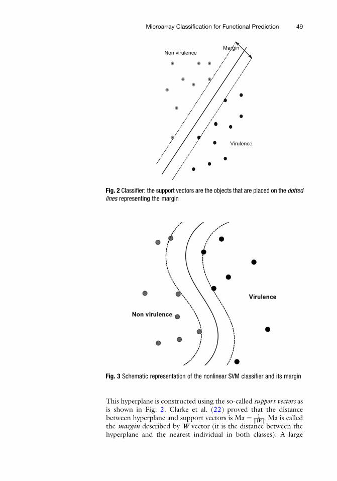
This hyperplane is constructed using the so-called support vectors asis shown in Fig. 2. Clarke et al. (22) proved that the distancebetween hyperplane and support vectors is Ma ¼ 1

jjWjj. Ma is calledthe margin described by W vector (it is the distance between thehyperplane and the nearest individual in both classes). A large

Fig. 3 Schematic representation of the nonlinear SVM classifier and its margin

Fig. 2 Classifier: the support vectors are the objects that are placed on the dottedlines representing the margin

Microarray Classification for Functional Prediction 49

margin implies flexibility and a small margin precision. Therefore itswidth should be chosen trading off these two properties.

When the highest value ofM is a constraint to a correct classifi-cation, the optimization problem can be expressed as follows:

minW,b1

2jjWjj2 constraint to yi W

0xi þ b

� �� 1 forall i ¼ 1, 2, . . . ,n

ð1ÞClarke et al. (22) show the last optimization problem can achieve tothe dual formulation, because it allows a less complex solution byquadratic programming:

minα1

2

Xn

i¼1

Xn

j¼1

αiα j yi y jx0ix j �

Xn

i¼1

αi

Constrain toXn

i¼1

αi yi ¼ 0 and0 � αi � C, i ¼ 1, 2, . . . ,n ð2Þ

Where the αi 2 ℝ for i=1, 2, � � �,n are Lagrange multipliersassociated with Eq. 1, finally the support vectors exist, based onthe following equations:

If α ¼ 0 where yi W0xi þ b

� �> 1

And

If α > 0 where yi W0xi þ b

� �¼ 1

The vectors xi that satisfy αi > 0 are support vectors (22).

The example code we use below is adapted from JP Vert’spractical session on SVM (http://cbio.ensmp.fr/~jvert/svn/tutorials/practical/svmbasic/svmbasic_notes.pdf).

n <- 150 # number of data points

p <- 2 # dimension

sigma <- 1 # variance of the distribution

meanpos <- 0 # centre of the distribution of positive

examples

meanneg <- 3 # centre of the distribution of negative

examples

npos <- round(n/2) # number of positive examples

nneg <- n-npos # number of negative examples

# Generate the positive and negative examples

xpos <- matrix(rnorm(npos*p,mean¼meanpos,sd¼sigma),

npos,p)

xneg <- matrix(rnorm(nneg*p,mean¼meanneg,sd¼sigma),

npos,p)

x <- rbind(xpos,xneg)

# Generate the labels

y <- matrix(c(rep(1,npos),rep(-1,nneg)))

50 Liliana Lopez Kleine et al.

# Visualize the data

plot(x,col¼ifelse(y>0,1,2))

legend("topleft",c(’Positive’,’Negative’),col¼seq(2),

pch¼1,text.col¼seq(2))

## Prepare a training and a test set (30 % of the data) ##

ntrain <- round(n*0.7) # number of training examples

tindex <- sample(n,ntrain) # indices of training samples

xtrain <- x[tindex,]

xtest <- x[-tindex,]

ytrain <- y[tindex]

ytest <- y[-tindex]

istrain¼rep(0,n)

istrain[tindex]¼1

plot(x,col¼ifelse(y>0,1,2),pch¼ifelse

(istrain¼¼1,1,2))

legend("topleft",c(’Positive Train’,’Positive Test’,’-

Negative Train’,’Negative Test’),

col¼c(1,1,2,2),pch¼c(1,2,1,2),text.col¼c(1,1,2,2))

# load the kernlab package

library(kernlab)

# train the SVM with C¼100

svp <- ksvm(xtrain,ytrain,type¼"C-svc",kernel¼’vanilladot’,

C¼100,scaled¼c())

# General summary

svp

# Use the built-in function to plot the classifier

plot(svp,data¼xtrain)

# Predict labels on test

ypred ¼ predict(svp,xtest)

table(ytest,ypred)

# Compute accuracy

sum(ypred¼¼ytest)/length(ytest)

3.4.3 Nonlinear Support

Vector Machine

Here we consider again the function to optimize (Eq. 1), but withthe mapped points in H done by the Φ function:

minW,b1

2jjWjj2 constrain to yi W

0Φ xið Þ þ b� �

� 1 for all

i ¼ 1, 2, . . . ,n ð3ÞA new parameter C to solve the optimization problem is needed.It controls the individuals that the model cannot classify in thecorrect class:

minW,b jjWjj2 þ CXn

i¼1

ξi

Constrain to yi W0Φ xið Þ þ b

� �� 1� ξi andξi � 0 for all

i ¼ 1, 2, . . . ,n ð4Þ

Microarray Classification for Functional Prediction 51

Similarly as in Eq. 2 the dual formulation is

minα1

2

Xn

i¼1

Xn

j¼1

αiα j yi y j K xi; x j

� ��Xn

i¼1

αi

Constrain toXn

i¼1

αi yi ¼ 0 and 0 � αi � C to i ¼ 1, 2, . . . ,n ð5Þ

Where αi are Lagrange multipliers and xi are support vectors. Theinequality 0<α< has to be satisfied. The result of the optimizationis the nonlinear classifier model, where the support vectors arethose objects that are placed on the dotted lines representing thelimit of the margin (Fig. 3).

# Train a nonlinear SVM

svp <- ksvm(x,y,type¼"C-svc",kernel¼’rbf’,kpar¼list

(sigma¼1),C¼1)

plot(svp,data¼x)

# Train a nonlinear SVM with automatic selection of sigma by

heuristic

svp <- ksvm(x,y,type¼"C-svc",kernel¼’rbf’,C¼1)

plot(svp,data¼x)

#Prediction of a class of tumor using the publicly available

dataset of gene expression.

# Load the ALL dataset

library(ALL)

data(ALL)

# Inspect them

?ALL

show(ALL)

print(summary(pData(ALL)))

#prediction of the type of the disease (B-cell or T-cell).

x <- t(exprs(ALL))

y <- substr(ALL$BT,1,1)

y <- ALL$BT

print(y)

n<-dim(exprs(ALL))[2]

ntrain <- round(n*0.7) # number of training examples

tindex <- sample(n,ntrain) # indices of training samples

xtrain <- x[tindex,]

xtest <- x[-tindex,]

ytrain <- y[tindex]

ytest <- y[-tindex]

istrain¼rep(0,n)

istrain[tindex]¼1

svp <- ksvm(xtrain,ytrain,type¼"C-svc",kernel¼’vanilladot’,

C¼100,scaled¼c())

# General summary

svp

# Predict labels on test

ypred ¼ predict(svp,xtest)

52 Liliana Lopez Kleine et al.

table(ytest,ypred)

# Compute accuracy

sum(ypred¼¼ytest)/length(ytest)

3.5 Extracting

Functional Predictions

Most reliable prediction methods (based on the classificationerrors) are chosen to assemble a list of genes whose product couldhave the function of interest (i.e., virulence, immunity, . . .), basedon the hypothesis that genes with similar gene expression profilesparticipate in the same molecular function. Moreover, genes thatare predicted by several methods, are more likely to be accuratelypredicted.

Assuming the list of genes that wants to be combined are list1and list2, a simple code to extract common elements is shownbelow.

list1<-c(1,2,3,4,5,6,7,8,9,10)

list2<-c(4,5,6,7,8,9,10,11)

combilist<-list1[list1%in%list2]

4 Notes

First difficulties can arise when genomic data is extracted frompublicly available databases, because gene expression data has dif-ferent formats and because gene names between data tables do notalways match. For example, if you are using microarray data fromNCBI (http://www.ncbi.nlm.nih.gov/) and information on par-ticipation in metabolic functions from KEGG (http://www.genome.jp/kegg/), gene names could differ. This needs to becorrected previously.

For the unsupervised methods of classification, it is convenientto obtain initial objective groups using the hierarchical methods,implemented in most of the specialized software packages. Thesecenters can be used as prior knowledge to apply the K-meansalgorithm, which presents a better performance in contrast withits hierarchical alternative. On the other hand, Kohonen’s methodis a better choice when nonlinear behaviors are suspected.

Supervised methods are useful when the categories to predictare known for some genes. Problems arise here when the categoriesare known only for a very small amount of genes. In that case it issuggested to filter genes based on any objective criterion (such asvariance or mean expression) and predict only for a subgroup ofgenes. Linear discriminant analysis is an useful method to explorepotential linear relationships among data and the dependentcategorical variable that represents the groups. If the covariancematrices among groups are not equal, the method could present apoor performance and a bad classification.

To study the performance of the methods proposed here,especially for the supervised methodologies, it is necessary to

Microarray Classification for Functional Prediction 53

estimate rates of good classification (or prediction) and, sensitivityand/or specificity rates, to study the performance of the empiricalproposed rule.

Finally, we recommend a previous training on R before thesemethods are applied in order to cope with common errorssuccessfully.

References

1. Dudoit S, Yang YH, Callow MJ, Speed TP(2002) Statistical methods for identifying dif-ferentially expressed genes in replicated cDNAmicroarray experiments. Stat Sinica 12(1):111–140

2. Moguerza JM, Munoz A (2006) Support vec-tor machines with applications. Statist Sci 21(3):299–426

3. R Core Team (2014) R: a language and envi-ronment for statistical computing. R Founda-tion for Statistical Computing, Vienna, http://www.R-project.org/

4. Lopez-Kleine L1, Molano N, Ospina L. Int JBioinform Res Appl. 2013;9(3):285–300. doi:10.1504/IJBRA.2013.053607. Using multi-variate methods to infer knowledge from geno-mic data

5. Lopez-Kleine L, Torres-Aviles F, Tejedor FH,Gordillo LA (2012) Virulence factor predic-tion in Streptococcus pyogenes using classifi-cation and clustering based on microarraydata. Appl Microbiol Biotechnol93:2091–2098. doi:10.1007/s00253-012-3917-3

6. Lopez-Kleine L, Romeo J, Torres-Aviles F(2013) Gene functional prediction using clus-tering methods for the analysis of tomatomicroarray data. In: Mohamad MS et al (eds)7th International conference on PACBB,AISC, vol 222, pp 1–6

7. Romeo JS, Torres-Aviles F, Lopez-Kleine L(2013) Detection of influent virulence andresistance genes in microarray data throughquasi likelihood modeling. Mol Genet Geno-mics 288(1–2):49–61. doi:10.1007/s00438-012-0730-8

8. Huber W, von Heydebreck A, Sueltmann H,Poustka A, Vingron M (2003) Parameter esti-mation for the calibration and variance stabili-zation of microarray data. Stat Appl Genet Mol2(1):Article 3

9. Gentleman RC, Carey VJ, Bates DM, BolstadB, Dettling M, Dudoit S, Ellis B, Gautier L, GeY, Hornik K, Gentry J, Hothorn T, Huber W,Iacus S, Irizarry R, Leisch F, Li C, Maechler M,Rossini AJ, Sawitzki G, Smith C, Smyth G,Tierney L, Yang JYH, Zhang J (2004) Biocon-ductor: open software development for

computational biology and bioinformatics.Genome Biol 5(10):R80

10. Rencher AC, Christensen WF (2012) Methodsof multivariate analysis, 3rd edn. Wiley, Hobo-ken, NJ

11. Izenman AJ (2008) Modern multivariate sta-tistical techniques: regression, classification,and manifold learning. Springer, New York

12. Kaufman L, Rousseeuw PJ (1990) Findinggroups in data: an introduction to cluster anal-ysis. Wiley, New York

13. Mojena R (1977) Hierarchical grouping meth-ods and stopping rules: an evaluation. ComputJ 20(4):359–363. doi:10.1093/comjnl/20.4.359

14. GlennW,Milligan GW, CooperMC (1985) Anexamination of procedures for determining thenumber of clusters in a data set. Psychometrika50(2):159–179

15. Hartigan JA, Wong MA (1979) A k-meansclustering algorithm. Appl Statist 28:100–108

16. Leiva-Valdebenito S, Torres-Aviles F (2010) Areview of the most common partition algo-rithms in cluster analysis: a comparative study.Rev Colomb Estad 33(2):321–339

17. Kohonen T (1982) Self-organizing formationof topologically correct feature maps. BiolCybern 43:59–69

18. Kohonen T (2001) Self-organizing maps, 3rdedn. Springer, New York

19. Friedman JH (1989) Regularized discriminantanalysis. JASA 84:165–175

20. van’t Veer LJ, Dai H, van de Vijver MJ, He YD,Hart AAM, Mao M, Peterse HL, van der KooyK, Marton MJ, Witteveen AT, Schreiber GJ,Kerkhoven RM, Roberts C, Linsley PS, Ber-nards R, Friend SH (2002) Gene expressionprofiling predicts clinical outcome of breastcancer. Nature 415:530–536

21. Scholkopf B, Smola A (2002) Learning withKernels: support vector machines, regulariza-tion, optimization, and beyond. The MITPress, Cambridge

22. Clarke B, Fokoue E, Zhang H (2009) Princi-ples and theory for data mining and machinelearning. Springer, New York

54 Liliana Lopez Kleine et al.

Methods in Molecular Biology (2016) 1375: 55–74DOI 10.1007/7651_2015_246© Springer Science+Business Media New York 2015Published online: 02 December 2015

Querying Co-regulated Genes on Diverse GeneExpression Datasets Via Biclustering

Mehmet Deveci, Onur K€uc€uktunc, Kemal Eren, Doruk Bozdag,Kamer Kaya, and €Umit V. Cataly€urek

Abstract

Rapid development and increasing popularity of gene expression microarrays have resulted in a number ofstudies on the discovery of co-regulated genes. One important way of discovering such co-regulations is thequery-based search since gene co-expressions may indicate a shared role in a biological process. Althoughthere exist promising query-driven search methods adapting clustering, they fail to capture many genes thatfunction in the same biological pathway because microarray datasets are fraught with spurious samples orsamples of diverse origin, or the pathways might be regulated under only a subset of samples. On the otherhand, a class of clustering algorithms known as biclustering algorithms which simultaneously cluster boththe items and their features are useful while analyzing gene expression data, or any data in which items arerelated in only a subset of their samples. This means that genes need not be related in all samples to beclustered together. Because many genes only interact under specific circumstances, biclustering may recoverthe relationships that traditional clustering algorithms can easily miss. In this chapter, we briefly summarizethe literature using biclustering for querying co-regulated genes. Then we present a novel biclusteringapproach and evaluate its performance by a thorough experimental analysis.

Keywords: Biclustering, Microarray, Gene expression, Clustering

“What we call chaos is just patterns we haven’t recognized. What wecall random is just patterns we can’t decipher.”

— Chuck Palahniuk, Survivor

1 Introduction

The microarray technology enables large-scale genomic research byallowing the measurement of the expression levels of thousands ofgenes in parallel. Expression levels of genes in various samples arecollected and stored in a gene expression matrix. Mining these geneexpression matrices can provide insights into gene functions andaids in the development and treatment of complex diseases. Thediscovery of related genes is a challenging task and has been thefocus of many research studies [1–4] that search for more sophisti-cated analysis methods. Most of the time, however, researchers

55

focus on a specific gene or a gene set rather than exploring thewhole dataset. Query-based search algorithms [5–10] are proven tobe very useful when the objective is to rank the genes according tohow strongly they are correlated with the queried gene(s). Forexample, several genes in S. cerevisiae database are categorized andannotated by Hibbs et al. [6]. Similarly, top-ranked genes co-regulated with breast cancer associated tumor suppressors,BRCA1 and BRCA2, are found to be regulating the mitotic spindleand cytokinesis by Bozdag et al. [9]. In analyzing this torrent ofnew data, unsupervised learning methods such as clustering areimportant as the first step. In particular, a class of clustering algo-rithms known as biclustering is useful for analyzing gene expressiondata, or any data whose items are related in only a subset of theirsamples. Biclustering methods cluster both the items and theirfeatures simultaneously. In gene expression context, this meansthat genes need not be related in all samples to be clusteredtogether. Because many genes only interact under specific circum-stances, biclustering may recover relationships that traditional clus-tering algorithms can miss.

In this chapter, first, we briefly survey the literature on biclus-tering and proposed algorithms. Then we introduce a novel biclus-tering algorithm, Correlated Patterns Biclustering (CPB), whichattempts to find genes that are related on a subset of their featureswith a query gene. As mentioned above, identifying the genes co-regulated with a gene of important function is crucial to understandbiochemical and genetic pathways in which the gene participates.To quantify gene relationships, CPB uses the Pearson correlationcoefficient (PCC), an effective and widely used metric in this type ofanalysis to quantify co-regulation between pairs of genes [2, 4].CPB’s novel approach avoids costly pairwise correlation calcula-tions in a manner that also increases its accuracy. It also allowsassigning genes to multiple biclusters, because many genes partici-pate in multiple biological pathways. We further introduce a uniquemethod for combining results from multiple datasets, which isimportant for uncovering uncommon genetic relationships. Initialtesting on artificial data shows that CPB outperforms other biclus-tering methods in finding multiple types of biclusters. CPB’s per-formance for querying the microarray data is similarly promising: itwas able to find many genes that have high correlation withBRCA1, BRCA2, and p53. Of those genes, half are alreadyknown to be involved in cancer processes, and the others arepromising new candidates for further investigation. The sourcecode of the framework, documentation, and sample datasets isavailable at http://bmi.osu.edu/hpc/software/cpb/.

The methods in this chapter extend the framework proposed byBozdag et al. [9] to increase the efficiency of the algorithms as wellas the consistency and relevancy of the results. The novelty of theproposed algorithm can be summarized as follows:

56 Mehmet Deveci et al.

l A grid-based method is used for generating initial biclusters,which covers the whole dataset.

l Results are investigated and the statistically insignificant biclus-ters are filtered out with a non-parametric scheme.

l The biclustering method is tested on various models, noiselevels, and overlap ratios; compared with other techniques.

l Correlation scores of the genes are computed and combinedmore efficiently.

The key advantages of the proposed query-based search frame-work are:

l It finds co-regulated genes with a given reference gene on anumber of diverse microarray datasets having the same genes.This is the case for data obtained from a single microarray.

l PCC-based biclustering technique is able to discover constant-row, shift, scale, and shift-scale models with positive and nega-tive correlations.

l CPB is extremely efficient compared to other PCC-based meth-ods because of a novel correlation calculation.

l Filtering step increases the relevance of the results while elim-inating insignificant and overlapping biclusters.

The rest of the chapter is organized as follows: In Section 2,biclustering algorithms from the literature are briefly surveyed.Section 3 describes the CPB algorithm. The results of the proposedalgorithm and framework’s experimental evaluation are given inSection 4. Section 5 concludes the chapter.

2 Biclustering of the Microarray Data

Biclustering refers to a class of methods that perform simultaneousclustering of both rows and columns of a data matrix. It was firstintroduced to gene expression data analysis by Cheng and Church[11]. This initial algorithm was followed by numerous biclusteringalgorithms to identify additive, multiplicative [12, 13], or morecomplex relationships [14–22] between the rows and columns of adata matrix that correspond to genes and samples, respectively.

A straightforward two-phase approach to identify the biclustersis applying standard clustering algorithms to the genes and samplesseparately in the first step, and combine the results in the secondone [23]. However, the research on biclustering is focused to amore integrated approach in which the genes and samples areanalyzed simultaneously. Several randomized or deterministic algo-rithms based on both novel and existing techniques from variousdomains, such as independent component analysis, singular valuedecomposition, simulated annealing, and local search, have been

Querying Co-regulated Genes on Diverse Gene Expression Datasets Via Biclustering 57

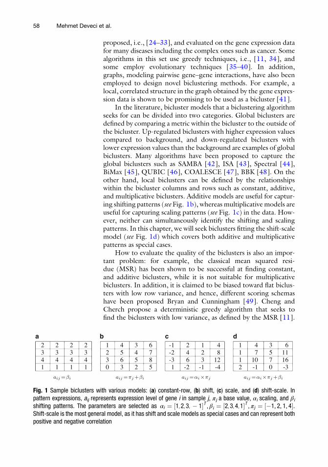
proposed, i.e., [24–33], and evaluated on the gene expression datafor many diseases including the complex ones such as cancer. Somealgorithms in this set use greedy techniques, i.e., [11, 34], andsome employ evolutionary techniques [35–40]. In addition,graphs, modeling pairwise gene–gene interactions, have also beenemployed to design novel biclustering methods. For example, alocal, correlated structure in the graph obtained by the gene expres-sion data is shown to be promising to be used as a bicluster [41].

In the literature, bicluster models that a biclustering algorithmseeks for can be divided into two categories. Global biclusters aredefined by comparing a metric within the bicluster to the outside ofthe bicluster. Up-regulated biclusters with higher expression valuescompared to background, and down-regulated biclusters withlower expression values than the background are examples of globalbiclusters. Many algorithms have been proposed to capture theglobal biclusters such as SAMBA [42], ISA [43], Spectral [44],BiMax [45], QUBIC [46], COALESCE [47], BBK [48]. On theother hand, local biclusters can be defined by the relationshipswithin the bicluster columns and rows such as constant, additive,and multiplicative biclusters. Additive models are useful for captur-ing shifting patterns (see Fig. 1b), whereas multiplicative models areuseful for capturing scaling patterns (see Fig. 1c) in the data. How-ever, neither can simultaneously identify the shifting and scalingpatterns. In this chapter, we will seek biclusters fitting the shift-scalemodel (see Fig. 1d) which covers both additive and multiplicativepatterns as special cases.

How to evaluate the quality of the biclusters is also an impor-tant problem: for example, the classical mean squared resi-due (MSR) has been shown to be successful at finding constant,and additive biclusters, while it is not suitable for multiplicativebiclusters. In addition, it is claimed to be biased toward flat biclus-ters with low row variance, and hence, different scoring schemashave been proposed Bryan and Cunningham [49]. Cheng andCherch propose a deterministic greedy algorithm that seeks tofind the biclusters with low variance, as defined by the MSR [11].

a b c d

Fig. 1 Sample biclusters with various models: (a) constant-row, (b) shift, (c) scale, and (d) shift-scale. Inpattern expressions, aij represents expression level of gene i in sample j, πj a base value, αi scaling, and βishifting patterns. The parameters are selected as αi ¼ ½1, 2, 3, � 1�T , βi ¼ ½2, 3, 4, 1�T , π j ¼ ½�1, 2, 1, 4�.Shift-scale is the most general model, as it has shift and scale models as special cases and can represent bothpositive and negative correlation

58 Mehmet Deveci et al.

Similarly, the xMOTIFs algorithm has been proposed to captureconserved gene expression motifs that are the biclusters with con-served rows in discretized dataset [50]. A more complex relation-ship among the genes has been later studied in order-preservingsubmatrix problem (OPSM) [1, 51]. The authors propose a deter-ministic greedy algorithm that seeks biclusters for which the col-umns can be sorted in increasing order for all rows in the bicluster.Although additive and multiplicative biclusters can be captured byOPSM algorithm, it fails to capture constant biclusters. Surveys onbiclustering of gene expression data, the proposed algorithms, andtheir evaluation via bicluster validation from a biological point ofview can be found in [3, 45, 52–56].

2.1 PCC-Based

Biclustering

PCC is a measure that evaluates positive and negative linear rela-tionships between vectors. It is commonly used in clustering geneexpression data [2, 4] due to its power in capturing both shiftingand scaling patterns. For a PCC-based biclustering on gene expres-sion dataset, the correlation of two genes is calculated on somespecified columns since those genes may or may not be correlatedon every experiment. Therefore, our PCC-based similarity measurebetween rows r and s on selected columns Y is calculated with:

pccðr, s,Y Þ ¼

Xi∈Y

ðri � r Þðs i � s Þ�����

�����ffiffiffiffiffiffiffiffiffiffiffiffiffiffiffiffiffiffiffiffiffiffiffiffiffiffiffiffiffiffiffiffiffiffiffiffiffiffiffiffiffiffiffiffiffiffiffiffiffiXi∈Y

ðri � r Þ2Xi∈Y

ðs i � s Þ2r , ð1Þ

where the equation runs on select columns, and the absolute valueof the expression gives a result in [0, 1] interval.

PCC-based biclusteringwas recently proposed in [9, 57]. In [57],the authors present the bi-correlation clustering algorithm (BCCA),which tries to find biclusters using Pearson correlation. They alsodiscuss the complexity of computing pairwise PCCs, and the ineffi-ciency of the method. Bozdag et al. [9] discuss potential complexityissues of an exhaustive search using PCC, and propose that, instead ofcomputing all pairwise PCC values, a center-like vector (tendencyvector) is sufficient and more efficient at finding correlated rows.

3 Correlated Pattern Biclusters

Given a query gene and a set of microarray datasets, we compute aranked list of co-regulated genes in three steps. Here we give thedetails of these steps: In the first step, the CPB algorithm recoversa set of biclusters (Section 3.1). In the next step, we filter outstatistically insignificant biclusters (Section 3.2). Finally, the corre-lation scores gathered from different datasets (Section 3.3). Theoverview of the framework is given in Fig. 2.

Querying Co-regulated Genes on Diverse Gene Expression Datasets Via Biclustering 59

3.1 The CPB

Algorithm

LetR and C denote the set of rows and columns of a data matrix A,respectively. Each element arc ∈ A represents the relation betweenrow r and column c. A bicluster B ¼ (X, Y ) is a subset of rowsX ¼ { x1, . . ., xn} and a subset of columns Y ¼ { y1, . . ., ym}, wheren � N, and m � M.

Definition 1 (Correlated Pattern Biclusters Algorithm). Given a datamatrix A, reference row rr, PCC threshold ρ, and minimum number ofcolumns γ, CPB finds a bicluster B ¼ (X, Y) such that rr ∈ X, m � γ,8xi ,xj∈X pccðxi, xj ,Y Þ � ρ.

CPB starts with an initial bicluster B ¼ (X, Y ) and improves itby iteratively moving rows and columns in and out of the biclusterusing a search technique similar to local search methods. Algo-rithm 1 outlines the proposed biclustering algorithm. Importantsteps, i.e., generation of the initial biclusters, computing tendencyvector T and normalization parameters, updating rows and columnsare described in detail in the following subsections.

Algorithm 1 Correlated Pattern Biclusters

1: function CPB(A, B, rr, w, γ, ρ )2: B = (X, Y ) is an initial bicluster s.t. rr ∈X3: ρc ← 2/3ρ ; ρΔ = 1/12ρ ; γc = m; γΔ = m−γ

44: repeat5: step ← 06: repeat7: step ← step + 1; Bsave ← B8: Compute T, αi, βi

9: if step mod 2 = 1 then10: Update X such that11: ∀xi ∈ X, pcc(xi, T, Y )>ρc

12: else13: Find row r with smallest pcc(r, T, Y )>ρc

14: Update Y such that15: ∀yk ∈Y, ERROR(yk)>ERROR(r)16: end if17: until step > 20 or B = Bsave

18: ρc ← ρc + ρΔ; γc ← γc − γΔ

19: until ρc > ρ20: return B = (X, Y )21: end function

Fig. 2 Overview of the proposed framework

60 Mehmet Deveci et al.

3.1.1 Generating Initial

Biclusters

Selecting the rows and columns of the initial bicluster is importantsince the algorithm converges to a more stable one by adding andremoving rows and columns to this bicluster. In [9], initial biclus-ters were chosen randomly, and the algorithm runs efficiently whendiscovering small number of biclusters embedded in synthetic data-sets. However, we observe that when there are multiple biclustersthis approach does not provide a consistent mechanism to returnmultiple biclusters with good coverage of the whole dataset.

In CPB, we generate initial biclusters with a grid-basedapproach. We first shuffle the row and column numbers of thedataset, and then partition the dataset into a coarse-grain grid of10 � 2 initial biclusters. The query gene rr is inserted into eachbicluster, if necessary. At the end, all genes and conditions in thedataset are assigned to at least one initial bicluster. Repeating theprocess gives us enough initial biclusters to find co-regulated genesand corresponding conditions. In addition, different runs obtainmore than 75 % of the top-ranked co-regulated genes with thegrid-based initialization, even though the generation of the initialbiclusters is randomized.

3.1.2 Computing

Normalization Parameters

and Tendency Vector

In order to avoid making pairwise comparisons of all rows, wecompute a tendency vector that represents an average of the rowsof the bicluster. We compute a normalized data value

axiyk ¼axiyk � αxi

βxi

for each xi ∈ X and yk ∈ Y, where αxi and βxi are shifting andscaling parameters associated with row xi, respectively. Then, eachelement tk of tendency vector T is computed as the arithmetic meanof axiyk on all rows xi ∈ X.

To ensure that the reference row rr has a larger impact ondecision mechanisms of the algorithm, we assign a larger weight,ω, to the reference row when computing the vector T. Total con-tribution from rows except rr is multiplied by (1�ω) and contribu-tion from rr is multiplied by ω, where ω is an input parameter. Largevalues for ω allow discovering patterns that resemble rr moreclosely, whereas small values reduce sensitivity, hence offer a highertolerance to noise. Therefore, if a reference row and ω specified, theelements are calculated with

tk ¼ω� axiyrr þ ð1� ωÞ �

Xk∈X�frrg

axiyk

jX j : ð2Þ

We compute T,αxi and βxi using an iterative process. Initially weset αxi ¼ 0 and βxi ¼ 1, and compute T. Then, we apply leastsquares fitting on pairs fðt1, axiy1Þ, . . . , ðtm, axiymÞg to obtain thebest shifting and scaling parameters that maximize alignment of

Querying Co-regulated Genes on Diverse Gene Expression Datasets Via Biclustering 61

each row xi with the tendency vector T. We assign intercept andslope obtained in least squares fitting toαxi and βxi , respectively. T isupdated using these parameters, and the process iterates untilconvergence.

3.1.3 Updating the Rows

of a Bicluster

For a row r to be included in X, we require pcc(r, xi, Y ) > ρ for allxi ∈ X. To avoid testing this condition against all xi ∈ X, weutilize the tendency vector T, and only test whether pcc(r, T, Y) isgreater than another threshold ρ0 instead. ρ0 is selected such thatpcc(r, T, Y) > ρ0 must ensure pcc(r, xi, Y ) > ρ for all xi ∈ X.However, PCC lacks transitivity property [58] and has a complexformula that strongly depends on the values and the length of thevectors. Although it is analytically difficult to compute a lowerbound for ρ0, it was empirically shown that there exists a lowerbound proportional to ρ [9].

In Algorithm 1, we start with a relaxed threshold and slowlytighten it at Line 18. While tightening ρ0, we relax the constraint onminimum number of columns. This allows sweeping the searchspace between two extreme combinations of these parameters.The algorithm uses five tightening steps and initial values of

ρ0c ¼ 2=3ρ

0and γc ¼ jY j (Line 3).

3.1.4 Updating the

Columns of a Bicluster

Using PCC to measure the coherence between the columns is toorestrictive. For example, although the rows in Fig. 1d are perfectlycorrelated, Pearson correlation between columns is less than 1.Therefore, we use root mean square error to assess the coherenceof the columns. It is computed as:

ERRORðykÞ ¼ffiffiffiffiffiffiffiffiffiffiffiffiffiffiffiffiffiffiffiffiffiffiffiffiffiffiffiffiffiffiffiffiffiffiffi1

n

Xni¼1

ðaxiyk � tkÞ2s

, ð3Þ

where yk ∈ Y and n ¼ jY j. For a column c =2Y, we computeERROR(c) in a similar way, by using a value tc analogous to tkthat quantifies tendency of rows xi ∈ X in column c.

In CPB, only the columns having ERROR below a threshold εare included in the bicluster. In order to have comparable ERRORthreshold for the column selection with respect to row addition, weselect ε in relation to ρ0. To establish this relation, first we note thatERROR can also be computed for rows, and it is a comparablemetric for rows and columns. For a row xi ∈ X, ERROR(xi)

is computed as

ffiffiffiffiffiffiffiffiffiffiffiffiffiffiffiffiffiffiffiffiffiffiffiffiffiffiffiffiffiffiffiffiffiffiffi1m

Xmk¼1

ðaxiyk � tkÞ2s

. Then, it is observed that

ERROR(r) generally implies a high pcc(r, T, Y) [9]. Therefore,by setting ε to the ERROR of row r that has the smallestpcc(r, T, Y) above threshold ρ0c (Line 13), we prevent the algorithmfrom returning imbalanced biclusters (i.e., very small or very highnumber of columns).

62 Mehmet Deveci et al.

3.2 Filtering

Biclusters Found by

Random Chance

Any dataset contains small biclusters with a high Pearson correla-tion value by random chance. Although we specify a lower boundfor PCC ρ0 and minimum number of columns γ, especially when γ issmall, in addition to larger biclusters, CPB recovers suchsmall biclusters. To eliminate randomly found biclusters in anon-parametric fashion, we developed following method. Suppose ¼ fB1,B2, . . . ,Bzg be the set of biclusters found by differentruns of CPB on a data matrix A. We first generate A0 by shufflingthe elements ofA. Then, we find the bicluster Bmaxwith the highestnumber of rows in A0, and use its dimension n0 as a threshold tofilter biclusters in . Algorithm 2 summarizes the filtering process.Note that the parameter n0 is unique for each dataset, but thismethod empirically finds a lower bound for n0. The more biclustersgenerated from the shuffled dataset, the better the estimate of n0.

Algorithm 2 Filter Random Biclusters.

1: function FilterRandomBiclusters(A, B, γ, ρ )2: A ← Shuffle(A); B ← {}3: for each row ri in A do4: B ← B ∪ CPB(A , ri, 0.5, γ, ρ )5: end for6: n ← argmaxBi∈B′ ni

7: for each bicluster Bi in B do8: (ni, mi) ← size[Bi]9: if ni ≤ n then10: B ← B \ {Bi}11: end if12: end for13: return B

14: end function

In addition to filtering out the statistically insignificant biclus-ters, we also remove those that have substantial overlaps. For anybicluster pair that has an overlap of 75 % or more, we remove thesmaller bicluster.

3.3 Combining

Correlation

Information

CPB often produces different resulting biclusters due to the ran-dom selection of initial biclusters. Information from these biclus-ters, each including the reference row rr, is merged to score eachrow’s relationship with rr.

In [9], bicluster uniqueness (BU) measure was proposed tocalculate the correlation score of the genes. Although BU is ableto capture the information redundancy caused by overlappingbiclusters, we present a similar but more efficient scoring functionto be used instead.

Let ¼ fB1,B2, . . . ,Bzg be the set of biclusters found bydifferent runs of CPB on a data matrix A, and with reference rowrr. Suppose IR(r) and IC(c) denote the maximal subset of thatcontain the given row and column, respectively.

Querying Co-regulated Genes on Diverse Gene Expression Datasets Via Biclustering 63

Definition 2 (Correlation Score (CS)). A score is assigned to a row rbased on the number of experiments in which r is co-regulated with rr by:

CSðrÞ ¼Xc∈C

j IRðrÞ \ ICðcÞ j : ð4Þ

To increase significance and consistency of our findings, weapply our method on different datasets separately and combinecorrelation scores. To achieve this in a meaningful way, we requiredatasets to have the same row labels. In gene expression dataanalysis, this requirement can be met by merging results onlyfrom datasets obtained using the same microarray chip.

Definition 3 (Gene Correlation Score (GCS)). Let ¼ fA1,A2, . . . ,Apg be the set of (microarray) datasets with the samerow labels (genes). Given a reference row rr and datasets , genecorrelation score G C S of a row r is calculated with

GCSðr, rrÞ ¼XAv∈

CSðrÞCSðrrÞ : ð5Þ

4 Experimental Results

We test CPB on the probes of three tumor suppressor genes (i.e.,BRCA1, BRCA2, and p53) as queries to reveal co-regulated genesinvolved in the complex process of tumor formation. Experimentson 40 large datasets, each with 22,283 probe sets, show that theresults are remarkably enriched for genes that have a role in cancerprogression, tumor growth and metastasis regulation, and DNAdegradation and repair. We also compare our results with anotherquery-based framework to see how successfully each method findsknown and unexplored genes co-regulated with tumor suppressors.While the ratios of known cancer-related genes are similar, theproposed framework finds more unexplored genes that are likelyto be missed by earlier clustering-based methods. CPB’s perfor-mance for querying the microarray data is promising: it was able tocapture many genes that are highly correlated with BRCA1,BRCA2, and p53. We observed that of those genes, half are alreadyknown to be involved in cancer processes, and the others arepromising new candidates for further investigation.

We first define some evaluation metrics and test CPB on syn-thetic datasets generated with biclusters with (1) different models,(2) increasing noise levels, and (3) increasing overlaps betweenembedded biclusters. We selected four other biclusteringalgorithms; δ-biclusters [11], OPSM [1], BBC [17], andBCCA [57], for comparison, due to their success at capturingshift-scale biclusters.

We test CPB on a number of human microarray datasets usingfour probes of breast cancer associated BRCA1 and BRCA2 genes,

64 Mehmet Deveci et al.

and two probes of p53 tumor suppressor gene as queries. Thecorrelation scores of the genes are combined, and the top-rankedgenes are further studied. We also compare our results with MEMframework [8] in terms of the algorithms’ effectiveness of retrievingundiscovered cancer-related genes.

4.1 Experiments on

Synthetic Datasets

We first define recovery and relevance metrics to evaluate the resultsof biclustering algorithms. For each experiment, a synthetic datasetis generated with 1000 rows and 200 samples. Then two 60 � 60biclusters with the given model are embedded into the dataset. Theaverage score of 100 replication of the same experiment is reported.

4.1.1 Evaluation Metrics Similar to recall and precision metrics, recovery and relevancescores are proposed to evaluate the biclustering results. Thesemeasures can be defined to compare a single found bicluster againstan expected one, as well as a set of found biclusters against a set ofexpected ones.

Let e and f be expected and found biclusters, respectively. Therecovery score of a found bicluster against an expected one iscalculated by dividing the intersection area by the area of theexpected bicluster:

recðe, f Þ ¼ j e \ f jj e j , ð6Þ

where the recovery score reaches to 1 if and only if e � f .Similarly, relevance score is calculated by dividing the intersec-

tion area by the area of the found bicluster:

relðe, f Þ ¼ j e \ f jj f j , ð7Þ

where the relevance score reaches to 1 if and only if f � e. Examplesof how these scores are computed are given in Fig. 3.

Using these rec and rel measures, we define recovery and rele-vance scores to compare two sets. Let E and F be a set of expected

Fig. 3 Example expected/found biclusters with their recovery and relevance scores

Querying Co-regulated Genes on Diverse Gene Expression Datasets Via Biclustering 65

and found biclusters, respectively. The set-based recovery score iscalculated by taking the mean of the maximum recovery score foreach expected bicluster. An equivalent approach is used forrelevance.

RECðE, F Þ ¼ 1

j E jXe∈E

maxf ∈F

recðe, f Þ ð8Þ

RELðE,F Þ ¼ 1

j F jXf∈F

maxe∈E

relðe, f Þ ð9Þ

4.1.2 Effects of the

Bicluster Model

Biclustering methods often focus on detecting specific types ofbiclusters, as mentioned in Background section. In this experiment,we compare the success rate of CPB with other algorithms ondetecting biclusters generated with various models. Constant-row,shift, scale, and shift-scale models were chosen for this experiment.Examples of these models are given in Fig. 1.

The resulting recovery and relevance scores (see Fig. 4a–d)show that CPB is the only algorithm that can fully recover biclustersgenerated with all four models with a high relevance score. BBCwas able to find shifted and constant-row biclusters with a slightlylower relevance score. BCCA was expected to display similar resultsto CPB since they both use Pearson correlation; however, it wasonly able to fully recover shift biclusters. OPSM could not identifyshift, scale, or shift-scale biclusters although they are all valid order-preserving submatrices. Our experiments show that when a baserow is scaled with a value between �1 and 1, the expression rank-ings of the columns of a bicluster row lie in a narrow range alongthe row; therefore, OPSM fails to discover it. Despite this limita-tion, OPSM was able to identify one of the shifted biclusters, sinceit reports a single bicluster for each size of column. The δ-biclustersalgorithm performed poorly on all the datasets, among which it canpartially recover only constant-row biclusters. The other models arenot captured by the metric, which was previously discussed in [53].

For the noise and overlap experiments, CPB and other meth-ods were compared on shift biclusters since the shift model issuccessfully recovered by most of the algorithms (see Fig. 4b).

4.1.3 Effects of the Noise Microarrays results are perturbed by many sources of noise. Inorder to measure the sensitivity of CPB to noise, an error value εwas added to each element of the synthetic datasets. The experi-ments were run with various noise levels: each error value wasdrawn from a normal distribution with zero mean and varianceequal to the chosen noise level.

Figure 4e shows the recovery and relevance scores of the algo-rithms on datasets with varying noise levels. OPSM is dramaticallyaffected by noise since it may violate the order-preserving structure.

66 Mehmet Deveci et al.

a

e

f

b c d

Fig. 4 Experiments on synthetic datasets: (a–d) with different bicluster models, (e) under noise, and (g) withoverlapping biclusters

Querying Co-regulated Genes on Diverse Gene Expression Datasets Via Biclustering 67

Since BCCA checks for pairwise correlation score for each row, thismethod is more likely to be affected by the increasing noise.Although BBC seems to be insensitive to noise in recovery plot,its relevance score drops slightly with noise addition (see Fig. 4e).CPB is the second best algorithm that is resistant to noise eventhough it has a linear metric. Moreover, the noise resistance of CPBcan be improved by adjusting a better PCC threshold. We fixedρ ¼ 0. 9 in order to be consistent with the rest of the experiments.

We also experimented with relative noise, in which the noise isadded to each element with respect to its expression value, i.e.,element x becomes x + x ε. We observed results similar to theprevious experiment.

4.1.4 Effects

of the Overlap

A gene may take roles in several functions in a cell, each of whichmay be occurring simultaneously in a given sample; therefore, theremight be overlaps between biclusters. In this experiment we testhow CPB and other algorithms perform with increasing overlaps ofbiclusters. The datasets are generated with two overlapping biclus-ters. The overlapping regions of these biclusters are increased by 10rows and 10 columns at each step. The expression values in thethese regions are not assumed to be additive; instead, shift valuesfor rows and base vector are chosen in a way to allow both of thebiclusters to have the same expression value at overlapping regions.

Figure 4f shows the results of the overlap test. We observe thatCPB and BCCA are both insensitive to increasing overlap, whileBCCA fails to recover a very small portion of the biclusters. BBC isaffected more than BCCA in terms of recovery; also, its relevancescore drops with increasing overlap. Although OPSM recovers onlyone of the biclusters, it increases its recovery score by includingmore of the overlapping region with increasing overlap.

4.2 Identifying Genes

Co-regulated with

BRCA1, BRCA2, p53

In this experiment, we employ CPB to identify the most correlatedgenes with BRCA1, BRCA2, and p53, which are highly penetrantcancer specific tumor suppressors. CPB was run on 40 differentdatasets obtained from the GPL96 series (GDS{1064, 1284, 1615,2113, 2362, 2649, 2954, 3116, 3312, 3716, 1067, 1329, 1815,2190, 2373, 2736, 3057, 3128, 3471, 534, 1209, 1375, 1956,2255, 2519, 2767, 3096, 3233, 3514, 596, 1220, 1479, 1975,2297, 2643, 2771, 3097, 3257, 3517, 987}), all of which have thesame set of probes. The results of each dataset are then combinedwith Gene Correlation Score function.

Table 1 gives the top-ranked genes for the probes of BRCA1,BRCA2, and p53. We observe that more than 50 % of thegenes found by our framework are already investigated in cancerresearch, suggesting that CPB is indeed finding genes involvedwith cancer.

68 Mehmet Deveci et al.

Among those, for example, MBD2 is shown to have a role incancer progression and can be therapeutically targeted in aggressivebreast cancers [59]. KLK10 provides important prognostic infor-mation in early breast cancer patients [60]. CHRNA4 polymorph-isms are found to activate factors that participate in DNA

Table 1Associated top-ranked genes for 6 probes of BRCA1, BRCA2, and p53

BRCA1 BRCA2 p53

204531_s_at 211851_x_at 208368_s_at 214727_at 201746_at 211300_s_at

1 C1orf105 H49077 CHRNA4 C1orf105 C1orf105 C1orf105

2 GPR98 C1orf105 C1orf105 ACRV1 H49077 PCNXL2

3 H49077 ARID4B MTMR8 GFRA4 GFRA4 GFRA4

4 CHRNA4 MTMR8 ACRV1 MTMR8 ARID4B U88898

5 SLC17A1 MBD2 GFRA4 AGTR2 MTMR8 H49077

6 GPX5 AK022006 H49077 PRO2958 AK022006 CHRNA4

7 PCNXL2 SLC17A1 PCNXL2 H49077 UBQLN3 ACRV1

8 MTMR8 CSRP3 PRO2958 ACRV1 ACRV1 MTMR8

9 ARID4B PRO2958 U88898 U88898 GNRHR PPP3CC

10 GFRA4 GFRA4 SLC17A1 SLC17A1 CHRNA4 NKX3-1

11 MBD2 NOS1 NKX3-1 GNRHR GPR98 GNRHR

12 IL17A PPP3CC ACRV1 PPP3CC RNF185 ACRV1

13 AK022006 CHRNB3 PPP3CC MBD2 SLC17A1 MBD2

14 NOS1 MAPK11 AGTR2 SPINLW1 KLK10 GNPTAB

15 ALPI ACRV1 FAM55D GNPTAB U05589 CHRNB3

16 KLK10 GNPTAB SNX1 AK000787 GPX5 ACRV1

17 PRO2958 IL17A TREX2 AK023690 OR7C2 AK000787

18 CSRP3 NEK1 GPR98 OR5I1 P2RY4 GPR98

19 PPP1R3A U05589 LEP BTNL8 PPP3CC SPINLW1

20 ACRV1 IFNA5 M78162 EPAG PCNXL2 AL162044

21 GNPTAB GPX5 CSRP3 C22orf33 AK023690 ARID4B

22 AL117549 GNA11 KRT38 RPS6KA6 TREX2 ACRV1

23 NEK1 KLK10 TBR1 GPR98 PRO2958 AW139195

24 AK023690 GJB3 EPAG MYL1 RBMY2FP GPX5

25 MYL1 SLC7A11 MBD2 PCNXL2 IL17A AK022006

Genes that have cancer-related studies found in PubMed are highlighted

Querying Co-regulated Genes on Diverse Gene Expression Datasets Via Biclustering 69

degradation and repair, specifically the level of p53 participating inDNA repair [61].

Some genes, highly correlated with p53 in the list, are alsoinvestigated in other cancer types. For instance, 4 messengerRNA biomarkers, including ACRV1, may differentiate pancreaticcancer patients from noncancer subjects [62]. GFRA4 is predomi-nantly expressed in normal and malignant thyroid medullarycells [63]. Of those, which are also correlated with BRCA1 andBRCA2 genes, can be further studied to see if they are up- or down-regulated in cancer patients.

The genes that have not already appeared in the literature mayplay an as-yet unknown role in cancer-related processes. Thesegenes are open for further research.

4.3 Comparison with

Other Query-Based

Frameworks

There are a limited number of studies on query-based discovery ofco-regulated genes in the literature. Gene recommender [5] ana-lyzed Rb protein complex to find new co-regulated genes in worms(specifically C. elegans) using a technique similar to biclustering.SPELL [6], a PCC-based clustering framework was tested on S.cerevisiae datasets, where several genes were categorized and anno-tated. A probabilistic biclustering framework, QDB [7], was testedon some synthetic and yeast microarray datasets. Adler et al. [8]propose a query engine (MEM) to search for correlated genesacross many datasets. Zhao et al. proposed ProBic [10], a probabi-listic biclustering algorithm, and tested on E. coli to detect highquality biclusters in the presence of noise.

Among those query-driven search methods, we could compareour framework on cancer-related genes with only MEM [8],because the other studies are either specialized in non-humanorganisms, or resource is not accessible. Using MEM framework,we retrieved the genes correlated with the selected probes ofBRCA1, BRCA2, and p53 genes with Pearson correlation. Top-ranked genes are then investigated to find whether the gene isclaimed to be cancer-related in a research study in medicalliterature.

In Table 2 we compare our results with MEM’s based on howsuccessful each method is on finding known and unexplored genes.Since all samples (columns) of a microarray dataset were included insimilarity calculations before biclustering, the top-ranked genesdiscovered by MEM are expected to be investigated before. Whilethe ratios of known cancer-related genes are similar, we argue thatour framework finds more unexplored genes that are likely to bemissed by earlier clustering-based methods.

Although PCC is the default similarity measure, we also runMEM with absolute Pearson correlation, which is expected tocapture negative correlations as in our pcc function (see Eq. (1)).However, the results on six probes between two runs of MEMframework are 87 % overlapping. Absolute PCC could only

70 Mehmet Deveci et al.

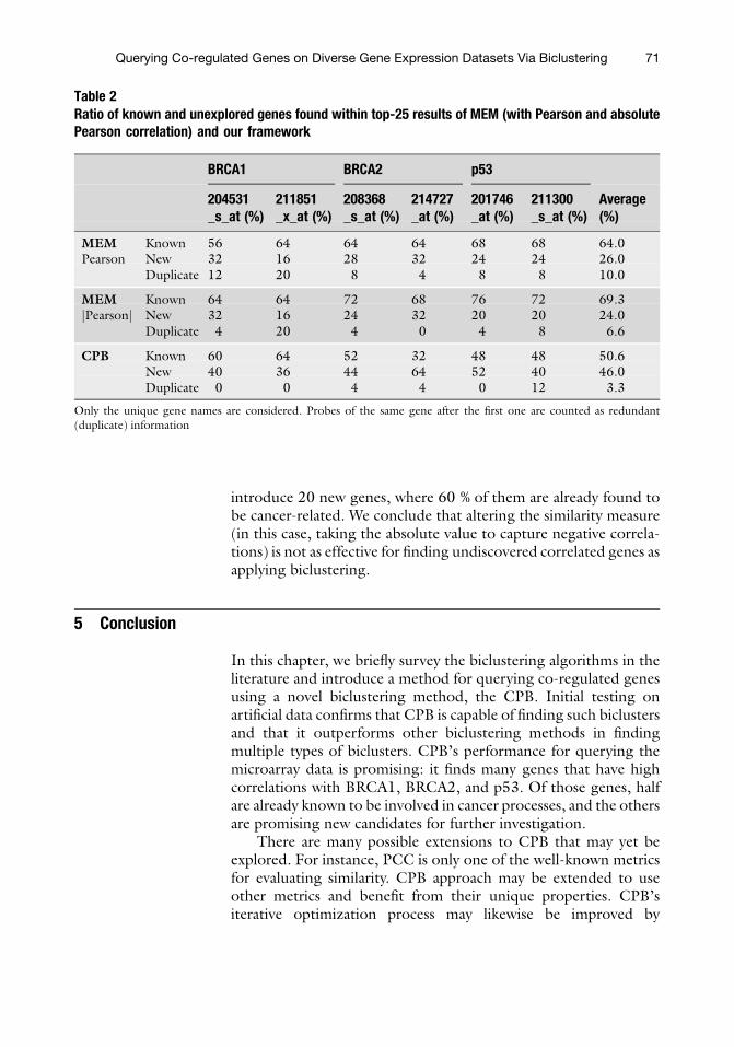
introduce 20 new genes, where 60 % of them are already found tobe cancer-related. We conclude that altering the similarity measure(in this case, taking the absolute value to capture negative correla-tions) is not as effective for finding undiscovered correlated genes asapplying biclustering.

5 Conclusion

In this chapter, we briefly survey the biclustering algorithms in theliterature and introduce a method for querying co-regulated genesusing a novel biclustering method, the CPB. Initial testing onartificial data confirms that CPB is capable of finding such biclustersand that it outperforms other biclustering methods in findingmultiple types of biclusters. CPB’s performance for querying themicroarray data is promising: it finds many genes that have highcorrelations with BRCA1, BRCA2, and p53. Of those genes, halfare already known to be involved in cancer processes, and the othersare promising new candidates for further investigation.

There are many possible extensions to CPB that may yet beexplored. For instance, PCC is only one of the well-known metricsfor evaluating similarity. CPB approach may be extended to useother metrics and benefit from their unique properties. CPB’siterative optimization process may likewise be improved by

Table 2Ratio of known and unexplored genes found within top-25 results of MEM (with Pearson and absolutePearson correlation) and our framework

BRCA1 BRCA2 p53

204531_s_at (%)

211851_x_at (%)

208368_s_at (%)

214727_at (%)

201746_at (%)

211300_s_at (%)

Average(%)

MEM Known 56 64 64 64 68 68 64.0Pearson New 32 16 28 32 24 24 26.0

Duplicate 12 20 8 4 8 8 10.0

MEM Known 64 64 72 68 76 72 69.3jPearsonj New 32 16 24 32 20 20 24.0

Duplicate 4 20 4 0 4 8 6.6

CPB Known 60 64 52 32 48 48 50.6New 40 36 44 64 52 40 46.0Duplicate 0 0 4 4 0 12 3.3

Only the unique gene names are considered. Probes of the same gene after the first one are counted as redundant(duplicate) information

Querying Co-regulated Genes on Diverse Gene Expression Datasets Via Biclustering 71

choosing initial biclusters differently or using a mathematical opti-mization method to avoid the local maximas.

6 Acknowledgments

This work was supported in parts by National Institutes of Health/National Cancer Institute (grant number R01CA141090); by theDepartment of Energy (grant number DE-FC02-06ER2775); andby the National Science Foundation (grants numbers CNS-0643969, OCI-0904809, OCI-0904802).

References

1. Ben-Dor A, Chor B, Karp R, Yakhini Z (2002)Discovering local structure in gene expressiondata: The order-preserving submatrix problem.In: Proceedings of the International Confer-ence on Computational Biology, pp 49–57

2. Jiang D, Pei J, Zhang A (2003) DHC: adensity-based hierarchical clustering methodfor time series gene expression data. In: Pro-ceedings IEEE Symposium on BioInformaticsand Bioengineering, pp 393–400

3. Madeira SC, Oliveira AL (2004) Biclusteringalgorithms for biological data analysis: a survey.IEEE/ACM Trans Comput Biol Bioinform 1(1):24–45

4. Pujana MA, Han J-DJ, LM Starita, StevensKN, Tewari M, Ahn JS, Rennert G, MorenoV, Kirchhoff T, Gold B, Assmann V, ElShamyWM, Rual J-F, Levine D, Rozek LS, GelmanRS, Gunsalus KC, Greenberg RA, Sobhian B,Bertin N, Venkatesan K, Ayivi-GuedehoussouN, Sole X, Hernandez P, Lazaro C, NathansonKL, Weber BL, Cusick ME, Hill DE, Offit K,Livingston DM, Gruber SB, Parvin JD, VidalM (2007) Network modeling links breast can-cer susceptibility and centrosome dysfunction.Nat Genet 39(11):1338–1349

5. Owen AB, Stuart J, Mach K, Villeneuve AM,Kim S (2003) A gene recommender algorithmto identify coexpressed genes in C. elegans.Genome Res 13(8):1828–1837

6. Hibbs MA, Hess DC, Myers CL, HuttenhowerC, Li K, Troyanskaya OG (2007) Exploring thefunctional landscape of gene expression:directed search of large microarray compendia.Bioinformatics 23:2692–2699

7. Dhollander T, Sheng Q, Lemmens K, DeMoor B, Marchal K, Moreau Y (2007)Query-driven module discovery in microarraydata. Bioinformatics 23:2573–2580

8. Adler P, Kolde R, Kull M, Tkachenko A, Peter-son H, Reimand J, Vilo J (2009) Mining forcoexpression across hundreds of datasets usingnovel rank aggregation and visualization meth-ods. Genome Biol 10:R139

9. Bozdag D, Parvin JD, Cataly€urek €UV (2009) Abiclustering method to discover co-regulatedgenes using diverse gene expression datasets.In: Proceedings of 1st International Confer-ence on Bioinformatics and ComputationalBiology, pp 151–163

10. ZhaoH, Cloots L, Van den Bulcke T, Wu Y,DeSmet R, Storms V, Meysman P, Engelen K,Marchal K (2011) Query-based biclusteringof gene expression data using probabilistic rela-tional models. BMC Bioinf 12(Suppl 1):S37

11. Cheng Y, Church GM (2000) Biclustering ofexpression data. In: Proceedings of Interna-tional Conference on Intelligent Systems forMolecular Biology, pp 93–103

12. Segal E,TaskarB,GaschA, FriedmanN,KollerD(2001)Rich probabilisticmodels for gene expres-sion. Bioinformatics 17(suppl_1):S243–S252

13. Wang H, Wang W, Yang J, Yu PS (2002) Clus-tering by pattern similarity in large data sets. In:Proceedings of ACM SIGMOD

14. Lazzeroni L, Owen A (2000) Plaid models forgene expression data. Tech. Rep., StanfordUniversity

15. Mitra S, Banka H (2006) Multi-objective evo-lutionary biclustering of gene expression data.Pattern Recognit 39(12):2464–2477

16. Mejıa-Roa E, Carmona-Saez P, Nogales R,Vicente C, Vazquez M, Yang XY, Garcıa C,Tirado F, Pascual-Montano A (2008)bioNMF: a web-based tool for nonnegativematrix factorization in biology. Nucleic AcidsRes 36(suppl 2):W523–W528

72 Mehmet Deveci et al.

17. Gu J, Liu JS (2008) Bayesian biclustering ofgene expression data. BMC Genomics 9(Suppl1):S4

18. Hochreiter S, Bodenhofer U, Heusel M, MayrA, Mitterecker A, Kasim A, Khamiakova T, VanSanden S, Lin D, Talloen W et al (2010) Fabia:factor analysis for bicluster acquisition. Bioin-formatics 26(12):1520–1527

19. Painsky A, Rosset S (2012) Exclusive rowbiclustering for gene expression using a combi-natorial auction approach. In: Proceedings ofthe 2012 I.E. 12th International Conferenceon Data Mining, pp 1056–1061. IEEE Com-puter Society

20. Joung J-G, Kim S-J, Shin S-Y, Zhang B-T(2012) A probabilistic coevolutionary biclus-tering algorithm for discovering coherent pat-terns in gene expression dataset. BMC Bioinf13(Suppl 17):S12

21. Flores JL, Inza I, Larranaga P, Calvo B (2013)A newmeasure for gene expression biclusteringbased on non-parametric correlation. ComputMethods Prog Biomed 112(3):367–397

22. Sun P, Speicher NK, Rottger R, Guo J, Baum-bach J (2014) Bi-force: large-scale biclusterediting and its application to gene expressiondata biclustering. Nucleic Acids Res. doi:10.1093/nar/gku201

23. Chakraborty A (2005) Biclustering of geneexpression data by simulated annealing. In:Proceedings of Eighth International Confer-ence on High-Performance Computing inAsia-Pacific Region, 2005, pp 627–632

24. Liew AW-C, Law N-F, Yan H (2011) Recentpatents on biclustering algorithms for geneexpression data analysis. Recent Pat DNAGene Seq 5(2):117–125

25. Hussain SF (2011) Bi-clustering gene expres-sion data using co-similarity. In: Proceedings ofthe 7th International Conference on AdvancedData Mining and Applications - Volume Part I,ADMA’11, pp 190–200. Springer, Berlin/Heidelberg

26. An J, Liew AW-C, Nelson CC (2012) Seed-based biclustering of gene expression data.PLoS ONE 7:e42431, 08

27. Kiraly A, Abonyi J, Laiho A, Gyenesei A (2012)Biclustering of high-throughput gene expres-sion data with bicluster miner. In: IEEE 12thInternational Conference on Data MiningWorkshops (ICDMW), 2012, pp 131–138

28. Liu J, Wang J, Wang W (2004) Biclustering ingene expression data by tendency. In: Proceed-ings of IEEE Computational Systems Bioinfor-matics Conference, pp 182–193. IEEEComputer Society

29. Liu J, Wang J, Wang W (2004) Gene ontologyfriendly biclustering of expression profiles. In:Proceedings of IEEE Computational SystemsBioinformatics Conference, pp 436–447.IEEE Computer Society

30. Madeira S, Oliveira A (2005) A linear timebiclustering algorithm for time series geneexpression data. In: Casadio R, Myers G (eds)Algorithms in bioinformatics. Lecture Notes inComputer Science, vol 3692, pp 39–52,Springer, Berlin/Heidelberg

31. Pontes B, Giraldez R, Aguilar-Ruiz JS (2013)Configurable pattern-based evolutionarybiclustering of gene expression data. Algo-rithms Mol Biol 8:4

32. Yang W-H, Dai D-Q, Yan H (2011) Findingcorrelated biclusters from gene expressiondata. IEEE Trans Knowl Data Eng23:568–584

33. Yoon S, Nardini C, Benini L, De Micheli G(2005) Discovering coherent biclusters fromgene expression data using zero-suppressedbinary decision diagrams. IEEE/ACM TransComput Biol Bioinf 2:339–354

34. Angiulli F, Cesario E, Pizzuti C (2008) Ran-dom walk biclustering for microarray data. InfSci 178(6):1479–1497

35. Bryan K (2005) Biclustering of expression datausing simulated annealing. In: Proceedings ofthe 18th IEEE Symposium on Computer-Based Medical Systems, CBMS’05, (Washing-ton, DC, USA), pp 383–388. IEEE ComputerSociety

36. Bryan K, Cunningham P, Bolshakova N (2006)Application of simulated annealing to thebiclustering of gene expression data. Trans InfTech Biomed 10:519–525

37. Bleuler S, Prelic A, Zitzler E (2004) An EAframework for biclustering of gene expressiondata. In: Congress on Evolutionary Computa-tion, 2004 (CEC2004), vol 1, pp 166–173

38. Divina F, Aguilar-Ruiz J (2006) Biclustering ofexpression data with evolutionary computation.IEEE Trans Knowl Data Eng 18:590–602

39. Nepomuceno JA, Troncoso A, Aguilar-Ruiz JS(2010) Correlation-based scatter search fordiscovering biclusters from gene expressiondata. In: Proceedings of the 8th EuropeanConference on Evolutionary Computation,Machine Learning and Data Mining in Bioin-formatics, EvoBIO’10, pp 122–133. Springer,Berlin/Heidelberg

40. Nepomuceno JA, Troncoso A, Aguilar-Ruiz JS(2011) A comparative analysis of biclusteringalgorithms for gene expression data. BioDataMining 4:3

Querying Co-regulated Genes on Diverse Gene Expression Datasets Via Biclustering 73

41. Erten C, Sozdinler M (2009) Biclusteringexpression data based on expanding localizedsubstructures. In: Rajasekaran S (ed) Bioinfor-matics and computational biology. LectureNotes in Computer Science, vol 5462,pp 224–235. Springer, Berlin/Heidelberg

42. Tanay A, Sharan R, Shamir R (2002) Discover-ing statistically significant biclusters in geneexpression data. Bioinformatics 18(Supple-ment 1):136–144

43. Bergmann S, Ihmels J, Barkai N (2003) Itera-tive signature algorithm for the analysis oflarge-scale gene expression data. Phys Rev EStat Nonlinear Soft Matter Phys 67:031902

44. Kluger Y, Basri R, Chang JT, Gerstein M(2003) Spectral biclustering of microarraydata: coclustering genes and conditions.Genome Res 13(4):703–716

45. Prelic A, Bleuler S, Zimmermann P, Wille A,B€uhlmann P, Gruissem W, Hennig L, Thiele L,Zitzler E (2006) A systematic comparisonand evaluation of biclustering methods forgene expression data. Bioinformatics22:1122–1129

46. Li G, Ma Q, Tang H, Paterson AH, Xu Y(2009) QUBIC: a qualitative biclustering algo-rithm for analyses of gene expression data.Nucleic Acids Res 37(15):e101

47. Huttenhower C, Mutungu KT, Indik N, YangW, Schroeder M, Forman JJ, Troyanskaya OG,Coller HA (2009) Detailing regulatory net-works through large scale data integration.Bioinformatics 25:3267–3274

48. Voggenreiter O, Bleuler S, GruissemW (2012)Exact biclustering algorithm for the analysis oflarge gene expression data sets. BMC Bioinf 13(Suppl 18):A10

49. Bryan K, Cunningham P (2006) Bottom-upbiclustering of expression data. In: IEEE Sym-posium on Computational Intelligence andBioinformatics and Computational Biology,2006 (CIBCB ’06), pp 1–8

50. Murali T, Kasif S (2003) Extracting conservedgene expression motifs from gene expressiondata. Pac Symp Biocomput 8:77–88

51. Liu J, Wang W (2003) Op-cluster: clusteringby tendency in high dimensional space. In:Proceedings of IEEE International Conferenceon Data Mining, p 187

52. Freitas AV, Ayadi W, Elloumi M, Oliveira J,Oliveira J, Hao J-K (2013) Survey on bicluster-ing of gene expression data, pp 591–608.Wiley, New York

53. Bozdag D, Kumar A, Cataly€urek €UV (2010)Comparative Analysis of Biclustering

Algorithms. In: ACM International Confer-ence on Bioinformatics and ComputationalBiology

54. Chia BKH, Karuturi RKM (2010) Differentialco-expression framework to quantify goodnessof biclusters and compare biclustering algo-rithms. Algorithms Mol Biol 5(1):8

55. Eren K, Deveci M, K€uc€uktunc O, Cataly€urek€UV (2012) A comparative analysis of bicluster-ing algorithms for gene expression data. BriefBioinform

56. Oghabian A, Kilpinen S, Hautaniemi S, Czei-zler E (2014) Biclustering methods: Biologicalrelevance and application in gene expressionanalysis. PloS one 9(3):e90801

57. Bhattacharya A, De RK (2009) Bi-correlationclustering algorithm for determining a set ofco-regulated genes. Bioinformatics 25(21):2795–2801

58. Casella G, Wells MT (1993) Is Pitman close-ness a reasonable criterion: comment. J AmStat Assoc 88(421):70–71

59. Mian O, Wang S, Zhu S, Gnanapragasam M,Graham L, Bear H, Ginder G (2011) Methyl-binding domain protein 2-dependent prolifer-ation and survival of breast cancer cells. MolCancer Res 9(8):1152–62

60. Kioulafa M, Kaklamanis L, Stathopoulos E,Mavroudis D, Georgoulias V, Lianidou ES(2009) Kallikrein 10 (KLK10) methylation asa novel prognostic biomarker in early breastcancer. Ann Oncol 20:1020–1025

61. Dorszewska J, Florczak J, Rozycka A,Jaroszewska-Kolecka J, Trzeciak WH,Kozubski W (2005) Polymorphisms of theCHRNA4 gene encoding the alpha4 subunitof nicotinic acetylcholine receptor as related tothe oxidative DNA damage and the level ofapoptotic proteins in lymphocytes of thepatients with Alzheimer’s disease. DNA CellBiol 24:786–794

62. Zhang L, Farrell JJ, Zhou H, Elashoff D, AkinD, Park N-H, Chia D, Wong DT (2010) Sali-vary transcriptomic biomarkers for detection ofresectable pancreatic cancer. Gastroenterology138(3):949–957, e1–7

63. Lindahl M, Poteryaev D, Yu L, Arumae U,Timmusk T, Bongarzone I, Aiello A, PierottiMA, Airaksinen MS, Saarma M (2001) Humanglial cell line-derived neurotrophic factorreceptor alpha 4 is the receptor for persephinand is predominantly expressed in normal andmalignant thyroid medullary cells. J Biol Chem276:9344–9351

74 Mehmet Deveci et al.

Methods in Molecular Biology (2016) 1375: 75–89DOI 10.1007/7651_2015_237© Springer Science+Business Media New York 2015Published online: 11 April 2015

MetaMirClust: Discovery and Exploration of EvolutionarilyConserved miRNA Clusters

Wen-Ching Chan and Wen-chang Lin

Abstract

Recent emerging studies suggest that a substantial fraction of microRNA (miRNA) genes is likely to formclusters in terms of evolutionary conservation and biological implications, posing a significant challenge forthe research community and shifting the bottleneck of scientific discovery from miRNA singletons tomiRNA clusters. In addition, the advance in molecular sequencing technique such as next-generationsequencing (NGS) has facilitated researchers to comprehensively characterize miRNAs with low abundanceon genome-wide scale in multiple species. Taken together, a large scale, cross-species survey of groupedmiRNAs based on genomic location would be valuable for investigating their biological functions andregulations in an evolutionary perspective. In the present chapter, we describe the application of effectiveand efficient bioinformatics tools on the identification of clustered miRNAs and illustrate how to use therecently developed Web-based database, MetaMirClust (http://fgfr.ibms.sinic.aedu.tw/MetaMirClust) todiscover evolutionarily conserved pattern of miRNA clusters across metazoans.

Keywords: MetaMirClust, microRNA cluster, Data mining, Synteny

1 Introduction

MicroRNAs (miRNAs) are, of 21–23 nucleotides (nt) long in theirmature forms, a recently identified class of endogenous small non-coding RNA molecules, which play important roles in gene regula-tion via the RNA interference pathway (1–4). In 1993, when thefirst miRNA lin-4 was identified in Caenorhabditis elegans, thenegative regulation pair between lin-4 and its target lin-14 wasthought as an individual case (5). As a result, miRNAs have notgained the attention of researchers until a second similar system oflet-7 was observed (6), and then its homologous transcripts wereextensively investigated in animal and plant genomes. In these twodecades, a considerable body of evidence suggests that miRNAsplay important gene-regulatory roles related to organism develop-ment, cell differentiation, and tumor progression and oncogenesis(7–11). Currently, newly discovered miRNA genes either by exper-imental or computational approaches have steadily increased asevident by the amount of records in the miRBase registry (12)and other resources (13, 14). In recent years, many studies have

75

attempted to gain insights into the biogenesis, expression,targeting, and evolution of individual miRNA gene in differentspecies. Some well-studied examples in human are, for instance,mir-34b and mir-129 which serve as tumor-suppressor miRNAsconnected to DNA methylation-associated silencing in gastric can-cer (10);mir-196a is overexpressed in primary gastric cancer tissuescompared to adjacent normal ones (9); three individual loci ofmir-9 are simultaneously hypermethylated in gastric cancer and arelikely to serve as tumor suppressive miRNAs (8). Correspondingly,a substantial amount of literature has demonstrated miRNAs ascrucial negative regulators in diverse physiological and develop-mental processes at the posttranscriptional level (15).

Up to date, a handful of miRNA clusters have been reported inanimal genomes. To the best of our knowledge, Altuvia et al. wasthe first group that identified conserved regions of miRNA clusterssystematically (16). Then, Yu et al. adopted the same method toenlarge the extent of conserved miRNA cluster (17), and thuschecked the expression profile of identified human miRNA clusters.Accumulating studies have illustrated that clustered miRNA geneslocated on polycistronic transcripts might be expressed at similarlevels and coordinately involve in an intricate regulatory network.These miRNA clusters are usually derived from polycistrons withinthe length from few hundred nucleotides to almost million basepairs (18–21). For instance, mir-17 cluster and its paralogous clus-ters are one of the well-studied cases. In 2004, Tanzer et al. havetried to reconstruct the phylogenetic evolution of mir-17 clusterfamily mainly in nine metazoan genomes and have revealed at leastthree paralogous clusters related to themir-17 cluster family, whichare mir-17-92, mir-106-92, and mir-106-25, and governed by tan-dem duplications (22).

A growing range of studies has further demonstrated that theaberrant expression of miRNAs in cluster families plays an impor-tant role in cancer oncogenesis and metastasis (23–25). In additionto the known function of mir-92a as negative regulator of angio-genesis, an overexpression pattern of the mir-17-92 cluster(13q31.3) comprising seven miRNAs has been discovered in 19lung cancer cell lines (26). In renal cell carcinoma (RCC), therestoration of the downregulated mir-143/145 cluster (5q32) inRCC cells revealed significant inhibition of cancer cell proliferationand invasion via a putative target gene, hexokinase-2 (HK2) (27).In bladder cancer (BC), five downregulated clusters: mir-1/133a(18q11.2 and 20q13.33), mir-206/133b (p12.2), let-7c/mir-99a(21q21.1), mir-143/145 (5q32), and mir-195/497 (17p13.1),were identified from 950 candidates by the genome-wide miRNAexpression signature analysis, and the following transfection assayof mir-195/497 into BC cell lines has confirmed their function astumor suppressors in BC (25). It is believed that miRNAs inclusters might represent putative bifunctional regulators, of which

76 Wen-Ching Chan and Wen-chang Lin

miRNAs in high expression level can act as oncogenes by repressingtumor suppressors, and when in low level they can turn over tobehave as tumor suppressors through a negative regulation ofoncogenes (28). Although the entire regulatory mechanisms ofclustered miRNA genes remain largely uncharacterized, it is likelythat these miRNA clusters may function more efficiently in a com-plicated miRNA-mediated network than individual miRNA alone(29). Therefore, identification of evolutionary conserved miRNAclusters is an important first step for the research society towardelucidating miRNA-cluster-mediated pathways in cancer researchand might provide new insights into the potential miRNA-basedtherapeutics for cancer.

Many resources were developed to investigate miRNA genes.However, only a handful of resources dedicate to an efficient andextensive investigation of miRNA clusters (20, 21). Generally,miRNA clusters were arbitrarily defined by a fixed distance (e.g.,10 Kb) (12), and only few studies systematically investigating theconservation patterns of clustered miRNA genes across metazoanspecies (20). Here, we illustrate the synergistic potential of Meta-MirClust and miRBase for exploring miRNA clusters conservedacross species in evolution.

The remainder of the chapter is organized as follows. First, theMaterials section highlights the technical prerequisites for the iden-tification of miRNA clusters used inMetaMirClust; second, we givean overview of available databases that enlarge the scope of miRNAgenes; third, we introduce how to identify miRNA clusters (Mir-Clust) in different maximum inter-miRNA distances (MIDs) as wellas a simple case study of using and browsing MirClust; fourth, weoutline the use of MetaMirClust for exploring metazoan conservedmiRNA clusters and their hierarchically evolutionary structure;fifth, we describe an advanced case study that uses bioinformaticstools and additional annotation files to uncover the synteny regionsflanking miRNA clusters between human and mouse. Finally, in theNotes section, we briefly comment on practical issues and highlightpotential pitfalls of the methods that are outlined in this chapter.

2 Materials

MetaMirClust is a Web-based database and can be browsed via auser-friendly interface implemented according to the protocols ofHyperText Markup Language (HTML) and Cascading Style Sheets(CSS). For general users who focus on browsing data in MetaMir-Clust, the community user can easily access it using a computerwith an Internet network. For instance, it can be a desktop com-puter running Microsoft Windows, an Apple computer runningMac OS, or a LINUX platform. A few commonly used browsersinclude (1) Mozilla Firefox (http://www.firefox.com/), (2)

miRNA Cluster Discovery in Metazoan Genomes 77

Microsoft Internet Explorer (http://www.microsoft.com/ie/), (3)Apple Safari (http://www.apple.com/de/safari/), and (4) GoogleChrome (https://www.google.com/intl/en/chrome/).

For advanced users who want to re-perform the whole analysisprocedure and/or follow-up analyses (i.e., the identification ofsynteny regions between human and mouse), beyond the essentialWeb browser, it is recommended to install an advanced text editor,e.g., Sublime Text 2/3 (http://www.sublimetext.com/) or Pro-grammer’s Notepad (http://www.pnotepad.org/), which caneffectively and efficiently facilitate scripting jobs and which manip-ulates large files (e.g., table-delimited BED files with gene modelsfrom UCSC Table Browser) and/or data format conversions.When dealing with BED format files, BEDTools 2 (https://github.com/arq5x/bedtools2) is one of fundamental tools,which efficiently manages the operations like merging, intersecting,and/or subtracting between two BED files. In addition, to build aSQL-like environment to contain data downloaded from publicresources like miRBase or to store intermediate results generatedthrough the pipeline, MySQL is one of the best choices for a fast,multi-threads/users and robust database management system. InMetaMirClust, we introduced a data mining approach, i.e., FP-growth (30, 31), to efficiently discover highly conserved sets ofmiRNA genes upon miRNA clusters (MirClust). The implementa-tion version of FP-growth algorithm by Borgelt is available todownload (http://www.borgelt.net/fpgrowth.html). Similarly,the final results after the mining procedure are restored intoMySQL database for querying and browsing via the Web-basedinterface. Finally, for visualization, it is also useful to install theperl models like GD (http://search.cpan.org/~lds/GD/) as wellas the R statistics software (http://www.r-project.org/) to presentresults in image files for visual inspection.

3 Methods

3.1 Homology Search

of miRNA Genes

A comprehensive understanding of miRNA clusters will require anextensive survey of the coverage of miRNA genes in genomes.Previously, miRNA genes were identified through cloning andsequencing of small-RNA libraries. However, miRNA genes couldbe overlooked due to low expression levels. In this decade, the ever-growing data adopted next-generation sequencing (NGS) tech-nique to identify miRNA genes has been incorporated into publicdatabases like miRBase. Since those studies were mainly focusingon a small set of species, it is still necessary to conduct an extensivehomology search based on known miRNA genes collected in miR-Base to enlarge the scope of miRNA genes across mammals. Thecurrent version of MetaMirClust has been performed based onknown miRNA genes reported in miRBase (Release 16: Sept

78 Wen-Ching Chan and Wen-chang Lin

2010) and predicted homologous miRNA genes in ZooMir(http://insr.ibms.sinica.edu.tw/zoomir/) (14). The data of theZooMir version used in the current MetaMirClust are dumpedfrom MySQL and can be downloaded (http://insr.ibms.sinica.edu.tw/ZooMir/ZooMir.Candidates_3.tar.bz2). Using the char-acteristics of sequence- and structure-conservation of miRNAgenes, additional 14,989 homologous precursor miRNA candi-dates in 56 genomes have been identified according to 11,839animal miRNA entries reported in miRBase 16.0. In addition, weclassified miRNA genes by reassigning miRNA classes based on thesequence similarity with same prefix of their entry names withoutconsidering species abbreviations used in miRBase.

3.2 Identification

of miRNA Clusters

(MirClust)

Recent studies have revealed that the clustering propensity ofmiRNA genes is higher than previously evaluated and they usuallyoccur on polycistronic transcripts (17, 32–36). To investigate clus-tered miRNA genes derived from the same polycistronic transcript,researchers usually adopt adjacent miRNA genes located on thesame strand to form miRNA clusters. Two or more consecutivemiRNA genes on the same strand of individual chromosome areconsidered to form a cluster according to their adjacent distance. InmiRBase, 10 Kb is used to report clustered miRNAs when usersbrowse an individual miRNA gene. Take hsa-mir-25(chr7:99,691,183-99,691,266:-) as example, miRBase will displayhsa-mir-93 (chr7:99,691,391-99,691,470:-) and hsa-mir-106b(chr7:99,691,616-99,691,697:-) as adjacent miRNA genes within10 Kb as shown in Fig. 1. As a result, using different adjacentdistance might result in a different data set of miRNA clusters.Meanwhile, the clustered miRNAs reported in miRBase are lackof evolutionary conservation across species. Four different maxi-mum inter-miRNA distances (MIDs); 1 Kb, 3 Kb, 10 Kb, and50 Kb, were commonly used to identify clustered miRNA genes(MirClust). To illustrate the procedure of identification of miRNAclusters (MirClust), we prepared two BED file composed of human(hg19) precursor/mature miRNA genes (reported in miRBase v.16or ZooMir) (http://fgfr.ibms.sinica.edu.tw/MetaMirClust/data/pre.mir.bed; http://fgfr.ibms.sinica.edu.tw/MetaMirClust/data/mat.mir.bed) as a sample data set for readers to identify miRNAclusters (MirClust) in human. In addition, the BED file of individ-ual mature miRNA genes was prepared for the retrieval of miRNA

Fig. 1 The hsa-mir-25-106b cluster reported in miRBase. By the default MID of 10 Kb used in miRBase, thissnapshot figure shows two adjacent miRNA genes, hsa-mir-106b and hsa-mir-93, when querying hsa-mir-25

miRNA Cluster Discovery in Metazoan Genomes 79

clusters with their corresponding mature miRNAs. The individualprocesses were listed as follows.

1. Sort precursor miRNA genes:

sort -k1,1 -k2,2n -k6,6 pre.mir.bed > pre.mir.sort.bed

2. Group miRNA genes to form miRNA clusters based on user-defined MID

bedtools merge -s -d 10000 -c 4,6,4 -o collapse,distinct,count -i pre.mir.sort.bed > mir.clust.bed

3. Remove singleton miRNA clusters

awk ’BEGIN{OFS¼FS¼"\t"}{if ($6 > 1) {print $0}}’ mir.clust.be > mir.clust.filter.bed

4. (Optional) Retrieve mature miRNA genes for each miRNAcluster

bedtools intersect -wo -a mir.clust.filter.bed -b mat.mir.bed >mir.clust.mat.bed

The above command would create two intermediate files (i.e.,pre.mir.sort.bed and mir.clust.bed) plus one output file for the finalresult of miRNA clusters (i.e., mir.clust.filter.bed). First, to preparethe sorted BED file as the input file of BEDTools in the followingprocess, the human miRNA genes in the BED file were sortedaccording to their genomic location plus strand information. Sub-sequently, using the merge command in the BEDTools package,adjacent miRNA genes were grouped according to the user-definedMID (here, 10 Kb). The grouped miRNAs passing the third step byfiltering singleton miRNA clusters will create miRNA clusters inhuman in this sample example. Correspondingly, the whole proce-dure can be achieved by piping into one command line: bedtoolsmerge -s -d 10000 -c 4,6,4 -o collapse,distinct,count -i<(sort -k1,1 -k2,2n -k6,6 pre.mir.bed) | awk ’BEGIN{OFS¼FS¼"\t"}{if ($6 >1) {print $0}}’ > mir.clust.filter.bed.

By comparing miRNA clusters discovered in a short MID tothose in a longer one, three scenarios are discovered: (1) forming anewmiRNA cluster bymerging singletonmiRNAgenes, (2) enlarg-ing a small miRNA cluster by recruiting singleton miRNA genes,and (3) producing a large miRNA cluster by merging at least twosmall miRNA clusters. According to our previous observation (20),when considering a long MID, these newly involved clusteredmiRNA genes are apt to generate new miRNA clusters instead ofenlarging miRNA clusters in a short MID. It is suggestive of thatmiRNA genes are prone to form clusters, and those miRNA clustersare separately located far away from each other. Table 1 shows thedistributions of numbers of miRNA clusters (MirClust) identifiedusing four different MID in nine representative species, includingCaenorhabditis elegans (worm, ce6), Drosophila melanogaster(fly, dm3),Danio rerio (zebrafish, danRer6),Gallus gallus (chicken,

80 Wen-Ching Chan and Wen-chang Lin

galGal3), Canis familiaris (dog, canFam2), Bos taurus(cow, bosTau4), Mus musculus (mouse, mm9), Rattus norvegicus(rat, rn4), and Homo sapiens (human, hg19). According to thesample example, Fig. 2 lists two miRNA clusters (MirClust) identi-fied on chromosome 13 in human according to the MID of 10 Kb,which aremir-16-1/15a (13q14.2) andmir-17-92 (13q31.3). Thecommunity users can retrieve the detailed information of individualmature miRNA genes for each miRNA clusters through the forth,optional command listed above. Correspondingly, through ourWeb-based interface (http://fgfr.ibms.sinica.edu.tw/MetaMirClust/MirClustStat.php), the community users can browse relatedinformation ofmir-17-92 (13q31.3) as shown in Fig. 3. The links toexternal browsers like UCSC Genome Browser (https://genome.ucsc.edu/) are provided to obtain more information about miRNAclusters (e.g., conservation levels and transcriptions in RefSeq orGenBank). Figure 4 shows several default tracks in the genomiclocation flankingmir-17-92 (13q31.3) in UCSC Genome Browser.

Table 1Distributions of numbers of identified miRNA clusters in nine representative species

MID

Species UCSC accession 1 Kb 3 Kb 10 Kb 50 Kb

Caenorhabditis elegans ce6 13 18 26 38

Drosophila melanogaster dm3 19 18 21 33

Danio rerio danRer6 38 55 61 73

Gallus gallus galGal3 22 41 54 72

Canis familiaris canFam2 50 49 57 74

Bos taurus bosTau4 56 54 61 81

Mus musculus mm9 78 65 69 84

Rattus norvegicus rn4 57 60 63 70

Homo sapiens hg19 66 74 79 100

Fig. 2 Two miRNA clusters identified on chromosome 13 in human. Based on miRNA genes identified inmiRBase and ZooMir and the use of MID of 10 Kb, two miRNA clusters can be revealed on chromosome 13.One is mir-15a/16 (13q14.2) in the length of 229 nt on the plus strand and the other is mir-17-92 (13q31.3) inthe length of 787 nt on the minus strand

miRNA Cluster Discovery in Metazoan Genomes 81

Fig. 3 The mature miRNA genes located in mir-17-92. The mir-17-92 (13q31.3) cluster located on chromo-some 13 consists of six precursor miRNA genes and will encode 12 mature miRNA genes

Fig. 4 MetaMirClust data of mir-17-92 shown in UCSC Genome Browser. Viewing the cluster information ofhuman mir-17-92 (13q31.3) cluster using public genome browser like UCSC Genome Browser, additionalpieces of evidence such as transcriptional regions, histone modifications, and conservation level and so oncan facilitate users to gain more insights of miRNA clusters of interest

3.3 Discovery

of Metazoan

miRNA Clusters

(MetaMirClust)

by FP-Growth

Algorithm

Most previous works only focused on studying the evolutionaryand functional implications of limited specific miRNA clustersamong a few species. No systematic and efficient approach hasbeen performed before MetaMirClust to analyze the conservationpattern of miRNA clusters on global-wide scale. To interrogate theconservation level of the clusters of miRNA genes in large numbersof metazoan genomes, we adopted a data mining approach todiscover the conserved co-occurrence modules of miRNA genesupon miRNA clusters identified under the same MID. Filteringsingleton miRNA clusters identified in MirClust as mentioned inthe previous procedure, we conducted the analysis by utilizing theFP-growth algorithm implemented by Borgelt (http://www.borgelt.net/fpgrowth.html) to detect the conserved co-occurrencesets of miRNA genes in terms of miRNA clusters defined within thesame MID. These frequent co-occurrence sets present highly con-served combinations of miRNA genes through miRNA clusters inmetazoan species, which are defined as metazoan miRNA clusters.Based on nine representative species same as listed in Table 1, weprepared an aggregate file (http://fgfr.ibms.sinica.edu.tw/MetaMirClust/data/nine.mir.clust.csv) consisting of all miRNAclusters using the previous procedure to identify MirClust. Thefollowing command can be used to discover co-occurred miRNAgenes across selected species.

1. Discover co-occurred miRNA genes across species

fpgrowth -s-7 -q0 nine.mir.clust.csv nine.meta.mir.clust.csv

According to the output result (i.e., nine.meta.mir.clust.csv),there are 84 evolutionarily conserved miRNA clusters (MetaMir-Clust) identified in at least seven out of nine representative species.Among those evolutionarily conserved miRNA clusters, mir-17-92(13q31.3) is the largest group containing five miRNA classes withsix precursor miRNA genes. Figure 5 shows the conservation pat-tern of mir-17-92 (13q31.3) in MetaMirClust. The length of themir-17-92 (13q31.3) cluster varies from 717 (Loxodonta africana)to 1,028 (Gasterosteus aculeatus) nucleotides (nt) in 20 metazoangenomes, which confirmed the estimation of the mir-17 clusterlength as 1 kb reported previously.

In MetaMirClust, to investigate the recruitment processbetween evolutionarily conserved miRNA clusters, we also recon-structed the hierarchical structure using the sets of co-occurredmiRNA genes. The community users can directly select one ofevolutionarily conserved miRNA clusters of interest from theMeta-MirClust list (http://fgfr.ibms.sinica.edu.tw/MetaMirClust/MetaMirClustStat.php) or select one of miRNA classes from thesearch page in MetaMirClust (http://fgfr.ibms.sinica.edu.tw/MetaMirClust/MetaMirClustSearch.php) to obtain the hierarchi-cal information involving the selected miRNA cluster and the

miRNA Cluster Discovery in Metazoan Genomes 83

occurrence in each species under different MIDs. Take mir-25 asexample, the search result under the MID of 10 Kb is shown asTable 2 with all evolutionarily conserved miRNA clusters contain-ing the target mir-17 miRNA. For visualization, the drawing ofconservation pattern upon genomes across species has beenprovided in MetaMirClust as shown in Fig. 6.

4 Notes

4.1 Data Preparation

from Diverse Sources

InmiRNA research,miRBase is themost critical repository, in whichcomputational and experimental miRNA genes have been collected,and a searchable database. Recently, due to the advance inmolecularsequencing technique like next-generation sequencing (NGS),miRBase have obtained ever-growing miRNA genes identifiedfrom the screening experiments (37). Currently, the miRBase data-base provides two major formats of archive files: raw-text and SQL-like files. The former includes dat and fa files in EMBL and fastaformats, respectively. They are easily for the community users tocheck the RNA sequences of precursor and mature miRNA genes.On the other hand, the SQL-like files dumped directly from miR-Base contain more information, which is normalized and store intoindividual tables in terms of database management. For advancedusers, the latter files will be more efficient to retrieve related data

Fig. 5 The conservation pattern of mir-17-92 across metazoan. The mir-17-92 (13q31.3) cluster has beenrevealed to conserve across 20 species in terms of evolution in our data set and occurs 24 instances amongthese species

84 Wen-Ching Chan and Wen-chang Lin

Table2

Hierarchicalstructureof

differentrecruitm

entof

mir-25-106

miRNA Cluster Discovery in Metazoan Genomes 85

Fig. 6 The evolutionarily conserved patterns of mir-25-106. This figure shows the conservation pattern of themir-25-106 (7q22.1) across 15 species according to the proportion of genomic distance

86 Wen-Ching Chan and Wen-chang Lin

from joining tables by using the SQL language. For our predictedmiRNA genes across metazoans, the dumped data from ZooMir(http://insr.ibms.sinica.edu.tw/ZooMir/ZooMir.Candidates_3.tar.bz2) can be easily incorporated into the latest version ofmiRBase.

4.2 Understanding

the Basics of Data

Mining and Machine

Learning

In recent years with the large-scale and genome-wide data generatedby ever-developing molecular biology technique, the huge amountof data have become the major challenge for biologists to manipu-late and analyze them using conventional approaches. Increasingevidence suggests that data mining and machine learningapproaches can facilitate researchers to efficiently and effectivelyconquer the massive number of data like in biological research.For instance, in MetaMirClust we introduced a data miningapproach to efficiently discover highly conserved sets of miRNAgenes upon miRNA clusters. By treating miRNA genes as items,FP-growth algorithm can be utilized to mining the frequent itemsets without using candidate generations, of which it can dramati-cally improve performance in terms of memory space and runningtime. The algorithm first compresses the input data into a tree-basedstructure, FP-tree, in which all frequent item sets can be retrievedafter easily tracing the entire tree. By iteratively tracing the sub FP-tree based on conditional frequent item sets, the algorithm canefficiently reduce the search costs by avoiding the problem intro-duced in other approaches to look for short fundamental patternsrecursively. Subsequently, the identified frequent item sets using theFP-growth algorithm are equivalent to the frequently co-occurredmiRNA genes in terms of clusters. Based on those conservation setsof miRNA genes, we can further reconstruct the hierarchical struc-ture of conservation patterns across metazoans to facilitate thecommunity users to gain more insights into the recruitment processof miRNA genes in clusters in evolution perspective.

4.3 Investigation of

Conservation Between

miRNA Clusters and

Flanking Protein-

Coding Genes

To test whethermiRNA clusters are co-conservedwith their flankingprotein-coding genes, we have conducted a downstream analysis, inwhich the linkage of known protein-coding genes in the vicinity ofevolutionarily conserved miRNA clusters between human andmouse were interrogated. We focused only on the nearest adjacentknown genes located in the upstream/downstream regions of con-served miRNA clusters upon the same strand between those twospecies. The genomic information of the protein-coding genes inhuman (hg19) andmouse (mm9)were downloaded from theUCSCGenomeBrowser (https://genome.ucsc.edu/). In addition, the lift-Over program (http://genome.ucsc.edu/cgi-bin/hgLiftOver)downloaded from UCSC Genome Browser was utilized to find thebest mapping of genomic locations between human and mouse if amiRNA cluster occurs in multiple locations. The homologousannotations between known protein-coding genes were identified

miRNA Cluster Discovery in Metazoan Genomes 87

according to the HomoloGene release 64 fromNCBI (http://www.ncbi.nlm.nih.gov/homologene). As a result, our result demon-strated that 24 out of 37 genomic regionswere co-conserved accord-ing to the evolutionarily conserved miRNA clusters and theircorresponding adjacent protein-coding genes. Nine out of thirty-seven genomic regions were partially con-served with eitherupstream or downstream protein-coding genes. Intriguingly, all sixconserved miRNA clusters located in the intronic regions wereentirely conserved with their host protein-coding genes. This maysuggest that the conservation pattern could be largely extended frommiRNA clusters to their adjacent protein-coding genes.

References

1. Ambros V (2004) The functions of animalmicroRNAs. Nature 431(7006):350–355

2. Bartel DP (2004) MicroRNAs: genomics, bio-genesis, mechanism, and function. Cell 116(2):281–297

3. He L, Hannon GJ (2004) MicroRNAs: smallRNAs with a big role in gene regulation. NatRev Genet 5(7):522–531

4. Lee Y et al (2002) MicroRNA maturation:stepwise processing and subcellular localiza-tion. EMBO J 21(17):4663–4670

5. Lee RC, Feinbaum RL, Ambros V (1993) TheC. elegans heterochronic gene lin-4 encodessmall RNAs with antisense complementarityto lin-14. Cell 75(5):843–854

6. Reinhart BJ et al (2000)The 21-nucleotide let-7RNA regulates developmental timing inCaenor-habditis elegans. Nature 403(6772):901–906

7. Tsai KW et al (2010) Epigenetic regulation ofmiR-196b expression in gastric cancer. GenesChromosomes Cancer 49(11):969–980

8. Tsai KW et al (2011) Aberrant hypermethyla-tion of miR-9 genes in gastric cancer. Epige-netics 6(10):1189–1197

9. Tsai KW et al (2012) Aberrant expression ofmiR-196a in gastric cancers and correlationwith recurrence. Genes Chromosomes Cancer51(4):394–401

10. Tsai KW et al (2011) Epigenetic regulation ofmiR-34b and miR-129 expression in gastriccancer. Int J Cancer 129(11):2600–2610

11. Berezikov E (2011) Evolution of microRNAdiversity and regulation in animals. Nat RevGenet 12(12):846–860

12. Griffiths-Jones S (2004) The microRNA regis-try. Nucleic Acids Res 32(Database issue):D109–D111

13. Li SC et al (2010) Discovery and characteriza-tion of medaka miRNA genes by next genera-tion sequencing platform. BMC Genomics 11(Suppl 4):S8

14. Li SC et al (2010) Identification of homolo-gous microRNAs in 56 animal genomes. Geno-mics 96(1):1–9

15. WuHH, Lin WC, Tsai KW (2014) Advances inmolecular biomarkers for gastric cancer: miR-NAs as emerging novel cancer markers. ExpertRev Mol Med 16:e1

16. Altuvia Y et al (2005) Clustering and conserva-tion patterns of human microRNAs. NucleicAcids Res 33(8):2697–2706

17. Yu J et al (2006) Human microRNA clusters:genomic organization and expression profile inleukemia cell lines. Biochem Biophys Res Com-mun 349(1):59–68

18. Sewer A et al (2005) Identification of clusteredmicroRNAs using an ab initio predictionmethod. BMC Bioinformatics 6:267

19. Hertel J et al (2006) The expansion of themetazoan microRNA repertoire. BMC Geno-mics 7:25

20. Chan WC et al (2012) MetaMirClust: discov-ery of miRNA cluster patterns using a data-mining approach. Genomics 100(3):141–148

21. Mathelier A, Carbone A (2013) Large scalechromosomal mapping of human microRNAstructural clusters. Nucleic Acids Res 41(8):4392–4408

22. Tanzer A, Stadler PF (2004) Molecular evolu-tion of a microRNA cluster. J Mol Biol 339(2):327–335

23. Calin GA, Croce CM (2006) MicroRNA sig-natures in human cancers. Nat Rev Cancer 6(11):857–866

24. Laddha SV et al (2013) Genome-wideanalysis reveals downregulation of miR-379/miR-656 cluster in human cancers. Biol Direct8:10

25. Itesako T et al (2014) The microRNAexpression signature of bladder cancer by deepsequencing: the functional significance of themiR-195/497 cluster. PLoS One 9(2):e84311

88 Wen-Ching Chan and Wen-chang Lin

26. Hayashita Y et al (2005) A polycistronicmicroRNA cluster, miR-17-92, is overexpressedin human lung cancers and enhances cell prolif-eration. Cancer Res 65(21):9628–9632

27. Yoshino H et al (2013) Tumor-suppressivemicroRNA-143/145 cluster targetshexokinase-2 in renal cell carcinoma. CancerSci 104(12):1567–1574

28. Esquela-Kerscher A, Slack FJ (2006) Onco-mirs: microRNAs with a role in cancer. NatRev Cancer 6(4):259–269

29. Zhang Y, Zhang R, Su B (2009) Diversity andevolution of MicroRNA gene clusters. SciChina C Life Sci 52(3):261–266

30. Han JW et al (2004) Mining frequent patternswithout candidate generation: a frequent-pattern tree approach. Data Min Knowl Discov8(1):53–87

31. Chen L, Liu W (2013) Frequent patternsmining in multiple biological sequences. Com-put Biol Med 43(10):1444–1452

32. MegrawM et al (2007) miRGen: a database forthe study of animal microRNA genomic orga-nization and function. Nucleic Acids Res 35(Database issue):D149–D155

33. Lai EC et al (2003) Computational identifica-tion of Drosophila microRNA genes. GenomeBiol 4(7):R42

34. Lagos-Quintana M et al (2003) New micro-RNAs from mouse and human. RNA 9(2):175–179

35. Berezikov E et al (2005) Phylogenetic shadow-ing and computational identification of humanmicroRNA genes. Cell 120(1):21–24

36. Alexiou P et al (2010) miRGen 2.0: a databaseof microRNA genomic information and regu-lation. Nucleic Acids Res 38(Database issue):D137–D141

37. Kozomara A, Griffiths-Jones S (2014) miR-Base: annotating high confidence microRNAsusing deep sequencing data. Nucleic Acids Res42(Database issue):D68–73

miRNA Cluster Discovery in Metazoan Genomes 89

Methods in Molecular Biology (2016) 1375: 91–103DOI 10.1007/7651_2015_280© Springer Science+Business Media New York 2015Published online: 10 September 2015

Analysis of Gene Expression Patterns Using Biclustering

Swarup Roy, Dhruba K. Bhattacharyya, and Jugal K. Kalita

Abstract

Mining microarray data to unearth interesting expression profile patterns for discovery of in silico biologicalknowledge is an emerging area of research in computational biology. A group of functionally related genesmay have similar expression patterns under a set of conditions or at some time points. Biclustering is animportant data mining tool that has been successfully used to analyze gene expression data for biologicallysignificant cluster discovery. The purpose of this chapter is to introduce interesting patterns that may beobserved in expression data and discuss the role of biclustering techniques in detecting interestingfunctional gene groups with similar expression patterns.

Keywords: Data mining, Expression patterns, Bi-clustering, Microarray

1 Introduction

With the rapid growth of DNA microarray technology, it is nowpossible to analyze expression patterns of many genes in a system-atic and comprehensive manner at the genomic level [1]. The studyof expression patterns of genes in different experimental conditionsmay enable one to understand the dynamic behavior of genes andpathways involved in biological processes. A gene expression level isa numerical value that measures how a particular gene is over-expressed or under-expressed in comparison with its activity innormal conditions. Analysis of expression patterns can be helpfulin discovering groups of genes that participate in similar biologicalprocesses or functions. Various biotechnology laboratories andpharmaceutical companies involved in in silico drug design canidentify molecular targets that may interact with the drugs. Micro-array analysis can assist drug companies in choosing the mostappropriate candidates for participation in clinical trials of newdrugs [2]. Wide availability of diagnostic DNA microarrays haspositively impacted cancer research compared to other recent tech-nologies since they are relatively easy to make and use.

One major goal of analyzing expression data is to discoverfunctionally similar genes. Co-regulation is a common phenome-non in gene expression. Expression patterns with similar tendencyor behavior are normally termed as positively regulated and

91

inverted behavior as negatively regulated [3]. Finding positivelyand negatively co-regulated gene clusters from gene expressiondata is a real need. A group of co-regulated genes may form geneclusters that can encode proteins, which interact amongst them-selves and take part in common biological processes. Genes withsimilar (or inverted) expression profiles are very likely to be regula-tors of one another or be regulated by some other common parentgene [4, 5]. It has been observed that small sets of genes are co-regulated and co-expressed under certain conditions, their behaviorbeing almost inactive for other conditions. Discovering groups ofgenes with similar or inverted expression profiles under a set ofconditions leads to the concept of biclustering expression data. Wediscuss here various expression patterns identified in microarraydata and how, based on these patterns, biological knowledge canbe extracted in the form of biclusters.

1.1 Patterns in Gene

Expression Data

With the help of microarray experiments one can simultaneouslymonitor the expression levels of genes at a genome scale. Datagenerated from microarray experiments, measuring relative expres-sion levels of genes in a sample and in a controlled population canbe represented in the form of a matrix or vector [6], often calledgene expression matrix. Formally, it can be defined as follows.

Definition 1 (Gene Expression Data). Let G ¼ {G1, G2, . . ., Gm} be aset of m genes and R ¼ {T1, T2, . . ., Tn} be the set of n conditions ortime points at which the genes’ expression levels are recorded in amicroarray dataset. The gene expression dataset X can be representedas an m � n matrix, Xm�n where each entry xi, j in the matrix corre-sponds to the logarithm of the relative abundance of mRNAcorresponding to a gene.

To gain better understanding of genes and their behavior insidethe cell, various patterns can be derived by analyzing the change inexpression levels of the genes. The notion of patterns in microarraydata is introduced in [7] as below.

Definition 2 (Expression Pattern). Given a gene Gi, its expressionvalues under a single condition or a series of varying conditions liewithin a certain range. Gi is a vector of real numbers within the range[a, b], denoted as Gi@[a, b], and is called an item. The values in Gi arelimited inclusively between a and b.

A set containing one single item is called a pattern. A set of severalitems, which come from different genes is also called a pattern. So, apattern looks like:

fGi1@½ai1, bi1�, . . . ,Gik@½aik, bik�g

where it 6¼ is, 1 � t, s � k, if k > 1.

92 Swarup Roy et al.

Example data (Table 1) from Homo sapiens microarray dataset,GDS825, taken from NCBI1 and their respective profile plots areshown in Fig. 1.

From a biological point of view, patterns play an important rolein discovering functions of genes, disease targets, or gene interac-tions [8]. A number of different patterns have been identified inbiologically significant gene groups.

1.1.1 Shifting and

Scaling Patterns

In shifting patterns [7], the gene profiles show similar trends, butdistance-wise, they may not be close to each other (see Fig. 2).

In terms of expression values, the gene patterns are separatedby more or less constant vertical distances among them. Formally,shifting patterns can be defined as follows

Definition 3 (Shifting Pattern). Given two gene expression profilesGi ¼ {Ei1, Ei2, . . ., Eik} and Gj ¼ {Ej1, Ej2, . . ., Ejk} with k expressionvalues, a profile is called a shifting pattern with respect to another

Table 1Sample gene expression data from Homo sapiens

ORF C1 C2 C3 C4

GALNT5 �3.474 �3.837 �4.644 �5.059

APOE �2 �1.943 �1.786 �1.737

IDH3B 1.449 1.299 0.993 0.832

2

1

0

−1

−2

−3

−4

−5

0.5

Exp

ress

ion

leve

l

1.5 2.5

Conditions

Homo sapiens

GALNT5

APOE

IDH3B

3.5 4.51 2 3 4

Fig. 1 Profile plot of Homo sapiens expression data

1www.ncbi.nlm.nih.gov.

Gene Expression Patterns 93

profile, if expression value Eip can be related to Ejp with a constantadditive factor πij for the p ¼ 1. . . k. For genes Gi and Gj, the fact canbe represented as follows.

Eip � E jp

�� �� � πij : ð1Þ

Similarly, scaling patterns in gene expression roughly have mul-tiplicative distance among the patterns. Scaling pattern can bedefined as follows.

Definition 4 (Scaling Pattern). Given two gene expression profilesGi ¼ {Ei1, Ei2, . . ., Eik} and Gj ¼ {Ej1, Ej2, . . ., Ejk} with k expressionvalues, a profile is called a scaling pattern with respect to anotherprofile, if expression value Eip can be related to Ejp with constantmultiplicative factor ζij for the p ¼ 1. . . k. For genes Gi and Gj, thefact can be represented as follows.

Eip=E jp � ζij or E jp=Eip � ζij : ð2Þ

As shown in Fig. 2, values of G2 are roughly three times largerthan those of G3, and values of G1 are roughly three times largerthan those of G2. In nature, it may so happen that due to differentenvironmental stimuli or conditions, the pattern G3 responds tothese conditions similarly, although G1 is more responsive or moresensitive to the stimuli than the other two.

1.1.2 Coherent Patterns A group of genes showing similar pattern tendency across differentconditions is called coherent. Such a group shows predominantlyone kind of co-expression in the expression profiles of all membergenes. Co-expressed genes are likely to be involved in the samecellular processes. In practice, co-expressed genes may belong tothe same or similar functional categories indicating co-regulated

6090

80

70

60

50

40

30

20

10

0

50

40

30

20

10

00 2 4

G1G2G3

G1G2G3

Conditions

Shifting Patterns Scaling PatternsE

xpre

ssio

n le

vel

Exp

ress

ion

leve

l

Conditions6 0 2 4 6

Fig. 2 Expression profile plot shows Shifting and Scaling patterns

94 Swarup Roy et al.

families [5]. Coherent gene expression patterns may characterizeimportant cellular processes and may provide a foundation forunderstanding regulation mechanisms in the cells [9]. The patternsshown in Fig. 2 are examples of coherent patterns.

1.1.3 Co-regulated

Patterns

Often, coherent patterns are divided into two categories, namely,positively regulated patterns and negatively regulated or invertedpatterns. Sometimes, a group of genes that are positively or nega-tively regulated are also called co-regulated genes. In Fig. 1, humangenes, GLANT5 and IDH3B, show similar patterns or positivelyregulated patterns. On the other hand, IDH3B andGLANT5 showinverted or negative patterns with APOE. Biologically all threegenes are very significant. As suggested Gene Ontology, the threegenes are involved in regulation of plasma lipoprotein particle levelsand triglyceride-rich lipoprotein particle remodeling. Pronouncedinverted or negative patterns can be observed in Fig. 3, takenfrom NCBI Rat dataset GDS3702. Gene Ontology suggests thatboth are responsible for regulation of interferon-beta production. Agroup of genes may share a combination of both positive andnegative co-regulation under a few conditions or at some timepoints.

Thus, gene expression data analysis involves pattern finding.Data mining is the study of techniques that extract patterns fromlarge amounts of data. As a result, data mining provides the pri-mary tools for gene expression data analysis. Biclustering is animportant data mining tool for analyzing biologically significantgene groups. Below we present a brief discussion of biclusteringtechniques.

500

Mrps26

Pfn2450

400

350

300

250

200

150

100

50

2 4 6Conditions

Exp

ress

ion

leve

l

GDS3702 (Rat)

8 10 12

Fig. 3 Expression profile of RAT genes showing negative-regulation

Gene Expression Patterns 95

1.2 Biclustering of

Co-regulated Genes

Clustering is a popular data analysis tool in genomic studies, partic-ularly in the context of gene-expression microarrays [10–12]. Eachmicroarray provides expression measurements for thousands ofgenes and clustering is a useful exploratory technique to analyzegene expression data since it groups similar genes together andallows biologists to identify groups of potentially meaningfulgenes, which have related functions or are co-regulated, which inturn helps find the relationships among them in the form of generegulatory networks [5]. It has frequently been observed that sub-sets of genes are co-regulated and co-expressed under a subset ofenvironmental conditions or time points [13]. Biclustering algo-rithms tackle the problem of finding a set of sub-matrices whereeach sub-matrix or bicluster meets a certain homogeneity criterion.

Given a gene expression dataset DN�M, where G ¼ {G1, G2,. . . GN} is a set ofN genes andR ¼ {T1, T2, . . ., TM} is the set ofMconditions or time points, biclusters can be defined as follows.

Definition 5 (Biclusters). Biclusters are a set of sub-matrices of thematrix D ¼ (N, M) with dimensions I1 � J1, . . . Ik � Jk such thatIi � N, Ji � M 8i{1, . . ., k}, where each sub-matrix (bicluster) meets agiven homogeneity criterion.

Madeira and Oliveira [14] identify four different categories ofbiclusters based on homogeneity criterion, namely:

1. Constant biclusters,2. Biclusters with constant values on either columns or rows,3. Biclusters with coherent values, and4. Biclusters with coherent evolutions.

A comprehensive survey of different biclustering techniques forgene expression data clustering can be found in [15, 16]. In geneexpression analysis, patterns play a more important role thanexpression values [17]. As a result, the value based homogeneitycriterion mentioned above may not be suitable for grouping bio-logically significant genes.

2 Materials

Technological improvements in high-throughput DNA microarraytechnology is instrumental in the tremendous growth of publiclyavailable gene expression data. This growing amount of expressiondata requires concurrent development of adequate bioinformaticstools for comprehensive analysis of the data for extractingbiological knowledge. A number of online and offline tools areavailable for biclustering of gene expression data. We mentionhere a few of the leading, freely available biclustering packages(Table 2).

96 Swarup Roy et al.

2.1 Data Sources A plethora of real expression data produced by different biotech-nology labs are freely available online. In this chapter, we use somedatasets from Table 3 for experimentation and demonstration.

2.2 Evaluating

Quality of Biclusters

From the point of view of biological data analysis, a cluster isbiologically significant if it can produce functionally enrichedgroups of genes. A majority of the literature on biclustering evalu-ates and reports results based on functional enrichment of theclusters against Gene Ontology (GO). To determine the statisticalsignificance of the association of a particular GO term with a groupof genes in a cluster, various online tools from the GO Project2 areavailable. In Table 4, we report some freely available tools.

These tools use the hypergeometric distribution to calculatethe p-value or q-value, which evaluates whether the clusters havesignificant enrichment in one or more function groups. The p-valueis computed as follows:

Table 2Freely available Biclustering software packages

Package Availability Web site Platform Method(s) Reference

Expander 6.3 Download http://acgt.cs.tau.ac.il/expander/ Java Samba [18]

Bic_AT Plus Download http://people.ee.ethz.ch/sop/bicat/ Java BiMax, CC, [19]ISA, xMotif,OPSM

BiGGEsTS Download http://kdbio.inesc-id.pt/software/biggests/

Java CCC, e-CCC, [20]

CC-TSB

BiVisu Download http://www.eie.polyu.edu.hk/nflaw/Biclustering/

Matlab BiVisu [21]

QServer Online http://csbl.bmb.uga.edu/publications/materials/ffzhou/QServer/

Web QUBIC [22]

PAGE Download http://www.niehs.nih.gov/research/resources/software/biostatistics/page/

Java q-Clustering [23]

CoBi Download https://sites.google.com/site/swarupnehu/publications/resources

Java CoBi [24]

2 http://www.geneontology.org.

Gene Expression Patterns 97

p ¼ 1�Xki¼0

fi

� �g � fn � i

� �

gn

� � : ð3Þ

The p-value gives the probability of seeing at least k genes outof the total n genes in a cluster annotated with a particular GO

Table 3Short description of data sources

Organism DatasetNo. ofgenes

No. ofsamples Source

YeastDB 2884 17 http://arep.med.harvard.edu/biclustering/yeast.matrixYeast Sporulation 474 7 http://cmgm.stanford.edu/pbrown/sporulation

Yeast_KY 237 17 http://faculty.washington.edu/kayee/cluster/YeastCho(cell cycle)

384 17 http://faculty.washington.edu/kayee/cluster

Rat Rat_CNS 112 9 http://faculty.washington.edu/kayee/cluster

Human GDS3712 325 12 NCBIFibroblast 517 13 http://www.sciencemag.org/feature/data/984559.hsl/Serum

Mouse GDS958 308 12 NCBI

Rice Thaliana 138 8 http://homes.esat.kuleuven.be/sistawww/bioi/thijs/Work/Clustering.html

Table 4GO-based cluster evaluation tools

Tool Platform Type Url

FuncAssociate 2 Web Online http://llama.mshri.on.ca

Fatigo Web Online http://fatigo.bioinfo.cnio.es

GOTermFinder Web Online http://go.princeton.edu,http://db.yeastgenome.org/cgi-bin/GO/goTermFinder

OntoExpress Web Online http://vortex.cs.wayne.edu

GeneMANIA Web Online www.genemania.org

DAVID 6.7 Web Online http://david.abcc.ncifcrf.gov

AGO Matlab Offline www.k-space.org/alakwa/AGO/AGO.zip

98 Swarup Roy et al.

termf, given the total number of genes in the whole genome g andthe number of genes in the whole genome that are annotated withthat GO term f. It is important to note that p-value measureswhether a cluster is enriched with genes from a particular categoryto a greater extent than what would be expected by chance. If themajority of genes in a cluster appears in one category, the p-value ofthe category is small. That is, the closer the p-value to zero, themore the probability that the particular GO term is associated withthe group of genes. The Q-value is the minimal False DiscoveryRate (FDR) at which this gene appears significant. Q-values areestimated using the Benjamini Hochberg procedure [25].

3 Methods

This approach to clustering was originally introduced by Hartigan[26] and later applied by Cheng and Church [27] to expressiondata to capture the coherence of a subset of genes under a subset ofconditions. Several techniques have been proposed to find qualitybiclusters from expression data. In Cheng and Church’s approach,the degree of coherence is measured using the concept of meansquared residue (MSR) and the algorithm greedily inserts/removesrows and columns to arrive at a certain number of biclusters,achieving some predefined residue score. The lower the score, thestronger the coherence exhibited by the biclusters, and better is thequality of the biclusters. Following Cheng and Church, a numberof biclustering techniques have been proposed [27–37] to deter-mine quality biclusters.

A greedy iterative search [27, 28] based approach finds a localoptimal solution with an expectation to finally obtain a globallygood solution. A divide and conquer [26] approach divides thewhole problem into sub-problems and solves them recursively.Finally, it combines all the solutions to solve the original problem.In exhaustive biclustering [35], the best biclusters are identifiedusing exhaustive enumeration of all possible biclusters extant in thedata, in exponential time. A detailed categorization of heuristicapproaches is available in [29]. A number of techniques based onmetaheuristics, such as evolutionary and multi-objective evolution-ary framework, have also been explored [30] to generate and itera-tively refine an optimal set of biclusters. All of them use MSR as themerit function.

An MSR based technique is effective in finding optimized max-imal biclusters. From a biological point of view, the interest residesin finding biclusters with subsets of genes showing similar behaviors,not similar values. Interesting and relevant patterns from abiological point of view, such as shifting and scaling patterns, maynot be detected using this measure as it considers only expressionvalues, not the patterns or tendencies of gene expression profile. It isimportant to discover this type of patterns because frequently the

Gene Expression Patterns 99

genes can present similar behavior although their expression levelsvary in range or magnitude. Aguilar-Ruiz [31] proves that MSR isnot a good measure to discover patterns in data when the varianceamong gene values is high, that is, when the genes present scalingand shifting patterns. To detect biologically relevant biclusters withscaling and shifting patterns, a scatter search based approach hasbeen proposed [32]. This method uses a fitness function based onlinear correlation among genes and an improvement method toselect just the positively correlated genes.

Often, it has been observed that genes share local rather thanglobal similarity in their gene expression profiles and only under afew conditions or time points [13]. Thus, correlation based tech-nique may not be effective when computing pair-wise similarityamong gene expression profiles. Other than that, various pattern-based approaches have also been proposed [33, 34, 38, 39] fordiscovery of biclusters where expression levels of genes rise and fallat a subset of conditions or time points.

Recently, it has been observed that [3] co-regulated genes alsoshare negative patterns or inverted behaviors, which existingpattern-based approaches are unable to detect. CoBi [24] (Core-gulated Biclustering) captures biclusters among both positively andnegatively regulated genes as co-regulated genes. It considers bothup- and down-regulation trends and similarity in degrees of fluctu-ation under consecutive conditions for expression profiles of twogenes as a measure of similarity between the genes. It uses a newBiClust tree for generating biclusters in polynomial time that needsa single pass over the dataset.

3.1 Performance

Comparison

We compare the performance of a few biclustering methods takinginto account functional enrichment of the biclusters. We considerfour biclustering techniques: Bimax [40], Cheng and Church(CC) [27], OPSM [41], and CoBi [24]. For the purpose of com-parison, we set the parameter values of other algorithms as recom-mended in the original papers. The functional enrichment of eachbicluster is measured usingQ-values associated with GO categories.For each bicluster, we calculate average of the percentage of thenumber of genes from the bicluster with a given function against allgenes in the genome with the function. Figure 4 shows the averageof functional enrichments of each bicluster obtained by differentbiclustering algorithms from four different datasets [24].

From the graphs it is clearly evident that CoBi outperforms allthree algorithms in obtaining functionally enriched biclusters.However, for the YeastCho dataset, the Cheng and Church (CC)approach performs better than other algorithms.

100 Swarup Roy et al.

4 Notes

Biclustering is a promising and important data mining tool foranalyzing gene expression data. A number of techniques are avail-able for biclustering. Most are greedy in nature and often compu-tationally expensive. Moreover, they ignore positive- and negative-regulation patterns when performing biclustering. As mentioned in[42], a bicluster is considered a quality bicluster when participatinggenes exhibit consistent trends and similar degrees of fluctuationunder consecutive conditions. We consider both up- and down-regulation trends and similarity in degrees of fluctuations underconsecutive conditions for expression profiles of two genes as ameasure of similarity between the genes. Compared to other meth-ods discussed above, the design of CoBi has been motivated by adesire to handle the outstanding issues mentioned above and as aresult, it exhibits promising results.

25

12

10

8

6

4

2

0

30

25

20

15

10

5

0

20

15

10

Avg

.Per

cent

age

of E

nric

hed

Bic

lust

ers

Avg

.Per

cent

age

of E

nric

hed

Bic

lust

ers

Avg

.Per

cent

age

of E

nric

hed

Bic

lust

ers

Avg

.Per

cent

age

of E

nric

hed

Bic

lust

ers

5

0

Bicluster AlgorithmsCoBi BiMax CC

Yeast Sporulation

Yeast DB YeastKY

Yeast Cho

OPSM

Bicluster Algorithms

CoBi BiMax CC OPSM

Bicluster AlgorithmsCoBi BiMax CC OPSM

Bicluster Algorithms

CoBi BiMax CC OPSM

25

20

15

10

5

0

Fig. 4 Comparison on functionally enriched biclusters obtained by different biclustering techniques

Gene Expression Patterns 101

References

1. KurellaM,Hsiao L, Yoshida T, Randall J, ChowG, Sarang S, Jensen R, Gullans S (2001) Dnamicroarray analysis of complex biologic pro-cesses. J Am Soc Nephrol 12:1072–1078

2. Kraljevic S, Stambrook PJ, Pavelic K (2004)Accelerating drug discovery. EMBO Rep5:837–842

3. YuH, Luscombe N, Qian J, GersteinM (2003)Genomic analysis of gene expression relation-ships in transcriptional regulatory networks.Trends Genet 19:422–427

4. Gasch A, Eisen M et al (2002) Exploring theconditional coregulation of yeast gene expres-sion through fuzzy k-means clustering.Genome Biol 3:1–22

5. Tavazoie S, Hughes J, Campbell M, Cho R,Church G et al (1999) Systematic determina-tion of genetic network architecture. NatGenet 22:281–285

6. Grant R (2004) Computational genomics: the-ory and application. Horizon Bioscience,Cambridge

7. Li J, Wong L (2001) Emerging patterns andgene expression data. Genome Inform Ser12:3–13

8. Alberts B, Johnson A et al (2002) Studyinggene expression and function. In: Molecularbiology of the cell, 4th edn

9. Spellman P, Sherlock G, Zhang M, Iyer V,Anders K, Eisen M, Brown P, Botstein D,Futcher B (1998) Comprehensive identifica-tion of cell cycle-regulated genes of the yeastsaccharomyces cerevisiae by microarray hybri-dization. Mol Biol Cell 9:3273–3297

10. Ben-Dor A, Shamir R, Yakhini Z (1999) Clus-tering gene expression patterns. J Comput Biol6:281–297

11. Chipman H, Hastie TJ, Tibshirani R (2003)Clustering microarray data. In: Statistical anal-ysis of gene expression microarray data, vol1. Chapman & Hall/CRC, Boca Raton,pp 159–200

12. Ahmed HA, Mahanta P, Bhattacharyya D,Kalita JK (2011) Gerc: tree based clusteringfor gene expression data. In: 2011 I.E. 11thinternational conference on bioinformatics andbioengineering (BIBE), IEEE, pp 299–302

13. Mitra S, Banka H (2006) Multi-objective evo-lutionary biclustering of gene expression data.Pattern Recogn 39:2464–2477

14. Madeira SC, Oliveira AL (2004) Biclusteringalgorithms for biological data analysis: a survey.IEEE/ACM Trans Comput Biol Bioinform1:24–45

15. Kriegel HP, Kroger P, Zimek A (2009) Clus-tering high-dimensional data: a survey on sub-space clustering, pattern-based clustering andcorrelation clustering. ACM Trans Knowl Dis-cov Data (TKDD) 3:1

16. Mahanta P, Ahmed H, Bhattacharyya D, KalitaJK (2011) Triclustering in gene expression dataanalysis: a selected survey. In: 2011 2ndnational conference on emerging trends andapplications in computer science (NCETACS),IEEE pp 1–6

17. Roy S, Bhattacharyya DK, Kalita JK (2014)Reconstruction of gene co-expression networkfrom microarray data using local expressionpatterns. BMC Bioinf 15:S10

18. Shamir R, Maron-Katz A, Tanay A, Linhart C,Steinfeld I, Sharan R, Shiloh Y, Elkon R (2005)Expander—an integrative program suite formicroarray data analysis. BMC Bioinf 6:232

19. Barkow S, Bleuler S, Prelic A, Zimmermann P,Zitzler E (2006) Bicat: a biclustering analysistoolbox. Bioinformatics 22:1282–1283

20. Goncalves JP, Madeira SC, Oliveira AL (2009)Biggests: integrated environment for bicluster-ing analysis of time series gene expression data.BMC Res Notes 2:124

21. Cheng KO, Law NF, Siu WC, Lau T (2007)Bivisu: software tool for bicluster detection andvisualization. Bioinformatics 23:2342–2344

22. Zhou F, Ma Q, Li G, Xu Y (2012) Qserver: abiclustering server for prediction and assess-ment of co-expressed gene clusters. PloS one7:e32660

23. Leung E, Bushel PR (2006) Page: phase-shifted analysis of gene expression. Bioinfor-matics 22:367–368

24. Roy S, Bhattacharyya DK, Kalita JK (2013)Cobi: pattern based co-regulated biclusteringof gene expression data. Pattern Recogn Lett34:1669–1678

25. Benjamini Y, Hochberg Y (1995) Controllingthe false discovery rate: a practical and powerfulapproach to multiple testing. J R Stat Soc Ser B(Methodological) 57:289–300

26. Hartigan JA (1972) Direct clustering of a datamatrix. J Am Stat Assoc 67:123–129

27. Cheng Y, Church G (2000) Biclustering ofexpression data. In: Proceedings of 8th inter-national conference on intelligent systemsfor molecular biology, ICISMB’00, vol 8,pp 93–103

28. Yang J, Wang H, Wang W, Yu P (2003)Enhanced biclustering on expression data. In:Proceedings of the 3rd IEEE symposium on

102 Swarup Roy et al.

bioinformatics and bioengineering, 2003, pp321–327

29. Madeira S, Oliveira A (2004) Biclustering algo-rithms for biological data analysis: a survey.IEEE/ACMTransComputBiol Bioinf 1:24–45

30. Banka H, Mitra S (2006) Evolutionary biclus-tering of gene expressions. Ubiquity 7:1–12

31. Aguilar-Ruiz J (2005) Shifting and scaling pat-terns from gene expression data. Bioinformat-ics 21:3840–3845

32. Nepomuceno J, Troncoso A, Aguilar-Ruiz Jet al (2011) Biclustering of gene expressiondata by correlation-based scatter search. Bio-Data Min 4:3

33. Pei J, Zhang X Cho M, Wang H, Yu P (2003)Maple: a fast algorithm for maximal pattern-based clustering. In: Proceedings of the 3rdIEEE international conference on data mining,2003 (ICDM’03), IEEE, pp 259–266

34. Wang H, Chu F, Fan W, Yu P, Pei J (2004) Afast algorithm for subspace clustering by pat-tern similarity. In: Proceedings of the 16thinternational conference on scientific andstatistical database management, 2004, IEEE,pp 51–60

35. Tanay A, Sharan R, Shamir R (2002) Discover-ing statistically significant biclusters in geneexpression data. Bioinformatics 18:S136–S144

36. Roy S, Bhattacharyya DK, Kalita JK (2012)Deterministic approach for biclustering of

co-regulated genes from gene expressiondata. In: Proceedings of the 16th interna-tional conference on KES12, FAIA, vol 243,pp 490–499

37. Eren K, Deveci M, K€uc€uktunc O, Cataly€urek€UV (2013) A comparative analysis of bicluster-ing algorithms for gene expression data. BriefBioinform 14:279–292

38. Wang H, Wang W, Yang J, Yu P (2002) Clus-tering by pattern similarity in large data sets. In:Proceedings of the international conference onmanagement of data. ACM SIGMOD’02,ACM, pp 394–405

39. Zhao Y, Yu J, Wang G, Chen L, Wang B, Yu G(2008) Maximal subspace coregulated geneclustering. IEEE Trans Knowl Data Eng 20:83–98

40. Prelic A, Bleuler S et al (2006) A systematiccomparison and evaluation of biclusteringmethods for gene expression data. Bioinfor-matics 22:1122–1129

41. Ben-Dor A, Shamir R, Yakhini Z (1999) Clus-tering gene expression patterns. J Comput Biol6:281–297

42. Ji L, Mock K, Tan K (2006) Quick hierarchicalbiclustering on microarray gene expressiondata. In: Proceedings of the 6th IEEE sympo-sium on bioinformatics and bioengineering,2006 (BIBE’06), IEEE, pp 110–120

Gene Expression Patterns 103

Methods in Molecular Biology (2016) 1375: 105–116DOI 10.1007/7651_2015_241© Springer Science+Business Media New York 2015Published online: 14 May 2015

Using Semantic Similarities and csbl.gofor Analyzing Microarray Data

Kristian Ovaska

Abstract

Cellular phenotypes result from the combined effect of multiple genes, and high-throughput techniquessuch as DNA microarrays and deep sequencing allow monitoring this genomic complexity. The large scaleof the resulting data, however, creates challenges for interpreting results, as primary analysis often yieldshundreds of genes. Gene Ontology (GO), a controlled vocabulary for gene products, enables semanticanalysis of such gene sets. GO can be used to define semantic similarity between genes, which enablessemantic clustering to reduce the complexity of a result set. Here, we describe how to compute semanticsimilarities and perform GO-based gene clustering using csbl.go, an R package for GO semantic similarity.We demonstrate the approach with expression profiles from breast cancer.

Keywords: Gene ontology, Semantic similarity, Measure, Hierarchical clustering, Expressionmicroarray, Data analysis

1 Introduction

Many normal and pathological cellular phenotypes result from thecombined effect of several genes and proteins. For instance, canceris caused by aberrations on several large protein pathways (1), andthere are more than 100 known cancer-driving genes (2). A goal oflife sciences is to identify and elucidate the mechanics of such genemodules. High-throughput measurement techniques, such asDNA microarrays and deep DNA sequencing, allow monitoringentire or substantial portions of whole genomes in parallel, yieldinglarge-scale molecular data. For instance, DNA microarrays can beused to measure the expression of all known genes of a species. Thehigh dimensionality and interconnectedness of such data, however,creates challenges for analyzing and interpreting the results. Afterprimary statistical analysis, hundreds of result genes may need to beevaluated. Manual inspection of such gene sets is time-consuming,subjective, and error-prone. Automated bioinformatics methodscan help in interpretation by reducing the dimensionality and com-plexity of gene sets.

One approach to reducing the complexity of a gene set is togroup similar genes together, which decreases the dimensionality

105

and allows inspecting shared features of similar genes (i.e., clusters).This type of analysis requires the definition of a similarity measure,which assigns high numerical values for similar genes and low valuesfor dissimilar genes. What, exactly, “similarity of genes” means issubjective, and there are different approaches for defining such ameasure.

Several advanced similarity metrics are defined using GeneOntology (GO), a controlled vocabulary for describing gene prod-uct features (3). GO allows expressing the knowledge on genesusing a formalism that is both human- and machine-readable. GOis composed of three ontologies, which capture different aspects ofcell biology: biological processes (BP), cellular components (CC),andmolecular functions (MF). Each ontology consists of GO terms(concepts), which are the “words” of the vocabulary, and theirhierarchical relationships. For example, the proto-oncogene epider-mal growth factor receptor (EGFR) is described in GO by terms suchas signal transduction (BP), plasma membrane (CC), and proteinkinase activity (MF) (4). Annotating a gene with a specific term,such as plasma membrane, also implies annotation with the lessspecific parent term(s), such as membrane.

1.1 Semantic

Similarity Using Gene

Ontology

The formal structure of GO allows defining semantic similarity (SS)between genes using the idea that similar genes share similar GOannotations. More than two dozen such measures have beendefined, and it is not always clear which one is the best for a givenpurpose (5). However, usually the choice of a default measure issufficient. Here, we first illustrate the use of one simple and effectiveSS measure, Resnik similarity (6, 7). Then, we briefly survey themain features of other measures.

As an example, we compute the similarity of two hypotheticalgenes, A and B, using the Resnik measure. Gene A is annotatedwith the GO terms plasma membrane (CC) and signal transduction(BP), and gene B with mitochondrial membrane (CC) and regula-tion of signaling (BP) (Fig. 1). Resnik similarity is a “pairwise”similarity measure, which means that it defines similarity betweenindividual GO terms, but not, as such, for genes. Gene similarity isobtained in a second step from term similarities. Hence, we firstcompute the pairwise similarities between GO terms of A and B.The ontologies BP, CC, and MF are handled individually, so thesimilarity of terms from different ontologies is zero.

To compute the term similarity between plasma membrane andmitochondrial membrane, Resnik similarity first evaluates the speci-ficity of all GO terms, as intuitively specific terms are more informa-tive and contribute more to similarity than generic terms. In Resniksimilarity, specificity is based on empirical usage of the terms in geneannotations: a less frequently used term is more specific than acommonly used one. This is formalized as term information content(IC) as follows. We compute the number of genes annotated with a

106 Kristian Ovaska

certain GO term (n), and compare it to the number of all genes inthe annotation corpus (N). Then, the probability that a randomgene is annotated with the term is p ¼ n/N. Now, the IC of theterm is defined using an information theoretical approach: IC ¼�log2 p. In our example (Fig. 1), 20 genes, out of a corpus of 100genes with annotation inCC, are annotatedwithmembrane. The ICofmembrane is then �log2 20/100 ¼ 2.32, and the IC of the rootterm cellular component is �log2 100/100 ¼ 0.

The next step in Resnik similarity is to use the network struc-ture of GO to find the common ancestors between plasma mem-brane and mitochondrial membrane to capture the “semanticoverlap.” In our example, the common ancestors are membraneand cellular component. Out of these ancestors, Resnik similarityselects the one with the highest IC to quantify the similarity. In ourcase, the ICs are 2.32 and 0, respectively. Thus, membrane is themost informative common ancestor (MICA). The Resnik similarityis then the IC of that term, i.e., 2.32. The similarity between signaltransduction and regulation of signaling is computed in asimilar fashion. The common ancestors of these terms are signaling(IC ¼ �log2 12/80 ¼ 2.74) and biological process (IC ¼ 0), andthe Resnik similarity is 2.74.

Pairwise term similarities establish the matrix shown in Table 1.There are several methods to obtain a gene similarity from thismatrix. A simple and, in many cases, effective method is todefine gene similarity as the maximum of the matrix. Hence, the“Resnik/max” similarity between genes A and B is max(2.32, 0,0, 2.74) ¼ 2.74.

cellular component

membrane

plasma membrane organelle membrane

mitochondrial membrane

biological process

signaling

signal transduction regulation of signaling

B

AA B

100

20

5 11

3

80

12

6 7

Fig. 1 Illustration of a GO network structure that is used to compute semantic similarity between genes A andB using the Resnik measure. Small subsets of the ontologies cellular component and biological processare shown here. Links between GO terms denote “is a” or “part of” relationships so that child terms are morespecific than parent terms. The annotations for genes A and B are shown next to the relevant GO terms. Thefigures next to each GO term are usage frequencies in a hypothetical annotation corpus, used for computinginformation content. For example, 20 genes are annotated with membrane or one of its child terms. Usagefrequencies are decreasing when following paths from the root node to leaf nodes because annotation with achild term implies annotation with ancestor terms

Using Semantic Similarities and csbl.go for Analyzing Microarray Data 107

1.2 Semantic

Similarity Measure

Dimensions

Resnik similarity is a good first choice for an SS measure, but forspecific applications other measures may need to be considered.Understanding the differences between various measures isfacilitated by categorization of measures along feature dimensions(5, 8, 9). Most differences between SS measures can be understoodalong three such dimensions. First, a major differentiator betweenSS measures is whether they directly define an SS measure forcomplete GO term sets (groupwise), or if they define an SSmeasure for individual GO terms (pairwise), which must then betransformed into gene similarity. Resnik similarity belongs to thepairwise family.

Second, measures differ in how they evaluate GO term speci-ficity. Resnik similarity uses the empirical information contentobtained from an annotation corpus. An alternative is to use theGO graph structure so that a term with high depth (long distanceto ontology root node) is considered to be more specific.Some measures do not explicitly consider term specificity at all.IC-based methods are considered the most accurate option (5).

Third, some measures, such as Resnik, consider only onecommon ancestor to evaluate the similarity of two terms; forIC-based methods, this is usually the MICA. Other measuresconsider all common ancestors, which may provide additionalvalue over MICA (5).

2 Materials

In Materials, we demonstrate how to use a semantic similaritymeasure package for R, csbl.go (10), to cluster genes obtainedfrom an expression microarray experiment.

2.1 Breast Cancer

Example Data Set

The clustering demonstration is done using example data frominvasive breast cancer from The Cancer Genome Atlas (TCGA)(11). The publicly available data consist of Agilent G4502A expres-sion microarrays, including both tumors (TCGA codes 01 and 06)and adjacent healthy tissue (TCGA code 11) for control. Prepro-cessed level 3 data, containing cy5/cy3 log-ratios, were downloaded

Table 1Pairwise GO term Resnik similarities for genes A (columns) and B (rows)

Plasmamembrane (A)

Signaltransduction (A)

Mitochondrial membrane (B) 2.32 0

Regulation of signaling (B) 0 2.74

108 Kristian Ovaska

fromTCGA on 2014-06-23, resulting in 529 tumor and 61 controlsamples. Using the log-ratios for tumor samples, we obtainedBonferroni-corrected p-values using a two-sided one-sample t-test.Genes with a p-value below 0.0001 and linear fold change above8 (or below 1/8) were considered as differentially expressed. Thesestrict criteria were used to obtain a relatively small gene set suitablefor illustrating GO-based analysis. The analysis resulted in 168differentially expressed genes (DEGs).

2.2 Custom Data

Sets

The csbl.go package requires (1), minimally, a gene set, and (2),optionally, an expression or other quantitative matrix for the geneset. The genes are represented as a set of database identifiers. Anygenome database can be used, as long as identifiers in the gene set,expression matrix, and GO annotation source match.

2.3 Computational

Environment

csbl.go requires a Windows or a Linux machine (32 or 64 bit), withan installation of the R programming environment (http://www.r-project.org/). R version 2.12+ or 3.0+ is recommended.

3 Methods

3.1 Installing csbl.go Running an up-to-date version of csbl.go is recommended, as theGO structure and annotations are frequently updated.

1. Install the packages required by csbl.go. In Windows, open thegraphical R environment; in Linux, open the interactive R shell(using administrator privileges). From the Bioconductor (12)library, csbl.go requires the Biobase, annotate, and GO.dbpackages. From CRAN, cluster and RUnit are required.These are all installed with the following:

source("http://bioconductor.org/biocLite.R")biocLite(c("Biobase", "annotate", "GO.db"))install.packages(c("cluster", "RUnit"))

2. Download csbl.go from http://csbi.ltdk.helsinki.fi/csbl.go/. Make sure you download the correct archivefor your platform (Linux, Windows).

3. In Windows, using the graphical R environment, install thepackage from the downloaded local ZIP file (Packages !Install package(s) from local zips files). In Linux, open thesystem shell (e.g., Bash), change to the download directory,and install using R CMD INSTALL (file).tar.gz (withadministrator privileges).

4. It is recommended to ensure successful installation by runningbuilt-in tests by entering the interactive R prompt and typing:

library(csbl.go)run.tests.csbl.go()

Using Semantic Similarities and csbl.go for Analyzing Microarray Data 109

3.2 Obtaining GO

Annotations for

Differentially

Expressed Genes

Using csbl.go requires that the genes under analysis are annotatedwith GO terms. This information is obtained from genome orproteome databases, or directly from the Gene Ontology database.In our breast cancer example, we use Biomart from R to annotatethe 168 DEGs using the Uniprot database.

First, install the biomaRt Bioconductor package using:

source("http://bioconductor.org/biocLite.R")biocLite("biomaRt")

DEGs, together with their expression values, are in a tab-delimited file deg.txt, which looks like the following example(numeric values are for demonstration purposes):

Hybridization REF TCGA-XX-YYYY-01A-ZZZ TCGA-XX-YYYY-01A-ZZZ . . .

Gene1 2.55 6.59Gene2 0.98 4.33. . .

The important column here is the first one, which containsHUGO gene identifiers. Other columns contain expression valuesfor TCGA samples.

The genes are annotated with the following R script, whichwrites annotated.txt that contains entries for those genes thathave one or more GO annotations:

library(biomaRt)IN <- "deg.txt"OUT <- "annotated.txt"ORGANISM <- "Homo sapiens"

uniprot <- useMart("unimart", "uniprot")table.in <- read.table(IN, header¼TRUE, sep¼"\t")table.out<-data.frame(GeneName¼table.in[,1],GO¼NA)

for (row.index in 1:nrow(table.in)) {gene.name <- table.in[row.index, 1]annotation <- getBM("go_id",

c("gene_name", "proteome_name"),list(gene.name, ORGANISM), uniprot)

table.out[row.index, "GO"] <- paste(annotation[,1], collapse¼" ")

}table.out <- table.out[nchar(table.out$GO) > 0,]write.table(table.out, OUT,

row.names¼FALSE, col.names¼FALSE, quote¼FALSE)

110 Kristian Ovaska

The output is in a format supported by csbl.go, in which thefirst column contains a gene name and the rest of the line containsone or more GO identifiers:

TF GO:0008199 GO:0006826 GO:0006879 GO:0005576SNCA GO:0014059 GO:0005737PVALB GO:0005509 GO:0005634 GO:0043234 GO:0051480GO:0030424 GO:0005737. . .

3.3 Clustering Genes

Using GO Similarity

and Expression

Combining expression values and GO annotations of DEGs, wecompute semantic similarities between genes and use these forhierarchical clustering. Breast cancer samples are, in turn, clusteredusing expression values. Clustering is done with the following Rscript:

library(csbl.go)EXPRESSION <- "deg.txt"ANNOTATION <- "annotated.txt"CUT <- 0.4

set.prob.table(organism¼TAXONOMY.HUMAN,type¼"similarity")expr <- read.table(EXPRESSION, header¼TRUE, row.names¼1,

sep¼"\t", stringsAsFactors¼FALSE)expr <- expr[, 1:20] # For demonstrationresult <- go.heatmap(expr, ANNOTATION, metric¼"Resnik",

go.cut¼CUT, margins¼c(15, 5))print(result$members[[6]])print(result$desc[[6]])

In csbl.go, we first specify the species from which the gene set isobtained with set.prob.table. Then, we read the expressionmatrix into memory and take a subset of the first 20 samples toobtain a more readable clustering visualization for demonstrationpurposes. GO-based clustering is performed with go.heatmap,which takes the in-memory expression matrix and the GO annota-tion file as mandatory arguments. The expression matrix must haverow (gene) and column (sample) names. Clustering yields (1) a heatmap visualization shown in Fig. 2, and (2) a data structure describ-ing the clusters obtained. Details on go.heatmap can be obtainedfrom its help page, shown with ?go.heatmap in R.

3.4 Interpreting GO

Clustering Results

From the right margin of Fig. 2, we see that the GO-based cluster-ing resulted in six gene clusters, G1 to G6. Each cluster containsgenes that are semantically similar (i.e., share similar GO annota-tions). From the heat map, we can observe expression values withinthe gene clusters. On the X axis, the three leftmost samples are

Using Semantic Similarities and csbl.go for Analyzing Microarray Data 111

healthy adjacent tissue, as seen from their TCGA sample codes(TCGA.XX.YYYY.11.); these samples were used in the visualizationfor demonstration. Their expression profiles are clearly differentfrom the tumor samples, seen both visually and in the dendrogramon the top.

The data structure result returned by go.heatmap containsdetails about the gene clusters. result$members is a list of geneidentifiers for each cluster, and result$desc is a list of R data

low high

TC

GA

.BH

.A0B

V.11

A.3

1R.A

089.

07

TC

GA

.BH

.A18

Q.1

1A.3

4R.A

12D

.07

TC

GA

.E2.

A15

M.1

1A.2

2R.A

12D

.07

TC

GA

.A8.

A07

C.0

1A.1

1R.A

034.

07

TC

GA

.AO

.A0J

L.01

A.1

1R.A

056.

07

TC

GA

.E2.

A15

A.0

6A.1

1R.A

12D

.07

TC

GA

.B6.

A0R

M.0

1A.1

1R.A

084.

07

TC

GA

.B6.

A0R

I.01A

.11R

.A05

6.07

TC

GA

.A1.

A0S

D.0

1A.1

1R.A

115.

07

TC

GA

.B6.

A0I

E.0

1A.1

1R.A

034.

07

TC

GA

.BH

.A18

R.0

1A.1

1R.A

12D

.07

TC

GA

.A8.

A08

C.0

1A.1

1R.A

00Z

.07

TC

GA

.A8.

A09

N.0

1A.1

1R.A

00Z

.07

TC

GA

.E2.

A15

C.0

1A.3

1R.A

12D

.07

TC

GA

.AO

.A0J

A.0

1A.1

1R.A

056.

07

TC

GA

.A8.

A09

D.0

1A.1

1R.A

00Z

.07

TC

GA

.E2.

A10

8.01

A.1

3R.A

10J.

07

TC

GA

.B6.

A0W

S.0

1A.1

1R.A

115.

07

TC

GA

.A2.

A0T

1.01

A.2

1R.A

084.

07

TC

GA

.BH

.A0D

G.0

1A.2

1R.A

12P

.07

Samples

G1

G2

G3

G4G5G6

GO

gro

ups

cut

Fig. 2 Results of GO-based clustering for TCGA breast cancer samples. On the X axis, a subset of 20 samplesis shown; they are clustered using expression values, which are visualized in the heat map. The Y axisrepresents genes, which are clustered using Resnik similarity. The selected cut point in the dendrogram on theleft results in six gene clusters, denoted G1 to G6

112 Kristian Ovaska

frames that describe common GO terms shared by members of thecluster. In the following example, we see the details for cluster G6:

# result$members[[6]][1] "PCOLCE2" "MSR1"# result$desc[[6]]

goid priori information desc4 GO:0004872 0.04280044 4.546231 receptor activity2 GO:0016020 0.30805812 1.698726 membrane

This cluster contains two genes, PCOLCE2 and MSR1, thatboth code membrane proteins with receptor activity. The prioricolumn is the probability of the GO term in the annotation corpus,and information is the corresponding information content.Clusters sharing high-IC GO terms are generally the mostinteresting.

3.5 Computing Gene

Similarity Matrix

In addition to GO-based clustering, csbl.go contains lower levelfunctionality for computing similarities. The following R scriptproduces a similarity matrix sim between all the genes, usingResnik/max similarity.

library(csbl.go)ANNOTATION <- "annotated.txt"set.prob.table(organism¼TAXONOMY.HUMAN,type¼"similarity")ent <- entities.from.text(ANNOTATION)sim <- entity.sim.many.allont(ent, "Resnik", "max")

4 Notes

4.1 Creating Custom

GO Probability Tables

The csbl.go package is bundled with GO term probability tables forHomo sapiens, Saccharomyces cerevisiae, Caenorhabditis elegans,Drosophila melanogaster, Mus musculus, Rattus norvegicus, Arabi-dopsis thaliana, andXenopus tropicalis. The GO annotation corporafor these are obtained from the database provided by the GeneOntology Consortium (GOC). Building a custom GO probabilitytable may be necessary if: (a) you work with a species other than theabove, or (b) you use a different database for obtaining GO anno-tations for your gene set than GOC. Whereas condition (a) isobvious, (b) is more subtle. GO analysis gives best results whenthe background probabilities (ICs) are computed from the samedatabase that is used for annotation. If different databases are used,results may be inaccurate because the expected (a priori) GO termusage is different from actual usage. The degree of inaccuracy

Using Semantic Similarities and csbl.go for Analyzing Microarray Data 113

depends on the degree of differences in the two databases, so it isdifficult to give general rules on (b). To create a custom GO table:

1. Obtain GO annotations for all genes or genes products in yourorganism from the database of your choice. The annotationsare stored in a text format similar to the one inSection Obtaining GO annotations for differentially expressedgenes.

2. A script (prob_tables_from_text.r) to create probabilitytables from text-based GO annotations is in the inst/toolsdirectory of the csbl.go source package, or tools in the Win-dows binary package. This needs to be invoked from the shell.First change to the directory containing the script.

3. Assuming here that the GO annotations are in annotation.txt, create the custom GO table with:

R --slave --args annotation.txt test 9606"My annotation" < prob_tables_from_text.r

Note that there should be no newline after 9606. Here, test isa name for your table, 9606 is the NCBI taxonomy ID (in thiscase, human), and the text in quotes is a description of thetable. The output is written to test-similarity.csv.

4. In R, load the custom GO table with:

set.prob.table(filename¼"test-similarity.csv").

4.2 Loading GO

Tables for Bundled

Species

For loading a bundled GO probability table into memory, csbl.gorequires an NCBI taxonomy identifier as a parameter to set.prob.table. The following constants represent the identifiers ofbundled species: TAXONOMY.HUMAN, TAXONOMY.YEAST, TAXON-OMY.C_ELEGANS, TAXONOMY.DROSOPHILA, TAXONOMY.MOUSE,TAXONOMY.RAT, TAXONOMY.ARABIDOPSIS and TAXONOMY.XENOPUS.

4.3 Optimizing the

Dendrogram Cut

Parameter

for Clustering

Hierarchical clustering uses a “cut” parameter with range from 0 to1 to determine how to obtain gene clusters from the clusteringdendrogram. This parameter is named go.cut in the go.heatmapfunction and corresponds to the h parameter in cut.dendrogram.A lower value favors smaller clusters. Often, it is necessary to trydifferent values of go.cut to obtain a suitable set of clusters.The cut threshold can be seen in the left margin of the heat map,aiding manual optimization.

4.4 Alternative

Semantic Similarity

Measures

In addition to Resnik similarity, csbl.go supports several othersemantic similarity measures (10). The measure is set with themetric and multiple arguments of go.heatmap; a full list isavailable with ?go.heatmap. As of June 2014, the supported

114 Kristian Ovaska

methods are Resnik (6), ResnikGraSM, Lin (13), LinGraSM, Jiang-Conrath (14), JiangConrathGraSM, Relevance (15), Kappa (16),Cosine (17), WeightedJaccard (18), and CzekanowskiDice (19).The GraSM variants are an improvement over the basic measures(20). For pairwise measures (Resnik, Lin, JiangConrath, and Rele-vance), the method for obtaining a gene similarity from GO termsimilarity also needs to be specified. Options include max (default),avg, and rcmax (15).

4.5 Alternative

Software Tools for

Computing Similarity

In addition to csbl.go, alternative software packages for semanticsimilarity computation include GOSemSim (21), GOSim (22), andSML (23).

4.6 Running Without

Expression Data

GO-based clustering can be executed also when expression or otherquantitative data is not available, using only the annotated gene set.This is done by supplying NULL as the first argument to go.heat-map, i.e., go.heatmap(NULL, ANNOTATION.FILE).

4.7 Integration with

Anduril Workflow

Framework

The core functionality of csbl.go has been integrated with theAnduril workflow framework (24) available from http://anduril.org. The relevant Anduril components are GOClustering(GO-based clustering) and GOProbabilityTable (creating customGO tables). GO annotations can be fetched using, for example,BiomartAnnotator (various databases) or KorvasieniAnnotator(Ensembl).

Acknowledgements

I thank Tiia Pelkonen for proofreading.

References

1. Hanahan D, Weinberg RA (2011) Hallmarksof cancer: the next generation. Cell144:646–674

2. Vogelstein B, Papadopoulos N, Velculescu VEet al (2013) Cancer genome landscapes. Sci-ence 339:1546–1558

3. Ashburner M, Ball C, Blake J et al (2000) Geneontology: tool for the unification of biology.Nat Genet 25:25–29

4. Rebhan M, Chalifa-Caspi V, Prilusky J et al(1998) GeneCards: a novel functional geno-mics compendiumwith automated data miningand query reformulation support. Bioinfor-matics 14:656–664

5. Guzzi PH, Mina M, Guerra C et al (2012)Semantic similarity analysis of protein data:

assessment with biological features and issues.Brief Bioinform 13:569–585

6. Resnik P (1995) Using information content toevaluate semantic similarity in a taxonomy. Pro-ceedings of the 14th international joint confer-ence on artificial intelligence, vol 1, pp448–453

7. Lord P, Stevens R, Brass A et al (2003) Inves-tigating semantic similarity measures across thegene ontology: the relationship betweensequence and annotation. Bioinformatics19:1275–1283

8. Mazandu GK, Mulder NJ (2013) Informationcontent-based gene ontology semantic similar-ity approaches: toward a unified frameworktheory. BioMed Res In 2013:292063

Using Semantic Similarities and csbl.go for Analyzing Microarray Data 115

9. Harispe S, Sanchez D, Ranwez S et al (2014) Aframework for unifying ontology-based seman-tic similarity measures: a study in the biomedi-cal domain. J Biomed Inform 48:38–53

10. Ovaska K, Laakso M, Hautaniemi S (2008)Fast gene ontology based clustering for micro-array experiments. BioData Mining 1:11

11. The Cancer Genome Atlas Network (2012)Comprehensive molecular portraits of humanbreast tumours. Nature 490:61–70

12. Gentleman RC, Carey VJ, Bates DM et al(2004) Bioconductor: open software develop-ment for computational biology and bioinfor-matics. Genome Biol 5:R80

13. Lin D (1998) An information-theoretic defini-tion of similarity. Proceedings of the 15th inter-national conference on machine learning,pp 296–304

14. Jiang J, Conrath D (1997) Semantic similaritybased on corpus statistics and lexical taxonomy.Proceedings of international conference onresearch in computational linguistics, pp 19–33

15. Schlicker A, Domingues F, Rahnenf€uhrer J et al(2006) A new measure for functional similarityof gene products based on gene ontology.BMC Bioinformatics 7:302

16. Huang D, Sherman B, Tan Q et al (2007) TheDAVID gene functional classification tool: anovel biological module-centric algorithm tofunctionally analyze large gene lists. GenomeBiol 8:R183

17. Bodenreider O, Aubry M, Burgun A (2005)Non-lexical approaches to identifying

associative relations in the gene ontology. PacSymp Biocomput 2005:91–102

18. Pesquita C, Faria D, Bastos H et al (2008)Metrics for GO based protein semantic similar-ity: a systematic evaluation. BMC Bioinformat-ics 9:S4

19. Brun C, Chevenet F, Martin D et al (2004)Functional classification of proteins for theprediction of cellular function from aprotein-protein interaction network. GenomeBiol 5:6

20. Couto FM, Silva MJ, Coutinho PM (2007)Measuring semantic similarity betweengene ontology terms. Data Knowl Eng61:137–152

21. Yu G, Li F, Qin Y et al (2010) GOSemSim: anR package for measuring semantic similarityamong GO terms and gene products. Bioinfor-matics 26:976–978

22. Frohlich H, Speer N, Poustka A et al (2007)GOSim – an R-package for computation ofinformation theoretic GO similarities betweenterms and gene products. BMC Bioinformatics8:166

23. Harispe S, Ranwez S, Janaqi S et al (2014) Thesemantic measures library and toolkit: fastcomputation of semantic similarity and related-ness using biomedical ontologies. Bioinformat-ics 30:740–742

24. Ovaska K, Laakso M, Haapa-Paananen S et al(2010) Large-scale data integration frameworkprovides a comprehensive view on glioblastomamultiforme. Genome Med 2:65

116 Kristian Ovaska

Methods in Molecular Biology (2016) 1375: 117–121DOI 10.1007/7651_2015_249© Springer Science+Business Media New York 2015Published online: 14 May 2015

Ontology-Based Analysis of Microarray Data

Agapito Giuseppe and Marianna Milano

Abstract

The importance of semantic-based methods and algorithms for the analysis and management of biologicaldata is growing for two main reasons. From a biological side, knowledge contained in ontologies is moreand more accurate and complete, from a computational side, recent algorithms are using in a valuable waysuch knowledge. Here we focus on semantic-based management and analysis of protein interaction net-works referring to all the approaches of analysis of protein–protein interaction data that uses knowledgeencoded into biological ontologies.Semantic approaches for studying high-throughput data have been largely used in the past to mine

genomic and expression data. Recently, the emergence of network approaches for investigating molecularmachineries has stimulated in a parallel way the introduction of semantic-based techniques for analysis andmanagement of network data. The application of these computational approaches to the study of micro-array data can broad the application scenario of them and simultaneously can help the understanding ofdisease development and progress.

Keywords: Data mining, Expression patterns, Bi-clustering, Microarray

1 Introduction

The accumulation of data about proteins, genes, and smallmolecules on a large scale caused the possibility to look at molecularmachineries on a system level scale. After the rise of the systemsbiology, more recently the network biology (1), i.e., the disciplinethat bring together molecular biology and network theory, hasgained a big interest.

In this scenario, data about genes constitute the fundamentalbuilding blocks (2) used to grow models and theories.

Let us consider for instance interactions among proteins,named protein–protein interactions (PPI). Proteins play their roleusually by interacting with them or other macromolecules. Aninteraction usually involves a contact with surfaces of two or moreproteins.

Due to the introduction of high-throughput techniques, manyexperimental datasets have been produced causing the introductionof computer science methods to manage, store, and analyze PPIdata (3). The whole set of protein interactions of a single species are

117

also referred to as Protein to Protein Interaction Network (PIN).PINs have been easily modeled by using undirected graphs (4)where nodes are associated with proteins and edges represent inter-actions among proteins.

PPI data have been collected in many public databases.Usually, PPI databases contain raw data, e.g., the identifiers of

the interacting proteins, and some annotation related to the reli-ability of the stored data.

The accumulation of raw experimental data about genes andproteins have been accompanied by the accumulation of functionalinformation, i.e., knowledge about function. The assembly, organi-zation, and analysis of this data have given a considerable impulse toresearch (5). Usually, biological knowledge is encoded by usingannotation terms, i.e., terms describing for instance function orlocalization of genes and proteins. Such annotations are oftenorganized into ontologies, which offer a formal framework toorganize in a formal way biological knowledge.

For instance, Gene Ontology (GO) (6) provides a set of anno-tations (namely GO Terms) of biological aspects, structured intothree main taxonomies: Molecular function (MF), Biological Pro-cess (BP), and Cellular Component (CC). Annotations are oftenstored in publicly available databases, for instance, a main resourcefor GO annotations is the Gene Ontology Annotation (GOA)database (7). The availability of well-formalized functional dataenabled the development of algorithms and methods to analyzeproteins and genes from a semantic perspective.

Historically, first approaches were referred to as functionalenrichment algorithms. They have been developed to determinethe statistical significance of the presence (or the absence) of a GOterm in a set of gene products or proteins (8). Despite the existenceof more than 60 freely available tools, the functional analysisof large list is still a challenge. Classical algorithms referred toGene Enrichment Algorithms (GEA) or Gene Set EnrichmentAlgorithms (GSEA), do not cope with the topological informationcontained in protein or gene interaction network. More recently,network enrichment analysis (NEA) approaches that extends theclassical approaches to network links between genes in the experi-mental set and those in the functional categories (9).

More recently, a set of algorithms, referred to as SemanticSimilarity Measures (SSMs), have been developed to compare in aquantitative way set of terms belonging to the same ontology. SSMstake in input two or more ontology terms and produce as output avalue representing their similarity.

This enabled the possibility to use such formal instruments forthe comparison and analysis of proteins and genes (10, 11). Manyworks have focused on: (1) the definition of ad-hoc semantic mea-sures tailored to the biological scenario (12); (2) the introductionof algorithms for the functional analysis of interactomics data (13);

118 Agapito Giuseppe and Marianna Milano

and (3) finally the building of semantic similarity networks (SSN),i.e., edge-weighted graph whose nodes are genes or proteins, andedges represent semantic similarities among them (14).

2 Semantic Similarity Measures

While sequence or structure-based similarity of genes and proteinshas been largely investigated in the past, the similarity based onfunctions presents a more complex scenario. In fact, while primaryand tertiary structures can be compared in terms of number ofshared amino acids or in terms of spatial conformation. The com-parison of the functions needs the introduction of a comparisonmetrics between terms that are often expressed in natural language.

The adoption of ontologies for managing annotations providesa means to compare entities on aspects that would otherwise not becomparable. For instance, if two gene products are annotatedwithin the same schema, we can compare them by comparing theterms with which they are annotated (15, 16).

The annotations of biological concepts are currently organizedin simple taxonomies or more complex ontologies, such as GeneOntology or Open Biomedical Ontologies (OBO), (17). The useof ontologies enables the comparison of annotations in terms ofanalysis of the ontology schema. Thus, the problem to define thesemantic similarity of two terms can be solved in terms of analysis ofthe underlying ontology. While the semantic similarity among twobiomedical or biological concepts is not a trivial problem, thesemantic similarity among terms that come from a commonschema, e.g., a taxonomy has been largely investigated and can besolved in an efficient way. In the same way, if two biological con-cepts, e.g., proteins are annotated with terms organized by usingan ontology, the problem of the determination of their semanticsimilarity can be solved in terms of semantic similarity of the anno-tating terms.

Several approaches are available to quantify the semantic simi-larity between terms or annotated entities in an ontology repre-sented as a directed acyclic graph (DAG) such as GO.

We here presents a brief categorization on the basis of accord-ing to the strategy used for the calculation: (1) Term InformationContent (IC), (2) Term Depth, (3) based on a common ancestor,(4) based on all common ancestors, (5) Path Length, and (6)Vector Space Models (VSM). Measures based on Term Depth andIC evaluate terms similarity on the basis of the specificity of theterms. Measures based on a common ancestor first select a commonancestor of two terms according to its properties, and then evalu-ates the semantic similarity on the basis of the distance among theterms and their common ancestor and the properties of the com-mon ancestor. Techniques based on Path Length correlate

Ontology-Based Analysis of Microarray Data 119

measures of the length of the path connecting the two terms.VSM-based measures initially represent the set of the annotationsof proteins as vectors. Then, the similarity is evaluated by consider-ing the distance among vectors that are defined using topologicalconsiderations.

Proteins and genes are annotated with a set of GO terms, so toassess the functional similarity between gene products it is necessaryto compare sets of terms rather than single terms. All the proposedapproaches are based on the comparison of terms and on thecombination of the results, i.e., the pairwise similarity of annota-tions calculated using an existing measure. The simplest way tomeasure the semantic similarity between two gene products is tocalculate the pairwise semantic similarity among the terms thatannotate the gene products and successively to combine such pair-wise similarity by using some formulas such as the average, themaximum, or the sum. Other approaches are based on the repre-sentation of two gene products as the induced subgraph of annota-tion or as a point in a vector space induced by annotations (18, 19).

Semantic similarity measures are affected by three main pro-blems (20):

Annotation length.The number of annotations per protein (i.e., theGO Terms associated with each protein) is highly variable withinthe same GO taxonomy and over different species. Consequently,the resulting similarity score is affected by this variability. Conse-quently, comparing proteins with few annotations is more likely toreturn low similarity scores, even if the proteins are related.

Evidence codes. The task of associating with proteins the GO Termsthat describe their functions and properties, called annotation, isperformed with different methods. Without entering into details,they range from experimentally verified to electronIcally infErredAnnotations (IEA). SSMs usually do not weight annotations on thebasis of their ECs, and one has to choose between including poten-tially unreliable annotations to increase the number of annotationsat the expenses of the quality or ignoring them but drasticallyreducing the number of annotations considered.

Shallow annotations. Several proteins are annotated with genericGO terms. These annotations do not identify the specific role orfunction of the protein, but only suggest the area in which theproteins operate.

120 Agapito Giuseppe and Marianna Milano

References

1. Barabasi AL, Oltvai ZN (2004) Networkbiology: understanding the cell’s functionalorganization. Nat Rev Genet 5(2):101–113

2. Cannataro M, Guzzi PH, Veltri P (2010) Pro-tein-to-protein interactions: technologies,databases, and algorithms. ACM ComputSurv. doi:10.1145/1824795.1824796

3. Ciriello G et al (2012) AlignNemo: a localnetwork alignment method to integratehomology and topology. PLoS One. doi:10.1371/journal.pone.0038107

4. West DB (2000) Introduction to graph theory,2nd edn. Prentice Hall, New York

5. Blake JA, Bult CJ (2006) Beyond the datadeluge: data integration and bio-ontologies. JBiomed Informat 39(3):314–320

6. Harris MA et al (2004) The gene ontology(go) database and informatics resource.Nucleic Acids Res 32:258–261

7. Barrell D et al (2009) The GOA database in2009-an integrated gene ontology annotationresource. Nucleic acids Research. doi:10.1093/nar/gkn803

8. HuangDW, Sherman BT, Lempicki RA (2009)Bioinformatics enrichment tools: paths towardthe comprehensive functional analysis of largegene lists. Nucleic Acids Res 37(1):1–13

9. Alexeyenko A et al (2012) Network enrichmentanalysis: extension of gene-set enrichment anal-ysis to gene networks. BMC Bioinformatics.doi:10.1186/1471-2105-13-226

10. GuzziPHet al (2012)Semantic similarity analysisof protein data: assessment with biological fea-tures and issues. Brief Bioinform 13(5):569–585

11. Smoot ME et al (2011) Cytoscape 2.8: newfeatures for data integration and network visu-alization. Bioinformatics 27(3):431–432

12. Pesquita C et al (2009) Semantic similarity inbiomedical ontologies. PLoS Comput Biol.doi:10.1371/journal.pcbi.1000443

13. Dai X et al (2014) A comprehensive semanticsimilarity measurement for predicting the func-tion of gene products. J Bionanosci 8(4):287–292

14. Agapito G, Guzzi PH, Cannataro M (2013)Visualization of protein interaction networks:problems and solutions. BMC Bioinformatics.doi:10.1186/1471-2105-14-S1-S1

15. Guzzi PH, Cannataro M (2012) Cyto-sevis:semantic similarity-based visualisation of pro-tein interaction networks. EMB-Net J doi:http://dx.doi.org/10.14806/ej.18.A.397

16. Cannataro M et al (2007) Using ontologies forpreprocessing and mining spectra data on thegrid. Future Generat Comput Syst 23(1):55–60

17. Smith B et al (2007) The OBO foundry: coor-dinated evolution of ontologies to support bio-medical data integration. Nat Biotechnol 25(11):1251–1255

18. Popescu M, Keller JM, Mitchell JA(2006) Fuzzy measures on the gene ontologyfor gene product similarity. IEEE/ACMTrans Comput Biol Bioinformatics 3(3):263–274

19. Yu G, Li F et al (2010) GOSemSim: an Rpackage for measuring semantic similarityamong GO terms and gene products. Bioinfor-matics 26(7):976–978

20. Guzzi PH, Mina M (2012) Towards the assess-ment of semantic similarity analysis of proteindata: main approaches and issues. ACM SIG-Bioinformatics Rec 2(3):17–18

Ontology-Based Analysis of Microarray Data 121

Methods in Molecular Biology (2016) 1375: 123–136DOI 10.1007/7651_2015_242© Springer Science+Business Media New York 2015Published online: 12 March 2015

Integrated Analysis of Transcriptomic and ProteomicDatasets Reveals Information on Protein Expressivityand Factors Affecting Translational Efficiency

Jiangxin Wang, Gang Wu, Lei Chen, and Weiwen Zhang

Abstract

Integrated analysis of large-scale transcriptomic and proteomic data can provide important insights into themetabolic mechanisms underlying complex biological systems. In this chapter, we present methods toaddress two aspects of issues related to integrated transcriptomic and proteomic analysis. First, due to thefact that proteomic datasets are often incomplete, and integrated analysis of partial proteomic data mayintroduce significant bias. To address these issues, we describe a zero-inflated Poisson (ZIP)-based model touncover the complicated relationships between protein abundances and mRNA expression levels, and thenapply them to predict protein abundance for the proteins not experimentally detected. The ZIPmodel takesinto consideration the undetected proteins by assuming that there is a probability mass at zero representingexpressed proteins that were undetected owing to technical limitations. The model validity is demonstratedusing biological information of operons, regulons, and pathways. Second, weak correlation betweentranscriptomic and proteomic datasets is often due to biological factors affecting translational processes.To quantify the effects of these factors, we describe a multiple regression-based statistical frameworkto quantitatively examine the effects of various translational efficiency-related sequence features onmRNA–protein correlation. Using the datasets from sulfate-reducing bacteria Desulfovibrio vulgaris, theanalysis shows that translation-related sequence features can contribute up to 15.2–26.2 % of the totalvariation of the correlation between transcriptomic and proteomic datasets, and also reveals the relativeimportance of various features in translation process.

Keywords: Transcriptome, Proteome, Correlation, Zero-inflated Poisson regression, Prediction,Undetected proteins, Translation, Sequence features

1 Introduction

Due to revolutionary improvements in high-throughput DNAsequencing technologies, several thousand microbial genomesfrom almost all known major phylogenetic lineages have been fullysequenced, and many more are nearing completion (1–3). Variouscomputational-based annotation and comparative genomic analysesof DNA sequences have provided biologists with informationregarding gene function, genome structures, biological pathways,metabolic and regulatory networks, and evolution of microbialgenomes, which has greatly enhanced our understanding of

123

microbial metabolism (4–8). However, to fully elucidate microbialmetabolism and its responses to environmental factors, it isnecessary to include functional characterization and accurate quan-tification of all levels of gene products, mRNA, proteins andmetabolites, as well as their interaction. In the past decade, signifi-cant efforts in improving analytical technologies pertaining tomeasuring mRNA, proteins, and metabolites have been made.These efforts have led to the generation of several new “omics”research fields: transcriptomics, proteomics, metabolomics,interactomics, and so on (9–14). To date, although a great deal ofinformation regarding cellular metabolism has been acquiredthrough application of individual “omics” approaches (15), it isalso becoming clear that any single “omics” approach may not besufficient to characterize the complexity of biological systems (16).Moreover, in cells many levels of regulation occur after genes havebeen transcribed, such as posttranscriptional, translational, andposttranslational regulation, and all forms of biochemical controlsuch as allosteric or feedback regulation. Taking this view intoaccount, it is hard to believe that functional genomics can stop atthe mRNA level or any single level of information. In fact,integrated multi-“omics” approaches have been applied recentlyand the studies have enabled researchers to unravel globalregulatory mechanisms and complex metabolic networks in variouseukaryotic organisms (17–20).

One of the key tasks for integrated transcriptomic and proteomicanalysis is to identify relationships between protein abundances andconcentrations of their cognate mRNA. Although one wouldhypothesize that the correlation between mRNA expression levelsand protein abundance will be strong based on the central dogma ofmolecular genetics, support from experimental data is not immedi-ately apparent. Most recent studies have either failed to find a corre-lation between protein andmRNAabundances (16) or haveobservedonly a weak correlation (21–23). It is now accepted that modestcorrelation between mRNA expression and protein abundance inlarge-scale datasets is explained in part by experimental challenges,such as technological limitations, and in part by fundamentalbiological factors in the transcription and translation processes(24–26).

While transcriptomic analysis produces data on transcript levelsfor most genes in a given genome, proteomic datasets are oftenincomplete due to the imperfect identification of coding sequenceswithin a genome and the limited sensitivity of current peptidedetection technologies (27). Current technologies allow detectionof only one-half to two-third of all coded proteins (22, 28, 29).In prior comparisons of transcriptomic and proteomic data,undetected proteins were often assigned a concentration value ofzero, and excluded from the correlation analysis. This unrealisticsimplification could adversely affect interpretation of relationships

124 Jiangxin Wang et al.

between transcriptomic and proteomic data. For instance, currenttechnologies for proteomic analysis tend to be biased towardsdetection of relatively abundant proteins. Correlation patternsbetween transcriptomic and proteomic data for these highlyexpressed genes are unlikely valid for the entire genome sincecorrelation patterns may be different for lowly expressed genes.Hence, improved methods of coping with missing protein abun-dance values are necessary for integrative analysis of transcriptomicand proteomic datasets. To address issues with the missing proteo-mics data, one recent tactic was to integrate Gene Ontology (GO)information into the data imputation; the approach could enhancethe imputation even when the missing fraction is large (30).Using transcriptomic and proteomic datasets collected fromDesulfovibrio vulgaris, we recently proposed a novel Zero-inflatedPoisson (ZIP) regression model in which we assumed that100 � p % (0 < p < 1) of the genes with a proteomic abundancelevel of zero could be unexpressed genes or expressed genes thatwere undetected due to technical limitations (31).

Efficiency of protein biosynthesis depends on many factors, (1)initial anchoring of ribosomes onto the mRNA depends on com-plementary binding of the Shine–Dalgarno (SD) sequence ~10bases upstream of the start codon and a sequence close to the30end of the 16S rRNA in the 30S ribosomal subunit; (2) nonran-dom use of synonymous codons in the coding region of highlyexpressed Escherichia coli genes indicates that sequences furtherdownstream of the start codon could be of importance for transla-tion efficiency (32); (3) translation efficiency also depends on theavailability of various amino acids. Among 20 amino acids, costs ofsynthesis vary from 12 to 74 high-energy phosphate bonds permolecule (33). The evidence of natural selection of amino acidusage to enhance metabolic efficiency has been found in theproteomes of E. coli and Bacillus subtilis (33); (4) translationtermination depends upon the attachment of a release factor (RF)in the place of a tRNA in the ribosomal complex. In addition,studies showed that nucleotide distribution around the stopcodons, especially the base following the stop codon, is significantlybiased and is related to translation termination efficiency (34).

In this chapter, we describe statistical protocols to address thetwo aspects of the issues related to integrated transcriptomic andproteomics datasets: (1) a Zero-inflated Poisson (ZIP) regressionmodel to infer protein abundance for proteins undetected byproteomic analysis, probably due to technical limitation; and (2) amultiple regression model to quantify effects of biological factors(i.e., sequence features) related to translational efficiency on corre-lation between transcriptomic and proteomic datasets. Using thesample transcriptomic and proteomic datasets collected fromDesulfovibrio vulgaris grown under various conditions, the (ZIP)

Integrated Analysis of Transcriptomic and Proteomic Datasets Reveals. . . 125

model can predict protein abundance for all undetected proteins inD. vulgaris, and the multiple regression analysis of all translation-related sequence features show that they together contribute up to15.2–26.2 % of the total variation of mRNA–protein correlation.

2 Materials

2.1 Datasets The transcriptomic and proteomic datasets collected fromDesulfovibrio vulgaris are used. The datasets consist of the whole-genome mRNA expression and LC–MS/MS proteome abundancedata from D. vulgaris in two different growth stages—log andstationary—and under two distinct types of media: lactate- orformate-based. To minimize variations between microarray andproteomic measurements, identical cell samples from each growthcondition were split and used to isolate both the RNA and proteinsfor analyses. A detailed description of the datasets is provided in ourprevious publication (26, 29, 35, 36). The raw intensity valuesfrom both datasets are normalized with a quantile normalizationusing anR package (caret) available through the R project (http://www.r-project.org/).

Quality of the datasets is assessed by calculating Pearsoncorrelation coefficients among multiple replicates. The analysisshows that correlation coefficients of the microarray experimentsare from 0.97 to 0.99 among replicate samples (31, 37), andcorrelation coefficients of LC–MS/MS measurements normalizedby amino acid composition are 0.86–0.92 among replicates. Thecorrelation between mRNA expression and normalized proteinabundance is modest: 0.54–0.63 (p-value, 0.001) by Pearsoncorrelation coefficient for all conditions.

2.2 Genome

Information

The cellular functional categories of all genes in the target genomeare downloaded from the Comprehensive Microbial Resource ofTIGR (http://cmr.tigr.org) (35) and NCBI (http://www.ncbi.nlm.nih.gov/). On the basis of the original annotation, thegenes/proteins are classified into 19 cellular functional categories.On the basis of the original annotation, the genes and proteinsare classified into different cellular functional categories. Thesecategories are included in the model as possible predictors ofprotein abundance. Gene annotation attributes such as sequencelength, protein length, molecular weight, and GC content andtriple codon counts of all genes in the target genome are down-loaded from the TIGR or NCBI resource. Continuous numericalvalues are gathered for the molecular weight of each gene. The GCcontent reflects the proportion of nucleotides G or C in the targetgenome. The triple codon information includes counts for all 64triple codon combinations in the genetic code.

126 Jiangxin Wang et al.

The complete genome of target species and its ORF calls andannotation of D. vulgaris are downloaded from NCBI Genbankand the TIGR resource. Genes transcribed in the same directionhaving intergenic regions <15 bp are defined as one operon. Genelists of all metabolic pathways defined for target genomes of interestwere downloaded from the KEGG database (http://www.genome.jp/kegg/kegg2.html).

3 Methods

3.1 Zero-Inflated

Poisson Regression

Model

3.1.1 Model Construction

and Validation

The Poisson regression model, one of the so-called generalizedlinear models (38), was used to model the relationship betweenproteomic abundance and mRNA expression.

1. In the Poisson regression model, for protein abundances (Y ),we assume that the mean (λ) of the Poisson distribution dependson log-scaled mRNA abundance (X), and therefore λ ¼ exp(α + β � X), which ensures that the expected value is nonneg-ative. This Poisson regression model provides a valid frameworkto integrate two types of expression data; however, it providesno explanation for the fact that ~83 % genes have zero proteo-mic abundance.

2. We then ascribe the high percentage of proteins with zeroabundance to technical limitations in the proteomic analyses,such as detection sensitivity. Therefore, a nonstandard mixturemodel, the ZIP regression model (39), is proposed to analyzethe data. In this model, we assume that 100 � p % of the geneswith proteomic abundance level of 0 may be unexpressed genesor expressed genes that were undetected owing to the technicallimitations. Thus, the proteomic abundance, y, is distributed asfollows: y ¼ 0, probability mass at zero, with probability p;where y follows a Poisson regression distribution with probabil-ity (1 � p). Therefore the observed protein abundance (y)follows a mixture model:

f yð Þ ¼ p þ 1� pð Þ � exp �λð Þ�δ� 1� pð Þexp �λð Þ λy

y!

� �1�δ

ð1Þlog it pð Þ ¼ log p= 1� pð Þ ¼ α0 þ β0x½ �;

(a) where the indicator δ ¼ 1 if y ¼ 0; otherwise δ ¼ 0. Wealso assume that p is dependent on the mRNA level (x)through a logit model:

(b) where α0 and β0 are the intercept and slope in the logitmodel.

Integrated Analysis of Transcriptomic and Proteomic Datasets Reveals. . . 127

3. Parameters in the ZIP regression model are estimated withmaximum likelihood methods through SAS Proc NLMIXED(SAS code is available upon request). This model allowsprediction of protein abundances for all genes, even underthe current technical limitations.

4. To describe the variation within a dataset, such as “molarabundance” of proteins within one operon, the coefficient ofvariation (CV) for each set of proteins is computed. The CV isdefined as the ratio of the standard deviation and the mean ofthe “molar abundance” for a set of proteins (40) where thecalculation of CV score is independent of the sample size.

5. Based on the ZIP model, we are able to predict the abundanceof proteins that were undetectable owing to current technicallimitations. The prediction of the protein abundance for a geneis expressed by

0 � p þ exp α þ β � xð Þ � 1 pð Þ,

where x is the mRNA abundance of that gene on a log scale and

p = exp α0 þ β0 � xð Þ=�1 þ exp α0 þ β0 � xð Þ, which is the

probability that the product of the gene was not expressed ornot detected simply owing to technical limitations.

6. For those expressed genes, we can further develop the ZIPmodel into a Potential inference from ZIP regression (P-ZIP)model to predict potential proteomic abundance. In this case,100 % of the prediction should rely on the true distribution ofthe protein abundance from the Poisson distribution instead ofassigning the probability p to 0 mass; i.e., the prediction isexp α þ β � xð Þ.

3.1.2 Validation 1. Cross validation: Cross validation is a technique for modelassessment that includes randomization. Input data is parti-tioned into K equal parts where K – 1 sets are used totrain the model and the other set is used to calculate predictionerrors (41). This is repeated K times, yielding K predictionerrors values. An average and standard deviation (SD) can beextracted to select the most representative model for futureprediction. Once the best model has been selected based oncross validation, it is evaluated based on its coefficient of deter-mination (R2) that represents the variation explained by themodel. The coefficient of determination (R2) is a statisticalmeasure representing the percentage of variance explained bythe model. R2 values range from 0 to 1. The closer the R2 to 1the better the model is explaining the variance of the data.Furthermore, as an alternative means to assess the goodnessof the model, we study the predictions of small sets of genesgrouped based on pathway, operon, and regulon information.

128 Jiangxin Wang et al.

In order to describe the variation within a dataset, such as“molar abundance” of proteins within one operon, we com-pute the coefficient of variation (CV) for each set of proteins.

2. Validation by biological knowledge: The information usedincluded gene organization information such as operon, andgene function information such as regulon and pathway. Wetest the mode prediction by assuming that relationshipsbetween genes in operons, regulons, and pathways are tighterthan those between random gene sets. The “molar abundance”of all proteins using protein abundance divided by molecularweight is calculated, and it is hypothesized that the “molarabundance” of pathway member proteins, i.e., ribosomal pro-teins, should be roughly at the same level. To evaluate thesimilarity of the “molar abundance” among the ribosomalprotein set, the CV values are calculated and compared withthat calculated for the whole genome excluding the genes fromthe set. The validation is conducted by calculating the CVwithin conditions for every operon, regulon, and pathway oftarget species. These groups of genes are thought to have lessdispersion than a random set of genes by virtue of their intrinsicbiological relationship. To compare CV values we also performa permutation test in the following way. A CV is computedfrom the protein prediction values for a set of randomlyselected genes. This step is repeated a thousand times throughresampling of genes without replacement. Repeating thiscalculation a thousand times provided a CV-distribution tocalculate mean, SD, and percentile scores for groups withrandom genes per condition.

3.2 Effects of

Sequences on

Correlation of

Transcriptomic and

Proteomic Datasets

3.2.1 Identification and

Analysis of Shine–Dalgarno

Sequences

Two different methods are used:

1. Free energy-based method:

(a) An analysis similar to what was described by Osada et al.(42) is performed first, where the base-pairing potentialsbetween the 30 tail of 16S rRNA and 50-UTR of all genes arecalculated and averaged by positions to view the overalltrend in the whole genome.

(b) Sequences cctgcggctggatcacctccttt (NC_002937 andNC_005863) and cctgcggttggatcacctcctta (U00096)from the 30 end of 16S rRNA are extracted and used tocalculate the free energy values for D. vulgaris and E. coli,respectively.

(c) The C programs used to perform the calculation areprovided by Dr. Y. Osada of the Institute for AdvancedBiosciences of Keio University.

Integrated Analysis of Transcriptomic and Proteomic Datasets Reveals. . . 129

(d) To determine the effects of SD sequence during proteintranslation, the 25-base and 50-base nucleotide sequencesimmediately upstream of the start codon of each gene areextracted, and the free energy for base pairing of 16S rRNAwith SD sequence for each gene is calculated. Eachextracted sequence is aligned with the 30 tail of 16S rRNAto compute the minimal free energy (MFE) with theJava Applet at http://www.mag.keio.ac.jp/%7Ersaito/Research/BasePAP/BasePAP.html (implemented by Dr.Y. Osada) (42).

(e) Since it is possible that various lengths of 16S rRNA tailsused in the calculation might affect the accuracy of theMFE values, different sequence lengths (such as 13, 20,and 23 bp) are used.

2. Probabilistic method:

(a) This method use a “seed” sequence to train a probabilisticmodel of SD sequences, which was then used to find the SDsequences in regions upstream of start codons of all genes.A good seed sequence is the 30 end of the 16S rRNA (43).

(b) Two window sizes, 25 and 50, are used to search for SDsequences using the RBSFinder program (43).

3.2.2 Identification of

Start Codon, Stop Codon,

and Their Contexts

The identity of each start codon and stop codon is treated as acategorical variable during multiple regression analysis. The startcodon context is defined as the upstream 30 bases and downstream9 codons of the start codon. Therefore, each sequence of startcodon context is 60 bases long, including the start codon. Toevaluate the potential of each start codon context to form a stablemRNA secondary structure, the minimum free energy of thisregion is computed with the Vienna package RNAfold (44, 45).The stop codon and the base immediately downstream of the stopcodon are regarded as the stop codon context. Each combination istreated as a categorical variable in multiple regression analysisdescribed below.

3.2.3 Analyses of the

Overall Codon Usage and

Amino Acid Usage

The major trends in codon usage and amino acid usage are revealedwith a correspondence analysis. The relative synonymous codonusage (RSCU) is used in the correspondence analysis to removethe effects of amino acid usage. For amino acid usage, the rawcodon counts are added up for each amino acid and used as inputin the correspondence analysis. The CodonW software (http://codonw.sourceforge.net) is used for the correspondence analysis,generating four major axes accounting for most of the variations incodon usage or amino acid usage of D. vulgaris genes or proteins,respectively (46).

130 Jiangxin Wang et al.

3.2.4 Correlation and

Regression Analysis

1. Correlation coefficients, such asPearson’s correlation coefficientand Spearman’s rank correlation coefficient, are computed(47). To obtain a reliable correlation between mRNA andprotein abundance, only proteins with variations among mea-surement replicates less than threefold were included.

2. Single regression analyses are performed to measure correlationpattern between mRNA and protein abundance as describedbefore (31, 48). Fold change in original scale is equivalent tothe arithmetic difference in the log scale, also called range ofsamples (49). For instance, max y1; y2; y3

� �=min y1; y2; y3

� �= 3

is equivalent to log max y1; y2; y3� ��

-logmin y1; y2; y3� ��

= log 3ð Þ. Previously, we reported the proteomic-mRNA corre-lation through RmRNA

2 from a simple regression:

yi ¼ αþmRNAi � β ð2Þwhere mRNAi is the log of mRNA expression level for the ithgene (31).

3. Multiple regression analyses are performed to measure correla-tion pattern between mRNA and protein abundance and quan-titative effects of sequence features according to the followingequation:

yi ¼ αþmRNAi � β þ ∑k

j¼1β j xi j ; ð3Þ

where xij refers to jth covariate (measuring sequencefeature such as codon usage, k is the number of covariates ofa particular sequence feature) of the ith gene, βj representsthe slope for the jth covariate (31). Particularly, theR2

mRNA,sequences�R2mRNA

1�R2mRNA

as the adjusted R2 is used for the mRNA–

protein correlation. For each covariate, the standard F-test canbe used to examine whether they are significant (p-value of theF-test reported) (48).

4. Since the variation from each of these effects may not beadditive, their joint effects on the mRNA–protein correlationare analyzed in a single multiple regression analysis by using thefollowing equation:

yi ¼ αþmRNAi � β þ ∑m

j¼1β j xi j ð4Þ

where all sequence features are included as covariates (m is thetotal number of all covariates). P-values associated with eachcovariate are also measured.

5. To evaluate the multiple regression model itself, bootstrap testsare run by keeping sequence features unchanged for all genes,while randomly permutating their proteomic abundanceamong the genes so that the proteomic abundance of a given

Integrated Analysis of Transcriptomic and Proteomic Datasets Reveals. . . 131

gene is randomly assigned to a different gene. The bootstraptests are run by randomly selecting 1,000 permutations foreach test. For each permutation, a multiple regression is fittedand R2 is reported. The bootstrap p-value is reported as theprobability that the simulated R2 is larger than the R2 asso-ciated with the real data. A smaller p-value suggests the R2

obtained for the real model is statistically more significant.

6. The two null models for the bootstrap tests are:

(a) The contribution by mRNA levels and all sequence featuresis not larger than mRNA level alone.

(b) The contribution by mRNA levels and all sequence featuresis no larger than that by mRNA levels and initiation-relatedsequence features (excluding elongation and terminationrelated sequence features), respectively.

4 Conclusion

High-throughput experimentation measuring mRNA and proteinexpression provides rich sources of information for better under-standing of the metabolic mechanisms underlying complexbiological systems. With only partial proteomic data, the power ofintegrative transcriptomic and proteomic analysis could be limitedand the analyses could be biased. There exists, therefore, an urgentneed to develop methodologies to accurately estimate missingproteomic data to provide deeper insight into metabolic mechan-isms underlying complex biological systems. Estimating missingproteomic data is not a trivial task (31, 50). The data-driven ZIPregression-based was developed model for integrative analysis ofthese two different types of large-scale genomic data. This approachis a significant improvement over previous methods since it allowsundetected proteins (those with an assigned protein abundancevalue of zero) to be assigned a predicted abundance based on themRNA levels. This allows us to include the abundance of proteinsthat were undetected owing to experimental or technical limita-tions in our investigations. Moreover, the validity of this model isevaluated using bioinformatics approaches. For example, in a com-parison of the predicted protein abundance patterns of genesbelonging to the same operons (representing groups of proteinsthat are expected to have similar molar abundance values), theresults demonstrate that the CV of estimated protein abundancevalues within operons is indeed smaller than that for randomgroups of proteins.

Although it is widely accepted that gene regulation in prokar-yotes occurs also at the level of translation (51), few systematic

132 Jiangxin Wang et al.

quantitative analysis has been performed on the effects of varioustranslation-related sequence features on mRNA–protein correlation,and it remains unclear how strong the translation regulation is.Using themultiple regressionmethoddescribed above, a quantitativemeasurement of effects of various sequence features on translationefficiency can be performed using transcriptomic and proteomicdatasets. Using transcriptomic and proteomic datasets from D. vul-garisgrownunder three conditions,multiple regression analyses of allsequence features showed that the sequence features togethercontribute up to 15.2–26.2 % of the total variation ofmRNA–proteincorrelation, suggesting that regulation at the translational level isindeed involved in determining mRNA–protein correlation in D.vulgaris. In addition, the analysis of all sequence features in the singleunified statistical framework also allows quantitative comparison ofthe contribution of various features, whichmay lead to newbiologicalinsight on microbial metabolism. For example, it has been suggestedthat translation initiation is a rate-limiting step when compared withthe elongation and termination stages of protein biosynthesis(52, 53). However, the study using D. vulgaris transcriptomic andproteomic datasets found that features related to translation initiation(start codon and start codon context) play only a minor role indetermining mRNA–protein correlation; to the contrary, thesequence features involved in translation elongation, such as codonusage and amino acid usage, may be more important in determiningmRNA–protein correlation in D. vulgaris. Although further valida-tion is still needed, this result is consistent with an early study thatshows codon bias has the greatest influence on protein expressionlevels (54).

Finally, caution should be taken when biological interpretationsof the predicted protein expression values and effects of sequencefeatures on translation process are conducted, as all the predictionsand calculation are constrained by the quality of the experimentaltranscriptomic and proteomics data which are used as model input,and further validation by either experimental or alternative compu-tational methodologies is still needed.

5 Notes

ZIP model: In a previous study using multiple regressions, Nie et al.(37) found that mRNA abundance alone can explain only 20–28 %of the total variation of protein abundance, suggesting mRNA–protein correlation cannot be determined solely on the basis ofmRNA abundance.

ZIP Advantages: First, for the proteins that have been experimen-tally detected, the predicted protein abundance level values arecorrected with their mRNA levels being taken into consideration.

Integrated Analysis of Transcriptomic and Proteomic Datasets Reveals. . . 133

Second, for the proteins undetected by experimental methods(in the case of this study, >80 % of the proteins in the D. vulgarisgenome), the model predicts their protein abundance values.

Sequence features on correlation: Free energy-based method alignsthe 30 end of 16S rRNA and 50-UTR of an mRNA and then uses adynamic programming algorithm to find the minimum free energyof a window of specific size (42).

Sequence features on correlation: Although D. vulgaris is a GC-richspecies, the sequence of the 16S rRNA 30 tail is highly similar tothat of most other prokaryotes and it contains the typical anti-SDsequence ctcct, which complements with the default seed sequenceaggag used in the RBSFinder program.

Sequence features on correlation: It is noteworthy that while ourprevious studies have determined the effects of experimentalchallenges and various physical properties of mRNA or proteins,such as analytic variation, stability of mRNAs and proteins, and thecellular functional category of genes/proteins (31), the methoddescribed here focuses on the impact of the sequences to theproteomic and mRNA correlation pattern. An attempt has alsobeen made to integrate all biological features and experimentalchallenges into one multiple regression model, and we have foundthat>71 % of mRNA–protein correlation variation can be account-able (unpublished data), suggesting that using the methodsdescribed here we have identified most of the factors that canpotentially affect mRNA–protein correlation.

Sequence features on correlation: F-test results show that the con-tributions by translation-level sequence features are significantlyindependent of the contributions by errors and protein stabilitywith a P-value <0.0001.

Sequence features on correlation: The results from the D. vulgarisdatasets show that the p-values for the first bootstrap null hypothesisare 0 for the contributions computed in all growth conditions, andthe p-value for second bootstrap null hypothesis is less than 0.0001for all three conditions. The results demonstrate that correlation ofmRNA expression and protein abundance is affected at a fairlysignificant level by multiple sequence features related to transla-tional efficiency in D. vulgaris.

References

1. Medini D, Serruto D, Parkhill J, Relman DA,Donati C, Moxon R, Falkow S, Rappuoli R(2008) Microbiology in the post-genomic era.Nat Rev Microbiol 6:419–430

2. Kyrpides NC (2009) Fifteen years of microbialgenomics: meeting the challenges and fulfillingthe dream. Nat Biotechnol 27:627–632

3. Uchiyama I, Mihara M, Nishide H, Chiba H(2013) MBGD update 2013: the microbialgenome database for exploring the diversity ofmicrobial world. Nucleic Acids Res 41(Data-base issue):D631–D635

4. Schoolnik GK (2001) The accelerating conver-gence of genomics and microbiology. GenomeBiol 2: REPORTS4009

134 Jiangxin Wang et al.

5. Ward N, Fraser CM (2005) How genomics hasaffected the concept of microbiology. CurrOpin Microbiol 8:564–571

6. Sharan R, Ideker T (2006) Modeling cellularmachinery through biological network com-parison. Nat Biotechnol 24:427–433

7. Cardenas E, Tiedje JM (2008) New tools fordiscovering and characterizing microbial diver-sity. Curr Opin Biotechnol 19:544–549

8. Rocha EP (2008) The organization of the bac-terial genome. Annu Rev Genet 42:211–223

9. Fiehn O (2001) Combining genomics, meta-bolome analysis, and biochemical modelling tounderstand metabolic networks. Comp FunctGenomics 2:155–168

10. Singh OV, Nagaraj NS (2006) Transcrip-tomics, proteomics and interactomics: uniqueapproaches to track the insights of bioremedia-tion. Brief Funct Genomic Proteomic4:355–362

11. Lin J, Qian J (2007) Systems biology approachto integrative comparative genomics. ExpertRev Proteomics 4:107–119

12. Kandpal R, Saviola B, Felton J (2009) The eraof omics unlimited. Biotechniques46:351–355

13. Ishii N, Tomita M (2009) Multi-omics data-driven systems biology of E. coli. In: Lee SY(ed) Systems biology and biotechnology ofEscherichia coli. Springer, Dordrecht, TheNetherlands, pp 41–57

14. Tang YJ, Martin HG, Myers S, Rodriguez S,Baidoo EE, Keasling JD (2009) Advances inanalysis of microbial metabolic fluxes via 13Cisotopic labeling. Mass Spectrom Rev28:362–375

15. Park SJ, Lee SY, Cho J, Kim TY, Lee JW, ParkJH, Han MJ (2005) Global physiologicalunderstanding and metabolic engineering ofmicroorganisms based on omics studies. ApplMicrobiol Biotechnol 68:567–579

16. Gygi SP, Rochon Y, Franza BR, Aebersold R(1999) Correlation between protein andmRNA abundance in yeast. Mol Cell Biol19:1720–1730

17. Hegde PS, White IR, Debouck C (2003) Inter-play of transcriptomics and proteomics. CurrOpin Biotechnol 14:647–651

18. Mootha VK, Lepage P, Miller K, BunkenborgJ, Reich M, Hjerrild M, Del-monte T, Ville-neuve A, Sladek R et al (2003) Identification ofa gene causing human cytochrome c oxidasedeficiency by integrative genomics. Proc NatlAcad Sci U S A 100:605–610

19. Mootha VK, Bunkenborg J, Olsen JV, HjerrildM, Wisniewski JR, Stahl E, Bolouri MS, RayHN, Sihag S et al (2003) Integrated analysis of

protein composition, tissue diversity, and generegulation in mouse mitochondria. Cell115:629–640

20. Alter O, Golub GH (2004) Integrative analysisof genome-scale data by using pseudoinverseprojection predicts novel correlation betweenDNA replication and RNA transcription. ProcNatl Acad Sci U S A 101:16577–16582

21. Greenbaum D, Jansen R, Gerstein M (2002)Analysis of mRNA expression and proteinabundance data: an approach for the compari-son of the enrichment of features in the cellularpopulation of proteins and transcripts. Bioin-formatics 18:585–596

22. Ideker T, Thorsson V, Ranish JA, Christmas R,Buhler J, Eng JK, Bumgarner R, Goodlett DR,Aebersold R, Hood L (2001) Integrated geno-mic and proteomic analyses of a systematicallyperturbed metabolic network. Science292:929–934

23. Washburn MP, Koller A, Oshiro G, Ulaszek G,Plouffe D, Deciu C, Winzeler E, Yates JR III(2003) Protein pathway and complex cluster-ing of correlated mRNA and protein expressionanalyses in Saccharomyces cerevisiae. Proc NatlAcad Sci U S A 100:3107–3112

24. Greenbaum D, Colangelo C, Williams K, Ger-stein M (2003) Comparing protein abundanceand mRNA expression levels on a genomicscale. Genome Biol 4:117.1–117.8

25. Beyer A, Hollunder J, Nasheuer HP, WilhelmT (2004) Posttranscriptional expression regu-lation in the yeast Saccharomyces cerevisiae on agenomic scale. Mol Cell Proteomics3:1083–1092

26. Nie L, Wu G, Zhang W (2006) Correlation ofmRNA expression and protein abundanceaffected by multiple sequence features relatedto translational efficiency in Desulfovibrio vul-garis: a quantitative analysis. Genetics174:2229–2243

27. Wilkins MR, Pasquali C, Appel RD, Ou K,Golaz O, Sanchez J, Yan JX, Gooley AA,Hughes G et al (1996) From proteins to pro-teomes: large scale protein identification bytwo-dimensional electrophoresis and aminoacid analysis. Biotechnology (NY) 14:61–65

28. Scherl A, Francois P, Charbonnier Y, DeshussesJM, Koessler T, Huyghe A, Bento M, Stahl-Zeng J, Fischer A et al (2006) Exploringglycopeptide-resistance in Staphylococcusaureus: a combined proteomics and transcrip-tomics approach for the identification ofresistance-related markers. BMC Genomics7:296

29. Zhang W, Gritsenko M, Moore RJ, Culley DE,Nie L, Petritis K, Strittmat-ter EF, Camp DG,

Integrated Analysis of Transcriptomic and Proteomic Datasets Reveals. . . 135

Smith RD, Brockman FJ (2006) A proteomicview of Desulfovibrio vulgaris metabolism asdetermined by liquid chromatography coupledwith tandem mass spectrometry. Proteomics6:4286–4299

30. Tuikkala J, Elo L, Nevalainen OS, Aittokallio T(2006) Improving missing value estimation inmicroarray data with gene ontology. Bioinfor-matics 22:566–572

31. Nie L, Wu G, Brockman FJ, Zhang W (2006)Integrated analysis of transcriptomic and pro-teomic data of Desulfovibrio vulgaris: zero-inflated Poisson regression models to predictabundance of undetected proteins. Bioinfor-matics 22:1641–1647

32. Collins RF, Roberts M, Phoenix DA (1995)Codon bias in Escherichia coli may modulatetranslation initiation. Biochem Soc Trans23:76

33. Akashi H, Gojobori T (2002) Metabolic effi-ciency and amino acid composition in the pro-teomes of Escherichia coli and Bacillus subtilis.Proc Natl Acad Sci U S A 99:3695–3700

34. Tate WP, Poole ES, Dalphin ME, Major LL,Crawford DJ et al (1996) The translationalstop signal: codon with a context, or extendedfactor recognition element? Biochimie78:945–952

35. Heidelberg JF, Seshadri R, Haveman SA,Hemme CL et al (2004) The genome sequenceof the anaerobic, sulfate-reducing bacteriumDesulfovibrio vulgaris Hildenborough. NatBiotechnol 22:554–559

36. Zhang W, Culley DE, Scholten JC, Hogan M,Vitiritti L, Brockman FJ (2006) Global tran-scriptomic analysis of Desulfovibrio vulgaris ondifferent electron donors. Antonie Van Leeu-wenhoek 89:221–237

37. Nie L, Wu G, Zhang W (2006) Correlationbetween mRNA and protein abundance inDesulfovibrio vulgaris: a multiple regression toidentify sources of variations. Biochem BiophysRes Commun 339:603–610

38. McCullagh P, Nelder JA (1989) Generalizedlinear models. Chapman and Hall, BocaRaton, FL

39. Lambert D (1992) Zero-inflated Poissonregression, with an application to defects inmanufacturing. Technometrics 34:1–14

40. Johnson RA (2005) Miller and Freund’s prob-ability and statistics for engineers. Pearsonprentice Hall

41. Hastie T, Tibshirani R, Friedman J (2001) Theelements of statistical learning-data mining,

inference, prediction. Springer, New York,NY, USA

42. Osada Y, Saito R, Tomita M (1999) Analysis ofbase-pairing potentials between 16S rRNA and50 UTR for translation initiation in variousprokaryotes. Bioinformatics 15:578–581

43. Suzek BE, Ermolaeva MD, Schreiber M, Salz-berg SL (2001) A probabilistic method foridentifying start codons in bacterial genomes.Bioinformatics 17:1123–1130

44. Hofacker IL (2003) Vienna RNA secondarystructure server. Nucleic Acids Res31:3429–3431

45. Hofacker IL, Stadler PF (2006) Memoryefficient folding algorithms for circularRNA secondary structures. Bioinformatics22:1172–1176

46. Wu G, Nie L, Zhang W (2006) Relationbetween mRNA expression and sequenceinformation in Desulfovibrio vulgaris: combi-natorial contributions of upstream regulatorymotifs and coding sequence features to varia-tions in mRNA abundance. Biochem BiophysRes Commun 344:114–121

47. Devore J, Farnum N (2005) Applied statisticsfor engineers and scientists. ThompsonLearning, Belmont, CA

48. Ott RY, Longnecker M (2001) An introduc-tion to statistical methods and data analysis.Thompson Learning, Pacific Grove, CA

49. Montgomery DC (2001) Introduction to sta-tistical quality control (Wiley series in statisticsand probability). Wiley, New York

50. Nie L, Wu G, Culley DE, Scholten JC, ZhangW (2007) Integrative analysis of transcriptomicand proteomic data: challenges, solutions andapplications. Crit Rev Biotechnol 27:63–75

51. Lange R, Hengge-Aronis R (1994) The cellu-lar concentration of the S subunit of RNApolymerase in Escherichia coli is controlled atthe levels of transcription, translation, and pro-tein stability. Genes Dev 8:1600–1612

52. Rocha EP, Danchin A, Viari A (1999) Transla-tion in Bacillus subtilis: roles and trends ofinitiation and termination, insights from agenome analysis. Nucleic Acids Res27:3567–3576

53. Romby P, Springer M (2003) Bacterial transla-tional control at atomic resolution. TrendsGenet 19:155–161

54. Lithwick G, Margalit H (2003) Hierarchy ofsequence-dependent features associated withprokaryotic translation. Genome Res13:2665–2673

136 Jiangxin Wang et al.

Methods in Molecular Biology (2016) 1375: 137–153DOI 10.1007/7651_2015_252© Springer Science+Business Media New York 2015Published online: 02 July 2015

Integrating Microarray Data and GRNs

L. Koumakis, G. Potamias, M. Tsiknakis, M. Zervakis, and V. Moustakis

Abstract

With the completion of the Human Genome Project and the emergence of high-throughput technologies,a vast amount of molecular and biological data are being produced. Two of the most importantand significant data sources come from microarray gene-expression experiments and respective databanks(e,g., Gene Expression Omnibus—GEO (http://www.ncbi.nlm.nih.gov/geo)), and from molecular path-ways and Gene Regulatory Networks (GRNs) stored and curated in public (e.g., Kyoto Encyclopedia ofGenes and Genomes—KEGG (http://www.genome.jp/kegg/pathway.html), Reactome (http://www.reactome.org/ReactomeGWT/entrypoint.html)) as well as in commercial repositories (e.g., IngenuityIPA (http://www.ingenuity.com/products/ipa)). The association of these two sources aims to give newinsight in disease understanding and reveal new molecular targets in the treatment of specific phenotypes.Three major research lines and respective efforts that try to utilize and combine data from both of these

sources could be identified, namely: (1) de novo reconstruction of GRNs, (2) identification of Gene-signatures, and (3) identification of differentially expressed GRN functional paths (i.e., sub-GRN paths thatdistinguish between different phenotypes). In this chapter, we give an overview of the existing methods thatsupport the different types of gene-expression and GRN integration with a focus on methodologies thataim to identify phenotype-discriminant GRNs or subnetworks, and we also present our methodology.

Keywords: Microarray, Gene expression, Gene regulatory networks, Pathways, Functional pathways,Bioinformatics, Systems biology

1 Introduction

In recent years, high-throughput data capture technology, as withmicroarray platforms, have vastly improved life scientists’ abilityto detect and quantify gene, protein, and metabolite expression.The most common type, two-color microarrays, can measure theexpression of tens of thousands of genes with a single chip (1).Applications include measuring gene expression in different devel-opmental stages, identifying biomarkers for particular phenotypesor diseases, and monitoring treatment response.

In the systems biology framework, scientists follow a “holistic”approach in order to explore and study the behaviour of biologicalcomponents. System biology provides a global view of the dynamicinteractions in a biological system. On the molecular level, thepurpose of the underlying systems biology computationalapproaches is to ascertain the interactions and dynamic behavior

137

of molecules within a cell (2). The molecular mechanismsdetermine how cells interact and how they develop and maintainhigher levels of organization and function. Systems biology tries toformulate these mechanisms in mathematical models.

Currently bioinformatics community focuses on moreenhanced methods for gene selection on microarrays mainly byadding and amalgamating knowledge from other sources, such asGRNs. Integrating GRN information into the class comparison,discovery, and prediction process is an important issue in bioinfor-matics, mainly because the provided information possesses a truebiological content. By changing the focus from individual genes toa set of genes or pathways, the gene set analysis (GSA) approachenables the understanding of cellular processes as an intricate net-work of functionally related components. A performance evalua-tion of GSA methodologies (3) concluded that the inclusion ofadditional biological features such as topology or covariates wouldbe more useful than simple gene selection approaches. In addition,utilizing more domain knowledge is likely to reveal more insights inthe analysis.

Similar to bioinformatics, systems biology community tookadvantage of the human genome and the microarray technologyto reconstruct and validate gene regulatory networks in an auto-matic way. GRN reconstruction or reverse engineering aims towardthe inference GRN models from data (in most of the cases fromgene expression data). In the literature, a large number of compu-tational methods are reported with the target of inferring generegulatory networks from expression data (4).

A relatively new line of research in the field is the identificationof the most discriminant GRNs, or parts of GRNs that differentiatebetween specific phenotypes by coupling GRNs and microarraydata. Assessment of the discriminant power of (sub)networks isbased on the identification of those genes whose expression valuesare consistent, i.e., could be justified, by their corresponding inter-action pattern in the target GRN.

The study of the function, structure, and evolution of GRNs incombination with microarray gene-expression profiles is essentialfor contemporary biology research. Due to limitations in DNAmicroarray technology—due to the different platforms utilised, tothe different experimental protocols, and mainly to small samplesizes, higher differential expressions of a gene do not necessarilyreflect a greater likelihood of the gene being related to a disease andtherefore, focusing only on the candidate genes with the highestdifferential expressions might not be the optimal procedure (5, 6).

Based on our knowledge, we propose a taxonomy of the meth-odologies that combine gene-expression data and GRNs in order toidentify and assess discriminant pathway and subpathways (Fig. 1)and a taxonomy of methodologies which identify and assess dis-criminant pathway and sub-pathways (Fig. 2).

138 L. Koumakis et al.

A general observation concerns the different levels of knowl-edge extraction from theGRNs employed by the different methods.The first category naming pathway selection focuses on theidentification of differentially expressed pathways using microarraydata. Within this approach information about the topology, theexisting subpaths, as well as the reactions/relationships betweengenes in a pathway are ignored. The second category subpathway

Fig. 1 Integration of microarray data with gene regulatory networks

Fig. 2 Taxonomy of discriminant pathways and sub-pathways

Integrating Microarray Data and GRNs 139

selection using topology goes one step further and tries to identify thediscriminant pathways or subpathways. Within this approach iden-tification and selection of the most discriminant paths ignore thepresent gene relations/regulations. The last and most informativecategory is the subpathway selection using regulatory mechanisms.This approach takes advantage of the GRN topology as well as thetype of GRN gene relations (e.g., activation or inhibition).

Initial efforts used GRN information as groups (plain list) ofassociated genes in order to identify the most discriminant andphenotype-differentiating genes. Molecular pathways effectivelyreduced the resulting sets of genes, extracted from a gene set analysisapproach, and in some cases improved prediction performance. ButGRNs encompass much more knowledge form just a plain list ofgenes. Recently, more and more methods take advantage of theGRNs topology and the underlying gene interaction patterns.

Pathway selection methodologies show similarities with genesignatures in terms of the level of information used over the years.Although GRNs hold important information about the structureand correlation among genes that should not be neglected, most ofthe currently available methods in pathway selection do not fullyexploit it. In the literature, one can find three categories ofmethodologies that focus on the identification and selectionof discriminant pathways and subpathways, based on the differentlevels of knowledge extraction from target GRNs. Initially the focuswas on the identification of differentially expressed pathways (as awhole) using microarray data. Then the efforts concentrated on theknowledge of the GRN topology using decomposition mechanismsto reveal discriminant subpathways based on the graph theoryconcepts and network visualization toolkits. Recently moreadvanced methodologies are developed, which takes in consider-ation not only the topology of the GRNs but also the regulationtype (activation/inhibition) of the interaction link that connectstwo or more genes.

One can easily identify three main categories of methodologiesaccording to the level of the utilised GRN information. The cate-gories are pathway selection using GRNs as list of genes, subpathwayselection using the topology of GRNs, and subpathway selectionmethodologies using the underlying GRN gene regulatory interac-tions. The last category—being in its infancy—exhibits the fewermethodologies so far, but it takes the most out of GRNs and gene-expression data compared to the other two, and is a promisingalternative for the identification of the regulatory mechanisms thatunderlie and putatively govern various phenotypes.

The subpathway selection using the underlying GRN generegulatory interactions approach solves the major problem of theset enrichment strategies that refers to the conflicting constrainsbetween GRNs and gene-expression data. A typical example of theconflicting constrains is reflected in the situation when two

140 L. Koumakis et al.

significantly up-regulated genes increase the enrichment of the setin microarray expression data, even if the first gene inhibits theother in a GRN.

2 Method

We introduce a new methodology for the identification ofdifferentially expressed functional paths or subpaths within a generegulatory network (GRN) using microarray data analysis. Theanalysis takes advantage of interactions among genes (e.g., activa-tion, inhibition) as nodes of a graph network, which are derivedfrom expression data.

We propose a novel perception of GRNs and gene expressiondata (Fig. 3). Initially we locate all functional paths encoded inGRNs and we try to assess which of them are compatible with thegene-expression values of samples that belong to different clinicalcategories (diseases and phenotypes). The differential power of theselected paths is computed and their biological relevance is assessed.The whole approach is applied on a set of microarray studies withthe target of revealing putative regulatory mechanisms that governthe treatment responses of specific phenotypes.

GRN and gene-expression data matching aims to differentiateGRN paths and identify the most prominent functional sub-pathsfor the given samples. In other words, the quest is for the subpathsthat exhibit high-matching scores for one of phenotypic class andlow-matching scores for the other. This is a paradigm shift from themining of differential genes to the mining of GRN functionalsubpaths. The algorithm for differential subpath identification isinherently simple.

Figure 4 provides an indicative example of the gene expressionlimitation, where samples S1, S2, S3 belong to the “+” class andsamples S4, S5 belong to the “�” class. At the first sight, we can seethat no gene or no group of genes can discriminate 100 % our twoclasses (“+” and “�”).

Figure 5 highlights the paradigm shift from the mining ofdifferential genes to the mining of GRN functional subpaths.Given the same example as previously, we check our samples againstknown sub-paths of GRNs.

The first path (IL-1R ! TRADD) satisfies samples 1,2,3,5.Second path (IL-1R ! TRADD —| FLIP) satisfies samples S1,S2, S3. Third path satisfies all samples and the fourth path doesn’tsatisfy any sample. The green arrow indicates that the second pathyields the maximum differential power, and it contains a potentialfunction differentiation since it contains only with samples thatbelong to the “+” class (“!”: activation; “—|”: inhibition).

We rely on a novel approach for GRN processing that takes intoaccount all possible functional interactions in the network. Gene-

Integrating Microarray Data and GRNs 141

Fig. 3 Flow of operations

142 L. Koumakis et al.

expression samples profiles and their phenotype assignments areextracted form microarray data, and all targeted GRNs are evalu-ated for the identification of the most informative ones.

The method unfolds into three modular steps.

1. Data preprocessing: On the one hand, gene expression valuesare discretized into two states with values 1 and 0 for up-regulated and down-regulated genes. On the other hand,each target GRN is decomposed into its constituent subpaths.

2. Data annotation: Each subpath is interpreted on the basis of itsfunctional active-state, represented by a binary ordered-vectorwith active states, resulting into its active-state ordered vector<1,1,0> for the corresponding genes.

Fig. 4 Gene expression data example

Fig. 5 Matching functional sub-paths and gene-expression profiles

Integrating Microarray Data and GRNs 143

3. Analysis (data mining): The binary ordered-vector of eachsubpath is aligned and matched against all (discretized) binarygene-expression sample profiles. The subpaths are taking theplace of sample descriptor features and utilized for the con-struction of subpath based phenotype prediction models.

2.1 Data

Preprocessing

We utilize discretization of the gene-expression continuous valuesinto the core of the gene-selection process. Discretization of a givengene’s expression values means that each value is assigned to aninterval of numbers that represents the expression-level of the genein the given samples. A variable set of such intervals may be utilizedand assigned to naturally interpretable values e.g., low, high. Giventhe situation that, in most of the cases, we are confronted with theproblem of selecting genes that discriminates between two classes(i.e., disease-states) and we believe that it is convenient to follow atwo-interval discretization of gene-expression patterns. Below wegive a general statement of the discretization problem when twoclasses are present, followed by an algorithmic process that heur-istically solves it. Therefore, expression value represented with0 indicates a nonexpressed or underexpressed gene, whereas valueof 1 indicates overexpressed gene. These values are being derivedusing the following process (as also shown in Fig. 6):

Fig. 6 The gene discretization process

144 L. Koumakis et al.

1. The expression levels of gene A over the total number ofsamples are sorted in descending order.

2. The midpoints between each two consecutive values arecalculated.

3. For eachmidpoint, the samples are clustered into two subgroups,H and L.

4. For each midpoint, an information gain formula is applied,which computes the entropy (7) of the system in respect to itsdivision into subgroups. IG(μκ) is the Information Gain of thesystem for midpoint μκ. E(L) is the total entropy of the systemtaking into account their prior assignment into classes (e.g.,case–control), whereas E(L/μκ) ¼ E(Hκ,Lκ) is the entropy ofthe system taking into account its division into subgroupsaround midpoint μκ.

5. Finally, the midpoint that results in the highest informationgain is selected as the one which best discriminates against thetwo subgroups, and all the samples in the H group are consid-ered to be overexpressed getting a value of 1, whereas the onesin the L group are the nonexpressed/underexpressed, getting avalue of 0.

This discretization process is applied to each gene separately,and the final dataset is a matrix of discretized values. A similarapproach has been used before in other expression profiling studies(8, 9). Figure 7 shows an indicative example of a “dummy” micro-array with five genes (rows) and six samples (columns) categorizedinto two classes, normal and diseased. To the left of the figure wecan see the absolute or normalized values of our “dummy” micro-array and to the right we have the discretized matrix when weapplied the proposed methodology.

On the other hand, the origin of concurrent knowledge aboutGRNs does not come from any concrete theoretic framework.However, although incomplete, this knowledge covers almostevery biology function such as metabolism, genetic/environmental

Fig. 7 Microarray discretization, an indicative example

Integrating Microarray Data and GRNs 145

information processing, cellular processes, human diseases, anddrug development, while it is constantly under refinement andenrichment. We chose to incorporate KEGG data for our analysis.Since its first introduction in 1995, KEGG DB for pathways hasbeen widely used as a reference knowledge base for understandingbiological pathways and functions of cellular processes. The knowl-edge from KEGG has proven of great value by numerous works in awide range of fields (10).

Although it has been shown that KEGG has some errors (11),they are not so prominent and can be counterbalanced by thesimplicity, the variety and the standard ontology that KEGG pro-vides. Through KEGG public database, pathways can be down-loaded in KGML1 format. KGML (stands for KEGG MarkupLanguage) is an exchange format of KEGG graph objects includingGRNs. The GRN is described through standard graph annotation.Nodes can be either genes, groups of genes, compounds, or othernetworks. Edges can be one of the gene relations known from thebiology theory (activation, inhibition, expression, indirect, phos-phorylation, diphosphorylation, ubiquination, association, and dis-sociation). Each gene relation has a different semantic that depictsthe precise biology phenomenon that happens during the regula-tion of the specific network.

Our approach relies on a novel processing for GRN that takesinto account all possible functional interactions of the network. Thedifferent interactions correspond to the different functional sub-paths that can be followed during the regulation of a target gene.

GRNs are downloaded from the KEGG repository. With anXML parser (based on the specifications of KEGG’s KGML repre-sentation of GRNs), we obtain all the internal network semantics.In a subsequent step, all possible functional network subpaths areextracted as exemplified in Fig. 8.

2.2 Data Annotation We exploit microarray experiments and respective gene-expressiondata for which we expect (suspect) the targeted GRNs play animportant role. These paths uncover and present potential under-lying gene regulatory mechanisms that govern the gene-expressionprofile of the samples under investigation. Such a discovery mayguide the fine classification of samples as well as the reclassificationof diseases, based on the most prominent molecular evidence. Thesamples of a binary transformed (discretized) gene-expressionmatrix are matched against targeted molecular pathways andrespective GRN functional paths (retrieved form the pathwaydecomposition).

A translation between the genes identifiers used in the geneexpression data to the corresponding KEGG identifiers is needed.

1 http://www.kegg.jp/kegg/xml/

146 L. Koumakis et al.

Both the GRNs and the gene expression data have to use the sameids. GRNs use gene ids while gene expression platforms use probes.A probe is a specific segment of single-strand DNA that is comple-mentary to a desired gene. For example, if the gene of interestcontains the sequence AATGGCACA, then the probe will containthe complementary sequence TTACCGTGT. When added to theappropriate solution, the probe will match and then bind to thegene of interest.

Due to the large number of databases and associated IDs, theconversion of gene identifiers is one of the initial and central steps inmany workflows related to genomic data analysis. In the literatureand the web, we can find several freely available ID conversiontools. Although each tool has distinct features and strengths, asreviewed by Khatri et al. (12), they all adopt a common corestrategy to systematically map a large number of interesting genesin a list to the associated biological annotation.

The mapping from a thesaurus to another rises the many to oneissue which in our case many probes from the gene expressiondataset are assigned to the same KEGG gene ID. We check themultiple probes for the gene and place a logic OR for the assess-ment of the gene’s value. This is actually the selection of the valueof the probe with the highest intensity out of all the probes thatmap to the same gene.

Then we need to identify the subpaths that exhibit high-matching scores for one of phenotypic class and low-matching

Fig. 8 Functional-path decomposition: Left: A target part of an artificial GRN; Right: The ten decomposedfunctional sub-paths

Integrating Microarray Data and GRNs 147

scores for the others. Each GRN subpath is interpreted accordingto Kauffman’s principles and semantics (13):

1. The network is a directed graphwith genes (inputs and outputs)being the graph nodes and the edges between them represent-ing the causal links between them, i.e., the regulatory reactions.

2. Each node can be in one of the two states, “ON,” the gene isexpressed or up-regulated (i.e., the respective substance beingpresent) or, “OFF,” the gene is not-Expressed or down-regulated.

3. Time is viewed as proceeding in discrete steps—at each step thenew state of a node is a Boolean function of the prior states ofthe nodes with arrows pointing towards it.

In order to cope with and reveal functional regulatory mechan-isms we impose the following requirement over the formed sub-paths: for a subpath to be considered as functional it should be“active” during the GRN regulation process—in other words weassume that all genes in a subpath are functional. For example,consider the reaction A ! B, if A is “ON” then the activation/expression (“!”) regulatory reaction is active, resulting into theactivation/expression of gene B (“ON”)—the same holds for aninhibition (—|) reaction. In the case that gene A is “OFF” then thereaction is considered as inactive with the state of the regulatedgene B to remain undetermined. Under this assumption, a path-module is just a subpath (atomic or more complex) for which all itsreactions are considered as active. So, the state of all genes engagedin a path-module that forms an ordered regulation pattern, e.g., thepattern of the complex regulatory mechanism A ! D —| C is<“ON,” “ON,” “OFF”>.

The samples of abinary transformed (discretized)gene-expressionmatrix are matched against functional path-modules of targetGRNs. We follow an information-theoretic gene-expression discreti-zation process.

2.3 Data Analysis As an example, assume the gene-expression binary profiles of sixartificial samples for genes A, B, D and C—with “1” to denote“ON” and “0” to denote “OFF”—three of them are assigned tophenotype-1 (S1, S2, and S3) and the other three to phenotype-2(S4, S5, and S6)—refer to Fig. 9.

Furthermore, assume the artificial GRN shown in the left partof Fig. 9, and its subpath A ! B ! D —| C (in bold). We follow alogic-gates process that aims to match the path-module instance ofthe subpath with the respective samples’ binary instances. Theprocess results into the formation of an ordered pattern that indi-cate the samples for which the target sub-path is consistent with(“1”s) or not (“0”s), i.e., the respective path-moduleA¼“ON” ! B¼“ON” ! D¼“ON” —| C¼“OFF” is active.

148 L. Koumakis et al.

Note that for the finally inferred pattern of Fig. 9,<1,0,1,0,0,0>, value “1” occurs in positions one and three,which means that the examined path-module is active for samplesone and three; in all other samples it is inactive (“0”). As samplesone and three belong to phenotype-1, the target path-modulematches 2 out of 3 phenotype-1 samples, and zero phenotype-2samples. In general, assume that there are S1 and S2 samplesthat belong to phenotype-1 and phenotype-2, respectively, andthat path-module Pi matches Si;1 and Si;2 samples formphenotype-1 and phenotype-2, respectively. Formula 1, computesthe differential power of a path-module with respect to the twophenotypic classes;

Formula 1

Si ;1=S1 � Si ;2=S2

The formula posses a polarity characteristic according the classphenotype: positive for class S1 and negative for class S2; e.g., forthe above example, the differential power of path-moduleA¼“ON” ! B¼“ON” ! D¼“ON” —| C¼“OFF” is (2/3)– 0 ¼ 0.67, and as it positive it is interpreted and considered as aregulation mechanism that governs phenotype-1.

After the decomposition of each of these pathways into itsfunctional components, each subpath has been matched againstthe respective samples’ gene-expression profiles of the respectivemicroarray studies. The result is an array of sub-paths with binary

Fig. 9 Matching gene-expression sample profiles with GRN functional path-modules: a logic-gates approach

Integrating Microarray Data and GRNs 149

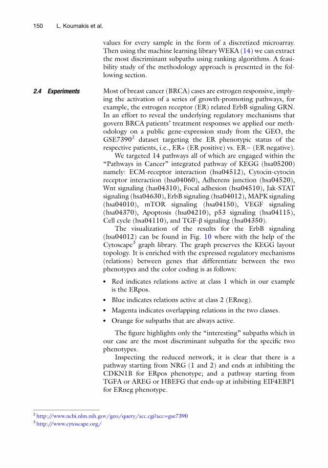
values for every sample in the form of a discretized microarray.Then using the machine learning library WEKA (14) we can extractthe most discriminant subpaths using ranking algorithms. A feasi-bility study of the methodology approach is presented in the fol-lowing section.

2.4 Experiments Most of breast cancer (BRCA) cases are estrogen responsive, imply-ing the activation of a series of growth-promoting pathways, forexample, the estrogen receptor (ER) related ErbB signaling GRN.In an effort to reveal the underlying regulatory mechanisms thatgovern BRCA patients’ treatment responses we applied our meth-odology on a public gene-expression study from the GEO, theGSE73902 dataset targeting the ER phenotypic status of therespective patients, i.e., ER+ (ER positive) vs. ER� (ER negative).

We targeted 14 pathways all of which are engaged within the“Pathways in Cancer” integrated pathway of KEGG (hsa05200)namely: ECM-receptor interaction (hsa04512), Cytocin-cytocinreceptor interaction (hsa04060), Adherens junction (hsa04520),Wnt signaling (has04310), Focal adhesion (hsa04510), Jak-STATsignaling (hsa04630), ErbB signaling (hsa04012), MAPK signaling(hsa04010), mTOR signaling (hsa04150), VEGF signaling(hsa04370), Apoptosis (hsa04210), p53 signaling (hsa04115),Cell cycle (hsa04110), and TGF-β signaling (hsa04350).

The visualization of the results for the ErbB signaling(hsa04012) can be found in Fig. 10 where with the help of theCytoscape3 graph library. The graph preserves the KEGG layouttopology. It is enriched with the expressed regulatory mechanisms(relations) between genes that differentiate between the twophenotypes and the color coding is as follows:

l Red indicates relations active at class 1 which in our exampleis the ERpos.

l Blue indicates relations active at class 2 (ERneg).

l Magenta indicates overlapping relations in the two classes.

l Orange for subpaths that are always active.

The figure highlights only the “interesting” subpaths which inour case are the most discriminant subpaths for the specific twophenotypes.

Inspecting the reduced network, it is clear that there is apathway starting from NRG (1 and 2) and ends at inhibiting theCDKN1B for ERpos phenotype; and a pathway starting fromTGFA or AREG or HBEFG that ends-up at inhibiting EIF4EBP1for ERneg phenotype.

2 http://www.ncbi.nlm.nih.gov/geo/query/acc.cgi?acc¼gse73903 http://www.cytoscape.org/

150 L. Koumakis et al.

According to recent literature, the aforementioned results arequite relevant to the estrogen-receptor status. Based on a search ofthe related biomedical literature we focus our exploration on themechanisms underlying the resistance to pure estrogen antagonists(e.g., fulvestrant). Recent studies show the significant role of bothErbB3 and ErbB4 as alternative targets for the treatment of BRCApatients. As Sutherland notes in ref. (15): “the initial growth inhib-itory effects of fulvestrant appear compromised by cellular plasticitythat allows rapid compensatory growth stimulation via ErbB-3/4.Further evaluation of pan-ErbB receptor inhibitors in endocrine-resistant disease appears warranted.” In addition, Hutcheson et al.in ref. (16) investigated whether induction of ErbB3 and/or ErbB4may provide an alternative resistance mechanism to antihormonalaction. Their conclusion is that fulvestrant treatment is sensitive tothe actions of the ErbB3/4 ligand HRGb1 (NRG1) with enhancedErbB3/4-driven signaling activity, and significant increases in cellproliferation.

3 Discussion and Conclusions

Current trend in GRNs and gene expression data is the subpathwayselection using regulatory mechanisms, which seems that it is at itsfirst steps and could possibly gain a momentum. Our assumption

Fig. 10 Results of GSE7390 over 14 cancer related pathways

Integrating Microarray Data and GRNs 151

for that momentum amplifies with the similarities we can findbetween the discriminant gene regulatory (sub)networks andmicroarray gene selection methodologies.

Apart the proposed procedure, only four (4) other tools takeadvantage of the underlying GRN gene regulation mechanisms,naming GGEA (17), SPIA (18), TEAK (19), and PATHOME (20).The main difference of the proposed methodology from these foursystems is the handling of the gene regulatory mechanisms. To ourknowledge all the other methodologies count with a +1 the activa-tions and�1 the inhibitions. Each subpath gets a final score which isalso used as a ranking mechanism. Contrary, our approach strictlychecks and takes into account only subpaths that are functional(according to the gene relations and the expression values). Ourapproach is binary and leads to distinction between functional andnonfunctional subpaths per sample instead of a representation of thesub-path per class (the sum).

Our methodology relies on a novel approach for GRN proces-sing that takes into account all possible functional interactions ofthe network. The phenotype information is extracted from micro-arrays and all the selected GRNs are evaluated for the identificationof the most informative GRNs at the specific phenotype. Theefficient ranking of subpaths provides the most differentiating andprominent GRN functional subpaths for the respective target phe-notypes. The formula posses a polarity characteristic according theclass phenotype, i.e., positive for class S1 and negative for class S2.These subpaths present evidential molecular mechanisms that gov-ern the disease itself, its type, its state or other targeted diseasephenotypes (e.g., positive or negative response to specific drugtreatment). The methodology was applied on a gene-expressionstudy with the target of identifying putative mechanisms thatunderlie and govern the treatment response of breast cancerpatients according to their ER-status profiles. Results were quiteindicative and strongly supported by the relevant biomedicalliterature.

It is known that integrating heterogeneous data sources is moreeffective than working within the boundaries of a single scientifictechnology/field. Bioinformatics and systems biology has proventhat taking advantage of the knowledge from each other can aid therelevant scientific communities in their research endeavours or evenreveal and create new research domains. In most of the cases thereare levels of integration as well as levels of knowledge to be utilised.Extracting out the most of the knowledge will always give us morenatural and meaningful, as well as more accurate results.

152 L. Koumakis et al.

Acknowledgment

This work was supported by the European Community’s SeventhFramework Programme (FP7/2007-2013) under grant agreementN� 270089 and by the European Union (European Social Fund—ESF) and by the European Union (European Social Fund—ESF)and Greek national funds through the Operational Program “Edu-cation and Lifelong Learning” of the National Strategic ReferenceFramework (NSRF)—Research Funding Program: Heracleitus IIInvesting in knowledge society through the European Social Fund.

References

1. Brown PO, Botstein D (1999) Exploring thenew world of the genome with DNA microar-rays. Nat Genet 21:33–37

2. Huang Y, Zhao Z, Xu H, Shyr Y, Zhang B(2012) Advances in systems biology: computa-tional algorithms and applications. BMC SystBiol 6(3)

3. Hung J-H, Yang T-H, Zhenjun H, Weng Z,DeLisi C (2012) Gene set enrichment analysis:performance evaluation and usage guidelines.Brief Bioinform 13(3):281–291

4. Heckera M, Lambecka S, Toepferb S, van Som-erenc E, Guthke R (2009) Gene regulatorynetwork inference: data integration in dynamicmodels—a review. Biosystems 96(1):86–103

5. Ein-Dor L, Kela I, Getz G, Givol D, Domany E(2005) Outcome signature genes in breast can-cer: is there a unique set? Bioinformatics 21(2):171–178

6. Iwamoto T, Pusztai L (2010) Predicting prog-nosis of breast cancer with gene signatures: arewe lost in a sea of data? Genome Med 2(11):81

7. Shannon CEA (1948) Mathematical theory ofcommunication. Bell Sys Tech J 27(3):379–423

8. Potamias G, Koumakis L, Moustakis V (2004)Gene selection via discretized gene-expressionprofiles and greedy feature-elimination. MethAppl Artif Intelligence 3025:256–266

9. Li L, Weinberg CR, Darden TA, Pedersen LG(2001) Gene selection for sample classificationbased on gene expression data: study of sensi-tivity to choice of parameters of the GA/KNNmethod. Bioinformatics 17(12):1131–1142

10. Kanehisa M, Araki M, Goto S, Hattori M, Hir-akawa M, Itoh M, Yamanishi Y (2008) KEGGfor linking genomes to life and the environ-ment. Nucleic Acids Res 36:480–484

11. Ott MA, Gert V (2006) Correcting ligands,metabolites, and pathways. BMC Bioinformat-ics 7(1):517

12. Khatri P, Draghici S (2005) Ontological analy-sis of gene expression data: current tools, lim-itations, and open problems. Bioinformatics21:3587–3595

13. Kauffman SA (1993) The origins of order: self-organization and selection in evolution.Oxford University Press, New York

14. Hall M, Frank E, Holmes G, Pfahringer B,Reutemann P, Ian H (2009) The WEKA datamining software: an update. SIGKDDExplora-tions 11(1)

15. Sutherland RL (2011) Endocrine resistance inbreast cancer: new roles for ErbB3 and ErbB4.Breast Cancer Res 13(3):106

16. Hutcheson IR et al (2007) Heregulin beta1drives gefitinib-resistant growth and invasionin tamoxifen-resistant MCF-7 breast cancercells. Breast Cancer Res 9(4):50

17. Geistlinger L, Csaba G, K€uffner R, Mulde N,Zimmer R (2011) From sets to graphs towardsa realistic enrichment analysis of transcriptomicsystems. Bioinformatics 27(13):366–373

18. Tarca AL, Draghici S, Khatri P, Hassan SS,Mittal P, Kim JS, Kim CJ, Kusanovic JP,Romero R (2009) A novel signaling pathwayimpact analysis. Bioinformatics 25(1):75–82

19. Judeh T, Johnson C, Kumar A, Zhu D (2013)TEAK: Topology Enrichment Analysis frame-worK for detecting activated biological sub-pathways. Nucleic Acids Res 41(1):1425–1437

20. Nam S, Chang HR, Kim KT et al (2014)PATHOME: an algorithm for accuratelydetecting differentially expressed subpathways.Oncogene 33(41):4941–4951

Integrating Microarray Data and GRNs 153

Methods in Molecular Biology (2016) 1375: 155–167DOI 10.1007/7651_2015_284© Springer Science+Business Media New York 2015Published online: 28 October 2015

Biological Network Inference from Microarray Data,Current Solutions, and Assessments

Swarup Roy and Pietro Hiram Guzzi

Abstract

Currently in bioinformatics and systems biology there is a growing interest for the analysis of associationsamong biological molecules at a network level. A main research in this area is represented by the inference ofbiological networks from experimental data. Biological network inference aims to reconstruct network ofinteractions (or associations) among biological molecules (e.g., genes or proteins) starting from experi-mental observations. The current scenario is characterized by a growing number of algorithms for theinference, while few attention has been posed on the determination of fair assessments and comparisons.Current assessments are usually based on the comparison of the algorithms using reference networks orgold standard datasets. Here we survey some selected inference algorithms and we compare currentassessments. We also present a systematic listing of freely available inference and assessment tools for easyreference. Finally we outline some possible future directions of research, such as the use of a priorknowledge into the assessment process.

Keywords: Biological network inference, Assessment, Gene regulatory network, Gold standard, GeneOntology, Graph theory

1 Introduction

Bioinformatics and systems biology are recentlymoving towards themodeling of the association among biological molecules, e.g., genesor proteins, on a system level. The common assumption of thisresearch area is that biological molecules have a dense set of associa-tions among them that need to be modeled and represented toimprove the knowledge in molecular biology. The best formalismto represent such complex world comes from graph theory [1, 2].

There exist different representations on the basis of the consid-ered molecules and kind of associations. Here we focus on generegulatory networks. In such kind of networks nodes representgenes while edges represent association in terms of regulation(i.e., positive or negative regulation) [3]. These networks areoften referred to as gene regulatory networks (GRNs).

The initial step of analysis is the inference of networks fromexpression data derived from microarray experiments. Formally, abiological network inference algorithm aims to reconstruct

155

network of interactions (or associations) among biological genesstarting from experimental observations. The reconstruction ofGRNs is an important area since it enables for instance the compar-ison of GRNs of different states (e.g., health or disease) or theinvestigation of the progression of diseases [4] as well as the visualinspection of network properties [5]. To cope with this problem anumber of different algorithms has been introduced in the past(see for instance [6]).

Once that networks have been determined, there is the need toevaluate the ability of the algorithms in terms of reliability of thenetwork, i.e., how many false positive (or incoherent associationsamong genes) and how many false negatives (or missing associa-tions) are expected using a particular algorithm. The Dialogue onReverse Engineering Assessment andMethods (DREAM) [7] proj-ect has introduced a rigorous methodology for an objective assess-ment of biological network reconstruction algorithms. DREAMassessment relies on three main steps: (1) periodically organizersprovide a set of experimental data, (2) researchers try their ownalgorithms on these datasets and submit resulting networks, and(3) organizers score networks on the basis of gold standard data-sets. DREAM challenge use mainly yeast and worm data and thescoring is obtained only with topological consideration (i.e., thenumber of true/false-positive edges).

Limitations of this approach have been yet discussed on somerecent articles (see for instance Siegenthaler et al.).

Here we present some of the network inference algorithms andwe discuss main classes in which they may be categorized. Then wediscuss currently network assessment methods.

2 Basic of Gene Network Structure

Graph theory offers the best formalism to represent informationmodeled as a network [8]. A graph G¼(V,E) is a structured com-posed by a set of nodes V and a set of edges E, i.e., pair of nodes.Graphs are usually distinguished by the kind of edges. A majordistinction is made among directed and undirected networks.In directed networks edges are directed, i.e., are sorted pairs ofnodes, while in undirected network edges have no direction [9].

Gene regulatory networks can be represented by using graphs[8] where nodes are associated to genes, and edges represent asso-ciations among proteins. The simplest representation uses an undi-rected graph, while more refined models use directed and weightededges to integrate the information about the kind of biochemicalassociation and its direction. The undirected graph represents sig-nificant association or co-expression over a series of gene expressionmeasurements. They often referred as gene association network orgene co-expression network [10]. The directed edges in GRNs

156 Swarup Roy and Pietro Hiram Guzzi

correspond to causal influences between gene activities (nodes).These could include regulation of transcription by transcriptionfactors, but also less intuitive causal effects between genes involvingsignal transduction or metabolism. For instance, Fig. 1 representsthe association of some selected genes in yeast. As evidences, graphtakes into account only the presence (or absence) of an associationamong nodes. Differently, Fig. 2 is an example of the same networkcorredated with the information about the direction of nodes. Asevident, it is possible to individuate which node influences andwhich node is influenced by. More sophisticated models mayinclude the kind of influence (e.g., positive or negative).

A genemay directly influence the activity of other target gene orgene product. Influence may be indirect by coding a transcriptionfactor (TF) that in turn regulates another gene. A possible causalrelationship in GRN is shown in Fig. 3. Apparently, four differenttypes of causal relationship may be possible in a living cell. Based onthe above figure we can derive following causal relationship [11].

1. A gene can enhance the activity of more than one gene (rela-tionship between A, B, C, and D).

2. A gene’s activity may be influenced by more than one gene(relationship between B, D, and F). Often F is referred asCollider [12].

YCR084C

YCL067CYFL026W

YNL145W

YHR084W

YMR043WYDR461W

YKR097W

YJL157C YAL040C

YPR113W

YIL015W

Fig. 1 Shows a graph representing a portion of a real GRN

Biological Network Inference from Microarray Data, Current Solutions, and Assessments 157

YCR084C

YFL026W

YHR084W

YDR461W

YCL067C

YIL015W

YNL145W

YMR043W

YPR113W

YAL040CYJL157C

YKR097W

Fig. 2 Shows a graph representing a directed graph modeling of a GRN

Fig. 3 Shows possible causal dependency in GRN graph

158 Swarup Roy and Pietro Hiram Guzzi

3. Gene can also influence the activity of itself (node B).

4. A gene may inhibit activity of other gene (D inhibits E).Inhibition or negative regulation may also follow above threerelationships, i.e., many to one, one-to-many, and self.

Once that a GRN is modeled by using graphs, the study ofbiological properties can be done using graph-based algorithms[1], and associating graph properties to the biological propertiesof the modeled GRN [13].

3 Network Inference Algorithms

A number of techniques have been proposed for network inference.Existing techniques for finding gene networks can be broadly cate-gorized as (i) computational approaches, and (ii) literature-basedapproaches. The computational approach mainly uses statistical,machine learning, or soft-computing techniques [14, 15] as discov-ery tools. On the other hand, a literature-based approach gathersrelevant published information on genes and their interrelation-ships and constructs networks based on such documented informa-tion. The literature-based approach is capable of building networkswith high biological relevance but is computationally expensive.A biomedical literature search-based technique is used in [16, 17]to construct gene relation networks by mapping literature knowl-edge into gene expression data.

Network models such as Bayesian [18] and Boolean networks[19] are used to infer interrelationships among genes. GraphicalGaussian models (GGM) [20] and categorical Bayesian networks(CBN) [21] are used to infer networks of differentially expressedgenes using Bayesian network. Kwon et al. [22], extract generegulatory relationships for cell cycle-regulated genes with activa-tion or inhibition between gene pairs. Recently, Jump3 [23], ahybrid Boolean network and decision tree-based method, hasbeen proposed to predict regulatory network from time-seriesdata. Regulatory relationships have also been deduced from corre-lation of co-expressions, between DNA-binding transcription reg-ulator and its target gene, by using a probabilistic expression model[24]. Although standard statistical techniques for extracting rela-tionships can come up with multiple models to fit the data, theyoften require additional data to resolve ambiguities. Soft comput-ing tools like fuzzy sets, neuro-computing, evolutionary comput-ing, and their hybridization are alternatives for handling real-lifeambiguities. Mitra et al. [25] propose a bi-clustering technique toextract simple gene interaction networks. They use continuouscolumn multi-objective evolutionary bi-clustering to extract rankcorrelated gene pairs. Such pairs are used to construct the genenetwork for generating relationship between a transcription factor

Biological Network Inference from Microarray Data, Current Solutions, and Assessments 159

and its target’s expression level. Similarly, Jung and Cho [4] alsopropose an evolutionary computation-based approach for con-struction of gene (interaction) networks from gene expressiontime-series data. It assumes an artificial gene network and comparesit with the reconstructed network from the gene expression time-series data generated by the artificial network. Next, it employs realgene expression time-series data to construct a gene network byapplying the proposed approach. Mutual information [26, 27] orcorrelation coefficient [28, 29] based approaches have been pro-posed for extracting gene-gene interaction networks. It has beenobserved that a pair of genes with high mutual information arenonrandomly associated with each other biologically or withbiological significance. Butte et al. [26] compute comprehensivepair-wise mutual information for all genes in an expression dataset.By picking a threshold mutual information and using only associa-tions at or above the threshold, they construct relevance networks.A number of additional mutual information-based approaches havealso been proposed. Some of the well-known algorithms in thiscategory are CLR [30], ARACNE [31], and MRNET [32].GENIE3 [33] is a Random Forest-based method that model theinference as a regression problem. Recently, GeCON [34] a patternbased co-expression network inference method has been proposedcapable of detecting undirected co-regulated network with regula-tion information (+ or�). A summery of various inference methodsdiscussed above is reported in Table 1.

4 Network Inference Assessment

Formally, the assessment of network inference algorithm refers tothe possibility to score (or rank) inferred networks in terms ofdistance among inferred and real networks. A similar problem hasbeen posed in some other bioinformatics fields (such as proteinstructure prediction). However in such fields, the existence of realstructures, i.e., proteins whose structure was determined and con-firmed by in vitro experiments, made the assessment more simple.The CASP challenge published for each edition the primarysequence of an unknown protein. Then researcher try to determinethe spatial structure. Finally candidate structures are compared withrespect to the real structure revealed by in vitro experiments. More-over there is not a gold-standard experiments for establishing thetrue network structure (i.e., the ground truth) for real networks.Consequently, all the assessment are designed on top of in silicostandard (i.e., simulated network) since existing networks cannotbe used since their identity may not be hidden [35–37].

4.1 In Silico

Assessment Methods

As introduced before the assessment of GRN algorithms has beenlargely discussed within the Dialogue on Reverse EngineeringAssessment and Methods (DREAM) project [38]. The project is

160 Swarup Roy and Pietro Hiram Guzzi

organized on an annual basis and researchers from all the world mayparticipate on this context. The structure of the competition isquite simple. For each year, organizer provides many test datasetto the community of participant. Then researchers may test theirown algorithms on these datasets and they may determine a candi-date network for each dataset. Once completed, researchers sendcandidate network to the organizers for the analysis of results.

Network analysis is based on the comparison of candidatenetwork with a priori-determined network (one for each dataset)that represents reference or gold standard network. The measure ofdistance from the gold standard network is calculated by evaluatingthe confusion matrix, i.e., a matrix containing the numbers of truepositives/negatives and false positives/negatives. All the submis-sion are reviewed manually by the organizers and submission arethen scored by deriving receiver operating characteristics (ROC) orprecision-recall.

Table 1Synopsis of GRN inference methods

Algorithm Approach

Inferrednetworktype Package Platform

Assessment basedon (type of data)

GGM Bayesian network Undirected GeneNeta R Synthetic (statically simulated)and real (breast cancer)

CBN Bayesian network Directed CatNetb R Real (breast, lung, gastric, andrenal cancer)

GENIE3 Random Forest Directed GENIE3c R, MatLab Synthetic (DREAM4) andreal (E. coli)

CLR Mutual information Undirected MINETd R Real (E. coli)

ARACNE Mutual information Undirected MINETe R Synthetic (random network)and real (human B cells)

MRNET Mutual information Undirected MINETf R Synthetic (sRogers andSynTReN)

GeCON Expression patternsimilarity

Undirected GeCONg Java Synthetic (DREAM4), real(yeast, human, rat, mouse,rice)

JUMP3 Decision tree andBoolean network

Directed Jump3h Matlab DREAM4, IRMA

ahttp://strimmerlab.org/software/genenet/bhttp://cran.r-project.org/web/packages/catnetchttp://www.montefiore.ulg.ac.be/huynh-thu/software.htmldhttp://minet.meyerp.comehttp://minet.meyerp.comfhttp://minet.meyerp.comghttps://sites.google.com/site/swarupnehu/publications/resourceshhttp://homepages.inf.ed.ac.uk/vhuynht/misc/jump3.zip

Biological Network Inference from Microarray Data, Current Solutions, and Assessments 161

The DREAM challenge is currently the de-facto standard forthe assessment of biological network inference, but there are somedrawbacks that have been analyzed in some recent works.

As noted in [39], a missing assumption in DREAM challenge isthat the network inference problem is an undetermined problemsince experimental data do not containing all the needed informa-tion to reconstruct network completely. In other word, a singlemicroarray experiment do not examine all the biological molecules.For instance, some microarray platforms do not cover all the tran-scriptome, or some transcripts are missing for experimental biasessuch as errors during the experiments, noise in the data, and thenumber and types of network gene perturbation experiments. Allthese factors make the network inference an underdeterminedproblem. Consequently, as investigated in [39], some gene inter-actions cannot be inferred and more than one network can agreewith the data.

To cope with this problem, Siegenthaler et al. proposed a novelassessment procedure that incorporates the inferability of generegulatory interactions by redefining the confusion matrix interms of inferability of the network, i.e., the possibility of thenetwork to be determined from data. The inferability of GRNswas analyzed based on the causal information that could beextracted from experiments. Authors used data from the DREAM4 In Silico Network Inference Challenge to score their assessmentand to show the concept of inferability from experiments.

A new performance score was introduced based on a redefini-tion of the confusion matrix, by taking into consideration non-inferable gene regulations. Results confirmed the same bestperforming teams as in the DREAM 4 inference challenge, butthey changed in a significant way the overall team rankings.

4.2 Assessment

Against Biological

Truth

Limited availability of true gold standard network (of all livingorganisms) for validation of a candidate inference method imposesan additional challenge to the system biologist to select a suitableinference method for their experimentation.

Literature-based known interactions are explored to validate aninference method from biological significance point of view. Exper-imentally validated regulators collected from publicly availabledatabases like RegulonDB [40] are used to assess the performanceof an inference method [33]. Pathways provide a way of linking thefunctionality of groups of genes to specific biological processes.Well-established methodologies such as Gene Set EnrichmentAnalysis (GSEA) [41] help in differentiating pathways as functionalunits from experimental populations. Manually curated pathwaysbased on expert knowledge and existing literature obtained fromthe Kyoto Encyclopedia of Genes and Genomes (KEGG, http://www.genome.jp/kegg/pathway.html) are another alternative mea-sure used for validation [21].

162 Swarup Roy and Pietro Hiram Guzzi

To evaluate the biological significance of a inference method,researchers explored an alternative measure based on Gene Ontol-ogy (GO) against functional, biological enrichment of a group ofgenes derived from inferred network modules [34]. More a methodis able to generate biologically significant modules (in terms ofp value) more they are relevant.

Next we highlight on some of the publicly available softwaretools for in silico inference and validation of an inferred network.

5 Software for Network Reconstruction and Assessments

A number of software tools, both web and desktop versions areavailable to facilitate the in silico reconstruction and visualization ofgene regulatory networks from microarray expression data. Someof the tools also provide an integrated platform for assessment ofinferred network against gold standard synthetic network. Readersmay refer [42] for a comprehensive review on various availablesoftware tools.

GeneNetWeaver (GNW) [43] is a Java-based reverse engineer-ing tool for generating synthetic benchmark expression datasetsfrom gold standard DREAM challenge network. E. coli and Yeasttranscriptional regulatory networks are integrated as test case forbenchmark. Comparative assessment of inference algorithmsagainst DREAM challenge data can also be performed with thehelp GNW. Cytoscape [44] is a powerful tool most suitable forlarge-scale network analysis. Cytoscape supports directed, undi-rected, and weighted graphs and comes along with powerful visualstyles thereby allowing users to change the properties of nodes oredges. Plenty of elegant layout algorithms including cyclic andspring-embedded layouts are available for visualization. GENeVis[45] is a Java desktop application that allows visualization of generegulatory networks. STARNET2 [46] facilitates discovery of puta-tive gene regulatory networks in a variety of species (Homo sapiens,Rattus norvegicus, Mus musculus, Gallus gallus, Danio rerio, Dro-sophila, C. elegans, S. cerevisiae, Arabidopsis, and Oryza Sativa) bygraphing networks of genes that are closely co-expressed across alarge heterogeneous set of preselected microarray experiments.NetBioV [47] (Network Biology Visualization) is an R packagethat allows visualization of large network data in biology and medi-cine. Fast MEDUSA [48] is a parallel program to infer gene regu-latory networks from gene expression and promoter sequenceswhich is implemented in C++. BANJO [49] a software applicationand framework for structure learning of static and dynamic Bayes-ian networks. LegumeGRN [50] is a specialized tool for legumespecies. The tool is pre-loaded with gene expression data for Med-icago, Lotus, and Soybean. A summery of few of the tools are listedin Table 2.

Biological Network Inference from Microarray Data, Current Solutions, and Assessments 163

6 Conclusion

The analysis of associations among biological molecules at a systemlevel is a large research area in bioinformatics and systems biology.The workflow of research in this area starts with molecular biologyexperiments that investigate the behavior of molecules. Then a setof analysis algorithms have to be used to infer associations amongmolecules. This research has a main role in determination ofmechanisms of regulations of the expression of genes. In such acontext algorithms aim to reconstruct network of interactions (orassociations) in genes starting from experimental observationsobtaining gene regulatory network. The current scenario is char-acterized by a growing number of algorithms for the inference,while few attention has been posed on the determination of fairassessments and comparisons. Current assessments are usuallybased on the comparison of the algorithms using reference net-works or gold standard datasets. Here we surveyed some selectedinference algorithms and we compare current assessments. To thebest of our knowledge there are some open problems and chal-lenges. First of all, since the structure of real regulatory networks isfar to be complete, the network inference remains still an

Table 2Few free GRN inference and visualization tools

Tool Platform Availability Visualization Plug-ins Url

GNW Java Off-line Yes No http://gnw.sourceforge.net/

GENeVis Java Off-line Yes Yes http://www.win.tue.nl/mwestenb/genevis/

Cytoscape Java Off-line/Online

Yes Yes http://www.cytoscape.org/

GeneNetwork C++ Online Yes No http://www.genenetwork.org/webqtl/main.py

STARNET2 web application Online Yes No http://vanburenlab.tamhsc.edu/starnet2.html

LegumeGRN J2EE Online Yes No http://legumegrn.noble.org

Osprey Java Online Yes No http://biodata.mshri.on.ca/osprey/servlet/Index

NetBioV R Off-line Yes No http://bivi.co/visualisation/netbiov

FastMEDUSA C++ Off-line Yes No https://wiki.nci.nih.gov/display/NOBbioinf/FastMEDUSA

164 Swarup Roy and Pietro Hiram Guzzi

undetermined problem. Consequently the investigation of alterna-tive methods of assessment under the absence of a gold standardmethods is a key area. Moreover the research may be helped by theintroduction of prior knowledge (e.g., biological ontologies) onthe assessment and during the inference may help to filter outpossible low quality networks [53]. The scenario we envision ischaracterized by the use of ontologies both in the assessmentphase and during the inference of network. Considering the assess-ment phase it should be pointed out that low attention has beenposed on the evaluation of the inferred network with respect todiseases or phenotypes. Briefly speaking, all the current assessmentmethods are not able to quantify how much inferred networks arerelated to biology since they are related only to topology. Theproblem has been investigated in other fields such as biologicalnetwork alignment [51, 52] Moreover, ontologies may also beused during the generation of candidate networks in a similar wayas proposed for inferable network by Siegenthaler et al. In that workthe inferability notion is used to filter out low scoring network,while in the scenario we envision ontologies may be used to filterout low-scoring network from a biological point of view.

References

1. Cannataro M, Guzzi PH, Veltri P (2010) Pro-tein-to-protein interactions: technologies,databases, and algorithms. ACM ComputSurv (CSUR) 43(1):1

2. Cannataro M, Guzzi PH, Sarica A (2013) Datamining and life sciences applications on thegrid. WIREs Data Mining Knowl Discov 3(3):216–238

3. Levine M, Davidson EH (2005) Gene regu-latory networks for development. Proc NatlAcad Sci U S A 102(14):4936–4942

4. Jung SH, Cho K-H (2004) Identification ofgene interaction networks based on evolution-ary computation, AIS. Springer, New York, pp428–439

5. Agapito G, Guzzi PH, Cannataro M (2013)Visualization of protein interaction networks:problems and solutions. BMC Bioinformatics14(Suppl 1):S1

6. Marbach D, Prill RJ, Schaffter T, Mattiussi C,Floreano D, Stolovitzky G (2010) Revealingstrengths and weaknesses of methods for genenetwork inference. Proc Natl Acad Sci 107(14):6286–6291

7. Karr JR, Williams AH, Zucker JD, Raue A,Steiert B, Timmer J, Kreutz C, Wilkinson S,Allgood BA, Bot BM et al (2015) Summary ofthe DREAM8 parameter estimation challenge:

toward parameter identification for whole-cellmodels. PLoS Comput Biol 11(5):e1004096

8. Godsil C, Royle GF (2013) Algebraic graphtheory, vol 207. Springer Science & BusinessMedia, New York

9. Cannataro M, Guzzi PH, Veltri P (2010)Impreco: distributed prediction of proteincomplexes. Futur Gener Comput Syst 26(3):434–440

10. Fuente ADI (2010) What are gene regulatorynetworks? Handbook of research on computa-tional methodologies in gene regulatory net-works. IGI Global, Hershey, PA, pp 1–27

11. Roy S, Das D, Choudhury D, Gohain GG,Sharma R, Bhattacharyya DK (2013) Causalityinference techniques for in-silico gene regu-latory network, Mining intelligence and knowl-edge exploration. Springer, New York,pp 432–443

12. Olsen C, Meyer PE, Bontempi G (2009) Infer-ring causal relationships using information the-oretic measures. In Proceedings of the 5thBenelux Bioinformatics Conference (BBC09)

13. Mina M, Guzzi PH (2014) Improving therobustness of local network alignment: designand extensive assessment of a Markovclustering-based approach. IEEE/ACM TransComput Biol Bioinformatics 11(3):561–572

Biological Network Inference from Microarray Data, Current Solutions, and Assessments 165

14. Mitra S, Das R, Hayashi Y (2011) Genetic net-works and soft computing. IEEE/ACM TransComput Biol Bioinformatics 8(1):94–107

15. Nagrecha S, Lingras PJ, Chawla NV (2013)Comparison of gene co-expression networksand Bayesian networks, Intelligent Informationand Database Systems. Springer, New York, pp507–516

16. Karopka T, Scheel T, Bansemer S, Glass A(2004) Automatic construction of gene rela-tion networks using text mining and geneexpression data. Med Inform Internet Med 29(2):169–183

17. Ozg€ur A, Vu T, Erkan G, Radev DR (2008)Identifying gene-disease associations usingcentrality on a literature mined gene-interaction network. Bioinformatics 24(13):i277–i285

18. Friedman N, Linial M, Nachman I, Pe’er D(2000) Using Bayesian networks to analyzeexpression data. J Comput Biol 7(3–4):601–620

19. Davidich MI, Bornholdt S (2008) Booleannetwork model predicts cell cycle sequence offission yeast. PLoS One 3(2), e1672

20. Sch€afer J, Strimmer K (2005) An empiricalBayes approach to inferring large-scale geneassociation networks. Bioinformatics 21(6):754–764

21. Balov N (2013) A categorical networkapproach for discovering differentiallyexpressed regulations in cancer. BMC MedGenet 6(Suppl 3):S1

22. Kwon AT, Hoos HH, Ng R (2003) Inferenceof transcriptional regulation relationships fromgene expression data. Bioinformatics 19(8):905–912

23. Sanguinetti G et al (2015) Combining tree-based and dynamical systems for the inferenceof gene regulatory networks. Bioinformatics 31(10):1614–1622

24. Segal E, Taskar B, Gasch A, Friedman N, KollerD (2001) Rich probabilistic models for geneexpression. Bioinformatics 17(Suppl 1):S243–S252

25. Mitra S, Das R, Banka H, Mukhopadhyay S(2009) Gene interaction–an evolutionarybiclustering approach. Information Fusion 10(3):242–249

26. Butte AJ, Kohane IS (2000) Mutual informa-tion relevance networks: functional genomicclustering using pairwise entropy measure-ments, vol 5, Pacific symposium on biocom-puting. World Scientific, Singapore, pp418–429

27. Eisen MB, Spellman PT, Brown PO, BotsteinD (1998) Cluster analysis and display of

genome-wide expression patterns. Proc NatlAcad Sci 95(25):14863–14868

28. Tong AHY, Lesage G, Bader GD, Ding H, XuH, Xin X, Young J, Berriz GF, Brost RL, ChangM et al (2004) Global mapping of the yeastgenetic interaction network. Science 303(5659):808–813

29. Kuo WP, Mendez E, Chen C, Whipple ME,Farell G, Agoff N, Park PJ (2003) Functionalrelationships between gene pairs in oral squa-mous cell carcinoma, AMIA annual symposiumproceedings. American Medical InformaticsAssociation, Bethesda, MD, p 371

30. Faith JJ, Hayete B, Thaden JT, Mogno I,Wierzbowski J, Cottarel G, Kasif S, Collins JJ,Gardner TS (2007) Large-scale mapping andvalidation of escherichia coli transcriptionalregulation from a compendium of expressionprofiles. PLoS Biol 5(1):e8

31. Margolin AA, Nemenman I, Basso K, WigginsC, Stolovitzky G, Favera RD, Califano A(2006) Aracne: an algorithm for the recon-struction of gene regulatory networks in amammalian cellular context. BMC Bioinfor-matics 7(Suppl 1):S7

32. Meyer PE, Kontos K, Lafitte F, Bontempi G(2007) Information-theoretic inference oflarge transcriptional regulatory networks.EURASIP J Bioinforma Syst Biol 2007:79879

33. Huynh-Thu VA, Irrthum A, Wehenkel L,Geurts P (2010) Inferring regulatory networksfrom expression data using tree-based meth-ods. PLoS One 5(9):e12776

34. Roy S, Bhattacharyya DK, Kalita JK (2014)Reconstruction of gene co-expression networkfrom microarray data using local expression pat-terns. BMC Bioinformatics 15(Suppl 7):S10

35. Moult J, Fidelis K, Kryshtafovych A, Rost B,Hubbard T, Tramontano A (2007) Criticalassessment of methods of protein structureprediction-round vii. Proteins 69(S8):3–9

36. Mendes P, Sha W, Ye K (2003) Artificial genenetworks for objective comparison of analysisalgorithms. Bioinformatics 19(Suppl 2):ii122–ii129

37. Marbach D, Schaffter T, Mattiussi C, FloreanoD (2009) Generating realistic in silico genenetworks for performance assessment ofreverse engineering methods. J Comput Biol16(2):229–239

38. Stolovitzky G, Monroe D, Califano A (2007)Dialogue on reverse-engineering assessmentand methods. Ann N Y Acad Sci 1115(1):1–22

39. Siegenthaler C, Gunawan R (2014) Assessmentof network inference methods: how to copewith an underdetermined problem. PLoS One9(3):e90481

166 Swarup Roy and Pietro Hiram Guzzi

40. Gama-Castro S, Jimenez-Jacinto V, Peralta-GilM, Santos-Zavaleta A, Penaloza-Spinola MI,Contreras-Moreira B, Segura-Salazar J,Muniz-Rascado L, Martnez-Flores I, SalgadoH et al (2008) RegulonDB (version 6.0): generegulation model of escherichia coli k-12beyond transcription, active (experimental)annotated promoters and textpresso naviga-tion. Nucleic Acids Res 36(suppl 1):D120–D124

41. Subramanian A, Tamayo P, Mootha VK,Mukherjee S, Ebert BL, GilletteMA, PaulovichA, Pomeroy SL, Golub TR, Lander ES et al(2005) Gene set enrichment analysis: aknowledge-based approach for interpretinggenome-wide expression profiles. Proc NatlAcad Sci U S A 102(43):15545–15550

42. Kharumnuid G, Roy S (2015) Tools for in-silico reconstruction and visualization of generegulatory networks (GRN). In 2nd IEEEinternational conference on advance comput-ing and communication engineering(ICACCE’ 2015)

43. Schaffter T, Marbach D, Floreano D (2011)Genenetweaver: in silico benchmark genera-tion and performance profiling of networkinference methods. Bioinformatics 27(16):2263–2270

44. Smoot ME, Ono K, Ruscheinski J, Wang P-L,Ideker T (2011) Cytoscape 2.8: new featuresfor data integration and network visualization.Bioinformatics 27(3):431–432

45. Baker C, Carpendale MT, Prusinkiewicz P, Sur-ette MG (2002) Genevis: visualization tools forgenetic regulatory network dynamics. In Pro-ceedings of the conference on Visualization’02.IEEE Computer Society, 2002, pp 243–250

46. Jupiter D, Chen H, VanBuren V (2009) Star-net 2: a web-based tool for accelerating discov-ery of gene regulatory networks usingmicroarray co-expression data. BMC Bioinfor-matics 10(1):332

47. Tripathi S, Dehmer M, Emmert-Streib F(2014) Netbiov: an r package for visualizinglarge network data in biology and medicine.Bioinformatics 30(19):2834–2836

48. Bozdag S, Li A, Wuchty S, Fine HA (2010)Fastmedusa: a parallelized tool to infer generegulatory networks. Bioinformatics 26(14):1792–1793

49. Smith VA, Yu J, Smulders TV, Hartemink AJ,Jarvis ED (2006) Computational inference ofneural information flow networks. PLoS Com-put Biol 2(11):e161, pp. 1436–1449

50. Wang M, Verdier J, Benedito VA, Tang Y,Murray JD, Ge Y, Becker JD, Carvalho H,Rogers C, Udvardi M et al (2013) Legumegrn:a gene regulatory network prediction server forfunctional and comparative studies. PLoS One8(7):e67434

51. Faisal FE, Meng L, Crawford J, Milenkovic T(2015) The post-genomic era of biological net-work alignment. EURASIP J Bioinforma SystBiol 2015:3

52. Ciriello G, Mina M, Guzzi PH, Cannataro M,Guerra C (2012) AlignNemo: a local networkalignment method to integrate homology andtopology. PLoS One 7(6):e38107. doi:10.1371/journal.pone.0038107

53. Guzzi PH, Milano M, Roy S (2015) Towardsthe assessment of GRN algorithms based on(disease) ontology. In: Proceedings of theACM conf on bioinformatics, computationalbiology and health informatics (BCB’15)

Biological Network Inference from Microarray Data, Current Solutions, and Assessments 167

Methods in Molecular Biology (2016) 1375: 169–179DOI 10.1007/7651_2015_248© Springer Science+Business Media New York 2015Published online: 24 May 2015

A Protocol to Collect Specific Mouse Skeletal Musclesfor Metabolomics Studies

Zhuohui Gan, Zhenxing Fu, Jennifer C. Stowe, Frank L. Powell,and Andrew D. McCulloch

Abstract

Due to the highly sensitive nature of metabolic states, the quality of metabolomics data depends on thesuitability of the experimental procedure. Metabolism could be affected by factors such as the method ofeuthanasia of the animals and the sample collection procedures. The effects of these factors onmetabolites aretissue-specific. Thus, it is important to select proper methods to sacrifice the animal and appropriateprocedures for collecting samples specific to the tissue of interest. Here, we present our protocol to collectspecific mouse skeletal muscles with different fiber types for metabolomics studies. We also provide a protocolto measure lactate levels in tissue samples as a way to estimate the metabolic state in collected samples.

Keywords: Skeletal muscle, Dissection, Euthanasia, Metabolomics, Lactate, Amplex Red

1 Introduction

Skeletal muscle is the most abundant tissue in humans and verte-brate animals, which suggests the possibility to carry across-speciesmetabolic studies. Additionally, skeletal muscle is also a relativelyfeasible tissue to collect for metabolomics studies, especially forhealthy humans. Several types of skeletal muscles can be identifiedby their composition (1). These skeletal muscles could have differ-ent metabolisms. For example, soleus muscle is identified as anoxidative muscle, while plantaris muscle is identified as a glycolyticmuscle, although the details can vary for a given muscle betweenspecies and with training. Therefore, the dissection of specific skel-etal muscles is necessary for some metabolic studies. The request ofspecific skeletal muscle for metabolomics raises two issues. Firstly,the collection of muscle requires the animal to be anesthetized oreuthanized in advance, which may impact the metabolic levels inanimals. Another issue involves muscle sample collection once theanimals are ready to use. Since metabolic status in muscle tissue canbe changed with the active enzymes very rapidly, it is important toinstantaneously stop the inherent enzymatic activity so that themetabolic state can be reserved for further analysis (2, 3).

169

Several methods are widely used for mouse euthanasia,including: anesthesia, decapitation, cervical dislocation, and elec-tric shock. Studies suggest that these methods themselves couldaffect the metabolic state in tissue (4–6), for example, anes-thetics, such as ketamine and isoflurane, are known to suppressmetabolic functions (7–13). Thus, the selection of a method tosacrifice the animal is the first step. For this purpose, severalmethods of euthanasia including: decapitation, cervical disloca-tion, and pentobarbital sodium, were tested. We selected lactateas an easy indicator of metabolic state. Lactate is a metabolitesensitive to the metabolic state with a relatively stable tissueturnover rate around 0.2 mM/min. The lactate levels in boththe dissected glycolytic muscles and oxidative muscles weremeasured with an Amplex Red-based assay. Amplex Red is ahighly sensitive and selective probe of hydrogen peroxide(H2O2). This assay converts lactate into H2O2 in the presenceof lactate oxidase and produces a resorufin signal by the reactionbetween Amplex Red and the resulting H2O2 in the presence ofhorseradish peroxidase.

O2 þ L � lactate��������������!lactate oxidasepyruvateþH2O2

H2O2 þ AmplexRed��������������!horseradish peroxidaseresorufinþH2O

The experimental results indicate that both decapitation and pen-tobarbital sodium injection result in a higher lactate level in bothglycolytic plantaris muscles and oxidative soleus muscles com-pared with cervical dislocation, as shown in Fig. 1a. The higherlactate level usually suggests hypoxia in the tissue. This may becaused by the depth of anesthesia with pentobarbital sodium,which depresses ventilation, or by the involuntary contractionsof limbs after decapitation. In order to minimize the effect of theeuthanasia method on the metabolic state in mouse skeletal mus-cle, cervical dislocation was selected as the preferred method formouse muscle collection. It is noteworthy that the optimizedmethod of euthanasia is tissue specific. For example, pentobarbitalsodium is regarded as a good anesthetic to collect tissues for thepurpose of cardiac physiology and mitochondrial functions (5,14). However, some studies report that pentobarbital sodiumimpacts cerebral metabolism (15). Hence, pentobarbital sodiumis not an optimized euthanasia method for brain-relevant meta-bolic studies. Similarly, cervical dislocation is reported to changelung platelet serotonin (16), but compared with the effects ofother euthanasia methods on mouse skeletal muscle, it is theoptimal choice. Therefore, it is important to take the tissue typeinto consideration when selecting the euthanasia method for met-abolic studies.

170 Zhuohui Gan et al.

Several methods have been developed to quickly inhibitenzymatic activity, such as in situ clamping by cryogenic blocktongs or flash freezing in liquid nitrogen (2). Needle biopsy fol-lowed by flash freezing is widely used to collect human musclesamples for metabolic studies (17–19). With this approach, the

0.00

0.40

0.80

1.20

1.60

2.00

Cervical Dislocation Decaptation Pentobarbital

Lac

tate

in

tiss

ue h

omog

enat

e (m

M) plantaris

soleus **

# #

0.00

0.40

0.80

1.20

1.60

2.00

Flash Freezing Tongs Freezing In-Situ Dissection

Lac

tate

in

tiss

ue h

omog

enat

e (m

M) plantaris

soleus

*

#

a

b

Fig. 1 (a) The comparison of euthanasia methods on lactate level in mouse skeletal muscles. Two types ofmouse skeletal muscles, plantaris and soleus, were dissected from the flash-frozen legs which were cut frommice sacrificed by the assigned methods. The sample size for each data point is 3–4. The values aremean � s.d. *: different from the lactate level in plantaris muscles from mice sacrificed by cervicaldislocation, p < 0.05. #: different from the lactate level in soleus muscles from mice sacrificed by cervicaldislocation, p < 0.05. (b) The comparison of collection methods on lactate level in mouse skeletal muscles.Two types of mouse skeletal muscles, plantaris and soleus, were dissected from legs processed with theassigned methods. The mice were sacrificed by cervical dislocation. The sample size for each data point is3–4. The values are mean � s.d. *: different from the lactate level in plantaris muscles from flash-frozen legs,p < 0.05. #: different from the lactate level in soleus muscles from flash-frozen legs, p < 0.05

A Protocol to Collect Specific Mouse Skeletal Muscles for Metabolomics Studies 171

whole collection process can be completed in seconds and hencepreserves the metabolic state in human muscles. However, thevolume of mouse skeletal muscle is quite small. This makes itdifficult to collect a specific mouse muscle by biopsy, especiallyconsidering the relatively large amount of tissue required for meta-bolic analyses. Thus, the dissection of the muscle becomes neces-sary in order to collect enough specific mouse skeletal muscle formetabolic studies. To dissect the muscle first or to freeze the musclefirst becomes a question. Methods to dissect fresh muscles exist(20), but will require modification if the tissue is first frozen.Aluminum-block tongs at liquid nitrogen temperatures are widelyused to freeze tissues (liver, lung) in situ for metabolic studies (21).Whether the aluminum- block tongs are sufficient to freeze skeletalmuscles, which are located near the bone, is also a question.To answer these questions, we measured the lactate levels of mus-cles dissected from fresh mouse legs and then flash-frozen in liquidnitrogen, muscles dissected from legs frozen by aluminum blocktongs in situ, and muscles dissected from mouse legs which hadbeen rapidly removed from the euthanized animal and flash-frozenin liquid nitrogen. The dissection experiments show that it is feasi-ble to dissect specific muscles from frozen-and-then-partiallythawed mouse legs. Figure 1b shows no statistical difference inlactate levels between muscles dissected from aluminum-block-tong frozen legs and muscles dissected from liquid nitrogenflash-frozen legs, but both groups of muscles have a lower lactatelevel compared with muscles dissected from fresh legs. Based onthis result, either in situ block tong freezing or whole-leg liquidnitrogen flash freezing is appropriate. To simplify the experiment,we collect the muscles by rapidly removing the mouse legs just aftereuthanasia and flash freezing the legs completely in liquid nitrogen.We then dissect the desired muscles from the partially thawedlegs on ice. The whole leg removal takes a couple of seconds.The whole leg can be frozen completely in liquid nitrogen in twentyseconds. The advantage of this method is that the low-temperaturein the barely thawed leg gives us a dissection time window.

In the following protocol, the process of preparing the miceand the muscle collection steps are outlined. The assay that we usedto measure lactate level in collected muscles is also described.

2 Materials

2.1 Materials for

Muscle Dissection

1. A dewar containing liquid nitrogen.

2. A dissection tray containing ice.

3. Tissue forceps.

4. Surgical scissors.

172 Zhuohui Gan et al.

5. Iris scissor.

6. Hemostat (Halsted mosquito forceps).

7. Aluminum foil.

8. Indelible marker pen.

9. Disposable latex or nitrile gloves, gown or clean lab coat, andeye protection.

10. Disposal container.

11. Cryotubes.

2.2 Materials

for Amplex Red-Based

Lactate Assay

1. 1� phosphate buffered saline (PBS), PH7.4 (noCa2+, noMg2+).

2. L-lactate standard (Sigma, part #71718).Mix 10 μL of 100 mM lactate sample with 990 μL deionized

water to get a 1 mM lactate solution. Prepare lactate standardsamples using deionized water with lactate concentrations at 0,20, 50, 100, 200, and 300 μM, respectively. Store at �20 �C.

0 μM 20 μM 50 μM 100 μM 200 μM 300 μM

1 mM Lactate (μL) 0 20 50 100 200 300

H2O (μL) 1,000 980 950 900 800 700

3. Amplex Red stock (Sigma, part #90101).Add 5 mg Amplex Red powder into 1.943 mL DiMethyl-

SulphOxide (DMSO) to get 10 mM Amplex Red stock.Aliquot and store the stock at �20 �C.

4. Horseradish peroxidase (HRP) stock (Sigma, part#P2088).Add 2 mg HRP powder into 1 mL 1� PBS to get

500 U/mL HRP stock, and store on ice. Prepare fresh, anddo not store for further use.

5. Lactate oxidase (LOX) stock (Sigma, part#L0638).Add 1mL 1� PBS to 50U lactate oxidase powder, aliquot as

100 μL each and store at �20 �C.

6. 96-well white flat-bottom plate.

7. Pipettes and tips.

8. 0.5 or 1.5 mL Tubes.

9. Tube storage rack.

10. Ice bucket containing ice.

11. Marker pen.

12. A slotted metal spoon or other apparatus to remove samplesfrom liquid nitrogen.

13. Tissue homogenizer.

We use Kontes Glass DUALL® 20 tissue grinder to homoge-nize mouse muscles. There are some alternative tools. A

A Protocol to Collect Specific Mouse Skeletal Muscles for Metabolomics Studies 173

comparison is available at http://opsdiagnostics.com/notes/mouseldh.htm.

14. Refrigerated Micro centrifuge (temperature setting to 4 �C).

15. Disposal container.

16. Gloves, gown and eye protection.

CAUTION: Liquid nitrogen is very cold and can cause burns andfrost bite. Wear protective gloves when handling liquid nitrogenfrozen samples and proceed with extreme caution while workingwith liquid nitrogen.

3 Methods

1. Obtain mice with the same age, sex, and strain.

2. House mice in the animal room for at least 1 day.

3. Withhold food from experimental mice for at least 4 h beforethe sample collection to minimize metabolic variance caused bydigestion.

4. Prepare several pieces of aluminum foil 200 � 200 in size. Labelthe foil on the center of the shinier side with sample name andother identifying information.

5. Label 1.5–2 mL cryotubes. Keep on ice.

6. Cover the dissection tray with aluminum foil for dissectionsurgery.

7. Move the mouse to the surgery room and sacrifice themouse byrapid cervical dislocation, making sure that the mouse beingeuthanized is separated from any others to be studied, so theyare not stressed. The operator must be well trained (seeNote 1).

8. Immediately cut off both of the mouse’s hind legs using largesharp surgical scissors.

9. Wrap the leg in the aluminum foil, tissue touching the matte(less shiny) side of the foil. Ensure limb is completely sealed infoil and rapidly drop it into the dewar containing liquid nitro-gen (see Note 2).

10. If the samples will not be processed on the same day, store thefrozen samples at �80 �C or in liquid nitrogen. Otherwise, thelegs will be completely frozen in 20 s and the dissection processcan begin.

11. Remove a frozen leg from the liquid nitrogen using the slottedmetal spoon or other apparatus, open the aluminum foil andplace the leg on the aluminum foil of the dissection tray filledwith ice.

12. Allow the leg to thaw for approximately 2 min.

174 Zhuohui Gan et al.

13. Make a small incision along the skin of the lower leg around the“ankle,” and then tear off the entire skin covering the leg.

14. Remove the membrane surrounding the leg musclesusing forceps or cut the membrane using a dissection scissors(see Note 3).

15. Gently separate the rear tendons from the bone, clamp the reartendons very distally underneath the heel using a hemostat, andcut with Iris scissors.

16. Pull and separate the posterior muscles from the bone with thehemostat. If it is still hard to move the posterior muscles,wait for a few more minutes to thaw the leg a little more(see Note 4).

17. Dissect soleus from the posteriors muscles by pulling the soleusfrom its proximal tendon until the distal tendon and cut out thesoleus using a dissection scissors. Put the dissected soleus into acyrotube and freeze in liquid nitrogen or homogenize in assaybuffer immediately (see Note 5). The location of the soleusmuscle in a frozen-thawed leg is indicated in Fig. 2a.

Fig. 2 (a) The location of soleus muscle in a flash-frozen and then thawed mouseleg. The soleus muscle is identifiable and dissectible in frozen-thawed mouse leg.The integrity of soleus muscle keeps well. (b) The location of plantaris muscle in aflash-frozen and then thawed mouse leg after the soleus muscle is removed. Theplantaris muscle is identifiable and dissectible with a good integrity

A Protocol to Collect Specific Mouse Skeletal Muscles for Metabolomics Studies 175

18. Separate the two distal tendons and find the plantarismuscle, cut its tendon. Pull the plantaris muscle by holdingthe distal end of its tendon, and cut the proximal end (seeNote6). Put the dissected plantaris into a cytotube and freezein liquid nitrogen or homogenize in assay buffer immediately(see Note 7). The location of plantaris muscle in a frozen-thawed leg is shown in Fig. 2b.

19. Store the dissected muscles at �80 �C if it won’t be usedimmediately. Otherwise, proceed to homogenization.

3.1 Supplement:

Amplex Red-Based

Lactate Assay

This assay was developed to detect lactate levels in dissected musclesamples. This is not a part of the muscle collection protocol, but anoption for metabolic measurement. This protocol is sufficient torun 20 lactate measurement reactions (see Note 8).

1. Label tubes for Amplex Red solution, HRP solution, LOXsolution and at least two tubes for each sample.

2. Take Amplex Red stock, HRP stock, lactate oxidase stock andlactate standards out of the freezer to thaw.

3. Mix 100 μL Amplex Red stock and 900 μL 1� PBS toget 1 mM Amplex Red solution, store on ice (this is AR-PBS)(see Note 9).

4. Mix 20 μL HRP stock and 80 μL 1� PBS to get 100 U/mLHRP solution, store on ice (this is HRP-PBS).

5. Mix 10 μL lactate oxidase stock and 90 μL 1� PBS to get5 U/mL lactate oxidase solution (this is LOX-PBS).

6. Homogenize the muscle sample with the ratio of 1 mg per30 μL 1� PBS, in ice bath.

7. Centrifuge the tube containing homogenate at 13,000 � g for10 min, 4 �C to remove insoluble material.

8. Move the supernatant and transfer into clean tubes.

9. Dilute the supernatant with 1� PBS 1:10 (see Note 10), storeon ice.

10. Add 45 μL AR-PBS to each cell, the total number of cells is thesum of the cells for sample measurements and the cells for thelactate standard curve which requires six cells.

11. Add 5 μL HRP-PBS to each cell.

12. Measure the colorimetric absorbance at 571 nm as the back-ground signal (abs1) at room temperature.

13. Add 45 μL diluted supernatant or lactate standards (0, 20,50, 100, 200, and 300 μM) to each cell, mix by slightly shaking(see Note 11).

14. Measure the colorimetric absorbance at 571 nm as themeasurement of H2O2 in supernatant samples (abs2).

176 Zhuohui Gan et al.

15. Add 5 μL LOX-PBS to each cell, mix by slightly shaking.

16. Allow reaction to occur for 15 min at room temperature, andthen measure the colorimetric absorbance at 571 nm as themeasurement of lactate in supernatant samples and standards(abs3).

17. Calculate each sample’s lactate absorbance value, abs ¼ abs3-abs2-abs1.

18. Determine the conversion equation between the concentra-tions of lactate standard samples and its corresponding absvalues (see Note 12).

19. Convert abs of muscle samples to its lactate concentration bythe conversion equation.

4 Notes

1. An improper cervical dislocation may affect metabolic state.The faster and cleaner the cervical dislocation, the better.

2. A thinner aluminum foil allows faster freezing of legs in theliquid nitrogen. Other containers such as cryotubes might notwork as well as aluminum foil.

3. The removal of the outer membrane facilitates the muscledissection. Otherwise, the muscles would be bound together.

4. It is important to dissect the muscles at the appropriate tem-perature. If the leg is thawed too much, the muscles will be softand might undergo metabolic degradation. When the leg is lessthawed, it is hard to dissect the intact soleus and plantarismuscles since the muscles are still frozen together. The besttime point is when you can barely move the posterior muscleswith the hemostat.

5. The soleus is quite visible since its color is deep red as anoxidative muscle. The mean quantity of an intact mouse soleusmuscle is ~6–9 mg.

6. The plantaris is bigger than the soleus, with a moderate redcolor. Sometimes, you can see the tendon sticking to the plan-taris. The mean quantity of an intact mouse plantaris muscle is~11–16 mg.

7. A well-trained operator could finish the dissection of the soleusand plantaris muscles in a couple of minutes. Faster is better.

8. This protocol has been well tested with the total 100 μL mix-ture in each cell. It might be okay to adjust the total volume to asmaller value such as 50 μL or less for 384-well plate. When youadjust the total volume, please adjust the required volumes ofall relevant solutions proportionally. The final concentration

A Protocol to Collect Specific Mouse Skeletal Muscles for Metabolomics Studies 177

of Amplex Red in each cell shall be 450 μM. The finalconcentration of HRP in the cells shall be 5 U/mL. Thefinal concentration of LOX in the cell shall be 0.25 U/mL.The concentrations of enzymes are fixed, while the concentra-tion of Amplex Red is adjustable as long as the resulting signal isin the linear range of the standard curve.

9. In this protocol, we use 100 μL Amplex Red stock for 20measurements. To save Amplex Red, you can calculate andadjust the required amount of Amplex Red stock based onyour desired number of measurements, such as 4 μL AmplexRed stock/measurement.

10. For mouse skeletal muscle, we recommend 1:5 or 1:10 as thedilution factor. For different tissues, the lactate level could bedifferent. You need to select a proper dilution ratio to ensure theabsorbance signal is in the linear range of the standard curve.

11. The maximum concentration of lactate standard can’t bebeyond 450 μM since the final concentration of Amplex Redin the cell is 450 μM. You need to adjust the supernatant tolocate the absorbance value in the 0–450 μM. If the concentra-tion of lactate in the measured supernatant is beyond 450 μM,the extra H2O2 produced from lactate will react with AmplexRed’s product, resorufin, and result in a decrease in the absor-bance value. This is the reason why the original supernatant isdiluted.

12. Take abs ¼ a � [lactate] + b as the conversion equation,deduce a, b using least square method or use the regressionfunction which is available in Excel, Matlab, R, and a lot ofother software.

Acknowledgements

Grant NIH/NHLBI 1P01HL098053 supported this manuscriptpreparation.

References

1. Mizunoya W, Wakamatsu J, Tatsumi R et al(2008) Protocol for high-resolution separationof rodent myosin heavy chain isoforms in amini-gel electrophoresis system. Anal Biochem377(1):111–113

2. Fiehn O (2002) Metabolomics – the linkbetween genotypes and phenotypes. PlantMol Biol 48(1–2):155–171

3. Noack S, Wiechert W (2014) Quantitativemetabolomics: a phantom? Trends Biotechnol32(5):238–244

4. Evans CA, Kerkut GA (1981) Effect of nem-butal anesthesia, electric shock, and shockavoidance conditioning on acetylcholinesteraseactivity and protein content in various regionsof the rat brain. Neurosci Behav Physiol 11(6):614–620

5. Marquez-Julio A, French IW (1967) The effectof ether, pentobarbital, and decapitation onvarious metabolites of rat skeletal muscle. CanJ Biochem 45(9):1323–1327

178 Zhuohui Gan et al.

6. Pence HH, Pence S, Kurtul N et al (2003) Thealterations in adenosine nucleotides and lacticacid levels in striated muscles following deathwith cervical dislocation or electric shock. SoudLek 48(1):8–11

7. Rezin GT, Goncalves CL, Daufenbach JF et al(2009) Acute administration of ketaminereverses the inhibition of mitochondrial respi-ratory chain induced by chronic mild stress.Brain Res Bull 79(6):418–421

8. Chang Y, Chen TL, Sheu JR et al (2005) Sup-pressive effects of ketamineonmacrophage func-tions. Toxicol Appl Pharmacol 204(1):27–35

9. de Oliveira L, Fraga DB, De Luca RD et al(2011) Behavioral changes and mitochondrialdysfunction in a rat model of schizophreniainduced by ketamine. Metab Brain Dis 26(1):69–77

10. Pravdic D, Hirata N, Barber L et al (2012)Complex I and ATP synthase mediate mem-brane depolarization and matrix acidificationby isoflurane in mitochondria. Eur J Pharmacol690(1–3):149–157

11. Zhang Y, Xu Z, Wang H et al (2012) Anes-thetics isoflurane and desflurane differentlyaffect mitochondrial function, learning, andmemory. Ann Neurol 71(5):687–698

12. Kohro S,HoganQH,Nakae Yet al (2001)Anes-thetic effects on mitochondrial ATP-sensitive Kchannel. Anesthesiology 95(6):1435–1440

13. Braun S, Gaza N, Werdehausen R et al (2010)Ketamine induces apoptosis via the mitochon-drial pathway in human lymphocytes and neu-ronal cells. Br J Anaesth 105(3):347–354

14. Takaki M, Nakahara H, Kawatani Y et al (1997)No suppression of respiratory function of

mitochondrial isolated from the hearts ofanesthetized rats with high-dose pentobarbitalsodium. Jpn J Physiol 47(1):87–92

15. Du F, Zhang Y, Iltis I et al (2009) In vivoproton MRS to quantify anesthetic effects ofpentobarbital on cerebral metabolism andbrain activity in rat. Magn Reson Med 62(6):1385–1393

16. Yamamoto Y, Hasegawa H, Ikeda K et al(1988) Cervical dislocation of miceinduces rapid accumulation of plateletserotonin in the lung. Agents Actions 25(1–2):48–56

17. Fischer JC, Ruitenbeek W, Stadhouders AMet al (1985) Investigation of mitochondrialmetabolism in small human skeletal musclebiopsy specimens. Improvement of prepara-tion procedure. Clin Chim Acta 145(1):89–99

18. Boros-Hatfaludy S, Fekete G, Apor P (1986)Metabolic enzyme activity patterns in musclebiopsy samples in different athletes. Eur J ApplPhysiol Occup Physiol 55(3):334–338

19. Bergstrom J (1975) Percutaneous needlebiopsy of skeletal muscle in physiological andclinical research. Scand J Clin Lab Invest 35(7):609–616

20. Antal C, Teletin M, Wendling O et al (2007)Tissue collection for systematic phenotyping inthe mouse. Curr Protoc Mol Biol Chapter 29:Unit 29A 24

21. Winder WW, Fuller EO, Conlee RK (1983)Adrenal hormones and liver cAMP in exercis-ing rats – different modes of anesthesia. J ApplPhysiol Respir Environ Exerc Physiol 55(5):1634–1636

A Protocol to Collect Specific Mouse Skeletal Muscles for Metabolomics Studies 179

Methods in Molecular Biology (2016) 1375: 181–194DOI 10.1007/7651_2015_250© Springer Science+Business Media New York 2015Published online: 14 May 2015

Functional Analysis of microRNA in Multiple Myeloma

Maria Teresa Di Martino, Nicola Amodio, Pierfrancesco Tassone,and Pierosandro Tagliaferri

Abstract

MicroRNAs (miRNAs) are short non coding RNAs that regulate the gene expression and play a relevantrole in physiopathological mechanisms such as development, proliferation, death, and differentiation ofnormal and cancer cells. Recently, abnormal expression of miRNAs has been reported in most of solid orhematopoietic malignancies, including multiple myeloma (MM), where miRNAs have been found deeplydysregulated and act as oncogenes or tumor suppressors. Presently, the most recognized approach fordefinition of miRNA portraits is based on microarray profiling analysis. We here describe a workflow basedon the identification of dysregulated miRNAs in plasma cells from MM patients based on Affymetrixtechnology. We describe how it is possible to search miRNA putative targets performing whole geneexpression profile on MM cell lines transfected with miRNA mimics or inhibitors followed by luciferasereporter assay to analyze the specific targeting of the 30untranslated region (UTR) sequence of a mRNA byselected miRNAs. These technological approaches are suitable strategies for the identification of relevantdruggable targets in MM.

Keywords: microRNA, miRNA, Microarray profiling, miRNA replacement, miRNA inhibition,Transfection

1 Introduction

Multiple myeloma (MM) is an incurable hematologic disorder inwhich malignant plasma cells accumulate in the bone marrow. MMis characterized by a range of genetic aberrations leading to clinicalheterogeneity in the patient population. The specific mechanismsleading to the development of plasma cell disorders and progressionto symptomatic MM have not been fully elucidated. Treatmentoptions for patients with MM have significantly improved withinthe past decade, resulting in enhanced response rates and survival;treatment options outside of clinical trials are currently limited tocombinations of bortezomib, thalidomide and its analogs (IMiDs),chemotherapy and steroids (dexamethasone, prednisone). High-dose melphalan with stem cell transplantation is considered ineligible patients. Although these agents are effective in the treat-ment of a majority of MM patients, the clinical outcome is worst forpatients which can be defined as high-risk. Specifically, the

181

treatment results are clearly unsatisfactory for MM patients bearingthe t(4;14) translocation which represents therefore a substantialchallenge (1).

microRNAs (miRNAs) are small evolutionary conserved non-coding RNAs that bind to the 30-untranslated region (UTR) oftarget mRNAs, resulting in translation repression or mRNA degra-dation, and play important roles in cellular processes such as prolif-eration, development, differentiation, and apoptosis. Thedysregulation of these tiny and important molecules in differenttypes of cancers including MM are widely described and make itpromising target for new therapeutic approach (2–9). Moreover,recent promising findings are supporting the idea of miRNA-basedpersonalized therapeutic strategies in MM (2, 4, 10–19). Advancesin the oligonucleotide chemistry and formulation of miRNAmimics or antisense oligonucleotides (miRNA inhibitors) haveadded a new value in the enhancement of their therapeutic andcommercial potential (7, 20).

We recently reported that new molecular-based targetedapproaches, including the use of specific mimics or inhibitors,have provided an example of personalized treatments of MM.For instance, miR-29b replacement strategies are effective againstMM in preclinical models (10, 12, 21). Moreover, we describedthat p53-mutated MM may have benefit by treatment with miR-34a mimics (15) if delivered with appropriate nanovectors (13,19). We also demonstrated that the use of miR-221 inhibitors mayprovide benefit for patients with t(4;14) MM representing apotential targeted and personalized therapeutic approach. Basedon our preclinical data, it is conceivable that these therapies maybenefit a subset of patients with the t(4;14) translocation, partic-ularly those with increased expression of miR-221/222 (4, 14,22). miR-21 (16) and miR-125a-5p (17) inhibitors were alsofound to be promising anti-MM therapeutic agents when deliv-ered in vitro and in vivo in MM models.

During last decade, microarray technologies have emerged as aflexible method for analyzing large numbers of nucleic acid frag-ments in parallel. Based on base-pairing rules microarrays provide amedium for matching known and unknown DNA targets, as wellautomating the process of identifying the unknowns. This tech-nique accommodates parallel analysis for gene expression, as well as,allows gene discovery and therefore provides simultaneously infor-mation on several thousand of genes. Moreover, noncoding (nc)RNA microarray platforms have been recently developed, revealingdifferential expression patterns of microRNA, as well as of longncRNA.

Aberrant miRNA expression in MM as shown by microarrayanalysis has been reported (23), indicating that miRNA dysregu-lation characterizes the progression of the disease, modulatesimportant pathways involved in MM cell survival and reflects the

182 Maria Teresa Di Martino et al.

different MM genetic subtypes (23). Global miRNA expressionprofiling data in MM further underlined the role of miRNAdysregulation in cancer and their potential use in therapy,and gives a solid rationale for the development of effective toolsfor selective delivery of miRNAs and anti-miRNAs to myelomacells (9).

At this aim the Affymetrix platform represents a comprehensivetool for microarray technology. The experimental workflow ofmiRNA functional analysis for our approach is represented inFig. 1, that schematically shows our strategy for the detection ofdysregulated miRNAs in MM samples as compared to normalplasma cells. We then briefly describe how to replace in MM cellsdownregulated miRNAs or to use specific inhibitors for upregu-lated miRNAs, which potentially act as tumor suppressors or asoncomiRs, and how we validate a miRNA-specific targeting byluciferase reporter assay. Our flow includes the evaluation ofmiRNA replacement/inhibition on whole gene expression bymicroarray analysis, the study of specific targets at mRNA level byreal-time PCR and at protein level by Western Blot analysis.

Fig. 1 The figure shows the workflow of procedures for miRNA functional analysis. First the detection ofdysregulated miRNAs by differential miRNA profiling. Then the replacement of downregulated miRNAs orspecific inhibition of upregulated miRNAs, and the validation of miRNA-specific targeting by (1) the luciferasereporter assay, (2) the whole gene expression analysis by microarray, (3) the study of specific targets at mRNAlevel by real-time PCR and (4) at protein level by Western Blot analysis

Functional Analysis of microRNA in Multiple Myeloma 183

2 Materials

2.1 Screening by

miRNA Profiling

1. CD138 MicroBeads human (Miltenyi Biotec, catalog no.130-051301).

2. RNeasy® Mini kit (Qiagen, catalog no. 74104).

3. TRIzol reagent (US Patent No. 5,346,994). Ready-to-usereagent for the homogenization or cell lysis that maintainsthe integrity of the RNA.

4. Affymetrix® FlashTag™ Biotin HSR RNA Labeling Kit (cata-log no. 901910, sufficient for 10 reactions).

5. Affymetrix® miRNA 2.0, 3.0, or 4.0 Array (catalog no.901753, 902017, or 902411, respectively, contains 2 arrays),designed to interrogate a different miRBase Release up toall mature miRNA sequences in miRBase Release 20, as for4.0 Array.

Equipment

1. NanoDrop 1000 Spectrophotometer (www.nanodrop.com).

2. Microarray Affymetrix® workstation (hybridization oven, flu-idic station, Scanner; www.affymetrix.com).

2.2 Synthetic miRNA

Overexpression

or Inhibition

2.2.1 Transient

Transfection

1. miRNA mimics (miRVana™ catalog no. 4464070, 5 nmol lyo-philized pellet) are small, chemically modified double-strandedRNAs that mimic endogenous miRNAs and enable miRNAfunctional analysis by upregulation of miRNA activity.

2. miRNA inhibitors (miRVana™ catalog no. 4464066, 5 nmollyophilized pellet) are small, chemically modified single-stranded RNA molecules designed to specifically bind to andinhibit endogenous miRNA molecules and enable miRNAfunctional analysis by downregulation of miRNA activity.

3. Negative control (Life Technologies).

4. Neon® Transfection System 100 μL kit (Invitrogen™), catalogno. MPK10025. The Neon® Transfection System 100 μL Kitincludes 1 mL resuspension buffer R, 1 mL resuspension bufferT, 75 mL E electrolytic buffer, 25 reaction delivery tips, fiveelectroporation tubes.

5. Exponentially growing MM cell lines.

6. Six-well plates.

7. RPMI-1640 medium.

8. Fetal bovine serum.

Equipment

1. Neon® Transfection System (Catalog Number MPK5000).

2. Neon® Pipette (Catalog Number MPP100).

184 Maria Teresa Di Martino et al.

3. Neon® Pipette Station (Catalog Number MPS100).

4. Equipment for cell culture: CO2 Incubator, laminar flow cabin.

2.2.2 miRNA Quantitative

Analysis

1. tRNA isolation: TRIzol® Reagent (Life Technologies), chloro-form, isopropanol, 75 % ethanol, and nuclease-free water.

2. TaqMan® MicroRNA Reverse Transcription Kit (AppliedBiosystems).

3. TaqMan® MicroRNA Assays (Applied Biosystems).

4. NanoDrop 1000 Spectrophotometer.

5. Optical 96-well reaction plates with barcode (AppliedBiosystems).

6. Viia7 Dx real-time PCR system (Applied Biosystems).

2.3 Analysis

of Target Modulation

2.3.1 Gene Profiling

1. RNeasy® Mini kit (Qiagen, catalog no. 74104).

2. TRIZOL reagent (US Patent No. 5,346,994). Ready-to-usereagent for the homogenization or cell lysis that maintains theintegrity of the RNA.

3. Affymetrix® GeneChip WT PLUS Reagent Kit (catalog no.902309, sufficient for 10 reactions).

4. Affymetrix® GeneChip Hybridization, Wash, and Stain Kit(catalog no. 900720, sufficient for 30 reactions).

5. Affymetrix® GeneChip Hybridization Control Kit (catalog no.900454, sufficient for 30 reactions) including Control OligoB2, 3 nM (catalog no. 900301).

6. Affymetrix® GeneChip Human Transcriptome Array 2.0 (cata-log no. 902233, contains 2 arrays), designed to empower next-generation expression profiling studies, this array provides theability to go beyond gene-level expression profiling byproviding the coverage and accuracy required to detect allknown transcript isoforms produced by a gene. Thishigh-resolution array design contains an unprecedented >6.0million probes covering coding transcripts and noncoding tran-scripts. 70 % of the probes on this array cover exons for codingtranscripts, and the remaining 30 % of probes on the array coverexon–exon splice junctions and noncoding transcripts. Theunparalleled coverage of this array provides the deepest insightinto all coding and noncoding transcripts available.

Equipment

1. NanoDrop 1000 Spectrophotometer (www.nanodrop.com).

2. Microarray Affymetrix® workstation (hybridization oven, flu-idic station, Scanner, www.affymetrix.com).

Functional Analysis of microRNA in Multiple Myeloma 185

Additionally support.

Library Files

GeneChip® Human Transcriptome Array 2.0 Analysis(zip, 303 MB).

GeneChip® Human Transcriptome Array 2.0 AGCC Library FileInstaller (zip, 109 KB).

2.3.2 Luciferase

Reporter Assay for miRNA-

Target Validation

1. Plasmid constructs (30 UTR of the gene of interest is cloned inpEZX-MT01 vector, Genecopoeia).

(a) 400 mL LB liquid medium: 10 g/L tryptone; 5 g/L yeastextract, 10 g NaCl.

(b) Kanamycin for bacterial selection.

(c) LB-Kanamycin bacterial plates: LB liquid media plus 8 g/Lagar. Autoclave, cool down to about 50 �C in a water bathand add Kanamycin to have the final concentration of25 μg/mL; mix well and distribute 15–20 mL of mediumper 10 cm plate.

(d) Maxi prep kit (PureLink® HiPure Plasmid Maxiprep Kit,Invitrogen, Life Technologies) for isolation of high purityplasmid from bacteria.

2. MM cell transfection and 30 UTR luciferase reporter assay.

(a) Exponentially growing MM cells.

(b) miRVANA miRNA mimics (Applied Biosystems).

(c) Six-well plates.

(d) RPMI-1640 medium.

(e) Fetal bovine serum (FBS).

(f) Dual-Glo Luciferase Assay kit (Promega).

Equipment

1. Neon electroporation system (Life technologies).

2. Plate reader for luminesce detection.

3 Methods

3.1 Screening by

miRNA Profiling

Plasma cells from human peripheral blood mononuclear cells(PBMCs) bone marrow are isolated at >90 %, purity as determinedby flow cytometry, by the use of CD138 magnetic beads sortingaccording to the manufacturer’s instructions (www.miltenyibiotec.com); subsequently total RNA (tRNA) including smallRNA fractions is extracted by a modified Qiagen protocol(www.qiagen.com). Briefly, 5 � 104 cells are lysed by 250 μL ofTRIzol® solution, then the aqueous phase is loaded on the Qiagencolumn. After two washings by high speed centrifugation at r.t. the

186 Maria Teresa Di Martino et al.

tRNA is eluted from the column by loading 15 μL of RNase-freewater directly on the top of the filter in the column followed by afurther 5 min incubation at r.t. The RNA solution is collected andimmediately stored at �80 �C.

miRNA expression profiling is carried out according to theAffymetrix (www.affymetrix.com) recommended protocol. Briefly,after quantification of tRNA by NanoDrop spectrophotometry,300 ng is processed using the FlashTag labeling kit according tothe manufacturer’s instructions (www.affymetrix.com), which isbased on a tailing reaction followed by ligation of the biotinylatedsignal molecule to the target RNA sample. The 45-min assay, fromthe extracted RNA sample to the labeled target, does not involvecomplex reactions such as amplification or purification steps thatcan reduce the yield or can bias the results by introducing falsepositives or false negatives. The labeled RNA is then hybridized toAffymetrix GeneChip microRNA arrays which is scanned by theGeneChip Scanner 3000 7G.

Expression values for miRNAs are extracted from CEL filesusing Affymetrix miRNA QC tool software (RMA normalizedand log2-transformed), for miRNA 2.0 and 3.0 Array, or Affyme-trix® Expression Console™ Software (version 1.3.1 and higher) for4.0 Array, including array quality control. 4.0 Array provides theopportunity of data filtering by the use of analysis options by thefollowing 4 filtering options:

1. Analysis of all organisms.

2. Mouse only.

3. Human only.

4. Rat only.

By selecting either the human, mouse, or rat only analysisoption, only the probe sets for the selected organism(s) are reportedin the analysis output. In the previously miRNA Array Release (i.e.,2.0 and 3.0) analyzed by QC Tool, the analysis for single organismwas performed by different tools. After generating the signal sum-marization, differential expression analysis can be performed andresults can be visualized by Affymetrix® Transcriptome AnalysisConsole (TAC) Software. Both Expression Console Software andTAC Software can be free downloaded from www.affymetrix.com.

The analyses are performed on log2 transformed data. First,hierarchical agglomerative clustering of the samples is performedby Pearson’s correlation coefficient and average linkage as distanceand linkage metrics, respectively, on those probes whose averagechange in expression levels varied at least twofold from the meanacross the dataset; P value threshold for sample enrichment isdefault set at 0.5. Supervised analyses are carried out usingDChip software (www.hsph.harvard.edu/cli/complab/dchip).The threshold for significance is determined by fold change analysisapplied on the expression values of the miRNAs.

Functional Analysis of microRNA in Multiple Myeloma 187

3.2 Synthetic miRNA

Overexpression

or Inhibition

3.2.1 Transient

Transfection

The following procedure refers to the transfection of RPMI-8226MM cells.

The day before the transfection, MM cells are seeded at5.0 � 105 cells/mL in RPMI-1640 containing 10 % heath inacti-vated FBS and 1 % penicillin-streptomycin.

MM cells are transfect by the Neon transfection system (LifeTechnologies): briefly, 1.0 � 106 cells are used for each transfec-tion point, washed in PBS and resuspended in 100 μL of buffer R.Add 2 μL of 100 μM miRNA mimics or inhibitors or negativecontrol (NC). The mix is resuspend and electroporated by the useof the Neon pipette and 100 μL tips at the following electropora-tion conditions: 1,050 V, 30 ms, 1 pulse. Transfected cells areseeded into a six-well plate containing 2 mL of pre-warmed growthmedium without antibiotics. The plate is incubated into a 37 �C/5 % CO2 incubator and cells collected 24 and 48 h after transfectionand analyzed for miRNA and target expression.

3.2.2 miRNA Quantitative

Analysis

tRNA Isolation

0.5 mL TRIzol® Reagent is added to 1 � 106 harvested cells; cellsample are lysed by pipetting the cells up and down several times.The homogenized sample is incubated for 5 min at room tempera-ture then 0.2 mL of chloroform are added. After shaking vigorouslyby hand for 15 s, the tube is incubated for 2 min at room tempera-ture. The sample is then centrifuged at 12,000 � g for 15 min at4 �C. The aqueous phase is now transferred into a fresh Eppendorftube avoiding to draw any of the interphase or organic layer into thepipette. After adding of 0.5 mL of 100 % isopropanol to theaqueous phase, mix well the sample and incubate for 10 min atroom temperature. After centrifugation at 12,000 � g for 10 minat 4 �C the supernatant is discarded from the tube, and the RNApellet washed with 1 mL of 75 % ethanol. After centrifugation at7,500 � g for 5 min at 4 �C, the supernatant is discarded and theRNA pellet air-dried for 5–10 min. The RNA pellet is then resus-pended in nuclease-free water by pipetting up and down severaltimes. The concentration is measured by NanoDropspectrophotometer.

cDNA Generation and qRT-

PCR Performance and

Analysis

To prepare the RT master mix using the TaqMan® MicroRNAReverse Transcription Kit (Applied Biosystems) components, thekit components are allowed to thaw on ice. Before use, the RTprimer tubes are vortexed. The RT master mix is prepared in apolypropylene tube on ice, gently mixed and then centrifuged.

Note: RT master mix for each sample consists of:

– 100 mM dNTPs (with dTTP): 0.15 μL.– MultiScribe™ Reverse Transcriptase, 50 U/μL: 1.0 μL.– 10� Reverse Transcription Buffer: 1.50 μL.– RNase Inhibitor, 20 U/μL: 0.19 μL.

188 Maria Teresa Di Martino et al.

– Nuclease-free water: 4.16 μL.– Each 15-μL RT reaction consists of 7 μL master mix, 3 μL of 5�

RT primer, and 5 μL RNA sample diluted at 10 ng/L.

qRT-PCR The stock cDNA is 15 times diluted to the working concentrationusing nuclease-free water.

Then the following components are combined into one reac-tion: 5 μL of diluted cDNA, 1 μL of 20� TaqMan probe, 4 μL ofnuclease free water, and 10 μL TaqMan Universal Master Mixwithout UNG AmpErase. The reaction mixture is transferred toeach well of an optical 96-well PCR microplate which is then sealedwith an ultra clear sealing film. The plate is briefly centrifuged andthe RT-PCR run is performed on a real-time PCR system, such asthe Viia7 Dx instrument (Applied Biosystems) with the followingconditions: 95 �C, 10 min (enzyme activation); 95 �C, 15 s (dena-turation) and 60 �C, 1 min (annealing/ extension), for 40 cycles.The results, analyzed by the comparative Ct method or 2-ΔΔCtmethod (24) for miRNAs relative expression (corrected to a refer-ence miRNA such as RNU44 or RNU6), can be reported as therelative fold change versus the control sample.

3.3 Analysis of

Target Modulation

To identify mRNA targets which can contribute to explain the roleof miRNAs in MM, Affymetrix gene expression profiling is per-formed. Target mRNAs are then evaluated as possible miRNAtargets by luciferase reporter assay by the use of the 30 UTRmutated and wild type sequence of the miRNA-target gene clonedin pEZX-MT01 vector (Genecopoeia).

3.3.1 Gene Profiling Total RNA (tRNA) including small RNA fractions, is extracted fromtransfected MM cells using a modified protocol from Qiagen asabove described. tRNA samples consist of a combination of ribo-somal RNA (rRNA), messenger RNA (mRNA), transfer RNA(tRNA), and other small RNA species with the rRNA fraction con-stituting the vast majority (non-rRNA depleted). Gene expressionprofiling (GEP) is then carried out according to the Affymetrixrecommended protocol. Briefly, after quantification of tRNA byNanoDrop Spectrophotometry, 100 ng is processed using the Gen-eChip WT PLUS Reagent Kit according to manufacturer’s instruc-tions (www.affymetrix.com), which uses a reverse transcriptionpriming method that primes the entire length of each RNA tran-script, including both poly-A and non-poly-A mRNA to providecomplete transcriptome. By the use of 100 ng of tRNA withoutrRNA depletion 10 μg of cRNA is obtained to be carried into thesecond cycle. The cRNA concentration is measured by UV spectro-photometry (NanoDrop) following beads purification. Total cRNAyield is calculated bymultiplying the measured concentration by the

Functional Analysis of microRNA in Multiple Myeloma 189

estimated elution volume (10.5 μL). Generally total cRNA yieldgenerates sufficient cRNA for the following reaction. Ten micro-grams of cRNA is in fact used to generate second cycle, first strandcDNA. In cases where cRNA concentration is low, the volume ofcRNA could be reduced by SpeedVac to a maximum of 6.5 μL. Thesecond strand (ss) cDNA yield is, as previously, measured by UVSpectrophotometry (NanoDrop). The total yield of single strandedcDNAwas calculated bymultiplying themeasured concentration bythe estimated elution volume (28 μL). The 100 ng of RNA inputstarting amounts (without rRNA reduction) generated sufficientsingle stranded cDNA in the second cycle to generate a hybridizationcocktail containing 5.5 μg of labeled target. The yield of singlestranded cDNA is fairly consistent across all samples as is expectedsince we use a constant mass (10 μg) of cRNA as input into this step.Target preparation was carried out exactly as described in theWholeTranscript (WT) Sense Target Labeling Assay Manual. 5.5 μg ofsingle-stranded cDNA is then fragmented, labeled, and hybridized.The kit generates amplified and biotinylated sense-stranded DNAtargets, coupled with GeneChip® WT Terminal Labeling and Con-trols Kit (Affymetrix) is adequate for preparing hybridization-readytargets. Hybridization cocktail is prepared according to manualinstruction (www.affymetrix.com) using 5.2 μg of labeled RNA. Atotal of 200 μL were loaded on each Affymetrix Human Transcrip-tome Array (HTA) 2.0. Hybridized arrays were labeled and washedusing theHybridization,Wash and Stain Kit on a GeneChip® Fluid-ics Station 450 with the appropriate fluidics scripts (see manual fordetails; ExpressionWash, Stain and Scan User Manual for CartridgeArrays). Arrays are subsequently scanned on a GCS3000 7G Scan-ner. CEL file are generated after quality control of array scan.

Data Processing

and Analysis

All resulting CEL files for each array type are processed as a singlegroup via the Affymetrix Power Tools (APT) package using sketchnormalization and the RMA algorithm to summarize probesetsignal. QC metrics from the APT report file shows, the meanperfect match (PM) and mean background intensity for all of thesamples included in the analysis.

Expression values for gene are extracted from CEL files usingAffymetrix® Transcriptome Analysis Console (TAC) software. Dif-ferent GeneChip® Array have been developed in the last decade bythe company. For the older GeneChip Whole Transcriptome (WT)Arrays, log2-transformed expression values are extracted from CELfiles and normalized using Transcript Cluster Annotations, androbust multi-array average (RMA) procedure in Expression Con-sole (EC) software (Affymetrix Inc.). The analyses are then per-formed on log2 transformed data generated from EC. Afterhierarchical clustering of the samples, enabled to group eithergenes, specimens or both with similar expression patterns,

190 Maria Teresa Di Martino et al.

supervised analyses is carried out using DChip software (www.hsph.harvard.edu/cli/complab/dchip). The threshold for significance isdetermined by fold change analysis applied on the expression valuesof the transcript.

These microarray experiment procedures offer the unique pos-sibility to select a subset of differentially expressed genes betweentwo classes of samples (i.e., transfected versus control) and thusproviding a global picture of the modification induced by miRNAmimics or inhibitors treatment on the expression pattern across theentire genome of the myeloma cell.

New miRNA targets could be identified by GEP analysis andthen will validated by in vitro and in vivo experiments to delineatethe mechanism of action of miRNA mimics or inhibitors in MM.

In addition it could be suggested the development of noveltherapies by targeting molecules involved in cell survival, migra-tion, as well as drug resistance pathways or for the use of miRNAmimics or inhibitors in combination therapy regimen.

Then pathway analysis could be applied by the use of the foldchange genes list, for example, loading into Ingenuity PathwayAnalysis (IPA®) software. This tool will be of support to revealbiological pathways modulated by miRNAs overexpression orsilencing. For example after miR-221/222 knockdown, we identi-fied by IPA modulation of canonic pathways involved in cell prolif-eration signals and activation of immune response (20).

The information derived frommolecular profiling technologieswill translate into the definition of the whole transcriptome pertur-bation induced by miRNA replacement or inhibition and pathwayanalysis will define the scenario by integrating the experimental datawith previous stored knowledge.

This approach will offer the opportunity for the identificationof therapeutical targets as well as pathways involved in crucialcellular function as angiogenesis or bone marrow drive survival ordrug resistance.

All these finding will be finally validated by protein analysis,which at present mostly rely on flow cytometry, immunofluores-cence or western blotting analysis.

3.3.2 Luciferase

Reporter Assay for miRNA-

Target Validation

The following procedure is based on the use of 30 UTR sequence ofthe selected mRNA cloned in pEZX-MT01 vector, specificallydesigned by and purchased from Genecopoeia. The 30 UTR ofinterest—or a deletion mutant lacking the predicted miRNA targetsequence(s)—is specifically cloned in such vector containing bothFirefly and Renilla luciferase reporters.

Amplification

of Plasmid DNA

50 ng of plasmid DNA containing the wild type 30 UTR sequenceof the gene of interest cloned in pEZX-MT01 (Genecopoeia)—or adeletion mutant lacking the miRNA-target sequence—is added to50 μL of competent cells (DH5α, Life Technologies). After 20 min

Functional Analysis of microRNA in Multiple Myeloma 191

of incubation on ice, the cells underwent heat shock at 42 �C for40 s and immediately placed on ice for 3 min. 250 μL of S.O.C.medium are added to the cells and incubated at 37 �C for an hour.100 μL of the bacterial culture are then spread on a pre-warmed(37 �C) culture plate containing kanamycin and incubated over-night at 37 �C.

Culture bacterial colonies: one individual colony is touched with asterile pipette tip which is then released in a sterile culture tubecontaining 3 mL of liquid LB medium + kanamycin. Place thetubes with the bacterial culture in a 37 �C incubator with agitation.After 6 h, transfer 200 μL into 400 mL of LB broth containingkanamycin and leave overnight. The isolation of plasmid DNA isperformed by PureLink® HiPure Plasmid Maxiprep Kit (Life Tech-nologies) according to the manufacturer’s protocol.

MM Cells Transfection The following procedure refers to the transfection of RPMI-8226MM cells.

The day before the transfection, MM cells are seeded at5.0 � 105 cells/mL in RPMI-1640 containing 10 % FBS and 1 %penicillin-streptomycin. The transfection of MM cells is obtainedby the Neon transfection system (Life Technologies): briefly, use1.0 � 106 cells, washed in PBS and resuspended in 100 μL ofbuffer R. 2 μL of 100 μM miRNA mimics and 2.5 μL of the wildtype 30 UTR plasmid concentrated at 1 μg/μL are then added. TheNeon pipette and 100 μL tips are used for electroporation at thefollowing conditions: 1,050 V, 30 ms, 1 pulse. The transfected cellsare seeded into a six-well plate containing 2 mL of pre-warmedgrowth medium without antibiotics. The same procedures is per-formed using a deletion mutant lacking the miRNA-targetsequence. The plate is incubated in 37 �C/5 % CO2 incubator for24 h.

Note: prepare the following controls:

(a) Mix 2.5 μg of empty vector (pEZX-MT01) with either 100 nMmiRNA mimic or negative control (NC).

(b) 2.5 μg of empty vector (pEZX-MT01) alone.

(c) 2.5 μg of the 30 UTR-pEZX-MT01 plasmid alone.

(d) 2.5 μg of the mutated 30 UTR-pEZX-MT01 plasmid alone.

30 UTR Luciferase

Reporter Assay

24 h after the transfection, MM cells are collected and lysed with200 μL of passive lysis buffer contained into the Dual LuciferaseReporter Assay System (Promega). After incubation at r.t. for10 min the cells are centrifuged at 2,320 rcf for 5 min and thesuperrnatants collected. The Luciferase Assay Reagent II and theStop & Glo buffer (Dual-Glo Luciferase Assay Kit) are thawed atr.t. and the content of one bottle of Luciferase Assay Reagent II is

192 Maria Teresa Di Martino et al.

transfered to the bottle of Luciferase Assay Substrate to create theDual-Glo Luciferase Reagent. The solution is then mixed thor-oughly by inversion.

Measuring Firefly luciferase: 30 μL of cell lysates are incubatedwith 100 μL of the luciferase substrate for 10 min into a white 96-well plate appropriate for luminescence and the Firefly lumines-cence is measured by reader set up for 96-well plates (GloMax,Promega).

Measuring Renilla luciferase activity: 100 μL of Dual-Glo Stop& Glo Reagent are added to each well and, after mix, incubated forat least 10 min at room temperature and the Renilla luminescencemeasured in a plate reader.

The ratio of luminescence from the experimental reporter(Firefly) to the control reporter (Renilla) is calculated for eachwell, and the average of at least three replicates is determined.The results are normalized for the specific miRNA mimic versusthe control treatment.

The final aim of the luciferase assay is to validate the mRNA as aspecific target of the miRNA under investigation. It is important tomake clear that the UTR microRNA target can be predicted byseveral software like TargetScan. Such prediction needs molecularvalidation by luciferase assays in order to formally prove the realmiRNA targeting, because the biological activity is not regulated bythe identified nucleotide sequence alone. It has also to be consid-ered that miRNA luciferase assay measures the mRNA stability andare different from the traditional luciferase assays aimed to measurethe transcriptional activity of a DNA sequence.

References

1. Anderson KC (2014) Multiple myeloma.Hematol Oncol Clin North Am 28:xi–xii.doi:10.1016/j.hoc.2014.08.001

2. Tagliaferri P et al (2012) Promises and chal-lenges of microRNA-based treatment of multi-ple myeloma. Current Cancer Drug Targets12:838–846

3. Tassone P, Tagliaferri P (2012) Editorial: newapproaches in the treatment of multiple mye-loma: from target-based agents to the new eraof microRNAs (dedicated to the memory ofProf. Salvatore Venuta). Curr Cancer DrugTargets 12:741–742

4. Rossi M et al (2013) From target therapy tomiRNA therapeutics of human multiple mye-loma: theoretical and technological issues inthe evolving scenario. Curr Drug Targets14:1144–1149

5. Rossi M et al (2014) MicroRNA and multiplemyeloma: from laboratory findings to transla-tional therapeutic approaches. Curr PharmBiotechnol 15:459–467

6. Misso G et al (2013) Emerging pathways asindividualized therapeutic target of multiplemyeloma. Expert Opin Biol Ther 13(Suppl1):S95–S109. doi:10.1517/14712598.2013.807338

7. Misso G et al (2014) Mir-34: a new weaponagainst cancer? Mol Ther Nucleic Acids 3:e194. doi:10.1038/mtna.2014.47

8. Lionetti M et al (2013) Biological and clinicalrelevance of miRNA expression signatures inprimary plasma cell leukemia. Clin Cancer Res19:3130–3142. doi:10.1158/1078-0432.CCR-12-2043

9. Lionetti M, Agnelli L, Lombardi L, Tassone P,Neri A (2012)MicroRNAs in the pathobiologyof multiple myeloma. Curr Cancer Drug Tar-gets 12:823–837

10. Amodio N et al (2013) miR-29b inducesSOCS-1 expression by promoter demethyla-tion and negatively regulates migration of mul-tiple myeloma and endothelial cells. Cell Cycle12:3650–3662. doi:10.4161/cc.26585

Functional Analysis of microRNA in Multiple Myeloma 193

11. Amodio N, Di Martino MT, Neri A, TagliaferriP, Tassone P (2013) Non-coding RNA: a novelopportunity for the personalized treatment ofmultiple myeloma. Expert Opin Biol Ther 13(Suppl 1):S125–S137. doi:10.1517/14712598.2013.796356

12. Amodio N et al (2012) DNA-demethylatingand anti-tumor activity of synthetic miR-29bmimics in multiple myeloma. Oncotarget3:1246–1258

13. Di Martino MT et al (2014) In vivo activity ofmiR-34a mimics delivered by stable nucleicacid lipid particles (SNALPs) against multiplemyeloma. PloS One 9:e90005. doi:10.1371/journal.pone.0090005

14. DiMartinoMTet al (2014) In vitro and in vivoactivity of a novel locked nucleic acid (LNA)-inhibitor-miR-221 against multiple myelomacells. PloS One 9:e89659. doi:10.1371/journal.pone.0089659

15. DiMartinoMTet al (2012) Synthetic miR-34amimics as a novel therapeutic agent for multi-ple myeloma: in vitro and in vivo evidence. ClinCancer Res 18:6260–6270. doi:10.1158/1078-0432.CCR-12-1708

16. Leone E et al (2013) Targeting miR-21 inhi-bits in vitro and in vivo multiple myeloma cellgrowth. Clin Cancer Res 19:2096–2106.doi:10.1158/1078-0432.CCR-12-3325

17. Leotta M et al (2014) A p53-dependent tumorsuppressor network is induced by selectivemiR-125a-5p inhibition in multiple myelomacells. J Cell Physiol 229:2106–2116. doi:10.1002/jcp.24669

18. Rossi M et al (2013) miR-29b negatively reg-ulates human osteoclastic cell differentiationand function: implications for the treatmentof multiple myeloma-related bone disease. JCell Physiol 228:1506–1515. doi:10.1002/jcp.24306

19. Scognamiglio I et al (2014) Transferrin-conjugated SNALPs encapsulating 20-O-methylated miR-34a for the treatment of mul-tiple myeloma. Biomed Res Int 2014:217365.doi:10.1155/2014/217365

20. Monroig PD, Chen L, Zhang S, Calin GA(2014) Small molecule compounds targetingmiRNAs for cancer therapy. Adv Drug DelivRev. doi:10.1016/j.addr.2014.09.002

21. Amodio N et al (2012) miR-29b sensitizes mul-tiple myeloma cells to bortezomib-induced apo-ptosis through the activation of a feedback loopwith the transcription factor Sp1. Cell DeathDis3:e436. doi:10.1038/cddis.2012.175

22. DiMartinoMTet al (2013) In vitro and in vivoanti-tumor activity of miR-221/222 inhibitorsin multiple myeloma. Oncotarget 4:242–255

23. Lionetti M et al (2009) Identification of micro-RNA expression patterns and definition of amicroRNA/mRNA regulatory network in dis-tinct molecular groups of multiple myeloma.Blood 114:e20–e26. doi:10.1182/blood-2009-08-237495

24. Livak KJ, Schmittgen TD (2001) Analysis ofrelative gene expression data using real-timequantitative PCR and the 2(-Delta Delta C(T)) method. Methods 25:402–408. doi:10.1006/meth.2001.1262

194 Maria Teresa Di Martino et al.

Methods in Molecular Biology (2016) 1375: 195–206DOI 10.1007/7651_2015_245© Springer Science+Business Media New York 2015Published online: 26 June 2015

Microarray Analysis in Glioblastomas

Kaumudi M. Bhawe and Manish K. Aghi

Abstract

Microarray analysis in glioblastomas is done using either cell lines or patient samples as starting material. Asurvey of the current literature points to transcript-based microarrays and immunohistochemistry (IHC)-based tissue microarrays as being the preferred methods of choice in cancers of neurological origin.Microarray analysis may be carried out for various purposes including the following:

i. To correlate gene expression signatures of glioblastoma cell lines or tumors with response to chemo-therapy (DeLay et al., Clin Cancer Res 18(10):2930–2942, 2012)

ii. To correlate gene expression patterns with biological features like proliferation or invasiveness of theglioblastoma cells (Jiang et al., PLoS One 8(6):e66008, 2013)

iii. To discover new tumor classificatory systems based on gene expression signature, and to correlatetherapeutic response and prognosis with these signatures (Huse et al., Annu Rev Med 64(1):59–70,2013; Verhaak et al., Cancer Cell 17(1):98–110, 2010)

While investigators can sometimes use archived tumor gene expression data available from repositoriessuch as the NCBI Gene Expression Omnibus to answer their questions, new arrays must often be run toadequately answer specific questions. Here, we provide a detailed description of microarray methodologies,how to select the appropriate methodology for a given question, and analytical strategies that can be used.Experimental methodology for protein microarrays is outside the scope of this chapter, but basic samplepreparation techniques for transcript-based microarrays are included here.

Keywords: Microarray, Glioblastoma, Gene-expression

1 Introduction

Glioblastoma, the most common malignant primary brain tumor,carries an invariably poor prognosis (3, 5, 6). Targeting underlyingbiological foundations of the disease will be crucial to developingmore effective treatment strategies (3, 5, 6). Transcriptionalprofiling through microarray analysis and protein expressionprofiling through immunohistochemistry (IHC)-based microar-rays represent vital resources for researchers seeking to accomplishthese goals (3, 5, 6).

Here, we first describe protocols for gathering gene expressiondata with transcript-based microarrays. Next, we review the variousmethods of data analysis and clustering along with merits and

195

demerits of each approach. Finally, we highlight important consid-erations to keep in mind while selecting the optimal approach totest your particular hypothesis.

2 Materials

2.1 Sample Types

and Associated

Culture Media and

Equipment

1. Cells.

a. Glioblastoma cells.

i. Types of cells.

1. Glioblastoma-derived tumor-initiating stem cells (7).

2. Glioma cell lines such as A172, CCF-SSTG1,T98G,U373MG, U178MG, TP365MG, U118MG,U251MG, GL15, U105MG, U251MG, U343MG,U373MG, and SF767 (8, 9).

3. Primary glioblastoma cultures.

ii. Normal control cells for comparison.

1. Neural stem cells such as CB541 and CB660 (10).

2. Peripheral blood collected in blue-top monojecttubes (3.5 % sodium citrate anticoagulant, TeromoCorp., Japan) (10).

b. Medium.

i. Stem-cell medium (8) 9 made of DMEM/F-12 contain-ing 20 % bovine serum albumin, insulin and transferrin(BIT)-serum-free supplement, and basic fibroblast andepidermal growth factors (Provitro, 20 ng/mL each) (8).

ii. DMEM, containing 10 % fetal bovine serum (FBS).

iii. RPMI-1640 Medium (Sigma-Aldrich Sweden AB,Stockholm, Sweden) (9).

2. Tissue.

a. Patient glioblastoma specimens.

i. Flash-frozen paraffin-embedded (FFPE) tumor sections[11)—poorer quality RNA fromparaffin sections requiresspecial preparatory protocols and stringent purity criteria.

ii. Frozen tumor pieces

b. Frozen pieces from subcutaneous or intracranial xenograftstreated with vehicle versus drug of interest.

2.2 Materials

for Transcript-Based

Microarrays

RNA Isolation

1. RecoverAll Total Nucleic Acid Isolation Kit (Ambion, Inc.) (1).

2. RNeasy kit (Qiagen).

3. TotalPrep RNA Amplification kit (Illumina).

4. Blood and Cell Culture Kit (Qiagen).

5. DNaseI (Invitrogen).

196 Kaumudi M. Bhawe and Manish K. Aghi

6. Cesium chloride column.

7. Ultracentrifuge.

Assessment of RNA Quality

8. ND-1000 spectrophotometer (NanoDrop Technologies,Wilmington, DE) (9).

9. Agilent 2100 bioanalyzer (Agilent).

Hybridization-Ready Sample Preparation

10. SuperscriptII (Invitrogen).

11. Reference total RNA obtained from nonneoplastic humanbrain tissue samples of five individuals (Bio-Chain) (8).

12. HybBag mixing system with 1� OneArray HybridizationBuffer (Phalanx Biotech) (11).

13. Salmon sperm DNA (Promega) (11).

14. Molecular Dynamics™ Axon 4100A scanner (11).

15. ABI PRISM 7900 (Applied Biosystems) (8) for RT-PCR forvalidating the transcript-based microarray data.

16. Absolute SYBR Green ROX Mix (ABgene).

17. Biotin-16-UTP.

18. Cy5 NHS ester (GE Healthcare Life Sciences) (11).

Microarrays and Signal Detection

19. Illumina Human whole-genome Sentrix-6V2 BeadChip array.

20. Affymetrix GeneChip expression arrays (Human GenomeU133 Plus 2.0 Array) (9).

21. Whole-Genome DASL Assay with HumanRef-8 BeadChips(Illumina, Inc.; San Diego, CA) (1).

22. Whole Human Genome Oligo Microarray 4x44K (Agilent) (1).

23. Human HT-12 v4 Expression BeadChip Kits (Illumina; SanDiego, CA) (1).

24. Human Whole Genome OneArray v2 (Phalanx Biotech) (11).

25. GeneChip Expression Analysis Technical Manual (Rev. 5, Affy-metrix Inc., Santa Clara, CA) (9).

26. Fluidics Station 450 (Affymetrix Inc.) for washing and stainingmicroarrays.

27. 45 �C incubator, capable of rotation up to 60 rpm.

28. Bead station array scanner.

29. GeneChip® Scanner 3000 7G (Affymetrix Inc.) (9).

2.3 Ways of

Classifying Transcript-

Based Microarrays

1. Length of probe—arrays can be classified into “complementaryDNA (cDNA) arrays,” which use long probes of hundreds orthousands of base pairs (bps), and “oligonucleotide arrays,”

Microarray Analysis in Glioblastomas 197

which use short probes (usually 50 bps or less). Manufacturingmethods include “deposition” of previously synthesizedsequences and “in situ synthesis.”

2. Manufacturing technique—Usually, cDNA arrays are manufac-tured using deposition, while oligonucleotide arrays aremanufactured using in situ technologies. In situ technologiesinclude “photolithography” (e.g., Affymetrix, SantaClara,CA),“ink-jet printing” (e.g., Agilent, Palo Alto, CA), and “electro-chemical synthesis” (e.g., Combimatrix, Mukilteo, WA) (12).

3. Number of samples— “Single-channel arrays” analyze a singlesample at a time, whereas “multiple-channel arrays” can ana-lyze two or more samples simultaneously. An example of anoligonucleotide, single-channel array is the Affymetrix Gene-Chip (12).

2.4 Types of Protein

Microarrays

1. Analytical/capture microarrays, where a library of antibodies,aptamers, or affibodies arrayed on the support surface act ascapture molecules since each binds specifically to a particularprotein: Samples such as cell lysates can be then applied to thearray, and a variety of detection methods can be used to deter-mine the relative levels of array proteins found in the samplesolution (13).

2. Functional protein microarrays/target protein microarrays,which are constructed by immobilizing large numbers of pur-ified proteins and are used to identify protein–protein, pro-tein–DNA, protein–RNA, protein–phospholipid, andprotein–small-molecule interactions, to assay enzymatic activityand to detect antibodies and demonstrate their specificity. Theydiffer from analytical arrays in that they contain full-lengthfunctional proteins or protein domains and can in some casesbe used to study the biochemical activities of the entire prote-ome in a single experiment (13).

3. Reverse-phase protein arrays (RPPA), so called because in thiscase, the sample, which can be cell lysate or complex tissuelysate, is applied to the microarray, and then probed with anti-bodies against the target proteins of interest. Methods of detec-tion are usually chemiluminescence, fluorescence, orcolorimetry. Reference peptides are printed on the arrays toallow for protein quantification of the sample lysates (13).

4. Tissue microarrays (TMA) probed using IHC protocols arewhere laser-capture-microdissected tissue may be spotted inan array format, and then assayed with a variety of antibodiestowards expressed proteins. The added benefit of IHC-basedarrays is the fact that expression and tissue localization ofproteins can be simultaneously studied. A significant drawbackis the lack of molecular weight verification of identified

198 Kaumudi M. Bhawe and Manish K. Aghi

proteins, which means that the detection antibodies must bethoroughly validated using western blotting prior to use in theIHC technique.

2.5 Typical Workflow

of Microarray-Based

Experiments

Illustrated in Fig. 1 is the typical workflow of microarray-basedexperiments. Note that although protein-based microarrays areoutside the scope of this chapter, the analysis methodologiesdescribed here can be applied irrespective of whether expressionlevels are measured based on transcript or protein.

2.6 Examples

of Software

and Databases Used

for Microarray Data

Clustering and

Analysis

2.6.1 Software

1. Bioconductor packages.

a. DESeq (normalizing tag counts for transcriptome tagsequencing) (7).

b. Signaling pathway impact analysis (SPIA) (7).

c. Affy.

d. Org.Hs.,e.g.,(tests forenrichmentofgeneontologyterms)(7).

e. DNAcopy (7).

Fig. 1 A representative microarray-based experimental workflow. Shown are thetypical steps taken in microarray analysis from sample processing to dataanalysis

Microarray Analysis in Glioblastomas 199

f. CGHcall.

g. CGHnormaliter (correction for intensity dependence).

h. Bead array R package (svn release 1.7.0) (8).

i. Lumi R package (release 1.1.0) for variance stabilizing andspline normalizing (8).

2. Recount program (to correct for potential sequencing errorsduring transcriptome tag sequencing) (7).

3. TagDust (7).

4. Bowtie short read aligner (to remove tags coming from mito-chondrial RNA or rRNA) (7).

5. limma (comparing between microarrays) (7).

6. Ingenuity Pathways Knowledge Base and Analysis Software(www.ingenuity.com) (8).

7. BLAT (Kent 2002) (14).

8. AltAnalyze (15, 16) for quintile normalization to look at dif-ferential gene expression (14).

9. Partek genomic suite (http://www.partek.com/) for analysis ofthe microarray data (14).

10. Significance Analysis of Microarrays (SAM) 3.0 (Stanford Uni-versity) for statistical analyses (17).

11. Imagene 6.0 data extraction software (BioDiscovery Inc.) (17).

12. AROMA (18).

2.6.2 Databases 13. Gene Ontology.

14. Kyoto Encyclopedia of Genes and Genomes (KEGG) pathwaydatabase.

15. The Cancer Genome Atlas (TCGA) dataset consisting of 397glioblastoma cases.

16. NCI-60 expression data from CellMiner (9).

17. Database for Annotation, Visualization and Integrated Discov-ery (DAVID) Bioinformatics Resources 6.7 (http://david.abcc.ncifcrf.gov/home.jsp) for Gene Set Enrichment Analysis(GSEA) (9).

18. Biocarta.

19. PANTHER.

20. SPSS 16.0 (SPSS Inc., Chicago) (17).

21. ArrayExpress database (accession no. E-MEXP-3296) (1).

22. GenePixPro™ Software (11).

23. C5.BP.V3.0 (gene ontology: biological processes) and C2.CP.V3.0 (canonical pathways) MSigDB gene sets for GSEA (11).

24. Chinese glioma genome atlas (2).

200 Kaumudi M. Bhawe and Manish K. Aghi

3 Methods for Transcript-Based Microarrays

1. Based on your initial sample, use the appropriate reagents forisolating total RNA (items 1–4, Section 2.2). In most cases, thespecific instructions are given by the kit manufacturers.

2. Determine RNA quality and integrity utilizing an Agilent 2100Bioanalyzer (Agilent Technologies) and absorbance at A260/A280. Only high-quality RNA, having a RIN of >7.0 and anA260/280 absorbance ratio of >1.8, should be utilized forfurther experimentation. This step is particularly importantfor RNA derived from paraffin-embedded tissue, whose puritymay be limited, often requiring re-purification (11).

3. Most microarrays require 2 μg of high-quality total RNA fromeach sample. Most microarrays require conversion of RNA tobiotinylated fragmented complementary RNA (cRNA). cRNAis necessary because the oligonucleotides are in the sense direc-tion and so one has to use antisense RNA. Amplification isnecessary since most microarrays require about 25–100 μg oftotal RNA to be hybridized (14). Microarrays are generallyclassified into two broad categories based on their method ofsynthesis. The two categories are spotted microarrays and oli-gonucleotide microarrays. In the case of spotted microarrays,the probes can be oligonucleotides, cDNA, or small fragmentsof PCR products corresponding to mRNAs, and they aresynthesized prior to deposition on the array surface and arethen “spotted” onto glass. For such spotted arrays one can useeither mRNA, cDNA, or cRNA because both strands are usedas probes on the microarray (13). In the case of oligonucleotidemicroarrays, probes can be either produced by piezoelectricdeposition with full-length oligonucleotides or in situ synthe-sis. While spotted microarrays are more amenable to in-houseprinting for custom-made arrays, oligonucleotide microarrayshave higher probe density and also higher reproducibility fromone array to another in terms of experimental results. Biotinyla-tion of the test sample is necessary when the microarray hasstreptavidin to capture the RNA.

4. On any given microarray, once the capture probe is immobi-lized to the substrate, it is important to perform two additionalsteps prior to using the microarray. If a covalent chemistry wasused for immobilization, any residual reactive groups on thesurface should be removed. This is commonly called quenchingthe surface. Under certain conditions, this is also referred to ascapping. For example, residual epoxide (EP) groups can bereacted with an amine compound such as ethanolamine,whereas aldehyde groups can be reduced to alcoholsusing sodium borohydride. The second process is commonly

Microarray Analysis in Glioblastomas 201

called blocking. Once residual reactive groups are destroyed,the issue of nonspecific adsorption will need to be addressed.What you choose to block with depends on several factors suchas the treated surface, hybridization cocktail, and samplematrix. Common blocking agents include detergents such asTween 20, salmon sperm DNA, tRNA, or proteins such asbovine serum albumin (BSA) (19).

5. The key physicochemical process involved in microarrays ishybridization. Samples are typically hybridized overnight(12–16 h) at a temperature between 42 and 45 �C.

6. The arrays hybridized with sample must then be washed,stained, and scanned with methods appropriate for the micro-array of choice. For example, for Affymetrix microarrays, youcan use the Fluidics Station 450 (Affymetrix Inc.) and scan withthe GeneChip Scanner 3000 7G (Affymetrix Inc.) (9).

7. The first step in any analysis is to apply a background correctionwhich accounts for the percent of intensity coming from non-specific binding to the microarray. Background correction canbe applied using the intensity levels in the vicinity of spots in thecase of spotted arrays. In the case of high-density arrays, mis-match probes can be used to estimate the amount of signalcoming from nonspecific binding.

8. After background correction, the data is generally log-transformed. The log transformation improves the characteristicsof the data distribution and allows the use of classical parametricstatistics for analysis.With two-channel arrays, the intensity valuesof the twocompeting samples are expressedas ratios and then log-transformed. In contrast, with single-channel technology (e.g.,Affymetrix), the “absolute” expression level of the genes is log-transformed. Logarithmic transformation also converts multipli-cative error into additive error (12).

9. Normalization of the raw data is a subsequent necessary step sothat the final data can be compared across platforms. The aim ofnormalization is to remove any systematic biases that may becausing artifactual intensity variance between samples onaccount of inherent differences in dye characteristics, arraymanufacturing, and spatial location of the sample on a givenarray. Some examples of freely available normalization tools areBioconductor packages such as MAS 5.0, Robust MicroarrayAverage (RMA), and GC-RMA33 for single-channel arrays,and LOESS normalization for two-channel arrays (12).

10. Once the data is normalized, it can be used for hypothesistesting. Analysis methods described from this point on canalso be used for meta-analysis of existing expression data indatabases such as KEGG, TCGA, DAVID, ArrayExpress data-base, and others.

202 Kaumudi M. Bhawe and Manish K. Aghi

11. Currently, there are three major types of applications oftranscript-based microarrays in medicine. The first involvesfinding differences in expression levels between predefinedgroups of samples. This is called a “class comparison” experi-ment. A second application, “class prediction,” involves identi-fying the class membership of a sample based on its geneexpression profile. This requires the construction of a classifier(a mathematical model) able to analyze the gene expressionprofile of a sample and predict its class membership. The classi-fier is constructed based on a representative set of samples withknown class membership. This classifier will then be used toassess the likelihood of developing glioblastoma in patients notincluded in construction of the classifier. The third type ofapplication involves analyzing a given set of gene expressionprofiles with the goal of discovering subgroups that share com-mon features. This application is known as “class discovery.”For example, the expression profiles of a large number ofpatients with glioblastoma will be measured with the goal ofidentifying subgroups of patients who have a similar geneexpression profile. This effort is conducted to generate amolecular taxonomy of disease. In other words, how manymolecular types of glioblastoma are in a sample of patientsaffected by the disease? (12).

12. An unsupervised clustering analysis can be carried out in orderto search for obvious patterns. Clusters identified in such amanner can then be further validated (1). These clusters canbe graphically illustrated in the form of “heatmaps” showingupregulated and downregulated gene sets from one sample tothe next (Fig. 2).

13. If there is no clustering detected then an unbiased gene selec-tion approach may be used, where the samples to be comparedare clustered on high-variance probes (top 98th percentile andabove) (1), and then examined for correlations with any classesestablished through other means such as histopathology orimaging.

14. In class comparison and class discovery studies, the expressioncharacterization of the groups (e.g., health vs. disease) is oftenfollowed by “functional profiling.” The purpose of this task isto gain insight into the biological processes that are altered indisease. GSEA is currently the most widely used method offunctional profiling. GSEA is a computational method thatdetermines whether an a priori-defined set of genes showsstatistically significant, concordant differences between twobiological states (e.g., phenotypes) (19). When comparingtwo distinct biological phenotypes, there are some major lim-itations to the simple approach of identifying the genes thatshow the largest expression differences across the phenotypesin question. The limitations are as follows:

Microarray Analysis in Glioblastomas 203

i. No individual gene may meet the threshold for statisticalsignificance, due to a small signal-to-noise ratio.

ii. In case of a long list of statistically significant genes withoutknown biological connections between them, it becomesdifficult to interpret the data meaningfully.

iii. Since cellular processes typically involve a large number ofgenes acting in concert, seemingly minor expressionchanges in a set of related genes may be more interestingto follow up on as compared to a small set of unrelatedgenes that show largely statistically significant differences inexpression levels between the groups compared.

iv. When different groups study the same biological system,the list of statistically significant genes from the two studiesmay show very little overlap while there may be identicalgenetic pathways being affected that remain undetectedbecause of a limitation in the analysis methodology.

GSEA is a computational protocol that seeks to get around thelimitations listed above (20).

Fig. 2 A representative heatmap of gene expression obtained by microarray analysis. Shown is an unpublishedheatmap showing differentially expressed genes in a glioblastoma cell engineered to express shRNA targetingautophagy gene ATG7

204 Kaumudi M. Bhawe and Manish K. Aghi

4 Notes

1. The sample preparation technique greatly limits the range ofmicroarrays that can be used for a given study. Most transla-tional studies begin with FFPE samples, while studies aimed atdeciphering underlying molecular pathways might use cell linesas beginning material. Cell line-derived samples are invariablyof higher quality than frozen tissue-derived samples, which inturn are of significantly higher quality than FFPE samples.While cell line-derived samples or frozen tissue-derived samplescan be used directly as starting material for most commerciallyavailable arrays, FFPE material, on the other hand, suffers fromhaving degraded and low-quality RNA. As a result, specializedmicroarray assays such as the cDNA-mediated annealing, selec-tion, extension, and ligation (DASL) assay by Illumina must beused when working with FFPE samples. The DASL assay usesrandom priming in the cDNA synthesis, and therefore does notdepend on an intact poly(A) tail for T7-oligo-d(T) priming. Inaddition, the assay requires a relatively short target sequence ofabout 50 nucleotides for query oligonucleotide annealing,allowing the assay to perform well with significantly degradedRNAs (21).

2. The subsequent algorithms and software packages used foranalysis are usually linked to the particular microarray of choice.However the underlying analysis strategies are common acrosssoftware packages, and need to be chosen based on the type ofstatistical analysis deemed necessary to answer the questionsposed by the researchers. Here we have presented in detail aprototypical microarray experimental workflow. Depending onsample type, microarray choice, and software used, readersmust draw parallels or make choices based on their own uniqueresearch goals.

References

1. DeLay M, Jahangiri A, Carbonell WS, Hu YL,Tsao S, Tom MW, Paquette J, Tokuyasu TA,Aghi MK (2012) Microarray analysis verifiestwo distinct phenotypes of glioblastomas resis-tant to antiangiogenic therapy. Clin Cancer Res18(10):2930–2942. doi:10.1158/1078-0432.ccr-11-2390

2. Jiang T, Tie X, Han S, Meng L, Wang Y, Wu A(2013) NFAT1 Is highly expressed in, and reg-ulates the invasion of, glioblastoma multiformecells. PLoS One 8(6):e66008. doi:10.1371/journal.pone.0066008

3. Huse JT, Holland E, DeAngelis LM (2013)Glioblastoma: molecular analysis and clinical

implications. Annu Rev Med 64(1):59–70.doi:10.1146/annurev-med-100711-143028

4. Verhaak RG, Hoadley KA, Purdom E, Wang V,Qi Y, Wilkerson MD, Miller CR, Ding L,Golub T, Mesirov JP, Alexe G, Lawrence M,O’Kelly M, Tamayo P, Weir BA, Gabriel S,Winckler W, Gupta S, Jakkula L, Feiler HS,Hodgson JG, James CD, Sarkaria JN, BrennanC, Kahn A, Spellman PT, Wilson RK, SpeedTP, Gray JW,MeyersonM, Getz G, Perou CM,Hayes DN, Cancer Genome Atlas ResearchNetwork (2010) Integrated genomic analysisidentifies clinically relevant subtypes of glio-blastoma characterized by abnormalities in

Microarray Analysis in Glioblastomas 205

PDGFRA, IDH1, EGFR, and NF1. CancerCell 17(1):98–110. doi:10.1016/j.ccr.2009.12.020

5. Bao ZS, Zhang CB, Wang HJ, Yan W, Liu YW,Li MY, Zhang W (2013) Whole-genomemRNA expression profiling identifies func-tional and prognostic signatures in patientswith mesenchymal glioblastoma multiforme.CNS Neurosci Ther 19(9):714–720. doi:10.1111/cns.12118

6. Tivnan A, McDonald KL (2013) Currentprogress for the use of miRNAs in glioblastomatreatment. Mol Neurobiol. doi:10.1007/s12035-013-8464-0

7. Engstrom PG, Tommei D, Stricker SH, EnderC, Pollard SM, Bertone P (2012) Digital tran-scriptome profiling of normal andglioblastoma-derived neural stem cells identi-fies genes associated with patient survival.Genome Med 4(10):76. doi:10.1186/gm377

8. Ernst A, Hofmann S, Ahmadi R, Becker N,Korshunov A, Engel F, Hartmann C, FelsbergJ, Sabel M, Peterziel H, Durchdewald M, HessJ, Barbus S, Campos B, Starzinski-Powitz A,Unterberg A, Reifenberger G, Lichter P,Herold-Mende C, Radlwimmer B (2009)Genomic and expression profiling of glioblas-toma stem cell-like spheroid cultures identifiesnovel tumor-relevant genes associated with sur-vival. Clin Cancer Res 15(21):6541–6550.doi:10.1158/1078-0432.ccr-09-0695

9. Sooman L, Ekman S, Andersson C, KultimaHG, Isaksson A, Johansson F, Bergqvist M,Blomquist E, Lennartsson J, Gullbo J (2013)Synergistic interactions between camptothecinand EGFR or RAC1 inhibitors and betweenimatinib and Notch signaling or RAC1 inhibi-tors in glioblastoma cell lines. Cancer Che-mother Pharmacol 72(2):329–340. doi:10.1007/s00280-013-2197-7

10. Zeeberg BR, Kohn KW, Kahn A, Larionov V,Weinstein JN, Reinhold W, Pommier Y (2012)Concordance of gene expression and functionalcorrelation patterns across the NCI-60 cell linesand the cancer genome atlas glioblastoma sam-ples. PLoS One 7(7):e40062, doi: 10.1371/journal.pone.0040062.g001. 10.1371/jour-nal.pone.0040062.t001. 10.1371/ journal.pone.0040062.t002

11. Quann K, Gonzales DM, Mercier I, Wang C,Sotgia F, Pestell RG, Lisanti MP, Jasmin J-F(2013) Caveolin-1 is a negative regulator oftumor growth in glioblastoma and modulateschemosensitivity to temozolomide. CellCycle 12(10):1510–1520. doi:10.4161/cc.24497

12. Tarca ALRRDS (2006) Analysis of microarrayexperiments of gene expression profiling. Am JObstet Gynaecol 192(2):15

13. Hartmann M, Roeraade J, Stoll D, TemplinMF, Joos TO (2009) Protein microarrays fordiagnostic assays. Anal Bioanal Chem 393(5):1407–1416. doi:10.1007/s00216-008-2379-z

14. Solomon O, Oren S, Safran M, Deshet-UngerN, Akiva P, Jacob-Hirsch J, Cesarkas K, KabesaR, Amariglio N, Unger R, Rechavi G, Eyal E(2013) Global regulation of alternative splicingby adenosine deaminase acting on RNA(ADAR). RNA 19(5):591–604. doi:10.1261/rna.038042.112

15. Emig D, Salomonis N, Baumbach J, LengauerT, Conklin BR, Albrecht M (2010) AltAnalyzeand DomainGraph: Analyzing and visualizingexon expression data. Nucleic Acids Res 38:W755–W762

16. Salomonis N, Schlieve CR, Pereira L, Wahl-quist C, Colas A, Zambon AC, Vranizan K,Spindler MJ, Pico AR, Cline MS, et al. (2010)Alternative splicing regulates mouse embryonicstem cell pluripotency and differentiation. ProcNatl Acad Sci 107:10514–10519

17. Lin Y, Zhang G, Zhang J, Gao G, Li M, ChenY, Wang J, Li G, Song S-W, Qiu X, Wang Y,Jiang T (2013) A panel of four cytokines pre-dicts the prognosis of patients with malignantgliomas. J Neuro-Oncol 114(2):199–208.doi:10.1007/s11060-013-1171-x

18. Godoy PR, Mello SS, Magalhaes DA, DonairesFS, Nicolucci P, Donadi EA, Passos GA,Sakamoto-Hojo ET (2013) Ionizingradiation-induced gene expression changes inTP53 proficient and deficient glioblastoma celllines. Mutat Res 756(1–2):46–55. doi:10.1016/j.mrgentox.2013.06.010

19. Matson RS, Wadia PP, Miklos DB, Song Y,Wang D, Yamada M, Martinsky T (2009)Microarray methods and protocols. CRCPress, Boca Raton, FL

20. Subramanian A, Tamayo P, Mootha VK,Mukherjee S, Ebert BL, GilletteMA, PaulovichA, Pomeroy SL, Golub TR, Lander ES,Mesirov JP (2005) Gene set enrichment analy-sis: a knowledge-based approach for interpret-ing genome-wide expression profiles. Proc NatlAcad Sci U S A 102(43):15545–15550.doi:10.1073/pnas.0506580102

21. Doerks T, Copley RR, Schultz J, Ponting CP,Bork P (2002) Systematic identification ofnovel protein domain families associated withnuclear functions. Genome Res 12(1):47–56,10.1101/

206 Kaumudi M. Bhawe and Manish K. Aghi

Methods in Molecular Biology (2016) 1375: 207–221DOI 10.1007/7651_2015_247© Springer Science+Business Media New York 2015Published online: 14 May 2015

Analysis of microRNA Microarrays in Cardiogenesis

Diego Franco, Fernando Bonet, Francisco Hernandez-Torres,Estefania Lozano-Velasco, Francisco J. Esteban,and Amelia E. Aranega

Abstract

microRNAs are a subclass of noncoding RNAs which have been demonstrated to play pivotal roles inmultiple cellular mechanisms. microRNAs are small RNA molecules of 22–24 nt in length capable ofmodulating protein translation and/or RNA stability by base-priming with complementary sequences ofthe mRNAs, normally at the 30untranslated region. To date, over 2,000 microRNAs have been alreadyidentified in humans, and orthologous microRNAs have been also identified in distinct animals and plantsranging a wide vast of species. High-throughput analyses by microarrays have become a gold standard toanalyze the changes on microRNA expression in normal and pathological cellular or tissue conditions. Inthis chapter, we provide insights into the usage of this uprising technology in the context of cardiacdevelopment and disease.

Keywords: microRNA, Microarrays, Cardiac development, Meta-analyses

1 Background

Cardiac development is a complex process inwhichmultiple cell typesare involved (1–3). From the early stages of cardiogenic specificationsoon after gastrulation, the heart progressively acquires a tubularshape formedby an inner endothelial lining and anoutermyocardiumlayer (4). The heart is the first organ to display left-right asymmetry(5, 6) and more importantly, it is the first organ to be functionalduring organogenesis (2). Soon after the heart start to pump, atrialand ventricular chambers are progressively configured and valve pri-mordia are formed in the intertwining areas, i.e., outflow tract, atrio-ventricular canal, and inflow tract (2). Subsequently, the heart isseparated and each of these structures becomes divided into left andright parts (7, 8). Over the last decades, we have gained crucialinsights into the molecular mechanisms that govern cardiac morpho-genesis. Given the complexity of cardiac morphogenesis, multiplepathways and transcriptional factors are involvedduring cardiogenesisat different stages, as recently reviewed (9, 10). In the last years, anovel layer of complexity is emerging in the cardiovascular

207

development field, namely the post-transcriptional regulatorynetworks driven by noncoding RNAs. Among noncoding RNAs,microRNAs have emerged as a pivotal mechanism is cardiovasculardevelopment, since targeted deletion of the microRNAs processingribonuclease Dicer resulted in severe cardiovascular defects. More-over, targeted deletion of single microRNAs, such as miR-1 andmiR-126, respectively, also resulted in severe cardiovascular develop-ment impairment (11, 12). In view of the important contribution ofdistinct microRNAs in cardiovascular field, great efforts have beendevoted to map the microRNA microarray fingerprints of distinctnormal and abnormal cardiovascular contexts (see for a recent review(13–15)). In this chapter, we provide insights into the usage ofmicroRNAmicroarray analyses in the field of cardiovascular develop-ment, aswell as insights as how toproceed further beyond the classicalmicroarray approach, such as microarray meta-analyses.

2 Materials and Methods

Initial steps to ensure appropriate microRNA microarray analysesstart already on the experimental design. Considering a simpleexperiment in which a control and an experimental condition willbe analyzed, triplicates of each biological assay should be per-formed. After experimentation, each condition should be processedfor RNA isolation, array hybridization, data acquisition and nor-malization, as detailed in the following subheadings. In addition,several other steps are also recommended such as independentvalidation and assessment of predicted functional roles. Examplesof the latter are also illustrated below.

2.1 Isolation of RNA

for microRNA

Microarrays

Purification and preparation of total RNA that includes small RNAs(<200 nt) from a biological samples is the first critical step for asuccessful expression profiling analysis of microRNAs. Therefore,the method used for RNA simple preparation is critical to thesuccess of the experiment. An important limitation is that nakedRNA is extremely susceptible to degradation by endogenous ribo-nucleases (RNases) that are present in all living cells. Thus, the keyto successful isolation of high-quality RNA is to ensure that neitherendogenous nor exogenous RNases are introduced during theextraction procedure. We normally used a TRIzol-based isolationprotocol to isolate total RNA, without any special requirements forsmall RNA enrichment, as detailed below.

2.1.1 Tissue

Homogenization

Homogenize 100 mg of tissue or cell pellet in 2 ml of TRIzolreagent using an Ultra Turrax tissue homogenizer, or cell pellet in0.2 ml of TRIzol reagent using a Pellet Pestle Cordless Motor, andincubate them at room temperature (20–30 �C) for 2–3 min. Add0.6 ml of chloroform or 60 μl in the case of cell pellet, and vortex

208 Diego Franco et al.

samples vigorously for 15 s. Centrifuge the samples at 5,100 � gfor 15 min at 4 �C. Following centrifugation, the mixture separatesinto lower Green phenol phase, an interphase, and a colorless upperaqueous phase. RNA remains exclusively in the aqueous phase.Transfer upper aqueous phase carefully without disturbing theinterphase into fresh tube.

2.1.2 RNA Precipitation Measure the volume of the aqueous phase and add isopropyl alco-hol at 1:1 proportion. Incubate samples at room temperature(20–30 �C) for 10 min and centrifuge 6,300 � g for 15 min at4 �C. Remove the supernatant completely. The RNA precipitate,often invisible before centrifugation, forms a pellet on the side andat bottom of the tube.

2.1.3 RNA Wash Wash the RNA pellet once adding 0.2 ml of filter-sterilized 75 %ethanol and centrifuge at 5,500 � g for 5 min at 4 �C. Remove allleftover ethanol. It is important avoid completely drying the RNApellet as this greatly will decrease its solubility. Redissolve RNApellet in 35–50 μl of Milli-Q water RNAse-free by passing solutiona few times through a pipette tip. Measure the samples in Nano-Drop 2000c and keep it in the freezer (�80 �C) until further use.

2.1.4 DNAse Treatment 1. Prepare the following mixture:

ComponentIndividualreaction

Total RNA 10–50 μg

10� Incubation Buffer 5 μl

DNase I recombinant, RNase-free 2.5–10 units

Optionally: RNaseOUT Recombinant RibonucleaseInhibitor

10 units

Milli-Q water, RNase-free Up to 50 μl

Incubate at 25 to 37 �C for 15–20 min.

2. Stop the reaction by adding 2 μl of 0.2 M EDTA (pH 8.0) to afinal concentration of 8 mM and heating to 75 �C for 10 min.The concentration of EDTA has to be taken into account for allsubsequent applications.

3. Add 50 μl of Phenol RNA (pH 4.7) and 50 μl of chloroformand vortex samples vigorously for 15 s. Centrifuge the samplesat 16,000 � g for 10 min at 4 �C.

4. Following centrifugation, the mixture separates into a lowerphenol phase and an upper aqueous phase. RNA remains exclu-sively in the aqueous phase. Transfer upper aqueous phasecarefully into fresh tube.

Analysis of microRNA Microarrays in Cardiogenesis 209

5. Measure the volume of the aqueous phase and add thefollowing reagents as stated below:

(a) 1/10 Volume of 3 M sodium acetate, pH 4.5.

(b) Two volumes of ice-cold absolute ethanol.

Mix and freeze (�20 �C) at least for 30 min.

6. Centrifuge the samples at 16,000 � g for 10 min at 4 �C.Remove the supernatant completely. The RNA precipitate,often invisible before centrifugation, forms a pellet on theside and bottom of the tube.

7. Finally repeat step 2.1.3 (RNA wash).

2.2 Required

Reagents

1. Milli-Q water, nuclease-free.

2. TriPure Isolation Reagent (TRIzol) (Roche).

3. Chloroform.

4. Isopropyl alcohol.

5. 70 % ethanol.

6. DNase I recombinant, RNase-free (Roche).

7. RNaseOUT™ Recombinant Ribonuclease Inhibitor(Invitrogen).

8. 0.2 M EDTA pH 8.0.

9. Phenol RNA extraction pH 4.7 (Sigma).

10. Ice-cold absolute ethanol.

11. Sodium acetate 3 M, pH 4.5.

2.3 Equipment 1. Gas extraction hood.

2. Powder-free gloves.

3. Refrigerated centrifuge

4. Micropipettes.

5. Vortex mixer.

6. Eppendorf 1.5 ml microcentrifuge tubes.

7. Ultra Turrax tissue homogenizer.

2.4 Protocol Tips The following precautions should be taken to prevent RNase con-tamination and degradation of the RNA sample and reagents:

l Always use gloves.

l Use nuclease-free, low nucleic acid binding plasticware andfilter barrier pipette tips.

l Keep tubes capped whenever possible.

l Make sure your equipment and solution are RNAse-free.

210 Diego Franco et al.

l Keep samples on ice as much as possible. For long-time storage,RNA may be stored at �80 �C. Avoid repeated freezing andthawing cycles.

l Avoid contact with skin or clothing.

l Safety glasses are highly recommended.

l Avoid vapor breathing.

l Work in a chemical safety hood.

3 microRNA Microarray Platform Selection

As previously said, biological triplicates are needed in order toperform appropriate microRNA microarray analyses, in analogywith strategies of mRNA microarray studies. However, in contrastto mRNA microarrays, in which, on average a single copy of eachgene is spotted into each chip, on the microRNA microarrays, onaverage triplicates or quadruplicates of each microRNA is spottedinto each chip. Thus, this question has opened the possibility ofusing single or duplicate replicas of each microRNA sets. In ourexperience, we have used several strategies, starting from doing theconventional approach, i.e., three biological experiments each ofthe analyzed on distinct chips, to a more risky but much cheaperapproach, pooled biological samples (>3 per condition) into asingle quadruplicate containing chip per condition. Within thefirst condition, 9 reads per microRNA were obtained while withinthe second approach 4 reads per microRNA were generated. Inboth cases, appropriate statistical analyses can be performed (>3reads per condition). Since distinct biological questions were askedon each experiment it is difficult to assess which of the approach wasmost adequately developed. However, validation analyses of a rep-resentative set of those microRNAs identified by microRNAmicro-array analyses revealed a rather similar validation rate (>80 %).Thus, it is rather likely that running one single microarray percondition leads to similarly robust differentially expressed micro-RNA identification.

We have used two distinct microRNA microarray platforms todissect differentially expressed microRNAs in distinct biologicalcontexts, mainly cardiac and skeletal muscle development. On theone handwe usedN-codemiRVana arrays (Life Technology) and onthe other hand Agilent arrays. Generating microRNA analyses withmirVana arrays required that each biological sample is hybridized toa single array and all arrays (6 in the case of a 2 conditions, 3 replicaanalyses) are run in parallel. On the other hand, Agilent arrayscontained 8 arrays within a single glass and therefore hybridization,probe clearance and signal scanning were always run simultaneously.In our experience, both platforms were successfully used and

Analysis of microRNA Microarrays in Cardiogenesis 211

identification of differentially expressedmicroRNAs was achieved inboth cases. However, it is important to highlight that miRVanaarrays displayed larger data variations as compared to Aligent arrays,yet miRVana arrays were more versatile for experimentation design.Our data are in line within a recent report by Callari et al. (16) sincein several cases, discordant results are obtained within similar phys-iopathological conditions, suggesting that a large variability on dataacquisition and analyses. These authors compared four distinctmicroarray platforms (Agilent, Exiqon, Illumina, Miltenyi) withinthe same biological context, colon cancer tissues. They found a pooroverlap among differentially expressed genes. Interestingly, thosedifferentially expressed microRNA with high concordant correla-tion among distinct platform where equally validated by qRT-PCR.Thus, these data suggest that independent of the selected platform,validation by qRT-PCR is compulsory.

In any case, after choosing the appropriate platform andexperimental design, arrays hybridization, clearance and inputscreening was externalized to a national microarray analyses plat-form (Genoma Espana, Madrid) and more recently to a commercialSME (Bioarrays, SL, Alicante). Hybridization conditions, clearanceand input screening were performed by specialized staff and rawdata were obtained. To our point of view this is rather convenientfor small to medium academic institutions in which acquiring andusing microarray analyses platform is rather unaffordable.

4 microRNA Data Analysis, Normalization and Representation

In microRNA profiling experiments, using microarray technology,an adequate analysis has to be achieved in order to avoid incorrectconclusions. As in mRNA gene expression microarray procedures,the data analysis pipeline usually includes preprocessing, normali-zation, parametric or nonparametric statistical analysis to detectthose microRNAs differentially expressed in our experimentalmodel, multivariate data exploration and gene enrichment func-tional analyses. We also follow this well established pipeline in ourmicroRNA profiling studies in cardiogenesis, which were carriedout using free software as described below. In general, microRNAmicroarray preprocessing and statistical analyses are performed call-ing Bioconductor functions (bioconductor.org/) in R software(r-project.org).

1. Once the raw data are obtained (after background correction,which depends on platform), we usually impute those densi-tometry values <1 using the KNN algorithm implemented inthe Bioconductor impute package (bioconductor.org/packages/release/bioc/html/impute.html). Then, all dataare transformed to the logarithmic scale (log2).

212 Diego Franco et al.

2. As described elsewhere (17), choosing anoptimal normalizationmethod is a particular and important aspect to correct systematicand technical (nonbiological) variability among arrays. Becausequantile normalization has been confirmed as one of the mostrobust methods, data is then normalized using the quartilesnormalization function implemented in the Bioconductorlimma package (bioconductor.org/packages/release/bioc/html/limma.html).

3. Statistically significant differences between groups are generallyidentified using the t-test and multiple hypothesis correction(false discovery rate, FDR) implemented in the multtest pack-age (bioconductor.org/packages/release/bioc/html/mult-test.html). Applying a Student’s t-test with a limited numberof samples (for example, four in each experimental group) isinappropriate as the obtained statistical significance is notrobust; in this situation the mean and the standard deviationcould be easily biased by outliers. Thus, a nonparametric statis-tical test can be used as a rough filter to narrow down the list ofmost relevant microRNAs. The Rank Product method, imple-mented in the RankProd package, (bioconductor.org/packages/release/bioc/html/RankProd.html) has proven tobe superior, in our experience, to other statistical methods formicroarray data analysis. Moreover, this approach includes amultiple hypothesis test, for raw p-value correction, to ascertaina false positive rate similar to false discovery rate correction.These, and others, statistical approaches are also implementedin the user-friendly TM4microarray software suite (tm4.org/).

4. Microarray data is generally represented using multivariateprocedures. Heat maps of hierarchical clustering, the unsuper-vised way of grouping samples based only on their gene expres-sion similarities, may be obtained using free software Clusterand TreeView (rana.lbl.gov/EisenSoftware.htm) or the TM4microarray software suite (tm4.org/); principal componentanalysis graphs can be easily represent with this last platform.

5. When necessary, Venn diagrams can be easily drawn withVENNY (bioinfogp.cnb.csic.es/tools/venny/).

5 microRNA Validation

microRNA arrays are powerful tools for studying the regulatorymechanisms mediated by miRNAs during heart development andtheir importance inheartdiseases.Currently,miRNAarray technologyis very useful in establishing broad patterns of miR genes expressionand in screening for differential gene expression during these pro-cesses. In addition, miRNA studies can also facilitate the discovery ofbiomarkers and disease signatures. However, array results can be

Analysis of microRNA Microarrays in Cardiogenesis 213

influencedby each stepof the complex assay, fromarraymanufacturingto sample preparation (extraction, labeling, hybridization and imageanalysis (18–20)). For that reason, validation of expression differencesmust be accomplished with an alternate method to ensure a robustdata quality for publication. In this sense, real-time PCR is currentlythe most accurate and reproducible approach to gene quantificationand, hence, for miRNA array validation.

In our lab we use the miRCURY LNA™ Universal RT micro-RNA PCR system (Exiqon) for microRNA arrays validation. This isa microRNA-specific, LNA-based system designed for sensitive andaccurate detection of microRNA by quantitative real-time PCRusing SYBR® Green. The method is based on universal reversetranscription (RT) followed by real-time PCR amplification withLNA enhanced primers.

5.1 First-Strand

cDNA Synthesis (RT)

1. Adjust each of the template RNA samples to a concentration of5 ng/μl. Dilute template RNA using nuclease-free water.

2. Gently thaw the 5� Reaction buffer and nuclease-free water,and immediately place on ice. Mix by vortexing. Immediatelybefore use, remove the Enzyme mix from the freezer, mix byflicking the tubes and place on ice. Spin down all reagents.

3. If performing first-strand cDNA synthesis on multiple RNAsamples, it is recommended to prepare an RT working solutionof the 5� Reaction buffer, water and Enzyme mix as follow:

Reagent Volume (μl)

5� Reaction buffer 2

Nuclease-free water 5

Enzyme mix 1

Template total RNA (5 ng/μl) 2

Total volume 10

4. Mix the reaction by very gentle vortexing or pipetting to ensurethat all reagents are thoroughlymixed. Aftermixing, spin down.

5. Perform retrotranscription reaction following the next steps

(a) Incubate for 60 min at 42 �C.

(b) Heat-inactivate the reverse transcriptase for 5 min at 95 �C.

(c) Immediately cool to 4 �C.

(d) Store at 4 �C or freeze.

6. Immediately before use, dilute only the amount of cDNAtemplate needed for the planned real-time PCR reactions80� in nuclease-free water (e.g., add 395 μl nuclease-freewater to each 5 μl of reaction. It is not recommended to storethe 1:80 dilution of cDNA.

214 Diego Franco et al.

5.2 qPCR Protocol Although Exiqon has optimized qPCR experiments by using themiRCURY LNA™ ExiLENT SYBR® Green master mix, our expe-rience shows how LNA™ PCR primer sets can be used with othersSYBR® Green master mixes such as GoTaq® qPCR Master Mix(Promega) with similar results. Whatever the master mix is usedproceed as follow:

1. Place cDNA (from previous step), nuclease-free water, andPCR Master mix on ice and thaw for 15–20 min. Protect thePCR Master mix vials from light. Immediately before use, mixthe PCRMaster mix by pipetting up and down. The rest of thereagents are mixed by vortexing and spun down.

2. When multiple real-time PCR reactions are performed with thesame microRNA primer set, it is recommended to prepare aprimer master mix working-solution of the PCR primers andthe PCR Master mix as follow:

Reagent Volume (μl)

PCR Master mix 5

PCR primer mix 1

Diluted cDNA template 4

Total volume 10

3. Mix the reaction by gentle pipetting to ensure that all reagentsare mixed thoroughly. After mixing cap tubes or strips, seal theplate with optical sealing as recommended by the manufac-turer. Spin down in a centrifuge (1,500 � g for 1 min). Theexperiment can be paused at this point. Store the reactionsprotected from light at 4 �C for up to 24 h.

4. Perform real-time PCR amplification followed by meltingcurve analysis according to the user’s qPCR instrument; opticalread as well as melting curve analyses depends on qPCR instru-ment used by the costumer. The relative level of expression ofeach miR gene can be calculated through Livak analysis method(21) by using 5S and 6U as internal controls.

6 Functional GO Analyses of Differentially Expressed microRNAs

microRNA microarray analyses often results in a long list ofmicroRNAs differentially upregulated or downregulated in experi-mental versus control status or within different developmentalstages (22–27). As an example, we compared differential expressionprofile of microRNAs in the developing ventricular chamber atthree distinct stages by microarrays which resulted in the

Analysis of microRNA Microarrays in Cardiogenesis 215

identification of 66/486 (~13 %) microRNAs upregulated 24/486(~5 %) between E12.5 and E15.5 ventricular chambers, and 41/486 (~8 %) microRNAs upregulated between E15.5 and E18.5stages (27). Finding out the functional relevance of these differen-tially expressed microRNAs is a triple challenge. On the one hand, asingle microRNA can target tens to hundreds distinct mRNAs(TargetScan; Miranda on-line predictive software), on the otherhand, microRNAs normally decreased mRNA stability or proteintranslation (28), but in other cases, it might exclusively alter proteinexpression without modification of mRNA levels (29) or evenenhance mRNA/protein expression (29–32). Thirdly, most micro-RNA microarray assays are performed using tissue homogenates,such as our own case (27). Therefore correlation between micro-RNA and mRNA expression levels is not enough to provide puta-tive cause-effect relationships.

We have used different approaches to trim down the list ofputative microRNA–mRNA interaction in the cardiovascular con-text as detailed below. Our first approach to untangle such generegulatory network was to collect of all putative gene targets of allupregulated (107 microRNAs; ~60,000 putative target genes) anddownregulated (61 microRNAs; ~35,000 putative target genes)microRNAs during ventricular development, respectively and dogene ontology analyses. Estimates of putative target genes weregenerated using TargetScan, yet other predictive on-line tools arealso available. We used TargetScan because a multi-species 30UTRcomparative algorism is used, which we think is the most appropri-ate method to date to minimize false positive. Gene ontologyanalyses can be currently performed using multiple tools (www.geneontology.org), such as Bioconductor (www.biocondutor.org), DAVID (http://david.abcc.ncifcrf.gov), or GeneTools(http://www.genetools.microarray.ntnu.no) We used DAVID tosearch for putative signaling pathways involved in differentiallyexpressed microRNAs during ventricular development. Tgf-betaand Mapk signaling were among the most statistically significantGO terms identified. In line with these predictions, several micro-RNAs displayed increasing expression levels during ventriculardevelopment, such as miR-24, miR-125 and miR-143, have beenrecently reported to regulate mapk signaling in different biologicalcontexts (33–36).

1. Identify all putative mRNA targets of all differentially expressedmicroRNAs. Generate an Excel file.

2. Get on-line with DAVID (http://david.abcc.ncifcrf.gov).

3. Select functional annotation.

4. Upload the list of all putative mRNA targets.

5. Select the appropriate gene nomenclature identifier (if collectedfrom TargetScan it will be the Official Gene Symbol identifier).

216 Diego Franco et al.

6. Run the application and select Functional Categories, GeneOntology Terms or Pathways.

7. Using Pathways and selecting thereafter KEGG pathways, itprovides a nice signaling flowchart in which relevant genesfrom the input list are marked.

CALCIUM SIGNALING PATHWAY

NCX

PMCA

GPCR Gs ADCYcAMP

Depletionof Ca2+ stores

Ca2+

PKA PLN

SERCA

IP3R

?

NAADPR

RYR

CALMCaN

PHK

MLCK

TnC

VDAC ANT

Contraction

Metabolism

MAPKsignalng pathway

Apoptosis

Long term potentiation

Long term depression

Phosphatidylinositolsignaling pathway

ExocytosisSecretion

Other signaling pathways

ProliferationFertilizationLearning and memory

Cyp-D

MCU

Mitochondrion

Neurotransmitter,autacoid

Neurotransmitter,autacoid

Growth factor

Antigen

Sperm

04020 4/15/14

Neurotransmitter,hormone,autacoid

Membranedepolarization

VOCs

ER/SR

ER/SR

+P

Na+

Na+

CAMK

NOS

ADCY

PDE1

FAK2

IP3 3K

PKC

STIMORAI

CaV1CaV2CaV3

ROC

GPCR

PTK

TCR

BCR

CD38

NADH

SPHK

PLCζ

PLCε

PLCγPLCβ

PLCδ

ATP

cAMP

IP3

DAG

cADPR

NAADP

S1P

?

?

Gq

NCX

8. Identified targets are cross-checked back to provide micro-RNA–mRNA putative interactions. (For example, PDE1 issearched into TargetScan to provide the list of putative target-ing microRNAs. miR-18, originally in our differentiallyexpressed input list is now identified).

9. Select putative target gene (e.g., PDE1 in calcium handlingsignaling pathway).

10. Search putative microRNAs binding sites in Target Scan (allputative miRNAs).

11. Identify putative microRNA–mRNA interaction (e.g., miR-18-original list, miR-128 was not in the original list).

12. Design biochemical assays to provide direct functional evidenceof mRNA–microRNA interactions (e.g., luciferase-based assaysas reported by Chinchilla et al. (27).

While such an approach provides a general overview of the generegulatory networks that are putatively regulated by those differen-tially expressed microRNAs, it is rather tedious to search for indi-vidual microRNA-mRNA partnership and moreover large numberof false positive might arise since tissue mismatch (e.g., mRNA in

Analysis of microRNA Microarrays in Cardiogenesis 217

myocardial cell but microRNA in cardiac fibroblasts) is notaccounted for.

We therefore have envisioned novel in silico approaches to sortout the limitations previously reported. On the one hand, aliterature-based approach in conjunction with curate analyses oftarget mRNA expression databases has been envisaged. On theother hand, microRNA microarray meta-analyses have been devel-oped. In the following subheadings we provide background infor-mation on the application range and their limitations.

7 Literature-Based Functional Analyses of Differentially Expressed microRNAs

Taken as a paradigm the list of upregulated and downregulatedmicroRNA within a cellular context, for instance cardiac develop-ment, and taken GO functional analyses as a first step, a short list ofputative microRNAs are selected to target a discrete gene regu-latory network. Thus, all components of these regulatory networksare then scrutinized by PubMed search for previously identifiedinvolvement within the cardiovascular development field. Geneswith a previous track record of involvement in cardiovascularresearch are further carried on to scrutinize into tissue expressiondatabases such as Genepaint (www.genepaint-org). Double positivegenes are more likely to be bona fide target of differentiallyexpressed microRNAs within such a biological context. Ourproof-of-principle on this approach came from searching for noveltargeted by a triplet of microRNAs that were capable of interferingwith endocardial cushion EMT. Conjugation of common targetscreening, followed by literature-based selection and gene expres-sion database comparison trimmed down ~1,200 putative genesinto 14 candidate genes. Gain-of-function analyses within musclecells, provided evidence that 12/14 (85 %) were functionally vali-dated (Bonet et al. in preparation).

8 Meta-analyses of Differentially Expressed microRNAs in the CardiovascularContext

An alternative way to delimit the bone fide microRNAs involved ina discrete cellular pathway or morphogenetic event might come bycomparing our own results with those already published in similarrelated conditions or processes within public database such as GEO(http://www.ncbi.nlm.nih.gov/geo/) or ArrayExpress (http://www.ebi.ac.uk/arrayexpress/). We have compared the microRNAexpression profile in different models of cardiogenesis: ventricularchamber development (27), induced pluripotent stem cell (iPS)-derived cardiomyocytes (GSE32935) from Gene Expression

218 Diego Franco et al.

Omnibus (ncbi.nlm.nih.gov/geo/) and the aging heart(GSE35672). Data were obtained from different platforms (Mir-Vana v2.0–miRBase version 8.0, Illumina Human v2 MicroRNAexpression beadchip datasets, and ExiqonMouse microRNA v11.0,respectively). To achieve an appropriate comparison, for eachgroup:

1. Data is first independently log2 transformed.

2. An intra-normalization, using the quantiles function, is carriedout as described above. Such function was implemented in theBioconductor limma package (bioconductor.org) run in Rsoftware (www.r-project.org).

3. Probes are Z-scored xi � xð Þ=SDð Þ.4. As an unsupervised way of grouping samples, based only on

their gene expression similarities, a hierarchical clustering iscarried out. Hierarchical clustering (euclidean distance andcomplete linkage), an unsupervised way of grouping samplesbased only on their gene expression similarities, was carried outusing TM4 software suite (tm4.org).

Using such an approach we reported the value that microRNAmicroarrays to understand the role of microRNAs in cardiovasculardevelopment (14). Meta-analyses comparing microRNA signatureof the developing ventricular chambers with two additional condi-tions revealed similar microRNA signatures in the developing car-diac chambers and the differentiating and maturing cardiomyocytesderived from induced pluripotent stem cells (17/35; 48 %) whichare not altered in the adult and aging heart (0/10). Furthermore,such a proof-of-principle microRNA microarray meta-analyses pro-vide also novel hints, as decoding a subset of microRNAs thatbehave in opposite pattern during in vitro (iPS-derived) andin vivo (chamber maturation) cardiogenesis (7/35; 20 %), openingnew avenues to dissect the functional role of these microRNAs inthe cardiovascular setting. Moreover, future meta-analyses studies,including not only healthy conditions, but emerging microRNAsignatures of diseased status, such as atrial fibrillation, cardiachypertrophy or ischemia will certainly increase our understandingof microRNA biology in the normal and diseased heart. In addi-tion, microRNA microarrays also provided novel insights into theintricate biology of microRNA transcriptional regulation and puta-tive target recognition, broadening thus the spectrum of theirapplicability.

Analysis of microRNA Microarrays in Cardiogenesis 219

References

1. Kelly RG, Buckingham ME (2002) Theanterior heart-forming field: voyage to thearterial pole of the heart. Trends Genet18:210–216

2. Moorman AF, Christoffels VM, Anderson RH,van den Hoff MJ (2007) The heart-formingfields: one or multiple? Philos Trans R SocLond B Biol Sci 362:1257–1265

3. Kelly RG (2012) The second heart field. CurrTop Dev Biol 100:33–65

4. Lopez-Sanchez C, Garcıa-Martınez V (2011)Molecular determinants of cardiac specifica-tion. Cardiovasc Res 91:185–195

5. de Castro Mdel P, Acosta L, Domınguez JN,Aranega A, Franco D (2003) Molecular diver-sity of the developing and adult myocardium:implications for tissue targeting. Curr DrugTargets Cardiovasc Haematol Disord3:227–239

6. Campione M, Ros MA, Icardo JM, Piedra E,Christoffels VM, Schweickert A, Blum M,Franco D, Moorman AF (2001) Pitx2 expres-sion defines a left cardiac lineage of cells: evi-dence for atrial and ventricular molecularisomerism in the iv/iv mice. Dev Biol 231(1):252–264

7. Franco D, Campione M, Kelly R, Zammit PS,Buckingham M, Lamers WH, Moorman AF(2000) Multiple transcriptional domains, withdistinct left and right components, in the atrialchambers of the developing heart. Circ Res 87(11):984–991

8. Franco D, Lamers WH, Moorman AF (1998)Patterns of expression in the developing myo-cardium: towards a morphologically integratedtranscriptional model. Cardiovasc Res38:25–53

9. Chinchilla A, Franco D (2006) Regulatorymechanisms of cardiac development and repair.Cardiovasc Hematol Disord Drug Targets6:101–112

10. Franco D, Chinchilla A, Aranega AE (2012)Transgenic insights linking pitx2 and atrialarrhythmias. Front Physiol 3:206

11. Zhao Y, Ransom JF, Li A, Vedantham V, vonDrehleM,Muth AN, Tsuchihashi T, McManusMT, Schwartz RJ, Srivastava D (2007) Dysre-gulation of cardiogenesis, cardiac conduction,and cell cycle in mice lacking miRNA-1-2. Cell129:303–317

12. Fish JE, Santoro MM, Morton SU, Yu S, YehRF, Wythe JD, Ivey KN, Bruneau BG, StainierDY, Srivastava D (2008) miR-126 regulatesangiogenic signaling and vascular integrity.Dev Cell 15:272–284

13. Espinoza-Lewis RA, Wang DZ (2012)MicroRNAs in heart development. Curr TopDev Biol 100:279–317

14. Bonet F, Hernandez-Torres F, Esteban FJ,Aranega A, Franco D (2013) Comparative ana-lyses of microRNA microarrays during cardio-genesis: functional perspectives. Microarrays2:81–96. doi:10.3390/microarrays2020081

15. Bonet F, Hernandez-Torres F, Franco D(2014) Towards the therapeutic usage ofmicroRNAs in cardiac disease and regenera-tion. Exp Clin Cardiol 20:720–756

16. Callari M, Dugo M, Musella V, Marchesi E,Chiorino G, Grand MM, Pierotti MA, Dai-done MG, Canevari S, De Cecco L (2012)Comparison of microarray platforms for mea-suring differential microRNA expression inpaired normal/cancer colon tissues. PLoSOne 7(9):e45105

17. Meyer SU, Pfaffl MW, Ulbrich SE (2010) Nor-malization strategies for microRNA profilingexperiments: a “normal” way to a hidden layerof complexity? Biotechnol Lett 32(12):1777–1788

18. Der SD, Zhou A, Williams BR, Silverman RH(1998) Identification of genes differentiallyregulated by interferon alpha, beta, or gammausing oligonucleotide arrays. Proc Natl AcadSci U S A 95:15623–15628

19. Eisen M, Brown P (1999) DNA arrays foranalysis of gene expression. Meth Enzymol303:179–205

20. Winzeler EA, Schena M, Davis RW (1999)Fluorescence-based expression monitoringusing microarrays. Meth Enzymol 306:3–18

21. Livak K, Schmittgen T (2001) Analysis of rela-tive gene expression data using real-time quan-titative PCR and the 2�ΔΔCT method.Methods 25:402–408

22. Cheng Y, Ji R, Yue J, Yang J, Liu X, Chen H,Dean DB, Zhang C (2007) MicroRNAs areaberrantly expressed in hypertrophic heart: dothey play a role in cardiac hypertrophy? Am JPathol 170(6):1831–1840

23. Wang Y, Weng T, Gou D, Chen Z, ChintagariNR, Liu L (2007) Identification of rat lung-specific microRNAs by microRNA microarray:valuable discoveries for the facilitation of lungresearch. BMC Genomics 8:29

24. Wang J, Xu R, Lin F, Zhang S, Zhang G, Hu S,Zheng Z (2009) MicroRNA: novel regulatorsinvolved in the remodeling and reverse remo-deling of the heart. Cardiology 113(2):81–88

25. Matkovich SJ, Van Booven DJ, Youker KA,Torre-Amione G, Diwan A, Eschenbacher

220 Diego Franco et al.

WH, Dorn LE, Watson MA, Margulies KB,Dorn GW 2nd (2009) Reciprocal regulationof myocardial microRNAs and messengerRNA in human cardiomyopathy and reversalof the microRNA signature by biomechanicalsupport. Circulation 119(9):1263–1271

26. Naga Prasad SV, Duan ZH, Gupta MK, Sur-ampudi VS, Volinia S, Calin GA, Liu CG, Kot-wal A, Moravec CS, Starling RC, Perez DM,Sen S, Wu Q, Plow EF, Croce CM, Karnik S(2009) Unique microRNA profile in end-stageheart failure indicates alterations in specific car-diovascular signaling networks. J Biol Chem284(40):27487–27499

27. Chinchilla A, Lozano E, Daimi H, Esteban FJ,Crist C, Aranega AE, Franco D (2011) Micro-RNA profiling during mouse ventricular matu-ration: a role for miR-27 modulating Mef2cexpression. Cardiovasc Res 89(1):98–108

28. Condorelli G, Latronico MV (2014) Cavar-retta E. microRNAs in cardiovascular diseases:current knowledge and the road ahead. J AmColl Cardiol 63(21):2177–2187

29. Vasudevan S (2012) Posttranscriptional upre-gulation by microRNAs. Wiley Interdiscip RevRNA 3(3):311–330

30. Steitz JA, Vasudevan S (2009) miRNPs: versa-tile regulators of gene expression in vertebratecells. Biochem Soc Trans 37(Pt 5):931–935

31. Letonqueze O, Lee J, Vasudevan S (2012)MicroRNA-mediated posttranscriptionalmechanisms of gene expression in proliferatingand quiescent cancer cells. RNA Biol 9(6):871–880

32. Lee S, Vasudevan S (2013) Post-transcriptionalstimulation of gene expression by microRNAs.Adv Exp Med Biol 768:97–126

33. Papadopoulos GL, Reczko M, Simossis VA,Sethupathy P, Hatzigeorgiou AG (2009) Thedatabase of experimentally supported targets: afunctional update of TarBase. Nucleic AcidsRes 37:D155–D158

34. Fiedler J, Jazbutyte V, Kirchmaier BC,Gupta SK, Lorenzen J, Hartmann D,Galuppo P, Kneitz S, Pena JT, Sohn-Lee Cet al (2011) MicroRNA-24 regulates vascular-ity after myocardial infarction. Circulation124:720–730

35. Mayorga ME, Penn MS (2012) miR-145 isdifferentially regulated by TGF-β1 and ischae-mia and targets disabled-2 expression and wnt/β-catenin activity. J Cell Mol Med16:1106–1113

36. Li DF, Tian J, Guo X, Huang LM, Xu Y, WangCC, Wang JF, Ren AJ, Yuan WJ, Lin L (2013)Induction of microRNA-24 by HIF-1 protectsagainst ischemic injury in rat cardiomyocytes.Physiol Res 61:555–565

Analysis of microRNA Microarrays in Cardiogenesis 221

Erratum to: Classification and Clustering on MicroarrayData for Gene Functional Prediction Using R

Liliana Lopez Kleine, Rosa Montano, and Francisco Torres-Aviles

Erratum to: Methods in Molecular BiologyDOI 10.1007/7651_2015_240

There is an error in given name and family name of the author Liliana Lopez Kleine.The correct name should read as Liliana Lopez-Kleine (given name: Liliana and familyname: Lopez-Kleine)

The online version of the original chapter can be found under

http://dx.doi.org/10.1007/7651_2015_240

Methods in Molecular Biology (2016) 1375: 223DOI 10.1007/7651_2015_256© Springer Science+Business Media New York 2015Published online: 27 November 2015

223

INDEX

A

Affymetrix ......................... 1–9, 183, 184, 185, 187, 189,

190, 197, 198, 202

Amplex red ..........................................170, 173, 176, 178

Assessment................ 128, 138, 147, 155–165, 197, 208

B

Biclustering................................. 18, 55–72, 91–101, 159

Bioinformatics ....................................................13, 15, 18

Biological network inference ............................... 155–165

C

Cancer samples .............................................1–9, 111, 112

Cardiac development ........................................... 207, 218

Classification.....................................................41–54, 146

Cloud computing..............26, 27, 29, 30, 31, 32, 33, 35

Clustering ................................18, 21, 27, 35, 41–53, 56,

57, 59, 64, 70, 79, 96, 97, 98, 99, 108, 111, 112,

113, 114, 115, 159, 187, 190, 195, 199, 203,

213, 219

Correlation ................ 19, 29, 56, 57, 58, 59, 62, 63, 64,

65, 66, 68, 70, 71, 100, 124, 125, 126, 129, 131,

133, 134, 140, 159, 160, 187, 212, 216

D

Data analysis .................................. 11–22, 25–38, 41, 57,

64, 95, 96, 97, 141, 147, 148, 195, 199,

212–213

Databases ..............................................17, 18, 19, 56, 77,

78, 84, 109, 110, 113, 114, 118, 127, 146, 200,

202, 218

Data mining................................78, 83, 87, 95, 101, 144

Dissection ..........................169, 171, 172, 174, 175, 177

E

Euthanasia ................................................... 170, 171, 172

Expression microarray.......................................... 108, 212

Expression patterns ........................................92, 161, 191

F

Functional pathways .............................................. 21, 162

Functional prediction................................................41–54

G

Gene expression .........................................................2, 11,

12, 16, 17, 29, 30, 31, 41, 43, 52, 53, 55–72, 91,

92, 93, 94, 95, 96, 99, 100, 101, 137, 138, 140,

141, 143, 144, 146, 147, 148, 149, 150, 151,

152, 156, 159, 160, 163, 182, 183, 189, 195,

200, 203, 204, 212, 213, 218, 219

Gene ontology......................................................... 17, 20,

21, 29, 95, 97, 106, 110, 113, 118, 119, 125,

163, 200, 216, 217

Gene regulatory networks (GRNs)..............96, 137–153,

155, 156, 157, 158, 159, 160, 161, 162, 163,

164, 216, 217, 218

Gene target ................................................ 11, 13, 19, 216

Glioblastoma ........................................................ 195–205

Gold standard...................................................... 156, 160,

161, 162, 163, 164, 165

Graph theory ............................................... 140, 155, 156

H

Hierarchical clustering .................. 44, 46, 111, 114, 190,

213, 219

L

Lactate .......................................126, 170, 171, 172, 173,

176, 177, 178

M

Measure ...................................................... 19, 59, 62, 63,

66, 70, 71, 99, 100, 101, 105, 106, 107, 108,

114, 120, 128, 131, 137, 161, 162, 163, 172,

176, 177, 193, 209, 210

Meta-analyses ...............................................208, 218–219

Metabolomics ...............................................124, 169–178

MetaMirClust ............................................................75–88

Microarray data analysis ..............................12–13, 25–38,

105–115, 141, 212–213

Microarray profiling ............................................. 208, 212

Microarrays ..................................................... 1–9, 12–13,

15, 20, 21, 25–38, 41–54, 55, 56, 57–59, 64, 66,

70, 71, 91, 92, 93, 96, 105–115, 117–120, 126,

137–153, 155–165, 182, 183, 184, 185, 191,

195–205, 207–219

225

Methods in Molecular Biology (2016) 1375: 225–226DOI 10.1007/7651_2015© Springer Science+Business Media New York 2016

microRNA ............................. 1–9, 11–22, 32, 34, 75–88,

181–193, 207–213, 214, 219

cluster...................................................................75–88

inhibition ....................................................... 183, 184,

188, 191

microarray................................................................ 1–9

replacement .................................................... 183, 191

Multivariate data analysis ...............................43, 212, 213

N

Next-generation sequencing (NGS) ................ 12, 13–15,

16, 17, 18, 20, 21, 25, 28, 31, 32, 78, 84

Normalization .................................................1–9, 13, 17,

31, 43, 60, 61, 126, 190, 200, 202, 208,

212–213, 219

O

Ontologies .............. 20, 21, 29, 106, 107, 118, 119, 165

P

Pathways ....................................................................1, 20,

21, 56, 75, 77, 91, 105, 123, 127, 128, 129,

138, 139, 140, 146, 149, 150, 151, 162, 182,

191, 199, 200, 204, 205, 207, 216, 217, 218

Prediction ...................13, 17, 18, 19, 20, 22, 29, 41–54,

128, 129, 133, 138, 140, 144, 160, 193, 203, 216

Proteome .............................................110, 125, 126, 198

S

Semantic similarity ............................ 106, 107, 108, 114,

115, 118, 119–120

Sequence features .............. 125, 126, 131, 132, 133, 134

Skeletal muscle .............................................169–178, 211

Synteny ......................................................................77, 78

Systems biology................. 117, 137, 138, 152, 155, 164

T

Transcriptome ......................................34, 162, 185, 186,

187, 189, 190, 191, 199, 200

Transfection..................................76, 184, 186, 188, 192

Translation......................................... 124, 125, 130, 132,

133, 134, 146, 182, 216

U

Undetected proteins ................................... 124, 126, 132

Z

Zero-inflated Poisson regression..................................127

226 MICROARRAY DATA ANALYSIS: METHODS AND APPLICATIONS

Index