Imre Gaspar Editor - RNA Detection

RNA Detection

Imre Gaspar Editor

Methods and Protocols

Methods in Molecular Biology 1649

ME T H O D S I N MO L E C U L A R B I O L O G Y

Series EditorJohn M. Walker

School of Life and Medical Sciences,University of Hertfordshire, Hatfield,

Hertfordshire AL10 9AB, UK

For further volumes:http://www.springer.com/series/7651

http://www.springer.com/series/7651

http://www.springer.com/series/7651

RNA Detection

Methods and Protocols

Edited by

Imre Gaspar

Developmental Biology Unit, EMBL Heidelberg, Heidelberg, Germany

EditorImre GasparDevelopmental Biology UnitEMBL HeidelbergHeidelberg, Germany

ISSN 1064-3745 ISSN 1940-6029 (electronic)Methods in Molecular BiologyISBN 978-1-4939-7212-8 ISBN 978-1-4939-7213-5 (eBook)DOI 10.1007/978-1-4939-7213-5

Library of Congress Control Number: 2017957614

© Springer Science+Business Media LLC 2018, corrected publication February 2018Open Access Chapter 10 is licensed under the terms of the Creative Commons Attribution 4.0 International License(http://creativecommons.org/licenses/by/4.0/). For further details see license information in the chapter.This work is subject to copyright. All rights are reserved by the Publisher, whether the whole or part of the material isconcerned, specifically the rights of translation, reprinting, reuse of illustrations, recitation, broadcasting, reproductionon microfilms or in any other physical way, and transmission or information storage and retrieval, electronic adaptation,computer software, or by similar or dissimilar methodology now known or hereafter developed.The use of general descriptive names, registered names, trademarks, service marks, etc. in this publication does not imply,even in the absence of a specific statement, that such names are exempt from the relevant protective laws and regulationsand therefore free for general use.The publisher, the authors and the editors are safe to assume that the advice and information in this book are believed tobe true and accurate at the date of publication. Neither the publisher nor the authors or the editors give a warranty,express or implied, with respect to the material contained herein or for any errors or omissions that may have been made.The publisher remains neutral with regard to jurisdictional claims in published maps and institutional affiliations.

Cover Caption: Localization of oskar mRNA (in cyan, labelled with a set of FIT probes) to the posterior pole of adeveloping Drosophila oocyte (on the right). oskar mRNA is transcribed in the nurse cells (on the left) and transportedthrough cytoplasmic bridges into the oocyte by cytoplasmic dynein. In the oocyte, localization of oskar to the posteriorpole is mediated by kinesin heavy chain (in red, labelled with mKate2 fluorescent protein). Note, that oskar mRNA isexclusively expressed in the female germ-line (nurse cells and the oocyte) and it is absent from the somatic follicularepithelium (on the right, marked by kinesin) surrounding the oocyte.

Printed on acid-free paper

This Humana Press imprint is published by Springer NatureThe registered company is Springer Science+Business Media LLC New YorkThe registered company address is: 233 Spring Street, New York, NY 10013, U.S.A.

http://creativecommons.org/licenses/by/4.0/

Preface

In the last couple of years, research based on high-throughput assays revealed that the RNAworld is much more complex than initially anticipated entangling virtually all areas of celland developmental biology. Semiautomated visual screens demonstrated that large fractionof the transcriptome is distributed nonuniformly within the cell, suggesting the presence ofunderlying active localization mechanisms. On the other hand, the nonbiased capture ofRNA interactome showed that 8–10% of the total proteome could directly bind (m)RNA,including hundreds of novel RNA binding proteins, such as enzymes of fundamentalbiosynthesis pathways, components of the cytoskeleton, the endocytosis, and secretorypathways. Some of these novel RNA-binding proteins harbor low-complexity domains,making them capable of spontaneously self-assembling into higher-order structures bothin vitro and in vivo, dynamically forming RNA-containing membraneless organelles, such asCajal bodies, nuclear speckles, and paraspeckles, RNA and stress granules, nuage or germgranules. In specimen previously considered homogeneous including tumorous malforma-tions, quantitative RNA imaging and correlative high-content imaging coupled with singlecell transcriptome analysis demonstrated a high degree of heterogeneity which directlyimpacts prognosis and possible therapy. As revealed by in vivo functional assays of single-molecule sensitivity, this heterogeneity is mainly due to the stochastic nature of the under-lying biological processes, such as transcription and translation.

The advances in RNA biology render advanced RNA detection and visualization toolsinvaluable to cell and developmental biologists as well as to medical researchers andpracticing clinicians. Although the amount of technology development in the last coupleof years renders it impossible to cover every possible aspects of RNA detection, this volumeaims to introduce the various concepts and the methods of detecting RNA in biologicalmaterial in a variety of model systems. The detailed protocols and the tips and tricks of thepresented assays will allow the optimization and the adaptation of these methods to addressdifferent biological questions of RNA, and hopefully, this volume of the MiMB seriesbecomes a useful everyday companion of every novel or experienced scientists of theexpanding RNA world.

Heidelberg, Germany Imre Gaspar

v

Contents

Preface . . . . . . . . . . . . . . . . . . . . . . . . . . . . . . . . . . . . . . . . . . . . . . . . . . . . . . . . . . . . . . . . . . . . . vContributors . . . . . . . . . . . . . . . . . . . . . . . . . . . . . . . . . . . . . . . . . . . . . . . . . . . . . . . . . . . . . . . . xi

1 The Secret Life of RNA: Lessons from Emerging Methodologies . . . . . . . . . . . . . 1Caroline Medioni and Florence Besse

2 Quantification of 20-O-Me Residues in RNA Using Next-GenerationSequencing (Illumina RiboMethSeq Protocol). . . . . . . . . . . . . . . . . . . . . . . . . . . . . . 29Lilia Ayadi, Yuri Motorin, and Virginie Marchand

3 Identifying the m6A Methylome by Affinity Purification and Sequencing . . . . . . 49Phillip J. Hsu and Chuan He

4 PARIS: Psoralen Analysis of RNA Interactions and Structureswith High Throughput and Resolution . . . . . . . . . . . . . . . . . . . . . . . . . . . . . . . . . . . . 59Zhipeng Lu, Jing Gong, and Qiangfeng Cliff Zhang

5 Axon-TRAP-RiboTag: Affinity Purification of Translated mRNAsfrom Neuronal Axons in Mouse In Vivo . . . . . . . . . . . . . . . . . . . . . . . . . . . . . . . . . . . 85Toshiaki Shigeoka, Jane Jung, Christine E. Holt, and Hosung Jung

6 LCM-Seq: A Method for Spatial Transcriptomic Profiling UsingLaser Capture Microdissection Coupled with PolyA-BasedRNA Sequencing . . . . . . . . . . . . . . . . . . . . . . . . . . . . . . . . . . . . . . . . . . . . . . . . . . . . . . . 95Susanne Nichterwitz, Julio Aguila Benitez, Rein Hoogstraaten,Qiaolin Deng, and Eva Hedlund

7 Spatial Transcriptomics: Constructing a Single-Cell ResolutionTranscriptome-Wide Expression Atlas . . . . . . . . . . . . . . . . . . . . . . . . . . . . . . . . . . . . . 111Kaia Achim, Hernando Martınez Vergara, and Jean-Baptiste Pettit

8 Single mRNA Molecule Detection in Drosophila . . . . . . . . . . . . . . . . . . . . . . . . . . . . 127Shawn C. Little and Thomas Gregor

9 Detection and Automated Analysis of Single Transcripts at SubcellularResolution in Zebrafish Embryos . . . . . . . . . . . . . . . . . . . . . . . . . . . . . . . . . . . . . . . . . 143L. Carine Stapel, Coleman Broaddus, and Nadine L. Vastenhouw

10 Super-Resolution Single Molecule FISH at the DrosophilaNeuromuscular Junction. . . . . . . . . . . . . . . . . . . . . . . . . . . . . . . . . . . . . . . . . . . . . . . . . 163Joshua S. Titlow, Lu Yang, Richard M. Parton, Ana Palanca,and Ilan Davis

11 Detection of mRNA and Associated Molecules by ISH-IEMon Frozen Sections. . . . . . . . . . . . . . . . . . . . . . . . . . . . . . . . . . . . . . . . . . . . . . . . . . . . . . 177Catherine Rabouille

12 Hybridization Chain Reaction for Direct mRNA DetectionWithout Nucleic Acid Purification . . . . . . . . . . . . . . . . . . . . . . . . . . . . . . . . . . . . . . . . 187Yao Xu and Zhi Zheng

vii

13 In Situ Detection of MicroRNA Expression with RNAscope Probes . . . . . . . . . . 197Viravuth P. Yin

14 Padlock Probes to Detect Single Nucleotide Polymorphisms . . . . . . . . . . . . . . . . . 209Tomasz Krzywkowski and Mats Nilsson

15 Quantifying Gene Expression in Living Cells with RatiometricBimolecular Beacons . . . . . . . . . . . . . . . . . . . . . . . . . . . . . . . . . . . . . . . . . . . . . . . . . . . . 231Yantao Yang, Mingming Chen, Christopher J. Krueger, Andrew Tsourkas,and Antony K. Chen

16 Optimizing Molecular Beacons for Intracellular Analysis of RNA . . . . . . . . . . . . . 243Mingming Chen, Yantao Yang, Christopher J. Krueger,and Antony K. Chen

17 Live Imaging of Nuclear RNPs in Mammalian Complex Tissuewith ECHO-liveFISH . . . . . . . . . . . . . . . . . . . . . . . . . . . . . . . . . . . . . . . . . . . . . . . . . . . 259Dan Ohtan Wang

18 In Vivo Visualization and Function Probing of Transport mRNPsUsing Injected FIT Probes . . . . . . . . . . . . . . . . . . . . . . . . . . . . . . . . . . . . . . . . . . . . . . . 273Jasmine Chamiolo, Imre Gaspar, Anne Ephrussi, and Oliver Seitz

19 Visualizing RNA in Live Bacterial Cells Using Fluorophore-and Quencher-Binding Aptamers . . . . . . . . . . . . . . . . . . . . . . . . . . . . . . . . . . . . . . . . . 289Murat Sunbul, Ankita Arora, and Andres J€aschke

20 Method for Imaging Live-Cell RNA Using an RNA Aptamerand a Fluorescent Probe . . . . . . . . . . . . . . . . . . . . . . . . . . . . . . . . . . . . . . . . . . . . . . . . . 305Shin-ichi Sato, Kenji Yatsuzuka, Yousuke Katsuda, and Motonari Uesugi

21 RNA Live Imaging in the Model Microorganism Ustilago maydis. . . . . . . . . . . . . 319Sabrina Zander, Kira M€untjes, and Michael Feldbr€ugge

22 Real-Time Fluorescence Imaging of Single-Molecule EndogenousNoncoding RNA in Living Cells . . . . . . . . . . . . . . . . . . . . . . . . . . . . . . . . . . . . . . . . . . 337Hideaki Yoshimura and Takeaki Ozawa

23 Live Imaging of mRNA Synthesis in Drosophila. . . . . . . . . . . . . . . . . . . . . . . . . . . . . 349Hernan G. Garcia and Thomas Gregor

24 Imaging Newly Transcribed RNA in Cells by Using a ClickableAzide-Modified UTP Analog . . . . . . . . . . . . . . . . . . . . . . . . . . . . . . . . . . . . . . . . . . . . . 359Anupam A. Sawant, Sanjeev Galande, and Seergazhi G. Srivatsan

25 Detection of the First Round of Translation: The TRICK Assay . . . . . . . . . . . . . . 373Franka Voigt, Jan Eglinger, and Jeffrey A. Chao

26 Imaging Translation Dynamics of Single mRNAMolecules in Live Cells . . . . . . . . . . . . . . . . . . . . . . . . . . . . . . . . . . . . . . . . . . . . . . . . . . 385Suzan Ruijtenberg, Tim A. Hoek, Xiaowei Yan,and Marvin E. Tanenbaum

27 Systematic Detection of Poly(A)+ RNA-Interacting Proteinsand Their Differential Binding. . . . . . . . . . . . . . . . . . . . . . . . . . . . . . . . . . . . . . . . . . . . 405Miha Milek and Markus Landthaler

viii Contents

28 Isolation and Characterization of Endogenous RNPsfrom Brain Tissues . . . . . . . . . . . . . . . . . . . . . . . . . . . . . . . . . . . . . . . . . . . . . . . . . . . . . . 419Rico Schieweck, Foong yee Ang, Renate Fritzsche, and Michael A. Kiebler

29 Individual Nucleotide Resolution UV Cross-Linkingand Immunoprecipitation (iCLIP) to Determine Protein–RNA Interactions . . . 427Christopher R. Sibley

30 RNA Tagging: Preparation of High-Throughput Sequencing Libraries . . . . . . . . 455Christopher P. Lapointe and Marvin Wickens

31 RAP-MS: A Method to Identify Proteins that Interact Directlywith a Specific RNA Molecule in Cells. . . . . . . . . . . . . . . . . . . . . . . . . . . . . . . . . . . . . 473Colleen A. McHugh and Mitchell Guttman

Erratum to: Super-Resolution Single Molecule FISH at the DrosophilaNeuromuscular Junction . . . . . . . . . . . . . . . . . . . . . . . . . . . . . . . . . . . . . . . . . . . . . . . . . . . . . E1

Index . . . . . . . . . . . . . . . . . . . . . . . . . . . . . . . . . . . . . . . . . . . . . . . . . . . . . . . . . . . . . . . . . . . . . . 489

Contents ix

https://doi.org/10.1007/978-1-4939-7234-0_32

https://doi.org/10.1007/978-1-4939-7234-0_32

https://doi.org/10.1007/978-1-4939-7234-0_32

https://doi.org/10.1007/978-1-4939-7234-0_32

https://doi.org/10.1007/978-1-4939-7234-0_32

https://doi.org/10.1007/978-1-4939-7234-0_32

https://doi.org/10.1007/978-1-4939-7234-0_32

https://doi.org/10.1007/978-1-4939-7234-0_32

https://doi.org/10.1007/978-1-4939-7234-0_32

https://doi.org/10.1007/978-1-4939-7234-0_32

https://doi.org/10.1007/978-1-4939-7234-0_32

https://doi.org/10.1007/978-1-4939-7234-0_32

https://doi.org/10.1007/978-1-4939-7234-0_32

https://doi.org/10.1007/978-1-4939-7234-0_32

https://doi.org/10.1007/978-1-4939-7234-0_32

https://doi.org/10.1007/978-1-4939-7234-0_32

https://doi.org/10.1007/978-1-4939-7234-0_32

https://doi.org/10.1007/978-1-4939-7234-0_32

https://doi.org/10.1007/978-1-4939-7234-0_32

https://doi.org/10.1007/978-1-4939-7234-0_32

https://doi.org/10.1007/978-1-4939-7234-0_32

https://doi.org/10.1007/978-1-4939-7234-0_32

https://doi.org/10.1007/978-1-4939-7234-0_32

https://doi.org/10.1007/978-1-4939-7234-0_32

https://doi.org/10.1007/978-1-4939-7234-0_32

https://doi.org/10.1007/978-1-4939-7234-0_32

https://doi.org/10.1007/978-1-4939-7234-0_32

https://doi.org/10.1007/978-1-4939-7234-0_32

https://doi.org/10.1007/978-1-4939-7234-0_32

https://doi.org/10.1007/978-1-4939-7234-0_32

https://doi.org/10.1007/978-1-4939-7234-0_32

https://doi.org/10.1007/978-1-4939-7234-0_32

https://doi.org/10.1007/978-1-4939-7234-0_32

https://doi.org/10.1007/978-1-4939-7234-0_32

https://doi.org/10.1007/978-1-4939-7234-0_32

https://doi.org/10.1007/978-1-4939-7234-0_32

https://doi.org/10.1007/978-1-4939-7234-0_32

https://doi.org/10.1007/978-1-4939-7234-0_32

https://doi.org/10.1007/978-1-4939-7234-0_32

https://doi.org/10.1007/978-1-4939-7234-0_32

https://doi.org/10.1007/978-1-4939-7234-0_32

https://doi.org/10.1007/978-1-4939-7234-0_32

https://doi.org/10.1007/978-1-4939-7234-0_32

https://doi.org/10.1007/978-1-4939-7234-0_32

https://doi.org/10.1007/978-1-4939-7234-0_32

https://doi.org/10.1007/978-1-4939-7234-0_32

https://doi.org/10.1007/978-1-4939-7234-0_32

https://doi.org/10.1007/978-1-4939-7234-0_32

https://doi.org/10.1007/978-1-4939-7234-0_32

https://doi.org/10.1007/978-1-4939-7234-0_32

https://doi.org/10.1007/978-1-4939-7234-0_32

https://doi.org/10.1007/978-1-4939-7234-0_32

https://doi.org/10.1007/978-1-4939-7234-0_32

https://doi.org/10.1007/978-1-4939-7234-0_32

https://doi.org/10.1007/978-1-4939-7234-0_32

https://doi.org/10.1007/978-1-4939-7234-0_32

Contributors

KAIA ACHIM � Developmental Biology Unit, European Molecular Biology Laboratory,Heidelberg, Germany

FOONG YEE ANG � Cell Biology, Biomedical Center, Medical Faculty, LMUMunich, Planegg-Martinsried, Germany

ANKITA ARORA � Institute of Pharmacy and Molecular Biotechnology, Heidelberg University,Heidelberg, Germany

LILIA AYADI � IMoPA UMR7365 CNRS-Lorraine University, BioPole Lorraine University,Vandoeuvre-les-Nancy, France

JULIO AGUILA BENITEZ � Department of Neuroscience, Karolinska Institutet, Stockholm,Sweden; Department of Cell and Molecular Biology, Karolinska Institutet, Stockholm,Sweden

FLORENCE BESSE � Universite Cote d’Azur, CNRS, Inserm, iBV, Nice, FranceCOLEMAN BROADDUS � Center for Systems Biology Dresden, Max Planck Institute of

Molecular Cell Biology and Genetics, Dresden, GermanyJASMINE CHAMIOLO � Department of Chemistry, Humboldt University Berlin, Berlin,

GermanyJEFFREY A. CHAO � Friedrich Miescher Institute for Biomedical Research, Basel, SwitzerlandANTONY K. CHEN � Department of Biomedical Engineering, College of Engineering, Peking

University, Haidian District, Beijing, ChinaMINGMING CHEN � Department of Biomedical Engineering, College of Engineering, Peking

University, Haidian District, Beijing, China; Peking-Tsinghua Center for Life Sciences,Peking University, Beijing, China; Academy for Advanced Interdisciplinary Studies,Peking University, Beijing, China

ILAN DAVIS � Department of Biochemistry, University of Oxford, Oxford, UKQIAOLIN DENG � Department of Cell and Molecular Biology, Karolinska Institutet,

Stockholm, SwedenJAN EGLINGER � Friedrich Miescher Institute for Biomedical Research, Basel, SwitzerlandANNE EPHRUSSI � European Molecular Biology Laboratory (EMBL) Heidelberg, Heidelberg,

GermanyMICHAEL FELDBR€uGGE � Institute for Microbiology, Heinrich-Heine University D€usseldorf,

Cluster of Excellence on Plant Sciences (CEPLAS), D€usseldorf, GermanyRENATE FRITZSCHE � Cell Biology, Biomedical Center, Medical Faculty, LMU Munich,

Planegg-Martinsried, GermanySANJEEV GALANDE � Center of Excellence in Epigenetics, Indian Institute of Science Education

and Research, Pune, Pune, IndiaHERNAN G. GARCIA � Department of Molecular and Cell Biology, University of California,

Berkeley, CA, USA; Department of Physics and Biophysics Graduate Group, University ofCalifornia, Berkeley, CA, USA

IMRE GASPAR � European Molecular Biology Laboratory (EMBL) Heidelberg, Heidelberg,Germany

JING GONG � MOE Key Laboratory of Bioinformatics, Beijing Advanced Innovation Centerfor Structural Biology, Center for Synthetic and Systems Biology, Tsinghua-Peking Joint

xi

Center for Life Sciences, School of Life Sciences, Tsinghua University, Haidian, Beijing,China

THOMAS GREGOR � Department of Physics, Lewis-Sigler Institute for Integrative Genomics,Princeton University, Princeton, NJ, USA

MITCHELL GUTTMAN � Division of Biology and Biological Engineering, California Instituteof Technology, Pasadena, CA, USA

CHUAN HE � Department of Chemistry, Institute for Biophysical Dynamics, The University ofChicago, Chicago, IL, USA; Howard Hughes Medical Institute, The University of Chicago,Chicago, IL, USA; Department of Biochemistry and Molecular Biology, The University ofChicago, Chicago, IL, USA

EVA HEDLUND � Department of Neuroscience, Karolinska Institutet, Stockholm, SwedenTIM A. HOEK � Hubrecht Institute, KNAWand University Medical Center Utrecht, Utrecht,

The NetherlandsCHRISTINE E. HOLT � Department of Physiology, Development and Neuroscience, University

of Cambridge, Cambridge, UKREIN HOOGSTRAATEN � Department of Neuroscience, Karolinska Institutet, Stockholm,

Sweden; Department of Translational Neuroscience, Brain Center Rudolf Magnus,Utrecht, Netherlands

PHILLIP J. HSU � Department of Chemistry, Institute for Biophysical Dynamics, TheUniversity of Chicago, Chicago, IL, USA; Howard Hughes Medical Institute, TheUniversity of Chicago, Chicago, IL, USA; Committee on Immunology, The University ofChicago, Chicago, IL, USA

ANDRES J€aSCHKE � Institute of Pharmacy and Molecular Biotechnology, HeidelbergUniversity, Heidelberg, Germany

HOSUNG JUNG � Department of Anatomy, Brain Research Institute, and Brain Korea 21PLUS Project for Medical Science, Yonsei University College of Medicine, Seoul, Republic ofKorea

JANE JUNG � Department of Anatomy, Brain Research Institute, and Brain Korea 21 PLUSProject for Medical Science, Yonsei University College of Medicine, Seoul, Republic of Korea

YOUSUKE KATSUDA � Institute for Integrated Cell-Material Sciences (WPI-iCeMS), KyotoUniversity, Kyoto, Japan

MICHAEL A. KIEBLER � Cell Biology, Biomedical Center, Medical Faculty, LMU Munich,Planegg-Martinsried, Germany

CHRISTOPHER J. KRUEGER � Department of Biomedical Engineering, College of Engineering,Peking University, Haidian District, Beijing, China; Wallace H Coulter Department ofBiomedical Engineering, Georgia Institute of Technology, Atlanta, GA, USA

TOMASZ KRZYWKOWSKI � Science for Life Laboratory, Department of Biochemistry andBiophysics, Stockholm University, Solna, Sweden

MARKUS LANDTHALER � RNA Biology and Posttranscriptional Regulation, Max Delbr€uckCenter for Molecular Medicine Berlin, Berlin Institute for Molecular Systems Biology,Berlin, Germany

CHRISTOPHER P. LAPOINTE � Department of Biochemistry, University of Wisconsin-Madison,Madison, WI, USA

SHAWN C. LITTLE � Department of Cell and Developmental Biology, University ofPennsylvania Perelman School of Medicine, Philadelphia, PA, USA

ZHIPENG LU � Department of Dermatology, Center for Personal Dynamic Regulomes,Stanford University, Stanford, CA, USA

xii Contributors

VIRGINIE MARCHAND � IMoPA UMR7365 CNRS-Lorraine University, BioPole LorraineUniversity, Vandoeuvre-les-Nancy, France; Next-Generation Sequencing Core Facility,FR3209 BMCT, CNRS-Lorraine University, BioPole Lorraine University, Vandoeuvre-les-Nancy, France

COLLEEN A.MCHUGH � Division of Biology and Biological Engineering, California Instituteof Technology, Pasadena, CA, USA

CAROLINE MEDIONI � Universite Cote d’Azur, CNRS, Inserm, iBV, Nice, FranceMIHA MILEK � RNA Biology and Posttranscriptional Regulation, Max Delbr€uck Center for

Molecular Medicine Berlin, Berlin Institute for Molecular Systems Biology, Berlin,Germany

YURI MOTORIN � IMoPA UMR7365 CNRS-Lorraine University, BioPole LorraineUniversity, Vandoeuvre-les-Nancy, France; Next-Generation Sequencing Core Facility,FR3209 BMCT, CNRS-Lorraine University, BioPole Lorraine University, Vandoeuvre-les-Nancy, France

KIRA M€uNTJES � Heinrich-Heine University D€usseldorf, Institute for Microbiology, Cluster ofExcellence on Plant Sciences (CEPLAS), D€usseldorf, Germany

SUSANNE NICHTERWITZ � Department of Neuroscience, Karolinska Institutet, Stockholm,Sweden

MATS NILSSON � Science for Life Laboratory, Department of Biochemistry and Biophysics,Stockholm University, Solna, Sweden

TAKEAKI OZAWA � Department of Chemistry, School of Science, The University of Tokyo, Tokyo,Japan

ANA PALANCA � Department of Biochemistry, University of Oxford, Oxford, UKRICHARD M. PARTON � Department of Biochemistry, University of Oxford, Oxford, UKJEAN-BAPTISTE PETTIT � European Bioinformatics Institute (EMBL-EBI), European

Molecular Biology Laboratory, Hinxton, Cambridgeshire, UKCATHERINE RABOUILLE � Hubrecht Institute of the KNAW/University Medical Centre

Utrecht, Utrecht, The Netherlands; Department of Cell Biology, University Medical CenterUtrecht, Utrecht, The Netherlands; Department of Cell Biology, University Medical CenterGroningen, Groningen, The Netherlands

SUZAN RUIJTENBERG � Hubrecht Institute, KNAW and University Medical Center Utrecht,Utrecht, The Netherlands

SHIN-ICHI SATO � Institute for Integrated Cell-Material Sciences (WPI-iCeMS), KyotoUniversity, Kyoto, Japan

ANUPAM A. SAWANT � Department of Chemistry, Indian Institute of Science Education andResearch, Pune, Pune, India

RICO SCHIEWECK � Cell Biology, Biomedical Center, Medical Faculty, LMU Munich,Planegg-Martinsried, Germany

OLIVER SEITZ � Department of Chemistry, Humboldt University Berlin, Berlin, GermanyTOSHIAKI SHIGEOKA � Department of Physiology, Development and Neuroscience, University

of Cambridge, Cambridge, UKCHRISTOPHER R. SIBLEY � Division of Brain Sciences, Department of Medicine, Imperial

College London, London, UKSEERGAZHI G. SRIVATSAN � Department of Chemistry, Indian Institute of Science Education

and Research, Pune, Pune, IndiaL. CARINE STAPEL � Max Planck Institute of Molecular Cell Biology and Genetics, Dresden,

Germany

Contributors xiii

MURAT SUNBUL � Institute of Pharmacy and Molecular Biotechnology, Heidelberg University,Heidelberg, Germany

MARVIN E. TANENBAUM � Hubrecht Institute, KNAW and University Medical CenterUtrecht, Utrecht, The Netherlands

JOSHUA S. TITLOW � Department of Biochemistry, University of Oxford, Oxford, UKANDREW TSOURKAS � Department of Biomedical Engineering, University of Pennsylvania,

Philadelphia, PA, USAMOTONARI UESUGI � Institute for Integrated Cell-Material Sciences (WPI-iCeMS), Kyoto

University, Kyoto, Japan; Institute for Chemical Research, Kyoto University, Kyoto, JapanNADINE L. VASTENHOUW � Max Planck Institute of Molecular Cell Biology and Genetics,

Dresden, GermanyHERNANDO MARTINEZ VERGARA � Developmental Biology Unit, European Molecular Biology

Laboratory, Heidelberg, GermanyFRANKA VOIGT � Friedrich Miescher Institute for Biomedical Research, Basel, SwitzerlandDAN OHTAN WANG � Institute for Integrated Cell-Material Sciences (WPI-iCeMS), Kyoto

University, Kyoto, Japan; The Keihanshin Consortium for Fostering the Next Generation ofGlobal Leaders in Research (K-CONNEX), Kyoto, Japan

MARVIN WICKENS � Department of Biochemistry, University of Wisconsin-Madison, Madison,WI, USA

YAO XU � Department of Biochemistry and Molecular Biology, Institute of Basic MedicalSciences, Chinese Academy of Medical Sciences and School of Basic Medicine, Peking UnionMedical College, Beijing, China

XIAOWEI YAN � Department of Cellular and Molecular Pharmacology, University ofCalifornia, San Francisco, San Francisco, CA, USA

LU YANG � Department of Biochemistry, University of Oxford, Oxford, UKYANTAO YANG � Department of Biomedical Engineering, College of Engineering, Peking

University, Haidian District, Beijing, ChinaKENJI YATSUZUKA � Institute for Chemical Research, Kyoto University, Kyoto, JapanVIRAVUTH P. YIN � Mount Desert Island Biological Laboratory, Kathryn W. Davis Center for

Regenerative Biology and Medicine, Salisbury Cove, ME, USAHIDEAKI YOSHIMURA � Department of Chemistry, School of Science, The University of Tokyo,

Tokyo, JapanSABRINA ZANDER � Heinrich-Heine University D€usseldorf, , Institute for Microbiology,

Cluster of Excellence on Plant Sciences (CEPLAS), D€usseldorf, GermanyQIANGFENG CLIFF ZHANG � MOE Key Laboratory of Bioinformatics, Beijing Advanced

Innovation Center for Structural Biology, Center for Synthetic and Systems Biology,Tsinghua-Peking Joint Center for Life Sciences, School of Life Sciences, Tsinghua University,Haidian, Beijing, China

ZHI ZHENG � Department of Biochemistry and Molecular Biology, Institute of Basic MedicalSciences, Chinese Academy of Medical Sciences and School of Basic Medicine, Peking UnionMedical College, Beijing, China

xiv Contributors

Chapter 1

The Secret Life of RNA: Lessons from EmergingMethodologies

Caroline Medioni and Florence Besse

Abstract

The last past decade has witnessed a revolution in our appreciation of transcriptome complexity andregulation. This remarkable expansion in our knowledge largely originates from the advent of high-throughput methodologies, and the consecutive discovery that up to 90% of eukaryotic genomes aretranscribed, thus generating an unanticipated large range of noncoding RNAs (Hangauer et al.,15(4):112, 2014). Besides leading to the identification of new noncoding RNA species, transcriptome-wide studies have uncovered novel layers of posttranscriptional regulatory mechanisms controlling RNAprocessing, maturation or translation, and each contributing to the precise and dynamic regulation of geneexpression. Remarkably, the development of systems-level studies has been accompanied by tremendousprogress in the visualization of individual RNA molecules in single cells, such that it is now possible toimage RNA species with a single-molecule resolution from birth to translation or decay. Monitoringquantitatively, with unprecedented spatiotemporal resolution, the fate of individual molecules has beenkey to understanding the molecular mechanisms underlying the different steps of RNA regulation. This hasalso revealed biologically relevant, intracellular and intercellular heterogeneities in RNA distribution orregulation. More recently, the convergence of imaging and high-throughput technologies has led to theemergence of spatially resolved transcriptomic techniques that provide a means to perform large-scaleanalyses while preserving spatial information. By generating transcriptome-wide data on single-cell RNAcontent, or even subcellular RNA distribution, these methodologies are opening avenues to a wide range ofnetwork-level studies at the cell and organ-level, and promise to strongly improve disease diagnostic andtreatment.In this introductory chapter, we highlight how recently developed technologies aiming at detecting and

visualizing RNA molecules have contributed to the emergence of entirely new research fields, and todramatic progress in our understanding of gene expression regulation.

Key words RNA detection, Transcriptomics, RNA structure, RNA localization, In vivo RNA imag-ing, Transcription, Translation, Ribonucleoprotein complexes, Interactome

1 Uncovering RNA Regulation via Large Scale Approaches

The advent of deep RNA sequencing (RNA-seq) technologies andtheir applications to various transcriptomes has revealed the unex-pected complexity of eukaryotic RNA repertoires, composed of aplethora of noncoding species and a large number of alternative

Imre Gaspar (ed.), RNA Detection: Methods and Protocols, Methods in Molecular Biology,vol. 1649, DOI 10.1007/978-1-4939-7213-5_1, © Springer Science+Business Media LLC 2018

1

transcripts [1]. Recently, implementations of deep sequencingtechniques adapted to comprehensive analysis of 30 ends, specificRNA modifications or detection of translation events, have greatlyenhanced our ability to interrogate gene regulation at the posttran-scriptional level, leading to the discovery of new tunable regulatorylayers. Furthermore, emerging technologies providing an up-to-the-single-cell spatial resolution have paved the way for spatiallyresolved transcriptomics, a new field that integrates both RNAprofiling of defined cell types and retrieval of positional informa-tion. These approaches have a broad spectrum of applications in thestudy of regulatory networks underlying developmental processesor disease progression [2].

1.1 Multilevel

Regulation of RNA

Processing Revealed

by Transcriptomic

Methods

Posttranscriptional processing of RNAs is a several-step process thatdoes not end with splicing of intronic regions. 30 end sequencing,indeed, has revealed that alternative cleavage and polyadenylationof RNAs (APA) is pervasive in all eukaryotes examined so far, andthat up to 70% of human genes use APA to generate transcripts thatdiffer in the length of their 30 UTRs [3, 4]. While the biologicalfunctions of APA remain to be demonstrated at a global scale,transcriptomic analyses have shown that this process is tightly regu-lated in response to differentiation programs as well as externalsignals [4]. For example, a widespread shift toward usage of proxi-mal poly(A) sites has been associated with increased cell prolifera-tion [3, 5]. Furthermore, although promoter-distal poly(A)isoforms tend to be enriched in neuronal tissues [6], changes inproximal/distal 30UTR ratios are observed for specific groups ofgenes in response to neuronal activity [7]. Development of noveltechniques tailored to transcriptome-wide detection of nucleosidemodifications has also revealed the prevalence and the diversity ofRNA posttranscriptional modifications, giving birth to the expand-ing field of epitranscriptomics [8, 9]. Interestingly, large-scale map-pings of modifications such as A-to-I editing, nucleosidemethylation (m6A, m5C, m1A) or pseudo-uridinylation (Ψ) haveshown that modifications are enriched at specific transcript loca-tions, suggesting mark-specific functions. m6A, for example, pref-erentially decorates the stop codon vicinity and large internal exons,while m1A clusters around the AUG start codon and is associatedwith enhanced translation [10, 11]. Further highlighting potentialregulatory functions of posttranscriptional RNA modifications,RNAmarks are dynamically regulated in response to differentiationprograms or environmental stimuli, and conserved across evolution[8, 9]. Although the impact of RNA modifications on dynamicregulation of gene expression still remains largely unclear, large-scale analyses are now paving the way to a better understanding ofthe role of the epitranscriptome.

2 Caroline Medioni and Florence Besse

1.2 Not Just

Sequence:

Transcriptome-Wide

Capture of High-Order

Structures

mRNAs or noncoding RNAs (ncRNAs) are not linear single-stranded molecules, but rather adopt 3D structures that are essen-tial for their processing and function, yet not trivial to capture. Toget a global idea about the RNA structurome landscape, Chang andcoworkers implemented a method that identifies flexible single-stranded bases in RNAs for all four nucleotides, in living cells.Profiling mRNA structure in mouse embryonic stem cells, theyfound that m6A methylation induces characteristic RNA structuresthat may be relevant for the control of gene expression [12]. Morerecently, Rouskin and coworkers developed a mutational profilingapproach that, instead of generating population-average structures,provides multiple structural features at a single-molecule resolution[13]. This enables detailed studies of structural heterogeneity, inparticular isoform-specific RNA structures, in cellular environ-ments. As an alternative approach, three groups introduced cross-linking-based high-throughput strategies that capture RNA–RNAduplexes in cells, and identify the corresponding sequence pairs[14–16]. With these methods, both intramolecular and intermo-lecular base-pairing interactions can be mapped, giving insightsinto internal RNA structural conformations and higher-orderstructures respectively. Strikingly, the first applications of thesemethods have revealed intermolecular interactions involving allmajor classes of RNA, such as ncRNA–ncRNA interactions,ncRNA–mRNA interactions as well as mRNA–mRNA interactions.Furthermore, they have highlighted the preponderance of long-range, often conserved and dynamic internal interactions withinand between 50 and 30UTRs and coding sequences [15]. Suchinteractions might be particularly relevant, as efficiently translatedmRNAs tend to exhibit long-range end-to-end interactions, whichsupports the previously proposed circularization model for ribo-some recycling and efficient mRNA translation [14]. In contrast,poorly translated mRNAs tend to contain clusters of short-rangeinteractions near the beginning of the transcript, consistent withtranslation inhibition by structured elements in 50 UTRs [14]. Byproviding a global view on how transcript structural organizationcan impact gene regulation, these methods have opened the doorfor functional studies of the conformational changes occurring inresponse to various conditions.

1.3 Large-Scale

Spatiotemporal

Mapping of

Translation Profiles

As revealed by the limited correlation between mRNA and proteinlevels [17], translational control is an essential and regulated step indetermining levels of protein expression. With the development ofribosomal profiling methods, in which deep sequencing is used tocomprehensively map and quantify ribosome footprints, it hasbecome possible to get instantaneous and sensitive detection oftranslation events [18]. Notably, ribosome profiling not onlyenables dynamic transcriptome-wide measurements of translationalrates under various conditions, but also provides detailed

The Secret Life of RNA 3

information about the identity of translation products [19]. Thishas led to the discovery of a large number of unanticipated foot-prints that fall outside canonical coding regions, and correspond totranslated short ORFs (sORFs) found in previously annotatednoncoding RNAs, regulatory ORFs (such as uORFs) that contrib-ute to translational regulation of downstream ORFs, or alternativestart or stop sites generating extended protein isoforms [19–21].Interestingly, recent implementations of the ribosome profilingapproach now allow monitoring translational events localized tospecific subcellular compartments or specific cell types. Inproximity-specific ribosome profiling, for example, purification ofribosomal subunits that are biotinylated locally by the restrictedactivity of the BirA biotin ligase is performed prior to ribosomeprofiling. Using this technique, Weissman and coworkers were ableto monitor translation at two distinct entry points to the ER and atthe mitochondrial membrane, thus providing detailed insights intocotranslational translocation of proteins into these organelles [22,23]. In translating ribosome affinity capture (TRAP), purificationof a tagged ribosomal subunit expressed cell-type specifically iscoupled to RNA-seq to profile the entire translated mRNA com-plement of defined cell populations. This method has enabledprecise and dynamic profiling of specific neuronal cell types inmammalian brains, providing insights into the molecular changesunderlying both neuronal cell differentiation programs and differ-ential responses to specific drugs [24, 25]. Together, the versatilityof developed translation profiling strategies makes it now possibleto explore with unprecedented spatiotemporal resolution changesin both conventional and unconventional translational events.

1.4 Toward Spatially

Resolved

Transcriptomics

Until recently, most of our knowledge about transcriptome-wideregulations was derived from bulk assays applied to entire cellpopulations or tissues. Ensemble averaging methodologies, how-ever, prevent the analysis of intracellular dynamics and mask bio-logically meaningful cellular heterogeneities. Recent single-cellRNA-seq technologies developed to overcome these limits nowallow profiling of single-cell transcriptional landscapes [26].Although limited in sensitivity, these fourth generation sequencingtechniques can quantify intrapopulation heterogeneity and enablestudies of cell states at very high resolution. Single-cell RNA-seq,for example, has been successfully used to deconvolve heteroge-neous cell populations, and identify novel and/or rare cell types incomplex tissues such as intestine, spleen, or brain [26–31]. It is alsocommonly used to study cell state transitions and to map celltrajectories over the course of dynamic processes such as differenti-ation or response to external stimulation. Detailed analyses of celltrajectories have led to the discovery of previously masked interme-diate differentiation states, as well as key signaling pathways andregulators triggering switches in cellular state or fate [26, 32–34].


A major caveat of most single-cell isolation procedures, however, isthat information about cell original spatial environment is lostduring cell isolation. Thus, computational methods have recentlybeen developed to infer the initial 3D position of isolated cells fromtheir transcriptomic profiles using reference gene expression mapsobtained by in situ hybridizations [35, 36]. Alternatively,approaches in which RNA is captured from tissue sections havebeen developed [37, 38]. In the zebrafish embryo, for example,sequencing of serial consecutive sections along different axes wasused in combination with image reconstruction to generate 3Dgene expression atlases at different developmental stages [38]. Inmouse brains, the so-called spatial transcriptomics method has beenused to visualize RNA distribution. In this method, histologicalsections are deposited on arrays that capture and label RNAsaccording to their position [39]. Together, single-cell and spatiallyresolved transcriptomic approaches now allow detailed and dynam-ics studies of gene regulatory networks. By enabling precise moni-toring of disease progression and by revealing heterogeneities intumor samples, they also have a profound impact on disease prog-nosis and definition of optimal therapeutic strategies [39–41].

2 Single-Molecule Approaches for Quantitative and Subcellular Analyses of RNAs

Single-molecule approaches have recently emerged as a powerfulmeans to resolve individual RNA molecules within individual cells,and thus to overcome the limits of large-scale averaging analyses.Single-molecule FISH (smFISH) methods, in particular, nowenable absolute quantification of transcript copy number as wellas subcellular visualization of single RNA molecules in culturedcells or tissues. Strikingly, the high resolution and fidelity of theseapproaches have revealed the prevalence of subcellular RNA locali-zation, and led to the discovery of a previously masked, but biolog-ically relevant, cell-to-cell variability in gene expression.

2.1 Detecting Single

RNA Molecules

2.1.1 From Conventional

FISH to smFISH Methods

Conventional FISH methods, in which long antisense probesrecruit enzymes that catalyze fluorogenic reactions, have beenused in a wide range of cell types and organisms to qualitativelyassess RNA distribution and abundance. These methods, while verysensitive, generate a strong experimental variability that preventssignal calibration and quantification. Over the last past 10 years,different approaches have been developed to detect single RNAmolecules with photonic microscopy systems [42, 43]. Theseapproaches have aimed on one hand at enhancing individual signalbrightness and on the other hand at improving signal-to-noiseratio.

The first group of methodologies, pioneered by the Singergroup [44] and further implemented by the Tyagi and Van


Oudenaarden groups [45], is based on the hybridization along thetarget RNA of multiple short oligonucleotide probes, each labeledwith one or several fluorophores. The collective fluorescence arisingfrom the binding of such arrayed probes generates a strong andlocalized signal detectable as a single diffraction-limited spot.Importantly, automatic detection and quantification of individualfluorescent spots obtained with these smFISH techniques gener-ated numbers of molecules similar to those obtained by RT-QPCR[45]. The second group of methods uses signal amplification as ameans to overcome the limited sensitivity of probes with directfluorescence encountered in particular when working with RNAof small size. In hybridization chain reaction (HCR)-based meth-ods, for example, target-specific probes trigger the self-assembly ofmetastable fluorescent RNA hairpins into large amplification poly-mers, resulting in a 200-fold increase in signal brightness [46, 47].In branched DNA (bDNA) FISH, target specific probes create alanding platform for amplifier DNA molecules that in turn capturemultiple labeled probes, resulting in enhanced brightness and sig-nal-to-noise ratio [48]. Consistent with the robustness of thismethod, a very good correlation was obtained at the transcrip-tome-wide level between mean bDNA spot count per cell andtranscript abundance measured with RNA-seq [49].

Thus, single-molecule approaches are providing tools for quan-titative and spatially resolved analyses, opening the doors todetailed mechanistic studies of RNA regulatory processes in a cel-lular context.

2.1.2 Quantifying

Transcript Copy Numbers

Because they provide unique means to accurately count copy num-bers in individual cells, smFISH methods have been used to deriveabsolute measure of mRNA synthesis, nuclear export or decay. Inmammalian cells and Drosophila embryos, for example, precisecount of reporter or endogenous transcripts revealed both largecell-to-cell variations in transcript numbers, and poor correlationsbetween nascent transcription and cellular transcript levels, reveal-ing that transcription occurs in burst [50, 51]. In yeast, smFISH-based analyses showed that the stability switch observed for twomRNAs exhibiting mitosis-dependent decay depends on promoteractivity rather than cis-regulatory sequences [52].

Quantification of absolute copy numbers has also providedopportunities to implement mathematical models for complexgene expression programs, and in particular to understand theestablishment and interpretation of morphogen gradients. In Dro-sophila embryo, for example, Bicoid morphogen gradient could beaccurately modeled by incorporating smFISH quantitative dataabout the distribution of individual bicoid mRNA molecules [53].In C. elegans vulva induction model, measurements of EGF-induced gene expression at single-mRNA resolution, combinedwith mathematical modeling, revealed that downstream gene


expression is not controlled exclusively by the external gradient, butalso by dynamic changes in the sensitivity of induced cells [54].

2.1.3 Spatially Resolving

Individual RNA Molecules

Being able to spatially resolve individual RNA molecules made itpossible to precisely dissect the molecular processes underlyingvarious aspects of RNA regulation. By positioning probe setsalong the β-actin transcription unit, for example, Singer and cow-orkers were able to estimate transcription initiation and terminationrates in response to serum activation [44]. To study the couplingbetween transcription and splicing, Tyagi and coworkers made useof two sets of probes targeting respectively an intronic sequenceand the 30UTR of a reporter mRNA. They showed that RNAbinding splicing regulators can induce posttranscriptional splicingof specific introns [55]. Spatially detecting single molecules ofdifferent RNA species also provides a unique means to compareregulatory properties and establish correlation that would bemasked by bulk assays. Indeed, quantification of nascent transcriptsproduced by loci located in different chromosomal contextsrevealed the existence of chromosome-specific transcriptionalregulations [56]. Furthermore, comparison of the transcriptionalfrequency of individual alleles within the same nucleus showedthat the bursts in transcription observed for independent allelesdo not correlate in default state [57, 58], but get coordinated inresponse to signaling pathways [57]. Finally, the development ofmethods via which transcripts with single nucleotide changescan be discriminated has provided a means to detect somatic muta-tions in patient samples, and thus to improve molecular diseasediagnostics [59, 60]. Padlock probe-based methods, which relyon target-dependent circularization and amplification of probes[59, 61], have for example been used to detect point mutations ina frequently activated oncogene, and to study intratumor hetero-geneity [62].

Combining single-molecule labeling with super-resolutionimaging techniques is now the ongoing challenge, and promisesto provide insights into the precise molecular and cellular interac-tions of RNA molecules with their environment [63].

2.1.4 Toward Systems

Level Analyses

High throughput has classically been a limitation of image-basedmethodologies. However, recent progress in automatic image cap-ture and processing, as well as combinatorial labeling of RNAmolecules, has provided means to work at the transcriptomic scalein individual cells. By analyzing both the copy number and thesubcellular distribution of about a thousand mRNAs in indepen-dent cultured HeLa cells, for example, Pelkmans and coworkerswere able to cluster transcripts into functionally related groupsusing extracted features [49]. Strikingly, such clustering analysesrevealed that spatial patterns of individual mRNAs were morepowerful at identifying functionally relevant signatures than were


mean spot counts. In their study, however, different mRNAs wereimaged in different cells, preventing an analysis of covariations ingene expression levels. To overcome this limit, multiplexing FISHtechniques enabling the simultaneous detection of hundreds tothousands of transcripts have recently been developed [64–66].These methods have led to the discovery of gene clusters withsubstantially correlated expression patterns, as well as to functionalpredictions for unannotated genes belonging to these clusters.Ultimately, the objective of spatially resolved transcriptomic meth-ods is to obtain exact cartographies of the entire transcriptomes ofindividual cells. As a first step toward this goal, in situ sequencingmethods have been implemented over the last past 5 years [2, 67,68]. In the FISSEQ next-generation fluorescent in situ RNAsequencing approach, for example, 3D in situ RNA-seq librariescross-linked to the cellular protein matrix are created andsequenced using SOLiD partition sequencing [68]. Notably, suchapproaches not only provide quantitative and spatial informationabout RNA abundance and localization, but can also be used tomonitor the behavior of alternatively spliced variants [68], or tovisualize intratumoral heterogeneity in patient samples [62, 69].Application of multiplexing and in situ sequencing methods tocomplex tissues and organisms is now the next step [46, 47, 66,68, 70, 71], and should provide information on network-levelregulatory processes at play during cell differentiation and diseaseprogression [41].

2.2 Revealing Cell-

to-Cell Heterogeneity

in RNA Content

By enabling highly accurate measurements of individual RNAcopy numbers, smFISH methods have revealed a previously under-estimated cell-to-cell variability, with differences in transcript levelsreaching up to 50% between genetically identical cells [51, 72–74].While cell-to-cell variability may be a strategy used by unicellularorganisms to improve the chances that a clonal population adapts tovariable conditions, it seems not optimal for carrying out the pre-cise programs underlying the early development or the complextissue homeostasis characteristic of multicellular organisms [74].Thus, this observation raises questions about how organisms copewith such a variability, but also about the origin of the observedfluctuations. Gene expression variability has been proposed to arisefrom both intrinsic sources (such as the inherent randomness ofbiochemical reactions) and extrinsic sources (such as variations incell fitness or local environment). To determine whether cell-to-cellvariability is stochastic, or rather determined by contextual para-meters that may influence mRNA homeostasis, Pelkmans and cow-orkers compiled for millions of isolated mammalian cells bothtranscript count and a multivariate set of 183 features that quantifycellular phenotypic state as well as population context [72]. Strik-ingly, they uncovered that relating contextual features to regulatorystate predicts the vast majority of the measurable variance, and thus


that heterogeneities in cell morphometry or microenvironment arethe dominant source of cell-to-cell variability in this system.

How is such a predictability compatible with the transcriptionalnoise observed in a wide range of organisms, and caused by sto-chastic bursts of transcription followed by periods of promoterquiescence [51, 56–58, 73, 75, 76]? Increasing evidence suggeststhat buffering mechanisms exist to reduce noise [74]. Nuclearretention of mRNAs, for example, has been shown to efficientlydampen fluctuations in transcriptional activity [72, 77], indicatingthat cellular compartmentalization provides a global means to con-fine transcriptional noise to the nucleus, without affecting steady-state levels. As proposed in the context of homeostatic liver tissue[73] or developing organisms [58], spatiotemporal averaging canalso overcome molecular noise and reconcile highly pulsatile tran-scription with precise cytoplasmic accumulation. Indeed, after aver-aging over active loci and over long timescale (such as few hours ofdevelopment) the contribution of intrinsic noise strongly decreases,and gene expression regulation becomes limited by extrinsic fac-tors. In this context, constructing gene regulatory networks thatminimize such an extrinsic variability is key, and appears to be astrategy adopted by both unicellular [78] and multicellular organ-isms [58].

2.3 The Prevalence

of RNA Subcellular

Localization

High-content, microscopy-based, smFISH experiments performedin cultured mammalian cells have provided transcriptome-levelspatial information about the subcellular distribution of transcripts[49, 64]. These studies revealed that transcripts exhibit strikinglocalization patterns, ranging from perinuclear or peripheral accu-mulations to more polarized accumulations. Complementary FISHanalyses performed in differentiated cells, at the tissue-level, havefurther shown that virtually all the transcripts examined exhibitedsubcellular localization in some cell type, at some stage of Drosoph-ila development [79–81]. Indeed, 661 of the 726 expressed tran-scripts (91%) analyzed in third instar larval tissues were localized inat least one cell type, the most common localization pattern beingclustering within cytoplasmic foci [81]. Interestingly, subcellularRNA localization appears to be the norm rather than the exceptionfor both coding and noncoding RNAs, as the vast majority ofanalyzed long ncRNAs were subcellularly localized during embryo-genesis. Furthermore, comparison of subcellular localization acrossentire developmental programs, or between cell types, revealed thatthe capacity of RNAs to localize appears to depend both on devel-opmental stage and cell type [79, 81]. By comparing the genearchitecture of transcripts exhibiting subcellular localization versushomogenous distribution in theDrosophila ovary, Jambor and cow-orkers additionally found that subcellularly localized RNAs derivefrom genes with statistically longer and conserved noncodingregions, consistent with the importance of cis-regulatory sequences


in controlling RNA fate [79]. The discovery of the prevalence ofRNA localization raises the question of its global functional impor-tance. While various examples have shown that the targeting ofmRNAs to specific subcellular destinations provides a reservoir forlocal translation and onsite accumulation of the correspondingproteins [82, 83], more recent work combining global transcrip-tomics and proteomics analyses in invasive cells has revealed littlecorrelation between the relative accumulation of mRNAs and pro-teins in cell protrusions [84]. This may reflect the need for transla-tional activation of localized mRNAs in response to external signals,as shown extensively in neuronal cells. Alternatively, these resultsraise the intriguing possibility that mRNA targeting, by keepingtranscripts away from their site of translation in the cell body, mayalso be used as a means to globally suppress translation. A system-atic assessment of the accumulation pattern and the expressionlevels of proteins produced from localized mRNAs under variousconditions should help getting a more comprehensive view on thisregulatory process.

3 Live Imaging Approaches for Dynamic Analyses of RNAs

Having access to the temporal dimension is essential to preciselystudy posttranscriptional regulatory mechanisms. Besides classicalinjection of exogenous fluorescently labeled RNAs, many meth-odologies have been recently developed to visualize RNA dynamicsin living cells or organisms, ranging from hybridization with fluoro-genic probes to RNA tagging systems [42, 43]. These tools, whencombined with the latest microscopy systems, allow live imaging ofsingle molecules and precise dissection of all RNA regulatory steps,from transcription to translation. By providing unprecedented spa-tiotemporal resolution, they are also particularly useful to unravelthe in vivo mechanisms involved in subcellular RNA targeting.

3.1 RNA Detection

in Living Samples

3.1.1 Detecting

Endogenous RNAs with

Live FISH Methods

Live FISH methods, in which injected or transfected labeled anti-sense probes hybridize to target RNAs, have been implemented tomonitor endogenous RNAs in real-time, reaching a close to single-molecule resolution. As working on living samples is incompatiblewith hybridization under denaturing conditions, or with washesremoving unbound probes, several strategies have been developedto increase probe brightness and reduce background signals. Signalamplification is a first strategy adopted to produce the bright andphotostable fluorescence required for live imaging. HCR-mediatedsignal amplification, for instance, was used to image low abundanceRNAs such as miRNAs in living mammalian cells [85]. Alterna-tively, multiply labeled tetravalent MTRIP probes were developed,and used in particular to quantify viral RNA production and char-acterize individual viral particles in real-time [86, 87]. Designing


probes that only fluoresce upon association with target RNAs isanother strategy adopted to minimize background signals due tounbound probes. Molecular Beacons, for example, consist in oli-gonucleotides flanked by both a fluorophore and a quencher; theyare designed such that fluorescence is quenched in the unboundstate and unquenched upon binding to target RNA [88]. Latestgeneration beacons, optimized to overcome the instability andnuclear retention problems associated with the original molecules,have been successfully used in living cells. In primary cortical neu-rons, they enabled the dynamic study of axonal mRNA transport,and of the role of the RNA binding Protein TDP43 in this process[89, 90]. Two alternative methods, both using DNA intercalatingdyes of the thiazole orange family to produce probes whose fluo-rescence dramatically increase upon binding, have been developedto study the spatiotemporal dynamics of RNAs in living cells ortissues. DNA FIT probes were used to track oskarmRNAmoleculestransported to the posterior pole of living Drosophila oocyte [91,92], while ECHO-Fish probes were successfully used to dynami-cally monitor single RNA intranuclear foci in vertebrate cells [93].

3.1.2 Aptamer-Based

Imaging of RNAs

In aptamer-based tagging approaches, RNA motifs that bind cog-nate molecules with high affinity are used to tag RNAs of interest.Spinach aptamers, for example, bind to and activate the fluores-cence of DFHBI, a membrane permeable fluorogen compoundanalogous to GFP [94]. With the optimization of Spinach intobrighter and more stable variants, and the further development ofnovel light-up aptamers such as RNA Mango, it is now possible tofollow the dynamics of abundant RNAs in living organisms rangingfrom bacteria or yeast to human cells [95–100]. In a second groupof approaches, RNAs of interest are tagged with stem-loop struc-tures selectively recognized by coexpressed fluorescently taggedphage coat proteins. First developed by Singer and coworkers tostudy the transport of Ash1 mRNA in living yeast [101], the MS2stem loops/MCP-GFP binary system has since then been exten-sively applied to various cell types and whole organisms such asDrosophila, Xenopus, zebrafish, and mouse [102–105]. Interest-ingly, orthogonal phage coat protein–RNA tethering systems suchas PCP/PP7 [106] or λN/BoxB [107] have been implemented,enabling both differential intramolecular labeling and simultaneousimaging of several RNA species. Of note, however, adding relativelylong RNA tags may affect the regulation of RNAs under analysis.Furthermore, most of the studies performed to date rely onreporter RNAs expressed from engineered constructs. A notableexception has been provided by the Singer group, which generateda transgenic mice expressing MS2-tagged β-actin mRNA from theendogenous locus to dynamically analyze β-actin subcellular locali-zation [105]. With the development of CRISPR techniques,endogenous tagging of RNAs should become standard in theforthcoming years.


3.1.3 Engineering

Fluorescent Proteins for

Recognition of Endogenous

RNAs

To overcome the limits of monitoring genetically modified RNAs,fluorescent RNA binding proteins (RBPs) designed to detectendogenous RNAs have been generated. For example, fusion pro-teins between a fluorescent molecule and two Pum-HD RNA-binding domains engineered to each recognize specific eight basesequences present in target RNAs were designed to reveal mRNAdynamics within living mammalian cells [108, 109]. Another inter-esting approach is the RNA targeting cas9 (Rcas9) method that hasrecently emerged as a new method for tracking endogenous RNAswithin living cells [110]. Here, the PAM sequence is provided by aseparate oligonucleotide (PAMmer) that hybridizes on the targetRNA, generating a landing platform for fluorescent nuclease-inactive Cas9 proteins. Remarkably, RCas9 enabled the trackingof β-actin mRNA trafficking to stress granules in living humancells without altering RNA or encoded protein levels [110]. Effortsto implement this method in vivo, in whole organisms, areunderway.

3.2 Kinetic

Dissection of RNA

Regulatory Processes:

From Transcription to

Translation

The concomitant improvement of RNA tagging methods andimaging system sensitivity has led to a considerable increase insignal-to-noise ratio which, when combined with optimizedsingle-particle tracking algorithms and mathematical modeling,enables the kinetic dissection of single RNA regulatory steps.

By tagging reporter transcripts with PP7 at the 50 or 30 ends,Singer and coworkers were for example able to differentially analyzetranscription initiation, elongation and termination steps [106].This revealed that gene firing rate is directly determined by thesearch times of rate-limiting trans-activating factors. Dynamicmonitoring of transcription has also been performed in the contextof entire Drosophila embryos [111, 112], revealing that the Bicoidtranscription factor is not required for transcription initiation, butrather for persistence of transcriptional activity [112]. Interestingly,combining orthogonal tagging with dual color imaging allowed tosimultaneously follow the transcription of independent RNAs, suchas sense and antisense transcripts produced from the same locus[113] or allelic copies of the same gene [76], but also to performdual labeling of a given transcript and follow its maturation. Bydifferentially tagging intronic and exonic sequences of the samereporter pre-mRNA using PP7 (or λN) and MS2 stem loops,different groups were able to measure splicing kinetics of β-globinreporter genes. Carmo-Fonseca and coworkers, for example,demonstrated that splicing rate depends on splice site strength,but also on intron length, such that it is limited by the rate oftranscription by RNA pol II [114]. Furthermore, Larson and cow-orkers showed that β-globin terminal intron splicing occurs stochas-tically before and after transcript release, thus indicating there is nocheckpoint controlling the sequence of events [115].


Dual color imaging has also been key in dynamically studyingnucleocytoplasmic export, a poorly studied yet active and selectivestep of RNA trafficking. By coimaging with high spatiotemporalresolution nuclear pore components and reporter mRNAs, theSinger and Shav-Tal groups were able to resolve individual transientsteps of the nuclear export process. They show that the rate-limiting step for mRNA export is in fact not the transition throughthe nuclear pore itself, but rather access to nuclear pores, a processrelying on nucleoplasmic diffusion [116, 117].

Until recently, live imaging of translation was prevented by thelimited signal produced by single nascent proteins, and the back-ground produced by already translated polypeptides. These limitshave recently been overcome by the development of novel single-molecule imaging approaches, in which the 30UTR of reportermRNAs is tagged with PP7 or MS2 stem loops, and the 50 endsof their ORFs with arrays of short peptide epitopes (SunTag orFlag/HA epitopes) recognized with high affinity by genetically-encoded fluorescent antibodies [118–121]. With these approaches,single translated mRNAs are visualized as bright colabeled punctae,and can be imaged over hours, providing precise measurements ofthe rates of translation initiation and translocation, or ribosomenumbers [120, 121]. Interestingly, the Singer and Tanenbaumgroups were able to show using the SunTag approach that transla-tion, like transcription, occurs in burst, with “on” behaviors inter-posed by long periods of no translation [119, 120].

3.3 Unraveling

Spatiotemporal

Control of RNA

Localization and

Translation

3.3.1 Transporting RNAs

to Specific Destinations

While asymmetric localization of endogenous transcripts had beenobserved since the early 80s [83], first line of evidence for cytoplas-mic mRNA transport came from pioneer experiments, where exog-enous fluorescently tagged RNAs were injected in Drosophilaembryos and Xenopus oocytes [122, 123]. As revealed by liveimaging of injected RNAs, and subsequently of in vivo-producedMS2-tagged transcripts, mRNAs undergo complex motions thatare characterized either by directed motion or by passive diffusion[82, 83]. Diffusion of localizing mRNAs has been observed inprimary fibroblasts, where the accumulation of endogenous MS2-β-actin mRNA at the leading edge appears to be mediated mainlyby diffusion and trapping [124]. Directed transport of mRNAsrelies on different mechanisms: it is mostly characterized by fastbiased bidirectional motion along cytoskeletal elements, anddirectly implies molecular motors such as kinesins, dyneins, andmyosins. Strikingly, live imaging analyses have shown that large netmRNA displacement at the population level does not necessarilyinvolve strong biases at the single-molecule level. Indeed, trackingof individual MS2-tagged oskar mRNAs in Drosophila oocytesrevealed a relatively small excess of kinesin-dependent mRNAmovements toward the posterior pole [125].


A complex regulation of molecular motors has been describedin different studies [104, 125–128], and is responsible for directedtargeting of mRNAs to their precise final destination. By followingin vivo the transport of MS2-tagged Vg1 RNAs localizing to thevegetal pole of Xenopus oocytes, Mowry and coworkers observeddistinct transport kinetics and directionality in different regions ofthe oocyte. While dynein is responsible for the unidirectional RNAtransport characteristics of the upper vegetal cytoplasm, kinesin-1 isrequired for the bidirectional transport observed in the lower veg-etal cytoplasm [104]. A tight temporal coordination in motoractivities is also very important for the coupling between transportand anchoring at destination. As revealed by quantitative imagingin Drosophila oocytes, for example, a strong interplay betweenkinesin and dynein, and between the actin and microtubule cytos-keletons, is required for posterior accumulation of mRNA-containing germ granules [128].

How are these molecular motors recruited to actively trans-ported mRNAs? As shown by Bullock and coworkers, RNA bindingproteins (RBPs) associating with localizing elements play a key rolein this process. Indeed, a specific structure found in mRNAs loca-lizing apically in Drosophila embryos was shown to trigger RBP-mediated recruitment of dynein and directed transport [126].Interestingly, the recruitment of molecular motors by RBPs canbe induced by external stimuli. Following MS2-tagged camKIIαmRNA in cultured neurons, Bassell and coworkers were able toshow an increase in kinesin-dependent dendritic targeting ofcamKIIα RNA and its associated RBP FMRP upon mGluR activa-tion, and a concomitant increase in the association between FMRPand Kif5 Kinesin [127].

3.3.2 Visualizing

Translation in Space

and Time

Until recently, detection of proteins synthesized locally, in specificsubcellular compartment was challenging. With the advent of noveltagging strategies, it is now possible to map mRNA translation witha high spatiotemporal resolution in living cells or organisms. In theTRICK method, for example, PP7 and MS2 tags recognized bydistinct fluorescent peptides are inserted respectively in the codingregion and 30UTR of reporter RNAs, such that dually labeledRNAs lose their PCP signal upon ribosomal elongation [129].By enabling the discrimination of translated from untranslatedmRNAs, and the monitoring of the first round of translation, theTRICK method has been particularly useful in proving that oskarmRNA is not translated until it reaches the posterior pole of Dro-sophila oocyte. The use of the alternative SunTag approach to imagetranslation of single mRNA molecules revealed for the first timecell-compartment specific heterogeneities of translation [118]. Liveimaging of local translation in dendrites of primary hippocampalneurons, for example, provided evidence for a variability in mRNAtranslation rates, with translation rate higher in proximal than in the


distal region of dendrites [118, 130]. Interestingly, and opposite tothe previous assumption that mRNAs are transported in a silenttranslational state, those studies also demonstrated that activetransport of mRNAs can occur after mRNAs have already initiatedtranslation.

Together, RNA tagging has provided new insights into thekinetics and mechanisms of sequential RNA regulatory steps inliving cells or organisms. Although most of the studies performedso far have used exogenously introduced reporter RNAs, imple-mentation of the CRISPR/Cas9 strategy now enables to efficientlytag endogenous RNAs and work in a more physiological context. Acurrent challenge is now to develop multicolor imaging and multi-plexing methods to simultaneously image various RNAs, in thecontext of tissues or organisms.

4 Characterization of Ribonucleoprotein Complexes

Regulation of RNA production, maturation, transport, and expres-sion involves the recruitment of RNA binding proteins (RBPs), andthe formation of ribonucleoprotein (RNP) complexes of definedcomposition and structure [131]. Thus, uncovering the full land-scape of RNA–protein interactions is of capital importance tounderstand RNA regulatory processes. Complementary protein-centric and RNA-centric methods have been developed to purifyRNP complexes and identify their RNA and protein content [132].These approaches have provided unprecedented insight into themolecular bases of RNA–protein interactions, but have alsorevealed the importance of RBP-ncRNA interactions, as well asthe extent and complexity of the mRNA interactome. In vivo,RNAs and proteins are frequently packaged into dynamic high-order assemblies that contain multiple RNA and protein molecules.Recent studies exploring the physical and molecular bases of theseassemblies have revealed that they exhibit characteristics of liquiddroplets [133].

4.1 Identifying the

Composition of RNP

Complexes

4.1.1 Identifying RNAs

Bound to RBPs

Protein-centric methods largely rely on immunoprecipitation ofRBPs followed by large scale sequencing to identify their associatedRNAs. While native populations of coprecipitated RNAs are iden-tified with RIP-seq, RNA fragments cross-linked to the RBP ofinterest are sequenced and analyzed in CLIP methods, therebyproviding precise information on the binding sites of RBPs totarget RNAs [134–137]. Notably, recent implementation hasbeen made to isolate the intramolecular and intermolecular RNAduplexes bound by given RBPs, which revealed in the case of theStaufen protein the high prevalence of long-range intramolecularRNA duplexes in the 30UTRs of target RNAs [138]. Although RIPand CLIP approaches have provided invaluable information about


posttranscriptional regulatory networks, these methods require alarge quantity of material and are not well-adapted to map RNA–protein interactions in vivo, in specific cell types. To circumventthese issues, complementary approaches have been recently devel-oped in which fusions between a given RBP and the catalyticdomain of an RNA modifying enzyme are expressed in specifictissues. Transcriptomes are then sequenced to identify the transcriptsspecifically modified (and therefore bound) by the chimeric proteins.In the TRIBE method, for example, the catalytic domain of theRNA-editing enzyme ADAR was fused to three RBPs (HRP48,FRM1, and NonA), allowing for the identification of RNA targetsfrom a subset of 150 fly neurons [139]. In the RNA taggingmethod,the C. elegans poly(U) polymerase PUP-2 was used to covalentlymark the RNA targets of the yeast Puf3 protein [140].

4.1.2 Identifying RBPs

Bound to RNAs

RNA-centric approaches are based on affinity capture of selectedRNAs and subsequent identification of associated molecules [132],and have been particularly helpful to uncover the regulatory part-ners of noncoding RNAs. In in vitro approaches, synthetic RNAbaits tagged with aptamers are used to capture proteins from cellu-lar extracts. S1m aptamers, for example, were combined with AUrich elements (ARE) to identify ARE-binding proteins and poten-tial regulators of mRNA degradation [141]. In in vivo approaches,native RNA–protein complexes assembled in cellular contexts arepurified. This can be achieved by expression of aptamer-taggedRNA variants in cells or tissues followed by RNA-based affinitychromatography, as first optimized in bacteria for the purificationof complexes containing MS2-tagged small regulatory RNAs[142]. Alternatively, RNP complexes can be purified by stringentpurification methods, in which biotinylated antisense probes areused to capture endogenous RNAs. Coupled to mass spectrometry,such purifications were for example used to identify proteins inter-acting with the long noncoding RNA Xist, providing new insighton the role of this RNA in chromatin-dependent gene silencing[143–145].

4.1.3 An Increasing

Interactome

As described, most methods implemented to characterize RNA–protein interactions provide information about the interactome ofone RNA (or one RBP) at a time. In order to have a more compre-hensive view of posttranscriptional gene regulatory networks, twogroups have developed RNA interactome capture methods to sys-tematically identify the proteome bound to poly(A) transcripts, andto globally map the sites of protein–RNA interactions [146–148].Strikingly, mRNA interactome studies uncovered hundreds of pro-teins that were previously unknown to bind RNA and did notcontain recognizable RNA interaction domains. Cross-linkedRNA binders belong to a broad spectrum of protein families includ-ing kinases, metabolic enzymes, or isomerases implicated in


spliceosome and ribonucleoprotein dynamics, raising the intriguingpossibility that RNAs might control many cellular processes bydirectly tuning protein activity. Furthermore, mapping studieshave shown on one hand the widespread binding of proteins to30UTR regions, and on the other hand, the prevalence of RNAbinding to intrinsically disordered regions [148]. Initially devel-oped in cultured cells, oligo(dT)-based capture of RNA interac-tomes has been implemented in living organisms such as yeasts, fliesor plants [149–152]. Ephrussi and coworkers, in particular, com-pared the repertoire of RBPs bound to poly(A) RNAs preparedfrom early and late embryos, thus revealing that the RNA inter-actome exhibits an important plasticity during development [151].

4.2 Assembly of

RNAs and Associated

Proteins into Higher-

Order, Dynamic

Granules

In cells, various RNP assemblies control RNA biogenesis, trans-port, or expression, and are visualized as particles or granules foundin both nuclear and cytoplasmic compartments [131, 153]. Asillustrated in neuronal cells, where endogenous RNP granules char-acterized by specific markers were purified using multistep bio-chemical purification, granules are heterogeneous in term of RNAand protein contents [154]. To date, the precise stoichiometry ofRNA granules is still unclear, but smFISH methods have revealedthat the number of RNAmolecules contained in individual RNPs isnot uniform, and appears to vary in function of both granule-typeand cellular context [155–160]. In the Drosophila germ line, forexample, nanos is transported as single copies to the posterior poleof the oocyte, while oskar mRNA assembles into multiple copiesprior to transport [158]. Furthermore, nanos granules are remo-deled when reaching the posterior pole, such that nanos mRNAmolecules assemble into homotypic clusters that recruit the RNAbinding protein Vasa, generating germ cell granules [158, 159]. Inmammals, quantitative analysis of the distribution of endogenousMS2-β-actin mRNA revealed that single copies of β-actin mRNAwere present in RNP granules at the leading edge of primaryfibroblasts [124], whereas about 25% of RNPs contained morethan one β-actin mRNA molecule in primary cultures of neurons[157]. Interestingly, this number decreases with distance from thesoma, and is modulated by neuronal activity. Furthermore, neuro-nal stimulation was shown to trigger a transient increase in mRNAgranule accessibility, likely reflecting complex disassembly andengagement in local translation [157].

Dynamic remodeling and turnover of RNA granules is notrestricted to germ cells or neurons, but is observed in various celltypes in response to developmental signals or environmental stres-ses, raising the question of how these large complexes are dynami-cally assembled and regulated. As revealed by recent work, RNAgranules may form through phase separation, generating reversibleassemblies with semiliquid behavior [133, 161, 162]. RBPs,including translational repressors and RNA helicases, play a critical


role in this process by promoting the establishment of multivalentinteractions. Highlighting the need for dynamic interactions withinRNP assemblies, mutations in the disordered regions of variousRBPs have been shown to alter phase separation by generatingtoxic, aggregation-prone proteins inducing the abnormal compac-tion of RNPs into pathological inclusions [133, 163].

Remarkably, RNA granules not only set the basis for efficientand flexible compartmentalization of the cell cytoplasm, but arethemselves organized into subdomains that result from the differ-ential clustering of RNAs and proteins [159, 164–167]. In Dro-sophila oocyte, for example, in situ hybridization combined withelectron microscopy revealed that gurken and bicoid mRNAsoccupy distinct positions within P bodies: while gurken mRNAwas found enriched at the periphery, bicoid mRNA was found inthe central domain [165]. Interestingly, such a differential distribu-tion reflects mRNA translational state, as gurken mRNA associateswith its translational activator Orb at the edge of P bodies, where itis translated. Furthermore, centrally localized and repressed bicoidmRNA is released from P-bodies upon egg activation to becomeactively translated.

Together, our understanding of the molecular bases of RNA–protein recognition and assembly into RNP complexes has dramat-ically improved over the last past years. Efforts have however to bedone to study RNA–protein interactions with a high spatiotempo-ral resolution, in living cells or organisms [168]. As a first steptoward this goal, Singer and coworkers have combined endogenoussingle RNA and protein detection with two-photon fluorescencefluctuation analysis to directly measure the association of the trans-lational repressor ZBP1 with β-actin mRNA in living fibroblasts.This revealed a stronger association between ZBP1 and β-actinmRNA at the nuclear periphery than at the leading edge, consistentwith the localized translation of β-actin at the front of migratingcells [130].

5 Perspectives

With the advent of transcriptomic methods and the concomitantimplementation of functional single-molecule imaging, our viewon the “central dogma of molecular biology” has changed dramat-ically. Although it is now clear that RNA regulation is much morecomplex that initially anticipated, and that RNA has a large range offunctions, methodological challenges are still ahead to continueimproving spatiotemporal detection of RNA molecules. Optimiza-tion of spatially resolved fourth-generation sequencing technolo-gies, for example, is needed to improve sensitivity and datainterpretation [169]. Furthermore, improvements have to bemade to visualize RNA molecules and regulatory partners in their


3D environment with high sensitivity and temporal resolution. Inthis respect, recently developed super-resolution microscopy tech-niques reaching unprecedented resolution hold great promises, asthey enable highly accurate codetection of transcripts and asso-ciated molecules or cellular structures [170, 171]. A major futurechallenge will be to bridge the gap between visualization andfunctional study of RNAs in living samples. Latest developmentsin genome engineering techniques [172], together with the imple-mentation of tools to remotely control RNA activity [173], make itnow possible to manipulate RNAs. Applying such methods at thesystems-level should help comprehensively explore RNA functions,and in particular elucidate the role of newly discovered noncodingspecies or the impact of RNA binding to protein activity. Impor-tantly, this will also provide an integrative view on posttranscrip-tional strategies that have been adopted along evolution.

Acknowledgments

Work in F.B.’s lab is supported by the ARC (grant #PJA20141201623), the ANR (through the RNAGRIMP researchgrant and the ‘Investments for the Future’ LABEX SIGNALIFEprogram # ANR-11-LABX-0028-01), and the JPND (FlySMALSgrant). The authors apologize to colleagues whose relevant studiescould not be cited because of space limitations.

References

1. Hangauer MJ, Carpenter S, McManus MT(2014) Discovering the complexity of themetazoan transcriptome. Genome Biol 15(4):112. doi:10.1186/gb4172

2. Crosetto N, Bienko M, van Oudenaarden A(2015) Spatially resolved transcriptomics andbeyond. Nat Rev Genet 16(1):57–66. doi:10.1038/nrg3832

3. Elkon R, Ugalde AP, Agami R (2013) Alter-native cleavage and polyadenylation: extent,regulation and function. Nat Rev Genet 14(7):496–506. doi:10.1038/nrg3482

4. Tian B, Manley JL (2013) Alternative cleav-age and polyadenylation: the long and shortof it. Trends Biochem Sci 38(6):312–320.doi:10.1016/j.tibs.2013.03.005

5. Sandberg R, Neilson JR, Sarma A, Sharp PA,Burge CB (2008) Proliferating cells expressmRNAs with shortened 30 untranslatedregions and fewer microRNA target sites. Sci-ence 320(5883):1643–1647. doi:10.1126/science.1155390

6. Lianoglou S, Garg V, Yang JL, Leslie CS,Mayr C (2013) Ubiquitously transcribedgenes use alternative polyadenylation toachieve tissue-specific expression. Genes Dev27(21):2380–2396. doi:10.1101/gad.229328.113

7. Flavell SW, Kim TK, Gray JM, Harmin DA,Hemberg M, Hong EJ, Markenscoff-Papadimitriou E, Bear DM, Greenberg ME(2008) Genome-wide analysis of MEF2 tran-scriptional program reveals synaptic targetgenes and neuronal activity-dependent poly-adenylation site selection. Neuron 60(6):1022–1038. doi:10.1016/j.neuron.2008.11.029

8. Gilbert WV, Bell TA, Schaening C (2016)Messenger RNA modifications: form, distri-bution, and function. Science 352(6292):1408–1412. doi:10.1126/science.aad8711

9. Roundtree IA, He C (2016) RNAepigenetics—chemical messages for


https://doi.org/10.1186/gb4172

https://doi.org/10.1038/nrg3832



https://doi.org/10.1016/j.tibs.2013.03.005

https://doi.org/10.1126/science.1155390


https://doi.org/10.1101/gad.229328.113

https://doi.org/10.1101/gad.229328.113

https://doi.org/10.1016/j.neuron.2008.11.029


https://doi.org/10.1126/science.aad8711

https://doi.org/10.1126/science.aad8711

posttranscriptional gene regulation. CurrOpin Chem Biol 30:46–51. doi:10.1016/j.cbpa.2015.10.024

10. Dominissini D, Nachtergaele S, Moshitch-Moshkovitz S, Peer E, Kol N, Ben-HaimMS, Dai Q, Di Segni A, Salmon-Divon M,Clark WC, Zheng G, Pan T, Solomon O,Eyal E, Hershkovitz V, Han D, Dore LC,Amariglio N, Rechavi G, He C (2016) Thedynamic N(1)-methyladenosine methylomein eukaryotic messenger RNA. Nature 530(7591):441–446. doi:10.1038/nature16998

11. Linder B, Grozhik AV, Olarerin-George AO,Meydan C, Mason CE, Jaffrey SR (2015) Sin-gle-nucleotide-resolution mapping of m6Aand m6Am throughout the transcriptome.Nat Methods 12(8):767–772. doi:10.1038/nmeth.3453

12. Spitale RC, Flynn RA, Zhang QC, Crisalli P,Lee B, Jung JW, Kuchelmeister HY, BatistaPJ, Torre EA, Kool ET, Chang HY (2015)Structural imprints in vivo decode RNA regu-latory mechanisms. Nature 519(7544):486–490. doi:10.1038/nature14263

13. Zubradt M, Gupta P, Persad S, LambowitzAM, Weissman JS, Rouskin S (2017) DMS-MaPseq for genome-wide or targeted RNAstructure probing in vivo. Nat Methods 14(1):75–82. doi:10.1038/nmeth.4057

14. Aw JG, Shen Y, Wilm A, Sun M, Lim XN,Boon KL, Tapsin S, Chan YS, Tan CP, SimAY, Zhang T, Susanto TT, Fu Z, NagarajanN, Wan Y (2016) In vivo mapping of eukary-otic RNA Interactomes Reveals Principles ofhigher-order organization and regulation.Mol Cell 62(4):603–617. doi:10.1016/j.molcel.2016.04.028

15. Lu Z, Zhang QC, Lee B, Flynn RA, SmithMA, Robinson JT, Davidovich C, GoodingAR, Goodrich KJ, Mattick JS, Mesirov JP,Cech TR, Chang HY (2016) RNA duplexmap in living cells reveals higher-order tran-scriptome structure. Cell 165(5):1267–1279.doi:10.1016/j.cell.2016.04.028

16. Sharma E, Sterne-Weiler T, O’Hanlon D,Blencowe BJ (2016) Global mapping ofhuman RNA-RNA interactions. Mol Cell 62(4):618–626. doi:10.1016/j.molcel.2016.04.030

17. Vogel C, Marcotte EM (2012) Insights intothe regulation of protein abundance fromproteomic and transcriptomic analyses. NatRev Genet 13(4):227–232. doi:10.1038/nrg3185

18. Ingolia NT, Ghaemmaghami S, Newman JR,Weissman JS (2009) Genome-wide analysisin vivo of translation with nucleotide

resolution using ribosome profiling. Science324(5924):218–223. doi:10.1126/science.1168978

19. Brar GA, Weissman JS (2015) Ribosomeprofiling reveals the what, when, where andhow of protein synthesis. Nat Rev Mol CellBiol 16(11):651–664. doi:10.1038/nrm4069

20. Raj A, Wang SH, Shim H, Harpak A, Li YI,Engelmann B, Stephens M, Gilad Y, PritchardJK (2016) Thousands of novel translatedopen reading frames in humans inferred byribosome footprint profiling. Elife 5:e13328.doi:10.7554/eLife.13328

21. Wethmar K (2014) The regulatory potentialof upstream open reading frames in eukaryoticgene expression. Wiley Interdiscip Rev RNA 5(6):765–778. doi:10.1002/wrna.1245

22. Jan CH, Williams CC, Weissman JS (2014)Principles of ER cotranslational translocationrevealed by proximity-specific ribosomeprofiling. Science 346(6210):1257521.doi:10.1126/science.1257521

23. Williams CC, Jan CH, Weissman JS (2014)Targeting and plasticity of mitochondrial pro-teins revealed by proximity-specific ribosomeprofiling. Science 346(6210):748–751.doi:10.1126/science.1257522

24. Heiman M, Schaefer A, Gong S, Peterson JD,Day M, Ramsey KE, Suarez-Farinas M,Schwarz C, Stephan DA, Surmeier DJ, Green-gard P, Heintz N (2008) A translationalprofiling approach for the molecular characteri-zation of CNS cell types. Cell 135(4):738–748.doi:10.1016/j.cell.2008.10.028

25. Shigeoka T, Jung H, Jung J, Turner-BridgerB, Ohk J, Lin JQ, Amieux PS, Holt CE(2016) Dynamic axonal translation in develop-ing and mature visual circuits. Cell 166(1):181–192. doi:10.1016/j.cell.2016.05.029

26. Liu S, Trapnell C (2016) Single-cell transcrip-tome sequencing: recent advances andremaining challenges. F1000Res 5. doi:10.12688/f1000research.7223.1

27. Grun D, Lyubimova A, Kester L, WiebrandsK, Basak O, Sasaki N, Clevers H, van Oude-naarden A (2015) Single-cell messenger RNAsequencing reveals rare intestinal cell types.Nature 525(7568):251–255. doi:10.1038/nature14966

28. Macosko EZ, Basu A, Satija R, Nemesh J,Shekhar K, Goldman M, Tirosh I, Bialas AR,Kamitaki N, Martersteck EM, Trombetta JJ,Weitz DA, Sanes JR, Shalek AK, Regev A,McCarroll SA (2015) Highly parallelgenome-wide expression profiling of individ-ual cells using nanoliter droplets. Cell


https://doi.org/10.1016/j.cbpa.2015.10.024

https://doi.org/10.1016/j.cbpa.2015.10.024

https://doi.org/10.1038/nature16998

https://doi.org/10.1038/nmeth.3453




https://doi.org/10.1016/j.molcel.2016.04.028


https://doi.org/10.1016/j.cell.2016.04.028







https://doi.org/10.1038/nrm4069


https://doi.org/10.7554/eLife.13328

https://doi.org/10.1002/wrna.1245





https://doi.org/10.12688/f1000research.7223.1

https://doi.org/10.12688/f1000research.7223.1



161(5):1202–1214. doi:10.1016/j.cell.2015.05.002

29. Jaitin DA, Kenigsberg E, Keren-Shaul H, Ele-fant N, Paul F, Zaretsky I, Mildner A, CohenN, Jung S, Tanay A, Amit I (2014) Massivelyparallel single-cell RNA-seq for marker-freedecomposition of tissues into cell types. Sci-ence 343(6172):776–779. doi:10.1126/science.1247651

30. Zeisel A, Munoz-Manchado AB, CodeluppiS, Lonnerberg P, La Manno G, Jureus A,Marques S, Munguba H, He L, Betsholtz C,Rolny C, Castelo-Branco G, Hjerling-LefflerJ, Linnarsson S (2015) Brain structure. Celltypes in the mouse cortex and hippocampusrevealed by single-cell RNA-seq. Science 347(6226):1138–1142. doi:10.1126/science.aaa1934

31. Usoskin D, Furlan A, Islam S, Abdo H, Lon-nerberg P, Lou D, Hjerling-Leffler J, Haegg-strom J, Kharchenko O, Kharchenko PV,Linnarsson S, Ernfors P (2015) Unbiasedclassification of sensory neuron types bylarge-scale single-cell RNA sequencing. NatNeurosci 18(1):145–153. doi:10.1038/nn.3881

32. Bendall SC, Davis KL, Amir el AD, TadmorMD, Simonds EF, Chen TJ, Shenfeld DK,Nolan GP, Pe’er D (2014) Single-cell trajec-tory detection uncovers progression and reg-ulatory coordination in human B celldevelopment. Cell 157(3):714–725. doi:10.1016/j.cell.2014.04.005

33. Tang F, Barbacioru C, Bao S, Lee C, Nord-man E, Wang X, Lao K, Surani MA (2010)Tracing the derivation of embryonic stem cellsfrom the inner cell mass by single-cell RNA-Seq analysis. Cell Stem Cell 6(5):468–478.doi:10.1016/j.stem.2010.03.015

34. Luo Y, Coskun V, Liang A, Yu J, Cheng L, GeW, Shi Z, Zhang K, Li C, Cui Y, Lin H, LuoD,Wang J, Lin C, Dai Z, ZhuH, Zhang J, LiuJ, Liu H, deVellis J, Horvath S, Sun YE, Li S(2015) Single-cell transcriptome analysesreveal signals to activate dormant neuralstem cells. Cell 161(5):1175–1186. doi:10.1016/j.cell.2015.04.001

35. Achim K, Pettit JB, Saraiva LR, Gavriouch-kina D, Larsson T, Arendt D, Marioni JC(2015) High-throughput spatial mapping ofsingle-cell RNA-seq data to tissue of origin.Nat Biotechnol 33(5):503–509. doi:10.1038/nbt.3209

36. Satija R, Farrell JA, Gennert D, Schier AF,Regev A (2015) Spatial reconstruction ofsingle-cell gene expression data. Nat Biotech-nol 33(5):495–502. doi:10.1038/nbt.3192

37. Combs PA, Eisen MB (2013) SequencingmRNA from cryo-sliced Drosophila embryosto determine genome-wide spatial patterns ofgene expression. PLoS One 8(8):e71820.doi:10.1371/journal.pone.0071820

38. Junker JP, Noel ES, Guryev V, Peterson KA,Shah G, Huisken J, McMahon AP, BerezikovE, Bakkers J, van Oudenaarden A (2014)Genome-wide RNA tomography in the zeb-rafish embryo. Cell 159(3):662–675. doi:10.1016/j.cell.2014.09.038

39. Stahl PL, Salmen F, Vickovic S, Lundmark A,Navarro JF, Magnusson J, Giacomello S, AspM, Westholm JO, Huss M, Mollbrink A, Lin-narsson S, Codeluppi S, Borg A, Ponten F,Costea PI, Sahlen P, Mulder J, Bergmann O,Lundeberg J, Frisen J (2016) Visualizationand analysis of gene expression in tissue sec-tions by spatial transcriptomics. Science 353(6294):78–82. doi:10.1126/science.aaf2403

40. Patel AP, Tirosh I, Trombetta JJ, Shalek AK,Gillespie SM, Wakimoto H, Cahill DP, NahedBV, Curry WT, Martuza RL, Louis DN,Rozenblatt-Rosen O, Suva ML, Regev A,Bernstein BE (2014) Single-cell RNA-seqhighlights intratumoral heterogeneity in pri-mary glioblastoma. Science 344(6190):1396–1401. doi:10.1126/science.1254257

41. Wills QF, Mead AJ (2015) Application ofsingle-cell genomics in cancer: promise andchallenges. Hum Mol Genet 24(R1):R74–R84. doi:10.1093/hmg/ddv235

42. Gaspar I, Ephrussi A (2015) Strength in num-bers: quantitative single-molecule RNAdetection assays. Wiley Interdiscip Rev DevBiol 4(2):135–150. doi:10.1002/wdev.170

43. Pitchiaya S, Heinicke LA, Custer TC, WalterNG (2014) Single molecule fluorescenceapproaches shed light on intracellular RNAs.Chem Rev 114(6):3224–3265. doi:10.1021/cr400496q

44. Femino AM, Fay FS, Fogarty K, Singer RH(1998) Visualization of single RNA tran-scripts in situ. Science 280(5363):585–590

45. Raj A, van den Bogaard P, Rifkin SA, vanOudenaarden A, Tyagi S (2008) Imagingindividual mRNA molecules using multiplesingly labeled probes. Nat Methods 5(10):877–879. doi:10.1038/nmeth.1253

46. Choi HM, Beck VA, Pierce NA (2014) Multi-plexed in situ hybridization using hybridiza-tion chain reaction. Zebrafish 11(5):488–489. doi:10.1089/zeb.2014.1501

47. Shah S, Lubeck E, Schwarzkopf M, He TF,Greenbaum A, Sohn CH, Lignell A, ChoiHM, Gradinaru V, Pierce NA, Cai L (2016)






https://doi.org/10.1126/science.aaa1934


https://doi.org/10.1038/nn.3881

https://doi.org/10.1038/nn.3881



https://doi.org/10.1016/j.stem.2010.03.015



https://doi.org/10.1038/nbt.3209



https://doi.org/10.1371/journal.pone.0071820



https://doi.org/10.1126/science.aaf2403



https://doi.org/10.1093/hmg/ddv235

https://doi.org/10.1002/wdev.170

https://doi.org/10.1021/cr400496q

https://doi.org/10.1021/cr400496q


https://doi.org/10.1089/zeb.2014.1501

Single-molecule RNA detection at depth byhybridization chain reaction and tissue hydro-gel embedding and clearing. Development143(15):2862–2867. doi:10.1242/dev.138560

48. Player AN, Shen LP, Kenny D, Antao VP,Kolberg JA (2001) Single-copy gene detec-tion using branched DNA (bDNA) in situhybridization. J Histochem Cytochem 49(5):603–612

49. Battich N, Stoeger T, Pelkmans L (2013)Image-based transcriptomics in thousands ofsingle human cells at single-molecule resolu-tion. Nat Methods 10(11):1127–1133.doi:10.1038/nmeth.2657

50. Pare A, Lemons D, Kosman D, Beaver W,Freund Y, McGinnis W (2009) Visualizationof individual Scr mRNAs during Drosophilaembryogenesis yields evidence for transcrip-tional bursting. Curr Biol 19(23):2037–2042. doi:10.1016/j.cub.2009.10.028

51. Raj A, Peskin CS, Tranchina D, Vargas DY,Tyagi S (2006) Stochastic mRNA synthesis inmammalian cells. PLoS Biol 4(10):e309.doi:10.1371/journal.pbio.0040309

52. Trcek T, Larson DR, Moldon A, Query CC,Singer RH (2011) Single-molecule mRNAdecay measurements reveal promoter- regu-lated mRNA stability in yeast. Cell 147(7):1484–1497. doi:10.1016/j.cell.2011.11.051

53. Little SC, Tkacik G, Kneeland TB, WieschausEF, Gregor T (2011) The formation of theBicoid morphogen gradient requires proteinmovement from anteriorly localized mRNA.PLoS Biol 9(3):e1000596. doi:10.1371/journal.pbio.1000596

54. van Zon JS, Kienle S, Huelsz-Prince G, Bar-koulas M, van Oudenaarden A (2015) Cellschange their sensitivity to an EGFmorphogengradient to control EGF-induced geneexpression. Nat Commun 6:7053. doi:10.1038/ncomms8053

55. Vargas DY, Shah K, Batish M, Levandoski M,Sinha S, Marras SA, Schedl P, Tyagi S (2011)Single-molecule imaging of transcriptionallycoupled and uncoupled splicing. Cell 147(5):1054–1065. doi:10.1016/j.cell.2011.10.024

56. Levesque MJ, Raj A (2013) Single-chromosome transcriptional profiling revealschromosomal gene expression regulation. NatMethods 10(3):246–248. doi:10.1038/nmeth.2372

57. Kalo A, Kanter I, Shraga A, Sheinberger J,Tzemach H, Kinor N, Singer RH, Lionnet

T, Shav-Tal Y (2015) Cellular levels of signal-ing factors are sensed by beta-actin alleles tomodulate transcriptional pulse intensity. CellRep 11(3):419–432. doi:10.1016/j.celrep.2015.03.039

58. Little SC, Tikhonov M, Gregor T (2013) Pre-cise developmental gene expression arisesfrom globally stochastic transcriptional activ-ity. Cell 154(4):789–800. doi:10.1016/j.cell.2013.07.025

59. Larsson C, Grundberg I, Soderberg O, Nils-son M (2010) In situ detection and genotyp-ing of individual mRNA molecules. NatMethods 7(5):395–397. doi:10.1038/nmeth.1448

60. Zhang K, Li JB, Gao Y, Egli D, Xie B, Deng J,Li Z, Lee JH, Aach J, Leproust EM, Eggan K,Church GM (2009) Digital RNAallelotyping reveals tissue-specific and allele-specific gene expression in human. Nat Meth-ods 6(8):613–618. doi:10.1038/nmeth.1357

61. Nilsson M, Barbany G, Antson DO, GertowK, Landegren U (2000) Enhanced detectionand distinction of RNA by enzymatic probeligation. Nat Biotechnol 18(7):791–793.doi:10.1038/77367

62. Grundberg I, Kiflemariam S, Mignardi M,Imgenberg-Kreuz J, Edlund K, Micke P,Sundstrom M, Sjoblom T, Botling J, NilssonM (2013) In situ mutation detection andvisualization of intratumor heterogeneity forcancer research and diagnostics. Oncotarget 4(12):2407–2418. doi:10.18632/oncotarget.1527

63. Mito M, Kawaguchi T, Hirose T, Nakagawa S(2016) Simultaneous multicolor detection ofRNA and proteins using super-resolutionmicroscopy. Methods 98:158–165. doi:10.1016/j.ymeth.2015.11.007

64. Chen KH, Boettiger AN, Moffitt JR, Wang S,Zhuang X (2015) RNA imaging. Spatiallyresolved, highly multiplexed RNA profilingin single cells. Science 348(6233):aaa6090.doi:10.1126/science.aaa6090

65. Lubeck E, Cai L (2012) Single-cell systemsbiology by super-resolution imaging andcombinatorial labeling. Nat Methods 9(7):743–748. doi:10.1038/nmeth.2069

66. Lubeck E, Coskun AF, Zhiyentayev T, AhmadM, Cai L (2014) Single-cell in situ RNAprofiling by sequential hybridization. NatMethods 11(4):360–361. doi:10.1038/nmeth.2892

67. Ke R, Mignardi M, Pacureanu A, Svedlund J,Botling J, Wahlby C, NilssonM (2013) In situsequencing for RNA analysis in preserved


https://doi.org/10.1242/dev.138560



https://doi.org/10.1016/j.cub.2009.10.028


https://doi.org/10.1371/journal.pbio.0040309





https://doi.org/10.1038/ncomms8053






https://doi.org/10.1016/j.celrep.2015.03.039








https://doi.org/10.1038/77367

https://doi.org/10.18632/oncotarget.1527

https://doi.org/10.18632/oncotarget.1527

https://doi.org/10.1016/j.ymeth.2015.11.007






tissue and cells. Nat Methods 10(9):857–860.doi:10.1038/nmeth.2563

68. Lee JH, Daugharthy ER, Scheiman J, KalhorR, Yang JL, Ferrante TC, Terry R, Jeanty SS,Li C, Amamoto R, Peters DT, Turczyk BM,Marblestone AH, Inverso SA, Bernard A,MaliP, Rios X, Aach J, Church GM (2014) Highlymultiplexed subcellular RNA sequencing insitu. Science 343(6177):1360–1363. doi:10.1126/science.1250212

69. Janiszewska M, Liu L, Almendro V, Kuang Y,Paweletz C, Sakr RA, Weigelt B, Hanker AB,Chandarlapaty S, King TA, Reis-Filho JS,Arteaga CL, Park SY, Michor F, Polyak K(2015) In situ single-cell analysis identifiesheterogeneity for PIK3CA mutation andHER2 amplification in HER2-positive breastcancer. Nat Genet 47(10):1212–1219.doi:10.1038/ng.3391

70. Choi HM, Chang JY, Trinh le A, Padilla JE,Fraser SE, Pierce NA (2010) Programmablein situ amplification for multiplexedimaging of mRNA expression. Nat Biotech-nol 28(11):1208–1212. doi:10.1038/nbt.1692

71. Sylwestrak EL, Rajasethupathy P, Wright MA,Jaffe A, Deisseroth K (2016) Multiplexedintact-tissue transcriptional analysis at cellularresolution. Cell 164(4):792–804. doi:10.1016/j.cell.2016.01.038

72. Battich N, Stoeger T, Pelkmans L (2015)Control of transcript variability in singlemammalian cells. Cell 163(7):1596–1610.doi:10.1016/j.cell.2015.11.018

73. Bahar Halpern K, Tanami S, Landen S, Cha-pal M, Szlak L, Hutzler A, Nizhberg A, Itz-kovitz S (2015) Bursty gene expression in theintact mammalian liver. Mol Cell 58(1):147–156. doi:10.1016/j.molcel.2015.01.027

74. Symmons O, Raj A (2016) What’s luck got todo with it: single cells, multiple fates, andbiological Nondeterminism. Mol Cell 62(5):788–802. doi:10.1016/j.molcel.2016.05.023

75. Sanchez A, Golding I (2013) Genetic deter-minants and cellular constraints in noisy geneexpression. Science 342(6163):1188–1193.doi:10.1126/science.1242975

76. Hocine S, Raymond P, Zenklusen D, ChaoJA, Singer RH (2013) Single-molecule analy-sis of gene expression using two-color RNAlabeling in live yeast. Nat Methods 10(2):119–121. doi:10.1038/nmeth.2305

77. Bahar Halpern K, Caspi I, Lemze D, Levy M,Landen S, Elinav E, Ulitsky I, Itzkovitz S(2015) Nuclear retention of mRNA in

mammalian tissues. Cell Rep 13(12):2653–2662. doi:10.1016/j.celrep.2015.11.036

78. Lin Y, Sohn CH, Dalal CK, Cai L, ElowitzMB (2015) Combinatorial gene regulation bymodulation of relative pulse timing. Nature527(7576):54–58. doi:10.1038/nature15710

79. Jambor H, Surendranath V, Kalinka AT, Mej-strik P, Saalfeld S, Tomancak P (2015) Sys-tematic imaging reveals features and changinglocalization of mRNAs in Drosophila devel-opment. eLife 4. doi:10.7554/eLife.05003

80. Lecuyer E, Yoshida H, Parthasarathy N, AlmC, Babak T, Cerovina T, Hughes TR, Toman-cak P, Krause HM (2007) Global analysis ofmRNA localization reveals a prominent role inorganizing cellular architecture and function.Cell 131(1):174–187. doi:10.1016/j.cell.2007.08.003

81. Wilk R, Hu J, Blotsky D, Krause HM (2016)Diverse and pervasive subcellular distributionsfor both coding and long noncoding RNAs.Genes Dev 30(5):594–609. doi:10.1101/gad.276931.115

82. Buxbaum AR, Haimovich G, Singer RH(2015) In the right place at the right time:visualizing and understanding mRNA locali-zation. Nat Rev Mol Cell Biol 16(2):95–109.doi:10.1038/nrm3918

83. Medioni C, Mowry K, Besse F (2012) Princi-ples and roles of mRNA localization in animaldevelopment. Development 139(18):3263–3276. doi:10.1242/dev.078626

84. Mardakheh FK, Paul A, Kumper S, Sadok A,Paterson H, McCarthy A, Yuan Y, MarshallCJ (2015) Global analysis of mRNA, transla-tion, and protein localization: local translationis a key regulator of cell protrusions. Dev Cell35(3):344–357. doi:10.1016/j.devcel.2015.10.005

85. Li L, Feng J, Liu H, Tong L, Tang B (2016)Two-color imaging of microRNA withenzyme-free signal amplification via hybridi-zation chain reactions in living cells. Chem Sci7:1940–1945

86. Alonas E, Lifland AW, Gudheti M, VanoverD, Jung J, Zurla C, Kirschman J, Fiore VF,Douglas A, Barker TH, Yi H, Wright ER,Crowe JE Jr, Santangelo PJ (2014) Combin-ing single RNA sensitive probes withsubdiffraction-limited and live-cell imagingenables the characterization of virus dynamicsin cells. ACS Nano 8(1):302–315. doi:10.1021/nn405998v

87. Jung J, Lifland AW, Zurla C, Alonas EJ, San-tangelo PJ (2013) Quantifying RNA-protein





https://doi.org/10.1038/ng.3391



















https://doi.org/10.1101/gad.276931.115

https://doi.org/10.1101/gad.276931.115



https://doi.org/10.1016/j.devcel.2015.10.005


https://doi.org/10.1021/nn405998v

https://doi.org/10.1021/nn405998v

interactions in situ using modified-MTRIPsand proximity ligation. Nucleic Acids Res 41(1):e12. doi:10.1093/nar/gks837

88. Tyagi S, Kramer FR (1996) Molecular bea-cons: probes that fluoresce upon hybridiza-tion. Nat Biotechnol 14(3):303–308.doi:10.1038/nbt0396-303

89. Alami NH, Smith RB, Carrasco MA, WilliamsLA, Winborn CS, Han SS, Kiskinis E, Win-born B, Freibaum BD, Kanagaraj A, Clare AJ,Badders NM, Bilican B, Chaum E, ChandranS, Shaw CE, Eggan KC, Maniatis T, Taylor JP(2014) Axonal transport of TDP-43 mRNAgranules is impaired by ALS-causing muta-tions. Neuron 81(3):536–543. doi:10.1016/j.neuron.2013.12.018

90. Chen AK, Davydenko O, Behlke MA, Tsour-kas A (2010) Ratiometric bimolecular bea-cons for the sensitive detection of RNA insingle living cells. Nucleic Acids Res 38(14):e148. doi:10.1093/nar/gkq436

91. Hovelmann F, Gaspar I, Ephrussi A, Seitz O(2013) Brightness enhanced DNA FIT-probes for wash-free RNA imaging in tissue.J Am Chem Soc 135(50):19025–19032.doi:10.1021/ja410674h

92. Hovelmann F, Gaspar I, Loibl S, Ermilov EA,Roder B, Wengel J, Ephrussi A, Seitz O(2014) Brightness through local constraint–LNA-enhanced FIT hybridization probes forin vivo ribonucleotide particle tracking.Angew Chem 53(42):11370–11375. doi:10.1002/anie.201406022

93. Oomoto I, Suzuki-Hirano A, Umeshima H,Han YW, Yanagisawa H, Carlton P, Harada Y,Kengaku M, Okamoto A, Shimogori T, WangDO (2015) ECHO-liveFISH: in vivo RNAlabeling reveals dynamic regulation of nuclearRNA foci in living tissues. Nucleic Acids Res43(19):e126. doi:10.1093/nar/gkv614

94. Paige JS, KY W, Jaffrey SR (2011) RNAmimics of green fluorescent protein. Science333(6042):642–646. doi:10.1126/science.1207339

95. Ouellet J (2016) RNA fluorescence withlight-up Aptamers. Front Chem 4:29.doi:10.3389/fchem.2016.00029

96. Lu Z, Filonov GS, Noto JJ, Schmidt CA, Hat-kevich TL, Wen Y, Jaffrey SR, Matera AG(2015)Metazoan tRNA introns generate stablecircular RNAs in vivo. RNA21(9):1554–1565.doi:10.1261/rna.052944.115

97. Arora A, Sunbul M, Jaschke A (2015) Dual-colour imaging of RNAs using quencher- andfluorophore-binding aptamers. Nucleic AcidsRes 43(21):e144. doi:10.1093/nar/gkv718

98. Guet D, Burns LT, Maji S, Boulanger J, Her-sen P, Wente SR, Salamero J, Dargemont C(2015) Combining Spinach-tagged RNA andgene localization to image gene expression inlive yeast. Nat Commun 6:8882. doi:10.1038/ncomms9882

99. Dolgosheina EV, Jeng SC, Panchapakesan SS,Cojocaru R, Chen PS, Wilson PD, HawkinsN, Wiggins PA, Unrau PJ (2014) RNAmango aptamer-fluorophore: a bright, high-affinity complex for RNA labeling and track-ing. ACS Chem Biol 9(10):2412–2420.doi:10.1021/cb500499x

100. Zhang J, Fei J, Leslie BJ, Han KY, KuhlmanTE, Ha T (2015) Tandem Spinach Array formRNA imaging in living bacterial cells. SciRep 5:17295. doi:10.1038/srep17295

101. Bertrand E, Chartrand P, Schaefer M, ShenoySM, Singer RH, Long RM (1998) Localiza-tion of ASH1 mRNA particles in living yeast.Mol Cell 2(4):437–445

102. Campbell PD, Chao JA, Singer RH, MarlowFL (2015) Dynamic visualization of transcrip-tion and RNA subcellular localization in zeb-rafish. Development 142(7):1368–1374.doi:10.1242/dev.118968

103. Forrest KM, Gavis ER (2003) Live imaging ofendogenous RNA reveals a diffusion andentrapment mechanism for nanos mRNAlocalization in Drosophila. Curr Biol 13(14):1159–1168

104. Gagnon JA, Kreiling JA, Powrie EA, WoodTR, Mowry KL (2013) Directional transportis mediated by a dynein-dependent step in anRNA localization pathway. PLoS Biol 11(4):e1001551. doi:10.1371/journal.pbio.1001551

105. Lionnet T, Czaplinski K, Darzacq X, Shav-TalY, Wells AL, Chao JA, Park HY, de Turris V,Lopez-Jones M, Singer RH (2011) A trans-genic mouse for in vivo detection of endoge-nous labeled mRNA. Nat Methods 8(2):165–170. doi:10.1038/nmeth.1551

106. Larson DR, Zenklusen D, Wu B, Chao JA,Singer RH (2011) Real-time observation oftranscription initiation and elongation on anendogenous yeast gene. Science 332(6028):475–478. doi:10.1126/science.1202142

107. Daigle N, Ellenberg J (2007) LambdaN-GFP: an RNA reporter system for live-cellimaging. Nat Methods 4(8):633–636.doi:10.1038/nmeth1065

108. Yamada T, Yoshimura H, Inaguma A, OzawaT (2011) Visualization of nonengineered sin-gle mRNAs in living cells using genetically


https://doi.org/10.1093/nar/gks837

https://doi.org/10.1038/nbt0396-303



https://doi.org/10.1093/nar/gkq436

https://doi.org/10.1021/ja410674h

https://doi.org/10.1002/anie.201406022


https://doi.org/10.1093/nar/gkv614



https://doi.org/10.3389/fchem.2016.00029

https://doi.org/10.1261/rna.052944.115




https://doi.org/10.1021/cb500499x

https://doi.org/10.1038/srep17295







https://doi.org/10.1038/nmeth1065

encoded fluorescent probes. Anal Chem 83(14):5708–5714. doi:10.1021/ac2009405

109. Yoshimura H, Inaguma A, Yamada T, OzawaT (2012) Fluorescent probes for imagingendogenous beta-actin mRNA in living cellsusing fluorescent protein-tagged pumilio.ACS Chem Biol 7(6):999–1005. doi:10.1021/cb200474a

110. Nelles DA, Fang MY, O’Connell MR, Xu JL,Markmiller SJ, Doudna JA, Yeo GW (2016)Programmable RNA tracking in live cells withCRISPR/Cas9. Cell 165(2):488–496.doi:10.1016/j.cell.2016.02.054

111. Garcia HG, Tikhonov M, Lin A, Gregor T(2013) Quantitative imaging of transcriptionin living Drosophila embryos links polymer-ase activity to patterning. Curr Biol 23(21):2140–2145. doi:10.1016/j.cub.2013.08.054

112. Lucas T, Ferraro T, Roelens B, De Las HerasChanes J, Walczak AM, Coppey M, DostatniN (2013) Live imaging of bicoid-dependenttranscription in Drosophila embryos. CurrBiol 23(21):2135–2139. doi:10.1016/j.cub.2013.08.053

113. Lenstra TL, Coulon A, Chow CC, Larson DR(2015) Single-molecule imaging reveals aswitch between spurious and functionalncRNA transcription. Mol Cell 60(4):597–610. doi:10.1016/j.molcel.2015.09.028

114. Martin RM, Rino J, Carvalho C, KirchhausenT, Carmo-Fonseca M (2013) Live-cell visual-ization of pre-mRNA splicing with single-molecule sensitivity. Cell Rep 4(6):1144–1155. doi:10.1016/j.celrep.2013.08.013

115. Coulon A, Ferguson ML, de Turris V, Palan-gat M, Chow CC, Larson DR (2014) Kineticcompetition during the transcription cycleresults in stochastic RNA processing. eLife 3.doi:10.7554/eLife.03939

116. Grunwald D, Singer RH (2010) In vivo imag-ing of labelled endogenous beta-actin mRNAduring nucleocytoplasmic transport. Nature467(7315):604–607. doi:10.1038/nature09438

117. Mor A, Suliman S, Ben-Yishay R, Yunger S,Brody Y, Shav-Tal Y (2010) Dynamics of sin-gle mRNP nucleocytoplasmic transport andexport through the nuclear pore in livingcells. Nat Cell Biol 12(6):543–552. doi:10.1038/ncb2056

118. Wang C, Han B, Zhou R, Zhuang X (2016)Real-time imaging of translation on singlemRNA transcripts in live cells. Cell 165

(4):990–1001. doi:10.1016/j.cell.2016.04.040

119. Wu B, Eliscovich C, Yoon YJ, Singer RH(2016) Translation dynamics of singlemRNAs in live cells and neurons. Science352(6292):1430–1435. doi:10.1126/science.aaf1084

120. Yan X, Hoek TA, Vale RD, Tanenbaum ME(2016) Dynamics of translation of singlemRNA molecules in vivo. Cell 165(4):976–989. doi:10.1016/j.cell.2016.04.034

121. Morisaki T, Lyon K, DeLuca KF, DeLuca JG,English BP, Zhang Z, Lavis LD, Grimm JB,Viswanathan S, Looger LL, Lionnet T, Stase-vich TJ (2016) Real-time quantification ofsingle RNA translation dynamics in livingcells. Science 352(6292):1425–1429.doi:10.1126/science.aaf0899

122. King ML, Messitt TJ, Mowry KL (2005) Put-ting RNAs in the right place at the right time:RNA localization in the frog oocyte. Biol Cell97(1):19–33. doi:10.1042/BC20040067

123. St Johnston D (2005) Moving messages: theintracellular localization of mRNAs. Nat RevMol Cell Biol 6(5):363–375. doi:10.1038/nrm1643

124. Park HY, Lim H, Yoon YJ, Follenzi A, Nwo-kafor C, Lopez-Jones M, Meng X, Singer RH(2014) Visualization of dynamics of singleendogenous mRNA labeled in live mouse.Science 343(6169):422–424. doi:10.1126/science.1239200

125. Zimyanin VL, Belaya K, Pecreaux J, GilchristMJ, Clark A, Davis I, St Johnston D (2008)In vivo imaging of oskar mRNA transportreveals the mechanism of posterior localiza-tion. Cell 134(5):843–853. doi:10.1016/j.cell.2008.06.053

126. Bullock SL, Nicol A, Gross SP, Zicha D(2006) Guidance of bidirectional motor com-plexes by mRNA cargoes through control ofdynein number and activity. Curr Biol 16(14):1447–1452. doi:10.1016/j.cub.2006.05.055

127. Dictenberg JB, Swanger SA, Antar LN,Singer RH, Bassell GJ (2008) A direct rolefor FMRP in activity-dependent dendriticmRNA transport links filopodial-spine mor-phogenesis to fragile X syndrome. Dev Cell14(6):926–939. doi:10.1016/j.devcel.2008.04.003

128. Sinsimer KS, Lee JJ, Thiberge SY, Gavis ER(2013) Germ plasm anchoring is a dynamicstate that requires persistent trafficking. CellRep 5(5):1169–1177. doi:10.1016/j.celrep.2013.10.045


https://doi.org/10.1021/ac2009405

https://doi.org/10.1021/cb200474a














https://doi.org/10.1038/ncb2056









https://doi.org/10.1042/BC20040067













129. Halstead JM, Lionnet T, Wilbertz JH, Wip-pich F, Ephrussi A, Singer RH, Chao JA(2015) Translation. An RNA biosensor forimaging the first round of translation fromsingle cells to living animals. Science 347(6228):1367–1671. doi:10.1126/science.aaa3380

130. Wu B, Buxbaum AR, Katz ZB, Yoon YJ,Singer RH (2015) Quantifying protein-mRNA interactions in single live cells. Cell162(1):211–220. doi:10.1016/j.cell.2015.05.054

131. Mitchell SF, Parker R (2014) Principles andproperties of eukaryotic mRNPs. Mol Cell 54(4):547–558. doi:10.1016/j.molcel.2014.04.033

132. McHugh CA, Russell P, Guttman M (2014)Methods for comprehensive experimentalidentification of RNA-protein interactions.Genome Biol 15(1):203. doi:10.1186/gb4152

133. Courchaine EM, Lu A, Neugebauer KM(2016) Droplet organelles? EMBO J 35(15):1603–1612. doi:10.15252/embj.201593517

134. Konig J, Zarnack K, Luscombe NM, Ule J(2011) Protein-RNA interactions: new geno-mic technologies and perspectives. Nat RevGenet 13(2):77–83. doi:10.1038/nrg3141

135. Ule J, Jensen KB, Ruggiu M, Mele A, Ule A,Darnell RB (2003) CLIP identifies Nova-regulated RNA networks in the brain. Science302(5648):1212–1215. doi:10.1126/science.1090095

136. Konig J, Zarnack K, Rot G, Curk T, KayikciM, Zupan B, Turner DJ, Luscombe NM, UleJ (2010) iCLIP reveals the function ofhnRNP particles in splicing at individualnucleotide resolution. Nat Struct Mol Biol17(7):909–915. doi:10.1038/nsmb.1838

137. Hafner M, Landthaler M, Burger L, KhorshidM, Hausser J, Berninger P, Rothballer A,Ascano M, Jungkamp AC, Munschauer M,Ulrich A, Wardle GS, Dewell S, Zavolan M,Tuschl T (2010) PAR-CliP—a method toidentify transcriptome-wide the binding sitesof RNA binding proteins. J Vis Exp 41.doi:10.3791/2034

138. Sugimoto Y, Vigilante A, Darbo E, Zirra A,Militti C, D’Ambrogio A, Luscombe NM,Ule J (2015) hiCLIP reveals the in vivo atlasof mRNA secondary structures recognized byStaufen 1. Nature 519(7544):491–494.doi:10.1038/nature14280

139. McMahon AC, Rahman R, Jin H, Shen JL,Fieldsend A, Luo W, Rosbash M (2016)TRIBE: hijacking an RNA-editing enzyme

to identify cell-specific targets of RNA-binding proteins. Cell 165(3):742–753.doi:10.1016/j.cell.2016.03.007

140. Lapointe CP,Wilinski D, Saunders HA,Wick-ens M (2015) Protein-RNA networksrevealed through covalent RNA marks. NatMethods 12(12):1163–1170. doi:10.1038/nmeth.3651

141. Leppek K, Stoecklin G (2014) An optimizedstreptavidin-binding RNA aptamer for purifi-cation of ribonucleoprotein complexes iden-tifies novel ARE-binding proteins. NucleicAcids Res 42(2):e13. doi:10.1093/nar/gkt956

142. Said N, Rieder R, Hurwitz R, Deckert J,Urlaub H, Vogel J (2009) In vivo expressionand purification of aptamer-tagged smallRNA regulators. Nucleic Acids Res 37(20):e133. doi:10.1093/nar/gkp719

143. Chu C, Zhang QC, da Rocha ST, Flynn RA,Bharadwaj M, Calabrese JM, Magnuson T,Heard E, Chang HY (2015) Systematic dis-covery of Xist RNA binding proteins. Cell161(2):404–416. doi:10.1016/j.cell.2015.03.025

144. McHugh CA, Chen CK, Chow A, Surka CF,Tran C, McDonel P, Pandya-Jones A, BlancoM, Burghard C, Moradian A, Sweredoski MJ,Shishkin AA, Su J, Lander ES, Hess S, PlathK, Guttman M (2015) The Xist lncRNAinteracts directly with SHARP to silence tran-scription through HDAC3. Nature 521(7551):232–236. doi:10.1038/nature14443

145. Minajigi A, Froberg JE, Wei C, Sunwoo H,Kesner B, Colognori D, Lessing D, Payer B,Boukhali M, Haas W, Lee JT (2015) Chro-mosomes. A comprehensive Xist interactomereveals cohesin repulsion and an RNA-directed chromosome conformation. Science349(6245). doi:10.1126/science.aab2276

146. Baltz AG, Munschauer M, Schwanhausser B,Vasile A, Murakawa Y, Schueler M, Youngs N,Penfold-Brown D, Drew K, Milek M, WylerE, Bonneau R, SelbachM, Dieterich C, Land-thaler M (2012) The mRNA-bound prote-ome and its global occupancy profile onprotein-coding transcripts. Mol Cell 46(5):674–690. doi:10.1016/j.molcel.2012.05.021

147. Castello A, Fischer B, Eichelbaum K, HorosR, Beckmann BM, Strein C, Davey NE,Humphreys DT, Preiss T, Steinmetz LM,Krijgsveld J, Hentze MW (2012) Insightsinto RNA biology from an atlas of mammalianmRNA-binding proteins. Cell 149(6):1393–1406. doi:10.1016/j.cell.2012.04.031










https://doi.org/10.15252/embj.201593517

https://doi.org/10.15252/embj.201593517




https://doi.org/10.1038/nsmb.1838

https://doi.org/10.3791/2034





https://doi.org/10.1093/nar/gkt956


https://doi.org/10.1093/nar/gkp719




https://doi.org/10.1126/science.aab2276





148. Castello A, Fischer B, Frese CK, Horos R,Alleaume AM, Foehr S, Curk T, Krijgsveld J,Hentze MW (2016) Comprehensive identifi-cation of RNA-binding domains in humancells. Mol Cell 63(4):696–710. doi:10.1016/j.molcel.2016.06.029

149. Beckmann BM, Horos R, Fischer B, CastelloA, Eichelbaum K, Alleaume AM, Schwarzl T,Curk T, Foehr S, Huber W, Krijgsveld J,Hentze MW (2015) The RNA-binding pro-teomes from yeast to man harbour conservedenigmRBPs. Nat Commun 6:10127. doi:10.1038/ncomms10127

150. Wessels HH, Imami K, Baltz AG, Kolinski M,Beldovskaya A, Selbach M, Small S, Ohler U,Landthaler M (2016) The mRNA-boundproteome of the early fly embryo. GenomeRes 26(7):1000–1009. doi:10.1101/gr.200386.115

151. Sysoev VO, Fischer B, Frese CK, Gupta I,Krijgsveld J, Hentze MW, Castello A,Ephrussi A (2016) Global changes of theRNA-bound proteome during the maternal-to-zygotic transition in Drosophila. NatCommun 7:12128. doi:10.1038/ncomms12128

152. Reichel M, Liao Y, Rettel M, Ragan C, EversM, Alleaume AM, Horos R, Hentze MW,Preiss T, Millar AA (2016) In Planta determi-nation of the mRNA-binding proteome ofArabidopsis etiolated seedlings. Plant Cell 28(10):2435–2452. doi:10.1105/tpc.16.00562

153. Buchan JR (2014) mRNP granules. Assem-bly, function, and connections with disease.RNA Biol 11(8):1019–1030. doi:10.4161/15476286.2014.972208

154. Fritzsche R, Karra D, Bennett KL, Ang FY,Heraud-Farlow JE, Tolino M, Doyle M,Bauer KE, Thomas S, Planyavsky M, Arn E,Bakosova A, Jungwirth K, Hormann A, PalfiZ, Sandholzer J, Schwarz M, Macchi P,Colinge J, Superti-Furga G, Kiebler MA(2013) Interactome of two diverse RNAgranules links mRNA localization to transla-tional repression in neurons. Cell Rep 5(6):1749–1762. doi:10.1016/j.celrep.2013.11.023

155. Amrute-Nayak M, Bullock SL (2012) Single-molecule assays reveal that RNA localizationsignals regulate dynein-dynactin copy numberon individual transcript cargoes. Nat Cell Biol14(4):416–423. doi:10.1038/ncb2446

156. Batish M, van den Bogaard P, Kramer FR,Tyagi S (2012) Neuronal mRNAs travel sin-gly into dendrites. Proc Natl Acad Sci U S A109(12):4645–4650. doi:10.1073/pnas.1111226109

157. Buxbaum AR, Wu B, Singer RH (2014) Sin-gle beta-actin mRNA detection in neuronsreveals a mechanism for regulating its trans-latability. Science 343(6169):419–422.doi:10.1126/science.1242939

158. Little SC, Sinsimer KS, Lee JJ, Wieschaus EF,Gavis ER (2015) Independent and coordinatetrafficking of single Drosophila germ plasmmRNAs. Nat Cell Biol 17(5):558–568.doi:10.1038/ncb3143

159. Trcek T, Grosch M, York A, Shroff H, Lion-net T, Lehmann R (2015) Drosophila germgranules are structured and contain homoty-pic mRNA clusters. Nat Commun 6:7962.doi:10.1038/ncomms8962

160. Tubing F, Vendra G, Mikl M, Macchi P,Thomas S, Kiebler MA (2010) Dendriticallylocalized transcripts are sorted into distinctribonucleoprotein particles that display fastdirectional motility along dendrites of hippo-campal neurons. J Neurosci 30(11):4160–4170. doi:10.1523/JNEUROSCI.3537-09.2010

161. Weber SC, Brangwynne CP (2012) GettingRNA and protein in phase. Cell 149(6):1188–1191. doi:10.1016/j.cell.2012.05.022

162. Hyman AA, Weber CA, Julicher F (2014)Liquid-liquid phase separation in biology.Annu Rev Cell Dev Biol 30:39–58. doi:10.1146/annurev-cellbio-100913-013325

163. King OD, Gitler AD, Shorter J (2012) Thetip of the iceberg: RNA-binding proteins withprion-like domains in neurodegenerative dis-ease. Brain Res 1462:61–80. doi:10.1016/j.brainres.2012.01.016

164. Hubstenberger A, Noble SL, Cameron C,Evans TC (2013) Translation repressors, anRNA helicase, and developmental cues con-trol RNP phase transitions during early devel-opment. Dev Cell 27(2):161–173. doi:10.1016/j.devcel.2013.09.024

165. Weil TT, Parton RM, Herpers B, Soetaert J,Veenendaal T, Xanthakis D, Dobbie IM, Hal-stead JM, Hayashi R, Rabouille C, Davis I(2012) Drosophila patterning is establishedby differential association of mRNAs with Pbodies. Nat Cell Biol 14(12):1305–1313.doi:10.1038/ncb2627

166. Wang JT, Smith J, Chen BC, Schmidt H,Rasoloson D, Paix A, Lambrus BG, CalidasD, Betzig E, Seydoux G (2014) Regulation ofRNA granule dynamics by phosphorylation ofserine-rich, intrinsically disordered proteins inC. elegans. Elife 3:e04591. doi:10.7554/eLife.04591






https://doi.org/10.1101/gr.200386.115

https://doi.org/10.1101/gr.200386.115



https://doi.org/10.1105/tpc.16.00562

https://doi.org/10.1105/tpc.16.00562

https://doi.org/10.4161/15476286.2014.972208

https://doi.org/10.4161/15476286.2014.972208




https://doi.org/10.1073/pnas.1111226109





https://doi.org/10.1523/JNEUROSCI.3537-09.2010

https://doi.org/10.1523/JNEUROSCI.3537-09.2010



https://doi.org/10.1146/annurev-cellbio-100913-013325

https://doi.org/10.1146/annurev-cellbio-100913-013325

https://doi.org/10.1016/j.brainres.2012.01.016







167. Wheeler JR, Matheny T, Jain S, Abrisch R,Parker R (2016) Distinct stages in stress gran-ule assembly and disassembly. Elife 5:e18413.doi:10.7554/eLife.18413

168. Zurla C, Jung J, Santangelo PJ (2016) Canwe observe changes in mRNA “state”? Over-view of methods to study mRNA interactionswith regulatory proteins relevant in cancerrelated processes. Analyst 141(2):548–562.doi:10.1039/c5an01959a

169. Ke R, Mignardi M, Hauling T, Nilsson M(2016) Fourth generation of next-generationsequencing technologies: promise and conse-quences. Hum Mutat 37(12):1363–1367.doi:10.1002/humu.23051

170. Chen BC, Legant WR, Wang K, Shao L,Milkie DE, Davidson MW, Janetopoulos C,Wu XS, Hammer JA 3rd, Liu Z, English BP,Mimori-Kiyosue Y, Romero DP, Ritter AT,Lippincott-Schwartz J, Fritz-Laylin L, Mul-lins RD, Mitchell DM, Bembenek JN, Rey-mann AC, Bohme R, Grill SW, Wang JT,

Seydoux G, Tulu US, Kiehart DP, Betzig E(2014) Lattice light-sheet microscopy: imag-ing molecules to embryos at high spatiotem-poral resolution. Science 346(6208):1257998. doi:10.1126/science.1257998

171. Ma J, Liu Z, Michelotti N, Pitchiaya S, Veer-apaneni R, Androsavich JR, Walter NG, YangW (2013) High-resolution three-dimensionalmapping of mRNA export through thenuclear pore. Nat Commun 4:2414. doi:10.1038/ncomms3414

172. Doudna JA, Charpentier E (2014) Genomeediting. The new frontier of genome engi-neering with CRISPR-Cas9. Science 346(6213):1258096. doi:10.1126/science.1258096

173. You M, Jaffrey SR (2015) Designing opto-genetically controlled RNA for regulatingbiological systems. Ann N Y Acad Sci1352:13–19. doi:10.1111/nyas.12660



https://doi.org/10.1039/c5an01959a

https://doi.org/10.1002/humu.23051







https://doi.org/10.1111/nyas.12660

Chapter 2

Quantification of 20-O-Me Residues in RNA UsingNext-Generation Sequencing (Illumina RiboMethSeqProtocol)

Lilia Ayadi, Yuri Motorin, and Virginie Marchand

Abstract

RNA 20-O-methylation is one of the ubiquitous nucleotide modifications found in many RNA types frombacteria, archaea, and eukarya. We and others have recently published accurate and sensitive detection ofthese modifications on native RNA at a single base resolution by high-throughput sequencing technologies.Relative quantification of these modifications is still under progress and would probably reduce the numberof false positives due to 3D RNA structure. Therefore, here, we describe a reliable and optimized protocolfor quantification of 20-O-Methylations based on alkaline fragmentation of RNA coupled to a commonlyused ligation approach followed by Illumina sequencing. For this purpose, we describe how to preparein vitro transcribed yeast 18S and 25S rRNA used as a reference for unmodified rRNAs and to comparethem to purified 18S and 25S rRNA from yeast total RNA preparation. These reconstructed rRNA mixeswere combined at different ratios and processed for RiboMethseq protocol.This technique will be applicable for routine parallel treatment of biological and clinical samples to

decipher the functions of 20-O-methylations in normal and pathologic processes or during development.

Key words 20-O-methylation, High-throughput sequencing, RNA modification, Ribose methyla-tion, Alkaline fragmentation

1 Introduction

Modulation of RNA properties by posttranscriptional mechanismsof RNA modification is a newly discovered layer for regulation ofgene expression. At the level of epitranscriptome, these dynamicand regulated RNA modification events contribute to RNA-RNAand RNA-protein interactions, modulate alternative splicing,mRNA translation, RNA transport and localization [1, 2]. Thecurrent major challenge in the field is a careful mapping of differentRNA modifications in coding and noncoding RNAs, as well asprecise quantification of the modification rate for every given site.Taking into account that at least thousands of RNA modifiednucleotides expected to be present in higher eukaryotic


29

transcriptome, this task is unimaginable without appropriatehigh-throughput analysis techniques. Next-generation sequencingapproaches invented for mapping of certain RNA modificationsgenerally provide extremely valuable information on the locationof RNAmodification sites, but these methods are rarely able to givean estimation of the modification rate. This applies to popularantibody-based enrichment protocols, developed for m6A andm1A [3, 4], and also to variants of CMCT-based PseudoU-Seq[5–7]. Only bisulfite conversion/nonconversion of m5C residuescan deliver some quantitative information [8, 9], as well asboth recently reported variants of RiboMethSeq developed for20-O-methylation analysis [10, 11].

Standard RiboMethSeq protocol relies on the protection of the30-adjacent phosphodiester bond in RNA from alkaline hydrolysis,when the ribose moiety is methylated at the 20-OH position. Allother phosphodiester bonds remain sensitive to alkaline cleavage,creating a more or less regular cleavage profile. When a givenphosphodiester bond remains protected, this is an indication forthe presence of 20-O-methylation. In principle, such protectionfrom cleavage can be used as a quantitative measure of methylationrate at a given nucleotide, assuming zero protection for unmodifiednucleotide and complete protection for its modified counterpart.Evaluation of the modification rate can be done using calculatedScoreC (MethScore) which takes into account the variability incoverage for neighboring nucleotides and the protection at agiven position [10, 11].

In this work we describe the method of 20-O-Me quantificationin RNA, demonstrating a linear dependence between the propor-tion of unmodified yeast rRNA in the mixture and the calculatedvalues of MethScore. Individual quantification of methylated siteswas performed using calibration mixtures composed of purifiedmodified rRNA fractions and corresponding unmodified syntheticrRNA transcripts. MethScore values demonstrate linear depen-dence from the level of modification, providing a way for precisequantification.

2 Materials

Prepare all solutions using RNase-free water. Wear gloves to pre-vent degradation of RNA samples by RNases.

2.1 Yeast rDNA PCR

Amplification

1. Specific forward and reverse primers (10 μM) for yeast 18S and25S rDNA amplification.

Two pairs of DNA oligonucleotides are used to amplify yeastfull-length 18S (1800 pb) and 25S (3396 pb) rDNA frag-ments, respectively. Forward primers are designed with an

30 Lilia Ayadi et al.

upstream T7 RNA polymerase promoter (underlined in thesequence) to perform T7 transcription.18S forward primer:50-TAATACGACTCACTATAGGTATCTGGTTGATCCTG-CCAGTAG-30.18S reverse primer: 50-TAATGATCCTTCCGCAGGTTC-30.25S forward primer:50-TAATACGACTCACTATAGGGTTTGACCTCAAATCA-GGTAGG-30.25S reverse primer: 50-ACAAATCAGACAACAAAGGC-30

2. 25 ng/μL plasmid DNA template pHW18 (see Note 1).

3. 2.5 U/μL Pfu DNA polymerase.

4. 10� Pfu DNA polymerase buffer.

5. dNTP mix: 1.25 mM each.

6. RNase-free water.

7. Individual RNase-free 0.2 mL PCR tubes.

8. PCR thermal cycler (e.g., Agilent SureCycler 8000).

9. RNAse-free 1.5 mL microcentrifuge tubes.

10. Phenol–chloroform mix (1:1, v/v).

11. 3 M Na-Acetate (NaOAc) in water, pH 5.2.

12. 96% ethanol.

13. 75% ethanol.

14. Tabletop centrifuge.

2.2 In Vitro Yeast

rDNA Transcription

and RNA Purification

2.2.1 In Vitro Yeast rDNA

Transcription

1. 5� Transcription buffer: 400 mM HEPES–KOH, pH 7.5,120 mM MgCl2, 10 mM spermidine, 200 mM DTT.

2. 40 U/μL RiboLock RNase Inhibitor.

3. rNTP mix: 12.5 mM each.

4. 400 nM 18S and 450 nM 25S PCR templates.

5. 20 U/μL T7 RNA polymerase.

6. RNAse-free 1.5 mL microcentrifuge tubes.

7. 37 �C incubator.

8. 1 U/μL RQ1 RNase-free DNase.

2.2.2 Purification of In

Vitro Transcripts


2. Phenol–chloroform mix (1:1, v/v).

3. Chloroform.

4. 5 M ammonium acetate (NH4OAc).

5. 10 mg/mL glycogen coprecipitant.

6. Refrigerated tabletop centrifuge.

7. 96% ethanol.

Quantification of 20-O-Me by RiboMethSeq 31

8. 80% ethanol.

9. Mini Quick Spin RNA column (e.g., Roche).

10. UV spectrophotometer (e.g., NanoDrop 2000c).

2.3 Yeast Total RNA

Extraction

1. Yeast cell culture (5 mL of yeast culture grown to an OD600

of 5–9).

2. AE buffer: 50 mM NaOAc in water, pH 5.2, 10 mM EDTA.

3. 10 w/v % SDS.


5. 1.5 mL RNase-free microcentrifuge tubes.

6. Acid phenol, pH 4.5.

7. Phenol–chloroform–isoamyl alcohol mix (25:24:1, v/v).

8. Chloroform.

9. 3 M NaOAc in water, pH 5.2.

10. 96% ethanol.

11. 80% ethanol.

12. Dry ice.


14. Water bath or heating block, set to 65 �C.

2.4 Purification of

18S and 25S rRNA

from Yeast Total RNA

1. Low Melting agarose (e.g., Lonza Nu Sieve® GTG® Agarose).

2. 10� TBE buffer: 108 g Tris, 55 g boric acid, 9.3 g EDTA,pH 8, H2O qsp 1 L.


4. 1� TBE buffer: 100 mL of 10� TBE and 900 mL of RNase-free water.

5. Microwave oven.

6. Agarose gel electrophoresis chamber.

7. Electrophoresis power supply.

8. 3 μg/μL yeast total RNA preparation.


10. 6�DNA loading dye: 1.9 mM xylene cyanol, 1.5 mM bromo-phenol blue, and 25% glycerol.

11. SYBR® Gold Nucleic Acid Gel Stain 10,000� concentrate inDMSO (Invitrogen).

12. UV 365 nm transilluminator.

13. Scalpel or razor blade.

14. Heat block preheated at 65 �C.

15. Ultrapure phenol buffered with Tris–HCl pH 8.0.


16. Chloroform.


18. 96% ethanol.

19. 80% ethanol.


2.5 Yeast rRNA

Reconstruction

1. 18S and 25S in vitro transcripts.

2. 18S and 25S purified RNAs.

3. 3 μg/μL yeast total RNA preparation.



6. Agilent 2100 Bioanalyzer.

7. Agilent RNA 6000 Pico kit (50–5000 pg/μL).8. Chip priming station (Agilent).

2.6 Alkaline

Hydrolysis and RNA

Fragmentation Quality

Control

2.6.1 Alkaline Hydrolysis

1. Sodium bicarbonate buffer: 100 mM NaHCO3 pH 9.2.


3. Individual RNase-free 0.2 mL PCR tubes.

4. PCR Thermal cycler (e.g., Agilent SureCycler 8000).

5. RNase-free 1.5 mL microcentrifuge tubes.

6. Refrigerate tabletop centrifuge.

7. 96% ethanol.

8. 80% ethanol.

9. 15 mg/mL GlycoBlue coprecipitant (e.g., Ambion).


11. Dewar containing liquid nitrogen.

2.6.2 RNA Fragmentation

Quality Control

1. Agilent 2100 Bioanalyzer (Agilent Technologies).

2. Agilent RNA6000Pico kit (quantitative range 50–5000 pg/μL).3. Chip priming station (Agilent Technologies).


2.7 End-Repair 1. RNase-free water.

2. 5 U/μL Antarctic Phosphatase.

3. Antarctic Phosphatase Buffer 10�.

4. 10 U/μL T4 PNK.

5. T4 PNK Buffer 10�.

6. 10 mM ATP.

7. 40 U/μL RiboLock RNase Inhibitor.


8. 0.2 mL RNase-free PCR tubes, strips of 8.

9. Flat PCR Caps, strips of 8.

10. PCR thermal cycler.

2.8 RNA Purification 1. RNeasy MinElute Cleanup kit (Qiagen).

2. 96% ethanol.

3. 80% ethanol.

2.9 Library

Preparation Using

NEBNext® Multiplex

Small RNA Library

Prep Set for Illumina®

1. NEBNext® Multiplex Small RNA Library Prep Set forIllumina® (set 1 or 2, New England Biolabs) (see Note 2).

2. 0.2 mL PCR tubes, strips of 8.

3. Flat PCR Caps, strips of 8.

4. PCR thermal cycler.

2.10 Library

Purification Using

GeneJET PCR

Purification Kit

1. GeneJET® PCR Purification kit or equivalent.



4. 1.5 mL DNA low-binding tubes.

2.11 Library

Quantification and

Quality Assessment

2.11.1 Library

Quantification

1. Fluorometer able to quantify DNA library with high sensitivity(e.g., Qubit® 2.0 fluorometer).

2. Qubit® dsDNA HS Assay kit (0.2–100 ng).

3. Thin-walled polypropylene tubes of 500 μL compatible withthe fluorometer (e.g., Qubit® Assay Tube or Axygen® PCR-05-C tubes).

2.11.2 Library Quality

Assessment

1. Agilent 2100 Bioanalyzer (Agilent Technologies).

2. Agilent HS DNA kit (quantitative range 5–500 pg/μL).3. Chip priming station (Agilent Technologies).


2.12 Library

Sequencing

1. An Illumina sequencer (starting fromMiSeq to different HiSeqmodels).

2. Any appropriate sequencing kit for a single read length of35–50 nt.

3 Methods

3.1 Yeast rDNA PCR

Amplification

1. Mix in a PCR tube 1 μL of pHW18 template, 0.5 μL of eachcorresponding forward and reverse primers, 5 μL Pfu DNApolymerase buffer, 8 μL dNTP mix, and 1 μL Pfu DNA poly-merase in a total volume of 50 μL.


2. Perform PCR on a thermal cycler using the following programparameters: 95 �C for 5 min; 25 cycles [denaturation 95 �C for30 s, hybridization 55 �C for 30 s, elongation 72 �C for 4 min(18S) or 7 min (25S)]; 72 �C for 7 min. Cool down to 20 �C.

3. Optional: check PCR amplification using agarose gel (seeNote 3).

4. Transfer your PCR reaction in a 1.5 mL RNase-free microcen-trifuge tube.

5. Adjust the volume of the reaction to 200 μL with RNase-freewater. Add 200 μL of phenol–chloroform mix and proceed toextraction. After centrifugation for 10 min at 16,000 � g,transfer the upper (aqueous) phase to a new 1.5 mL microcen-trifuge tube.

6. Precipitate PCR template by the addition of 1/10th volume3 M sodium acetate and three volumes of 96% ethanol. Mix byinverting the tube several times. Incubate for 15 min at�80 �Cand centrifuge for 15 min at 12,000–16,000 � g at 4 �C.

7. Remove the supernatant and wash the pellet with 75% ethanol.

8. Dry and dissolve pellet in 20 μL of sterile water.

3.2 In Vitro Yeast

rRNA Transcription


1. In a 1.5 mL RNase-free microcentrifuge tube, settle the tran-scription reaction in a final volume of 50 μL by mixing at roomtemperature the components in the following order: 10 μL oftranscription buffer, 1 μL of RNase inhibitor, 16 μL of rNTPmix, 12.5 μL (18S) or 11.1 μL (25S) of DNA template(100 nM final), and 3 μL of T7 RNA polymerase.

2. Incubate at 37 �C for 2 h (see Note 4).

3. Digest the DNA template by addition of 1 μL of DNase RQ1and incubation for 20 min at 37 �C.

4. Adjust the volume of the reaction to 200 μL with sterile waterand proceed to phenol–chloroform mix extraction followed bya chloroform extraction.

5. Precipitate the RNA transcript by addition of three volumes of96% ethanol in the presence of 20 μL of ammonium acetate and1 μL of glycogen. Mix by inverting the tube several times.

6. Incubate for 15 min at �80 �C and centrifuge for 15 min at12,000–16,000 � g at 4 �C.

7. After centrifugation, the RNA pellet is washed with 80% etha-nol, dried, and dissolved in RNase-free water.

8. Purify transcripts from unincorporated nucleotides by gel fil-tration on a Quick Spin RNA column according to the manu-facturer’s instructions.

9. Quantify RNA using the UV spectrophotometer.


10. Check the quality of the transcripts by using the Agilent 2100Bioanalyzer (see Note 5) (see Subheading 3.4) and proceed toyeast rRNA reconstruction.

3.3 Yeast Total RNA

Extraction

The protocol for total yeast RNA isolation using hot acid phenol isadapted from [12].

1. Transfer yeast cells in 1.5 mL microcentrifuge tubes and pelletcells by centrifugation at 2500 rpm (600� g) for 5 min at roomtemperature. Discard the supernatant.

2. Resuspend the cells in 1 mL of RNase-free water. Centrifugefor 1 min at full speed at room temperature. Discard thesupernatant.

3. Resuspend the cell pellet in 400 μL of AE buffer.

4. Add 40 μL of 10% SDS and vortex until the pellet is completelyresuspended.

5. Add 440 μL of acid phenol. Vortex.

6. Incubate for 4 min at 65 �C and then cool rapidly the mixtureon dry ice for 2–3 min.

7. Centrifuge the samples for 10 min at maximum speed at roomtemperature. Transfer carefully the aqueous (upper) phase to anew 1.5 mL microcentrifuge tube.

8. Add 420 μL of phenol–chloroform–IAA, vortex and centrifugefor 10 min at full speed at room temperature.

9. Transfer the aqueous phase to a new 1.5 mL centrifuge tube.Add 400 μL of chloroform. Vortex and centrifuge at full speedat room temperature for 10 min.

10. Transfer the aqueous phase to a new 1.5 mL centrifuge tube.Add 40 μL of 3 M NaOAc and 1 mL of 96% ethanol. Place at�80 �C for at least 30 min.

11. Centrifuge for 30 min at 4 �C at full speed.

12. Discard the supernatant and wash pellet with 500 μL of 80%ethanol.

13. Centrifuge for 10 min at 4 �C at full speed.

14. Discard the supernatant, centrifuge again your samples for ashort spin.

15. Remove any liquid left.

16. Incubate your samples with open lid for 2 min at 37 �C and5 min at room temperature.

17. Resuspend the pellet with 50 μL of RNase-free water.

18. Quantify yeast total RNA samples by measuring A260nm usinga UV-spectrophotometer (see Note 6). Check the quality ofyour samples by using the Agilent 2100 Bioanalyzer (see Sub-heading 3.4).


3.4 Purification of

18S and 25S rRNA

from Yeast Total RNA

The protocol for RNA isolation is derived from [13]. The aim ofthis technique is to avoid any UV irradiation together with ribonu-clease contamination that causes severe fragmentation of RNAentrapped in agarose gels.

1. Prepare 1% low-melting agarose by mixing 1 g of agarose with100 mL of 1� TBE and heating the preparation in a microwaveoven at intermediate power. This percentage of agarose gel isappropriate for separation of 18S from 25S rRNA (Fig. 1).

Fig. 1 General overview of 20-O-methylation quantification using RNP reconstruction for 18S and 25S rRNA.Yeast 18S and 25S full-length rDNA were PCR amplified from plasmid pHW18 using specific forward(containing a T7 RNA polymerase promoter) and reverse primers. The PCR templates were then used forin vitro transcription and RNP reconstruction. In vivo 18S and 25S rRNA were gel-purified using a yeast totalRNA preparation and used for RNP reconstruction. In vitro rRNA and in vivo rRNA were equimolar mixed andcompared to yeast total RNA preparation and further used in different ratios for RiboMethSeq Protocol


Cool down the gel at room temperature and poor it to a gelchamber with appropriate combs until complete solidification.

2. When the gel is ready, place it in an agarose gel electrophoresischamber, and then fill the chamber with 1� TBE until the gelsurface is covered.

3. In a 1.5 mL RNase-free microtube, prepare a mix containing1.3 μL of yeast total RNA with 5 μL of gel loading dye and33.7 μL of RNase-free water.

4. Load 10 μL of the mix into 4 adjacent wells on the gel.

5. Connect the gel electrophoresis chamber to a power supply andrun electrophoresis at constant 60 V for 4–5 h.

6. When the electrophoresis is over, cut from top to bottom thetwo external lanes surrounding the central lanes of the gel witha clean scalpel and stain them in 50 mL of 1� TBE containing5 μL of SYBR Gold dye for 15 min under gentle shaking.

7. Locate the bands of interest (18S and 25S rRNA) using a long-wavelength UV-lamp (λ¼ 365 nm) and excise those two bandsout from the gel with a scalpel.

8. Reconstitute the entire gel and cut the corresponding gel slicescontaining the RNA fragments of interest from the nonstainedmiddle lanes of the gel with a clean and sharp scalpel blade.

9. Place the gel slices in separate RNase-free 1.5 mL tubes andweight them.

10. Elute the RNAs from the gel in an equal volume (w/v) ofRNase-free water. Melt the agarose gel by heating until com-plete gel dissolution (takes about 30 min).

11. Proceed to phenol extraction (see Note 7) followed by a chlo-roform extraction step. Precipitate eluted RNA by the additionof 1/10th volume of 3M sodium acetate and 3 volumes of 96%ethanol for 15 min at�80 �C followed by a centrifugation stepof 15 min at 12,000–16,000 � g in a refrigerated tabletopcentrifuge.

12. Wash the pellet with 80% ethanol, dry and dissolve it in 20 μLof RNase-free water.

13. Quantify the 18S and 25S rRNA by measuring A260nm using aUV-spectrophotometer Check the quality of the purified RNAby using the Agilent 2100 Bioanalyzer (see Subheading 3.4)and proceed to yeast rRNA reconstruction (Fig. 1).

3.5 Yeast rRNA

Reconstruction

1. Mix equimolar amounts of 18S and 25S in vitro RNA tran-scripts (see Note 8) in a 1.5 mL Eppendorf tube to get 100 ngat a final concentration of 10 ng/μL.

2. Follow the same procedure with purified 18S and 25S RNA.


3. Dilute your RNA mixes to 3–5 ng/μL with RNase-free waterto be within the optimal range concentration of the assay (PicoRNA chip).

4. Dilute the yeast total RNA preparation used as a control to3–5 ng/μL with RNase-free water.

5. Add 1–1 μL of your diluted RNA samples to 11 different1.5 mL tubes already containing 5 μL of RNA marker (greencap vial) (see Note 9). Mix by pipetting up and down.

6. Mix 1 μL of the ladder (seeNote 10) with 5 μL of RNAmarker.Mix by pipetting up and down.

7. Prepare the chip priming station. Adjust the syringe clip to thehighest top position.

8. Load 9 μL of the gel–dye mix in the well marked with a “G”surrounded by a black circle.

9. Close the chip priming station properly and press the plungerof the syringe until it is held by the clip.

10. Wait for 30 s and then release the clip.

11. Wait for 5 s until the plunger stops and pull it slowly back to the1 mL position of the syringe.

12. Open the chip priming station and load 9 μL of the gel–dye mixin the 2 other wells marked “G.”

13. Load 9 μL of the conditioning solution (white cap vial) in thewell marked “CS.”

14. Load 6 μL of the diluted ladder in the well marked with aladder.

15. Load 6 μL of the diluted RNA samples in the wells marked1–11.

16. Inspect the chip and make sure that no liquid spill is present onthe edges of the wells.

17. Insert the chip in the Agilent 2100 Bioanalyzer and close thelid.

18. Select the following assay “Eukaryote Total RNA Pico seriesII” in the 2100 expert software screen.

19. Press “Start” to begin the chip to run (see Note 11).

20. After the run, immediately remove the chip and clean theelectrodes with the electrode cleaner filled with 350 mL ofRNase-free water (see Note 12).

21. Analyze the results of the chip (Fig. 1).

22. Inspect visually if the reconstructed mixes are comparable withthe control (see Note 13).


23. Report each area for 18S and 25S rRNA indicated for each laneunder the electropherogram and compare them between thelanes.

24. On this basis, adjust the quantity for each in vitro and purifiedrRNA compared to the control lane.

25. When these in vitro and purified rRNA reconstituted mixes areready to use (seeNote 14), combine them in different stoichio-metric proportions to obtain 1:0; 0.75:0.25; 0.5:0.5;0.25:0.75, and 0:1 mixes.

26. Proceed with alkaline hydrolysis.

3.6 Alkaline

Hydrolysis and RNA

Fragmentation Quality

Control

3.6.1 Alkaline Hydrolysis

1. Prepare one 1.5 mL tube per sample to be analyzed containing10 μL of 3 M NaOAc, 1 μL of GlycoBlue, and 1 mL of 96%ethanol for subsequent precipitation of the sample (“precipita-tion tubes,” store at �20 �C until further use).

2. Dilute your RNA samples to a concentration of 10 ng/μL withRNase-free water.

3. To individual PCR tubes, add 5 μL of each of your dilutedRNA samples, keep on ice until further use.

4. Add 5 μL of sodium bicarbonate buffer andmix by pipetting upand down.

5. Incubate in a thermal cycler preheated at 95 �C. Start a timerand incubate for 10 min (see Note 15).

6. Proceed with the next sample every 30 s.

7. Stop each reaction after 10 min at 95 �C by spinning down thePCR microcentrifuge tube and add the whole sample into thecorresponding 1.5 mL precipitation tube from step 1.

8. Mix by inverting the tubes several times and throw them intoliquid nitrogen.

9. Recover your samples from the liquid nitrogen and centrifugethem for 30 min at 4 �C at full speed in a microcentrifuge.

10. Remove the supernatant and make sure not to lose the pellet.

11. Wash with 600 μL of 80% ethanol.

12. Centrifuge your samples for 10 min at 4 �C at full speed.

13. Remove the supernatant.

14. Centrifuge your samples for a short spin.

15. Remove any liquid left.

16. Incubate your samples with open lid for 2 min at 37 �C and5 min at room temperature.

17. Resuspend the pellet with 20 μL of RNase-free water.


3.6.2 RNA Fragmentation

Quality Control

1. Prepare your samples by mixing 5 μL of RNA marker (greencap vial) with 1 μL of your fragmented RNA samples.

2. With the rest of gel–dye mix, load 9 μL in the well marked “G”surrounded with a black circle and proceed as described inSubheading 3.5 from steps 9 to 19.

3. Analyze the results obtained, the overall mean size of the RNAfragments should be around 50–100 nts.

3.7 End-Repair 1. Combine 16 μL of your treated RNA samples in a PCR tubeswith 2 μL of phosphatase buffer, 1 μL of RiboLock RNaseInhibitor, and 1 μL of Antarctic Phosphatase.

2. Mix by pipetting up and down.

3. Incubate the PCR tubes for 30 min at 37 �C then for 5 min at70 �C to inactivate the phosphatase and store for indefinitehold at 4 �C in a thermal cycler.

4. Add the following components to the previous mix: 17 μL ofRNase-free water, 5 μL of PNK buffer, 5 μL of ATP, 1 μL ofRiboLock RNase Inhibitor, 2 μL of PNK enzyme.

5. Incubate in a thermal cycler for 1 h at 37 �C and immediatelyproceed to the next step.

3.8 RNA Purification All the reagents except ethanol used for RNA purification are partof RNeasy MinElute Cleanup kit.

1. Transfer the sample to a new 1.5 mL tube, and to adjust thefinal volume to 100 μL, add 50 μL of RNase-free water.

2. Add 350 μL of RLT buffer, mix by vortexing.

3. Add 675 μL of 96% ethanol and mix by inverting the tube upand down (see Note 16).

4. Transfer 700 μL of the sample to an RNeasy MinElute spincolumn (stored at 4 �C until use). Centrifuge for 30 s at8000 � g.

5. Repeat the step 4 with the rest of the sample. Then, add500 μL of RPE buffer to the column. Centrifuge for 30 s at8000 � g.

6. Discard the flow-through. Add 750 μL of 80% ethanol. Centri-fuge for 2 min at 8000 � g.

7. Transfer the column to a new collection tube and centrifuge atfull speed for 5 min with the lid open.

8. Transfer the column to a new 1.5 mL tube (provided with thekit). Add 10 μL of RNase-free water in the center of the columnfilter. Wait for 1 min.

9. Centrifuge at full speed for 1 min to elute. The recoveredvolume is about 9 μL.


3.9 Library

Preparation Using

NEBNext® Multiplex

Small RNA Library

Prep Set for Illumina®

1. Mix 6 μL of RNA sample with 1 μL of 30SR adaptor (green capvial) in a PCR tube.

2. Incubate for 2 min at 70 �C in a preheated thermal cycler.Transfer immediately to ice.

3. Add 10 μL of 30 Ligation Buffer (green cap vial) and 3 μL of 30

Ligation Enzyme (green cap vial).

4. Incubate for 1 h at 25 �C in a thermal cycler.

5. Add 4.5 μL of RNase-free water and 1 μL of SR RT primer(pink cap vial).

6. Incubate for 5 min at 75 �C, 15 min at 37 �C and 15 min at25 �C.

7. Within the last 15 min of incubation, add 1.1� n (n¼ numberof samples) μL of the 50 SR adaptor (yellow cap vial, previouslyresuspended in 120 μL of RNase-free water and stored at�80 �C) into an individual PCR tube.

8. Denature the 50SR adaptor in a thermal cycler for 2 min at70 �C and immediately place the tube on ice (see Note 17).

9. Add 1 μL of previously denatured 50SR adaptor, 1 μL of50Ligation Reaction Buffer (yellow cap vial), and 2.5 μL ofLigase Enzyme Mix (yellow cap vial).

10. Incubate for 1 h at 25 �C in a thermal cycler.

11. Add the following components to the adaptor ligated RNAmix from the previous step: 8 μL of First strand synthesisreaction buffer (red cap vial), 1 μL of Murine RNase inhibitor(red cap vial), 1 μL of ProtoScript II reverse transcriptase (redcap vial) and mix well by pipetting up and down.

12. Incubate for 1 h at 50 �C.

13. Immediately proceed to PCR amplification (seeNote 18). Addthe following components to the RT reaction mix from theprevious step: 50 μL of LongAmp Taq Master Mix (blue capvial), 2.5 μL of SR primer (blue cap vial), 2.5 μL of indexprimer (see Note 19), and 5 μL of RNase-free water. Mix well.

14. Perform the following PCR cycling conditions: 1 cycle of initialdenaturation for 30 s at 94 �C, 12–15 cycles of denaturation15 s at 94 �C, annealing 30 s at 62 �C, extension 15 sec at70 �C, 1 cycle of final extension for 5 min at 70 �C and store at20 �C for indefinite hold.

3.10 Purification

of the Library Using

GeneJET PCR

Purification Kit

1. Transfer the PCR mix to a 1.5 mL tube, and add 100 μL ofbinding buffer. Mix thoroughly.

2. Transfer the solution to the purification column. Centrifuge atfull speed for 30 s. Discard the flow-through.


3. Add 700 μL of wash buffer to the column and centrifuge at fullspeed for 30 s. Discard the flow-through.

4. Centrifuge the empty column for 1 additional min.

5. Transfer the column to a clean 1.5 mL DNA low binding tube.Add 30 μL of Elution buffer to the center of the columnmembrane and centrifuge at full speed for 1 min.

6. Store the purified library at �20 �C until further use.

3.11 Library

Quantification and

Quality Assessment

3.11.1 Library

Quantification

Before starting the experiments, incubate all solutions of the QubitdsDNA HS assay kit at room temperature for at least 30 min. Thekit provides the concentrated assay reagent, dilution buffer, andprediluted standards.

1. Prepare the dye working solution by diluting the concentratedassay reagent 1:200 in dilution buffer. Prepare 200 μL ofworking solution for each sample and two additional standards.

2. Prepare the two standards annotated “C” and “D” by mixing10 μL of standard with 190 μL of working solution.

3. Add working solution to 1 μL of RNA sample to obtain 200 μLin total.

4. Vortex the tubes for 2 s and incubate them for 2 min at roomtemperature.

5. Insert the tubes into the Qubit® 2.0 Fluorometer and proceedwith measurements: on the home screen of the Qubit® 2.0Fluorometer, choose the type of assay (e.g., “HS DNA”) forwhich you want to perform a new calibration.

6. Press “Yes” to read new standards.

7. When indicated, insert the standard tube and press “Read.”Standard #1 and #2 correspond to standards “C” and “D,”respectively.

8. Once the calibration is done, insert each sample and press“Read” to make the measurements. Check that the value ofyour samples is within the assay’s range, and press “CalculateStock Conc” (see Note 20).

3.11.2 Quality

Assessment

Before starting the experiments, incubate all solutions of the Agi-lent High Sensitivity DNA kit at room temperature for at least30 min in the dark. Vortex them and spin them down before use.

1. Add 15 μL of High sensitivity DNA dye concentrate (blue capvial) into a High Sensitivity DNA gel matrix vial (red cap vial).

2. Vortex for 10 s and transfer the gel–dye mix to the center of thespin filter.

3. Centrifuge for 10 min at 2240 � g (see Note 21).


4. Add 1 μL of each of your library to 11 different tubes of 1.5 mLalready containing 5 μL of RNAmarker (green cap vial). Mix bypipetting up and down.

5. Mix 1 μL of the ladder (yellow cap vial) with 5 μL of Highsensitivity DNA marker (green cap vial). Mix by pipetting upand down.

6. Prepare the chip priming station. Adjust the syringe clip to thelowest top position.

7. Load 9 μL of the gel–dye mix in the well marked with a “G”surrounded by a black circle.

8. Close the chip priming station properly and press the plungerof the syringe until it is held by the clip.

9. Wait for 1 min and then release the clip.

10. Wait for 5 s. Until the plunger stops and pull it slowly back tothe 1 mL position of the syringe.

11. Open the chip priming station and load 9 μL of the gel–dye mixin the 3 other wells marked “G.”

12. Load 6 μL of the diluted ladder in the well marked with aladder.

13. Load 6 μL of the diluted library samples in the wells labeled1–11.

14. Insert the chip in the Agilent 2100 Bioanalyzer, close the lidand select the following assay “High Sensitivity DNA” in the2100 expert software screen.

15. Press “Start” to begin the chip to run.

16. After the run, immediately remove the chip and clean theelectrodes with the electrode cleaner filled with 350 μL ofRNase-free water.

17. Analyze the results of the chip. The range size of each libraryshould be between 150 and 300 bp.

3.12 Library

Sequencing

1. For sequencing, libraries are multiplexed and diluted to 8–12pM final concentration.

2. Sequencing depth or coverage depends on the length of targetRNA and can roughly be estimated at 1000 reads per RNA nt.

3. Sequencing length may vary from 35 to 50 nt in a single readmode.

4. Analyze the results (Fig. 2).


4 Notes

1. Plasmid pHW18 was a generous gift from Dr. D. Tollervey. Itwas used as a template to amplify yeast 18S and 25S rDNA.

2. The kit NEBNext® Multiplex Small RNA Library Prep Set forIllumina® (set 1) (NEB, E7300S) includes a set of 12 barcod-ing primers (numbered 1–12) that will be used for multiplexingreactions during PCR amplification. There is also a version set2 with primers (numbers 13–24). If you do not need thesebarcoding primers, you may order a similar kit without theprimers and use any other source of barcoding primers (Illu-mina, Epicentre, NEB).

3. After PCR, amplification may be checked by loading 1/10 ofthe PCR reaction on a 1.5% agarose gel.

Fig. 2 MethScore values for 20-O-methylation sites in 18S and 25S rRNA for various proportions of unmodifiedT7 rRNA transcript and naturally modified rRNA from yeast. Representative 20-O-methylation sites wereselected and their calculated MethScores are traced according to proportion of modified and unmodified rRNAsequence in the mix. Five points were measured: 100:0 (100% of in vitro rRNA transcript) to 0:100 (100% ofmature rRNA), with intermediate 75:25, 50:50, and 25:75 ratios. The right bottom panel shows the meanMethScore values for all sites in 18S and 25S rRNA. Linear regression curves are also plotted. Correlation ofobserved MethScore and methylation rate is >0.95 for all tested positions


4. Incubation may be further continued for 4–6 h depending ontranscription efficiency.

5. The quality of the RNA transcripts may be checked just beforeyeast rRNA reconstruction. For 25S rRNA, the transcript wasnot pure and was further purified on low-melting agarose gelusing the procedure described in section “3.3. Purification of18S and 25S rRNA from yeast total RNA.”

6. The typical amount of RNA obtained with 1 mL of a haploidwild-type yeast culture (BY4741 or BY4742) grown to anOD600 of 5–9 is about 30–50 μg.

7. To ensure that RNA is devoid of any contaminant duringphenol extraction, it is advisable to perform phenol extractiontwice since the interphase is important. A very careful pipettingof the aqueous phase into a new tube should be performed toavoid the presence of contaminants.

8. The quality of in vitro transcripts and purified rRNA may bechecked on Bioanalyzer 2100 before yeast rRNAreconstruction.

9. In case you are working with less than 11 samples, in the emptywells replace RNA with 1 μL of RNase-free water.

10. The ladder loaded in the Pico RNA chip is provided in aseparate package and may be prepared before the experiment:spin down the tube and transfer 10 μL to a RNase-free tube.Heat for 2 min at 70 �C. Cool down on ice and add 90 μL ofRNase-free water. Prepare 5 μL aliquots using the Safe-LockPCR tubes provided in the kit and store them at �70 �C.Before use, thaw one tube and keep it on ice. The ladder isquite stable at �70 �C and may be used at least 4 months.

11. The Agilent 2100 Bioanalyzer is very sensitive to vibrations andthis may affect your results. Therefore make sure that no vibra-tions will occur during the run.

12. RNase contamination problems of the Bioanalyzer electrodesare very frequent and will affect the RNA integrity number ofyour samples. Therefore, if the Agilent 2100 Bioanalyzer is alsofrequently used to run DNA chips, it is strongly recommendedto use a dedicated electrode cartridge only for RNA assays. Inaddition, we recommend for each chip to load an internal RNAcontrol (total RNA preparation with a known RIN> 9). If youencounter contamination problems, soak the electrode car-tridge into an RNaseZap® decontamination solution (Ambion)for at least 10 min, then rinse the electrodes with RNase-freewater and let them dry out for at least one night.

13. The RNA quantity may be decreased to a minimal startingamount of 5–10 ng without considerably affecting coverageand calculation of the MethScore.


14. The rRNA ratio 25S/18S calculated for yeast total RNA prep-aration used as a control should be equivalent to 25S and 18SrRNA in vitro and in vivo mixes.

15. If the in vitro transcripts or total RNA samples (from yeast,human, and bacteria) are of good quality (RIN > 8), fragmen-tation time is around 10 min. However this time may bedecreased with RNA of poor quality (4–6 min) or may beincreased with RNA species of higher stability (i.e., tRNAs)(12–14 min). We recommend testing 3–4 different times offragmentation to define the appropriate conditions for hydro-lysis. In general for long RNAs the optimal size distribution isaround 50–100 nt, while for short RNAs (<200 nts), 20–50 ntis the appropriate size distribution.

16. Ethanol quantity is increased compared to the manufacturer’srecommendations in order not to lose the small RNA frag-ments during the RNA binding to the silica membrane.

17. Do not leave the heated adapter on ice for more than 5–10 minbefore proceeding to the next step; this may impact yourlibrary preparation.

18. We recommend proceeding immediately with PCR amplifica-tion. However, if it is not possible, inactivate the RT by heatingfor 15 min at 70 �C and cool down the reaction at 20 �C for1–3 h or safely store the reactions at �20 �C for overnight.

19. Make sure to use only combinations of compatible primers forbarcoding. Most Illumina sequencers use a green laser (or LED)to read G and T nucleotides and a red laser (or LED) to read Aand C nucleotides. Within each sequencing cycle, at least onenucleotide for each color channel must be read in the index toensure proper reading of the barcode sequence. Use as a refer-ence the following guide (ScriptSeq™ Index PCR primers,Illumina) for verification of barcode compatibility or checkcompatibility with Illumina Experimental Manager software.

20. This quantification step is crucial. Make sure to quantify allyour libraries properly since an underestimated or overesti-mated quantification will interfere with subsequent sequencingreads proportion and quality.

21. The High Sensitivity DNA gel–dye mix is stable for 1 month at4 �C protected from light.

Acknowledgments

This work was supported by joint ANR-DFG grant HTRNAMod(ANR-13-ISV8-0001/HE 3397/8-1) and AO LorraineUniversity-Lorraine Region “Aberrant RNA methylation in can-cer” funding to YM.


References

1. Liu N, Pan T (2016) N6-methyladenosine-encoded epitranscriptomics. Nat Struct MolBiol 23(2):98–102. doi:10.1038/nsmb.3162

2. Fu Y, Dominissini D, Rechavi G, He C (2014)Gene expression regulation mediated throughreversible m(6)A RNA methylation. Nat RevGenet 15(5):293–306. doi:10.1038/nrg3724

3. Dominissini D, Moshitch-Moshkovitz S,Schwartz S, Salmon-Divon M, Ungar L, Osen-berg S, Cesarkas K, Jacob-Hirsch J, AmariglioN, Kupiec M, Sorek R, Rechavi G (2012)Topology of the human and mouse m6ARNA methylomes revealed by m6A-seq.Nature 485(7397):201–206. doi:10.1038/nature11112

4. Dominissini D, Nachtergaele S, Moshitch-Moshkovitz S, Peer E, Kol N, Ben-Haim MS,Dai Q, Di Segni A, Salmon-Divon M, ClarkWC, Zheng G, Pan T, Solomon O, Eyal E,Hershkovitz V, Han D, Dore LC, AmariglioN, Rechavi G, He C (2016) The dynamic N(1)-methyladenosine methylome in eukaryoticmessenger RNA. Nature 530(7591):441–446.doi:10.1038/nature16998

5. Carlile TM, Rojas-Duran MF, Zinshteyn B,Shin H, Bartoli KM, Gilbert WV (2014) Pseu-douridine profiling reveals regulated mRNApseudouridylation in yeast and human cells.Nature 515(7525):143–146. doi:10.1038/nature13802

6. Schwartz S, Bernstein DA, Mumbach MR,Jovanovic M, Herbst RH, Leon-Ricardo BX,Engreitz JM, Guttman M, Satija R, Lander ES,Fink G, Regev A (2014) Transcriptome-widemapping reveals widespread dynamic-regulatedpseudouridylation of ncRNA and mRNA. Cell159(1):148–162. doi:10.1016/j.cell.2014.08.028

7. Lovejoy AF, Riordan DP, Brown PO (2014)Transcriptome-wide mapping of pseudouri-dines: pseudouridine synthases modify specificmRNAs in S. cerevisiae. PLoS One 9(10):e110799. doi:10.1371/journal.pone.0110799

8. Squires JE, Patel HR, Nousch M, Sibbritt T,Humphreys DT, Parker BJ, Suter CM, Preiss T(2012) Widespread occurrence of 5-methylcytosine in human coding and non-coding RNA. Nucleic Acids res 40(11):5023–5033. doi:10.1093/nar/gks144

9. Schaefer M, Pollex T, Hanna K, Lyko F (2009)RNA cytosine methylation analysis by bisulfitesequencing. Nucleic Acids res 37(2):e12.doi:10.1093/nar/gkn954

10. Birkedal U, Christensen-Dalsgaard M, KroghN, Sabarinathan R, Gorodkin J, Nielsen H(2015) Profiling of ribose methylations inRNA by high-throughput sequencing. AngewChem Int 54(2):451–455. doi:10.1002/anie.201408362

11. Marchand V, Blanloeil-Oillo F, Helm M,Motorin Y (2016) Illumina-based RiboMeth-Seq approach for mapping of 20-O-Me residuesin RNA. Nucleic Acids res 44(16):e135.doi:10.1093/nar/gkw547

12. Schmitt ME, Brown TA, Trumpower BL(1990) A rapid and simple method for prepara-tion of RNA from Saccharomyces cerevisiae.Nucleic Acids Res 18(10):3091–3092.PMCID: PMC330876

13. Ryohei U (2008) A rapid protocol for isolationof intact RNA fraction of specific molecularweight for synthesis of large-sized cDNAs.Ann Microbiol 58:765–769













https://doi.org/10.1093/nar/gks144

https://doi.org/10.1093/nar/gkn954



https://doi.org/10.1093/nar/gkw547

Chapter 3

Identifying the m6A Methylome by Affinity Purificationand Sequencing

Phillip J. Hsu and Chuan He

Abstract

N6-methyladenosine (m6A) is the most abundant internal modification in eukaryotic mRNA, and is newlyemerging as a key posttranscriptional mRNA regulator. Recent research has uncovered insight into thelocation and function of m6A sites on a large scale, in part due to the transcriptome-wide identification ofm6A sites by high-throughput sequencing (m6A-seq). Here, we present a protocol for m6A-seq, whichmaps the m6A methylome by affinity purification and sequencing.

Key words N6-methyladenosine, Transcriptome, Methylome, Affinity purification, Sequencing

1 Introduction

Posttranscriptional modifications in eukaryotic messenger RNAs(mRNAs) play a crucial role in fine-tuning gene expression inresponse to changing conditions. Newly emerging as a key post-transcriptional mRNA regulator isN6-methyladenosine (m6A), themost abundant internal modification in mRNA [1]. m6A regulatesmRNA stability, localization, and translation; and is essential for life[2–4]. Research on m6A, discovered over 4 decades ago, initiallyadvanced slowly due to lack of available methods. Previous meth-ods to identify m6A sites were time-consuming and low-throughput, relying on isolation of specific transcripts followed byfragmentation to single nucleotides and biochemical analysis. Suchanalytical methods had the capacity to analyze only several tran-scripts at a time—much less the entire methylome. However, recentadvances in next-generation sequencing have brought about tech-niques to gain insight into the location and function of m6A sites ona large scale. In particular, m6A-seq, a high-throughput sequencingmethod introduced in 2012 to accurately identify m6A sitesthroughout the transcriptome, has begun to reveal the landscapeof the m6A methylome [5, 6].


49

m6A-seq consists of affinity purification of m6A-marked RNAfragments using an m6A-specific antibody, followed by high-throughput sequencing and identification of m6A-enriched sites.The affinity purified fragments are around 100–150 nucleotideslong, and may contain the m6A at any location. Analysis of theoverlap between the fragments and the genome, as well as a com-parison of fragments from affinity purified (“IP”) and unpurified(“input”) samples, allows organization of the fragments into“peaks.” Identification of the midpoint of the peak helps to localizethe m6A. Because m6A is typically present on a consensus motif ofDRACH (D ¼ A, G, U; R ¼ A, G; H ¼ A, C, U), identification ofthis motif may help further identify the exact location of the m6A[5, 7].

m6A-seq is nonetheless limited in its ability to pinpoint m6A atsingle-nucleotide resolution. Most DRACH sites across thegenome do not contain m6A, and peaks may not have a clearmidpoint due to uneven fragmentation or clusters of m6A residues.Recent updates to m6A-seq have improved on this limitation. Aphotocrosslinking-assisted m6A-sequencing strategy, PA-m6A-seq,provides a higher resolution transcriptome-wide map of m6A, andmiCLIP, a method based on UV-induced antibody-RNA crosslink-ing, provides single-nucleotide resolution localization of m6Aacross the transcriptome [8, 9]. Furthermore, m6A-seq does notprovide a stoichiometric analysis of the fraction of modified tran-scripts. A recent improvement, m6A-LAIC-seq, quantitatively iden-tifies the proportion of a m6A-containing transcripts of a given gene(9, reviewed in 10). Although these limitations of m6A-seq havebeen met, a remaining challenge and area of active research is thedevelopment of a method to sequence m6A in low-abundancesamples or in single cells.

Here we present our protocol for m6A-seq. Similar protocolshave been published elsewhere [6, 12–14]. A detailed bioinformat-ics analysis pipeline has been published by the author of the originalprotocol [12].

2 Materials

Prepare all solutions using DEPC-treated nuclease-free water andmolecular grade reagents. Be sure to prepare all reagents supple-mented with SUPERase inhibitor or BSA freshly, as integrity maybe compromised if left at 4 �C or RT.

2.1 Reagents 1. Cultured cells or tissues as a source of RNA. Any cell line ortissue is suitable for this procedure. As a reference, one conflu-ent 10 cm plate of HeLa cells provides ~100 μg of total RNA,2–5% of which is mRNA. At least 1 μg of polyA-selectedmRNAis required.

50 Phillip J. Hsu and Chuan He

2. RNeasy Plus Mini Kit (Qiagen, see Note 1).

3. mRNA Miniprep Kit (e.g., Sigma-Aldrich GenElute).

4. Gel Extraction Kit (e.g., Qiagen MinElute)

5. 4–20%TBE Gels, 10 well.

6. 0.5� TBE buffer.

7. RNA Loading Dye, (2�).

8. Low Range ssRNA Ladder.

9. SYBR Gold Nucleic Acid Gel Stain (10,000� Concentrate inDMSO).

10. TruSeq Stranded mRNA Library Preparation Kit Set A(Illumina).

11. β-mercaptoethanol.

12. 100% ethanol.

13. 70% ethanol, freshly prepared in DEPC-treated nuclease-freewater.

14. 3 M sodium acetate pH 5.2.

15. 2.5% low melting point agarose gel with 0.5 μg/mL ethidiumbromide.

16. 1� TAE buffer.

17. 50 mg/mL UltraPure BSA.

18. PBS, sterile.

19. Protein A beads for Immunoprecipitation (e.g., ThermoScientific Dynabeads).

20. SUPERase In RNase Inhibitor (20 U/μL) (Ambion).

21. Agencourt AMPure XP Beads (Beckman Coulter).

22. FastStart Essential DNA Green Master (Roche).

23. 5� IP buffer: 50 mM Tris–HCl, pH 7.4, 750 mM NaCl, and0.5% NP-40.

24. Wash buffer (kept on ice, prepared fresh): 5� IP buffer dilutedto 1� in nuclease-free water, supplemented with 0.1% SUPER-ase inhibitor.

25. 20 mMm6A solution: dissolve 10 mg of m6A monophosphatesodium salt in 1.3 mL of DEPC-treated nuclease-free water.Aliquot and store at �20 �C; use within 12 months.

26. m6A-specific antibody solution, 0.5 mg/mL: reconstitute50 μg of affinity purified anti-m6A rabbit polyclonal antibody(Synaptic Systems, cat. no. 202003) in 100 μL of DEPC-treated nuclease-free water. Aliquot and store at �20 �C;avoid multiple freeze–thaw cycles; use within 12 months.

27. Blocking buffer: wash buffer supplemented with 0.5 mg/mLUltraPure BSA.

Identifying the m6A Methylome 51

28. Elution buffer (100 μL per reaction, kept on ice, preparedfresh): 20 μL of 5� IP buffer, 1 μL of SUPERase inhibitor,33 μL of 20 mM m6A solution, 46 μL of DEPC-treatednuclease-free water. Final concentrations: 1� IP buffer;6.7 mM m6A.

2.2 Equipment 1. Low-adhesion microcentrifuge tubes (1.5–1.75 mL).

2. Thin-walled PCR tubes with flat cap.

3. 0.65 mL Bioruptor Pico Microtubes (Diagenode).

4. Heating block.

5. Refrigerated benchtop microcentrifuge (capable of>16,000 � g).

6. Cell scrapers.

7. Magnetic rack for 1.6 mL tubes.

8. Head-over-tail rotator.

9. Thermal cycler.

10. Vortex mixer.

11. Spectrophotometer (e.g., NanoDrop Technologies ND-1000or equivalent).

12. Sonication device (e.g., Diagenode Bioruptor Pico orequivalent).

13. Pipettes.

14. Pipette tips with filters.

15. Gel electrophoresis system.

16. Weigh boats.

17. Weighing scale.

18. Transilluminator.

19. Gel imager.

20. Cell lifters.

3 Methods

3.1 RNA Isolation Timing: 3 h

1. Remove media from the cells by pouring or pipetting, and washthe cells gently with 10 mL of ice-cold PBS (see Note 2). Add2 mL of ice-cold PBS to the cells, and scrape the cells from theplate using a cell lifter. Pipette the suspended cells into a 15 mLtube, and centrifuge at 4 �C for 5 min at 300 � g. Carefullyremove the supernatant, and proceed immediately to step 2.


2. Isolate the RNA using the RNeasy kit following the manufac-turer’s protocol, being sure to use the gDNA Eliminator Col-umns to remove genomic DNA. Elute using 100 μL of DEPC-treated nuclease-free water.

3. (Recommended): determine RNA integrity using an Agilent2100 Bioanalyzer or by agarose gel electrophoresis.

4. If desired, isolate the mRNA using the GenElute mRNA mini-prep kit (seeNote 3). Perform both the first and second elutionusing 50 μL of DEPC-treated nuclease-free water rather thanthe supplied elution buffer, as the components of the elutionbuffer may interfere with downstream steps. Measure the con-centration of the mRNA via spectrophotometer.

3.2 RNA

Fragmentation,

Antibody Binding, and

Affinity Purification

Timing: Day 1—8 to 11 h + overnight incubation; Day 2—1 h

1. Adjust the volume of 1 μg of polyA-enriched mRNA to 100 μLin a 0.65 mL Bioruptor PicoMicrotube (seeNote 4). Insert thetubes into the Bioruptor Pico sonication device prechilled to4 �C. Fragment the RNA for 30 cycles of 30 s on/30 s off,which will produce fragments of 100–150 nucleotides.

2. (Recommended): verify RNA fragmentation using an Agilent2100 Bioanalyzer or by TBE gel electrophoresis (see Note 5).

3. Save 5% (5 ng) of the fragmented mRNA as input at �80 �C.

4. Make IP mixture (500 μL per reaction): 950 ng (95 μL) offragmented mRNA, 100 μL of 5� IP buffer, 12.5 μL of m6A-specific antibody (0.5 mg/mL), 5 μL of SUPERase inhibitor,and 287.5 μL of DEPC-treated nuclease free water.

5. Rotate the IP mixture on a head-over-tail rotor at 4 �C for 2 h(see Note 6).

6. Gently resuspend the Protein A beads using a vortex mixer.Wash 60 μL of Protein A beads per reaction 3 times in ice-coldwashbuffer using amagnetic rack.Resuspend theProteinAbeadsin 500 μL of blocking buffer and rotate for 1 h (seeNote 7).

7. Remove the blocking buffer from the Protein A beads, andwash twice with 500 μL of wash buffer. Remove the washbuffer, and add the IP mixture to the washed Protein Abeads, and rotate the mixture on a head-over-tail rotor at4 �C for 2 h.

8. Wash the beads–RNA mixture in wash buffer 3 times using amagnetic rack.

9. Add 50 μL of elution buffer to the beads, and incubate themixture for 1 h at 4 �C with continuous shaking (see Note 8).

10. Remove and save the supernatant as eluent in a 1.5 mL lowadhesion tube, keeping it on ice.

11. Repeat steps 9 and 10 and combine the two eluents.


12. Add 0.1 volumes (10 μL) of 3 M sodium acetate to the com-bined eluents, followed by 2.5 volumes (275 μL) of 100%ethanol. Mix well, and incubate the sample at �80 �C over-night, or longer if desired (the RNA is stable at �80 �C at thispoint). Do not add a glycogen carrier to the mixture, as it mayinterfere with downstream steps by precipitating free m6A(see Note 9).

13. Centrifuge the tube at 16,000 � g at 4 �C for 25 min. Removethe supernatant, being careful to not disturb the pellet at thebottom of the tube. The pellet will not be visible.

14. Wash the pellet with 1 mL of 70% ethanol in DEPC-treatednuclease free water, and centrifuge the tube at 16,000 � g at4 �C for 15 min. Remove all of the supernatant, being carefulto not disturb the pellet at the bottom of the tube. Let thepellet air-dry on ice for 10 min, and resuspend the pellet with13 μL of DEPC-treated nuclease free water. Do not measurethe RNA concentration, as it is too low to measure at thispoint.

3.3 Library

Preparation, Quality

Control, and

Sequencing

Timing: 1–2 days for library preparation and quality control; 5 daysfor sequencing

1. Use 5 μL of the affinity purified m6A-enriched RNA (“IP”) and2 μL of the input saved in Subheading 3.2 as starting materialfor mRNA library preparation. Transfer the sample to an 8-tube PCR strip. Add 3 μL of DEPC-treated nuclease-free waterto the input sample. Save the remaining mRNA as backup incase library preparation fails.

2. Add 12 μL of Fragment, Prime, Finish Mix from the IlluminaTruSeq Stranded mRNA Library Preparation Kit to each sam-ple. Place the PCR strip containing the sample onto the ther-mal cycler, and run at 94 �C for 20 s, 4 �C hold, to prepare theRNA for first strand synthesis. Immediately proceed to the nextstep.

3. Perform first strand cDNA synthesis, second strand cDNAsynthesis, adenylation, and adapter ligation according to themanufacturer’s instructions.

4. Measure the concentration of the cDNA library using qPCR:use 10 μL of 2� Roche FastStart Essential DNA Green Mastermix, 2 μL of the Illumina PCR Primer Cocktail, 7 μL of DEPC-treated nuclease-free water, and 1 μL of the cDNA library.Determine the Ct at the midpoint of the qPCR amplificationcurve.

5. Enrich DNA fragments using the PCR kit provided in theTruSeq Stranded mRNA Library Preparation Kit. Use threefewer cycles than the Ct at the midpoint of the qPCR


amplification curve calculated in the previous step. Adjust theamount of Input and IP cDNA template so that the samenumber of PCR cycles can be applied (see Note 10).

6. Purify the cDNA from the PCR mixture using AgencourtAMPure XP Beads following the manufacturer’s instructions.

7. Analyze RNA size on an Agilent 2100 Bioanalyzer. Ensure thatfragments are 200–250 bp in length, and that few or no dimersare present (dimers are seen at ~127 bp).

8. If the Bioanalyzer analysis indicates that primer dimers arepresent, perform size selection using gel electrophoresis:

9. Run the PCR product on a 2.5% low melting point agarose gelwith 0.5 μg/mL ethidium bromide in 1� TAE buffer at 90 Vfor 40 min along with the DNA marker provided in the Illu-mina kit.

10. Use a transilluminator to image the gel. Use a clean, sharpscalpel to isolate the higher band around 200–250 bp, whichcontains the cDNA library, being careful to avoid the lowerband at 127 bp, which consists of primer dimers.

11. Weigh the gel fragment in a colorless tube, and add 3 volumesof Buffer QG from the MinElute Gel Extraction Kit to the gelslice.

12. Let the gel slice completely dissolve in the Buffer QG at roomtemperature (~10 min).

13. Isolate the cDNA library by following the remaining steps ofthe MinElute Gel Extraction Kit manufacturer’s protocol.

14. Elute with 10 μL of DEPC-treated nuclease-free water (seeNote 11).

15. Deep sequence the cDNA library using an Illumina HiSeqplatform (or similar).

4 Notes

1. Although the RNeasy Plus Mini Kit is an efficient method topurify total RNA from limited samples of animal cells or tissues,it isolates only RNA molecules longer than 200 nt. This proce-dure enriches mRNA species, since RNAs below the <200nucleotide cutoff, such as miRNAs, tRNAs, and smallerrRNAs, are excluded. If the user wishes to analyze RNA speciesshorter than 200 nt, an alternative is to use the Direct-zol™RNA Miniprep Plus kit (Zymo Research)with on-columnDNAse I digestion, following the manufacturer’s protocol.

2. Do not detach the cells from the plate using trypsin, as this maycompromise RNA integrity. If using easily detached cells, such


as HEK293T, pipette the ice-cold PBS gently onto the edge ofthe cell culture dish when washing to minimize loss of cells.Work quickly when scraping cells; scrape the cells in a 4 �C coldroom if possible to minimize RNA degradation. Be sure to keepall samples on ice throughout the entirety of the procedure.

3. It is generally not necessary to remove any trace amounts ofribosomal RNA left over from the mRNA purification step, asthe majority of the reads will be of mRNA. However, if thesequencing results show that there is too much ribosomalRNA, it is possible to perform a second round of polyA selec-tion using the GenElute kit, or to further deplete ribosomalRNA using RiboMinus Eukaryote System v2 (Ambion). If youwish to analyze pre-mRNA as well as mRNA, it is possible toextract total RNA using the RNeasy kit, which will removesmall RNAs, and then use the RiboMinus Eukaryote Systemv2 directly to remove ribosomal RNAs.

4. Be sure to use at least 1 μg of mRNA as starting material, or itmay not be possible to construct the library. If library construc-tion fails, consider starting with more mRNA, i.e., 2–10 μg.

5. If using TBE gel electrophoresis: wash the wells of a 4–20%TBE gel, thoroughly with 0.5� TBE buffer, and prerun for10 min at 180 V at 4 �C in 0.5� TBE buffer. Dilute 15 ng(1.5 μL) of fragmented RNA to 10 μL, and add 10 μL of RNALoading Dye, (2�). Denature the RNA at 70 �C for 3 min.Carefully load the RNA onto the gel along with 15 ng of NEBLow Range ssRNA ladder in an adjacent lane, and run at 180 Vfor 50 min at 4 �C. Add 3 μL of SYBR Gold Nucleic Acid GelStain to 30 mL fresh 0.5� TBE buffer, and mix well. Carefullyremove the gel and allow it to soak in the SYBR Gold NucleicAcid Gel Stain diluted in 0.5� TBE buffer for 10 min at roomtemperature. Image using a gel imager. The nucleic acid sizeshould center around 100–150 nucleotides.

6. Be sure to use Low Adhesion tubes to allow more thoroughwashing and mixing, and to avoid sample loss. Be sure to wrapthe caps of the tubes in Parafilm to prevent them from acciden-tally popping open.

7. Minimize bead loss by using low retention pipette tips. Foreach wash, remove the tube from the magnetic stand, and makesure the beads are well resuspended. Place the tube back on themagnetic rack, and make sure that all beads have cleared fromsolution before removing the supernatant by waiting 30–60 s.

8. Competitive elution produces less background compared tosolvent extraction of the bead-antibody solution.

9. Do not mix the sodium acetate and isopropanol beforehand, asthe mixture may precipitate.


10. It is recommended to perform the PCR reaction at half scale,saving half of the template in case more or fewer PCR cycles areneeded.

11. DNA libraries may be stored at �20 �C until sequencing.

References

1. Desrosiers R, Friderici K, Rottman F (1974)Identification of methylated nucleosides in mes-senger RNA from Novikoff hepatoma cells.Proc Natl Acad Sci U S A 71:3971–3975.doi:10.1073/pnas.71.10.3971

2. Wang X, Lu Z, Gomez A et al (2014) N6-methyladenosine-dependent regulation ofmessenger RNA stability. Nature505:117–120. doi:10.1038/nature12730

3. Wang X, Zhao BS, Roundtree IA et al (2015)N6-methyladenosine modulates messengerRNA translation efficiency. Cell 161:1388–1399. doi:10.1016/j.cell.2015.05.014

4. Bokar JA (2005) The biosynthesis and func-tional roles of methylated nucleosides ineukaryotic mRNA. In: Grosjean H (ed) Fine-tuning of RNA functions by modification andediting, vol 12. Springer, Berlin, pp 141–177.doi:10.1007/b106365

5. Dominissini D, Moshitch-Moshkovitz S,Schwartz S et al (2012) Topology of thehuman and mouse m6A RNA methylomesrevealed by m6A-seq. Nature 485:201–206.doi:10.1038/nature11112

6. Meyer KD, Saletore Y, Zumbo P et al (2012)Comprehensive analysis of mRNA methylationreveals enrichment in 30 UTRs and near stopcodons. Cell 149:1635–1646. doi:10.1016/j.cell.2012.05.003

7. Wei C, Moss B (1977) Nucleotide sequences atthe N6-methyladenosine sites of HeLa cellmessenger ribonucleic acid. Biochemistry16:1672–1676. doi:10.1021/bi00627a023

8. Chen K, Lu Z, Wang X et al (2014) High-resolution N(6)-methyladenosine (m(6) A)map using photo-crosslinking-assisted m(6) Asequencing. Angew Chem Int Ed Engl:1–5.doi:10.1002/anie.201410647

9. Linder B, Grozhik A V, Olarerin-George AOet al (2015) Single-nucleotide-resolutionmapping of m6A and m6Am throughout thetranscriptome. Nat Methods 12:767–772.doi:10.1038/nmeth.3453

10. Molinie B, Wang J, Lim KS, et al (2016) m 6 A-LAIC-seq reveals the census and complexity ofthe m 6 A epitranscriptome. doi: 10.1038/nmeth.3898

11. Shi H, He C (2016) A glance at N6-methyladenosine in transcript isoforms. NatMethods 13:624–625. doi:10.1038/nmeth.3928

12. Dominissini D, Moshitch-Moshkovitz S,Salmon-Divon M et al (2013) Transcriptome-wide mapping of N(6)-methyladenosine by m(6)A-seq based on immunocapturing and mas-sively parallel sequencing. Nat Protoc8:176–189. doi:10.1038/nprot.2012.148

13. Dominissini D, Moshitch-Moshkovitz S,Amariglio N, Rechavi G (2015)Transcriptome-wide mapping of N6-methyladenosine by m6A-seq, 1st ed. RNAModif. doi: 10.1016/bs.mie.2015.03.001

14. Schwartz S, Agarwala SD, Mumbach MR et al(2013) High-resolution mapping reveals a con-served, widespread, dynamic mRNA methyla-tion program in yeast meiosis. Cell 155:1409–1421. doi:10.1016/j.cell.2013.10.047


https://doi.org/10.1073/pnas.71.10.3971



https://doi.org/10.1007/b106365




https://doi.org/10.1021/bi00627a023







https://doi.org/10.1038/nprot.2012.148

https://doi.org/10.1016/bs.mie.2015.03.001


Chapter 4

PARIS: Psoralen Analysis of RNA Interactions andStructures with High Throughput and Resolution

Zhipeng Lu, Jing Gong, and Qiangfeng Cliff Zhang

Abstract

RNA has the intrinsic propensity to form base pairs, leading to complex intramolecular and intermolecularhelices. Direct measurement of base pairing interactions in living cells is critical to solving transcriptomestructure and interactions, and investigating their functions (Lu and Chang, Curr Opin Struct Biol36:142–148, 2016). Toward this goal, we developed an experimental method, PARIS (Psoralen Analysisof RNA Interactions and Structures), to directly determine transcriptome-wide base pairing interactions(Lu et al., Cell 165(5):1267–1279, 2016). PARIS combines four critical steps, in vivo cross-linking, 2D gelpurification, proximity ligation, and high-throughput sequencing to achieve high-throughput and near-base pair resolution determination of the RNA structurome and interactome in living cells. In this chapter,we aim to provide a comprehensive discussion on the principles behind the experimental and computationalstrategies, and a step-by-step description of the experiment and analysis.

Key words Psoralen, Cross-linking, AMT (40-aminomethyltrioxsalen hydrochloride), RNA structure,RNA–RNA interaction, 2D gel electrophoresis, Proximity ligation, High-throughput sequencing

1 Introduction

RNA structures and interactions are the building blocks of manymacromolecular machines that drive basic cellular processes. Nota-ble examples include the rRNAs and tRNAs in protein synthesis,spliceosomal snRNAs in intron removal, microRNAs in mRNArepression, small nucleolar and small cajal body RNAs (snoR-NAs/scaRNAs) in guiding RNA modifications, and ribozymes incatalyzing a variety of chemical reactions [1, 2]. The recent adventof high-throughput sequencing has led to the discovery of largenumbers of long ncRNAs whose functions are under active inves-tigations [3]. A picture is emerging for the lncRNAs where amultitude of sequence and structure motifs act as scaffolds inguiding the formation of functional protein–RNA complexes [4].Even the previously well-studied smaller RNAs have been sug-gested to play more regulatory roles due to the variations in


59

sequence, structure, expression pattern, RNA–protein complexcompositions, and functions [5–8].

A detailed description of the physical basis of RNAmolecules isan important step toward understanding their functions in physiol-ogy and pathology; however, structural analysis of RNA has been adaunting task for the entire RNA field. Since the first crystal struc-ture was solved for the phenylalanine tRNA in the 1970s [9, 10],great progress has been made in the high-resolution analysis ofmany purified and “well-behaving” RNA molecules. Nevertheless,the vast majority of RNAs in living cells are large, highly dynamicand complex, and thus their structures are very challenging to solveby using most conventional methods, such as crystallography,nuclear magnetic resonance (NMR) and cryo-electron microscopy(cryo-EM). Recently developed chemical approaches, such asDMS-seq and icSHAPE, can measure RNA flexibility in cells[11–13], yet the measurements are one dimensional. In otherwords, interacting regions are not directly determined, but inferredbased on the nucleotide reactivity. Modeling of structure with theflexibility measurement is often inaccurate, especially for longrange, dynamic and complex structures [14].

On the molecular level, RNA structures and interactions aresimilar, both primarily made of stacking base pairs, or helices. Togain a global view of RNA helices in living cells, the key is todetermine base pairing relationships, and the most commonlyused chemical for such purpose is psoralen, a family of photo-cross-linkers that reversibly react with staggered pyrimidines onopposite strands [15]. Originally discovered in the early 1970s,psoralens were widely used for the analysis of the structures andinteractions of abundant RNAs, such as rRNAs and snRNAs [16].In conjunction with two-dimensional (2D) gel electrophoresis ornorthern blots using multiple probes, prominent psoralen cross-linking events can be used to determine base pairing partners,either within one RNA, or between two RNAs [17–20]. Thisclassical method, however, is low throughput and laborious.

To directly determine double stranded RNA with high resolu-tion on a global scale, we invented a new method, PARIS, whichcombines four critical techniques, psoralen cross-linking, 2D gelpurification, proximity ligation, and high-throughput sequencing.The PARIS method employs a cell-permeable and reversible photo-cross-linker AMT (40-aminomethyltrioxsalen) to covalently linkRNA duplexes in living cells. The cross-linked RNA are partiallydigested with RNase and run through two-dimensional gels toselectively purify cross-linked RNA fragments, which make up asmall fraction of all RNA fragments. Then proximity ligation is usedto join the trimmed duplexes and the resulting chimeras can besequenced and used to determine RNA structure and interaction.In this protocol, we provide a detailed step-by-step description,with explanations for the principle behind some critical steps. We

60 Zhipeng Lu et al.

also discussed some alternative solutions to tailor the analyticmethod for specific usage. Several of the library preparation stepshave been optimized since the original protocol to make it moreefficient [21].

2 Materials

All the materials used for RNA work should be RNase free. Com-mon reagents and equipment are not listed here.

2.1 Basic Reagents 1. PBS.

2. S1 nuclease (e.g., ThermoFisher).

3. 10 w/v % SDS (sodium dodecyl sulfate) in water.

4. Proteinase K (e.g., Ambion).

5. ShortCut RNase III (e.g., NEB).

6. Gel loading dye, orange, 6�.

7. TRIzol LS reagent (e.g., Life Technologies).

8. Chloroform.

9. 100% ethanol.

10. 80% ethanol.

11. Isopropanol.

12. 100% DMSO.

13. 3 M Na-Acetate pH 5.5.

14. Glycogen (e.g., GlycoBlue, 15 mg/mL).

15. RNase inhibitor (e.g., Thermo Scientific SuperaseIn andRiboLock).

16. T4 RNA ligase 1 (ssRNA ligase), high concentration (e.g.,NEB).

17. RecJf exonuclease (e.g., NEB, cat. no. M0264).

18. 50 Deadenylase (e.g., NEB, cat. no. M0331).

19. Ultrapure TBE buffer, 10� (e.g., Life Technologies).

20. SequaGel UreaGel System, (National Diagnostics).

21. Ultrapure TEMED (e.g., Invitrogen).

22. Ammonium persulfate (APS).

23. Reverse transcriptase (e.g., Invitrogen SuperScript III).

24. 10 mM Deoxynucleotide solution mix (dNTPs).

25. Magnetic streptavidin beads (e.g., Life Technologies Dyna-beads MyOne streptavidin C1).

26. Magnetic SPRI beads (e.g., Beckman-Coulter AMPure XP).

PARIS: Psoralen Analysis of RNA Interactions and Structures 61

27. 20% N-Lauroylsarcosine sodium salt solution (e.g., Sigma-Aldrich).

28. Deoxycholic acid sodium salt (e.g., Thermo Fisher Scientific).

29. D-Biotin.

30. RNase cocktail enzyme mix (Ambion, cat. no. AM2286).

31. RNase H (e.g., Enzymatics).

32. DNA ladder, 25 bp.

33. Denaturing PAGE loading buffer (e.g., Ambion Gel loadingbuffer II).

34. SYBR Gold nucleic acid gel stain, 10,000� (e.g., LifeTechnologies).

35. 40 w/v % acrylamide–bis solution, 29:1.

36. CircLigase II ssDNA ligase (e.g., Epicentre, cat. no.CL9025K).

37. Phusion high-fidelity (HF) PCR master mix with HF buffer(e.g., NEB).

38. SYBR Green I nucleic acid gel stain, 10,000� (e.g., LifeTechnologies).

2.2 Oligos Used

for Library Preparation

1. Preadenylated and 30-biotin blocked RNA adapter (PAGE pur-ified): /5rApp/AGATC GGAAG AGCGG TTCAG/3Biotin/. This designed adapter is important for efficient ligation on the30 end of RNA.

2. RT-primer-1 (DNA, standard desalting purification). /5phos/WWW NNN ATCACG NNNNN TACCC TTCGC TTCACACACA AG/iSp18/GGATCC /iSp18/TACTG AACCGC,W ¼ A/T and N ¼ A/T/G/C are used to discriminate PCRduplicates, “ATCACG” is the specific experimental barcode, /iSp18/ is a spacer to prevent PCR from forming concatemers).The following is a list of 24 barcodes: 1. ATCACG, 2.CGATGT, 3. TTAGGC, 4. TGACCA, 5. ACAGTG, 6.GCCAAT, 7. CAGATC, 8. ACTTGA, 9. GATCAG, 10.TAGCTT, 11. GGCTAC, 12. CTTGTA, 13. AGTCAA, 14.AGTTCC, 15. ATGTCA, 16. CCGTCC, 17. GTCCGC, 18.GTGAAA, 19. GTGGCC, 20. GTTTCG, 21. CGTACG, 22.GAGTGG, 23. ACTGAT, 24. ATTCCT. The quality of theoligonucleotide synthesis should be verified by polyacrylamidegel electrophoresis; however, bulk PAGE purification beforeuse in RT reactions is not necessary.

3. P3Tall v4 primer (PAGE purified): GGCAT TCCTG CTGAACCGCT CTTCC GATCT. P6Tall v4 primer (PAGE purified):CTCTT TCCCC TTGTG TGTGA AGCGA AGGGT.


4. P3-Solexa PCR primer (PAGE purified): 50-CAAGC AGAAGACGGCATACGAGATCGGTCTCGGCATTCCTGCTGAACCGC TCTTC CGATC T-30.

5. P6-Solexa PCR primer (PAGE purified): 50-AATGA TACGGCGACC ACCGA GATCT ACACT CTTTC CCTAC ACGACGCTCT TCCGA TCT-30.

6. P6_custom_SeqPrimer (PAGE purified): CACTC TTTCCCCTTG TGTGT GAAGC GAAGG GTA.

2.3 Regent Setup 1. AMT: dissolve 40-aminomethyltrioxsalen in water at a finalconcentration of 1 mg/mL. Store it at �20 �C.

2. Urea/SDS solution containing 4 M urea and 0.1% SDS inwater. Store it at room temperature.

3. 10 w/v % APS: Dissolve 5 g of APS in a final volume of 50 mLof nuclease-free water. Store it at 4 �C for up to 6 months.

4. 6 w/v % UreaGel denaturing PAGE solution. Prepare 1 L ofUreaGel denaturing polyacrylamide gel stock solution by mix-ing 240 mL of UreaGel System concentrate, 660 mL of Urea-Gel System diluent, and 100 mL of UreaGel System buffer.Store it at 4 �C.

5. 6 w/v % Native PAGE solution: Prepare gel stock solution bymixing 100 mL of 10� TBE solution and 150 mL of 40%acrylamide–bis solution in a final volume of 1 L of nuclease-free water. Store it at 4 �C.

6. Native PAGE solution for first dimension gel. To make 20 mLgel solution, use 6 mL from 40% stock (Bio-Rad 29:1), 2 mL10� TBE, 12 mL water, 20 μL TEMED, and 200 μL 10% APS.Make it fresh for use.

7. Gel Crushing Buffer: 500 mM NaCl, 1 mM EDTA, pH 8.0,and 0.1% SDS.

8. Bead Binding Buffer. The final component concentrations are100 mM Tris–HCl pH 7.0, 1 M NaCl, 10 mM EDTA, and0.2 v/v % Tween 20. Prepare the buffer in nuclease-free water.Store it at 4 �C.

9. Streptavidin beads. Prepare 20 μL of magnetic streptavidinbeads for each PARIS sample by washing the beads twice with1 mL of bead binding buffer. After washing, resuspend thebeads in 10 μL of bead binding buffer per PARIS sample, andstore them on ice until needed.

10. Bead Wash Buffer. Final component concentrations are100 mM Tris–HCl pH 7.0, 4 M NaCl, 10 mM EDTA, and0.2 v/v % Tween 20. Prepare the buffer in nuclease-free water.Store it at 4 �C.


11. 10 w/v % Sodium deoxycholic acid solution (NaDOC): Mix5 g of deoxycholic acid sodium salt in 50 mL of nuclease-freewater. Store it at room temperature.

12. RNase H buffer, 10�. Final component concentrations are0.5 M HEPES pH 7.5, 0.75 M NaCl, 30 mM MgCl2,1.25 w/v % N-lauroylsarcosine sodium salt, 0.25 w/v %NaDOC, and 50 mM DTT. Prepare the buffer in nuclease-free water. If a precipitate forms, briefly warm it at 37 �C so thatit dissolves into solution. Freshly prepare the solution.

13. SYBR Green I, 25�. Make a 1:400 dilution from SYBR GreenI nucleic acid gel stain (10,000�) in DMSO. Store it at�20 �C.

14. Proximity ligation mixture (10 μL/sample): 2 μL 10� T4RNA ligase buffer, 5 μL T4 RNA ligase (high concentration),1 μL SuperaseIn, 1 μL 10 mM ATP, and 1 μL water.

15. Adapter ligation mixture (10 μL/sample): 2 μL 10� T4 RNAligase buffer, 1 μL 0.1 M DTT, 5 μL 50 v/v % PEG8000, 1 μL10 μM preadenylated and 30-biotinylated RNA adapter, and1 μL High Concentration T4 RNA ligase 1.

16. Reverse transcriptase enzyme mix (8 μL/sample): 4 μL 5�First Strand Buffer, 0.75 μL 40 U/μL RiboLock, 1 μL100 mM DTT, 1 μL dNTPs (10 mM each), and 1.25 μLSuperScript III reverse transcriptase.

17. RNaseA/T1/H elution mix (50 μL/sample): 5 μL 10� RNaseH Buffer, 12.5 μL 50 mM D-biotin, 1 μL P3-Tallv2 primer,1 μL RNase cocktail enzyme mix, 1 μL RNase H, and 30.5 μLRNase-free water.

18. Circularization reaction mix (4 μL/sample): 2 μL 10� CircLi-gase II buffer, 1 μL 50 mM MnCl2, and 1 μL CircLigase II.

19. qPCR reaction mixture (10.5 μL/sample): 10 μL 2� PhusionHF PCR master mix, 0.2 μL 25� SYBR Green I, and 0.25 μLP3/P6 TalI v4 PCR primer mix (20 μM forward and 20 μMreverse).

2.4 Equipment 1. 10–15 well gel cassette (e.g., BioRad mini-Protean 3).

2. PAGE apparatus (e.g., CSB Scientific).

3. High-voltage electrophoresis power supply (e.g., Bio-Rad).

4. Freeze dryer/lyophilizer (e.g., Labconco).

5. Spectrophotometer (e.g., Thermo Scientific NanoDrop).

6. Agilent Bioanalyzer.

7. Thermomixer.

8. UV cross-linker (e.g., Stratagene Stratalinker 2400 model).


9. 254 nm and 365 nm emission UV bulbs (e.g., AgilentTechnologies).

10. Gel imager (e.g., Bio-Rad Gel Doc XR+).

11. 300 nm blue light transilluminator (e.g., Clare ChemicalResearch Dark Reader).

12. qPCR machine capable of removal of individual samples amidreaction (e.g., Stratagene Mx3005p).

13. 1.5 mL siliconized microcentrifuge tubes (e.g., MidSci).

14. 0.5 mL 10 kDa cutoff Centrifugal Filter Unit (e.g., MilliporeAmicon Ultra-0.5 10 k).

15. Centrifuge tube filters, 0.45 μm (e.g., Sigma-Aldrich CorningCostar Spin-X).

16. DNA purification columns (e.g., Zymo Research, DNA Clean& Concentrator-5 columns).

17. RNA purification columns (e.g., Zymo Research, RNA Clean& Concentrator-5 columns).

18. Magnetic Eppendorf-tube stand (e.g., Thermo FisherDynaMag2).

2.5 Software 1. Java, Perl, and Python interpreters.

2. Trimmomatic [22].

3. icSHAPE pipeline (https://github.com/qczhang/icSHAPE).

4. fastQC (http://www.bioinformatics.babraham.ac.uk/projects/fastqc/).

5. STAR [23].

6. SAMtools [24].

7. samPairingCalling.pl (https://github.com/qczhang/paris).

8. mfold [25].

9. sam2ngmin.py (https://github.com/zhipenglu/).

10. IGV genome browser [26].

11. maf_extract_ranges_indexed.py (bxpython package, https://github.com/bxlab/bx-python).

12. RNAalifold [27].

13. SISSIz [28].

14. Alternativestructure.py (https://github.com/zhipenglu/duplex).

15. RNAcofold (from the Vienna RNA package).


https://github.com/qczhang/icSHAPE

http://www.bioinformatics.babraham.ac.uk/projects/fastqc/

http://www.bioinformatics.babraham.ac.uk/projects/fastqc/

https://github.com/qczhang/paris

https://github.com/zhipenglu/

https://github.com/bxlab/bx-python


https://github.com/zhipenglu/duplex


3 Methods

The following is a detailed description of the PARIS method(Fig. 1). Indicators of successful implementation are included forthe critical steps. Standard experimental procedures like TRIzolextraction and ethanol precipitation of RNA are not described indetails here and readers should refer to manufacturers’ manuals.

Live cells + AMT Live cells – AMT

Control lysate Crosslinked lysate

Crosslinked RNAControl RNA

Crosslinked RNAfragments

Control RNAfragments

Control RNAgel slices

Crosslinked RNAgel slices

Blank in upperdiagonal

Crosslinked RNA inupper diagonal

Crosslinked andligated RNA

Ligated RNA

PARIS libraries

S1 nuclease is essential for recovery of crosslinked RNA and fragmentation. Proteinase K removes proteins and ensures that all crosslinking is directly between RNA molecules

Further fragment long double stranded RNA

Duplex RNA run in base-paried conformation

Duplex RNA run in extended conformation

Only crosslinked RNA duplexes are purified

All sequenced fragments from crosslinked RNA

In vivo crosslinking of duplexes

PARIS

UV 365nm on ice andUrea/SDS lysis

S1/PK then Trizolpurification

ShortCut digestion

First dimensionnative PAGE

Second dimensiondenatured PAGE

Explanation

Proximity ligation

UV 254nm reverse crosslinking

Use 20ug input RNA

Get about 10-15 ug fragmented RNA

UV 254nm reversal causes RNA damage, so the amount of usable RNA is lower than expected.

Proximity ligation joins the ends of each duplex

Ligate pre-adenylated adaptersBarcoded reverse transcription

cDNA circularizationLibrary PCR and gel purification

Fig. 1 Outline of the PARIS experimental strategy. Major steps are explained on the right side


The library preparation part (Subheadings 3.5 and 3.6) wasadapted from a similar protocol for icSHAPE and modified [29].The principles of data analysis have been described in the supple-mental methods in the PARIS paper [21], and a step-by-step pro-tocol is provided here (Fig. 4). Custom scripts for the analysis ofPARIS data were published in Github: https://github.com/qczhang/paris, https://github.com/zhipenglu/duplex.

3.1 Psoralen Cross-

Linking

1. Before performing psoralen cross-linking, design the experi-ment with the cross-linker capacity in mind. The Stratalinker2400 model cross-linker can hold five 15 cm or ten 10 cmplates.

2. On the day of cross-linking, prepare the AMT cross-linkingsolution containing 0.5 mg/mL AMT and 1� PBS. Use PBSas control.

3. To cross-link RNA in vivo, adherent cells are cultured to ~70%confluent as usual. Remove media from tissue culture plates,wash with PBS and add 0.4 mL of PBS or AMT cross-linkingsolution to each 10 cm plate. Use 1 mL solution per 15 cmplate.

4. Incubate cells for 30 min at the normal cell culture conditions(e.g., 37 �C, 5% CO2 in incubator for mammalian cells). At thesame time make sure the 365 nm light bulbs are installed in thecross-linker. Cross-linking in the presence of AMT loosens cellsfrom the plate for certain cell lines, such as HEK 293T, and,therefore, care should be taken in adding and removing liquidfrom the plate.

5. Place ice trays in the cross-linker and put cell culture plates onice. Irradiate cells with 365 nm UV, 15 cm away from the lightbulbs. Swirl the plates every 10 min and make sure that they arehorizontal and the liquid covers all the cells (see Note 1).

6. Remove cross-linking solution after cross-linking. Scrape offcells in 1 mL chilled PBS, transfer to 1.5 mL tubes and centri-fuge at 4 �C, 400 � g for 5 min.

7. Remove PBS from the tubes, snap-freeze cell pellets on dry iceand store pellets at�80 �C. Control pellets are white and AMTcross-linked pellets are yellowish. The difference in color is anindicator for successful cross-linking (Fig. 2a, see Note 2) Thepellet from a 10 cm plate should be around 30 μL, optimal for asingle S1/PK reaction.

3.2 S1/PK Extraction

and ShortCut Digestion

1. Resuspend cell pellet from a 10 cm plate in 200 μL urea/SDSsolution. Control samples can be very viscous and hard todissolve. Use a pipet to dislodge pellet and shake vigorouslyto suspend the pellet. AMTcross-linked cell pellets are easier to





break up and resuspend in urea/SDS solution as the DNA isfragmented by UV 365 nm in the presence of AMT.

2. To the lysed cells add 60 μL 5� S1 nuclease buffer, 2 μL S1nuclease and mix well. Expect ~300 μL final volume. Performthe S1 digestion at room temperature for 10 min with frequentpipetting or vortexing to break viscous material.

3. To the S1 digested lysate add 33 μL 10% SDS (final concentra-tion 1%) and 2 μL proteinase K (PK, 20 mg/mL, final 0.1 μg/μL). Samples should become clear soon after adding SDS. Per-form the PK digestion at 50 �C for 30 min in a thermomixer, at100 � g to mix the suspension (see Note 3).

4. After PK digestion, add 0.9 mL TRIzol LS reagent and mixvigorously. Then add 180 μL chloroform and mix vigorously.Phase separation is faster in control samples than +AMT sam-ples, another visible difference between control and cross-linked samples (Fig. 2b). Complete the RNA extraction follow-ing the standard TRIzol protocol.

5. Quantify the purified RNA using a spectrophotometer andanalyze the quality using Bioanalyzer. An example Bioanalyzertrace file is shown in Fig. 2c. Also see the previous PARISpublication for another example [21]. The AMT cross-linkedsample should have a broad peak between 2000 and 4000 ntfor human, mouse, andDrosophila cells, an important indicatorof successful cross-linking and RNA extraction (see Note 4).

6. Use 20 μg S1/PK purified RNA for ShortCut RNase III diges-tion, in order to reduce the RNA fragments to smaller size (see

Fig. 2 Example results of AMT cross-linking and RNA fragmentation. (a) AMT cross-linked cell pellets (right)have a darker color than the non-cross-linked ones (left). (b) After S1/PK digestion, adding TRIzol andchloroform, phase separation is faster for the non-cross-linked cells (left) than the cross-linked cells (right),so the cross-linked samples have a milky appearance. (c) S1/PK extraction produces a characteristic broadpeak between 2000 and 4000 nt in the Bioanalyzer electrophoretic trace of cross-linked cells. The height ofthe broad peak is variable among cell types and different batches of experiments. (d) ShortCut RNase IIIdigestion reduces RNA to a smaller size (usually below 150 nt) to facilitate 2D gel purification and librarypreparation


Note 5). Each ShortCut reaction in 50 μL volume includes20 μg RNA, 4 μL ShortCut RNase III, 5 μL 200 mM MnCl2,and 5 μL ShortCut buffer. The reaction is incubated at 37 �Cfor 20 min.

7. After ShortCut digestion, purify RNA using the standard TRI-zol method and resuspend RNA in 15 μL water. Determineconcentration of the samples by spectrophotometer and ana-lyze size distribution using Bioanalyzer (Fig. 2d). Typically, theAMT cross-linked samples have a stronger tail above 100 ntthan the control samples.

3.3 Purification

of Cross-Linked RNA

by 2D Gel

1. Prepare the 12% 1.5 mm thick native first dimension gel usingthe BioRad Mini-Protean 3 gel cassette (Fig. 3a). The 1.5 mmthick gel is used here to facilitate the removal of air bubblesfrom the second dimension. Use 15-well combs so that eachlane is narrower and the second dimension has a higher resolu-tion. After the gel solidifies, pull the comb very slowly to avoidthe deforming well dividers.

2. To each 15 μL sample add 5 μL 6� Orange G loading dye.Load 3 μL dsRNA ladder as molecular weight marker. Run thefirst dimension gel at 100 V for 70min in 0.5� TBE. Orange Gshould be 4/5 way to bottom. Usually we have a startingcurrent of 15 mA and a starting power of 1.5 W.

3. After electrophoresis finishes, stain the gel with 2 μL SYBRGold in 20 mL 0.5� TBE, incubate for 5 min. Image the gelusing 300 nm transillumination (not the 254 nm epi-illumination, which reverses the psoralen cross-linking). Excise

First dimension

Sec

ond

dim

ensi

on

Pour second dimension gel from here

Firs

t dim

ensi

on

30-1

50 b

p

1D: native

2D: d

enat

ured

–AMT +AMT

A B C

Fig. 3 Diagram and example result for 2D gel purification of cross-linked and digested RNA. (a) First dimensionnative gel. Gel slices containing RNA around 30–150 bp are usually cut out from the first dimension for thesecond dimension. (b) Second dimension denatured gel. Gel slices are aligned between the glass platesbefore pouring the urea denatured gel solution at the bottom of the gel plates (as indicated by the arrow in themiddle). (c) An example second dimension gel. The yellow-boxed area indicate the cross-linked RNA to beextracted for library preparation


each lane between 30 and 150 bp from the first dimension gel(Fig. 3a). The second dimension gel can usually accommodatethree gel splices.

4. Prepare the 20% 1.5 mm thick urea denatured second dimen-sion gel using the UreaGel system. For 20 mL gel solution, use16 mL UreaGel concentrate, 2 mL UreaGel diluent, 2 mLUreaGel buffer, 8 μL TEMED, and 160 μL 10% APS. AddTEMED and APS right before pouring the gel.

5. To make the second dimension gel, put the square plate hori-zontally and arrange gel slices in a “head-to-toe” manner with2–5 mm gap between them (Fig. 3b). Leave 1 cm space at thetop of the notched plate so that the second dimension gelwould completely encapsulate the first dimension gel slices.

6. Apply 20–50 μL 0.5� TBE buffer on each gel slice to avoid airbubbles when placing the notched plate on top of the gel slices.Remove the excess TBE buffer after the cassette is assembled,and leave 2 mm space at the bottom of the notched plate tofacilitate pouring the second dimension gel.

7. Pour and gel solution from the bottom of the plates, whileslightly tilting the plates to one side to avoid air bubbles build-ing up between the plates. If there are air bubbles, use the thinloading tips to draw them out.

8. Use ~60 �C prewarmed 0.5� TBE buffer to fill the electropho-resis chamber to facilitate denaturation of the cross-linkedRNA. Run the second dimension at 30 W for 40 min tomaintain high temperature and promote denaturation. Runthe gel for 50 min. The voltage starts around 300 V andgradually increases to 500 V, while the current starts around100 mA and gradually decreases to 60 mA.

9. After electrophoresis, stain the gel with SYBR Gold the same asthe first dimension gel and image the gel using 300 nm transil-lumination (Fig. 3c).

8. Excise the gel containing the cross-linked RNA from the 2D geland transfer it to a new 10 cm cell culture dish. Crush the gel bygrinding with the cap of a 15 mL tube.

9. Add 300 μL crushing buffer to gel debris. Transfer the gel slurryto a 15 mL tube by shoveling with a cell scraper.

10. Add additional 1.2 mL crushing buffer and rotate at 4 �Covernight.

11. Transfer ~0.5 mL gel slurry to Spin-X 0.45 μm column. Spin atroom temperature, 3400 � g for 1 min. Continue until all gelslurry is filtered.

12. Aliquot 500 μL of the filtered RNA sample to an Amicon 10 k0.5 mL column. Spin at 4 �C, 12,000 � g for 5 min. Repeat


until all of the filtered RNA sample flowed through thecolumn.

13. Wash the column with 300 μL water and spin the column at4 �C, 12,000 � g for 5 min.

14. Invert and place the column in a new collection tube, and spinat 4 �C, 6000 � g for 5 min. Recover ~85 μL RNA from eachcolumn (~170 μL total from two columns).

15. Precipitate the RNA using the standard ethanol precipitationmethod, with glycogen as a carrier. Alternatively, the RNA canbe purified using the Zymo RNA clean and concentrator-5columns.

16. Reconstitute RNA in 11 μL water and dilute 1 μL RNA samplefor Bioanalyzer analysis. The RNA sample should have a broadsize distribution between 30 and 150 nt in the Bioanalyzertrace. The yield is typically 0.1–0.5% from 20 μg S1/PKextracted input RNA.

3.4 Proximity

Ligation and

Photoreversal of

Cross-Linking

1. Add 10 μL proximity ligation mixture to 10 μL of RNA, mixwell and incubate at room temperature overnight.

2. Boil the ligation mixture at 95 �C for 2 min. After heat dena-turation, the samples may turn turbid. Spin down the insolublematerial at 6000 � g for 5 min and retain the supernatant.

3. To the 20 μL clarified ligation product, add 40 μL water, 1 μLGlycoBlue and 6 μL 3 M sodium acetate, and mix well.

4. Then add 150 μL pure ethanol and precipitate by centrifuga-tion at 16,000 � g for 20 min.

5. Wash the pellet with 80% ethanol and resuspend in 12 μL water.

6. To reverse the AMT cross-linking, put the samples on a cleansurface with ice beneath it. Irradiate with 254 nm UV for15 min and recover about 10 μL RNA.

3.5 Adapter Ligation

and Reverse

Transcription

1. Add 10 μL adapter ligation mixture to 10 μL RNA and performthe adapter ligation reaction for 3 h at room temperature.

2. After adapter ligation add the following reagents to remove freeadapters: 3 μL 10� RecJf buffer, 2 μL RecJf, 1 μL 50 dead-enylase, 1 μL SuperaseIn, and 3 μL water. Incubate at 37 �C for1 h.

3. Then purify RNA with Zymo RNA clean and Concentrator-5or ethanol precipitation. Reconstitute RNA in 11 μL water.

4. To the purified RNA add 1 μL of custom RT primer 1 (withbarcode).

5. Heat the samples to 70 �C for 5 min in a PCR block, cool thesamples to 25 �C by stepping down 1 �C every 1 s (50 steps);hold at 25 �C.


6. Add 8 μL reverse transcriptase mix to the RNA and heat thesamples at 25 �C for 3 min, 42 �C for 5 min, 52 �C for 30 min;hold at 4 �C.

7. Wash 10 μL of C-1 beads per sample with 100 μL Bead BindingBuffer three times.

8. Resuspend beads in 5 μL Bead Binding Buffer per sample. Add5 μL bead suspension to the completed reverse transcriptionreaction.

9. Rotate at room temperature for 30 min.

10. Transfer bead suspension to new 1.5 mL tube. Let it settle onmagnet and remove supernatant.

11. Add 500 μL Bead Wash Buffer to each sample and invert thetubes four times to mix.

12. Insert the samples into a magnetic stand for 1 min, and thenremove the supernatant.

13. Wash 4 more times with 500 μL Bead Wash Buffer and twicewith 500 μL 1� PBS.

14. Resuspend beads in 50 μL RNaseA/T1/H elution mix andincubate them at 37 �C for 30 min at 100� g in a thermomixer.

15. Add 1 μL 100% DMSO and heat at 95 �C for 4 min. Brieflyspin down samples and transfer eluted cDNA to a new tube.

16. Purify the cDNA using Zymo concentrator-5 columns.

17. Elute twice with 6 μL water to recover ~10 μL cDNA.

3.6 cDNA

Circularization, Library

PCR, and Sequencing

1. Add 4 μL circularization reaction mix to the cDNA sample andincubate them at 60 �C for 100 min, followed by 80 �C for10 min. At the same time, warm up the lamps in the qPCRmachine by starting the program (the warm-up takes about20 min).

2. Add 10.5 μL qPCR reaction mix to each circularized cDNAsample. Transfer cDNA to optical PCR tubes (each tube shouldbe separate so that individual tubes can be taken out of theqPCR machine when the fluorescence signal reaches a definedpoint).

3. Set up the following qPCR program. Choose SYBR, initial95 �C, 45 s, 10 cycles of: 95 �C, 15 s; 65 �C, 30 s; 72 �C, 45s, detect fluorescence at extension step (a set of nine cycles).Take sample out once amplification reaches exponential phase.

4. Transfer PCR product to 1.5 mL tube. Add 30 μL Ampure XPbeads and 75 μL isopropanol.

5. Incubate for 5 min at RT.

6. Let the beads settle on the magnet for 5 min.


7. Remove the supernatant and wash the beads twice with 80%ethanol at RT.

8. Elute DNA with 10 μL water twice each tube (~20 μL eluateper sample). Pool elute and add 20 μL 2� Phusion HF mas-termix and 2 μL 20 μM P3/P5 Solexa PCR primer (final1 μM).

9. Run PCR reaction (95 �C, 45 s; 3 cycles of 95 �C, 15 s; 65 �C,20 s; 72 �C, 45 s; and 4 �C on hold).

10. Purify reaction by standard Zymo concentrator-5 columnprotocol.

11. Elute with 8 μL water and add 2 μL Orange G loading dye.

12. Run a 6% native TBE gel at 100 V for 75 min, until the dye justran off the gel.

13. Stain gel in SYBR Gold for 3 min. Image gel at 0.5, 1, and 2 sexposure times. Cut out the DNA from 175 bp and above(corresponding to >40 bp insert).

14. Use a syringe needle to punch a hole in the bottom of a0.65 mL tube.

15. Transfer the gel slice to 0.65 mL tube and insert into a 2 mLcollection tube. Spin at room temperature, 16,000 � g for5 min. The gel slice gets sheared into slurry by passing throughthe hole.

16. Remove the 0.65 mL tube and add 300 μL water to the slurry.Shake at 55 �C, 100 � g overnight in a thermomixer.

17. Pass the gel slurry through a Spin-X 0.45 μm column torecover the DNA library.

18. Add 5� volume Zymo DNA binding buffer and flow-throughZymo concentrator-5 column.

19. Wash with 200 μL Washing buffer once and elute twice with8 μL water (recover ~15 μL library). Quantify library by a high-sensitivity Bioanalyzer assay.

20. Barcoded libraries can be pooled together for sequencing ifnecessary.

21. Sequence the libraries on an Illumina sequencer using standardconditions and the P6_Custom_seqPrimer. Usually, a 70 ntsingle end sequencing reaction is enough for PARIS. Themultiplexing and random barcodes are sequenced togetherwith the insert.

3.7 Basic Analysis:

Trimming, Mapping,

and Filtering

1. Sequencing data are usually provided in zipped fastq files. First,the reads are trimmed to remove the adapter sequences. If thedata are multiplexed, split the library. See Fig. S1H of thePARIS paper for an overview of the analysis strategy [21].The analysis outline is summarized in Fig. 4. Assume that the


file name prefix is x. The following are a preferred set of filename conventions. Having standard file names makes the man-agement of files easier.

x.fastq.gz: zipped raw data x_trim3.fastq: after removing the 30

end adapter sequencesx_trim3_nodup.fastq: after removing PCRduplicatesx_trim3_nodup_bcnn.fastq: split libraries with barcodenn, such as 01, 02 . . .x_trim_nodup_bcnn.fastq: after removing 50

PARIS data (fastq)

Chimerc.out.samChimeric.out.junction

DG, XG, and NG groups

PARIS data (fastq)

Aligned.out.sam (non-gapped and gapped)

Gapped primary reads

Remove adapters Remove PCR duplicates

Split libraries

STAR map to genomes

Remove secondaryalignments and non-

gapped reads

Remove spliced readsand define read groups

Inter-molecular groups Intra-molecular groups (samfile and read group)

IGV visualization

Phylogenetic analysis:alignment based

RNA-RNA interactions

Chimerc.out.samChimeric.out.junction

STAR map to curated RNA references

Do not use normal aligned reads

Visualize interactions

Alternative structures

Phylogenetic analysis:direct comparison

Fig. 4 The PARIS analysis pipeline, modified from the PARIS paper [21]. Major analyses outlined here includeDG and NG assembly, visualization of RNA structure data and models in IGV, two approaches of phylogeneticanalysis, analysis of alternative structures, identification and visualization of RNA–RNA interactions


end adapter sequences x_trim_nodup_bcnn_starSSAligned.out.sam: reads mapped to STAR index for species SS, normally aligned.x_trim_nodup_bcnn_starSSChimeric.out.sam: same as above, forthe chimeric reads

2. Trim the 30 end adapter sequences using Trimmomatic [22].

java -jar trimmomatic-0.32.jar SE -threads 16

-phred33 x.fastq.gz x_trim3.fastq ILLUMINACLIP:

P6SolexaRC35.fa:3:20:10 SLIDINGWINDOW:10:30 MIN-

LEN:28

3. Remove the duplicates using the built-in random barcodes andreadCollapse (from the icSHAPE pipeline).

readCollapse -U x_trim3.fastq -O x_trim3_nodup.

fastq

4. Split the trimmed and collapsed libraries using splitFastqLi-brary (from the icSHAPE pipeline). L is a list of barcode andfile name strings. D is the directory to store the split libraries

splitFastqLibrary -U x_trim3_nodup.fastq -l L -b 6:6

-s -d D

5. Trim the 50 adapter sequences. HEADCROP:17 option is usedto trim off the designed random and multiplexing barcodes.

java -jar trimmomatic-0.32.jar SE -threads 16

-phred33 x_trim3_nodup_bc01.fastq x_trim_no-

dup_bc01.fastq HEADCROP:17 MINLEN:20

6. Quality of the x_trim_nodup.fastq file was visualized usingfastQC.

7. Map reads to a genome index of choice using STAR [23] (seeNotes 6 and 7). The parameters chosen here are to reduce thepenalty for gapped reads and allow mapping of chiastic reads.Some of the options can be adjusted for specific purposes, suchas –outFilterMultimapNmax and –alignSJoverhangMin.

STAR –runMode alignReads –genomeDir /seq/STAR/in-

dex/starSS/ –readFilesIn x_trim_nodup_bc01.fastq

–outSAMtype SAM –outFileNamePrefix x_trim_no-

dup_bc01_starSS –outReadsUnmapped Fastq –outSAMat-

tributes All –alignIntronMin 1 –scoreGapNoncan -4

–scoreGapATAC -4 –chimSegmentMin 15 –chimJunctionO-

verhangMin 15 –runThreadN 8


8. Convert SAM to BAM format, sort the BAM file and extractprimary mapped reads using SAMtools [24].

samtools view -b -F 0x900 -o x_trim_nodup_bc01_

starSSAligned_prim.out_sorted.bam x_trim_no-

dup_bc01_starSSAligned.out_sorted.bam

9. Extract gapped reads from the Aligned.out_sorted.bam file.The non-gapped reads do not contain the structure informa-tion and therefore discarded (see Note 8).

samtools view x_trim_nodup_bc01_starSSAligned_prim.

out_sorted.bam | awk ’$6 ~ /N/’ x_trim_nodup_bc01_

starSSAligned_prim_N.out_sorted.sam

10. To load SAM files into IGV for visualization, the SAMtoolspackage is commonly used in the following three steps. Thesethree steps can be used for any of the SAM files generatedthroughout the analysis.

samtools view -bS -o x.bam x.samsamtools sort x.bam

x_sorted

samtools index x_sorted.bam

3.8 Advanced

Analysis and

Visualization

1. Assemble duplex groups (DGs) using the samPairingCal-ling.pl script (https://github.com/qczhang/paris). Giventhe volume and complexity the RNA structures andRNA–RNA interactions. Here are two options for the assemblyof DGs. First, the DGs can be assembled for all mapped reads.Second, DGs can be assembled for individual RNA transcripts.The second approach is preferred for detailed analysis since it ismuch faster than the first one. The processing first removedgapped reads that are gapped as a result of splicing and furtherremoved PCR duplicates. Then the gapped reads are sorted bycoordinates and then processed to obtain DGs with a two-stepgreedy algorithm. First, generate intermediate DGs. Each readis either added to an existing DG or used to establish a newDGbased on the criteria: all reads in a DGmust share at least 5 nt inboth arms. Second, merge the intermediate DGs as long as themaximum gap of both arms is less than 10 nt and the maximumlength of both arms of the final DG less than 30 nt. Toguarantee the validity of the identified DG, we filter low qualityDGs by two criteria: first, each DG must have two uniquegapped reads that have different termini. Second, DG connec-tion score(connection_A_B/sqrt(coverage_A*coverage_B), Aand B representing the two arms) should be great than 0.01 (seeNote 9).



perl samPairingCalling.pl -i x_Aligned_prim_N.sam

-j x_Chimeric.out.junction -s x_Chimeric.out.sam

-o x_geometric -g genome.fa -z chrom.sizes -a gen-

ome.gtf -t genome.fa -l 15 -p 2 -c geometric

1>x_geometric.stdout 2>x_geometric.log

Annotation of the command:x_Aligned_prim_N.sam: normalgapped reads x_Chimeric.out.sam and x_Chimeric.out.junc-tion: chiastic reads and junctionsgenome.fa: genome referen-cechrom.sizes: two columns, chromosome name andsizegenome.gtf: genome annotation file from UCSC GenomeBrowsergeometric: using geometric mean of the coverage onthe two arms for normalization.

This assembly step produces two main output files: *geometricsamand *geometric (while using the geometric option). The samfile can be used directly to assemble NGs in the next step, whilethe other file contains all connections that can be used forRNA–RNA interaction analysis (step 6).

2. Assemble nonoverlapping groups (NGs). To efficiently packthe DGs in the IGV genome browser, the DGs are furtherassembled into NGs using sam2ngmin.py (from the “duplex”scripts, https://github.com/zhipenglu/). NG is a newcustom-defined tag in the SAM file format. Then convert theNG-assembled SAM file to indexed BAM file for visualizationon IGVas above (step 10). The *geometricsam file is producedfrom the DG assembly step.

python sam2ngmin.py x_trim_nodup_norm_starhg38_geo-

metricsam x_trim_nodup_norm_starhg38_geometric_NG-

min.sam

3. The secondary structure model of an RNA can be prepared in aBED format, which is quite similar to the commonly used‘connect’ format described in the mfold program [25]. Thisstructure model can be uploaded to the IGV genome browser[26], in parallel with the PARIS DGs (Fig. 5). The file mustinclude a track line specifying “track graphType¼arc”. Eachrecord line must contain the first three columns of a bed file:chrom, start and end, where the start and end represent thebase pair. Note that the start position follows standard BED fileconvention and is zero-based (first base on a sequence is posi-tion 0). Note that one can import a known secondary RNAstructure after converting to the arc type bed (e.g., https://github.com/zhipenglu/duplex/ct2bed.py to convert the con-nection format to the arc bed type file).The following small


https://github.com/zhipenglu

https://github.com/zhipenglu/duplex/ct2bed.py

https://github.com/zhipenglu/duplex/ct2bed.py

example represents a hypothetical stem loop (also describedhere: https://www.broadinstitute.org/igv/node/284).

track graphType¼arc

chr1 10 25 stemloop1






4. Visualization of RNA structure models and PARIS data on IGVgenome browser. Upon loading files with DG, XG andNG tagsto IGV (see Note 10), specify the following options by rightclicking in the alignments panel. Color alignments by > tag >DG or XGGroup alignments by > tag > NG

5. For high-level visualization of RNA architecture, each DG canbe represented by one arc (see Fig. 2c in the PARIS paper for anexample [21]). To visualize all DGs in one transcript, extractthe DGs from the *geometric file (from step 1). The start andend of the DG are used as the anchor points of the arc. Thevisualization is similar to the step 3 (see Note 11).

6. Analysis of RNA–RNA interactions. PARIS directly identifiesall RNA–RNA interactions. The comprehensiveness of PARISmakes the analysis and visualization challenging. To identifyRNA–RNA interactions from PARIS data with high confi-dence, reads are mapped to indices of specific subset ofRNAs, each one as a small “chromosome”. For example, onecan use all nonredundant human RNAs from Rfam, miRNAs

DG1

DG2

Structure modelshown as arcs

U4 snRNA

Duplex Groups (DGs)

Fig. 5 An example visualization of RNA structures in IGV. The structure model is in the linear format(quasi-concentric arcs for an RNA duplex). A subset of gapped reads is assembled into two DGs. The twoDGs can be assembled into one NG, since they do not overlap with each other. For more examples, see thePARIS paper [21]


https://www.broadinstitute.org/igv/node/284

from miRBase, and/or nonredundant RNAs from the humantranscriptome annotations as references. After mapping readsto these references, chiastic reads were assembled into duplexgroups and filtered to remove interactions within RNAs andones with identical break points. Normal gapped reads are notused since these are all for RNA structures, not RNA–RNAinteractions. The remaining chiastic reads are used to identifyRNA–RNA interactions.

7. To visualize the interaction between a pair of RNAs, use thefollowing script. This analysis produces a pair of tracks for theinteracting RNAs, highlighting the regions involved in interac-tion (see Fig. 6 for two examples). The SAM files from theprevious step are used as the input. Parameters are definedwithin the following script.

python intrxn_specificity.py

80 100human SNORD16

mouse SNORD16 mouse U6

human U680

hu

SNORD16 box D U6(potential methylation)**** C77

CGUAAUUUGCGUCUUACUCUGUUCUCAGCGAC&GCGCAAGGAUGACACGCAAAUUCGUG...(((((((((.(((.(..............&.......).))).)))))))))....

A

B

25 302520151050

0 20 40 60

20

15

SN

OR

D16

:U6

cove

rage

(H

EK

)S

NO

RD

16:U

6co

vera

ge (

mE

S)

SN

OR

D16

:U6

cove

rage

(m

ES

)

SN

OR

D16

:U6

cove

rage

(H

EK

)

10

50

0123456789

0123456789

0

0 0 20 40 60 80 10020 40 60 80

20 40 60 80

Fig. 6 Analysis and visualization of a new interaction between SNORD16 (or U16) and U6 in human HEK 293Tcells and mouse ES cells. (a) The blue highlighted regions are the sequences involved in base pairing. (b) Theinteraction model. Box D is a characteristic sequence motif in the C/D box snoRNAs. SNORD16 is known toguide modification of 18S rRNA (snoRNABase) [30]. Here, we show that it may also guide the modification ofU6 snRNA at C77, the same site as the SNORD10 target (snoRNABase) [31], but the base pairing is less perfectcompared to the SNORD10–U6 interaction. For more examples, see Fig. 5 and Fig. S6 the PARIS paper [21]


8. Phylogenetic analysis of RNA structure. The two arm intervalsof each DG were used to extract multiple alignments fromwhole-genome alignments of 23 amniote vertebrate species(Ensembl, hg38 version) with the python script maf_extrac-t_ranges_indexed.py (bxpython package, https://github.com/bxlab/bx-python). RNAalifold was used to predict a consensusstructure from the alignments for each DG with or withoutinter-arm base-pairing constraints [27]. The significance ofeach conserved structure was assessed using SISSIz shufflingwith the RIBOSUM matrix [28].

./paris_covariation.sh

9. For the direct comparison between human and mouse struc-tures determined by PARIS, the mouse DGs were lifted frommm10 to hg38 coordinates using the liftOver utility and themm10ToHg38.over.chain file (UCSC). The liftOver programwas run with the following parameters. The minMatch wasreduced from the default so that most regions can be properlyaligned between species. In order to visualize the mouse PARISreads on the human genome in IGV, the mouse PARIS readswere first converted to bed format using bedtools, lifted tohg38 coordinates, and then converted back to bam formatusing bedtools. It is noted that this strategy is limited by thequality of the available genome alignments, and improvementof these alignments is beyond the scope of the current study.

liftOver -minMatch¼0.2 -minBlocks¼0.2 -fudgeThick

10. Analysis of alternative structures using the alternativestructure.py script (https://github.com/zhipenglu/duplex). Alternativestructures are defined as helices that overlap on one arm bymore than 50%. In practice, DGs were intersected with eachother to identify pairs of DGs that have one pair of overlappedarms (left-left, left-right or right-right), but not two pairs at thesame time. Inter-arm structures were predicted using RNAco-fold and significant overlapping of base pairs were used asanother filter for alternative structures (at least 50% overlap).This script requires RNAcofold (from the Vienna RNA pack-age) and python intervaltree module in proper paths. The x.bed file contains all the DGs in a BED format while the refer-ence.fa contains the reference sequence. The x.alt is the output.

python alternativestructure.py x.bed reference.fa

x.alt




https://github.com/zhipenglu/

4 Notes

1. The 30 min irradiation time was chosen for strong cross-linking; however, shorter times may be useful for certain appli-cations where rapid changes for RNA structures are expected.The cross-linking step performed on ice bed may cause coldshock and should be noted here. This condition, even thoughstill likely to affect cell physiology, is very close to normal cellculture condition.

2. The quality and concentration of the solution can be measuredby NanoDrop, which gives a characteristic spectrum with twomajor peaks at 250 and 300 nm [32]. The absorbance of AMTat 300 nm is 25,000/M cm [33].

3. Strong psoralen cross-linking turns RNA into extensive net-works of interconnected molecules that are insoluble evenunder strong denatured and chaotropic conditions like TRIzol.Direct lysis of AMT cross-linked cells produces significantamount of insoluble material. S1 nuclease digestion is necessaryto recover cross-linked RNA from the lysate. Psoralen cross-links RNA to protein to some extent and proteinase K diges-tion is also necessary to recover RNA from the lysate [34, 35].S1 nuclease is resistant to certain denaturation conditions [36].For example, S1 is active in 9 M urea. SDS can inactivate S1activity at a concentration above 0.1% but proteins can complexwith SDS to maintain S1 activity. When supplemented withmanganese buffer, ShortCut converts double stranded RNAto 18–25 bp fragments with 50-phosphate and 30-hydroxylgroups that are can be directly used for proximity ligation.

4. The S1 and PK digestion of cell lysate is hard to control sincethe reaction is performed in suspension not solution. In gen-eral, the S1 digestion should greatly reduce the viscosity of thesuspension. After S1/PK digestion, the addition of TRIzolshould yield a clear solution. The RNA size distribution isvariable especially regarding the height of the broad peakbetween 2000 and 4000 nt. Therefore, it is necessary to per-form the cross-linking and digestion experiments at the samefor a set of conditions that need to be compared.

5. Both S1 nuclease and ShortCut RNase III are chosen for thefragmentation because they produce 50-P and 30-OH that canbe ligated directly in subsequent steps. In addition, the combi-nation of S1 nuclease and ShortCut RNase III helps producethe maximal amount of cross-linked dsRNA fragments ofappropriate size. RNase A and T1 do not produce clonableends and therefore not used in these experiments.

6. The preprocessed PARIS sequencing reads can be mapped tothe whole genome or a selected subset of gene, such as 45S


rRNAs, mitochondrial rRNAs, snRNAs, and XIST. A STARindex is needed for each reference. To make these mini-reference STAR indices, it is important to note that a customvalue is needed for the --genomeSAindexNbases option,calculated as min(14, log2(GenomeLength)/2 � 1) (see theSTAR manual for details).

7. For a smaller subset of RNA interaction analysis, the STARmapping parameter may need to be adjusted for better perfor-mance. For instance, while looking the interaction landscape ofrRNAs, mapping parameter -outFilterMultimapNxax is set to10 to reduce ambiguously mapped reads.

8. The STAR mapping produces normally mapped reads(Aligned.out.sam) and chiastically mapped reads (Chimeric.out.junction and Chimeric.out.sam), all of which will be usedfor building RNA structures. Normal: LLLLLL-RRRRRR,chiastic: RRRRRR-LLLLLL, L for bases from the left arm,while R for the right arm. The Chimeric.out.sam is a namingconvention from STAR, and it should not be confused withother definitions of “chimeric”; therefore, we use chiastic torefer to the RRRRRR-LLLLLL type alignments.

9. The coverage of the two arms in DG score calculation is differ-ent from the gapped reads connecting them, because eachregion could be covered by multiple DGs, and some of themare likely to be alternative structures, which are pervasive in thetranscriptome.

10. Output files from the samPairingCalling.pl program containboth DG and XG (Chiastic Group) tags. The XG tag is used todifferentiate normal gapped reads and chiastic reads, where thetwo arms are swapped in relative position. Chiastic reads alsoinclude additional reads that are mapped to different strands ordifferent chromosomes. XG:i:0 for normal gapped, XG:i:1 forchiastic on the same strand of the same chromosome, and XG:i:2 for all others.

11. Visualization of entire bam files is not recommended sincelong-range and especially intermolecular interactions wouldextremely compress the DGs in arcs or read alignments.Instead, individual RNAs should be extracted from the bamfiles (aligned gapped reads) and bed files (arcs representingDGs) using the SAMtools and BEDtools programs. Examplesand instructions can be downloaded from the followinglink https://www.dropbox.com/s/1oqkcfzlfafdahq/PARIS_visdata.tgz?dl¼0.


https://www.dropbox.com/s/1oqkcfzlfafdahq/PARIS_visdata.tgz?dl=0



Acknowledgment

The authors wish to thank Dr. Howard Chang at Stanford Univer-sity for his generous support and encouragement. Z.L. is a LaytonFamily Fellow of the Damon Runyon-Sohn Foundation PediatricCancer Fellowship Award (DRSG-14-15). This work was sup-ported by the National Natural Science Foundation of China(31671355) and the National Thousand Young Talents Programof China to Q.C.Z., and by the Jump Start Award for Excellence inResearch to Z.L. (Stanford University, award No. 106).

References

1. Cech TR, Steitz JA (2014) The noncodingRNA revolution-trashing old rules to forgenew ones. Cell 157(1):77–94. doi:10.1016/j.cell.2014.03.008

2. Mattick JS, Makunin IV (2006) Non-codingRNA. Human molecular genetics 15 Spec No1:R17-29. doi:10.1093/hmg/ddl046

3. Rinn JL, Chang HY (2012) Genome regula-tion by long noncoding RNAs. Annu Rev Bio-chem 81:145–166. doi:10.1146/annurev-biochem-051410-092902

4. Wang KC, Chang HY (2011) Molecularmechanisms of long noncoding RNAs. MolCell 43(6):904–914. doi:10.1016/j.molcel.2011.08.018

5. Lu Z, Matera AG (2014) Developmental anal-ysis of spliceosomal snRNA isoform expression.G3 5(1):103–110. doi:10.1534/g3.114.015735

6. O’Reilly D, Dienstbier M, Cowley SA, Vaz-quez P, Drozdz M, Taylor S, James WS, Mur-phy S (2013) Differentially expressed, variantU1 snRNAs regulate gene expression in humancells. Genome Res 23(2):281–291. doi:10.1101/gr.142968.112

7. Jia Y, JC M, Ackerman SL (2012) Mutation ofa U2 snRNA gene causes global disruption ofalternative splicing and neurodegeneration.Cell 148(1–2):296–308. doi:10.1016/j.cell.2011.11.057

8. Lu Z, Guan X, Schmidt CA,Matera AG (2014)RIP-seq analysis of eukaryotic Sm proteinsidentifies three major categories of Sm-containing ribonucleoproteins. Genome Biol15(1):R7. doi:10.1186/gb-2014-15-1-r7

9. Kim SH, Quigley GJ, Suddath FL, McPhersonA, Sneden D, Kim JJ, Weinzierl J, Rich A(1973) Three-dimensional structure of yeastphenylalanine transfer RNA: folding of thepolynucleotide chain. Science 179(4070):285–288

10. Robertus JD, Ladner JE, Finch JT, Rhodes D,Brown RS, Clark BF, Klug A (1974) Structureof yeast phenylalanine tRNA at 3 A resolution.Nature 250(467):546–551

11. Rouskin S, Zubradt M, Washietl S, Kellis M,Weissman JS (2014) Genome-wide probing ofRNA structure reveals active unfolding ofmRNA structures in vivo. Nature 505(7485):701–705. doi:10.1038/nature12894

12. Ding Y, Tang Y, Kwok CK, Zhang Y, Bevilac-qua PC, Assmann SM (2014) In vivo genome-wide profiling of RNA secondary structurereveals novel regulatory features. Nature 505(7485):696–700. doi:10.1038/nature12756

13. Spitale RC, Flynn RA, Zhang QC, Crisalli P,Lee B, Jung JW, Kuchelmeister HY, Batista PJ,Torre EA, Kool ET, Chang HY (2015) Struc-tural imprints in vivo decode RNA regulatorymechanisms. Nature 519(7544):486–490.doi:10.1038/nature14263

14. Lu Z, Chang HY (2016) Decoding the RNAstructurome. Curr Opin Struct Biol36:142–148. doi:10.1016/j.sbi.2016.01.007

15. Cimino GD, Gamper HB, Isaacs ST, Hearst JE(1985) Psoralens as photoactive probes ofnucleic acid structure and function: organicchemistry, photochemistry, and biochemistry.Annu Rev Biochem 54:1151–1193. doi:10.1146/annurev.bi.54.070185.005443

16. Thompson JF, Hearst JE (1983) Structure ofE. coli 16S RNA elucidated by psoralen cross-linking. Cell 32(4):1355–1365

17. Ross A, Brimacombe R (1979) Experimentaldetermination of interacting sequences in ribo-somal RNA. Nature 281(5729):271–276

18. Calvet JP, Pederson T (1979) Heterogeneousnuclear RNA double-stranded regions probedin living HeLa cells by crosslinking with thepsoralen derivative aminomethyltrioxsalen.Proc Natl Acad Sci U S A 76(2):755–759




https://doi.org/10.1093/hmg/ddl046

https://doi.org/10.1146/annurev-biochem-051410-092902

https://doi.org/10.1146/annurev-biochem-051410-092902



https://doi.org/10.1534/g3.114.015735

https://doi.org/10.1534/g3.114.015735

https://doi.org/10.1101/gr.142968.112

https://doi.org/10.1101/gr.142968.112



https://doi.org/10.1186/gb-2014-15-1-r7




https://doi.org/10.1016/j.sbi.2016.01.007

https://doi.org/10.1146/annurev.bi.54.070185.005443

https://doi.org/10.1146/annurev.bi.54.070185.005443

19. Calvet JP, Pederson T (1981) Base-pairinginteractions between small nuclear RNAs andnuclear RNA precursors as revealed by psoralencross-linking in vivo. Cell 26(3 Pt 1):363–370

20. Hausner TP, Giglio LM, Weiner AM (1990)Evidence for base-pairing between mammalianU2 and U6 small nuclear ribonucleoproteinparticles. Genes Dev 4(12A):2146–2156

21. Lu Z, Zhang QC, Lee B, Flynn RA, Smith MA,Robinson JT, Davidovich C, Gooding AR,Goodrich KJ, Mattick JS, Mesirov JP, CechTR, Chang HY (2016) RNA duplex map inliving cells reveals higher-order transcriptomestructure. Cell 165(5):1267–1279. doi:10.1016/j.cell.2016.04.028

22. Bolger AM, Lohse M, Usadel B (2014) Trim-momatic: a flexible trimmer for Illuminasequence data. Bioinformatics 30(15):2114–2120. doi:10.1093/bioinformatics/btu170

23. Dobin A, Davis CA, Schlesinger F, Drenkow J,Zaleski C, Jha S, Batut P, ChaissonM, GingerasTR (2013) STAR: ultrafast universal RNA-seqaligner. Bioinformatics 29(1):15–21. doi:10.1093/bioinformatics/bts635

24. Li H, Handsaker B, Wysoker A, Fennell T,Ruan J, Homer N, Marth G, Abecasis G, Dur-bin R, Genome Project Data Processing S(2009) The Sequence Alignment/Map formatand SAMtools. Bioinformatics 25(16):2078–2079. doi:10.1093/bioinformatics/btp352

25. Zuker M (2003) Mfold web server for nucleicacid folding and hybridization prediction.Nucleic Acids Res 31(13):3406–3415

26. Robinson JT, Thorvaldsdottir H, Winckler W,Guttman M, Lander ES, Getz G, Mesirov JP(2011) Integrative genomics viewer. Nat Bio-technol 29(1):24–26. doi:10.1038/nbt.1754

27. Lorenz R, Bernhart SH, Honer Z, SiederdissenC, Tafer H, Flamm C, Stadler PF, Hofacker IL(2011) ViennaRNA Package 2.0. AlgorithmsMol Biol 6:26. doi:10.1186/1748-7188-6-26

28. Gesell T, von Haeseler A (2006) In silicosequence evolution with site-specific interac-tions along phylogenetic trees. Bioinformatics22(6):716–722. doi:10.1093/bioinformatics/bti812

29. Flynn RA, Zhang QC, Spitale RC, Lee B,Mumbach MR, Chang HY (2016)Transcriptome-wide interrogation of RNA sec-ondary structure in living cells with icSHAPE.Nat Protoc 11(2):273–290. doi:10.1038/nprot.2016.011

30. Kiss-Laszlo Z, Henry Y, Bachellerie JP,Caizergues-Ferrer M, Kiss T (1996) Site-specific ribose methylation of preribosomalRNA: a novel function for small nucleolarRNAs. Cell 85(7):1077–1088

31. Tycowski KT, You ZH, Graham PJ, Steitz JA(1998) Modification of U6 spliceosomal RNAis guided by other small RNAs. Mol Cell 2(5):629–638

32. Hearst JE (1981) Psoralen photochemistry.Annu Rev Biophys Bioeng 10:69–86. doi:10.1146/annurev.bb.10.060181.000441

33. Grass JA, Hei DJ, Metchette K, Cimino GD,Wiesehahn GP, Corash L, Lin L (1998) Inacti-vation of leukocytes in platelet concentrates byphotochemical treatment with psoralen plusUVA. Blood 91(6):2180–2188

34. Sastry SS, Ross BM, P’Arraga A (1997) Cross-linking of DNA-binding proteins to DNA withpsoralen and psoralen furan-side monoadducts.Comparison of action spectra with DNA-DNAcross-linking. J Biol Chem 272(6):3715–3723

35. Sastry SS, Spielmann HP, Hoang QS, PhillipsAM, Sancar A, Hearst JE (1993) Laser-inducedprotein-DNA cross-links via psoralen furansidemonoadducts. Biochemistry 32(21):5526–5538

36. Zechel K, Weber K (1977) Degradation ofnucleic acids in cell lysates by S1 nuclease inthe presence of 9 M urea and sodium dodecyl-sulfate. Eur J Biochem 77(1):133–139




https://doi.org/10.1093/bioinformatics/btu170


https://doi.org/10.1093/bioinformatics/bts635

https://doi.org/10.1093/bioinformatics/bts635

https://doi.org/10.1093/bioinformatics/btp352

https://doi.org/10.1093/bioinformatics/btp352


https://doi.org/10.1186/1748-7188-6-26

https://doi.org/10.1093/bioinformatics/bti812

https://doi.org/10.1093/bioinformatics/bti812



https://doi.org/10.1146/annurev.bb.10.060181.000441

https://doi.org/10.1146/annurev.bb.10.060181.000441

Chapter 5

Axon-TRAP-RiboTag: Affinity Purification of TranslatedmRNAs from Neuronal Axons in Mouse In Vivo

Toshiaki Shigeoka, Jane Jung, Christine E. Holt, and Hosung Jung

Abstract

Translating ribosome affinity purification (TRAP) is a widely used technique to analyze ribosome-boundmRNAs in particular target cells that express a tagged ribosomal protein. We developed axon-TRAP-RiboTag, a TRAP-based method that allows purification and identification of translated mRNAs fromdistal neuronal axons in mouse, and identified more than 2000 of translated mRNAs in retinal ganglion cell(RGC) axons in vivo. The use of Cre-negative littermate control to filter out false-positive signals allowsunbiased detection, and combining TRAP with in vitro ribosome run-off enables identification of activelytranslated mRNAs. Here, we describe a detailed protocol to identify translated mRNAs in RGC axons inmouse in vivo. This method can be applied to any neurons whose cell bodies and distal axons areanatomically separated.

Key words Ribosome, Translation, mRNAs, Immunoprecipitation, Axon, Neuron

1 Introduction

Translation is a key step that controls the abundance of proteins inthe cell [1], and therefore it is crucial to profile translated mRNAsin a specific cell population in vivo to understand how cells regulatetheir gene expression within an organism. Translating ribosomeaffinity purification (TRAP), affinity purification of ribosomes car-rying an epitope-tagged ribosomal protein (RP) from a specific cellpopulation, is a useful approach to obtain cell type-specific profilesof ribosome-bound mRNAs [2–8]. This technique utilizes a genet-ically engineered animal that expresses an epitope-tagged RP, suchas EGFP (enhanced green fluorescence protein)-Rpl10a andRpl22-HA (hemagglutinin), in a genetically defined population ofcells. Using a cell type-specific promoter that drives the expressionof the tagged RP, ribosome–mRNA complexes can be specificallypurified from the cells where the promoter is active in a tissue, anorgan, or an organism. Compared to RNase protection-based ribo-some profiling, TRAP has the advantage that it generates sequence


85

information on the untranslated regions (UTRs) of isoforms, whichwould be lost by RNase treatment, although the ribosome profilingcan reveal the number of ribosomes bound to a single mRNAspecies which would accurately reflect the translational rate.

Previously, we developed axon-TRAP, a subcellular TRAPmethod that allows specific isolation of ribosome-bound mRNAsfrom the distal RGC axons in Xenopus tadpoles in vivo [4]. Werecently extended this technique to mouse, using RiboTag [6], aknockin mouse line in which Cre-mediated recombination labelsthe 60S subunit ribosomal protein L22 (Rpl22) with hemaggluti-nin (HA) tags (Rpl22-HA). We crossed this mouse with a Pax6-alpha-Cre [9], in which distal neural retinal progenitors transientlyexpress Cre, leading to permanent HA-labeling of ribosomes inRGCs (Fig. 1a, red area in the eye). This new technique, termedaxon-TRAP-RiboTag, involves affinity purification of HA-tagged

Retinal axons

A B

HA-tagged ribosome Superior

colliculus

Cre(+)Cre(-)

Nonspecificallybound mRNA

+ RRL

Translatingribosome

Stalledribosome

‘Run off’

Doesn’t run off

Dissection

Lysis and affinity-

purification

RNA-sequencing

Run-offNo

Run-off

Affinity-purification

RNA-sequencing

DEGanalysis

Ribosome-bound mRNAs

Translated mRNAs

DEGanalysis

Split Cre (+) Iy

sate

Fig. 1 Timeline of the experiments. (a) Axon-TRAP for RGCs. We crossed the RiboTag mouse with the Pax6-alpha-Cre to express HA-tagged ribosomes in RGCs. The affinity purification of HA-tagged ribosome–mRNAcomplexes from the superior colliculus (SCs), where RGC axons terminate, enables translational profiling ofdistal RGC axons in vivo by deep sequencing. To exclude false-positive signals, we compared the RNA-seqdata from TRAPed mRNAs between the Cre-positive and -negative littermates. (b) In vitro ribosome run-offassay. To distinguish translated mRNAs from translation-stalled mRNAs, we carried out in vitro ribosome run-off assay, which allows translational elongation in vitro in the presence of rabbit reticulocyte lysate (RRL)

86 Toshiaki Shigeoka et al.

ribosome–mRNA complexes from the superior colliculus (SCs) inthe midbrain, where RGC axons terminate, and enables transla-tional profiling of distal RGC axons at different developmentalstages in vivo by deep sequencing [5] (Fig. 1a).

Major technical problems of TRAP-based approaches stemfrom nonspecific binding of mRNAs expressed from cells that donot express the tagged ribosome during the affinity-purificationstep, which inevitably generates false-positive signals, particularlywhen combined with sensitive detection methods such as deepsequencing. This becomes particularly problematic when themRNAs bound to tagged ribosomes represent only a small fractionof the total mRNA in the dissected tissue. For example, the mRNAstranslated in distal RGC axons represent a very small fraction of thetotal mRNAs present in the superior colliculus, where many neu-rons and glia contain their ownmRNAs.We addressed this problemby “differential expression analysis” on biological replicates of Cre-positive and -negative groups, which controls for all potentialcauses of nonspecific mRNA binding [5] (Fig. 1a).

Another key problem of TRAP-based approaches is that theypurify all ribosome-bound mRNAs, not specifically translatedmRNAs. As ribosome-bound mRNAs include not only translatedmRNAs but also translation-stalled mRNAs, such as those boundto the translational repressor FMRP [10], TRAPed mRNAs do notnecessarily represent the translatome (i.e., the entire set of trans-lated mRNAs). To address this point, we carried out in vitro ribo-some run-off assay to distinguish translated mRNAs fromtranslation-stalled mRNAs. When allowed to continue translationalelongation in vitro in the presence of rabbit reticulocyte lysate andtranslation initiation inhibitors, only the mRNAs that were beingtranslated at the time of tissue preparation resume translation andfinally “run-off” the tagged ribosome (Fig. 1b). Quantitative anal-ysis of TRAPed mRNAs with and without run-off unbiasedly iden-tifies translated mRNAs [5].

Here, we describe a detailed protocol for the axon-TRAP-RiboTag of RGC axons in vivo and a method for in vitro ribosomerun-off to validate whether axon-TRAPed mRNAs were beingtranslated. Although the protocol is designed for mouse RGCaxons, this approach might be applied to other axons, subcellularcompartments and cells.

2 Materials

2.1 Tissue

Preparation

1. Mouse embryos or adult mice generated through crossesbetween a homozygotic RiboTag mouse and a Cre-expressingmouse (see Note 1). If a hemizygotic Cre-expressing mouse isused for the crossing, Cre-negative littermates can be used asthe negative control for TRAP.

Isolation of In Vivo Axonal Translatome 87

2. Liquid nitrogen in a container (see Note 2).

3. Dissection tools: forceps, fine scissors, and springbow dissect-ing scissors.

2.2 Lysis and

Immunoprecipitation

Prepare all solutions using RNase-free water, buffers, and labware.

1. A Dounce homogenizer.

2. CHX-Lysis buffer: 20 mM HEPES–KOH, 5 mM MgCl2,150 mM KCl, 1 mM DTT, 1 v/v % NP40, 200 U/mLSUPERase In, 100 μg/mL cycloheximide, and CompleteEDTA-free Protease Inhibitor Cocktail (see Note 3).

3. Wash buffer: 20 mM HEPES–KOH, 5 mM MgCl2, 350 mMKCl, 1 mM DTT, 1 v/v % NP40, and 100 μg/mLcycloheximide.

4. Polyclonal anti-HA antibody (Abcam, ab9110).

5. Magnetic Protein G beads (e.g., Thermo Fisher ScientificDynabeads).

6. A rotator for Eppendorf tubes in a cold room (4 �C).

7. Magnetic Eppendorf stand (e.g., Thermo Fisher ScientificDynaMag).

8. RNeasy mini kit (Qiagen).

9. 2-mercaptoethanol.

2.3 Run-Off

Translation

1. A Dounce homogenizer.

2. RO-lysis buffer: 20 mMHEPES-KOH, 5 mMMgCl2, 150 mMKCl, 1 mMDTT, 200 U/mL SUPERase In, Complete EDTA-free Protease Inhibitor Cocktail (Roche, cOmplete), 1% volumeof amino acid mix (�leucine), and 1% volume of amino acid mix(�methionine) (amino acids mixes are included in Flexi RabbitReticulocyte Lysate System (Promega, L4540).

3. Flexi Rabbit Reticulocyte Lysate System (Promega, L4540).

4. 100 μg/mL Harringtonine stock solution.

5. 5 mM 4E1RCat stock solution.

6. 5 mg/mL cycloheximide.

7. Wash buffer: 20 mM HEPES-KOH, 5 mM MgCl2, 350 mMKCl, 1 mM DTT, 1% NP40, and 100 μg/mL cycloheximide(see Note 4).

3 Methods

3.1 Mouse Breeding 1. A Pax6-alpha-Cre hemizygotic male mouse is mated with aRiboTag homozygotic female mouse. Each litter is expectedto have roughly equal numbers of Cre-positive (the experimen-tal group) and Cre-negative (the negative control) animals.


3.2 Tissue

Preparation

In order to minimize the RNA degradation, prepare the snap-frozen tissue samples as quickly as possible.

1. Dissect the tissues that contain the target cells or subcellularcompartments. Dissect another tissue for genotyping (seeNote 4). In case of RGC axons, the rostral half of the superiorcolliculi is quickly dissected.

2. Place the tissue into a prelabeled Eppendorf tube.

3. Secure the lid, and then place the tube directly into the liquidnitrogen.

4. The frozen tissues can be stored in a liquid nitrogen storagetank or �80 �C freezer.

5. Genotype for the Cre transgene for each tissue sampleprepared.

3.3 Lysis and

Preclearing

1. Prepare the CHX-lysis buffer (lysis buffer with cycloheximide)immediately before the use.

2. Place the frozen tissues into a Dounce homogenizer containing500 μL ice-cold CHX-lysis buffer (5–10 w/v % tissues in CHX-lysis buffer). If necessary, pull two to four tissue samples for thesame genotype (i.e., pull Cre-positive tissues in one tube, andCre-negative tissues in another tube). For RGC axons, we usedthree or four pairs of superior colliculi.

3. On ice, homogenize the tissues gently but thoroughly untillysate becomes clear. If using the same Dounce homogenizerfor multiple samples, homogenize Cre-negative tissues first.Wash the homogenizer multiple times with RNase-free water,and once with CHX-lysis buffer.

4. Centrifuge the lysate at 16,000 � g at 4 �C for 10 min. Care-fully take the supernatant and transfer to a prechilled tube. Thesupernatant contains tagged ribosome–mRNA complexes. Ifnecessary, 5 μL of supernatant can be stored as the “input” forTRAP. During this step, prepare the magnetic Protein G beadsas in steps 5–7.

5. Resuspend the magnetic Protein G beads in the vial, and trans-fer 40 μL to a new tube.

6. Place the tube on the magnet to separate the beads from thesolution, and remove the supernatant.

7. Resuspend the beads in 40 μL of CHX-lysis buffer and repeatthe step 6.

8. Transfer the supernatant after centrifugation (step 4) to thewashed beads (step 7).

9. Rotate the tube (head-to-toe rotation) for 1 h in cold room(preclearing step to minimize nonspecific binding of mRNAsto the Protein G beads).


10. Place the tube containing lysate and the beads on the magnetand transfer the supernatant to a prechilled new tube on ice.

3.4

Immunoprecipitation


1. Add 2.5 μL Rabbit anti-HA antibody to the precleared lysate(step 10 of Subheading 3.3) and rotate the tube (head-to-toerotation) in cold room overnight.

2. Wash 40 μL Dynabeads with CHX-lysis buffer as steps 5–7 ofthe Subheading 3.3, and add it to the lysate containing theantibody (step 1). Do not let the beads dry out.

3. After 4 h of head-to-toe rotation in cold room, place the tubeon a prechilled magnet on ice and remove the supernatant.Do not let the beads dry out. The beads contain taggedribosome–mRNA complexes. The supernatant at this step canbe saved as the “unbound fraction.”

4. Add 500 μL of wash buffer to the beads and rotate it for 5 minin cold room.

5. Repeat the washing step (steps 3 and 4) at least three timesmore (total four washing steps are recommended).

6. Add 500 μL of wash buffer to the beads, and transfer the bufferand beads to a new prechilled tube (see Note 5).

7. Remove wash buffer from the beads using a DynaMag magnet,and resuspend the beads in 100 μL of CHX-lysis buffer.

8. Add 350 μL of RLT buffer (RNeasy mini kit) containing 2-Mercaptoethanol (see Note 6). Vortex vigorously and incubatefor 5 min at room temperature. During this step, mRNAs aredissociated from the tagged ribosome.

9. Centrifuge for 30 s using a benchtop centrifuge and collect thesupernatant using a DynaMag magnet at room temperature.The supernatant contains axon-TRAPed mRNAs.

10. Add 250 μL of 100% ethanol to the supernatant (step 9).

11. Purify RNA using RNeasy mini kit (Qiagen). Perform on-column DNase digestion to remove potential DNAcontamination.

12. Elute RNA from the column in 14 μL of RNase-free water (seeNote 7).

13. Proceed to cDNA synthesis (see Note 8).

3.5 In Vitro

Ribosome Run-Off

For the run-off experiments, we use run-off (RO)-lysis buffer thatdoes not contain any detergent and cycloheximide (see Note 9).

1. Prepare the RO-lysis buffer immediately before theexperiment.


2. Place the frozen tissues into the Dounce homogenizers con-taining 400 μL of ice-cold RO-lysis buffer (10 w/v % tissues inRO-lysis buffer).

3. Centrifuge the lysate at 16,000 � g at 4 �C for 10 min. Duringthis step, prepare the rabbit reticulocyte lysate (RRL) as follow-ing steps 4–6.

4. Add the 8 μL harringtonine (100 μg/mL stock solution) and4 μL 4E1RCat (5 mM stock solution) to 188 μL RRL, and mixgently. For the “no run-off” control, add 8 μL cycloheximideto the mix (see Note 10)

5. Preincubate RRL at 30 �C for 5 min

6. Transfer the supernatant (step 3) to the tube and mix it gently.

7. Split the lysate (step 6) into two tubes. One of two tubes can beused for the “no run-off” control.

8. Add 200 μL of RRL mix (step 4) to 200 μL of the lysate (step7), and incubate at 30 �C for 30 min.

9. Add 800 μL ice-cold CHX-lysis buffer to the run-off reactionand incubate the tube on ice for 5 min to stop the translationelongation.

10. Proceed to immunoprecipitation, following the steps 5–10 ofthe Subheading 3.3 and then Subheading 3.4.

4 Notes

1. Make sure that no cells in the target tissue (which contains axonterminals of interest and in this case is the rostral half of thesuperior colliculus) express tagged ribosomes. Histologicalassays using any Cre reporter mice (e.g., Rosa26-Stop-LoxP-EGFP) is a good start. Confirm this in the RiboTag � Cremouse to be studied using HA immunohistochemical detec-tion. PCR-based detection of chromosomal DNA that under-went Cre-mediated recombination is a more sensitive method.The “normal” RiboTag allele and “recombined” RiboTagallele can be distinguished by PCR (Fig. 2) [5]. The targettissue should not contain a detectible level of the recombinedRiboTag allele. Use the following primers to detect normaland recombined RiboTag alleles: RiboTag fwd, 50-GGGAGGCTTGCTGGATATG-30, andHA rev, 50-ACATCG-TATGGGTATAGATCC-30 (Fig. 2).

2. Wear safety glasses or a face shield when using liquid nitrogen.

3. Prepare all solutions just before the experiment.


4. If genotyping is needed, prepare tail or toe biopsies for geno-mic DNA PCR experiments. Clean the equipment to avoidcarry-over/cross contamination between samples.

5. This step can reduce the false-positive signals due to nonspe-cific binding of mRNAs to the tube.

6. Alternatively, you can carry out a competitive elution usingexcessive HA peptides (Sigma, I2149). After step 7 of Sub-heading 3.4, resuspend the beads containing the tagged ribo-some–mRNA complexes in 100 μL of 100 μg/mL HA peptidein CHX-lysis buffer. Vortex vigorously and incubate for 5 minat room temperature. Take the supernatant on a DynaMagmagnet and transfer the supernatant to a prechilled tube onice. The supernatant contains axon-TRAPed mRNAs. Proceedto step 8. Omit step 9 (as the bead is removed). Although thecompetitive elution reduces the total amount of purifiedmRNAs, it can improve the signal-to-noise ratio by increasingthe specificity.

7. We estimated that approximately 40% of HA-tagged translatingribosomes could be purified using this protocol.

8. If abundant mRNAs are isolated, they can be sequenced bytypical RNA sequencing protocols. Alternatively, TRAPedmRNAs can be amplified by a PCR-based method beforesequencing. We amplified cDNA by the method developed byAzim Surani and colleagues for single cell transcriptomics,which utilizes PCR-based amplification of polyadenylatedRNAs [11]. We followed the detailed protocol up to Step 41described in this paper [11] to make double-strand DNAs fordeep sequencing. Successful axon-TRAP can be validated byagarose gel electrophoresis of cDNAs amplified from Cre-positive and Cre-negative samples. Cre-positive samples shouldgenerate stronger bands (Fig. 3).

Retina SC

Unrecombined

Recombined(Rpl22-HA)

Cre

e4 e3 e2 e1

Cre

RiboTag

e4-HA

e3 e2 e1

Cre (expressed in retina)

e4-HA

RiboTag fwd >>> <<< HA rev

Fig. 2 PCR-based detection of Cre-mediated recombination. Cre-mediated recombination converts the normalRiboTag allele to the HA-tagged, recombined allele (see the gene model on the right). These two alleles can bedistinguished by the primers depicted in the diagram. Genomic DNAs were extracted from the retina(containing the cell bodies of RGCs) and the superior colliculus (SC, containing the axon terminals of RGCs)of RiboTag mice with or without Pax6-alpha-Cre allele. Cre-mediated “RiboTag” is detectable only in theretina but not in the superior colliculus


9. Because the efficiency of the lysis in this condition is signifi-cantly lower than in the condition using detergents and cyclo-heximide, a larger amount of starting materials is needed.

10. Harringtonine and 4E1RCat are added to inhibit the transla-tion initiation [12].

Acknowledgments

This work was supported by Samsung Science and TechnologyFoundation under Project Number SSTF-BA1602-13 (to H.J.)and by Wellcome Trust Programme Grant (085314/Z/08/Z)(to C.E.H.).

Eye SC

cre + - + -

INPUT(1/50 TRAP)

TRAP

0.25(kb)

0.5

1.0

2.0

5.0

0.25(kb)

0.5

1.0

2.0

5.0

Fig. 3 Expected results. Double strand cDNAs made from TRAPed RNAs fromneonatal mice (postnatal day 0.5). Three eyes or three pairs of superior colliculiwere lysed in ~500 μL CHX-lysis buffer. Total 10 μL of this lysate was used asinput (upper), and 500 μL lysate was TRAPed (lower). Polyadenylated RNA wasmade into double strand DNA using the method described by Tang andcolleagues [11]


References

1. Schwanhausser B, Busse D, Li N, Dittmar G,Schuchhardt J, Wolf J, Chen W, Selbach M(2011) Global quantification of mammaliangene expression control. Nature 473(7347):337–342. doi: nature10098 [pii]10.1038/nature10098

2. Heiman M, Schaefer A, Gong S, Peterson JD,Day M, Ramsey KE, Suarez-Farinas M,Schwarz C, Stephan DA, Surmeier DJ, Green-gard P, Heintz N (2008) A translationalprofiling approach for the molecular character-ization of CNS cell types. Cell 135(4):738–748. doi:10.1016/j.cell.2008.10.028

3. Dougherty JD, Schmidt EF, Nakajima M,Heintz N (2010) Analytical approaches toRNA profiling data for the identification ofgenes enriched in specific cells. Nucleic AcidsRes 38(13):4218–4230. doi:10.1093/nar/gkq130

4. Yoon BC, Jung H, Dwivedy A, O’Hare CM,Zivraj KH, Holt CE (2012) Local translationof extranuclear lamin B promotes axon mainte-nance. Cell 148(4):752–764. doi:10.1016/j.cell.2011.11.064

5. Shigeoka T, Jung H, Jung J, Turner-Bridger B,Ohk J, Lin JQ, Amieux PS, Holt CE (2016)Dynamic axonal translation in developing andmature visual circuits. Cell 166(1):181–192.doi:10.1016/j.cell.2016.05.029

6. Sanz E, Yang L, Su T, Morris DR, McKnightGS, Amieux PS (2009) Cell-type-specific isola-tion of ribosome-associated mRNA from com-plex tissues. Proc Natl Acad Sci U S A 106(33):13939–13944. doi:10.1073/pnas.0907143106

7. Doyle JP, Dougherty JD, Heiman M, SchmidtEF, Stevens TR, Ma G, Bupp S, Shrestha P,

Shah RD, Doughty ML, Gong S, GreengardP, Heintz N (2008) Application of a transla-tional profiling approach for the comparativeanalysis of CNS cell types. Cell 135(4):749–762. doi:10.1016/j.cell.2008.10.029

8. Fang Y, Gupta V, Karra R, Holdway JE, Kiku-chi K, Poss KD (2013) Translational profilingof cardiomyocytes identifies an early Jak1/Stat3 injury response required for zebrafishheart regeneration. Proc Natl Acad Sci U S A110(33):13416–13421. doi:10.1073/pnas.1309810110

9. Marquardt T, Ashery-Padan R, Andrejewski N,Scardigli R, Guillemot F, Gruss P (2001) Pax6is required for the multipotent state of retinalprogenitor cells. Cell 105(1):43–55

10. Darnell JC, Van Driesche SJ, Zhang C, HungKY, Mele A, Fraser CE, Stone EF, Chen C, FakJJ, Chi SW, Licatalosi DD, Richter JD, DarnellRB (2011) FMRP stalls ribosomal transloca-tion on mRNAs linked to synaptic functionand autism. Cell 146(2):247–261. doi:10.1016/j.cell.2011.06.013

11. Tang F, Barbacioru C, Nordman E, Li B, XuN,Bashkirov VI, Lao K, Surani MA (2010) RNA-Seq analysis to capture the transcriptome land-scape of a single cell. Nat Protoc 5(3):516–535. doi:10.1038/nprot.2009.236

12. Cencic R, Hall DR, Robert F, Du Y, Min J, Li L,QuiM,Lewis I, Kurtkaya S,Dingledine R, FuH,KozakovD, Vajda S, Pelletier J (2011) Reversingchemoresistance by small molecule inhibition ofthe translation initiation complex eIF4F. ProcNatl Acad Sci U S A 108(3):1046–1051.doi:10.1073/pnas.1011477108

















Chapter 6

LCM-Seq: A Method for Spatial TranscriptomicProfiling Using Laser Capture Microdissection Coupledwith PolyA-Based RNA Sequencing

Susanne Nichterwitz, Julio Aguila Benitez, Rein Hoogstraaten,Qiaolin Deng, and Eva Hedlund

Abstract

LCM-seq couples laser capture microdissection of cells from frozen tissues with polyA-based RNAsequencing and is applicable to single neurons. The method utilizes off-the-shelf reagents and direct lysisof the cells without RNA purification, making it a simple and relatively cheap method with high reproduc-ibility and sensitivity compared to previous methods. The advantage with LCM-seq is also that tissuesections are kept intact and thus the positional information of each cell is preserved.

Key words Motor neuron, Dopamine neuron, RNA sequencing, Laser capture microscopy, Smart-seq2, HistoGene, Cresyl violet, Rapid antibody staining

1 Introduction

An ability to decipher gene expression within individual cells and/or small, distinct neuronal populations will be fundamental toimprove our understanding of normal biological processes andmechanisms of neuronal vulnerability to disease. Tissue samplesare often in scarcity, in particular patient samples, and cellularheterogeneity can mask biological functions and/or disease path-ways when tissues are analyzed as a whole or in bulks of hundreds tothousands of cells. It is therefore vital that gene expression can bestudied in small tissue samples, minute cellular populations andeven in individual cells. Toward this goal, we have developed anew method, LCM-seq, that combines laser capture microdissec-tion/microscopy (LCM) with polyA-based Smart-seq2 RNAsequencing [1]. This method allows for efficient and robust


Susanne Nichterwitz and Julio Aguila Benitez contributed equally to this work.

95

sequencing of neurons isolated from mouse and human postmor-tem tissues down to single cells. We utilized LCM as it enablesprecise isolation of individual cells from postmortem tissues. Astissue sections used for the procedure remain intact it preservesthe positional information of each captured cell. LCM can success-fully be applied to tissues from any embryonic or postnatal stage. Itis particularly advantageous for adult animal tissues and humanpostmortem samples that do not easily allow for tissue dissociation.Smart-seq2 is a widely used method for single-cell RNA sequencingwith increased sensitivity and reproducibility compared to othermethods [2]. Furthermore, Smart-seq2 allows for a single tubereaction with direct lysis of live cells and subsequent cDNA librarypreparation, which we have adapted to cells isolated by LCM. Ournewly developed method LCM-seq enables spatial transcriptomicprofiling down to the single cell level, thus enabling the deductionof gene expression in intact tissues at a significantly improvedresolution.

2 Materials

General note. Clean all work benches, instruments and equipmentwith RNaseZAP and wipe with wet tissue (H2O or 70% ethanol).Use certified RNase/DNase-free materials and molecular biologygrade reagents whenever available. Use filter tips. Wear gloves at alltimes when handling materials and change gloves regularly. Clean-ing gloves regularly with RNaseZap wipes is recommended, partic-ularly before touching LCM slides. Keep samples as cold as possibleat all times and minimize handling to avoid degradation and con-tamination. Keep dedicated reagents, materials, and equipment forRNA work separately whenever possible.

2.1 Tissue

Dissection

1. 5% avertin (2,2,2-tribromoethanol) in PBS.

2. 7 mL PE Pasteur pipette, cut to a spoon.

3. 2-methylbutane (Isopentane), approximately 10 mL.

4. Metal container for freezing reagent.

5. Styrofoam box with dry ice.

6. Dissection tools.

7. RNaseZap wipes.

8. Nuclease-free 1.5 mL tubes and aluminum foil for tissuestorage, labeled and precooled on dry ice.

9. �80 �C freezer.

2.2 Tissue

Cryosectioning

1. Cryostat, �20 �C.

2. RNaseZap wipes.

96 Susanne Nichterwitz et al.

3. Embedding medium (OCT).

4. Embedding molds.

5. Block of dry ice.

6. Forceps, precooled on dry ice.

7. Razor blade or scalpel to trim tissue block.

8. Slide box.

9. LCM membrane slides (e.g., 1.0 PEN membrane glass slides,Zeiss).

10. Pencil to label slides, permanent marker to label embeddingmold.

11. Brushes to handle tissue sections and cleaning of blade.

2.3 Tissue Staining

and LCM

1. Leica LMD7000 (any LMD microscope can be used, butdepending on the vendor it might change which microscopeslides and collector tubes are used), preferably enclosed in aclean chamber equipped with a fan and a UV lamp.

2. Thermometer, hygrometer.

3. RNaseZap wipes.

4. One styrofoam box with dry ice and one with wet ice.

5. Staining containers (e.g., conventional 50 mL centrifugetubes): 2� ddH2O (for HistoGene staining only), 2� 75%ethanol, 1� 95% ethanol, and 1� 99.7% ethanol, 25 mL each.

6. Pipette boy, clean; 25 mL pipette tips, sterile.

7. 99.7% ethanol.

8. Nuclease-free ddH2O.

9. HistoGene staining solution (Arcturus) or 1% cresyl violetacetate solution in 75% ethanol adjusted to pH 8.0 with 3 MTris–HCl.

10. Plastic staining tray, 5 mL pipette tips, sterile, to place slides on.

11. Lint-free tissue wipes.

12. Slide forceps.

13. Slide box.

14. Pipettes and filter tips (1–10 μL and 200 μL).15. Timer.

16. Lysis buffer: 0.2% Triton X-100, 2U/μLRNase inhibitor, kepton ice, prepared freshly for every session.

17. 0.2 mL RNase/DNase-free PCR tubes (see Note 11).

18. Microcentrifuge (e.g., VWR Ministar silverline).

19. Parafilm.

Spatial Transcriptomic Profiling Using LCM-seq 97

2.4 Antibody Based

Rapid Tissue Staining

1. Aluminum foil to cover light-sensitive staining solutions.

2. 15 mL centrifuge tubes.

3. Staining containers with 25 mL of ddH2O and PBS (replacedwith fresh liquids for every wash).

4. Staining containers for dehydration: 1� 50% ethanol, 1� 75%ethanol, 1� 95% ethanol and 1� 99.7% ethanol, 25 mL each.

5. Shaker.

6. Acetone, ice cold in a staining container (25 mL per staining).

7. Freshly made 0.25% Triton X-100 in PBS to dilute primary andsecondary antibodies (500 μL per slide).

8. Primary antibody (volume is dependent on the antibody con-centration needed), kept on ice until diluted for use.

9. Secondary antibody (the volume is dependent on the antibodyconcentration needed), kept on ice until diluted for use.

10. 2.5 mL of streptavidin–biotin solution (ABC solution, e.g.,Vector Laboratories Vectastain ABC kit Elite) in a 15 mLtube (covered with foil and kept in motion for 30 min priorto use).

11. 2.5 mL of diaminobenzidine solution (DAB solution, e.g.,Vector Laboratories DAB Kit) in a 15 mL tube (covered withfoil and kept in motion for 2–3 min prior to use).

12. 1000 μL pipette and filter tips.

2.5 Library

Preparation

1. Thermocycler, if possible dedicated to this procedure.

2. Iron thermal block stand.

3. Styrofoam box with ice.

4. Vortex.

5. Microcentrifuge.

6. Pipettes and filter tips for different volumes.

7. Timer.

8. Nuclease-free 1.5 mL tubes for preparation of master mixes.

9. PCR tubes.

10. Nuclease-free ddH2O.

11. PEG (polyethylene glycol) 8000.

2.5.1 Reverse

Transcription and PCR

Amplification

1. Reverse transcription kit (e.g., Invitrogen SSRT II).

2. ERCC spike ins (2.5 � 105 dilution in ddH2O, prepare ali-quots in a sterile laminar flow hood and store at�80 �C, do notfreeze-thaw).

3. dNTPs mix (10 mM each nucleotide).


4. oligo-dT:50AAGCAGTGGTATCAACGCAGAGTACTTTTTTTTTTT-TTTTTTTTTTTTTTTTTTTVN30 (HPLC purified, store at10 μMconcentration in ddH2O at�20 �C for several months),can be freeze-thawed several times.

5. TSO-LNA oligo: 50AAGCAGTGGTATCAACGCAGAGTACrGrG + G30

(HPLC purified, store at 100 μM concentration in ddH2O at�80 �C, several freeze–thaw cycles are ok).

6. ISPCR primer: 50AAGCAGTGGTATCAACGCAGAGT30

(HPLC purified, store at 10 μM concentration in H2O at�20 �C for several months), can be freeze-thawed severaltimes.

7. High fidelity hot start PCR mix (e.g., Kapa HiFi HotStartReady Mix).

8. Master mix 1 (Reverse transcription 1): 1 μL dNTPs mix, 1 μLOligo dT, 0.1 μL ERCC spike-ins, 2.1 μL per sample.

9. Master mix 2 (Reverse transcription 2): 2 μL 5� SSRT IIbuffer, 0.5 μL 100 mM DTT, 2 μL 5 M Betaine, 0.1 μL 1 MMgCl2, 0.25 μL RNase inhibitor, 0.5 μL SSRT II enzyme, and0.1 μL TSO-LNA oligo; 5.45 μL sample.

10. Master mix 3 (PCR): 12.5 μL 2� KAPA HiFi HotStart Readymix, 0.2 μL ISPCR primer, and 2.3 μL ddH2O; 15 μL persample.

2.5.2 Bead Purification 1. 80% ethanol, prepared fresh every week.

2. 96-well plates (V-bottom).

3. Magnetic stand for 96-well plates.

4. Vortex.

5. Magnetic beads, hydrophilic.

6. 19.5% and 24% PEG bead solution: magnetic beads in 19.5 or24% PEG 8000, 1 MNaCl, 10 mMTris–HCl pH¼ 8.0, 1 mMEDTA, 0.01% Igepal CA630, and 0.05% sodium azide.

7. Elution buffer (EB): 10 mM Tris–HCl, pH 8.5 (e.g., Qiagen).

2.5.3 Tagmentation and

Sequencing Index Ligation

1. Nextera XT Index Kit (Illumina).

2. 5� TAPS-Mg buffer: 50 mM TAPS-NaOH pH 8.5 and25 mM MgCl2.

3. 0.2% SDS in ddH2O.

4. High fidelity PCR enzyme (e.g., Kapa Hifi DNA polymerase kitwith dNTPs).

5. Master mix 4 (Tagmentation): 5 μL 40% PEG 8000, 4 μL 5�TAPS-Mg, and 0.4 μL ~12.5 μM Tn5 enzyme (see Note 20)[3]; 9.4 μL per sample.


6. Master mix 5 (Index ligation and enrichment PCR): 10 μL 5�high fidelity PCR buffer, 1.5 μL dNTPs, 1 μL high fidelity PCRenzyme, and 2.5 μL ddH20; 15 μL per sample.

3 Methods

3.1 Tissue

Dissection

1. Clean work benches and tools and prepare all materials needed.

2. Anesthetize animals (using 5% avertin or other anaesthetic) anddecapitate.

3. Dissect tissues as rapidly as possible, place the tissue into a smallplastic spoon (cut from PE pasteur pipette) and snap-freeze bysubmerging the tissue in 2-methylbutane on dry ice (seeNote 1).

4. Place tissues in RNase/DNase-free tubes or in clean aluminumfoil (see Note 1) on dry ice for transportation and store at�80 �C until further processed.

3.2 Tissue

Sectioning

1. Clean work benches and tools with 70% ethanol andRNaseZap.

2. If embedding of the tissue is required (see Note 2) use pre-chilled cryo embeddingmedium to avoid tissue thawing duringembedding. Place a labeled mold filled with OCT on an evenblock of dry ice. Wait a few seconds until the OCT in thebottom of the mold is frozen (turns white), but the top layeris still liquid. Place the spinal tissues onto the bottom of themold using cold forceps. Leave the tissue block on dry ice for5–10 min until it is completely frozen. Place the mold in thecryostat to equilibrate to the sectioning temperature (wait atleast 30 min before sectioning). Remove the plastic mold andtrim away any excess OCT from the tissue block (using a razorblade). Brains (and other larger tissues) do not need embed-ding prior to sectioning. Mount the tissue or the tissue block(embedded tissue) on a chuck with OCT and wait until it isproperly frozen.

3. Label LCM slides and place them into the cryostat in a plasticslide box (to cool down) that is kept in the cryostat at �20 �Cduring sectioning.

4. Section tissues at�20 �C at the required thickness (seeNote 3).Place tissue sections on membrane glass LCM slides. To betterattach sections, “melt” the tissue onto the LCM slide by plac-ing a finger or a metal heat stick on the back of the slide justunderneath the section (see Note 4).

5. Store slides with tissue sections at �80 �C until further pro-cessed (see Note 5).


3.3 Histological

Tissue Staining for

Laser Capture

Microdissection

Transport slides (in slide boxes) on dry ice. Use forceps to moveslides between staining containers, wear gloves, and clean theseregularly with RNaseZap. For examples of histological stainingssee Fig. 1.

1. Before initiating the staining, switch on the LCM system(microscope, laser, computer, start LMD software) and turnon the UV light and fan in the LCM chamber if available.

Fig. 1 Examples of HistoGene and cresyl violet stainings of mouse and human spinal cords at differentmagnifications. (a–d, i–l) Note that the HistoGene staining in general gives a better contrast. (e–h, m–p) Smallnonneuronal cells are more visible after staining with cresyl violet. (a, e, i, m) Images taken at 5�magnification provide a good overview of the tissue morphology for reference. (b, f, j, n) Images takenprior to microdissection at 20� magnification are a helpful reference to identify cells of interest. (c, g, k, o)Note the slightly decreased contrast at 40� magnification with less distinct nuclei of the cells. To avoidcontamination with surrounding cells, keep cutting outlines close to the cells. (d, h, l, p) Tissue after isolationof cells. Scale bar in m (applicable to a, e, i, m) ¼ 400 μm, in n (applicable to b, f, j, n) ¼ 100 μm and inp (applicable to c, d, g, h, k, l, o, p) ¼ 50 μm)


2. Thaw slides for 30 s at room temperature by placing horizon-tally on a clean surface (e.g., 5 mL pipette tips on plastic tray).

3. Place into 75% ethanol for 30 s (see Note 6).

4. For HistoGene staining: incubate slides in ddH2O for 30 s andsubsequently dry by briefly tilting them onto lint-free tissue(skip this step for cresyl violet staining).

5. Place slides horizontally, cover with HistoGene or cresyl violetstaining solution (~200 μL) for 20–60 s (see Note 7), thenremove staining solution by tilting slides onto lint-free tissue.

6. For HistoGene staining: wash in ddH2O for 30 s (skip this stepfor cresyl violet staining).

7. Dehydrate by moving slides through rising ethanol concentra-tions (75, 95 and 99.7% ethanol, 30 s each) followed by tiltingthe slides onto lint-free tissue.

8. Place slides into a dry, new slide box and initiate the LCMprocedure.

3.4 Rapid Antibody

Tissue Staining for

Laser Capture

Microdissection

Transport slides (in slide boxes) on dry ice. Use forceps to moveslides between staining containers, wear gloves and clean these reg-ularly with RNaseZap. For examples of antibody stainings see Fig. 2.

Fig. 2 Examples of tyrosine hydroxylase antibody staining and staining Nissl of human midbrain dopamineneurons. Midbrain dopamine (mDA) neurons in the ventral tegmental area visualized using a (a–d) quick THantibody staining or (e–h) by using cresyl violet. (a–b, e–f) Low magnification images provide an importantanatomical reference that later aid in interpreting the corresponding sequencing data. (c, d) While the THantibody facilitates high specificity for laser dissection of dopaminergic cells, it lacks the ability to visualizesurrounding nuclei of small cells that could be a source of contamination. (g, h) In contrast, when the cresylviolet is combined with the presence of neuromelanin, a feature of adult human midbrain dopamine neurons,the staining also reveals the nuclei of small cells and could aid in enriching the target population. Scale bars ine (applicable to a, e)¼ 2000 μm, in f (applicable to b, f)¼ 400 μm and in h (applicable to c, d, g, h)¼ 50 μm.Human tissues were kindly received from the Netherlands Brain Bank (NBB) and the National DiseaseResearch Interchange (NDRI)


1. Before initiating the staining, switch on the LCM system(microscope, laser, computer, start LMD software) and turnon the UV light and fan in the LCM chamber if available. Thawslides for 1 min at room temperature by placing them horizon-tally on a clean surface (e.g., 5 mL pipette tips on plastic tray).

2. Place into acetone for 5 min (see Note 8).

3. Incubate the slides three times in PBS (1 min each time) andsubsequently dry the slides by briefly tilting these onto lint-freetissue. Note that after each step in the antibody staining proce-dure the solutions are removed and slides are dried briefly bysimply tilting these onto lint-free tissue.

4. Place slides horizontally, cover with ~250 μL, of primary anti-body staining solution for 4 min (see Note 9), then removestaining solution.

5. Wash the slides three times in PBS (2 min each time) andsubsequently dry briefly.

6. Place slides horizontally and cover the tissues with ~250 μLsecondary antibody staining solution for 4 min (see Note 10),then remove staining solution.

7. Wash the slides three times in PBS (2 min each time) andsubsequently dry the slides briefly.

8. Place slides horizontally, cover with ~250 μL of ABC solutionfor 4 min, then remove staining solution.

9. Wash the slides three times in PBS (2 min each time) andsubsequently dry the slides briefly.

10. Place slides horizontally, cover with ~250 μL of DAB solutionfor 1–2 min, then remove staining solution.

11. Wash the slides two times in PBS (2 min each time) andsubsequently dry briefly.

12. Wash in ddH2O for 30 s, then dehydrate the tissues by movingslides through rising ethanol concentrations (50, 75, 95, and99.7% ethanol, 30 s each) followed by briefly drying the slides.

13. Place slides into a dry, new slide box, air-dry the slidescompletely and initiate the LCM procedure.

3.5 Isolation of Cells

by Laser Capture

Microdissection

Perform LCM (as exemplified by using a Leica LMD7000, cellscaptured by gravity, see Note 11):

1. Turn off the UV light in LCM chamber.

2. Place the open slide box (with slides in a horizontal position)into the LCM chamber with the fan still running for 3–5min todry slides properly. Subsequently turn off the fan.


3. Place 0.2 mL PCR tubes into the collector and check tubes forobvious contamination (change if contaminated) (see Fig. 3).

4. Place slides into the slide holder with the membrane facingdown.

5. Create “fast overview” of slides at 1.25� magnification tofacilitate navigation.

6. Search for cells of interest at 5 or 10� magnification (seeNote 12 and Figs. 1 and 2).

7. Microdissect at 40� magnification: draw cutting outlinesclosely to the cells to avoid contamination with other celltypes (see Notes 3 and 13 and Figs. 1 and 2).

8. Capture cells into RNase/DNase-free 0.2 mL PCR tubes (drycap).

9. When sufficient numbers of cells have been collected, inspectthe collector and unload the tube holder (see Fig. 3).

10. Add a small volume of lysis buffer and pipette up and down afew times to resuspend all cells (see Note 14).

11. Spin down samples in a microcentrifuge for 15 s.

12. Seal PCR tubes with Parafilm, label and snap-freeze on dry ice(see Note 15).

13. Store samples at �80 �C until further processed.

3.6 cDNA and

Sequencing Library

Preparation

All of the following steps are carried out on ice if not otherwisespecified.

Fig. 3 PCR tube caps as seen in the tube holder of the LCM (Leica LMD7000). (a) Cap before and (b) aftercollection of individual cells by laser microdissection at 5� magnification. Note that the collected cells herehave relatively large soma sizes of >200 μm2 while smaller cells will be harder to see. (c) Collected cells can“hide” in uneven parts of the cap, especially when statics are high. If collection of a precise number of cells isrequired, it is advisable to check the collector carefully at a higher magnification (20�). Scale bar in b(applicable to a, b) ¼ 400 μm and in c ¼ 50 μm


3.6.1 Reverse

Transcription and PCR

Amplification

1. Preheat thermocycler to 72 �C.

2. Prepare master mix 1 and 2 and place the metal tube rack onice.

3. Retrieve LCM-isolated cell samples from �80 �C.

4. Spin down the samples in a microcentrifuge and transfer intoPCR tube strips (optional, see Note 16).

5. Add 2.1 μL of master mix 1 (do not pipette up and down toavoid loss of material) and spin down.

6. Incubate for 3 min at 72 �C to open the secondary structures ofthe RNA molecules.

7. Spin down and place back on ice (oligo dTs anneal during snapcooling).

8. Add 5.45 μL of master mix 2 and spin down.

9. Initiate the RT reaction by heating samples at 42 �C for 90min.Subsequently incubate samples at 50 �C for 2 min and at 42 �Cfor 2 min, and repeat this for 10 cycles. Finally, incubatesamples at 70 �C for 15 min. The RT reaction takes approxi-mately 2.5 h after which samples are spun down.

10. Prepare the PCR master mix 3, add 15 μL per sample and spindown.

11. Use the following program for PCR; 3 min at 98 �C, then18 cycles of (20 s at 98 �C, 15 s at 67 �C, and 6 min at 72 �C)(seeNote 17). End the PCR with a 5 min incubation at 72 �C.The PCR is approximately 2.5 h in length. Spin down thesamples.

3.6.2 Bead Purification 1. Take the 19.5% PEG bead solution out of the fridge at least20 min before starting the purification.

2. Transfer cDNA (25 μL) into a 96-well plate.

3. Mix the 19.5% PEG bead solution well by vortexing.

4. Add 25 μL of the 19.5% PEG bead mix to the cDNA, set thepipet to 50 μL and mix well by pipetting up and down tentimes, while being careful not to produce bubbles.

5. Cover the plate and incubate at room temperature for 8 min.

6. Place the plate (covered) on a magnetic stand and leave for5 min.

7. Take off the supernatant while being careful not to disturb thebeads.

8. Wash by adding 200 μL of 80% ethanol toward the oppositeside of the beads, shake gently, then remove ethanol, repeatonce.


9. Leave the plate without cover to air-dry the beads. Dry beadpellets will have tiny cracks (see Note 18).

10. Add 17 μL EB; flush toward the beads.

11. Take the well plate off the magnetic stand.

12. Pipet up and down ten times and incubate for 2 min at roomtemperature (cover).

13. Place the plate back on the magnetic stand for 2 min (cover).

14. Collect a slightly smaller volume (16 μL), to not transfer anybeads with the eluted DNA, and place this into low bindingtubes.

15. Perform quality and quantity control of cDNA libraries using aBioanalyzer instrument (see Fig. 4 for examples of cDNAprofiles) or measure concentration in the next step using aQubit instrument.

Fig. 4 cDNA library profiles generated from mouse and human LCM dissected cells. (a, b) Examples ofBioanalyzer profiles of cDNA libraries generated from mouse spinal motor neurons after HistoGene stainingfrom 60 and 1 cells, respectively. Libraries from 10 to 150 mouse cells typically show a peak between 800 and1200 bp. Depending on the degradation status/quality of the tissue, the curve can be flatter or show a morepronounced peak than in the 60 cell example depicted here. Libraries from singe cells typically have a barelyrecognizable peak at around 1200 bp and the concentration can be as low as 0.1 ng/μL (100–9000 bp range).(c, d) Human cDNA profiles typically indicate markedly more RNA degradation as reflected by a peak shift tosmaller fragment sizes or (c), a flat curve without a distinct peak (d) and in general lower cDNA yield.FU ¼ fluorescence units (amount of cDNA), bp ¼ base pairs (fragment size)


3.6.3 Tagmentation and

Sequencing Index Ligation

1. Preheat the PCR machine to 55 �C.

Prepare the tagmentation master mix 4 on ice, mix well (seeNotes 19 and 20).

2. Transfer 1 ng of cDNA per sample to a PCR tube and adjust thevolume with ddH2O to 10.6 μL.

3. Add 9.4 μL of master mix 4 (to a total volume of 20 μL), pipetup and down five times.

4. Incubate at 55 �C for 5 min.

5. Immediately add 5 μL 0.2% SDS (see Note 21) (pipet up anddown five times) and incubate for 5 min at room temperatureto strip enzymes from the DNA.

6. Prepare PCR master mix 5 on ice.

7. Place tubes back on ice.

8. Add 5 μL index primers (5 μL each, diluted 1:5 in ddH2O).Choose a unique combination of two sequencing indexesindices (N7xx and S5xx) for each sample if they are to besequenced on the same lane. Be careful not to confuse lids ofdifferent tubes to avoid cross contamination.

9. Add 15 μL of PCR master mix (master mix 5), pipet up anddown (total volume 50 μL now).

10. Use the following program for the final enrichment PCR;3 min at 72 �C, 30 s at 95 �C, then 10 cycles (see Note 22)of 10 s at 95 �C, 30 s at 55 �C, and 30 s at 72 �C. Finalize with5 min incubation at 72 �C and set the PCR machine to hold at4 �C thereafter.

11. Spin down samples and transfer to a 96-well plate for beadpurification.

3.6.4 Bead Purification 1. Take the 24% PEG bead solution out of the fridge at least20 min prior to initiating the purification.

2. For protocol see Subheading 3.6.2, use 24% PEG beads nowand add 50 μL of bead mix (1:1) in step 3.

3.6.5 Pooling of Samples

for Sequencing

1. Measure concentration of sequencing libraries on Qubit.

2. Pool equal amounts of DNA for sequencing in one lane (seeNote 23).

4 Notes

1. The duration of the freezing process depends on the size of thetissue and can be judged by the color change. It takes approxi-mately 7 s for an adult mouse brain to freeze and 3 s for a spinalcord. Do not submerge tissues too long as they may crack.


Spinal cord dissections take a maximum of 15 min from decap-itating the animal and brains can be retrieved in less than 3 min.For storage of particularly brittle tissues, e.g., spinal cords fromneonatal mice, use small tubes. Other tissues, e.g., brains, canbe stored in aluminum foil.

2. Embed thin, brittle tissues, e.g., spinal cords, in cryo embed-ding medium (OCT) to avoid tissues from rupturing duringsectioning. Avoid creating bubbles in the OCT (as these willrender the sectioning uneven).

3. The thickness of the tissue sections depends on the size andshape of the cells of interest. To ensure that one cell is spanningthe entire depth of the section, use a section thickness equal tothe minimal radius of your cells as a guideline. Only capturecells that have a visible nucleus surrounded by cytoplasm. Thiswill maximize the RNA content of your sample and minimizethe risk of collecting several cell layers hidden underneath yourcell.

4. When placing tissue sections on membrane LCM slides, avoidtouching the membrane with sharp objects like forceps or cryo-blades. The membrane is highly fragile and keeping it intact iscrucial for good staining and drying of the slide for LCM.

5. Sectioned tissue can be stored for several weeks on slides priorto performing LCM. However, faster processing is recom-mended for better staining and LMD cutting outcomes.

6. When staining sections from OCT embedded tissue, carefullyagitate the staining containers at every step to ensure that theOCT is properly removed.

7. The incubation time with HistoGene and cresyl violet stainingsolution is variable for different tissues and cell types. Deter-mine the optimal staining time by starting with 20 s incuba-tion. Prolong the incubation time if necessary, but keep it asshort as possible to minimize RNA degradation. Additionally,in our hands cresyl violet seems to better visualize the nuclei ofsmall glial cells that surround the neurons, enabling separateisolation also of these.

8. Acetone should be fresh for every staining and ice coldbefore use.

9. The primary antibody for the rapid staining is used at a highconcentration. For example, we use the sheep-anti TH anti-body at a 1/25 dilution for LCMwhile we normally utilize it at1/1000 for immunohistochemistry and confocal imaging. Inaddition, the antibody needs to show a high degree of specific-ity to recognize only the protein and cells of interest. Toincrease the versatility of LCM-seq, we have tested and shownthat an increased incubation time for the primary antibody forup to 1 h still results in sequencing data of high quality [1].


10. The secondary antibody should be of high quality and used at ahigh concentration to minimize incubation times and thusunnecessary degradation of tissues. Here, we use a 1/25 dilu-tion of an antibody that is used at 1/500 in standard immu-nohistochemistry applications.

11. The relative humidity during LCM for downstream RNA pro-cessing should optimally be between 20 and 40%. RNA degra-dation increases with rising humidity whereas low humidity canincrease statics and hamper the collection process if using acollection system based on gravity. However, we have success-fully processed samples collected at a relative humidity between10 and 60% and at temperatures between 20 and 29 �C. Werecommend taking notes of temperature and relative humidityto enable a correlation of these parameters with sample quality.Furthermore, the use of anti-statics devices such as the MiltyZerostat gun may improve collection of cells. Note that alsothe choice of PCR tubes may have an influence on statics and inour hands, PCR soft tubes from Biozym Scientific work well.

12. We highly recommend saving microscope images of yourstained sections pre-LCM at 10 or 20� magnification as wellas post-microdissection as a reference. Pre-microdissectionimages can be helpful to identify cells with a clear nucleus andnucleolus, as the contrast at 40� magnification can be low.

13. Optimal laser settings depend on many factors including dry-ness of the slide, humidity in the chamber, thickness of thetissue, and tissue morphology, but also on personal preferencesand may be adjusted throughout the LCM process. As a guide-line, adjust the laser power and aperture from low to high at thebeginning of every session. Move to the “no cap” position andstart outlining an area outside of your region of interest, butwith similar tissue morphology. Adjust laser settings until thecutting line is neat and thin and the membrane with the tissuedetaches from the slide. Decreasing the speed of the laser willaid in keeping the cutting line thin as lower laser power andaperture are needed. When using a system based on gravity(such as Leica’s), inspect the collector after isolating an easilycountable number of cells to get an estimate of the actualnumber of cells that are collected into the cap. Keep in mindthat statics can vary significantly throughout a session. Checkthe collector regularly if collecting large numbers of cells overseveral hours.

14. The volume of lysis buffer depends on the number of cellscollected; for 50–150 cells, we use 5 μL. Do not pipette thelysis buffer up and down when collecting a very small numberof cells (up to 10), to avoid losing cells in the pipette tip.Furthermore, we recommend to place the tube back into the


tube holder for inspection to ensure that no cells remain inthe cap.

15. Keep time from thawing of slides for LCM to freezing thesamples below 2 h.

16. For small numbers of collected cells, perform RT and PCRamplification in the collection tube to avoid loss of material.For a larger amount of cells collected, it is ok to transfersamples to PCR strips to facilitate handling.

17. The number of PCR cycles depends on the input material andshould be determined for each project. 18 PCR cycles aresufficient for 1–150 LCM dissected motor neurons(>200 μm2 area).

18. The time to air-dry the bead pellet is variable (5–15 min). Donot over-dry the magnetic beads. If some pellets are dry beforeothers, already add the elution buffer to these while leaving theplate on the magnetic stand.

19. Pipette PEG slowly as it is very viscous and a final concentra-tion in the 8–10% range is critical.

20. Preparation of sequencing libraries can be achieved using theNextera XT DNA Library Preparation Kit (Illumina) using themanufacturer’s recommendations. However, to reduce cost wehave instead used a recombinant Tn5 enzyme produced inhouse as described in detail in (3). The volume of Tn5 neededfor tagmentation can vary between batches of the enzyme andwe have observed a loss of enzymatic activity over time. Testand adjust the volume for every new batch or when tagmenta-tion is becoming inefficient.

21. Be precise when preparing and pipetting the 0.2% SDS solu-tion. A slightly higher concentration of SDS may inhibit thePCR reaction.

22. The number of cycles can be increased to 12 if input DNA ismuch less than 1 ng.

23. The amount of samples that will be sequenced in one lanedepends on the sequencing platform and the sequencingdepth desired (i.e., a specific biological question). Only poolsamples that have unique combinations of sequencing indices(N7xx and S5xx). For recommended combinations of indicessee Illumina’s guideline for sample pooling.

References

1. Nichterwitz S, Chen G et al (2016) Laser capturemicroscopy coupled with Smart-seq2 for precisespatial transcriptomic profiling. Nat Commun7:12139. doi:10.1038/ncomms12139

2. Picelli S et al (2013) Smart-seq2 for sensitivefull-length transcriptome profiling in single

cells. Nat Methods 10:1096–1098. doi:10.1038/nmeth.2639

3. Picelli S et al (2014) Tn5 transposase and tag-mentation procedures for massively scaledsequencing projects. Genome Res24:2033–2040. doi:10.1101/gr.177881.114





https://doi.org/10.1101/gr.177881.114

Chapter 7

Spatial Transcriptomics: Constructing a Single-CellResolution Transcriptome-Wide Expression Atlas

Kaia Achim, Hernando Martınez Vergara, and Jean-Baptiste Pettit

Abstract

The method described here aims at the construction of a single-cell resolution gene expression atlas for ananimal or tissue, combining in situ hybridization (ISH) and single-cell mRNA-sequencing (scRNAseq).A high resolution and medium-coverage gene expression atlas of an animal or tissue of interest can be

obtained by performing a series of ISH experiments, followed by a process of image registration and geneexpression averaging. Using the overlapping fraction of the genes, concomitantly obtained scRNAseq datacan be fitted into the spatial context of the gene expression atlas, complementing the coverage by genes.

Key words Spatial transcriptomics, Image registration, Single-cell mRNA-seq, Gene expression

1 Introduction

Themolecular composition of cells defines their development, identityand function. mRNA expression is one of the components of thismolecular composition. Recent advances in RNA expression studiesprovide excellent tools for the assessmentof this part of cellular identity.

The method described here is an integrative approach that com-bines two cutting-edge high-throughput methods: universally appli-cable single-cell mRNA sequencing techniques, and the generationof ISH-based gene expression atlases. The integration of these twotechnologies combines their respective advantages, that is, transcrip-tomics and spatial profiling, allowing the generation of single-cellresolution transcriptome-wide full-body expression atlases.

For performing the ISH and scRNA-seq, researcher is free touse their favorite established protocol, such as ones described in thisbook. In this chapter, we summarize, first, the requirements for theacquisition and processing of the imaged ISH data to generate anexpression atlas; second, the methods for single-cell dissociationand for obtaining an initial quality-control of the raw scRNAseqread count data; and third, the computational pipeline for theintegration of these data (spatial mapping).


111

2 Materials

2.1 In Situ

Hybridization (ISH)

For ISH, researchers are free to use their favorite establishedprotocol.

2.2 Imaging of

the ISH Samples

1. Since large numbers of samples need to be imaged for theconstruction of the ISH atlas, access to a microscope withautomatization possibility is advisable. We use Leica SP8 with40� oil immersion objective, and use the mark-and-find func-tion for automated serial acquisition of image stacks.

2.3 Generation of a

Gene Expression Atlas

1. Fiji [1].

2. Python.

3. ITK [2].

4. R-Bioconductor [3] software.

5. Obtain the scripts published in Asadulina et al. 2012 [4] andVergara et al. 2016 [5].

2.4 Single-Cell

mRNA-Sequencing

(scRNAseq) and

Mapping the

scRNAseq Data

to the Reference

Transcriptome

For the scRNAseq, the researcher is free to use any availableapproach (see Note 1) Here, we have used the C1 Single-cellAuto Prep platform by Fluidigm.

1. Obtain the C1 Single-cell Auto Prep IFC for mRNA-seq,designed to fit your cell size range (see Notes 2 and 3).

2. Obtain the following kits and reagents: SMARTer Ultra LowInput RNA Kit and ADVANTAGE-2 PCR kit (Clontech),ERCC spike-in RNA (Ambion,) Nextera XT DNA SamplePreparation kit (Illumina)

3. Install bowtie2 [6] and HTseq1 [7].

2.5 Spatial Mapping

Tools

1. Install R [3].

2. The R scripts for spatial mapping are published in Achim et al.(2015) [8].

Download these scripts via the following link: https://github.com/jbogp/nbt_spatial_backmapping.

3. The BioWeb3D [9] based interface for the visualization of thereference voxels and spatial mapping results can be accessed viathe following link: http://www.ebi.ac.uk/~jbpettit/map_viewer/

2.6 Data

Management Solutions

1. Since significant amounts of rawmetadata will be produced andprocessed, a strategy for the storage, management, and stream-lined data processing should be developed, preferably prior tostarting with the experiments.

112 Kaia Achim et al.

https://github.com/jbogp/nbt_spatial_backmapping

https://github.com/jbogp/nbt_spatial_backmapping

http://www.ebi.ac.uk/~jbpettit/map_viewer/


3 Methods

Themethods described in this section cover, first, the principles andsteps of generating gene expression atlases; second, the protocol forobtaining quality filtered and normalized scRNAseq count data;and third, the bioinformatic approach for the matching the scRNA-seq and ISH data together in its original spatial context.

3.1 Generation of a

Gene Expression Atlas

The protocol described in this section makes use of high-throughput microscopy and different image analysis steps to find,for each gene, averaged expression patterns.

Gene expression atlases make use of corresponding landmarksbetween different images to align them using image registration.Alongside, the spatial profiles of different genes can be fitted to acommon reference, allowing coexpression analysis in silico. Thisprinciple has been employed to build expression maps for highlystereotypic tissues achieving cellular resolution [10], extended tofull-body atlases using universal markers [4] and more recently,combined with image analysis to achieve a general method forbuilding single-cell resolution expression atlases for complex bodyplans. We have used this protocol to generate a whole-body atlas forthe three-segmented worm Platynereis dumerilii [5].

3.1.1 High-Throughput

Microscopy

In order to build an ISH-based gene expression atlas, we need rawmicroscopy data that consists of a series of stacks (virtual slices) ofthe samples (e.g., 3D tissue or animal), each containing at least twochannels:

1. The first channel (DAPI) is common to all the stacks, and willprovide landmark information to calculate the spatial transfor-mation (registration). This channel is referred to as the targetchannel during the registration process.

2. The second channel (ISH signal) contains the specific gene-expression information that will be registered, guided by thetarget channel.

3. Image the samples including at least the target and gene expres-sion channels. The acquisition resolution should be equal in x,y, and z axes to generate isotropic stacks that facilitate thesubsequent 3D processing (see Note 4).

4. For each genetic marker, depending on the desired final reso-lution of the atlas, a minimum number of samples need to beimaged (see Note 4).

3.1.2 Generating

a Reference

In this step, we build a reference template, which will be used toregister all the individual samples to the same three-dimensionalframework. This reference ideally constitutes an average represen-tation of the target channel (DAPI) and can be built by iterative

Spatial Transcriptomics 113

rounds of registration between different samples. The scriptsnecessary for these steps can be found in [4].

1. Select the target channels of a relatively large number of sam-ples. This number depends on the stereotypicity of the animaland the quality of the imaging, but a rule of thumb is above ahundred.

2. Roughly orient each sample to the same position (e.g., anteriorside up and ventral side forward).

3. Measure the size of all the samples, and select one of them (e.g.,one that has a median size) as the preliminary reference.

4. Perform a round of rigid registration (e.g., using the plugin‘Rigid Registration’ in Fiji) to the preliminary reference, andaverage over the aligned samples to create a “rigid reference.”

5. Perform a round of affine registration over the oriented sam-ples to the rigid reference, and average the resulting stacks tocreate an “affine reference.”

6. Perform a round of affine registration, followed by deformableregistration, over the oriented samples to the affine reference, andaverage the resulting stacks to create a “deformable reference.”

7. At this point, it is advised to inspect the registered individualsand remove from the oriented samples those that do not regis-ter properly.

8. Repeat step 6, registering to the deformable reference, andaverage to create the “final reference.” We have not foundany significant improvements by repeating this step further,but it is advisable to check for each case, as further iterationrounds might improve the final reference.

3.1.3 Sample

Registration and Averaging

The next step requires the alignment of the individual samples tothe reference template. During the image registration process, theintensity patterns of the target channel are compared with those ofthe reference to calculate a geometrical transformation that can bebased on rigid and/or nonrigid registration methods (scaling,translation, rotation, shearing and local deformations). The samegeometrical transformation is then applied to the second channel,which overlays the expression signal onto the common reference.

1. For each sample for each gene, use the script “Affine_Defor-mable_Registration.py” in Vergara et al. (2016) [5] to registerboth channels.

2. Use “Average_registered.py” to average the signal channelsand create a canonical representation of the gene expression.

3. Detemine, for each gene, a binary threshold for each expressionpattern. This can be done manually (see [4]) or using a moresystematic image analysis procedure that adjust the threshold ina gene and body region-dependent manner (see [5]).


3.1.4 Building the Gene

Expression Atlas

The alignment of different expression patterns to the same refer-ence can be used to generate a gene expression atlas, which consistsof a matrix of determined three-dimensional points (voxels), eachcontaining binary (e.g., expressed or not expressed) informationfor the expression of every included gene.

The script “ProSPr_6dpf_SuperVoxelPixCount.R” in [5] canbe used to generate the matrix which will be referred to in step 2 ofSubheading 3.3.3.

3.2 Obtaining Single-

Cell RNAseq Data

1. Prepare your single cell suspension (see Note 5).

2. Follow the Fluidigm company instructions for the chippriming, loading of the cells and on-chip lysis, reverse tran-scription and PCR. We recommend adding ERCC spike-inmolecules to the Clontech lysis mix.

3. Harvest the cDNA from the Fluidigm IFC and follow theIllumina instructions for the DNA fragmentation, barcodingand paired-end sequencing on Illumina platform.

4. Map the raw sequence data against reference transcriptomeusing bowtie2 [6].

5. Obtain the expression counts for each gene by runningHTseq1 [7].

3.3 Spatial Mapping

to the Reference

Transcriptome

In this section, we will match the scRNAseq data and the ISH atlas,to find the probable locations of the sequenced cells. We have usedthis method to identify the probable locations of cells sequencedfrom the 48 h post fertilization Platynereis dumerilii larvae, demon-strating that the spatial mapping successfully identified the locationsof the original cells in 80%of cases [8].Our spatialmapping approachhas several advantages: (a) it does not require a priori labeling orknown spatial landmarks, (b) using the specificity index (Subheading3.3.4) rather than direct read count as a gene expression measureeffectively removes technical noise problems and (c) a transcriptome-wide correspondence score (Subheading 3.3.5) provides an addi-tional buffer for noise, as it means that themapping cannot be drivenby a single landmark gene with a spatial expression profile that differsfrom all other genes expressed in the cell of interest.

To start this protocol, we need, on the one hand, the spatiallyreferenced gene expression data from the ISH-based atlas (Sub-heading 3.1), and, on the other hand, the gene expression matrixobtained by the scRNAseq method of choice (Subheading 3.2),and the spatial mapping R scripts (Subheading 2.2).

3.3.1 Quality Filtering

of RNA-Seq Data

1. For quality filtering of the data, we removed the cells (a) wheremore than 10% of the total read counts accounted for the spike-in sequences, and (b) where less than 1200 unique transcriptswere detected. Depending on the cell capture platform, addi-tional quality filters may need to be developed in order toremove samples that contain multiple cells (Note 6).


3.3.2 Subsetting and

Normalization of RNA-Seq

Data

1. Select only the genes that are represented in the atlas, andcreate a RNA_seq.csv file, containing in rows the cells thatyou want to map against the atlas, and in columns, the genesfor which expression data is present in the atlas.

2. For normalization, calculate tpm [11] for the final dataset.

3.3.3 Spatial Mapping:

Formatting and Loading

the Data

1. Load the downloaded analysis functions in R:

source("spatial_mapping.R")

2. The data should be organized in the following files:

atlas: table containing binary expression data values for Nvoxels (rows) and M genes (columns), such as one created inSubheading 3.1.4.3D_coordinates_atlas: table containing the spatial coordinatesfor the voxels in the atlas. This table should contain no header.RNA_seq: table containing normalized RNA-seq counts valuesfor the quality-filtered cells in rows and the genes in columns.This table should contain only the genes common between theRNA-seq profiles and the selected atlas, and the order of thegenes must be identical in the RNA_seq.csv and atlas.csv files.

3. Load your data in R:

atlas <- read.table("atlas",header¼TRUE,sep¼"\t")

coordinates <- read.table("3D_coordinates_atlas",header¼FALSE,sep¼",")

rna_seq <- read.table("RNA_seq",header¼TRUE,sep¼"\t")


Specificity Index

1. In order to filter out noise and better match the RNAseq andISH data, we define a specificity ratio (seeNote 7), rc,m for eachcell-gene combination:

rc,m ¼ Dc,m

1C

PCa¼1 Da,m

where C � M is the read count matrix D with C cells and Mgenes, so that Dc,m describes the normalized number of readsmapped to cell c for gene m.

The specificity index is calculated at the spatial mappingscript step:

specificity_matrix <- specificity_scores(rna_seq)


Optionally, we can apply specificity scores also on the atlas(symmetrical penalization, see Note 8). For that, run the fol-lowing script:

number_of_points_in_altas <� 1000

atlas_specificity_score <� 1/apply(atlas,2,function(x){length(x[x > 0])/number_-

of_points_in_altas})

2. If you decide to apply asymmetrical penalization, i.e., onlypenalize mismatches when the gene is expressed in the scRNA-seq and not in the atlas, set the atlas_specificity_scoreas a vector of 0’s:

atlas_specificity_score <� as.numeric(vector(length ¼ num-

ber_of_points_in_altas))


Correspondence Score

1. To map back each sequenced single cell to its localization in thereference ISH dataset, we use a scoring system where we calcu-late the correspondence between every cell-voxel combination.

The correspondence scores are calculated at the spatialmapping script step:

results_scores ¼ sapply(seq_along(rna_seq[,1]),function(cell_num) {

print(paste("Mapping cell",cell_num))

cell ¼ rna_seq[cell_num,]

specificity_score <- specificity_matrix[cell_num,]

# Set the threshold for binarization of the RNA-seq counts # data

count_threshold <- 10

binary_expression_cell<-sapply(cell,function(x){ifelse

(x>count_threshold,1,0)})

# Launch the mapping against the atlas for the cell

mapping_result_cell <-spatial_map_scoring(specificity_score,binary_

expression_cell, atlas_specificity_score,atlas)

# Create the folder for mapping results, if it doesn’t exist:

dir.create(file.path(".", "mapping_results"), showWarnings ¼ FALSE)

# Save the mapping results in a file in mapping_results folder:

write.table(file¼paste("mapping_results/mapping_result_cell_",cell_num,

sep¼""), mapping_result_cell)

mapping_result_cell

})


This scoring system compares the binary vector of expressionprovided by the whole mount ISH data with a binarized version ofthe expression pattern for each sequenced cell. To binarize theexpression vectors, we used a threshold of 10 reads above which agene was considered expressed. This was configured by the variablecount_threshold in the script above.

Mathematically, the score Sec , eref between the binary expressionvector ec from single cell c and eref from voxel ref in the ISH datasetis defined as:

s c, ref ¼XMm¼1

f rc,mec,m; eref ,m� �

with

f rc,mec,m; eref ,m� � ¼

t rc,m� �

, ec,m ¼ eref ,m ¼ 1�t rc,m

� �, ec,m ¼ 1, eref ,m ¼ 00, Otherwise:

8<:

and

t rc,m� � ¼ rc,m

1þ rc,m

This scoring scheme is designed to assess the correspondencebetween a single cell and each reference voxel with regard to thespecificity ratio of each gene for the considered single cell. Thespecificity scores are transformed to fall in the interval [0,1] follow-ing an algebraic function, t, which avoids giving too much weightto exceptionally specific genes and quickly reduces the weight ofnonspecific genes that may hinder the precision of the mapping.


Selecting the Confidence

Thresholds

1. For a single cell c, once the scores against every voxel in thereference dataset are computed and sorted, we need to define ascore threshold above which we consider the voxels as thepotential area where the single cell was located.

To find this threshold, we will perform a simulation studyby generating random “simulated single cells.” We start with100x coverage (100 simulated samples per sequenced cell).Each simulated single cell is created by randomly shuffling thespecificity scores for all genes in each sequenced cell.

The simulated dataset is generated at the spatial mappingscript step:

generate_simulated_data(specificity_matrix,100,"simulated_data/")

2. The command above will create C datasets containing 100simulated cells each. Each dataset has two files:

n.data : table of specificity scoresn_bin.data : table of binary expression inferred from the spec-ificity scores


3. In subsequent steps, we apply the mapping method to this setof randomly generated samples and summarize the results fordifferent thresholds.

From this null distribution, we choose three differentthresholds corresponding to different levels of confidence inthe mapping:

High confidence mapping: choose the number of voxelsand the mapping score combination that is true for maximumof 10% of simulated samples, i.e., the probability of a simulatedcell mapping back with the same criteria is less than 10%;

Medium confidence mapping: the probability of asimulated cell mapping back with these criteria should be lessthan 30%;

Low confidence mapping: the probability of a simulatedcell mapping back with these criteria should be less than 50%.

4. Example of the mapping of 10 simulated datasets:

#Iterate over 10 simulated datasets:

cell_counter ¼ 1

mapping_simulated_list ¼ list()

for(dataset in 1:10) {

randomCells ¼ read.table(paste("simulated_data/",dataset,"_bin.data",

sep¼""))

randomRatios ¼ read.table(paste("simulated_data/",dataset,".data",sep¼""))

# map each simulated cell

for(cell_i in 1:100) {

print(cell_i)

mapping_simulated_list[[cell_counter]] <- spatial_map_scoring(randomRa-

tios[cell_i,],randomCells[cell_i,],atlas_specificity_score,atlas)

cell_counter¼ cell_counter +1

}

}

#convert to a data frame:

mapping_simulated ¼ data.frame(mapping_simulated_list)

colnames(mapping_simulated)¼paste("cell_",1:length(mapping_simulated_list),sep¼"")

5. In the next step, we set the range of threshold scores and thenumber of voxels above that score for the evaluationof the results.

As the thresholds are arbitrary and dataset dependent,choose the threshold_score numbers based on the mean scoresacross the whole simulated dataset.

6. Set the threshold_number around the number of voxels thatconstitute 1–2 cell sizes. For example, if the mean score is 0 andone cell in the atlas is covered by 5–10 voxels:


threshold_score <- seq(-2,2,1)

threshold_number <- seq(5,15,5)

# Compute the number of simulated cells meeting the requirements # for the selected

combinations of scores and the number of voxels # above that score:

number_cells_above ¼ matrix(nrow¼length(threshold_score),ncol¼length(threshold_-

number))

for(j in 1:length(threshold_number)){

print(j)

number_cells_above[,j] ¼ unlist(lapply(seq_along(threshold_score),function(i){

sup¼ apply(mapping_simulated,2,function(x){

length(x[x>threshold_score[i]])

})

length(sup[sup>threshold_number[j]])

}))

}

number_cells_above¼ data.frame(number_cells_above)

rownames(number_cells_above)¼ as.character(threshold_score)

colnames(number_cells_above)¼ as.character(threshold_number)

# Compute the proportions

proportion_cells_thresholds ¼ number_cells_above/(dim(mapping_simulated)[2])

proportion_cells_thresholds

7. Running this script should generate a table just as follows:

Voxels

Score 5 10 15

�2 0.69 0.51 0.5

�1 0.39 0.31 0.25

0 0.25 0.25 0.19

1 0.17 0.17 0.17

2 0.15 0.07 0.07

Based on this table, we can define the values for the threshold-ing of the mapping results for sequenced cells:


# high confidence: as seen from the table (bold italics), 7% of # simulated samples reach

threshold 2 for at least 10 voxels

# set the minimum score:

h_thres ¼ 2

# and minimum number of mapped voxels:

h_thres_num ¼ 10

# medium confidence values (marked in the table in bold):

m_thres ¼ -1

m_thres_num ¼ 10

# low confidence values (marked in the table in italics):

l_thres ¼ -2

l_thres_num ¼ 15

8. Using these values, we now summarize the results forsequenced cells:

results <- summary_results(results_scores,h_thres,m_thres,l_thres,h_thres_num,

m_thres_num,l_thres_num)

9. In this final step, summary output table will be generated,containing the number of voxels that passed the threshold foreach sequenced cell, and the mapping confidence level.

3.4 Visualization 1. We can visualize the reference datapoints and the voxels thereinthat correspond to the single cells according to the mappingresults, using the mapping visualization tool at: http://www.ebi.ac.uk/~jbpettit/map_viewer/ (based on BioWeb3D [9]).

2. For importing to Bioweb3D, the mapping results need to bescaled:

scaled_results <-scale_res(results_scores,h_thres,m_thres,l_thres,h_thres_num,

m_thres_num,l_thres_num,rownames(rna_seq))

write.table(file¼"scaled_results.csv",sep¼",",scaled_results,row.names¼FALSE,

quote¼FALSE)

3. For visualization, import the 3D_coordinates_atlas tableas the main dataset and scaled_results table as cluster data.




4 Notes

1. scRNAseqmethod: An array of different scRNAseq approachesare available to date: C1 Single Cell AutoPrep System (Flui-digm), CEL-seq2 [12], Smart-seq2 [13], Drop-seq [14], andInDrops [15], to name just a few. In these methods, single cellsare first captured using either droplet- or laminar flow basedmicrofuidic devices or fluorescence-activated cell sorting (FACS)for the distribution of cells into reaction wells. The capture andamplification of single cell RNA relies on the recognition of thepoly-A tail of mRNA molecules by reverse transcription primer.Reverse transcribed cDNAmolecules are subsequently amplifiedby PCR (Smart-seq, Smart-seq2, Drop-seq) or in vitro transcrip-tion (CEL-seq2, InDrops).

2. Variations in cell size and transcriptional activity: As men-tioned, several scRNAseq methods are available to date. Someof these methods are limited to a particular cell size range,which sets limits to the coverage of the whole cell population,as well as increases technical noise and complicates the normal-ization procedures. It is known that larger or transcriptionallymore active cells with more mRNA molecules yield more com-plex RNAseq libraries, due to technical reasons.

3. Complexity of the cell population: The approach describedhere relies on the assumption that the data are a diverse collec-tion of cells from several different cell types. Thus, while ourapproach is ideal for the identification of different cell typesfrom a relatively balanced population, detection of rare andunderrepresented cell types is more challenging.

4. Critical parameters for building a gene expression atlas:The two most critical parameters to consider when building agene expression atlas are the imaging resolution (pixel size) andthe minimum number of samples required to get a good aver-aged expression for each individual marker (e.g., gene), as bothimpact the final atlas resolution. A proper analysis of these andother technical parameters is advised before acquiring the datato build the atlas. For an example on one method to do this, seeVergara et al. 2016 [5].

5. Cell preparation and cell viability: Good quality of scRNAseqdata is essential for reliable results. Low complexity scRNAseqsamples map to spatial reference with poor confidence andbroadly. By our experience, good cell viability (>90% viablecells) and short preprocessing time of single-cell preparations iskey to good quality sequencing samples.

We encourage testing different treatments to obtain singlecell suspensions. The cell dissociation procedure should beoptimized for speed and completeness, while minimizing the


cell death events. In most cases, enzymatic treatment of thetissue is required. Some examples of enzymes suitable for gen-tle cell dissociation are Collagenase II (e.g., Roche LiberaseTM) or Papain (E.G. Worthington Biochemical Corporation).Addition of calcium chelators such as EDTA can facilitate thedissociation process and reduce the probability ofreaggregation.

Cell numbers and concentration can be quantified forexample using FACS, MACS or hemocytometer. Single-cellmRNAseq methods typically require large numbers of inputcells, of which only a fraction is eventually captured.

In our case, we performed no labelling or staining of cellsprior to capture, allowing extremely short (<1 h) preparationtimes before cell lysis, and obtained extremely high qualityscRNA data, while even DNA staining with Hoechst reducedthis quality significantly.

6. The possibility of multiple cells existing per sample:Most ofthe available scRNAseq methods (e.g., droplet- and FACS-sorting based methods) capture cells blindly, i.e., it is notpossible to determine the number of cells per sample by imag-ing of visual observation. Therefore, the possibility of multiplecells per sample should be considered. Naturally, in the cases ofmultiple cells in the sequencing sample the spatial mappingshould perform with lower confidence. Therefore, the casesof multiple cells could be identified by lower mapping preci-sion, or multiple mapped sites per sample, however, it is alsopossible that the cell type of same molecular profile occurs inmultiple sites in the tissue or animal, complicating this inter-pretation. Thus, the identification of cell numbers per sampleshould include other parameters, such as number or transcriptsdetected, the amount of cDNA, or ERCC spike-in ratios.

7. Considerations to the specificity score calculation: To calcu-late specificity of each gene, we compare its level of expression ina cell with its average expression level across all cells. This dam-pens technical noise, and efficiently filters out housekeepinggenes that are expressed highly, but ubiquitously across allcells. However, calculating the gene’s specificity only againstthe background of sampled cells can lead to both false positiveand false negative calls, if the sampled cell set is small. Werecommend sampling at least 10x the number of cell types thatare hypothetically present in the tissue of interest, and evenhigher numbers if some of the expexted cell types are under-represented. Transcriptional bursts or random fluctuations inexpression can lead to an uncharacteristic, short-term high-level expression of a gene, also resulting in a false-positive expres-sion calls. In the mapping step, using a scoring function that


incorporates information from all genes mitigates against thislimitation.

8. Scoring the mismatches between scRNAseq and spatial ref-erence: symmetric vs asymmetric penalization scheme: Forthe correspondence score calculation, the user can choosebetween two penalization schemes: symmetric and asymmetric.The asymmetric scheme only penalizes mismatches when thegene is expressed in the RNA-seq data and not in the referenceatlas, while the symmetric scheme also penalizes similarly mis-matches that arise when a gene is not expressed in the RNA-seqbut expressed in the reference atlas.

For symmetrical penalization, specificity scores need to becomputed on the whole reference dataset. This can be done inthe same way as described for the single cell data. Since thereference dataset is binarized, the resulting specificity score foreach gene will fall in the interval [0,1] thus suppressing theneed to transform these data. In this context the scoring systembecomes:

s c, ref ¼XMm¼1

f rc,mec,m; eref ,m� �

with

f rc,mec,m; eref ,m� � ¼

t rc,m� �

, ec,m ¼ eref ,m ¼ 1�t rc,m

� �, ec,m ¼ 1, eref ,m ¼ 0

�r 0ref ,m, ec,m ¼ 0, eref ,m ¼ 10, Otherwise

8>><>>:

and

t rc,m� � ¼ rc,m

1þ rc,m

and

r 0ref ,m ¼ D0ref ,m

1N

PNa¼1 D

0a,m

With ||Ref|| x M read count matrix, D0, where D0ref,m is the

binary expression in voxel ref for gene m. N is the number ofvoxels in the reference atlas.

References

1. Schindelin J, Arganda-Carreras I, Frise E, Kay-nig V, Longair M, Pietzsch T, Preibisch S,Rueden C, Saalfeld S, Schmid B, Tinevez JY,White DJ, Hartenstein V, Eliceiri K, TomancakP, Cardona A (2012) Fiji: an open-source

platform for biological-image analysis. NatMethods 9(7):676–682. doi:10.1038/nmeth.2019

2. Yoo TS, Ackerman MJ, Lorensen WE, Schroe-der W, Chalana V, Aylward S, Metaxas D, Whi-taker R (2002) Engineering and algorithm




design for an image processing Api: a technicalreport on ITK–the insight toolkit. Stud HealthTechnol Inform 85:586–592

3. R Core Team (2014) R: a language and envi-ronment for statistical computing. http://www.R-project.org/

4. Asadulina A, Panzera A, Veraszto C, Liebig C,Jekely G (2012) Whole-body gene expressionpattern registration in Platynereis larvae. Evo-devo 3(1):27. doi:10.1186/2041-9139-3-27

5. Vergara HM, Bertucci PY, Hantz P, ToschesMA, Achim K, Vopalensky P, Arendt D (2017)Whole-organism cellular gene-expression atlasreveals conserved cell types in the ventral nervecord of Platynereis dumerilii. Proc Natl AcadSci U S A. 114:5878–5885. doi:10.1073/pnas.1610602114

6. Langmead B, Salzberg SL (2012) Fast gapped-read alignment with bowtie 2. Nat Methods 9(4):357–359. doi:10.1038/nmeth.1923

7. Anders S, Pyl PT, Huber W (2015) HTSeq–apython framework to work with high-throughput sequencing data. Bioinformatics31(2):166–169. doi:10.1093/bioinformatics/btu638

8. Achim K, Pettit JB, Saraiva LR, GavriouchkinaD, Larsson T, Arendt D, Marioni JC (2015)High-throughput spatial mapping of single-cell RNA-seq data to tissue of origin. Nat Bio-technol 33(5):503–509. doi:10.1038/nbt.3209

9. Pettit JB, Marioni JC (2013) bioWeb3D: anonline webGL 3D data visualisation tool.BMC Bioinformatics 14:185. doi:10.1186/1471-2105-14-185

10. Tomer R, Denes AS, Tessmar-Raible K, ArendtD (2010) Profiling by image registrationreveals common origin of annelid mushroombodies and vertebrate pallium. Cell 142(5):800–809. doi:10.1016/j.cell.2010.07.043

11. Wagner GP, Kin K, Lynch VJ (2012) Measure-ment of mRNA abundance using RNA-seqdata: RPKM measure is inconsistent amongsamples. Theory Biosci 131(4):281–285.doi:10.1007/s12064-012-0162-3

12. Hashimshony T, Senderovich N, Avital G, Klo-chendler A, de Leeuw Y, Anavy L, Gennert D,Li S, Livak KJ, Rozenblatt-Rosen O, Dor Y,Regev A, Yanai I (2016) CEL-Seq2: sensitivehighly-multiplexed single-cell RNA-Seq.Genome Biol 17:77. doi:10.1186/s13059-016-0938-8

13. Picelli S, Bjorklund AK, Faridani OR, SagasserS, Winberg G, Sandberg R (2013) Smart-seq2for sensitive full-length transcriptome profilingin single cells. Nat Methods 10(11):1096–1098. doi:10.1038/nmeth.2639

14. Macosko EZ, Basu A, Satija R, Nemesh J, She-khar K, Goldman M, Tirosh I, Bialas AR,Kamitaki N, Martersteck EM, Trombetta JJ,Weitz DA, Sanes JR, Shalek AK, Regev A,McCarroll SA (2015) Highly parallel genome-wide expression profiling of individual cellsusing Nanoliter droplets. Cell 161(5):1202–1214. doi:10.1016/j.cell.2015.05.002

15. Klein AM, Mazutis L, Akartuna I, TallapragadaN, Veres A, Li V, Peshkin L, Weitz DA, Kirsch-ner MW (2015) Droplet barcoding for single-cell transcriptomics applied to embryonic stemcells. Cell 161(5):1187–1201. doi:10.1016/j.cell.2015.04.044


http://www.r-project.org/

http://www.r-project.org/

https://doi.org/10.1186/2041-9139-3-27








https://doi.org/10.1186/1471-2105-14-185

https://doi.org/10.1186/1471-2105-14-185


https://doi.org/10.1007/s12064-012-0162-3

https://doi.org/10.1186/s13059-016-0938-8

https://doi.org/10.1186/s13059-016-0938-8





Chapter 8

Single mRNA Molecule Detection in Drosophila

Shawn C. Little and Thomas Gregor

Abstract

Single molecule fluorescent in situ hybridization (smFISH) enables quantitative measurements of geneexpression and mRNA localization. The technique is increasingly popular for analysis of cultured cells but isnot widely applied to intact organisms. Here, we describe a method for labeling and detection of singlemRNA molecules in whole embryos of the fruit fly Drosophila melanogaster. This method permitsmeasurements of gene expression in absolute units, enabling new studies of transcriptional mechanismsunderlying precision and reproducibility in cell specification.

Key words Single molecule, FISH, Quantitation, Fluorescence imaging, Drosophila

1 Introduction

Single molecule approaches to biology provide unprecedentedaccess to direct observations of many key biological activities [1].Single molecule mRNA counting has proven invaluable for exam-ining gene expression heterogeneity among otherwise identicalcells [2–5]. Quantifying gene expression through single moleculefluorescent in situ hybridization (smFISH) has become increasinglypopular as a method for absolute quantification of gene expressionin cultured cells [6–9]. Although the use of smFISH in intactorganisms has not yet been as widely adopted, interest and demon-strated applications of the method are increasing [10–13].

Here, we present a detailed protocol for single molecule detec-tion of mRNA in Drosophila embryos using multiple short oligo-nucleotides directly conjugated to fluorophore [4, 14–17]. Weprovide details regarding probe preparation, embryo fixation, andin situ hybridization conditions for smFISH. We detail three meth-ods for mounting embryos to maximize signal, minimize noise, andmaintain tissue morphology. We discuss confocal scanning condi-tions for optimal generation of high-quality images for quantitativeanalysis.


127

2 Materials

2.1 Generating

Fluorescent Probes

with DNA–Fluorophore

Coupling

Except where noted, use purified deionized water for preparingsolutions.

1. Oligonucleotides: 48–96 DNA oligonucleotides, each 20nucleotides in length, complementary to a transcript of interestand bearing a 30 amine modification (see Note 1). Each oligoshould be at concentration of 100 μM. Store at �20 �C.

2. Fluorophore: Dissolve 1 mg of NHS ester-bearing fluorescencedye in 200 μL of N,N-dimethylformamide (DMF, molecularbiology grade). Prepare immediately prior to use (see Note 2).

3. 1 M sodium bicarbonate: Weigh 0.84 g NaHCO3 and transferto a 15 mL conical tube containing 9.2 mL water. Mix well byvortexing until dissolved. Add 5 N NaOH to obtain pH 9.0.Use immediately or aliquot and store at �20 �C (see Note 3).

4. 5 M potassium acetate: Weigh 49.1 g KCH3COO. Add gradu-ally to beaker containing 45 mL water with stirring to dissolve.Use a 100 mL graduated cylinder to bring volume to 100 mLwith additional water. Store at room temperature.

5. DEPC-treated water (see Note 4).

2.2 HPLC Purification

of Labeled

Oligonucleotides

1. Buffer A: 0.1 M triethylammonium acetate, pH 6.5, filteredand degassed.

2. Buffer B: Acetonitrile, HPLC grade.

3. C18 reverse phase HPLC column (10 μm particle size, 300 Apore size, 4.6 mm i.d. � 250 mm).

4. Spectrophotometer.

2.3 Embryo

Collection and Cross-

Linking

1. Apple juice agar plates, yeast paste, and collection cages (seeNote 5).

2. Wire mesh collection baskets: Use wire-cutting scissors to cutsteel gauze (e.g., Alfa Aesar Type 304 stainless steel mesh) intosmall squares approximately 1.5 � 1.5 cm. Fold the edgesupward and inward to create roughly circular-shaped metalbaskets.

3. Scintillation vials, 20 mL volume.

4. Pasteur pipettes.

5. Heptane, HPLC grade.

6. Bleach: 7% sodium hypochlorite solution.

7. Distilled or reverse osmosis water.

8. Phosphate-buffered saline (PBS, 10�): in 1 L beaker, add to800 mL water 80 g NaCl, 2 g KCl, 14.4 g dibasic sodium

128 Shawn C. Little and Thomas Gregor

phosphate (Na2HPO4), and 2.4 g monobasic potassium phos-phate (KH2PO4). Stir until dissolved.

9. 4% paraformaldehyde fixation buffer: Combine 1 mL 20%methanol-free paraformaldehyde solution (e.g., ElectronMicroscopy Sciences 15713) with 0.5 mL 10� PBS in3.5 mL water in scintillation vial. Vortex briefly to mix.

10. Methanol, certified ACS reagent grade.

2.4 In Situ

Hybridization

1. PTw: PBS (phosphate-buffered saline, 1�) + 0.1 v/v % Tween20. Store at room temperature.

2. SSC, 20�: In 1 L beaker, add to 800 mL water 175.3 g NaCland 88.2 g sodium citrate. Stir until dissolved. Adjust pH to7.2 with HCl. Tranfer to 1 L graduated cylinder and adjustvolume to 1 L with additional water. Stir again, then autoclave.Store at room temperature.

3. FISH wash buffer: Combine 7 mL deionized formamide (seeNote 6) with 4 mL 20� SSC and 9 mL DEPC-treated water.Add Tween 20 to 0.1 v/v %. Make fresh on the day of use.

4. Hybridization buffer: 10 w/v % dextran sulfate, 0.01 w/v %salmon sperm ssDNA, 1 v/v % (2 mM) vanadyl ribonucleoside,0.2 w/v % RNase-free BSA, 4� SSC, 35 v/v % deionizedformamide, and 0.1 v/v % Tween 20 in DePC-treated water(see Note 7).

5. DAPI (40,6-diamidino-2-phenylindole) solution: Make a stocksolution by dissolving 10 mg of powder in 10 mL of methanol.The solution can be stored at 4 �C for an indefinite period.Make a working solution by diluting the stock by a factor of4000 volume:volume in PTw and use immediately.

6. Nutator rotating platform shaker.

2.5 Mounting

Embryos on Slides

1. Mounting media: Aqua-Poly/Mount (Polysciences), ProlongGold Antifade Mountant (Life Technologies), or VectashieldAntifade (Vector Laboratories) mounting medium (see Note8).

2. 23 gauge needle.

3. Nail polish.

4. Glass slides.

5. No. 1.5 cover glass.

3 Methods

1. Calculate the volume of each individual oligonucleotide to usefor conjugation. 1 mg of fluorophore dissolved in 200 μLDMFprovides adequate fluorophore to conjugate 266 μL of

Single mRNA Molecule Detection in Drosophila 129

3.1 Probe-

Fluorophore Chemical

Coupling

combined oligonucleotide at a concentration 100 μM. There-fore, the volume of each individual oligonucleotide will changedepending on the number of oligonucleotides per probe set.For example, a set of 48 oligonucleotides uses 266/48 ¼ 5.5 μL of each oligonucleotide. Smaller volumes ofcombined oligonucleotides may also be used as long as all ofthe following volumes are scaled appropriately.

2. Combine all oligos in a single 1.5 mL Eppendorf.

3. Add 0.25� volumes of fresh 1 M sodium bicarbonate andbriefly vortex.

4. Add fluorophore in DMF at concentration of 5 μg/μL. Thevolume of fluorophore should be 0.6� the combined volumeof oligonucleotides and sodium bicarbonate.

5. Apply gentle agitation at room temperature for 2 h protectedfrom light on a rocking platform.

6. If necessary to contain the combined volume of the reagentsadded in steps 7 and 8, divide solution into 2 tubes of equalvolume.

7. Add 0.11� volumes of 5 M potassium acetate pH ~5.2 andvortex briefly.

8. Add 2.5� volumes of 100% ethanol to each tube and vortexbriefly.

9. Immerse tubes in a bath of dry ice and ethanol for 2 h.

10. Centrifuge for 30 min at full speed in a microfuge at 4 �C. Acolored pellet will form.

11. Completely remove ethanol without disturbing pellet. Allowto air dry briefly.

12. Add 50 μL DEPC-treated water, or 25 μL per tube if dividedinto two tubes, and resuspend pellet by vigorous tapping. Thecontents can then be combined into a single tube if divided.

13. The oligonucleotide mixture in water may be stored at 4 �C for>1 week.

3.2 HPLC Purification

of Labeled

Oligonucleotide Probes

After conjugation, a fraction of oligonucleotides will remain unla-beled and must be separated from labeled probes by HPLC.

1. Load material from the conjugation reaction on column equi-librated in 95% Buffer A/5% Buffer B.

2. Linearly increase percentage of Buffer B to 50% over the first25 min. Unlabeled oligonucleotides will tend to elute from thecolumn prior to minute 14. In our experience, oligonucleo-tides labeled with Atto 565 will elute between about minute 14and minute 16. Oligonucleotides labeled with Atto 633 elute


between about minutes 16 and 21. Collect eluate from instru-ment during these times.

3. At minute 26, increase Buffer B to 95% and maintain throughminute 40. Excess unconjugated fluorophore will elute fromthe column (see Note 9).

4. Buffer B can then be decreased to 5% at minutes 41 through 50to reequilibrate the column. The labeled oligonucleotides maybe kept in elution buffer at 4C for up to a week.

5. Remove solvent from probes using a vacuum concentrator“speed vac.” Place no more than 500 μL of eluate in eachtube. With a moderate amount of heating, solvent will evapo-rate in about 1.5–2 h. Do not overdry, otherwise it may bedifficult to resuspend pellet. Make a stock solution by resus-pending in 100 μL DePC treated water (see Note 10).

6. Measure the probe concentration of a 1:50 or 1:100 dilution ofstock solution with a spectrophotometer or NanoDrop todetermine absorbance at the appropriate wavelength. Thisvalue can then be used with the molar extinction coefficientof the fluorophore to calculate the concentration of probe.Typically, the stock concentration is between 0.5 and 5 μM ofeach individual labeled oligonucleotide, depending on theamount of starting material and the efficiency of labeling.

7. Prepare a working dilution of probe in hybridization buffer (seeNote 11).

3.3 Embryo Fixation

in Paraformaldehyde

1. Exchange agar plate on cup of adult flies for new plate with adollop of yeast paste. Leave plates on for desired period of timeat 25 �C. Use timed collections to increase fraction of embryosat a given age.

2. Collect agar plate containing embryos and replace with newplate on cup. Dissolve chorion by adding bleach for 1 min withgentle swirling.

3. Pour embryos into wire mesh basket. Wash extensively with DIwater to remove remaining chorion and excess bleach.

4. In a scintillation vial, place 5 mL of heptane and 5 mL offixation buffer. Vortex for 15 s, then allow phases to separatefor 1–2 min (see Note 12).

5. Immerse mesh basket containing embryos. Be sure the basketdrops below the interface between the aqueous and organicphases. This is where the embryos will accumulate.

6. Remove mesh basket from the vial. Check that no embryosremain on the basket. If some are present, the basket can beimmersed again. After removing the basket, rinse it in water toensure no embryos remain.


7. Cap vial and place onto an orbital shaker set to about 200 rpm.Allow to shake for 20–25 min.

8. Remove vial from shaker. Using a Pasteur pipette, remove allthe paraformaldehyde solution (the lower layer) while mini-mizing the removal of embryos.

9. When only heptane and embryos remain in the vial, quickly add5 mL methanol. Recap the vial and vortex vigorously for at least30 s and up to 1min. After vortexing, allow vial to rest for 5min.This step extracts most embryos from the vitelline membrane.Extracted embryos will sink to the bottom of the vial.

10. With a fresh Pasteur pipette, remove sunken embryos from vialand place into a fresh Eppendorf tube. Allow embryos to settleto bottom of tube. With a fresh Pasteur pipette remove asmuch methanol from the tube as possible without exposingembryos to air.

11. Add 1–1.5 mL methanol to tube, ensuring that embryos aremixed and dislodged from the bottom of the tube. Thisensures efficient washing. Allow embryos to settle. With afresh Pasteur pipette, remove as much methanol as possible.

12. Repeat step 11 at least two and up to five more times. Thisensures that heptane is removed from embryos. The samePasteur pipette may be used for these methanol washes.

13. Add 1 mL methanol. Store embryos at �20 �C until use (seeNote 13).

3.4 In Situ

Hybridization

1. Using a Pasteur pipette, transfer a volume containing approxi-mately 25–50 μL of fixed embryos in a fresh Eppendorf tube.Allow embryos to settle and remove as much liquid as possiblewithout exposing embryos to air.

2. Pipet 1 mL PTw, mix, allow embryos to settle, remove PTwusing a Pasteur pipet, and repeat this step 3 more times.

3. Pipet 1 mL PTw and place embryos on Nutator for 20 min.Remove PTw.

4. Pipet 1 mL FISH wash buffer and mix by inverting tube slowlya few times. Allow embryos to settle. Remove wash buffer.Repeat this step one more time.

5. Pipet 1 mL FISH wash buffer and mix by inverting. Place tubeon Nutator for 20 min.

6. While incubation is underway, preheat diluted probes to 37 �C.

7. Remove tube from Nutator and allow embryos to settle.Remove nearly all the wash buffer without removing embryos.

8. Slowly pipet 80–100 μL probe at working dilution. Embryoswill rise and float in a layer of wash buffer on top of viscoushybridization buffer. Tomix embryos and probe, tap the side of


the tube many times and continue until “Schlering lines” areno longer seen (see Note 14).

9. Place embryos at 37 �C for at least 1.5 h and up to 16 h (seeNote 15). For short incubation times (less than 6 h), mix byvigorous tapping every 20–30 min. Protect samples from expo-sure to light.

10. Remove diluted probe with a pipetman. Used probe can bestored at �20 �C for future use and can be reused at least twomore times.

11. Add 1 mL wash buffer preheated to 37 �C. Allow embryos tosettle. Remove wash buffer with a Pasteur pipette.

12. If using long incubation times (>6 h), add 1 mL preheatedwash buffer, place tube at 37 �C for 1 h, remove buffer, andrepeat. For shorter incubation times, repeat step 11 two moretimes.

13. Add 1 mL PTw. Allow embryos to settle, then remove PTw.Repeat this step once.

14. If desired, stain embryos with DAPI by diluting DAPI stock1:4000 in PTw. Add 1 mL diluted DAPI to tube. Place onNutator platform rocker for 30 s. Remove and allow embryosto settle (usually takes another 30 s). Remove DAPI solution.Add 1 mL PTw, allow embryos to settle, remove PTw, andrepeat three more times (see Note 16).

3.5 Mounting

Embryos for Imaging

in Auqa-Poly/Mount

1. Mounting in Aqua-Poly/Mount: Aqua-Poly/Mount is awater-soluble gelling mounting medium. It provides the bestoption for maintaining structural integrity of embryos and forcarefully orienting embryos on slides. However, it also yieldsthe lowest signal-to-noise ratio. It is appropriate for experi-ments that utilize large numbers of probes and thereby gener-ate a high signal.

2. Using a wide-mouth pipet tip rinsed several times in PTw,transfer up to 400 embryos to a glass slide that has beencleaned with 70% ethanol and dried.

3. Under stereo dissecting microscope, push embryos into a smallpile in the middle of the slide. Use a small piece of paper towelto wick away most of the PTw without allowing embryos todry.

4. Deposit directly on the pile of embryos a drop of Aqua-Poly/Mount. Using 23 gauge needle, gently mix embryos intomedium until “Schlering lines” are no longer visible.

5. Use needle to arrange embryos in desired orientation on slide.If medium begins gelling, add a few microliters of water.


6. When embryos are in desired orientation, allow to dry for a fewminutes at room temperature. This minimizes embryos shiftingwhen cover glass is added.

7. Place a small droplet of Aqua-Poly/Mount on a cover glass andgently spread toward edges using a closed pair of forceps,avoiding introducing bubbles.

8. Carefully lay cover glass onto mounted embryos. It often worksbest to hold the cover glass at one edge an angle and slowlytilting the glass down onto the embryos. This helps reduce theintroduction of air bubbles.

9. If desired, embryos can be flattened slightly by placing a smallweight on the cover glass (see Note 17).

10. Allow slide to gel for >6 h before imaging (see Note 18).Protect slides from light.

3.6 Mounting

Embryos in Prolong

Gold

1. Prolong Gold is a hardening mounting medium that offershigh signal-to-noise compared to Aqua-Poly/Mount. How-ever, unlike Aqua-Poly/Mount, embryos have a stronger ten-dency to shrivel and become distorted if left for more than ashort period before applying the cover glass. In addition, Pro-long Gold is much less pliable than Aqua-Poly/Mount as itbegins to cure. The curing process begins within minutes of airexposure. This allows for much less time to arrange or orientembryos on a slide. Nevertheless, if orientation of everyembryo is not critical, Prolong Gold is preferred for generatinghigh signal-to-noise data.

2. Using a wide-mouth pipet tip rinse several times in PTw,transfer up to 400 embryos to a glass slide that has beencleaned with 70% ethanol and dried. Remove the majority ofthe excess PTw with a piece of paper towel.

3. Under stereo dissecting microscope, use a 23 gauge needle toseparate and arrange embryos on the glass slide. Do not allowembryos to become overly dry, as they can shrink dramaticallyand introduce artifacts. Add more PTw if too much bufferevaporates.

4. When embryos are in desired arrangement on the slide, place adroplet (about 25–30 μL) of Prolong Gold on a clean coverglass and set aside.

5. Use a small folded piece of paper towel to wick away most ofthe PTw surrounding the embryos. Perform this step in under1 min to avoid the start of the curing process of the mountanton the cover glass.

6. Carefully lay cover glass onto mounted embryos. It often worksbest to hold the cover glass at one edge an angle and slowly


tilting the glass down onto the embryos. This helps reduce theintroduction of air bubbles.

7. Use a paper towel to remove excess Prolong Gold from aroundthe edges of the cover glass.

8. Allow medium to cure for 48 h at room temperature beforeimaging. Protect slides from light during curing process (seeNote 19).

3.7 Mounting

Embryos in

Vectashield

1. Vectashield provides the highest signal-to-noise ratio of themountants we have tested. However, it is not a hardeningmedium. It is not possible to orient embryos. It can be chal-lenging to maintain separation between embryos duringmounting. Nevertheless, Vectashield is useful for generatingusable data from probes/mRNAs that generate low signal,such as in experiments with small numbers of probes. Althougha hardening version of Vectashield is available, it is not appro-priate for thick specimens such as embryos.

2. Using a wide-mouth pipet tip rinsed several times in PTw,transfer embryos to a glass slide that has been cleaned with70% ethanol and dried. Remove the majority of the excess PTwwith a piece of paper towel.

3. Under stereo dissecting microscope, use a 23 gauge needle toseparate and arrange embryos on the glass slide. Do not allowembryos to become overly dry, as they can shrink dramaticallyand introduce artifacts. Add more PTw if too much bufferevaporates.

4. When embryos are in desired arrangement on the slide, place adroplet (about 25–30 μL) of Vectashield on a clean cover glassand set aside.

5. Use a small folded piece of paper towel to wick away most ofthe PTw surrounding the embryos.

6. Carefully lay cover glass onto mounted embryos. It works bestto keep the droplet of Vectashield in the middle of the coverglass and drop the glass directly onto the embryos.

7. Use a paper towel to remove excess Vectashield from aroundthe edges of the cover glass. This will also help to flatten theembryos. Do not overflatten.

8. Seal the cover glass to the slide with nail polish and allow to dry.Slide may be imaged immediately (see Note 20).

3.8 Confocal

Microscopy

1. Acquire 3D stacks by laser scanning confocal microscopy usinga high magnification, high NA objective (e.g., 63� NA 1.4).Example images are shown in Fig. 1. We have principally used aLeica SP5 equipped with GaAsP “HyD” avalanche photodiodedetectors in photon counting mode (see Note 21). For thick


specimens such as embryos, confocal microscopy is essential tovisualize diffraction-limited objects. Wide-field fluorescencemicroscopy, used in many studies of cultured cells, is inappro-priate because of the overwhelming signal from out-of-focusplanes.

2. Voxel size: For most applications, diffraction-limited objectsare most effectively detected by our customMATLAB softwarein images obtained with pixels of 76� 76 nm and a z incrementof between 250 and 420 nm (see Note 22).

3. Total section thickness: We typically collect image stacks span-ning 10–20 μm in z (see Note 23).

Fig. 1 Single molecule mRNA detection in Drosophila embryos. (a) Low magnification image of an embryoapproximately 2 h after fertilization following the twelfth nuclear division cycle and labeled with probescomplementary to the gene hunchback (hb). Embryo is oriented with anterior to the left. Green: hb expression;magenta: DAPI stain to highlight nuclei. (b) Single confocal slice through the nuclear layer illustrating nascenttranscription sites and single mRNAs. (c) Series of adjacent confocal slices surrounding a single mRNAillustrating detection on multiple z planes. Scale bars: 50 μm (a), 5 μm (b), 2 μm (c)


4. Scanner settings and image acquisition: To improve our abilityto locate and measure the signal of diffraction-limited objects,we sum the fluorescence of multiple scans, usually between 4and 8, of the same volume. This is usually best accomplished bysetting “line accumulation” to between 4 and 8 iterations. Fordual-color imaging, we use sequential scans, alternating chan-nels with every line, in order to minimize cross talk betweenchannels. Because of the small numbers of fluorophores, thescanning speed often must be 2–8 times slower than thattypically used for most confocal imaging applications.

5. Laser power: As with all fluorescent imaging, an important goalis to obtain images of high quality while minimizing photo-bleaching. Therefore it is desirable to use as little laser power asnecessary to provide sufficient excitation to lift signal abovebackground or autofluorescence. The laser power necessary toachieve this goal is experiment-specific and depends on thenumber of probes employed, the efficiency of the hybridiza-tion, the amount of background and autofluorescence, and thesensitivity of the photodetectors. The necessary laser powermust therefore be determined empirically (see Note 24).

6. As controls for single molecule counting, it is advisable whenpossible to perform the labeling and imaging on embryos thatare heterozygous for mRNA-null mutations in a gene of inter-est. Counts and particle densities can be compared betweensimilarly staged embryos of different genotypes. In the absenceof compensation mechanisms, heterozygotes will producemRNAs at half the rate of wild-type embryos. In addition,mRNA-null homozygous embryos can be used as controls forbackground fluorescence.

3.9 Analysis Upon request, custom MATLAB analysis software is availablewhich provides semiautomated threshold detection and which out-puts spatial coordinates and estimates of fluorescence intensity fromTIFF image stacks.

4 Notes

1. For a given mRNA target, we usually utilize at least 48 oligo-nucleotides designed using the oligo RNA FISH probe designtool provided online by Biosearch Technologies (http://biosearchtech.com/products/rna-fish/custom-stellaris-probe-sets). Using this tool, we design 20-mers complementary to atranscript of interest with a minimum spacing of two nucleotidesbetween oligonucleotides. This ensures that presence of fluor-ophore does not hinder binding of neighboring probe. Largernumbers of probes increases signal of single transcripts. To


http://biosearchtech.com/products/rna-fish/custom-stellaris-probe-sets



maximize utilization of unique sequences, implement repeatmasking. CG content of each oligonucleotide should bebetween 40 and 60%. Avoid short repeats and continuousstretches of A/T longer than 5 nt. We obtain 30-amine-modifiedoligonucleotides from Biosearch Technologies (Petaluma, CA)in 96-well format. Each oligo bears a single free amine at its 30

end. We order oligos bearing the mdC(TEG-Amino) 30 modifi-cation at the 10 nmol delivered scale. Other modifications thatadd additional free amines may also be used, although we havenot tested them in our protocol. Oligos from Biosearch Tech-nologies may be ordered in solution at a concentration of100 μM. This is essentially a lifetime supply for most genes wehave studied. Biosearch Technologies states that the aminegroup will remain reactive for 6 months when stored at�20 �C with minimal freeze–thaw cycles. We have successfullyconjugated fluorophore to oligos over the course of more than3 years even with several freeze–thaw cycles.

2. We have had excellent success with the “Atto” family of fluor-ophores. We typically use Atto 565 NHS ester and Atto 633NHS ester. The Atto dyes exhibit photostability and minimalphotobleaching even under prolonged excitation. We have alsosuccessfully used Alexa 514 NHS ester and Alexa 594 NHSester. The NHS reactive group is unstable. For best results, usedyes in the coupling reaction immediately upon arrival. Ifnecessary, store unopened package at �20 �C. Prolonged stor-age is not recommended. Condensation of water in the air ontothe fluorophore will tend to inactivate reagent. Therefore, ifstored at �20 �C, allow package to reach room temperaturebefore opening. During the coupling reaction, protect the dyefrom light as much as possible. It is usually convenient to order1 mg of fluorophore. Immediately before performing the cou-pling, open the packaging and dissolve the 1 mg of powder in200 μL DMF.

3. Freshly made sodium bicarbonate solution is the most effec-tive. Alternately, small aliquots can be made and stored at�20C. After thawing, discard any unused portion.

4. Add 0.1 mL diethylpyrocarbonate (DEPC) to 100 mL of waterin 250 mL beaker. Stir for >12 h. Autoclave for >15 min toremove DEPC.

5. Reference 18 provides a concise description of a simple methodfor obtaining large numbers of embryos [18].

6. Formamide is often deionized prior to shipment from supplier.However, in our experience, superior results are obtained bydeionizing formamide in-house, even when using materialmarked by the manufacturer as deionized. To deionize form-amide, place a large volume (100–500 mL) of formamide in a


500 mL beaker with a stir bar and add 10 w/v % deionizingresin, e.g., mixed bed resin for deionizing (Sigma-AldrichM8032). Stir for 1 h at low speed using the lowest stirringspeed that does not allow the resin to settle at the bottom of thebeaker. After 1 h, filter out the resin using a vacuum-drivenfilter sterilizer. Aliquot and store at �20 �C until needed. Withour FISH wash buffer recipe with 35% formamide, it is conve-nient to make either 3.5 or 7.0 mL aliquots for 10 or 20 mL ofwash buffer.

7. The solution of dextran sulfate, SSC, and water can be heatedto ~60 �C and vortexed repeatedly until the dextran has dis-solved. Allow the solution to cool to room temperature beforeadding the formamide and other components.

8. Different mountants are useful for different applications. Iforientation and morphology of embryos is crucial, Aqua-Poly/Mount is preferred. For small numbers of probes wherethe signal-to-noise is too low in Aqua-Poly/Mount, Vecta-Shield is preferred, although morphology is often distorted.For a balance between orientation/morphology and signal-to-noise, Prolong Gold offers a reasonable compromise.

9. There can be unconjugated free fluorophore after the reaction.Do not collect the free fluorophore. Atto 633 elutes at aroundminute 24 and 25 and shows no absorption at 260 nm. Atto565 elutes around minute 18 and shows weak absorption at260 nm.

10. Probes may be stored for years at �20 �C until ready for use.We have found that repeated freeze–thaw cycles have no dis-cernable impact on probe performance.

11. We have obtained best results with a working concentration ofaround 1–2 nM for each individual labeled oligonucleotide.Note that the hybridization buffer is viscous compared to thestock solution. Vigorous vortexing for at least 1 min is recom-mended for thorough mixing of probe stock in hybridizationbuffer. Diluted probe can be stored indefinitely at �20 �C.Diluted probe tolerates many freeze–thaw cycles without lossof performance. If using previously diluted probe stored at�20 �C, warm to 37 �C prior to adding to embryos.

12. The mixing and vortexing can be performed during the cho-rion removal (step 2).

13. Superior results tend to be obtained from embryos stored<1 week at �20 �C.

14. Mixing of embryos in all solutions is essential. When mixingembryos and probe, embryos that contact with a surface thathas not been first coated with hybridization buffer will tend tostick to the tube. Thus, gentle tapping is advised at first. This


will begin mixing embryos and hybridization buffer while alsosplashing the sides of the tube in hybridization buffer. Asmixing continues, the tapping can become more and morevigorous. Embryos will also tend to become more and moretransparent as mixing continues into hybridization buffer.

15. For some well-behaved probe sets, a minimal incubation timewill produce high quality images. Others probe sets or mRNAsrequire longer incubation times. Optimal incubation time isbest determined empirically.

16. Stained embryos may be stored at 4 �C for at least a week, butbest results are obtained by proceeding directly to mounting.

17. A small amount of weight generated by, for example, a stack ofsmall coins, can be placed onto a piece of Kimwipes folded overonto the cover glass. This will slightly flatten the embryos,which can be advantageous for placing many nuclei withinthe same imaging plane. However, caution is warranted: toomuch weight or too long application will distort the tissue.These distortions will alter the apparent density of mRNAmolecules and will lead to increased measurement error inassessing mRNA density.

18. Embryos mounted in Aqua-Poly/Mount may be stored at 4 �Cfor up to a month prior to imaging. However, in our experi-ence, superior results are obtained when imaged within a fewdays of mounting.

19. Embryos mounted in Prolong Gold may be stored at roomtemperature for up to a month prior to imaging. In our expe-rience, superior results are obtained when imaged within a fewdays of mounting.

20. Embryos mounted in Vectashield may be stored at 4 �C for upto a month after mounting. In our experience, superior resultsare obtained when imaged within 1 or 2 weeks of mounting.

21. Low noise, high sensitivity detectors are essential for imagingdim objects labeled with few fluorophores. The “hybrid detec-tors” found on most current Leica scanning confocal systemsoffer high performance. These detectors can be operated ineither “standard” mode or photon counting mode. Standardmode offers the option to apply gain and offset settings toamplify signal and reduce putative background. This can beuseful for counting objects, but can also be misleading formaking quantitative measurements. For quantitative measure-ments of fluorescence, photon counting mode is stronglypreferred.

22. Efficient detection of diffraction limited objects requires high-resolution images. A simple calculation of Nyquist sampling formost commercial confocal setups can be found at https://svi.


https://svi.nl/NyquistCalculator

nl/NyquistCalculator. This provides an initial estimate for ade-quate sampling density, that is, the number of pixels per unit ofdistance. In practice, for the fluorophores we employ on aLeica SP5, we have had good success with pixels of dimension76 � 76 nm in xy. In addition, we deliberately sample in theaxial (z) direction more frequently than strictly required, inorder to ensure that all true objects appear onmultiple adjacentimaging planes. We use this feature as a powerful means ofseparating true objects from background signal. This proce-dure is described in detail in reference 4. We have used zsampling intervals as small as 250 nm [4] and as large as420 nm [15].

23. Total section thickness depends on the particular experimentor application. For example, to count most or all zygoticallyexpressed mRNAs typically requires a total imaging thicknessof at least 15 μm. Alternatively, to estimate the total number ofall transcripts in whole embryos, then it is required to image avery thick section spanning tens of microns. At the otherextreme, if objects of interest are found in roughly the sameimaging plane, this shortens data collection time. Because thequantification software requires multiple z planes, it is impera-tive to image at least 3 z slices, and probably more are advisedin most cases.

24. Our experiments typically require us to image both relativelydim and relatively bright objects, for example, single mRNAsthat produce a low level of signal and nascent transcription siteswhich can contain the equivalent of 50–100mRNAs. To simul-taneously image both single mRNAs and bright sites of tran-scription, we employ Leica’s HyD detectors in photoncounting mode. The low noise of these detectors allows us toeasily discern single mRNAs from background and simulta-neously to measure the fluorescence of transcription sites with-out saturating the detector. We can thus apply a single scan tocapture all data simultaneously. We determine the magnitudeof laser power empirically for every probe set with the goal ofminimizing photobleaching during prolonged scanning whilestill providing adequate signal to separate true objects fromnoise. As a general rule, objects that are clearly discernable byeye in confocal stacks will be most readily separated frombackground noise during the analysis steps. We have foundthat traditional photomultiplier tubes (PMTs) do not offersufficient dynamic range for both reliable detection of singlemRNAs and nonsaturated transcription sites in the same scan.However, traditional PMTs may still be used by performingtwo scans of the same sample at two different laser intensities. Alow-power scan is first taken for measuring the intensities oftranscription sites, followed by a high power stack that


https://svi.nl/NyquistCalculator

saturates the signal from transcription sites but provides highsignal from individual mRNAs so that they may be separatedfrom imaging noise. We have not extensively tested othermicroscopes or imaging configurations. Overall, to determineoptimal parameter settings, a simple rule of thumb is that animage that looks good by eye will always generate more reliableresults; the more distinct and the brighter objects appear com-pared to the surrounding background, the more easily andreliably those objects will be detected by the software.

References

1. Chen H, Larson DR (2016) What have single-molecule studies taught us about gene expres-sion? Genes Dev 30(16):1796–1810. doi:10.1101/gad.281725.116

2. Chong S, Chen C, Ge H, Xie XS (2014) Mech-anism of transcriptional bursting in bacteria.Cell 158(2):314–326. doi:10.1016/j.cell.2014.05.038

3. Gandhi SJ, Zenklusen D, Lionnet T, SingerRH (2011) Transcription of functionallyrelated constitutive genes is not coordinated.Nat Struct Mol Biol 18(1):27–34. doi:10.1038/nsmb.1934

4. Little SC, Tikhonov M, Gregor T (2013) Pre-cise developmental gene expression arises fromglobally stochastic transcriptional activity. Cell154(4):789–800. doi:10.1016/j.cell.2013.07.025

5. Raj A, Peskin CS, Tranchina D, Vargas DY,Tyagi S (2006) Stochastic mRNA synthesis inmammalian cells. PLoS Biol 4(10):e309.doi:10.1371/journal.pbio.0040309

6. Chen KH, Boettiger AN, Moffitt JR, Wang S,Zhuang X (2015) RNA imaging. Spatiallyresolved, highly multiplexed RNA profiling insingle cells. Science 348(6233):aaa6090.doi:10.1126/science.aaa6090

7. Schwabe A, Bruggeman FJ (2014) Single yeastcells vary in transcription activity not in delaytime after a metabolic shift. Nat Commun5:4798. doi:10.1038/ncomms5798

8. Skinner SO, Xu H, Nagarkar-Jaiswal S, FreirePR, Zwaka TP, Golding I (2016) Single-cellanalysis of transcription kinetics across the cellcycle. Elife 5:e12175. doi:10.7554/eLife.12175

9. Taniguchi Y, Choi PJ, Li GW, Chen H, BabuM, Hearn J, Emili A, Xie XS (2010) Quantify-ing E. coli proteome and transcriptome withsingle-molecule sensitivity in single cells. Sci-ence 329(5991):533–538. doi:10.1126/science.1188308

10. Bahar Halpern K, Tanami S, Landen S, ChapalM, Szlak L, Hutzler A, Nizhberg A, Itzkovitz S(2015) Bursty gene expression in the intactmammalian liver. Mol Cell 58(1):147–156.doi:10.1016/j.molcel.2015.01.027

11. Bayer LV, Batish M, Formel SK, Bratu DP(2015) Single-molecule RNA in situ hybridiza-tion (smFISH) and immunofluorescence (IF)in the Drosophila egg chamber. Methods MolBiol 1328:125–136. doi:10.1007/978-1-4939-2851-4_9

12. Bolkova J, Lanctot C (2016) Quantitative geneexpression analysis in Caenorhabditis elegansusing single molecule RNA FISH. Methods98:42–49. doi:10.1016/j.ymeth.2015.11.008

13. Stapel LC, Lombardot B, Broaddus C, Kain-mueller D, Jug F, Myers EW, Vastenhouw NL(2016) Automated detection and quantifica-tion of single RNAs at cellular resolution inzebrafish embryos. Development 143(3):540–546. doi:10.1242/dev.128918

14. Femino AM, Fay FS, Fogarty K, Singer RH(1998) Visualization of single RNA transcriptsin situ. Science 280(5363):585–590

15. Little SC, Tkacik G, Kneeland TB, WieschausEF, Gregor T (2011) The formation of theBicoid morphogen gradient requires proteinmovement from anteriorly localized mRNA.PLoS Biol 9(3):e1000596. doi:10.1371/journal.pbio.1000596

16. Petkova MD, Little SC, Liu F, Gregor T(2014) Maternal origins of developmentalreproducibility. Curr Biol 24(11):1283–1288.doi:10.1016/j.cub.2014.04.028

17. Raj A, van den Bogaard P, Rifkin SA, vanOudenaarden A, Tyagi S (2008) Imaging indi-vidual mRNA molecules using multiple singlylabeled probes. Nat Methods 5(10):877–879.doi:10.1038/nmeth.1253

18. Bachmann A, Knust E (2008) The use of P-element transposons to generate transgenicflies. Methods Mol Biol 420:61–77. doi:10.1007/978-1-59745-583-1_4


https://doi.org/10.1101/gad.281725.116

https://doi.org/10.1101/gad.281725.116















https://doi.org/10.1007/978-1-4939-2851-4_9

https://doi.org/10.1007/978-1-4939-2851-4_9







https://doi.org/10.1007/978-1-59745-583-1_4

https://doi.org/10.1007/978-1-59745-583-1_4

Chapter 9

Detection and Automated Analysis of Single Transcriptsat Subcellular Resolution in Zebrafish Embryos

L. Carine Stapel, Coleman Broaddus, and Nadine L. Vastenhouw

Abstract

Single molecule fluorescence in situ hybridization (smFISH) is a method to visualize single mRNAmolecules. When combined with cellular and nuclear segmentation, transcripts can be assigned to differentcellular compartments resulting in quantitative information on transcript levels at subcellular resolution.The use of smFISH in zebrafish has been limited by the lack of protocols and an automated image analysispipeline for samples of multicellular organisms. Here we present a protocol for smFISH on zebrafishcryosections. The protocol includes a method to obtain high-quality sections of zebrafish embryos, ansmFISH protocol optimized for zebrafish cryosections, and a user-friendly, automated analysis pipeline forcell segmentation and transcript detection. The software is freely available and can be used to analyzesections of any multicellular organism.

Key words smFISH, Zebrafish, Cryosections, Automated cell segmentation, Transcript detection

1 Introduction

An important feature of multicellular organisms is their large varietyof cell types. Each cell type is characterized by a specific geneexpression profile which provides information about the functionof the cell. Spatial information on gene expression is often obtainedby in situ hybridization [1, 2]. However, this technique provideslimited cellular resolution and is not quantitative due to nonlinearsignal amplification [1, 2]. Quantitative information on geneexpression is often obtained by qPCR or RNA-sequencing butthese techniques only detect highly abundant transcripts whensingle cells are analyzed, and precise spatial information is lost[3–5].

Single molecule fluorescence in situ hybridization (smFISH) isa method to visualize single transcripts at subcellular resolution intheir original tissue context [6–11]. Stellaris smFISH is a popularmethod because it is straightforward and affordable, and its quan-titative nature has been thoroughly tested [7]. The method makes


143

use of up to 48 individually labeled 20 nucleotide-long oligonu-cleotides that hybridize to their target RNA [7]. The accumulationof a large number of probes on a single transcript produces adiffraction limited signal that can easily be distinguished frombackground [7]. However, smFISH gives the best results whenused on thin samples like single cells or tissue sections, and noprotocols were available for zebrafish yet. Furthermore, availableanalysis pipelines for quantification of transcripts at cellular resolu-tion in multicellular organisms relied on manual cell segmentationwhich is very labor-intensive and time-consuming [8, 12–14].

We previously developed a protocol for smFISH on zebrafishcryosections as well as an automated analysis pipeline for transcriptdetection and cell segmentation (Fig. 1) [15]. As input samples forour smFISH protocol, we use cryosections of zebrafish embryosembedded in OCT. Although sectioning at early zebrafish stages isdifficult because cells are large and embryos fragile, our protocolgenerates high quality sections at a broad range of developmentalstages. We then adapted a protocol for Stellaris smFISH on tissuesections [8] for use on these zebrafish sections (Fig. 1a). With theresulting protocol, even very low transcript levels can be detected athigh specificity and sensitivity. To increase image analysis speed andthroughput, we developed a freely available analysis pipeline forautomated transcript detection and semiautomated cell segmenta-tion. This pipeline can be applied to sections of zebrafish and othermulticellular organisms (Fig. 1b) [15]. The transcript analysis pipe-line enables quantification of transcript levels, as well as quantifica-tion of the number of active transcription sites (transcription foci),and the number of transcripts per focus (Fig. 1b6). Nuclear seg-mentation is integrated in the transcript analysis pipeline to be ableto assign transcripts to nuclei or cytoplasm. The membrane seg-mentation pipeline we developed consists of three parts. First, arandom forest pipeline in KNIME is used to predict for each pixelwhether it is part of the membrane, a membrane intersection point(vertex), or background (Fig. 1b2). Then, the PathFinder plugin inFiji uses these predictions to generate a cell mask (Fig. 1b3). Finally,the Fiji Cell annotation tool can be used to correct small errors inthe segmentation, and to group cells according to cell type(Fig. 1b4). The resulting cell mask can be used in combinationwith the transcript analysis pipeline in Fiji to assign transcripts toindividual cells and nuclei (Fig. 1b6).

Here, we describe (1) a method for high-quality cryosectioningof zebrafish embryos, (2) an optimized smFISH protocol for use onzebrafish cryosections, and (3) a pipeline for (semi)automated tran-script detection and cell segmentation that can be applied tosmFISH samples of any multicellular organism.

144 L. Carine Stapel et al.

2 Materials

2.1 Embryo

Embedding

1. Zebrafish embryos.

2. Embryo medium: 5 mM NaCl, 0.17 mM KCl, 0.33 mMCaCl2, 0.33 mM MgSO4 in deionized water.

Fig. 1 Protocol and analysis pipeline for smFISH in zebrafish. (a) Overview of the smFISH method on sectionsof zebrafish embryos. (b) Membrane segmentation and transcript detection pipeline. Scale bar: 10 μm.Membrane staining (b1) is used to calculate the probability that pixels belong to membrane (green), ormembrane intersection points (vertices, magenta) (b2). Paths are traced from vertices over the membranes togenerate a cell segmentation (b3). Small errors in the segmentation (asterisk and arrowhead in b3) aremanually corrected to finalize the cell mask (b4). smFISH signal (b5) is used to identify single transcripts(magenta) and transcription foci (white) and combined with the cell (green) and nuclear (blue) segmentations(b6). Images are maximum projections of 17 z-slices spaced by 0.3 μm

smFISH and Automated Analysis in Zebrafish 145

3. PBS: 137 mM NaCl, 2.7 mM KCl, 4.3 mM Na2HPO4,1.47 mM KH2PO4 in nuclease-free water. Adjust pH to 7.4with HCl.

4. PBT: 0.1 v/v % Tween 20 in PBS.

5. Fixative: 4% formaldehyde in PBT.

6. Cryoprotection solution: 30% sucrose in PBS.

7. Tissue-Tek® OCT compound (optimal cutting temperaturecompound) (Fig. 2a).

8. Cryo incubation solution: prepare a solution of 30% sucrose ina 50/50 mixture of PBS with OCT.

9. Isopentane.

10. Petri dish, 100 mm diameter.

11. Caps of Eppendorf tubes (see Note 1).

12. Pipet pump for glass pipets to transfer dechorionated embryos(e.g., The Pipet Pump, Bel-Art Scienceware) (Fig. 2a).

Fig. 2 Embedding of zebrafish embryos for cryosectioning. (a) Samples are equilibrated in OCT in a 6-wellstaining dish and embedded in the cap of an Eppendorf tube under a dissecting scope. (b) Embryos areoriented laterally with their animal caps facing in the same direction to ensure optimal section quality. The redarrow on the Eppendorf cap indicates their orientation so that the cryo-block can be mounted on the cryostatwith the animal caps facing toward the blade. (c) A beaker with isopentane is cooled to �80 �C in a bucketwith liquid nitrogen. A sieve may be used to hold the beaker. (d) The cryo-block is rapidly frozen in theprecooled isopentane


13. Glass pipet.

14. 6-well staining plate (Fig. 2a).

15. Embryo manipulator (e.g., nickel-plated pin holder withcurved pin, Fine Science Tools).

16. Large liquid nitrogen container (Fig. 2c).

17. Large sieve (Fig. 2c).

18. 250 mL beaker.

19. Sharp forceps.

20. Blunt-end forceps.

21. Low-temperature thermometer (to �100 �C).

22. Incubator set to 28 �C.

23. Stereomicroscope.

2.2 Cryosectioning 1. Glass cleaning detergent (e.g., Mucasol).

2. Milli-Q water.

3. 100% ethanol.

4. 0.1 w/v % poly-L-lysine (MW 150,000–300,000 Da) in Milli-Q water.

5. 22 � 22 mm selected #1.5 coverslips (0.17+/� 0.0005 mm)(see Note 2).

6. Coverslip holder (e.g., XL Wash-N-Dry coverslip rack, Diver-sified Biotech) (Fig. 3b).

7. Slide staining dish or beaker to fit coverslip holder (Fig. 3b).

8. Anti-roll plate for cryostat.

9. Cryostat blade.

10. Specimen stage for cryostat.

11. Thick and thin brush.

12. 6-well plate.

13. Parafilm.

14. Sonication bath.

15. Cryostat (e.g., Microm HM560).

2.3 smFISH (Incl.

Imaging)

1. 70% ice-cold ethanol in Milli-Q water (store at �20 �C).

2. 2� SSC diluted from 20� SSC (commercial, RNase free).

3. 5 μg/mL proteinase K in 2� SSC.

4. smFISH wash buffer: 10% formamide and 2� SSC in nuclease-free water (see Note 3).

5. smFISHhybridizationbuffer: 10w/v%dextran sulfate, 10 v/v%formamide, 1 mg/mL E. coli tRNA, 2� SSC, 0.02 w/v % BSA,and 2 mM Vanadyl-ribonucleoside complex in nuclease-freewater (seeNote 3).


6. Custom Stellaris smFISH probes, diluted to 25 μM in Milli-Qwater (see Note 4).

7. 1 mg/mL DAPI.

8. Phalloidin–Alexa 488 (see Note 5).

9. GLOX buffer: 10 mM Tris, pH 7.5, 2� SSC, and 0.4 w/v %glucose (in nuclease-free water).

10. GLOX mounting medium: GLOX buffer, 47 μg/mL glucoseoxidase, and 0.58 mg/mL catalase suspension.

11. Microscope slides.

12. Nail polish.

13. Epifluorescence microscope with suitable filter sets, a high NAobjective, and a sensitive camera (see Note 6).

2.4 Data Analysis For additional information on how to install the plugins, you mayconsult the documentation associated with Stapel et al. 2016 [15].

1. Fiji (http://fiji.sc/Fiji)

(a) Activate update sites “MS-ECS-2D” and “3D ImageJSuite”.

2. KNIME

Background information and more details on how to installKNIME for the applications described in this chapter can befound at http://tinyurl.com/KNIME-MS-ECS. Briefly:

Fig. 3 Sample preparation for smFISH. (a) The cryo-block is mounted on the cryostat with the animal capsfacing toward the blade of the cryostat (red arrow). (b) Coverslips are placed in a coverslip holder and arecoated with poly-L-lysine in a slide staining dish to increase adhesion of sections to the coverslips. (c) Multiplesections can be placed on a single coverslip. (d) Cryosections on a coverslip. Note the orientation. While theyolk is damaged, the animal caps are intact. (e) Coverslips with sections are placed section-up in a 6-wellplate for smFISH washes. (f) Coverslips are placed section-down on a drop of hybridization mix in a Parafilm-coated petri dish for probe hybridization overnight


http://fiji.sc/Fiji)

http://tinyurl.com/KNIME-MS-ECS

(a) In the KNIME.ini file in your KNIME installation folder:set Xmx to –Xmx4g or –Xmx6g and –XX:MaxPermSize to–XX:MaxPermSize ¼ 512 m.

(b) Ensure your KNIME update sites include “KNIME Ana-lytics Platform Update Site” and “Stable CommunityContributions”.

(c) Add update site “MPI-CBG” with location ‘https://community.knime.org/download/de.mpicbg.knime.ip.update’

(d) Install the following tools (see Note 7):

l KNIME External Tool Support (Labs).

l KNIME Image Processing.

l KNIME Image Processing—Supervised ImageSegmentation.

l KNIME Quick Forms.

l KNIME Quick Forms (legacy).

l KNIME Virtual Nodes.

(e) Install the KNIME MS-ECS-2D workflow via “tinyurl.com/KNIME-MS-ECS”. On this page you can also findmore background information on how to install KNIME.

(f) The pipeline is available in versions for Mac or Linux.

3 Methods

Carry out all washes and rinses in 1 mL unless otherwise specified.Use RNase-free solutions and wear gloves at all times to pre-

vent RNase contamination.

3.1 Embryo

Embedding

1. Collect embryos in the chorion in a petri dish and let themdevelop in embryo medium to the desired stage (see Note 8).

2. Fix embryos in a round bottom 2 mL tube in 4% formaldehydein PBT overnight at 4 �C or for 4 h at RT.

3. Rinse embryos in PBTandmanually dechorionate them in PBTunder a dissecting scope using sharp forceps. Put embryos backin a 2 mL tube with PBT.

4. Equilibrate embryos in 30% sucrose in PBS until they sink (seeNote 9).

5. Rinse embryos twice in fresh 30% sucrose in PBS (seeNote 10).

6. Replace with fresh 30% sucrose in cryo incubation solution.Make sure that embryos are mixed well with the medium andleave for 5 days at 4 �C (see Note 11).

7. Equilibrate embryos in OCT by moving them through twoconsecutive baths of OCT (see Notes 12 and 13) (Fig. 2a).


https://community.knime.org/download/de.mpicbg.knime.ip.update%E2%80%99





8. Embed multiple embryos in the cap of an Eppendorf tube (seeNote 14) (Fig. 2b). Fill the cap with OCT so that a dome ofOCT extends from the cap.

9. Cool ~100 mL isopentane in a 250 mL beaker to �80 �C in aliquid nitrogen bath (see Note 15) (Fig. 2c). Use blunt-endtweezers to carefully immerse the sample in the precooledisopentane until it freezes and the OCT turns white (about5 s) (Fig. 2d).

10. Use blunt-end tweezers to take the frozen block out of theisopentane. Drain off excess isopentane, wrap the block inplastic wrap and aluminum foil (mark stage and date on thefoil) and store in a tightly sealed bag at �80 �C (see Note 16).

3.2 Coating

Coverslips

1. Prepare a sonication bath with clean demi water.

2. Load selected #1.5 coverslips (see Note 2) into a coverslipholder and place them in a glass container (Fig. 3b).

3. Fill the container with 1:20 Mucasol in Milli-Q water until thecoverslips are covered, and sonicate for 10 min.

4. Rinse the coverslips and the container with Milli-Q water untilall traces of detergent are gone.

5. Place the coverslip holder back in the container and fill with100% ethanol. Sonicate for 10 min.

6. Drain excess ethanol from the coverslip holder. Submergecoverslips in 1:10 poly-L-lysine in Milli-Q water for 30 min tocoat (see Note 17).

7. Drain excess poly-L-lysine from the coverslip holder and let thecoverslips air-dry overnight.

3.3 Cryosectioning 1. Set cryostat block and blade temperature to �17 �C (see Note18).

2. Take a cryo-block out of the �80 �C freezer and mount it to aspecimen stage using OCT (seeNote 19). Let the block equili-brate to cryostat temperature for 30 min.

3. Align the anti-roll plate parallel to the cryostat blade with asmall distance between plate and blade to guide sectionsbetween.

4. Mount the sample on the cryostat so that the blade will hit theyolk last (see Note 20) (Fig. 3a).

5. Make 8–10 μm sections and quickly mount the sections on thecoated coverslips that you prepared under Subheading 3.2 (seeNotes 21–23) (Fig. 3c).

6. Let the sections dry at room temperature for a couple ofminutes (see Note 23) before storing them at �80 �C (seeNotes 24 and 25) (Fig. 3d).


3.4 smFISH 1. Take coverslips with sections from �80 �C and place them in a6-well plate (Fig. 3e). Post-fix the sections in 4% formaldehydein PBS for 15 min (see Notes 26 and 27).

2. Rinse sections twice with PBS.

3. Rinse with 70% ice cold ethanol and replace with fresh 70%ethanol. Keep for 4–8 h at 4 �C to permeabilize the sample (seeNote 28).

4. Rehydrate the sections in 2� SSC.

5. Treat with 5 μg/mL proteinase K in 2� SSC for 10 min whilegently shaking (see Note 29).

6. Wash 2 � 5 min with 2 mL 2� SSC while gently shaking.

7. Rinse sections with wash buffer and replace with fresh washbuffer. Let equilibrate for 5 min.

8. Thaw 100 μL hybridization buffer per sample and add 0.7 μLsmFISH probe (25 μM) (see Notes 4, 30 and 31).

9. Coat the bottom of a petri dish with Parafilm and place a 95 μLdrop of hybridization buffer with probe on the Parafilm(Fig. 3f). Take a coverslip with sample and carefully remove asmuch wash buffer as possible with a piece of filter paper with-out touching the sections. Carefully place the coverslip section-down on the drop of hybridization buffer (Fig. 3f), close butdo not seal the petri dish and incubate overnight for 14–16 h at30 �C.

10. The next day, pipet 100 μL wash buffer on the corner of thecoverslip and carefully peel the coverslip off the Parafilm,making sure to not dislodge the sample. Place the coverslip ina 6-well plate with the sections facing up.

11. Rinse once with wash buffer.

12. Wash twice with wash buffer for 30 min at 30 �C withoutshaking. For membrane staining, add 1:100 phalloidin–Alexa488 (or another fluorophore) to the second wash step (seeNote 5). For DNA staining, add 0.5 μg/mL DAPI to thesecond wash step.

13. Rinse once with GLOX buffer and leave in fresh GLOX bufferat 4 �C until mounting (see Note 32).

14. Mount in GLOX mounting medium. Place 25 μL GLOXmounting medium on a microscope slide and slowly lowerthe smFISH sample down on the drop to prevent bubbles.Remove excess mounting medium by carefully touching apiece of filter paper to the side of the coverslip.

15. Tightly seal the sample with nail polish to prevent evaporationof the mounting medium and proceed to imaging.


16. Image your samples on an epifluorescence microscope with ahigh NA objective and a sensitive camera (see Notes 6 and 33)(Fig. 1b5). Use z-spacing of 0.3 μm or less to capture eachtranscript in multiple z-slices (see Note 34).

3.5 Image Analysis Here, we describe all steps required for image analysis. For morebackground information on the image analysis tools, you mayconsult the documentation associated with Stapel et al. 2016 [15].

3.5.1 Membrane

Segmentation

These steps can be skipped if one is not interested in assigningtranscripts to individual cells.

1. Open your image in Fiji and duplicate the central membraneslice of the z-stack (e.g., slice 10 for a z-stack of 19 slices)(Fig. 1b1) using the function “Duplicate” (see Note 35).

2. If you are analyzing multiple images at the same time, resize allimages to the exact same size. This is a requirement for themembrane prediction pipeline in KNIME that we will use inthe next steps. You can use Fiji function “Canvas size” for this.Save the image in ‘.tiff’ format and collect all membrane imagesfor which you want to generate segmentations in a singlefolder.

3. Start KNIME and open the workflow “MS-ECS-2D_2.0”(Fig. 4). Double click on the node “Image reader” at step 2.1(Fig. 4) and select the membrane images that you generated inthe previous steps (see Note 36).

4. Reset the node “Prediction” at step 2.2 (Fig. 4) by right-clicking on the node and selecting “Reset”.

5. Double click on the node “Prediction” and then on “Run cas-caded RF” to open these nodes. Now double click on the node“Image Resizer” to configure this node. Set X, Y, and Z todownsample your images and speed up the analysis (seeNote 37).

6. Wait until the prediction is finished. The node will show a greencheck mark. Now use the node “Image Writer” at step 2.3 towrite the result images to a folder on your computer (Fig. 4).

7. Sort the membrane probability and the vertex probabilityimages (Fig. 1b2) into separate folders.

8. Open Fiji and start the plugin PathFinder which is part of theMS-ECS-2D update site (see Note 38). Select the folder withyour original membrane images (see step 2), the folder with themembrane probability images (see step 7), and the folder withvertex probability images (see step 7) as prompted (see Note39). While the PathFinder plugin is running, several imagewindows will pop up and disappear again.

9. Once the run is finished, all pop-up windows will have disap-peared and you will find a folder “results” inside the folder with


your original membrane images. Open the image that ends on“_scaled” in Fiji and duplicate the first channel using the“Duplicate” function. This channel contains a mask of thesegmented cells (“Cell Masks”, Fig. 1b4). In addition, openthe original membrane image that you used to run the segmen-tation (see step 2).

10. Start the Fiji plugin “Cell annotation” that is part of the MS-ECS-2D update site (Plugins > Cell transcript > Cell annota-tion) (see Note 40) (Fig. 5). Select the Original image and itsmatching “Cell Masks” image. You can ignore the Nucleichannel and Membrane channel fields.

11. In the Cell annotation tool, set the mode to “Correction”.Correct any under-segmentations by drawing missing linespressing the left mouse button. Correct any over-segmentations

Fig. 4 KNIME cascaded random forest pipeline. The KNIME cascaded random forest pipeline consists of twosteps. In step 1 the pipeline is trained to recognize membrane, membrane intersection points (vertex points)and background on a small set of representative membrane images (see Note 36). Details on training can befound at “tinyurl.com/KNIME-MS-ECS”. Once the pipeline has been trained it can be used repeatedly topredict membrane and vertex points in step 2. In step 2.1, membrane images are loaded. In step 2.2 thecascaded random forest pipeline is run. Before running this step, the downsampling factor needs to beadjusted to the pixel size of the images (see Note 38). In step 2.3 the results can be viewed and written to thecomputer for further processing



by breaking excessive lines by pressing the left mouse button andthe Alt key simultaneously. Go to “Label inspection” mode tocheck whether you have made all necessary corrections (Fig. 5).

12. Use “get Masks” or simply close the Annotation control win-dow to finalize your masks image and save it (see Note 41)(Fig. 5).

3.5.2 Transcript

Detection

1. Open the original z-stack image that you acquired on themicroscope. In addition, open the Cell mask image that yougenerated in the previous steps in Fiji if you would like to assigntranscripts to cells (see Note 42).

2. Start the “Cell transcript analysis” plugin which is part of theMS-ECS-2D update site (plugins > Cell transcript > Celltranscript analysis). Select the smFISH image and cell maskand adjust the settings to your sample (Fig. 6a).

3. First, run the Transcript analysis plugin once to generate a plotof maximum distributions (‘_MaxDistrib_*.png’) (see Fig. 6b).This plot will help you to determine the appropriate transcriptdetection threshold. The threshold should be set betweenbackground and transcript signal peaks (see Fig. 6b). You canzoom into the plot by dragging a rectangle around the area ofinterest (see Fig. 6b2). Identify the transcript detection thresh-old that is appropriate for your smFISH sample.

Fig. 5 The Cell annotation plugin. The Cell annotation pipeline in Fiji can be usedto correct over- and under-segmentations (Correction mode) by drawing missinglines and breaking excessive lines. In the Annotation mode, cells can beassigned to a specific group, for example based on cell type. In the Labelinspection mode (depicted here), the final cell segmentation results can bechecked


Fig. 6 The Transcript analysis plugin. (a) User interface for the Transcript analysis plugin. Before running theTranscript analysis plugin in Fiji, the user is prompted to select smFISH input and mask images, and to setparameters for nuclear segmentation, transcript detection, foci detection and data display in a user interface.The values depicted in this screenshot are good starting values for the analysis of pregastrulation stage

4. Rerun the Cell transcript analysis pipeline with the identifiedtranscript detection threshold (see Note 43).

5. Check the file that ends in “_ResultImg.tif” to determine iftranscripts, transcription foci and nuclei were detected cor-rectly. Adjust the parameters for transcription foci and nucleidetection if necessary (see Note 44).

6. The file that ends on “_cell.txt” (see Note 45) contains thequantitative data of the transcript detection pipeline includingcell size, nuclear size, number of transcripts per cell, number oftranscription foci per cell, number of transcripts in each tran-scription focus, cell type (if you generated a cell type mask) andcell position. You can import this data into your favorite pro-gram (e.g., Excel, Prism, R) to analyze it.

�

Fig. 6 (continued) embryos imaged on systems similar to ours. Below, we will explain the function of eachparameter. Nuclear segmentation parameters: (1). Nuclei channel: channel that contains the image of thenuclei. (2). Nuclei size: radius of the largest expected nucleus in the sample in pixels. This can be measured inthe image with the line tool in Fiji. (3). Nuclei threshold adjustment: this value only needs to be modified ifnuclear detection is poor. This value should be decreased if weak nuclei are not detected properly. Transcriptsegmentation parameters: (1) Transcript channel(s): channel(s) containing smFISH results. Separate channelsshould be separated by a comma. (2) Transcript typical radius: can be measured in the image and is typicallytwo or three pixels. (3) Spot (¼ transcript) minimum intensity: determine the value of this parameter based onthe spot intensity distribution (see panel B), after running the pipeline a first time. Before the transcriptdetection threshold has been determined, fill in arbitrary values for each smFISH channel, separated bycommas. Foci segmentation parameters: (1). Foci intensity and (2). Volume threshold adjustments can bemade if foci detection is poor. Values should be increased in case of over-detection and decreased in case ofunder-detection. A value should be entered for each smFISH channel, separated by commas. (3) Nucleienlargement: this value is used to capture transcription foci that are located at the edge of the nucleus andusually does not need to be changed. (4) Foci maximum radius: this parameter sets a maximum to the foci sizeto prevent that large, nonspecific accumulations of probe are detected as foci. The maximum radius can bemeasured in the image. The standard setting of 10 pixels works well for our samples. Miscellaneousparameters: provide options for data display and storage and are self-explanatory. (b) Setting a transcriptdetection threshold. After running the Transcript analysis pipeline a first time with an arbitrary transcriptdetection threshold, a “Maxima distribution” image will be generated for each analyzed smFISH channel. Thisplot can be used to determine the optimal intensity threshold for transcript detection. (b1) The axes of theoriginal plot are not well suited to determine the transcript detection threshold due to the large number ofbackground spots that is detected. The user will need to zoom into the area of interest of the plot, which islocated right next to the background signal by dragging a box around this area (red dashed line). (b2) Afterzooming in to the area of interest, a unimodal peak for the transcript intensities can be observed. Thetranscript detection threshold (black line) should be set between the background signal (left) and the unimodalpeak for the transcript signal (right). The same threshold should be used for all images from the same sample(coverslip) that were acquired with the same microscope settings


4 Notes

1. We use Eppendorf caps to embed our samples. Alternatively,commercial molds can be used but we prefer the small size ofEppendorf caps. For early stages, coloring the bottom of thecap/embedding mold with a black marker can improve visibil-ity of the embryos (Fig. 2b).

2. Mounting sections on coverslips instead of slides improveslight transmission and image quality because it places the sam-ple directly at the microscope objective without a barrier ofmounting medium. We prefer using 22 � 22 mm coverslips.Although protocols from the company that sells StellarissmFISH probes suggest to use #1 coverslips, we obtain optimalresults with #1.5 coverslips. Selected #1.5 coverslips are opti-mized for the light path of most microscopes.

3. The concentration of formamide in the smFISH and hybridi-zation buffers can be increased from 10% to up to 25% toreduce background signal. However, we find that this oftenresults in a loss of signal and find that optimizing probe con-centration is a more efficient way to increase the signal to noiseratio (see Note 28).

4. Probes can be designed using freely available software fromStellaris (https://www.biosearchtech.com/support/tools/design-software/stellaris-probe-designer). We recommend blasting theprobe sequences that are suggested by this webtool againstthe zebrafish genome to make sure they exclusively hybridizeto your transcript of interest. When choosing a fluorophore forprobe labeling, select fluorophores in the red or far-red spec-trum. Fluorophores with shorter wavelengths produce poorresults due to auto fluorescence in zebrafish samples. Whichexact fluorophore is optimal for your needs will depend on thefilter sets on your microscope.

5. We use phalloidin to mark cell outlines and enable automatedcell segmentation. Alternatively, membranes can be visualizedusing a transgenic line (e.g., a lyn::fluorescent protein line), orby injecting mRNA that codes for a membrane localized fluo-rescent protein at the 1-cell stage. For the choice of fluorescentprotein, we have obtained good results with tdTomato, whichwas still visible after the smFISH protocol. GFP, on the otherhand, loses its activity in the smFISH protocol and will need tobe detected using an antibody (see Note 29).

6. We use a Delta Vision system equipped with an OlympusUPlan SApochromat 100� 1.4 oil objective, an EDGE/sCMOS camera and the following filter sets: 435/48 (DAPI),525/36 (Alexa 488), 594/45 (CalFluor 610-labeled smFISHprobes), 676/34 (Quasar 670-labeled smFISH probes. We


https://www.biosearchtech.com/support/tools/design-software/stellaris-probe-designer

https://www.biosearchtech.com/support/tools/design-software/stellaris-probe-designer

have also obtained good results with a 60� 1.3NA siliconobjective. It is also possible to image your samples on aspinning disk microscope with comparable objectives and cam-era, but results might be more difficult to interpret for probesets with low signal to noise ratios.

7. Uncheck “Group items by category” to be able to searchthrough an alphabetically ordered list of all tools. This makesit easy to find the required tools.

8. While we optimized the protocol for embryonic stages up togastrulation (shield stage), it also works well at later stages. Wewill indicate small changes in the embedding procedure thatcan be taken into account when working with post-gastrulationstages.

9. Embryos at pregastrulation stages will sink within 30 min; laterstages might take longer to sink.

10. It is important to rinse the embryos several times in sucrose/PBS to remove any Tween remaining from the fixation step, asthis decreases embedding quality.

11. While a 5-day incubation time seems excessive, in our hands ithas led to greatly improved section quality at (pre)gastrulationstages without loss of RNA signal. Make sure to keep embryosin the dark if you are working with a fluorescent transgenic line(see Note 5). At post-gastrulation stages, 5-day incubation isnot necessary and one can proceed with the next steps of theprotocol as soon as embryos sink to the bottom of the tube.

12. We prefer using 6-well staining plates and an embryo manipu-lator (Fig. 2) to move embryos through OCT (see Subheading2.1, items 14 and 15; Fig. 2a).

13. From this step onward keep embryos and liquids at 4 �C asmuch as possible to enhance freezing speed and improveembryo integrity.

14. Make sure to orient all embryos in the same direction and notethe orientation on the embedding cap/mold with a marker.This will improve section quality later (see Note 20) (Fig. 2b).

15. Check the temperature with a low-temperature thermometer.After use, isopentane can be stored in a glass bottle and reused.

16. Section quality will be optimal if blocks are sectioned within 1week. However, it is possible to obtain good sections whenblocks have been stored for several months.

17. Poly-L-lysine for coverslip coating can be stored in a plasticcontainer and reused up to three times.

18. Temperatures might need to be optimized depending on yourcryostat. However, we recommend to use relatively high tem-peratures for the best results. As a reference, we use block and


blade temperatures of around �20 �C for many other sampletypes on the same cryostat.

19. After mounting the cryo-block to the specimen stage, removethe mold and check whether any cracks are present. If so, repaircracks with OCT (use the quick-freeze option on your cryostatto rapidly freeze the newly applied OCT). Cracks can occur dueto rapid freezing of the OCT in a confined space. Althoughcracks can be prevented by freezing at lower temperatures, thisalso decreases embryo integrity and is therefore notrecommended.

20. The yolk can fracture during sectioning. By sectioning throughthe yolk last, you ensure that this does not affect embryointegrity.

21. Sectioning results are best when the cryo-block is relativelywarm. If the block is too cold and your sections contain cracksor roll up tightly it can help to briefly warm up the block beforecutting a section by pressing your thumb to the block for acouple of seconds. Make sure to wear clean gloves to notcontaminate the sample with RNases!

22. The anti-roll plate will keep the section flat. Lift the plate tomount your section to a coverslip. You can use a thin brush toprevent the section from rolling up (Fig. 3c).

23. We use 6–12 coverslips per embryo and put sections obtainedfrom multiple positions in the embryo on each single coverslip(see Fig. 2e). Make sure to not leave the sections out at RT formore than 20 min before storing them at �80 �C as this canaffect smFISH quality.

24. We store sections in 6-well plates, sealed with Parafilm. Sec-tions can be stored at �80 �C for a long time. Up to 6 months,we have not observed a decrease in sample quality.

25. Sections should be kept at �80 �C for at least 1 h beforecontinuing with the smFISH protocol. This will improvesmFISH results.

26. Add the fixative to each section immediately after taking it outof the freezer, without letting it thaw. This will prevent RNAdegradation.

27. Add solutions to the side of the well and not directly on thecoverslip to avoid dislodging the sections.

28. In some protocols, sections are kept in ethanol for up to amonth. However, in our hands this reduces smFISH quality.

29. This treatment is optional but improves signal/noise for mostof our probe sets. Mild proteinase K treatment can digestproteins that cover the RNA of interest and reveal smFISHprobe binding sites. Make sure to optimize treatment


conditions to your aliquot of proteinase K since excessive pro-tein digestion will affect sample integrity.

30. If signal/noise is poor in your samples, the best way to opti-mize this is by changing probe concentrations in the hybridiza-tion buffer. We usually test ranges from 0.2–1.5 μL probe(25 μM stock solution) per 100 μL buffer.

31. smFISH can easily be combined with antibody staining to, forexample, boost the signal of a transgenic line, or to detect theprotein encoded by your mRNA of interest. For antibodystaining, add the primary antibody to the overnight hybridiza-tion step (Subheading 3.4, step 9) and the secondary antibodyto the first wash step (Subheading 3.4, step 12). Antibodystaining can also be performed after smFISH staining. Beaware that this will lead to a reduction of smFISH signal.

32. GLOX mounting medium is a simple and quick mountingmedium which can be used when imaging within 24 h ofsample preparation (coverslips can be stored in GLOX bufferat 4 �C until mounting and imaging). For longer-term storage,other mounting mediums like prolong GOLD or Vectashieldare recommended. When using mounting mediums like pro-long GOLD or Vectashield, make sure that no liquid is left onthe sample before mounting. A small amount of liquid canform a barrier between the sample and the mounting medium,preventing the mounting medium from penetrating the sam-ple. This will lead to rapid bleaching of your sample.

33. Acquire images starting with the longest wavelength and workyour way down to shorter wavelengths. This will minimizebleaching across fluorophores because shorter wavelengthscarry higher energy levels and induce more bleaching.

34. Using z-spacing of maximally 0.3 μm ensures that individualtranscripts are detected in more than one z-slice and that notranscripts are missed in the acquisition. This aids computa-tional transcript detection.

35. Pressing the letter “l” in Fiji will open a command searchingwindow. Although all commands are accessible through themenu, this is a quick way to find commands without having tobrowse through the menu structure.

36. The KNIME workflow consists of a training phase and a pre-diction phase (Fig. 4). After training the workflow once, it canbe used to produce predictions for different samples. We havetrained the pipeline on zebrafish membrane images, and haveproduced high-quality predictions for samples from zebrafishas well as other species using this pipeline. Therefore, wesuggest that you use our pretrained pipeline on your samples.If the available pipeline produces poor results for your samples,you can consider retraining the pipeline with your own


samples. Details on how to do this can be found on the follow-ing webpage: “tinyurl.com/KNIME-MS-ECS”.

37. The downsampling factor that you use in the prediction phaseshould correspond to the downsampling factor that was usedto train the pipeline. To train the pipeline we used a factor of0.33 for data with pixel size 0.1072 μm. If the pixel size in yoursamples is different, you should scale the downsampling factorfor the prediction phase accordingly. For example, if your pixelsize is 1.5� larger than ours, use a downsampling factor of 0.5.

38. We have found that the standard settings of the PathFinderplugin will give good results in many cases. If you observestrong over- or under-segmentation you may change the Seg-mentation parameters. Increasing the threshold for vertex,membrane path, or membrane pixel detection will reduceover-segmentation. Decreasing the small cell removal parame-ter will also reduce over-segmentation.

39. Image names do not need to match between folders, but makesure that the order of images is identical between folders as thePathFinder plugin will work its way down the file list.

40. Cell segmentation will not be fully accurate. You can use theCell annotation tool (Fig. 5) to correct small segmentationerrors that might have been made in the PathFinder tool. Inaddition to cell segmentation correction, the “Cell annota-tion” tool can be used to define different cell types. Optionsare preset for early embryonic cell types, namely EVL (envel-oping layer, #1), YSL (yolk syncytial layer, #2), DEL (deeplayer, #3), and Outside (#4) for regions outside of the embryo.

41. Before opening the Cell annotation tool again to start withyour next image, you will need to Reset startup tools in Fiji(press� in the Fiji menu bar and then Restore Startup Tools).

42. If you are not interested in assigning transcripts to single cells,you do not need to use the membrane segmentation pipelineto generate a cell mask. Instead, you can use the “Cell annota-tion” plugin to outline your areas of interest and use theresulting file as a mask or use no mask at all.

43. To ensure reproducibility, we recommend to use the sametranscript detection thresholds for all images of the same sam-ple (coverslip) that were acquired in the same imaging session.

44. To ensure reproducibility, we recommend to use the sameparameters for nuclei segmentation and foci segmentation forall images of similar embryonic stages that were acquired at thesame pixel size.

45. Additional data files that are generated are: a file with theanalysis parameters (‘_parameters.txt’), a file with transcriptdetection information per channel (‘_spot_*.txt’), a log file



(‘.log’), and a scatter plot that indicates which spots have beenidentified as transcripts and which have been identified as foci,based on their intensity and size (‘_ScatterPlot_*.png’). Thesefiles provide more background information on the results andthe analysis.

Acknowledgments

This work was supported by MPI-CBG core funding, a HumanFrontier Science Program Career Development Award [CDA-00060/2012-C] to NLV; and a Boehringer Ingelheim FondsPhD fellowship to LCS. We thank Pavel Vopalensky for criticallyreading the manuscript, Julia Eichhorn for taking photos of thesectioning procedure, and Jan Philipp Junker and Alexander vanOudenaarden for initial advice on smFISH.

References

1. Thisse C, Thisse B (2008) High-resolution insitu hybridization to whole-mount zebrafishembryos. Nat Protoc 3:59–69. doi:10.1038/nprot.2007.514

2. Tomancak P, Berman BP, Beaton A et al (2007)Global analysis of patterns of gene expressionduring drosophila embryogenesis. GenomeBiol 8:R145. doi:10.1186/gb-2007-8-7-r145

3. Gr€un D, Kester L, van Oudenaarden A (2014)Validation of noise models for single-cell tran-scriptomics. Nat Methods 11:637–640.doi:10.1038/nmeth.2930

4. Junker JP, Noel ES, Guryev V et al (2014)Genome-wide RNA tomography in the zebra-fish embryo. Cell 159:662–675. doi:10.1016/j.cell.2014.09.038

5. Satija R, Farrell JA, Gennert D et al (2015)Spatial reconstruction of single-cell geneexpression data. Nat Biotechnol 33:495–502.doi:10.1038/nbt.3192

6. Raj A, Peskin CS, Tranchina D et al (2006)Stochastic mRNA synthesis in mammaliancells. PLoS Biol 4:e309. doi:10.1371/journal.pbio.0040309

7. Raj A, van den Bogaard P, Rifkin SA et al(2008) Imaging individual mRNA moleculesusing multiple singly labeled probes. NatMethods 5:877–879. doi:10.1038/nmeth.1253

8. Lyubimova A, Itzkovitz S, Junker JP et al(2013) Single-molecule mRNA detection and

counting in mammalian tissue. Nat Protoc8:1743–1758. doi:10.1038/nprot.2013.109

9. Wang F, Flanagan J, Su N et al (2012) Techni-cal advance. J Mol Diagn 14:22–29. doi:10.1016/j.jmoldx.2011.08.002

10. Little SC, Tikhonov M, Gregor T (2013) Pre-cise developmental gene expression arises fromglobally stochastic transcriptional activity. Cell154:789–800. doi:10.1016/j.cell.2013.07.025

11. Boettiger AN, Levine M (2013) Rapid tran-scription fosters coordinate snail expression inthe drosophila embryo. Cell Rep 3:8–15.doi:10.1016/j.celrep.2012.12.015

12. Bahar Halpern K, Tanami S, Landen S et al(2015) Bursty gene expression in the intactmammalian liver. Mol Cell 58:147–156.doi:10.1016/j.molcel.2015.01.027

13. Itzkovitz S, Lyubimova A, Blat IC et al (2011)Single-molecule transcript counting of stem-cell markers in the mouse intestine. Nat CellBiol 14:106–114. doi:10.1038/ncb2384

14. Oka Y, Sato TN (2015) Whole-mount singlemolecule FISH method for zebrafish embryo.Sci Rep 5:8571. doi:10.1038/srep08571

15. Stapel LC, Lombardot B, Broaddus C et al(2016) Automated detection and quantifica-tion of single RNAs at cellular resolution inzebrafish embryos. Development143:540–546. doi:10.1242/dev.128918




https://doi.org/10.1186/gb-2007-8-7-r145










https://doi.org/10.1016/j.jmoldx.2011.08.002

https://doi.org/10.1016/j.jmoldx.2011.08.002








Chapter 10

Super-Resolution Single Molecule FISH at the DrosophilaNeuromuscular Junction

Joshua S. Titlow, Lu Yang, Richard M. Parton, Ana Palanca, and Ilan Davis

Abstract

The lack of an effective, simple, and highly sensitive protocol for fluorescent in situ hybridization (FISH) atthe Drosophila larval neuromuscular junction (NMJ) has hampered the study of mRNA biology. Here, wedescribe our modified single molecule FISH (smFISH) methods that work well in whole mountDrosophilaNMJ preparations to quantify primary transcription and count individual cytoplasmic mRNA molecules inspecimens while maintaining ultrastructural preservation. The smFISH method is suitable for high-throughput sample processing and 3D image acquisition using any conventional microscopy imagingmodality and is compatible with the use of antibody colabeling and transgenic fluorescent protein tags inaxons, glia, synapses, and muscle cells. These attributes make the method particularly amenable to super-resolution imaging. With 3D Structured Illumination Microscopy (3D-SIM), which increases spatialresolution by a factor of 2 in X, Y, and Z, we acquire super-resolution information about the distributionof single molecules of mRNA in relation to covisualized synaptic and cellular structures. Finally, wedemonstrate the use of commercial and open source software for the quality control of single transcriptexpression analysis, 3D-SIM data acquisition and reconstruction as well as image archiving managementand presentation. Our methods now allow the detailed mechanistic and functional analysis of sparse as wellas abundant mRNAs at the NMJ in their appropriate cellular context.

Key words smFISH, Single molecule fluorescence in situ hybridization, Structured Illumination,Super-resolution imaging, 3D-SIM, Drosophila melanogaster, Larval neuromuscular junction,mRNA localization, Synapse

1 Introduction

In situ hybridization has been a mainstay of cell and developmentalbiology for determining where and when genes are expressed inwild-type or mutant cells and tissues. The recent development ofsingle molecule fluorescent in situ hybridization (smFISH) meth-ods have increased the sensitivity, ease of application of FISHmethodology, and enabled multiplexing with antibodies against

Imre Gaspar (ed.), RNA Detection: Methods and Protocols, Methods in Molecular Biology,vol. 1649, DOI 10.1007/978-1-4939-7213-5_10, © The Author(s) 2018

The original version of this chapter was revised. An erratum to this chapter can be found at https://doi.org/10.1007/978-1-4939-7213-5_32

163

http://crossmark.crossref.org/dialog/?doi=10.1007/978-1-4939-7213-5_10&domain=pdf

specific proteins [1–3]. This next generation FISH approach usesapproximately 50 short, fluorochrome-labeled DNA oligonucleo-tide (oligos) probes, which are approximately 20 bp in length. Suchtiled oligonucleotides sets are designed to bind to nonoverlappingregions of a transcript. The large number of probes means that thetechnique is sensitive enough to detect the majority of individualmRNA molecules in a tissue, achieving a very high signal–noiseratio. The detected individual transcripts appear as bright foci andany off-target labeling by individual oligonucleotides appears asdim, diffuse signal, or low-intensity punctae [1]. Using shorterprobes also provides better tissue penetration and enables lessharsh hybridization conditions, maintaining antigenicity for anti-body staining and making the technique especially suitable forwhole mounted tissues.

The study of RNA biology in neuroscience has been held backby the lack of suitable methods for high quality in situ hybridizationin some key experimental models and tissues. Drosophila in partic-ular is an excellent model system for elucidating molecular mechan-isms of neuronal development and function in all parts of thenervous system [4–6]. One of the key models for studying synapticplasticity and physiology is the larval neuromuscular junction(NMJ) preparation of the body wall musculature. This system alsohas tremendous potential for studying the role of RNA metabolismin plasticity and physiology [7, 8]. However, while smFISH hasbeen used successfully in Drosophila oocytes and embryos [9, 10],only traditional RNA FISH methods have been used in the NMJ[11–13]. Such methods have not been widely adopted due tovariability, poor signal–noise ratios, and limited sensitivity for sparsetranscript expression. Here, we describe our modified smFISHprotocol for visualizing single mRNA molecules in the larval NMJtogether with endogenous fluorescent proteins and antibody mar-kers. To complement the single transcript sensitivity of smFISH, weused 3D structured illumination microscopy (3D-SIM), a superresolution imaging technique that provides enhanced spatial infor-mation regarding the RNA’s subcellular environment [14]. Theincreased optical resolution of methods like 3D-SIM [15] providea more accurate representation of whether a transcript resides in oris adjacent to a particular RNP granule or subcellular compartment(see Note 1). Furthermore, the relatively mild hybridization andwash conditions required for smFISH allow tissue morphology tobe well preserved for meaningful biological interpretations.

Resolving individual transcripts in an intact tissue is extremelypowerful for investigating gene expression and mRNA localization.To fully realize the benefits of single transcript detection, an auto-mated quantification workflow saves time and reduces variability.Various computer programs have been developed to automatesegmentation and quantification of the number of foci in animage. We used FindFoci, an open source ImageJ (Fiji) pluginthat is part of the GDSC suite [16]. We also used an open source

164 Joshua S. Titlow et al.

MatLab program called FISHQuant that allows automated seg-mentation and fluorescence intensity calculations [17], and auser-friendly commercial solution, namely the spot counting algo-rithm in Imaris. We found that all three programmes performedsimilarly with our in situ data in automated quantitation of tran-script numbers. To quality control acquisition of raw 3D-SIM dataand the 3D-SIM reconstructions we used the ImageJ (Fiji) pluginSIMcheck [18]. Finally, we managed the relatively large numberand size of image files with OMERO and created summary figureswith OMERO-Figure, a platform that enables public distributionof the raw image files.

2 Materials

2.1 smFISH Probes DNA oligonucleotide probes (Stellaris® RNA FISH) were pur-chased from LGC BioSearch Technologies (California, USA) andsequences were selected using the company’s online probedesigner. Alternatively, one could design 30–50 30 primary aminelabeled 18-mer DNA oligonucleotides that cover a region of thechosen gene, order a plate of HPLC-purified oligonucleotides(available from most manufacturers who synthesize PCR primers)and conjugate fluorochromes to the probes oneself [3]. Probesdescribed here were labeled by the manufacturer with either Quasar570 or Quasar 670 dyes, as using orange and red emitters mini-mizes background from autofluorescence in the NMJ.

2.2 Larva

Neuromuscular

Junction Dissection

1. Dissecting microscope with light source.

2. 35 mm petri dish.

3. Sylgard or similar elastomer [19].

4. Insect pins.

5. Microdissection scissors and forceps.

6. Saline buffer: 70 mMNaCl,5 mMKCl, 20 mMMgCl2, 10 mMNaHCO3, 5 mM trehalose, sucrose 115 mM, and 5 mMHEPES, pH 7.2.

2.3 Fixation and

Hybridization (See

Note 2)

1. Fix solution: PBS, 0.3%Triton X, 4% formaldehyde from freshlythawed aliquots of 16% EM grade PFA.

2. PBTX: PBS, 0.3%Triton X.

3. Bovine serum albumin (nuclease-free).

4. 70% ethanol.

5. Wash buffer: 10% 20� SSC (3 M NaCl, 0.3 M sodium citrate,pH 7.0), 10% freshly thawed deionized formamide, 80%DEPC-treated water.

6. Hybridization buffer: 10 w/v % dextran, 250 nM smFISHprobe in Wash buffer.

Super Resolution smFISH in the Drosophila NMJ 165

7. (Optional) for immunohistochemistry: appropriate primaryand secondary antibodies diluted in Wash buffer.

8. (Optional) to counterstain axon terminals: dye conjugatedanti-horseradish peroxidase antibody diluted 1:100 in Washbuffer.

9. (Optional) to counterstain nuclei: 1 μg/mL DAPI in Washbuffer.

2.4 Mounting 1. Glass slide and glass coverslips (High Precision No. 1.5 cover-slips for 3D-SIM).

2. Double-sided adhesive tape.

3. Vectashield mounting medium.

4. 100 nm Tetraspek beads.

2.5 Image

Acquisition

1. For conventional imaging: wide-field epifluorescence micro-scope, spinning disk or laser scanning confocal microscopewith a 60� or 100� 1.3–1.4NA oil or silicone oil immersionobjective. We used an Ultra- VIEW VoX from PerkinElmermounted on an IX81 Olympus microscope with 60� 1.35NA oil immersion objective and an electron-multiplyingcharge-coupled device camera (ImagEM; HamamatsuPhotonics).

2. For 3D-SIMmicroscopy: images are acquired on a DeltaVisionOMX, V3-Blaze (GE) with 60� 1.3 NA silicone oil immersionobjective from Olympus (see Note 3).

2.6 Image

Processing and

Analysis

1. ImageJ/FIJI with SIMcheck and FindSpot plug-ins.

2. fairSIM [24].

3. OMERO server (https://www.openmicroscopy.org/site/support/omero5.2/sysadmins/unix/server-installation.html).

4. (Optional) Matlab with the FISHQuant script.

5. (Optional) Imaris.

3 Methods

3.1 Larva

Neuromuscular

Junction Dissection

1. Video protocols for Drosophila larva dissection are availableonline [20, 21]. Pin the larva dorsal side up on a 35 mm Petridish filled half way with Sylgard, by placing pins at the anteriorand posterior ends.

2. Cover the larva with a few drops of saline buffer.

3. Use microdissection scissors to create a small incision at thecentre of the dorsal midline.


https://www.openmicroscopy.org/site/support/omero5.2/sysadmins/unix/server-installation.html

https://www.openmicroscopy.org/site/support/omero5.2/sysadmins/unix/server-installation.html

4. Extend the incision along the dorsal midline toward theposterior end, then from the centre towards the anteriorend of the larva, make the cuts as superficial as possible so asnot to damage the underlying nervous system and muscletissues.

5. Carefully remove gut tissue by holding the trachea with forcepsand cutting the tracheal attachments at each abdominal seg-ment. After cutting the trachea on either side the gut tissue andother organs can be carefully removed all at once, leaving thebrain and nerves intact.

6. Place two pins into the outer “shoulders” of the anterior bodywall and gently stretch the tissue away from the midline. Do thesame for the posterior side.

7. At this point the brain can either be removed, by cutting thenerves just above the muscle tissue, or properly positioned forin situ imaging by gently stretching the head pin.

3.2 Fixation 1. Replace the dissection buffer with fix solution and incubate bygentle rocking at room temperature for 25 min.

2. Remove the fix buffer and rinse 3� with PBTX.

3. (Optional) If immunohistochemistry is to be performed, blockthe tissue by incubating for 60 min in PBTX with 1% RNAsefree bovine serum albumin.

4. Carefully transfer the tissue to a 0.75 mL microcentrifuge tubefilled with 0.2 mL 70% ice-cold ethanol and incubate for4–24 h at 4 �C.

3.3 Hybridization 1. Replace the ethanol with 0.2 mL wash buffer and incubate for10 min at 38 �C with gentle rocking.

2. Replace the wash buffer with 0.1 mL hybridization buffer andincubate for at least 4 h (ideally overnight) at 38 �C with gentlerocking.

3.4 Washing and

Counterstain

1. Remove the hybridization buffer and rinse 3� with 0.2 mLwash buffer.

2. Incubate the tissue in 0.2 mL wash buffer for 45 min at 38 �Cwith gentle rocking.

3. (Optional) For counterstaining, add secondary antibodies(1:500 dilution) and/or DAPI. To label axon terminals in theNMJ use dye conjugated anti-horseradish peroxidase antibody(1:100 dilution) (see Note 4).

4. (Optional) If tissues are counterstained, remove excess dye bywashing 3� in the wash solution and incubating at roomtemperature for 15 min with gentle rocking.


3.5 Mounting 1. Remove the wash buffer and incubate tissue in Vectashield forseveral minutes (see Note 5).

2. Place thin strips of double-sided tape across a glass microscopeslide spaced about as wide as the coverslip.

3. Place a drop (~30 μL) of Vectashield at the centre of the slide,between the strips of tape.

4. Position the tissues dorsal side up in the Vectashield and care-fully place a coverslip on the strips of tape (see Note 6).

5. Seal the coverslip with multiple layers of clear nail varnish,taking care not to let the varnish come in contact with theVectashield.

6. For super-resolution imaging with silicone immersion lens (NA1.3): dilute Vectashield to 70% with water and use High Preci-sion No. 1.5 coverslips.

3.6 Image

Acquisition on the

Spinning Disk

Confocal Microscope

1. Acquire optical sections of the region of interest using optimalimaging configuration for your system, i.e., choosing appropri-ate beam splitter, emission filter, laser power, and pixel size.

2. Exposure times of 600–800 ms are often required for camera-based imaging systems. The slowest scan speed and line aver-aging are often necessary on scanning confocal systems.

3. Single transcripts generally appear as discrete punctae withconsistent intensities. An exception is in the nucleus where ahigh concentration of nascent transcripts form a much largerand brighter fluorescent focus at the gene locus (Fig. 1b).

3.7 Image

Acquisition for 3D-SIM

1. Acquire 3D-SIM data according to manufacturer’s guidelinesand good imaging practices, balancing signal–noise and bleach-ingwhile correcting for spherical aberration [22, 23]. Check rawdata with the open source ImageJ plugin SIMcheck (Fig. 2).

2. Perform image reconstruction using commercial software thataccompanies the instrument (in our case, SoftWORX by GE forthe OMX V3) or an open-source alternative, such as fairSIM[24]. For multichannel imaging you will need to register chan-nels using Tetraspec beads data and an appropriate image reg-istration software.

3. Check the quality of reconstruction using SIMcheck (Fig. 2).

3.8 Image

Management Using the

OMERO Database

(Open Microscopy

Environment)

1. Install an OMERO server and import your data to it with theOMERO.insight client software [25–27]. Use the “tagging”facilities to organize your imaging data. The initial installationand subsequent super-user management of the server requiressome degree of system administration experience. OMEROsoftware is open source and released by the OME Consortiumat www.openmicroscopy.org. Look at the online video tutor-ials, such as http://help.openmicroscopy.org/importing-data-


http://www.openmicroscopy.org

http://help.openmicroscopy.org/importing-data-5.html

5.html and at the installation instructions. This client-serversoftware integrates visualization, data mining, and image anal-ysis of biological microscopy images. OMERO through its useof the Bio-Formats importer (http://www.openmicroscopy.org/site/products/bio-formats) and conversion to OME-TIF supports over 140 image file formats and the raw datacan be managed from the web or exported from the onlineplatform to a third party software like ImageJ (Fiji).

2. Use the OMERO web browser to view and organize the pri-mary imaging data using searchable tags.

3. Use OMERO to share the data between collaborating scientistsfrom any location with Internet access.

Fig. 1 Example of smFISH data acquired from the larva neuromuscular junction (NMJ) with spinning diskconfocal (sdConfocal) or 3D structured illumination microscopy (3D-SIM). (a) Schematic of the larva filletpreparation indicating the location of an NMJ and the major subcellular compartments. (b) Merged 3Dprojection of a specimen labeled with smFISH probe (magenta) and Alexa 647-conjugated anti-HRP counter-stain (blue). Image was acquired on a spinning disk confocal with 60� 1.35 NA oil objective. (c) sdConfocalimage of MSP-300-smFISH: a coding region of MSP-300 mRNA was hybridized with a probe set containing 48short oligos (18 nts) individually labeled with Quasar 570. (d) The MSP-300::YFP fusion protein is easilydetected in the smFISH preparation. Nuclei and NMJ axons were labeled with DAPI and Alexa 647-conjugatedanti-HRP respectively (e, f). Box in f shows the relative region of a bouton, (see g–j). Enhancementin resolution can be seen by comparing widefield (g) and deconvolved (h) images of the MSP-300 label to3D-SIM reconstructions (i, j)


http://help.openmicroscopy.org/importing-data-5.html

http://www.openmicroscopy.org/site/products/bio-formats

http://www.openmicroscopy.org/site/products/bio-formats

4. Create and highlight figures from typical data sets usingOMERO.figure (video http://figure.openmicroscopy.org/videos.html). OMERO.figure uses unique OMERO IDs foreach image, from which the figure panels are made, to link tothe original raw image data. Therefore, figures can be adjustedwith great ease and other scientists in a team can easily view theoriginal data. While OMERO-Figure can be used to add someannotations to the figure panels, we find that publication readyfigures require the use of other image manipulation software.

3.9 Image Analysis

(See Note 7)

3.9.1 Find Foci

1. Install and open the FindFoci GUI application in ImageJ;Plugins >GDSC > FindFoci > FindFocus GUI [16].

2. Open an image in ImageJ and split the channels; Image >Color > Split Channels.

3. Select the smFISH channel in the FindFoci GUI.

4. The GUI has a live preview mode that displays identification ofpoints under various threshold settings. Using the configura-tion shown in Fig. 3, adjust the “Background param” slideruntil labels appear over each spot (Fig. 4b).

5. Number and features of the foci can be obtained from themeasurement table or exported as a text file.

Fig. 2 Representative output from SIMcheck. For detailed explanation of these plots and statistics see [18]


http://figure.openmicroscopy.org/videos.html

http://figure.openmicroscopy.org/videos.html

Fig. 3 Thresholding parameters for counting spots in the FindFoci ImageJ plugin. With these settings (a) the“Background param” slider is adjusted until all spots are identified in the image. The FISHQuant and ImarisSpots applications use intensity thresholding (b), which is used to provide an initial separation betweenbackground and high intensity spots (arrow), which are then refined using additional parameters


3.9.2 FISHQuant (Fig. 4c) 1. Save images to be analyzed into separate channels, FISH chan-nel and marker channels for segmentation, and start the FISH-Quant application in Matlab [17].

2. Follow the FISHQuant manual for loading data, filtering theimage, and thresholding the spots.

3. Adjust the threshold parameters until each of the spots aremarked in the GUI tool. The intensity profile will typicallyshow an obvious separation between background and realspots (Fig. 3b).

Fig. 4 Quantification of transcript number using different spot counting applications. Each application has aGUI that displays which spots are detected as threshold parameters are adjusted. Nuclear regions, which canbe segmented automatically with the DAPI channel, are shown here as circled regions. (a) Maximum projectedstack of spinning disk confocal images showing MSP-300 smFISH sample. (b) Spots detected using theImageJ FindFoci plugin. (c) Spots detected using the MatLab FishQuant software. (d) Spots detected using theSpots tool in Imaris


4. Export the thresholded spots text file to determine the numberof transcripts.

3.9.3 Imaris Spots

(Fig. 4d)

1. Open the image with Imaris.

2. Choose the Spots tool.

3. Provide an estimated diameter for the spots (350 nm workswell).

4. Slide the spot quality threshold tool until foci are accuratelyidentified. The intensity profile will typically show an obviousseparation between background signal and labeled mRNA(Fig. 3b).

5. Save the statistics text file to determine the number of transcripts.

4 Notes

1. Conventional confocal and widefield deconvolution micros-copy techniques have a lateral resolution limit of ~250 nmand ~500 nm in the axial direction for green-emitting fluoro-chromes. 3D-SIM can enhance the lateral resolution to~125 nm and axial resolution to ~250 nm. The effectivemeasured diameter (full width half max) of a 1 kb foldedmRNA molecule is ~150 nm in the red channel [28].

2. Fresh reagents (especially SSC and deionized formamide) areimportant for obtaining optimal signal-to-noise ratio. For bestresults, flash-freeze 1 mL aliquots of deionized formamide withliquid nitrogen and store at �80 �C. Reagents should beprepared with DEPC-treated water and autoclaved wheneverpossible.

3. It is important to correct for spherical aberration by matchingthe refractive index of the mountant with the immersion oil, orby adjusting the correction collar of the objective. 3D-SIM isvery sensitive to artefacts caused by spherical aberration, par-ticularly when imaging at depths greater than a few micronsfrom the coverslip. While it is possible to correct sphericalaberration to some extent when imaging deep with an oilimmersion 1.42 NA objectives, we find the best results areobtained when imaging deep with a silicone immersion objec-tive, such as the 60� /1.3 from Olympus. Adaptive opticsapproaches hold the most promise for correcting aberrationand remote focusing [29], but have not yet been popularized inoff-the-shelf instruments.

4. Endogenous fluorescent proteins are well-preserved for confo-cal imaging but often bleach too quickly to acquire high qualitySIM images. To overcome this problem, label fluorescent pro-teins with antibodies, such as the Chromotek lama anti-GFPantibody, coupled to a highly photo-stable Alexa Fluor or Atto


dye of choice. The further the dye chosen emits into the redwavelengths, the better the signal–noise ratio because ofreduced tissue autofluorescence, but the lower the resolutionachievable, which is particularly important if 3D-SIM is used.The further the dye chosen emits into the red wavelengths thebetter the signal to background ratio because of reduced tissueautofluorescence, but the lower the resolution achievable,which IS particularly important if 3D-SIM is used.

5. To limit aberrations, the mounting mediummust penetrate thetissue evenly so that the refractive index inside the cell matchesthe lens immersion oil, as much as possible.

6. After placing NMJ preparations on the glass slide, pipette 1 μLof 100 nm Tetraspek beads directly onto one of the prepara-tions to use for aligning the different channels and for testingthe quality of the point spread function (PSF).

7. All three software solutions support batch analysis. FindFociperformance is not as accurate as the others for data with lowsignal-to-noise. It is difficult to identify transcripts in ImarisSpots with segmented regions of interest, e.g., the nucleus.

Acknowledgments

We thank Talila Volk (Weizmann Institute of Science, Rehovot,Israel) for the Msp300 antibody; Flybase and the BloomingtonDrosophila Stock Center for resources. We also thank David Ish-Horowicz and members of the Davis lab for discussions and com-ments on the manuscript. This work was supported by a WellcomeTrust Senior Basic Biomedical Research Fellowship (096144) to I.D., Wellcome Trust Strategic Awards (091911 and 107457/Z/15/Z) supporting advanced microscopy at Micron Oxford (http://micronoxford.com), and a Clarendon scholarship to LY.

References

1. Femino AM et al (1998) Visualization of singleRNA transcripts in situ. Science 280(5363):585–590

2. Raj A et al (2008) Imaging individual mRNAmolecules using multiple singly labeled probes.Nat Methods 5(10):877–879

3. Batish M, Raj A, Tyagi S (2011) Single mole-cule imaging of RNA in situ. MethodsMol Biol714:3–13

4. Dubnau J, Tully T (1998) Gene discovery inDrosophila: new insights for learning andmemory. Annu Rev Neurosci 21:407–444

5. Skoulakis EM, Grammenoudi S (2006)Dunces and da Vincis: the genetics of learningand memory in Drosophila. Cell Mol Life Sci63(9):975–988

6. Walkinshaw E et al (2015) Identification ofgenes that promote or inhibit olfactory mem-ory formation in Drosophila. Genetics 199(4):1173–1182

7. Pradhan SJ et al (2012) The conserved P bodycomponent HPat/Pat1 negatively regulatessynaptic terminal growth at the larval Drosoph-ila neuromuscular junction. J Cell Sci 125(Pt24):6105–6116

8. Nesler KR et al (2013) The miRNA pathwaycontrols rapid changes in activity-dependent syn-aptic structure at the Drosophila melanogasterneuromuscular junction. PLoSOne 8(7):e68385

9. Abbaszadeh EK, Gavis ER (2016) Fixed andlive visualization of RNAs in Drosophilaoocytes and embryos. Methods 98:34–41


http://micronoxford.com

http://micronoxford.com

10. Trcek T et al (2015) Drosophila germ granulesare structured and contain homotypic mRNAclusters. Nat Commun 6:7962

11. Karr J et al (2009) Regulation of glutamatereceptor subunit availability by microRNAs. JCell Biol 185(4):685–697

12. Gardiol A, St Johnston D (2014) Staufen tar-gets coracle mRNA to Drosophila neuromus-cular junctions and regulates GluRIIA synapticaccumulation and bouton number. Dev Biol392(2):153–167

13. Packard M et al (2015) Nucleus to synapseNesprin1 railroad tracks direct synapse matura-tion through RNA localization. Neuron 86(4):1015–1028

14. Gustafsson MG et al (2008) Three-dimensional resolution doubling in wide-fieldfluorescence microscopy by structured illumi-nation. Biophys J 94(12):4957–4970

15. Schermelleh L, Heintzmann R, Leonhardt H(2010) A guide to super-resolution fluores-cence microscopy. J Cell Biol 190(2):165–175

16. Herbert AD, Carr AM, Hoffmann E (2014)FindFoci: a focus detection algorithm withautomated parameter training that closelymatches human assignments, reduces humaninconsistencies and increases speed of analysis.PLoS One 9(12):e114749

17. Mueller F et al (2013) FISH-quant: automaticcounting of transcripts in 3D FISH images.Nat Methods 10(4):277–278

18. Ball G et al (2015) SIMcheck: a toolbox forsuccessful super-resolution structured illumi-nation microscopy. Sci rep 5:15915

19. Verstreken P, Ohyama T, Bellen HJ (2008) FM1-43 labeling of synaptic vesicle pools at the

Drosophila neuromuscular junction. MethodsMol Biol 440:349–369

20. Brent JR, Werner KM, McCabe BD (2009)Drosophila larval NMJ dissection. J Vis Exp(24):–1107

21. Smith, R. and J.P. Taylor, (2011). Dissectionand imaging of active zones in the Drosophilaneuromuscular junction. J Vis Exp, (50): 2676

22. Dobbie IM et al (2011) OMX: a new platformfor multimodal, multichannel wide-field imag-ing. Cold Spring Harb Protoc 2011(8):899–909

23. Demmerle J et al (2015) Assessing resolutionin super-resolution imaging. Methods 88:3–10

24. Muller M et al (2016) Open-source imagereconstruction of super-resolution structuredillumination microscopy data in ImageJ. NatCommun 7:10980

25. Allan C et al (2012) OMERO: flexible, model-driven data management for experimental biol-ogy. Nat Methods 9(3):245–253

26. Burel JM et al (2015) Publishing and sharingmulti-dimensional image data with OMERO.Mamm Genome 26(9–10):441–447

27. Li S et al (2016) Metadata management forhigh content screening in OMERO. Methods96:27–32

28. Gopal A et al (2012) Visualizing large RNAmolecules in solution. RNA 18(2):284–299

29. Kner P et al (2010) High-resolution wide-fieldmicroscopy with adaptive optics for sphericalaberration correction and motionless focusing.J Microsc 237(2):136–147

Open Access This chapter is licensed under the terms of theCreative Commons Attribution 4.0 International License(http://creativecommons.org/licenses/by/4.0/), which permitsuse, sharing, adaptation, distribution and reproduction in anymedium or format, as long as you give appropriate credit to theoriginal author(s) and the source, provide a link to the CreativeCommons license and indicate if changes were made.

The images or other third party material in this chapter areincluded in the chapter’s Creative Commons license, unless indi-cated otherwise in a credit line to the material. If material is notincluded in the chapter’s Creative Commons license and yourintended use is not permitted by statutory regulation or exceedsthe permitted use, you will need to obtain permission directly fromthe copyright holder.


http://creativecommons.org/licenses/by/4.0/

Chapter 11

Detection of mRNA and Associated Molecules by ISH-IEMon Frozen Sections

Catherine Rabouille

Abstract

The use of tagged RNA probes to directly hybridize frozen sections of chemically fixed tissues, followed bythe tag detection with specific antibodies and gold conjugates form the core of the in situ hybridization(ISH)-immunoelectron microscopy (IEM) method that we have developed and successfully used to detectendogenous gurken and bicoid mRNAs in Drosophila oocytes.

Key words In situ hybridization, Electron microscopy, Frozen sections, Immunoelectron microscopy,ISH-IEM, Ultrastructure, mRNA detection

1 Introduction

Cell polarization is established by the differential localization ofproteins. This can occur through their posttranslational targetingmediated by protein domains interacting with specific effectors. Itcan also occur through localized translation followed by the asym-metric cellular localization of their mRNAs [1]. In this regard, thebest-studied examples of localized mRNAs are gurken, bicoid, andoskar in the developing Drosophila oocyte [2, 3].

Determining protein localization at the ultrastructural level atthe electron microscopy (EM) level is classically achieved byimmuno-EM on ~70 nm ultrathin frozen sections of chemicallyfixed tissues that are obtained by a process called cryo-sectioning.These preserve both the cell ultrastructure and protein antigenicity.Primary antibodies against specific antigens are then used that aredetected by gold conjugates [4].

On the other hand, mRNA localization is achieved by RNA insitu hybridization (ISH) that is a method of choice for mRNAdetection in cells or tissues. This uses tagged antisense RNA strands(RNA probes) that specifically hybridize to their complementarymRNAs. The tag (digoxigenin (DIG) or biotin) is then visualized


177

with specific antibodies that are detected by enzymatic reactions(alkaline phosphatase and peroxidase). So far, this technique hasbeen mostly developed for light microscopy methods that do notinform on the surrounding ultrastructure, such as the presence ofcytoskeletal elements, organelles, or membrane-less assemblies. Toallow for the ultrastructural analysis of mRNA localization at theEM level, we have developed a post embedding method combiningISH with EM, that we called ISH-IEM [5]. Of note, this is not thefirst EMmethod to be developed (see references in [5]), but the onepresented in this article allows the simultaneous visualization ofmRNAs and proteins on the same frozen section [6, 7].

Although we use frozen sections to preserve protein antigenic-ity, the cellular morphology is somewhat compromised and oneimportant aspect of this ISH-IEM method is to postfix the frozensections before their hybridization.

The fixed frozen sections are then hybridized (ISH) with DIGor biotin labeled antisense RNA probes overnight in a humidchamber. This allows an efficient hybridization (transfer andannealing of the antisense probe to the target mRNA). At leastfor gurken mRNA in Drosophila egg chambers, the optimal tem-perature is 55 �C, and addition of dextran sulfate to the hybridiza-tion buffer allows for a more efficient detection [5].

The tagged probes are then detected by immunoelectronmicroscopy (IEM) using anti-DIG or anti-biotin antibodies.Those are visualized by protein A conjugated to colloidal goldparticles (PAG) according to the protocol developed by [4].

As protein antigenicity is retained in frozen sections, they canbe detected using specific primary antibodies together withmRNAs, as performed for classical double immunolabeling [4].

We used this protocol on gurken mRNA and bicoid mRNAboth localized at the (dorso)-anterior corner of the stage 9 Dro-sophila oocyte and successfully showed that there were localized toP-bodies (Fig. 1) [5–7]. Note that the procedure that is describedbelow can easily be adapted to fluorescence detection on thicksections [5].

2 Materials

Many reagents are toxic and should be handled with care in thefume hood and using gloves.

2.1 Fixatives (See

Notes 1 and 2)

1. 4% paraformaldehyde (PFA): prills 95 w/v % to be diluted in0.1 M phosphate buffer (not PBS) at pH 7.4 to make a 16%stock that can be frozen. Prepare 4% solution fresh from frozen16% stock.

178 Catherine Rabouille

2. 2% PFA + 0.2% glutaraldehyde (GA) in 0.1M phosphate bufferat pH 7.4. Prepare fresh from 16% PFA and 8% EM grade GAstocks.

3. 1% PFA for postfixation in 0.1 M PBS at pH 7.4 for samplestorage. Prepare fresh from stock.

4. 1% GA for postfixation in 0.1 M PBS at pH 7.4. Prepare freshfrom stock.

2.2 Tissue

Preparation and

Sectioning

1. 12% Gelatin: (Twee Torens). Prepare 12 w/v % gelatin asdescribed in [4]. Briefly, resuspend 12 g gelatin in 100 mL0.1 M phosphate buffer. Stir for 5 min at RT (~21 �C). Incu-bate for 6 h at 60 �C and stir every 30 min. After the gelatin isdissolved, lower the temperature to 37 �C and add 100 μL of20 w/v % sodium azide. Filter the solution in 5 mL vials. Placein the refrigerator until use (see Note 3).

2. 2.3 M sucrose (D(+)-saccharose).

Fig. 1 ISH-IEM of localized mRNAs in Drosophila oocytes. (a) High magnification visualization of endogenousgurken mRNA in stage 9 Drosophila oocyte by ISH-IEM on ultrathin frozen sections of a 4% paraformaldehyde(PFA)-fixed stage 9 wild-type oocyte hybridized with a biotin-labeled gurken RNA probe followed by a rabbitanti-biotin antibody and protein A gold (PAG 15 nm) (arrows) and Me31B (PAG 10 nm) marking the P-bodies.Note that gurken mRNA is at the edge of the P-bodies as described in [7]. (b) High magnification visualizationof endogenous bicoid mRNA in similar section but detected by a DIG labeled bicoid probe followed by sheepanti-DIG antibody, a rabbit anti-sheep antibody and PAG 5 nm. Note that bicoidmRNA is preferentially found inthe interior of the P-bodies [7]. Scale bars: 500 nm

mRNA Detection by EM 179

3. Methylcellulose (MC): 25 centipoises. 2 w/v% MC stocksolution was prepared and stored as described in [4].

4. Methylcellulose–sucrose: Mix 2 w/v % methylcellulose with2.3 M sucrose 1:1 ratio and stir for at least 15 min at 4 �Cbefore use. Prepare fresh.

5. Roughened aluminum rivets.

6. Ultracryomicrotome (e.g., Leica Microsystems Ultracut FCS)to cut ultrathin frozen sections.

7. Diamond knife (e.g., Drukker International).

8. Nickel grids: hexagonal, 50 mesh (VECO-Stork) supportinga carbon-coated formvar film as described in [4] (see Note 4).

2.3 Probe

Preparation

1. 1 μL of DNA plasmid (pGEM-T including promoter SP6 andT7 or Blue Script including promoter T7 and T3) can be usedto generate sense and antisense RNA probe using eitherDIG-RNA labeling kit (e.g., Roche, cat. no. 11175025910)or Biotin-UTP (e.g., Roche, cat. no. 11388908910). Theprobes can be stored at �20 �C.

2.4 ISH on Frozen

Sections

1. 20� SSC: 3 M NaCl, 300 mM sodium citrate.

2. Prehybridization buffer: 50% deionized formamide (from aminimum 99.5% stock), 2� SSC from a 20� stock in dH2O,pH 6.5 treated with diethyl pyrocarbonate (DEPC). The buffermust be freshly prepared.

3. Hybridization buffer: 50% deionized formamide, 2� SSC (asabove), 10 w/v % dextran sulfate (sodium salt from Leuconostocspp.), 50 μg/mL heparin (sodium salt, grade I-A from porcineintestinal mucosa, and 100 μg/mL E. coli transfer RNA (fromEscherichia coliBacteria strain W) in DEPC-treated dH2O,pH 6.5.

4. 2 μg/mL DIG or biotin labeled antisense probe diluted inhybridization buffer.

5. Hybridization chamber made of 6 and 9 cm glass petri dish-es and filter paper soaked with 50% formamide in dH2O (seeNote 5 and also [5]).

6. Hot plate at 55 �C.

7. Microfuge caps.

2.5 Antibodies

and Detection

Antibodies and Protein-A Gold (PAG) conjugates are diluted in 1%BSA in PBS. All dilutions should be prepared fresh.

1. 0.15 w/v % glycine in PBS.

2. 1 and 0.1 w/v % BSA in PBS.


3. Rabbit anti-biotin (Rockland) to detect the biotinylated probe,diluted 1:10,000 in 1% BSA in PBS.

4. To detect the DIG-labeled probe: Sheep anti-DIG Fab frag-ments coupled to alkaline phosphatase (DIG-AP, 1:500,Roche), or sheep anti-DIG Fab fragments coupled to HRP(DIG-HRP, 1:1000, Roche), diluted in 1% BSA in PBS.

5. Rabbit anti-sheep IgG (1:750, Nordic) in 1% BSA in PBS.

6. Protein-A Gold (PAG) conjugates diluted in 1% BSA in PBS(see [4]). PAG can be purchased at the Department of CellBiology, UMC-Utrecht by subscription. For contact and infor-mation: [email protected].

2.6 Contrasting 1. 4 w/v % uranyl acetate (UA) (SPI-CHEM) pH 4.0 preparedand stored as described in [4].

2. 2% UA-oxalate, pH 7.0. Mix 4% UA and 0.3 M oxalic acid in1:1 ratio. Adjust pH to 7.0 with 25% NH4OH.

3. Uranyl acetate–methyl cellulose (UA-MC) pH 4.0. Mix 4%UAwith 2% MC in 1:9 ratio by stirring gently. The mixture can bestored in the dark at 4 �C for up to 3 months. This reagent isrequired for embedding and contrasting.

4. Wire loops with plastic handle. Loop diameter should slightlyexceed the diameter of the EM grids.

2.7 Viewing Transmission electron microscope (e.g., Jeol) to view sections.Note that any electron microscope with an 80 kV power isadequate.

3 Methods

3.1 Tissue Fixation From anaesthetize fattened 2-day-old Drosophila female flies underCO2, excise the whole ovaries in Ringer buffer using two pairs offorceps and transfer them immediately to one of the two fixatives(above) for 3–4 h at room temperature. When using 4% PFA,continue with an overnight incubation at 4 �C. After fixation,replace the fixative by 1% PFA in 0.1 M phosphate buffer at 4 �Cfor storage (see Note 2) [5, 8].

3.2 Embedding

and Ultrathin

Cryosectioning

1. Dissect the ovaries into ovarioles and staged egg chambers ingelatin and make blocks (as described in [5, 8]).

2. Incubate blocks in 2.3 M sucrose overnight at 4 �C in a rotator.

3. Freeze blocks on roughened aluminum rivets with flat head inliquid nitrogen.


4. Cut ultrathin frozen sections (70–80 nm) at �120 �C in anultracryomicrotome [4] and collect them with a drop ofmethylcellulose–sucrose on Nickel 50 mesh grids supportinga carbon-coated formvar film (Fig. 2).

3.3 ISH on Grids 1. After washing the excess of MC–sucrose by floating the grids(sections-side down) on drops of DEPC-treated PBS for10 min at 37 �C, post-fix them in 1% GA in PBS for 5 min atRT or in 4% PFA in PBS for 15 min at 37 �C (see Note 6)

Fig. 2 Schematics representation of critical steps of the ISH-IEM method. (a) Ultrathin frozen sections of aDrosophila egg chamber embedded in a gelatin block are cut on a diamond knife in an ultramicrotome. (b) Thesections are collected on a formvar coated EM nickel grid. (c) Grids are incubated in a humid hybridizationchamber in microfuge caps


2. Prehybridization: After rinsing the fixative on three drops ofPBS at 37 �C, incubate the grids (sections side down) in pre-hybridization buffer for 15 min at 37 �C, followed by 5 min ona hot plate at 55 �C (see Note 7).

3. Denature the probe at the final concentration of 2 μg/mL ofhybridization buffer in a boiling water for 10 min followed bycooling down on ice for 2 min (see Note 8).

4. Hybridization: This is performed at at 55 �C (for grk mRNA,see Note 7) in a formamide-saturated humid chamber made a6 cm petri dish covering a piece of Parafilm that is placed on topof filter papers soaked in 50% formamide.

5. Place cutoff caps of 0.5 mL microfuge tubes flat-side down onthe Parafilm and fill them with 200 μL hybridization buffercontaining the denatured probe.

6. Place the chamber on a hot plate at 55 �C and transfer the gridsonto the probe-containing hybridization buffer in the micro-fuge caps. Cover the caps with 6 cm petri dish, cover again witha 9 cm petri dish (to avoid evaporation) and incubate forovernight. It is important to ensure that the chamber will bemoist for 16 h. Excess filter papers and formamide can be used(see Note 5) (Fig. 2) [5].

3.4 Double

Immunolabeling (IEM)

of mRNA and Protein

1. After rinsing the grids in prehybridization buffer and coolingdown at RT, float the grids section side on PBS, then on0.15 w/v % glycine in PBS (glycine reduces the residual alde-hyde groups from the fixative to enable antibody reactivity) andthen on 1% BSA in PBS to reduce nonspecific binding of theantibodies during the next steps.

2. Detect the antisense-tagged probe using a primary antibodyto the tag (DIG and biotin) and PAG conjugates as described[4, 8].

3. Incubate the grid with anti-biotin or anti-DIG antibody:

(a) For biotinylated probes: Incubate grid for 1 h on a 5 μLdroplet of polyclonal rabbit anti-biotin antibody dilutedin 1% BSA in PBS.

(b) For DIG labeled probes: Incubate grid for 20 min on a5 μL droplet of sheep anti-DIG antibody diluted in 1%BSA in PBS. Then rinse in five drops of 1% BSA in PBS for10 min. Incubate grid for 20 min on a 5 μL droplet ofrabbit anti-sheep antibody diluted in 1% BSA in PBS.

4. Rinse in five drops of 1% BSA in PBS for 10 min.

5. Incubate grid for 20 min on a 5 μL droplet of PAG (5, 10, 15,or 20 nm size) diluted in 1% BSA in PBS (see Note 9).

6. Rinse in two drops of 0.1% BSA in PBS and then in PBS.

7. Stabilize the reaction by a 5 min incubation on 1% GA in PBS.


8. For protein detection after mRNA, proceed with double ortriple labeling of the sections, by repeating steps 1–4 usingappropriate primary antibodies and PAG of different sizes [4].Rabbit polyclonal antibodies are directly detected by PAG (step5). Mouse and sheep monoclonal antibodies are decorated by arabbit anti-mouse and anti-sheep IgGs, respectively, followedby PAG (step 3a).

3.5 Contrasting 1. Wash the grids in ten drops of dH2O for 10 min.

2. Contrast the sections by floating the grids for 5–10 min on 2%UA oxalate.

3. Pass the grids over one or two drops of UA-MC [6] and leavethem in the third drop for 5–10 min on ice.

4. Use a wire loop to scoop the grid from the UA-MC, removeexcess UA-MC by dragging the loop with grid over a filterpaper and let the grid dry in air for at least 10 min.

5. Pinch out the grid from the wire loop and store the grid in agrid box.

6. Visualize the results by using a transmission electron micro-scope at 80 kV.

4 Notes

1. Most of the reagents involved in the procedure are toxic. Theyneed to be manipulated in the fume hood and with gloves.

2. For easier comparison, the two ovaries from the same femalecan be fixed differently. Fixation is the key step in this protocol.The resulting morphology and labeling depend on the fixativeused. Furthermore, fixation should be performed at RT, not at4 �C and the fixative diluted in phosphate buffer pH 7.4, notPBS. The ovaries have to be fixed immediately upon excisionand should not be stored in the Ringer buffer. Other tissues canalso be used but their fixation might need to be done byperfusion (not only by immersion) to keep an optimal ultra-structure, for instance for rat liver or brain [5]

3. Most commercial gelatins give a precipitate (probably calciumphosphate) when prepared in phosphate buffer, but they can beprepared in different buffers (e.g., Tris–HCl or Tris-bufferedsaline). The concentration should be adjusted to the desiredstiffness of the resulting pellets [4].

4. Nickel grids: 50 mesh grids are optimal for viewing sections oflarge cells such as the Drosophila oocytes. For small cells,smaller meshes are adequate and provide a stronger support.However, only nickel grids are suitable for the ISH procedure


as copper dissolves in the hybridization buffer. Sections mightfold or be lost from the grids during the procedure and this canbe fixed by preparing many grids for each labeling [5]

5. Make sure the humid chamber remains moist for the entireprocedure. This is critical. Grids should not dry out. If neces-sary, add filter papers to the chamber and an excess of 50%formamide [5]

6. Hybridization might lead to a loss of morphology because ofharsh extraction during formamide incubation and to a lowimmune-reactivity. This can be solved by cutting thicker sec-tions, and post-fixing them harder (with GA or acrolein), butbe aware that it might, for some mRNAs, lead to near orcomplete loss of detection). The choice of fixatives dependson the antigenicity of the protein you want to visualize with themRNA.

7. The melting temperature (Tm, at which 50% of the RNA mole-cules are single-stranded) increases linearly with the %G and the%C present in the RNA.

The Tm is also dependent on the molar content of protonsin the solution and the formamide percentage in the buffer.This is summarized in the following equation:

Tm ¼ 81.5 �C + 16.6 � log[Na+] + 0.41 � (%GC) � 0.63 � (% formamide) [9, 10]. The annealing tempera-ture of nucleotides is considered to be 5 �C lower than the Tm.

8. The specificity of the antisense probes needs to be checkedusing different controls. The best are hybridizations with thesense probe or without probe, and preincubation with RNaseA(10 μg/mL � 1 in PBS at 37 �C for 15 min) before thehybridization procedure.

In case of nonspecific labeling and/or high background,you can assess which steps create it by omitting the primary orsecondary antibodies (if used) and skip the double labeling.Also use sections from other species where the mRNA is notexpressed.

9. Of note, the anti-DIG antibody used in this protocol is raisedin sheep, and cannot be directly recognized by PAG and neces-sitates the need of a bridging rabbit anti sheep antibody thatcan lead to the clustering of the PAG. This could be an advan-tage for less abundant transcripts.

Acknowledgments

I thank Dr. Bram Herpers (Leiden, NL) in collaboration with IlanDavis and his group (Oxford, UK), and TimWeil (Cambridge, UK)for developing and using this technique.


References

1. Lawrence JB, Singer RH (1986) Intracellularlocalization of messenger RNAs for cytoskele-tal proteins. Cell 45(3):407–415

2. Grunert S, St Johnston D (1996) RNA locali-zation and the development of asymmetry dur-ing Drosophila oogenesis. Curr Opin GenetDev 6(4):395–402

3. Riechmann V, Ephrussi A (2001) Axis forma-tion during Drosophila oogenesis. Curr OpinGenet Dev 11(4):374–383

4. Slot JW, Geuze HJ (2007) Cryosectioning andimmunolabeling. Nat Protoc 2(10):2480–2491. doi:10.1038/nprot.2007.365

5. Herpers B, Xanthakis D, Rabouille C (2010)ISH-IEM: a sensitive method to detect endog-enous mRNAs at the ultrastructural level. NatProtoc 5(4):678–687. doi:10.1038/nprot.2010.12

6. Delanoue R, Herpers B, Soetaert J, Davis I,Rabouille C (2007) Drosophila Squid/hnRNP helps Dynein switch from a gurkenmRNA transport motor to an ultrastructuralstatic anchor in sponge bodies. Dev Cell 13

(4):523–538. doi:10.1016/j.devcel.2007.08.022

7. Weil TT, Parton RM, Herpers B, Soetaert J,Veenendaal T, Xanthakis D, Dobbie IM, Hal-stead JM, Hayashi R, Rabouille C, Davis I(2012) Drosophila patterning is establishedby differential association of mRNAs with Pbodies. Nat Cell Biol 14(12):1305–1313.doi:10.1038/ncb2627

8. Herpers B, Rabouille C (2004) mRNA locali-zation and ER-based protein sorting mechan-isms dictate the use of transitional endoplasmicreticulum-golgi units involved in gurken trans-port in Drosophila oocytes. Mol Biol Cell 15(12):5306–5317. doi:10.1091/mbc.E04-05-0398

9. Howley PM, Israel MA, Law MF, Martin MA(1979) A rapid method for detecting andmapping homology between heterologousDNAs. Evaluation of polyomavirus genomes.J Biol Chem 254(11):4876–4883

10. Le Guellec D (1998) Ultrastructural in situhybridization: a review of technical aspects.Biol Cell 90(4):297–306









https://doi.org/10.1091/mbc.E04-05-0398


Chapter 12

Hybridization Chain Reaction for Direct mRNA DetectionWithout Nucleic Acid Purification

Yao Xu and Zhi Zheng

Abstract

Hybridization chain reaction (HCR) provides a feasible solution for nucleic acid detection without targetamplification. By highly specific sandwich hybridization, target RNA can be directly captured onto solidsupport and detected using HCR with fluorescent dyes. Here, we describe a novel method for malaria RNAdetection based on sandwich hybridization and two-dimensional HCR, without involving nucleic acidpurification or any enzymatic reaction, using ordinary oligonucleotides without labeling or modification.

Key words Hybridization chain reaction, mRNA detection, Sandwich hybridization

1 Introduction

Hybridization chain reaction is a new class of enzyme-free fluores-cent signal amplification method for nucleic acid detection. In thisprocedure, the target DNA/RNA initiates a hybridization cascadebetween two hairpin sequences through toehold mediated stranddisplacement to realize signal amplification [1, 2]. The two speciesof hairpin monomers of the HCR are metastable and can coexist inthe solution until triggered by the target DNA to form a nickedDNA double helix analogous to alternating copolymers (Fig. 1),which can be seen in agarose gel electrophoresis (Fig. 2). AlthoughHCR-based signal amplifications have been described for nucleicacid biosensing [3, 4], there are several drawbacks significantlyimpeding the practical application of these methods: (1) as a highlysensitive signal amplification method, HCR inevitably amplifiesbackgrounds, decreasing specificity. These backgrounds could beproduced by physical nonspecific adsorption of hairpin sets, orcaused by leakiness in toehold-mediated HCR (i.e., hairpin poly-merization in the absence of initiating target DNA), especially forreal sample detection when the components are complicated. (2)The sensitivity of toehold-mediated HCR amplification is not


187

a(Toehold)

b(Stem)

c (Loop)

b

c

b

a

b

Hairpin set Triggers chain

reaction

Cascade chainreaction

...

Target (initiator)

a

b

a

b

c

b

a

b

c

b

a

b

c

b

a

b

Nicked double strand

b a

H1 H2

Fig. 1 Linear hybridization chain reaction in solution. All hairpin probes have a structure of toehold-stem-loop.Letters marked with asterisk are complementary to the corresponding unmarked letter. Target DNA hybridizeswith hairpin in H1 via base pairing to single-stranded toehold “a”, mediating a branch migration that opens thestem of the hairpin, exposing a “c*-b*” sticky end. This complex further opens hairpin H2 by base pairing to“c*” to form a new complex containing a “b*-a*” sticky end, which is the same to the target. Thus, a cascadechain reaction is generated to form a nicked double strand polymer. Figure adapted from [5] with permissionfrom Elsevier

Fig. 2 Effect of initiator concentration on HCR amplification. Lanes 1 and 2: 1 μM A1 and 1 μM A2,respectively. Lane 3: DL2000 DNA marker. Lanes 4–7: four different concentrations of initiator (100, 50,10, and 0 nM) in a 1 μM mixture of A1 and A2. Figure adapted from [5] with permission from Elsevier

sufficient for clinical applications. Linear, one-dimensional chainreactions are adopted in most current HCR amplification methods.Although branched HCR or other higher dimensional amplifica-tion may presumably give much higher sensitivity, the challenges ofsteric hindrance and the difficulties to form branched oligonucleo-tides in solution still make it hard to realize.

Here, we demonstrate an improved HCR-based RNA detec-tion method (Figs. 3 and 4) [5]. By adopting a sandwich RNAcapturing assay, the nucleic acid extraction procedure is bypassed,allowing high-throughput, ELISA-like sample processing in 96-well plates. Simultaneously, a novel, onsite two-dimensionalbranched HCR assembly is made possible by detecting target cap-tured on solid support. The sensitivity and the specificity of RNAdetection were improved compared with the traditional linear HCR.

2 Materials

All oligonucleotides are purchased commercially and are PAGE-purified. Ultrapure water and analytical grade reagents are used inall runs. 5� SSC buffer (750 mM NaCl, 75 mM sodium citrate,pH 7.4) is used for all hybridization reactions unless indicatedspecifically.

2.1 Agarose Gel

Electrophoresis

1. Standard equipment of running agarose gels (electrophoresistank, power supply, gel tray, and combs).

Target

X1

X1

X1

X2

X2

X2

Hybridize and wash

X2

X2

X2

The 2nd dimension HCR

Hybridize and wash

Target

X1

X1

X1

A1A1

A2A2

X1X2

A1

A2

The 1st dimension HCR

... ...

...

...

...

Fig. 3 Two-dimensional HCR on solid surface (see Note 10). In the 2D HCR, The target probe hybridizes on its30-half with the capture probe conjugated on the solid surface; the 50-half of the target then opens the hairpinprobe X1*, triggering the cascade chain reaction of the hairpin set X* to form a nicked double helix with extrasingle-strand hangout branches. After washing, hairpin set A is added; the overhang branches from X1*opened A1 and initiated the HCR of the hairpin set A, generating a 2D HCR product. SYBR Green I is employedin the detection phase to generate fluorescent signals. We also detected the fluorescent signal generated byhairpin sets with the same sequences but labeled with fluorescein isothiocyanate (FITC). It was observed thatunlabeled hairpin probes generated higher signal than labeled probes [5]. Figure adapted from [5] withpermission from Elsevier

Hybridization Chain Reaction for Direct RNA Detection 189

Capture Probe

CEsLEs

Mix lysate with all probes

Add hairpin Set X

Add hairpin Set A

Capture Stage

Amplification Stage

! !!

Adaptor

Target RNA

... ...

...

...

... ...

...

...

...

...

...

...

Fig. 4 Schematic illustration of the direct RNA detection assay. For each targetRNA, the capture hybridization method is done with a series of oligonucleotideprobes (CEs and LEs), each of these probes containing a target-specificsequence which is complementary to a different region of the target, and anadditional “tail” sequence that is independent of the target sequence but caninteract with either the solid support (CEs) or the adaptor (LEs). The CEs and LEssandwich the target RNA through target-specific hybridizations. The common CEtail sequences hybridize to the capture probe conjugate on the surface of eachwell in 96-well plate and capture the associated target RNA onto the plate. Theadaptors bind to the common LE tails and initiate the on-site 2D HCR after theaddition of hairpins. Figure adapted from [5] with permission from Elsevier

190 Yao Xu and Zhi Zheng

2. UV transilluminator.

3. Resolving gel buffer and running buffer (1� TBE): 90 mMTris, 89 mM boric acid, and 2.0 mM EDTA, pH 8.0.

Add about 100 mL water to a 1 L graduated cylinder. Weigh10.89 g Tris, 5.50 g boric acid, and 0.75 g EDTA, and thentransfer to the cylinder. Add water to a volume of 900 mL. Mixand adjust pH with HCl. Make up to 1 L with water. Store atroom temperature.

4. 1% Agarose with 1 ng/mL ethidium bromide (see Note 1).

5. DL2000 DNA marker: Store at 4 �C.

6. Loading buffer.

2.2 RNA Detection 1. Tabletop centrifuge with plate adapter.

2. Heat incubator.

3. Fluorescence plate reader.

4. Tinfoil sealing film.

5. Dissolving buffer: TE.

6. Stock hybridization buffer (20� SSC): 3 M NaCl, 0.3 Msodium citrate, store at 4 �C.

7. Hybridization buffer: 5� SSC (diluted from 20� SSC), store at4 �C.

8. Wash buffer: 0.1� SSC containing 0.3 g/L lithium dodecylsulfate, store at 4 �C.

9. Capture 96-well plate functionalized with a 22-base DNAsequence (capture probe, Fig. 4), (Diacurate), store at 4 �C(see Note 2).

10. Blood sample with P. falciparum, store at�20 �C (seeNote 3).

11. Lysis mixture (Diacurate), store at room temperature.

12. 50 mg/mL Proteinase K, store at �20 �C (see Note 3).

13. Hairpin sets: DNA sequences designed independently usingNUPACK [5] (http://www.nupack.org).

14. 100 μM oligonucleotide probes in TE: include CEs and LEs,designed by Diacurate to specifically capture malaria RNA,store at �20 �C. Dilute all probes to 10 μMwith hybridizationbuffer before use (see Note 4).

l CE (Capture Extender).

CE probe contains two regions: region I on 30-end has thecomplementary sequence with capture probe and region IIon 50-end can hybridize with target RNA. A “TTTTT”sequence is inserted between the two regions.

l LE (Label Extender).


http://www.nupack.org

LE probe contains two regions: region I on 30-end hybri-dizes with adaptor probe and region II on 50-end has com-plementary sequence with target RNA. A “TTTTT”sequence is inserted between the two regions.

l A1 50ACA CA GAA AGG GAA ACG AGT CC CGTTTC CCT TTC.

l A2 50CGT TTC CCT TTC TGT GT GAA AGG GAAACG GGA CT.

l X1* 50CGT TTC CCT TTC TGT GT TTTTT ATA TCCCTC GCC GAA TCC TAG ACT CAA AGT AGT CTAGGA TTC GGC GAG.

X1*0 consists of two regions: region I on 30-end has the samesequence with probe X1 and region II on 50-end is a hangoutbranch that can initiate the polymerization of hairpin set A.A “TTTTT” sequence is inserted into the two regions.

l X2 50 AGT CTA GGA TTC GGC GAG GGA TAT CTCGCC GAA TCC TAG ACT ACT TTG.

l Italic sequence indicates the toehold region, bold typefaceindicates loop sequences, and underline indicates stemsequences.

15. Target oligo: 50 AGT CTA GGA TTC GGC GAG GGA TATTTTTT CTC TTG GAA AGA AAG TG.

The target oligo can hybridize on its 30-half with the captureprobe on a solid support; the 50-half of “Target oligo” caninitiate the polymerization of hairpin set X*. A “TTTTT”sequence is inserted between the two regions.

16. Adaptor: AGT CTA GGATTCGGCGAG GGATAT TTTTTATG CTT TGA CTC AGA AAA CGG TAA CTT C.

17. 4� SYBR Green I: dilute with 4� SSC before use, store at 4 �C(see Note 5).

3 Methods

Carry out all procedures at room temperature unless otherwisespecified.

3.1 Preparation 1. All hairpin probes are heated to 95 �C for 2 min and thenallowed to cool to room temperature for 1 h before use.

3.2 Linear HCR by

1.5% Agarose Gel

Electrophoresis

1. Mix 7 μL of water, 1 μL of probe A1, and 1 μL of probe A2,1 μL of target with different concentrations and 1 μL of waterfor control, incubate at room temperature for 4 h.


2. Add loading buffer to each of the reactions, mix thoroughlyand centrifuge for several seconds.

3. Carefully load DL2000 DNA marker and samples into differ-ent lanes of the gel.

4. Run agarose gels at 150 V for 40 min, until the sample linereaches approximately 75–80% of the way down the gel.

5. Visualize the gels at UV light (Fig. 2).

3.3 Two-

Dimensional HCR for

an Oligo Target on

Solid Surface (See

Fig. 3)

1. Dilute target probe (Target oligo) to 10, 1, 0.1, 0.01, and0.001 nM respectively in hybridization buffer (see Note 6).

2. Add 100 μL of above solutions to individual capture wells.

3. Seal the wells with tinfoil sealing film and incubate at 46 �C for1 h (see Note 7).

4. Tear the film, then quickly decant the wells and wash with300 μL of wash buffer for three times, with quick decantingin between (see Note 8).

5. Centrifuge the plate upside-down for 1 min at 600� g after thefinal wash and decant.

6. Mix 120 μL of hybridization buffer, 15 μL of probe X1*, and15 μL of probe X2 (see Notes 9 and 10).

7. Add 100 μL of above mixture to the capture plate, seal andincubate at room temperature for 2 h.

8. Repeat wash steps (steps 4 and 5).

9. Mix 120 μL of hybridization buffer, 15 μL of probe A1, and15 μL of probe A2.



12. Add 150 μL of 4� SYBR Green I in 4� SSC buffer to thereaction wells, and then incubate at room temperature for15 min in the dark place.

13. Quantify the resulting fluorescence with a plate reader.

3.4 Direct RNA

Detection in Blood

Sample (See Fig. 4,

Note 11)

1. Thaw the blood sample with P. falciparum at 4 �C before use(see Note 3).

2. Lyse 10 μL of thawed blood sample with 50 μL of lysis mixture,85 μL of water, and 2 μL of 50 mg/mL proteinase K at 60 �Cfor 1 h with vigorous shaking.

3. Mix the lysate with 1.5 μL of respective CEs and LEs probes(see Note 12).

4. Add 100 μL of the above mixture to the capture plate, then sealthe wells with tin foil and incubate at 58 �C overnight withoutshaking (see Note 13).


5. Quickly decant the wells and wash with 300 μL of wash bufferfor three times, with quick decanting in between.

6. Centrifuge the plate upside-down for 1 min at 600� g after thefinal wash and decant.

7. Add 100 μL of 1 μM adaptor probe in hybridization buffer tothe wells.

8. Seal the wells with tinfoil sealing film and incubate at 46 �C for1 h.

9. Tear the film, then quickly decant the wells and wash with300 μL of wash buffer for three times, with quick decantingin between.

10. After the final wash, centrifuge the plate upside-down for 1 minat 600 � g to remove residual liquid.

11. Mix 120 μL of hybridization buffer, 15 μL of probe X1*, and15 μL of probe X2 (the final concentration of each hairpinprobe is 1 μM).

12. Add 100 μL of the above mixture to the capture plate and sealthe wells, incubate at room temperature for 2 h.


14. Mix 120 μL of hybridization buffer, 15 μL of probe A1, and15 μL of probe A2.



17. Add 150 μL of 4� SYBR Green I in 4� SSC buffer to thereaction wells, and then incubate at room temperature for15 min in the dark place.

18. Quantify the resulting fluorescence with a plate reader.

4 Notes

1. Ethidium bromide should be kept away from light in roomtemperature. As EtBr is a known mutagen, be careful whenoperate with this chemical and during the process of agarose gelelectrophoresis.

2. Take the plate out from refrigerator and warm to room tem-perature before use. The capture plate is sealed with plastic film,so tear the film of specific wells where you want to add yoursample to.

3. Blood sample and Proteinase K should be thawed at 4 �C andoperated on ice throughout the procedure.


4. Centrifuge the lyophilized oligonucleotides at 600 � g for2 min and carefully add TE to the tube after centrifuging todissolve the probes to 100 μM with vigorous shaking.

5. SYBR Green I must be protected from light and stored at 4 �C.The concentration of SYBR Green I stock solution is 10,000�and the optimal final concentration is 4�. Dilute directly fromstock solution before use.

6. Target probe (Target oligo) consists of two regions that linkedwith a ‘TTTTT’ structure. The first region located on the 30-end can hybridize with capture probe in the 96-well plate, andthe second region on the 50-end triggers the cascade chainreaction of two hairpin sets.

7. Make sure the wells are completely sealed so the solution in thewell won’t evaporate during incubation.

8. Unlike previously reported HCR systems in solution, our assayis an on-site amplification technology. Leaky hairpins will bewashed off without contributing to the background. Thus, wecan maximize polymerization without being overly concernedabout leakiness by using shorter hairpins, improving the sensi-tivity and making hairpin design easier.

9. Mix the hairpin probes just before use. Probe X1* and probeX2 are paired with final concentration of 1 μM. Cascade chainreaction will be triggered in the presence of target probe.

10. Hairpin probe X1* has an additional hangout sequence at the50-end that does not form double strand structure after poly-merization, but instead, act as the initiating probe for thesecond step of polymerization.

11. The direct RNA detection assay is comprised of two parts: thefirst part is a specific RNA capture, and the second part is signalamplification through 2-dimensional hybridization chain reac-tions. Multiple LE probes per target could be a first step tosignal amplification by providing many initial probes for thesubsequent detection. Adaptor probes that simultaneouslyhybridize to the tails of LEs mediate the capture and amplifica-tion systems. The introduction of adaptor probe enables inde-pendent designing of DNA probes in capture stage anddetection stage, making the assay more flexible. As a result,the method can be used to detect any suitable RNA or DNAtargets by designing new target-specific CEs and LEs probes,while keeping the same hairpin sets used in this study. Also, asequence of “TTTTT” is inserted into the two binding regionsof adaptor probe, resulting in better signal amplification thanthat without “TTTTT”.

12. Multiple oligonucleotide probes capture the RNA on 96-wellplate in the capture stage. Based on our previous study, this


design offered cooperative hybridization between the captureprobes on the solid surface and the multiple CEs binding toone target, presumably leading to a stronger capture thansingle CE–capture probe interaction [5], which makes surethat only the specific target can be captured to the solid surfaceand further trigger downstream cascade reactions.

13. As the hybridization is taken place at a temperature (58 �C)that is higher than the annealing temperature of single CE orLE probe, single probes or hairpins will be washed off andcannot be stably immobilized on the solid surface to causenonspecific absorption. Leaky hairpin polymerization productswithout binding to the target will be washed off as well withoutcausing background.

References

1. Dirks RM, Pierce NA (2004) Triggered amplifi-cation by hybridization chain reaction. Proc NatlAcad Sci U S A 101(43):15275–15278. doi:10.1073/pnas.0407024101

2. Choi HM, Beck VA, Pierce NA (2014) Next-generation in situ hybridization chain reaction:higher gain, lower cost, greater durability. ACSNano 8(5):4284–4294. doi:10.1021/nn405717p

3. Dong J, Cui X, Deng Y, Tang Z (2012) Ampli-fied detection of nucleic acid by G-quadruplexbased hybridization chain reaction. BiosensBioelectron 38(1):258–263. doi:10.1016/j.bios.2012.05.042

4. Spiga FM, Bonyar A, Ring B, Onofri M, VinelliA, Santha H, Guiducci C, Zuccheri G (2014)Hybridization chain reaction performed on ametal surface as a means of signal amplificationin SPR and electrochemical biosensors. BiosensBioelectron 54:102–108. doi:10.1016/j.bios.2013.10.036

5. Xu Y, Zheng Z (2016) Direct RNA detectionwithout nucleic acid purification and PCR:Combining sandwich hybridization with signalamplification based on branched hybridizationchain reaction. Biosens Bioelectron79:593–599. doi:10.1016/j.bios.2015.12.057




https://doi.org/10.1021/nn405717p

https://doi.org/10.1021/nn405717p

https://doi.org/10.1016/j.bios.2012.05.042





Chapter 13

In Situ Detection of MicroRNA Expressionwith RNAscope Probes

Viravuth P. Yin

Abstract

Elucidating the spatial resolution of gene transcripts provides important insight into potential genefunction. MicroRNAs are short, singled-stranded noncoding RNAs that control gene expression throughbase-pair complementarity with target mRNAs in the 30 untranslated region (UTR) and inhibiting proteinexpression. However, given their small size of ~22- to 24-nt and low expression levels, standard in situhybridization detection methods are not amendable for microRNA spatial resolution. Here, I describe atechnique that employs RNAscope probe design and propriety amplification technology that providessimultaneous single molecule detection of individual microRNA and its target gene. This method allowsfor rapid and sensitive detection of noncoding RNA transcripts in frozen tissue sections.

Key words MicroRNAs, In situ hybridization, RNA detection, Immunohistochemistry, RNAscope

1 Introduction

In situ nucleic acid hybridization (ISH) is an essential technique inbiology to define the cellular distribution of nucleic acids withinfrozen tissues. Typically, a labeled segment of complementary DNAor RNA nucleic acid strand (probe) is used to localize a nucleic acidsequence of interest. First described in the 1950s by Gall andcolleagues in studies of Drosophila salivary glands and Xenopusoocytes, ISH has become an important first step to defining genefunction [1–3].

With advances in technology and popularity in transcriptomesequencing, our understanding of RNA biology has greatlyexpanded, and now includes both coding and noncoding classifica-tion. One subclass of noncoding RNAs are small, single-strandedregulatory RNAs termed microRNAs. Two different enzyme com-plexes are responsible for processing microRNA transcripts intotheir functional single-stranded unit of ~22-nt. In the nucleus, anRNAse III-like enzyme, Drosha, cleaves microRNA transcripts toproduce a ~65-nt stem-loop structure. Once transported into the


197

cytoplasm, these precursor microRNAs are cleaved by the essentialenzyme Dicer, into single-stranded functional units [4].

MicroRNAs were originally identified from C. elegans geneticscreens for defects in developmental transitions [5, 6]. Within thelast 7–10 years, there has been an explosion of studies documentingthe expanded roles of miRNAs, which now include organogenesis,stem cell maintenance and brain and cardiac morphogenesis andtissue regeneration [7–12]. MicroRNAs regulate gene expression atthe posttranscriptional level, by binding to the 30 UTR of targetmRNAs and inhibiting protein translation. An individual micro-RNA is capable of regulating a large set of target genes, rangingfrom 10 to 500 target mRNAs [13, 14]. Thus, to understandmicroRNA biology, one must ideally detect both microRNA andtarget gene.

Detection of microRNAs is confounded by both its small sizeand low expression levels. The use of locked nucleic acid probestargeting the mature sequence has been successfully used to detecthighly abundant microRNAs [15]. However, often these protocolsare incompatible with simultaneous detection of a potential targetgene. Advanced Cell Diagnostics (ACD) has recently pioneeredprobe design and amplification strategies that maximize signalintensity while suppressing background noise (Fig. 1, https://acdbio.com/). Here, I describe this approach on adult zebrafishheart cryosections detecting microRNA-101a and fosab mRNA.

Fig. 1 Experimental paradigm of a multiplex RNAscope amplification of ISHsignal. Sections are hybridized with multiple probes designed for two differenttarget genes. Through a series of amplification chemistry with propriety technol-ogy, each probe signal is amplified. Addition of chromogenic substrates enablesdetection of RNAs

198 Viravuth P. Yin

https://acdbio.com

https://acdbio.com

2 Materials and Solutions

All solutions are prepared using reverse osmosis water and filter-sterilized prior to use. Aliquots are kept frozen at �20 �C andworking solutions are stored at 4 �C.

2.1 Reagents and

Buffers

1. 100% ethanol.

2. 3% hydrogen peroxide.

3. 100% CitriSolv (Fisher Scientific): CitriSolv is a d-limonene-based solvent and clearing agent used for histology. It driesslowly without residue and will not harden or shrink tissue. It isa safer alternative to xylene.

4. 1� PBS: To make 1 L of PBS, dissolve 8.0 g NaCl, 0.2 g ofKCl, 1.44 g of Na2HPO4�2H2O, and 0.2 g of KH2PO4 in800 mL water. Adjust pH to 7.4 with 10 N NaOH. Addwater to a final volume of 1 L.

5. RNAScope kit with AMP1-6, AP-Fast Red, and HRP-Greenbuffers for chromogenic detection of the targets (ACDbio).

6. Custom probes against the target RNA species (ACDbio, seeNote 1).

7. Tissue fixation buffer: 4 w/v % PFA, 4 w/v % sucrose,0.12 mM CaCl2, 0.08 M Na2HPO4 and 0.02 M NaH2PO4

pH 7.4. Prepare 100 mL stock solutions of 1 M CaCl2, 0.2 MNa2HPO4, and 0.2 M NaH2PO4, with the latter two solutionsat pH 7.4. Combine 8 g sucrose, 24 μL 1 M CaCl2, 77 mL0.2 M Na2HPO4, and 23 mL 0.2 M NaH2PO4 into ~180 mLof water. Slowly heat and stir the solution in a hood. Graduallyadd 8 g PFA until completely dissolved. Adjust the volume to200 mLwith water and filter-sterilize with a 0.45 μm bottle topfilter unit. Store aliquots of 15 mL at �20 �C indefinitely.Working solution is stored at 4 �C and is good for 1 week.

8. Sucrose equilibration buffer: 30 w/v % sucrose solution inwater. Weigh 150 g sucrose and dissolve to a final volume of500 mL of water. Gentle heating and stirring aids in dissolvingsucrose. Filter-sterilize with a 0.45 μm bottle top filter unit.Store aliquots in 50 mL and freeze at �20 �C.

9. Antigen retrieval buffer: To unmask epitopes made unavailableby fixation, make a solution composed of 10 mM citric acid,0.05% Tween 20. Add 1.92 g anhydrous citric acid in a 1 Lbeaker and dissolve it in water. Adjust the pH to 6.0 with 10 NNaOH. Add 0.5 mL 100% Tween 20 and adjust volume to 1 Lwith water. Store at room temperature for 3 months. ProperpH is critical for efficient antigen retrieval.

10. Tissue Freezing Medium (TFM) (Polysciences): A supportmatrix for embedding tissues for cryosectioning that freezes

ISH Detection of MicroRNA and Target Gene mRNAs 199

tissue quickly without promoting crystallization even at themost extreme temperatures.

11. Wash buffer (1� PBT): To make 1 L of PBT, add 1 mL ofTriton-X-100 to 1 L of PBS (see Note 2). Store at roomtemperature indefinitely.

12. Red detection reagent: For the detection of alkaline phospha-tase (AP), solutions AP-Fast Red B and A of the RNAScope kitmust be combined in a 1:60 ratio in a separate centrifuge tubeto create a working solution (see Note 2).

13. Green detection reagent: To detect horseradish peroxidase(HRP, make a 1:50 ratio mixture of HRP-Green-B to HRP-Green-A of the RNAScope kit in a separate centrifuge tube (seeNote 3).

14. EcoMount mounting medium (Biocare).

2.2 Equipment 1. Cryostat equipped with a microtome blade (e.g., Leica1860UV cryostat).

2. Plastic embedding molds.

3. Iridectomy scissors.

4. Dumont #5 fine-tip forceps.

5. 1.5 mL Eppendorf tubes.

6. Superfrost/Plus microscope slides (e.g., Fisherbrand).

7. Drierite desiccant.

8. Coplin jars.

9. 500 mL beaker.

10. Aluminum foil.

11. Thermometer.

12. Heating plate.

13. Hydrophobic pen.

14. Paper towels.

15. Modified Tupperware (see Fig. 2 and Note 4).

16. Serological pipettes.

17. Hybridization incubator.

3 Methods

3.1 Tissue

Preparation

The zebrafish heart is a two-chambered organ with one atrium andventricle (Fig. 3). For orientation purposes during histology, it isimportant to extract the heart with the chambers and the outflowtract together. All methods are carried out at room temperatureunless otherwise specified.

200 Viravuth P. Yin

1. Hearts are dissected from adult zebrafish using iridectomyscissors and Dumont #5 fine-tip forceps and placed directlyinto 1.5 mL centrifuge tube containing 1 mL of tissue fixative.Fix hearts at room temperature for 1 h. Alternatively, keephearts in fixative overnight at 4 �C (see Note 5).

Fig. 2 A humidified chamber for ISH incubations. Serological pipettes are cut to the appropriate length andattached to the bottom surface of the Tupperware with laboratory tape. The distance between the each set ofpipettes is adjusted to accommodate the width of the slide. Water soaked paper towels are placed inside thechamber to create a moist environment for incubations

Fig. 3 The adult zebrafish heart. The zebrafish heart is a two-chambered organ. When extracting the organ forhistology, it is important to keep the outflow tract, atrium, and ventricle as one unit to serve as landmarks inhistology


2. Remove fixative solution and replace with 1 mL 30% sucrose.Allow tissues to equilibrate for 2 h to overnight at 4 �C (seeNote 6).

3. Transfer the equilibrated tissue into a plastic embedding mold.Orient the tissue with the ventricle flat on the bottom of themold.

4. With a Kimwipes, absorb as much of the sucrose solution aspossible.

5. Slowly add Tissue Freezing Medium to cover the entire tissue,filling the mold to about ¾ of the way full. If necessary, reposi-tion the tissue with Dumont #5 forceps.

6. Freeze the embedded tissue at �80 �C for at least 2 h prior toproceeding. Tissues may be stored frozen in blocks indefinitely(see Note 7).

3.2 Tissue

Sectioning

1. Before sectioning, equilibrate the tissue block to the tempera-ture of the cryostat chamber, at �25 �C, for 30 min.

2. Section tissues at a thickness of 10 μm on cryostat and transfersections onto Superfrost/Plus microscope slides (see Note 8).

3. Allow sections to air-dry overnight at room temperature. Wegenerally add Drierite desiccant into the slide box with theslides to facilitate faster drying. Slides can be used immediatelyor stored at �20 �C for up to 1 year.

4. When ready to perform the probe hybridization, warm theslides at room temperature for 1 h. This is usually sufficienttime to ensure the slides are dry and warm.

3.3 Antigen Retrieval 1. Before proceeding to pretreatment, fill a Coplin jar with anti-gen retrieval buffer and place the Coplin jar inside a 500 mLbeaker. Add water to the beaker until the water level reaches~3/4 of the Coplin jar. Using aluminum foil, cover the entireassembly. Take care to ensure that water is not splashing intothe antigen retrieval buffer.

2. Place a thermometer inside the Coplin jar and apply heat inincrements until the citrate solution reaches a temperature of atleast 100 �C. If the solution is heated too quickly, the Coplin jarwill crack. While the antigen buffer is heating, proceed with thefollowing steps (see Note 9).

3. Outline the tissue sections on each slide with a hydrophobicpen in order to create a barrier to hold incubation solutions. Becautious to not touch the tissues. Allow the ink barrier to drycompletely.

4. Rinse the slides in 1� PBS for 5 min in a Coplin jar. Gentlymove slides up and down to remove Tissue Freezing Medium.

202 Viravuth P. Yin

5. Remove slides from Coplin jar and gently tap on a stack ofpaper towels to remove excess PBS. It is not necessary tocompletely dry slides before proceeding.

6. With slides on the bench, add 500 μL of 3% hydrogen peroxidesolution to each slide. Incubate for 10 min at room tempera-ture (see Note 10).

7. Rinse twice with filtered water in Coplin jars. It is best totransfer the slides from one Coplin jar to another instead ofdecanting the water.

8. With a pair of blunt forceps, transfer the slides into the boilingantigen retrieval buffer. Incubate for 10 min (see Note 11).

9. Transfer the slides directly into a clean Coplin jar with water.Gently agitate by moving slides up and down four times.

10. Repeat this wash by moving slides into a clean Coplin for a totalof three washes.

11. Wash slides in 100% ethanol. Gently move slides up and downfive times. Transfer slides to a stack of paper towels and allow toair-dry ~2 min.

12. Redraw a barrier around the tissues with the hydrophobic pen.It is important to ensure that there are no gaps in the barrier.

3.4 Hybridization Hybridization and amplification of the in situ RNA signal isperformed in accordance with ACD suggested protocol with fewmodifications. Two critical factors during this process are: (1) main-taining hybridization temperature at 40 �C and (2) keeping slidesmoist between washes and/or incubation steps (see Note 12).

1. Place slides directly onto the serological pipettes within thehumidified chamber and add 4–6 drops of ACD Protease Plussolution onto the sections. Add more drops if necessary tocover all sections (see Note 13).

2. Cover the chamber with the Tupperware lid and close tightly.Incubate at 40 �C for 30 min (see Note 3; Fig. 3).

3. Wash slides with water in a Coplin jar. Provide gently agitationby moving slides up and down four times. Repeat wash for atotal of three washes.

4. Conjugated RNA probe is provided in a dropper bottle fromACD. Add a sufficient amount of the probe mixture to cover allsections on slides (see Note 13). Incubate at 40 �C for 2 h. Ifnecessary, this incubation may be extended to up to 6 h (seeNote 14).

5. Wash slides with 1� PBT buffer in Coplin jars at room temper-ature. Agitate by moving slides up and down during the 2 minwash. Repeat this wash for a total of three times.


6. Remove slides from Coplin jars and gently tap on a stack ofpaper towels to displace excess liquid.

7. Place slides in your humidified chamber and add sufficientAMP 1 solution to cover all sections. Incubate at 40 �C for30 min.

8. Wash slides as described in step 5. Remove excess water bytapping slides on a stack of paper towels.

9. Place slides into the humidified chamber and add AMP 2 solu-tion to cover all sections. Incubate at 40 �C for 15 min.

10. Wash slides in Coplin jars using the same procedure asdescribed in step 5.

11. Place washed slides in humidified chamber and add sufficientAMP 3 solution to cover all sections. Cover the chamber withthe Tupperware lid and Incubate at 40 �C for 30 min.

12. Wash slides with 1� PBT buffer in Coplin jars at room temper-ature. Agitate by moving slides up and down during the 2 minwash. Repeat this procedure for a total of three washes.

13. Remove excess liquid by tapping slides on a stack of papertowels.

14. Return washed slides to humidified chamber and add enoughAMP 4 solution to cover all sections. Close the chamber andincubate for 15 min at 40 �C.



17. Return washed slides to humidified chamber and add enoughAMP 5 solution to cover all sections. Close chamber andincubate for 30 min at room temperature.



20. Place washed slides into humidified chamber and add enoughAMP 6 solution to cover all sections. Cover the chamber andincubate for 15 min at room temperature.



204 Viravuth P. Yin

3.5 Signal Detection

and Mounting

Detection of amplified in situ signal is dependent on the desiredchemistry and probe design. Here we describe the detection ofconjugated HRP-based green probe directed against microRNA-101a and AP-based Fast Red probes designed to detect fosabmRNA (Fig. 4). Red and green signals are detected sequentially.

1. Add ~200 μL of the freshly prepared Red working solutiondirectly to the sections and incubate for 30 min at room tem-perature. Cover the entire humidified chamber with aluminumfoil to keep the slides in the dark.

2. Tap slides on a stack of paper towels to remove as much of thedetection solution as possible. Transfer slides directly into aCoplin jar with 1� PBT buffer. Agitate by moving slides up anddown during the 2 min wash. Repeat this wash for a total ofthree times.


4. For detection of HRP-Green, add ~200 μL of freshly preparedGreen working solution to slides. Cover the humidified cham-ber and wrap with aluminum foil. Incubate for 10 min at roomtemperature.

5. Tap slides on a stack of paper towels to remove as much of thedetection solution as possible.

6. Transfer slides directly into a Coplin jar with reverse osmosiswater. Agitate by moving slides up and down during the 2 minwash. Repeat this wash for a total of three times.

7. Remove excess liquid by tapping slides on a stack of papertowels (see Note 15).

8. Dry slides in a hybridization oven at 60 �C for 30 min. It iscritical that slides are completely dry.

9. Immerse slides into 100% CitriSolv in a Coplin jar.

Fig. 4 RNAscope ISH detection of microRNA-101 and fosab with RNAscope probes. Uninjured and regenerat-ing zebrafish hearts were extracted and cryosectioned at 10 μm and hybridized with either a negative controlor microRNA-101a (green) or fosab (red) probes. Scale bar ¼ 50 μm


10. Remove slides and immediately coverslip with 3–5 drops ofEcoMount mounting medium. Be cautious to avoid trappingair bubbles, as they may interfere with image capture.

11. Allow slides to dry on the bench for 5–10 min.

12. Image slides on brightfield to capture signal. Figure 4 showsrepresentative images of microRNA-101a (green) and fosab, atarget gene (red) on adult zebrafish regenerating hearts [11].

4 Notes

1. Custom RNA probes are designed by Advanced Cell Diagnos-tics with propriety RNAscope amplification technology. Thistechnology is based on synthesis of multiple RNA probes tohybridize across a target sequence. Upon hybridization, thesignal is enhanced through a series of amplification steps anddetected either by fluorescence or by chromogenic enzymaticreactions (Fig. 1). In this example, I ordered a probe directedagainst 500-bp of the microRNA primary sequence and 800-bp of a target gene.

2. Advanced Cell Diagnostics (ACD) provides a 50� concen-trated wash buffer that needs to be diluted with water to 1�working concentration. We routinely use 1� PBT as a substi-tute and have not observed changes to signal intensity

3. In my experience ~200 μL is sufficient to cover all sections. Mixcontents by pipetting up and down 3–5 times before use. Oncethe working solution is made, it must be used within 15 min.

4. To create a hybridization chamber, select an appropriate sizeTupperware with a secure lid. Cut 5 mL serological pipettes tothe length of a Tupperware and attach them onto the bottomsurface in parallel at a distance that will support your slides,with laboratory tape (Fig. 2). During hybridization, it is impor-tant that you place water soaked paper towels in the bottom ofthe Tupperware to create a humidified chamber. All incuba-tions are performed in a humidified chamber at 40 �C unlessotherwise noted.

5. It is important to not overfix the tissue as this may inducenonspecific cross-linking, thereby interfering with RNAdetection.

6. The tissue will sink to the bottom of the centrifuge tube whenequilibration is complete. Residual 4% PFA does not interferewith subsequent tissue processing.

7. The clear Tissue Freezing Medium will turn into a white solidsubstance indicating that the tissue block has solidified.

8. It is critical to use Superfrost/Plus coated slides as sectionsadhere more efficiently.

206 Viravuth P. Yin

9. Fixation can alter protein biochemistry such that the epitope ofinterest becomes masked and is no longer assessable by theprobe. Citrate boiling is one technique of antigen retrieval inwhich the masking of an epitope is reversed and epitope–probebinding is restored.

10. This treatment will inactive endogenous phosphatase activityand reduce background staining.

11. It is important to maintain the temperature above 100 �C toensure successful antigen retrieval.

12. ACD sells a hybridization oven that addresses the aforemen-tioned concerns very well. However, I find that using a mod-ified Tupperware and a standard incubator works equally aswell.

13. I find that using a P1000 pipette tip to spread the solution ishelpful to achieve complete coverage.

14. We have not noticed changes to signal intensity or backgroundnoise with longer incubation times

15. At this point, you can counterstain the slides with 50% hema-toxylin solution using standard staining protocols. However, inour experience, counterstains have a tendency to dampen sig-nal intensity.

Acknowledgment

This work was supported by Institutional Development Awards(IDeA) from the National Institute of General Medical Sciencesof the National Institutes of Health under grant numbers P20-GM104318 and P20-GM103423, and an American Heart Associ-ation Scientist Development Grant (11SDG7210045) to V.P.Y.

References

1. Callan HG (1986) Lampbrush chromosomes.Mol Biol Biochem Biophys 36:1–252

2. Gall JG (2016) The origin of in situ hybridiza-tion – a personal history. Methods 98:4–9

3. Lampasona AA, Czaplinski K (2016) RNAvoyeurism: a coming of age story. Methods98:10–17

4. Denli AM, Tops BB, Plasterk RH, Ketting RF,Hannon GJ (2004) Processing of primarymicroRNAs by the microprocessor complex.Nature 432(7014):231–235

5. Lee RC, Feinbaum RL, Ambros V (1993) TheC. elegans heterochronic gene lin-4 encodessmall RNAs with antisense complementarityto lin-14. Cell 75(5):843–854

6. Reinhart BJ, Slack FJ, BassonM, Pasquinelli AE,Bettinger JC,RougvieAE,HorvitzHR,RuvkunG (2000) The 21-nucleotide let-7 RNA regu-lates developmental timing in Caenorhabditiselegans. Nature 403(6772):901–906

7. Zhao Y, Samal E, Srivastava D (2005) Serumresponse factor regulates a muscle-specificmicroRNA that targets Hand2 during cardio-genesis. Nature 436(7048):214–220

8. Forstemann K, Tomari Y, Du T, Vagin VV,Denli AM, Bratu DP, Klattenhoff C, TheurkaufWE, Zamore PD (2005) Normal microRNAmaturation and germ-line stem cell mainte-nance requires Loquacious, a double-strandedRNA-binding domain protein. PLoS Biol 3(7):e236


9. Giraldez AJ, Cinalli RM, Glasner ME, EnrightAJ, Thomson JM, Baskerville S, HammondSM, Bartel DP, Schier AF (2005) MicroRNAsregulate brain morphogenesis in zebrafish. Sci-ence 308(5723):833–838

10. Hatfield SD, ShcherbataHR, Fischer KA,Naka-hara K, Carthew RW, Ruohola-Baker H (2005)Stem cell division is regulated by the microRNApathway. Nature 435(7044):974–978

11. Beauchemin M, Smith A, Yin VP (2015)Dynamic microRNA-101a and Fosab expres-sion controls zebrafish heart regeneration.Development 142(23):4026–4037

12. Yin VP, Lepilina A, Smith A, Poss KD (2012)Regulation of zebrafish heart regeneration bymiR-133. Dev Biol 365(2):319–327

13. Giraldez AJ, Mishima Y, Rihel J, Grocock RJ,Van Dongen S, Inoue K, Enright AJ, Schier AF(2006) Zebrafish MiR-430 promotes deadeny-lation and clearance of maternal mRNAs. Sci-ence 312(5770):75–79

14. Kloosterman WP, Plasterk RH (2006) Thediverse functions of microRNAs in animaldevelopment and disease. Dev Cell 11(4):441–450

15. Silahtaroglu AN, Nolting D, Dyrskjot L, Bere-zikov E, Moller M, Tommerup N, Kauppinen S(2007) Detection of microRNAs in frozen tis-sue sections by fluorescence in situ hybridiza-tion using locked nucleic acid probes andtyramide signal amplification. Nat Protoc 2(10):2520–2528

208 Viravuth P. Yin

Chapter 14

Padlock Probes to Detect Single Nucleotide Polymorphisms

Tomasz Krzywkowski and Mats Nilsson

Abstract

Rapid development of high-throughput DNA analyzation methods has enabled global characterization ofgenetic landscapes and aberrations in study subjects in a time and cost effective fashion. In most methods,however, spatial tissue context is lost since sample preparation requires isolation of nucleic acids out of theirnative environment. We hereby present the most recent protocol for multiplexed, in situ detection ofmRNAs and single nucleotide polymorphisms using padlock probes and rolling circle amplification. Wetake advantage of a single nucleotide variant within conserved ACTB mRNA to successfully differentiatehuman and mice cocultured cells and apply presented protocol to genotype PCDH X and Y homologs inhuman brain. We provide a method for automated characterization and quantitation of target mRNA insingle cells or chosen tissue area. mRNA of interest, harboring a polymorphism, is first reverse-transcribedto cDNA. Allele specific padlock probes are hybridized to the cDNA target and enzymatically circularizedmaintaining a physical link with the parent mRNA molecule. Lastly, circularized probes are replicated insitu, using rolling circle amplification mechanism to facilitate detection.

Key words Padlock probe, Single nucleotide polymorphism, SNP, mRNA genotyping, In situ, Singlemolecule, Single-cell

1 Introduction

Successful prevention of many diseases and accurate therapy guid-ance relies on the ability to correctly identify high-risk geneticaberrations that contribute to disease formation and progress. Atpresent, most commonly practiced methods that allow for multi-plexed mutation screening include primer extension [1, 2] andhigh-throughput new generation deep sequencing methods(NGS) [3]. Direct visualization of molecules, including mRNAs,overcomes the loss of information dictated by cell population aver-aging and provides perspective into spatiotemporal regulation ofbiological processes, often governed by single-cell, stochasticevents. Recent developments of traditional fluorescent RNA insitu hybridization (FISH) including mRNA barcoding [4], differ-ent variants of in situ amplification like branched DNA (bDNA)FISH [5] and hybridization chain reaction (HCR) [6] have made


209

quantitation and localization of mRNAs feasible. Although variousFISH approaches facilitate assessment of mRNA levels in individualcells, single nucleotide polymorphism (SNP) genotyping remainschallenging since accurate sequence recognition is negatively cor-related with length of probes hybridizing to the target mRNA.

This chapter introduces an up-to-date protocol and outlinesthe list of notes and hints to conduct successful multiplexed mRNASNP detection in situ, using padlock probes (PLP) and rolling circleamplification (RCA). PLP is a continuous, single stranded DNAoligonucleotide with two terminal, target-specific arms (30 arm and50 arm) connected by a DNA linker [7]. During target base pairing,PLP arms hybridize juxtaposed leading to probe circularization.Unlike traditional FISH approaches that solely rely on probe-mRNA hybridization, accuracy of SNP recognition with PLPs isdriven by a mismatch-sensitive, thermostable DNA ligase. Differ-entiation between correct and incorrect target is practically binaryand results in sealing the nick between probe arms rendering theprobe circularized [8].

The PLP-based SNP detection protocol comprises series orenzymatic reactions, beginning with mRNA to cDNA reverse tran-scription (RT). To maximize the conversion rate, target specific RTprimer contains several chemically modified DNA bases where 20-O, 40-methylene bridge locks the ribose pucker in C30 endo con-formation [9]. Such “locked” nucleic acids DNA analogues (LNAs)display much higher RNA/DNA hybridization affinity than con-ventional nucleic acids. After the newly synthesized cDNA strand ischemically cross-linked with formaldehyde, original mRNA mole-cule is degraded by ribonuclease H (RNase H is an endoribonu-clease that specifically targets and hydrolyzes RNA phosphodiesterbonds in RNA/DNA heteroduplexes). Part of the mRNA that washybridized to LNA bases within a RT primer is protected fromdegradation thus cDNA remains physically linked with the originaltarget mRNA (Fig. 1). Next, allele-specific PLPs are hybridized andligated to respective cDNA targets using Thermus thermophilusDNA ligase (Tth ligase) (see Note 1). Depending on the totallength of hybridizing arms (typically between 30 and 40 bp) PLPmakes ~2–4 full helical turns and becomes physically threadedaround or “locked” to the cDNA. This stability allows for applica-tion of more stringent washing to ensure removal of incorrectlyhybridized probes. Unidirectional rolling circle amplification of thetarget cDNA is initiated by the ϕ29 DNA polymerase and tem-plated by the target bound PLP [10]. DNA polymerase continu-ously extends the cDNA yielding 102–103 tandem copies of theoriginal template (PLP) [11] maintaining physical contact with theoriginal mRNA molecule (Fig. 1).

The single stranded RCA product (RCP) coils up spontane-ously into ~500 nm size DNA blob which is “decorated” withfluorophore-conjugated oligonucleotides (detection/decorator

210 Tomasz Krzywkowski and Mats Nilsson

oligonucleotides), complementary to the motif repeated in theamplicon. Local concentration of decorator probes creates a brightspeckle readily differentiated from the background with standardEPI fluorescent microscope, even in samples with relatively highautofluorescence. By customizing PLP linker sequence, uniquerecognition motifs can be designed for each SNP or mRNA to bedetected in the experiment. Multiplexing capacity is therefore lim-ited to the number of decorator probes that can be differentiatedwith the available microscope system.

Each RCP represents a successful event of PLP hybridization,ligation, and amplification; thus, each observed signal represents asingle SNP, making mRNA genotyping with padlock probes bothqualitative and quantitative. Robustness and specificity of the pro-tocol, combined with straightforward RCP localization allow user

cDNA

Reverse transcription

LNA primer

ACTB mRNA

mRNA degradationProbe ligation

Rolling circleamplification

Decorator probehybridization

A/ G

T/ C

T CA G

Padlock probefor human ACTB SNP

Padlock probefor mouse ACTB SNP

*****

***

* *

**

**

**

Fig. 1 Outline of in situ RNA genotyping using padlock probes and target primed rolling circle amplification. AnmRNA molecule harboring a sequence variant (ACTB in the presented example) is converted into cDNA byreverse transcription, using target-specific LNA primer. Subsequently, the mRNA is degraded using RnaseH,padlock probes for the respective alleles hybridize to the target sequence and circularize upon DNA ligation.RCA generates a single-stranded DNA concatamer, which collapses into a typically half micrometer-sized DNAball and contains hundreds of tandem repeated sequences that are complementary to the original padlockprobe. Finally, fluorescently labeled decorator probes hybridize with their complementary motifs on the RCAproduct. Different DNA backbones of PLP for human and mouse allele allow efficient discrimination of RCPusing unique, differently fluorophore-conjugated decorator probes (green and red). Exclamation mark: pointsin the protocol when the experiment can be paused (see Note 23)

SNP Detection with Padlock Probes 211

for easy SNP and mRNA mapping with subcellular resolution. Inthe present chapter, we exploit a SNP within conserved ACTBmRNA to discriminate human and mice cocultured cells andapply described protocol to genotype PCDH11 homologs in pre-served brain tissue.

2 Materials

2.1 RT Primers 1. 100 μM p_hsa_ACTB b 50-C+TG+AC+CC+AT+GC+CC+ACCATCACGCCC.

2. 100 μM p_mmu_ACTB b 50-C+TG+AC+CC+AT+TC+CC+ACCATCACACCC.+ ¼ LNA-modified base.

For mRNA genotyping, we highly recommend using LNAmodified primers [9] to maximize RT rate (random decamers canbe used as universal RT primers, however the RT efficiency is lowerprobably due to lower hybridization strength). Primer should bedesigned in accordance with standard PCR primer design instruc-tions (only a single, “reverse” primer is required for in situ RT).Primers should be 20–25 bp long, ~50% GC content and mini-mized probability of forming 30 hairpins, homodimer or hetero-dimer. Online tools like primer3 [12] are a great start as theysuggest the best “right” RT primer with all thermodynamic para-meters accounted for. LNA substitutions have to be suggested bythe researcher and we typically substitute 3–7 DNA bases with LNAderivatives (seeNote 2). Primer hybridization site should be down-stream (30) and as close to the SNP as possible (see Note 3 andSupplementary Note 3 in [13]). Once LNA primer sequence isdetermined, it should be evaluated for potential off target RTpriming to prevent formation of false-positive cDNA and signals.Blastn against RefSeq mRNA database is recommended http://blast.ncbi.nlm.nih.gov/Blast.cgi. Figure 2 shows the ACTBmRNA in human and mouse with SNP highlighted, illustratingtypical design example for both LNA primer and allele specificPLPs.

2.2 Padlock Probes

and Decorator Probes

1. 2 μM hsa_ACTB 50 GCCGGCTTCGCGGGCGAAAAAAAAAAAA CCTCAATGCACATGTTTGGCTCCAAAAAAAAAAA ACGGCGCCGGCATGTGCAAG.

2. 2 μM mmu_ACTB 50 GCCGGCTTCGCGGGCGAAAAAAAAAAAA CCTCAATGCTGCTGCTGTACTACAAAAAAAAAAA ACGGCGCCGGCATGTGCAAA.

Underline ¼ target complementary arms, italic ¼ detectionprobe complementary sequence.


http://blast.ncbi.nlm.nih.gov/Blast.cgi


Manual design of PLPs is possible and it can be done relativelyquickly after gaining experience. However, to avoid makingerrors or for designing of multiple probes we recommendusing open-source, automated ProbeMaker software [14] (seeNote 4). PLP arms are designed to span SNP target in thetarget cDNA. For optimal and efficient SNP genotyping, weadvise to adjust probe arms to that their melting temperatures(Tm) exceed ligation temperature by 5–10 �C considering liga-tion reaction conditions (see Note 5). If multiple probes areused in the same experiment, Tm of all PLPs arms should besimilar to ensure comparable performance and minimize thebackground. As a rule of thumb, PLP backbone should belonger than total length of both arms (target) by approximately10 bp (according to our experience, shortened backbonesresult in lower detection yield, probably because cDNA needsto “bend” to accommodate both PLP arms). Discriminatingnucleotide of the PLP (hybridizing to the SNP) should alwaysbe placed on the 30 arm terminus [15] (in bold, seeNote 6) andphosphate group on the 50 terminus to allow for probe ligation.PLP can be ordered pre-phosphorylated by a vendor of choice(pre 50-phosphorylated oligonucleotides, synthesized by IDT(http://idtdna.com) using Ultramer® chemistry work well inour hands) or phosphorylated manually according to the stan-dard phosphorylation protocol (see Note 7). After RCA, the“decorator motif” amplified in the RCP is utilized to visualizethe amplification product through hybridization of a fluores-cently labeled decorator oligonucleotides thus different motifs

GG(A/C)ATGGGTCAGAAGGAAAGGA/--/ /-/TGCCGAGGCCGTACACGTT(T/C)CGGCCGAAGCGCCCGCT-/47 bp/-CCC(A/G)CACTACCACCC(T/G)TACCCAGTC

ACTB mRNAcDNA

ACGGCTCCGGCATGTGCAA A/G GCCGGCTTCGCGGGCGA

+. . + . + . + . . ++

LNA primer

GCCGGCTTCGCGGGCGA AAAAAAAAAAA AAAAAAAAAAA ACGGCGCCGGCATGTGCAA(A/G)CCTCAATGCTGCTGCTGTACTACCCTCAATGCACATGTTTGGCTCC

Mou 112 --ACGGCTCCGGCATGTGCAAAGCCGGCTTCGCGGGCGACGATGCTCCCCGGGCTGTATT--171Hum 117 --ACGGCTCCGGCATGTGCAAGGCCGGCTTCGCGGGCGACGATGCCCCCCGGGCCGTCTT--176

C

3’ arm5’ arm

linker segmentallele specific detection motif

linker segment

B

A

CATCATGTCGTCGTCGTAACTCCCCTCGGTTTGTACACGTAACTCC

Fig. 2 Padlock probe and LNA-primer design for human and mouse ACTB mRNA. (a) Pairwise alignment ofmouse and human ACTB mRNAs with a SNP detected highlighted. (b) LNA primers (orange; LNA bases: bold;SNPs: green for human, red for mouse) hybridize with ACTBmRNA. During the ligation step, mRNA is degradedfrom mRNA/cDNA heteroduplex except where it was bound to LNA bases in RT primer. Padlock arms formatching allele hybridize with the target, while discriminative 30 base (symbolized as a triangle at the end ofthe 30 arm) is located over the interrogated T/C SNP. Reporter sequence (green/red) is amplified and used laterfor detection. (c) 50! 30 full-length sequence of the padlock probe, with different parts of the probe indicated


http://idtdna.com

are used for every target to allow discrimination (unless multi-ple SNPs are to be visualized simultaneously, seeNote 8). Oncethe full PLP sequence is designed we strongly advice evaluationof probe secondary structure and off-target binding. We typi-cally use mfold [16] (http://mfold.rna.albany.edu) or OligoA-nalyzer for secondary structure predictions. Use predictionparameters adjusted for ligation reaction conditions (see Note5). Every change in PLP sequence (different decorator motif orlinker sequence) should be followed by a secondary structureprediction (see Note 9). To prevent formation of false-positivesignals PLP target sequence (cDNA) should be blasted (http://blast.ncbi.nlm.nih.gov/Blast.cgi.) against refseq mRNAdatabase.

3. 10 μM hsa_DO 50 CCTCAATGCACATGTTTGGCTCC.

4. 10 μM mmu_DO 50 CCTCAATGCTGCTGCTGTACTAC.Decorator probes (see Note 8).

2.3 Reagents All enzymes should be stored at �20 �C. Other reagents are storedat room temperature (RT) unless stated different.

1. 40 U/μL RNase Inhibitor (e.g., DNA GdanskRIBOPROTECT).

2. TRANSCRIPTME—RnaseH-reverse transcriptase 200 U/μLand buffer (DNA Gdansk, see Note 10).

3. 40 U/μL Tth DNA ligase (e.g., GeneCraft).

4. 5 U/μL RNaseH.

5. 10 U/μL Phi29 DNA polymerase and buffer (e.g., ThermoScientific).

6. Biological sample: cultured cells (alive) or tissue (fresh or freshfrozen). Fixed or freshly frozen tissues should be stored at�80 �C.

7. Diethylpyrocarbonate (DEPC). Stored at 4 �C (see Note 11)Known carcinogen. Work under a fume hood, wear gloves.

8. RNase and DNase inactivators.

9. 70, 85, and 99.5 v/v % ethanol.

10. Xylene.

11. 0.1 M hydrochloric acid.

Highly corrosive. Work under fume hood with rubber PVC glovesand eyes protection.

12. 3.7% formaldehyde in PBS (see Note 12).

Known carcinogen. Use nitrile gloves, eyes protection and handlepowder in the chemical fume hood.

13. Pepsin, lyophilized powder, 2.500U/mg protein (seeNote 13).

14. 0.25%trypsin–EDTA.


http://mfold.rna.albany.edu



15. SlowFade® Gold Antifade Mountant (Thermo Scientific) orequivalent mounting medium (see Note 14).

16. 100 mM Hoechst 33342.Store stock Hoechst 33342 solution at �20 �C. Workingsolutions (protected from light) can be stored at 4 �C for acouple of months.

2.4 Buffers and

Solutions

All concentrated buffers are provided together with enzymes andstored according to vendor specification. Custom-made buffersshould be prepared from DEPC-treated PBS or ddH2O (see Note15) and can be kept at RT for up to one month. We also recom-mend aliquoting DEPC-ddH2O and DEPC-PBS into smallervolumes (50 mL) to minimize contamination.

1. Phosphate buffered saline (1� PBS): 137 mM NaCl, 10 mMsodium phosphate, 2.7 mM KCl, and DEPC-ddH2O pH 7.4.

2. Washing buffer (PBS-T): 0.05% Tween 20 in 1� PBS.

3. Saline-sodium citrate buffer (20� SSC): 3 M NaCl and300 mM trisodium citrate in DEPC-ddH2O pH 7.

4. RT-mix (50 μL per chamber): 5 μL 10� RT-reverse transcrip-tase buffer, 1 μL 40 U/μL RNase Inhibitor, 0.5 μL 20 μg/μLBSA, 2.5 μL 10 mM dNTPs mix, 0.5 μL 100 μM LNA primeror 2.5 μL 100 μM random decamers, and TRANSCRIPTME-reverse transcriptase (we typically use 5 U/μL for cell lines and20 U/μL for tissue sections). Fill up to 50 μL with DEPC-ddH2O.

5. Ligation mix (50 μL per chamber): 5 μL 10� Tth ligase buffer,2.5 μL 2 μM padlock probe(s), 4 μL 5 U/μL RNase H, 0.5 μL20 μg/μL BSA, 2.5 μL 1 M KCl, 10 μL 100% formamide, and1.25 μL 200 U/μL TTh ligase. Fill up to 50 μL with DEPC-ddH2O

6. RCA mix (50 μL per chamber): 5 μL 10� Phi29 DNA poly-merase buffer, 1.25 μL 10 mM dNTPs mix, 0.5 μL 20 μg/μLBSA, 5 μL 50% glycerol, and 5 μL 10 U/μL Phi29 DNApolymerase. Fill up to 50 μL with DEPC-ddH2O.

7. Hybridization mix (50 μL per chamber): 5 μL 20� SSC, 10 μL100% formamide, 0.5 μL 10 μM Decorator probe(s), 1.5 μL,and 100 mM Hoechst 33342. Fill up to 50 μL with DEPC-ddH2O.

2.5 Equipment 1. Diamond pen.

2. Forceps.




5. Humidity chamber (e.g., empty slide or tips box with papertowel soaked with water).

6. Fluorescence microscope.

7. Secure-Seal hybridization chambers (Grace Bio-Labs) (seeNote 16).

8. Coverslips (see Note 17).

9. Coplin jars.

10. Adhesive microscopy slides (e.g., Menzel Gl€aser SuperFrost®).

11. 150 mm � 25 mm culture dish used for cell fixation.

3 Methods

3.1 General

Guidelines and

Controls

RNases can maintain enzymatic activity even after prolonged auto-claving. Therefore, special measures should be taken when workingwith RNA.

1. We recommend designating bench area dedicated to RNAwork only.

2. All bench surfaces, pipettes, or glassware should be treated withcommercially available RNase- and DNAse-inactivating agents.We usually wipe benches with 100% ethanol after suchtreatment.

3. Sterile, disposable, free plasticware (pipette tips, slide boxes,tubes, and flasks) work best in our hands and ensure RNase-free conditions.

4. We recommend validating efficiency and specificity of newPLPs on synthetic DNA targets.

5. Ligation fidelity can be monitored in vitro as a high molecularweight band on denaturing PAGE gel (linear PLPs and tem-plates migrate faster than circularized PLPs).

6. RCA can be monitored in vitro (templates provide the 30 –OHgroup as a RCA primer, just as cDNA in regular protocol) bystaining RCPs with either intercalating dyes (SYBR dyes) ordecorator probes and visualized under a microscope (5–10 μLof stained RCA mix can be mounted on a microscope slide) orq-PCR system.

7. As a biological positive and negative controls, cell lines with/without target of interest provide a good model to evaluateassay specificity and sensitivity.

8. In accordance with good research practice, different day repli-cates are recommended, since variation in handling slides or incell lines growth may influence the final result.


9. Finally, we recommend frequent assessment of the whole gen-otyping procedure on well-established system (see Note 18) toensure maximum detection sensitivity.

3.2 Specimen

Pretreatment

3.2.1 Adherent Cells

1. Culture cells in a flask until 80–90% confluence.

2. Wash cells twice with one PBS, add dislodge cells by adding1 mL/25 cm2 0.25% trypsin–EDTA for a 1–2 min. AspirateTrypsin-EDTA andmonitor cells trypsinization under a bright-field microscope.

3. Resuspend the cells in appropriate culturing medium (FBS in amedium inactivates the trypsin).

4. Place sterile microscope slides in a 150 mm � 25 mm culturedish and add ~22 mL of medium to cover the slides. Cellsadhere to most type of slides.

5. Carefully, seed total 3 mL of suspended cells directly on theslides (see Note 19).

6. Carefully, transfer the closed dish into the incubator and incu-bate the cells under appropriate conditions to allow them toadhere to the microscope slides (see Note 20).

7. Wash the slides twice with cold 1� PBS and transfer the slidesto a sterile Coplin jar or sterile slides transport box.

8. Fix the cells with 3.7% formaldehyde at room temperature for20 min.

9. Discard the formaldehyde and wash the slides twice with 1�PBS (see Note 21).

10. Gradually dehydrate and pre-permeabilize the cells in ethanolseries (70, 85, and 99.5% each step for 3 min).

11. Air-dry the slides and store at �80 �C (long-term storage) or�20 �C (up to 2 weeks).

12. Use pencil to note a fixation date, cell type and number of thepassage on the slide’s writable area (permanent markers maydissolve upon contact with ethanol and cause severeautofluorescence).

13. Upon use, thaw slides at room temperature.

14. Attach Secure-Seal chamber(s) and rehydrate the cells by add-ing 1� PBS-T into the chamber (see Note 22).

15. Remove DEPC-PBS-T and permeabilize the cells by adding0.1 M HCl for 5 min.

16. Remove HCl and wash the cells twice with PBS-T (see Note23).

3.2.2 Freshly Frozen

Tissue

1. Tissue sections, mounted on microscope slides (see Note 24)are stored at �80 �C until use.


2. Thaw slides at RT.

3. Fix the tissue in 1� PBS for 45 min. Use a sterile Coplin Jar orperform fixation directly in the chamber (depending on speci-men area).

4. Wash once with 1� PBS for 5 min.

5. (Optional) Permeabilize the tissue by incubating with pre-warmed pepsin in 0.1 M HCl at 37 �C. Digestion with250 U/mL (0.1 mg/mL) pepsin for 5 min is a good startingpoint in our experience. Optimal conditions need to be identi-fied for the respective specimen (see Notes 13 and 25).

6. Wash once with 1� PBS for 5 min.

7. Dehydrate the tissue section in the ethanol series (70, 85, and99.5% ethanol, 3 min each).

8. Air-dry and mount Secure-Seal chambers (if fixation was con-ducted in the Coplin Jar).

9. Rehydrate the tissue by in 1� PBS-T.

3.2.3 Formalin-Fixed,

Paraffin-Embedded (FFPE)

Tissue

1. Tissue sections, mounted on microscope slides (see Note 24)are stored at �80 �C until use.

2. Thaw samples at RT.

3. Dewax samples by submerging slides in a solvent series inseparate Coplin jars:

15 min xylene, 10 min xylene, 2 � 2 min 100% ethanol,2 � 2 min 95% ethanol, 2 � 2 min 70% ethanol, 5 minDEPC-H2O, 5 min 1� PBS.

4. Permeabilize the tissue by incubating with pre-warmed pepsinin 0.1 M HCl at 37 �C (see Notes 13 and 25).

5. Wash with 1� PBS for 5 min.

6. Postfix the tissue in 3.7% formaldehyde for 10 min at roomtemperature.

7. Wash twice with 1� PBS for 5 min.

8. Dehydrate the tissue section in the ethanol series (70, 85, and99.5% ethanol, each step for 3 min).

9. Air-dry the slides and mount Secure-Seal chambers.

10. Rehydrate the tissue with 1� PBS-T.

3.3 SNP Detection

Protocol

Below, we present an updated protocol for mRNA SNP genotypingin cell lines, fresh frozen and FFPE tissue sections. We operate at50 μL reaction volumes that can be adjusted if necessary (use largerSecure-Seal chambers, see Note 16). To minimize introduction ofcontaminants into chambers, work in as clean environment aspossible—place a clean paper towel between lab bench and theslide; change gloves and washing buffers frequently. At


temperatures above room temperature, Secure-Seal chamber inletsshould be covered with standard PCR film to prevent evaporationof reaction mix. To further reduce evaporation, all incubations andreactions are performed in a humidified box.

3.3.1 Reverse

Transcription

1. Apply the RT mix to the chamber.

2. Cover the chamber inlets and incubate the slides at 45 �C. Theoptimal incubation time needs to be determined experimen-tally. One hour long RT when using LNA-modified target-specific primers is usually sufficient. RT with random decamersis typically conducted overnight.

3. Wash the chamber once with 1� PBS-T.

3.3.2 Postfixation Postfixation is an important step during which the newly synthe-sized cDNA strand cross-links to the adjacent chemical groups ofproteins side chains.

1. We typically fix cell culture for 10 min and tissue sections for upto 45 min at room temperature in 3.7% formaldehyde (seeNote12). Postfixation time should also be optimized for everyspecimen.

2. Wash the chamber twice with 1� PBS-T.

3. At this point, the protocol can be halted and samples stored fora couple of days at 4 �C in 1� PBS.

3.3.3 mRNA

Degradation, Padlock

Probe Hybridization and

Ligation

1. Apply the Ligation mix to the chamber.

2. Cover the chamber inlets and incubate the slides at 37 �C for30 min.

3. Transfer the slide to 45 �C incubator for 45 min (seeNote 26).



3.3.4 Rolling Circle

Amplification

1. Apply the RCA mix into the chamber.

2. Cover the chamber inlets and incubate the slides at 37 �C for�1 h (see Note 27).



3.3.5 Decorator Probe

Hybridization and Nuclei

Counterstaining

From this step onward, light-sensitive compounds will be used.Protect decorator probes as well as DNA intercalating dyes fromprolonged, direct light exposure. Samples should be kept in a dark(covered) during and after incubations.


1. Apply the Hybridization mix to the chamber.

2. Incubate the slide at RT for ~20 min (see Note 28).


4. Mark the position of the chamber on the backside of the slidewith a diamond pen and remove the Secure-Seal chamber (seeNote 29).

5. Passing the specimen through an ethanol series (70, 85, and99.5% ethanol, each for 3 min) dehydrates sample, cleans theslide from contaminants and removes any glue residues.

6. Air-dry, apply Slow-Fade medium on the coverslip (or speci-men directly) and gently, mount the specimen (see Note 30).

7. Use pencil to note date and type of experiment on the slide’swritable area (permanent markers may dissolve upon contactwith ethanol)

8. Signal and specimen are stable for a long time (blue-yellowvisible light spectrum dyes for at least one year, far red dyesare less stable) when kept at 4 �C and protected from light.

3.3.6 Image Acquisition

and Analysis

1. Mounted slides can be imaged immediately. Conventionalwide-field epifluorescence microscopes are usually sufficient toimage RCA products in tissue sections and cells.

2. Make sure to use filters appropriate for nuclear staining andfluorophores used in the experiment (see Note 31).

3. Depending on the level of detail desired, use appropriate objec-tive (we typically use 10�, 20� and 40� high numerical aper-ture objectives).

4. To ensure accurate signal quantitation during image analysis,carefully adjust exposure time for a signal channels (abundantRCPs might be hard to segment if overexposed).

5. We typically acquire 5–10 μm thick z-stack of images to captureRCPs in all focal planes (if possible, preview the specimen todefine” first” and” last” stack corresponding to RCPs presentin the lowest and highest stack and capture all images withinthis range).

6. Z-Stacks with multiple focal planes are combined to a single 2Dmaximum intensity projection (MIP) image that can be used inimage analysis. We recommend taking images from severalpositions for each experiment (depending on cell density) toaccount for cell-to-cell expression variations.

7. Open-source programs such as CellProfiler [17] or ImageJ canbe used for image analysis (see Note 32).

3.4 Anticipated

Results

1. Every discrete, fluorescent detected signal originates from asingle, successful detection of the SNP (Fig. 3).


2. All RCPs should be localized to the cytoplasm, however RCPscan occasionally dissociate out of cells and generate RCPs onthe glass slide (such signals should be disregarded).

3. RCPs can be easily distinguished from cellular autofluorescenceby their defined brightness, shape and size.

4. Finally, RCP signal should be visible only in a single, fixedfluorescence channels (checking other channels is a good mea-sure to evaluate signal specificity). Figure 3 shows ACTBmRNA genotyping in human BJhTERT and mouse MEFfibroblast cells. Mutation within the gene allowed designingtwo PLPs, which arms differ by only a single, 30 terminal base(G/A in human/mouse). When PLPs for both alleles wereused together in cocultured cells, SNP specific signals wereexclusively generated in either human or mouse cells.

5. We applied the protocol to genotype and differentiate PCDHX and Y chromosome homologs in human embryo medullaoblongata section. This study provided detailed insight into thespatial distribution of PCDH11X/Y and NLGN4X/Y inhuman developing nervous tissue. Observed patterns sug-gested the significant development complexity in the malecentral nervous system even if single cell expression data was

Fig. 3 In situ SNP detection of ACTBmRNA in human BjhTERT and mouse MEF cell line. Detection of ACTB SNPin human and mouse cell lines is represented as color-coded RCPs. Green: Detection of human ACTB; Red:Detection of mouse ACTB SNP. Size of the scale bar in the inset 50 μm


limited (see Note 33). Figure 4 shows a selected example ofPCDH X/Y genotyping. Whole study including technicalaspects and results is published in [18].

4 Notes

1. Tth DNA ligase exhibits significantly greater thermal stabilityand ligation specificity over traditional DNA ligases [15] and itworks very well for SNP genotyping in our hands. Greaterpolymorphism discrimination specificity is generally observedwhen the discriminating nucleotide is present on the 30 end ofthe PLP arm [15]. Alternative DNA ligases can be used forconventional mRNA detection and genotyping [13] or

Fig. 4 In situ PCDH11X/Y SNP detection in male, Medulla oblongata embryo. Human male Medulla oblongatasection is simultaneously hybridized with a single ACTB PLP, five probes for X chromosome PCDH11 homologand five for Y chromosome homolog of PCDH11. (a) Full Medulla oblongata section scan. Inset highlighted inyellow enlarged in b, c. (b) The same region of the section with staining for ACTB (green) and (c) PCDH11X/Y(cyan and red respectively). Size of the scale bar in the inset 50 μm. Probe sequences and experiment setuppublished in [18]


mitochondrial DNA genotyping [19], however the SNP detec-tion specificity should be evaluated experimentally for everytarget with appropriate controls (see Subheading 3.1).

2. LNA modified primers can be purchased from EXIQON(http://www.exiqon.com) with standard desalting as an ade-quate purification method. Use TE buffer (pH 8.0) to resus-pend oligonucleotides to 100 μM stock. Accurate LNA basessubstitution is crucial for optimal primer functionality. Too fewLNA substitutions will have a minimal impact of the primermelting point, while too many may stabilize any predictedhairpins, homodimers, or off-target binding. Once primersequence is known, we strongly advice computing primer sec-ondary structure using any web-based secondary structure pre-diction tools. The OligoAnalyzer 3.1 tool from IntegratedDNA Technologies (IDT), http://eu.idtdna.com/calc/analyzer works good in our hands as many parameters that usuallyinfluences DNA folding can be specified (RT conditions pre-sented in this chapter are the following: LNA primer concen-tration 1 μM; monovalent and divalent cation concentration50 mM and 4 mM respectively; and RT temperature 45 �C).LNA bases should be introduced as close to the primer 50 endas possible, interspaced with one or more conventional DNAbases. Consecutive LNAs, evenly distributed in the primersequence or 30 end concentrated LNA substitutions should beavoided [20]. Based on secondary structure and homodimerformation predictions, LNAs should not be introduced inregions where dimer or hairpin formation probability is high.If no such positions are available, another primer from theprimer3 list can be evaluated.

3. In our experience, longer distance between the SNP and theprimer hybridization site negatively influences successfulcDNA conversion and results in lowered signal amount (seeSupplementary Note 3 and Fig. 2 in [13]). Primer can bepositioned as close as 5 bp downstream SNP as long as PLPhybridization site is not overlapping with LNA bases (LNAbases likely prevent efficient PLP displacement during RCA).

4. ProbeMaker is available at http://probemaker.sourceforge.net/for both OSX and Windows platforms. Program allowsimporting single or batch cDNA targets in FASTA format forautomated PLP design for each allele-specific variant (SNPwithin the sequence should be annotated as [N/N]). It is upto the user to define PLP arms binding properties like Tm andbackbone sequence (including linkers and decorator probemotif). Since ProbeMaker does not correct the PLP arms Tm

for the formamide presence so we typically set PLP arms Tm at55–60 �C. Guide with examples how to use the software isavailable online.


http://www.exiqon.com

http://eu.idtdna.com/calc/analyzer

http://eu.idtdna.com/calc/analyzer

http://probemaker.sourceforge.net

http://probemaker.sourceforge.net

5. Asymmetric arms are acceptable. We discourage designingoverextended PLP arms. Even though the PLP can still gener-ate detectable signal, high Tm can prevent probe melting if aPLP for another allele is transiently bound (in such case, theligation will not take place and SNP will be “lost”). Monova-lent and divalent ion concentrations, formamide, PLP concen-tration, and temperature influence the Tm of PLP arms. Thehybridization and ligation reaction conditions exemplified inthis chapter are the following: 75 mM monovalent ions,10 mM divalent ions, 20% formamide, 0.1 μM padlock probeconcentration, and 45 �C.

6. PLP backbone consists of “decorator motif” and linkers(Fig. 2c). Decorator motif in the PLP backbone and thecorresponding decorator oligonucleotide have identicalsequences (20–25 bp). While decorator motifs are unique forevery mRNA or SNP target, linkers can be propagated as longas PLP secondary structure is not compromised. We typicallyuse series of adenine nucleotides to match correct backbonelength as they have minimal effect on PLP secondary structure(other bases are acceptable but can have greater impact on thestructure).

7. PLP phosphorylation protocol: 10 μMfinal PLP concentration(can be changed if desired); 0.2 U/μL of T4 PNK kinase (e.g.,Thermo Scientific); 1� PNK kinase buffer; 1 mM ATP andH2O in a final volume of 50 μL. Mix should be incubated at37 �C for 30 min, followed by enzyme inactivation at 65 �C for20 min. Phosphorylated PLPs are stored at �20 �C for fewmonths. Though we use large excess of primers and PLPs inboth RT and ligation step of this protocol, slow retention ofoligonucleotides on the wall of the tubes, combined with fre-quent freezing–thawing can influence probes performance. Werecommend realiquoting oligonucleotides older than6 months.

8. Decorator oligonucleotides can be conjugated with a fluoro-phore on any terminus. We routinely use 6-Carboxyfluorescein, Texas Red, Cyanine or Alexa Fluor®

dyes. Decorator probe sequence should be blasted (http://blast.ncbi.nlm.nih.gov/Blast.cgi.) against refseq mRNA data-base to minimize nonspecific oligo binding and autofluores-cence build-up.

9. Though PLPs are surprisingly tolerant to secondary structures,one should select PLP with the highest free energy. Smallinternal loops or hairpins are acceptable but should be avoidedin the region involving recognition of the target sequence (canlimit hybridization of PLP arms) or within decoration motif(can hinder hybridization of the decorator probe). Shortening




an arm where a strong hairpin is present can aid hybridizationand can be compensated by extending another arm. Finally, ifPLPs are used in a set, formation of heterodimers or probabilityof probe-on-probe ligation should be evaluated. We commonlyuse “two-state melting” engine to evaluate multiple probehybridization probability (http://unafold.rna.albany.edu/?q¼DINAMelt/Two-state-melting).

10. Enzymes (including reverse transcriptase, RNase inhibitor,phi29 polymerase and RnaseH) from well-known vendors likeNEB or Fermentas (Thermo Fisher Scientific) performs equallywell in our hands.

11. DEPC inhibits RNases present in water, buffers or labware byirreversible, covalent modification of selected amino acids [21].Following DEPC treatment, all solutions should be autoclavedto break down DEPC residue. Less dangerous alternatives toDEPC, such as DMPC, can be considered.

12. We recommend using freshly prepared formaldehyde solutionsin DEPC-PBS. Working solutions can be prepared form either37% methanol-stabilized stock solution or from paraformalde-hyde powder. Aliquots of 3.7% formaldehyde in DEPC-PBS in1 mL (used during the experiment) and 15 mL (for cell fixa-tion) can be stored at �20 �C. Do not freeze and thaw.

13. Lyophilized pepsin batches may vary in activity, even from thesame supplier. Every new batch of pepsin should be tested onestablished model. We typically detect housekeeping gene(ACTB or GAPDH) in the same tissue type to evaluate detec-tion reproducibility.

14. Far-red dyes are more susceptible to photobleaching. Slow-Fade® Gold Antifade Mountant works best in our experience.

15. Keep 0.1 v/v % DEPC in PBS or ddH2O for at least 1 h at37 �C (or overnight at RT), followed by autoclaving.

16. Secure-Seal chambers come in different sizes, shapes anddepths. For experiments performed on fixed cell lines, wetypically use ~50 μL chambers (round, 9 mm diameter, and0.8 mm deep). For larger cell areas or larger tissue specimen,100 μL or 350 μL chambers can be used.

17. To achieve optimal optical resolution, cover glass thicknessneeds to be adjusted for the microscope setup used.

18. For low copy number transcripts we typically genotype KRAScodon 12 SNPs [13] and for abundant mRNAs, ACTB inhuman/mouse fibroblasts can be detected.

19. Unlike in many in situ hybridization methods, where cells aregrown or coverslips, we grow cells on the microscope slidesdirectly. We found slides to be more resistant to breaking(especially when applying and pealing the silicone chambers


http://unafold.rna.albany.edu/?q=DINAMelt/Two-state-melting



off) and on the slides, multiple experiments can be run inparallel (up to eight), making the work more convenient.Also, multiple consecutive tissue section can be placed on asingle slide to facilitate fast experimenting and imaging.

20. Optimal seeding conditions should be identified experimen-tally for every cell line. For cells with large cytoplasm, 3 mLsuspension is usually enough to create homogenous cell layeron each slide. Cells with smaller cytoplasm can be seeded athigher density. In our experience, overnight incubation allowscells to adhere to slides efficiently. Extended incubation canresult in cell proliferation on-slide (too dense or clumped cellsare difficult to analyze by image analysis software).

21. Formaldehyde, HCl and formamide should be disposed inaccordance to local lab regulations.

22. Tween 20, as a surfactant, coats the chambers, facilitates bufferexchange and prevents formation of” dead spaces” inside thechamber. As a detergent, it can provoke bubble formation. Werecommend adding a buffer into a chamber when slide isslightly tilted (gravity helps to fill up the chamber evenly).

23. Experiment can be halted at this point if necessary. In suchcase, replace 1� PBS-T with 1� PBS and keep the slide at 4 �Cfor up to 24 hours. We recommend proceeding with the pro-tocol without interruptions until the cDNA is synthesized tominimize risk for mRNA degradation.

24. Any slides that enhance adhesion of tissue sections can be used.(SuperFrost Plus® from Menzel-Gl€aser work very well in ourhands). Sections should be as thin as possible (preferably fewcell layer). Thinner sections are more prone to break and foldduring cutting. We commonly use 10 μm thick sections.

25. The fixation time needs to compromise optimal fixative diffu-sion and minimize loss of tissue content. We recommend prag-matic evaluation of fixation parameters (consecutive sectionsshould be used for each condition). Fixation time may vary fordifferent tissues and different specimen thicknesses.Housekeeping gene is a good candidate for such optimizationstudies. Use conditions showing maximal signal amount.

26. RNase H has the highest activity at 37 �C. It degrades RNAfrom mRNA/cDNA heteroduplex during the first 37 �C incu-bation. After 30 min, sample is transferred to 45 �C which isthe optimal temperature for the Tth ligase. Addition of form-amide into the mix lowers dsDNA stability (Tm of PLP arms/cDNAduplex). This enables extension of PLP arms thatstrengthens probe “locking” on cDNA and gives a good bal-ance between arms melting and specific binding.


27. The optimal temperature for phi29 polymerase is 37 �C. Wetypically conduct RCA for 1 h. If RCA is performed for severalhours (or over-night) at 37 �C, RCPs may start to fragmentwhat could interfere with accurate signal counting. If largeRCPs are desired (thick tissue sections or those with highautofluorescence), we advise doing RCA at RT over-night.Such approach will generate very large but compact RCPs.

28. In a multiplexed reaction (when more than one decoratorprobe is used), we recommend incubation at 37 �C for30 min (to minimize nonspecific binding of the oligonucleo-tides). In such case, cover the chamber inlets to prevent mixevaporation.

29. A double edge razor can be used to facilitate complete removalof the Secure-Seal chamber.

30. We typically apply 5–7 μL of mounting medium for single,50 μL Secure-Seal chamber. Remove excess of the medium bygently pressing the slide against a coverslip (excess of mediumwill be absorbed by the paper towel).

31. We use a Zeiss Axioplan II Epifluorescence microscopeequipped with a 100-W mercury lamp and a Hamamatsu,C4742-95 CCD camera. The following filter setup providesgood wavelength separation and minimal crosstalk betweendifferent channels. 38HE (Zeiss) for imaging GFP/FITC/FAM dyes; SP102v2 (Chroma) for imaging Cy3 (minimalcrass talk with 38HE filter); SP103v2 (Chroma) for imagingCy3.5/TexasRed; SP104v2 (Chroma) for imaging Cy5;49007 (Chroma) for imaging Cy7/Alexa 7.5 dyes.

32. CellProfiler is a great, user-friendly tool to aid biologists inimage processing and analysis. With respect to presented pro-tocol, CellProfiler offers scripts for cell segmentation (defini-tion of the nucleus and the cytoplasm), RCP segmentation,and assignment of RCPs to individual cells or fluorescencemeasurements. All scripts can be implemented in automatedpipeline, allowing for batch image processing. An examplescript for cell and RCP identification is available at CellProfilerwebsite http://www.cellprofiler.org. Briefly, gray scale TIFFimages (offering highest resolution, JPEG images are pro-cessed faster and can also be used) from individual fluorescencechannels are loaded into the pipeline. Cells are segmented tonuclei and cytoplasm and RCPs are identified and related toneighboring cells. Finally, number of RCPs for each cell isexported as a .csv file, which can be used for post-analysisprocessing.

33. The overall sensitivity of mRNA detection in situ in cell linesusing the protocol provided has been estimated to be ~30%[13]. This efficiency parameter is valid for high quality samples


http://www.cellprofiler.org

(freshly prepared cell lines) and might be lower in fresh frozenmaterial or older, more degraded FFPE sections. mRNA detec-tion efficiency can be further decreased if more than five LNAprimers are used simultaneously (most likely due to formationof strong primer–primer hybrids, enhanced by the presence ofLNA analogs). Pragmatic primer evaluation to minimize prob-ability of primer dimer formation in the whole probe poolcould possibly decrease this effect. Assuming that protocolwas executed as presented and all reagents where fresh, fullyactive (enzymes) and RNase free, we still observe signal varia-tion for certain mRNAs with similar RPKM values. If mRNA ishighly structured in the target SNP region, redesigning anLNA primer (or using random decamers) can aid RT. Rela-tively low sensitivity of the in situ protocol can limit single cellmRNA detection for low expression level transcripts. Thoughwe routinely detect single cell SNP in mRNAs with RPKM ~9like KRAS ([22] Fig. S1, [23] Supplementary Table 1) suc-cessful qualitative or quantitative analyses of mRNA might notrequire single cell resolution.Measurement ofKRAS codon 12and 13 point mutations ratio in selected whole-specimen areawas shown to be a good approach for molecular diagnosticscoring in colorectal cancer [22]. In [18], allele signal densityestimation plots were used to elucidate expression patterndifferences in specimen where single cell data was limited.

References

1. Kitpipit T, Tobe SS, Kitchener AC et al (2012)The development and validation of a singleSNaPshot multiplex for tiger species and sub-species identification – implications for forensicpurposes. Forensic Sci Int Genet 6:250–257

2. Huang C, Chang M, Huang M, Lee F (2011)Rapid identification of Lactobacillus plantarumgroup using the SNaPshot minisequencingassay. Syst Appl Microbiol 34:586–589

3. Diekstra A, Bosgoed E, Rikken A et al (2015)Translating Sanger-based routine DNA diag-nostics into generic massive parallel ion semi-conductor sequencing. Clin Chem61:154–162

4. Lubeck E, Cai L (2012) Single-cell systemsbiology by super-resolution imaging and com-binatorial labeling. Nat Methods 9:743–748

5. Player AN, Shen LP, Kenny D et al (2001)Single-copy gene detection using branchedDNA (bDNA) in situ hybridization. J Histo-chem Cytochem 49:603–612

6. Choi HMT, Beck V, Pierce N (2014) Next-generation in situ hybridization chain reaction:higher gain, lower cost, greater durability. ACSNano 8:4284–4294

7. Nilsson M, Malmgren H, Samiotaki M et al(1994) Padlock probes: circularizing oligonu-cleotides for localized DNA detection. Science265:2085–2088

8. Nilsson M, Baner J, Mendel-Hartvig M et al(2002) Making ends meet in genetic analysisusing padlock probes. Hum Mutat19:410–415

9. Petersen M, Wengel J (2003) LNA: a versatiletool for therapeutics and genomics. TrendsBiotechnol 21:74–81

10. Fire A, Xu SQ (1995) Rolling replication ofshort DNA circles. Proc Natl Acad Sci U S A92:4641–4645

11. Baner J, Nilsson M, Mendel-Hartvig M, Land-egren U (1998) Signal amplification of padlockprobes by rolling circle replication. NucleicAcids Res 26:5073–5078

12. Untergasser A, Cutcutache I, Koressaar T et al(2012) Primer3-new capabilities and inter-faces. Nucleic Acids Res 40:1–12

13. Larsson C, Grundberg I, Soderberg O (2010)In situ detection and genotyping of individualmrna molecules. Nat Methods 7:395–397


14. Stenberg J, Nilsson M, Landegren U (2005)ProbeMaker: an extensible framework fordesign of sets of oligonucleotide probes.BMC Bioinformatics. doi:10.1186/1471-2105-6-229

15. Luo J, Bergstrom DE, Barany F (1996)Improving the fidelity of Thermus thermophi-lus DNA ligase. Nucleic Acids Res24:3071–3078

16. Zuker M (2003) Mfold web server for nucleicacid folding and hybridization prediction.Nucleic Acids Res 31:3406–3415

17. Carpenter AE, Jones TR, Lamprecht MR et al(2006) CellProfiler: image analysis software foridentifying and quantifying cell phenotypes.Genome Biol 7:R100

18. Johansson MM, Lundin E, Qian X et al (2016)Spatial sexual dimorphism of X and Y homologgene expression in the human central nervoussystem during early male development. BiolSex Differ 7:5

19. Larsson C, Koch J, Nygren A et al (2004) Insitu genotyping individual DNA molecules bytarget-primed rolling-circle amplification ofpadlock probes. Nat Methods 1:227–232

20. Levin JD, Fiala D, Samala MF et al (2006)Position-dependent effects of locked nucleicacid ( LNA ) on DNA sequencing and PCRprimers. Nucleic Acids Res 34:1–11

21. Wolf B, Lesnaw JA, Reichmann ME (1970) Amechanism of the irreversible inactivation ofbovine pancreatic ribonuclease by diethylpyro-carbonate. Eur J Biochem 13:519–525

22. Grundberg I, Kiflemariam S, Mignardi M et al(2013) In situ mutation detection and visuali-zation of intratumor heterogeneity for cancerresearch and diagnostics. Oncotarget4:2407–2418

23. Ke R, Mignardi M, Pacureanu A et al (2013) Insitu sequencing for RNA analysis in preservedtissue and cells. Nat Methods 10:857–860


https://doi.org/10.1186/1471-2105-6-229

https://doi.org/10.1186/1471-2105-6-229

Chapter 15

Quantifying Gene Expression in Living Cellswith Ratiometric Bimolecular Beacons

Yantao Yang, Mingming Chen, Christopher J. Krueger,Andrew Tsourkas, and Antony K. Chen

Abstract

Molecular beacons (MBs), a class of oligonucleotide-based probes, have enabled researchers to studyvarious RNA molecules in their native live-cell contexts. However, it is also increasingly recognized that,when delivered into cells, MBs have the tendency to be sequestered into the nucleus where they maygenerate false positive signals. In an attempt to overcome this issue, MBs have been synthesized withchemically modified oligonucleotide backbones to confer greater biostability. Alternatively, strategies havebeen developed to minimize nuclear entry. In the latter approach, we have combined functional elements ofMBs with functional elements of siRNAs that facilitate nuclear export to create a new RNA imagingplatform called ratiometric bimolecular beacons (RBMBs). We showed that RBMBs exhibited long-termcytoplasmic retention, and hence a marginal level of false positive signals in living cells. Subsequent studiesdemonstrated that RBMBs could sensitively and accurately quantify mRNA transcripts engineered tocontain multiple tandem repeats of an MB target sequence at the single-molecule level. In this chapter,we describe the synthesis of RBMBs and their applications for absolute quantification and tracking of singlemRNA transcripts in cells.

Key words Molecular beacons, Ratiometric bimolecular beacons, RNA imaging, Single-moleculedetection, Single-molecule fluorescence in situ hybridization, Quantifying gene expression

1 Introduction

Subcellular trafficking and localization of specific RNA moleculesare crucial activities underlying many cellular processes, includingembryonic development, stem cell differentiation and neuronalgrowth. Knowledge of RNA activities at the single-molecule levelis expected to facilitate understanding of the roles that RNAs play inthe regulation of these processes. One tool that has been used tostudy RNA in living cells is the molecular beacon [1], a class ofantisense stem-loop-forming oligonucleotide (oligo) probe withthe ends labeled with a fluorophore and a quencher. In the unhy-bridized state, self-complementation of the stem sequences at the


231

ends of the probe places the quencher in close proximity to thereporter fluorophore to quench its fluorescence. Hybridization ofthe target RNA to the loop domain disrupts the stem, opening theprobe and thus separating the quencher from the reporter, whichcan then emit a detectable fluorescence upon excitation.

Although many studies have used MBs for RNA detection,increasing evidence has indicated that MBs have limited accuracyand sensitivity for detecting intracellular RNAs, owing to theirtendency to be sequestered in the nucleus and generate false-positive signals [2–4]. Additionally, because heterogeneous deliv-ery can result in large variations in intracellular MB fluorescence, itcould be difficult to determine whether high MB fluorescencereflects high RNA expression or uneven MB delivery. To overcomethese drawbacks, we developed a novel probe called ratiometricbimolecular beacons (RBMBs) (Fig. 1) [5]. RBMBs are synthesizedby hybridizing a stem-loop forming oligo and a linear oligo. Thestem-loop forming oligo has a short and a long stem arm, and issingly labeled with a reporter dye at its short-arm terminus (50-end). The longer arm is perfectly complementary to the linearoligo, which is labeled with a quencher and a reference dye at thetwo termini. Hybridization of the two oligos brings the quencherinto close proximity to the reporter dye to quench its fluorescence,while the reference dye is situated at the far end of the hybrid andthus remains unquenched. Additionally, hybridization results in a2-base (UU) single-stranded overhang at the 30-end of the duplex,which resembles an siRNA molecule that is efficiently exportedfrom the nucleus by exportin [5].

We have shown that, similar to MBs, RBMBs can emit a distin-guishable fluorescence signal when hybridized to target RNA.Additionally, the siRNA-like domain functions to facilitate nuclearexport and the unquenched reference dye allows for measurementsof reporter fluorescence to adjust for cell-to-cell variability inRBMB delivery. Furthermore, we have shown that these attributesrender RBMBs more effective for sensitive and accurate intracellu-lar measurements of RNA (Fig. 1), as compared with conventionalMBs [5, 6]. In this chapter, we describe synthesis of RBMBs andthe assessment of their utility for quantifying single engineeredmRNA transcripts in cells.

2 Materials

2.1 Plasmids 1. pLenti-d2EGFP-96mer encodes a transcript harboring 96 tan-dem repeats of the 50-base sequence: 50-CAG-GAGTTGTGTTTGTGGACGAAGAGCACCAGCCAGCT-GATCGACCTCGA-30 downstream of the d2EGFP codingsequence. The underlined sequence is the MB target sequence.When cotransfected with viral packaging vectors into a cell

232 Yantao Yang et al.

suitable for virus packaging, such as the HEK-293FT cell, theresulting lentiviral particles containing the pLenti-d2EGFP-96mer gene can be efficiently introduced into host cells (seeNotes 1 and 2).

2.2 Cell Culture 1. HEK-293FT.

2. HT1080 cells.

3. HT1080-d2EGFP-96mer cells that stably express engineeredd2EGFP mRNA transcripts with 96 tandem repeats in the 30-untranslated region (UTR), generated by infecting HT1080cells with pLenti-d2EGFP-96mer.

4. Minimum essential media (MEM) supplemented with 1% Pen/Strep and 10% FBS.

5. Phenol red-free solution of 0.25% trypsin and 1 mM EDTA.

6. 1� phosphate-buffered saline (PBS), free of Mg+2 and Ca+2.

2.3 RBMB Design

and Synthesis

1. Oligonucleotides: RBMBs are composed of two 20-O-methylRNA oligonucleotides, denoted as Oligo 1 and Oligo 2. Oligo

Fig. 1 Design of RBMBs and strategies for assessing RBMB performance for imaging single RNA transcripts incells. (a) RBMBs are stem-loop-forming oligo probes that possess a reporter dye, quencher, and referencedye. In the absence of target, the reporter dye is held in close proximity to the quencher, leading to a low-fluorescent state. Hybridization of the loop-domain to a complementary target separates the reporter dye andquencher, resulting in the restoration of fluorescence. The reference dye remains unquenched independent ofthe RBMB configuration. The 30-UU overhang drives nuclear export. (b) To assess the ability of RBMBs toquantify RNA copy numbers in single cells, smFISH is performed following microporation of RBMBs. In thisfigure, smFISH probes are green, while RBMB reporter dye and reference dye are red and magenta,respectively. Hybridization of the RBMBs or smFISH probes to each RNA transcript results in bright punctatespots within cells when imaged by conventional fluorescence microscopy. Colocalization of RBMB signal withthe smFISH signal indicates successful detection of the RNA transcript by RBMBs (Reproduced from [6] withpermission from Oxford University Press)

Ratiometric Bimolecular Beacons 233

1 is labeled with a CF640R (Biotium) reporter dye at the 50-end and has the sequence

50-mCmUmUmCmGmUmCmCmAmCmAmAmAmCmAmCmAmAmCmUmCmCmUmGmAmAmGmGmAmCmGmGmCmAmGmCmGmUmGmCmAmGmCmUmCmUmU-30.The underlined sequences are self-complementary to drive theformation of the hairpin structure, the sequence in bold iscomplementary to the target, while the sequence in italicshybridizes to Oligo 2. Oligo 2 is labeled at the 50-end with anAlexa Fluor 750® reference dye and at the 30-end with an IowaBlack RQ-Sp quencher and has the sequence: 50-mGmAmGmCmUmGmCmAmCmGmCmUmGmCmCmG-mUmC-3.

2. Phosphate buffer: 48 mM K2HPO4, 4.5 mM KH2PO4, and14 mM NaH2PO4, pH 7.2.

3. Prep grade gel filtration column (e.g., GEHealthcare Superdex200 or Superdex 75).

4. 10,000MW cutoff centrifugal device (e.g., Millipore MicroconYM-10).

5. UV-Vis spectrophotometer.

2.4 Microporation 1. Microporation system (e.g., Thermo Fisher Neon transfectionsystem).

2. MEM without antibiotics, supplemented with 10% FBS and1� GlutaMAX (Thermo Fisher).

3. Resuspension buffer R (Thermo Fisher).

4. Electroporation buffer (Thermo Fisher).

5. Electroporation Gold Tips (10 μL size) (Thermo Fisher).

6. Electroporation tube (Thermo Fisher).

7. Microporator Pipette (Thermo Fisher).

8. 8-well chambered cover glass (e.g., Nalgene Nunc Lab-Tek).

2.5 Single-Molecule

Fluorescence In Situ

Hybridization

1. Nuclease-free water.

2. 4 w/v % paraformaldehyde diluted in 1� PBS.

3. 70 v/v % ethanol, prepared from anhydrous ethanol.

4. 2� SSC.

5. Wash buffer (2� SSC, 10 v/v % formamide).

6. Hybridization buffer (10 w/v % dextran sulfate, 2� SSC, 10 v/v % formamide).

7. d2EGFP FISH probes [7], a set of singly labeled probes thatare complementary to different regions of the d2EGFP codingsequence.

8. Parafilm.


2.6 Microscope and

Imaging Software

1. An inverted widefield fluorescence microscope. We use anOlympus IX81 motorized inverted fluorescence microscopeequipped with a back-illuminated EMCCD camera (Andor), aSOLA Light Engine (Lumencor, Beaverton, OR), and aCoolLED pE-100 (740 nm, CoolLED pE-100).

2. 100� NA 1.45 objective lens.

3. Filter set for DAPI (D350/50, D460/50, 400dclp).

4. Filter set for TMR (HQ545/30, HQ620/60, Q570lp).

5. Filter set for CF640R (ET620/60x, ET700/75 m, T660lpxr).

6. Filter set for Alexa®750 (HQ710/75, HQ810/90 m,Q750lp).

7. FIJI software.

8. MATLAB (Version R2014b 64-bit, MathWorks) software.

3 Methods

3.1 RBMB Synthesis 1. Hybridize Oligo1 and Oligo2: Combine equimolar quantitiesof Oligo 1 and Oligo 2 in phosphate buffer in a low-retentionmicrocentrifuge tube so that the final concentration of eacholigo is 50 μM and the total volume is at least 50 μL.

2. Incubate the oligos on a thermomixer at 37 �C overnight.

3. Separate RBMBs from unhybridized oligos using a Superdex200 or a Superdex 75 prep-grade column.

4. Concentrate purified RBMBs using a Microcon YM-10 centrif-ugal device (see Note 3).

5. Determine the final concentration of the RBMBs on aspectrophotometer.

3.2 Cellular Delivery

of RBMBs

RBMBs are delivered into cells by microporation, a physicalmethod that previous studies show enables efficient cellular deliveryof oligo probes with high viability [5]. Specific procedures toperform microporation are described below:

1. Seed cells in tissue culture flasks in MEM growth media with-out phenol red or antibiotics and let them grow overnight. Becautious not to exceed 70% confluence on day 2 (see Note 4).

2. Aspirate the media from the cells.

3. Rinse the cells with 5 mL of 1� PBS for about 2 min.

4. Aspirate the PBS and add 1 mL of phenol red-free trypsin/EDTA.

5. Following incubation of the cells in trypsin for several minutes,add media to neutralize the enzyme (see Note 5).

6. Gently resuspend the cells in media.


7. Transfer 1–1.5 mL of the cell suspension to a microcentrifugetube.

8. Pellet the cells by centrifugation at 200 � g for 5 min at 4 �C.

9. Aspirate the media and gently resuspend the cell pellet in 1 mLof 1� PBS.

10. Count cells.

11. Pellet the appropriate number of cells for microporation at400 � g for 5 min at 4 �C. 30,000 HT1080 cells are used foreach microporation (see Note 6).

12. Aspirate the PBS and resuspend the cell pellet in resuspensionbuffer R at 30,000 cells per 10 μL.

13. Add 1 μL of RBMBs per 10 μL of cells such that the finalconcentration of RBMB is between 0 and 5 μM and pipettegently to mix (see Notes 7 and 8).

14. Microporate 10 μL of the cell suspension (approximately30,000 cells) with 2 pulses for 25 ms at 950 V (see Note 9).

15. Followingmicroporation, transfer microporated cells to amicro-centrifuge tube prefilled with 1.5 mL of cell culture media.

16. Pellet the cells at 400 � g for 5 min at 4 �C.

17. Aspirate the media, being careful not to disturb the cell pellet.Add 1.5 mL of cell culture media to resuspend the pellet.

18. Repeat steps 16–17 another two times (seeNotes 10 and 11).

19. After the last wash, resuspend the cells in 250 μL of cell culturemedia.

20. Seed the cells in one well of an 8-well chambered cover glassuntil the samples are ready for imaging.

3.3 Single-Molecule

Fluorescence In Situ

Hybridization

1. Carefully pipette out the media from each seeded well of the 8-well chambered cover glass.

2. Gently wash the cells thrice with 250 μL 1� PBS.

3. After carefully pipetting out the PBS, in each well gently add250 μL of 4% PFA prewarmed at 37 �C.

4. Incubate the cells in 4% PFA for 10 min at room temperature.

5. After removing PFA, add 300 μL 1� PBS to each well. Incu-bate the sample in 1� PBS for about 5 min. Carefully pipetteout the 1� PBS and repeat this step once more.

6. After removing 1� PBS, add 400 μL of 70% ethanol.

7. Close the lid and wrap the chambered cover glass with Parafilmto minimize evaporation.

8. Store the chamber, protected from light, at 4 �C for at least16 h.

9. Carefully pipette out the 70% ethanol.


10. Gently add 350 μL wash buffer, incubate for 5 min, andcarefully pipette off. Repeat this step once more.

11. After gently removing the wash buffer, add 250 μL of theTAMRA-labeled d2EGFP mRNA smFISH probe sets(250 nM in hybridization buffer).

12. Store the chambered cover glass in a humidified chamber at 37 �Cfor at least 16 h covered with Parafilm to minimize evaporation.

13. Gently pipette out the d2EGFP smFISH probes.

14. Quickly and gently wash each well by adding 350 μL of washbuffer and incubating for 5 min. Repeat this step twice. Do notallow wells to dry between washes.

15. After the second wash, gently add 400 μL wash buffer to eachwell. Incubate the samples in a humidified chamber at 37 �Cfor 30 min. The samples should be covered with tinfoil.

16. Aspirate wash buffer and wash the samples twice with 2� SSC.Do not let the samples dry between washes.

17. Aspirate the 2� SSC and gently add another 300 μL of 1� PBSto each sample. It is optional to include DAPI in the 1� PBS.

18. Image in three dimensions with 0.25 μm increments in the z-direction using Cy5 and TRITC filter sets.

19. Save the images for each channel as a TIFF image stack.

3.4 RNA

Identification and 3D-

Colocalization

Analysis

1. Open the image stack for each channel using Fiji [8] (see Note12).

2. Draw a Region of Interest (ROI) around the cell of interestusing the ‘Freehand selections’ tool.

3. Open the ROI Manager by selecting Analyze > Tools > ROIManager.

4. Add the ROI to the list in the ROI Manager. This ROI will beused after completing steps 5–9. Be sure not to close the ROIManager toolbar before obtaining the spot information forboth Cy5 and TRITC channels. (This ROI is used for bothchannels and should not be deleted.)

5. Enhance particulate objects by selecting Process > SubtractBackground and set the rolling ball radius to 2.0 pixels. Makesure to process all images (see Notes 13 and 14).

6. Identify particles in an image sequence by selecting Plugins >LoG3D. Set sigma X and sigma Y to 1, and sigma Z to 0. Select‘Process slice per slice’ (see Notes 15–17).

7. Filter out particles contributed by background noise by select-ing Image> Adjust> Threshold. Adjust the threshold value sothe puncta resemble the bright spots visible in each slice of theoriginal image sequence. Apply the threshold, with back-ground pixels set to NaN, to all images in the stack.


8. Apply the preset ROI (step 4) to the filtered stack by selectingit from the ROI manager. The ROI should appear in each sliceof the image sequence.

9. Identify single spots within the ROI by selecting Plugins >Macros > FindStackMaxima. Find the local maxima in eachslice by selecting Find Maxima and setting the Noise Toleranceto 10, Output Types to Single Points and Exclude Edge Max-ima (see Notes 18 and 19).

10. Invert the local maxima stack by selecting Edit > Invert. Select“Yes” to process all images (see Note 20).

11. Repeat steps 1–10 for the second fluorescence channel usingthe same ROI saved in the ROI manager.

12. In each processed stack, use a custom MATLAB program toidentify which 2D local maxima are 3D local maxima to removeovercounted maxima and for 3D colocalization analysis (seeNotes 21 and 22). Representative fluorescence images andanalysis results are shown in Figs. 2 and 3.

Fig. 2 Fluorescent images and analysis of engineered RNA transcripts in cells following RBMB delivery andsmFISH. Five hours following microporation of HT1080-d2EGFP-96mer cells with 0.8 μM RBMBs, the cellswere then fixed and smFISH was performed. (a) GFP, (b) DAPI, (c) RBMB-reference dye (Alexa 750), (d)smFISH probes (TMR) and (e) RBMB-reporter dye (CF640R) were acquired. Images (a) and (b) are widefieldfluorescence images. Images (c), (d) and (e) are maximum intensity projection images. (f) A merged image of(b), (d) and (e). Individual spots in the smFISH and RBMB-reporter channels were identified and used tocalculate the percent colocalization between the two signals using custom a MATLAB program. (g) ExampleMATLAB analysis that identifies smFISH (green) and RBMB-reporter (red) signals within the region outlined bya white box in panel (f). Identified colocalization events are enclosed within black circles. (h) MATLAB outputoverlaid on the source micrograph (Reproduced from [6] with permission from Oxford University Press)


4 Notes

1. Due to the multiple tandem repeats, the plasmid should beamplified in Escherichia coli MAX Efficiency Stbl2 (ThermoFisher) at 30 �C to minimize recombination, which results insequence deletion and/or rearrangement.

2. d2EGFP is a destabilized protein derived from EGFP and has ashorter intracellular lifetime than EGFP. Genes encodingEGFP or other proteins can also be used, provided that theprotein expression can easily be detected at the single-cell leveland that the mRNA sequence is unique in the cell type ofinterest to allow for the design of specific smFISH probes forsingle-molecule RNA detection.

3. Avoid centrifugation at speeds>5000� g to avoid the RBMBsdrying on the membrane.

4. To achieve high transfection efficiency and cell viability, it isimportant to ensure that cells are not >70% confluent prior tomicroporation.

5. Enough time should be given for trypsinization to ensure all ofthe cells are detached from the surface. Avoid vigorously pipet-ting the cells.

Fig. 3 Quantifying single RNA transcripts using RBMBs and smFISH. Five hours following microporation ofHT1080-d2EGFP-96mer cells with 0.05–4.8 μM of RBMBs, the cells were fixed and permeabilized andsmFISH was performed to assess the accuracy of MBs for detecting single RNA transcripts. (a) A customMatlab program was written to analyze the percentage of MB signals that were colocalized with smFISHsignals (open circles) and the percentage of smFISH signals that were colocalized with MB signals (blackdiamonds) in individual cells. Data represent mean � standard deviation of at least 20 cells. (b) RNA copynumber per cell reported by smFISH and RBMBs (0.8 μM) are in good agreement (Reproduced from [6] withpermission from Oxford University Press)


6. The number of cells used per microporation is cell type-specificand may affect transfection efficiency and viability. A detailedlist of cell types and the number of cells to use per micropora-tion can be found on the Neon transfection system website:https://www.thermofisher.com/us/en/home/life-science/cell-culture/transfection/transfection-selection-misc/neon-transfection-system.html.

7. Avoid introducing air bubbles during pipetting, as they cancause sparks during microporation that reduce transfectionefficiency and cell viability.

8. We tested a range of RBMB concentrations (0.05–4.8 μM). Wefound 0.8 μM to be an optimal concentration.

9. Microporation parameters are cell type-specific. See the NeonTransfection system website (see Note 6) for optimal para-meters for each cell line.

10. As untransfected probes can emit background fluorescence andthus hamper sensitive RNA detection, make sure that aftermicroporation cells are sufficiently washed with enoughmedia to remove untransfected probes.

11. After each wash, it is recommended not to aspirate out all ofthe wash media as this may increase the risk of aspirating outthe loose cell pellet formed by the small number of cells.

12. Analysis can be performed using Fiji or ImageJ. Fiji can bedownloaded at: http://fiji.sc/. ImageJ can be downloaded at:https://imagej.nih.gov/ij/.

13. In our experience, setting rolling ball radius to 2.0 pixels canenhance particulate objects without losing too much informa-tion for RNA analysis. It is recommended that the operatortries different parameters to find an optimal value.

14. The background can be further subtracted from the ROI of thecell. This could be achieved by measuring the pixel intensity ofseveral ROIs outside the cell and subtracting the average valuefrom the total image using Process > Math > Subtract.

15. The LoG3D plugin can be downloaded from: http://bigwww.epfl.ch/sage/soft/LoG3D/. To activate, place the file in the‘Plugin’ folder of Fiji or ImageJ.

16. Images appear in gray scale after processing.

17. In our experience, these parameters enable accurate identifica-tion of particulate objects. It is recommended that the operatortries different parameters to find optimal values for theirmicroscopy setup.

18. The ‘FindStackMaxima.ijm’ file should be placed in theMacrosfolder of Fiji or ImageJ. Install the file by selecting Plugins >


https://www.thermofisher.com/us/en/home/life-science/cell-culture/transfection/transfection-selection-misc/neon-transfection-system.html



http://fiji.sc

https://imagej.nih.gov/ij

http://bigwww.epfl.ch/sage/soft/LoG3D

http://bigwww.epfl.ch/sage/soft/LoG3D

Macros > Install. The plugin can be obtained from: https://imagej.nih.gov/ij/macros/.

19. In our experience, setting noise tolerance to 10 enables betteridentification of spots. The operator should optimize thisparameter for his or her images.

20. Be sure to invert the “black spot” images into “white spot”images and save as image sequence format before MATLABanalysis.

21. Based on our smFISH results, we determined that discreteRNA transcripts are distributed at least 1 pixel from oneanother. Therefore, a script should be written to compare theintensity of each local maximum in each slice with the intensityof the neighboring pixels in that slice and the slices immediatelyabove and below (nine pixels in the slice above, eight surround-ing pixels in the same slice, and nine pixels in the slice below).Each 3D maximum represents a single RNA transcript. Theoperator should determine how many slices and pixels areneeded for RNA analysis within his or her images.

22. After RNA transcripts in smFISH and MB images are deter-mined as described in Note 21, a script should be written toassess the extent of colocalization between the two signals in3D. In our program, an MB to smFISH colocalization eventoccurs if within a 3 � 3 � 3 voxel of a smFISH local maximumthere is an MB 3D local maximum. Vice versa, we consider ansmFISH to MB localization event if within a 3 � 3 � 3 pixelcube of an MB local maximum there is a smFISH local maxi-mum. A 5 � 5 � 5 pixel cube can also be used for comparisonbetween MB and smFISH signals to reduce the impact of localmaxima uncertainty.

Acknowledgments

This project was supported by grants from the National BasicResearch Program of China (2016YFA0100702), the NationalNatural Science Foundation of China (81371613) and the BeijingNatural Science Foundation (7162114).

References

1. Tyagi S, Kramer FR (1996) Molecular beacons:probes that fluoresce upon hybridization. NatBiotechnol 14(3):303–308. doi:10.1038/nbt0396-303

2. Chen AK, Behlke MA, Tsourkas A (2007)Avoiding false-positive signals with nuclease-vulnerable molecular beacons in single living

cells. Nucleic Acids Res 35(16):e105. doi:10.1093/nar/gkm593

3. Mhlanga MM, Vargas DY, Fung CW, KramerFR, Tyagi S (2005) tRNA-linked molecular bea-cons for imaging mRNAs in the cytoplasm ofliving cells. Nucleic Acids Res 33(6):1902–1912. doi:10.1093/nar/gki302


https://imagej.nih.gov/ij/macros

https://imagej.nih.gov/ij/macros



https://doi.org/10.1093/nar/gkm593


https://doi.org/10.1093/nar/gki302

4. Tyagi S, Alsmadi O (2004) Imaging native beta-actin mRNA in motile fibroblasts. Biophys J 87(6):4153–4162. doi:10.1529/biophysj.104.045153

5. Chen AK, Davydenko O, Behlke MA, TsourkasA (2010) Ratiometric bimolecular beacons forthe sensitive detection of RNA in single livingcells. Nucleic Acids Res 38(14):e148. doi:10.1093/nar/gkq436

6. Zhang X, Song Y, Shah AY, Lekova V, Raj A,Huang L, BehlkeMA, Tsourkas A (2013) Quan-titative assessment of ratiometric bimolecularbeacons as a tool for imaging single engineeredRNA transcripts and measuring gene expression

in living cells. Nucleic Acids Res 41(15):e152.doi:10.1093/nar/gkt561

7. Raj A, van den Bogaard P, Rifkin SA, van Oude-naarden A, Tyagi S (2008) Imaging individualmRNA molecules using multiple singly labeledprobes. Nat Methods 5(10):877–879. doi:10.1038/nmeth.1253

8. Schindelin J, Arganda-Carreras I, Frise E, Kay-nig V, Longair M, Pietzsch T, Preibisch S, Rue-den C, Saalfeld S, Schmid B, Tinevez JY, WhiteDJ, Hartenstein V, Eliceiri K, Tomancak P, Car-dona A (2012) Fiji: an open-source platform forbiological-image analysis. Nat Methods 9(7):676–682. doi:10.1038/nmeth.2019


https://doi.org/10.1529/biophysj.104.045153








Chapter 16

Optimizing Molecular Beacons for IntracellularAnalysis of RNA

Mingming Chen, Yantao Yang, Christopher J. Krueger,and Antony K. Chen

Abstract

Conventional molecular beacons (MBs) have been used extensively for imaging specific endogenous RNAsin living cells, but their tendency to generate false-positive signals as a result of nuclease degradation and/ornonspecific binding limits sensitive and accurate imaging of intracellular RNAs. In an attempt to overcomethis limitation, MBs have been synthesized with various chemically modified oligonucleotide backbones toconfer greater biostability. We have recently developed a new MB architecture composed of 20-O-methylRNA (2Me), a fully phosphorothioate (PS) modified loop domain and a phosphodiester stem (2Me/PSLOOP MB). We showed that this new MB exhibits a marginal level of false-positive signals and enablesaccurate single-molecule imaging of target RNA in living cells. In this chapter, we describe detailedmethods that led us to conclude that, among various PS-modified configurations, the 2Me/PSLOOP MBis an optimal design for intracellular RNA analysis.

Key words Molecular beacons, 20-O-methyl RNA, Phosphorothioate, Ratiometric imaging, Live-cellRNA detection, False-positive signals

1 Introduction

Over the past decade, it has become evident that cell fate anddisease evolution are significantly influenced by the expressionlevel, trafficking, and localization of specific RNA molecules. Tobetter understand the molecular mechanisms underlying theseprocesses, a variety of oligonucleotide-based probes have beendeveloped to enable direct visualization of RNA molecules in livingcells. One widely employed technology is the molecular beacon(MB), a stem-loop-forming oligonucleotide probe labeled with afluorescent reporter and a quencher at the two termini [1]. In thenonhybridized state, the fluorophore is held in close proximity tothe quencher as a result of self-annealing of the short arm sequencesthat form the stem domain. Hybridization of the loop domain totarget RNA transcripts opens the stem, restoring MB fluorescence


243

by separating the fluorophore from the quencher. This simple yeteffective design has led to widespread use of MBs to study theintracellular behavior of various RNA molecules including mRNA[2–11], viral RNA [12–15], and noncoding RNA [16, 17].

Although MBs are considered useful tools for RNA analysis invarious cellular contexts, it has become increasingly evident that inthe cellular environment, MBs—particularly when synthesized witha backbone composed of DNA or 20-O-methyl RNA (2Me)—arefrequently sequestered in the nucleus where they are degraded bynucleases and/or bound nonspecifically by stem-loop binding pro-teins. Either of these activities can cause separation of the fluoro-phore and the quencher, leading to generation of backgroundfluorescence that can hamper accurate and sensitive detection oftarget RNA.

One strategy to reduce MB nonspecific opening has been tochemically modify the backbone to confer greater biostability. Wehave recently shown the feasibility of this approach by incorporat-ing 2Me MBs with phosphorothioate (PS) internucleotide linkagesin place of conventional phosphodiester bonds. By optimizing thenumber and location of PS modifications within the MB backbone,we found that the design with full PS modification of the loop andno PS modification of the stem (2Me/PSLOOP MB) exhibits theleast false-positive signals in cells. In this chapter, we describe theratiometric imaging methods that were utilized to evaluate theextent of nonspecific interactions ofMB architectures with differentPS configurations in living cells (see Note 1). We expect the meth-ods introduced here can be easily adapted for analysis of intracellu-lar performance of MB architectures with other chemistries, andshould benefit the design of more advanced MBs or MB-basedprobes for in vivo applications.

2 Materials

2.1 Cell Culture 1. HeLa cells.

2. Dulbecco’s Modified Eagle’s Medium (DMEM) without phe-nol red and without antibiotics, supplemented with 10% FBSand 1� GlutaMAX (Thermo Fisher).

3. Phenol red-free solution of 0.25% trypsin and 1 mM EDTA.

2.2 Oligonucleotides 1. 2Me

50-mGmUmCmAmCmCmUmCmAmGmCmGmUmAmAm-GmUmGmAmUmGmUmCmGmUmGmAmC-30.

2. 2Me/PSSTEM

50-mG*mU*mC*mA*mC*mCmUmCmAmGmCmGmUm-AmAmGmUmGmAmUmGmUmC*mG*mU*mG*mA*mC-30.

244 Mingming Chen et al.

3. 2Me/PS10-LOOP.

50-mGmUmCmAmCmC*mUmC*mAmG*mCmG*mUmA*-mAmG*mUmG*mA*mUmG*mUmC*mGmUmGmAmC-30.

4. 2Me/PSLOOP

50-mGmUmCmAmCmC*mU*mC*mA*mG*mC*mG*mU*-mA*mA*mG*mU*mG*mA*mU*mG*mU*mC*mGmUmG-mAmC-30.

5. 2Me/PSALT

50-mG*mUmC*mAmC*mC*mUmC*mAmG*mCmG*mU-mA*mAmG*mUmG*mA*mUmG*mUmC*mGmU*mGmA*mC-30.

6. 2Me/PSFULL

50-mG*mU*mC*mA*mC*mC*mU*mC*mA*mG*mC*mG*mU*mA*mA*mG*mU*mG*mA*mU*mG*mU*mC*mG*mU*mG*mA*mC-30.

Underlined letters indicate the MB stem. m represents 20-O-methyl RNA modification. * represents PS linkage modification.The MBs are labeled with a Cy5 fluorophore at the 50-end and anIowa Black® RQ-Sp quencher at the 30-end. These MBs are com-plementary to luciferase RNA but not to endogenous RNAs inmammalian cells, and under ideal circumstances will remain closed,and thus quenched, in the cellular environment.

1. Luciferase target RNA oligonucleotides

50-GUCAGGACAUCACUUACGCUGAGUUU-30.

2.3 Microporation 1. Microporation system (e.g., Thermo Fisher Neon transfectionsystem).

2. 1� phosphate buffered saline (PBS), Mg2+- and Ca2+-free.

3. Resuspension buffer R (Thermo Fisher).

4. Electroporation buffer (Thermo Fisher).

5. Electroporation Gold Tips (10 μL size) (Thermo Fisher).

6. Electroporation tube (Thermo Fisher).

7. 8-well chambered cover glass (e.g., Nalgene Nunc Lab-Tek).

8. 10 μg/mL fibronectin.

9. Refrigerated microcentrifuge.

2.4 Microinjection 1. Microinjection system (e.g., Eppendorf Femtojet and Inject-man NI 2).

2. Microinjection capillary (e.g., Eppendorf Femtotip I).

3. Microloader.

Optimizing Molecular Beacons 245

4. Microinjection buffer: 48 mM K2HPO4, 4.5 mM KH2PO4,and 14 mM NaH2PO4, pH 7.2 (see Note 2).

5. Glass bottom dish (e.g., MatTek).

6. Microcentrifuge.

2.5 Microscope and

Imaging Software

1. An inverted widefield fluorescence microscope. We use anOlympus IX83 Motorized inverted fluorescence microscopeequipped with a back-illuminated EMCCD camera (Andor)and an MT-20E excitation source (Olympus).

2. 40� 0.95NA objective lens.

3. Filter set for DAPI, EGFP, and TAMRA (e.g., OlympusMT20).

4. Filter set for Cy5 (ET620/60�, ET700/75m, and T660lpxr).

5. Filter set for IRDye® 800 (ET710/75x, ET810/90m, andT760lpxr).

6. cellSens Dimension image acquisition software (Olympus).

7. Fiji software for image analysis (see Note 3).

2.6 Synthesis of

Reference-Dye

Labeled Dextran

1. IRDye®800-NHS ester (e.g., Li-Cor) dissolved in anhydrousDMSO or DMF (see Note 4).

2. Reaction buffer: 50 mM sodium borate buffer, pH 8.

3. Elution buffer: 48 mM K2HPO4, 4.5 mM KH2PO4, and14 mM NaH2PO4, pH 7.2.

4. Aminodextran solution: 2.5 mg/mL aminodextran(MW ¼ 10 kDa) in reaction buffer.

5. Gel chromatography columns (e.g., GE Healthcare NAP-5).

6. Centrifugal filter units, YM-3, 3000MW cutoff (e.g., MilliporeCentricon).

7. Microcentrifuge.

8. Thermomixer.

9. Spectrophotometer (e.g., Thermo Scientific BioMate 3S).

2.7 Preparation of

Microemulsion

Samples

1. Span-80.

2. Tween 80.

3. Mineral oil.

4. 5 mL glass vials.

5. 50 mL tubes.

6. Magnetic stirrer and magnetic stir bars.

7. Glass pipettes.

8. Electronic scale.


3 Methods

3.1 Preparation of

Reference Dye-

Labeled Controls (See

Note 5)

1. React 150 μL of the aminodextran solution with IRDye®800NHS ester at a dye to dextran molar ratio of 3:1 on a thermo-mixer overnight at 25 �C.

2. Purify the mixture on a NAP-5 gel chromatography column inelution buffer to remove unbound dye.

3. Concentrate the purified IRDye® 800-labeled dextran solutionon a centrifugal filter unit.

4. Determine the concentration of IRDye® 800 fluorophoreusing a spectrophotometer.

3.2 Establishment of

In Vitro Standard

Measurements

To create aqueous bubbles containing the IRDye® 800-labeleddextran and nonhybridized or fully hybridized MBs, water-in-oilemulsions are prepared as follows:

1. On an electronic scale, tare a 50 mL tube. Add 24 g of mineraloil.

2. Use a glass pipette to add 447 mg of Span 80 dropwise to themineral oil.

3. Vortex the mixture vigorously.

4. Use a glass pipette to add 54 mg of Tween 80 dropwise to themineral oil.

5. Vortex the mixture vigorously.

6. Add a 3 mL aliquot of the above mixture to a glass vial and stirusing a magnetic stirrer. Make sure the stir bar is immersedunder the emulsion surface. Stir for 1–2 min (see Note 6).

7. While stirring, add 1–2 μL of aqueous samples containing 5 μMnonhybridized or fully hybridized MBs (previously hybridizedwith 20 μM RNA target for at least 1 h at room temperature)and 1 μM IRDye®800-labeled dextran in a dropwise fashioninto the emulsion to form water-in-oil microemulsion bubbles.

8. After stirring for 3–5 min more, take an aliquot of the emulsionsample and place it on a glass bottom dish for microscopyimaging and analysis (see Note 7).

9. Example images of microemulsion bubbles acquired using theCy5 and IRDye®800 filter sets are shown in Fig. 1 (see Notes8 and 9).

Microporation is used to deliver MB–dextran mixtures because itenables rapid and highly efficient delivery of MBs and dye-labeled


3.3 Cellular Delivery

of MB–Dextran

Mixtures

dextran into a large number of cells with high viability, as shown inour previous studies [18, 19].

Day 1:

1. Coat the glass-bottom wells of the 8-well chambered coverglass by adding 250 μL fibronectin per well and incubateovernight at 37 �C (see Note 10).

2. Seed cells in T-25 flasks in DMEM growth media withoutphenol red or antibiotics so that they will be no more than70% confluent on the day of the experiment (see Note 11).

Day 2:

3. Aspirate the media from the cells and rinse the flask using 5 mLof prewarmed 1� PBS for about 2 min.

4. Aspirate the PBS and add 1 mL of phenol red-free trypsi-n–EDTA; incubate for 1 min at room temperature.

5. Aspirate half of the trypsin (about 500 μL) and incubate at 37 �Cto detach all of the cells from the flask surface (see Note 12).

Fig. 1 Fluorescent microscopy images of microemulsion bubbles containing MBs and IRDye®800-labeleddextran in the presence and absence of nucleic acid targets. FMB denotes the fluorescence signals of the MB.FREF denotes the fluorescence signal of the dextran (scale bar, 10 μm)


6. Neutralize the remaining trypsin by adding 4.5 mL of cellculture media.

7. Resuspend the cells by pipetting gently. Make sure there are nocell clumps (see Note 13).

8. Transfer 1 mL of the cell suspension to a 1.5 mL microcentri-fuge tube and pellet the cells by centrifugation at 200 � g for5 min at 4 �C.

9. Aspirate the media and gently resuspend the cell pellet in 1 mLof 1� PBS. Make sure there are no cell clumps.

10. Count the cells.

11. Pellet the required number of cells necessary for micropora-tion (generally 50,000 cells per microporation) by centrifuga-tion at 400 � g for 5 min at 4 �C (see Note 14).

12. Aspirate the PBS and resuspend the cell pellet in resuspensionbuffer R at 5000 cells per μL.

13. Add 2 μL of sample containing MBs and IRdye® 800-labeleddextran for every 10 μL of cells such that the final concentra-tions of MBs and IRDye® 800-labeled dextran are 5 and 1 μM,respectively.

14. Gently mix the cells with MBs by pipetting.

15. Microporate 10 μL of the cell suspension (roughly 50,000cells) at 1005 V with a 35 ms pulse width and 2 pulses total(see Note 14).

16. Transfer microporated cells to a microcentrifuge tube prefilledwith 1.5 mL of cell culture media.

17. Pellet the cells at 400 � g for 5 min at 4 �C.

18. Aspirate the media. Be careful not to disturb the cell pellet. Add1.5 mL of cell culture media to resuspend the pellet.

19. Repeat steps 15 and 16 another two times (see Notes 15 and16).

20. After the last wash, resuspend the cells in ~250 μL of cellculture media.

21. Seed the cells into a well of the 8-well chambered cover glasspreviously coated with fibronectin (see Note 17).

22. Image the cells using both Cy5 and IRDye® 800 filter sets atvarious time points.

3.4 Total

Fluorescence

Quantification

1. Using Fiji, open a pair of images corresponding to the Cy5 andIRDye®800 fluorescence of one object (microemulsion bubbleor cell).

2. Stack the Cy5 and IRDye® 800 images using the functionImage > Stacks > Convert Images to Stack.


3. Use the “Freehand Selections” tool to draw a Region of Inter-est (ROI) around the object. This object ROI is automaticallyapplied to the two channel images within the same stack.

4. For each image, measure the total integrated fluorescence den-sity and area (in pixels) within the object ROI by selectingAnalyze > Measure.

5. For each image, measure the average background fluorescenceby first drawing at least four ROIs in areas just outside the cellof interest (see Note 18).

6. Measure the mean fluorescence density (per pixel) within each“background” ROI by selecting Analyze > Measure.

7. Compute the average of the mean fluorescence densities of thefour background ROIs. Multiply this value by the area of theobject ROI to obtain the total background fluorescence inten-sity within the object ROI.

8. Subtract the total background fluorescence intensity from thetotal integrated fluorescence density within the object ROI toobtain the total object fluorescence.

3.5 Quantifying the

Extent of Nonspecific

Opening

1. After quantifying fluorescence signals of MBs and IRDye®800in water-in-oil emulsions and cells using the method describedabove, nonspecific opening of MBs can be determined as pre-viously described [18], according to the following equation:

%MBs opened ¼ Rcell �RBUBBLES,CLOSED

RBUBBLES,OPENED �RBUBBLES,CLOSED� 100%:

2. RCELL is the fluorescence ratio of living cells, and RBUBBLES,

CLOSED and RBUBBLES,OPENED are the fluorescence ratios ofaqueous bubbles prepared from water-in-oil emulsions ofunhybridized MBs (0% opened) and MBs hybridized withexcess complementary targets (100% opened), respectively(see Note 19).

3. Example images and resulting analysis that led us to concludethat the 2Me/PSLOOP MB is the most stable configurationamong the different PS modified and non-PS modified MBsare shown in Fig. 2 (see Note 20).

3.6 Assessing the

Intracellular

Functionality of MBs

While 2Me/PSLOOP MBs exhibit the least nonspecific signals, it isalso important to confirm that they still retain the ability to hybrid-ize to target RNA in living cells. This can be achieved by micro-injecting excess fully complementary synthetic target RNAmolecules into cells previously microporated with MBs. If theMBs are functionally active, injection of complementary targetRNA should lead to an increase in MB fluorescence.


1. Seed HeLa cells microporated with 5 μMMBs so that they willbe 10–30% confluent at the time of experiment.

2. Dilute the target RNA stock to a concentration of 20 μM inMicroinjection buffer.

3. Centrifuge the target RNA sample for 20 min at 21,000 � g.Use the supernatant for injection as the pelleted debris can clogthe microinjection capillary.

Fig. 2 Nonspecific opening of non-PS-modified and PS-modified anti-luciferase MBs in living cells. (a)Representative images of MBs in HeLa cells, acquired at 10 h following microporation. The MBs are notcomplementary to any known endogenous RNAs. The inset shows an expanded segment of the image. Thearrow points to a bright punctum in the nucleus. (b) Quantification of the extent of MB nonspecific opening overtime. Each data point represents the mean � standard error from at least 40 cells (scale bar, 10 μm)(Reproduced from [19] with permission from Elsevier)


4. Use a microloader to load the microinjection capillary with3–5 μL of the diluted target RNA solution. This volume issufficient for injection of several hundreds of cells. (seeNote 21).

5. Attach the filled microinjection capillary to the microscopecapillary holder.

6. Position the microinjection capillary with the joystick so that thetip is at the center of the field of the view on the microscope.

7. Retract the capillary by pressing the “Home” button on themicroinjection system.

8. Place the glass bottom dish containing cells microporated withMBs on the microscope stage.

9. Find the focal plane.

10. Press the “Home” button to return the tip to the originalposition at the center of the field of view on the microscope.Slowly lower the microinjection capillary to immerse the tip inthe media (if not already immersed) but not yet in contact withany cells.

11. Adjust the compensation pressure to be at least 15 psi (seeNote22).

12. Adjust the injection parameters to Pi (injection pres-sure) ¼ 100 psi and Ti (injection time) ¼ 1 s (see Note 23).

13. Press “Quick Clean” several times to remove the residual air inthe tip of the capillary.

14. Use the joystick to move the tip over the top of a cell.

15. Set the Z limit (injection level).

(a) Focus on a cell.

(b) Lower the tip to gently touch the cell membrane until agentle wave traverses through the cell from the site ofinjection.

(c) Press the “Limit” key on the InjectMan NI 2 controlboard to set the height as the Z limit.

16. Raise the capillary approximately 20–30 μm above the cell sothat it can be moved freely without touching the cells, with thetip still visible. This height corresponds to the search level.

17. Move the microinjection capillary out of the field of view usingthe joystick.

18. Focus on a cell to be injected.

19. Acquire fluorescent images of the cell using the Cy5 filter set.

20. Use the joystick to move the capillary over the top of theimaged cell.


21. Press the injection button on the joystick to inject the targetRNA solution into the cell. The needle will return to the searchlevel after injection.

22. Move the microinjection capillary out of the field of view usingthe joystick.

23. Acquire fluorescent images of the cell at different time pointsusing the Cy5 filter set. Example images are shown in Fig. 3 (seeNote 24).

4 Notes

1. To quantify the extent of MB nonspecific opening in livingcells, it is important to recognize that MBs can still emit

Fig. 3 Functionality analysis of 2Me/PSLOOP and conventional MBs in living cells. Excess complementary RNAtargets were injected into HeLa cells 8 and 24 h after microporation of 2Me/PSLOOP, 2Me/PSFULL or 2Me MBs.Fluorescent images were acquired before and within several minutes after injection. (a) Representative pre-and post-injection fluorescent images. (b) 2Me/PSLOOP MBs exhibited greatest signal enhancement uponinjection of the targets into the cells. Each data point represents the mean � SD from at least 10 cells.Asterisk represents significant differences (p < 0.05) from both 2Me/PSFULL and 2Me MBs (scale bar, 10 μm)(Reproduced from [19] with permission from Elsevier)


background fluorescence even when closed, due to imperfectquenching of the fluorophore by the quencher. Thus, whendelivered into cells, background fluorescence, nonspecificinteractions and cell-to-cell variations in MB delivery can alllead to misinterpretation of high uptake efficiency for MBhybridization signals. Ratiometric imaging, a technique thatenables correction for unequal probe delivery, has been a pop-ular technique for normalizing delivery efficiency in studiesinvolving the use of fluorescent probes [20]. In the context ofMBs, the technique generally involves comparing the fluores-cence of the MBs of interest with that of an optically distinct,nonreactive reference probe both in solution and codeliveredinto cells. Comparing the fluorescence ratio of the MBs to thereference probe in cells with that obtained under well-controlled conditions provides a means for determiningwhether the MB signal in cells reflects MB hybridization ornonspecific opening. Using this approach, we identified thatMBs with a fully PS-modified loop domain and a phosphodie-ster stem (2Me/PSLOOP MB) exhibit the lowest false-positivesignal among the six different MB architectures tested in livingcells.

2. 1� PBS can also be used as microinjection buffer.

3. ImageJ can also be used for image analysis. Fiji can be down-loaded at: http://fiji.sc/. ImageJ can be downloaded at:https://imagej.nih.gov/ij/.

4. Dissolve the appropriate quantity of IRDye® 800 NHS ester in1–5 μL anhydrous DMSO or DMF before reacting with theaminodextran. Make sure the volume of DMSO or DMF is lessthan 10% of the total reaction mixture.

5. To identify MB backbone architectures that are stable in livingcells, it is critical to use an appropriate control that enablesnormalization of cell-to-cell variations in delivery. As the back-bone stability is unknown, it might not be appropriate to use anunquenched beacon as a normalization reference, as bothquenched and unquenched beacons may be degraded. Alterna-tively, we have previously used fluorescently labeled dextran as ameans for normalizing cellular delivery of molecular beacons[18, 19]. The IRDye®800-labeled dextran used in this studyhas a molecular weight (~10 kDa) similar to theMBs, thereforethe two molecules were expected to exhibit similar transfectionefficiencies when codelivered into cells by microporation, asshown in our previous results [18, 19].

6. Microemulsion bubbles form a range of sizes, and increasingthe stirring speed can reduce bubble sizes.

7. Experimenters should try to image bubbles that have sizessimilar to cells.


http://fiji.sc


8. It is recommended to allowmicroemulsion bubbles to settle onthe imaging surface (cover glass) for a few minutes beforeimaging.

9. Microemulsions should be prepared fresh and used withinhours after preparation.

10. We have found that after microporation HeLa cells adherefaster and spread better on fibronectin-coated surfaces.

11. To achieve high transfection efficiency and cell viability, it iscritical that cells are well-spread and not overconfluent beforebeing subjected to microporation experiments.

12. The flask should be incubated at 37 �C for enough time toensure all of the cells are fairly rounded and detached from thesurface.

13. To achieve high cell viability after microporation, gentle pipet-ting to minimize shearing of the cells is critical.

14. The number of cells used per microporation is cell line-specificand may affect the transfection efficiency and viability. Adetailed list of cell line and the number of cells to use permicroporation can be found on the Neon transfection systemwebsite: https://www.thermofisher.com/us/en/home/life-science/cell-culture/transfection/transfection-selection-misc/neon-transfection-system.html.

15. It is important to wash the cells with enough media to removeunincorporated probes, which can contribute to backgroundfluorescence and hamper accurate fluorescence quantification.

16. After every wash, it is recommended not to aspirate out theentire washmedia as this risks aspirating out the loose cell pelletformed by the small number of cells.

17. Prior to seeding the cells into the 8-well chamber, it is criticalto wash the chamber with 1� PBS to remove unbound fibro-nectin. Residual unbound fibronectin can inhibit cell attach-ment to the surface.

18. We have found that taking multiple ROIs around the objectgives more accurate assessment of the total background fluo-rescence within the object ROI.

19. To determine the extent of MB nonspecific opening in cellsbased on fluorescence measurements acquired in solution andin cells, it is important to make sure that the emission proper-ties of the MB reporter dye and reference dye are the same insolution and in living cells. We have previous published amethod for assessing the sensitivity of commercially availablefluorophores to changes in environment [20].

20. We have shown that the 2Me/PSLOOP MB was the most stableconfiguration in other cell types including HEK-293, Jurkat,


and primary BJ cells. Additionally, we also found that for adifferent set of MBs with unique stem and loop lengths andsequences, the 2Me/PSLOOP architecture also generated theleast false-positive signals in HeLa cells. This suggests that theadvantages of the 2Me/PSLOOP design can be generalized toother MB sequences.

21. Slowly pipette the target RNA solution into the microinjectioncapillary to avoid creating air bubbles.

22. Compensation pressure is necessary to avoid entry of cell cul-ture media into the injection capillary, which can dilute theprobe.

23. Injection parameters and amounts vary with different celltypes. The operator should adjust as necessary.

24. Figure 3 shows injection of excess targets at 8 and 24 h post-microporation of the 2Me/PSLOOP MBs, 2Me MBs, or 2Me/PSFULL MBs. Signal enhancement was significantly greater forthe 2Me/PSLOOP MBs as compared with 2Me and 2Me/PSFULL MBs. Thus, in addition to being less susceptible tononspecific opening, the 2Me/PSLOOP MB was also morefunctionally active in living cells.

Acknowledgments

This project was supported by grants from the National BasicResearch Program of China (2016YFA0100702), the NationalNatural Science Foundation of China (81371613), and the BeijingNatural Science Foundation (7162114).

References

1. Tyagi S, Kramer FR (1996)Molecular beacons:probes that fluoresce upon hybridization. NatBiotechnol 14(3):303–308. doi:10.1038/nbt0396-303

2. Bratu DP, Cha BJ, Mhlanga MM, Kramer FR,Tyagi S (2003) Visualizing the distribution andtransport of mRNAs in living cells. Proc NatlAcad Sci U S A 100(23):13308–13313.doi:10.1073/pnas.2233244100

3. Santangelo PJ, Nix B, Tsourkas A, Bao G(2004) Dual FRET molecular beacons formRNA detection in living cells. Nucleic AcidsRes 32(6):e57. doi:10.1093/nar/gnh062

4. Tyagi S, Alsmadi O (2004) Imaging nativebeta-actin mRNA in motile fibroblasts. Bio-phys J 87(6):4153–4162. doi:10.1529/biophysj.104.045153

5. Drake TJ, Medley CD, Sen A, Rogers RJ, TanW (2005) Stochasticity of manganese superox-ide dismutase mRNA expression in breast car-cinoma cells by molecular beacon imaging.Chembiochem 6(11):2041–2047. doi:10.1002/cbic.200500046

6. Vargas DY, Raj A, Marras SA, Kramer FR,Tyagi S (2005) Mechanism of mRNA trans-port in the nucleus. Proc Natl Acad Sci U S A102(47):17008–17013. doi:10.1073/pnas.0505580102

7. Chen AK, Behlke MA, Tsourkas A (2007)Avoiding false-positive signals with nuclease-vulnerable molecular beacons in single livingcells. Nucleic Acids Res 35(16):e105. doi:10.1093/nar/gkm593

8. Chen AK, Behlke MA, Tsourkas A (2008) Effi-cient cytosolic delivery of molecular beaconconjugates and flow cytometric analysis of





https://doi.org/10.1093/nar/gnh062



https://doi.org/10.1002/cbic.200500046






target RNA. Nucleic Acids Res 36(12):e69.doi:10.1093/nar/gkn331

9. Wu Y, Yang CJ, Moroz LL, Tan W (2008)Nucleic acid beacons for long-term real-timeintracellular monitoring. Anal Chem 80(8):3025–3028. doi:10.1021/ac702637w

10. Rhee WJ, Bao G (2009) Simultaneous detec-tion of mRNA and protein stem cell markers inlive cells. BMC Biotechnol 9:30. doi:10.1186/1472-6750-9-30

11. Catrina IE, Marras SA, Bratu DP (2012) Tinymolecular beacons: LNA/20-O-methyl RNAchimeric probes for imaging dynamic mRNAprocesses in living cells. ACS Chem Biol 7(9):1586–1595. doi:10.1021/cb300178a

12. Santangelo P, Nitin N, LaConte L, WoolumsA, Bao G (2006) Live-cell characterization andanalysis of a clinical isolate of bovine respiratorysyncytial virus, using molecular beacons. J Virol80(2):682–688. doi:10.1128/JVI.80.2.682-688.2006

13. Wang A, Salazar AM, Yates MV, MulchandaniA, Chen W (2005) Visualization and detectionof infectious coxsackievirus replication using acombined cell culture-molecular beacon assay.Appl Environ Microbiol 71(12):8397–8401.doi:10.1128/AEM.71.12.8397-8401.2005

14. Wang W, Cui ZQ, Han H, Zhang ZP, Wei HP,Zhou YF, Chen Z, Zhang XE (2008) Imagingand characterizing influenza A virus mRNAtransport in living cells. Nucleic Acids Res 36(15):4913–4928. doi:10.1093/nar/gkn475

15. Yeh HY, Yates MV, Mulchandani A, Chen W(2008) Visualizing the dynamics of viral repli-cation in living cells via Tat peptide delivery of

nuclease-resistant molecular beacons. ProcNatl Acad Sci U S A 105(45):17522–17525.doi:10.1073/pnas.0807066105

16. Kloc M, Wilk K, Vargas D, Shirato Y, Bilinski S,Etkin LD (2005) Potential structural role ofnon-coding and coding RNAs in the organiza-tion of the cytoskeleton at the vegetal cortex ofXenopus oocytes. Development 132(15):3445–3457. doi:10.1242/dev.01919

17. Yang L, Lin C, Liu W, Zhang J, Ohgi KA,Grinstein JD, Dorrestein PC, Rosenfeld MG(2011) ncRNA- and Pc2 methylation-dependent gene relocation between nuclearstructures mediates gene activation programs.Cell 147(4):773–788. doi:10.1016/j.cell.2011.08.054

18. Chen AK, Behlke MA, Tsourkas A (2009) Sub-cellular trafficking and functionality of 20-O-methyl and 20-O-methyl-phosphorothioatemolecular beacons. Nucleic Acids Res 37(22):e149. doi:10.1093/nar/gkp837

19. Zhao D, Yang Y, Qu N, Chen M, Ma Z, Krue-ger CJ, Behlke MA, Chen AK (2016) Single-molecule detection and tracking of RNA tran-scripts in living cells using phosphorothioate-optimized 20-O-methyl RNA molecular bea-cons. Biomaterials 100:172–183. doi:10.1016/j.biomaterials.2016.05.022

20. Chen AK, Cheng Z, Behlke MA, Tsourkas A(2008) Assessing the sensitivity of commer-cially available fluorophores to the intracellularenvironment. Anal Chem 80(19):7437–7444.doi:10.1021/ac8011347



https://doi.org/10.1021/ac702637w

https://doi.org/10.1186/1472-6750-9-30

https://doi.org/10.1186/1472-6750-9-30


https://doi.org/10.1128/JVI.80.2.682-688.2006

https://doi.org/10.1128/JVI.80.2.682-688.2006

https://doi.org/10.1128/AEM.71.12.8397-8401.2005







https://doi.org/10.1016/j.biomaterials.2016.05.022

https://doi.org/10.1016/j.biomaterials.2016.05.022

https://doi.org/10.1021/ac8011347

Chapter 17

Live Imaging of Nuclear RNPs in Mammalian ComplexTissue with ECHO-liveFISH

Dan Ohtan Wang

Abstract

Multiplex RNA detection with fluorescence microscopy offers high spatial and temporal resolution requiredfor addressing complex behaviors of RNA in living cells. Using chemically engineered linear oligonucleotideprobes that emit fluorescence upon hybridization to target RNA, we have devised an imaging methodsuitable for studies of the dynamic regulation of nuclear RNPs, an important and yet poorly understoodcellular pathway of gene expression. This new method labels specific sequences of RNA components inRNPs and thus avoids overexpression of fluorescent marker proteins that may result in entangled experi-mental results. Using this method, we observe in living brain tissue spatially constrained nuclear RNA fociunder dynamic regulation in response to cellular transcriptional activity with individual cell heterogeneity.

Key words Exciton, Fluorescence microscopy, RNA labeling, Thiazole orange, In vivoelectroporation

1 Introduction

In the nucleus, local concentrations of specific RNA and proteins(RNPs: ribonucleoprotein complex) have long been observed atsubnuclear organelles such as nucleoli, nuclear speckles, para-speckles, Cajal bodies, histone locus bodies, and promyelocyticleukemia bodies. These functionally specialized regions are promi-nent under light and electron microscopy and have shown closerelation to nuclear structures and organization [1–4]. Concen-trated nuclear RNPs have also been observed at pathological ribo-nuclear foci that contain abnormally lengthened repeat sequencesin degenerative human muscular and nervous systems [5, 6]. Fur-thermore, nuclear-retained noncoding RNA species have emergedto be critical regulators of chromatin structure, transcription activ-ity, RNA processing and modification, gene expression dynamics,and nuclear compartmentalization [7–10]. These discoveriesimpose new demands for a suitable imaging method that labelsspecific RNA species and effectively monitors nuclear RNPs with


259

spatiotemporal resolution for understanding and manipulatingnuclei in both physiological and pathological states.

Newly developed fluorescent probes with tunable photochem-ical properties (light absorption, quantum yields, emission fluores-cence wavelengths, emission fluorescence intensities, etc.) areuseful in live-cell imaging. When property changes are dependenton interaction with target nucleic acids (e.g., through hybridiza-tion), detecting such changes enables quick, simple, and reliablenucleic acid detection in both fixed and live cells [11–18]. Alongthe same line, we have previously applied exciton-based fluorescentprobes to detect DNA and RNA molecules in situ with multiplecolor choices [19–26].

These linear, 13–50 nt oligonucleotide probes carry a singlethymine or cytosine residue labeled with a homodimer of thiazoleorange (TO, 4-[3-methyl-2,3-dihydro(benzo-1,3-thiazole)-2-methyllidene]quinolinium iodide. The TO homodimer-thymine/cytosine was named “D514” (doubly labeled dyes with an excita-tion maximum at 514 nm) and the oligonucleotide probes werenamed “ECHO” (exicton-controlled hybridization-sensitive fluo-rescent oligonucleotide probes). The excitonic interaction betweenthe two TO dyes strongly inhibits photon release, resulting efficientphotoquenching [27, 28]. Upon hybridization, bis-intercalation ofTO into the double stranded nucleic acids both substantiallyreduces the interchromophoric interaction and restricts theenergy-loss rotation around the methine bond of TO, resulting inrobust fluorescent emission from both TO dyes (see Note 1) [29].Taking advantage of the excellent on–off ratio of ECHOprobes, wepreviously developed fluorescent in situ hybridization method(ECHO-FISH) in fixed cells, a wash-free protocol that largelyreduces the labor time associated with conventional FISH method[19, 30, 31].

In this chapter, we describe a step-by-step protocol of ECHO-liveFISH to label nuclear U3 snoRNA and 28rRNA in living mousebrains. The method section is divided into four parts: (1) designingeffective sequence of ECHO probes and in vitro characterization;(2) introducing ECHO probes to living mouse brain; (3) tissueslice preparation for imaging; (4) typical results, control experi-ments, and troubleshooting. Detailed protocols for ECHO probesynthesis have been described and we encourage readers interestedin synthesizing the probes in their own lab capacity to find usefulinformation from those sources [21, 30, 31].

2 Materials

2.1 Probes 1. ECHO-liveFISH probes targeting poly(A) RNA, 28S rRNA orU3 snoRNA (Fig. 1a, d) (e.g., GeneDesign, Inc.)

260 Dan Ohtan Wang

Fig. 1 Designing effective sequences of ECHO probes and in vitro characterization. (A) Transcript-specificECHO probes (black lines) generated against U3 snoRNA, 28S rRNA, and poly(A) RNA (gray lines). Knownfunctional motifs are labeled along the transcripts (masked areas). (B) Kinetics of hybridization-dependentfluorescence activation measured with stopped-flow technique. Fluorescence intensity of 50 nM probes (y) vs.the lapsed time (sec) after mixing with 1400 nM target oligonucleotides (x). Gray lines: 10 trials ofmeasurements; green line: fitted curve (y ¼ ce-Kx + A). Fluorescence activation occurs within tens ofmilliseconds in the presence of target oligonucleotides. (C) K value representing effective affinity plottedagainst the concentrations of target oligonucleotides. K ¼ Kon[target oligo] + Koff, KD ¼ Koff/Kon. (D) A list ofRNA targets and probe sequences; (E) Spectral measurement (535–700 nm) of poly(A) and U3 snoRNA probes(0.2 μM) in the absence (gray) or presence (green) of complimentary DNA oligonucleotide solutions (0.2 μM).D514-random was mixed with d(A)23 where no fluorescence activation was observed (on–off ratio of 1.1).(Reproduced from [24] with permission from Oxford University Press)

2.2 In Vitro

Measurement

of Fluorescence

Activation Kinetics

1. Stopped-flow spectrafluorometer (e.g., Applied PhotophysicsModel SX20).

2. Spectrofluorophotometer (e.g., Shimazu RF-5300PC).

3. 50 nM and 0.2 μM ECHO-liveFISH probes in PBS.

4. 0.2, 0.35, 0.7, 1.4, and 2.8 μM RNA/DNA single-strandedoligonucleotides of targeted sequences in PBS.

5. Dilution buffer in fluorophotospectral measurement: 4� SSC,0.5 mM EDTA, 10% dextran sulfate, and 10% deionized form-amide in dH2O.

2.3 In Vivo

Electroporation

1. Stereomicroscope.

2. Micromanipulator (e.g., Narishige MM-3).

3. Pulse generator (e.g., Nepagene NEPA21).

4. Tweezer-type cathode electrodes (e.g., Nepagene CUY650P3).

5. Adaptor cable (e.g., Nepagene C118).

6. Hook-type anode electrode (e.g., Nepagene C117).

7. Foot switch (e.g., Nepagene C200).

8. Injection microsyringe (e.g., ITO Corporation MS-NE05 with33-G needle connected to the anode).

9. Tweezers.

10. Gauge 27–33 needles.

11. 70% ethanol.

12. Sterile ddH2O.

13. 200 ng/μL ECHO-liveFISH probes in TE with 0.1% fastgreen dye.

14. 3 μg/μL DsRed2-B23 expressing DNA plasmids in TE with0.1% fast green dye.

15. 200 ng/μL Cy5-d(T)30 in TE with 0.1% fast green dye.

2.4 Generating Brain

Slices and Stabilizing

for Fluorescence

Imaging

1. CO2 incubator.

2. Vibratome.

3. Stereomicroscope mounted with digital camera.

4. Confocal laser scanning microscope mounted with live-cellimaging chamber (e.g., Olympus FV1000).

5. Temperature and CO2 control modules.

6. ϕ27 mm-hole glass-bottom dish.

7. Slice anchor.

8. Artificial cerebrospinal fluid (ACSF):124 mM NaCl, 3 mMKCl, 26 mM NaHCO3, 2 mM CaCl2/2H2O, 1 mMMgSO4/7H2O, 1.25 mM KH2PO4, and 10 mM D-glucose,bubbled with a gas mixture of 95% O2/5% CO2 before use.

262 Dan Ohtan Wang

9. 3% agarose/ACSF.

10. Collagen solution (e.g., Nitta Gelatin Cellmatrix).

2.5 Image and

Statistical Analysis

1. Image J (NIH).

2. Imaris (Bitplane).

3. Prism (Graphpad).

3 Methods

3.1 Designing

Effective Sequence

of ECHO Probes and In

Vitro Characterization

3.1.1 Design Probe

Sequence

Target-dependent emission efficiency of ECHO probes can beattenuated by (1) intramolecular interaction; (2) intermolecularself-dimerization; (3) mismatching base pairs; and (4) tertiarystructures of target RNA [21]. Additional considerations aretaken to avoid nonspecific detection by (1) sequence-homologysearch against genome sequence of the target species (e.g., mm9)to guarantee single identity of detection sequence; (2) avoid func-tional structures of the RNA to be detected and select single-stranded region predicted by popular RNA structure predictionprograms (e.g., M-fold, RNA-fold, Fig. 1a).

1. Intramolecular and intermolecular interaction within the probesequences can be predicted using NABiT software [21]; Probesequences with maximal scores of 100 are usually chosen forsynthesis.

2. Unique target identity with 100% complementarity can beconfirmed by BLAST search against the RefSeq database.

3.1.2 Kinetic

Measurement Using

Stopped Flow Assay

Probe characterization in vitro, including kinetics analysis andon–off ratio measurement, is used to predict how well a probemay work in vivo.

1. Kinetic measurements are carried out at room temperatureusing a stopped-flow spectrafluorometer equipped with dualphotomultiplier tubes. Excitation 500 nm, filter set 520/35 nm (Fig. 1b).

2. 50 nM probes and 0.35, 0.7, 1.4, or 2.8 μM target RNA/DNAare dissolved separately in PBS, and mixed by firing the injec-tion piston with simultaneous collection of fluorescence inten-sity as a function of time with millisecond resolution.

3. At least six experiments are performed and the average fluores-cence intensity value is plotted against time.

4. Activation time is the time required for the probe fluorescenceto reach half maximal intensity (t1/2) (Fig. 1b).

5. Kinetics of hybridization-dependent fluorescence activation isfitted to y ¼ ce�Kx + A; y: fluorescence intensity; x: lapsed time

Nuclear RNP Dynamics in Mammalian Tissue 263

after mixing. K is then plotted against the concentrations oftarget oligonucleotides (Fig. 1c).

6. To calculate effective affinityKD, linear regression is conductedon all K values, K ¼ Kon[target oligo] + Koff. KD is calculatedas KD ¼ Koff/Kon (Fig. 1c).

3.1.3 Validating

Sequence Selectivity

In Vitro

1. To measure sequence-selective fluorescence activation, fluores-cence spectra of the probes in the absence or presence ofcomplementary RNA/DNA is measured using a cuvette witha 1-cm path length.

2. ECHO-liveFISH probes are mixed with equimolar (non)com-plementary RNA/DNA molecules in Dilution buffer by vor-texing, incubated up to 5 min in Eppendorf tubes andtransferred to cuvette for measurement (Fig. 1e).

3. The mixture is excited at 514 nm (1.5 nm bandwidths) andfluorescence emission between 535 and 700 nm is recorded.

4. A sum of fluorescence intensity between 535 and 700 nm iscalculated as the probe on–off ratio (on: with complementarysequence; off: without complementary sequence) (Fig. 1e).

3.2 Introducing ECHO

Probes into Living

Mouse Brain

Intact cell membranes are not permeable to ECHO probes, whichare water-soluble and hydrophilic; therefore, delivery methodsassisting ECHO probes to cross plasma membrane are required.Thus, we have adapted an in vivo electroporation protocol that hasbeen used to deliver DNA plasmids into postnatal mouse cerebellato study migration behavior of cerebellar cells [32]. This methodallows oligonucleotide probes to be directly injected into the brainregions through a needle electrode (an anode, Fig. 2a, seeNote 2).

1. Connect a pair of tweezer-type cathode electrodes with anadaptor cable, hook-type anode electrode and a foot switch toelectrical pulse generator, and prepare sterilized surgery tools(see Note 3).

2. Stabilize an injection microsyringe with a 33-G needleconnected to the anode onto the micromanipulator at a tiltingangle of 60� (Fig. 2a).

3. Anesthetize a postnatal day 7–9 ICR mouse by covering itsentire body with ice for 6–7 min (see Note 4).

4. Rinse the injection needle connected to the microsyringe bydrawing in and pushing out 70% EtOH and sterile water alter-natively three times and load 0.8 μL of sample solutions(ECHO probes or DNA plasmids) into the injection syringeby pulling back the plunger.

5. Lay the anesthetized mouse on a surgery booster and mountwith a Band-Aid (Fig. 2b).

264 Dan Ohtan Wang

6. Clean the head–neck region of the anesthetized mice with apiece of Kimwipes wet with 70% ethanol then sterile 1� PBSimmediately before surgery and carry out the subsequent sur-gical procedures under a stereomicroscope.

7. Cut open the skin of the head–neck region along the midline toexpose the underlying muscle and skull.

8. Disconnect the muscle fibers with tweezers and drill throughthe skull with a gauge 27–30 needle for injection.

9. Lower the loaded injection needle through the drilled hole intothe interlobular space between lobule V and VI of the mousecerebellum to a depth of 0.5 mm (see Note 5);

10. Gently inject the sample solution into the interlobular space(see Note 6);

11. Hand-hold a pair of tweezer-type cathode electrodes and gentlypress against the sides of the occipital region (see Note 7).

12. Step on the foot switch to deliver electrical pulses (6 pulses of70 V for 50 ms-duration with 150 ms-intervals for postnatalday 7 mouse, Fig. 2c) (see Note 8).

13. Stitch up the cut.

14. Revive the mice by keeping them on a 37 �C warm plate formore than 3 hours to recover and return to the litter untilfurther experiments.

3.3 Tissue Slice

Preparation for

Imaging

A conventional inverted confocal fluorescence microscope can beused to observe nuclear RNP foci in individual cells given that theworking distance of the lens can reach the healthy electroporatedcells located next to the injection sites. To allow accessibility, weslice the cerebellum into thin sections that can be mounted ontoglass bottom dishes for high-resolution single photon confocalfluorescence imaging.

1. Quickly dissect out mouse brains and transfer into ice-coldartificial cerebrospinal fluid (ACSF) bubbled with a gas mixtureof 95% O2/5% CO2. Fluorescence can be observed in injectedbrain regions using a stereomicroscope (Fig. 2d)

2. Embed the brains in 3% agarose/ACSF gel and section hori-zontal or sagittal slices (300 μm-thickness) using a vibratomeslicer.

3. Select slices under stereomicroscope and mount 2–3 slices ontoa ϕ27 mm-hole glass-bottom dish, press slices down by a sliceanchor if necessary and soak in ACSF (Fig. 3a).

4. Mount the dishes on to the stage of confocal microscopeequipped with closed chamber with 95% O2/5% CO2 influx.

5. Acquire single snapshot images and time-lapse images on aconfocal microscope (see Note 9).


Fig. 2 In vivo electroporation procedure to deliver ECHO probes into living mouse brains. (A) Our experimentalsetup to conduct in vivo electroporation in P7–9 mice. (B) An anesthetized mouse stabilized on a plastic box lidwith injecting/anode needle in its cerebellum and a pair of cathodes pressed against its ears. (C) Illustration ofinjection site and current delivery procedure. Green dots: probe injection sites (0.5 mm from the surface). (D)Dorsal fluorescence view of P7 cerebellum electroporated with D514-d(T)12. (E) An open-book configuration ofelectroporated brain on a glass-bottom dish to reveal the inner layers of cells. Fast green dye can be used to

266 Dan Ohtan Wang

6. (Optional) Add drug solutions directly into the soaking ACSFwhen necessary.

7. Alternatively, the brains can be cut along the sagittal midlineinto halves and “collagen-glue” them onto glass bottom dish inan open-book configuration. Individual speckles could beobserved in both sectioned slices and also in the halved hemi-spheres (Fig. 2e, f).

8. Probe delivery efficiency can be estimated after a post-fixedDAPI staining that labels all nuclei (Fig. 2g).

3.4 Typical Results,

Validation, Control

Experiments, and

Troubleshooting

3.4.1 Typical Results

1. As demonstrated in Fig. 3b, a large population of granule cells inthe external and inner granule layer of the cerebellum becomesfluorescent due to RNA hybridization. Magnified images revealat single nuclear level foci-like fluorescence patterns similar forU3 snoRNA and 28S rRNA that are both localized to nucleoli,but distinct from poly (A) RNA concentrated at nuclear speckles(Fig. 3c). At this resolution, sub-nucleolar localization of U3snoRNA and 28S rRNA cannot be distinguished (Fig. 3c).However the two RNA species have been shown to segregateafter transcription inhibition, suggesting localization on distinctand independent RNPs [33, 34].

2. Time-lapse imaging can be performed up to hundreds offrames within several hours due to the molecular stability ofthe probes and photostability of the dyes. Movement trackingof individual foci by monitoring changes in their position andfluorescence intensity over time revealed that all three nuclearRNPs are stable with little positional change detected (Fig. 3f).

3.4.2 Estimating

Sensitivity and Specificity

of the liveECHO-Probes

1. To understand whether the detection of focal concentration ofthe target RNA is dependent on the hybridization-sensitiveproperty of the ECHO probes, we electroporated Cy5-d(T)30in parallel experiments as described in Subheading 3.2.

2. Both probes hybridize to poly(A) tails; however, Cy5-d(T)30probes result in noisy background and diffuse fluorescence innuclei, whereas readily distinguishable nuclear speckles withconcentrated poly(A) fluorescence were observed upon elec-troporation of D514-(U)22. Thus, in vivo poly(A)

�

Fig. 2 (continued) guide high-magnification imaging; (F) Bright-field (F1) and fluorescence (F2) views in a pairof sagittally partitioned brain halves. The fluorescence is most intense in cells adjacent to the interlobularspace. Cer, cerebellum; md, midbrain. (G) Confocal images of permeabilized cerebellar slices stained withDAPI (blue) after in vivo electroporation of ECHO probe (green). One out of every three cells in the affectedregions contained D514 fluorescence, indicating that delivery efficiency is roughly 30%. Images wereacquired by LSM780 (Zeiss). Scale bars: 1 mm (F) and 20 μm (G). (Panels F and G are reproduced from[24] with permission from Oxford University Press)


Fig. 3 Target recognition specificity validated by fluorescence patterns and colocalization with proteinmarkers. (A) Preparation illustration of acute brain slices from electroporated mice. (B) A representativeconfocal image from acute cerebellar slices prepared soon after in vivo electroporation. EGL: external granulelayer, ML: molecular layer, PL: Purkinje layer, IGL: inner granule layer. (C) Confocal images of poly(A), U3snoRNA, and 28S rRNA in individual cerebellar granule cells after electroporation. Intranuclear foci containingtarget RNA concentrations are readily distinguished. The number and shape are consistent with foci of nuclearspeckles and nucleoli. (D) Electroporation of oligonucleotide probes labeled with a conventional dye Cy5-d(T)30

268 Dan Ohtan Wang

concentration at nuclear speckles cannot be recapitulated witha Cy5-dye labeled oligonucleotide DNA probe, indicating thatboth hybridization-sensitive and nuclease-resistant propertiesof ECHO probes are important for effective detection of targetRNA (Fig. 3d).

3. To validate detection specificity, colocalization with proteinmarkers is used. Protein B23 has been identified as a markerprotein for nucleoli and when it is tagged with DsRed2, itscolor separation from D514 RNA probes allows simultaneousdetection of U3 snoRNA (or 28S rRNA) and B23 proteins.

4. DsRed2-B23 is expressed in the cerebellum from a DNAexpression plasmid using the in vivo electroporation protocol(Subheading 3.2).

5. Colocalized fluorescence signals indicate target-specific detec-tion by ECHO-liveFISH (Fig. 3e). Likely, these foci are physi-cally associated with chromatin and nuclear matrix that restrictstheir random movement.

3.4.3 Assaying Possible

RNA Interference Caused

by ECHO-liveFISH

siRNA and microRNA target RNA through hybridization, raisingthe possibility of probe-induced degradation and translation repres-sion of the target RNA.

1. To test this possibility, we perform qRT-PCR to assess theexpression level of the target RNA before and after electropo-ration of the probes.

2. Additionally, since 28S rRNA play critical roles in global proteinproduction, we assess functional interference on 28S rRNA bymeasuring gross protein production rate in imaged cells (e.g.,puromycin labeling as described in SUnSET assay [35]).

�

Fig. 3 (continued) showed high fluorescence background at both intracellular and extracellular locations (D1).No distinguishable intranuclear structures were resolved by Cy5-d(T)30 labeling (D2). In contrast, D514-(U)22reveals robust fluorescence in nuclei with relatively low background (D3); At higher magnification, D514-(U)22reveals readily distinguishable poly(A) nuclear speckles in individual cerebellar cells (D4). (E) Colocalizationbetween DsRed2-B23 and D514-28S at the nucleoli of electroporated granule neurons. P10 mice expressingDsRed2-B23 DNA plasmids were perfused and cerebellar slices were processed for DsRed2 and DAPI stainingsimultaneously with D514-28S hybridization. Overlapping DsRed2 and D514 fluorescence at nuclear fociindicates colocalization between B23 proteins and 28S rRNA (white arrowheads). Scale bars: 20 μm (B, D1, 3)and 2.5 μm (C, D2, 4, E). Imaging parameter: 405 nm excitation and 425–475 nm detection, 488 nm excitationand 500–600 nm detection, and 635 nm excitation and 561 nm excitation and 566–703 nm detection wereused to monitor DAPI, EGFP, and DsRed2 fluorescence respectively. Images were acquired in 0.994 μm pixelsize and 8 μs pixel dwell times. Image stacks of 32.48-μm depth were taken at z-step intervals of 2.32 μm. (F)Time-lapse confocal imaging of poly(A), U3 snoRNA, and 28S rRNA foci in cerebellar granule cells. Top, asnapshot of nuclear foci imaged in acute cerebellar slices after in vivo electroporation. Bottom, Track-linepresentations of individual fluorescent foci over time (progressing from red to blue, 0–40 minutes). (Panels B,C, E, and F are reproduced from [24] with permission from Oxford University Press)


4 Notes

1. The interaction of TO also adds thermal stability to the probe:DNA/RNA duplex, indicated by a 7–9 �C increase in Tm for13 nt probes.

2. The needle is reusable. For conducting multiple experiments,rinse with 70% ethanol and H2O whenever changing samplesolution and at the beginning and the end of experiments.

3. Tools can be sterilized by autoclave or alternatives.

4. Fresh ice should be used and frequently changed during theexperiment. Slushy ice can result in lower reviving rate, possiblydue to better heat transfer efficiency.

5. We use a marker pen to mark 1 mm from the tip of the injectionneedle for depth indication.

6. The fast green dye should not spread too fast and too far intothe neighboring area. Oligonucleotide probe solution mayspread faster than plasmid solution because of lower viscosity.

7. Bleeding should be avoided but it happens during the proce-dure. We use a piece of Kimwipes to get rid of blood or anyexcessive liquid from the animal’s head before proceeding withthe surgery.

8. A twitch of muscle on the head is normally observed due to thepassing current. The twitching itself is harmless but it causesrepositioning of the injecting needle and further damage to thebrain tissue. We try to avoid such damage by retracting theneedle/anode electrode to the surface of the skin immediatelyafter electroporation.

9. Electroporated ECHO probes automatically accumulate in thenucleus. This phenomenon has been observed for in culturedcells and for other short linear oligonucleotide probes.

References

1. Fong KW, Li Y, Wang W, Ma W, Li K, Qi RZ,Liu D, Songyang Z, Chen J (2013) Whole-genome screening identifies proteins localizedto distinct nuclear bodies. J Cell Biol 203(1):149–164. doi:10.1083/jcb.201303145.jcb.201303145 [pii]

2. Sutherland HG, Mumford GK, Newton K,Ford LV, Farrall R, Dellaire G, Caceres JF,BickmoreWA (2001) Large-scale identificationof mammalian proteins localized to nuclearsub-compartments. Hum Mol Genet 10(18):1995–2011

3. Misteli T (2007) Beyond the sequence: cellularorganization of genome function. Cell 128

(4):787–800. doi:10.1016/j.cell.2007.01.028. S0092-8674(07)00126-2 [pii]

4. Sleeman JE, Trinkle-Mulcahy L (2014)Nuclear bodies: new insights into assembly/dynamics and disease relevance. Curr OpinCell Biol 28:76–83. doi:10.1016/j.ceb.2014.03.004. S0955-0674(14)00029-5 [pii]

5. Mankodi A, Lin X, Blaxall BC, Swanson MS,Thornton CA (2005) Nuclear RNA foci in theheart in myotonic dystrophy. Circ Res 97(11):1152–1155. doi:10.1161/01.RES.0000193598.89753.e3. 01.RES.0000193598.89753.e3 [pii]

270 Dan Ohtan Wang

https://doi.org/10.1083/jcb.201303145



https://doi.org/10.1016/j.ceb.2014.03.004

https://doi.org/10.1016/j.ceb.2014.03.004

https://doi.org/10.1161/01.RES.0000193598.89753.e3

https://doi.org/10.1161/01.RES.0000193598.89753.e3

6. Lee YB, Chen HJ, Peres JN, Gomez-Deza J,Attig J, Stalekar M, Troakes C, Nishimura AL,Scotter EL, Vance C, Adachi Y, Sardone V,Miller JW, Smith BN, Gallo JM, Ule J, HirthF, Rogelj B, Houart C, Shaw CE (2013) Hex-anucleotide repeats in ALS/FTD form length-dependent RNA foci, sequester RNA bindingproteins, and are neurotoxic. Cell Rep 5(5):1178–1186. doi:10.1016/j.celrep.2013.10.049. S2211-1247(13)00648-7 [pii]

7. Mao YS, Sunwoo H, Zhang B, Spector DL(2011) Direct visualization of the co-transcriptional assembly of a nuclear body bynoncoding RNAs. Nat Cell Biol 13(1):95–101.doi:10.1038/ncb2140. ncb2140 [pii]

8. Quinodoz S,GuttmanM(2014)Long noncod-ing RNAs: an emerging link between gene reg-ulation and nuclear organization. Trends CellBiol 24(11):651–663. doi:10.1016/j.tcb.2014.08.009. S0962-8924(14)00146-9 [pii]

9. Chaumeil J, Le Baccon P, Wutz A, Heard E(2006) A novel role for Xist RNA in the forma-tion of a repressive nuclear compartment intowhich genes are recruited when silenced. GenesDev 20(16):2223–2237. doi:10.1101/gad.380906. 20/16/2223 [pii]

10. Hacisuleyman E, Goff LA, Trapnell C, Wil-liams A, Henao-Mejia J, Sun L, McClanahanP, Hendrickson DG, Sauvageau M, Kelley DR,Morse M, Engreitz J, Lander ES, Guttman M,Lodish HF, Flavell R, Raj A, Rinn JL (2014)Topological organization of multichromoso-mal regions by the long intergenic noncodingRNA Firre. Nat Struct Mol Biol 21(2):198–206. doi:10.1038/nsmb.2764.nsmb.2764 [pii]

11. Tyagi S, Kramer FR (1996)Molecular beacons:probes that fluoresce upon hybridization. NatBiotechnol 14(3):303–308. doi:10.1038/nbt0396-303

12. Biggins JB, Prudent JR, Marshall DJ, RuppenM, Thorson JS (2000) A continuous assay forDNA cleavage: the application of "breaklights" to enediynes, iron-dependent agents,and nucleases. Proc Natl Acad Sci U S A 97(25):13537–13542. doi:10.1073/pnas.240460997. 240460997 [pii]

13. Whitcombe D, Theaker J, Guy SP, Brown T,Little S (1999) Detection of PCR productsusing self-probing amplicons and fluorescence.Nat Biotechnol 17(8):804–807. doi:10.1038/11751

14. Holland PM, Abramson RD, Watson R, Gel-fand DH (1991) Detection of specific polymer-ase chain reaction product by utilizing the 50–30exonuclease activity of Thermus aquaticusDNA polymerase. Proc Natl Acad Sci U S A88(16):7276–7280

15. Prigodich AE, Randeria PS, Briley WE, KimNJ, Daniel WL, Giljohann DA, Mirkin CA(2012) Multiplexed nanoflares: mRNA detec-tion in live cells. Anal Chem 84(4):2062–2066.doi:10.1021/ac202648w

16. Hovelmann F, Gaspar I, Ephrussi A, Seitz O(2013) Brightness enhanced DNA FIT-probesfor wash-free RNA imaging in tissue. J AmChem Soc 135(50):19025–19032. doi:10.1021/ja410674h

17. Sato S, Watanabe M, Katsuda Y, Murata A,Wang DO, Uesugi M (2015) Live-cell imagingof endogenous mRNAs with a small molecule.Angew Chem Int Ed Engl 54(6):1855–1858.doi:10.1002/anie.201410339

18. Asanuma H, Akahane M, Niwa R, Kashida H,Kamiya Y (2015) Highly sensitive and robustlinear probe for detection of mRNA in cells.Angew Chem Int Ed Engl 54(14):4315–4319.doi:10.1002/anie.201411000

19. Wang DO, Matsuno H, Ikeda S, Nakamura A,Yanagisawa H, Hayashi Y, Okamoto A (2012)A quick and simple FISH protocol withhybridization-sensitive fluorescent linear oligo-deoxynucleotide probes. RNA 18(1):166–175.doi:10.1261/rna.028431.111.rna.028431.111 [pii]

20. Wang DO, Okamoto A (2012) ECHO probes:Fluorescence emission control for nucleic acidimaging. J Photoch Photobio C 13(2):112–123. doi:10.1016/j.jphotochemrev.2012.03.001

21. Ikeda S, Kubota T, Kino K, Okamoto A (2008)Sequence dependence of fluorescence emissionand quenching of doubly thiazole orangelabeled DNA: effective design of ahybridization-sensitive probe. BioconjugChem 19(8):1719–1725. doi:10.1021/bc800201m

22. Ikeda S, Kubota T, Yanagisawa H, Yuki M,Okamoto A (2009) Synthesis of exciton-controlled fluorescent probes for RNA imag-ing. Nucleic Acids Symp Ser (Oxf)53:155–156. doi:10.1093/nass/nrp078.nrp078 [pii]

23. Ikeda S, Okamoto A (2008) Hybridization-sensitive on-off DNA probe: application ofthe exciton coupling effect to effective fluores-cence quenching. Chem Asian J 3(6):958–968.doi:10.1002/asia.200800014

24. Oomoto I, Suzuki-Hirano A, Umeshima H,Han YW, Yanagisawa H, Carlton P, Harada Y,Kengaku M, Okamoto A, Shimogori T, WangDO (2015) ECHO-liveFISH: in vivo RNAlabeling reveals dynamic regulation of nuclearRNA foci in living tissues. Nucleic Acids Res 43(19):e126. doi:10.1093/nar/gkv614. gkv614[pii]





https://doi.org/10.1016/j.tcb.2014.08.009


https://doi.org/10.1101/gad.380906

https://doi.org/10.1101/gad.380906






https://doi.org/10.1038/11751

https://doi.org/10.1038/11751

https://doi.org/10.1021/ac202648w





https://doi.org/10.1261/rna.028431.111

https://doi.org/10.1016/j.jphotochemrev.2012.03.001

https://doi.org/10.1016/j.jphotochemrev.2012.03.001

https://doi.org/10.1021/bc800201m

https://doi.org/10.1021/bc800201m

https://doi.org/10.1093/nass/nrp078

https://doi.org/10.1002/asia.200800014


25. Ohmachi M, Fujiwara Y, Muramatsu S,Yamada K, Iwata O, Suzuki K, Wang DO(2016) A modified single-cell electroporationmethod for molecule delivery into a motileprotist, Euglena gracilis. J Microbiol Methods130:106–111. doi:10.1016/j.mimet.2016.08.018. S0167-7012(16)30228-7 [pii]

26. Hayashi G, Yanase M, Takeda K, Sakakibara D,Sakamoto R, Wang DO, Okamoto A (2015)Hybridization-sensitive fluorescent oligonucle-otide probe conjugated with a bulky modulefor compartment-specific mRNA monitoringin a living cell. Bioconjug Chem 26(3):412–417. doi:10.1021/acs.bioconjchem.5b00090

27. Schins JM, Agronskaia A, de Grooth BG,Greve J (1999) Orientation of the chromo-phore dipoles in the TOTO-DNA system.Cytometry 37(3):230–237. doi:10.1002/(SICI)1097-0320(19991101)37:3<230::AID-CYTO10>3.0.CO;2-# [pii]

28. Kasha M (1963) Energy Transfer Mechanismsand the Molecular Exciton Model for Molecu-lar Aggregates. Radiat Res 20:55–70

29. Nygren J, Svanvik N, Kubista M (1998) Theinteractions between the fluorescent dye thiazoleorange and DNA. Biopolymers 46(1):39–51.doi:10.1002/(SICI)1097-0282(199807)46:1<39::AID-BIP4>3.0.CO;2-Z [pii]

30. Wang DO, Okamoto A (2015) Visualization ofnucleic acids with synthetic exciton-controlledfluorescent oligonucleotide probes. Methods

Mol Biol 1262:69–87. doi:10.1007/978-1-4939-2253-6_5

31. Wang DO, Okamoto A (2015) ECHO-FISHfor gene transcript detection in neuronal andother cells and subcellular compartments. In:Hauptmann G (ed) In Situ HybridizationMethods. NeuroMethods 99:559–584.doi:10.1007/978-1-4939-2303-8_30

32. Umeshima H, Hirano T, Kengaku M (2007)Microtubule-based nuclear movement occursindependently of centrosome positioning inmigrating neurons. Proc Natl Acad Sci U S A104(41):16182–16187. doi:10.1073/pnas.0708047104. 0708047104 [pii]

33. Jacob MD, Audas TE, Uniacke J, Trinkle-Mulcahy L, Lee S (2013) Environmental cuesinduce a long noncoding RNA-dependentremodeling of the nucleolus. Mol Biol Cell 24(18):2943–2953. doi:10.1091/mbc.E13-04-0223. mbc.E13-04-0223 [pii]

34. Burger K, Muhl B, Harasim T, Rohrmoser M,Malamoussi A, Orban M, Kellner M, Gruber-Eber A, Kremmer E, Holzel M, Eick D (2010)Chemotherapeutic drugs inhibit ribosome bio-genesis at various levels. J Biol Chem 285(16):12416–12425. doi:10.1074/jbc.M109.074211. M109.074211 [pii]

35. Schmidt EK, Clavarino G, Ceppi M, Pierre P(2009) SUnSET, a nonradioactive method tomonitor protein synthesis. Nat Methods 6(4):275–277. doi:10.1038/nmeth.1314.nmeth.1314 [pii]

272 Dan Ohtan Wang

https://doi.org/10.1016/j.mimet.2016.08.018

https://doi.org/10.1016/j.mimet.2016.08.018

https://doi.org/10.1021/acs.bioconjchem.5b00090


https://doi.org/10.1007/978-1-4939-2253-6_5

https://doi.org/10.1007/978-1-4939-2253-6_5

https://doi.org/10.1007/978-1-4939-2303-8_30





https://doi.org/10.1074/jbc.M109.074211

https://doi.org/10.1074/jbc.M109.074211


Chapter 18

In Vivo Visualization and Function Probing of TransportmRNPs Using Injected FIT Probes

Jasmine Chamiolo, Imre Gaspar, Anne Ephrussi, and Oliver Seitz

Abstract

Fluorogenic hybridization methods, such as the use of FIT probes, enable the in vivo detection of specificmRNAs transcribed from their endogenous, genetically nonmodified loci. Here, we describe the design,synthesis and injection of nuclease resistant FIT probes into developing Drosophila oocytes to detectendogenous localizing mRNAs as wells as to probe function of structural RNA elements.

Key words mRNA transport, Injection, Live cell imaging, Locked nucleic acid, Forced intercalationof thiazole orange

1 Introduction

To understand the steps of the complex and highly dynamic bio-genesis of mRNPs, such as transcription, splicing, nuclear export,cytoplasmic localization, translation, storage, and decay, themRNAs of interest have to be studied in vivo in their subcellularcontext and in relation to their continuously changing bindingpartners that compose the RNPs.

Hybridization techniques using conventional chromogenic orfluorescent labels require a differentiation step—mostly washes—todiscriminate between target and background. Since such steps can-not be performed in vivo, probes with different types of fluorogeniclabeling were developed over the past 2 decades: molecular beacons[1], hybridizing RNA aptamers [2], exciton-controlledhybridization-sensitive fluorescent oligonucleotide (ECHO [3,4]) and forced intercalation of thiazole orange (FIT) probes [5].Through different mechanisms these probe molecules substantiallyincrease their fluorescence upon hybridization to target (respon-siveness) and when delivered to target cells—e.g., by microinjec-tion—they enable the detection of endogenous transcriptmolecules with great specificity. FIT probes rely on the fluorescence


273

increase of the DNA intercalating dye thiazole orange (TO) [5].TO is used as a base surrogate, replacing one of the internal bases ofa target specific oligonucleotide. Upon mismatch-free duplex for-mation, the dye is positioned in a high viscosity microenvironmentthat limits conformational changes of TO and thus activates itsfluorescence. Injecting as few as three different nuclease resistantFIT probes we successfully visualized the oskar transport mRNAs indeveloping Drosophila oocytes [6]. A locked nucleic acid (LNA)nucleotide adjacent to TO uniquely increased the brightness of theFIT probes and also contributed to nuclease resistance. Weobtained identical results of the RNP transport properties to thatmeasured with the reference oskar-MS2(10x), MCP-EGFP (orMCP-mCherry) transgenic system. The different fluorescencespectrum of TO, EGFP (or mCherry) fluorescent proteins allowedthe simultaneous visualization of two labels. Moreover, targetingthe localization element (LE) of the endogenous transcript that isresponsible for the intra-ooplasmic, kinesin-1 mediated transportof oskar mRNPs [7] with a FIT-probe, we could recapitulate thefindings of our previous transgenic mutagenesis analysis while hav-ing visual confirmation on the probe–target duplex formation andthe consequent disruption of the LE [6]. Here, we describe theprobe design, synthesis and analysis procedures as well as themicroinjection and live cell imaging of developing Drosophilaoocytes.

2 Materials

Prepare all solutions using ultrapure water (ddH2O) and analyticalgrade reagents unless indicated otherwise. Follow waste disposaland safety regulations as indicated on the reagent storingcontainers.

2.1 Probe Synthesis 1. 30-Spacer-C3-CPG (1 μmol, pore size 500 A) and 2’O-Me-RNA phosphoramidites (e.g., Link Technologies).

2. DNA phosphoramidites (e.g., Thermo Fisher Scientific).

3. LNA phosphoramidites (e.g., Exiqon).

4. Dye monomer synthesis is carried out according to F. Hovel-mann et al., Chem.Sci., 2016, 7, 128–135.

5. DNA synthesizer (e.g., MerMade-4 Synthesizer Bioautomation).

6. Activator: Hyacinth DMT-solution (e.g., emp Biotech).

7. Capping A: THF–lutidine–acetic anhydride (e.g., empBiotech).

8. Capping B: 10 v/v % 1-methylimidazole in THF (e.g., empBiotech).

274 Jasmine Chamiolo et al.

9. Oxidizer: 0.02 M iodine in pyridine, water, and THF0.4:9:90.6 (v:v:v) (e.g., emp Biotech).

10. Deblock: 6% dichloroacetic acid in methylchloride (e.g., empBiotech).

11. Acetonitrile for DNA-synthesis.

2.2 Probe Cleavage

and Purification

1. 32% aqueous ammonia.

2. 55 �C rocking heating block.

3. 80% aqueous AcOH.

4. iProOH.

5. 3 M ammonium acetate.

6. Reversed Phase HPLC e.g., 1105 HPLC System from Gilson,using a Waters X-Bridge BEH130 C18 column (10� 150 mm,5 μm) at a flow rate of 8 mL/min at 55 �C.(DMTr-on: 15–40% B in 10 min, A ¼ 0.1 M triethylammo-nium acetate, aq. pH 7.4; B ¼ MeCN)(DMTr-off: 5–20% B in 10 min, A ¼ 0.1 M triethylammoniumacetate, aq. pH 7.4; B ¼ MeCN)

2.3 Probe Analytic 1. Reversed Phase HPLC, e.g., 1105 HPLC System from Gilsonby using a Waters X-Bridge BEH130 C18 column(4.6 � 250 mm, 5 μm) at a flow rate of 1.5 mL/min at 55 �C.

(10–50% B in 10 min, A ¼ 0.1 M triethylammonium acetate,aq. pH 7.4; B ¼ MeCN).

2. MALDI-TOF mass spectra (e.g., Shimadzu Axima Confi-dence) in positive mode with HPA matrix (1:1 mixtureof ¼ 50 mg/mL 3-hydroxypicolinic acid in MeCN/H2O 1:1and 50 mg/mL diammonium citrate in MeCN/H2O 1:1).

2.4 In Vitro

Measurements

1. Fluorescence spectrometer (e.g., Varian Cary Eclipse).

2. 10 mm quartz cuvettes.

3. Phosphate buffer: 10 mM Na2HPO4, 100 mM NaCl, pH 7.0.

4. UV–Vis spectrometer (e.g., Varian Cary Bio 100).

5. ATTO 520 and ATTO 590 fluorescent dyes.

2.5 Fly Husbandry

and Dissection

Flies are raised on standard cornmeal agar at 25 �C in humidifiedincubators.

1. Dissection microscope station equipped with CO2 pistol andpad to anesthetize the flies.

2. 100% ethanol.

3. Dissection buffer (BRB80): 80 mM PIPES–KOH, pH 6.9,1 mM EGTA, and 2 mM MgCl2.

In vivo mRNP Detection by FIT Probes 275

4. Oocyte cultivation medium: full S2 cell culture medium, 15%fetal bovine serum (FBS), 1% streptomycin–penicillin antibio-tics mixture. Store at 4 �C until required. Before use, freshlyadd 200 μg/mL human insulin.

5. A 3–9 well dissection plate.

6. Dumont #4 and #5 forceps.

7. Two sharpened tungsten needles mounted in handles.

8. Voltalef 10S halocarbon oil.

2.6 Wash-Free

Fluorescent in Situ

Hybridization (FISH)

1. Fixative: Mix a vial (10 mL) of 16% electron-microscopy gradeparaformaldehyde (PFA) with 30mL sterilized phosphate buff-ered saline (PBS, pH 7.4). Filter through 0.22 micron sizeparticle filter to remove aggregates and other impurities.Store at 4 �C until required.

2. Wash buffer (IBEX): 10 mM Tris–HCl, pH 7.5–7.7, 100 mMKCl, 1 mM EDTA, 0.3 v/v % Triton-X-100.

3. 20 mg/mL Proteinase K (optional).

4. Ethylene carbonate (EC, optional).


6. Tube stands.

7. Micropipettes.

8. Nutator.

9. 37 �C rocking heating block.

10. 22 mm � 22 mm coverslips, nontreated glass slides to mountthe specimen.

11. Coverslip sealant, e.g., transparent, nonglittering nail polish.

2.7 Microinjection 1. Eppendorf Femtotips II microinjection capillaries or

2. Borosilicate capillaries (e.g., Sutter 100-50-10).

3. Micropipette puller with 3 � 3 mm box filament to makemicroinjection capillaries (e.g., Sutter P-97).

4. Injection buffer (IB): 10 mM Tris–HCl, pH 7.5–7.7, 100 mMKCl, 1 mM MgCl2.

5. Table-top microcentrifuge.

6. Microinjector (e.g., Eppendorf Femtojet series).

7. Incised plastic slide (see Fig. 1b) and 22 � 22 mm coverslips.

8. Double sided tape.

9. Thin plastic sheet, e.g., used X-ray films.

10. 2–3 mm wide strips of Whatman 3 mm filter paper.


2.8 Microscopy 1. Inverted confocal microscope with a low and a high magnifica-tion, high numerical aperture objective (e.g., Leica SP8 with a20� dry and a 63� 1.4 NA objective).

2. 488 nm or 514 nm laser lines to excite thiazole orange (TO).

3. 561 nm or 594 nm laser lines to excite quinoline blue (QB).

Fig. 1 Preparation of the Drosophila egg chambers for in vivo injection andimaging. (a) Separation and alignment of the ovarioles at the cultivating med-ium–halocarbon oil interface with two tungsten needles. After the separation isfinished, the excess of medium is blotted away. (b) Schematics of the incisedplastic slide. The coverslip is held by a thin plastic sheet cut in a U-shape (thinoutline) that is secured to the plastic slide (thick outline) by two strips of dualfaced adhesive tapes (gray rectangles)


3 Methods

3.1 Probe Design 1. Choose the target sequence (preferentially 18–20 nucleotidesin length) you want to detect in cells.

2. Check the number of copies, structure, singularity, and thespecificity of the target.

3. For nuclease resistant probes the combined use of 20O-MeRNA, DNA, and LNA (XL) is required.

4. The optimal position of the dye has to be determined byreplacing different nucleotides by the Ser(TO/QB)-monomer(see Note 1).

5. Afterwards all probes have to be measured under the sameconditions to compare the fluorescence properties.

3.2 Probe Synthesis All phosphoramidites are used according to manufacturesinstructions.

1. After synthesis the CPGs are dried under reduced pressure.

2. The CPG is deprotected in 1 mL of aqueous ammonia (32%)for 2.5 h at 55 �C.

3. After centrifugation the supernatant is collected.

4. The volatiles are removed at reduced pressure and the residuesare dissolved in water.

5. The crude product is purified DMTr-on by preparative RP-HPLC.

6. Afterwards, the DMTr group is removed upon treatment with300 μL of 80% aqueous AcOH for 15 min at roomtemperature.

7. The detritylation mixture is treated with 1 mL iPrOH and theresulting precipitate again purified by RP-HPLC DMTr-off.

8. Finally, the oligonucleotides are desalted by precipitation with3 M ammonium acetate (10% vol.) and 1 mL iPrOH. Thepellets are dissolved in water (Millipore) and analyzed.

3.3 Probe

Characterization

1. The amount of substance is determined using Lambert–Beerlaw, the absorption at 260 nm and the calculated extinctioncoefficient e.g., https://eu.idtdna.com/calc/analyzer.

2. The purity is identified by using analytical RP-HPLC-UV(Absorption: 260 nm) with 1 nmol of probe solved in water.

3. Characterization by MALDI-TOF mass spectrometry requiresapprox. 1 nmol of probe in HPA matrix for measurements inthe positive detection mode.


https://eu.idtdna.com/calc/analyzer

3.4 In Vitro Analysis

of the Probes

1. The fluorescence and absorption measurements are performedwith a 0.5 μM concentration of probe in 10 mm quartz cuv-ettes with phosphate buffer.

2. For melting analysis the absorbance at 260 nm is monitoredduring a thermal cycle (three times 25–90 �C in 0.5 �C/min)with 1 eq of RNA target.

3. First the fluorescence of the probe is measured in the singlestranded state, without the target nucleic acid (see Note 2):

TO: λex ¼ 485 nm, λem ¼ 500–700 nmQB: λex ¼ 560 nm, λem ¼ 575–750 nm

4. Next, the absorption spectrum (700–220 nm, 1 nm steps) ofthe probe is measured in the same cuvette.

5. 5 eq RNA is added and the fluorescence measurement (step 3)is repeated for the double stranded probe.

6. Steps 3–5 are performed three times per analyzed probe andthree times for the blank.

7. The average of three fluorescence measurements (correctedwith the fluorescence of the blank and normalized by theabsorption at 260 nm) is calculated for both the single anddouble stranded states of the probes.

8. The responsiveness of the probes is calculated with followingformula:

I�I0¼ Ids

IssThe readout of the fluorescence intensity: TO ¼ 535 nm,QB ¼ 605 nm.

9. The extinction coefficient for every wavelength is calculated asfollows:

ε xð Þ ¼ Absx � ε 260ð ÞAbs 260ð Þ

10. The quantum yields of the single and double stranded statesare evaluated measuring the ATTO dyes (ATTO 520 for TOand ATTO 590 for QB) under the same conditions as theprobes using following formula:

QY ¼RIProbe � Absref �QYrefR

Iref � Absprobe


11. The brightness is calculated as follows:

Br ¼ QY � ε 485=560ð Þ1000

� �

12. The probes with the best fluorescence properties (brightnessand responsiveness) are tested by wash-free FISH (Subhead-ing 3.6) and subsequently may be used for in vivovisualization.

3.5 Fly Dissection 1. Take a clean 3–9 well dissection plate, fill one well with 100%ethanol (~2 mL) and two wells with BRB80.

2. Anesthetize the females prepared for dissection (see Note 3)and transfer them into the well containing the ethanol, makesure they sink to the bottom (see Note 4).

3. After 30 s incubation, transfer them to the next well withBRB80 and wash away the ethanol. Transfer them to thethird well.

4. Using the #4 forceps crush the thorax of the fly and hold itsteady. With the #5 forceps gently grab the ventral side of theabdomen close to the posterior tip and with a firm movementopen it.

5. Isolate the bulging ovaries and separate them from the rest ofthe internal organs (e.g., intestines, Malpighian tubules, andthe oviduct).

6. Carry on with the wash-free FISH or the microinjectionprotocols.

3.6 Wash-Free FISH To test whether the probes have access to the target RNA in itsnative context and conformation and that the RNA–probe duplexyields sufficient signal–noise ratio a rapid wash-free FISH is carriedout.

1. Transfer the dissected ovaries into 500 μL fixative in a 1.5 mLEppendorf tube and nutate them for 20 min at room tempera-ture (see Note 5).

2. Remove the fixative and wash with 1 mL IBEX three times10 min.

3. Add 500 μL fresh IBEX prewarmed to 37 �C and place theovaries into the heating block (see Note 6).

4. Add the probe(s) to be tested at a 10–50 nM per probeconcentration.

5. Rock for 20 min with 1200–1400 RPM at 37 �C.

6. Take the tube out of the heating block and allow the ovaries tosettle at room temperature.


7. Transfer the ovaries in a 20–25 μL volume to a nontreatedclean glass slide with a P200 micropipette using a cut 200 μLpipette tip

8. With the two tungsten needles separate the ovarioles and flat-ten the ovaries as much as possible.

9. Gently lay on top of the ovaries a 22 � 22 mm coverslip, makesure that there are no air bubbles trapped between the two glasssurfaces.

10. Seal the edges of the coverslip with nail polish or with someother coverslip sealant.

11. Image with a high magnification, highNA objective that wouldbe used for the in vivo imaging and analyze the intensity of thespecific signal relative to the cytoplasmic background. Theobserved contrast is a good proxy to estimate the in vivoperformance of the microinjected probes. The following mod-ifications of the wash-free FISH protocol will address the dif-ferent mechanisms that may underlie the insufficient contrast.

3.6.1 Troubleshooting:

Inefficient Target

Recognition

To make the target segment of the mRNA more available forhybridization, insert these steps between steps 2 and 3 of Subhead-ing 3.6 (see Notes 6 and 7).

1. Add 1 μg/mL Proteinase K to the last IBEX wash and digestthe specimen for 5 min.

2. Remove the digestion solution and add 500 μL IBEX + 0.05%SDS preheated to 92 �C. Incubate for 5 min at 92 �C.

3. Add 1 mL ice-cold IBEX and chill on ice for 1–2 min. Proceedwith Subheading 3.6, step 3 but extend the incubation time to60 min.

3.6.2 Troubleshooting:

High Degree of Unspecific

Activation of the Probe

Fluorescence

To test the degree of unspecific activation of the probe make thefollowing modifications of Subheading 3.6 (see Notes 7 and 8):

1. Supplement the IBEX used for hybridization at Subheading3.6, step 3 with 15% EC.

2. After the hybridization (Subheading 3.6, step 5) wash thespecimen with 1 mL IBEX once at 37 �C and then twice at25 �C for 3 � 10 min.

3.7 Preparation of

Microinjection

Capillaries (Optional)

The aim is to obtain Type B microinjection capillaries with 5–7 mmlong taper and 0.5–1.0 μm tips. On a Sutter P-97 micropipettepuller with 3 � 3 mm box filament we use the following program:

1. Determine the RAMP temperature of one glass capillary fromthe batch.

2. Enter the following one line program into the puller:


HEAT: RAMP + 5 C, PULL ¼ 35, VEL ¼ 75, TIME¼ 130 d,PRESSURE ¼ 500

3. Insert a new capillary and execute the program.

4. Repeat step 3 to obtain at least 8–10 microinjection capillaries.

3.8 Microinjection

and Imaging

1. Prepare the probe(s) for injection by diluting to 2–10 μM/probe final concentration in injection buffer.

2. Spin down at min 12,000 � g for 2 min to remove any aggre-gates or impurities that may clog the microinjection needle.Transfer the supernatant to a clean tube.

3. Load 1.5–2.5 μL of the prepared mixture into a microinjectionneedle and mount it into the capillary holder of the injectorsystem (see Note 9).

4. Place a drop of Voltalef 10S oil onto a clear coverslip and focusit with a low magnification objective on the stage of the injec-tion microscope.

5. Using the micromanipulator of the injection system, plungethe tip of the microinjection needle into the oil (see Note 10).

6. Apply some positive pressure to the needle and observe theflow of the injection solution. Adjust the pressure and durationof the injection until a small (diameter ~20–50 μm) liquidbubble forms under the oil. Typically, this happens at1000–1200 hPa applied for 0.2–0.3 s using a gas operatedinjector (see Note 11).

7. Leave the tip under the oil until preparing the specimen (seeNote 12).

8. Dissect ovaries as described in Subheading 3.5 and transferthem onto one side of a clean coverslip in a small drop ofBRB80 with the #5 forceps.

9. Place them into a drop of oocyte cultivating medium (5 μL) inthe middle of the same coverslip for 10s.

10. Transfer them to another drop of cultivating medium close tothe other side of the same coverslip. Place a drop of Voltalef10S oil adjacent to the specimen that the two drops form aninterface.

11. Using cleaned tungsten needles, separate the ovarioles fromeach other. Isolate those that contain oocytes in the appropri-ate developmental stage(s) and using the germarium as handle,pull the ovarioles to the medium–oil interface with one needle.Move the young egg chambers under the oil and leave the restin the medium. Remove the late oogenetic stages from theovarioles if you do not need them, as they may hinder injectionof the earlier oocytes (Fig. 1a).


12. After the ovarioles are positioned, blot away the cultivatingmedium using the Whatman filter strips. This will also removeall the egg chambers that are not fixed under the oil. TheVoltalef 10S oil will subsequently invade the space of the culti-vating medium. With some filter strips, smear the edges of theoil to ensure isolation of the selected ovarioles from the atmo-sphere. Also, blot away the two other drops on the coverslipfrom steps 8 and 9.

13. Under the oil, arrange the ovarioles as such that the appropri-ate egg chambers are physically accessible for the microinjec-tion needle (Fig. 1a)

14. Place and secure the coverslip onto the incised plastic slide(Fig. 1b).

15. To transfer the specimen to the injection microscope, firstretract the needle from the storing oil droplet. Carefully placethe specimen holder onto the stage and return the needle untilits tip is in the oil droplet that covers the ovarioles (see Note10).

16. Check if the microinjection settings are correct and adjust ifnecessary (step 6).

17. Focus the specimen and adjust the tip position to bring it intofocus.

18. Slowly approach an egg chamber and try to move the tip intoit. A successful piercing is indicated by initial distortion andsudden relaxation of the surface of the egg chamber (see Note13).

19. Once the tip is inside the oocyte, inject with the determinedpressure. Look for the injection effect. Ideally, the organelles(e.g., yolk granules) should be slightly displaced by the injec-tion volume and fluorescence of the probes should be detected(see Note 14).

20. Either focus on another egg chamber and repeat steps 18 and19 or proceed with microscopy.

3.9 Imaging the

Probe Labeled

Transcripts

1. Transfer the specimen to the injection microscope and/orswitch to the high magnification imaging objective.

2. Set up the detection settings as follows (see Note 15):

(a) 488 nm or 514 nm laser excitation, 525 nm–575 nmdetection window in case of TO labeled probes (Fig. 2).

(b) 561 nm or 594 nm excitation, 605 nm–655 nm detectionwindow in case of QB labeled probes.

3. We recommend acquiring images with a minimum of twofoldoversampling in the lateral dimensions (x and y) and with atemporal resolution where the imaged mRNPs do not changetheir position by more than a particle diameter between


adjacent frames. The resolution of the images we typicallyacquire are 120 nm � 120 nm � 800 nm at 3.3–5 Hz (seeNote 16).

4 Notes

1. The dye should be at least 2–3 nucleotides away from theterminus.

2. The temperature of measurement should be the same as thetemperature of the in vivo experiments.

3. To obtain ovaries that contain all developmental stages and thatare not in a relative nutrient deficient state, place 5–6 femalesand the same number of males into a fresh vial containing thestandard food and granular baker’s yeast 16–24 h beforedissection.

4. The hydrophobic wax covering the cuticle is dissolved by theethanol wash preventing the fly from floating on the surface ofthe dissection buffer. This brief wash does not affect the viabil-ity of the ovaries.

Fig. 2 Injected Drosophila oocyte. (a–a") Z-stack of a Stage 9 oocyte expressing the oskarMS2-MCP-EGFPreporter system [8] (green, a") injected with a mixture of three TO-labeled LNA mixmer FIT probes that targetoskar mRNA (magenta, a"). The site of the injection is marked by a microdamage in the follicular epithelium(arrow, a0). Note that there is a mild aspecific accumulation of the injected probes in the nuclei (e.g., nursecells o the left). (b–b") Time projection of 4 s (12 frames) of an in vivo time lapse acquisition. OskarmRNPs arehighlighted with MCP-EGFP (green, a") and TO (magenta, b0). Yellow arrowheads (b) indicate streaks drawn bymRNPs moving along a linear trajectory. These trajectories are marked by both MCP-EGFP and TO


5. Since PFA and formaldehyde covalently cross-link proteinmolecules to RNA and also break the sugar phosphate back-bone of nucleic acids, prolonged fixation will result in greatlyreduced FISH quality.

6. Since the purpose of the wash-free FISH analysis is to keep theRNA in its native state, those steps of a classical FISH protocolthat make the RNA more available for hybridization (e.g.,limited Proteinase K digestion and denaturation of RNA sec-ondary structures by high temperature) are omitted.

7. These modifications will reduce the likelihood of unspecificbinding. Optionally the hybridization temperature may beincreased up to the melting temperature of the probes.

8. If neither of the modifications described in Subheadings 3.6.1and 3.6.2 improve the signal to background ratio, the likelycause of the poor contrast is the insufficient activation of theprobe fluorescence by duplex formation (low in situ respon-siveness). While the inefficient target recognition of the probeinevitably requires that a different segment of the RNA istargeted, insufficient or unspecific activation of the probe fluo-rescence may be solved by moving the TO dye to anotherposition within the same sequence.

9. In case of a gas operated injector, load the microinjectionneedle from the back with an Eppendorf capillary loading tip.Make sure that the solution reaches the very tip of the capillarybefore inserting it into the holder. Use gravity and/or firmshaking of the capillary to increase the speed of this process.When using an oil based injector, plunge the tip of the injector-mounted needle into a drop of the probe solution placed onto acoverslip under the injection microscope. Apply negative pres-sure to load the tip from the front.

10. Plunging the tip into any liquid drops on a glass surfacerequires special care to prevent damaging the needle. Turn onthe transmission light of the microscope and navigate the tipinto the light cone while keeping a 1–2 cm distance from theglass. Once the light gleams on the needle, gently lower it untilit touches the surface of the liquid. Then switch to the eyepieceof the microscope and slowly move the needle in the lateraldirections (x and y) until you find the tip. Usually, it appearsrather unfocused, mostly just as a shadow. Focus to it by usingthe focus control of the microscope. Then by coadjusting theaxial position of the micromanipulator and the microscopefocus, the tip can be lowered slowly until it reaches the glasssurface. When the tip is seen bending elevate its positionslightly to prevent any damage to occur.

11. Sometimes the tip of the needle is sealed—especially if it wasself-made—or gets clogged. If no liquid bubbles appear despite


the highest available pressure applied, position the stage suchthat the tip only slightly reaches trough the edge of the glassslide or coverslip. Slowly lower the needle until the tip bendsand snaps onto the other side of the glass. Now, slowly raise thetip till it bends and snaps back to focus. Usually, this maneuveropens the tip without affecting the final diameter and thus thepiercing ability. However, if it fails repeatedly or the tip getsbroken, replace the needle and start over from step 3 of Sub-heading 3.7.

12. Exposing the tip to open air for prolonged periods will causeclogging, so keep it under the oil also when preparing orimaging the specimen.

13. Assessing the axial position of the tip relative to the specimen isdifficult. As a rule of thumb look for indications of physicalinteraction, e.g., movement, rotation and distortion of thespecimen and bending of the tip. Movement of the specimenindicates too large tip diameter and a consequent inappropriatepiercing pressure, whereas rotation of the egg chambers sig-nifies too lateral hit which usually stems from a too shallowangle of the needle. Ideally, this angle is between 30 and 45�

relative to the glass plane holding the specimen.

14. It may happen that the tip gets stuck in the perivitelline spacebetween the oocyte and the follicular epithelium. In such cases,formation of a liquid bubble can be observed after injection,accompanied by an immensely bright fluorescent signal of theprobe around and within the oocyte due that it gets endocy-tosed by the oocyte into yolk granules. Due to the intensity ofthis aspecific fluorescence, the affected oocyte cannot be usedfor mRNP imaging even after reinjection.

15. TO and QB labeled probes can be simply combined with simul-taneous imaging of red (e.g., mCherry) or green fluorescentproteins (e.g., EGFP), respectively due to the differences inthe emission and absorption spectra of these fluorescent mole-cules. Using microscopes equipped with a supercontinuumbased light source (e.g., a white-light laser) TO can be combinedwith EGFP with minimal cross-talk using the following sequen-tial scan setup: 470 nm laser line and 480–520 nm detectionwindow to image GFP and 525 nm laser line and 535–575 nmdetection window to image TO (Fig. 2).

16. We found no decline in oskar mRNP motility within the firsthour after dissection. Very little or no RNP motility and asubsequent formation of larger RNP aggregates over thecourse of an hour are indicative of either inefficient insulinsignaling or probable interference of the probe with normalmRNP biogenesis. To distinguish between the two scenarios,repeat the microinjection and imaging using cultivationmedium made with a fresh aliquot of human insulin.


References

1. Tyagi S, Kramer FR (1996) Molecular beacons:probes that fluoresce upon hybridization. NatBiotechnol 14(3):303–308. doi:10.1038/nbt0396-303

2. Sato S, Watanabe M, Katsuda Y, Murata A,Wang DO, Uesugi M (2015) Live-cell imagingof endogenous mRNAs with a small molecule.Angew Chem 54(6):1855–1858. doi:10.1002/anie.201410339

3. Oomoto I, Suzuki-Hirano A, Umeshima H,Han YW, Yanagisawa H, Carlton P, Harada Y,Kengaku M, Okamoto A, Shimogori T, WangDO (2015) ECHO-liveFISH: in vivo RNAlabeling reveals dynamic regulation of nuclearRNA foci in living tissues. Nucleic Acids Res 43(19):e126. doi:10.1093/nar/gkv614

4. Okamoto A (2011) ECHO probes: a concept offluorescence control for practical nucleic acidsensing. Chem Soc Rev 40(12):5815–5828.doi:10.1039/c1cs15025a

5. Kohler O, Jarikote DV, Seitz O (2005) Forcedintercalation probes (FIT probes): thiazole

orange as a fluorescent base in peptide nucleicacids for homogeneous single-nucleotide-poly-morphism detection. Chembiochem 6(1):69–77. doi:10.1002/cbic.200400260

6. Hovelmann F, Gaspar I, Loibl S, Ermilov EA,Roder B, Wengel J, Ephrussi A, Seitz O (2014)Brightness through local constraint–LNA-enhanced FIT hybridization probes for in vivoribonucleotide particle tracking. Angew Chem53(42):11370–11375. doi:10.1002/anie.201406022

7. Ghosh S, Marchand V, Gaspar I, Ephrussi A(2012) Control of RNPmotility and localizationby a splicing-dependent structure in oskarmRNA. Nat Struct Mol Biol 19(4):441–449.doi:10.1038/nsmb.2257

8. Zimyanin VL, Belaya K, Pecreaux J, GilchristMJ, Clark A, Davis I, St Johnston D (2008) Invivo imaging of oskar mRNA transport revealsthe mechanism of posterior localization. Cell134(5):843–853. doi:10.1016/j.cell.2008.06.053







https://doi.org/10.1039/c1cs15025a







Chapter 19

Visualizing RNA in Live Bacterial Cells UsingFluorophore- and Quencher-Binding Aptamers

Murat Sunbul, Ankita Arora, and Andres J€aschke

Abstract

To elucidate the roles, dynamics, and regulation of RNAs, it is vital to be able to visualize the RNA ofinterest (ROI) in living cells noninvasively. Here, we describe a novel live-cell RNA imaging method usingfluorophore- and quencher-binding aptamers, which can be genetically fused to the ROI. In this method,new membrane permeable and nonfluorescent fluorophore–quencher conjugates were utilized, and weshowed that their fluorescence increases dramatically upon binding to fluorophore- or quencher-bindingaptamers. This phenomenon allowed for labeling the ROI with many different colored fluorophores andalso dual-color imaging of two distinct RNAs in live bacteria. Our approach uses small RNA tags and smallmolecule fluorophores for labeling, thereby minimal perturbation on the function and dynamics of theRNA of interest is expected.

Key words Aptamer, Fluorophore, RNA imaging, RNA localization, Contact quenching, Live cellimaging, Fluorescence microscopy, RNA trafficking, SRB-2 aptamer, DNB aptamer

1 Introduction

RNAs play a diverse role in living cells ranging from translation ofproteins, regulation and silencing of genes to catalysis of chemicalreactions and epigenetics. A mainstay of regulatory processes hasbeen spatial and temporal localization of various RNAs to specificsites, which can be dictated by local or external stimuli [1]. Addi-tionally, it has been previously shown that even bacterial cellsspatially organize their RNAs to promote functional compartmen-talization in the absence of organelles [2, 3]. Furthermore, locali-zation of bacterial RNAs can regulate their interactions withnucleases and control their stability [4]. However, methods tovisualize RNAs and study their dynamics in live bacterial cells arestill in their infancy [5]. Therefore, in order to completely under-stand the function of RNAs in living cells, new approaches forimaging of intracellular RNA are of vital importance.


289

1.1 RNA Imaging

Using a Fluorophore-

Binding Aptamer

Previously, several short RNA sequences (aptamers) which bind tospecific fluorogenic dyes [6–8] or fluorophores such as fluorescein[9], sulforhodamine B [9], and tetramethylrhodamine [10] havebeen developed by using Systematic Evolution of Ligands by EXpo-nential enrichment (SELEX) [11]. However, they were not utilizedfor in vivo RNA imaging applications, presumably due to lowaffinity, toxicity of the dyes or high background fluorescence incells. Lately, an aptamer, named Spinach, that binds to 3,5-difluoro-4-hydroxybenzylidine imidazolinone (DFHBI, a mimicof the GFP chromophore) has been developed and utilized forin vivo RNA imaging [12]. Spinach was genetically encoded tothe target RNAs, which become fluorescent upon binding of thefluorogenic dye to the aptamer. The first generation Spinach apta-mer and DFHBI dye were further coevolved to create more stable,smaller and brighter aptamers [13–15]. In addition to Spinach andits derivatives, recently an aptamer, named Mango, with anextremely high affinity to thiazole orange was discovered andappeared to be a promising tool for in vivo RNA imaging [16].

We recently developed a new method combining contact-quenched (seeNote 1) fluorogenic dyes and a fluorophore-bindingaptamer to image RNA in live bacterial cells (see Fig. 1a) [17]. Thismethod was based on noncovalent interactions between afluorophore-binding aptamer (SRB-2, sulforhodamine B bindingaptamer) and a fluorophore (SR, sulforhodamine B) (see Fig. 2a). Inthis approach, the fluorescence of SR was diminished drastically by

Fig. 1 Principles of the RNA imaging method based on fluorophore- and quencher-binding aptamers. Thecontact-quenched fluorophore–quencher conjugates (OFF) light up upon binding to (a) a fluorophore bindingaptamer, or (b) a quencher-binding aptamer (ON). RNA of interest can be fused to one of the fluorescenceenhancing aptamers and imaged in the presence of the fluorophore–quencher conjugate. F denotes anyfluorophore and Q denotes a contact quencher. Images were reproduced from [22] with permission fromOxford University Press

290 Murat Sunbul et al.

attaching a very efficient contact quencher (DN, dinitroaniline) viaa triethylene glycol linker to yield a fluorogenic dye (SR-DN) (seeFig. 3). The fluorescence of SR-DN increases ~100-fold uponbinding to SRB-2 and this dye was utilized to image an RNA ofinterest genetically fused to SRB-2 in live bacteria.

1.2 RNA Imaging

Using a Quencher-

Binding Aptamer

Even though fluorophore-binding aptamers are invaluable tools forin vivo RNA imaging, a new aptamer has to be generated for eachfluorophore with a different structure and a different color, whichhampers the multiplexing potential of fluorophore-binding apta-mers. Therefore, we decided to generate an RNA aptamer thatbinds to dinitroaniline, which was previously discovered as a generaland very efficient contact quencher [17, 18]. With this quencher-binding aptamer, RNA of interests can be easily labeled with differ-ent colored fluorophores (see Fig. 1b). It is worth mentioning thatquencher-binding aptamers were previously developed; however,the quenching mechanism of the fluorescent dyes were based onPeT [19, 20] or FRET [21] quenching. Due to incomplete

Fig. 2 Mfold-predicted secondary structure of (a) SRB-2 aptamer and its binding partner sulforhodamine B(SR); (b) DNB aptamer and its binding partner dinitroaniline (DN)

Fig. 3 Structures of the fluorogenic dyes used in this protocol. Dinitroaniline (DN) and p-nitrobenzylamine (MN)are the contact quenchers used in this protocol. RG-DN rhodamine green dinitroaniline, TMR-DN tetramethylr-hodamine dinitroaniline, SR-DN sulforhodamine dinitroaniline, TR-DN TexasRed dinitroaniline, SR-MN sulfor-hodamine p-nitrobenzylamine

Visualizing RNA with Fluorogenic Aptamers in vivo 291

disruption of the PeT and FRET quenching upon binding of theaptamer to the quencher, the fluorescence turn-on ratios obtainedin both scenarios were too low (~4–8-fold enhancement) for prac-tical imaging purposes.

An RNA aptamer showing high affinity and specificity towarddinitroaniline was generated by SELEX and named dinitroaniline-binding (DNB) aptamer (see Fig. 2b) [22]. We also synthesized arange of fluorogenic dyes spanning across the visible spectrum byconjugating known dyes (FL: fluorescein, RG: rhodamine green,TMR: tetramethylrhodamine, SR: sulforhodamine, TR: TexasRed)to the dinitroaniline (DN) contact quencher (see Fig. 3) andshowed that the fluorescence of all the fluorophores was quenchedefficiently. Next, the DNB aptamer was found to bind all of thefluorogenic dyes, leading to fluorescence increase ranging from 5-to 73-fold in vitro and in living cells (see Note 2). When expressedin E. coli, the DNB aptamer could be labeled and visualized withdifferent colored fluorophores and can be used as a geneticallyencoded tag to image target RNAs. Furthermore, combiningcontact-quenched fluorogenic dyes with orthogonal DNB andSRB-2 aptamers allowed dual-color imaging of two differentfluorescence-enhancing RNA tags in living cells, opening new ave-nues for studying RNA co-localization and trafficking.

In this chapter, we describe a detailed protocol of our aptamerbased RNA imaging method for labeling stable and highly abun-dant RNAs in live bacterial cells. Moreover, using tandem repeats ofthe DNB aptamer, we explain how to label GFP mRNA in live E.coli.

2 Materials

2.1 Plasmid

Construction

1. pET28 plasmid (Agilent Technologies).

2. pET-tRNA (see Note 3).

3. pET-SRB2 and pET-DNB containing SRB-2 and DNB apta-mers, respectively (see Fig. 4b, Note 3).

4. pET-SRB2-DNB (see Fig. 4c, Note 4).

5. pET-GFP-4xDNB and pET-GFP-8xDNB (see Fig. 4d,Note 5).

6. Oligonucleotide primers one of which should contain SRB-2 or DNB sequence (see Note 6) (SRB-2: 50

GGAACCTCGCTTCGGCGATGATGGAGAGGCGCAAGGTTAACC GCCTCAGGTTCC; DNB: 50 GGTGCCTTATTCCGGACGCCGGGCCCGAATGCTGCT ACGGCAGTCGAAGACAACATCGCGCCCTTCGGAGGCACC).

7. dNTP (10 mM of each nucleotide) solution.

8. Thermostable DNA polymerase.


9. PCR purification kit (e.g., Qiagen).

10. Restriction enzymes.

11. DNA ligase.

12. 1% agarose and gel electrophoresis equipment.

13. 10 mg/mL ethidium bromide.

14. 1� TAE (Tris–acetate–EDTA) Buffer: 40 mMTris–acetate and1 mM EDTA at pH 8.3.

15. Mini-prep kit (Qiagen).

2.2

Fluorophore–Quencher

Conjugates

Fluorogenic dyes used in this study are not commercially available.Therefore, they have to be synthesized and purified as described inthe literature [17, 23] (see Note 7).

1. 100 μM of RG-DN (in DMSO), 100 μM of TMR-DN (inDMSO), 100 μM of SR-DN (in DMSO), 100 of μM SR-MN(in DMSO), 100 μM of TR-DN (in DMSO).

2.3 Bacterial Growth 1. BL21 Star™ (DE3) (Invitrogen), and DH5α™ (Invitrogen)competent E. coli strains.

2. 1 M isopropyl-β-D-thio-galactopyranoside (IPTG).

3. 30 mg/mL kanamycin (Kan) in water.

4. Autoclaved Luria–Bertani (LB) media: 10 g tryptone/L, 5 gyeast extract/L, and 5 g NaCl/L.

5. LB-agar plates containing 30 μg/mL of kanamycin.

6. 50 mL baffled Erlenmeyer flask.

Fig. 4 (a) A general scheme for a cloning vector for RNA imaging with aptamers. P denotes a promotersequence, ROI denotes an RNA of interest and T denotes a terminator sequence. A single copy or tandemrepeats of the aptamer should be fused to the ROI. (b) Cloning vector used for expressing tRNA (negativecontrol, pET-tRNA) or aptamers (SBR-2 or DNB) embedded in a tRNA scaffold (pET-SRB2 and pET-DNB). (c)Cloning vector used for expressing both SRB-2 and DNB aptamers in E. coli (pET-SRB2-DNB). (d) A generalscheme of a cloning vector for mRNA imaging in bacteria (pET-GFP-4xDNB and pET-GFP-8xDNB)


7. Incubator and shaker at 37 �C.

8. Spectrophotometer.

2.4 Microscopy and

Image Analysis

1. 8-well Nunc™ Lab-Tek™ II chambered cover glass (ThermoScientific).

2. 50 μg/mL poly-D-lysine: poly-D-lysine hydrobromide (molec-ular weight 30,000–70,000 g/mol, lyophilized powder) isdissolved in PBS at a concentration of 1 mg/mL and kept asa stock solution at 4 �C. 50 μg/mL poly-D-lysine is preparedfreshly by diluting the stock with dH2O (see Note 8).

3. Cells transformed with either a plasmid carrying the RNA ofinterest fused to the aptamer tag or a plasmid carrying the RNAof interest without the aptamer tag (negative control).

4. 1 M isopropyl-β-D-thio-galactopyranoside (IPTG).

5. Live-cell imaging solution (Invitrogen): 20 mM HEPES,140 mM NaCl, 2.5 mM KCl, 1.8 mM CaCl2, and 1 mMMgCl2, pH 7.4. This solution is always supplemented withadditional 5 mM MgCl2 and 20 mM glucose and will bereferred as “imaging solution” in the following sections.

6. Fluorogenic dyes: 100 μM of RG-DN, TMR-DN, SR-DN,TR-DN, and SR-MN (all of them dissolved in DMSO).

7. An automated wide field epifluorescence microscope, e.g., aNikon TiE equipped with a Nikon 100� Plan Apo lambda oilimmersion objective (NA 1.45), a cooled CCD HamamatsuOrca-AG camera and a TokaiHit INU ZILCS incubator box.

8. Incubator and a shaker at 37 �C.

9. Fiji image analysis software (https://fiji.sc/).

3 Methods

3.1 Expression

Plasmids

1. Both SRB-2 (54-nucleotide) and DNB (75-nucleotide) apta-mers are quite small and do not require special scaffolds forRNA imaging in bacterial cells. Therefore, they can be directlyfused to either 30 or 50 of the RNA of interest during PCR byusing forward and reverse primers one of which carries theaptamer sequence (see Note 6).

2. Restriction sites should also be included in the primer sequenceand the PCR product can be cloned into the multiple cloningsite (MCS) of pET28 plasmid (see Note 6).

3. (Optional) To image less stable and low abundant RNAs tan-dem repeats of SRB-2 or DNB aptamers can be utilized whichincreases the signal-to-noise ratio (see Note 5).

4. Using appropriate restriction enzymes substitute theGFPcodingsequence (cds) with the cds of the RNA of interest in pET-GFP-4xDNB or pET-GFP-8xDNB plasmids (see Fig. 4d,Note 5).


https://fiji.sc/

3.2 Induction of

Reporter RNA

Expression in Bacteria

Plasmids encoding the aptamer or aptamer tagged ROI should betransformed into an appropriate bacterial strain expressing T7 RNApolymerase. Induction with IPTG initiates the transcription of theRNA aptamers, which are imaged subsequently.

1. Transform BL21 Star™ (DE3) competent E. coli cells withexpression plasmids (pET-tRNA, pET-SRB2, or pET-DNB)encoding for the respective aptamers or tRNA scaffold (con-trol) (see Notes 9 and 10).

2. Plate transformed cells on LB-agar plates supplemented with30 μg/mL of kanamycin for selection of the bacteria carryingthe plasmids.

3. Pick a single colony from each plate and start overnight cul-tures in 5 mL of LB medium supplemented with 30 μg/mL ofkanamycin by incubating the colony at 37 �C with vigorousshaking at 150 rpm.

4. Measure the optical density (OD600) for a 1:10 dilution of eachovernight culture.

5. Start a fresh culture using the overnight culture as a starterculture with an OD600 of 0.05 in a 50 mL baffled Erlenmeyerflask containing 10 mL of LB medium with 30 μg/μLkanamycin.

6. When the OD600 reaches 0.4, the cultures are induced with1 mM IPTG and shaken additionally for 3 h (see Note 11) at37 �C.

3.3 Imaging

Aptamers in Bacteria

This section gives details about the steps for imaging various apta-mers transcribed after the induction of pET expression vectors inlive E. coli cells.

3.3.1 Preparation of the

Poly-D-Lysine Coated Glass

Chamber Slides

Bacterial cells do not adhere to glass slides. To ensure adhesion ofthe bacterial cells to a glass surface during imaging, the glass slidesmust be coated with poly-D-lysine (see Note 12).

1. 8-well Nunc™ Lab-Tek™ II chambered cover glass slides areremoved from packaging and coated with 250 μL of 50 μg/mLpoly-D-lysine and incubated at room temperature for30–45 min (see Note 8).

2. The poly-D-lysine solution is aspirated and the chamber slidesare washed twice with 400 μL sterile Millipore water to removeexcess poly-D-lysine.

3. The excess water is aspirated after the final wash and the slidesare allowed to air-dry at room temperature.

3.3.2 Preparation

of E. coli for Imaging

1. Prepare E. coli cells expressing aptamers and tRNA scaffold(negative control) as described in Subheading 3.2.


2. Aliquot 0.2 mL of culture from each Erlenmeyer flask andtransfer to a fresh microcentrifuge tube. Pellet the cells at4400 � g for 1 min at room temperature.

3. Remove the LBmedia and suspend the cells in 1 mL of imagingsolution (see Note 13).

4. Pellet the cells again at 4400 � g for 1 min at room tempera-ture, remove the imaging solution, and resuspend the cells in1 mL of imaging solution.

5. Add 0.2 mL of cell suspension to poly-D-lysine coated 8-wellglass chamber slides (Subheading 3.3.1) and incubate the cellsexpressing SRB-2, DNB and tRNA scaffold (negative control)at 37 �C for 30–45 min to promote the adhesion of bacterialcells to the surface.

6. Gently wash the wells twice with 0.4 mL of imaging solution toremove unattached E. coli cells.

7. Finally add 300 μL of imaging solution containing 1 μM of theappropriate fluorogenic dye (RG-DN, TMR-DN, SR-DN, orTR-DN) and incubate the cells at 37 �C for 10 min beforeimaging (see Note 14).

Cells expressing SRB-2 aptamer should be incubated withSR-DN (see Fig. 5a). Cells expressing DNB aptamer can beincubated with one of RG-DN, TMR-DN, SR-DN, or TR-DN. (See Fig. 5b). Cells expressing tRNA scaffold were incu-bated with RG-DN, TMR-DN, SR-DN, and TR-DN.

3.3.3 Imaging the

Aptamers

1. Place the 8-well slide with immobilized E. coli in the pre-warmed incubation chamber at 37 �C attached to themicroscope.

2. Use the 100� objective under bright-field illumination tofocus on adherent E. coli cells.

3. For the fluorescence illumination, a metal halide lamp and thefollowing filter settings are used: for RG-DN: 470/30 nmexcitation filter, 495 nm dichroic beam splitter, 525/30 nmemission filter; for TMR-DN and SR-DN: 560/40 nm excita-tion filter, 595 nm dichroic beam splitter, 630/60 nm emissionfilter; for TR-DN: 580/20 nm excitation filter, 595 nmdichroic beam splitter, 630/60 nm emission filter.

4. Focus on the well with cells expressing either SRB-2 or DNBincubated with the appropriate fluorogenic dye and determinethe suitable exposure time for each dye such that one obtainshighest fluorescent signal without saturating the pixels.

5. Acquire both bright-field and fluorescent illumination images.

6. Acquire the images of the bacteria carrying pET-tRNA plasmidby using exactly the same exposure time. This image will beused for comparisons.


Fig. 5 (a) Imaging SRB-2 aptamer in live E. coli with SR-DN dye. Bacteria were transformed with either pET-SRB2 or pET-tRNA plasmid. Transcription was induced with IPTG and bacteria were incubated with 1 μM ofSR-DN (red) for 10 min and imaged at 37 �C. (b) Imaging DNB aptamer in live E. coli with variousfluorophore–dinitroaniline conjugates. Bacteria were transformed with either pET-DNB or pET-tRNA plasmid.Transcription was induced with IPTG. Bacteria were incubated with 1 μM of RG-DN (green), TMR-DN (yellow),SR-DN (red) or TR-DN (magenta) for 10 min and imaged at 37 �C. Scale bar, 3 μm


7. For background correction, Fiji/ImageJ image analysis soft-ware is used to manually pick a surface area where no E. colicells are attached (seeNote 15) and the mean fluorescent signalobtained is subtracted from the whole image.

3.4 Dual-Color RNA

Imaging

There is an increasing demand to develop methods that allow forimaging of multiple RNAs simultaneously in living cells, whichfacilitates studies on RNA co-localizations and RNA-RNA interac-tions. To image two RNAs simultaneously inside live bacterial cells,the quencher-binding aptamer (DNB) was combined with afluorophore-binding aptamer (SRB-2). Using two cognate pairsof fluorogenic dye–aptamer, namely, SR-MN–SRB-2 and RG-DN–DNB, we were able to successfully image two ROIs in live E.coli (see Note 16).

1. The expression plasmid (pET-SRB2-DNB) and control plas-mids (pET-DNB and pET-SRB2) are transformed into BL21Star™ (DE3) competent E. coli cells and transcription isinduced as mentioned previously in Subheading 3.2.

2. The glass slides are coated with poly-D-lysine as described inSubheading 3.3.1.

3. E. coli cells expressing the SRB-2 and DNB aptamers areprepared for imaging as described in Subheading 3.3.2 exceptfor the following steps.

4. After washing the unattached E. coli cells (step 6 of Subhead-ing 3.3.2), the wells are incubated with 300 μL of imagingsolution containing 1 μM of SR-MN and 1 μM of RG-DN.

5. Aptamers in live bacteria are imaged as mentioned in Subhead-ing 3.3.3. Filter sets for SR-MN dye are as same as the ones forSR-DN (see Fig. 6).

3.5 mRNA Imaging

with Tandem Repeats

of DNB

Imaging mRNA in live bacteria can be quite challenging since theyare not necessarily very abundant and their half-life can be veryshort, on the order of several minutes. To this end, tandem repeatsof DNB aptamer can be very advantageous to increase the signal-to-noise ratio in imaging. Here, we use two different plasmids tolabel GFP mRNA; one has only four repeats of DNB (pET-GFP-4xDNB), while the other one contains 8 repeats of DNB (pET-GFP-8xDNB).

1. Both plasmids and pET-GFP (control plasmid) without DNBaptamer are transformed into BL21 Star™ (DE3) competentE. coli cells and transcription is induced as mentioned previ-ously in Subheading 3.2.

2. The glass slides are coated with poly-D-lysine as described inSubheading 3.3.1.


3. E. coli cells expressing the GFP protein and GFP mRNA withor without DNB tandem repeats are prepared for imaging asdescribed in Subheading 3.3.2 except for the following steps.

4. After washing the unattached E. coli cells (step 6 of Subhead-ing 3.3.2), the wells are incubated with 300 μL of imagingsolution containing 1 μM of TMR-DN.

5. Both GFP protein and mRNA in live bacteria are imaged asmentioned in Subheading 3.3.3. Filter sets for GFP are as sameas the ones for RG-DN (see Fig. 7 and Note 17).

4 Notes

1. Contact quenching is a type of static quenching where thefluorophore and quencher interact with each other to form anonfluorescent intramolecular ground state dimer with its owndistinct absorption spectrum.

Fig. 6 Dual-color imaging of SRB-2 and DNB aptamers in live E. coli with RG-DN (green, 1 μM) and SR-MN(red, 1 μM). Fluorescence signal in both red and green channels was detected in cells expressing both DNBand SRB-2, while cells expressing either DNB or SRB-2 showed fluorescence only in the green or red channel,respectively. Scale bar, 5 μm. Images were reproduced from [22] with permission from Oxford UniversityPress


2. The fluorogenic dyes RG-DN, TMR-DN, SR-DN, and TR-DN show 6-, 73-, 56-, and 15-fold fluorescence enhancementupon binding to DNB, respectively, and the dissociation con-stants are calculated to be 4.48 � 0.60 μM, 0.35 � 0.05 μM,0.80� 0.10 μM, and 18.0� 1.8 μM, respectively. The best dyefor DNB aptamer is TMR-DN, because it shows the highestfluorescence turn-on ratio and has the lowest KD.

3. To image RNA in bacterial cells, we used several differentplasmids in this protocol. The first plasmid (pET-tRNA)expresses only the tRNA scaffold and was used as a negativecontrol to evaluate the background fluorescence due to non-specific binding of the fluorogenic dyes to cellular biomole-cules. pET-SRB2 and pET-DNB plasmids contain SRB-2 andDNB aptamers, respectively, embedded in a tRNA scaffoldplaced between T7 promoter and T7 terminator sequences(see Fig. 4b).

Fig. 7 Imaging of GFP mRNA in live bacteria. Bacteria were transformed with pET-GFP, pET-GFP-4xDNB, orpET-GFP-8xDNB and transcription was induced with IPTG. Bacteria were incubated with 1 μM of TMR-DN (red)for 10 min and both GFP protein (green) and GFP mRNA (red) were imaged at 37 �C. GFP mRNA was found tolocalize at the poles of the bacteria. Scale bar, 3 μm


4. For dual-color RNA imaging experiments, we created a singleplasmid (pET-SRB2-DNB) which expresses both SRB-2 andDNB aptamers embedded in the tRNA scaffold from their ownindependent T7 promoter/terminator systems (see Fig. 4c). Itis also possible to use two different plasmids for the samepurpose: one transcribes an ROI-1-SRB2 fusion and theother one transcribes an ROI-2-DNB fusion. They should becompatible to each other and carry different antibiotic selec-tion markers. Bacteria can be transformed with both of theplasmids and expression of both transcripts can be induced bythe addition of IPTG.

5. We prepared two plasmids (pET-GFP-4xDNB or pET-GFP-8xDNB) for the imaging of GFP mRNA in live bacteria. Inthese plasmids, GFP is expressed from the T7/lacO promoterand tandem repeats (4 or 8 times) of DNB were fused to the 30

UTR region of the GFP gene right after the stop codon (seeFig. 4d). Any RNA of interest can be substituted for GFP bytaking advantage of the restriction enzyme sites before andafter the GFP sequence. Alternatively, tandem repeats ofDNB can be cut out from the plasmids (pET-GFP-4xDNB orpET-GFP-8xDNB) by using appropriate restriction enzymes,purified on an agarose gel, and used as a cassette, which can becloned into any plasmid carrying the gene of interest.

6. Since SRB-2 andDNB aptamers are quite small in size, they caneasily be fused to the ROI during PCR by using a relativelylong primer. Primer design for the PCR depends if the aptamerwill be fused to the 30 or 50 end of the ROI. For example, if theaptamer is to be fused to the 50 end of the ROI, forward primershould contain an appropriate restriction site sequence, eitherSRB-2 or DNB aptamer sequence, and a gene specificsequence, respectively (50–30 direction). Whereas, the reverseprimer should contain an appropriate restriction site sequenceand a reverse complementary of the gene specific sequence,respectively (50–30 direction). If the aptamer is to be fused tothe 30 end of the ROI, forward primer should contain anappropriate restriction site sequence and a gene specificsequence, respectively (50–30 direction), whereas the reverseprimer should contain an appropriate restriction site, thereverse complementary of either SRB-2 or DNB aptamer, andthe reverse complementary of a gene specific sequence, respec-tively (50–30 direction). Finally, PCR product can be cloned intoany vector of interest (e.g., pET vectors) by using restrictionsite digestion and ligation reactions.

7. The synthesized dyes for in vivo imaging applications have tobe extremely pure. Since the contact-quenched dyes are non-fluorescent, any fluorescent impurity would dramaticallydecrease the turn-on ratios.


8. Prepare the working solution of poly-D-lysine freshly each timejust before it is needed. Stock solution can be stored at 4 �C.Avoid multiple cycles of freeze–thaw of poly-D-lysine stocksolution. Numerous freeze-thaw cycles decrease the efficiencyof bacterial cells adhesion to the slide.

9. Other E. coli strains can also be used as long as they have thegene for T7 RNA polymerase expression, because all pETplasmids that we use here carry a T7 promoter/terminatorsystem.

10. Perform a fresh transformation of the expression plasmids eachtime to ensure efficient expression of the desired RNAaptamers.

11. IPTG induction can be carried out for 2–4 h. In our experi-ence, no significant increase in fluorescence intensity isobserved between 2-h and 4-h induction times.

12. To ensure proper adhesion of bacterial cells it is important touse borosilicate glass chambers instead of the polymer basedslides.

13. Imaging solution must be used in live-cell imaging experimentsas it offers the following two advantages over LB medium: (1)components of LB medium prevent adherence of E. coli topoly-D-lysine-treated dishes, (2) live-cell imaging medium hasa lower background fluorescence than LB medium.

14. We observed different levels of background fluorescence fordifferent dyes. For example, we obtained the worst signal-to-noise ratio with TR-DN and the best ratio with TMR-DN.

15. Choose the area with no cells attached carefully by usingbright-field illumination and avoid selecting attached bacterialcells by mistake.

16. It is important to ensure that the dye–aptamer pairs used fordual imaging are orthogonal to each other, i.e., they do notbind to each other and they do not interfere with each other.Previously, the SRB-2 aptamer was used to image RNA in livebacterial cells using the SR-DN dye. However, the combina-tion of the DNB–SRB-2 aptamer pair with the RG-DN(green)–SR-DN (red) dye pair would not allow dual-colorimaging of two different RNA molecules since the DNB apta-mer would bind to both dyes due to the presence of the sameDN contact quencher. Therefore, we conjugated another con-tact quencher, namely, p-nitrobenzylamine (MN), to yield SR-MN for exclusive labeling of the SRB-2 aptamer. This newcombination, SRB-2/SR-MN and DNB/TMR-DN, allowedfor simultaneous labeling of two distinct RNAs in a single livebacterium.


17. We clearly see GFP mRNA localization at the poles of bacteria.However, this data should be interpreted very carefully. pETplasmids localize at the poles, and this is the reason why we spotmRNAs (and partially GFP protein) at the poles of the bacteria.

Acknowledgments

This work is supported by Helmholtz Initiative on Synthetic Biol-ogy. Murat Sunbul thanks the Alexander von Humboldt Founda-tion for a postdoctoral fellowship. Ankita Arora thanks the DAADfor a doctoral fellowship.

References

1. Martin KC, Ephrussi A (2009) mRNA locali-zation: gene expression in the spatial dimen-sion. Cell 136(4):719–730. doi:10.1016/j.cell.2009.01.044

2. Broude NE (2011) Analysis of RNA localiza-tion and metabolism in single live bacterialcells: achievements and challenges. Mol Micro-biol 80(5):1137–1147. doi:10.1111/j.1365-2958.2011.07652.x

3. Montero Llopis P, Jackson AF, Sliusarenko O,Surovtsev I, Heinritz J, Emonet T, Jacobs-Wagner C (2010) Spatial organization of theflow of genetic information in bacteria. Nature466(7302):77–81. doi:10.1038/nature09152

4. Keiler KC (2011) RNA localization in bacteria.Curr Opin Microbiol 14(2):155–159. doi:10.1016/j.mib.2011.01.009

5. Kannaiah S, Amster-Choder O (2016) Meth-ods for studying RNA localization in bacteria.Methods 98:99–103. doi:10.1016/j.ymeth.2015.12.010

6. Babendure JR, Adams SR, Tsien RY (2003)Aptamers switch on fluorescence of triphenyl-methane dyes. J Am Chem Soc 125(48):14716–14717

7. Constantin TP, Silva GL, Robertson KL,Hamilton TP, Fague K, Waggoner AS, Armi-tage BA (2008) Synthesis of new fluorogeniccyanine dyes and incorporation into RNAfluoromodules. Org Lett 10(8):1561–1564.doi:10.1021/ol702920e

8. Lee J, Lee KH, Jeon J, Dragulescu-Andrasi A,Xiao F, Rao J (2010) Combining SELEXscreening and rational design to develop light-up fluorophore-RNA aptamer pairs for RNAtagging. ACS Chem Biol 5(11):1065–1074

9. Holeman LA, Robinson SL, Szostak JW, Wil-son C (1998) Isolation and characterization of

fluorophore-binding RNA aptamers. Fold Des3(6):423–431

10. Carothers JM, Goler JA, Kapoor Y, Lara L,Keasling JD (2010) Selecting RNA aptamersfor synthetic biology: investigating magnesiumdependence and predicting binding affinity.Nucleic Acids Res 38(8):2736–2747. doi:10.1093/nar/gkq082. gkq082 [pii]

11. Ellington AD, Szostak JW (1990) In vitroselection of RNA molecules that bind specificligands. Nature 346(6287):818–822. doi:10.1038/346818a0

12. Paige JS, KYW, Jaffrey SR (2011) RNAmimicsof green fluorescent protein. Science 333(6042):642–646. doi:10.1126/science.1207339

13. Strack RL, Disney MD, Jaffrey SR (2013) Asuperfolding Spinach2 reveals the dynamicnature of trinucleotide repeat-containingRNA. Nat Methods 10(12):1219–1224.doi:10.1038/nmeth.2701

14. Song W, Strack RL, Svensen N, Jaffrey SR(2014) Plug-and-play fluorophores extend thespectral properties of Spinach. J Am Chem Soc136(4):1198–1201. doi:10.1021/ja410819x

15. Filonov GS, Moon JD, Svensen N, Jaffrey SR(2014) Broccoli: rapid selection of an RNAmimic of green fluorescent protein byfluorescence-based selection and directed evo-lution. J Am Chem Soc 136(46):16299–16308. doi:10.1021/ja508478x

16. Dolgosheina EV, Jeng SCY, PanchapakesanSSS, Cojocaru R, Chen PSK, Wilson PD, Haw-kins N, Wiggins PA, Unrau PJ (2014) RNAmango aptamer-fluorophore: a bright, high-affinity complex for RNA labeling and tracking.ACS Chem Biol 9(10):2412–2420. doi:10.1021/cb500499x




https://doi.org/10.1111/j.1365-2958.2011.07652.x

https://doi.org/10.1111/j.1365-2958.2011.07652.x


https://doi.org/10.1016/j.mib.2011.01.009

https://doi.org/10.1016/j.mib.2011.01.009



https://doi.org/10.1021/ol702920e



https://doi.org/10.1038/346818a0

https://doi.org/10.1038/346818a0




https://doi.org/10.1021/ja410819x

https://doi.org/10.1021/ja508478x



17. Sunbul M, J€aschke A (2013) Contact-mediated quenching for RNA imaging in bac-teria with a fluorophore-binding aptamer.Angew Chem Int Ed 52(50):13401–13404.doi:10.1002/anie.201306622

18. Sadhu KK,Mizukami S, Watanabe S, Kikuchi K(2010) Turn-on fluorescence switch involvingaggregation and elimination processes for beta-lactamase-tag. Chem Commun (Camb) 46(39):7403–7405. doi:10.1039/c0cc02432e

19. Sparano BA, Koide K (2005) A strategy for thedevelopment of small-molecule-based sensorsthat strongly fluoresce when bound to a specificRNA. J Am Chem Soc 127(43):14954–14955

20. Sparano BA, Koide K (2007) Fluorescent sen-sors for specific RNA: a general paradigm using

chemistry and combinatorial biology. J AmChem Soc 129(15):4785–4794

21. Murata A, Sato S, Kawazoe Y, Uesugi M(2011) Small-molecule fluorescent probes forspecific RNA targets. Chem Commun (Camb)47(16):4712–4714. doi:10.1039/c1cc10393h

22. Arora A, Sunbul M, J€aschke A (2015) Dual-colour imaging of RNAs using quencher- andfluorophore-binding aptamers. Nucleic AcidsRes 43(21):e144. doi:10.1093/nar/gkv718

23. Sunbul M, Nacheva L, J€aschke A (2015)Proximity-induced covalent labeling of pro-teins with a reactive fluorophore-binding pep-tide tag. Bioconjug Chem 26(8):1466–1469.doi:10.1021/acs.bioconjchem.5b00304



https://doi.org/10.1039/c0cc02432e

https://doi.org/10.1039/c1cc10393h

https://doi.org/10.1039/c1cc10393h



Chapter 20

Method for Imaging Live-Cell RNA Using an RNA Aptamerand a Fluorescent Probe

Shin-ichi Sato, Kenji Yatsuzuka, Yousuke Katsuda, and Motonari Uesugi

Abstract

Live-cell imaging of mRNA dynamics is increasingly important to understanding spatially restricted geneexpression. We recently developed a convenient and versatile method that uses a gene-specific RNA aptamerand a fluorescent probe to enable spatiotemporal imaging of endogenous mRNAs in living cells. Themethod was validated by live-cell imaging of the endogenous mRNA of β-actin. The new RNA-imagingtechnology might be useful for live-cell imaging of any RNA molecules.

Key words Live-cell imaging, mRNA, RNA aptamer, Small molecule, Chemical biology

1 Introduction

Imaging of RNAs in living cells is a powerful approach to under-standing the intracellular dynamics of RNA and for measuringspatiotemporal gene expression. A number of different methodshave been developed for detecting RNA targets [1–15]. The use ofmolecular beacons, the fluorescence of which changes upon bind-ing to native mRNA targets, offers one of the best approaches[16–19]. Although such molecular beacons could provide valuableinformation about RNA dynamics in live cells, this method suffersfrom several potential drawbacks: injection of beacons into livingcells might damage the cells, and poor stability of beacons in cellswould produce background fluorescence. New technology forRNA imaging is needed to overcome these drawbacks. We recentlydeveloped a convenient and versatile method that permits spatio-temporal imaging of specific native RNAs in living cells [20, 21].The method employs transfection of a plasmid encoding a gene-specific RNA aptamer, combined with a cell-permeable syntheticsmall molecule, BHQ1-Cy3, the fluorescence of which is restoredonly when the RNA aptamer hybridizes with its cognitive mRNA.Here, we describe the synthesis of BHQ1-Cy3, the selection of the


305

BHQ1 aptamer, and the construction of RT aptamers that hybrid-ize to the target RNA. This imaging technology could provide newinsights into RNA function and gene expression.

2 Materials

All solutions are prepared using ultrapure water (purchased fromMerck Millipore) and analytical grade reagents. Reagents areprepared and stored at room temperature unless otherwise indi-cated. Distilled water and special grade solvents and reagents areused for chemical syntheses.

2.1 Reagents 1. EAH Sepharose™ 4B resin (General Electric).

2. BHQ1 carboxylic acid (e.g., Biosearch Technologies) (seeNote 1).

3. BHQ1 amine (e.g., Biosearch Technologies) (see Note 1).

4. 4-(4,6-dimethoxy-1,3,5-triazin-2-yl)-4-methylmorpholiniumchloride n-hydrate (DMT-MM; e.g., Wako Pure ChemicalIndustries).

5. Triethylamine.

6. Acetic acid.

7. Dioxane.

8. Methanol.

9. Fmoc-β-Ala-Wang Resin (0.18 meq/g; e.g., PeptidesInternational).

10. N,N-dimethylformamide (DMF).

11. Dichloromethane.

12. 20 v/v % piperidine in DMF (e.g., Watanabe ChemicalIndustries).

13. Fmoc-amido-dPEG4™-acid (e.g., Quanta BioDesign).

14. N,N0-diisopropylcarbodiimide (e.g., Wako Pure ChemicalIndustries).

15. 1-Hydroxybenzotriazole monohydrate (HOBt; e.g., WakoPure Chemical Industries).

16. Cy3-NHS-ester (e.g., Lumiprobe) (see Note 1).

17. Acetic anhydride (e.g., Tokyo Chemical Industry) (seeNote 2).

18. Trifluoroacetic acid (TFA; e.g., Wako Pure ChemicalIndustries).

19. Triisopropylsilane (e.g., Tokyo Chemical Industry).

20. O-(6-chlorobenzotriazol-1-yl)-N,N,N0,N0-tetramethyluro-nium hexafluorophosphate (HCTU; e.g., Wako Pure ChemicalIndustries).

306 Shin-ichi Sato et al.

21. N,N-diisopropylethylamine (e.g., Wako Pure ChemicalIndustries).

22. PCR Master mix (e.g., Toyobo KOD FX Neo).

23. 3 M sodium acetate buffer Solution pH 5.2.

24. 70% ethanol.

25. TE Buffer Solution pH 8.0.

26. T7 in vitro transcription kit including DNase (Thermo FisherScientific MEGAscript® T7 Kit).

27. 10 M ammonium acetate solution pH 7.0.

28. DNA purification columns (e.g., General Electric NAP-5).

29. 0.22 μm centrifugal filter units (e.g., Merck Millipore Ultra-free®-MC, GV 0.22 μm).

30. Reverse transcription (RT) kit (e.g., Toyobo ReverTra Ace®

qPCR RT Kit).

31. EcoRI, BamHI, BglII, and HindIII restriction enzymes.

32. DNA Ligation Kit (e.g., Takara Bio < Mighty Mix>).

33. Competent high DH5α E. Coli (e.g., Toyobo Co., Ltd.).

34. Miniprep Kit (e.g., QIAGEN QIAprep Spin Miniprep).

35. Midiprep Kit (e.g., QIAGEN HiSpeed Plasmid Midi).

36. 4% PFA in 0.1 M PBS (e.g., Muto Pure Chemicals).

37. pUC19 DNA (e.g., Takara Bio).

38. pSuper.neo vector (Oligoengine).

39. LB plate containing 100 μg/mL of carbenicillin.

40. 1� PBS.

41. Hoechst 33342 (e.g., Dojindo Molecular Technologies).

2.2 Oligonucleotides 1. N60 template DNA: 50-GAA TTC CGC GTG TGC ACACC–N60–GTC CGT TGG GAT CCT CAT GG-30.

2. Forward primer: 50-GCT AAT ACG ACT CAC TAT AGGGAA TTC CGC GTG TGC ACA CC-30 (T7 promotersequence is underlined).

3. Reverse primer: 50-CCA TGA GGA TCC GAA CGG AG-30.

4. RT aptamer template 1: 50-GAT CCC CGG AGC AAT GATGGC CTA GATAAATTC GGA GCT TGATCT TCA TTTTTA-30 (RNA recognition arms are underlined, and theBHQ1-binding loop is bold).

5. RT aptamer template 2: 50-AGC TTA AAA ATG AAG ATCAAG CTC CGA ATT TAT CTA GGC CAT CAT TGC TCCGGG -30.

Live-Cell RNA Imaging with a Small Molecule 307

2.3 Buffers and

Reaction Mixes

1. PCR mixture: 10 μL N60 template DNA, 250 μL 2� KOD FXNeo buffer, 100 μL dNTP mixture (2 mM each), 10 μL 10 μMForward primer, 10 μL 10 μM Reverse primer, 10 μL 1.0 U/μL KOD FX Neo, and 110 μL RNase-free water.

2. In vitro transcription mixture: 8 μL template DNA, 2 μL 10�T7 reaction buffer, 2 μL 2 mM ATP, 2 μL 2 mM CTP, 2 μL2 mM GTP, and 2 μL 2 mM UTP, 2 μL T7 enzyme mix.

3. RT reaction mixture: 7 μL template RNA, 0.5 μL 10 μMreverse primer, 2 μL 5� RT reaction buffer, and 0.5 μL RTenzyme mix.

4. Ligation mixture: 5 ng insert DNA, 5 ng linearized plasmidDNA, RNAse free water up to 1 μL, and 1 μL Ligation mix.

5. Annealing buffer: 10 mM Tris–HCl, pH 7.6, 100 mM KCl,and 5 mM MgCl2.

6. 2� SSC buffer: 300 mMNaCl, 30 mM sodium citrate, pH 7.0,50 v/v % formamide.

7. Prehybridization buffer: 300 mM NaCl, 30 mM sodium cit-rate, pH 7.0, 10 w/v % dextran sulfate, 2 mM vanadyl-ribonucleoside complex, 0.02 w/v % RNase-free BSA, 40 μgE. coli tRNA, and 30 v/v % formamide.

2.4 Cell Culture Cells are maintained in Dulbecco’s modified Eagle medium, sup-plemented with 100 units/mL penicillin, 100 μg/mL streptomy-cin sulfate, and 10 v/v % fetal bovine serum, at 37 �C in ahumidified 5% CO2 incubator.

1. Trypsin–EDTA (0.25%), phenol red (e.g., Thermo FisherScientific).

2. Dulbecco’s modified Eagle medium (e.g., Thermo FisherScientific).

3. Penicillin–streptomycin, Liquid (10,000 units penicillin;10,000 μg streptomycin) (e.g., Thermo Fisher Scientific).

4. Fetal bovine serum (e.g., Biowest).

5. Transfection Reagent (e.g., Promega FuGENE® HD).

6. PDL-Coated Glass Bottom ViewPlate-96 (PerkinElmer).

7. CO2 incubator.

2.5 Equipment 1. HPLC system (e.g., Shimadzu Prominence).

2. 5 μm, 20.0 � 100 mm preparative columns (e.g., GL SciencesInertsil ODS-3).

3. Fluorescence spectrometer (e.g., PerkinElmer LS 55).

4. Spectrophotometer (e.g., Hitachi High-Technologies U-3010).

5. Tabletop high-speed microcentrifuge.


6. Thermal cycler.

7. Confocal microscope (e.g., Yokogawa Electric CV1000).

8. LC-MS system (e.g., Shimadzu LCMS-2010EV).

9. 2.2 μm, 3 � 50 mm analytical columns (e.g., Shimadzu GLCShim-pack XR-ODS).

10. Freeze dryer (e.g., Tokyo Rikakikai FDU-1200).

3 Methods

3.1 Preparation of

the BHQ1-Immobilized

Resin

1. Place 0.5 mL of EAH Sepharose™ 4B resin in a Poly-PrepChromatography Column and allow to drain by gravity.

2. Wash the resin thoroughly with at least three bed-volumes ofdioxane–H2O (3:1, v/v).

3. Add 1.0 μmol BHQ1 carboxylic acid, 0.10 mmol triethyla-mine, and 0.10 mmol DMT-MM in 0.5 mL of dioxane–H2O(3:1, v/v) to the drained resin, and shake the suspension atroom temperature overnight (see Note 3).

4. Drain the coupling solution from the resin, and add 0.50 mmolacetic acid and 0.50 mmol DMT-MM freshly prepared in0.5 mL of dioxane–H2O (3:1, v/v) to cap unreacted aminogroups on the resin.

5. After overnight incubation, drain the resin and wash thor-oughly with dioxane–H2O (1:1, v/v) followed by metha-nol–H2O (1:1, v/v).

6. Resuspend the resin with methanol–H2O (1:3, v/v) to make a50% slurry. Store at 4 �C until use.

3.2 Preparation of

BHQ1-Cy3 Probe

Synthesis of the BHQ1-Cy3 probe is summarized in Scheme 1.

1. Deprotect the Fmoc group of 1.5 μmol Fmoc-β-Ala-WangResin (see Note 4) with 20% piperidine in DMF three times10 min.

2. The resin is then washed with DMF three times 10 min.

3. To conjugate the linker, 7.4 μmol Fmoc-amido-dPEG4™-acid, 7.4 μmol N,N0-diisopropylcarbodiimide, and 7.4 μmolHOBt in 20 μL of DMF are added to the resin and incubated atroom temperature for 1 h (seeNote 5) to obtain Compound 1.

4. Wash the resin with DMF three times 10 min.

5. To deprotect the Fmoc group, the resin is treated with 20%piperidine in DMF three times 10 min (see Note 5).

6. Wash the resin with DMF three times 10 min.


7. To conjugate the fluorophore, apply 3.0 μmol Cy3-NHS-esterin 36 μL DMSO to the resin, and incubate it overnight at roomtemperature in the dark to obtain Compound 2.

8. The resin is then washed with DMF and dichloromethane (seeNote 6).

9. To cap the unreacted amino groups on the resin, the resin istreated with 0.5 mL 25% acetic anhydride in dichloromethaneat room temperature for 5 min.

10. Wash the resin with dichloromethane three times for 1 min.

11. To cleave Compound 3 from the resin, TFA–triisopropylsila-ne–H2O (95:2.5:2.5) is added to the resin and incubated atroom temperature for 2 h.

12. The mixture is then filtered and concentrated in vacuo, and theresidue is lyophilized with H2O.

13. To couple with BHQ1, the residue is dissolved in a solution of3.0 μmol HCTU and 3.0 μmol HOBt in 20 μL DMSO, and isincubated at room temperature for 10 min.

14. Subsequently, 7.9 μmol N,N-diisopropylethylamine and3.0 μmol BHQ1 amine are added to the dissolved residue,and the mixture is incubated overnight at room temperaturein the dark to obtain Compound 4 (BHQ1-Cy3 probe) (seeNote 7).

O

O

NHFmoc O

O

NH

O

ONHFmoc

O

O

NH

O

O

HN

O4

4

HO

O

NH

O

O

HN

O4

NH

O

NH

O

O

HN

O4

β-Ala-wang resin

step 1

BHQ1 Cy3

Cy3

Cy3

1

2

3

4 (BHQ1-Cy3)

step 2

step 4 step 5step 3

step 6 step 7 step 8

Scheme 1 Synthesis of BHQ1-Cy3 probe


15. The mixture is diluted and acidified with 0.6 mL of 10 v/v %TFA in acetonitrile–H2O (1:1).

16. The mixture is then purified by HPLC (0–3 min: CH3CN,60%; 3–23 min: CH3CN, 60–80% at RT, tR ¼ 19.2 min).Compound 4 (BHQ1-Cy3 probe) is obtained as a dark purpleamorphous solid (1.5 mg, 82% based on the resin) by lyophili-zation (see Note 8).

17. The BHQ1-Cy3 probe is dissolved in DMSO and stored at�30 �C.

3.3 In Vitro Selection

of RNA Aptamers

In vitro selection is performed according to standard procedure forisolating RNA aptamers for BHQ1 [22–24] (Fig. 1). The selectioncycle is repeated several times to enrich RNA species specificallybound to BHQ1.

3.3.1 Preparation of DNA

Pools (See Note 9)

1. Prepare the PCR mixture in PCR tubes.

2. Place the tubes in a thermal cycler and perform the PCRamplification using the following program: 2-min initial dena-turation at 94 �C, followed by 30 sequential cycles of

NH

ONH

O O

N

NN

NN

NO2

OMe

NH

ONH

O O

N

NN

NN

NO2

OMe

T7 promoterRandomized

sequence (N60)

DNA pool

Unbound RNA

cDNA pool

DNA pool RNA pool

Binding to compoundimmobilized resin

Transcription by T7RNA polymerase

Regeneration bytranscription

Amplificationby PCR

Reversetranscription

Washing

Elution

Fig. 1 In vitro selection of BHQ1 aptamers


denaturation at 98 �C for 10 s, annealing at 55 �C for 30 s, andextension at 68 �C for 30 s.

3. Precipitate the DNA by adding a one-tenth volume of 3 Msodium acetate and a 1.1 volume of isopropanol. Centrifugethe sample at 15,000 � g for 10 min to pellet the DNA.

4. Remove the supernatant carefully, and rinse the pellet with 70%ethanol.

5. Air-dry the pellet for 5 min, and dissolve it in a 20-μLTE buffersolution.

3.3.2 Preparation of RNA

Pools

1. Prepare the in vitro transcription reaction at room temperaturein the order as described in the Materials.

2. Incubate the reaction mixture overnight at 37 �C.

3. Add 1 μL of DNase and incubate for 15 min at 37 �C.

4. Precipitate the RNA by adding a one-third volume of 10 Mammonium acetate and a 1.5 volume of isopropanol. Centri-fuge the sample at 15,000 � g for 10 min at 4 �C to pellet theRNA.

5. Thoroughly remove the supernatant, and dissolve the pellet in0.5 mL of RNase-free water.

6. Apply the sample to the preequilibrated NAP-5 column,and elute the sample with 1 mL of RNase-free water(see Note 10).

7. Precipitate the RNA by adding a one-tenth volume of 3 Msodium acetate and a 1.1 volume of isopropanol. Centrifugethe sample at 15,000 � g for 10 min to pellet the RNA.

8. Remove the supernatant, and rinse the pellet with 70% ethanol.

9. Air-dry the pellet for 5 min, and dissolve it in 100 μL of theannealing buffer.

10. Use the solution as an RNA pool for in vitro selection.

3.3.3 In Vitro Selection of

RNA Aptamer to BHQ1-

Immobilized Resin (See

Note 11)

1. Place 20 μL of the BHQ1-immobilized resin (50% slurry) in anempty centrifugal filter unit, and wash the resin three timeswith 400 μL of the annealing buffer.

2. Apply the RNA pool solution to the resin, and incubate on icefor 30 min with manual shaking every 3 min.

3. Drain and wash the resin with annealing buffer to removeunbound RNAs.

4. Elute the bound RNAs 3 times with 130 μL of the annealingbuffer saturated with free BHQ1 amine.

5. Precipitate the RNAs by adding a one-tenth volume of 3 Msodium acetate and a 1.1 volume of isopropanol. Centrifugethe sample at 15,000 � g for 10 min to pellet the RNA.


6. Remove the supernatant and rinse the pellet with 70% ethanol.

7. Air-dry the pellet for 5 min, and dissolve it in a 15-μLTE buffersolution.

3.3.4 Reverse

Transcription

1. Heat the eluted resin-bound RNA for 5 min at 65 �C, thenimmediately chill it on ice.

2. Prepare the RT reaction mixture.

3. The reaction is performed for 15 min at 37 �C, followed byheat-inactivation of RTase at 98 �C for 5 min.

4. 4.6 μL of the reverse-transcribed products are used as templatesfor PCR amplification to generate the DNA pool for the nextround of selection (see Note 12).

3.3.5 Cloning and

Sequencing of RNA

Aptamers for BHQ1

1. After the final round of selection, digest the resulting DNApool with restriction enzymes EcoRI and BamHI.

2. Prepare the ligation mixture with EcoRI and BamHI pUC19plasmid as a vector.

3. Incubate the mixture for 30 min at 16 �C to allow the ligationreaction.

4. Transform DH5α with the ligation product, and heat shock at42 �C for 1 min and spread the cells on an LB plate containing100 μg/mL of carbenicillin.

5. Incubate the plate overnight at 37 �C.

6. Select a single colony and culture overnight at 37 �C in a liquidLB medium, and isolate the plasmid using the QIAprep SpinMiniprep Kit.

7. Sequence the insert DNA using primers in the vector backbone(see Note 13).

3.4 Preparation of

RNA-Targeting

Aptamer (RT-Aptamer)

The specific RNA-recognition aptamer is prepared as shown inFig. 2.

1. The stem region is removed from the BHQ1-binding stem-loop structure [20], leading to the formation of a flexibleBHQ1-binding loop that lacks in BHQ1-binding activity.

2. Two short RNA sequences (RNA targeting arms),complementary to a 24-base oligonucleotide in a targetRNA sequence, are attached to the flexible structure (seeNote 14).

3. The RNA-targeting arms hybridize to a target RNA, conse-quently forming the BHQ1-binding loop on the target mRNA(see Note 15).


3.5 Fluorescence In

Situ Hybridization

(FISH) in Fixed Cells

with the RT-Aptamer

[25]

1. Fix HeLa cells on 96-well plates (3.0 � 103 cells per well) witha 4% paraformaldehyde at room temperature for 15 min.

2. Wash the cells twice with PBS.

3. Permeabilize the cells with 70% ethanol overnight at 4 �C.

4. Soak the cells in 2� SSC buffer at 50 �C for 15 min.

5. Incubate the cells at 37 �C for 24 h with the prehybridizationbuffer.

6. Incubate the cells with 100 ng of the RT-aptamer in 2� SSCbuffer (50 μL) for 2 h at 37 �C.

7. Treat the cells with 30 μL of 1 μg/mL Hoechst 33342 in2� SSC buffer at 37 �C for 30 min.

8. Add a 30 μL of 5 μM BHQ1-Cy3 probe in 2� SSC buffer,incubate at 37 �C for 30 min, and then wash out excess probewith 2� SSC buffer.

9. Observe the target RNAs under a confocal microscope (seeNote 16).

3.6 Preparation of an

Expression Vector

Encoding RT-Aptamer

[26–28]

1. Prepare the dsDNA template encoding RT-aptamer by anneal-ing two 100 μM synthetic ssDNA oligos, RT aptamer tem-plates 1 and 2 [Fig. 3] in annealing buffer.

2. Prepare the ligation mixture using BglII–HindIII linearizedpSuper.neo plasmid as a vector, and incubate the mixture for30 min at 16 �C to allow the ligation reaction.

3. Transform DH5α with the ligation product, and heat shock at42 �C for 1 min and spread the cells on an LB plate containing100 μg/mL of carbenicillin.

CUGG

G

GG

GCC

C

U

U

UU

A

A

AAAA

U

A

UU

A

U

G

C

C

GA

CAUAG

GAG

RNA Targeting Arm

Removal of stem region

Addition ofRT arm

Recognition of target RNA

UU

5’3’

’3’5AAUGAAGAUCAAGAUCAUUGCUCC

Target RNA

5’ 3’

CUA

C

GA

G

G

UA U

GC

AAAU

A

CG

A UCG

U

U

UGC GC GC G

G GG

U

-

.

.-

5’ 3’

A UG CAA G GA G

CUA

C

GA

GG

UAU

GC

AAAU

UUUC G

GAUU AU U C U GC

C CUCGU UCU AAA U G A A G A U CAAGA

5’3’ .

-

- - - - - - - - - - - - - - - - - - - -

-

-----

CUGG

G

GG

GCC

C

U

U

UU

A

A

AAAA

U

Fig. 2 Preparation of the BHQ1-binding RNA aptamer


4. Incubate the plate overnight at 37 �C.

5. Select a single colony, and culture in a liquid LB mediumovernight at 37 �C, and isolate the plasmid using a PlasmidMidi Kit.

6. Sequence the insert DNAs using a universal primer (seeNote 13).

3.7 Live-Cell

Imaging of mRNA

Targets with RT-

Aptamers

1. Seed HeLa cells on 12-well plates (1.0� 105 cells per well) andculture overnight at 37 �C.

2. Transfect the cells with the pSuper.neo vector encoding an RT-aptamer by using FuGENE HD Transfection Reagent, accord-ing to the manufacturer’s protocol [29].

3. Detach the cells from the plates with 0.25 w/v % trypsi-n–EDTA and reseed the cells on 96-well plates(5.0 � 103 cells per well) in the complete growth medium.

4. Culture the cells for 4 h at 37 �C in a humidified 5% CO2

incubator.

5. Stain the cells with the BHQ1-Cy3 probe (final concentration:5 μM) and Hoechst 33,342 (final concentration: 1 μg/mL) inthe complete growth medium (50 μL) for 5 min at 37 �C in ahumidified 5% CO2 incubator (see Notes 17 and 18).

6. Wash the cells with 1� PBS, and observe the RNA targetsunder a confocal microscope (see Note 16).

4 Notes

1. A 5 w/v % solution in DMSO is prepared before use.

2. A 25 v/v % solution in CH2Cl2 is prepared immediately beforeuse.

3. We used DMT-MM as a coupling reagent, but other water-soluble coupling reagents can be used.

4. Fmoc-β-Ala-Wang Resin should be swelled in DMF prior tothe coupling reactions.

’3’5

5’3’

GGAGCAATGATGGCCTAGATAAATTCGGAGCTTGATCTTCATTTTTTTCCTCGTTACTACCGGATCTATTTAAGCCTCGAACTAGAAGTAAAAAAA

mRNA-targetingaptamer sequence

pSuper RNA polymerase IIItranscriptional terminator

Fig. 3 Design and construction of an expression vector encoding the RT-aptamer


5. Reaction progress can be monitored using the Kaiser test.

6. The resin should be washed until the waste solution is colorless.

7. We monitored the reaction progress with LC-MS.

8. The yield is normally expected to be around 80% or higher. Ifthe yield is considerably lower than this value, we recommendthat the whole process should be repeated with new reagents;especially the Cy3-NHS stock solution, the cleavage solution,and HCTU.

9. In the preparation of the first DNA pool, we used a sufficientamount of DNA template to maintain the diversity of thelibrary.

10. A NAP-5 column is equilibrated with three column-volumes ofRNase-free water.

11. The percentage of RNA bound to the resin is calculated as 100(AbsT�AbsF)/AbsT, where AbsT is the UVabsorbance of theRNA solution before binding to the resin, and AbsF is that ofthe flow-through fraction.

12. PCR was stopped during the positive acceleration phase toavoid nonspecific amplification. The purity of PCR productswas assessed by 8 w/v % native polyacrylamide gelelectrophoresis.

13. M13-RV was used as a universal primer for sequencing.

14. The RNA targeting arms are connected with a three-base-pairstem segment through U mononucleotide bridges.

15. We normally single out an effective siRNA site as an RT-aptamer recognition sequence. Such a site might exhibit highlevels of exposure for hybridization.

16. Cell images were taken with a vertical range of 4 μm anddisplayed as maximum intensity projection (MIP). Time-lapseimages were taken at 20–30 s intervals for up to 10 min. Thecell images were taken with a vertical range of 2 μm, and eachimage stack was then projected onto a single plane.

17. We added the BHQ1-Cy3 probe from a stock solution inDMSO (1 mM) and Hoechst 33,342 from a stock solution inH2O (1 mg/mL) to wells filled with media.

18. Overstaining (>5 min) results in an increase of backgroundfluorescence.

Acknowledgment

This work was supported in part by JSPS (26220206 to M.U. and26440005 to S.S.), ZE Research Program, IAE (ZE27B-18 to S.S.), and an iCeMS research acceleration grant. iCeMS is supported


by World Premier International Research Center Initiative (WPI),MEXT, Japan. This work was inspired by the international andinterdisciplinary environments of the JSPS Core-to-Core Program,“Asian Chemical Biology Initiative.” We also thank M. Nakashimafor manuscript preparation.

References

1. Tyagi S (2009) Imaging intracellular RNA dis-tribution and dynamics in living cells. NatMethods 6:331–338

2. Lampasonaa AA, Czaplinski K (2016) RNAvoyeurism: a coming of age story. Methods98:10–17

3. Park HY, Lim H, Yoon YJ, Follenzi A, Nwoka-for C, Lopez-Jones M, Meng X, Singer RH(2014) Visualization of dynamics of singleendogenous mRNA labeled in live mouse. Sci-ence 343:422–424

4. Santangelo PJ, Lifland AW, Curt P, Sasaki Y,Bassell GJ, Lindquist ME, Crowe JE Jr (2009)Single molecule-sensitive probes for imagingRNA in live cells. Nat Methods 6:347–349

5. Lionnet T, Czaplinski K, Darzacq X, Shav-TalY, Wells AL, Chao JA, Park HY, de Turris V,Lopez-Jones M, Singer RH (2011) A trans-genic mouse for in vivo detection of endoge-nous labeled mRNA. Nat Methods 8:165–170

6. Mili S, Moissoglu K, Macara IG (2008)Genome-wide screen reveals APC-associatedRNAs enriched in cell protrusions. Nature453:115–119

7. Shav-Tal Y, Darzacq X, Shenoy SM, Fusco D,Janicki SM, Spector DL, Singer RH (2004)Dynamics of single mRNPs in nuclei of livingcells. Science 304:1797–1800

8. Paige JS, Nguyen-Duc T, Song W, Jaffrey SR(2012) Fluorescence imaging of cellular meta-bolites with RNA. Science 335:1194

9. Song W, Strack RL, Jaffrey SR (2013) Imagingbacterial protein expression using geneticallyencoded RNA sensors. Nat Methods10:873–875

10. Strack RL, Disney MD, Jaffrey SR (2013) Asuperfolding Spinach2 reveals the dynamicnature of trinucleotide repeat-containingRNA. Nat Methods 10:1219–1224

11. Hovelmann F, Gaspar I, Loibl S, Ermilov EA,Roder B, Wengel J, Ephrussi A, Seitz O (2014)Brightness through local constraint—LNA-enhanced FIT hybridization probes for in vivoribonucleotide particle tracking. Angew ChemInt Ed 53:11370–11375

12. Ozawa T, Natori Y, Sato M, Umezawa Y(2007) Imaging dynamics of endogenous

mitochondrial RNA in single living cells. NatMethods 4:413–419

13. Wang DO, Matsuno H, Ikeda S, Nakamura A,Yanagisawa H, Hayashi Y, Okamoto A (2012)A quick and simple FISH protocol withhybridization-sensitive fluorescent linear oligo-deoxynucleotide probes. RNA 18:166–175

14. Wang DO, Okamoto A (2015) Visualization ofnucleic acids with synthetic excitation-controlled fluorescent oligonucleotide probes.Methods Mol Biol 1262:166–175

15. Oomoto I, Suzuki-Hirano I, Umeshima H,Han YW, Yanagisawa H, Carlton P, Harada Y,Kengaku M, Okamoto A, Shimogori T, WangDO (2012) ECHO-liveFISH: in vivo RNAlabeling reveals dynamic regulation of nuclearRNA foci in living tissues. Nucl Acids Res 43:e126

16. Tyagi S, Kramer FR (1996)Molecular beacons:probes that fluoresce upon hybridization. NatBiotechnol 14:303–308

17. Bratu DP, Cha BJ, Mhlanga MM, Kramer FR,Tyagi S (2003) Visualizing the distribution andtransport of mRNAs in living cells. Proc NatlAcad Sci U S A 100:13308–13313

18. Sokol DL, Zhang X, Lu P, Gewirtz AM (1998)Real time detection of DNA-RNA hybridiza-tion in living cells. Proc Natl Acad Sci U S A95:11538–11543

19. Tyagi S, Alsmadi O (2004) Imaging nativebeta-actin mRNA in motile fibroblasts. Bio-phys J 87:4153–4162

20. Murata A, Sato S, Kawazoe Y, Uesugi M(2011) Small-molecule fluorescent probes forspecific RNA targets. Chem Commun47:4712–4714

21. Sato S, Watanabe M, Katsuda Y, Murata A,Wang DO, Uesugi M (2015) Live-cell imagingof endogenous mRNAs with a small molecule.Angew Chem Int Ed 54:1855–1858

22. Ellington AD, Szostak JW (1990) In vitroselection of RNA molecules that bind specificligands. Nature 346:818–822

23. Tuerk C, Gold L (1990) Systematic evolutionof ligands by exponential enrichment: RNAligands to bacteriophage T4 DNA polymerase.Science 249:505–510


24. Robertson DL, Joyce GF (1990) Selectionin vitro of an RNA enzyme that specificallycleaves single-stranded DNA. Nature344:467–468

25. Yoshimura H, Inaguma A, Yamada T, Ozawa T(2012) Fluorescent probes for imaging endog-enous β-actin mRNA in living cells using fluo-rescent protein-tagged pumilio. ACS ChemBiol 7:999–1005

26. Tuschl T (2002) Expanding small RNA inter-ference. Nat Biotechnol 20:446–448

27. Brummelkamp TR, Bernards R, Agami R(2002) A system for stable expression of shortinterfering RNAs in mammalian cells. Science296:550–552

28. Brummelkamp TR, Bernards R, Agami R(2002) Stable suppression of tumorigenicityby virus-mediated RNA interference. CancerCell 2:243–247

29. http://www.promega.jp/resources/protocols/technical-manuals/101/fugene-hd-transfection-reagent-protocol/


http://www.promega.jp/resources/protocols/technical-manuals/101/fugene-hd-transfection-reagent-protocol



Chapter 21

RNA Live Imaging in the Model Microorganism Ustilagomaydis

Sabrina Zander, Kira M€untjes, and Michael Feldbr€ugge

Abstract

An essential feature of protein expression is the tight regulation of when and where a protein is translatedfrom its cognate mRNA. This spatiotemporal expression is particularly important in guaranteeing thecorrect and efficient targeting of proteins to defined subcellular sites. In order to achieve local translation,mRNAs must be deposited at specific locations. A common mechanism is the active transport of mRNAsalong the actin or microtubule cytoskeleton. To study such dynamic transport processes in vivo RNA liveimaging is the method of choice. This method is based on the principle that defined binding sites for aheterologous RNA-binding protein (RBP) are inserted in the 30 UTR of target mRNAs. Coexpression ofthe RBP fused to a fluorescent protein enables mRNA detection in vivo using fluorescence microscopytechniques. In this chapter we describe the well-established method of studying microtubule-dependentmRNA transport in the eukaryotic model microorganism Ustilago maydis. The presented experimentaldesign and the microscopic techniques are applicable to a broad range of other organisms.

Key words mRNPs, Dual color microscopy, Endosomal mRNA transport, Early endosomes, Micro-tubule-dependent transport

1 Introduction

Every cell needs to determine precisely when and where mRNAs areto be translated into proteins. This spatiotemporal expression is, forexample, crucial to support compartmentalization in eukaryoticcells. Therefore, it is rather common that mRNAs localize to aspecific subcellular site in the cytoplasm for the precise delivery ofthe encoded protein [1–4]. A prominent mechanism for mRNAlocalization is their active transport along the cytoskeleton [5–7].For long-distance movement mRNAs are transported along micro-tubules [5]. A well-studied example in eukaryotic microorganismsis endosomal mRNP transport in U. maydis, a trafficking processthat is needed for the efficient unipolar growth of infectious hyphae


Sabrina Zander and Kira M€untjes contributed equally to this work.

319

[8, 9]. Endosomal movement along microtubules is mediated bythe concerted action of plus-end directed kinesin-3 type motorKin3 and minus-end directed cytoplasmic dynein Dyn1/2 [10].The associated transport machinery distributes mRNAs and ribo-somes throughout the hyphae to avoid aberrant gradients ofmRNAs and translated proteins around the nucleus [11, 12].Importantly, endosomal transport of septin mRNAs and encodedproteins is needed for assembly of heteromeric septin complexesand their delivery and incorporation into higher-order filaments atthe growth pole of hyphae (Fig. 1a; [13, 14]).

Key players for mRNA transport are RNA-binding proteins(RBPs) that recognize specific cis-acting elements within thecargo mRNAs [15, 16]. The so-called RNA zip codes can byrecognized by their primary sequence or their more complex ter-tiary structures. Recent evidence revealed that RBPs act in concertto increase affinity and specificity for the interaction with distinctRNA elements forming a higher-order structure called mRNP(mRNA ribonucleoprotein complex; [6, 16]). The key RNA-binding protein of septin mRNA transport in U. maydis is Rrm4,which contains three N-terminal RNA recognition motifs for RNA-binding and a C-terminal MademoiseLLE domain for interactionwith the adaptor-like protein Upa1 [8, 17–19]. The latter connects

Fig. 1 Concept of RNA live imaging in U. maydis. (a) Schematic representation illustrating endosomal mRNAtransport including the RNA live imaging concept in U. maydis. cdc3 mRNA (blue) is bound by the RNA bindingprotein Rrm4. In the 30 UTR stem-loops are integrated that are bound by RNA-binding proteins tagged withfluorescence proteins (green). The endosomal transport machinery is shown in gray (Rab5a, small G protein;Yup1, SNARE; Hok1, motor adaptor; Kin3, plus-end directed kinesin; septins Cdc3, Cdc10, Cdc11, and Cdc12are indicated as bean-like shapes). (b) Scheme of RNA live imaging depicting mRNA with stem-loops in 30

UTR. These stem-loops are recognized by an RNA-binding protein (RBP, red) coupled to a fluorescence protein(FP, green). (c) Comparison of three different systems for the visualization of mRNA: in the λN system the RBP(λN*; brown) binds as a monomer, in the PP7 system the RBP (PCP; pink) binds as a dimer and in the MS2system the RBP (MCP; light blue) is already expressed as a synthetically fused tandem dimer

320 Sabrina Zander et al.

Rrm4-containing mRNPs with the endosomal surface by a lipid-binding FYVE domain (Fig. 1a; [9, 18]). In essence, microtubule-dependent transport of early endosomes is not only needed forendocytic sorting to the vacuole but also for long-distance trans-port of mRNPs and even of whole organelles such as peroxisomes[7, 20].

To study mRNA localization fluorescent in situ hybridization isa very powerful technique that has been perfected down to thesingle molecule level. However, in order to study dynamic pro-cesses RNA live imaging is the method of choice [21]. RNA liveimaging was first applied studying mating type switching in Saccha-romyces cerevisiae [22]. Inserting binding sites for the MS2 phagecoat protein in the 30 UTR of mating type switch repressor ASH1mRNA enabled live recording of mRNA transport [22]. The strat-egy of inserting binding sites in the 30 UTR was also used in othersystems to study, for example, the influence of RBP targeting ondecay or to visualize translation in vivo [23–25]. The system has tobe applied carefully because of an accumulation of intermediates ofmRNA degradation containing MS2 binding sites [23, 26, 27].However, processively moving mRNAs are less likely to be affectedby such problems.

A related example is the coat protein of bacteriophage PP7(PCP), an RNA phage of Pseudomonas aeruginosa, and its cognateRNA stem-loops (PBS; [28]). Importantly, the MS2 and PP7 coatproteins share only 15% sequence identity and their cognate RNAstem-loops differ from each other [28]. Thus, they can be simulta-neously used to detect two mRNAs without interference. Anotherin vivo RNA labeling system is derived from the anti-terminatorprotein N from phage λ. The first 22 residues of the λN peptideare sufficient for recognition of its boxB RNA hairpins [29]. Thus, asmall truncated version is used for RNA live imaging (Fig. 1c; [11,30]). All phage proteins are fused at their C-terminus to fluorescenceproteins and no alterations in RNA-binding have been described.

In this chapter we report on the use of RNA live imagingduring microtubule-dependent transport in U. maydis. The grow-ing hyphae of this organism provide a highly organized stereotypicmicrotubule cytoskeleton ideal to study transport of motilemRNAs and their interactions with mRNP composing proteinmolecules in vivo. We describe the experimental design and thestrategy of constructing such RNA tracking systems. This includesboth multimerization of the binding sites and the fluorescenceproteins (FPs) to increase sensitivity. Furthermore, it is advisableto fine-tune the expression of the RBP-FP fusion to obtain optimalsignal-to-noise ratios. Alternatively, we present the use of a nuclearlocalization signal (NLS) for the RBP-FP fusion. Thereby,unbound RBP-FPs are targeted from the cytoplasm to the nucleus,also improving the signal-to-noise ratio. Finally, we compare differ-ent phage proteins as well as the quantification of the results likevelocity, amount and distances traveled.

RNA Live Imaging in U. maydis 321

2 Materials

2.1 Plasmids 1. pmax pona 12xTRICK 24xMS2SL (Addgene #64542, [25]).

2. Potef-mCherry-cdc3-16boxB-30 UTR (Addgene #86465,[13]).

3. phage ubc nls ha pcp gfp (Addgene #64539, [25]).

4. Potef-λN*-3xGfp-NLS (Addgene #86780, [18]).

5. pST4 TET CMV intron renilla 24xPP7 24xMS2 (Addgene#84444, [25]).

6. phageUBCNLS-HA-2xMCP-tagRFP (Addgene #64541, [25]).

2.2 PCR Oligos

and Cloning

Underlined sequence represents target specific portion of the PCRoligos, sequence highlighted in bold shows the newly introducedrestriction site.

1. PP7loops-SacII-Fwd:50CCGCCGCGGACACGGCCGTGTATTA.

2. PP7loops-SacII-Rev:50CCGCGGGCTGATCCACTCGAGAGATC.

3. PP7CP-BamHI-Fwd:50GGCGGATCCATGTCCAAAACCATCGTTCTTTCGG.

4. PP7CP-BamHI-Rev:50CATGGATCCTGAACGGCCCAGCGGCACAAGGTTGACG.

5. BamHI and SacII restriction enzymes (e.g., New EnglandBiolabs).

2.3 Working

Solutions for U. maydis

[31, 32]

1. Trace elements: 0.06 w/v % H3BO3, 0.14 w/v % MnCl2·4H2O, 0.4 w/v % ZnCl2, 0.4 w/v % Na2MoO4·2 H2O,0.1 w/v % FeCl3·6 H2O, 0.04 w/v % CuSO4·5 H2O, addddH2O, sterile filter.

2. Salt solution: 16 w/v % KH2PO4, 4 w/v % Na2SO4, 8 w/v %KCl, 1.32 w/v % CaCl2, 8 v/v % trace elements, 1 w/v %MgSO4 (water free), add ddH2O, sterile filter.

3. Vitamin solution: 0.1w/v% thiaminehydrochloride, 0.05w/v%riboflavin, 0.05 w/v % pyridoxine, 0.2 w/v % calcium panto-thenate, 0.05 w/v % p-aminobenzoic acid, 0.2 w/v % nicotinicacid, 0.2 w/v % choline chloride, 1 w/v % myo-inositol, addddH2O, sterile filter.

4. Completemedium (CM): 0.25 w/v% casamino acids, 0.1 w/v%yeast-extract, 1.0 v/v % vitamin solution, 6.25 v/v % salt solu-tion, 0.05 w/v % herring sperm DNA, 0.15 w/v % NH4NO3,add deionized water, adjust pH with 5 M NaOH to 7.0, addglucose (CM-glc) or arabinose (CM-ara) solution after auto-claving (1% f.c.).


5. Nitrate minimal medium (NM): 0.3 w/v % KNO3, 6.25 v/v %salt solution, add deionized water, adjust pH with 5MKOH to7.0, add glucose (glc) or arabinose (ara) solution after auto-claving (1% f.c.).

6. Sodium citrate sorbitol solution (SCS): Solution 1: 20 mM tri-Na-citrate, 1 M sorbitol; Solution 2: 20 mM citric acid, 1 Msorbitol; add solution 2 to solution 1 until pH 5.8 is reached,autoclave.

7. Sorbitol, Tris–HCl, CaCl2 (STC): 1 M sorbitol, 10 mMTris–HCl pH 7.5, 100 mM CaCl2, sterile filter.

8. STC/PEG: 40 v/v % PEG 3350 in STC-buffer.

9. RegLight: 1.0 w/v % yeast extract, 0.4 w/v % Bacto peptone,0.4 w/v % sucrose, 18.22 w/v % sorbitol, 1.5 w/v % agar, adddeionized water and autoclave.

10. Selection antibiotics, e.g., hygromycin.

11. Protoplasting solution: 12.5 mg/mL Trichoderma lysingenzymes in SCS, filter-sterilize through a 22 μm filter, solutionhas to be fresh for optimal enzymatic activity.

12. Glass reaction tubes, baffled flasks 250 and 100 mL, petridishes, rotation wheel, shaker.

2.4 General

Microscopy Equipment

for Live Cell Imaging of

U. maydis [31]

1. Wide-field fluorescence microscope. We use a Zeiss AxioObserver.Z1 in combination with a Photometrics CoolSNAPHQ2 CCD camera.

2. Laser illumination to excite GFP (488 nm/100 mW) ormCherry (561 nm/150 mW).

3. 63� NA 1.4 or 100� NA 1.3 objectives.

4. Filter sets for GFP: ET 470/40�, ET 252/50 m, T495_PXR.

5. Filter sets for mCherry: ET 560/40�, ET 630/75 m, T585lp.

6. For dual-color microscopy we use a VS-LMS4 Laser Merge-System (Visitron Systems).

7. MetaMorph (Molecular Devices, version 7) is used to controlthe microscopes, to process and analyze the acquired images.

8. Microscope slides with 76 � 26 mm (e.g., Marienfeld).

9. High precision coverslips with 18 � 18 mm, D ¼ 170 � 5 μm(e.g., Zeiss).

10. 3 w/v % melted agarose (e.g., Bio-Rad).

3 Methods

An important requirement for the detection of mRNAs in fungalmodel systems is the stable integration of heterologous RNA stem-loops in the 30 UTR of the mRNA of interest (Fig. 1b). This can be


achieved by integration at the endogenous locus using standardtechniques adapted from model fungi [32–34]. In addition, thecorresponding RBP fused to a fluorescence protein needs to becoexpressed. For this, we recommend ectopic expression at definedloci in U. maydis [35]. To ensure high quality RNA live imaging,the expression level of the RBP has to be adjusted by using suitablepromoters. To achieve a high signal-to-noise ratio during RNA liveimaging, the RBP can be fused to an NLS to remove cytoplasmicbackground fluorescence (see Subheading 3.5).

3.1 Cloning of the

Reporter Constructs

Mainly three systems are used to visualize mRNAs in living cells:The MS2, PP7 and λN system (Fig. 1c). All three systems wereapplied for the visualization of cdc3 mRNA in U. maydis.

1. To visualize cdc3 mRNA in vivo two plasmids have to begenerated. The first one encodes the RBP coupled to a fluores-cence protein. The other plasmid contains cognate stem-loops,integrated into the 30 UTR of the gene of interest (GOI).

2. To construct the MS2 and PP7 containing plasmids for RNAlive imaging the already available cdc3-16boxB/λN system wasused [13, 18]. As an example, the construction of the PP7system is described in the following steps.

3. The plasmid “pmax pona 12xTRICK 24xMS2SL” was used forthe amplification of 12 PP7 stem-loops. To amplify the PP7stem-loops the PCR oligonucleotides PP7loops-SacII-Fwdand PP7loops-SacII-Rev can be used. For cloning SacII restric-tion sites were integrated upstream and downstream of thestem-loops. The resulting PCR product was inserted into the30 UTR of cdc3 using the plasmid “Potef-mCherry-cdc3-16boxB-30 UTR”. Here, 16 copies of the boxB stem-loopswere replaced with 12 copies of the PP7 stem-loops usingSacII restriction sites (see Note 1).

4. The PP7 RNA-binding coat protein was taken from the plas-mid “phage ubc nls ha pcp gfp”. For amplification of the PP7coat protein PCR oligonucleotides PP7CP-BamHI-Fwd andPP7CP-BamHI-Rev can be used. The resulting PCR productswere integrated into plasmid “Potef-λN*-3xGfp-NLS” byreplacing the λN* protein using BamHI restriction sites.

5. The MS2 loops and the MS2 RNA-binding protein wereintegrated in the same way as described for the PP7 system,using the “pST4 TET CMV intron renilla 24xPP7 24xMS2”and “phage UBC NLS-HA-2xMCP-tagRFP” plasmids as tem-plates of the MS2 loop array and the MS2 coat protein,respectively.

3.2 Generation

of U. maydis Strains

To generate U. maydis strains the desired constructs are integratedin the genome by homologous recombination. The homologousflanking regions should be about 1 kb in size [33, 34]. To this end,


linearized constructs can be transformed into U. maydis proto-plasts. A detailed visual protocol showing the procedure is available[32]. In brief:

1. Inoculate a preculture in 3 mL CM-glc and incubate it on arotating wheel for 24 h at 28 �C.

2. Inoculate a main culture in 50 mL CM-glc and allow growthuntil exponential phase (OD600 of around 0.8).

3. Pellet cells for 5 min, 1500 � g and wash the pellet in 25 mLSCS.

4. Resuspend the pellet in 2 mL protoplasting solution and incu-bate cells for 5–20 min at room temperature (RT). Checkprotoplasting process under the microscope and stop processwhen 30–40% of the cells are round or resemble pinheads.

5. Wash 3� in 10 mL cold SCS, centrifuge at 1000� g for 5 min.Keep protoplasts on ice.

6. Wash once in 10mL cold STC and resuspend the pellet in 1 mLcold STC. Make 100 μL aliquots in prechilled tubes and freezethem at �80 �C until further use.

7. For transformation prepare two-layered selection plates(12 mL for each layer). Bottom layer contains RegLight agarwith antibiotic, e.g., hygromycin (double amount of the usualconcentration; 400 μg/mL), the upper layer contains onlyRegLight agar.

8. Thaw protoplast on ice and add 1 μL heparin (15 mg/mL) and1 μg linearized plasmid. Incubate for 10 min on ice.

9. Add 500 μL STC/PEG to the transformation tube. Incubatefor 15 min on ice.

10. Distribute cells on two transformation plates.

11. Incubate plates at 28 �C for 5–10 days.

12. To confirm correct transformants genomic DNA of potentiallypositive candidates are extracted and homologous integrationevents need to be verified by Southern blot experiments [32,33, 35].

3.3 Live Cell Imaging

of a Highly Motile RNA-

Binding Protein

RBPs are key components orchestrating mRNA transport. There-fore, analyzing the localization of motile RBPs like Rrm4 from U.maydis can give a first insight into the transport machinery ofmRNAs.

1. To visualize the subcellular localization of Rrm4, fuse thecoding sequence of GFP C-terminally to Rrm4 using standardcloning techniques [33, 34] (see Note 2).

2. Do not alter the endogenous promoter to avoid overexpressionartifacts. This is achieved by designing the integration eventdownstream of the coding sequence.


3. Transform the generated Rrm4-GFP expression plasmid intoU. maydis as described in Subheading 3.2 [32–34].

4. Inoculate yeast-like growing cells in 3 mL of CM-glc in a glasstube and grow culture on rotation wheel for 24 h at 28 �C.

5. Inoculate a main-culture in a 250 mL baffled flask by mixing15 μL of the 24 h culture with 30 mL CM-glc medium andincubate it for 15–20 h shaking with 200 rpm at 28 �C.

6. For induction of hyphal growth measure the optical density(OD600) of the cultures and centrifuge the corresponding vol-ume at 3500� g for 5 min to obtain an OD600 of 0.5 in 20 mL.Wash oncewithNM-glcmedia and resuspend the cells in 20mLof the same media to induce hyphal growth (see Note 3).Continue shaking with 200 rpm at 28 �C for 7–8 h.

7. Prepare agarose cushions by pipetting 250 μL melted agarosesolution on a microscope slide. Add a second slide directly ontop of the agarose drop, parallel to the lower slide. After20–30 min one slide can be removed by carefully sliding itsideways.

8. Pipet 1 μL of the cell culture onto the cushion, distribute thecell culture by swaying the slide and let it dry for 1–2 min (seeNote 4).

9. To visualize motile Rrm4-GFP signals choose appropriate illu-mination for the excitation of chosen fluorophores (here GFP,488 nm excitation); use the 63� or the 100� objective andapply a laser power (100 mW) of 30–40%.

10. Record movies with 150 frames and 150 ms exposure time ateach frame (see Note 5).

11. Use the camera in stream mode to visualize movementthroughout the hyphae and ensure the fastest acquisition.Rrm4 shuttles bidirectionally along microtubules throughoutthe whole cell (Fig. 2a).

12. After recording moving Rrm4-Gfp signals, convert the movieinto a kymograph, which plots traveled distance over timeusing the software package MetaMorph (Fig. 2a and b; seeNote 6). Processively moving Rrm4-Gfp signals are depictedas diagonal lines (Fig. 2a and b).

13. The velocity of moving RBPs can be measured by marking suchprocessive Rrm4-Gfp signals. For this, the start and end pointof the moving signal is connected by a line (Fig. 2b). Thetravelled distance per time represents the velocity of themoving signal (Software package Metamorph, Version 7).


Fig. 2 Components of the endosomal mRNA transport. (a) DIC image of an Rrm4-GFP expressing hypha 6 hafter induction of hyphal growth with corresponding fluorescence image and kymograph (scale bar, 10 μm,inverted fluorescence image). (b) Example for velocity measurement within a kymograph generated by thesoftware package MetaMorph (inverted image). The red line indicates a processively moving signal from thehyphal tip toward the basal pole (right to left). Based on the position, distance and elapsed time the velocitywas calculated. (c) Schematic representation of the components of the RNA live imaging technique in U.maydis. The upper part shows the RNA-binding protein (RBP) fused to three fluorescence proteins (FP)expressed at the ectopic ips locus in U. maydis. Expression is either driven by an arabinose-inducible promoterPcrg or a constitutively active promoter Potef. The lower part shows the locus of the gene of interest (GOI). Itsexpression is either driven by Potef or by the endogenous promoter. 16 boxB stem-loops (red) are inserted inthe 30 UTR. (d) Micrograph showing cdc3mRNA signals in hypha indicated by black arrowheads (top, scale bar10 μm, inverted image). Kymograph visualizes movement of cdc3 mRNA (black arrowheads). (e) Kymographsof the described strain to visualize the colocalization of mRNA (green) and Rrm4 (red). Arrowhead markscolocalization event (inverted images). (f) Kymographs of the described strain to visualize the colocalization ofmRNA (green) and encoded protein (red). Arrowheads mark colocalization event (inverted images)


3.4 RNA Live

Imaging of Endosomal

mRNA Transport

in U. maydis

Shuttling mRNAs in hyphae of U. maydis can be also detectedusing the λN system.

1. Fuse a modified λN* peptide to GFP multimers (either doubleor triple GFP can be used; Fig. 2c and d; see Note 7). Thewhole construct can be expressed either with a constitutivelyactive promoter or an inducible promoter (Potef, or Pcrg, respec-tively; [33]).

2. For the generation of an mRNA construct, PCR amplify anarray of boxB RNA stem-loops (typically 16 repeats) and insertit into the 30 UTR of the target mRNA (e.g., cdc3; seeNote 8).

3. To analyze possible colocalization and comigration of themRNA of interest (cdc3B16) and cognate RBP (Rrm4 fused tomCherry) use high-speed dual-color microscopy (Fig. 2e).

4. To this end cotransform the λN*-GFP plasmid and the gener-ated cdc3B16 expression plasmid (λN system) into a strainexpressing a functional RBP-FP fusion.

5. Comparably, colocalization experiments with an mRNA andthe encoded protein can be performed.

6. For this purpose a strain can be used in which the GOI is fusedto mCherry to visualize the protein localization and boxBstem-loops are integrated into the 30 UTR of the same con-struct. Here, the plasmid “Potef-mCherry-cdc3-16boxB-30

UTR” can be used directly.

7. Coexpress the λN* peptide fused to a triple GFP and the fusionprotein of Cdc3-mCherry to visualize and analyze the coloca-lization of both mRNA and encoded protein (Fig. 2f).

8. After transformation ofU. maydis (see Subheading 3.2), inocu-late yeast-like cells in 3 mL of CM-glc in a glass tube and growculture on rotation wheel for 24 h at 28 �C.

9. Inoculate a main-culture in a 250 mL baffled flask with 30 mLCM-ara (1% w/v f.c.) medium (dilute the 24 h culture to~1:1000) to induce the Pcrg promoter or CM-glc (1% w/v f.c.)medium (dilute the 24 h culture to ~1:2000) if the expression iscontrolled by Potef promoter. Incubate cells 15–20 h shakingwith 200 rpm at 28 �C (seeNote 9).

10. For induction of hyphal growth adjust OD600 to 0.5 in 20 mLand shift the cells to NM-ara or NM-glc media by centrifuga-tion at 3500 � g for 5 min (see Note 10). Wash once in thesame media and resuspend cells in 20 mL. Continue shaking at200 rpm at 28 �C for 7–8 h (see dilute the 24 h culture to ~).

11. To prepare microscopy follow steps 7 and 8 in Subheading 3.3.

12. To visualize moving mRNA choose appropriate illuminationfor the excitation of chosen fluorophores (GFP or mCherry).


Use the 63� or the 100� objective and use a laser power(100 mW) of 20–30%.

13. Record movies with 150 frames and 150 ms exposure time (seeNote 5).

14. Use the camera in stream mode to visualize movement andensure the fastest acquisition.

15. After recording moving mRNAs, convert the movie into akymograph using the software package MetaMorph (see Note6). Comparable to the analysis of the movement of Rrm4signals (see Subheading 3.3), the velocity and the distance canbe measured with the software package MetaMorph (see Note11).

16. For the simultaneous detection of mRNA and protein a two-channel imager is used. The imager splits green and red emis-sion lights and detects them on separate regions of the CCDcamera chip. Use a 100� Plan-Neofluar (NA 1.3) objectivewith the respective laser lines for imaging (see Note 12).

17. To ensure minimal photobleaching first determine the minimallaser power to detect the signal for each fluorophore (see Note13). To decrease photobleaching alternating laser excitation(msAlex) together with DualView technology can be applied[31].

3.5 RNA Live

Imaging Comparing

Heterologous RBP with

and without NLS

Signal-to-noise ratio during RNA live imaging can be improved bya fusion of the RBP to a NLS (Fig. 3a).

1. PCR amplify the λN* as described for PP7 coat protein inSubheading 3.1. Fuse it in frame to GFP multimers and anNLS sequence. Alternatively, the plasmid “Potef-λN*-3xGfp-NLS” can be used directly.

2. The desired plasmid is transformed using a strain (see Subhead-ing 3.2), which harbors 16 boxB stem-loops integrated intothe 30 UTR of the cdc3 mRNA (Fig. 3b and c).

3. The NLS ensures the targeting of the unbound RBPs into thenucleus and therefore decrease the cytoplasmic background.

4. Perform microscopic analysis as described above (Subheading3.4, steps 8–14).

5. Adjust the contrast of the recorded movies with available soft-ware packages (here: MetaMorph, Version 7) to visualizemoving mRNAs (Fig. 3b and c).

6. Analyze the movement of mRNAs using kymographs. Becauseof the lower cytoplasmic background using an RBP with anNLS, moving mRNA signals can be visualized over extendedperiods of time (Fig. 3b and c, right).


3.6 RNA Live

Imaging Comparing

Different Heterologous

RBPs

1. In contrast to the already described boxB loops, the PP7 stem-loop consists of 25 nucleotides (nt) and theMS2 stem-loop hasa size of 19 (nt). For binding of the MS2 coat protein both ofthe single stranded-adenosine (A) residues at the top of thestem and the bulged-A are essential (Fig. 4a). For the PP7stem-loop (PBS) a similar bulged-A is needed for tightestbinding of the RPB (Fig. 4a).

2. The RBP deriving from the bacteriophage λ binds to the RNAstem-loops as a monomer (Fig. 1c; [36]). Twenty-two aminoacids of the RBP are sufficient for binding. Furthermore, threepoint mutations in the λN-peptide increase the binding to thecognate boxB stem-loops (λN*; [36]).

3. The coat proteins of MS2 and PP7 bind as dimers to theirRNA-binding sites (Fig. 1c; [28, 37]). In contrast to thePCP, the MCP is already expressed as a dimer which is thenfused to different numbers of fluorescent proteins.

4. PCR amplify the PP7 or MS2 stem-loops (typically 12 or 24repeats, respectively) and insert it into the 30 UTR of the target(e.g., cdc3) as described in Subheading 3.1 (seeNotes 1 and 14).

5. Generate a fusion of the cognate RBP fused to GFP multimersas described in Subheading 3.1.

Fig. 3 mRNA visualization with and without a NLS sequence. (a) Schematic representation showing thedifference between RNA live imaging using a RBP-FP with or without a nuclear localization sequence (NLS). (b)Background adjusted fluorescence image of a strain expressing λN* coupled to GFP and cdc3mRNA with boxBstem-loops (left, scale bar 10 μm). mRNA signal is marked by arrowheads, note the strong cytoplasmicbackground. Kymograph corresponding to the indicated area (right) visualizes movement of the correspondingsignal (inverted images). (c) Background-adjusted fluorescence image of a strain expressing λN* coupled toGFP with an NLS and cdc3 mRNA with 16 boxB stem-loops (left, scale bar 10 μm). Arrowhead marks motilemRNA. Kymograph on the right visualizes movement of the corresponding signal (inverted images)


6. Cotransform the desired constructs in U. maydis as describedin Subheading 3.2 (see Note 14).

7. Perform the microscopic analysis as described above and gen-erate kymographs (Subheading 3.4, steps 8–15; Fig. 4b).

8. To find the best suited setup, compare the different systems inrespect to the number of detectable moving mRNAs (mRNPcomplexes), the velocity of moving signals and the covereddistance (Fig. 4c–e).

Fig. 4 Analysis of RNA live imaging of cdc3 comparing different systems. (a) Schematic representation of thesecondary structures of boxB, PP7, and MS2 RNA stem-loops. (b) Kymographs of labeled cdc3 mRNA withthree different RBPs (λN*, PCP, and MCP) fused to triple GFP and containing an NLS (inverted images).Arrowheads indicate moving mRNPs. Hyphae were analyzed 8 h post induction. (c) Number of processivelymoving RBP-FP signals per 100 μm of hyphae containing different systems for RNA live imaging (error barsrepresent s.e.m.; 30 cells were analyzed in three independent experiments). (d) Velocity of observed signals inhyphae containing different RNA live imaging systems (total directed signals; error bars represent s.e.m., 30cells were analyzed in three independent experiments; one way ANOVA, α ¼ 0.05). (e) Range of movement ofsignals in hyphae containing different RNA live imaging systems (n¼ 3, data points and median are indicated)


9. For quantification of the number of moving mRNAs analyzeabout 30 cells. Calculation of the number of moving mRNAper cell is depending on the length of the analyzed hyphae(Fig. 4c). In our case, most mRNAs can be detected simulta-neously with the MS2 system and by either the PP7 or the λNsystem.

4 Notes

1. In order to adapt the system to other target mRNAs with forexample altered expression levels or to use the system in otherorganisms it is advisable to fine tune the number of stem-loopsto obtain optimal results. Therefore, it might be necessary todesign the array of stem-loops de novo. In this case, we recom-mend using the sequence information given in Fig. 4a for thestem-loops and separate the stem-loops by spacer sequences ofabout 40 nucleotides. The spacer sequences should vary toimprove genetic stability and expression of the tagged mRNA[38]. After optimization of the sequence we strongly recom-mend to verify correct stem-loop folding in silico using the webprogram mFold (http://unafold.rna.albany.edu/?q¼mfold).The required plasmid DNA can be ordered by various compa-nies offering gene synthesis. If then for example an array of 16stem-loops is available, oligonucleotides for PCR reactions canbe easily directed against the spacer sequences to obtain PCRproducts containing for example 6, 8, or 12 stem-loops.

2. To construct vectors encoding a C-terminal fusion of the RBPfused to a fluorescent protein we recommend the use of theversatile Golden-Gate cloning system recently established forU. maydis [34]. In brief, the stop codon of the RBP of interestis replaced by a sequence encoding a short linker amino acidsequence AANAAT, which is fused to the start codon of the FPsuch as GFP. This is achieved by using the DNA sequenceGCGGCCAACGCGGCCACC [33]. Thereby an SfiI restric-tion enzyme site (underlined) is introduced that can also beused for further standard cloning procedures, if for example theFP should be replaced by a different color (e.g., replace GFPwith mCherry; [33]).

3. Switching the nitrogen source induces the hyphal growth ofU.maydis due to the expression of the responsible genes with thenar1 promoter [39].

4. Swaying the microscope slide ensures an appropriate distribu-tion of cells. It is highly recommended to let the cell suspensiondry on the slide to increase plane orientation of hyphae.

5. For better visualization the exposure time can be adjustedranging from 100 to 250 ms.


http://unafold.rna.albany.edu/?q=mfold

http://unafold.rna.albany.edu/?q=mfold

6. For the generation of kymographs other software packagesthan MetaMorph like the Zeiss software (Zen; Zeiss) or Fiji(ImageJ, https://imagej.nih.gov/ij/ [40, 41]) are available.

7. The gene encoding the λN*-peptide carries three point muta-tions [36]. These mutations increase the binding to the cog-nate boxB stem-loops. The peptide is expressed ectopically inthe ips locus of U. maydis. The expression of the RBP is drivenby the arabinose inducible promoter Pcrg1 or the constitutivelyactive promoter Potef. Three GFP molecules are fused to the C-terminus of the λN*-peptide without a visible effect on RNAbinding.

8. Sixteen boxB stem-loops are integrated in the 30 UTR of thecdc3 mRNA. The stem-loops are integrated 100 bp down-stream of the stop codon of Cdc3, followed by 600 bp30UTR sequence. In between each stem-loop a linker sequenceof 8 bp is used. The whole construct is integrated at theendogenous locus by homologous recombination.

9. The switch to arabinose as single carbon source for the induc-tion of the Pcrg results in a slower growth rate. To obtaincomparable culture densities to the strains expressing theRBP with the Potef promoter the ratio of inoculation has tobe adjusted.

10. In comparison to strains grown in glucose containing media, adelay in filament induction can be observed in strains growingin media containing arabinose. This is due to arabinose assingle carbon source.

11. Measured velocities for moving mRNAs should be comparableto the velocity of moving RBPs if they localize in identicalcomplexes.

12. Using camera chip binning 2 can improve signal-to-noise ratiothus facilitating detection.

13. The 488 nm laser also bleaches mCherry. Therefore, laserpower has to be adjusted carefully.

14. Make sure that an increased number of integrated stem-loopsand therefore extended 30 UTR do not decrease mRNAstability.

Acknowledgments

We thank lab members for critical comments on the manuscript aswell as Dr. Jeffrey A. Chao for plasmids and helpful advice on RNAlive imaging. Our research was in part financed by grants from theGerman Science Foundation through DFG-FOR2333, DFG-Fe448/8-1; DFG-Fe448/9-1, DFG-EXC1024 CEPLAS andDFG-CRC1208.



References

1. Buxbaum AR, Haimovich G, Singer RH(2015) In the right place at the right time:visualizing and understanding mRNA localiza-tion. Nat Rev Mol Cell Biol 16(2):95–109.doi:10.1038/nrm3918

2. Jansen RP (2001) mRNA localization: messageon the move. Nat Rev Mol Cell Biol 2(4):247–256

3. St Johnston D (2005) Moving messages: theintracellular localization of mRNAs. Nat RevMol Cell Biol 6(5):363–375

4. Martin KC, Ephrussi A (2009) mRNA locali-zation: gene expression in the spatial dimen-sion. Cell 136(4):719–730

5. Tekotte H, Davis I (2002) Intracellular mRNAlocalization: motors move messages. TrendsGenet 18(12):636–642

6. Jansen RP, Niessing D, Baumann S,Feldbr€ugge M (2014) mRNA transport meetsmembrane traffic. Trends Genet 30:408–417.doi:10.1016/j.tig.2014.07.002

7. Salogiannis J, Reck-Peterson SL (2016) Hitch-hiking: a non-canonical mode of microtubule-based transport. Trends Cell Biol. doi:10.1016/j.tcb.2016.09.005

8. Vollmeister E, Feldbr€ugge M (2010) Posttran-scriptional control of growth and developmentin Ustilago maydis. Curr Opin Microbiol13:693–699

9. Haag C, Steuten B, Feldbr€ugge M (2015)Membrane-coupled mRNA trafficking infungi. Annu Rev Microbiol 69:265–281.doi:10.1146/annurev-micro-091014-104242

10. Schuster M, Sreedhar K, Fink G, Collemare J,Roger Y, Steinberg G (2011) Kinesin-3 anddynein cooperate in long-range retrogradeendosome motility along a non-uniformmicrotubule array. Mol Biol Cell22:3645–3657

11. Konig J, Baumann S, Koepke J, Pohlmann T,Zarnack K, Feldbr€ugge M (2009) The fungalRNA-binding protein Rrm4 mediates long-distance transport of ubi1 and rho3 mRNAs.EMBO J 28:1855–1866

12. Higuchi Y, Ashwin P, Roger Y, Steinberg G(2014) Early endosome motility spatially orga-nizes polysome distribution. J Cell Biol 204(3):343–357. doi:10.1083/jcb.201307164

13. Baumann S, Konig J, Koepke J, Feldbr€ugge M(2014) Endosomal transport of septin mRNAand protein indicates local translation on endo-somes and is required for correct septin fila-mentation. EMBO Rep 15:94–102

14. Zander S, Baumann S, Weidtkamp-Peters S,Feldbr€ugge M (2016) Endosomal assembly

and transport of heteromeric septin complexespromote septin cytoskeleton formation. J CellSci 129:2778–2792

15. Bohl F, Kruse C, Frank A, Ferring D, JansenRP (2000) She2p, a novel RNA-binding pro-tein tethers ASH1 mRNA to the Myo4p myo-sin motor via She3p. EMBO J 19(20):5514–5524

16. M€uller M, Heym RG, Mayer A, Kramer K,Schmid M, Cramer P, Urlaub H, Jansen RP,Niessing D (2011) A cytoplasmic complexmediates specific mRNA recognition and local-ization in yeast. PLoS Biol 9(4):e1000611.doi:10.1371/journal.pbio.1000611

17. Becht P, Konig J, Feldbr€ugge M (2006) TheRNA-binding protein Rrm4 is essential forpolarity in Ustilago maydis and shuttles alongmicrotubules. J Cell Sci 119:4964–4973

18. Pohlmann T, Baumann S, Haag C, AlbrechtM,Feldbr€ugge M (2015) A FYVE zinc fingerdomain protein specifically links mRNA trans-port to endosome trafficking. Elife 4. doi:10.7554/eLife.06041

19. Feldbr€ugge M, Zarnack K, Vollmeister E, Bau-mann S, Koepke J, Konig J, M€unsterkotter M,Mannhaupt G (2008) The posttranscriptionalmachinery of Ustilago maydis. Fungal GenetBiol 45:S40–S46

20. Guimaraes SC, Schuster M, Bielska E, DagdasG, Kilaru S, Meadows BR, Schrader M, Stein-berg G (2015) Peroxisomes, lipid droplets, andendoplasmic reticulum “hitchhike” on motileearly endosomes. J Cell Biol 211(5):945–954.doi:10.1083/jcb.201505086

21. Lampasona AA, Czaplinski K (2016) RNA voy-eurism: a coming of age story. Methods98:10–17. doi:10.1016/j.ymeth.2015.11.024

22. Bertrand E, Chartrand P, Schaefer M, ShenoySM, Singer RH, Long RM (1998) Localizationof ASH1 mRNA particles in living yeast. MolCell 2(4):437–445

23. Garcia JF, Parker R (2016) Ubiquitous accu-mulation of 30 mRNA decay fragments in Sac-charomyces cerevisiae mRNAs withchromosomally integrated MS2 arrays. RNA22(5):657–659. doi:10.1261/rna.056325.116

24. Wu B, Eliscovich C, Yoon YJ, Singer RH(2016) Translation dynamics of singlemRNAs in live cells and neurons. Science.doi:10.1126/science.aaf1084

25. Halstead JM, Lionnet T, Wilbertz JH, WippichF, Ephrussi A, Singer RH, Chao JA (2015)Translation. An RNA biosensor for imagingthe first round of translation from single cells



https://doi.org/10.1016/j.tig.2014.07.002



https://doi.org/10.1146/annurev-micro-091014-104242

https://doi.org/10.1083/jcb.201307164




https://doi.org/10.1083/jcb.201505086


https://doi.org/10.1261/rna.056325.116

https://doi.org/10.1261/rna.056325.116


to living animals. Science 347(6228):1367–1671. doi:10.1126/science.aaa3380

26. Haimovich G, Zabezhinsky D, Haas B, Slobo-din B, Purushothaman P, Fan L, Levin JZ,Nusbaum C, Gerst JE (2016) Use of the MS2aptamer and coat protein for RNA localizationin yeast: a response to “MS2 coat proteinsbound to yeast mRNAs block 50 to 30 degrada-tion and trap mRNA decay products: implica-tions for the localization of mRNAs by MS2-MCP system”. RNA 22(5):660–666. doi:10.1261/rna.055095.115

27. Garcia JF, Parker R (2015) MS2 coat proteinsbound to yeast mRNAs block 50 to 30 degrada-tion and trap mRNA decay products: implica-tions for the localization of mRNAs by MS2-MCP system. RNA 21(8):1393–1395. doi:10.1261/rna.051797.115

28. Chao JA, Patskovsky Y, Almo SC, Singer RH(2008) Structural basis for the coevolution of aviral RNA-protein complex. Nat Struct MolBiol 15(1):103–105. doi:10.1038/nsmb1327

29. Tan R, Frankel AD (1995) Structural variety ofarginine-rich RNA-binding peptides. Proc NatlAcad Sci U S A 92(12):5282–5286

30. Daigle N, Ellenberg J (2007) LambdaN-GFP:an RNA reporter system for live-cell imaging.Nat Methods 4(8):633–636

31. Baumann S, Takeshita N, Gr€un N, Fischer R,Feldbr€ugge M (2015) Live cell imaging ofendosomal trafficking in fungi. In: Tang BL(ed) Methods in molecular biology: membranetrafficking, vol 1270, 2nd edn. Springer, NewYork, pp 347–363

32. Bosch K, Frantzeskakis L, Vranes M, Kamper J,Schipper K, Gohre V (2016) Genetic manipu-lation of the plant pathogen Ustilago maydis tostudy fungal biology and plant microbe inter-actions. J Vis Exp 115. doi:10.3791/54522

33. Brachmann A, Konig J, Julius C, Feldbr€uggeM(2004) A reverse genetic approach for

generating gene replacement mutants in Usti-lago maydis. Mol Genet Genomics272:216–226

34. Terfr€uchte M, Johnk B, Fajardo-Somera R,Braus G, Riquelme M, Schipper K, Feldbr€uggeM (2014) Establishing a versatile Golden Gatecloning system for genetic engineering infungi. Fungal Genet Biol 62:1–10

35. Loubradou G, Brachmann A, Feldbr€ugge M,Kahmann R (2001) A homologue of the tran-scriptional repressor Ssn6p antagonizes cAMPsignalling in Ustilago maydis. Mol Microbiol40:719–730

36. Austin RJ, Xia T, Ren J, Takahashi TT, RobertsRW (2002) Designed arginine-rich RNA-binding peptides with picomolar affinity. J AmChem Soc 124(37):10966–10967

37. Peabody DS, Lim F (1996) Complementationof RNA binding site mutations in MS2 coatprotein heterodimers. Nucleic Acids Res 24(12):2352–2359

38. Wu B, Miskolci V, Sato H, Tutucci E, Ken-worthy CA, Donnelly SK, Yoon YJ, Cox D,Singer RH, Hodgson L (2015) Synonymousmodification results in high-fidelity geneexpression of repetitive protein and nucleotidesequences. Genes Dev 29(8):876–886. doi:10.1101/gad.259358.115

39. Brachmann A, Weinzierl G, K€amper J, Kah-mann R (2001) Identification of genes in thebW/bE regulatory cascade in Ustilago maydis.Mol Microbiol 42(4):1047–1063

40. Schneider CA, Rasband WS, Eliceiri KW(2012) NIH Image to ImageJ: 25 years ofimage analysis. Nat Methods 9(7):671–675

41. Schindelin J, Arganda-Carreras I, Frise E, Kay-nig V, Longair M, Pietzsch T, Preibisch S,Rueden C, Saalfeld S, Schmid B, Tinevez JY,White DJ, Hartenstein V, Eliceiri K, TomancakP, Cardona A (2012) Fiji: an open-source plat-form for biological-image analysis. Nat Meth-ods 9(7):676–682. doi:10.1038/nmeth.2019




https://doi.org/10.1261/rna.055095.115

https://doi.org/10.1261/rna.055095.115

https://doi.org/10.1261/rna.051797.115

https://doi.org/10.1261/rna.051797.115

https://doi.org/10.1038/nsmb1327

https://doi.org/10.3791/54522

https://doi.org/10.1101/gad.259358.115

https://doi.org/10.1101/gad.259358.115


Chapter 22

Real-Time Fluorescence Imaging of Single-MoleculeEndogenous Noncoding RNA in Living Cells

Hideaki Yoshimura and Takeaki Ozawa

Abstract

Visualizing RNA in living cells is increasingly important to facilitate accumulation of knowledge about therelation between specific RNA dynamics and physiological events. Single-molecule fluorescence imaging oftarget RNAs is an excellent approach to analyzing intracellular RNA motion, but it requires specialtechniques for probe design and microscope setup. Herein, we present a principle and protocol of anRNA visualization probe based on an RNA binding protein of the Pumilio homology domain (PUM-HD).We also describe the setup and operation of a microscope, and introduce an application to visualizetelomeric repeats-containing RNA with telomeres and a telomere-related protein: hnRNPA1. This imagingtechnique is applicable to visualization of different RNAs, especially including repetitive sequences, in livingcells.

Key words Fluorescence imaging, Single molecule, Repetitive RNA, PUM-HD

1 Introduction

Generally, RNA has been considered merely as a messenger ofgenetic information. However, the importance of intracellulartransportation and localization of mRNA for physiological phe-nomena has been recognized recently [1, 2]. Furthermore, variousnoncoding RNAs have been implicated in many biological events,especially controlling chromatin states [3, 4]. Noncoding RNAsshow such unique dynamics and localization in their functions aslocalization on particular loci on chromosomes and formation ofparticle-like structures called speckles [5, 6]. Consequently, theimplication of dynamics and localization of RNAs in their functionspromotes them as a target of interest in the bioimaging field.Nevertheless, live cell imaging studies of RNAs have not performedintensively, in contrast to live cell fluorescence imaging studies ofvarious proteins, which have provided a great deal of informationfor elucidating the mechanisms of biological phenomena. A majorreason for the delay of development on RNA imaging technique is


337

the difficulty of labeling target RNAs in living cells. RNA cannot befused with fluorescent or tag proteins through genetic engineering.

A possible approach to label target RNAs in living cells is to usean RNA binding protein that specifically addresses the target RNAs.In the simplest design, fusing the RNA binding protein to a fluo-rescent protein such as enhanced green fluorescent protein (EGFP)produces a fluorescent probe to label the target RNA. To generalizethis approach, the RNA binding protein must have the followingfeatures: selective recognition of substantial length of RNAsequence to assure the specificity to the target RNA, capability oftailor-made design for variety of RNA sequences, and sufficientaffinity to the target RNA sequence for labeling in living cells.Pumilio homology domain (PUM-HD) of human PUMILIO 1 isa promising candidate for RNA binding proteins to be used in RNAprobes. The PUM-HD consists of eight repeated motifs, each ofwhich binds specifically to an RNA base through formation ofhydrogen bonds and van der Waals interaction [7]. Then an 8-base sequence of RNA is captured completely by a PUM-HD. Anoteworthy feature of PUM-HD is its design flexibility [8].Reported crystal structures of PUM-HD allow the production oftailor-made design of PUM-HD mutants to recognize particularRNA sequences. We previously succeeded in labeling endogenousβ-actin mRNA in living cells using a PUM-HD based probe [9–11]consisting of two subunits including different PUM-HD mutantstargeting particular sites in the 30UTR of β actin mRNA and splitfluorescent protein fragments. Upon these two subunits attachedon a β actin mRNA at a time, fluorescent protein reconstitution isinduced: the probe fluoresces. Consequently, β actin mRNA can bevisualized selectively in living cells using fluorescence microscopy.

Using a PUM-HD based probe, we recently visualized single-molecule motion of telomeric repeat-containing RNA (TERRA),which is a noncoding RNA transcribed from telomeres, and whichtherefore contains a telomeric repeat sequence region [12]. Inaddition to the biological importance of TERRA and telomeres,RNAs including repetitive sequences have arisen as targets of inter-est in many biological fields. For instance, genes containing CAGrepeats are known to introduce diseases [13]. The origin of thediseases is suspected not only as the translated proteins but alsoRNAs. In addition, several repetitive sequences provide markers forRNA splicing or translation [14, 15]. About 20% of the totalgenome is now regarded as regions of repetitive sequences. There-fore, RNAs including repetitive sequences are anticipated as impor-tant targets to elucidate functions of the RNAs and mechanisms ofphysiological events and diseases.

This chapter introduces the principles and methods of simulta-neous visualization of TERRA, telomeres, and a telomere relatedprotein hnRNPA1 in living cells [12]. We designed a fluorescentprobe that targets the telomeric repeat region to label using a

338 Hideaki Yoshimura and Takeaki Ozawa

PUM-HD mutant; PUM-HD was mutated to address thesequence UUAGGGUU (designated as mPUMt). Telomereswere visualized using a fusion protein of iRFP and TRF1. ThenhnRNPA1 was fused to a SNAP tag and was conjugated with a redfluorescent dye, tetramethylrhodamine (TMR). We introduced thegenes of these three probes into living cells and observed themusing TIRF microscopy. Herein, we describe details of methods forthis sample preparation and observation.

2 Materials

2.1 Plasmids (See

Note 1)

1. NLS-GN-mPUMt-GC/pcDNA3.1(+).

2. hnRNPA1-SNAPf/pcDNA3.1(+).

3. iRFP-TRF1/pCLNCX.

4. pCL-10A1 (a packaging vector in RetroMax system).

2.2 Cell Culture and

Transfection

1. Gag293 cells.

2. U2OS cells.

3. Dulbecco’s modified Eagle’s medium (DMEM) supplementedwith 10% fetal bovine serum (FBS).

4. Trypsin solution (0.005 w/v %).

5. Opti-MEM.

6. Lipofectamine 2000 (Invitrogen Corp.).

7. Lipofectamine LTX (Invitrogen Corp.).

8. Polybrene.

9. Phosphate-buffered saline (PBS). Autoclaved before storage atroom temperature.

10. Glass-bottomed dish (e.g., Asahi Glass Co., Japan).

11. CO2 incubator.

2.3 Fluorescence

Microscopy

Observation

1. Hanks’ balanced salt solution (HBSS).

2. MEM nonessential amino acids solution (100�, Gibco).

3. Imaging medium: HBSS containing 1� MEM nonessentialamino acids solution, 2.5 g/L glucose, 2 mM glutamine,1 mM sodium pyruvate, and 10 mM HEPES pH 7.4.

4. 1 μM SNAP-TMR.

5. Inverted fluorescence microscope, (e.g., Olympus IX81),equipped with a 100� 1.49 NA oil immersion objective, anda home-built excitation optical system.

6. EM-CCD camera (e.g., ImagEM; Hamamatsu PhotonicsK.K.).

Spatiotemporal Imaging of Single Telomeric-Repeat Containing RNA 339

7. sCMOS camera (e.g., ORCA Flash 4.0 V2; Hamamatsu Pho-tonics K.K.).

8. MetaMorph software (Molecular Devices).

9. 488 nm laser (e.g., Coherent Sapphire 488 LP).

10. 561 nm laser (e.g., Coherent Sapphire 561 LP).

11. 647 nm laser (e.g., CUBE; Coherent Inc.).

12. Optical materials (Sigma Koki Co. Ltd., see Fig. 3).

Convex lenses of f ¼ 10 and 200 for beam expanders, f ¼ 50and 250 for relay lenses.

13. Optical filters (Semrock Inc.).

FF662-FDi01 for split iRFP fluorescence and shorter ones.FF580-FDi01 for split TMR and GFP fluorescence.FF01-697/58 for iRFP fluorescence bandpass filter.FF01-609/54 for TMR fluorescence bandpass filter.FF03-525/50 for GFP fluorescence bandpass filter.

3 Methods

3.1 Design of PUM-

HD-Based RNA Probes

In visualization of TERRA, a PUM-HD-based RNA recognitionmethod and a split fluorescent protein reconstitution techniquewere adopted to create the TERRA probe. Before introducingdetails of the methods and protocols of sample preparation andobservation of TERRA in living cells, we herein describe the prin-ciples of RNA recognition by PUM-HD, split fluorescent proteinfragments reconstitution technique, and the probe design.

1. PUM-HD is an RNA binding domain of human PUMILIO1,an RNA binding protein that associates with 30UTR of mRNAsto control gene translation in collaboration with other proteinssuch as eIF4 [16]. Hall et al. reported the crystal structure ofPUM-HD (Fig. 1a) [7], and demonstrated that PUM-HDconsists of eight repeated motifs (repeat 1–8). In each motif,three amino acids form hydrogen bonds and van der Waalsinteraction specifically to a single RNA base. Actually, PUM-HD completely recognizes an 8-base RNA sequence ofUGUAYAUA (Y is C or U) (Fig. 1b and c).

2. Although no motifs that would recognize a cytosine base arepresent in the wild-type PUM-HD, a study using screening ona random mutagenesis method generates a motif that recog-nizes a cytosine base selectively [17].

3. Based on information from the crystal structure, PUM-HD canbe modified e.g., by site directed PCR mutagenesis to recog-nize 8-base RNA sequences that are different from the originalone by inducing site-specific substitution of particular amino


acids participating in RNA recognition [8] (see Fig. 1d andNote 2).

4. In addition to the usage of PUM-HD, employment of a fluo-rescent protein reconstitution technique is important for thedesign of PUM-HD based probes for sensitive and precisemonitoring of the target RNA. Fluorescence from excessprobes that is not binding to the target RNA causes a highbackground signal and disturb detection of the target RNA.The fluorescent protein reconstitution technique is a strategyto reduce the background fluorescence signal from excessprobe molecules [18, 19].

5. For the fluorescent protein reconstitution technique, N-terminal and C-terminal fragments of EGFP (GN and GC,respectively) are used. When the two fragments become mutu-ally close, they cause a reconstitution reaction to form thestructure of the full-length protein and regain their originalfluorescence [19–21]. Using this technique, RNA probes canbe designed to emit fluorescence just upon binding to thetarget RNA. Although the approach on fluorescent proteinreconstitution is effective to eliminate background fluorescenceand to improve the signal-to-background ratio in the obtainedimages, this approach has some limitations. An important limi-tation is the slow rate of the reconstitution reaction. Thereaction of the pair of EGFP fragments, from mutual approach

Fig. 1 Crystal structure and RNA recognition of PUM-HD. (A) Crystal structure of PUM-HD. (B) Enlarged imagesof the amino acids–RNA interacting portions. (C) Combination of RNA recognizing amino acids in the eightrepeated motifs in the wild-type PUM-HD. (D) The universal code of RNA recognizing amino acids at the third,fourth, and seventh positions in the second helix, and recognized the RNA bases. X indicates positions atwhich any amino acid is acceptable


to completing the fluorophore formation, takes tens of min-utes, which possibly prevents a precise time-course analysis ofthe target molecules. Another limitation is on the necessity tointroduce two expression plasmids of the two fluorescent pro-tein fragments into the sample cells. The amount of reconsti-tuted fluorescent protein generated in individual sample cells isdependent on the expression levels of the respective fragments.Controlling the expression of the respective two fragments inindividual cells is difficult when using a general technique on aplasmid transfection method. This limitation might inducemisconceptions from quantitative analyses, especially of singlecells.

6. One method to avoid these limitations is to use a full-lengthfluorescent protein with a very low expression level [10]. Thefull-length fluorescent protein approach requires only a singleexpression vector to generate the probe in target cells. As onemight expect, excess probe containing a full-length fluorescentprotein causes a severe background signal that critically ham-pers the detection of target molecules. Therefore, the use offull-length fluorescent protein-based probe requires strictercontrol of the expression level of the probe. Consequently,although an option to use full-length fluorescent proteinbased probes is applicable, a split fluorescent protein reconsti-tution approach is the prime choice for RNA probe design.

7. Based on these methods and principles, we designed TERRAprobe, in which GN and GC were fused respectively to the N-terminal and C-terminus of mPUMt [12]. This probe alonedoes not emit fluorescence. In the presence of TERRA, whichhas a telomere repeat region, multiple probe molecules bind tothe repetitive region. Then, a GN portion and GC portions intwo adjacent probes cause a reconstitution reaction to yieldfull-length EGFP. Consequently, the present probe fluores-cently labels TERRA with low background. This strategy isexpected to be applicable to visualize various RNAs includingrepetitive sequences. The following sections present our pro-tocols of simultaneous observation of TERRA, telomeres, andhnRNPA1 using the present TERRA probe (NLS-GN-mPUMt-GC, Fig. 2), a telomere probe (iRFP-TRF1), andhnRNPA1-SNAPf.

3.2 Cell Sample

Preparation


iRFP-TRF1 Expressing

U2OS Cell Line Through

Viral Infection

1. Transfect the iRFP-TRF1/pCLNCX and the packaging vectorinto Gag293 cells using Lipofectamine 2000™.

2. Change the cultivation medium to D-MEM containing 10%FBS 8 h after transfection.

3. 24 h after transfection, take the supernatant containing viralparticles and mix it with 50% fresh medium and polybrene.


4. Place the virus-containing mixture to U2OS cells for infection.

5. After 4 h of infection, remove the medium and replace it withfresh D-MEM containing 10% FBS.

6. Culture the infected U2OS cells in DMEM containing 10%FBS.


Observed Cell Sample

Expressing iRFP-TRF1,

hnRNPA1-SNAPf, and the

TERRA Probe

1. Culture the infected U2OS cells in DMEM containing 10%FBS on glass-bottomed dishes.

2. Introduce plasmids of hnRNPA1-SNAPf/pcDNA3.1(+) andNLS-GN-mPUMt-GC/pcDNA3.1(+) into the cells usingLipofectamine LTX™ according to the manufacturer’s proto-col (see Note 3).

3. Incubate the cells for 4–6 h.

4. Incubate the cells with 0.1 μM SNAP-TMR for 30 min in aCO2 incubator to stain hnRNPA1-SNAPf.

5. Wash the cells with DMEM containing 10% FBS to eliminateunbound SNAP-TMR.

6. Replace the cell cultivation medium with imaging medium.

7. Place the sample onto the microscope stage after setting themicroscope for observations.

3.3 Microscopy

3.3.1 Construction and

Tuning of the Microscope

Setup

1. Place optical components as Fig. 3 shows *.

2. Modulate the diaphragms’ height to make their centers identi-cal to that of optical port of the microscope (H¼ 193.5 mm foran Olympus IX 81; Olympus Optical Inc.).

Fig. 2 Schematic of the principle of the present TERRA probe: (A) illustration of the probe, which consists of anN-terminal EGFP fragment (GN); a PUM-HD mutant mPUMt that is modified to recognize an RNA of aUUAGGGUU sequence, and a C-terminal EGFP fragment; (B) mechanism of the probe function to labelTERRA selectively (Reproduced from [12] with permission from Nature Publishing Group)


3. Put all lenses off. Modulate the positions and angles of thelasers and mirrors to make the laser light pass through thecenters of the respective diaphragms. Then the laser lightgoes horizontally at the height of the optical port of themicroscope.

4. Put the expanders and relay lenses into the laser lines andoptimize the line in the same manner as done before puttingthe lenses.

5. Tune on the cameras and modulate the laser position to be thecenter of the field of view.

3.3.2 Observation 1. Turn on the excitation lasers.

2. Place appropriate neutral density filters in respective laser lines.

3. Modulate the full mirror angle to have the laser light passvertically from the objective.

4. Modulate the distance between the beam expander lenses tomake the laser light be a parallel beam.

5. Place a sample glass-bottom dish on the microscope stage.

6. Make the incident angle of the laser light be large to satisfy theTIRF condition.

7. Focus at the upper surface of the glass bottom. Small particlesof fluorescent substances adsorbing on the surface of the glasswill be detected.

8. Modulate the incident angle of the excitation laser light to beslightly smaller to make oblique illumination (see Note 4).

9. Optimize the focus position roughly to observe intracellularRNAs. Find a cell expressing the probes at an appropriate level.

Fig. 3 Layout of optical setup in the microscope system to monitor the dynamics of TERRA, telomeres, andhnRNPA1 in living cells


10. After finding an appropriate cell, fine-tune the focus to anappropriate position for observation of the target RNA.

11. Capture images (Fig. 4) and movies.

4 Notes

1. The expression plasmids and their sequence information areavailable from the authors’ lab (http://www.chem.s.u-tokyo.ac.jp/~analyt/en/home_en.html).

2. The dissociation constant of PUM-HD mutants to the recog-nized 8-base RNA is largely dependent on the three RNA basesat the 50 terminus [8]. When the three bases are 50-UGU-30,the dissociation constant is reported to be nanomolar, whereasthe three-base sequence is not UGU, the dissociation constantis approximately 100 nM. In case of mPUMt, the initial three-base sequence is UUA. The dissociation constant was 100 nM.

3. A short incubation time after transfection of the TERRA probeis recommended to avoid excess expression of the probe. Giventhe irreversible reaction of EGFP reconstitution, overexpres-sion of the probe molecule results in accumulation of recon-stituted EGFP, which outnumbers TERRA and whichgenerates a severe background fluorescence signal in the obser-vation. Therefore, the expression level of the probe is expectedto be sufficiently small by making the incubation time after thetransfection much shorter than described in the transfectionreagent manufacturer’s protocols.

4. In oblique illumination, making the light thin results in a highsignal-to-noise ratio because background fluorescence fromout-of-focus regions is eliminated, whereas the visible fieldarea becomes small [22]. In case of our TERRA observation,the target RNA localizes in the nucleus. We made the

Fig. 4 Images of TERRA using present methods: (A) TERRA labeled with the present probe, (B) iRFP-TRF1 thatrepresent telomeres, (C) hnRNPA1-SNAP-TMR, and (D) merge image


http://www.chem.s.u-tokyo.ac.jp/~analyt/en/home_en.html

http://www.chem.s.u-tokyo.ac.jp/~analyt/en/home_en.html

diaphragm narrow to generate a thin excitation laser beam.When cytoplasmic RNA is the target of the observation, exci-tation light with larger diameter will be better to observe theentire cytoplasmic region simultaneously.

References

1. Martin KC, Ephrussi A (2009) mRNA locali-zation: gene expression in the spatial dimen-sion. Cell 136(4):719–730. doi:10.1016/j.cell.2009.01.044. S0092-8674(09)00126-3[pii]

2. Buxbaum AR, Haimovich G, Singer RH(2015) In the right place at the right time:visualizing and understanding mRNA localiza-tion. Nat Rev Mol Cell Biol 16(2):95–109.doi:10.1038/nrm3918. http://www.nature.com/nrm/journal/v16/n2/abs/nrm3918.html#supplementary-information

3. Geisler S, Coller J (2013) RNA in unexpectedplaces: long non-coding RNA functions indiverse cellular contexts. Nat Rev Mol CellBiol 14(11):699–712. doi:10.1038/nrm3679

4. Heward JA, Lindsay MA (2014) Long non-coding RNAs in the regulation of the immuneresponse. Trends Immunol 35(9):408–419.doi:10.1016/j.it.2014.07.005

5. Engreitz Jesse M, Sirokman K, McDonel P,Shishkin AA, Surka C, Russell P, GrossmanSharon R, Chow Amy Y, Guttman M, LanderEric S (2014) RNA-RNA interactions enablespecific targeting of noncoding RNAs tonascent pre-mRNAs and chromatin sites. Cell159(1):188–199. doi:10.1016/j.cell.2014.08.018

6. Oomoto I, Suzuki-Hirano A, Umeshima H,Han Y-W, Yanagisawa H, Carlton P, HaradaY, Kengaku M, Okamoto A, Shimogori T,Wang DO (2015) ECHO-liveFISH: in vivoRNA labeling reveals dynamic regulation ofnuclear RNA foci in living tissues. NucleicAcids Res. doi:10.1093/nar/gkv614

7. Wang X, McLachlan J, Zamore PD, Hall TMT(2002) Modular recognition of RNA by ahuman pumilio-homology domain. Cell 110(4):501–512. doi:10.1016/S0092-8674(02)00873-5

8. Cheong CG, Hall TMT (2006) EngineeringRNA sequence specificity of pumilio repeats.Proc Natl Acad Sci U S A 103(37):13635–13639. doi:10.1073/pnas.0606294103

9. Yamada T, Yoshimura H, Inaguma A, Ozawa T(2011) Visualization of nonengineered singlemRNAs in living cells using genetically

encoded fluorescent probes. Anal Chem 83(14):5708–5714. doi:10.1021/ac2009405

10. Yoshimura H, Inaguma A, Yamada T, Ozawa T(2012) Fluorescent probes for imaging endog-enous beta-actin mRNA in living cells usingfluorescent protein-tagged pumilio. ACSChem Biol 7(6):999–1005. doi:10.1021/cb200474a

11. Yoshimura H, Ozawa T (2016) Chapter 3:Monitoring of RNA dynamics in living cellsusing PUM-HD and fluorescent proteinreconstitution technique. In: Grigory SF,Samie RJ (eds) Methods in enzymology, vol572. Academic Press, New York, pp 65–85.doi:10.1016/bs.mie.2016.03.018

12. Yamada T, Yoshimura H, Shimada R, HattoriM, Eguchi M, Fujiwara TK, Kusumi A, OzawaT (2016) Spatiotemporal analysis with a genet-ically encoded fluorescent RNA probe revealsTERRA function around telomeres. Sci Rep6:38910. doi:10.1038/srep38910

13. Green KM, Linsalata AE, Todd PK (2016)RAN translation—what makes it run? BrainRes 1647:30–42. doi:10.1016/j.brainres.2016.04.003

14. Matsui M, Corey DR (2016) Non-codingRNAs as drug targets. Nat Rev Drug Discov.Advance online publication. doi:10.1038/nrd.2016.117

15. Faulkner GJ, Kimura Y, Daub CO, Wani S,Plessy C, Irvine KM, Schroder K, Cloonan N,Steptoe AL, Lassmann T, Waki K, Hornig N,Arakawa T, Takahashi H, Kawai J, ForrestARR, Suzuki H, Hayashizaki Y, Hume DA,Orlando V, Grimmond SM, Carninci P(2009) The regulated retrotransposon tran-scriptome of mammalian cells. Nat Genet 41(5):563–571. http://www.nature.com/ng/journal/v41/n5/suppinfo/ng.368_s1.html

16. Vardy L, Orr-Weaver TL (2007) Regulatingtranslation of maternal messages: multiplerepression mechanisms. Trends Cell Biol 17(11):547–554. doi:10.1016/j.tcb.2007.09.002

17. Filipovska A, Razif MF, Nygard KK, RackhamO (2011) A universal code for RNA recogni-tion by PUF proteins. Nat Chem Biol 7(7):425–427. doi:10.1038/nchembio.577






https://doi.org/10.1016/j.it.2014.07.005




https://doi.org/10.1016/S0092-8674(02)00873-5

https://doi.org/10.1016/S0092-8674(02)00873-5



https://doi.org/10.1021/ac2009405



https://doi.org/10.1016/bs.mie.2016.03.018




https://doi.org/10.1038/nrd.2016.117

https://doi.org/10.1038/nrd.2016.117

http://www.nature.com/ng/journal/v41/n5/suppinfo/ng.368_S1.html

http://www.nature.com/ng/journal/v41/n5/suppinfo/ng.368_S1.html



https://doi.org/10.1038/nchembio.577

18. Ozawa T, Yoshimura H, Kim SB (2013)Advances in fluorescence and bioluminescenceimaging. Anal Chem 85(2):590–609. doi:10.1021/ac3031724

19. Yoshimura H, Ozawa T (2014) Methods ofsplit reporter reconstitution for the analysis ofbiomolecules. Chem Rec 14(3):492–501.doi:10.1002/tcr.201402001

20. Magliery TJ, Wilson CGM, Pan W, Mishler D,Ghosh I, Hamilton AD, Regan L (2005)Detecting protein�protein interactions with agreen fluorescent protein fragment reassembly

trap: scope and mechanism. J Am Chem Soc127(1):146–157. doi:10.1021/ja046699g

21. Ozawa T, Nogami S, Sato M, Ohya Y, Ume-zawa Y (2000) A fluorescent indicator fordetecting protein�protein interactions in vivobased on protein splicing. Anal Chem 72(21):5151–5157. doi:10.1021/ac000617z

22. Tokunaga M, Imamoto N, Sakata-Sogawa K(2008) Highly inclined thin illuminationenables clear single-molecule imaging in cells.Nat Methods 5(2):159–161. doi:10.1038/nmeth1171


https://doi.org/10.1021/ac3031724

https://doi.org/10.1021/ac3031724

https://doi.org/10.1002/tcr.201402001

https://doi.org/10.1021/ja046699g

https://doi.org/10.1021/ac000617z



Chapter 23

Live Imaging of mRNA Synthesis in Drosophila

Hernan G. Garcia and Thomas Gregor

Abstract

mRNA synthesis is one of the earliest readouts of the activity of a transcribed gene, which is of particularinterest in the context of metazoan cell fate specification. These processes are intrinsically dynamic andstochastic, which makes in vivo single-cell measurements inevitable. Here, we present the application of atechnology that has been widely used in single celled organisms to measure transcriptional activity indeveloping embryos of the fruit fly Drosophila melanogaster. The method allows for quantification ofinstantaneous polymerase occupancy of active gene loci and thereby enables the development and testingof models of gene regulation in development.

Key words Nascent mRNA, Transcription activity, Quantitative live imaging, Fluorescence,Drosophila

1 Introduction

The observation of mRNA transcript production in real time hasbecome a familiar routine in the context of single cells [1–3]. Thismethod entails the use of an mRNA tagging system in whichnascent transcripts are tagged with multiple repeats of a stem loopsequence that is recognized by a cognate binding protein (Fig. 1a).The latter is constitutively expressed and fused to a fluorescentprotein that can be visualized using standard live microscopy tech-niques [4–6]. The stem loop cluster binds multiple fluorescentproteins resulting in spatially localized fluorescence at the genelocus, which is further enhanced by each additional polymerasethat is engaged in transcriptional elongation (Fig. 1b). In the fruitflyDrosophila melanogaster, this MS2 system has been implementedto study maternal mRNA transport in oocytes [7] and transcription[8–13].

Here we present a detailed protocol to visualize and quantifynascent transcripts in living fly embryos using the MS2 stem loopsystem (Fig. 1c). Details are provided regarding the transgenic


349

construct design and implementation, embryo handling for liveimaging, and various suitable microscopy techniques. We discussconfocal and two-photon imaging conditions for optimal highquality images for quantitative analysis. In particular, we discusscalibration of the fluorescence signal to obtain absolute units interms of numbers of actively transcribing RNA Polymerase II(PolII) molecules.

(C)

(A) (D)

(E)

DNA

mRNA signal

10 µm

promoter

RNA polymerase

nascentmRNA

stem loop sequence

mRNA bindingprotein + GFP

num

ber

of a

ctiv

eP

olII

mol

ecul

es

0

20

40

60

80

100

(B)

sample holder

insert holderbreathablemembrane

hydrophobicside glue

embryos(F)

0 10 20 30 40 50 60time (min)

Fig. 1 Quantifying transcriptional dynamics in live fly embryos. (a) 24 repeats of the MS2 loop sequence areadded to a gene that, when transcribed, fold into a stem loop that is recognized by an mRNA binding proteinfused to GFP; fluorescence is proportional to transcriptional activity. (b) Typical field of view showing sites oftranscription in single nuclei. (c) Number of actively transcribing Pol II molecules as a function of time for alabeled site of nascent transcript formation. (d–f) Sample holder and breathable membrane for embryomounting

350 Hernan G. Garcia and Thomas Gregor

2 Materials

2.1 Creating MS2

Reporter Constructs

and Transgenic Fly

Lines

1. Plasmid pCR4-24XMS2SL-stable [4] (Addgene #31865) tomake a new MS2 reporter construct.

2. Plasmids pIB-hbP2-P2P-lacZ-αTUb30UTR [14] or pBφ-eve2-MS2-yellow [10] for plasmids ready for transgenesis usingrecombination mediated cassette exchange (RMCE) [15] orsingle attP site integration [16], respectively.

3. Transformation competent E. coli (e.g., XL1-Blue).

4. Stbl2 competent E. coli cells (Life Technologies 10268-019).

5. Bloomington Drosophila stock center fly lines #27388 (forRMCE) or #9750 (single attP).

6. In-house microinjection setup to generate transgenics or third-party company such as Bestgene (www.thebestgene.com) orRainbow Transgenics (www.rainbowgene.com).

2.2 Fly Lines 1. yw;His2Av-mRFP;Pnos-MCP-EGFP [8] from BloomingtonDrosophila Stock Center (#60340) expresses MCP-GFP andHistone-RFP maternally.

2. yw;P2P-MS2-lacZ and yw;P2P-lacZ reporter fly lines [8] forabsolute calibration of PolII molecules actively transcribing(available upon request).

2.3 Embryo

Collection

1. Apple juice agar plates.

2. Active dry yeast (e.g., Fleischmann’s ADY 2192).

3. Halocarbon oil 27 (e.g., Sigma-Aldrich).

4. Absorbent paper towels.

5. 20% bleach.

6. Distilled or reverse osmosis water.

2.4 Embryo

Mounting

1. Breathable Lumox Film (e.g., Sarstedt 94.6077.317).

2. Double-sided sticky tape.

3. 50 mL conical tubes.


5. Heptane.

6. Platform rocker (Nutator).


8. Scintillation vial.

9. Embryo and membrane slide holder (http://www.sculpteo.com/en/gallery/public/hggarcia/).

10. Dumont #5 forceps.

11. Round brush (size 0 or smaller).

Live Imaging of mRNA Synthesis in Drosophila 351

http://www.thebestgene.com

http://www.rainbowgene.com

http://www.sculpteo.com/en/gallery/public/hggarcia

http://www.sculpteo.com/en/gallery/public/hggarcia

2.5 Imaging 1. Custom-built 2-photon microscope [17] with a Zeiss 25� 0.8NA objective, GaAsP photomultipliers (HamamatsuH10770PA-40 SEL), Pockel Cell or neutral density filters tomodulate laser output, Coherent power meter #1159770 andScanImage control software (www.scanimage.org).

2. Confocal microscope with high sensitivity photodetectors. Weuse a Leica SP8 with 63�, 1.4 NA objective, Argon andHelium-Neon lasers, or white light laser and HyD detectorsand a Zeiss 780 with 40�, 1.4 NA objective, Argon andHelium-Neon lasers and HyD detectors.

3. Diagnostic slides for measuring flat field (Chroma #92001).

2.6 Data Analysis 1. Mathworks Matlab.

2. FlyRNAQuant(github.com/PrincetonUniversity/FlyRNAQuant).

3 Methods

The protocol begins with the creation of transgenicDrosophila linesbearing stem loop-tagged reporter constructs. The mounting ofembryos onto a custom-made slide sample holder (Fig. 1d–f) isdescribed. This sample holder makes it possible to flatten theembryos and have as many nuclei as possible in the same focalplane. Lastly, the imaging protocol for the measurement of tran-scriptional activity in live embryos is described.

3.1 Creating DNA

Reporter Molecules

1. Use the unique restriction sites in pIB-hbP2-P2P-lacZ-αTUb30UTR (RMCE) or pBφ-eve2-MS2-yellow (single attPinsertion) to insert new regulatory regions using regular cut-ting-and-pasting with restriction enzymes or using Gibsonassembly (vector maps available at benchling.com/garcialab).

2. Transform the newly generated plasmids into supercompetentcells such as XL1-Blue.

3. Some of the MS2 stem loops can be lost during the previousstep. Before sequencing colonies screen them by digestingcandidate plasmids using restriction enzymes such as EcoRVand running an analytical gel. Send for sequencing with primersfor the new insert and for the stem loops.

4. Once sequencing is confirmed transform the plasmid into Stbl2cells for archival purposes.

5. Generate transgenic flies by injecting the newly generated vec-tor in-house or through a company.

3.2 Embryo Glue 1. Densely pack a 50 mL conical tube with strips of double-sidedsticky tape.

2. Fill the tube with heptane.


http://www.scanimage.org

http://github.com/PrincetonUniversity/FlyRNAQuant

http://benchling.com/garcialab

3. Mix the tube overnight on a nutator.

4. Using forceps extract the tape and pipette the heptane intoEppendorf tubes.

5. Spin down the tubes at maximum speed on a tabletopcentrifuge.

6. Pipette the supernatant into a scintillation vial and store at4 �C.

3.3 Preparing the

Sample Holder for Live

Imaging of Embryos

1. Identify the hydrophobic side of the permeable membraneusing a sharpie: it will be harder to write on the hydrophobicside.

2. Cut a 2 cm � 2 cm square.

3. Mount the membrane into the membrane holder as shown inFigs. 1d and e.

4. Apply a thin line of glue to the membrane (Fig. 1e). This gluewill avoid embryo rolling during sample preparation.

3.4 Preparing

Transgenic Embryos

for Live Imaging

1. Two days before imaging prepare a cage of flies containing50–100 virgin females of His-RFP;MCP-GFP flies and 20–40males containing the reporter construct.

2. 90 min before preparing the embryos replace the plate in thecage for a new one with fresh yeast.

3. After the waiting time replace the plate again.

4. Cover plate with halocarbon oil and image embryos using adissecting scope with trans-illumination (see Note 1).

5. Using the forceps pick early embryos [18] and transfer them toa small (1 cm � 1 cm) cutout of a paper towel.

6. Cover with bleach for 1 min.

7. Absorb bleach using a paper towel and wash with water for1 min.

8. Absorb water and transfer paper towel to a petri dish withwater. Undamaged embryos will float.

9. Using the brush transfer embryos to a small dry cutout of papertowel.

10. Pick embryos one by one in the right orientation using thebrush and place them on the glue on the membrane (Fig. 1f)(see Note 2).

11. Put two drops of halocarbon oil on embryos and place an18� 18mm1.5 cover glass on them. Let the sample sit for 1min.

12. Inspect the samples for embryo flattening. If embryos needfurther flattening use the side of a Kimwipes to absorb oil fromthe side of the cover glass. Monitor cover glass so that it doesnot slide and the embryos so that they do not explode.


13. This sample can be used both on an upright or inverted micro-scope configuration.

3.5 Setting Up the

Microscopes for

Imaging

Turn on the microscope system and lasers at least 90 min beforeimaging the embryos.

3.5.1 2-Photon

Microscopy for Live

Imaging

1. Set the TiSa laser wavelength to 970 nm.

2. Set up power meter at the objective exit.

3. Park scanner or set it to a high zoom of 80 or larger and scan.

4. Measure power and use the Pockel Cell or the neutral densityfilter to adjust it to 10 mW.

5. Set scanning to a pixel size of 220 nm, 512 pixels per line, 256lines per frame, and a frequency of 250Hz per line (4 ms/line).

6. Set Z-stack continuous acquisition to ten slices separated by1 μm, each slice is averaged three times.

3.5.2 Confocal

Microscopy for Live

Imaging

1. Use a 488 nm and a 561 nm laser excitation lines.

2. Set up power meter at the 10� objective exit, zoom to 40�,and find the right laser power settings for a 35 μW outputpower in 488 nm and 20 μWoutput power in 561 nm.

3. Set scanning to a pixel size of 220 nm, 512 pixels per line, 256lines per frame and a frequency of 400 Hz per line and bidirec-tional scanning.

4. Set Z-stack continuous acquisition to 21 slices separated by0.5 μm, each slice is averaged three times.

3.6 Live Imaging 1. Find the embryos using brightfield illumination and save theirpositions using an automated XY stage.

2. Using fluorescence illumination look for an embryo whosenuclei are just migrating to the surface.

3. Find the nuclei and transcription spots, and start a continuousacquisition by centering the Z-stack on the middle of the nuclei(see Notes 3 and 4).

4. The sample should be monitored regularly as nuclei and theirtranscription spots tend to drift during acquisition. Adjust thecenter of the Z-stack as needed throughout the experiment.

5. Once done with the acquisition take an image of the fullembryo image in order to determine the correct AP positionof the zoomed-in image and to check for photobleaching (seeNote 5).

6. Using the same acquisition parameters of the Z-stack measurethe flat field using diagnostic slides for measuring flat field (seeNote 6).


3.7 Live Data

Analysis

1. Download the FlyRNAQuant software and manual.

2. Install the software as instructed in the manual and download asample data set.

3. Follow the analysis of the sample data set all the way to the endto ensure the full functionality of the code.

4. Transfer the obtained data to the analysis computer with anal-ysis software.

5. Go through the different steps detailed in the manual for theautomated analysis.

6. If single cell information is required, particular attention needsto be paid to the curation step of the traces.

3.8 Calibration of

Absolute Number of

Active PolII Molecules

1. Measure the transcriptional activity of reporter fly line P2P-MS2-lacZ as described in Subheadings 3.3, 3.4, 3.6, and 3.7.

2. Integrate the fluorescence over nuclear cycle 13 to infer thenumber of total number of mRNA molecules produced asdescribed in [8].

3. Measure the number of mRNA molecules produced by thereporter line P2P-lacZ in the cytoplasm during mitosis 12and mitosis 13 using the single-molecule FISH (smFISH)protocol described in Chapter 8 of this book [19].

4. Take the difference of mRNA molecules obtained by smFISHduring mitosis 12 and 13 and compare it to the quantityobtained by live imaging during the same developmentalstage in order to calibrate the arbitrary fluorescence units ofthe MS2-MCP-EGFP reporter [8].

4 Notes

1. The halocarbon oil allows to easily image through the embryosand score their developmental time.

2. Mounting a typical amount of 16 embryos usually ensuresfinding several in the right orientation and developmentalstage for imaging.

3. If no spots or low fluorescent signal is detected, check and/orincrease laser power. Image the flat field slide as a means tomake sure that the detectors are working properly.

4. If the imaging conditions are checked and the problem of no/low signal persists, it is possible that the MS2 stem loops werelost during the cloning procedure. Check the number of loopsas in step 3 of Subheading 3.1 both in the transgenic fly line,and the plasmid originally used to generate this line. If neces-sary, rescreen bacterial colonies.


5. If pronounced photobleaching on the MCP-GFP channel isdetected reduce the laser power and/or reduce the frequencyof acquisition.

6. The laser power will have to be reduced dramatically so as tonot saturate and damage the detectors.

Acknowledgments

The authors are grateful through support provided by the Prince-ton Dickie Fellowship (H.G.), the Burroughs Wellcome FundCareer Award at the Scientific Interface (H.G.), the SloanResearch Foundation (H.G.), the Searle Scholars Program (T.G.and H.G.), the Shurl & Kay Curci Foundation (H.G.), the HumanFrontier Science Program (H.G.), and the National Institutes ofHealth Grants P50 GM071508 and R01 GM097275 (T.G.).

References

1. Fusco D, Accornero N, Lavoie B, Shenoy SM,Blanchard JM, Singer RH, Bertrand E (2003)Single mRNA molecules demonstrate probabi-listic movement in living mammalian cells.Curr Biol 13(2):161–167

2. Golding I, Paulsson J, Zawilski SM, Cox EC(2005) Real-time kinetics of gene activity inindividual bacteria. Cell 123(6):1025–1036

3. Larson DR, Zenklusen D, Wu B, Chao JA,Singer RH (2011) Real-time observation oftranscription initiation and elongation on anendogenous yeast gene. Science 332(6028):475–478. doi:10.1126/science.1202142. 332/6028/475 [pii]

4. Bertrand E, Chartrand P, Schaefer M, ShenoySM, Singer RH, Long RM (1998) Localizationof ASH1 mRNA particles in living yeast. MolCell 2(4):437–445. S1097-2765(00)80143-4[pii]

5. Yunger S, Rosenfeld L, Garini Y, Shav-Tal Y(2010) Single-allele analysis of transcriptionkinetics in living mammalian cells. Nat Meth-ods 7(8):631–633. doi:10.1038/nmeth.1482.nmeth.1482 [pii]

6. Lionnet T, Czaplinski K, Darzacq X, Shav-TalY, Wells AL, Chao JA, Park HY, de Turris V,Lopez-Jones M, Singer RH (2011) A trans-genic mouse for in vivo detection of endoge-nous labeled mRNA. Nat Methods. doi:10.1038/nmeth.1551. nmeth.1551 [pii]

7. Forrest KM, Gavis ER (2003) Live imaging ofendogenous RNA reveals a diffusion andentrapment mechanism for nanos mRNA

localization in Drosophila. Curr Biol 13(14):1159–1168

8. Garcia HG, Tikhonov M, Lin A, Gregor T(2013) Quantitative imaging of transcriptionin living Drosophila embryos links polymeraseactivity to patterning. Curr Biol 23(21):2140–2145. doi:10.1016/j.cub.2013.08.054

9. Lucas T, Ferraro T, Roelens B, De Las HerasChanes J, Walczak AM, Coppey M, Dostatni N(2013) Live imaging of bicoid-dependent tran-scription in Drosophila embryos. Curr Biol 23(21):2135–2139. doi:10.1016/j.cub.2013.08.053

10. Bothma JP, Garcia HG, Esposito E, Schlissel G,GregorT, LevineM (2014)Dynamic regulationof eve stripe 2 expression reveals transcriptionalbursts in living Drosophila embryos. Proc NatlAcad Sci U S A 111(29):10598–10603. doi:10.1073/pnas.1410022111

11. Bothma JP, Garcia HG, Ng S, Perry MW, Gre-gor T, Levine M (2015) Enhancer additivityand non-additivity are determined by enhancerstrength in the Drosophila embryo. Elife 4.doi:10.7554/eLife.07956

12. Ferraro T, Esposito E, Mancini L, Ng S, LucasT, CoppeyM, Dostatni N,Walczak AM, LevineM, Lagha M (2016) Transcriptional memory inthe Drosophila embryo. Curr Biol 26(2):212–218. doi:10.1016/j.cub.2015.11.058

13. Fukaya T, Lim B, Levine M (2016) Enhancercontrol of transcriptional bursting. Cell.doi:10.1016/j.cell.2016.05.025
















14. Chen H, Xu Z, Mei C, Yu D, Small S (2012) Asystem of repressor gradients spatially orga-nizes the boundaries of bicoid-dependent tar-get genes. Cell 149(3):618–629. doi:10.1016/j.cell.2012.03.018

15. Bateman JR, Lee AM, Wu CT (2006) Site-specific transformation of Drosophila viaphiC31 integrase-mediated cassette exchange.Genetics 173(2):769–777. doi:10.1534/genetics.106.056945. genetics.106.056945 [pii]

16. Venken KJ, He Y, Hoskins RA, Bellen HJ(2006) P[acman]: a BAC transgenic platformfor targeted insertion of large DNA fragmentsin D. melanogaster. Science 314(5806):1747–1751. doi:10.1126/science.1134426

17. Liu F, Morrison AH, Gregor T (2013)Dynamic interpretation of maternal inputs bythe Drosophila segmentation gene network.Proc Natl Acad Sci U S A 110(17):6724–6729. doi:10.1073/pnas.1220912110

18. Figard L, Sokac AM (2011) Imaging cell shapechange in living Drosophila embryos. J Vis Exp(49). doi:10.3791/2503

19. Little SC, Tikhonov M, Gregor T (2013) Pre-cise developmental gene expression arises fromglobally stochastic transcriptional activity. Cell154(4):789–800. doi:10.1016/j.cell.2013.07.025




https://doi.org/10.1534/genetics.106.056945

https://doi.org/10.1534/genetics.106.056945



https://doi.org/10.3791/2503



Chapter 24

Imaging Newly Transcribed RNA in Cells by Usinga Clickable Azide-Modified UTP Analog

Anupam A. Sawant, Sanjeev Galande, and Seergazhi G. Srivatsan

Abstract

Robust RNA labeling and imaging methods that enable the understanding of cellular RNA biogenesis andfunction are highly desired. In this context, we describe a practical chemical labeling method based on abioorthogonal reaction, namely, azide–alkyne cycloaddition reaction, which facilitates the fluorescenceimaging of newly transcribed RNA in both fixed and live cells. This strategy involves the transfection ofan azide-modified UTP analog (AMUTP) into mammalian cells, which gets specifically incorporated intoRNA transcripts by RNA polymerases present inside the cells. Subsequent posttranscriptional click reactionbetween azide-labeled RNA transcripts and a fluorescent alkyne substrate enables the imaging of newlysynthesized RNA in cells by confocal microscopy. Typically, 50 μM to 1 mM of AMUTP and a transfectiontime of 15–60 min produce significant fluorescence signal from labeled RNA transcripts in cells.

Key words Nucleotide analog, Click chemistry, Bioorthogonal reaction, Posttranscriptional chemicalmodification, Azide–alkyne cycloaddition reaction, RNA labeling, RNA imaging

1 Introduction

Bioconjugation strategy based on chemoselective azide–alkynecycloaddition reaction has become a powerful tool to functionalizeRNA both in vitro and in cells [1–6]. Usually alkyne group isincorporated into RNA by chemical or enzymatic methods andfurther functionalization is accomplished by carrying out acopper-catalyzed azide–alkyne cycloaddition (CuAAC) reactionwith the desired probe containing azide group [7–15]. This isbecause alkyne-containing phosphoramidite and nucleotide tri-phosphate (NTP) substrates used in the chemical and enzymaticRNA labeling methods are highly stable and easily accessible. How-ever, the use of cytotoxic Cu catalysts in the cycloaddition reactionbetween alkyne-labeled nucleic acid and azide counterpart is amajor concern, especially in the study of RNA in live cells [16].

In comparison to alkyne functionality, azide group can undergoa wider variety of bioorthogonal chemical reactions namely


359

CuAAC, strain-promoted azide–alkyne cycloaddition (SPAAC) andazide–phosphine Staudinger ligation reactions. Although the ver-satility of azide group has been well exploited in labeling andimaging glycans, proteins, and lipids, incorporation of clickableazide group into nucleic acids has remained a challenge [17–21].This is largely due to the (1) instability of azide substrates undersolid-phase oligonucleotide synthesis conditions and (2) lack ofeffective methods to incorporate metabolically stable azide groupinto cellular RNA. We have recently developed a tool box of azide-modified UTP analogs, which can be conveniently introduced intoRNA oligonucleotides by transcription reaction [22–24]. Theazide-labeled RNAs have been subsequently functionalized post-transcriptionally with several biophysical probes by using click reac-tions. Notably, endogenous RNA polymerases specificallyincorporate one of the nucleotide analogs, 5-azidomethyl UTP(AMUTP, Fig. 1), into cellular RNA transcripts [24]. This labelingprocess further facilitated the visualization of newly synthesizedRNA in fixed and live cells by using CuAAC and SPAAC reactionswith a suitable fluorescent alkyne substrate.

Here, we provide a detailed stepwise protocol for in situ label-ing of cellular RNAwith azide group and subsequently image newlytranscribed RNA by using click reactions. In the first part, experi-mental procedure to image cellular RNA in fixed cells by usingCuAAC reaction is described. In the second part, we enumeratethe steps to visualize azide-labeled cellular RNA in live cells byusing SPAAC reaction with a fluorescent cyclooctyne probe.

2 Materials

Prepare all solutions using autoclaved water and analytical gradereagents, and store at room temperature (unless indicated other-wise). In this work, we have used fluorescent dyes Alexa 594 alkyneand Cy3 DBCO (Fig. 1). Store these probes in a deep freezer (�20or �40 �C). In this work, we have used the transfecting agentDOTAP (N-[1-(2,3-dioleoyloxy)propyl]-N,N,N-trimethylammo-nium methylsulfate), which is procured from Roche. Follow ourreported stepwise procedure to prepare AMUTP from 5-azidomethyluridine (AMU), which is now available with Jena Bio-science GmbH [23, 24]. Store media and reagents required for cellculture experiments at 4 �C (unless indicated otherwise).

2.1 Buffer Solutions

for Cell Culture and

Click Reactions

1. HEPES buffered saline (HBS): 20 mM HEPES, 150 mMNaCl, pH 7.4. Weigh 2.6 g of HEPES and 4.38 g of NaCl ina 500 mL graduated cylinder. Allow HEPES and NaCl todissolve completely by adding 400 mL of autoclaved water.Adjust the pH of the buffer to 7.4 by dropwise addition of1 M NaOH and finally adjust the volume to 500 mL by adding

360 Anupam A. Sawant et al.

autoclaved water. Sterilize by filtering HBS solution usingsterile 0.2 μm syringe filter inside the cell culture hood andstore at 4 �C (see Note 1).

2. 1� Phosphate buffer saline (1� PBS): 10 mM phosphatebuffer containing 138 mM NaCl, 2.7 mM KCl, pH 7.4. Dis-solve one pack of PBS powder in 1000 mL of Milli-Q water.Autoclave 1� PBS and then filter through sterile 0.2 μmsyringe filter inside the cell culture hood. Aliquot 1� PBS in50 mL sterile Falcon tubes inside biosafety cabinet and store at4 �C (see Note 1).

3. Tris buffered saline (TBS): 50 mM Tris base, 150 mM NaCl,pH 7.4. Dissolve 6.05 g of Tris base and 8.76 g of NaCl in1000 mL graduated cylinder containing 800 mL of autoclavedwater. Adjust the pH to 7.4 by slowly adding 1 M HCl. Adjustthe volume to 1000 mL by adding autoclaved water. Aliquotthe TBS solution in 50 mL Falcons and store at 4 �C. ThawTBS buffer at RT prior to further use.

2.2 Cell Culture 1. CO2 cell culture incubator.

2. Cell culture dishes.

3. Sterile coverslips.

4. Dulbecco’s modified Eagle’s medium (DMEM) in 10% fetalbovine serum (FBS): Aliquot 45 mL of plain DMEM in sterile

Fig. 1 Chemical structure of 5-azidomethyl UTP (AMUTP) and fluorescent dyes,Alexa 594 alkyne and Cy3 DBCO

Imaging Newly Transcribed RNA in Cells 361

50 mL Falcon using sterile serological pipette. Add 5 mL ofheat inactivated FBS using sterile serological pipette and gentlymix the media (see Note 2). Pipette out 500 μL of Pen-StrepStock (100�, 10,000 U/mL, penicillin and streptomycin) andadd to the above solution. Gently mix this cell culture mediaand store at 4 �C (see Note 1).

5. 1 μg/μL DOTAP Transfection reagent (Roche, see Note 3).

6. 1� Opti-MEM (Reduced Serum Minimum Essential Media):Opti-MEM is a modification of Eagle’s Minimal EssentialMedium, buffered with HEPES. Aliquot 40 mL of Opti-MEM in sterile Falcons and store at 4 �C in the dark foroptimum performance.

7. AMUTP (60 mM): Prepare 60 mM AMUTP stock solution inautoclaved water and store at �40 �C. Thaw it on an ice bathbefore use.

8. Transfection mix: In a plastic vial, prepare 50 μL of 12 mMAMUTP in HBS buffer by mixing 10 μL of 60 mM AMUTPand 40 μL of HBS buffer. In another vial, prepare a 100 μLDOTAP solution containing 30 μL of 1 μg/μL DOTAP and70 μL of HBS. Transfer the 12 mM AMUTP into the aboveDOTAP solution and mix well. Incubate this mix at RT for15 min. After 15 min add 450 μL of reduced serum media(Opti-MEM) and mix gently to generate the transfection mix(final volume 600 μL and 1 mM AMUTP). Prepare this mix inbiosafety cabinet and just before transfection experiments.

9. 3.7% formaldehyde: Prepare working solution of 3.7 v/v %formaldehyde solution by diluting 5 mL of 37% formaldehydein 45 mL of 1� PBS in 50 mL sterile Falcon. Store 3.7%formaldehyde solution at room temperature.

10. Triton X 0.5% solution: Prepare a primary stock of 10 w/v %Triton X-100 solution by dissolving 1 g of Triton X-100 in8 mL of 1� PBS in 15 mL sterile Falcon. Mix stock solutioncarefully by stirring the Falcon on a rotor to avoid frothing (seeNote 4). Add 1� PBS to make 10 mL stock solution of 10%Triton X-100 and mix well. Prepare 50 mL working solution of0.5% Triton X-100 by diluting 2.5 mL of 10% Triton X-100using 45 mL 1� PBS. Store 0.5% Triton X-100 solution atroom temperature.

11. Live cell imaging media: Prepare live cell imaging mediumusing DMEM (Life Technologies, Catalog No. 31053028) in10% FBS. Take 45 mL of plain DMEM in a sterile 50 mLFalcon and add 5 mL of heat inactivated FBS using sterileserological pipette and gently mix the media. Store this livecell imaging medium at 4 �C (see Note 1).

12. (Optional) 2 μM actinomycin D in Opti-MEM (see Note 5).


2.3 Reagents for

Azide–Alkyne

Cycloaddition Reaction

1. 7.5 mM Alexa594 alkyne: Prepare a stock solution of AlexaFluor® 594 alkyne (7.5 mM) by adding 69 μL of DMSO to0.5 mg Alexa Fluor® 594 (Thermo Scientific). Vortex thesolution, spin and store at �40 �C (see Note 6).

2. 10 mM Cy3 DBCO: Prepare a primary stock solution of20 mM Cy3 DBCO by adding 101 μL of DMSO to 2 mgCy3 DBCO vial (Click Chemistry Tools). Mix the content wellby pipetting and vortexing and prepare 50 μL working stock of10 mM Cy3 DBCO in DMSO. Store Cy3 DBCO stock solu-tions at �40 �C (see Note 6).

3. 100 mM CuSO4: Freshly prepare the CuSO4 solution (1 mL)using autoclaved water. Store this solution at 4 �C (seeNote 7).

4. 100 mM sodium ascorbate: Freshly prepare the sodium ascor-bate solution by dissolving 19.81 mg of sodium ascorbate in1 mL of autoclaved water. Store sodium ascorbate solution at4 �C (see Note 7).

5. CuAAC reaction mix (per coverslip): 429 μL TBS buffer, 20 μL100 mM CuSO4, 1 μL 7.5 mM Alexa594 alkyne, 50 μL100 mM sodium ascorbate. Prepare freshly by adding ingredi-ents in the indicated order at step 5 of Subheading 3.2.

6. Cyclooctyne dye solution (per coverslip): 0.5 μL 10 mM Cy3DBCO in 500 μL 1� PBS containing 0.01% Triton X. Preparefreshly at step 2 of Subheading 3.3.

7. Triton X 0.01% solution: 0.01% Triton-X-100 in 1� PBS.

8. Washing buffer: 1� PBS containing 2 mM sodium azide.

2.4 DNA Staining

Dyes

1. 1 mg/mL DAPI: Prepare DAPI stock solution using 1� PBSin an amber-colored 1.5 mL Eppendorf tube. Mix well bypipetting and vortexing until DAPI dissolves completely.Store this stock solution at 4 �C in the dark. Prepare 500 μL2 μg/mL working solution for staining DNA freshly by dilut-ing DAPI stock 1:500 in 1� PBS (see Note 8).

2. 20 mM Hoechst 33342: Store Hoechst 33342 stock solutionat �20 �C. Thaw the vial at RT and freshly prepare 1 μM stocksolution of Hoechst dye (1 mL) in the complete DMEM byserial dilution (see Note 9).

3 Methods

Reagents, buffers, media, and labware such as pipettes, plastic vials,and Falcons necessary for cell culture experiments should be ster-ilized by wiping with 70% aqueous ethanol and then only trans-ferred to the cell culture hood. A flowchart of steps involved in theimaging of cellular RNA by using azide–alkyne cycloaddition reac-tion is provided in Fig. 2.


3.1 Transfection of

AMUTP into Cells

1. Culture mammalian cells (e.g., HeLa cells) in completeDMEM supplemented with 10% FBS (see Notes 1 and 3).

2. Seed 0.3–0.5 million HeLa cells in a 6-well plate containingglass cover slips. Place the plate in the CO2 incubator at 37

�Cfor 24 h (see Note 10).

3. Take a new 6-well dish and add 1 mL of HBS to each well andtransfer the coverslips with cells to the individual wells with thehelp of a forceps.

4. Remove HBS using aspirator and carefully add 600 μL of theAMUTP transfection mix over the coverslip.

5. Gently swirl the plate in clockwise and anticlockwise directionso that the transfection mix covers the surface of the coverslip.Place the plate in the CO2 incubator at 37

�C for 1 h (seeNote3).

Fig. 2 Flowchart depicting the stepwise procedure for imaging newly transcribed RNA in cells by using AMUTP.Azide-labeled RNA transcripts were detected by performing CuAAC/SPAAC reactions in fixed/live cells


3.2 Imaging RNA in

Fixed Cells by Using

CuAAC Reaction

1. After transfecting AMUTP for 1 h, remove the transfectionmix. Wash the cells in each well three times with 1 mL of 1�PBS (see Note 11).

2. Add freshly prepared 1 mL of 3.7% formaldehyde in 1� PBS toeach well and incubate for 15 min at RT.

3. Remove the fixative and wash the cells in each well twice with1 mL of 1� PBS.

4. Add 1 mL of Triton X 0.5% solution to each well and furtherincubate the cells at RT for 15 min.

5. Meantime prepare fresh CuAAC reaction mix.

6. Remove the Triton X 0.5% solution (step 4), then wash thecells in each well with 1 mL of 1� PBS (3 � 5 min). Removethe wash solution.

7. Add 500 μL of freshly prepared CuAAC reaction mix to eachwell. Swirl the plate gently to insure even distribution of reac-tion mix over the coverslip.

8. Incubate the plate for 30 min at RT in dark.

9. Remove the reaction cocktail and wash the cells with 1 mL ofwash buffer (1� PBS containing 2 mM sodium azide) for20 min and rinse again with 1 mL of 1� PBS.

10. Counter-stain the DNA by using DAPI (500 μL, 2 μg/mL) indark for 2 min at RT. Wash the coverslips with 1 mL of 1� PBS(see Note 8).

11. Remove the coverslip and place it upside-down on a micro-scope slide containing 10 μL of SlowFade Gold AntifadeMountant (Invitrogen). Seal the edges of coverslip using nailpolish.

12. Image the cells using a confocal laser scanning microscope withan oil immersion objective at 40� or 63� (Fig. 3, see Notes 5and 12).

3.3 Imaging RNA in

Fixed Cells by Using

SPAAC Reaction

1. Perform the steps as enumerated in Subheading 3.1 (steps1–6) and 3.2 (steps 1–4).

2. Prepare a fresh cyclooctyne dye solution and transfer it to thecoverslip.

3. Swirl the plate gently to insure even distribution of reactionmix over the coverslip.

4. Incubate the plate for 2 h at RT in dark.

5. Wash cells once with 1 mL of Triton X 0.01% solution. Further,wash the cells with 1 mL of 1� PBS for 5 min. Repeat thiswashing step with 1� PBS two more times.

6. Counter-stain DNA with DAPI and image the cells by follow-ing the steps 9–12 described in Subheading 3.2 (Fig. 4).


3.4 Imaging RNA in

Live Cells by Using

SPAAC Reaction

1. Culture HeLa cells in complete DMEM supplemented with10% FBS (see Note 1).

2. Seed 0.3–0.4 million HeLa cells in a 35 mm dish having a glasssurface. Place the dish in the CO2 incubator at 37

�C for nearly12 h (see Note 13).

3. Remove the media from the culture dish and carefully transfer600 μL of the transfection mix containing AMUTP into thedish.

Fig. 3 Imaging cellular RNA transcription using AMUTP. Cultured HeLa cells weretransfected with AMUTP (1 mM) for 1 h using DOTAP. The cells were then fixed,permeabilized and the AMU-labeling was detected by performing CuAACreaction with Alexa 594 alkyne. This figure has been reproduced bypermission of Nucleic Acids Research: Oxford Journals [24]


4. Gently swirl the dish in a clockwise and anticlockwise directionso that the transfection mix covers the surface of the cells. Placethe dish in the CO2 incubator at 37

�C for 1 h.

5. Wash the cells with 1 mL of complete DMEM and add 1 mL ofprecooled Triton X 0.01% solution containing 40 μM ofcyclooctyne dye Cy3 DBCO. Incubate at 4 �C for 12 minand wash three times with 1 mL of 1� PBS.

6. Supplement the cells with 1 mL of freshly prepared DMEMcontaining 40 μMof Cy3DBCO. Place the dish immediately inthe incubator at 37 �C for 30 min.

Fig. 4 Imaging cellular RNA transcription using AMUTP under copper-freeSPAAC reaction conditions. HeLa cells were transfected with 1 mM of AMUTPfor 1 h. The cells were fixed and stained by SPAAC reaction using Cy3 DBCO. Thisfigure has been reproduced by permission of Nucleic Acids Research: OxfordJournals [24]


7. After SPAAC staining (30 min at 37 �C), remove the media andadd 1 mL of Hoechst 33342 (1 μM) prepared in completeDMEM to the cells. Place the dish immediately in the incuba-tor at 37 �C for 30 min.

8. Wash the cells once with 1 mL of live cell imaging mediumprepared as mentioned in Subheading 2.2.

9. Add 1 mL of live cell imaging medium and image the cellsusing a confocal laser scanning microscope with an oil immer-sion at 63� (see Notes 12 and 14, Fig. 5).

Fig. 5 Imaging cellular RNA transcription using AMUTP under copper-free SPAACreaction conditions in live HeLa cells. The AMU-labeled RNA transcripts in livecells were detected by treating the cells with Cy3 DBCO. This figure has beenreproduced by permission of Nucleic Acids Research: Oxford Journals [24]


4 Notes

1. Thaw buffer solutions andmedia required for cell culture in thewater bath (37 �C) containing autoclave water prior to use incell culture experiments. Sterilize the bottles and Falcons bywiping with 70% ethanol, and then transfer them into theculture hood. Always open the reagents and media inside thecell culture hood only.

2. See manufacturer’s instruction for thawing FBS. We usuallythaw the frozen stock of the heat inactivated FBS in +4 �Cfridge and complete the thawing process at room temperature.FBS should be mixed few times during the thawing process bygently swirling the bottle. Aliquot 30–40 mL and store in deepfreezer. Working aliquot of FBS can be also stored at 4 �C.Avoid vigorous shaking while handling FBS as it is susceptibleto frothing.

3. The following RNA labeling protocol has been developedusing HeLa cells with an optimized AMUTP concentration of1 mM and transfection time of 1 h. However, we have per-formed experiments to test a range of AMUTP concentrations(50 μM–4.0 mM) and transfection time (15 min–3 h) to deter-mine the best labeling condition in HeLa cells. Apparently,longer incubation times (�3 h) and concentrations ofAMUTP �2 mM resulted in detectable reduction in cellularRNA staining. In our experiments, DOTAP served as a signifi-cantly better transfecting agent for AMUTP as compared toLipofectamine. Although this protocol will also work for othercell lines, it is recommended that the concentration of AMUTPand transfection time should be optimized for each of the celllines.

4. Detergents are main constituents of Triton X-100 and exces-sive shaking will lead to frothing. Therefore, handle Triton X-100 carefully to avoid cross contamination during processingcells.

5. In order to confirm the specific incorporation of AMUTP intocellular RNA, we treat the cells with actinomycin D (RNApolymerase inhibitor). Essentially, the described procedurecan be adopted wherein actinomycin D (final concentration2 μM, 600 μL) prepared in Opti-MEM is added before trans-fecting AMUTP. The cells are incubated in CO2 incubator at37 �C for 5 h. Remove 150 μL of actinomycin D solution andadd freshly prepared 150 μL of transfection mix and incubatefor 1 h. Perform the fixation, permeabilization, and click stain-ing reaction as mentioned in Subheading 3.2.

6. Thaw the vials at RT and spin it well prior to use. Store thestocks of fluorescent dyes in deep freezer (�20 or �40 �C) and


avoid extended exposure to light. Dye stocks can be eitherwrapped using aluminum foil or stored in amber-colored tubes.

7. Degassing of DMSO and autoclaved water used for preparingthe stock solutions for CuAAC reaction is recommended.However, in our cell-based experiments we have observedefficient staining by click reaction even when reagents stockswere not degassed.

8. DAPI is light sensitive therefore all stock solution preparationand staining should be performed in the dark. Store the stocksolutions at 4 �C in amber-colored plastic vials.

9. Freshly prepare stock solutions in dark and inside cell culturehood. Working solution to stain DNA in live cells must bethawed in a 37 �C water bath. Make sure that the stainingsolution is warm (~37 �C) to avoid heat shock to cells. Storethe stock solutions at �20 �C in amber-colored plastic vials.

10. Typically we use 100 mm dish for culturing the cells. Depend-ing on the cell count prepare cell suspension in the completemedia required for seeding into 6-well dish. Prior to seeding,place sterile glass coverslip in each well and pipette the mediacontaining the cells at the center of the well. Swirl the plate verycarefully to make sure uniform distribution of cells on glasscoverslip. Place the plate in the incubator after properly label-ing the wells. The incubation time should be optimized to get~70% cell confluence.

11. After washing the cells with 1� PBS, the fixation, permeabili-zation, and click staining can be performed outside the cellculture hood.

12. Always perform a control staining reaction with cells treatedwith transfecting mix without AMUTP.

13. The incubation time should be optimized to get ~70% cellconfluence.

14. It is best to image live cells after click and Hoechst stainingimmediately to minimize cell death.

Acknowledgments

This work was supported by the Department of Science and Tech-nology, India, SERB grant (EMR/2014/000419) to S.G.S. andthe Centre of Excellence in Epigenetics grant from the Departmentof Biotechnology, Government of India to S.G. The authors wishto thank Arun Tanpure, Progya Mukherjee, Soumitra Athavale,Rahul Jangid, and Ashwin Kelkar for discussion and help withwork that has led to the optimization of these protocols.


References

1. El-Sagheer AH, Brown T (2010) New strategyfor the synthesis of chemically modified RNAconstructs exemplified by hairpin and hammer-head ribozymes. Proc Natl Acad Sci U S A 107(35):15329–15334

2. Paredes E, Evans M, Das SR (2011) RNAlabeling, conjugation and ligation. Methods54(2):251–259

3. Schulz D, Rentmeister A (2014) Currentapproaches for RNA labeling in vitro and incells based on click reactions. Chembiochem15(16):2342–2347

4. Jao CY, Salic A (2008) Exploring RNA tran-scription and turnover in vivo by using clickchemistry. Proc Natl Acad Sci U S A 105(41):15779–15784

5. Grammel M, Hang H, Conrad NK (2012)Chemical reporters for monitoring RNA syn-thesis and poly (A) tail dynamics. Chembio-chem 13(8):1112–1115

6. Qu D, Zhou L, Wang W, Wang Z, Wang G,Chi W, Zhang B (2013) 5-Ethynylcytidine as anew agent for detecting RNA synthesis in livecells by “click” chemistry. Anal Biochem 434(1):128–135

7. Gramlich PM, Wirges CT, Manetto A, Carell T(2008) Postsynthetic DNA modificationthrough the copper-catalyzed azide–alkynecycloaddition reaction. Angew Chem Int Ed47(44):8350–8358

8. El-Sagheer AH, Brown T (2010) Click chem-istry with DNA. Chem Soc Rev 39(4):1388–1405

9. Gramlich PM, Warncke S, Gierlich J, Carell T(2008) Click–click–click: single to triple modi-fication of DNA. Angew Chem Int Ed 47(18):3442–3444

10. Xu Y, Suzuki Y, Komiyama M (2009) Clickchemistry for the identification of G-quadruplex structures: discovery of aDNA–RNA G-quadruplex. Angew Chem IntEd 48(18):3281–3284

11. Paredes E, Das SR (2011) Click chemistry forrapid labeling and ligation of RNA. Chembio-chem 12(1):125–131

12. Ishizuka T, Kimoto M, Sato A, Hirao I (2012)Site-specific functionalization of RNA mole-cules by an unnatural base pair transcriptionsystem via click chemistry. Chem Commun 48(88):10835–10837

13. Phelps KJ, Ibarra-Soza JM, Tran K, Fisher AJ,Beal PA (2014) Click modification of RNA atadenosine: structure and reactivity of 7-ethynyl-and 7-triazolyl-8-aza-7-deazaadeno-sine in RNA. ACS Chem Biol 9(8):1780–1787

14. Samanta A, Krause A, J€aschke A (2014) Amodified dinucleotide for site-specific RNA-labelling by transcription priming and clickchemistry. Chem Commun 50(11):1313–1316

15. Sawant AA,Mukherjee PP, Jangid RK, GalandeS, Srivatsan SG (2016) A clickable UTP analogfor the posttranscriptional chemical labelingand imaging of RNA. Org Biomol Chem14:5832–5842

16. Kennedy DC, McKay CS, Legault MC, Daniel-son DC, Blake JA, Pegoraro AF, Stolow A,Mester Z, Pezacki JP (2011) Cellular conse-quences of copper complexes used to catalyzebioorthogonal click reactions. J Am Chem Soc133(44):17993–18001

17. Weisbrod SH, Marx A (2007) A nucleosidetriphosphate for site-specific labelling of DNAby the Staudinger ligation. Chem Commun18:1828–1830

18. Neef AB, Luedtke NW (2014) An azide-modified nucleoside for metabolic labeling ofDNA. Chembiochem 15(6):789–793

19. Kiviniemi A, Virta P, Lonnberg H (2008) Uti-lization of intrachain 40-C-azidomethylthymi-dine for preparation ofoligodeoxyribonucleotide conjugates by clickchemistry in solution and on a solid support.Bioconjug Chem 19(8):1726–1734

20. Pourceau G, Meyer A, Vasseur J-J, Morvan F(2009) Azide solid support for 30-conjugationof oligonucleotides and their circularization byclick chemistry. J Org Chem 74(17):6837–6842

21. Santner T, Hartl M, Bister K, Micura R (2013)Efficient access to 30-terminal azide-modifiedRNA for inverse click-labeling patterns. Bio-conjug Chem 25(1):188–195

22. Rao H, Sawant AA, Tanpure AA, Srivatsan SG(2012) Posttranscriptional chemical functiona-lization of azide-modified oligoribonucleotidesby bioorthogonal click and Staudinger reac-tions. Chem Commun 48(4):498–500

23. Rao H, Tanpure AA, Sawant AA, Srivatsan SG(2012) Enzymatic incorporation of an azide-modified UTP analog into oligoribonucleo-tides for post-transcriptional chemical functio-nalization. Nat Protoc 7(6):1097–1112

24. Sawant AA, Tanpure AA, Mukherjee PP, Atha-vale S, Kelkar A, Galande S, Srivatsan SG(2016) A versatile toolbox for posttranscrip-tional chemical labeling and imaging of RNA.Nucleic Acids Res 44(2):e16


Chapter 25

Detection of the First Round of Translation: The TRICK Assay

Franka Voigt, Jan Eglinger, and Jeffrey A. Chao

Abstract

Quantitative fluorescence microscopy techniques are frequently applied to answer fundamental biologicalquestions. Single-molecule RNA imaging methods have enabled the direct observation of the initial steps ofthe mRNA life cycle in living cells, however, the dynamic mechanisms that regulate mRNA translation arestill poorly understood. We have developed an RNA biosensor that can assess the translational state ofindividual mRNA transcripts with spatiotemporal resolution in living cells. In this chapter, we describe howto perform a TRICK (translatingRNA imaging by coat protein knock-off) experiment and specifically focuson a detailed description of our image processing and data analysis procedure.

Key words mRNA translation, TRICK, MS2/PP7 stem-loops, Coat proteins, Quantitative fluores-cence microscopy in live cells, Single-RNA imaging

1 Introduction

Ribosomes translate mRNAs to produce protein. mRNA transla-tion is a highly regulated process that allows appropriate proteinproduction in response to specific cellular needs. Ensemble mea-surements have contributed to our understanding of translationregulation by assessing ribosome occupancy and protein abundanceon a genome-wide scale [1, 2]. These methodologies, however, canprovide only limited insight into complex regulatory mechanismsthat rely on the spatial or temporal distribution of individual mole-cules within the same cell. Single-molecule fluorescence micros-copy, on the other hand, can image individual mRNAs in livingcells [3] and has been used to investigate transcriptional dynamicsin both prokaryotes and eukaryotes [4, 5].

In order to deepen our understanding of the spatiotemporalregulation of translation, we have established a dual-color singleRNA imaging-based assay that can assess the translational state ofindividual mRNA molecules in living cells [6]. The TRICK (trans-lating RNA imaging by coat protein knock-off) assay takes advan-tage of the fact that the translating ribosome removes all proteins


373

associated with the coding sequence of an mRNA transcript duringthe first round of translation (Fig. 1a). A TRICK reporter transcriptcontains translatable PP7 stem-loops in the coding sequence andMS2 stem loops in the 30 UTR. Since these orthogonal RNA stem-

A

Untranslated mRNA

Translated mRNA

NUCLEUS

NLS-PCP-GFP NLS-MCP-Halo

B C D

NLS-PCP-GFP NLS-MCP-Halo Tracks

Fig. 1 Detecting the first round of translation. (a) Schematic representation of the TRICK assay. The translatingribosome (black) removes GFP-labeled PP7 coat proteins (NLS-PCP-GFP, green) from the coding region. Halo-labeled MS2 coat proteins (NLS-MCP-Halo, magenta) remain bound to the 30 UTR. Figure modified from [6]and reprinted, with permission, from The American Association for the Advancement of Science© 2015. (b, c)Representative live cell images of a HeLa cell expressing NLS-PCP-GFP, NLS-MCP-Halo and a TRICK reporter.b ¼ GFP, c ¼ Halo labeled with JF549. The ROI is shown in yellow. Several segmented spots are marked bywhite circles. (d) Superposition of tracks acquired for both channels after SPT in five frames

374 Franka Voigt et al.

loops can be bound by PP7 andMS2 coat proteins (PCP andMCP)fused to spectrally distinct fluorescent proteins, an untranslatedmRNA will be dual-labeled [7, 8]. Upon the first round of transla-tion, the translating ribosome displaces all proteins bound to thecoding region of the reporter mRNA including the fluorescentsignal arising from the PCP without displacing the MCP signal.Since both MCP and PCP fluorescent fusion proteins containnuclear localization sequences rebinding of PCP to the transcriptafter translation does not occur. TRICK measures the translationalstate of a transcript as a function of the colocalization of the PCPand MCP fluorescent labels. This chapter briefly explains how toperform a TRICK experiment and focuses on the subsequent imageand data analysis.

2 Materials

2.1 Sample

Preparation

1. A cell line is needed that stably expresses fluorescently labeledMCP and PCP as well as a TRICK mRNA reporter transcript.Specifically, we use the HeLa 11HTcell line [9], which containsa single doxycycline-inducible locus for recombinase-mediatedcassette exchange of the TRICK reporter and stably expressesNLS-PCP-GFP and NLS-MCP-Halo. It is available uponrequest from the Chao laboratory. Alternatively, lentiviraltransfer plasmids encoding NLS-PCP-GFP and NLS-MCP-Halo are available from Addgene (Addgene IDs 64539,64540, 64544, and 84443). TRICK expression and colocaliza-tion control plasmids that can serve as cloning templates arealso available on Addgene (Addgene IDs 84443, 84444) [6].

2. Cell culture incubator.

3. Gibco™ Dulbecco’s Modified Eagle’s Medium (DMEM) sup-plemented with 10 v/v % tetracycline-free FBS and 1 v/v %penicillin and streptomycin (pen/strep).

4. Automated cell counter and counting slides (e.g., Bio-Rad).

5. Imaging dish, 35 mm, high, glass bottom (e.g., ibidi μ-Dish).

6. Fluorobrite™ DMEM imaging medium + 10% FBS.

7. 1 μg/mL doxycycline in Fluorobrite™ DMEM imagingmedium + 10% FBS.

8. 100 nMHalo-labeling Janelia Fluor 549 (JF549; HHMI JaneliaResearch Campus) in DMEM + 10% FBS.

9. Phosphate-buffered saline (PBS).

2.2 Image

Acquisition

1. Multipoint confocal spinning disk microscope, e.g., an Olym-pus IX81 inverted microscope equipped with a CSU-X1 scan-head (Yokogawa) and Borealis modification (Andor) featuring

TRICK Assay 375

a dichroic beam-splitter in the scanhead (Semrock Di01-T488/568—13 � 15 � 0.5), 100� 1.45NA PlanApoTIRFM oil immersion objective (Olympus), two back-illuminated EvolveDelta EMCCD cameras (Photometrics),green (Semrock, FF01-617/73-25) and red (Semrock, FF02-525/40-25) emission filters, beam-splitter between cameras(Chroma, 565DCXR), solid-state lasers (100 mW 491 nmand 100 mW 561 nm; Cobolt), and motorized X, Y, Z-Piezocontrolled stage (ASI).

2. Incubation chamber around the microscope to provide heatingand CO2 regulation.

3. Multicolor calibration slide for channel alignment (e.g., Argo-light, type SLF-001).

2.3 Data Processing

and Analysis

1. FijiImageJ [10] including the TrackMate plugin [11].

2. KNIME Analytics Platform (version 3.2.1, [12]).

3. RStudio (version 0.99.896) with the ggplot2 package installed[13].

3 Methods

TRICK is a single-molecule technique that distinguishes untrans-lated from translated mRNAs by assessing the presence of twospectrally distinct fluorescent labels bound to the open readingframe (ORF) and 30 UTR of a reporter transcript. Subheadings3.1 and 3.2 briefly explain how to perform a TRICK experiment.More detailed instructions on how to design reporter constructs,generate stable cell lines and best acquire images have beendescribed by Halstead et al. [14].

Subsequently, Subheadings 3.3 and 3.4 provide detailed pro-tocols on how to perform the image processing and data analysispart of a TRICK experiment. They focus on the challenges andadvantages of multiple-channel single-particle tracking (SPT) usingthe Fiji plugin TrackMate [10, 11, 15] and provide detailed instruc-tions on how to employ a KNIME [12] data processing pipeline forspot-based track colocalization. The analysis pipeline and a sampledata set are available for download on the Chao lab web site(http://www.fmi.ch/research/groupleader/?group¼132).

3.1 Performing a

TRICK Experiment

1. To generate a TRICK reporter construct, integrate a PP7cassette into the coding sequence and an MS2 cassette intothe 30UTR of the RNA of interest. This can be done by excisionand gel extraction of the complete PP7-stop codon-MS2 frag-ment via SalI and ClaI restriction enzyme sites from the RenillaTRICK reporter construct (Addgene ID 84443) described byHalstead et al. [6]. Alternatively, the PP7 (SalI/XhoI) andMS2


http://www.fmi.ch/research/groupleader/?group=132

http://www.fmi.ch/research/groupleader/?group=132

(BamHI/ClaI) cassettes can be individually cloned intoreporter constructs. Conventional PCR amplification of thePP7 and MS2 cassettes described here is not recommendeddue to the repetitiveness of the DNA sequences. A co-localization control plasmid (see Subheading 3.4.3) can begenerated by introduction of a stop codon in front of the PP7cassette using site-directed mutagenesis.

2. Seed 30,000 HeLa cells stably expressing NLS-MCP-Halo,NLS-PCP-GFP and the TRICK reporter construct in 2 mLDMEM+ 10% FBS + 1% Pen/Strep into a 35 mm imaging dish~48 h prior to the experiment. Take care that cells are homo-geneously distributed within the dish to improve cytoplasmicimaging of mRNAs (see Note 1).

3. Incubate cells for 2 days at 37 �C and 5% CO2. Longer orshorter incubation times are possible depending on the cell linebeing used.

4. Immediately prior to the experiment, prewarm PBS and Fluor-obrite™ DMEM + 10% FBS to 37 �C.

5. Halo-label cells by incubation with 1 mL 100 nM JF549 inDMEM + 10% FBS for 30 min at 37 �C and 5% CO2.

6. Remove medium from cells, wash three times with PBS andadd prewarmed Fluorobrite™ DMEM + 10% FBS + 1 μg/mLdoxycycline to induce TRICK reporter expression.

7. Since TRICK measures the first round of translation, it isimportant to consider the timing of induction and the acquisi-tion of images. For the HeLa cell line we use, TRICK tran-scripts begin to enter the cytoplasm approximately 45 min afterdoxycycline addition.

3.2 Image

Acquisition

1. Equilibrate the incubation chamber of the microscope to 37 �Cand 5% CO2.

2. Align cameras prior to image acquisition using a multicolorcalibration slide.

3. Identify suitable cells for image acquisition using the red laser(MCP-Halo channel) at low intensities to reduce photobleach-ing prior to the experiment. Choose cells with well-resolved(high signal/noise) diffraction-limited mRNA particles (diam-eter approximately 4 pixels or 0.36 μm for optical settingsdescribed above) at densities that facilitate SPT.

4. Image cells in both channels simultaneously using laser powers,camera gain and exposure time compatible with SPT. Exposuretimes should be no longer than 50 ms to ensure that fastmoving particles can be unambiguously tracked betweensubsequent frames. Laser power should be adapted to yieldmaximum signal intensity while limiting bleaching the samples,

TRICK Assay 377

which would prevent accurate spot detection in the last framesof the image series. Camera gain can be adjusted with respect tothe laser power and should result in optimal signal-to-noiseratios without saturation of the detector.

5. Collect 10–50 frame image series per region of interest.

6. To facilitate SPT, take special care to image cells with low tomedium spot density in the region of interest. High particledensities can often lead to false assignment of displacements inbetween neighboring particles and will complicate SPT.

3.3 Single-Particle

Tracking Using

TrackMate

To assess the translational state of individual mRNAs, it is necessaryto reconstruct their trajectories using SPT. For an informativeTRICK experiment, it is further essential to track the mRNAmovement in both channels independently.

The Fiji plugin TrackMate performs SPT as a two-step process:First, it localizes individual particles (spot detection). Second, itlinks particle positions in consecutive frames into tracks (tracking).TrackMate outputs all positions assumed by a particle throughoutthe time course of the experiment as a list of coordinates that servesas input for the track colocalization pipeline described under Sub-heading 3.4.

3.3.1 Image Preparation

in Fiji

1. Before starting TrackMate, make sure that the channels areprecisely aligned. To correct potential offset between channels,use a suitable method for channel alignment, e.g., the “Trans-late” command or the descriptor-based registration plugin.Use the “Search” option within the “Help” menu to find Fijicommands mentioned throughout this chapter.

2. Decide how many frames to include in the analysis and, ifneeded, reduce the length of the image series accordinglyusing the “Slice Keeper” function. Accurate tracking is bestperformed on a small number of frames (typically 3–10) sincethis limits the number of data points that has to be visuallyinspected (see Note 2).

3. Optionally, reduce randomly distributed noise by application ofthe “Bandpass filter” (filtering small objects below three pixels).

4. Select a single region of interest (ROI, yellow in Fig. 1b and c)via the freehand selection tool (see Notes 3 and 4). Make sureto use the same ROI in both channels by using the “RestoreSelection” function or the ROI Manager, but track both chan-nels individually.

3.3.2 Spot Detection 1. Launch TrackMate while having the first image series selected.Check that image parameters are loaded correctly. If not, cali-brate using the image “Properties” function in Fiji and“Refresh source” in the TrackMate graphical user interface


(GUI). Alternatively, edit the calibration settings in the Track-Mate GUI. Make sure that both image series are calibrated thesame way.

2. Detect spots using the “Laplacian of Gaussian” (LoG) detec-tor. Alternatively, use the “differences of Gaussian” (DoG)detector as a quicker approximation of the LoG detector.

3. Optimize detector settings for the detection of single mRNAparticles. Choose an “Estimated blob diameter” that is slightlybigger than the expected spot size (approximately four pixels or0.36 μm in the imaging set-up described above) and an inten-sity “Threshold” that detects all, even weak intensity spotsthroughout the whole image series.

4. Visually inspect detected spots in all frames either using the“Preview” function or after spot detection has been performed.For inspection, choose the “Hyperstack Displayer” to super-pose the segmentation results over the images (white circles inFig. 1b–d).

5. Do not threshold or filter the detected spots. All filtering canbe done later as part of the track colocalization pipeline.

6. Make sure that all visible spots are detected in all images. If not,go back and repeat the spot detection using a reduced intensitythreshold or larger spot diameter. A slight overdetection is nota problem since all spots that cannot be linked to form trackswill be discarded during tracking.

3.3.3 Tracking 1. Choose the “Simple LAP tracker” as particle-linking algorithmsince it allows gaps and prevents track merging or splittingevents.

2. Set the “Linking max distance” to match physiological diffu-sion coefficients observed for individual mRNA particles, i.e.,0.1–0.8 μm to account for diffusion coefficients between0.009 μm2/s [16] and 3.42 μm2/s [17] that have beenobserved for different types of transcripts in various subcellularlocalizations.

3. Set the “Gap-closing max frame gap” to 2 in order to allowsingle frame gaps in tracks. Gap size is defined as the framedifference, which is 2 if one frame is missing.

4. Set the “Gap-closing max distance” to a multiple of the “Link-ing max distance” that matches the allowed frame gap if parti-cle density is low and correct tracking likely. Otherwise, reducethe “Gap-closing max distance” to values similar to the “Link-ing max distance” to allow gaps only for low mobility particles.

5. Perform tracking, do not filter tracks and click through the GUIuntil the “Display Options” interface is reached. Apply the inter-face to change track appearance to facilitate visual inspection.

TRICK Assay 379

6. Examine all tracks to see whether they describe spot movementaccurately. If not, go back and change tracking parametersaccordingly.

7. Optimal tracking is always a trade-off between large linkingdistances that allow tracking of highly mobile particles and falselinking of arbitrary spots resulting from spot detection errors.The choice of parameters should be optimized depending onthe images being analyzed and their effect should be systemati-cally evaluated.

8. Export the tracking results via the “Analysis” button in the“Display Options” interface. To this aim, save the “Spots intracks statistics” table that pops up as an .xls file with exactly thesame name as the image series used for tracking.

9. Repeat all steps from Subheadings 3.3.2 and 3.3.3 for thesecond channel using identical tracking but not necessarilyidentical spot detection parameters since each channel mayhave different signal-to-noise ratios.

3.4 Spot-Based

Track Colocalization in

KNIME

TRICK assesses the translational state of individual mRNA tran-scripts via detection of two spectrally distinct fluorescent labels andrelies on the pairwise colocalization of tracks obtained after inde-pendent SPT in both fluorescent channels.

Pairwise colocalization analysis is performed by measuring thedistances of all spots belonging to the first channel to all spots in thesecond channel. Using the measured distances, colocalizing pairs ofspots are determined by selecting mutual nearest neighbors. Toaccommodate for cases where two spots in one channel have thesame nearest neighbor in the other channel, the mutual nearestneighbor analysis is recursively performed on all unpaired spotsuntil every spot is assigned to a pair. Spot pairs are classified ascolocalizing if their distance is below a user-defined cutoff.

Tracks are classified as colocalizing if they contain a user-defined minimum number of colocalizing spot pairs (usually two).All tracks shorter than a user-defined minimum track length (usu-ally three frames) that were not classified as colocalizing areexcluded from the analysis. All other tracks are called orphans andrepresent translated mRNAs.

3.4.1 Data Preparation 1. Assemble both .xls files exported after SPT of the two channelsalong with both image series used for tracking in a single folderfor each cell. Make sure that coordinate files and image seriesare named identically (except for the file extension).

2. Combine the folders containing tracking and imaging data foreach cell in one or several parent folders.


3.4.2 Track

Colocalization

1. Open the Track-based colocalization analysis workflow inKNIME.

2. Configure and execute the “Parameter input” node (#391) bychoosing the parent folder that combines the tracking andimaging data folders as input directory. Enter the “File Exten-sion” of the coordinate files (xls) and choose “Channel identi-fiers” that distinguish input files belonging to both channels.Tick “Load images for quality control” to load image files intothe pipeline. Identify image files by providing the image fileextension (e.g., tif). Define the distance cutoff below which aspot pair is classified as colocalizing (default ¼ 0.3 μm). Enterthe pixel size to calibrate imaging data (default ¼ 0.09 μm,depending on microscope set-up). Choose “channel 1 and2 plotting colors” from the scroll down menus in case defaults(channel 1 ¼ red, channel 2 ¼ green) do not apply.

3. Configure and execute the “Filtering parameters” node(#405). Choose the minimum track length that is to beincluded in the analysis (default ¼ three frames) and the mini-mum number of spot colocalizations necessary to define a trackas colocalizing (default ¼ two events).

4. Execute and view the “Interactive Segmentation View” node(#454). It provides a control mechanism that allows superposi-tion of the spot coordinates of channel 1 over the image files ofthe same channel. Open the interactive view panel by double-clicking an image in the (segmented) labeling column. Use the“Bounding Box Renderer” to visually check that spot coordi-nates match spot positions.

5. Execute and view the “JavaScript Table View” node (#427).The branches leading to this node perform the colocalizationanalysis. For quality control purposes, they generate line plotsshowing the tracks belonging to each channel in the colorsdefined under point 2. Tracks that are classified as colocalizingare depicted in opaque colors while orphan tracks are shownsemitransparent (alpha ¼ 0.2).

6. Inspect the line plots (Fig. 1d) that are generated for each celland included in the output table of node #427. If colocaliza-tion analysis was performed satisfactory, continue with point 7.If not, refine the parameters to improve results quality. Specifi-cally, test different cutoff values if track classification does notmatch visually determined colocalization. Return to Subhead-ings 3.3.2 or 3.3.3 to improve the tracking of individual cells incase orphan tracks appear systematically or track patternsrepeatedly differ between channels.

7. Execute the “XLS Sheet Appender” node (#438) to activatethe branch that calculates the statistics of the colocalizationanalysis.

TRICK Assay 381

8. Inspect the interactive table generated by “JavaScriptTable View” node (#426). It contains the results of the colo-calization analysis for each cell. Table columns depict: (a) thenumber of tracks discarded from the analysis based on theminimum track length and colocalization criteria defined innode #405 (“Excluded Tracks” for channel 1/2); (b) thenumber of colocalizing and orphan tracks for each channel;(c) the total number of tracks (¼ colocalizing + orphan)included in the analysis of each channel; (d) the ratio of colo-calizing tracks over total included tracks for both channels(“Ratio Colocalized/Total” for channel 1/2).

9. Inspect the colocalization ratio for the green PCP-GFP chan-nel (channel 2). Since green spots should never be presentwithout red spots, this ratio defines the detection efficiency.

10. Inspect the colocalization ratio for the red MCP-Halo channel(channel 1). This ratio represents the untranslated fraction ofmRNAs observed in each cell. Use the detection efficienciesdefined above to normalize the translation ratios per cell.

3.4.3 Iterative Tracking

and Analysis Cycles

Optimal tracking and colocalization is an iterative process(see Notes 5–7). Therefore, go back in the analysis pipeline andrepeat individual steps as many times as it takes to refine parametersthat give the best possible detection efficiency:

1. Before performing a TRICK experiment, it is important toassess the colocalization of a dual-labeled transcript that con-tains both PP7 and MS2 stem-loops in the 30 UTR of thereporter construct (addgene ID 84444). Since the colocaliza-tion of the fluorescent signals of this transcript is not transla-tion-dependent, this analysis is a measure of the maximumcolocalization that can be achieved. Using the HeLa cell lineand microscope setup described above, we achieve colocaliza-tion of 89 � 7% in the red and 91 � 6% in the green channel.

2. If orphan tracks accumulate in a specific area of the cell, thisoften indicates reduced spot detection efficiency due to highbackground fluorescence in perinuclear zones. Repeat SPTusing a different ROI that excludes the problematic area(see Note 8).

3. If multiple short tracks localize close to each other, this canindicate too short linking distances. Repeat Subheading 3.3.3using a larger “linking max distance”.

4. If a large number of short tracks are excluded from analysis, thiscould be due to overdetection of spots that are arbitrarily linkedto short tracks. Increase intensity “Threshold” or reduce “Esti-mated blob diameter” during Subheading 3.3.2.


3.4.4 Output 1. Inspect the results of the translation analysis that are saved in a“KNIME_Results.xlsx” file in the parent folder that served asinput directory. The file contains two sheets, one giving asummary and one showing the results for each cell includedin the analysis.

2. Find the line plots of colocalizing and orphan tracks for eachcell as .png files (superposed to representative cell image inFig. 1d) named after the channel 1 input files in each subfolder.

4 Notes

1. Consider seeding cells more than 48 h prior to the experiment(at lower densities) to yield larger cells that are widely spreadout on the imaging dish. Reduced cell thickness can increasesignal/noise via reduction of background fluorescence result-ing from fluorescent objects above or below the focal plane.

2. To lessen intensity loss due to photobleaching try the “BleachCorrection” function in Fiji using histogram matching. Notethat spot detection can get error-prone if long time series areanalyzed.

3. Only analyze those regions in a cell that facilitate SPT, i.e.,choose ROIs that exclude low signal/noise areas. However,make sure not to bias the analysis with repeated selection ofsimilar ROIs.

4. Always select an ROI to prevent false-positive spot detection atimage boundaries.

5. Good SPT is essential since it generates the data that will beused in the analysis. Refine SPT until the results match thephysiological conditions as well as possible.

6. Best SPT results are achieved at low till medium particle den-sities. There are two options to reduce the average density oflabeled particles dependent on the type of experiment per-formed: (1) use very short induction times, start imaging�30 min after induction and do not remove doxycycline fromthe medium; (2) use longer induction times (1–2 h), removedoxycycline from the medium and start imaging �1 h aftertranscription shut-off.

7. Reduced spot densities allow less stringent tracking parameters,i.e., larger gaps at increased gap closing distances. Set higher“Linking max distances” (Subheading 3.3.3) to allow trackingof highly mobile particles in low particle densities.

8. Overdetect spots to make sure not to miss any particles in noisydata sets.

TRICK Assay 383

Acknowledgments

The authors would like to thank all members of the Chao lab fortheir joint efforts in developing the TRICK analysis pipeline, inparticular, Johannes Wilbertz for providing test data and IvanaHorvathova for generation of the colocalization control. We fur-ther thank the Facility for Advanced Imaging and Microscopy atFMI for data acquisition and analysis support. Research in the Chaolab is supported by the Novartis Research Foundation and the SwissNational Science Foundation.

References

1. Ingolia NT, Ghaemmaghami S, Newman JRS,Weissman JS (2009) Genome-wide analysisin vivo of translation with nucleotide resolutionusing ribosome profiling. Science324:218–223

2. Schwanh€ausser B, Busse D, Li N, Dittmar G,Schuchhardt J, Wolf J, Chen W, Selbach M(2011) Global quantification of mammaliangene expression control. Nature 473:337–342

3. Fusco D, Accornero N, Lavoie B, Shenoy SM,Blanchard J-M, Singer RH, Bertrand E (2003)Single mRNA molecules demonstrate probabi-listic movement in living mammalian cells.Curr Biol 13:161–167

4. Golding I, Paulsson J, Zawilski SM, Cox EC(2005) Real-time kinetics of gene activity inindividual bacteria. Cell 123:1025–1036

5. Larson DR, Zenklusen D, Wu B, Chao JA,Singer RH (2011) Real-time observation oftranscription initiation and elongation on anendogenous yeast gene. Science 332(6028):475–478. doi:10.1126/science.1202142

6. Halstead JM, Lionnet T, Wilbertz JH, WippichF, Ephrussi A, Singer RH, Chao JA (2015)Translation. An RNA biosensor for imagingthe first round of translation from single cellsto living animals. Science 347(6228):1367–1671. doi:10.1126/science.aaa3380

7. Bertrand E, Chartrand P, Schaefer M, ShenoySM, Singer RH, Long RM (1998) Localizationof ASH1 mRNA particles in living yeast. MolCell 2:437–445

8. Beach DL, Salmon ED, Bloom K (1999)Localization and anchoring of mRNA in bud-ding yeast. Curr Biol 9:569–578

9. Weidenfeld I, Gossen M, Low R, Kentner D,Berger S, Gorlich D, Bartsch D, Bujard H,Schonig K (2009) Nucleic Acids Res 37(7):e50. doi:10.1093/nar/gkp108

10. Schindelin J, Arganda-Carreras I, Frise E, Kay-nig V, Longair M, Pietzsch T, Preibisch S,Rueden C, Saalfeld S, Schmid B, Tinevez J-Y,White DJ, Hartenstein V, Eliceiri K, TomancakP, Cardona A (2012) Fiji: an open-source plat-form for biological-image analysis. Nat Meth-ods 9:676–682

11. Tinevez J-Y, Perry N, Schindelin J, HoopesGM, Reynolds GD, Laplantine E, BednarekSY, Shorte SL, Eliceiri KW (2017) TrackMate:an open and extensible platform for single-particle tracking. Methods 115:80–90

12. Berthold, MR, Cebron, N, Dill, F, Gabriel,TR, Kotter, T, Meinl, T, et al. (2009)KNIME - the Konstanz information miner:version 2.0 and beyond. ACM SIGKDDExplorations Newsletter 11(1):26–31.doi:10.1145/1656274.1656280

13. Wickham, H. (2009). ggplot2. New York, NY:Springer Science & Business Media. doi:10.1007/978-0-387-98141-3

14. Halstead JM, Wilbertz JH, Wippich F, LionnetT, Ephrussi A, Chao JA (2016) TRICK: asingle-molecule method for imaging the firstround of translation in living cells and animals.Methods Enzymol 572:123–157

15. Jaqaman K, Loerke D, Mettlen M, Kuwata H,Grinstein S, Schmid SL, Danuser G(2008) Robust single-particle tracking in live-cell time-lapse sequences. Nat Methods5:695–702

16. Shav-Tal Y, Darzacq X, Shenoy SM, Fusco D,Janicki SM, Spector DL, Singer RH (2004)Dynamics of single mRNPs in nuclei of livingcells. Science 304:1797–1800

17. Ma J, Liu Z, Michelotti N, Pitchiaya S, Veer-apaneni R, Androsavich JR, Walter NG, YangW (2013) High-resolution three-dimensionalmapping of mRNA export through the nuclearpore. Nat Commun 4:2414







https://doi.org/10.1145/1656274.1656280

https://doi.org/10.1007/978-0-387-98141-3

https://doi.org/10.1007/978-0-387-98141-3

Chapter 26

Imaging Translation Dynamics of Single mRNA Moleculesin Live Cells

Suzan Ruijtenberg, Tim A. Hoek, Xiaowei Yan, and Marvin E. Tanenbaum

Abstract

mRNA translation is a key step in decoding the genetic information stored in DNA. Regulation oftranslation efficiency contributes to gene expression control and is therefore important for cell fate andfunction. Here, we describe a recently developed microscopy-based method that allows for visualization oftranslation of single mRNAs in live cells. The ability to measure translation dynamics of single mRNAs willenable a better understanding of spatiotemporal control of translation, and will provide unique insights intotranslational heterogeneity of different mRNA molecules in single cells.

Key words mRNA, Translation, Single molecule imaging, Fluorescence, Microscopy, SunTag

1 Introduction

Translation of mRNAs into proteins is a key step in gene expressionand is of critical importance for fine-tuning cellular protein levels.In recent years, different methods have provided many new andimportant insights into the regulation of translation, yet manyquestions remain. For example, it is still unclear whether allmRNAs transcribed from the same gene are translated with similarefficiencies, or whether translational heterogeneity exists amongsuch mRNAs. Similarly, it is largely unknown how translation effi-ciencies are controlled in space and time. An important reason forour limited understanding of translational control is that manycurrent methods to assess translation efficiency rely onpopulation-based measurements and frequently require fixation orlysis of the cells to obtain a measurement of translation efficiency. Asa consequence, mainly snapshots of average translation efficienciesof thousands of mRNA molecules have been obtained. A majoradvance in measuring translation efficiency of single mRNAs in livecells was recently achieved by our lab, as well as several other labs[1–5].


385

Here, we describe a microscopy-based method, which allowsquantitative measurements of ribosome initiation and elongationon individual mRNAmolecules in live cells. This approach providesa powerful and widely applicable tool to study dynamics and regu-lation of translation. In this method, a reporter mRNA is designedwhich encodes a proteins of interest (POI) fused at its N-terminusto an array of antibody peptide-epitopes, derived from the SunTagsystem that we previously developed [6]. The SunTag peptideepitopes are recognized by a single chain antibody fragment fusedto superfolderGFP (sfGFP) [6], which is coexpressed in cells withthe reporter mRNA. When the reporter mRNA is translated, thepeptide epitopes emerge from the ribosome while the fused POI isundergoing synthesis (Fig. 1a, upper panel). Binding of the GFP-fused antibodies to the nascent peptide epitopes results in a brightgreen labeling of the nascent polypeptide, which can be observedunder the microscope as a bright fluorescent dot at the site oftranslation (Fig. 1b), providing a real-time readout of the transla-tion of the reporter mRNA. In addition to fluorescent labeling ofthe nascent polypeptide, the mRNA molecule is fluorescentlylabeled in a second color through the MS2- or PP7-based labelingsystem [7, 8] (Fig. 1a, upper panel, b). In order to improve the longterm tracking of mRNA molecules, we have devised an mRNAtethering system, which reduces mRNA mobility and allows track-ing of individual mRNA molecules for extended periods of time(>1 h) (Fig. 1a, lower panel, b). In this chapter we provide detailson how to design, carry out, and interpret experiments to imagetranslation dynamics of an mRNA of interest and in a cell type ofchoice.

2 Materials

2.1 Plasmids 1. Translational reporter, containing the 24 SunTag peptides and24 PP7 binding sites (for example pcDNA4TO-24xGCN4_v4-kif18b-24xPP7, Addgene #74928).

2. scFv-GFP (for example pHR-scFv-GCN4-sfGFP-GB1-dWPRE, Addgene #60907).

3. PCP-mCherry (for example pHR-tdPP7-3xmCherry, #74926,or pHR-PP7-2xmCherry-CAAX, #74925).

4. AgeI, BamHI, EcoRI, HindIII, and MluI restriction enzymesfor cloning.

2.2 Cell Culture 1. Glass bottom cell culture dishes suitable for live-cell micros-copy. Most high magnification microscope objectives aredesigned for glass with a thickness of 0.17 mm. We routinelyuse 96-well glass bottom dishes (Matriplate, Brooks).

386 Suzan Ruijtenberg et al.

Fig. 1 Imaging translation of single mRNA molecules. (a) Schematic representation of the fluorescent labelingof nascent polypeptides using the SunTag system and the labeling of mRNA using the PP7 system. A gene ofinterest is fused to an array of SunTag peptides. When the mRNA is translated, scFv-GFP antibodies will bindto the SunTag peptides that emerge from the ribosome, resulting in a bright fluorescent spot at the site oftranslation and thus allowing real-time observation of protein synthesis. To visualize the mRNA, 24 PP7

Imaging Translation in Live Cells 387

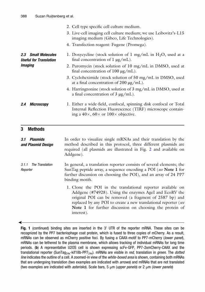
2. Cell type specific cell culture medium.

3. Live-cell imaging cell culture medium; we use Leibovitz’s-L15imaging medium (Gibco, Life Technologies).

4. Transfection reagent: Fugene (Promega).

2.3 Small Molecules

Useful for Translation

Imaging

1. Doxycycline (stock solution of 1 mg/mL in H2O, used at afinal concentration of 1 μg/mL).

2. Puromycin (stock solution of 10 mg/mL in DMSO, used atfinal concentration of 100 μg/mL).

3. Cycloheximide (stock solution of 50 mg/mL in DMSO, usedat a final concentration of 200 μg/mL).

4. Harringtonine (stock solution of 3 mg/mL in DMSO, used ata final concentration of 3 μg/mL).

2.4 Microscopy 1. Either a wide-field, confocal, spinning disk confocal or TotalInternal Reflection Fluorescence (TIRF) microscope contain-ing a 40�, 60� or 100� objective.

3 Methods

3.1 Plasmids

and Plasmid Design

In order to visualize single mRNAs and their translation by themethod described in this protocol, three different plasmids arerequired (all plasmids are illustrated in Fig. 2 and available onAddgene).

3.1.1 The Translation

Reporter

In general, a translation reporter consists of several elements; theSunTag peptide array, a sequence encoding a POI (see Note 1 forfurther discussion on choosing the POI), and an array of 24 PP7binding motifs.

1. Clone the POI in the translational reporter available onAddgene (#74928). Using the enzymes AgeI and EcoRV theoriginal POI can be removed (a fragment of 2587 bp) andreplaced by any POI to create a new translational reporter (seeNote 1 for further discussion on choosing the protein ofinterest).

�

Fig. 1 (continued) binding sites are inserted in the 30 UTR of the reporter mRNA. These sites can berecognized by the PP7 bacteriophage coat protein, which is fused to three copies of mCherry. As a result,mRNAs can be observed as mCherry positive foci. By fusing a CAAX-motif to PP7-mCherry (lower panel),mRNAs can be tethered to the plasma membrane, which allows tracking of individual mRNAs for long timeperiods. (b) A representative U2OS cell is shown expressing scFv-GFP, PP7-2xmCherry-CAAX and thetranslational reporter (SunTag24x-kif18b-PP724x). mRNAs are visible in red, translation in green. The dottedline indicates the outline of a cell. A zoomed-in view of the white-boxed area is shown, containing both mRNAsthat are undergoing translation (two examples are indicated with arrows) and mRNAs that are not translated(two examples are indicated with asterisks). Scale bars, 5 μm (upper panels) or 2 μm (lower panels)


2. Alternatively, start with a vector of choice and a POI of choiceand clone the individual elements of the translational reporter(i.e., SunTag and PP7 binding sites) into this vector.

(a) Since the SunTag peptide array forms a repetitivesequence, it is difficult to amplify the array by PCR. Wetherefore recommend cloning strategies based on enzy-matic digestion and ligation (see Note 2 for more infor-mation about PCR-based cloning strategies of the SunTagarray). To insert the SunTag array (consisting of 5–24SunTag peptides (see Note 3 about the use of differentnumbers of SunTag peptides)) at the N-terminus of thePOI, use HindIII and AgeI restriction enzymes to digestthe translational reporter plasmid available on Addgene(#74928). This results in two fragments (9141 and1819 bp). The smaller fragment contains the 24� SunTagpeptides, which can be cloned into the desired vector.

(b) Clone the 24 PP7 binding motifs into the 30 UTR of themRNA to label the mRNA independently of translation.Use BamHI and EcoRI to digest the translational reporterplasmid available on Addgene (#74928). This results intwo fragments (9492 and 1468 bp), the smaller of whichcontains the PP7 binding motives. Since this array of shorthairpin sequences is highly repetitive, we recommendcloning methods based on digestion and ligation ratherthan through PCR-based cloning.

(c) Clone a promoter of choice upstream of the reportercoding sequence. Expression of the reporter mRNA istypically driven by a doxycycline-inducible promoter toallow temporal control of reporter mRNA expression (seeNote 4 about the use of an inducible promoter). Thispromoter can be obtained from plasmid (#74928), byusing the enzymes MluI and HindIII or by PCR.

Fig. 2 Schematic overview of the plasmids used for the translation imaging method. Region of plasmid that istranscribed into mRNA is shown in black, other DNA in grey. Thin black lines indicate noncoding parts of themRNA, thick black lines indicate coding sequences. The SunTag peptides are shown in light blue with greenstripes representing individual peptides (eight shown), the PP7 binding sites in dark blue, sfGFP in green, andmCherry in red. All plasmids are available on Addgene (see text for catalog number)


3.1.2 sfGFP-Tagged

Antibody that Binds the

SunTag Peptide (scFv-GFP)

The scFv-GFP binds with high affinity to the SunTag peptides,which results in the fluorescent labeling of nascent polypeptides assoon as they emerge from the ribosome exit tunnel [2–5].

1. PCR amplify the scFv-GFP coding sequence and clone it into aplasmid containing the promoter appropriate to your cell typeof choice.

3.1.3 mCherry-Fused

PCP (PP7-mCherry)

Dependent on whether or not the aim is to tether the mRNAs tothe plasma membrane, plasmid #74926 (untethered) or plasmid#74925 (tethered) can be used as a template. Using PCR-basedmethods, either PP7 alone, PP7 fused to mCherry or PP7 fused tomCherry and a CAAX domain can be amplified and placed into avector of choice (see Note 5 on tethering the mRNA to the mem-brane). Note that plasmids containing multiple copies of mCherrycannot be amplified by PCR and need to be cloned by digestion–-ligation methods.

3.1.4 Exchanging

Fluorescent Proteins

The three plasmids described above enable visualization of both thereporter mRNA (PP7-mCherry, red) and its translation (scFv-GFP,green) in live cells (Fig. 1b). In principle, the color of the fluores-cent proteins (e.g., GFP and mCherry) can be changed, but thefunctionality of the newly designed constructs needs to be carefullytested, as, for example, addition of sfGFP to the antibody has beenshown to be important for preventing scFv aggregation in mam-malian cells [6] (see Note 6 for further comments on fluorescentproteins fused to the scFv antibody).

1. Exchange fluorescent protein using PCR-based cloningmethods.

2. Test expression level of newly created fusion protein by tran-sient transfection in cell type of choice.

3. Examine aggregation state in cells of fusion protein after tran-sient transfection using widefield or confocal microscopy(bright fluorescent foci in transfected cells indicate proteinaggregation).

3.2 Creating a Cell

Line for Imaging

Translation

3.2.1 Choosing a

Suitable Cell Type

We have performed the majority of our experiments in U2OS cells.However, similar SunTag-based translation imaging has been suc-cessfully performed in neurons and HeLa cells [2–4], suggestingthat the translation imaging approach described here can be per-formed in most cell types (seeNote 7 on how to choose the best celltype for your experiment).

3.2.2 Delivering the

Plasmids

To create a cell line in which translation can be imaged, the plasmidsdescribed above can be delivered into cells with standard methodssuch as transfection or viral transduction. Because of the repetitivesequences present in the reporter mRNA plasmid (e.g., the PP7


binding sites and the sequence encoding the SunTag peptides),virus titers may be low, and transfection may be preferred overviral transduction. To transfect the plasmids into U2OS cells in a6 cm cell culture dish (transient or stable transfection; see Note8 about transient versus stable transfections) the following Fugene(Promega) transfection protocol can be used. Please note that othercell types may require other transfection protocols.

1. Warm up DMEM medium without serum and without anti-biotics (DMEM �/�) to 37 �C.

2. Make a mastermix (number of reactions +1) of Fugene (Pro-mega) containing 100 μL DMEM �/� and 2 μL Fugene per6 cm dish.

3. Mix by tapping vigorously.

4. Spin down 3 s to collect medium in bottom of the tube.

5. Incubate the master mix for ~5 min at room temperature.

6. Make the DNA mix containing 1 μg total DNA pertransfection.

7. Add 100 μL of DMEM/Fugene mastermix to the DNA andmix by pipetting.

8. Incubate for 5–15 min at room temperature.

9. Add 3 mL of fresh cell culture medium to the cells.

10. Add the transfection mix to the cells.

11. After 24 h wash the cells (note: this is not essential).

3.3 Preparing Cells

for Imaging

1. Approximately 12–24 h before imaging plate the cells contain-ing the reporter plasmid, PP7-mCherry (�CAAX) and thescFv-GFP, in a glass bottom dish (we routinely use 96-wellsglass bottom dishes) at the intended densities (~50% con-fluency). Depending on the experimental design and celltype, cells can also grow for longer time periods on the glasssurface.

2. Immediately before transferring the glass-bottom dish contain-ing the transfected cells to the microscope, replace the culturemedium with prewarmed imaging medium per 96-well (seeNote 9 about the use of imaging medium).

3. Set the temperature at the microscope to 37 �C for mammaliancells. Changes in temperature may result in cellular stress,which could influence the process of translation. We foundtemperatures between 36 and 37.5 �C to be acceptable formost human cell lines.

4. When imaging for longer time periods, it is important toprevent evaporation of the cell culture medium, as this mayresult in changes in medium composition. We recommend


keeping a lid on the imaging plate whenever possible to preventevaporation.

5. When using a doxycycline-inducible promoter to express thetranslation reporter, add doxycycline (used at a final concentra-tion of 1 μg/mL) approximately 10 min before the start ofimaging. Addition of doxycycline to the cells will generallyinduce expression of the reporter mRNAs within 15–30 min(see Note 10 about how to add doxycycline to the cells).Adding doxycycline immediately before the start of imagingallows imaging the first rounds of translation of newly tran-scribed mRNAs as well. In addition, adding doxycycline justbefore the start of imaging prevents cytoplasmic depletion ofscFv-GFP, which occurs when high levels of SunTag protein arepresent in the cell (see below and Note 11 about the levels ofscFv-GFP).

6. Select cells for imaging that have the correct levels of GFP- andmCherry-tagged proteins, and in which the translationreporter is expressed. (see Note 12 for more details about theexpression levels of mCherry, see Note 11 and Fig. 3 for moredetails about scFv-GFP levels, see Note 13 for more informa-tion on how to select cells with the correct levels of transla-tional reporter). Note that the number of cells that can beimaged at the same time is limited when a high time resolutionis required.

3.4 Imaging

and Image Acquisition

Different optical imaging techniques, including widefield, pointscanning confocal, spinning disc confocal, TIRF and light sheetmicroscopy can be used for imaging translation (seeNote 14 aboutthe advantages and disadvantages of different imaging techniques).

Fig. 3 Different pools of scFv-GFP present in cells. Expression of scFv-GFP in the presence of a reporter mRNAresults in the appearance of three different pools of GFP in the cell: (1) a pool of unbound, freely diffusing scFv-GFP, (2) a pool of scFv-GFP bound to mature SunTag proteins, which have 24 SunTag peptides and are thus~24 times brighter than the single scFv-GFP molecules, and (3) a pool of scFv-GFP bound to the newlysynthesized SunTag peptides which represent sites of translation. Translation sites are usually 1–20�brighter than single SunTag proteins, as multiple ribosomes can bind to a single mRNA molecule


1. Select the appropriatemicroscope objective. In general, we imagewith a 100� NA1.49 oil-immersion objective to obtain a highresolution and good sensitivity. Objectives with lower NA ormagnification may also be used to image translation sites withmultiple ribosomes, butmight fail to reliably detect themCherry-labeled mRNA or single ribosomes translating an mRNA.

2. Set the appropriate laser power and exposure time. Laser powerand exposure time settings depend on the objective, micro-scope, camera and specifics of the experimental design. In thecase of the tethered mRNA assay, low laser power in combina-tion with a long exposure time provides the highest imagequality and signal-to-noise ratio. Long exposure times (in therange of 500 ms) will cause motion blurring of the highlymotile, GFP-labeled mature SunTag proteins and will thereforeresult in a more homogenous background signal. Since teth-ered mRNAs diffuse more slowly and are therefore not motionblurred at 500 ms exposure times, long exposure times willhelp to distinguish translation sites from background signal.

3. Find the correct focal plane to imaging mRNAs and translationsites. When the mRNA is tethered to the plasma membrane, itis important to focus the objective slightly above the plasmamembrane of the cells during the imaging, as this is where thefluorescence associated with both the mRNA and the ribo-somes translating the tethered mRNAs is located (see Note15 on how to focus on both the mRNA and translation sites).

4. Set the time interval for time-lapse imaging. In order to imagetranslation dynamics and allow measurements of translation ini-tiation and elongation, we usually acquire an image every 30 s. Ingeneral, shorter time intervals make it easier to detect short livedevents or to track individual mRNAs over time, while imagingwith longer time intervals results in reduced photobleaching andphototoxicity, which allows imaging for longer time periods. Inexperiments in whichmRNAs are tethered, we found a 30 s timeinterval to be a good compromise between high temporal reso-lution and photobleaching for most of our experiments. How-ever, when mRNAs are not tethered, a higher temporalresolution may be required to achieve accurate mRNA tracking.

5. Start image acquisition.

6. Add drugs which interfere with translation, as required byexperimental setup. In most experiments, we recommend toadd drugs after 10–30 min of imaging, when 10–50 transla-tions sites are present per cell. Adding the drugs during imag-ing allows one to observe their immediate effects ontranslation. After addition of the drugs (see Subheading 3.5),cells should be imaged for another 5–30 min to observe theeffect on translation.


3.5 Drugs that

Interfere with

Translation as Tools to

Study Translation

Dynamics

Several drugs that are known to interfere with translation can beadded to the cells to measure specific aspects of translation dynam-ics. Note that when adding drugs to the medium, it is advisable topredilute the drug in large volume (~20% of final volume) (seeNote10 on adding drugs to the cells).

1. Puromycin (used at 100 μg/mL). Puromycin binds the elon-gating nascent polypeptide chain, thereby releasing the nascentpolypeptide from the ribosome and dissociating the ribosomalsubunits from the mRNA. Addition of puromycin to the cellsresults in the disappearance of bright GFP spots (translationsites) within 1 min after addition. Puromycin can therefore beused as a tool to verify whether the observed GFP spots areactive translation sites. Make a 10 mg/mL stock concentrationof puromycin in DMSO, which can be diluted to a concentra-tion of 700 μg/mL (7� the final concentration) in imagingmedium. Of this dilution, add 50 μL to the 300 μL imagingmedium present in a well of a 96 well-plate, to create a finalconcentration of 100 μg/mL.

2. Cycloheximide (used at 200 μg/mL). Cycloheximide (CHX)binds to the E-site of the ribosome, preventing release of theribosome-bound tRNA and ribosomal translocation along themRNA. Thus, CHX treatment results in stalling of ribosomeson themRNA and should lead to the stabilization of GFP signalat translation sites. CHX may therefore be used to addresswhether changes in GFP intensity at sites of translation arecaused by altered ribosomal occupancy. Make a 50 mg/mLstock concentration of cycloheximide in DMSO, which can bediluted to a concentration of 1400 μg/mL (7� the final con-centration) in imaging medium. Of this dilution, add 50 μL tothe 300 μL imaging medium present in a well of a 96 well-plate,to create a final concentration of 200 μg/mL.

3. Harringtonine (used at 3 μg/mL). Harringtonine is a smallmolecule translation inhibitor that specifically blocks transloca-tion of ribosomes at the initiation codon, without affectingdownstream ribosomes. As a consequence, upon harringtoninetreatment ribosomes downstream of the start codon will com-plete translation normally and dissociate from the mRNA one-by-one after translation termination, resulting in a gradualdecrease of the translation site GFP signal. Measuring thedecay rate of GFP fluorescence from single mRNAs, and fittingthe data to a simple mathematical model [5], allows estimationof ribosome translocation rates on a given mRNA transcript.The duration of ribosome run-off is dependent on the lengthof the POI. In case of the translational reporter Addgene#74928, run-off can be observed within 5–15 min after har-ringtonine addition. Starting from a 3 mg/mL stock


concentration of harringtonine in DMSO, make a dilution of21 μg/mL (7� the final concentration) in imaging medium. Ofthis dilution, add 50 μL to the 300 μL imaging medium presentin a well of a 96 well-plate, to create a final concentration of3 μg/mL.

3.6 Image Analysis Using the translation imaging method described here, the GFP-intensity of translation sites can be used to determine quantitativefeatures of translation, including ribosome density on mRNAs,translation initiation rates, ribosome translocation rates and ribo-some stalling. Determining these characteristics of translationrequires (1) precise quantification of GFP intensities and (2) carefulinterpretation of the GFP fluorescence intensity.

3.6.1 Measuring GFP

Intensities and Determining

the Number of Ribosomes

on an mRNA

The GFP intensity reports on the number of ribosomes on anmRNA. In some cases, it is sufficient to determine the relativenumber of ribosomes on each mRNA, in which case comparingGFP intensities between translation sites is possible. However, forother experiments it is useful to determine the absolute number ofribosomes on an mRNA. Below, we describe a step-wise protocolon how to measure GFP intensities and how these fluorescenceintensity measurements can be used to calculate the number ofribosomes present on an mRNA.

In order to determine the number of ribosomes on an mRNAbased on the GFP intensity of the translation site, it is important tocompare the observed GFP intensity of a translation site with theGFP intensity of a single mature SunTag protein. Visualizing singlemature SunTag proteins requires imaging with a short exposuretime (10–30 ms) and a sensitive camera as a single SunTag proteincontains at most 24 GFP molecules (in contrast to translation sites,which can contain >100 GFPs). Use a laser power that is suffi-ciently high to allow detection of single SunTag proteins, butwithout saturating camera pixel intensities at the much brightertranslation sites. Single SunTag molecules are detectable on eitherEMCCD or sCMOS cameras.

1. Measure the GFP intensity of a single mature protein.

(a) Draw a region of interest (ROI) around each fluorescentspot that represents a freely diffusing mature SunTagprotein (see Note 16 on how to select foci representingmature SunTag proteins). Use an ROI that is as small aspossible, but large enough to also accommodate transla-tion sites.

(b) Measure the mean fluorescence intensity in the ROI.

(c) Measure the mean background GFP intensity in the cell,by using a large ROI which does not contain any GFPfoci.


(d) Subtract the mean background intensity from the meanspot intensity to obtain the intensity of a single SunTagprotein.

2. Measure GFP intensity of a translation site.

(a) Draw a ROI (of the same size as used for measuring singlemature proteins) around each translation site.

(b) Measure the average fluorescence intensity of each trans-lation site.

(c) Subtract the mean background intensity (measured instep 1c) from the mean translation site intensity to calcu-late the mean intensity of a translation site.

3. In experiments where substantial photobleaching is observed,correction for photobleaching of the fluorescence intensities iscritical (see Note 17 for further discussion aboutphotobleaching).

4. Divide the mean GFP intensity of the translation sites by themean intensity of the single mature SunTag proteins.

5. The value calculated in step 4 provides an estimate of thenumber of SunTag arrays present at a translation site (seeNote 18 and Fig. 4 for a further description on how to inter-pret GFP intensity).

3.6.2 Image Analysis

Software to Measure GFP

Intensities

In order to analyze the images obtained by microscopy, differentimage analysis software packages can be used, including Matlab,Python, and ImageJ. The choice for a specific software packagemainly depends on the experimenter’s previous experience andpersonal preference. For unique or complex questions, customanalysis software may be required, making Matlab and Pythongood options. However, for many simple types of analysis, existingImageJ plugins can be used. Currently, several plugins are availablewhich allow, for example, counting of the number of translationspots per cell, measuring the intensities of individual translationspots, or tracking translation spots over time. One simple ImageJplugin that is useful for the analysis of translation dynamics is thespot_counter ImageJ plugin (http://fiji.sc/SpotCounter) devel-oped by Nico Stuurman. This plugin counts the number of transla-tion spots in a cell over time, and determines the fluorescenceintensity of individual spots.

4 Notes

1. Choosing the gene of interest in the translation reporter. Inprinciple, any gene can be introduced in the translationreporter, and the choice will mainly depend on the goal ofthe experiment. However, it is important to take into account


http://fiji.sc/SpotCounter

that other regulatory sequences outside the coding region,such as the 30 and 50 UTR, may influence translation efficiencyas well and can also be inserted into the reporter construct,either on their own or together with the coding sequence. Ifthe goal of the experiment is not related to the regulation of aspecific gene, but rather to study global translational controlmechanisms, the specific mRNA sequence inserted down-stream of the SunTag sequence may not be critical and differentsequences can be inserted. The length of the reporter sequence

Fig. 4 Interpreting GFP fluorescence intensities of translation sites. The scFv-GFP intensity associated with a single ribosome depends on the location of theribosome along the mRNA. The GFP intensity will initially increase as theribosome synthesizes successive SunTag peptides (illustrated in the figure bythe binding of 1, 2, or 3 scFv-GFP antibodies). Ribosome-associated fluores-cence reaches a maximum once all SunTag peptides have been synthesized andwill remain constant while the ribosomes translate the remaining sequence ofthe mRNA. As a consequence, ribosomes at the 30 end of the mRNA are labeledbrighter, than those at the 50 end. When the number of ribosomes on an mRNA iscalculated based on GFP intensity, these position-dependent effects of GFPintensity need to be taken into account. A simple mathematical model can beused, as described in the text


is, however, an important parameter to take into account. Thelonger the reporter gene, the more ribosomes can be presenton the mRNA simultaneously, affecting the brightness of thetranslation sites. The use of longer reporter genes (1–2 kb) istherefore advisable and will facilitate further analysis.

2. Cloning the SunTag peptide array sequence. The SunTag pep-tide array contains a somewhat repetitive sequence and is there-fore difficult to amplify by PCR. The SunTag sequence is codonscrambled (i.e., different codons are used to encode the sameamino acid sequence in each peptide) to minimize the degree ofrepeated nucleotide sequences. Codon scrambling allows PCRamplification to some extent, but some clones after PCR-basedcloning will have small deletions. Therefore, cloning strategiesthat circumvent PCR-based amplification of this sequence arepreferable.

3. The number of SunTag peptides in the reporter gene. Thereporter construct that is used by us and others [2–5] generallycontains 24 SunTag peptides. However, shorter arrays (five orten copies of the SunTag peptide [5]) or longer arrays (56copies [2]) can also be used to image translation). Comparisonbetween reporter mRNAs containing either 5, 10 or 24 Sun-Tag copies revealed that ribosome density on these mRNAs wasvery similar, indicating that increased number of SunTag pep-tides does not detectably alter translation initiation or elonga-tion rates of the reporter mRNA. Lowering the number ofSunTag peptides will make the imaging of translation sites,especially at low ribosome occupancy, more challenging as itdecreases the translation-associated GFP signal. Therefore,having a high copy number of SunTag peptides will be favor-able in most situations. However, some specific experimentalsetups, such as the integration of the SunTag sequence into anendogenous gene locus by CRISPR/Cas9, may benefit fromthe use of shorter and less repetitive peptide arrays.

4. Using an inducible promoter to express a reporter mRNA. Theadvantage of using an inducible promoter is that it allowstemporal control of mRNA synthesis. Expressing the reportermRNA only during the imaging experiment has two mainadvantages; first, it prevents accumulation of high level ofrelatively bright mature SunTag proteins, which hinders theimaging of translation sites. (See also Note 13 about theexpression level of the translational reporter.) Second, limitingthe levels of mature SunTag protein will also prevent depletionof the freely diffusible pool of scFv-GFP antibody from thecytoplasm. If mature SunTag protein levels become too high,the majority of scFv-GFP is bound to mature protein and istherefore not available to bind nascent SunTag peptides attranslation sites. As a consequence, newly made SunTag


peptides emerging from the ribosome are labeled incompletely,limiting the fluorescence of translation sites.

5. Tethering the mRNA to the plasma membrane. PP7-mCherrybinds with high affinity to the hairpin sequence present in the 30

UTR of the reporter plasmid, resulting in fluorescent labelingof mRNA molecules. However, due to the rapid diffusion ofsingle mRNAs, it is challenging to track single mRNAs overlonger periods of time. In order to improve long-term trackingof individual mRNAs, a CAAX prenylation motif can be fusedto the PCP. The CAAX motif anchors the PCP to the plasmamembrane, which results in tethering of the reporter mRNAscontaining the PCP binding sites to the plasma membrane.Membrane tethering of mRNAs reduces their mobility, facil-itating long-term tracking of individual mRNA molecules(Fig. 1a, lower panel, b; [5]). Importantly, membrane tether-ing of mRNAs also allows a specialized form of microscopy,called TIRF microscopy, which significantly improves the sig-nal-to-noise ratio of the image. So far, we have not observedany differences in translation dynamics between tethered anduntethered mRNAs ([5] and unpublished results). However,under certain conditions tethering of the mRNA to the mem-brane could affect translation, for example when translation ofthe reporter mRNA is spatially regulated. Appropriate controlsshould therefore be performed in experiments involvingmRNA tethering.

6. The importance of fusing sfGFP to the SunTag antibody tocreate scFv-GFP. The SunTag antibody has a tendency toaggregate at high expression levels in the cytoplasm of mam-malian cells. To optimize intracellular expression of the anti-body, a variety of N- and C-terminal fusion proteins known toenhance protein solubility were tested. Fusion of one variant ofGFP, called sfGFP [9], to the C-terminus of the antibodyresulted in soluble expression of the antibody even at highexpression levels [5]. Therefore, when changing the fluoro-phore fused to the antibody, it is important to test whetherthe newly created antibody–fluorescent protein fusion does notaggregate in cells.

7. Choosing a suitable cell type. In principle, most cell types can beused to study translation using the method described here.However, there are some features which may be worthwhile totake into account when choosing a cell type. The most impor-tant aspect of a cell type is whether the plasmids described abovecan be efficiently delivered into the cells. In addition, it is impor-tant to consider whether the cell type can be imaged using highresolution microscopy. For example, cells grown in suspensionmay be more difficult to image than flat, adherent cells.


8. Transient versus stable transfection. In general, the plasmidsrequired for translation imaging (see Subheading 2.1) can beeither transiently transfected or used to generate cell lines stablyexpressing the genes of interest. While the use of a stable cell linewill generally make results slightly more reproducible, a transienttransfection will save time, as it allows for imaging of translationof a specific reporter 1 day after transfection. Since PP7-mCherry and scFv-GFP are used in every experiment, we rec-ommend making a cell line in which both PP7-mCherry andscFv-GFP are stably expressed. This cell line can then be used tointroduce different reporter mRNAs to study their translation.Note that in some cases we observed that stable expression ofPP7-mCherry led to lysosomal accumulation of mCherry signal.Lysosomal accumulation was not detected when PP7 was fusedto other fluorophores, such as GFP. mCherry-positive lysosomesare readily distinguishable from reporter mRNAs based on size,shape, intensity and motile properties, and therefore do nothinder the imaging of mRNAs, unless their localization overlapswith an mRNA molecule.

9. Using CO2-independent, phenol red free imaging medium.Replacing the normal cell growth medium (generally CO2-dependent media containing phenol red) with CO2-indepen-dent, phenol red-free imaging medium ensures a correct pHover the course of the experiment and, in addition prevents thatphenol red from interfering with fluorescence imaging. Weroutinely use Leibovitz-L-15 imaging medium which is CO2-independent and free of phenol red, and therefore ideal for live-cell microscopy. Note that appropriate levels of serum andantibiotics should still be added to the imaging medium. Alter-natively, an optimal pH during the experiment can be achievedby having a CO2 supply in the microscope imaging chamber.

10. Diluting drugs before addition to the cells. We recommendprediluting drugs that need to be added to the cells during theimaging experiment in a large volume (~20% of final volume)before adding it to the cells. This ensures quick diffusionthrough the imaging medium so that the drug rapidly reachesthe cells without repeated pipetting (which can cause cellularstress). We usually make a 7� dilution, of which we add 50 μLto the 300 μL imaging medium present per 96 well.

11. Expression levels of scFv-GFP. Expression of scFv-GFP in thepresence of a reporter mRNA results in the appearance of threedifferent populations of GFP particles in the cell: (1) a pool offreely diffusing scFv-GFP, (2) a pool of scFv-GFP bound toSunTag proteins which have completed translation and havebeen released from the ribosome (and thus contain a singleSunTag peptide array), referred to as “mature proteins,” and(3) a pool of scFv-GFP bound to the nascent SunTag peptides


which represent sites of translation (Fig. 3). scFv-GFP expres-sion levels need to be sufficiently high to bind all SunTag pep-tides present in both the mature SunTag proteins and the newlysynthesized nascent SunTag polypeptides as they emerge fromthe ribosomes. If scFv-GFP levels are too low, all antibody willbe bound tomature SunTag protein, and the newly synthesized,nascent SunTag peptides will not be (completely) fluorescentlylabeled. On the other hand, if scFv-GFP levels are too high, thiswill give a strong background fluorescence of unbound scFv-GFP that can mask the signal of translation sites.

12. Expression levels of PP7-mCherry. The expression levels ofPP7-mCherry should be high enough to saturate binding tothe PP7 binding sites, but low enough to prevent high back-ground fluorescence of PP7-mCherry not bound to an mRNA.In addition, high expression of PP7-mCherry can cause accu-mulation in lysosomes, resulting in bright red dots in the cell(see also Note 8 about lysosomal accumulation of PP7-mCherry).

13. Expression level of the translational reporter. For most experi-ments it is useful to select cells or a cell line for imaging with ahigh number of transcripts, as this enables the imaging of manytranslation events in one experiment. However, very highexpression of the reporter also results in rapid antibody deple-tion (i.e., a situation in which the majority of antibody is boundto mature protein, resulting in weak labeling of translationsites, see Note 11) and might impair long-term tracking ofmRNAs (as moving mRNAs are more likely to cross paths).Optimal expression levels of the reporter mRNA thereforedepends on the specific experimental conditions. Inducibleexpression of the reporter reduces some of the problems ofhigh expression levels of the mRNA reporter (i.e., antibodydepletion) and is therefore generally beneficial. An additionalapproach to prevent high levels of labeled, mature SunTagprotein in the cells involves fusion of the SunTag protein to adegron to ensure its rapid degradation after its synthesis iscompleted. This approach has been successfully used toincrease the signal-to-noise ratio during imaging experiments[3, 4]. When selecting cells with the correct level of the trans-lational reporter, it is important to note that in case of veryhigh levels of mature SunTag protein expression, the GFPsignal in the cell may appear homogenous throughout thecell without clear SunTag punctae, because each SunTag pro-tein is labeled with so few scFv-GFP molecules that individualSunTag-labeled proteins can no longer be distinguished fromunbound scFv-GFP molecules based on their fluorescenceintensity.


14. Advantages and disadvantages of different imaging systems.Widefield microscopy: Widefield microscopy allows imaging ofrelatively thick Z-sections, facilitating mRNA tracking in 3Dwith limited number of Z-slices acquired. The reduced numberof Z-slices required for tracking mRNAs in 3D may cause lessphotobleaching, and increase the time resolution that can beachieved. A drawback of widefield imaging, however, is that thesignal-to-noise ratio is lower due to increased out-of-focuslight, and therefore only moderately to strongly translatingmRNAs (i.e., mRNAs translated by multiple ribosomes) willbe detectable. Point scanning confocal microscopy: With pointscanning confocal microscopy, a higher signal-to-noise ratiocan be achieved (compared to widefield microscopy). How-ever, point scanning confocal microscopy is slow and causesrelatively high levels of photobleaching and phototoxicity, andis therefore less suitable for long-term live-cell imaging.Spinning disc confocal microscopy: Similar to point scanningconfocal microscopy, the use of spinning disc confocal micros-copy allows imaging with a high signal-to-noise ratio. How-ever, spinning disc confocal imaging is faster than pointscanning confocal microscopy and may cause lower levels ofphototoxicity to the sample. It is therefore suitable for imagingtranslation of single mRNA molecules with high sensitivityover longer time periods, and is our system of choice for themajority of experiments involving the translation imaging sys-tem. Total Internal Reflection Fluorescence (TIRF) microscopy:TIRFmicroscopy greatly reduces background signal and there-fore increases the signal-to-noise ratio. However, only fluores-cent molecules that are located close to the glass surface (e.g.,near the plasma membrane at the bottom of the cell) can beobserved, so tethering of the mRNAs to the membrane isrecommended when imaging translation sites using TIRF. Anadditional disadvantage of TIRF microscopy is that the illumi-nation of cells is generally uneven, which hinders quantitativemeasurements of fluorescence intensities. Light sheet micros-copy: Light sheet microscopy can potentially be used to imagetranslation in thick samples, such as tissues and embryos ofvarious model organisms.

15. Finding the correct focal plane for imaging mRNAs and trans-lation sites using the plasma membrane tethering approach.Although red mRNAs and green translation spots largely colo-calize, we noted that the mRNA fluorescence signal localizesslightly below (i.e., closer to the plasma membrane) than thetranslation signal. This is expected as mCherry is fused directlyto the CAAX domain, and thus very close to the plasma mem-brane, whereas the GFP is connected to the membranethrough mCherry, the mRNA, and the nascent chain, and


will thus localize slightly further toward the cell interior(Fig. 1a, lower panel). Therefore, care should be taken toensure both the mRNA and translation signal are in focus.

16. Selecting foci representing mature SunTag proteins to deter-mine their fluorescence intensity. Since mature proteins are nottethered to the plasma membrane and are relatively small com-pared to translation sites, they diffuse rapidly in 3D throughoutthe cell. Imaging mature SunTag proteins and measuring theirfluorescence intensity is complicated by their fast diffusion, asthe rapid movement of single SunTag protein causes motionblurring of the fluorescent foci in the image. In addition, rapidmovement of mature SunTag proteins in the Z-axis causesmany spots to be slightly out of focus when images areacquired. Both issues involving focus and motion blurringaffect the fluorescence intensity of mature SunTag proteins.To minimize abovementioned issues, imaging with a short(10–30 ms) exposure time is recommended, which will reducemotion blurring. In addition, manually selecting foci for quan-tification that appear in focus will help alleviate abovemen-tioned issues.

17. Correcting for photobleaching. As a consequence of exposingfluorophores to excitation light, photobleaching occurs overtime, reducing the intensity of GFP measured at translationsites. The rate at which photobleaching occurs can be deter-mined by measuring the GFP signal of a large area in the cell(potentially the whole cell or field of imaging). Choosing anarea of the cell lacking translation spots to measure bleachingrates ensures that such measurements are not affected byappearance and disappearance of mRNAs. In experimentswhere substantial photobleaching is observed, correction forphotobleaching of the fluorescence intensities of translationsites is critical.

18. Interpreting the scFv-GFP fluorescence intensity to measuretranslation dynamics. The GFP signal observed at translationsites is a result of the nascent SunTag peptides bound by scFv-GFP antibodies. Importantly, ribosomes on the 50 end of themRNA have not yet translated all the SunTag peptides, andthus have fewer antibodies and fewer GFPs associated withthem as compared to ribosomes at the 30 end of the mRNA(Fig. 4). As a result, the GFP intensity associated with a ribo-some at the 50 end of the mRNA is lower than with a ribosomeat the 30 end of the mRNA (which has synthesized the entireSunTag peptide array). As a consequence, the measured GFPintensity at a translation site is not directly related to thenumber of ribosomes on the mRNA. To correctly translateGFP intensity to ribosome number, both ribosome densityand ribosome location along the mRNA need to be taken


into account. A simple mathematical model can be used tocalculate the number of ribosomes from the measured GFPintensities [5].

Acknowledgment

This work was supported by a by a fellowship of the Dutch CancerSociety (KWF) to M.E.T. and a Veni grant from the NetherlandsOrganization for Scientific Research (NWO) to S.R.

References

1. Morisaki T, Lyon K, DeLuca KF, DeLuca JG,English BP, Zhang Z, Lavis LD, Grimm JB,Viswanathan S, Looger LL, Lionnet T, StasevichTJ (2016) Real-time quantification of singleRNA translation dynamics in living cells. Science(New York, NY) 352(6292):1425–1429.doi:10.1126/science.aaf0899

2. Pichon X, Bastide A, Safieddine A, Chouaib R,Samacoits A, Basyuk E, Peter M, Mueller F,Bertrand E (2016) Visualization of singleendogenous polysomes reveals the dynamics oftranslation in live human cells. J Cell Biol 214(6):769–781. doi:10.1083/jcb.201605024

3. Wang C, Han B, Zhou R, Zhuang X (2016)Real-time imaging of translation on singlemRNA transcripts in live cells. Cell 165(4):990–1001. doi:10.1016/j.cell.2016.04.040

4. Wu B, Eliscovich C, Yoon YJ, Singer RH (2016)Translation dynamics of single mRNAs in livecells and neurons. Science (New York, NY) 352(6292):1430–1435. doi:10.1126/science.aaf1084

5. Yan X, Hoek TA, Vale RD, Tanenbaum ME(2016) Dynamics of translation of singlemRNA molecules in vivo. Cell 165(4):976–989. doi:10.1016/j.cell.2016.04.034

6. Tanenbaum ME, Gilbert LA, Qi LS, WeissmanJS, Vale RD (2014) A protein-tagging system forsignal amplification in gene expression and fluo-rescence imaging. Cell 159(3):635–646. doi:10.1016/j.cell.2014.09.039

7. Bertrand E, Chartrand P, Schaefer M, ShenoySM, Singer RH, Long RM (1998) Localizationof ASH1 mRNA particles in living yeast. MolCell 2(4):437–445

8. Chao JA, Patskovsky Y, Almo SC, Singer RH(2008) Structural basis for the coevolution of aviral RNA-protein complex. Nat Struct Mol Biol15(1):103–105. doi:10.1038/nsmb1327

9. Pedelacq JD, Cabantous S, Tran T, TerwilligerTC, Waldo GS (2006) Engineering and charac-terization of a superfolder green fluorescent pro-tein. Nat Biotechnol 24(1):79–88. doi:10.1038/nbt1172



https://doi.org/10.1083/jcb.201605024







https://doi.org/10.1038/nsmb1327

https://doi.org/10.1038/nbt1172

https://doi.org/10.1038/nbt1172

Chapter 27

Systematic Detection of Poly(A)+ RNA-Interacting Proteinsand Their Differential Binding

Miha Milek and Markus Landthaler

Abstract

RNA-binding proteins are dynamic posttranscriptional regulators of gene expression. Identification ofmRNA-binding proteins in a given experimental setting is thus of great importance. We describe aprocedure to enrich for direct poly(A)+ RNA protein binders by 4-thiouridine-enhanced UV cross-linkingand oligo(dT) purification. Subsequent nuclease-mediated release of RNA-binding proteins (RBPs) frommRNA allows for detection of eluted proteins by mass spectrometry. In addition, we provide a comparativeapproach to detect differences in RBP binding activity upon a biological stimulus.

Key words Protein–RNA interactions, RNA-binding proteins, Photoactivatable ribonucleoside, 4-Thiouridine, UV cross-linking, Oligo(dT) affinity purification, Mass spectrometry

1 Introduction

To systematically identify proteins binding to mRNA, a quantitativeapproach termed mRNA interactome capture was recently pub-lished [1, 2]. This method exploits in vivo UV cross-linking, oligo(dT) affinity purification, and mass spectrometry to identify theproteins directly bound to poly(A)+ RNA. Since its initial publica-tion, interactome capture has been successfully applied to othercultured mammalian cells [3–5], Drosophila embryos [6, 7], Cae-norhabditis elegans [8], Plasmodium falciparum [9], Arabidopsisthaliana [10, 11], and yeast [4, 12]. A common feature of thisapproach is to stabilize the protein–RNA interactions by eitherconventional (UV 254 nm) or photoactivatable ribonucleoside(PAR)-enhanced (UV 365 nm) cross-linking. As in cross-linkingand immunoprecipitation (CLIP)-related techniques [13–16],covalent bonds are formed at the site of direct contact between anucleotide in the RNA and an amino acid in the binding proteinmolecule [17]. This linkage allows for stringent oligo(dT) affinitypurification under denaturing conditions and highly selectiverecovery of protein–mRNA complexes.


405

Compared to other gene expression regulators such as tran-scription factors, RNA-binding proteins (RBPs) show higherexpression [18], are able to act both cotranscriptionally and post-transcriptionally in a concerted manner [19, 20] and are highlyresponsive to external cues, such as DNA damage [21]. Therefore,they represent an important avenue for future research utilizingsystems-wide approaches. An exciting feature of mRNA interac-tome capture is thus to systematically, quantitatively and differen-tially analyze the RBPs that change their binding activity uponcertain biological stimuli.

Here, we describe our procedure for isolation and differentialanalysis of poly(A)+ RNA-bound proteins. Initially, mammaliancells in culture are incubated with 4-thiouridine (4SU), resultingin metabolic labeling of cellular RNA. Following the application ofbiological stimulus to one cell population, all samples are exposedto UV light facilitating the formation of direct protein–RNA cross-links in living cells and stabilization of protein–RNA complexesbefore cell lysis (Fig. 1). An important feature of our method isthe usage of a calibrator “heavy” SILAC-labeled lysate [22] that isspiked into the samples corresponding to both experimental con-ditions and allows for quantitative comparisons between them.After a stringent oligo(dT) affinity purification and enrichment ofpoly(A)+ RNA, the cross-linked proteins are identified and quanti-fied using mass spectrometry. Afterward, the “heavy” SILAC inten-sity allows for the correction of between replicate variability due toseparate MS runs, amount of starting material and/or efficacy ofoligo(dT) affinity purifications. We present a detailed experimentalprocedure that may be easily applied to different cell culture sys-tems and stimulus specific responses.

2 Materials

2.1 Equipment 1. General cell culture equipment, e.g., incubator and dishes.

2. UV cross-linker device (Stratalinker or similar) with UV365 nm light bulbs.

3. 15- and 50-mL Falcon tubes.

4. Heating block at 80 �C.

5. Magnetic stands for Eppendorf tubes, 15- and 50-mL Falcontubes (e.g., Thermo Fisher Scientific DynaMag-2, -15, and -50magnets).

6. Sterile cell scrapers.

7. Needles and syringes, 23- and 26-G.

8. Centrifugal filters with 10,000 MW cutoff and 15-mL volume(e.g., Millipore. Amicon Ultra-15 Centrifugal Filter).

406 Miha Milek and Markus Landthaler

9. Rotating wheel for falcon tubes.

10. Liquid nitrogen.

2.2 Solutions We routinely use distilled water (MilliQ grade) to prepare thesolutions described below.

1. Adherent cell line, such as HEK293, HeLa, U2OS, and MCF-7 (ATCC).

( )

AAAAAA

X

m/z

Label RNA with photoactivatable ribonucleoside4-thiouridine (4SU)

Oligo(dT) affinity purificationT T T T T T

T T T T T T

Mass spectrometryDetermine differential binders(normalize to “heavy” intensity)

4SU

Covalently crosslink RNA to protein(UV365 nm irradiation)

Lyse

inte

nsity

AAAAAA

AAAAAA

X

X

XX

4SU

(denaturing, 1% LiDS)

Spike-in SILAC “heavy” lysate into both samples

AAAAAAAAAAAA

AAAAAA

X

X

XX

m/z

AAAAAAAAAAAA

AAAAAA

X

X

XX

X X

X X

X

X X

X

untreated sampletreated sample

treated cells untreated cells

protein-RNA crosslinks

AAAAAA

XXX

AAAAAA

XX

XAAAAAA

XX

X

AAAAAA

XX

AAAAAA

X

AAAAAA

X

nuclease digestion

AAAAAA

XXX

AAAAAA

X X

AAAAAA

XX

AAAAAA

XX

AAAAAA

X

AAAAAA

X

nuclease digestion

4SU

SILAC “heavy”

UV crosslink

Lyse

standard culture media (non-SILAC)

Treat cells

inte

nsity

4SU4SU

4SU4SU AAAAAA

Fig. 1 Graphical representation of experimental procedure to detect differential protein binding to poly(A)+ RNAupon biological stimulus. In order to be able to accurately normalize the data between two experimentalconditions, we rely upon the usage of “heavy” SILAC lysate obtained from separately cultured “heavy”-labeledcells. Cell lysates obtained from untreated or treated “light” cells are spiked with the same volume of “heavy”SILAC lysate, followed by oligo(dT) affinity purification. Protein–mRNA-containing eluates are then nuclease-treated, concentrated and used in mass spectrometry runs. The measured light peptide intensities can benormalized to the heavy intensities, which are present due to the spike-in

Isolation and Differential Analysis of RBPs 407

2. Nonlabeled/“light” cell culture medium: mix 0.5 L ofDulbecco’s modified Eagle’s medium (DMEM) containinghigh glucose (4.5 g/L), 50 mL of fetal bovine serum, 5 mLof 200 mM L-glutamine, and 5 mL of 10,000 U/mLpenicillin-streptomycin. Store at 4 �C.

3. 0.5 M 4-thiouridine (4SU) solution: Dissolve 1 g of 4SU(ChemGenes) in 7.68 mL of deionized water. Aliquot andstore at �20 �C protected from light.

4. Phosphate buffered saline (PBS). Store at 4 �C.

5. 5 M lithium chloride solution. Dissolve 106 g of LiCl powderby heating and agitation in 0.5 L of deionized water and storeat 4 �C.

6. 20 w/v % lithium dodecyl sulfate (LiDS) solution. Wear pro-tective mask and glasses when handling LiDS powder. Dissolve100 g of LiDS powder with agitation in 0.5 L of water andstore at room temperature.

7. IGEPAL CA-630 (NP-40 substitute). Store at roomtemperature.

8. Lysis/binding buffer: 100 mM Tris, pH 7.5, 500 mM LiCl,10 mM EDTA, 1 w/v % lithium-dodecylsulfate/LiDS, 5 mMDTT, and 1� complete Mini EDTA-free protease inhibitorcocktail. Store at room temperature. Immediately before useadd 0.25 mL of 1 M DTT and one tablet of complete miniEDTA-free protease inhibitor cocktail (Roche) per 50 mL ofworking lysis/binding buffer.

9. Washing buffer: 50 mM Tris, pH 7.5, 140 mM LiCl, 2 mMEDTA, 0.5% IGEPAL-CA630, 0.5 mM DTT, and 1� com-plete mini EDTA-free protease inhibitor cocktail. Store at 4 �C.Immediately before use add 25 μL of 1 M DTT and one tabletof complete Mini EDTA-free protease inhibitor cocktail(Roche) per 50 mL of working buffer.

10. Magnetic oligo(dT) beads (e.g., Thermo Fisher ScientificOligo(dT)25 Dynabeads, component of the mRNA DIRECTkit).

11. Low-salt elution buffer: 10 mM Tris, pH 7.5. Store at 4 �C.The elution buffer provided in the mRNA DIRECT kit(Thermo Fisher Scientific) may also be used.

12. Concentrating buffer: 10 mM Tris, pH 7.5, 50 mM NaCl.Store at 4 �C.

13. 100 U/μL RNase I solution. Store at �20 �C.

14. 125 U/μL benzonase solution. Store at �20 �C.

15. 1 M MgCl2. Dissolve 4.76 g of MgCl2 in 50 mL of deionizedwater. Store at 4 �C.


16. 0.4 M Arg10 solution: Reconstitute 62.1 mg of 13C6,15N4 L-

arginine HCl (Cambridge Isotope Laboratories) in 700 μLdeionized water. Store at �20 �C.

17. 0.8 M Lys8 solution. Reconstitute 128.1 mg of 13C6,15N4 L-

lysine 2HCl (Cambridge Isotope Laboratories) in 700 μL deio-nized water. Store at �20 �C.

18. SILAC “heavy” cell culture medium:Mix 0.5 L of high glucoseSILAC DMEM (PAA or Thermo Fisher Scientific), 50 mL ofdialyzed fetal bovine serum, 5 mL of 200 mM L-glutamine,5 mL of 10,000 U/mL penicillin-streptomycin, 0.5 mL of0.4 M Arg10 and 0.5 mL of 0.8 M Lys8. Filter the mediumthrough 0.2 μm filter membrane and store at 4 �C.

3 Methods

3.1 Cell Culture and

UV Cross-Linking

1. Culture adherent cells in desired medium until 40–70 % con-fluence and incubate them in the presence of 100–200 μM4-thiouridine (4SU) for 6–10 h. Duration and concentrationof 4SU treatment may have to be optimized (see Note 1).

2. (Optional: Apply an additional labeling pulse with 100 μM4SU 1–2 h prior to UV cross-linking to ensure the labeling ofshort-lived transcripts.)

3. Decant culture medium and place the dishes on ice. Wash oncewith 5–10 mL ice-cold PBS to remove the residual culturemedium. Make sure you remove most of the liquid beforeexposure to UV light (see Note 2). Next, cross-link cells withUV light with a wavelength of 365 nm and energy of 0.2 J/cm2

using a UV cross-linker. Repeat this process for all remainingdishes in culture.

4. Immediately harvest UV-exposed cells by scraping them off in5 mL of ice-cold PBS using a cell scraper. Process a secondbatch of cells without exposing them to UV light. This sampleserves as a background control.

5. Transfer cell suspensions into 50-mL falcon tubes and pelletcells by centrifugation with 400� g at 4 �C for 5 min. Wash thecell pellet once with ice-cold PBS. Collect cells and freezepellets in liquid nitrogen or continue with the cell lysis.

3.2 Cell Lysis and

Oligo(dT) Purification

1. Lyse cells in approximately five times the cell pellet volume oflysis/binding buffer containing 5 mM DTT and CompleteMini EDTA-free protease inhibitor cocktail by pipetting upand down and incubate the extract for 15 min on ice (seeNote 3). If sample volumes exceed 50 mL, aliquot in several50-mL falcon tubes.


2. Pass the lysate with a syringe several times through a 23- and26-G needle (see Note 4). Afterward, save 0.2 mL of inputlysate for downstream analyses (e.g., Western analysis and RNAextraction) and store it at �80 �C.

3. Pre-wash the magnetic oligo(dT) beads in 5 mL of lysis/bind-ing buffer in a 15 mL Falcon tube and concentrate them on amagnet. Afterward, resuspend beads into the cell extract byfirst taking them up in 1 mL of the prepared lysate and trans-ferring them to the tube containing the remaining lysate (seeNote 5).

4. Incubate for 1 h at room temperature on a rotating wheel (seeNote 6).

5. Concentrate beads on magnet. The initial concentration of thebeads on the magnet may take from 10 min to 1 h.

6. Carefully collect supernatant and place it into a new tube foradditional rounds of oligo(dT) precipitation (see Note 7).

7. Wash beads two times in one sample volume of room-temperature lysis/binding buffer. For each washing step, rotatethe tubes 2–5 min on a rotating wheel at room temperature.Afterward, concentrate the beads on magnet and carefullyremove the supernatant (see Note 8).

8. Wash beads two times in one sample volume of room-temperature washing buffer containing 0.5 mM DTT andcomplete EDTA-free protease inhibitor cocktail. For eachwashing step, rotate the sample 2–5 min on a rotating wheelat room temperature. Afterward, concentrate the beads onmagnet and carefully remove the supernatant.

9. For the third washing step, resuspend beads in 1mL of washingbuffer and transfer to a fresh 1.5-mL tube. Afterward, concen-trate the beads on magnet and remove the supernatant.

10. Wash beads once with 1 mL of ice-cold low-salt elution bufferto remove traces of IGEPAL CA-630 (see Note 9). Concen-trate beads with magnet and remove supernatant.

11. Resuspend beads in 0.5–1 mL of low-salt elution buffer andincubate them for 2 min at 80 �C. Remove supernatant into anew precooled 15-mL falcon tube and place it on ice as quicklyas possible. Pool the eluates from different aliquots. Once theeluate is removed, immediately cool down the beads by placingthem on ice (see Note 10).

12. Repeat the elution step 11 once more.

13. Perform several additional rounds of oligo(dT) affinity purifi-cations. We typically perform two additional rounds with onlyone elution per round for a total of three affinity purifications(see Note 11).


14. Keep the eluates on ice or store them at �80 �C until furtheruse. Wash and store oligo(dT) beads in lysis/binding buffer at4 �C. Reuse them up to three times.

3.3 Analyses of Oligo

(dT) Eluates

1. Save an aliquot of the eluate (100 μL) for further RNA analysesand store it at �80 �C (see Note 12).

2. To prepare the remaining eluate for mass spectrometry analysis,digest RNA by incubation with RNAse I and benzonase. Dilutethe RNAse I, benzonase and 1 M MgCl2 1:1000 in the eluateto obtain the final concentrations of 100 U/mL, 125 U/mLand 1 mM, respectively. Incubate for 1 h at 37 �C in a waterbath.

3. Concentrate the eluate by the 15 mL centrifugal filter. Loadyour sample into the filter unit and fill up the filter device withconcentrating buffer to a total volume of 14 mL. Centrifugethe filter unit at 4000 � g for 45 min at 4 �C (see Note 13).Recover the retentate from the filter device (approximately150 μL).

4. Analyze the protein sample by silver staining (Fig. 2a) andWestern analysis.

5. Submit the sample for mass spectrometry analysis and analyzethe data to obtain the identity of enriched RNA-binding pro-teins (see Note 14).

3.4 Detection of

Differences in Binding

Activity Upon a

Biological Stimulus

General consideration: If studying stress responses (e.g., oxidativestress, ER stress, and DNA damage), it is important to evaluate theeffect of perturbations (4SU treatment, UV exposure, SILACmedia incubation) on stress induction and cell growth, as well as4SU labeling efficacy (see Note 15).

1. Grow a population of cells in SILAC heavy media formulationand passage them at least six times before proceeding with theexperiment (see Note 16).

2. Once the SILAC cells are expanded and around 70–80% con-fluent, grow additional two populations of cells in “light” (i.e.,non-SILAC) media until 80% confluency.

3. Incubate all three cell populations with 200 μM 4SU for6–10 h (see Note 17).

4. Perform stimulation for one “light” cell population.

5. After the desired incubation, UV-cross-link the cells asdescribed in Subheading 3.1 (see Note 18).

6. Immediately harvest UV-exposed cells by scraping them off in5 mL ice-cold PBS using a rubber policeman. Transfer cellsuspensions into 50-mL falcon tubes and pellet them by centri-fugation (400 � g, 4 �C, 5 min). Wash the cell pellet once with


ice-cold PBS. Collect cells and freeze pellets in liquid nitrogenor continue with lysis (see Note 19).

7. Lyse ‘light” and “heavy” cells in approximately five times thecell pellet volume of lysis/binding buffer and incubate theextract for 15 min on ice.

8. Pass the lysate several times through a 23- and 26-G needle.Save an aliquot (0.2 mL) for downstream analyses and store itat �80 �C.

9. Spike-in the same volume of the heavy lysate into untreated andtreated “light” cell lysates. We typically mix “heavy” to “light”lysates in a 1:5 (v/v) ratio (see Note 20).

10. Prewash the magnetic oligo(dT) beads in 5 mL of lysis/bind-ing buffer. Afterward, resuspend them into the cell extract byfirst taking them up in 1 mL of the prepared lysate and trans-ferring them to the tube containing the remaining lysate.

11. Perform the incubation, washing, and elution steps asdescribed in Subheading 3.2.

A B

10

152025

30

50

85120200

kDa

input (0.0015%)

IR - +

eluate (8%)

- +

protein amount (ug)

0.1 0.25 0.5 1 5

1520

2530

5060

85

120

200kDa

input (0.02%)

eluate (4%)

UV4SU +

-++

+-

++

**

*nucleases *nucleases

Fig. 2 Quality control and analysis of oligo(dT) eluates. (a) Isolation of poly(A)+ RNA binding proteins. MCF-7cells were incubated in the presence of 200 μM 4SU for 16 h, UV cross-linked (0.2 J/cm2) or left untreated.After lysis and oligo(dT) purification, mRNA complexes were eluted and RNase treated. Indicated fractions oftotal input and eluate volumes were resolved with SDS-PAGE. Proteins were visualized using silver staining.(b) Example of determination of differential protein binding to poly(A)+ RNA upon DNA damage induction. MCF-7 cells were incubated in the presence of 200 μM 4SU for 16 h, followed by ionizing radiation (IR) exposure(10 Gy) to induce double strand breaks, and UV cross-linking (0.2 J/cm2). After oligo(dT) affinity purification,protein–mRNA complexes were eluted and RNase treated. Indicated fractions of total input and eluatevolumes were resolved with SDS-PAGE. Proteins were visualized using silver staining. To judge the amountof proteins in oligo(dT) eluates, increasing amounts (0.1–5 μg) of an MCF-7 NP40 lysate with a knownconcentration were loaded on the same gel


12. Analyze the oligo(dT) eluates as described in Subheading 3.3.Representative results are shown in Fig. 2b.

13. Submit the sample for mass spectrometry analysis and analyzethe data to obtain RNA-binding proteins that show differentialbinding upon stimulation (see Notes 21 and 22).

4 Notes

1. 4SU incorporation into RNA may be easily followed by dotblot analysis as described elsewhere [23]. Determine the con-ditions of incubations that give you a similar signal as 4SU-labeled RNA extracted from HEK293/HeLa/MCF-7 cellsthat were labeled for 6–10 h in the presence of 100–200 μM4SU.

2. It is critical to remove the culture medium to allow the maximalpenetration of UV light into the cells. Five 15-cm culturedishes will fit into the Stratalinker and can be UV irradiated atthe same time.

3. We typically lyse one cell pellet obtained from an 80–90%confluent 15-cm culture dish in 1–3 mL of lysis/bindingbuffer, depending on cell type. For HEK293 cells the amountof poly(A)+ RNA obtained from one 15-cm culture dish ishigh, requiring 3 mL of lysis buffer. Since the amount obtainedfrom MCF-7 cells is lower, we use 1 mL for lysis. In theexperiments shown in Fig. 2b, we used 60 dishes per sampleand lysed the cells in 60 mL of lysis/binding buffer. Note thatsuch a high amount of starting material can yield 50–150 μg ofeluted proteins, and this can be beneficial when a high numberof quantified proteins is needed. However, starting materialmay also be decreased to about 5–10 dishes per sample (yield0.5–5 μg) provided the mass spectrometry experiments arecarried out with the current state-of-the art sensitive MSequipment.

4. Due to the presence of strong detergent and high salt concen-tration, the lysate will be very viscous. Viscous material nor-mally floats at the top of the solution. For efficacy of oligo(dT)affinity purification it is critical to decrease viscosity and removeinsoluble material. Typically, we pass the lysate four timesthrough a 23-G needle, followed by 2 passes through a 26-Gneedle. Note that it takes around 20–30 min per sample toperform this step. Be careful to keep the lysate cold at all times.If insoluble/viscous material is still visible at the top after thisstep, try to remove it by pipetting the bottom layer of thesolution into a new precooled 50-mL falcon tube thus


separating it from the top viscous layer. To avoid RNA frag-mentation, sonication is not recommended.

5. We suggest to use 200 μL of oligo(dT)25 Dynabeads (bedvolume equal to approximately 15 mL of original oligo(dT)Dynabeads) per 60 mL of cell lysate.

6. Care should be taken to dry the outside of the tubes beforeclosing them, in order to prevent leakage during theincubation.

7. Keep the supernatant tube on ice until you are ready for thesecond incubation round with oligo(dT) beads. Alternatively,the supernatant may also be flash frozen in liquid nitrogen andkept at �80 �C until further use. If possible, prepare a secondbatch of oligo(dT) beads to start the second round of purifica-tions while performing the washing steps after the first round.This may significantly decrease the total processing time.

8. Avoid excessive foaming of the buffer as this may lead toretention of beads on the top of the solution. If this occurs,pipette the top of the solution several times up and down usinga 1000-μL pipette to suspend the floating beads.

9. These washing steps are critical for performing shotgun prote-omics that is incompatible with contaminating detergents(LiDS, IGEPAL-CA630) in the sample. Ideally, the compati-bility of the sample with downstream analyses should be dis-cussed with the scientists performing the mass spectrometry.

10. After the incubation at 80 �C, the beads must be concentratedand supernatant removed as quickly as possible. If processingmany tubes, perform the 2-min incubations at 80 �C for eachtube separately in order to avoid cooling down the sample andreannealing of the RNA to oligo(dT) beads.

11. We suggest elution in 0.5–1 mL of elution buffer per 100 μL(bed volume) of oligo(dT) beads. For 60 mL of starting celllysate, this results in 4–8 mL of eluate after completing all threeaffinity purification rounds. Typical yields can range from0.5–5 μg (low input amount) to 50–150 μg of total protein(high input amount). In our experience, some proteins (e.g.,AGO2) are readily detected in oligo(dT) eluates by Westernanalysis only after 2–3 rounds of affinity purification.

12. To analyze RNA in eluted samples by qRT-PCR and/or RNA-seq, RNA can be first treated with proteinase K to digest theproteins, followed by TRIzol extraction and further down-stream analyses.

13. Alternatively, precipitate proteins with 0.25� eluate volume oftrichloroacetic acid and incubation on ice for 1 h. Centrifuge atmaximum speed (16,000 � g, 30 min) and wash the pellettwice with 0.20� eluate volume of cold acetone. Removesupernatant, air-dry the pellet and resuspend it in the desired


volume of water. Note that due to denaturation some proteinscannot be effectively resuspended after TCA precipitation.

14. After receiving the dataset, compare the intensity values againstthose obtained from the non-cross-linked control sample.Compare log2-fold enrichments and rank the proteins accord-ingly. To validate novel RNA-binding protein candidates westably or transiently express FLAG/HA-tagged version of pro-teins of interest in cells, which are labeled for 6–10 h with100–200 μM 4SU. After cross-linking the cells with exposureto 365 nm UV light and the energy of 0.15 J/cm2 we followSubheading 3.3, steps 2–7 of a recently published PAR-CLIPprotocol [24] to examine the formation of protein–RNA com-plexes which can be detected by radiolabeling RNA in thesecomplexes.

15. Use a biological marker that should be induced upon stimulusand evaluate the effect of perturbations that are applied to bothunstimulated and stimulated cells, i.e., 4SU treatment, UVexposure and presence of SILAC media components. Forexample, in the case of DNA damage induction, a generalmarker for double strand break formation is phosphorylationof histone γ-H2AX. Quantity of γ-H2AX can be followed byWestern analysis or immunofluorescence microscopy.

16. In order to prevent the usage of large amounts of SILAC heavyculture media, grow the cells in small culture dishes for theinitial passages. Since cells generally grow slower in SILACmedia, we do not recommend diluting them lower than three-fold during passaging. Incorporation of “heavy” amino acidsinto proteins may be tested by performing a whole proteomeanalysis of nonlabeled/“light” and “heavy” cells. For success-ful incorporation, one would expect the distribution of SILACheavy-to-light ratios to be centered at 1. Although we have notobserved SILAC incorporation to be a critical issue inHEK293, HeLa, and MCF-7 cells, it may be of great impor-tance to some specialized cell cultures.

17. SILAC media may significantly affect the efficacy of RNAmetabolic labeling by 4SU. Perform optimizations as describedin Note 1.

18. If you have many culture dishes for treated cells, make sure thatthe incubation time will be the same for all of them by stimu-lating them at slightly delayed time points. We typically com-plete the cross-linking and harvesting of five 15-cm dishes in5–7 min.

19. It is a good idea to collect a separate aliquot of cells (1 mL) atthis point to test if the biological marker is present in treatedbut not in untreated cells before proceeding with the large-scale experiment.


20. The amount of spiked-in volume should be discussed with thescientist performing the mass spectrometry experiments.

21. After receiving the dataset, normalize the “light” peptideintensity data points by normalization factors obtained from“heavy” peptide intensity. Linear regression between the“heavy” intensity from both conditions may be applied andthe slope of the linear fit used as normalization factor. Alterna-tively, normalization may also be carried out by quantile nor-malization (preprocessCore, baySeq Bioconductor packages)[25] or DESeq2-style normalization which is based on geo-metric means [26]. Identify differential binders by computinglog2-transformed fold changes between treated and untreatedsample.

22. Differential amount of proteins in oligo(dT) eluates may arisedue to differences in amounts of total poly(A)+ RNA betweentreated and untreated cells as well as differences in total proteinabundance. Therefore, mRNA and protein levels should bequantified in input lysates by qRT-PCR, RNA-seq, Western,and whole proteome analysis. If changes can only be observedon the RBPome level, but not on the mRNA and protein levelthe differential binding activity for RNA-binding proteins wassuccessfully detected.

Acknowledgment

We thank Koshi Imami and Matthias Selbach (Max Delbr€uck Cen-ter for Molecular Medicine, Berlin) for their expertise in massspectrometry. This work was supported by an International Euro-pean Fellowship (Maria Sklodowska Actions FP7-PEOPLE-2011-IEF) and DFG grant LA 2941/5-1.

References

1. Baltz AG, Munschauer M, Schwanhausser B,Vasile A, Murakawa Y, Schueler M, Youngs N,Penfold-Brown D, Drew K, Milek M, Wyler E,Bonneau R, Selbach M, Dieterich C, Landtha-ler M (2012) The mRNA-bound proteomeand its global occupancy profile on protein-coding transcripts. Mol Cell 46(5):674–690.doi:10.1016/j.molcel.2012.05.021. S1097-2765(12)00437-6 [pii]

2. Castello A, Fischer B, Eichelbaum K, Horos R,Beckmann BM, Strein C, Davey NE, Hum-phreys DT, Preiss T, Steinmetz LM, KrijgsveldJ, Hentze MW (2012) Insights into RNA biol-ogy from an atlas of mammalian mRNA-binding proteins. Cell 149(6):1393–1406.

doi:10.1016/j.cell.2012.04.031. S0092-8674(12)00576-4 [pii]

3. Kwon SC, Yi H, Eichelbaum K, Fohr S, FischerB, You KT, Castello A, Krijgsveld J, HentzeMW, Kim VN (2013) The RNA-binding pro-tein repertoire of embryonic stem cells. NatStruct Mol Biol 20(9):1122–1130. doi:10.1038/nsmb.2638. nsmb.2638 [pii]

4. Beckmann BM, Horos R, Fischer B, CastelloA, Eichelbaum K, Alleaume AM, Schwarzl T,Curk T, Foehr S, Huber W, Krijgsveld J,Hentze MW (2015) The RNA-binding pro-teomes from yeast to man harbour conservedenigmRBPs. Nat Commun 6:10127. doi:10.1038/ncomms10127








5. Liepelt A, Naarmann-de Vries IS, Simons N,Eichelbaum K, Fohr S, Archer SK, Castello A,Usadel B, Krijgsveld J, Preiss T, Marx G,Hentze MW, Ostareck DH, Ostareck-LedererA (2016) Identification of RNA-binding pro-teins in macrophages by interactome capture.Mol Cell Proteomics 15(8):2699–2714.doi:10.1074/mcp.M115.056564

6. Wessels HH, Imami K, Baltz AG, Kolinski M,Beldovskaya A, Selbach M, Small S, Ohler U,Landthaler M (2016) The mRNA-bound pro-teome of the early fly embryo. Genome Res 26(7):1000–1009. doi:10.1101/gr.200386.115

7. Sysoev VO, Fischer B, Frese CK, Gupta I,Krijgsveld J, Hentze MW, Castello A, EphrussiA (2016) Global changes of the RNA-boundproteome during the maternal-to-zygotic tran-sition in Drosophila. Nat Commun 7:12128.doi:10.1038/ncomms12128

8. Matia-Gonzalez AM, Laing EE, Gerber AP(2015) Conserved mRNA-binding proteomesin eukaryotic organisms. Nat Struct Mol Biol22(12):1027–1033. doi:10.1038/nsmb.3128

9. Bunnik EM, Batugedara G, Saraf A, Prud-homme J, Florens L, Le Roch KG (2016) ThemRNA-bound proteome of the human malariaparasite Plasmodium falciparum. Genome Biol17(1):147. doi:10.1186/s13059-016-1014-0

10. Marondedze C, Thomas L, Serrano NL, LilleyKS, Gehring C (2016) The RNA-binding pro-tein repertoire of Arabidopsis thaliana. Sci Rep6:29766. doi:10.1038/srep29766

11. Reichel M, Liao Y, Rettel M, Ragan C, EversM, Alleaume AM, Horos R, Hentze MW, Pre-iss T, Millar AA (2016) In planta determinationof the mRNA-binding proteome of Arabidop-sis etiolated seedlings. Plant Cell. doi:10.1105/tpc.16.00562

12. Mitchell SF, Jain S, She M, Parker R (2013)Global analysis of yeast mRNPs. Nat StructMol Biol 20(1):127–133. doi:10.1038/nsmb.2468

13. Ule J, Jensen KB, Ruggiu M, Mele A, Ule A,Darnell RB (2003) CLIP identifies Nova-regulated RNA networks in the brain. Science302(5648):1212–1215. doi:10.1126/science.1090095. 302/5648/1212 [pii]

14. Konig J, Zarnack K, Rot G, Curk T, Kayikci M,Zupan B, Turner DJ, Luscombe NM, Ule J(2010) iCLIP reveals the function of hnRNPparticles in splicing at individual nucleotideresolution. Nat Struct Mol Biol 17(7):909–915. doi:10.1038/nsmb.1838

15. Licatalosi DD, Mele A, Fak JJ, Ule J, KayikciM, Chi SW, Clark TA, Schweitzer AC, BlumeJE, Wang X, Darnell JC, Darnell RB (2008)HITS-CLIP yields genome-wide insights intobrain alternative RNA processing. Nature 456(7221):464–469. doi:10.1038/nature07488

16. Hafner M, Landthaler M, Burger L, KhorshidM, Hausser J, Berninger P, Rothballer A,Ascano M Jr, Jungkamp AC, Munschauer M,Ulrich A, Wardle GS, Dewell S, Zavolan M,Tuschl T (2010) Transcriptome-wide identifi-cation of RNA-binding protein and microRNAtarget sites by PAR-CLIP. Cell 141(1):129–141. doi:10.1016/j.cell.2010.03.009

17. Kramer K, Sachsenberg T, Beckmann BM,Qamar S, Boon KL, Hentze MW, KohlbacherO, Urlaub H (2014) Photo-cross-linking andhigh-resolution mass spectrometry for assign-ment of RNA-binding sites in RNA-bindingproteins. Nat Methods 11(10):1064–1070.doi:10.1038/nmeth.3092

18. Gerstberger S, Hafner M, Tuschl T (2014) Acensus of human RNA-binding proteins. NatRev Genet 15(12):829–845. doi:10.1038/nrg3813

19. Keene JD (2007) RNA regulons: coordinationof post-transcriptional events. Nat Rev Genet 8(7):533–543. doi:10.1038/nrg2111

20. Keene JD (2007) Biological clocks and thecoordination theory of RNA operons and reg-ulons. Cold Spring Harb Symp Quant Biol72:157–165. doi:10.1101/sqb.2007.72.013

21. Dutertre M, Lambert S, Carreira A, Amor-Gueret M, Vagner S (2014) DNA damage:RNA-binding proteins protect from near andfar. Trends Biochem Sci 39(3):141–149.doi:10.1016/j.tibs.2014.01.003

22. Ong SE, Blagoev B, Kratchmarova I, Kristen-sen DB, Steen H, Pandey A, Mann M (2002)Stable isotope labeling by amino acids in cellculture, SILAC, as a simple and accurateapproach to expression proteomics. Mol CellProteomics 1(5):376–386

23. Radle B, Rutkowski AJ, Ruzsics Z, Friedel CC,Koszinowski UH, Dolken L (2013) Metaboliclabeling of newly transcribed RNA for highresolution gene expression profiling of RNAsynthesis, processing and decay in cell culture.J Vis Exp 78. doi:10.3791/50195

24. Garzia A, Meyer C, Morozov P, Sajek M,Tuschl T (2016) Optimization of PAR-CLIPfor transcriptome-wide identification of bind-ing sites of RNA-binding proteins. Methods.doi:10.1016/j.ymeth.2016.10.007

25. Hardcastle TJ, Kelly KA (2010) baySeq: empir-ical Bayesian methods for identifying differen-tial expression in sequence count data. BMCBioinformatics 11:422. doi:10.1186/1471-2105-11-422

26. LoveMI,HuberW,Anders S (2014)Moderatedestimation of fold change and dispersion forRNA-seq data with DESeq2. Genome Biol 15(12):550. doi:10.1186/s13059-014-0550-8


https://doi.org/10.1074/mcp.M115.056564

https://doi.org/10.1101/gr.200386.115



https://doi.org/10.1186/s13059-016-1014-0


https://doi.org/10.1105/tpc.16.00562

https://doi.org/10.1105/tpc.16.00562












https://doi.org/10.1101/sqb.2007.72.013

https://doi.org/10.1016/j.tibs.2014.01.003

https://doi.org/10.3791/50195


https://doi.org/10.1186/1471-2105-11-422

https://doi.org/10.1186/1471-2105-11-422

https://doi.org/10.1186/s13059-014-0550-8

Chapter 28

Isolation and Characterization of Endogenous RNPsfrom Brain Tissues

Rico Schieweck, Foong yee Ang, Renate Fritzsche,and Michael A. Kiebler

Abstract

Identification of physiological target RNAs and protein interactors bound to RNA-binding proteins is a keyprerequisite to understand the underlying mechanisms of posttranscriptional expression control and RNAgranule assembly. Here, we describe a multistep biochemical approach to isolate endogenous ribonucleo-protein particles from brain tissues by exploiting differential centrifugation and gradient fractionationfollowed by immunoprecipitation with monospecific, affinity-purified antibodies directed against selectedRNA-binding proteins. This protocol results in highly enriched endogenous ribonucleoprotein particlesthat then can be analyzed by mass spectrometry (for proteins composition) and microarray or RNAsequencing technologies (for target mRNAs).

Key words Neuronal RNA granules, Staufen2, Barentsz, Differential centrifugation, Gradient frac-tionation, Immunoprecipitation

1 Introduction

Ribonucleoprotein particles (RNPs) are highly diverse multimolec-ular complexes consisting of RNA binding proteins (RNPs), RNAand other protein interactors [1]. Those RNA granules are essentialto transport selected transcripts to specific compartments in thecell, thereby controlling local protein expression in mammalianneurons [2]. Research in the last decades has revealed their impor-tance for regulating neuronal signaling cascades necessary for excit-ability and the establishment of neuronal circuits [2]. In the last fewyears, a serious effort was taken by several groups to unravel thecomposition of these granules [3, 4].

To identify protein interactors and RNA targets of RBPs,immunoprecipitation is the method of choice. By definition, immu-noprecipitation is the isolation of protein-protein or protein–RNAcomplexes from lysates using antibodies directed against either anendogenous protein or peptide. Alternatively, exogenous RNPs


419

containing tagged RBPs can be immunoprecipitated usingantibodies directed against selected protein tags. Brain tissues arehighly heterogeneous and complex tissues challenging immuno-precipitation from crude lysates. Therefore, we developed acombinatorial approach to (1) enrich for RNPs and then (2) toperform immunoprecipitation using monospecific, affinity-purifiedantibodies [5, 6].

2 Materials

An essential prerequisite for immunoprecipitation is the availabilityof highly specific and purified antibodies. Therefore, we purifiedoverexpressed full-length Staufen2 (Stau2) and Barentsz (Btz)from E. coli cells and injected them into rabbits to generate poly-clonal antibodies. For immunoprecipitation, we exclusively usedaffinity-purified antibodies. As a control for immunoprecipitation,we routinely chose the preimmune sera of the same rabbit.

To isolate RNA granules, we prepared all solutions with RNase-free DEPC water and worked under RNase-free conditions.

2.1 Antibody

Coupling and Cross-

Linking to Protein A

Sepharose Beads

1. Phosphate buffered saline (PBS).

2. Antibody (Ab) (in PBS, affinity-purified).

3. Preimmune sera (PIS).

4. Protein A sepharose.

5. RNase inhibitor (e.g., Thermo Fisher Scientific Ribolock).

6. Ab and PIS solutions: 100 μg protein (antibody or PIS) in250 μL PBS.

7. 4� brain extraction buffer (BEB): 100 mM HEPES pH 7.3,600 mM KCl, 32% glycerol, and 0.4% NP-40.

8. Full BEB: 1�BEB supplementedwith 1mMDTT, EDTA-freeprotease inhibitor (e.g., Roche complete) and RNase inhibitor.

9. 0.2 M triethanolamine in PBS, pH 9.5 (TEA). Titrate withNaOH or KOH.

10. 40 mM dimethylpimelimidate dihydrochloride (DMP) in TEA(prepare always freshly for every single reaction step).

11. 200 mM ethanolamine in water pH 8.

12. 0.02% NaN3 in PBS.

13. Motor-driven Dounce homogenizer or a hand-drivenDouncer.

2.2 OptiPrep

Gradient Fractionation

1. Gradient mixer.

2. Polyallomer tubes (e.g., Beckmann 14 � 89 mm, for11–12 mL).

420 Rico Schieweck et al.

3. Ultracentrifuge.

4. Swing-out rotor (e.g., Beckmann SW41).

5. OptiPrep: 60 w/v % solution of iodixanol in dH2O (sterile)(e.g., Sigma Aldrich).

6. OptiPrep gradient solution: 15% and 30% OptiPrep in 1�BEB, 1 mM DTT, protease inhibitor.

2.3 Immuno-

precipitation

1. Blocking solution: 1.25 mg/mL BSA in 1� BEB + 0.125 mg/mL yeast tRNA.

2. 10 mg/mL yeast tRNA.

3. 1 mM MgCl2 in PBS.

4. RNase A + T1 mix.

5. 0.2 M glycine pH 2.5.

6. 1 M Tris–HCl pH 8.5.

7. Wash solutions: 1� BEB.

8. RNase elution buffer: 200 μg/mL RNase A/T1 and 1 mMMgCl2 in PBS, pH 7.1.

3 Methods

All steps for immunoprecipitation should be carried out on ice.Proteins and RNAs are eluted at room temperature (RT).

3.1 Antibody Cross-

Linking to Protein A

Sepharose Beads

1. Hydrate beads in 10 mL PBS at RT.

2. Incubate them on a shaker for 30 min.

3. Spin beads at 500 � g for 2 min.

4. Remove supernatant and resuspend in equal volume PBS(¼ 1:1 slurry).

5. Beads can be stored hydrated at 4 �C in PBS supplementedwith 0.02% NaN3.

6. Prepare Ab and PIS solution by diluting 100 μg protein in250 μL PBS, respectively.

7. Pipette 100 μL 1:1 slurry protein A sepharose beads (see Note1) into 1.5 mL tube (¼ 50 μL protein A sepharose beads), spinat 500 � g for 1 min, wash shortly three times with PBS.

8. Add Ab and PIS dilutions to the beads.

9. Incubate at 4 �C for 1 h constantly rotating.

10. Store supernatant for coupling test using a Coomassie gel (seeNote 2).

11. Wash beads at 4 �C by centrifuging at 500 � g for 1 min, threetimes with PBS, two times with TEA.

Isolation of RNA Granules 421

12. Add 1 mL 40 mM DMP (see Note 3) in TEA to the beads(cross-linking step).

13. Incubate at RT for 30 min, constantly rotating.

14. Wash beads 1� with TEA.

15. Repeat steps 12–14 three times.

16. Wash with 200 mM ethanolamine.

17. Incubate 2� with 200 mM ethanolamine for 10 min at RT.

18. Wash 2� with PBS.

19. Store beads in 1 mL PBS supplemented with 0.02% NaN3.

3.2 Brain

Homogenization and

Differential

Centrifugation

1. Brains are homogenized on ice in 5 mL full BEB using a motor-driven Dounce homogenizer or using a hand-driven Douncer(see Note 4).

2. Centrifuge at 20,000 � g for 15 min at 4 �C (resulting super-natant S20).

3. Chill the S20 supernatant (lysate) on ice.

3.3 OptiPrep

Gradient Fractionation

1. To prepare OptiPrep gradients (Fig. 1), we are using a gradientmixer. Prepare gradient solutions always freshly.

2. Rinse polyallomer tubes and gradient mixer with RNase-freewater, and fill the 15% chamber with 5 mL of 15% OptiPrepsolution. Then open the valve to remove air bubbles from thechamber connection and pipet the solution from the 30%chamber (front chamber) back. Remove the bubbles from theoutlet tubing of 30% chamber as well by filling with 30%OptiPrep solution and sucking the air from the outlet by a100 μL pipette. Make sure to have an equal volume (5 mL) ofcorresponding OptiPrep solutions in both chambers (see Note5).

3. Turn on the magnetic stirrer and open the two taps carefully, sothat the gradient solutions can mix and flow into the tube.

4. Upon pouring the gradients, turn off the magnetic stirrer andput the tube on ice.

5. Wash the gradient maker once with RNase-free water andrepeat the whole procedure for the second gradient.

6. Then, carefully add ~1.7 mL of the soluble brain lysate (S20) toeach gradient and centrifuge at 280,000 � g (40,000 rpm in aSW41 swing-out rotor) for 2.5 h at 4 �C (max. acceleration,slow deceleration).

7. Collect 11� 0.9 mL fractions from the top to the bottom ofthe gradient. Check every fraction on a Western blot (see Note6). Fractions can be flash-frozen in liquid nitrogen and storedat �80 �C until further use.


3.4 Immuno-

precipitation of RNPs

1. Pool OptiPrep fractions, which show an enrichment of theprotein of interest (in our case Stau2 and Btz) on a Westernblot. Add 2.22 μL Ribolock/mL of pooled fractions (see Note7).

2. Wash 100 μL protein A sepharose beads in PBS, then washthem twice in 1� BEB.

3. Add pooled fractions to the washed beads and incubate at 4 �Cfor 1 h constantly rotating (preclearing step).

4. In the meantime, wash Ab- and PIS-coupled beads 1� in PBSand 2� in 1� BEB.

Fig. 1 Workflow for neuronal RNP isolation and subsequent downstream analysis. The S20 of brainhomogenates is biochemically separated on an OptiPrep gradient (ranging from 15% to 30% of OptiPrep).Fractions enriched for Stau2 or Btz proteins are pooled and used for immunoprecipitation with highly specificand affinity purified antibodies (scheme modified from [6])


5. To block the beads, add 400 μL blocking solution to 50 μL Ab-or PIS-coupled beads and incubate at 4 �C for 1 h constantlyrotating.

6. Wash Ab- and PIS beads once in 1� BEB.

7. For immunoprecipitation, add 1.3 mL of precleared fractionsto 50 μL Ab- or PIS-beads, respectively. Add 5 μL of tRNA(10 mg/mL) and incubate for 1.5 h at 4 �C while constantlyrotating the samples.

8. Centrifuge samples at 500 � g at 4 �C for 5 min and saveunbound fraction.

9. Wash beads 4� in 1� BEB, 2� with 1 mM MgCl2 in PBS at4 �C (see Note 8).

3.5 Elution of the

Beads

Depending on the downstream analysis, the protein A beads can beeluted with RNase digestion (protein analysis) or by reversibleprotein denaturation with glycine (combined protein and RNAanalysis).

3.5.1 RNase Elution 1. Add 600 μL of elution buffer containing 200 μg/mL of RNaseA + T1 to the beads and incubate for 45 min at RT.

2. Centrifuge the beads at 500 � g and store the supernatant.

3. Wash beads once with 1� BEB and 2� with ice-cold water (seeNote 9).

3.5.2 Glycine Elution 1. Add 120 μL 0.2M glycine pH 2.5 to the beads. Incubate at RTfor 15 min under constant rotation.

2. Spin beads at 500 � g for 5 min, collect supernatant and miximmediately with 30 μL 1 M Tris–HCl pH 8.5.

3. Wash beads 2� with PBS.

4. Store beads in PBS supplemented with 0.02% NaN3 at 4�C (see

Note 10).

3.6 Analysis of RNPs To identify protein interactors of RBPs, elution fractions wereprocessed for mass spectrometry (see Note 11).

4 Notes

1. Depending on the antibody, sepharose A or G show differentcross-linking efficiencies. Beads for cross-linking have to betested.

2. Successful coupling of antibodies to protein A or G beadsresults in much reduced or almost absent IgG bands around55 and 25 kDa on a Coomassie gel.

3. DMP is unstable in aqueous solutions. Prepare DMP solutionsalways freshly before using.


4. Different RBPs behave differently during or upon lysis. Forevery protein, lysis conditions have to be optimized. Impor-tantly, Mili and Steitz raised the important experimental issuethat there might be reassociation of molecules, especially forRBPs, after cell lysis [7].

5. OptiPrep gradients have to be optimized for each RNP ofchoice. The migration of the respective RBP into the gradientstrongly depends on the granule density that is influenced bythe number of proteins and/or RNAs embedded in thoseparticles.

6. Check gradient fractions on Western blot. Generally, Stau2containing RNA granules are expected to accumulate in frac-tion 4–6 while Btz granules are predominately found in frac-tion 5–7 [6].

7. We recommend to compare Western blots with Coomassie gelsof the respective fractions. Pool those fractions that show asignal in the Western blot for your protein of interest and lessstaining intensity of the total protein.

8. RNase A + T1 requires Mg2+ to work. For RNA extraction, addTRIzol to the beads after washing. For RNA isolation, it isrecommended to increase the stringency of washing steps byincreasing NP-40 concentration.

9. The efficiency of RNA digestion strongly depends on the cho-sen RNase. This step has to be optimized. Keep in mind, someRNases cut only single stranded or double stranded RNA whileothers cut both.

10. Cross-linked beads can be reused several times. Importantly,the yield of proteins in the elution fraction is decreasing withfrequency of usage.

11. For analysis of protein interactors or RNA targets, we used thePIS from the same rabbit as negative control. For analyticalimmunoprecipitation, proteins eluted from antibody and PISbeads are precipitated by trichloroacetic acid or methanol chlo-roform extraction [8].

References

1. Kiebler MA, Bassell GJ (2006) Neuronal RNAgranules: movers and makers. Neuron51:685–690. doi:10.1016/j.neuron.2006.08.021

2. Jung H, Gkogkas CG, Sonenberg N, Holt CE(2014) Remote control of gene function by localtranslation. Cell 157:26–40. doi:10.1016/j.cell.2014.03.005

3. Doyle M, Kiebler MA (2012) A zipcodeunzipped. Genes Dev 26:110–113. doi:10.1101/gad.184945.111

4. Buxbaum AR, Haimovich G, Singer RH (2014)In the right place at the right time: visualizingand understanding mRNA localization. Nat RevMol Cell Biol 16:95–109. doi:10.1038/nrm3918

5. Heraud-Farlow JE, Sharangdhar T, Li X et al(2013) Staufen2 regulates neuronal target






https://doi.org/10.1101/gad.184945.111

https://doi.org/10.1101/gad.184945.111



RNAs. Cell Rep 5:1511–1518. doi:10.1016/j.celrep.2013.11.039

6. Fritzsche R, Karra D, Bennett KL et al (2013)Interactome of two diverse RNA granules linksmRNA localization to translational repression inneurons. Cell Rep 5:1749–1762. doi:10.1016/j.celrep.2013.11.023

7. Mili S, JA S (2004) Evidence for reassociation ofRNA-binding proteins after cell lysis :

implications for the interpretation of immuno-precipitation analyses. RNA 10:1692–1694.doi:10.1261/rna.7151404.mRNA

8. Wessel D, Fl€ugge UI (1984) A method for thequantitative recovery of protein in dilute solu-tion in the presence of detergents and lipids.Anal Biochem 138:141–143. doi:10.1016/0003-2697(84)90782-6






https://doi.org/10.1261/rna.7151404.mRNA

https://doi.org/10.1016/0003-2697(84)90782-6

https://doi.org/10.1016/0003-2697(84)90782-6

Chapter 29

Individual Nucleotide Resolution UV Cross-Linkingand Immunoprecipitation (iCLIP) to DetermineProtein–RNA Interactions

Christopher R. Sibley

Abstract

RNA-binding proteins (RBPs) interact with and determine the fate of many cellular RNA transcripts. Indoing so they help direct many essential roles in cellular physiology, while their perturbed activity cancontribute to disease etiology. In this chapter we detail a functional genomics approach, termed individualnucleotide resolution UV cross-linking and immunoprecipitation (iCLIP), that can determine the interac-tions of RBPs with their RNA targets in high throughput and at nucleotide resolution. iCLIP achieves thisby exploiting UV-induced covalent cross-links formed between RBPs and their target RNAs to both purifythe RBP–RNA complexes under stringent conditions, and to cause reverse transcription stalling that thenidentifies the direct cross-link sites in the high throughput sequenced cDNA libraries.

Key words iCLIP, CLIP, RNA-binding protein, RNA, Protein–RNA interactions, Post-transcriptional regulation

1 Introduction

The fate of a transcribed RNA is largely determined by interactionswith RNA-binding proteins (RBPs) [1, 2]. For example, RBPs canregulate the posttranscriptional processing, stability, localization,and translation of RNA transcripts as they progresses from tran-scription to degradation. According to a recent census, ~1542RBPs [2] are found in humans, with each RBP expected to interactwith hundreds-to-thousands of RNA targets. Conversely, individ-ual RNA transcripts can interact with hundreds of RBPs duringtheir lifetime [3, 4]. These RBP–RNA interactions occur becausethe RBPs are recruited to their specific target loci through recogni-tion of specific features (e.g., sequence motifs, secondary/tertiarystructures, and protein–protein interactions), with these featureswidely dispersed across the transcriptome. Unsurprisingly, this one-to-many activity means that numerous RBPs have fundamentalroles in cell biology [5, 6], while perturbed activity of several


427

RBPs contributes to various disease etiologies [1, 7–9]. Accord-ingly, RBPs have attracted considerable interest in recent years,while specialized techniques have been established in order todetermine the sites of RBP occupancy in a transcriptome-widemanner.

RBP–RNA interactions are primarily studied using variants ofthe RNA immunoprecipitation (RIP) and UV cross-linking andimmunoprecipitation (CLIP) techniques. RIP involves the immu-noprecipitation of a RBP together with its bound RNA that isconverted to cDNA then sequenced. Although native immunopre-cipitations are most commonly used [10], stability of interactions isin some cases strengthened through use of reversible paraformalde-hyde cross-linking. In contrast, CLIP-based approaches initially useUV cross-linking to form an irreversible covalent bond directlybetween RBPs and their target RNAs. Unlike the use of parafor-maldehyde that can cross-link protein–protein, protein–DNA, andprotein–RNA interactions, this UV-induced cross-linking is specificto protein–RNA interactions over zero-length distances [11, 12].This allows CLIP to use more stringent biochemical purification ofthe bound RNAs that reduces the signal-to-noise ratio, and whichalso helps eliminate non-specific interactions [12–16]. Accordingly,several CLIP protocols have now been developed (Table 1), as theyhave become the methods of choice for studying protein–RNAinteractions.

In this chapter we discuss the rationale and application of oneCLIP method in detail; individual nucleotide resolution UV-cross-linking and immunoprecipitation (iCLIP) [13, 19]. Like otherCLIP approaches, iCLIP involves cross-linking RBPs to theirRNA targets, immunoprecipitating the RBP-of-interest, digestingaway the RBP, and converting the bound RNA into a cDNA librarythat can be high-throughput sequenced. The advantage of iCLIPover other methods is that it specifically exploits the fact that~80–100% of cDNAs produced during the reverse transcriptionstep of the protocol truncate at the protein–RNA cross-link site(Fig. 1a). This truncation has been both experimentally and com-putationally validated [20, 27], and implies that CLIP protocolsrequiring cross-link read-through by the reverse transcriptase (e.g.,HITS-CLIP, CLIP-Seq, and PAR-CLIP) are losing informationduring library production. In contrast, by using an adapter config-uration that captures both truncation events and read-throughevents (Fig. 1b), iCLIP allows identification of the cross-link sitewith nucleotide resolution and permits quantitative assessment ofRBP-binding activity [19, 28]. The eCLIP protocol additionallyexploits this truncation event using a different adapter configura-tion, but fundamentally differs from iCLIP in its absence of aprotein–RNA complex visualization step [24]. We always recom-mend complex visualization to help identify or exclude contaminat-ing complexes contributing to the signal, reveal dimers/trimers

428 Christopher R. Sibley

Table 1Variants of UV cross-linking and immunoprecipitation

Method Difference Advantage Disadvantages References

CLIP Initial CLIPexperimentaldesign, based onSangersequencing

Stringent purificationof RBP–RNAcomplexes andidentification ofRNA binding sites

Low throughput [12]

HITS-CLIP/CLIP-seq

CLIP with longerPCR primers thatallow next-generationsequencing

High throughput,cross-link sites can bedetermined atnucleotideresolution from thedeletions in somereads

Requires cDNAs toread-through thecross-link site,deletions usual onlypresent in <10% ofreads

[16–18]

PAR-CLIP Incorporation ofphotoreactiveribonucleosidesinto RNAtranscripts allowsUV-A cross-linking

UV-A enhances cross-linking efficiency forsome RBPs, allowspulse-labelinganalysis of nascentRNA, cross-link sitecan be determinedby T–C transitions atribonucleosideincorporation sites

Presently restricted tocell lines, 4SU cancause toxicity,requires cDNAs toread-through thecross-link site, mostreads either lack T–Ctransitions or havemore than onetransition

[15]

iCLIP Adapter design andlibrarypreparationtargets dominantreversetranscriptiontruncation events

Captures both read-through anddominant truncationevents to identifycross-link sites withnucleotideresolution. Uniquemolecular identifiersallow quantitativestudy

Data interpretation issensitive to sub-optimal RNaseconditions and insertsize

[19, 20]

iCLAP Use of epitope tagsthat allowdenaturingpurification. Thiscan be either viapeptide tags andtheir associatedantibodies (e.g.,3X FLAG), or viaepitope tags thatallow directbinding to Strepand/or His beads

Allows analysis of RBPswith no/poorantibodies for iCLIP,purify RBP–RNAcomplexes underhighly denaturingconditions, nowpossible to add tagswith CRISPR/Cas9and combine withother protocols

Requires RBP taggingso not endogenousprotein (i.e.,functional testingof tagged proteinrequired)

[21, 22]

(continued)

iCLIP to Determine Protein-RNA Interactions 429

that may be of interest, allow accurate isolation of RNAs that are ofsuitable length for library construction, and to provide an addi-tional purification of free RNA that may stick to the beads used inthe immunoprecipitation.

The iCLIP protocol has been extensively optimized in recentyears, and we refer the reader to two closely related publicationsfrom the Ule [13] and Konig [29] research groups that will assist

Table 1(continued)

Method Difference Advantage Disadvantages References

CRAC Dual purificationthrough use ofcleavable bipartitetag that can allowpurificationwithoutantibodies

Allows analysis of RBPswith no/poorantibodies for iCLIP,purify RBP–RNAcomplexes underhighly denaturingconditions

Requires RBP taggingso not endogenous(i.e., functionaltesting of taggedprotein required)

[23]

eCLIP Modified iCLIPworkflowincludes 30

adapter ligated tocDNA to avoidcircularizationstep, and novisualization ofthe purifiedprotein–RNAcomplex

Reduced protocolduration andimproved efficiencyof ligation stepsallows high-throughput analysisof many RBPs

No complexvisualization canmean non-antigencontamination oflibrary. Blind cutmeans library may bedominated by shortRNAs around theantigen Mw that mayreduce efficiency inprotocol

[24]

Fast-iCLIP Modified librarypreparation toreduce iCLIPprotocol duration

Quick biotinpurification ofCLIP’d materialinstead ofprecipitations,improved efficiencyof circLigase step

Insert size selectiononly post-PCR maybias library towardshort products

[25]

irCLIP Furtheroptimization offast-iCLIPprotocol andintroduction ofan adapter fornon-radioactivevisualization ofthe purifiedprotein–RNAcomplex

Near-infrared adapter isas sensitive asradioactive labeling,dot blots allowmonitoring of RNAinputs into librarypreparation steps,increased recovery ofprotein–RNAcomplexes frommembrane, less tubetransfers

Less stringent sizeselection of cDNAinserts due to bead-based cleanups andPCR

[26]


aatgatacggcgaccaccgagatctacactctttccctaCACGACGCTCTTCCGATCT

gtccttacggctctggctagagcatacggcagaagacgaac

TCTAGCCTTCTCGCCAAGTC

RBP

254nM UV

UV cross-linking in vivo

RBP5’ 3’ RBP +5’ 3’

Immunoprecipitationof RBP-of-interest Adapter ligation

-Ab RNase

-UV

Excised membrane

H

ML

cDNA size selection

Reverse transcription

Protein-RNA complexvisualisation & excision

High Throughput Sequencing

Lysis andRNase I

digestion

3’ enddephosphorylation

SDS-PAGE

Proteinase K& RNA

extraction

RNAalkaline

hydrolysis

Crosslinked peptide

BamH1cutting

cDNAcircularisation

GATCCACGACGCTCTTCaaaa

GTTCAGCGCCAAGTC CTAGGTGCTGCGAGAAGGCTAGAnnnccaann

....RNA......cDNA..............

ctcccAGATCGGAAGAGCGGTTCAGaaaaaaaaaaaa/iAzideN/aaaaaaaaaaaa/Bio/

Circularised cDNA(Step 3.10.6)

= L3-IR-app (Step 3.5.8)= RT primer (Step 3.8.6)= Cut4oligo (Step 3.10.7)

= P5/P3 Solexa primers (Steps 3.11.6 / 12 /18)= BamH1 cut site (Step 3.10.9)GGATCC

CCTAGG

= Unaligned nucleotideslowercase

A.

B.

==

Fig. 1 The iCLIP protocol. (a) The iCLIP protocol begins by cross-linking samples in order to covalently bindRBPs and their RNA targets together. Samples are then lysed before a controlled RNase I digestion is carriedout in order to shorten cross-linked RNA fragments to lengths compatible with RNA sequencing. At this point


with experimental design alongside the current chapter. In thedescribed protocol we additionally incorporate the use of a non-radioactive adapter that will permit a broader use of the iCLIPapproach than the previous radioactivity-dependent method. Thisadapter was recently introduced in the related irCLIP method fromthe Khavari group, and has potential to allow accurate quantifica-tion of RNA inputs at different steps throughout library prepara-tion [26]. These additional benefits are not described in thischapter and the reader is directed toward the irCLIP manuscript.Instead, here the adapter is used simply as a substitute of thetraditional iCLIP adapter described previously.

The iCLIP approach is a multistep process and care must betaken at each in order to ensure protocol success and library fidelity.The appropriate use of controls can allow the protocol to be trou-bleshot in real time. However, Subheading 4 provides additionaltricks and troubleshooting tips to assist further.

2 Materials

2.1 Required

Equipment and

Consumables

1. 254 nm UV cross-linker.

2. PAGE Electrophoresis module (e.g., ThermoFisher Xcell II).

3. PAGE Transfer module (e.g., ThermoFisher Xcell II).�

Fig. 1 (continued) the RBP-of-interest is immunoprecipitated together with its bound cargo. Due to thepresence of the covalent bond this purification can be stringent to remove nonspecific interactions. This caninclude contaminating RBPs in complex with the RBP-of-interest, RBPs which nonspecifically bind to thebeads, or RNAs which stick to the beads. Once on the beads, the exposed RNA termini are manipulated toallow a universal adapter to be ligated to the 30 ends. In addition to providing a specified sequence with whichto carry out reverse transcription during library production (b), the adapter has a fluorophore attached whichallows analysis of the protein–RNA complexes following SDS-PAGE and transfer to nitrocellulose membrane toremove non-cross-linked RNA (Fig. 2a). Protein–RNA complexes are then purified from the membrane using acutting-mask made from the fluorescent image, before the protein is removed by proteinase K digestion andRNA extracted ahead of cDNA library preparation. Library preparation begins with reverse transcription usingbipartite adapters which are complementary to the ligated adapter at their 30 end (b). The remainder of theprimer completes the sequence of a 30 Solexa sequencing primer, and also contains a juxtaposed 50 Solexasequence in the opposing orientation followed by experimental barcodes (b). The reverse transcriptionreaction will truncate at the cross-link site, which still retains a covalently bound short polypeptide, inapproximately 80–100% of reactions. Following cDNA size selection and primer removal using a cDNA cuttingmask (Fig. 3) from a denaturing gel, the 50 Solexa sequence and barcodes of the reverse transcription primerare ligated to the 30 end of the cDNA in a circularization reaction. The 30 cDNA end corresponds either to thetruncation site (80–100%) or read-through sequence (0–20%), thereby capturing all CLIP events unlike othermethods (Table 1). These can be distinguished bioinformatically following sequencing. A BamH1 digestion ofthe circularized cDNA at a site in between the 50 and 30 Solexa primers results in a linear cDNA with 50 and 30

Solexa sequences appropriately located at either termini to permit PCR amplification of the library ahead ofquantification and next generation sequencing (Fig. 4). Importantly, random barcodes contained within thereverse transcription primer barcode region allow PCR duplicates to be filtered out during computationalanalysis to ensure quantitative nature of the approach is maintained. (b) Adapter and oligonucleotidealignments for the iCLIP protocol. Colours are matched to the adapters and oligonucleotides shown in (a)


4. Thermocycler.

5. qPCR machine.

6. 1.5/2 mL tube thermomixer.

7. 1.5 mL centrifuge.

8. Vacuum pump.

9. Sonicator.

10. Magnetic rack.

11. Acetate printing film.

12. Printer.

13. Near infrared imager (see Note 1).

14. Cell scrapers.

15. 15 mL centrifuge tubes.

16. 2 mL microcentrifuge tubes.

17. 1.5 mL microcentrifuge tubes.

18. Low-binding 0.5 mL microcentrifuge tubes (e.g., Thermo-Fisher AM12350).

19. Low-binding 1.5 mL microcentrifuge tubes (e.g., Thermo-Fisher AM12450).

20. PCR tubes.

21. qPCR tubes/microplates.

22. Sterile filters.

23. Protran 0.45 nitrocellulose membrane.

24. Whatman filter paper.

25. Razor blades.

26. 30 G syringe needles.

27. 16 G syringe needles.

28. Phase-lock heavy columns.

29. Costar-X filter spin columns (e.g., VWR International).

30. Proteus Clarification columns (e.g., Generon).

31. Glass prefilters.

2.2 Required

Reagents and

Solutions

1. 1� PBS.

2. Tris–HCl, pH 7.4.



5. NaCl solution.

6. Igepal CA-630.

7. SDS.


8. Sodium deoxycholate.

9. Urea.

10. EDTA pH 8.0.

11. MgCl2.

12. Tween 20.

13. Dithiothreitol.

14. PEG400.

15. LDS-4� sample buffer.

16. Methanol.

17. 20� MOPS-SDS running buffer.

18. 20� transfer buffer.

19. Neutral phenol–chloroform .

20. TE buffer pH 7.0.

21. TE buffer pH 8.0.

22. 3 M sodium acetate, pH 5.5.

23. 80% and 100% ethanol (molecular biology grade).

24. 1 M NaOH.

25. HEPES pH 7.3.

26. 2� TBE-UREA loading buffer.

27. TBE buffer.

28. Magnetic protein G/A beads.

29. RBP antibodies.

30. Anti-hnRNP C (positive control) (e.g., Santa Cruz sc-32308).

31. Protease inhibitor cocktail.

32. Anti-RNase antibody (e.g., Thermo Fisher AM 2690).

33. RNase I (e.g., Thermo Fisher).

34. Turbo DNase (e.g., Thermo Fisher).

35. T4 PNK (e.g., NEB).

36. RNase inhibitor (e.g., Promega RNasin).

37. T4 RNA ligase I.

38. Near infrared protein marker (e.g., Li-Cor Chameleon).

39. Antioxidant (e.g., Life Technologies, NP0005).

40. Reducing agent (e.g., Life Technologies, NP0004).

41. Proteinase K (e.g., NEB).

42. GlycoBlue.

43. 10 mM dNTPs.

44. Reverse transcriptase (e.g., ThermoFisher Superscript III).


45. Low molecular DNA weight marker (e.g., NEB).

46. SYBR safe.

47. Circligase II, MnCl2, and 10� buffer.

48. Fast Digest BamH1.

49. PCR mastermix (e.g., Thermo Fisher Accuprime supermix I).

50. Illumina qPCR library quantification kit (e.g., KapaBiosystems).

51. 4–12% protein denaturing precast gels (e.g., Thermo FisherNuPAGE) (see Note 2).

52. 6% TBE-UREA precast gels (e.g., Thermo Fisher).

53. 6% TBE precast gels (e.g., Thermo Fisher).

2.3 Required

Oligonucleotides

1. L3-IR-app adapter: /5Phos/AGATCGGAAGAGCGGTTCAGAAAAAAAAAAAA/iAzideN/AAAAAAAAAAAA/3Bio/

Adapter requires adenylation then click chemistry conjugationof the IRDye 800CWDBCO infrared dye (Li-Cor) before use.

2. RT-primers: /5Phos/NNAACCNNNAGATCGGAAGAGCGTCGTGgatcCTGAACCGC

underlined nucleotides can be replaced with different indexbarcodes e.g., RT1: AACC, RT2: ACAA, RT3: ATTG, RT4:AGGT, RT6: CCGG, RT7: CTAA, RT8: CATT.

3. Cut4oligo: 50GTTCAGGATCCACGACGCTCT TCaaaa.

4. P5 primer: 50AATGATACGGCGACCACCGAGATCTACACTCTTTCCCTACACGACGCTCTTCCGATCT.

5. P3 primer: 50CAAGCAGAAGACGGCATACGAGATCGGTCTCGGCATTCCTGCTGAACCGCTCTTCCGATCT.

2.4 Buffers 1. Lysis Buffer: 50 mM Tris–HCl, pH 7.4, 100 mM NaCl, 1%Igepal CA-630, 0.1% SDS, and 0.5% sodium deoxycholate.

Sterile filter and store at 4 �C.

2. High-Salt Wash: 50 mM Tris–HCl, pH 7.4, 1 M NaCl, 1 mMEDTA, 1% Igepal CA-630, 0.1% SDS, and 0.5% sodium deox-ycholate. Sterile filter and store at 4 �C.

3. PNK Buffer: 20 mM Tris–HCl, pH 7.4, 10 mM MgCl2, 0.2%Tween-20. Sterile filter and store at 4 �C.

4. 5� PNK pH 6.5 Buffer: 350 mM Tris–HCl, pH 6.5, 50 mMMgCl2, and 5 mM dithiothreitol. Use nuclease-free H2O.Dispense to 50 μL aliquots and store at �20 �C. Only usealiquots once.

5. 4� Ligation Buffer: 200 mM Tris–HCl, pH 7.8, 40 mMMgCl2, and 4 mM dithiothreitol. Use nuclease-free H2O.Dispense to 50 μL aliquots and store at �20 �C. Only usealiquots once.


6. PK Buffer: 100 mM Tris–HCl, pH 7.4, 50 mM NaCl, and10 mM EDTA. Sterile filter and store at 4 �C.

7. PK Buffer +7 M Urea: 100 mM Tris–HCl, pH 7.4, 50 mMNaCl, 10 mM EDTA, and 7 M Urea. Sterile filter and store at4 �C.

8. 1� NuPAGE MOPS-SDS buffer: Add 25 mL of 20� MOPS-SDS buffer to 475 mL of water.

9. 1� NuPAGE loading buffer (per sample): 5 μL 4� NuPAGELoading Buffer, 2 μL sample reducing reagent, and 13 μLnuclease-free H2O.

2.5 Reaction Mixes 1. PNK de-phosphorylation mix (per sample): 15 μL nuclease-free H2O, 4 μL of 5� PNK pH 6.5 Buffer, 0.5 μL PNK, and0.5 μL RNAsin.

2. Ligation mix (add reagents in the indicated order): 8.5 μLnuclease-free H2O, 5 μL of 4� ligation buffer, 0.5 μL T4RNA ligase, 0.5 μL RNAsin, 1.5 μL 1 μM L3-IR-app oligo,and 4 μL PEG 400.

3. Reverse transcription mix (per sample): 7 μL nuclease-freeH2O, 4 μL 5� RT buffer, 1 μL 0.1 M DTT, 0.5 μL RNasin,0.5 μL Superscript III.

4. Circularization mix (per sample): 6.5 μL nuclease-free H2O,0.8 μL 10� CircLigase II buffer, 0.4 μL 50 mM MnCl2, and0.3 μL CircLigase II.

5. Cut oligo mix (per sample): 25 μL nuclease-free H2O, 4 μLFastDigest buffer, and 1 μL 10 μM cut oligo.

6. Test-PCR mix (per sample): 3.75 μL ddH2O, 5 μL AccuPrimeSupermix 1, 0.25 μL 10 μM P5/P3 Solexa primer mix.

7. Final-PCR mix (per sample): 9 μL ddH2O, 20 μL AccuPrimeSupermix 1, and 1 μL 10 μM P5/P3 Solexa primer mix.

8. Universal qPCR Master mix (per sample): 12.4 μL qPCRMaster mix (Primer Premix and ROX High/Low should beadded to Master Mix prior to first use as per manufacturer’sinstructions), 3.6 μL ddH2O.

3 Methods

3.1 Sample

Collection

1. Remove media from cells growing at 80–90% confluency on a10 cm dish and replace with 6 mL of ice-cold PBS (seeNote 3).

Important: Samples should remain at 4 ˚C from this pointforward unless indicated.

Optional: To test if the signal is dependent on expectedantigen and not a contaminant RBP, use a control cell-linein which the RBP of interested is knocked down orknocked out (see Note 4).


2. Place plate on ice-filled tray which has dimensions suitable forUV cross-linker (see Note 5).

3. Ensure that cell culture dish lids are removed before irradiatingcells at 150 mJ/cm2 at 254 nm.

Important: Remember to proceed with some plates to step4 with no cross-linking. These will be used as a no UVcontrol (see Note 6).

4. Immediately harvest cells through gentle use of a cell scraper.Cells should be aliquoted into 2 mL samples (see Note 7).

5. Spin cell suspensions at 376� g for 1 min at 4 �C to pellet cells.

6. Remove supernatant and snap-freeze cells on dry ice. Store cellpellets at �80 �C until use.

3.2 Bead Preparation 1. Add 100 μL of protein G or protein A magnetic beads to amicrocentrifuge tube (see Note 8).

2. Place microcentrifuge tube on a magnetic rack, remove super-natant, then wash beads twice in 900 μL of lysis buffer. Beadsshould be resuspended by rotation for each wash (see Note 9).

3. Resuspend in 100 μL per sample of lysis buffer.

4. Transfer 100 μL of bead suspension to a second microcentri-fuge tube to act as no antibody control in order to confirm thatthe signal is dependent on antigen and not unspecific RBPs orRNA binding to beads (see Note 10).

5. To the first microcentrifuge tube add 2–10 μg antibody persample (see Note 11).

6. Rotate tubes in a cold room for 30–60 min while proceedingwith sample preparation (Subheading 3.3).

7. When lysate is ready wash beads in 1� high salt wash and2� lysis buffer. After final wash resuspend beads in 100 μLlysis buffer per sample. Proceed Subheading 3.4.

3.3 Sample

Preparation

1. Prepare 2.1 mL of ice-cold lysis buffer per sample by adding21 μL (1:100) proteinase inhibitor cocktail. For starting mate-rial with high RNase activity add an additional 2.1 μL anti-RNase per sample.

2. Resuspend cell pellets in 1 mL of prepared lysis buffer and placeon ice.

Recommended: At this stage the protein content of thelysates can be assessed with a Bradford assay. Samplesusing single pellets should be ~ 2 mg/mL and standardizedby removing lysate from samples with excess. Removedvolumes of lysate should be replaced with fresh lysis bufferto ensure identical 1 mL volumes.


3. Prepare a 1/1000 dilution of RNase I in 500 μL of ice-coldlysis buffer. This dilution is used for low RNase samples (seeNote 12).

4. Prepare a 1/10 dilution of RNase I in 15 μL of ice-cold lysisbuffer for high RNase condition (see Note 13).

5. Add 10 μL of low RNase dilution to all lysates together with2 μL Turbo DNase. To high RNase sample add additional10 μL of high RNase dilution.

6. Incubate samples for exactly 3 min at 37 �C while shaking at1100 rpm. After incubation immediately transfer samples to icefor 3 min.

7. Centrifuge lysates at >18,000 � g for 10 min at 4 �C andtransfer lysate to new 1.5 mL microcentrifuge tube. Take carenot to disturb pelleted debris during transfer.

8. Load 500 μL of lysate per sample into a Proteus Clarificationspin column and spin at >18,000 � g for 1 min. Transfer flow-through to a new 2 mL microcentrifuge tube. Repeat step withremaining lysate and combine accordingly.

9. Add 1mL of prepared ice-cold lysis buffer and place on ice untilbeads are washed and ready for immunoprecipitation.

Optional: At this stage 20 μL of lysate can be retained as apre-immunoprecipitation sample and used to evaluateimmunoprecipitation efficiency through western analysis.

3.4 Immuno-

precipitation

1. Ensure beads are uniformly resuspended before adding 100 μLof beads to cell lysates.

2. Rotate beads for 1 h at 4 �C in cold room.

Optional: Once beads have been separated from lysate on amagnetic rack, 20 μL of lysate can be retained as a post-immunoprecipitation sample. This can be used with previ-ously collected sample to evaluate immunoprecipitationefficiency through western analysis.

3. Discard supernatant and wash beads in 2� high salt wash.Rotate the second wash for 5 min in the cold room.

4. Wash beads 2� PNK wash buffer and re-suspend in 1 mL PNKwash buffer until ready to proceed with next step.

3.5 Adapter Ligation 1. Remove PNK wash buffer from beads and remove microcen-trifuge tubes from magnet for 30 s. Return microcentrifugetubes to magnet and remove any small volumes of buffer stillretained (see Note 14).

2. Remove beads from magnet and resuspend in 20 μL of de-phosphorylation mix.

3. Incubate samples for exactly 20 min at 37 �C while shaking at1100 rpm.


4. Wash with 1� PNK buffer.

5. Wash with 1� high salt wash buffer. Rotate the wash for 5 minin the cold room.

6. Wash with 2� PNK buffer and leave in final wash until ready forligation.

7. Remove PNK buffer from beads and remove microcentrifugetubes from magnet for 30 s. Return microcentrifuge tubes tomagnet and remove any small volumes of buffer still retained(see Note 14).

8. Remove beads from magnet and resuspend in 20 μL of ligationmix.

9. Incubate samples overnight at 16 �C while shaking at1100 rpm.

10. Wash with 1� PNK buffer.

11. Wash with 2� high salt wash buffer. Rotate the first wash for5 min in the cold room (see Note 15).

12. Wash with 1� PNK buffer and transfer to new 1.5 mL micro-centrifuge tube.

13. Wash with 1� PNK buffer and leave in final wash until readyfor SDS-PAGE.

3.6 Protein–RNA

Complex Visualization

1. Assemble the XCell III gel system according to manufacturer’sinstructions using a 4–12% NuPAGE Bis-Tris gel (see Note 2)and 1� MOPS-SDS buffer.

2. Add 500 μL of antioxidant to the upper chamber (seeNote 16).

3. Remove PNK buffer from beads and remove microcentrifugetubes from magnet for 30 s. Return microcentrifuge tubes tomagnet and remove any small volumes of buffer still retained(see Note 14).

4. Re-suspend beads in 20 μL of 1� NuPage sample loadingbuffer.

5. Incubate samples at 80 �C for 5 min to dissociate sample frombeads. The chameleon protein ladder does not need to beheated.

6. Spin down any precipitation of the samples using a desktopmicrocentrifuge then place on magnet to separate beads.

7. Load 20 μL of sample supernatant to gel using gel loading tips,and 5 μL of chameleon ladder. It is suggested that gaps are leftbetween samples to facilitate extraction of protein–RNA com-plexes from the membrane.

8. Run the gel for the 50 min at 180 V.


9. Prepare fresh transfer buffer by adding 25 mL of 20� transferbuffer and 50 mL of methanol to 425 mL of water.

10. Following SDS-PAGE remove gel cassette and carefully open.Assemble blotting “sandwich” and XCell III blotting moduleas per manufacturer’s instructions.

11. Transfer protein–RNA complexes for 1.5 h at 30 V.

12. Remove nitrocellulose transfer membrane and transfer to alight protected PBS containing box.

13. Visualize protein–RNA complexes using appropriate fluores-cent imager and return to PBS until protein–RNA complexisolation (see Fig. 2a).

14. Print image at 100% scale on acetate film. It is recommendedthat a grey scale image be printed to facilitate alignment ofladder markers between the film and the membrane (seeFig. 2a).

3.7 Protein–RNA

Complex Isolation and

RNA Purification

1. Make a cutting mask to guide protein–RNA complex excisionby drawing a box around protein–RNA signal that starts justabove the Mw of the RBP-of-interest (see Note 17). The highRNase condition can be used to assist accurate assessment of

Fig. 2 Protein–RNA complex visualization and RNase digestion analysis. (a) Fluorescent adapter labeledRNA–protein complexes visualized following SDS-PAGE. The fluorescent image has been converted to a grey-scale image. This is best suited to create the cutting mask that aids protein–RNA complex excision from themembrane (see step 14 of Subheading 3.6). Samples include no UV and no antibody negative controls, and agradient of RNase I conditions from which suitable digestions patterns can be determined. The immunopre-cipitated RBP is hnRNP C, and the arrowhead indicates both monomers and dimers particularly discernible inthe high RNase condition. Note that once optimal digestion conditions have been determined for RNase I onthe desired sample batch, only the high RNase and determined concentration (in this case 1:1000) need to becarried out for each new iCLIP experiment alongside the no UV and no antibody negative controls. The solid redmarkers indicate regions excised from the membrane using a cutting mask made from the gel image. Thedotted red markers indicate region that would be cut if comparisons between monomer and dimer were to bemade. (b) RNA size distributions from the different regions and different RNase concentrations indicated in cutregions from (a). Extracted RNA was denatured and run for 40 min at 180 V on a 6% TBE-UREA gel. Dotted redline indicates detectable size distributions of each RNase condition. Signal intensity can be limited relative toalternative radiolabeling methods due to maximum exposure time limits on some imaging machines


the antigens Mw. Cut out these boxes from the acetate film tocreate windows that locate protein–RNA signal (Fig. 2a).

2. Remove transfer membrane from PBS and wrap in Saran Wrap.Secure firmly to fixed cutting surface.

3. Align cutting mask with membrane by matching protein laddermarkers. Use windows to guide removal of nitrocellulose mem-brane segments containing protein–RNA complex. Removecoexcised saran wrap and cut membrane sections into smallpieces. Transfer to 1.5 mL microcentrifuge tube with the assis-tance of a 30 G syringe needle (see Note 18).

Recommended: The cut membrane can be reanalyzed toassess cutting accuracy.

4. Prepare proteinase K digest mix by adding 10 μL of proteinaseK to 200 μL of PK buffer per sample.

5. Add 200 μL of proteinase K digest mix to nitrocellulose mem-brane pieces and incubate for 20 min at 37 �C while shaking at1100 rpm.

6. Add 200 μL of PK-urea buffer and incubate for an additional20 min at 37 �C while shaking at 1100 rpm.

7. Transfer supernatant to Phase Lock Heavy gel columnstogether with 400 μL of neutral phenol–chloroform.

8. Incubate for 5 min at 30 �C while shaking at 1100 rpm.

9. Separate phases by centrifuging at >18,000 � g at room tem-perature for 5 min.

10. Taking care not to touch the gel matrix, transfer the aqueousupper phase to a new low-binding 1.5 mL microcentrifugetube.

11. Spin at >18,000 � g for 1 min then transfer to a new low-binding 1.5 mL microcentrifuge tube.

12. Purify RNA by adding 0.75 μL of GlycoBlue and 40 μL of 3 Msodium acetate pH 5.5, then mixing. Add 1 mL of ice-cold100% ethanol, mix again, then precipitate overnight at�20 �C.

3.8 Reverse

Transcription

1. Spin samples for 20 min at 4 �C and >18,000 � g.

2. Remove supernatant leaving ~50 μL around blue pellet. Add1 mL of ice-cold 80% ethanol (do not re-suspend) and spinsamples for additional 10 min at 4 �C and >18,000 � g.

3. Carefully remove all supernatant. Use a P10 pipette tip for lastfew μL of supernatant around pellet.

4. Air-dry pellet at room temperature for 5 min with lid opened.

5. Resuspend in 5 μL nuclease-free water and transfer to PCRtube (see Note 19, Fig. 2b).


6. Add 1 μL of 10 mM dNTPs and 0.5 μL of 0.5 pmol/μL RT#primer to each sample (see Note 20).

7. Denature RNA using the following thermocycler program:

(a) 70 �C 5 min

(b) 25 �C Forever

8. Add 13 μL of freshly prepared reverse transcription mix to eachsample and mix by pipetting. Carry out reverse transcriptionusing the following settings:

(a) 25 �C 5 min

(b) 42 �C 20 min

(c) 50 �C 40 min

(d) 80 �C 5 min

(e) 4 �C Forever

9. Add 1.65 μL of 1 M NaOH to each sample and incubate at98 �C for 20 min in order to cause alkaline hydrolysis of RNAthat can interfere with the CircLigase reaction.

10. Neutralize samples by adding 20 μL of HEPES pH 7.3.

Optional: At this stage samples to be multiplexed can becombined to reduce the number of samples to work with. Itis recommended that negative controls are kept separatefrom working samples.

11. Add 350 μL TE buffer, 0.75 μL GlycoBlue, and 40 μL 3sodium acetate pH 5.5, and mix. Add 1 mL of ice-cold 100%ethanol, mix again, then precipitate overnight at �20 �C.

3.9 cDNA

Purification and Size

Selection





5. Resuspend pellet in 12 μL of 1� TBE-UREA loading bufferprepared using nuclease free water. Also add 6 μL of 2� TBE-UREA loading buffer to 6 μL of a 1:30 dilution of low molec-ular weight marker.

6. Heat samples for 80 �C for 5 min directly before gel loading.


7. Assemble the XCell III gel system according to manufacturer’sinstructions using a 6% TBE-UREA gel (see Note 21) and fillchambers with TBE buffer.

8. While samples are heating flush UREA out of gel wells.

9. Load 12 μL of samples per well, allowing 1 well gaps betweensamples to facilitate gel cutting. Load ladder into a well at oneend of the gel.

10. Run the gel for 40 min at 180 V (see Note 22).

11. While gel is running, prepare 0.5 mLmicrocentrifuge tubes forgel crushing. Carefully using a 16 G syringe needle to pierce aclean hole in the bottom of 0.5 mL microcentrifuge tubes thenplace these inside new low-bind 1.5 mLmicrocentrifuge tubes.

12. Open the cassette and cut off the last lane containing theladder. Stain the ladder using SYBR Safe and an appropriateimager, and use to construct a cutting guide that is printed outat 100% scale and wrapped in saran wrap (see Note 23). Alter-natively, a pre-prepared cutting guide can be used (seeNote 22,Fig. 3).

13. Place the opened cassette upon the cutting guide and usemarkers to determine gel cut sites for each sample. The adapterand primer account for 52 nt. Cut sizes and correspondingcDNA insert sizes are below (see Note 24):

Fig. 3 cDNA size selection. Example cutting mask determined from low molecu-lar weight marker used for excising cDNA from denaturing TBE-UREA gel. Low,medium, and high cut sites determined by denatured ladder are indicated, whilegel cassette marks of the recommended TBE-UREA gel setup act as additionalalignment guides


Cut size: Insert size:

(a) Low band 70–80 nt 18–28 nt

(b) Medium band 80–100 nt 28–48 nt

(c) High band 100–150 nt 48–98 nt

14. Transfer gel pieces to pierced 0.5 mL tubes sitting inside newlow-binding 1.5 mL microcentrifuge tubes.

15. Spin samples at 10,000 � g to crush gel pieces.

16. Add 400 μL TE buffer and incubate for 1 h at 37 �C shaking at1100 rpm.

17. Place samples on dry ice to snap-freeze samples ahead of rapidgel expansion.

18. Incubate samples for 1 h at 37 �C shaking at 1100 rpm.

19. While incubating, place two glass filters per sample into aCostar Spin-X column.

20. Cut end of P1000 tip to allow suction of gel pieces. Transferbuffer and gel pieces to prepared coster spin-X column placedin low-bind 1.5 mL microcentrifuge tube and spin at>18,000 � g for 1 min.

21. Transfer flow-through to Phase Lock Heavy gel columnstogether with 400 μL of neutral phenol–chloroform.

22. Incubate for 5 min at 30 �C while shaking at 1100 rpm.

23. Separate phases by centrifuging at >18,000 � g at room tem-perature for 5 min.

24. Taking care not to touch the gel matrix, transfer the aqueousupper phase to a new low-binding 1.5 mL microcentrifugetube.

25. Spin at >18,000 � g for 1 min then transfer to a new low-binding 1.5 mL microcentrifuge tube.

26. Purify cDNA by adding 0.75 μL of GlycoBlue and 40 μL of3 M sodium acetate pH 5.5 then mixing. Add 1 mL of ice-cold100% ethanol, mix again, then precipitate overnight at�20 �C.

3.10 cDNA

Restructuring






5. Resuspend cDNA pellet in 8 μL of freshly prepared circulariza-tion mix and transfer to 0.2 mL PCR tubes.

6. Incubate for 1 h at 60 �C.

7. Add 30 μL of freshly prepared cut oligo mix to each PCR tube

8. Anneal the cut oligo with the following program:

(a) 95 �C 2 min

(b) 95 �C to 25 �C ramp 20 s for each oC

(c) 25 �C Forever

9. Add 2 μL of BamH1 to each PCR tube and incubate with thefollowing program:

(a) 37 �C 30 min

(b) 80 �C 5 min

(c) 25 �C Forever

10. Transfer samples to new low-bind 1.5 mL microcentrifugetubes.

11. Add 350 μL TE buffer, 0.75 μL GlycoBlue, and 40 μL 3sodium acetate pH 5.5, and mix. Add 1 mL of ice-cold 100%ethanol, mix again, then precipitate overnight at �20 �C.

3.11 cDNA Library

PCR


2. Remove supernatant leaving ~50 μL around blue pellet. Add1 mL of ice-cold 80% Ethanol (do not resuspend) and spinsamples for additional 10 min at 4 �C and >18,000 � g.



5. Resuspend the cDNA pellet in 22 μL nuclease-free water

6. Add 1 μL of resuspended cDNA to 9 μL of test-PCR mix.

7. Perform test PCR with the following program:

Time: Cycles:

(a) 94 �C 2 min 1

(b) 94 �C 15 s

65 �C 30 s 20/25

68 �C 30 s

(c) 68 �C 3 min 1

(d) 25 �C Hold Hold


Important: Following the PCR, do not open PCR tubes insame room where iCLIP library preparations (i.e., all stepsbefore step 8 of Subheading 3.11) were carried out. Allpost-PCR analysis and storage needs to be carried out inseparate room to avoid amplicon contamination.

8. Assemble the XCell III gel system according to manufacturer’sinstructions using a 6% TBE gel and TBE running buffer.

9. Add 2 μL of 6� loading dye to each PCR sample and 10 μL of1:30 low molecular weight marker. Load 12 μL of samples/ladder into gel wells.

10. Run gel for 30 min at 180 V

11. Remove gel from cassette and stain for 5 min in SYBR Safe inTBE buffer. Visualize using appropriate imager (Fig. 4a). TheP5/P3 primers account for 128 nt of PCR product. Appropri-ate PCR band sizes are therefore:

Fig. 4 cDNA library PCRs. (a) Example of final library PCR (steps 13–17 of Subheading 3.11) showing low,medium, and high bands. Both a low RNase sample and a no UV control sample are shown. (b) Example of acDNA library amplified with different PCR cycle numbers. Red boxes indicate secondary spurious products thatmigrate at a higher molecular weight to the expected products


Band size: Insert size:

(a) Low 145–155 nt 18–28 nt

(b) Medium 155–175 nt 28–48 nt

(c) High 175–225 nt 48–98 nt

Optional: Steps 6–11 of Subheading 3.11 can be repeatedwith adjusted cycling conditions to optimize cDNA libraryamplification (see Notes 25 and 26).

12. Once optimal PCR conditions are determined, add 10 μL ofresuspended cDNA to 30 μL of final-PCR mix:

13. Perform final PCR with the following program using one cycleless than optimal test-PCR (see Note 27):

Time: Cycles:

(a) 94 �C 2 min 1

(b) 94 �C 15 s

65 �C 30 s Test PCR-1

68 �C 30 s

(c) 68 �C 3 min 1

(d) 25 �C Hold Hold

14. Assemble the XCell III gel system according to manufacturer’sinstructions using a 6% TBE gel and TBE running buffer.

15. Add 2 μL of 6� loading dye to 10 μL aliquots of each final PCRsample and 10 μL of 1:30 low molecular weight marker. Load12 μL of samples/ladder into gel wells.

16. Run gel for 30 min at 180 V.

17. Remove gel from cassette and stain for 5 min in SYBR Safe inTBE buffer. Visualize using appropriate imager.

Optional: If sample is under-amplified then remainingPCR samples can be returned to thermocycler for 1–2additional cycles before proceeding.

18. Once optimal final PCR cycling number is confirmed thenrepeat final PCR (steps 13 and 14 of Subheading 3.11) usingappropriate cycle number. Pool final PCRs together.

19. If PCR products are of correct size then aliquots of differentsized PCR products can be combined in ratio of 1:5:5(Low–Medium–High), or 1:1 (Medium–High) if no lowband is included.

3.12 Library

Quantification

1. Prepare a 1:10 dilution of the final library, and then make serialdilutions to obtain 1:100, 1:1000, and 1:10,000 samples.


2. Prepare qPCR library quantification standards and nontem-plate controls as per manufacturer guidelines.

3. In technical triplicate, add 16 μL of universal qPCRMaster mixper qPCR plate/strip well.

4. Dispense 4 μL of non-template control, standards and seriallibrary dilutions into reaction wells accordingly.

5. Seal plate, spin down and transfer to qPCR instrument. RunqPCR with the following cycling protocol:

Time: Cycles:

(a) 95 �C 5 min 1

(b) 95 �C 30 s 35

60 �C 45 s

(c) Melt curve analysis (65–95 �C)

6. Determine concentration of library from qPCR standards andthen correct for library type and insert size using predeter-mined factor (see Notes 28 and 29).

7. Dilute library to 10 nM and submit >10 μL to sequencingfacility for sequencing. Provide facility with details about cor-rection factor from step 6 of Subheading 3.12 so that it can befactored into any repeat quantification. Sequencing can becarried out in single-end 50-nucleotide runs (see Notes 30and 31).

4 Notes

1. The adapter described in this protocol has the Li-Cor IRDye800CW dye conjugated. An imager capable of detecting the794 nm wavelength is required. The high wavelength reducesbackground and increases sensitivity to levels that are requiredin iCLIP. It is expected that additional fluorophores with highwavelength characteristics may be viable alternatives withappropriate imagers e.g., >600 nm.

2. It is critical that the pH is stably maintained during gel electro-phoresis in order to prevent alkaline hydrolysis of the RNA. Apour-your-own gel is not suitable, while the Novex NuPagegels and system are strongly recommended when using theMOPS-SDS running buffer.

3. The use of 1/3rd of a 10 cm dish for each sample is a guidelinesuitable for standard cell lines. Combining pellets, or usingsmaller/larger vessels can increase sample size for hard to


iCLIP proteins. It is also recommended that inputs are normal-ized by carrying out protein quantification following lysis anddiluting to standard amounts.

4. Silencing of the RBP-of-interest should be confirmed throughboth qRT-PCR and western blotting to ensure specificity ofknockdown. Appropriate silencing will reduce intensity of pro-tein–RNA smear in step 13 of Subheading 3.6 rather thanreducing size of smear.

5. It is important to keep the cross-linking conditions identicalbetween experiments. This includes the height between UVbulbs and exposed samples. Finding a suitable tray that fitsinside the cross-linker without interfering with the automaticcutoff switch will facilitate this.

6. The no UV control is critical to confirm that the signal is UVdependent and derived from cross-linked complexes. This con-trol requires samples to be prepared in identical manner toexperimental samples with the exception of UV cross-linking.Samples can be carried through to final PCR stage to assesslibrary preparation efficiency and assess background levels ofcontamination contributing to library signal. In some caseswhere the RBP is both abundant and a particularly strongbinder of RNA the no UV control may reveal some signal atthe expected molecular weight. However, this should appearmuch weaker relative to the low RNase conditions (Fig. 2a).

7. Less variable pellet sizes can be achieved by transferring 6 mLcell suspensions to a 15 mL falcon tube, mixing by pipetting,then separating cells into 2 mL aliquots.

8. Protein G beads work well with most antibodies except some-times rabbit. Protein A may work better with rabbit antibodiesbut protein A beads tend to stick to microcentrifuge tubes.

9. Wash steps are in 900 μL of indicated buffer unless specifiedotherwise. Washing steps involved magnetic separation ofbeads, supernatant removal, then resuspension of beads innew buffer.

10. The no antibody negative control can use half the input to anormal sample and be carried through to final PCR stage as incase of the no-UV control (see Note 6).

11. A positive control, such as anti-hnRNP C antibody [13, 19,28], may be used to confirm that iCLIP is working in the handsof the experimenter, and provide a comparator of antigen sizeagainst RBP-of-interest. It is strongly recommended that a newiCLIP setup is first tested with a positive control antibodybefore moving on to a new RBP.

12. The integrity of the iCLIP protocol and the subsequent bioin-formatics analysis strongly depends on optimal RNase


digestion conditions [20]. In order to ensure samples are notover or under digested, it is critical that each new batch ofRNase I is tested for activity on each batch of sample prepara-tions used. In test experiments, dilutions of RNase I shouldspan from 1:10–1:2000 (Fig. 2a). In addition to fluorescentprobe analysis following SDS-PAGE and nitrocellulose trans-fer, small aliquots of RNA extracted following proteinase-Kdigestions should be run on denaturing UREA gels in orderto accurately assess RNA sizes corresponding to each digestion.Suitable digestions will produce an enrichment of RNA frag-ments in the size range of 50–300 nt (Fig. 2b).

13. A high RNase is used to confirm that the signal is sensitive toavailability of RNase. It may also identify contaminatingsources of signal or dimer/trimer complexes. Half the inputto a normal sample should be used for the high RNase sample.High RNase will lead to a less heterogeneous pool of RNAlengths that will cause an intense signal above Mw of cross-linked antigen.

14. Enzymatic steps in Subheading 3.5 and gel loading step inSubheading 3.6 involve small volumes of 20 μL. Care shouldbe taken to remove all carryover of wash buffers that canincrease this volume. This can be achieved by removing themicrocentrifuge tubes from the magnet for 15 s to allow beadsto settle, then returning microcentrifuge tubes to the magnetand removing excess wash buffer.

15. Un-ligated adapter carried through into library preparationsteps can be processed and lead to sample contamination.Various steps are carried out to ensure unligated adapter isremoved. This includes stringent washing, transferring ofwashes to new tubes, nitrocellulose transfer following SDS-PAGE, and size selection following cDNA synthesis.

16. The use of the antioxidant and reducing reagent maintainsproteins in a reduced state during gel electrophoresis.Although use is optional, it is strongly recommended if theantibody bands run at a similar Mw to the RBP-of-interest.Without antioxidant and reducing reagent this will cause aband of reduced signal intensity across the protein–RNA com-plex smear in step 13 of Subheading 3.6.

17. Cross-linking efficiency is ~1%. The Mw of the RBP-of-interestis therefore excluded since this position will include the major-ity of immunoprecipitated protein with no cross-linked andlabeled RNA. Exclusion avoids potential saturation of protein-ase K. Note that each extra 20 nt of RNA will add ~7 kDa tothe molecular weight of the protein–RNA complex. Accord-ingly, high molecular weight RBPs or higher order complexes(e.g., dimers in Fig. 2a) may benefit from being run for


extended periods on higher percentage precast gels in order toprovide better resolution at these molecular weights.

18. The high RNase sample does not need to be excised. However,it is recommended that the no antibody and no UV negativecontrols are excised in order to assess library preparationintegrity.

19. At this stage an aliquot of RNA can be run on a TBE-UREAdenaturing gel to assess the size of the RNA fragments thathave been extracted. The optimal size of RNA is between 50and 300 nt (Fig. 2b). Since the cross-link site will be located atvariable positions within RNA fragments, this size range leadsto optimal cDNA insert sizes between 25 and 150 nt.

20. Variation will exist between different batches of reverse tran-scription primer [13]. It is therefore recommended to test eachnew batch of reverse transcription primers to identify those thatare producing optimal libraries. This can be achieved by takinga single low RNase sample up to step 5 of Subheading 3.8,then splitting the sample into equal aliquots for each reversetranscription primer. The remainder of the iCLIP protocolshould be completed up to the test PCR stage (step 11 ofSubheading 3.11) for each sample with no multiplexing. Thiswill allow evaluation of the performance of each RT primeragainst one another under identical conditions.

21. TBE-UREA gels are required to fully denature cDNA foraccurate size determination. Precast TBE-UREA gels haveshort shelf-lives and should be not used outside of indicateddates.

22. Consistent conditions for cDNA gels allow the user to decidewhether to use a previously made cutting guide or generate anew guide each time. Once it has been established that thedenaturing conditions used can fully separate the low molecu-lar weight marker into single stranded nucleotides (i.e., noladder double bands due to partial denaturing), then it ispossible to use a previous cutting guide if conditions havebeen kept identical (Fig. 3).

23. Ladder staining should be carried out as quickly as possible asthe TBE-UREA gels will start to swell once the cassette isopen. A practice run on a ladder is recommended before thefirst iCLIP experiment, while a premade cutting guide can alsobe used as indicated in Note 22.

24. Three bands are cut from each sample. This is to avoid PCRbias toward shorter fragments at later steps. The lowest bandcontains short insert sizes that are less mappable than themedium and high bands. However, they may contain shortRNAs including miRNAs. Unless short RNAs are desirable,the crushed low band can be stored at�20 �C for processing at


a later date if required. Should PCR analysis reveal inaccurateand high cutting, then the stored low band may also be pro-cessed to produce optimal cDNA libraries.

25. Over amplification of cDNA can lead to secondary productsappearing above the expected size (Fig. 4b) [13]. At highercycle numbers these products are too large to migrate on the6% TBE gels. These secondary products carry the necessarysequences required for flow-cell hybridization and so should beremoved through PCR optimization.

26. A low cycle final PCR (~15–21 cycles) will produce well-diversified libraries, while high PCR cycles (>25 cycles) willbe produce libraries where limited products are sequencedmany times over. It is suggested that an initial test PCR of25 cycles is carried out to ascertain where the amplificationstands relative to Fig. 4b libraries. Appropriate cycle numberchanges can then be made for a second test PCR to finalizeconditions. For example, if the test PCR has a similar appear-ance to the 25 PCR cycles in Fig. 4b, then the next test PCRshould be reduced by 4–5 cycles in order to get optimal ampli-fication at 20–21 cycles.

27. The final PCR uses 2.5-fold more concentrated input cDNAthan the test PCR. Accordingly, an adjustment of 1 reducedcycle results in optimal final PCR cycling number.

28. In our hands we find that the calculated concentration dividedby two results in accurate values for Illumina sequencing.However, it is recommended that relationships betweenqPCR and sequencing cluster density are closely monitoredover initial sequencing runs in order to optimize in a newiCLIP setup.

29. Alternatives to qPCR quantification can include Agilent Bioa-nalyser/TapeStation analysis together with Qubit quantifica-tion, e.g., [29].

30. Following high-throughput sequencing the bioinformaticsanalysis of iCLIP libraries requires demultiplexing, mapping,collapsing PCR duplicates using random barcodes, and deter-mination of the cross-link site. Note that the nucleotide imme-diately preceding the first nucleotide of a mapped read isconsidered the site of cross-linking. After replicate compari-sons, biological and technical replicates may be merged beforesubsequent analysis of the RBPs binding landscape.

31. Following bioinformatics removal of PCR duplicates based onrandom barcode evaluation and the merging of technical/biological replicates, an iCLIP library will ideally have~1 � 106 unique reads for analysis. However, libraries with>1 � 105 can allow sufficient information to perform a basicanalysis.


Acknowledgments

The iCLIP protocol described is based on previous versions devel-oped in the Ule and Konig labs by many individuals. I would like toextend thanks to all those who have contributed to the methoddevelopment over the years. I would also like to thank Prof. JernejUle for critical reading of the chapter, and Prof. Jernej Ule andFlora Lee for providing the adapter oligo used in this protocol. Thiswork is supported by an Edmond Lily Safra Fellowship to C.R.S.

References

1. Modic M, Ule J, Sibley CR (2013) CLIPingthe brain: studies of protein-RNA interactionsimportant for neurodegenerative disorders.Mol Cell Neurosci 56:429–435. doi:10.1016/j.mcn.2013.04.002


3. Baltz AG, Munschauer M, Schwanhausser B,Vasile A, Murakawa Y, Schueler M, Youngs N,Penfold-Brown D, Drew K, Milek M, Wyler E,Bonneau R, Selbach M, Dieterich C, Landtha-ler M (2012) The mRNA-bound proteomeand its global occupancy profile on protein-coding transcripts. Mol Cell 46(5):674–690.doi:10.1016/j.molcel.2012.05.021

4. Castello A, Horos R, Strein C, Fischer B,Eichelbaum K, Steinmetz LM, Krijgsveld J,Hentze MW (2013) System-wide identifica-tion of RNA-binding proteins by interactomecapture. Nat Protoc 8(3):491–500. doi:10.1038/nprot.2013.020

5. Jangi M, Sharp PA (2014) Building robusttranscriptomes with master splicing factors.Cell 159(3):487–498. doi:10.1016/j.cell.2014.09.054

6. Lunde BM, Moore C, Varani G (2007) RNA-binding proteins: modular design for efficientfunction. Nat Rev Mol Cell Biol 8(6):479–490. doi:10.1038/nrm2178

7. Nussbacher JK, Batra R, Lagier-Tourenne C,Yeo GW (2015) RNA-binding proteins in neu-rodegeneration: Seq and you shall receive.Trends Neurosci 38(4):226–236. doi:10.1016/j.tins.2015.02.003

8. Cookson MR (2017) RNA-binding proteinsimplicated in neurodegenerative diseases.Wiley Interdiscip Rev RNA 8(1). doi:10.1002/wrna.1397

9. Wurth L, Gebauer F (2015) RNA-binding pro-teins, multifaceted translational regulators incancer. Biochim Biophys Acta 1849

(7):881–886. doi:10.1016/j.bbagrm.2014.10.001

10. Jayaseelan S, Doyle F, Tenenbaum SA (2014)Profiling post-transcriptionally networkedmRNA subsets using RIP-Chip and RIP-Seq.Methods 67(1):13–19. doi:10.1016/j.ymeth.2013.11.001

11. Greenberg JR (1979) Ultraviolet light-inducedcrosslinking of mRNA to proteins. NucleicAcids Res 6(2):715–732

12. Ule J, Jensen K, Mele A, Darnell RB (2005)CLIP: a method for identifying protein-RNAinteraction sites in living cells. Methods 37(4):376–386. doi:10.1016/j.ymeth.2005.07.018

13. Huppertz I, Attig J, D’Ambrogio A, EastonLE, Sibley CR, Sugimoto Y, Tajnik M, KonigJ, Ule J (2014) iCLIP: protein-RNA interac-tions at nucleotide resolution. Methods 65(3):274–287. doi:10.1016/j.ymeth.2013.10.011

14. Gonzalez-Buendia E, Saldana-Meyer R, MeierK, Recillas-Targa F (2015) Transcriptome-wide identification of in vivo interactionsbetween RNAs and RNA-binding proteins byRIP and PAR-CLIP assays. Methods Mol Biol1288:413–428. doi:10.1007/978-1-4939-2474-5_24

15. Hafner M, Landthaler M, Burger L, KhorshidM, Hausser J, Berninger P, Rothballer A,Ascano M Jr, Jungkamp AC, Munschauer M,Ulrich A, Wardle GS, Dewell S, Zavolan M,Tuschl T (2010) Transcriptome-wide identifi-cation of RNA-binding protein and microRNAtarget sites by PAR-CLIP. Cell 141(1):129–141. doi:10.1016/j.cell.2010.03.009


17. Zhang C, Darnell RB (2011) Mapping in vivoprotein-RNA interactions at single-nucleotideresolution from HITS-CLIP data. Nat


https://doi.org/10.1016/j.mcn.2013.04.002

https://doi.org/10.1016/j.mcn.2013.04.002









https://doi.org/10.1016/j.tins.2015.02.003

https://doi.org/10.1016/j.tins.2015.02.003



https://doi.org/10.1016/j.bbagrm.2014.10.001

https://doi.org/10.1016/j.bbagrm.2014.10.001





https://doi.org/10.1007/978-1-4939-2474-5_24

https://doi.org/10.1007/978-1-4939-2474-5_24



Biotechnol 29(7):607–614. doi:10.1038/nbt.1873

18. Yeo GW, Coufal NG, Liang TY, Peng GE, FuXD, Gage FH (2009) An RNA code for theFOX2 splicing regulator revealed by mappingRNA-protein interactions in stem cells. NatStruct Mol Biol 16(2):130–137. doi:10.1038/nsmb.1545


20. Haberman N, Huppertz I, Attig J, Konig J,Wang Z, Hauer C, Hentze MW, Kulozik AE,Le Hir H, Curk T, Sibley CR, Zarnack K, Ule J(2017) Insights into the design and interpreta-tion of iCLIP experiments. Genome Biol 18(1):7. doi:10.1186/s13059-016-1130-x

21. Wang Z, Kayikci M, Briese M, Zarnack K, Lus-combe NM, Rot G, Zupan B, Curk T, Ule J(2010) iCLIP predicts the dual splicing effectsof TIA-RNA interactions. PLoS Biol 8(10):e1000530. doi:10.1371/journal.pbio.1000530

22. Van Nostrand EL, Gelboin-Burkhart C, WangR, Pratt GA, Blue SM, Yeo GW (2016)CRISPR/Cas9-mediated integration enablesTAG-eCLIP of endogenously tagged RNAbinding proteins. Methods. doi:10.1016/j.ymeth.2016.12.007

23. Bohnsack MT, Tollervey D, Granneman S(2012) Identification of RNA helicase targetsites by UV cross-linking and analysis ofcDNA. Methods Enzymol 511:275–288.doi:10.1016/B978-0-12-396546-2.00013-9

24. Van Nostrand EL, Pratt GA, Shishkin AA,Gelboin-Burkhart C, Fang MY, SundararamanB, Blue SM, Nguyen TB, Surka C, Elkins K,Stanton R, Rigo F, Guttman M, Yeo GW(2016) Robust transcriptome-wide discoveryof RNA-binding protein binding sites withenhanced CLIP (eCLIP). Nat Methods 13(6):508–514. doi:10.1038/nmeth.3810

25. Flynn RA, Martin L, Spitale RC, Do BT, SaganSM, Zarnegar B, Qu K, Khavari PA, Quake SR,Sarnow P, Chang HY (2015) Dissecting non-coding and pathogen RNA-protein interac-tomes. RNA 21(1):135–143. doi:10.1261/rna.047803.114

26. Zarnegar BJ, Flynn RA, Shen Y, Do BT, ChangHY, Khavari PA (2016) irCLIP platform forefficient characterization of protein-RNA inter-actions. Nat Methods 13(6):489–492. doi:10.1038/nmeth.3840

27. Sugimoto Y, Konig J, Hussain S, Zupan B,Curk T, Frye M, Ule J (2012) Analysis ofCLIP and iCLIP methods for nucleotide-resolution studies of protein-RNA interactions.Genome Biol 13(8):R67. doi:10.1186/gb-2012-13-8-r67

28. Zarnack K, Konig J, Tajnik M, Martincorena I,Eustermann S, Stevant I, Reyes A, Anders S,Luscombe NM, Ule J (2013) Direct competi-tion between hnRNP C and U2AF65 protectsthe transcriptome from the exonization of Aluelements. Cell 152(3):453–466. doi:10.1016/j.cell.2012.12.023

29. Sutandy FX, Hildebrandt A, Konig J (2016)Profiling the binding sites of RNA-bindingproteins with nucleotide resolution usingiCLIP. Methods Mol Biol 1358:175–195.doi:10.1007/978-1-4939-3067-8_11







https://doi.org/10.1186/s13059-016-1130-x





https://doi.org/10.1016/B978-0-12-396546-2.00013-9


https://doi.org/10.1261/rna.047803.114

https://doi.org/10.1261/rna.047803.114



https://doi.org/10.1186/gb-2012-13-8-r67

https://doi.org/10.1186/gb-2012-13-8-r67



https://doi.org/10.1007/978-1-4939-3067-8_11

Chapter 30

RNA Tagging: Preparation of High-ThroughputSequencing Libraries

Christopher P. Lapointe and Marvin Wickens

Abstract

Protein–RNA networks, in which a single protein binds and controls multiple mRNAs, are central inbiological control. As a result, methods to identify protein–RNA interactions that occur in vivo are valuable.The “RNA Tagging” approach enables the investigator to unambiguously identify global protein–RNAinteractions in vivo and is independent of protein purification, cross-linking, and radioactive labeling steps.Here, we provide a protocol to prepare high-throughput sequencing libraries for RNA Taggingexperiments.

Key words RNA Tagging, High-throughput sequencing, Protein–RNA interactions, Protein–RNAnetworks, RNA regulatory networks, Poly(U) polymerases, RNA, RNA-binding proteins

1 Introduction

Protein–RNA interactions underlie fundamental cellular functions.Single proteins often bind to hundreds of RNAs inside the cell tocontrol when the RNAs are made, where they are located, whenthey are degraded, and what they do [1–3]. These “protein–RNAnetworks” have important roles in the activity of protein-codinggenes, and thus underlie a diverse range of biological processes. As aresult, methods to identify transcriptome-wide protein–RNA inter-actions in vivo are valuable and multiple strategies have beendescribed, including several forms of CLIP (cross-linking andimmunopurification) [4–9].

We developed a facile and unambiguous approach, called RNATagging, which enables an investigator to identify and analyzeglobal protein–RNA interactions in vivo [10]. In the version ofRNA Tagging described here, we express an RNA-binding protein(RBP) of interest fused to a poly(U) polymerase (PUP) . TheRBP–PUP chimera covalently marks RNAs it binds in vivo with 30

terminal uridines, which we refer to as a “U-tag.” The U-taggedRNAs are then identified from a pool of total RNA extracted from


455

the cell using high-throughput sequencing. For applicationsinvolving mRNA networks, we commonly purify poly(A)-containing RNAs to obtain an enriched pool of mRNAs, but thiscan be dispensed with to allow nonadenylated RNAs to be cap-tured. The RNA Tagging strategy does not require cross-linking,protein purification, or radioactive-labeling steps. The data areunambiguous because the U-tags are directly detected via sequenc-ing and cells are lysed under denaturing conditions, which ensuresRNAs are U-tagged in vivo and not in the cell lysate. Furthermore,the approach highlights mRNAs that likely are regulated fromthose that likely are not. The TRIBE approach developed byMcMahon et al. is conceptually similar and uses ADAR as thetagging agent [11].

We describe here a detailed protocol to prepare RNA Tagginghigh-throughput sequencing libraries. We first outline our protocolto isolate total RNA from Saccharomyces cerevisiae in denaturingconditions (Subheading 3.1) (Fig. 1). We next describe our proto-cols to enrich for polyadenylated RNAs using poly(A) selection(Subheading 3.2) and rRNA depletion (Subheading 3.3) steps.To enable transcriptome-wide analyses, we then G–I tail all RNAs(Subheading 3.4), which both captures U-tags and ensures allRNAs have a common sequence at their 30 termini. Next, weselectively reverse transcribe U-tagged RNAs using a U-selectoligo that preferentially hybridizes to U-tags and the G–I tail(Subheading 3.5), synthesize the second strand of DNA(Subheading 3.6), and PCR amplify and purify the DNA libraries(Subheading 3.7). At the conclusion of this protocol, users willhave RNA Tagging libraries that are ready for analysis by high-throughput sequencing.

2 Materials

Use nuclease-free water to make all buffers. Test buffers to ensurethey are RNase-free before use.

2.1 Total RNA

Isolation from Yeast

1. Vortex.

2. Nuclease-free 1.75 mL microcentrifuge tubes.

3. Refrigerated general purpose centrifuge.


5. UV-Vis spectrophotometer (e.g., NanoDrop).

6. Agarose gel electrophoresis setup.

7. �20 to �50 �C freezer, and �80 �C freezer.

8. Optional: bioanalyzer.

9. Ice cold water.

456 Christopher P. Lapointe and Marvin Wickens

10. 425–600 μm acid-washed glass beads.

11. Phenol–chloroform–isoamyl alcohol (25:24:1) pH 6.7.

12. Chloroform.

13. 100% ethanol.

14. 80% ethanol.

15. TURBO DNaseI.

16. Nuclease-free water.

17. RNA Purification kit (e.g., GeneJET, ThermoFisherScientific).

Selectively RT Tagged RNAsAdd 3' adapter via U-select primer

5' UUUUU

5' UUUUUGGGIGGIGGGIGIGG

5'

5'

UUUUUGGGIGGIGGGIGIGG AAACCCCCCCCC

5'

5'

AAAAACCCCCCCCC

Isolate total RNA

G/I-tail all RNAs

5' TTTTTGGGGGGGGG5'AAAAACCCCCCCCC

NNNNNN

PCR amplify via 5' and 3' adapters and purify libraries

Poly(A) selection

Synthesize 2nd strand andadd the 5' adapter

RBP PUP

UUUUU

rRNA depletion

Analyze by paired-end high-throughput sequencing

Section 3.1

Section 3.2

Section 3.3

Section 3.4

Section 3.5

Section 3.6

Section 3.7

Fig. 1 Schematic of the RNA Tagging library preparation workflow. Adapted fromFig. 1 in Lapointe et al. [10]

RNA Tagging Library Preparation 457

18. RNA ISO Buffer: 0.2 M Tris–HCl pH 7.5, 0.5 M NaCl,0.01 M EDTA, 1 v/v % SDS. Filter-sterilize before first use(0.2 μm filter), and store at room temperature (see Note 1).

2.2 Poly(A) Selection 1. Adjustable temperature thermomixer.

2. Magnetic stand for 1.75 mL microcentrifuge tubes.

3. Dynabeads mRNA purification kit (ThermoFisher Scientific).

2.3 rRNA Depletion 1. Adjustable temperature thermomixer.

2. Nuclease-free 1.75 mL microcentrifuge tubes.

3. Thermocycler (0.2 mL tube volume).

4. Ribo-Zero Magnetic Gold kit for yeast (Epicentre/Illumina)(see Note 2).

5. Agencourt RNAclean XP beads (Beckman Coulter).

6. 80% ethanol (see Note 3).

2.4 G–I Tailing

of RNA

1. Nuclease-free 0.2 mL PCR strip tubes.


3. Yeast poly(A) polymerase (PAP) (Affymetrix, 74225Y).

4. 3 M sodium acetate (NaOAc) pH 5.5.

5. 15 mg/mL GlycoBlue.

6. G-I tailing master mix (per sample): 4 μL 5� PAP Reactionbuffer, 2 μL nuclease-free water, 1 μL 10 mM GTP, and 1 μL3.3 mM ITP.

2.5 U-Select Reverse

Transcription

1. Reverse transcriptase (e.g., SuperScript III ThermoFisherScientific).

2. Ribonuclease H (e.g., ThermoFisher Scientific).

3. PCR Purification kit (e.g., GeneJET, ThermoFisher Scientific).

4. 1 μM U-select oligo 50- GCCTTGGCACCCGAGAATTC-CACCCCCCCCCAAA-30.

The three adenosines on the 30 end of the U-select oligopreferentially anneal to RNAs that end in uridines (prior tothe G/I-tailing), thus selectively enriching for U-TaggedRNAs. The nine cytosines anneal to the G–I tail. The under-lined portion corresponds to Illumina 30 adapter sequence vitalfor PCR amplification.

5. RT master mix (per sample): 4 μL 5� SuperScript III ReactionBuffer, 1 μL 100 mM DTT, and 1 μL RNaseOUT (e.g.,ThermoFisher Scientific).

2.6 Second Strand

Synthesis of DNA

1. 5 U/μL Exo-Klenow Fragment DNA Polymerase I.



3. Second strand synthesis oligo 50-GTTCAGAGTTCTACAGTCCGACGATCNNNNNN-30.

The underlined portion corresponds to Illumina 50 adaptersequence vital for PCR amplification.

4. 10� Klenow Buffer: 500 mM Tris–HCl pH 7.5, 100 mMMgCl2, 10 mM DTT, and 0.5 mg/mL BSA. Store buffer at�20 �C.

5. S3 master mix (per sample):12 μL nuclease-free water, 10 μL10� Klenow Buffer 5 μL 10 mM dNTPs, and 10 μL 10 μMsecond strand synthesis oligo.

2.7 PCR

Amplification and

Size-Selection of

Libraries

1. GoTaq Green 2� PCR Master Mix (Promega).

2. 10 μM 50 PCR primer

50-AATGATACGGCGACCACCGAGATCTACACGTTCAGAGTTCTACAGTCCGA-30

3. 10 μM 30 Barcoded PCR Primer

5-CAAGCAGAAGACGGCATACGAGATNNNNNNGTGACTGGAGTTCCTTGGCACCCGAGAATTCCA-30. TheNNNNNN represents the unique barcode. Use a unique bar-code for each sample.


3 Methods

This protocol requires that the relevant RBP–PUP fusion proteinsalready be engineered and introduced into cells. Upon request, weprovide a kit that includes plasmids that encode the PUP-2 open-reading frame, free of charge to any academic lab.

3.1 Isolate Total RNA

from S. cerevisiae

Isolate total RNA from yeast in completely denaturing conditions(see Note 4).

Timing: steps 3–21: 1.5–2 h; steps 22–31: 3–4 h.

1. Place 25 mL of A660 ~ 0.5–0.8 cultures on ice for 5 min.

2. Harvest cultures by centrifugation at 1900 rcf for 5 min at4 �C.

3. Wash yeast pellets once with 40 mL of ice-cold water.

4. Resuspend yeast in 500 μL RNA ISO buffer.

5. Add ~200 μL of acid-washed beads.

6. Add 500 μL of phenol–chloroform–isoamyl alcohol.

7. Vortex for 20 s at room temp., then incubate for 20 s on ice.Repeat for a total of ten cycles.

8. Split into two tubes. Each sample is now in two tubes.


9. Add 375 μL RNA ISO buffer and 375 μL PCA.

10. Mix gently by several inversions.

11. Spin at max speed (16,100 � g) at 4 �C for 10 min.

12. Transfer aqueous phase to new tube.

13. Add equal volume PCA and mix gently.

14. Spin at max speed at 4 �C for 10 min.

15. Remove aqueous phase to new tube.

16. Add equal volume chloroform and mix gently.

17. Spin at max speed at 4 �C for 10 min.

18. Remove aqueous phase to new tube.

19. Add 1mL of 100% ethanol, mix gently. Incubate for at least 1 hat �50 �C (see Note 5).

20. Spin at max speed at 4 �C for 20 min. Remove supernatant.

21. Wash pellet at least once in 80% ethanol (see Note 6).

22. Resuspend RNA pellets in 43 μL of nuclease-free water.

23. Combine the two tubes for each sample (back to one tube persample), add 10 μL of 10� TURBO DNase Buffer and 4 μL(8 U) of TURBO DNase.

24. Incubate for 1 h at 37 �C (see Note 7).

25. Clean reactions with an RNA Purification kit (e.g., using the“RNA cleanup protocol” of the GeneJET kit).

26. Elute in 30 μL of nuclease-free water.

27. Determine the concentration of total RNA (see Note 8).

28. Analyze isolated RNA by agarose gel electrophoresis to assessRNA quality. Load 500 ng of total RNA (see Note 9).

29. Store RNA at �80 �C until next step.

3.2 Poly(A) Selection Many small, noncoding RNAs end in several uridine residues. Todecrease the number of these “background” RNAs in our libraries,we enrich for polyadenylated RNAs (seeNote 10). This step can beomitted, but the resulting libraries will be primarily composed ofsmall noncoding RNAs, such as SCR1 (�90% of the sample). Thusdeeper sequencing (larger numbers of reads) will be required toidentify the complete collection of U-tagged RNAs.

Timing: ~1 h.

1. Prior to starting, let the aliquots of beads and buffers warm toroom temp (~15 min), slow thaw RNAs on ice (15–20 min),and set a thermomixer to 65 �C.

2. Use 75 μg of total RNA per sample and adjust volume to100 μL using nuclease-free water.


3. Heat RNA solution to 65 �C in the thermomixer for 2 min todisrupt secondary structures.

4. Place samples on ice until use in step 9.

5. Set the thermomixer to 70 �C.

6. Transfer 200 μL of well-resuspended Dynabeads to a micro-centrifuge tube.

7. Place tube on magnet. Discard supernatant.

8. Add 100 μL of Binding Buffer to calibrate the beads. Mix well.

9. Place tube back on magnet and discard the supernatant.

10. Add 100 μL of Binding Buffer to the beads. Mix well.

11. Add the RNA (from step 3) to the bead solution. It’s impor-tant to have a 1:1 ratio of RNA volume to Binding Buffervolume.

12. Mix beads thoroughly.

13. Gently vortex samples briefly every 30 s for 5 min at roomtemp.

14. Place tube on magnet to separate beads. Remove thesupernatant.

15. Wash with 200 μL Washing Buffer B. Mix thoroughly.

16. Place tube on magnet. Remove all of the supernatant.

17. Repeat steps 15–16.

18. After removing all of the supernatant from the second wash,add 28 μL of water.

19. Resuspend the beads well.

20. Heat the samples to 70 �C in the thermomixer for 2 min.

21. Place the samples on the magnet immediately.

22. Collect the supernatant. This is your poly(A)þ mRNA.

3.3 rRNA Depletion The poly(A) selection efficiently removes small, noncoding RNAs(such as snRNAs and SCR1) but there is bleed through of rRNAs.Thus, we use this step to remove the remaining rRNAs (see Note10). This step can be omitted, but the resulting libraries will beprimarily composed of rRNAs (90–95% of the sample).

Timing: ~2 h.

1. Prior to starting: let the magnetic beads and associated bufferswarm to room temperature (~15 min), slow thaw reagentsstored at �80 �C on ice (15–20 min), set a thermocycler to68 �C, set a thermomixer to 50 �C, and aliquot the neededvolume of RNA Clean XP beads (see Subheading 3.3.4) andstore them at room temp until use in Subheading 3.3.4 (seeNote 11).


3.3.1 Bead Washing 1. For each reaction, pipet 225 μL of Ribo-Zero magnetic beadsinto a 1.75 mL centrifuge tube. Pipet slowly to avoid airbubbles. Store the unused beads at 4 �C.

2. Place tubes on magnetic stand for >1 min.

3. Remove and discard the supernatant.

4. Remove the tube from the stand and add 225 μL of water toeach tube. Mix well by repeated pipetting or vortexing atmedium speed.

5. Repeat steps 2–4. Remove the tube from the stand. Add 65 μLof Magnetic Bead Resuspension Solution to each tube. Mixwell by pipetting or vortexing on medium speed.

6. Add 1 μL of RiboGuard RNase Inhibitor and mix briefly byvortexing.

7. Keep the tubes at room temp until needed in Subheading3.3.3.

3.3.2 Treatment of Total

RNA with Ribo-Zero rRNA

Removal Solution

1. For each sample, combine the following in an RNase-free0.2 mL PCR strip-tube (volumes reflect 1 reaction):

4 μL Ribo-Zero Reaction Buffer

26 μL poly(A)þ RNA

10 μL Ribo-Zero rRNA Removal Solution

2. Gently mix the reaction by pipetting and incubate at 68 �C for10 min in a thermocycler.

3. Store the rest of the unused kit at �80 �C.

4. Remove the reaction tube and incubate at room temperaturefor 5 min.

3.3.3 Magnetic Bead

Reaction and rRNA

Removal (See Note 12)

1. Using a pipette, add the treated RNA sample to the washedmagnetic beads and immediately mix by pipetting at least tentimes to thoroughly mix the sample. Then, vortex the tube atmedium setting for 10 s and place at room temperature.

2. Incubate the samples at room temperature for 5 min.

3. Then, mix the reactions by vortexing at medium speed for 10 sand place at 50 �C for 5 min. Avoid any significant condensa-tion during this step (e.g., make sure the cover for the thermo-mixer is on the instrument during the incubation to keep thelids of the tubes exposed to warm air).

4. Remove the tubes from the 50 �C heat block and place on amagnetic stand for >1 min.

5. While on the stand, carefully remove the supernatant (this isyour rRNA-free RNA!) and place in a labeled, RNase-freetube.


6. If there are residual beads in the supernatant, repeat the mag-netic separation.

7. Place the RNA on ice and immediately proceed to RNAcleanup.

3.3.4 Agencourt

RNAClean XP Bead

Mediated RNA Cleanup

1. Mix the Agencourt RNAClean XP beads well by vortexing.

2. Add 160 μL of the mixed beads to each reaction containing85–90 μL of rRNA-depleted sample. Mix thoroughly by pipet-ting >10 times. Vortex gently.

3. Incubate at room temperature for 15 min. During the incuba-tion prepare a fresh 80% ethanol solution.

4. Place the tube on a magnetic stand for >5 min.

5. Remove the supernatant without disturbing the beads.

6. With the tube still on the stand, add 400 μL of fresh 80%ethanol without disturbing the beads.

7. Incubate at room temperature for 1 min.

8. Remove the ethanol supernatant.

9. Repeat the 80% ethanol wash for a total of two wash steps.

10. Allow the tube to air dry on the magnetic stand (seeNote 13).

11. Add 12 μL of RNase-free water to the tube and immediatelyand thoroughly mix.

12. Incubate the tubes at room temperature for 2 min.

13. Place the tubes on the magnetic stand for at least 5 min.Transfer the clear supernatant to a new tube, always leaving1–2 μL behind to prevent carryover of the beads to the nextsteps.

3.4 G-I Tailing of

RNA

This protocol adds a known sequence to the 30 end of all RNAs thatcan be exploited to reverse transcribe the RNA (see Note 14).

Timing: steps 1–22: ~2.5 h; steps 23–28: ~1 h.

1. For each sample, aliquot 8 μL of the G-I tailing master mix intonuclease-free 0.2 mL PCR strip-tubes.

2. For each sample, add 10 μL of the appropriate poly(A)þ/rRNA-depleted RNA and mix.

3. Add 2 μL of 600 U/μL Yeast PAP to each reaction.


5. Add an additional 2 μL of 600 U/μL Yeast PAP to eachreaction.


7. Add 80 μL of nuclease-free water to each reaction (volumeshould now be ~100 μL).


8. Transfer reactions to 1.75 mL microcentrifuge tubes.

9. Add 100 μL of phenol–chloroform–isoamyl alcohol (25:24:1)pH 6.7 to each reaction.

10. Gently vortex or mix thoroughly.

11. Spin at max speed for 5 min at 4 �C.

12. Collect the aqueous phase (top layer, aim for 95–100 μL) andtransfer to a new tube (see Note 15).

13. Add an equal volume of chloroform.

14. Gently vortex or mix thoroughly.


16. Collect the aqueous phase (top layer, aim for 90 μL) andtransfer to a new tube.

17. Add 10 μL of 3 MNaOAc, 1 μL of 15 mg/mL GlycoBlue, and500 μL of 100% ethanol.

18. Mix thoroughly.

19. Incubate for at least 1 h at �50 �C (see Note 5).


21. Remove supernatant. Wash pellet with 70–80% ethanol.


23. Remove supernatant.

24. Pulse-spin and remove residual ethanol.

25. Resuspend pelleted RNA in 10 μL of nuclease-free water.

3.5 U-select Reverse

Transcription

Use the G-I nucleotides on the 30 end of the RNA to prime reversetranscription via the U-select oligo. The three adenosines on the 30

end of the U-select oligo preferentially anneal to RNAs that end inuridines (prior to the G/I-tailing), thus selectively enriching the U-Tagged RNAs. The U-select oligo also contains Illumina 30 adaptersequence (underlined).

Timing: ~2.5 h

1. Recommended: Also prepare –RT reactions for each sample as acomparison.

2. Assemble the following reaction in strip tubes (volumes reflectone reaction):

1 μL 1 μM U-select oligo

5 μL G-I-tailed RNA

1 μL 10 mM dNTP mix

6 μL nuclease-free water

3. Heat the reactions and the RT master mix to 65 �C for 5 min.


4. Cool the reactions and the RT master mix to 50 �C for 5 min.

Important: Perform steps 5 and 6 while the RNA/primer mixand the RTmaster mix are in the thermomixer. It’s importantto keep the reactions at 50 ˚C to maintain the U-selection.

5. Add 6 μL of the preheated (50 �C) RT master mix in thethermocycler to each reaction.

6. Add 1 μL of 200 U/μL SuperScript III reverse transcriptase toeach reaction.



9. Cool reactions to 4 �C.

10. Add 1 μL RNase H to each reaction.


12. Add 80 μL of water to increase reaction volume to ~100 μL.13. Clean cDNA using the GeneJET PCR Purification kit. (We do

not add isopropanol.)

14. Add 32 μL nuclease-free water to the dry column.

15. Incubate the water on the column for a least 2 min at roomtemperature.

16. Centrifuge at max speed for 2 min.


18. Combine elution fraction to get ~60 μL of cDNA for eachreaction.

3.6 Second Strand

Synthesis

Randomly synthesize the second strand of DNA that is comple-mentary to the cDNA sequence, while at the same time adding theIllumina 50 adapter sequence.

Timing: ~2 h

1. Prior to starting: aliquot the required volume of AgencourtRNAClean XP beads and keep them at room temperatureuntil use.

2. Aliquot 37 μL of S3 master mix for each reaction into 0.2 mLnuclease-free PCR strip tubes.

3. Add 60 μL purified cDNA to the S3 master mix for eachsample.

4. Add 3 μL of 5 U/μL Exo-Klenow fragment DNA polymerase Ito each reaction.


6. Cool to 4 �C.

7. Warm reactions to room temperature (see Note 16).



9. Add 100 μL of the mixed beads to each 100 μL of sample (seeNote 17).

10. Mix thoroughly by pipetting >10 times. Vortex gently.





15. Incubate at room temperature for 1 min while still on themagnetic stand.




19. Add 100 μL of nuclease-free water to the tube and immediatelyand thoroughly mix.


21. Place the tubes on the magnetic stand for 5 min. Transfer theclear supernatant to a new tube, always leaving 1–2 μL behindto prevent carryover of the beads to the next steps.




25. Place the tubes on the magnetic stand for 5 min. Transfer theclear supernatant to a new tube, always leaving 1–2 μL behindto prevent carryover of beads to the next steps.

3.7 PCR

Amplification and

Purification

Amplify the dsDNA and add the remaining 50 and 30 Illuminaadapter sequences for subsequent high-throughput sequencing.The PCR purification step efficiently removes adapter–adapter pro-ducts (50 Illumina adapter–30 Illumina adapter with no RNA insert)that will preferentially sequence.

Timing: ~2.5 h.

1. Assemble the following reaction for each sample:

83.3 μL 2� GoTaq Master Mix

6.7 μL 10 μM 50 PCR primer

6.7 μL 10 μM 30 barcoded PCR primer

20 μL Nuclease-free water

50 μL Purified cDNA


2. Aliquot 20 μL of the PCR reaction mix into eight separate0.2 mL nuclease-free PCR tubes.

3. Amplify via the following protocol (see Note 18):

(a) 94 �C: 2 min.

(b) 94 �C: 10 s.

(c) 40 �C: 2 min.

(d) 72 �C: 1 min.

(e) Go to step b once.

(f) 94 �C: 10 s.

(g) 55 �C: 30 s.

(h) 72 �C: 1 min.

(i) Go to step f seven times.

(j) 94 �C: 15 s.

(k) 55 �C: 30 s.

(l) 72 �C: 1 min.

(m) Go to step j fourteen times.

(n) 72 �C: 5 min.

(o) 4 �C: pause.

4. Warm Agencourt RNAClean XP beads and PCR samples toroom temperature before proceeding (�15 min).

5. Combine individual PCRs for each sample into a single1.75 mL microcentrifuge tube (see Note 19).

6. Measure the volume of each sample using a pipette.


8. Add 0.8 volumes (relative to sample volume) of the pre-warmed, mixed beads to each sample (see Note 20).

9. Mix thoroughly by pipetting >10 times. Vortex gently.





14. Incubate at room temperature for 1 min while still on themagnetic stand.







20. Place the tubes on the magnetic stand for 5 min. Transfer theclear supernatant to a new tube, always leaving 1–2 μL behindto prevent carryover of the beads to the next steps.


22. Add 15 μL of nuclease-free water to the dried beads andimmediately and thoroughly mix.


24. Place the tubes on the magnetic stand for 5 min.

25. Transfer the clear supernatant to a new tube, always leaving1–2 μL behind to prevent carryover of the beads to the nextsteps.

26. Store reactions at �80 �C until submission for high-throughput sequencing.

27. Analyze 2–4 μL of the libraries on a 1% agarose gel to checklibrary quality. See Fig. 2 for an image of our analysis with anexample library.

28. Optional: Topo–Cloning analysis of initial library preps isrecommended to ensure libraries are constructed correctly.

29. Analyze libraries by paired-end high-throughput sequencing.

– RT + RT

70

200

300400

500

700

1,000

1,500

DNAladder

Fig. 2 Image of ethidium bromide-stained agarose gel that shows an RNATagging library ready for analysis via high-throughput sequencing. The “þRT”lane is the sample, and the “�RT” lane is the negative control that lackedreverse transcriptase. The numbers to the left of the DNA ladder lane indicate thesize of the band (nucleotides)


4 Notes

1. The SDS in the buffer may precipitate at room temperature. Ifit does, heat the buffer very briefly in a 37 �C water buffer untilthe solution is clear.

2. For non-yeast experiments, substitute the yeast rRNA deple-tion kit with an rRNA depletion kit appropriate for the desiredorganism.

3. Prepare fresh 80% ethanol solution prior to each use.

4. If not using S. cerevisiae, proceedYeast directly to the poly(A)selection Subheading 3.2. Ensure total RNA was isolated indenaturing conditions.

5. If desired, an overnight incubation at �50 �C works well as astopping point.

6. Two washes with 80% ethanol work well.

7. We do this in 1.75 mL microcentrifuge tubes in a 37 �Cincubator.

8. We analyze 1:10 dilutions of total RNA using a NanoDropspectrophotometer.

9. Optionally, total RNA can be analyzed using a BioAnalyzer.

10. The poly(A) selection protocol is essentially done as recom-mended by the manufacturer.

11. Mix the Agencourt RNAClean XP beads very well prior toaliquoting. Also, pipette slowly to help avoid air bubbles.

12. Always add the treated RNA sample to the washed magneticbeads and immediately mix by pipetting. Immediate and thor-ough mixing prevents the beads from forming clumps that cansignificantly impact rRNA removal efficiency.

13. The beads shouldn’t over dry, but make sure there is no etha-nol remaining in the tube. The elution in the next step is only12 μL, so even very small volumes of ethanol could negativelyimpact the downstream enzymatic reactions. We typically addthe water once the beads go from glossy to more matte-likeappearance, just before they start cracking (thin white lines). Ittypically takes about 5 min. According to the manufacturer,overdrying reduces elution efficiency.

14. The G/I-tailing step can be replaced by a 30 ligation step.

15. The aqueous phase will likely have a white, cloudy precipitate.Do not worry about it. Just collect as much of the aqueousphase as possible, even if it includes the precipitate. The pre-cipitate will disappear once the second extraction is complete.

16. We let the cooled reactions sit on a lab bench for 5 min.


17. Use a 1:1 bead-to-reaction ratio (by volume) to efficientlyremove the second strand synthesis oligo.

18. We most often run this PCR protocol overnight. A standardcycling protocol (94 �C for 10 s; 55 �C for 30 s; 72 �C 1 min;repeated 25 times) would likely work fine, too.

19. Add the eight PCR reactions per sample into a single 1.75 mLtube, but keep each of the samples in separate 1.75 mL tubes.There should be 140–150 μL per sample.

20. For example, add 120 μL of beads to 150 μL of sample.

Acknowledgments

We would like to thank Melanie Preston, Shruti Waghray, HugoMedina, Brian Carrick, Harriet Saunders, Daniel Wilinski, andother members of the Wickens lab for their feedback on this proto-col. We also thank Laura Vanderploeg and the BiochemistryDepartment Media Lab at UW-Madison for help with preparingfigures. We appreciate the excellent assistance of the University ofWisconsin DNA Sequencing Facility. We are grateful for fundingfrom NIH (GM R01 50942), and for Genentech, Wharton, andBiochemistry Scholar fellowships to C.P.L.

References

1. Keene JD (2007) RNA regulons: coordinationof post-transcriptional events. Nat Rev Genet 8(7):533–543. doi:10.1038/nrg2111

2. Konig J, Zarnack K, Luscombe NM, Ule J(2011) Protein-RNA interactions: new geno-mic technologies and perspectives. Nat RevGenet 13(2):77–83. doi:10.1038/nrg3141


4. Ule J, Jensen KB, Ruggiu M, Mele A, Ule A,Darnell RB (2003) CLIP identifies Nova-regulated RNA networks in the brain. Science302(5648):1212–1215. doi:10.1126/science.1090095


6. Hafner M, Landthaler M, Burger L, KhorshidM, Hausser J, Berninger P, Rothballer A,Ascano M Jr, Jungkamp AC, Munschauer M,

Ulrich A, Wardle GS, Dewell S, Zavolan M,Tuschl T (2010) Transcriptome-wideidentification of RNA-binding protein andmicroRNA target sites by PAR-CLIP. Cell141(1):129–141. doi:10.1016/j.cell.2010.03.009


8. Van Nostrand EL, Pratt GA, Shishkin AA,Gelboin-Burkhart C, Fang MY, SundararamanB, Blue SM, Nguyen TB, Surka C, Elkins K,Stanton R, Rigo F, Guttman M, Yeo GW(2016) Robust transcriptome-wide discoveryof RNA-binding protein binding sites withenhanced CLIP (eCLIP). Nat Methods 13(6):508–514. doi:10.1038/nmeth.3810

9. Zarnegar BJ, Flynn RA, Shen Y, Do BT, ChangHY, Khavari PA (2016) irCLIP platform forefficient characterization of protein-RNA inter-actions. Nat Methods 13(6):489–492. doi:10.1038/nmeth.3840















10. Lapointe CP, Wilinski D, Saunders HA,Wickens M (2015) Protein-RNA networksrevealed through covalent RNA marks. NatMethods 12(12):1163–1170. doi:10.1038/nmeth.3651

11. McMahon AC, Rahman R, Jin H, Shen JL,Fieldsend A, Luo W, Rosbash M (2016)TRIBE: hijacking an RNA-editing enzyme toidentify cell-specific targets of RNA-bindingproteins. Cell 165(3):742–753. doi:10.1016/j.cell.2016.03.007






Chapter 31

RAP-MS: A Method to Identify Proteins that Interact Directlywith a Specific RNA Molecule in Cells

Colleen A. McHugh and Mitchell Guttman

Abstract

RNA molecules interact with proteins to perform a variety of functions in living cells. The binding partnersof many RNAs, in particular the newly discovered class of long noncoding RNAs (lncRNAs), remain largelyunknown. RNA antisense purification coupled with mass spectrometry (RAP-MS) is a method that enablesthe identification of direct and specific protein interaction partners of a specific RNA molecule. BecauseRAP-MS uses direct RNA–protein cross-linking methods coupled along with highly denaturing purifica-tion conditions, RAP-MS provides a short list of high confidence protein interactors.

Key words RNA–protein interactions, UV cross-linking, Mass spectrometry, RNA purification, Pro-tein purification, Antisense nucleic acid capture, RNA-binding proteins

1 Introduction

Long noncoding RNAs (lncRNAs) are emerging as a new class ofcellular regulators that play important roles in gene regulation,chromatin structure, and cell fate during development [1], yet themechanisms by which most lncRNAs work remain unknown.Addressing this question requires knowledge of the protein inter-action partners that these RNA molecules use to achieve theirfunctions.

There have been technical challenges in addressing this goalbecause of a lack of available methods that can successfully isolatedirect RNA interacting proteins that occur in vivo (for a review ofmethods see McHugh et al. [1]). Briefly, methods that measure invitro association of an RNA with cellular proteins fail to separateinteractions that occur in vivo from those that occur in solution.Purifications of RNA-protein complexes from formaldehyde cross-linked samples identify both direct and indirect protein interactors,leading to a potentially long list of proteins making functionalcharacterization of these interactions challenging [1].


473

In recent years, methods such as cross-linking and immunopre-cipitation (CLIP) have been developed that have become the goldstandard for studying direct RNA–protein interactions in vivo [2].These methods utilize UV cross-linking to create a covalent linkbetween RNA and protein interactions and are coupled with strin-gent purification conditions to enable the precise genome-widemapping of the RNA binding sites of a specific protein [2]. Despitetheir success, CLIP methods are of more limited utility for identify-ing new protein interaction partners for a specific lncRNA.

To address this goal, we developed the RNA antisense purifica-tion coupled with mass spectrometry (RAP-MS) method to iden-tify proteins that directly and specifically interact with a target RNAmolecule (Fig. 1). The RAP-MS protocol uses ultraviolet light to

Fig. 1 Schematic of RAP-MS purification procedure from SILAC labeled mouseES cells. Target RNA and control RNA are captured from cross-linked SILAClabeled cell lysates and purified under denaturing conditions. The resultingprotein preparations are mixed and analyzed by mass spectrometry to identifyproteins that bind specifically and directly to the target RNA versus the controlRNA. Reproduced from [4]

474 Colleen A. McHugh and Mitchell Guttman

cross-link zero-distance interacting RNA and protein partners,followed by capture of the RNA of interest through hybridizationwith biotin-labeled DNA probes on streptavidin beads (Fig. 2).RAP-MS incorporates stringent washing with bufferscontaining high concentrations of denaturing and reducingagents to isolate only direct and specific proteins that are covalentlycross-linked in vivo to the target RNA (Fig. 3). Stable isotopelabeling of amino acids in cell culture (SILAC) tagging [3] is usedto compare multiple protein capture samples in a single mass spec-trometry experiment (Fig. 4), reducing instrument time and result-ing in highly accurate quantitation of relative protein levels in eachsample. At the end of the experiment, a short list of high-confidence direct protein interactors can be identified for a targetRNA, simplifying follow-up analysis and subsequent functionalassays.

The RAP-MS method has been validated on severalwell-characterized cellular RNAs (18S rRNA, U1 snRNA, and45S preribosomal RNA) and was successfully used to identifythe key functional proteins that interact with the Xist lncRNAduring the initiation of X chromosome inactivation during devel-opment [4].

Fig. 2 Example of purified RNA captured by RAP-MS for 18S rRNA. Agilent Bioanalyzer gel-like images fromRNA 6000 Pico chip for RNA Input (Inp), Flow-Through (FT), and Elution (El) samples from RAP-MS captures of18S performed in (a) UV254 cross-linked or (b) non-cross-linked control (20 million cells each). The target RNAis efficiently captured and recovered from both UV cross-linked and non-cross-linked lysates

Identification of Direct RNA Binding Proteins Using RAP-MS 475

2 Materials

Prepare all solutions using ultrapure water and the highest possiblepurity reagents. Whenever possible, use certified RNase- andDNase-free tubes and water for preparing samples. Please followall safety and waste disposal guidelines when disposing of wastematerials.

2.1 Specialized

Equipment and

Reagents

1. Custom-designed 90-mer DNA oligonucleotides with 50-bio-tin modification (see Note 1).

2. Sonicator with microtip (e.g., Branson).

3. Thermomixer with heating and shaking functions.

4. Magnetic separation rack for Eppendorf tubes, 15 mL tubes,and 96-well plates (e.g., Life Technologies DynaMag).

5. Peptide HPLC column (e.g., Michrom Bioresources peptideMicroTrap column).

6. HPLC system (e.g., Agilent 1200 HPLC system), with BufferA (0.2% formic acid) and Buffer B (100% acetonitrile).

Fig. 3 Example of interacting proteins captured by RAP-MS for 18S rRNA. Proteins from RAP-MS captures of18S in UV254 cross-linked and non-cross-linked N.C. control were separated by SDS-PAGE and transferred tonitrocellulose membrane. Each capture was performed from 20 million cells lysate. (a) Total protein staining ofinput (Inp) and elution (El) samples was performed with Blot FastStain (G Biosciences). Asterisk (*) indicatesbenzonase enzyme that was added to the elution sample. (b) For Western blotting, the same membrane wasprobed with an antibody (Abcam ab175213) against the rpS11 protein that is known to interact with 18s rRNA.Direct and specific 18S interacting proteins are recovered from the UV cross-linked sample, but not from thenon-cross-linked lysate


7. q-PCR and/or Agilent Bioanalyzer.

8. TurboDNase with high salt tolerance.

9. Glass dounce homogenizer, 2 mL size.

10. UV cross-linker with 254 nm wavelength bulbs (e.g.,Spectrolinker).

11. Vacuum lyophilizer.

12. Streptavidin-coated magnetic beads (e.g., Life TechnologiesDynabeads).

13. Protease inhibitor cocktail set III, EDTA free.

14. Benzonase nuclease.

15. Detergent removal columns (e.g., Life Technologies HiPPR).

Fig. 4 Example of SILAC ratio plot for proteins from RAP-MS captures. Capturesfrom more than one RNA target can be mixed and quantitated by mass spec-trometry. RAP-MS captures for U1 and 18S were performed in both heavy andlight lysates and resulting proteins were mixed together. Proteins identified intwo replicates with label swap (18S light label vs. U1 heavy label, 18S heavylabel vs. U1 light label) are plotted by their log2 SILAC ratio. Proteins thatreplicate in label-swap captures are high-confidence interactors for the targetRNA molecule. Known contaminants (keratins, trypsin, benzonase, and strepta-vidin) are always purified in the light labeled sample and can be excluded fromthe final list of interactors. Adapted from [4]


16. Sequencing grade modified trypsin (e.g., Promega).

17. Lysyl endopeptidase, mass spectrometry grade (e.g., Wako).

18. Liquid nitrogen.

2.2 SILAC Medium

Recipes for Cell

Culture

1. Heavy mouse embryonic stem cell SILAC medium: customDMEM/F-12 without lysine and arginine (Dundee Cell Pro-ducts), 0.398mMheavy arginine (Sigma #608033), 0.798mMheavy lysine (Cambridge Isotope Laboratories #CNLM-291-H), 0.2 mg/mL proline, 0.5� B-27 supplement (Life Technol-ogies #17504-044), 1� N2 supplement (Life Technologies#17502-048), 2 mg/mL bovine insulin, 1.37 μg/mL proges-terone, 5mg/mLBSAFraction V, 0.1mM2-mercaptoethanol,5 ng/mL murine LIF (GlobalStem #GSR-7001), and 0.1 μMPD0325901 inhibitor (SelleckChem #S1036), 0.3 μMCHIR99021 inhibitor (SelleckChem #S2924).

2. Light mouse embryonic stem cell SILAC medium: CustomDMEM/F12 without lysine and arginine, 0.398 mM lightarginine, 0.798 light lysine, 0.2 mg/mL proline, 0.5� B-27supplement, 1� N2 supplement, 2 mg/mL bovine insulin,1.37 μg/mL progesterone, 5 mg/mL BSA Fraction V,0.1 mM 2-mercaptoethanol, 5 ng/mL murine LIF, 0.1 μMPD0325901 inhibitor, and 0.3 μM CHIR99021 inhibitor.

2.3 Buffer Recipes

for RAP-MS Captures

1. Phosphate-buffered saline (1� PBS): 1 mM monobasic potas-sium phosphate, 155 mM sodium chloride, and 3 mM dibasicsodium phosphate.

2. 10 mM Tris–HCl pH 7.5.

3. 100 mM Tris–HCl pH 8.5.

4. Tris(2-carboxyethyl)phosphine (TCEP).

5. 8 M urea dissolved in 100 mM Tris–HCl pH 8.5.

6. 100 mM CaCl2.

7. 500 mM iodoacetamide.

8. 80 w/v % aqueous solution tricholoroacetic acid (TCA).

9. 98% formic acid.

10. 200� DNase salt solution: 500 mM MgCl2, 100 mM CaCl2.

11. Cell lysis buffer I: 10 mM HEPES pH 7.4, 20 mM KCl,1.5 mM MgCl2, 0.5 mM EDTA, 1 mM TCEP, and 0.5 mMphenylmethylsulfonyl fluoride (PMSF).

12. Cell lysis buffer I with dodecyl maltoside (DDM): 10 mMHEPES pH 7.4, 20 mM KCl, 1.5 mM MgCl2, 0.5 mMEDTA, 1 mM TCEP, 0.5 mM PMSF, and 0.1% DDM.

13. Cell lysis buffer II: 20 mM Tris–HCl pH 7.5, 50 mM KCl,1.5 mM MgCl2, 2 mM TCEP, 0.5 mM PMSF, 0.4% sodiumdeoxycholate, 1% DDM, and 0.1% N-lauroylsarcosine (NLS).


14. 1� Hybridization buffer: 10 mM Tris–HCl pH 7.5, 5 mMEDTA, 500 mM LiCl, 0.5% DDM, 0.2% SDS, 0.1% sodiumdeoxycholate, 4 M urea, and 2.5 mM TCEP.

15. Total cell lysis buffer: 10 mM Tris–HCl pH 7.5, 500 mM LiCl,0.5% DDM, 0.2% SDS, 0.1% sodium deoxycholate, 1� prote-ase inhibitor cocktail, and 1000 U/mL murine RNaseinhibitor.

16. Benzonase elution buffer: 20 mM Tris–HCl pH 8.0, 0.05%NLS, 2 mM MgCl2, and 0.5 mM TCEP.

17. NLS elution buffer: 20 mM Tris–HCl pH 8.0, 10 mM EDTA,2% NLS, and 2.5 mM TCEP.

18. Bead based nucleic acid purification kit (We use Life Technol-ogies Dynabeads® MyOne™ SILANE).

3 Methods

Maintain samples on ice and perform all centrifugation steps at 4 �Cunless otherwise noted. All buffers should be prepared beforestarting the protocol. Buffers containing urea should be freshlyprepared, or alternatively, can be prepared then immediately ali-quoted and frozen at �20 �C. Do not store urea buffers at roomtemperature for extended periods of time. Before beginning experi-ments, select the target RNA of interest and controls as needed (seeNote 2) and determine number of input cells to be used for eachcapture (see Note 3). If the cellular localization of the RNA isalready known, select the appropriate lysis method for the targetRNA; otherwise, use the whole cell lysis method (see Note 4).

3.1 Preparation of

SILAC Labeled Cell

Pellets

1. Initiate culture of cell line of interest. Once cells are growingwell, split into two parallel cultures in SILAC Heavy andSILAC Light medium and grow for at least three passages toincorporate SILAC labels (see Note 5).

2. Seed adherent cells on 15 cm tissue culture plate. Grow to70–90% confluence then remove medium from plate andreplace with 10 mL ice-cold 1� PBS. Rock gently for 10 sthen remove PBS wash. Add another 10 mL ice-cold PBS toplate to prevent cells from drying during cross-linking.

3. Place plates on a shallow tray of ice and UV cross-link at254 nm for a total energy of 0.8 J/cm2. Remove plates fromcross-linker and keep on ice for the remainder of the procedure.

4. Scrape cells from the plate using a cell lifter and transfer to asterile 15 mL tube. Cell suspensions from multiple plates canbe pooled at this point.

5. Pellet cells by centrifugation at 1000 � g for 5 min.


6. Remove supernatant and resuspend cells in cold PBS to a finalconcentration of 50 million cells per 1 mL of buffer, pipettinggently to break up pellet.

7. Aliquot 1 mL of PBS/cell mixture into microcentrifuge tubesand centrifuge at 1000 � g for 5 min. Remove supernatant byaspirating or pipetting gently. At this point, pellets may be flashfrozen in liquid nitrogen and stored at �80 �C.

3.2 Preparation of

Nuclear Lysates

1. Resuspend each cell pellet in 1 mL of Cell Lysis Buffer I.

2. Centrifuge at 3300 � g for 10 min. Discard supernatant andresuspend cell pellet in 1 mL of Cell Lysis Buffer I with 0.01%DDM.

3. Incubate for 10 min on ice, then transfer sample to a tissuehomogenizer and dounce with B (small clearance) pestle 20times to break cells (see Note 6).

4. Transfer sample to microcentrifuge tube, and pellet nuclei bycentrifugation at 3300 � g for 10 min.

5. Discard supernatant and resuspend pellet in 580 μL of CellLysis Buffer II.

6. Incubate for 10 min on ice, then sonicate on ice with microtipusing 5 W of power (25% duty) for 60 s total in pulses of 0.7 son, followed by 3.3 s off.

7. Add 1� DNase salt solution (3.75 μL) and 330 U TurboD-Nase (165 μL).

8. Incubate for 12 min at 37 �C.

9. Mix lysate with equal volume of 2� Hybridization Buffer(750 μL).

10. Centrifuge at 16,000 � g for 10 min at 4 �C.

11. Transfer supernatant to fresh tube and flash freeze in liquidnitrogen.

12. Store lysate at �80 �C until ready to perform RAP captures.

3.3 Preparation of

Whole Cell Lysates

1. Resuspend each cell pellet in 900 μLTotal Cell Lysis Buffer andincubate on ice for 10 min.

2. Pass cell suspension 3–5 times through a 26-G needle, thensonicate with a microtip at 5 W power for 30 s in pulses of 0.7 son followed by 1.3 s off.

3. Perform DNase treatment as described for nuclear lysate (steps7 and 8 of Subheading 3.2), then add salt and detergents toadjust sample buffer to match 1� Hybridization Buffer.

4. Centrifuge at 16,000 � g for 10 min to pellet insolublematerial.

5. Transfer the supernatant to a fresh tube and flash freeze inliquid nitrogen.

6. Store lysate at �80 �C until ready to perform RAP captures.


3.4 Preclearing of

Lysate

1. On the day of the experiment, warm frozen aliquots of eitherwhole cell lysate or nuclear lysate to 37 �C using a thermo-mixer. Pool samples in a single tube.

2. Transfer 1.2 mL of streptavidin-coated magnetic beads per 200million cell sample into a fresh microfuge tube (see Note 7).

3. Separate on magnetic rack and remove storage buffer frombeads.

4. Resuspend beads in 1 mL of 10 mM Tris–HCl pH 7.5 withgentle pipetting, then separate on magnetic rack and removesupernatant.

5. Repeat bead washes (step 4) for a total of four washes in10 mM Tris pH 7.5, and two washes in 1� HybridizationBuffer (see Note 8).

6. Magnetically separate and remove last wash from beads, thentransfer lysate to beads and resuspend by pipetting gently.

7. Incubate for 30 min at 37 �C with intermittent mixing at1100 rpm on thermomixer (30 s shaking, 30 s off).

8. Magnetically separate beads and transfer supernatant to freshtubes. Repeat this step to transfer lysate to fresh tubes a secondtime, to remove all traces of beads from sample.

9. Remove sample of 100,000 cells worth of lysate and transfer toPCR strip tube. This is the “RNA Input” sample.

3.5 RAP Captures of

Target RNA–Protein

Complexes

1. Denature appropriate quantity of probe by heating at 85 �C for3 min, then place on ice (see Note 7).

2. Mix lysate and probe, then incubate for 2 h at 67 �C withintermittent mixing at 1100 rpm on thermomixer (30 s shak-ing, 30 s off).

3. During the 2 h incubation, prepare streptavidin beads as previ-ously described (steps 4 and 5 of Subheading 3.4).

4. Magnetically separate beads and remove final wash from beads.

5. At the end of the 2 h incubation, remove sample of 100,000cells worth of lysate and transfer to PCR strip tube. This is the“RNA Input + Probe” sample.

6. Resuspend beads in lysate (see Note 8).

7. Incubate for 30 min at 67 �C with intermittent mixing at1100 rpm on thermomixer (30 s shaking, 30 s off).

8. Magnetically separate beads and remove supernatant.Take sample of 100,000 cells worth of supernatant andtransfer to PCR strip tube. This is the “RNA Flow-Through”sample.


9. Wash beads 3–6 times, with at least one bead volume of 1�Hybridization Buffer per wash. Incubate each wash for 5 min at67 �C.

10. Remove a sample of beads between 0.5% and 1% of the totalvolume and transfer to a PCR strip tube. This is the “RNAelution” sample.

3.6 Elution of

Captured Protein

1. Magnetically separate remaining beads and removesupernatant.

2. Resuspend beads in 1 mL of Benzonase Elution Buffer.

3. Add 125 U of benzonase nuclease to sample.

4. Incubate for 2 h at 37 �Cwith intermittent mixing at 1100 rpmon thermomixer (30 s shaking, 30 s off) to digest nucleic acidsand release proteins from beads.

5. Magnetically separate beads and transfer supernatant to a freshmicrocentrifuge tube. Repeat this step for a total of six transfersto fresh tubes to remove all traces of streptavidin beads. Thelast supernatant is the “protein elution” sample.

6. If desired, a second nonspecific elution can be performed byboiling the bead sample in NLS elution buffer for 2 min at95 �C. This elution will remove all remaining RNA as well asthe streptavidin and bound proteins from the beads and can beused to test for remaining RNA or protein after the benzonaseelution.

3.7 Elution of

Captured RNA

1. Take the “RNA elution” sample of beads from the final step ofSubheading 3.5 and separate on magnetic rack.

2. Remove and discard supernatant. Resuspend beads in 20 μL ofNLS Elution Buffer.

3. Heat samples for 2 min at 95 �C.

4. Magnetically separate and transfer supernatant containingeluted RNA to a fresh PCR strip tube.

5. Take the previously collected samples (RNA Input,Input + Probe, and Flow-Through) and dilute each sample to20 μL total volume with NLS Elution Buffer.

6. Add 1 mg/mL Proteinase K to each sample.

7. Incubate for 1 h at 52–55 �C to digest proteins.

8. Store samples at �20 �C for short term or �80 �C for longterm.

3.8 Quantitation of

Captured RNA

1. Perform SILANE bead based nucleic acid cleanup using thefollowing steps (for a 20 μL sample):

2. Aliquot 20 μL of beads per RNA sample into clean PCR striptubes. Magnetically separate beads and remove storage buffer.


3. Resuspend beads in 60 μL RLT Buffer (3� original samplevolume).

4. Transfer beads in RLT to 20 μL RNA sample and mix well.

5. Add 120 μL of 100% ethanol (6� original sample volume).Wait for 2 min for sample to bind beads.

6. Wash beads two times with 150 μL of 70% ethanol.

7. Remove supernatant and allow to air-dry for approximately5 min.

8. Elute RNA in water or desired buffer. In this case, elute RNAsamples by adding 26 μL of 1� TURBO DNase Buffer (dilutefrom 10� stock supplied by manufacturer).

9. Leave beads in tube. Perform DNase treatment to removebackground DNA by adding 1 μL of murine RNase inhibitorand 3 μL of TURBO DNase to each sample (30 μL totalreaction volume). Incubate for 20 min at 37 �C.

10. Perform a second SILANE cleanup using beads already in thetube:

11. Add 90 μL RLT Buffer to each 30 μL sample.

12. Add 180 μL of 100% ethanol and mix well.

13. Wait 2 min for sample to bind beads.

14. Wash beads two times with 70% ethanol.

15. Remove supernatant and allow beads to air dry approximately5 min.

16. Elute in 10 μL of UltraPure water.

17. Analyze RNA samples using Agilent Bioanalyzer or by RT-qPCR (see Note 9).

3.9 Mass

Spectrometry of

Captured Proteins

3.9.1 Protein

Precipitation

1. Add 10% final concentration of TCA to protein elution sample.Incubate at 4 �C overnight.

2. Centrifuge at 16,000 � g for 30 min to pellet protein.

3. Remove supernatant and replace with 1 mL of cold acetone.

4. Centrifuge at 16,000 � g for 15 min.

5. Remove supernatant and allow pellet to dry in open tube infume hood or on bench. Store protein elution samples at�20 �C.

3.9.2 In-Solution Digest

of Protein Samples for

Mass Spectrometry

1. Resuspend protein elution sample in 40 μL of freshly prepared8 M urea dissolved in 100 mM Tris–HCl pH 8.5.

2. Add 3 mM TCEP and incubate 20 min at room temperature.

3. Add 11 mM freshly prepared iodoacetamide and incubate for15 min at room temperature in the dark.


4. Digest samples with 0.1 μg Lysyl endopeptidase for 4 h at roomtemperature.

5. Dilute samples to final concentration of 2 M urea by addingappropriate volume of 100 mM Tris–HCl pH 8.5.

6. Add 1 mM CaCl2 to sample.

7. Digest with 0.1–0.5 g of trypsin overnight at roomtemperature.

3.9.3 Purify Peptides to

Remove Detergent

1. Use HiPPR resin spin columns to remove detergent accordingto manufacturer’s instructions.

2. Add 5% formic acid and centrifuge for 1 min at 16,000 � g.

3. Desalt by HPLC (see Note 10).

4. Collect fractions containing peptides.

5. Lyophilize peptides in SpeedVac.

6. Store samples at �20 �C until ready for mass spectrometry.

7. Resuspend samples in 0.2% formic acid and 5% acetonitrile.

8. Mix SILAC heavy labeled target RNA capture sample withSILAC light labeled control RNA capture sample, or viceversa (see Note 11).

9. Analyze mixed samples by mass spectrometry and quantifypeptide ratios using MaxQuant or similar analysis software(see Note 12).

4 Notes

1. Oligonucleotide probe design for RAP-MS captures. Design 90-nucleotide oligos that tile across the target RNA sequence ofinterest without overlapping. Probe design software is availableat www.lncRNA.caltech.edu/software.php. To avoid off-targethybridization, use BLAST, or similar alignment programs, toremove sequences that contain a perfect 30 base pair match oran imperfect (90%) identity 60 base pair match with anothertranscript or genomic region. Compare the oligos to Repeat-Masker annotations and remove probes that contain more than30 bases that overlap with a repeat annotation. Order oligoswith 50 biotin standard modification from an oligonucleotidesynthesis company such as Integrated DNA Technologies.Individual probes should be resuspended at 500 μM or 1 mMconcentration depending on the synthesis scale. Dilute probestocks 1:100 from 96-well plates or individual tubes into Ultra-Pure water. Mix all individual probes together to create a probestock to cover the length of the target RNA. We usually makeseveral aliquots of probe stock mixtures and store at �20 �C,


http://www.lncrna.caltech.edu/software.php

avoiding multiple freeze–thaw cycles. Sequences for controlcapture oligonucleotide probes for mouse RNA targets (U1,18S, and 45S) are available upon request.

2. Selection of appropriate controls. The U1 snRNA control andnon-cross-linked capture control are generally used as ourstandard negative controls. Antisense probes that do not bindthe target RNA, probes targeting a known mRNA, or othercontrols could also be used to evaluate the level and identify ofbackground or nonspecific proteins in the cell type of interest.Negative controls like antisense probes and non-cross-linkedsamples are important to perform to ascertain the level ofbackground but generally do not yield enough protein foruseful quantitation in mixed samples. We use U1 as a standardnuclear control for calculating SILAC ratios in mixing experi-ments, but 18S or other RNA capture controls could also beused.

3. Number of cells per capture. Volumes indicated are for 200million cells per capture. Increase or decrease the cell numberused for each capture depending on the abundance of thetarget RNA. For high abundance RNAs (U1, 18S, and 45S),between 20 and 200 million mouse embryonic stem cells areusually sufficient per capture. For lower abundance RNAs (Xistor other lncRNAs), we used between 200 and 800 millionmouse embryonic stem cells per capture. Other RNA targetsmay require different cell input numbers to reliably obtainsufficient quantities of captured protein for mass spectrometryanalysis.

4. Cell lysis method. Select either the nuclear lysis or whole cell lysismethod as needed for the target RNA. For nuclear RNAs thatare chromatin associated, like Xist, the nuclear lysis method isoptimal. If the lncRNA is not chromatin associated or a wholecell extraction method is preferred, the whole cell lysis proce-dure can be followed. For 18S rRNA captures shown here, thewhole cell lysis method was used. For Xist lncRNA capturesshown inMcHugh et al. 2015 [4], the nuclear lysis method wasused. Alternative methods for nuclear extraction, particularlythe method described in [5], are also compatible with RAP-MSas long as the guidelines for removing detergents and salts fromproteins before mass spectrometry analysis are followed.

5. Initiating SILAC cultures. Sample SILAC medium recipes formouse ES cell culture are provided above. SILAC mediumshould be adapted to fit the requirements of the desired cellline. The most important factor is to use base medium withoutlysine and arginine amino acids. Serum that has been dialyzedto remove unlabeled amino acids may be required to supportthe growth of some cell types. Cells should be grown in SILAC


medium for at least three generations and the incorporationshould be tested by mass spectrometry to ensure>95% labelingof peptides. It is also possible to perform experiments in label-free samples and identify and quantitate captured proteins byintensity of their peptides only. However, this approachrequires more controls and experimental replicates to obtain alist of high-confidence interactors with a target RNA, sincenonspecific contaminant proteins will likely dominate thetotal mass spectrum by intensity.

6. Douncing for cell lysis. Number of strokes for douncing to lysecells but retain nuclear integrity should be optimized for thecell type so that the cell membrane is broken but the nucleiremain intact. When establishing any cell lysis procedure, checkthe cells under a microscope to confirm appropriate lysis.

7. Selection of appropriate probe to lysate and bead to lysate ratios.The exact concentration of probe and streptavidin beadsneeded for a particular experiment will vary depending on thetarget concentration. Many targets will require a lower probeand bead quantity than is suggested here. Optimization of theRNA capture in small-scale lysates is advisable before scaling upfor protein identification experiments. The quantity of strepta-vidin beads and probe can be adjusted up or down relative tothe amounts given here, and capture temperatures rangingfrom 45 to 67 �C can be evaluated to determine the bestcombination for efficient capture of a particular target RNAmolecule.

8. Sample handling during magnetic bead captures. The buffersused for hybridization and washes contain detergents that maycreate bubbles and make magnetic separation of beads chal-lenging. Pipette gently to avoid creating bubbles when washingbeads, and ensure magnetic beads have separated sufficientlyfrom the liquid phase before removing and discardingsupernatants.

9. Samples for analysis of RNA yield. In the first experiment for anew target RNA, do a small-scale capture in 1–10 million cellslysate to test that probes and washes are performing asexpected. Collect and evaluate the RNA Input lysate, Inputplus Probe, Flowthrough, and Elution samples to evaluatewhere the target RNA is located at each step of the procedure.Captured RNA is usually of sufficient quantity to detect byAgilent Bioanalyzer or RT-qPCR analysis but may not beenough to detect on a standard agarose gel. If performingqPCR analysis, ensure that primers are designed such thatthey do not amplify a region contained within a single probesequence. Highly stable DNA:RNA hybrids formed duringRAP capture are not always completely removed duringSILANE cleanups, even after DNase treatment. Inclusion of


the Input plus Probe sample during RT-qPCR controls for anyDNA probe that was not removed during RNA cleanup.

10. Cleaning of peptides for mass spectrometry. It is imperative thatpeptide samples be fully cleaned to remove all detergents andsalts that may interfere with analysis. The method describedhere uses a combination of detergent-binding resin and adesalting column, but Stop-and-Go extraction tips [6] orother methods may also be used as an alternative.

11. Mixing samples for mass spectrometry. Accurate mixing is impor-tant to achieve correct SILAC peptide ratios. Take a smallamount of unmixed peptide sample (about one tenth of thetotal sample) and perform a short quantitation run on the massspectrometer to get an accurate measurement of the amount ofprotein present in each sample. Perform peptide searches foreach sample. Filter to remove common contaminants using thedatabase provided by MaxQuant or other analysis software.Finally, calculate the median peptide intensity for each sampleand mix heavy and light SILAC samples based on the medianintensity of peptides in the sample. Protein concentration mea-surement methods like Bradford or Coomassie assays could beused to estimate sample concentration instead of a quantitationMS run, but these methods may not be accurate enough toprecisely measure the concentration of small amounts of cap-tured protein in the final RAP-MS sample.

12. Mass spectrometry data analysis and identification of finalRNA–protein interactors list. At the end of this protocol, sam-ples are ready for LC-MS measurements using the desiredinstrument. For example, a nanoflow LC system (ProxeonEASy-nLC1000) coupled to a hybrid linear ion trap OrbitrapElite mass spectrometer (Thermo Fisher Scientific) was usedfor the experiments described in McHugh et al. [4]. Max-Quant analysis software was used for peptide searches and tocalculate SILACmedian peptide ratios for proteins with at leasttwo matched SILAC pairs. Other software may be used toidentify and quantitate peptides after SILAC labeling. Judi-cious use of background controls including non-cross-linkedsamples and a variety of nontarget RNAs (U1, 18S, or others)can help distinguish real and specific interactors from proteinsthat interact with many RNA molecules in the cell. We excludeknown contaminants from the final protein list, including ker-atins and proteins introduced during the sample purificationand preparation process (such as streptavidin, benzonase, andtrypsin, Fig. 4), as well as naturally biotinylated proteins likehistones that can contaminate the preparation by binding tostreptavidin beads. The threshold SILAC ratio was set at �3.0for Xist vs. U1 experiments but high or lower cutoff may beappropriate for other combinations of target RNA and controlsamples.


Acknowledgments

We thank Christine Surka, Alexander Shishkin, and Jesse Engreitzfor their help in developing theRAP-MSmethod and ParhamPeyda,Tony Szempruch, and Ward Walkup IV for their helpful commentson themanuscript. This workwas supported by a CaltechDivision ofBiology and Biological Engineering Fellowship and a National Insti-tute of GeneralMedical Sciences of the National Institutes ofHealthPathway to Independence Award (K99GM120494) to C.A.M., aswell as theNewYork StemCell Foundation, anNIHDirector’s EarlyIndependence Award (DP5OD012190), the Edward MallinckrodtFoundation, Sontag Foundation, Searle Scholars Program, Pew-Steward Scholars program, and funds from the California Instituteof Technology to M.G.

References

1. McHugh CA, Russell P, Guttman M (2014)Methods for comprehensive experimental iden-tification of RNA-protein interactions. GenomeBiol 15(1):203

2. Ule J, Jensen KB, Ruggiu M, Mele A, Ule A,Darnell RB (2003) CLIP identifies Nova-regulated RNA networks in the brain. Science302(5648):1212–1215

3. Ong SE, Blagoev B, Kratchmarova I, KristensenDB, Steen H, Pandey A, Mann M (2002) Stableisotope labeling by amino acids in cell culture,SILAC, as a simple and accurate approach toexpression proteomics. Mol Cell Proteomics 1(5):376–386

4. McHugh CA, Chen C, Chow A, Surka CF, TranC, McDonel P, Pandya-Jones A, Blanco M,

Burghard C, Moradian A, Sweredoski MJ,Shishkin AA, Su J, Lander ES, Hess S, Plath K,Guttman M (2015) The Xist lncRNAdirectly interacts with SHARP to silence tran-scription through HDAC3. Nature 521(7551):232–236

5. Gagnon KT, Li L, Janowski BA, Corey DR(2014) Analysis of nuclear RNA interference(RNAi) in human cells by subcellular fraction-ation and Argonaute loading. Nat Protoc 9(9):2045–2060

6. Rappsilber J, Ishihama Y, Mann M (2003) Stopand Go extraction tips for matrix-assisted laserdesorption/ionization, nanoelectrospray, andLC/MS sample pretreatment in proteomics.Anal Chem 75(3):663–670


Erratum to: Super-Resolution Single Molecule FISHat the Drosophila Neuromuscular Junction

Joshua S. Titlow, Lu Yang, Richard M. Parton, Ana Palanca, and Ilan Davis

Erratum to:Chapter 10 in: Imre Gaspar (ed.), RNA Detection: Methods and Protocols,Methods in Molecular Biology, vol. 1649,https://doi.org/10.1007/978-1-4939-7213-5_10

This chapter was originally published under© Springer Science+Business Media LLC 2018,but has now been republished © The Author(s).

Imre Gaspar (ed.), RNA Detection: Methods and Protocols, Methods in Molecular Biology,vol. 1649, https://doi.org/10.1007/978-1-4939-7213-5_32, © Springer Science+Business Media LLC 2018

The updated online version of this chapter can be found athttps://doi.org/10.1007/978-1-4939-7213-5_10

E1

http://crossmark.crossref.org/dialog/?doi=10.1007/978-1-4939-7213-5_32&domain=pdf

INDEX

A

Affinity purifications....................................49–57, 85–93,

405–407, 410, 412, 414, 420, 423

Alkaline fragmentation.................................................... 30

4’-Aminomethyltrioxsalen hydrochloride

(AMT)........................................63, 67, 68, 70, 81

Antibody staining................................102, 103, 160, 164

Aptamer ..........................................................11, 305–316

Automated cell segmentation.............................. 144, 157

Axons .................................................11, 85–93, 167, 169

Azide-alkyne cycloaddition reaction ................... 359, 362

Azide-modified UTP analogs (AMUTP) ........... 359–370

B

Bacteria ....................................11, 16, 47, 289–296, 298,

299, 301–303, 355

Bioinformatics ..............................50, 113, 432, 449, 452

Bioorthogonal reaction.................................................359

Biotin .................................................................4, 62, 177,

179, 180, 183, 430, 474, 476, 484

Blood sample ............................................... 191, 193, 194

BoxB-λN system........................................... 11, 321, 324,

327–331, 333

Branched DNA (bDNA) ..........................................6, 209

C

Cell culture

Gag293 cells ................................................... 339, 341

HEK-293FT cells .................................................... 233

HeLa cells ....................................................7, 50, 244,

251, 256, 314, 315, 364, 366, 369, 389

HT1080 cells.................................................. 233, 236

MCF-7 ................................................... 407, 412, 415

U2OS cells............................................. 339, 343, 389

Chemical synthesis ........................................................306

Click chemistry..............................................................434

Contact quenching ....................290, 291, 299, 301, 302

Cre-recombination.............................................86, 87, 92

Cresyl violet ...........................................97, 101, 102, 108

Cycloheximide...................................88–90, 93, 388, 393

D

Danio rerio, see Zebrafish

Differential centrifugation ............................................422

Digoxigenin (DIG) .......................................................177

2-Dimensional HCR............................................ 189, 193

3D Structured Illumination Microscopy

(3D-SIM)........................165, 168, 169, 173, 174

Direct lysis without RNA purification .....................81, 96

Doxycycline ................................................ 375, 377, 383,

388, 389, 392

Drosophila melanogaster, see Fruitfly

E

Electron microscopy (EM) ................................... 18, 129,

177, 259, 276

ELISA-like assay ............................................................189

Embryos ............................................ 3, 87, 96, 127, 144,

164, 221, 231, 349, 402, 477

Endosomal mRNA transport ......................320, 327–329

Escherichia Coli (E.coli), see Bacteria

Exciton-controlled hybridization-sensitive

fluorescent oligonucleotide probe

(ECHO)...................................................... 11, 259

Expression atlases ............................................5, 111–113,

115, 122

Expression plasmids ................................... 269, 294, 295,

298, 302, 326, 328, 342, 345

F

FIJI, see ImageJ

FISHQuant ................................................. 166, 171, 172

Fixation

chemical ................................................................... 177

freezing ................................... 96, 106, 110, 158, 159

Fluorescence imaging ......................................... 262, 265,

338–345, 400

Fluorescent in situ hybridization

(FISH)....................................................... 276, 321

Fluorescent oligonucleotides............................... 260, 273

Fluorescent protein

split GFP................................................ 227, 303, 338

superfolder GFP (sfGFP)..............386, 388, 389, 399

Fluorogenic detection............................................ 10, 273

Fluorogenic oligonucleotides ........................................... 5

Forced intercalation of thiazole orange

probe (FIT).........................................11, 273–286

Freezing ................................................................ 159, 224

Fruitfly ...........................................................................349

Imre Gaspar (ed.), RNA Detection: Methods and Protocols, Methods in Molecular Biology,vol. 1649, DOI 10.1007/978-1-4939-7213-5, © Springer Science+Business Media LLC 2018

489

G

Gel electrophoresis

agarose gel electrophoresis .........................32, 38, 53,

92, 187, 189, 194, 456, 460

2D PAGE gel electrophoresis................................. 432

urea PAGE electrophoresis ..................................... 432

G–I tailing of RNA .............................................. 457, 463

Gradient fractionation ................................ 421, 422, 425

H

Halo-tag................................................................ 374, 377

Harringtonine .................................. 88, 91, 93, 388, 393

High-throughput sequencing ................................ 49, 59,

60, 452, 455, 466, 468

Histogenes....................................97, 101, 102, 106, 108

Hybridization chain reaction (HCR)........................6, 10,

187–196, 209

Hybridizations.......................................... 5, 35, 129, 146,

165, 178, 200, 209, 232, 243, 260, 273, 316,

321, 452, 475

I

Image registration ....................................... 113, 114, 168

ImageJ................................................ 148, 166, 169, 220,

240, 254, 298, 333, 396

Immunoelectron microscopy (IEM) .................. 178, 183

Immunohistochemistry, see Antibody staining

Immunoprecipitation........................................15, 51, 88,

90, 91, 420, 421, 423, 425, 428–430, 432, 438

Individual nucleotide resolution UV

cross-linking and immunoprecipitation

(iCLIP)............................................ 428, 431, 432,

434, 436–439, 441, 442, 444, 445, 447–452

In situ hybridization (ISH) .......................................5, 18,

112, 127, 129, 132, 133, 143, 177, 225, 260

In situ hybridization (ISH)–Immuno-electron

microscopy (IEM) ................................... 177, 178,

180, 181, 184, 185

In vivo electroporation ..............262, 264, 266, 268, 269

In vivo hybridization.............................................. 10, 473

Interactomes.....................................................15, 16, 405

K

KNIME....................................................... 144, 148, 149,

152, 153, 160, 376, 380, 381, 383

L

Larval neuromuscular junction ....................................164

Laser capture microscopy/microdissection

(LCM)................................................96–100, 103,

105, 106, 108–110

LCM-Seq .......................................................96–100, 103,

105, 106, 108–110

Live-cell RNA detection

of endogenous RNA ................................................. 12

LiveFISH .......................................................................259

Locked nucleic acid (LNA) .................................. 99, 198,

210–213, 215, 219, 223, 228, 274, 278, 284

M

m6A sequencing, see N6-methyladenosine (m6A)

sequencing

Mass spectrometry (MS)....................................... 16, 278,

405–407, 410, 412–414, 416, 424, 474, 475,

478, 483–485, 487

Methylome ...................................................49–51, 53–57

Microinjection ..................................................... 245, 251,

252, 254, 256, 273, 274, 276, 280–283, 285,

286, 351

Microporation ..................................................... 233–236,

238–240, 245, 247, 249, 253–256

MicroRNA (miRNA) ........................................10, 55, 59,

79, 197–201, 203–207, 269, 451

Microscopy-photon microscopy

brightfield microscopy .......................... 206, 217, 354

point scanning confocal microscopy ...................... 402

spinning disc confocal microscopy......................... 402

TIRF microscopy .................................................... 402

wide-field epifluorescence microscopy ..................148,

152, 220, 227, 294

Molecular beacon (MB) ....................................... 10, 231,

243–250, 252, 254–256, 273, 305

Mouse

brain ...........................................5, 106, 260, 264–266

spinal cord ...................................................... 101, 106

mRNA genotyping............................................... 211, 221

mRNA localization...................................... 177, 303, 319

mRNA transport .............................................11, 13, 320,

325, 327–329, 349

MS2-MCP system ................................................ 284, 355

N

N6-methyladenosine (m6A) sequencing ......................... 2,

30, 49–51, 53–57

Nascent mRNA .................................................6, 13, 136,

141, 349, 389, 393

Nascent polypeptide............................................ 386, 387,

389, 393

Neurons .............................................................2, 4, 9, 11,

14, 16, 17, 85–93, 95, 102, 110, 164, 231, 389,

419, 423

Non coding RNA

long non-coding RNA (lncRNA) ................... 16, 473

490RNA DETECTION: METHODS AND PROTOCOLSIndex

O

2’-O-methyl RNA....................................... 233, 244, 245

Oocytes ..................................................... 11, 13, 18, 164,

177–179, 184, 197, 274, 276, 282–284, 286, 349

Optimal cutting temperature (OCT)

compound......................................... 97, 100, 108,

144, 146, 149, 150, 158, 159

P

Padlock probes ....................................... 7, 209–211, 213,

215–220, 222–228

PAR-CLIP ................................................... 415, 428, 429

Phi29 DNA polymerase....................................... 213, 215

Phosphorothioate (PS) ............................... 244, 250, 251

Plasmodium falciparum................................................405

Poly(U) polymerase (PUP) ...........................16, 455, 459

Poly-A+ RNA.................................................................122

PP7-PCP system ..............................................11–14, 321

Protein–RNA interactions ........... 16, 405, 427–453, 455

Proximity ligation ....................................... 60, 64, 70, 81

Psoralen ............................................................. 59–65, 67,

68, 70–78, 80–82

Psoralen analysis of RNA interactions and

structures (PARIS) ........................................59–83

Pumilio homology domain (PUM-HD) ............. 12, 338,

340–342

Puromycin ................................................... 269, 388, 393

Q

Quantitation ............................................... 165, 209, 220,

475, 482, 485, 487

Quencher .......................................................11, 232–234,

243, 254, 289–296, 298, 299, 301–303

R

Ratiometric bimolecular beacon

(RBMB) ................................................... 232, 233,

235, 236, 238–240

Ratiometric imaging ............................................ 244, 254

Reporter constructs ................................... 324, 351–353,

376, 382, 397, 398

Retinal ganglion cell (RGC)....................... 86, 87, 89, 92

Reverse transcription (RT) ..................................... 70, 98,

99, 105, 115, 122, 210, 211, 219, 307, 313, 428,

429, 432, 436, 441, 451, 464, 465

RiboMethSeq ...........................................................29–33,

35, 37–39, 41, 42, 44, 46, 47

Ribose methylation ......................................................... 30

Ribosomal RNA (rRNA) .......................... 30, 55, 59, 475

Ribosomes ........................................ 3, 85, 320, 373, 386

RiboTag .....................................................................85–93

RNA affinity purification (RAP)......................... 474–477,

480, 481, 484–487

RNA binding proteins (RBPs) ............................... 11, 12,

14–16, 320, 324–331, 333, 338, 340, 410, 412,

413, 415, 416, 419, 425, 427, 429, 431, 434,

436, 440, 449, 455, 473–488

RNA capture............................................. 5, 16, 195, 338,

406, 456, 474, 475, 482, 484–486

RNA modifications ..................................... 2, 29, 59, 245

RNA polymerase ..................................................... 31, 35,

37, 295, 302, 360, 369

RNA structures ................................................... 3, 59, 60,

74, 77, 79, 81, 82, 263

RNA structurome ............................................................. 3

RNA tagging .............................. 10–12, 15, 16, 455–470

RNA-RNA interaction .............................. 74, 77–79, 298

RNAscope............................................ 197–201, 203–207

Rolling circle amplification (RCA)..................... 210, 211,

213, 215, 216, 219, 223, 227

S

Saccharomices cerevisae, see Yeast

Sandwich hybridization .............................. 189, 190, 440

SELEX ...........................................................................292

Single molecule ................................................... 127, 136,

143, 163–170, 173, 174, 238

Single nucleotide polymorphism (SNP) ............ 209–211,

213, 215–220, 222–228

Single-cell mRNA-seq................................. 111, 112, 123

Single-molecules ................................................. 3, 6, 8, 9,

11, 13, 14, 18, 337–346, 355, 373, 376

Smart-seq2.............................................................. 95, 122

Spatial transcriptomics ....................................... 5, 95–124

Stable isotope labelling by amino acids

(SILAC) ................................................... 406, 407,

409, 410, 415, 474, 475, 477, 479, 484, 485, 487

Structured illumination ................................................169

SunTag.............................................................13, 14, 386,

388, 389, 392, 393, 395, 397, 398, 400, 401, 403

Super-resolution imaging ................................................. 7

Synapse ................................................................... 51, 164

Systematic Evolution of Ligands by

EXponential enrichment (SELEX)...................290

T

Telomeric-repeat containing RNA

(TERRA).........................338, 340, 342, 343, 345

Thiazole orange (TO).........................260, 273, 277, 290

4-Thiouridine (4SU) .......................................... 406, 408,

410, 412, 415, 429

Tissue sectioning

cryosectioning ......................144, 146, 150, 181, 199

RNA DETECTION: METHODS AND PROTOCOLSIndex 491

Transcription ................................................ 4, 31, 70, 79,

82, 98, 115, 141, 144, 210, 267, 273, 295, 307,

349, 360, 373, 427

Transcriptomes .................................................... 1, 3, 4, 6,

8, 9, 16, 30, 49, 50, 111–113, 115–119,

121–124, 197, 427, 456

Transfection......................................................... 234, 238,

254, 255, 305, 308, 315, 339, 341, 342, 345,

362, 364, 369, 388, 389, 391, 400

Transgenesis

stable ........................................................................ 351

transient ................................................................... 351

Translating ribosome affinity purification

(TRAP) ..................................................... 4, 85–93

Translating RNA imaging by coat protein

knock-off assay (TRICK) ..........14, 324, 373–384

Translation.................................................... 2, 29, 49, 85,

114, 177, 198, 269, 273, 289, 338, 373, 385, 427

Translatomes ................................................................... 87

U

Ultrastructure....................................................... 177, 184

Ustilago maydis (U.maydis)................................. 319–333

UV crosslinking................................................... 405, 408,

428–430, 474

W

Wash-free FISH........................................... 280, 281, 285

Y

Yeast .......................................................... 6, 30, 128, 284,

293, 322, 351, 421, 456

Z

Zebrafish

embryo..................... 5, 143–146, 148–153, 156–162

heart ....................................................... 200, 201, 205

492RNA DETECTION: METHODS AND PROTOCOLSIndex

Imre Gaspar Editor - RNA Detection

Documents

Transcript of Imre Gaspar Editor - RNA Detection