Circulation of Geldart D type particles: Part II—Low solids fluxes
22
Circulation of Geldart D type particles: Part II—Low solids fluxes Measurements and computation under dilute conditions Mayank Kashyap n , Dimitri Gidaspow Department of Chemical and Biological Engineering, Illinois Institute of Technology, Chicago, IL 60616, USA article info Article history: Received 2 June 2010 Received in revised form 17 September 2010 Accepted 23 December 2010 Available online 7 January 2011 Keywords: Low solids flux Gamma ray densitometer Particle image velocimetry Dispersion coefficient Kinetic theory Computational fluid dynamics abstract In Part I of this paper, solids slugging phenomena were studied for high solids fluxes. In this study, the solids slugging was eliminated for extremely low solids fluxes. Here, gamma ray densitometry and PIV techniques were used to measure radially averaged solids volume fractions, and solids laminar and turbulent properties near the wall, respectively. The PIV system measured turbulent properties for solids, such as stresses, granular temperatures, and dispersion coefficients, non-invasively near the wall, in the developing region. This study was the first known measurement of solids dispersion coefficients in the axial and radial directions, using the PIV technique. A two-dimensional kinetic theory based IIT CFD code was used to perform simulations. The measured and computed radially averaged total granular temperatures, axial and radial solids and axial gas dispersion coefficients, reasonably agreed with the literature. This study also showed the capabilities of the kinetic theory based CFD codes to reasonably match the solids dispersion coefficients measured using the PIV technique. & 2010 Elsevier Ltd. All rights reserved. 1. Introduction The circulating fluidized beds (CFBs) exhibit complex hydro- dynamics due to the interactions between gas and solid phases. One of the main parameters required for good understanding of the CFBs is the solids velocity, as it affects mixing, and heat and mass transfer, which can influence the overall reaction rate in fluidized bed reactors. Similar to the axial mixing of solids, the radial mixing of solids is also very important, otherwise, the conversion efficiency reduces due to poor contact of solids with gas. Zhang et al. (2009) described solids mixing as a significant parameter in designing fluidized bed reactors, especially for reactors processing solids feedstock, such as fluidized bed boilers for coal combustion and fluid catalytic cracking (FCC) regenerators for burning coke deposited in catalysts. The mixing influences the residence time distribution (RTD) in a fluidized bed, hence, affect- ing the reaction conversion and selectivity. Solids mixing is gen- erally studied using saline (Bader et al., 1988; Rhodes et al., 1991), ferromagnetic (Avidan and Yerushalmi, 1985), thermal (Lee and Kim, 1990), radioactive (May, 1959; Ambler et al., 1990; Mostoufi and Chaouki, 2001), carbon (Winaya et al., 2007) or phosphores- cent (Wei et al., 1998; Ran et al., 2001; Du et al., 2002) tracers. However, experiments with solid tracers are difficult to carry out in fluidized beds due to the lack of continuous sampling; need for frequent replacements; existence of residual tracers; transferring of heat to gas flow and column walls; safety concerns; applications in only dilute fluidized bed systems. Hence, a non-invasive particle image velocimetry (PIV) technique (Gidaspow et al., 2004; Tartan and Gidaspow, 2004; Jung et al., 2005) can be used to measure solids mixing using a colored rotating transparency to obtain the direction of the movement of particles in the fluidized bed systems. In this study, the gamma ray densitometry was used to measure radially averaged solids volume fractions. The operation of the IIT riser under high gas velocity–low solids flux conditions almost eliminated solids slugging phenomena observed in Part I of this paper (Kashyap et al., 2011). The PIV technique was utilized to measure laminar and turbulent properties for Geldart D type particles, simultaneously in the axial and radial directions, such as instantaneous and hydrodynamic velocities, laminar and Reynolds stresses, laminar and turbulent granular temperatures, and laminar and turbulent dispersion coefficients, near the wall. This study was the first to utilize PIV technique to measure solids dispersion coefficients in the axial and radial directions using autocorrelation method. The hydrodynamics of the fluidized particles were modeled using a two-dimensional kinetic theory based IIT CFD code with standard gas–solid drag, without modification. The CFD simula- tions near the wall computed the axial solids velocity, laminar and turbulent granular temperatures, axial laminar and turbulent Contents lists available at ScienceDirect journal homepage: www.elsevier.com/locate/ces Chemical Engineering Science 0009-2509/$ - see front matter & 2010 Elsevier Ltd. All rights reserved. doi:10.1016/j.ces.2010.12.043 n Corresponding author. Tel.: +1 312 730 5955. E-mail address: [email protected] (M. Kashyap). Chemical Engineering Science 66 (2011) 1649–1670
-
Upload
independent -
Category
Documents
-
view
1 -
download
0
Transcript of Circulation of Geldart D type particles: Part II—Low solids fluxes
Chemical Engineering Science 66 (2011) 1649–1670
Contents lists available at ScienceDirect
Chemical Engineering Science
0009-25
doi:10.1
n Corr
E-m
journal homepage: www.elsevier.com/locate/ces
Circulation of Geldart D type particles: Part II—Low solids fluxesMeasurements and computation under dilute conditions
Mayank Kashyap n, Dimitri Gidaspow
Department of Chemical and Biological Engineering, Illinois Institute of Technology, Chicago, IL 60616, USA
a r t i c l e i n f o
Article history:
Received 2 June 2010
Received in revised form
17 September 2010
Accepted 23 December 2010Available online 7 January 2011
Keywords:
Low solids flux
Gamma ray densitometer
Particle image velocimetry
Dispersion coefficient
Kinetic theory
Computational fluid dynamics
09/$ - see front matter & 2010 Elsevier Ltd. A
016/j.ces.2010.12.043
esponding author. Tel.: +1 312 730 5955.
ail address: [email protected] (M. Kashyap).
a b s t r a c t
In Part I of this paper, solids slugging phenomena were studied for high solids fluxes. In this study, the
solids slugging was eliminated for extremely low solids fluxes. Here, gamma ray densitometry and PIV
techniques were used to measure radially averaged solids volume fractions, and solids laminar and
turbulent properties near the wall, respectively.
The PIV system measured turbulent properties for solids, such as stresses, granular temperatures,
and dispersion coefficients, non-invasively near the wall, in the developing region. This study was the
first known measurement of solids dispersion coefficients in the axial and radial directions, using the
PIV technique. A two-dimensional kinetic theory based IIT CFD code was used to perform simulations.
The measured and computed radially averaged total granular temperatures, axial and radial solids and
axial gas dispersion coefficients, reasonably agreed with the literature. This study also showed the
capabilities of the kinetic theory based CFD codes to reasonably match the solids dispersion coefficients
measured using the PIV technique.
& 2010 Elsevier Ltd. All rights reserved.
1. Introduction
The circulating fluidized beds (CFBs) exhibit complex hydro-dynamics due to the interactions between gas and solid phases.One of the main parameters required for good understanding ofthe CFBs is the solids velocity, as it affects mixing, and heat andmass transfer, which can influence the overall reaction rate influidized bed reactors. Similar to the axial mixing of solids, theradial mixing of solids is also very important, otherwise, theconversion efficiency reduces due to poor contact of solidswith gas.
Zhang et al. (2009) described solids mixing as a significantparameter in designing fluidized bed reactors, especially forreactors processing solids feedstock, such as fluidized bed boilersfor coal combustion and fluid catalytic cracking (FCC) regeneratorsfor burning coke deposited in catalysts. The mixing influences theresidence time distribution (RTD) in a fluidized bed, hence, affect-ing the reaction conversion and selectivity. Solids mixing is gen-erally studied using saline (Bader et al., 1988; Rhodes et al., 1991),ferromagnetic (Avidan and Yerushalmi, 1985), thermal (Lee andKim, 1990), radioactive (May, 1959; Ambler et al., 1990; Mostoufiand Chaouki, 2001), carbon (Winaya et al., 2007) or phosphores-cent (Wei et al., 1998; Ran et al., 2001; Du et al., 2002) tracers.
ll rights reserved.
However, experiments with solid tracers are difficult to carry outin fluidized beds due to the lack of continuous sampling; need forfrequent replacements; existence of residual tracers; transferringof heat to gas flow and column walls; safety concerns; applicationsin only dilute fluidized bed systems. Hence, a non-invasive particleimage velocimetry (PIV) technique (Gidaspow et al., 2004; Tartanand Gidaspow, 2004; Jung et al., 2005) can be used to measuresolids mixing using a colored rotating transparency to obtain thedirection of the movement of particles in the fluidized bed systems.
In this study, the gamma ray densitometry was used tomeasure radially averaged solids volume fractions. The operationof the IIT riser under high gas velocity–low solids flux conditionsalmost eliminated solids slugging phenomena observed in Part Iof this paper (Kashyap et al., 2011). The PIV technique wasutilized to measure laminar and turbulent properties for GeldartD type particles, simultaneously in the axial and radial directions,such as instantaneous and hydrodynamic velocities, laminar andReynolds stresses, laminar and turbulent granular temperatures,and laminar and turbulent dispersion coefficients, near the wall.This study was the first to utilize PIV technique to measure solidsdispersion coefficients in the axial and radial directions usingautocorrelation method.
The hydrodynamics of the fluidized particles were modeledusing a two-dimensional kinetic theory based IIT CFD code withstandard gas–solid drag, without modification. The CFD simula-tions near the wall computed the axial solids velocity, laminarand turbulent granular temperatures, axial laminar and turbulent
M. Kashyap, D. Gidaspow / Chemical Engineering Science 66 (2011) 1649–16701650
solids dispersion coefficients, and radial laminar solids dispersioncoefficients, close to the measurements. The measurements andcomputations showed good agreement for the radially averagedsolids volume fractions. The radially averaged total granulartemperatures, axial and radial solids and axial gas dispersioncoefficients, were in reasonable agreement with the literature.This study showed the capabilities of the kinetic theory based CFDcodes, such as the IIT CFD code, to design fluidized bed reactorswithout using properties, such as dispersion coefficients, asinputs, and to reasonably match solids dispersion coefficientswith the experiments.
2. Measurements of solids volume fractions
2.1. Experimental setup
A two-story circulating fluidized bed (CFB) or riser described inPart I of this paper (Kashyap et al., submitted for publication), wasused in this study.
2.2. System properties
The particles used for the circulation in the IIT CFB werealumina ceramic particles, with the mean size of 1093 mm and thedensity of 2985 kg/m3, lying in the category of Geldart D typeparticles (Gidaspow, 1994). Table 1 gives details on the systemgeometry and properties in Cases A and B analyzed in this study.The solids volume fractions and turbulent properties for solidswere measured using the gamma ray densitometer and particleimage velocimetry (PIV), respectively. The solids volume fractionswere measured in Cases A and B, whereas, the turbulent proper-ties were measured only in Case B. The solids volume fractionswere measured in the riser section: axially (y-axis) at a height of4.5 m from the supporting grid at the bottom of the riser, radiallyaveraged (x-axis), and tangentially at the plane z¼0 (passingthrough the center). The turbulent properties were measured in
Table 1System geometry and properties for solids volume fraction measurements using gamm
Geometry/property, symbol Case A
Value
Riser pipe material Acrylic
Riser inner diameter, D 0.0762
Riser height, H 7.3
Measuring axial distance from the bottom of reactor, Hmeasurement 4.5
Measuring horizontal distance from right wall of riser, Xmeasurement
(Kashyap et al., 2011)
0–0.07
Measuring distance from the plane, z¼0, Zmeasurement
(Kashyap et al., 2011)
0 (pass
Downcomer inner diameter, Ddowncomer 0.1016
Bottom connecting pipe diameter, Dbottom connecting pipe 0.0762
Bottom connecting pipe angle with horizontal, ahorizontal 45
Particle diameter, dp 1093
Particle density, rs 2985
Packing fraction, es, max: 0.66
Fluidizing gas Air
Operating temperature, Tg 298
Gas density, rg 1.2
Gas viscosity, mg 1.8�1
Terminal velocity, Ut 9.93
Minimum fluidization velocity, Umf 0.68
Minimum slugging velocity, Ums 1.48
Superficial gas velocities, Ug 19.4, 1
17.86
Riser inlet solids flux condition Slightly
Time step, Dt 1�10�
Steady state for time averaging, tsteady Variabl
the riser section: axially (y-axis) at a height of 4.5 m from thesupporting grid at the bottom of the riser, radially (x-axis) nearthe right wall or away from the side inlet at the bottom of the CFB,and at the plane z¼0 (passing through the center).
Elaborative details pertaining to the system properties, such asthe packing fraction, minimum fluidization velocity, terminalvelocity, minimum slugging velocity, time step, etc., given inTable 1 are same as those from Part I of this paper (Kashyap et al.,2011).
The experiments were performed by varying the superficialgas velocity between 12.43 and 19.4 m/s, which was much higherthan the terminal velocity of the particles. The solids fluxes intothe riser controlled by moving the gate value installed in the pipeconnecting the downcomer with the riser were significantlylower than those in Part I of this paper (Kashyap et al., 2011). Inboth Cases A and B in this study, the gate valve connecting thedowncomer with the riser was slightly opened, with the openingsmaller in Case B. At low solids fluxes in this study, the solidsslugging phenomena observed in Part I of this paper (Kashyapet al., 2011) were eliminated at a height of 4.5 m, and wasreduced significantly in the dense bottom section. The time aver-aging for different experimental runs was done at steady state fortime periods from 0–18 to 0–42 s.
2.3. Gamma ray densitometry
The gamma ray densitometry technique used for the measure-ment of solids volume fractions is described in Part I of this paper(Kashyap et al., 2011).
2.4. Description of gamma ray densitometer system
The voltage data from the gamma ray densitometer wererecorded by the data collection system for conversion to thesolids volume fractions for 18–42 s with a 1 ms sampling time, foreach experimental run. This gave a total of 18,000–42,000 points
a ray densitometer.
Case B Unit
Value
Acrylic Dimensionless
0.0762 m
7.3 m
4.5 m
62 (radially averaged) 0–0.0762 (radially averaged) m
ing through center) 0 (passing through center) m
0.1016 m
0.0762 m
45 deg
1093 mm
2985 kg/m3
0.66 Dimensionless
Air Dimensionless
298 K
1.2 kg/m3
0�5 1.8�10�5 kg/(m s)
9.93 m/s
0.68 m/s
1.48 m/s
9.14, 18.64, 18.38, 12.43 m/s
opened gate valve Slightly opened gate valve
(less than that in Case A)
Dimensionless
3 1�10�3 s
e between runs Variable between runs s
0
0.04
0.08
0.12
0.16
0.2
0 5 10 15 20 25 30
Time (s)
Sol
ids
volu
me
fract
ion
(-)
Ug = 19.4 m/s
0
0.0008
0.0016
0.0024
0.0032
0.004
0 1 2 3 4
Frequency (Hz)
Pow
er s
pect
ral d
ensi
ty (-
)
5
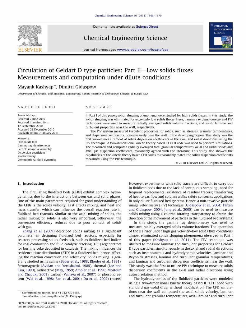
Fig. 1. (A) Time variation of solids volume fraction (es ¼ 0:0137) and (B) FFT
analysis (f¼0.03 Hz), in Case A, at a superficial gas velocity of 19.4 m/s.
M. Kashyap, D. Gidaspow / Chemical Engineering Science 66 (2011) 1649–1670 1651
for analysis, per experimental run. At least three sets of data weretaken under each set of conditions.
2.5. Theory of operation and calibration
The mathematical basis for the gamma ray densitometrytechnique to measure the solids volume fractions was the Beer–Lambert–Bouguer law or simply the Beer’s law. The details on thetheory of operation and calibration of the gamma ray densit-ometer are given in Kashyap (2010).
2.6. Solids volume fraction analysis
For Cases A and B in this study, the experiments were per-formed under high superficial gas velocity–low solids flux condi-tions, as against high superficial gas velocity–high solids fluxconditions in Part I of this paper (Kashyap et al., 2011). This paperpresents two sets of results, one from each case. Additional resultsare presented in Kashyap (2010).
Data were taken by keeping the gate valve connecting thedowncomer with the riser slightly opened. The solids flux into theriser was higher in Case A than in Case B. At least threeexperiments were performed at each superficial gas velocity,and the solids volume fractions from the selected runs wereaveraged over time. The solids volume fractions obtained fromthese experiments were averaged over the radius of the riser.
The circulation of particles in the IIT riser under low solids fluxconditions, in Cases A and B, did not show solids slug flowbehavior at any superficial gas velocity.
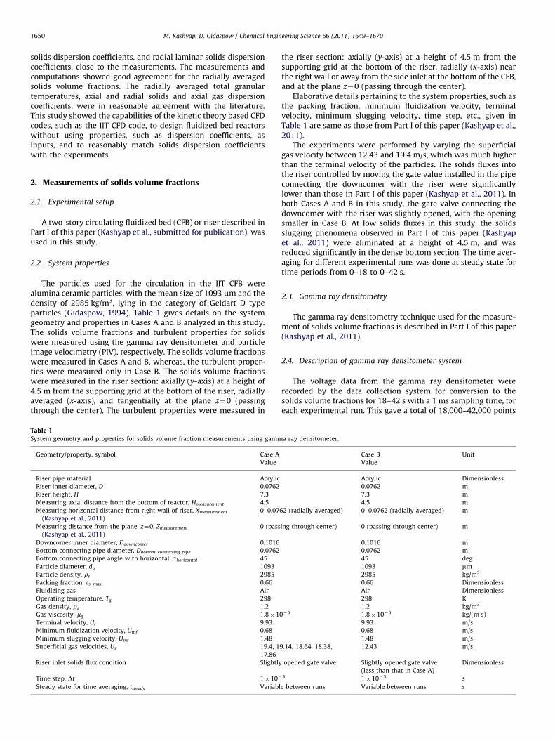
Figs. 1(A) and 2(A) show variations of solids volume fractionswith time for one experimental run each in Cases A and B,respectively. The time averaged solids concentration were 1.4%solids in Case A and 2% solids in Case B, at superficial gasvelocities of 19.4 and 12.43 m/s, respectively. Additional detailson the measured solids volume fractions at other superficial gasvelocities are given in Kashyap (2010). The solids concentrationvaried between 1.4% and 2.6% solids at superficial velocitybetween 12.43 and 19.4 m/s.
2.7. Fast Fourier transform (FFT) analysis of solids volume fraction
In Case A, the measured dominant frequency was 0.03 Hzat a superficial gas velocity of 19.4 m/s, as shown in Fig. 1(B).Fig. 2(B) shows that in Case B, the dominant frequency was0.048 Hz at a superficial gas velocity of 12.43 m/s. Additionalexperimental results are given in Kashyap (2010).
Table 2 summarizes the time and radially averaged solidsvolume fractions, dominant frequencies and power spectral den-sities, obtained from the FFT analysis in this study and in Kashyap(2010), at various superficial gas velocities and at two solids fluxes.
Part I of this paper (Kashyap et al., 2011) provides combinedresults from this study at low solids fluxes, Part II of this paper(Kashyap et al., 2011) and additional results in Kashyap (2010),for the standard deviation and deviation from maximum solidsvolume fraction in the time series.
3. Particle image velocimetry (PIV) technique
The particle image velocimetry (PIV) technique for the mea-surement of particle velocities is well known in gas–liquid–solidflows (Bahary, 1994; Gidaspow et al., 1995) and gas–solidflows (Gidaspow and Huilin, 1996; Tartan and Gidaspow, 2004;Gidaspow et al., 2004; Jung et al., 2005; Kashyap, 2010). The PIVtechnique can be used to measure particle velocities in the axial(y-axis), radial (x-axis) and tangential (z-axis) directions, using a
charge-coupled device (CCD) attached to a camera. The principleof operation of this technique with the use of a rotating transpar-ency is described elsewhere (Kashyap, 2010; Kashyap et al.,submitted for publication).
A thin ruler or scale with numbers clearly visible, was attachedto the inside wall of the fluidized bed, for calibration, to incorpo-rate the refraction and reflection of light caused by the riser walls.The CCD camera was focused on the scale to read a known orcalibrated length of 1 cm, without particles. The scale was thenremoved from the fluidized bed before taking data with thefluidized particles to avoid any obstruction of the flow by thescale near the wall. The zoom and focus of the CCD camera werethen unchanged while capturing the streaks. All clearly visiblestreaks on each frame were analyzed with a reasonable assump-tion that the fluctuations of particles were very close to the wall.The lengths of the streak lines were measured in reference to thecalibrated length. In comparison with the results obtained fromthe CFD simulations, the results from experiments were assumedto have been obtained at the wall. In this study, the data weretaken near the inside surface of the wall of the riser withoutdrilling a hole for a probe, as against different radial positionswith the use of intrusive probes, as used by Tartan and Gidaspow(2004). The probes tend to change the flow pattern of particles atthe point of contact.
Moreover, the flow pattern is important near the wall, as theparticle velocities decrease significantly near the walls as com-pared to the center, giving isotropic behavior. This can help in

0
0.04
0.08
0.12
0.16
0.2
0 5 10 15 20Time (s)
Sol
ids
volu
me
fract
ion
(-)
Ug = 12.43 m/s
0
0.002
0.004
0.006
0.008
0.01
0 1 2 3 4 5
Frequency (Hz)
Pow
er s
pect
ral d
ensi
ty (-
)
Fig. 2. (A) Time variation of solids volume fraction (es ¼ 0:0202), and (B) FFT
analysis (f¼0.048 Hz), in Case B, at a superficial gas velocity of 12.43 m/s.
Table 2Summary of FFT analysis from experiments at various gas velocities and two solids
fluxes.
Case Ug (m/s) es f (Hz) Power spectral
density (–)
Case A 19.4 0.0137 0.03 0.0036
Case A 19.14 0.0208 0.058 0.0037
Case A 18.64 0.0234 0.046 0.0073
Case A 18.38 0.022 0.06 0.0055
Case A 17.86 0.026 0.07 0.0088
Case B 12.43 0.0202 0.048 0.009
M. Kashyap, D. Gidaspow / Chemical Engineering Science 66 (2011) 1649–16701652
defining good boundary conditions. The radial position of the CCDcamera was opposite to the solids inlet at the bottom. The datawere taken at a height of 4.5 m from the bottom. The analysis ofthe streaks was done manually. Hence, the analysis was tedious,and required high precision during the selection and analysis of asmany streaks as visibly possible.
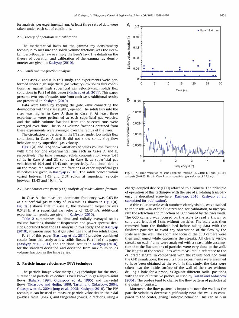
Fig. 3(A) shows a schematic diagram of the particle imagevelocimetry (PIV) measurement system with a rotating transpar-ency to show the length and duration of streaks lines. Fig. 3 showsa sketch of the (B) typical, and (C) actual, particle streak images ofthe 1093 mm particles, captured by the CCD camera. The instan-taneous particle velocities were measured by dividing the lengthsof the streak lines by the exposure time of 1/250 s, which corre-sponded to the inverse of the shutter speed of the camera. Theactual photographs of the fiber-optic light source and the colored
rotating transparency, Sony CCD camera, and Sony camera adap-ter are given elsewhere (Kashyap, 2010).
Table 3 summarizes the system geometry and properties forthe PIV measurements using the CCD camera. A small section ofthe acrylic riser was replaced by a glass pipe to take PIV data byavoiding abrasion by the particles. The PIV experiments wereperformed under extremely dilute conditions of Case B describedin Table 1. The superficial gas velocity was 12.43 m/s. The timestep between two frames was 3.33�10�2 s.
Despite the capabilities of the PIV technique to measureparticle velocities in the axial, radial and tangential directions,the velocities were measured only in the axial and radial direc-tions in this study with a reasonable assumption that thevelocities and turbulent properties in the radial and tangentialdirections were close to each other. To measure the velocities inthe tangential direction, the CCD camera could be moved to theperpendicular plane (Tartan and Gidaspow, 2004), but at theexpense of the use of an intrusive probe.
The analysis of the particle velocity in this study was done for5 s. Overall, 850 particle streaks in 151 frames were analyzed inthis study. It took 5 days to manually finish the tedious analysis.The typical numbers of streaks obtained in each frame werebetween 3 and 10.
It can be assumed from the radially averaged solids volumefraction of 0.02 in Fig. 2(A) that the solids volume fraction at thewall was between 0.01 and 0.05. Hence, the solids flux at the wallcalculated from Ws¼rsesvs (Eq. (3.9) in Gidaspow, 1994), wasbetween 13.1 and 65.5 kg/(m2 s), where, es was the solids volumefraction; Ws was the solids flux into the riser; vs was the solidsvelocity (axial instantaneous).
3.1. Particle velocities
3.1.1. Instantaneous particle velocity
The instantaneous velocities of particles in the axial and radialdirections were measured from the streak lengths along with theangle made with vertical, in each frame (Kashyap, 2010; Kashyapet al., submitted for publication). The instantaneous particlevelocities were used to obtain laminar properties, or propertiesof the particles.
3.1.2. Hydrodynamic velocity
The hydrodynamic velocities due to the fluctuation of clustersrather than individual particles, in the axial and radial directions,were obtained from the average of instantaneous velocities ineach frame (Kashyap, 2010; Kashyap et al., submitted for publi-cation). The time increment between two frames was equal to1/30th of a second. The hydrodynamic velocities were used toobtain turbulent properties, or properties of the clusters.
Fig. 4(A) shows the fluctuations of instantaneous velocities inthe axial and radial directions. The fluctuations of hydrodynamicvelocities in the axial and radial directions are shown in Fig. 4(B).The fluctuations of the instantaneous and hydrodynamic velocitiesin the axial direction were higher than those in the radial directiondue to higher gradient of axial velocity caused by the turbulencesor velocity fluctuations in the direction of the flow. The instanta-neous and hydrodynamic velocities in the axial direction weremainly positive, signifying that the net solids flow was upward inthe IIT riser. However, there were also movement of particles andclusters in the downward direction. The radial instantaneous andhydrodynamic velocity fluctuations were significant in positive andnegative directions due to the movement of particles and clusterstowards the right and left walls, respectively.
The mean axial instantaneous velocity was 0.44 m/s, as com-pared to the mean radial instantaneous velocity of �0.019 m/s.
Fluidized bed
PC with Image-Pro
PlusTM
CCD camera system
Electrical motor
Rotating transparency
Fiber optic light source
Upflow
y
x
Fig. 3. (A) PIV system, and sketches of the (B) typical, and (C) actual, streak images captured by the CCD camera.
M. Kashyap, D. Gidaspow / Chemical Engineering Science 66 (2011) 1649–1670 1653
The mean axial hydrodynamic velocity was 0.45 m/s, as comparedto the mean radial hydrodynamic velocity of �0.024 m/s. Theinstantaneous and hydrodynamic velocities were close to eachother in the axial as well as radial directions, thus, showing thateach frame roughly represented the whole time series, and the totalnumbers of particles in each frame were reasonably good. Both theinstantaneous and hydrodynamic velocities showed anisotropy.
3.2. Particle and Reynolds stresses
3.2.1. Laminar particle stresses
The laminar particle stress was measured from the fluctuatinginstantaneous velocity in the axial, radial or tangential direction.It defined oscillations on the level of particles. The laminarstresses were called normal if i¼ j, and they were called shear if
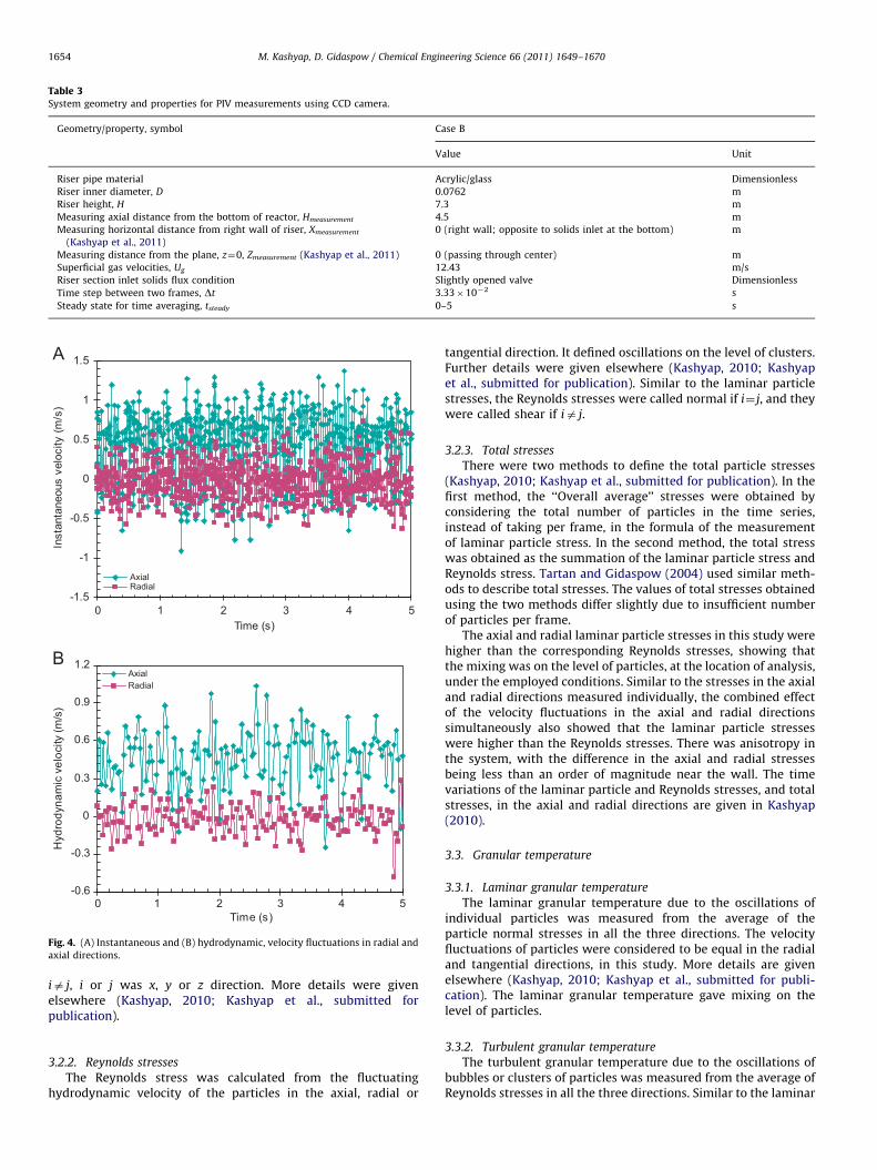
Table 3System geometry and properties for PIV measurements using CCD camera.
Geometry/property, symbol Case B
Value Unit
Riser pipe material Acrylic/glass Dimensionless
Riser inner diameter, D 0.0762 m
Riser height, H 7.3 m
Measuring axial distance from the bottom of reactor, Hmeasurement 4.5 m
Measuring horizontal distance from right wall of riser, Xmeasurement
(Kashyap et al., 2011)
0 (right wall; opposite to solids inlet at the bottom) m
Measuring distance from the plane, z¼0, Zmeasurement (Kashyap et al., 2011) 0 (passing through center) m
Superficial gas velocities, Ug 12.43 m/s
Riser section inlet solids flux condition Slightly opened valve Dimensionless
Time step between two frames, Dt 3.33�10�2 s
Steady state for time averaging, tsteady 0–5 s
-1.5
-1
-0.5
0
0.5
1
1.5
0 1 2 3 4 5
0 1 2 3 4 5
Time (s)
Inst
anta
neou
s ve
loci
ty (m
/s)
AxialRadial
-0.6
-0.3
0
0.3
0.6
0.9
1.2
Time (s)
Hyd
rody
nam
ic v
eloc
ity (m
/s)
AxialRadial
Fig. 4. (A) Instantaneous and (B) hydrodynamic, velocity fluctuations in radial and
axial directions.
M. Kashyap, D. Gidaspow / Chemical Engineering Science 66 (2011) 1649–16701654
ia j, i or j was x, y or z direction. More details were givenelsewhere (Kashyap, 2010; Kashyap et al., submitted forpublication).
3.2.2. Reynolds stresses
The Reynolds stress was calculated from the fluctuatinghydrodynamic velocity of the particles in the axial, radial or
tangential direction. It defined oscillations on the level of clusters.Further details were given elsewhere (Kashyap, 2010; Kashyapet al., submitted for publication). Similar to the laminar particlestresses, the Reynolds stresses were called normal if i¼ j, and theywere called shear if ia j.
3.2.3. Total stresses
There were two methods to define the total particle stresses(Kashyap, 2010; Kashyap et al., submitted for publication). In thefirst method, the ‘‘Overall average’’ stresses were obtained byconsidering the total number of particles in the time series,instead of taking per frame, in the formula of the measurementof laminar particle stress. In the second method, the total stresswas obtained as the summation of the laminar particle stress andReynolds stress. Tartan and Gidaspow (2004) used similar meth-ods to describe total stresses. The values of total stresses obtainedusing the two methods differ slightly due to insufficient numberof particles per frame.
The axial and radial laminar particle stresses in this study werehigher than the corresponding Reynolds stresses, showing thatthe mixing was on the level of particles, at the location of analysis,under the employed conditions. Similar to the stresses in the axialand radial directions measured individually, the combined effectof the velocity fluctuations in the axial and radial directionssimultaneously also showed that the laminar particle stresseswere higher than the Reynolds stresses. There was anisotropy inthe system, with the difference in the axial and radial stressesbeing less than an order of magnitude near the wall. The timevariations of the laminar particle and Reynolds stresses, and totalstresses, in the axial and radial directions are given in Kashyap(2010).
3.3. Granular temperature
3.3.1. Laminar granular temperature
The laminar granular temperature due to the oscillations ofindividual particles was measured from the average of theparticle normal stresses in all the three directions. The velocityfluctuations of particles were considered to be equal in the radialand tangential directions, in this study. More details are givenelsewhere (Kashyap, 2010; Kashyap et al., submitted for publi-cation). The laminar granular temperature gave mixing on thelevel of particles.
3.3.2. Turbulent granular temperature
The turbulent granular temperature due to the oscillations ofbubbles or clusters of particles was measured from the average ofReynolds stresses in all the three directions. Similar to the laminar

M. Kashyap, D. Gidaspow / Chemical Engineering Science 66 (2011) 1649–1670 1655
granular temperature, the velocity fluctuations of bubbles ofclusters were considered equal in the radial and tangentialdirections. The turbulent granular temperature gave mixing onthe level of clusters.
3.3.3. Total granular temperature
Similar to the stresses, there were two methods to definethe total granular temperature (Kashyap, 2010; Kashyap et al.,submitted for publication), one using the ‘‘Overall average’’stresses, and second using the summation of laminar and turbu-lent granular temperatures.
The laminar and turbulent granular temperatures in this studywere 0.07 and 0.026 m2/s2, respectively. Hence, the granulartemperature due to oscillations of particles was larger than thegranular temperature due to the oscillations of clusters, showingthat the mixing was on the level of particles, rather than on thelevel of clusters. The time variations of the laminar, turbulent andtotal granular temperatures are given in Kashyap (2010).
Table 4 summarizes the particle and cluster velocities, laminarand Reynolds stresses, and laminar and granular temperatures,at three different time intervals of 0–5, 0–4.5 and 0–4 s. Thevelocities and stresses in the axial direction were higher thanthose in the radial direction in view of the higher gradient of axialvelocity than the radial velocity, caused by the turbulences orvelocity fluctuations in the direction of the flow. However, thedifferences were less than an order of magnitude. This was inaccordance to the results obtained by Tartan and Gidaspow(2004), showing that near the walls, the stresses in the tangential,radial and axial directions were close to each other.
The laminar stresses were higher than the Reynolds stresses,giving laminar granular temperature higher than the turbulentgranular temperature. Therefore, the mixing was on the level ofparticles.
The granular temperatures and other properties described inTable 4 did not change significantly between the three timeintervals, i.e. 0–5, 0–4.5, and 0–4 s, showing that the time intervalof 5 s used for time averaging was sufficient to obtain steady stateresults for the laminar and turbulent properties. The total stressesand granular temperatures obtained using the two methods des-cribed earlier did not show significant differences due to limitednumber of particles per frame.
3.4. Dispersion coefficient
The dispersion coefficient was measured using the autocorre-lation method as the product of the variance of the fluctuatingvelocity, either instantaneous or hydrodynamic, and the Lagran-gian integral time scale. The autocorrelation method for themeasurement of laminar and turbulent dispersion coefficientswas described elsewhere (Kashyap, 2010; Kashyap et al., sub-mitted for publication).
Table 4Comparison of particle velocities, stresses, and granular temperatures, at three differen
Property (unit) Direction Laminar Turbulent
5 s 4.5 s 4 s 5 s
Instantaneous velocity (m/s) Axial 0.44 0.44 0.43 –
Instantaneous velocity (m/s) Radial �0.02 �0.01 �0.02 –
Hydrodynamic velocity (m/s) Axial – – – 0.45
Hydrodynamic velocity (m/s) Radial – – – �0.02
Stress (m2/s2) Axial 0.12 0.12 0.13 0.05
Stress (m2/s2) Radial 0.04 0.04 0.04 0.01
Stress (m2/s2) Shear �0.01 �0.01 �0.01 �0.004
Granular temperature (m2/s2) – 0.07 0.07 0.07 0.03
The Lagrangian integral time scale cannot be measured for theanalysis of instantaneous velocities, as the frame rate, t, cannot bedefined for each particle velocity in a frame. Hence, the Lagrangianintegral time scale for the laminar dispersion coefficient wasequated to that for the turbulent dispersion coefficient (Kashyap,2010; Kashyap et al., submitted for publication). This assumptionwas reasonable in view of the fact that the time averaged instan-taneous and hydrodynamic velocities were reasonably close toeach other. Hence, differences between the laminar and turbulentdispersion coefficients were induced by the differences betweenthe laminar and Reynolds stresses.
Breault et al. (2008) described that the time period for whichthe analysis for the dispersion coefficient is carried out should begreater than 10 times the Lagrangian integral time scale (Brodkey,1967). In this study, the Lagrangian integral time scales for theradial and axial velocity fluctuations were always less than 0.5 s,which was one-tenth of the total time for analysis.
The measured laminar dispersion coefficients in the axial andradial directions in this study were 7�10�4 and 6�10�4 m2/s,respectively. The turbulent dispersion coefficients in the axial andradial directions were 5.65�10�4 and 3.07�10�4 m2/s, respec-tively. Hence, similar to the stresses and granular temperatures,the laminar type solids dispersion coefficients were higher thanthe turbulent type dispersion coefficients, showing that themixing was on the level of particle. The axial dispersion coeffi-cients were slightly higher than those in the radial direction.
4. Computational fluid dynamics simulations using kinetictheory based IIT code
Two-dimensional computational fluid dynamics (CFD) simula-tions were performed for the circulation of large alumina ceramicparticles in the IIT riser, with the standard kinetic theory basedIIT CFD code described in Gidaspow (1994) and Gidaspow andJiradilok (2009), and available in M-FIX and commercial codes,such as FLUENT, with Johnson and Jackson (1987) boundaryconditions. The code was used to simulate the circulation oflarge alumina ceramic particles in the IIT riser under diluteconditions, and to reasonably match the radially averaged solidsvolume fractions measured using the gamma ray densitometer,and granular temperatures and solids dispersion coefficientsmeasured near the wall, using the PIV experiments, all at a heightof 4.5 m.
4.1. Hydrodynamic model
The hydrodynamic model incorporated in the kinetic theorybased IIT CFD code used in Cases 1 and 2 of this study is given inPart I of this paper (Kashyap et al., 2011).
t time intervals.
Total (summation) Total (Overall average)
4.5 s 4 s 5 s 4.5 s 4 s 5 s 4.5 s 4 s
– – – – – – – –
– – – – – – – –
0.45 0.45 – – – – – –
�0.02 �0.02 – – – - – –
0.05 0.05 0.17 0.18 0.18 0.18 0.18 0.19
0.01 0.01 0.05 0.05 0.05 0.05 0.05 0.05
�0.002 �0.003 �0.01 �0.01 �0.01 �0.01 �0.01 �0.01
0.03 0.03 0.1 0.1 0.1 0.09 0.09 0.1
M. Kashyap, D. Gidaspow / Chemical Engineering Science 66 (2011) 1649–16701656
4.2. System description and computational domain
The computational domain for the simulations is shown in Part Iof this paper (Kashyap et al., 2011). Table 5 presents the systemgeometry and properties for the CFD simulations in Cases 1 and 2,using the IIT CFD code. The details on the system geometry andproperties were almost same as those in Part I of this paper(Kashyap et al., 2011), with a few changes.
Similar to Case 1 in Part I of this paper (Kashyap et al., 2011), inCase 1 of this study, the restitution coefficients of 0.9 and 0.96(Gidaspow and Huilin, 1998b) were input in the CFD code forparticle–particle and particle–wall collisions, respectively. Theradially averaged solids volume fractions measured at a heightof 4.5 m, using the gamma ray densitometer, in Cases A and B,under dilute conditions, reasonably matched the results obtainedfrom simulations in Case 1. However, the granular temperaturesand solids dispersion coefficients near the right wall, at a height of4.5 m, computed in Case 1, were much higher than those obtainedexperimentally using the PIV technique. Therefore, the particle–particle and particle–wall collisions were reduced to 0.7 each inCase 2 of this study to reasonably match the values of thegranular temperatures and solid dispersion coefficients, with theexperiments.
The simulations were performed for 35 and 28 s in Cases 1 and2, respectively. Despite the fact that the quasi-steady state insidethe riser was obtained much earlier due to high inlet gasvelocities, the simulation results were averaged for 10–35 s inCase 1 and the averaging was done for 12–28 s in Case 2. Accord-ing to Jiradilok et al. (2006), 25 or 16 s was enough for theestimation of turbulent properties.
4.3. Initial and boundary conditions
Reasonable initial and boundary conditions are extremelyimportant to obtain realistic results from the CFD simulations.Table 6 summarizes the initial and boundary conditions forthe CFD simulations performed using the kinetic theory based
Table 5System geometry and properties for CFD simulations using the IIT CFD code, in Cases
Geometry/property, symbol Case 1
Value
Geometry type Two-dimensional
Riser inner diameter, D 0.0762
Riser height, H 7.3
Side inlet diameter, Dside inlet 0.0762
Outlet diameter, Doutlet 0.0762
Particle diameter, dp 1093
Particle density, rs 2985
Packing fraction, es, max 0.66
Acceleration due to gravity, g 9.81
Fluidizing gas Air
Operating temperature, Tg 298
Gas density, rg 1.2
Gas viscosity, mg 1.8�10�5
Terminal velocity, Ut 9.93
Minimum fluidization velocity, Umf 0.68
Minimum slugging velocity, Ums 1.48
Particle–particle restitution coefficient, e 0.9
Particle–wall restitution coefficient, ew 0.96
Specularity coefficient, f 0.6
Number of grids in x-direction� grid size 17�0.508
Number of grids in y-direction� grid size 1�1, 7�2.54, 6�1.27, 99�6.91
3�1
Time step, Dt 1�10�5
Steady state for time averaging, tsteady 10–35
IIT CFD code in Cases 1 and 2. The initial and boundary condi-tions in Cases 1 and 2 of this study were similar to those inCase 1 in Part I of this paper (Kashyap et al., 2011), with thedifferences in the inlet solids flux and the superficial gas velocity.The IIT riser was operated under relative dilute conditions, with-out formation of prominent solids slugs, as compared to thedense conditions with evident solids slugs, in Part I of this paper(Kashyap et al., 2011). The radially averaged solids volumefractions measured in Cases A and B in this study, at a height of4.5 m, were lower than those measured in Cases A and B in Part Iof this paper (Kashyap et al., 2011). Hence, the inlet solids fluxwas reduced to 251 kg/(m2 s) in Cases 1 and 2 for simulations inthis study, as compared to 313 kg/(m2 s) in Part I of this paper(Kashyap et al., 2011).
The bottom inlet was used for air at a superficial gas velocityof 30 m/s in Case 1, same as that in Case 1 in Part I of this paper(Kashyap et al., 2011). Although the radially averaged solidsvolume fractions measured experimentally in Cases A and B ofthis study were in reasonable agreement with the values fromsimulations in Case 1, the granular temperatures and solids dis-persion coefficients were significantly different from the experi-ments. Hence, to reasonably match the granular temperaturesand solids dispersion coefficients, besides changing the restitutioncoefficients, the superficial gas of air at the bottom inlet was alsovaried to 14 m/s in Case 2 of the simulations. This superficial gasvelocity was still different from 12.43 m/s employed for the PIVexperiments.
The superficial gas velocities of 30 and 14 m/s in the CFD simu-lations were different from those used in the experiments due tothe missing third dimension in the simulations. As explained inPart I of this paper (Kashyap et al., 2011), Table 7 summarizes thehypothetical values of the depth of the riser, W, for differentsuperficial gas velocities in the experiments, which were obtainedby equating the mass flow rate entering the riser in the experi-ments and simulations. The riser depth, W, of the order of0.03–0.08 m was reasonably good for the selection of the super-ficial gas velocities of 30 and 14 m/s in CFD simulations for thisriser system, in Cases 1 and 2, respectively.
1 and 2.
Case 2 Unit
Value
Two-dimensional Dimensionless
0.0762 m
7.3 m
0.0762 m
0.0762 m
1093 mm
2985 kg/m3
0.66 Dimensionless
9.81 m/s2
Air Dimensionless
298 K
1.2 kg/m3
1.8�10�5 kg/(m s)
9.93 m/s
0.68 m/s
1.48 m/s
0.7 Dimensionless
0.7 Dimensionless
0.6 Dimensionless
17�0.508 cm
, 7�2.54, 1�1, 7�2.54, 6�1.27, 99�6.91, 7�2.54,
3�1
cm
1 � 10�5 s
12–28 s
Table 7Hypothetical depth of the riser in the two-dimensional CFD simulations per-
formed at the superficial gas velocities of 30 and 14 m/s, at different superficial gas
velocities used in experiments.
Superficial gas velocity in
experiments, Ug, expt (m/s)
Depth of riser, W (m),
for Ug, CFD¼30 m/s
Depth of riser, W (m),
for Ug, CFD¼14 m/s
Case A
17.86 0.0356 0.0763
18.38 0.0366 0.0785
18.64 0.0372 0.0796
19.14 0.0382 0.0818
19.4 0.0387 0.0829
Case B
12.43 0.0248 0.0531
Table 6Initial and boundary conditions used in the IIT CFD code, in Cases 1 and 2.
Condition, symbol Case 1 Case 2 Unit
Value Value
Bottom inlet conditionsGas velocity, Ug 30 14 m/s
Solids volume fraction, es 0 0 –
Side inlet conditions
Gas velocity, Uginlet0.24 0.24 m/s
Solids velocity, Usinlet0.24 0.24 m/s
Solids volume fraction, esinlet0.35 0.35 –
Granular temperature, yinlet 0.01 0.05 m2/s2
Inlet solids flux, Wsinlet251 251 kg/(m2 s)
Initial conditions
Gas velocity, Uginitial0 0 m/s
Solids velocity, Usinitial0 0 m/s
Solids volume fraction, esinitial0 0 –
Outlet conditionPressure, Poutlet 1.01325�105 1.01325�105 N/m2
Boundary conditions
Solid phase (Johnson and Jackson, 1987)
Velocity : vs,w ¼�6mses,maxffiffiffiffiffiffiffiffiffiffiffiffiffiffiffiffiffiffiffiffiffiffiffiffiffiffiffiffiffiffi
3pfrsesgo
ffiffiffiypq @vs,w
@n4
Granular temperature : yw ¼�ksygs, w
@yw
@n4 þ
ffiffiffiffiffiffiffiffiffiffiffiffiffiffiffiffiffiffiffiffiffiffiffiffiffiffiffiffiffiffiffiffiffiffiffiffiffiffiffiffiffiffi3pfrsesv2
s,slipgoy3=2
6es,maxgs, w
vuut
where gs, w ¼
ffiffiffiffiffiffiffiffiffiffiffiffiffiffiffiffiffiffiffiffiffiffiffiffiffiffiffiffiffiffiffiffiffiffiffiffiffiffiffiffiffiffiffi3pð1�e2
wÞesrsgoy3=2
4es, max
s
Gas phase
vx,w¼vy,w¼0
M. Kashyap, D. Gidaspow / Chemical Engineering Science 66 (2011) 1649–1670 1657
5. Simulation results
The primary considerations for obtaining reliable results fromthe simulations were to reasonably match the radially averagedsolids volume fractions and fast Fourier transform (FFT) frequen-cies for solids volume fractions with the results from the gammaray densitometer experiments, and to match the computedgranular temperatures and solids dispersion coefficients nearthe right wall, with the PIV experiments, all properties at a heightof 4.5 m. The inlet superficial gas velocity, restitution coefficientsfor particle–particle and particle–wall collisions, specularity coef-ficient and inlet solids flux from the side inlet, were varied inorder to match these properties.
The primary computed properties and locations for computa-tion of data within the fluidized bed in this study were similar tothose in Part I of this paper (Kashyap et al., 2011). It should benoted that although the gamma ray experiments were performedradially averaged, the PIV data in this paper were taken very close
to the right wall, i.e. at r/R¼1, by calibrating the CCD camera forthe depth of the field next to the wall. The results in thesimulations in Cases 1 and 2 were analyzed axially (y-axis) atthe heights of 2, 4.5 and 6 m to mark the dense region, position ofthe gamma ray densitometer and PIV measurements, and thedilute region in the riser, respectively. The radial distributions ofthe computed properties were plotted between r/R¼�1 and 1,where r/R¼0 was the radial center (x-axis).
5.1. Solids volume fraction distribution
The instantaneous solids volume fraction contours at differenttimes in Cases 1 and 2 are shown in Fig. 5(A) and (B), respectively.While Case 1 showed a very shallow dense region at the bottom,Case 2 exhibited the existence of dense bottom and dilute topregions, typical of turbulent fluidization (Jiradilok et al., 2006).These results were in agreement with the conclusions made byJiradilok et al. (2006) that the decrease in the particle–particlerestitution coefficient increases the particle–particle collisions,hence, increasing the solids volume fractions in the dense phase.Fig. 5(B) even showed the movement of dense solids slugs of theorder of 25–45% solids, up in the riser, in Case 2, similar to Case 1 inPart I of this paper (Kashyap et al., 2011). However, the solids slugswere not evident at a height of 4.5 m, similar to the experiments.
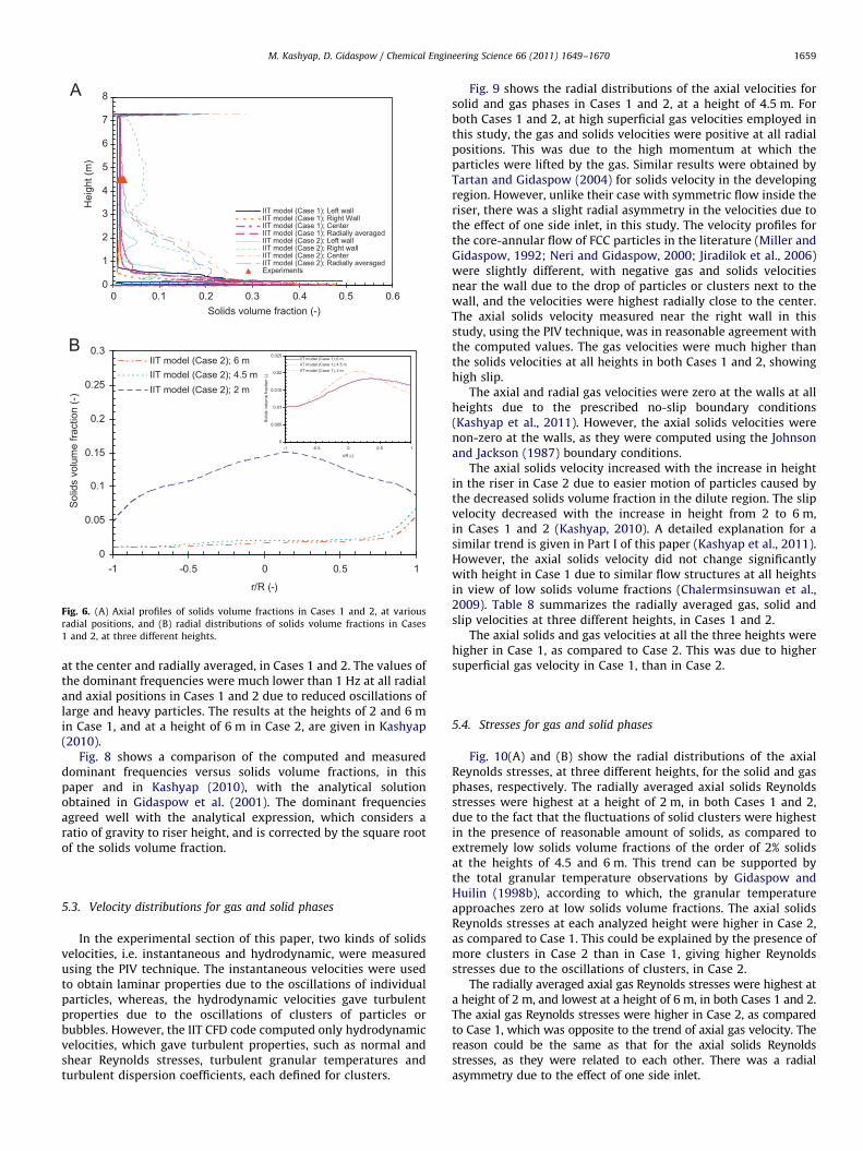
Fig. 6(A) shows the axial profiles of the solids volume fractionsat various radial positions, in Cases 1 and 2. The solids volumefractions were high in the dense bottom region with some fluc-tuations in the values due to the inlet effect. The dense bottomregion was shallower in Case 1, as compared to Case 2. Hence, dueto lower restitution coefficients in Case 2, the turbulent regimewas observed only in Case 2, not in Case 1 (Jiradilok et al., 2006).Besides, along the length of the riser, the solids volume fractionswere higher in Case 2, as compared to those in Case 1, due tolower superficial gas velocity in the former case. As shown in
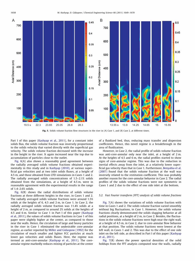
19.5 s 22.3 23.65 13.55 s25.05 26.8 28.3 13.9 14.25 14.65 15 15.55
Fig. 5. Solids volume fraction flow structures in the riser in (A) Case 1, and (B) Case 2, at different times.
M. Kashyap, D. Gidaspow / Chemical Engineering Science 66 (2011) 1649–16701658
Part I of this paper (Kashyap et al., 2011), for a constant inletsolids flux, the solids volume fraction was inversely proportionalto the solids velocity that varied directly with the superficial gasvelocity. The solids volume fraction decreased with the increasein the height in the riser. It again increased near the top due toaccumulation of particles close to the outlet.
Fig. 6(A) also shows a reasonably good agreement betweenthe radially averaged solids volume fractions obtained experi-mentally in this study and in Kashyap (2010), at various super-ficial gas velocities and at two inlet solids fluxes, at a height of4.5 m, and those obtained from CFD simulations in Cases 1 and 2.The radially averaged solids concentrations of 1.5–2.1% solidsobtained from the simulations, at a height of 4.5 m, were inreasonable agreement with the experimental results in the rangeof 1.4–2.6% solids.
Fig. 6(B) shows the radial distributions of solids volumefractions at three different heights in the riser, in Cases 1 and 2.The radially averaged solids volume fractions were around 1.5%solids at the heights of 6, 4.5 and 2 m, in Case 1. In Case 2, theradially averaged solids volume fraction was 11.4% solids at aheight of 2 m, as compared to around 2% solids at the heights of4.5 and 6 m. Similar to Case 1 in Part I of this paper (Kashyapet al., 2011), the values of solids volume fractions in Case 1 of thispaper were slightly higher at the center, as compared to thosenear the walls. Hence, the circulation of large and heavy particlesin the riser in Case 1 eliminated the undesirable core-annularregime, as earlier reported by Miller and Gidaspow (1992) for thecirculation of much smaller and lighter FCC particles at muchlower gas velocities and solids fluxes. Here, the regime wastermed as anti-core-annular (Kashyap et al., 2011). The core-annular regime markedly reduces mixing of particles at the center
of a fluidized bed, thus, reducing mass transfer and dispersioncoefficients. Hence, this novel regime is a breakthrough in thearea of fluidization.
However, in Case 2, the radial profile of solids volume fractionwas anti-core-annular only near the inlet, at a height of 2 m.At the heights of 4.5 and 6 m, the radial profiles started to showsigns of core-annular regime. This was due to the reduction ininertial effects away from the inlet, at a relatively lower super-ficial gas velocity than that in Case 1. Furthermore, Benyahia et al.(2007) found that the solids volume fraction at the wall wasinversely related to the restitution coefficient. This was probablyanother reason for the core-annular behavior in Case 2. The radialprofiles of the solids volume fractions were not symmetric inCases 1 and 2 due to the effect of one side inlet at the bottom.
5.2. Fast Fourier transform (FFT) analysis of solids volume fractions
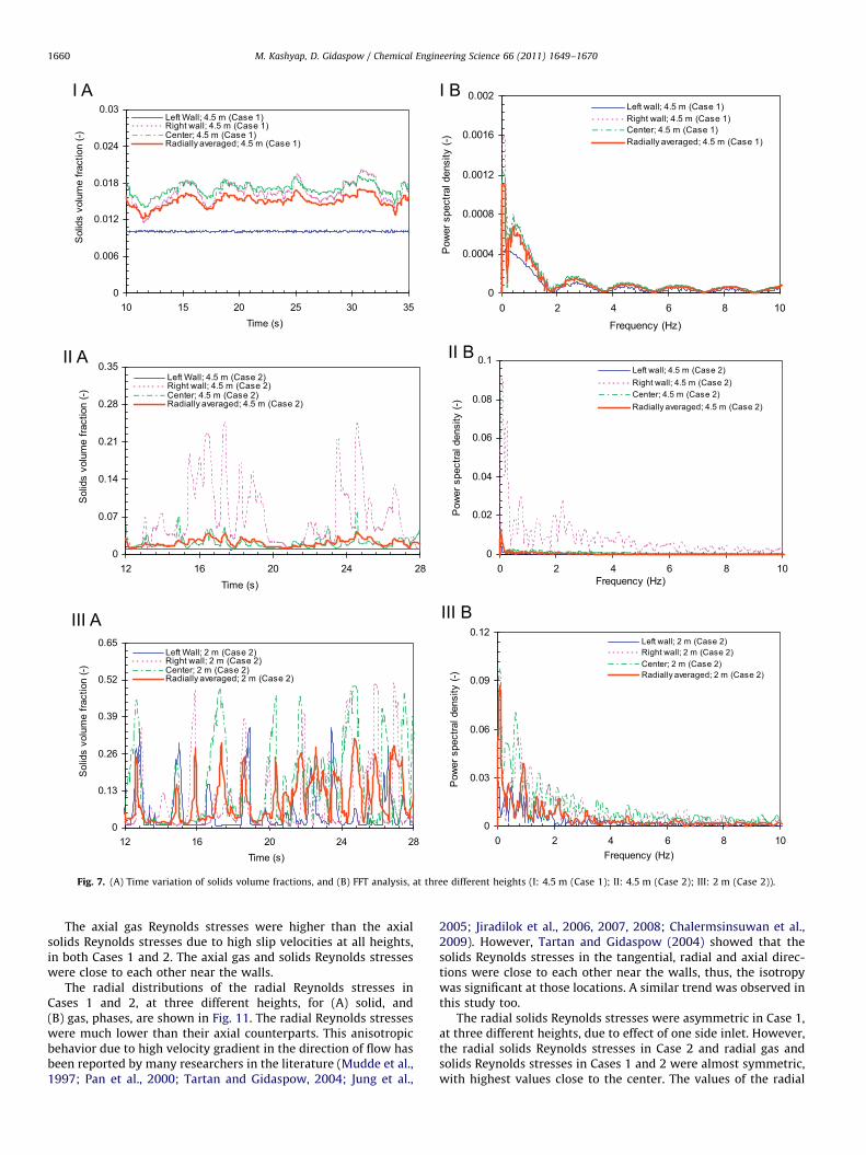
Fig. 7(A) shows the variations of solids volume fraction withtime in Cases 1 and 2. The solids volume fraction varied smoothlywithout big fluctuations, in Case 1. However, the solids volumefractions clearly demonstrated the solids slugging behavior at allradial positions, at a height of 2 m, in Case 2. Besides, the fluctua-tions in the solids volume fractions were high near the right wall,at a height of 4.5 m, in Case 2, due to core-annular flow behaviorat that position. The solids volume fractions were lowest at theleft wall, in Cases 1 and 2. This was due to the effect of one sideinlet on the left side, as described in Part I of this paper (Kashyapet al., 2011).
Fig. 7(B) shows the power spectral densities of the solidholdups from the FFT analysis computed near the walls, radially
0
1
2
3
4
5
6
7
8
0 0.1 0.2 0.3 0.4 0.5 0.6Solids volume fraction (-)
Hei
ght (
m)
IIT model (Case 1); Left wallIIT model (Case 1); Right WallIIT model (Case 1); CenterIIT model (Case 1); Radially averagedIIT model (Case 2); Left wallIIT model (Case 2); Right wallIIT model (Case 2); CenterIIT model (Case 2); Radially averagedExperiments
0
0.05
0.1
0.15
0.2
0.25
0.3
-1 -0.5 0 0.5 1
r/R (-)
Sol
ids
volu
me
fract
ion
(-)
IIT model (Case 2); 6 mIIT model (Case 2); 4.5 mIIT model (Case 2); 2 m
Fig. 6. (A) Axial profiles of solids volume fractions in Cases 1 and 2, at various
radial positions, and (B) radial distributions of solids volume fractions in Cases
1 and 2, at three different heights.
M. Kashyap, D. Gidaspow / Chemical Engineering Science 66 (2011) 1649–1670 1659
at the center and radially averaged, in Cases 1 and 2. The values ofthe dominant frequencies were much lower than 1 Hz at all radialand axial positions in Cases 1 and 2 due to reduced oscillations oflarge and heavy particles. The results at the heights of 2 and 6 min Case 1, and at a height of 6 m in Case 2, are given in Kashyap(2010).
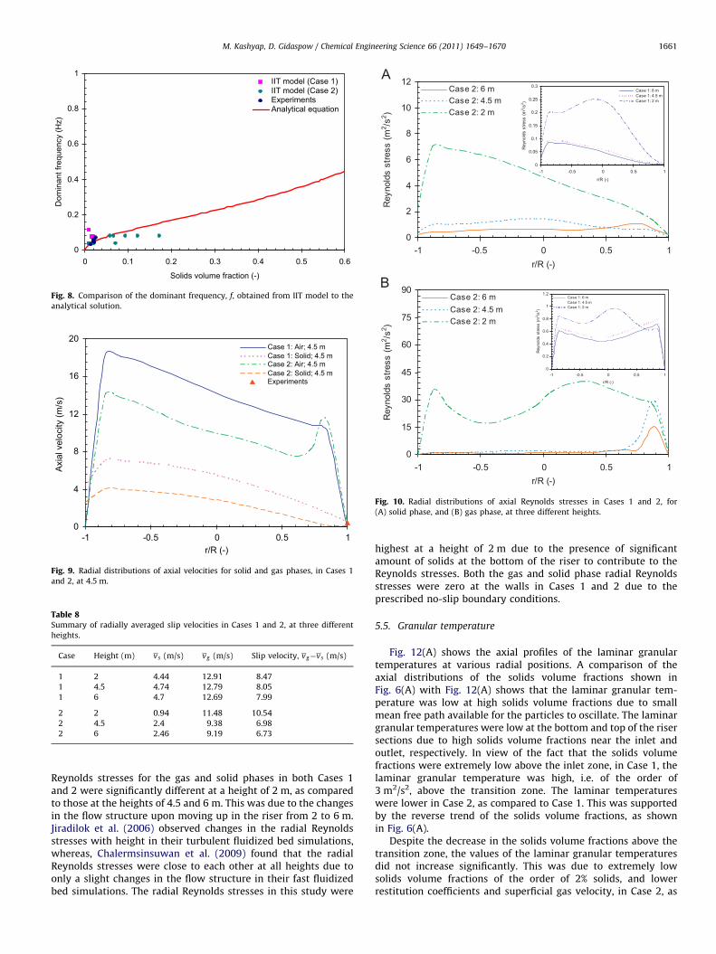
Fig. 8 shows a comparison of the computed and measureddominant frequencies versus solids volume fractions, in thispaper and in Kashyap (2010), with the analytical solutionobtained in Gidaspow et al. (2001). The dominant frequenciesagreed well with the analytical expression, which considers aratio of gravity to riser height, and is corrected by the square rootof the solids volume fraction.
5.3. Velocity distributions for gas and solid phases
In the experimental section of this paper, two kinds of solidsvelocities, i.e. instantaneous and hydrodynamic, were measuredusing the PIV technique. The instantaneous velocities were usedto obtain laminar properties due to the oscillations of individualparticles, whereas, the hydrodynamic velocities gave turbulentproperties due to the oscillations of clusters of particles orbubbles. However, the IIT CFD code computed only hydrodynamicvelocities, which gave turbulent properties, such as normal andshear Reynolds stresses, turbulent granular temperatures andturbulent dispersion coefficients, each defined for clusters.
Fig. 9 shows the radial distributions of the axial velocities forsolid and gas phases in Cases 1 and 2, at a height of 4.5 m. Forboth Cases 1 and 2, at high superficial gas velocities employed inthis study, the gas and solids velocities were positive at all radialpositions. This was due to the high momentum at which theparticles were lifted by the gas. Similar results were obtained byTartan and Gidaspow (2004) for solids velocity in the developingregion. However, unlike their case with symmetric flow inside theriser, there was a slight radial asymmetry in the velocities due tothe effect of one side inlet, in this study. The velocity profiles forthe core-annular flow of FCC particles in the literature (Miller andGidaspow, 1992; Neri and Gidaspow, 2000; Jiradilok et al., 2006)were slightly different, with negative gas and solids velocitiesnear the wall due to the drop of particles or clusters next to thewall, and the velocities were highest radially close to the center.The axial solids velocity measured near the right wall in thisstudy, using the PIV technique, was in reasonable agreement withthe computed values. The gas velocities were much higher thanthe solids velocities at all heights in both Cases 1 and 2, showinghigh slip.
The axial and radial gas velocities were zero at the walls at allheights due to the prescribed no-slip boundary conditions(Kashyap et al., 2011). However, the axial solids velocities werenon-zero at the walls, as they were computed using the Johnsonand Jackson (1987) boundary conditions.
The axial solids velocity increased with the increase in heightin the riser in Case 2 due to easier motion of particles caused bythe decreased solids volume fraction in the dilute region. The slipvelocity decreased with the increase in height from 2 to 6 m,in Cases 1 and 2 (Kashyap, 2010). A detailed explanation for asimilar trend is given in Part I of this paper (Kashyap et al., 2011).However, the axial solids velocity did not change significantlywith height in Case 1 due to similar flow structures at all heightsin view of low solids volume fractions (Chalermsinsuwan et al.,2009). Table 8 summarizes the radially averaged gas, solid andslip velocities at three different heights, in Cases 1 and 2.
The axial solids and gas velocities at all the three heights werehigher in Case 1, as compared to Case 2. This was due to highersuperficial gas velocity in Case 1, than in Case 2.
5.4. Stresses for gas and solid phases
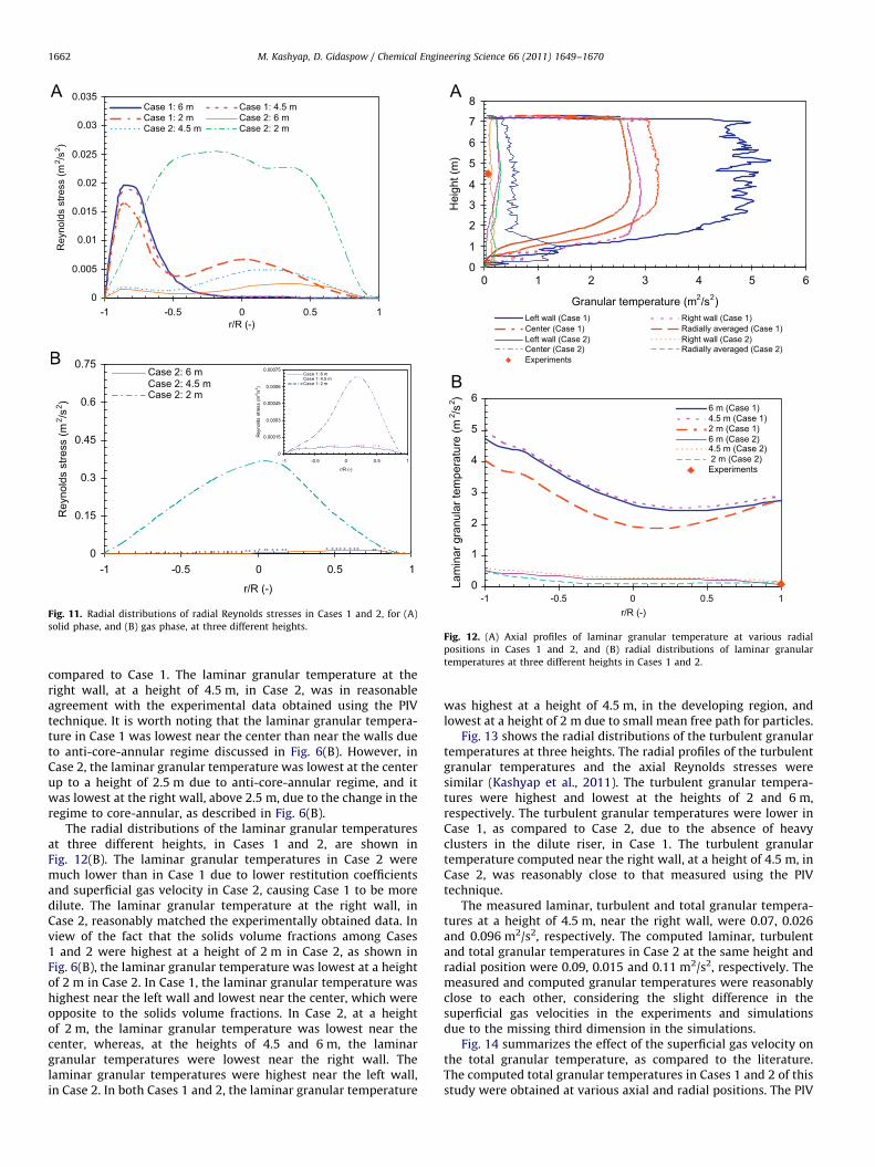
Fig. 10(A) and (B) show the radial distributions of the axialReynolds stresses, at three different heights, for the solid and gasphases, respectively. The radially averaged axial solids Reynoldsstresses were highest at a height of 2 m, in both Cases 1 and 2,due to the fact that the fluctuations of solid clusters were highestin the presence of reasonable amount of solids, as compared toextremely low solids volume fractions of the order of 2% solidsat the heights of 4.5 and 6 m. This trend can be supported bythe total granular temperature observations by Gidaspow andHuilin (1998b), according to which, the granular temperatureapproaches zero at low solids volume fractions. The axial solidsReynolds stresses at each analyzed height were higher in Case 2,as compared to Case 1. This could be explained by the presence ofmore clusters in Case 2 than in Case 1, giving higher Reynoldsstresses due to the oscillations of clusters, in Case 2.
The radially averaged axial gas Reynolds stresses were highest ata height of 2 m, and lowest at a height of 6 m, in both Cases 1 and 2.The axial gas Reynolds stresses were higher in Case 2, as comparedto Case 1, which was opposite to the trend of axial gas velocity. Thereason could be the same as that for the axial solids Reynoldsstresses, as they were related to each other. There was a radialasymmetry due to the effect of one side inlet.
0
0.006
0.012
0.018
0.024
0.03
10 15 20 25 30 35Time (s)
Sol
ids
volu
me
fract
ion
(-)
Left Wall; 4.5 m (Case 1)Right wall; 4.5 m (Case 1)Center; 4.5 m (Case 1)Radially averaged; 4.5 m (Case 1)
0
0.0004
0.0008
0.0012
0.0016
0.002
0 2 4 6 8
Frequency (Hz)
Pow
er s
pect
ral d
ensi
ty (-
)
10
Left wall; 4.5 m (Case 1)Right wall; 4.5 m (Case 1)Center; 4.5 m (Case 1)Radially averaged; 4.5 m (Case 1)
0
0.13
0.26
0.39
0.52
0.65
12 16 20 24 28Time (s)
Sol
ids
volu
me
fract
ion
(-)
Left Wall; 2 m (Case 2)Right wall; 2 m (Case 2)Center; 2 m (Case 2)Radially averaged; 2 m (Case 2)
0
0.03
0.06
0.09
0.12
0 2 4 6 8Frequency (Hz)
Pow
er s
pect
ral d
ensi
ty (-
)
10
Left wall; 2 m (Case 2)Right wall; 2 m (Case 2)Center; 2 m (Case 2)Radially averaged; 2 m (Case 2)
0
0.07
0.14
0.21
0.28
0.35
12 16 20 24 28Time (s)
Sol
ids
volu
me
fract
ion
(-)
Left Wall; 4.5 m (Case 2)Right wall; 4.5 m (Case 2)Center; 4.5 m (Case 2)Radially averaged; 4.5 m (Case 2)
0
0.02
0.04
0.06
0.08
0.1
0 2 4 6 8Frequency (Hz)
Pow
er s
pect
ral d
ensi
ty (-
)
10
Left wall; 4.5 m (Case 2)Right wall; 4.5 m (Case 2)Center; 4.5 m (Case 2)Radially averaged; 4.5 m (Case 2)
Fig. 7. (A) Time variation of solids volume fractions, and (B) FFT analysis, at three different heights (I: 4.5 m (Case 1); II: 4.5 m (Case 2); III: 2 m (Case 2)).
M. Kashyap, D. Gidaspow / Chemical Engineering Science 66 (2011) 1649–16701660
The axial gas Reynolds stresses were higher than the axialsolids Reynolds stresses due to high slip velocities at all heights,in both Cases 1 and 2. The axial gas and solids Reynolds stresseswere close to each other near the walls.
The radial distributions of the radial Reynolds stresses inCases 1 and 2, at three different heights, for (A) solid, and(B) gas, phases, are shown in Fig. 11. The radial Reynolds stresseswere much lower than their axial counterparts. This anisotropicbehavior due to high velocity gradient in the direction of flow hasbeen reported by many researchers in the literature (Mudde et al.,1997; Pan et al., 2000; Tartan and Gidaspow, 2004; Jung et al.,
2005; Jiradilok et al., 2006, 2007, 2008; Chalermsinsuwan et al.,2009). However, Tartan and Gidaspow (2004) showed that thesolids Reynolds stresses in the tangential, radial and axial direc-tions were close to each other near the walls, thus, the isotropywas significant at those locations. A similar trend was observed inthis study too.
The radial solids Reynolds stresses were asymmetric in Case 1,at three different heights, due to effect of one side inlet. However,the radial solids Reynolds stresses in Case 2 and radial gas andsolids Reynolds stresses in Cases 1 and 2 were almost symmetric,with highest values close to the center. The values of the radial
0
0.2
0.4
0.6
0.8
1
0 0.1 0.2 0.3 0.4 0.5 0.6
Solids volume fraction (-)
Dom
inan
t fre
quen
cy (H
z)
IIT model (Case 1)IIT model (Case 2)ExperimentsAnalytical equation
Fig. 8. Comparison of the dominant frequency, f, obtained from IIT model to the
analytical solution.
0
4
8
12
16
20
-1 -0.5 0 0.5 1r/R (-)
Axia
l vel
ocity
(m/s
)
Case 1: Air; 4.5 mCase 1: Solid; 4.5 mCase 2: Air; 4.5 mCase 2: Solid; 4.5 mExperiments
Fig. 9. Radial distributions of axial velocities for solid and gas phases, in Cases 1
and 2, at 4.5 m.
Table 8Summary of radially averaged slip velocities in Cases 1 and 2, at three different
heights.
Case Height (m) vs (m/s) vg (m/s) Slip velocity, vg�vs (m/s)
1 2 4.44 12.91 8.47
1 4.5 4.74 12.79 8.05
1 6 4.7 12.69 7.99
2 2 0.94 11.48 10.54
2 4.5 2.4 9.38 6.98
2 6 2.46 9.19 6.73
0
2
4
6
8
10
12
-1 -0.5 0 0.5 1r/R (-)
Rey
nold
s st
ress
(m2 /s
2 )
0
15
30
45
60
75
90
-1 -0.5 0 0.5 1r/R (-)
Rey
nold
s st
ress
(m2 /s
2 )
Case 2: 6 mCase 2: 4.5 mCase 2: 2 m
Case 2: 6 mCase 2: 4.5 mCase 2: 2 m
Fig. 10. Radial distributions of axial Reynolds stresses in Cases 1 and 2, for
(A) solid phase, and (B) gas phase, at three different heights.
M. Kashyap, D. Gidaspow / Chemical Engineering Science 66 (2011) 1649–1670 1661
Reynolds stresses for the gas and solid phases in both Cases 1and 2 were significantly different at a height of 2 m, as comparedto those at the heights of 4.5 and 6 m. This was due to the changesin the flow structure upon moving up in the riser from 2 to 6 m.Jiradilok et al. (2006) observed changes in the radial Reynoldsstresses with height in their turbulent fluidized bed simulations,whereas, Chalermsinsuwan et al. (2009) found that the radialReynolds stresses were close to each other at all heights due toonly a slight changes in the flow structure in their fast fluidizedbed simulations. The radial Reynolds stresses in this study were
highest at a height of 2 m due to the presence of significantamount of solids at the bottom of the riser to contribute to theReynolds stresses. Both the gas and solid phase radial Reynoldsstresses were zero at the walls in Cases 1 and 2 due to theprescribed no-slip boundary conditions.
5.5. Granular temperature
Fig. 12(A) shows the axial profiles of the laminar granulartemperatures at various radial positions. A comparison of theaxial distributions of the solids volume fractions shown inFig. 6(A) with Fig. 12(A) shows that the laminar granular tem-perature was low at high solids volume fractions due to smallmean free path available for the particles to oscillate. The laminargranular temperatures were low at the bottom and top of the risersections due to high solids volume fractions near the inlet andoutlet, respectively. In view of the fact that the solids volumefractions were extremely low above the inlet zone, in Case 1, thelaminar granular temperature was high, i.e. of the order of3 m2/s2, above the transition zone. The laminar temperatureswere lower in Case 2, as compared to Case 1. This was supportedby the reverse trend of the solids volume fractions, as shownin Fig. 6(A).
Despite the decrease in the solids volume fractions above thetransition zone, the values of the laminar granular temperaturesdid not increase significantly. This was due to extremely lowsolids volume fractions of the order of 2% solids, and lowerrestitution coefficients and superficial gas velocity, in Case 2, as
0
0.005
0.01
0.015
0.02
0.025
0.03
0.035
-1 -0.5 0 0.5 1r/R (-)
Rey
nold
s st
ress
(m2 /s
2 )
Case 1: 6 m Case 1: 4.5 mCase 1: 2 m Case 2: 6 mCase 2: 4.5 m Case 2: 2 m
0
0.15
0.3
0.45
0.6
0.75
-1 -0.5 0 0.5 1
r/R (-)
Rey
nold
s st
ress
(m2 /s
2 )
Case 2: 6 mCase 2: 4.5 mCase 2: 2 m
Fig. 11. Radial distributions of radial Reynolds stresses in Cases 1 and 2, for (A)
solid phase, and (B) gas phase, at three different heights.
0
1
2
3
4
5
6
7
8
0 1 2 3 4 5 6
Granular temperature (m2/s2)
Hei
ght (
m)
Left wall (Case 1) Right wall (Case 1)Center (Case 1) Radially averaged (Case 1)Left wall (Case 2) Right wall (Case 2)Center (Case 2) Radially averaged (Case 2)Experiments
0
1
2
3
4
5
6
-1 -0.5 0 0.5 1r/R (-)
Lam
inar
gra
nula
r tem
pera
ture
(m2 /s
2 )
6 m (Case 1)4.5 m (Case 1)2 m (Case 1)6 m (Case 2)4.5 m (Case 2) 2 m (Case 2)Experiments
Fig. 12. (A) Axial profiles of laminar granular temperature at various radial
positions in Cases 1 and 2, and (B) radial distributions of laminar granular
temperatures at three different heights in Cases 1 and 2.
M. Kashyap, D. Gidaspow / Chemical Engineering Science 66 (2011) 1649–16701662
compared to Case 1. The laminar granular temperature at theright wall, at a height of 4.5 m, in Case 2, was in reasonableagreement with the experimental data obtained using the PIVtechnique. It is worth noting that the laminar granular tempera-ture in Case 1 was lowest near the center than near the walls dueto anti-core-annular regime discussed in Fig. 6(B). However, inCase 2, the laminar granular temperature was lowest at the centerup to a height of 2.5 m due to anti-core-annular regime, and itwas lowest at the right wall, above 2.5 m, due to the change in theregime to core-annular, as described in Fig. 6(B).
The radial distributions of the laminar granular temperaturesat three different heights, in Cases 1 and 2, are shown inFig. 12(B). The laminar granular temperatures in Case 2 weremuch lower than in Case 1 due to lower restitution coefficientsand superficial gas velocity in Case 2, causing Case 1 to be moredilute. The laminar granular temperature at the right wall, inCase 2, reasonably matched the experimentally obtained data. Inview of the fact that the solids volume fractions among Cases1 and 2 were highest at a height of 2 m in Case 2, as shown inFig. 6(B), the laminar granular temperature was lowest at a heightof 2 m in Case 2. In Case 1, the laminar granular temperature washighest near the left wall and lowest near the center, which wereopposite to the solids volume fractions. In Case 2, at a heightof 2 m, the laminar granular temperature was lowest near thecenter, whereas, at the heights of 4.5 and 6 m, the laminargranular temperatures were lowest near the right wall. Thelaminar granular temperatures were highest near the left wall,in Case 2. In both Cases 1 and 2, the laminar granular temperature
was highest at a height of 4.5 m, in the developing region, andlowest at a height of 2 m due to small mean free path for particles.
Fig. 13 shows the radial distributions of the turbulent granulartemperatures at three heights. The radial profiles of the turbulentgranular temperatures and the axial Reynolds stresses weresimilar (Kashyap et al., 2011). The turbulent granular tempera-tures were highest and lowest at the heights of 2 and 6 m,respectively. The turbulent granular temperatures were lower inCase 1, as compared to Case 2, due to the absence of heavyclusters in the dilute riser, in Case 1. The turbulent granulartemperature computed near the right wall, at a height of 4.5 m, inCase 2, was reasonably close to that measured using the PIVtechnique.
The measured laminar, turbulent and total granular tempera-tures at a height of 4.5 m, near the right wall, were 0.07, 0.026and 0.096 m2/s2, respectively. The computed laminar, turbulentand total granular temperatures in Case 2 at the same height andradial position were 0.09, 0.015 and 0.11 m2/s2, respectively. Themeasured and computed granular temperatures were reasonablyclose to each other, considering the slight difference in thesuperficial gas velocities in the experiments and simulationsdue to the missing third dimension in the simulations.
Fig. 14 summarizes the effect of the superficial gas velocity onthe total granular temperature, as compared to the literature.The computed total granular temperatures in Cases 1 and 2 of thisstudy were obtained at various axial and radial positions. The PIV
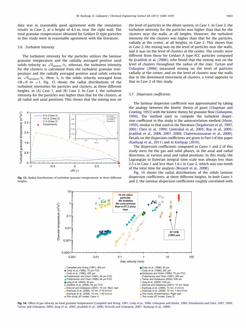
M. Kashyap, D. Gidaspow / Chemical Engineering Science 66 (2011) 1649–1670 1663
data was in reasonably good agreement with the simulationresults in Case 2, at a height of 4.5 m, near the right wall. Thetotal granular temperatures obtained for Geldart D type particlesin this study were in reasonable agreement with the literature.
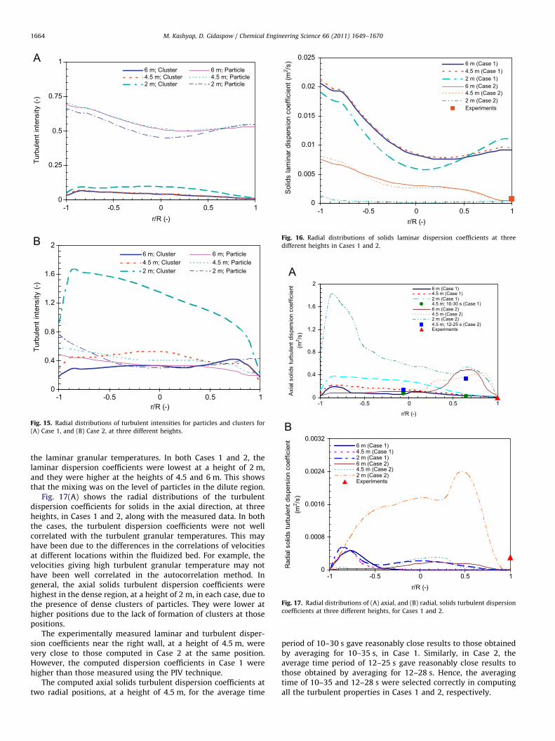
5.6. Turbulent intensity
The turbulent intensity for the particles utilizes the laminargranular temperature and the radially averaged positive axialsolids velocity as,
ffiffiffiyp
laminar=vs, whereas, the turbulent intensityfor the clusters is calculated from the turbulent granular tem-perature and the radially averaged positive axial solids velocityas,
ffiffiffiyp
turbulent=vs. Here, vs is the solids velocity averaged fromr/R¼0 to ¼1. Fig. 15 shows the radial distributions of theturbulent intensities for particles and clusters, at three differentheights, in (A) Case 1, and (B) Case 2. In Case 1, the turbulentintensity for the particles was higher than that for the clusters, atall radial and axial positions. This shows that the mixing was on
0
0.8
1.6
2.4
3.2
4
-1 -0.5 0 0.5 1r/R (-)
Turb
ulen
t gra
nula
r tem
pera
ture
(m2 /s
2 )
6 m (Case 2)4.5 m (Case 2)2 m (Case 2)Experiments
Fig. 13. Radial distributions of turbulent granular temperatures at three different
heights.
0.0001
0.001
0.01
0.1
1
10
0.001 0.01 0.1Gas v
Gra
nula
r tem
pera
ture
(m2 /s
2 )
10 nm siparticle
-No bubb-No core-anflow in IIT 2
riser
mµ005;)1991(gnaWdnallebpmaCCCFmµ07;)6991(.lateydoC
mµ024;)6991(.lateydoCCCFmµ49;)7991(nehCdnaiksnehsaloPCCFmµ49;)9991(nehCdnaiksnehsaloP
mµ24;)5002(.lategnuJCCFmµ45;)6002(.latekolidariJ
Driscoll and Gidaspow (2007); 10 nm; Rect. bedmc/Vk07.0;mn01;)8002(.latepayhsaKmc/Vk04.1;mn01;)8002(.latepayhsaK
)1esaC;ledomTII(ydutssihT
Fig. 14. Effect of gas velocity on total granular temperature (Campbell and Wang, 1991
Tartan and Gidaspow, 2004; Jung et al., 2005; Jiradilok et al., 2006; Driscoll and Gidas
the level of particles in the dilute system, in Case 1. In Case 2, theturbulent intensity for the particles was higher than that for theclusters near the walls, at all heights. However, the turbulentintensity for the clusters was higher than that for the particles,radially at the center, at all heights, in Case 2. This shows thatin Case 2, the mixing was on the level of particles near the walls,and it was on the level of clusters at the center. The results weredifferent from those for Geldart A type FCC particles computedby Jiradilok et al. (2006), who found that the mixing was on thelevel of clusters throughout the radius of the riser. Tartan andGidaspow (2004) measured mixing on the level of particlesradially at the center, and on the level of clusters near the wallsdue to the downward movement of clusters, a trend opposite tothat in Case 2 of this study.
5.7. Dispersion coefficients
The laminar dispersion coefficient was approximated by takingthe analogy between the kinetic theory of gases (Chapman andCowling, 1953) with the kinetic theory for granular flow (Gidaspow,1994). The method used to compute the turbulent disper-sion coefficient in this study is the autocorrelation method (Hinze,1959), similar to that used in the literature (Degaleesan et al., 1997,2001; Chen et al., 1999; Limtrakul et al., 2005; Roy et al., 2005;Jiradilok et al., 2006, 2007, 2008; Chalermsinsuwan et al., 2009).Details on the dispersion coefficients are given in Part I of this paper(Kashyap et al., 2011) and in Kashyap (2010).
The dispersion coefficients computed in Cases 1 and 2 of thisstudy were for the gas and solid phases, in the axial and radialdirections, at various axial and radial positions. In this study, theLagrangian or Eulerian integral time scale was always less than2.5 s in Case 1 and less than 1.6 s in Case 2, which was one-tenthof the total time for analysis (Breault et al., 2008).
Fig. 16 shows the radial distributions of the solids laminardispersion coefficients, at three different heights. In both Cases 1and 2, the laminar dispersion coefficients roughly correlated with
1 10 100elocity (m/s)
lica s les nular story
IIT CFB
mµ36;)6991(.lateydoCmµ792;)6991(.lateydoC
CCFmµ57;)6991(niliuHdnawopsadiGmµ382;)7991(nehCdnaiksnehsaloP
mµ035;)4002(wopsadiGdnanatraTmµ035;)5002(.lategnuJ
resiR;mn01;)7002(wopsadiGdnallocsirDKashyap et al. (2008); 10 nm; 0 kV/cm
mc/Vk50.1;mn01;)8002(.latepayhsaKllawthgiR;)stnemirepxE(ydutssihT
)2esaC;ledomTII(ydutssihT
; Cody et al., 1996; Gidaspow and Huilin, 1996; Polashenski and Chen, 1997, 1999;
pow, 2007; Kashyap et al., 2008).
0
0.25
0.5
0.75
1
-1 -0.5 0 0.5 1r/R (-)
Turb
ulen
t int
ensi
ty (-
)
6 m; Cluster 6 m; Particle4.5 m; Cluster 4.5 m; Particle2 m; Cluster 2 m; Particle
0
0.4
0.8
1.2
1.6
2
-1 -0.5 0 0.5 1r/R (-)
Turb
ulen
t int
ensi
ty (-
)
6 m; Cluster 6 m; Particle4.5 m; Cluster 4.5 m; Particle2 m; Cluster 2 m; Particle
Fig. 15. Radial distributions of turbulent intensities for particles and clusters for
(A) Case 1, and (B) Case 2, at three different heights.
0
0.005
0.01
0.015
0.02
0.025
-1 -0.5 0 0.5 1r/R (-)
Sol
ids
lam
inar
dis
pers
ion
coef
ficie
nt (m
2 /s) 6 m (Case 1)
4.5 m (Case 1)2 m (Case 1)6 m (Case 2)4.5 m (Case 2)2 m (Case 2)Experiments
Fig. 16. Radial distributions of solids laminar dispersion coefficients at three
different heights in Cases 1 and 2.
0
0.4
0.8
1.2
1.6
2
-1 -0.5 0 0.5 1
Axi
al s
olid
s tu
rbul
ent d
ispe
rsio
n co
effic
ient
(m2 /s
)
6 m (Case 1)4.5 m (Case 1)2 m (Case 1)4.5 m; 10-30 s (Case 1)6 m (Case 2)4.5 m (Case 2)2 m (Case 2)4.5 m; 12-25 s (Case 2)Experiments
0
0.0008
0.0016
0.0024
0.0032
-1 -0.5 0 0.5
r/R (-)
r/R (-)
Rad
ial s
olid
s tu
rbul
ent d
ispe
rsio
n co
effic
ient
(m2 /s
)
1
6 m (Case 1)4.5 m (Case 1)2 m (Case 1)6 m (Case 2)4.5 m (Case 2)2 m (Case 2)Experiments
Fig. 17. Radial distributions of (A) axial, and (B) radial, solids turbulent dispersion
coefficients at three different heights, for Cases 1 and 2.
M. Kashyap, D. Gidaspow / Chemical Engineering Science 66 (2011) 1649–16701664
the laminar granular temperatures. In both Cases 1 and 2, thelaminar dispersion coefficients were lowest at a height of 2 m,and they were higher at the heights of 4.5 and 6 m. This showsthat the mixing was on the level of particles in the dilute region.
Fig. 17(A) shows the radial distributions of the turbulentdispersion coefficients for solids in the axial direction, at threeheights, in Cases 1 and 2, along with the measured data. In boththe cases, the turbulent dispersion coefficients were not wellcorrelated with the turbulent granular temperatures. This mayhave been due to the differences in the correlations of velocitiesat different locations within the fluidized bed. For example, thevelocities giving high turbulent granular temperature may nothave been well correlated in the autocorrelation method. Ingeneral, the axial solids turbulent dispersion coefficients werehighest in the dense region, at a height of 2 m, in each case, due tothe presence of dense clusters of particles. They were lower athigher positions due to the lack of formation of clusters at thosepositions.
The experimentally measured laminar and turbulent disper-sion coefficients near the right wall, at a height of 4.5 m, werevery close to those computed in Case 2 at the same position.However, the computed dispersion coefficients in Case 1 werehigher than those measured using the PIV technique.
The computed axial solids turbulent dispersion coefficients attwo radial positions, at a height of 4.5 m, for the average time
period of 10–30 s gave reasonably close results to those obtainedby averaging for 10–35 s, in Case 1. Similarly, in Case 2, theaverage time period of 12–25 s gave reasonably close results tothose obtained by averaging for 12–28 s. Hence, the averagingtime of 10–35 and 12–28 s were selected correctly in computingall the turbulent properties in Cases 1 and 2, respectively.
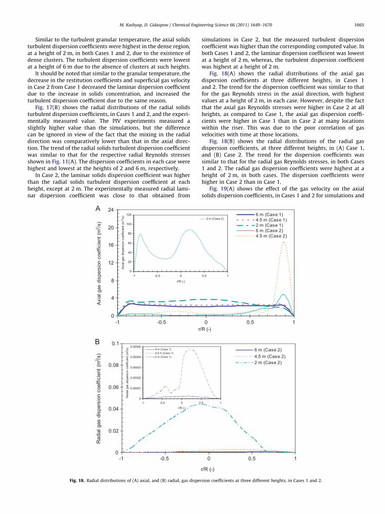
M. Kashyap, D. Gidaspow / Chemical Engineering Science 66 (2011) 1649–1670 1665
Similar to the turbulent granular temperature, the axial solidsturbulent dispersion coefficients were highest in the dense region,at a height of 2 m, in both Cases 1 and 2, due to the existence ofdense clusters. The turbulent dispersion coefficients were lowestat a height of 6 m due to the absence of clusters at such heights.
It should be noted that similar to the granular temperature, thedecrease in the restitution coefficients and superficial gas velocityin Case 2 from Case 1 decreased the laminar dispersion coefficientdue to the increase in solids concentration, and increased theturbulent dispersion coefficient due to the same reason.
Fig. 17(B) shows the radial distributions of the radial solidsturbulent dispersion coefficients, in Cases 1 and 2, and the experi-mentally measured value. The PIV experiments measured aslightly higher value than the simulations, but the differencecan be ignored in view of the fact that the mixing in the radialdirection was comparatively lower than that in the axial direc-tion. The trend of the radial solids turbulent dispersion coefficientwas similar to that for the respective radial Reynolds stressesshown in Fig. 11(A). The dispersion coefficients in each case werehighest and lowest at the heights of 2 and 6 m, respectively.
In Case 2, the laminar solids dispersion coefficient was higherthan the radial solids turbulent dispersion coefficient at eachheight, except at 2 m. The experimentally measured radial lami-nar dispersion coefficient was close to that obtained from
0
0.02
0.04
0.06
0.08
0.1
Rad
ial g
as d
ispe
rsio
n co
effic
ient
(m2 /s
)
0
4
8
12
16
20
24
-1 -0.5
-1 -0.5
r/
Axi
al g
as d
ispe
rsio
n co
effic
ient
(m2 /s
)
0
20
40
60
80
100
120
Axi
al g
as d
ispe
rsio
n co
effic
ient
(m/s
)
Fig. 18. Radial distributions of (A) axial, and (B) radial, gas disper
simulations in Case 2, but the measured turbulent dispersioncoefficient was higher than the corresponding computed value. Inboth Cases 1 and 2, the laminar dispersion coefficient was lowestat a height of 2 m, whereas, the turbulent dispersion coefficientwas highest at a height of 2 m.
Fig. 18(A) shows the radial distributions of the axial gasdispersion coefficients at three different heights, in Cases 1and 2. The trend for the dispersion coefficient was similar to thatfor the gas Reynolds stress in the axial direction, with highestvalues at a height of 2 m, in each case. However, despite the factthat the axial gas Reynolds stresses were higher in Case 2 at allheights, as compared to Case 1, the axial gas dispersion coeffi-cients were higher in Case 1 than in Case 2 at many locationswithin the riser. This was due to the poor correlation of gasvelocities with time at those locations.
Fig. 18(B) shows the radial distributions of the radial gasdispersion coefficients, at three different heights, in (A) Case 1,and (B) Case 2. The trend for the dispersion coefficients wassimilar to that for the radial gas Reynolds stresses, in both Cases1 and 2. The radial gas dispersion coefficients were highest at aheight of 2 m, in both cases. The dispersion coefficients werehigher in Case 2 than in Case 1.
Fig. 19(A) shows the effect of the gas velocity on the axialsolids dispersion coefficients, in Cases 1 and 2 for simulations and
r/R (-)
6 m (Case 2)4.5 m (Case 2)2 m (Case 2)
0 0.5 1
0 0.5 1
R (-)
6 m (Case 1)4.5 m (Case 1)2 m (Case 1)6 m (Case 2)4.5 m (Case 2)
sion coefficients at three different heights, in Cases 1 and 2.
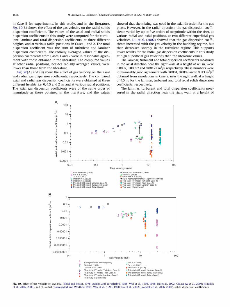
M. Kashyap, D. Gidaspow / Chemical Engineering Science 66 (2011) 1649–16701666
in Case B for experiments, in this study, and in the literature.Fig. 19(B) shows the effect of the gas velocity on the radial solidsdispersion coefficients. The values of the axial and radial solidsdispersion coefficients in this study were computed for the turbu-lent, laminar and total dispersion coefficients, at three differentheights, and at various radial positions, in Cases 1 and 2. The totaldispersion coefficient was the sum of turbulent and laminardispersion coefficients. The radially averaged values of the dis-persion coefficients from Cases 1 and 2 were in reasonable agree-ment with those obtained in the literature. The computed valuesat other radial positions, besides radially averaged values, werelower than those from the literature.
Fig. 20(A) and (B) show the effect of gas velocity on the axialand radial gas dispersion coefficients, respectively. The comparedaxial and radial gas dispersion coefficients were obtained at threedifferent heights, i.e. 6, 4.5 and 2 m, and at various radial positions.The axial gas dispersion coefficients were of the same order ofmagnitude as those obtained in the literature, and the values
0.0001
0.001
0.01
0.1
1
10
100
0.01 0.1Gas
Axi
al s
olid
s di
sper
sion
coe
ffici
ent (
m2 /s
)
Thiel and Potter (1978)Wei et al. (1995)Du et al. (2002)Jiradilok et al. (2006)Jiradilok et al. (2008)This study (IIT model; Laminar; Case 1)This study (IIT model; Turbulent; Case 2)This study (IIT model; Total; Case 2)
0.00000001
0.0000001
0.000001
0.00001
0.0001
0.001
0.01
0.1
1
11.0Gas ve
Rad
ial s
olid
s di
sper
sion
coe
ffici
ent (
m2 /s
)
Koenigsdorf and Werther (1995)Wei et al. (1998)Jiradilok et al. (2006)This study (IIT model; Turbulent; CasThis study (IIT model; Total; Case 1)This study (IIT model; Laminar; CaseThis study (Experiments)
Fig. 19. Effect of gas velocity on (A) axial (Thiel and Potter, 1978; Avidan and Yerusha
et al., 2006, 2008), and (B) radial (Koenigsdorf and Werther, 1995; Wei et al., 1995, 19
showed that the mixing was good in the axial direction for the gasphase. However, in the radial direction, the gas dispersion coeffi-cients varied by up to five orders of magnitude within the riser, atvarious radial and axial positions, at two different superficial gasvelocities. Du et al. (2002) showed that the gas dispersion coeffi-cients increased with the gas velocity in the bubbling regime, butthen decreased sharply in the turbulent regime. This supportslower results for the radial gas dispersion coefficients in this studyat high superficial gas velocities than the literature values.
The laminar, turbulent and total dispersion coefficients measuredin the axial direction near the right wall, at a height of 4.5 m, were0.0007, 0.00057 and 0.00127 m2/s, respectively. These numbers werein reasonably good agreement with 0.0004, 0.0009 and 0.0013 m2/s2
obtained from simulations in Case 2, near the right wall, at a heightof 4.5 m, for the laminar, turbulent and total axial solids dispersioncoefficients, respectively.
The laminar, turbulent and total dispersion coefficients mea-sured in the radial direction near the right wall, at a height of
1 10 100velocity (m/s)
Avidan and Yerushalmi (1985)Wei et al. (1998)Gidaspow et al. (2004)NETL riser (Experiment); 812 µm cork particlesThis study (IIT model; Turbulent; Case 1)This study (IIT model; Total; Case 1)This study (IIT model; Laminar; Case 2)This study (Experiments)
00101locity (m/s)
Wei et al. (1995)Du et al. (2002)Jiradilok et al. (2008)
e 1) This study (IIT model; Laminar; Case 1)This study (IIT model; Turbulent; Case 2)
2) This study (IIT model; Total; Case 2)
lmi, 1985; Wei et al., 1995, 1998; Du et al., 2002; Gidaspow et al., 2004; Jiradilok
98; Du et al., 2002; Jiradilok et al., 2006, 2008), solids dispersion coefficients.
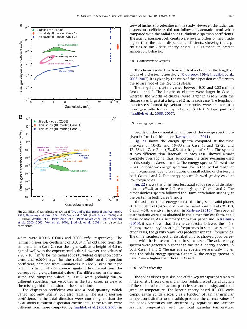
Gayán et al. (1997)Sternéuset al.
(2002)
Werther et al. (1992)
Amos et al. (1993)
Wei et al. (2001)Sternéus et al.
(2000); hotSternéus et al. (2000); cold
0 2 4 6 8 10 12 14 3010-7
10-6
10-5
10-4
10-3
10-2
10-1
100
101
102
103
Rad
ial g
as d
ispe
rsio
n co
effic
ient
(m2 /s
)
Gas velocity (m/s)
Jiradilok et al. (2008) This study (IIT model; Case 1) This study (IIT model; Case 2)
Dry and White (1989)
Namkung and Kim
(1998, 1999)Li and Weinstein (1989)
Wei et al. (2001)
0 2 4 6 8 10 12 14 3010-4
10-3
10-2
10-1
100
101
102
Axi
al g
as d
ispe
rsio
n co
effic
ient
(m2 /s
)
Gas velocity (m/s)
Jiradilok et al. (2008) This study (IIT model; Case 1) This study (IIT model; Case 2)
Fig. 20. Effect of gas velocity on (A) axial (Dry and White, 1989; Li and Weinstein,
1989; Namkung and Kim, 1998, 1999; Wei et al., 2001; Jiradilok et al., 2008), and
(B) radial (Werther et al., 1992; Amos et al., 1993; Gayan et al., 1997; Sterneus
et al., 2000, 2002; Wei et al., 2001; Jiradilok et al., 2008), gas dispersion
coefficients.
M. Kashyap, D. Gidaspow / Chemical Engineering Science 66 (2011) 1649–1670 1667
4.5 m, were 0.0006, 0.0003 and 0.0009 m2/s, respectively. Thelaminar dispersion coefficient of 0.0004 m2/s obtained from thesimulations in Case 2, near the right wall, at a height of 4.5 m,agreed well with the experimental value. However, the values of2.96�10�6 m2/s for the radial solids turbulent dispersion coeffi-cient and 0.0004 m2/s2 for the radial solids total dispersioncoefficient, obtained from simulations in Case 2, near the rightwall, at a height of 4.5 m, were significantly different from thecorresponding experimental values. The differences in the mea-sured and computed values in Case 2 were probably due todifferent superficial gas velocities in the two cases, in view ofthe missing third dimension in the simulations.
The dispersion coefficient was also a local quantity, whichvaried not only axially, but also radially. The gas dispersioncoefficients in the axial direction were much higher than theaxial solids turbulent dispersion coefficients. These results weredifferent from those computed by Jiradilok et al. (2007, 2008) in
view of higher slip velocities in this study. However, the radial gasdispersion coefficients did not follow a systematic trend whencompared with the radial solids turbulent dispersion coefficients.The axial dispersion coefficients were several orders of magnitudehigher than the radial dispersion coefficients, showing the cap-abilities of the kinetic theory based IIT CFD model to predictanisotropic behavior.
5.8. Characteristic lengths
The characteristic length or width of a cluster is the length orwidth of a cluster, respectively (Gidaspow, 1994; Jiradilok et al.,2006, 2007). It is given by the ratio of the dispersion coefficient tothe square root of the Reynolds stress.
The lengths of clusters varied between 0.07 and 0.82 mm, inCases 1 and 2. The lengths of clusters were larger in Case 1,whereas, the widths of clusters were larger in Case 2, with thecluster sizes largest at a height of 2 m, in each case. The lengths ofthe clusters formed by Geldart D particles were smaller thanthose generally formed by cohesive Geldart A type particles(Jiradilok et al., 2006, 2007).
5.9. Energy spectrum
Details on the computation and use of the energy spectra aregiven in Part I of this paper (Kashyap et al., 2011).
Fig. 21 shows the energy spectra computed at the timeintervals of 10–35 and 10–30 s in Case 1, and 12–25 and12–28 s in Case 2, at r/R¼0.8, at a height of 4.5 m. The spectraat two different time intervals, in each case, showed almostcomplete overlapping, thus, supporting the time averaging usedin this study in Cases 1 and 2. The energy spectra followed the�5/3 Kolmogorov energy spectrum law in the inertial range, athigh frequencies, due to oscillations of small eddies or clusters, inboth Cases 1 and 2. The energy spectra showed gravity wave atlow frequencies.
Fig. 22 shows the dimensionless axial solids spectral distribu-tions at r/R¼0, at three different heights, in Cases 1 and 2. Thedimensionless spectra followed the Hinze correlation strongly atthe center, in both Cases 1 and 2.
The axial and radial energy spectra for the gas and solid phasesat the heights of 6, 4.5 and 2 m, at the radial positions of r/R¼0.8,0 and �0.8, are given in detail in Kashyap (2010). The spectraldistributions were also obtained in the dimensionless form, at allthese positions. As a summary from this paper and in Kashyap(2010), it was shown that the energy spectra followed the �5/3Kolmogorov energy law at high frequencies in some cases, and inother cases, the gravity wave was predominant at all frequencies.The dimensionless spectral distribution also showed good agree-ment with the Hinze correlation in some cases. The axial energyspectra were generally higher than the radial energy spectra, inboth Cases 1 and 2. The gas energy spectra were mostly higherthan the solids energy spectra. Generally, the energy spectra inCase 2 were higher than those in Case 1.
5.10. Solids viscosity
The solids viscosity is also one of the key transport parametersin the kinetic theory of granular flow. Solids viscosity is a functionof the solids volume fraction, particle size and density, and totalgranular temperature. The kinetic theory based IIT CFD codecomputes the solids viscosity as a function of laminar granulartemperature. Similar to the solids pressure, the correct values ofthe solids viscosities are obtained by replacing the laminargranular temperature with the total granular temperature.
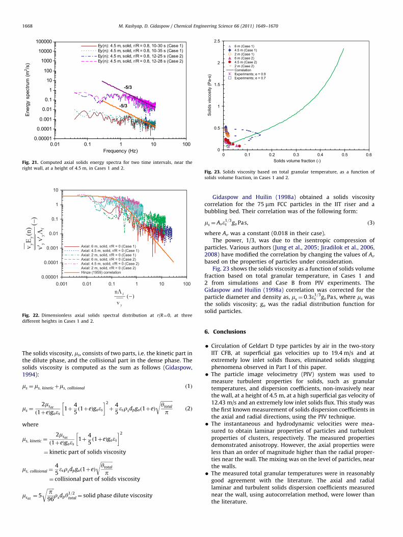
0.00001
0.0001
0.001
0.01
0.1
1
10
100
1000
10000
100000
0.01 0.1 1 10 100Frequency (Hz)
Ene
rgy
spec
trum
(m2 /s
)
Ey(n): 4.5 m, solid, r/R = 0.8, 10-30 s (Case 1)Ey(n): 4.5 m, solid, r/R = 0.8, 10-35 s (Case 1)Ey(n): 4.5 m, solid, r/R = 0.8, 12-25 s (Case 2)Ey(n): 4.5 m, solid, r/R = 0.8, 12-28 s (Case 2)
-5/3
-5/3
Fig. 21. Computed axial solids energy spectra for two time intervals, near the
right wall, at a height of 4.5 m, in Cases 1 and 2.
0.00001
0.0001
0.001
0.01
0.1
1
10
0.001 0.01 0.1 1 10 100
Axial: 6 m, solid, r/R = 0 (Case 1)Axial: 4.5 m, solid, r/R = 0 (Case 1)Axial: 2 m, solid, r/R = 0 (Case 1)Axial: 6 m, solid, r/R = 0 (Case 2)Axial: 4.5 m, solid, r/R = 0 (Case 2)Axial: 2 m, solid, r/R = 0 (Case 2)Hinze (1959) correlation
)(
'v'v
)n(E
v
fy
y
yy
)(v
n
y
f
Fig. 22. Dimensionless axial solids spectral distribution at r/R¼0, at three
different heights in Cases 1 and 2.
0
0.5
1
1.5
2
2.5
0 0.1 0.2 0.3 0.4 0.5 0.6Solids volume fraction (-)
Sol
ids
visc
osity
(Pa-
s)
6 m (Case 1)4.5 m (Case 1)2 m (Case 1)6 m (Case 2)4.5 m (Case 2)2 m (Case 2)CorrelationExperiments; e = 0.9Experiments; e = 0.7
Fig. 23. Solids viscosity based on total granular temperature, as a function of
solids volume fraction, in Cases 1 and 2.
M. Kashyap, D. Gidaspow / Chemical Engineering Science 66 (2011) 1649–16701668
The solids viscosity, ms, consists of two parts, i.e. the kinetic part inthe dilute phase, and the collisional part in the dense phase. Thesolids viscosity is computed as the sum as follows (Gidaspow,1994):
ms ¼ ms, kineticþms, collisional ð1Þ
ms ¼2msdil
ð1þeÞgoes1þ
4
5ð1þeÞgoes
� �2
þ4
5esrsdpgoð1þeÞ
ffiffiffiffiffiffiffiffiffiffiytotal
p
rð2Þ
where
ms, kinetic ¼2msdil
ð1þeÞgoes1þ
4
5ð1þeÞgoes
� �2
¼ kinetic part of solids viscosity
ms, collisional ¼4
5esrsdpgoð1þeÞ
ffiffiffiffiffiffiffiffiffiffiytotal
p
r¼ collisional part of solids viscosity
msdil:¼ 5
ffiffiffiffiffiffip
96
rrsdpy
1=2total ¼ solid phase dilute viscosity
Gidaspow and Huilin (1998a) obtained a solids viscositycorrelation for the 75 mm FCC particles in the IIT riser and abubbling bed. Their correlation was of the following form:
ms ¼ Ave1=3s go Pas, ð3Þ
where Av was a constant (0.018 in their case).The power, 1/3, was due to the isentropic compression of
particles. Various authors (Jung et al., 2005; Jiradilok et al., 2006,2008) have modified the correlation by changing the values of Av
based on the properties of particles under consideration.Fig. 23 shows the solids viscosity as a function of solids volume
fraction based on total granular temperature, in Cases 1 and2 from simulations and Case B from PIV experiments. TheGidaspow and Huilin (1998a) correlation was corrected for theparticle diameter and density as, ms ¼ 0:3e1=3
s go Pas, where ms wasthe solids viscosity; go was the radial distribution function forsolid particles.
6. Conclusions
�
Circulation of Geldart D type particles by air in the two-storyIIT CFB, at superficial gas velocities up to 19.4 m/s and atextremely low inlet solids fluxes, eliminated solids sluggingphenomena observed in Part I of this paper. � The particle image velocimetry (PIV) system was used tomeasure turbulent properties for solids, such as granulartemperatures, and dispersion coefficients, non-invasively nearthe wall, at a height of 4.5 m, at a high superficial gas velocity of12.43 m/s and an extremely low inlet solids flux. This study wasthe first known measurement of solids dispersion coefficients inthe axial and radial directions, using the PIV technique.
� The instantaneous and hydrodynamic velocities were mea-sured to obtain laminar properties of particles and turbulentproperties of clusters, respectively. The measured propertiesdemonstrated anisotropy. However, the axial properties wereless than an order of magnitude higher than the radial proper-ties near the wall. The mixing was on the level of particles, nearthe walls.
� The measured total granular temperatures were in reasonablygood agreement with the literature. The axial and radiallaminar and turbulent solids dispersion coefficients measurednear the wall, using autocorrelation method, were lower thanthe literature.
M. Kashyap, D. Gidaspow / Chemical Engineering Science 66 (2011) 1649–1670 1669
�
A two-dimensional kinetic theory based IIT CFD code was usedto model the circulation of Geldart D type particles in the IITriser, under high gas velocity–low inlet solids flux conditions.Two simulations were performed for Cases 1 and 2, with e¼0.9,ew¼0.96 and Ug¼30 m/s in Case 1, and e¼0.7, ew¼0.7 andUg¼14 m/s in Case 2. The radially averaged solids volumefractions measured using gamma ray densitometer and com-puted in Cases 1 and 2, at a height of 4.5 m, were around 2%.The transport of particles in the dense region, in Case 2, was bydense solids slug motion, and the IIT CFD code successfullymodeled turbulent fluidization in Case 2. The computed solidsconcentrations in Case 2 were higher than those in Case 1. � Core-annular regime was computed in dilute region, in Case 2.However, in the dense region in Case 2 and at all heights inCase 1, core-annular regime was absent.
� The FFT analysis of the measured and computed solids volumefractions gave dominant frequencies less than 0.1 Hz, in agree-ment with an analytical solution.
� The turbulent properties, such as Reynolds stresses, granulartemperatures, dispersion coefficients, and energy spectra, werelocal quantities that changed with location in the fluidized bed.The turbulent properties showed high slip and anisotropy. Theturbulent intensities showed that mixing was on the level ofparticles at all radial and axial positions, in Case 1. However, inCase 2, mixing was on the level of particles near the walls, andit was on the level of clusters at the center.
� The Reynolds stresses and turbulent granular temperatureswere highest at dense bottom. They were higher in Case 2 thanin Case 1 due to limited clusters in later case. However, thelaminar granular temperatures were higher in Case 1 than inCase 2 due to higher restitution coefficients and inlet gasvelocity in former case.
� The axial solids velocity, laminar and turbulent granulartemperatures, axial laminar and turbulent solids dispersioncoefficients, and radial laminar solids dispersion coefficient,computed in Case 2 near the right wall, at a height of 4.5 m,were close to the experimentally measured values. Neverthe-less, the computed radial turbulent solids dispersion coefficientwas lower than the measured value at same location.
� The computed total granular temperatures, radially averagedaxial and radial solids dispersion coefficients, and axial gasdispersion coefficients, were in reasonable agreement with theliterature. However, the radial gas dispersion coefficients wereseveral orders of magnitude lower than the literature. Hence,the kinetic theory based CFD codes, such as the IIT CFD code,are capable of designing fluidized bed reactors without usingproperties, such as dispersion coefficients, as inputs. The IITCFD code was also able to reasonably match the measuredsolids dispersion coefficients using the PIV technique. Thediameters and lengths of clusters computed from characteristiclengths were 0.016 and 0.07–0.82 m, respectively.
� The energy spectra showed that the �5/3 Kolmogorov energyspectrum law was followed at some locations, in the axial andradial directions, for solid and gas phases, at high frequencies.The dimensionless form of the spectral distribution showedreasonably good agreement with the Hinze correlation, at somelocations.
� The solids viscosity correlation with the solids volume fractionswas modified as, ms ¼ 0:3e1=3s go Pa s.
Nomenclature
Cd drag coefficient (dimensionless)dp diameter of particles (m)
D inner diameter of the riser (m)e particle–particle restitution coefficient (dimensionless)ew particle–wall restitution coefficient (dimensionless)EiðnÞ energy spectrum function (m2/s)f dominant frequency (Hz)go radial distribution function for solid particles
(dimensionless)H riser height (m)P pressure (N/m2)r radial distance from center (m)R radius of riser (m)t time interval (s)Dt time step (s)tsteady steady state time range (s)Ug superficial gas velocity (m/s)x radial direction (dimensionless)y axial direction (dimensionless)z tangential direction (dimensionless)
Greek letters
bB gas–solid drag coefficient for hydrodynamic model B(kg/m3 s)
eg gas volume fraction or voidage (dimensionless)es solids volume fraction (dimensionless)ks conductivity of the fluctuating energy (kg/m s)gs collisional dissipation of dilute phase solid fluctuating
energy (kg/m s3)ls solids bulk viscosity (kg/m s)mph. viscosity of phase ph (kg/m s)tph: stress tensor for phase ph. (Pa)y granular temperature (m2/s2)f specularity coefficient (dimensionless)4f space integral scale (m)
Subscripts
g gas phaseinitial initialinlet inletoutlet outletph: gas or solid phases solid phase
Acknowledgment
The authors gratefully acknowledge the partial financial supportby UOP and the U.S. Department of Energy University Grant(DE-FG26-06NT42736). They also want to acknowledge Dr. VeerayaJiradilok of Illinois Institute of Technology, and Dr. William Koves andDr. Reza Mostofi of UOP, for constructive suggestions, discussions andinteractions regarding the studies in this paper. Their contribution ishighly appreciated.
References
Ambler, P.A., Milne, B.J., Berruti, F., Scott, D.S., 1990. Residence time distribution ofsolids in a circulating fluidized bed: Experimental and modeling studies.Chem. Eng. Sci. 45, 2179–2186.
Amos, G., Rhodes, M.J., Mineo, H., 1993. Gas mixing in gas–solids riser. Chem. Eng.Sci. 48, 943–949.
Avidan, A., Yerushalmi, J., 1985. Solids mixing in an expanded top fluid bed. AIChEJ. 31, 835–841.
Bader, R., Findlay, J., Knowlton, T.M., 1988. Gas/solids flow pattern in a 30.5 cmdiameter circulating fluidized bed. In: Basu, P., Large, J.F. (Eds.), CirculatingFluidized Bed Technology II. Pergamon Press, Oxford, UK, pp. 127–137.
M. Kashyap, D. Gidaspow / Chemical Engineering Science 66 (2011) 1649–16701670
Bahary, M., 1994. Experimental and computational studies of hydrodynamics intwo and three phase fluidize beds. Ph.D. Thesis, Illinois Institute of Technology,Chicago, IL, USA.
Benyahia, S., Syamlal, M., O’Brien, T.J., 2007. Study of the ability of multiphasecontinuum models to predict core-annulus flow. AIChE J. 53, 2549–2568.
Breault, R.W., Guenther, C.P., Shadle, L.J., 2008. Velocity fluctuation interpretationin the near wall region of a dense riser. Powder Technol. 182, 137–145.
Brodkey, R.S., 1967. The Phenomena of Fluid Motions, 2nd ed. Addison-Wesley,Massachusetts.
Campbell, C., Wang, D., 1991. Particle pressures in gas-fluidized beds. J. FluidMech. 227, 495–508.
Chalermsinsuwan, B., Piumsomboon, P., Gidaspow, D., 2009. Kinetic theory basedcomputation of PSRI riser: Part I—Estimate of mass transfer coefficient. Chem.Eng. Sci. 64, 1195–1211.
Chapman, S., Cowling, T.G., 1953. The Mathematical Theory of Non-uniform Gases,2nd ed. Cambridge University Press, UK.
Chen, J., Li, F., Degaleesan, S., Gupta, P., Al-Dahhan, M.H., Dudukovic, M.P.,Toseland, B.A., 1999. Fluid dynamic parameters in bubble columns withinternals. Chem. Eng. Sci. 54, 2187–2197.
Cody, G.D., Goldfarb, D.J., Storch Jr., G.V., Norris, A.N., 1996. Particle granulartemperatures in gas fluidized beds. Powder Technol. 87, 211–232.
Degaleesan, S., Dudukovic, M., Pan, Y., 2001. Experimental study of gas-inducedliquid-flow structures in bubble columns. AIChE J. 47, 1913–1931.
Degaleesan, S., Dudukovic, M.P., Toseland, B.A., Bhatt, B.L., 1997. A two-compart-ment convective-diffusion model for slurry bubble column reactors. Ind. Eng.Chem. Res. 36, 4670–4680.
Driscoll, M.C., Gidaspow, D., 2007. Wave propagation and granular temperature influidized beds of nanoparticles. AIChE J. 53, 1718–1726.
Dry, R.J., White, C.C., 1989. Gas residence-time characteristics in a high-velocitycirculating fluidized bed of FCC catalyst. Powder Technol. 58, 17–23.
Du, B., Fan, L.-S., Wei, F., Warsito, W., 2002. Gas and solids mixing in a turbulentfluidized bed. AIChE J. 48, 1896–1909.
Gayan, P., de Diego, L.F., Adanez, J., 1997. Radial gas mixing in a fast fluidized bed.Powder Technol. 94, 163–171.
Gidaspow, D., 1994. Multiphase Flow and Fluidization: Continuum and KineticTheory Descriptions. Academic Press, New York.
Gidaspow, D., Bahary, M., Wu, Y., 1995. Hydrodynamic models for slurry bubblecolumn reactors. Presentation at the AIChE Meeting, Miami Beach, Florida.
Gidaspow, D., Huilin, L., 1996. Collisional viscosity of FCC particles in a CFB. AIChEJ. 42, 2503–2510.
Gidaspow, D., Huilin, L., 1998a. A comparison of gas–solid and liquid–solidfluidization using kinetic theory and statistical mechanics. In: Fan, L.S.,Knowlton, T.M. (Eds.), Fluidization IX. Engineering Foundation, New York,pp. 661–668.
Gidaspow, D., Huilin, L., 1998b. Equation of state and radial distribution functionsof FCC particles in a CFB. AIChE J. 44, 279–293.
Gidaspow, D., Huilin, L., Mostofi, R., 2001. Large scale oscillations or gravity wavesin a riser and bubbling beds. In: Kwauk, M., Li, J., Yang, W.C. (Eds.), FluidizationX. Engineering Foundation, New York, pp. 317–323.
Gidaspow, D., Jiradilok, V., 2009. Computational Techniques: The Multiphase CFDApproach to Fluidization and Green Energy Technologies (Includes CD-ROM).Nova Science Publishers, New York.
Gidaspow, D., Jonghwun, J., Singh, R.K., 2004. Hydrodynamics of fluidization usingkinetic theory: an emerging paradigm 2002 Flour-Daniel lecture. PowderTechnology 148, 123–141.
Hinze, J.O., 1959. Turbulence: An Introduction to Its Mechanism and Theory.McGraw-Hill, Inc., New York.
Jiradilok, V., Gidaspow, D., Breault, R.W., 2007. Computation of gas and soliddispersion coefficients in turbulent risers and bubbling beds. Chem. Eng. Sci.62, 3397–3409.
Jiradilok, V., Gidaspow, D., Breault, R.W., Shadle, L.J., Guenther, C., Shi, S., 2008.Computation of turbulence and dispersion of cork in the NETL riser. Chem.Eng. Sci. 63, 2135–2148.
Jiradilok, V., Gidaspow, D., Damronglerd, S., Koves, W.J., Mostofi, R., 2006. Kinetictheory based CFD simulations of turbulent fluidization of FCC particles in ariser. Chem. Eng. Sci. 61, 5544–5559.
Johnson, P.C., Jackson, R., 1987. Frictional-collisional constitutive relations forgranular materials, with application to plane shearing. J. Fluid Mech. 176,67–93.
Jung, J., Gidaspow, D., Gamwo, I.K., 2005. Measurement of two kinds of granulartemperatures, stresses, and dispersion in bubbling beds. Ind. Eng. Chem. Res.44, 1329–1341.
Kashyap, M., 2010. Measurements and computation of dispersion and masstransfer coefficients in fluidized beds. Ph.D. Thesis, Illinois Institute ofTechnology, Chicago, Illinois.
Kashyap, M., Chalermsinsuwan, B., Gidaspow, D. Measurements of turbulence in acirculating fluidized bed using PIV techniques. Particuology, Submitted forpublication.
Kashyap, M., Gidaspow, D., Driscoll, M., 2008. Effect of electric field on thehydrodynamics of fluidized nanoparticles. Powder Technol. 183, 441–453.
Kashyap, M., Gidaspow, D., Koves, W.J., 2011. Circulation of Geldart D typeparticles: Part I — High solids fluxes. Measurements and computation undersolids slugging conditions. Chem. Eng. Sci. 66, 183–206.
Koenigsdorf, R., Werther, J., 1995. Gas–solids mixing and flow structure modelingof the upper dilute zone of a circulating fluidized bed. Powder Technol. 82,317–329.
Lee, G.S., Kim, S.D., 1990. Axial mixing of solids in turbulent fluidized beds. Chem.Eng. J. 44, 1–9.
Li, J., Weinstein, H., 1989. An experimental comparison of gas backmixing influidized beds across the regimes spectrum. Chem. Eng. Sci. 44, 1697–1705.
Limtrakul, S., Chen, J., Ramachandran, P.A., Dudukovic, M.P., 2005. Solids motionand holdup profiles in liquid fluidized beds. Chem. Eng. Sci. 60, 1889–1900.
May, W.G., 1959. Fluidized-bed reactor studies. Chem. Eng. Prog. 55, 49–56.Miller, A., Gidaspow, D., 1992. Dense, vertical gas–solid flow in a pipe. AIChE J. 38,
1801–1815.Mostoufi, N., Chaouki, J., 2001. Local solid mixing in gas–solid fluidized beds.
Powder Technol. 114, 23–31.Mudde, R.F., Lee, D.J., Reese, J., Fan, L.S., 1997. Role of coherent structures on
Reynolds stresses in a 2-D bubble column. AIChE J. 43, 913–926.Namkung, W., Kim, S.D., 1998. Gas backmixing in a circulating fluidized bed.
Powder Technol. 99, 70–78.Namkung, W., Kim, S.D., 1999. Gas backmixing in the dense region of a circulating
fluidized bed. Korean J. Chem. Eng. 16, 456–461.Neri, A., Gidaspow, D., 2000. Riser hydrodynamics: simulation using kinetic
theory. AIChE J. 46, 52–67.Pan, Y., Dudukovic, M.P., Chang, M., 2000. Numerical investigation of gas-driven
flow in 2-D bubble columns. AIChE J. 46, 434–449.Polashenski Jr., W., Chen, J.C., 1997. Normal solid stress in fluidized beds. Powder
Technol. 90, 13–23.Polashenski Jr, W., Chen, J.C., 1999. Measurement of particle phase stresses in fast
fluidized beds. Ind. Eng. Chem. Res. 38, 705–713.Ran, X., Wei, F., Wang, Z., Jin, Y., 2001. Lateral solids dispersion in a high-density
riser with swirling air flow. Powder Technol. 121, 123–130.Rhodes, M.J., Zhou, S., Hirama, T., Cheng, H., 1991. Effects of operating conditions
on longitudinal solids mixing in a circulating fluidized bed riser. AIChE J. 37,1450–1458.
Roy, S., Kemoun, A., Al-Dahhan, M.H., Dudukovic, M.P., 2005. Experimental investi-gation of the hydrodynamics in a liquid–solid riser. AIChE J. 51, 802–835.
Sterneus, J., Johnsson, F., Leckner, B., 2000. Gas mixing in circulating fluidized-bedrisers. Chem. Eng. Sci. 55, 129–148.
Sterneus, J., Johnsson, F., Leckner, B., 2002. Characteristics of gas mixing in acirculating fluidized bed. Powder Technol. 126, 28–41.
Tartan, M., Gidaspow, D., 2004. Measurement of granular temperature and stressesin risers. AIChE J. 50, 1760–1775.
Thiel, W.J., Potter, O.E., 1978. The mixing of solids in slugging gas fluidized beds.AIChE J. 24, 561–569.
Wei, F., Chen, W., Jin, Y., Yu, Z.Q., 1995. Lateral and axial mixing of the dispersedparticles in CFB. J. Chem. Eng. Jpn. 28, 506–510.
Wei, F., Cheng, Y., Jin, Y., Yu, Z., 1998. Axial and lateral dispersion of fine particlesin a binary-solid riser. Can. J. Chem. Eng. 76, 19–26.
Wei, F., Yang, Y., Jia, X., Jin, Y., 2001. Hydrodynamics and lateral gas dispersion in ahigh density circulating fluidized bed reactor with bluff internals. ChineseJ. Chem. Eng. 9, 291–296.
Werther, J., Harte, E.U., Kruse, M., 1992. Radial gas mixing in the upper dilute coreof a circulating fluidized bed. Powder Technol. 70, 293–301.
Winaya, I.N.S., Shimizu, T., Yamada, D., 2007. A new method to evaluate horizontalsolid dispersion coefficient in a bubbling fluidized bed. Powder Technol. 178,173–178.
Zhang, Y., Lu, C., Shi, M., 2009. Evaluating solids dispersion in fluidized beds of fineparticles by gas backmixing experiments. Chem. Eng. Res. Des. 87, 1400–1408.