P

A

УН

POQ

AGRICU

НИВЕРЗИТЕИНСТ

UNIVERSITYINSTIT

QOPTEH

ULTURНАУЧSCIEN

ЕТ У БЕОГРАТИТУТ ЗА ПY OF BELGRTUTE OF AG

Година XYear XX

RIVHNIRAL EЧНИ ЧАСОNTIFIC JOU

АДУ, ПОЉООЉОПРИВ

RADE, FACUGRICULTUR

XXXVIII БрXXVIII, No.

VREIKA

NGINEОПИС URNAL

ОПРИВРЕДНРЕДНУ ТЕХ

ULTY OF AGRAL ENGINEE

ој 3, 2013.3, 2013.

ISSN 0UDK

DNA

EERIN

НИ ФАКУЛТХНИКУ RICULTUREERING

0554-5587 K 631 (059)

A

G

ТЕТ,

E,

Издавач (Publisher) Универзитет у Београду, Пољопривредни факултет, Институт за пољопривредну технику, Београд-Земун University of Belgrade, Faculty of Agriculture, Institute of Agricultural Engineering, Belgrade-Zemun Уредништво часописа (Editorial board) Главни и одговорни уредник (Editor in Chief) др Горан Тописировић, професор, Универзитет у Београду, Пољопривредни факултет

Уредници (National Editors) др Ђукан Вукић, професор, Универзитет у Београду, Пољопривредни факултет др Стева Божић, професор, Универзитет у Београду, Пољопривредни факултет др Мирко Урошевић, професор, Универзитет у Београду, Пољопривредни факултет др Мићо Ољача, професор, Универзитет у Београду, Пољопривредни факултет др Анђелко Бајкин, професор, Универзитет у Новом Саду, Пољопривредни факултет др Милан Мартинов, професор, Универзитет у Новом Саду,Факултет техничких наука др Душан Радивојевић, професор, Универзитет у Београду, Пољопривредни факултет др Драган Петровић, професор, Универзитет у Београду, Пољопривредни факултет др Раде Радојевић, професор, Универзитет у Београду, Пољопривредни факултет др Милован Живковић, професор, Универзитет у Београду, Пољопривредни факултет др Зоран Милеуснић, професор, Универзитет у Београду, Пољопривредни факултет др Рајко Миодраговић, доцент, Универзитет у Београду, Пољопривредни факултет др Александра Димитријевић, доцент, Универзитет у Београду, Пољопривредни факултет др Милош Пајић, доцент, Универзитет у Београду, Пољопривредни факултет др Бранко Радичевић, доцент, Универзитет у Београду, Пољопривредни факултет др Иван Златановић, доцент, Универзитет у Београду, Пољопривредни факултет др Милан Вељић, професор, Универзитет у Београду, Машински факултет др Драган Марковић, професор, Универзитет у Београду, Машински факултет др Саша Бараћ, професор, Универзитет у Приштини, Пољопривредни факултет, Лешак др Предраг Петровић, Институт "Кирило Савић", Београд дипл. инг. Драган Милутиновић, ИМТ, Београд Инострани уредници (International Editors) Professor Peter Schulze Lammers, Ph.D., Institut fur Landtechnik, Universitat, Bonn, Germany Professor László Magó, Ph.D., Szent Istvan University, Faculty of Mechanical Engineering, Gödöllő, Hungary Professor Victor Ros, Ph.D., Technical University of Cluj-Napoca, Romania Professor Sindir Kamil Okyay, Ph.D., Ege University, Faculty of Agriculture, Bornova - Izmir, Turkey Professor Stavros Vougioukas, Ph.D., Aristotle University of Tessaloniki Professor Nicolay Mihailov, Ph.D., University of Rousse, Faculty of Electrical Enginering, Bulgaria Professor Silvio Košutić, Ph.D., University of Zagreb, Faculty of Agriculture, Croatia Professor Selim Škaljić, Ph.D., University of Sarajevo, Faculty of Agriculture, Bosnia and Hercegovina Professor Dragi Tanevski, Ph.D., "Ss. Cyril and Methodius" University in Skopje, Faculty of Agriculture, Macedonia Professor Zoran Dimitrovski, Ph.D., University "Goce Delčev", Faculty of Agriculture, Štip, Macedonia Professor Sitaram D. Kulkarni, Ph.D., Agro Produce Processing Division, Central Institute of Agricultural Engineering, Bhopal, India Контакт подаци уредништва (Contact) 11080 Београд-Земун, Немањина 6, тел. (011)2194-606, 2199-621, факс: 3163-317, 2193-659, e-mail: gogi@agrif.bg.ac.rs, жиро рачун: 840-1872666-79. 11080 Belgrade-Zemun, str. Nemanjina No. 6, Tel. 2194-606, 2199-621, fax: 3163-317, 2193-659, e-mail: gogi@agrif.bg.ac.rs, Account: 840-1872666-79

POQOPRIVREDNA TEHNIKA

НАУЧНИ ЧАСОПИС

AGRICULTURAL ENGINEERING SCIENTIFIC JOURNAL

УНИВЕРЗИТЕТ У БЕОГРАДУ, ПОЉОПРИВРЕДНИ ФАКУЛТЕТ, ИНСТИТУТ ЗА ПОЉОПРИВРЕДНУ ТЕХНИКУ

UNIVERSITY OF BELGRADE, FACULTY OF AGRICULTURE, INSTITUTE OF AGRICULTURAL ENGINEERING

WEB адреса www.jageng.agrif.bg.ac.rs

Издавачки савет (Editorial Council) Проф. др Властимир Новаковић, Проф. др Милан Тошић, Проф. др Петар Ненић, Проф. др Марија Тодоровић, Проф. др Драгиша Раичевић, Проф. др Ђуро Ерцеговић, Проф. др Ратко Николић, Проф. др Драгољуб Обрадовић, Проф. др Божидар Јачинац, Проф. др Драган Рудић, Проф. др Милош Тешић Техничка припрема (Technical editor) Иван Спасојевић, Пољопривредни факултет, Београд

Лектура и коректура: (Proofreader) Гордана Јовић

Превод: (Translation) Весна Ивановић, Зорица Крејић, Миљенко Шкрлин Штампа (Printed by) "Академска издања" – Земун Часопис излази четири пута годишње Тираж (Circulation) 350 примерака Претплата за 2014. годину износи 2000 динара за институције, 500 динара за појединце и 100 динара за студенте по сваком броју часописа. Радови објављени у овом часопису индексирани су у базама (Abstracting and Indexing): AGRIS i SCIndeks Издавање часописа помоглo (Publication supported by) Министарство просвете и науке Републике Србије

На основу мишљења Министарства за науку и технологију Републике Србије по решењу бр. 413-00-606/96-01 од 24. 12. 1996. године, часопис ПОЉОПРИВРЕДНА ТЕХНИКА је ослобођен плаћања пореза на промет робе на мало.

S A D R Ž A J OKSIDACIONI OTPOR PREMAZA NANETIH PLAZMA ELEKTROLITIČKOM OKSIDACIJOM NA LEGURAMA ALUMINIJUMA Yury Kuznetsov...................................................................................................................................1-9 OPTIMIZACIJA ELEKTRIČNIH PARAMETARA SILIKONSKIH HETERO-SPOJNIH SOLARNIH ĆELIJA Veliyana Zneliyazova, Krasimira Shtereva.....................................................................................11-18 UPOREDNA PROCENA PROIZVODNIH VARIJANTI UREĐAJA ZA PROIZVODNJU KONCENTROVANE STOČNE HRANE Prakash Prabhakar Ambalkar, Praveen Chandra Bargale, Jai Singh.............................................19-26 MODEL EVAPORATIVNOG SISTEMA HLAĐENJA SKLADIŠNOG PROSTORA U TROPSKIM USLOVIMA Chinenye Ndukwu, Seth Manuwa, Olawale Olukunle, Babatunde Oluwalana...............................27-39 RAZVOJ KRIVIH SUŠE – POLOŽAJA – UČESTALOSTI U PARAMBIKULAM - ALIYAR BASENU, TAMIL NADU, INDIJA Muthiah Manikandan, Dhanapal Tamilmani....................................................................................41-55 RAZVOJ VAZDUŠNOG RASPRSKIVAČA ZA ZAŠTITU CVEĆA U ZAŠTIĆENOM PROSTORU Sachin Vilas Wandkar, Shailendra Mohan Mathur, Babasaheb Sukhdeo Gholap, Pravin Prakash Jadhav...................................................................................................................57-72 TEORIJSKO I EKSPERIMENTALNO ISTRAŽIVANJE JAČINE LEMLJENIH SPOJEVA (METAL METAL – METAL KERAMIKA) Vladimir Goncharenko................................................................................................................... 73-84

KINETIKA SUŠENJA TANKOG SLOJA LISTOVA KANE Dattatreya M. Kadam, Manoj Kumar Gupta, Vaijayanta M Kadam.............................................. 85-100

STEPENI AERODINAMIKE I PROTOKA ČVRSTE MATERIJE U ODVODNIM KANALIMA ZA SUŠENJE KARDAMOMA (2. deo) Murugesan Balakrishnan, Velath Variyathodiyil Sreenarayanan, Ashutosh Singh, Gopu Raveendran Nair, Rangaraju Viswanathan, Grama Seetharama Iyengar, Vijaya Raghavan........................................................................................................................ 101-110

ANALIZA KAPLJICA VODE: KLASIČNI I KVANTNI HIDRODINAMIČKI OKVIRI Daniele De Wrachien, Giulio Lorenzini, Stefano Mambretti, Marco Medici............................... 111-122

C O N T E N T S OXIDATION RESISTANCE OF THE COATINGS OBTAINED BY PLASMA ELECTROLYTIC OXIDATION ON ALUMINIUM ALLOYS Yury Kuznetsov.................................................................................................................................. 1-9 OPTIMIZATION OF THE ELECTRICAL PARAMETERS OF SILICON HETEROJUNCTION SOLAR CELLS Veliyana Zneliyazova, Krasimira Shtereva.................................................................................... 11-18

COMPARATIVE EVALUATION OF PRODUCTION VARIANTS OF ANIMAL FEED PLANT Prakash Prabhakar Ambalkar, Praveen Chandra Bargale, Jai Singh............................................ 19-26 A SIMPLE MODEL FOR EVAPORATIVE COOLING SYSTEM OF A STORAGE SPACE IN A TROPICAL CLIMATE Chinenye Ndukwu, Seth Manuwa, Olawale Olukunle, Babatunde Oluwalana...............................27-39 DEVELOPMENT of DROUGHT SEVERITY – AREAL EXTENT – FREQUENCY CURVES IN THE PARAMBIKULAM - ALIYAR BASIN, TAMIL NADU, INDIA Muthiah Manikandan, Dhanapal Tamilmani................................................................................... 41-55 DEVELOPMENT OF AIR ASSISTED SPRAYER FOR GREENHOUSE FLORICULTURE CROPS Sachin Vilas Wandkar, Shailendra Mohan Mathur, Babasaheb Sukhdeo Gholap, Pravin Prakash Jadhav.................................................................................................................. 57-72

THEORETICAL AND EXPERIMENTAL RESEARCH OF STRENGTH OF SOLDERED JOINTS (METAL OF SHARE – METAL CERAMICS) Vladimir Goncharenko................................................................................................................... 73-84

THIN LAYER DRYING KINETICS OF HENNA LEAVES Dattatreya M. Kadam, Manoj Kumar Gupta, Vaijayanta M. Kadam............................................. 85-100

AERODYNAMIC AND SOLIDS CIRCULATION RATES IN SPOUTED BED DRYING OF CARDAMOM (Part 2) Murugesan Balakrishnan, Velath Variyathodiyil Sreenarayanan, Ashutosh Singh, Gopu Raveendran Nair, Rangaraju Viswanathan, Grama Seetharama Iyengar, Vijaya Raghavan........................................................................................................................ 101-110

WATER DROPLETS ANALYSIS: THE CLASSICAL AND QUANTUM HYDRODYNAMIC FRAMEWORKS Daniele De Wrachien, Giulio Lorenzini, Stefano Mambretti, Marco Medici............................... 111-122

Univerzitet uPoljoprivredInstitut za pNaučni časoPOLJOPRIGodina XXBroj 3, 201Strane: 1 –

UDK: 669.7

OBT

Chair of T

Abstraobtaining tuse; that al

This poxide ceramelectrolyte

Corros1. Acc

by Alterna2. PolaBoth

plasma elean alloy, ccompared w

Key waluminum

* Corre

u Beogradu dni fakultet oljoprivrednu teopis IVREDNA TEHNXVIII 3. 9

717:66.018:621

OXIDATITAINED B

FacultyTechnology of

act: Plasma thin layer oxidllows considerpaper outlinesmic coatings . sion tests of thcording to ASate Immersion arization teststests of corro

ectrolytic oxidcorrosion ratewith non-coat

words: oxidealloy, corrosi

esponding autho

ehniku

NIKA

1.794.61:667.6

ION RESISBY PLASM

ON ALU

Y

Orel Statty of Agricultuf Construction

Orel,

electrolytic ode ceramic corably increases the results oformed by PE

he samples weSTM G44 “Sta

in Neutral 3.5s. osion resistan

dation significes of PEO coated samples.

e-ceramic coion medium, p

or. E-mail: kent

STANCE OMA ELECTUMINIUM A

ury Kuznetso

te Agrarian U

ural Machinernal Materials Russian Fede

oxidation (PEoatings on mace their durabiliof experimentEO on various

ere performedandard Practic5% Sodium C

nce of alumincantly improvated samples

ating, plasmpole curve.

tury@rambler.r

Institute

AGRIC

OF THE COTROLYTIC

ALLOYS

ov*

University, ry and Power and Technica

eration

EO) is one ochine elementity. tal studies ons aluminum a

d using the folce for Exposu

Chloride Soluti

num alloys ces corrosion rare by the fa

ma-electrolytic

ru, tkmiots@ram

UniversityFaculty o

e of Agricultural Scie

CULTURAL ENY

OriginalnOriginal sci

OATINGSC OXIDAT

Supply, al Service Org

of the new mts of different

n corrosion realloys using К

lowing two mure of Metals ion”,

clearly demonresistance: deactor of 2.5-8

c oxidation,

mbler.ru

y of Belgrade of Agriculture

Engineering ntific Journal

NGINEERING Year XXXVIII

No. 3, 2013. pp: 1 – 9

ni naučni rad ientific paper

ION

ganization,

methods of t purpose of

esistance of КОН-Н3ВО3

methods: and Alloys

nstrate that epending on 80 lower as

electrolyte,

Kuznetsov Y.: Oksidacioni otpor premaza.../Polj. tehn. (2013/3), 1 - 9 2

INTRODUCTION

Plasma electrolytic oxidation (PEO) implies formation of coatings on the surface of conducting material in electrolyte in a high voltage mode to ensure local microplasma discharges traveling along the surface when the material is anodically polarized [1,2].

PEO is a multifactor-controlled process. The quality of PEO coating can be controlled by compositions of electrolyte and alloy, temperature of electrolyte, treatment time and voltage, anodic current density, and the ratio of cathode to anodic current density, etc. [3]. High quality coatings can be formed by suitable selection of deposition parameters.

This process has a lot of advantages over conventional methods, such as anodic treatment, electrophoresis, plasma and flame spraying, etc.

Among the major advantages of plasma electrolytic oxidation are: formation of oxide ceramic coatings with good physical and mechanical properties (such as hardness, wear and corrosion resistance, adhesion to metal substrate, fatigue resistance); minimization of production space and shorter technological process because no thorough preparation of item and structure surfaces is needed; safe to the environment.

MATERIALS AND METHODS

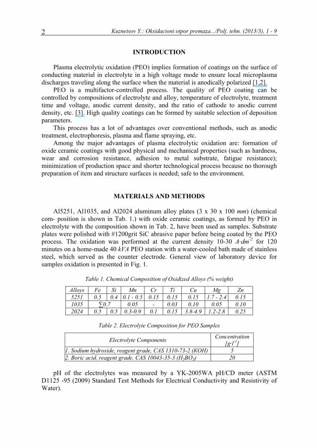
Al5251, Al1035, and Al2024 aluminum alloy plates (3 х 30 х 100 mm) (chemical com- position is shown in Tab. 1.) with oxide ceramic coatings, as formed by PEO in electrolyte with the composition shown in Tab. 2, have been used as samples. Substrate plates were polished with #1200grit SiC abrasive paper before being coated by the PEO process. The oxidation was performed at the current density 10-30 A·dm-2 for 120 minutes on a home-made 40 kVA PEO station with a water-cooled bath made of stainless steel, which served as the counter electrode. General view of laboratory device for samples oxidation is presented in Fig. 1.

Table 1. Chemical Composition of Oxidized Alloys (% weight)

Alloys Fe Si Mn Cr Ti Cu Mg Zn 5251 0.5 0.4 0.1 - 0.5 0.15 0.15 0.15 1.7 - 2.4 0.15 1035 ∑0.7 0.05 - 0.03 0.10 0.05 0.10 2024 0.5 0.5 0.3-0.9 0.1 0.15 3.8-4.9 1.2-2.8 0.25

Table 2. Electrolyte Composition for PEO Samples

Electrolyte Components Concentration [g·l-1]

1. Sodium hydroxide, reagent grade, CAS 1310-73-2 (КОН) 5 2. Boric acid, reagent grade, CAS 10043-35-3 (H3BO3) 20

рН of the electrolytes was measured by a YK-2005WA pH/CD meter (ASTM

D1125 -95 (2009) Standard Test Methods for Electrical Conductivity and Resistivity of Water).

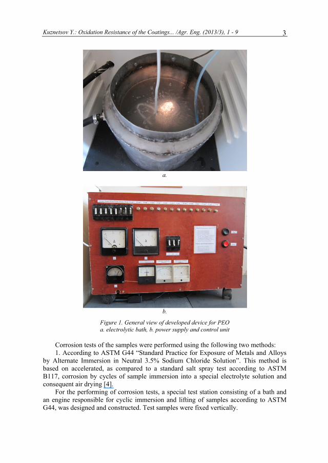
Kuznetsov Y.: Oxidation Resistance of the Coatings... /Agr. Eng. (2013/3), 1 - 9 3

a.

b.

Figure 1. General view of developed device for PEО a. electrolytic bath, b. power supply and control unit

Corrosion tests of the samples were performed using the following two methods: 1. According to ASTM G44 “Standard Practice for Exposure of Metals and Alloys

by Alternate Immersion in Neutral 3.5% Sodium Chloride Solution”. This method is based on accelerated, as compared to a standard salt spray test according to ASTM B117, corrosion by cycles of sample immersion into a special electrolyte solution and consequent air drying [4].

For the performing of corrosion tests, a special test station consisting of a bath and an engine responsible for cyclic immersion and lifting of samples according to ASTM G44, was designed and constructed. Test samples were fixed vertically.

Kuznetsov Y.: Oksidacioni otpor premaza.../Polj. tehn. (2013/3), 1 - 9 4

The salt solutions were prepared by dissolving 3.5 ± 0.1 weight parts of NaCl (rea-gent grade, CAS 7647-14-5) in 96.5 parts of water (distilled or deionized water, reagent grade, ASTM 1193, type IV). The volume of the electrolyte solution in the bath was regulated in such a manner that at least 32 ml of the electrolyte were taken per 1 cm2 of the total surface area of a sample.

Total duration of tests was 240 hours, with the electrolyte temperature of 18-20°С. Samples have been immersed in the solution for 10 minutes and then dried on air for 50 minutes.

On completion of tests, samples were rinsed by a jet of tap water and then by distill-ed water. Solid corrosion products were removed from the surface by mechanical and chemical means which were not affecting evaluation of test results as per ASTM G44.

Corrosion parameters were assessed in terms of mass loss per unit of surface area (g·m-2) according to Eq. 1.

поSттт 10 −=Δ (1)

where: Δm [g·m-2] - mass loss per unit of surface area, m0 [g] - mass of the sample before tests, m1 [g] - mass of the sample after tests and removal of corrosion products, Sпо [m2] - sample surface area. Corrosion rate was determined according to Eq. 2.

,corcor

mKtΔ

= (2)

where: Kcor [g·m-2·year-1] - corrosion rate, tcor [years] - test duration. Experimental device presented in Fig. 2 is used for carrying out corrosion tests. Samples were weighed on ViBRA AF-220E analytical balance. 2. Potentiodynamic polarization tests were performed on Autolab PGSTAT12 Potentiostat – Galvanostat controlled by General Purpose Electrochemical System – GPES 4.9 software in a standard corrosion cell. Tests were performed

according to ASTM G 59 Standard Test Method for Conducting Potentiodynamic Polarization Resistance.

The potentiodynamic polarization tests were carried out in 3.5 wt.% NaCl, and the solution was prepared using analytical grade reagents. A three-electrode cell with a specimen as a working electrode, saturated calomel electrode (SCE) as a reference electrode and stainless steel plate as a counter electrode was employed. Linear Sweep Voltammetry procedure was used for each specimen so that the sweeping rate was 1 mV/s and the scanning range was from about −250 mV to +250 mV vs. the open circuit potential. The tested area was 1 cm2, with the remaining surface masked by a lacquer. The Tafel Extension Method was used to measure corrosion current densities, corrosion potential and corrosion rates.

Kuznetsov Y.: Oxidation Resistance of the Coatings... /Agr. Eng. (2013/3), 1 - 9 5

Figure 2. Experimental device for carrying out corrosion tests at intermittent immersion:

1. bath, 2. Samples, 3. balance

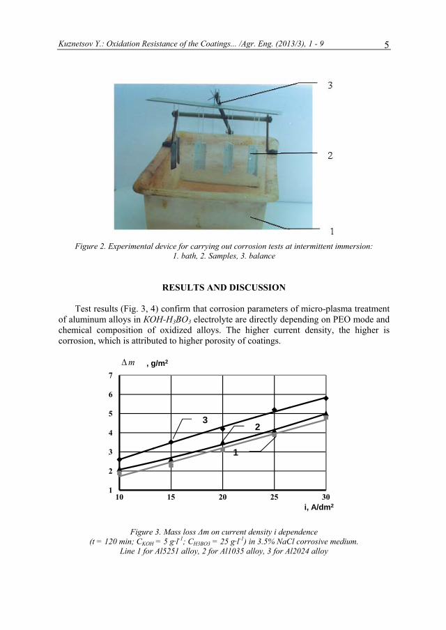
RESULTS AND DISCUSSION

Test results (Fig. 3, 4) confirm that corrosion parameters of micro-plasma treatment of aluminum alloys in КОН-Н3ВО3 electrolyte are directly depending on PEO mode and chemical composition of oxidized alloys. The higher current density, the higher is corrosion, which is attributed to higher porosity of coatings.

Figure 3. Mass loss Δm on current density i dependence

(t = 120 min; СKOH = 5 g·l-1; СH3BO3 = 25 g·l-1) in 3.5% NaCl corrosive medium. Line 1 for Al5251 alloy, 2 for Al1035 alloy, 3 for Al2024 alloy

1

2

3

4

5

6

7

10 15 20 25 30

, g/m2

i, A/dm2

mΔ

32

1

Kuznetsov Y.: Oksidacioni otpor premaza.../Polj. tehn. (2013/3), 1 - 9 6

Figure 4. Corrosion rate Кcor vs. current density i dependence

(t = 120 min; СKOH = 5 g·l-1; СH3BO3 = 25 g·l-1) in 3.5% NaCl corrosive medium. Line 1 for Al5251 alloy, 2 for Al1035 alloy, 3 for Al2024 alloy.

It deserves to be noted that pacing corrosion is observed for current densities of 10-

20 А·dm-2, while only corrosion spots are observed for 20-30 А·dm-2. This should be attributed to corrosive medium penetrating through the pores to induce corrosion beneath the coating. Coatings are destroyed due to the presence of chlorine ions, since because of their small radius [5] they are capable of penetrating inside the coatings and destroy those. The interaction between the coating and corrosive medium results in adsorption of medium surfactants. Chlorine ions are capable of expelling oxygen out of crystalline Al2O3-containing coating, and the surface is therefore enriched with chlorine. Al2024 coatings are less corrosion resistant than those on Al5251 and Al1035. This is apparently due to the fact that the alloy contains copper which intensifies corrosion. Magnesium and silicon presence in oxidized alloys results in reduced number of through pores and reduced corrosion. This is attributed to formation of magnesium and silicon oxides with lower melting temperatures, as compared to aluminum oxide. Plasma electrolytic oxidation implies high temperatures, and magnesium and silicon oxides therefore more intensively melt and fill the pores, thereby improving protective properties.

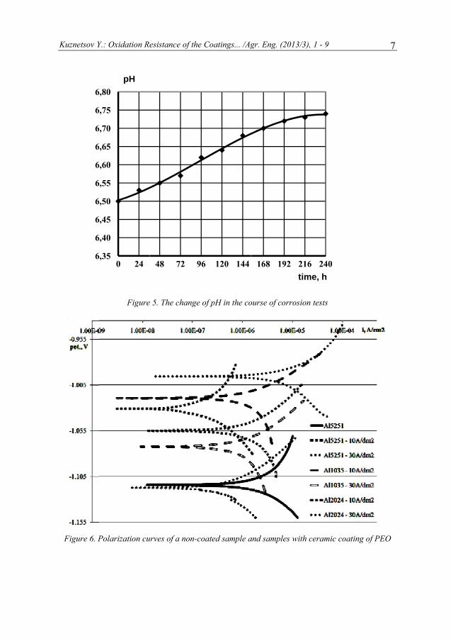
Intensity of the study process can be judged by рН changes in the corrosive medium. Research results are shown in Fig. 5.

Sodium hydroxide is formed due to chemical interaction between the coating and corrosive medium, which results in higher рН of the medium.

Fig. 6 shows polarization curves of a non-coated sample and samples with ceramic coating of PEO.

The Tafel Extension Method was used to measure corrosion current densities, corrosion potential and corrosion speeds. Results are shown in Tab. 3 [6, 7].

Kuznetsov Y

Figure 6. P

6

6

6

6

6

6

6

6

6

6

Y.: Oxidation Re

Figure

Polarization cu

6,35

6,40

6,45

6,50

6,55

6,60

6,65

6,70

6,75

6,80

0 24

pH

esistance of the

e 5. The change

urves of a non-c

48 72 9

e Coatings... /Ag

of рН in the co

coated sample a

96 120 144

gr. Eng. (2013/

ourse of corrosi

and samples wit

168 192 2t

/3), 1 - 9

ion tests

th ceramic coat

216 240ime, h

7

ting of PEO

Kuznetsov Y.: Oksidacioni otpor premaza.../Polj. tehn. (2013/3), 1 - 9 8

Table 3. Corrosion measurement of alloys aluminum without and with PEO

Unit Al5251 without PEO

Al1035 Al5251 Al2024 10A·dm-2 30A·dm-2 10A·dm-2 30A·dm-2 10A·dm-2 30A·dm-2

Corrosion current densities

[µA·cm-2] 15,99 2,66 1,68 0,93 0,98 3,77 4,30

Corrosion potential [V] - 1,126 -1,015 -1,072 -1,042 -1,118 -1,055 - 0,996

Polarization resistance [kOhm] 0,145 2,059 0,355 0,4815 1,418 6,654 1,175

Corrosion speed [µ/year] 230,0 2,9 3,0 9,5 14,8 48,5 89,1

CONCLUSION

Both tests of corrosion resistance of aluminum alloys clearly demonstrate that plasma electrolytic oxidation significantly improves corrosion resistance: depending on an alloy, corrosion rates of PEO coated samples are by the factor of 2.5-80 lower as compared with non-coated samples.

The higher current density, the higher is the porosity and the number of corroding cracks in the coating. Corrosion rate is linearly dependent on oxidation current density for all alloys studied. With the increasing content of non-oxidizable alloying ingredients (like copper in Al2024), coating contains more and more porous oxides with no protective properties. This is also associated with much lower corrosion resistance, as compared to dilute alloys.

BIBLIOGRAPHY

[1] Malyshev, V.N., Zorin, K.M. 2007. Features of microarc oxidation coatings formation technology in slurry electrolytes. Applied Surface Science 254 (2007), p.p. 1511–1516.

[2] Snizhko, L.O., Yerokhin, A.L., Pilkington, A., Gurevina, N.L., Misnyankin, D.O., Leyland, A., Matthews, A. 2004. Anodic processes in plasma electrolytic oxidation of aluminum in alkaline solutions. Electrochimica Acta 49 (2004), p.p. 2085–2095.

[3] Krysman, W., Kurze, P., Dittrich, H.G. 1984. Process characteristic and parameters of anodic oxidation by spark discharge. Crystal. Res. Technol. 19 (1984), p. 973.

[4] ASM Metal – Handbook, volume 13 – Corrosion, manual, etc. I. ASM International. Handbook Committee, 1987, ISBN 0-87170-007-7.

[5] Rosenfeld, I.L. 1970. Korrozia i Zashita Metallov (Corrosion and Protection of Metals) – М.: Metallurgia Publishing House, 1970, p. 237.

[6] Кuznetsov, Y, Kossenko, А, Lugovskoy, А. 2011. Studies on corrosion resistance of coatings formed by plasma electrolytic oxidation on aluminum alloys. The optimization of the composition, structure and properties of metals, oxides, composites, nano and amorphous materials. Tenth Israeli-Russian Bi-National Workshop 2011, Proceedings. Jerusalem, Israel, 2011. (307), p.p. 297-303.

Kuznetsov Y.: Oxidation Resistance of the Coatings... /Agr. Eng. (2013/3), 1 - 9 9

[7] Кuznetsov, Y. Corrosion testings of coatings being obtained by plasma electrolytics-oxidition. International Scientific Conference „Energy Efficiency and Agricultural Engineering“. International Comission Of Agricultural Engineering (CIGR), European Society of Agricultural Engineers (EurAgEng), Association of Agricultural Engineering in Southeastern Europe (AAESEE), Bulgarian National Society of Agricultural Engineers (BAER). May 17-18, 2013, Ruse, Bulgaria. Conference Proceedings. ISSN 1311-9974, p.p. 554-559.

OKSIDACIONI OTPOR PREMAZA NANETIH PLAZMA ELEKTROLITIČKOM OKSIDACIJOM

NA LEGURAMA ALUMINIJUMA

Yury Kuznetsov

Državni Poljoprivredni Univerzitet Orel, Fakultet za poljoprivredne i pogonske mašine, Katedra za tehnologiju konstruktivnih materijala i organizaciju tehničkog servisa,

Orel, Ruska Federacija

Sažetak: Plazma elektrolitička oksidacija (PEO) je jedan od novih metoda za dobijanje oksidno keramičkih premaza u tankim slojevima na elementima mašina različite namene, što značajno produžava njihov vek trajanja.

U ovom radu su izneti rezultati eksperimentalnih istraživanja otpora na koroziju oksidno keramičkih premaza nanetih pomoću PEO na različite aluminijumske legure upotrebom elektrolita КОН-Н3ВО3.

Testovi korozije na uzorcima su izvođeni upotrebom sledeće dve metode: 1. Prema ASTM G44 “Standardna praksa za izlaganje metala i legura alternativnim

potapanjem u neutralni 3.5% rastvor natrijum hlorida”, 2. Testovi polarizacije. Oba testa otpornosti na koroziju aluminijumskih legura jasno su pokazala da plazma

elektrolitička oksidacija značajno poboljšava otpornost na koroziju: zavisno od legure, stepeni korozije PEO zaštićenih uzoraka su 2.5-80 puta niži u poređenju sa uzorcima bez premaza.

Ključne reči: oksido-keramički premaz, plazma elektrolitička oksidacija, elektrolit, legura aluminijuma, korozivno sredstvo, polna kriva.

Prijavljen: Submitted: 13.06.2013.

Ispravljen: Revised: 17.06.2013.

Prihvaćen: Accepted: 18.07.2013.

Kuznetsov Y.: Oksidacioni otpor premaza.../Polj. tehn. (2013/3), 1 - 9 10

Univerzitet uPoljoprivredInstitut za pNaučni časoPOLJOPRIGodina XXXBroj 3, 2013Strane: 11 –

UDK: 620.9

OPTI

U

Abstracells modep-layers afhave been (c-Si) solaobtained mSi(p)/a-Si(pwafer. The(37.96 mAintroducingon crystalachieving care demon

Key w

Duringextraordinaglobal PV 1.5 TWp in

* Corre

u Beogradu dni fakultet oljoprivrednu teopis IVREDNA TEHNXVIII 3. – 18

91

IMIZATIOSILICON

Ve

University of RD

act: We used eling to determffect the electrcarried out on

ar cells and hmaximum solap+) solar celle open-circuit

A·cm-2), and thg thin layers oline silicon, conversion efstrated.

words: modelin

g the last twary growth, winstalled cap

n 2030 [2,11].

esponding autho

ehniku

NIKA

ON OF THEN HETERO

eliyana Zneliy

Ruse, Faculty oDepartment of

the AFORS-mine how the rical parameten hetero-junctihetero-junctioar energy conls with a bact voltage (VOhe fill factor of intrinsic andand by optim

fficiencies ove

ng, simulation

IN

wo decades thwith an averapacities of 10.

or. E-mail: KSh

E ELECTROJUNCTIO

yazova, Kras

of Electrical Ef Electronics,

-HET simulatthickness and

ers and the deion (HJ) amorn solar cells

nversion efficick surface fieOC) (728.3 mV(FF) (82.06%d doped amormizing the ther 20% and cu

n, hetero-junct

TRODUCTI

he solar photoage growth ra02 GW at the

htereva@ecs.un

Institute

AGRIC

RICAL PARON SOLAR

simira Shtere

Engineering aRuse, Bulgari

ion program d material proevice performrphous siliconwith intrinsi

iency is 22.68ld (BSF) con

V), short circu%) of the solarphous hydroghickness of turrent densitie

tion solar cell,

ON

ovoltaic (PV) tes exceedingend of 2012

ni-ruse.bg

UniversityFaculty o

e of Agricultural Scie

CULTURAL ENY

OriginalnOriginal sci

RAMETERR CELLS

eva*

and Automatioia

for hetero-junoperties of the

mance. Simulatn (a-Si)/crystalc thin layer 8% for a-Si (nntact on a p-tuit current dear cells are imgenated siliconthe layers. Pos higher than

l, efficiency.

industry hasg 40% per ye are expected

y of Belgrade of Agriculture

Engineering ntific Journal

NGINEERING Year XXXVIII No. 3, 2013. pp: 11 – 18

ni naučni rad ientific paper

RS OF

on,

nction solar e n-, i-, and tion studies lline silicon (HIT). The n)/a-Si(i)/c-type silicon ensity (JSC) mproved by n, deposited otential for 35 mA·cm-2

s shown an ear [1]. The d to exceed

Zneliyazova V., et al.: Optimizacija električnih parametara.../ Polj. tehn. (2013/3), 11 - 18 12

The wafer-based silicon technology maintains its leading position and the highest market share of around 80%, because of: (i) the technology maturity, which provides a reliable product with commercial module efficiencies ranging from 12 to 20%, and (ii) the existing manufacturing capacities [1,3].

The new generation thin film PV technologies have emerged as a response to the shortage of silicon feedstock and in order to reduce the material use per Wp. Their market share increased more than 3 times (from 6% to16-20%) for the period from 2005 through 2010 [1]. The research efforts have been focused on the development of the solar cells based on hydrogenised amorphous silicon (a-Si:H), copper indium gallium diselenide (CIGS) and cadmium telluride (CdTe). Among the advantages of these technologies are the usage of less material, a monolithically integrated cell, lower cost and large area. However, the reported module efficiency (η) of a-Si (6÷10%), CdTe (10.9%) and CIGS (9.5%), are lower than those of crystalline silicon (c-Si) modules [3-5]. Silicon hetero-junction solar cells (SHJ) and hetero-junction solar cells with intrinsic thin layer (HIT), are a promising hybrid amorphous silicon (a-Si)/crystalline silicon (c-Si) technology developed by Sanyo. As a response to rapidly growing demand, the company increased the production capacity of HIT solar cells more than 3 times for the period from 2006 through 2010, to 600 MW [6]. The HIT solar cells became very attractive due to a unique conversion efficiency (higher than 22% in laboratory cells and 20% in commercially produced cells) combined with a low temperature device processing [7,12]. Compared to conventional diffused solar cells, HIT solar cells have a higher open-circuit voltage (VOC) and a better temperature coefficient due to the reduced carrier recombination at the interface.

Numerical simulations are an important tool for gaining a better insight in material properties and processes in solar cells and hence, for the improvement of the devices. The large numbers of variables that influence the solar cell performance, such as the thickness of the layers and their physical parameters (density of states, a band gap, carrier concentration and mobilities) make it difficult, and economically ineffective to evaluate experimentally the effects of each variable on the cells characteristics. We have employed the numerical program, AFORS-HET v.2.4.1 to investigate the influence of the structure and the material parameters on the solar cell performance. Our previous research showed that an efficiency of 21.63% can be obtained by optimizing of the n-emitter layer thickness of the hetero-junction a-Si/c-Si solar cell [8].

In this paper, we present the numerical simulation study of hetero-junction cells (a-Si(n)/c-Si(p)), hetero-junction cells with intrinsic thin layer (a-Si(n)/a-Si(i)/c-Si(p)) and hetero-junction cells with intrinsic thin layer and back surface field (BSF) layer (a-Si(n)/a-Si(i)/c-Si(p)/a-Si(p+)), using the software AFORS-HET. The simulations were used to optimize the thickness of the n-, i-, and p-layers and thereby to increase the solar cells efficiency.

MATERIAL AND NUMERICAL SIMULATION METHODOLOGY

Solar Cell Structures Numerical simulation of a-Si/c-Si hetero-junction solar cells was carried out by

AFORS-HET, version 2.4.1, computer software with the aim to investigate the effects of

Zneliyazova V., et al.: Optimization of the Electrical.../Agr. Eng. (2013/3), 11 - 18 13

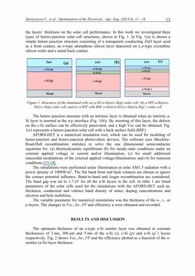
the layers’ thickness on the solar cell performance. In this work we investigated three types of hetero-junction solar cell structures, shown in Fig. 1. In Fig. 1(a) is shown a simple hetero-junction structure consisting of a transparent conducting ZnO layer used as a front contact, an n-type amorphous silicon layer deposited on a p-type crystalline silicon wafer and a metal back contact.

Figure 1. Structures of the simulated cells (a) a HJ a-Si(n)/c-Si(p) solar cell; (b) a HIT a-Si(n)/a-

Si(i)/c-Si(p) solar cell, and (c) a HIT with BSF a-Si(n)/a-Si(i)/c-Si(p)/a-Si(p+) solar cell

The hetero-junction structure with an intrinsic layer is obtained when an intrinsic a-Si layer is inserted at the n/p interface (Fig. 1(b)). By inserting of this layer, the defects on the c-Si surface can be effectively passivated, and a high Voc can be obtained. Fig. 1(c) represents a hetero-junction solar cell with a back surface field (BSF).

AFORS-HET is a numerical simulation tool, which can be used for modeling of homo-junction and hetero-junction photovoltaic devices. The software uses Shockley-Read-Hall recombination statistics to solve the one dimensional semiconductor equations for: (a) thermodynamic equilibrium (b) for steady-state conditions under an external applied voltage or current and/or illumination; (c) for small additional sinusoidal modulations of the external applied voltage/illumination; and (4) for transient conditions [13,14].

The simulations were performed under illumination at solar AM1.5 radiation with a power density of 1000W/m2. The flat band front and back contacts are chosen to ignore the contact potential influence. Band-to-band and Auger recombination are considered. The band gap was set to 1.7 eV for all the a-Si layers in the cell. In table 1 are listed parameters of the solar cells used for the simulations with the AFORS-HET such as, thickness, conduction and valence band density of states, doping concentrations and electron and hole mobilities.

The variable parameter for numerical simulations was the thickness of the n-, i-, or p-layers. The changes in Voc, Jsc, FF and efficiency η were obtained and recorded.

RESULTS AND DISCUSSION

The optimum thickness of an n-type a-Si emitter layer was obtained at constant thicknesses of 3 nm, 300 μm and 5 nm of the a-Si (i), c-Si (p) and a-Si (p+) layers respectively. Fig. 2 shows Voc, Jsc, FF and the efficiency plotted as a function of the n-emitter (a-Si) layer thickness.

Zneliyazova V., et al.: Optimizacija električnih parametara.../ Polj. tehn. (2013/3), 11 - 18 14

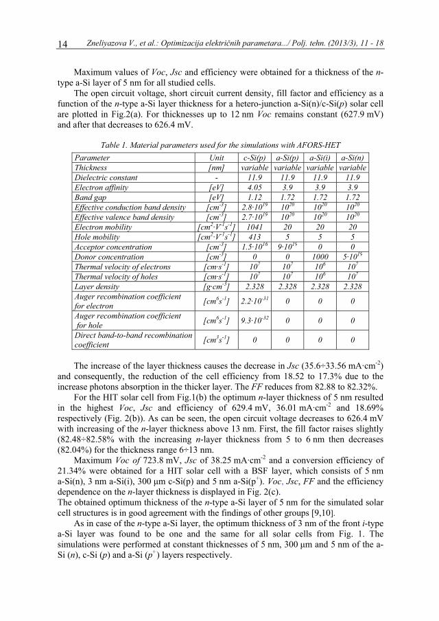
Maximum values of Voc, Jsc and efficiency were obtained for a thickness of the n-type a-Si layer of 5 nm for all studied cells.

The open circuit voltage, short circuit current density, fill factor and efficiency as a function of the n-type a-Si layer thickness for a hetero-junction a-Si(n)/c-Si(p) solar cell are plotted in Fig.2(a). For thicknesses up to 12 nm Voc remains constant (627.9 mV) and after that decreases to 626.4 mV.

Table 1. Material parameters used for the simulations with AFORS-HET

Parameter Unit c-Si(p) a-Si(p) a-Si(i) a-Si(n) Thickness [nm] variable variable variable variable Dielectric constant - 11.9 11.9 11.9 11.9 Electron affinity [eV] 4.05 3.9 3.9 3.9 Band gap [eV] 1.12 1.72 1.72 1.72 Effective conduction band density [cm-3] 2.8·1019 1020 1020 1020 Effective valence band density [cm-3] 2.7·1019 1020 1020 1020 Electron mobility [cm2·V-1s-1] 1041 20 20 20 Hole mobility [cm2·V-1s-1] 413 5 5 5 Acceptor concentration [cm-3] 1.5·1016 9·1019 0 0 Donor concentration [cm-3] 0 0 1000 5·1019 Thermal velocity of electrons [cm·s-1] 107 107 106 107 Thermal velocity of holes [cm·s-1] 107 107 106 107 Layer density [g·cm-3] 2.328 2.328 2.328 2.328 Auger recombination coefficient for electron [cm6s-1] 2.2·10-31 0 0 0

Auger recombination coefficient for hole [cm6s-1] 9.3·10-32 0 0 0

Direct band-to-band recombination coefficient [cm3s-1] 0 0 0 0

The increase of the layer thickness causes the decrease in Jsc (35.6÷33.56 mA·cm-2)

and consequently, the reduction of the cell efficiency from 18.52 to 17.3% due to the increase photons absorption in the thicker layer. The FF reduces from 82.88 to 82.32%.

For the HIT solar cell from Fig.1(b) the optimum n-layer thickness of 5 nm resulted in the highest Voc, Jsc and efficiency of 629.4 mV, 36.01 mA·cm-2 and 18.69% respectively (Fig. 2(b)). As can be seen, the open circuit voltage decreases to 626.4 mV with increasing of the n-layer thickness above 13 nm. First, the fill factor raises slightly (82.48÷82.58% with the increasing n-layer thickness from 5 to 6 nm then decreases (82.04%) for the thickness range 6÷13 nm.

Maximum Voc of 723.8 mV, Jsc of 38.25 mA·cm-2 and a conversion efficiency of 21.34% were obtained for a HIT solar cell with a BSF layer, which consists of 5 nm a-Si(n), 3 nm a-Si(i), 300 μm c-Si(p) and 5 nm a-Si(p+). Voc, Jsc, FF and the efficiency dependence on the n-layer thickness is displayed in Fig. 2(c). The obtained optimum thickness of the n-type a-Si layer of 5 nm for the simulated solar cell structures is in good agreement with the findings of other groups [9,10].

As in case of the n-type a-Si layer, the optimum thickness of 3 nm of the front i-type a-Si layer was found to be one and the same for all solar cells from Fig. 1. The simulations were performed at constant thicknesses of 5 nm, 300 μm and 5 nm of the a-Si (n), c-Si (p) and a-Si (p+) layers respectively.

Zneliyazova V., et al.: Optimization of the Electrical.../Agr. Eng. (2013/3), 11 - 18 15

The optimum thickness of the p-type c-Si wafer varies, depending on the solar cell structure. Maximum conversion efficiency of 22.68% (Voc of 728.3 mV, Jsc of 37.25 mA·cm-2 and FF of 82.06%) were obtained for a HIT solar cell with a BSF layer and a wafer thickness of 250 μm.

4 6 8 10 12 1417

18

19

Emitter thickness [nm]

Effic

ienc

y [%

]

(d)

82,4

82,6

82,8

FF [%

]

33

34

35

36

J SC [m

A/c

m2 ]

626

627

628

629a-Si(n)/c-Si (p)

V OC [m

V]

4 6 8 10 12 1417

18

19

Emitter thickness [nm]

Effic

ienc

y [%

]

(b)

82,2

82,4

82,6

FF

[%]

3334353637

J SC [m

A/c

m2 ] 626

628

630a-Si(n)/a-Si(i)/c-Si (p)

V OC[m

V]

a. b.

4 6 8 10 12 14

20,3820,7621,0421,34

Emitter thickness [nm]

Effic

ienc

y [%

]

(a)

77,0777,0877,0977,22

FF [%

]

36,5337,2237,7238,25

J SC [m

A/c

m2]

722,4

723,8

a-Si(n)/a-Si(i)/c-Si (p/a-Si(p+)

V OC [m

V]

c.

Figure 2. Dependence of VOC, JSC, FF and efficiency on the n-emitter layer thickness for: a. a HJ a-Si(n)/c-Si(p) solar cell; b. a HIT a-Si(n)/a-Si(i)/c-Si(p) solar cell;

c. a HIT with BSF a-Si(n)/a-Si(i)/c-Si(p)/a-Si(p+) solar cell

The conversion efficiency as a function of the thickness of the p-type c-Si wafer for a HJ a-Si(n)/c-Si(p) solar cell, a HIT a-Si(n)/a-Si(i)/c-Si(p) solar cell, and a HIT with BSF

Zneliyazova V., et al.: Optimizacija električnih parametara.../ Polj. tehn. (2013/3), 11 - 18 16

a-Si(n)/a-Si(i)/c-Si(p)/a-Si(p+) solar cell is plotted in Fig. 3(a). In Fig 3(b) are displayed plots of VOC as a function of the thickness of the p-type c-Si wafer for three solar cell structures.

50 100 150 200 250 300

14

16

18

20

22

24

Effic

ienc

y [%

]

p-type c-Si thickness [nm]

a-Si(n)/a-Si(i)/c-Si(p)/a-Si(p+) a-Si(n)/a-Si(i)/c-Si(p) a-Si(n)/c-Si(p)

(a)

50 100 150 200 250 300

600

650

700

750

800

V OC [m

V]p-type c-Si thickness [nm]

a-Si(n)/a-Si(i)/c-Si(p)/a-Si(p+) a-Si(n)/a-Si(i)/c-Si(p) a-Si(n)/c-Si(p)

(b)

a. b.

Figure 3. a. Conversion efficiency as a function of the thickness of the p-type c-Si wafer b. Open circuit voltage VOC as a function of the thickness of the p-type c-Si wafer

Although, the surface defects can be passivated by the deposition of a thin (3 nm) i-type

layer on the front side of the c-Si wafer, it does not have a significant impact on the cell parameters (Fig. 3). Оn contrary, the deposition of a BSF layer strongly affected these parameters (Fig. 3). Some authors [10] attributed the influence of the p+-type BSF layer on the solar cell parameters to the formation of a barrier for the opposite polarity charge carriers.

0,0 0,2 0,4 0,6 0,8 1,0

-1,6

-1,2

-0,8

-0,4

0,0

J SC [m

A/c

m2 ]

Voltage [V]

a-Si(n)/c-Si(p) a-Si(n)/a-Si(i)/c-Si(p)/a-Si(p+)

Figure 4. Current-voltage characteristics of a HJ a-Si(n)/c-Si(p) solar cell and a HIT

a-Si(n)/a-Si(i)/c-Si(p)/a-Si(p+) solar cell with a BSF layer

A plot of the short circuit current density as a function of the applied voltage is shown in Fig. 4 for two solar cells with optimized thicknesses of the layers building the structure, a HJ a-Si(n)/c-Si(p) solar cell and a HIT a-Si(n)/a-Si(i)/c-Si(p)/a-Si(p+) solar cell with a BSF layer. It is obvious that the introduction of the p+-type BSF layer improves the solar cell characteristics, resulting in higher values of Voc, Jsc, FF and the efficiency.

Zneliyazova V., et al.: Optimization of the Electrical.../Agr. Eng. (2013/3), 11 - 18 17

CONCLUSIONS

The AFORS-HET program was utilized for optimizing the thickness of the n-, i- and p-layers of a simple HJ solar cell (a-Si(n)/c-Si(p)), a HIT solar cell (a-Si(n)/a-Si(i)/c-Si(p)), and a HIT solar cell with BSF (a-Si(n)/a-Si(i)/c-Si(p)/a-Si(p+)) toward the aim to improve the device performance and to obtain a high efficiency solar cell.

The obtained optimum thicknesses of the n-type a-Si layer (5 nm) and of the t i-type a-Si layer (3 nm) were found to be one and the same for all studied solar cells. The optimum thickness of the p-type c-Si wafer varies, depending on the solar cell structure. Maximum conversion efficiency of 22.68% (Voc of 728.3 mV, Jsc of 37.25 mA·cm-2 and FF of 82.06%) were obtained for a HIT solar cell with a BSF layer and a wafer thickness of 250 μm.

It was found that although the surface defects can be passivated by the deposition of a 3 nm i-type layer on the front side of the c-Si wafer, it does not have a significant impact on the cell parameters. On contrary, the deposition of a BSF layer strongly affected these parameters due to maybe, the formation of a barrier for the opposite polarity charge carriers. The introduction of the p+-type BSF layer improves the solar cell characteristics, resulting in higher values of Voc, Jsc, FF and the efficiency.

BIBLIOGRAPHY

[1] Jager-Waldau, A. 2011. Quo Vadis photovoltaics, EPJ Photovoltaics, 2, 20801, 1-10. [2] Delbos, S. 2012. Kësterite thin films for photovoltaics: a review. EPJ Photovoltaics 3, 35004, 1-13. [3] Green, M.A., Emery, K., Hishikawa, Y., Warta, W. 2009. Solar Cell Efficiency Tables

(Version 33). Progress in Photovoltaics: Research and Application, 17, 85–94. [4] Radue, C., Dyk, E.E. 2007. Pre-deployment evaluation of amorphous silicon photovoltaic

modules. Solar Energy Materials & Solar Cells, 91, 129–136. [5] Shah, A., Meier, J., Buechel, A., Kroll, U., Steinhauser, J., Meillaud, F., Schade, H., Dominé,

D. 2006. Towards very low-cost mass production of thin-film silicon photovoltaic (PV) solar modules on glass. Thin Solid Films, 502, 292 – 299.

[6] Tsunomura, Y., Yoshimine, Y., Taguchi, M., Baba, T., Kinoshita, T., Kanno, H., Sakata, H., Maruyama, E., Tanaka, M. 2009. Twenty-two percent efficiency HITsolar cell. Solar Energy Materials & SolarCells, 93, 670–673.

[7] Como, N. H., Acevedo, A. M. 2010. Simulation of hetero-junction silicon solar cells with AMPS-1D. Solar Energy Materials & Solar Cells, 94, 62–67.

[8] Zheliyazova, V., Shtereva, K. 2013. Optimization of the Parameters of Solar Cells through Numerical Simulations, Proceedings of 5th conference on Energy Efficiency and Agricultural Engineering, 17-18 May 2013, Ruse, Bulgaria, 488-495.

[9] Schmidt, M., Korte, L., Laades, A., Stangl, R., Schubert, Ch., Angermann, H., Conrad, E., Maydell, K. 2007. Physical aspects of a-Si:H/c-Si hetero-junction solar cells. Thin Solid Films, 515, 7475–7480.

[10] Dwivedi, N., Kumar, S., Bisht, A., Patel, K., Sudhakar, S. 2013. Simulation approach for optimization of device structure and thickness of HIT solar cells to achieve ~27% efficiency. Solar Energy, 88, 31–41.

[11] European Photovoltaic Industry Association, Global Market Outlook for Photovoltaics 2013-2017. 2013. Available through: http://www.epia.org/news/publications/ [6 May 2013].

Zneliyazova V., et al.: Optimizacija električnih parametara.../ Polj. tehn. (2013/3), 11 - 18 18

[12] Levi, D., Iwaniczko, E., Page, M., Wang, Q., Branz, H., Wang, T. 2006. Silicon Heterojunction Solar Cell Characterization and Optimization Using In Situ and Ex Situ Spectroscopic Ellipsometry “Preprint”. 2006. Conference Paper NREL/CP-520-39932. Available through: www.nrel.gov/docs/fy06osti/39932.pdf [14 April 2013].

[13] Stangl, R., Geipel, T., Dubiel, M., Kriegel, M., El-Shater, Th., Lips, K. AFORS-HET 3.0: First Approach to a Two-Dimensional Simulation of Solar Cells. Available through: dubielnet.de/max/BachelorThesis/aforshetpaper.pdf [12 March 2013]

[14] Froitzheim, A., R. Stangl, L. Elstner, M. Kriegel, W. Fuhs, AFORS-HET: A Computer-Program for the Simulation of Heterojunc-Tion Solar Cells to be Distributed for Public Use. Available through: www.helmholtz-berlin.de/media/media/...HET/...het/published1.pdf. [12 March 2013].

OPTIMIZACIJA ELEKTRIČNIH PARAMETARA SILIKONSKIH HETERO-SPOJNIH SOLARNIH ĆELIJA

Veliyana Zneliyazova, Krasimira Shtereva

Univerzitet Ruse, Fakultet za elektrotehniku i automatizaciju,

Institut za elektroniku, Ruse, Bugarska

Sažetak: Program za simulaciju AFORS-HET za modeliranje hetero-spojnih solarnih ćelija upotrebljen je za određivanje uticaja debljine i karakteristika materijala n-, i-, i p-slojeva na električne parametre i karakteristike uređaja. Simulacije su izvođene na hetero-spojnim (HJ) solarnim ćelijama od amorfnog silikona (a-Si)/kristalnog silikona (c-Si) i hetero-spojnim solarnim ćelijama sa intrinsičnim slojem (HIT). Postignuta je maksimalna efikasnost konverzije sunčeve energije od 22.68% za a-Si (n)/a-Si(i)/c-Si(p)/a-Si(p+) solarne ćelije sa zadnjim površinskim (BSF) kontaktom na p-tipu silikonske obloge. Napon otvorenog kola od (VOC) (728.3 mV), gustina struje kratkog kola (JSC) (37.96 mA·cm-2) i faktor punjenja (FF) (82.06%) solarnih ćelija su unapređeni uvođenjem tankih slojeva intrinsičnog i obogaćenog amorfnog hidrogenizovanog silikona, deponovanog na kristalnom silikonu i optimizacijom debljine slojeva. Predstavljen je potencijal za postizanje efikasnosti konverzije veće od 20% i gustine struje veće od 35 mA·cm-2.

Ključne reči: modeliranje, simulacija, hetero-spojna solarna ćelija, efikasnost.

Prijavljen: Submitted: 13.06.2013.

Ispravljen: Revised:

Prihvaćen: Accepted: 24.07.2013.

Univerzitet uPoljoprivredInstitut za pNaučni časoPOLJOPRIGodina XXXBroj 3, 2013Strane: 19 –

UDK: 631.3

PR

Pra

Cent

Abstrabalanced, o/aqua farmmanufactudevelopmereason forestablishmjustificatioidea througcapital (rate of retuevaluated, requiremenvariant 03 All these 0for appropr

Key weconomic v

* Corre

u Beogradu dni fakultet oljoprivrednu teopis IVREDNA TEHNXVIII 3. – 26

3

CORODUCTIO

akash Prabha

tral Institute o

act: A pelletoptimally pro

ming may beuring technoloent of feed pr wanting to

ment of feed mon of manufacgh determinat), breakeven

urn (IRR in pvariant No.

nt under mixand 04 for so

04 productionriate selection

words: livestovariability par

esponding autho

ehniku

NIKA

OMPARATON VARIA

akar Ambalk

of AgriculturaBh

tized feed processed, cost ae adapted as ogy may be

production unachieve such

manufacturing cturing of feeion of econompoint (month)er cent). Four

01 and 02 xed / integratolely dairy feen variants havn on capacity u

ock-aqua feedrameters, com

or. E-mail: ppa_

TIVE EVALANTS OF A

kar*, Praveen

al Engineeringhopal, MP, Ind

roduction uniand time effec

a potential e commercianit accordinglh an objectivunit. The feed

ed productionmic variables o), payback perr different pelare specifica

ed farming (ed requiremene been presenutilization and

d, feed produmparative eval

_65@yahoo.co

Institute

AGRIC

LUATION ANIMAL F

n Chandra Ba

g, Technology dia

it to cater thctive availabibusiness entelized throughy established

ve is to warrad production

n volume by on productionriod (a), benelletized feed pally designed(livestock-cropnts have been nted as economd marketability

uction varianluation and IN

.in

UniversityFaculty o

e of Agricultural Scie

CULTURAL ENY

OriginalnOriginal sci

OF FEED PLA

argale, Jai Sin

Transfer Divi

he need of nlity of feed foerprise. The h modular d

d at CIAE, Bant investmeneconomy is anacceptance o

n variant such efit cost ratio aproduction vad for multicup-fish) combitaken into conmically viabley of the finish

nts, capacity NR.

y of Belgrade of Agriculture

Engineering ntific Journal

NGINEERING Year XXXVIII No. 3, 2013. pp: 19 – 26

ni naučni rad ientific paper

ANT

ngh

ision,

nutritionally or livestock feed pellet

design and Bhopal. The nt made in nalyzed the f profitable as working

and internal ariants were ultural feed ination and nsideration. e enterprise hed feed.

utilization,

Ambalkar P.P., et al.: Uporedna procena proizvodnih.../Polj. tehn. (2013/3), 19 - 26 20

INTRODUCTION

Farmers now realized maintaining of quality animals with appropriate feeding is vital to meet increased domestic and export demand of livestock / aqua products. The proportion of crossbred / improved breeds of animals has necessitated higher demand for nutritionally balanced and optimally processed feed. The kind of quality feed availability at cost and time effective scale would be the pre-requisite for sustainability of livestock and aquaculture enterprises in the region.

Further, to ensure quality and time effective feed production, the primary goal is to be very particular into the production and marketability aspects. Hence, the primary objective of feed formulation, processing and production is to provide livestock breeds and fish in particular with quality feed having sufficient nutritional balance, efficacy, digestibility, palatability, acceptability, storability, handling and ease of transport [6].

In this regard, an aqua (multipurpose) feed production pilot plant has been established at Central Institute of Agricultural Engineering, Bhopal, India producing aqua, poultry and cattle processed feed. The scope of the CIAE livestock-aqua feed pilot plant had been further augmented in view of harnessing potential demand of multicultural activities (livestock-crop-fish) combination for production of feed for aquatic, avian / ovine and bovine farming [7].

Therefore, the plant is considered to be the best fit design for promotion and development of integrated farming (agriculture-animal husbandry-aquaculture-rural industries) activities. In this paper, under the comparative evaluation of feed plant variants, the variant No.01 is considered as CIAE livestock-aqua feed production unit [1].

However, other feed production variant, such as variant No. 02 or other may be opted on the basis of scale-up and downsizing of CIAE, Bhopal feed plant respectively for facilitating and encouraging multicultural (integrated agricultural-animal husbandry- aquaculture) activities. However, in many regions within the country and outside, wherein only dairy enterprise is feasible due to socio-economic impact [5], the exclusive establishment of dairy feed production unit is found to be better judgmental from sustainability and profitability view point for all stakeholders.

Consequent upon, exclusive installation of dairy feed production unit, elimination of some of the unit operation machinery and its accessories (viz. water container for steam, water supply arrangement for steam generation, steam generator, water softener, steam conditioner, steam valve and steam supply line, hot water jacket in paddle mixer conveyor unit, pellet crumbler unit and small configuration pellet dies for pellet diameter varies from 3-4 mm) would result in substantial cost reduction on dairy feed production. The basis for selection of particular feed production plant design is required to be finalized both on techno-economic feasibility scale as well as on socio and ecological parameters [4] if scale of benefit is to be visualized.

MATERIAL AND METHODS

It is based on demand forecasting analysis dairy and poultry, dairy and aquaculture as well as dairy, poultry and aquaculture (integrated farming) the feed production variant No.1 and No.2 may be installed and commissioned. Further, dairy alone is also one of

Ambalkar P.P., et al.: Comparative Evaluation.../Agr. Eng. (2013/3), 19 - 26 21

the activities, in which India has the distinction of evolving new technologies on one hand and successfully adapting the promising technologies on the other. Hence, dairy has enough potential to initiate feed production unit establishment at the cottage or small level of enterprise [2]. Therefore, solely for catering pelletized feed requirement for dairy enterprise variant No. 03 or 04 may be opted (Table 1).

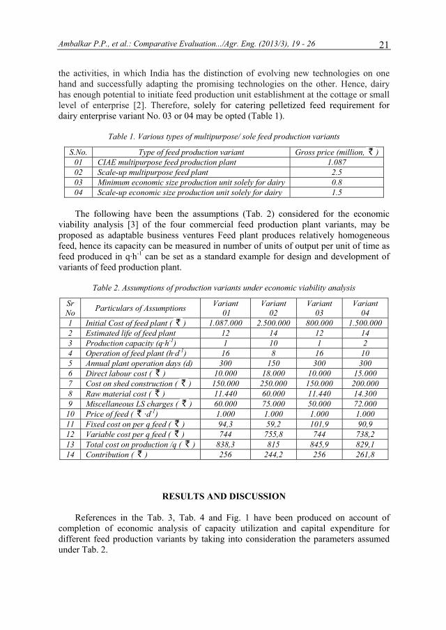
Table 1. Various types of multipurpose/ sole feed production variants

S.No. Type of feed production variant Gross price (million, ) 01 CIAE multipurpose feed production plant 1.087 02 Scale-up multipurpose feed plant 2.5 03 Minimum economic size production unit solely for dairy 0.8 04 Scale-up economic size production unit solely for dairy 1.5

The following have been the assumptions (Tab. 2) considered for the economic

viability analysis [3] of the four commercial feed production plant variants, may be proposed as adaptable business ventures Feed plant produces relatively homogeneous feed, hence its capacity can be measured in number of units of output per unit of time as feed produced in q·h-1 can be set as a standard example for design and development of variants of feed production plant.

Table 2. Assumptions of production variants under economic viability analysis

Sr No Particulars of Assumptions Variant

01 Variant

02 Variant

03 Variant

04 1 Initial Cost of feed plant ( ) 1.087.000 2.500.000 800.000 1.500.000 2 Estimated life of feed plant 12 14 12 14 3 Production capacity (q·h-1) 1 10 1 2 4 Operation of feed plant (h·d-1) 16 8 16 10 5 Annual plant operation days (d) 300 150 300 300 6 Direct labour cost ( ) 10.000 18.000 10.000 15.000 7 Cost on shed construction ( ) 150.000 250.000 150.000 200.000 8 Raw material cost ( ) 11.440 60.000 11.440 14.300 9 Miscellaneous LS charges ( ) 60.000 75.000 50.000 72.000

10 Price of feed ( ·d-1) 1.000 1.000 1.000 1.000 11 Fixed cost on per q feed ( ) 94,3 59,2 101,9 90,9 12 Variable cost per q feed ( ) 744 755,8 744 738,2 13 Total cost on production /q ( ) 838,3 815 845,9 829,1 14 Contribution ( ) 256 244,2 256 261,8

RESULTS AND DISCUSSION

References in the Tab. 3, Tab. 4 and Fig. 1 have been produced on account of completion of economic analysis of capacity utilization and capital expenditure for different feed production variants by taking into consideration the parameters assumed under Tab. 2.

Ambalkar P.P., et al.: Uporedna procena proizvodnih.../Polj. tehn. (2013/3), 19 - 26 22

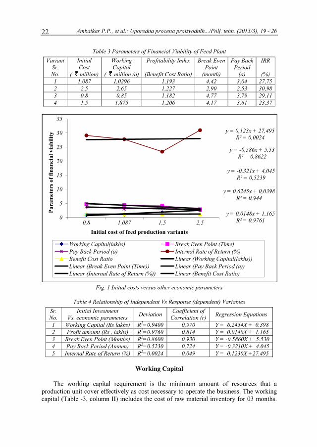
Table 3 Parameters of Financial Viability of Feed Plant Variant

Sr. No.

Initial Cost

( million)

Working Capital

( million /a)

Profitability Index

(Benefit Cost Ratio)

Break EvenPoint

(month)

Pay Back Period

(a)

IRR

(%) 1 1,087 1,0296 1,193 4,42 3,04 27,75 2 2,5 2,65 1,227 2,90 2,53 30,98 3 0,8 0,85 1,182 4,77 3,79 29,11 4 1,5 1,875 1,206 4,17 3,61 23,37

Fig. 1 Initial costs versus other economic parameters

Table 4 Relationship of Independent Vs Response (dependent) Variables

Sr. No.

Initial Investment Vs. economic parameters Deviation Coefficient of

Correlation (r) Regression Equations

1 Working Capital (Rs lakhs) R2=0.9400 0,970 Y = 6.2454X + 0.398 2 Profit amount (Rs , lakhs) R2=0.9760 0,814 Y = 0.0140X + 1.165 3 Break Even Point (Months) R2=0.8600 0,930 Y = -0.5860X + 5.530 4 Pay Back Period (Annum) R2=0.5230 0,724 Y = -0.3210X + 4.045 5 Internal Rate of Return (%) R2=0.0024 0,049 Y = 0.1230X +27.495

Working Capital

The working capital requirement is the minimum amount of resources that a

production unit cover effectively as cost necessary to operate the business. The working capital (Table -3, column II) includes the cost of raw material inventory for 03 months.

y = 0,6245x + 0,0398R² = 0,944

y = -0,586x + 5,53R² = 0,8622

y = -0,321x + 4,045R² = 0,5239

y = 0,123x + 27,495R² = 0,0024

y = 0,0148x + 1,165R² = 0,97610

5

10

15

20

25

30

35

0,8 1,087 1,5 2,5

Para

met

ers o

f fin

anci

al v

iabi

lity

Initial cost of feed production variants

Working Capital(lakhs) Break Even Point (Time)Pay Back Period (a) Internal Rate of Return (%)Benefit Cost Ratio Linear (Working Capital(lakhs))Linear (Break Even Point (Time)) Linear (Pay Back Period (a))Linear (Internal Rate of Return (%)) Linear (Benefit Cost Ratio)

Ambalkar P.P., et al.: Comparative Evaluation.../Agr. Eng. (2013/3), 19 - 26 23

This has been the fixed amount that remains more or less permanently invested for ones as working capital in production unit. There has been excellent correlation of 0.94 exists with the initial cost of feed plant vs. working capital. It is higher the initial capital investment the greater would be the capacity to produce feed and ultimately more of the raw material and finished feed inventory would require to use into the plant operational system. However, for higher capacity plant the high working capital investment require assured market of quality processed feed. Many a times due to socio economic problems the total operational days of production unit may get drastically reduced.

Profitability Index (PI)

The profitability index (PI) or benefit cost ratio (BCR) (Eqt. 1) is an alternative way

of stating the net present value (NPV) help in choice of profitable feed plant variant pertaining to marketability. A shortcoming of BCRs is that, by definition, they ignore non-monetized impacts.

PI = Present Value of Cash Inflows / of Cash Outflows (1)

A profitability index of 1.0 means one has achieved exactly one’s set target of

sustainability of enterprise i.e. rate of return greater than 1.0 means one has exceeded one’s pre-set rate of return. It is most commonly used method for comparing economic alternatives. The objective is to determine whether the benefit (gained) in return to any cost (spent) is favorable.

The profitability index (Table 3 and column IV) varies from 1,193 (variant No.1), 1,227 (variant No. 2), 1,182 (variant No. 3) and 1,206 (variant No. 4). The profitability index reveals that variant 2 and variant 4 shows PI values more than 1,2 reflect that variants having maximum capacity utilization due to assured product utilization back-up farming practices would generate more income and benefit.

Break Even Points

Break-even is the point at which total revenue equals total costs (Eq. 2, 3 and 4). At

levels of output below the break-even point the business will be making a loss vice versa a profit. Due to its simplicity a new business will often have to present a breakeven analysis to its bank in order to get a loan. However, its disadvantage is that, it assumes that everything produced is sold; often not all output will be sold.

Contribution = Selling Price - Variable cost (2)

Break Even Point ( ) = (Fixed Costs X Sales) / (Contribution) (3)

Brake even Point Feed Sold (q) = Fixed Costs / Contribution per (q) (4)

It is from Tab. 3, the breakeven point of variant 02 (Table 3 column (V)) have the

least value i.e. 2.90 indicates that opportunity exists for encouraging investment if forward, backward and sideway linkages are well facilitated (i.e. vertical and horizontal integration of feed production unit) to sustain in the production catchment.

Ambalkar P.P., et al.: Uporedna procena proizvodnih.../Polj. tehn. (2013/3), 19 - 26 24

Pay Back Period

Payback period is simple to compute (Eq. 5), provides some information on the risk of the investment and provides a crude measure of liquidity. It does not indicate any concrete decision criteria to understand whether an investment increases the feed production firm's value. However, as a drawback, it provides no measure of profitability.

Pay Back Period = No. of preceding years before final recovery + (Balance recoverable amount / cash flow during the year of final

recovery) (5)

The payback period (Table 3, column (VI)) payback period is least and second to

the least i.e. 2.53 a and 3.04 a for variant 2 and variant 1 respectively, point out that sustainability and profitability of multicultural activities are always beneficial for on farm management of agriculture-aquaculture-animal husbandry-agro-industrial activities to encourage for sustainability for growing human population requirement.

Internal Rate of Return

The internal rate of return is a rate of return used in capital budgeting to measure

and compare the profitability of investments. It is considered to be very important economic parameter for investment viability factor analysis for variant selection. It is that rate which equates the present value of the future cash inflows with the cost of the investment which produces them. IRR calculates (Eq. 6) an alternative cost of capital including an appropriate risk premium. It takes into account the time value of money. The cost of capital if less than IRR then project proposal may be considered as an alternative for investment decision.

IRR = Lower rate of discount + (Net present value at lower rate of discount / Difference in present values at lower and higher discount

rates) X (Difference in two rates of discount) (6)

The internal rate of return IRR (table 3, column (VII)) is greatest and second to the

greatest are 30.98 % and 29.11 % for variant 2 and 3 respectively, point out that strong linkage under production-supply chain, would ultimately ensure higher IRR shall foresee encouraging economic returns. As per (Fig. 1) initial investment has excellent correlation with working capital, profitability index and breakeven point. However, there has been moderate correlation exist with payback period and poor correlation observed with initial investment versus internal rate of return (IRR) for all the variants investigated under optional studies.

CONCLUSIONS

Out of above four feed production variants, variant No. 01 and No. 02 may be opted for integrated agriculture-aquaculture-animal husbandry activities. The variant no. 01 may be opted for limited demand of feed. On the other hand, if sufficient feed demand is

Ambalkar P.P., et al.: Comparative Evaluation.../Agr. Eng. (2013/3), 19 - 26 25

available for sustainable multicultural activities (such as dairy, goat , poultry enterprise inclusive of aquaculture farms) then production variant No. 2 has maximum economic returns i.e. least time for breakeven point, payback period and high percentage of internal rate of return (IRR) and top most profitability index. The government subsidy and local economic impact may also be considered as crucial deciding factors for variant No. 01 and variant No. 02. While variant 3 or 4 may be opted solely for feed production for dairy enterprise. Therefore, reliable information about economic viability may emerge on appropriate capacity utilization of feed production unit.

In case if investor wants to play under safe game-plan by avoiding risks and also confined with limited investment potential for augmentation of feed business then the best idea would be to choose production variant no. 3 though herein breakeven point and payback period are little longer but internal rate of return is high in comparison to other variant 1 and 4. Variant No. 02 has ultimately least of working capital requirement, early payback period, greater internal rate of return, better profitability index than that of variant no.3.

The idea floated on account of economic analysis through application of parameters viz. Working Capital, Profitability Index (PI), Break Even Point (BEP), Pay Back Period (PBP), Internal Rate of Return (IRR), may either be implemented or rejected under the specific choice of alternative available for production variants may it be integrated farming/ mixed farming or eventually organized dairy development in unit way or under the cluster approach. Herein, the ultimate objective is to grow more nutritious food for growing human population. In this direction, establishment of unit like multipurpose feed production variant or exclusive dairy feed production unit based on maximum capacity utilization of available resources would prove to be a boon to generate sufficient scope for sustainable and profitable returns under agrarian economy.

BIBLIOGRAPHY

[1] Ambalkar, P.P., Singh, J., Bhandarkar, D.M. 2003. Techno-economic feasibility of feed plant in rural sector. 37th ISAE annual convention and symposium, January 29-31, 2003, MPUAT, Udaipur, India.

[2] Banerjee, G.D., Banerjee, S. 2004. Tea Industry – A Road Map Ahead. Abhijeet Publications, Delhi, pp-37-54.

[3] Koutsoyiannis, A,1979. Modern Microeconomics. The Macmillan Publication. London. [4] Olaloku, E.A. 1976. Milk production in West Africa: Objective and Research approaches.

Journal of the Association for the Advancement of Agricultural Sciences in Africa 3(1). p.p. 5-13.

[5] Pullan, N.B., Grindle, R.J. 1980. Productivity of white Fulani cattle on the Jos Plateau Nigeria. IV. Economic factors. Tropical Animal Health and Production. 12, p.p. 161-170.

[6] Sarkar, S.K. 2002. Freshwater Fish Culture - Volume 1- Integrated Fish Farming. Daya Publication, p.p. 247-260.

[7] Singh, J., Singh, G. 2001. Aqua Feed Plant Broacher, Central Institute of Agricultural Engineering, Nabibagh, Berasia Road, Bhopal,MP, India.

Ambalkar P.P., et al.: Uporedna procena proizvodnih.../Polj. tehn. (2013/3), 19 - 26 26

UPOREDNA PROCENA PROIZVODNIH VARIJANTI UREĐAJA ZA PROIZVODNJU KONCENTROVANE STOČNE HRANE

Prakash Prabhakar Ambalkar, Praveen Chandra Bargale, Jai Singh

Centralni institut za poljoprivrednu tehniku, Odsek za transfer tehnologija, Bhopal, MP, Indija

Sažetak: Uređaj za proizvodnju peletirane hrane koja zadovoljava potrebe za balansiranom ishranom, optimalnim preradom, troškovima i efikasnim iskorišćenjem vremena pri ishrani životinja / riba može se prilagoditi za profitabilnu proizvodnju. Tehnologija proizvodnje peletiranog hraniva može da se komercijalizuje modularnom konstrukcijom i razvojem uređaja za proizvodnju hraniva prema onom koji je razvijen u Centralnom institutu za poljoprivrednu tehniku u Bhopal-u u Indiji. Razlog za postizanje ovog cilja je sigurna investicija u razvoj uređaja za proizvodnju hraniva. Analizirana je ekonomska opravdanost proizvodnje određene količine hraniva prihvatanjem profitabilne ideje kroz određivanje ekonomskih promenljivih uticaja na proizvodnu varijantu, kao što su radni kapital ( ), tačka rentabilnosti (mesec), period otplate (a), odnos prihoda i troškova i interna stopa prinosa (IRR u procentima). Proučavane su četiri različite varijante proizvodnje peletirane hrane. Varijante br. 01 i 02 su posebno predviđene za višekomponentnu hranu kod mešovitog / integrisanog stočarstva (životinja-biljka-riba), a kombinacija varijanti 03 i 04 samo za ishranu muznih krava. Sve 4 varijante su predstavljen kao ekonomski održiva preduzeća za odgovarajući izbor kapaciteta i konkurentnosti finalnog proizvoda.

Ključne reči: stočna hrana, varijante proizvodnje hraniva, korišćenje kapaciteta, parametri ekonomske varijabilnosti, uporedna procena i INR.

Prijavljen: Submitted: 18.07.2013.

Ispravljen: Revised:

Prihvaćen: Accepted: 18.09.2013.

Univerzitet uPoljoprivredInstitut za pNaučni časoPOLJOPRIGodina XXBroj 3, 2013Strane: 27 –

UDK: 536.7

A SIMO

Chineny

1MichaeTec

2FederaTechno3Feder

Abstramodel for system in transfer oexperimenevaporativconsideredthat the cdifferent tvarious cdeterminedwide range

Key w

* Corre

u Beogradu dni fakultet oljoprivrednu teopis IVREDNA TEHNXVIII

3. – 39

7

MPLE MODOF A STOR

ye Ndukwu1*,

l Okpara Univchnology, Dep

al University ology, Departmral University

Technolo

act: This paexperimentala tropical c

of wide rannts have beenve cooler ded the thermalcooling pad temperature acooling efficd. In additione of temperat

words: evapora

esponding autho

ehniku

NIKA

DEL FOR ERAGE SPA

Seth Manuw

versity of Agrpartment of A

Umudikof Technologyment of Agricuof Technology

ogy, DepartmeAkure,

aper deals wl validation o

climate. It alnge of tempn performed esigned for l properties ois a plain pat the two suciency at din the values otures is also p

ative cooling,

or. Email: nduk

EVAPORAACE IN A T

wa2, Olawale O

riculture, Collegricultural an

ke, Abia State,y Akure, Schoultural Engine

gy Akure, Schoent of Food Sc Ondo State, N

ith the deveof the performso presentederatures basduring Janu

storage of of the materiorous wall b

urfaces. The pfferent rang

of the coefficpresented.

cooling pad,

kwumcu@gmai

Institute

AGRIC

ATIVE COOTROPICAL

Olukunle2, B

ege of Enginend Bio Resour Nigeria ol of Engineereering, Akure,

ool of Agricultcience and TeNigeria

elopment of mance of a smd the coefficised on existuary to Febrfruits and vial of the cobounded by predicted and

ge of inlet ient of conve

model equatio

l.com

UniversityFaculty o

e of Agricultural Scie

CULTURAL ENY

OriginalnOriginal sci

OLING SYL CLIMAT

Babatunde Ol

eering and Engrces Engineeri

ring and Engi, Ondo State, ture and Agricchnology,

a simple mamall evaporatiient of conveting model.

ruary 2013 fvegetables. Toling pad antwo convect

d experimentatemperature

ective heat tra

on, heat transf

y of Belgrade of Agriculture

Engineering ntific Journal

NGINEERING Year XXXVIII

No. 3, 2013. pp: 27 – 39

ni naučni rad ientific paper

YSTEM TE

uwalana3

gineering ing,

ineering Nigeria cultural

athematical ive cooling ective heat

Extensive for a small The model nd assumed tive airs at al value of

has been ansfer for a

fer

Ndukwu C., et al.: Model evaporativnog sistema.../Polj. tehn. (2013/3), 27 - 39

28

INTRODUCTION

The basic principle of evaporative cooling is cooling by evaporation. When water

evaporates, it draws energy from its surroundings, which produces a considerable cooling effect. Evaporative cooling occurs when air, that is not too humid, passes over a wet surface (humidifier). The movement of the air can be passive i.e. when the air flows naturally through the pads or active with fans or blowers. The driving force for heat and mass transfer between air and water is the temperature and partial vapor pressure differences. Water is the working fluid in evaporative cooling thus it is environmentally friendly [1]. Due to the low humidity of the incoming air some of the water evaporates. This evaporation causes two favorable changes: a drop in the dry-bulb temperature and a rise in the relative humidity of the air. This non-saturated air cooled by heat and mass transfer is forced through enlarged liquid water surface area for evaporation by utilizing blowers or fans. Some of the sensible heat of the air is transferred to the water and becomes latent heat by evaporating some of the water. The latent heat follows the water vapor and diffuses into the air. In a DEC (direct evaporative cooling), the heat and mass transferred between air and water decreases the air dry bulb temperature (DBT) and increases its humidity, keeping the enthalpy constant (adiabatic cooling) in an ideal process. However, 100% saturation is impossible for direct evaporative coolers due to two reasons [2]. Firstly, most of the pads are loosely packed or with cells, therefore the process air can easily escape between the pads without sufficient contact with the water. After water evaporates, it enters the air as water vapor and conveys the heat absorbed during evaporation back to the air in the form of latent heat. The effectiveness of this system is defined as the rate between the real decrease of the DBT and the maximum theoretical decrease that the DBT could have if the cooling were 100% efficient and the outlet air were [1]. Practically, wet porous materials or pads provide a large water surface in which the air moisture contact is achieved and the pad is wetted by dripping water onto the upper edge of vertically mounted pads. According to [1] experimental studies are reliable and convincible; but they are usually costly and too tasking. In addition, the experiment results were obtained under various testing conditions which are affected by the environmental conditions with given inlet parameters and the results may be different when testing conditions is changed. Modeling analysis of evaporative cooling system is essential to explain the heat and mass transfer process in evaporative cooling and to predict the process outputs at various conditions. Over the years a number of models have been developed to describe direct evaporative cooling systems, not supported with a heat exchanger. [3, 4, 5, 6]

Most of these models ignore the thermal properties of the cooling pad material which will definitely affect the temperature drop inside the cooling chamber no matter how small. The models consider the heat and mass transfer that occur at the surface of the pad but in actual fact the cooling pad is a plain porous wall with thickness. Also the heat and mass transfer is not only on the surface but across the thickness with the air at the outer surface at different temperature from the air at the inner surface. The paper presents a simple model for direct evaporative cooling, incorporating the thermal properties and the thickness of the material of the pad in the heat and mass transfer process in a tropical environment. It also presents wide range of heat transfer coefficient at the tested conditions.

Ndukwu C., et al.: A Simple Model for Evaporative.../Agr. Eng. (2013/3), 27 - 39

29

MATERIAL AND METHODS

Basic Mathematical Model

Model assumptions 1. The system is one dimensional. 2. The system is adiabatic. 3. The inside and the outside temperature of the air is different. 4. The two surfaces of the cooling pad are at different temperatures. 5. The cooling pad is surrounded by air at the two surfaces. 6. The heat transfer coefficient is different for the ambient air and the air bounding

the cooling pad on the inside the cooler. 7. The cooling pad is a plain porous wall bounded by two convective fluids (air) at

different temperatures. 8. The surface of the pad is completely wet. 9. The pad and the cold air inside are at the same temperature. 10. The water inlet and outlet temperature is the same. 11. The cooling pad is rigid.

Basic model equation On the assumption that the cooling pad is a plain porous wall bounded by two

convective fluids (air) outside the pad surface and inside the cooler, each at different temperature, the elementary sensible heat flux in terms of overall temperature and thermal properties of the pad for Fig. 1 is given by:

Figure 1. Scheme of the heat transfer process

across the porous evaporative cooling pad

(1) where: q [W·m-2] - heat flux, h1 [W·m-2·K-1] - convective heat transfer coefficient of the outside air, T1 [°C] - outside air temperature, T2 [°C] - inlet temperature to the porous pad, A [m2] - surface area of the pad.

Ndukwu C., et al.: Model evaporativnog sistema.../Polj. tehn. (2013/3), 27 - 39

30

) dA (2)

where: x23 [m] - thickness of the porous pad, k23 [W·m-1·K-1] - thermal conductivity of the pad material, T2 [°C] - inlet air temperature into the porous pad, T3 [°C] - exit air temperature from the porous pad, A [m2] - surface area of the pad.

(3) where: h2 [W·m-2·K-1] - convective heat transfer coefficient of the inside air, T3 [°C] - exit air temperature from the porous pad, T4 [°C] - inside air temperature of the evaporative space.

The heat balance for the three equations gave:

1 1 (4)

[7] gave the mass flow rate of re-circulating water evaporating into air from a

surface in terms of the mass transfer coefficient for evaporative cooler as:

ώώ

ώ (5)

where: ώ [kg·h-1] - mass flow rate of water, hD [kg·m-2·s-1] - convective mass transfer coefficient, ω [kg·kg-1] - humidity ratio, ωs [kg·kg-1] - moist air specific humidity. He gave the simplified solution as:

ώ (6) Based on equation 6 [6] stated that the water mass flow rate does not remain

constant due to the process of evaporation. Simultaneous heat and mass transfer takes place at the air–water interface. [5] analyzed the interface of air – liquid of direct evaporative cooling system, by energy conservation and gave the heat passing through the air -water interface as:

(7) where: ma [kg·h-1] - mass flow rate of air,

Ndukwu C., et al.: A Simple Model for Evaporative.../Agr. Eng. (2013/3), 27 - 39

31

Cpu [kJ·kg-1·K-1] - humid specific heat.

Were Cpu is given by:

(8) where: cpa [kJ·kg-1·K-1] - specific heat of dry air, cpv [kJ·kg-1·K-1] - specific heat of vapor. Since the quantity of heat loss by draft air and the cooling pad is equal to heat

passing through air- water interface. The overall energy balance on the process fluid and the cooling pad will be:

1 1 (9)

The above equation can be integrated resulting in:

1

1 1 (10)

The integration will yield:

1 1 1 (11)

(TI-T4/T1-TW) is the evaporative efficiency or effectiveness and is represented by . With the hypothesis that air and vapor are perfect gases, [5] gave the enthalpy

change as:

(12) were: hvs [kJ·kg-1] - vapour enthalpy of water at the surface temperature. Assuming that hvs ≈ hlvs the above equation becomes:

(13) were: hlvs [kJ·kg-1] - specific enthalpy of water at the surface temperature of the cooling pad, hg [kJ·kg-1] - specific enthalpy of saturated water vapour.

Ndukwu C., et al.: Model evaporativnog sistema.../Polj. tehn. (2013/3), 27 - 39

32

However in the presence of difference in enthalpy the term hls(ws-w) is neglected [8] therefore the change in enthalpy for the direct evaporative cooler can be written as:

(14) were: ΔH [kJ·kg-1] - change in enthalpy, ΔT [°C] - temperature difference.

Therefore:

(15)

(16) were: W [m] - width of the pad, L [m] - length of the pad. Therefore:

1 1 1 (17)

1 1 1 (18)

The convective heat transfer is calculated from the Nusselt number as follows:

(19)

Where k is the thermal conductivity of air, l is the characteristic length and is given

by [5] as:

ℓ (20)

where: ℓ [m3] - volume occupied by the pad. [9] gave a correlation to determine the heat transfer coefficient for a rigid

evaporative media as:

Ndukwu C., et al.: A Simple Model for Evaporative.../Agr. Eng. (2013/3), 27 - 39

33

0.1.

. (21)

where: х [m] - thickness of the pad, Re [-] - Reynolds number, Nu [-] - Nusselt number, Pr [-] - Prandtl number.

(22)

were: v [m·s-1] - air speed, ν  [m2·s-1] - kinematic viscosity. Also, the Prandtl number Pr is given by: (23) Where [m2·s-1] is the thermal diffusivity which is given by:

(24)

where: ρ [kg·m-3] - density of air. The mass flow rate was generated from the continuity equation as follows:

(25) were A1 is the area of the pad covered by each of the three fan since the pad is

divided into three compartments.

Experimental Tests

An experimental test was conducted with palm fruit fiber as the cooling pad material at inlet air velocities of 4.0 m·s-1 and exit speed of 1.6 m·s-1. The characteristic length of the pad is 0.3 with a height of 1 m. The pad was divided into three equal area with each mounted with an axial fan delivering 0.5 kg·s-1 of air at a pad face velocity of 1.6 m·s-1. The test facility figure 2 was located under an open shade built under a whistling pine tree. This is to reduce direct action of the sun and expose the cooler to natural air. The test was carried out in January and February of 2013; this period presented the extremes of the temperature within the year. At this period, there was rain for 8 days, which presented very high ambient relative humidity of 80 %. In addition, the period presented extreme low humidity of 28 % and very high temperature of 45°C. The palm fruit fiber was loaded into the pad holder at a thickness of 30 mm and a parking density of 20 - 22 kg·m-3. The upper water tank delivers water at a rate of 10 cm3·s-1. The water flows

34

through thpump. Thethermocouwire termincotton woospeed of anemometewas positiothe temperinside the hours. Thepsychometshade and

The co

the performfollows:

whereTdb [°Ts [°Tw [°

Ndukw

he pad by grave cooler is l

uple (omega dnals inserted iol soaked insithe fan wa

er (±0.1 m·s-1

oned inside thrature and humtwo tanks to me relative humtric chart. In athe ambient w

ooling efficienmance of dir

: C] - dry bulb tC] - dry bulb tC] - wet bulb

wu C., et al.: Mo

vity into the oaded with 2

data logger, Hinto the coolinide the water

as determined). Two ABS the shade and midity of the ameasure the wmidity and thaddition, the wwere calculated

Figure 2. Evap

Perfo

ncy defined byrect evaporati

temperature otemperature o

b temperature

odel evaporativ

bottom tank 2 kg of pumHH1147) (±0.ng chamber. Oto measure th

d with vane temperature ananother outdo

ambient. Twowater temperahe enthalpy owet bulb tempd also from th

porative cooling

rmance Eval

y Equation 25ive cooling sy

of the outside aof the inside aiof the outside

vnog sistema.../P

and re-circulampkin (cucurb

.1°C) was poOne of the terhe wet bulb te

microprocesnd humidity coor where the analogue the

ature. The dataof the cooler perature and thhe psychometr

g system test rig

luation

5 is a widely uystems [11, 1

air, ir,

e air.

/Polj. tehn. (201

ates back withbita) and amasitioned throuminals was coemperature [1ssor (AM-48clock (±0.1°C ere is no shadermometers wea were loggedwere obtainehe enthalpy oric chart.

g

used index for12]. They we

13/3), 27 - 39

h the water aranthus. A ugh the hot overed with 10]. The air 26) digital and 1.0 %)

de to record ere inserted d every two ed from the of inside the

r evaluating ere used as

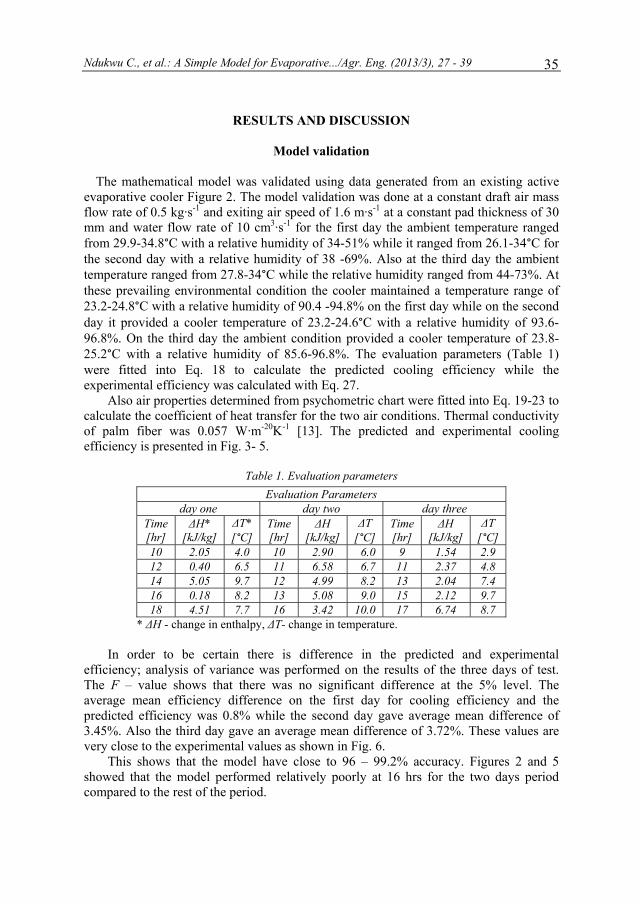
Ndukwu C., et al.: A Simple Model for Evaporative.../Agr. Eng. (2013/3), 27 - 39

35

RESULTS AND DISCUSSION

Model validation

The mathematical model was validated using data generated from an existing active

evaporative cooler Figure 2. The model validation was done at a constant draft air mass flow rate of 0.5 kg·s-1 and exiting air speed of 1.6 m·s-1 at a constant pad thickness of 30 mm and water flow rate of 10 cm3·s-1 for the first day the ambient temperature ranged from 29.9-34.8°C with a relative humidity of 34-51% while it ranged from 26.1-34°C for the second day with a relative humidity of 38 -69%. Also at the third day the ambient temperature ranged from 27.8-34°C while the relative humidity ranged from 44-73%. At these prevailing environmental condition the cooler maintained a temperature range of 23.2-24.8°C with a relative humidity of 90.4 -94.8% on the first day while on the second day it provided a cooler temperature of 23.2-24.6°C with a relative humidity of 93.6-96.8%. On the third day the ambient condition provided a cooler temperature of 23.8-25.2°C with a relative humidity of 85.6-96.8%. The evaluation parameters (Table 1) were fitted into Eq. 18 to calculate the predicted cooling efficiency while the experimental efficiency was calculated with Eq. 27.

Also air properties determined from psychometric chart were fitted into Eq. 19-23 to calculate the coefficient of heat transfer for the two air conditions. Thermal conductivity of palm fiber was 0.057 W·m-20K-1 [13]. The predicted and experimental cooling efficiency is presented in Fig. 3- 5.

Table 1. Evaluation parameters

Evaluation Parameters day one day two day three

Time [hr]

ΔH* [kJ/kg]

ΔT* [°C]

Time [hr]

ΔH [kJ/kg]

ΔT [°C]

Time [hr]

ΔH [kJ/kg]

ΔT [°C]

10 2.05 4.0 10 2.90 6.0 9 1.54 2.9 12 0.40 6.5 11 6.58 6.7 11 2.37 4.8 14 5.05 9.7 12 4.99 8.2 13 2.04 7.4 16 0.18 8.2 13 5.08 9.0 15 2.12 9.7 18 4.51 7.7 16 3.42 10.0 17 6.74 8.7

* ΔH - change in enthalpy, ΔT- change in temperature.

In order to be certain there is difference in the predicted and experimental efficiency; analysis of variance was performed on the results of the three days of test. The F – value shows that there was no significant difference at the 5% level. The average mean efficiency difference on the first day for cooling efficiency and the predicted efficiency was 0.8% while the second day gave average mean difference of 3.45%. Also the third day gave an average mean difference of 3.72%. These values are very close to the experimental values as shown in Fig. 6.

This shows that the model have close to 96 – 99.2% accuracy. Figures 2 and 5 showed that the model performed relatively poorly at 16 hrs for the two days period compared to the rest of the period.

Ndukwu C., et al.: Model evaporativnog sistema.../Polj. tehn. (2013/3), 27 - 39

36

Figure 3. Hourly predicted and experimental cooling efficiency (%) for day one

Figure 4. Hourly predicted and experimental cooling efficiency (%) for day two

Figure 5. Hourly predicted and experimental cooling efficiency (%) for day three

60

70

80

90

100

10 11 12 13 16 18

Cooling efficiency (%

)

Time (hrs)

predicted efficiency(%) experimental efficiency(%)

60

70

80

90

100

9 11 13 15 17

Cooling efficiency (%

)

Time (hrs)

predicted efficiency(%) experimental efficiency(%)

60

70

80

90

100

9 11 13 15 17

Cooling efficiency (%

)

Time (hrs)

Ndukwu C., et al.: A Simple Model for Evaporative.../Agr. Eng. (2013/3), 27 - 39

37

Figure 6. Average daily experimental and predicted efficiency

The best fit equation for the experimental and predicted value is given by:

2.745exp 16.03 exp 68.76 (27) where: ε [%] - cooling efficiency.

The above equation has R2 value of 100%. The value of the Reynolds number at the inlet shows that the air is turbulent (Re >

5000) which is typical of force convection. Though the air enters into the cooling pad as a turbulent flow but it emerges as a laminar flow inside the cooling chamber (Re < 5000) as shown in Table 1. This shows that the cells of the cooling pad absorb some of the energy from the air.

CONCLUSION The equation for predicting the cooling efficiency of a direct evaporative cooler for

storage has been presented and validated. The model considered the thermal conductivity and thickness of the cooling pad material. The model has 96 – 99.2% accuracy. The plotting of the cooling efficiency relationship with time showed an exponential behavior. The results showed that the cooling efficiency of the systems gradually improves as the day goes by and peaks in the afternoon when the ambient temperature is highest in a tropical environment like Africa. At this period much cooling is required to maintain the cooler within the storage temperature, therefore the high efficiency. In the evening the ambient temperature decreases as shown from fig 3 - 5 and consequently the cooling efficiency decreases. The information presented could be useful in the design of evaporative cooling for other purposes.

60

70

80

90

100

1 2 3

Efficiency (%

)

Day

Average experimental Efficiency(%) 

Average Predicted Efficiency(%) 

Ndukwu C., et al.: Model evaporativnog sistema.../Polj. tehn. (2013/3), 27 - 39

38

REFERENCES

[1] Xuan, Y.M., Xiao, F., Niu, X.F., Huang, X., Wang, S.W. 2012. Research and application of

evaporative cooling in China: A review (I). Renewable and Sustainable Energy Reviews Volume 16, Issue 5, p.p. 3535-3546.

[2] Di, Y.H., Liu, J.P., Huang, X. 2010. Climate demarcating for application of evaporative cooling air conditioning HVAC, 40 (2) pp. 108–111.

[3] Al-Helal, I., Short, T.H. 2003. A CFD study of naturally and ventilated greenhouses in extreme arid climates. ASAE Paper no. 99-5011 in Cooling Fan-ventilated Greenhouses: a Modelling Study. Biosystems Engineering 84 (3), p.p. 315–329.

[4] Liao, C., Chiu, K. 2002. Wind Tunnel Modeling the System Performance of Alternative Evaporative Cooling Pads in Taiwan Region. Building and Environment, No. 37, p.p. 177-187.

[5] Camargo, J.R., Ebinuma, C.D., Cardoso, S. 2003. A mathematical model for direct evaporative cooling air conditioning system. Engenharia Térmica, No. 4, p.p. 30-34.

[6] Qiang, T.W., Shen, H.G., Feng, J.M., Liang, R.J. 2006. Application of direct evaporative cooling air conditioning in moderate and high humid area of China. Refrigeration and Air-conditioning, 27 (3), pp. 21–25.

[7] Qureshi, B.A., Zubair, M.A. 2006. Comprehensive design and rating study of evaporative coolers and condensers. Part I. Performance evaluation. International Journal of Refrigeration 29, p.p. 645–658.

[8] El-dessouky, H.T., Ettouney, H.M., Bouhamra, W. 2000. A novel air conditioning system membrane air drying and evaporative cooling. Trans IChemE, Vol. 78, Part A, pp 999- 1009.

[9] Dowdy, J.A., Karabash, N.S. 1987. Experimental Determination of Heat and Mass Transfer Coefficients in rigid Impregnated Cellulose Evaporative Media. ASHRAE Transactions, part 2, v. 93., p.p. 382-395.

[10] Anyanwu, E.E. 2004. Design and measured performance of a porous evaporative cooler for preservation of fruits and vegetables. Energy conversion and management 45, p.p. 2187–2195.

[11] Jain. D. 2007. Development and testing of two-stage evaporative cooler. Building and Environment, 42, p.p. 2549–2554.

[12] Ndukwu, M. C. 2011. Development of Clay Evaporative Cooler for Fruits and Vegetables Preservation. Agricultural Engineering International: CIGR Journal, 13(1), p.p. 1-8.

[13] Krishpersad, M. 2012. Renewable building thermal insulation-oil palm fiber. International journal of engineering and technology 2, p.p. 475-479.

[14] Ditchfield, C., Tadini, C.C., Singh, R.K., Toledo, R.T. 2006. Velocity and temperature profile, heat transfer coefficient and residence time distribution of temperature dependent Herschel bukly fluid in tubular heat exchanger. Journal of food engineering 79, p.p. 632 -638.

Ndukwu C., et al.: A Simple Model for Evaporative.../Agr. Eng. (2013/3), 27 - 39

39

MODEL EVAPORATIVNOG SISTEMA HLAĐENJA SKLADIŠNOG PROSTORA U TROPSKIM USLOVIMA

Chinenye Ndukwu*1, Seth Manuwa2, Olawale Olukunle2, Babatunde Oluwalana3

1Poljoprivredni univerzitet Michael Okpara, Fakultet za inženjering i inženjersku tehnologiju, Institut za inženjering u poljoprivredi i bio-resursima,

Umudike, Abia State, Nigeria 2Federalni tehnološki univerzitet Akure, Fakultet za inženjering i inženjersku

tehnologiju, Institut za inženjering u poljoprivredi, Akure, Ondo State, Nigeria 3Federalni tehnološki univerzitet Akure, Fakultet za poljoprivredu i poljoprivrednu

tehnologiju, Institut za hranu i prehrambenu tehnologiju, Akure, Ondo State, Nigeria

Sažetak: Ovaj rad se bavi razvojem jednostavnog matematičkog modela za eksperimentalnu ocenu performansi malog evaporativnog rashladnog sistema u tropskim klimatskim uslovima. Predstavljen je i koeficijent konvektivnog prenosa toplote velikog opsega temperature na osnovu postojećeg modela. Obimni eksperimenti su izvođeni tokom januara i februara 2013 sa malim evaporativnim uređajem za hlađenje skladišta za voće i povrće. Model je uzeo u razmatranje termičke osobine materijala rashladnog sloja i pretpostavio da je rashladni sloj ravan porozni zid ograničen sa dva konvektivna sloja vazduha na različitim temperaturama na obe granične površine. Određene su izračunate i eksperimentalne vrednosti različitih efikasnosti hlađenja pri različitim opsezima ulaznih temperature. Uz to, predstavljene su i vrednosti koeficijenata konvektivnog prenosa toplote za veliki opseg temperatura.

Ključne reči: evaporativno hlađenje, rashladni sloj, jednačina modela, prenos toplote

Prijavljen: Submitted: 02.07.2013.

Ispravljen: Revised: 20.09.2013.

Prihvaćen: Accepted: 21.09.2013.

Ndukwu C., et al.: Model evaporativnog sistema.../Polj. tehn. (2013/3), 27 - 39

40

Univerzitet uPoljoprivredInstitut za pNaučni časoPOLJOPRIGodina XXXBroj 3, 2013Strane: 41 –

UDK: 574.4

DEVEL– FREQ

Tamil N

Abstrainformatiostudy, the drought infrequency this purpocorresponddeveloped grid point rain gaugeaveraged mDrought seSPI valuesas to descanalysis of2000s. Thedrought pmanageme

Key wweighted c

* Corre

This ReseaNew D

u Beogradu dni fakultet oljoprivrednu teopis IVREDNA TEHNXVIII 3. – 55

4

LOPMENTQUENCY C

Mu

Nadu AgricultuInstitute, De

act: Assessmn for sustainaStandardized

ndex was applof meteorolog

ose, the basindence to appr

by spatial inusing monthl

e stations. Remean areal raineverity-areal

s to assess the cribe and chaf SPI suggestse SAF curvesreparedness p

ent within the

words: extremcumulative ann

esponding authoresearch work arch (CSIR), HDelhi under res

ehniku

NIKA

T OF DROUCURVES IBASIN, TA

uthiah Manik

ural Universitepartment of S

Coimbat

ment and charable water red Precipitationlied to investigical drought n was dividedroximately 1.

nterpolation tely rainfall dategional reprenfall were useextent-frequendrought sever

aracterize thes that the basis developed inplan in the basin.

me value typenual drought s

or. E-mail: muthwas financiall

Human Resourcesearch fellowsh

UGHT SEVIN THE PAAMIL NAD

andan*, Dhan

ty, AgriculturaSoil & Water Ctore, Tamil Na

racterizationsources plannn Index (SPIigate the tempin the Paramb

d into 97 grid03% of total

echnique withta for the persentative of Sed to charactency (SAF) curity and areal spatial and in suffered sevn this study cregion and p

e I distributiseverity

hiahmanikanday supported bye Development

hip program.

Institute

AGRIC

VERITY –ARAMBIKDU, INDIA

napal Tamilm

al EngineeringConservation adu, India

of regional dning and manI) a most widporal characte

bikulam-Aliyad-cells of 5 l area. Griddeh the help of iod of 40 yeaSPI values crize the tempo

urves were coextent with rerecurrence p

vere droughtscan be used fplanning sus

ion, GIS, rai

an29@gmail.coy the Council ot Group (Extra

UniversityFaculty o

e of Agricultural Scie

CULTURAL ENY

OriginalnOriginal sci

AREAL EKULAM - AA

mani

g College & REngineering,

droughts provnagement. In dely used raieristics, areal

ar basin, Tami× 5 km withed monthly rGIS capabilit

ars (1972-201calculated fromoral variation onstructed usiespect to retur

patterns of dr in the 1970s,

for the develotainable wate

nfall, SAF cu

om of Scientific anMural Researc

y of Belgrade of Agriculture

Engineering ntific Journal

NGINEERING Year XXXVIII No. 3, 2013. pp: 41 – 55

ni naučni rad ientific paper

EXTENT ALIYAR

Research

vide useful the present

infall based extent and

il Nadu. For h each grid rainfall was ties at each 1) from 28 m spatially of drought.

ing gridded rn period so rought. The , 1980s and

opment of a er resource

urves, SPI,

nd Industrial ch Division),

Manikandan M., et. al.: Razvoj krivih suše – položaja.../Polj. tehn. (2013/3), 41 - 55 42

INTRODUCTION

Drought is a disastrous natural phenomenon that has significant impact on socio-economical, agricultural, and environmental spheres. Drought occurs in virtually all climatic zones, such as high as well as low rainfall areas and is mostly related to the reduction in the amount of rainfall received over an extended period of time, such as a season or a year [1]. In general, drought gives an impression of water scarcity resulted due to insufficient rainfall, high evapo-transpiration, and over-exploitation of water resources or combination of these parameters [2]. Drought impacts both surface and groundwater resources and can lead to reduced water supply, deteriorated water quality, crop failure, reduced range productivity, diminished power generation, disturbed riparian habitats, and suspended recreation activities, as well as affect a host of economic and social activities. Drought differs from other natural hazards in that its onset and end are difficult to determine. It develops slowly, and its impacts may remain for years after termination of the event. Timely determination of the level of drought will assist the decision making process to reduce the impacts of droughts. These types of information may be obtained through drought monitoring.

The definition of drought has been important for drought monitoring and analysis. Drought has been categorized into meteorological (lack of precipitation), hydrological (drying of surface water storage), agricultural (lack of root zone soil moisture), and socio-economic (lack of water supply for socioeconomic purposes) ones. The first three categories are referred as environmental indicators and the last category is considered as a water resources indicator [3]. This study focuses on the meteorological drought which is defined as deficit of rainfall over a region within a certain time interval.

Droughts are usually assessed and monitored by drought indices. A drought index is typically a single value used for indicating the severity of a drought and is far more useful than raw data in understanding the drought conditions over an area. The most commonly used meteorological drought indices are: 1) Rainfall deciles; 2) the Palmer Drought Severity Index (PDSI); 3) Percent of Normal; 4) Z-index; and 5) the Standardized Precipitation Index (SPI). The SPI was used in this study because SPI quantifies the rainfall deficit for multiple time scales and reflects the impact of drought on the availability of different types of water resources. For example, soil moisture is highly affected by the short term rainfall anomalies, whereas stream-flow, groundwater and reservoir storage slowly respond to longer-term rainfall anomalies.

As droughts are regional in nature and commonly cover large areas and extend for long time periods, it is important to study such events within a regional context. Information on regional drought characteristics provides critical values for different water based activities, and should be included in strategic short and long-term plans for adequate water resource management. The properties of regional droughts can be studied by analyzing the spatial pattern of at-site (point) droughts or one can study regional drought characteristics like the area covered by drought and total rainfall deficit over the drought area. A method to estimate severity-area-frequency curves has been used in this study to estimate the return periods of annual regional droughts [4].

Drought is a frequent phenomenon in India and drought areas are mainly confined to the Peninsular and Western parts of the country and there are only few pockets in the central, eastern, northern and southern parts. Out of 329 Million ha of total geographical area in India about 107 Million ha of lands are subjected to different degrees of water

Manikandan M., et al.: Development of Drought Severity.../Agr. Eng. (2013/3), 41 - 55 43

stress and drought conditions [5]. More than 100 districts spread over 13 states of India have been identified as drought prone districts, out of these, about 8 districts occur in the Tamil Nadu [6]. The western regions of Tamil Nadu (Coimbatore and Tiruppur districts) have suffered with severe droughts at many times in the past. Due to the growth of population and expansion of agricultural, energy and industrial sectors, the demand for water has increased manifold and even water scarcity has been occurring almost every year. Other factors, such as climate change and contamination of water supplies, have further contributed to the water scarcity. In recent years, floods and droughts have been experienced with higher peaks and severity levels. Assessment of droughts is of primary importance for water resources planning and management. This requires understanding historical droughts in the region as well as different concepts of droughts that will be helpful to investigate different drought properties. The present study was carried out in the Parambikulam-Aliyar basin spread over drought prone districts of Coimbatore and Tiruppur, Tamil Nadu. The main objective of this study is to analyze the temporal variation of droughts and construct the Drought Severity–Areal Extent – Frequency curves for spatial analyze of regional drought.

MATERIAL AND METHODS

Study area and data used: Parambikulam-Aliyar basin (referred as PAP basin) is located in the south western part of the Peninsular India covering areas in Kerala and Tamil Nadu States (Fig. 1). Parambikulam Aliyar river basin is the only basin in Tamil Nadu having west flowing rivers. Bharathapuzha river or Ponnani river and Chalakudi river are the two important major rivers are originating in Tamil Nadu State at South Western part of Coimbatore district in the Anamalai hill ranges of Western Ghats. Parambikulam – Aliyar basin is drained by west flowing rivers viz. Valayar, Koduvadiaru, Uppar, Aliyar and Palar (tributaries of Bharathapuzha river) and Parambikulam, Solaiyar and Nirar (tributaries of Chalakudi river). They are grouped into 4 sub basins such as Valaiyar sub basin, Aliyar sub basin, Palar sub basin, and Solaiyar sub basin and spread over an area of 2.388,72 km2. One third of the basin area (822,73 km2) is covered with hills and dense forest cover. This basin is bounded in north and east by Cauvery basin, south and west by Kerala State. This basin area lies (except the ayacut area) within the coordinates of North latitude between 10° 10’ 00” to 10°57’20” and East longitudes 76°43’00” to 77° 12’30”. Parambikulam-Aliyar river basin has an undulating topography with maximum contour elevation in the plain is 300m and the maximum spot height in the plain is 385m above MSL. The temperature slowly rises to its maximum in summer up to May and afterwards shows a gradual decline. The maximum temperature ranges from 36°C to 41°C and the minimum temperature varies from 14°C to 31°C. The major crops grown in the catchment are Paddy, Coconut, Groundnut, Vegetables, Cotton, Tapioca, Maize and Sugarcane. Northern parts of the basin include Thondamuthur, Madukkarai, Sultanpet and Kinathukadavu block; Central parts include Pollachi North, Pollachi South, Anamalai and Udumalaipet block; Southern parts include Valparai and some parts of Anamalai block.

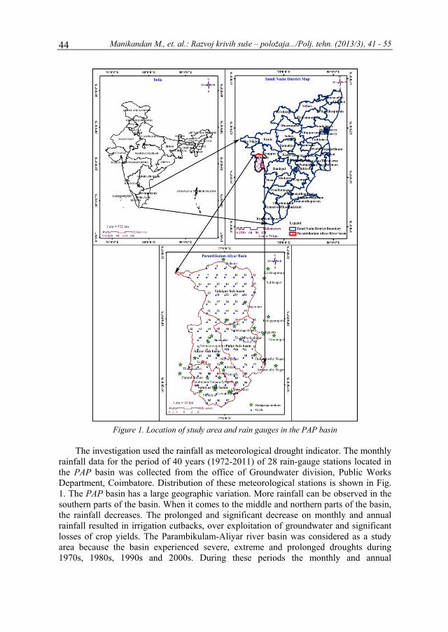
Manikandan M., et. al.: Razvoj krivih suše – položaja.../Polj. tehn. (2013/3), 41 - 55 44

Figure 1. Location of study area and rain gauges in the PAP basin

The investigation used the rainfall as meteorological drought indicator. The monthly

rainfall data for the period of 40 years (1972-2011) of 28 rain-gauge stations located in the PAP basin was collected from the office of Groundwater division, Public Works Department, Coimbatore. Distribution of these meteorological stations is shown in Fig. 1. The PAP basin has a large geographic variation. More rainfall can be observed in the southern parts of the basin. When it comes to the middle and northern parts of the basin, the rainfall decreases. The prolonged and significant decrease on monthly and annual rainfall resulted in irrigation cutbacks, over exploitation of groundwater and significant losses of crop yields. The Parambikulam-Aliyar river basin was considered as a study area because the basin experienced severe, extreme and prolonged droughts during 1970s, 1980s, 1990s and 2000s. During these periods the monthly and annual

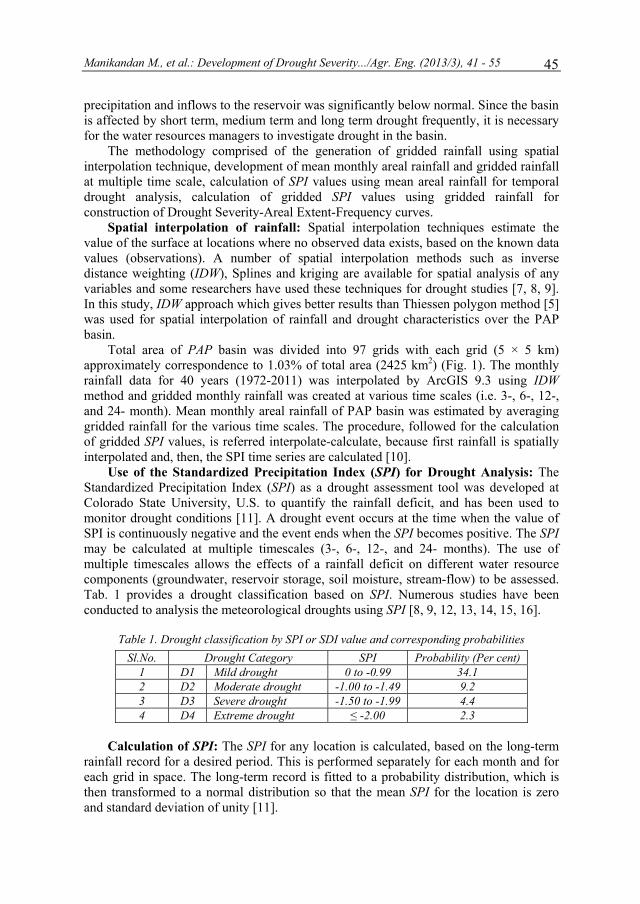
Manikandan M., et al.: Development of Drought Severity.../Agr. Eng. (2013/3), 41 - 55 45

precipitation and inflows to the reservoir was significantly below normal. Since the basin is affected by short term, medium term and long term drought frequently, it is necessary for the water resources managers to investigate drought in the basin.

The methodology comprised of the generation of gridded rainfall using spatial interpolation technique, development of mean monthly areal rainfall and gridded rainfall at multiple time scale, calculation of SPI values using mean areal rainfall for temporal drought analysis, calculation of gridded SPI values using gridded rainfall for construction of Drought Severity-Areal Extent-Frequency curves.

Spatial interpolation of rainfall: Spatial interpolation techniques estimate the value of the surface at locations where no observed data exists, based on the known data values (observations). A number of spatial interpolation methods such as inverse distance weighting (IDW), Splines and kriging are available for spatial analysis of any variables and some researchers have used these techniques for drought studies [7, 8, 9]. In this study, IDW approach which gives better results than Thiessen polygon method [5] was used for spatial interpolation of rainfall and drought characteristics over the PAP basin.

Total area of PAP basin was divided into 97 grids with each grid (5 × 5 km) approximately correspondence to 1.03% of total area (2425 km2) (Fig. 1). The monthly rainfall data for 40 years (1972-2011) was interpolated by ArcGIS 9.3 using IDW method and gridded monthly rainfall was created at various time scales (i.e. 3-, 6-, 12-, and 24- month). Mean monthly areal rainfall of PAP basin was estimated by averaging gridded rainfall for the various time scales. The procedure, followed for the calculation of gridded SPI values, is referred interpolate-calculate, because first rainfall is spatially interpolated and, then, the SPI time series are calculated [10].

Use of the Standardized Precipitation Index (SPI) for Drought Analysis: The Standardized Precipitation Index (SPI) as a drought assessment tool was developed at Colorado State University, U.S. to quantify the rainfall deficit, and has been used to monitor drought conditions [11]. A drought event occurs at the time when the value of SPI is continuously negative and the event ends when the SPI becomes positive. The SPI may be calculated at multiple timescales (3-, 6-, 12-, and 24- months). The use of multiple timescales allows the effects of a rainfall deficit on different water resource components (groundwater, reservoir storage, soil moisture, stream-flow) to be assessed. Tab. 1 provides a drought classification based on SPI. Numerous studies have been conducted to analysis the meteorological droughts using SPI [8, 9, 12, 13, 14, 15, 16].

Table 1. Drought classification by SPI or SDI value and corresponding probabilities

Sl.No. Drought Category SPI Probability (Per cent) 1 D1 Mild drought 0 to -0.99 34.1 2 D2 Moderate drought -1.00 to -1.49 9.2 3 D3 Severe drought -1.50 to -1.99 4.4 4 D4 Extreme drought ≤ -2.00 2.3

Calculation of SPI: The SPI for any location is calculated, based on the long-term

rainfall record for a desired period. This is performed separately for each month and for each grid in space. The long-term record is fitted to a probability distribution, which is then transformed to a normal distribution so that the mean SPI for the location is zero and standard deviation of unity [11].

Manikandan M., et. al.: Razvoj krivih suše – položaja.../Polj. tehn. (2013/3), 41 - 55 46

The gamma distribution is defined by its probability density function is:

Γ

/ for x > 0 (1) where: α > 0 [-] - shape factor, β > 0 [-] - scale factor, x > 0 [mm] - amount of rainfall. Γ(α) is the gamma function which is defined as

∞ (2)

Fitting the distribution to the data requires that α and β be estimated. Edwards and

McKee (1997) [17] suggested a method for estimating these parameters using the approximation of Thom (1958) [18] for maximum likelihood as follows:

1

4 1 143 (3)

(4)

Where: ln

∑ ln

for n observations. (5)

The resulting parameters are then used to find the cumulative probability of an

observed rainfall event for the given month or any other time scale.

1Γ

/ (6)

Substituting t for / reduces the above equation to incomplete gamma function:

1Γ

(7)

Since the gamma function is undefined for x = 0 and a precipitation distribution

may contain zeros, the cumulative probability becomes:

1 (8) where q is the probability of zero precipitation. If m is the number of zeros in a

rainfall time series, q can be estimated by m/n. In this analysis, a small amount of rainfall was substituted for zero rainfall for each grid. This substitution does not affect the distribution of precipitation.

Manikandan M., et al.: Development of Drought Severity.../Agr. Eng. (2013/3), 41 - 55 47

The cumulative probability, H(x), is then transformed to the standard normal random variable Z with a mean of zero and a variance of one, which is the value of SPI [12, 17].

For 0<H(x)≤0.5

1 (9)

Where

ln1

(10)

For 0.5<H(x)<1

1 (11)

Where

ln1

1 (12)

c0=2.515517 c1=0.802853 c2=0.010328 d1=1.432788 d2=0.189269 d3=0.001308

Construction of drought Severity-Areal Extent-Frequency (SAF) curves:

Regional drought analysis is useful for declaring the drought condition or determining the drought severity during a particular year. A regional drought is assumed when a significant fraction of the total area of the region is under drought conditions or, in other words, when the sum of the areas affected by local drought reaches a selected areal threshold so that it is very important to assess the drought for the entire region. Frequency of drought occurrence cannot fully cover the study of droughts, unless it is quantitatively related to other aspects such as severity and areal extent of droughts. This led to the development of drought severity-area-frequency (SAF) curves. SAF curves are one of the most useful methods to assess drought in a region, which was proposed by Henriques and Santos (1999) [19] and the same procedure was adopted by Kim et al., 2002; Loukas and Vasiliasdes, 2004; Mishra and Desai, 2005; Zhang et al., 2012 [7, 10, 5, 20]. In this study annual SAF curves were developed based on weighted cumulative drought severity at multiple time scales.

The weighted annual cumulative SAF curves were developed according to the following procedure: (1) The monthly SPI values for each grid for every year were calculated at multiple time scales of 3-, 6-, 12-, and 24-months; (2) The annual weighted cumulative drought severity in each grid was estimated by multiplying the annual sum of SPI in monthly dry spells (negative SPI values) for a particular time scale by the probability of drought occurrence for each year; (3) The probability of annual drought occurrence for each year and in each grid was estimated by dividing the number of months that have a negative SPI value for the particular time scale by 12; (4) The drought severity associated with the areal extents (in terms of percentage of total area) taking different areal thresholds into account was obtained; (5) To find out the best

Manikandan M., et. al.: Razvoj krivih suše – položaja.../Polj. tehn. (2013/3), 41 - 55 48

distribution for the frequency analysis, drought severity was tested using different probability distributions; (6) Frequency analysis was performed using selected probability distribution for each drought areal extent percentage to associate the drought severity with return periods; (7) Weighted annual cumulative SAF curves were developed for the particular time scale and repeated the analysis for different time scale. In this analysis each drought event can be allotted uniformly for a particular year, avoid intermittence, and the duration of dry spells within a particular year is implicitly taken into account.

Analysis of drought frequency: The frequency analysis is commonly used in hydrology and meteorology to assess the return period of particular events. Frequency analysis is performed using the selected probability distribution for annual average drought severity at different return periods. In this study, the annual cumulative drought severity has negative values. To be applied before fitting to an available distribution, the negative values of average annual drought severity were transformed to positive values in order to represent the extreme condition and to analyze the associated risk of droughts using the exceedance probability. Various theoretical probability distributions were statistically tested before fitting the observed drought severity. The commonly used probability distributions viz. Normal, Lognormal, Gamma, and Extreme Value Type I were used to evaluate the best fit probability distribution for SPI_12 annual drought severity and tested by non parametric Kolgomorov–Smirnov (K-S) test and parametric Chi-Square tests at 5 per cent and 1 per cent significance levels.

The annual cumulative drought severity XT to be estimated for a given return period (T) may be represented as the mean μ plus the departure ΔXT of the variate from mean.

XT=μ+∆XT (13)

The departure may be taken as equal to the product of the standard deviation σ and a

frequency factor KT; that is, ΔXT = KTσ. The departure ΔXT and the frequency factor KT are functions of the return period and type of probability distribution to be used in the analysis [21]. The expected annual drought severity at various return periods 5, 10, 25, 50, 75 and 100 years were worked out by the best fit probability distribution.

RESULTS AND DISCUSSION

Analysis of rainfall: Gridded rainfall was developed using spatial interpolation technique in GIS environment and mean areal rainfall was calculated from the spatially averaged gridded rainfall. The mean annual areal rainfall over the whole PAP basin was about 1410.04 mm and it was distributed unevenly in space and time. The mean annual precipitation varied from about 511 mm at the northern plain areas to more than 4328 mm at the southern mountain areas. The average cumulative areal rainfall was compared with normal cumulative areal rainfall over the study period for identifying the worst rainfall deficit years (Fig. 2). From this analysis, it was found that the PAP basin experienced rainfall deficits during the periods of 1970s, 1980s and 2000s. During these three periods the monthly and annual precipitation was considerably below normal. Especially, the year 1982, 1976 and 2002 are the first, second and third driest years, respectively. The prolonged and remarkable decrease of monthly and annual

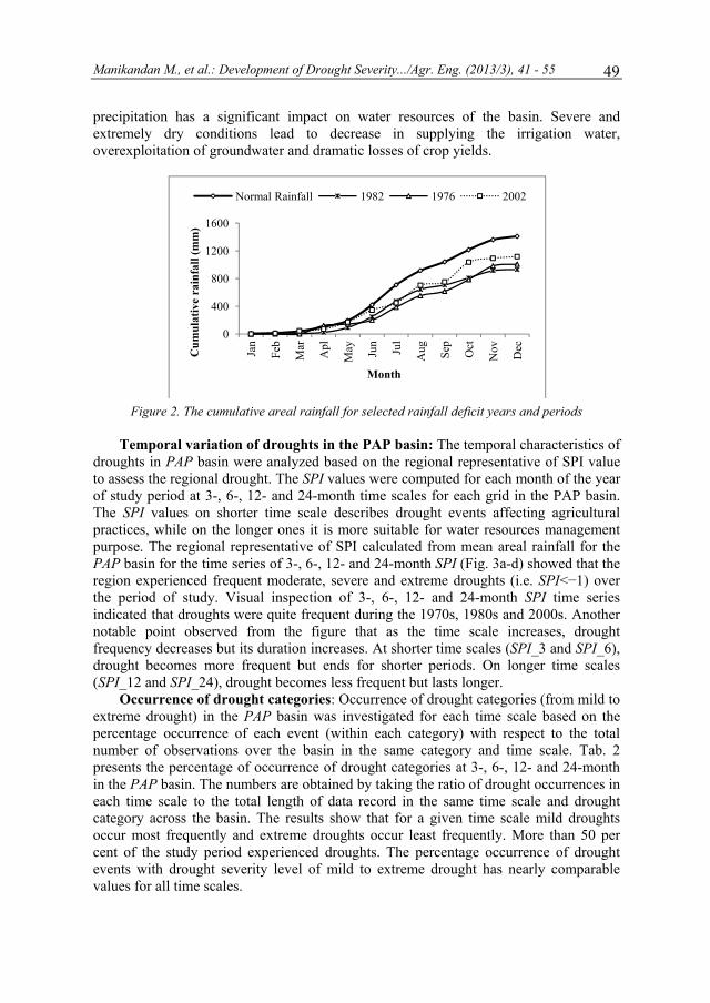
Manikandan M., et al.: Development of Drought Severity.../Agr. Eng. (2013/3), 41 - 55 49

precipitation has a significant impact on water resources of the basin. Severe and extremely dry conditions lead to decrease in supplying the irrigation water, overexploitation of groundwater and dramatic losses of crop yields.

Figure 2. The cumulative areal rainfall for selected rainfall deficit years and periods

Temporal variation of droughts in the PAP basin: The temporal characteristics of

droughts in PAP basin were analyzed based on the regional representative of SPI value to assess the regional drought. The SPI values were computed for each month of the year of study period at 3-, 6-, 12- and 24-month time scales for each grid in the PAP basin. The SPI values on shorter time scale describes drought events affecting agricultural practices, while on the longer ones it is more suitable for water resources management purpose. The regional representative of SPI calculated from mean areal rainfall for the PAP basin for the time series of 3-, 6-, 12- and 24-month SPI (Fig. 3a-d) showed that the region experienced frequent moderate, severe and extreme droughts (i.e. SPI<−1) over the period of study. Visual inspection of 3-, 6-, 12- and 24-month SPI time series indicated that droughts were quite frequent during the 1970s, 1980s and 2000s. Another notable point observed from the figure that as the time scale increases, drought frequency decreases but its duration increases. At shorter time scales (SPI_3 and SPI_6), drought becomes more frequent but ends for shorter periods. On longer time scales (SPI_12 and SPI_24), drought becomes less frequent but lasts longer.

Occurrence of drought categories: Occurrence of drought categories (from mild to extreme drought) in the PAP basin was investigated for each time scale based on the percentage occurrence of each event (within each category) with respect to the total number of observations over the basin in the same category and time scale. Tab. 2 presents the percentage of occurrence of drought categories at 3-, 6-, 12- and 24-month in the PAP basin. The numbers are obtained by taking the ratio of drought occurrences in each time scale to the total length of data record in the same time scale and drought category across the basin. The results show that for a given time scale mild droughts occur most frequently and extreme droughts occur least frequently. More than 50 per cent of the study period experienced droughts. The percentage occurrence of drought events with drought severity level of mild to extreme drought has nearly comparable values for all time scales.

0

400

800

1200

1600

Jan

Feb

Mar

Apl

May Jun

Jul

Aug Se

p

Oct

Nov DecCum

ulat

ive

rain

fall

(mm

)

Month

Normal Rainfall 1982 1976 2002

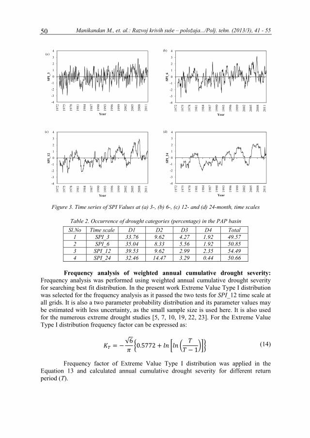
Manikandan M., et. al.: Razvoj krivih suše – položaja.../Polj. tehn. (2013/3), 41 - 55 50

Figure 3. Time series of SPI Values at (a) 3-, (b) 6-, (c) 12- and (d) 24-month, time scales

Table 2. Occurrence of drought categories (percentage) in the PAP basin

Sl.No Time scale D1 D2 D3 D4 Total 1 SPI_3 33.76 9.62 4.27 1.92 49.57 2 SPI_6 35.04 8.33 5.56 1.92 50.85 3 SPI_12 39.53 9.62 2.99 2.35 54.49 4 SPI_24 32.46 14.47 3.29 0.44 50.66

Frequency analysis of weighted annual cumulative drought severity:

Frequency analysis was performed using weighted annual cumulative drought severity for searching best fit distribution. In the present work Extreme Value Type I distribution was selected for the frequency analysis as it passed the two tests for SPI_12 time scale at all grids. It is also a two parameter probability distribution and its parameter values may be estimated with less uncertainty, as the small sample size is used here. It is also used for the numerous extreme drought studies [5, 7, 10, 19, 22, 23]. For the Extreme Value Type I distribution frequency factor can be expressed as:

√60.5772 1 (14)

Frequency factor of Extreme Value Type I distribution was applied in the

Equation 13 and calculated annual cumulative drought severity for different return period (T).

-4

-3

-2

-1

0

1

2

3

4

1972

1975

1978

1981

1984

1987

1990

1993

1996

1999

2002

2005

2008

2011

SPI_

3

Year

(a)

-4

-3

-2

-1

0

1

2

3

4

1972

1975

1978

1981

1984

1987

1990

1993

1996

1999

2002

2005

2008

2011

SPI_

6

Year

(b)

-4

-3

-2

-1

0

1

2

3

4

1972

1975

1978

1981

1984

1987

1990

1993

1996

1999

2002

2005

2008

2011

SPI_

12

Year

(c)

-4

-3

-2

-1

0

1

2

3

4

1972

1975

1978

1981

1984

1987

1990

1993

1996

1999

2002

2005

2008

2011

SPI_

24

Year

(d)

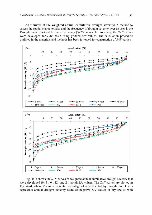
Manikandan M., et al.: Development of Drought Severity.../Agr. Eng. (2013/3), 41 - 55 51

SAF curves of the weighted annual cumulative drought severity: A method to assess the spatial characteristics and the frequency of drought severity over an area is the Drought Severity-Areal Extent- Frequency (SAF) curves. In this study, the SAF curves were developed for PAP basin using gridded SPI values. The calculation procedure outlined in the materials and methods has been followed for construction of SAF curves.

Fig. 4a-d shows the SAF curves of weighted annual cumulative drought severity that

were developed for 3-, 6-, 12- and 24-month SPI values. The SAF curves are plotted in Fig. 4a-d, where X axis represents percentage of area affected by drought and Y axis represents annual drought severity (sum of negative SPI values in dry spells) with

-30

-25

-20

-15

-10

-5

010 20 30 40 50 60 70 80 90 100

Dro

ught

seve

rity

(SPI

_3)

Areal extent (%)

5-year 10-year 25-year 50-year 75-year100-year 1982 1974 1976

(4a)

-35

-30

-25

-20

-15

-10

-5

010 20 30 40 50 60 70 80 90 100

Dro

ught

seve

rity

(SPI

_6)

Areal extent (%)

5-year 10-year 25-year 50-year 75-year100-year 1976 1982 1974

(4b)

Manikandan M., et. al.: Razvoj krivih suše – položaja.../Polj. tehn. (2013/3), 41 - 55 52

different return periods. Most severe drought years recorded during the period of analysis was selected based on highest annual drought severity and driest years were drawn in the SAF curves to indentify the recurrence pattern and spatial extent of selected droughts.

Figure 4. Severity-Areal extent-Frequency curves of the weighted annual cumulative drought severity for (a) 3-, (b) 6-, (c) 12- and (d) 24-month SPI series compared to historical drought

Fig. 4a illustrates the SAF curves of SPI_3 for the PAP basin and the figure

demonstrates that three annual droughts with the highest weighted annual cumulative drought severity in the PAP basin occurred during 1982, 1974 and 1976. The drought

-40

-35

-30

-25

-20

-15

-10

-5

010 20 30 40 50 60 70 80 90 100

Dro

ught

seve

rity

(SPI

_12)

Areal extent (%)

5-year 10-year 25-year 50-year 75-year100-year 1983 1974 1976

(4c)

-45

-40

-35

-30

-25

-20

-15

-10

-5

010 20 30 40 50 60 70 80 90 100

Dro

ught

seve

rity

(SPI

_24)

Areal extent (%)

5-year 10-year 25-year 50-year 75-year100-year 1983 1974 1984

(4d)

Manikandan M., et al.: Development of Drought Severity.../Agr. Eng. (2013/3), 41 - 55 53

that occurred in 1982 has an associate return period of above 100 years with more than 50 per cent of the areal extent. The drought event that occurred in 1974 and 1976 has an associate return period between 25 to 50 years. The most three severe drought year for SPI_6 based on weighted annual cumulative drought severity was 1976, 1982 and 1974 (Fig. 4b). From the figure, it can be observed that the 1976 drought year has an associate return period of 50 to 100 years. The drought that occurred in 1982 and 1974 has an associate return period between 25 to 50 years.

The droughts of 1983, 1976 and 1974 assessed by SPI_12 time series have return period between 10 to 25 years (Fig. 4c) and the curve of drought year 1974 runs between the return periods of 10 to 100 years with an increasing areal extent. The drought that occurred in 1983, 1974 and 1984 for 24- month time series have an associate return period between 10 to 50 years (Fig. 4d). From this analysis the year 1974, 1976, 1982, 1983, and 1985 were the severe drought years have large spatial extent and have return period between 10-50 years. Using these curves one can easily identify the drought severity associated with return period drought for a particular drought event.

CONCLUSIONS

This study was focused on analyzing temporal variation and areal extent and frequency of severe droughts in the PAP Basin using the SPI as an indicator of drought severity. The SPI was computed using gridded rainfall at multiple time scales. The temporal analysis of drought was done with mean areal rainfall and SAF curves were developed with gridded rainfall over the basin. The temporal and spatial drought analyses indicated that PAP basin experience quite frequent moderate and severe droughts on monthly basis. The region has experienced prolonged and severe droughts in terms of severity and durations in the 1970s, 1980s and 2000s. In particular, the persistent and prolonged drought of 1974-1976 and 1982-1985 seriously affected urban water supply, agricultural irrigation, ground water as well as reduction of inflows to the reservoir. The drought severity – areal extent - frequency curve constructed in this study contains drought severity and drought area with respect to drought return period so as to describe and characterize the spatial and recurrence patterns of droughts. It is shown that the drought that occurred in the 1970s and 1980s was associated with a return period of 25 to 50 years with a large areal extent. The identification of the temporal characteristics of droughts and construction of SAF curves in the PAP basin will be useful for the development of a drought preparedness plan in the region and for sustainable water resource planning and management.

BIBLIOGRAPHY

[1] Mishra, A.K., Singh, V.P. 2010. A review of drought concepts. Journal of Hydrology, 391, p.p. 202-216.

[2] Bhuiyan, C. 2004. Various drought indices for monitoring drought condition in Aravalli Terrain of India. Proceedings of the XXth ISPRS Congress, Istanbul, Turkey, p.p. 12–23.

[3] Wilhite, D.A. 2000. Drought as a natural hazard: concepts and definitions. Drought: a global assessment, Vol. 1. W. D.A. Routlegde, New York, USA, p.p. 1–3.

Manikandan M., et. al.: Razvoj krivih suše – položaja.../Polj. tehn. (2013/3), 41 - 55 54

[4] Hisdal, H., Tallaksen, L. M. 2003. Estimation of regional meteorological and hydrological drought characteristics: A case study for Denmark. Journal of Hydrology, 281, 3, p.p. 230-247.

[5] Mishra, A.K., Desai, V.R. 2005. Spatial and temporal drought analysis in the Kansabati river basin, India. International Journal of River Basin Management, 3(1), p.p. 31-41.

[6] Gupta, A.K, Tyagi, P., Sehgal, V.K. 2011. Drought disaster challenges and mitigation in India: strategic appraisal. Current science, 100 (12), p.p. 1795-1806.

[7] Kim, T., Valdes, J.B., Aparicio, J. 2002. Frequency and spatial characteristics of droughts in the Conchos River Basin, Mexico. Water International, 27(3), p.p. 420–430.

[8] Edossa, D.C., Babel, M.S., Gupta, A.D. 2010. Drought analysis in the Awash River Basin, Ethiopia. Water Resource Management, 24, p.p. 1441–1460.

[9] Moradi, H.R., Rajabi, M., Faragzadeh, M. 2011. Investigation of meteorological drought characteristics in Fars province, Iran. Catena, 84, p.p. 35–46.

[10] Loukas, A., Vasiliades, L. 2004. Probabilistic analysis of drought spatiotemporal characteristics in Thessaly region, Greece. Natural Hazards and Earth System Sciences, 4, p..p 719–731.

[11] McKee, T.B., Doesken, N.J., Kliest, J. 1993. The relationship of drought frequency and duration to time scales. Proceedings of the 8th Conference on Applied Climatology, 17–22 January, Anaheim, CA. American Meteorological Society, Boston, MA, USA, p.p. 179–184.

[12] Hughes, B.L., Saunders, M.A. 2002. A drought climatology for Europe. International Journal of Climatology, 22, p.p. 1571–1592.

[13] Patel, N.R., Chopra, P., Dadhwal, V.K. 2007. Analyzing spatial patterns of meteorological drought using standardized precipitation index. Meteorological Applications, 14(4), 329-336.

[14] Pradhan, S., Sehgal, V.K., Das, D.K., Singh, R. 2011. Analysis of meteorological drought at New Delhi using SPI. Journal of Agrometeorology, 13(1), p.p. 68-71.

[15] Manikandan, M., Tamilmani, D. 2013. Analysis of meteorological drought characteristics in the Parambikulam-Aliyar basin, Tamil Nadu. Madras Agricultural Journal, 100 (1-3), p.p. 236-243.

[16] Manikandan, M., Tamilmani, D. 2013. Development of drought vulnerability maps in the Parambikulam - Aliyar Basin, Tamil Nadu, India. Scientific Research and Essays, 8 (20), p.p. 778-790.

[17] Edwards, D.C., McKee, T.B. 1997. Characteristics of 20th Century Drought in the United States at Multiple Timescales. Colorado State University, Fort Collins, Climatology Report, p.p. 97-2.

[18] Thom, H.C.S. 1958. A Note on Gamma Distribution. Monthly Weather Review, 86, p.p. 117–122. [19] Henriques, A.G., Santos, M.J.J. 1999. Regional drought distribution model. Physics and

Chemistry of Earth Part B, 24 (1–2), p.p. 19–22. [20] Zhang. Q, Xiao. M, Chen. X. 2012. Regional evaluations of the meteorological drought

characteristics across the Pearl River Basin, China. American Journal of Climate Change, 1, p.p. 48-55.

[21] Chow,V.T. 1951. A generalized formula for hydrologic frequency analysis. Transactions American Geography Union, 32 (2), p.p. 231–237.

[22] Lana, X., Serra, C., Burgue˜no, A. 1998. Spatial and Temporal Characterization of Annual Extreme Droughts in Catalonia (Northern Spain). International Journal of Climatology, 18, p.p. 93–110.

[23] Dalezios, N.R., Loukas, A., Vasiliades, L., Liakopoulos, E. 2000. Severity-Duration-Frequency Analysis of Droughts and Wet Periods in Greece. Hydrological Sciences Journal. 45 (5), p.p. 665–680.

Manikandan M., et al.: Development of Drought Severity.../Agr. Eng. (2013/3), 41 - 55 55

RAZVOJ KRIVIH SUŠE – POLOŽAJA – UČESTALOSTI U PARAMBIKULAM - ALIYAR BASENU, TAMIL NADU, INDIJA

Muthiah Manikandan, Dhanapal Tamilmani

Poljoprivredni univerzitet Tamil Nadu, Fakultet za poljoprivrednu tehniku,

Institut za konzervaciju zemljišta i voda, Coimbatore, Tamil Nadu, Indija

Sažetak: Procena i karakterizacija regionalnih suša daju korisne informacije za održivo planiranje i upravljanje vodenim resursima. U ovom istraživanju primenjen je Standardizovani indeks padavina (SPI), kao najšire primenjeni indeks suše zasnovan na padavinama, za ispitivanje vremenskih karakteristika, prostornog oblika i učestalosti suše u basenu Parambikulam-Aliyar, Tamil Nadu. Za ovu svrhu basen je podeljen na 97 mrežnih ćelija dimenzija 5 × 5 km, tako da svaka ćelija odgovara približno 1.03% ukupne površine. Mesečne padavine u mreži razvijene su tehnikom prostorne interpolacije uz pomoć GIS-a u svakoj tački mreže korišćenjem podataka o mesečnim padavinama za period od 40 godina (1972-2011) iz 28 mernih stanica. Regionalne reprezentativne SPI vrednosti izračunate iz prostorno prosečnih vrednosti padavina korišćene su za karakterizaciju vremenskih varijacija suše. Krive suše-prostornog položaja-učestalosti (SAF krive) su konstruisane korišćenjem mrežnih SPI vrednosti za procenu jačine suše i prostornog položaja u odnosu na povratni period, tako da se opišu i karakterišu prostorni i povratni oblici suše. Analiza SPI vrednosti pokazuje da su basen pogodile jake suše 1970-tih, 1980-tih i 2000-tih. Razvijene SAF krive mogu se koristiti za razradu plana pripravnosti u sušnim periodima u regionu i planiranje održivog upravljanja vodenim resursima u basenu.

Ključne reči: distribucija ekstremnih vrednosti tipa I, GIS, padavine, SAF krive, SPI, masena kumulativna godišnja suša

Prijavljen: Submitted: 23.07.2013.

Ispravljen: Revised:

Prihvaćen: Accepted: 14.09.2013.

Manikandan M., et. al.: Razvoj krivih suše – položaja.../Polj. tehn. (2013/3), 41 - 55 56

Univerzitet uPoljoprivredInstitut za pNaučni časoPOLJOPRIGodina XXXBroj 3, 2013Strane: 57 –

UDK: 631 (

D

Departm

Abstrato floricultassisted spwas designvelocity atcentrifugalin the sleevnecessary pmotor. Theof developvelocity (9droplet sizartificial pdensity (2positions w

Key wdensity

* Corre

AuthoReseafacilit

u Beogradu dni fakultet oljoprivrednu teopis IVREDNA TEHNXVIII 3. – 72

(059)

DEVELOPMGREE

SachinBabasa

Maharana

ment of Farm

act: Floricultuture productioprayer was dened and madet each outlet. Tl blower of caves. A horizonpressure in the whole assemped sprayer w9, 12, 16 and 2ze, droplet deplant canopy. 5-35 droplets

were observed

words: greenh

esponding authoors sincerely tharch and Deveties and funds f

ehniku

NIKA

MENT OF ENHOUSE

Vilas Wandkaheb Sukhdeo

a Pratap UnivCollege of TeMachinery an

ure is one of thon are insects, veloped for g

e with fiber reThe boom waapacity 0.40 mntal triplex po

he nozzles. Blmbly of the spas evaluated i20 m·s-1) and ensity and un

The optimus per cm2) and for air veloci

house, floricu

or. E-mail: sach

hank to Shree Selopment Founfor this research

AIR ASSIFLORICU

kar*, Shaileno Gholap, Pra

versity of Agriechnology andnd Power Eng

he major sectpests and dis

greenhouse floeinforced PVCas developed tm3·s-1 was useower pump of ower and pumrayer was moin the laboratpump discharniformity coe

um results of nd uniformityity of 20 m·s-1

ulture, air as

hinwandkar85@harad Patel, thendation, Mumbh work.

Institute

AGRIC

STED SPRULTURE C

dra Mohan Mavin Prakash

culture and Td Engineeringgineering Uda

tors in Indian seases. Thereforicultural croC material in to support aird on the syste

f 16 l·min-1 capmp were operaounted on the tory to study trge (2.5, 4.5, 7efficient at sif droplet size y coefficient ( and pump dis

ssisted spraye

@gmail.com e Managing Dibai (India) fo

UniversityFaculty o

e of Agricultural Scie

CULTURAL ENY

OriginalnOriginal sci

RAYER FOCROPS

Mathur, h Jadhav

Technology, g, aipur, Rajastha

agriculture. Mfore, a motor oops. A taperedorder to get

r sleeve and nem to producepacity was usated by 3.73 ktrolley. The pthe effect of d7 and 9 l·min-

ix different p(100-150 µm

(near unity) ascharge of 2.5

er, droplet si

rector, ASPEE or providing a

y of Belgrade of Agriculture

Engineering ntific Journal

NGINEERING Year XXXVIII No. 3, 2013. pp: 57 – 72

ni naučni rad ientific paper

OR

an, India

Main threats operated air d air sleeve uniform air

nozzles. The e air stream ed to create kW electric

performance different air -1) levels on positions of m), droplet at all plant

5 l·min-1.

ize, droplet

Agricultural all necessary

Wandkar S.V., et al.: Razvoj vazdušnog rasprskivača.../Polj. tehn. (2013/3), 57 - 72 58

INTRODUCTION

Floriculture in India is being viewed as a high growth Industry. Commercial floriculture is becoming important from the export angle. Indian floriculture industry has been shifting from traditional flowers to cut flowers for export purposes. According to a report of the Agricultural and Processed Food Products Export Development Authority (APEDA), Government of India, the total area under flower crops was estimated around 34,000 hectares, which included 24,000 hectares under traditional flowers such as marigold, jasmine, aster, rose, chrysanthemum, tuberose and 10,000 hectares under modern flowers like cornation, rose, gerbera, gladiolous, anthurium. Returns from floricultural products were estimated at Rs. 205 Crores, which included Rs. 105 Crores from traditional and Rs. 100 Crores from modern flowers [13].

Floricultural crops are more susceptible to pests and diseases during their flowering stages. Generally, chemical pesticides are used for controlling pests and diseases. Traditionally farmers use the knapsack sprayer for the application of pesticides. But, the manually operated knapsack sprayer has a number of limitations: it is labor intensive, have low application accuracy and require serious safety precautions. Performance depends on skill of operator; manual application often results in an uneven distribution of the pesticide.

Air assisted spraying is considered as one of the better pesticide application technique. The air assisted spraying system contributes towards: reduction in spray drift and loss on the ground, an increase in the agrochemical deposits levels and coverage rate of the abaxial surface leaves, improvement in the penetration of the spray droplets into the canopy as well as enabling a reduction in both dosage and in application volume [7]. Incorporation of air assistance in the spraying system improves the deposition uniformity in the entire plant canopy structure, spray deposition on the lower part of the plant leaves, where most pests harbor [3]. The air sleeve boom spraying technology is based on air assisted spraying. This system essentially consists of a blower, nozzles, pump and sleeve or duct. The sleeves, made of PVC material, are inflated with the air mass generated by blower. The sleeve has number of holes at bottom for delivering air. The spray droplets produced by nozzles are transported to a target through a stream of air coming out of sleeve orifices which results in better control over spray droplets and deposition [6].

Shahare et al. [8, 9] developed a tractor operated air sleeve boom sprayer for cotton crop for better deposition of pesticide throughout the canopy and evaluated its performance in the field for cotton crop with findings that higher air velocity improves the deposition of pesticide on whole canopy of cotton crop. Sirohi et al. [10] developed an air-assisted hydraulic sprayer for improved deposition of pesticides in different canopy structures of vegetable crops. Bauer and Raetano [1] evaluated the effects from air speed variation on spraying sleeve boom and conclude that the use of air assistance resulted in better deposit levels on the abaxial surface of the folioles positioned in the lower portion of the plants.

Therefore, efforts have been made to develop an air assisted sprayer for pesticide applications in floricultural crops and the performance of the sprayer was evaluated in the laboratory to study the effect of different air velocity and pump discharge levels on droplet size, droplet density and uniformity coefficient at different positions on plant.

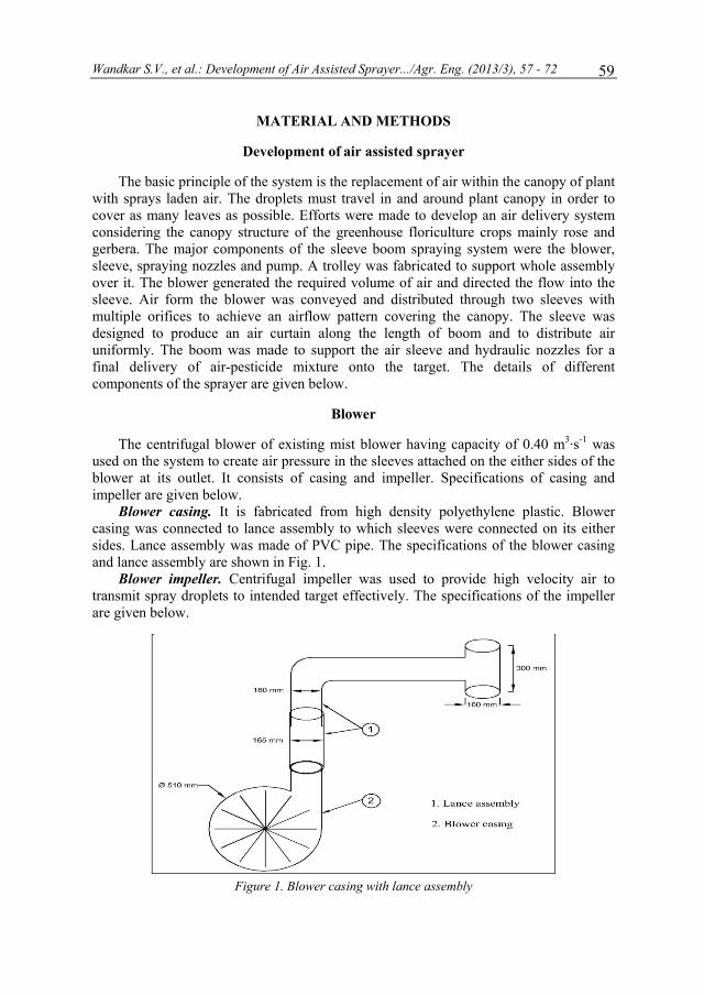
Wandkar S.V., et al.: Development of Air Assisted Sprayer.../Agr. Eng. (2013/3), 57 - 72

59

MATERIAL AND METHODS

Development of air assisted sprayer

The basic principle of the system is the replacement of air within the canopy of plant with sprays laden air. The droplets must travel in and around plant canopy in order to cover as many leaves as possible. Efforts were made to develop an air delivery system considering the canopy structure of the greenhouse floriculture crops mainly rose and gerbera. The major components of the sleeve boom spraying system were the blower, sleeve, spraying nozzles and pump. A trolley was fabricated to support whole assembly over it. The blower generated the required volume of air and directed the flow into the sleeve. Air form the blower was conveyed and distributed through two sleeves with multiple orifices to achieve an airflow pattern covering the canopy. The sleeve was designed to produce an air curtain along the length of boom and to distribute air uniformly. The boom was made to support the air sleeve and hydraulic nozzles for a final delivery of air-pesticide mixture onto the target. The details of different components of the sprayer are given below.

Blower

The centrifugal blower of existing mist blower having capacity of 0.40 m3·s-1 was

used on the system to create air pressure in the sleeves attached on the either sides of the blower at its outlet. It consists of casing and impeller. Specifications of casing and impeller are given below.

Blower casing. It is fabricated from high density polyethylene plastic. Blower casing was connected to lance assembly to which sleeves were connected on its either sides. Lance assembly was made of PVC pipe. The specifications of the blower casing and lance assembly are shown in Fig. 1.

Blower impeller. Centrifugal impeller was used to provide high velocity air to transmit spray droplets to intended target effectively. The specifications of the impeller are given below.

Figure 1. Blower casing with lance assembly

Wandkar S.V., et al.: Razvoj vazdušnog rasprskivača.../Polj. tehn. (2013/3), 57 - 72 60

Material : Stainless steel No. of blades : 48 Type of blade : Forward curved Blade inlet angle : 16º Blade outlet angle : 160º Inner diameter : 220 mm Outer diameter : 300 mm Width of impeller : 140 mm

Air sleeve

A horizontal flexible air duct was designed to generate an air curtain with a uniform air velocity profile throughout the length of boom by tapering the duct (sleeve) towards the close end. Let ‘L’ be the length of sleeve equal to swath width and ‘Do’ its diameter at the inlet (at the exit of blower) whereas the other end of sleeve is closed. It has ‘n’ number of orifices of uniform cross section throughout its length (Fig. 2). The air is blown into the duct from the blower and forced out through the orifices. As it is required to have uniform distribution of air along the duct, it was decided to taper the duct so that vertical air velocity will remain constant along its length [4]. Thus, to maintain uniform distribution of air along the length of the duct, the diameter of the duct at different cross sections (Dx) was determined as shown below. Let Do, diameter of duct at X = 0 and Do = 0 at X = LS (Fig. 2).

Figure 2. Tapered air duct

The air flow at the duct entrance can be calculated from continuity equation as:

Q = A · V (1) where: Q [m3·s-1] - air flow at the duct entrance, A [m2] - area of cross-section, V [m·s-1] - air velocity.

The cross sectional area, at X = 0 and diameter Do, can be found as

2oD

4A ⋅=

π (2)

where: π [-] - constant (3.14),

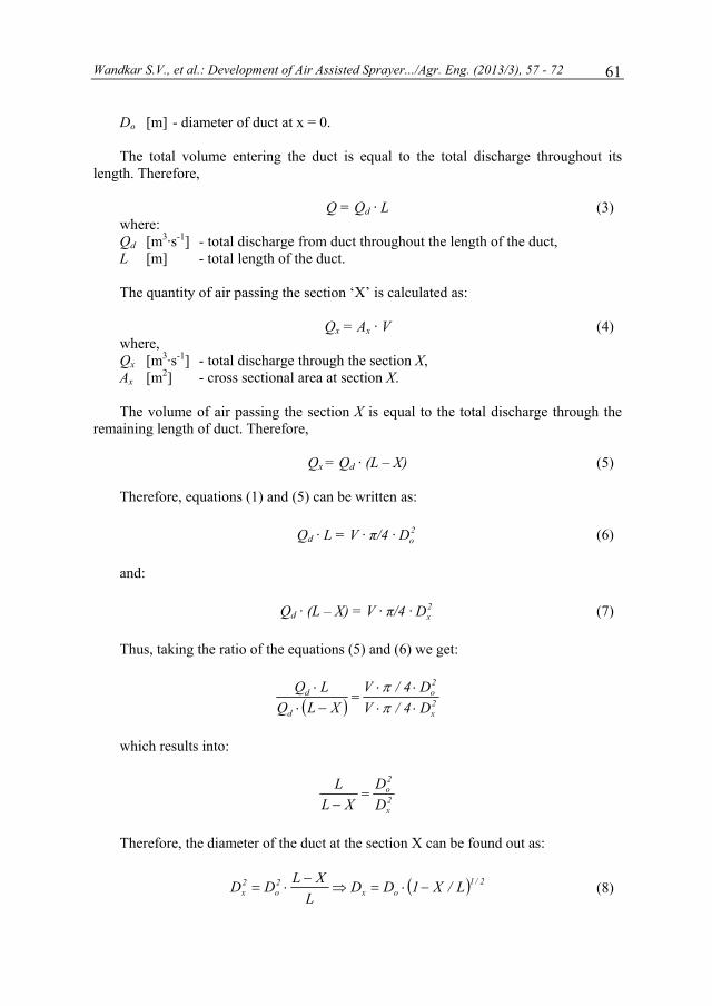
Wandkar S.V., et al.: Development of Air Assisted Sprayer.../Agr. Eng. (2013/3), 57 - 72

61

Do [m] - diameter of duct at x = 0.

The total volume entering the duct is equal to the total discharge throughout its length. Therefore,

Q = Qd · L (3) where: Qd [m3·s-1] - total discharge from duct throughout the length of the duct, L [m] - total length of the duct.

The quantity of air passing the section ‘X’ is calculated as:

Qx = Ax · V (4) where, Qx [m3·s-1] - total discharge through the section X, Ax [m2] - cross sectional area at section X.

The volume of air passing the section X is equal to the total discharge through the remaining length of duct. Therefore,

Qx = Qd · (L – X) (5)

Therefore, equations (1) and (5) can be written as:

Qd · L = V · π/4 · 2

oD (6)

and:

Qd · (L – X) = V · π/4 · 2xD (7)

Thus, taking the ratio of the equations (5) and (6) we get:

( ) 2x

2o

d

d

D4/VD4/V

XLQLQ

⋅⋅⋅⋅

=−⋅⋅

ππ

which results into:

2x

2o

DD

XLL

=−

Therefore, the diameter of the duct at the section X can be found out as:

( ) 2/1ox

2o

2x L/X1DD

LXLDD −⋅=⇒

−⋅= (8)

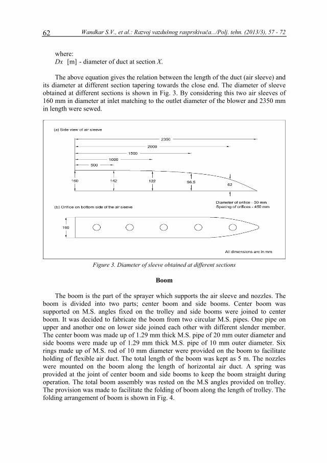
Wandkar S.V., et al.: Razvoj vazdušnog rasprskivača.../Polj. tehn. (2013/3), 57 - 72 62

where: Dx [m] - diameter of duct at section X. The above equation gives the relation between the length of the duct (air sleeve) and

its diameter at different section tapering towards the close end. The diameter of sleeve obtained at different sections is shown in Fig. 3. By considering this two air sleeves of 160 mm in diameter at inlet matching to the outlet diameter of the blower and 2350 mm in length were sewed.

Figure 3. Diameter of sleeve obtained at different sections

Boom

The boom is the part of the sprayer which supports the air sleeve and nozzles. The

boom is divided into two parts; center boom and side booms. Center boom was supported on M.S. angles fixed on the trolley and side booms were joined to center boom. It was decided to fabricate the boom from two circular M.S. pipes. One pipe on upper and another one on lower side joined each other with different slender member. The center boom was made up of 1.29 mm thick M.S. pipe of 20 mm outer diameter and side booms were made up of 1.29 mm thick M.S. pipe of 10 mm outer diameter. Six rings made up of M.S. rod of 10 mm diameter were provided on the boom to facilitate holding of flexible air duct. The total length of the boom was kept as 5 m. The nozzles were mounted on the boom along the length of horizontal air duct. A spring was provided at the joint of center boom and side booms to keep the boom straight during operation. The total boom assembly was rested on the M.S angles provided on trolley. The provision was made to facilitate the folding of boom along the length of trolley. The folding arrangement of boom is shown in Fig. 4.

Wandkar S.V., et al.: Development of Air Assisted Sprayer.../Agr. Eng. (2013/3), 57 - 72

63

Figure 4. Front view of the air assisted sprayer showing the folding arrangement of the boom

Trolley

The total assembly of the sprayer was supported on the trolley. Trolley was

arbitrarily designed by considering row to row spacing of crops; it was decided to keep the width of trolley as 420 mm and its length as 1300 mm.

Trolley had four wheels of 200 mm diameter and one handle was provided at rear end for its operation. The trolley was fabricated from 38.1 mm × 38.1 mm × 5 mm section M.S. angle and it was provided with two M.S. angles at front side to support boom over it.

Power unit and nozzles

An electric motor of 5 HP was used as a power unit. It was used to drive the blower and pump. The power is transmitted to blower and pump through ‘A’ section of ‘V’ grooved belt and pulley (Fig. 5). Hollow cone plastic nozzles were selected for the study. In this study the spacing of nozzles was 450 mm as used in a conventional boom sprayer.

Accessories

A horizontal triplex power pump (HTP) was used to generate pressure on the spray fluid which worked in the oil bath and produced maximum discharge of 16 l·min-1 at the pressure of 2.75 × 105 Pa. The pump had two deliveries and one bypass hose, pressure gauge, agitator and a pressure control valve to stabilize pressure. A high density polyethylene (HDPE) tank of 25 liter capacity was used for pesticide (Fig. 5). The bypass hose from HTP pump was connected to the tank at the bottom of the tank. The pressurized liquid from pump was brought to the nozzles with the help of hoses. The diameter of hose was 8 mm and made of heavy duty plastic.

Wandkar S.V., et al.: Razvoj vazdušnog rasprskivača.../Polj. tehn. (2013/3), 57 - 72 64

Figure 5. Side view of sprayer showing pesticide tank, blower, electric motor and pump

Performance evaluation of the air assisted sprayer

The laboratory experiments were conducted to study sprayer performance with

different air velocities and pump discharges for droplet size, droplet density and uniformity coefficient at different plant positions. Air velocities of 9 m·s-1, 12 m·s-1, 16 m·s-1 and 20 m·s-1; and pump discharges of 2.5 l·min-1, 4.5 l·min-1, 7 l·min-1 and 9 l·min-1 were used. The different air velocities were obtained by changing the rotations per minute (RPM) of blower by using different combinations of driver and driven pulleys and pump discharge was obtained by using different nozzles having the discharge rates of 0.25, 0.45, 0.70 and 0.90 l·min-1. An artificial plant canopies were prepared with hibiscus plant spaced at recommended spacing of 300 mm. The spraying height was kept as 800 mm during the experiments. To facilitate the evaluation of spray penetration into the canopy of plant, glossy papers of size 44 × 44 mm were stapled onto the leaf in different plant locations, i.e. top position of plant canopy, upper leaf surface (TU); top position of plant canopy, lower leaf surface (TL); middle position of plant canopy, upper leaf surface (MU); middle position of plant canopy, lower leaf surface (ML); bottom position of plant canopy, upper leaf surface (BU) and bottom position of plant canopy, lower leaf surface (BL). The sprayer was operated at speed of 1 km/hr for spraying in laboratory. Royal blue indigo dye was mixed with water to prepare coloured spray solution. During the experiments impression of spray solution was collected on glossy papers and then the glossy papers were taken for further analysis using a droplet image analyzer. Droplet size and droplet density were measured by using Image-Pro software.

RESULTS AND DISCUSSION

The developed air assisted sprayer was operated at four air velocities and four pump discharges in the laboratory and its performance was studied for droplet size, droplet density and uniformity coefficient at various locations in artificial plant canopy.

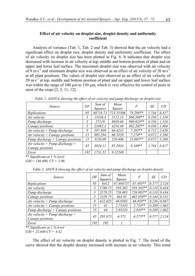
Wandkar S.V., et al.: Development of Air Assisted Sprayer.../Agr. Eng. (2013/3), 57 - 72

65

Effect of air velocity on droplet size, droplet density and uniformity coefficient

Analysis of variance (Tab. 1, Tab. 2 and Tab. 3) showed that the air velocity had a

significant effect on droplet size, droplet density and uniformity coefficient. The effect of air velocity on droplet size has been plotted in Fig. 6. It indicates that droplet size decreased with increase in air velocity at top, middle and bottom position of plant and on upper and lower leaf surface. The maximum droplet size was observed with air velocity of 9 m·s-1 and minimum droplet size was observed as an effect of air velocity of 20 m·s-1 at all plant positions. The values of droplet size observed as an effect of air velocity of 20 m·s-1 at top, middle and bottom position of plant and on upper and lower leaf surface was within the range of 100 µm to 150 µm, which is very effective for control of pests in most of the crops [2, 5, 11, 12].

Table 1. ANOVA showing the effect of air velocity and pump discharge on droplet size

Source DF Sum of Squares

Mean Square F SE CD

Replications 95 68718.73 723.35506 79.294** 1.744 6.417 Air velocity 3 15336.4 5112.13 560.388** 0.356 1.310 Pump discharge 3 27119 9039.68 990.923** 0.356 1.310 Canopy positions 5 21082.3 4216.46 462.205** 0.436 1.604 Air velocity × Pump discharge 9 597.809 66.4233 7.281** 0.712 2.620 Air velocity × Canopy positions 15 995.294 66.3529 7.274** 0.872 3.208 Pump discharge × Canopy positions 15 3156.09 210.406 23.065** 0.872 3.208 Air velocity × Pump discharge × Canopy positions 45 3834.11 85.2024 9.340** 1.744 6.417

Error 192 1751.52 9.12249 ** Significant at 1 % level GM = 146.400, CV = 2.06

Table 2. ANOVA showing the effect of air velocity and pump discharge on droplet density

Source DF Sum of Squares

Mean Square F SE CD

Replications 95 6412 67.494737 67.495** 0.577 2.124 Air velocity 3 1780.75 593.583 593.583** 0.118 0.434 Pump discharge 3 2178.25 726.083 726.083** 0.118 0.434 Canopy positions 5 2329.75 465.95 465.950** 0.144 0.531 Air velocity × Pump discharge 9 422.625 46.9583 46.958** 0.236 0.867 Air velocity × Canopy positions 15 41 2.73333 2.733** 0.289 1.062 Pump discharge × Canopy positions 15 44 2.93333 2.933** 0.289 1.062 Air velocity × Pump discharge × Canopy positions 45 295.875 6.575 6.575** 0.577 2.124

Error 192 192 1 ** Significant at 1 % level GM = 22.646 CV = 4.42

The effect of air velocity on droplet density is plotted in Fig. 7. The trend of the

curve showed that the droplet density increased with increase in air velocity. This trend

Wandkar S.V., et al.: Razvoj vazdušnog rasprskivača.../Polj. tehn. (2013/3), 57 - 72 66

was found similar in almost all positions of the plant. The maximum droplet density obtained through the plant canopy on the upper leaf surface on target plant was at 20 m·s-1 air velocity and minimum mean droplet density was observed with air velocity of 9 m·s-1.

Table 3. ANOVA showing the effect of air velocity and pump discharge on uniformity coefficient

Source DF Sum of Squares

Mean Square F SE CD

Replications 95 7.9546075 0.083732711 11.214** 0.050 0.184 Air velocity 3 3.61837 1.20612 161.527** 0.010 0.037 Pump discharge 3 1.25115 0.41705 55.852** 0.010 0.037 Canopy positions 5 2.07801 0.415601 55.658** 0.012 0.046 Air velocity × Pump discharge 9 0.715272 0.0794747 10.643** 0.020 0.075 Air velocity × Canopy positions 15 0.664458 0.0442972 5.932** 0.025 0.092 Pump discharge × Canopy positions 15 0.221771 0.0147848 1.980* 0.025 0.092 Air velocity × Pump discharge × Canopy positions 45 3.08083 0.0684629 9.169** 0.050 0.184

Error 192 1.43367 0.00746701 *, ** Significant at 5 % and 1 % level respectively GM = 1.449 CV = 5.96

Figure. 6. Effect of air velocity on droplet size at different plant positions

The trend of the curve (Fig. 8) showed that uniformity coefficient decreased with

increase in air velocity from 9 m·s-1 to 20 m·s-1. Uniformity coefficient observed as an effect of air velocity of 20 m·s-1 was within the recommended range. The reason behind this phenomenon was that the increased air velocity reduces the droplet size and increases droplet density throughout the plant canopy resulting in uniform distribution throughout the plant canopy.

100

120

140

160

180

200

9 12 16 20

Dro

plet

Siz

e, µ

m

Air Velocity, m/s

Top UpperTop LowerMiddle UpperMiddle LowerBottom UpperBottom Lower

R² = 0.95

R² = 0.96

R² = 0.88

R² = 0.97R² = 0.98R² = 0.98

Wandkar S.V., et al.: Development of Air Assisted Sprayer.../Agr. Eng. (2013/3), 57 - 72

67

Figure 7. Effect of air velocity on droplet density at different plant positions

Figure 8. Effect of air velocity on uniformity coefficient at different plant positions

Effect of pump discharge on droplet size, droplet density and uniformity coefficient

The pump discharge was set at 2.5 l·min-1, 4.5 l·min-1, 7 l·min-1 and 9 l·min-1 and the

effect on deposition of droplets at six different plant positions was studied. Analysis of variance (Tab. 1, Tab. 2 and Tab. 3) showed that the pump discharge had a significant effect on droplet size, droplet density and uniformity coefficient. Fig. 9 shows that the droplet size observed as an effect of pump discharge of 2.5 l·min-1 was within the recommended range. These values are significantly lower than the values of droplet size obtained as an effect of other pump discharge levels at all plant positions. The droplet size was found to decrease from top to bottom position of plant. Higher values of droplet size were observed at upper leaf surface than at lower leaf surface.

The effect of pump discharge on droplet density at different plant positions is shown in Fig. 10. The maximum droplet density was deposited at top position of the plant and upper leaf surface as an effect of pump discharge of 2.5 l·min-1. It was also observed that droplet density decreased with increase in pump discharge from 2.5 l·min-1 to 9 l·min-1 at all plant positions. The maximum mean droplet density was observed with pump discharge of 2.5 l·min-1.

10

15

20

25

30

35

40

9 12 16 20

Dro

plet

Den

sity

, Nos

./sq.

cm

Air Velocity, m/s

Top UpperTop LowerMiddle UpperMiddle LowerBottom UpperBottom Lower

R² = 0.99

R² = 0.99

R² = 0.99

R² = 0.99R² = 0.98R² = 0.99

1

1.2

1.4

1.6

1.8

2

9 12 16 20

Uni

form

ity

Coe

ffic

ient

Air Velocity, m/s

Top UpperTop LowerMiddle UpperMiddle LowerBottom UpperBottom Lower

R² = 0.90

R² = 0.99

R² = 0.99

R² = 0.91R² = 0.97R² = 0.91

Wandkar S.V., et al.: Razvoj vazdušnog rasprskivača.../Polj. tehn. (2013/3), 57 - 72 68

Figure 9. Effect of pump discharge on droplet size at different plant positions

Figure 10. Effect of pump discharge on droplet density at different plant positions

Figure 11. Effect of pump discharge on uniformity coefficient at different plant positions

The effect of pump discharge on uniformity coefficient is shown in Fig. 11. The

trend of the curve showed that uniformity coefficient increased with increase in pump

100

120

140

160

180

200

2.5 4.5 7 9

Dro

plet

Siz

e, µ

m

Pump Discharge, L/min

Top UpperTop LowerMiddle UpperMiddle LowerBottom UpperBottom Lower

R² = 0.98

R² = 0.99

R² = 0.99

R² = 0.99R² = 0.99R² = 0.99

10

15

20

25

30

35

40

2.5 4.5 7 9

Dro

plet

Den

sity

, Nos

./sq.

cm

Pump Discharge, L/min

Top UpperTop LowerMiddle UpperMiddle LowerBottom UpperBottom Lower

R² = 0.99

R² = 0.99

R² = 0.99

R² = 0.98R² = 0.99R² = 0.98

1

1.2

1.4

1.6

1.8

2

2.5 4.5 7 9

Uni

form

ity

Coe

ffic

ient

Pump Discharge, L/min

Top UpperTop LowerMiddle UpperMiddle LowerBottom UpperBottom Lower

R² = 0.99

R² = 0.94

R² = 0.96

R² = 0.99R² = 0.96R² = 0.99

Wandkar S.V., et al.: Development of Air Assisted Sprayer.../Agr. Eng. (2013/3), 57 - 72

69

discharge from 2.5 l·min-1 to 9 l·min-1. Uniformity coefficient observed as an effect of pump discharge of 2.5 l·min-1 was within the recommended range.

The optimum droplet size, droplet density and uniformity coefficient were obtained at pump discharge of 2.5 l·min-1.

Combined effect of air velocity and pump discharge on droplet size, droplet density

and uniformity coefficient

Analysis of variance (Tab. 1, Tab. 2 and Tab. 3) showed that the combine effect of air velocity and pump discharge on droplet size, droplet density and uniformity coefficient was significant at 99 per cent level of confidence.

Multiple regression analysis was performed to develop a combined relationship among the air velocity, pump discharge and droplet size at all plant positions. The equation of following form was obtained:

S = a + b1 · V + b2 · Q + b3 · V · Q (9)

where: S [µm] - droplet size, V [m·s-1] - air velocity, Q [l·min-1] -pump discharge, a, b1, b2, b3 - regression coefficients. The regression coefficients for above equation are presented in Tab. 4.

Table 4. Regression coefficients for linear relationship of droplet size

with air velocity and pump discharge

Plant Position RegressionConstant

(a)

RegressionCoefficient

(b1)

RegressionCoefficient

(b2)

RegressionCoefficient

(b3) R2 Computed F

Top Upper 163.208 -2.532 3.030 0.168 0.97 110.818** Lower 157.268 -2.247 3.161 0.011 0.95 67.362**

Middle Upper 159.324 -2.424 2.397 0.192 0.98 216.577** Lower 159.477 -2.548 1.670 0.073 0.95 81.829**

Bottom Upper 151.993 -2.193 2.728 0.167 0.99 374.028** Lower 158.119 -2.555 0.368 0.128 0.98 160.470**

** Significant at 1 % level The equation shown below was obtained for the combined effect of air velocity and

pump discharge at all plant positions on droplet density.

D = a + b1 · V + b2 · Q + b3 · V · Q (10) where: D [Nos. per cm2] - droplet density. The regression coefficients for above equation are presented in Tab. 5.

Wandkar S.V., et al.: Razvoj vazdušnog rasprskivača.../Polj. tehn. (2013/3), 57 - 72 70

Table 5. Regression coefficients for linear relationship of droplet density with air velocity and pump discharge

Plant Position Regression Constant

(a)

RegressionCoefficient

(b1)

RegressionCoefficient

(b2)

RegressionCoefficient

(b3) R2 Computed F

Top Upper 23.787 0.753 -1.033 -0.009 0.99 492.989** Lower 18.684 0.696 -0.645 -0.025 0.98 173.875**

Middle Upper 24.513 0.598 -1.386 -0.011 0.99 309.773** Lower 18.734 0.578 -0.818 -0.015 0.97 136.328**

Bottom Upper 21.763 0.717 -1.186 -0.010 0.99 274.980** Lower 15.387 0.664 -0.587 -0.025 0.97 145.275**

** Significant at 1 % level Multiple regression analysis was also performed to study the combined effect of air

velocity and pump discharge on uniformity coefficient at all plant positions. It gives following form of equation.

U = a + b1 · V + b2 · Q + b3 · V · Q (11)

where: U [-] - uniformity coefficient,

The regression coefficients for above equation are presented in Tab. 6.

Table 6. Regression coefficients for linear relationship of uniformity coefficient

with air velocity and pump discharge

Plant Position Regression Constant

(a)

RegressionCoefficient

(b1)

RegressionCoefficient

(b2)

RegressionCoefficient

(b3) R2 Computed F

Top Upper 1.580 -0.026 0.001 0.002 0.97 113.848** Lower 1.796 -0.036 0.040 0.000 0.92 41.743**

Middle Upper 1.685 -0.028 -0.011 0.002 0.96 93.519** Lower 1.805 -0.034 0.042 0.000 0.92 45.186**

Bottom Upper 1.668 -0.025 -0.007 0.002 0.95 79.418** Lower 1.802 -0.032 0.046 0.000 0.92 43.717**

** Significant at 1 % level

CONCLUSIONS

On the basis of laboratory experiments following conclusions were drawn: 1. Droplet size and uniformity coefficient of developed air assisted sprayer was

found to be decreased linearly with the increase in air velocity and decrease in pump discharge.

2. The droplet density was found to increase with increase in air velocity and decrease in pump discharge at all plant positions.

3. The recommended droplet size i.e. between 100 µm to 150 µm was obtained at air velocity of 20 m·s-1 and pump discharge of 2.5 l·min-1.

4. The developed air assisted sprayer exhibited better deposition efficiency with the air velocity of 20 m·s-1 and pump discharge of 2.5 l·min-1.

Wandkar S.V., et al.: Development of Air Assisted Sprayer.../Agr. Eng. (2013/3), 57 - 72

71

BIBLIOGRAPHY

[1] Bauer, F.C., Raetano, C.G. 2003. Air-assisted boom sprayer and spray deposition on bean plants. Scientia Agricola (Piracicaba, Braz.) 60(2), 211-215.

[2] Ennis, W.B. 1979. Introduction to crop protection. A. Soc. Agro., Madison: 267-292. [3] Hadar, E. 1980. Development criteria for air assisted ground crop sprayer. Degania sprayer,

Degania Bet, 15230, Israel, 23-26. [4] Hall, C.W. 1970. Principle of air movement. Drying of Farms Crops. Lyall Book Depot.

Ludhiana. [5] Lake, J R., Taylor, W.A. 1974. Effect of the form of a deposit on the activity of Barban

applied to Avena Fatua (L). Weed Research, 14: 13-18. [6] Manor, G.A., Hofman, O.R., Phishler, G., Epstin, Y., Nakash, T., Jakobi, M. 1989. Air stream

facilitate application of cotton foliage treatment. Transactions of ASAE 32(1), 37-40. [7] Raetano, C.G. 2005. Air assistance in sleeve boom sprayers. Available through:

www.jacto.com/PDF/white_papers/AirAssist_Sleeve_Boom_Sprayers.pdf [Accessed 20th Aug. 2013.]

[8] Shahare, P.U., Thakre, S.K., Mathur, S.M., Bhatt, Y.C. 2010. Sleeve Boom Sprayer I: Design and Development of Tractor Mounted Sleeve Boom Sprayer for Cotton. Agricultural Mechanization in Asia, Africa and Latin America, 41(2), 48-54.

[9] Shahare, P.U., Thakre, S.K., Mathur, S.M., Bhatt, Y.C. 2010. Sleeve Boom Sprayer II: Performance Evaluation of a Tractor Mounted Sleeve Boom Sprayer for Cotton. Agricultural Mechanization in Asia, Africa and Latin America, 41(3), 21-29.

[10] Sirohi, N.P.S., Gupta, P., Mani, I. 2008. Development of air-assisted hydraulic sprayer for vegetable crops. IE (I) Journal-AG, 89.

[11] Smith, D B., Burt, E.C., Lloyd, E.P. 1975. Selection of optimum sprays droplets sizes for Ball weevil and drift control. J. Eco. Ento., 68: 415-417.

[12] Willson, J.P., Hedden, O.K., Sleesman, J.P. 1963. Spray droplet size as related to disease and insect control on row crops. Ohio. Agric. Expt. Stn. Res. Bulletin, USA: 945-50.

[13] Yadawad, S.M., Kadapatti, R.G. 2011. Floriculture - present status and scope. Gloden Research Thoughts, 1(6), 1-4.

RAZVOJ VAZDUŠNOG RASPRSKIVAČA ZA ZAŠTITU CVEĆA U ZAŠTIĆENOM PROSTORU

Sachin Vilas Wandkar, Shailendra Mohan Mathur,

Babasaheb Sukhdeo Gholap, Pravin Prakash Jadhav

Univerzitet za poljoprivredu i tehnologiju Maharana Pratap, Fakultet za tehnologiju i inženjering, Institut za poljoprivredne mašine i pogonski

inženjering Udaipur, Rajasthan, India

Sažetak: Cvećarstvo je jedna od glavnih oblasti indijske poljoprivrede. Ovu proizvodnju najviše ugrožavaju insekti, štetočine i bolesti. Zato je vazdušni rasprskivač na motorni pogon razvijen za zaštitu cvećarskih kultura u zaštićenom prostoru. Konusni usmerivač vazduha je konstruisan i napravljen od ojačanog PVC materijala kako bi dao

Wandkar S.V., et al.: Razvoj vazdušnog rasprskivača.../Polj. tehn. (2013/3), 57 - 72 72

ujednačenu brzinu strujanja vazduha u svakom izlaznom otvoru. Nosač je razvijen kao oslonac za usmerivač vazduha i mlaznice. U sistem je ugrađen centrifugalni duvač kapaciteta 0.40 m3·s-1 koji stvara vazdušnu struju u usmerivačima. Horizontalna trostruka pogonska pumpa kapaciteta 16 l·min-1 je upotrebljena za obezbeđenje potrebnog pritiska u mlaznicama. Duvač i pumpa dobijaju pogon od elektromotora snage 3.73 kW. Ceo sklop rasprskivača postavljen je na kolica. Kod razvijenog rasprskivača u laboratoriji su ispitivani uticaji različitih brzina vazduha (9, 12, 16 i 20 m·s-1) i kapaciteta pumpe (2.5, 4.5, 7 i 9 l·min-1) na veličinu kapljica, gustinu kapljica i koeficijent ujednačenosti u šest različitih položaja veštačkog biljnog krova. Optimalni rezultati veličine kapljica (100-150 µm), gustine kapljica (25-35 kapljica po cm2) i koeficijenta ujednačenosti kod svih položaja biljke su dobijeni za brzinu vazduha od 20 m·s-1 i kapacitet pumpe od 2.5 l·min-1.

Ključne reči: zaštićeni prostor, cvećarstvo, vazdušni rasprskivač, veličina kapljice, gustina kapljica

Prijavljen: Submitted: 26.06.2013.

Ispravljen: Revised: 10.08.2013

Prihvaćen: Accepted: 22.08.2013.

Univerzitet uPoljoprivredInstitut za pNaučni časoPOLJOPRIGodina XXXBroj 3, 2013Strane: 73 –

UDK: 631.3

THE

OrelChair of T

Abstraobtained eestimate thstress condsoldered jsamples, tsoldered sajoint for m119,6…12

Key wnormal str

In recmachines, fixing the connectionpracticabil

* Corre

u Beogradu dni fakultet oljoprivrednu teopis IVREDNA TEHNXVIII 3. – 84

312.021.3:621.7

EORETICSTR

(META

l State AgrariaTechnology of

act. This artiequivalent strhe soldered jodition taking points strengththe overlappinamples tests o

metal of share 0,6 MPa at cl

words: plow shesses, solderin

cent years toparticularly, pplates to sha

n decreases thity and efficie

esponding autho

ehniku

NIKA

791.3.004.67

CAL AND ERENGTH OAL OF SHA

Vladi

an University,Constructiona

Orel, th

icle presents resses distribuoints strength place in the elh are definedng area and on force of teЛ65 and metaearance gap 0

hare, metal cerng, hardness,

IN

o increase theplow shares mare surface. Ihe share poteency of opera

or. E-mail: vova

EXPERIMEOF SOLDEARE – MET

imir Gonchar

, Faculty of Aal Materials ahe Russian Fed

theoretical eutions along taking into cements under

d in the articgroove depth

ear and shearal ceramic pla

0,5...0,75 mm,

ramic plate, hrestoration.

TRODUCTI

e wear resistmetal ceramicsInadequate adential resourceating surface f

aniii@rambler.

Institute

AGRIC

ENTAL REERED JOINTAL CERA

renko*

grotechnics aand Organizatderation

estimate of sthe share lenonsideration cloading. The

cle. Clearanceh are referrer showed thatate of alloy ВК that is proved

hydrogen-oxyg

ON

tance of opes plates are usedhesive strenge [1]. Researformation by m

ru

UniversityFaculty o

e of Agricultural Scie

CULTURAL ENY

OriginalnOriginal sci

ESEARCHNTS AMICS)

and Energy Suption of Technic

soldered strangth. It is sucomplicated cmain factors

e gap betweed to these fat strength σВ К-8, correspod with the theo

gen flame, tan

ration bodiesed. The problegth of today ches are diremetal ceramic

y of Belgrade of Agriculture

Engineering ntific Journal

NGINEERING Year XXXVIII No. 3, 2013. pp: 73 – 84

ni naučni rad ientific paper

H OF

upply, cal Service,

in and the uggested to character of influencing

en soldered actors. The of soldered nds to σВ = ory.

ngential and

s of tillage em arises at used glued

ected to the cs hard-face

Goncharenko V.: Teorijsko i eksperimentalno istraživanje.../Polj. tehn. (2013/3), 73 - 84 74

plates applying braze welding aiming at the plow share restoration and increasing its resource by 4-5 times.

Purpose is to estimate the hardness of soldered connection and the peculiarities of strain-stress state at soldering the metal ceramics plates to plow share blade using the hydrogen-oxygen flame.

MATERIALS AND METHODS

To test the soldering applying electrolyser “Energya-1,5 УХЛ4” we carried out the calculations of tangential τ and normal stresses σ1, σ2 and the distribution of stresses along the length of the soldered connection, also we carried out laboratory tests of soldered pieces for cutting (τср), tear (σв) using device ИР-500.

RESULTS AND DISCUSSION

To solve the problem of application of the electrolysers in the repair industry particularly for metal ceramics plates soldering to plow share is necessary to solve the following problems: to investigate the soldering mechanism with hydrogen-oxygen flame usage, to develop and optimize the technological solutions of realization of soldering with hydrogen-oxygen flame; to investigate the hardness of soldered connections for cutting and compression; to calculate economic efficiency of electrolysers application at plow share restoration.

At estimation of the soldered connections the complicated type of strain-stress state appearing in their elements at on-load was taken into consideration. The hardness of soldered connection is defined first of all by peculiarities of strain-stress state in soldered joint. That is why the main attention we pay to the analysis of stresses in soldered joints of overlapped soldered connections. If we suppose that stresses in a joint do not exceed the solder alloy elastic limit then for soldered connection it is possible to use the data obtained for glued and soldered connections in the limits of elasticity.

Strain-stress state in soldered joint in overlapped soldered connections is considered to be plain. Tangential τ and normal stresses σ1, σ2, are created in soldered joint under the influence of external forces. Tangential stresses according to [2-5] correspond to 0,5…0,6 from acceptable values of normal stresses:

σ=τ )6,0...5,0( (1) where: τ [MPa] - tangential stress, σ [MPa] - normal stress. More than that, as the connecting elements are inset it is necessary to calculate the

connections for tear by normal stresses. Tangential stresses concentrators will be higher, the higher the ratio of elasticity

modules of connected elements Е1 and Е2 to solder alloy elasticity module E.

Goncharenk

Stressdistributedand the cotangential appear.

l - la

where

ko V.: Theoretic

es, accordingd in the followorresponding t

stresses τ an

ap length, mm; P - f

Figure 2. Tyσ1 - axial str

e:

cal and Experim

g to Sazhin (1wing way. In to them deformnd the corres

Figure 1. oveδ - soldered joi

force, Н; b – lap

ype of the strainess, MPа; σ2 -

δ

mental Researc

1964) [3], in the connectinmations appe

sponding to th

rlapped soldereint thickness, mp width, mm; b

n-stress state intear stress, MP

2 εεδ−=

⋅dx

dj

h.../Agr. Eng. (

overlapped sng elements nar ε1 and ε1 inhem angular d

ed connection:mm; h1, h2 - elem

1 – piece length

n overlapped soPа; τ - tangentia

1ε

(2013/3), 73 - 84

soldered connnormal stressen the soldereddeformations

ments thickness,h, mm

oldered joint: al stress, MPа

4 75

nections are s σ1 and σ2 d joint only

j (Fig. 2)

mm;

(2)

Goncharenko V.: Teorijsko i eksperimentalno istraživanje.../Polj. tehn. (2013/3), 73 - 84 76

δ [mm] - soldered joint thickness, ε1 [-] - axial deformation, ε2 [-] - tear deformation. From equilibrium condition of soldered connection we obtain:

τ

σ−=

⋅dxdh 11

τ

σ=

⋅dxdh 22

b/Рhh 2211 =⋅σ+⋅σ

(3)

where σ1 [MPa] - axial stress, σ2 [MPa] - tear stress, h1, h2 [mm] - elements thickness, P [N] - force, b [mm] - lap width. According to Guck’s law:

111 εσ ⋅= E

222 εσ ⋅= E

Gj ⋅=τ

(4)

where: E1, E2 [10-9Pa] - elasticity modules of joint elements related to elasticity

module of alloy Е, j [-] - angular deformation, G [MPa] - shear module of soldered seam Solution to equations (4) – (6) gives: 0222 =⋅+′⋅−′′ σβσασ ПП (5) where:

2σ′′ [MPа] - the second derived function of stresses,

2σ′ [MPа] - the first derived function of stresses,

ППП /ψβ=α [1·mm-1] - ratio showing the changes of stiffness properties of metal of share Л-65 at its connection with soldered element (metal ceramics alloy ВК-8),

)hE/(G 11П ⋅⋅δ=β [1·mm-2] - aspect ratio of shear stiffness and tension to joint width and soldered element (metal

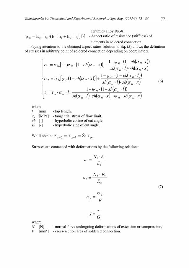
Goncharenko V.: Theoretical and Experimental Research.../Agr. Eng. (2013/3), 73 - 84 77

ceramics alloy ВК-8), )hEhE/(hE 221122П ⋅+⋅⋅=ψ [-] - Aspect ratio of resistance (stiffness) of

elements in soldered connection. Paying attention to the obtained aspect ratios solution to Eq. (5) allows the definition

of stresses in arbitrary point of soldered connection depending on coordinate x.

( )( )[ ] ( )( )( ) ( )

( )( )[ ] ( )( )( ) ( )

( )( )( ) ( ) ( )⎪

⎪⎪

⎩

⎪⎪⎪

⎨

⎧

⋅⋅−⋅⋅⋅⋅−⋅−

⋅⋅⋅=

⋅⋅⋅⋅−⋅−

+⋅−=

⋅⋅⋅⋅−⋅−

−⋅−⋅−=

xshxchlshlshl

xshlshlch

xch

xshlshlchxch

ПППП

ПППm

ПП

ППППl

ПП

ПППП

αψαααψ

αττ

αααψ

αψσσ

αααψ

αψσσ

11

111

1111

22

101

(6)

where: l [mm] - lap length, τm [MPa] - tangential stress of flow limit, ch [-] - hyperbolic cosine of cut angle, sh [-] - hyperbolic sine of cut angle. We’ll obtain: mlxx τττ ⋅== == 80 . Stresses are connected with deformations by the following relations:

1

111 E

FN ⋅=ε

2

222 E

FN ⋅=ε

Ey

y

σε =

Gj τ=

(7)

where: N [N] - normal force undergoing deformations of extension or compression, F [mm2] - cross-section area of soldered connection.

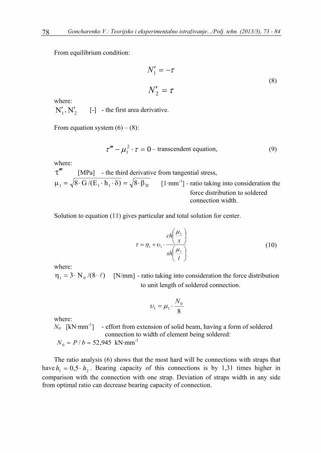
Goncharenko V.: Teorijsko i eksperimentalno istraživanje.../Polj. tehn. (2013/3), 73 - 84 78

From equilibrium condition:

τ−=′1N

τ=′2N

(8)

where:

1N′ , 2N′ [-] - the first area derivative. From equation system (6) – (8):

021 =⋅−′′′ τμτ – transcendent equation, (9)

where: τ ′′′ [MPа] - the third derivative from tangential stress,

П111 8)hE/(G8 β⋅=δ⋅⋅⋅=μ [1·mm-1] - ratio taking into consideration the force distribution to soldered

connection width. Solution to equation (11) gives particular and total solution for center.

⎟⎠⎞

⎜⎝⎛

⎟⎠⎞

⎜⎝⎛

⋅+=

lsh

xch

1

1

11 μ

μ

υητ (10)

where: )8/(N3 01 l⋅⋅=η [N/mm] - ratio taking into consideration the force distribution

to unit length of soldered connection.

80

11N⋅= μυ

where: N0 [kN·mm-1] - effort from extension of solid beam, having a form of soldered connection to width of element being soldered: 945,52/0 == bРN kN·mm-1

The ratio analysis (6) shows that the most hard will be connections with straps that

have 21 5,0 hh ⋅= . Bearing capacity of this connections is by 1,31 times higher in comparison with the connection with one strap. Deviation of straps width in any side from optimal ratio can decrease bearing capacity of connection.

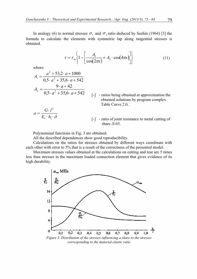
Goncharenk

In anaformula toobtained.

where

1 =A

2 =A

=E

a

PolynoAll theCalcul

each other Maxim

less than shigh durab

ko V.: Theoretic

alogy (6) to noo calculate th

τ

e:

,355,02,53

2

2

+⋅⋅+

aa

355,09

2 +⋅+⋅

aa

δ⋅⋅⋅

11

2

hElG

ominal functioe described delations on thewith error to

mum stresses vstresses in the bility.

Figure 3. Dis

cal and Experim

ormal stresseshe elements

⎩⎨⎧

⎢⎣

⎡−= mττ

c1

5426,1000+⋅

+a

a

5426,542

+⋅+

a

ons in Fig. 3 aependences she ratios for st5% that is a revalues obtainemaximum lo

stribution of thecorrespondin

mental Researc

s 1σ and 2σ rwith symme

( ) + Ax

Aπ2cos

1

[-] - ratios obtai

Table

[-] - ratio share

are obtained.how good reprtresses obtainesult of the coed at the calcu

oaded connect

e stresses influeg to the materia

h.../Agr. Eng. (

ratio deduced etric lap alon

( )⎭⎬⎫⎥⎦

⎤⋅ xA π4cos2

s being obtainned solutions e Curve 2.0,

of joint resiste Л-65.

roducibility. ed by differen

orrectness of thulations on cution element t

encing a share tal elastic ratio

(2013/3), 73 - 84

by Sazhin (19ng tangential

⎭⎬⎫

ned at approxiby program c

tance to metal

nt ways coorhe presented m

utting and tear that gives evid

to the stresses

4 79

964) [3] the stresses is

(11)

mation the complex

l cutting of

rdinate with model. are 5 times

dence of its

Goncharenko V.: Teorijsko i eksperimentalno istraživanje.../Polj. tehn. (2013/3), 73 - 84 80

For alloy ВК-8 stresses values correspond to 115…120 MPа. The calculation results and their checking according to III and IV failure theory

show that the equivalent stresses in the given soldered connection reach 25…28 MPа, that is as mentioned above considerably lower than the ultimate values obtained at the experiment.

III – failure theory [ ] 1204 22экв =σ≤τ⋅+σ=σ MPа.

IV – failure theory [ ] 1153 22экв =σ≤τ⋅+σ=σ MPа.

The suggested type of connection can bear the calculated load excess by 4…5 times. That gives the evidence reliability of connection at dynamic effects with the dynamic response factor ( дk ) 5=дk and is a good result.

To proof the theoretical calculations the investigations of experimental determination of the soldered connections indicators according to the requirements of the state standard at using hydrogen-oxygen flame are carried out.

Results of experimental research

It is proved that with the overlapping area increase the joint strength increases too. The rational overlapping area is 288…320 mm2 (Fig. 4, б). At overlapping area increase more than stated values the ultimate strength decreases. It corresponds to the dependence of solder flowing area from contact angle (Fig. 5). For example, for alloy ВК-8 at contact angle decrease β=16о solder flowing area increases (S=395 mm2), but at increase of β=25о solder flowing area decreases (S=316 mm2). Such kind of dependence is typical for share steel Л-65. The obtained data corresponds to the necessary technical requirements.

At increase of slot depth strength increases (Fig. 4, c), the rational slot depth is 4…4,5 mm. The mentioned depth is provided with the ultimate share thickness.

The analysis of slot between soldered samples (Fig. 4, a) showed that the optimal strength of the soldered joint 123 MPa is obtained when slot is 1,0 mm. Rational slot between soldered samples is 0,5…0,75 mm. Thus the soldered joint strength will be 120…121 MPa. It is connected with the fact that when the slots are more than 0,8 mm the layered directed crystallization resulting in fraction formation is observed.

To define the influence of the main factors, influencing on the strength change σВ, and also their mutual interaction complete factor test is done 23. Investigated factors: х1 – slot between soldered samples, δ, mm; х2 – the overlapping area of metal ceramics plates, S, mm2; х3– slot depth, l, mm. Response function у is strength σВ of soldered samples from metal ceramics (ВК-8) and share steel (Л65), MPa.

Goncharenko V.: Theoretical and Experimental Research.../Agr. Eng. (2013/3), 73 - 84 81

a. b.

c. Figure 4. Dependence of strength σВ of soldered sample joint from metal ceramics (ВК-8) and

share metal (Л65) from: a. slot between soldered samples δ, mm,

b. solder flowing areas S, mm2, c. slot depth l, mm.

a) b)

Figure 5. Dependence of solder flowing area from contact angle for materials from metal ceramics plate ВК-8 (a) and share metal Л65 (b)

σв, МПа

108110112114116118120122124126

0,25 0,5 0,75 1 1,25δ, мм

σв, МПа

114115

116117118119

120

121

224 256 288 320 352S, мм2

σв, МПа

95

100

105

110

115

120

125

2,5 3 3,5 4 4,5l, мм

S, мм2

285

288

291

294

297

300

27 28 30 31 33βo

S, мм2

300

320

340

360

380

400

16 19 21 24 25 βo

Goncharenko V.: Teorijsko i eksperimentalno istraživanje.../Polj. tehn. (2013/3), 73 - 84 82

The investigated process is adequately described with the regression equation:

Y=41,5649+34,4625х1+0,1767х2+8,3407хз-0,0107х1х2+3,3926x1х3+ +0,0162х2хз-22,97х1

2-0,0004х22-1,1493хз2

(12)

The given equation rather precisely describes the factor influence depending on the

slot between soldered samples, slot depth and plate overlapping area. Regression coefficient calculations and other statistical indicators were carried out

with computing aids usage, application soft Microsoft Excel. According to the analysis the change of soldered joint strength is maximally influenced with the slot between soldered samples and minimally with slot depth. The influence of plate overlapping area is inconsiderable.

It follows from the theory that the most dangerous section along the tangent stresses is midsection of soldered seam. Maximum normal stress at the boundary of soldered seam, according to the chart (Fig. 3), but the most dangerous will be the section of soldered seam where tangent and normal stresses are great. The results agree with theory because the practically obtained correlation is x/l=0,45, but in theory is x/l=0,5.

Overlapping of three charts (Fig. 4, a, b, c) with single scale of abscissas allows to chose the rational parameters of overlapping area, slot depth, slot between soldered samples using three maximum peak stresses. Matching them with Fig. 3 shows good reproducibility according to III and IV strength theory.

At the same time we determined: wetting along the contact angle and spreading radius; gap-filling with solder alloy; corrosive resistance; adhesive strength; we carried out the metallographic observations.

In Orel State Agrarian University soldered hydrogen-oxygen device “Energya-1,5 УХЛ4” [6] was used at the investigation of the soldered process with application of hydrogen-oxygen flame.

CONCLUSIONS

1. As the result of the analysis the theoretical dependences of ultimate stress σВ of soldered joints of samples from share metal (Л65) and metal-ceramics plate (ВК-8) from clearance gap between soldered samples δ, from overlapping area of plate S and groove depth l are obtained. The most rational values of ultimate stress will be provided at S=256…320 mm2, δ=0,5…1,0 mm, l=3,5…4,0 mm.

2. The suggested type of connection can bear the calculated load excess by 4…5 times. That gives the evidence reliability of connection at dynamic effects with the dynamic response factor ( дk ) 5=дk .

3. Adhesive strength of metal-ceramics plates on share metal obtained by means of soldering using hydrogen-oxygen flame depends on overlapping area, groove depth and clearance gap between soldered samples.

4. Soldered sample tests using hydrogen-oxygen flame on force of tear and shear demonstrated strength σВ of soldered joint for metal of share Л65 and metal-ceramics plate was σВ = 119,6…120,6 MPa at clearance gap 0,5...1,0 mm, that is proved with the theory.

Goncharenko V.: Theoretical and Experimental Research.../Agr. Eng. (2013/3), 73 - 84 83

5. The mentioned full 2-leveled factor experiment of type 23, that was done in the local time limit demonstrates that the theoretical values of ultimate stress σВ practically do not differ from experimental values.

6. The technology of plow share restoration by soldering using hydrogen-oxygen flame with high strength properties of soldered connections is developed. It allows reducing the production cost of restoration using cheap hydrogen-oxygen gas mixture being obtained as a result of water electrolyser and through utilization of metal ceramics plates in tool-producing industry.

BIBLIOGRAPHY

[1] Goncharenko, V.V. 2007. Technology of restoration and hardening of plow shares with metal ceramics plates (Технология восстановления и упрочнения лемехов плугов металлокерамическими пластинами). Dissertation of candidate of technical sciences. Faculty of Mechanization and Technical Service, Russian State Agrarian Extramural University, Moscow.. 158p.

[2] Fesik, S.P. 1982. Reference book of resistance of materials (Справочник по сопротивлению материалов). S.P. Fesik. – Kiev : Budivelnik. 290 p.

[3] Sazhin, A.M. 1964. Stress calculation in adhesive joints of metal plates at shear (Расчет напряжений в клеевых соединениях металлических пластин при сдвиге). Vestnik of Machinostroenye. №11. P.43-48.

[4] Kuznetsov, О.А. 1987. Hardness of soldered joints (Прочность паяных соединений). Machinostroenye, P.40-41.

[5] Goncharenko, V.V. 2013. Stress calculation of soldered joints (metal ceramics) at plow shares restoration. Proceedings of the union of scientists. Fifth conference „Energy efficiency and agricultural engineering”. – Ruse, Bulgaria, 17-18 may, p.p. 539-543, ISSN 1311-9974

[6] Goncharenko, V.V. 2009. Pat. 2344913 Russian Federation, МПК7 В23Р6/00, В23К1/00, А01В15/04. Way of plow share restoration (Способ восстановления лемехов плугов). Published 27.01.2009, Bulletin. №3. – 3 p.

TEORIJSKO I EKSPERIMENTALNO ISTRAŽIVANJE JAČINE LEMLJENIH SPOJEVA

(METAL METAL – METAL KERAMIKA)

Vladimir Goncharenko

Državni Poljoprivredni Univerzitet Orel, Fakultet za poljoprivrednu tehniku i energetiku, Katedra za tehnologiju konstruktivnih materijala i organizaciju tehničkog

servisa, Orel, Ruska Federacija

Sažetak. Ovaj rad predstavlja teorijsku procenu jačine lema i postignutih ekvivalentnih distribucija duž spoja. Predloženo je da se proceni jačina lemljenih spojeva uzimajući u obzir komplikovani karakter uslova kojima su elementi izloženi pod

Goncharenko V.: Teorijsko i eksperimentalno istraživanje.../Polj. tehn. (2013/3), 73 - 84 84

opterećenjem. U radu su definisani osnovni faktori koji utiču na jačinu lemljenih spojeva. Zazor između lemljenih uzoraka, zona preklapanja i dubina su svrstani u ove faktore. Testovi lemljenih spojeva na sile kidanja i smicanja pokazali su da jačina σВ lemljenog spoja metala Л65 i metal-keramičke ploče legure ВК-8, odgovara intervalu σВ = 119,6…120,6 MPa pri zazoru 0,5...0,75 mm, što je teorijski dokazano.

Ključne reči: plužno smicanje, metal-keramička ploča, vodonično-kiseonični plamen, tangencijalna i normalna opterećenja, lemljenje, tvrdoća, obnova.

Prijavljen: Submitted: 13.06.2013.

Ispravljen: Revised: 10.07.2013.

Prihvaćen: Accepted: 28.07.2013.

Univerzitet uPoljoprivredInstitut za pNaučni časoPOLJOPRIGodina XXXBroj 3, 2013Strane: 85 –

UDK: 582.8

TH

Datt

1Ce

2In

Abstracarcinogeneffect of ditunnel dryDrying of hat higher tmoisture rmodel satimoisture dtemperatur4.31·10-10 mto make thfineness m

Key wenergy

Hennaof Africa, all over theStates. The

* Corre

u Beogradu dni fakultet oljoprivrednu teopis IVREDNA TEHNXVIII 3. – 100

872

HIN LAYER

tatreya M. K

entral InstitutePO: P

Infosys Limited3Karn

act: Henna lnic, anti-inflamifferent dryinger was emplohenna leaves temperature. Tratio data. Amsfactorily desdiffusivity (Dre. Effective mm2·s-1 and acthe powder an

modulus of 1.3

words: henna,

a (Lawsonia insouthern Asia

e world include variety of he

esponding autho

ehniku

NIKA

R DRYING

Kadam1, Mano

e of Post-HarvPAU campus, Ld, Electronic nataka State D

leaves are wmmatory, analg conditions ooyed and the prominently o

Twelve thin lamong the matscribed the dryDeff) of basil

moisture diffuivation energy

nd the powde685.

mathematica

IN

nermis, syn. La, and northerding Australiaenna plant var or. E-mail: mnj

G KINETIC

oj Kumar Gu

vest EngineeriLudhiana-141City, Phase I,

Department of

well known flgesic and ant

on kinetics of hleaves were doccurred in faayer-drying mthematical moying behaviorleaves increa

fusivity of heny was 27.03 ker had averag

al modeling, d

TRODUCTI

L. alba) is natrn Australia in

a, the Mediterrries from regi off@gmail.com

Institute

AGRIC

CS OF HEN

upta2*, Vaijay

ing and Techn1004 (Punjab) Bangalore, Kf Horticulture,

for their costipyretic prophenna leaves, dried at 40, 4

alling rate perimodels were fodels investigr with highestased with thenna leaves ra

kJ·mol-1. The dge particle siz

drying, moistu

ON

tive to tropican semi-arid zranean, Africaion to region a

m

UniversityFaculty o

e of Agricultural Scie

CULTURAL ENY

p

OriginalnOriginal sci

NNA LEAV

yanta M. Kad

nology (CIPHE), India Karnataka, Ind, India

smetic agent erties. To invthe laboratory

45, 50, 55, 60iod and dryingfitted to the exgated, the Mit r2 values. The increase in anged from 2dried leaves wze of 0.2069

ure diffusivity,

al and subtropiones. The pla

a, and in Southand different

y of Belgrade of Agriculture

Engineering ntific Journal

NGINEERING Year XXXVIII No. 3, 2013.

pp: 85 – 100

ni naučni rad ientific paper

VES

dam3

HET),

dia

with anti-vestigate the y models of 0 and 65°C. g was faster xperimental dilli-Kucuk he effective

drying air 2.24·10-10 to were ground mm with a

y, activation

ical regions ant is found hern United plants have

Kadam D.M., et al.: Kinetika sušenja tankog sloja.../Polj. tehn. (2013/3), 85 -100 86

different coloring properties and the color of the powder also varies. Henna is a tall shrub or small tree 2 to 6 m high. It is glabrous, multi-branched with spine tipped branch lets. Henna is commercially cultivated in western India, Pakistan, Iran, Yemen, Morocco and Sudan.

Herbal medicines are in great demand in the developed as well as developing countries for primary healthcare because of their wide biological and medicinal activities, higher safety margins and less cost. Henna has been used for thousands of years for its medicinal properties and cosmetic properties. Henna is worldwide known as cosmetic agent with anti-carcinogenic, anti-inflammatory, analgesic and antipyretic properties [1]. Alcoholic extracts of henna, leaves showed mild antibacterial activity against, Micrococcus pyrogenes var Aureus and Eschericia coli [2]. The tannin and the gallic acid seem to have a complimentary beneficial effect. Several studies have been dedicated to explore the medicinal value of henna leaves. Henna leaves have been effective in management of burn wound infections [3], and henna leaves extract can be used as sources of natural antioxidants [1]. Researchers studied the stability of henna paste for skin decoration, tattooing and hair dyeing [4]. Researchers have also applied henna dye on wool fabric to impart antimicrobial characteristics and found the treated fabrics were antimicrobial [5, 6]. Henna produces a red-orange dye molecule called laws one. This molecule has an affinity for bonding with protein, and thus has been used to dye skin, hair, fingernails, leather, silk and wool. The color produced by pure natural henna ranges from orange to red, to black cherry and to near black color. The color of henna powder depends not only on the variety of the plant, storage conditions, pasting method but also on the drying method and dying process parameters. Most of the henna is traded in powder form after drying and grinding of dried leaves. So, drying of the leaves is an interesting area of the research to ascertain optimized drying conditions of the leaves. The presented study evaluates drying kinetics of henna leaves.

THEORETICAL CONSIDERATIONS

Mathematical formulation

The moisture contents of henna leaves during the experiments were expressed in dimensionless form as moisture ratios (MR) with the help of the following equation [7-12].

e

e

MMMM

MR−−

=0

(1)

where: M [%] - mean henna leaves moisture content, Mo [%] - initial moisture content, Me [%] - equilibrium moisture content. Me value is very small compared to those of Mo and M. So, the Me value can be

neglected and the moisture ratio can be simplified and can be expressed as [10-15]:

Kadam D.M., et al.: Thin Layer Drying Kinetics.../ Agr. Eng. (2013/3), 85 - 100 87

0M

MMR = (2)

Table 1. Thin layer drying models considered for the study

S.No. Name of the model Model equation 1 Newton MR = Exp(-k*t) 2 Page MR = Exp(-k * t ** n) 3 Modified Page 1 MR = Exp(-(k * t) ** n) 4 Henderson and Pabis MR = a * Exp(- k * t) 5 Logarithmic MR = a * Exp(- k * t) + c 6 Two-term MR = a * Exp(-k * t) + b * Exp(-n * t) 7 Two-term exponential MR = a * Exp(-k * t) + (1-a) * Exp(-k *a* t) 8 Wang and singh MR = 1 + (a * t) + (b * (t ** 2)) 9 Diffusion approach MR = a * Exp(-k * t) + (1-a) * Exp(-k *b* t)

10 Modified Henderson and Pabis MR = a * Exp(-k * t) + b * Exp(-n * t) + c * Exp(-m * t) 11 Verma et al. MR = a * Exp(-k * t) + (1-a) * Exp(-m* t) 12 Midilli-Kucuk MR = a * Exp(-k *( t ** n)) + b * t

Data were fit to 12 thin layer drying models to ascertain the best model which can

describe the drying behavior of the product (Table 1). To determine the best fit model, non-linear regression analysis was done using the STATISTICA. The coefficient of determination, r2, was one of the primary and main criteria for selecting the best equation to account for variation in the drying curves of dried samples [8, 16, 17]. In addition to coefficient of determination, the goodness of fit was determined by the statistical parameters such as reduced chi-square (χ2), mean bias error (MBE), and root mean square error (RMSE). The best fit was evaluated on the basis of highest r2 value, and lowest values of χ2, MBE and RMSE [17-20]. The above parameters were calculated as per the following relationships:

zN

MRMRN

iiprei

−

−=

∑=1

2..exp

2)(

χ (3)

∑=

−=N

iiipre MRMR

NMBE

1.exp. )(1

(4)

2/1

1

2.exp. )(1

⎥⎦

⎤⎢⎣

⎡−= ∑

=

N

iiipre MRMR

NRMSE (5)

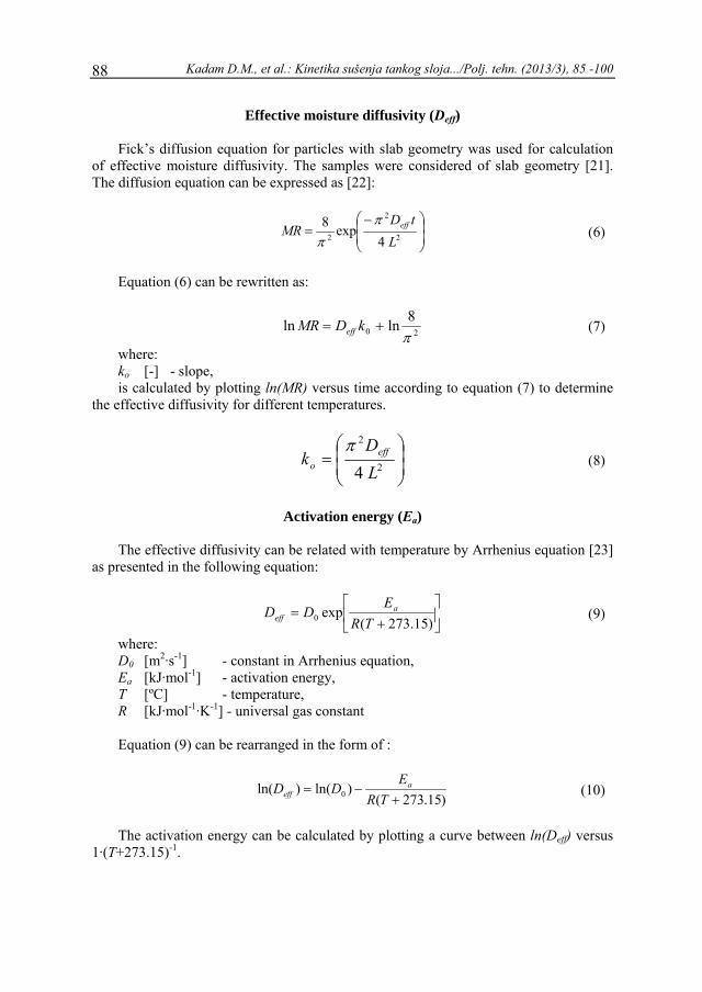
Kadam D.M., et al.: Kinetika sušenja tankog sloja.../Polj. tehn. (2013/3), 85 -100 88

Effective moisture diffusivity (Deff)

Fick’s diffusion equation for particles with slab geometry was used for calculation of effective moisture diffusivity. The samples were considered of slab geometry [21]. The diffusion equation can be expressed as [22]:

⎟⎟⎠

⎞⎜⎜⎝

⎛ −= 2

2

2 4exp8

LtD

MR effππ

(6)

Equation (6) can be rewritten as:

208lnlnπ

+= kDMR eff (7)

where: ko [-] - slope, is calculated by plotting ln(MR) versus time according to equation (7) to determine

the effective diffusivity for different temperatures.

⎟⎟⎠

⎞⎜⎜⎝

⎛= 2

2

4 LD

k effo

π (8)

Activation energy (Ea)

The effective diffusivity can be related with temperature by Arrhenius equation [23]

as presented in the following equation:

⎥⎦

⎤⎢⎣

⎡+

=)15.273(

exp0 TRE

DD aeff

(9)

where: D0 [m2·s-1] - constant in Arrhenius equation, Ea [kJ·mol-1] - activation energy, T [ºC] - temperature, R [kJ·mol-1·K-1] - universal gas constant Equation (9) can be rearranged in the form of :

)15.273(

)ln()ln( 0 +−=

TRE

DD aeff

(10)

The activation energy can be calculated by plotting a curve between ln(Deff) versus

1·(T+273.15)-1.

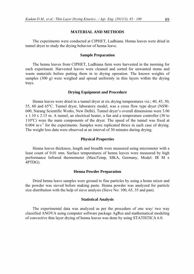
Kadam D.M., et al.: Thin Layer Drying Kinetics.../ Agr. Eng. (2013/3), 85 - 100 89

MATERIAL AND METHODS

The experiments were conducted at CIPHET, Ludhiana. Henna leaves were dried in tunnel dryer to study the drying behavior of henna leave.

Sample Preparation

The henna leaves from CIPHET, Ludhiana farm were harvested in the morning for

each experiment. Harvested leaves were cleaned and sorted for unwanted stems and waste materials before putting them in to drying operation. The known weights of samples (300 g) were weighed and spread uniformly in thin layers within the drying trays.

Drying Equipment and Procedure

Henna leaves were dried in a tunnel dryer at six drying temperatures viz.; 40, 45, 50,

55, 60 and 65°C. Tunnel dryer, laboratory model, was a cross flow type dryer (NSW-600, Narang Scientific Works, New Delhi). Tunnel dryer’s overall dimensions were 3.06 x 1.10 x 2.15 m. A tunnel, an electrical heater, a fan and a temperature controller (30 to 110°C) were the main components of the dryer. The speed of the tunnel was fixed at 0.004 m·s-1 for the experiments. Samples were replicated thrice in each case of drying. The weight loss data were observed at an interval of 30 minutes during drying.

Physical Properties

Henna leaves thickness, length and breadth were measured using micrometer with a

least count of 0.01 mm. Surface temperatures of henna leaves were measured by high performance Infrared thermometer (MaxiTemp, SIKA, Germany, Model: IR M x 4PTDG).

Henna Powder Preparation Dried henna leave samples were ground to fine particles by using a home mixer and

the powder was sieved before making paste. Henna powder was analyzed for particle size distribution with the help of sieve analysis (Sieve No: 100, 65, 35 and pan).

Statistical Analysis The experimental data was analyzed as per the procedure of one way/ two way

classified ANOVA using computer software package AgRes and mathematical modeling of convective thin layer drying of henna leaves was done by using STATISTICA 6.0.

Kadam D.M., et al.: Kinetika sušenja tankog sloja.../Polj. tehn. (2013/3), 85 -100 90

RESULTS AND DISCUSSION

Physical Dimensions of Fresh Henna Leaves

The physical dimensions of henna leaves are presented in Table 2. The average thickness, length and central breadth of leaves were about 0.26 mm, 18.42 mm, and 7.82 mm, respectively. The surface area of the leaves was ranged from 63.90 to 205.00 mm2 with an average of 149.42 mm2.

Table 2. Physical dimension of henna leaves (mm)

Sample Thickness(mm)

Length(mm)

Breadth(mm)

Surface area(mm2)

1 0.27 19.63 7.46 146.40 2 0.26 17.42 7.95 138.49 3 0.26 22.60 7.36 166.33 4 0.27 16.80 12.13 203.70 5 0.27 21.75 7.31 188.99 6 0.26 14.20 5.14 73.02 7 0.25 19.20 8.28 158.97 8 0.26 14.20 4.50 63.90 9 0.25 20.00 10.25 205.00

Mean 0.26 18.42 7.82 149.42

Drying Behavior of Henna Leaves

Moisture content of fresh henna leaves was 66.954% (w.b). Table 3. presents the drying time at different drying temperature regime in tunnel dryer. Minimum time (270 min) was recorded at 65°C, whereas maximum time (540 min) was observed for henna leaves drying in tunnel dryer at 40°C.

Table 3. Drying time for henna leaves in tunnel dryer

S. No. Drying air

temperature (°C)

Henna leaves drying time

(min) 1 65 270 2 60 300 3 55 360 4 50 420 5 45 510 6 40 540

Drying of the leaves mainly occurred in falling rate period. Figure 1. shows the plot

between moisture losses with respect to time for the samples dried in tunnel dryer at

Kadam D.M

different dThe moistustarted to dtemperaturto increasesometimescontributintime intervrate periodSimilar finFigure 1 stunnel drye

Moistu(Table 1) aTable 4. ddata.

In all temperaturvalues of rmodel withapproach (layer dryinreported fexaminatiotemperatur

M., et al.: Thin L

drying temperaure depletion pdecrease. Theres in tunnel de, this period s a portion ofng for moisturval between (d was observndings were oshows moistuer at different

Math

ure ratio and and the mode

depicts on the

cases, the r2

res, indicatingr2 and lowest h highest r2 va(0.9984). Thung behavior offor hot air don of the r2, res (Table 4).

Layer Drying K

atures. The mper hour was me similar pattedryer. In some

is known asf energy is ure loss. A cons(30 min) betwed for all samobserved by [

ure ratio variatemperatures

Figure 1. MR

hematical Mo

drying time ls were evalu mentioned p

2 values wereg a good fit o

values of χ2,alue of 0.9987us, Midilli-Kuf henna leave

drying of aprχ2, MBE an

The constants

Kinetics.../ Agr. E

more was the tmore in the inern was obsere cases dryings heating periutilized to heastant rate perioween two succmples for dry[10] for basil

ation with res.

R of tunnel dried

odels for Fitti

data were fi

ated on the baparameters to

e greater thanf the data. Th MBE and RM7 followed Mucuk model ms when dried ricots [15, 1nd RMSE shos of the model

Eng. (2013/3),

emperature, thnitial drying prved for all sa rate was initiod. Heating pat the materiaod was not obcessive observying of hennal leaves and bspect to time

d henna leaves

ing Drying C

tted for 12 thasis of r2, χ2, ascertain the

n 0.90 excephe results (TaMSE were obtodified Page

marginally betin tunnel drye9], rosehip [owed that thls are presente

85 - 100

he faster was eriod and subamples dried ially low and tperiod observal instead of bserved becausvations. A sin

a leaves in tuby [11] for mfor henna dr

Curves

hin layer dryMBE and RMbest fit of th

t for Page mable 4) show ttained for Mi1 (0.9985) antter representer. Similar fin[8] and plume all models

ed in Table 5(a

91

the drying. sequently it at different then started

ved because completely

se of higher ngle falling

unnel dryer. mint leaves. rying in the

ying models MSE values. he observed

model at all that highest dilli-Kucuk

nd Diffusion ted the thin ndings were m [20]. An

vary with a-c).

Kadam D.M., et al.: Kinetika sušenja tankog sloja.../Polj. tehn. (2013/3), 85 -100 92

Table 4. Mathematical models statistical analyses results of thin layer tunnel drying of Henna leaves

S.no. Model name

Modelequation

Drying temp.(°C) R2 Chi sq MBE RMSE

1 Newton MR = Exp(-k t) 65 0.97042 0.00369 -0.00396 0.01824 60 0.95016 0.00664 -0.00039 0.02343 55 0.98806 0.00127 -0.00340 0.00950 50 0.99000 0.00089 -0.00605 0.00742 45 0.97141 0.00315 -0.00078 0.01285 40 0.94089 0.00737 0.00146 0.01918 2 Page MR = Exp(-k t n) 65 0.45550 0.07650 0.00000 0.07823 60 0.32056 0.10065 0.00000 0.08652 55 0.37623 0.07245 0.00000 0.06867 50 0.38350 0.05879 0.00000 0.05828 45 0.23870 0.08901 0.00000 0.06630 40 0.18953 0.10705 0.00000 0.07100 3 Modified Page 1 MR = Exp (-(k t)n) 65 0.99157 0.00118 0.00248 0.00973 60 0.99558 0.00066 0.00124 0.00698 55 0.99736 0.00031 -0.00204 0.00447 50 0.99010 0.00094 -0.00608 0.00739 45 0.99855 0.00017 0.00040 0.00289 40 0.99580 0.00055 0.00256 0.00511 4 Henderson and Pabis MR = a Exp(- k t) 65 0.97440 0.00360 -0.01045 0.01696 60 0.96452 0.00526 -0.01457 0.01977 55 0.99081 0.00107 -0.00783 0.00834 50 0.99017 0.00094 -0.00514 0.00736 45 0.98280 0.00201 -0.01015 0.00997 40 0.96479 0.00465 -0.01436 0.01480 5 Logarithmic MR = a Exp(- k t) + c 65 0.98137 0.00299 0.00000 0.01447 60 0.98520 0.00247 0.00000 0.01277 55 0.99711 0.00037 0.00000 0.00467 50 0.99462 0.00056 0.00000 0.00544 45 0.99369 0.00079 0.00000 0.00604 40 0.98359 0.00230 0.00000 0.01010 6 Two-term MR = a Exp(-k t) +b Exp(-n t) 65 0.98737 0.00237 -0.00421 0.01191 60 0.99308 0.00132 -0.00762 0.00873 55 0.99563 0.00062 -0.00486 0.00575 50 0.99039 0.00108 -0.00561 0.00728

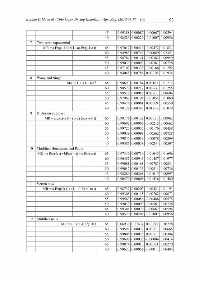
Kadam D.M., et al.: Thin Layer Drying Kinetics.../ Agr. Eng. (2013/3), 85 - 100 93

45 0.99388 0.00082 -0.00667 0.00594 40 0.98529 0.00220 -0.01007 0.00956 7 Two-term exponential MR = a Exp (-k t) +(1 - a) Exp(-k a t) 65 0.97017 0.00419 -0.00472 0.01831 60 0.94983 0.00743 -0.00089 0.02351 55 0.98784 0.00141 -0.00382 0.00959 50 0.99039 0.00092 -0.00561 0.00728 45 0.97107 0.00338 -0.00166 0.01292 40 0.94048 0.00786 0.00038 0.01924 8 Wang and Singh MR = 1 + a t + b t 2 65 0.98693 0.00184 0.00187 0.01212 60 0.98570 0.00212 0.00966 0.01255 55 0.99518 0.00056 0.00961 0.00604 50 0.97962 0.00194 -0.01054 0.01060 45 0.99476 0.00061 0.00509 0.00550 40 0.98129 0.00247 0.01265 0.01079 9 Diffusion approach MR = a Exp(-k t)+ (1- a) Exp(-k b t) 65 0.99176 0.00132 0.00051 0.00962 60 0.99602 0.00066 -0.00215 0.00662 55 0.99723 0.00035 -0.00176 0.00458 50 0.99039 0.00099 -0.00562 0.00728 45 0.99845 0.00019 -0.00078 0.00299 40 0.99586 0.00058 -0.00244 0.00507

10 Modified Henderson and Pabis MR = a Exp(-k t) + bExp(-n t) + c Exp(-mt) 65 0.97440 0.00719 -0.01045 0.01696 60 0.96452 0.00946 -0.01457 0.01977 55 0.99081 0.00168 -0.00783 0.00834 50 0.99017 0.00135 -0.00514 0.00736 45 0.98280 0.00268 -0.01015 0.00997 40 0.96479 0.00608 -0.01436 0.01480

11 Verma et al. MR = a Exp(-k t)+ (1 - a) Exp(-m t) 65 0.98737 0.00203 -0.00421 0.01191 60 0.99308 0.00115 -0.00762 0.00873 55 0.99563 0.00056 -0.00486 0.00575 50 0.99039 0.00099 -0.00561 0.00728 45 0.99388 0.00076 -0.00667 0.00594 40 0.98529 0.00206 -0.01007 0.00956

12 Midilli-Kucuk MR = a Exp(-k t n)+ b t 65 0.06939 0.17434 0.13295 0.10228 60 0.99598 0.00077 0.00001 0.00665 55 0.99805 0.00028 0.00001 0.00384 50 0.99690 0.00035 -0.00004 0.00414 45 0.99874 0.00017 0.00003 0.00270 40 0.99623 0.00056 -0.00011 0.00484

Kadam D.M., et al.: Kinetika sušenja tankog sloja.../Polj. tehn. (2013/3), 85 -100 94

Table 5a. Mathematical models statistical analyses constants

and standard errors of thin layer tunnel drying of Henna leaves

S. no.

Model name

Model equation

Drying temp. (°C)

Constant Std Error

K N A K N A

1 Newton

MR = Exp(-k t) 65 0.011828 0.000873 60 0.008577 0.000745 55 0.008234 0.000300 50 0.006917 0.000194 45 0.005400 0.000254 40 0.004861 0.000335

2 Page MR = Exp(-k t n) 65 1.403437 0.000000 0.375025 0.000000 60 1.157232 0.000000 0.319137 0.000000 55 1.278839 0.000000 0.279142 0.000000 50 1.250749 0.000000 0.226350 0.000000 45 1.163550 0.000000 0.231642 0.000000 40 1.109421 0.000000 0.233868 0.000000

3 Modified Page 1 MR = Exp (-(k t)n) 65 0.011312 1.397826 0.000398 0.102615 60 0.008219 1.563206 0.000173 0.076078 55 0.007991 1.206282 0.000131 0.036930 50 0.006893 1.018002 0.000204 0.050701 45 0.005201 1.378942 0.000047 0.026223 40 0.004658 1.625569 0.000067 0.055497

4 Henderson and Pabis MR = a Exp(- k t) 65 0.012430 1.057635 0.001064 0.052995 60 0.009437 1.110480 0.000856 0.060281 55 0.008601 1.046831 0.000355 0.026411 50 0.006842 0.989086 0.000259 0.023182 45 0.005917 1.101172 0.000275 0.032313 40 0.005552 1.154763 0.000364 0.048090

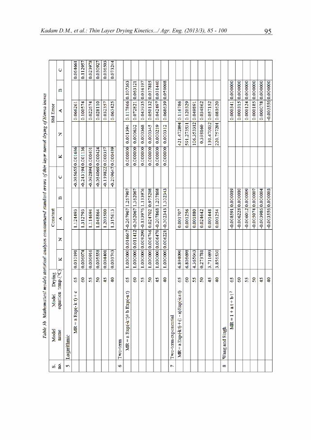
Kadam D.MM., et al.: Thin LLayer Drying KKinetics.../ Agr. E

Eng. (2013/3), 85 - 100 95

96

Kadam DD.M., et al.: Kinnetika sušenja ttankog sloja.../PPolj. tehn. (20133/3), 85 -100

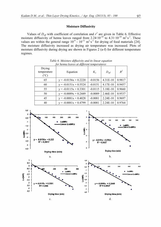
Kadam D.M

Valuemoisture dvalues are The moistmoisture dregimes.

M., et al.: Thin L

s of Deff with diffusivity of

within the geture diffusivitdiffusivity dur

Tab

Drying temperature

(°C) 65 60 55 50 45 40

a.

c.

Layer Drying K

Mo

coefficient ohenna leaves

eneral range 1ty increased aring drying are

ble 6. Moisturefor henna lea

Equ

y = -0.015y = -0.015y = -0.011y = -0.0089y = -0.008y = -0.008

Kinetics.../ Agr. E

isture Diffusi

f correlation ranged from

10-9 - 10-11 m2

as drying air e shown in Fi

e diffusivity and aves at different

uation

6x + 0.2220 1x + 0.5524 5x + 0.3301 9x + 0.2449 1x + 0.4028 1x + 0.4799

Eng. (2013/3),

ivity

and r2 are givm 2.24·10-10 to

2·s-1 for dryingtemperature

igures 2 (a-f)

d its linear equat temperatures

Ko D

-0.0156 4.31-0.0151 4.17-0.0115 3.18-0.0089 2.46-0.0081 2.24-0.0081 2.24

85 - 100

ven in Table 6o 4.31·10-10 mg of food matwas increasefor different t

ation

Deff R2

1E-10 0.98177E-10 0.94578E-10 0.96606E-10 0.95374E-10 0.96974E-10 0.9764

b.

d.

97

6. Effective m2·s-1. These

terials [24]. ed. Plots of temperature

7 7 0 7 7 4

98

Figure 2.

Activa

from the temperaturdiscussed 27.04 kJ·mother highmixer to an

The dr65°C at an about 270 leave was henna leavminimum drying air leaves withranged fromtemperaturThe finene

[1] Hoseinextract

Kadam D

e.

Effect of differ

a.

ation energy iproduct. Mo

re and the sloin material an

mol-1, which isly perishable n average part

rying studies interval of 5°to 540 minuteabout 0.2611

ves occurred in case of 65temperature.

h highest r2 vm 2.24·10-10 tre. The activatess modulus of

n, H., Zinab, D.ts (Lawsonia In

D.M., et al.: Kin

rent drying air t(Ln (MR) Vs.

65°C, b. 60°C,

Ac

s the minimumisture diffusiope of the plnd methods ss within the racommodities

ticle size of 0.

CO

on henna leav°C in a tunnel es to dry a 300mm and havimainly in fa

5°C temperatuMidilli-Kucu

value of 0.99to 4.31·10-10 mtion energy fof powder was

BI

2007. Phenoliermis). World J

netika sušenja t

temperature on Drying time) ofc. 55°C, d. 50°

ctivation Ene

m energy requivity (on loglot was used ection. The aange of 12.87. The dried h.2069 mm wit

ONCLUSION

ves was carriedryer with be

0 g of henna leing moisture calling rate peure samples auk model des

987. Effectivem2·s-1 and it inor the henna l1.3685 and av

BLIOGRAPH

c Compounds aJournal of Dair

tankog sloja.../P

moisture diffusof henna leavesC, e. 45°C, f. 40

rgy

uired to initiatg scale) value

to calculate tactivation ener7 – 58.15 kJ·mhenna leaves wth a fineness m

NS

ed at different elt speed of 30eaves samplescontent of 66.eriod. The drand it increasscribed the dr

moisture difncreased with tleaves was fouverage particl

HY

and Antioxidanry and Food Sci

Polj. tehn. (2013

f.

sivity during tun

0°C

te the moistures were plottthe activationrgy of henna

mol-1 reported were ground umodulus of 1.3

temperatures0 rpm. Tunnels. The thickne.95% w.b. Thrying time resed with the rying behavioffusivity of hethe increase inund to be 27.0le size was 0.2

nt Activity of Hiences, 2(1), 38

3/3), 85 -100

nnel drying

re migration ted against

n energy as leaves was by [25] for

using home 3685 [26].

s from 40 to l dryer took

ess of henna he drying of quired was decrease in

or of henna enna leaves n drying air 03 kJ·mol-1. 2069 mm.

Henna Leaves 8-41.

Kadam D.M., et al.: Thin Layer Drying Kinetics.../ Agr. Eng. (2013/3), 85 - 100 99

[2] Kikuzaki, H., Nakatani, N. 1993. Antioxidant effects of some ginger constituents. Journal of Food Science, 58(14), 1407-1410.

[3] Muhammad, H, Muhammad, S. 2005. The use of Lawsonia inermis linn. (henna) in the management of burn wound infections. African Journal of Biotechnology, 4 (9), 934-937.

[4] Verma, N., Mehra, D., Niyogi, U., Khandal, R. 2008. Retention of color intensity in henna paste during storage. Radiance, 7(2), 118-121.

[5] Dev, V., Venugopal, J., Sudha, S., Deepika, G., Ramkrishna, S. 2009. Dyeing and antimicrobial characteristics of chitosan treated wool fabrics with henna dye. Carbohydrate Polymers, 75 (4), 646–650.

[6] Chaudhary, G., Goyal, S., Poonia, P. 2010. Lawsonia inermis Linnaeus: A Phytopharmacological Review. International Journal of Pharmaceutical Sciences and Drug Research, 2(2), 91-98

[7] Midilli, A. 2001. Determination of pistachio drying behaviour and conditions in solar drying systems. International Journal of Energy Research, 25, 715-725.

[8] Erenturk, S., Gulaboglu, M., Gultekin, S. 2004. The thin layer drying characteristics of rosehip. Biosystems Engineering, 89 (2), 159 – 166.

[9] Kadam, D., Samuel, D. 2006. Convective flat-plate solar heat collector for cauliflower drying. Biosystems Engineering, 93 (2), 189-198.

[10] Kadam, D, Goyal, R., Gupta, M. 2011. Mathematical modeling of convective thin layer drying of basil leaves. Journal of Medicinal Plants Research, 5(19), 4721-4730.

[11] Kadam, D., Goyal, R., Singh, K., Gupta, M. 2011. Thin layer convective drying of mint leaves. Journal of Medicinal Plants Research, 5(2), 164-170.

[12] Pangavhane, D., Sawhney, R., Sarsavadia, P. 1999. Effect of various dipping pre-treatment on drying kinetics of Thompson seedless grapes. Journal of Food Engineering, 39, 211-216.

[13] Kadam, D., Dhingra, D. 2011. Mass transfer kinetics of banana slices during osmo-convective drying. Journal of Food Process Engineering, 34 (2), 511–532.

[14] Kadam, D., Nangare, D., Singh, R., Kumar, S. 2011. Low-cost greenhouse technology for drying onion (Allium cepa l.) Slices. Journal of Food Process Engineering, 34 (1), 67–82.

[15] Doymaz, I. 2004. Effect of pre-treatments using potassium metabisulphite and alkaline ethyl oleate on the drying kinetics of apricots. Biosystems Engineering, 89(3), 281 – 287.

[16] Ozdemir, M., Devres, Y. 1999. The thin layer drying characteristic of hazelnuts during roasting. Journal of Food Engineering, 42, 225-233.

[17] Yaldiz, O., Ertekin, C., Uzun, H. 2001. Mathematical modeling of thin layer solar drying of sultana grapes. Energy – An International Journal, 26, 457 – 465.

[18] Sarsavadia, P., Sawhney, R., Pangavhane, D., Singh, S. 1999. Drying behavior of brined onion slices. Journal of Food Engineering, 40, 219 – 226.

[19] Togrul, I., Pehlivan, D. 2002. Mathematical modeling of solar drying of apricots in thin layers. Journal of Food Engineering, 55, 209 – 216.

[20] Goyal, R., Kingsly, A., Manikanthan, M., Ilyas, S. 2007. Mathematical modeling of thin layer drying kinetics of plum in a tunnel dryer. Journal of Food Engineering, 79, 176 – 180.

[21] Doymaz, I., Tugrul, N., Pala, M. 2006. Drying characteristics of dill and parsley leaves. Journal of Food Engineering, 77, 559-565.

[22] Crank, J. 1975. Mathematics of diffusion. Clarendon Press, Oxford, UK. [23] Simal, S., Mulet, A., Tarrazo, J., Rosello, C. 1996. Drying models for green peas. Food

Chemistry, 55, 121-128.

Kadam D.M., et al.: Kinetika sušenja tankog sloja.../Polj. tehn. (2013/3), 85 -100 100

[24] Maskan, A., Kaya, S., Maskan, M. 2002. Hot air and sun drying of grape leather (pestil). Journal of Food Engineering, 54, 81-88.

[25] Senadeera, W., Bhandari, B., Young, G., Wijesinghe, B. 2003. Influence of shapes of selected vegetable materials on drying kinetics during fluidized bed drying. Journal of Food Engineering, 58, 277–283.

[26] Sahay, K., Singh, K. 1994. Unit Operations of Agricultural Processing. 1st Ed. Vikas Publishing House Pvt. Ltd, New Delhi, India.

KINETIKA SUŠENJA TANKOG SLOJA LISTOVA KANE

Dattatreya M. Kadam1, Manoj Kumar Gupta2, Vaijayanta M Kadam3

1Centralni institut za post-žetveni inženjering i tehnologiju, PO: PAU campus, Ludhiana-141004 (Pendžab), Indija

2Infosys Limited, Electronic City, Phase I, Bangalor, Karnataka, Indija 3Državni institut za hortikulturu, Karnataka, Indija

Sažetak: Listovi kane su dobro poznati po svojim kozmetičkim agensima sa anti-kancerogenim, anti-inflamatornim, analgetskim i anti-piretičkim svojstvima. Laboratorijski modeli tunelske sušare su korišćeni za sušenje listova na 40, 45, 50, 55, 60 i 65°C i ispitivanje uticaja različitih uslova kinetiku sušenja listova kane. Period sušenja listova kane se skraćivao i sušenje je bilo brže pri višoj temperature. Dvanaest modela sušenja tankog sloja je poređeno sa eksperimentalnim podacima o odnosima vlage. Među matematičkim modelima koji su ispitivani, model Midilli-Kucuk je na zadovoljavajući način opisao ponašanje pri sušenju sa najvišim vrednostima r2. Efektivna difuzija vlage (Deff) listova povećala se sa povećanjem temperature vazduha za sušenje. Efektivna difuzija vlage listova kane iznosila je od 2.24·10-10 do 4.31·10-10 m2·s-1, a energija aktivacije 27.03 kJ·mol-1. Osušeni listovi su mleveni u prah sa prosečnim dimenzijama čestica od 0.2069 mm i modulom finoće 1.3685.

Ključne reči: kana, matematičko modeliranje, sušenje, difuzija vlage, energija aktivacije

Prijavljen: Submitted: 23.06.2013.

Ispravljen: Revised: 07.07.2013.

Prihvaćen: Accepted: 30.07.2013.

Univerzitet uPoljoprivredInstitut za pNaučni časoPOLJOPRIGodina XXXBroj 3, 2013Strane: 101

UDK: 631.5

AERS

MAs

Depar

Abstraused withvelocity, swhile varyusing cardthrough thprinciples in accordawhere the spouting vaverage cy

Key wrate, averCylindrica

* Corre

The aDevel(NSE

u Beogradu dni fakultet oljoprivrednu teopis IVREDNA TEHNXVIII 3. – 110

536

RODYNAMSPOUTED

Murugesan Bahutosh Singh

Gram

rtment of Foo2McGill UMacdonal

act: Two dimh draft tubessolids circulaying slant andamom. The vhe beds are di

of dimensionance with the

first part incvelocity andycle time.

words: Spoutinrage cycle tial Spouted Bed

esponding autho

authors are grlopment Agenc

ERC) of Canada

ehniku

NIKA

MIC AND SD BED DRY

alakrishnan1,h2, Gopu Ravma Seetharam

1Tamil Nadod and AgriculUniversity, Depld Campus, St

mensional spos to study sation rate an

ngle, draft tubvariables whiiscussed. Empnal analysis e collected dcludes the an

d the second

ng pressure dime, dimensiod (CSB), curin

or. E-mail: vijay

rateful for the cy (CIDA) and

a.

SOLIDS CIYING OF C

, Velath Vari

veendran Nairma Iyengar2, V

du Agriculturaltural Processpartment of Bte-Anne-de-Be

outed bed unitpouting pres

nd average cybe height, seich affect thepirical correland similitud

data. The artinalysis for sp

parts includ

drop, minimumonal analysis

ng chambers, r

ya.raghavan@m

financial suppd Natural Scie

Institute

AGRIC

IRCULATICARDAMO

iyathodiyil Srr2, RangarajuVijaya Ragha

al University,s Engineering,

Bioresource Enellevue, Quebe

ts with flexibssure drop aycle time. Tparation dist

e spouting preations were d

de. The develcle has been

pouting pressdes the solid

m spouting ves, Elettaria rectangular o

mcgill.ca

port provided ences and Eng

UniversityFaculty o

e of Agricultural Scie

CULTURAL ENY

p

OriginalnOriginal sci

ION RATEOM (Part 2

reenarayananu Viswanathaavan2*

g,, Coimbatorengineering, ec, Canada

ble bed dimenand minimumhe data wereance and heiessure drop adeveloped folloped correla divided into

sure drop andds circulation

elocity, solids cardamomumrifices

by Canadian ineering Resea

y of Belgrade of Agriculture

Engineering ntific Journal

NGINEERING Year XXXVIII No. 3, 2013.

pp: 101 – 110

ni naučni rad ientific paper

ES IN 2)

n1, an1,

e, India

nsions were m spouting e collected ight of bed and airflow llowing the ations were o two parts d minimum n rate and

circulation m, Conical-

International arch Council

Balakrishnan M., et al.: Stepeni aerodinamike i protoka.../Polj. tehn. (2013/3), 101 - 110 102

INTRODUCTION

Spouted bed technology is very useful for drying solids that are sticky, have irregular texture and vary widely in particle size distribution. Application of vigrous movements of solids in spouted bed helps in uniform drying but the performance depends widely on the cyclic movement of the solid particles and also on the properties related to solid circulation such as cycle time and fraction of this time spent in the spout and annular zones [1]. The solid circulation rate in a two dimensional spouted bed dryer is estimated using the particle velocity above the cone and the paricle voidage in the spout or in the downcomer [2]. In the spout, the particle velocity is measured by tracking the particle but in the downcomer the particle velocity is influenced by the inlet air velocity, the inlet nozzle width, spout width and the separation distance between the draft tubes. Several researchers have tried to develop mathematical models for solid circulation rate, but they lack a soud understanding of parametric relationships. Hence for a two dimensional spouted bed dryer it is important to conduct proper experimental studies to explain the relation between factors and how they are influenced by the presence of draft tubes.

In a spouted bed dryer the continous movement of particles between the spout and the downcomer has a significant effect on the its performance. In 1959 Thorley, et al. [6] investigated conical-cylindrical spouted beds without draft tubes indicating that the cycle time can be quantified with or without solid circulation rate in conjugation with particle properties, bed geometry and volumetric gas flow. They calculated the mean cycle time by dividing the total mass of particles in the bed by the solids circulation rate. The approach appllied by Thorley et al. (1959) [6] agrees well with measured values and are compatible for estimation of cycle time [2].

In the present study, parameters such as spouting pressure drop, minimum spouting velocity, solid circulation rate and average cycle time have been considered for the development of mathematical models based on dimensional analysis and similitude principles for a batch type slotted 2DSB with draft tube [3-5]. In part 1 of the study we analaysed mathematical models based on spouting pressure drop and minimum spouting velocity. The intent of Part 2 of the study is to investigate the influence of solids circulation rate and average cycle time on the spouting characteristics of spouted bed with draft tube while taking into account grain particle parameters in order to provide a sound basis for the design of commercially viable units.

MATERIAL AND METHODS

Details on the theory and model development are provided in the Part 1 of the study. The assumptions made to generate mathematical models for solids circultation rate and average cycle time are same as mentioned in Part 1 of the study. Tables 1 and 2 represent the pertinent and repeating variables considered for the mathematical modeling.

The chosen variables were convenient for the experimental and analytical phase of the study. The time taken by particles to make the journey from the top of the down comer back to their starting point is of considerable interest in solids mixing, heat treatment and drying applications. Previous studies have shown that the proportion of time spent by a particle in the draft tube is insignificant compared to time spent in the down comer [6-8]. Hence, the average cycle time should be dependent on the total mass of solids in the bed, the solids

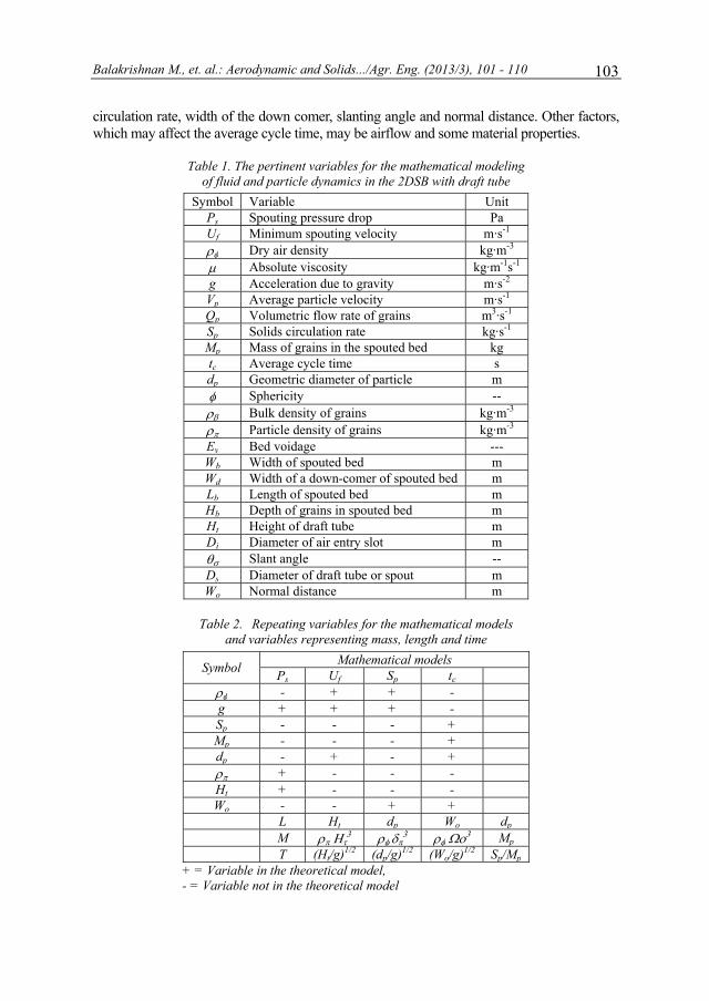
Balakrishnan M., et. al.: Aerodynamic and Solids.../Agr. Eng. (2013/3), 101 - 110

103

circulation rate, width of the down comer, slanting angle and normal distance. Other factors, which may affect the average cycle time, may be airflow and some material properties.

Table 1. The pertinent variables for the mathematical modeling

of fluid and particle dynamics in the 2DSB with draft tube Symbol Variable Unit

Ps Spouting pressure drop Pa Uf Minimum spouting velocity m·s-1 ρφ Dry air density kg·m-3 μ Absolute viscosity kg·m-1s-1 g Acceleration due to gravity m·s-2 Vp Average particle velocity m·s-1 Qp Volumetric flow rate of grains m3·s-1 Sp Solids circulation rate kg·s-1 Mp Mass of grains in the spouted bed kg tc Average cycle time s dp Geometric diameter of particle m φ Sphericity -- ρβ Bulk density of grains kg·m-3 ρπ Particle density of grains kg·m-3 Ev Bed voidage --- Wb Width of spouted bed m Wd Width of a down-comer of spouted bed m Lb Length of spouted bed m Hb Depth of grains in spouted bed m Ht Height of draft tube m Di Diameter of air entry slot m θσ Slant angle -- Ds Diameter of draft tube or spout m Wo Normal distance m

Table 2. Repeating variables for the mathematical models

and variables representing mass, length and time

Symbol Mathematical models Ps Uf Sp tc

ρφ - + + - g + + + - Sp - - - + Mp - - - + dp - + - + ρπ + - - - Ht + - - - Wo - - + +

L Ht dp Wo dp M ρπ Ητ

3 ρφ δπ3 ρφ Ωο3 Mp

T (Ht/g)1/2 (dp/g)1/2 (Wo/g)1/2 Sp/Mp + = Variable in the theoretical model, - = Variable not in the theoretical model

Balakrishnan M., et al.: Stepeni aerodinamike i protoka.../Polj. tehn. (2013/3), 101 - 110 104

The variables that were important for the analysis of air and solids dynamics were selected. A list of variables for the mathematical modeling of 2DSBs with draft tube is given in Tab. 1. It should be noted that not all of these variables are necessarily important for each operational phase of spouted beds.

The normal distance (Wo) of the orifice was calculated from relationship of separation distance (HE) and slant angle (θs): Wo = HE cosθs

Solids circulation rate: The relevant variables given in Tables 1-2 for the development

of the model for the solids circulation rate (average particle velocity) were arranged:

F (Vp, Uf, ρ f, μ, g, dp, ρp, φ, Ev, Wo, Ds, θs, Lb, Di, Ht)=0 (1) Taking the considered variables in Eq. 1 and using the repeating variables, the

following dimensionless numbers were developed:

F [Vp/(gWo)0.5,dp/Wo, Uf2/gWo, μ2/gρf2Wo

3, ρp-ρf/ρf, φ, Ev, Lb/Wo, θs, Wb/Wo, Ds/Di, Ht/Wo]=0 (2)

The PI numbers given in Eq. 2 were transformed in to the following dimensionless

numbers in Eq. 3:

Vp/(gWo)0.5 = F[dp/Wo, Fr, Ar, ρp-ρf/ρf, φ, Ev ,Lb/Wo, θs, Ds/Di, Ht/Wo]=0 (3)

Where, Fr and Ar are Froude number and Archimedes number respectively. The theoretical solids circulation rate would then be Eq. 4:

Sp = ρbAdVp (4) Where, Ad is the cross-sectional area of the downcomers. Or:

Sp/ρbAd(gWo)0.5 = = F[dp/Wo, Fr, Ar, ρp-ρf/ρf, φ, Ev, Lb/Wo, θs, Ds/Di, Ht/Wo] = 0 (5)

Average cycle time: The relevant variables from Tab. 1, which may constitute the

mathematical model of average cycle time, are shown:

F (tc, Sp, Mp, dp, φ, Wo, θs, Hb,Wd) = 0 (6)

Taking the pertinent variables from Eq. 6 and using the variables in Tables 1-2 the following dimensionless PI numbers were generated:

F(tcSp/Mp, φ, , θs, Wo/dp, Hb/dp, Wd/dp) = 0 (7) The dimensionless numbers in Eq. 7 were transformed in to the following DPs to

simplify the relationship for average cycle time as shown below:

tcSp/Mp= F(φ, , θs, Wo/dp, Hb/Wo, Wd/dp) = 0 (8)

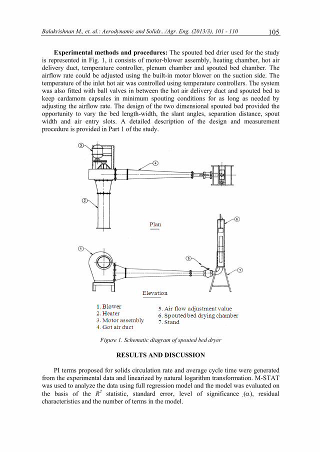
Balakrishnan M., et. al.: Aerodynamic and Solids.../Agr. Eng. (2013/3), 101 - 110

105

Experimental methods and procedures: The spouted bed drier used for the study is represented in Fig. 1, it consists of motor-blower assembly, heating chamber, hot air delivery duct, temperature controller, plenum chamber and spouted bed chamber. The airflow rate could be adjusted using the built-in motor blower on the suction side. The temperature of the inlet hot air was controlled using temperature controllers. The system was also fitted with ball valves in between the hot air delivery duct and spouted bed to keep cardamom capsules in minimum spouting conditions for as long as needed by adjusting the airflow rate. The design of the two dimensional spouted bed provided the opportunity to vary the bed length-width, the slant angles, separation distance, spout width and air entry slots. A detailed description of the design and measurement procedure is provided in Part 1 of the study.

Figure 1. Schematic diagram of spouted bed dryer

RESULTS AND DISCUSSION

PI terms proposed for solids circulation rate and average cycle time were generated

from the experimental data and linearized by natural logarithm transformation. M-STAT was used to analyze the data using full regression model and the model was evaluated on the basis of the R2 statistic, standard error, level of significance (α), residual characteristics and the number of terms in the model.

Balakrishnan M., et al.: Stepeni aerodinamike i protoka.../Polj. tehn. (2013/3), 101 - 110 106

Solids circulation rate/average particle velocity: The average particle velocities observed over all the runs were in the range of 0.76-1.25 cm·sec−1. The lowest particle velocity was 0.76 cm·sec−1 in the case of cardamom dried at air temperature 40°C, 45° slant angle, 5 cm separation distance and draft tube height of 40 cm and the highest was 1.25 cm·sec−1 in the case of cardamom dried at air temperature 50°C, 60° slant angle, 7.5 cm separation distance and draft tube height of 60 cm with tempering period for 30 min. The solids circulation rates were calculated from the average particle velocity, the effective cross-sectional area of the down comers and the average bulk density. Plots of solids circulation rate versus draft tube heights for various slant angles and separation distances have been shown in Figs. 2-3. It may be observed that the solids circulation rate increased with separation distance. Possible cause for this trend as explained by Buchanan and Wilson (1965) [9], Khoe and Brakel (1983) [1] and Claflin and Fane (1984) [10] for Conical-cylindrical spouted beds and Law et al. (1984) [11] and Kalwar et al. (1992) [2] for two-dimensional spouted beds.

The solids circulation increased as the draft tube height increased from 40-60 cm and its magnitude increased with separation distance as shown in Figs. 2-3. The solids circulation rate was almost the same when the draft tube height was increased from 50-60 cm, but the difference became greater as the separation distance increased due to the higher number of capsules entering the draft tube.

Figure 2. Effect of draft height (Ht) on solid circulation rate for cardamom

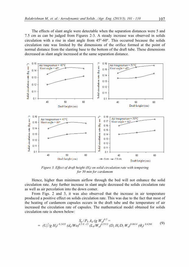
Balakrishnan M., et. al.: Aerodynamic and Solids.../Agr. Eng. (2013/3), 101 - 110

107

The effects of slant angle were detectable when the separation distances were 5 and 7.5 cm as can be judged from Figures 2-3. A steady increase was observed in solids circulation with a rise in slant angle from 45°-60°. This occurred because the solids circulation rate was limited by the dimensions of the orifice formed at the point of normal distance from the slanting base to the bottom of the draft tube. These dimensions decreased as slant angle increased at the same separation distance.

Figure 3. Effect of draft height (Ht) on solid circulation rate with tempering

for 30 min for cardamom

Hence, higher than minimum airflow through the bed will not enhance the solid circulation rate. Any further increase in slant angle decreased the solids circulation rate as well as air percolation into the down comer.

From Figs. 2 and 3, it was also observed that the increase in air temperature produced a positive effect on solids circulation rate. This was due to the fact that most of the heating of cardamom capsules occurs in the draft tube and the temperature of air increased the circulation rate of capsules. The mathematical model obtained for solids circulation rate is shown below:

Sp / Pb Ad (g Wo)0.5 = = (Uf

2/g Ht)–0.2435 (dp/Wo)6.5 E -15 (Lb/Wo)0.5513 (Ds Ht/Di Wo)0.0614 (θs) 0.6268 (9)

Balakrishnan M., et al.: Stepeni aerodinamike i protoka.../Polj. tehn. (2013/3), 101 - 110 108

with R2 = 96.51%, standard error of estimate = 0.0225 and α = 0.0001. A print out of residuals against selected model predictions is shown in Fig. 4b. The plot of observed and predicted values for the solids circulation rate model is plotted in Figure 4a. The developed model predicted the collected data with an average error of ±1.8%. The predictions from the solids circulation rate model have been presented in Fig. 4a, which showed a good agreement.

Average cycle time: The cycle times of particles in the case of 45° were 16-20% greater

than the slant angle of 60° because of longer particle paths and the mass of grains in the bed. The shortest particle cycle time of 105 sec was observed when the slant angle was 60°, separation distance was 7.5 cm, draft tube height of 40 cm and air temperature of 50°C with tempering period of 30 min. The longest cycle time of 200 sec was found when slant angle was 45°, separation distance was 5 cm, draft tube height of 60 cm and air temperature of 40°C.

(a) (b)

Figure 4. (a) Comparison of solids circulation rate measured with solids circulation rate predicted by Eq. 9 (b) Residual plot for solids circulation rate model, Eq. 9

For any given geometry, the particle cycle time decreases with the distance of

particles in the down comer.

(a) (b)

Figure 5. (a) Comparison of observed cycle time data Vs predicted cycle time by Eq. 10 (b) Residual plot average cycle time model, Eq. 10

The cycle time data from the drying runs were regressed against the dimensionless

numbers. In principle, the average cycle time should be equal to the mass of particles in the bed divided by the solids circulation rate. But this was not so in the study. The problem could

Balakrishnan M., et. al.: Aerodynamic and Solids.../Agr. Eng. (2013/3), 101 - 110

109

be due to the effect of separation distance on the cycle time distribution of individual particles. The mathematical model developed for average cycle time is given in Eq. 10.

tc Sp / Mp = (dp/Wo) 0.9495 (HbWd/Wodp) –0.9975 (θs)1.11 (10)

with R2 = 81.63%, standard error of estimate = 0.0618 and significance level = 0.0001. The model predictions versus observed average cycle times are shown in Fig. 5a. It is concluded that the developed model fits the collected data with an average error of ±12%. A print out of residual against selected model predictions is shown in Fig. 5b.

CONCLUSIONS

In part 1 of the study we concluded that spouting pressure drop increases with an increase in separation distance and slant angle. It was also observed that increase in draft tube height led to an increase in spouting pressure drop. We also concluded that minimum spouting velocity increases as the separation distance and draft tube height increase and as the slant angle decreases. In Part 2 of the study it was observed that solid circulation rates (average particle velocity in the down comers) were also affected by separation distance, draft tube height, slant angle and vary with spouting velocity. The average particle times were found to vary with slant angle. Emperical models were developed for solids circulation rate and average cycle time and were found to be in close agreement with expeimental data.

BIBLIOGRAPHY

[1] Khoe, G., Brakel, V.J. 1983. Drying characteristics of a draft tube spouted bed. The Canadian Journal of Chemical Engineering, 1983. 61(3): p. 411-418.

[2] Kalwar, M., Raghavan, G., Mujumdar, A. 1992. Spouting of two-dimensional beds with draft plates. The Canadian Journal of Chemical Engineering, 1992. 70(5): p. 887-894.

[3] Osorio-Revilla, G., Elías-Serrano, R., Gallardo-Velázquez, T. 2004. Drying of Liquid Feedstocks in a Spout-Fluid-Bed with Draft-Tube Submerged in Inert Solids: Hydrodynamics and Drying Performance. The Canadian Journal of Chemical Engineering, 2004. 82(1): p. 142-147.

[4] Osorio-Revilla, G., López-Suárez, T., Gallardo-Velázquez, T. 2004. Simultaneous Drying and Cleaning of Guava Seeds in a Spout-Fluid Bed with Draft Tube. The Canadian Journal of Chemical Engineering, 2004. 82(1): p. 148-153.

[5] Stocker, R.K., Eng, J.H., Svrcek, W.Y., Behie, L.A. 1989. Ultrapyrolysis of propane in a spouted-bed reactor with a draft tube. AIChE Journal, 1989. 35(10): p. 1617-1624.

[6] Thorley, B., Saunby, J.B., Mathur, K.B., Osberg, G.L. 1959. An analysis of air and solid flow in a spouted wheat bed. The Canadian Journal of Chemical Engineering, 1959. 37(5): p. 184-192.

[7] Becker, H.A. 1961. An investigation of laws governing the spouting of coarse particles. Chemical Engineering Science, 1961. 13(4): p. 245-262.

[8] Gay, E. 1970. Air Flow Requirements and Bed Turnover Time for a Spouted Leed Peanut Dryer. ASAE, 22p. 1970.

Balakrishnan M., et al.: Stepeni aerodinamike i protoka.../Polj. tehn. (2013/3), 101 - 110 110

[9] Buchanan, R., Wilson, B. 1965. The fluid-lift solids recirculator. Mech. Chem. Eng. Trans, 1965. 1(1): p. 117-124.

[10] Claflin, J.K., Fane, A.G. 1984. Gas distribution and heat transfer in a draft-tube spouted bed. In AIChE symposium series, ISSN 0065-8812. American institute of chemical engineers. 1984, vol. 80, no241, pp. 17-23

[11] Law, L., et al. 1984. Pressure drop and particle circulation studies in modified slot spouted beds. Drying'84Hemisphere, New York, 1984: p. 386-389.

STEPENI AERODINAMIKE I PROTOKA ČVRSTE MATERIJE U ODVODNIM KANALIMA ZA SUŠENJE KARDAMOMA (2. deo)

Murugesan Balakrishnan1, Velath Variyathodiyil Sreenarayanan1,

Ashutosh Singh2, Gopu Raveendran Nair2, Rangaraju Viswanathan1, Grama Seetharama Iyengar2, Vijaya Raghavan2

1Institut za inženjering prehrambenih i poljoprivrednih procesa,

Poljoprivredni Univerzitet Tamil Nadu, India 2Institut za inženjering bioresursa, Univerzitet McGill,

Kampus Macdonald, Ste-Anne-de-Bellevue, Quebec, Kanada

Sažetak: Za proučavanje pada pritiska u odvodnom kanalu, minimalne brzine odvođenja materijala, stepena cirkulacije čvrstog materijala i prosečnog vremena ciklusa korišćene su dvodimenzionalne jedinice odvodnih kanala sa fleksibilnim dimenzijama. Podaci su prikupljani variranjem ugla nagiba, visine pripremnog kanala, rastojanja pri separaciji i visine kanala. Analizirane su veličine koje utiču na pad pritiska u odvodnom kanalu i protok kroz kanal. Razvijene su empirijske zavisnosti korišćenjem simulacije i dimenzione analize. Razvijene zavisnosti su bile u skladu sa prikupljenim podacima. Rad je podeljen u dva dela pri čemu se prvi deo bavi analizom pada pritiska u odvodnom kanalu i minimalnom brzinom odvođenja a drugi deo stepenom protoka čvrste materije i prosečnim vremenom ciklusa.

Ključne reči: Pad pritiska pri odvođenju materijala, minimalna brzina odvođenja, stepen protoka čvrste materije, prosečno vreme ciklusa, dimenziona analiza, Elettaria cardamomum, konično-cilindrični kanal za odvođenje (CSB), komore za konzervaciju, pravougaoni otvori

Prijavljen: Submitted: 04.05.2013.

20.07.2013.

Ispravljen: Revised: Prihvaćen: Accepted:

Univerzitet uPoljoprivredInstitut za pNaučni časoPOLJOPRIGodina XXXBroj 3, 2013Strane: 111

UDK: 027.5

TH

Daniele

1 Univer

Abstraunderstandproblem itheoreticala useful toground. Thalone is asparameter due to elecwater moldroplet dyquantum amulti-dropaims of thhighlightinphenomenain analogyclassical fl

Key wand quantu

* Corre

u Beogradu dni fakultet oljoprivrednu teopis IVREDNA TEHNXVIII 3. – 122

54

WHE CLASS

e De Wrachie

rsity of Milan, 2 University o

3Univers

act: The desigding of the kininvolves both studies the clol to describehe problem bssessed but a dependencies

ctrical interactlecules. An aynamics in spapproach. In thplet alternativehe present pang the new pea. On the who

y to the well-eluid dynamic e

words: spray pum mechanics

esponding autho

ehniku

NIKA

WATER DRICAL AND

FRA

en1, Giulio Lo

Department oof Parma, Depsity of Campin

gn of a sprinklnematics of thh theoreticallassical mech the trajectori

becomes evenmulti-droplet

s, it is also obtions between alternative to rinkler irrigathis context, thes need to beaper which ferspectives of ole, the new astablished conequations into

particles kines, sprinkler wa

or. E-mail: giul

ROPLETS D QUANTU

RAMEWOR

orenzini2*, Ste

of Environmenpartment of Innas, Faculdad

ler irrigation she droplets dul and experianical approaes of water dr

n more complt system is acserved an intethe hydrogentraditional cl

tion, has beenhe whole classe discussed anfocuses on thf a deeper comapproach leadncept of classo the so-called

ematics, singlater droplets,

lio.lorenzini@u

Institute

AGRIC

ANALYSIUM HYDRRKS

efano Mambr

ntal and Agricndustrial Enginde de Tecnolog

system is alwauring their aeimental consch, based on troplets from thicated when nccounted for. er-droplet recin and the oxyglassical procen recently prosic-quantum and pinpointedhe theoretical mprehension is to the conceical trajectory

d quantum equ

le- and multi-mathematical

unipr.it

UniversityFaculty o

e of Agricultural Scie

CULTURAL ENY

pp

OriginalnOriginal sci

IS: RODYNAM

retti3, Marco

cultural Scienneering, Italy,gia, Brazil

ays associatederial path. Ressiderations. Athe Newton’she sprinkler nnot just a sinIn addition t

iprocal repulsgen atoms of thedures, to anaoposed in theand single-drod and these ar

part of the in the spray fept of quantumy and allows tuations.

-droplet systel modelling

y of Belgrade of Agriculture

Engineering ntific Journal

NGINEERING Year XXXVIII No. 3, 2013.

p: 111 – 122

ni naučni rad ientific paper

MIC

Medici2

nces, Italy ,

d with a full solving this Among the law, offers ozzle to the

ngle droplet o the inter-ion, mainly he different alyse water e form of a oplet versus re the main issue, thus

flow related m trajectory to recast the

ems, classic

De Wrachien D., et al.: Analiza kapljica vode.../Polj. tehn. (2013/3), 111 - 122 112

INTRODUCTION

Albeit the process of a liquid particle moving within a gaseous phase may describe many different technical applications, broadly investigated in many scientific sectors and from many different points of view, a complete, clear and generally applicable mathematical modelling is still far from having been achieved. Very recently Molle et al. [1] gave an extremely useful experimental contribution in the field of irrigation, which will be of substantial usefulness for future investigations and modelling attempts. The results of the present paper were mainly reached by featuring the sprinkler irrigation context. The outcomes, if suitably adapted, may also apply to other fields and aims, such as pesticides distribution, heat removal or fire suppression, to name but a few. The fundamental problem is not just that of solving the equations ruling the development of the system and of the phenomenon but, upstream of that, it lies in the characterization of such equations. According to the Authors of this paper such hurdle can be attributed to a not complete understanding of the system-process evolution. This of course should not be taken as a form of underestimation of the analytical difficulties due to the mutual interrelationships between the parameters that govern the process, on the one hand, and the characteristics of the particles involved, on the other. In fact the main thematic scientific literature [2-6] tries to overcome such computational complication binding the solutions achieved to the specific case studies faced. In general, however, the kinematic analysis of sprinkler water droplets during their aerial path is devised adopting a Newtonian approach and considering a single-droplet system. A ballistic form of the same viewpoint, based on a Newtonian approach for a single-droplet system, was also proposed by the Authors [7-9]. This approach will be described in the paper as a classic/single-droplet model. Coming again to the “not complete understanding of the system-process evolutions” quoted above, the issue has very recently led the Authors of the present work to the belief that to fully comprehend and describe the phenomenon another viewpoint could be considered: the quantum one [10]. The results which were arrived at [11] were in the form of the time-dependent Schroedinger's equation (TDSE) and of the Scale Relativity Theory [12] written as a Riccati equation. The former, in particular, was written for single-droplet systems, seen as waves and material particles [13] and considering a Lagrangian or Eulerian description for both steady and transient states. The present paper, therefore, will treat further possibilities to study the kinematic behaviour of both single- and multi-droplet systems during their aerial path in according to both the classic (i.e. Newtonian) and quantum approach. Moreover, a new procedure, the so-called Density Functional Theory for many-particle systems, has been highlighted, that allows to design a common 3-D space for the assessment of both the droplet trajectories and their interactions, and, so, to recast the TDSE into the quantum fluid-dynamic (continuity and Navier-Stokes) equations [14].

The basic picture that emerges is that of a multi-component fluid mixture moving into a 3-D space under the effects of common electric and magnetic fields and classic and quantum potentials.

De Wrachien D., et al.: Water Droplets Analysis.../Agr. Eng. (2013/3), 111 - 122 113

THE CLASSIC MECHANICAL PICTURE

We do not wish to review the whole classic approach, as reported in the literature, but to explore the modelling possibilities in relation to the topic of the present paper. Anyway some more information on spray kinematics modelling (mainly Lagrangian) both in sprinkler irrigation and in chemical sprays contexts are also available [3,15-17], while spray drift Lagrangian modelling is treated in [18], and in [19]. Recently the Authors defined the following simplified analytical model feasible to solve water droplets kinematics, based on the Second Principle of Dynamics [7-9]:

⎪⎩

⎪⎨

⎧

−−=

−=•••

•••

ngykym

xkxm2

2

(1)

developed in terms of parametric equations:

( ) ⎟⎠⎞

⎜⎝⎛ += 1ln 0 t

mkv

kmtx x (2)

( )tkvm

mvtxx

x

0

0

+=

• (3)

( )

⎟⎟⎟⎟⎟

⎠

⎞

⎜⎜⎜⎜⎜

⎝

⎛

−

⎟⎟⎟⎟⎟

⎠

⎞

⎜⎜⎜⎜⎜

⎝

⎛

−=

mkng

tg

mn

vmk

gmn

vmk

kmhty

y

y

0

0

arctancos

arctancos

ln

(4)

( )⎥⎥⎦

⎤

⎢⎢⎣

⎡⎟⎟⎠

⎞⎜⎜⎝

⎛+−−=

•

yvngkt

mngk

kngty 0arctantan (5)

where: f [-] - friction factor according to Fanning [20], g [m·s-2] - gravity, h [m] - initial y co-ordinate,

2Afk ρ

= [kg·m-1] - friction coefficient,

m [kg] - particle mass,

De Wrachien D., et al.: Analiza kapljica vode.../Polj. tehn. (2013/3), 111 - 122 114

n [kg] - droplet actual mass (buoyancy), t [s] - time,

xv0 , yv0 [m·s-1] - initial horizontal and vertical velocity components, x, y [m] - co-ordinates along the horizontal and vertical axes, •x , •

y [m·s-1] - velocities along the horizontal and vertical axes, ••x , ••

y [m·s-2] - accelerations along the horizontal and vertical axes. Being the model analytical, albeit simplified, it is applicable to a variety of problems

but the more reliable results were obtained for high Reynolds numbers. Obviously, as mentioned above, the model presented is one of the possible ones which can describe a single-droplet system from a classic viewpoint: the choice was mainly due to the fact that such model is tightly related to the second law of dynamics, as previously mentioned. To complete the topic, anyway, one may in general face the kinematic analysis of a multi-droplet system (i.e. composed of N droplets) from a classic viewpoint by means of the following analytical expression [21]:

( ) ( )tQVdt

tQdm kk

k ⋅−∇=2

2 (6)

where: mk [kg] - k-th particle mass (1 ≤ k ≤ N), Q [m] - classic trajectory, V [kg·m·s-2] - potential function accounting for time dependence,

k∇ [m-1] - 3-D gradient operator referred to the k-th particle. The classical procedure needs a quantitative approach to check how reliable the

predictions are. In order to validate the kinematic model just reported, comparisons of field measurements and theoretical values have been already reported in literature [2, 6, 8]. In conclusion the model here defined proves to be kinematically reliable in its predictions from a qualitative and quantitative points of view, particularly when droplets having a “not too small” diameter are considered.

Quantum mechanics for a single particle

The discrepancies between a classic Vs. quantum description, on the one hand, and

between a single-droplet Vs. multi-droplet one, on the other, may be highlighted examining the following expressions for single- and multi-droplet systems (respectively) as compared to those in the previous section of this paper [11, 21]:

( ) ( )tFdt

tQdm =2

2

(7)

( ) ( )tQVV

dttQdm t

qukk

k ⎟⎠⎞

⎜⎝⎛∇= ψ

2

2

(8)

where:

De Wrachien D., et al.: Water Droplets Analysis.../Agr. Eng. (2013/3), 111 - 122 115

F [N] - force, ħ [J·s] - the Dirac constant,

ψψψ

2

1

2

2j

N

j jqu m

V t∇

−= ∑=

h

[kg·m·s-2] - quantum potential, (1 ≤ j < k ≤ N).

Comparing Eq. (8) with Eq. (6), the first useful consideration is that, if the quantum

potential tends to zero, then the quantum and classic kinematic pictures tend to coincide. But as a quantum viewpoint presumes that the “object” evaluated is not just a material particle but also a wave, then for each element of a multi-droplet system one may write the TDSE as:

( ) ( ) ( ) ( )txt

DitxtxVmtxD ,,,21,22 rrrr ψψψ ⋅⎟

⎠⎞

⎜⎝⎛∂∂

⋅⋅−=⋅⋅⋅−∇ (9)

With: ( ) ( ) ( )[ ]txStxRtx ,exp,,

rrr⋅=ψ (10)

where: D [m2·s-1] - diffusion coefficient, i [-] - imaginary unit, R [-] - wave amplitude, S [rad] - wave phase. Eq. (9) can be re-written in the form of continuity and Euler-type “quantum fluid-

dynamic equations”, respectively [11, 14, 22]:

( ) ( ) ( )[ ] 0,,, =⋅∇+∂∂ txvtxtxt

rrrr ρρ (11)

( ) ( ) ( ) ( ) ( )[ ]txQtxVm

txvtxvt

txvt

,,1,,, rrrrrrrr+∇⋅−=⎥⎦

⎤⎢⎣⎡ ∇⋅+∂∂

≡∂∂

(12)

where: ρ [kg·m-3] - density, vr [m·s-1] - velocity. Eq. (9) can be re-worked by means of Nottale's Scale Relativity theory [12] using a

probability density function for a semi-infinite domain [23] for writing the second law of dynamics in the complex field:

Wt

mu∂∂

⋅=∇− (13)

where: u [m2·kg·s-2] - scalar potential, W [m·s-1] - complex velocity.

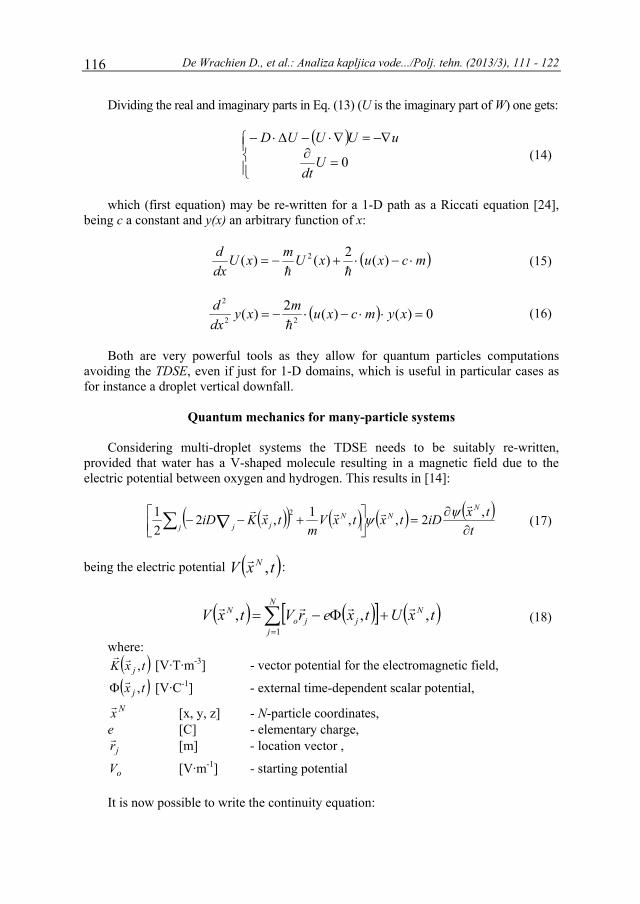
De Wrachien D., et al.: Analiza kapljica vode.../Polj. tehn. (2013/3), 111 - 122 116

Dividing the real and imaginary parts in Eq. (13) (U is the imaginary part of W) one gets:

( )

⎪⎩

⎪⎨⎧

=∂

−∇=∇⋅−Δ⋅−

0Udt

uUUUD(14)

which (first equation) may be re-written for a 1-D path as a Riccati equation [24],

being c a constant and y(x) an arbitrary function of x:

( )mcxuxUmxUdxd

⋅−⋅+−= )(2)()( 2

hh(15)

( ) 0)()(2)( 22

2

=⋅⋅−⋅−= xymcxumxydxd

h(16)

Both are very powerful tools as they allow for quantum particles computations

avoiding the TDSE, even if just for 1-D domains, which is useful in particular cases as for instance a droplet vertical downfall.

Quantum mechanics for many-particle systems

Considering multi-droplet systems the TDSE needs to be suitably re-written,

provided that water has a V-shaped molecule resulting in a magnetic field due to the electric potential between oxygen and hydrogen. This results in [14]:

( )( ) ( ) ( ) ( )t

txiDtxtxVm

txKiDN

Nj

Njj ∂

∂=⎥⎦

⎤⎢⎣⎡ +−−∑ ∇

,2,,1,221 2

rrrrr ψψ

(17)

being the electric potential ( )txV N ,r

:

( ) ( )[ ] ( )∑=

+Φ−=N

j

Njjo

N txUtxerVtxV1

,,, rrrr(18)

where: ( )txK j ,rr

[V·T·m-3] - vector potential for the electromagnetic field,

( )tx j ,r

Φ [V·C-1] - external time-dependent scalar potential,

Nxr

[x, y, z] - N-particle coordinates, e [C] - elementary charge,

jrr

[m] - location vector ,

oV [V·m-1] - starting potential

It is now possible to write the continuity equation:

De Wrachien D., et al.: Water Droplets Analysis.../Agr. Eng. (2013/3), 111 - 122 117

( ) 0,),(

1=∇+

∂∂ ∑

=

N

k

Nkk

NNtxj

ttx rrr

ρ (19)

and the Euler-type equation:

( )( ) ( ) ( ) =×∇×−+∇+∂

∂ ∑∑ ),(),(1),(,),( txvtxvtxvtxvt

txv Njk

Njj jk

Njj k

Nj

Nk rrrrrrrrrr

δ

( ) [ ]),(),(),(1,),(),( 0 txQtxUtxVm

txBtxvcetxEe NNN

kN

kkrrrrrrrrr

++∇−⎟⎠⎞

⎜⎝⎛ ×+−=

(20)

where: ),(),( 2 txRtx NNN rr

=ρ [m-3] - N-particle density,

( ) ),(),(, txvtxtxj Nk

NNNk

rrrrrρ= [m-2·s-1] - flow-fluid density,

),(),(),( txAmcetxS

mtxv NN

kN

krrhrr

−∇= [m·s-1] - k-th particle field velocity,

( )t

txAc

txtxEN

jk ∂∂⋅−Φ−∇=

),(1,),(r

rrr

[V·m-1] - external electric field,

( ) ),(, txcurlAtxB Nk

rrr= [T] - external magnetic field. ),( txU Nr [C2·m-2] - mutual inter-electrical Coulomb repulsion.

C [-] - numerical coefficient, ),( txA Nr [V·s·m-1] - vector potential of the classic forces, ),( txS Nr [rad] - wave function phase.

The first integrations of Eq. (19) and Eq. (20) were carried out by Madelung [25],

and the work was successively extended by Bohm [26, 27].

Quantum mechanics within a Density Functional Framework (DFF)

The quantum mechanics approach for many-particle systems leads to the continuity (15) and Eulero (16) equations in configuration space, thus involving the N-particle density ),( tx NN r

ρ with the 3N-D velocity field (corresponding to the k-th particle) given by:

( )txAmcetxS

mtxv k

Nk

Nk ,),(),( rrrhrr

⎟⎠⎞

⎜⎝⎛−∇⎟

⎠⎞

⎜⎝⎛= (21)

The quantum mechanical equations are, however, appealing only if they are in 3-D space in terms of the basic variables ),( txrρ and ),( txJ

rr and for N-particle systems, as a sprinkler spray flow, to obtain the continuity and Euler equations of quantum mechanics in 3-D space one can resort to the DFF which employs a partitioning of the particle-density and the current-density variables [14]. The DFF provides a single-particle based approach for the description of the motion of many-particle systems in 3-D space. In the context of the DFF, the single particle density and the current density (for the k-th particle trajectory)

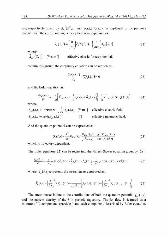
De Wrachien D., et al.: Analiza kapljica vode.../Polj. tehn. (2013/3), 111 - 122 118

are, respectively, given by ),(2 txR Nk

r and ),(),( txvtx kkrrr

ρ , as explained in the previous chapter, with the corresponding velocity field now expressed as:

( )txAmcetxS

mtxv effkk ,),(),( rrrhrr

⎟⎠⎞

⎜⎝⎛−∇⎟

⎠⎞

⎜⎝⎛= (22)

where: ( )txAeff ,r

r

[V·s·m-1] - effective classic forces potential. Within this ground the continuity equation can be written as:

( ) 0,),(=∇+

∂∂ txj

ttx

kk rrr

ρ (23)

and the Euler equation as:

( ) [ ]),(),(1,),(1),(),( txQtxVm

txBtxvc

txEme

ttxv

keffeffkeffk rrrrrrrrrr

+∇−⎥⎦⎤

⎢⎣⎡ ×+−=

∂∂

(24)

where:

),(1),(),( txAtc

txtxE effeffrrrrr

∂∂

−Φ−∇=

[V·m-1] - effective electric field,

( ) )),((, txAcurltxB effeffrrrr

= [T] - effective magnetic field. And the quantum potential can be expressed as:

),(

),(4),(

),(),(2

),(22

2

2

txtx

mtxtxtx

mtxQ

k

k

k

kkk r

rh

r

rrhr

ρρ

ρρρ ∇

−∇

∇= (25)

which is trajectory dependent. The Euler equation (22) can be recast into the Navier-Stokes equation given by [28]:

( ) ),(),(),(1,),(1),(),(),( txTtxVtxm

txBtxjc

txEtxme

ttxj

keffkeffkeffkk rrrrrrrrrrrrr

∇+∇−⎥⎦⎤

⎢⎣⎡ ×+−=

∂∂ ρρ (26)

where ( )txTk ,

rrrepresents the stress tensor expressed as:

⎥⎥⎦

⎤

⎢⎢⎣

⎡∇⎟

⎠⎞

⎜⎝⎛−+∇∇⎟

⎠⎞

⎜⎝⎛= ),(),(

2),(),(

),(1),(

2),(

22

txtxm

txjtxjtx

txm

txT kkkkk

kkrrhrrrr

rrhrr

ρρρ

ρ

(27)

The stress tensor is due to the contributions of both the quantum potential ( )txQk ,

rr

and the current density of the k-th particle trajectory. The jet flow is featured as a mixture of N components (particles) and each component, described by Euler equation,

De Wrachien D., et al.: Water Droplets Analysis.../Agr. Eng. (2013/3), 111 - 122 119

is characterized by common effective electric and magnetic fields, and by a trajectory-dependent quantum force of stress tensor [14].

For many-particle systems, as a sprinkler spray flow, the DFF represents a versatile tool for description of equilibrium as well as dynamical characteristics of the system. The basic picture is that of a multi-component fluid mixture moving in common effective electric and magnetic fields and component-specific quantum potentials.

This approach leads to the concept of quantum trajectory, in analogy to the well-established concept of classical trajectory and can represent an exciting area of research in sprinkler irrigation systems and, more generally, in the agricultural environment.

THE DYNAMICAL AND NUMERICAL APPROXIMATIONS

In any case an analytical “closed form” solution of the equations describing the quantum kinematics of particles is obviously extremely difficult and even the most advanced techniques often fail to achieve such purpose, albeit in the years to come this attempt will not be abandoned. This is why, recently, different forms of approximation have been introduced to treat the “quantum fluid-dynamic equations”: among those, literature reports numerical and dynamical approximations [29], which are both currently being developed. The formers may rely on Eulerian, Lagrangian or Arbitrary Lagrangian-Eulerian descriptions, all characterised by advantages and disadvantages. Lagrangian descriptions are easier in the form through which they write down the equations, as the grid moves with the particle and follows its evolution; but they become difficult to handle as, step after step, the grid becomes non-uniform with problems in the accuracy of the flow solution. Eulerian descriptions are complicate at the beginning of the simulation, due to an increased analytical complication, but prove to be more practical afterwards as the grid does not change with time. A uniform grid following the flow evolution is instead met in the Arbitrary Lagrangian-Eulerian descriptions, also adopted in some computational fluid dynamics codes.

Within each of the three procedures, a given numerical approach can be further subdivided into different algorithms for evaluating derivatives and propagating in time such as the meshless Moving Least Squares (MLS) [29]. The MLS tends to average out any numerical error which may be accumulating in the solution ,helping by this means to stabilize the computational process. The advantages of Mesh based approaches include, also, computational efficiency, higher resolution, accuracy and stability.

The dynamical approximations do not rely in a mathematically-simplified description of the problem but in a physically-simplified one by superimposing some particular conditions (e.g. incompressible flow) or neglecting some other characteristics considered not so relevant to the whole picture. Several approximate methods have been developed in recent years, such as the Linearized Quantum Force (LQF), the Derivative Propagation Method (DPM) and the Vibrational Decoupling Scheme (VDS) [22]. Obviously it would not be inconceivable to imagine a mixed numerical-dynamical approximation approach and we feel that on this aspect research will invest a part of its future resources: in relation to this challenge one should highlight that quantum trajectories can be treated quite similarly to the classic ones when considering, for the particles treated, the suitable relations among the dynamic and the potential part of the problem.

De Wrachien D., et al.: Analiza kapljica vode.../Polj. tehn. (2013/3), 111 - 122 120

CONCLUSIONS

Remarkable progress has recently been made in the development and application of quantum trajectories as a computational tool for solving the TDSE, which involves the time evolution of the wave function. In the Quantum Theory of Motion (QTM) the complete description of a physical system needs the simultaneous presence of the “wave” and the “particle”.

The wave motion is governed by the TDSE, and the motion of a particle guided by that wave, for a given initial position, is characterized by a velocity defined as the gradient of the phase of the wave function. An assembly of initial positions will constitute an ensemble of particle motions (the so-called quantum trajectories or Bohmian trajectories), guided by the same wave, and the probability of having the particle in a given region of space at a given time is provided by the quantum mechanical TD probability density [30].

A crucial link between QTM and Quantum Fluid Dynamics (QFD) is the quantum potential. In QTM, the particles are under the stress of forces originated from both classical and quantum potentials, while in QFD the fluid motion takes place under the influence of the external classical potential augmented by the quantum potential.

In addition to featuring water droplet ballistics in a sprinkler spray flow, novel quantum trajectory methods are being developed for a broad range of dynamical problems such as mixed classical-quantum dynamics density matrix evaluation in dissipative systems, and electronic non-adiabatic dynamics.

In this context, the present investigation starts from recent hypothesis made by the same Authors of this paper: a water droplet could be treated as a quantum object, characterised both by material particle and by wave properties. Thus the TDSE may be employed to study the process and a parallel classic-quantum description may be achieved, both for single-droplet and for multi-droplet systems. The latter systems are not only affected by the usual fluid-dynamic parameters but the mutual repulsions and attractions between particles are to be accounted for, in the form of electric-magnetic potentials bound to the molecular structure of water: this allows one to re-write the TDSE and the so-called “quantum fluid-dynamic equations” in a novel and more complete form. Future studies will deepen the novel modelling approach suggested to make it more and more suitable for practical applications.

BIBLIOGRAPHY

[1] Molle, B., Tomas, S., Hendawi, M., Granier, J. 2012. Evaporation and wind drift losses during sprinkler irrigation influenced by droplet size distribution. Irrigation and Drainage, 61(2), 240–250.

[2] Edling, R.J. 1985. Kinetic energy, evaporation and wind drift of droplets from low pressure irrigation nozzles. Transactions of the ASAE, 28 (5): 1543 – 1550.

[3] Keller, J., Bliesner, R.D. 1990. Sprinkler and Trickle irrigation. Van Nostrand Reinhold, New York. [4] Kincaid, D.C., Longley, T.S. 1989. A water droplet evaporation and temperature model.

Transactions of the ASAE, 32 (2), 457–463. [5] Kinzer, G.D., Gunn, R. 1951. The evaporation, temperature and thermal relaxation-time of

freely falling waterdrops. Journal of Meteorology, 8(2), 71-83.

De Wrachien D., et al.: Water Droplets Analysis.../Agr. Eng. (2013/3), 111 - 122 121

[6] Thompson, A.L., Gilley, J.R., Norman, J.M. 1993. A sprinkler water droplet evaporation and plant canopy model: II. Model applications. Transactions of the ASAE, 36 (3), 743-750.

[7] De Wrachien, D., Lorenzini, G. 2006. Modelling jet flow and losses in sprinkler irrigation: overview and perspective of a new approach. Biosystems Engineering, 94 (2), 297-309.

[8] Lorenzini, G. 2004. Simplified modelling of sprinkler droplet dynamics. Biosystems Engineering, 87 (1), 1-11.

[9] Lorenzini, G. 2006. Water droplet dynamics and evaporation in an irrigation spray, Transactions of the Asabe, 49 (2), 545–549.

[10] Dirac, P.A. 1931. Quantized singularities in the electromagnetic field. Proceedings of the Royal Society, A133, 1-60.

[11] De Wrachien, D., Lorenzini, G., Mambretti, S. 2012. Water droplet trajectories in an irrigation spray: the classic and Quantum Mechanical pictures. 40th International Symposium on Agricultural Engineering, Opatija (Croatia), 85-96.

[12] Nottale, L. 1992. The theory of scale relativity. International Journal of Modern Physics, 7(20), 4899-4935.

[13] Goldstein, S., Tumulka, R., Zanghi, N. 2011. Bohmian trajectories as the foundation of quantum mechanics. Quantum Trajectories (ed. Chattaraj), CRC Press, Taylor and Francis Group, 1-15.

[14] Ghosh, S.K. 2011. Quantum fluid dynamics within the framework of density functional theory. Quantum Trajectories (ed. Chattaraj), CRC Press, Taylor and Francis Group, 183-195.

[15] Teske, M.E., Hermansky, C.G., Riley, C.M. 1998. Evaporation rates of agricultural spray material at low relative wind speeds. Atomization and Spray 8, 471-478.

[16] Teske, M.E., Thistle, H.W., Eav, B. 1998. New ways to predict aerial spray deposition and drift. Journal of Forestry, 96(6), 25-31.

[17] Teske, M.E., Ice, G.G. 2002. A one-dimensional model for aerial spray assessment in forest streams. Journal of Forestry, 100(3), 40-45.

[18] Hewitt, A.J., Johnson, D.A., Fish, J.D., Hermansky, C.G., Valcore, D.L. 2002. Development of spray drift task force database for aerial applications. Environmental Toxicology and Chemistry, 21(3), 648-658.

[19] Bird, S.L., Perry, S.G., Ray, S.L., Teske, M.E. 2002. Evaluation of the AGDISP aerial spray algorithms in the AgDRIFT model. Environmental Toxicology and Chemistry, 21 (3), 672-681.

[20] Bird, R.B., Steward, W.E., Lighfoot, E.N. 1960. Transport Phenomena, Wiley and Sons, New York.

[21] Lopreore, C.L., Wyatt, R.E. 1999. Quantum wave packet dynamics with trajectories. Physical Review Letters, 82, 5190-5193.

[22] Wyatt, R.E. 2005. Quantum Dynamics with Trajectories. Introduction to Quantum Dynamics, Springer, 1-405.

[23] Hermann, R.P. 1997. Numerical simulation of a quantum particle in a box. Journal of Physics 1: Mathematical and General, 30(11), 3967-3975.

[24] Al-Rashid, S.N.T., Habeeb, M.A., Amed, K.A. 2011. Application of the scale relativity (ScR) theory to the problem of a particle in a finite one-dimensional square well (FODSW) potential. Journal of Quantum Information Science, 1, 7-17.

[25] Madelung, E. 1926. Eine anschauliche Deutung der Gleichung von Schroedinger. Naturwissenschaften,14 (45), 1004–1004.

[26] Bohm, D. 1952. A suggested interpretation of the quantum theory in terms of "hidden variables – I, Physical Review, 85 (2), 166–179.

De Wrachien D., et al.: Analiza kapljica vode.../Polj. tehn. (2013/3), 111 - 122 122

[27] Bohm, D. 1952. A suggested interpretation of the quantum theory in terms of "hidden variables – II, Physical Review, 85 (2), 180–193.

[28] Holland, P. 2011. Quantum field dynamics from trajectories. Quantum Trajectories (ed. Chattaraj). CRC Press, Taylor and Francis Group, 73-86.

[29] Kendrick, B.K. 2011. Direct numerical solution of the quantum hydrodynamic equation of motion. Quantum Trajectories (ed. Chattaraj), CRC Press, Taylor and Francis Group, 325-344.

[30] Chattaraj, P. K. 2011. Quantum Trajectories , CRC Press, London.

ANALIZA KAPLJICA VODE: KLASIČNI I KVANTNI HIDRODINAMIČKI OKVIRI

Daniele De Wrachien1, Giulio Lorenzini2, Stefano Mambretti3, Marco Medici2

1 Univerzitet u Milanu, Institut za ekološke i poljoprivredne nauke, Italija

2 Univerzitet u Parmi, Institut za industrijski inženjering, Italija 3Univerzitet u Kampinasu, Tehnološki fakultet, Brazil

Sažetak: Konstrukcija sistema za navodnjavanje sa rasprskivačima uvek je praćena potpunim razumevanjem kinematike kretanja kapljica kroz vazduh. Rešavanje ovog problema uključuje, kako teorijska, tako i eksperimentalna razmatranja. Među teorijskim studijama, klasični mehanički pristup, zasnovan na Njutnovim zakonima, daje korisno sredstvo za opis putanja kretanja kapljica vode od rasprskivača do tla. Problem postaje još komplikovaniji kad se ne posmatra samo jedna sama kapljica, već system više kapljica. Pored inter-parametarskih zavisnosti, proučavano je i među-kapljično uzajamno odbijanje, najviše usled električnih interakcija između atoma vodonika i kiseonika iz različitih molekula vode. Alternativa tradicionalnim klasičnim postupcima za analizu dinamike vodenih kapljica pri rasprskavanju, nedavno je ponuđena u obliku kvantnog pristupa. U ovom kontekstu treba proučiti ceo sistem klasičnog i kvantnog pristupa kao i alternative jedno-kapljične i više-kapljične strukture, pa su ovo osnovni ciljevi predstavljenog rada, koji se fokusira na teorijski deo problema, čime naglašava nove perspektive i celovitije obuhvata fenomen toka rasprsnutog spreja. Uopšte, novi pristup vodi do koncepta kvantne putanje u analogiji sa dobro ustanovljenim konceptom klasične trajektorije i dozvoljava da se prerade klasične jednačine dinamike fluida u tzv. kvantne jednačine.

Ključne reči: kinematika čestica spreja, jedno- i više-kapljični sistemi, klasična i kvantna mehanika, kapljice rasprsnute vode, matematičko modeliranje

Prijavljen: Submitted: 02.07.2013.

Ispravljen: Revised: 17.07.2013.

Prihvaćen: Accepted: 02.08.2013.

CIP – Каталогизација у публикацији Народна библиотека Cрбије, Београд

631(059)

ПОЉОПРИВРЕДНА техника : научни часопис = Agricultural engineering : scientific journal / главни и одговорни уредник Горан Тописировић. – Год. 1, бр. 1 (1963)- . - Београд; Земун : Институт за пољопривредну технику, 1963- (Београд : Штампарија ”Академска издања”) . – 25 cm Тромесечно. – Прекид у излажењу од 1987-1997. године ISSN 0554-5587 = Пољопривредна техника COBISS.SR-ID 16398594