Numerical simulation of particulate-flow in spiral separators: Part I. Low solids concentration...

Applied Mathematical Modelling 37 (2013) 198–215

Contents lists available at SciVerse ScienceDirect

Applied Mathematical Modelling

journal homepage: www.elsevier .com/locate /apm

Numerical simulation of particulate-flow in spiral separators: Part I.Low solids concentration (0.3% & 3% solids)

M.A. Doheim a, A.F. Abdel Gawad b,1, G.M.A. Mahran c,⇑, M.H. Abu-Ali a, A.M. Rizk a

a Mining and Metallurgical Eng. Dept., Faculty of Engineering, Assiut University, Egyptb Mechanical Power Eng. Dept., Faculty of Engineering, Zagazig University, Egyptc King Abdulaziz University, Jeddah 21589, Saudi Arabia

a r t i c l e i n f o

Article history:Received 4 August 2011Received in revised form 19 January 2012Accepted 7 February 2012Available online 18 February 2012

Keywords:Spiral separatorParticulate flowNumerical simulationTurbulence modelingGravity separationCFD

0307-904X/$ - see front matter � 2012 Elsevier Incdoi:10.1016/j.apm.2012.02.022

⇑ Corresponding author. Tel.: +966 501956842.E-mail address: [email protected] (G.M

1 Currently: Mech. Eng. Dept., Umm Al-Qura Unive

a b s t r a c t

The aim of the present study is the simulation of the particulate flow in spiral separators.The study is based on Eulerian approach and turbulence modeling. The results focus onparticulate-flow characteristics such as the velocity, the distribution, and concentrationof particulates on the spiral trough. The predicted results are compared with the experi-mental findings from LD9 coal spiral. The comparison shows good agreement and indicatesthat the most accurate turbulence model is RNG K–e.

� 2012 Elsevier Inc. All rights reserved.

1. Introduction

The spiral concentrator is considered as one of the most efficient and simple operating units for processing of mineralsand coals. Because of its relative simplicity and high efficiency, it is widely used under a variety of circuit configurations.Since, their first-introduction by Humphreys in the 1940s, spirals have proved to be a cost effective and an efficient meansof concentrating a variety of ores. Spirals are environment friendly, rugged, compact and cost effective. Most of the publica-tions concerning spirals focused on their design and operation. Wills [1] presented a comprehensive review of such paperswithin the period from 1940s until the mid 1980s. It is clear that most spiral designs were evolved through empirical anal-ysis. Many empirical models, which are based on experimental data, are stated. The drawback of these empirical models isthat if the type of spiral, the minerals or the particle-size range are changed, new experimental data must be collected tomodify the coefficients or even to change the mathematical model itself.

A fluid-flow mechanistic model is based on fluid mechanics equations. A mechanistic model incorporates the geometry ofthe device in the model. These models were started by Burch [2] when he assumed the pulp to be a liquid of uniform vis-cosity. He also assumed that the secondary flow would not affect the primary flow. Wang and Andrews [3] introduced a firststep in the development of a mechanistic model of the spiral operation. The model determines the flow fields for simplifiedrectangular spiral sections. Jancar et al. [4,5] investigated the fluid flow on LD9 spiral using their developed code. All thesemodels were developed with time to be more reliable. Mathews et al. [6,7] presented CFD modeling of the fluid flow on a

. All rights reserved.

.A. Mahran).rsity, Makkah, Saudi Arabia.

http://dx.doi.org/10.1016/j.apm.2012.02.022

mailto:[email protected]

http://dx.doi.org/10.1016/j.apm.2012.02.022

http://www.sciencedirect.com/science/journal/0307904X

http://www.elsevier.com/locate/apm

Nomenclature

C1, C2, Pm, Pkk, Cm, Ckk constants and parameters of RSM turbulence modelC1e, C2e, Cl constants of k–e turbulence modelCij convection term, RSMCD drag coefficient, (dimensionless)Cfr,ls coefficient of friction between solid phase particlesDT,ij turbulent diffusion term, RSMDL,ij molecular diffusion term, RSMds diameter of particles of phase (m)els the coefficient of restitution.ess the coefficient of restitution for particle, (dimensionless)Flift lift force (N)f different exchange coefficient models (dimensionless)Gk generation of turbulence kinetic energyGx generation of x~g gravitational accelerationH spiral height (m)h height loss (m)~kc turbulent kinetic energy of continuous phaseL spiral separator length (m)L(r) mainstream distance (m)Lc characteristic length (m)mp, mq masses of particles p & q (kg)n number of turns of spiral separatornp, nq number of particlesPij stress production term, RSMQwater water flow rate (m3/hr)R angular distance in the mainstream direction from the spiral inlet (m)Re Reynolds number (dimensionless)Rls, Rsl interaction force between phasesRe mean rate of strain, RNG k–e modelr radial distance from centerline axis (m)ri inner radius (m)ro outer radius (m)S modulus of the mean rate of strain tensor, RNG k–e modelts time per a single iteration (S)t⁄ non-dimensional time = t� ¼ Uints

Lc

� �Ti turbulence intensityUin inlet velocity (m/s)u spiral separator pitch (m)ð�qu0iu

0jÞ Reynolds stresses

~v velocity vectorW trough width = (ro � ri) (m)x mainstream directionx-velocity primary velocity (m/s)Yk and Yx dissipation of k and x due to turbulence, SST k–x modely cross-stream direction.y-velocity secondary velocity (m/s)z depth-wise direction

Greeka volume fractiona(r) spiral separator descent angle (�)a⁄, a1, rk, rx SST k–x model constants.dij Kronecker deltae=e kinetic energy dissipation rateeij dissipation term, RSMhs granular temperature (K)/ij pressure strain term, RSM/ij,w wall-reflection term, RSM

M.A. Doheim et al. / Applied Mathematical Modelling 37 (2013) 198–215 199

Uk effective diffusivity for kUx effective diffusivity for xl dynamic viscosity (kg/ms)ls solid shear viscosity (kg/ms).ls,fr fractional viscosity (kg/ms)ls,col collisional part of shear viscosity (kg/ms)leff effective viscosity (kg/ms)lt turbulent viscosity (kg/ms)mt eddy viscosity (m2/s) = lt/qGR,ij interaction between the continuous and dispersed phaseq density (kg/m3)r surface tension coefficientrk turbulent Prandtl number for kre turbulent Prandtl number for erx turbulent Prandtl number for x��sq phase stress–strain tensor (Pa)ss particulate relaxation timex specific dissipation ratew channel curvature of spiral separator

AbbreviationsCFD Computational Fluid DynamicsCPU Central Processing UnitLD9 a type of spiral separatorPC Personal ComputerPISO Pressure-Implicit with Splitting of Operators algorithmPRESTO Pressure Staggering OptionQUICK Quadratic Upwind Interpolation SchemeRNG Renormalization GroupRSM Reynolds Stress ModelVOF Volume of Fraction

Subscriptseff effectivei, j direction/phase indicesk turbulence kinetic energyq fluid phase (either air or water)t turbulentw wall

200 M.A. Doheim et al. / Applied Mathematical Modelling 37 (2013) 198–215

spiral trough. Also, Mathews et al. [8] suggested a dilute particle flow model and used isotropic RNG k–e turbulence modeland Lagrangian method for this purpose. Doheim et al. [9,10] developed a two-phase (water and air) computational modelbased on VOF method. They take into account the effect of surface tension force. Also, four turbulence models were employedto specify the most accurate and suitable one in the spiral separator simulation.

Mishra and Tripathy [11] developed a simulation tool based on the discrete element method (DEM) to understand theseparation process in spiral and used it for design purpose. They report preliminary results of simulation as to the splitterposition on the spiral trough for maximum separation efficiency. It is observed that separation efficiency is maximum cor-responding to a specific radial position and height of the splitter location. Suchandan et al. [12] suggested a mathematicalmodel to simulate the particle and flow behavior in a iron ore processing spiral. The modeling framework addressed threemain components of the spiral process, namely, geometry of the spiral and its trough, fluid motion along the curvilinear pathof the spiral and principal forces acting on a particle. These components have been integrated seamlessly by assuming thatthe particles eventually attain dynamic equilibrium in the forward longitudinal direction and static equilibrium in the trans-verse direction. The model predicts relative density distribution as a function of equilibrium radial position for different par-ticle sizes. It also computes particle size variation as a function of equilibrium radial position for various values of relativedensity. Sensitivities of radial equilibrium distribution of particle size and relative density with respect to pitch and width ofthe spiral and also mean flow depth have been analyzed. The model provided an analytical tool for better understanding ofthe separation behavior of particles in a spiral for processing iron ore. Liang et al. [13] used the numerical simulation forPHOENICS, the paper gave a quantitative analysis about the distribution of flow field and pressure field for different viscosityand flow rate.


The shortcomings of previous spiral models are: solid percent boundary condition lower than industrial solid percent, twoturbulence models only (k–e, RNG k–e) were investigated, assumption of particles had single size and single density, and thelift force affecting on the particles flow did not take into considerations.

The present study suggests a particulate-flow computational model based on Eulerian approach. This study treats most ofthe spiral models shortcomings. Modeling of the particulate-flow on spiral separator is the second step in simulation of spiralseparator. The prediction of water free-surface profile on the spiral trough is naturally the first step [9,10]. The effect of par-ticle size, inter-particle collisions and the forces acting on the particle are taken into account. Since, the flow is turbulent inthe spiral trough, four turbulence models, namely: k–e, RNG k–e, Realizable k–e, and RSM models are employed. Although,Reynolds stress model is the most accurate RANS turbulence model for highly swirling flow [14,15], nobody tried to useRSM for spiral separator CFD model before, testing RSM strengthens the originality of this work. Also, the RNG k–e modelis in better agreement than RSM with experimental velocity profiles for low swirl [16]. One of the objectives is to obtainthe most appropriate turbulence model for the present problem. The present model is validated using the experimental dataof Holtham et al. [17–19].

2. Spiral separator description

2.1. Geometry of spiral separator

A spiral separator consists of an open channel that wraps around the central supporting column. The number of turns (n)varies from 3 to 10. Most modern designs [20,21] have 5–7. The trough width usually ranges from 0.25 to 0.35 m. The designparameters of the spiral separator can be listed as: spiral pitch (u), profile shape, length (L), and inner and outer trough radii(ri,ro) that govern the curvature (w) of the channel. The parameters are shown in Fig. 1 and defined as follows [8,18]:

Pitch: u = 2pr tan(a) (m)

Fig. 1. Schematic drawing of a spiral separator [22].

Curvature: w = (ri + ro)/2W (dimensionless)

Descent angle: a(r) = tan�1(u/2pr) (�)
Trough width: W = ro � ri (m) Height loss: h = Rrtan(a) (m) Spiral height: H = n ⁄ u (m) Mainstream distance: L(r) = Rr/cos(a) (m)
where R is the angular distance in the mainstream direction from the spiral inlet (=2pa, on full turn), r is the radial dis-tance from the centerline axis, H is the spiral height and W is the trough width. The geometrical parameters for LD9 spiral[8,17,18] are stated in Table 1.

2.2. Particulate flow behaviour

The flow of particles and droplets in fluids is a subcategory of multi-component, multiphase flows, which covers a widespectrum of flow conditions and applications [23]. Modeling particle separation in a spiral trough is a complex process,which requires knowledge of particle transport behavior under different flow regimes. It is a recent trend in research on spir-al technology to model particle behavior in flowing films in spiral troughs [24,25]. In general, the motion of particles dependson the particle properties (size, density and shape), the operating conditions (slurry density and flow rate) and the spiraldesign (pitch, trough shape, inclination, and number of turns). Particle separation is achieved by the combined action ofstratification, film sizing, gravitational, and centrifugal forces, which occurs when mineral pulp, generally finer than3 mm in particle size, flows down a helical trough. As pulp flows down the trough, each element is subjected to a centrifugal

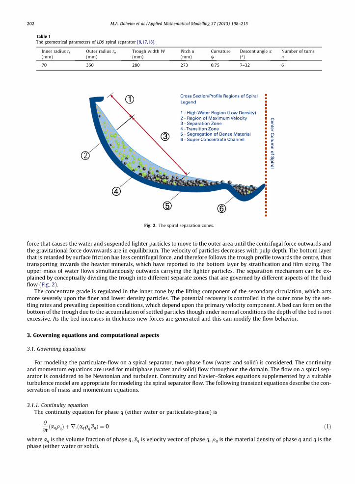
Table 1The geometrical parameters of LD9 spiral separator [8,17,18].

Inner radius ri

(mm)Outer radius ro

(mm)Trough width W(mm)

Pitch u(mm)

Curvaturew

Descent angle a(�)

Number of turnsn

70 350 280 273 0.75 7–32 6

Fig. 2. The spiral separation zones.


force that causes the water and suspended lighter particles to move to the outer area until the centrifugal force outwards andthe gravitational force downwards are in equilibrium. The velocity of particles decreases with pulp depth. The bottom layerthat is retarded by surface friction has less centrifugal force, and therefore follows the trough profile towards the centre, thustransporting inwards the heavier minerals, which have reported to the bottom layer by stratification and film sizing. Theupper mass of water flows simultaneously outwards carrying the lighter particles. The separation mechanism can be ex-plained by conceptually dividing the trough into different separate zones that are governed by different aspects of the fluidflow (Fig. 2).

The concentrate grade is regulated in the inner zone by the lifting component of the secondary circulation, which actsmore severely upon the finer and lower density particles. The potential recovery is controlled in the outer zone by the set-tling rates and prevailing deposition conditions, which depend upon the primary velocity component. A bed can form on thebottom of the trough due to the accumulation of settled particles though under normal conditions the depth of the bed is notexcessive. As the bed increases in thickness new forces are generated and this can modify the flow behavior.

3. Governing equations and computational aspects

3.1. Governing equations

For modeling the particulate-flow on a spiral separator, two-phase flow (water and solid) is considered. The continuityand momentum equations are used for multiphase (water and solid) flow throughout the domain. The flow on a spiral sep-arator is considered to be Newtonian and turbulent. Continuity and Navier–Stokes equations supplemented by a suitableturbulence model are appropriate for modeling the spiral separator flow. The following transient equations describe the con-servation of mass and momentum equations.

3.1.1. Continuity equationThe continuity equation for phase q (either water or particulate-phase) is

@

@tðaqqqÞ þ r:ðaqqq~vqÞ ¼ 0 ð1Þ

where aq is the volume fraction of phase q;~vq is velocity vector of phase q, qq is the material density of phase q and q is thephase (either water or solid).


3.1.2. Momentum equationsThe momentum equations for two phases [(fluid and particulate) or (water and solids)] represent a multi-fluid granular

model to describe the flow behavior of a fluid–solid mixture. The solid-phase stresses are derived by making an analogy ofthe random particle motions arising from particle-particle collisions. The momentum conservation equations for the fluid(liquid (water, l)) and particulate (solids, s) are:

@

@tðalql~v lÞ þ r � ðalql~v l~v lÞ ¼ �alrpþr � sl þ alql~g þ~Flift;l þ

XN

l¼1

Rsl ð2Þ

@

@tðasqs~v sÞ þ r � ðasqs~v s~v sÞ ¼ �asrp�rps þr � ss þ asqs~g þ~Flift;s þ

XN

l¼1

Rls ð3Þ

where sq is the qth phase stress–strain tensor.

sq ¼ aqlq r~vq þr~vTq

� �þ aq kq �

23lq

� �r:~vqI ð4Þ

where, lq and kq are the shear and bulk viscosity of phase q, FLift,qis a lift force, p is the pressure shared by all phases vq, isvelocity of phase q (liquid or solid (particulate-phase), vl is velocity of liquid phase, vs is velocity of solid phase, and Rsl or Rsl isan interaction force between phases.

Eqs. (2) and (3) must be closed with appropriate expressions for the inter-phase force Rsl.This force depends on the fric-tion, pressure, cohesion and other effects, and is subject to the conditions that Rsl = �Rsl and Rll = 0.

The simple interaction term is:

~Rsl ¼ kslð~v s �~v lÞ~Rls ¼ klsð~v l �~v sÞ

ð5Þ

where Rsl is an interaction force between phases, Ksl (=Kls) is the inter-phase momentum-exchange coefficient between fluidor solid phase (l) and solid phase (s), and N is the total number of phases.

Flift ¼ �0:5qqapj~vq �~vpj � ðr �~vqÞ ð6Þ

3.2. Turbulence models

The turbulence models considered in this study are k–e, RNG k–e, Realizable k–e and the Reynolds-Stress Model (RSM).

3.2.1. k–e mixture turbulence modelThe mixture turbulence model represents the first extension of the single-phase k–e model. The k and e equations describ-

ing this model are as follows:

@

@tðqmkÞ þ r:ðqm~vmkÞ ¼ r �

lt;m

rkrk

� �þ Gk;m � qme ð7Þ

and

@

@tðqmeÞ þ r � qm~vmeð Þ ¼ r �

lt;m

rere

� �þ e

kðC1eGk;m � C2eqmeÞ ð8Þ

where the mixture density and velocity, qm and ~vm, are computed from:

qm ¼XN

i¼1

aiqi ð9Þ

~vm ¼PN

i¼1aiqi~v iPNi¼1aiqi

ð10Þ

The turbulent viscosity, lt,m, is calculated from the following equation:

lt;m ¼ qmClk2

eð11Þ

The production of turbulence kinetic energy, Gk,m, is computed from:

Gk;m ¼ lt;mðr~vm þ ðr~vmÞTÞ : r~vm ð12Þ


The model constants in these equations are the same as those described in ‘‘standard k–e model [13,26,27]’’. C1e (=1.44), C2e(=1.92), Cl (=0.09), rk (=1.0) and re (=1.3) are model constants.

3.2.2. The RNG k–e modelThe RNG-based K–e turbulence model is derived from the instantaneous Navier–Stokes equations. The derivation is based

on a mathematical technique called ‘‘renormalization group’’ (RNG) method [28]. Transport equations for the RNG K–e modelhave a similar form to the standard k–e model:

@

@tðqkÞ þ @

@xiðqkuiÞ ¼

@

@xjakleff

@k@xj

� �þ Gk � qe ð13Þ

@

@tðqeÞ þ @

@xiðqeuiÞ ¼

@

@xjaeleff

@e@xj

� �þ C1e

ekðGkÞ � C2eq

e2

k� Re ð14Þ

The RNG turbulence model is more sensitive to the mean rate of strain because of Re in Eq. (14).where Gk is the generation of turbulence kinetic energy due to the mean velocity gradient. Gk may be defined as follows:

Gk ¼ �qu0iu0j

@uj

@xið15Þ

The effective viscosity, leff, is given by:

leff ¼ l 1þffiffiffiffiffiffiffiffiffiffiffiffiClqklffiffiffiep

s !2

ð16Þ

The main difference between the RNG and standard k–e models lies in the additional term in the e equation and is given by:

Re ¼Clqg3 1� g

g0

� �e2

1þ bg3

8<:

9=; e2

kð17Þ

where, g = S � k/e and S is the modulus of the mean rate of strain tensor. The model constants are set as C1e = 1.42, C2e = 1.68,Cl = 0.0845, rk = 1.0, and re = 1.3.

3.2.3. The realizable k–e modelThe realizable k–e model [29] is a relatively recent development and differs from the standard k–e model in two impor-

tant ways:

� The realizable k–e model contains a new formulation for the turbulent viscosity.� A new transport equation for the dissipation rate, e, has been derived from an exact equation for the transport of the

mean-square vorticity fluctuation.

The term ‘‘realizable’’ means that the model satisfies certain mathematical constraints on the Reynolds stresses, consistentwith the physics of turbulent flows. Neither the standard k–e model nor the RNG k–e model is realizable.

The modeled transport equations for k and e are:

@

@tðqkÞ þ @

@xjðqkujÞ ¼

@

@xjlþ lt

rk

� �@k@xj

� �þ Gk þ Gb � qe� YM þ Sk ð18Þ

and

@

@tðqeÞ þ @

@xjðqeujÞ ¼

@

@xjlþ lt

re

� �@e@xj

� �þ qC1Se � qC2

e2ffiffiffiffiffimep þ C1e

ek

C3eGb þ Se ð19Þ

Where,

C1 ¼max 0:43;g

gþ 5

� �; g ¼ S

ke; S ¼

ffiffiffiffiffiffiffiffiffiffiffiffi2SijSij

q

As in other k–e models, the eddy viscosity is computed from:

lt ¼ qClk2

eð20Þ

The difference between the realizable k–e model and the standard and RNG k–e models is that Cl is no longer constant. It iscomputed from:


Cl ¼1

A0 þ AskU�

e

ð21Þ

where,

U� �ffiffiffiffiffiffiffiffiffiffiffiffiffiffiffiffiffiffiffiffiffiffiffiffiffiffiffiSijSij þ ~Xij

~Xij

qð22Þ

and

~Xij ¼ Xij � 2eijkxk

Xij ¼ Xij � eijkxk

where Xij is the mean rate-of-rotation tensor viewed in a rotating reference-frame with the angular velocity xk. The modelconstants A0 and As are given by

A0 ¼ 4:04; As ¼ffiffiffi6p

cos /

where,

/ ¼ 13

cos�1ðffiffiffi6p

WÞ; W ¼ SijSjkSki

~S3; ~S ¼

ffiffiffiffiffiffiffiffiffiSijSij

q; Sij ¼

12

@uj

@xiþ @ui

@xj

� �

It can be seen that Cl is a function of the mean strain and rotation rates, the angular velocity of the system rotation and theturbulence fields (k and e). Cl in Eq. (20) can be shown to recover the standard value of 0.09 for an inertial sub-layer in anequilibrium boundary layer. The model constants are

C1e ¼ 1:44; C2 ¼ 1:9; rk ¼ 1:0; re ¼ 1:2

3.2.4. The Reynolds-Stress Model (RSM)The transport equation for the primary phase Reynolds stresses are [30–33]:

@

@t�aq~Rij

� �þ @

@xkð�aq~Uk

~RijÞ ¼ ��aq ~Rik@ ~Uj

@xkþ ~Rjk

@ ~Ui

@xk

!þ @

@xk�al @

@xkð~RijÞ

� �� @

@xk½�aq�ui�uj�uk� þ �ap

@�ui

@xjþ @

�uj

@xi

� �

� �aq~eij þPR;ij ð23Þ

The variables in Eq. (23) are per continuous phase. The last term of Eq. (23), PR,ij, takes into account the interaction betweenthe continuous and the dispersed phase turbulence. A general model for this term can be of the form.

PR;ij ¼ kdcC1;dcðRdc;ij � Rc;ijÞ þ kdcC2;dc;iadc;ibdc;j ð24Þ

where C1 and C2 are unknown coefficients, adc,i is the relative velocity, bdc,j is the drift or the relative velocity and Rdc,ij is theunknown particulate-fluid velocity correlation.

To simplify this unknown term, the following assumption has been made:

PR;ij ¼23

dijPk ð25Þ

where dij is the Kronecker delta, pk is the modified version of the original simonin model:

Pk ¼ Kdcð~kdc � 2~kc þ ~Vrel:~VdriftÞ ð26Þ

where ~kc is the turbulent kinetic energy of the continuous phase, ~kdc is the continuous-dispersed phase velocity covarianceand ~Vrel & ~Vdrift are stand for the relative and the drift velocities, respectively.

3.3. Computational domain

The computational domain for particulate-flow is different from that used for fluid flow. This is because the free-surfacelocation and particle flow cannot be calculated simultaneously. During modeling of fluid flow only, the free-surface profilewas obtained. The free-surface profile formed the upper boundary of the computational domain and thus remained fixedduring the coupled water-particle calculation. The computational domain consists of one complete turn of the LD9 spiral sep-arator. The number of cells are 150 � 40 � 10 in the mainstream, cross-stream and depth-wise directions respectively. Thetotal number of cells is 60,000. The computational grid is a structured mesh consisting of hexahedral control volumes. Care-ful consideration was paid to minimize the dependence of solution on the mesh by improving the clustering of cells nearsolid walls until results are almost constant. The investigation was carried out using a different number of cells, namely:45,000, 52,500, 60,000, 67,500 and 75,000. It was found that the number of cells in the range of 60,000 gives the same results

Fig. 3. Particulate computational domain of LD9 spiral and its trough section with reduced cells for clarity.


as the higher numbers of cells. The least y+ from the wall for the first node was about 4. The suggested computational do-main is shown in (Fig. 3).

3.4. Boundary conditions

Four boundaries are surrounding the suggested domain, namely: inlet plane, outlet plane, solid walls. At the inlet bound-ary of the spiral, velocity components and volume fractions of solids are specified to give the desired flow rates of slurry. Atexit of the domain (outlet plane), velocity gradients are set to zero. At the trough bottom, no-slip conditions are suggested forwater only. At the top surface of the computational domain, fixed surface is used. The trough wall-roughness constant wasset to 0.5. Standard wall function is suitable for the used mesh with such small cells near the solid walls. The water phase onspiral separator is assumed to have constant physical properties. Thus, the assumed properties are q water = 1000 kg/m3, lwater = 0.0009 kg/m s. (Table 2) shows the details of densities (qp) and sizes (Dp) of used particles.

3.5. Numerical treatment

The model of particulate-flow uses a time-dependent formulation. The numerical solution is based on finite volumemethod. The equations were discretized using the Quadratic Upwind Interpolation (QUICK) scheme for momentum, pressure,volume fraction, turbulent kinetic energy, and turbulent dissipation rate, Also phase coupled SIMPLE for pressure-velocitycoupling. Courant number is important in finite-difference formulation rather than finite volume method. The courant num-ber should be calculated for three-dimensional domain. According to Eq. (27) and based on the smallest grid size in all thethree dimensions. Usually, the value of Courant number is less than 1, here the Courant number value for all models areabout from 0.7 to 0.8. The calculated time step value ranges from 0.0013 to 0.0014 second. Hence, we select time step(Dt) = 0.001 second, This value was chosen to make the solution is stable and to give the required predictions in a reasonablecomputer run-time according to the computer specifications. Residuals of all variables were restricted to 1 � 10�5. A vali-dated commercial code [31] was used to solve the above equations of the model.

Dt �Xn

i¼1

uxi

Dxi6 C ð27Þ

where:� u is the velocity (whose dimension is Length/Time)� Dt is the time step (whose dimension is Time)� Dx is the length interval (whose dimension is Length),� C is Courant number (whose dimensionless constant)

Table 2The properties of used particles.

Particle type Density (qp)(kg/m3)

Diameter (Dp)(Micrometer)

Glass beads 2440 75 530 –Quartz 2650 75 530 1400Coal 1450 75 530 –


The interval length it is not required to be the same for each spatial variable Dxi, i = 1, . . . ,n. This ‘‘degree of freedom’’ canbe used in order to somewhat optimize the value of the time step for a particular problem, by varying the values of the dif-ferent interval in order to keep it not too small.

4. Results and discussions

In the present work, the numerical results of particulate-flow in LD9 spiral separator at flow rate of 6 m3/hr are comparedwith the experimental studies [17,34]. The model was investigated at low solid percentages starting at 0.3% and increasing to3%. The particulate-flow parameters are shown in the following sections.

4.1. Model predictions at 0.3% solids

To validate the model of particulate-flow, experimental results of 0.3% solids were used. The pulp flow rate is 6 m3/hr. Theused particles in this case are shown in Table 3.

4.1.1. Particle distributionsDistributions of particles of different sizes across the spiral separator trough are very important for both design engineers

and operators. (Figs. 4 and 5) show the cumulative weight-percentage of glass beads as a function of radial distance for par-ticle sizes 75 lm and 530 lm, respectively. (Fig. 6) shows the cumulative weight percent of quartz particles (q = 2650 kg/m3)that have a particle size 1400 lm.

Generally, (Figs. 4–6) show a good agreement between the predicted and experimental results. It means that the partic-ulate-model is reliable and may help the designers and operators to develop spiral separators. Moreover, the model may helpthe operators to control the operating conditions. The RNG k–e turbulence model results are the most accurate according toerror comparison for different turbulence models table [4]. This conclusion is based on the error-analysis of the sum-squaresof the difference between predicted and measured values. Details of the error-analysis are shown in Section 4.1.4. All themodels under-predict the values of Cumulative weight distribution of the very small particles (75 lm-particles) near thecentral column have not agreement with experimental results. The area near the central column needs more considerations.

Table 3The particles in case of 0.3% solids.

Particles type Density (q) (Kg/m3) Size (d) (lm) Mix ratio

Glass beads 2440 75 1Glass beads 2440 530 1Quartz 2650 1400 1

Radial distance from central column (m)

Cum

ulat

ive

wei

ght (

%)

0 0.05 0.1 0.15 0.2 0.25 0.30

20

40

60

80

100

Experimental ValuesRNG K-e ModelK-e ModelRealizable K-e ModelRSM

Fig. 4. Cumulative weight distribution of 75 lm-particles as a function of radial distance for glass beads across the LD9 spiral trough, at 0.3% solids [34].


Cum

ulat

ive

wei

ght (

%)

0 0.05 0.1 0.15 0.2 0.25 0.30

20

40

60

80

100




Cum

ulat

ive

wei

ght (

%)

0 0.05 0.1 0.15 0.2 0.25 0.30

20

40

60

80

100



Fig. 7. Sampling streams employed on the spirals [17].


4.1.2. Pulp velocityThe available experimental data of pulp velocity, to validate the model results, are given in the form of mean-stream

velocity. It means that the LD9 spiral trough is divided into eight streams by putting seven splitters as shown in (Fig. 7).

0.00

0.50

1.00

1.50

2.00

2.50

1 2 3 4 5 6 7Stream Number

Mea

n Ve

loci

ty (m

/s)

ExperimentalK-eRNg. K-eRealizable K-eRSM

+ 8

Fig. 8. The predicted and experimental values of mean-stream pulp velocity, at 0.3% solids [17].

Fig. 9. The predicted pulp-velocity contours (m/s) at 0.3% solids.


Fig. 10. The predicted pulp-velocity contours (m/s) at 0.3% solids.


(Fig. 8) shows the predicted values of mean-stream velocity compared with the experimental data. It is clear from thefigure that there is a good agreement between the predicted and experimental values especially for RNG K–e turbulencemodel .The velocity increases smoothly in the outward-direction away from the centerline of the spiral trough.

The pulp velocity contours (m/s) of the four turbulence models are shown in (Figs. 9 and 10), these figures show the veloc-ity contours in vertical and horizontal directions, All predicted results of different turbulence models have the same trendwith small differences in values.

4.1.3. Stream flow-rate(Fig. 11) shows the predicted stream flow-rate. The flow rate increases smoothly outwards till the seventh stream and

decreases again at the eighth stream. The flow rate is low in the eighth stream according to the distribution of pulp flowon the spiral trough.

4.1.4. Comparison between turbulence modelsTo determine the turbulence model that gives the best predictions for the investigated problem of particulate-flow model,

a detailed comparison was carried out. The comparison is based on the sum-of-the-squares of the errors between the numer-ical predictions and the experimental values. The experimental results [17,34,35] were taken as the reference values. (Tables4 and 5) show the sum of square errors comparison between different turbulence models.

(Table 4) shows calculations of square errors for cumulative weight in case of 75 lm size for radial distance from the cen-tral column of the spiral trough. This table shows an example about the calculated data in (Table 5). Each of the values that

Fig. 11. The predicted values of stream flow rate at 0.3% solids.

Table 4Calculation of sum of square errors for all turbulence models in case of cumulative weight % of 75 lm size.

Exp.value

Different turbulence models

k–e model Realizable k–e model RNG k–e RSM

Predictedcum. %

Error* Sq.error

Predictedcum. %

Error Sq.error

Predictedcum. %

Error Sq.error

Predictedcum. %

Error Sq.error

0 0 0 0 0 0 0 0 0 0 0 0 047.50 33.2 �14.3 204.49 32.90 �14.6 213.16 35.01 �12 156 30.15 �17.4 301.02348.44 38.35 �10.1 101.808 37.61 �10.8 117.29 40.03 �8.4 70.728 35.71 �12.7 162.05349.38 46.88 �2.5 6.25 46.30 �3.08 9.4864 47.45 �1.9 3.7249 45.42 �3.96 15.681650.00 51.92 1.92 3.6864 53.12 3.12 9.7344 51.62 1.62 2.6244 54.95 4.95 24.502551.00 53.01 2.01 4.0401 54.05 3.05 9.3025 52.51 1.51 2.2801 56.11 5.11 26.112152.00 54.26 2.26 5.1076 55.62 3.62 13.104 53.61 1.61 2.5921 57.03 5.03 25.300953.14 55.17 2.03 4.1209 56.09 2.95 8.7025 54.62 1.48 2.1904 58.20 5.06 25.603654.63 56.81 2.18 4.7524 57.31 2.68 7.1824 56.13 1.5 2.25 59.31 4.68 21.902456.00 58.94 2.94 8.6436 59.01 3.01 9.06 58.52 2.52 6.3504 61.19 5.19 26.936159.38 61.88 2.5 6.25 62.19 2.81 7.8961 61.37 1.99 3.9601 64.51 5.13 26.316962.75 65.31 2.56 6.5536 66.47 3.72 13.838 64.82 2.07 4.2849 67.11 4.36 19.009665.00 68.07 3.07 9.4249 69.15 4.15 17.223 67.48 2.48 6.1504 70.14 5.14 26.419668.86 71.04 2.18 4.7524 72.40 3.54 12.532 70.31 1.45 2.1025 73.15 4.29 18.404172.71 75.35 2.64 6.9696 75.87 3.16 9.9856 74.23 1.52 2.3104 77.78 5.07 25.704974.00 76.16 2.16 4.6656 76.79 2.79 7.7841 75.81 1.81 3.2761 78.15 4.15 17.222578.00 79.95 1.95 3.8025 81.42 3.42 11.696 79.41 1.41 1.9881 82.53 4.53 20.520986.00 88.12 2.12 4.4944 89.81 3.81 14.516 87.75 1.75 3.0625 90.17 4.17 17.3889100.0 100.0 0 0 100.0 0 0 100.0 0 0 100.0 0 0R 389.81 492.49 275.88 800.10

Sq. error = (Error⁄)2.R = Sum of square errors.* Error = Predicted value � Experimental value.


appear in the (Table 5) represents the summation of the squared-errors, and covers the numerical results of others. It is no-ticed that RNG k–e predictions are the closest to the experimental results. Thus, RNG k–e is the best model for computing theparticulate-flow of spiral separators. It is also obvious that the present predictions of k–e are better than the correspondingpredictions of Mathews et al. [8] using k–e model, this is due to majority of the factors affecting the spiral flow is taking intoconsideration, increasing the number of cells, and the time step is smaller. Thus, the present computational scheme givescomparatively better results. It is highly recommended to use RNG k–e model in such type of problems.

4.2. Model predictions at 3% solids

The particulate-flow model was investigated for 3% solids using RNG. k–e model. RNG k–e model was chosen because it isthe most accurate turbulence model in the case of 0.3% solids. The particles in this case are glass beads of sizes 75 and530 lm with density of 2440 kg/m3. The ratio of mix between two sizes is 1:1. This solid percent was chosen to checkthe validity of the model in the case of solid percent more than 0.3% solids.

4.2.1. Particle distributions(Fig. 12) shows the predicted cumulative weight-distribution on the spiral trough as a function of radial distance. It is

clear from (Fig. 12) that the smaller sizes go towards the outer region of the spiral trough while the larger sizes go towardsthe inner region. This figure helps the operators to choose the position of splitters to determine the amount of concentrate.

Table 5The sum of square errors comparison for different turbulence models.

Solid % Quantity k–e Realizable k–e RNG. k–e RSM Matthews et al. [11]

0.3 Cumulative weight (%) (Size = 75 lm) 389.8 492.5 275.9 800.1 765.8Cumulative weight (%) (Size = 530 lm) 1329.7 1858.5 810.9 3202.7 1954.7Cumulative weight (%) (Size = 1400 lm) 500.2 924.6 430.9 1276.1 779.3Mean stream velocity (m/s) 0.358 0.379 0.327 0.412 Not done


4.2.2. Pulp velocity(Fig. 13) shows the predicted mean-stream velocity. This figure shows that the mean-stream velocity increases smoothly

towards the outer region of the spiral trough. The mean-stream velocity in this case is similar to the case of 0.3% solids(Fig. 8). It means that the model results have a good degree of accuracy. The pulp-velocity contours distribution is shownin (Fig. 14).

4.2.3. Stream flow-rateThe predicted stream flow-rate of 3% solids case is shown in (Fig. 15). There is a good agreement between the case of 3%

solids (Fig. 15) and the case of 0.3% solids (Fig. 11).

4.3. Computational run-time

The computations were carried out using a personal computer (PC) with the following specifications:

Radial Distance from Central Column (m)

Cum

ulat

ive

wei

ght (

%)

0 0.05 0.1 0.15 0.2 0.25 0.30

20

40

60

80

100

75 Microns530 Microns

Fig. 12. Cumulative weight distribution of glass beads at 3% solids for 75 lm and 530 lm particle sizes.

Fig. 13. The predicted values of mean-stream pulp velocity at 3% solids.

Fig. 14. The predicted pulp-velocity contour (m/s) at 3% solids.

Fig. 15. The predicted values of stream flow rate at 3% solids.

Table 6Comparison of the run time for different turbulence models.

No. Turbulence model Dimensionless

time t� ¼ Vin �tsLc

� � Relative Running

Time t�Modelt�K�eModel

� �1 k–e 34.2857 1.0002 Realizable k–e 34.9714 1.023 RNG k–e 34.9714 1.024 RSM 38.7428 1.13


1. Processor: Intel Pentium 4 (3.2 GHz, Cache 2 MB).2. Memory: 4 GB Ram.3. Hard disk: 160 GB.

(Table 6) shows a comparison of the run-time of particulate-flow for different turbulence models. Where, Uin is the inletvelocity (m/s), ts is the time per a single iteration (S), and Lc is a characteristic length (m). Here, it is taken as the stream-wise


length of one turn of the spiral separator. t⁄ is the non-dimensional time. (Table 6) indicates that there is a considerable in-crease in the run-time when employing the RSM. The increase is 13% over the run-time of the standard k–e model.

(Table 6) indicates that there are increases in the run-time when employing the turbulence models: Realizable k–e, RNGk–e and RSM. The increases are 2, 2 and 13%, respectively, over the run-time of the standard k–e model. The above discussionsshowed that the RNG k–e turbulence model has moderate run time. RSM consumes much run-time in comparison to othermodels.

5. Conclusions

From the previous results and discussions, the following conclusions can be stated:

1. Comparisons between the predicted and the experimental values at 0.3% solids indicate that good agreement, especially incase of RNG k–e model.

2. The suggested computational models can be applied for similar spiral separators that have different dimensions.3. RSM needs the most computational effort among all turbulence models. It is the most expensive turbulence model com-

pared to the other turbulence models. It requires 13% more CPU run-time compared to the standard k–e model. Moreover,RSM needs more computer memory.

4. The developed models should be very useful for the design engineers to develop the spiral separators and reduce the costof real experimental models. Also, they are very useful for operators to control the operating conditions and reduce thetime-consumptions and cost of trials to obtain the best operating conditions.

5. The present study is a step towards modeling of the particulate-flow on spiral separators at realistic industrial solid per-cent (about 15–40%).

References

[1] B.A. Wills, Mineral Processing Technology, Fifth edition., Pergamon Press, 1996.[2] C.R. Burch, Helicoid performance and fine cassiterite-contributed remarks, Trans. Inst. Min. Metall. 71 (1962) 406–415.[3] Spiral Concentrators, J. Minerals Engineering, 7 (11), (1994) 1363–1385.[4] M.L. Jancar, P.N. Holtham, J.J. Davis, C.A.J. Fletcher, Approaches to the Development of Coal Spiral Models, An International symposium, Soc. Mining,

Metal and Exploration Littliton, USA, 1995, pp. 335–345.[5] JancarT., C.A.J. Fletcher, P.N. Holtham, J.A. Reizes, Computational and experimental investigation of spiral separator hydrodynamics, in: Proc. XIX Int.

Mineral Processing Congress, San Francisco, USA, 1995.[6] B.W. Matthews, C.A.J. Fletcher, A.C. Partridge, Computational simulation of fluid and dilute particulate flows on spiral concentrators, Appl. Math.

Model. 22 (1998) 965–979.[7] B.W. Matthews, C.A.J. Fletcher, A.C. Partridge, S. Vasquez, Computations of curved free surface water flow on spiral concentrators, J. Hydraul. Eng. 125

(11) (1999) 1126–1139.[8] B.W. Matthews, C.A.J. Fletcher, T.C. Partridge, Particle Flow Modeling on Spiral Concentrators: Benefits of Dense Media for Coal Processing? in: Second

International Conference on CFD in the Minerals and Process Industries, CSIRO, Melbourne, Australia, 6–8 December, 1999.[9] M.A. Doheim, A.F. Abdel Gawad, G.M. Mahran, M.H. Abu-Ali, A.M. Rizk, Computational prediction of water-flow characteristics in spiral separators: Part

I, Flow depth and turbulence intensity, J. Eng. Sci. 34 (4) (2008) 935–950 (Faculty of Engineering, Assiut University).[10] M.A. Doheim, A.F. Abdel Gawad, G.M. Mahran, M.H. Abu-Ali, A.M. Rizk, Computational prediction of water-flow characteristics in spiral separators:

Part II, The primary and secondary flows, J. Eng. Sci. 34 (4) (2008) 951–961 (Faculty of Engineering, Assiut University).[11] B.K. Mishra, A. Tripathy, A preliminary study of particle separation in spiral concentrators using DEM, Int. J. Miner. Process. 94 (3-4) (2010) 192–195.[12] K. Suchandan, P. Kumari, K. Bhattacharyya, R. Singh, A mathematical model to characterize separation behavior of a spiral for processing iron ore using

a mechanistic approach, in: Proceedings of the XI International Seminar on Mineral Processing Technology (MPT-2010), NML Jamshedpur, India, Dec2010.

[13] Y. Liang, M. Ling, H. Sheng, Numerical simulation of flow field in spiral separator, Tech. Automat. Appl. 6 (2011).[14] Khairy. Elsayed, Chris. Lacor, The effect of cyclone inlet dimensions on the flow pattern and performance, Appl. Math. Model. 35 (4) (2011) 1952–1968.[15] B. Wang, D.L. Xu, K.W. Chu, A.B. Yu, Numerical study of gas–solid flow in a cyclone separator, Appl. Math. Model. 30 (2006) 1326–1342.[16] A. Escue, J. Cui, Comparison of turbulence models in simulating swirling pipe flows, Appl. Math. Model. 34 (4) (2010) 2840–2849.[17] A.B. Holland-Batt, P.N. Holtham, Particle and fluid motion on spiral separators, J. Minerals Eng. 4 (3–4) (1991) 457–482.[18] P.N. Holtham, Primary and secondary fluid velocities on spiral separators, J. Minerals Eng. 5 (1) (1992) 79–91.[19] K.J. Golab, P.N. Holtham, Validation of a computer model of fluid flow on the spiral separator, Innovation in Physical Separation Technologies, Mozely

Memorial Symp., Inst. Min. Metall., London, 1997.[20] P.O.J. Davies, R.H. Goodman, J.A. Deschamps, Recent development in spiral design, construction and application, J. Minerals Eng. 4 (3-4) (1991) 437–

456.[21] A.B. Holland-Batt, A study of the potential for improved separation of fine particles by use of rotating spirals, J. Minerals Eng. 5 (10–12) (1992) 1099–

1112.[22] P.C. Kapur, T.P. Meloy, Spiral observed, Int. J. Miner. Process. 53 (1998) 15–28.[23] C. Crowe, M. Sommerfeld, Y. Tsuji, Multiphase Flows with Droplets and Particles, CRC Press, Florida, 1998.[24] Y. Atasoy, D.J. Spottiswood, A study of particle separation in a spiral concentrator, J. Minerals Eng. 8 (10) (1995) 1197–1208.[25] D.M. Snider, Three fundamental granular flow experiments and CPFD predictions, Powder Technol. 176 (2007) 36–46.[26] B.E. Launder, D.B. Splading, The numerical computation of turbulent flows, Comput. Methods Appl. Mech. Eng. 3 (1974) 269–289.[27] M. Narasimha, P.K. Sripriya, P.K. Banerjee, CFD modelling of hydrocyclone–prediction of cut size, Int. J. Miner. Process. 75 (2005) 53–68.[28] V. Yakhot, S.A. Orszag, Renormalization group analysis of turbulence I. Basic theory, J. Sci. Comput. 1 (1) (1986) 1–51.[29] T.-H. Shih, W.W. Liou, A. Shabbir, Z. Yang, J. Zhu, A new k–e Eddy-viscosity model for high reynolds number turbulent flows – model development and

validation, Comput. Fluids 24 (3) (1995) 227–238.[30] Andrew. Escue, Jie. Cui, Comparison of turbulence models in simulating swirling pipe flows, Appl. Math. Model. 34 (10) (2010) 2840–2849.[31] Fluent 6.3.26 User’s Guide, <www.fluentusers.com>, Fluent Inc., USA, 2006.

http://www.fluentusers.com


[32] A.F. Abdel Gawad, A new approach to minimize the wind load on interfering tall buildings based on numerical and optimization techniques, in:Al-Azhar Engineering Eighth International Conference, Cairo, Egypt, December 24–27, 2004.

[33] R. Ben-Mansour, M.A. Habib, H.M. Badr, S. Anwar, Comparison of different turbulence models and flow boundary conditions in predicting turbulentnatural convection in a vertical channel with isoflux plates, Arabian J. Sci. Eng. 32 (2B) (2007).

[34] P.N. Holtham, Experimental validation of a fundamental model of coal spirals, Australian Coal Association Research Program (ACARP) 1 (1997).[35] P.N. Holtham, Particle transport in gravity concentrators and the Bagnold effect, Miner. Eng. 5 (2) (1992) 205–221.

Numerical simulation of particulate-flow in spiral separators: Part I. Low solids concentration...

Documents

Transcript of Numerical simulation of particulate-flow in spiral separators: Part I. Low solids concentration...