Equations of state for solids under strong compression
48
This article was downloaded by: [BUPMC - Bibliothèque Universitaire Pierre et Marie Curie], [Mr S. Klotz] On: 22 July 2013, At: 09:00 Publisher: Taylor & Francis Informa Ltd Registered in England and Wales Registered Number: 1072954 Registered office: Mortimer House, 37-41 Mortimer Street, London W1T 3JH, UK High Pressure Research: An International Journal Publication details, including instructions for authors and subscription information: http://www.tandfonline.com/loi/ghpr20 Equations of state for solids under strong compression W. B. Holzapfel a a Fachbereich Physik, Universität-GH Paderborn, D-33095, Paderborn, Germany Published online: 19 Aug 2006. To cite this article: W. B. Holzapfel (1998) Equations of state for solids under strong compression, High Pressure Research: An International Journal, 16:2, 81-126, DOI: 10.1080/08957959808200283 To link to this article: http://dx.doi.org/10.1080/08957959808200283 PLEASE SCROLL DOWN FOR ARTICLE Taylor & Francis makes every effort to ensure the accuracy of all the information (the “Content”) contained in the publications on our platform. However, Taylor & Francis, our agents, and our licensors make no representations or warranties whatsoever as to the accuracy, completeness, or suitability for any purpose of the Content. Any opinions and views expressed in this publication are the opinions and views of the authors, and are not the views of or endorsed by Taylor & Francis. The accuracy of the Content should not be relied upon and should be independently verified with primary sources of information. Taylor and Francis shall not be liable for any losses, actions, claims, proceedings, demands, costs, expenses, damages, and other liabilities whatsoever or howsoever caused arising directly or indirectly in connection with, in relation to or arising out of the use of the Content.
-
Upload
khangminh22 -
Category
Documents
-
view
1 -
download
0
Transcript of Equations of state for solids under strong compression
This article was downloaded by: [BUPMC - Bibliothèque Universitaire Pierreet Marie Curie], [Mr S. Klotz]On: 22 July 2013, At: 09:00Publisher: Taylor & FrancisInforma Ltd Registered in England and Wales Registered Number: 1072954Registered office: Mortimer House, 37-41 Mortimer Street, London W1T 3JH,UK
High Pressure Research: AnInternational JournalPublication details, including instructions forauthors and subscription information:http://www.tandfonline.com/loi/ghpr20
Equations of state for solidsunder strong compressionW. B. Holzapfel aa Fachbereich Physik, Universität-GH Paderborn,D-33095, Paderborn, GermanyPublished online: 19 Aug 2006.
To cite this article: W. B. Holzapfel (1998) Equations of state for solids under strongcompression, High Pressure Research: An International Journal, 16:2, 81-126, DOI:10.1080/08957959808200283
To link to this article: http://dx.doi.org/10.1080/08957959808200283
PLEASE SCROLL DOWN FOR ARTICLE
Taylor & Francis makes every effort to ensure the accuracy of all theinformation (the “Content”) contained in the publications on our platform.However, Taylor & Francis, our agents, and our licensors make norepresentations or warranties whatsoever as to the accuracy, completeness,or suitability for any purpose of the Content. Any opinions and viewsexpressed in this publication are the opinions and views of the authors, andare not the views of or endorsed by Taylor & Francis. The accuracy of theContent should not be relied upon and should be independently verified withprimary sources of information. Taylor and Francis shall not be liable for anylosses, actions, claims, proceedings, demands, costs, expenses, damages,and other liabilities whatsoever or howsoever caused arising directly orindirectly in connection with, in relation to or arising out of the use of theContent.

This article may be used for research, teaching, and private study purposes.Any substantial or systematic reproduction, redistribution, reselling, loan,sub-licensing, systematic supply, or distribution in any form to anyone isexpressly forbidden. Terms & Conditions of access and use can be found athttp://www.tandfonline.com/page/terms-and-conditions
Dow
nloa
ded
by [
BU
PMC
- B
iblio
thèq
ue U
nive
rsita
ire
Pier
re e
t Mar
ie C
urie
], [
Mr
S. K
lotz
] at
09:
00 2
2 Ju
ly 2
013
Ilryh Pressure Research, 1998, Vol. 16, pp. 81 Reprints available directly from the publishel Photocopying permitted by license only
126 (1 1998 OPA (Overseas Publishers Association) N.V. Published hy license under
the Gordon and Breach Science Publishers imprint.
Printed in India.
Feature Article
EQUATIONS OF STATE FOR SOLIDS UNDER STRONG COMPRESSION
W. B. HOLZAPFEL
Fachbereich Physik, Universitat-GH Paderborn, 0-33095 Paderborn, Germany
(Received 29 April 1998; Injina1,forrn 5 May 1998)
The historical and theoretical background for the different mathematical forms commonly used to represent equations of state (EOS) for solids is reviewed and some criteria are discussed which allow to select some specific forms, which are not only convenient mathematical forms but bring out the physical meaning of the data. Some examples are discussed with emphasis on recent experimental and theoretical data including noble gas solids, simple metals and a few metals with special “anomalies” to illustrate the differences involved in the use of different EOS forms and to point out the specific physical reasons for differences in specific EOS forms.
Keywords: Equation of states; strong compression; effective potentials; thermal effects; linearization schemes
1. INTRODUCTION
The work of G. Mie [I] and E. Griineisen [2 ,3 ] presented a first theoretical basis to understand the physics involved in an “equation of state” (EOS) which gives the functional dependence of the thermo- dynamic variables pressure, P, volume, V, temperature, T, number of particles, N , and other variables characterizing a specific state of a given solid either in the form f ( P , V , T, N ) = 0 or in equivalent forms P = P(V, T, N ) or V = V(P, T, N ) or even T = T ( P , V, N ) . Histori- cally, these forms were called “thermal” EOS to distinguish these relations from the “chaloric” EOS relations given by the internal energy U = U(P, T, N ) . With the variables P, T, and N in this form,
81
Dow
nloa
ded
by [
BU
PMC
- B
iblio
thèq
ue U
nive
rsita
ire
Pier
re e
t Mar
ie C
urie
], [
Mr
S. K
lotz
] at
09:
00 2
2 Ju
ly 2
013
82 W. B. HOLZAPFEL
U = U(P, T, N ) as well as V = V(P, T , N ) represent incomplete descriptions of the given thermodynamic system. In contrast, the complete thermodynamic description is given by “thermodynamic potentials”, some times also called “Massieu - Gibbs-functions” as for instance, the (Helmholtz) free energy F(T, V, N ) , the Gibbs free energy G(T, P , N ) , the internal energy U(S, V , N ) and the enthalpy H(S, P, N ) . However, these functions must be presented with respect to their “canonical” thermodynamic variables, as given above.
Nevertheless, the two EOS relations V = V(P, T , N ) and U =
U(P, T , N ) together can be combined in such a way, that a complete description of the corresponding thermodynamic system is obtained, motivating intensive studies on both forms of EOS.
On the other hand, statistical thermodynamics together with quantum theory of solids established the basis for the description of all these macroscopic (thermodynamic) relations in terms of micro- scopic properties of the system which are involved in the partition function Z( V , r ) = (exp(-Pfi)) whereby kT = 1/p brings in the Boltzmann constant k , fi represents the Hamiltonian of the system, and ( ) stands for the expectation value. If one knows the energies En(V) for all the eigenstates of the system, numerated here just with one index n, one can formally write down for this many body system the closed form [4 - 81
which determines by the relations
F( V, T, N ) = -( l / ( k T ) ) In Z( V, T, N ) PtV. T , N ) = -aF/aV\ , S( V, T, N ) = -aF/arI ,
also the inverted “equations of state” V = V(P, T, N ) and T = T(S , V , N ) = T ( S , V ( P , T ) , N)+T = T(S, P , N ) . Therefore, Z determines in fact all the other thermodynamic functions like G = F + PV, I/ = F + TS, or H = U + PV, and, if necessary, also with respect to their canonical variables.
From a theoretical point of view, one can notice immediately that P = P( V , T ) is directly related to Z(V, T ) , whereas the inverted form D
ownl
oade
d by
[B
UPM
C -
Bib
lioth
èque
Uni
vers
itair
e Pi
erre
et M
arie
Cur
ie],
[M
r S.
Klo
tz]
at 0
9:00
22
July
201
3
EOS FOR SOLIDS UNDER STRONG COMPRESSION 8 3
V = V(P, T ) requires, that this inversion can be performed unambigu- ously, which is in fact not always the case as for instance for solids at negative pressures, where V(P, T ) is double valued. It should be noticed also that the free energy F = F ( V , T ) can be regained by integrating PdV but the integration of the inverse form VdP finds only technical applications.
Therefore, an EOS in the form V = V ( P , T ) may be considered as a useful mathematical relation, describing the same surface in PVT- space, however, the form P = P( V , T ) carries more physical meaning!
The meaning of this statement becomes even more clear, if one considers solids within the usual quasiharmonic approximation, where the total energy of a given state En is decomposed into the (electronic) energy of the static lattice, ESL, the energy of the phonons, EPh = Ezp + Eth, with the zeropoint energy of all the phonons, Ezp, and thermal excitations, Eth, and in addition possible contributions from defects, ED, and electronic excitations, EE. Thereby, these terms are usually treated as independent from each other and anharmonic contributions are only added afterwards [5 , 9- 121.
This usual decomposition of En leads directly to a factorization of Z( V, 7') = Z S L ' Z p h ' Z I ) ' Z E and to a decomposition of F = FsL + FPh + Fo + FE and P = PSL + Pph + PD + PE, as discussed in many text books [5,9, 10,121. Thereby, FSL = EsL and similarly Fzp = Ezp applies, since both EsL and Ezp depend only on V and not on T.
Usually, one neglects at moderate temperatures the contributions from defects and electronic excitations, as well as explicit anharmonic contributions, which go beyond the concept of quasiharmonic solids. Also magnetic interactions or specific electron-phonon interactions are left out in this approximation. This means for instance, that these treatments are not directly applicable to solids with a crossover of different electronic ground states (Valence Fluctuations; Inter-Configu- ration-Fluctuations), which deserve therefore some special considera- tions [ 13 - 181. Similarly, solids near the melting curve and especially strongly compressed fluids and degenerate plasmas have to be treated with special care [ 191. Thus the following discussion will be restricted only to such simple cases, where P = PsL( V ) + PPh( V , T ) represents a good approximation. At this point one may recall that the commonly used Mie-Gruneisen approximation represents a further restriction, which takes into account a volume dependence of PPh( V , T ) = D
ownl
oade
d by
[B
UPM
C -
Bib
lioth
èque
Uni
vers
itair
e Pi
erre
et M
arie
Cur
ie],
[M
r S.
Klo
tz]
at 0
9:00
22
July
201
3
84 W. B. HOLZAPFEL
Pzp(O( V ) ) + Pth( T/0( V ) ) , but only through the volume dependence of a characteristic temperature 6( V ) , entering into the contribution Pzp for zero point motion and into the thermal pressure Pth(~)), which depends in this approximation only on the reduced temperature T = T/B( V ) . Within this well known Mie-Griineisen approximation an (average) phonon-Griineisen parameter ye = -dln B/dln V can be defined and the characteristic temperature 6 is related to an average phonon energy (hw) transformed to temperature units by the use of 0 = (hw)/k. Within the Debye model for the phonon spectrum, 0 is usually replaced by the Debye temperature 6D = (4/3)8, which is re- lated to a cut-off frequency wn = (4/3) (w) for the case of a Debye phonon spectrum. For a Debye solid, the energy of the zero point motion is therefore k0/2 = (3/8) ken and this relation will be applied later.
In the Einstein model, 0 is the corresponding Einstein temperature, and in a pseudo-Debye model [20], discussed later in Section 3, 6 represents just the corresponding pseudo-Debye temperature. The original (thermodynamic) definition of the Griineisen parameter
results in the same value y = yo within the rigorous Mie-Gruneisen approximation.
Here and through this review, I.U.P.A.P. recommended symbols, units and nomenclature are used [21], which means, that the isothermal bulk modulus K = - 8P/81nVlT is represented [7, 9, 121 by the letter K and not by B as often done non-systematically. 01 = 3 In VjaT I p represents the (isobaric) volume expansion coefficient, and Cv = dU/3TJv the isochoric heat capacity. However, since only isothermal but no adiabatic processes, and only volume expansions but no linear expansions are considered here, the index Ton K and the index V on a are just omitted for convenience. Since various deviations from the simple Mie-Griineisen model are well known, one should notice that the temperature dependence of Cv is often represented within the Debye model, but with the use of a temperature dependent Debye temperature OD( V, T ) . Since this temperature dependence reflects primarily a drastic difference of the phonon density of states with respect to the assumptions of the Debye model, this special deviation from the Mie-Gruneisen assumption can be
Dow
nloa
ded
by [
BU
PMC
- B
iblio
thèq
ue U
nive
rsita
ire
Pier
re e
t Mar
ie C
urie
], [
Mr
S. K
lotz
] at
09:
00 2
2 Ju
ly 2
013
EOS FOR SOLIDS UNDER STRONG COMPRESSION 85
removed to a large extend by the use of a reasonably adjusted “pseudo-Debye” model [20].
On the other hand, there are also more serious deviations from the Debye model, which lead for instance to negative values of the thermal volume expansion coefficient Q at low temperatures in Si and Ge [l 13 due to the fact, that some of the “mode Griineisen parameters” yi =
- dlnwi/dln V are negative. This means that the “dispersion” of the mode Griineisen parameters
can cause significant deviations from the original Mie-Griineisen model [3] in such a way, that in addition to the Griineisen y according to Eq. (1 . l ) different Griineisen parameters can be defined [12, 22-25] like
where Ui and Ci represent the internal energy and heat capacity of an Einstein oscillator, respectively, and the summation counts all the individual modes i. At high temperatures ( T > O), however, all these Griineisen parameters approach the same value y within the quasiharmonic approximation.
To keep the following discussion as simple as possible, only Mie- Griineisen solids corresponding to no dispersion in yi-y will be considered here, and in this case, only one (temperature independent) Griineisen parameter y = 7 t h = yph = yo represents all the relevant effects. Obviously, negative thermal expansion at low temperatures is not treated within this approximation. However, the volume dependence of y, represented by r7 = dlny/dlnVIT, must be kept as an important additional quantity, which will be crucial in the discussion of thermal effects in Section 3.
It is interesting to note already here, that no dispersion of y implies that the Poisson ratio can not change with pressure, and the pressure dependence of the bulk modulus K’ determines by the Slater formula [9] in this rigorous Mie-Griineisen approach not only
Dow
nloa
ded
by [
BU
PMC
- B
iblio
thèq
ue U
nive
rsita
ire
Pier
re e
t Mar
ie C
urie
], [
Mr
S. K
lotz
] at
09:
00 2
2 Ju
ly 2
013
86 W. B. HOLZAPFEL
but also all the higher order volume derivatives of ysl like for instance
However, this rigorous Mie-Gruneisen approach is mostly not a good approximation and at least an independent (thermodynamic) average value for y instead of ysl seems to be necessary for a more realistic representation of the experimental data. If complete knowledge about the phonon dispersion and the mode Gruneisen parameters is not available, other realistic representations of the different sections of the phonon spectra can also be valuable [25].
2. EOSFORMS
2.1. Effective Atom or Ion Potentials
The concept of Mie and Gruneisen [ 3 , 7 , 9 , 121 to brake up an EOS for solids into a static lattice component PsL(V) and a temperature dependent (phonon) part Pph(B, T ) with T = T/B( V ) led subsequently to many different EOS forms depending on the actual form for the interatomic interactions used for the static lattice part.
The interatomic potential originally applied by Mie and Gruneisen [2,3] and later called Lennard-Jones (LJ) potential uses just two inverse power laws in the interatomic distance r with exponents n and m for the attractive and repulsive parts, respectively. This choice allows for a direct summation over all the coordination shells and gives for the static lattice energy of the solid under isotropic compression just two simple inverse power laws with the exponents nl3 and mi3 for the volume dependence. The famous 6-12 LJ potential corresponds to a 2-4 form in volume, and if one considers the exponents as free parameters, one obtains for the pressure (of the static lattice) the Mie-Gruneisen form MG3 in Table I, whereby the number 3 indicates, that 3 free parameters are involved in this form in addition to the equilibrium volume V, at zero pressure.
For various reasons the repulsive part of interatomic potentials was later often represented by an exponential term, which results in the well known [9] Born-Mayer potential, if r-’ is used in the attractive D
ownl
oade
d by
[B
UPM
C -
Bib
lioth
èque
Uni
vers
itair
e Pi
erre
et M
arie
Cur
ie],
[M
r S.
Klo
tz]
at 0
9:00
22
July
201
3
TA
BL
E I
EOS
for
stro
ng c
ompr
essi
on c
hara
cter
ized
by
K !-
= 5
/3 in
com
pari
son
with
oth
er f
orm
s fo
r fin
ite s
trai
n
Nam
e E
OS
KL
Dow
nloa
ded
by [
BU
PMC
- B
iblio
thèq
ue U
nive
rsita
ire
Pier
re e
t Mar
ie C
urie
], [
Mr
S. K
lotz
] at
09:
00 2
2 Ju
ly 2
013
88 W. B. HOLZAPFEL
term to represent the inter-ionic Coulomb interactions typical for ionic solids. While the lattice sum over the Coulomb terms leads to the famous Madelung numbers [26] for the different lattices, a summation over different nearest neighbor shells for the exponential term does not result in a simple form in volume. However, the exponential term decreases very steeply with increasing distance and therefore an “effective” nearest neighbor interaction can conveniently represent the repulsive term. More flexibility is finally obtained, if the attractive term is used with an adaptable exponent IZ as shown in Table I by the form labeled BM3 to point out, that this form corresponds to a generalized effective Born-Mayer potential with three free parameters (besides Vo).
Other forms, which are related to “effective” nearest neighbor potentials can be derived from an Effective Morse potential, labeled EM2 in Table I, or from an Effective Rydberg potential, labeled ER2, respectively. This last form was advertised as “universal EOS” [27], and later modified by a series expansion in the exponent [28] as shown in Table I with the label MVL for “modified Vinet form of order L”. By adding the series expansion, these authors confess already that the second order form MV2, identical to ER2, is not “universal”. Therefore, the label “universal” seems to be only misleading and should be abandoned! Since both, the effective Rydberg and the effective Morse potential, lead to a finite energy at ultimate compression, one can not expect that the corresponding EOS forms ER2, EM2, and similarly MVL can model solids under very strong compression.
This obvious fact was confirmed to some extend in a recent study [29] on the EOS of Al, where series expansions of the form MVL with L = 5 and L = 8 were fitted to the data. Both fits show an oscillatory behavior of the coefficients in the series expansions, large variations in the higher order coefficients, when the number of coefficients was increased, and an increase in the values of the higher order coefficients typical for divergent series expansions, pointing to the fact that a divergence at strong compression is inherently build into the ansatz MVL.
With these problems in mind, an EOS based on a modified Rydberg potential including at first [30,31] still a series expansion in the exponent was proposed with the label HOL, as shown in Table I. This D
ownl
oade
d by
[B
UPM
C -
Bib
lioth
èque
Uni
vers
itair
e Pi
erre
et M
arie
Cur
ie],
[M
r S.
Klo
tz]
at 0
9:00
22
July
201
3
EOS FOR SOLIDS UNDER STRONG COMPRESSION 89
form keeps some similarity to the form MVL, however, it includes already the correct asymptotic behavior near x + 0 by the exponent n = 5 in the leading l /x” term instead of n = 2 in the forms ER2 and MVL.
Nevertheless, this form involves still the weakness, that the numerical prefactor does not automatically lead to a close approach towards the well established Thomas-Fermi behavior of all solids under strong compression [4, 5,7] just before one enters into the range, where ultimately strong relativistic effects modify the x p 5 term, which is typical only for the nonrelativistic “free electron” Fermi gas and turns over into an term in the ultra-relativistic region [32,33], typically at values of x < 0.01.
This extreme relativistic region, which is of interest for considera- tions on stellar evolutions and for future fusion experiments, will not be considered further in the following discussion. Therefore, an EOS form with the correct asymptotic approach towards the nonrelativistic Fermi gas behavior is considered to be completely satisfactory for the common solid state physics. The form H l L with the new parameter co = -1n(3Ko/PFGo) incorporates this requirement by the comparison of the zero pressure bulk modulus, KO, with the pressure of a Fermi gas P F G ~ = ~ F G ( Z / V ~ ) ~ ’ ~ for the average electron density, Z/Vo, where Z represents the atomic number and Vo the atomic volume for an elemental solid. For more complex solids, Z stands for the total electron number in the crystallographic unit cell with the correspond- ing volume Vo.
For solids near ambient conditions, where Z and Vo are usually well known, the coupling between KO and co leads to a specially useful first order form H11 (ck = 0 for k # 0), where all the higher order pressure derivatives of K are already reasonably fixed by the given values of 2, Vo and KO. This correlation is shown in Table I just for the case of Kb = 3 + (2/3)co = 3 - (2/3) I I I ( ~ K ~ / P ~ G ~ ) .
In many cases, not only the pressure but also the total energy of the solid is interesting, for instance for a comparison with first principle calculations. The integration E( V ) = -3 Vo J,“ P(x)x2dx is in fact straightforward for the effective potential forms, MG3, BM3, EM2 and ER2, however, the series expansions in the exponents of MVL and HOL for L 2 3, and for H1L already for L 2 2, do not allow for closed form integrations in these cases. D
ownl
oade
d by
[B
UPM
C -
Bib
lioth
èque
Uni
vers
itair
e Pi
erre
et M
arie
Cur
ie],
[M
r S.
Klo
tz]
at 0
9:00
22
July
201
3
90 W. B. HOLZAPFEL
Whereas MVL for L = 2 results on integration directly in an effective Rydberg potential, the forms H02 and H11 lead on integration to one term with the exponential integral function, eint(x) = S,"(exp(-x)/x)dx, which is a well-behaved analytical function incorporated usually in modern mathematical tools 1341. A simple approximation can be given for the special combination
mei(x) = x . exp(x) . eint(x) = (x2 + alx + a2)/(x2 + blx + 62)
with [35] al = 2.334133, a2 = 0.250621, bl = 3.330657, and b2 =
1.681534. With this form one obtains for the total energy in the case of H11:
E(x)=(9/2).KoVo.x-*exp(co(l - x ) ) . [ I - (2+co)x (2.1) \ , + ( 2 + c0)x. mei(cox)]
In the case H02, only co is replaced by the free parameter c in this form.
If one considers integrability in closed form as an essential requirement for a convenient analytical representation of EOS data, one may reject all the forms MVL, HOL and HlL for L L 2 , respectively. But closed form integration can be incorporated easily into such forms by an Adapted Polynomial expansion of the order L, as shown in Table I with the label APL.
In fact, for L = 3 this form can be considered as a superposition of the effective Rydberg potential with the next lower order potential AP2, which provides thereby the correct asymptotic behavior at x 3 0 together with the flexibility of a niultiparameter potential. For L = 1 one obtains again the same functional form Eq. (2.1) for the total energy E(x), since AP1= H1 1. The higher order corrections LIE, for L 2 2 show first of all a lower value for the exponent of the leading term 1/x3-L, but otherwise a structure similar to the form Eq. (2.1).
In passing, i t could be noted that many different polynomial expansions could be used to modify the leading term H 1 1 ~ APl, as indicated previously [36] with the form H22. The special form APL has been selected now to obtain
Dow
nloa
ded
by [
BU
PMC
- B
iblio
thèq
ue U
nive
rsita
ire
Pier
re e
t Mar
ie C
urie
], [
Mr
S. K
lotz
] at
09:
00 2
2 Ju
ly 2
013
EOS FOR SOLIDS UNDER STRONG COMPRESSION 91
(1) simple relations for both the cohesive energy Eo = -E(l) and for the higher order derivatives of KO with respect to the series coefficients c k , and
(2) a series, where the coefficients c k are only weakly correlated and do not change much, when the number of coefficients is increased.
With these considerations in mind, one may return also to the effective Rydberg potential ER2 of Table I and modify it accordingly into a series expansion as shown in Table I with the label ARL for “Adapted Rydberg potential of the order L”, representing (1) an analytically simple EOS form, with (2) simple forms also for the bulk modulus KO and its higher order derivatives, (3) a simple form for the total energy E, and (4) a reasonable decoupling of the parameters c k in the sense that an increase in the order of the equation used in fitting experimental data does not strongly modify the parameter values with respect to the lower order fit. In fact, a somewhat similar form can be found without reference to the Rydberg potential also in the literature WI.
While the form ARL may be reasonable for “closed shell systems” like the solid noble gases and simple molecular solids, where the closed shells are preserved over a wide range in compression, the approach towards the limiting Thomas-Fermi behavior under strong compres- sion in metallic systems is definitely better modeled by the form APL. In fact, this approach towards the Thomas-Fermi behavior is indicated in Table I by the values for Kd, = 5 / 3 .
If one considers a further generalization of the effective Rydberg potential in the form GRL, one can ask oneself, whether there are any physical reasons for the selection of special values for m and n. As just discussed, rn = 2 may be reasonable for closed shell configurations but only rn = 5 accounts for the correct very high pressure regime ( K L = 5 / 3 ) . n = 1, 2, or 3 could be selected for various reason, however, n = 1 appears to be the most reasonable choice, since all the higher order forms represent basically additional power series terms which can be incorporated directly in c k . This general consideration supports the choice of the special form APL.
In fact, the form APL models correctly both limiting values for x + O and x+ DC) not only for the pressure but also for the (static
Dow
nloa
ded
by [
BU
PMC
- B
iblio
thèq
ue U
nive
rsita
ire
Pier
re e
t Mar
ie C
urie
], [
Mr
S. K
lotz
] at
09:
00 2
2 Ju
ly 2
013
92 W. B. HOLZAPFEL
lattice) energy, and therefore, the form APL can be considered as an interpolation for the whole range of x , whereas all the other effective potentials represent at the best one sided extrupolutions, when one considers these forms in the range x-0 outside the range of the measured data.
A different justification for the use of the APL forms can be derived also from the following considerations: The form
E,(x) = Eo(c + n - 1 - (c + n ) x ) . X-" . exp(c( 1 - x)) (2.2)
represents a generalized Rydberg potential, which corresponds to the original Rydberg potential for n = 0 with its unreasonable finite value for ERY(0) = Eo. (c - l)exp(c) at x = 0, but with a reasonable representation of closed shell repulsions at x M 1. For n = 1, Eq. (2.2) represents the repulsion of a screened Coulomb potential at short internuclear distances, which appears to be already more reasonable for strong compression. For n = 2, one obtains an effective potential which describes correctly the dominant Fermi gas contribution of the electrons at very strong compression. The EOS forms corresponding to these effective nearest neighbor potentials are given by
P,(x) = 3Ko . (1 - x) . xpnp3 . exp(c(1 - x)) (2.3)
' [ 1 - (1 - x) . c(c + n ) / ( (c + n)2 ~ n)]
If we consider the case n = 2, we find essential features of the form APL, however, the condition for an asymptotic approach towards the Fermi gas limit results in a transcendental equation for co in the form:
This disadvantage of Eq. (2.3) seems not to be balanced by the simpler potential form Eq. (2.2) in comparison with the form APL given by Eq. (2.1). This means, that APL can be related to a superposition of different generalized Rydberg potentials, whereby additional con- strains on the parameters e, could be used to eliminate the terms with the mei-function. Nevertheless, the form APL appears to be more convenient for wide spread applications with the minor inconvenience in its integrated form Eq. (2.1). D
ownl
oade
d by
[B
UPM
C -
Bib
lioth
èque
Uni
vers
itair
e Pi
erre
et M
arie
Cur
ie],
[M
r S.
Klo
tz]
at 0
9:00
22
July
201
3
EOS FOR SOLIDS UNDER STRONG COMPRESSION 93
2.2. Macroscopic Finite Strain Theory
On a macroscopic (thermodynamic) level, one may not care about the microscopic interatomic interactions and thermal excitations but treat the solid classically as an elastic medium characterized by first and higher order elastic coefficients in the stress - strain relations and in the corresponding relations for the internally stored elastic energy. The situation becomes especially simple if one treats only elastically isotropic solids and only volume-strain. In terms of a generalized finite strainf = (x-” - 1) with x = (V/ Vo)’l3 as before with integer values for n with y1 = 2 for Eulerian strain or -2 for Lagrangian strain, the elastic energy can be written as a power series in the strain and this “finite strain” approach results directly in the series expansion for the pressure denoted with GSL for a generalized finite strain of order L in Table I. The special value of n = 2 was chosen by Birch [38,39] and this form BEL in Table I is therefore usually referred to as Birch (or Birch - Murnaghan) Equation. The order L in this form here is lowered by one in comparison with some other common nomencla- ture, where the order refers to the order in the series expansion of the elastic energy (starting with a “second order” term as the leading term).
This finite strain theory can be applied to solids (or even liquids and gases) around any reference state characterized by a set of values P,, V,, T, with the corresponding empirical elastic coefficients, which are for an isothermal EOS commonly the bulk modulus K, and its (isothermal) pressure derivatives K : , K : , . . . (in the reference state). However, as noted before [40], an extrapolation of any BEL or GSL form beyond the range of the fitted data is not supported by any theory and leads in fact in many cases to rapid divergences with respect to reasonable theoretical extrapolations. For instance BE2 predicts for values of Kb > 6 total instability of the solid (Eo < 0) and for KL < 3 a negative pressure at strong compression. Similar limitations are also observed for other finite strain forms (GSL with
In spite of these obvious deficiencies and weak theoretical foundations, the form BEL has found wide spread applications, apparently, because the choice n = 2 results for the first order form BE1 in Kb = 4, which is a good first order approximation for most
n # 2).
Dow
nloa
ded
by [
BU
PMC
- B
iblio
thèq
ue U
nive
rsita
ire
Pier
re e
t Mar
ie C
urie
], [
Mr
S. K
lotz
] at
09:
00 2
2 Ju
ly 2
013
94 W. B. HOLZAPFEL
solids. However, there is no guarantee at all, that higher order corrections are small and convergent!
2.3. Invertible EOS Forms
Some authors [41-451 found it interesting or necessary to develop inverted EOS forms V = V(P, T ) . In some cases, both P = P(V, T ) and V = V(P, T ) represent thereby simple analytical forms. One EOS of this type is the still commonly used Murnaghan equation [41,42], denoted MU2 in Table I. This form corresponds to the assumption K”( V ) = 0, in contrast to most experimental and theoretical data, which cover typically the range 1 < -KoK// < 20.
Since the cohesive energy of a solid can be derived from an inverted EOS form only, if the two branches for V(P, T ) in the region P < 0 are given, it is not astonishing, that none of the current invertable forms represents the EOS data reasonably in the region of negative pressures near the rupture pressure, which was recently also denoted as pseudo spinodal pressure [45]. None of these forms results in a reasonable value for the cohesive energy.
Therefore, all these forms may be considered to have no physical background, but represent just useful analytical forms, when an inverted form is really necessary.
2.4. EOS Forms from Shock Wave Results
In shock wave studies, many solids show a linear dependence between the measured shock and particle velocities along a given Hugoniot curve, which relates all the states that can be reached in single shock experiments starting from the same initial state. With the conservation laws used in shock wave evaluations, the assumption of a perfect linearity [46] results in the form labeled MS2 in Table I. This form is included here only for a later comparison of isothermal data derived from shock wave measurements with the original Hugoniot data but not as an example for a reasonable representation of isotherms.
With typical values for Kb > 3, infinite pressures are predicted by this form for a critical volume V,. = Vo(Kb - 3) / (Kb + I ) , which is D
ownl
oade
d by
[B
UPM
C -
Bib
lioth
èque
Uni
vers
itair
e Pi
erre
et M
arie
Cur
ie],
[M
r S.
Klo
tz]
at 0
9:00
22
July
201
3
EOS FOR SOLIDS UNDER STRONG COMPRESSION 95
reasonable indeed for the Hugoniot relation, but indicates on the other hand, that this form is not suitable for isothermal data, where it results upon integration also in an unreasonable value for the cohesive energy Eo.
2.5. Miscellaneous Other Forms
Extended Mie-Gruneisen potentials [4,9,47,48] using series expansion in x P k with up to seven terms for (0 5 k 5 6) are very flexible, however, the Thomas-Fermi solution for strong compression is more directly modeled with the exponential term included in APL, which shows therefore much more rapid convergence at least for “regular” solids.
On theoretical grounds two reasonable forms for strong compres- sion [49,50] included already earlier the same leading term as APL, however, the remaining part appeared to be so inconvenient that these forms have found no later applications.
Finally, one may note also that a modification of the Murnaghan EOS by Keane [51] removed one of the essential limitations of the Murnaghan form, namely the assumption K“ = 0, by introducing a limiting value Kb, # Kb. With Kb, = 513, this form would model to a large extend the Fermi gas pressure at strong compression missing only the correct prefactor, however, similar to the situation with the Murnaghan form, the integration to infinite expansion does not result in a finite value for the cohesive energy Eo.
3. THERMAL EFFECTS
Most commonly, the EOS of a solid is represented by a set of isotherms P = P( V, T ) in P- V-T-space by the use of empirical functions for the isotherms with temperature dependent parameters Vo(T), &(T) and Kb( T ) , whereby the Gruneisen parameter y = aKV/ Cv correlates the temperature dependences of the volume thermal expansion coefficient a, the isothermal bulk modulus K , the volume V and the heat capacity at constant volume Cv. It can be noted here, that the adiabatic Ks with the isobaric C p results in the same y = aKsV/ C p . As mentioned before, y at constant volume should be independent D
ownl
oade
d by
[B
UPM
C -
Bib
lioth
èque
Uni
vers
itair
e Pi
erre
et M
arie
Cur
ie],
[M
r S.
Klo
tz]
at 0
9:00
22
July
201
3
96 W. B. HOLZAPFEL
of temperature for what one would call then a Mie-Gruneisen solid. However, in many cases [23,52] deviations from this possible constancy of y have been observed.
In fact, the use of temperature dependent parameters like Vo(7‘), &(T) and Kb( T ) together with some empirical EOS forms may be convenient, but it obscures the physical content of an EOS. Physical (or artificial) “anomalies” in EOS data represented in this way are not easily recognized, and the relations of EOS data with the partition function or the thermodynamic potentials of the given solid are not directly revealed.
A rigorous application of the thermodynamic relations mentioned in the introduction seems to be more desirable. To keep this discussion as simple as possible, only the simplest, non trivial case will be considered here by the restriction to the previously defined “Mie- Griineisen solid”. Let us recall the assumptions made in this case:
(1) It is assumed (at least at first) that the quasi-harmonic approxi- mation applies, which means, ‘that all the electronic excitations of the solid are well decoupled from the phonons, or, in a more rigorous sense, that also all the electron-phonon coupling can be neglected. This means, that systems with valence fluctuations, heavy fermions or even superconductivity are expected to show some thermal “anomalies” not included in this approach.
(2) In the same spirit, magneto-elastic effects are ignored. ( 3 ) Electronic excitations are treated separately. (4) Anharmonicities are included at first only by the use of volume
dependent mode frequencies w, with corresponding mode Griinei- sen parameters y L = -dlnwi/lnV, whereby the index i includes not only the wave vector but also the polarization of the different modes.
( 5 ) For the Mie-Griineisen solid, the dispersion of the mode Gruneisen parameters is neglected, by setting all yz = y. The whole phonon spectrum is thereby represented by a fixed shape with just one characteristic phonon frequency w or by the use of a corresponding characteristic temperature 6) = hw/k together with y = -dlnw/ dlnV = -dlnO/dlnV for the single Griineisen parameter of this model. Within this (rigorous) approximation, y is temperature independent and identical to the original Griineisen parameter.
Dow
nloa
ded
by [
BU
PMC
- B
iblio
thèq
ue U
nive
rsita
ire
Pier
re e
t Mar
ie C
urie
], [
Mr
S. K
lotz
] at
09:
00 2
2 Ju
ly 2
013
EOS FOR SOLIDS UNDER STRONG COMPRESSION 97
(6) Since the Debye model for the phonon spectrum shows various deficiencies [lo, 521 and leads to complicated analytical forms for the phonon contributions to all the thermodynamic functions only the “pseudo Debye” model 1201 will be used for the general discussion of Mie-Griineisen solids in this section.
In the quasiharmonic (qh) case, specially simple analytical forms are obtained with respect to the scaled temperature r = Ti0 for
when a the Simple Pseudo-Debye model (SPD) is used
with UPhqh = 3Nk0(3/8 + T4/(a + T ) 3 ) (SPD) (3.2)
For the corresponding logarithmic volume derivative one obtains
TC,, = dln Cvqh/aln VI, = y . 12a2/(4a2 + 5ar + r2) (SPD) (3.4)
With a = ( 5 / ~ ~ ) ‘ ’ ~ = 0.3716, the parameter 0 coincides with the usual Debye temperature at low temperatures and with a = (1/120)”2 =
0.0913 at high temperatures. Therefore, a = 0.2 represents a reasonable average value for the present discussion.
A more precise representation of the quasiharmonic phonon contributions to the internal energy and the related properties is provided by the Adaptive Pseudo-Debye (APD) model [20] with its four free parameters 0, u j ( i = 0,1,2) and u3 = 1 in the forms:
(APD) (3.5)
and
Dow
nloa
ded
by [
BU
PMC
- B
iblio
thèq
ue U
nive
rsita
ire
Pier
re e
t Mar
ie C
urie
], [
Mr
S. K
lotz
] at
09:
00 2
2 Ju
ly 2
013
98 W. B. HOLZAPFEL
If one constrains this form in such a way that 13 represents the Debye temperature and both the high and low temperature limits of the Debye model are reproduced exactly, one obtains a. = 5/7r4 = 0.0513, at = 0.0127, a2 = 0.430, and a3 = 1 with a standard deviation of 2% in a fit of the Debye C ~ T ) . If a. is not constrained, the standard deviation is reduced to 1.3% with a0 = 0.0276, al = 0.0641, a2 = 0.3878 and a3 = 1. However, due to the fact that the Debye model does not represent the phonon density of states of any real solid reasonably, especially at higher phonon energies, 0 together with a. to a2 should be considered as free parameters for any accurate representation of CVqh.
On the other hand, deviations in real solids from the Debye model are often represented just by an (unreasonable) temperature depen- dence of the Debye temperature [lo]. Since these temperature dependences of the Debye temperature reflect to a large extend only deficiencies of the Debye model but not of the Mie-Gruneisen model, one volume dependent characteristic temperature O( V ) with fixed values ai extends the applicability of the Mie-Griineisen model to the much wider class of substances, where the isochoric temperature dependence of the Griineisen parameter is negligible.
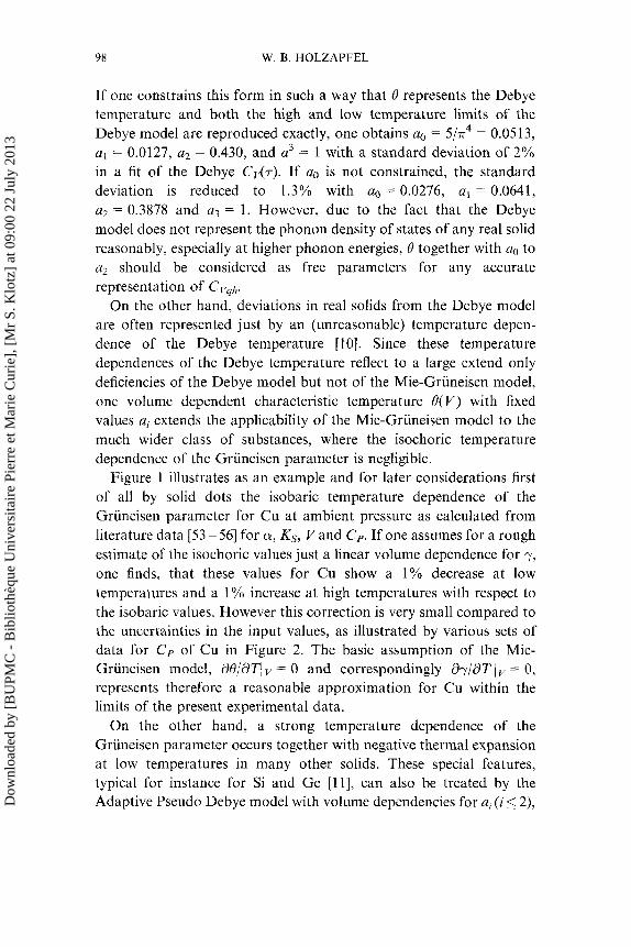
Figure 1 illustrates as an example and for later considerations first of all by solid dots the isobaric temperature dependence of the Gruneisen parameter for Cu at ambient pressure as calculated from literature data [53 - 561 for a, Ks, Vand Cp. If one assumes for a rough estimate of the isochoric values just a linear volume dependence for y, one finds, that these values for Cu show a 1% decrease at low temperatures and a 1% increase at high temperatures with respect to the isobaric values. However this correction is very small compared to the uncertainties in the input values, as illustrated by various sets of data for C p of Cu in Figure 2. The basic assumption of the Mie- Griineisen model, aO/aTi I/ = 0 and correspondingly ay/dT 1 I/ = 0, represents therefore a reasonable approximation for Cu within the limits of the present experimental data.
On the other hand, a strong temperature dependence of the Griineisen parameter occurs together with negative thermal expansion at low temperatures in many other solids. These special features, typical for instance for Si and Ge [ I l l , can also be treated by the Adaptive Pseudo Debye model with volume dependencies for ai (i 5 2), D
ownl
oade
d by
[B
UPM
C -
Bib
lioth
èque
Uni
vers
itair
e Pi
erre
et M
arie
Cur
ie],
[M
r S.
Klo
tz]
at 0
9:00
22
July
201
3
EOS FOR SOLIDS UNDER STRONG COMPRESSION 99
I I I I I I I
0 200 400 600 800 Temperature (K)
FIGURE 1 Griineisen parameter for Cu at ambient pressure calculated from literature data [53 - 561 for a, Ks, V and C,. Typical uncertainties are illustrated by error bars just for a few selected values.
Y
Y, -3
Q v
0 Ly59 200 0 Ma60
0 GM41 I
4 PI54
- APD - - SPD
v Ma62
I I I I I I I I I 1 " 0 200 400 600 800 1000
Temperature (K)
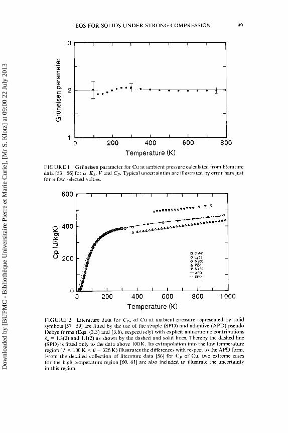
FIGURE 2 Literature data for Cp, of Cu at ambient pressure represented by solid symbols [57-591 are fitted by the use of the simple (SPD) and adaptive (APD) pseudo Debye forms (Eqs. (3.3) and (3.6), respectively) with explicit anharmonic contributions 6, = 1.3(2) and 1.1(2) as shown by the dashed and solid lines. Thereby the dashed line (SPD) is fitted only to the data above 100K. Its extrapolation into the low temperature region ( T < 100 K < 0 = 326K) illustrates the differences with respect to the APD form. From the detailed collection of literature data [56] for Cp of Cu, two extreme cases for the high temperature region [60, 611 are also included to illustrate the uncertainty in this region. D
ownl
oade
d by
[B
UPM
C -
Bib
lioth
èque
Uni
vers
itair
e Pi
erre
et M
arie
Cur
ie],
[M
r S.
Klo
tz]
at 0
9:00
22
July
201
3
100 W. B. HOLZAPFEL
but these “anomalies” will not be worked out here, since they would lead beyond the simple Mie-Gruneisen approach.
Finally, the Mie-Gruneisen model can incorporate in the total internal energy also explicit anharmonic contributions [ 121 in addition to the quasiharmonic (qh) contributions of the phonons. The additional parameter A can represent this explicit anharmonic con- tribution to first order, for instance within the SPD-model by the form:
The quasiharmonic heat capacity CVqh of Eq. (3.3) is then modified into an “anharmonic’* heat capacity
with 6, = A .KV/ (3Nk0 .y2 ) . For typical values of 0 < A < 0.1 or 6, M 1 the last approximation in Eq. (3.8) is very useful, since it gives a simple form also for the evaluation of
C p = C v ( l + a y T ) MCCVqh(lS(l +6,) .ayT+6, (ayT)*) (3.9).
Reasonable estimates of anharmonic corrections in addition to the quasiharmonic value r C q h of Eq. (3.4) can be obtained now from Eq. (3.8), if one defines at first r6 = dln 6,/d In I/ and retains then only the most significant term of the small explicit anharmonic correction:
whereby two other dimensionless logarithmic volume derivatives are used:
r,, = a Ina /d ln VI , and rr = dlny/a ln VI ,
Eq. (3.10) indicates, that the decrease of rCgh at low temperatures from rCqh(O) = 37 to rCgh +O for 7 >> 1, as shown by Eq. (3.4), is at least partly compensated by an (almost) linear increase of the explicit anharmonic contribution with increasing temperature for 6, > 0. D
ownl
oade
d by
[B
UPM
C -
Bib
lioth
èque
Uni
vers
itair
e Pi
erre
et M
arie
Cur
ie],
[M
r S.
Klo
tz]
at 0
9:00
22
July
201
3
EOS FOR SOLIDS UNDER STRONG COMPRESSION 101
The new parameter Fly, originally introduced [62] with the letter q, is often called “Anderson- Gruneisen” parameter and labeled [12, 631 (nonsystematically) with the letter ST. Furthermore, the letter q is mostly used for the parameter rr. The definition of the (thermo- dynamic) Griineisen parameter Eq. (1.1) results with this nomencla- ture in an other useful relation:
rr = re - rc ~ K’ + 1 (3.11)
which allows to evaluate within the Mie-Griineisen approach explicitly the temperature dependence for K( V, T ) in the form
and for
whereby the isobaric derivative Eq. (3.12) is some times labeled as “total” temperature dependence, and the labels “explicit” and “implicit” are attached to the isochoric Eq. (3.13) and to the remaining difference term, respectively [64].
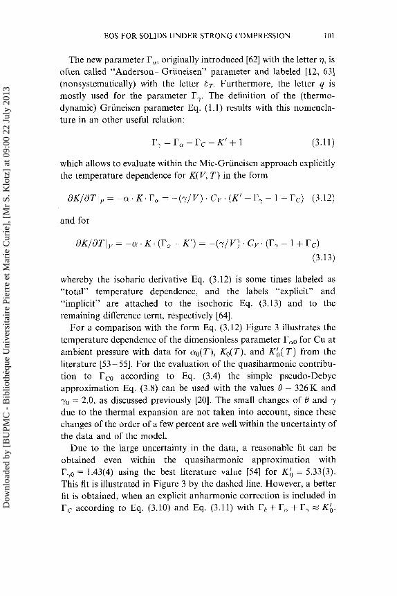
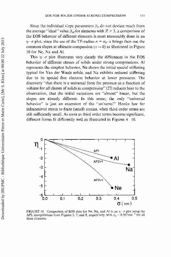
For a comparison with the form Eq. (3.12) Figure 3 illustrates the temperature dependence of the dimensionless parameter rlyo for Cu at ambient pressure with data for ao(T), Ko(T) , and Kb( T ) from the literature [53 - 551. For the evaluation of the quasiharmonic contribu- tion to according to Eq. (3.4) the simple pseudo-Debye approximation Eq. (3.8) can be used with the values B = 326K and yo = 2.0, as discussed previously [20]. The small changes of B and y due to the thermal expansion are not taken into account, since these changes of the order of a few percent are well within the uncertainty of the data and of the model.
Due to the large uncertainty in the data, a reasonable fit can be obtained even within the quasiharmonic approximation with rYo = 1.43(4) using the best literature value [54] for Kb = 5.33(3). This fit is illustrated in Figure 3 by the dashed line. However, a better fit is obtained, when an explicit anharmonic correction is included in rC according to Eq. (3.10) and Eq. (3.11) with r6 + rn +rr M Kb. D
ownl
oade
d by
[B
UPM
C -
Bib
lioth
èque
Uni
vers
itair
e Pi
erre
et M
arie
Cur
ie],
[M
r S.
Klo
tz]
at 0
9:00
22
July
201
3
102 W. B. HOLZAPFEL
8 I I I I I
r x 7 -
6 I T 1 -
3 r a o 0 KO
x T,,-K0 - - Kb(average)
. - rao-K0(qh-fit:6,=0) - Tao-Kb(fit with %=1.1)
* . . x
- rao(best fit)
- _ .
“0 100 200 300 400 500 600 700 800 Temperature (K)
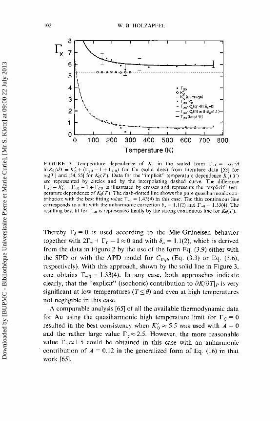
FIGURE 3 Temperature dependence of KO in the scaled form rxo = -ag’d In Ko/dT = Kb + (Fro - 1 + rco) for Cu (solid dots) from literature data [53] for cro(T) and [54,55] for Ko(T). Data for the “implicit” temperature dependence K : ( T ) are represented by circles and by the interpolating dashed curve. The difference r x 0 - Kb = rYo - 1 + l?co is illustrated by crosses and represents the “explicit” tem- perature dependence of Ko(T). The dash-dotted line shows the pure quasiharmonic con- tribution with the best fitting value rro = 1.43(4) in this case. The thin continuous line corresponds to a fit with the anharmonic correction 6, = 1.1(2) and rcyo = 1.33(4). The resulting best fit for r,, is represented finally by the strong continuous line for Ko(T).
Thereby ro = 0 is used according to the Mie-Gruneisen behavior together with 2r, + rC - 1 = 0 and with 6, = 1.1 (2), which is derived from the data in Figure 2 by the use of the form Eq. (3.9) either with the SPD or with the APD model for C,,, (Eq. (3.3) or Eq. (3.6), respectively). With this approach, shown by the solid line in Figure 3, one obtains = 1.33(4). In any case, both approaches indicate clearly, that the “explicit” (isochoric) contribution to dK/dTlp is very significant at low temperatures ( T I 0) and even at high temperatures not negligible in this case.
A comparable analysis [65] of all the available thermodynamic data for Au using the quasiharmonic high temperature limit for rC = 0 resulted in the best consistency when Kb RZ 5.5 was used with A = 0 and the rather large value r,=2.5. However, the more reasonable value F,= 1.5 could be obtained in this case with an anharmonic contribution of A = 0.12 in the generalized form of Eq. (16) in that work [65]. D
ownl
oade
d by
[B
UPM
C -
Bib
lioth
èque
Uni
vers
itair
e Pi
erre
et M
arie
Cur
ie],
[M
r S.
Klo
tz]
at 0
9:00
22
July
201
3
EOS FOR SOLIDS UNDER STRONG COMPRESSION 103
The situation becomes even more complex, if one considers the temperature dependence of Kh in detail for instance in the form of the normalized parameter
With Eq. (3.12) one obtains
(3.15)
and with (3.11)
A comparison with the thermodynamic identity
shows immediately, that the term - KoK: in Eq. (3.16) represents an isothermal or implicit thermal contribution to and the other two terms in Eq. (3.16) result from isochoric or explicit contributions.
For the representation of EOS data in extended P-T regions, it is useful to introduce [66] an other dimensionless parameter
B = a - 2 a a / d ~ ~ , = K’ + 2(r, - 1 + rc) src / (ayT) (3.18)
= l / a . dlna/dTl,
Rather few data for these parameters can be found in the literature and naturally only with very low accuracies [66]. One is therefore interested at least in rough estimates of these values and in their temperature dependences, for instance for the simple case of a Mie-Gruneisen solid with specially simple variations in y(V, T ) and Cv(V, T ) .
Since, usually little is known about the detailed variation of y(V), one smooth interpolation between the value for “infinite” pressures, ym and the value yI at the reference state with volume V,. is given [67] D
ownl
oade
d by
[B
UPM
C -
Bib
lioth
èque
Uni
vers
itair
e Pi
erre
et M
arie
Cur
ie],
[M
r S.
Klo
tz]
at 0
9:00
22
July
201
3
104 W. B. HOLZAPFEL
by the form
with the free parameter q and either 112 or 213 for ym depending on different assumptions [67 - 691.
Eq. (3.19) gives
rr = (1 - ~ c o / ~ r ) 4 (3.20)
and
Typical values for q M yr M 1.5 and ry0 M 2 give dr,/dln V I T ( p = o) M 1, however, with very large uncertainty!
Since, on the other hand, TC depends strongly on T, one may use for numerical convenience the pseudo-Debye form for rC either in the form Eq. (3.4) for the quasiharmonic case or in the form Eq. (3.10) incorporating explicit anharmonic contributions. With the assumption r6 = dS,/dlnV = 0 and F a + rr M rr M Kb in the anharmonic correc- tion, one obtains than
Finally, one may want to separate terms in Eq. (3.16) with no explicit temperature dependence from a strongly temperature dependent term AT in the form
with
AT = 3(ry0 + i)rCqhO + 6,. Po(Zo - + rro) . QTT (3.24)
whereby higher order corrections have been neglected. As one can see, A, decreases strongly from its large value at low temperatures D
ownl
oade
d by
[B
UPM
C -
Bib
lioth
èque
Uni
vers
itair
e Pi
erre
et M
arie
Cur
ie],
[M
r S.
Klo
tz]
at 0
9:00
22
July
201
3
EOS FOR SOLIDS UNDER STRONG COMPRESSION 105
A,(O) = 3 (Fro + 1). 3y0 % 40 to zero at high temperatures (7 >> 1) in the quasiharmonic case (6, = 0) where rCqh+O. However, when explicit anharmonic contributions are taken into account with 6, # 0, one finds a strong linear increase due to the last term at high temperatures. This means for Eq. (3.23) that AT will dominate at low temperatures the first term -K&; % 5, which becomes the leading term at higher temperatures but only as long as the explicit anharmonic term remains sufficiently small.
In fact, estimates of Kb( T ) using just the first term on the right hand side of Eq. (3.23) only [70] showed large discrepancies with respect to the experimental data and the remaining terms can reasonably account for the differences [66].
Similarly, explicit anharmonic contributions may effect the value of 8 in its high temperature limit ( T > 0) also very much, since (3.18) with (3.1 1) and rCgh + 0 results in
ti -+ K' + 2 ( r r - 1) + (1 + a T ~ ) . K / . s,
whereby typical values for 6 , ~ 1 indicate that the last term gives indeed very essential contributions.
Since many authors use still now just only complicated forms [70] for the implicit temperature dependence of Ko(T) like K(T,, VO(T)) and, neglect any explicit quasiharmonic or anharmonic contributions, the total temperature dependence is given here just for Mie-Gruneisen solids in their high temperature limit (AT = T - T, > 0 and T, > 0):
This form illustrates already clearly, that the quasiharmonic and anharmonic contributions represented by rrr - 1 and 6,, respectively, can be modeled in the linear term by the artificial use of a larger value [70] for K : as discussed before with respect to the data for Cu in Figure 3. In the quadratic term the uncertainties in the estimate of - K,K; by the use of different second order EOS forms are small in any case in comparison with the contributions and uncertainties from rr and S, and do not need complicated analytical forms [70].
Due to these multiple involvements of volume and temperature in the temperature dependent parameters of the common EOS forms D
ownl
oade
d by
[B
UPM
C -
Bib
lioth
èque
Uni
vers
itair
e Pi
erre
et M
arie
Cur
ie],
[M
r S.
Klo
tz]
at 0
9:00
22
July
201
3
106 W. B. HOLZAPFEL
barely any discussion of temperature dependent parameters KO( T ) and Kb( T ) extends into the low temperature region (T < Q), where the closed forms become rather lengthy [66]. Therefore better insight into normal or unusual EOS behavior is obtained, if these variations are visualized by appropriate “scaling” or linearization schemes.
4. LINEARIZATION SCHEMES
4.1. General Concepts
When pressures much higher than the initial bulk modulus KO are applied to a solid, it becomes difficult to visualized any specialties of an EOS in a simple P- V-plot. Also with logarithmic plots (log P versus V ) , one obtains infinite values not only for V+ 0 but also for P 4 0. Therefore, special “linearization schemes” have been proposed in the past [27,30, 31, 39,461 to represent the data for low and high pressures in such a way that almost linear curves are obtained for the “generalized stress coefficients” 7 with respect to the “generalized strains”f (Tab. 11). Thereby, 70 (forf = 0 or V/ Vo = x = I ) is related in a simple way to the bulk modulus KO, and the slope parameter 7 ; recovers primarily additional information on Kb. As illustrated in Table 11, different EOS forms result in different linearization schemes, with initial slopes 7 ; depending on the second order parameter c2 of the related EOS form. Obviously, very different values are obtained for these normalized slopes for a given value of Kb by the different linearization schemes. If on considers one typical set of experimental data with realistic experimental uncertainties in the pressure measure- ment for instance with an uncertainty in pressure of AP = 0.1 GPa + 0.02. P, one may notice that the standard deviation ap of the fits with any of the previously discussed EOS forms in a range with P,,, < 0.5 KO does barely depend on the specific form used in the fit, however, there will be obvious differences in the correlation coefficients r for the different linearization schemes just due to the different slopes in each of these schemes. For a typical value of Kb = 5 the “best” r value (closest to 1) is observed in the MVL-scheme representing the linearization used with the “universal” EOS [27]. However, these “best correlations” result only from the fact that this procedures generates a large (normalized) slope 710 = 6, whereas the D
ownl
oade
d by
[B
UPM
C -
Bib
lioth
èque
Uni
vers
itair
e Pi
erre
et M
arie
Cur
ie],
[M
r S.
Klo
tz]
at 0
9:00
22
July
201
3
TAB
LE I
1 V
F86,
Ho9
lb c
orre
spon
d to
[39
, 30,
46,
27,
311
res
pect
ivel
y D
iffer
ent l
inea
rizat
ion
sche
mes
with
gen
eral
ized
str
ess f
(x)
and
diff
eren
t slo
pe p
aram
eter
s 7;
. T
he r
efer
ence
s B
i78,
Ho9
la, S
m98
,
Dow
nloa
ded
by [
BU
PMC
- B
iblio
thèq
ue U
nive
rsita
ire
Pier
re e
t Mar
ie C
urie
], [
Mr
S. K
lotz
] at
09:
00 2
2 Ju
ly 2
013
106: W. B. HOLZAPFEL
linearization scheme HOL gives already the much smaller slope q: = 3 , and even smaller (normalized) slopes are produced in the BEL scheme qh/Ko = 0.75. In the GSL scheme, n = 3 would result in qb = 0 or zero slope, and a correspondingly poor correlation parameter r + 0, since r i q b . Ax/uv for small slopes qb over the range Ax and a finite standard deviation a? for the q values. A comparison of r values for different linearization schemes must take these-dependences of r on the specific slopes of the different schemes into account. Since this is usually not done, most discussions of r values with respect to these linearization schemes are useless. “Standard deviations” either along the P or V axis, a p or uv, of the experimental data with respect to the fitted curves must also be taken with much caution, because these values depend very much on the specific weighting scheme used in these fits and on the distribution of data in the given P- Y range. Therefore, the visualization of EOS data together with fits of different EOS forms in any of the linearization schemes appears to give the most reliable information as illustrated with the APL scheme for a few examples in the Figures 4 to 9.
0.2 0.4 0.6 0.8 1 .o X
0.0
FIGURE 4 EOS data for A1 at room temperature from shock wave measurements [71-731 (SW), from X-ray diffraction [74] (XR), from theoretical calculations [75 -791 (TH) and from ultrasonic measurements [go] (US) re resented in the APL-linearization
MV2, BE2, MU2, and MS2 are calculated for the same values of KO and Kb. scheme 17 = ln(P/PFc) - In(1 -x) with x = (V/Vo) I/! The different EOS forms APl,
Dow
nloa
ded
by [
BU
PMC
- B
iblio
thèq
ue U
nive
rsita
ire
Pier
re e
t Mar
ie C
urie
], [
Mr
S. K
lotz
] at
09:
00 2
2 Ju
ly 2
013
EOS FOR SOLIDS UNDER STRONG COMPRESSION 109
0.0 0.2 0.4 0.6
FIGURE 5 EOS data for Cu at room temperature from shock wave measurements [71, 721 (SW), from theoretical calculations [81,82] (TH), from SESAME [83], and from ultrasonic measurements [54] (US) represented in the APL-linearization scheme r) = In(P/PFG) - In(1 - x ) with x = (V/V0)”l. The different EOS-forms API, MV2, BE2, MU2, and MS2 are calculated for the same values of KO and KA.
1 .o Oa8 x 0.0 0.2 0.4 0.6 1 .o Oa8 x 0.0 0.2 0.4 0.6
FIGURE 6 EOS data for Ag at room temperature (SW), from shock wave measurements [71] (SW), from X-ray diffraction [84] (XR), from SESAME [83], and from ultrasonic measurement [85] (US) represented in the APL-linearization scheme r) = In(P/PFG) ~ In(1 - x) x = (V/VO)”~. The different EOS forms API, MV2, BE2, MU2, and MS2 are calculated for the same values of KO and KA. D
ownl
oade
d by
[B
UPM
C -
Bib
lioth
èque
Uni
vers
itair
e Pi
erre
et M
arie
Cur
ie],
[M
r S.
Klo
tz]
at 0
9:00
22
July
201
3
I10 W. B. HOLZAPFEL
1 .o Om8 x 0.0 0.2 0.4 0.6
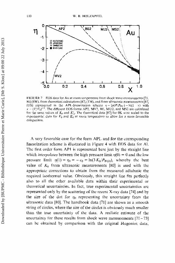
FIGURE 7 EOS data for Au at room temperature from shock wave measurements [7 I , 861 (SW), from theoretical calculations [87] (TH), and from ultrasonic measurements [85] (US) represented in the APL-linearization scheme rj = ln(P/PFG) - In(1 - x) with x = (V/V0)”3. The different EOS forms AP2, MV2, BE, MU2, and MS2 are calculated for the same values of KO and Kb. The theoretical data 1871 for OK were scaled to the experimental data for V, and KO at room temperature to allow for a more favorable comparison.
A very favorable case for the form APL and for the corresponding linearization scheme is illustrated in Figure 4 with EOS data for Al. The first order form AP1 is represented here just by the straight line which interpolates between the high pressure limit ~ ( 0 ) = 0 and the low pressure limit ~ ( 1 ) = q0 = - co = ln(3 KO/PFGO), whereby the best value of KO from ultrasonic measurements [80] is used with the appropriate corrections to obtain from the measured adiabatic the required isothermal value. Obviously, this straight line fits perfectly also to all the other available data within their experimental or theoretical uncertainties. In fact, true experimental uncertainties are represented only by the scattering of the recent X-ray data [74] and by the size of the dot for 7 0 representing the uncertainty from the ultrasonic data [80]. The handbook data [71] are shown as a smooth string of circles, where the size of the circles is obviously much smaller than the true uncertainty of the data. A realistic estimate of the uncertainty for these results from shock wave measurements [71- 731 can be obtained by comparison with the original Hugoniot data, D
ownl
oade
d by
[B
UPM
C -
Bib
lioth
èque
Uni
vers
itair
e Pi
erre
et M
arie
Cur
ie],
[M
r S.
Klo
tz]
at 0
9:00
22
July
201
3
EOS FOR SOLIDS UNDER STRONG COMPRESSION i l l
represented here schematically by the doted line corresponding to the form MS2. Since the difference between the Hugoniot curve and the isothermal data corresponds to the thermal correction, which may have been estimated with an accuracy of about 5% at the best, 5% of this difference represent a realistic estimate of the true uncertainty for the SW data. Some of these data [72] were supported by first principle calculations, and an eight order form MV8 was used to represent these data [29], but it can be seen that the first order form APl seems to fit these data already perfectly within their probable uncertainty.
In fact, a second order form MV2 with the same values for Vo, KO and Kb as in the straight line form AP1 results in the rapidly diverging dash line MV2 and the same data with the second order Birch form BE2 result in a similarly strong deviation in the opposite direction, The largest deviations are observed for the still commonly used second order Murnaghan form MU2, and the form MS2 should not be taken as an isotherm but rather as an illustration of the original Hugoniot data.
A fit of the static X-ray measurements with the forms MV2 and BE2 with the same values for Vo and KO would still appear to be reasonable, however, the values for Kb for these fits deviate in opposite directions from the value for AP1.
In addition, APl fits also to all the theoretical data [75-791 in the upper pressure region of Figure 4, where all the other (second order) forms diverge.
These results indicate therefore quite clearly that
(1) extrapolations of the forms MV2, BE2, or MU2 beyond the range of the fitted data result in rapid divergences with respect to any reasonable behavior ( ~ ( 0 ) = 0),
(2) the fitted parameter values (here just Kb for the given values of Vo and KO) depend on the EOS form used in the fit,
(3) in the special case of Al, even the first order form AP1 fits already perfectly all the data, whereas the 5th and 8th order MVL forms used in the representation of the shock wave and theoretical data [29] show no convergence of the series but rather alternating signs in subsequent coefficients for the higher order fits with large correlations in these coefficients, typical for diverging series expansions.
Dow
nloa
ded
by [
BU
PMC
- B
iblio
thèq
ue U
nive
rsita
ire
Pier
re e
t Mar
ie C
urie
], [
Mr
S. K
lotz
] at
09:
00 2
2 Ju
ly 2
013
112 W. B. HOLZAPFEL
These observations are supported also very clearly by the inspection of similar data for Cu, Ag, and Au in Figures 5, 6, and 7, respectively, and it has been pointed out [20], that the form AP2 with only minor second order corrections can be used in all these cases for the experimental realization of a pressure scale.
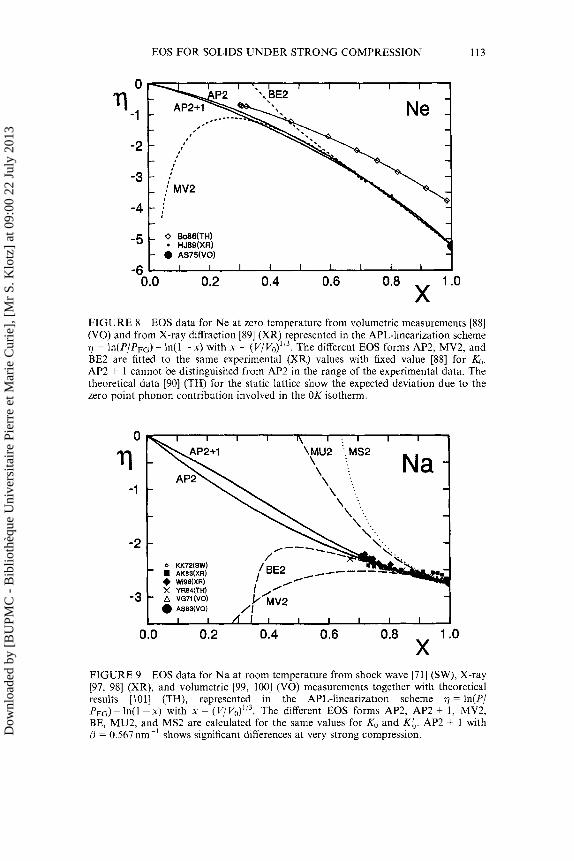
Stronger deviations from the “simple” behavior represented by the linear interpolation corresponding to the form AP1(= HI 1) are expected in many cases: Atomic and molecular solids with closed shell electronic configurations like the noble gas solids or solid H2, NZ, 02, CH4, and others Van der Waals solids, but not H20 or NH3 with their stronger hydrogen bonding, have been shown [30,31,36] to fit to convex q-x plots represented by the form AP2 with c2 > 0 as illustrated in Figure 8 just for the case of Ne. Van der Waals solids with their closed shell configurations had given in fact the earlier theoretical justification for the use of the simple exponential repulsion incorporated in the Born- Mayer, Morse, or Rydberg potential, and it is therefore natural that any EOS based on an effective Rydberg potential like ER2 = MV2 in Table I represents Ne and other Van der Waals solids over a large range of compression equally well (or even better?) than the more general second order form AP2. However, when these solids approach finally the metallic state, deviations from the extrapolated MV2 form are always expected.
At this point, it is useful to recall, that the Thomas-Fermi model [9 1, 921 predicts a universal EOS for the static lattices of all kinds of solids in a scaled form: PTF = Z’Oi3 P*(cr) using the Thomas-Fermi radius a = (ZV/(47~/3))”~ with the atomic number 2 and the atomic volume V for elements. “Average” atomic numbers and volumes [19] 2 = Cn,Z,/Cn, and V = Cn,V,/Cn, must be used for compounds and alloys with stoichiometric numbers n, for each species i. Different averaging schemes have been proposed [92], but this simplest average [19] seems to work best at least for alkali halides [93].
If one excludes the region of strong relativistic effects at extremely high compressions (a << 0.01 nm) one finds [30] for PTF + PFG( V/Z). exp (- PTF’CT) with PTF = (2/3)1’3/~2’3/ag = 7.696061(l)nm-’ [30], which results for the 77-x plots in an average “ideal” slope parameter PJd = PTF - (a;’) = 5.67nm-’. Taking into account additional Z dependent corrections for exchange, correlation and quantum effects [94 - 961 and individual values for the zero pressure TF-radius go, very
-
Dow
nloa
ded
by [
BU
PMC
- B
iblio
thèq
ue U
nive
rsita
ire
Pier
re e
t Mar
ie C
urie
], [
Mr
S. K
lotz
] at
09:
00 2
2 Ju
ly 2
013
EOS FOR SOLIDS UNDER STRONG COMPRESSION 113
0.0 0.2 0.4 0.6
FIGURE 8 EOS data for Ne at zero temperature from volumetric measurements 1881 (VO) and from X-ray diffraction [89] (XR) represented in the APL-linearization scheme 7 = h(P/PFG) - ln(1 - x) with x = (V/V,4”3. The different EOS forms AP2, MV2, and BE2 are fitted to the same experimental (XR) values with fixed value [88] for KO. AP2 t 1 cannot be distinguished from AP2 in the range of the experimental data. The theoretical data [90] (TH) for the static lattice show the expected deviation due to the zero point phonon contribution involved in the OK isotherm.
1 .o Oa8 \I 0.0 0.2 0.4 0.6
FIGURE 9 EOS data for Na at room temperature from shock wave 1711 (SW), X-ray [97, 981 (XR), and volumetric [99, 1001 (VO) measurements together with theoretical results [I011 (TH), represented in the APL-linearization scheme 1) = In(P/ PFG) - ln(1 - x ) with x = (V/V0)”3. The different EOS forms AP2, AP2 + 1, MV2, BE, MU2, and MS2 are calculated for the same values for KO and Kb. AP2 + 1 with p = 0.567 nm-’ shows significant differences at very strong compression. D
ownl
oade
d by
[B
UPM
C -
Bib
lioth
èque
Uni
vers
itair
e Pi
erre
et M
arie
Cur
ie],
[M
r S.
Klo
tz]
at 0
9:00
22
July
201
3
114 W. B. HOLZAPFEL
similar but individually adjusted slope parameters
can be obtained also.
plot at very strong compression (x 4 0), one obtains the condition If one requires, that the form APL reproduces this slope in the 7-x
This condition implies for the form AP3, that the parameter c3 becomes fixed by the value of /? (either P L d or P,). One obtains in this way an effective second order EOS to be labeled here AP2 + 1.
For Ne, the fit of AP2 + 1 to the same OK data used in the fit of AP2 but now with the prefixed values for KO, V,, and p = pill = 5.67nm-’ gives for the last parameter Kb = 9.8 to be compared with the AP2 value Kb = 9.2. As illustrated also in Figure 8, the differences in these fits are marginal in the range of the experimental data, however, AP2 + 1 should model more precisely the ultimate behavior at very high compression.
The data for Na in Figure 9 illustrate some different behavior with opposite, concave deviations (c2 < 1) with respect to the “simple” API form. These deviations can be related to the facG that just one free electron per atom contributes to the repulsion at moderate compres- sion with only minor contributions from the 10 inner core electrons. This reduced effective electron number results at first in the rather low slope near ambient conditions, however with an unusual increase in q, when the core repulsion begins to contribute significantly to the total pressure. This special behavior of Na (and Li) requires at least the use of a form AP2. When the “ideal” slope at ultimate compression is used as additional constrain, the constrained third order form AP2 + 1 shows even a steeper anomaly in Figure 9, and one may notice that this form fits especially well to the most recent additional data [98].
On the other hand, one can note that the q-x plots for the “simple” solids in Figures 4 to 7 do not deviate much from the expected “ideal” slopes. Therefore, both the forms AP1 and API + 1 are almost identical in these cases and are omitted for this reason in these figures. D
ownl
oade
d by
[B
UPM
C -
Bib
lioth
èque
Uni
vers
itair
e Pi
erre
et M
arie
Cur
ie],
[M
r S.
Klo
tz]
at 0
9:00
22
July
201
3
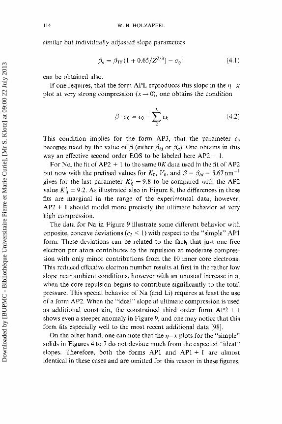
EOS FOR SOLIDS UNDER STRONG COMPRESSION 115
Since the individual slope parameters pa do not deviate much from the average “ideal” value Pid for elements with 2 > 3, a comparison of the EOS behavior of different elements is most reasonably done in an q-0 plot, since the use of the TF-radius c = go. x brings then out the common slopes at ultimate compassion (x 4 0) as illustrated in Figure 10 for Ne, Na and Al.
This q-a plot illustrates very clearly the differences in the EOS behavior of different classes of solids under strong compressions. A1 represents the simplest behavior, Ne shows the initial special stiffening typical for Van der Waals solids, and Na exhibits reduced stiffening due to its special free electron behavior at lower pressures. The discovery “that there is a universal form for pressure as a function of volume for all classes of solids in compression” [27] reduces here to the observation, that the initial variations are “almost” linear, but the slopes are already different. In this sense, the only “universal behavior” is just an extension of the “universal” Hooks law for infinitesimal strain to finite (small) strains, when third order terms are still sufficiently small. As soon as third order terms become significant, different forms fit differently well as illustrated in Figures 4- 10.
-3
-4
-5
-6
- - - - - - -
I I I I I I I I I
0.0 0.1 0.2 0.3 0.4 0.5 CJ(nm)
FIGURE 10 Comparison of EOS data for Ne, Na, and AI in an 7 - u plot using the APL interpolations from Figures 3, 7, and 8, respectively, with p, = 0.567nm-’ for all three elements. D
ownl
oade
d by
[B
UPM
C -
Bib
lioth
èque
Uni
vers
itair
e Pi
erre
et M
arie
Cur
ie],
[M
r S.
Klo
tz]
at 0
9:00
22
July
201
3
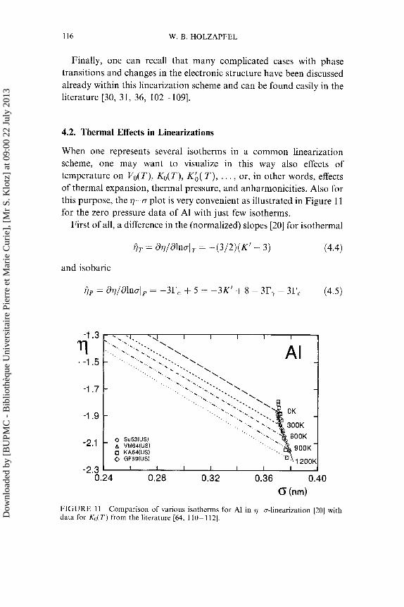
1 I6 W. B. HOLZAPFEL
Finally, one can recall that many complicated cases with phase transitions and changes in the electronic structure have been discussed already within this linearization scheme and can be found easily in the literature [30, 31, 36, 102- 1091.
4.2. Thermal Effects in Linearizations
When one represents several isotherms in a common linearization scheme, one may want to visualize in this way also effects of temperature on Vo(T), Ko(T), Kb( T ) , . . . , or, in other words, effects of thermal expansion, thermal pressure, and anharmonicities. Also for this purpose, the 7-0 plot is very convenient as illustrated in Figure 11 for the zero pressure data of A1 with just few isotherms.
First of all, a difference in the (normalized) slopes [20] for isothermal
f j T = dq/dlnal, = -(3/2)(K’ - 3) (4.4)
and isobaric
f j p = dq/dlno/, = -3r, + 5 = -3K’ + 8 - 317, - 3rc (4.5)
0 (nm)
FIGURE 11 data for &(T) from the literature [64, 110- 1121.
Comparison of various isotherms for A1 in 7-a-linearization [ZO] with
Dow
nloa
ded
by [
BU
PMC
- B
iblio
thèq
ue U
nive
rsita
ire
Pier
re e
t Mar
ie C
urie
], [
Mr
S. K
lotz
] at
09:
00 2
2 Ju
ly 2
013
EOS FOR SOLIDS UNDER STRONG COMPRESSION 117
variations can be seen immediately by the comparison of the ambient pressure data qo(T) (solid line) with respect to the isothermal data q(cr) taken from Figure 3 for 300K and represented here by the short dashed line. Some discrepancy in the experimental data for Ko(T) becomes obvious in this presentation of the literature data [64, 110- 1121 as discussed previously [20]. An almost constant slope of qo(T) can be noticed at high temperatures. The steeper slope at low T can be traced back to the strong variation of r C ( T ) discussed in Section 3 . The absolute value of the slope at high T( > 0) depends not only on Kb and r r but through rC also on the strength of explicit anharmonicities as shown by Eq. (4.5). The evaluation of rr values from these slopes must take into account the amount of explicit anharmonicities as discussed already in Section 3 with respect to the data for Cu, but here one can notice that the experimental data for 7 j T and f j p give directly
A detailed comparison of f i T and ijp for Al, Cu, Ag, and Au will not be given here, since it can be found already in the literature [20], however, for the “simple” solids discussed in Section 2.1 a simple rule can be derived from Eq. (1.3). In a first approximation one obtains for “simple” Mie-Griineisen solids:
which gives in the high temperature limit (with rC = 0):
This correlation of both slopes is seen indeed in many of the corresponding 7-0 plots [20]. Some other new aspects concern the slope at very strong compression q(0) = dq/dal,=, = p and its relation to thermal effects.
For “simple” solids, represented for instance at room temperature by the first order form APl, one could try to use straight line interpolations between qo(T) and q, = 0 for all the isotherms. This implies for all the slope parameters p( T ) = --7jpo( T)/ao( T ) .
However, the behavior at very strong compression imposes one additional constrain on the slopes. First of all B increases continuously D
ownl
oade
d by
[B
UPM
C -
Bib
lioth
èque
Uni
vers
itair
e Pi
erre
et M
arie
Cur
ie],
[M
r S.
Klo
tz]
at 0
9:00
22
July
201
3
118 W. B. HOLZAPFEL
for ym > 0, which implies that the zero point pressure dominates ultimately any thermal contribution for any finite temperature. Nevertheless [69], the zero point pressure of the lattice becomes negligible (Pzp/P + 0) as long as yw < 213. In fact, for yw = 213, the lattice would behave like a Fermi gas, but the mass of these particles would be very large compared with the electron mass and therefore Pph/P + (me/mp)/(Z5/3.A4), where the electron - proton mass ratio me/ mp and atomic mass number M together with the atomic charge number Z result again in a very small total ratio, almost equal to zero! This means that all the isotherms of a given material have the same asymptotic variation at strong compression and this implies in the 7-0 plots for the ultimate slopes
with a weak temperature dependence through ao(T). For a “simple” solid, where co(T) = P(T).ao(T) = (3/2) (Kb - 3) but also co =
1n(3Ko/PFGo), one obtains then from r m O = -ag’dlnKo/dT = -dlnKo/dlnao3 = (Kb + 1)/2 with r m o = Kb + ry0 + I‘co - 1 the new correlation ry0 + rco = (3 - Kb)/2 , which requires for a “sim- ple” quasiharmonic Mie-Griineisen solid in its high temperature limit due to rc = 0 and Fyo M Kb/3 from Eq. (4.7) that Kb M 2, which is an unreasonably small value.
In other words, one finds that the form AP1 can represent pre- cisely just one and only one isotherm and all the other isotherms must be described at least by the next higher order form AP2 with a temperature dependent parameter c2, if one insists on the correct asymptotic behavior for very strong compression. Similarly, the second order form AP2 results with the same constrain of the ulti- mate slope Eq. (4.9) into specific constrains for kb, which are not unreasonable but also to rigid for the general Mie-Gruneisen case. Therefore, any solid with a static lattice pressure PsL represented by the simple APl or AP2 forms will require in general higher order forms APL to represent all its isotherms. This result applies already if a simple Mie-Griineisen model is used for the thermal pressure and no other excitations are included yet. However, as shown in Figure 11, these deviations from the simple AP1 form can be indeed just marginal. D
ownl
oade
d by
[B
UPM
C -
Bib
lioth
èque
Uni
vers
itair
e Pi
erre
et M
arie
Cur
ie],
[M
r S.
Klo
tz]
at 0
9:00
22
July
201
3
EOS FOR SOLIDS UNDER STRONG COMPRESSION 119
4.3. The EOS of Cu and Au
To illustrate the consequences of these considerations, one must look at the EOS data for some specific substances in detail.
Since the EOS data for Au are often recommended as possible reference for the realization of a practical pressure scale, it appears to be useful to look more closely at first at the available room temperature data, which were presented already in the overview given in Figure 7 and which are illustrated in more detail again in Figure 12. Obviously, the recommended “best” data [86] show some spurious curvature in their upper pressure range amounting to pressure differences with respect to AP2 of about 9 % at IOOGPa, the highest pressure of this study. In fact, this error can be traced back to the uncertainty in the thermal corrections used for the original shock wave data and a similar error, however, with a completely erroneous value for KO can be noticed in the AIP-handbook data [71]. The present slope, represented by AP2 in close agreement with the ultrasonic value [85] for K O (not represented in this graph), is strongly supported by the theoretical data [87] and should be used as basis for a complete
-3.4
-3.6
-3.8
-4.0
-4.2 1 I 1 I I I 1 1 .oo
X 0.85 0.90 0.95
FIGURE 12 EOS data for Au at room temperature represented in an expanded APL plot with 17 = ln(P/PFG) - ln(1 - x ) with x = (V/V0)’’3. The presented interpolation AP2 starting from the ultrasonic data [85] (US) is compared with the AIP hand book data [71] (SW) and the later “best” EOS data [86] (SW). Theoretical data [87] (TH), which are scaled to the same V,, show almost the same slope as the AP2 interpolation and the same linearity. D
ownl
oade
d by
[B
UPM
C -
Bib
lioth
èque
Uni
vers
itair
e Pi
erre
et M
arie
Cur
ie],
[M
r S.
Klo
tz]
at 0
9:00
22
July
201
3
120 W. B. HOLZAPFEL
(temperature dependent) set of isotherms [113] as discussed in the previous section.
The data for Cu at room temperature, however, seem to be more reliable. Only the SESAME data [83] appear to deviate significantly from the “experimental” data and also from AP1. For the determina- tion of a complete set of isotherms Figure 13 presents at first the experimental data for &(T) from ultrasonic measurements [85] in the form qo(T) = 1n(3Ko/PFGo). Thereby, the scaling with PFGO(T) reduces the slope of this curve and the use of the Mie-Griineisen approach allows to decompose qo(T) into qo( T ) = qfL+ ln(1 + KPhO
(Vo, T ) / & L ( VO)) with a contribution from the static lattice and a second term representing the corrections from the phonons. The static lattice part
is almost linear in the narrow range of ao(T) and the phonon part
In ( l+ KP~/KSL) = In ( ~ + ( y + 1 - r r ) P P h / & L - y 2 ~ c v / ( v . KsL))
-3.22
-3.28
-3.34
c u
FIGURE 13 Ultrasonic data for &(T) of Cu from the literature [54, 55, 1141 (solid symbols and solid curve) are used in this 7 - u scaling to determine with the use of the phonon corrections given in the text the corresponding data for the bulk modulus KsL(v of the static lattice (open symbols and thin line). A few isotherms are added for comparison as dashed lines. D
ownl
oade
d by
[B
UPM
C -
Bib
lioth
èque
Uni
vers
itair
e Pi
erre
et M
arie
Cur
ie],
[M
r S.
Klo
tz]
at 0
9:00
22
July
201
3
EOS FOR SOLIDS UNDER STRONG COMPRESSION 121
decrease with some curvature from its low temperature value of In( 1 + (y + 1 - r,)D .3/8) M 0.0 12 to small negative values of the same order of magnitude at high temperatures (T > Q) when the values of y = 2, rr = 1.1(2) and D = 3NkQ. y/(KsL. V ) = 0.01 7(2) from the literature [20] are used together with appropriate forms (Eqs. 3.1 - 3.8) for PPh.
When this phonon part is subtracted from the experimental data in Figure 13 one obtains indeed an almost linear curve for the remaining &, which can be used directly to fit a form AP2 to the corresponding EOS of the static lattice with VSLo = Vo(OK>~exp(-3D/8) = 0.01161 (2) nm3 for Cu. vfL( V S L ~ ) = -3.206( 1) results in KsLo = 145.14(8) GPa and the normalized slope +j:L = -3K$,, + 5 = -9.9( 1) gives KkLO =
4.97(3). These data together result in c2 = - 0.25(6) according to the form given in Table I for AP2. Since the absolute value of c2 is significantly larger than its uncertainty, the best representation of the static lattice pressure for Cu is indeed given by the corresponding form AP2. All the other isotherms are best represented by the addition of the appropriate thermal pressures. However, for many practical case (with P < 10GPa) one may still use the form AP1 with the appropriate values for Vo( T ) and KO( T ) from the literature [53 - 55, 114, 1161 since a rough estimate of q ( T ) gives c2(700K)=0 or Ic2(T)I < 0.2 in the range lOOK < T < 1400K, corresponding to a total uncertainty in P below 1 %. A more detailed discussion of these data will be given elsewhere in comparison with a similar evaluation of the EOS for Ag, Au, and other common reference materials [113].
5. CONCLUSIONS
The comparison of different “convenient” mathematical forms for the representation of EOS data shows that most of these forms diverge at strong compression with respect to the well known ultimate quantum statistical behavior and can therefore not be used for any reasonable extrapolation of measured or theoretical data beyond the given range of data. Similarly, most of these forms show also unreasonable behavior at negative pressures in the range, which is interesting for a correlation of the binding energy with ultimate rupture strength and D
ownl
oade
d by
[B
UPM
C -
Bib
lioth
èque
Uni
vers
itair
e Pi
erre
et M
arie
Cur
ie],
[M
r S.
Klo
tz]
at 0
9:00
22
July
201
3
122 W. B. HOLZAPFEL
other elastic properties. Requirements for correct asymptotic behavior at very strong compression together with constrains on integrability and weak correlations of the adjustable parameters lead to the Adapted Polynomial series expansion APL with L temperature dependent parameters ci( T ) , which represent the usual temperature dependent parameters KO, Kb, K i , . . . for given Vo(T). A comparison with the Mie-Griineisen model shows on the one hand, that many recent discussions of EOS data neglect the explicit temperature dependences of these parameters KO, Kb, . . . , and only very few groups consider in their parameter correlations effects from explicit anharmonicities, which are easily incorporated into a rigorous pseudo-Debye model for the thermal pressure within the Mie-Griineisen approximation.
All these effects can be incorporated into the APL form, and a comparison of the Mie-Griineisen model with the ultimate conver- gence of all the APL forms at strong compression indicates that the form AP2 for one isotherm together with experimental data for V,(T) and Ko(T) can give good estimates for all the other isotherms. Thereby, best insight into the quality and consistency of the data is obtained by the representation of the data in the APL “linearization scheme”, which helps to visualize also possible anomalies in the EOS behavior in comparison with many experimental (or theoretical) artefacts. Differences in bonding type and electronic instabilities have been elaborated in this way as illustrated for a few examples in previous reviews [36, 106, 1151.
Accurate EOS data also with accurate treatment of the thermal effects will be needed in the near future for a variety of “reference materials” when one wants to derive pressure and temperature from accurate lattice parameter measurements on suitable pairs of these reference materials under pressure [ 1 171. At present, very few reliable data for this application can be found, however, some work along these lines is in progress at least for the most common reference materials [ 1 131.
Acknowledgements
Patient support in the preparation of many of the Figures and in the handling of the manuscript was provided by Olga Degtyareva, Sigrid Weeke and Werner Sievers. D
ownl
oade
d by
[B
UPM
C -
Bib
lioth
èque
Uni
vers
itair
e Pi
erre
et M
arie
Cur
ie],
[M
r S.
Klo
tz]
at 0
9:00
22
July
201
3
EOS FOR SOLIDS UNDER STRONG COMPRESSION 123
References
Mie, G. (1903). Ann. d. Phys. IV (Leipzig), 11, 657. Griineisen, E. (1912). Ann. d. Phys. IV (Leipzig), 39, 257. Griineisen, E. (1926). Handbuch der Physik, 10, 22. Godwal, B. K., Sikka, S. K. and Chidambaram, R. (1983). Phys. Rep., 102, 121. Eliezer, S., Ghatak, A,, Hora, H. and Teller, E. (1986). An Introduction to Equations of State Theory and Applications, Cambridge University Press, Cam bridge. Hecht, Ch. E. (1990). Statistical Thermodynamics and Kinetics Theory, Freeman, New York. Pokier, J.-P. (1991). Introduction to the Physics of the Earth's Interior, Cambridge University Press, Cambridge. Gathers, G. R. (1994). Selected Topics in Shock Wave Physics and Equation of State Modeling, World Scientific, Singapore. Zharkov, V. N. and Kalinin, V. A. (1971). Equations of State for Solids at High Pressures and Temperatures, Consultants Bureau, New Y ork. Kiefer, S. W. (1979). Rev. Geophys. Space Phys., 17, 1. Kagaya, H. M. and Soma, T. (1993). Solid State Commun., 85, 617. Anderson, 0. L. (1995). Equations of State of Solids for Geophysics and Ceramic Science, Oxford University Press, New York. Aptekar, I. L. and Ponyatovsky, Ye. G . (1968). Phys. Met. Metallogr., 25, 777. Aptekar, I. L. and Ponyatovsky, Ye. G. (1968). Met. Metallogr., 25, 1049. Thompson, J. D., Fisk, Z., Lawrence, J. M., Smith, J. L., Marten, R. (1983). Marten, Phys. Rev. Lett., 50, 1081. Lawrence, J. M., Thompson, J. D., Fisk, 2. and Smith, J. L. (1984). Alloys Phys. Rev. B, 29, 4017. Wohlleben, D. (1984). Statistical Thermodynamics of Mixed Valence at low Temperatures, p. 8 5 , In: Physics and Chemistry of Electrons and Ions in Condensed Matter, Eds. Acrivos, R.V. and Reidel, D., Dordrecht-Holland. Rohler, J., Wohlleben, D., Kappler, J. P. and Krill, G. (1984). Phys. Lett., 4, 220. Moore, R. M., Warren, K. H., Young, D. A. and Zimmerman, G. B. (1988). Phys. Fluids, 31, 3059. Holzapfel, W. B. (1994). J . Phys. Chem. Solids, 55, 711. Cohen, E. R. and Giacomo, P. (1987). Symbols, Units, Nomenclature and Fundamental Constants in Physics (1987 Revision, Document I.U.P.A.P.-25), Physica, 146(A), 1. Barron, T. H. I(. (1955). Phil. Mag., 46, 720. Demarest, H. H. Jr. (1972). Phys. Earth Planet. Interiors, 6, 146. Guinan, M. W. and Steinberg, D. J. (1974). J . Phys. Chem. Solids, 35, 1501. Kieffer, S. W. (1976). J . Geophys. Res., 81, 3025. Westphal, W. H. (1952). Physikalisches Worterbuch, Springer, Berlin. Vinet, P., Ferrante, J., Smith, J. R. and Rose, J. H. (1986). J. Phys. C : Solid State Phys., 19, 1467. Vinet, P., Rose, J. H., Ferrante, J. and Smith, J. R. (1989). J . Phys.: Condens. Matter, 1, 1941. Moriarty, J. A. (1995). High Pressure Res., 13, 343. Holzapfel, W. B. (1991). Europhys. Lett., 16, 67. Holzapfel, W. B. (1991). Equations of States and Scaling Rules for Molecular Solids under Strong Compression, p. 61, In: Molecular Solids under Pressure, Eds. Pucci, R. and Piccitto, G., North-Holland, Amsterdam. Kirzhnits, D. A. (1972). Sov. Phys. USPEKHZ, 145, 512. Riffert, H., Miither, H., Herold, H. and Ruder, H. (1996). Matter at High Densities in Astrophysics, Springer, Berlin.
Dow
nloa
ded
by [
BU
PMC
- B
iblio
thèq
ue U
nive
rsita
ire
Pier
re e
t Mar
ie C
urie
], [
Mr
S. K
lotz
] at
09:
00 2
2 Ju
ly 2
013
124 W. B. HOLZAPFEL
[34] Fuchssteiner, B., Drescher, K., Kemper, A,, Kluge, O., Morisse, K., Naundorf, H., Oevel, G., Postel, F., Schutze, T., Sick, G. and Sorgatz, A. (1996). MuPAD User’s Manual, The MuPAD Group, Wiley -Teubner, Chichester.
[35] Abramowitz, M. and Stegun, 1. A. (1970). Handbook of Muthematicul Functions, Dover, New York.
[36] Holzapfel, W. B. (1996). Rep. Prog. Phys., 59, 29. [37] Lee, E. S., Lee, S. S., Jhung, K. S. and Kim, 1. H. (1989). J . Phys.: Condens.
Mutter, 1, 9805. [38] Birch, F. (1947). Phys. Rev., 71, 809. [39] Birch, F. (1978). J . Geophys. Res., 83, 1257. [40] Bell, P. M., Mao, H. K. and Xu, J. A. (1987). Error Analysis of Parameter-Jtfing
in Equations of State for Mantle Minerals, p. 447, In: High-pressure Research in Mineral Physics, Eds. Manghnani, M. H. and Syono, Y., TERRAPUB, Tokyo.
[41] Murnaghan, F. D. (1937). Am. J . Math., 59, 235. [42] Murnaghan, F. D. (1944). Proc. Natl. Acad. Sci., 30, 244. [43] Huang, Y. K . and Chow, C. Y. (1974). J . Phys. D : Appl. Phys., 7, 2021. [44] Freund, J. and Ingalls, R. (1989). J . Phys. Chem. Solids, 50, 263. [45] Baonzd, V. G., Ciceres, M. and Nunez, J. (1995). Phys. Rev. B, 51, 28. [46] Smith, G. S. (1989). Phys. Lett. A , 140, 431. [47] Bardeen, J. (1938). J . Chem. Phys., 6, 367. 1481 Kromer, S. B., Funtikov, A. I., Urlin, V. D., Kolesnikova, A. N. (1962). Zh. Eksp.
Teor. Fiz., 42, 686. [49] McMillan, W. G. (1958). Phys. Rev., 111, 479. 1501 Barnes, J. F. (1967). Phys. Rev. A , 153, 269. [51] Keane, A. (1954). Austr. J . Phys., 7, 322. [52] Ruppin, R. (1972). Solid State Commun., 10, 1053. [53] Touloukian, Y. S . , Kirby, R. K., Taylor, R. E. and Desai, P. D. (1975). Thermal
Expansion, Metallic Elements and Alloys, Thermophysicul Properties of Matter, 12, IFI/Plenum, New York.
1541 Van’t Klooster, P., Trappeniers, N. J . and Biswas, S. N. (1979). Physica, B97, 65. [55] Chang, Y. A. and Himmel, L. (1966). J . Appl. Phys., 37, 3567. [56] Touloukian, Y. S. and Buyco, E. H. (1970). Specific Heat, Metallic Elements and
Alloys, Therrnophysiral Properties of Matter, 4, lFI/Plenum, New York. [57] Giauque, W. F. and Meads, P. F. (1941). J . Am. Chem. Soc., 63, 1897. [58] Lyusternik, V. E. (1959). Pribory i Tekhn. Experim., 4, 127. 1591 Martin, D. L. (7960). Can. J . Phys., 38, 17. [60] Picklestimer, M. L. (1954). Thesis, Univ., Tennessee. [61] Masuda, Y. (1962). Sci. Rept. Res. Inst., Tohoku Univ., A14(3), 156. [62] Gilvarry, J. J. (1957). J . Appl. Phys., 28, 1253. [63] Stacey, F. (1994). In: High Pressure Science and Technology, Eds. Schmidt, S . C.,
Shaner, J . W., Samara, G. A. and Ross, M., AIP Press, New York, p. 899. [64] Gerlich, D. and Fisher, E. S. (1969). J . Phys. Chern. Solids, 30, 1197. [65] Anderson, 0. L., Isaak, D. G. and Yamamoto, S. (1989). J . Appl. Phys., 65, 1534. [66] Anderson, 0. L., Oda, H., Chopelas, A. and Isaak, D. G. (1993). Phys. Chem.
Minerals, 19, 369. [67] Al’tshuler, L. V. and Brusnikin, S. E. (1987). J. Appl. Mech. and Tech. Phys., 28,
192. [68] Zharkov, V. N., Trubitsyn, V. P. and Hubbard, W. B. (1978). Physics of Planefary
Interiors, Pachard Publ., Tucson. [69] Petrov, Y. V. (1994). High Pressure Res., 12, 119. [70] Vinet, P., Smith, J. R. and Rose, J. H. (1987). Phys. Rev. B, 35, 1945. [71] Kennedy, G. C . and Keeler, R. N. (1972). In: AIP Handbook, Ed. Gray, D. E.,
McGraw-Hill, New York, p. 4. 1721 Nellis, W. J., Moriarty, J. A,. Mitchell, A. C. , Ross, M., Dandrea, R. G. and
Ashcroft, N. W. (1988). Phys. Rev. Lett., 60, 1414. Dow
nloa
ded
by [
BU
PMC
- B
iblio
thèq
ue U
nive
rsita
ire
Pier
re e
t Mar
ie C
urie
], [
Mr
S. K
lotz
] at
09:
00 2
2 Ju
ly 2
013
EOS FOR SOLIDS UNDER STRONG COMPRESSION 125
[73] Mitchell, A. C., Nellis, W. J., Moriarty, J. A,, Heinle, R. A,, Holmes, R. E. and Tipton, R. E. (1991). J. Appl. Phys., 69, 2981-86.
[74] Greene, R. G., Luo, H. and Ruoff, A. L. (1994). Phys. Rev. Lett., 15, 2075. [75] McMahan, A. K. and Ross, M. (1979). Shell Structure Effects in Compressed
Aluminium, In: High-pressure Science and Technology, Eds. Timmerhaus, K. D. and Barber, M. S., Plenum, New York, p. 920.
[76] Godwal, B. K., Sikka, S. K. and Chidambaram, R. (1981). Phys. Rev. Lett., 47, 1144.
[77] Boettger, J. C. and Trickey, S. B. (1984). Phys. Rev. B, 29, 6434-42. [78] Nikiforov, A. F., Novikov, V. G. and Uvarov, V. B. (1987). Use of Quasiclassic
Approach in a Modijied Hartree-Fock-Slater Model Internal Report TVT, 25, pp. 12-21, reported in: Bushman, A. V., Lomonosov, I. V. and Fortov, V. E. (1992). Equations of States of Metals by High Energy Demity, Russian Academy of Sciences, Inst. of Chemical Physics, Chernogolovka.
[79] Meyer-ter-Vehn, J . and Zittel, W. (1988). Phys. Rev. B, 37, 8647. [80] Lincoln, R. C. and Ruoff, A. L. (1973). Phys. Rev., 44, 1239. [81] Kalitkin, N. N. and Kus’mina, L. V. (1975). Tables qf Thermodynamik Functions
of Materials of High Energy Density, Internal report, IPM, Acad. of Science CCCP, Nr. 35, Moscow, reported in: Bushman, A. V., Lomonosov, I. V. and Fortov, V. E. (1992). Equations of States of Metals by High Energy Density, Russian Academy of Sciences, Inst. of Chemical Physics, Chernogolovka.
[82] Albers, R. C., McMahan, A. K. and Muller, J. E. (1985). Phys. Rev. B, 31, 3435. [83] Young, D. (1997). Lawrence Livermore Laboratory, communicated with
permission. [84] GroRhans, W. A. (1987). Rontgenbeugung an einigen Seltenen Erden unter
Druck, Thesis, Paderborn. [85] Biswas, S. N., Van’ Klooster, P. and Trappeniers, N. (1981). Physica B, 103, 235. [86] Jamieson, J. C., Fritz, J. N. and Manghnani, M. H. (1992). In: High Pressure
Research in Geophysics, Eds. Akimoto, S. and Manghnani, M. H., Center for Acad. Publ., Tokyo.
[87] Godwal, B. K., Ng, A. and Jeanloz, R. (1992). High Pressure Res., 10, 687. [88] Anderson, M. S. and Swenson, C. A. (1975). J . Phys. Chem Solids, 36, 145. [89] Hemley, R. J., Jephcoat, A. P., Zha, C. S., Mao, H. K., Finger, L. W. and Cox,
D. E. (1989). Equation of State of Solid Neon from X-Ray Diffraction Measure- ments to 110 GPa, pp. 21 1-217, In: High Pressure Science Technology, Ed. Novikov, N. V. Naukova Dumka, Kiev.
[90] Boettger, J. C. (1986). Phys. Rev. B, 33, 6788. [91] Feynman, R. P., Metropolis, N. and Teller, E. (1949). Phys. Rev., 75, 1561. [92] Knopoff, L. (1965). Phys. Rev., 138, A1445. [93] Kohler, U., Johannsen, P. G. and Hlozapfel, W. B. (1997). J . Phys.: Condens.
Matter, 9, 5581. [94] Kalitkin, N. N. (1960). Sov. Phys. JETP, 11, 1106. [95] Kalitkin, N. N. and Govorukhina, I. A. (1965). Sov. Phys. Solid State, 2, 287. [96] Salpeter, E. E. and Zapolsky, H. S. (1967). Phys. Rev., 158, 876. [97] Aleksandrov, I. V., Kachinski, V. N., Makarenko, I. N . and Stishov, S. M. (1983).
JETP Lett., 36, 411. [98] Winzenkick, M. (1996). Energiedispersive Rontgenstrukturuntersuchungen an
Alkali- und Erdalkalimetallen unter hohem Druck, Thesis, Paderborn. [99] Vaidya, S. N., Getting, I. C. and Kennedy, G. C. (1971). J . Phys. Chem. Solids,
32, 2545. -loo] Anderson, M. S. and Swenson, C. A. (1983). Phys. Rev. B, 28, 5395. jlOl] Young, D. A. and Ross, M. (1984). Phys. Rev. B, 29, 682. [lo21 Queisser, G. and Holzapfel, W. B. (1991). Appl. Phys. A , 53, 114. [I031 Kriiger, T. and Holzapfel, W. B. (1992). Phys. Rev. Lett., 69, 305.
Dow
nloa
ded
by [
BU
PMC
- B
iblio
thèq
ue U
nive
rsita
ire
Pier
re e
t Mar
ie C
urie
], [
Mr
S. K
lotz
] at
09:
00 2
2 Ju
ly 2
013
126 W. B. HOLZAPFEL
Holzapfel, W. B., Kriiger, Th., Sievers, W. and Vijayakumar, V. (1993). Jpn. J . Appl. Phys., 32, 16. Vohra, Y. K. and Holzapfel, W. B. (1993). High Press. Res., 11, 223. Holzapfel, W. B. (1993). Physica B, 190, 21. Benedict, U. and Holzapfel, W. B. (1993). High Pressure Studies-Structural Aspects, Chapter 113, p. 245, In: Handbook on the Physics und Chemistry of Rare Earths, 17, Lanthanide/Actinide: Physics-I, Eds. Gschneidner, K. A. Jr., Eyring, L. Lander, G. H. and Choppin, G. R., North-Holland, Amsterdam. Zhao, Y. C., Porsch, F. and Holzapfel, W. B. (1994). Phys. Rev. B, 49, 815. Winzenick, M. and Holzapfel, W. B. (1996). Phys. Rev. B, 53, 2151. Sutton, P. M. (1953). Phys. Rev., 91, 816. Vallin, J. , Mongy, M., Salama, K. and Beckrnann, 0. (1964). J . Appl. Phys., 35, 1825. Kamm, G. N. and Alers, G. A. (1964). J . Appl. Phys., 35, 327. Sievers, W., Degtyareva, 0. and Holzapfel, W. B. (to be published). Overton, W. C. Jr. and Gaffney, J. (1955). J . Phys. Rev., 98, 969. Winzenick, M. and Holzapfel, W. B. (1996). Structural Systematics and Equations of States for the Alkaline Earth Metals under Pressure, p. 384, In: High Pressure Science and Technology’, Ed. Trzeciakowski, W., World Scientific, Singapore. Simmons, G. and Wang, H. (1971). Single crystal Elastic Constants and Calculated Aggregate Properties: A Handbook, M.I.T. Press, Cambridge, Ma. Zhao, Y., von Dreele, R. B., Weidner, D. J. and Schiferl, D. (1997). High Pressure Res., 15, 369.
Dow
nloa
ded
by [
BU
PMC
- B
iblio
thèq
ue U
nive
rsita
ire
Pier
re e
t Mar
ie C
urie
], [
Mr
S. K
lotz
] at
09:
00 2
2 Ju
ly 2
013