PHYSICS REPORTS

DENSITY FUNCTIONAL THEORY:FOUNDATIONS REVIEWED

Eugene S. KryachkoBogolyubov Institute for Theoretical Physics, Kiev, 03680 Ukraine

andEduardo V. Ludena

Centro de Quımica, Instituto Venezolano de Investigaciones Cientıficas,IVIC, Apartado 21827, Caracas 1020-A, Venezuela

Prometheus Program, Senescyt, EcuadorGrupo Ecuatoriano para el Estudio Experimental y Teorico de

Nanosistemas, GETNano, USFQ, N104-E, Quito, EcuadorEscuela Politecnica Superior del Litoral, ESPOL, Guayaquil, Ecuador

1

“Looking into the future I expect thatwavefunction-based and density-based theories

will, in complementary ways, continue not onlyto give us quantitatively more accurate results, but

also contribute to a better physical/chemical under-standing of the electronic structure of matter.”

W. Kohn, Nobel Lecture, January 28, 1999

DENSITY FUNCTIONAL THEORY:FOUNDATIONS REVIEWED

Eugene S. KryachkoBogolyubov Institute for Theoretical Physics, Kiev, 03680 Ukraine1

andEduardo V. Ludena

Centro de Quımica, Instituto Venezolano de Investigaciones Cientıficas,IVIC, Apartado 21827, Caracas 1020-A, Venezuela 2

Prometheus Program, Senescyt, EcuadorGrupo Ecuatoriano para el Estudio Experimental y Teorico de

Nanosistemas, GETNano, USFQ, N104-E, Quito, EcuadorEscuela Politecnica Superior del Litoral, ESPOL, Guayaquil, Ecuador3

Editor: S. D. Peyerimhoff Received April 2014

Contents:1. INTRODUCTION2. DENSITY FUNCTIONAL ENTOURAGE2.1. The N -representability problem for the reduced 2-matrix2.2. N -representability in PDFT2.3. N -representability in NOFT2.4. The Hohenberg-Kohn formalism2.4.1. The original Hohenberg-Kohn theorem2.4.2. Lieb’s reformulation of the original Hohenberg-Kohn proof2.4.3. A re-statement of the Hohenberg-Kohn theorem2.4.4. Some further comments on the Hohenberg-Kohn theorem2.4.5. The Hohenberg-Kohn theorem in finite subspaces

1E-mail address: eugene.kryachko@ulg.ac.be2Permanent address.3E-mail address: popluabe@yahoo.es

2

2.5. The energy functional F [ρ] in HKS-DFT2.5.1. Levy’s constrained search definition of F [ρ] in HKS-DFT2.5.2. The universality of the energy functional F [ρ] in HKS-DFT2.5.3. The absence of universality of F [ρ] in ab initio DFT2.5.4. The locality problem in DFT2.5.5. A new justification for hybrid functionals in DFT2.5.6. Explicit dependence of F [ρ] on the external potential2.5.7. N -dependent universal functionals generated by construction2.5.8. Some comments on non-empirical ‘Jacob’s ladder’ functionals2.5.9. Some Conclusions on HKS-DFT2.6. The N -representability problem in HKS-DFT2.6.1. Introductory considerations2.6.2. Relation between N -representability problem of the 2-matrix andN -representability of F [ρ] in HKS-DFT2.6.3. N -representability conditions on the exchange-correlation hole3. THE SPIN SYMMETRY PROBLEM IN HKS-DFT3.1. Introductory background3.2. Theoretical foundations for the treatment of spin in HKS-DFT3.3. The restricted and unrestricted spin methods in HKS-DFT4. THE CONCEPT OF LOCAL-SCALING DFT4.1. Prelude4.2. Mathematical preliminaries: Local-scaling transformations4.3. Local-scaling transformations and one-electron densities4.3.1. Locally-scaled one-electron densities: Isotropic transformations4.3.2. Locally-scaled one-electron densities: Non-isotropic transformations4.4. Local-scaling transformations: Many-electron wavefunctions and orbits4.5. Local-scaling transformations and the energy density functional4.5.1. Exact non-universal functionals for model systems via local-scaling transformations4.5.2. Energy density functional: Definition4.5.3. Functional N -representability and the Levy variational principle

4.5.4. The concept of “orbit”, O[i]L , and its importance in the reformulation

of the variational principle4.5.5. Local-scaling transformations and the rigorous definition of the concept of “orbit”4.5.6. Proof of the proposition Av ⊂ NΦ

4.5.7. Explicit construction of the energy density functional within an orbit4.5.8. Orbit variational principle and Euler-Lagrange equation4.5.9. Example: Variational preliminaries4.5.10. Global variational principle: The concept of local-scaling self-consistent field4.5.11. Correlation energy decomposition4.6. Intra-orbit optimization schemes

3

4.6.1. Intra-orbit optimization4.6.2. Euler-Lagrange equation for intra-orbit optimization of ρ(r, s)4.6.3. Euler-Lagrange equation for intra-orbit optimization of [ρ(r, s)]1/2

4.6.4. Euler-Lagrange equations for the intra-orbit optimization of N orthonormal orbitals:Kohn-Sham-like equations

4.6.5. The Hohenberg-Kohn orbit O[HK]L and the Kohn-Sham equations

4.6.6. Variational intra-orbit optimization of trial wavefunctions4.6.7. Non-variational intra-orbit optimization of trial wavefunctions4.7. Inter-orbit optimization schemes4.7.1. Inter-orbit optimization4.7.2. Inter-orbit optimization of CI wavefunctions via density-constrained variation4.7.3. Inter-orbit optimization through the combined use of position and momentumenergy functionals4.8. Density-constrained variation of the kinetic energy in HKS-DFT4.9. Spin symmetry in LS-DFT4.10. The treatment of excited states in LS-DFT4.10.1. Calculation of the excited state 2 1S for the helium atom5. LST-DFT: APPLICATIONS: FROM ATOMS, VIA DIATOMICS, TO CLUSTERS5.1.LST-DFT: Applications to the beryllium atom5.1.1. Calculation of the energy and wavefunction for the beryllium atom at the Hartree-Focklevel by in the context of local-scaling transformations5.1.2. Intra- and inter-orbit calculation of a Hartree-Fock wavefunction5.1.3. Non-variational calculations for simple configuration interaction wavefunctionsfor beryllium5.1.4. Variational calculations for simple configuration interaction wavefunctions for beryllium5.1.5. Determination of Kohn-Sham orbitals and potentials for berylliumby means of local-scaling transformations5.2. LST-DFT: diatomics and clusters5.2.1. Diatomic molecules5.2.2. Extension to polyatomic molecules6. DISPERSION MOLECULAR FORCES6.1. Introduction7. FUTURE PERSPECTIVES7.1. On The Eve of Submission: Thoughts-Conclusions8. ACKNOWLEDGEMENTSAppendix AAppendix B: Generation of density transformations for diatomic molecules

4

Abstract

Guided by the above motto (quotation), we review a broad range ofissues lying at the foundations of Density Functional Theory, DFT, atheory which is currenly omnipresent in our everyday computationalstudy of atoms and molecules, solids and nano-materials, and whichlies at the heart of modern many-body computational technologies.The key goal is to demonstrate that there are definitely the ways toimprove DFT. We start by considering DFT in the larger contextprovided by reduced density matrix theory (RDMT) and natural or-bital functional theory (NOFT), and examine the implications that N -representability conditions on the second-order reduced density matrix(2-RDM) have not only on RDMT and NOFT but, also, by extension,on the functionals of DFT. This examination is timely in view of thefact that necessary and sufficient N -representability conditions on the2-RDM have recently been attained.

In the second place, we review some problems appearing in theoriginal formulation of the first Hohenberg-Kohn theorem which isstill a subject of some controversy. In this vein we recall Lieb’s com-ment on this proof and the extension to this proof given by Pino et al.[Theor. Chem. Acc. 123 (2009) 189] and in this context examine theconditions that must be met in order that the one-to-one correspon-dence between ground-state densities and external potentials remainsvalid for finite subspaces (namely, the subspaces where all Kohn-Shamsolutions are obtained in practical applications).

We also consider the issue of whether the Kohn-Sham equationscan be derived from basic principles or whether they are postulated.We examine this problem in relation to ab initio DFT. The possi-bility of postulating arbitrary Kohn-Sham-type equations, where theeffective potential is by definition some arbitrary mixture of local andnon-local terms, is discussed.

We also deal with the issue of whether there exists a universalfunctional, or whether one should advocate instead the construction ofproblem-geared functionals. These problems are discussed by makingreference to ab initio DFT as well as to the local-scaling-transformationversion of DFT, LS-DFT.

In addition, we examine the question of the accuracy of approxi-mate exchange-correlation functionals in the light of their non-observanceof the variational principle. Why do approximate functionals yieldreasonable (and accurate) descriptions of many molecular and con-densed matter properties? Are the conditions imposed on exchangeand correlation functionals sufficiently adequate to produce accuratesemi-empirical functionals? In this respect, we consider the questionof whether the results reflect a true approach to chemical accuracy or

5

are just the outcome of a virtuoso-like performance which cannot besystematically improved. We discuss the issue of the accuracy of thecontemporary DFT results by contrasting them to those obtained bythe alternative RDMT and NOFT.

We discuss the possibility of improving DFT functionals by ap-plying in a systematic way the N -representability conditions on the2-RDM. In this respect, we emphasize the possibility of constructing2-matrices in the context of the the local scaling transformation ver-sion of DFT to which the N -representability condition of RDM theorymay be applied.

We end up our revision of HKS-DFT by considering some of theproblems related to spin symmetry and discuss some current issuesdealing with a proper treatment of open-shell systems. We are partic-ularly concerned, as in the rest of this paper, mostly with foundationalissues arising in the construction of functionals.

We dedicate the whole Section 4 to the local-scaling transforma-tion version of density functional theory, LS-DFT. The reason is thatin this theory some of the fundamental problems that appear in HKS-DFT, have been solved. For example, in LS-DFT the functionals are,in principle, designed to fulfill v- and N -representability conditionsfrom the outset. This is possible because LS-DFT is based on densitytransformation (local-scaling of coordinates proceeds through densitytransformation) and so, because these functionals are constructed fromprototype N -particle wavefunctions, the ensuing density functionalsalready have built-in N -representability conditions. This theory ispresented in great detail with the purpose of illustrating an alternativeway to HKS-DFT which could be used to improve the construction ofHKS-DFT functionals. Let us clearly indicate, however, that althoughappealing from a theoretical point of view, the actual application ofLS-DFT to large systems has not taken place mostly because of tech-nical difficulties. Thus, our aim in introducing this theory is to fostera better understanding of its foundations with the hope that it maypromote a cross-hybridization with the already existing approaches.Also, to complete our previous discussion on symmetry, in particular,spin-symmetry, we discuss this issue from the perspective of LS-DFT.

Finally, in Section 6, we discuss dispersion molecular forces em-phasizing their relevance to DFT approaches.

6

1 INTRODUCTION

A review article or a book are usually written in order to summarize theresults of researches collected in numerous papers. This year is remarkablefor Density Functional Theory, DFT, for two reasons: 2014 marks half acentury [1, 2] of the Hohenberg-Kohn theorem [3] and it is actually the 30thanniversary of the work of Runge and Gross establishing the basis for time-dependent DFT, TDDFT [4].

The Hohenberg-Kohn theorem [3, 5, 6, 7, 8]4 lies at the heart of DFT,or more precisely, of the Hohenberg-Kohn-Sham version of DFT, HKS-DFT.In this half a century, a period when a large number of books [10, 11, 12,13, 17, 18, 19, 20, 21, 22, 23, 24, 25, 26, 27, 28, 29, 30, 31, 32, 33, 34, 35,36, 37, 38, 39, 40, 516, 42, 43, 44, 45, 46, 47]5 and an overwhelming numberof papers and reviews (see e.g., [49, 50, 51, 52, 53, 54, 55, 56, 57, 58, 59,60, 61, 62, 63, 64, 65, 66, 67, 68, 69, 70, 71, 72, 73, 74, 75, 76, 77, 78, 79,80, 81, 82]6 have been published, and myriads of conferences on DFT havebeen held worldwide7: Paris (1995), Vienna (1997), Rome (1999), Madrid(2001), Brussels (2003), Geneva (2005), Amsterdam (2007), Lyon (2009),and Athens (2011), just to name a few, density functional theory becamethe most popular and useful computational approach to study both many-electron systems in their ground states, as well as a wide variety of nano-materials, whose caculations were unthinkable just a few decades ago. Thisgrowth might be ascribed to the simplicity of its computational methodsand to the apparent transparency of the physical concepts underlying it.Moreover, the reason for its popularity that we observe in Figure 1 stems froma good balance between reasonable and useful accuracy (e. g., bond lengths,vibrational frequencies, elastic constants are calculated with errors of lessthan a few percent, and thus are sufficiently accurate for many applicationsin solid state physics, chemistry, materials science, biology, geology and manyother fields), speed, lower computational cost, and computational efficiency.The HKS-DFT [3, 5, 6, 11, 34] is the most widely used many-body methodfor electronic structure calculations of atoms, molecules, solids, and solidsurfaces8.

4Extension to finite temperatures is straightforward by virtue of Mermin’s proof [9] ofthe Hohenberg-Kohn theorem for the free energy at a finite temperature.

5The book [13] was reviewed in the papers [14, 15, 16].6The comprehensive list of papers on DFT and related topics dated by 1989 was givenin [13].

7Quoted from A. K. Theophilou [83].8In fact, the currently developed Conquest linear scaling density functional theory code[84, 85] allows to perform DFT calculations on millions of atoms.

7

Figure 1: The numbers of papers (in kilopapers) corresponding to the searchof a topic “DFT” in Web of Knowledge (grey) for different and the mostpopular density functional potentials: B3LYP citations (blue), and PBEcitations (green, on top of blue). This figure is adapted from Ref. [79].

In 1998, Walter Kohn was awarded the Nobel Prize in Chemistry for “hisdevelopment of the density-functional theory”9.

Quantum mechanical solvability of N -electron systems is exhausted bythe hydrogen (N = 1) [86] and the helium atoms (N = 2) [87] (see also[88, 89]). That is why, with the development of material science, fine chem-istry, molecular biology and many branches of condensed-matter physics,the question of how to deal with the quantum mechanics of many-particlesystems formed by thousands of electrons and hundreds of nuclei, has at-tained unusual relevance. The basic difficulty is that an exact solution tothis problem by means of a straightforward application of the Schrodingerequation, either in its numerical, variational or perturbation-theory versions,is nowadays out of the reach of even the most advanced supercomputers. Itis for this reason that alternative ways for handling the quantum-mechanical

9http://www.nobelprize.org/nobel prizes/chemistry/laureates/1998/; see also [7].

8

many-body problem have been vigorously pursued during the last few yearsby both quantum chemists and condensed matter physicists. As a conse-quence of these efforts, density functional theory has emerged as a viableoption for handling this problem [13, 34, 17, 19].

Density functional theory finds its roots in the approach which Thomasand Fermi elaborated shortly after the creation of quantum mechanics [90,91]. The Thomas-Fermi theory of atoms may be interpreted as a semiclassicalapproximation, where the energy of a system is written as a functional of theone-particle density [92, 93] (see also [94] for the recent historical review).This theory has been modified throughout several decades by a number ofauthors who have generalized it by including additional density-dependentterms obtained through gradient expansions of the energy [95, 96, 97, 98,99, 100, 101]. These developments, attempting to express the total energyof a many-particle system as just a functional of the one-particle density,although plausible from a practical point of view, lacked a firm foundation[102].

In 1964 Hohenberg and Kohn [3] advanced a theorem which states thatthe exact ground-state energy is a functional (a function of a function) ofthe exact ground-state one-particle density. This theorem, in a formal sense,justifies earlier attempts directed at generalizing the Thomas-Fermi theory.Unfortunately, it does not tell how to construct this functional, i.e., it is anexistence theorem for the energy-density functional. This explains the fact ofwhy so much effort has been dedicated to the task of obtaining approximatefunctionals for the description of the ground-state properties of many-particlesystems. Undoubtedly, the Hohenberg-Kohn theorem has spurred much ac-tivity in DFT. In fact, most of the developments in this field are based onits tenets and as a result of the application of a large variety of approximatefunctionals (Jacob’s ladder: see Subsection 2.5.8), DFT [1-34] has become abasic tool in contemporary quantum chemistry [30, 103, 104]. However, asshown some decades ago by Lieb [49] and, more recently, by several authors[24, 67, 105, 106, 107, 108, 109] due to its subtleties, this theory cannot beconsidered as yet to be entirely elaborated. For example, in the approachfor the treatment of many-body systems based on the reduced second-orderdensity matrix, an approach which strictly complies with the dictums ofquantum mechanics, there arises the N -representability problem of the re-duced 2-matrix [110, 111, 102, 13]. The question of why apparently in DFTthere does not arise the N -representability problem as in RDM theory (beingthat at least conceptually DFT emerged from RDM) was initially raised ingreat bewilderment by Lowdin [102] and has been repeatedly discussed inrecent years [13, 102, 112, 113, 115, 116, 117, 118].

The relevance of this question for DFT lies in that, due to the approxi-

9

mate nature of all functionals based on the HK theorem, these functionals are“functionally” non-N -representable. This simple means that all approximatemethods based on the HK theorem are not in a one to one correspondencewith either the Schrodinger equation or with the variational principle fromwhich this equation ensues [115, 116]. Thus, the specter of the 2-matrixN -representability problem creeps back in density functional theory. Unfor-tunately, the immanence of such a problem has not been adequately appreci-ated until very recently [119]. For a long time it has been mistakenly assumedthat this 2-matrix N -representability condition in density matrix theory maybe translocated into N -representability conditions on the one-particle density[116]. As the latter problem is trivially solved [120, 121], it was concludedthat N -representability is of no account in HKS-DFT. As discused in detailelsewhere [116], this is far from being the case. Hence, the lack of functionalN -representability occurring in all these approximate versions, introduces avery serious defect and leads to erroneous results.

We also discuss some assumptions made in the proof of the HK theorem inthe present paper and their implications on the first Hohenber-Kohn theoremin a finite subspace of Hilbert space. The reason for this is that because therealizations of HKS-DFT take place via the Kohn-Sham equations, and inpractical applications these equations are solved in finite basis sets, effectivelythen, the treatment of HKS-DFT is carried out in a finite subspace of Hilbertspace. The question then arises about the possibility of extending the Kohn-Sham first theorem to finite subspaces. We discuss this question and showthat unless some very stringent conditions are met, in a finite subspace theone-to-one relation between densities and external potentials is lost.

But in addition to the lack of compliance with N -representability condi-tions and difficulties in extending the application of the first HK theorem to fi-nite subspaces, there are still other problems that beset DFT. They have to dowith how to properly include symmetry (i.e., properties of all operators com-muting with the Hamiltonian of a given system). Of course, among the sym-metry operators we have those describing spin. Currently, we observe thatDFT is far from giving a consistent and quantitatively accurate descriptionof open-shell spin systems, as the currently available approximate functionalsshow unsystematic errors in the (inaccurate) prediction of energies, geome-tries, and molecular properties [122, 123, 124, 125, 126, 127, 128, 129, 130].Although there are efforts to obtain correct results for spectroscopic proper-ties depending on spin density this problem remains as an open one in DFTresearch.

Clearly, these symmetry difficulties stem from unsolved foundational prob-lems in DFT and are related to fractional charges and to fractional spins.Thus, these basic unsolved issues in the HKS-DFT point toward the need for

10

a basic understanding of foundational issues. That is why, the key idea ofthis review is to deeply analyze the conceptual grounds of the HKS-DFT todevelop “density-based theories for a better physical-chemical understandingof the electronic structure of matter.”

True, after a half of century of intensive efforts in developing DFT, andconsidering the undeniable successes it has had in the calculation of manytypes of properties, it is to be expected that DFT should have logicallyreached a mature stage. However, DFT still remains, in some sense, ill-defined: many of DFT statements were ill-posed or not rigorously proved(recall, for example the title of Section 8 of [79]: “Background: First Prin-ciples or Unprincipled?”). In the present review we deal with some of theseissues. Let us mention in this respect that beyond the ability to produceaccurate results for some properties (recall, however, the implied criticismin Bartlett et al., [131]: ”Ab initio DFT: Getting the right anwer for theright reason”), the persistence of foundational issues has fostered a deviationtoward more aptly-grounded theories based on the reduced 1- and 2-orderdensity matrices. This may be interpreted as a sign of a spiral return to theold N-representability problem [110].

Given these background problems, we are more inclined to regard DFTas a not fully grown theory but rather as an approximate one. In this sense,we follow Mel Levy who at the 15th International Workshop on QuantumSystems in Chemistry and Physics (Cambridge University, England, 2010),introduced, instead the term DFA to define “density functional approxima-tion” which, we believe, quite appropriately describes contemporary DFT.

2 DENSITY FUNCTIONAL ENTOURAGE

2.1 The N-representability problem for the reduced 2-matrix

Within the Born-Oppenheimer approximation [132], let us consider the Hamil-tonian operator for a stable Coulomb molecular system M that consists ofthe following two subsystems:• The electronic: N electrons of the mass me and the charge −e whose posi-tions in the spin-configurational space are determined by the correspond-ing radii vectors r1, r2, . . . , rN ∀ri ∈ <3, i = 1, 2, . . . , N and the spinsσ1, σ2, . . . , σN where each σi, i = 1, 2, . . . , N takes the value from Z2 =±1/2, the discrete two-dimensional spin space.• The nuclear: M nuclei carrying the nuclear charges ZαMα=1 and locatedat Rα ∈ R3Mα=1.

11

According to Lowdin’s definition [133, 134]: “A system of electrons andatomic nuclei is said to form a molecule if the Coulombic Hamiltonian H ′

with the centre of mass motion emoved has a discrete ground state energyEo” (see also [135, 136, 137] and references therein) where the total Hamil-

tonian H := H = He + Tnn + Unn is, respectively, the sum of the elec-tronic Hamiltonian operator, the nuclear kinetic energy operator, and thenuclear-nuclear Coulomb interaction energy operator. Consider, within theBorn-Oppenheimer approximation, the electronic Hamiltonian operator (inatomic units) of M:

HNe,v = Te + Uee + Ven = −1

2

N∑i=1

∇2ri

+N∑

1=i<j

1

|ri − rj|+

N∑i=1

v(ri) (1)

where Te is the nuclear kinetic energy operator, Uee the nuclear-nuclearCoulomb interaction energy operator, and the “external”, electron-nuclearpotential is defined as

v(ri) :=M∑α=1

Zα|ri −Rα|

. (2)

He acts on the class LN of “admissible”N -electron wavefunctions Ψ(r1, s1; . . . ;rN , sN) obeying the following conditions [138]:(Fi) the wavefunction normalization:

〈Ψ |Ψ〉 =∑

s1,...,sN

∫d3r1 . . .

∫d3rN |Ψ(r1, s1; . . . ; rN , sN)|2 <∞ (3)

implying that LN ⊂ L2σ(R3N ⊗ ZN

2 ), the Hilbert space of antisymmetric,square-integrable N -electron wavefunctions. Henceforth it is assumed thatan arbitrary Ψ ∈ LN is normalized to unity: 〈Ψ |Ψ〉 = 1;

(Fii) the boundness from below of the expectation value 〈Ψ | He |Ψ〉 > −∞:In fact, (Fii) results from the aforementioned definition of a molecule whose

lowest energy is finite. If Uee and Ven are of Coulomb type, (Fii) is equivalentto

Te[Ψ] = 〈Ψ |Te |Ψ〉 <∞ (4)

implying that Ψ ∈ LN is a differentiable function of all spatial coordinates,together with each component of ∇riΨ ∈ LN .

Because this Hamiltonian (1) contains at most two-particle operators, itcan be rewritten as

HNe =

N−1∑i=1

N∑j=i+1

KN2 (ri, rj) ≡

N−1∑i=1

N∑j=i+1

1

N − 1(h(ri)+h(rj))+

1

|ri − rj|, (5)

12

where h(r) = −12∇2

r + v(r).One can prove [13, 139] that the conditions (Fi) and (Fii) fully determine

the space LN of “admissible” N -electron wavefunctions and guarantee thatthe energy functional

E[Ψ] ≡ 〈Ψ | HNe,v |Ψ〉. (6)

is thus well defined. Its lowest energy, the infimum, is equal to the ground-state electronic energyEo as the lowest eigenenergy of theN -body Schrodingerequation

HNe,vΨo = Eo(v)Ψo, (7)

is attained at the ground-state electronic wavefunction Ψo, that is

Eo(v) ≡ infE[Ψ]

= E[Ψ]|Ψ=Ψo∈LN .

Ψ ∈ LN(8)

In view of Eq. (5), the energy functional of Eq. (6) can be expressed asa functional of the reduced 2-matrix which is defined by

D2Ψ(x1, x2;x′1, x

′2) =

N(N − 1)

2

∫d4x3 · · ·

∫d4xNΨ∗(x1, x2, . . . , xN)Ψ(x′1, x

′2, . . . , xN).

(9)

Using this 2-matrix and the reduced two-particle Hamiltonian KN2 (~r1, ~r2) of

Eq. (5), we have the exact equivalence

E[Ψ] = E[D2

Ψ

]≡ Tr2

[KN

2 D2Ψ

](10)

=

∫d4x1

∫d4x2K

N2 (~r′1, ~r

′2)D2

Ψ(x1, x2;x′1, x′2)|x′1=x1, x′2=x2 .

where x ≡ (r, s).The variational problem given by Eq. (8) but where we have introduced

the energy functional in Eq. (10) can be rewritten as:

E0(v) = infTr[KN

2 D2Ψ]

(11)

Ψ ∈ LND2

Ψ ∈ P2N [Ψ]

whereP2N [Ψ] = D2

Ψ | LN2 |Ψ >< Ψ|, Ψ ∈ LN (12)

is the set of normalized 2-matrices obtainable from wavefunctions. However,in order to get rid of reference to N-particle wavefunctions, consider thefollowing variational problem:

E0(v) = infTr[KN

2 D2]

(13)

D2 ∈ P2N = D2|N− representability conditions

13

where P2N is characterized as the sub-domain of all 2-matrices whose pre-

images are in LN under the mapping (9). Notice that since the operator

KN2 (~r1, ~r2) is explicitly defined by Eq. (5), the functional equivalence (i.e.,

the functional one-to-one correspondence)

Tr2

[KN

2 D2]⇐⇒ Tr2

[KN

2 D2Ψ

](14)

can be fulfilled if at all steps of the variation there is a one to one correspon-dence between D2 and D2

Ψ, as well as between their respective variations δD2

and δD2Ψ. The functional N -representability is explicitly given by

E[Ψ]⇐⇒ E [D2] ≡ Tr2

[KN

2 D2],

D2 ∈ P2N ≡ D2 |D2 ←− Ψ ∈ LN. (15)

In other words, the functional equivalence of Eq.(14) can be met just byrequiring that D2 be N -representable and this, in turn, means that one mustdetermine the necessary and sufficient conditions for characterizing P2

N asa set containing N -representable 2-matrices. If not enough conditions areimposed in order to properly characterized P2

N , the minimum of Eq. (13) isnot attained at Eo but at some other energy E ′o < Eo (see e.g.[140] for thediscussion of Bopp’s work on p.669). Thus, the upper-bound constraint ofthe quantum mechanical variational principle no longer applies and one canget “variational” energies which are below the exact one [141].

In fact, it was empirically verified at the beginning of 2-RDM theory thatminimization of the energy expression without imposing conditions on this2-RDM leads to values of the energy below the exact ground-state value.[142, 143] This was denoted by Coleman as the 2-matrix N -representabilityproblem [140]

The exact (albeit formal) N -representability conditions have been knownfor a long time: [144]: D2 isN -representable if and only if for everyN -particle

Hamiltonian HN the following inequality is satisfied:

E0[HN ] ≤ Tr[KN2 D

2] (16)

A given D2 that does not satisfy Eq. (16) is not N -representable. Conversely,

if D2 is not N -representable, then there exits at least one HN that will violatethe inequality (16) [145].

There has been a long history of how Density Matrix Functional Theory,DMFT, has slowly evolved in the last almost five decades and how little bylittle, N -representability conditions for density matrices, (not just formal asthose of Garrod and Percus but conditions susceptible of being implemented)in particular for the 2-RDM have been discovered. These efforts, of course,

14

have been followed by the development of practical computational schemesleading to algorithms whose levels of efficiency are nowadays competitivewith those of the usual quantum chemistry programs. In fact, the presentsituation of DMFT looks highly promising not only in view of this com-putational progress but mainly because of the recent discovery of completeN -representability conditions for the 2-RDM (for some recent reviews, see[146, 147]).

The development of 2-RDM theory may be separated in the followingfour stages. A first stage, which is marked by the studies of the properties ofreduced density matrices carried out by Lowdin in 1955 [148] and McWeenyin 1960 [149] based on the pioneering works of Dirac in 1930 and 1931 [151,152] and Husimi in 1940 [153]; by the unsuccessful attempts to obtain theenergy by direct variation of the 2-RDM undertaken by Mayer in 1955 [142]and Tredgold in 1957 [143]); by the recognition and formulation of the N -representability problem by Coleman in 1963 [140] (see also [154, 155]) and bythe construction of a formal solution to this problem by Garrod and Percusin 1964 [144] 10.

The second stage is characterized by the reduction of the Schrodingerequation to a hierarchy of equations relating RDM of different orders: see,e.g. Cohen and Frishberg) [159], and Nakatsuji in 1976 [160], Alcoba andValdemoro in 2001 [161]. This reduction has received the generic name of“Contracted Schrodinger Equation” , CSE. These CSEs have been derivedboth in their Hermitian and anti-Hermitian [162, 163] versions. If the RDMwhich are connected through the CSE are N -representable then, according toNakatsuji’s theorem, [160] the CSE is equivalent to the Schrodinger equation.Harriman, however, pointed out to the difficulties of the CSE approach whenthe RDMs do not satisfy N -representability conditions [162].

For a number of years the CSE remained as a theoretical finding whichhad little possibility of being applied to solve the quantum many-body prob-lem. However, an important development ocurred when Valdemoro et al. ad-vanced a way to “reconstruct” the higher-order RDM in terms of lower-orderones [164, 165]. This effort, certainly stimulated other developments such athose of Nakatsuji and collaborators and of Mazziotti [166, 167, 168, 169].These advances, once again, restored the high expectations that had been pre-viously placed on methods based on RDMs. Moreover, through these worksit became evident that the N -representability conditions for the 2-RDM areintimately tied to the reconstruction of the 3- and 4-RDM in the context ofthe CSE formalism. As a result, the N -representability problem became a

10For a comprehensive description and bibliography of this stage, see Refs. [156, 157,158].

15

basic ingredient of the cumulant theory for RDM ensuing from these devel-opments [168, 170, 171, 169, 172]. For some more recent applications anddiscussions of this approach, see Refs [173, 174].

The third stage is related to the identification of the applied mathemati-cal problem arising in the treatment of RDMs as semidefinite programming.This problem had certainly attracted the attention of mathematicians andengineers (see, for example the early work of Vandenberghe and Boyd [175]plus other more recent ones [176, 177, 178, 179]) Thus, useful tools alreadydeveloped in applied mathematics were identified and adapted to the par-ticular application at hand, namely, the direct optimization of the 2-RDM[180, 181, 182, 183, 184, 185, 186, 187, 188]. These efforts are still beingextended to other domains of physics [189]. This third stage also com-prises application of computer codes based on semidefinite programming tothe actual calculation of the 2-RDM subject to N -representability condi-tions [190, 191, 192]. In fact, these mathematical and computational devel-opments made it possible to systematically assess the effect that the pro-gressive inclusion of tighter N -representability conditions had on the energy[193, 194, 195, 196, 197]. This has lead to the possibility of approaching theaccuracy of traditional and very exact quantum chemical calculations suchas those based on the Coupled-Cluster method [198, 199]. In fact, Nakata etal. [199] have obtained the following inequalities for the energies when theN -representability conditions are progressively included:EPQ ≤ EPQG ≤ EPQGT1 ≤ EPQGT1T2 ≤ EPQGT1T2′ ≤ EfullCI .In the above expression, the energies are characterized by the imposition ofa set of N -representability conditions. For example, EPQ is the variationalenergy obtained when the conditions P and Q are imposed in the variation;similarly, EPQGT1T2 is the variational energy obtained under conditions P ,Q, G, T1 and T2. These variational energies give lower bounds because thevariational 2-RDM are non-N -representable. However, the very interestingfinding of these authors is that they progressively approach the upper-boundenergy given by EfullCI . Summing up, as in the variational upper boundcalculations based on wave functions, where the accuracy is improved whenthe variational space is made larger, in the 2-RDM theory, the accuracy isalso improved by imposition of more N -representability conditions.

Finally, we are fathoming a fourth stage marked by important mathe-matical developments such as Mazziotti’s very recent discovery of completeN -representability conditions for the 2-RDM and higher order reduced den-sity matrices [200, 201]. The implementation in practical applications of some(not necessarily of all) these conditions, will certainly allow the calculationof lower bounds which may be systematically improved.

No doubt, faster and more efficient computer codes will be developed

16

to implement these new ideas. Thus, these recent developments, obviouslyplace 2-RDM theory in a very bright perspective.

2.2 N-representability in PDFT

Pair density functional theory, PDFT, is an approach based on the pairdensity P 2(r1, r2), which is defined as the diagonal part of the 2-RDM,

P 2(r1, r2) ≡ D2(r1, r2; r1, r2) (17)

Bearing in mind that the electron-electron energy and the external energyare linear functionals of P 2:

Eee[P2] =

∫d3r1

∫d3r2

P 2(r1, r2)

|r1 − r2|(18)

Eext[P2] =

∫d3r1

∫d3r2V

N2 P 2(r1, r2) (19)

where V N2 = (v(r1) + v(r2))/(N − 1)), PDFT is formulated in terms of the

following functional defined for the kinetic energy part:

T [P 2] = inf< ΨD2

P2|T |ΨD2

P2>

(20)

P 2 ∈ P2N [P 2] ≡ P 2|N− representable

ΨD2P2−→ P 2 (fixed)

ΨD2P2∈ LN

In this expression, P2N [P 2] is the set containing the N -representability condi-

tions on P 2. Clearly, P2N [P 2] ⊂ P2

N . Since T is a sum of 1-particle operators,we can rewrite the functional as:

T [P 2] = infTr[TN2 D

2P 2 ]

(21)

P 2 ∈ P2N [P 2]

D2P 2 −→ P 2 (fixed), D2

P 2 ∈ P2N

where TN2 = (t(r1) + (t(r2))/(N − 1) and D2P 2 is the 2-RDM that yields the

fixed pair-density P 2.The ground-state energy can then be obtained through the variational

principle:

E0 = infT [P 2] + Eee[P

2] + Eext[P2]

(22)

P 2 ∈ P2N [P 2]

17

Thus, we see that once again, the N -representability conditions D2P 2 ∈ P2

N

on the 2-RDMs also appear here in the definition of the functional T [P 2]through Eq. (20). However, in addition, in this case it is also required thatwe know the set P2

N [P 2] of N -representability conditions for P 2.Since T [P 2] is not a linear functional of P 2, it is defined in terms of the

2-RDM yielding P 2. We have here the additional problem of how to approx-imate T [P 2] fulfilling, of course, the N -representability conditions stipulatedby Eq. (20).

Although the above schematic presentation of PDFT captures, from ourperspective, the essence of this theory, it is worth mentioning that there hasbeen a long and consistent effort devoted to its rigorous formulation and tothe presentation of approximations for the kinetic energy functional. Thereader is referred to an extensive literature on this theme: [202, 203, 204,205, 206, 207, 208, 209, 210, 211, 212, 213, 214, 215, 216, 217, 218, 219, 220,221, 222, 223, 224, 225, 226, 227, 228, 229].

There is an additional point related to PDFT and N -representability thatwe would like to briefly touch in here. Resorting to the Lieb’s functional (Leg-endre transform functional, vide infra, Eq. (62)), a method has been devisedfor PDFT where it is not necessary to resort to N -representability conditionsfor the pair-density. [208, 210] Although formally correct, Lieb’s functionalrequires knowledge of the exact ground-state energy, which is precisely whatis being sought through the variational principles described above. In thewords of the authors of this method: “by using the Legendre transformfunctional the ground-state energy can be obtained by using the variationalprinciple for the energy without restricting oneself to N-representable den-sity matrices. This must be considered a purely theoretical result, however:direct implementation of the Legendre transform functional is prohibitivebecause evaluating the Legendre transform functional is even more difficultthan solving the Schrodinger equation directly”[210].

2.3 N-representability in NOFT

The normalized reduced first-order density matrix or 1-RDM D1Ψ is defined

by:

D1Ψ(r1; r′1) = N

∫dr2 · · ·

∫drNΨ(r1, r2, ..., rN)Ψ(r′1, r2, ..., rN) (23)

The kinetic plus the external energy are linear functionals of the 1-RDM:

T [Ψ] + Eext[Ψ] ≡< Ψ|T + Vext|Ψ >= Tr[h0D1] (24)

18

where h0(ri) ≡ (t(ri)+ vext(ri)). In view of Eq. (24), the following functionalof the 1-RDM can be defined [293]:

W [D1] = inf< ΨD1|Vee|ΨD1 >

D1 ∈ E1

N ≡ D1 : 0 ≤ D1 ≤ qI, D1 ≥ 0, T rD1 = N, (D1)† = D1ΨD1 −→ D1 (fixed)

ΨD1 ∈ LN (25)

In this expression, E1N is the set containing the ensemble N -representability

conditions on D1, [110], q is the highest eigenvalue of D1, I is the unit matrix,and ΨD1 is an N -particle wave function that yields the fixed 1-RDM D1.

Since Vee is a sum of 2-particle operators, we can rewrite the functionalas:

W [D1] = infTr[vD2

D1 ]

(26)

D1 ∈ E1N

D2D1 −→ D1 (fixed), D2

D1 ∈ P2N

where v = 1/|ri − rj| and D2D1 is the 2-RDM that yields the fixed 1-RDM

D1.Thus, we see that once again, theN -representability conditionsD2

D1 ∈ P2N

on the 2-RDMs also appear here in the definition of the functional W [D1]through Eq. (26).

It is interesting to observe under the present perspective, i.e., bearing inmind the need to impose N -representability conditions, that the initial works[120, 230, 231, 232] (see also [233]) attempting to obtain Euler-Lagrange equa-tions of motion for the 1-RDM, when the 1-RDM is expressed in terms ofthe natural orbital expansion, namely, D1(r; r′) =

∑∞i=1 niχi(r)χ∗i (r

′), led tothe paradoxical situation in which all partially occupied natural spin orbitals0 ≤ ni ≤ 1 had to belong to the same degenerate eigenvalue of a natural or-bital one-particle equation: hχi = εiχi. However, in the variational treatmentof Nguyen-Dang, Ludena and Tal [234] where built-in N -representability con-ditions were included from the outset, this paradoxical results did not emerge[234, 235, 236].

A fairly complete historical account of the formulation and developmentof density matrix theory based on the 1-RDM can be found in the reviewarticle of Piris [237]. The simplest case in which the energy can be expressedas a functional of the 1-RDM is, of course, the Hartree-Fock approximation.The exchange term is just a functional of the occupied Hartree-Fock orbitals:

Ex[ni, χi] = −1

2

m∑i=1

m∑j=1

f(ni, nj)

∫dx

∫dx′

χi(x)χi(x′)χj(x)χj(x

′)

|r− r′|

19

where x ≡ (r, s) denotes both the spatial and spin coordinates and wherem→∞.

Several approximations to the function f(ni, nj) define different types offunctionals such as those of Muller [238], Goedecker-Umrigar [239], Csanyiand Arias [240], Buijse and Baerends [241, 242], Gritsenko-Pernal-Baerends[243], Sharma et al. [244], and Lathiotakis et al. [245, 246, 247, 248]. Themathematical characteristics of the Muller functional, taken as a paradig-matic example, has been extensively studied [249]. The accuracy of theseapproximate functionals has been assessed with respect to traditional quan-tum chemistry methods [246]. The lack of size consistency in these function-als has been recently analyzed [248].

In the approach of Piris [250, 251] to NOFT although the functionals arealso based on occupation numbers and natural orbitals, theN -representabilityconditions have been systematically included for the formulation of progres-sively more complete functionals. Piris’ work is essentially based on thereconstruction of the 2-RDM by means of an explicit formulation of thecumulant expansion.[168, 170, 171, 169]. The particular reconstruction func-tional for the two-particle cumulant is presented in Ref.[252] and it is basedon the introduction of some auxiliary matrices ∆, Π and Λ, expressed interms of natural orbitals and their occupation numbers. The matrix ele-ments of these matrices are required to satisfy some necessary conditions forthe N -representability of the 2-RDM [237, 250, 251, 253, 254, 255].

Of course, progressive enforcement of these N -representability conditionsplus some different ways of approximating the off-diagonal elements of thematrix ∆ have led to the appearance of different versions of these functionals,generically denoted as Piris Natural Orbital Functional i, PNOFi. In general,the performance of these functionals is comparable to those of best quantumchemistry methods in the sense that chemical accuracy is being attained bythe PNOFi [246] in particular by Piris et al. [250, 251].

In fact, Pernal [256] has recently shown that the N -particle functionalgenerated from an ansatz wave function such as the antisymmetrized prod-uct of strongly orthogonal geminals leads to the the same result as Piri’sPNOF5 functional, where the latter is a functional generated by progressiveinclusion of N -representability conditions. This example shows that perhapsthe unity of quantum theory on many-particle systems can be attained bycareful handling of top-down and bottom-up methods.

20

2.4 The Hohenberg-Kohn formalism

The basic postulate of the many-electron density functional theory [3, 5, 11,13, 17, 19, 34, 516] suggests, first, the existence of the so called functional

E [ρ(x)] =

E [ρ(r)] spin-restricted functionalE [ρ↑(r), ρ↓(r)] spin-polarized functional

(27)

that has the meaning of the energy and depends, in some functional manner,on one-electron density ρ(r),

ρΨ(r) := N∑

s1,...,sN

∫d3r2 . . .

∫d3rN |Ψ(r, s1; r2, s2; . . . ; rN , sN)|2,Ψ ∈ LN

(28)or on its both spin components, ρΨ↑(r) and ρΨ↓(r),

ρΨ s(r) := ρΨ(r, s) = N∑

s2,...,sN

∫d3r2 . . .

∫d3rN |Ψ(r, s; r2, s2; . . . ; rN , sN)|2, s =↑, ↓ .

(29)The latter yield together ρΨ(r) = ρΨ↑(r)+ρΨ↓(r). Each ρΨ s(r) is normalizedto Ns so that N↑ +N↓ = N .

The second suggestion is that: (i) the infimum of E [ρ(r)] does exist and(ii)

Eo ≡ infE[Ψ]

= E[Ψ]|Ψ=Ψo = inf

E [ρ(r)]

= E [ρΨ(r)]|Ψ=Ψo

Ψ ∈ LN ρ ∈ PN(30)

where PN is the class of the one-electron densities defined as the functionsρ(r) : <3 → <1

+ (<1+ stands for the nonnegative semi-axis of <1) associated

with a Coulomb system of N electrons and obeying the following conditions:(Di) ρ(r) is non-negative everywhere in <3;(Dii) ρ(r) is normalized to the total number N of electrons,∫

<3

d3rρ(r) = N. (31)

(31) merely implies that the square root of ρ(r) is a square-integrable func-

tion, i. e. [ρ(r)]1/2 ∈ L2(<3);(Diii) ρ(r) is a continuously differentiable function of r almost everywherein <3. It is a well-behavedness of densities.

Formally, this postulate looks rather strong. However, as widely accepted,it is guaranted by the Hohenberg-Kohn theorem [3] (for the developments ofthe Hohenberg-Kohn theorem see [257, 258, 233, 259, 260, 261, 262, 263]).

21

Equation (31) assumes the existence of the “Functional mapping”

F : E[Ψ] 7→ E [ρΨ(r)] (32)

that implicitly presumes the existence of the “Variable mapping”

V : Ψ→ ρΨ(r)

V−1 : ρΨ(r)→ Ψ (33)

Obviously, the mapping (33) is valid if, first, the sets of “variables” on itsleft- and righ-hand sides are defined. Second, the symbol←→ does not meanat all that this is precisely a one-to-one correspondence. The sub-mapping of(33), V : Ψ→ ρΨ(r), is given by the reduction mapping, either (28) or (29),that is, ρΨ(r) = V(Ψ) and PN ≡ VLN . Besides, the reduction mapping hasanother facet - this is a so called N -representability: any one-electron den-sity obtained via V possesses its own image in LN . Generally speaking, theinverse mapping V−1 is one-to-many, that is, a given one-electron density hasmany preimages in LN . It is trivial to show this. Let us consider any stabletwo-electron system which ground-state wavefunction and one-electron den-sity are Ψo(r1, r2)[α(s1)β(s2)− β(s1)α(s2)] and ρo(r), respectively. The two-electron Slater determinant

√ρo(r1)ρo(r2)[α(s1)β(s2) − β(s1)α(s2)]/2 pos-

sesses the same one-electron-density ρo(r) as well. Q. E. D. The Hohenberg-Kohn theorem [1] (see also [257, 258]) states however that there exists a one-to-one correspondence between the ground-state wavefunctions and ground-state densities.

Can the exact ground-state energy, defined as the extremum of the vari-ational functional E[Ψ] in Eq. (6), be written as a functional of the one-particle density? An affirmative answer to this question was given by Ho-henberg and Kohn in 1964 [3]. On p. B864 of [1], Hohenberg and Kohn statethat they “... develop an exact formal variational principle for the ground-state energy, in which the density” ρ(r) (in a widely accepted notation) “is thevariable function. Into this principle enters a universal functional” F [ρ(r)],“which applies to all electronic systems in their ground state no matter whatthe external potential is.”

2.4.1. The original Hohenberg-Kohn theoremFollowing Hohenberg and Kohn [1], let us consider “a collection of an ar-

bitrary number of electrons, enclosed in a large box and moving under theinfluence of an external potential v(r) and mutual Coulomb repulsion.” TheHamiltonian HN

e of a given N -electron system is shown by Eq. (1) whereVen is the interelectronic Coulomb operator, and v(ri) in Eq. (2) is the to-tal external potential. Hohenberg and Kohn [1] further assume (p. B865

22

in [1]) that HNe possesses the least bound-state (ground-state) wavefunction

Ψo(r1, r2, ..., rN) ∈ LN (spins are omitted for simplicity) and the latter isnondegenerate. According to (28), define the corresponding ground-stateone-electron density

ρo(r) ≡ N

∫ N∏i=2

d3ri | Ψo(r, r2, ..., rN) |2, (34)

“which is clearly a functional of v(r)” (p. B865, Ref. [1]), that is, there existsuch mappings

v(r)⇒ Ψo(r1, r2, ..., rN)⇒ ρo(r). (35)

Proposal 1 (Hohenberg-Kohn theorem [1]): “v(r) is a unique func-tional” of ρ(r), “apart from a trivial additive constant.”Proof (p. B865, Ref. [1]): “The proof proceeds by reductio ad absurdum.”

Consider a system of N electrons interacting with a positive backgroundthrough an “external” potential

V (~r1, ..., ~rN) =N∑i=1

v(~ri). (36)

The many-electron Hamiltonian for such a system is (here we emphasize itsv-dependence and not its N -dependence as in Eq. (1):

Hv = Ho + V (37)

where Ho is defined by

Ho = −1

2

∑∇2

ri+

N−1∑i=1

N∑j=i+1

1

|ri − rj|. (38)

It is assumed that the single-particle external potential is such that it pos-sesses a ground-state wavefunction Ψv

o. The one-electron density ρvo(r) asso-ciated with Ψv

o is defined by

ρvo(r1) = N

∫d3r2 · · ·

∫d3rN |Ψv

o(r1, ..., rN)|2. (39)

It is assumed the existence of two “external” potentials v(r) and v′(r)such that

v(r) 6= v′(r) + constant. (40)

Via Eqs. (36) and (38), v(r) and v′(r) define the Hamiltonians Hv andHv′ associated with two different N -electron systems. It is further assumed

23

the existence of the ground-state normalized wavefunctions Ψ(vo ∈ HN and

Ψv′o ∈ HN of Hv and Hv′ , respectively. By virtue of Eq. (39), Ψv

o and Ψv′o

yield the corresponding ground-state one-electron densities ρvo(r) and ρv′o (r).

Hohenberg and Kohn [1] finally assume that(i) Ψv

o 6= Ψv′o

(ii) ρvo(r) = ρv′o (r) = ρo(r).

Applying the Rayleigh-Ritz variational principle, one obtains

Evo = 〈Ψv

o | Hv | Ψvo〉

(i),Eq.(8)< 〈Ψv′

o | Hv | Ψv′

o 〉Eq.(37)

= 〈Ψv′

o | Hv′ | Ψv′

o 〉+ 〈Ψv′

o | V − V ′ | Ψv′

o 〉Eq.(7)

= Ev′

o +

∫d3r[v(r)− v′(r)]ρo(r) (41)

and

Ev′

o = 〈Ψv′

o | Hv′ | Ψ′

o〉(i),Eq.(8)< 〈Ψv

o | Hv′ | Ψvo〉

Eq.(37)= 〈Ψv

o | Hv | Ψvo〉+ 〈Ψv

o | V ′ − V | Ψvo〉

Eq.(7)= Ev

o −∫d3r[v(r)− v′(r)]ρo(r) (42)

where the formulas used are indicated above the signs.Hohenberg and Kohn then concluded (p. B865, Ref. [1]) that adding (41)

to (42) “leads to the inconsistency”

Evo + Ev′

o < Evo + Ev′

o , (43)

and therefore, (43) implies that the assumption (ii) fails. “Thus v(r) is (towithin a constant) a unique functional of ρ(r)”, “since, in turn, v(r) fixes Hwe see that the full many-particle ground state is unique functional of ρ(r)”.Q. E. D.

2.4.2. Lieb’s reformulation of the original Hohenberg-Kohn proofConsider a system of N electrons interacting with a positive background

through an “external” potential.In the present notation, Lieb’s statement of this theorem (Theorem 3.2 of

Ref. [49]) is the following: Suppose Ψvo (respectively, Ψv′

o ) is a ground statefor v (respectively, v′) and v 6= v′ + constant. Then ρv0(r) 6= ρv

′0 (r). Lieb’s

proof starts from the suppositions that ρv0(r) = ρv′

0 (r) = ρ0 and Ψvo 6= Ψv′

o

because they satisfy different Schrodinger equations, and proceeds as in theoriginal proof showing that this leads to a contradiction. As it was mentioned

24

above, the argument for writing the strict inequalities [Eqs. (5)and (6)] inHohenberg-Kohn’s paper [3] is based on the assumption that Ψv

o and Ψv′o

satisfy different Schrodinger equations, namely, that Ψvo 6= Ψv′

o .The fact that the space of single particle potentials is not specified in the

original Hohenberg-Kohn proof was remedied in Lieb’s proof (p.251 [49]) byselecting this space as Y = L3/2(R3) + L∞(R3) 11 and by demanding thatv(r) ∈ Y . This choice - which follows from the requirement that ρ1/2 ∈H1(R3) - guarantees that the integral

∫d3rρ(r)v(r) (in fact, the essentially

self-adjoint character of the Hamiltonian [264]) is well defined.An important difference arises, however, from the fact that Lieb notes that

in order to prove the statement that Ψvo and Ψv′

o satisfy different Schrodingerequations it is necessary to show that the equivalence V (r1, ..., rN)Ψ(r1, ..., rN)= V ′(r1, ..., rN)Ψ(r1, ..., rN) implies that v(r) = v′(r).

Fulfillment of this condition requires that the Ψvo corresponding to the

external potential v ∈ Y not vanish on a set of positive measure. As hasbeen indicated by Lieb [49] (p. 255), the unique continuation theorem maybe invoked to guarantee that Ψv

o not vanish in an open set. However, thistheorem strictly holds only for v ∈ L3

loc although it is believed to hold alsofor v ∈ Y . But let us mention that there are subtle problems related to thespace to which a single particle potential belongs and to its relation to thewavefunction. Thus, for example, as shown by Englisch and Englisch [265],for a one particle case there exists a non-vanishing density ρ (or equivalently,a non-vanishing wavefunction given as Ψ = ρ1/2) which does not arise fromany v, in the sense that for a v = ρ−1/2∇2ρ1/2,−∇2 + v cannot be definedas semibounded operator. Precisely in order to avoid these difficulties, analgebraic proof of the Hohenberg-Kohn theorem was advanced where theseissues are avoided.

2.4.3. A re-statement of the Hohenberg-Kohn theorem

Pino et al. [266] have presented a proof which is essentially based on Lieb’sversion of the HK theorem (Theorem 3.2 and Remark (ii) on page 255 ofRef. [49]) in which, in order to avoid some mathematical complications,however, the assumption that Ψv

o 6= Ψv′o have been removed, i.e., the case

where v 6= v′+constant but Ψvo = Ψv′

o is considered ( this is precisely case I ofKryachko [257]; see also p. 27 below) and where the condition on the groundstate wavefunction that it vanishes at most on a zero-measure set has beenadded.

11Recall that f(x) ∈ Lm if∫dx |f(x)|m <∞. f ∈ Lm

loc if f ∈ Lm and it is integrable inany bounded set. f ∈ H1 if f,∇f ∈ L2.

25

Let Ho be the Hamiltonian of an electronic Coulomb system without ex-ternal potential (cf. Eq. (38). In fact, the form of Ho is not very important,as the proof is essentially algebraic. Consider that the many-electron Hamil-tonian Hv is given by Eq. (1). In addition. Y is defined as in the above

Section. Assume that ρvo is the ground-state density of Hv if there exists a

ground-state wavefunction Ψvo of Hv. E

vo is its corresponding eigenvalue.

Proposal 1’ (Hohenberg-Kohn [1]): Let v, v′ be in Y . Let ρvo be a ground

state density of Hv and ρv′o a ground state density of Hv′ . Assume that the

ground state wavefunction Ψvo of Hv vanishes at most on a Lebesgue’s zero-

measure set of R3N . Suppose that ρvo = ρv′o . Then almost everywhere in the

Lebesgue’s measure sense (a.e.)

v(r)− v′(r) = (Evo − Ev′

o )/N. (44)

Proof: We essentially make explicit what was implicit in Lieb’s proof [49].Let us introduce the notation ∆E = Ev′

o − Evo , ∆v = v′ − v and ∆V =∑N

i=1 ∆v(ri). We have then Hv = Hv′ −∆V and

Evo = 〈Ψv

o|Hv|Ψvo〉 ≤ 〈Ψv′

o |Hv|Ψv′

o 〉 = Ev′

o −∫ρv′

o ∆v. (45)

where the equal sign must be included as we are not assuming that for v 6= v′

+constant the condition Ψvo 6= Ψv′

o holds.So we get a ≥ 0 where a = ∆E −

∫ρo∆v, and ρo = ρvo = ρv

′o . Reversing

v and v′ we get similarly a ≤ 0. So a = 0 and this implies also that allthe preceding inequalities are in fact equalities. In particular, we have Ev

o =

〈Ψv′o |Hv|Ψv′

o 〉 so Ψv′o is also a ground state of Hv: HvΨ

v′o = Ev

oΨv′o . In the

same way: Hv′Ψvo = Ev′

o Ψvo. Using also HvΨ

vo = EoΨ

vo and Hv′ − Hv = ∆V ,

by subtraction we obtain

∆V Ψvo = ∆E Ψv

o. (46)

or, equivalently,(∆V −∆E)Ψv

o = 0. (47)

Since we have by assumption that Ψ vanishes at most on a set of zero measure(we take it to be a nodeless ground state wavefunction) it follows from Eq,(46) that ∆V = ∆E almost everywhere for (r1, .., rN) ∈ R3N , except in a setof zero measure. Then setting r1 = · · · = rN = r we obtain N ∆v(r) = ∆E(see also Harriman’s comments in page 641 of Ref. [267] and the Appendix).Q. E. D

2.4.4. Some further comments on the Hohenberg-Kohntheorem

26

“It makes all the difference in the world whetherwe put Truth in the first or in the second place.”

E. C. G. Boyle

“In the density functional theory (DFT) literature,whenever the matter of mathematically rigorousfoundations arises, a 1983 paper by Elliott Lieb[49] justly looms large. It propounds what couldreasonably be called the “standard framework”.

Although (or perhaps because) the communityseems generally to regard it as a satisfactory

foundation, the literature gives evidencethat it is not widely understood. Standard

DFT textbooks ... and reviews ... spillvery little ink on such matters since

they have much else to cover.”

Paul E. Lammert [263]

Let now examine Eq.(43). It is obviously self-contradictory: (43) is de-duced under the assumption that (40) is true together with the to-be-refutedassumptions (i) and (ii) both composing the negation of the Hohenberg-Kohn theorem. (43) then appears to be absurd in a sense of being obviouslyfalse and therefore the statement of the Hohenberg-Kohn theorem is true.This might, logically speaking, imply that one of the to-be-refuted assump-tions, (i) or (ii), or simultaneously both, (i) and (ii), lead to the contradic-tion with (40) or they are a priori invalid in a sense that one of them or bothare incompatible with (40) and therefore, the statement of the Hohenberg-Kohn theorem is not true unless it is proved in the other way (see below).Explicitly, all these cases are the following:(I) Ψ

(1)o = Ψ

(2)o = Ψo.

This directly gives ρ(1)o = ρ

(2)o = ρo, that is, (ii) does hold. This also

yields that

V1 ≡ V2 ≡ Eo −(Te + Vee)Ψo

Ψo

(48)

if V1 and V2 are multiplicative operators, as suggested by Eq. (2). (48)clearly contradicts (40). However, there is no “inconsistency” because thelast terms in the last lines of Eqs. (41) and (42) simply vanish.

(II) Ψ(1)o 6= Ψ

(2)o and ρ

(1)o 6= ρ

(2)o .

27

This is precisely in the line of the original reasoning by Hohenberg andKohn [1] proving that different external potentials determine different ground-state one-electron densities.(III) Ψ

(1)o = Ψ

(2)o and ρ

(1)o 6= ρ

(2)o .

These two relations contradict to each other due to (39).(IV) A self-contradiction (ad absurdum) of Eq. (43) might also mean that theto-be-refuted assumptions (i) or/and (ii) of the Hohenberg-Kohn theoremare self-contradictory with Eq. (40) and this is precisely the case of many-electron Coulomb systems with Coulomb-type class of external potentials. Inother words, the original reductio ad absurdum proof of the Hohenberg-Kohntheorem based on the assumption (40) is incompatible with the ad absurdumassumption (ii) since the Kato theorem is valid for such systems [268].

The Kato cusp theorem [268] (see also [269, 270]) determines the characterof the singularity of the exactN -electron wavefunction at the electron-nucleuscoalescence point, where the external potential v(r) of the Coulomb form (seeEq. (2.2) and the conditions i) and ii) on p. 154 and Theorem I on p. 156of [271]; in atomic units)

v(r) = −ΣMα=1

Zα| r−Rα |

(49)

is singular, and states that if the external potential is of the above form (49),any N -electron eigenwavefunction Ψ of H with v(r) and its one-electrondensity ρΨ satisfy the following electron-nucleus cusp conditions [271]: d

driΨ(r1, r2, ..., ri, ..., rN)

ri=Rα

= −ZαΨ(r1, r2, ..., ri−1,Rα, ri+1, ..., rN),

i = 1, 2, ..., N d

drρΨ(r)

r=Rα

= −2ZαρΨ(Rα) (50)

where Ψ(r1, r2, ..., ri, ..., rN) is the average of Ψ taken over the sphere ri =const for the fixed values of the remaining coordinates. Therefore, the trueone-electron density of the given N -electron system exhibits cusps (localmaxima) at the positions of the nuclei. Analyzing the topology of the givenground-state one-electron density ρo(r) over the whole coordinate space <3,one determines the positions of its cusps and evaluates the lhs of Eq. (28)(the last one) at these points. Altogether, the positions of the electron-nucleus cusps (as being always negative, see Eq. (28)) and the halves ofthe radial logarithmic derivatives of ρo(r), taken with the opposite sign atthese points, fully determine the external potential v(r), Eq. (27), of thegiven system. This constitutes a naıve interpretation of the Hohenberg-Kohn theorem originally proposed by Coleman [272], Bamzai and Deb [273],

28

Smith [274], and E. Bright Wilson (quoted by Lowdin [275, 276]; for therecent applications of the Kato theorem to the Hohenberg-Kohn theorem seealso [277, 278, 279]). Therefore, if a given pair of N -electron systems withthe Hamiltonians H1 and H2 of the type (1) are characterized by the sameground-state one-electron densities (≡ to-be-refuted assumption (ii)), theirexternal potentials v1(r) and v2(r) of the form (2) are identical. The lattercontradicts (22) and hence, the assumption (ii) cannot be used in the proofvia reductio ad absurdum of the Hohenberg-Kohn theorem together with theassumption (25). In other words, they are Kato-type incompatible with eachother [257, 258]. Hence,we arrive atProposal 2 (Kryachko [257]): The reductio ad absurdum proof of Pro-posal 1 is unsatisfactory, though the statement of the Hohenberg-Kohn the-orem is correct.Note 1 (Szczepaniak et al. [261]): “The Kato cusp condition can be usedto refute a to-be-refuted statement as an alternative to the original proof byHohenberg and Kohn applicable for Coulombic systems. Since alternativeways to prove falseness of the to-be-refuted statement in a reduction ad ab-surdum proof do not exclude each other, Kryachko’s criticism [Proposal 2] isnot justified.”12

Vice versa, the nuclei of the given N -electron system are isolated 3D point at-tractors behaving topologically as critical points of rank three and signatureminus three [281]. However, there exist some “particular many-electron sys-tems” which show local maxima of their ground-state one-electron density atnon-nuclear positions [282, 283, 284, 285, 286, 287, 288, 289, 290, 291, 292].These local non-nuclear maxima might be the true ones or might appearas a consequence of an incomplete, inadequate quantum mechanical treat-ment. Therefore, despite the present conclusion that the original proof ofthe Hohenberg-Kohn theorem by reductio ad absurdum is flawed in a sensethat its to-be-refuted assumption (ii) is incompatible, by virtue of the Katotheorem, with the assumption (22) (for a similar proof of the ensemble gen-eralization of the Hohenberg-Kohn theorem see Section II of [258]), the Katotheorem itself corroborates the existence of the one-to-one correspondencebetween the Coulomb-type class of external potentials (10) and the ground-state one-electron densities for nearly all many-electron except probably theaforementioned “particular” ones.

According to the work [1] by Hohenberg and Kohn, the Hohenberg-Kohntheorem implies the existence of the universal energy density functional forany isolated many-electron Coulomb system. This statement has been usu-ally interpreted as the second Hohenberg-Kohn theorem [2]. In the density

12See also [280].

29

functional theory, there exists the rigorous constructions of the universal en-ergy density functionals based on their own rigorous proofs of the Hohenberg-Kohn theorem - this is the Levy-Lieb energy density functional [293, 49].

2.4.5. The Hohenberg-Kohn theorem in finite subspaces

We first state a Hohenberg-Kohn theorem that holds in subspaces which arenot necessarily finite-dimensional.Proposal 3 (Infinite-dimensional subspaces): Let v, v′ be in Y . LetF be some subspace of the antisymmetric N -particle Hilbert space (in the

domains of Hv and Hv′) such that F be stable under the action of Hv and

Hv′ , i.e. (Hv F ⊂ F and Hv′ F ⊂ F ). Take ρvo a ground state density of the

restriction Hv|F and ρv′o a ground state density of Hv′ |F . Again, assume that

the ground state wavefunction vanishes at most on a set of zero measure.Suppose that ρvo = ρv

′o . Then

v(r)− v′(r) = (Ev0 − Ev′

0 )/N. (51)

Proof: It is carried out along the same steps as in Theorem 1, except for thefact that Ψv

o and Ψv′o must be in F in order to apply the variational principle

and obtain a = 0, and, hence, Evo = 〈Ψv′

o |Hv|Ψv′o 〉 implying that Ψv′

o is a

ground state of Hv|F . Q. E. D.We see, therefore, that it is possible to extend the HK formulation of

Density Functional Theory to a subspace F as long as the conditions ofstability of Proposal 3 are satisfied.

However, as shown in Proposal 4 below, it is not possible, in general,to satisfy the assumptions of Proposal 3. First note that if Hv(F ) ⊂ F

and Hv′(F ) ⊂ F then by taking the difference we obtain ∆V (F ) ⊂ F . We

recall also that the operator V associated to a scalar potential V is definedby (V (Ψ))(x) := V (x)Ψ(x).Proposal 4 (Finite-dimensional subspaces): Let F be a finite-dimensionalsubspace of L2(Rn) (n ≥ 1). We suppose that F = V ect(u1(x), . . . , uM(x))where the (ui(x)) is an orthonormal set (i.e.

∫uiu∗j = δij) and such that

M∑i=1

|ui(x)|2 > 0 for x ∈ Rn. Let V (x) be real-valued potential, and continu-

ous. Then(V (F ) ⊂ F ) =⇒ (V (x) = const on Rn).

Note 2: Proposal 4 also holds with weaker assumptions, such as, for in-

30

stance, F ⊂ L1loc(Rn) (the space of locally integrable functions on Rn), and

V ∈ H1loc(Rn) (i.e. V,∇V ∈ L2

loc(Rn)).Proof: We first remark that V behaves on F as an M ×M matrix since itis a linear operator. So there exists M = (mij) such that

V (x)ui(x) =∑

j=1,...,M

mijuj(x). (52)

Since uj is orthonormal, we have mij =∫Rn dxui(x)∗V (x)uj(x) using (52).

Since V is real we obtain mij = m∗ji and thus M is an hermitian matrix. So,we can diagonalize M in an orthonormal basis: there exists a unitary matrixP (P †P = PP † = Id) and a diagonal matrix D = diag(λ1, . . . , λM) such thatM = P †DP .Let us write ~u(x) = (u1(x), . . . , uM(x)). Then (52) reads V (x)~u = M~u.So V (x)P~u = PV (x)~u = PM~u = PP †DP~u = DP~u. Hence if we define~ψ(x) = P~u and denote (ψ0(x), . . . , ψM(x)) its components, we obtain:

V (x)ψi(x) = λiψi(x), i = 1, . . . ,M. (53)

We have simply diagonalized V (x) in an orthonormal basis set. Then let us

notice that∑M

i=1 |ψi(x)|2 = ||~ψ||2 = ||~u||2 =∑M

i=1 |ui(x)|2 since P is unitary.Obviously this quantity is non-negative and thus we have a.e. x ∈ Rn theexistence of an i ∈ 1, . . . ,M such that ψi(x) 6= 0. From Eq. (53) we obtainV (x) = λi for this x. This implies finally that the range of V is included inthe finite set λ1, . . . , λM. For a regular V (x) such as continuous or H1

loc

this means that V is a constant, which concludes the proof of Theorem 3.QED.

A consequence of Proposal 4 is that, in general, it is not possible tofulfill the stability conditions of Theorem 2 when F is finite dimensional,except if we suppose that V (x) and V ′(x) are constants as then they wouldtrivially satisfy the main conclusion of Theorem 2, namely, ∆V = const. Letus mention that this result is in agreement with the conclusion of Gorlingand Ernzerhof for local potentials in finite subspaces (see Eq. (A9) and thediscussion below in Ref. [294]).

2.5 The energy functional F [ρ] in HKS-DFT

Let us summarize the preceding Sections. The Hohenberg-Kohn Proposals1 and 1’ prove the existence of the unique functional E [ρ(r)], Eq. (27),whose infimum, ∀ ρ(r) ∈ PN , gives the ground state Eo. Whether Proposal

31

1 proves the existence of a variational problem for the ground state of amany-electron system is another question which will be discussed below andwhich is particularly related to the N-representability problem of HKS-DFT.If, anyway, as always stated, this variational problem, rhs of (30), does exist,it tells that a prohibitive multi-dimensional variational many-body problemis reduced to the search of a computationally accessible three-dimensionalone-electron density ρ(r). In this lies “a simple though revolutionary essenceof HKS-DFT” [295].

The energy density functional E [ρ(r)] differs from system to system, ac-cording to the external potential. It, however, contains a universal termcommon to all electronic systems:

E [ρ(r)] := F [ρ(r)] +

∫d3rv(r)ρ(r) (54)

where F [ρ(r)] is the universal functional whose existence and uniqueness isproved by the HK Proposal 1. By definition and linearity of the “Functionalmapping”, Eqs.(27) and (32), F [ρ(r)] is composed of two terms, vis., F [ρ(r)] =T [ρ(r)]+Uee[ρ(r)] , the kinetic functional and the electron-electron Coulombfunctional, correspondingly. The exact forms of the latter functionals areunknown.

2.5.1. Levy’s constrained search definition of F [ρ] inHKS-DFT

In the context of Levy’s constrained-search formulation of DFT [293], the uni-versal functional F [ρ], depending solely on the density is defined as [293, 49]

F [ρ] := inf< Ψρ|T + Vee|Ψρ >

(55)

ρ ∈ PN ≡ ρ : ρ ≥ 0,

∫ρ = N, ρ1/2 ∈ H1(R3)

Ψρ −→ ρ (fixed)

Ψρ ∈ LN

where the wavefunction Ψρ(r1, . . . , rN is an arbitraryN -particle wavefunctionin LN yielding the fixed density ρ ∈ PN . The variational principle for theenergy is:

E0[N, v] = infF [ρ] +

∫drv(r)ρ(r)

(56)

ρ ∈ PN

32

where clearly the infimum value of this functional coincides with the eigen-value of the Schrodinger equation (7) at the density ρ(r) = ρ0(r; v) where

ρ0(r; v) = N

∫d3r3 · · ·

∫d3rN |Ψ0

(r1, . . . , rN ; v(r)

)|2 (57)

The connexion of the above considerations with reduced 2-matrix theory isas follows. Let us first consider how we can redefine F [ρ] in terms only of thereduced 2-matrix, that is, without making any reference to the wavefunction[296]. Introducing the reduced internal two-particle operator:

T + Vee =N−1∑i=1

N∑j=i+1

[−∇2

ri+∇2

ri

2(N − 1)+

1

|ri − rj|

]=

N−1∑i=1

N∑j=i+1

KN0 (ri, rj) (58)

we can rewrite the internal part of the energy as

< Ψρ|T + Uee|Ψρ >= Tr[KN0 D

2ρ] (59)

whereD2ρ(r1, r2; r′1, r

′2) is assumed to come from the wavefunction Ψρ through

D2ρ =

N(N − 1)

2

∫dr3 · · ·

∫drNΨρ(r1, ..., rN)Ψρ(r

′1, r′2, r3, ..., rN). (60)

2.5.2. The universality of the energy functional F [ρ]in HKS-DFT

“As a result, we come to the conclusion thatthe Hohenbeg-Kohn lemma [1] cannot be a

justification of the existence of a “universal”density functional as a precise statement

or theorem.”

V. B. Bobrov and S. A. Trigger ([233], p. 733)

The term ‘universal’ as applied to the functional F [ρ], Eq. (55), is usedto denote the fact that since the external potential does not appear in itsdefinition (see Eq. (55), for example) and since the kinetic and electron-

electron interaction operators T and Vee are the same for any N -electronsystem, then F [ρ] should be one and the same for all N -electron systems.The concept of a universal functional F [ρ] was originally put forward by

33

Hohenberg and Kohn [3]. In the notation of the present article, this functionalis defined as

FHK [ρ(r)] =< Ψ|T + Vee|Ψ >; ρ ∈ PN ,Ψ ∈ LN (61)

where PN is the set of v-representable densities. According to these authors,FHK [ρ] is a universal functional valid for any external potential. Moreover,since the electron number N can be incorporated through the normalizationcondition on the density, the more general claim has been made assertingthat the same universal functional is valid for all N -electron systems (for adissenting opinion, see Lieb [49] and for a genuinelyN -independent functional(see Eschrig [24], Section 6.3).

The concept of universality of the functional FHK [ρ] is also asserted byLevy [293]: FHK [ρ] “is universal in that the same value is delivered for a giventrial v-representable ρ no matter what external potential is actually underconsideration.” However, a more cautious stance is adopted by Kutzelnigg[109] who says:“The name ‘universal’ has apparently been meant in thesense, that this functional is system independent, and, in some sense, inde-pendent of v. One must, however, keep in mind that in view of the bijectivemapping between v and ρ, any functional of v is a functional of ρ and viceversa. So there cannot be a functional of ρ independent of v.” Levy [293]also emphasizes the universality of the constrained-search functional FL[ρ]defined by Eq. (56). But since neither FHK [ρ] nor FL[ρ] are convex func-tionals for ρ ∈ PN , Lieb [49] defines a new convex and universal functionalFLieb[ρ] as the Legendre transform of the energy:

FLieb[ρ(r)] ≡ sup E0[v]−∫d3rv(r)ρ(r) (62)

v ∈ L3/2 + L∞

ρ ∈ X = L3 ∩ L1

However, Lieb asserts: “...there is also the crucial point that the ‘universalfunctional’ is very complicated and essentially uncomputable.”

Most of what has been done in HKS-DFT has been based on the conjecturethat the universal functional exists but is unattainable. This has justified,therefore, all efforts directed at the construction of approximate functionals.It also has provided the rationale for a virtuoso-like approach to the design ofa rather large assortment of functionals [297]. But, as a recent examinationof the most commonly used approximations shows [298] these functionals donot seem to be universal, not even in the case of the very simple sphericallysymmetric two-fermion systems. Comments on the universality of some ofthe currently used functionals is given in Subsection 2.5.8.

34

2.5.3. The absence of universality of F [ρ] in ab initio DFT

“In chemistry, it is traditional to referto standard approaches as ab initio,

while DFT is regarded as empirical.”

Kieron Burke [79]

“The history of the relations,the competition, the cooperation

and the irritations between DensityFunctional Theory (DFT) andab-initio Quantum Chemistry

(AIQC) is critically reviewed.”

The excerpt from The Abstract of Werner Kutzelnigg [73]

As emphasized by Gorling [107], the Hohenberg-Kohn theorem guaranteesthat the relation between the real electron system and the one-electron den-sity is equivalent to that between the Kohn-Sham system and the same den-sity. Moreover, since the choice of potential vs(r) defines the wavefunction,selecting vs(r) implies that we are choosing the Kohn-Sham wavefunction (iffthe latter exists: see Subsection 2.6.1, and the associated non-interacting ki-netic energy and exchange energy functionals) and through the one-electrondensity, also, the exact wavefunction of the real many-electron system (and,hence, its associated exact correlation functional). This gives rise to the pos-sibility of formulating an exact approach connecting wave-function theory tothe DFT structure, namely, to a system of one-particle equations with anoptimized local effective potential. This exact approach is known as ab initiodensity functional theory [299, 300, 301, 302, 303].

In what follows, we analyze ab initio DFT and within its context, discussthe problems of N -representability, v-representability, and universality of thefunctional F [ρ], or more precisely, of the exchange-correlation (xc) functionalEKSxc . For this purpose, we schematically consider some basic aspects of this

method and introduce explicitly for the sake of clarity, some of the steps leftout in the derivation already given by Gorling [107]. Our main difference

35

with the latter is that at no point do we introduce or use the definition of thelocal xc potential given by

vKSxc (r) =δEKS

xc

δρ(r)(63)

(about existence of this functional derivative see [82] and references therein).Actually, in DFT there exist hundreds of xc-approximations of vKSxc (r) (seee. g. Subsection 2.6.1). A soup of assorted xc-potentials is pictured in Fig.2. Among them we have: LDA (local-density approximation) [151, 304]Colle-Salvetti [305]Pc86 [306, 308, 309, 307]LYP [308]BLYP [308, 309]B3LYP [308, 309]Bc88 [310]PWc91 [311, 312, 307]ACM [313, 314, 315, 307]Generalized gradient approximations (GGAs) [316, 317, 318, 309] and in gen-eral, a meta-generalized gradient approximation (meta-GGA) which com-pletes the third rung of so called “Jacob’s ladder” of approximations (seeSubsection 2.5.8.), above the LDA and GGA rungs [316, 317, 318]xc-potential with 105 “empirical” parameters [319, 79]10-parameter GGA/exact-exchange density-functional theory-G2 (GGA-Ge,in short) [320]21-term TH1 functional [321].

We start from the requirement that the variational derivative of the totalenergy with respect to the Kohn-Sham potential be equal to zero (subject toorthonormalization condition on the occupied and unoccupied Kohn-Shamorbitals):

δE[Ψ]

δvs(r)= 0 (64)

Note that for a given E[Ψ], this variational condition defines the optimumKohn-Sham potential [322, 107]. This fact has been widely recognized; forexample, Kummel and Kronik say: “However, it is instructive to convinceoneself that the Sharp-Horton condition [... Eq. (64) above...] is equivalentot the Hohenberg-Kohn variational principle” [323].

For the present purpose, we consider the following form of the exactenergy functional:

E[Ψ] = Ts[ΦKS] + ECoul[ρ] + Eext[ρ] + EKS

xc [ρ] (65)

36

Figure 2: The alphabet ‘soup’ of available approximate functionals. Thisfigure is adapted from Ref. [79].

where Ts[ΦKS] is the Kohn-Sham non-interacting kinetic energy and EKS

xc [ρ]is the Kohn-Sham exchamge-correlation functional.

Since it is assumed that E[Ψ] is orbital dependent, the variational condi-tion can be rewritten as follows:

δE[Ψ]

δvs(r)=∑p

∫d3r′

δE

δφp(r′)

δφp(r′)

δvs(r)

= 0 (66)

The chain rule has been invoked and the summation goes over occupied andvirtual orbitals (the indices i, j run over occupied orbitals, a, b, over virtualones, and p, q over all orbitals).

Following Talman and Shadwick [324] we assume that the orbitals φp∞p=1

satisfy the Kohn-Sham-like equation(−1

2∇2

r + vs(r)

)φp(r) = Epφp(r) (67)

37

where again we stress the fact that the local potential

vs(r) = v(r) + vH(r) + vxc(r) (68)

obtains its optimal form through application of Eq. (64). Under these as-sumptions, it is easy to show [324] that

δφp(r′)

δvs(r)= Gp(r, r

′)φp(r) (69)

where the Green’s function is

Gp(r, r′) ≡

∑q 6=p

φq(r)φq(r′)

εp − εq(70)

A basic requirement in this procedure is that the density be given by

ρ(r) =N∑i=1

|φi(r)|2 (71)

From Eq. (71) it follows that the first three terms in the energy as givenby Eq. (65) only contain occupied orbitals, and thus, we have

N∑i=1

∫d3r′

δ(Ts[Φ

KS] + ECoul[ρ] + Eext[ρ])

δφi(r′)

δφi(r′)

δvs(r)+∞∑p=1

∫d3r′

δEKSxc

δφp(r′)

δφp(r′)

δvs(r)= 0

(72)Bearing in mind the well-known relations

δT [ΦKS]

δφi(r)= −1

2∇2

rφi(r) (73)

δECoulδφi(r)

= vH([ρ]; r)φi(r) (74)

δEextδφi(r)

= v(r)φi(r) (75)

and, in particular, the following one

δEKSxc

δφp(r)= vNLxc φp(r) (76)

where the non-local nature of the exchange correlation potential is stressed,we obtain

N∑i=1

φi(r)

∫d3r′

(− 1

2∇2 + vH(r′) + v(r)

)φi(r

′)Gi(r, r′)

+∞∑p=1

φp(r)

∫d3r′vNLxc φi(r

′)Gp(r, r′) = 0 (77)

38

Making use of Eq. (67) we can now rewrite Eq.(77) as follows:

N∑i=1

φi(r)

∫d3r′

(−εi+vKSxc (r)

)φi(r

′)Gi(r, r′) =

∞∑p=1

φp(r)

∫d3r′vNLxc φi(r

′)Gp(r, r′)

(78)which due to orbital orthogonality simplifies to:

N∑i=1

φi(r)

∫d3r′Gi(r, r

′)vKSxc (r)φi(r′) =

∞∑p=1

φp(r)

∫d3r′vNLxc φi(r

′)Gp(r, r′).

(79)Introducing the linear response function

X(r, r′) =δρ(r)

δvs(r′)=

N∑i=1

∞∑q>i

φi(r)φq(r)φq(r′)φi(r

′)

εi − εq(80)

we can rewrite Eq. (79) as∫d3r′X(r, r′)vKSxc (r′) =

∞∑p=1

φp(r)

∫d3r′Gp(r, r

′)vNLxc φi(r′). (81)

The above equation (81) establishes the basic relation between the localKohn-Sham exchange correlation potential vKSxc (r′) and the non-local ex-change correlation potential vNLxc obtained as the functional derivative of theorbital-dependent exchange-correlation functional [107, 299, 325]. Introduc-ing the definition of the Green’s function given by Eq. (70) we can rewriteEq. (81) as:∫

d3r′X(r, r′)vKSxc (r′) =∞∑p=1

∞∑q 6=p

φp(r)φr(r)

εp − εq

∫d3r′φq(r

′)vNLxc φp(r′). (82)

As shown by Gorling [326, 107] in the exchange-only case, Eq. (81) canbe used to generate a local potential from a non-local functional derivative.Since the orbital-dependent expression for the exchange energy is:

Ex[φi] = −1

2

N∑i=1

N∑k=1

∫d3r1φ

∗i (r1)φk(r1)

∫d3r2φ

∗k(r2)φi(r2)

1

|r1 − r2|(83)

taking its variational derivative w.r.t. φ∗i the non-local Hartree-Fock-likepotential (note that the orbitals are KS and not HF ones) is obtained:

δEx[φi]δφi(r1)

≡ vNLx φi(r1) = −N∑k=1

∫d3r2δ(σi, σk)φ

∗k(r2)φi(r2)

1

|r1 − r2|φk(r1).

(84)

39

Introducing this potential into Eq. (82) the exact exchange-only equationsare obtained defining the optimized electron potential, OEP:∫

d3r′X(r, r′)vOEPx (r′) =N∑i=1

∞∑a=N+1

φi(r)φa(r)

εi − εa< φi|vNLx |φa > . (85)

Similarly, when in ab-initio DFT Exc is separated into its exchange and cor-relation parts, i.e., Exc = Ex + Ec and some perturbation theory expansionis used to describe the correlation part, Ec =

∑∞i=1E

ic (implying a corre-

sponding summation for the correlation potential: vc(r) =∑∞

i=1 vic(r)), then

through application of Eq.(81), it is possible to generate equations for eachone of the contributions vic(r) to the local and multiplicative correlation po-tential. Note that an essential element of the Kohn-Sham procedure is thatthe Kohn-Sham determinant (namely, the zeroth-order wavefunction) alreadyyields the exact density. Hence, the contributions to all higher orders in thedensity must be zero. This condition, in turn, can be used to generate the suc-cessive approximations to the local correlation potentials [299, 301, 302, 303]Or, a perturbation theory can be developed requiring from the outset thatthe density be fixed. This requirement lies at the heart of the Gorling-Levyperturbation theory approach [327, 328, 329], where the multiplicative po-tential is defined by the condition that the one-particle density remains thesame along the adiabatic path [300, 107].

Formally, we can solve for the exchange-correlation potential by resortingto the inverse linear response function X−1(r, r′). The latter has the followingproperty: ∫

d3r′′X(r′, r′′)X−1(r′′, r) = δ(r′ − r). (86)

Actually, as discussed by Hirata et al. [330], the problem arising from thesingularity of X(r, r′) [and, hence, of the proper definition of the inverse func-tion X−1(r′′, r)] can be adequately handled and a unique potential can beobtained by imposing an appropriate boundary condition. Changing coordi-nate r to r′′ in Eq. (82), multiplying both sides by X(r′′, r) and integratingover coordinate r′′, we obtain, using Eq. (86):

vKSxc (r) =

∫d3r′′X−1(r′′, r)

∫d3r′

∑p

Gp(r′′, r′)φp(r

′′)δEKS

xc

δφp(r′). (87)

Basically, this is the same non-linear equation as Eq. (81). However, usingEq. (69) and

X−1(r′′, r) = X−1(r, r′′) =δvs(r

′′)

δρ(r)(88)

40

Eq. (87) can be rewritten as

vKSxc (r) =

∫d3r′

∫d3r′′

∑p

δEKSxc

δφp(r′)

δφp(r′)

δvs(r′′)

δvs(r′′)

δρ(r). (89)

An important aspect of Eq. (89) is that it is formally equivalent to Eq.(63) and, hence, the temptation arises to conclude from this relation thatone can bypass the solution of the non-linear equation expressed either interms of (81), (87) or (89) by just calculating the variational derivative ofthe functional EKS

xc as is indicated in Eq. (63). However, as pointed out byvan Leeuwen (see, for example, Eqs. (111) and (113) of Ref. [67]) the formalequivalence given by Eq. (63) implies that the functional derivative must becalculated through application of the chain rule of Eq. (89). The particularinterpretation of functional derivatives through response functions, turns outto be a general trait of the various types of realizations of the functionalsF [ρ] [67].

Some important aspects of this chain-rule procedure must be emphasized:(a) the chain rule introduces directly the v-representability condition throughthe expression for δvs(r

′′)/δρ(r) given by Eq. (88) and for δφp(r′)/δvs(r

′′) byEq. (69); (b) the N -representability condition is introduced by requiringthat EKS

xc ≡ EKSxc [Ψ] (i.e., that it be a functional of a wavefunction); (c) the

functional derivative δEKSxc /δφp(r

′) for an N -representable functional EKSxc is

a non-local function, and (d) the local potential vKSxc (r) is in practice calcu-lated by solving the non-linear equation (81). Hence, if one were to skip thethree steps involved in the chain-rule expression for vKSxc (r) and calculate itaccording to Eq. (63), then one would have to construct an expression for theenergy EKS

xc [ρ] which is a functional of ρ, and which concomitantly satisfiesboth the N -representability and the v-representability conditions. Moreover,one must deal with the problem of the non-locality of the function obtainedfrom orbital variation δEKS

xc /δφp(r′). Thus, if one wishes to bypass the non-

linear equation and solely rely on calculating the variational derivative of thefunctional EKS

xc [ρ] with respect to the density, one must design the functionalEKSxc [ρ] in such a way that all of the above mentioned conditions are satisfied.

It is our impression that such endeavor is difficult but not impossible in viewof the recently obtained N -representability conditions on the 2-matrix-

The fact that an orbital representation is adopted in ab initio DFT doesnot imply that it must be regarded as an approximate formulation of theusual DFT, which just depends on densities and density functionals. Inprinciple, nothing prevents us from obtaining through ab initio DFT the ex-act local potential, coming from the exact exchange-correlation functionals.The advantage is that, without loss of generality, by referring to orbital-

41

dependent energy functionals, it is possible to include by construction theN -representability condition on the functional. Moreover, through the ap-plication of the chain-rule for the evaluation of the functional derivative, oneguarantees observance of the v representability as well.

Now, since, for each particular many-body systems there is either a min-imizing wave function, or a minimizing ensemble, one can obtain an explicitexpression for the energy, which is particular to that system. Therefore, inab initio DFT, the notion of a universal functional is replaced by that par-ticular orbital-dependent energy expression. This fact, however, is not incontradiction with the basic definitions of DFT, as the theorems establishingthe existence of a functional derivative proper, or of a tangent derivative (see,for example Ref.[67, 331] for a discussion on this topic) neither imply nor es-tablish the existence of a universal functional. Moreover, these theoremsremain equally valid for system-dependent functionals.

In the words of Bartlett et al. [303]: “A negative aspect of ab initio DFTis that we sacrifice the universality of the functionals EXC [ρ] and its potentialVXC [ρ] by using orbital dependent forms. The hope of being able to “guess”EXC [ρ] and its potential and have the universal treatment of everything isseductive but its complexity [...] points to the difficulty. Not only must thedensity dependent potential and functional reflect the shell structure as afunction of r, and account for the self-interaction, but it must also reflectthe discontinuities with a change in particle number. Such a quantity will behighly difficult to obtain from model problems and consistency conditions.”

As a final comment to this Subsection, let us mention that when EKSxc [ρ] 6=

EKSxc [Ψ], i.e, when this functional does not come from a wavefunction, then

the ab initio DFT method is not N -representable. This occurs, for example,when EKS

xc [ρ] corresponds to an expression obtained from perturbation the-ory. Also, in any truncated version of the coupled cluster method, althoughthere is a wavefunction, the energy is not defined as a variational functional[332] and, hence, its corresponding EKS

xc [ρ] is not N -representable.

2.5.4. The locality problem in DFT

The complicated nature of the connection between the energy as an implicitfunctional of the one-particle density (through the dependence of the or-bitals on the density) and the postulation of a local exchange-correlationpotential through Eq. (64) has led to what is known as the “locality hypoth-esis” or “locality problem” in DFT that states that the functional derivativeof the Hohenberg-Kohn universal functional FHK [ρ(r)], Eq.(61), can be ex-pressed as a local multiplicative potential function, thus implying the basis ofKohn-Sham-DFT. In general, one has to discriminate between two functional

42

derivatives [333, 334]: the Gateaux, weak, derivative which generalizes the

idea of directional derivative: dF [ρo, δρ] = limλ→0

F [ρo + λδρ] − F [ρo]

/λ

, and the Frechet, strong, derivative: dF [ρo, δρ] = F [ρo + δρ] − F [ρo]. Thelatter, strong differentiability implies that if F [ρo] is Frechet differentiableat ρo ∈ PN , it is also Gateaux differentiable there. The Gateaux differ-entiability of FHK [ρ(r)] was demonstrated by Englisch and Englisch [331],based on the work of Lieb [49] (see also [67, 82] and references therein). It issufficient within the standard HKS-DFT where the variations are restrictedto normalized densities. On the other hand, beyond the domain of normal-ized densities, Lindgren and Salomonson [357] demonstrated that a Gateauxderivative is also a Frechet derivative. In the other words, the restrictionthe DFT treatment to normalized densities constitutes no limitation, andthus, in this sense, “DFT is complete without any additional parameters”(p. 032509-5 of Ref. [357]). Notice that the concept of functional differen-tiability in HKS-DFT raised by Lieb and Englisch and Englisch is related tothe concept of the unconventional density variation from any ground-statedensity which was first introduced by Perdew and Levy [335] and Englischet al. [336], and recently studied by Wang [337].

In fact, the “locality hypothesis” arises when one attempts to derive or-bital equations in DFT (viz., the Kohn-Sham equations) by varying the en-ergy functional given by Eq. (65) with respect to the density-dependentorbital φi([ρ]; r) subject to orthonormality constraints [338, 339, 340, 341,342, 343]. Consider, for example, the auxiliary functional

Ω[φi([ρ]; r)] = T [φi([ρ]; r)] + ECoul[ρ] + Eext[ρ] + EKSxc [ρ, φi([ρ]; r)]

−N∑i=1

N∑j=1

εij

(∫d3rφi(r)φj(r)− δij

). (90)

From the variational condition

δΩ[φi([ρ]; r)]δφ∗i ([ρ]; r)

+ c.c. = 0 (91)

and making use of Eqs. (73), (74), (75) and (76), we obtain the Euler-Lagrange equations in the canonical form:(

− 1

2∇2

r + v(r) + vCoul([ρ], r) + vNLxc

)φi([ρ]; r) = εiφi([ρ]; r). (92)

However, when we make use of the chain-rule

δEKSxc [ρ, φi([ρ]; r)]δφi([ρ]; r)

=δEKS

xc [ρ, φi([ρ]; r)]δρ(r)

δρ(r)

δφ∗i ([ρ]; r)(93)

43

and setδρ(r)

δφ∗i ([ρ]; r)= φi([ρ]; r), (94)

these Euler-Lagrange equations become:(− 1

2∇2

r + v(r) + vCoul([ρ], r) +δEKS

xc [ρ, φi([ρ]; r)]δρ(r)

)φi([ρ]; r) = εiφi([ρ]; r).

(95)Clearly, if it is further assumed that Eq. (63) holds, then the Kohn-Shamequations are obtained as the result of this variation. But this is in contra-diction with what we obtain when we vary directly the energy as a functionalof the density-dependent orbitals (as shown in Eq. (92) [344]. This contra-diction can be clearly seen by introducing Eqs. (76) and (94) into Eq. (93):

vNLxc φi([ρ]; r) =δEKS

xc [ρ, φi([ρ]; r)]δρ(r)

φi([ρ]; r) (96)

Thus, the non-local character of the potential is not modified by thefact that the orbitals are density-dependent even though, in this case, thepotential is an implicit function of the density. The simple result evinced inEq. (96) is quite indicative of the fact that the variational derivative of afunctional of ρ does not necessarily have to be a local multiplicative function[345, 340].

To further illustrate this point, consider the energy expression for ex-change given in terms of the Slater local exchange potential [346]

Ex[ρ; φi] =1

2

∫d3r1ρ(r1)vSlat([ρ; φi]; r1), (97)

where

vSlat(r1) = − 1

ρ(r1)

N∑i=1

N∑k=1

δ(σi, σk)φ∗i (r1)φk(r1)

∫d3r2φ

∗k(r2)φi(r2)

1

|r1 − r2|.

(98)Taking the variational derivative we obtain

δEx[ρ]

δρ(r)=

1

2vSlat(r) +

1

2vresp(r), (99)

where we have defined the response potential by [347]

vresp(r) =

∫d3r′ρ(r′)

δvSlat(r′)

δρ(r). (100)

44

Clearly, by carrying out the variational derivative in the response potential,we obtain a first term that cancels (1/2)vSlat plus the non-local exchangepotential. This means that, in general, the response potential is non-localand it further implies that although the Slater potential is local by definition,its variational derivative with respect to the density is not.

In more general cases such as in the determination of orbital equationscorresponding to Jastrow-Feenberg type wavefunctions (written as the prod-uct of a Slater determinant times a correlation function) [348] applicationof the variational calculus leads to non-local potentials. Similarly, non-localpotentials also appear in the Euler-Lagrange equations obtained by orbitalvariation extensions of DFT [349].

Non-local potentials also arise in “generalized Kohn-Sham schemes,”namely, in variational approaches where also the orbital functional for theelectron-electron interaction energy Eee[φi] =< Ψ|Vee|Ψ > (Ψ is a Slaterdeterminant constructed from the orbital set φiNi=1), is added to the kineticenergy functional T [φi] [350]. Based on these schemes, hybrid approachescombining Hartree-Fock and Kohn-Sham exchange have been developed andthey have been invoked in order to justify the successful partial introductionof Hartree-Fock exchange into GGA functionals [351].

The generalized Kohn-Sham scheme has also been extended to the casewhere the energy is given by a many-body perturbation theory (MBPT)expansion. Variation with respect to the orbitals leads to a zeroth-orderwavefunction which approaches a determinant formed by Brueckner orbitalsas the order of the perturbation increases (and properly converges). A pro-posed Brueckner-Kohn-Sham scheme including electron correlation, leads toa non-local exchange correlation potential in contrast to the local one ap-pearing in the Kohn-Sham equations [352].

The intriguing fact about the above schemes is that when one progres-sively introduces explicit forms of the energy functionals (as functionals ofdensity-dependent orbitals –a fact that makes them implicit functions of theone-particle density–), then the purported locality of the Kohn-Sham poten-tial recedes. For example, when the exchange is included there arises theequality given by Eq. (96) showing that δEDFT

x [ρ]/δρ is not a local potential.The allegation that the explicit form of Ex[ρ] = Ex[φ([ρ]] cannot be known[see, for example, the paragraph following Eq. (3.3) of Ref.([350])] as we donot have access to explicit forms of the orbital set of density-dependent or-bitals φ([ρ] can be certainly set aside by resorting to the explicit density-orbitals generated by means of local-scaling transformations. This will bediscussed in Section 4, below.

Variation of the total energy E[ρ], Eq. (65), with respect to the one-

45

particle density, subject to the normalization constrain on the density yields∫d3rδρ(r)

(δTs[Φ

KS]

δρ(r)+ vH([ρ]; r) + v(r) +

δEKSxc [ρ]

δρ(r)− µ

)= 0 (101)

It has been customarily assumed that Eq. (63) holds and that in consequence,the variational derivative indicated by this equation does lead to a localmultiplicative potential vKSxc ([ρ]; r). In fact, the usual derivation of the Kohn-Sham equations relies on the assumed equivalence between stationarity withrespect to orbital variation and stationarity with respect to density variation[109].

But, it is our claim, for the reasons expounded in this Subsection, thatthe Kohn-Sham equations cannot be obtained as the Euler-Lagrange equa-tions of the variation of the exact energy functional with respect to orbitalsvariation. We also maintain that orbital and density variations are not equiv-alent. Instead, we would be inclined to consider them as postulated equationssatisfying Eq. (67) under the assumption that vs(r) is a local multiplicativepotential, whose optimal realization can be obtained by extremizing the vari-ational principle given by Eq. (64), or equivalently, through the chain-ruledefined by Eq. (89).

In closing this Subsection, let us mention that that there has been a verylively discussion and even some severe criticism concerning the “locality hy-pothesis” in DFT [338, 339, 340, 344, 349, 353, 354, 355, 356, 343, 357]. Ourpresent comments provide a hopefully useful perspective from where to assesscertain aspects of this discussion, although they do not exhaust the wholematter. In particular, we do not consider here the possibility – examinedby Lindgren and Salomonson – of introducing modified kinetic energy func-tionals, devised so as to incorporate explicit normalization constraints on thedensity-dependent orbitals and to yield local potentials [343, 357], though webelieve that this might be the problem that may tempt some mathematicallyinclined readers to further investigate it.

2.5.5. A new justification for hybrid functionals in DFT

In hybrid functionals, the local potential of the Kohn-Sham equations is mod-ified to give a room to mixed exchange functionals where in addtion to theOEP local potential (for recent review see e. g. [358]) or an approximationdevised at some rung of Jacob’s ladder in DFT (Subsection 2.5.8.), a Hartree-Fock non-local contribution is added. Similarly, in double hybrid functionals,in a ddition to the above changes in exchange, the local correlation potentialis replaced by a mixture of a non-local potential derived from a second-order

46

term in perturbation theory and a local term approximated in the contextof DFT.13 In what follows we show that the same variational principle, Eq.(65), can be used to define Kohn-Sham-type equations with hybrid poten-tials. As a simple example, let us consider the exchange-only case wherewe postulate that the form of the one-particle Hamiltonian appearing in Eq.(67) is given by

vs = v(r) + vH(r) + vhybx (102)

where the hybrid potential is made up from a local part and a non-local part(which we take here to have a HF form):

vhybx = vx(r) + avNLx (103)

with ≤ a ≤ 1. It is easily seen, introducing into Eq. (79) the definitions ofthe hybrid potentials given by Eqs.(103) and(104), that the local potentialtakes the form of

vx(r) = (1− a)vOEPx (r) (104)

Thus, the choice of any potential of the form

vs(r) = v(r) + vH(r) + (1− a)vOEPx (r) + avNLx (105)

leads to a legitimate Kohn-Sham-type equation and corresponding total en-ergies E[Ψ, a]. When a = 1 the variational condition given by Eq.(65) leadsto the Hartree-Fock equations. On the other hand, when a = 0 one obtainsthe Kohn-Sham exchange-only equations. Note that the minima for bothcases is not the same and that E[Ψ, a = 1] > E[Ψ, a = 0] [381].

Let us consider now the situation of a double hybrid functional definedby the following potential

vs = v(r) + vH(r) + (1− a)vOEPx (r) + avNLx + vhybc (106)

where we assume that the hybrid potential for correlation has the form

vhybc = vPT (2)c (r) + bvNL,GL(2)

c +∞∑

1=3

vGL(i)c (r) (107)

with ≤ b ≤ 1 and where vPT (2)c (r) is a second-order perturbation theory con-

tribution to the local correlation potential, vGL(i)c (r) for i = 3, ...,∞ are the

local potentials of the Goerling-Levy density matrix perturbation expansion,

13For reviews and representative articles on hybrid functionals see Refs. [359, 360, 361,362, 363, 364, 365, 366, 367, 368, 369, 323, 370, 371, 372, 373, 374, 375, 376, 377, 378, 379,380].

47

and vNL,GL(2)c is the nonlocal potential operator obtained from the Goerling-

Levy second-order term for the correlation energy, given by (see, for example,Eq. (60) of Ref.[302]; this same expression is also used for the constructionof a hybrid functional in Ref. [371]):

EGL(2)c = −1

4

∑i,j

∑a,b

∣∣∣ ∫ d3r1

∫d3r2φi(r1)φj(r2)(1/(|r1 − r2|))φa(r1)φb(r2)

∣∣∣2εi + εj − εa − εb

+∑i

∑a

∣∣∣ ∫ d3r1φi(r1)|vx(r1)− vNLx |φa(r1)∣∣∣2

εi − εa(108)

Going through the same steps as above, we can readily find

vPT (2)c (r) = (1− b)vGL(2)

c (r) (109)

where vGL(2)c (r) is the Goerling-Levy second-order correction to the correla-

tion energy.The above considerations allow us to conclude that through the varia-

tional principle given by Eq. (64) is is possible to design at will hybridfunctionals that will lead to Kohn-Sham-type equations.

2.5.6. Explicit dependence of F [ρ] on the external po-tential

In what follows we show that it is possible to construct F [ρ] in such a waythat its explicit dependence on the external potential is manifested. Thisfinding is certainly at odds with the universality of the functional.

Nakatsuji and Parr [382], using the integrated Hellmann-Feynman theo-rem [383] were the first ones to give an explicit expression for the ‘universal’functional F [ρ] of the Hohenberg-Kohn theory:

F [ρ(r, α)] = F [ρ(r, α0)] +

∫ α

α0

dα′∫d3rv(r, α′)∂ρ(r, α′)

∂α′(110)

In Eq. (110), the external potential v(r, α) depends both on the spatial co-ordinates and on the parameters α. The latter are customarily interpretedas the nuclear charge or the nuclear coordinates. Hence, F [ρ(r, α0)] couldcorrespond, for example, to an initial nuclear configuration. Note that theadditional term, contains the external potential but also the derivative ofthe density with respect to the nuclear parameters. In any event, F [ρ(r, α0)]would be as difficult to obtain as the funtional F [ρ(r, α)] for any other nu-clear configuration generically denoted by α. More recently, a similar result

48

has been obtained by Moscardo [384] who, however, emphasizes the factthat since F [ρ(r, α0)] is a constant, the functional F [ρ] “includes an explicitreference to the external potential, hence it is not a universal expression de-pending on the density.”He adds that for F [ρ] to be a universal functional,“it must include an infinity of dependencies on the external potential,”but, infact, it is very hard to imagine the way in which this could be accomplished.

We derive below an explicit expression for F [ρ], without assuming thatthe external potential depends on a parameter other than the electronic co-ordinates r. Hence, let us consider a local external potential v(r) whichis related to the Kohn-Sham one-particle local potential vs(r) through Eq.(68). Since we assume v(r) to be constant, all changes in δvs(r) come fromδvH(r) and δvxc(r), that is, from changes in the wavefunction (or orbitals).We further assume that the wavefunction depends on the potential vs(r), i.e.,Ψv

0 ≡ Ψvo(r1, ..., rN ; vs) and that it is normalized.

Since the total ground-state energy

Ev0 [Ψv

0] =< Ψv0|T + Vee + V |Ψv

0 > (111)

is stationary with respect to changes in the potential vs(r), we can minimizethe energy with respect to vs(r) by applying Eq. (64). Moreover, since fromEq. (61) we have

F [ρv0] ≡< Ψv0|T + Vee|Ψv

0 > (112)

carrying out the variation indicated by Eq. (64) we get

δF [ρv0]

δvs(r)+

∫d3r

δv(r)

δvs(r)ρv0(r) +

∫d3rv(r)

δρv0(r)

δvs(r)= 0 (113)

As we are assuming that v(r) is a constant function that does not depend onvs(r), we have that δv(r)/δvs(r)) = 0, and hence that:

δF [ρv0]

δvs(r)= −

∫d3rv(r)

δρv0(r)

δvs(r)(114)

Integrating this equations from vs ≡ v to the fully interacting vs, we have

F [ρv0; vs] = F [ρv0; vs = v]−∫ vs

v

dvs

[∫d3rv(r)Xv

o (r, r′; vs)

](115)

where Xvo ≡ δρv0/δvs is the response function. This is a non-universal func-

tional expressed very much in the spirit of the potential functionals intro-duced by Yang, Ayers and Wu [385].

Let us note that the above procedure implies the definition of a pathgoing from a system formed by non-interacting electrons in an external po-tential v to another one also of non-interacting electron but in a potential

49

vs. The path may be defined by the customary adiabatic path given by theelectron-electron interaction potential Vee(λ) = λ

∑i=1

∑j 6= i 1

|ri−rj | where

0 ≤ λ ≤ 1; hence, vs ≡ v corresponds to λ = 0 and the full vs to λ = 1. As aconsequence, the evaluation of F [ρv0; vs = v] can be readily carried out usingthe expression given by Eq. (56) but where only the kinetic energy operator

T is present.

2.5.7. N-dependent universal functionals generated byconstruction

Now, if we had at our disposal exact wavefunctions Ψ[i]0 for all two-particle

systems corresponding to acceptable external potentials, or, in general, forall N -particle systems, then we could construct using the same local-scalingtransformation method employed for the case of Hooke’s atom, the corre-sponding exact energy functional set F [ρ,Ψ

[i]0 ] which we could then use to

define the generalized universal functional for a given N :

F [ρ] = inf

∑i

wi[ρ]F[ρ,Ψ

[i]0

]∑

iwi[ρ] = 1

O[i]L ⊂ LN

Ψ[i]([ρ]),Ψ[i]0 ∈ O

[i]L (116)

Clearly, for a ground-state v-representable density ρ[j]0 this variational

scheme will attain its minimum value at F[ρ

[j]0 ,Ψ

[j]0

]as in this case wj[ρ

[j]0 ] = 1

and wi[ρ[j]0 ] = 0 for i 6= j. For non-v-representable densities, no such simpli-

fication of the wi[ρ]’s will occur. But, of course, the fact that wavefunctionsare needed to construct a functional that would give information that maybe already obtained from the wave functions themselves, necessarily begs thequestion. Hence, the above procedure cannot be considered as a practicalapproach. It was mentioned here just to emphasize the types of difficultiesthat beset the construction of truly universal functionals.

But, based on Eq. (13), a more convenient scheme can be designed. Tothis purpose, by means of local-scaling transformations (see Section 4), wemay construct a density-dependent 2-matrix, satisfying all spin and symme-try constraints required to properly characterize a given system,

D2([ρ]; r1, r2; r′1, r

′2

)=∑i,j,k,l

D2ijkl[ρ]Φijkl

([ρ]; r1, r2; r′1, r

′2

)(117)

50

where the variational coefficients are to be determined both by the densityρ and by the N -representability conditions (manifested as constraints link-ing the coefficients D2

ijkl[ρ]). In principle, the techniques used in 2-RDMtheory could be employed for this task, bearing in mind, however, such ascheme must at best be approximate as the full necessary and sufficient N -representability conditions on the 2-matrix could not in practice be applied.Nevertheless, in our opinion, this approach might prove to be quite useful asthe basis for the approximate design of empirical and semi-empirical func-tionals.

To finish this Subsection, let us say that in view of the above discus-sion, it seems reasonable to claim that the construction of the functionalF [ρ] appearing in Levy’s constrained search formulation of DFT seems to besomewhat of an impossible task. Contrary to what is usually asserted, [106],we have shown here that the possibility of its realization, heavily relies onthe knowledge of the N -representability conditions of the 2-matrix. But, inaddition, it would not follow that the functional is universal, as the 2-matrixcoefficients D2

ijkl[ρ] are system-dependent.

2.5.8. Some comments on non-empirical ‘Jacob’s lad-der’ functionals

Summing up, we claim in the present paper that the exact realization of thefunctional F [ρ] (for, example, as given by Eq. (116)) is not possible andthat its approximate realization based on Eq. (117) [exact only in the caseof infinite summations over the indexes i, j, k, l ] is only attainable if allnecessary and sufficient N -representability conditions on the 2-matrix areimposed. Moreover, we have shown that the direct variational derivative ofF [ρ] with respect to ρ leads to non-local potentials (in contrast with withwhat is obtained by application of the chain-rule, leading to non-linear equa-tions which define a local potential). Finally, we have shown that the conceptof universality of F [ρ] cannot be solidly founded.

Nevertheless, an impressive amount of work has been done in order todirectly construct explicit forms for the functional F [ρ]. The initial depen-dence on ρ has been extended to include the derivatives of ρ (∇ρ, ∇2ρ, etc.),and, more recently, the kinetic energy term τ and the paramagnetic currentdensity jσ (both of which, effectively incorporate the Kohn-Sham orbitals).Other modifications deal with partial inclusion of the Hartree-Fock exchange,satisfaction of various types of constraints (asymptotic behavior, density scal-ing transformations, reduction to low and high-density limits, etc.).14

14For up-to-date reviews, see Refs.[104, 297].

51

As a result of these progressive modifications, several families of densityfunctionals have been generated. Among these, we may mention the LDA,DGE, GGA meta-GGA, hyper-GGA, hybrid functionals, etc. These familieshave been assigned to particular rungs of what has been called “Jacob’sladder”[386] which actually was a classical visual metaphor as a spiral ladderor helical stairway for evolutionary processes.

From a practical point of view, it is clear that much progress has beenachieved in the construction of very accurate and useful energy density func-tionals. The various strategies employed in functional development have beenextensively discussed by Scuseria and Staroverov [104]. Of particular impor-tance to the present discussion is the use of systematic constraint satisfaction(see Table I of Ref. [387]) in order to generate the so-called “non-empirical”functionals. The reason why we have selected to discuss these functionals isthat since they have no empirical parameters, purportedly they reflect moreclosely true aspects of the exact universal functional.

There are the following points we would like to make. Although there havebeen some works where the N -dependence of functionals has been explicitlyincluded [388, 389, 390] in general this condition has not been incorporatedwhen designing functionals. Hence, the situation arises where in order to cal-ibrate these functionals it has become necessary to resort to such figments asthe self energy or the exchange energy of the hydrogen atom [391]. This, cer-tainly, would not had been necessary had the functionals been N -dependentfrom the outset. Note that for N = 1 the complete an exact functional F [ρ]for the hydrogen atom is given just by the von-Weizsacker kinetic energyterm.

The second, that the proper description of the exchange hole recentlyintroduced by Ludena et al. [105] (unifying some former definitions of theFermi hole) [392, 393, 394, 395, 13], demands that the self-interaction correc-tion be removed from the outset. However, in the modeling of non-empiricalfunctionals such as in the TPSS meta-GGA functional [317], this conditionis introduced in a roundabout way by imposing that the functional recoverthe hypothetical exchange energy of the hydrogen atom [396].

The third, that some important constraints used for tailoring non-empiricalfunctionals arise from the application of a constant scaling to the one-particledensity [387]. A constant scaling [397] is achieved by transforming r into thescaled vector rT = λr taking λ as a constant. This constant scaling is, there-fore, a particular case of local scaling for which λ ≡ λ(r), i.e., a function de-fined on <3 (Section 4 for further details). In consequence, the functionals ob-tained in the context of local-scaling transformations satisfy by constructionthe constant-scaling constraints. But, as shown above, these local-scalingfunctionals yield non-universal expressions. Therefore, any other procedure

52

making use of a lesser condition such as constant scaling but leading to uni-versal functionals, must have a restricted field of validity. Hence, the claimof universality based on this more restricted condition cannot be generallyvalid.

The fourth, that the sometimes spectacular performance of these univer-sal functionals [297] indicates the existence of underlying common propertiesof many-electron systems. In fact, let us recall that one of the main ac-complishments of DFT is its satisfactory description of the exchange andcorrelation holes. This becomes a highly difficult task in ordinary quan-tum chemical methods as the description of charge displacements about atest electron (i.e., the description of a hole) requires lengthy expansions andthe use of high-order spherical harmonics. So, perhaps, the great success ofHKS-DFT lies precisely in that it is able to describe some basic and commonaspects of electronic interactions (but of course, the role of error cancella-tion must be carefully assessed so as to eliminate the upsurge of right resultsfor the wrong reasons). Perhaps there are many cases where the introduc-tion of particular system-dependent corrections to these basic features (forthe purpose of attaining an exact description) have a small effect as the ba-sic contribution is already given by the functionals describing the commonaspects.

The fifth, that the enforcement of high and low density conditions plusthe correct asymptotic behavior, also captures some of the essential requisitesthat functionals must fulfill. In this respect, it would be worthwhile to ex-amine the connection between N -representability conditions on the 2-matrixand these asymptotic and density constraints.

The sixth, that HKS-DFT presents the serious drawback of not being sus-ceptible to systematic improvements leading to numbers that may be com-pared within a predetermined accuracy to the corresponding experimentalvalues. We stress here the adjective “systematic” because it aptly describesthe main difference between HKS-DFT and the everyday quantum mechan-ical methods. In the latter, accuracy can always be improved by resortingto well-established procedures, such as basis set enlargement, inclusion ofexcited configurations or incorporation of higher-order terms in perturbationtheory expansions, etc. In HKS-DFT there is not a clear-cut definition ofwhat one should considered as an improvement. Approximate functionalsdo not satisfy the variational principle (they yield for certain cases energieswhich are below the exact ones) and, hence, the idea of improvement in thesense of approaching monotonically the exact energy from above (as is thecase of strict upper bounds) does not apply. For this reason, Bartlett etal. recently observed that: “Density functional theory (DFT), in its currentlocal, gradient corrected, and hybrid implementations and their extensions,

53

is approaching an impasse”[303].Our suggestion is that since the description of fine-tuning effects of elec-

tronic systems demands that the particular aspects of the system-dependentfunctionals be incorporated as modifications or improvements to the HKS-DFT functionals an inversion be made concerning the actual way of han-dling this problem. Thus, instead of trying to refine functionals in order tomake them more general, or universal, precisely the opposite course of actionshould be adopted. Through these particular system-dependent modifica-tions, it would then be possible to attain a more controllable accuracy in thecalculated results.

2.5.9. Some Conclusions on HKS-DFT

The aim of the above Section has been to examine some basic aspects of theHohenberg-Kohn-Sham version of density functional theory (for a relatedwork see [266]). The important role this theory has played in the deter-mination of the properties of matter, and the need to devise well-definedprocedures for attaining a prescribed accuracy have certainly acted as moti-vations.

One of the basic tenets of HKS-DFT concerns the existence of a universalfunctional F [ρ]. In the quest of this functional, many approximations havebeen produced. By and large, these approximate functionals have enrichedmolecular and material science, not only because they have been fundamentalto the determination of the electronic structure of large enough systems,which could not be treated by the usual quantum chemical methods, butalso because some of them have shown to be surprisingly apt for explainingmany other important physical phenomena. But, on the other hand, thereare finer applications which demand a more exacting accuracy. To go beyondpresent-day developments, therefore, it becomes necessary to reassess HKS-DFT for the purpose of establishing well-defined and systematic ways toimprove current HKS-DFT results.

We have shown that the concept of N -representability of the functionalF [ρ], usually overlooked and often confused with the problem ofN -representa-bility of the one-particle density, or the 1-matrix, is a bona fide problem inDFT. As recently emphasized by Ayers and Liu [119] the N -representabilityproblem can be recast in terms of conditions on the behavior of the energyfunctional, and, particular, of the exchange and correlation holes. In fact,we presume that some recent efforts [108] where the variational problem isextensively modified through the generalization of Lieb’s Legendre transformansatz, might be also of importance in this task. Similarly, application ofMazziotti’s semidefinite programming might eventually prove useful in this

54

context.Also, we have attempted to carefully analyze the concept of universal-

ity. We hope to have shown that this concept is not contingent to theformulation of HKS-DFT (i.e., it does not have to be regarded as an inex-orable consequence following from its basic assumptions). In fact, the theoryimplies that the functional F [ρ] should be not only N dependent but alsosystem-dependent. Both of these dependencies clearly arise in the analysiswe have made of ab initio DFT, in the explict construction of a functionalF [ρ] depending on the external potential, and in the considerations we havepresented of the local-scaling transformation version of DFT. The latter, weshould stress once more, is nothing else than a generalization of the approachintroduced by Zumbach and Maschke [398] for the realization of Levy’s func-tional F [ρ].

Another point we have analyzed in the present work is whether or notthe local potential appearing in the Kohn-Sham equations may be directlyobtained from an energy functional fully expressed in terms of the density.By considering the controversy which arose with respect to the “locality”of potentials in orbital-DFT (a density functional theory given in terms ofdensity-dependent orbitals), we have shown that the functional derivativeof a F [ρ] with respect to ρ leads, generally, to non-local potentials. Localpotentials are obtained by a roundabout way involving the response functionand correspond to a different variational principle. In fact, we have exploitedthis characteristic to set up a novel way of justifying the introduction ofhybrid functionals in DFT.

In essence, we propose an inversion with respect to the usual thinkingapplied to DFT. Instead of attempting to improve the theory by includingrefinements on the functionals with the overt aim of getting closer and closerto the exact universal functional, we think that a more sensible alternative,in view of the facts that this functional is neither universal nor local, is todevice improvements on existing DFT-based approaches, trying to include asmany characteristics as possible of each particular physical system at hand,including wisely selected non-local parts in hybrid functionals.

Since the approximations geared at attaining the exact and universalfunctional cannot –in view of the non-universality of the functional– lead tothe exact result, the question remains as to whether all of these approxima-tions (including the non-empirical ones) conform a corpus of semiempiricalfunctionals in the sense that their defining functions or parameters have beenfixed with recourse to experimental values, or to general conditions (constant-scaling relations, asymptotic behavior, functional inequalities). We thinkthat an answer to this question is provided by Perdew et al.: “So is den-sity functional theory ab initio or semiempirical? We suggest that it can fall

55

in between as a non-empirical theory when the functionals are constructedby constraint satisfaction without empirical fitting. It is this middle waythat is advocated here.”[399] However, we think that general non-empiricalconstraint satisfaction is not enough, given the system-dependency of the en-ergy functional F [ρ]. Some ab initio aspects, reflecting particular propertiesof the systems at hand, must likely have to be introduced in order to attainthe fine-tuning necessary to reach highly accurate and reliable results.

It is, however, a very conditioned answer. In order to show the specificlimitations that must be fulfilled in order to make this answer true, let usstart by reformulating the variational principle for the energy as a functionalof the wavefunction.

Consider the Schrodinger equation HvΨvo = Ev

oΨvo, where Hv = T + U +∑N

i=1 v(ri) is the Hamiltonian for a particular external potential v(r). For an-other external potential v′(r) differing from v(r) by more than a constant weassume that there exists a ground-state wavefunction Ψv′

o satisfying the corre-

sponding Schrodinger equation for a Hamiltonian Hv′ = T + U+∑N

i=1 v′(ri).We assume, furthermore, that these external potentials belong to the setVN such that for every v(r) ∈ V there exists a ground-state wavefunctionΨvo ∈ LN(v) ⊂ LN , where LN(v) is the subset of ground-state wavefunctions

for Hamiltonians Hv, with v(r) ∈ V .Consider now the constrained variation of the energy

Evo = inf

Ev[Ψ

v′o ]

Ψv′o ∈ LN(v) ⊂ LN (118)

where the energy functional is defined by

Ev[Ψv′o ] = 〈Ψv′

o | Hv |Ψv′o 〉. (119)

It is clear, that if we wish to carry out this variation, we need to know firstthe necessary and sufficient conditions which define LN(v).

Thus, the seemingly inoffensive problem given by Eq.(119), runs intothe non-trivial difficulty of how to characterize LN(v) ⊂ LN . In fact, Eq.(119) states the wavefunction counterpart to the Hohenberg-Kohn variationalproblem for energy functionals where the latter are expressed in terms of theone-particle density.

For a one-particle density ρv′o (r) coming from the ground-state wavefunc-tion Ψv′

o , i.e.,

ρv′o (r1) = N∑σ1

∫d4x2 · · ·

∫d4xN

∣∣Ψv′o (x1, x2, · · · , xN)

∣∣2, (120)

56

Hohenberg and Kohn proved the existence of a functional Ev[ρv′o (r)] definedas [3]

Ev[ρv′o (r)] ≡ Ev[Ψv′o ] = 〈Ψv′

o |Hv|Ψv′o 〉. (121)

This functional satisfies the variational principle

Ev[ρv′o (r)] ≥ Ev[ρvo(r)] = Evo . (122)

It follows that the Hohenberg-Kohn variational problem is

Evo = inf

Ev[ρv′o (r)]

ρv′o (r) ∈ Av

(123)

where Av is the set of normalized one-particle densities which come fromground-state wavefunctions Ψv′

o , i.e., interacting-pure-state “v-representable”one-particle densities. Although, Hohenberg and Kohn [3] proved that at theextreme point of variation Ev

o = Ev[ρvo(r)] they did not provide either a way toconstruct Ev[ρv′o (r)] or to explicitly define the set Av. Hence, the variationalproblem given by Eq. (123) cannot be solved.

What would happen to Eq. (123) if instead of the correct, albeit un-known Ev[ρv′o (r)] = Ev[Ψ

v′o ] we were to introduce some arbitrary approximate

functional Eapprv [ρv′o (r)] 6= Ev[Ψv′o ]? The answer is that just as in the case of

the 2-matrix, the quantum mechanical variational principle would not holdand instead of Eq. (123) we would have

Evo = inf

Eapprv [ρv′o (r)]

ρv′o (r) ∈ Av

(124)

where the extremum Evo can lie either above or below the true Ev

o . Thiswould correspond to the case of “functional” non-v-representability. For thisreason, one cannot invoke the Hohenberg-Kohn theorems for the purpose ofclaiming rigor to procedures based on arbitrary approximate energy densityfunctionals [13].

2.6 The N-representability problem in HKS-DFT

“It is intriguing to think that, if there is norepresentability problem in the electron density

functional method based on the Hohenberg-Kohntheorem, then there can hardly be any representability

57

problem in the approach based on the reduced densitymatrices. Personally, I do not believe this is the case.”

P.-O. Lowdin [102]

“People sometimes erroneously state thatthere is no N-representabiility problem in

density functional theory.It is true that there is no N-representability problem

for the electron density: [...] the N-representabilityproblem in density-functional theory is not related to theN-representability of the electron density but instead to

the N-representability of the approximate functionalsthat are used to evaluate the energy”

P. W. Ayers and S. Liu [119]

2.6.1. Introductory considerations

Let us take a pause and reconsider the ground-state variational principle,Eq. (8), in the following equivalent form:

Eo ≤ E[Ψ], ∀ Ψ ∈ LN . (125)

As well known [132], the ground-state energy of the hydrogen atom Eo(H)= -0.5 Hartree which is the same for every hydrogen atom, independently ofits formation, for example on the Earth or the Moon. The computationalestimation of Eo(H) is Etheor

o (H) = -109 678.7717 cm−1 (-0.499 734 692 or-0.499 727 839 7 Hartree vs. -0.499 863 815 2 Hartree for the deuteriumatom [401, 402]).

Comparing Table 1 and Eq.(125), we conclude:Proposal 5 : The XC-density functional potentials GGA-Ge, TH1, Bx88/Bc95,and many others are non-representable.Proof: Proof trivially follows from that EDFTA

o ≤ EExacto where DFTA =

GGA-Ge, TH1, and Bx88/Bc95 for at least one many-electron system.Corrolary 1: For any DFTA = GGA-Ge, TH1, and Bx88/Bc95, theredoes not exist a many-electron wave function which “Variable mapping”,Eq. (33), results in the corresponding Kohn-Sham ground-state one-electrondensity.

2.6.2. Relation between the N-representability prob-lem of the 2-matrix and the N-representability of F [ρ]

58

Table 1: The ground-state energies, DFT Approximations and exact (inHartrees), of representative atoms and molecules.

System DFTA EDFTAo EExact

o [400]H GGA-Ge [320]: -0.502 -0.500

BLYP [308, 309]: -0.495TH1 [321]: -0.502

He GGA-Ge [320]: -2.909 -2.904Li GGA-Ge [320]: -7.486 -7.478

Bx88/Bc95 [307]: -7.482Be GGA-Ge [320]: -14.665 -14.667B GGA-Ge [320]: -24.651 -24.654C GGA-Ge [320]: -37.842 -37.845N GGA-Ge [320]: -54.585 -54.589O GGA-Ge [320]: -75.069 -75.067

BLYP [308, 309]: -75.085 -75.067TH1 [321]: -75.058 -75.067

F GGA-Ge [320]: -99.737 -99.734Ne GGA-Ge [320]: -128.937 -128.938

in HKS-DFT

Essentially, we recall here the arguments advanced previously [105]. Let us

redefine the N -electron Hamiltonian (1) as He(N, v) ≡ He

(r1, . . . , rN ; v(r)

),

namely,He(N, v) = Te(N) + Vee(N) + Vext(N, v) (126)

where the kinetic energy operator is

Te(N) ≡ Te(r1, . . . , rN

)= −1

2

N∑i=1

∇2ri, (127)

the electron-electron energy operator is

Vee(N) ≡ Vee(r1, . . . , rN

)=

N−1∑i=1

N∑j=i+1

1

|ri − rj|, (128)

and where the external potential is

Vext(N, v) ≡ Vext(v(r1), . . . , v(rN)

)=

N∑i=1

v(ri). (129)

59

Let emphasize here that the first two operators are functions of the totalnumber of particles N and the last one also of the one-particle externalpotential v(r). This Hamiltonian satisfies the Schrodinger equation

He(N, v)Ψ0(N ; v) = E0[N, v]Ψ0(N ; v). (130)

In (130), the ground-state wavefunction depends on N and also parametri-cally on the one-particle external potential v(r):

Ψ0(N, v) ≡ Ψ0

(r1, . . . , rN ; v(r)

)(131)

Note also that the ground-state energy E0[N, v] is a functional of both Nand v, precisely, a function of N and a functional of v.

A basic assertion in HKS-DFT, Proposal 1, concerns the existence ofthe universal functional F [ρ], depending solely on the density which in thecontext of Levy’s constrained-search formulation of DFT is defined in [293]via Eq.(56) of Subsection 2.5.1. The variational principle for the energy issimilarly given by Eq. (56) where clearly the infimum value of this functionalcoincides with the eigenvalue of the Schrodinger equation (7) at the densityρ(r) = ρ0(r; v) defined by Eq. (57).

The connexion of the above considerations with reduced 2-matrix theory(already discussed in Subsection 2.5.1) follows from the fact that we canredefine F [ρ] solely in terms of the reduced 2-matrix, that is, without makingany reference to the wavefunction [296]. Introducing the reduced internaltwo-particle operator:

T + Vee =N−1∑i=1

N∑j=i+1

[−∇2

ri+∇2

ri

2(N − 1)+

1

|ri − rj|

]≡

N−1∑i=1

N∑j=i+1

KN0 (ri, rj) (132)

we can rewrite the internal part of the energy as

< Ψρ|T + Vee|Ψρ >= Tr[KN0 D

2ρ] (133)

whereD2ρ(r1, r2; r′1, r

′2) is assumed to come from the wavefunction Ψρ through

the definition given by Eq. (9)In Subsection 2.1, after Eq.(13), we introduced the set P2

N ofN -representable2-matrices. This set in principle can be defined taking into account all theexplicit N -representability conditions on the 2-matrices given, for example,by Mazziotti [200, 201]. Symbollically, we can define it as:

P2N ≡ D2

ρ | all necessary and sufficient intrinsic conditions on

D2ρ to guarantee that it satisfies Eq. (9) (134)

60

We stress the adjective intrinsic for these conditions are given entirely interms of properties of the 2-matrices so as to eliminate all references towavefunctions. The N -representability conditions are then transferred tothe requirement that D2

ρ ∈ P2N .

Introducing Eq. (133) into Eq. (56) we are able to advance a definitionof F [ρ] that only involves intrinsically N-representable reduced 2-matrices:

F [ρ] = infTr[KN

0 D2ρ]

(135)

ρ ∈ PND2ρ −→ ρ (fixed), D2

ρ ∈ P2N

In view of the above it is reasonable to conclude that theN -representabilityproblem of the reduced 2-matrix [158] and the definition of the functionalF [ρ] are very closely related. Thus, as emphasized by Lowdin, the N -representability problem for the 2-matrix implies an equivalent N -representa-bility problem for the functional F [ρ] in DFT. Clearly, since in DFT theenergy is calculated via the functional F [ρ], one needs to know how tocompute this quantity observing the condition that the functional be N -representable. In addition, the one-particle density itself must come froma wavefunction, i.e., it must also be N -representable. The latter conditionof N -representability of the one-particle density is readily fulfilled by anyρ ∈ PN [120]. The former condition of functional N -representability on F [ρ]is, however, not so easily attainable.

The problem of the N -representability of F [ρ] has been largely ignored inDFT, albeit for a few exceptions [13, 102, 112, 113] (including its formulationwithin TD DFT in [114]). Among them, let us recall the formulation of v andN -representable functionals in the context of the local-scaling transformationversion of DFT, LS-DFT, [115, 116, 117] and the closely related work ofBokanowski [118].

It has been generally assumed that the N -representability conditions onthe functional F [ρ] are implicit in the representability conditions of the one-particle density [331, 265]. In this vein, Englisch and Englisch explicitly state:“Thus the real question concerning representability and the Hohenberg-Kohnformalism is whether every N -representable density is E − V -representable”[265]. The proofs of existence of functional derivatives of particular in-stances of the functional F [ρ] clearly require this characterization of the den-sity (as has been shown in great detail by van Leeuwen [67]). However, theexistence of these functional derivatives is not directly related to the problemof N -representability of the functional F [ρ].

In order to clarify this point, we refer here, to the work of Weiner andTrickey who in a manner akin to that of Kryachko and Ludena (see second

61

paragraph of p. 225 of Ref. [403]) define paths in N -particle operator spacesuch that N -particle operators are labeled by densities in a 1-1 fashion. Thesepaths are determined by optimization criteria which assure that the resultingfunctionals have well-defined functional derivatives irrespective of the topol-ogy of the density. The optimization (or minimization) of the functionalscontains according to Weiner and Trickey (p. 227, paragraph following Eq.(3.9) of Ref. [403]) three types of constraints: positivity, normalization anda fixed density.

Since in the context of LS-DFT one can actually construct wavefunctions(and more generally, N -matrices or ensembles of N -matrices ) that yield agiven density, it is possible to explore the question of whether or not thereare non-N -representable N -matrices (or ensembles) satisfying, nevertheless,the conditions of normalization, positivity and fixed density. For the case ofN = 2, such non-N -representable 2-matrices (or ensembles) which yield theexact density of Hooke’s atom, have been explicitly constructed (Section 3.2of Ref. [117]). The non-N -representability of these 2-matrices is establishedby the fact that they lead to energy values lower than 2.000 hartrees, the ex-act energy value for Hooke’s atom. This explicit construction shows that theabove conditions of positivity, normalization and a fixed density are neces-sary but not sufficient to guarantee the N -representability of the functionalF [ρ], as defined, for example in the work of Weiner and Trickey [403]. Inconsequence, as the N -representability problem for F [ρ] is not solved by theimposition of these conditions, it remains as an open problem for the exactF [ρ], and not only for approximations to this functional.

In fact it is only quite recently that the N -representability of F [ρ] hasbeen fully recognized as a true problem in HKS-DFT. In this respect, Ay-ers and Liu [119] have examined this problem in depth and have stated anumber of theorems dealing with the necessary and sufficient conditions forN -representability of the functional F [ρ]. Due to these efforts, it is verylikely that N -representability conditions will play an important role in thedesign and construction of future approximate HK-DFT functionals.

Finally, let us mention, moreover, that since the total energy can be ex-pressed as a known functional of the 2-matrix, there does not arise in 2-matrixtheory any problem concerning the construction of the energy functional. Im-position of the the N -representability conditions on the 2-matrix is all thatis required in this case for solving the many-body problem. However, theseconditions are not entirely known [158]. Although there are formal solutionsto the 2-matrix N -representability problem [144], there do not seem to existviable ones which could be used in actual calculations15. We should men-

15For some recent work see Refs. [157, 404, 405, 406, 407, 408, 409].

62

tion, nonetheless, a recent work of Mazziotti where by means of first-ordersemidefinite programming, very promising results have been obtained for the2-matrix [410, 411, 412].

For completeness, let us also mention that the N -representability condi-tion for the electron pair density has been the object of some recent renewedefforts [413, 414, 415, 106, 416]. For the case of the pair density, not onlyit is necessary to enforce N -representability conditions but also there arisesthe problem of how to construct a kinetic energy functional based on thisquantity. An extension of these conditions to k-distributions is discussed byAyers [416, 417].

2.6.3.N-representability conditions on the exchange-correlationhole

Rewrite the diagonal part of the 2-matrix i.e., the electron pair density interms of the pair correlation function h(r1, r2)

D2(r1, r2; r1, r2) =1

2ρ(r1)ρ(r2)[1 + h(r1, r2)] (136)

and defining the exchange-correlation hole function as

hxc(r1, r2) = ρ(r2)h(r1, r2) (137)

we see that the internal part of the energy appearing in Eqs. (10) and (138)can be expressed in terms of the exchange-correlation hole function, the one-particle density and the 1-matrix:

Tr[KN2 D

2ρ] = −1

2

∫d3r1∇2

r1D1ρ(r1, r

′1)∣∣r′1=r1

+ ECoul[ρ]

+1

2

∫d3r1ρ(r1)

∫d3u

hxc(r1,u)

u(138)

where u = r2 − r1 and ECoul[ρ] is the Coulomb energy

ECoul[ρ] ≡ 1

2

∫d3r1

∫d3r2

ρ(r1)ρ(r2)

|r2 − r1|(139)

Introducing Eq. (139) into Eq. (140) it is immediately seen, because thedensity ρ is fixed, that the N -representability conditions imposed by thisequation on the 2-matrix, must have their counterparts in terms of conditionson the 1-matrix and on the exchange-correlation hole function.

Ayers [418] has suggested the following possible formulation of the N -representability conditions of the exchange correlation hole in terms of the

63

density and the pair-correlation function:The pair of functions, ρ(r);h(r, r′), are ensemble N-representable iff∫d3rρ(r)w1(r)+

1

2

∫d3r

∫d3r′ρ(r1)ρ(r2)[1+h(r1, r2)]w2(r, r′) ≥ Ecl[w1, w2, N ]

(140)where the “classical” energy is the minimum energy position for N-pointson the potential energy surface defined by

Ecl[w1, w2] ≡ min

(N∑i=1

w1(ri) +1

2

∑j 6=i

w2(ri, rj)

)ri (141)

In the case of Kohn-Sham theory, where the non-interacting kinetic energy

T [ΦKS] ≡ 1

2

∫d3r∇r∇r′D

1KS(r, r′)∣∣r′=r

=1

2

N∑i=1

∫d3r(∇rφi(r)

)2

(142)

(with φi(r) denoting the Kohn-Sham orbitals) is explicitly introduced, theKohn-Sham exchange-correlation functional is defined as:

EKSxc [ρ] =

1

2

∫d3r1∇r1∇r1

(D1ρ(r1, r

′1)−D1KS

ρ (r1, r′1))∣∣

r′1=r1(143)

+1

2

∫d3r1ρ(r1)

∫d3u

hxc(r1,u)

u≡ 1

2

∫d3r1ρ(r1)

∫d3u

hKSxc (r1,u)

u

The explicit appearance of the correlation part of the kinetic energy inKohn-Sham theory, makes the formulation of N -representability conditionson the exchange-correlation hole, much more complicated. For a detaileddiscussion see the recent work of Ayers and Liu [119].

3 THE SPIN SYMMETRY PROBLEM IN

HKS-DFT

3.1 Introductory background

Let us start by recalling that, in order to fulfill the Pauli principle, the wavefunction in the Schrodinger equation is defined in the antisymmetric part of

64

the N -particle Hilbert space and, therefore, it depends on 3N space and Nspin coordinates. Since the Hamiltonian is non-relativistic, it commutes withthe total square spin operator S2 and with the total z-component operatorSz. This permits to classify the eigenfunctions fulfilling with the total S andSz quantum numbers. Moreover, because of the orthogonality properties ofthese functions it is possible to divide the N -particle Hilbert space into mu-tually orthogonal subspaces. Space symmetry, if any, should be taken intoaccount providing additional quantum numbers and a subsequent division ofthe N -particle Hilbert space into corresponding subspaces. This is an im-portant issue because suitable approximations to the exact wave function fora given state should be searched for in the appropriate subspace. For mostof the wave-function-based methods, this is indeed how the practice of thetheory is done. Space and spin symmetry are often imposed, resulting notonly in additional computational savings but also providing suitable approx-imations to the state of interest. In practical implementations, imposing thespace and spin symmetry is not always required but most often fulfilled bythe wave function obtained at the end of a given calculation. Indeed, devi-ations from the space and spin symmetry are clear indications of problemsin the calculation and, when these deviations are severe, one does not evenknow which electronic state the approximate wave function is related to.

While exact solutions to the Schrodinger equation are eigenfunctions ofall the oprrators that commute with the Hamiltonian, this is not the case forapproximate solutions. In this case application of the variational principleleads to lower energies that when the symmetry conditions are applied, asthese act as restrictions imposed on the free variation and thus lead to higherenergy values. This has been often referred as the symmetry dilemma afterLowdin’s famous paper [419] and has been the origin of an enormous numberof papers and of scientific debate, even from the early Hartree-Fock days [420],in particular related to the problems faced by the unrestricted implementa-tion as proposed independently by Pople and Nesbet [421] and Berthier [422].Nowadays, it is customarily accepted that controlling space and symmetryprovides a better guide than having just the lowest possible ground stateenergy. Indeed, space and spin symmetry requirements cannot be overlookedwhen dealing with properties which depend on energy differences. Atomicmultiplet splittings, magnetic coupling parameters and hyperfine couplingconstants are prototypical cases of open shell systems where accurate ex-perimental results exist which also require a theoretical treatment. In thesecases, a control of the spin space is necessary to obtain meaningful results.Systems with stretched bonds can also be considered as effectively containingopen shells and this involves the exploration of potential energy surfaces andthe characterization of transition state structures.

65

Let us mention that present-day HKS-DFT is not yet able to produceconsistent and quantitatively accurate results for open-shell spin systems.Moreover, the errors generated by the commonly used functionals do notshow systematic trends in the prediction of molecular properties [122, 123,124, 125, 126, 127, 128, 129, 130].

Now, let us consider the Kohn-Sham implementation of density functionaltheory. In this case, a single Slater determinant is used to guarantee thatthe non-interacting Fermion wave function used to provide the density (tobe plugged into the functional) fulfills the Pauli principle. For a closed shell

system this indeed defines completely S2 and Sz since the total Sz is zero and,hence, S can only be zero. Hence, for most of the existing stable molecules intheir nuclear equilibrium conformation, the spin symmetry is also imposedbeforehand in DFT Kohn-Sham calculations. The situation changes whenone considers open shell systems or situations far from the energy minima inthe potential energy surface since, in this case, a single Slater determinantmay not be sufficient to properly characterize the spin properties of the noninteracting system and, of course, of the system with interaction. In fact,for a given number of unpaired non-interacting electrons the use of a singleSlater determinant is not enough to define the spin quantum numbers ex-cept for the highest possible multiplicity. Instead of using different orbitalsfor different spins -the so-called spin-polarized [423, 424, 425, 426] versionof DFT equivalent to the spin-unrestricted Hartree-Fock method- one intro-duces spin symmetry breaking through spin polarization even for the highestspin multiplicity. Here, it is worth quoting a statement made by Lowdin backin 1963 on the occasion of a discussion on the Hartree-Fock theory chairedby Lykos and Pratt: “In my opinion, the Hartree-Fock scheme based on asingle determinant is in a dilemma with respect to the symmetry propertiesand the normal constants of motion” [420]. Precisely to escape from thisdilemma, general open shell Hartree-Fock [427] and extended Hartree-Fock[428, 429, 430] theories were proposed where both S and Sz are imposed be-forehand. Nevertheless, these methods face severe convergence problems andhave not been broadly used; a general discussion about these problems andpossible solutions has been reported [431].

With regard to the above discussion, it is worth pointing out that in thecase of Hartree-Fock theory and further improvements including explicitlyelectron correlation through configuration interaction techniques, imposingthe space and spin symmetry appears as a logical requirement since, as statedabove, in this way the variational search for an accurate enough approxima-tion to the wave function representing the state of interest is carried outin the Hilbert subspace where this wavefunction is actually contained. In a

66

similar way, the use of perturbation theory to improve a zeroth order wavefunction having the proper space and spin symmetry guarantees that at leastthe starting point has the symmetry properties of the exact wave function.

The use of multireference wavefunctions to describe open-shell systemshas become a general practice for wavefunction-based methods. In fact,through a combination of second-order perturbation theory with completeactive-space self-consistent field method, (CASPT2), the spin properties oftransition metal complexes have ebeen studied. But as usual with wavefunction-based methods, their extension to large systems remains prohibitive and forthis reason it becomes necessary to resort to DFT for the treatment of tran-sition metal complexes and clusters [122].

Thus, in the case of DFT and in particularly of the Kohn-Sham imple-mentation it is clear that ways must be devised to require that the auxiliarysystem fullfills symmetry requirements. One must be aware, however, thateven though imposing symmetry in DFT constitutes, no doubt, and option(albeit seldom realized in practice) [432, 433], ignoring symmetry require-ments results in a Kohn-Sham Hamiltonian that does not have the symme-try of the exact non-relativistic Hamiltonian and leads to a variety of brokensymmetry solutions.

The appearance of these broken symmetry solutions may have importantconsequences on the development of exchange correlation functionals. It isusually assumed that the broken symmetry solutions are a consequence of theapproximate nature of the existing exchange-correlation potentials. This isbecause the exact functional will provide the exact density and this will havethe symmetry of the exact wavefunction which, in turn, is that of the exactnon-relativistic Hamiltonian. Gorling has developed a constrained-searchDFT symmetrized with respect to the direct product group arising fromthe molecular point group and spin rotations [434]. However, this requiresthe use of symmetry-dependent functionals and potentials, a claim alreadyraised by Von Barth [426]. Indeed, it is argued that the use of non-symmetry-dependent density functionals may be a source of error.

In relation to the problem of computing the energy of atomic multiplets,the need for controlling space and spin symmetry has been recognized sincethe old days of the SCF Xα method: an earlier version of DFT including anapproximate exchange potential and neglecting electronic correlation. Bagusand Bennett [435] and Ziegler, Rauk and Baerends [436] developed proce-dures aimed at restoring the atomic symmetry thus guaranteeing that thecomputed energies correspond to a given value of the total space and spinangular momentum. This is indeed the only way to compute proper multipletenergy differences either by DFT or any other electronic structure method.The method proposed by Ziegler et al. [436] to approach the energy of atomic

67

multiplets in DFT is widely used and often known as the “sum rule”. Forthe calculation of atomic energies of transition metal atoms within the DFTframework, very recently a new scheme to occupy the real d orbitals that re-produces the energies of the (complex) angular momentum eigenstate resultshas been proposed [437]. However, atoms are not the only class of systemswhere standard Kohn-Sham DFT calculations face symmetry problems. Or-ganic diradicals, magnetic inorganic complexes, and also ionic solids contain-ing transition metal cations with unfilled d-shells are characterized by havinga set of low-lying states very close in energy with different magnetic orders;for a recent review see Ref.[438]. The simplest case is that of an organic di-radical such as the 1,1’,5,5’-tetramethyl-6,6’-dioxo-3,3’-biverdazyl radical ora dinuclear complex such as [Cu2Cl6]2−. Both compounds are characterizedby exhibiting two rather localized open shells with two electrons which arecoupled to form either a triplet or a singlet. In these two systems, the singletstate is the ground state because of the favorable antiferromagnetic couplingdue to the Anderson superexchange mechanism and higher order terms [439].The energy difference between these two states is related to the Heisenbergcoupling constant[440, 441] and, thus, the corresponding singlet-triplet gapbecomes a very important quantity. For the triplet state one can always im-pose Sz=1 and use spin polarized DFT to approach the energy of the triplet.However, for the case of the singlet the situation is more complex becausethe corresponding wave function has a strong multireference character. Thismay be easily understood by using [Cu2Cl6]2− as an example and by assum-ing that the two metal atoms and the two chlorine bridging ligands are inthe xy plane. In this case there is an unpaired dxy orbital on each Cu atom(dleftxy and drightxy ), and since the molecule is centro-symmetric, the resultingmolecular orbitals are ϕg ' 1√

2(dleftxy + drightxy ) and ϕu ' 1√

2(dleftxy − drightxy ).

The lowest singlet state is a linear combination of the |(doubly occ)ϕαgϕβg |and |(doubly occ)ϕαuϕβu| Slater determinants–hereafter the doubly occupiedone will not be explicitly written–with almost equal coefficients. This has in-deed a very important consequence, namely, that the singlet state is not purev-representable, or, in other words that the density of the open shell singletcannot be represented by a single Slater determinant. Noodleman suggestedusing a broken symmetry solution of the |dleft,αxy dright,βxy | type to describe thelow spin coupling and to use it to approximate the energy of the open shellsinglet [442, 443, 444]. Yamaguchi et al. used a similar approach, althoughwithin the UHF method [445, 446, 447]. In the case of weakly overlappingleft and right orbitals, it is straightforward to show that the energy computedfrom this ansatz lies exactly in the middle of the singlet-triplet gap [448, 449].This is because the broken symmetry solution is an almost equal mixture of

68

the singlet and triplet states. For the UHF wave functions this is undoubt-edly the case since S2 is well defined. For this and also for similar magneticsystems its expectation value 〈S2〉 is very close to 1.0, as expected from a

50% singlet (S2 = 0) and 50% triplet (S2 = 2) combination. Therefore,the energy of the broken symmetry solution has no physical meaning and ithas to be regarded just as a computational trick to obtain the energy of theopen-shell singlet state. However, in the case of KS-DFT one may argue thatS2 is not defined, that the broken symmetry solution is just used to providethe density, which is in turn plugged into E[ρ] to compute the energy andthat the variational theorem ensures that ultimately the lowest state withSz = 0 is the one that will be found. This line of reasoning suggests thatone needs not impose the spin symmetry to the singlet state but that oneshould instead impose it to the triplet state, since for a two unpaired electronsystem, requiring that Sz = 1 also fixes S2. The absurdity of insisting on thevalidity of the previous argument (that the broken symmetry just provides adensity and hence the resulting energy for Sz = 0 corresponds to the singlet)is clearly apparent when one changes from an antiferromagnetic system toa ferromagnetic one. In this case, the exact functional would bring up theenergy of the triplet when Sz = 1 but also when Sz = 0 since, unless S2

is imposed, it will reach the Sz = 0 component of the triplet. Clearly, theargument that spin symmetry does not need to be imposed leads to strongcontradictions and, as far as the property of interest is an energy differenceinvolving different spin states, imposing spin symmetry seems to be the onlylogical and contradiction-free ansatz.

The problems arising in the HK version of DFT when it is applied to spin-and space-degenerate systems have been very recently addressed by Kaplan[450]. That work showed rigourously that in the case of orthonormal orbitalsets (the most usual case), the electron density of an arbitrary N − electronsystem does not depend upon the total spin S and, therefore, for all values ofS it has the same form as it has for a single determinant wavefunction. Thusthe KS equations cannot distinguish the states with different total spin S.A critical survey of the existing DFT methods taking into account the totalspin was also done; it was shown that all these methods, including state-and orbital-dependent functional methods, modify the expression only forthe exchange energy and use the correlation functionals not correspondingto the total spin of the state that is being searched for.

The broken symmetry approach described above is a computationallyconvenient way to approximate energy differences of magnetic systems butclearly evinces many formal deficiencies. An alternative way to approach theopen-shell singlet of a magnetic system using DFT is to rely on ensemble

69

densities instead of pure state densities. The concept of ensemble densitieswas earlier suggested by Levy [451], Lieb [452], Englisch and Englisch [265]and Chayes et al. [453]. The conclusion of these important works is thatwhile not all densities of real systems are pure v-representable (p-VR), alldensities are strictly ensemble representable (E-VR). A density is ensemblev-representable when it arises from a weighted sum of densities, all inte-grating to N . The concept of ensemble representable densities has beenastonishingly ignored for many years in most practical implementations. Re-cently, Ulrich and Kohn extended the formal Kohn-Sham equations to E-VRphysical systems and provided conditions for the use of LDA and GGA inensemble densities [454]. Earlier, Filatov and Shaik [455] developed a ref-erence ensemble Kohn-Sham (REKS) formalism that provides an importantfirst step for the proper treatment of open-shell singlet electronic states, suchas those appearing in diradicals or in the magnetic systems described above.The REKS method makes use of an ensemble density as a reference systembut this does not mean that that any configuration interaction, with theconcomitant double counting of electron correlation is used. Quoting Filatovand Shaik, the name of the REKS method “is chosen to emphasize two keyfeatures: i) that the method relates to the variational energy of a symmetry-adapted density, and ii) that the method is not a configuration interactionapproach in the traditional sense, and that it does not involve the calculationof additional electron repulsion and exchange terms.” Unfortunately, the ap-plications of the REKS method are still quite limited but they have alreadyshown the method’s superior capability on a number of studies involving di-radicals [456, 457, 458, 459, 460, 461, 462] and magnetic systems [463, 464].In all cases, the REKS formalism avoids artificial symmetry breaking in open-shell singlet states with multireference character and paves the way for morerigorous studies of these systems based on DFT.

3.2 Theoretical foundations for the treatment of spinin HKS-DFT

A proper introduction of spin into the HKS-DFT is neither and easy noran obvious task. In this Subsection we follow the work of Ayers and Yang[465] as we consider that it lays down a very adequate framework for thetheoretical justification of a spin dependent energy functional. It must beemphasized, however, that as with the rest of HKS-DFT there are no explicitrecipes for the design of these functionals. In addition, as we have stressedin Section 2, the N -representability conditions must also be fulfilled by the

70

spin functionals.Consider the spin Hamiltonian

Hλ(vα, vβ;Nα, Nβ) ≡ T + λVee +N∑i=1

|αi > vα(ri) < αi|+ |βi > vβ(ri) < βi|

(144)where Nα + Nβ = N . Note that this definition includes the parameter 0 ≤λ ≤ 1 to span non-interacting and interacting systems. The wavefunctionΨλ is assumed to satisfy the Schrodinger equation for Hλ and to be aneigenfunction of all operators Oi that commute with Hλ. Correspondingto this system, consider the functional

W λρα,ρβ

[vα, vβ;Nα, Nβ] = Eλρα,ρβ

[vα, vβ;Nα, Nβ]−∫d3rρα(r)vα(r)−

∫d3rρβ(r)vβ(r)

(145)In terms of this functional, F λ[ρα, ρβ] is defined, following Lieb (see Eq. (62)),as the Legendre Transform functional:

F λLieb[ρα, ρβ] ≡ sup W λ

ρα,ρβ[vα, vβ;Nα, Nβ] (146)

vα, vβ ∈ L3/2 + L∞

ρα, ρβ ∈ X = L3 ∩ L1

A very important aspect of the work of Ayers and Yang [465] is that theyprove the existence and uniqueness of F λ

Lieb[ρα, ρβ]. The proof makes useof the fact that W λ

ρα,ρβ[vα, vβ;Nα, Nβ] is a concave functional of the spin

potentials vα and vβ.The Levy and Lieb spin-density functionals are related through the in-

equalityF λLevy[ρα, ρβ]] ≥ F λ

Lieb[ρα, ρβ] (147)

In the words of Ayers and Yang, “The mathematical foundations of theunrestricted Kohn-Sham theory and other similar theories that express theexchange-correlation energy as a functional of the spin density, then, arejust as firm mathematically as the roots of conventional theories of the totalelectron density.” One must be aware, however, that although the LegendreTransform procedure allows us to obtain sound mathematical statements, forpracticla application, one must still rely on the Levy version of the energyfunctional, or more properly, on approximations to this functional. Hence, inaddition to the symmetry conditions necessary to include spin in HKS-DFT,there arises still the problem of how to incorporate N -representability con-ditions, such as those discussed in the previous Section. Moreover, there are

71

some subtle problems having to do with the v-representability of the func-tional, which is manifested by holes below the Fermi level.

3.3 The restricted and unrestricted spin methods inHKS-DFT

In the previous Subsection we have shown that in the definition of the energydensity functional, and hence in the calculation of the total energy, the indi-vidual ρα and ρβ electron densities are required. So, instead of having a singleproblem for the total density ρ = ρα + ρβ, there arises a variational princi-ple involving both densities. However, this problem may be reformulated interms of ρ = ρα + ρβ and Q = ρα − ρβ.

A state of the interacting system with S > 0 will be (2S + 1)-fold de-generate, with the different degenerate wavefunctions ΨS,Ms correspondingto Ms = S, ...,−S. The reason is that for the true interacting system theHamiltonian commutes with S2 and Sz.

In HKS-DFT (i.e., Kohn-Sham equations plus energy functionals) dif-ferent definitions of the non-interacting (reference system) lead to differentapproximations for open-shell systems. In the spin-restricted case, the Hamil-tonian of the non-interacting reference system is taken to be independent ofspin. Of course, this yields equations such as those given in (67) and (68)whose solutions (Kohn-Sham orbitals) can be associated either with α of β

spins. This Hamiltonian commutes with S2 and Sz so that in general, fromthe Slater determinants characterizing these solutions, configuration statefunctions can be constructed to match the spin symmetry requirements ofthe exact interacting wavefunction.

Corresponding to the exact degenerate solutions ΨS,Ms

0 of the inter-acting systems we have the corresponding spin densities QMs

0 . In the spinrestricted case, the reference system is chosen so that its one-electron densitymatches the one of the fully interacting system. However, the spin densityQMss,0 will differ from QMs

0 .In the spin unrestricted method, the reference system is defined such that

both its total electron density and its spin density match those of the fullyinteracting system. In this case, the Hamiltonian is assumed to have a spincomponent as the one in Eq. (144). Of course, this leads to spin-dependentKohn-Sham equations whose solutions for α of β spins are different. In thiscase, it is possible to have both the charge density and the spin density of thenon-interacting system agree with those of the real one. However, a problem

72

arises because the Hsmiltonian of the spin-dependent non-interacting systemdoes not commute with S2. Unfortunately, this leads to spin contaminationwhich requires the adoption of further restrictions in order to correct it.

But more importantly, the different definitions of the non-interacting ref-erence system in the restricted and unrestricted formulations of HKS-DFThave consequences on the exchange- correlation energy functionals and hence,on the exchange correlation potentials. In fact, in the spin-unrestricted case,because the functionals depend on both the charge and spin densities, thecorresponding potentials must be obtained by variational derivatives of boththese variables. For a very interesting discussion on the various up-to-dateways of handling the difficulties that arise in the treatment of open shellsystems, the reader is referred to Ref. [122].

The complexity of the treatment of spin, can be appreciated by looking atthe exchange-correlation hole expression given by Eq. (139). A generaliza-tion of this expression to include spin-dependent 1-matrices and correlationholes is straightforward. Thus, the possibility of treating different spins and,of course, 1- and 2-matrices satisfying specific spin conditions, is open. Theproblem, as discussed in Section 2.6 is the need to design functionals includ-ing both spin-symmetry and N -representability conditions.

4 THE CONCEPT OF LOCAL-SCALING DFT

4.1 Prelude

The key idea behind the Hohenberg-Kohn is remarkable. Actually, it es-tablishes the one-to-one “Variable mapping” (33) between the ground-statewavefunction Ψo and ground-state one-electron density ρΨo(r): Ψo ←→ ρΨo(r).Generally speaking, the inverse of the Variable mapping from PN onto LNis one-to-many. We have already discussed this statement in the above Sub-section 2.4 and in Subsection 6.3 on p. 442 of the Kryachko Ludena book[13].

Let us think for a while and imagine that we have invented such mathe-matical apparatus that allows to partition, in geneal, Hilbert space LN intosuch subsets O[α]

N ⊂ LN[α], defined henceforth as orbits [466], where one-

to-one mapping between ρΨ ∈ PN and Ψ ∈ O[α]N is restored. This implies

that the basic premise in the Hohenberg-Kohn formalism - the possibility ofestablishing a one-to-one correspondence between energies as functionals of

73

wavefunctions and energies as functionals of the one-particle density - holds.That this is not at all evident follows from the fact that there exist in Hilbertspace a many-to-one correspondence between wavefunctions and densities.

The necessary mathematical apparatus is based on the class of transfor-mations which were dubbed, by Stoitsov and Petkov [467] (see also [18]),as local-scaling transformations. Any local-scaling transformation is definedon both, PN and, consistently, on LN . Local-scaling transformations gen-erate a group with respect to which LN is partitioned into orbits. Math-ematically speaking, local-scaling transformations employ as basic ingredi-ents density-dependent coordinates. The latter are obtained by means ofa generalized coordinate scaling involving an initial and a final density. Ifthe former is known, then the transformation depends on the final density,which may therefore be treated as the unknown variable (see, for details,the next Subsection 4.2). The way in which these density-dependent coor-dinates relate to the problem of calculating the energy of a many-electronsystem is the following. Given an initial many-electron wavefunction, thenby applying a local-scaling transformations to each one of the coordinates de-scribing the electron positions we can generate a transformed wavefunctionwhich is density-dependent both through its transformed coordinates as wellas through the Jacobian of the coordinate transformation. By evaluatingthe expectation value of this transformed wavefunction with respect to themany-particle Hamiltonian, we obtain by construction a density-dependentfunctional. If in this functional we treat the final density as the variationalvariable, we can minimize the energy by evaluating this functional over allpermissible functions representing the final density. Altogether this framesthe local-scaling-transformation density functional theory, LS-DFT.

The ideas on which LS-DFT is based are not entirely new. In factdensity-dependent coordinate transformations already appeared in the worksof Macke in 1955 [468], of March and Young in 1958 [469], and of Hall in 1960[470] (among others, [120, 471, 121]) and the construction of general energy-density functionals involving these transformations was independently ad-vanced in 1983 by Nyden and Parr [472], Ludena [473], Zumbach and Maschke[474] and further extended later on by Ghosh and Parr [475], Kozlowski andMarch [476], etc., (for a detailed review of these developments, see Ludenaand Lopez-Boada [477]). The initial formulation of LS-DFT was presentedin the works of Petkov, Stoitsov and Kryachko [478, 479, 480, 481] (see also[482]20) and of Kryachko and Ludena [483, 13, 115, 484, 485, 116, 486, 487].

20In fact, this work considers the U(n)-orbit surfaces on all many-electron 1-densitiesgeneralizing this way the works of G. Rosensteel and D. J. Rowe [Phys Rev. A 23 (1981)2794] and J. E. Harriman [Phys. Rev. A 17 (1978) 1249, 1257].

74

Some early applications of LS-DFT can be found in the works of Koga, Ya-mamoto, Ludena and Kryachko [488, 489, 490, 491, 492, 493, 494, 495, 496,497, 498, 499, 500]. More recent applications and developments are discussedin the works of Ludena, Kryachko, Lopez-Boada, Valderrama, Maldonado,Pino, Karasiev, Hinze, Koga and Colle [501, 502, 503, 504, 505, 506, 507,508, 509, 510, 477, 511, 512, 513, 514, 515, 516, 46]. Other more mathe-matically oriented developments on density transformations have been putforward by Bokanowski and Grebert [517, 518, 519] and, alternative formu-lations employing local-scaling transformations, by Pavlov et al. [520, 521].For completeness, let us also mention the work of Freed and Levy [522] wherethe problem is posed of how to convert the exact ground-state density ρ0(r),for an external potential v(r), into the ground-state density ρ(r) of anothersystem with external potential v(r) + Λ(r) (where Λ(r) is a “driving” poten-tial). This work leads to an integral equation relating ρ0(r) and ρ(r) (via thedensity-density correlation function) which, in general terms, may be inter-preted as a density transformation akin to those discussed above.

4.2 Mathematical preliminaries: Local-scaling trans-formations

Define on the Euclidean R3 the following mapping: R3 f−→ R3 such thatr ∈ R3 is mapped into

f(r) := f(r)er = f(r; er)er (148)

where er ≡ r/r ≡ er(Ω) is a unit vector, specified in R3 and defined by thespherical angles Ω = (θ, φ), and r =| r |. For a given er(Ω), the transforma-tion (152) that deforms R3 onto itself, nonuniformly in general, is referred toas a local-scaling transformation or LST for short [523, 524, 525, 483, 526, 13,527] and is the special class of point transformation [483, 528, 529, 530, 531].Hence, we haveProposal 6: LSTs satisfy all axioms of a group [466] and hence form thegroup F of local-scaling transformations.

A scalar function f(r) in Eq. (149) can be arbitrary, though often itbelongs to C1 or higher. In the former, f is a C1-diffeomorphism [466] on R3.

(149) nontrivially generalizes the scaling of Fock who used it to provein 1930 the virial theorem [397]: fλ(r) := λr where λ 6= 0 is a constantimplying that all vectors r ∈ R3 are scaled uniformly. Bearing in mind that

75

an arbitrary vector r is uniquely determined by its Cartesian coordinatesr = (x, y, z), the equivalent representation of (149) is the following

r ≡

xyz

f−→ f(r) ≡

xrf(x, y, z)

yrf(x, y, z)

zrf(x, y, z)

≡ fx(r)

fy(r)fz(r)

≡ xλ(r)

yλ(r)zλ(r)

(149)

where f(r) = σ(r)r.The fundamental idea of local-scaling transformations into density func-

tional theory was that of transforming a vector r ∈ R3 into another (de-formed) vector f(r) ∈ R3, which, however, conserves the same direction asthe original one. Because of this, the transformed vector can be writtenas f(r) ≡ λ(r)r. In view of the similarity between these transformationsand the more usual “scaling” transformations, the former have been called“local-scaling” transformations.

The Jacobian of (149) is given by

Jf(r); r ≡ Jf ; r =

1rf − x2

r3f + x

r∂f∂x

−xyr3f + x

r∂f∂y

−xzr3f + x

r∂f∂z

−xyr3f + y

r∂f∂x

1rf − y2

r3f + y

r∂f∂y

−yzr3f + y

r∂f∂z

−xzr3f + z

r∂f∂x

−yzr3f + z

r∂f∂y

1rf − z2

r3f + z

r∂f∂z

=

f 2

r3(x∂f

∂x+ y

∂f

∂y+ z

∂f

∂z) =

1

3r3r · ∇f 3. (150)

For the uniform scaling fλ := λr, the corresponding Jacobian is equal to

Jfλ; r =

∣∣∣∣∣∣λ 0 00 λ 00 0 λ

∣∣∣∣∣∣ = λ3. (151)

It is trivial to generalize a three-dimensional local-scaling transformation(149) on other dimensions, say RD, simply by considering a vector r as aD-dimensional one. If D = 1, f(r) is a function of a single variable r. Thecorresponding Jacobian Jf(r); r = df(r)/dr. Let consider some examplesof local-scaling transformations fLST :[1]: f [1] = [(1

r)m + ( δ√

r)m]−1/m, where δ - constant [532].

[2]: f [2] =

r(1 + ar2)1/3 if r ≤ R√

d−2

r2+ d−1

r+ do + d1r + dL ln r otherwise.

Thisformresultsfromtheasymptotesatsmallandlarger[533].

[3]([534]) : f[3] =

r if r ≤ a

a√

8ra− 8a

r+ a2

r2− 12 ln( r

a) otherwise

76

[4] Proposal 7 ([535]): Let Ω := ]−L/2, L/2[3⊆ <3 be a cube with volume

|Ω| = L3. f [4] is defined as a periodic deformation on the cube Ω if it is aC1-diffeomorphism on R3 that leaves Ω invariant: f [4](Ω) = Ω and if f [4](r +Lm) = f [4](r) + Lm for any m ∈ Z3 .

[5]: f[5]p,q,r is defined by the inverse function r(f

[5]p,q,r) = [f

[5]p,q,r]p(1 +α[f

[5]p,q,r]

q)r

where α, p, q, and r are variational parameters. If p = q = r = 1, r(f[5]p,q,r)

refers to the Hall’s transformation [536]. The other r(f[5]p,q,r) with q = r =

1, p = r = 1, and p = q = 1 were defined in [537, 538]. The Hall’s local-

scaling transformation is then f[5]1,1,1 = [(1 + 4αr)1/2 − 1]/(2α).

Let φ(r) be an arbitrary function given on domain Σ ⊂ R3. A local-scalingtransformation (149) transforms φ(r), generally speaking, into another func-tion

ψ(r) := φ(f(r)) (152)

within the Jacobian (153), depending on the normalization of φ(r) on Σ ifany. If φ(r) = exp(−r) is a simple exponential orbital, under the Hall’slocal-scaling transformation it converts to [537]:

ψ(r) =(1 + 4αr)1/2 − 1

2αr(1 + 4αr)1/4exp(−[(1 + 4αr)1/2 − 1]/(2α)) (153)

that was used in [539] to approximate the 1s orbital.

4.3 Local-scaling transformations and one-electron den-sities

Consider an N-electron atom or ion with the nucleus centered at the originof the Cartesian coordinate system. Let ρ(r) ∈ PN be one-electron densityassociated with a given atom and ρ(r) =

ρ(r, er) | r ∈ R1

+,Ω ≡ (θ, φ), 0 ≤θ ≤ π, 0 ≤ φ ≤ π

is merely a bundle of one-dimensional, one-parameter

curves when a direction er ≡ r/r ≡ er(Ω) is specified in <. er is a unitvector defined by a couple of spherical angles Ω = (θ, φ). For a given er(Ω),consider the curves ρ1(r) and ρ2(r) resulting from two given densities ρ1(r)and ρ2(r) such that ρ1(r) = ρ1(r, er) and ρ2(r) = ρ1(r, er) (see Fig. 3).These curves are continuously differentiable functions of r =| r | (recallDiii). Therefore, they are homotopically equivalent, or in other words, thereexists a deformation that maps ρ1(r) into ρ2(r) that can be written formallyas

ρ2(r) ∼ ρ1(f(r, er)) (154)

77

where f stands for this deformation and a wavy sign indicates that somethingto demand the normalization of one-electron densities (Dii) is missing. Therequired quantity is precisely the Jacobian of deformation f that acquires thefollowing particular realization: Jf(r); r = r∇f 3/3r3 with f(r) = f(r)er =f(r, er)er. Generalizing the latter equation over all directions in R3 resultsin that [13] formally,

ρ2(r) := Jf(r); rρ1(f(r))

≡ 1

3r3r · ∇f 3ρ1(f(r)). (155)

Figure 3: Homotopical deformation of ρ1(r) = ρ1(r, er) onto ρ2(r) = ρ1(r, er).

(156) looks as a first-order nonlinear differential equation for deformationf(r) for given densities ρ1 and ρ2. According to [540] and due to (Diii), its

78

solution does exist and it is unique that enables to define such deformationfor any pair of well-behaved densities (see below the footnotes16,17). To holdthe electron-nuclear Kato cusp, the nuclear position is invariant of f . If f isa uniform scaling fλ defined in Subsection 4.2, the latter equation takes theform

ρλ(r) = λ3ρ1(λr). (156)

Given er, combining Eqs.(155) and (156) yields

df(r, er)

dr=

r2ρ2(r, er)

f 2ρ1(f(r, er), er)(157)

or in spherical coordinates, along a chosen unit vector er determined byΩ = (θo, φo),

df(r, θo, φo)

dr=

r2ρ2(r, θo, φo)

f 2ρ1(f(r, θo, φo), θo, φo). (158)

Equation (158), or (159), is the first-order nonlinear differential equationfor deformation f(r) for given densities ρ1 and ρ2. Therefore, it has a solutionand this solution is unique (see e. g. [13] and references therein). Thisimplies that for any pair of well-behaved densities (again, see below thefootnotes12,13), one enables to determine the deformation that transforms oneof them into another. Hence F acts on PN transitively, that is, in algebraicterminology, PN is a single orbit with respect to F . For a given and fixeddensity ρ1(r), defined hereafter as the generator density ρg(r), Eq. (26) thenimpliesProposal 8: There exists the one-to-one correspondence between F and PNthat is explicitly expressed as f ∈ F ⇔ ρ

[g]f (r) := Jf ; rρg(f(r)).

In the integral form, Eq. (159) is as follows

f(r, θo, φo) =

[3

∫ r

ro

drr2ρ2(r, θo, φo)

ρ1(f(r, θo, φo), θo, φo)

]1/3

. (159)

Note that the rhs of (160) contains a cubic root that reflects that the groupF of local-scaling transformations acts on R3. It is shown in [514] that thedimensionality D of RD enters the corresponding Jacobian in the power Dand, respectively, the corresponding integral form as 1/D. This is on theone hand. On the other there exists another remarkable facet of Eq. (162).This equation is well-known in mathematics as the “Jacobian problem” [541,542, 543, 544, 518] which is formulated in this manner: Define the deformedone-electron density: J

(f(r); r

)ρo(f(r)

):=(f ∗ ρo

)(r) and rewrite the latter

as ρ = f ∗ ρo. The Jacobian problem is for given a function u, find a functionf such that J

(f(r); r

)= u.

79

Let us give one example of local scaling [545]. Pick two approximateground-state densities ρE and ρK of the helium atom in 3D position space,

ρE (r) = (1 + S2)−1π−1α3exp(−2αr) + β3exp(−2βr)

+2S(αβ)3/2exp[−(α + β)r],ρK (r) = 2ζ3π−1exp(−2ζr) (160)

and their momentum space analogues (see, e.g., [13]),

γE (p) = (1 + S2)−123π−2[α5(p2 + α2)−4 + β2(p2 + β2)−4

+2S(αβ)5/2(p2 + α2)−2(p2 + β2)−2],

γK (p) = 24ζ5π−2(p2 + ζ2)−4. (161)

Parameters α, β, and ζ may be taken at the following values:

α = 2.183171, β = 1.188531, ζ = 27/16 = 1.6875. (162)

One sees that above densities are spherically symmetric, so that a radial localscaling f = f(r) in the position space and g = g(p) in the momentum spaceabsolutely define the required deformations:

γE (p) := Jg(p); pγK (g(p)) (163)

ρE (r) := Jf(r); rρK (f(r)) (164)

These local scalings obey the following integral equations,∫ r

0

dxx2ρE (x) =

∫ f(r)

0

dyy2ρK (y),∫ p

0

dxx2γE (p) =

∫ g(p)

0

dyy2γK (y), (165)

that are equivalent to Eq.(159) and its momentum-space analogue, respec-tively. (166) can be analytically handled for the densities listed in (161)and (162). The resultant nonlinear algebraic equations are then solved nu-merically and local scalings f(r) and g(p) are plotted in Fig. 4. InsertingEqs.(162) into Eq. (166) and carrying out the integration analytically, oneobtains the asymptotes either for

(i) small p : g(p) =[γE (0)/γK (0)

]1/3p+O(p3) = 1.148093p+O(p3),

Jg(p); p = 1.513321 +O(p2)

or for(ii) large p : g(p) = 0.925733p+O(p−1),

Jg(p); p = 0.793337 +O(p−2). (166)

80

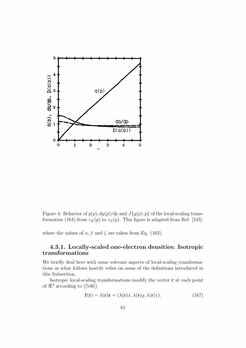
Figure 4: Behavior of g(p), dg(p)/dp and Jg(p); p of the local-scaling trans-formation (164) from γK (p) to γE (p). This figure is adapted from Ref. [545].

where the values of α, β and ζ are taken from Eq. (163).

4.3.1. Locally-scaled one-electron densities: Isotropictransformations

We briefly deal here with some relevant aspects of local-scaling transforma-tions as what follows heavily relies on some of the definitions introduced inthis Subsection.

Isotropic local-scaling transformations modify the vector r at each pointof R3 according to ([546])

f(r) = λ(r)r = (λ(r)x, λ(r)y, λ(r)z). (167)

81

These transformations keep the direction of the transformed vector f(r)constant and satisfy, as all density transformations, the following equationrelating an initial or “generating” density ρg(r) and a final density ρ(r):

ρ(r) = J(f(r); r

)ρg(f(r)

)(168)

where J(f(r); r

)is the Jacobian. For isotropic transformations the Jacobian

is

J(λ(r)r; r) =

∂λ(r)x∂x

∂λ(r)y∂x

∂λ(r)z∂x

∂λ(r)x∂y

∂λ(r)y∂y

∂λ(r)z∂y

∂λ(r)x∂z

∂λ(r)y∂z

∂λ(r)z∂z

= λ3(r)[1 + r · ∇r lnλ(r)]. (169)

From Eqs. (169) and (170) we obtain the following expression for λ(r)

λ(r) =

[ρ(r)

ρg(λ(r)r

)(1 + r · ∇r lnλ(r)

)]1/3

. (170)

Equation (171) is a first order differential equation for the transformationfunction λ(r). Introducing the function f(r) by means of the following equiv-alence,

λ(r) =f(r)

r, (171)

we can rewrite Eq. (169) as:

ρ(r)

ρg(f(r)

) =1

r3r · ∇rf

3(r). (172)

These transformations can be used to generate from an initial orbital setφ[i]

g,k(r)Nk=1 a new set of transformed orbitals as follows:

φ[i]ρ,k(r) = fφ

[i]g,k(r) =

[J(f(r); r)

]1/2φ

[i]g,k

(f(r)

)=

[ρ(r)

ρ[i]g

(f(r)

)]1/2

φ[i]g,k

(f(r)

).

(173)For the case of spherically-symmetric, or spherically-averaged densities:

ρ(r) =

∫ π

0

dθ sin θ

∫ 2π

0

dφρ(r, θ, φ), (174)

ρg(f) =

∫ π

0

dθ sin θ

∫ 2π

0

dφρg(f, θ, φ). (175)

82

the local-scaling function λ(r, θ, φ), Eq. (172), reduces to λ(r) and Eq. (159)becomes:

df(r)

dr=

r2

f 2(r)

ρ(r)

ρg(f(r)

) , (176)

and the scaling function λ(r) is given by:

λ(r) =f

r=

(ρ(r)

ρg(f)

)1/31 + r · ∇r lnλ(r)

−1/3

. (177)

From Eqs. (171) and (177) we obtain the chain rule:

d

dr=

(df

dr

)d

df=

(ρ(r)

ρg(f)

)5/31 + r · ∇r lnλ(r)

−2/3

.d

df(178)

Because for atoms we assume a separation between radial and angularfunctions, Eq. (244), these transformations only affect the radial part of the“generating” orbitals:

Rρ,nili(r) =

(df

dr

)1/2(f

r

)Rg,nili(f) =

√ρ(r)

ρg(f)Rg,nili(f). (179)

The local-scaling transformation function f(r) can be explicitly writtenas a function of the one-particle density ρ(r) by using Pade approximants[513, 547]. For a [1, 1] Pade approximant, this function becomes:

f(r) = r +2ρg(r)r∆N(r)

2ρ2g(r)r

3 +ρ′g(r)r + 2ρg(r)

∆N(r)

, (180)

where

∆N(r) =

∫ r

0

ρ(t)t2 dt−∫ r

0

ρg(t)t2 dt. (181)

Expressions for f(r) involving other types of more complex Pade approxi-mants have been presented elsewhere [513].

4.3.2. Locally-scaled one-electron densities: Non-isotropictransformations

In addition to the isotropic density transformations (or isotropic local-scalingtransformations) which are characterized by Eq. (168), we may consider alsonon-isotropic density transformations. In this case, we label the transformedvector as follows:

rT = (xT , yT , zT ) (182)

83

where the transformed coordinates are not isotropic. For example, in thepresent case we assume the following functional form for the transformedcoordinates:

xT = xT (x), yT = yT (x, y), zT = zT (x, y, z) (183)

Let us consider an orthonormal set φi(x, y, z) from which, according to Eq.(170) we obtain the transformed orbitals:

φTi (x, y, z) =

√ρ(x, y, z)

ρg(xT , yT , zT ).φi(x

T , yT , zT ) (184)

The orhogonality condition for the transformed orbitals is∫ ∞−∞

∫ ∞−∞

∫ ∞−∞

dxdydzφ∗Ti (x, y, z)φTi (x, y, z) = δij. (185)

Substituting Eq. (185) in Eq. (186) we obtain:∫ ∞−∞

∫ ∞−∞

∫ ∞−∞

dxdydzρ(x, y, z)

ρg(xT , yT , zT )φ∗i (x

T , yT , zT )φi(xT , yT , zT ) = δij (186)

Since by assumption φi(x, y, x) is orthonormal, the orthonormality of thetransformed set is guaranteed provided that

dxdydzρ(x, y, z)

ρg(xT , yT , zT )= dxTdyTdzT , (187)

or, equivalently,

dxdydzρ(x, y, z) = ρg(xT , yT , zT )dxTdyTdzT , (188)

In view of Eq. (185), the differential relations embodied by Eq.(189) can betransformed into the corresponding integral equation for xT (x) through thefollowing integration:∫ x

−∞dx

∫ ∞−∞

dy

∫ ∞−∞

dzρ(x, y, z) =

∫ xT (x)

−∞dxT

∫ ∞−∞

dyT∫ ∞−∞

dzTρg(xT , yT , zT )

(189)or ∫ x

−∞dxa(x) =

∫ xT (x)

−∞dxTag(x

T (x)) (190)

orA(x) = Ag(x

T (x)) (191)

84

Equation (192) is a transcendental equation that yields for x = xi thetransformed coordinate xTi = xT (xi).

From Eq. (189), we have

dxT (x)

dx=

∫∞−∞ dy

∫∞−∞ dzρ(x, y, z)∫∞

−∞ dyT∫∞−∞ dz

Tρg(xT , yT , zT )=

a(x)

ag(xT (x))(192)

Similarly, from Eq. (189) we also get

dxT (x)

dx=

∫ y−∞ dy

∫∞−∞ dzρ(x, y, z)∫ yT (x,y)

−∞ dyT∫∞−∞ dz

Tρg(xT , yT , zT )≡ B(x, y)

Bg(xT (x), yT (x, y))(193)

Equating (193) and (194) we obtain

B(x, y) =a(x)

ag(x)Bg(x

T (x), yT (x, y)). (194)

Equation (195) is a transcendental equation which for x = xi and y = yjyields the transformed coordinate yT (xi, yj) ≡ yTij.

The transcendental equation for the function zT (x, y, x) can also be ob-tained from Eq. (185) by writing

dxT (x)

dx

∂yT (x, y)

∂y=

∫∞−∞ dzρ(x, y, z)∫∞

−∞ dzTρg(xT , yT , zT )

≡ b(x, y)

bg(xT (x), yT (x, y))(195)

and

dxT (x)

dx

∂yT (x, y)

∂y=

∫ z−∞ dzρ(x, y, z)∫ zT (x,y,z)

−∞ dzTρg(xT , yT , zT )≡ C(x, y, z)

Cg(xT (x), yT (x, y), zT (x, y, z))

(196)Equating Eqs. (196) and (197), we obtain the following transcendental equa-tion

C(x, y, z) =b(x, y)

bg(xT (x), yT (x, y))Cg(x

T (x), yT (x, y), zT (x, y, z)) (197)

For a fixed values of the coordinates, x = xi, y = yj and z = zk, and us-ing the transformed coordinates xTi , yTij we can obtain through Eq. (198)zT (xi, yj, zk) = zTijk.

85

4.4 Local-scaling transformations: Many-electron wave-functions and orbits

To build the “Variable mapping” (33), let generalize the concept of the local-scaling transformations on LN . This is rather simple and straightforward:choose an arbitrary “reference” or generator wave function Φg(ri, σii=Ni=1 )where σi is spin of the ith electron and ρg(r) ∈ PN is the associated one-electron density, and then define a new wave function

Φf (ri, σi) = Φρ(ri, σi) ≡[ N∏i=1

J(f(ri); ri)]1/2

Φg(f(ri), σi) (198)

with the density ρ(r) ≡ ρg(f(r)) casting in Proposal 8. Φf is a locally scaledimage of the “reference” wave function. Formally speaking, Φf ≡ FΦg whereF ∈ F×N := [×]NF and F = (f, f, . . . , f) := f×N and (199) is nothing thenelse as the definition of the action of the group F×N on LN . Arbitrarinessin choosing Φg ensures the validity of the definition (199) on the entire LN .Due to the isomorphism of the groups F and F×N , it is obvious that a local-scaling transformation that maps a given pair of N-electron wave functionsinto each other matches unambiguously the local scaling that transformsthe corresponding one-electron densities into each other. However, althoughany pair of densities are locally scaled, this property no longer holds foran arbitrary pair of N-electron wave functions. Hence, LN is nontriviallypartitioned, with respect to the group F×N , into the orbits

LN =⋃i

O[i]. (199)

In this sense, the group F entangles PN and LN . By construction, an arbi-trary orbit O[i] is closed with respect to F×N , that is, for any pair Φ1 and Φ2

inO[i], there exists such local-scaling transformation F1⇒2 that Φ2 = F1⇒2Φ1.In the other words, if Φ1 is the generator wave function of O[i], for allF ∈ F×N , F1⇒2Φ1 ∈ O[i]. We thus proveProposal 9: There exists a one-to-one map of variables on any orbit in LN .Corrolary 9.1: Orbit O[i] is invariant relative to generator wave function.Corrolary 9.2: On each orbit O[i] ⊂ LN , there exists one and only oneN -electron wave function which one-electron density is ρ(r) ∈ PN .

Corrolary 9.3: For any given orbit O[k] ⊂ LN generated by Φ[k]g and the

latter one-electron density ρ[k]g , Fρ[k]

g exhausts the whole PN .Note 3: Corrolary 9.3 implies that any density ρ(r) ∈ PN isN -representable.In the other words, the group F of local-scaling transformations and its ac-tions on PN and LN defined above ensures the N-representability of PN .

86

The uniqueness of the local-scaling transformation as the solution of Eq.(159) guarantees that the transformed wavefunction Φ

[i]ρ is also unique. Thus,

for any ρ(r) ∈ PN there exists a unique wave function Φ[i]ρ generated by means

of local-scaling transformation from the arbitrary generator wave functionΦ

[k]g . The orbit in LN is actually the set of all the wave functions thus

generated which yield one-electron densities ρ(r) in PN :

O[i] ≡ Φ[i]ρ |Φ[i]

ρ −→ ρ(r); Φ[i]ρ ∈ LN ; ρ(r) ∈ PN. (200)

Therefore, the orbit patterns in LN predetermine the inverse “variable map-ping” V that was the premise in (32) and (33) and that naturally generalizesthe Hohenberg-Kohn theorem on the entire set PN .

Note that LN includes N -electron Slater determinants which are struc-turally invariant with respect to F×N . Define SN as the proper subset of LNconsisting of Slater determinants. Since F×NSN ⊆ SN , then SN =

⋃iOS

[i]

over all Slater orbits. Thus, we have:Corrolary 9.4: An arbitrary one-electron density ρ(r) ∈ PN isN -representableeven in SN .

Return to Eq.(199). Formally, Ψf ≡ FΨg. Arbitrariness in choosingΨg ensures the validity of the definition (199) on LN . It is obvious that alocal scaling that ”ties” a given couple of N-electron wavefunctions matchesunambiguously the local scaling transforming the corresponding one-electrondensities. However, although any pair of densities are locally scaled16, thisproperty no longer holds for an arbitrary pair of N-electron wavefunctions.To show the latter, we consider the following 2-electron wavefunctions which,on one side, are rather accurate approximations of the exact and Hartree-Fock ground states of the helium atom, and, on the other side, yield theone-electron densities (164), respectively,

Eckart wave function [548] :

ΨE (r1, r2) = (2 + 2S2)−1/2(αβ)3/2π−1[exp(−αr1 − βr2)

+exp(−βr1 − αr2)],

Kellner wave function [549] :

ΨK (r1, r2) = ζ3π−1exp[−ζ(r1 + r2)]. (201)

Their momentum-space representatives take on the following appearance,

ΦE (p1,p2) = (2 + 2S2)−1/223(αβ)5/2π−2

x[(p21 + α2)−2(p2

2 + β2)−2 + (p21 + β2)−2(p2

2 + α2)−2

ΦK (p1,p2) = 23ζ5π−2(p21 + ζ2)−2(p2

2 + ζ2)−2. (202)

16This statement demands a more rigor clarification: see the next footnote17.

87

Eckart position and momentum one-electron densities are tabulated inTable 2. It is worthwhile to make some notes. The first one. Any local scalingacts on spatial or momentum variables. Hence the singlet spin function hasbeen dropped out in Eqs.(202) and (203). Second. Kellner wavefunctionis easily arranged into a Slater determinant form together with the singletspin function. However, the Eckart one does not admit such a representation.Glancing at (199), one may quickly arrive at rather important result that if a“generator” wave function is a Slater determinant, Ψf does too for arbitrarylocal scaling. This implies that there does not exist such a local scalingthat maps ΨK into ΨE . Thefore, the total N-electron Hilbert space LNis partitioned with respect to local scalings - see Eq. (200), - that formgroup into disjoint classes, “orbits” defined in (201). Each orbit Oε in (200)is closed respectively to the group of local-scaling transformations, that is,for any pair of Ψ1 and Ψ2 from the orbit Oε there exists such local scalingf17→2 that Ψ2 = F17→2Ψ1. In other words, if we pick, for instance, Ψ1 as a”reference” or generating wave function and act on it by all local scalings,we cover the whole orbit Oε. One may immediately realize that there aresome orbits in LN with N ≥ 2 which are composed of Slater determinantsand some with more rich wavefunctions. For example, one may deliver twoorbits in L2, one is the Eckart orbit OE generated by ΨE , and the second isthe Kellner orbit OK made up by ΨK . The similar partition into orbits canbe carried out within the momentum space picture. Both pictures will beemployed below in parallel.

The third note is about the energy scale of ΨK and ΨE. With the optimalvalues (163) of parameters α, β, and ζ, EE = −(27/16)2 = −2.847656 andEK = −2.875661 (both in atomic units). As seen, EE lies above the Hartree-Fock limit energy EHF = −2.861680 for the helium atom [550] whereas EK

does below it.Let pick two orbits OE and OK in L2. Using the local scaling f(r)

[or g(p)] that obeys (199), one scales locally ΨK (or ΦK ) to that possessesexactly the Eckart one-electron density (or γK ) and, hence, incorporatessome correlation, say, at the level of one-electron densities, but still belongsto the Kellner orbit and for this reason remains within the Hartree-Fockapproximation. Equivalently, we are in position to construct the followingfour functions:

ΨK 7→ ΨK (ρE )⇒ ΦK (ρE )

ΦK 7→ ΦK (γE )⇐ ΨK (γE ). (203)

Symbol 7→ indicates local scaling, whereas⇒ (⇐ for its inverse) the Fouriertransform FT (FT−1, correspondingly) [554]: the momentum and position

88

Table 2: One-Electron Densities ρE (r) and γE (p) (after Koga et. al [545]).

| p |, | r | γE (p) ρE (r)Value % error Value % error

0.000 0.25760 0.91 1.75431 0.180.050 0.25614 0.91 1.45513 0.440.100 0.25177 0.91 1.20203 0.450.202 0.23503 0.90 0.82082 0.460.301 0.21090 0.88 0.56796 0.470.407 0.18078 0.84 0.38615 0.450.497 0.15427 0.80 0.27889 0.430.607 0.12374 0.72 0.18843 0.390.819 0.07642 0.52 0.08994 0.251.000 0.04908 0.28 0.04869 0.081.221 0.02828 -0.03 0.02354 -0.191.492 0.01457 -0.39 0.01002 -0.571.649 0.01001 -0.56 0.00620 -0.812.014 0.00433 -0.80 0.00212 -1.342.226 0.00273 -0.86 0.00117 -1.602.460 0.00166 -0.88 0.00061 -1.823.004 0.00057 -0.80 0.00015 -2.063.669 0.00017 -0.67 0.00003 -1.904.055 0.00009 -0.60 0.00001 -1.66

89

wavefunctions Φ(pk) and Ψ(rk) are, by definition, a pair of Fourier trans-forms, Φ(pk) := FT−1(Ψ(rk)

)≡ (2π)3N/2

∫drkexp

(−ı∑N

k=1 pkrk)Ψ(rk).

In the present treatment, FT merely reduces to the Hankel transforma-tion with the kernel jo(pr), the spherical Bessel function of the first kind.What concerns the computational work, one should note that the Hankeltransformation can be efficiently performed by means of the Talman’s nu-merical algorithm [552]. To facilitate the meaning of the diagram (12), fourwave functions given there are:ΨK (ρE ): Kellner-type position wave function with the Eckart position den-sityΦK (ρE ): Kellner-type momentum wave function with the Eckart positiondensityΦK (γE ):Kellner-type momentum wave function with the Eckart momentumdensityΨK (γE ):Kellner-type position wave function with the Eckart momentum den-sity.

Using now ΨK (γE ) and ΦK (ρE ), we calculate numerically their one-electron densities, ρKE (r) and γKE (p), respectively, and compare them inTable 3 with their prototypes, ρE (r) and γE (p). This shows a key linkagebetween one-electron densities in position and momentum spaces (see e.g.[13]). For given ρKE (r) and γKE (p), one evaluates their moments, 〈pn〉KE

and 〈rn〉KE , whose physical significance is well known. In a computationalaspect, the Romberg extrapolation technique [555] has been employed forpresent numerical integration. Results for those moments are displayed inTable 3.

Tables 3 demonstrates that the generated ρKE (r) and γKE (p) look verymuch like their prototypes. In the position space, the errors in ρKE with re-spect to ρE become relatively large for large r, but still remains 2% at most.For the moments, the agreement is pretty well: relative error < 2%, despitethe fact that it deviates with increasing n by modulo. In the momentumspace, the absolute value of error of γKE relative to γE reaches its maxi-mum equal to 0.91%, and the relative error for moments lies within ±0.7%.Overlaps between the wavefunctions themselves are

〈ΦK (γE ) | ΦE 〉 = 〈ΨK (γE ) | ΨE 〉 = 0.99768,

〈ΦK (ρE ) | ΦE 〉 = 〈ΨK (ρE ) | ΨE 〉 = 0.99767. (204)

(205) unambiguously shows how the new wave functions constructed withinthe Hartree-Fock framework become closer to their prototypes that carry agradual part of correlation [545]. Evaluation of energy of these new functions

90

Table 3: One-Electron Moments 〈pn〉KE and 〈rn〉KE (after Koga et. al [545]).

〈pn〉KE 〈rn〉KE

n Value % error Value % error-2 2.21414 0.69 5.98956 0.41-1 1.09856 0.36 1.69040 0.270 1.00000 0.00 1.00000 0.001 1.39357 -0.32 0.93446 -0.372 2.86094 -0.51 1.22833 -0.773 8.92808 -0.55 2.12522 -1.134 50.4035 -0.66 4.62179 -1.38

yields [545],

E[γKE ] = E[ΨK (γE )] = E[ΦK (γE )] = −2.86000,

E[ρKE ] = E[ΨK (ρE )] = E[ΦK (ρE )] = −2.86003, (205)

that is considerably lower the Kellner energy EK = −2.847656 and close toEHF =-2.861680. Energies (14) can be improved by relaxing parameters αand β from those given in (7). The result is

E[γKE ] = −2.86031 for α = 2.14767, β = 1.21978,

E[ρKE ] = −2.86039 for α = 2.14987, β = 1.22448. (206)

And the last example in this Subsection: consider the single-zeta approx-imated wave function Ψo for the first- and second-row ground-state atoms[550] as the reference one and construct its spherically averaged density

ρo(r) ≡∫dΩρo(r). (207)

ρo is the one-electron density associated with Ψo. Let ρ(r) be the spheri-cally averaged density built via the rule (207) from the near-Hartree-FockClementi-Roetti wave function Ψ [550]. One then defines a local scalings = s(r) that maps ρo(r) into ρ(r),

ρ(r) = J(s(r))ρo(s(r)). (208)

s(r) and J(s(r)) for the neon atom are plotted in Figures 1 and 2 of [553].Applying local scaling s(r) to Ψo results in Ψρ that is interpreted as a

possible parent wave function of the near-Hartree-Fock density. Now we are

91

ready to organize the Fourier transform Φρ of Ψρ and evaluate the associ-ated one-electron momentum density γρ(p) whose spherical averaging givesγρ(p). In a similar way, we find that near-Hartree-Fock γ(p) directly fromΨ(ri). The two densities γ(p) and γρ(p) are listed and compared in Table4. One sees that in a small momentum region p ≤ 0.8, γρ considerably differsfrom γ. Particularly, γ has a peak around p = 0.55, while γρ shows a mono-tonic behavior there. The momentum moments 〈pn〉ρ are also evaluated andsummarizedd in Table 4 for the first-row ground-state atoms. Percent errorsrelative to 〈pn〉γ are given in parentheses. We observe that the errors for themoments 〈pn〉 with positive n are less than 0.7%, except for 〈p4〉 of the Beatom, and therefore, the single-electron mapping employed is satisfactory.Estimates of the negative (n < 0) moments are less pleasant, because theerrors for them vary from −0.01% to +16.57%. Clearly, the large discrep-ancy arises from the poor behavior of γ ¯rho in the region of small momenta.Since the errors are rather small (at most 0.23%) for the Li and Be atoms,one can conclude that the origin of this discrepancy may be attributed to theincreasing number of p-electrons, whose orbitals, p-orbitals, are transformedin the concerted manner with s-orbials in our approach. Then, a possiblegeneralization toward improving the single-electron mapping between theposition and momentum densities is to use different local scalings for theelectrons with different orbital symmetries. Simply speaking, local-scalingnow acquires a subscript l corresponding to the azimuthal quantum number.In fact, the procedure produces much better estimates of the momentummoments as found in the results summarized in Table 4 for the first- andsecond-row atoms.

92

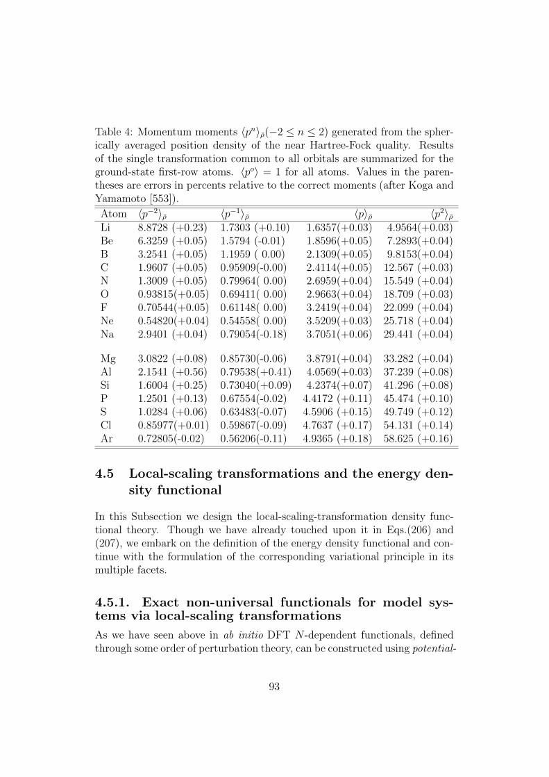
Table 4: Momentum moments 〈pn〉ρ(−2 ≤ n ≤ 2) generated from the spher-ically averaged position density of the near Hartree-Fock quality. Resultsof the single transformation common to all orbitals are summarized for theground-state first-row atoms. 〈po〉 = 1 for all atoms. Values in the paren-theses are errors in percents relative to the correct moments (after Koga andYamamoto [553]).

Atom 〈p−2〉ρ 〈p−1〉ρ 〈p〉ρ 〈p2〉ρLi 8.8728 (+0.23) 1.7303 (+0.10) 1.6357(+0.03) 4.9564(+0.03)Be 6.3259 (+0.05) 1.5794 (-0.01) 1.8596(+0.05) 7.2893(+0.04)B 3.2541 (+0.05) 1.1959 ( 0.00) 2.1309(+0.05) 9.8153(+0.04)C 1.9607 (+0.05) 0.95909(-0.00) 2.4114(+0.05) 12.567 (+0.03)N 1.3009 (+0.05) 0.79964( 0.00) 2.6959(+0.04) 15.549 (+0.04)O 0.93815(+0.05) 0.69411( 0.00) 2.9663(+0.04) 18.709 (+0.03)F 0.70544(+0.05) 0.61148( 0.00) 3.2419(+0.04) 22.099 (+0.04)Ne 0.54820(+0.04) 0.54558( 0.00) 3.5209(+0.03) 25.718 (+0.04)Na 2.9401 (+0.04) 0.79054(-0.18) 3.7051(+0.06) 29.441 (+0.04)

Mg 3.0822 (+0.08) 0.85730(-0.06) 3.8791(+0.04) 33.282 (+0.04)Al 2.1541 (+0.56) 0.79538(+0.41) 4.0569(+0.03) 37.239 (+0.08)Si 1.6004 (+0.25) 0.73040(+0.09) 4.2374(+0.07) 41.296 (+0.08)P 1.2501 (+0.13) 0.67554(-0.02) 4.4172 (+0.11) 45.474 (+0.10)S 1.0284 (+0.06) 0.63483(-0.07) 4.5906 (+0.15) 49.749 (+0.12)Cl 0.85977(+0.01) 0.59867(-0.09) 4.7637 (+0.17) 54.131 (+0.14)Ar 0.72805(-0.02) 0.56206(-0.11) 4.9365 (+0.18) 58.625 (+0.16)

4.5 Local-scaling transformations and the energy den-sity functional

In this Subsection we design the local-scaling-transformation density func-tional theory. Though we have already touched upon it in Eqs.(206) and(207), we embark on the definition of the energy density functional and con-tinue with the formulation of the corresponding variational principle in itsmultiple facets.

4.5.1. Exact non-universal functionals for model sys-tems via local-scaling transformations

As we have seen above in ab initio DFT N -dependent functionals, definedthrough some order of perturbation theory, can be constructed using potential-

93

dependent orbitals. However, in this exact procedure, the notion of “universalfunctional” is absent. Moreover, local potentials are obtained by means ofa roundabout approach involving non-linear equations, that is, they do notissue from the direct calculation of the functional derivative δF [ρ]/δρ. Inaddition, we have seen above that when the non-universal functional F [ρ]is constructed from a set of density-dependent orbitals, then the functionalderivative yields, in general, a non-local potential.

Although it is not readily realized, this universality is already absentin the procedure advanced by Zumbach and Maschke [398] for the actualconstruction of the energy functional in Levy’s constrained search (see alsoEnglisch and Englisch [331]). The reason is that to overcome the basic obsta-cle barring the realization of Levy’s procedure, namely, the unavailability of amethod to construct all wave functions that yield a given density [398], theseauthors generate –through the application of non-linear transformations–density-dependent plane waves from which a complete set of N -particle Slaterdeterminants is constructed. Then, when they expand any N -particle totalwavefunction in the subset formed by Slater determinants differing from eachother in at least two orbital indices, they are able to show that these wavefunctions, regardless of the values given to the expansion coefficients, yieldthe same density. The approximate forms of the ensuing density functionalsdepend, however, both on the density as well as on the expansion coefficients.Since these coefficients are variational parameters that take different valuesfor each specific system, it follows that these realizations of Levy’s functionalsare system-dependent and hence, non-universal.

The transformations used by Zumbach and Maschke are particular in-stances of the more general local-scaling transformations. The latter are atthe basis of the explicit constructive procedure denoted as the local-scalingtransformation version of the DFT, LS-DFT, [13, 115, 477, 546] (for a moremathematical approach to these transformations, see [118, 518, 544, 556]).This procedure is based on the fact that through the introduction of density-dependent coordinates rT ≡ rT ([ρ]; r) it becomes possible to obtain fromany N -particle wavefunction (and not only from Slater determinants formedby plane waves) density-dependent wavefunctions, and from them, energydensity functionals. Thus, starting from wavefunctions with the appropriateform for a particular system, the ground state energy can be determined bya fully variational approach involving optimization of the one-particle den-sity and of the parameters of the starting wavefunction for the system underconsideration. In particular, if we know the exact ground-state wavefunctionfor a given physical system, then, by introducing these density-dependentcoordinates into this exact wavefunction, we can generate the correspondingdensity-dependent wavefunction and through it, the exact density-dependent

94

functional for the particular system being considered. Since the functional issystem dependent, here too, the notion of “universal” functional is absent.

In what follows we illustrate what is sketched in the above paragraphand, in particular, we discuss the relation between the explicit constructiveprocedure embodied in LS-DFT and the implicit one exemplified by Levy’sconstrained search approach.

The density-dependent coordinate rT is obtained through the applica-tion of locally-scaled transformations to the coordinate r. Explicitly, thetransformed coordinate is given by rT =

√(xT )2 + (yT )2 + (zT )2 where the

Cartesian locally-scaled components are: xT = λ(r)x, yT = λ(r)y, and zT =λ(r)z. The local-scaling transformation function λ(r) is determined by solv-ing the following first-order differential equation:

λ(r) =

(ρ(r)

ρΨ(rT )

)1/3

L1(r)−1/3 (209)

where L1(r) = (1+r·∇r lnλ(r)). Given an arbitrary N -particle wavefunctionΨg(r1, ..., rN), through the application of local-scaling transformations, thefollowing density-dependent wavefunction is generated:

Ψ([ρ]; r1, ..., rN) =N∏i=1

√ρ(ri)

ρg(rTi )Ψg(r

T1 , ..., r

TN) (210)

Using this density-dependent wavefunction Ψ([ρ]) we can construct the density-dependent energy functional

E[Ψ([ρ])] =< Ψ([ρ])|Hv|Ψ([ρ]) >≡ E[ρ,Ψg] (211)

The variational principle in LS-DFT is written as:

E0 = inf

inf

E[Ψ[i]([ρ])

]≡ E

[ρ,Ψ[i]

g

]over all orbits Ψ[i]([ρ]),Ψ[i]

g ∈ O[i]L

O[i]L ⊂ LN Ψ[i]([ρ])↔ ρ(r) ∈ NN

Bader (212)

where O[i]L stands for an orbit, i.e., a subset containing all the N -particle

wave functions Ψ[i]([ρ]) generated by the local scaling transformations from

the generating wave function Ψ[i]g . The union of all orbits yields the complete

N -particle Hilbert space , namely, LN = ∪iO[i]L . Within an orbit, there is a

one-to-one correspondence between ρ(r) and Ψ[i]([ρ]), (i.e., Ψ[i]]([ρ] ↔ ρ(r) ∈

95

NNBader. The density set NN

Bader (Bader’s density set) contains all densitieswhich are homotopically equivalent, that is, that can be converted to eachother by means of a local-scaling transformation. Clearly, these densitiesbelong to the same equivalence class such that their topology is preservedupon application of these transformations17. Since

E[ρ,Ψ[i]

g

]= T

[ρ,Ψ[i]

g

]+ Vee

[ρ,Ψ[i]

g

]+

∫d3rv(r)ρ)r) (213)

we can define

F [ρ] = inf

T[ρ,Ψ[i]

g

]+ Vee

[ρ,Ψ[i]

g

]over all orbits

O[i]L ⊂ LN

Ψ[i]([ρ]),Ψ[i]g ∈ O[i]

L

ρ = ρfixed ∈ NBader (214)

and as a result, we can write the variational principle as

Eo = infF [ρ] +

∫d3rv(r)ρ(r)

ρ ∈ NBader (215)

We recognize in Eq. (215) an expression which is similar to Levy’s func-tional. There are, however, two differences: the first, that in the present caseT[ρ,Ψ

[i]g

]and Vee

[ρ,Ψ

[i]g

]can be explicitly constructed, provided, we have

the orbit generating wavefunctions Ψ[i]g . The second, that the condition on

the density ρ ∈ NBader ⊂ JN is much more restrictive than ρ ∈ JN .The generation of a density functional within each orbit is carried out

by direct application of local-scaling transformations to the generating wave-function. Thus, this is a well-defined constructive procedure [557, 558]. Sev-eral examples of how these density functionals have been generated in thecontext of LS-DFT have been previously presented. In particular, the de-tailed construction of kinetic and exchange energy functionals arising fromsingle Slater determinants has been examined in a series of papers [546, 510,

17The question of whether NNBader ⊂ PN or NN

Bader = PN is very subtle. Generallyspeaking, we suggest that NN

Bader is a proper subset of PN in order to distinguish a pairof one-electron densities with different topological patterns of Kato cusps where a local-scaling transformation is undefined, by its very construction.

96

513, 512, 559, 560, 561]. The kinetic energy functional for the non-interactingterm adopts the following general form:

Ts[ρ] = TW [ρ] +1

2

∫ ∞0

drr2ρ(r)5/3AN([ρ]; r) (216)

where TW [ρ] is the von Weizsacker term. Similarly, the exchange term be-comes:

Ex[ρ] = −1

2

∫ ∞0

drr2

kmax∑k=0

ρ(r)(4+k)/3BkN([ρ]; r) (217)

[for details on the definition of the different components, see, for example,Ref. ([546])]. An important aspect that we would like to emphasize con-cerning the above expressions is that the kinetic energy modulating factorA([ρ]; r) is both N -dependent and system-dependent. In the case of the ex-change functional, the summation over k is finite and is determined by thetriangle condition on the summation of spherical harmonics. Hence, for ex-change, not only does the term proportional to ρ(r)4/3 is present, but alsoall other terms containing powers of the density compatible with the angularexpansion. Again, these terms are system-dependent.

A model system for which there exists an exact analytic solution is Hooke’satom, a two-electron atom differing from the true one in that a harmonic po-tential replaces the Coulomb electron-nuclear one. The exact closed-formsolution [562, 563] is:

Ψ(r1, r2) =1

2π√

5π + 8√πφ(r1)φ(r2)

(1 +

r12

2

)(218)

where φ(r) = e−r2/4. We assume that this exact wavefunction is the gener-

ating wave function for the Hooke orbit: Ψ ≡ Ψ[Hooke]g .

Although analytic closed-form Hooke’s atom wave functions only existfor discrete values of the harmonic coupling constant, this fact does notintroduce any restriction in what follows, as the discrete constant just definesa particular type of external potential (such as Z = 2 defines the Coulombexternal potential for the He atom).

The locally-scaled wavefunction Ψ([ρ]), which depends on the arbitrarydensity ρ(r) is generated according to the prescription given by Eq. (199).Introducing this wave function and after some simplifications using Mathe-matica the kinetic energy functional is given explictly [564, 565] by:

T[ρ,Ψ[Hooke]

g

]≡ T [ρ] = TW [ρ] + 4π

∫ ∞0

dr r2 ρ(r)5/3 L1(r)4/3 F5/3(rT (r))

(219)

97

where the system-dependent kinetic energy enhancement factor (notice thatit depends on the Hooke’s atom orbital φ(x)) is:

F5/3(x) =φ(x)2

2√

2(16π + 10π3/2)(ρg(x))5/3− x2

8(ρΨ(x))2/3

− x(dρg(x)/dx)

4(ρΨ(x))5/3− (dρΨ(x)/dx)2

8(ρΨ(x))8/3(220)

For Hooke’s atom, the electron-electron interaction energy functional forthe locally-scaled wavefunction generates the following density functional:

Eee[ρ,Ψ[Hooke]

g

]≡ Eee[ρ] =

∞∑l=0

∫ ∞0

dr1r21ρ(r1)(l+4)/3F (l)

ee ([ρ]; r1) (221)

where the system-dependent electron-electron interaction enhancement fac-tors are:

F (l)ee ([ρ]; r1) =

4π

2l + 1

φ(rT1 )2

(rT1 )l+1ρΨ(rT1 )(l+4)/3L1(r1)(l+1)/3Il([ρ]; r1) (222)

(again, for details on the expressions appearing here, see Ref. [566]). Thetotal energy functional Etotal[v

Hookeext , ρ] satisfies the variational principle as in

all cases it yields an energy above the extremum value of 2.00000 hartrees;the latter value is attained only when the energy functional is computed usingthe exact Hooke’s atom density.

Combining Eqs. (208) and (210), we obtain the exact functional F [ρ] forHooke’s atom generated through the use of local-scaling transformations:

F [ρ] = T [ρ] + Eee[ρ] (223)

As expected, however, due to the presence of system-dependent terms in thisexact functional, it is not transferable to other two-electron systems such asHe, Li+ and Be2+ [566].

4.5.2. Energy density functional: Definition

Proposal 9 definitely allows to give the following rigorous definition of theenergy density functional

Ei[ρ(r)

]≡ Ei

[ρ(r); Φ[i]

g

]:= E[Φ]|Φ∈O[i]⊂LN (224)

and hence to express the “Functional mapping” (32) in the explicit way. Itis evident that this mapping is one-to-many and there exist as many density

98

functionals as there are orbits in LN . To derive Ei[ρ(r)

]that is defined on the

orbit O[i] ⊂ LN explicitly, let first write down the explicit expression for theenergy functional E[Φ

[i]g ] of the orbit-generating wave function Φ

[i]g in terms of

its 1- and 2-matrices, D1[i]g (x1, x

′1) and D

2[i]g (x1, x2;x1, x2), respectively, and

its one-electron density ρg(x):

E[Φ[i]g ] =

1

2

∫d4x1∇x1∇x′1

D1[i]g (x1;x′1)

∣∣x′1=x1

+

∫d4xρ(x)v(r) (225)

+

∫d4x1

∫d4x2

D2[i]g (x1, x2;x1, x2)

|r1 − r2|.

where∫d4x ≡

∑s

∫d3r. Let us apply the local-scaling transformation that

casts in Proposal 9 to the wavefunction Φ[i]g , precisely to its 1- and 2-

matrices, and its density. This yields:

D1[i]ρ (r1, s1; r′1, s

′1) =

[J(f(r1); r1

)J(f(r′1); r′1

)]1/2

D1[i]g (f(r1), s1; f(r′1), s′1), (226)

D2[i]ρ (r1, s1, r2, s2; r1, s1, r2, s2) = J

(f(r1); r1

)J(f(r2); r2

)(227)

D2[i]g (f(r1), s1, f(r2), s2; f(r1), s1, f(r2), s2),

andρ(r, s) = J

(f(r); r

)ρg(f(r), s

). (228)

Partitioning the 1- and 2-matrices, appearing in the rhs of Eqs. (227) and(228), into their local and non-local components:

D1[i]g (f(r1), s1; f(r′1), s′1) =

[ρg(f(r1), s1

)ρg(f(r′1), s′1

)]1/2

D1[i]g (f(r1), s1; f(r′1), s′1),

(229)

D2[i]g (f(r1), s1, f(r2), s2; f(r1), s1, f(r2), s2) =

1

2ρg(f(r1), s1

)ρg(f(r2), s2

)(

1 + F [i]xc,g(f(r1), s1, f(r2), s2)

)(230)

where D1[i]g is the non-local part of the 1-matrix and F [i]

xc,g is the non-localexchange-correlation factor. Therefore, the 1- and 2-matrices of (226) takethe appearance:

D1[i]ρ (r1, s1; r′1, s

′1) =

[ρ(r1, s1)ρ(r′1, s

′1)]1/2

D1[i]g (f(r1), s1; f(r′1), s′1), (231)

99

and

D2[i]ρ (r1, s1, r2, s2; r1, s1, r2, s2) =

1

2ρ(r1, s1)ρ(r2, s2)

(1+F [i]

xc,g(f(r1), s1, f(r2), s2)).

(232)Finally, we obtain [13]

E[Φ[i]ρ ] ≡ E

[ρ(x); Φ[i]

g

]=

1

8

∫d4x

[∇rρ(x)

]2ρ(x)

+1

2

∫d4xρ(x)∇r∇r′D

1[i]g (f(r), s; f(r′), s′)|x′=x

+

∫d4xρ(x)v(r)

+1

2

∫d4x1d

4x2

ρ(x1)ρ(x2)(

1 + F [i]xc,g(f(r1), s1, f(r2), s2)

)|r1 − r2|

. (233)

Few statements can be drawn from (234):(i) The kinetic energy density functional is composed of two components.The first, the von Weizsacker term, is local and orbit-invariant. The secondis non-local, orbit-dependent, and due to the one-third power in Eq. (160),transformed to the modified Thomas-Fermi term within the LDA;(ii) The exchage-correlation energy density functional is explicitly expressedas

Exc[Φ[i]ρ ] ≡ Exc

[ρ(x); Φ[i]

g

]:=

1

2

∫d4x1d

4x2ρ(x1)ρ(x2)F [i]

xc,g(f(r1), s1, f(r2), s2)

|r1 − r2|;

(234)

(iii) In fact, each density functional E[ρ(x); Φ

[i]g

]depends upon two basic

variables: the one-electron density ρ(x) and the generator wave function Φ[i]g .

Equation (234) expresses the energy as a functional of the one-electron den-sity ρ(x) within the orbit O[i]. True, Eq. (234) satisfies the condition ofN -representability;(iv) One of the orbits in the decomposion (196) of LN is actually the or-bit that contains the exact ground-state wave function. Refer it to as theHohenberg-Kohn orbit O[HK] ⊂ LN . If a generator wave function is chosento belong to O[HK], Eq. (214) then determines the Hohenberg-Kohn energydensity functional in the explicit manner.(v) Let recall Corrolary 9.4 (p.85) about a special place that the subsetSN of LN is placed, namely, that an arbitrary one-electron density is N -representable in SN . In this regard, consider a single Slater determinantformed from the set φ[i]

ρ,k(r) of locally-scaled one-particle orbitals defined

100

in Eq. (174):

Φ[i]ρ (r1, s1, · · · , rN , sN) ≡ det√

N ![φ

[i]ρ,1(r1)σms1 (s1) · · ·φ[i]

ρ,N(rN)σmsN (sN)]

(235)where the spin functions are denoted by σmsk (sk). The superscript [i] labels

the different “orbits” O[i]S associated with these sets. By an “orbit” we mean

the subclass O[i]S of the class SN of single Slater determinants where this

subclass is generated by means of Eq. (236) by isotropic local-scaling of the

initial (fixed) orthonormal set φ[i]g,k(r)Nk=1, according to Eq. (199) (if the

initial set depends on parameters, these must be fixed as different “orbits”are produced by different sets of parameters.) Clearly, for each such initialorbital set, since ρ spans the set NΦ (of all admissible densities), an infinitesubclass of Slater determinants is generated (which is closed under the actionof the continuous group of local-scaling transformations [13, 115]).

In the context of LS-DFT, the Hartree-Fock variational principle is [567]

EHFo = inf

inf

E[Φ

[i]ρ ]

.

over all orbits ρ(r) ∈ NΦ

O[i]S ⊂ SN Φ

[i]ρ ∈ O[i]

S

(236)

where E[Φ[i]ρ ] is the expectation value of Φ

[i]ρ with respect to the many-particle

Hamiltonian. This functional can also be written as a functional of the one-particle density ρ and the wavefunction Φ

[i]g formed from the initial orbitals.

Thus, we have the one-to-one correspondence between a functional of a wave-function and a functional of the one-particle density:

E[Φ[i]ρ ] = E [ρ,Φ[i]

g ]. (237)

Now, since we can always fix an arbitrary initial function Φ[i]g , it is clear that

the right-hand-side of Eq.(238) is just a functional of the one-particle densityρ, although its particular form depends on the initial function (a particularlysimple choice based on generalized Slater-type orbitals is shown below to leadto quite accurate results).

The functional E [ρ,Φ[i]g ] can be written in terms of the kinetic-, Coulomb-,

exchange-, and external-energy components:

E [ρ,Φ[i]g ] = T [ρ,Φ[i]

g ]+1

2

∫d3r1

∫d3r2

ρ(r1)ρ(r2)

|r1 − r2|+

∫d3rρ(r)v(r)+Ex[ρ,Φ

[i]g ],

(238)

101

respectively, where the kinetic energy functional is

T [ρ,Φ[i]g ] =

1

2

∑s1

∫d3r1∇r1∇r′1

D1[i]ρ (r1, s1; r ′1, s

′1)∣∣r′1=r1;s′1=s1

(239)

and where

Ex[ρ,Φ[i]g ] = −1

2

∑s1

∫d3r1

∑s2

∫d3r2

D1[i]ρ (r1, s1; r2, s2)D

1[i]ρ (r2, s2; r1, s1)

|r1 − r2|.

(240)is the exchange energy functional. The spin-dependent 1-matrix appearingin these expressions is defined by

D1[i]ρ (r1, s1; r2, s2) =

N∑k=1

φ[i]∗ρ,k(r1)σmsk (s1)φ

[i]ρ,k(r2)σmsk (s2). (241)

and its corresponding one-particle density, by

ρ(r) =N∑k=1

|φ[i]ρ,k(r)|2. (242)

For atoms, we can separate the radial and angular parts so that thelocally-scaled atomic orbital is given by

φρ,i(r) = Rρ,nili(r)Yli,mli (θ, φ), (243)

where we have assumed that the local-scaling transformation only affectsthe radial function (for an alternative and more general transformation, seeSubsection 3.3.2). Substituting Eq. (236) into the first term in the rhs ofEq.(226), integrating over the angular coordinates and using Eqs. (177)-(179)we arrive, after some straightforward algebra, to the following expression forthe kinetic energy functional (for simplicity we drop the “orbit” superindex):

T [ρ,Φg] = TW [ρ]+

∫ ∞0

dr r2ρ5/3(r)

[(1+r·∇ lnλ(r)

)4/3

τN+(

1+r·∇ lnλ(r))−2/3

κN

].

(244)Here, TW [ρ] is the Weiszacker kinetic energy functional [96]:

TW [ρ] =1

8

∫ ∞0

dr r2 (∇ρ(r))2

ρ(r), (245)

102

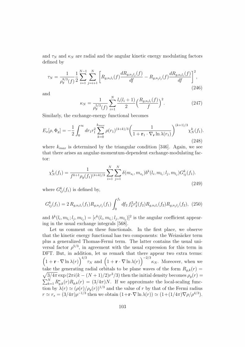
and τN and κN are radial and the angular kinetic energy modulating factorsdefined by

τN =1

ρ8/3g (f)

1

2

N−1∑i=1

N∑j=i+1

[Rg,nili(f)

dRg,nj lj(f)

df−Rg,nj lj(f)

dRg,nili(f)

df

]2

,

(246)and

κN =1

ρ5/3g (f)

N∑i=1

li(li + 1)

2

(Rg,nili(f)

f

)2

. (247)

Similarly, the exchange-energy functional becomes

Ex[ρ,Φg] = −1

2

∫ ∞0

dr1r21

kmax∑k=0

ρ(r1)(4+k)/3

(1

1 + r1 · ∇r lnλ(r1)

)(k+1)/3

χkN(f1).

(248)where kmax is determined by the triangular condition [346]. Again, we seethat there arises an angular-momentum-dependent exchange-modulating fac-tor:

χkN(f1) =1

fk+1ρg(f1)(4+k)/3

N∑i=1

N∑j=1

δ(msi ,msj)bk(li,mli ; lj,mlj)G

kij(f1).

(249)where Gk

ij(f1) is defined by,

Gkij(f1) = 2Rg,nili(f1)Rg,nj lj(f1)

∫ f1

0

df2 f22 r

k2(f2)Rg,nili(f2)Rg,nj lj(f2), (250)

and bk(li,mli ; lj,mlj) = [ck(li,mli ; lj,mlj)]2 is the angular coefficient appear-

ing in the usual exchange integrals [568].Let us comment on these functionals. In the first place, we observe

that the kinetic energy functional has two components: the Weizsacker termplus a generalized Thomas-Fermi term. The latter contains the usual uni-versal factor ρ5/3, in agreement with the usual expression for this term inDFT. But, in addition, let us remark that there appear two extra terms:(

1 + r · ∇ lnλ(r))4/3

τN and(

1 + r · ∇ lnλ(r))−2/3

κN . Moreover, when we

take the generating radial orbitals to be plane waves of the form Rg,k(r) =√3/4π exp (2πi(k − (N + 1)/2)r3/3) then the initial density becomes ρg(r) =∑Nk=1R

∗g,k(r)Rg,k(r) = (3/4π)N . If we approximate the local-scaling func-

tion by λ(r) ' (ρ(r)/ρg(r))1/3 and the value of r by that of the Fermi radius

r ' rs = (3/4π)ρ−1/3 then we obtain (1+r·∇ lnλ(r)) ' (1+(1/4π)∇ρ/ρ4/3).

103

Thus, we see that terms which are used in standard DFT also arise in a verynatural way in the present formulation. The difference, however, stems fromthe modulating factors which are particular to each physical system. Weprovide an approximate representation of these terms in the following sub-section.

For completeness, let us mention an early effort of Dawson and March [?](based on methods quite distinct from those employed here) that also led toan explicit kinetic energy functional containing the Weizsacker term plus acorrection involving the Thomas-Fermi factor.

4.5.3. Functional N-representability and the Levy vari-ational principle

It is illustrative to discuss the reformulation of the Hohenberg-Kohn theoryoriginally carried out by Levy [293] (and later, also by Lieb [571, 49, 603]),where instead of the stronger v-representability condition, all that is askedfor is compliance with the weaker N -representability condition for the energyfunctionals. Our discussion is based on Eq. (18) plus the assumption thatAv ⊂ NΦ, where Av is the set of v-representable densities (namely, densi-

ties coming from ground-state wavefunctions Ψv′o for Hamiltonians Hv′

with v′ ∈ V ) and NΦ is the set of N -representable densities. The latter isexplicitly defined by

NΦ ≡ ρ(r) |V −1 : ρ(r)←− Φ ∈ LN . (251)

(The truth of the above assumption, namely, Av ⊂ NΦ, is proved in Subsec-tion 4.5.6).

Bearing in mind that the same density ρ(r) can come from anyone of the

wavefunctions Φ[i]ρ for i = 1, ...,∞, the Levy variational principle [293] can

be stated as:

Evo = inf

inf

Ev[ρ(r); Φ

[i]ρ ]

.

ρ(r) ∈ NΦ Φ[i]ρ ∈ LN

ρ(r) = ρfixed(r)

(252)

The energy functional Ev[ρ(r); Φ[i]ρ ] is given by

Ev[ρ(r); Φ[i]ρ ] = 〈Φ[i]

ρ |T + Uee + V |Φ[i]ρ 〉 = 〈Φ[i]

ρ |T + Uee |Φ[i]ρ 〉+

∫d3rρ(r)v(r).

(253)

104

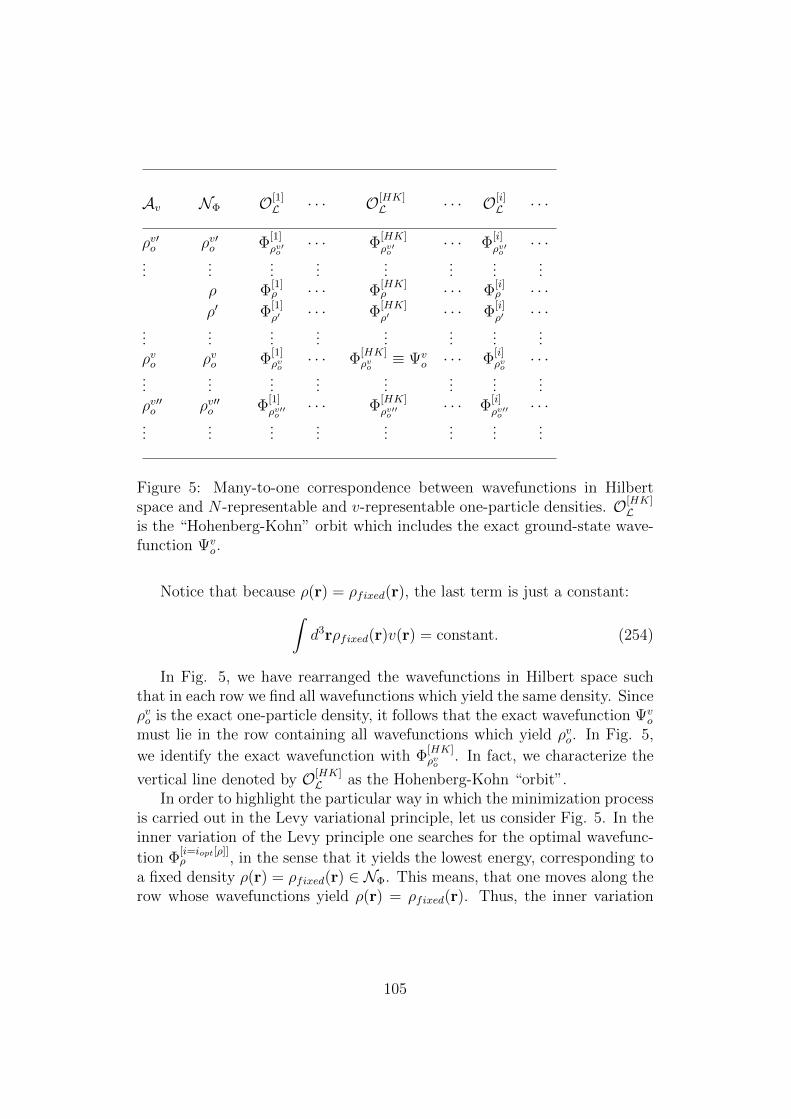
Av NΦ O[1]L · · · O[HK]

L · · · O[i]L · · ·

ρv′o ρv′o Φ[1]ρv′o

· · · Φ[HK]ρv′o

· · · Φ[i]ρv′o

· · ·...

......

......

......

...ρ Φ

[1]ρ · · · Φ

[HK]ρ · · · Φ

[i]ρ · · ·

ρ′ Φ[1]ρ′ · · · Φ

[HK]ρ′ · · · Φ

[i]ρ′ · · ·

......

......

......

......

ρvo ρvo Φ[1]ρvo

· · · Φ[HK]ρvo≡ Ψv

o · · · Φ[i]ρvo

· · ·...

......

......

......

...ρv′′o ρv′′o Φ

[1]ρv′′o

· · · Φ[HK]ρv′′o

· · · Φ[i]ρv′′o

· · ·...

......

......

......

...

Figure 5: Many-to-one correspondence between wavefunctions in Hilbertspace and N -representable and v-representable one-particle densities. O[HK]

Lis the “Hohenberg-Kohn” orbit which includes the exact ground-state wave-function Ψv

o.

Notice that because ρ(r) = ρfixed(r), the last term is just a constant:∫d3rρfixed(r)v(r) = constant. (254)

In Fig. 5, we have rearranged the wavefunctions in Hilbert space suchthat in each row we find all wavefunctions which yield the same density. Sinceρvo is the exact one-particle density, it follows that the exact wavefunction Ψv

o

must lie in the row containing all wavefunctions which yield ρvo. In Fig. 5,

we identify the exact wavefunction with Φ[HK]ρvo

. In fact, we characterize the

vertical line denoted by O[HK]L as the Hohenberg-Kohn “orbit”.

In order to highlight the particular way in which the minimization processis carried out in the Levy variational principle, let us consider Fig. 5. In theinner variation of the Levy principle one searches for the optimal wavefunc-

tion Φ[i=iopt[ρ]]ρ , in the sense that it yields the lowest energy, corresponding to

a fixed density ρ(r) = ρfixed(r) ∈ NΦ. This means, that one moves along therow whose wavefunctions yield ρ(r) = ρfixed(r). Thus, the inner variation

105

becomes

infEv[ρ(r); Φ

[i]ρ ] = F [ρ(r); Φ

[i=iopt[ρ]]ρ ] +

∫d3rρ(r)v(r)

Φ

[i]ρ ∈ LN

ρ(r) = ρfixed(r)(255)

where F [ρ(r); Φ[i=iopt[ρ]]ρ ] = 〈Φ[i=iopt[ρ]]

ρ |T + Uee|Φ[i=iopt[ρ]]ρ 〉. Note that we are

emphasizing the fact that the optimal wavefunction depends on the fixeddensity ρ(r) and hence for each row we have a different optimal wavefunction.

This implies, in turn, that the functional F [ρ(r); Φ[i=iopt[ρ]]ρ ] changes when we

go from one density to another, i.e., when we change rows.The outer variation spans over all possible N -representable densities, that

is, densities which belong to NΦ. Notice, that since the set of v-representabledensities Av is a subset of NΦ, in the Levy variational principle one considersdensities such as ρ(r) and ρ′(r) (see Fig. 5) which belong to NΦ but not toAv, namely, densities which are N -representable but not v-representable.In this sense, the Levy variational principle is more lax than the originalHohenberg-Kohn one; it leads, however, to the same extremum.

The following comments are in order with regard to the Levy variationalprinciple.

1. The energy functional Ev[ρ(r); Φ[i]ρ ] depends explicitly upon the wave-

function Φ[i]ρ . This poses the problem of how to construct a functional

which depends on the fixed one-particle density and which at the sametime allows us to scan all wavefunctions Φ[i]

ρ ∞i=1.

2. The dependence of the functional F [ρ(r); Φ[i=iopt[ρ]]ρ ] on the optimal

wavefunction for a given density makes it highly unlikely that thisshould be a “universal functional”. Thus, the search for such objects inthe Hohenberg-Kohn-Sham version of density functional theory standson feeble grounds.

3. The functional Ev[ρ(r); Φ[i]ρ ] is of a “dynamical” type. This means that

if we introduce a density ρ′(r) = ρ(r) + δρ(r), then the energy func-tional changes “dynamically” as for a fixed [i] the new wavefunction is

Φ[i]ρ′ = Φ

[i]ρ+δρ. The new functional is not merely Ev[ρ(r) + δρ(r); Φ

[i]ρ ] but

Ev[ρ(r) + δρ(r); Φ[i]ρ+δρ].

4. An actual realization of the Levy variational principle for some concretesystem has not taken place until now.

106

5. If instead of Ev[ρ(r); Φ[i]ρ ], we were to introduce some non-N -representable

functional Eapprv [ρ(r)] 6= E[Φ[i]ρ ], then the extremum need not be at-

tained at Evo , but at any other value either above or below the exact

energy. Furthermore, as no approximate functional currently used inthe Hohenberg-Kohn-Sham version of density functional theory (eitherin the local or non-local approximations), is endowed with the dynam-ical character demanded by the Levy variational principle, it followsthat all these approximate functionals, no matter how carefully theyhave been designed, are functionally non-N -representable and hencethe quantum mechanical variational principle does not apply to them.Again, the Levy variational principle cannot be invoked in order toassert the correctness of the energies computed using these functionals.

4.5.4. The concept of “orbit”, O[i]L , and its importance

in the reformulation of the variational principle

Let us go back to Fig. 5 and consider the “orbits” O[i]L for i = 1, · · · , HK, · · · .

These “orbits” or columns appearing in Fig. 5 are made up of wavefunctionsbelonging to Hilbert space. We assume, furthermore, that these “orbits” areendowed with the following characteristic: no two wavefunctions belongingto the same “orbit” can have the same density, i.e., there is a one-to-onecorrespondence between ρ(r) ∈ NΦ and Φ

[i]ρ ∈ O[i]

L . We assume, moreover,that the union of all “orbits” exhausts Hilbert space. Clearly, in terms ofthese “orbits”, the variational principle can be reformulated as follows [115]:

Evo = inf

inf

Ev[Φ

[i]ρ ]

.

over all orbits Φ[i]ρ ∈ O[i]

LO[i]L ⊂ LN

(256)

Note that the inner variation runs along a particular “orbit” O[i]L (i.e., a

column in Fig. 5).Because of the one-to-one correspondence between one-particle densities

ρ(r) ∈ NΦ and N -particle wavefunctions Φ[i]ρ ∈ O[i]

L within each one of the

“orbits” described in Fig. 5, the energy functional Ev[ρ(r); Φ[i]ρ ] is also in

a one to one correspondence with Ev[Φ[i]ρ ]. For this reason, the variational

principle of Eq. (24) can be recast as [115]:

Evo = inf

inf

Ev[ρ(r); Φ

[i]ρ ]

.

over all orbits ρ(r) ∈ NΦ

O[i]L ⊂ LN Φ

[i]ρ ∈ O[i]

L

(257)

107

Notice also that in view of the one to one correspondence between densi-ties and wavefunctions within an orbit, the variation of Ev[ρ(r); Φ

[i]ρ ] with

respect to the one-particle density ρ(r) is equivalent to the variation of

Ev[Φ[i]ρ ] with respect to the wavefunction Φ

[i]ρ ∈ O[i]

L . This equivalence il-lustrates the importance of the notion of “orbit” in guaranteeing functionalN -representability.

What is the specific nature of the energy functional Ev[ρ(r); Φ[i]ρ ] expressed

as a bona fide functional of the one-particle density? How can we guaranteethe one-to-one correspondence between densities and wavefunctions within agiven “orbit”? How can we generate a given “orbit” starting from an arbi-trary wavefunction in that “orbit” such that to any permissible density therecorresponds a unique wavefunction? As pointed out above, these questionsare at the root of the “functional” N -representability problem in densityfunctional theory. This problem, which becomes the stumbling block in den-sity matrix theory has been neglected in the Hohenberg-Kohn or Levy-Liebversions of density functional theory [102]. We show in what follows, how-ever, that a rigorous N -representable theory can be advanced by resortingto local-scaling transformations.

4.5.5. Local-scaling transformations and the rigorousdefinition of the concept of “orbit”

Local-scaling transformations made their appearance in density functionaltheory (although in a disguised manner) in the works of Macke [468, 569].Because the Thomas-Fermi theory corresponded to a free-electron gas model,and as such it was cast in terms of plane waves, any improvement on thistheory required the introduction of deformed plane waves. Thus, initiallylocal-scaling transformations were implicitly used when plane waves (definedin the volume V in R3 and having uniform density ρo = N/V ):

φ~kj(r) = V −1/2ei~kj ·r ≡

[ρoN

]1/2

ei~kj ·r for j = 1, ..., N (258)

were carried into the new deformed plane waves

ψ~kj(r) ≡[ρ(r)

N

]1/2

ei~kj ·f(r). (259)

Since these transformed orbitals satisfy the condition

|ψ~kj(r)|2 =1

Nρ(r) (260)

for all j = 1, ..., N , they are referred to as “equidensity orbitals” [121]. Thesetransformed orbitals have found many applications in density functional the-ory, such as, for example, in the construction of energy functionals expressed

108

in term of the one-particle density [570, 571, 473, 398, 472], or in the proofof N -representability of the one-particle density [121].

Consider the effect of applying a local-scaling transformation f to eachone of the coordinates appearing in the wavefunction Φg(r1, ..., rN) ∈ LN .The resulting wavefunction Φf (r1, ..., rN) is, hence, given by Eq. (199),

Φf (r1, ..., rN) ≡ f . . . f︸ ︷︷ ︸N−times

Φg(r1, ..., rN) =N∏i=1

[J(f(ri); ri

)]1/2Φg

(f(r1), ..., f(rN)

)(261)

where J(f(ri); ri

)is the Jacobian of the transformation. To guarantee unique-

ness, we restrict these transformations to those having positive definite Ja-cobians. It is clear that the transformed wavefunction maintains its nor-malization. Moreover, the following relation is obtained between the densityρΦf (r) of the transformed wavefunction and the density ρΦg(r) of the initialwavefunction:

ρΦf (r) = J(f(r); r

)ρΦg

(f(r)

). (262)

This fundamental relation between the densities is easily obtained from

ρΦf (r1) = N

∫d3r2 · · ·

∫d3rN |Φg(r1, ..., rN) |2v (263)

= J(f(r); r

)N

∫d3f(r2) · · ·

∫d3f(rN)|Φg

(f(r1), ..., f(rN)

)|2

where we have used the relation

d3r J(f(r); r

)= d3f(r). (264)

In order to properly assess the importance of local-scaling transformationsfor the formulation of a rigorous version of density functional theory, it is firstnecessary to deal with the topological features that characterize an atomicor molecular density. The most important feature of a one-electron densityis the presence of closed contour curves corresponding to a given value ofthe density [115]. These closed equidensity curves envelop each one of thenuclei up to the bond critical point located along the bond path joining twonuclei. There are, however, other closed equidensity contours which enveloppairs of nuclei, triplets of nuclei, etc., until we find those which envelop allnuclei. Let us consider the application of a local-scaling transformation tothe closed contour Sg(r;C) defined by ρΦg(r) − C = 0 for an initial densitycoming from Φg. The transformed closed contour becomes

Sf (r;C) = J(f(r); r

)Sg(f(r);C) =

[ρΦf (r)

ρΦg

(f(r)

)]Sg(f(r);C) (265)

109

where in in the right-hand side of Eq. (266), we have used the explicitexpression for the Jacobian given in Eq. (174). It is clear that the trans-formed contour has the same functional form as the initial one. The Jacobianjust creates the same constant factor at each point in R3 which multipliesSg(f(r);C), for all allowable values of C. Hence, a set of equidensity closedcontours in the initial density is mapped into a corresponding set of equiden-sity closed contours in the transformed density. This fact guarantees thatthe topological features of the initial density are maintained when this trans-formation is applied.

Let us notice that local-scaling transformations generalize Eq. (260); themost general deformed plane wave becomes

ψkj(r) ≡[

ρ(r)

ρg(f(r))

]1/2

eikj ·f(r) (266)

where ρg(f(r)) is the initial or generating density obtained from some orbit-generating wavefunction.

The Jacobian of the transformation acquires a particular realization forinitial and final densities expanded about the same single center. In such acase, we have:

J(f(r); r

)≡ 1

3rr · ∇f(r)3. (267)

Combining the above equation with Eq. (174), we obtain the following first-order differential equation for the evolution of the one-particle density as aresult of the application of local-scaling transformations:

ρ(r) =1

3rr · ∇f(r)3ρg(f(r)). (268)

In spherical coordinates, along a chosen path described by Ω = (θo, φo), thisequation can be rewritten as Eq. (159). Notice that because the one-particledensities are positive definite, the function f(r, θo, φo) is monotonously in-creasing. The uniqueness of the solution is guaranteed by chosing the con-dition f(r = 0, θo, φo) = 0 for all paths Ω. In integrated form, this trans-formation function is given by (160). The complete transformation f(r, θ, φ)is obtained by solving (159) over all angular directions. It is clear from Eq.(160), that the transformation function is a functional of the final one-particledensity ρ(r), for a given initial or generating density ρg(r):

f(r, θ, φ) = f([ρ(r)]; r, θ, φ

). (269)

Moreover, this transformation is unique.

110

The uniqueness of the density transformation has an important implica-tion: any two one-particle densities having the same topology are uniquelyconnected by means of the local-scaling transformation given by Eq. (160).Let us point out that as discussed by Bader et al. [572], the notion of topol-ogy of a one-particle density is closely related to the notion of molecularstructure. Consider, in the context of the Born-Oppenheimer approximationtwo nuclear configurations X and Y belonging to the nuclear configurationspace RQ ≡ Rα. The corresponding one-electrons densities are ρ(r, X) andρ(r, Y ), respectively. Consider the two vector fields ∇ρ(r, X) and ∇ρ(r, Y ).The nuclear configurations X and Y are equivalent if there exists a homeo-morphism between the vector fields ∇ρ(r, X) and ∇ρ(r, Y ). Precisely, thishomeomorphism guarantees that they have the same topological features,i.e., that they are contained in the equivalence class or “structural region” ofthe particular molecular graph or molecular structure.

Let us denote by NB (where B stands for Bader) the set of one-particledensities which in addition to being N -representable, i.e., to belonging tothe set NΦ, are endowed with those topological features that ensure thatthey are members of the equivalence class that defines a given molecularstructure. Clearly, we have that NB ⊂ NΦ. Let us consider now the classof N -particle wavefunctions Φ[i]

g ∞i=1 containing all wavefunctions in Hilbertspace which yield the same density ρg(r) ∈ NB. For any given final densityρ(r) ∈ NB, we have a unique coordinate transformation. Let us consider a

particular wavefunction Φ[k]g belonging to the above class. If we apply the

unique coordinate transformation f to each one of the coordinates of Φ[k]g ,

we obtain by analogy with Eq. (199):

Φ[k]ρ (r1, ..., rN) ≡ f . . . f︸ ︷︷ ︸

N−times

Φ[k]g (r1, ..., rN) =

N∏i=1

[J(f(ri); ri

)]1/2Φ[k]g

(f(r1), ..., f(rN)

).

(270)The uniqueness of the local-scaling transformation guarantees that the trans-formed wavefunction Φ

[k]ρ is also unique. Thus, for any ρ(r) ∈ NB there exists

a unique wavefunction Φ[k]ρ generated by means of local-scaling transforma-

tion from the arbitrary generating wavefunction Φ[k]g . The set of all the

wavefunctions thus generated yielding densities ρ(r) in NB is called an orbit

and is denoted by O[k]L :

O[i]L ≡ Φ

[i]ρ |Φ[i]

ρ −→ ρ(r); Φ[i]ρ ∈ LN ; ρ(r) ∈ NB. (271)

The uniqueness of the local-scaling transformation guarantees that withinan orbit O[i]

L ⊂ LN there exists a one to one correspondence between one

111

particle densities ρ(r) ∈ NB and N -particle wavefunctions Φ[i]ρ ∈ O[i]

L ⊂ LN .This very important result is fundamental for obtaining the explicit expres-sion for the energy density functional within an orbit. This is discussed inSubsection 4.5.7.

4.5.6. Proof of the proposition Av ⊂ NΦ

Let us now prove that the set Av of v-representable one-particle densities isa subset of NΦ. For this purpose, let us use local-scaling transformations.However, as these transformations can only be rigorously applied to densitiesbelonging to NB, i.e., to densities having the same topological features, weassume that the allowable external potentials v(r) ∈ V are such that theyalso yield densities belonging to NB. Let us consider the one-particle den-sity ρ(r) ∈ NB ⊂ NΦ corresponding to an arbitrary N -particle wavefunctionΦρ ∈ LN and the one-particle density ρvo(r) ∈ Av ⊂ NB. Since these den-sities have the same topological features, we can compute the local-scalingtransformation function f(r) that connects these densities by solving the firstorder differential equation (269) (for one center), or the corresponding gen-eralizations for several centers. Using this tranformation function, we canthen proceed to transform the wavefunction Φρ ∈ LN . As a result we obtainan N -particle wavefunction Φρvo ∈ LN yielding the one-particle density ρvo(r).However, since the transformed wavefunction belongs to Hilbert space, it isclear that we can complete the inclusions ρvo(r) ∈ Av ⊂ NB ⊂ NΦ. Theseinclusions clearly show that Av ⊂ NΦ. Since this constructive procedure canbe repeated for all densities belonging to Av, it is clear that we can constructthe corresponding N -particle wavefunction in LN . Thus, the above assertionis proved.

4.5.7. Explicit construction of the energy density func-tional within an orbit

The explicit expression for the energy functional E[Φ[i]g ] in terms of the 1-

matrix D1[i]g (x1, x

′1), the 2-matrix D

2[i]g (x1, x2;x1, x2) and the one particle den-

sity ρg(x) coming from the orbit-generating wavefunction Φ[i]g is given by Eq.

(226). In order to obtain from E[Φ[i]g ] the functional E[Φ

[i]ρ ] appearing in the

variational principle described by Eq. (30), we have to apply local-scaling

transformations to the wavefunction Φ[i]g , or in view of Eqs. (227) and (230),

to the 1-matrix D1[i]g , to the 2-matrix D

2[i]g and to the density ρg: the per-

tinent expressions for these transformations were derived in [115] (see also

112

Eqs. (229)-(233)). After some simple algebra we obtain [115]:

E[Φ[i]ρ ] ≡ E

[ρ(x); Φ[i]

g [fi]]

(272)

=1

8

∫d4x

[∇rρ(x)

]2ρ(x)

+1

2

∫d4xρ(x)∇r∇r′D

1[i]g (f(r), s; f(r′), s′)|x′=x

+

∫d4xρ(x)v(r) (273)

+1

2

∫d4x1

∫d4x2

ρ(x1)ρ(x2)(

1 + F [i]XC,g(f(r1), s1, f(r2), s2)

)|r1 − r2|

.

(274)

It is important to notice that the energy density functional E[ρ(x); Φ

[i]g [f(ri)]

]depends upon the one-particle density ρ(x) and also upon the initial wave-

function Φ[i]g [fi]

]. Thus, we are led to the following equality:

E[ρ(x); Φ[i]

g [f(ri)]]

= E[ρ(x); Φ[i]

ρ [ri]], (275)

where in the right-hand side, the dependence of this functional on the trans-formed wavefunction Φ

[i]ρ [ri]

]evaluated at the untransformed coordinates

ri is highlighted.Bearing in mind Eq. (173), it is clear that Eq. (276) expresses the energy

as a functional of the one-particle density ρ(x) within an orbit O[i]L . Notice

that in the present case the functional given by Eq. (276) is of a “dynami-cal type” as any change in the density ρ(x) brings about the correspondingchange in the form of the functional through the introduction of f([ρ(r]; r)into the non-local parts of the energy expression. It is precisely this dynami-cal character that allows the functional to modify itself so as to maintain theone to one correspondence with E[Φ

[i]ρ ]. For this reason, Eq. (50) satisfies

the condition of functional N -representability.

4.5.8. Orbit variational principle and Euler-Lagrangeequation

The variational principle of the energy density functional theory based on thedefinition (216) is a straightforward consequence of the quantum mechanicalvariational principle (8) and the “Functional mapping” (32). It is clearlyorbit-dependent or, equivalently, it is of the intra-orbit type.

Let consider the energy density functional E [ρ(r, s); Φ[i]g ] given by Eq.

(275) and defined within the O[i] only. In this functional, ρ(r, s) stands forthe density variable resulted from the initial density ρg(r, s) associated with

113

the generator wave function Φ[i]g . The extremum of E [ρ(r, s); Φ

[i]g ] on PN is

attained at the ith-optimal density ρ[i]opt(r, s) which is obtained by varying

the following auxiliary functional

E [ρ(r, s); Φ[i]g ]− µ[i]

(∫d4x ρ(r, s)−N

)(276)

where µ[i] is the Lagrange multiplier that accounts for the normalization ofthe density and that actually plays the role of a chemical potential on theorbit O[i]. Therefore, the stationary ground-state variational principle forthe energy density functional E [ρ(r, s); Φ

[i]g ] is given by

δ

δρ(r, s)

E [ρ(r, s); Φ[i]

g ]− µ[i](∫

d4x ρ(r, s)−N)

= 0, ρ(r, s) ∈ PN , (277)

we obtain the following integro-differential equation for the one-electron den-sity [133]:

1

8

[∇ρ(r, s)

ρ(r, s)

]2

− 1

4

∇2ρ(r, s)

ρ(r, s)+ v

[i]T,g

([ρ(r, s)]; r, s

)+ v(r)

+ vH([ρ(r, s)]; r

)+ v[i]

xc,g

([ρ(r, s)]; r, s

)= µ[i]

(278)

where vH([ρ(r, s)]; r) =∫d4xρ(r, s)|r− r ′|−1 is the Hartree potential, and

v[i]T,g

([ρ(r, s)]; r, s

)=

1

2

[∇r∇r ′D

1[i]g

(f(r), s; f(r ′), s′

)]r ′=r,s′=s

+ ρ(r, s)δ

δρ(r, s)

([∇r∇r ′D

1[i]g

(f(r), s; f(r ′), s′

)]r ′=r,s′=s

)(279)

is the potential originated from the non-local component of the kinetic energyin (207), and

v[i]xc,g

([ρ(r, s)]; r, s

)= E [i]

xc,g

([ρ(r, s); Φ[i]

g ]; r, s)+ρ(r, s)

δE [i]xc,g

([ρ(r, s); Φ

[i]g ]; r, s

)δρ(r, s)

,

(280)the exchange-correlation potential resulted from the non-local part of theelectron-electron interaction where

E [i]xc,g

([ρ(r1, s1); Φ[i]

g ]; r1, s1

)=

1

2

∫d4x2

ρ(r2, s2)F [i]xc,g

(f(r1), s1; f(r2), s2

)|r1 − r|

.

(281)

114

Solving Eq.(279) for the given generator wave function Φ[i]g , we obtain the

i-th optimal or i-th approximate ground-state density ρ[i]o (r, s) ∈ PN and the

i-th optimal or i-th ground-state energy

E[i]o ≡ Ei

[ρo(r)

](282)

that simply casts as the i-th orbit variational principle:

E[i]o ≡ inf

E[Φ]

= E[Φ]|

Φ=Ψ[i]o ∈O[i]⊂LN

= infEi[ρΦ]

.

Φ ∈ O[i] ⊂ LN ρΦ → Φ ∈ O[i]

(283)

The next step is to substitute the densities ρ1(r) and ρ2(r) by ρ[i]g (r) and

ρ[i]o (r) in Eq.(156) correspondingly and to solve the latter. The solution is the

i-th optimal local-scaling transformation f[i]o (r) ∈ F which is further applied

to Φ[i]g to get, via Eq.(199), the i-th optimal, ground-state wave function

Φ[i]o ∈ LN . True, generally speaking, the latter is the approximate ground-

state wave function that yields an upper bound to the exact ground-stateenergy Eo which is attained, by definition, only at the Hohenberg-Kohn orbitO[HK], that is, E

[HK]o = Eo.

4.5.9. Example: Variational preliminaries

The problem we are now facing in applying the variational calculus to thedensity functional is how to properly describe the set of one-electron densities.One may define, for instance, trial densities as [573, 574]

ρ(r) =n∑i=1

ciraiexp(−birdi). (284)

Certainly, this set, say A, does not cover all trial densities for atoms andtheir ions. It reveals, however, pretty good results that we observe below.Let further partition A into the following subsets:

115

n = 1 :

A1 : a1 = 0, d1 = 1;A2 : d1 = 1;

A3 : a1 = 0;A4 : none of above

n = 2 :

A5 : a1 = a2 = 0, d1 = d2 = 1, c = c2/c1;

A6 : a1 = a2, d1 = d2 = 1, c = c2/c1;

A7 : a1 = a2 = 0, d1 = d2, c = c2/c1;

A8 : a1 = 0, d1 = d2 = 1, c = c2/c1

n = 3 :

A9 : a1 = a2 = a3 = 0, d1 = d2 = d3 = 1, c = c2/c1, c′ = c3/c1;

A10 : a1 = 0, d1 = d2 = d3 = 1, c = /c2/c1, c′ = c3/c1;

n = 4 :

A11 : a1 = 0, d1 = d2 = d3 = d4 = 1, c = c2/c1, c′ = c3/c1, c” = c4/c1.

(285)

As seen from (286), all trial densities that belong to A, excepting those fromA3,4,7, are precisely linear combinations of generalized Slater-type functions.This allows to handle the integrals in Eq.(166), determining the requiredlocal scaling, analytically by means of the formula [575]∫ x

0

dttbexp(−ct) = c−(b+1)γ(b+ 1, cx) (286)

for x > 0 and b > −1. Here γ(a, x) is incomplete gamma function. Fora given set of parameters, the energy density functional EHF [ρ; parameters]has been evaluated numerically using the Romberg integration method [555],and the parameters have been optimized to minimize the energy via thePowell method of conjugate directions. The results for the optimal energyand optimal density for the He-isoelectronic series are mounted in Table 5.One sees that the five-parameter densities from the subset A9 compares wellwith the near-Hartree-Fock limit.

At the next step we show the results for the ground-state Li and Beatoms within the spin-restricted density functional theory [574] and for theLi within its spin-polarized version [494, 484]. In the former case, the single-zeta wave function with two exponents ζ1 and ζ2 is chosen as that generatesa trial orbit. The optimized values for energy are given in Table 6.Comparing these data with the known single-zeta and near-Hartree-Fock val-ues clearly demonstrates the improved quality of our density functional vari-ational method. In spin-polarized density functional calculations for the Li

116

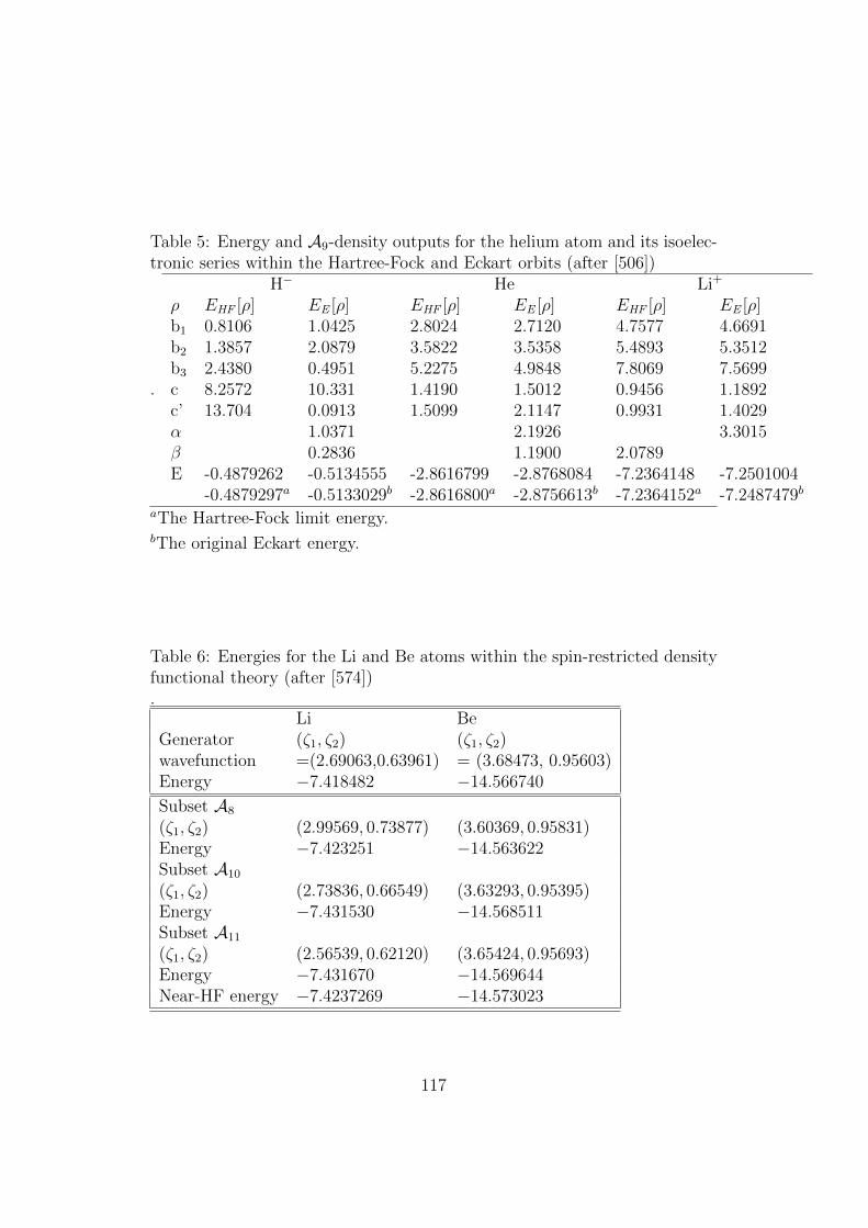
Table 5: Energy and A9-density outputs for the helium atom and its isoelec-tronic series within the Hartree-Fock and Eckart orbits (after [506])

.

H− He Li+

ρ EHF [ρ] EE [ρ] EHF [ρ] EE [ρ] EHF [ρ] EE [ρ]b1 0.8106 1.0425 2.8024 2.7120 4.7577 4.6691b2 1.3857 2.0879 3.5822 3.5358 5.4893 5.3512b3 2.4380 0.4951 5.2275 4.9848 7.8069 7.5699c 8.2572 10.331 1.4190 1.5012 0.9456 1.1892c’ 13.704 0.0913 1.5099 2.1147 0.9931 1.4029α 1.0371 2.1926 3.3015β 0.2836 1.1900 2.0789E -0.4879262 -0.5134555 -2.8616799 -2.8768084 -7.2364148 -7.2501004

-0.4879297a -0.5133029b -2.8616800a -2.8756613b -7.2364152a -7.2487479b

aThe Hartree-Fock limit energy.bThe original Eckart energy.

Table 6: Energies for the Li and Be atoms within the spin-restricted densityfunctional theory (after [574]).

Li BeGenerator (ζ1, ζ2) (ζ1, ζ2)wavefunction =(2.69063,0.63961) = (3.68473, 0.95603)Energy −7.418482 −14.566740

Subset A8

(ζ1, ζ2) (2.99569, 0.73877) (3.60369, 0.95831)Energy −7.423251 −14.563622Subset A10

(ζ1, ζ2) (2.73836, 0.66549) (3.63293, 0.95395)Energy −7.431530 −14.568511Subset A11

(ζ1, ζ2) (2.56539, 0.62120) (3.65424, 0.95693)Energy −7.431670 −14.569644Near-HF energy −7.4237269 −14.573023

117

atom [494], we have used again the Clementi-Roetti single-zeta wave functionto generate a trial orbit. α and β densities are optimized separately, withinA11 and A9 subsets, respectively. The result is the following: the optimaldensity yields the energy −7.431859 that is lower the generator single-zetaenergy by 0.013377.

4.5.10. Global variational principle: The concept oflocal-scaling self-consistent field

The orbit variational principle (216) deduced in Subsection 4.5.1 is solely de-fined on a particular orbit. The reason is trivial: this is precisely that orbitwhere the energy density functional is defined according to Eq. (278). Incontrast, the global ground-state quantum mechanical variational principle(8) is carried out over the whole Hilbert space LN . Within the local-scalingformulation of the density functional approach is achieved due to the factthat the energy density functional in fact depends on two basic variables oftheory: one - the one-electron density - is the key variable of the densityfunctional theory and the other is the generator wave function that deter-mines an orbit. Hence, the orbit partinioning (200) of LN is governed by theorbit generators. Therefore,

Eo = inf

inf

E [ρ(r); Φ

[i]g ]

.

over all orbits ρ(r) ∈ DNO[i] ⊂ LN

(287)

(268) implies that the search for the exact ground-state wave function mustbe carried out by a combined intra-orbit and inter-orbit minimization [13].The former reflects the charge consistency variational principle, whereas thelatter the inter-orbit one, the orbit consistency which is actually the varia-tional principle of the “inter-orbit” self-consistent field thus resembling theKohn-Sham self-consistent field approach and results in inter-orbit “jumps”that finally leads to the exact, Hohenberg-Kohn orbit.

4.5.11. Correlation energy decomposition

A rigorous procedure for accomplishing a decomposition of the correlationenergy into its dynamical and non-dynamical components has been recentlyput forward in the context of LS-DFT [511]. We briefly comment here onsome of the main aspects of this decomposition for the purpose of indicatinghow it is possible to define a reference wavefunction which differs from theexact one in just the dynamical part of electron correlation. Then, we use

118

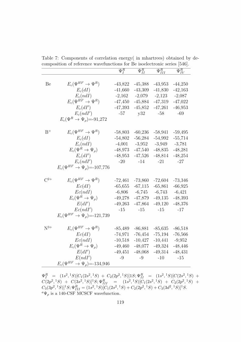
Table 7: Components of correlation energy( in mhartrees) obtained by de-composition of reference wavefunctions for Be isoelectronic series [546].

ΨRI ΨR

II ΨRIII ΨR

IV

Be Ec(ΨHF → ΨR) -43,822 -45,388 -43,953 -44,250Ec(dI) -41,660 -43,309 -41,830 -42,163Ec(ndI) -2,162 -2,079 -2,123 -2,087

Ec(ΨHF → ΨR) -47,450 -45,884 -47,319 -47,022Ec(dI

′) -47,393 -45,852 -47,261 -46,953Ec(ndI

′) -57 y32 -58 -69Ec(Ψ

R → Ψρ)=-91,272

B+ Ec(ΨHF → ΨR) -58,803 -60,236 -58,941 -59,495Ec(dI) -54,802 -56,284 -54,992 -55,714Ec(ndI) -4,001 -3,952 -3,949 -3,781

Ec(ΨR → Ψρ) -48,973 -47,540 -48,835 -48,281

Ec(dI′) -48,953 -47,526 -48,814 -48,254

Ec(ndI′) -20 -14 -21 -27

Ec(ΨHF → Ψρ)=-107,776

C2+ Ec(ΨHF → ΨR) -72,461 -73,860 -72,604 -73,346Ec(dI) -65,655 -67,115 -65,861 -66,925Ec(ndI) -6,806 -6,745 -6,743 -6,421

Ec(ΨR → Ψρ) -49,278 -47,879 -49,135 -48,393

E(dI ′) -49,263 -47,864 -49,120 -48,376Ec(ndI ′) -15 -15 -15 -17

Ec(ΨHF → Ψρ)=-121,739

N3+ Ec(ΨHF → ΨR) -85,489 -86,881 -85,635 -86,518Ec(dI) -74,971 -76,454 -75,194 -76,566Ec(ndI) -10,518 -10,427 -10,441 -9,952

Ec(ΨR → Ψρ) -49,460 -48,077 -49,324 -48,446

E(dI ′) -49,451 -48,068 -49,314 -48,431E(ndI ′) -9 -9 -10 -15

Ec(ΨHF → Ψρ)=-134,946

ΨRI = (1s2, 1S)[C1(2s2, 1S) + C2(2p2, 1S)]1S; ΨR

II = (1s2, 1S)[C(2s2, 1S) +

C(2p2, 1S) + C(3s2, 1S)]1S; ΨRIII = (1s2, 1S)[C1(2s2, 1S) + C2(2p2, 1S) +

C3(3p2, 1S)]1S; ΨRIII = (1s2, 1S)[C1(2s2, 1S) + C2(2p2, 1S) + C3(3d2, 1S)]1S.

aΨρ is a 140-CSF MCSCF wavefunction.

119

this reference wavefunction to separate the calculation of the correlation en-ergy into two parts: Ec(Ψ

HF → ΨR) and Ec(ΨR → Ψexact) (see Eq.(293)

below). We claim that these two components are related to “long-range”and “short-range” correlation, respectively, and that due to their essentiallydifferent nature, they can be treated by entirely different methods.

Correlation energy is defined by Lowdin [576] as the difference betweenthe exact non-relativistic and the restricted Hartree-Fock energies:

Ec ≡ Eexact0 − EHF

0 = E [ρexact,Ψexact]− E [ρHF ,Ψ

HF ]. (288)

Note that as shown in the right-hand-side of Eq. (289) the correlation energycan also be written as the difference of energy functionals of the type given byEq. (276). In fact, when we add and substract the functional E [ρHF ,Ψ

exact]

(which represents the expectation value with respect to H of the wavefunctionΨexactρHF

, namely, of a locally-scaled exact wavefunction that yields the Hartree-Fock density) we obtain:

Ec =(E [ρexact,Ψ

exact]− E [ρHF ,Ψexact]

)+(E [ρHF ,Ψ

exact]− E [ρHF ,ΨHF ]),

= Ec(ndI) + Ec(dI), (289)

where Ec(nd I) and Ec(d I) label the non-dynamical and dynamical compo-nents of the correlation energy along a path that we denote as I. A locally-scaled exact wavefunction that yields the Hartree-Fock density can be gen-erated in practice by applying local-scaling transformations connecting theexact and the Hartree-Fock densities, to each one of the coordinates of the“exact” wavefunction (for a particular system). The transformed wavefunc-tion is given by

ΨexactρHF

(r1, s1, · · · , rN , sN

)≡

N∏i=1

√ρHF (ri)

ρexact(f(ri))Ψρexact

(f(r1), s1, · · · , f(rN), sN

)(290)

where f(r) = λ(r)r is the locally-scaled vector satisfying Eq. (173). In theactual applications described below, “exact” wavefunctions correspond eitherto highly accurate CI expansions or MCSCF wavefunctions.

A similar decomposition along a different path (which we label path II)is obtained by adding and substracting E [ρexact,Ψ

HF ] to Eq. (290):

Ec =(E [ρexact,Ψ

exact]− E [ρexact,ΨHF ])

+(E [ρexact,Ψ

HF ]− E [ρHF ,ΨHF ]),

= Ec(dII) + Ec(ndII). (291)

The interpretation of the decomposition described by Eq. (290) is the fol-lowing: the non-dynamical component, Ec(ndI), represents the change in

120

correlation energy arising from the transformation of the exact wavefunctionlocally-scaled to give ρHF to the exact wavefunction proper. Notice thatthere is no change in the “form” of the wavefunction but just in the type ofdensity the wavefunction associates with. On the other hand, the dynamicalcomponent Ec(dI) stems from the change in the “form” of the wavefunction(it goes from ΨHF to Ψexact, although the latter is constrained to associatewith the Hartree-Fock density). Thus, in a way, the dynamical correlationalong path I corresponds to the formation of the Coulomb hole (at fixedHartree-Fock density).

Now, let us consider an intermediate reference wavefunction ΨR lyingsomewhere along the way between the the Hartree-Fock wavefunction and theexact one. For example, when there are near-degeneracies about the Hartree-Fock level, then a reference wavefunction can be constructed such that itincorporates these near-lying states. In this case, the Lowdin’s correlationenergy can be decomposed in the following way:

Ec =(E [ρR,Ψ

R]− E [ρHF ,ΨHF ])

+(E [ρexact,Ψ

exact]− E [ρR,ΨR])

= Ec(ΨHF → ΨR) + Ec(Ψ

R → Ψexact). (292)

We assume that ΨR is a variational wavefunction whose energy expectationvalue is located below the Hartree-Fock energy and above the exact one. It ispossible, as we did above, to decompose Ec(Ψ

R → Ψexact) into its dynamicaland non-dynamical components along paths I ′ and II ′:

Ec(ΨR → Ψexact) =

(E [ρexact,Ψ

exact]− E [ρR,Ψexact]

)(293)

+(E [ρR,Ψ

exact]− E [ρR,ΨR])

= Ec(ΨR → Ψexact, nd I ′) + Ec(Ψ

R → Ψexact, dI ′)

and

Ec(ΨR → Ψexact) =

(E [ρexact,Ψ

exact]− E [ρexact,ΨR])

(294)

+(E [ρexact,Ψ

R]− E [ρR,ΨR])

= Ec(ΨR → Ψexact, d II ′) + Ec(Ψ

R → Ψexact, ndII ′)

From the variational character of ΨR, it follows that Ec(ΨR → Ψexact, ndII ′) ≥

0 and also that Ec(ΨR → Ψexact, nd I ′) ≤ 0 allowing the possibility of finding

a reference wavefunction for which in both cases the equal sign holds or, atleast, for which these quantities approach zero as closely as possible. In order

121

to see what is at stake when this condition is satisfied, let us look in detailat the nature of the non-dynamical correlation term

Ec(ΨR → Ψexact, nd II ′) =

(E [ρexact,Ψ

R]− E [ρR,ΨR])

=(T [ρexact,Ψ

R]− T [ρR,ΨR])

+1

2

∫d3r1

∫d3r2

(ρexact(r1)ρexact(r2)− ρR(r1)ρR(r2)

)|r1 − r2|

+

∫d3r[ρexact(r)− ρR(r)]v(r)

+(Exc[ρexact,ΨR]− Exc[ρR,ΨR]

). (295)

It is clear that the magnitude of this difference depends upon the proximitybetween ρR and ρexact: when both are equal, it is identically zero.

In order to rigorously define the reference wavefunction ΨR, we considera finite set of one-particle orbitals φimi=1 where m > N from which weconstruct a finite set of Slater determinants ΦI. These, in turn can beused to construct a set of configuration state functions ΨCSF

I satisfyingthe angular momentum an spin symmetry requirements of the system underconsideration. Then, the reference wavefunction is expanded over this set,

ΨR =∑I

CIΨCSFI (296)

and the coefficients of this expansion are determined so as to minimize thetotal energy subject to the constraint that point by point

ρR(r) = ρexact(r) (297)

(Similar variational problems have been considered earlier by Nguyen-Danget al. [234] and by Zhao et al. [577].) In Eq. (297) the configuration statefunctions are linear combinations of Slater determinants:

ΨCSFI =

∑K

aKΦK (298)

where the expansion coefficients aK are fixed by the operators L2 and LZ ,

S2 and SZ , and where ΦK is the Slater determinant

ΦK(r1, · · · , rN) =det√N !φK1(r1) · · ·φKN (rN). (299)

122

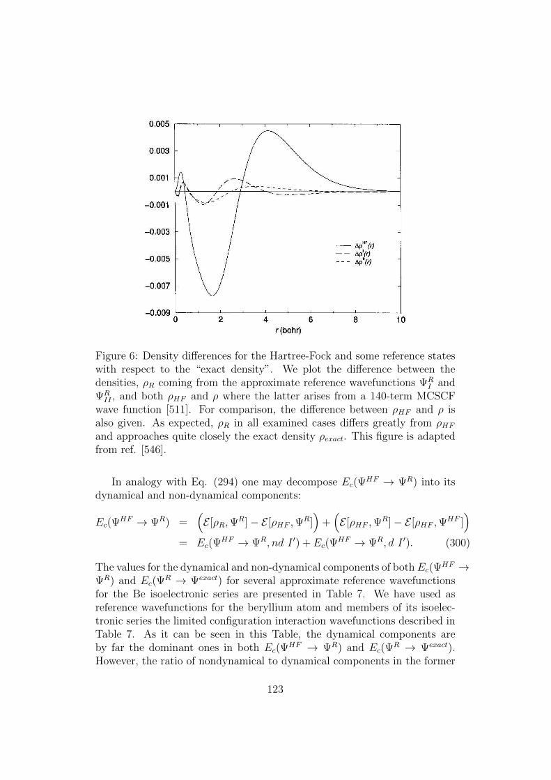
Figure 6: Density differences for the Hartree-Fock and some reference stateswith respect to the “exact density”. We plot the difference between thedensities, ρR coming from the approximate reference wavefunctions ΨR

I andΨRII , and both ρHF and ρ where the latter arises from a 140-term MCSCF

wave function [511]. For comparison, the difference between ρHF and ρ isalso given. As expected, ρR in all examined cases differs greatly from ρHFand approaches quite closely the exact density ρexact. This figure is adaptedfrom ref. [546].

In analogy with Eq. (294) one may decompose Ec(ΨHF → ΨR) into its

dynamical and non-dynamical components:

Ec(ΨHF → ΨR) =

(E [ρR,Ψ

R]− E [ρHF ,ΨR])

+(E [ρHF ,Ψ

R]− E [ρHF ,ΨHF ])

= Ec(ΨHF → ΨR, nd I ′) + Ec(Ψ

HF → ΨR, d I ′). (300)

The values for the dynamical and non-dynamical components of both Ec(ΨHF →

ΨR) and Ec(ΨR → Ψexact) for several approximate reference wavefunctions

for the Be isoelectronic series are presented in Table 7. We have used asreference wavefunctions for the beryllium atom and members of its isoelec-tronic series the limited configuration interaction wavefunctions described inTable 7. As it can be seen in this Table, the dynamical components areby far the dominant ones in both Ec(Ψ

HF → ΨR) and Ec(ΨR → Ψexact).

However, the ratio of nondynamical to dynamical components in the former

123

is of the order of 10−1, whereas in the latter is of 10−3. But beyond thiscomparison, we observe in this Table that a remarkable gain in correlationenergy takes place by the mere addition of the (2p2,1 S) configuration tothe Hartree-Fock wavefunction. This gain is comparable to the whole im-provement corresponding to Ec(Ψ

R → Ψexact). By adding other low-lyingconfigurations one just gets a very slight improvement. Hence, it seems thatthe two components Ec(Ψ

HF → ΨR) and Ec(ΨR → Ψexact) are of a different

nature and that, in consequence, they should be treated by different densityfunctional methods.

The fact that such a large correlation energy improvement is obtained forEc(Ψ

HF → ΨR) through the addition of configurations that have a manifestinfluence on the density (a global quantity for the system) shows that thispart of the correlation energy has a long-range character. The effect on one-particle density is examined in Fig. 6 where we plot the difference betweenthe densities ρR (coming from the approximate reference wavefunctions ΨR

I

and ΨRII) and both ρHF and ρ (the latter arising from a 140-term MCSCF

wavefunction [578]). For comparison, the difference between ρHF and ρ isalso given. As expected, ρR in all cases examined differs greatly from ρHFand approaches quite closely the exact density ρexact.

In marked contrast with what happens with Ec(ΨHF → ΨR), we observe

that Ec(ΨR → Ψexact) can only be improved through the use of very large

configuration interaction expansions which do not show much effect on theone-particle density. One may conclude, therefore, that Ec(Ψ

R → Ψexact) isdue chiefly to short-range interactions.

Since according to Eq. (293) the “long-range” part of the correlationenergy is defined by Ec(Ψ

HF → ΨR) = E [ρR,ΨR] − E [ρHF ,Ψ

HF ], it followsthat local-scaling transformations can be used for the purpose of constructingan explicit density functional expression. For the functional E [ρR,Ψ

R] thiswould involve just the inclusion of some small modifications on the methodalready applied to E [ρHF ,Ψ

HF ] in Section II. Let us remark, that in thiscase, Ec(Ψ

HF → ΨR, d I ′) is the dynamical contribution to the “long-range”correlation energy.

We claim, on the other hand, that the calculation of the “short-range”component Ec(Ψ

R → Ψexact, d I ′) requires that we include in some adequateway the local Coulomb hole. We propose that this can be accomplished bymeans of an explicit use of a correlation factor. The problem of how to dealwith Ec(Ψ

R → Ψexact, d I ′) in the context of LS-DFT is treated below [546].In [579], the electron correlation in terms of a cluster expansion based on

a single Slater determinant is treated. To extend these ideas to deal withdynamical “short-range” correlation, where instead of a determinant we havea multi-reference wavefunction ΨR.

124

Consider the following approximation to the exact wavefunction

Ψ(r1, · · · , rN) = C(r1, · · · , rN)ΨR(r1, · · · , rN), (301)

where the N -particle correlation function C is the product of two-particlecorrelation functions g(ri, rj):

C(r1, · · · , rN) =∏i>j

g(ri, rj), (302)

and where ΨR is defined as the linear combination of configuration statefunctions described by Eq.(297). We assume that the ΨCSF

I ’s are constructedfrom a simple set such as the generalized Slater-type orbitals described byEqs.(A1)-(A5) of Appendix A. Clearly, since these orbitals are at best ap-proximations to the Kohn-Sham orbitals, we cannot expect ΨR to yield theexact density. Hence, the approximate wavefunction given by Eq.(302) can beimproved through the application of density transformations. The density-transformed wavefunction becomes, therefore,

Ψρ(r1, · · · , rN) = C(f1, · · · , fN)ΨR(r1, · · · , rN), (303)

where ΨR is the density transformed reference wavefunction defined by Eqs.(297) and (299) but where in the transformed Slater determinants (300) eachone of the initial orbitals has been locally-transformed. Thus, Eq. (300)becomes:

ΦK(r1, · · · , rN) =det√N !

√ρ(r1)

ρΨ(f1)φK1(f1), · · · ,

√ρ(rN)

ρΨ(fN)φKN (fN)

. (304)

As it has been shown elsewhere [579], the energy expression takes the form

E[Ψρ] ≡〈ΨR

∣∣∣∣∏Ni>j g

2(fi, fj)

[H +

∑i<j u(fi, fj) +

∑Ni=1

∑Nj 6=i∑N

k 6=i,j Fijk

]∣∣∣∣ΨR〉

〈ΨR

∣∣∣∣∏Ni>j g

2(fi, fj)

∣∣∣∣ΨR〉≥ Eo,

(305)where

u(fi, fj) = −1

2

(∇2

ri+∇2

rj

)g(fi, fj)

g(fi, fj)−∇rig(fi, fj) · ∇ri +∇rjg(fi, fj) · ∇rj

g(fi, fj)(306)

125

and

Fijk = −1

2

∇2rig(fi, fj)

g(fi, fj)− ∇rig(fi, fj) · ∇rig(fi, fk)

g(fi, fj)g(fi, fk). (307)

By resorting to the Aviles-Hartog-Tolhoek cluster expansion [580, 581]we can rewrite the energy as

E[Ψρ] =1

〈Ψρ|Ψρ〉∂IN(β)

∂β

∣∣∣∣β=0

=N∑k=1

E(k)[Ψρ], (308)

where IN(β) is the cluster subintegral

In(β) = 〈Φ|n∏i>j

g(fi, fj)eβHn

n∏i>j

g(fi, fj)|Φ〉, (309)

and where the cluster energy contributions E(k)[Ψρ] are [582]

E(k)[Ψρ] = Cn,k∂ lnYk(β)

∂β

∣∣∣∣β=0

. (310)

The cluster functions Yk(β) are defined through

In(β) =n∏k=1

YCn,kk (β) (311)

where Cn,k = n!/(n− k)!k!. In the FAHT cluster expansion we can approx-imate IN of Eq. (312) by assuming that the cluster functions Yk(β) areequal to 1 after a given value of k ≤ N . Hence, for a second order clusterexpansion (which is obtained by requiring that Yk(β) = 1 for k = 3, ..., N)the energy is approximated by

E[Ψρ] ' E(1)[Ψρ] + E(2)[Ψρ]. (312)

By substracting from this expression E[ΨR] we obtain the following approx-imate expression for the dynamical “short-range” correlation:

Ec(ΨR → Ψρ, d) ' E(1)

c [Ψρ] + E(2)c [Ψρ]− E[ΨR]

=〈ΨR|

∑Ni<j(1 + φ(fi, fj))uij|ΨR〉

〈ΨR|ΨR〉+ 〈ΨR|φ(f1, f2)|ΨR〉

+〈ΨR|

∑Ni<j hij|ΨR〉

〈ΨR|ΨR〉

∞∑k=1

(−1)k

(〈ΨR|φ(f1, f2)|ΨR〉〈ΨR|ΨR〉

)k

+〈ΨR|

∑Ni<j φ(fi, fj)hij|ΨR〉

〈ΨR|ΨR〉+ 〈ΨR|φ12|ΨR〉, (313)

126

where φij is given by g2(fi, fj) = 1 + φ(fi, fj) and where the two-particleoperator is

hij = Fi + Fj + vij (314)

with vij = 1/|ri − rj| and Fi = (1/2)∇2ri− Z/ri. It is clear that through

the presence of the transformed vector fi = fi([ρ]; r) in φ(fi, fj) and also inthe wavefunction ΨR (see Eq. (305)) the whole expression in (314) is animplicit functional of the one-particle density ρ. Clearly, Eq. (314) can betransformed into an explicit functional of ρ by using the procedure advancedin [579].

4.6 Intra-orbit optimization schemes

The variational principle advanced in Eq. (284) states that the search for theexact ground-state wavefunction must be carried out by a combined intra-orbit and inter-orbit minimization [583, 557, 558, 584]. Thus, a practicalimplementation of this variational principle requires that we develop ways ofchoosing an orbit, of constructing the energy functional within this selectedorbit, of attaining the minimum value for the energy within this orbit andfinally of jumping from one orbit to another so as to repeat in this neworbit the minimization process. Of course, through this repeated intra-orbitand inter-orbit optimization, one should finally arrive at an orbit yielding asufficiently accurate upper bound to exact ground-state energy, i.e., to anorbit close enough (energy-wise) to the Hohenberg-Kohn one. In the latter,by definition, the exact ground-state wavefunction is found.

In order to discuss some of the aspects arising in a practical realizationof the variational principle given by Eq. (30), let us consider Fig. 7. In thisFigure, we have schematically represented the steps involved in intra-orbitoptimization and have indicated how this optimization followed by inter-orbitjumping defines a self-consistent procedure leading eventually to a solutionthat is as exact as we wish it to be [557, 558]. We discuss in what followsthese steps in detail.

4.6.1. Intra-orbit optimization

The first thing we must do is select a particular orbit. This is done by choos-ing an initial wavefunction, as the choice of the initial wavefunction deter-mines the orbit. Consider, for example, an arbitrary wavefunction Φ

[i]g ∈ O[i]

L .

127

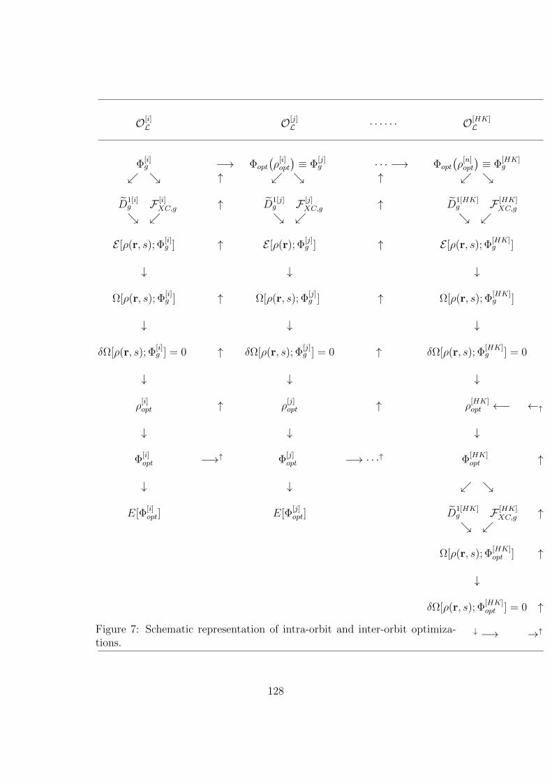
O[i]L O[j]

L · · · · · · O[HK]L

Φ[i]g −→ Φopt

(ρ

[i]opt

)≡ Φ

[j]g · · · −→ Φopt

(ρ

[n]opt

)≡ Φ

[HK]g

↑ ↑

D1[i]g F [i]

XC,g ↑ D1[j]g F [j]

XC,g ↑ D1[HK]g F [HK]

XC,g

E [ρ(r, s); Φ[i]g ] ↑ E [ρ(r); Φ

[j]g ] ↑ E [ρ(r, s); Φ

[HK]g ]

↓ ↓ ↓

Ω[ρ(r, s); Φ[i]g ] ↑ Ω[ρ(r, s); Φ

[j]g ] ↑ Ω[ρ(r, s); Φ

[HK]g ]

↓ ↓ ↓

δΩ[ρ(r, s); Φ[i]g ] = 0 ↑ δΩ[ρ(r, s); Φ

[j]g ] = 0 ↑ δΩ[ρ(r, s); Φ

[HK]g ] = 0

↓ ↓ ↓

ρ[i]opt ↑ ρ

[j]opt ↑ ρ

[HK]opt ←− ←↑

↓ ↓ ↓

Φ[i]opt −→↑ Φ

[j]opt −→ · · ·↑ Φ

[HK]opt ↑

↓ ↓

E[Φ[i]opt] E[Φ

[j]opt] D

1[HK]g F [HK]

XC,g ↑

Ω[ρ(r, s); Φ[HK]opt ] ↑

↓

δΩ[ρ(r, s); Φ[HK]opt ] = 0 ↑

↓ −→ →↑Figure 7: Schematic representation of intra-orbit and inter-orbit optimiza-tions.

128

This can be a configuration interaction wavefunction or some trial wave-function incorporating inter-particle coordinates. These wavefunctions mustallow for a proper representation of the important physical aspects of theproblem at hand. Thus, a configuration interaction wavefunction shouldcontain the minimal set of configurations necessary for the description ofelectronic correlation. As is well-known, a configuration interaction wave-function contains expansion coefficients and orbital parameters which areoptimized by energy minimization. In the case of the orbit-generating wave-function, however, these coefficients and parameters need not be the optimalones. In fact, all that is needed are educated guesses for these numbers[557, 558]. The reason for this arbitrary choice of initial wavefunction is thatlocal-scaling transformations modify the orbitals from which this wavefunc-tion is constructed so as to yield an optimal wavefunction for the particularset of initial coefficients and parameters. In Section 5.2, we give some nu-merical examples for simple configuration interaction wavefunctions of the Beatom corresponding to different arbitrary choices of the initial wavefunctions.

The important aspect we wish to emphasize here is that once the orbit-generating wavefunction is chosen, we can obtain explicit expressions for thenon-local part of the 1-matrix, D

1[i]g (r, s; r′, s′) as well as for the non-local part

of the 2-matrix, that is, for the exchange-correlation factor F [i]XC,g(r1, s1; r2, s2).

That these explicit expressions are essential for setting up the energy as afunctional of the one-particle density, follows from Eq. (234). Notice that

the energy functional in Eq. (234) contains D1[i]g

(f([ρ]; r), s; f([ρ]; r′), s′

)and

F [i]XC,g

(f([ρ]; r1), s1; f([ρ]; r2), s2

)where f([ρ]; r) is the object vector function

resulting from the local-scaling transformation of r. Because this object vec-tor function, as it can clearly be seen from Eq. (229), is a function (albeitimplicit) of the one-particle density ρ(r, s), it follows that the energy densityis also an implicit function of ρ(r, s), or equivalently, that the energy for each

orbit O[i]L is a functional of ρ(r, s). In Fig. 7, we indicate by means of slanted

arrows that Φ[i]g produces D

1[i]g and F [i]

g . These quantities, in turn, enter into

the construction of the energy functional E [ρ(r, s); Φ[i]g ].

The next step in this intra-orbit optimization procedure is the creationof an auxiliary functional Ω[ρ(r, s); Φ

[i]g ] made up from the energy functional

E [ρ(r, s); Φ[i]g ] plus the auxiliary conditions which must be imposed on the

variational variables. Notice that there are many ways of carrying out thisvariation. In Subsections 4.6.1, 4.6.2 and 4.6.3, we treat the intra-orbit varia-tion with respect to ρ(r, s), [ρ(r, s)]1/2 and the set of N orthonormal orbitals

φi(r) Ni=1, respectively. Clearly, by setting δΩ[ρ(r, s); Φ[i]g ] = 0, one obtains

the Euler-Lagrange equations corresponding to each one of the above cases.The direct construction of the exact energy density functional E [ρ(r, s);

129

Φ[HK]g ] within the Hohenberg-Kohn orbit, requires that we know some orbit-

generating wavefunction Φ[HK]g . But this is tantamount to knowing the exact

ground-state wavefunction Φ[HK]ρvo

≡ Ψvo. Hence, in principle, it would be to-

tally unecessary to carry out the variation of this energy density functional asin order to construct it we should have solved first the many-body problem athand. Nevertheless, from a purely formal angle, such variation is importantin that for N orbitals, it leads to the Kohn-Sham equations. This aspect ofthe problem is discussed in Section 4.6.4.

In Sections 4.6.5 and 4.6.6 we discuss two important alternative meth-ods to intra-orbit optimization. Both are based on the use of local-scalingtransformations in order to produce sets of transformed orbitals which arethen directly employed in the calculation of the total energy. In the non-variational case, we deal with arbitrary orbitals which are locally-scaled inorder to yield the Hartree-Fock one-particle density, which we assume to beknown beforehand. In the second method, the final density is optimized byenergy minimization. But as in the previous case, locally-scaled transformedorbitals are used in the energy calculation.

4.6.2. Euler-Lagrange equation for intra-orbit optimiza-tion of ρ(r, s)

Let us consider now the energy density functional E [ρ(r, s); Φ[i]g ] of Eq. (234).

In this functional, ρ(r, s) stands for any one of the final densities generatedfrom the initial density ρg(r, s) coming from the orbit-generating wavefunc-

tion Φ[i]g . Clearly, the extremum of this functional is attained at the optimal

density ρ[i]opt(r, s). This density satisfies the Euler-Lagrange equation arising

from the variation of the functional E [ρ(r, s); Φ[i]g ] - subject to the normal-

ization condition∫d4x ρ(r, s) = N - with respect to the one-particle density

ρ(r, s). Explicitly, this amounts to varying the auxiliary functional

Ω[ρ(r, s); Φ[i]g ] ≡ E [ρ(r, s); Φ[i]

g ]− µ[i](∫

d4x ρ(r, s)−N)

(315)

where µ[i] is the Lagrange multiplier that accounts for the normalization ofthe density. Setting this variation equal to zero,

δΩ[ρ(r, s); Φ[i]g ]

δρ(r, s)= 0 , (316)

we obtain as a result, the following integro-differential equation for the one-

130

particle density [585, 586]:

1

8

[∇ρ(r, s)

ρ(r, s)

]2

− 1

4

∇2ρ(r, s)

ρ(r, s)+ v

[i]T,g

([ρ(r, s)]; r, s

)+ v(r)

+ vH([ρ(r, s)]; r

)+ v

[i]XC,g

([ρ(r, s)]; r, s

)= µ[i]. (317)

In addition to the external potential v(r) and the Hartree or Coulomb po-tential vH([ρ(r, s)]; r) =

∫d4xρ(r, s)|r− r ′|−1, we have in this expression the

potential v[i]T,g which arises from the non-local part of the kinetic energy in

Eq. (234):

v[i]T,g

([ρ(r, s)]; r, s)

)=

1

2

[∇r∇r ′D

1[i]g

(f(r), s; f(r ′), s′

)]r ′=r,s′=s

+ ρ(r, s)δ

δρ(r, s)

([∇r∇r ′D

1[i]g

(f(r), s; f(r ′), s′

)]r ′=r,s′=s

).

(318)

The exchange-correlation potential coming from the non-local part of theelectron-electron interaction term is:

v[i]XC,g

([ρ(r, s)]; r, s

)= E [i]

XC,g

([ρ(r, s); Φ[i]

g ]; r, s)+ρ(r, s)

δE [i]XC,g

([ρ(r, s); Φ

[i]g ]; r, s

)δρ(r, s)

,

(319)where we have defined

E [i]XC,g

([ρ(r1, s1); Φ[i]

g ]; r1, s1

)=

1

2

∫d4x2

ρ(r2, s2)F [i]XC,g

(f(r1), s1; f(r2), s2

)|r1 − r2|

.

(320)

Notice that the optimal energy value within orbit O[i]L is E [ρ

[i]opt(r, s); Φ

[i]g ].

This value is an upper bound to the optimal energy value within the Hohenberg-Kohn orbit, which, of course, is just the exact ground-state energy: E [ρ

[HK]opt (r, s);

Φ[HK]g ] = Ev

o .

4.6.3. Euler-Lagrange equation for intra-orbit optimiza-tion of [ρ(r, s)]1/2

Let us consider the “shape- wavefunction” [587] u(r, s) ≡ u(x) and its com-plex conjugate u∗(r, s) which satisfy the relation ρ(x) = u(x)u∗(x). It is

131

clear that the shape function is equal to [ρ(x)]1/2 times an arbitrary phasefactor: u(x) = [ρ(x)]1/2eiχ(r). Assuming u(x) to be the basic variable, theauxiliary variational functional becomes

Ω[u(x)u∗(x); Φ[i]g ] ≡ E [u(x)u∗(x); Φ[i]

g ]− µ[i](∫

d4xu(x)u∗(x)−N). (321)

In terms of u(x), the local kinetic energy contribution (i.e., the Weizsackerterm) can be written as:

TW [ρ(x)] =1

2

∫d4x

(∇ru

∗(x))(∇ru(x)

). (322)

In order to derive the Euler-Lagrange equation for u(x) let us set the variationequal to zero:

δΩ[u(x)u∗(x); Φ[i]g ]

δu∗(x)+ c.c = 0. (323)

The resulting equation for the “shape- wavefunction” is [585, 586, 588, 589,567]:[−1

2∇2 + v

[i]T,g([u

∗(x), u(x)];x) + v(r) + vH([u(x), u(x)]; r)

+ v[i]XC,g([u

∗(x), u(x)];x)]u(x) = µu(x)

(324)plus the corresponding equation for its complex conjugate u∗(x).

The potential v[i]T,g([u

∗(x), u(x)];x) which arises from the non-local part ofthe kinetic energy is given by

v[i]T,g([u

∗(x), u(x)];x) = ∇r∇r′D[i]g

([u∗(x), u(x)]; f(r), s; f(r ′), s′

)∣∣x=x′

+ u∗(x)δ

δu∗

[∇r∇r′D

[i]g ([u∗(x), u(x)]; r, r ′)

∣∣x=x′

].

(325)

As in Eq. (64), v(r) is the external potential, and v[i]H ([u∗(x), u(x), ]; r) is the

ordinary Hartree potential. The exchange-correlation potential v[i]XC,g([u

∗(x), u(x)];x)is given by

v[i]XC,g([u

∗(x), u(x)];x) =

∫d4x ′

u∗(x ′)u(x ′)

|r− r ′|F [i]XC,g([u

∗(x), u(x)]; r, r ′)

+ u∗(x)

∫d4x ′

u∗(x ′)u(x ′)

|r− r ′|δ

δu∗

[F [i]XC,g([u

∗(x), u(x)]; r, r ′)].

(326)

132

4.6.4. Euler-Lagrange equations for the intra-orbit op-timization of N orthonormal orbitals: Kohn-Sham-likeequations

Consider the single Slater determinant

ΦSD[i]g (x1, · · · , xN) ≡ det√

N ![φ

[i]g,1(x1) · · ·φ[i]

g,N(xN)] (327)

constructed from the set φ[i]g,k(x)Nk=1. This wavefunction associates with

the one-particle density ρg(x). Let us consider a final density ρ(x) possessingthe same topology as ρg(x) such that we can obtain solving Eq. (158) thetransformation function f(r). Applying this transformation to all coordi-

nates of the wavefunction ΦSD[i]g (x1, · · · , xN), we can produce a transformed

wavefunction ΦSD[i]ρ (x1, · · · , xN) that satisfies Eq. (199). These local-scaling

transformations, carry therefore a single Slater determinant into another sin-gle Slater determinant.

Let us define the subclass SN as consisting of all single Slater determi-nants. It is clear that SN is not a subspace of LN because a linear combinationof Slater determinants is not in general equal to a single Slater determinant.By arguments similar to those expounded in Subsection 4.4 (Corrolary 9.4,

p.85), it follows that SN can be decomposed into the orbits O[i]S defined by

O[i]S ≡ Φ

SD[i]ρ |ΦSD[i]

ρ −→ ρ(x); ΦSD[i]ρ ∈ SN ; ρ(x) ∈ NB. (328)

Clearly, we have in the present case that the union of all orbits exhauststhe subclass: SN = ∪∞i=1O

[i]S . The action of local-scaling transformations

on the initial orbitals leads to the new orbital set φ[i]ρ,k(x)Nk=1, where the

transformed orbitals are connected to the generating ones by the relation

φ[i]ρ,k(x) = fφ

[i]g,k(x) =

[J(f(r); r)

]1/2φ

[i]g,k

(f(r), s)

)=

[ρ(r, s)

ρg(f(r), s)

)]1/2

φ[i]g,k

(f(r), s)

).

(329)These transformed orbitals preserve the orthonormalization condition∫

d4xφ∗[i]ρ,k(x)φ

[i]ρ,l(x) = δkl. (330)

From the single Slater determinant

ΦSD[i]ρ (r1, s1, · · · , rN , sN) ≡ det√

N ![φ

[i]ρ,1(r1, s1) · · ·φ[i]

ρ,N(rN , sN)] (331)

133

constructed from these transformed one-particle orbitals, one obtains theone-particle density

ρ(x) =N∑k=1

∣∣φ[i]ρ,k(x)

∣∣2, (332)

as well as the non-interacting kinetic energy term:

Ts[φ[i]

ρ,k(x)]

=N∑k=1

1

2

∫d4x∇rφ

[i]ρ,k(x)∇r ′φ

[i]ρ,k(x

′)∣∣x′=x

(333)

=1

8

∫d4x

[∇rρ(x)

]2ρ(x)

+1

2

∫d4xρ(x)∇r∇r′D

1SD[i]g (f(r), s; f(r′), s′)|x′=x,

where D1SD[i]g is the non-local part of the 1-matrix of the non interacting

system.Following Kohn and Sham [5], let us consider the following auxiliary

functional:

Ω[φ[i]ρ,k(x); Φ[i]

g ] ≡ E [φ[i]ρ,k(x); Φ[i]

g ] + Ts[φ[i]

ρ,k(x)]− Ts

[φ[i]

ρ,k(x)]

(334)

−N∑k=1

N∑l=1

λkl

(∫d4xφ

∗[i]ρ,k(x)φ

[i]ρ,l(x)− δkl

)where the λkl are the Lagrange multipliers enforcing orbital orthonormal-ity. Bearing in mind Eqs. (50) and (79) we can rewrite this auxiliary func-tional as

Ω[φ[i]ρ,k(x); Φ[i]

g ] = Ts[φ[i]

ρ,k(x)]

+ Eext[ρ(x)] + ECoulomb[ρ(x)]

+ EKS[i]XC,g

[ρ(x); Φ[i]

g [fi]]

(335)

−N∑k=1

N∑l=1

λkl

(∫d3xφ

∗[i]ρ,k(x)φ

[i]ρ,l(x)− δkl

)where Eext[ρ(x)] =

∫d4xρ(x)v(r),

ECoulomb[ρ(x)] = (1/2)∫d4x1

∫d4x2ρ(x1)ρ(x2)|r1 − r2|−1 and

EKS[i]XC,g

[ρ(x); Φ[i]

g [fi]]

=1

2

∫d4xρ(x)∇r∇r′

[D1[i]g (f(r), s; f(r′), s′)

− D1SD[i]g (f(r), s; f(r′), s′)

]∣∣∣x′=x

(336)

+1

2

∫d4x1

∫d4x2

ρ(x1)ρ(x2)F [i]XC,g(f(r1), s1, f(r2), s2)

|r1 − r2|.

134

Varying the auxiliary functional Ω[φ[i]ρ,k(x); Φ

[i]g ] with respect to the one-

particle orbital leads us to

δTS[φ[i]

g,k(x)]

δφ[i]ρ,k(x)

+δ

δρ(x)

(Eext[ρ(x)] + ECoulomb[ρ(x)] + E

KS[i]XC,g

([ρ(x)]; Φ[i]

g

)) δρ(x)

δφ[i]ρ,k(x)

−N∑k=1

N∑l=1

λklδ

δφ[i]ρ,k(x)

(∫d3xφ

∗[i]ρ,k(x)φ

[i]ρ,l(x)− δkl

)= 0 (337)

from where the following Kohn-Sham-like single particle equations are ob-tained:[−1

2∇2 + v(r) + vH

([ρ(x)]; r

)+ v

KS[i]XC,g

([ρ(x)];x

)]φ

[i]ρopt,k(x) =

∑l=1

λklφ[i]ρopt,l(x).

(338)Notice that v(r), and vH

([ρ(x)]; r

)appearing in Eq.(339) are the same as

those in Eq.(64). The Kohn-Sham-like exchange correlation potential vKS[i]XC,g

([ρ(x)];x

)is, however, substantially different from the exchange-correlation potentialdefined in Eq. (64). The contribution arising from the non-local part ofthe kinetic energy (first term on the right-hand side of Eq. (337)) is pos-itive and thus counterbalances the negative contribution coming from theexchange-correlation energy proper (second term).

The partial cancellation of correlation effects arising from the 1- and 2-matrices is a well-known fact in Kohn-Sham theory [13, 590]. As is to be

expected, it also appears in the Kohn-Sham-type equations for an orbit O[i]L .

We would like to emphasize, nevertheless, that all terms in Eq. (339) canbe explicitly calculated. In principle, therefore, within a particular orbitO[i]L , the exchange-correlation energy term as well as the Kohn-Sham-type

exchange-correlation potential can be explicitly obtained. The accuracy ofthe results depends, clearly, on our selection of the orbit-generating functionsΦ

[i]g ∈ O[i]

L ⊂ LN and Φ[i]g ∈ O[i]

S ⊂ SN .

4.6.5. The Hohenberg-Kohn orbit O[HK]L and the Kohn-

Sham equations

Let assume that we are able to select an orbit-generating wavefunction Φ[HK]g

belonging to the Hohenberg-Kohn orbit (for an interacting system) O[HK]L ⊂

LN . From this wavefunction we can obtain the non-local part of the 1-matrix, D

1[HK]g (x1, x

′1) and the exchange-correlation factor F [HK]

XC,g (x1, x2) (thenon-local part of the 2-matrix). Equation (339), however, also involves thenon-local part of the 1-matrix for the single Slater determinant (for a non-interacting system). Clearly, this function does not belong to LN but to the

135

subclass SN . Let us denote by ΦSD[HK]g this generating wavefunction for the

non-interacting Hohenberg-Kohn orbit O[HK]S ⊂ SN .

The action of a local-scaling transformation of the density within the in-teracting Hohenberg-Kohn orbit carries the wavefunction Φ

[HK]g ∈ O[HK]

L ⊂LN into the transformed wavefunction Φ

[HK]ρ ∈ O[HK]

L ⊂ LN . The sameoccurs within the non-interacting Hohenberg-Kohn orbital where the wave-function Φ

SD[HK]g ∈ O[HK]

S ⊂ SN goes into ΦSD[HK]ρ ∈ O[HK]

S ⊂ SN . The

energy minimum is attained within O[HK]L when ρ(x) = ρexacto (x). However,

it is precisely at this exact density that one obtains the optimal orbital setφ[HK]

ρexacto ,k(x)Nk=1 satisfying the one-particle equations given by Eq. (340). Inthis way, one sees that there exists a direct link - through the one-particledensity - between the minimization of the energy functional of Eq. (278) in

O[HK]L and the solution of the Kohn-Sham equations (340). In canonical form

the Kohn-Sham equations are [5]:[−1

2∇2+v(r)+vH

([ρexacto (x)]; r

)+v

KS[HK]XC,g

([ρexacto (x)];x

)]ψ

[HK]ρexacto ,k(x)=EKSk ψ

[HK]ρexacto ,k(x).

(339)

4.6.6. Variational intra-orbit optimization of trial wave-functions

In this procedure [583, 558], one starts from an orbit generating wavefunction

Φ[i]o,g

(ri, si

)for the ground state of an N -particle system. Such a wavefunc-

tion may be given, for example, by the linear combination of “configurationstate functions” (cf., Eq. (297)):

Φ[i]o,g

(ri, si

)=

M∑I=1

Co[i]I,g ψ

CSF [i]I,g

(ri, si

)(340)

where the latter are expanded in terms of single Slater determinants:

ψCSF [i]I,g

(ri, si

)=∑j

Aj[ψCSF [i]I,g ]Φ

SD[i]j,g

(ri, si

). (341)

The coefficients Aj[ψCSF [i]I,g ] are fixed by symmetry (i.e., by the fact that the

ψCSF [i]I,g ’s must be simultaneous eigenfunctions of the operator set Oi that

commutes with H). As a result, the only variational parameters are the

expansion coefficients Co[i]I,g of Eq. (86) for the approximate expansion of

the ground-state wavefunction.

136

Because the determinants ΦSD[i]j,g appearing in the expansions of the

“configuration state functions” are constructed from a single-orbital set φ[i]g,k(r,

s)Kk=1 where K > N , the effect of local-scaling transformations involves thereplacement in each one of the single-Slater determinants of Eq. (299) of the

initial orbitals by transformed orbitals belonging to the set φ[i]ρ,k(r, s)Kk=1.

Thus, we are led to the set of transformed Slater determinants ΦSD[i]j,ρ . We

assume that this transformation takes place from a generating density ρo,g(r)to a final density ρo,f (r) ≡ ρ(r) expressed as

ρ(r) =I∑i=1

ai rbie−ci (342)

where ai, bi, ci are variational parameters. Since the transformed orbitalsare obtained in numerical form, in order to evaluate the total energy onerequires the use of programs that can handle numerical functions. The de-termination of the lowest energy value for the functional E [ρ(r, s); Φ

[i]o,g] with

Φ[i]o,g belonging to the orbit OL[i] can then be realized by means of the opti-

mization of the non-linear parameters ai, bi, ci of the trial final density.The procedure described here for configuration interaction wavefunctions

can be extended to explicitly-correlated wavefunctions [591, 592]. There isno conceptual difficulty in this extension other than the fact that one mustperform all integrations numerically.4.6.7. Non-variational intra-orbit optimization of trialwavefunctions

Clearly, the difficult part of the procedure sketched in Subsection 4.6.5 isthe optimization of the one-particle density. Nevertheless, one can set upa variant of this procedure by choosing a fixed and previously determinedfinal one-particle density [583, 557]. Approximate one particle densities canbe readily obtained for atomic systems from Hartree-Fock wavefunctions.Although for small molecules this is still feasible, for larger ones even theHartree-Fock method becomes prohibitive. In these cases, one can computeapproximate densities by solving single-particle equations with Xα or Kohn-Sham potentials (in the local-density and non-local-density ansatzs). But, onthe other hand, experimentally determined one-particle densities are becom-ing available for small molecules in the gaseous phase as well as for moleculessusceptible of forming crystal structures [593].

In the non-variational procedure, one sets up an arbitrary orbit-generatingwavefunction whose form is designed so as to contain “the physics” of theproblem under consideration. If one were to choose a configuration interac-tion wavefunction, it would be wise to select a minimal basis set and carry

137

out the optimization of both orbital exponents and expansion coefficients.Because the technology for performing small-scale configuration interactioncalculations is available, this step does not present any difficulty. However,because of the limited bases used in the construction of orbitals, the vari-ational results of this limited expansion are usually quite distant from theoptimal ones. The idea is to produce by means of local-scaling transforma-tions a wavefunction which in addition to having an appropriate form for thedescription of electronic correlation yields at the same time the fixed one-particle density which one has chosen as a final density in the local-scalingtransformation.

That electronic correlation is not too sensitive to the form of the one-particle density is a well-known fact. In Section 5.2, we provide some nu-merical results of this non-variational energy optimization procedure for theberyllium atom and also analyze the effect on the correlation energy of se-lecting different final densities.

4.7 Inter-orbit optimization schemes

4.7.1. Inter-orbit optimization

Let us go back to Fig. 7. There we have sketched by means of steps formedby arrows the orbit-jumping processes whereby a “density-optimal” wave-function Φ

[i]opt ∈ O

[i]L is carried into another wavefunction Φopt

(ρ

[i]opt

)which we

define as the orbit-generating wavefunction Φ[j]g for orbit O[j]

L . In order to

see what is meant by Φopt

(ρ

[i]opt

)consider again the energy expression given

by Eq. (234) and assume that it is evaluated at ρ[i]opt. Notice that the energy

functional E[Φ[i]opt] ≡ E

[ρ

[i]opt(x); Φ

[i]g [fi]

]is a minimum within O[i]

L , but thatthis minumum is not the absolute one which by definition occurs at the exactdensity and at the Hohenberg-Kohn orbit O[HK]

L . An improvement of the en-

ergy functional E[ρ

[i]opt(x); Φ

[i]g [fi]

]at fixed density ρ

[i]opt(x) can be attained,

therefore, by varying the wavefunction Φ[i]g [fi]. We must keep in mind,

however, that within orbit O[i]L we cannot find a wavefunction that yields a

lower energy. Hence, it follows that any wavefunction that lowers the value ofthe above functional must belong to an orbit different from O[i]

L . Thus, whenas the result of variation the energy is lowered, “orbit jumping” must havenecessarily occurred [583, 558]. The optimal wavefunction obtained by this

inter-orbit optimization at fixed density ρ[i]opt(x) is denoted by Φopt

(ρ

[i]opt

)and

138

since this wavefunction does not belong to orbit O[i]L , we can safely assume

that it is the orbit-generating wavefunction Φ[j]g for orbit O[j]

L . One shouldremark that although “orbit jumping” is carried out at fixed density, thewavefunction Φopt

(ρ

[i]opt

)need not yield the fixed density ρ

[i]opt(x). In view of

this fact, it is then possible to perform a local-scaling transformation in orderto carry the wavefunction Φopt

(ρ

[i]opt

)into another one that yields ρ

[i]opt(x). If

we denote this new wavefunction by Φ[j]ith−opt, it follows that

E[Φ[j]ith−opt] ≤ E[Φ

[i]opt] (343)

as Φ[j]ith−opt is attained by inter-orbit optimization of Φ

[i]opt. Furthermore, we

have that for any two different orbits O[i]L and O[j]

L , the following inequalitieshold:

E[Φ

[j]opt

]≤ E

[Φ

[j]ith−opt

]≤ E

[Φ

[i]opt

]≤ E

[Φ[i]g

], i 6= j, (344)

where Φ[j]opt is the optimal wavefunction in orbit O[j]

L . In what follows, wediscuss some practical procedures for accomplishing inter-orbit optimization.

4.7.2. Inter-orbit optimization of CI wavefunctions viadensity-constrained variation

Consider again a configuration interaction wavefunction given by Eq. (86).

After density optimization within orbit O[i]L , one has [583, 558]

Φ[i]o,ρopt

(ri, si

)=

M∑I=1

Co[i]I,g ψ

CSF [i]I,ρopt

(ri, si

). (345)

Taking into account that local-scaling transformations do not modify theexpansion coefficients Co[i]

I,g but just carry the initial orbitals φ[i]g,k(r, s)Kk=1

into the transformed orbitals φρopt,k(r, s)Kk=1, we can still optimize thesecoefficients by solving the variational problem

H[ρopt]~Co[ρopt] = Eo[ρopt]~Co[ρopt] (346)

where the matrix elements are

H[ρopt]IJ = 〈ψCSF [i]I,ρopt |H |ψ

CSF [i]J,ρopt 〉. (347)

The optimal coefficients ~Co(opt)[ρopt] =[Co(opt)1 [ρopt] · · ·Co(opt)

M [ρopt]]

then yield

the new orbit-generating wavefunction Φ[j]o,g ≡ Φopt(ρ

[i]opt), for the orbit O[j]

L .

139

The explicit form of this wavefunction is

Φ[j]o,g ≡ Φopt(ρ

[i]opt) =

M∑I=1

Co(opt)I ψ

CSF [i]I,ρopt

(ri, si

). (348)

The intra-orbit variation of the new wavefunction Φ[j]o,g can then be achieved

by means of the procedure indicated in Subsection 4.6.4. Of practical im-portance is the fact that once the orbit is defined by Φ

[j]o,g, it does not matter

where we start the density minimization leading to the optimal energy withinorbit O[j]

L . There exists some transformation f such that we can generate a

wavefunction Φ[j]o,g defined as follows:

Φ[j]o,g =

M∑I=1

Co(opt)I ψ

CSF [i]I,g

(ri, si

)(349)

where the single-particle orbitals entering in the construction of the con-figuration state functions belong to the initial set φ[i]

g,k(r, s)Kk=1.Since forsimplicity, we can choose this set to be formed by analytic functions (i.e.,Slater-type or Gaussian-type orbitals, Eq. (343)), the solution to Eq. (340)can be carried out by direct analytic integration provided that the final den-sity is given by Eq. (330). Specific calculations for the beryllium atom usingthe inter-orbit optimization scheme described above, are given in Section 5.1.

4.7.3. Inter-orbit optimization through the combineduse of position and momentum energy functionals

Without resorting specifically to “orbit-jumping”, it is still possible to carryout inter-orbit optimization by combining intra-orbit optimizations performedin coordinate and momentum spaces [584]. In order to see how this can beachieved, consider the Fourier transformation of the orbit generating wave-function Φ

[i]g (r1, · · · , rN) ≡ Φ

[i]g (rj):

Φ[i]g (~p1, · · · , ~pN) = F TΦ[i]

g (r1, · · · , rN) (350)

where we define the Fourier transformation operator as

F T = (2π)−3N/2

∫ N∏i=1

d3ri exp(−i

N∑k=1

~pk · rk). (351)

From the Fourier-transformed wavefunction Φ[i]g (~p1, · · · , ~pN) ≡ Φ

[i]g (~pj) one

140

can obtain the momentum density π[i]g (~p) by means of the reduction

πg(~p) ≡ πΦ

[i]g (pj)

(~p) = N

∫d3~p2 · · ·

∫d3~pNΦ∗[i]g (~p1, · · · , ~pN)Φ[i]

g (~p1, · · · , ~pN).

(352)

Although the wavefunctions Φ[i]g (~p1, · · · , ~pN) and Φ

[i]g (r1, · · · , rN) are con-

nected by a Fourier transformation, their corresponding momentum and po-sition one-particle densities π

[i]g (~p) and ρ

[i]g (r), respectively, are not. This fact

implies, in turn, that intra-orbit optimizations in position and momentumspaces are not equivalent.

As discussed in Subsection 4.6.1, starting from an orbit generating wave-function Φ

[i]g (r1, · · · , rN) in position space, we may compute the optimal

one-particle density ρ[i]opt(r) ≡ ρ

Φ[i]opt(rj)

(r) by optimizing the energy func-

tional E[ρ(x); Φ

[i]g

]subject to a normalization condition on the density. In

other words, the optimal wavefunction Φ[i]opt(r1, · · · , rN) within the position

orbit O[i]L is obtained by means of a local-scaling transformation of the orbit-

generating wavefunction.Application of a Fourier transformation to Φ

[i]opt(r1, · · · , rN) produces the

wavefunction Φ[i]opt(p1, · · · ,pN) in momentum space. We have used a tilde to

indicate that this Fourier-transformed wavefunction does not necessarily cor-respond to the optimal wavefunction Φ

[i]opt(p1, · · · ,pN) within the momentum

orbit P [i]L . The latter satisfies the extremum condition of the variational min-

imization of the energy functional E[π(p); Φ

[i]g

]subject to the normalization

condition∫d3pπ(p) = N .

We base the present inter-orbit optimization scheme precisely on the factthat Φ

[i]opt (p1, · · · ,pN) and Φ

[i]opt(~p1, · · · , ~pN) are not necessarily equal. The

following functional (constructed in analogy with Eq. (278))

Ω[π(~p); Φ[i]

g (sj)]

= E[π(~p); Φ[i]

g (sj)]− µ[i]

p

(∫d3~pπ(~p)−N

)(353)

attains its extremum

δ

δπ(p)Ω[π(p); Φ[i]

g (sj)]

= 0 at πopt(p) ≡ πΦ

[i]opt(pj)

(p). (354)

In Eq. (355), the momentum transformation vector function s(p) has the

same role in momentum orbit P [i]L as f(r) in position orbit O[i]

L .

Taking the inverse Fourier transformation of Φ[i]opt(p1, · · · ,pN), one gets

the wavefunction Φ[j]g (r1, · · · , rN) in position space:

Φ[j]g (r1, · · · , rN) = IFTΦ

[i]opt(p1, · · · ,pN). (355)

141

The wavefunction Φ[j]g (r1, · · · , rN) in position space belongs to an orbit O[j]

Ldifferent from O[i]

L (where [i] 6= [j]) in view of the fact that Φ[i]opt(p1, · · · ,pN)

and Φ[i]opt(p1, · · · ,pN) are different. In fact, Φ

[i]opt(p1, · · · ,pN) was obtained

by solving the additional variational problem described by Eq.(355).It is clear from the above considerations, that starting from an orbit-

generating wavefunction Φ[i]g (r1, · · · , rN) for orbit O[i]

L in position space, by acombined application of intra-orbit optimizations in position and momentumspaces, coupled to the use of Fourier and inverse Fourier transformations,one can produce a new wavefunction Φ

[j]g (r1, · · · , rN) which is the orbit-

generating wavefunction for orbit O[j]L , with [i] 6= [j].

4.8 Density-constrained variation of the kinetic energyin HKS-DFT

The importance of the density-constrained variation of the kinetic energy of anon-interacting system (e.g., Eq. (143)) lies on the fact of its equivalence withthe solution to the exact Kohn-Sham equations [594]. Thus, this constrainedvariation provides an alternative or inverse route for calculating Kohn-Shamorbitals and potentials.

The direct route, obviously, involves the solution of the canonical Kohn-Sham equations of Eq. (339). This is, however, not feasible because we do notknow the expression for the exact Kohn-Sham exchange-correlation potentialvKS[HK]XC,g . Of course, the reason for our lack of knowledge arises from the

fact that in order to obtain the potential we first must have at our disposalthe exact exchange-correlation functional E

KS[HK]XC,g

[ρ(x); Φ

HK]g [fi

]given by

Eq. (337), as the potential is just the functional derivative of the latter.But, as can be seen from Eq. (82), the exact exchange-correlation functional

requires that we know the orbit-generating wavefunctions for O[HK]L as well

as for O[HK]S . This is tantamount to knowing the exact solutions for both the

interacting and non-interacting N -electron problems.The above difficulty has been bypassed in actual applications of the Kohn-

Sham equations by resorting to approximate exchange-correlation function-als. These functionals, however, as discussed in Sections 4.6.2 - 4.6.4, do notcomply with the requirement of functional N -representability. The calcula-tion of the exact Kohn-Sham exchange-correlation potential is nonethelessfeasible by means of the “inverse method” provided that one has the ex-act ground-state one-particle density ρ(r). Although such densities can beobtained from experiment, the most accurate ones are obtained from highly

142

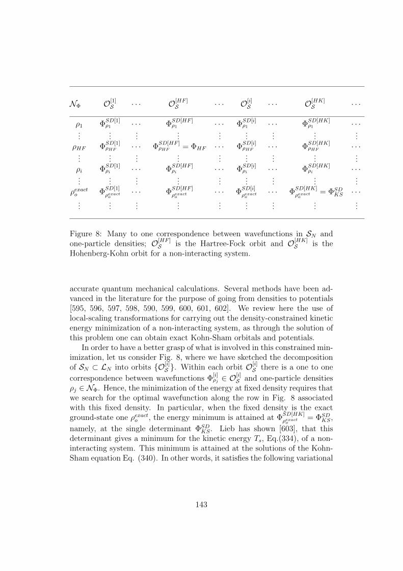
NΦ O[1]S · · · O[HF ]

S · · · O[i]S · · · O[HK]

S · · ·

ρ1 ΦSD[1]ρ1 · · · Φ

SD[HF ]ρ1 · · · Φ

SD[i]ρ1 · · · Φ

SD[HK]ρ1 · · ·

......

......

......

......

...ρHF Φ

SD[1]ρHF · · · Φ

SD[HF ]ρHF = ΦHF · · · Φ

SD[i]ρHF · · · Φ

SD[HK]ρHF · · ·

......

......

......

......

...ρi Φ

SD[1]ρi · · · Φ

SD[HF ]ρi · · · Φ

SD[i]ρi · · · Φ

SD[HK]ρi · · ·

......

......

......

......

...ρexacto Φ

SD[1]ρexacto

· · · ΦSD[HF ]ρexacto

· · · ΦSD[i]ρexacto

· · · ΦSD[HK]ρexacto

= ΦSDKS · · ·

......

......

......

......

...

Figure 8: Many to one correspondence between wavefunctions in SN andone-particle densities; O[HF ]

S is the Hartree-Fock orbit and O[HK]S is the

Hohenberg-Kohn orbit for a non-interacting system.

accurate quantum mechanical calculations. Several methods have been ad-vanced in the literature for the purpose of going from densities to potentials[595, 596, 597, 598, 590, 599, 600, 601, 602]. We review here the use oflocal-scaling transformations for carrying out the density-constrained kineticenergy minimization of a non-interacting system, as through the solution ofthis problem one can obtain exact Kohn-Sham orbitals and potentials.

In order to have a better grasp of what is involved in this constrained min-imization, let us consider Fig. 8, where we have sketched the decompositionof SN ⊂ LN into orbits O[i]

S . Within each orbit O[i]S there is a one to one

correspondence between wavefunctions Φ[i]ρj ∈ O

[i]S and one-particle densities

ρj ∈ NΦ. Hence, the minimization of the energy at fixed density requires thatwe search for the optimal wavefunction along the row in Fig. 8 associatedwith this fixed density. In particular, when the fixed density is the exactground-state one ρexacto , the energy minimum is attained at Φ

SD[HK]ρexacto

= ΦSDKS,

namely, at the single determinant ΦSDKS. Lieb has shown [603], that this

determinant gives a minimum for the kinetic energy Ts, Eq.(334), of a non-interacting system. This minimum is attained at the solutions of the Kohn-Sham equation Eq. (340). In other words, it satisfies the following variational

143

principle:

Ts[ψ[HK]ρexacto ,k(x)] ≡ 〈ΦSD[HK]

ρexacto

∣∣T ∣∣ΦSD[HK]ρexacto

〉 = min〈ΦSD[k]

ρexacto

∣∣T ∣∣ΦSD[k]ρexacto〉.

ΦSD[k]ρexacto

∈ SN

ΦSD[k]ρexacto

−→ ρexacto (x) ∈ NΦ

(356)The equivalence between this variational principle and the Kohn-Sham equa-tions given by Eq. (340) may be established as follows. Consider the variation

of Ts[φ[i]ρ,k] whose explicit form is that of Eq. (334). Let us construct the

auxiliary functional

Ω[φ[i]

ρ,k(x); Φ[i]g ]]

= Ts[φ[i]

ρ,k(x); Φ[i]g ]]−

∫d4xω(x)

( N∑k=1

φ∗[i]ρ,k(x)φ

[i]ρ,k(x)− ρexacto

)(357)

−N∑k=1

N∑l=1

Ekl(∫

d4xφ∗[i]ρ,k(x)φ

[i]ρ,l(x)− δkl

)where the generalized Lagrange multiplier ω(x) introduces the condition thatthe density be equal to ρexacto and where, in addition, the orthonormality con-dition among orbitals is taken into account. Upon variation of this auxiliaryfunctional with respect to the orbitals φ

∗[i]ρ,k(x), one obtains a system of equa-

tions that, when diagonalized, yields the canonical Kohn-Sham equations:[−1

2∇2 + ω(x)

]ψ

[HK]ρexacto ,k(x) = Ekψ[HK]

ρexacto ,k(x). (358)

Comparing Eq. (359) with Eq. (340), it is clearly seen that the Lagrangemultiplier function ω(x) takes the role of the effective Kohn-Sham potentialwhich comprises the one-particle potentials appearing in Eq. (340):

ω(x) = vKS[HK]eff

([ρexacto (x)];x

)= v(r)+vH

([ρexacto (x)]; r

)+v

KS[HK]XC,g

([ρexacto (x)];x

).

(359)Thus, it is the same whether we solve the Kohn-Sham equations (340) orwhether we deal with the constrained variational principle given by Eq. (357).

Let us now indicate how local-scaling transformations can be used in orderto carry out the constrained minimization of the kinetic energy functional[601, 602]. The strategy that we have adopted is first to select a Slater

determinant ΦSD[i]g , such as the one appearing in Eq. (328), as the trial

wavefunction which generates the particular orbit O[i]S ⊂ SN . For the case of

144

atoms, the one-particle orbitals φg,i(r) from which this Slater determinantis constructed are explicitly given by φg,nlm(r) = Rg,nl(r)Yl,ml(θ, φ), wherethe subindex i has been replaced by the quantum numbers n, l,m. The radialfunctions are expanded as

Rnl(r) =

Ml∑j=1

cnljχlj(r) (360)

where the primitive functions are assumed to be Slater-type orbitals:

χlj(r) = Nlj rnlj−1 exp(−αljr) = (2αlj)

nlj+1/2/((2nlj)!

)1/2rnlj−1 exp(−αljr).

(361)The orbitals defining the orbit-generating wavefunction (Eq. (328)) depend,

therefore, on the variational parameters α[i]lj . For a particular choice of

these parameters, say, α[i]lj we have a particular one-particle density

ρg([α[i]lj ];x) =

L∑l=0

Ml∑p=1

Ml∑q=1

GSDlpq χlp([α

[i]lj ]; r)χlq([α

[i]lj ]; r), (362)

where GSDlpq =

∑Nln=1 2(2l + 1)cnlpcnlq. Let us identify the final density with

some accurate approximation ρCI(r) to the exact ground-state density ρexacto (r)coming from a large configuration interaction wavefunction:

ρCI(r) =L∑l=0

Ml∑p=1

Ml∑q=1

GCIlpqχlp(r)χlq(r). (363)

In Eq. (364), GCIlpq =

∑Nln=1 λnl2(2l+1)cnlpcnlq and the λnl’s are the occupation

numbers of the 1-matrix. In order to distinguish the primitive functionsentering in the expansion of ρg and ρCI , the latter have been labelled by atilde. Because Eqs. (363) and (364) give analytic expressions for the initialand final densities, Eq. (173) can be explicitly integrated. The task of findingthe transformation function f(r) is, hence, changed into an interpolationproblem for a transcendental function.

Solving Eq. (173) and using the transformation function f(r), we can

generate the set of locally-scaled orbitals φ[i]ρCI ,k

(x) according to the recipe

given by Eq. (330). Specifically, the transformed radial orbitals RTnl(r) are:

RTnl(r) =

[J(f(r); r

)]1/2

Rnl(f(r)) =

[ρf (r)

ρg(f(r))

]1/2

Rnl(f(r)). (364)

145

Every time the orbital parameters are changed, one produces a new wave-function belonging to a different orbit. This follows from the one to onecorrespondence between N -representable densities and wavefunctions withina given orbit. As a result, optimization of these transformed orbitals inthe kinetic energy expression leads to the minimum value Ts[φ[HK]

ρCI ,k] corre-

sponding to the parameters α[HK]k . The orbitals φ[HK]

ρCI ,k are, in general,

non-canonical Kohn-Sham orbitals, i.e., they are solutions to Eq. (339). Inorder to generate from these functions the canonical Kohn-Sham orbitals,i.e., the solutions to Eq. (340), one must perform an orthogonal transforma-tion. In Section 5.1, we give a specific example of this constrained variationfor the case of the beryllium atom and obtain both the canonical Kohn-Shamorbitals and the exchange-correlation potential.

4.9 Spin symmetry in LS-DFT

In conventional quantum mechanics, a wavefunction describing the ground orexcited states of a many-particle system must be a simultaneous eigenfunc-tion of the set of operators that commute with the Hamiltonian. Thus, forexample, for an adequate description of an atom, in addition to the Hamilto-nian operator, one must introduce the angular momentum and spin operators

L2, S2, Lz, Sz and the parity operator Π.In variational treatments of many-particle systems in the context of con-

ventional quantum mechanics, these symmetry conditions are explicitly in-troduced either in a direct constructive fashion or by resorting to projectionoperators. In the usual versions of density functional theory, however, littleattention has been payed to this problem. The basic question, in our opinion,has to do with how to incorporate these symmetry conditions - which mustbe fulfilled by either an exact or approximate wavefunction - into the energydensity functional.

The symmetry problem is trivially solved in the local-scaling version ofdensity functional theory because we can include the symmetry conditionsin our choice of orbit-generating or initial wavefunction Φ

[i]g [604]. Since it

is from this initial wavefunction that we obtain D1[i]g and F [i]

XC,g, namely, thenon-local quantities appearing in the energy functional of Eq. (234), it followsthat the symmetry properties of the parent wavefunction are transferredto the variational functional. Notice, therefore, that symmetry is not asimportant for the density as it is for the Fermi and Coulomb holes, whichare related, to D

1[i]g and F [i]

XC,g, respectively.One of the most challenging problems in density functional theory has to

146

do with how to extend DFT to deal with multiplicities arising from spin andangular momentum restrictions on atomic and molecular systems A numberof authors have considered this problem in the context of the Hohenberg-Kohn-Sham version of DFT [605, 606, 607, 608, 609, 610, 611, 612, 613,614].We discuss in this Section how this problem can be successfully treatedin the context of LS-DFT.

The Hamiltonian operator H for atoms commutes with the total angular

momentum operators L2 and LZ , with the total spin operators S2 and SZ andwith the parity operator π. This property implies that the eigenfunctions ofH must be simultaneous eigenfunctions of all these operators. This conditionhas consequences on the structure of the 1-matrix and, hence, on the energydensity functionals discussed above.

In order to illustrate the restrictions that angular momentum and spinintroduce in density functionals, we discuss in what follows the particularcase of the carbon atom at the restricted Hartree-Fock level and constructexplicit functionals for its multiplets.

Consider the configuration 1s22s22p2 for the carbon atom. Because ofangular momentum and spin degeneracy there arise fifteen micro-states forthis configuration. Since the differences in these micro-states are due to thedifferent couplings of 2p orbitals with spin functions, we deal, for simplicityonly with 2p2. The fifteen micro-states for two equivalent 2p orbitals are[615]:

φ1 = (1+0+), φ2 = (1+0−), φ3 = (1−0−),φ4 = (1+ − 1−), φ5 = (1+ − 1−), φ6 = (1−1−),φ7 = (0+ − 1+), φ8 = (0+ − 1−), φ9 = (0− − 1−),φ10 = (1+1−), φ11 = (1−0+), φ12 = (1− − 1+),φ13 = (0− − 1+), φ14 = (−1+ − 1−), φ15 = (0+0−).

(365)

The nine functions corresponding to the 3P term are:

ψ1 = φ1, ψ2 =1√2

(φ2 + φ11), ψ3 = φ3,

ψ4 = φ4, ψ5 =1√2

(φ5 + φ12), ψ6 = φ6,

ψ7 = φ7, ψ8 =1√2

(φ8 + φ13), ψ9 = φ9.

(366)

147

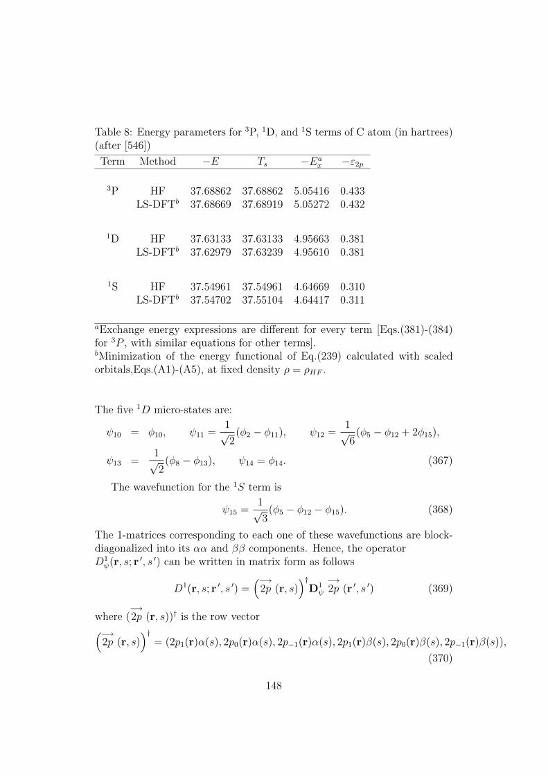
Table 8: Energy parameters for 3P, 1D, and 1S terms of C atom (in hartrees)(after [546])

Term Method −E Ts −Eax −ε2p

3P HF 37.68862 37.68862 5.05416 0.433LS-DFTb 37.68669 37.68919 5.05272 0.432

1D HF 37.63133 37.63133 4.95663 0.381LS-DFTb 37.62979 37.63239 4.95610 0.381

1S HF 37.54961 37.54961 4.64669 0.310LS-DFTb 37.54702 37.55104 4.64417 0.311

aExchange energy expressions are different for every term [Eqs.(381)-(384)for 3P , with similar equations for other terms].bMinimization of the energy functional of Eq.(239) calculated with scaledorbitals,Eqs.(A1)-(A5), at fixed density ρ = ρHF .

The five 1D micro-states are:

ψ10 = φ10, ψ11 =1√2

(φ2 − φ11), ψ12 =1√6

(φ5 − φ12 + 2φ15),

ψ13 =1√2

(φ8 − φ13), ψ14 = φ14. (367)

The wavefunction for the 1S term is

ψ15 =1√3

(φ5 − φ12 − φ15). (368)

The 1-matrices corresponding to each one of these wavefunctions are block-diagonalized into its αα and ββ components. Hence, the operatorD1ψ(r, s; r ′, s ′) can be written in matrix form as follows

D1(r, s; r ′, s ′) =(−→

2p (r, s))†

D1ψ

−→2p (r ′, s ′) (369)

where (−→2p (r, s))† is the row vector(−→

2p (r, s))†

= (2p1(r)α(s), 2p0(r)α(s), 2p−1(r)α(s), 2p1(r)β(s), 2p0(r)β(s), 2p−1(r)β(s)),

(370)

148

Table 9: Kohn-Sham x-only energy characteristics for multiplets of C atom(in Rydbergs) (after [546])

Term Value LST-DFTa LST-DFTb [614] HFc

3P −ε1s 20.766 20.706 20.707 22.651−ε2s 1.497 1.498 1.505 1.411−ε2p 0.860 0.860 0.867 0.867T 75.3756 75.3732 75.372 75.3772E -75.3706 -75.3736 -75.372 -75.3772Edx -10.0233 -10.0239 -10.0305∫

vKSρdv -121.6204 -121.4996∑i εi − T -121.6230 -121.4997 -121.530

1D −ε1s 20.698 20.622 20.607 22.703−ε2s 1.400 1.396 1.398 1.437−ε2p 0.766 0.761 0.763 0.763T 75.2628 75.2602 75.259 75.2627E -75.2575 -75.2606 -75.258 -75.2627Edx -9.9883 -9.9886 9.9935∫

vKSρdv -120.9901 -120.8187∑i εi − T -120.9929 -120.8188 -120.795

1S −ε1s 20.610 20.503 20.481 22.783−ε2s 1.268 1.252 1.252 1.479−ε2p 0.639 0.623 0.623 0.620T 75.1000 75.0966 75.099 75.0992E -75.0919 -75.0970 -75.094 -75.0992Edx -9.9325 -9.9321 9.9349∫

vKSρdv -120.1318 -119.8523∑i εi − T -120.1355 -119.8523 -119.811

aMinimization of kinetic energy calculated with scaled orbitals, Eqs.(A1)-(A5), at fixed density ρ = ρHF .bMinimization of kinetic HF energy calculated with scaled even-temperedorbitals(eight-term for s- and six-term for p-orbitals) at fixed densityρ = ρHF .cThe HF values obtained by numerical program of Froese-Fischer [616].dCalculated with spherical averaging (see, e.g., [617] with Slater orbitals,Eqs.(A1)-(A5) at the fixed ρ = ρHF

149

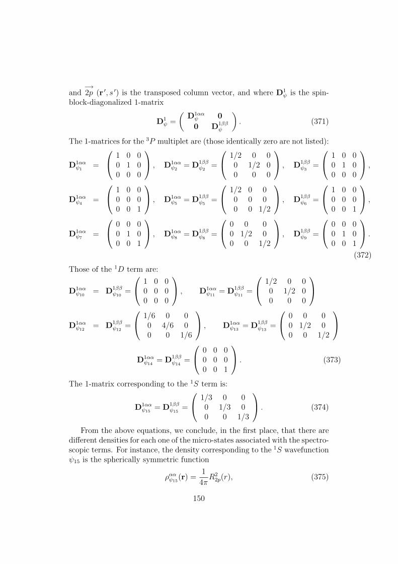
and−→2p (r ′, s ′) is the transposed column vector, and where D1

ψ is the spin-block-diagonalized 1-matrix

D1ψ =

(D1ααψ 0

0 D1ββψ

). (371)

The 1-matrices for the 3P multiplet are (those identically zero are not listed):

D1ααψ1

=

1 0 00 1 00 0 0

, D1ααψ2

= D1ββψ2

=

1/2 0 00 1/2 00 0 0

, D1ββψ3

=

1 0 00 1 00 0 0

,

D1ααψ4

=

1 0 00 0 00 0 1

, D1ααψ5

= D1ββψ5

=

1/2 0 00 0 00 0 1/2

, D1ββψ6

=

1 0 00 0 00 0 1

,

D1ααψ7

=

0 0 00 1 00 0 1

, D1ααψ8

= D1ββψ8

=

0 0 00 1/2 00 0 1/2

, D1ββψ9

=

0 0 00 1 00 0 1

.

(372)

Those of the 1D term are:

D1ααψ10

= D1ββψ10

=

1 0 00 0 00 0 0

, D1ααψ11

= D1ββψ11

=

1/2 0 00 1/2 00 0 0

D1ααψ12

= D1ββψ12

=

1/6 0 00 4/6 00 0 1/6

, D1ααψ13

= D1ββψ13

=

0 0 00 1/2 00 0 1/2

D1ααψ14

= D1ββψ14

=

0 0 00 0 00 0 1

. (373)

The 1-matrix corresponding to the 1S term is:

D1ααψ15

= D1ββψ15

=

1/3 0 00 1/3 00 0 1/3

. (374)

From the above equations, we conclude, in the first place, that there aredifferent densities for each one of the micro-states associated with the spectro-scopic terms. For instance, the density corresponding to the 1S wavefunctionψ15 is the spherically symmetric function

ρααψ15(r) =

1

4πR2

2p(r), (375)

150

whereas, the density for the MS = 0 and ML = 0 wavefunction ψ5 of the 3Pterm is

ρααψ5(r) =

3

8πR2

2p(r) sin2 θ, (376)

and that for the MS = 0 and ML = 0 wavefunction ψ12 of the 1D term is

ρααψ12(r) =

1

8πR2

2p(r)(sin2 θ + 4 cos2 θ). (377)

Nevertheless, for the 3P ensemble operator

D2([3P ]r1, s1, r2, s2; r ′1, s′1, r′2, s′2) =

1

9

9∑i=1

|ψi(r1, s1, r2, s2)〉〈ψi(r ′1, s ′1r ′2, s ′2)|

(378)the ensemble 1-matrix becomes exactly that of the 1S term and is given byEq. (375) and, hence, the ensemble density becomes the spherically symmet-ric function of Eq. (376). The same 1-matrix (376) is also found for the 1Densemble operator

D2([1D]r1, s1, r2, s2; r ′1, s′1, r′2, s′2) =

1

5

14∑i=10

|ψi(r1, s1, r2, s2)〉〈ψi(r ′1, s ′1r ′2, s ′2)|.

(379)In the second place, we observe that for the calculation of the kinetic

energy for the carbon atom (whose ground-state is 3P ) it does not matterwhether we use the ensemble 1-matrix or any one of the 1-matrices corre-sponding to the 3P micro-states. The point is that, because the angularpart is integrated out, we obtain the same kinetic energy functional for allmicro-states belonging to this term. In fact, any one of the micro-states be-longing to the 3P , 1D or 1S terms yield the same kinetic energy functional.Moreover, since the ensemble 1-matrices for the 3P and 1D terms are thesame and are equal to the 1-matrix of the 1S state, it follows that the kineticenergy functional does not discriminate among micro-states or ensembles (atleast those with equal weights [614]).

In spite of the fact that all micro-states and ensembles yield the samekinetic energy functional, they do not lead to the same kinetic energy valuebecause the radial densities of the different multiplets are not equal. Thispoint is illustrated in Table 8, where we present several values for the kineticenergy of the carbon atom multiplets, evaluated by direct minimization ofthe total energy functional with the restriction - imposed by means of local-scaling transformations- that the minimizing orbitals yield the radial Hartree-Fock density of the particular multiplet.

151

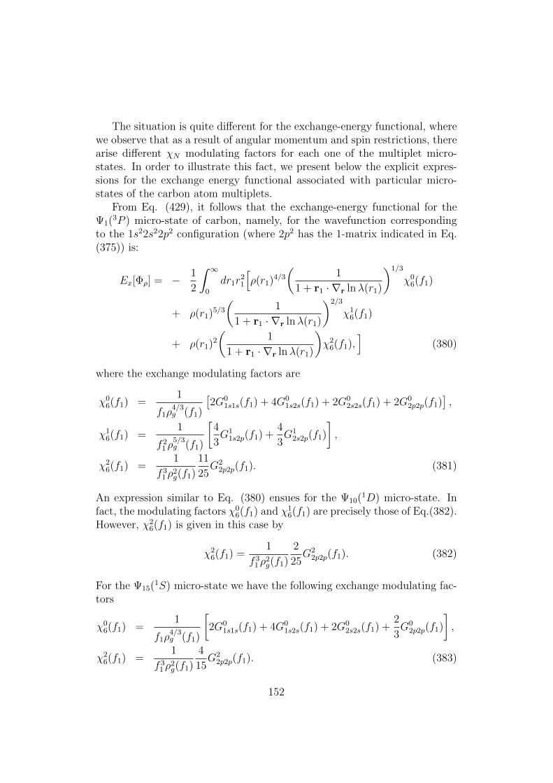
The situation is quite different for the exchange-energy functional, wherewe observe that as a result of angular momentum and spin restrictions, therearise different χN modulating factors for each one of the multiplet micro-states. In order to illustrate this fact, we present below the explicit expres-sions for the exchange energy functional associated with particular micro-states of the carbon atom multiplets.

From Eq. (429), it follows that the exchange-energy functional for theΨ1(3P ) micro-state of carbon, namely, for the wavefunction correspondingto the 1s22s22p2 configuration (where 2p2 has the 1-matrix indicated in Eq.(375)) is:

Ex[Φρ] = − 1

2

∫ ∞0

dr1r21

[ρ(r1)4/3

(1

1 + r1 · ∇r lnλ(r1)

)1/3

χ06(f1)

+ ρ(r1)5/3

(1

1 + r1 · ∇r lnλ(r1)

)2/3

χ16(f1)

+ ρ(r1)2

(1

1 + r1 · ∇r lnλ(r1)

)χ2

6(f1),]

(380)

where the exchange modulating factors are

χ06(f1) =

1

f1ρ4/3g (f1)

[2G0

1s1s(f1) + 4G01s2s(f1) + 2G0

2s2s(f1) + 2G02p2p(f1)

],

χ16(f1) =

1

f 21ρ

5/3g (f1)

[4

3G1

1s2p(f1) +4

3G1

2s2p(f1)

],

χ26(f1) =

1

f 31ρ

2g(f1)

11

25G2

2p2p(f1). (381)

An expression similar to Eq. (380) ensues for the Ψ10(1D) micro-state. Infact, the modulating factors χ0

6(f1) and χ16(f1) are precisely those of Eq.(382).

However, χ26(f1) is given in this case by

χ26(f1) =

1

f 31ρ

2g(f1)

2

25G2

2p2p(f1). (382)

For the Ψ15(1S) micro-state we have the following exchange modulating fac-tors

χ06(f1) =

1

f1ρ4/3g (f1)

[2G0

1s1s(f1) + 4G01s2s(f1) + 2G0

2s2s(f1) +2

3G0

2p2p(f1)

],

χ26(f1) =

1

f 31ρ

2g(f1)

4

15G2

2p2p(f1). (383)

152

In this case χ16(f1) is the same as that of Eq. (381).

In Table 9, we present LS-DFT results for the multiplets of carbon. Welist for comparison the corresponding Hartree-Fock values. The LS-DFTcalculations are based on a density-constrained minimization of the energyfunctional described by Eq.(275) where Φg is the multiplet wavefunction con-structed from the set of generalized Slater-type orbitals (A1)-(A5) (in thiscase, one of the wavefunctions Ψi). The multiplet Hartree-Fock densitieswere taken to be the constraining ones. Although we do not show the partic-ular exchange energies for each one of the micro-states (they have differentvalues which, however, when combined with the direct Coulomb term lead tothe same two-electron energy expression for each multiplet), we do presentthe average exchange energy which, for example, for the 3P multiplet is

Eavx

(3

P)≡ 1

9

9∑i=1

Ex

[Ψi

(3

P)]

= −G0(1s1s)− 2G0(1s2s)−G0(2s2s)

−2

3G1(1s2p)− 2

3G1(2s2p) +G0(2p2p)− 6

25G2(2p2p),

(384)

where Gk(ij) are the usual exchange integrals [346]. The results obtainedby means of the explicit energy-density functionals advanced here lead tovalues which are in close agreement with the Hartree-Fock ones. The errorin all cases studied is of the order of millihartrees. Moreover, all the energiescalculated satisfy the variational principle as they are upper bounds to theHartree-Fock results. In particular, the value of the ε2p orbital energy is inexcellent agreement with the corresponding Hartree-Fock value.

In Table 9, we present results of density-constrained kinetic energy mini-mizations for these multiplets, namely, Kohn-Sham exchange-only values forsingle-particle energies, kinetic, exchange and total energies. In addition weinclude values for

∫vKSρdv and

∑i εi−T . For comparison we have also listed

Hartree-Fock as well as values recently reported by Nagy [614]. The local-scaling transformation results have been obtained by using both generalizedSlater-type orbitals and even-tempered orbital expansions (with eight func-tions for s- and six functions for p-orbitals). We observe, in the first place,that although the kinetic energies obtained from the even-tempered orbitalexpansion show improvements of the order of millihartrees with respect tothose based on generalized Slater-type orbitals, they are still above those pre-sented by Nagy [614] (Rydbergs are used in this Table for ease of comparisonwith Nagy’s results). But, in view of the fact that the even-tempered orbitalbasis is flexible enough, our results should closely approach the extremum of

153

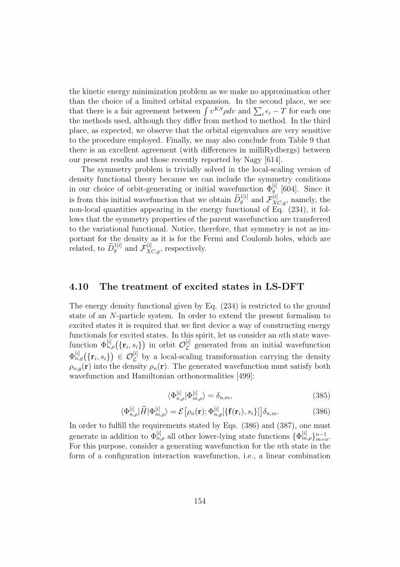
the kinetic energy minimization problem as we make no approximation otherthan the choice of a limited orbital expansion. In the second place, we seethat there is a fair agreement between

∫vKSρdv and

∑i εi − T for each one

the methods used, although they differ from method to method. In the thirdplace, as expected, we observe that the orbital eigenvalues are very sensitiveto the procedure employed. Finally, we may also conclude from Table 9 thatthere is an excellent agreement (with differences in milliRydbergs) betweenour present results and those recently reported by Nagy [614].

The symmetry problem is trivially solved in the local-scaling version ofdensity functional theory because we can include the symmetry conditionsin our choice of orbit-generating or initial wavefunction Φ

[i]g [604]. Since it

is from this initial wavefunction that we obtain D1[i]g and F [i]

XC,g, namely, thenon-local quantities appearing in the energy functional of Eq. (234), it fol-lows that the symmetry properties of the parent wavefunction are transferredto the variational functional. Notice, therefore, that symmetry is not as im-portant for the density as it is for the Fermi and Coulomb holes, which arerelated, to D

1[i]g and F [i]

XC,g, respectively.

4.10 The treatment of excited states in LS-DFT

The energy density functional given by Eq. (234) is restricted to the groundstate of an N -particle system. In order to extend the present formalism toexcited states it is required that we first device a way of constructing energyfunctionals for excited states. In this spirit, let us consider an nth state wave-function Φ

[i]n,ρ

(ri, si

)in orbit O[i]

L generated from an initial wavefunction

Φ[i]n,g

(ri, si

)∈ O[i]

L by a local-scaling transformation carrying the densityρn,g(r) into the density ρn(r). The generated wavefunction must satisfy bothwavefunction and Hamiltonian orthonormalities [499]:

〈Φ[i]n,ρ|Φ[i]

m,ρ〉 = δn,m, (385)

〈Φ[i]n,ρ|H|Φ[i]

m,ρ〉 = E[ρn(r); Φ[i]

n,g[f(ri), si]]δn,m. (386)

In order to fulfill the requirements stated by Eqs. (386) and (387), one must

generate in addition to Φ[i]n,ρ all other lower-lying state functions Φ[i]

m,ρn−1m=o.

For this purpose, consider a generating wavefunction for the nth state in theform of a configuration interaction wavefunction, i.e., a linear combination

154

of configuration state functions:

Φ[i]n,g

(ri, si

)=

M∑I=1

CnI,gψ

CSF [i]I,g

(ri, si

)≡ ~Cn

g~ψCSF [i]†g , (387)

where ~Cng = (Cn

1,g, ..., CnM,g),

~ψCSF [i]g ≡ (ψ

CSF [i]1,g , ..., ψ

CSF [i]M,g ) and ~ψ

CSF [i]†g is its

transposed. Let us assume that the expansion coefficients are generated bysolving the eigenvalue problem

H~Cn†g = EnS~C

n†g , (388)

where the matrix elements of H and S are

HIJ = 〈ψCSF [i]I,g |H|ψCSF [i]

J,g 〉, SIJ = 〈ψCSF [i]I,g |ψCSF [i]

J,g 〉. (389)

In this way the fulfillment of wavefunction and Hamiltonian orthogonality isguaranteed.

By means of a local-scaling transformation carrying the initial densityρn,g(r) into the object density ρn(r), we can obtain a transformation functionfn(r) from which, in turn, we can generate the transformed wavefunctions

Φ[i]m,ρ

(ri, si

)=

M∑I=1

CmI,gψ

CSF [i]I,ρ

(ri, si

)≡ ~Cm

g~ψCSF [i]†ρ (390)

for all states m = 0, ..., n.Because local-scaling transformations preserve the orthonormality of basis

functions, condition (386) is immediately fulfilled. Hamiltonian orthogonal-ity, Eq.(387), however, is not satisfied. For this reason, one must solve theeigenvalue equation [499]

H[ρn, ~Cρn ]~Cn†ρn = EnS[ρn, ~Cρn ]~Cn†

ρn (391)

so as to obtain wavefunctions which satisfy Eq. (55). In Eq. (60) we em-phasize the fact that the matrix elements depend on the final density ρn.Moreover, because this density is obtained from the transformed wavefunc-tion, they also depend on the expansion coefficients. Thus, Eq. (60) must besolved iteratively. In Subsection 4.10.1 we present some results obtained bythe above procedure for the 21S state of the helium atom.

In the local-scaling procedure embodied in Eq. (391) because the opti-mization is performed with respect to the particular density ρn correspondingto the excited state Φ

[i]n,ρ

(ri, si

), one is searching for an energy E

[ρn(r); Φ

[i]n,g]

which is an upper bound to the exact energy En,exact. This upper-bound

155

character of the calculated energy is guaranteed by the Hylleraas-Undheim-MacDonald theorem.

A generalization of the above procedure can be readily made by a con-certed local-scaling transformation which carries an initial density ρg(r) ≡1M

∑M−1j=0 ρj,g(r) into a final density ρ(r) ≡ 1

M

∑M−1j=0 ρj(r). As discussed

elsewhere [500], this generalization corresponds to adopting Katriel’s super-particle approach. Again, the upper-bound character is preserved by the factthat

∑M−1j=0 E

[ρn(r); Φ

[i]n,g ≥

∑M−1j=0 Ej,exact.

The energy density functional given by Eq. (234) is restricted to theground state of an N -particle system. In order to extend the present formal-ism to excited states it is required that we first device a way of constructingenergy functionals for excited states. In this spirit, let us consider an nthstate wavefunction Φ

[i]n,ρ

(ri, si

)in orbit O[i]

L generated from an initial wave-

function Φ[i]n,g

(ri, si

)∈ O[i]

L by a local-scaling transformation carrying thedensity ρn,g(r) into the density ρn(r). The generated wavefunction mustsatisfy both wavefunction and Hamiltonian orthonormalities [499]:

〈Φ[i]n,ρ|Φ[i]

m,ρ〉 = δn,m, (392)

〈Φ[i]n,ρ|H|Φ[i]

m,ρ〉 = E[ρn(r); Φ[i]

n,g[f(ri), si]]δn,m. (393)

In order to fulfill the requirements stated by Eqs. (386) and (387), one must

generate in addition to Φ[i]n,ρ all other lower-lying state functions Φ[i]

m,ρn−1m=o.

For this purpose, consider a generating wavefunction for the nth state in theform of a configuration interaction wavefunction, i.e., a linear combinationof configuration state functions:

Φ[i]n,g

(ri, si

)=

M∑I=1

CnI,gψ

CSF [i]I,g

(ri, si

)≡ ~Cn

g~ψCSF [i]†g , (394)

where ~Cng = (Cn

1,g, ..., CnM,g),

~ψCSF [i]g ≡ (ψ

CSF [i]1,g , ..., ψ

CSF [i]M,g ) and ~ψ

CSF [i]†g is its

transposed. Let us assume that the expansion coefficients are generated bysolving the eigenvalue problem

H~Cn†g = EnS~C

n†g , (395)

where the matrix elements of H and S are

HIJ = 〈ψCSF [i]I,g |H|ψCSF [i]

J,g 〉, SIJ = 〈ψCSF [i]I,g |ψCSF [i]

J,g 〉. (396)

In this way the fulfillment of wavefunction and Hamiltonian orthogonality isguaranteed.

156

By means of a local-scaling transformation carrying the initial densityρn,g(r) into the object density ρn(r), we can obtain a transformation functionfn(r) from which, in turn, we can generate the transformed wavefunctions

Φ[i]m,ρ

(ri, si

)=

M∑I=1

CmI,gψ

CSF [i]I,ρ

(ri, si

)≡ ~Cm

g~ψCSF [i]†ρ (397)

for all states m = 0, ..., n.Because local-scaling transformations preserve the orthonormality of basis

functions, condition (54) is immediately fulfilled. Hamiltonian orthogonality(Eq. (55)), however, is not satisfied. For this reason, one must solve theeigenvalue equation [499]

H[ρn, ~Cρn ]~Cn†ρn = EnS[ρn, ~Cρn ]~Cn†

ρn (398)

so as to obtain wavefunctions which satisfy Eq. (386). In Eq. (401) weemphasize the fact that the matrix elements depend on the final density ρn.Moreover, because this density is obtained from the transformed wavefunc-tion, they also depend on the expansion coefficients. Thus, Eq. (401) mustbe solved iteratively. In Section 5.5 we present some results obtained by theabove procedure for the 21S state of the helium atom.

In the local-scaling procedure embodied in Eq. (60) because the optimiza-tion is performed with respect to the particular density ρn corresponding tothe excited state Φ

[i]n,ρ

(ri, si

), one is searching for an energy E

[ρn(r); Φ

[i]n,g]

which is an upper bound to the exact energy En,exact. This upper-boundcharacter of the calculated energy is guaranteed by the Hylleraas-Undheim-MacDonald theorem.

A generalization of the above procedure can be readily made by a con-certed local-scaling transformation which carries an initial density ρg(r) ≡1M

∑M−1j=0 ρj,g(r) into a final density ρ(r) ≡ 1

M

∑M−1j=0 ρj(r). As discussed

elsewhere [500], this generalization corresponds to adopting Katriel’s super-particle approach. Again, the upper-bound character is preserved by the factthat

∑M−1j=0 E

[ρn(r); Φ

[i]n,g ≥

∑M−1j=0 Ej,exact.

In conventional quantum mechanics, a wavefunction describing the groundor excited states of a many-particle system must be a simultaneous eigenfunc-tion of the set of operators that commute with the Hamiltonian. Thus, forexample, for an adequate description of an atom, in addition to the Hamilto-nian operator, one must introduce the angular momentum and spin operators

L2, S2, Lz, Sz and the parity operator Π.In variational treatments of many-particle systems in the context of con-

ventional quantum mechanics, these symmetry conditions are explicitly in-troduced either in a direct constructive fashion or by resorting to projection

157

operators. In the usual versions of density functional theory, however, littleattention has been payed to this problem. The basic question, in our opinion,has to do with how to incorporate these symmetry conditions - which mustbe fulfilled by either an exact or approximate wavefunction - into the energydensity functional.

The symmetry problem is trivially solved in the local-scaling version ofdensity functional theory because we can include the symmetry conditionsin our choice of orbit-generating or initial wavefunction Φ

[i]g [604]. Since it

is from this initial wavefunction that we obtain D1[i]g and F [i]

XC,g, namely, thenon-local quantities appearing in the energy functional of Eq. (234), it followsthat the symmetry properties of the parent wavefunction are transferredto the variational functional. Notice, therefore, that symmetry is not asimportant for the density as it is for the Fermi and Coulomb holes, whichare related, to D

1[i]g and F [i]

XC,g, respectively.The energy density functional given by Eq. (234) is restricted to the

ground state of an N -particle system. In order to extend the present formal-ism to excited states it is required that we first device a way of constructingenergy functionals for excited states. In this spirit, let us consider an nthstate wavefunction Φ

[i]n,ρ

(ri, si

)in orbit O[i]

L generated from an initial wave-

function Φ[i]n,g

(ri, si

)∈ O[i]

L by a local-scaling transformation carrying thedensity ρn,g(r) into the density ρn(r). The generated wavefunction mustsatisfy both wavefunction and Hamiltonian orthonormalities [499]:

〈Φ[i]n,ρ|Φ[i]

m,ρ〉 = δn,m, (399)

〈Φ[i]n,ρ|H|Φ[i]

m,ρ〉 = E[ρn(r); Φ[i]

n,g[f(ri), si]]δn,m. (400)

In order to fulfill the requirements stated by Eqs. (386) and (387), one must

generate in addition to Φ[i]n,ρ all other lower-lying state functions Φ[i]

m,ρn−1m=o.

For this purpose, consider a generating wavefunction for the nth state in theform of a configuration interaction wavefunction, i.e., a linear combinationof configuration state functions:

Φ[i]n,g

(ri, si

)=

M∑I=1

CnI,gψ

CSF [i]I,g

(ri, si

)≡ ~Cn

g~ψCSF [i]†g , (401)

where ~Cng = (Cn

1,g, ..., CnM,g),

~ψCSF [i]g ≡ (ψ

CSF [i]1,g , ..., ψ

CSF [i]M,g ) and ~ψ

CSF [i]†g is its

transposed. Let us assume that the expansion coefficients are generated bysolving the eigenvalue problem

H~Cn†g = EnS~C

n†g , (402)

158

where the matrix elements of H and S are

HIJ = 〈ψCSF [i]I,g |H|ψCSF [i]

J,g 〉, SIJ = 〈ψCSF [i]I,g |ψCSF [i]

J,g 〉. (403)

In this way the fulfillment of wavefunction and Hamiltonian orthogonality isguaranteed.

By means of a local-scaling transformation carrying the initial densityρn,g(r) into the object density ρn(r), we can obtain a transformation functionfn(r) from which, in turn, we can generate the transformed wavefunctions

Φ[i]m,ρ

(ri, si

)=

M∑I=1

CmI,gψ

CSF [i]I,ρ

(ri, si

)≡ ~Cm

g~ψCSF [i]†ρ (404)

for all states m = 0, ..., n.Because local-scaling transformations preserve the orthonormality of basis

functions, condition (386) is immediately fulfilled. Hamiltonian orthogonality(Eq. (387)), however, is not satisfied. For this reason, one must solve theeigenvalue equation [499]

H[ρn, ~Cρn ]~Cn†ρn = EnS[ρn, ~Cρn ]~Cn†

ρn (405)

so as to obtain wavefunctions which satisfy Eq. (387). In Eq. (401) weemphasize the fact that the matrix elements depend on the final density ρn.Moreover, because this density is obtained from the transformed wavefunc-tion, they also depend on the expansion coefficients. Thus, Eq. (60) must besolved iteratively. In Section 4.10.1 we present some results obtained by theabove procedure for the 21S state of the helium atom.

In the local-scaling procedure embodied in Eq. (60) because the optimiza-tion is performed with respect to the particular density ρn corresponding tothe excited state Φ

[i]n,ρ

(ri, si

), one is searching for an energy E

[ρn(r); Φ

[i]n,g]

which is an upper bound to the exact energy En,exact. This upper-boundcharacter of the calculated energy is guaranteed by the Hylleraas-Undheim-MacDonald theorem.

A generalization of the above procedure can be readily made by a con-certed local-scaling transformation which carries an initial density ρg(r) ≡1M

∑M−1j=0 ρj,g(r) into a final density ρ(r) ≡ 1

M

∑M−1j=0 ρj(r). As discussed

elsewhere [500], this generalization corresponds to adopting Katriel’s super-particle approach. Again, the upper-bound character is preserved by the factthat

∑M−1j=0 E

[ρn(r); Φ

[i]n,g ≥

∑M−1j=0 Ej,exact.

4.10.1. Calculation of the excited state 2 1S for the he-lium atom

159

In order to illustrate the treatment of excited states in the local-scaling ver-sion of density functional theory, consider an orbit-generating wavefunction(see Eq. (56)) [499]

Φ[1]1,g = C1

1,g[1s2] + C1

2,g[1s2s] + C13,g[2s

2], (406)

for the first excited singlet state 21S of helium. The orbitals entering into inEq. (407) are hydrogenic functions defined by

1s = (α3/π)1/2exp(−α r),2s = [β3/π(3λ2 − 3λ+ 1)]1/2(1− λβ r)exp(−β r). (407)

We require that λ = (α+β)/3β in order to guarantee orbital orthonormality,i.e., 〈1s|2s〉 = 0. The one-particle density for the first excited state arisingfrom the above wavefunction is

ρ1,g(r) =(2(C1

1,g)2 + (C1

2,g)2)(1s)2 + 2

√2C1

2,g(2C11,g + C1

3,g)(1s2s)

+((C1

2,g)2 + 2(C1

3,g)2)(2s)2. (408)

The optimal untransformed wavefunction gives the best 21S energy E1,g =−2.143 000 6 hartrees for the optimum orbital parameters

α = 1.99176, β = 0.52058, (409)

with the corresponding eigenvector

C11,g = 0.12066 C1

2,g = 0.99256 C13,g = −0.01614. (410)

Assuming that the final density has the form given by Eq. (343), we canperform a local-scaling transformation and following the procedure advancedin Section 4.5.9, optimize the parameters α and β of the initial orbitals, theexpansion coefficients (which are automatically optimized by matrix diago-nalization) and the parameters of the final density. When this is done, weobtain for the optimal density parameters reported in Koga [499] (namely,for a density such as the one given in Eq. (343) with i = 1, ..., 4, but wherea1 and b1 are set at the fixed values of 1 and 0, respectively), the energyvalue E1,g = −2.144 140 3 hartrees. This value, although coming from a verysimple trial wavefunction, is already quite close to the exact energy which isE1,g = −2.145 974 0 hartrees [618, 619]. Thus, again, we show that the local-scaling version of density functional theory leads to upper bounds to theexact energies. Clearly, the exact values can be obtained when the variationis carried out in an orbit which is sufficiently close to the Hohenberg-Kohnorbit, where by definition, the exact wavefunctions for the ground and ex-cited states are found.

160

5 LST-DFT: APPLICATIONS: FROM ATOMS,

VIA DIATOMICS, TO CLUSTERS

According to the paradigm of science, experiment always plays a role as acriterion of truth for any theory or model. In modern science, this criterionhas been replaced by, or shifted to, the computational experiment whose goalconsists in performing computational simulations of a given theory (model)and in comparing the results with the data, either obtained from previousexperiments or from a correct general theory. The intention of this Section isfirst, to present some computational applications of LS-DFT and compare theresults obtained with both HKS-DFT results and other data, e. g. ab initioor/and experimental data. Another aim, nevertheless, has to do with showingthat in its local-scaling version, density functional theory recovers all thecharacteristics of traditional quantum mechanics in the sense that it can yieldin a consistent framework results that can be systematically improved. This,in a sense is important because there is the accepted dogma that because theexact ”universal” functional is unattainable, all we are left to do is toy withapproximations. Certainly, LS-DFT shows that there is a rigorous methodfor constructing functionals to any desired degree of accuracy. But, as italways happens with rigor, there is a price one has to pay in terms of thecomplexity of the theory and of the difficulties arising in its implementation.

It is worth noticing that the local-scaling version of density functionaltheory is still in its infancy with regard to its applications. Below we onlyshow those examples which emphasize some strengths of this approach, suchas, for example, preserving the N-representability. As being formally exact- as inferred from the general quantum variational principle - in order tobecome a useful tool in the hands of practicing quantum chemists, LST-DFT requires that a number of numerical developments be carried out. Theproblem is that some of the methods for energy improvement, such as, for ex-ample, those indicated in Subsections 4.6.1, 4.6.2 and 4.6.3 demand that wedepart substantially from the usual quantum chemical approaches based onatomic or molecular orbitals, or density functional theory formulations basedon local or non-local approximations. Moreover, if we were to employ meth-ods that use Kohn-Sham-like orbitals, such as those advanced in Subsections4.6.3 and 4.6.4, we face the problem of handling the exchange-correlationfunctional in a manner entirely different from that applied in the case oflocal and non-local density functional approximations. Only those methodsdescribed in Subsections 4.6.5 and 4.6.6 and 4.7.1 can be implemented by astraightforward incorporation of local-scaling transformations to numericalatomic or molecular programs.

161

Although work is being done along the non-traditional lines, in practi-cal terms, it is much easier to develop methods which do not require sub-stantial new programming. For this reason, we present here non-variational(Subsection 5.1.2) and variational (Subsection 5.1.3) calculations of atomicconfiguration wavefunctions. They correspond to realizations of the methodsadvanced in Subsections 4.6.5, 4.6.6 and 4.7.1. In addition, we present resultsof density-constrained calculations. These fall into two categories. One com-prises the optimization of a wavefunction at the fixed Hartree-Fock density(Subsection 5.1.1), and the other the determination of the minimum for thenon-interacting kinetic energy at fixed “exact” density (Section 5.1.4).

For atoms, we have taken as a prototype the beryllium atom. The rea-son for this choice stems from the fact that in this four-electron system onefinds already a great deal of the complexities present in larger systems. Tocomputation-oriented readers, our choice of such small system for the purposeof illustrating the application of the local-scaling version of density functionaltheory, might seem somewhat inadequate. In fact, due to the staggering de-velopment of computational methods based on the Hohenberg-Kohn-Shamversion of density functional theory, quantum chemists have become accus-tomed to associating density functional methods with the calculation of largemolecules. Let us remark, however, that our intention is to present here num-bers that arise from rigorous procedures which lead eventually to the exactsolution of the quantum mechanical many-body problem. In this vein, weemphasize in the calculations discussed below the capability of the presenttheory to produce strict upper bounds. This theory allows us, in addition,to improve these upper bounds until a desired accuracy is attained.

In the case of molecules we discuss some first-row hydrides and homonu-clear diatomic molecules. As for clusters, we discuss an application to sodiumand aluminum clusters.

5.1 LST-DFT: Applications to the beryllium atom

The Hartree-Fock method involves the optimization - via energy minimiza-tion - of a single Slater determinant wavefunction. This process is usuallycarried out by solving the single-particle Hartree-Fock equations. From theHartree-Fock orbitals one can construct the Hartree-Fock density ρHF . Thus,in the spirit of the local-scaling version of density functional theory, we dealbelow with the calculation of the Hartree-Fock wavefunction and energy bymeans of a constrained variation at fixed density ρ(r) = ρHF (r) as well as byintra-orbit and inter-orbit optimizations.

162

In what follows, we also present calculations of intra- and inter-orbit op-timizations for the ground state 1S of the belyllium atom. For the firstexample, we take the simplest type of CI expansion, namely, a single Slaterdeterminant for the configuration [1s22s2] and apply variational and non-variational techniques to determine upper bounds to the Hartree-Fock en-ergy. For the second example, we take a configuration interaction expansioncontaining the configurations [1s22s2], [1s22p2], [2p22s2] and [1s2s2p2].

5.1.1. Calculation of the energy and wavefunction forthe beryllium atom at the Hartree-Fock level by in thecontext of local-scaling transformations

Consider an orbit-generating wavefunction, ΦSD[i]g [xi] such as the one given

by Eq. (328), constructed from the atomic orbitals φ[i]g,k(xi) which are

products of radial functions times spherical harmonics. We assume that theradial functions are expanded as in Eq. (361) in terms of Slater type orbitals(Eq. (362)). The energy as a functional of the density and of the orbit-generating wavefunction is given by

E[ρ(x); ΦSD[i]

g [fi]

= E[ρ(x); φ[i]

ρ,k(xi)], (411)

where in the right-hand side, we have emphasized the fact that the energyis a functional of both the density and of the density-transformed orbitalsφ[i]

ρ,k(xi). For the beryllium atom at the Hartree-Fock level, these trans-

formed orbitals are 1sT [i] ≡ φ[i]ρ,100(r) = R

T [i]10 (r)/

√4π and 2sT [i] ≡ φ

[i]ρ,200(r) =

RT [i]20 (r)/

√4π. Notice that according to Eq. (330), these transformed orbitals

depend upon the generating orbitals and the initial and final densities. But,as the initial orbitals depend on the expansion coefficients c10j, c20j as wellas and on the primitive function parameters n0j, α0j, it follows that theenergy functional appearing in Eq. (412) can be expressed as

E[ρ(x); ΦSD[i]

g [fi]

= E[ρ(x); c10j, c20j, n0j, α0j

]. (412)

In Table 10, we list the initial and optimal expansion coefficients and orbitalparameters for Clementi-Roetti-type [550] 1s and 2s functions. The opti-mization procedure was carried out at fixed density ρ(r) = ρHF (r) (wherethe Hartree-Fock density is that associated with the Clementi-Roetti wave-function), taking as variational parameters the expansion coefficients and theorbital exponents. To maintain orbital orthogonality, after each change in thevariational parameters, the orbitals were subjected to Schmidt orthogonal-ization. Notice that the optimal parameters appearing in Table 1 correspondto non-canonical Hartree-Fock orbitals.

163

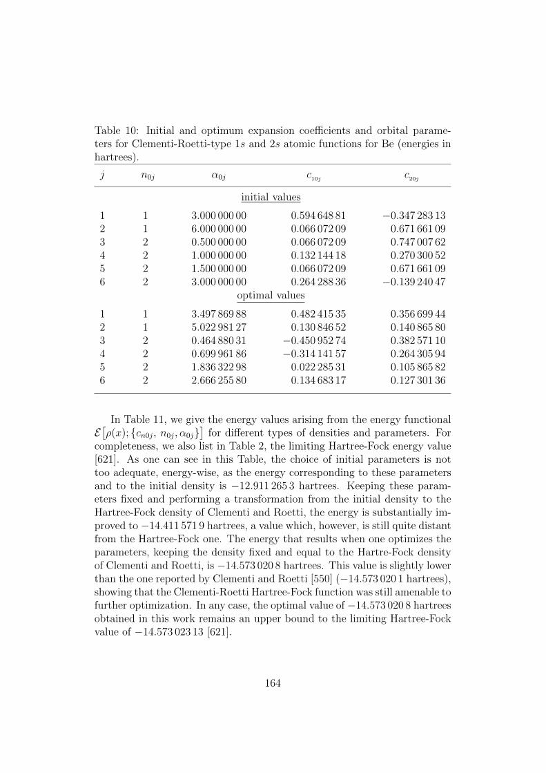
Table 10: Initial and optimum expansion coefficients and orbital parame-ters for Clementi-Roetti-type 1s and 2s atomic functions for Be (energies inhartrees).

j n0j α0j c10j

c20j

initial values

1 1 3.000 000 00 0.594 648 81 −0.347 283 132 1 6.000 000 00 0.066 072 09 0.671 661 093 2 0.500 000 00 0.066 072 09 0.747 007 624 2 1.000 000 00 0.132 144 18 0.270 300 525 2 1.500 000 00 0.066 072 09 0.671 661 096 2 3.000 000 00 0.264 288 36 −0.139 240 47

optimal values

1 1 3.497 869 88 0.482 415 35 0.356 699 442 1 5.022 981 27 0.130 846 52 0.140 865 803 2 0.464 880 31 −0.450 952 74 0.382 571 104 2 0.699 961 86 −0.314 141 57 0.264 305 945 2 1.836 322 98 0.022 285 31 0.105 865 826 2 2.666 255 80 0.134 683 17 0.127 301 36

In Table 11, we give the energy values arising from the energy functionalE[ρ(x); cn0j, n0j, α0j

]for different types of densities and parameters. For

completeness, we also list in Table 2, the limiting Hartree-Fock energy value[621]. As one can see in this Table, the choice of initial parameters is nottoo adequate, energy-wise, as the energy corresponding to these parametersand to the initial density is −12.911 265 3 hartrees. Keeping these param-eters fixed and performing a transformation from the initial density to theHartree-Fock density of Clementi and Roetti, the energy is substantially im-proved to −14.411 571 9 hartrees, a value which, however, is still quite distantfrom the Hartree-Fock one. The energy that results when one optimizes theparameters, keeping the density fixed and equal to the Hartre-Fock densityof Clementi and Roetti, is −14.573 020 8 hartrees. This value is slightly lowerthan the one reported by Clementi and Roetti [550] (−14.573 020 1 hartrees),showing that the Clementi-Roetti Hartree-Fock function was still amenable tofurther optimization. In any case, the optimal value of −14.573 020 8 hartreesobtained in this work remains an upper bound to the limiting Hartree-Fockvalue of −14.573 023 13 [621].

164

Table 11: Values (in hartrees) of the energy density functionalE[ρ; cn0j, n0j, α0j] for a single Slater determinant constructed fromClementi-Roetti-type orbitals.

density parameters E[ρ; cn0j, n0j , α0j]

initial, CRTa initial −12.911 265 3Hartree-Fock, CRb initial −14.411 571 9Hartree-Fock, CRb optimized −14.573 020 8Hartree-Fock, CRb CRb −14.573 020 1d

Limiting Hartree-Fock energyc −14.573 023 13

aCRT = Clementi-Roetti-type.bCR = Clementi-Roetti, Ref. [89]cFrom Ref. [90].dFrom Ref. [95].

5.1.2. Intra- and inter-orbit calculation of a Hartree-Fock wavefunction

Let us consider now, the optimization - by a combined intra- and inter-orbitvariation - of the energy density functional given by Eq. (412) . Clearly,when we perform an intra-orbit variation we modify the one-particle den-sity ρ(x). But when we perform an inter-orbit variation at fixed density,

we just modify the orbitals φ[i]ρ,k(xi). For simplicity, we take these orbitals

to be locally-scaled Raffenetti-type functions. The Raffenetti Rn0(r) radialorbitals [551] are expanded in terms of set of 1s Slater-type orbitals, i.e.,orbitals having n0j = 1 for all j, where the orbital exponents are defined byα0j = αβj. In the present case we do not consider the orbital coefficients asvariational parameters; these are obtained by Schmidt orthonormalizationof the Raffenetti initial values [551]. Hence, the energy density functionalbecomes explicitly:

E[ρ(x); ΦSD[i]

g [fi]

= E[ρ(x);α[i], β[i]

]. (413)

In Table 12, we list the values of the parameters α[i] and β[i] used in thepresent calculations. The values corresponding to orbit O[1]

S are arbitrary

ones. These arbitrary values give rise to a set φ[1]g,k([α

[1], β[1]];xi). FromTable 13, we see that the energy corresponding to the orbit-generating wave-function is −13.894 697 4 hartrees. The intra-orbit minimization is performedfrom the density ρg(x) to the final density ρK(x) given by Eq. (285) (wherethe summation spans from i = 1 to i = 4) having 13 variational parameters

165

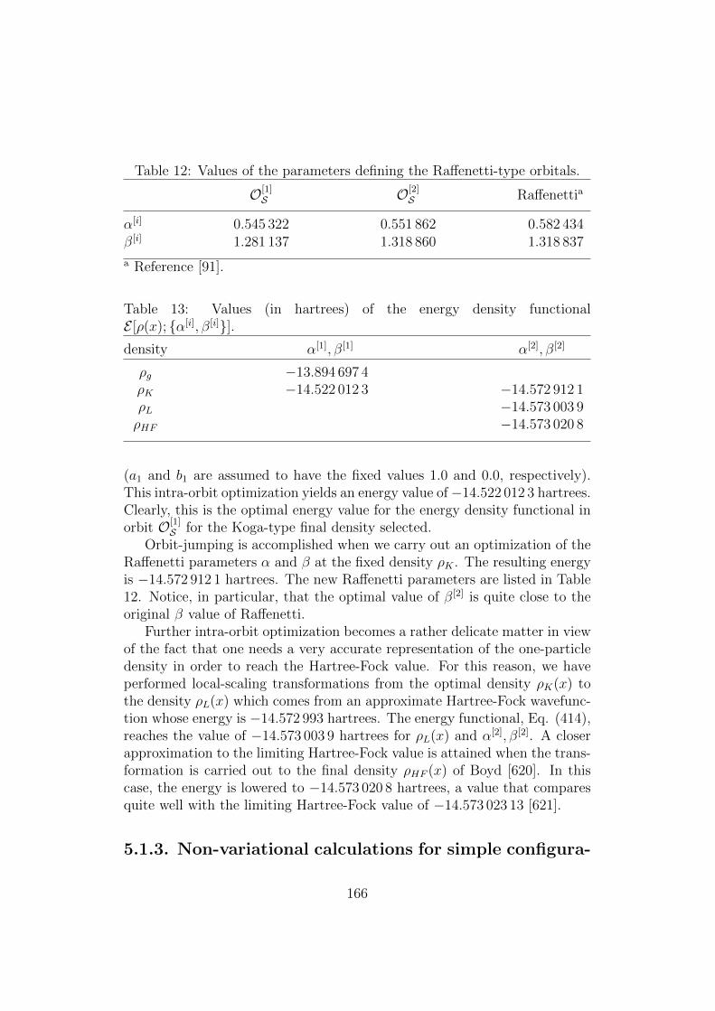
Table 12: Values of the parameters defining the Raffenetti-type orbitals.

O[1]S O[2]

S Raffenettia

α[i] 0.545 322 0.551 862 0.582 434β[i] 1.281 137 1.318 860 1.318 837

a Reference [91].

Table 13: Values (in hartrees) of the energy density functionalE [ρ(x); α[i], β[i]].density α[1], β[1] α[2], β[2]

ρg −13.894 697 4ρK −14.522 012 3 −14.572 912 1ρL −14.573 003 9ρHF −14.573 020 8

(a1 and b1 are assumed to have the fixed values 1.0 and 0.0, respectively).This intra-orbit optimization yields an energy value of−14.522 012 3 hartrees.Clearly, this is the optimal energy value for the energy density functional inorbit O[1]

S for the Koga-type final density selected.Orbit-jumping is accomplished when we carry out an optimization of the

Raffenetti parameters α and β at the fixed density ρK . The resulting energyis −14.572 912 1 hartrees. The new Raffenetti parameters are listed in Table12. Notice, in particular, that the optimal value of β[2] is quite close to theoriginal β value of Raffenetti.

Further intra-orbit optimization becomes a rather delicate matter in viewof the fact that one needs a very accurate representation of the one-particledensity in order to reach the Hartree-Fock value. For this reason, we haveperformed local-scaling transformations from the optimal density ρK(x) tothe density ρL(x) which comes from an approximate Hartree-Fock wavefunc-tion whose energy is −14.572 993 hartrees. The energy functional, Eq. (414),reaches the value of −14.573 003 9 hartrees for ρL(x) and α[2], β[2]. A closerapproximation to the limiting Hartree-Fock value is attained when the trans-formation is carried out to the final density ρHF (x) of Boyd [620]. In thiscase, the energy is lowered to −14.573 020 8 hartrees, a value that comparesquite well with the limiting Hartree-Fock value of −14.573 023 13 [621].

5.1.3. Non-variational calculations for simple configura-

166

tion interaction wavefunctions for beryllium

Let us consider a configuration interaction wavefunction for the berylliumatom such as the one given by Eq. (346). Let us take as as our primitiveorbitals a single zeta basis set formed by two s functions (χ01(r), and χ02(r))and one p function (χ11(r)) (cf. Eq. 106)). From this basis set one ob-tains the one-particle orbitals 1s, 2s and 2p which, in turn, give rise to thefollowing configurations: [1s22s2],[1s22p2],[2p22s2], and [1s2s2p2]. Thus, theexpansion of Eq. (346) runs, in the present case, over four configuration statefunctions. In Table 14, we list the orbital parameters defining three different

Table 14: Orbital parameters for the 1s, 2s and 2p functions appearing inthe configuration interaction wavefunction for Be.

1s 2s 2pj c10j c20j n0j α0j c11j n1j α1j

Set A

1 0.997 13 0.243 95 1 3.455 00 1.000 00 2 0.750 002 0.012 38 −1.026 46 2 0.970 00

Set B

1 0.997 59 0.204 44 1 3.684 78 1.000 00 2 0.981 402 0.012 39 −1.018 24 2 0.956 03

Set C

1 0.997 51 0.210 92 1 3.684 18 1.000 00 2 0.982 502 0.012 39 −1.019 49 2 0.974 37

sets of initial orbitals 1s, 2s and 2p. Set A contains arbitrary values for theorbital exponents for the s and p orbitals. In set B, these values are chosenso that the maximum of the r2χ2

01(r) coincides with the K-shell maximumof the Be Hartree-Fock density and r2χ2

02(r) and r2χ211(r), with that of the L

shell. In set C, the orbital exponents are optimized by minimizing the energyof the configuration interaction wavefunction.

The energy density functional corresponding to an orbit-generating wave-function such as the one described above is given by

E[ρ(x); Φ[i]

o,g[fi]

= E[ρ(x); Co[i]

I,ρ ]. (414)

where in the right-hand side we emphasize the fact that the orbit-generatingwavefunction for an orbit O[i]

L could correspond to the optimal wavefunction

167

obtained in an orbit-jumping minimization from the previous orbit at fixeddensity ρ(x). Since the orbital set entering in the expansion of the configu-ration interaction wavefunction remains unchanged due to the fact that thedensity is fixed, the only variational parameters are the expansion coefficientsCo[i]

I,ρ .

Table 15: Configuration interaction expansion coefficients for the approxi-mate ground-state wavefunctions Φ

[r]0,ρ(1s) of the beryllium atom for orbits

[i] = 1, . . . , 4 and densities ρ = ρg, ρHF , ρCI and ρK .

I ψCSFI,g Co[1]I,ρg

Co[2]I,ρHF

Co[3]I,ρCI

Co[4]I,ρK

Wavefunction constructed from set A

1 [1s22s2] −0.958 96 −0.957 46 −0.955 58 −0.956 312 [1s22p2] 0.283 27 0.288 37 0.294 60 0.292 243 [2s22p2] −0.012 14 −0.010 43 −0.009 33 −0.008 574 [1s2s2p2] 0.000 21 0.000 04 0.000 03 0.000 05

Wavefunction constructed from set B

1 [1s22s2] −0.950 49 −0.951 06 −0.951 31 −0.951 142 [1s22p2] 0.310 71 0.308 90 0.308 16 0.308 703 [2s22p2] −0.005 20 −0.007 50 −0.006 16 −0.006 314 [1s2s2p2] 0.000 75 0.000 79 0.000 77 0.000 77

Wavefunction constructed from set C

1 [1s22s2] −0.949 67 −0.950 09 −0.950 20 −0.950 262 [1s22p2] 0.313 21 0.311 86 0.311 55 0.311 363 [2s22p2] −0.005 16 −0.008 47 −0.007 14 −0.007 304 [1s2s2p2] 0.000 71 0.000 78 0.000 75 0.000 76

In Table 15, we list the optimal expansion coefficients calculated by diag-onalizing the Hamiltonian matrix for the configuration state functions con-structed from the transformed one-particle orbitals. These orbitals are ob-tained by applying local-scaling transformations (whose final density is ρ(x))to the initial orbitals belonging to the sets A, B and C, described above. Thefinal density, in the case of non-variational calculations, can be ρHF (x), thatis, the Hartree-Fock density obtained from the Clementi-Roetti wavefunction[550], or ρCI(x), the configuration interaction density corresponding to theEsquivel-Bunge 650-term wavefunction [622]. The density ρK(x) appearingalso in this table is the Koga density described in Eq. (285). As the param-eters for ρK(x) are determined variationally, transformations to this density

168

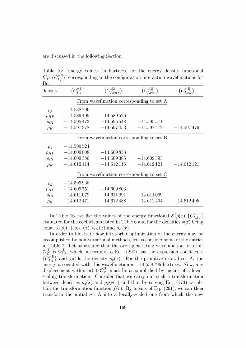
are discussed in the following Section.

Table 16: Energy values (in hartrees) for the energy density functional

E [ρ; Co[i]I,ρ ] corresponding to the configuration interaction wavefunctions for

Be.

density Co[1]I,g Co[2]

I,ρHF Co[3]

I,ρCI Co[4]

I,ρK

From wavefunction corresponding to set A

ρg −14.538 796ρHF −14.589 499 −14.589 526ρCI −14.595 473 −14.595 548 −14.595 571ρK −14.597 378 −14.597 453 −14.597 472 −14.597 476

From wavefunction corresponding to set B

ρg −14.599 524ρHF −14.609 808 −14.609 833ρCI −14.609 386 −14.609 385 −14.609 393ρK −14.612 114 −14.612 115 −14.612 121 −14.612 121

From wavefunction corresponding to set C

ρg −14.599 936ρHF −14.609 751 −14.609 803ρCI −14.611 079 −14.611 091 −14.611 099ρK −14.612 471 −14.612 488 −14.612 494 −14.612 495

In Table 16, we list the values of the energy functional E[ρ(x); Co[i]

I,ρ ]

evaluated for the coefficients listed in Table 6 and for the densities ρ(x) beingequal to ρg(x), ρHF (x), ρCI(x) and ρK(x).

In order to illustrate how intra-orbit optimization of the energy may beaccomplished by non-variational methods, let us consider some of the entriesin Table 7. Let us assume that the orbit-generating wavefunction for orbitO[1]L is Φ

[1]o,g, which, according to Eq. (297) has the expansion coefficients

Co[1]I,g and yields the density ρg(x). For the primitive orbital set A, the

energy associated with this wavefunction is −14.538 796 hartrees. Now, anydisplacement within orbit O[1]

L must be accomplished by means of a local-scaling transformation. Consider that we carry out such a transformationbetween densities ρg(x) and ρHF (x) and that by solving Eq. (173) we ob-tain the transformation function f(r). By means of Eq. (291), we can thentransform the initial set A into a locally-scaled one from which the new

169

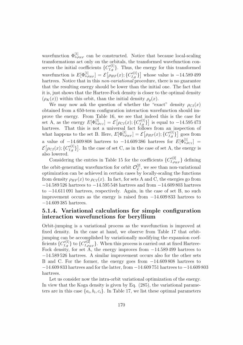
wavefunction Φ[1]o,ρHF can be constructed. Notice that because local-scaling

transformations act only on the orbitals, the transformed wavefunction con-serves the initial coefficients Co[1]

I,g . Thus, the energy for this transformed

wavefunction is E[Φ[1]o,ρHF ] = E

[ρHF (x); Co[1]

I,g ]

whose value is −14.589 499hartrees. Notice that in this non-variational procedure, there is no guaranteethat the resulting energy should be lower than the initial one. The fact thatit is, just shows that the Hartree-Fock density is closer to the optimal density(ρK(x)) within this orbit, than the initial density ρg(x).

We may now ask the question of whether the “exact” density ρCI(x)obtained from a 650-term configuration interaction wavefunction should im-prove the energy. From Table 16, we see that indeed this is the case forset A, as the energy E[Φ

[1]o,ρCI ] = E

[ρCI(x); Co[1]

I,g ]

is equal to −14.595 473hartrees. That this is not a universal fact follows from an inspection ofwhat happens to the set B. Here, E[Φ

[1]o,ρHF ] = E

[ρHF (x); Co[1]

I,g ]

goes from

a value of −14.609 808 hartrees to −14.609 386 hartrees for E[Φ[1]o,ρCI ] =

E[ρCI(x); Co[1]

I,g ]. In the case of set C, as in the case of set A, the energy is

also lowered.Considering the entries in Table 15 for the coefficients Co[2]

I,ρHF defining

the orbit-generating wavefunction for orbit O[2]L , we see than non-variational

optimization can be achieved in certain cases by locally-scaling the functionsfrom density ρHF (x) to ρCI(x). In fact, for sets A and C, the energies go from−14.589 526 hartrees to −14.595 548 hartrees and from −14.609 803 hartreesto −14.611 091 hartrees, respectively. Again, in the case of set B, no suchimprovement occurs as the energy is raised from −14.609 833 hartrees to−14.609 385 hartrees.

5.1.4. Variational calculations for simple configurationinteraction wavefunctions for beryllium

Orbit-jumping is a variational process as the wavefunction is improved atfixed density. In the case at hand, we observe from Table 17 that orbit-jumping can be accomplished by variationally modifying the expansion coef-ficients Co[1]

I,g to Co[2]I,ρHF

. When this process is carried out at fixed Hartree-Fock density, for set A, the energy improves from −14.589 499 hartrees to−14.589 526 hartrees. A similar improvement occurs also for the other setsB and C. For the former, the energy goes from −14.609 808 hartrees to−14.609 833 hartrees and for the latter, from−14.609 751 hartrees to−14.609 803hartrees.

Let us consider now the intra-orbit variational optimization of the energy.In view that the Koga density is given by Eq. (285), the variational parame-ters are in this case ai, bi, ci. In Table 17, we list these optimal parameters

170

Table 17: Optimum parameters of the Koga density ρK obtained by mini-mization of the energy density functional.

i ai bi ci

For wavefunction from set A1 1.0a 0.0a 8.481 152 −0.312 90 1.937 19 5.191 463 0.170 50 0.3b 4.648 604 0.007 50 1.196 59 1.720 15

For wavefunction from set B

1 1.0a 0.0a 8.478 102 −0.331 33 1.937 95 5.185 533 0.177 28 5.0b 4.653 354 0.007 12 1.205 72 1.697 95

For wavefunction from set C

1 1.0a 0.0a 8.478 072 −0.330 42 1.937 95 5.185 833 0.178 83 5.0b 4.653 084 0.007 16 1.205 52 1.698 43

aParameters set to these values.bTimes 10−6.

for an intra-orbit optimization of the energy in orbit O[1]L for wavefunctions

constructed from the primitive sets A, B and C. The results of these opti-mizations are given in Table 17. For example, for set A, the initial energy−14.538 796 hartrees is improved to the value −14.597 378 hartrees. Similarlowerings occur for sets B and C. Thus, for set B, we have that the energygoes from −14.599 524 hartrees to −14.612 114 hartrees and for set C, from−14.599 936 hartrees to −14.612 471 hartrees.

Orbit-jumping at fixed optimized density ρK(x) leads to the optimal ex-

pansion coefficients Co[4]I,ρK. For set A, the optimal energy is −14.597 476

hartrees, for set B, −14.612 121 hartrees and for set C, −14.612 495 hartrees.Considering that the optimal energy for an untransformed function is

−14.599 936 hartrees (first entry for set C in Table 7), we see that local-scaling transformations have a considerable effect on these configuration in-teraction wavefunctions. Since the best locally-scaled energy is −14.612 495hartrees (last entry for set C in Table 17), we observe that these transforma-tions improve the energy by −0.012 559 hartrees.

171

5.1.5. Determination of Kohn-Sham orbitals and poten-tials for beryllium by means of local-scaling transforma-tions

According to Eq. (357), in order to reach the kinetic energy minimum,

one must span the set ΦSD[k]ρ of single Slater determinants which are con-

strained to give the fixed density ρ(x) = ρexacto (x). This set, in turn, can bereadily generated by means of local-scaling transformations. Consider, forthe beryllium atom, a single Slater determinant for the configuration 1s22s2:

ΦSD[1]g (r1, s1, · · · , r4, s4) ≡

det√4!

[R10

([α0j; c10j

]; r1

)α(s1) · · ·R20

([α0j; c20j

]; r4

)β(s4)

].

(415)

Carrying out a local-scaling transformation between the one-particle densityρg(r) associated with Φ

SD[1]g and the fixed “exact” density ρCI(r) of Esquivel

and Bunge [622], using Eq. (330), we obtain a set of transformed orbitalsfrom which we can generate a set formed by the following transformed single-Slater determinants:

ΦSD[1]ρCI

(r1, s1, · · · , r4, s4) ≡det√

4!

[RT

10

([α0j; c10j

]; r1

)α(s1) · · ·RT

20

([α0j; c20j

]; r4

)β(s4)

].

(416)

Because of the dependence of the determinants forming this set on theorbital expansion coefficients as well as on the orbital exponents, it is clearthat the optimal determinant which minimizes the kinetic energy for thenoninteracting system can be reached by varying these orbital parameters. Atthe extremum of this constrained variation we have, therefore, the followinginequality for the kinetic energy functional:

Ts[ρo] ≤ Ts[ρo; αmin0j ; cminn0j ]

≡ 22∑

n=1

∫drr2RT

n0

([αmin0j ; cminn0j

]; r)(−1

2∇2)RTn0

([αmin0j ; cminn0j

]; r).

(417)

How closely Tmins approaches the exact kinetic energy for a noninteractingsystem depends on our choice of the primitive orbital set. In the case reviewed

172

here [601], the transformed orbitals belong to the Clementi-Roetti-type set.With this choice we obtain Tmins = 14.593 163 hartrees.

The orbitals RT (min)n0 2

n=1 are not yet the canonical Kohn-Sham orbitalsof Eq. (340). The canonical Kohn-Sham orbitals are obtained by rotatingthe former ones through an angle θ = θKS. Explicitly, the rotated orbitalsare:

Rθ10(r) = cos θR

T (min)10 (r) + sin θR

T (min)20 (r)

Rθ20(r) = − sin θR

T (min)10 (r) + cos θR

T (min)20 (r). (418)

Once the canonical Kohn-Sham orbitals are obtained, it is a straight-forward matter to invert the Kohn-Sham equations in order to obtain theKohn-Sham effective potentials and the orbital eigenvalues. The procedurefor carrying out this inversion has been discussed in detail elsewhere [601].Let us just indicate here that by using local-scaling transformations we canreproduce the value EKS10 = 0.342 6 hartrees reported by Almbladh and Pe-droza [597]. Moreover, the Kohn-Sham orbitals orbitals computed by thepresent method [602], are in excellent agreement with those computed byZhao and Parr [590].

An iterative procedure can be set up in order to calculate the effectiveKohn-Sham potential. The details of this procedure are given elsewhere[601, 602]. Once this potential is obtained, we can analize it in terms ofits components and extricate from it the Kohn-Sham exchange-correlationpotential which, in turn, can be written as a sum of the exchange and thecorrelation potentials:

vKSXC([ρo(r)]; r

)= vKSX

([ρo(r)]; r

)+ vKSC

([ρo(r)]; r

). (419)

The calculation of vKSX([ρo(r)]; r

)reported in this work was done by ap-

plying the same density-constrained variation for the kinetic energy given byEq. (102), using, however, a final fixed density equal to the Hartree-Fockone. In Fig. 9, we plot vKSXC

([ρo(r)]; r

)and its components vKSX

([ρo(r)]; r

)and vKSC

([ρo(r)]; r

)for the Clementi-Roetti function.

We may conclude from Fig. 9, that by implementing the density-constrainedmethod described above, in the context of local-scaling transformations, weobtain the same potential reported by Almbladh and Pedroza [597]. An im-portant point we would like to stress with respect to the present method isthat it is based on the constrained minimization of the kinetic energy, andfor this reason, it is not necessary to deal at any point of the calculation withthe evaluation of two-electron integrals.

173

0.5

0.0

−1

−2

−3

0 1 2 3 4r (bohrs)

vX

vXC

vC

q

I

Figure 9: Exchange-correlation, exchange-only and correlation Kohn-Shampotentials.

5.2 LST-DFT: diatomics and clusters

5.2.1. Diatomic molecules

In this Subsection we shall deal with applications of the density transfor-mations discussed in Eqs. (B23) and (B24) of Appendix B to some selecteddiatomic molecules. We discuss the non-variational improvement broughtabout on the total energy when these transformations are applied to simplewavefunctions. In addition, we present results for the density-constrainedkinetic energy minimization at fixed Hartree-Fock density (this procedure isequivalent to the Kohn-Sham x−only method).

Let us first consider the effect on the energy of applying these densitytransformations in order to achieve a non-variational improvement of simplewavefunctions (constructed from limited basis sets). The transformationscarry the initial density of these trial wavefunctions to the the Hartree-Fock

174

Table 18: Total, Exchange, and Kinetic Energies (in hartrees) for BestLimited LCAO-MO (BL) and Their Density-Transformed MO for DiatomicMolecules LiH(1Σ+) and Li2(1Σ+

g ) (HartreeFock Results Included) [546].

Species R Method -Etotal T -Ex −εHOMO

LiH(1Σ+) 3.015 BL 7.9699 7.9788 2.1716 0.299LS-DFT 7.9814 7.9971 2.1467 0.300

HF 7.9874 7.9913 2.1468 0.302

Li2(1Σ+g ) 5.051 BL 14.8415 14.8667 3.6125 0.181

LS-DFT 14.8638 14.8961 3.5642 0.180HF 14.8716 14.8894 3.5653 0.182

density. By means of this transformation a new orbital set and its corre-sponding 1-matrix (242) can be constructed. Introducing this transformed1-matrix into Eqs. (240) and (241) then the energy can be evaluated throughEq. (239). We employ in the present calculations the numerical diatomicmolecule programs developed by Laaksonen, Pyykko and Sundholm [623]and modified by Kobus et al. [624]. These are numerical programs thatapply the finite difference method to the solution of the diatomic moleculeHartree-Fock problem. These programs have been adapted by us for thepurpose of including the density-transformation routines.

In Table 18, we present some results for LiH(1Σ+) and Li2(1Σ+g ), where

the trial wavefunctions are the best limited LCAO-MO (BL) of Ransil [625].Each molecular orbital is constructed as a linear combination of atomic func-tions. The latter are optimized single-ζ Slater functions. As it can be seenfrom this Table, for LiH(1Σ+), the total energy of the BL wavefunction differsby 0.0175 hartrees from the Hartree-Fock value. This distance is consider-ably diminished as a result of the density transformation which lowers it to0.0060 hartrees. Perhaps the most interesting result in this respect is the im-provement on the exchange energy that differs from the Hartree-Fock one injust 0.0001 hartrees as opposed to 0.0248 hartrees in the case of the untrans-formed wavefunction. Similar results are also obtained for the homonucleardiatomic molecule Li2(1Σ+

g ).For completeness, we show in Figs. 10 and 11 the difference between the

HF and the BL densities (which in this case play the role of ρg) for LiH(1Σ+)and Li2(1Σ+

g ), respectively. In this figures, this difference has been magnifiedby a factor of ten. These graphs illustrate how very slight redistributions inthe total density (such as those observed here) can lead to energy changes of

175

Figure 10: Hartree-Fock density and differences between HF and ρg densitiesfor the molecule LiH(1Σ+);Re = 3.015 bohr. This figure is adapted from Ref.[546].

the order of 0.01 hartrees.Variational calculation for diatomic molecules involving density transfor-

mations will be presented elsewhere. It is clear that the energy functionaldescribed by Eq. (239) can be minimized by introducing some paramet-ric expression for the one-particle density ρ. The results presented here forρ = ρHF are, therefore, just upper bounds to this minimum.

As is well known, a density-constrained minimization of the kinetic energyof a non-interacting N -particle system is equivalent to solving the variationalproblem involved in the Kohn-Sham method. When this minimization iscarried out with ρ = ρHF we have the exchange-only Kohn-Sham results.

For the kinetic energy minimization at the exchange-only level, we haveused two types of Hartree-Fock densities (when available): numerical den-sities obtained by the numerical HF program [623, 624] and analytic densi-ties of Cade and Huo [626, 627, 628]. In Table VII we present results forthe kinetic energy Ts, the total and exchange energies as well as for the

176

Figure 11: Hartree-Fock density and difference between HF and ρg densitiesfor the molecule Li2(1Σ+

g );Re = 5.051 bohr. This figure is adapted from ref.[546].

highest occupied molecular orbital eigenvalue for the the diatomic hydridesLiH(1Σ+), BeH(2Σ+), BH(1Σ+) and HF(1Σ+). For comparison purposes wehave included the corresponding Hartree-Fock values.

The same type of analysis has been extended to the homonuclear diatomicmolecules Li2(1Σ+

g ) and F2(2Σ+g ), and also to the heteronuclear diatomic

molecule LiF(1Σ+). The results are presented in Table 19 (for F2(2Σ+g ) the

analytic Hartree-Fock densities were not available at the selected R).Since the calculation of Ts in the Kohn-Sham method is done by resorting

to a minimum principle, these Ts values should lie below those of the Hartree-Fock kinetic energy. Similarly, the total Kohn-Sham exchange-only energiesshould be upper bounds to the Hartree-Fock ones. These variational con-

177

Table 19: Kohn–Sham x-only energy values and their differences fromHartreeFock values for selected diatomic hydrides (in hartrees) [546].

Species/ ∆ Method -Ts -Etotal -Ex −εHOMO

LiH(1Σ+) HF 7.9913 7.9874 2.1468 0.302R = 3.015 KS 7.9910 7.9870 2.1461 0.302

∆ 0.0003 0.0004 0.0007HFa 7.9913 7.9873 2.1468 0.302KSb 7.9909 7.9869 2.1460 0.302

∆ 0.0004 0.0004 0.0008

BeH(2Σ+) HFa 15.1494 15.1531 3.0859 0.313R = 2.538 KSb 15.1478 15.1510 3.0822 0.309

∆ 0.0016 0.0021 0.0037

BH(1Σ+) HF 25.1200 25.1316 4.1325 0.348R = 2.329 KS 25.1185 25.1300 4.1294 0.347

∆ 0.0015 0.0016 0.0031

HF(1Σ+) HF 100.0267 100.0708 10.4283 0.650R = 1.7328 KS 100.0249 100.0686 10.4243 0.650

∆ 0.0018 0.0022 0.0040HFa 100.0274 100.0703 10.4287 0.650KS 100.0253 100.0684 10.4246 0.650

∆ 0.0021 0.0019 0.0041aHartree-Fock-Roothan method [626, 627, 628].bKS method at fixed Hartree-Fock density.

178

straints are satisfied by the results listed in Tables VII and VIII. Moreover,the exchange energies computed from the Kohn-Sham x−only orbitals arein close agreement with the Hartree-Fock values (and also lie above them).We also observe a striking similarity between the εHOMO values (except forBeH(2Σ+), in all other cases the differences are of the order of, or less than,a millihartree).

In order to establish a common platform for valid comparisons with re-sults of the Amsterdam Group [629, 630, 631, 632], work is currently underway with Hartree-Fock and “exact” densities provided to us by Gritsenko.Hopefully, this will allow us to assess the accuracy of both approaches tothe calculation of “exact” density functional quantities such as Ts, Tc, theKohn-Sham exchange and correlation potentials, etc., for diatomic molecules.

5.2.2. Extension to polyatomic molecules

We comment here on two alternatives having to do with the application oflocal-scaling transformations to polyatomic systems. The first refers to adecomposition of a molecular system into atom-centered subsystems [512]and the second, to the treatment of subsystems in a periodic solid.

Let us rewrite the energy functional given by Eq. (239) as

E[Φρ] =

∫d3r1ε([ρ], r1), (420)

where we assume that, in general, the energy density ε([ρ], r1) is a multi-center function. Following Becke [633], we assume that the multi-center inte-gration can be carried out by decomposing the whole space into a collectionof “fuzzy cells”. Under this decomposition, the energy functional becomes

E(n)[Φρ] =

∫d3r1ωn(r)ε([ρ(n)], r

(n)1 ), (421)

where ωn(r) is a relative weight function associated with a center n [633] thatis unity about nucleus n but vanishes in a continuous and well-behaved man-ner near any other nucleus. It also satisfies the condition

∑n=1 ωn(r) = 1.

In terms of this decomposition, ε([ρ(n)], r(n)1 ) becomes an atom-centered func-

tional generated by the spherically-averaged local-scaling transformation car-rying the vector r(n) ≡ (r(n), θ(n), ϕ(n)) into ~f (n) ≡ (f (n), θ(n), ϕ(n)). Expand-ing the transformed molecular orbitals (about each nucleus n) by

φρ,i((r(n), θ(n), ϕ(n)) =

∑p

Ci(p)φρ,i(p)((r(n), θ(n), ϕ(n)), (422)

179

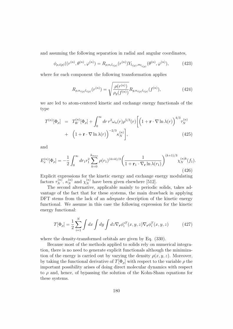
and assuming the following separation in radial and angular coordinates,

φρ,i(p)((r(n), θ(n), ϕ(n)) = Rρ,nili(p)(r

(n))Yli(p),mli(p) (θ(n), ϕ(n)), (423)

where for each component the following transformation applies

Rρ,ni(p)li(p)(r(n)) =

√ρ(r(n))

ρg(f (n))Rg,ni(p)li(p)(f

(n)), (424)

we are led to atom-centered kinetic and exchange energy functionals of thetype

T (n)[Φρ] = T(n)W [Φρ] +

∫ ∞0

dr r2ωn(r)ρ5/3(r)

[(1 + r · ∇ lnλ(r)

)4/3

τ(n)N

+(

1 + r · ∇ lnλ(r))−2/3

κ(n)N

], (425)

and

E(n)x [Φρ] = −1

2

∫ ∞0

dr1r21

kmax∑k=0

ρ(r1)(4+k)/3

(1

1 + r1 · ∇r lnλ(r1)

)(k+1)/3

χ(n)kN (f1).

(426)Explicit expressions for the kinetic energy and exchange energy modulatingfactors τ

(n)N , κ

(n)N and χ

(n)N have been given elsewhere [512].

The second alternative, applicable mainly to periodic solids, takes ad-vantage of the fact that for these systems, the main drawback in applyingDFT stems from the lack of an adequate description of the kinetic energyfunctional. We assume in this case the following expression for the kineticenergy functional:

T [Φρ] =1

2

N∑i=1

∫dx

∫dy

∫dz∇rφ

∗Ti (x, y, z)∇rφ

Ti (x, y, z) (427)

where the density-transformed orbitals are given by Eq. (330).Because most of the methods applied to solids rely on numerical integra-

tion, there is no need to generate explicit functionals although the minimiza-tion of the energy is carried out by varying the density ρ(x, y, z). Moreover,by taking the functional derivative of T [Φρ] with respect to the variable ρ theimportant possibility arises of doing direct molecular dynamics with respectto ρ and, hence, of bypassing the solution of the Kohn-Sham equations forthese systems.

180

Figure 12: The CPU timings in units of timings for Na2 as a function of thenumber of orbitals for all the clusters. This figure is adapted from Ref. [634].

5.2.3. Clusters

It would be rather natural to finish this Section with some words of sup-port of the LST-DFT like these, e. g.:“The LSDFT is a rigorous formulationof DFT, constructive in nature, and satisfies the N and v representabilityconditions on the energy functional. In principle, the method is applicableto Hartree-Fock or Kohn-Sham Hamiltonians and yields the correspondingorbitals and energies” which we borrow from the paper by Kanhere et al.[634]. This work develops the algorithm which is based on LST for electronicstructure calculations that scales linearly with the size of the system. Its keyfeature is the absence of the orthogonalization step during iterative minimiza-

181

tion. The feasibility and potential of this algorithm by applying it to totalenergy calculations for a variety of small clusters, viz., Na2, Na7Al, Na20, Si4,and Al13 which represent 2-, 10-, 20-, 16- and 39-electronic systems18.

Figure 13: The generating charge density (dashed line) and the final chargedensity (continuous line) for Na20 cluster along the x axis. This figure isadapted from Ref. [634].

The timings of these calculations [634] are those for total energies ob-tained to within 0.005 hartree of the Kohn-Sham total energies with identicalparameters such as energy cutoff, cell dimension, pseudopotential, etc. (Allthe calculations except for Si use the local Bachelet-Hamann-Schluter pseu-dopotential [635]. For Si, a semiempirical local pseudopotential of [636] wasused. It may be noted that the inclusion of nonlocality is straightforward

18In some sense, such treatment of molecular clusters is quite symbolic bearing in mindKohn’s Nobel lecture [7] where he announced the treatment [after E. Nusterer, P. Blochl,K. Schwarz, Angew. Chem. 35 (1996) 175] of the system of methanol encapsulted in acage of the zeolite sodalite as large clusters of Si, Al, and oxygen atoms.

182

and does not pose any problems.).

Figure 14: The generating wavefunction (dashed line) and the final wave-function (continuous line) corresponding to the first state (a), the eighthstate (b), and the highest occupied state (c) for the Na20 cluster along the xaxis.This figure is adapted from Ref.[634].

The CPU timings in units of timings for Na2 as a function of the numberof orbitals for all the studied clusters are shown in Fig. 12. The timingsrequired to generate the initial guess are not included. As expected, thegraph displays a linear behavior. The next Figure 13 shows the generatingdensity ρg(r) (shown by a dashed line) and the final density ρ(r) shown bya continuous line. Figure 14 pictures the generating wavefunctions for thefirst, eighth state, and highest occupied state (all shown by a dashed line), re-spectively, and the corresponding final wavefunctions (by a continuous line).

183

The latter two figures are drawn along the x axis for the Na20 cluster. Theydefinitely illustrate the ability of LST to continuously deform the generatordensity and wave functions toward the final self-consistent density and wavefunctions in about 40-50 iterations. The final density and wave functions arevirtually indistinguishable from the full self-consistent Kohn-Sham density.Here, however,it is worth noticing that, in contrast to Proposal 5, this opti-mized one-electron density, notwithstanding of how close to the Kohn-Shamone it is, is definitely N -representable. Together with the authors of thispaper, we would like to conclude that this “method is easily parallelizableand therefore has the potential to deal with large real life systems.”

6 DISPERSION MOLECULAR FORCES

6.1 Introduction

“Some people think that there is an air between molecules.”

A. S. Kompaneets [637]

In nature there exist only four basic types of forces: gravitational, electromag-netic, strong, and weak. The electromagnetic interaction is the interactionbetween particles which carry on an electric charge. Electromagnetic interac-tion binds the electrons and the nuclei inside the atom, and the atoms insidea molecule, and governs the interaction between atoms and molecules. Theseare referred to as so called intermolecular interactions [637, 638, 639, 640].Indeed, intermolecular interactions play the important role in the world:True, we ‘touch’ them everywhere, at a macroscopic scale, in our everydaylife. It is rather hard to imagine what would be the world without them- obviously, it would be quite dramatic compared to the ideal gases whichsurround us! Simply imagine that would be no such molecules as the DNAand RNA. The intuitively clear idea of that atoms and molecules do interactwith each other is a very old indeed and dates back to the ancient times.Let recall, in particular, Democritus, Leukippos, and Lucretius whose philo-sophical thoughts on the interaction through a direct contact were developedand rationalized by R. Boscovich in his “Theory of Natural Science Reducedto the Single Law of Forces Existing in Nature” (1758) and independentlyby A. C. Clairault in “Theorie de la Figure de la Terre” (1743). A typicalpotential of the interaction of two s-state atoms, discussed by Boscovich indetail, roughly features a weak attraction at large distances, smaller or equalto the sum of van der Waals radii of atoms, and a strong repulsion at the

184

Table 20: Van der Waals radii RvdW (in A) of atoms.

Atom RvdW Atom RvdW Atom RvdW Atom RvdW

H 1.20 He 1.30 N 1.50 O 1.40F 1.35 Ne 1.40 P 1.90 S 1.85Cl 1.80 Ar 1.70 As 2.00 Se 2.00Br 1.95 Kr 1.80 Sb 2.20 Te 2.20I 2.15 Xe 2.05

short ones which arises due to non-vanishing effective size, or core, of eachinteracting atoms. Hence, the potential reaches the minimum at some in-termediate distance where atoms are bonded in a molecule. By definition,the van der Waals (vdW) radius, RvdW , of a given atom is the halve of theshortest distance observed in crystals between corresponding nuclei. TypicalvdW radii of atoms are given in Table 20. At the distances beyond the sumof van der Waals radii of atoms, they experience a specific, van der Waalsinteraction often referred to as the dispersion interaction between atoms, af-ter Johannes Diderik van der Waals who first postulated its existence in thewell-known equation of state, Eq.(428), derived in his PhD thesis in 1837 andwhich won him the 1910 Nobel Prize in Physics19. van der Waals molecules,which are, by definition, bound by long-range dispersion forces, representthe most weakly bonded form of molecular matter [642] (for the recent spec-troscopic detection of the LiHe molecule see [644]) and are often referred tomolecular forces. Many chemical and biochemical processes involve van derWaals interactions [637, 640, 642, 643] which are often referred to molecu-lar interactions. This interaction potential shed a light on the deviations ofgases from the ideal behavior which van der Waals explained by consideringa vessel filled by a gas of atoms. Within ithin this vessel, the pressure exertedby a gas of atoms on its wall is lower compared to that predicted by the idealgas law since the atoms may collide with the wall and are thus retained bythe attraction they undergo from the other atoms in the bulk of the gas thatresults in the presurre P obeying the equation [641],[

P + an2

V 2

](V −Nb) = NRT (428)

19http://www.nobelprize.org/nobelprizes/physics/laureates/1910/waals-bio.html.

185

where a is a so-called vdW factor and b = (16πN/3)R3vdW . In some sense, b

corresponds to an account of the effective core of an atom and a originatesfrom the attractive forces between atoms: its increase lowers the pressure P .

The dispersion interaction energy between the ground-state molecules isalways negative. The attractivity of van der Waals force between an atomand a molecule at some mutual orientations was proved by Lieb and Thirring[645] and generalized to any orientation in 2006 by Lewin [646]. The leadingterm of the dispersion energy is the dipole-dipole term which is proportionalto 1/R6 [647] [see below Eq.(437)] and determined by a change in the zero-point vibrational energy of electric field created by zero-point vibrations offluctuating dipole moments of interacting species [648, 649]. Since the zero-point fluctuations are the quantum phenomenon, the dispersion interactionshave the quantum origin, as though in the beginning of the 70ies, Boyer[650, 651, 652, 653, 654] derived the London formula for the dispersion in-teractions within the classical electrodynamics, additionally assuming theexistence of the classical electromagnetic zero-point radiation. In fact, thevan der Waals forces are cohesive attractions between molecules which op-erate at long intermolecular separations. The unified treatment of the vander Waals forces was developed in 1954 by E. M. Lifshitz [655, 656] and fur-ther by Zaremba and Kohn [657], Langreth, Lundqvist and their co-workers[658, 659, 660, 661] (see also [662] and references therein).

From a quantitative viewpoint, van der Waals forces between moleculescorrespond to interactions between electric dipoles. Generally speaking, thereexist three types of electric dipoles in molecules. These are permanent, in-duced, and temporary dipoles. If a molecule M under study consists of thepositive nuclear charges q1 = Z1, ..., qM = ZM and negative electron chargese1, ..., eN , its total permanent dipole moment (see Table 21 for dipole mo-ments of selected molecules) is defined as

do =M∑α=1

qαRα +N∑i=1

eiri (429)

do is distinct from zero in some state if the centre of charge of the nuclei, Rn ≡∑Mα=1 qαRα/

∑Mα=1 qα, does not coincide with that of the electron subsystem,

rn ≡∑N

i=1 eiri/∑N

i=1 ei. If do 6= 0, a moleculeM is called polar. Permanentdipole moments of neutral molecules usually vary from zero to 15 Debye (D)that is reflected in Table 21.

Any pair of polar molecules, M1 and M2, separated by a distance R12,in the states n and m, respectively, interact with each other by their dipoles,

186

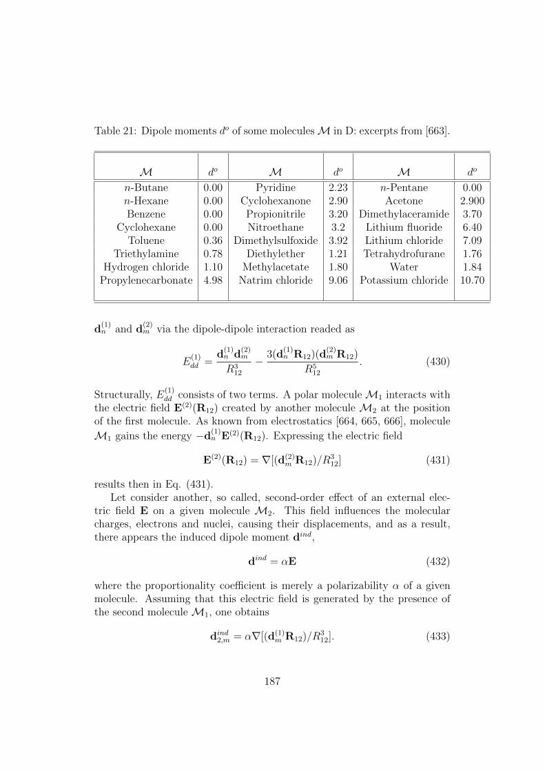
Table 21: Dipole moments do of some moleculesM in D: excerpts from [663].

M do M do M do

n-Butane 0.00 Pyridine 2.23 n-Pentane 0.00n-Hexane 0.00 Cyclohexanone 2.90 Acetone 2.900Benzene 0.00 Propionitrile 3.20 Dimethylaceramide 3.70

Cyclohexane 0.00 Nitroethane 3.2 Lithium fluoride 6.40Toluene 0.36 Dimethylsulfoxide 3.92 Lithium chloride 7.09

Triethylamine 0.78 Diethylether 1.21 Tetrahydrofurane 1.76Hydrogen chloride 1.10 Methylacetate 1.80 Water 1.84

Propylenecarbonate 4.98 Natrim chloride 9.06 Potassium chloride 10.70

d(1)n and d

(2)m via the dipole-dipole interaction readed as

E(1)dd =

d(1)n d

(2)m

R312

− 3(d(1)n R12)(d

(2)m R12)

R512

. (430)

Structurally, E(1)dd consists of two terms. A polar moleculeM1 interacts with

the electric field E(2)(R12) created by another molecule M2 at the positionof the first molecule. As known from electrostatics [664, 665, 666], molecule

M1 gains the energy −d(1)n E(2)(R12). Expressing the electric field

E(2)(R12) = ∇[(d(2)m R12)/R3

12] (431)

results then in Eq. (431).Let consider another, so called, second-order effect of an external elec-

tric field E on a given molecule M2. This field influences the molecularcharges, electrons and nuclei, causing their displacements, and as a result,there appears the induced dipole moment dind,

dind = αE (432)

where the proportionality coefficient is merely a polarizability α of a givenmolecule. Assuming that this electric field is generated by the presence ofthe second molecule M1, one obtains

dind2,m = α∇[(d(1)m R12)/R3

12]. (433)

187

Therefore, the interaction of the permanent dipole d(1)n ofM1 with the dipole

dind2,n that is induced on M2 by M1 takes the following expression

E(2)dd =

d(1)n dind2,n

R312

−3(d

(1)n R12)(dind2,nR12)

R512

(434)

that is known as the Keesom dipole-dipole interaction [667].By a straightforward analogy, the dipole-dipole interaction of two mutu-

ally induced dipoles on M1 and M2 is described by the expression

E(2)dd =

dind1,ndind2,m

R312

−3(dind1,nR12)(dind2,nR12)

R512

. (435)

If the distance R12 between dipoles is small enough compared to the wave-length λ, corresponding to transitions between the ground and excited states,within the second- and higher-order Rayleigh-Schrodinger perturbation the-ory as [637, 656] there appear, as first shown by F. London [656], the disper-sion interaction [656]

E(2)disp = −

∑m,n 6=0

|〈Ψ(1)n Ψ

(2)m |V12|Ψ(1)

0 Ψ(2)0 〉|2

(E(1)n − E(1)

0 ) + (E(2)m − E(2)

0 )

(436)

where Ψ(i)n is the n-state eigenfunction of Mi, i = 1, 2 and V12 is the electro-

static interaction between molecules M1 and M2.The dispersion energy is traditionally represented by means of the mul-

tipole expansion [641]

E(2)disp = −

∞∑n=6

CnRn

(437)

where Cn are dispersion constants among which C6 corresponds to dipole-dipole interaction, C8 dipole-quadrupole and C10 to dipole-octupole anddipole-quadrupole interactions.

Dispersion interactions play a role of the attractive interaction betweenrare gas atoms and are also one of the important intermolecular interactionsthat govern the molecular organic world [205, 213]. Dispersion interactionsare mostly responsible for the heats of sublimation of hydrocarbon molecules,make significant contributions to the solvent properties of polar and apolarneutral compounds [669, 670] and are also important for crystal packing oforganic molecules [671] as well as for the stacking of nucleic acids in DNA

188

[640, 672]. The world of dispersion interaction is rich (see e. g., [673, 674,675, 676, 677, 678, 679, 680, 681] and references therein), despite the factthat it is a weaker form of intermolecular attractions. Dispersion forces asone of the two types of van der Waals force, are also known as ”Londonforces”, named after F. London [656].

Density functional theory [682, 683, 684, 685] as one of the approachto evaluate electron correlation is considerably less demanding on computa-tional resources than the MP2 or CCSD(T) methods. DFT might thereforebe considered as a powerful computational tool, if it can adequately describeand accurately evaluate intermolecular interactions. The suitability of DFTfor the evaluation of dispersion interaction has been an important issue inthe recent literature [686, 687, 688, 689, 690, 691, 692, 693, 694] that is mir-rored in Table 22. While DFT calculations with local exchange-correlationfunctionals lead to overestimate binding energies of weakly bound systems, itwas reported that nonlocal exchange-correlation functionals very often under-estimate the attraction [687, 688, 689]. The DFT calculations with Becke’sexchange and Lee, Yang, and Parr’s correlation functionals, BLYP [682, 683],and Becke’s three-parameter functional combined with Lee, Yang, and Parr’scorrelation functional, B3LYP, [683, 685] also fail to evaluate the attractivedispersion interaction between hydrocarbon molecules [689, 690, 691]. Re-cently Zhang et al. and Wesolowski et al. reported that the Becke exchangefunctional due to its erroneous asymptotic behavior at low density is re-sponsible for the failure in the evaluation of the attraction between weaklybound systems [692, 693, 694]. It was shown, however, that other nonlocalexchange-correlation functionals such as Perdew and Wang’s exchange andcorrelation functionals, PW91, [684] are possible alternatives to describe thebinding between rare gas dimers or other systems. The performance of someexchange-correlation functionals and the PW91 one in particular for the rep-resentative van der Waals systems is demonstrated in Table 22. Notice thatthe PW91 functional is a general functional, i.e. it is not biased towards thedescription of intermolecular interaction. In this investigation we will exam-ine the basis set dependence of the interaction energies, and benchmark thoseagainst the results obtained from MP2 and CCSD(T) theory. For compari-son, the results with the BLYP and B3LYP are also presented. Interestingly,DFT adequately describes, on the one hand, atoms and molecules as stablemany-electron systems and on the other, the molecules formed under interac-tion of its composing molecules. However, its description of those molecularinteractions is not always perfect. The simplest DFT approximation widelyused in computational practice is the local density approximation (LDA)[134], based on the properties of the uniform electron gas. In principle, DFTyields the exact ground-state energy, including long-range van der Waals en-

189

ergies, very important in organic chemistry and elsewhere. However, thecommonly used LDA and GGA, designed for nonuniform electron gases, failto capture the essence of vdW energies. The latter reflect correlated mo-tions of electrons due to the Coulomb interactions between distant, evennonoverlapping atoms, molecules, and solids. In [4] Kohn and co-authorspropose a first-principles approach, which contains the following ingredients:(i) The density distribution, ρ(r), is approximated by the LDA or GGA.(ii) The Coulomb interaction is divided into short and long-range parts, ofwhich only the latter contributes to vdW energies. (iii) The contributionof the long-range interactions to the energy is expressed by the so calledadiabatic connection formula. (iv) This expression is transformed into thetime domain, avoiding the need to solve a self-consistent equation for thedensity-density response function.

6.2 Dispersion-Corrected DFT approaches

“DFT methods with currently available functionalsfailed completely for London-type clusters

for which no minimum was foundat the potential energy surfaces.”

P. Hobza, J. Reschel and J.Sponer [689]

Density functional theory is often the preferred electronic structure methodto study moderate and large systems. This preference reflects the efficiencyof DFT compared to correlated wavefunction theories such as coupled clus-ter theory even though accuracy, and more importantly, predictability (asin systematic convergence to the right answer), are sacrificed. DFT whichincorporates currently accepted exchange-correlation functionals can be usedwith reasonable reliability on chemically bound systems around the equilib-rium geometry but inevitably fail when applied to systems which are boundby weak van der Waals forces [687, 689, 690, 698, 699] and, to a lesser degreefor chemically bound systems away from equilibrium, like transition states[700]. These failings of density functional theory are well known [30]. Here,we address weak interactions. Attempts to compute weak intermolecularforces using DFT fall into two categories. Some would simply modify func-tionals until reasonable results are obtained (see Ref. [701] and referenceswithin). Others would focus on an add-on correction that explicitly intro-duces the van der Waals C6 coefficient. This can be made to work, but itis unsatisfactory that the weak interactions do not occur naturally as theywould in wave function methods. This is the experimental or computational

190

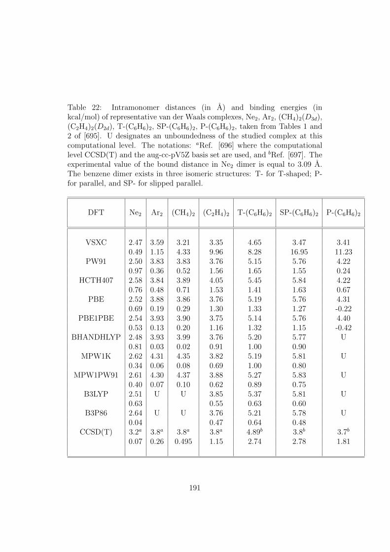
Table 22: Intramonomer distances (in A) and binding energies (inkcal/mol) of representative van der Waals complexes, Ne2, Ar2, (CH4)2(D3d),(C2H4)2(D2d), T-(C6H6)2, SP-(C6H6)2, P-(C6H6)2, taken from Tables 1 and2 of [695]. U designates an unboundedness of the studied complex at thiscomputational level. The notations: aRef. [696] where the computationallevel CCSD(T) and the aug-cc-pV5Z basis set are used, and bRef. [697]. Theexperimental value of the bound distance in Ne2 dimer is equal to 3.09 A.The benzene dimer exists in three isomeric structures: T- for T-shaped; P-for parallel, and SP- for slipped parallel.

DFT Ne2 Ar2 (CH4)2 (C2H4)2 T-(C6H6)2 SP-(C6H6)2 P-(C6H6)2

VSXC 2.47 3.59 3.21 3.35 4.65 3.47 3.410.49 1.15 4.33 9.96 8.28 16.95 11.23

PW91 2.50 3.83 3.83 3.76 5.15 5.76 4.220.97 0.36 0.52 1.56 1.65 1.55 0.24

HCTH407 2.58 3.84 3.89 4.05 5.45 5.84 4.220.76 0.48 0.71 1.53 1.41 1.63 0.67

PBE 2.52 3.88 3.86 3.76 5.19 5.76 4.310.69 0.19 0.29 1.30 1.33 1.27 -0.22

PBE1PBE 2.54 3.93 3.90 3.75 5.14 5.76 4.400.53 0.13 0.20 1.16 1.32 1.15 -0.42

BHANDHLYP 2.48 3.93 3.99 3.76 5.20 5.77 U0.81 0.03 0.02 0.91 1.00 0.90

MPW1K 2.62 4.31 4.35 3.82 5.19 5.81 U0.34 0.06 0.08 0.69 1.00 0.80

MPW1PW91 2.61 4.30 4.37 3.88 5.27 5.83 U0.40 0.07 0.10 0.62 0.89 0.75

B3LYP 2.51 U U 3.85 5.37 5.81 U0.63 0.55 0.63 0.60

B3P86 2.64 U U 3.76 5.21 5.78 U0.04 0.47 0.64 0.48

CCSD(T) 3.2a 3.8a 3.8a 3.8a 4.89b 3.8b 3.7b

0.07 0.26 0.495 1.15 2.74 2.78 1.81

191

fact which has not been still proved. Though, the problem of descriptionof London dispersion in DFT using (semi) local exchange-correlation func-tionals is a well-known problem [704, 705] since the first diagnostic in 1994[704].

A step in the right direction was made by Engel et al. [702] who ob-tained reasonable results for the helium and neon dimers. In [703], Bartlettand co-workers proposed ab initio density functional theory has been ap-plied for the weakly interacting, He2, [He-Be]2+, Ne2 and Be2 that results infair agreement with the highly accurate coupled-cluster method. Generally,one assumes that the cause lies in the local character of the widely usedcorrelation functionals, which, in contrast to the correlation contributionin post-Hartree-Fock methods such as Møller-Plesset or coupled cluster, onlyutilize information on the density of the system at one point and are thereforeunsuitable for the description of a nonlocal phenomenon such as dispersion.Attempts to introduce nonlocal correlation to DFT, such as the random phaseapproximation (RPA) [706, 707] or the nonlocal van der Waals functionals,[708, 709, 710, 711] are being investigated, but unfortunately the improve-ment comes with a significant increase in the computational cost. Since therelatively low computational cost of DFT is one of the major factors respon-sible for its status as the most widely used quantum chemical method today,a range of more pragmatic approaches has been developed to correct the per-formance of DFT for dispersion interactions. Part of these methods rely onreparametrization of existing local correlation functionals, [712, 713, 714] mo-tivated by the fact that dispersion is partially included in many functionalsand that a suitable reparametrization will allow one to achieve the aspiredresults more consistently. The drawback of such an approach is that thestrong empirical character decreases the reliability. For instance, the perfor-mance of the reparametrized functionals often decreases for properties otherthan the electronic energy. Other attempts are based on adding a correctionterm, representing the dispersion energy, to the energy calculated using stan-dard DFT methods. Also in this category, one can find highly empirical butcomputationally attractive methods [715, 716, 717, 718, 719, 720, 721, 722]based on parameters fitted to reproduce high-level results, as well as themethods with deeper theoretical foundation but computationally more ex-pensive, where ab initio information of the systems is used to evaluate thedispersion energy, such as the static or frequency dependent polarizabilities[716, 717, 718, 719, 720] or the dipole moment of the exchange-correlationhole (XDM) [723, 724, 725, 726, 727]. Another noteworthy approach isthe adaptation of the symmetry adapted perturbation theory [728] to theframework of DFT, i.e., SAPT(DFT) [729, 730, 731, 732]. SAPT(DFT)has a significant computational advantage against the highly scaling SAPT

192

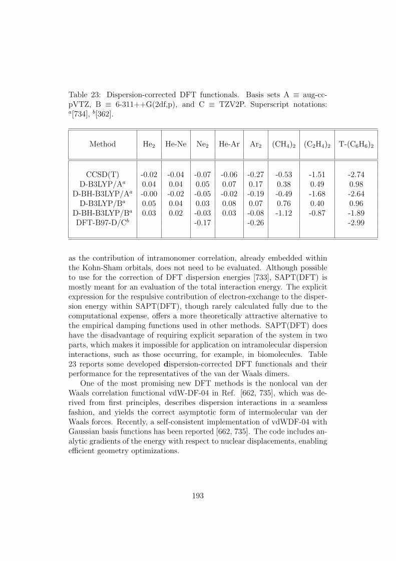
Table 23: Dispersion-corrected DFT functionals. Basis sets A ≡ aug-cc-pVTZ, B ≡ 6-311++G(2df,p), and C ≡ TZV2P. Superscript notations:a[734], b[362].

Method He2 He-Ne Ne2 He-Ar Ar2 (CH4)2 (C2H4)2 T-(C6H6)2

CCSD(T) -0.02 -0.04 -0.07 -0.06 -0.27 -0.53 -1.51 -2.74D-B3LYP/Aa 0.04 0.04 0.05 0.07 0.17 0.38 0.49 0.98

D-BH-B3LYP/Aa -0.00 -0.02 -0.05 -0.02 -0.19 -0.49 -1.68 -2.64D-B3LYP/Ba 0.05 0.04 0.03 0.08 0.07 0.76 0.40 0.96

D-BH-B3LYP/Ba 0.03 0.02 -0.03 0.03 -0.08 -1.12 -0.87 -1.89DFT-B97-D/Cb -0.17 -0.26 -2.99

as the contribution of intramonomer correlation, already embedded withinthe Kohn-Sham orbitals, does not need to be evaluated. Although possibleto use for the correction of DFT dispersion energies [733], SAPT(DFT) ismostly meant for an evaluation of the total interaction energy. The explicitexpression for the respulsive contribution of electron-exchange to the disper-sion energy within SAPT(DFT), though rarely calculated fully due to thecomputational expense, offers a more theoretically attractive alternative tothe empirical damping functions used in other methods. SAPT(DFT) doeshave the disadvantage of requiring explicit separation of the system in twoparts, which makes it impossible for application on intramolecular dispersioninteractions, such as those occurring, for example, in biomolecules. Table23 reports some developed dispersion-corrected DFT functionals and theirperformance for the representatives of the van der Waals dimers.

One of the most promising new DFT methods is the nonlocal van derWaals correlation functional vdW-DF-04 in Ref. [662, 735], which was de-rived from first principles, describes dispersion interactions in a seamlessfashion, and yields the correct asymptotic form of intermolecular van derWaals forces. Recently, a self-consistent implementation of vdWDF-04 withGaussian basis functions has been reported [662, 735]. The code includes an-alytic gradients of the energy with respect to nuclear displacements, enablingefficient geometry optimizations.

193

7 FUTURE PERSPECTIVES

7.1 On The Eve of Submission: Thoughts-Conclusions

Seriously, Density Functional Theory has marked the scientific lifes of bothof the authors of this review. The root of our intention and motivation inwriting this review has been to show all facets of the HKS-DFT from dif-ferent angles, primarily from the conceptual one, without skewing issues oravoiding difficult areas where consensus has not been reached (or may neverbe reached). For this reason, we are aware and duly accept the fact that thepresent review will not be treated in the same, homogeneously equal mannerby the entire DFT community consisting of DFT developers, DFT practi-tioners, and DFT mathematicians working in many-body quantum theory.We hope that our review will contribute to show the entire DFT communitythat still much work has to be done to realize Kohn’s motto quoted at thebeginning of this review. Our aim has been to show possible paths towardthe improvement of DFT. However, we should give a word of warning: thesedifferent paths may not contribute to simplicity. Let us remember that oneof the main characteristics of present-day DFT has been its simplicity: sim-plicity of concepts, simplicity of computations and simplicity of vizualization.Perhaps it may not be possible to retain these advantages in efforts to createor implement more elaborate versions of DFT.

In the present work we have addressed, within the context the local-scaling transformation version of density functional theory, the generation ofexplicit functionals for first- and second-row atoms, as well as the applicationof density transformations to diatomic molecules and clusters.

In the work devoted to atoms, special emphasis has been placed on theproblem of how to incorporate angular momentum and spin symmetry in thegeneration of these explicit functionals. The fact that a number of alternativemethods [605, 606, 607, 608, 609, 610, 611, 612, 613, 614] have been advancedin the context of conventional DFT is quite indicative as to a lack of generalagreement in this matter. A possible solution to this problem within the LS-DFT context has been presented here. Of particular interest in this respectare the explicit exchange functionals we have advanced in Section 3 for themultiplets of carbon atom.

It is true enough, however, that one of the alluring aspects of conventionalDFT is the universality of the functionals employed [11, 17, 19]. Nevertheless,there seems to be a limit (in terms of accuracy) as to what one can achievewith these universal functionals. In fact, there is a tendency to restrain thisuniversality to classes of systems and to search for particular functionals that

194

meet the characteristics of given systems. On the other hand, the function-als that emerge from LS-DFT are not entirely universal in the sense thatthese functionals contain modulating factors that are system-specific. But,as has been shown in the case of atoms, these functionals do contain severalof the elements appearing in the conventional universal functionals. For in-stance, in the kinetic energy functional given by Eq. (220), in addition tothe Weizsacker term, there arises a Thomas-Fermi-like term that containsthe usual factor ρ5/3.

There are three basic aspects of correlation energy that we have summar-ily addressed in the present article. The first is that due to the emergenceof the reference wavefunction ΨR the correlation energy can be decomposedinto “long-range” and “short-range” contributions. The second is that thedynamical component of the long-range part (which is by far the dominantterm) can be treated within the usual LS-DFT scheme and, hence, that ex-plicit functionals can be readily obtained by slightly modifying the methodsalready employed for E [ρ,ΨHF ]. The third is that the dynamical short-rangecorrelation component can be treated by means of a cluster-type expansionexpressed as an explicit functional of the one-particle density.

The relevance of developing density transformations for diatomic moleculeslies in that it is quite important to have exact results against which to as-sess the validity of approximations. In this respect, density transformationsallow us to calculate accurate Kohn-Sham orbitals and potentials through adensity-constrained kinetic energy minimization. For this reason, they rep-resent a valid alternative to the usual DFT treatments [629, 630, 631, 632].

However, with respect to the generation of explicit density functionalsfor diatomic molecules the situation is not as straightforward as it is foratoms. The reason is that the density transformations for prolate-spheroidalcoordinates turn out to be rather complicated and hence the steps for goingfrom these transformations to explicit density functionals are not evident.Nevertheless, exact results can be obtained in a numerical fashion. Moreover,these numerical results can be used to calibrate center-based functionals (orfunctionals for non-spherical atoms). This would correspond to a strategywhereby the functional for the whole molecule is decomposed into a collectionof atom-centered functionals. This alternative has been discussed in Ref.[512].

195

8 ACKNOWLEDGEMENTS

One of us, - in the co-authors’ order - E.S.K., appreciates a long-term col-laboration and support of Mario Stoitsov† and Ivan Zhelyaskov Petkov†, ofGeorg Zundel† and his family, Jean-Louis Calais† who was the first personin sharing my point of view on the Hohenberg-Kohn theorem, John Averyand Jens Peder Dahl, John Coleman and Bob Erdahl, Per-Olov Lowdin† andErkki Brandas, Julian Schwinger†, Alexander S. Davydov† and Ilya Kaplan,Fank Harris, Roy McWeeny and Brian Sutcliffe and Enrico Clementi, BobParr and Paul Ayres, Rich Bader† and Hiroshi Nakatsuji, Ingvar Lindgren,Jerome Percus and Jim Talman, Vitaly Glushkov, and many, many colleaguesand friends, and the close co-authors, Eduardo Ludena and Toshi Koga, inparticular. During the time, we developed the LST-DFT, initially with M.Stoitsov and I. Zh. Petkov, and further, with E. Ludena and T. Koga, Ialways felt the permanent, continuously differentiable and faithful supportof the Alexander v. Humboldt Foundation. I also wish to thank Sigrid Pey-erimhoff and Stefan Grimme for their kind help without which the presentreview will never see the light in such merit format.

E.V.L. would like to express his gratitude to SENESCYT, Ecuador, forgiving him the opportunity to participate in the Prometheus Program.

We both are gratefull to the Reviewers for their extremely valuable com-ments and suggestions.

Appendix A

Let us consider now an explicit realization of the modulating factors appear-ing in the kinetic-energy and exchange-energy functionals. For this purpose,we introduce the following generalized Slater-type orbitals:

Rg,1s(r) ≡ N1s exp (−α1srβ), (A1)

Rg,2s(r) ≡ N2s

(1 +B2s r

)exp (−α2sr

β), (A2)

Rg,3s(r) ≡ N3s

(1 +B3s r + C3s r

2)

exp (−α3srβ), (A3)

Rg,2p(r) ≡ N2p r exp (−α2prβ), (A4)

Rg,3p(r) ≡ N3p

(1 +B3p r

)r exp (−α3pr

β), (A5)

196

where the normalization constants are given by

N1s = (β)1/2(2α1s)3/(2β)Γ(3)−1/2, (A6)

N2s = (β)1/2(2α2s)3/(2β)

(Γ(3) +

2B2s

(2α2s)1/βΓ(4) +

B22s

(2α2s)2/βΓ(5)

)−1/2

,(A7)

N3s = (β)1/2(2α3s)3/(2β)

(Γ(3) +

2B3s

(2α3s)1/βΓ(4) +

2C3s +B23s

(2α3s)2/βΓ(5)

+2B3sC3s

(2α3s)3/βΓ(6) +

C23s

(2α3s)4/βΓ(7)

)−1/2

, (A8)

N2p = (β)1/2(2α2p)5/(2β)Γ(5)−1/2, (A9)

N3p = (β)1/2(2α3p)5/(2β)

(Γ(5) +

2B3p

(2α3p)1/βΓ(6) +

B23p

(2α3p)2/βΓ(7)

)−1/2

.

(A10)

The orthogonalization parameters are

B2s = −A12Γ(3)

Γ(4), B3s =

a

c, C3s =

b

c, B3p = −(α2p + α3p)

1/β Γ(5)

Γ(6),

(A11)where

a = (A323 − A12A

223 − A2

13A23)Γ(3)Γ(4)Γ(5) + A12A213Γ(3)2Γ(6), (A12)

b = (A213A

223 − A13A

323 + A12A13A

223)Γ(3)Γ(4)2Γ(5)− A23A

213Γ(3)2Γ(5)

, (A13)

c = (A23A13 − A223)Γ(4)2Γ(5)− A12A13Γ(3)Γ(3)Γ(6) + A12A13Γ(3)Γ(5)2.

(A14)

In the above expressions, Aij ≡ (αis + αjs)1/β and we have used the Gamma

function

Γ(k) ≡ Γ(k/β) =

∫ ∞0

rk/β−1e−rdr. (A15)

The emphasis we have placed in writing in detail the generalized Slater-typeorbitals stems from the fact that once they are known, then it is possible toinsert them into Eqs. (11), (12), (249) and (250) in order to obtain explicitanalytic expressions for the modulating factors τN , κN and χN , respectively.This, in turn, allows us to express the kinetic energy and exchange-energyfunctionals as explicit functionals of the transformation function f([ρ]; r).The final step for the purpose of converting these expressions into bona fidefunctionals of the one-particle density ρ is achieved when f([ρ]; r) is written

197

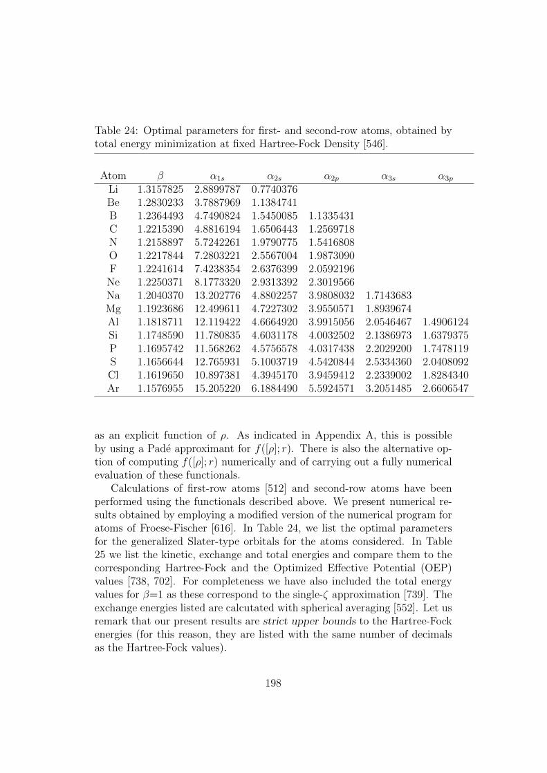
Table 24: Optimal parameters for first- and second-row atoms, obtained bytotal energy minimization at fixed Hartree-Fock Density [546].

Atom β α1s α2s α2p α3s α3p

Li 1.3157825 2.8899787 0.7740376Be 1.2830233 3.7887969 1.1384741B 1.2364493 4.7490824 1.5450085 1.1335431C 1.2215390 4.8816194 1.6506443 1.2569718N 1.2158897 5.7242261 1.9790775 1.5416808O 1.2217844 7.2803221 2.5567004 1.9873090F 1.2241614 7.4238354 2.6376399 2.0592196Ne 1.2250371 8.1773320 2.9313392 2.3019566Na 1.2040370 13.202776 4.8802257 3.9808032 1.7143683Mg 1.1923686 12.499611 4.7227302 3.9550571 1.8939674Al 1.1818711 12.119422 4.6664920 3.9915056 2.0546467 1.4906124Si 1.1748590 11.780835 4.6031178 4.0032502 2.1386973 1.6379375P 1.1695742 11.568262 4.5756578 4.0317438 2.2029200 1.7478119S 1.1656644 12.765931 5.1003719 4.5420844 2.5334360 2.0408092Cl 1.1619650 10.897381 4.3945170 3.9459412 2.2339002 1.8284340Ar 1.1576955 15.205220 6.1884490 5.5924571 3.2051485 2.6606547

as an explicit function of ρ. As indicated in Appendix A, this is possibleby using a Pade approximant for f([ρ]; r). There is also the alternative op-tion of computing f([ρ]; r) numerically and of carrying out a fully numericalevaluation of these functionals.

Calculations of first-row atoms [512] and second-row atoms have beenperformed using the functionals described above. We present numerical re-sults obtained by employing a modified version of the numerical program foratoms of Froese-Fischer [616]. In Table 24, we list the optimal parametersfor the generalized Slater-type orbitals for the atoms considered. In Table25 we list the kinetic, exchange and total energies and compare them to thecorresponding Hartree-Fock and the Optimized Effective Potential (OEP)values [738, 702]. For completeness we have also included the total energyvalues for β=1 as these correspond to the single-ζ approximation [739]. Theexchange energies listed are calcutated with spherical averaging [552]. Let usremark that our present results are strict upper bounds to the Hartree-Fockenergies (for this reason, they are listed with the same number of decimalsas the Hartree-Fock values).

198

Table 25: Total, kinetic, and exchange energies for ground states of neutralatoms A. Hartree-Fock and OEP values are included for comparison (inhartrees) [546]. Note that −EHF

total = T THFc and t for ‘total’ and ‘LS’ for‘LS-DFT’.

A −Eat −ELS

t −EOEPbt −EHF

t TLS −EOEPbx −ELSe

x −EHFex

Li 7.4184820 7.4326353 7.43250 7.4327269 7.4328807 1.781 1.781249 1.781186Be 14.556740 14.572470 14.57243 14.573023 14.573610 2.666 2.666947 2.666914B 24.498370 24.527667 24.52834 24.529061 24.529620 3.742962 3.743797C 37.622389 37.686695 37.68891 37.688619 37.689194 5.014164 5.015232N 54.268899 54.398488 54.40340 54.400934 54.401827 6.604 6.489698 6.490722O 74.540362 74.805922 74.81208 74.809399 74.812503 8.134316 8.134839F 98.942114 99.402954 99.40922 99.409349 99.415044 10.00273 10.00343Ne 127.81219 128.53684 128.5454 128.54710 128.55594 12.105 12.10693 12.10835Na 161.12392 161.84417 161.8566 161.85893 161.87344 14.013 14.01732 14.01752Mg 198.85779 199.58802 199.6116 199.61464 199.64127 15.988 15.99431 15.99429Al 241.15376 241.84121 241.8733 241.87671 241.91185 18.06924 18.06960Si 288.08997 288.80725 288.8507 288.85436 288.90071 20.25960 20.26027P 339.90989 340.65832 340.7150 340.71878 340.77786 22.634 22.56907 22.57008S 396.62761 397.42942 397.5016 397.50490 397.57908 24.97405 24.97531Cl 458.52370 459.39162 459.4776 459.48207 459.57038 27.50947 27.51161Ar 525.76526 526.71369 526.8122 526.81751 526.91757 30.175 30.18118 30.18494

aRef. [617]. These are the single-z calculations corresponding to the b = 1 non-

scaled orbitals [Eqs.(A1)-(A5)]. bRef. [736].cThese quantities are equal up to

digits quoted. d[737].eThe exchange energy for open-shell atoms was calculated

by averaging over the possible ways of occupying the magnetic states of the open

shells, which is equivalent to carrying out a spherical averaging (see, e.g., [617]).

199

We may conclude from Table 25 that the LS-DFT exchange energy func-tionals approach quite closely the corresponding Hartree-Fock ones. In factthe difference in exchange energy, in all the cases treated here, is of the or-der of millihartrees or even less. There is a larger discrepancy in the kineticenergy values as the difference between the LS-DFT and the Hartree-Fockvalues can get as large as one tenth of a hartree (in the case of Ar, for ex-ample). Even though this discrepancy may seem large, let us remark thatthe LS-DFT kinetic energy functionals are quite accurate when compared toother DFT kinetic energy functionals (see, for example, Ref. [740]).

For completeness we have included in Table 25 also the OEP total energyvalues [738]. It is observed that these values are closer to the Hartree-Fockones than the corresponding LS-DFT energies. Let us remark, however, thatthe OEP values are obtained by means of a minimization process that in-volves the iterative solution of one-particle equations and that in this senseit is a method that shares many of the characteristics of the Hartree-Fockapproximation (although in the spirit of DFT, the potential is local). Inthe present case, the LS-DFT energies are obtained from explicit functionalswhich contain as variational parameters αi and β. As shown elsewhere,when we use for first-row atoms a set βi, we obtain values which are prac-tically undistinguishable from the OEP ones [512], but in this case it is notpossible to obtain explicit analytic expressions for the functionals becausesome integrals cannot be calculated analytically. Thus, we would like tostress the fact that the LS-DFT values reported here are the closest approx-imations to Hartree-Fock values available in the literature for explicit DFTfunctionals.

Of particular importance is the fact that the present functionals leadin a natural way to atomic shell structure. Crucial in this respect is theeffect of the modulating factors, and in particular of τN . For this reason,we consider below, somewhat in detail the term τN corresponding to the 2Pstate of the aluminum atom. This term consists of six micro-states. We selectarbitrarily the micro-state with MS = 1/2 and ML = 0 with configuration1s22s22p63s23pα0 .

The explicit expression for the modulating factor τ of aluminum is givenby

τ = τKL + τKM + τLL + τLM + τMM (A16)

where we have collected the terms corresponding to each atomic shell and

200

Figure 15: The Hartree-Fock density and modulating factor for the groundstate of the Al atom.This figure is adapted from Ref. [546].

intershell. These terms are defined by

τIJ =1

2ρ8/3g (f)

ωIJ

ωKL = 4W1s2s + 12W1s2p

ωKM = 4W1s3s + 2W1s3p

ωLL = 12W2s2p

ωLM = 4W2s3s + 2W2s3p + 4W2p3s + 6W2p3p

ωMM = 2W3s3p (A17)

201

where

Wij =

(Rg,ni,li(f)

dRg,nj ,lj(f)

df−Rg,nj ,lj(f)

dRg,ni,li(f)

df

)2

. (A18)

Figure 16: The Hartree-Fock density and and KL and LM components ofthe modulating factor, τ for the ground state of the Al atom. This figure isadapted from Ref. [546].

In Fig. A1, we compare 4π r2ρHF (r) for aluminum with τ (down-scaledby a factor of 200). The remarkable fact is that the first and second maximaof τ are placed precisely at the first and second minima, respectively, ofthe radial distribution, namely, at the inter-shell boundaries. In the outerregion, τ goes to infinity rather sharply. It is clear from Fig. A1 that thekinetic energy modulating factor is responsible for the formation of sharplydefined potential basins coinciding with the atomic shells. But also, in areverse sense, the modulating factor τ is implicitly determined by the localand global minima of the radial distribution.

The behavior of the different shell- and intershell-components of τ aregiven in Figs. A2 and A3. It is observed that the first maximum is almost

202

entirely given by τKL. Similarly, the second maximum is accounted for byτLM . The contribution of τKM is practically zero and that of τLL is negligible.On the other hand, the sharp pick up of τ in the outer region is due to thecontribution τMM .

The point of the above analysis is to discriminate among the relativeimportance of the various components to the modulating factor in view tointroducing simpler approximations expressed as functions of the density andperhaps even as functions that are “universal” for some classes of systems.

Figure 17: The Hartree-Fock density and and KM, LL, and MM componentsof the modulating factor, τ , for the ground state of the Al atom. This figureis adapted from Ref. [546]

.

203

Appendix B: Generation of density transfor-

mations for diatomic molecules

In the general procedure for determining a density transformation advancedby Moser [541] and more recently by Bokanowski and Greber [517], one con-siders two volume elements τ = g(r)d3r and σ = h(r)d3r in the unit cubeQ ≡ [0, 1]3. If

∫Qg(r)d3r =

∫Qh(r)d3r then there exits a transformation

rρ = rρ(r) such that g(rρ(r))d3rρ = h(r)d3r.Given a wavefunction formed by plane waves whose density is ρ0 = N in

the unit cube, then by applying the coordinate-transformation operator Rρ1

to each one of the coordinates of this wavefunction, we can generate a trans-formed wavefunction containing density-scaled plane waves that associateswith the density ρ1(r). This density in connected to the initial one through

ρ1(r) = J(rρ1 ; r

)ρ0(rρ1), (B1)

where J(rρ1 ; r

)is the Jacobian. Similarly, for a density ρ2(r) we have

ρ2(r) = J(rρ2 ; r

)ρ0(rρ2). (B2)

The general density transformation from ρ1 to ρ2 satisfies the equation

ρ2(r) = J(~f ; r)ρ1(~f). (B3)

If we denote the operators for the transformations given in Eqs. (B1), (B2),

and (B3) by Rρ1 , Rρ2 , and f , respectively, we observe that they are relatedthrough the equation

f = (Rρ1)−1oRρ2 , (B4)

or equivalently byRρ1of = Rρ2 , (B5)

where (Rρ1)−1 denotes the inverse transformation. We now introduce the

decomposition of the above vectors in terms of their components in prolatespheroidal coordinates:

r = (rλ, rµ, rϕ),

~f = (fλ, fµ, fϕ),

rρ1 = (R1λ, R1µ, R1ϕ),

rρ2 = (R2λ, R2µ, R2ϕ). (B6)

204

These coordinates are defined by the relations

x =R

2

((λ2 − 1)(1− µ2)

)1/2

cosϕ,

y =R

2

((λ2 − 1)(1− µ2)

)1/2

sinϕ,

z =R

2λµ. (B7)

From the right-hand-side of Eq. (B5) it follows that

Rρ2o(rλ, rµ, rϕ) =(R2λ(rλ, rµ, rϕ), R2µ(rλ, rµ, rϕ), R2ϕ(rλ, rµ, rϕ)

)=

(R2λ(λ, µ, ϕ), R2µ(λ, µ, ϕ), R2ϕ(λ, µ, ϕ)

), (B8)

where, following the procedure of Zumbach and Maschke [474], we have de-fined

R2λ(λ, µ, ϕ) =

∫ µ−1ρ2(λ, µ, ϕ)

(λ2 − µ′2

)dµ∫ 1

−1ρ2(λ, µ, ϕ)

(λ2 − µ2

)dµ

,

R2µ(λ, µϕ) =

∫ λ1

∫ 1

−1ρ2(λ′, µ, ϕ)

(λ2 − µ2

)dµdλ∫∞

1

∫ 1

−1ρ2(λ, µ, ϕ)

(λ2 − µ2

)dµdλ

,

R2ϕ(λ, µ, ϕ) =

∫ ϕ0

∫∞1

∫ 1

−1ρ2(λ′, µ, ϕ)

(λ2 − µ2

)dµdλdϕ∫ aπ

0

∫∞1

∫ 1

−1ρ2(λ′, µ, ϕ)

(λ2 − µ2

)dµdλdϕ

. (B9)

Similarly, from the left-hand-side of Eq. (B5) it follows that

Rρ1ofo(rλ, rµ, rϕ) = Rρ1o(

(fλ(λ, µ, ϕ), fµ(λ, µ, ϕ), fϕ(λ, µ, ϕ))

=(R1λ(fλ, fµ, fϕ), R2µ(fλ, fµ, fϕ), R2ϕ(fλ, fµ, fϕ)

)=

(R1λ(λT , µT , ϕT ), R1µ(λT , µT , ϕT ), R2ϕ(λT , µT , ϕT )

).

(B10)

In Eq. (B10) the transformed prolate spheroidal coordinates are related to

the Cartesian components of the vector ~f = (fx.fy, fz) as follows:

fx =R

2

((λ2

T − 1)(1− µ2T ))1/2

cosϕT ,

fy =R

2

((λ2

T − 1)(1− µ2T ))1/2

sinϕT ,

fz =R

2λTµT . (B11)

205

and the components of the transformed vector are given by

R1λ(λT , µT , ϕT ), =

∫ µT−1

ρ2(λT , µT , ϕT )(λ2T − µ2

T

)dµT∫ 1

−1ρ2(λT , µT , ϕT )

(λ2T − µ2

T

)dµT

,

R1µ(λT , µT , ϕT ), =

∫ λT1

∫ 1

−1ρ2(λT , µT , ϕT )

(λ2T − µ2

T

)dµTdλT∫∞

1

∫ 1

−1ρ2(λT , µT , ϕT )

(λ2T − µ2

T

)dµTdλT

,

R2ϕ(λT , µT , ϕT ) =

∫ ϕT0

∫∞1

∫ 1

−1ρ2(λT , µT , ϕT )

(λ2T − µ2

T

)dµTdλTdϕT∫ aπ

0

∫∞1

∫ 1

−1ρ2(λT , µT , ϕT )

(λ2T − µ2

T

)dµTdλTdϕT

. (B12)

Equating each one of the components of Eqs. (B9) and (B12) we obtainthe following integral equations for the determination of the transformedcoordinates: ∫ µ

−1ρ2(λ, µ, ϕ)

(λ2 − µ′2

)dµ∫ 1

−1ρ2(λ, µ, ϕ)

(λ2 − µ2

)dµ

=

∫ µT−1

ρ2(λT , µT , ϕT )(λ2T − µ2

T

)dµT∫ 1

−1ρ2(λT , µT , ϕT )

(λ2T − µ2

T

)dµT

(B13)∫ λ1

∫ 1

−1ρ2(λ′, µ, ϕ)

(λ2 − µ2

)dµdλ∫∞

1

∫ 1

−1ρ2(λ, µ, ϕ)

(λ2 − µ2

)dµdλ

=

∫ λT1

∫ 1

−1ρ2(λT , µT , ϕT )

(λ2T − µ2

T

)dµTdλT∫∞

1

∫ 1

−1ρ2(λT , µT , ϕT )

(λ2T − µ2

T

)dµTdλT

(B14)∫ ϕ0

∫∞1

∫ 1

−1ρ2(λ′, µ, ϕ)

(λ2 − µ2

)dµdλdϕ∫ aπ

0

∫∞1

∫ 1

−1ρ2(λ′, µ, ϕ)

(λ2 − µ2

)dµdλdϕ

=

∫ ϕT0

∫∞1

∫ 1

−1ρ2(λT , µT , ϕT )

(λ2T − µ2

T

)dµTdλTdϕT∫ aπ

0

∫∞1

∫ 1

−1ρ2(λT , µT , ϕT )

(λ2T − µ2

T

)dµTdλTdϕT

(B15)

Each one of these equations must then be solved either by a numerical pro-cedure or by resorting to Pade approximants.

Let us now discuss a simpler way to generate the integral equations forthe local-scaling transformations of diatomic molecules. Applications of thismethod to polyatomic molecules (or solids) is discussed in Subsection 3.3.2.Consider the diatomic molecule orthonormal orbital set:

ψi(λ, µ, ϕ) = φi(λ, µ)eimiϕ (B16)

206

and its associated one-particle density (which depends only on coordinatesλ and µ):

ρ(λ, µ) =∑ij

Cijψ∗i (λ, µ, ϕ)ψj(λ, µ, ϕ) =

∑ij

δmimjφi(λ, µ)φj(λ, µ). (B17)

Let us assume that from the orthonormal set of one-particle functions ψi(λ, µ, ϕ)we obtain the density-transformed orbitals

ψTi (λ, µ, ϕ) =

√ρ2(λ, µ)

ρ1(λT , µT )ψi(λT , µT , ϕT ). (B18)

We now impose the orthonormality condition on these transformed orbitals:(R

2

)2 ∫ ∞1

dλ

∫ 1

−1

dµ

∫ 2π

0

dϕ(λ2 − µ2)ψ∗Ti (λ, µ, ϕ)ψTj (λ, µ, ϕ) = δij. (B19)

Substituting Eq. (B18) into Eq. (B19) we see that the orthonormality con-dition is now given by the differential equation:

dλdµdϕ(λ2 − µ2)ρ2(λ, µ) = dλTdµTdϕT (λ2T − µ2

T )ρ1(λT , µT ). (B20)

In order to integrate Eq. (B20), we assume the following functional form forthe transformed coordinates:

µT ≡ µT (µ),

λT ≡ λT (λ, µ),

ϕT = ϕ, (B21)

where we have explicitly set ϕT equal to ϕ in view of the fact that thiscoordinate fades out in the density of diatomic molecules. Using (B21) thedifferential relation (B20) simplifies to

dµdλ(λ2 − µ2)ρ2(λ, µ) = dµTdλT (λ2T − µ2

T )ρ1(λT , µT ). (B22)

Equation (B22) can be integrated over all space for both variables. This leadsto an equality in the normalization of both densities. Another expression isobtained when µ on the lhs is integrated from −1 to µ and µT in the right-hand-side from −1 to µT (while λ and λT are integrated over all space):∫ µ

−1

dµ

∫ ∞1

dλ(λ2 − µ2

)ρ2(λ, µ) =

∫ µT

−1

dµT

∫ ∞1

dλT

(λ2T − µ2

T

)ρ2(λT , µT ).

(B23)

207

Also, from Eq. (B22) we can integrate λ on the lhs from 1 to λ and λT in theright-hand-side from 1 to λT and then solve for dµT/dµ. However, anotherexpression for dµT/dµ can be obtained when we integrate λ and λT from 1to ∞. By equating the expressions for dµT/dµ, we obtain:∫ λ

1dλ(λ2 − µ′2

)ρ2(λ, µ)∫∞

1dλ(λ2 − µ2

)ρ2(λ, µ)

=

∫ λT1

dλT

(λ2T − µ2

T

)ρ2(λT , µT )∫∞

1dλT

(λ2T − µ2

T

)ρ2(λT , µT )

. (B24)

Equations (B23) and (B24) constitute the basis for the calculation of densitytransformations in diatomic molecules. Clearly, the transformed coordinateµT (µ) calculated by solving Eq. (B23) enters as a fixed quantity in Eq.(B24)which in turn allows us to determine λT (λ, µ). The alternative choice

λT ≡ λT (λ),

µT ≡ µT (λ, µ),

ϕT = ϕ, (B25)

could not be used as it was observed to lead to numerical unstabilities.

References

[1] W. Kohn, C. D. Sherrill, Editorial: Reflections on fifty years of densityfunctional theory, J. Chem. Phys. 140 (2014) 18A201.

[2] A. D. Becke, Perspective: Fifty years of density-functional theory in chemi-cal physics, J. Chem. Phys. 140 (2014) 18A301.

[3] P. Hohenberg, W. Kohn, Inhomogeneous electron gas, Phys. Rev. 136 (1964)B864-B87120.

[4] E. Runge, E. K. U. Gross, Density-functional theory for time-dependentsystems, Phys. Rev. Lett. 52 (1984) 997-1000.

[5] W. Kohn, L. J. Sham, Self-consistent equations including exchange andcorrelation effects, Phys. Rev. 140 (1965) A1133-A1138.

[6] P. C. Hohenberg, W. Kohn, L. J. Sham, The beginnings and some thoughtson the future, Adv. Quantum Chem. 21 (1990) 7-26.

20According to the American Physical Society, this paper was cited 15,323 times.

208

[7] W. Kohn, Electronic structure of matter - wave functionsand density functional, Nobel Lecture, January 28, 1999,http://www.nobelprize.org/nobel prizes/chemistry/laureates/1998/kohn-lecture.pdf [Reprinted in: Uspekhi Fiz. Nauk 172 (2002) 336–348 (2002)].

[8] W. Kohn, P. Vashishta, General density functional theory, in S. Lundqvist,N. H. March (Eds.), Theory of the Inhomogeneous Electron Gas, Plenum,New York, 1983, Ch. 2, p. 79-184.

[9] N. D. Mermin, Thermal properties of the inhomogeneous electron gas, Phys.Rev. 137 (1964) A1441-A1443.

[10] J. Keller, J. L. Gazquez (Eds.), Density Functional Theory, Lecture Notesin Physics, Vol. 187, Springer, Berlin, 1983.

[11] R. G. Parr, W. Yang, Density Functional Theory of Atoms and Molecules,Oxford University Press, Oxford, 1989.

[12] S. B. Trickey (Ed.), Density functional theory of many-electron systems,Adv. Quantum Chem., Vol. 21, Academic, New York, 1990.

[13] E. S. Kryachko, E. V. Ludena, Energy Density Functional Theory of Many-Electron Systems, Kluwer Academic Publishers, Dordrecht, 1990, 850 pp.

[14] E. Clementi, Book reviews: Energy Density Functional Theory of Many-Electron Systems. By Eugene S. Kryaschko (Institute of Theoretical Physics,Kiev, USSR) and Eduardo V. Ludena (Venezuelan Institute for TheoreticalPhysics, Caracas,Venezuela), J. Am. Chem. Soc. 113 (1991) 733.

[15] J.-L. Calais, Book review: Energy Density Functional Theory of Many-Electron Systems. E. S. Kryachko and E.V. Ludena, Kluwer, Dordrecht,1990. 864 pp., Int. J. Quantum Chem. 41 (1992) 525.

[16] J. Cioslowski, Book reviews: Energy Density Functional Theory of Many-Electron Systems. By Eugene S. Kryaschko (Institute of Theoretical Physics,Kiev, USSR) and Eduardo V. Ludena (Venezuelan Institute for TheoreticalPhysics, Caracas,Venezuela), J. Am. Chem. Soc. 113 (1991) 4369-4370.

[17] R. M. Dreizler, E. K. U. Gross, Density Functional Theory, Springer, Berlin,1990.

[18] I. Zh. Petkov, M. V. Stoitsov, Nuclear Density Functional Theory, OxfordStudies in Physics, Clarendon Press, Oxford, U.K., 1991.

[19] N. H. March, Electron Density Theory of Atoms and Molecules, AcademicPress, New York, 1992.

209

[20] D.P. Chong (Ed.), Recent Advances in Density Functional Methods, WorldScientific, Singapore, 1995.

[21] E.K.U. Gross, R.M. Dreizler (Eds.), Density Functional Theory, NATO ASISeries, Vol. B337, Plenum, New York, 1995.

[22] J.M. Seminario, P. Politzer (Eds.), Modern Density Functional Theory: ATool for Chemistry, Elsevier, Amsterdam, 1995.

[23] B. B. Laird, R. B. Ross, T. Ziegler (Eds.), Chemical Applications of Density-Functional Theory, ACS Symposium Series, Vol. 629, ACS, Washington,1996.

[24] H. Eschrig, The Fundamentals of Density Functional Theory, Teubner,Sttutgart, 1996.

[25] R.F. Nalewajski, Density functional theory I-IV, in: R.F. Nalewajski (Ed.),Topics in Current Chemistry, Springer, Berlin, 1996, pp.180-183.

[26] J. M. Seminario (Ed.), Recent Developments and Applications of DensityFunctional Theory, Elsevier, Amsterdam, 1996.

[27] J.F. Dobson, G. Vignale, M.P. Das, Electronic Density Functional Theory.Recent Progress and New Directions, Plenum Press, New York, 1998.

[28] P. Geerlings, F. de Proft, W. Langenaeker (Eds.), Density Functional The-ory. A Bridge between Chemistry and Physics, VUB University Press, Brus-sels, 1999.

[29] J.Cioslowski (Ed.), Many-Electron Densities and Reduced Density Matrices,Kluwer Academic/Plenum Publishers, New York, 2000.

[30] W. Koch and M.C. Holthausen, A Chemist’s Guide to Density FunctionalTheory, Wiley-VCH, Weinheim, 2000.

[31] V. E. van Doren, C. van Alsenoy, P. Geerlings (Eds.), Density FunctionalTheory and Its Applications to Materials, American Institute of Physics,2001.

[32] K.D. Sen (Ed.), Reviews in Modern Quantum Chemistry: A Celebration ofthe Contribution of Robert G. Parr, World Scientific, 2002.

[33] C. Fiolhais, F. Nogueira, and M. Marques (Eds.), A Primer in DensityFunctional Theory, Springer, Berlin, 2003.

[34] J. P. Perdew, S. Kurth, in: C. Fiolhais, F. Nogueira, and M.Marques (Eds.),A Primer in Density Functional Theory, Lecture Notes in Physics vol. 620,Springer, Berlin, 2003.

210

[35] N. Kaltsoyanis, J. E. McGrady (Eds.), Principles and Applications of Den-sity Functional Theory in Inorganic Chemistry I, Structure and Bonding,Vol. 112, Springer, Berlin, 2004, 194 pp.

[36] N. Kaltsoyanis, J. E. McGrady (Eds.), Principles and Applications of Den-sity Functional Theory in Inorganic Chemistry II, Structure and Bonding,Vol. 113, Springer, Berlin, 2004, 244 pp.

[37] V. Sahni, Quantal Density Functional Theory, Springer, Berlin, 2004.

[38] M. A. L. Marques, C. A. Ullrich, F. Nogueira, A. Rubio, K. Burke, E. K. U.Gross (Eds.) Time-Dependent Density Functional Theory, Lecture Notes inPhysics, Vol. 706, Springer, Berlin, 2006. 589 pp.

[39] P. K. Chattaraj, (Ed.), Chemical Reactivity Theory. A Density FunctionalView, CRC Press, 2009.

[40] D.S. Sholl, J.A. Steckel, Density Functional Theory: A Practical Introduc-tion, Wiley, New York, 2009.

[41] E. S. Kryachko, Density functional approach to many-electron systems: thelocal-scaling-transformation formulation, in: A. K. Roy (Ed.), Theoreticaland Computational Developments in Modern Density Functional Theory,Nova Publishers, New York, 2012. Ch. 6, pp. 169-187.

[42] E. Engel, R. M. Dreizler, Eds. Density Functional Theory. An AdvancedCourse. Springer, Berlin, 2011. 531 pp.

[43] D. Stalke, Ed. Electron Density and Chemical Bonding II. TheoreticalCharge Density Studies. Structure and Bonding, Vol. 147. Springer, Berlin,2012.

[44] M. A. L. Marques et al. (Eds.), Fundamentals of Time-Dependent DensityFunctional Theory. Lecture Notes in Physics, vol. 837. Springer, Berlin,2012. 559 pp.

[45] C. A. Ullrich, Time-Dependent Density-Functional Theory: Concepts andApplications. Oxford Graduate Texts. Oxford University Press, New York,2012, 526 pp.

[46] E. S. Kryachko, Density functional theory and molecular interactions: dis-persion interactions, in: M. V. Putz, D. M. Mingos (Eds.), Applications ofDensity Functional Theory to Biological and Bioinorganic Chemistry, Struc-ture and Bonding, Vol. 150, Springer, Heidelberg, 2013, Ch.2, pp. 65-96.

[47] T. A. Wesolowski, Y. A. Wang, Recent Advances in Orbital-Free DensityFunctional Theory, World Scientific, Singapore, 2013.

211

[48] M. Schluter, L. J. Sham, Density functional theory, Phys. Today 35 (1982)36-43.

[49] E.H. Lieb, Density functionals for Coulomb systems, Int. J. Quantum Chem.24 (1983) 243-277.

[50] R. McWeeny, Density functions and density functionals, Phil. Mag. B 69(1994) 727-735.

[51] R. G. Parr, Density functional theory, Annu. Rev. Phys. Chem. 34 (1983)631-659.

[52] R. G. Parr, Aspects of density functional theory, Phil. Mag. B 69 (1994)737-743.

[53] L. Fritsche, Density functional theory of superconductivity, Phil. Mag. B 69(1994) 859-870.

[54] A. K. Theophilou, Density functional theory for excited states, Phil. Mag.B 69 (1994) 771-777.

[55] R. G. Woolley, The density functional theorem and Huckel theories, Phil.Mag. B 69 (1994) 745-753.

[56] G. G. Hoffman, L. R. Pratt, Comparison of electron density functional mod-els, Mol. Phys. 82 (1994) 245-261.

[57] M. Levy, A. Gorling, Recent constrained-search advances for approximatingdensity functionals, Phil. Mag. B 69 (1994) 763-769.

[58] A. Nagy, Exact and approximate exchange potentials in the density func-tional theory, Phil. Mag. B 69 (1994) 779-785.

[59] A. Nagy, Density functional. Theory and application to atoms and molecules,Phys. Rep. 298 (1998) 1-79.

[60] R. Singh, B.M. Deb, Developments in excited-state density functional the-ory, Phys. Rep. 311 (1999) 47-94.

[61] Y. He, J. Grafenstein, E. Kraka, D. Cremer, What correlation effects arecovered by density functional theory? Mol. Phys. 98 (2000) 1639-1658.

[62] D. M. Brink, Density functional theory, Nucl. Phys. News 12 (2002) 27-32.

[63] I. Lindgren, S. Salomonson, Brueckner orbitals and density-functional the-ory, Int. J. Quantum Chem. 90 (2002) 294-308.

212

[64] V. Polo, E. Kraka, D. Cremer, Electron correlation and the self-interactionerror of density functional theory, Mol. Phys. 100 (2002) 1771-1790

[65] A. M. Alonso, A. Cuevas, On smoothed bootstrap for density functionals,J. Nonparametric Stat. 15 (2003) 467-477.

[66] P. Geerlings, F. De Proft, W. Langenaeker, Conceptual density functionaltheory, Chem. Rev. 103 (2003) 1793-1873.

[67] R. van Leeuwen, Density functional approach to the many-body problem:key concepts and exact functionals, Adv. Quantum Chem. 43 (2003) 25-94.

[68] I. Lindgren, S. Salomonson, Differentiability in density functional theory,Adv. Quantum Chem. 43 (2003) 95-117.

[69] M. A. L. Marques, E. K. U. Gross, Time-dependent density functional the-ory, Annu. Rev. Phys. Chem. 55 (2004) 427-455

[70] N. C. Handy, The molecular physics lecture 2004: (i) Density functionaltheory, (ii) Quantum Monte Carlo, Mol. Phys. 102 (2004) 2399-2409.

[71] A. D. Boese, W. Klopper, J. M. L. Martin, Anharmonic force fields andthermodynamic functions using density functional theory, Mol. Phys. 103(2005) 863-876.

[72] B. G. Levine, C. Ko, J. Quenneville, T. J. Martinez, Conical intersectionsand double excitations in time-dependent density functional theory, Mol.Phys. 104 (2006) 1039-1051.

[73] W. Kutzelnigg, Density functional theory (DFT) and ab-initio quantumchemistry (AIQC). Story of a difficult partnership, in: G. Maroulis and T.Simos (Eds.), Trends and Perspectives in Modern Computational Science,Lecture Series on Computer and Computational Sciences, Brill AcademicPublishers, Leiden, The Netherlands, 2006, Vol. 6, pp. 23-62.

[74] S. Kossmann, B. Kirchner, F. Neese, Performance of modern density func-tional theory for the prediction of hyperfine structure: meta-GGA and dou-ble hybrid functionals, Mol. Phys. 105 (2007) 2049-2071.

[75] J. Tao, J. P. Perdew, A. Ruzsinszky, G. E. Scuseria, G. I. Csonka, V. N.Staroverov, Meta-generalized gradient approximation: non-empirical con-struction and performance of a density functional, Phil. Mag. 87 (2007)1071-1084.

[76] C. A. Jimenez-Hoyos, B. G. Janesko, G. E. Scuseria, V. N. Staroverov, J.P. Perdew, Assessment of a density functional with full exact exchange andbalanced non-locality of correlation, Mol. Phys. 107 (2009) 1077-1088.

213

[77] J. W. D. Connolly, QTP in the 60s: John C. Slater and the beginnings ofdensity functional theory, Mol. Phys. 108 (2010) 2863-2866.

[78] D. Lee, K. Burke, Finding electron affinities with approximate density func-tionals, Mol. Phys. 108 (2010) 2687-2701.

[79] K. Burke, Perspective on density functional theory, J. Chem. Phys. 136(2012) 150901 [1-9].

[80] K. Capelle, V. L. Campo Jr., Density functionals and model hamiltonians:pillars of many-particle physics, Phys. Rep. 528 (2013) 91-159.

[81] Y. Cornaton, O. Franck, A. M. Teale, E. Fromager, Analysis of double-hybrid density functionals along the adiabatic connection, Mol. Phys. 111(2013) 1275-1294.

[82] S. Kvaal, U. Ekstrom, A. M. Teale, T. Helgaker, Differentiable but exactformulation of density-functional theory, e-preprint arXiv: 1312.3734 (2013),14 pp.; J. Chem. Phys. 140 (2014) 18A518.

[83] A. K. Theophilou, Welcome to the 14th international density functionalconference, Int. J. Quantum Chem. 113 (2013) 619.

[84] D R Bowler, T Miyazaki, Calculations on millions of atoms with DFT:Linear scaling shows its potential, e-preprint arXiv: 0911.3584 (2009), 11pp.

[85] C. O’Rourke, D. R. Bowler, Linear scaling real time TDDFT in the Con-Quest code, e-print arXiv: 1404.5776, 33 pp.

[86] A. Bethe, E. E. Salpeter, Quantum mechanics of one- and two-electron sys-tems, in: Encyclopedia of physics, Vol. 35, Springer, Berlin, 1957.

[87] V. A. Fock, On the Schrodinger equation for the atom of helium. Izv. Akad.Nauk SSSR, Ser. Fiz. (in Russian) 18 (1954) 161-172 [Engl. trans.: K. NorskVidensk. Selsk. Forh. 31 (1958) 138-152].

[88] E. W. Schmid, H. Ziegelmann, The quantum mechanical three-body prob-lem, Pergamon, Oxford, 1974.

[89] A. R. P. Rau, The negative ion of hydrogen, in: G. Srinivasan (Ed.) FromWhite Dwarfs to Black Holes: The Legacy of S. Chandrasekhar, The Uni-versity of Chicago Press, London, 1996, Ch. 5, pp. 65-102.

[90] L.H. Thomas, The calculation of atomic fields, Proc. Cambridge Phil. Soc.23 (1927) 542-548.

214

[91] E. Fermi, Un metodo statistico per la determinazione di alcune proprietadell’atomo, Rend. Accad. Naz. Lincei 6 (1927) 602-607.

[92] N.H. March, The Thomas-Fermi approximation in quantum mechanics,Adv. Phys. 6 (1957) 1-101.

[93] E.H. Lieb, Thomas-Fermi and Related Theories of Atoms and Molecules,Rev. Mod. Phys. 53 (1981) 603-641;Errata, Ibid. 54 (1982) 311(E).

[94] A. Zangwill, Hartree and Thomas: the forefathers of density functional the-ory, Arch. Hist. Exact. Sci. (2013) 331-348 .

[95] P.A.M. Dirac, Note on exchange phenomena in the Thomas-Fermi atom,Proc. Cambridge Phil. Soc. 26 (1930) 376-385.

[96] C.F.von Weizsacker, Zur theorie der kernmassen, Z. Phys. 96 (1935) 431-458.

[97] D.A. Kirzhnitz, Quantum corrections to Thomas-Fermi equation, Zh. Eksp.Teor. Fiz. 32 (1957) 115-123; [Sov. Phys. JETP 5 (1975) 64].

[98] C.H. Hodges, Quantum corrections to the Thomas-Fermi approximation andthe Kirzhnits method, Can. J. Phys. 51 (1973) 1428-1437.

[99] B. Grammaticos, Semiclassical approximations for nuclear Hamiltonians II.Spin-dependent potentials, A. Voros, Ann. Phys. 129 (1979) 153-171.

[100] D.R. Murphy, Sixth-order term of the gradient expansion of the kinetic-energy density functional, Phys. Rev. A 24 (1981) 1682-1688.

[101] W. Yang, Gradient correction in Thomas-Fermi theory, Phys. Rev. A34(1986) 4575-4585.

[102] P.-O. Lowdin, Some aspects on the development of the theory of reduceddensity matrices and the representability problem, in: R. Erdahl, V.H. Smith(Eds.), Density Matrices and Density Functionals, D. Reidel, Dordrecht,1987, pp. 21-49.

[103] J. Kohanoff and N.I. Gidopoulos, Density Functional Theory: Basics, NewTrends and Applications, in: S. Wilson (Ed.) Handbook of MolecularPhysics and Quantum Chemistry, Molecular Electronic Structure, Wiley,Chichester, 2003, Vol. 2, Part 5, Chapter 26, pp 532?568.

[104] G.E. Scuseria and V.N. Staroverov, Progress in the development ofexchange-correlation functionals, in: Theory and Application of Compu-tational Chemistry: The First Forty Years, C.E. Dykstra, G. Frenkling,K.S. Kim, G.E. Scuseria (Eds.), (Elsevier, Amsterdam, 2005), Ch. 24. pp.669-724.

215

[105] E. V. Ludena, J.M. Ugalde, X. Lopez, J. Fernandez-Rico, G. Ramırez, Areinterpretation of the nature of the Fermi hole, J. Chem. Phys. 120 (2004)540-547.

[106] P.W. Ayers, M. Levy, Generalized density-functional theory: conqueringthe N -representability problem with exact functionals for the electron pairdensity and the second-order reduced density matrix, J. Chem. Sci. 117(2005), 507-514.

[107] A. Gorling, Orbital- and state-dependent functionals in density-functionaltheory, J. Chem. Phys. 123 (2005) 062203 [1-16].

[108] P.W. Ayers, S. Golden, M.Levy, Generalizations of the Hohenberg-Kohntheorem: I. Legendre transform constructions of variational principles fordensity matrices and electron distribution functions, J. Chem. Phys. 124(2006) 054101.

[109] W. Kutzelnigg, Density functional theory in terms of a Legendre transfor-mation for beginners, J. Mol. Struct. (Theochem) 768 (2006) 163-173.

[110] A.J. Coleman, Structure of fermion density matrices, Rev. Mod. Phys. 35(1963) 668-687.

[111] A.J. Coleman, Reduced density matrices: 1929-1989, in: R. Erdahl, V.H.Smith (Eds.), Density Matrices and Density Functionals, D. Reidel, Dor-drecht, 1987, pp. 5-19.

[112] R. McWeeny, Density-functions and density functionals, Phil. Mag. B 69(1994) 727-735.

[113] E.V. Ludena, J. Keller, The importance of pure-state N -representability inthe derivation of extended Kohn-Sham equations, Adv. Quantum Chem. 21(1990) 46-67.

[114] M. H. Cohen, A. Wasserman, N -representability and stationarity in time-dependent density-functional theory, Phys. Rev. A 71 (2005) 032515-[1-9].

[115] E.S. Kryachko and E.V. Ludena, Formulation of N- and v- representabledensity-functional theory. I. Ground state, Phys. Rev. A 43 (1991) 2179-2193.

[116] E.S. Kryachko and E.V. Ludena, The N-representability problem and thelocal-scaling version of density functional theory, in: Condensed Matter The-ories, A. N. Proto and J. L. Aliaga (Eds.). Plenum, New York, 1992, Vol. 7,pp.229-241.

216

[117] E.V. Ludena, V.V. Karasiev, A. Artemyev, and D. Gomez, in: J. Cioslowski(Ed.) Many-Electron Densities and Reduced Density Matrices, Kluwer, NewYork, 2000, p.209.

[118] O. Bokanowski, New N-representability results involving symmetry and ap-plication to the density-functional theory formalism, J. Math. Chem. 26(1999) 271-296.

[119] P. W. Ayers, S. Liu, Necessary and sufficient conditions for the N-representability of density functionals, Phys. Rev. A 75 (2007) 022514.

[120] T. L. Gilbert, Hohenberg-Kohn theorem for nonlocal externai potentiais,Phys. Rev. B 12 (1975) 2111-2120.

[121] J.E. Harriman, Orthonormal orbitals for the representation of an arbitrarydensity, Phys. Rev. A 24 (1981) 680-682.

[122] C.R. Jacob, M. Reiher, Spin in density-functional theory, Int. J. QuantumChem. 112 (2012) 3661-3684.

[123] M. Podewitz, T. Weymuth, M. Reiher, In: Modeling of Molecular Proper-ties; P. Comba (Ed.) Wiley-VCH, Weinheim, 2011; pp. 137-163.

[124] A. Ghosh, Just how good is DFT? J. Biol. Inorg. Chem. 11 (2006) 671-673.

[125] C. J. Cramer, D. G. Truhlar, Density functional theory for transition metalsand transition metal chemistry, Phys. Chem. Chem. Phys. 11 (2009) 10757-10816.

[126] A. Ghosh, P. R. Taylor, High-level ab initio calculations on the energeticsof low-lying spin states of biologically relevant transition metal complexes:a first progress report, Curr. Opin. Chem. Biol. 7 (2003) 113-124.

[127] J. N. Harvey, DFT computation of relative spin-state energetics of transitionmetal compounds, Struct. Bond. 112 (2004) 151-183.

[128] C. Herrmann, L. Yu, M. Reiher, Spin states in polynuclear clusters: The[Fe2O2] core of the methane monooxygenase active site, J. Comput. Chem.27 (2006) 1223-1239.

[129] M. Swart, Accurate spin-state energies for iron complexes, J. Chem. TheoryComput. 4 (2008) 2057-2066.

[130] S. Ye, F. Neese, Accurate Modeling of spin-state energetics in spin-crossoversystems with modern density functional theory, Inorg. Chem. 49 (2010) 772-774.

217

[131] R. Bartlett, I. Schweiger, V. Lotrich, Ab initio DFT: Getting the right an-swer for the right reason, J. Mol. Struct. (Theochem) 771 (2006) 1-8.

[132] R. McWeeny, B. T. Sutcliffe, Methods of Molecular Quantum Mechanics,Academic Press, London, 1969.

[133] P.-O. Lowdin, The mathematical definition of a molecule and molecularstructure, In: J. Maruani (Ed.) Molecules in Physics, Chemistry, and Biol-ogy, Vol. II; Kluwer: Dordrecht, 1988. pp. 3-60.

[134] P.-O. Lowdin, On the importance of theory in the future development ofchemistry, J. Mol. Struct. (Theochem) 230 (1991) 1-3.

[135] R. G. Woolley, B. T. Sutcliffe, P.-O. Lowdin and the quantum mechanics ofmolecules, in: E. J. Brandas, E. S. Kryachko (Eds.), Fundamental World ofQuantum Chemistry. A Tribute to the Memory of Per-Olov Lowdin, Vol. I;Kluwer: Dordrecht, 2003, pp. 21-65.

[136] B. Sutcliffe, Some observations on P.-O. Lowdin’s definition of a molecule,Int. J. Quantum Chem. 90 (2002) 66-79.

[137] E. S. Kryachko, The force field picture of molecular shape response, Int. J.Quantum Chem. 108 (2008) 1930-1938.

[138] R. Ahlrichs, Basic mathematical properties of electronic wave functions inconfigurational space, in M. Defranceschi and J. Delhalle (Eds.), NumericalDetermination of the Electronic Structure of Atoms, Diatomic and Poly-atomic Molecules, Kluwer, Dordrecht, 1989. pp. 1-15.

[139] E. H. Lieb, Variational principle for many-fermion systems, Phys. Rev. Lett.46 (1981) 457-459; see also: E. H. Lieb, Variational principle for many-fermion systems, Ibid. 47 (1981) 69-69.

[140] A.J. Coleman, Structure of Fermion Density Matrices, Rev. Mod. Phys. 35(1963) 668-687.

[141] E. Clementi, S.J. Chakravorty, G. Corongiu, J.R. Flores and V. Sonnad,in: Modern Techniques in Computational Chemistry, E. Clementi (ed.),ESCOM, Leiden, 1991, p. 23.

[142] J. E. Mayer, Electron correlation, Phys. Rev. 100 (1955) 1579-1586.

[143] R. H. Tredgold, Density matrix and the many-body problem, Phys. Rev.105 (1957) 1421-1423.

[144] C. Garrod, J. K. Percus, Reduction of the N-particle variational problem,J. Math. Phys. 5 (1964) 1756-1775.

218

[145] D. Van Neck, P. W. Ayers, Necessary conditions for the N -representabilityof the second-order reduced density matrix: upper bounds on the P and Qmatrices, Phys.Rev. A 75 (2007) 032502.

[146] D.A. Mazziotti, Two-electron reduced density matrix as the basic variablein many-electron quantum chemistry and physics, Chem. Rev. 112 (2012)244-262.See also, D. A. Mazziotti (Ed.) Reduced-Density-Matrix Mechanics: WithApplications to Many-Electron Atoms and Molecules, Wiley, Hoboken, NJ,2007.

[147] M. Nakata, M. Fukuda, K. Fujisawa, Variational approac to electronicstructure calculations on second-order reduced density matrices and N -representability problem, Lecture Note Series, Vol. 9 (2012) 1-32.

[148] P.-O. Lowdin, Quantum theory of many-particle systems I. Physical inter-pretations by means of density matrices, natural spin-orbitals, and conver-gence problems in the method of configurational interaction? Phys. Rev. 97(1955) 1474-1489.

[149] R. McWeeny, Some recent advances in density matrix theory, Rev. Mod.Phys. 32 (1960) 335-369.

[150] P.A.M. Dirac, Quantum mechanics of many-electron systems, Proc. R. Soc.A 123 (1929) 714-733.

[151] P.A.M. Dirac, Note on exchange phenomena in Thomas atom, Proc. Cam-bridge Phil. Soc. 26 (1930) 376-385.

[152] P.A.M. Dirac, Note on the interpretation of the density matrix in the many-electron problem, Proc. Cambridge Phil. Soc. 27 (1931) 240-243.

[153] K. Husimi, Some formal properties of the density matrix, Proc. Phys. Math.Soc. Jpn. 22 (1940) 264-314.

[154] A. J. Coleman, The convex structure of electrons, Int. J. Quantum Chem.11 (1977) 907-916.

[155] A. J. Coleman, Reduced density operators and the N-particle problem, Int.J. Quantum Chem. 13 (1978) 67-82.

[156] E. R. Davidson, Reduced Density Matrices in Quantum Chemistry, Aca-demic Press, London, 1976.

[157] J. Cioslowski (Ed.), Many-Electron Densities and Reduced Density Matrices,Kluwer, New York, 2000.

219

[158] A.J. Coleman, V.I. Yukalov, Reduced Density Matrices: Coulson’s Chal-lenge, Springer, New York, 2000.

[159] L. Cohen, C. Frishberg, Hierarchy equations for reduced density matrices,Phys. Rev. A 13 (1976) 927-930.

[160] H. Nakatsuji, Equation for the direct determination of the density matrix,Phys. Rev. A 14 (1976) 41-50.

[161] D.R. Alcoba and C. Valdemoro, Family of modified-contracted Schrodingerequations, Phys. Rev. A 64 (2001) 062105.

[162] J.E. Harriman, Limitation of the density-equation approach to many-electron problems, Phys. Rev. A 19 (1979) 1893-1895.

[163] W. Kutzelnigg, Generalized K-particle Brillouin conditions and their use forthe construction of correlated electronic wavefunctions, Chem. Phys. Lett.64 (1979) 383-387.

[164] C. Valdemoro, Aproximating the second-order reduced density matrix interms of the first-order one, Phys. Rev. A 45 (1992) 4462-4467.

[165] F. Colmenero, C. Valdemoro, Approximating q-order reduced density ma-trices in terms of the lower-order ones. II. Applications, Phys. Rev. A 47(1993) 979-987.

[166] H. Nakatsuji, K. Yasuda, Direct determination of the quantum-mechanicaldensity matrix using the density equation, Phys. Rev. Lett. 76 (1996) 1039-1042.

[167] D.A. Mazziotti, Contracted Schrodinger equation: determining quantumenergies and tw-particle density matrices without wave functions, Phys. Rev.A 57, 4219 (1998) 4219-4243.

[168] D.A. Mazziotti, approximate solution for electron correlation through theuse of Schwinger probes, Chem. Phys. Lett. 289 (1998) 419-427.

[169] D.A. Mazziotti, Complete reconstruction of reduced density matrices, Chem.Phys. Lett. 326 (2000) 212-218.

[170] D.A. Mazziotti, Pursuit of N-representability for the contracted Schrodingerequation through density-matrix reconstruction, Phys. Rev. A 60 (1999)3618-3626.

[171] W. Kutzelnigg, D. Mukherjee, Direct determination of the cumulants of thereduced density matrices, Chem. Phys. Lett. 317 (2000) 567-574.

220

[172] M. Nooijen, M. Wladyslawski, A. Hazra, Cumulant approach to the directcalculation of reduced density matrices: a critical analysis, J. Chem. Phys.118 (2003) 4832-4848.

[173] D.R. Alcoba, C. Valdemoro, The correlation contracted Schrodinger equa-tion: an accurate solution of the G-particle-hole hypervirial, Int. J. QuantumChem. 109 (2009) 3178-3190

[174] D.A. Mazziotti, Parametrization of the two-electron reduced density matrixfor its direct calculation without the many-electron wave function: general-izations and applications, Phys. Rev. A 81 (2010) 062515.

[175] L. Vandenbergue, S. Boyd, Semidefinite programming, SIAM Rev., 38(1996) 49-50.

[176] M.J. Todd, Semidefinite optimization, Acta Numer. 19 (2001) 515-560.

[177] E. A. Yildirim, M. J. Todd, Sensitivity analysis in linear programming andsemidefinite programming using interior-point methods, Math. Program.Ser. A 90 (2001) 229-261.

[178] S. Boyd, L. Vandenberghe, Convex Optimization, Cambridge UniversityPress, Cambridge, 2009.

[179] S. Pironio, M, Navascues, A. Acio, Convergent relaxations of polynomialoptimization problems with noncommuting variables, SIAM J. Optim. 20(2010) 2157-2180.

[180] M. Nakata, H. Nakatsuji, M. Ehara, M. Fukuda, K. Nakata, K. Fujisawa,Variational calculations of fermion second-order reduced density matrices bysemidefinite programming algorithm, J. Chem. Phys. 114 (2001) 8282-8292.

[181] D. A. Mazziotti, R. M. Erdahl, Uncertainty relations and reduced den-sity matrices: mapping many-body quantum mechanics onto four particles,Phys. Rev. A 63 (2001) 042113.

[182] S. Burer, R. D. C. Monteiro, A nonlinear programming algorithm for solvingsemidefinite programs via low-rank factorization, Math. Program. 95 (2003)329-357.

[183] D. A. Mazziotti, Realization of quantum chemistry without wave functionsthrough first-order semidefinite programming, Phys. Rev. Lett. 93 (2004)213001.

[184] D. A. Mazziotti, Exactness of wave functions from two-body exponentialtransformations in many-body quantum theory, Phys. Rev. A 69 (2004)012507.

221

[185] M. Fukuda, B. J. Braams, M. Nakata, M. L. Overton, J. K. Percus,M.Yamashita, Z. Zhao, Large-scale semidefinite programs in electronic struc-ture calculation, Math. Program. Ser. B 109 (2007) 553-580.

[186] M. Fukuda, M. Nakata, M.Yamashita, Semidefinite programming: formula-tions and primal-dual interior-point methods, Adv. Chem. Phys. 134 (2007)103-118.

[187] M. Nakata, B.J. Braams, K. Fujisawa, M. Fukuda, J.K. Percus,M.Yamashita, Z. Zhao, Variational calculation of second-order reduceddensity matrices by strong N-representability conditions and an accuratesemidefinite programming solver, J. Chem.Phys. 128 (2008) 164113.

[188] M, Yamashita, K. Fujisawa, M. Fukuda, K. Nakata, M. Nakata, Algorithm925: parallel solver for semidefinite programming problem having sparseschur complement matrix, ACM Trans. Math. Softw. 39 (2012) 1-22.

[189] T. Baumgratz, M.B. Plenio, Lower bounds for ground states of condensedmatter systems, New J. Phys. 14 (2012) 023027.

[190] D. A. Mazziotti, Variational minimisation of atomic and molecular ground-state energies via the two-particle reduced density matrix, Phys. Rev. A 65(2002) 062511.

[191] D. A. Mazziotti, Variational method for solving the contracted Schrodingerequation through a projection of the N-particle power method onto the two-particle space, J. Chem. Phys. 116 (2002) 1239-1249.

[192] G. Guidofalvi and D. A. Mazziotti, Boson correlation energies via varia-tional minimization with the two-particle reduced density matrix: exactN-representability conditions for harmonic interactions, Phys. Rev. A 69(2004) 042511.

[193] K. Yasuda, Uniqueness of the solution of the contracted Schrodinger equa-tion, Phys. Rev. A 65 (2002) 052121.

[194] M. Nakata, M. Ehara, H. Nakatsuji, Density Matrix Variational Theory:Strength of Weinhold-Wilson Inequalities, in: E.J. Brandas and E.S Kry-achko (Eds.), Fundamental World of Quantum Chemistry, Vol. 1, KluwerAcademic Publishers, 2003, pp. 543-557.

[195] D. A. Mazziotti, Variational two-electron reduced density matrix theoryfor many-electron atoms and molecules: implementation of the spin- andsymmetry-adapted T2 condition through first-order semidefinite program-ming, Phys.Rev. A 72 (2005) 032510.

222

[196] G. Guidofalvi and D. A. Mazziotti, Computation of quantum phase transi-tions by reduced-density-matrix mechanics, Phys. Rev. A 74 (2006) 012501.

[197] D. R. Alcoba, C. Valdemoro, L. M. Tel, E. Perez-Romero, Controlling theN- and S-representability of the second-order reduced density matrix: thedoublet-state case, Phys. Rev. A 77 (2008) 042508.

[198] Z. Zhao, B.J. Braams, M. Fukuda, M. L. Overton, J. K. Percus, The reduceddensity matrix method for electronic structure calculations and the role ofthree-index representability, J. Chem. Phys. 120 (2004) 2095-2125.

[199] M. Nakata, B. J. Braams, K. Fujisawa, M. Fukuda, J. K. Percus, M. Ya-mashita, Z. Zhao, Variational calculation of second-order reduced densitymatrices by strong N-representability conditions and an accurate semidefi-nite programming Solver, J. Chem. Phys. 128 (2008) 164113.

[200] D. A. Mazziotti, Structure of fermionic density matrices: complete N-representability conditions, Phys. Rev. Lett. 108 (2012) 263002.

[201] D. A. Mazziotti, Significant conditions for the two-electron reduced densitymatrix from the constructive solution of N-representability, Phys. Rev. A 85(2012) 062507.

[202] M. Levy, P. Ziesche, The pair density functional of the kinetic energy andits simple scaling property, J. Chem. Phys. 115 (2001) 9110-9112.

[203] F. Furche, Towards a practical pair density-functional theory for many elec-tron systems, Phys. Rev. A 70 (2004) 022514.

[204] A. Nagy, Density-matrix functional theory, Phys. Rev. A 66 (2002) 022505.

[205] A. Nagy, C. Amovilli, Effective potential in density matrix functional theory,J. Chem. Phys. 121 (2004) 6640-6648.

[206] B. Hetenyi, L. Brualla, S. Fantoni, Quantum monte carlo algorithm basedon two-body density functional theory for fermionic many-body systems:Application to 3He, Phys. Rev. Lett. 93 (2004) 170202.

[207] J.K. Percus, At the boundary between reduced density-matrix and densityfunctional theories, J. Chem. Phys. 122 (2005) 234103.

[208] P.W. Ayers, M. Levy, Generalized density-functional theory: conqueringthe N-representability problem with exact functionals for the electron pairdensity and the second-order reduced density matrix, J. Chem. Sci. 117(2005) 507-514.

223

[209] A. Nagy, Hierarchy of equations in the generalized density functional theory,Int. J. Quantum Chem. 106 (2006) 1043-1051.

[210] P.W. Ayers, S. Golden, M. Levy, Generalizations of the Hohenberg-Kohntheorem: I. Legendre transform constructions of variational principles fordensity matrices and electron distribution functions, J. Chem. Phys. 124(2006) 054101.

[211] M. Higuchi, K. Higuchi, A proposal of the approximate scheme for calculat-ing the pair density, Physica B 387 (2007) 117-121.

[212] M. Higuchi, K. Higuchi, Pair density-functional theory by means of thecorrelated wave function, Phys. Rev. A 75 (2007) 042510.

[213] M. Higuchi, K. Higuchi, Pair density functional theory utilizing the non-interacting reference system: an effective initial theory, Phys. Rev. B 78(2008) 125101.

[214] B. Hetenyi, A.W. Hauser, Extended Hartree-Fock method based on pairdensity functional theory, Phys. Rev. B 77 (2008) 155110.

[215] K. Higuchi, M. Higuchi, Computational schemes for the ground-state pairdensity, J. Phys.: Condens. Matter 21 (2009) 064206.

[216] K. Higuchi, M. Higuchi, Computational pair density functional theory: aproposal for the kinetic energy functional, Phys. Rev. B 82 (2010) 155135.

[217] M. Higuchi, K. Higuchi, Correction method for obtaining the variationallybest ground-state pair density, Phys. Rev. A 84 (2011) 044502.

[218] E.R. Davidson, N-representability of the electron pair density, Chem. Phys.Lett. 246 (1995) 209-213.

[219] S.Kh. Samvelyan, N-representability of diagonal elements of second-orderreduced density matrices, Int. J. Quantum Chem. 65 (1997) 127-142.

[220] M.-E. Pistol, N-representability of two-electron densities and density ma-trices and the application to the few-body problem, Chem. Phys. Lett. 400(2004) 548-552.

[221] P. W. Ayers, E.R. Davidson, Necessary conditions for the N-representabilityof pair distribution functions, Int. J. Quantum Chem. 106 (2006) 1487-1498.

[222] P. Gori-Giorgi, A. Savin, System-adapted correlation energy density func-tionals from effective pair interactions, Phil. Mag. 86 (2006) 2643-2659.

[223] M.-E. Pistol, Characterization of N-representable n-particle densities whenN is infinite, Chem. Phys. Lett. 417 (2006) 521-523.

224

[224] M.-E. Pistol, Relations between N-representable n-particle densities, Chem.Phys. Lett. 422 (2006) 363-366.

[225] M.-E. Pistol, N-representable distance densities have positive Fourier trans-forms, Chem. Phys. Lett. 431 (2006) 216-218.

[226] P.W. Ayers, Using classical many-body structure to determine electronicstructure: an approach using k-electron distribution functions, Phys. Rev.A 74 (2006) 042502.

[227] P.W. Ayers, S. Liu, Necessary and sufficient conditions for the N-representability of density functionals, Phys. Rev. A 75 (2007) 022514.

[228] P.W. Ayers, E.R. Davidson, Linear inequalities for diagonal elements ofdensity matrices, Adv. Chem. Phys. 134 (2007) 443-483.

[229] M.-E. Pistol, Investigations of random pair densities and the application tothe N-representability problem, Chem. Phys. Lett. 449 (2007) 208-211.

[230] R. A. Donnelly and R. G. Parr, Elementary properties of an energy func-tional of the first-order reduced density matrix, J. Chem. Phys. 69 (1978)4431-4439 .

[231] R. A. Donnelly, On a fundamental difference between energy functionalsbased on first- and on second-order density matrices, J. Chem. Phys. 71(1979) 2874-2879.

[232] S.M. Valone, Consequences of extending 1-matrix energy functionals frompure-state representable to all ensemble representable 1 matrices, J. Chem.Phys. 73 (1980) 1344-1349.

[233] V. B. Bobrov, S. A. Trigger, The Problem of the Universal Density Func-tional and the Density Matrix Theory, JETP 143 (2013) 729-734.

[234] T. T. Nguyen-Dang, E. V. Ludena, Y. Tal, Variation of the energy functionalof the reduced first-order density operator, J. Mol. Struct. (Theochem) 120(1985) 247-264.

[235] E. V. Ludena, A. Sierraalta, Necessary conditions for the mapping of gammainto ρ, Phys. Rev. A 32 (1985) 19-25.

[236] E. V. Ludena, Variational principle with built-in pure state N-representability conditions, In: R. Erdahl, V. H. Smith Jr. (Eds.) DensityMatrices and Density Functionals, Reidel, Dordrecht, 1987, pp. 289-303.

[237] M. Piris, in: Reduced Density-Matrix Mechanics with Applications to Many-Electron Atoms and Molecules, Adv. Chem. Phys. 134, D.A. Mazziotti, Ed.;John Wiley and Sons: New York, 2007, Vol. 134, p. 387.

225

[238] A.M.K. Muller, Explicit approximate relation between reduced two- andone-particle density matrices,Phys. Lett. A 105 (1984) 446-452.

[239] S. Goedecker, C. J. Umrigar, A natural orbital functional for the many-electron problem, Phys. Rev. Lett. 81 (1998) 866-870.

[240] G. Csanyi, T. A. Arias, Tensor product expansions for correlation in quan-tum many-body systems, Phys. Rev. B 61 (2000) 7348-7352.

[241] E.J. Baerends, Exact exchange-correlation treatment of dissociated H2 indensity functional theory, Phys. Rev. Lett. 87 (2001) 133004.

[242] M.A. Buijse, E.J. Baerends, An approximate exchange-correlation hole den-sity as a functional of the natural orbitals, Mol. Phys. 100 (2002) 401-421.

[243] O. Gritsenko, K. Pernal, E. J. Baerends, An improved density matrix func-tional by physically motivated repulsive corrections, J. Chem. Phys. 122(2005) 204102.

[244] S. Sharma, J. K. Dowhurst, N. N. Lathiotakis, E. K. U. Gross, Reduceddensity matrix functional for many-electron systems, Phys. Rev. B 78 (2008)201103.

[245] N. N. Lathiotakis, N. Helbig, E. K. U. Gross, Performance of one-bodyreduced density-matrix functionals for the homogeneous electron gas, Phys.Rev. B 75 (2007) 195120.

[246] N. N. Lathiotakis, M. A. L. Marques, Benchmark calculations for reduceddensity-matrix functional theory, J. Chem. Phys. 128 (2008) 184103.

[247] N. N. Lathiotakis, N. Helbig, A. Zacarias, E. K. U. Gross, A functional ofthe one-body-reduced density matrix derived from the homogeneous electrongas: performance for finite systems, J. Chem. Phys. 130 (2009) 064109.

[248] N. N. Lathiotakis, N. I. Guidopoulos, N. Helbig, Size consistency of explicitfunctionals of the natural orbitals in reduced density matrix functional the-ory, J. Chem. Phys. 132 (2010) 084105.

[249] R.L. Frank, E.H. Lieb, R. Seiringer, H. Siedentrop, Muller’s exchange-correlation energy in density-matrix-functional theory, Phys. Rev. A 76(2007) 052517.

[250] M. Piris, X. Lopez, F. Ruizperez, J.M. Matxain, J. M. Ugalde, A naturalorbital functional for multiconfigurational states, J. Chem. Phys. 134 (2011)164102.

226

[251] M. Piris, A Natural Orbital Functionals Based on an Explicit Approach ofthe Two-Electron Cumulant, Int. J. Quantum Chem. 113 (2013) 620-630.

[252] M. Piris, A new approach for the two-electron cumulant in natural orbitalfunctional theory, Int. J. Quantum Chem. 106 (2006) 1093-1104.

[253] M. Piris, Natural orbital functional theory: molecules and polymers, Recent.Res. Devel. Quantum Chem. 4 (2004) 1-26.

[254] M. Piris, J.M. Matxain, X. Lopez, J. M. Ugalde, The role of the positivityN-representability conditions in natural orbital functional theory, J. Chem.Phys. 133 (2010) 111101.

[255] J.M. Matxain, M. Piris, J. Uranga, X. Lopez, G. Merino, J. M. Ugalde, Thenature of chemical bonds from PNOF5 Calculations, Chem. Phys. Chem.13 (2012) 2297-2303.

[256] K. Pernal, The equivalence of the Piris natural orbital functional 5 (PNOF5)and the antisymmetrized product of strongly orthogonal geminal theory,Comput. Theor. Chem. 1003 (2013) 127-129.

[257] E. S. Kryachko, On the original proof by reductio ad absurdum of theHohenberg-Kohn theorem for many-electron coulomb systems, Int. J. Quan-tum Chem. 103 (2005) 818-823.

[258] E. S. Kryachko, Note - On the proof by reductio ad absurdum of the general-ized Hohenberg-Kohn theorem for ensembles of fractionally occupied statesof Coulomb systems, Int. J. Quantum Chem. 106 (2006) 1795-1798.

[259] L. Massa, A Note Suggesting an approximation for the Hohenberg and Kohnfunctional, Int. J. Quantum Chem. 90 (2002) 291-293.

[260] A. I. Panin, 1-Density operators and algebraic version of the Hohenberg-Kohn theorem, Int. J. Quantum Chem. 107 (2007) 858-874.

[261] W. Szczepaniak, M. Dulak, T. A. Wesolowski, Comment on “On the originalproof by reductio ad absurdum of the Hohenberg-Kohn theorem for many-electron Coulomb systems”, Int. J. Quantum Chem. 107 (2007) 762-763.

[262] K. D. Sen, E. Besalu, R. Carbo-Dorca, A Naive Look on the Hohenberg-Kohn Theorem, J. Math. Chem. 25 (1999) 253-257.

[263] P. E. Lammert, On F AND E, in DFT, e-print ArXiv 1402-1381 (2014), 26pp.

[264] M. Reed, B. Simon, Methods of Modern Mathematical Physics II., AcademicPress N.Y., 1975.

227

[265] H. Englisch, R. Englisch, Hohenberg-Kohn theorem and non-V-representable densities, Physica 121A (1983) 253-.268.

[266] R. Pino, O. Bokanowski, E.V. Ludena, R. Lopez Boada, A Re-Statementof the Hohenberg-Kohn Theorem and Its Extension to Finite Subspaces,Theor. Chem. Acc. 118 (2007) 557-561.

[267] J.E. Harriman, Geometry of Density Matrices. IV. The Relationship Be-tween Density Matrices and Densities, Phys. Rev. A 27 (1983) 632-645.

[268] T. Kato, On the eigenfunctions of many-particle systems in quantum me-chanics, Commun. Pure Appl. Math. 10 (1957) 151-177.

[269] W. A. Bingel, The behaviour of the second-order density matrix at thecoulomb singularities of the Schrodinger equation, Theor. Chim. Acta 5(1966) 341-345.

[270] A. E. Carlsson and N. W. Ashcroft, Asymptotic freedom in solids: A theo-rem, Phys. Rev. B 25 (1982) 3474-3481 and references therein.

[271] E. Steiner, Charge densities in atoms, J. Chem. Phys. 39 (1963) 2365-2366.

[272] A. J. Coleman, Calculation of first- and second-order density matrices, In:The Force Concept in Chemistry, B. M. Deb (Ed.), Van Nostrand, NewYork, 1981, pp. 418-448

[273] A. S. Bamzai, B. M. Deb, The role of single-particle density in chemistry,Rev. Mod. Phys. 53 (1981) 95-126; Erratum: The role of single-particledensity in chemistry, 53 (1981) 593(E).

[274] V. H. Smith, Jr., Concepts of charge density analysis: the theoretical ap-proach, In: Electron Distribution and the Chemical Bond, P. Coppens, M.B. Hall (Eds.), Plenum, New York, 1982, pp. 3-59.

[275] P.-O. Lowdin, Twenty-five years of Sanibel Symposia: A brief historic andscientific survey, Int. J. Quantum Chem. S19 (1986) 19-37.

[276] P.-O. Lowdin, On the representability problem in variational quantum the-ory, Book of Abstracts, 213th ACS National Meeting, San-Francisco, April13-17 (1997) American Chemical Society, Washington, D. C., 1997, p. 82.

[277] A. Nagy, Excited states in density functional theory, Int. J. Quantum Chem.70 (1998) 681-691.

[278] N. Moiseyev, Comment on calculations of excited states by the density func-tional theory, Chem. Phys. Lett. 321 (2000) 469-472.

228

[279] N. H. March, I. A. Howard, A. Holas, P. Senet, V. E. Van Doren, Nuclearcusp conditions for components of the molecular energy density relevant fordensity-functional theory, Phys. Rev. A 63 (2000) 012520 [1-5].

[280] E. S. Kryachko, Reply to Comment on ”On the Original Proof by Reductioad Absurdum of the Hohenberg-Kohn Theorem for Many-Electron CoulombSystems” [Szczepanik, W; Dulak, M.; Wesolowski, T. A., Int. J. QuantumChem. 103, 818 (2006)] , e-print ArXiv 061-0261 (2006), 3 pp.

[281] R. F. W. Bader, Atoms in Molecules. A Quantum Theory (Clarendon, Ox-ford, 1990).

[282] C. Gatti, P. Fantucci, G. Pacchioni, Charge density topological study ofbonding in lithium clusters, Theor. Chim. Acta 72 (1987) 433-458.

[283] W. L. Cao, C. Gatti, P. J. MacDougall, R. F. W. Bader, On the presenceof non-nuclear attractors in the charge distributions of Li and Na clusters,Chem. Phys. Lett. 141 (1987) 380-385.

[284] J. Cioslowski, Nonnuclear attractors in the lithium dimeric molecule, J.Phys. Chem. 94 (1990) 5496-5498.

[285] D. Cooper, A molecular catastrophe, Nature 346 (1990) 796-797.

[286] K. E. Edgecombe, R. O. Esquivel, V. H. Smith, Jr., and F. Muller-Plathe,Pseudoatoms of the electron density, J. Chem. Phys. 97 (1992) 2593-2599.

[287] G. I. Bersuker, C. Peng, J. E. Boggs, The nature of the covalent bond:the existence and origin of nonnuclear attractors, J. Phys. Chem. 97 (1993)9323-9329.

[288] R. O. Esquivel, J. Chen, M. J. Stott, R. P. Sagar, V. H. Smith, Jr., Pseu-doconvexity of the atomic electron density: lower and upper bounds, Phys.Rev. A 47 (1993) 936-943.

[289] R. O. Esquivel, R. P. Sagar, V. H. Smith, Jr., J. Chen, M.J. Stott, Pseudo-convexity of the atomic electron density: a numerical study, Phys. Rev. A47 (1993) 4735-4748.

[290] C. J. Mei, K. E. Edgecombe, V. H. Smith, Jr., A. Heilingbrunner, Topologi-cal analysis of the charge density of solids ?? BCC sodium and lithium, Int.J. Quantum. Chem. 48 (1993) 287-293.

[291] V. Luana, P. Mon-Sanchez, A. Costales, M. A. Blanco, A. M. Pendas, Non-nuclear maxima of the electron density of alkaline metals, J. Chem. Phys.119 (2003) 6341-6350.

229

[292] O. A. Zhikol, A. F. Oshkalo, O. V. Shishkin, O. V. Prezhdo, Non-nuclearattractors on Si?Si bond in quantum-chemical modeling as basis set inade-quacy, Chem. Phys. 288 (2003) 159-169 and references therein.

[293] M. Levy, Universal Variational Functionals of Electron Densities, First-Order Density Matrices and Natural Spin-Orbitals and Solution of the v-Representability Problem. Proc. Natl. Acad. Sci. USA 76 (1979) 6062-.

[294] A. Gorling, M. Ernzerhof, Energy differences between Kohn-Sham andHartree-Fock wave functions yielding the same electron density, Phys. Rev.A 51 (1995) 4501-4513.

[295] L. D. Site, Levy-Lieb Principle Meets Quantum Monte Carlo, ArXiv,Preprint 1311-5019 (2013), 14 pp.

[296] D.A. Mazziotti, Geminal functional theory: A synthesis of density and den-sity matrix methods, J. Chem. Phys. 112 (2000) 10125-10130.

[297] S.F. Sousa, P.A. Fernandes, M.J. Ramos, General performance of densityfunctionals, J. Phys. Chem. A 111 (2007) 10439-10452.

[298] J. Katriel, S. Roy, M. Springborg, Nonuniversality of commonly usedcorrelation-energy density functionals, J. Chem. Phys.124 (2006) 234111.

[299] I. Grabowski, S. Hirata, S. Ivanov, and R.J. Bartlett, Ab initio density func-tional theory: OEP-MBPT(2). A new orbital-dependent correlation func-tional, J. Chem. Phys. 116 (2002) 4415-4425.

[300] S. Ivanov, S. Hirata, I. Grabowski, R.J. Bartlett, Connections betweensecond-order Gorling-Levy and many-body perturbation approaches in den-sity functional theory, J. Chem. Phys. 118 (2003) 461-469.

[301] A. Beste, R.J. Bartlett, Independent particle theory with electron correla-tion, J. Chem. Phys. 120 (2004) 8395-8404.

[302] R.J. Bartlett, I. Grabowski, S. Hirata, S. Ivanov, The exchange-correlationpotential in ab initio density functional theory, J. Chem. Phys. 122 (2005)034104.

[303] R.J. Bartlett, V.F. Lotrich, I.V. Schweigert, Ab initio density functionaltheory: The best of both worlds?, J. Chem. Phys. 123 (2005) 062205.

[304] S. J. Vosko, L. Wilk, M. Nusair, Accurate spin-dependent electron liq-uid correlation energies for local spin density calculations: a critical anal-ysis, Can. J. Phys. 58 (1980) 1200-1211; See also Wikipedia: http ://en.wikipedia.org/wiki/Local − density approximation.

230

[305] R. Colle and O. Salvetti, A General Method for Approximating the Elec-tronic Correlation Energy in Molecules and Solids, J. Chem. Phys. 79 (1983)1404-1407, and references therein.

[306] J. P. Perdew, Density-functional approximation for the correlation energyof the inhomogeneous electron gas, Phys. Rev. B 33 (1986) 8822-8824; Er-ratum: Density-functional approximation for the correlation energy of theinhomogeneous electron gas, Ibid. 34 (1986) 7406(E).

[307] A. D. Becke, Density Functional Thermochemistry. IV. A New Dynami-cal Correlation Functional and Implications for Exact Exchange Mixing, J.Chem. Phys. 104 (1996) 1040- 1046.

[308] C. Lee, W. Yang, R. G. Parr, Development of the Colle-Salvetti correlation-energy formula into a functional of the electron density, Phys. Rev. B 37(1988) 785-789.

[309] A. D. Becke, Density-functional exchange-energy approximation with cor-rect asymptotic behavior, Phys. Rev. A 38 (1988) 3098-3100.

[310] A. D. Becke, Correlation energy of an inhomogeneous electron gas: Acoordinate-space model, J. Chem. Phys. 88 (1988) 1053-1062.

[311] J. P. Perdew, Unified theory of exchange and correlation beyond the lo-cal density approximation, in P. Ziesche and H.Eschrig (Eds.) ElectronicStructure of Solids, Akademie Verlag, Berlin, 1991, pp. 11-20.

[312] J. P. Perdew, J. A. Chevary, S.H. Vosko, K. A. Jackson, M. R. Pederson, D.J. Singh, C. Fiolhais, Atoms, molecules, solids, and surfaces: Applications ofthe generalized gradient approximation for exchange and correlation, Phys.Rev. B 46 (1992) 6671-6687.

[313] J. Baker, M. Muir, J. Andzelm, A study of some organic reactions usingdensity functional theory, J. Chem. Phys. 102 (1995) 2063-2079.

[314] J. Baker, J. Andzelm, M. Muir, P. R. Taylor, OH + H2 ? H2O + H. Theimportance of ’exact exchange’ in density functional theory, Chem. Phys.Lett. 237 (1995) 53-60.

[315] J. Baker, M. Muir, J. Andzelm, A. Scheiner, Hybrid Hartree-Fock density-functional theory functionals: the adiabatic connection method, in: Chem-ical Applications of Density-Functional Theory, Amer. Chem. Soc. Symp.Series, Washington, 1996, Ch. 24, pp. 342-367.

[316] J. P. Perdew and W. Yue, Accurate and simple density functional for theelectronic exchange energy: Generalized gradient approximation, Phys. Rev.B 33 (1986) 8800-8802.

231

[317] For meta-GGA and Jacob’s ladder see: J. Tao, J. P. Perdew, V. N.Staroverov, G. E. Scuseria, Climbing the density functional ladder: nonem-pirical meta–generalized gradient approximation designed for molecules andsolids, Phys. Rev. Lett. 91 (2003) 146401.

[318] For the extended study of PBE hybrids see: E. Fabiano, L. A. Constantin,F. Della Sala, Testing the broad applicability of the PBEint GGA functionaland its one-parameter hybrid form, Int. J. Quantum Chem. 113 (2013) 673-682.

[319] J. C. Snyder, M. Rupp, K. Hansen, K.-R. Mueller, and K. Burke, Findingdensity functionals with machine learning, e-print arXiv:1112.5441; Phys.Rev. Lett. (submitted).

[320] A. D. Becke, Density-functional thermochemistry. V. Systematic optimiza-tion of exchange-correlation functionals, J. Chem. Phys. 107 (1997), 8554-8560.

[321] D. J. Tozer, N. C. Handy, The Development of New Exchange-CorrelationFunctionals, J. Chem. Phys. 108 (1998) 2545-2555.

[322] T. Grabo, E.K.U. Gross, Density-functional theory using an optimizedexchange-correlation potential, Chem. Phys. Lett. 240 (1995) 141-150.

[323] S. Kummel, L. Kronik, Orbital-Dependent Density Functionals: Theory andApplications, Rev. Mod. Phys. 80 (2008) 3-60.

[324] J. D. Talman, W. F. Shadwick, Optimized effective atomic central potential,Phys. Rev. A 14 (1976) 36-40.

[325] E. J. Baerends, Exact exchange-correlation treatment of dissociated H2 indensity functional theory, Phys. Rev. Lett. 87 (2001) 133004.

[326] A. Gorling, New KS method for molecules based on an exchange chargedensity generating the exact local KS exchange potential, Phys. Rev. Lett.83 (1999) 5459-5462.

[327] A. Gorling, M. Levy, Exact Kohn-Sham scheme based on perturbation the-ory, Phys. Rev. A 50 (1994) 196-204.

[328] A. Gorling, M. Levy, DFT ionization formulas and a DFT perturbationtheory for exchange and correlation, Int. J. Quantum Chem. Symp. 29 (1995)93-108.

[329] M. Levy, Density-functional exchange correlation through coordinate scalingin adiabatic connection and correlation hole, Phys. Rev. A 43 (1991) 4637-4646.

232

[330] S. Hirata, S. Ivanov, I. Grabowski, R.J. Bartlett, K. Burke, J.A. Talman,Can optimized effective potentials be determined uniquely? J. Chem. Phys.115 (2001) 1635-1649.

[331] H. Englisch, R. Englisch, Exact density functionals for ground-state energies.I. General results, Phys. stat. sol. (b) 123 (1984) 711-721.

[332] J. Paldus, Coupled cluster methods, in: S. Wilson, P. F. Bernath,R.McWeeny (Eds.) Handbook of Molecular Physics and Quantum Chem-istry, vol. 2, Elements of Quantum Mechanics, John Wiley and Sons, UK,2003, pp.272-313.

[333] I. M. Glazman, Ju. I. Ljubic, Finite-Dimensional Linear Analysis: A Sys-tematic Presentation in Problem Form, MIT Press, Cambridge, MA, 1974,Ch. VI.

[334] S. Lang, Differential and Riemannian Manifolds, Springer, Berlin, 1995.

[335] J. P. Perdew, M. Levy, Extrema of the density functional for the energy:Excited states from the ground-state theory, Phys. Rev. B 31 (1985) 6264-6271.

[336] H. Englisch, H. Fiesler, A. Haufe, Density-functional calculations for excited-state energies, Phys. Rev. A 37 (1988) 4570-4576.

[337] Y. A. Zhang, Y. A. Wang, Are the unconvential density variations reallyunconventional? Int. J. Quantum Chem. 109 (2009) 3199-3216.

[338] R.K. Nesbet, Thomas–Fermi theory revisited, Int. J. Quantum Chem. 90(2002) 262-265.

[339] R. K. Nesbet, Kinetic energy as a density functional, Phys. Rev. A 65 (2001)010502(R).

[340] R.K. Nesbet, R. Colle, Tests of the locality of exact Kohn-Sham exchangepotentials, Phys. Rev. A 61 (1999) 012503.

[341] R. K. Nesbet, Local and nonlocal potential functions in density functionaltheory, Adv. Quantum Chem. 43 (2003) 1-23.

[342] I. Lindgren, S. Salomonson, Differentiability in density-functional theory,Adv. Quantum Chem. 43 (2003) 95-117.

[343] I. Lindgren, S. Salomonson, Comments on the locality in density-functionaltheory, Phys. Rev. A 67 (2003) 056501; I. Lindgren, S. Salomonson, Thelocality hypothesis in density-functional theory: An exact theorem, e-printArXiv 0402029 (2004), 13 pp.

233

[344] R. K. Nesbet, The exclusion principle for interacting electrons: Kohn–Shamversus Thomas–Fermi, Int. J. Quantum Chem. 100 (2004) 937-942.

[345] V. V. Karasiev and E.V. Ludena, The local exchange potential in densityfunctional theory, in: M. Belkacem and P.M. Dinh (Eds.) Condensed MatterTheories, Vol. 19, Nova Science Publishers, Commack, N.Y., 2005, Ch. 12.

[346] J.C. Slater, A simplification of the Hartree-Fock method, Phys. Rev. 81(1951) 385-390.

[347] O. V. Gritsenko, E. J. Baerends, Orbital structure of the Kohn-Sham ex-change potential and exchange kernel and the field-counteracting potentialfor molecules in an electric field, Phys. Rev. A 64 (2001) 042506

[348] C.E. Campbell, E. Krotscheck, T. Pang, Electron correlations in atomicsystems, Phys. Rep. 223 (1992) 1-42.

[349] R. K. Nesbet, Nonlocal potentials for short-range electronic correlation inatoms, molecules, and solids, Int. J. Quantum Chem. 100 (2004) 114-120.

[350] A. Seidl, A. Gorling, P. Vogl, J.A. Majewski, Generalized Kohn-Shamschemes and the band-gap problem, Phys. Rev. B 53 (1996) 3764-3774.

[351] A. Gorling, M. Levy, Hybrid schemes combining the Hartree?Fock methodand density-functional theory: underlying formalism and properties of cor-relation functionals, J. Chem. Phys. 106 (1997) 2675-2680.

[352] I. Lindgren, S. Salomonson, Bruechner orbitals and density-functional the-ory, Int. J. Quantum Chem. 90 (2002) 294-308.

[353] R. K. Nesbet, Kinetic energy in density-functional theory, Phys. Rev. A 58(1998) R12-R15.

[354] T. Gal, Wave-function-density relationship in density-functional theory,Phys. Rev. A 62 (2000) 044501.

[355] A. Holas and N.H. March, Comment on “Kinetic energy in density-functional theory”, Phys. Rev. A 64 (2001) 016501.

[356] R.K. Nesbet, Local and nonlocal potential functions in density functionaltheory, Adv. Quantum Chem. 43 (2003) 1-23.

[357] I. Lindgren, S. Salomonson, Differentiability in density-functional theory:Further study of the locality theorem, Phys. Rev. A 70 (2004) 032509.

234

[358] V. N. Glushkov, X. Assfeld, Constrained optimized effective potential ap-proach for excited states, in A. K. Roy (Ed.), Theoretical and ComputationalDevelopments in Modern Density Functional Theory, Nova Publishers, NewYork, 2012. Ch. 3, pp. 61-102.

[359] A.D. Becke, Density?functional thermochemistry. III. The role of exact ex-change, J. Chem. Phys. 98 (1993) 5648-5652

[360] J.G. Angyan, I.C. Gerber, A. Savin, J. Toulouse, van der Waals forces indensity functional theory: Perturbation long-range electron-interaction cor-rections. Phys. Rev. A 72 (2005) 012510.

[361] L. A. Curtiss, C. Redfern, K. Raghavachari, Assessment of Gaussian-3 anddensity-functional theories on the G3/05 test set of experimental energies,J. Chem. Phys. 123 (2005) 124107.

[362] S. Grimme, Semiempirical GGA-type density functional constructed with along-range dispersion correction, J. Comput. Chem. 27 (2006) 1787-1799.

[363] S. Grimme, Semiempirical hybrid density functional with perturbativesecond-order correlation, J. Chem. Phys. 124 (2006) 034108.

[364] T. Schwabe, S. Grimme, Towards chemical accuracy for the thermodynam-ics of large molecules: new hybrid density functionals including non-localcorrelation effects, Phys. Chem. Chem. Phys. 8 (2006) 4398-4401

[365] L.A. Curtiss, C. Redfern, K. Raghavachari, Gaussian-4 theory, J. Chem.Phys. 126 (2007) 084108.

[366] S. Grimme, F. Neese, Double-hybrid density functional theory for excitedelectronic states of molecules, J. Chem. Phys. 127 (2007) 154116.

[367] T. Schwabe, S. Grimme, Double-hybrid density functionals with long-rangedispersion corrections: higher accuracy and extended applicability, Phys.Chem. Chem. Phys. 9 (2007) 3397-3406.

[368] T. Beninhaus, R.A. DiStasio, Jr, R.C. Lochan, J.-D. Chai, M. Head-Gordon,J. Phys. Chem. A 112 (2008) 2702.

[369] Y. Zhao, D. G. Truhlar, The M06 suite of density functionals for maingroup thermochemistry, kinetics, noncovalent interactions, excited states,and transition elements: two new functionals and systematic testing of fourM06 functionals and twelve other functionals, Theor. Chem. Acc. 120 (2008)215-241.

[370] R. Atta-Fynn, A.K. Ray, Atomic adsorption on the (020) surface of α-Pu:A density functional study, Phys. Rev. B 77 (2008) 085105.

235

[371] Y. Zhang, X. Xu, W.A. Goddard III, Doubly hybrid density functional foraccuratedescriptions of nonbond interactions,thermochemistry, and thermo-chemical kinetics, Proc. Natl. Acad. Sci. USA 106 (2009) 4963-4968.

[372] R. Baer, E. Livshits, U. Salzner, Tuned Range-separated hybrids in densityfunctional theory, Annu. Rev. Phys. Chem. 61 (2010) 85-109.

[373] R.A. Evarestov, Hybrid density functional theory LCAO calculations onphonons in Ba(Ti,Zr,Hf)3, Phys. Rev. B 83 (2011) 014105.

[374] T. Gould, J. F. Dobson, Efficient, long-range correlation from occupied wavefunctions only, Phys. Rev. B 84 (2011) 241108-[1-5].

[375] R. Peverati, D. G. Truhlar, Communication: A global hybrid generalizedgradient approximation to the exchange-correlation functional that satisfiesthe second-order density-gradient constraint and has broad applicability inchemistry, J. Chem. Phys. 135 (2011) 191102

[376] J. Plumley, J. J. Dannemberg, A comparison of the behavior of func-tional/basis set combinations for hydrogen-bonding in the water dimer withemphasis on basis set superposition error, J. Comput. Chem. 32 (2011) 1519-1527.

[377] Z.D. Pozum, G. Henkelman, Hybrid density functional theory band struc-ture engineering in hematite, J. Chem. Phys. 134 (2011) 224706.

[378] K. Sharkas, J. Toulouse, A. Savin, Double-hybrid density-functional theorymade rigorous, J. Chem. Phys. 134 (2011) 064113.

[379] J. Toulouse, K. Sharkas, E. Bremond, C. Adamo, Communication: Ratio-nale for a new class of double-hybrid approximations in density-functionaltheory, J. Chem. Phys. 135 (2011) 101102.

[380] H. Kruse, S. Grimme, A geometrical correction for the inter- and intra-molecular basis set superposition error in Hartree-Fock and density func-tional theory calculations for large systems, J. Chem. Phys. 136 (2012)154101.

[381] V. Karasiev, E. Valderrama, E.V. Ludena, Analysis of various quantummechanical and DFT energy definitions. Application to atomic isoelectronicseries, J. Mol. Struct. (Theochem) 501-502 (2000) 195-206

[382] H. Nakatsuji, R.G. Parr, Variational principles which are functionals of elec-tron density, J. Chem. Phys. 63 (1975) 1112-1117.

[383] S. T. Epstein, A. C. Hurley, R. E. Wyatt, R. G. Parr, Integrated and IntegralHellmann?Feynman Formulas, J. Chem. Phys. 47 (1967) 1275-1285.

236

[384] F. Moscardo, F. Moscardo, The Hellmann–Feynman theorem and its relationwith the universal density functional, Chem. Phys. Lett. 428 (2006) 187-190..

[385] W. Yang, P.W. Ayers, Q. Wu, Potential functionals: dual to density func-tionals and solution to the v-representability problem, Phys. Rev. Lett. 92(2004) 146404.

[386] J.P. Perdew and K. Schmidt, Jacob?s ladder of density functional approx-imations for the exchange-correlation energy, in: V. Van Doren, C. VanAlsenoy, and P. Geerlings (Eds.), Density Functional Theory and its Appli-cations to Materials, AIP Melville, New York, 2001; AIP Conf. Proc. 577(2001) 1-20.

[387] V.N. Staroverov, G.E. Scuseria, J. Tao, J.P. Perdew, Tests of a ladder ofdensity functionals for bulk solids and surfaces, Phys. Rev. B 69 (2004)075102.

[388] J. P. Perdew, R. G. Parr, M. Levy, J. L. Balduz, Jr., Density-functional the-ory for fractional particle number: derivative discontinuities of the energy,Phys. Rev. Lett. 49 (1982) 1691-1694.

[389] A.J. Perez-Jimenez, F. Moscardo, J.C. Sancho-Garcıa, L.P. Abia, E. San-Fabian, J.M. Perez-Jorda, New approach to the design of density functionals,J. Chem. Phys. 114 (2001) 2022-2026.

[390] A.J. Perez-Jimenez, J.M. Perez-Jorda, L. Pastor-Abia, and J.C. Sancho-Garcıa, New correlation energy functionals with explicit dependence on thenumber of electrons, J. Chem. Phys. 116 (2002) 10571-10576.

[391] P.M.W. Gill, J.A. Pople, Exact exchange functional for the hydrogen atom,Phys. Rev. A 47 (1993) 2383-2385.

[392] V.W. Maslen, The Fermi, or exchange, hole in atoms, Proc. Phys. Soc. 69(1956) 734-740.

[393] J.C. Slater, A Simplification of the Hartree-Fock method, Phys. Rev. 81(1951) 385-390.

[394] R.J. Boyd, C.A. Coulson, The Fermi hole in atoms, J. Phys. B 7 (1974)1805-1816.

[395] C.A. Coulson, A.H. Nielson, Electron correlation in the ground state ofhelium, Proc. Phys. Soc. 78 (1961) 831-838.

[396] J.P. Perdew, J. Tao, V.N. Staroverov, and G.E. Scuseria, Meta-generalizedgradient approximation: Explanation of a realistic nonempirical densityfunctional, J. Chem. Phys. 120 (2004) 6898-6911.

237

[397] V. A. Fock, Bemerkung zum virialsatz, Z. Phys. 63 (1930) 855-858.

[398] G. Zumbach and K. Maschke, New approach to the calculation of densityfunctionals, Phys. Rev. A 28 (1983) 544-554; Erratum: New approach tothe calculation of density functionals, Ibid. A 29 (1984) 1585-1587(E).

[399] J.P. Perdew, A. Ruzsinszky, J. Tao, V.N. Staroverov, G.E. Scuseria, G.I.Csonka, Prescription for the design and selection of density functional ap-proximations: More constraint satisfaction with fewer fits, J. Chem. Phys.123 (2005) 062201.

[400] S. J. Chakravorty, S. R. Gwaltney, E. R. Davidson, F. A. Parpia, and C.Froese Fischer, Ground-state correlation energies for atomic ions with 3 to18 electrons, Phys. Rev. A 47 (1993) 3649-3670.

[401] G. W. Erickson, J Phys Chem Ref Data 6 (1977) 831.

[402] K. Strasburger, Modified Adiabatic Approximation: Charge Asymmetry inHD+ and HD, J Chem Phys 131 (2009) 134103.

[403] B. Weiner, S.B. Trickey, Time-dependent variational principle in densityfunctional theory, Adv. Quantum Chem. 35 (1999) 217-247.

[404] I. Balint, G, Dezso, I. Gyemant, A perfectly N-representable two-particledensity matrix for the electron correlation problem, J. Mol. Struct.(Theochem) 501-502 (2000) 125-131.

[405] G. Dezso, I. Balint, I. Gyemant, Application of two-electron reduced densitymatrices for determining correlation energy, J. Mol. Struct. (Theochem) 542(2001) 21-23.

[406] I. Balint, G. Dezso, I. Gyemant, A novel approach for calculating correlationenergy based on the two-electron density matrix formalism, Int. J. QuantumChem. 84 (2001) 32-38.

[407] G. Gidofalvi, D.A. Mazziotti, Boson correlation energies via variationalminimization with the two-particle reduced density matrix: exact N-representability conditions for harmonic interactions, Phys. Rev. A 69 (2004)042511.

[408] For recent development see: R. Chakraborty, D. A. Mazziotti, GeneralizedPauli conditions on the spectra of one-electron reduced density matrices ofatoms and molecules, Phys. Rev. A 89 (2014) 042505.

[409] T. Juhasz, D.A. Mazziotti, Perturbation theory corrections to the two-particle reduced density matrix variational method, J. Chem. Phys. 121(2004) 1201-1205.

238

[410] D.M. Mazziotti, Realization of quantum chemistry without wave functionsthrough first-order semidefinite programming, Phys. Rev. Lett. 93 (2004)213001.

[411] For the recent development see: S. Veeraraghavan, D. A. Mazziotti, Globalsolutions of restricted open-shell Hartree-Fock theory from semidefinite pro-gramming with applications to strongly correlated quantum systems, J.Chem. Phys. 140 (2014) 124106.

[412] G. Gidofalvi, D. A. Mazziotti, Molecule-optimized basis sets and hamiltoni-ans for accelerated electronic structure calculations of atoms and molecules,J. Phys. Chem. A 118 (2014) 495-502.

[413] E.R. Davidson, N-representability of the electron-pair density, Chem. Phys.Lett. 246 (1995) 209-213.

[414] S.K. Samvelyan, N-representability of diagonal elements of second-order re-duced density matrices, Int. J. Quantum Chem. 65 (1997) 127-142.

[415] M.-E. Pistol, N-Representability of two-electron densities and density ma-trices and the application to the few-body problem, Chem. Phys. Lett. 400(2004) 548-552.

[416] P. W. Ayers, Generalized density functional theories using the k-electrondensities: development of kinetic energy functionals, J. Math. Phys. 46(2005) 062107.

[417] P.W. Ayers, Using classical many-body structure to determine electronicstructure: An approach using k-electron distribution functions, Phys. Rev.A 74 (2006) 042502.

[418] P.W. Ayers, private communication to E. V. Ludena, August 1, 2006.

[419] P.-O. Lowdin, Some aspects of the correlation problem and possible ex-tensions of the independent particle model, Adv. Chem. Phys. 14 (1969)283-340.

[420] P. Lykos, G. W. Pratt, Discussion on the Hartree-Fock approximation, Rev.Mod. Phys. 35 (1963) 496-501.

[421] J. A. Pople, R. K. Nesbet, Self-consistent orbitals for radicals, J. Chem.Phys. 22 (1954) 571-572.

[422] G. Berthier, Extension de la methode du champ moleculaire self-consistenta l’etude des couches incompletes. Compt. Rend. Acad. Sci. C 238 (1954)91-94; J. Chim. Phys. Phys.-Chim. Biol. 52 (1954) 363.

239

[423] U. von Barth and L. Hedin, A local exchange-correlation potential for thespin polarized case.i, J. Phys. C: Solid St. Phys. 5 (1972) 1629-1642.

[424] A. K. Rajagopal, J. Callaway, Inhomogeneous electron gas, Phys. Rev. B 7(1973) 1912-1919.

[425] O. Gunnarsson, B. I. Lundqvist, Exchange and correlation in atoms,molecules, and solids by the spin-density-functional formalism, Phys. Rev.B 13 (1976) 4274-4298.

[426] U. von Barth, Local-density theory of multiplet structure, Phys. Rev. A 20(1979) 1693-1703.

[427] C. C.J. Roothaan, Self-consistent field theory for open shells of electronicsystems, Rev. Mod. Phys. 32 (1960) 179-185.

[428] P.-O. Lowdin, Quantum theory of many-particle systems. III. Extensionof the Hartree-Fock scheme to include degenerate systems and correlationeffects, Phys. Rev. 97 (1955) 1509-1520.

[429] W. A. Goddard, Improved quantum theory of many-electron systems. I.Construction of eigenfunctions of S2 which satisfy Pauli’s principle, Phys.Rev. 157 (1967) 73-80.

[430] I. Mayer, J. Ladik, G. Biczo, Spin projected extended Hartree-Fock equa-tions, Int. J. Quantum Chem. 7 (1973) 583-608.

[431] J.M. Bofill, H. Bono, J. Rubio, Analysis of the convergence of the gen-eral coupling operator method for one-configuration-type wave functions, J.Comput. Chem. 19 (1998) 368-376.

[432] H. Fukutome, Unrestricted Hartree–Fock theory and its applications tomolecules and chemical reactions, Int. J. Quantum Chem. 20 (1981) 955-1065.

[433] B. Weiner, S.B. Trickey, Fukutome symmetry classification of theKohn?Sham auxiliary one-matrix and its associated state or ensemble, Int.J. Quantum Chem. 69 (1998) 451-460.

[434] A. Gorling, Symmetry in density-functional theory, Phys. Rev. A 47 (1993)2783-2799.

[435] P. S. Bagus, B.I. Bennett, Singlet–triplet splittings as obtained from theXα-scattered wave method: A theoretical analysis, Int. J. Quantum Chem.9 (1975) 143-148.

240

[436] T. Ziegler, A. Rauk, E.J. Baerends, On the calculation of multiplet energiesby the hartree-fock-slater method, Theor. Chim. Acta 43 (1977) 261-271.

[437] E.R. Johnson, R.M. Dickson, A.D. Becke, Density functionals andtransition-metal atoms, J. Chem. Phys. 126 (2007) 184104 .

[438] I. de P.R. Moreira, F. Illas, A unified view of the theoretical descriptionof magnetic coupling in molecular chemistry and solid state physics, Phys.Chem. Chem. Phys. 8 (2006) 1645-1659.

[439] Ph. de Loth, P. Cassoux, J.P. Daudey, J.P. Malrieu, Ab initio direct cal-culation of the singlet-triplet separation in cupric acetate hydrate dimer, J.Am. Chem. Soc. 103 (1981) 4007-4016.

[440] W. Heisenberg, Zur theorie des ferromagnetismus, Z. Phys. 49 (1928) 619-636.

[441] J. H. Van Vleck, The theory of Electric and Magnetic Susceptibilities, Ox-ford Universtity Press, 1932.

[442] L. Noodleman, Valence bond description of antiferromagnetic coupling intransition metal dimers, J. Chem. Phys. 74 (1981) 5737-5743.

[443] L. Noodlesman, E.R. Davidson, Ligand spin polarization and antiferromag-netic coupling in transition metal dimers, Chem. Phys. 109 (1986) 131-143.

[444] L. Noodlesman, C.Y. Peng, D.A. Case and J.M. Mouesca, Orbital interac-tions, electron delocalization and spin coupling in iron-sulfur clusters, Coord.Chem. Rev. 144 (1995) 199-244.

[445] K. Yamaguchi, T. Fueno, N. Ueyama, A. Nakamura, M. Ozaki, Antiferro-magnetic spin couplings between iron ions in iron-sulfur clusters. A localizedpicture by the spin vector model, Chem. Phys. Lett. 164 (1989) 210-216.

[446] K. Yamaguchi, T. Tsunekawa, Y. Toyoda, T. Fueno, Ab initio molecularorbital calculations of effective exchange integrals between transition metalions, Chem. Phys. Lett. 143 (1988) 371-376.

[447] H. Nagao, M. Mitani, M. Nishino, Y. Yoshioka, K. Yamaguchi, Possibilitiesof charge-and/or spin-mediated superconductors and photo-induced super-conductor in the intermediate region of metal-insulator transitions, Int. J.Quantum Chem. 65 (1997) 947-964.

[448] R. Caballol, O. Castell, F. Illas, J.P. Malrieu, I. de P.R. Moreira, Remarkson the proper use of the broken symmetry approach to magnetic coupling,J. Phys. Chem. A 101 (1997) 7860-7866.

241

[449] F. Illas, I. de P.R. Moreira, C. de Graaf, V. Barone, Magnetic couplingin biradicals, binuclear complexes and wide gap insulators: A survey ofab initio wave function and density functional theory approaches, Theoret.Chem. Acc. 104 (2000) 265-272.

[450] I.G. Kaplan, Problems in DFT with the total spin and degenerate states,Int. J. Quant. Chem. 107 (2007) 2595-2603.

[451] M. Levy, Phys. Electron densities in search of Hamiltonians, Rev. A 26(1982) 1200-1208.

[452] E. H. Lieb, Density functionals for coulomb systems, Int. J. Quantum Chem.24 (1983) 243-277.

[453] J. T. Chayes, L. Chayes, M. B. Ruskai, Density Functional Approach toQuantum Lattice Systems, J. Stat. Phys. 38 (1985) 497-518.

[454] C. A. Ulrich and W. Kohn, Kohn-Sham theory for ground-state ensembles,Phys. Rev. Lett. 87 (2001) 093001.

[455] M. Filatov and S. Shaik, Chem. Phys. Lett. 304 (1999) 429.

[456] M. Filatov, S. Shaik, Tetramethyleneethane (TME) diradical: Experimentand density functional theory reach an agreement, J. Phys. Chem. A 103(1999) 8885-8889.

[457] M. Filatov and S. Shaik, Diradicaloids: Description by the spin-restricted,ensemble-referenced Kohn-Sham density functional method, J. Phys. Chem.A 104 (2000) 6628-6636.

[458] S.P. de Visser, M. Filatov, S. Shaik, REKS calculations on ortho-, meta-andpara-benzyne, Phys. Chem. Chem. Phys. 2 (2000) 5046-5048.

[459] M. Filatov, S. Shaik, Artificial symmetry breaking in radicals is avoidedby the use of the ensemble-referenced Kohn-Sham (REKS) method, Chem.Phys. Lett. 332 (2001) 409-419.

[460] S.P. de Visser, M. Filatov, S. Shaik, Myers-Saito and Schmittel cyclizationof hepta-1,2,4-triene-6-yne: A theoretical REKS study, Phys. Chem. Chem.Phys. 3 (2001) 1242-1245.

[461] M. Filatov, D. Cremer, Bonding in the ClOO(2A”) and BrOO(2A”) rad-ical: Nonrelativistic single-reference versus relativistic multi-reference de-scriptions in density functional theory, Phys. Chem. Chem. Phys. 5 (2003)2320-2326.

242

[462] S.P. de Visser, M. Filatov, P.R. Schreiner, S. Shaik, A REKS assessmentof the face-diagonal bond in 1,3-didehydrocubane and a comparison withbenzyne biradicals, Eur. J. Org. Chem. 31 (2003) 4199-4204.

[463] F. Illas, I. de P. R. Moreira, J. M. Bofill, M. Filatov, Extent and limitationsof density-functional theory in describing magnetic systems, Phys. Rev. B70 (2004) 132414.

[464] F. Illas, I. de P.R. Moreira, J.M. Bofill, M. Filatov, Spin symmetry require-ments in density functional theory: The proper way to predict magneticcoupling constants in molecules and solids, Theor. Chem. Acc. 115 (2006)587-597.

[465] P.W. Ayers, W. Yang, Legendre-transform functionals for spin-density-functional theory, J. Chem. Phys. 124 (2006) 224108 .

[466] S. Lang, Algebra, Addison-Wesley, Reading, Mass, 1965. § 5.

[467] I. Zh. Petkov, M. V. Stoitsov, Local scale transformation method for theground state of many particle systems, Theor. Math. Phys. 55 (1983) 407-418.

[468] W. Macke, Wave mechanical treatment of the Fermi gas, Phys. Rev. 100(1955) 992-993.

[469] N. H. March, W. H. Young, Variational Methods based on the DensityMatrix, Proc. Phys. Soc. 72 (1958) 182-192.

[470] G.G. Hall, Improved atomic wavefunctions using a functional transforma-tion, Proc. Phys. Soc. 75 (1960) 575-581.

[471] J.K. Percus, The role of model systems in the few-body reduction of theN-fermion problem, Int. J. Quantum Chem. 13 (1978) 89-124.

[472] M.R. Nyden and R.G. Parr, Restatement of conventional electronic wavefunction determination as a density functional procedure, J. Chem. Phys.78 (1983) 4044-4047.

[473] E.V. Ludena, An approximate universal energy functional in density func-tional theory, J. Chem. Phys. 79 (1983) 6174-6181.

[474] G. Zumbach and K. Maschke, New approach to the calculation of densityfunctionals, Phys. Rev. A 28 (1983) 544-554; Erratum: New approach tothe calculation of density functionals, Ibid. A 29 (1984) 1585-1587(E).

[475] S.K. Ghosh, R.G. Parr, Density-determined orthonormal orbital approachto atomic energy functionals, J. Chem. Phys. 82 (1985) 3307-3315.

243

[476] P.M. Kozlowski, N.H. March, Approximate density-external potential rela-tion and the pauli potential for systems with coulombic interaction, Int. J.Quantum Chem. 36 (1989) 741-748.

[477] E.V. Ludena and R. Lopez-Boada, Local-scaling transformation version ofdensity functional theory: Generation of density functionals, Top. Curr.Chem. 180 (1996) 169-224.

[478] I.Zh. Petkov, M.V. Stoitsov, E.S. Kryachko, Method of local-scaling trans-formations and density-functional theory in quantum chemistry. I, Int. J.Quantum Chem. 29 (1986) 149-162.

[479] E.S. Kryachko, I.Zh. Petkov, and M.V. Stoitsov, Method of local-scalingtransformations and density-functional theory in quantum chemistry. II, Int.J. Quantum Chem. 32 (1987) 467-472.

[480] E.S. Kryachko, I.Zh. Petkov, and M.V. Stoitsov, Method of local-scalingtransformations and density-functional theory in quantum chemistry. III,Int. J. Quantum Chem. 32 (1987) 473-489.

[481] E.S. Kryachko, I.Zh. Petkov, and M.V. Stoitsov, Errata:Method of local-scaling transformations and density-functional theory in quantum chemistry.III, Int. J. Quantum Chem. 34 (1988) 305-306(E).

[482] E. S. Kryachko, Some approaches to density functional theory, in: LocalDensity Approximations in Quantum Chemistry and Solid State Physics.J.P. Dahl and J. Avery, Eds. Plenum, New York, 1984, pp. 207-227.

[483] E. S. Kryachko, E.V. Ludena, Many-electron energy-density-functional the-ory: Point transformations and one-electron densities, Phys. Rev. A 35(1987) 957-964.

[484] E. S. Kryachko, E. V. Ludena, Formulation of N- and v-representabledensity-functional theory. II. Spin-dependent systems, Phys. Rev. A 43(1987) 2194-2198.

[485] E.S. Kryachko, E.V. Ludena, Relationship between the density-driven andthe local-scaling formulations of density functional theory, J. Chem. Phys.95 (1991) 9054-9059.

[486] E.S. Kryachko and E.V. Ludena, Local-scaling density functional theory,in: S. Fraga (Ed.) Computational Chemistry: Structure, Interactions andReactivity, Elsevier, Amsterdam, 1992, pp. 136-165.

[487] E.V. Ludena and E.S. Kryachko, Local-scaling density functional theory:prospects for applications to the electronic structure of atoms, Rev. Mex.Astronom. Astrofisica 23 (1992) 95-106.

244

[488] E.S. Kryachko and T. Koga, Electron densities in momentum and positionspaces. I. Mapping relation and density functional aspect, J. Chem. Phys.91 (1989) 1108-1113.

[489] T. Koga, Y. Yamamoto and E.S. Kryachko, Electron densities in momentumand position spaces. II. Application of density mapping to the helium groundstate, J. Chem. Phys. 91 (1989) 4785-4762.

[490] T. Koga, Phys. Point transformations applied to density-functional calcula-tions, Rev. A 41 (1990) 1274-1280.

[491] T. Koga, Local scaling transformations applied to density-functional calcu-lations of Li and Be atoms, Phys. Rev. A 42 (1990) 3763-3767.

[492] T. Koga, An energy functional of electron–pair density, J. Chem. Phys. 93(1990) 5856-5861.

[493] T. Koga and Y. Yamamoto, Mapping between position and momentum den-sities by the local scaling method, Phys. Rev. A 42 (1990) 6336-6341.

[494] T. Koga, E.S. Kryachko, Spin-polarized density functional calculationsbased on local-scaling transformations, J. Chem. Phys. 94 (1991) 2910-2914.

[495] E.S. Kryachko, T. Koga, Retrospective outlook on computational aspects ofenergy density functional theory: Clementi’s explicit and implicit contribu-tion, Int. J. Quantum Chem. 42 (1992) 591-626.

[496] E.S. Kryachko, E.V. Ludena, T. Koga, The computational local-scaling en-ergy density functional theory, in: E. Clementi (Ed.) Methods and Tech-niques in Computational Chemistry, METECC-94, Vol. B: Medium SizeSystems, STEF, Cagliari, 1993, pp. 23-77.

[497] T. Koga, Y. Yamamoto, E.V. Ludena, Nonvariational configuration interac-tion calculations by local scaling method, J. Chem. Phys. 94 (1991) 3805-3807.

[498] T. Koga, Y. Yamamoto and E.V. Ludena, Local-scaling density-functionalmethod: Intraorbit and interorbit density optimizations, Phys. Rev. A 43(1991) 5814-5820.

[499] T. Koga, Local-scaling density-functional theory for excited states, J. Chem.Phys. 95 (1991) 4306-4310.

[500] E.S. Kryachko, E.V. Ludena, T. Koga, Formulation of N- and v- repre-sentable density functional theory. III. Excited states, J. Math. Chem. 11(1992) 325-339.

245

[501] E.S. Kryachko, E.V. Ludena, R. Lopez-Boada, J. Maldonado, The exchange-only self-consistent field procedure in the local-scaling version of densityfunctional theory: some theoretical and practical considerations, in: Con-densed Matter Theories, L. Blum and F.B. Malik (eds.), Plenum, New York,1993, Vol. 8, pp. 373-383.

[502] E. V. Ludena, R. Lopez-Boada, J. Maldonado, T. Koga, E. S. Kryachko,Calculation of the defect kinetic energy in Kohn-Sham theory by means oflocal-scaling transformation, Phys. Rev. A 48 (1993) 1937-1943.

[503] E.V. Ludena, R. Lopez-Boada and J. Maldonado, in: Condensed MatterTheories, J.W. Clark, A. Sadiq and K.A. Shoaib (eds.), Nova Science Pub-lishers, Commack, N.Y., 1994, Vol. 9, p. 97.

[504] E.V. Ludena, R. Lopez-Boada, J. Maldonado, Exact exchange-only densityfunctional theory by means of local scaling transformations, J. Mol. Struct.(Theochem), 330 (1995) 33-39.

[505] E.V. Ludena, J. Maldonado, R. Lopez-Boada, T. Koga, E.S. Kryachko,Local-scaling transformations and the direct determination of Kohn-Shamorbitals and potentials for beryllium. J. Chem. Phys. 102 (1995) 318-326.

[506] E.V. Ludena, E.S. Kryachko, T. Koga, R. Lopez-Boada,J. Hinze, J. Mal-donado, E. Valderrama, The Local-scaling version of density functional the-ory: A practical method for rigorous calculations of many-electron systems,in: Theoretical and Computational Chemistry: Density Functional Calcu-lations. J.M. Seminario and P. Politzer (eds.), Elsevier, Amsterdam,1995,Vol. 2, Ch. 3, p.75-124.

[507] E.V. Ludena, R. Lopez-Boada and R. Pino, in: Condensed Matter Theories,E.V. Ludena, P. Vashishta and R.F. Bishop (eds.), Nova Science Publishers,Commack, N.Y., 1996, Vol. 11, p. 51.

[508] E.V. Ludena, R. Lopez-Boada, J. Maldonado, E. Valderrama, T. Koga, E.S.Kryachko, J. Hinze, Local-scaling version of density functional theory, Int.J. Quantum Chem. 56 (1995) 285-301.

[509] R. Pino, R., E.V. Ludena, R. Lopez-Boada, in: Condensed Matter Theories,J. Navarro and M. de Llano (eds.), Nova Science Publishers, Commack,N.Y., 1995, Vol. 10, p. 189.

[510] E.V. Ludena, R. Lopez-Boada, R. Pino, Approximate kinetic energy densityfunctionals generated by local-scaling transformations, Can. J. Chem. 74(1996) 1097-1105.

246

[511] E. Valderrama, E.V. Ludena, J. Hinze, Analysis of dynamical and nondy-namical components of electron correlation energy by means of local-scalingdensity-functional theory, J. Chem. Phys. 106 (1997) 9227-9235.

[512] R. Lopez-Boada, E.V. Ludena, R. Pino, V. Karasiev, Hartree-Fock energy-density functionals generated by local-scaling transformations: Applicationsto first-row atoms, J. Chem. Phys. 107 (1997) 6722-6731.

[513] R. Lopez-Boada, R. Pino, E.V. Ludena, Explicit expressions for Ts[ρ] andEx[ρ] by Means of Pade approximants to local-scaling transformations, Int.J. Quantum Chem. 63 (1997) 1025-1035.

[514] E. S. Kryachko, Modern developments in the energy density functionaltheory of many-electron systems. In Lecture Notes in Chemistry, Vol. 50,Springer, Berlin, 1989. pp. 503-522.

[515] E. S. Kryachko, Local-scaling many-electron density functional theory, inNew Methods in Quantum Theory, C. A. Tsipis, V. S. Popov, D. R. Her-schbach, J. S. Avery (Eds.), NATO ASI Series 3, Vol. 8, Kluwer, Dordrecht,1996. pp. 339-358.

[516] E. S. Kryachko, The Local-Scaling-Transformation Formulation. In The-oretical and Computational Developments in Modern Density FunctionalTheory. A. K. Roy (Ed.), Nova Publishers, New York, 2012. Ch. 6, pp.169-187.

[517] O. Bokanowski, B. Grebert, A decomposition theorem for wave functions inmolecular quantum chenistry, Math. Models Methods Appl. Sci. 6 (1996)437-466.

[518] O. Bokanowski, B. Grebert, Deformations of density functions in molecularquantum chemistry, J. Math. Phys. 37 (1996) 1553-1571.

[519] O. Maurice-Bokanowski, These de Doctorat de l’Universite Paul SabatierNo. 2374 (Universite Paul Sabatier, Toulouse, France, 1996).

[520] R.L. Pavlov, J. Maruani, Ya.I. Delchev, R. McWeeny, Density functionaltheory for open-shell systems using a local-scaling transformation scheme. I.Single-density energy functional, Int. J. Quantum Chem. 65 (1997) 241-256.

[521] R.L. Pavlov, F.E. Zakhariev, Ya.I. Delchev, J. Maruani, Density functionaltheory for open-shell systems using a local-scaling transformation scheme.II. Euler-Lagrange equation for f(r) versus that for ρ(r), Int. J. QuantumChem. 65 (1997) 257-268.

[522] K.F. Freed, M. Levy, Direct first principles algorithm for the universal elec-tron density functional, J. Chem. Phys. 77 (1982) 396-398.

247

[523] I.Zh. Petkov, M.V. Stoitsov, E.S. Kryachko, Method of local-scaling trans-formations and density-functional theory in quantum chemistry, Int. J.Quantum Chem. 29 (1986) 149-161.

[524] E.S. Kryachko, I.Zh. Petkov, M.V. Stoitsov, Method of local- scaling trans-formations and density-functional theory in quantum chemistry. II, Int. J.Quantum Chem. 32 (1987) 467-472.

[525] E.S. Kryachko, I.Zh. Petkov, M.V. Stoitsov, Method of local- scaling trans-formations and density-functional theory in quantum chemistry. III, Int. J.Quantum Chem. 32 (1987) 473-489.

[526] M.V. Stoitsov and I.Zh. Petkov, Density functional theory at finite temper-atures, Ann. Phys. (N.Y.) 184 (1988) 121-147.

[527] E. S. Kryachko, E. V. Ludena, Formulation of N - and v-representabledensity-functional theory. I. Ground states, Phys. Rev. A 43 (1991) 2179-2193.

[528] B. Podolsky, Quantum-Mechanically Correct Form of Hamiltonian Functionfor Conservative Systems, Phys. Rev. 32 (1928) 812-816.

[529] F. M. Eger, E. P. Gross, Point transformations and the many body problem,Ann. Phys. (N.Y.) 24 (1963) 63-88.

[530] N. M. Witriol, Many-Body point transformations, J. Math. Phys. 11 (1970)669-680.

[531] G. Carmi, Point transformations in quantum mechanics. I., The Relativisticpotential problem, Phys. Rev. D 7 (1973) 1038-1044.

[532] A. M. Moro, J. M. Arias, J. Gomez-Camacho, F. Perez-Bernal, Solution ofrelativistic Hartree-Bogoliubov equations in configurational representation:Spherical neutron halo nuclei, Phys. Rev. C 80 (2010) 054605.

[533] S. Pittel, M. V. Stoitsov, An improved single-particle basis for nuclear struc-ture studies far from stability, Phys. At. Nucl. 64 (2001) 1055–1059.

[534] M.V. Stoitsov, P. Ring, D. Vretenar, and G.A. Lalazissis, Solution of rel-ativistic Hartree-Bogoliubov equations in configurational representation:Spherical neutron halo nuclei, Phys. Rev. C 58 (1998) 2086-2091.

[535] O. Bokanowski, B. Grebert, N. J. Mauser, Rigorous derivation of the “Xα”exchange potential: a deformation approach, J. Mol. Struct. (Theochem)501-502 (2000) 47-58.

248

[536] G. G. Hall, Improved atomic wave functions using a functional transforma-tion, Proc. Phys. Soc. (London) 75 (1960) 575-581.

[537] M. J. ten Hoor, Hall transformation of exp( - r): Correction of the results,Int. J. Quantum Chem. 33 (1988) 563-566.

[538] M. J. ten Hoor, On generalised Hall transformations, J. Phys. B: At. Mol.Opt. Phys. 22 (1989) L89-L94.

[539] G. Hojer, Two-parameter exponential-type basis functions for atomic calcu-lations, Int. J. Quantum Chem. 15 (1979) 389-401.

[540] L. S. Pontryagin, Ordinary Differential Equations, Nauka, Moscow, 1970.331 pp.

[541] J. Moser, On the volume elements on a manifold, Trans. Amer. Math. Soc.120 (1965) 286-294.

[542] (a) B. Dacorogna, J. Moser, On a partial differential equation involving theJacobian determinant, Ann. Inst. Henri Poincare, Anal. non. lin. 7 (1990)1-26.

[543] Y. E. Dong, Prescibing the Jacobian determinant in Sobolev spaces, Ibid.11 (1994), 275-296.

[544] O. Bokanowski, B. Grebert, Utilization of deformations in molecular quan-tum chemistry and application to density-functional theory, Int. J. QuantumChem. 68 (1998) 221-231.

[545] T. Koga, Y. Yamamoto, E.S. Kryachko, Electron densities in momentumand position spaces. II. Application of density mapping to the helium groundstate, J. Chem. Phys. 91 (1989) 4758-4762.

[546] E.V. Ludena, V. Karasiev, R. Lopez-Boada, E. Valderrama, J. Maldonado,Local-scaling transformation version of density functional theory: applica-tion to atoms and diatomic molecules, J. Comput. Chem. 20 (1999) 155-183.

[547] A. Cuyt and L. Wuytack, Nonlinear Methods in Numerical Analysis, North-Holland Mathematical Studies Vol. 136, North-Holland, Amsterdam, 1998.

[548] C. Eckart, The theory and calculation of screening constants, Phys. Rev. 36(1930) 878-892.

[549] G. W. Kellner, Die ionisierungsspannung des heliums nach derSchrodingerschen theorie, Z. Phys. 44 (1927) 91-109.

[550] E. Clementi and C. Roetti, Roothaan-Hartree-Fock atomic wavefunctions,At. Data and Nucl. Data Tables 14 (1974) 177.

249

[551] R.C. Raffenetti, Even-tempered atomic orbitals. II. Atomic SCF wavefunc-tions in terms of even-tempered exponential bases, J. Chem. Phys. 59 (1973)5936-5949.

[552] J. D. Talman, LSFBTR: A subroutine for calculating spherical bessel trans-forms, Comput. Phys. Commun. 30 (1983) 93-99.

[553] T. Koga, Y. Yamamoto, Mapping between position and momentum densitiesby the local scaling method, Phys. Rev. A 42 (1990) 6336-6341.

[554] P. Kaijser, V. H. Smith, Jr., Evaluation of momentum distributions andcompton profiles for atomic and molecular systems, Adv. Quantum Chem.10 (1977) 37-76.

[555] See e. g.: M. J. Maron, Numerical Analysis, Macmillan, N. Y., 1982. p.306ff.

[556] O. Bokanowski, Symmetry requirement for a deformation operator relatedto density functional theory, J. Math. Phys. 41 (2000) 2568-2585.

[557] T. Koga, Y. Yamamoto, E.V. Ludena, Nonvariational configuration interac-tion calculations by local scaling method, J. Chem. Phys. 94 (1991) 3805-3807.

[558] T. Koga, Y. Yamamoto, and E. V. Ludena, Local-scaling density-functionalmethod: Intraorbit and interorbit density optimizations, Phys. Rev. A 43(1991) 5814-5820.

[559] V.V. Karasiev, E.V. Ludena, A.N. Artemyev, Electronic-structure kinetic-energy functional based on atomic local-scaling transformations, Phys. Rev.A 62 (2000) 062510.

[560] E.V. Ludena, V.V. Karasiev, L. Echevarrıa, Realizations of the noninter-acting kinetic energy functional enhancement factor through local-scalingtransformations: Atoms, Int. J. Quantum Chem. 91 (2003) 94-104.

[561] E.V. Ludena, V. Karasiev, P. Nieto, Exact and approximate forms of thekinetic energy functional Ts[ρ] for molecules obtained via local-scaling trans-formations, Theor. Chem. Acc. 110 (2003) 395-402.

[562] M. Taut, Two electrons in an external oscillator potential: Particular ana-lytic solutions of a Coulomb correlation problem, Phys. Rev. A 48 (1993)3561-3566.

[563] S. Kais, D.R. Hershbach, N.C. Handy, C.W. Murray, G.J. Laming, Densityfunctionals and dimensional renormalization for an exactly solvable model,J. Chem. Phys. 99 (1993) 417-425.

250

[564] A. Artemyev, E. V. Ludena, V. Karasiev, A DFT variational approachto Hooke’s atom based on local-scaling transformations, J. Mol. Str.(Theochem) 580 (2002) 47-55.

[565] E. V. Ludena, D. Gomez, V. Karasiev, P. Nieto, Exact analytic total energyfunctional for Hooke’s atom generated by local-scaling transformations, Int.J. Quantum Chem. 99 (2004) 297-307.

[566] D. Gomez, E.V. Ludena, V.V. Karasiev,and P. Nieto, Application of exactanalytic total energy functional for Hooke’s atom to He, Li+ and Be++:An examination of the universality of the energy functional in DFT, Theor.Chem. Acc. 116 (2006) 608-613

[567] E.S. Kryachko, E.V. Ludena, Formulation of N- and v- representable densityfunctional theory. V. Exchange-only self-consistent field, Int. J. QuantumChem. 43 (1992) 769-782.

[568] J.C. Slater, Quantum Theory of Atomic Structure, McGraw-Hill, New York,1960, Vol. I, p. 309.

[569] W. Macke, Zur wellenmechanischen Behandlung von Vielkorperproblemen,Ann. Phys. 452(17) (1955) 1-9.

[570] J. K. Percus, The role of model systems in the few-body reduction of theN-fermion problem, Int. J. Quantum Chem. 13 (1978) 89-124.

[571] E.H. Lieb, Density Functionals for Coulomb Systems, in: Physics as Nat-ural Philosophy: Essays in Honor of Laszlo Tisza on his 75th Birthday, H.Feshback and A. Shimony (eds.), MIT Press, Cambridge, MA, 1982, p. 111.

[572] R.F.W. Bader, T.T. Nguyen-Dang and Y. Tal, A topological theory of molec-ular structure, Rep. Progr. Phys. 44 (1981) 893-948.

[573] T. Koga, Point transformations applied to density-functional calculations,Phys. Rev. A 41 (1990) 1274-1280.

[574] T. Koga, Local scaling transformations applied to density-functional calcu-lations of Li and Be atoms, Phys. Rev. A 42 (1990) 3763-3767.

[575] I. S. Gradshteyn, I. M. Ryzhik, Table of Integrals, Series, and Products,Academic, N. Y., 1980. p. 317.

[576] P.-O. Lowdin, Correlation problem in many-eleetron quantum mechanies. I.Review of different approaches and discussion of some current ideas, Adv.Chem. Phys. 2 (1959) 207-322.

251

[577] Q. Zhao, R.C. Morrison, R.G. Parr, From electron densities to Kohn-Sham kinetic energies, orbital energies, exchange-correlation potentials, andexchange-correlation energies, Phys. Rev. A 50 (1994) 2138-2142.

[578] E. Valderrama, E.V. Ludena, J. Hinze, (unpublished).

[579] R. Lopez-Boada, E.V. Ludena, V. Karasiev and R. Colle, Int. J. QuantumChem. (in press).

[580] J.B. Aviles, Jr., Extension of the Hartree method to strongly interactingsystems, Ann. Phys. (N.Y.). 5 (1958) 251-281.

[581] C. D. Hartog, H. A. Tolhoek, Cluster developments for Jastrow wave func-tions II Introduction of irreducible cluster functions, Physica 24 (1958) 875-895 and references therein.

[582] E. Buendia and R. Guardiola, Cluster expansions and variational montecarlo in medium light nuclei, in: L. Blum and F.B. Malik (Eds.) CondensedMatter Theories, Plenum, New York, 1993, Vol. 8, pp. 301-314.

[583] E.S. Kryachko, E.V. Ludena, T. Koga, The computational local-scaling en-ergy density functional theory, in: E. Clementi (Ed.) Methods and Tech-niques in Computational Chemistry, METECC-94, Vol. B: Medium SizeSystems, STEF, Cagliari, 1993, p. 23-77.

[584] E.S. Kryachko, E.V. Ludena, R. Lopez-Boada, J. Maldonado, The exchange-only self-consistent field procedure in the local-scaling version of densityfunctional theory: some theoretical and practical considerations, in: Con-densed Matter Theories, L. Blum and F.B. Malik (Eds.), Plenum, New York,1993, Vol. 8, p. 373-383.

[585] G. Hunter, The exact Schrodinger equation for the electron density, in: Den-sity Matrices and Density Functionals, R. Erdahl and V.H. Smith (eds.),Reidel, Dordrecht, 1985, pp. 583-595.

[586] Reference [13], Section 8.11.

[587] A. Tachibana, Shape wave in density functional theory, Int. J. QuantumChem. 34 (1988) 309-323.

[588] M. Levy, J. P. Perdew, V. Sahni, Exact differential equation for the densityand ionization energy of a many-particle system, Phys. Rev. A 30 (1984)2745-2748.

[589] E.N. Lassettre, Momentum eigenfunctions in the complex momentum plane.VI. A local potential function, J. Chem. Phys. 83 (1985) 1709-1721.

252

[590] Q. Zhao, R.G. Parr, Quantities Ts[n] and Tc[n] in density-functional theory,Phys. Rev. A 46 (1992) 2337-2343.

[591] M. Caffarel, Stochastic Methods in quantum mechanics, in: Numerical De-termination of the Electronic Structure of Atoms, Diatomic and PolyatomicMolecules, M. Defranceschi and J. Delhalle (Eds.), Kluwer Academic Pub-lishers, Dordrecht, 1989, p. 85-105.

[592] J.D. Morgan III, The analytic structure of atomic and molecular wavefunc-tions and its impact on the rate of convergence of variational calculationsin: Numerical Determination of the Electronic Structure of Atoms, Diatomicand Polyatomic Molecules, M. Defranceschi and J. Delhalle (Eds.), KluwerAcademic Publishers, Dordrecht, 1989, p. 49-84.

[593] For a recent review, see the Proceedings of the Sagamore X Conference onCharge, Spin and Momentum Densities, Z. Naturforsch. 48 a (1993) Number1/2.

[594] M. Levy and J.P. Perdew, The Constrained Search Formulation of Den-sity Functional Theory, in: Density Functional Methods in Physics, R.M.Dreizler and J. da Providencia (eds.), Plenum, New York, 1985, p. 11-30.

[595] J. D. Talman, W. F. Shadwick, Optimized effective atomic central potential,Phys. Rev. A 14 (1976) 36-40.

[596] S.H. Werden and E.R. Davidson, On the calculation of potentials from den-sities, in: Local Density Approximations in Quantum Chemistry and SolidState Physics, J.P. Dahl and J. Avery (eds.), Plenum, New York, 1984, p.33-42.

[597] C. O. Almbladh, A. C. Pedroza, Density-functional exchange-correlationpotentials and orbital eigenvalues for light atoms, Phys. Rev. A 29 (1984)2322-2330.

[598] F. Aryasetiawan, M. J. Stott, Effective potentials in density-functional the-ory, Phys. Rev. B 38 (1988) 2974-2987.

[599] Q. Zhao, R.G. Parr, Constrained-search method to determine electronicwave functions from electronic densities, J. Chem. Phys. 98 (1993) 543-548.

[600] Y. Wang, R.G. Parr, Construction of exact Kohn-Sham orbitals from a givenelectron density, Phys. Rev. A 47 (1993) R1591-R1593.

[601] E. V. Ludena, R. Lopez-Boada, J. Maldonado, T. Koga, E. S. Kryachko,Calculation of the defect kinetic energy in Kohn-Sham theory by means oflocal-scaling transformations, Phys. Rev. A 48 (1993) 1937-1943.

253

[602] E.V. Ludena, R. Lopez-Boada and J. Maldonado, in: Condensed MatterTheories, J.W. Clark, A. Sadiq and K.A. Shoaib (eds.), Nova Science Pub-lishers, Commack, N.Y., 1994, Vol. 9, (in press). Plenum, New York, 1993,Vol. 8, p. 373.

[603] E.H. Lieb, Density-Functionals for Coulomb Systems, in: Density FunctionalMethods in Physics, R.M. Dreizler and J. da Providencia (Eds.), Vol. 123of NATO ASI Series; Series B: Physics. Plenum, New York, 1985, p. 31-80.

[604] E.V. Ludena and E.S. Kryachko, Local-scaling density functional theory:prospects for applications to the electronic structure of atoms, Rev. Mex.Astr. y Astrofis., 23 (1992) 95-106.

[605] T. Ziegler, A. Rauk, E.J. Baerends, On the calculation of multiplet energiesby the Hartree-Fock-slater method, Theor. Chim. Acta 43 (1977) 261-271.

[606] E. K. U. Gross, L. N. Oliveira, W. Kohn, Rayleigh-Ritz variational principlefor ensembles of fractionally occupied states, Phys. Rev. A 37 (1988) 2805-2808

[607] L.N. Oliveira, Density functional treatment of excited states, Adv. QuantumChem. 21 (1990) 135-154.

[608] A. Gorling, Symmetry in density-functional theory, Phys. Rev. A 47 (1993)2783-2799

[609] A.K. Theophilou, Density functional theory for excited states, Phil. Mag. B69 (1994) 771-777.

[610] R. McWeeny, Density functions and density functionals, Phil. Mag. B 69(1994) 727-735.

[611] A. Savin, On degeneracy, near-degeneracy and density functional theory,in: J.M. Seminario (Ed.) Recent Developments and Applications of ModernDensity Functional Theory, Elsevier, Amsterdam, 1996, p. 327-358.

[612] B.I. Dunlap,Symmetry and density-functional exchange and correlation, in:J.M. Seminario and P. Politzer (Eds.) Modern Density Functional Theory.A Tool for Chemistry, Elsevier, Amsterdam, 1995, p. 151-168.

[613] J. P. Perdew, A. Savin, K. Burke, Escaping the symmetry dilemma througha pair-density interpretation of spin-density functional theory, Phys. Rev. A51 (1995) 4531-4541.

[614] A. Nagy, Kohn-Sham equations for multiplets, Phys. Rev. A 57 (1998) 1672-1677.

254

[615] J. C. Slater, Quantum Theory of Atomic Structure, Vol. II; McGraw-Hill:New York, 1960, p. 84.

[616] C. Froese-Fischer, The Hartree-Fock Method for Atoms. A Numerical Ap-proach; Wiley: New York, 1977 (and references therein).

[617] J. D. Talman, A program to compute variationally optimized effectiveatomic potentials, Comp. Phys. Commun. 54 (1989) 85-94.

[618] C. L. Pekeris, 11S, 21S, and 23S states of Li+, Phys. Rev. 126 (1962) 143-143.

[619] C. L. Pekeris, 11S, 21S, and 23S states of H− and He, Phys. Rev. 126 (1962)1470-1476.

[620] R.J. Boyd, The radial density function for the neutral atoms from heliumto xenon, Can. J. Phys. 55 (1977) 452-455.

[621] C.F. Bunge, J.A. Barrientos, A. V. Bunge, Roothaan-Hartree-Fock groundstate atomic wavefunctions, At. Data and Nucl. Data Tables 53 (1993) 113-162.

[622] R.O. Esquivel, A.V. Bunge, Accurate electron density and one electron prop-erties for the beryllium atom, Int. J. Quantum Chem. 32 (1987) 295-312.

[623] L. Laaksonen, P. Pyykko, D. Sundholm, Fully numerical Hartree-Fock meth-ods for molecules, Comput. Phys. Reports 4 (1986) 313-344.

[624] J. Kobus, L. Laaksonen, D. Sundholm, A numerical Hartree-Fock programfor diatomic molecules, Comput. Phys. Commun. 98 (1996) 346-358.

[625] B. J. Ransil, Studies in molecular structure. II. LCAO-MO-SCF wave func-tions for selected first-row diatomic molecules, Rev. Mod. Phys. 32 (1960)245-254.

[626] P. E. Cade, W. M. Huo, Hartree-Fock-Roothaan wavefunctions for diatomicmolecules: I. First- and second-row hydrides AH, AH±, and AH∗, At. Dataand Nucl. Data Tables 12 (1973) 415-466.

[627] P. E. Cade, W. M. Huo, Hartree-Fock-Roothaan wavefunctions for diatomicmolecules: II. First-row homonuclear systems A2, A±2 , and A∗2, At. Data andNucl. Data Tables 13 (1974) 339-389.

[628] P. E. Cade, W. M. Huo, Hartree-Fock-Roothaan wavefunctions for diatomicmolecules: III first-row heteronuclear systems, AB, AB±, AB∗, At. Dataand Nucl. Data Tables 15 (1975) 1-39.

255

[629] O.V. Gritsenko, R. van Leeuven, E.J. Baerends, Molecular Kohn-Shamexchange-correlation potential from the correlated ab initio electron den-sity, Phys. Rev. A 52 (1995) 1870-1874.

[630] O.V. Gritsenko, R. van Leeuven, E.J. Baerends, Molecular exchange-correlation Kohn-Sham potential and energy density from ab initio first- andsecond-order density matrices: Examples for XH (X=Li, B, F), J. Chem.Phys. 104 (1996) 8535-8545.

[631] O.V. Gritsenko, P.R.T. Schipper, E.J. Baerends, Exchange and correlationenergy in density functional theory: Comparison of accurate density func-tional theory quantities with traditional Hartree?Fock based ones and gener-alized gradient approximations for the molecules Li2, N2, F2, J. Chem. Phys.107 (1997) 5007-5015.

[632] O. V. Gritsenko, E. J. Baerends, Electron correlation effects on the shapeof the Kohn-Sham molecular orbital, Theor. Chem. Acc. 96 (1997) 44-50.

[633] A. Becke, A multicenter numerical integration scheme for polyatomicmolecules, J. Chem. Phys. 88 (1988) 2547-2553.

[634] D. G. Kanhere, A. Dhavale, E. V. Ludena, V. Karasiev, Ab initio linearscaling method for electronic structure calculations via local scaling trans-formations, Phys. Rev. A 62 (2000) 065201-[1 -4].

[635] G.B. Bachelet, D.R. Hamann, M. Schluter, Pseudopotentials that work:from H to Pu, Phys. Rev. B 26 (1982) 4199-4228.

[636] J.A. Appelbaum, D.R. Hamann, Self-Consistent Pseudopotential for Si,Phys. Rev. B 8 (1973) 1777-1780.

[637] I. G. Kaplan, Introduction to Theory of Intermolecular Interactions (in Rus-sian), Nauka, Moscow, 1982, p. 20.

[638] I. G. Kaplan, Intermolecular Interactions: Physical Picture, ComputationalMethods and Model Potentials, Wiley, Chichester, 2006.

[639] P. L. Huyskens, W. A. P. Luck, T. Zeegers-Huyskens, Intermolecular Forces.An Introduction to Modern Methods and Results, Springer, Berlin, 1991.

[640] P. Hobza and R. Zahradnik, Intermolecular Complexes, Academia, Prague,1988.

[641] J. N. Israelachvili, Intermolecular and Surface Forces, Academic, London,1985. Section 2.4.

256

[642] B. L. Blaney, G. E. Ewing, Van der Waals molecules, Annu. Rev. Phys.Chem. 27 (1976) 553-586.

[643] A. Y. Kipnis, B. E. Yavelov, J. S. Rowlinson, Van der Waals and MolecularSciences, Oxford, New York, 1996.

[644] N. Tariq, N. A. Taisan, V. Singh, J. D. Weinstein, Spectroscopic detectionof the LiHe molecule, Phys. Rev. Lett. 110 (2013) 153201 [1-5].

[645] E. H. Lieb, W. E. Thirring, Universal nature of van der Waals forces forCoulomb systems, Phys Rev A 34 (1986) 40-46.

[646] M. Lewin, Solution of a mountain pass problem for the isomerization of amolecule with one free atom, Ann Henri Poincare 7 (2006) 365-379.

[647] M. Reinganum, Krafte elektrischer Doppelpunkte nach der statistischenmechanik und anwendung auf molekulare und ionenwirkungen, Ann. Phys.(Paris) 38 (1912) 649-668.

[648] R. Eisenschitz, F. London, Uber das Verhaltnis der van der WaalsschenKrafte zu den homoopolaren bindungskraften, Z. Phys. 60 (1930) 491-527.

[649] F. London, Zur theorie und systematik der molekularkrafte, Z. Phys. 63(1930) 245-279.

[650] T. H. Boyer, Asymptotic Retarded van der Waals forces derived from clas-sical electrodynamics with classical electromagnetic zero-point radiation,Phys. Rev. A 5 (1972) 1799-1802.

[651] T. H. Boyer, Unretarded London-van der Waals Forces derived from classicalelectrodynamics with classical electromagnetic zero-point radiation, Phys.Rev. A 6 (1972) 314-319.

[652] T. H. Boyer, Retarded van der Waals Forces at all distances derived fromclassical electrodynamics with classical electromagnetic zero-point radiation,Phys. Rev. A 7 (1973) 1832-1840.

[653] T. H. Boyer, Van der Waals forces and zero-point energy for dielectric andpermeable materials, Phys. Rev. A 9 (1974) 2078-2084.

[654] T. H. Boyer, Any classical description of nature requires classical electro-magnetic zero-point radiation, Am. J. Phys. 79 (2011) 1163-1167.

[655] E. M. Lifshitz, Theory of molecular forces of atraction between solid bodies,Zh. Eksp. Teor. Fiz. 29 (1955) 94-110.

[656] I. E. Dzyaloshinskii, E. M. Lifshitz, L. P. Pitaevskii, The general theory ofvan der Waals forces, Uspekhi Fiz. Nauk 73 (1961) 381-422.

257

[657] E. Zaremba, W. Kohn, Van der Waals interaction between an atom and asolid surface, Phys. Rev. B 13 (1976) 2270-2285.

[658] B. I. Lundqvist, Y. Andersson, H. Shao, S. Chan, D. C. Langreth, Densityfunctional theory including van der Waals forces, Int. J. Quantum Chem.56 (1995) 247-255.

[659] Y. Andersson, D. C. Langreth, B. I. Lundqvist, van der Waals Interactionsin density-functional theory, Phys. Rev. Lett. 76 (1996) 102-105.

[660] Y. Andersson, E. Hult, H. Rydberg, P. Apell, B. I. Lundqvist, and D. C.Langreth, Van der Waals interactions in density functional theory, in: J. F.Dobson, G. Vignale, M.P. Das (Eds.) Electronic Density Functional Theory:Recent Progress and New Directions, Plenum, 1998, pp.243-260.

[661] O. Gunnarsson, M. Jonson, B. I. Lundqvist, Descriptions of exchange andcorrelation effects in inhomogeneous electron systems, Phys. Rev. B 20(1979) 3136-3164

[662] O. A. Vydrov, T. V. Voorhis, Benchmark Assessment of the accuracy of sev-eral van der Waals density functionals, J. Chem. Theory Comput. 8 (2012)1929-1934.

[663] Al. McClellan, Tables of Experimental Dipole Moments. Rahara Enterprises,El Cerrito, 1974.

[664] P. Debye, Polar Molecules, Chemical Catalogue, New York, 1929.

[665] H. Sack, in: E. Marx (Ed.), Handbuch der Radiologie Die Theorien derRadiologie, Akademische Verlaggesellschaft, Leipzig, 1934.

[666] See also: E. S. Kryachko, O. E. Yanovitskii, Number of states of a quantumrigid dipole in a cosine-type potential well, Phys. Rev. A 40 (1989) 5533-5541.

[667] W. H. Keesom, On the second virial coefficient for monatomic gases and forhydrogen below the Boyle-point”, Comm. Phys. Lab. Univ. Leiden Supple-ment, Ed. By H. Kamerlingh Onnes, Eduard Ijdo Printer, Leiden, Supple-ment 24a (1912) No. 121-132, 3-9.

[668] A. D. Buckingham, P. W. Fowler, J. M. Hutson, Theoretical studies of vander Waals molecules and intermolecular forces, Chem. Rev. 88 (1988) 963-988.

[669] W. L. Jorgensen, J. D. Madura, C. J. Swenson, Optimized intermolecularpotential functions for liquid hydrocarbons, J. Am. Chem. Soc. 106 (1984)6638-6646.

258

[670] A. D. MacKerell, Jr., M. J. Karplus, Importance of attractive van der Waalscontribution in empirical energy function models for the heat of vaporizationof polar liquids, J. Phys. Chem. 95 (1991) 10559-10560.

[671] A. I. Kitaigorodsky, Molecular Crystals and Molecules, Academic, New Yorkand London, 1973.

[672] J. Sponer P. Hobza, MP2 and CCSD(T) study on hydrogen bonding, aro-matic stacking and nonaromatic stacking, Chem. Phys. Lett. 267 (1997)263-270.

[673] A. D. Buckingham, in B. Pullman (Ed.) Intermolecular Interactions: FromDiatomics to Biopolymers, Wiley, Chichester, 1978.

[674] G. Chalasinski, M.M. Szczesniak, Origins of structure and energetics of vander Waals clusters from ab initio calculations, Chem. Rev. 94 (1994) 1723-1765.

[675] A. J. Stone, The Theory of Intermolecular Forces, Clarendon, Oxford, 1996.

[676] S. Tsuzuki and K. Tanabe, Basis set effects on the intermolecular interactionenergies of methane dimers obtained by the Moeller-Plesset perturbationtheory calculation, J. Phys. Chem. 95 (1991) 2272-2278.

[677] S. Tsuzuki, T. Uchimaru, K. Tanabe, Basis set effects on the intermolecularinteraction of hydrocarbon molecules obtained by an ab initio molecularorbital method: evaluation of dispersion energy, J. Mol. Struct. (Theochem)307 (1994) 107-118.

[678] C. Møller and M. S. Plesset, Note on an approximation treatment for many-electron systems, Phys. Rev. 46 (1934) 618-622.

[679] R. Krishnan, J. A. Pople, Approximate fourth-order perturbation theory ofthe electron correlation energy, Int. J. Quantum Chem. 14 (1978) 91-100.

[680] J. A. Pople, M. Head-Gordon, K. Raghavachari, Quadratic configuration in-teraction. A general technique for determining electron correlation energies,J. Chem. Phys. 87 (1987) 5968-5975.

[681] S. Tsuzuki, T. Uchimaru, K. Matsumura, M. Mikami, K. Tanabe, Effectsof basis set and electron correlation on the calculated interaction energiesof hydrogen bonding complexes: MP2/cc-pV5Z calculations of H2O-MeOH,H2O-Me2O, H2O-H2CO, MeOH-MeOH, and HCOOH-HCOOH complexes,J. Chem. Phys. 110 (1996) 11906-11910.

[682] A. D. Becke, Density-functional exchange-energy approximation with cor-rect asymptotic behavior, Phys. Rev. A 38 (1988) 3098-3100.

259

[683] C. Lee, W. Yang, R. G. Parr, Development of the Colle-Salvetti correlation-energy formula into a functional of the electron density, Phys. Rev. B 37(1988) 785-789.

[684] J. P. Perdew, Y. Wang, Accurate and simple analytic representation of theelectron-gas correlation energy, Phys. Rev. B 45 (1992) 13244-13249.

[685] A. D. Becke, Density-functional thermochemistry. III. The role of exact ex-change, J. Chem. Phys. 98 (1993) 5648-5652.

[686] D. J. Lackes, R. G. Gordon, Pair interactions of rare-gas atoms as a testof exchange-energy-density functionals in regions of large density gradients,Phys. Rev. A 47 (1993) 4681-4690.

[687] S. Kristyan, P. Pulay, Can (semi)local density functional theory account forthe London dispersion forces? Chem. Phys. Lett. 229 (1994) 175-180.

[688] J. M. Perez-Jorda, A. D. Becke, A density-functional study of van der Waalsforces: rare gas diatomics, Chem. Phys. Lett. 233 (1995) 134-137.

[689] P. Hobza, J. Spooner, T. Reschel, Density functional theory and molecularclusters, J. Comput. Chem. 16 (1995) 1315-1325.

[690] E. J. Meijer and M. Sprik, A density-functional study of the intermolecularinteractions of benzene, J. Chem. Phys. 105 (1996) 8684-8689.

[691] S. Tsuzuki, T. Uchimaru, K. Tanabe, Intermolecular interaction potentialsof methane and ethylene dimers calculated with the Moller-Plesset, coupledcluster and density functional methods, Chem. Phys. Lett. 287 (1998) 202-208.

[692] Y. Zhang, W. Pan, W. Yang, Describing van der Waals interaction in di-atomic molecules with generalized gradient approximations: The role of theexchange functional, J. Chem. Phys. 107 (1997) 7921-7925.

[693] T. A. Wesolowski, O. Parisel, Y. Ellinger, J. Weber, Comparative study ofbenzeneX (X = O2, N2, CO) complexes using density functional theory:The importance of an accurate exchange-correlation energy density at highreduced density gradients, J. Phys. Chem. A 101 (1997) 7818-7825.

[694] R. B. Zhang, K. R. F. Somers, E. S. Kryachko, M. T. Nguyen, T. Zeegers-Huyskens, A. Ceulemans, Hydrogen bonding to π-systems of indole and1-methylindole: Is there any OH· · ·Phenyl bond? J. Phys. Chem. A 109(2005) 8028-8034.

260

[695] E. R. Johnson, R. A. Wolkow, G. A. DiLabio, Application of 25 densityfunctionals to dispersion-bound homomolecular dimers, Chem. Phys. Lett.394 (2004) 334-338.

[696] S. Tsuzuki, H.P. Luthi, Interaction energies of van der Waals and hydrogenbonded systems calculated using density functional theory: Assessing thePW91 model, J. Chem. Phys. 114 (2001) 3949-3957.

[697] M.O. Sinnokrot, E.F. Valeev, C.D. Sherrill, Estimates of the ab initio limitfor π − π interactions: the benzene dimer, J. Am. Chem. Soc. 124 (2002)10887-10893.

[698] C. Tuma, A.D. Boese, N.C. Handy, Predicting the binding energies of H-bonded complexes: A comparative DFT study, Phys. Chem. Chem. Phys.17 (1999) 3939-3947.

[699] A.K. Rappe, E.R. Bernstein, Ab initio calculation of nonbonded interac-tions: are we there yet? J. Phys. Chem. A 104 (2000) 6117-6128.

[700] G.A. Jones, M.N. Paddon-Row, M.S. Sherburn, C.I. Turner, On theendo/exo stereoselectivity of intramolecular Diels-Alder reactions of hexadi-enylacrylates: an interesting failure of density functional theory, Org. Lett.4 (2002) 3789-3792.

[701] T. van Mourik, R.J. Gdanitz, A critical note on density functional theorystudies on rare-gas dimers, J. Chem. Phys. 116 (2002) 9620-9623.

[702] E. Engel, A. Hock, R.M. Dreizler, van der Waals bonds in density-functionaltheory, Phys. Rev. A 61, 032502 (2000).

[703] V. F. Lotrich, R. J. Bartlett, I. Grabowski, Intermolecular potential energysurfaces of weakly bound dimers computed from ab initio density functionaltheory: The right answer for the right reason, Chem. Phys. Lett. 405 (2005)43-48.

[704] S. Kristyan, P. Pulay, Can (semi)local density functional theory account forthe London dispersion forces? Chem. Phys. Lett. 229 (1994) 175-180.

[705] J. M. Perez-Jorda, A. D. Becke, A density-functional study of van der Waalsforces: rare gas diatomics, Chem. Phys. Lett. 233 (1995) 134-137.

[706] V. Lotrich, R. J. Bartlett, External coupled-cluster perturbation theory:Description and application to weakly interaction dimers. Corrections tothe random phase approximation, J. Chem. Phys. 134 (2011) 184108.

[707] H. Eshuis, F. Furche, A parameter-free density functional that works fornoncovalent interactions, J. Phys. Chem. Lett. 2011, 2, 983-989.

261

[708] J. F. Dobson, B. P. Dinte, Constraint satisfaction in local and gradientsusceptibility approximations: application to a van der Waals density func-tional, Phys. Rev. Lett. 76 (1996) 1780-1783.

[709] M. Dion, H. Rydberg, E. Schroder, D. C. Langreth, B. I. Lundqvist, Van derWaals density functional for general geometries, Phys. Rev. Lett. 92 (2004)246401.

[710] O. A. Vydrov, T. V. Voorhis, Nonlocal van der Waals density Functionalmade simple, Phys. Rev. Lett. 103 (2009) 063004.

[711] K. Lee, E Murray, L. Kong, B. I. Lundqvist, D. C. Langreth, Higher-accuracy van der Waals density functional, Phys. Rev. B 82 (2010)081101(R).

[712] Y. Zhao, D. G. Truhlar, The M06 suite of density functionals for main groupthermochemistry,thermochemical kinetics, noncovalent interactions, excitedstates,and transition elements: two new functionals and systematic testingoffour M06-class functionals and 12 other functionals, Theor. Chem. Acc. 120(2008) 215-241.

[713] X. Xu, W. A. Goddard III, The X3LYP extended density functional for ac-curate descriptions of nonbond interactions, spin states, and thermochemicalproperties, Proc. Natl. Acad. Sci. U.S.A. 101 (2004) 2673-2677.

[714] Y. Zhang, A. Vela, D. R. Salahub, Reparameterization of a meta-generalizedgradient approximation functional by combining TPSS exchange with τ1correlation, Theor. Chem. Acc. 118 (2007) 693-707.

[715] S. Grimme, Accurate description of van der Waals complexes by densityfunctional theory including empirical corrections, J. Comput. Chem. 25(2004) 1463-1473.

[716] T. Sato, H. Nakai, Density functional method including weak interactions:Dispersion coefficients based on the local response approximation, J. Chem.Phys. 131 (2009) 224104.

[717] T. Sato, H. Nakai, Local response dispersion method. II. Generalized mul-ticenter interactions, J. Chem. Phys. 133 (2010) 194101.

[718] A. Tkatchenko, M. Scheffler, Accurate molecular van der Waals interactionsfrom ground-state electron density and free-atom reference data, Phys. Rev.Lett. 102 (2009) 073005.

[719] S. Grimme, J. Antony, S. Ehrlich, H. Krieg, A consistent and accurate abinitio parametrization of density functional dispersion correction (DFT-D)for the 94 elements H-Pu, J. Chem. Phys. 132 (2010) 154104.

262

[720] F. Neese and F. Wennmohs, ORCA, An ab initio, DFT and semiempiricalSCF-MO package, Version 2.9.

[721] A. Krishtal, K. Vannomeslaeghe, D. Geldof, C. Van Alsenoy, P. Geerlings,Importance of anisotropy in the evaluation of dispersion interactions, Phys.Rev. A 83 (2011) 024501.

[722] A. Krishtal, K. Vanommeslaeghe, A. Olasz, T. Veszpremi, C. Van Alsenoy,P. Geerlings, Accurate interaction energies at density functional theory levelby means of an efficient dispersion correction, J. Chem. Phys. 130 (2009)174101.

[723] A. D. Becke, E. R. Johnson, Exchange-hole dipole moment and the disper-sion interaction revisited, J. Chem. Phys. 127 (2007) 154108.

[724] F. O. Kannemann, A. D. Becke, Van der Waals interactions in density-functional theory: intermolecular complexes, J. Chem. Theory Comput. 6(2010) 1081-1088.

[725] S. N. Steinmann, C. Corminboeuf, A system-dependent density-based dis-persion correction, J. Chem. Theory Comput. 6 (2010) 1990-2001.

[726] S. N. Steinmann, C. Corminboeuf, A generalized-gradient approximationexchange hole model for dispersion coefficients, J. Chem. Phys. 134 (2011)044117.

[727] A. Olasz, K. Vanommeslaeghe, A. Krishtal, T. Veszpremi, C. Van Alsenoy,P. Geerlings, The use of atomic intrinsic polarizabilities in the evaluation ofthe dispersion energy, J. Chem. Phys. 127 (2007) 224105.

[728] B. Jeziorski, R. Moszynski, K. Szalewicz, Perturbation theory approach tointermolecular potential energy surfaces of van der Waals complexes, Chem.Rev. 94 (1994) 1887-1930.

[729] A. Heβelmann, G. Jansen, Intermolecular dispersion energies from time-dependent density functional theory, Chem. Phys. Lett. 367 (2003) 778-784.

[730] A. Heβelmann, G. Jansen, M. Schutz, Density-functional theory-symmetry-adapted intermolecular perturbation theory with density fitting: A new ef-ficient method to study intermolecular interaction energies, J. Chem. Phys.122 (2005) 014103.

[731] A. J. Misquitta, K. Szalewicz, Symmetry-adapted perturbation-theory cal-culations of intermolecular forces employing density-functional descriptionof monomers, J. Chem. Phys. 122 (2005) 214109.

263

[732] A. J. Misquitta, R. Podeszwa, B. Jeziorski, K. Szalewicz, Intermolecularpotentials based on symmetry-adapted perturbation theory with dispersionenergies from time-dependent density-functional calculations, J. Chem.Phys.123 (2005) 214103.

[733] L. Rajchel, P. S. Zuchowski, M. M. Szczesniak, G. Chalasinski, Density func-tional theory approach to noncovalent interactions via monomer polarizationand Pauli blockade, Phys. Rev. Lett. 104 (2010) 163001.

[734] A. Krishtal, D. Geldof, K. Vanommeslaeghe, C. Van Alsenoy, P. Geerlings,Evaluating London dispersion interactions in DFT: A nonlocal anisotropicBuckingham–Hirshfeld model, J. Chem. Theory Comput. 8 (2012) 125-134.

[735] O. A. Vydrov, T. V. Voorhis, Improving the accuracy of the nonlocal vander Waals density functional with minimal empiricism, J. Chem. Phys. 130(2009) 104105.

[736] Y. Li, J. B. Krieger, G. J. Iafrate, Self-consistent calculations of atomicproperties using self-interaction-free exchange-only Kohn-Sham potentials,Phys Rev A 47 (1993) 165-181.

[737] E. Engel, S. H. Vosko, Exact exchange-only potentials and the virial relationas microscopic criteria for generalized gradient approximations, Phys Rev B47 (1993) 13164-13174.

[738] J.B. Krieger, Y. Li, G.J. Iafrate, Construction and application of an accu-rate local spin-polarized Kohn-Sham potential with integer discontinuity:Exchange-only theory, Phys. Rev. A 45 (1992) 101-126.

[739] E. Clementi, D.L. Raimondi, Atomic screening constants from SCF func-tions, J. Chem. Phys. 38 (1963) 2686-2689.

[740] E.V. Ludena, R. Lopez-Boada, V. Karasiev, R. Pino, E. Valderrama, J.Maldonado, R. Colle, J. Hinze, Recents developments in the local-scalingtransformation version of density functional theory, Adv. Quantum Chem.33 (1999) 49-70.

264